Approximations, Simulation, and Accuracy of Multivariate Discrete Probability Distributions in...
285
Transcript of Approximations, Simulation, and Accuracy of Multivariate Discrete Probability Distributions in...


A mis Padres por darme alas.
A las hormigas, por tı.

Acknowledgments
Anyone that has done a PhD can tell you how hard it can be, but only a few will tell you
that anyone with at least an average IQ could do it. This last statement I believe to be true. A
PhD surely requires a lot of effort also. Nonetheless, the main component of a PhD is not how
smart you are, or how hard you work, but the people that nurture you intellectually, emotionally,
and financially. To all of you: “THANK YOU” from the bottom of my heart.
In my case, I owe my intellectual support to J. Eric Bickel. He persevered with me as my
advisor throughout the time it took me to complete this research and to write the dissertation. The
inspiration for this work came from his curiosity to understand the relation between known models
of uncertainty and the underlying uncertainty faced in real applications. I must say that I first met
Eric at a moment in my life in which I was considering leaving the PhD program. With neither
advisor nor money, my motivation was at its lowest. It was Eric’s motivation and trust that put
me back on track, and for that I have no words to let you know how grateful I am.
I would like to thank the members of my dissertation committee, David P. Morton, John
J. Hasenbein, James S. Dyer, and Larry W. Lake, for their time and their insightful comments. I
know that at times the discussions were tough, but the insights, ideas, and rigor greatly helped to
strengthen this dissertation. I just want to let you know that you taught me well, and a portion of
this work belongs to you.
Among all the people that I needed to acknowledge, the most important one is my mother,
Maria Rosa Cendejas Huerta. As an immigrant, it is not easy to move to a new country; at times
it is lonely and stressful. But I was lucky, because since the first day, I had with me two things:
the sense that someone cares about me unconditionally, and the fact that no matter what, someone
ii

has my back. These two things might seem trivial, but you would be surprised at how few people
can count them.
During this journey, I met who has become the most important person in my life, Sabrina
Amador Vargas. As you can imagine, she has been the day-to-day moral and intellectual support
of this work. As a scientist, Sabrina works with ants, and her arguments and perceptions about
new ideas have always provided a different perspective that enriched my research. Without you,
doing this dissertation would not have been this much fun.
As I said before, money is also an important component. I want to thank the institutions
that provided the necessary financial support for this dissertation: ConsejoNacional de Ciencia y
Tehnologıa (CONACYT), the Fulbright Foundation, the National Science Foundation under CA-
REER Grant No. SES-0954371, and the Center for Petroleum Asset Risk Management (CPARM).
It surely was money well spent.
I must acknowledge as well the many friends, colleagues, students, and teachers who as-
sisted, advised, and supported my research and writing efforts over the years. Unfortunately the
page is running out of lines, but I can say to all of you: thank you for helping me keep perspective
on what is important in life and helping me to release the pressure during hard times. For that, I
will drink tonight.
iii

Approximations, Simulation, and Accuracy of
Multivariate Discrete Probability Distributions
in Decision Analysis
Publication No.
Luis Vicente Montiel Cendejas, Ph.D.
The University of Texas at Austin, 2012
Supervisor: J. Eric Bickel
Many important decisions must be made without full information. For example, a woman
may need to make a treatment decision regarding breast cancer without full knowledge of important
uncertainties, such as how well she might respond to treatment. In the financial domain, in the wake
of the housing crisis, the government may need to monitor the credit market and decide whether
to intervene. A key input in this case would be a model to describe the chance that one person (or
company) will default given that others have defaulted. However, such a model requires addressing
the lack of knowledge regarding the correlation between groups or individuals.
How to model and make decisions in cases where only partial information is available is
a significant challenge. In the past, researchers have made arbitrary assumptions regarding the
missing information. In this research, we developed a modeling procedure that can be used to
analyze many possible scenarios subject to strict conditions. Specifically, we developed a new
Monte Carlo simulation procedure to create a collection of joint probability distributions, all of
which match whatever information we have. Using this collection of distributions, we analyzed the
accuracy of different approximations such as maximum entropy or copula-models. In addition, we
proposed several new approximations that outperform previous methods.
The objective of this research is four-fold. First, provide a new framework for approximation
iv

models. In particular, we presented four new models to approximate joint probability distributions
based on geometric attributes and compared their performance to existing methods.
Second, develop a new joint distribution simulation procedure (JDSIM) to sample joint
distributions from the set of all possible distributions that match available information. This
procedure can then be applied to different scenarios to analyze the sensitivity of a decision or to
test the accuracy of an approximation method.
Third, test the accuracy of seven approximation methods under a variety of circumstances.
Specifically, we addressed the following questions within the context of multivariate discrete distri-
butions:
1. Are there new approximations that should be considered?
2. Which approximation is the most accurate, according to different measures?
3. How accurate are the approximations as the number of random variables increases?
4. How accurate are they as we change the underlying dependence structure?
5. How does accuracy improve as we add lower-order assessments?
6. What are the implications of these findings for decision analysis practice and research?
While the above questions are easy to pose, they are challenging to answer. For Decision Anal-
ysis, the answers open a new avenue to address partial information, which bring us to the last
contribution.
Fourth, propose a new approach to decision making with partial information. The ex-
ploration of old and new approximations and the capability of creating large collections of joint
distributions that match expert assessments provide new tools that extend the field of decision
analysis. In particular, we presented two sample cases that illustrate the scope of this work and its
impact on uncertain decision making.
v

Table of Contents
Acknowledgments ii
Abstract iv
List of Tables x
List of Figures xiii
Chapter 1. Background And Motivation 1
1.1 Contributions . . . . . . . . . . . . . . . . . . . . . . . . . . . . . . . . . . . . . . . . 4
1.2 Motivation . . . . . . . . . . . . . . . . . . . . . . . . . . . . . . . . . . . . . . . . . 4
1.3 General Approach . . . . . . . . . . . . . . . . . . . . . . . . . . . . . . . . . . . . . 11
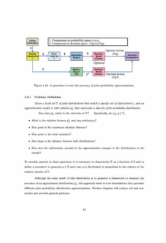
1.3.1 Problem Definition . . . . . . . . . . . . . . . . . . . . . . . . . . . . . . . . . 13
1.3.2 Sampling Procedure . . . . . . . . . . . . . . . . . . . . . . . . . . . . . . . . 14
1.3.3 Measures . . . . . . . . . . . . . . . . . . . . . . . . . . . . . . . . . . . . . . . 15
1.4 Literature Review . . . . . . . . . . . . . . . . . . . . . . . . . . . . . . . . . . . . . 16
1.5 Dissertation Outline . . . . . . . . . . . . . . . . . . . . . . . . . . . . . . . . . . . . 18
Chapter 2. Approximation Methods 19
2.1 Existing Approximation Models . . . . . . . . . . . . . . . . . . . . . . . . . . . . . . 19
2.1.1 Independence Approximation Model . . . . . . . . . . . . . . . . . . . . . . . 19
2.1.2 Underlying Event Model . . . . . . . . . . . . . . . . . . . . . . . . . . . . . . 20
2.1.3 Maximum Entropy Model . . . . . . . . . . . . . . . . . . . . . . . . . . . . . 21
2.1.4 First Example to Illustrate the Various Models . . . . . . . . . . . . . . . . . 22
2.2 Proposed Approximation Models . . . . . . . . . . . . . . . . . . . . . . . . . . . . . 23
2.2.1 Analytic Center . . . . . . . . . . . . . . . . . . . . . . . . . . . . . . . . . . . 23
2.2.2 Chebyshev’s Center . . . . . . . . . . . . . . . . . . . . . . . . . . . . . . . . . 25
2.2.3 Maximum Volume Inscribed Ellipsoid Center . . . . . . . . . . . . . . . . . . 26
2.2.4 Dynamic Average Sample Center . . . . . . . . . . . . . . . . . . . . . . . . . 28
vi

Chapter 3. Generating Collections of Joint Probability Distributions 30
3.1 State of Knowledge . . . . . . . . . . . . . . . . . . . . . . . . . . . . . . . . . . . . . 31
3.2 Sampling Example to Illustrate Proposed Technique . . . . . . . . . . . . . . . . . . 32
3.3 General Procedure . . . . . . . . . . . . . . . . . . . . . . . . . . . . . . . . . . . . . 34
3.3.1 Problem Statement . . . . . . . . . . . . . . . . . . . . . . . . . . . . . . . . . 34
3.3.2 Notation . . . . . . . . . . . . . . . . . . . . . . . . . . . . . . . . . . . . . . . 34
3.3.3 Constraints . . . . . . . . . . . . . . . . . . . . . . . . . . . . . . . . . . . . . 37
3.4 Sampling Procedure . . . . . . . . . . . . . . . . . . . . . . . . . . . . . . . . . . . . 42
3.4.1 Hit-and-Run Sampler . . . . . . . . . . . . . . . . . . . . . . . . . . . . . . . . 42
3.4.2 Sampling Non-Full-Dimensional Polytopes . . . . . . . . . . . . . . . . . . . . 43
3.4.3 Stopping Time . . . . . . . . . . . . . . . . . . . . . . . . . . . . . . . . . . . 43
3.5 Sampling in Practice . . . . . . . . . . . . . . . . . . . . . . . . . . . . . . . . . . . . 46
3.6 The Sea Urchin Effect . . . . . . . . . . . . . . . . . . . . . . . . . . . . . . . . . . . 48
Chapter 4. Measures of Accuracy 52
4.1 Proposed Measures of Accuracy . . . . . . . . . . . . . . . . . . . . . . . . . . . . . . 53
4.1.1 Maximum Absolute Difference . . . . . . . . . . . . . . . . . . . . . . . . . . . 53
4.1.2 Total Variation . . . . . . . . . . . . . . . . . . . . . . . . . . . . . . . . . . . 54
4.1.3 Euclidean Distance . . . . . . . . . . . . . . . . . . . . . . . . . . . . . . . . . 54
4.1.4 Kullback-Leibler Divergence . . . . . . . . . . . . . . . . . . . . . . . . . . . . 55
4.1.5 χ2 Distance . . . . . . . . . . . . . . . . . . . . . . . . . . . . . . . . . . . . . 56
4.1.6 Entropy Difference . . . . . . . . . . . . . . . . . . . . . . . . . . . . . . . . . 56
4.2 Illustration . . . . . . . . . . . . . . . . . . . . . . . . . . . . . . . . . . . . . . . . . 57
Chapter 5. Accuracy of Joint Probability Approximations 59
5.1 Selected Families of Multivariate Distributions . . . . . . . . . . . . . . . . . . . . . 59
5.1.1 Approximating the Hypergeometric Joint Distribution . . . . . . . . . . . . . 60
5.1.2 Approximating the Multinomial Joint Distribution . . . . . . . . . . . . . . . 67
5.1.3 Accuracy Findings in Hypergeometric and Multinomial Families . . . . . . . . 74
5.2 Unconstrained Multivariate Distributions . . . . . . . . . . . . . . . . . . . . . . . . 74
5.2.1 Findings in Unconstrained Truth Sets . . . . . . . . . . . . . . . . . . . . . . 83
5.3 Symmetrically Constrained Multivariate Distributions . . . . . . . . . . . . . . . . . 84
5.3.1 Effects of Increasing the Number of Constraints . . . . . . . . . . . . . . . . . 84
5.3.2 Symmetric Marginal Constraints . . . . . . . . . . . . . . . . . . . . . . . . . 89
5.3.3 Symmetric Marginal and Rank Correlation Constraints . . . . . . . . . . . . . 101
5.3.4 Findings in Symmetrically Constrained Truth Sets . . . . . . . . . . . . . . . 119
vii

5.4 Arbitrarily Constrained Multivariate Distributions . . . . . . . . . . . . . . . . . . . 119
5.4.1 Arbitrary Marginal Constraints . . . . . . . . . . . . . . . . . . . . . . . . . . 120
5.4.2 Arbitrarily Marginal Correlation Constraints . . . . . . . . . . . . . . . . . . . 126
5.4.3 Findings in Arbitrarily Constrained Truth Sets . . . . . . . . . . . . . . . . . 134
Chapter 6. A New Approach to Decision Analysis 135
6.1 Optimal Sequential Exploration . . . . . . . . . . . . . . . . . . . . . . . . . . . . . . 135
6.1.1 Joint Distributions Simulation Model . . . . . . . . . . . . . . . . . . . . . . . 137
6.1.2 Optimal Sequential Exploration Information . . . . . . . . . . . . . . . . . . . 138
6.1.3 Encoding The Information Constraints . . . . . . . . . . . . . . . . . . . . . . 139
6.1.4 Sampling From T . . . . . . . . . . . . . . . . . . . . . . . . . . . . . . . . . . 141
6.1.5 Decision Formulation . . . . . . . . . . . . . . . . . . . . . . . . . . . . . . . . 143
6.1.6 Optimal Strategies . . . . . . . . . . . . . . . . . . . . . . . . . . . . . . . . . 145
6.1.6.1 Accuracy of the Joint Distribution Approximations . . . . . . . . . . 149
6.1.6.2 Alternative Strategies . . . . . . . . . . . . . . . . . . . . . . . . . . . 151
6.1.6.3 One Step Strategies . . . . . . . . . . . . . . . . . . . . . . . . . . . . 153
6.1.7 Final Comments . . . . . . . . . . . . . . . . . . . . . . . . . . . . . . . . . . 156
6.2 Eagle Airlines . . . . . . . . . . . . . . . . . . . . . . . . . . . . . . . . . . . . . . . . 157
6.2.1 Introduction . . . . . . . . . . . . . . . . . . . . . . . . . . . . . . . . . . . . . 157
6.2.2 Proposed Approach . . . . . . . . . . . . . . . . . . . . . . . . . . . . . . . . . 158
6.2.3 Illustrative Example . . . . . . . . . . . . . . . . . . . . . . . . . . . . . . . . 159
6.2.4 Application to Eagle Airlines Decision . . . . . . . . . . . . . . . . . . . . . . 163
6.2.4.1 Case 1: Given Information Regarding Marginals Alone . . . . . . . . 163
6.2.4.2 Case 2: Given Marginals and Only One Rank Correlation . . . . . . . 168
6.2.4.3 Case 3: Given Information Regarding Marginals and All Rank Cor-relations Coeficients . . . . . . . . . . . . . . . . . . . . . . . . . . . . 172
6.2.4.4 Comparing the Three Information Cases . . . . . . . . . . . . . . . . 174
6.2.4.5 Decision Robustness . . . . . . . . . . . . . . . . . . . . . . . . . . . . 176
6.2.5 Final Comments . . . . . . . . . . . . . . . . . . . . . . . . . . . . . . . . . . 177
Chapter 7. Future Research 179
7.1 The Randomized Ping-Pong Sampler . . . . . . . . . . . . . . . . . . . . . . . . . . . 179
7.2 Measures of Precision . . . . . . . . . . . . . . . . . . . . . . . . . . . . . . . . . . . 183
7.2.1 Volume Ratio . . . . . . . . . . . . . . . . . . . . . . . . . . . . . . . . . . . . 183
7.2.2 Long and Short Diameters . . . . . . . . . . . . . . . . . . . . . . . . . . . . . 184
7.3 Bounds of Polyhedra . . . . . . . . . . . . . . . . . . . . . . . . . . . . . . . . . . . . 185
viii

7.3.1 Geometric Space Bounds . . . . . . . . . . . . . . . . . . . . . . . . . . . . . . 186
7.3.1.1 Approximation Model . . . . . . . . . . . . . . . . . . . . . . . . . . . 186
7.3.1.2 Heuristic Model . . . . . . . . . . . . . . . . . . . . . . . . . . . . . . 187
7.3.2 Information Space Bounds . . . . . . . . . . . . . . . . . . . . . . . . . . . . . 188
7.3.2.1 Approximation Model . . . . . . . . . . . . . . . . . . . . . . . . . . . 189
7.3.2.2 Heuristic Model . . . . . . . . . . . . . . . . . . . . . . . . . . . . . . 190
Appendix 191
Appendix A. Hit and Run Sampler and Ping-Pong Sampler Plots 192
Appendix B. Additional Derivations 195
B.1 Kendall τ . . . . . . . . . . . . . . . . . . . . . . . . . . . . . . . . . . . . . . . . . . 195
B.2 Lovasz Lower Bound . . . . . . . . . . . . . . . . . . . . . . . . . . . . . . . . . . . . 197
B.3 Symmetric Perturbations . . . . . . . . . . . . . . . . . . . . . . . . . . . . . . . . . 198
Appendix C. Additional Results 200
C.1 Hypergeometric Families Accuracy And Histograms. . . . . . . . . . . . . . . . . . . 201
C.2 Multinomial Families Accuracy And Histograms. . . . . . . . . . . . . . . . . . . . . 206
C.3 Effects Of Increasing The Number Of Constraints. . . . . . . . . . . . . . . . . . . . 211
C.4 Raw Statistics in Symm. Marginal Constrained Sets. . . . . . . . . . . . . . . . . . . 215
C.5 Standard Dev. Marginal and Correlation Symm. Sets. . . . . . . . . . . . . . . . . . 220
C.6 Percentage Of Accuracy Marginal, and Correlation Information. . . . . . . . . . . . 230
Appendix D. A New Approach to DA 246
D.1 Moment Matching Discretization Procedure . . . . . . . . . . . . . . . . . . . . . . . 246
D.2 Rank Correlation Range in Discrete Distributions . . . . . . . . . . . . . . . . . . . 247
D.3 Absolute Bounds for Risk Profiles . . . . . . . . . . . . . . . . . . . . . . . . . . . . 248
References . . . . . . . . . . . . . . . . . . . . . . . . . . . . . . . . . . . . . . . . . . . . 249
Vita 258
ix

List of Tables
1.1 Joint Distributions for a Series of Events. . . . . . . . . . . . . . . . . . . . . . . . . 12
1.2 Correlations for Different Distributions . . . . . . . . . . . . . . . . . . . . . . . . . . 12
2.1 True Joint pmf. . . . . . . . . . . . . . . . . . . . . . . . . . . . . . . . . . . . . . . . 22
2.2 Marginals and Pairwise Information. . . . . . . . . . . . . . . . . . . . . . . . . . . . 22
2.3 Joint PMF Approximations. . . . . . . . . . . . . . . . . . . . . . . . . . . . . . . . . 23
3.1 Notation example. . . . . . . . . . . . . . . . . . . . . . . . . . . . . . . . . . . . . . 36
3.2 Discrete Vs Continuous Measures . . . . . . . . . . . . . . . . . . . . . . . . . . . . . 48
5.1 Hypergeometric Distribution and Approximations. . . . . . . . . . . . . . . . . . . . 61
5.2 Percentage Of Accuracy For The Hypergeometric Distribution. Part One. . . . 65
5.3 Multinomial Distribution and Approximations. . . . . . . . . . . . . . . . . . . . . . 69
5.4 Percentage Of Accuracy For The Monomial Distribution. Part One. . . . . . . . . . 72
5.5 Percentage Of Accuracy In Sets With Marginal Information Part One. . . . . . . . . 99
5.6 Percentage Of Accuracy In Sets With Marginal Information Part Two. . . . . . . . . 100
5.7 Percentage Of Accuracy In Sets With Marginal and Correlation InformationUsing 5 Binary Random Variables Part One. . . . . . . . . . . . . . . . . . . . . . . 115
5.8 Percentage Of Accuracy In Sets With Marginal and Correlation InformationUsing 5 Binary Random Variables Part Two. . . . . . . . . . . . . . . . . . . . . . . 116
5.9 Percentage Of Accuracy In Sets With Marginal and Correlation InformationUsing 5 Binary Random Variables Part Three. . . . . . . . . . . . . . . . . . . . . . 117
5.10 Percentage Of Accuracy In Sets With Marginal and Correlation InformationUsing 5 Binary Random Variables Part Four. . . . . . . . . . . . . . . . . . . . . . . 118
5.11 Percentage Of Accuracy In Asymmetric Sets With Marginal Information. . . . . . . 125
5.12 Percentage Of Accuracy In Asymmetric Sets With Marginal and CorrelationConstraints, Part One. . . . . . . . . . . . . . . . . . . . . . . . . . . . . . . . . . . . 133
5.13 Percentage Of Accuracy In Asymmetric Sets With Marginal and CorrelationConstraints, Part Two. . . . . . . . . . . . . . . . . . . . . . . . . . . . . . . . . . . . 134
6.1 Example Well Data Part One. . . . . . . . . . . . . . . . . . . . . . . . . . . . . . . . 139
6.2 Example Well Data Part Two. . . . . . . . . . . . . . . . . . . . . . . . . . . . . . . 139
6.3 Example Well Data Part Three. . . . . . . . . . . . . . . . . . . . . . . . . . . . . . . 140
x

6.4 Joint Probability Distribution Approximations . . . . . . . . . . . . . . . . . . . . . 148
6.5 Accuracy Results. . . . . . . . . . . . . . . . . . . . . . . . . . . . . . . . . . . . . . . 150
6.6 Profit Statistics For Full Strategies Based on Approx. Distributions. . . . . . . . . . 152
6.7 Profit Statistics For Full Strategies Based on Selected Strategies. . . . . . . . . . . . 152
6.8 Expected Profit Statistics For Six Myopic Strategies. . . . . . . . . . . . . . . . . . . 155
6.9 Fractiles and Spearman Correlations for Critical Input Variables. . . . . . . . . . . 161
6.10 Marginal Distributions For Eagle Airlines. . . . . . . . . . . . . . . . . . . . . . . . . 161
6.11 Spearman Rank Correlations Implied by CR’s Procedure. . . . . . . . . . . . . . . . 162
6.12 Extended fractiles. . . . . . . . . . . . . . . . . . . . . . . . . . . . . . . . . . . . . . 163
6.13 Mean, Std. Dev. and Risk for scenario one. . . . . . . . . . . . . . . . . . . . . . . . 164
6.14 Mean, Std. Dev. and Risk for scenario two. . . . . . . . . . . . . . . . . . . . . . . . 170
6.15 Mean, Std. Dev. and Risk for scenario three. . . . . . . . . . . . . . . . . . . . . . . 172
6.16 Decision Accuracy. . . . . . . . . . . . . . . . . . . . . . . . . . . . . . . . . . . . . 177
B.1 Fair Convergence . . . . . . . . . . . . . . . . . . . . . . . . . . . . . . . . . . . . . . 197
C.1 Percentage Of Accuracy For The Hypergeometric Distribution. Part Two. . . . 205
C.2 Percentage Of Accuracy For The Hypergeometric Distribution. Part Three. . . 205
C.3 Percentage Of Accuracy For The Monomial Distribution. Part Two. . . . . . . . . . 210
C.4 Percentage Of Accuracy For The Monomial Distribution. Part Three. . . . . . . . . 210
C.5 Accuracy Values For 3 Binary Variables With Marginal Constraints. . . . . . . . . . 215
C.6 Accuracy Values For 4 Binary Variables With Marginal Constraints. . . . . . . . . . 216
C.7 Accuracy Values For 5 Binary Variables With Marginal Constraints. . . . . . . . . . 217
C.8 Accuracy Values For 6 Binary Variables With Marginal Constraints. . . . . . . . . . 218
C.9 Accuracy Values For 7 Binary Variables With Marginal Constraints. . . . . . . . . . 219
C.10 Percentage Of Accuracy In Sets With Marginal and Correlation InformationUsing 3 Binary Random Variables Part One. . . . . . . . . . . . . . . . . . . . . . . 230
C.11 Percentage Of Accuracy In Sets With Marginal and Correlation InformationUsing 3 Binary Random Variables Part Two. . . . . . . . . . . . . . . . . . . . . . . 231
C.12 Percentage Of Accuracy In Sets With Marginal and Correlation InformationUsing 3 Binary Random Variables Part Three. . . . . . . . . . . . . . . . . . . . . . 232
C.13 Percentage Of Accuracy In Sets With Marginal and Correlation InformationUsing 3 Binary Random Variables Part Four. . . . . . . . . . . . . . . . . . . . . . . 233
C.14 Percentage Of Accuracy In Sets With Marginal and Correlation InformationUsing 4 Binary Random Variables Part One. . . . . . . . . . . . . . . . . . . . . . . 234
C.15 Percentage Of Accuracy In Sets With Marginal and Correlation InformationUsing 4 Binary Random Variables Part Two. . . . . . . . . . . . . . . . . . . . . . . 235
xi

C.16 Percentage Of Accuracy In Sets With Marginal and Correlation InformationUsing 4 Binary Random Variables Part Three. . . . . . . . . . . . . . . . . . . . . . 236
C.17 Percentage Of Accuracy In Sets With Marginal and Correlation InformationUsing 4 Binary Random Variables Part Four. . . . . . . . . . . . . . . . . . . . . . . 237
C.18 Percentage Of Accuracy In Sets With Marginal and Correlation InformationUsing 6 Binary Random Variables Part One. . . . . . . . . . . . . . . . . . . . . . . 238
C.19 Percentage Of Accuracy In Sets With Marginal and Correlation InformationUsing 6 Binary Random Variables Part Two. . . . . . . . . . . . . . . . . . . . . . . 239
C.20 Percentage Of Accuracy In Sets With Marginal and Correlation InformationUsing 6 Binary Random Variables Part Three. . . . . . . . . . . . . . . . . . . . . . 240
C.21 Percentage Of Accuracy In Sets With Marginal and Correlation InformationUsing 6 Binary Random Variables Part Four. . . . . . . . . . . . . . . . . . . . . . . 241
C.22 Percentage Of Accuracy In Sets With Marginal and Correlation InformationUsing 7 Binary Random Variables Part One. . . . . . . . . . . . . . . . . . . . . . . 242
C.23 Percentage Of Accuracy In Sets With Marginal and Correlation InformationUsing 7 Binary Random Variables Part Two. . . . . . . . . . . . . . . . . . . . . . . 243
C.24 Percentage Of Accuracy In Sets With Marginal and Correlation InformationUsing 7 Binary Random Variables Part Three. . . . . . . . . . . . . . . . . . . . . . 244
C.25 Percentage Of Accuracy In Sets With Marginal and Correlation InformationUsing 7 Binary Random Variables Part Four. . . . . . . . . . . . . . . . . . . . . . . 245
xii

List of Figures
1.1 Tree Diagram. . . . . . . . . . . . . . . . . . . . . . . . . . . . . . . . . . . . . . . . . 1
1.2 Decision Analysis Cycle. . . . . . . . . . . . . . . . . . . . . . . . . . . . . . . . . . . 2
1.3 Probabilistic Dependence. . . . . . . . . . . . . . . . . . . . . . . . . . . . . . . . . . 7
1.4 Information Sets. . . . . . . . . . . . . . . . . . . . . . . . . . . . . . . . . . . . . . . 8
1.5 Binary Variables Example. . . . . . . . . . . . . . . . . . . . . . . . . . . . . . . . . . 9
1.6 Accuracy Vs Precision. . . . . . . . . . . . . . . . . . . . . . . . . . . . . . . . . . . . 10
1.7 Binary Variables Example Cont. . . . . . . . . . . . . . . . . . . . . . . . . . . . . . 10
1.8 Accuracy Vs Precision Cont. . . . . . . . . . . . . . . . . . . . . . . . . . . . . . . . 11
1.9 General approach. . . . . . . . . . . . . . . . . . . . . . . . . . . . . . . . . . . . . . 11
1.10 Testing Procedure. . . . . . . . . . . . . . . . . . . . . . . . . . . . . . . . . . . . . . 13
1.11 Sampling from T. . . . . . . . . . . . . . . . . . . . . . . . . . . . . . . . . . . . . . 14
1.12 Measuring Collection. . . . . . . . . . . . . . . . . . . . . . . . . . . . . . . . . . . . 15
2.1 Influence Diagrams for Diverse Approximation Methods. . . . . . . . . . . . . . . . . 20
2.2 Analytic Center. . . . . . . . . . . . . . . . . . . . . . . . . . . . . . . . . . . . . . . 24
2.3 Chebyshev’s Center. . . . . . . . . . . . . . . . . . . . . . . . . . . . . . . . . . . . . 25
2.4 Polyhedron Perturbation. . . . . . . . . . . . . . . . . . . . . . . . . . . . . . . . . . 27
2.5 Max Vol Ellipsoid Center. . . . . . . . . . . . . . . . . . . . . . . . . . . . . . . . . . 28
2.6 CVX Code For 4 Approximations. . . . . . . . . . . . . . . . . . . . . . . . . . . . . 29
3.1 Sampling: Illustrative Example. . . . . . . . . . . . . . . . . . . . . . . . . . . . . . . 33
3.2 Sampling: Illustrative Example Cont. . . . . . . . . . . . . . . . . . . . . . . . . . . 34
3.3 Hit and run sampler. . . . . . . . . . . . . . . . . . . . . . . . . . . . . . . . . . . . . 42
3.4 Fair Convergence . . . . . . . . . . . . . . . . . . . . . . . . . . . . . . . . . . . . . . 46
3.5 Hit and Run: Norm Distance From The Center . . . . . . . . . . . . . . . . . . . . 49
3.6 Hit and Run: Norm Distance From The Center Histogram . . . . . . . . . . . . . . 49
3.7 Polytope Partition . . . . . . . . . . . . . . . . . . . . . . . . . . . . . . . . . . . . . 50
3.8 Concentration Of Volume In A Polytope . . . . . . . . . . . . . . . . . . . . . . . . . 50
4.1 Accuracy Measures Illustration. . . . . . . . . . . . . . . . . . . . . . . . . . . . . . . 58
5.1 Hypergeometric Distributions And Approximations Part One. . . . . . . . . . . . . . 63
xiii

5.2 Hypergeometric Family Result Histograms Part One. . . . . . . . . . . . . . . . . . . 64
5.3 Hypergeometric Family, Algorithmic Degradation . . . . . . . . . . . . . . . . . . . . 66
5.4 Hypergeometric Distributions And Approximations. Means. . . . . . . . . . . . . . . 67
5.5 Hypergeometric Distributions And Approximations. Standard Dev. . . . . . . . . . . 67
5.6 Multinomial Distributions And Approximations Part One. . . . . . . . . . . . . . . . 70
5.7 Multinomial Family Result Histograms Part One. . . . . . . . . . . . . . . . . . . . . 71
5.8 Multinomial Distributions And Approximations. Means. . . . . . . . . . . . . . . . . 73
5.9 Multinomial Distributions And Approximations. Standard Deviation. . . . . . . . . 74
5.10 Histograms for Unconstrained Sets Changing # Variables. . . . . . . . . . . . . . . . 76
5.10 Cont. . . . . . . . . . . . . . . . . . . . . . . . . . . . . . . . . . . . . . . . . . . . . . 77
5.11 Mean and SD for Unconstrained Sets Changing # Variables. . . . . . . . . . . . . . 78
5.12 Symmetric Perturbations vs Dimensionality. . . . . . . . . . . . . . . . . . . . . . . . 79
5.13 Symmetric Perturbations For Metric Based Accuracy Measures. . . . . . . . . . . . . 79
5.14 Symmetric Perturbations For Information Based Accuracy Measures. . . . . . . . . . 80
5.15 Histograms for Unconstrained Sets Changing # Outcomes. . . . . . . . . . . . . . . 81
5.15 Cont. . . . . . . . . . . . . . . . . . . . . . . . . . . . . . . . . . . . . . . . . . . . . . 82
5.16 Mean and SD for Unconstrained Sets Changing # Outcomes. . . . . . . . . . . . . . 83
5.17 Effects Of Constraints 1. Histograms, Part One. . . . . . . . . . . . . . . . . . . . . 85
5.18 Effects Of Constraints 1. Histograms, Part Two. . . . . . . . . . . . . . . . . . . . . 86
5.19 Means for Sets Changing Constraints. . . . . . . . . . . . . . . . . . . . . . . . . . . 87
5.20 Standard Deviation for Sets Changing Constraints. . . . . . . . . . . . . . . . . . . . 88
5.21 Marginal Constraints Effects in Mean. . . . . . . . . . . . . . . . . . . . . . . . . . . 90
5.21 Cont. . . . . . . . . . . . . . . . . . . . . . . . . . . . . . . . . . . . . . . . . . . . . . 91
5.22 Marginal Constraints Effects. Standard Deviation. . . . . . . . . . . . . . . . . . . . 92
5.22 Cont. . . . . . . . . . . . . . . . . . . . . . . . . . . . . . . . . . . . . . . . . . . . . . 93
5.23 Description of ME Behavior. . . . . . . . . . . . . . . . . . . . . . . . . . . . . . . . 94
5.24 Joint Distribution Approximation Changes By Event (ME). . . . . . . . . . . . . . . 95
5.25 Description of ChSC Behavior. . . . . . . . . . . . . . . . . . . . . . . . . . . . . . . 95
5.26 Joint Distribution Approximation Changes By Event (ChSC). . . . . . . . . . . . . . 96
5.27 Joint Distribution Approximation Changes By Event. (AC, MVIE, DAC) . . . . . . 97
5.28 Marginal and Correlation Constraints Effects. Mean, 3 binary random variables. . . 102
5.28 Cont. . . . . . . . . . . . . . . . . . . . . . . . . . . . . . . . . . . . . . . . . . . . . . 103
5.29 Marginal and Correlation Constraints Effects. Mean, 4 binary random variables. . . 104
5.29 Cont. . . . . . . . . . . . . . . . . . . . . . . . . . . . . . . . . . . . . . . . . . . . . . 105
5.30 Marginal and Correlation Constraints Effects. Mean, 5 binary random variables. . . 106
xiv

5.30 Cont. . . . . . . . . . . . . . . . . . . . . . . . . . . . . . . . . . . . . . . . . . . . . . 107
5.31 Marginal and Correlation Constraints Effects. Mean, 6 binary random variables. . . 108
5.31 Cont. . . . . . . . . . . . . . . . . . . . . . . . . . . . . . . . . . . . . . . . . . . . . . 109
5.32 Marginal and Correlation Constraints Effects. Mean, 7 binary random variables. . . 110
5.32 Cont. . . . . . . . . . . . . . . . . . . . . . . . . . . . . . . . . . . . . . . . . . . . . . 111
5.33 UE Position in a series of Truth Sets . . . . . . . . . . . . . . . . . . . . . . . . . . . 112
5.34 ME Position in a series of Truth Sets . . . . . . . . . . . . . . . . . . . . . . . . . . . 113
5.35 Asymmetric Marginal Constraints. Mean For 3 random variables. . . . . . . . . . . . 121
5.36 Asymmetric Marginal Constraints. Mean For 4 random variables. . . . . . . . . . . . 122
5.37 Asymmetric Marginal Constraints. Mean For 5 random variables. . . . . . . . . . . . 123
5.38 Asymmetric Marginal Constraints. Mean For 6 random variables. . . . . . . . . . . . 124
5.39 Asymmetric Marginal and Correlation Constraints. . . . . . . . . . . . . . . . . . . . 127
5.39 Cont. . . . . . . . . . . . . . . . . . . . . . . . . . . . . . . . . . . . . . . . . . . . . . 128
5.40 Asymmetric Marginal and Correlation Constraints. Mean For 3 Random Vari-ables. . . . . . . . . . . . . . . . . . . . . . . . . . . . . . . . . . . . . . . . . . . . . 129
5.41 Asymmetric Marginal and Correlation Constraints. Mean For 4 Random Vari-ables. . . . . . . . . . . . . . . . . . . . . . . . . . . . . . . . . . . . . . . . . . . . . 130
5.42 Asymmetric Marginal and Correlation Constraints. Mean For 5 Random Vari-ables. . . . . . . . . . . . . . . . . . . . . . . . . . . . . . . . . . . . . . . . . . . . . 131
5.43 Asymmetric Marginal and Correlation Constraints. Mean For 6 Random Vari-ables. . . . . . . . . . . . . . . . . . . . . . . . . . . . . . . . . . . . . . . . . . . . . 132
6.1 Visualization of the truth set using geometric measures. . . . . . . . . . . . . . . . . 142
6.2 Visualization of the truth set using information measures. . . . . . . . . . . . . . . . 143
6.3 A Partial Decision Tree for the Sequential Drilling Problem. . . . . . . . . . . . . . . 144
6.4 Strategies derived from approximation joint distributions . . . . . . . . . . . . . . . 146
6.5 Most Common Optimal Strategies. . . . . . . . . . . . . . . . . . . . . . . . . . . . . 152
6.6 Fraction of Time Each Strategy is the Best Option. . . . . . . . . . . . . . . . . . . . 153
6.7 Strategies With Highest Frequencies. . . . . . . . . . . . . . . . . . . . . . . . . . . . 154
6.8 Frequency of Optimal Myopic Strategies. . . . . . . . . . . . . . . . . . . . . . . . . . 155
6.9 Stochastic Dominance Among Myopic Strategies. . . . . . . . . . . . . . . . . . . . . 156
6.10 Example characterization of the truth set T. . . . . . . . . . . . . . . . . . . . . . . . 159
6.11 Influence Diagram for Eagle Airline’s Decision. . . . . . . . . . . . . . . . . . . . . . 160
6.12 CR discretization. . . . . . . . . . . . . . . . . . . . . . . . . . . . . . . . . . . . . . 162
6.13 CDF Bounds Part One. . . . . . . . . . . . . . . . . . . . . . . . . . . . . . . . . . . 167
6.14 CDF Bounds Part Two. . . . . . . . . . . . . . . . . . . . . . . . . . . . . . . . . . . 168
6.15 CDF Bounds Part Three. . . . . . . . . . . . . . . . . . . . . . . . . . . . . . . . . . 170
xv

6.16 CDF Bounds Part Four. . . . . . . . . . . . . . . . . . . . . . . . . . . . . . . . . . . 171
6.17 CDF Bounds Part Five. . . . . . . . . . . . . . . . . . . . . . . . . . . . . . . . . . . 173
6.18 CDF Bounds Part Six. . . . . . . . . . . . . . . . . . . . . . . . . . . . . . . . . . . . 174
6.19 Mean Joint distributions. . . . . . . . . . . . . . . . . . . . . . . . . . . . . . . . . . 175
7.1 Ping Pong Sampler . . . . . . . . . . . . . . . . . . . . . . . . . . . . . . . . . . . . . 181
7.2 Ping Pong Sampler Step A. . . . . . . . . . . . . . . . . . . . . . . . . . . . . . . . . 181
7.3 Ping Pong Sampler Step B. . . . . . . . . . . . . . . . . . . . . . . . . . . . . . . . . 182
7.4 Ping-Pong: Norm Distance From The Center. . . . . . . . . . . . . . . . . . . . . . 182
7.5 Ping-Pong: Norm Distance From The Center Histograms. . . . . . . . . . . . . . . 183
7.6 Bounds for T. . . . . . . . . . . . . . . . . . . . . . . . . . . . . . . . . . . . . . . . . 186
A.1 Hit and Run: Norm Distance From The Center And Histograms . . . . . . . . . . . 193
A.2 Ping-Pong: Norm Distance From The Center And Histograms . . . . . . . . . . . . 194
C.1 Hypergeometric Distributions And Approximations Part Two. . . . . . . . . . . . . . 201
C.2 Hypergeometric Family Result Histograms Part Two. . . . . . . . . . . . . . . . . . 202
C.3 Hypergeometric Distributions And Approximations Part Three. . . . . . . . . . . . . 203
C.4 Hypergeometric Family Result Histograms Part Three. . . . . . . . . . . . . . . . . . 204
C.5 Multinomial Distributions And Approximations Part Two. . . . . . . . . . . . . . . . 206
C.6 Multinomial Family Result Histograms Part Two. . . . . . . . . . . . . . . . . . . . 207
C.7 Multinomial Distributions And Approximations Part Three. . . . . . . . . . . . . . . 208
C.8 Multinomial Family Result Histograms Part Three. . . . . . . . . . . . . . . . . . . . 209
C.9 Effects Of Constraints 2. Histograms, Part One. . . . . . . . . . . . . . . . . . . . . 211
C.10 Effects Of Constraints 2. Histograms, Part Two. . . . . . . . . . . . . . . . . . . . . 212
C.11 Effects Of Constraints 3. Histograms, Part One. . . . . . . . . . . . . . . . . . . . . 213
C.12 Effects Of Constraints 3. Histograms, Part Two. . . . . . . . . . . . . . . . . . . . . 214
C.13 Marginal and Correlation Constraints Effects. Standard Deviation For 3 binaryRandom Variables. . . . . . . . . . . . . . . . . . . . . . . . . . . . . . . . . . . . . . 220
C.13 Cont. . . . . . . . . . . . . . . . . . . . . . . . . . . . . . . . . . . . . . . . . . . . . . 221
C.14 Marginal and Correlation Constraints Effects. Standard Deviation For 4 binaryRandom Variables. . . . . . . . . . . . . . . . . . . . . . . . . . . . . . . . . . . . . . 222
C.14 Cont. . . . . . . . . . . . . . . . . . . . . . . . . . . . . . . . . . . . . . . . . . . . . . 223
C.15 Marginal and Correlation Constraints Effects. Standard Deviation For 5 binaryRandom Variables. . . . . . . . . . . . . . . . . . . . . . . . . . . . . . . . . . . . . . 224
C.15 Cont. . . . . . . . . . . . . . . . . . . . . . . . . . . . . . . . . . . . . . . . . . . . . . 225
C.16 Marginal and Correlation Constraints Effects. Standard Deviation For 6 binaryRandom Variables. . . . . . . . . . . . . . . . . . . . . . . . . . . . . . . . . . . . . . 226
xvi

C.16 Cont. . . . . . . . . . . . . . . . . . . . . . . . . . . . . . . . . . . . . . . . . . . . . . 227
C.17 Marginal and Correlation Constraints Effects. Standard Deviation For 7 binaryRandom Variables. . . . . . . . . . . . . . . . . . . . . . . . . . . . . . . . . . . . . . 228
C.17 Cont. . . . . . . . . . . . . . . . . . . . . . . . . . . . . . . . . . . . . . . . . . . . . . 229
xvii


• Measuring the decision quality.
• Selecting relevant uncertainties.
• Assessing probabilities and probabilistic dependence.
• Deriving risk attitude and risk tolerance for the DM.
All these steps have grown into sub-disciplines of decision analysis, each with its own exten-
sive literature. However, this dissertation will address problems related to probability assessment
and probabilistic dependence.
Modeling real-world decision situations often requires multivariate discrete probability dis-
tributions,1 which model not only uncertainty but how uncertain events relate to each other. In
finance, for example, the price of an asset over time is considered a random variable. However,
when managing a portfolio, brokers are concerned also with the interactions among prices of vari-
ous assets over time, since that can transform a bad portfolio into substantial revenue or vice versa.
In gas/oil exploration, wells can be wet or dry, meaning they have or lack a considerable deposit
of gas/oil, respectively. Geologists and other experts determine the probability of a well being wet
or dry, but having a complete discrete joint probability distribution for all combinations of well
outcomes provides important information about reservoir connections underground. Knowing this
information could greatly affect the expected revenue of the project, and in most cases, could change
the development plans. In medicine, drug development is considered a risky investment because it
takes many years for a drug to be approved by the FDA, and a company can go bankrupt if a series
of drugs fails the approval process. However, if there is a relation among the approval of Drug A,
Drug B, and Drug C, then a joint probability distribution could provide information about which
drug to develop first, thereby reducing the risk of bankruptcy.
In other words, the information about random events and their interactions is encoded
in multivariate joint probability distributions, making them an important tool in mathematical
modeling. The existence of a discrete joint probability distribution function has an impact on
the strategy used in optimization. For example, procedures such as stochastic optimization and
robust optimization are mainly concerned with optimization under uncertainty. However, they
differ in that the former assumes knowledge of the underlying probability distribution and the
latter disregards the underlying distribution. As a result, stochastic optimization provides results
1We will use the terms multivariable distributions and joint distributions interchangeably.
3
based on a higher degree of information, and robust optimization provides optimization over worst-
case scenarios. Both solutions are useful when a decision is considered, but the knowledge of a
probability distribution may provide information that changes the decision.
1.1 Contributions
This dissertation addresses decision situations for which partial information about the
joint probability distribution is known. From here, our first contribution was to develop four new
approximations to recreate a joint probability distribution. These approximations complement
existing models such as maximum entropy, which is still the most popular approximation method.
A second contribution develops a simulation procedure we named JDSIM, to create a collec-
tion of joint distribution approximations. We consider JDSIM to be a powerful method for helping
to characterize the uncertainty generated by the missing information about the joint distribution.
This dissertation will focus on the philosophy behind and tools generated from this procedure.
A third contribution develops the concept of accuracy of an approximation. Up to now,
there has been no clear procedure to test which approximation was best. Using JDSIM, we imple-
ment a procedure to determine the accuracy of several approximations under various scenarios.
Finally, our fourth contribution develops a new approach to decision analysis. We de-
scribe a new methodology for analyzing decisions in the face of partial information. We exemplify
our methodology by revisiting two decisions in the literature and providing fresh insights. This
contribution is the most applied of them all, but it perhaps has the greatest impact on society.
1.2 Motivation
In DA practice, it is common for the DM to work with people who deeply understand the
behavior of the random variables. These experts provide the decision analysis team with estimates
for the required assessments. Formally, assume the DM must choose an alternative a from a set A.
If there are no uncertainties, the DM needs merely to order the set by preference and
choose the most preferred option. Under uncertainty, however, it is common practice to use a
utility function that encodes risk behavior into the decision. Then, if there is an uncertainty X, the
utility of the pair {a, X} is u(a, X = x), which represents the utility as a function of the alternative
chosen and the realization of the uncertainty.
4
The DM then solves the problem
maxa∈A
EX
[u(a, X)
], (1.1)
which is the problem of finding the alternative that maximizes the DM’s expected utility.
The DA cycle derives this decision step by step. In the Framing phase, the DA team helps
the DM to define A, X, and u(·). The Deterministic phase studies X to observe which uncertainties
are relevant to the decision. During the Probabilistic phase, experts derive f(X) and the problem is
solved. Finally, during the Appraisal phase, a series of sensitivity analyses is performed to determine
if more information could be relevant to the problem.
It has been shown that for simple assessments, experts can provide accurate values (Licht-
enstein et al., 1982). However, experts face two important challenges. The first one appears when
there are two or more uncertainties, e.g., X = (X1, X2, . . . , Xn). In this case, the assessment pro-
cess becomes complex and often intractable. To illustrate, assume each variable in the vector X
is binary. Then, a simple joint probability distribution comprised of n binary random variables
requires the assessments of marginal probabilities, pairwise probabilities, three-way probabilities,
and so on. The total number of assessments is 2n − 1, which increases exponentially with n and
represents a real challenge for DA practice.
This exponential increase in the number of assessments is due to probabilistic dependence.
For example, if all variables were independent, only n assessments would be required, which is
feasible (Bickel et al., 2008). Then, by ignoring probabilistic dependence, we can simplify the
assessment process. However, this loss of information reduces the decision quality (Korsan, 1990).
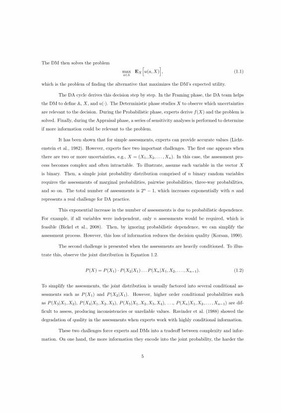
The second challenge is presented when the assessments are heavily conditioned. To illus-
trate this, observe the joint distribution in Equation 1.2.
P (X) = P (X1) · P (X2|X1) . . . P (Xn|X1, X2, . . . , Xn−1). (1.2)
To simplify the assessments, the joint distribution is usually factored into several conditional as-
sessments such as P (X1) and P (X2|X1). However, higher order conditional probabilities such
as P (X3|X1, X2), P (X4|X1, X2, X3), P (X5|X1, X2, X3, X4), . . ., P (Xn|X1, X2, . . . , Xn−1) are dif-
ficult to assess, producing inconsistencies or unreliable values. Ravinder et al. (1988) showed the
degradation of quality in the assessments when experts work with highly conditional information.
These two challenges force experts and DMs into a tradeoff between complexity and infor-
mation. On one hand, the more information they encode into the joint probability, the harder the
5

assessments and the higher the chance to compromise their quality. On the other hand, using less
information reduces the quantity of assessments, thus degrading the quality of the decision.
Despite its relevance, probabilistic dependence is often ignored because it greatly compli-
cates probability assessment (Korsan, 1990; Lowell, 1994). In fact, Winkler (1982) identified the
assessment and modeling of probabilistic dependence as one of the most important research topics
facing decision analysts. Miller (1990) argued, “We need a way to assess and process dependent
probabilities efficiently. If we can find generally applicable methods for doing so, we could make sig-
nificant advances in our ability to analyze and model complex decision problems.” These challenges
have gone largely unanswered.
The Decision Analysis Cycle derives joint distributions using experts and available data.
However, when based on partial information, such distributions are approximations of the “true”
joint distribution. That is, if all possible conditional probabilities could be assessed, the resultant
distribution would be unique and would match all the information at hand. The main goal is
therefore to get as close as possible to the true joint distribution using partial information. Every
approximation method generates a bias according to how it compensates for missing information,
i.e., by disregarding parts of the dependence structure.
Given a portfolio with three assets and for simplicity, that the DM’s only concern is with
respect to the assets going up or down, the resulting joint probability distribution would have eight
possibilities (Fig 1.3).
Figure 1.3(a) shows the initial tree structure. The question marks in the Figure are un-
knowns that an expert must assess. The expert starts by assessing P (asset 1 goes up), and then
works toward more complex assessments (Fig 1.3(b)). The next step is to assess P (asset 2 goes
up|asset 1 goes up) and P (asset 2 goes up|asset 1 goes down). These assessments capture the de-
pendence between assets 1 and 2. Figure 1.3(c) shows that the outcome of asset 2 depends on the
outcome of asset 1. Finally, we must assess P (asset 3 goes up|asset 1 and asset 2 go up), P (asset
3 goes up|asset 1 goes up and asset 2 goes down), P (asset 3 goes up|asset 1 goes down and asset
2 goes up), and P (asset 3 goes up|asset 1 and asset 2 go down). This completely determines the
discrete joint probability distribution using Equation 1.2 and the parameters in Figure 1.3(d).
For three assets, deriving a joint probability is a simple process that requires only seven
assessments. However, the general case is considerably more complicated. For example, Bickel
et al. (2008) considered a problem having six binary variables. This requires 63 assessments to fully
characterize the joint distribution, and some of these assessments are very difficult. If only 21 of the
6


To be able to measure accuracy efficiently requires the truth set T to be convex. However,
T is a function of the information gathered I, and may not always be convex. To demonstrate that,
assume that the truth set was created using two variables x1 and x2 with possible outcomes {2, 4}and {7, 8, 9}, respectively. If the only information known is the correlation ρ = 0.5, then P1(x1, x2)
and P2(x1, x2) from Table 1.1 are elements of T. However, the convex combination P3(x1, x2) is
not, because as shown in Table 1.2, the correlation for P3(x1, x2) does not equal 0.5.
Table 1.1: Joint Distributions for a Series of Events.
Event Joint Distributionsx1 x2 P1(x1, x2) P2(x1, x2) P3(x1, x2)
a
4 8 0.511 .163 .3382 7 0.117 .096 .1064 9 0.117 .096 .1062 8 0.255 .645 .45
aP3(x1, x2) = 1
2P1(x1, x2) + 1
2P2(x1, x2).
Table 1.2: Correlations forDifferent Distributions.
Distribution ρx1x2
P1(x1, x2) 0.5P2(x1, x2) 0.5P3(x1, x2) 0.46
Using correlations without the knowledge of the marginal distributions could result in sets
that are hard to work with (non-convex). Fortunately, marginal assessments are easy to perform,
and once known, T becomes a convex set. A later chapter will describe families of equations and
their requirements such that T is assured to be a convex set. Equations outside the proposed
families might generate a non-convex set and are left for future research.
Once T is defined, a method is required to sample the set T and provide random joint
distributions. These distributions can be used to generate comparisons against the selected ap-
proximation. Finally, a set of measures of accuracy is needed for these comparisons.
The use of the samples and the measures of accuracy with the approximate distribution
allows us to evaluate which approximation is most appropriate for a given situation. Figure 1.10
shows that by observing the behavior of a given approximation and its relation to the elements in
the set T, we can develop the tools required to understand the accuracy of an approximation.
The following sections formalize the problem and expand the general approach to charac-
terize the accuracy of an approximation. Additionally, we present a literature review and an outline
of the rest of the dissertation.
12


1.4 Literature Review
In 1940, Deming and Stephan were the first to use partial information to approximate an
unknown target. This problem was called “The matching of tabular data tables,” where the census
provided marginal information on the universal sample, and frequency information on a small
sample. The problem was to extrapolate the sample to the complete universe while preserving
consistency of the data tables. The approach to the matching of tabular data tables was concerned
only with finding a solution; the quality of such a solution was not fully explored.
Later, Shannon (1948) developed the function H(p1, p2, . . . , pn) to measure certainty in
probability distributions, which is the basis for the the definition of entropy. After Shannon,
Kullback and Leibler (1951) published a paper generalizing some of the fundamental concepts of
entropy and developed the concept of cross-entropy also known as KL divergence.
Using Shannon’s descriptive measure, Jaynes (1957, 1963) proposed a normative principle,
the principle of maximum entropy, to guide the assignment of probability distributions. This princi-
ple states that when information about an uncertainty does not uniquely specify a distribution, one
should assign the probability distribution with maximum entropy subject to the partial information.
The principle of maximum entropy is a generalization of Laplace’s principle of insufficient reason,
which states that knowing the possibilities with no additional information, one should assign equal
probabilities to all events. We will challenge some of these conclusions.
Jaynes (1968) presented an application of the maximum entropy principle and solved the
problem of choosing the correct priors on Bayesian estimation of probabilities. That same year,
Ireland and Kullback (1968) returned to the problem proposed by Deming and Stephan and applied
the concept of entropy by minimizing the KL divergence among tables. Later, Thomas (1979)
demonstrated how to apply the principle of maximum entropy to obtain a unique probability
distribution from bounded probabilities and moments.
The work already mentioned was the foundation for information theory and the basis for
several applications in relation to probability assessments. However, the main concern was still to
develop solutions to approximate joint probability distributions, without regard to the quality of
such solutions.
Jaynes (1982) considered the quality of the maximum entropy approximation and presented
the Entropy Concentration Theorem (ECT), which states that for a set of distributions that match
the same information, the distributions tend to concentrate near the point of maximum entropy. In
16

other words, an ε-Ball containing the maximum entropy distribution will be more heavily populated
than any other ε-Ball. This argument supports the maximum entropy approximation as a good
alternative. However, our work will show that the assumptions made by the ECT do not necessarily
yield an approximation having good accuracy. Therefore, the problem of measuring the accuracy
of an approximation is still unsolved.
In 1994, two authors published papers that advanced the understanding of accuracy in
a probability distribution. First, Mackenzie (1994) explored a discrete version of the theory of
copulas by Sklar (1959) and developed a method to recreate discrete maximum entropy copulas.
This work developed a family of copulas that share the same dependence structure, and from that
family, presented the copula with maximum entropy. Second, Lowell (1994) analyzed the sensitivity
to dependence on random variables for a decision process. The correlation structure of the joint
probabilities and their relation with entropy provide an important step in the development of the
theory. Moreover, Lowell was also interested in the possibility of reducing the size of the family
of distributions by detecting which information is most sensible. This was the first paper to deem
accuracy as being related to T.
Not all the distribution approximations follow the principle of maximum entropy, even
though professionals frequently assume independence to model joint distributions. Keefer (2004)
gave an interesting approximation that does not follow the principle of maximum entropy. This
method consists of finding an external variable that explains the correlation structure. The problem
with this method is its being limited to binary variables. To allow for this, the paper presented
evaluation tables comparing this method to other methods.
A similar procedure to the one used in Keefer (2004) was used later in Abbas (2006) and
Bickel and Smith (2006). Abbas presented a decision evaluation and quantified the changes gen-
erated by the entropy approximation and the number of assessments. Bickel and Smith presented
an entropy model for sequential exploration where the decision to drill an oil well is given by the
interactions among all random variables. Both papers measure the goodness of the approximation
by choosing appropriate measures and comparing maximum entropy to previous known approxima-
tions through a simulation process. The findings of these papers make clear that most of the time,
the entropy model has higher accuracy than previous models. All the previous work presented the
accuracy measures in terms of “relative accuracy,” that is, the accuracy of an approximation with
respect to other approximations. Hence, there is still work to be done in measuring the accuracy
of a distribution in relation to T, and not just in relation to other approximations.
17

1.5 Dissertation Outline
This introduction has briefly described the components of the joint probability distribution
evaluation procedure. The remainder of this dissertation is organized as follows:
Chapter 2 discusses methods to approximate probability distributions based on the geo-
metric properties of the set T. We review three existing approximations and introduce four new
approximations that have interesting properties. Chapter 3 presents a sampling procedure to create
a collection of distributions in the interior of T. Chapter 4 presents the measures of accuracy to be
used to compare the approximations to the truth set T. Chapter 5 presents our accuracy results
for a number of truth sets. Chapter 6 develops a new approach to model decisions with partial
information based on concepts described in previous chapters. Chapter 7 identifies future research
directions.
18

Chapter 2
Approximation Methods
Three models for approximating joint probability distributions were found in the literature.
This chapter presents these models and adds four new ones based on different centers of polyhedra.
2.1 Existing Approximation Models
The Independence Approximation (IA), the Underlying Event Model (UE), and the Max-
imum Entropy Model (ME) are three of the most discussed methods to recreate joint distributions
in the literature. The IA assumes that there are no dependencies among random variables. The
UE, proposed by Keefer (2004), assumes that all variables are conditionally independent given an
external random variable Y . Finally, the ME, described by Lowell (1994), uses concepts first de-
veloped by Kullback (1968) and Jaynes (1957) to recreate higher-order assessments from simple
conditional probabilities. The three approximations present different assumptions about the use
and manipulation of available information.
Figure 2.1 presents the influence diagrams or Bayesian networks (Howard and Matheson,
2005) for these three approximation methods in the case of three random variables. Case (a)
corresponds to a joint distribution based on full information, and cases (b-d) represent the IA, UE,
and ME approximations, respectively.
2.1.1 Independence Approximation Model
The Independence Approximation (IA) assumes there are no interactions among any of
the random variables. Under this model, the probability decomposition in Equation (1.2) becomes
Equation (2.1).
P (XIA) = P (X1)P (X2) . . . P (Xn). (2.1)
19


The UE works only with binary random variables and has no flexibility to incorporate more
information into the model. However, it is easy and fast to implement. The model defines pi as the
probability of success of variable i, and pj|k as the probability of success of variable j given that
variable k is a success. Then the following assessments are required:
• Assess the marginal probabilities, pi, i = 1, 2, . . . , n.
• Choose j and k that correspond to the largest and second largest values of pi, respectively.
• Assess pj|k and define p0 =pj
pj|k.
• Define pi|0 = pi
p0, i = 1, 2, . . . , n.
• Define p(i success, j success, k success ) = p0 · pi|0 · pj|0 · pk|0.
2.1.3 Maximum Entropy Model
Proposed initially by Jaynes (1957) and Kullback (1968), the Maximum Entropy model
(ME) derives an approximate distribution using partial information. Various authors, such as
Lowell (1994), Abbas (2006), and Bickel and Smith (2006), have expanded this model and found
interesting applications in the DA framework.
Maximization of entropy can be achieved through the minimization of the Kullback-Leibler
divergence (KL) between p and the IA noted as p, as described in Bickel and Smith (2006):
minp={p1,...,pn}
n∑i=1
pi ln(pi
pi
), (2.3)
s.t. A · p = b, (2.4)
p ≥ 0. (2.5)
The optimization is relative to p = {p1, . . . , pn} and subject to the set of linear constraints
A ·p = b that match the expert’s beliefs. However, it is easier to solve the problem by transforming
it into an unconstrained convex optimization model using the dual formulation as follows:
maxλ
(−
n∑i=1
pi · exp−1+P
j ai,jλj +∑
j
λjbj
), (2.6)
where i = 1, . . . , n indexes the n joint outcomes of p, and j indexes the rows of matrix A. The
21

vector b encodes the DM’s beliefs into the constraints A ·p = b. And the scalar ai,j is the element
of the ith column and the jth row of A.
Solving Equation (2.6) and finding the optimal λ∗ yields pi = pi · exp−1+P
j ai,jλ∗j . Then
the decomposition in Equation (1.2) becomes:
P (XME) = PX1 · · ·PXn· exp−1+
Pj ai,jλ∗
j = P (XIA) · exp−1+P
j ai,jλ∗j . (2.7)
Equation (2.7) is a modification of the IA, where exp−1+P
j ai,jλ∗j works as a discrete copula (Sklar,
1959; Nelsen, 2005) that corrects the IA to match the expert’s beliefs.
The ME is easy to implement and fast to solve. Additionally, the model has the flexibility
to manage any amount of information as long as it is consistent with a joint probability structure.
As with the truth set, the feasible region of the optimization problem is defined exclusively by linear
constraints. The ME provides a joint distribution with a rich information structure, that is, the
encoding of the outcomes of the joint distribution requires a maximum expected number of bits to
be described efficiently (Cover and Thomas, 2006).
2.1.4 First Example to Illustrate the Various Models
To illustrate these models, assume a discrete joint distribution (see Table 2.1), which in
most circumstances will be unknown. Although the joint probability mass function (pmf) can
not be observed, other information may be known, as shown in Table 2.2. As discussed before,
the amount of available information and the assumptions made by each particular model define a
uniquely approximated pmf. Table 2.3 shows the approximated pmfs for IA, UE, and ME.
Table 2.1: True joint pmf.
Joint events Real pmfx1 x2 x3 P (x1, x2, x3)
1 1 1 0.3001 1 0 0.0501 0 1 0.0501 0 0 0.1000 1 1 0.1250 1 0 0.1250 0 1 0.1250 0 0 0.125
Table 2.2: Marginal and pairwise information.
Marginal and conditional assessments
P (X1 = 1) 0.5P (X2 = 1) 0.6P (X3 = 1) 0.6
P (X2 = 1|X1 = 1) 0.700P (X3 = 1|X1 = 1) 0.700P (X3 = 1|X2 = 1) 0.708
22

Table 2.3: Joint pmf approximations.
Joint events IA pmf UE pmf ME pmf
1 1 1 0.1800 0.2509 0.26871 1 0 0.1200 0.1033 0.08151 0 1 0.1200 0.1033 0.08151 0 0 0.0800 0.0425 0.06850 1 1 0.1800 0.1741 0.15630 1 0 0.1200 0.0717 0.09360 0 1 0.1200 0.0717 0.09360 0 0 0.0800 0.1825 0.1563
In this example, more information results in a pmf closer to the original one. Unfortunately,
this cannot be generalized because the true distribution would be unknown in real life. Therefore,
direct comparisons are infeasible.
2.2 Proposed Approximation Models
We explore four “new” approximations based on different centers of polyhedra. The idea
of using centers of polyhedra as approximations is related to the center of mass (CM) of a convex
body with uniform density, as shown in Equation (2.8).
CM(T) =
∫x∈T
xdx∫x∈T
dx. (2.8)
We want to find a point inside T that shares similar properties with the CM, which has
been well studied. However, the CM is a difficult point to compute. As Ong et al. (2003) showed,
there are methods to calculate∫x∈T
dx exactly, but the efficiency of the algorithms is exponential
in the dimension of the set, making the CM unsuitable for practical applications.
Although it is not practical to calculate the CM for general polytopes, the concept itself
provides us with desirable properties, such as having a pmf far from the boundary and equidistant
to all the extreme points of T. The following new approximation models satisfy some of these
requirements under arbitrary polytopes.
2.2.1 Analytic Center
The analytic center (AC) has been mainly used to initialize interior point algorithms. The
simplicity of this model makes it easy to implement and quick to solve. The main idea is to generate
23

an optimization problem that pushes the solution as far as possible from boundaries. The model is
defined in Bertsimas and Tsitsiklis (1997) as:
max
n∑i=1
log pi,
s.t. Ap = b,
where p = {p1, . . . , pn} represents the joint distribution approximation. The model can be expanded
to use inequality constraints of the form Aj · p ≥ bj , where Aj is the jth row of A, by adding the
term log (Aj · p − bj) to the objective function. However, the rest of this dissertation considers
only equality constraints.
One disadvantage of AC is the inconsistency of the polytope representation. As shown by
Ye (1997), different representations of the same set have different AC solutions. For example, the
addition of a redundant constraint pushed the AC far from this constraint. Hence, it is in principle
a useful method so long as T its free of redundant constraints.
In Figure 2.2 (taken from Boyd and Vandenberghe, 2004), we can observe the analytic
center and the influence generated by the inequality constrains for a two dimensional polytope.
Figure 2.2: Analytic Center.
From the information perspective, if the ME yields the maximum “expected” number of
bits to encode the outcome of a random variable, then the AC yields the minimum “total” number
of bits to encode all the outcomes of a random variable. For example, Abbas (2006) provided an
intuitive interpretation of ME as the maximum expected number of yes/no questions needing to be
24


This model does require T to be a full dimensional set, i.e., the use of equality constraints
is not permitted. This is a problem since T is not a full dimensional polytope. To address this
problem, Model 2.9 is modified to become Model 2.10 by forcing xc to be constrained by Axc = b
while leaving the hypersphere to expand in the interior of the set defined by the inequality and
non-negativity constraints gTi x ≤ hi for i = 1, . . . , k. The new model becomes:
max r, (2.10a)
s.t. gTi xc + r||gT
i ||2 ≤ hi, i = 1, . . . , k, (2.10b)
Axc = b. (2.10c)
This modification defines the largest ball in the interior of Gx ≤ h whose center is on the
hyperplane Axc = b. One of the main advantages of ChSC is that it can be solved using linear
programing, which is easy to implement and fast to solve. The model provides a joint distribution
in the relative interior of T, while trying to increase the distance from xc to the boundary of the
set defined by the inequality and non-negativity constraints. In particular, if the only inequality
constraints are the non-negativity constraints (as assumed in this dissertation), ChSC provides an
approximation for which the smallest-probability event is maximized.
2.2.3 Maximum Volume Inscribed Ellipsoid Center
The maximum volume inscribed ellipsoid center (MVIE), first studied by Fritz (1948), uses
the relative interior of T to provide a center to the set of joint probability distributions. As with
ChSC, the MVIE assumes the set T to be full dimensional. MVIE creates a ball in the interior of
the set and expands its axes in an independent and symmetric way, generating an ellipse. When
the ellipse reaches the maximum volume (i.e., reaches the boundary of T), its center serves as a
center for the truth set.
One particular problem in the MVIE is the dimensionality of T. Each equality constraint
reduces the dimension by one degree, making the set unsuitable for the model, given the full-
dimensionality requirement. This problem can be solved by forcing the set T into a full dimensional
polytope T+ε by perturbing the space a distance ε > 0 into the two directions given by each vector
perpendicular to T. For example, by assuming T = {x|Ax = b, x ≥ 0}, perturbing T yields
T+ε = {x|Ax ≤ b + ε, Ax ≥ b − ε, x ≥ 0}. See Figure (2.4).
Using the perturbed set T+ε permits solving for the ellipsoid E(xc,E), where xc is the center
26


Algorithm Implementations.
The algorithms for the main four centers proposed in Chapter 2 were implemented in CVX: Matlab
Software for Disciplined Convex Programming (Grant and Boyd, 2011).
(a) Analytic Center. (b) Chebyshev’s Center.
(c) Entropy Center. (d) MVIE Center.
Figure 2.6: CVX code for AC, ChSC, ME, and MVIE approximations.
29

Chapter 3
Generating Collections of Joint Probability Distributions
Chapter 2 defined seven methods to use partial information to generate single joint dis-
tribution approximations. This chapter presents a simulation procedure to create not one, but a
collection of joint distributions uniformly sampled from a finite dimensional set consistent with the
given information. Specifically, our procedure generates a collection of finite-dimensional, discrete,
joint probability distributions whose marginals have finite support.
This procedure provides the necessary tools to create a collection of distributions that
serves as a discrete representation of T. Although the intention of this collection is to measure the
accuracy of the approximation methods presented in Chapter 2, it can be also used independently
to approach problems where the joint probability distribution is unknown.
The main idea of this sampling procedure is as follows. Consider a random vector X =
{X1, X2, . . . , Xn} with specified marginal distributions Fi(Xi) and correlation matrix ΣX . There
are infinitely many joint distributions G(X) that match these constraints. We refer to this set of
distributions as the “truth set” (T). By “truth” we mean that any distribution within this set is
consistent with the stated constraints and therefore could be the true joint distribution. Our goal is
to generate a collection of joint distributions Gi(X), i = 1 to N , that are consistent with the given
information, where N is the number of samples in our collection. As detailed below, we use the
Hit-and-Run (HR) sampler to produce a collection of samples uniformly distributed in T (Smith,
1984).
The method suggested here is fundamentally different from other methods of random vari-
ate generation such as NORTA (Ghosh and Henderson, 2003) and chessboard techniques (Macken-
zie, 1994; Ghosh and Henderson, 2001). These methods produce instantiations x of X based on a
single distribution G(X) that is consistent with a set of specified marginal distributions, correlation
matrix, and in the case of NORTA, the assumption that the underlying dependence structure can
be modeled with a normal copula. Thus, NORTA and the chessboard techniques produce random
variates based on a single distribution contained within T.
30

As will be seen, in our discrete setting, we envision the sample space of X as being fixed and
therefore seek to create a set of discrete probabilities that are consistent with the given information.
This focus is on generating probabilities G(X) rather than outcomes of X. Within the decision
analysis community, for example, the problem of specifying a probability distribution given partial
information is well known (Jaynes, 1968) and of great practical importance (Abbas, 2006; Bickel
and Smith, 2006). For example, suppose the average number rolled on a six-sided die is known
to be 4.5. What probability should one assign to each of the six faces? As discussed previously,
some possible approaches were described in Chapter 2. If we use ME (Jaynes, 1957, 1968), the
approximation will specify the (unique) probability mass function (pmf) that is closest to uniform,
while having a mean of 4.5. The procedure described in this chapter was developed to test the
accuracy of these approximations. Hence, it explores a larger number of probability distributions
uniformly sampled from T.
3.1 State of Knowledge
The literature does not directly address the creation of a collection of joint probability
distributions, but some papers have indirectly developed simple ideas in an attempt to generate
data to test different models. Keefer (2004) and Bickel and Smith (2006) used Bayesian trees to
create collections of joint probabilities with correlation matrices that on average approximate 12 .
Abbas (2006) instead sampled distributions using an order statistics method developed by David
(1981). These methods generate consistent arbitrary joint distributions. However, both produce
collections that are inconsistent with respect to pre-specified partial information.
Because no existing methodology can sample a collection of discrete joint probability dis-
tributions consistent with pre-specified partial information, we turn to methods for sampling the
interior of a polytope as a basis to develop a collection of joint distributions. Among different
sampling procedures, HR showed to be effective and easy to implement. However, it is not the
only possible sampling procedure. The following presents a brief review of alternative methods and
discusses their shortcomings.
The first set of sampling procedures are acceptance-rejection methods (von Newmann,
1963). These methods embed the region of interest S within a region D for which a uniform
sampling algorithm is known. For example, one might embed S within the union of non-overlapping
hyperrectangles or hyperspheres (Rubin, 1984) and then uniformly sample from D, rejecting points
that are not also in S. As noted by Smith (1984), this method suffers from two significant problems
31

as far as our work is concerned. First, embedding the region of interest within a suitable superset
may be very difficult (Rubin, 1984). Second, as the dimension of S increases, the number of
rejections per accepted sample (i.e., the rejection rate) grows exponentially. For example, Smith
(1984) showed that when S is a 100-dimensional hypercube and D is a circumscribed hypersphere,
1030 samples are required on average for every sample that is accepted. The polytopes that we
consider are at least this large and more complex.
The second alternative, described by Devroye (1986), consists of generating random points
within the polytope by taking random convex combinations of the polytope’s vertices. This method
is clearly infeasible for most problems of practical interest, since it requires specifying all of the
polytope’s vertices in advance. For high-dimensional polytopes, this is very difficult if not infeasible.
For example, consider a simple joint probability distribution comprised of eight binary random
variables, whose marginal distributions are known. The polytope encoding these constraints could
have up to 1013 vertices (McMullen, 1970). Although this is an upper bound, the number of vertices
likely to be encountered in real problems is still enormous (Schmidt and Mattheiss, 1977).
The final alternative is based on decomposition, in which the area of interest is divided
into non-overlapping segments for which uniform sampling is easy to perform. Again, this method
requires full knowledge of all the extreme points of T. Rubin (1984) provided a brief review of such
methods and noted that they entail “significant computational overhead” and are practical only for
low-dimensional polytopes.
HR is a random walk through the region of interest. As such, it avoids the above problems
because every sampled point is feasible and knowledge of the polytope’s vertices is not required.
The drawback of this method is that the samples are only asymptotically uniformly distributed,
implying that to bring the sample set acceptably close to uniform may entail numerous samples
(Rubin, 1984; Smith, 1984). This issue is addressed below.
3.2 Sampling Example to Illustrate Proposed Technique
To illustrate and motivate the proposed technique, suppose we are deciding whether to
market a new product. At present, we are uncertain about our production costs and whether
a competitor will enter the market. Let V1 represent that the competitor will enter the market
(V1 = 1) or will not (V1 = 0), and let V2 represent our production costs being high (V2 = 1) or low
(V2 = 0). These scenarios can be represented using the binary probability tree in Figure 3.1(a).
32


Notation:
Indices and sets:
I Set of available information.
V Set of random variables.
Vi ∈ V Random variable i in V.
OVi
Set of possible outcomes for
random variable Vi.
ωVi
r ∈ OVi
Realizations for random variable Vi
indexed by r = 1, 2, . . . , |OVi |.
USet of all joint outcomes,
U = OV1 × O
V2 × · · · × OV|V|
.
ωk ∈ UJoint outcomes ωk = {ωV1
r , ωV2
s , . . . , ωV|V|
z }indexed by k = 1, 2, . . .
∏Vi|OVi |.
Uω
Vir
Set of joint outcomes for which random
variable Vi obtains the value ωVi
r .
Uω
Vir ω
Vjs
Set of joint outcomes for which random
variables Vi and Vj obtain values ωVi
r and ωVj
s .
Data:
qω
Vir
Probability that Vi = ωVi
r .
qω
Vir ω
Vjs
Probability that Vi = ωVi
r and Vj = ωVj
s .
ρVi,Vj
Moment correlation between Vi and Vj .
ρrVi,Vj
Rank correlation between Vi and Vj .
σVi,Vj
Covariance between Vi and Vj .
mzVi
The zth moment of random variable Vi.
35
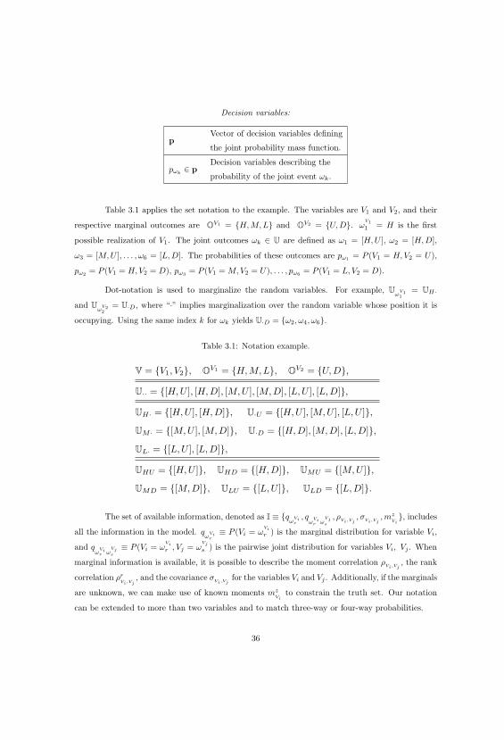
Decision variables:
pVector of decision variables defining
the joint probability mass function.
pωk∈ p
Decision variables describing the
probability of the joint event ωk.
Table 3.1 applies the set notation to the example. The variables are V1 and V2, and their
respective marginal outcomes are OV1 = {H,M,L} and O
V2 = {U, D}. ωV1
1 = H is the first
possible realization of V1. The joint outcomes ωk ∈ U are defined as ω1 = [H,U ], ω2 = [H,D],
ω3 = [M, U ], . . . , ω6 = [L, D]. The probabilities of these outcomes are pω1 = P (V1 = H,V2 = U),
pω2 = P (V1 = H,V2 = D), pω3 = P (V1 = M,V2 = U), . . . , pω6 = P (V1 = L, V2 = D).
Dot-notation is used to marginalize the random variables. For example, Uω
V11
= UH·
and Uω
V22
= U·D, where “·” implies marginalization over the random variable whose position it is
occupying. Using the same index k for ωk yields U·D = {ω2, ω4, ω6}.
Table 3.1: Notation example.
V = {V1, V2}, OV1 = {H,M,L}, O
V2 = {U, D},
U·· = {[H,U ], [H,D], [M,U ], [M,D], [L, U ], [L,D]},
UH· = {[H,U ], [H,D]}, U·U = {[H,U ], [M,U ], [L, U ]},UM · = {[M,U ], [M,D]}, U·D = {[H,D], [M,D], [L, D]},UL· = {[L,U ], [L, D]},
UHU = {[H,U ]}, UHD = {[H,D]}, UMU = {[M, U ]},UMD = {[M,D]}, ULU = {[L, U ]}, ULD = {[L,D]}.
The set of available information, denoted as I ≡ {qω
Vir
, qω
Vir ω
Vjs
, ρVi,Vj
, σVi,Vj
, mzVi}, includes
all the information in the model. qω
Vir
≡ P (Vi = ωVi
r ) is the marginal distribution for variable Vi,
and qω
Vir ω
Vjs
≡ P (Vi = ωVi
r , Vj = ωVj
s ) is the pairwise joint distribution for variables Vi, Vj . When
marginal information is available, it is possible to describe the moment correlation ρVi,Vj
, the rank
correlation ρrVi,Vj
, and the covariance σVi,Vj
for the variables Vi and Vj . Additionally, if the marginals
are unknown, we can make use of known moments mzVi
to constrain the truth set. Our notation
can be extended to more than two variables and to match three-way or four-way probabilities.
36

3.3.3 Constraints
The truth set can now be constrained to match the information provided by I. This
section presents families of equations that can be used to constrain T, creating a system of m
linear equations Ap = b and n non-negativity constraints p ≥ 0, where p = {pω1 , pω2 , . . . , pω|U|}.
A ∈ Rm×n defines the properties we want to constrain, and b ∈ R
m represents the available
information.
Matching Necessary Conditions
In all cases, the joint pmf must sum to one and each probability must be non-negative. We
represent these constraints with Equations (3.1a) and (3.1b).
∑ωk∈U
pωk= 1, (3.1a)
pωk≥ 0, ∀ωk ∈ U. (3.1b)
Equations (3.1a) through (3.1b) give the necessary and sufficient conditions for p to be a pmf
and are required in all cases. Equation (3.1a) reduces the dimension of the polytope T from n to
n − 1, and Equation (3.1b) limits T to positive quadrants. This constraint alone assures that T is
a compact set.
Matching Marginal and Pairwise Probabilities
A second set of equations is used when information is available regarding the marginal
and pairwise probabilities. Equation (3.2a) requires that the joint probabilities match the marginal
assessments, while Equation (3.2b) requires that they match pairwise joint assessments.∑ωk∈U
ωVir
pωk= q
ωVir
∀Vi ∈ V, ωVi
r ∈ OVi
, (3.2a)
∑ωk∈U
ωVir ω
Vjs
pωk= q
ωVir ω
Vjs
∀ Vi, Vj ∈ V, (ωVi
r , ωVj
s ) ∈ OVi × O
Vj
. (3.2b)
Equations (3.2a) and (3.2b) can be extended to cover three-way, four-way, or higher-order joint
probability information.
37

Equations Matching Moments
If the outcomes can be represented as numerical values instead of categorical data, moment
information can be matched using Equations (3.3a) through (3.3c). This family of equations is
useful for well-known continuous distributions, or simply when the moments are available. These
equations are always linear, making them easy to implement.∑ω
Vil∈O
Vi
[ω
Vi
l ·∑
ωk∈Uω
Vil
pωk
]= m1
Vi∀ Vi ∈ V, (3.3a)
∑ω
Vil∈O
Vi
[(ω
Vi
l )2 ·
∑ωk∈U
ωVil
pωk
]= m2
Vi∀ Vi ∈ V, (3.3b)
∑ω
Vil∈O
Vi
[(ω
Vi
l )z ·
∑ωk∈U
ωVil
pωk
]= mz
Vi∀ Vi ∈ V. (3.3c)
Equation (3.3a) matches the joint distribution with the expected value for variable Vi. Equation
(3.3b) matches the second moment and can be used to match variance if m1Vi
is known. Equation
(3.3c) is a generalization for the zth moment.
This equation can be illustrated by taking the example in Section 3.3.2 and providing
numerical values for the current outcomes {High=10, Medium=6, Low=2} and {Wet=10, Dry=1} for
V1 and V2, respectively. The first moments become:
10 ·∑
ωk∈UH
pωk+ 6 ·
∑ωk∈UM
pωk+ 2 ·
∑ωk∈UL
pωk= m1
V1,
10 ·∑
ωk∈UW
pωk+ 1 ·
∑ωk∈UD
pωk= m1
V2,
where
P (V1 = 10) =X
ωk∈UH
pωkP (V1 = 6) =
Xωk∈UM
pωkP (V1 = 2) =
Xωk∈UL
pωk,
P (V2 = 10) =X
ωk∈UW
pωkP (V2 = 1) =
Xωk∈UD
pωk.
If the marginal distributions are known, Equation 3.3 becomes redundant. However, in any
other scenario, the moment-matching family will be a relevant constraint.
38

Matching Covariance and Correlation
If the first moments for variables Vi and Vj are known, the joint distribution can be re-
stricted to match a given covariance σVi,Vj
. Moreover, the correlation can be matched if the vari-
ances for Vi and Vj are also known. Equations (3.4a) and (3.4b) match the covariance and moment
correlation, respectively.
∑ω
Vir ∈O
Vi
∑ω
Vjs ∈O
Vj
[ω
Vi
r · ωVj
s ·∑
ωk∈Uω
Vir ω
Vjs
pωk
]=σ
Vi,Vj+ m1
Vi· m1
Vj∀ Vi, Vj ∈ V, (3.4a)
∑ω
Vir ∈O
Vi
∑ω
Vjs ∈O
Vj
[ω
Vi
r · ωVj
s ·∑
ωk∈Uω
Vir ω
Vjs
pωk
]=ρ
Vi,Vj·√
σ2Vi
· σ2Vj
∀ Vi, Vj ∈ V, (3.4b)
where σ2Vi
is the variance of variable Vi, and ρVi,Vj
is the moment correlation of variables Vi and Vj .
Matching Spearman’s Correlation Coefficient
Another measure of variation that requires less information than Equations 3.4a and 3.4b,
and can be used with numerical as well as categorical information, is the Spearman’s rank correla-
tion. The rank correlation is defined as
ρrVi,Vj
=Cov(P (Vi ≤ ω
Vi
r ), P (Vj ≤ ωVj
s ))√V ar(P (Vi ≤ ω
Vi
r )) · V ar(P (Vj ≤ ωVj
s )). (3.5)
Unlike the Pearson product-moment correlation, rank correlation is invariant with respect
to the marginal outcomes. This and other characteristics make it a reliable measure of association.
(For more on rank correlation and assessment methods see Clemen and Reilly (1999) and Clemen
et al. (2000).) Rank correlation requires information only regarding the marginal probabilities for
Vi and Vj and can be described as a linear function. We start by introducing the H-volume (Nelsen,
2005) in Definition 3.3.1.
Definition 3.3.1. Let S1 and S2 be nonempty subsets of R and let H be a two-place real function,
H : R2 → R, such that DomH = S1 × S2. Let B = [x1, x2] × [y1, y2] be a rectangle all of whose
vertices are in DomH. Then, the H-volume of B is given by:
VH(B) = H(x2, y2) − H(x2, y1) − H(x1, y2) + H(x1, y1), (3.6)
39

where the first-order difference of H on B is �x2x1
H(x, y) = H(x2, y) − H(x1, y). Then, the H-
volume, VH(B), is the second-order difference of H on B.
VH(B) = �y2y1
�x2x1
H(x, y). (3.7)
Additionally, we provide a definition of the interval Iωk(Vi), in Definition 3.3.2.
Definition 3.3.2. Let ω+k (Vi) be the outcome ωVi
r of variable Vi at the joint outcome ωk and let
ω−k (Vi) be the outcome ωVi
r−1 of Vi at the joint outcome ωk. ωVi
r−1 is the outcome that precedes ωVi
r
in the marginal distribution of Vi. The cumulative probabilities that Vi is less than the outcomes
ω+k (Vi) and ω−k (Vj) are p+
k (Vi) = P (Vi ≤ ω+k (Vi)) and p−k (Vi) = P (Vi ≤ ω−k (Vi)), respectively.
These cumulative probabilities define the interval Iωk(Vi) as follows:
Iωk(Vi) ≡
[p+
k (Vi), p−k (Vi)
]. (3.8)
The intervals Iωk(Vi) and Iωk
(Vj) can be used to define a rectangular area Iωk(Vi)×Iωk
(Vj)
equivalent to B. Then, the H-volume can be used to define the rank correlation between Vi and
Vj as ∑ωk∈U
pωk
Vx2∗y2 [Iωk(Vi) × Iωk
(Vj)]
qω+k
(Vi)· qω
+k
(Vj)
=ρr
Vi,Vj+ 3
3, (3.9)
where qω+k
(Vi)= P (Vi = ω+
k (Vi)), which is the marginal probability of variable Vi having the
outcome ωVir at the joint outcome ωk. Additionally, the H-volume VH is as defined for H = x2 ·y2,
where x ∈ Iωk(Vi) and y ∈ Iωk
(Vj).
The rank correlation ρr is bounded by a scalar such that |am| < 1, where m is the maximum
number of possible outcomes of variables Vi and Vj . The bounds were proven by Mackenzie (1994)
for uniform discrete distributions. Mackenzie (1994) also proved that limm→∞ |am| = 1, meaning
that using more outcomes in each marginal distribution provides a more refined rank correlation
bounded by [-1, 1].
40

The derivation of Equation (3.9) starts from basic principles as follows:
ρrVi,Vj
+ 3 =Cov(FVi
, FVj)√
V ar(FVi) ∗ V ar(FVj
)+ 3 =
E(FVi, FVj
) − 14
112
+ 3, (3.10a)
12 · E(FVi, FVj
) =12
∫ 1
0
∫ 1
0
Vi · Vj · c(Vi, Vj) dVj dVi, (3.10b)
=12∑
ωk∈U
cωk(Vi, Vj) ·
∫ p+k
(Vi)
p−k
(Vi)
∫ p+k
(Vj)
p−k
(Vj)
Vi · Vj dVj dVi, (3.10c)
=3∑
ωk∈U
cωk(Vi, Vj)
[ [p+
k (Vi)p+k (Vj)
]2 − [p+
k (Vi)p−k (Vj)
]2− [
p−k (Vi)p+k (Vj)
]2+
[p−k (Vi)p
−k (Vj)
]2 ], (3.10d)
=3∑
ωk∈U
cωk(Vi, Vj)Vx2∗y2 [Iωk
(Vi) × Iωk(Vj)] , (3.10e)
=3∑
ωk∈U
pωk
Vx2∗y2 [Iωk(Vi) × Iωk
(Vj)]
qω+k
(Vi)· qω
+k
(Vj)
. (3.10f)
Note to Equation (3.10a) : Given FVi∼ U [0, 1], for which mean and variance are known.
Note to Equation (3.10b) : Expand the expectation.
Note to Equation (3.10c) : Create a partition of the integrals in rectangles. Set cωk(Vi, Vj) as
constant inside each rectangle (Mackenzie, 1994).
Note to Equation (3.10d) : Solve the integrals and evaluate each rectangle area.
Note to Equation (3.10e) : Substitute by the H-V olume.
Note to Equation (3.10f) : Set cωk(Vi, Vj) as in Equation 3.11.
For each rectangle area in B, the probability pωkis the volume of a body with base area qω
+k
(Vi)·
qω+k
(Vj)and height cωk
(Vi, Vj). This yields:
cωk(Vi, Vj) =
pωk
qω+k
(Vi)· qω
+k
(Vj)
. (3.11)
A similar derivation is possible for Kendall τ , but the resultant function is not linear and destroys
the convexity of the set. The derivation is presented in Appendix B.1.
41


Step 3: Choose a random direction di uniformly distributed over D.
Step 4: Find the line set L = T ∩ {x|x = xi + λdi, λ a real scalar}.
Step 5: Generate a random point uniformly distributed over xi+1 ∈ L.
Step 6: If i = N , stop. Otherwise, set i = i + 1 and return to Step 2.
HR was designed for full-dimensional polytopes. However, minor modifications allow it to
sample efficiently from non-full-dimensional sets. These modifications are presented in the following
section.
3.4.2 Sampling Non-Full-Dimensional Polytopes
As we noted in §3.3.3, the characterization of T describes the polytope as a system of m
linear equations and n non-negative variables: Ap = b, p ≥ 0. The HR sampler is designed to
sample points in full-dimensional polytopes. However, the polytope T is not full-dimensional, since
h = n − m < n. To overcome this problem, the projection of p ∈ Rn into the hyperplane Ap = b
is found using Equation (3.12), where I represents the identity matrix.
p = (I − AT (AAT )−1A)p + AT (AAT )−1b (3.12)
Then, a hypersphere D ∈ Rn in the full-dimensional space can be created by sampling independent
vectors of size n from the multivariate standard normal and normalizing them so that each vector
has equal magnitude. Using Equation 3.12, the direction set D can be projected into T. With
the proper scaling, the final result is a set of directions D ∈ T from which uniformly distributed
directions can be selected. The line L is created by extending the directions ±di ∈ D until p ≥ 0
is violated. The rest of the implementation is straightforward.
This step removes the non-full-dimensional problem by reducing the dimension from n to
n − m for all the steps that require this. T can now be treated as a full-dimensional polytope in
n − m dimensions.
3.4.3 Stopping Time
HR guarantees that the sampled collection eventually converges to the uniform distribution
over T (Smith, 1984). However, as pointed by Rubin (1984), the theoretical number of required
43
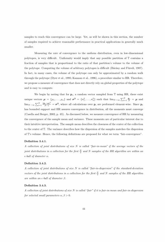
samples to reach this convergence can be large. Yet, as will be shown in this section, the number
of samples required to achieve reasonable performance in practical applications in generally much
smaller.
Measuring the rate of convergence to the uniform distribution, even in low-dimensional
polytopes, is very difficult. Uniformity would imply that any possible partition of T contains a
fraction of samples that is proportional to the ratio of that partition’s volume to the volume of
the polytope. Computing the volume of arbitrary polytopes is difficult (Barany and Furedi, 1987).
In fact, in many cases, the volume of the polytope can only be approximated by a random walk
through the polytope (Dyer et al., 1995; Kannan et al., 1996), a procedure similar to HR. Therefore,
we propose a measure of convergence that does not directly rely on global properties of the polytope
and is easy to compute.
We begin by noting that for pi, a random vector sampled from T using HR, there exist
unique vectors μ = {μ1, . . . , μn} and σ2 = {σ21 , . . . , σ2
n} such that limN→∞∑N
i=1pi
N= μ and
limN→∞∑N
i=1(pi−μ)2
N−1 = σ2, where all calculations over pi are performed element-wise. Since pi
has bounded support and HR assures convergence in distribution, all the moments must converge
(Casella and Berger, 2002, p. 65). As discussed below, we measure convergence of HR by measuring
the convergence of the sample mean and variance. These moments are of particular interest due to
their intuitive interpretation. The sample mean describes the closeness of the center of the collection
to the center of T. The variance describes how the dispersion of the samples matches the dispersion
of T’s volume. Hence, the following definitions are proposed for what we term “fair-convergence”.
Definition 3.4.1.
A collection of joint distributions of size N is called “fair-in-mean” if the average vectors of the
joint distributions in a collection for the first N2 and N samples of the HR algorithm are within an
ε-ball of diameter α.
Definition 3.4.2.
A collection of joint distributions of size N is called “fair-in-dispersion” if the standard-deviation
vectors of the joint distributions in a collection for the first N2 and N samples of the HR algorithm
are within an ε-ball of diameter β.
Definition 3.4.3.
A collection of joint distributions of size N is called “fair” if it is fair-in-mean and fair-in-dispersion
for selected small parameters α, β > 0.
44

These definitions have been expressed in Equations (3.13) and (3.14), where pi is the ith
sampled discrete probability distribution with n joint elements. To make notation easier, we use pi
and assume all calculations are performed element-wise except for || · ||2. Equation (3.13) computes
the average of the collection sampled after N iterations (∑N
i=1pi
N) and compares it to the average
after N2 iterations. If after N iterations the vector of averages is within an ε-ball of diameter α of
the previous vector (for some small α > 0), the sample is assumed to be fair-in-mean.
Equation (3.14) is the equivalent version for the variance, where
(∑N
j=1 pi − pj)2 = (Npi −
∑N
j=1 pj)2 = N2(pi −
PNj=1 pj
N)2 = N2(pi − μ)2
and where μ is the vector of averages for each joint element of the sample. Similarly, if after N
iterations the new vector of variances is within a ε-ball of diameter β of the previous vector (for
some small β > 0), the sample is assumed to be fair-in-dispersion.
∣∣∣∣∣∣∣∣∣∣
N∑i=1
pi
N−
N2∑
i=1
2 · pi
N
∣∣∣∣∣∣∣∣∣∣2
≤ α (3.13)
∣∣∣∣∣∣∣∣∣∣
N∑i=1
(∑N
j=1 pi − pj)2
N − 1−
N2∑
i=1
4 · (∑N2
j=1 pi − pj)2
(N2 − 1)
∣∣∣∣∣∣∣∣∣∣2
≤ β · N2 (3.14)
The implementation of this stopping time for the mean can be performed by keeping
track of∑N
i=1 pi at each iteration and dividing it by the number of samples at each checkpoint.
Additionally, using the recursion in Equation (3.15), we can keep track of the variance of each joint
element at each iteration.
(i − 1)σ2w,(i) = (i − 2)σ2
w,(i−1) +
(f(i)
i· f(i)
i − 1
),
f(i) =i−1∑j=1
pjw − (i − 1)pi
w ∀ i = 2, 3, . . . , N.
(3.15a)
σ2w,(1) = 0, ∀ w ∈ {1, 2, . . . , n}. (3.15b)
Our experience suggests that the number of samples required for fair convergence is on the
order of ≈ 109 of the theoretical lower bound of Lovasz (1998) (Appendix B.2). As an example,
Figure 3.4 and Table B.1 (Appendix B.2) provides illustrative results for fair convergence in six
unconstrained polytopes (Equation 3.1 only) of different dimensions.
45
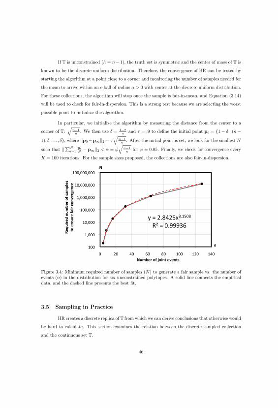
If T is unconstrained (h = n− 1), the truth set is symmetric and the center of mass of T is
known to be the discrete uniform distribution. Therefore, the convergence of HR can be tested by
starting the algorithm at a point close to a corner and monitoring the number of samples needed for
the mean to arrive within an ε-ball of radius α > 0 with center at the discrete uniform distribution.
For these collections, the algorithm will stop once the sample is fair-in-mean, and Equation (3.14)
will be used to check for fair-in-dispersion. This is a strong test because we are selecting the worst
possible point to initialize the algorithm.
In particular, we initialize the algorithm by measuring the distance from the center to a
corner of T:√
n−1n
. We then use δ = 1−τn
and τ = .9 to define the initial point p0 = {1 − δ · (n −1), δ, . . . , δ}, where ||p0 −p∞||2 = τ
√n−1
n. After the initial point is set, we look for the smallest N
such that ||∑N
i=1pi
N− p∞||2 < α = ϕ
√n−1
nfor ϕ = 0.05. Finally, we check for convergence every
K = 100 iterations. For the sample sizes proposed, the collections are also fair-in-dispersion.
Figure 3.4: Minimum required number of samples (N) to generate a fair sample vs. the number ofevents (n) in the distribution for six unconstrained polytopes. A solid line connects the empiricaldata, and the dashed line presents the best fit.
3.5 Sampling in Practice
HR creates a discrete replica of T from which we can derive conclusions that otherwise would
be hard to calculate. This section examines the relation between the discrete sampled collection
and the continuous set T.
46

To illustrate this relation, consider an unconstrained set T generated by a single random
variable with three outcomes p = {p1, p2, p3}. The set is a two-dimensional simplex (h = 2) located
in a three-dimensional coordinate system. The h-content of T is√
32 , and its projection into the
hyper-plane generated by {p ∈ T|p1, p2 ≥ 0, p3 = 0} has an h-content of 12 .
The integral of f(p1p2) = 1 − p1 − p2, along the projection of T is the volume under T,
which is known to be 13! , and is calculated as
V ol(T<1) =
∫ 1
0
∫ 1−p1
0
1 − p1 − p2 dp2 dp1 =1
3!= 0.166667.
Approximating the volume using N = 10, 000 samples created with HR yields the following:
V ol(T<1N ) =N∑
i=1
1 − pi1 − pi
2
2 · N = 0.167602,
where pi = {pi1, pi
2, pi3} is the ith distribution in the sample. For N = 10, 000, the original volume
is close to the approximate volume V ol(T<1) ≈ V ol(T<1N ). Alternative values of N = 1000
(N = 100, 000) yield V ol(T<1N ) = 0.16573 (0.166674). As N → ∞, V ol(T<1N ) → V ol(T<1),
which is granted by the definition of an integral (Strichartz, 2000).
The discrete approximation will now be examined under two measures of accuracy: Kullback-
Leibler divergence (KL), defined in Equation 3.16, and quadratic variation (QV), defined in Equa-
tion 3.17.
KLn(p||p) =n−1∑i=1
pi log
(pi
pi
)+ (1 −
n−1∑i=1
pi) log
(1 − ∑n−1
i=1 pi
1 − ∑n−1i=1 pi
), (3.16)
QVn(p, p) =
n−1∑i=1
|pi − pi|2 +∣∣∣ n−1∑
i=1
pi − pi
∣∣∣2. (3.17)
Both measures can be integrated numerically for the continuous case, and approximated
by sampling uniformly as follows:
∫ 1
0
∫ 1−p1
0
KLn(p||p) dp2 dp1 ≈N∑
k=1
KLn(pk||p) · 1
N · n!, (3.18)
∫ 1
0
∫ 1−p1
0
QVn(p, p) dp2 dp1 ≈N∑
k=1
QVn(pk, p) · 1
N · n!. (3.19)
47

Table 3.2 presents the results for both measures considering different values for N , where p =
{ 1n, . . . , 1
n} is the discrete uniform distribution.
Table 3.2: Discrete approximations for different values of N and its continuous measures.
Discrete Set KL3(p||p) QV3(p, p)N=10 0.158543 0.061775N=100 0.162837 0.067702N=1,000 0.182989 0.079307N=10,000 0.186991 0.081201N=100,000 0.183113 0.079546N=1,000,000 0.183643 0.079775
Continuous Set 0.191358 0.083333
As N increases, the discrete approximation gets closer to the continuous measure from
below. This behavior is explained by the convexity of the accuracy measures that reach their
maxima in the neighborhood of the vertices of T, where HR takes longer to sample (see Section
3.6). For large enough N , the collection sample converges to the uniform distribution over T, and
the gap between the discrete approximation and the continuous measure decreases. The reduction
of the gap is not a monotonic function of N because the sample has a random component, which
explains the decrease for N = 100, 000 in Table 3.2.
3.6 The Sea Urchin Effect
The spread of the volume in T causes an interesting and non-intuitive behavior, which is
reflected in HR’s sampled collection. Observing the Euclidean distance from the center of T to all
other joint distributions in the collection reveals that the collection becames more concentrated as
the dimension of the polytope increases. For example, consider three unconstrained polytopes of
dimensions 7, 31, and 127 generated using 3, 5, and 7 binary marginal random variables, respectively.
Measuring 20,000 samples in each polytope shows that the range of measures of the Euclidean
distance from the discrete uniform distribution on the first set (Figure 3.5(a)) goes from 0.1 to
0.65. In contrast, for the second and third sets (Figures 3.5(b) and 3.5(c)), the range goes from
0.07 to 0.25 and 0.05 to 0.1, respectively. At first sight, the algorithm’s sample appears to become
deficient as dimensionality increases. However, this effect is rather explained by the spread of the
volume in T.
48

(a) Three Variables. (b) Five Variables. (c) Seven Variables.
Figure 3.5: HR: Norm distance from the center of T. All variables are binary.
The distributions in Figure 3.5 yield the histograms shown in Figure 3.6. These figures
have been replicated in Appendix A Figure A.1 for marginal variables with three outcomes.
(a) Three Variables. (b) Five Variables. (c) Seven Variables.
Figure 3.6: HR histogram for the norm distance from the center of T. All variables are binary.
The increase in dimension of different geometric bodies may have unexpected results. For
example, in a hyper-cube, an increase in dimension pushes a large portion of the volume into the
corners. In the case of a hyper-sphere or a hyper-ellipsoid, a similar increase pushes the volume
into the outside shell of the geometric figure (Jimenez and Landgrebe, 1998). In the case of an
unconstrained polytope T, most of the volume mass is pushed away from the center and the corners,
becoming concentrated in the middle region.
To analyze the spread of the volume over T, we create a partition of an unconstrained
polytope (a unit simplex) from a corner to its base along the height (H), each cut’s being done at
equidistant steps as shown in Figure 3.7(a). Each part in the partition has volume V ol(Ti), and
the summation over a portion of the partition∑i
k=1 V ol(Tk) is the volume of the shadow area in
Figure 3.7(b), generated by a single cut of T perpendicular to H at a distance iSH, where S is the
total number of parts in the partition.
49


and with a cavity in the nucleus. This effect is generated by the volume dispersion and does not
change the basic properties of T such as convexity, compactness, and continuity.
The sea urchin effect challenges our intuition; adding more joint events into a distribution
increases the set of distributions that match the available information. However, the volume of
the set is more concentrated. This apparent paradox is resolved by observing that even though
T is larger, the n-content (the relative-interior volume) decreases, and the proportional volume in
the corners and the center decays faster, which results in a higher concentration of volume close
to the outside shell of the maximum-volume inner sphere. For example, consider the volume of
an unconstrained set V ol(T) =√
n+1n! , and let n → ∞. Then, even though we are considering the
largest possible set of joint distributions, every possible joint distribution exists in a neighborhood
with zero volume.
51

Chapter 4
Measures of Accuracy
The previous two chapters presented several joint probability distribution approximations
and a sampling methodology to create a collection of joint distributions that serves as a discrete
representation of the set T. This chapter presents a framework to compare the distribution approx-
imations to the sampled collection using a family of functions named “measures of accuracy.”
The five measures of accuracy proposed here are strict quasi-convex Lyapunov functions.
That is, the accuracy measures are monotonically increasing and positive everywhere, except for
one inflection point p∗A = qi, which has zero value. Many functions with these characteristics can
be used to define accuracy. However, those discussed here were chosen for their usefulness and
intuitive appeal.
• Maximum Absolute Difference.
• Total Variation.
• Euclidean Distance.
• Kullback−Leibler Divergence.
• χ2 Distance.
The first three measures of accuracy, maximum absolute difference, total variation, and
Euclidean distance, are also metrics and can be interpreted as distances in the interior of the truth
set. Kullback−Leibler divergence is not a metric because it does not follow the triangle inequality
and is not symmetric. However, it measures the difference on the number of information units
(bits) required to encode the outcome of a distribution qi given the assumption that the actual
distribution is p∗A. The χ2 distance is also not a metric, because it is not symmetric, but it is
commonly used in statistics and has an interpretation through the χ2 distribution.
In addition to these measures, we include the difference of entropy between the approxima-
tion and the samples in the collection. This is not formally a measure of accuracy, but it provides
a direct evaluation of the difference between the probabilistic dependence of two distributions.
Some of these measures of accuracy have been used in the literature. The maximum
absolute difference, the total variation, and KL divergence have been used in Abbas (2006) and
Bickel and Smith (2006) to measure differences among discrete probability distributions.
52

4.1 Proposed Measures of Accuracy
We begin by formalizing the meaning of measures of accuracy using definition 4.1.1.
Definition 4.1.1. Let M : Rn → R be a scalar function. M is a “measure of accuracy” if for
any two joint probability distributions, p = {p1, p2, · · · , pn} ∈ T ⊂ Rn, an arbitrary distribution in
the truth set, and p = {p1, p2, · · · , pn}, a distribution approximation, the following hold:
M(p, p) = 0 ∀ p = p. (4.1)
M(p, p) < M(p + αd, p) ∀ p �= p, d = (p − p), α > 0. (4.2)
This definition will be used to propose the following measures of accuracy.
4.1.1 Maximum Absolute Difference
The maximum absolute difference is also known as the L∞-Norm of f(i) = (pi − pi) for
i = 1, . . . , n and can be expressed as:
L∞n (p, p) = max{|p1 − p1|, · · · , |pn − pn|}, (4.3)
where p = {p1, p2, · · · , pn} ∈ T is any arbitrary distribution in the truth set, and p = {p1, p2, · · · , pn}is the approximation of interest.
L∞ is directly related to the Kolmogorov-Smirnov distance and has an important interpre-
tation under the two-sample Kolmogorov-Smirnov test, which measures the difference between two
empirical distributions p and p and shows statistical significance if√
n2 · L∞n > Kα, where the Kα
statistic comes from Pr(k ≤ Kα) = 1 − α and is distributed as:
Pr(k ≤ Kα) =
√2π
k
∞∑i=1
e−(2i−1)2π2
8k2 . (4.4)
The measure is bounded by 0 ≤ L∞n ≤ min{1,L1
n
2 }, where L1n is the L1-Norm, also known as total
variation.
53

4.1.2 Total Variation
Total Variation measures the sum of the absolute differences. It is also known as L1-Norm
of f(i) for i = 1, . . . , n and can be expressed as
L1n(p, p) =
n∑i=1
|pi − pi|. (4.5)
The L1-Norm between two distributions is zero if and only if the two distributions are
identical. This measure has a special relevance when consider the subspace where T is located,
because it is a natural metric for an n-polytope. Moreover, it constitutes a useful mathematical
tool to define bounds. For example, in Kullback (1967), a lower bound for KLn(p||p) was defined
in terms of the total variation as
KLn(p||p) ≥ L1n(p, p) − log (1 + L1
n(p, p)). (4.6)
Devroye and Lugosi (2000) presented an upper bound for L∞ as a function of L1:
L∞n (p, p) ≤ L1n(p, p)
2. (4.7)
Finally, L1 is invariant to the dimension of the vector p. Hence, it is more stable than the average
absolute distanceL1
n
nyet provides equivalent information.
4.1.3 Euclidean Distance
Using T as a framework, we can think of the direct distance between two points inside
a polyhedron. The Euclidean distance, also known as the L2-Norm (Bertsekas, 1999), measures
the length of the straight line connecting any two points (joint distributions in our setting). L2 is
defined as
L2n(p, p) =
[n∑
i=1
(pi − pi)2
] 12
. (4.8)
L2-Norm describes how an approximate distribution is related to the set T in a spherical
topology with center in p. The maximum and average distance from p to any arbitrary distribution
p in a sampled collection is defined as
54

maxp∈T
L2n(p, p) Ep∼U(T)
[L2
n(p, p)]. (4.9)
The level sets of L2 are defined as
L2α(p) = { p | L2
n(p, p)) ≤ α} (4.10)
for radius α. These sets help to calculate probabilities of different neighborhoods of p using the
frequencies generated by the sample of T.
4.1.4 Kullback-Leibler Divergence
Proposed by Kullback and Leibler (1951), Kullback-Leibler Divergence (KL) measures the
divergence or loss of information from the sampled distribution p to the approximation p. KL is
bounded below by zero, and the bound is tight if and only if p = p. KL Divergence is defined as:
KLn(p||p) =n∑
i=1
pi log
(pi
pi
). (4.11)
An intuitive expression for this measure is
KLn(p||p) =n∑
i=1
pi ln
(1
pi
)−
(−
n∑i=1
pi ln pi
)(4.12)
= Ep
[ln
(1
p
)]− H(p) ≥ 0. (4.13)
Then, if entropy (H) is the expected value on the number of bits necessary to encode a distribution.
KLn(p||p) is the expected number of “penalty” bits as a result of confusing p with p. In other
words, it is the increase in descriptive complexity due to incorrect information.
Given that limpi→0 Ep[ln 1p] = ∞, any approximation distribution needs to be in the interior
of T. That is, it can not contain elements equal to zero. As before, it is possible to observe values
for
maxp∈T
KLn(p||p) Ep∼U(T)
[KLn(p||p)
]. (4.14)
These values describe the maximum and average behavior of the penalties generated by choosing
55

p instead of a possible true distribution p. We can also observe the level sets:
KLα(p) = { p | KLn(p||p) ≤ α}. (4.15)
4.1.5 χ2 Distance
Correspondence analysis shows where the joint outcomes of p work as factors where the
probabilities describe attraction or rejection among outcomes. Then, the natural distance between
distributions is the χ2 distance. The name of this measure comes from the “Goodness-of-fit χ2
Test.” Here, the expected probabilities comprise the approximated distribution p. The χ2 distance
is defined as
χ2n(p, p) =
n∑i=1
(pi − pi)2
pi
. (4.16)
The measure provided by this metric can be interpreted as a standardized quadratic varia-
tion QVn(p, p), where outcomes with low expected probability are more unstable. This metric has
zero value if and only if p = p, and as a statistic, the χ2n(p, p) distance is distributed as χ2 with
n − m − 1, where m is the number of constraints in T.
4.1.6 Entropy Difference
As mentioned, entropy difference is not formally a measure of accuracy. However, it pro-
vides insight when we consider the description of the outcomes using two different distributions.
Proposed by Kullback and Leibler (1951) and later by Jaynes (1982), entropy difference
measures the expected value of the number of bits necessary to encode the outcomes of a distribu-
tion. Entropy difference is defined as
Hn(p) = −n∑
i=1
pi log(pi). (4.17)
Entropy difference is bounded by 0 ≤ Hn(p) ≤ ln(n), where the lower bound is reached for p =
{1, 0, · · · , 0} and the upper bound is reached for p = { 1n, · · · , 1
n}. Some values of interest for H are
maxp∈T
H(p), minp∈T
H(p), Ep∼U(T)
[H(p)
]. (4.18)
56

Based on H, the entropy difference for two distributions can be represented as
ΔH(p, p) = Hn(p) − Hn(p). (4.19)
This measure is bounded by −Hmax ≤ ΔH(p, p) ≤ Hmax, where ΔH(p, p) allows for negative
values. Positive values of ΔH indicate that the information structure of p is closer to uniform than
p, whereas negative values of ΔH imply that the information structure is farther from uniform.
Some values of interest are
maxp∈T
ΔH(p, p), minp∈T
ΔH(p, p), Ep∼U(T)
[ΔH(p, p)
]. (4.20)
4.2 Illustration
We now provide a small visualization of the measures of accuracy. For this purpose, we use
a binary random variable with estimated distribution p = {q1, 1− q1}. The estimated distribution
is compared then to all possible distributions p = {p1, 1 − p1}. We consider five different values of
q1: {0.1, 0.3, 0.5, 0.7, 0.9}, where p1 may range in the interval [0, 1].
Figure 4.1 shows the behavior of the measures in a binary setup with no assessment con-
straints. The measures are symmetric, convex, and except for Figure 4.1(e), (ΔH) are always
positive. An interesting characteristic of the first three measures is the linear shape, which can be
interpreted as alternative measures of distance from p to p. In contrast, the last three measures
show a non-linear behavior, which is related to the logarithmic nature of the information and the
rescale by p in the case of the χ2.
As shown in Figures 4.1(d) and 4.1(f), KL and χ2 distance are the most sensitive to extreme
values of p. In fact, these measures are undefined (∞) for p in the boundary of T. χ2 distance is
the most unstable of them all. Whereas, maximum absolute difference is the most stable one.
57


Chapter 5
Accuracy of Joint Probability Approximations
In this chapter, we test the accuracy of different approximations of joint distributions
described in Chapter 2, starting with known distribution families and gradually increasing their
complexity and generality. In §5.1, we test the Hypergeometric and Multinomial Families. In §5.2,
we test unconstrained truth sets and analyze the effects of increasing the number of random variables
and the number of outcomes. We also test the accuracy of sets having symmetric constraints
(e.g., equal marginal probabilities, or equal pairwise correlations). In §5.3, we test for effects of
adding constraints and of changing existing constraints. In §5.4, we test the accuracy of arbitrarily
constrained polytopes, the most general case, using marginal and rank correlation constraints and
generate random assessments.
The results presented in this chapter are based on the approximation methods, simulation
procedure, and measures of accuracy defined in Chapters 2, 3, and 4 respectively.
5.1 Selected Families of Multivariate Distributions
We start by measuring the differences between well-known multivariate distributions and
the approximations. Rather than use HR sampling, we create a sample from the respective family,
extract the marginal assessments, derive the distribution approximations, and measure the accuracy.
A similar comparison was done by Abbas (2006) and Bickel and Smith (2006) for a random set of
distributions based on binary variables.
We now extend the results from Abbas and from Bickel and Smith to observe how the
proposed approximations behave with respect to a known family of discrete joint distributions. We
have chosen two families of distributions with discrete and finite support: the hypergeometric and
multinomial distributions. These multivariate families allow us to control the number of outcomes
and permit some control over the probabilistic dependence in the distributions.
59

5.1.1 Approximating the Hypergeometric Joint Distribution
Generation of Hypergeometric Distributions: We consider the multivariate hypergeometric
distribution, which can be intuitively understood using urns and balls, as follows. For an urn with
a total of N balls, where the balls are of c different colors {Red, Green, Yellow,...}, there are mi
balls of color i = 1,...,c, where i = 1 represents Red, i = 2 represents Green, and so on. Then, if we
take n ≤ N balls from the urn, the hypergeometric distribution describes the probability of having
x1 Red balls, x2 Green balls, and so on. The different colors represent different variables, where
variable xi is bounded by [0, min (n, mi)].
To create an arbitrary hypergeometric distribution, we need to choose the number of colors
c and the number of balls taken n. We then randomly define mi for i = 1, 2, . . . , c using non-negative
integers, and set N =∑c
i mi. The joint probability mass function is defined as:
P (X1 = x1, X2 = x2, . . . , Xc = xc) =
(m1
x1
) · (m2
x2
). . .
(mc
xc
)(Nn
) .
We now provide an example of a specific hypergeometric distribution and the approxima-
tions derived from it using only marginal assessment information. Then, we present the accuracy
results for a large number of randomly generated hypergeometric distributions.
Procedure Example. An instance of a hypergeometric distribution for c = 3 and n = 8 is
presented in Table 5.1, which includes four approximations generated using only marginal infor-
mation taken from the original hypergeometric distribution. The first three columns in the table
describe the joint events of the distribution. The first event consists of selecting 8 Red balls from
the urn. The fourth column contains the probabilities of the joint events under the hypergeometric
distribution. For example, the probability of drawing 8 Red balls is 0.0004. Columns 5 to 8 are
approximations to the hypergeometric distribution. For each approximation, we calculate the prob-
abilities of the marginal events and use this information with the algorithms in Chapter 2. Each
of the approximations is distinct, even though they use the same information. These differences
are generated by assumptions made by each model. One objective of this work is to find which
assumptions provide better approximations.
In this instance, the maximum entropy (ME) approximation replicates exactly the original
distribution using only marginal information. This result will later be confirmed for a larger number
of samples. This shows that the hypergeometric family is the maximum entropy distribution.
Nonetheless, because of the hypergeometric distribution’s structure, it does not have independent
60

Table 5.1: Hypergeometric Distribution and Approximations.
Joint Events Probability Distributions
Red Green YellowHypergeometric
AC ChSC MVIE MEDistribution
8 0 0 0.00040 0.00040 0.00040 0.00040 0.00040
7 1 0 0.00290 0.00270 0.00270 0.00340 0.00290
7 0 1 0.00670 0.00680 0.00680 0.00610 0.00670
6 2 0 0.00500 0.00380 0.00380 0.00330 0.00500
6 1 1 0.03500 0.03290 0.03330 0.03590 0.03500
6 0 2 0.03500 0.03830 0.03790 0.03580 0.03500
5 3 0 0.00200 0.00330 0.00330 0.00310 0.00200
5 2 1 0.04200 0.04240 0.04220 0.03930 0.04200
5 1 2 0.12600 0.12900 0.12870 0.13430 0.12600
5 0 3 0.07000 0.06530 0.06580 0.06330 0.07000
4 3 1 0.01170 0.01320 0.01300 0.01410 0.01170
4 2 2 0.10500 0.10320 0.10360 0.10190 0.10500
4 1 3 0.17500 0.17670 0.17640 0.17080 0.17500
4 0 4 0.05830 0.05700 0.05710 0.06330 0.05830
3 3 2 0.02000 0.01560 0.01590 0.01410 0.02000
3 2 3 0.10000 0.10240 0.10230 0.10940 0.10000
3 1 4 0.10000 0.09930 0.09950 0.09470 0.10000
3 0 5 0.02000 0.02270 0.02250 0.02190 0.02000
2 3 3 0.01250 0.01320 0.01310 0.01410 0.01250
2 2 4 0.03750 0.03860 0.03850 0.03690 0.03750
2 1 5 0.02250 0.02070 0.02090 0.02190 0.02250
2 0 6 0.00250 0.00250 0.00250 0.00210 0.00250
1 3 4 0.00280 0.00370 0.00370 0.00370 0.00280
1 2 5 0.00500 0.00410 0.00420 0.00370 0.00500
1 1 6 0.00170 0.00170 0.00160 0.00210 0.00170
1 0 7 0.00010 0.00010 0.00010 0.00010 0.00010
0 3 5 0.00020 0.00020 0.00010 0.00020 0.00020
0 2 6 0.00020 0.00020 0.00020 0.00020 0.00020
0 1 7 0.00001 0.00001 0.00010 0.00010 0.00001
61

marginal variables. The comparison among these approximation distributions shows the effects of
the different assumptions in the model. For example, the analytic center (AC), Chebyshev’s center,
(ChSC) and maximum volume inscribed ellipsoid center (MVIE) create distributions that imply
higher probabilistic dependence.
This example is consistent with more general scenarios. In particular, we analyze three
sets with parameters c= 4, 5, and 6 (marginal variables), where each variable can have up to m=4,
3, and 8 different outcomes, respectively. For each of these sets we examine 100 hypergeomet-
ric distributions and observe the performance of the approximations with respect to the original
distribution.
Accuracy Results. Figure 5.1 shows the results for four approximations, each evaluated under
six measures (similar figures for five and six variables are shown in Appendix C, Figure C.1 and
C.3). Each sub-figure shows the results for a measure.
As with the initial example, ME matches the original distribution 100% of the time under
every measure used. The same behavior can be observed with five and six variables (see Appendix
C). As mentioned before, the hypergeometric family is the ME distribution with respect to the
sets generated with marginal information. In contrast, Figure 5.1 shows MVIE to have the worst
performance of all, which suggests that the center defined by the maximum volume inscribed
ellipsoid is far from the point of maximum entropy in the set defined by the marginal assessments.
Figure 5.2 shows the histograms for each approximation and each measure. The histograms
show the frequency of the measures for each approximation. Again, for all measures, the ME
approximation provides values close to zero (10−15), while the MVIE shows measures distributed
over a higher range of values. Finally, the AC and ChSC approximations show results close to each
other. Table 5.2 presents the percentage of time each approximation is the best, second best, third
best, and worst. Although the difference between ChSC and the AC is small in this particular case,
the former is slightly better about 80% of the time.
When the same experiment is run for different values of parameters c and n (Appendix C,
Figures C.2 and C.4, and Tables C.1 and C.2), the AC and the ChSC approximations sometimes
interchange, depending on the structure of the family studied. However, the ME approximation
clearly dominates the other three, whereas the MVIE center is clearly the weakest approximation.
Although neither the ChSC nor the AC dominates the other, the ChSC, being a linear
model, runs faster than the AC, which becomes unstable when variables take values close to zero.
Also, the ChSC model is easier to implement and requires fewer iteration adjustments.
62
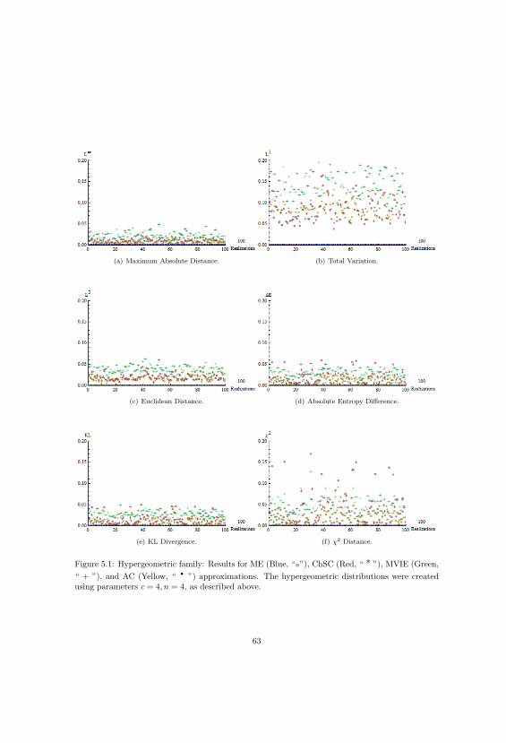
(a) Maximum Absolute Distance. (b) Total Variation.
(c) Euclidean Distance. (d) Absolute Entropy Difference.
(e) KL Divergence. (f) χ2 Distance.
Figure 5.1: Hypergeometric family: Results for ME (Blue, “@”), ChSC (Red, “ * ”), MVIE (Green,
“ + ”), and AC (Yellow, “ · ”) approximations. The hypergeometric distributions were createdusing parameters c = 4, n = 4, as described above.
63

(a) ME, L∞. (b) AC, L
∞. (c) ChSC, L∞. (d) MVIE, L
∞.
(e) ME, L1. (f) AC, L
1. (g) ChSC, L1. (h) MVIE, L
1.
(i) ME, L2. (j) AC, L
2. (k) ChSC, L2. (l) MVIE, L
2.
(m) ME, |ΔH|. (n) AC, |ΔH|. (o) ChSC, |ΔH|. (p) MVIE, |ΔH|.
(q) ME, KL. (r) AC, KL. (s) ChSC, KL. (t) MVIE, KL.
(u) ME, χ2. (v) AC, χ2. (w) ChSC, χ2. (x) MVIE, χ2.
Figure 5.2: Hypergeometric family histograms. From left to right, ME, AC, ChSC, and MVIE.From top to bottom, L∞, L1, L2, ΔH, KL, and χ2 distance measures.
64

Table 5.2: Percentage of hypergeometric distributions for which a given approximation obtained a given
ranking for a given measure, with parameters c = 4, n = 4.
% of distributions % of distributions % of distributions % of distributions
Approximation Measure Best Second best Third best Worst
ME
L∞ 100 0 0 0
L1 100 0 0 0
L2 100 0 0 0
|ΔH| 100 0 0 0
KL 100 0 0 0
χ2 100 0 0 0
AC
L∞ 0 13 87 0
L1 0 15 85 0
L2 0 15 85 0
|ΔH| 0 34 66 0
KL 0 22 78 0
χ2 0 50 50 0
ChSC
L∞ 0 86 6 8
L1 0 85 7 8
L2 0 85 7 8
|ΔH| 0 66 23 11
KL 0 78 12 10
χ2 0 50 28 22
MVIE
L∞ 0 1 7 92
L1 0 0 8 92
L2 0 0 8 92
|ΔH| 0 0 11 89
KL 0 0 10 90
χ2 0 0 22 78
Comparing Figure 5.3 to Figures 5.1(d) and 5.2(m) shows the degradation of the algorithms
with respect to the number of joint events. First, the ME approximation fails to replicate exactly the
hypergeometric distribution (Figure 5.3(b)), instead creating a distribution with less entropy than
the original, showing that the precision of the algorithms falters for large problems. In particular,
this last scenario has a total of 1,231 joint events and a variable for each event, which represents
a large problem for a non-linear model. In addition, the MVIE (not shown) shows to be sensitive
to increments in problem size, e.g., for c = 6, n = 8, obtaining a solution would have taken a large
amount of time.
65

(a) Absolute Entropy Difference. (b) Entropy, |ΔH|.
Figure 5.3: Hypergeometric family scatterplot and histogram using |ΔH| for distributions createdusing parameters c = 6, n = 8. (a) Scatterplot results for ME (Blue, “@”), ChSC (Red, “ * ”),
MVIE (unable to calculate), and AC (Yellow, “ · ”) approximations. (b) Histogram for the MEapproximation.
Summary of Accuracy Results. The data resulting from the above tests are now summarized
by presenting the mean and standard deviations of the measures of accuracy.
Figure 5.4 shows the aggregate mean for three scenarios: [c = 4, n = 4], [c = 5, n = 3], and
[c = 6, n = 8]. The results are shown using the mean and standard deviation for all approximation
distributions as proportions, i.e.,
p(·)
KL = 100 · KL(·)
KLE + KLAC + KLChSV + KLMV IE. (5.1)
Figure 5.4 shows that ME replicates the original distribution 100% of the time, having
proportion pE(·)
= 0 for any measure. The AC is shown to have similar characteristics to the ChSC.
On average, the worst results come from the MVIE approximation. The MVIE in scenario 3 was
not calculated due to long running times.
Table 5.2 and Figure 5.4 provide different conclusions about the accuracy of some of the
approximations. The percentage of accuracy describes which distribution is closest to the original
without regard of the magnitude of the error, whereas the mean proportion of accuracy describes
the error in relation to the magnitude of all the approximations. This explains the behavior of
|ΔH| in scenario 1 and χ2 in scenario 2 with respect to AC and ChSC approximations.
66

Mean Proportions of Accuracy
(a) Scenario 1. (c = 4, n = 4) (b) Scenario 2. (c = 5, n = 3) (c) Scenario 3. (c = 6, n = 8)
Figure 5.4: Hypergeometric family: Results for ME, AC, ChSC, and MVIE, in three scenarios observing
the mean proportion p(·)
KL= 100 · KL
(·)
KLE+KLAC+KLChSV +KLMV IE.
The standard deviation (SD) of the proposed measures is shown in Figure 5.5. As with the
mean proportions, ME matches the original approximation almost all the time. The dispersion of
the measures of accuracy corresponds to Figure 5.1. The SDs of AC, ChSC, and MVIE are similar.
However, the approximation with the worst accuracy (MVIE) is not always the one with the most
variation.
Standard Deviation
(a) Scenario 1. (c = 4, n = 4) (b) Scenario 2. (c = 5, n = 3) (c) Scenario 3. (c = 6, n = 8)
Figure 5.5: Hypergeometric family: Standard deviation for ME, AC, ChSC, and MVIE for each measure..
5.1.2 Approximating the Multinomial Joint Distribution
Generation of Multinomial Distributions. The multinomial distribution is an extension of
the binomial distribution, where we count the number of successful trials from n attempts. We can
think of it as taking n balls from an urn one at a time, and returning each ball before taking the
next one. Then the probability of a ball’s being red, for example, is constant for all trials. In the
multinomial distribution, we extend the concept of success used in the binomial distribution: if the
balls’ colors are {Red, Green, Yellow,...}, then we count the number of Reds, Greens, and so on.
67

As with the hypergeometric distribution, the different colors represent different random variables,
where each variable is bounded by [0, n].
An arbitrary multinomial distribution can be created by choosing the number of colors c
and the number of balls taken n. pi would be randomly defined for i = 1, 2, . . . , c using random
numbers in the interval [ 0 , 1 ] such that∑c
i pi = 1. The joint probability is defined as:
P (X1 = x1, X2 = x2, . . . , Xc = xc) =n!
x1! · x2! . . . xc!· px1 · px2 . . . pxc ∀
c∑i
xi = n.
We consider multinomial distributions from the following three sets of parameters [c, n]:
[4, 4], [5, 3], and [6, 8]. We create 100 multinomial distributions for each set of parameters and
compare the performance of the different approximations with respect to the original distribution.
As in the previous subsection, we will first show an example of a specific instance of a multinomial
distribution, and the approximations derived from it using only marginal assessment information.
Then, we present the accuracy results for a large number of randomly generated multinomial
distributions.
Procedure Example. Table 5.3 presents an instance of a multinomial distribution for c = 3 and
n = 8 and includes the four approximations generated using only marginal information taken from
the original distribution. Even though the same parameters are used as before, the events have a
different probability structure. In the hypergeometric distribution, each ball taken is assumed to
change the proportion of balls in the urn. But in the multinomial case, the proportion is constant,
which makes each draw independent.
ME replicates exactly the original distribution using only marginal information. Then, the
multinomial family, similarly to the hypergeometric, is the ME distribution for a specific set of
marginal assessments, which as before does not mean independence among marginal variables. The
following results support that the differences between these two families are given by the probability
and the structure of the marginal events and not by the interactions of dependence among marginal
variables.
Accuracy Results. Figure 5.6 displays the results for four approximations evaluated under the
six measures of accuracy. As with the previous example, ME matches the original distribution
100% of the time under any measure used. This result is similar to that in Figure 5.1, driving
equivalent conclusions for the multinomial case. Other results that support this claim are shown
in Appendix C Figures C.5 and C.7 for the other scenarios. Hence, ME is shown to be the most
accurate approximation for both tested families.
68

Table 5.3: Multinomial Distribution and Approximations.
Joint Events Probability Distributions
Red Green YellowMultinomial
AC ChSC MVIE MEDistribution
8 0 0 0.0063549 0.0063549 0.0063549 0.0063326 0.0063549
7 1 0 0.0123676 0.0098625 0.0103884 0.0097762 0.0123676
7 0 1 0.0324706 0.0349758 0.0344498 0.0350598 0.0324706
6 2 0 0.0105304 0.0098886 0.0101825 0.0093035 0.0105304
6 1 1 0.0552940 0.0532781 0.0543473 0.0482028 0.0552940
6 0 2 0.0725858 0.0752435 0.0738805 0.0809039 0.0725858
5 3 0 0.0051235 0.0072535 0.0066860 0.0077986 0.0051235
5 2 1 0.0403542 0.0412609 0.0409103 0.0461958 0.0403542
5 1 2 0.1059480 0.1086595 0.1081504 0.1089450 0.1059480
5 0 3 0.0927204 0.0869721 0.0883993 0.0812065 0.0927204
4 4 0 0.0015580 0.0025107 0.0022767 0.0026262 0.0015580
4 3 1 0.0163617 0.0160858 0.0160673 0.0162712 0.0163617
4 2 2 0.0644351 0.0630403 0.0637868 0.0581449 0.0644351
4 1 3 0.1127807 0.1162244 0.1149140 0.1192765 0.1127807
4 0 4 0.0740250 0.0712992 0.0721156 0.0728416 0.0740250
3 5 0 0.0003032 0.0003710 0.0003621 0.0003517 0.0003032
3 4 1 0.0039803 0.0030750 0.0031138 0.0029336 0.0039803
3 3 2 0.0209002 0.0177273 0.0186606 0.0168025 0.0209002
3 2 3 0.0548724 0.0559270 0.0556827 0.0581421 0.0548724
3 1 4 0.0720324 0.0727373 0.0723262 0.0724435 0.0720324
3 0 5 0.0378235 0.0400745 0.0397668 0.0392387 0.0378235
2 6 0 0.0000369 0.0000337 0.0000244 0.0000441 0.0000369
2 5 1 0.0005810 0.0003793 0.0001785 0.0003548 0.0005810
2 4 2 0.0038133 0.0030024 0.0031065 0.0028831 0.0038133
2 3 3 0.0133489 0.0138796 0.0138124 0.0142437 0.0133489
2 2 4 0.0262851 0.0272889 0.0270101 0.0262120 0.0262851
2 1 5 0.0276040 0.0261119 0.0266032 0.0275596 0.0276040
2 0 6 0.0120788 0.0130522 0.0130129 0.0124507 0.0120788
1 7 0 0.0000026 0.0000021 0.0000019 0.0000320 0.0000026
1 6 1 0.0000471 0.0000336 0.0000213 0.0000440 0.0000471
1 5 2 0.0003711 0.0003637 0.0004305 0.0003476 0.0003711
1 4 3 0.0016237 0.0022018 0.0022534 0.0023186 0.0016237
1 3 4 0.0042629 0.0050946 0.0049287 0.0049331 0.0042629
1 2 5 0.0067153 0.0060000 0.0059308 0.0054249 0.0067153
1 1 6 0.0058769 0.0051168 0.0052535 0.0057497 0.0058769
1 0 7 0.0022042 0.0022911 0.0022836 0.0022538 0.0022042
0 8 0 0.0000001 0.0000001 0.0000001 0.0000346 0.0000001
0 7 1 0.0000016 0.0000021 0.0000023 0.0000308 0.0000016
0 6 2 0.0000150 0.0000317 0.0000533 0.0000414 0.0000150
0 5 3 0.0000790 0.0002202 0.0003633 0.0002376 0.0000790
0 4 4 0.0002593 0.0004447 0.0004842 0.0004344 0.0002593
0 3 5 0.0005445 0.0005009 0.0003866 0.0004642 0.0005445
0 2 6 0.0007148 0.0005015 0.0004041 0.0004702 0.0007148
0 1 7 0.0005362 0.0004493 0.0004569 0.0004866 0.0005362
0 0 8 0.0001760 0.0001760 0.0001760 0.0001515 0.0001760
69
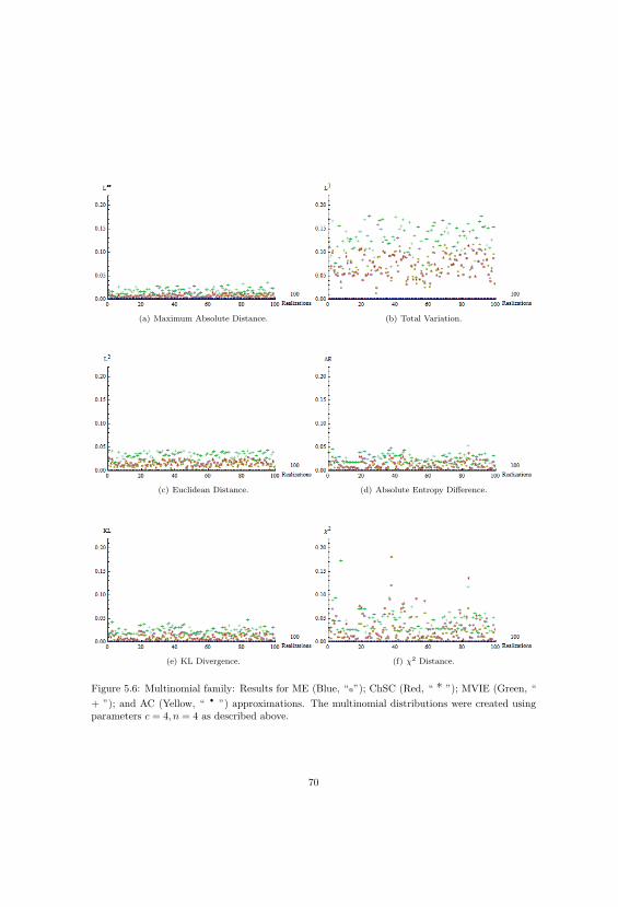
(a) Maximum Absolute Distance. (b) Total Variation.
(c) Euclidean Distance. (d) Absolute Entropy Difference.
(e) KL Divergence. (f) χ2 Distance.
Figure 5.6: Multinomial family: Results for ME (Blue, “@”); ChSC (Red, “ * ”); MVIE (Green, “
+ ”); and AC (Yellow, “ · ”) approximations. The multinomial distributions were created usingparameters c = 4, n = 4 as described above.
70

(a) Entropy, L∞. (b) Analytic, L
∞. (c) Chebyshev’s, L∞. (d) MVIE, L
∞.
(e) Entropy, L1. (f) Analytic, L
1. (g) Chebyshev’s, L1. (h) MVIE, L
1.
(i) Entropy, L2. (j) Analytic, L
2. (k) Chebyshev’s, L2. (l) MVIE, L
2.
(m) Entropy, |ΔH|. (n) Analytic, |ΔH|. (o) Chebyshev’s, |ΔH|. (p) MVIE, |ΔH|.
(q) Entropy, KL. (r) Analytic, KL. (s) Chebyshev’s, KL. (t) MVIE, KL.
(u) Entropy, χ2. (v) Analytic, χ2. (w) Chebyshev’s, χ2. (x) MVIE, χ2.
Figure 5.7: Multinomial family histogram results. From left to right, ME, AC, ChSC, and MVIE.From top to bottom, L∞, L1, L2, |ΔH|, KL, χ2 distance measures.
71

Figure 5.7 shows the histograms for each approximation and each measure with parameters
c = 4, n = 4. The histograms show in more detail the frequencies of the measures for each
approximation. Again, for all measures, ME provides values of zero, while the measures for MVIE
are more widely distributed. Finally, AC and ChSC show results similar to those described for
the hypergeometric family. Equivalent figures are shown in Appendix C Figures C.6 and C.8 for
[c = 5n = 3] and [c = 6, n = 8], respectively.
The histograms in Figure 5.7 provide insight into how the values of the measures of accuracy
are distributed. In general, the values have a slightly bell-shaped distribution without being normal.
These results and the percentages of accuracy in Table 5.4, have implications for the behavior of
the approximations. After sampling 100 distributions, ME was the best alternative for 96% of
the samples and second best for 4% of the samples by a slight margin of 10−7. Scatterplots and
histograms show ME as an exact approximation. Opposed to ME, MVIE approximation was the
worst alternative, with about 97% to 100% of the samples in the last column of Table 5.4.
Table 5.4: Percentage of monomial distribution for different approximations and measures withparameters c = 4, n = 4.
% of distributions % of distributions % of distributions % of distributions
Approximation Measure Best Second best Third best Worst
Entropy
L∞ 96 4 0 0
L1 96 4 0 0
L2 96 4 0 0
|ΔH| 96 4 0 0
KL 96 4 0 0
χ2 96 4 0 0
Analytic C
L∞ 4 3 90 3
L1 4 5 91 0
L2 4 3 93 0
|ΔH| 4 22 74 0
KL 4 10 86 0
χ2 4 35 61 0
ChSC
L∞ 0 93 7 0
L1 0 91 9 0
L2 0 93 7 0
|ΔH| 0 74 23 3
KL 0 86 13 1
χ2 0 61 30 9
MVIEC
L∞ 0 0 3 97
L1 0 0 0 100
L2 0 0 0 100
|ΔH| 0 0 3 97
KL 0 0 1 99
χ2 0 0 9 91
72
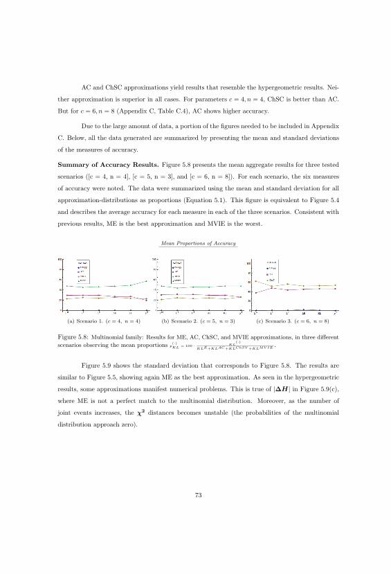
AC and ChSC approximations yield results that resemble the hypergeometric results. Nei-
ther approximation is superior in all cases. For parameters c = 4, n = 4, ChSC is better than AC.
But for c = 6, n = 8 (Appendix C, Table C.4), AC shows higher accuracy.
Due to the large amount of data, a portion of the figures needed to be included in Appendix
C. Below, all the data generated are summarized by presenting the mean and standard deviations
of the measures of accuracy.
Summary of Accuracy Results. Figure 5.8 presents the mean aggregate results for three tested
scenarios ([c = 4, n = 4], [c = 5, n = 3], and [c = 6, n = 8]). For each scenario, the six measures
of accuracy were noted. The data were summarized using the mean and standard deviation for all
approximation-distributions as proportions (Equation 5.1). This figure is equivalent to Figure 5.4
and describes the average accuracy for each measure in each of the three scenarios. Consistent with
previous results, ME is the best approximation and MVIE is the worst.
Mean Proportions of Accuracy
(a) Scenario 1. (c = 4, n = 4) (b) Scenario 2. (c = 5, n = 3) (c) Scenario 3. (c = 6, n = 8)
Figure 5.8: Multinomial family: Results for ME, AC, ChSC, and MVIE approximations, in three different
scenarios observing the mean proportions p(·)
KL= 100 · KL
(·)
KLE+KLAC+KLChSV +KLMV IE.
Figure 5.9 shows the standard deviation that corresponds to Figure 5.8. The results are
similar to Figure 5.5, showing again ME as the best approximation. As seen in the hypergeometric
results, some approximations manifest numerical problems. This is true of |ΔH| in Figure 5.9(c),
where ME is not a perfect match to the multinomial distribution. Moreover, as the number of
joint events increases, the χ2 distances becomes unstable (the probabilities of the multinomial
distribution approach zero).
73
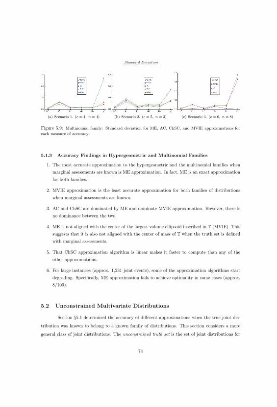
Standard Deviation
(a) Scenario 1. (c = 4, n = 4) (b) Scenario 2. (c = 5, n = 3) (c) Scenario 3. (c = 6, n = 8)
Figure 5.9: Multinomial family: Standard deviation for ME, AC, ChSC, and MVIE approximations for
each measure of accuracy.
5.1.3 Accuracy Findings in Hypergeometric and Multinomial Families
1. The most accurate approximation to the hypergeometric and the multinomial families when
marginal assessments are known is ME approximation. In fact, ME is an exact approximation
for both families.
2. MVIE approximation is the least accurate approximation for both families of distributions
when marginal assessments are known.
3. AC and ChSC are dominated by ME and dominate MVIE approximation. However, there is
no dominance between the two.
4. ME is not aligned with the center of the largest volume ellipsoid inscribed in T (MVIE). This
suggests that it is also not aligned with the center of mass of T when the truth set is defined
with marginal assessments.
5. That ChSC approximation algorithm is linear makes it faster to compute than any of the
other approximations.
6. For large instances (approx. 1,231 joint events), some of the approximation algorithms start
degrading. Specifically, ME approximation fails to achieve optimality in some cases (approx.
8/100).
5.2 Unconstrained Multivariate Distributions
Section §5.1 determined the accuracy of different approximations when the true joint dis-
tribution was known to belong to a known family of distributions. This section considers a more
general class of joint distributions. The unconstrained truth set is the set of joint distributions for
74

which the support is known but there is no information about partial or conditional assessments
(marginals, pairwise correlations, etc.). This case is of particular interest because all the approx-
imations proposed result in the discrete uniform distribution, i.e., the center of T. The study of
unconstrained sets help us to observe how the changes in the truth set T affect the proposed accuracy
measures for any given approximation. Of interest are two particular questions: How does changing
the number of random variables affect the accuracy of the approximation? How does changing the
number of outcomes for each random variable affect the accuracy of the approximation?
Sampling Details: To test the unconstrained set T, 100,000 distributions are obtained using the
HR sampler presented in Chapter 3. Then, we determine the “distance” (as defined by the measures
in Chapter 4) from each of the samples to the discrete uniform distribution using the six measures
proposed.
Six unconstrained sets are considered for this section. The first three correspond to joint
distributions with 3, 5, and 7 marginal random variables with two outcomes each. The last three
correspond to joint distributions with 3 marginal random variables with 2, 3, and 4 outcomes each.
Our results are presented in two parts. First, we consider the effects of increasing the
number of marginal variables in a joint distribution. For this part we present a summary of the
results and provide an in-depth analysis of the behavior of the sample and the measures of accuracy.
Next, we consider the effects of increasing the number of outcomes of the marginal variables in a
joint distribution. We present a summary of these results and link the observations to the analysis
presented in the first part.
Results for Number of Variables. Figure 5.10 shows the proportion-histograms after taking
100,000 samples for three unconstrained sets. The first set contains all joint distributions that can
be generated using three binary random variables. The second and third sets consider five and seven
binary random variables, respectively. This series of histograms shows how the sample changes as
the set increases in number of joint events and dimension.
As the number of variables increases, L∞ and Euclidean distance decrease. This reduction
is a direct effect of the concentration of volume in T. As described in Chapter 3, the volume
of T shrinks with dimensionality, and the shrinkage is exponentially higher as distance from the
center increases. Therefore, the sample concentrates its mass closer to the center. This result is
counterintuitive because the addition of a new dimension normally increases the existing space.
However, the n-content (relative interior volume) decreases, which increases the concentration of
the samples in T.
75

(a) 3 Var. L∞. (b) 5 Var. L
∞. (c) 7 Var. L∞.
(d) 3 Var. L1. (e) 5 Var. L
1. (f) 7 Var. L1.
(g) 3 Var. L2. (h) 5 Var. L
2. (i) 6 Var. L2.
Figure 5.10: Unconstrained sets (part one): Variations on accuracy measures as the number of binary
variables increases.
76

(j) 3 Var. |ΔH|. (k) 5 Var. |ΔH|. (l) 7 Var. |ΔH|.
(m) 3 Var. KL. (n) 5 Var. KL. (o) 7 Var. KL.
(p) 3 Var. χ2. (q) 5 Var. χ2. (r) 7 Var. χ2.
Figure 5.10: Unconstrained sets (part two): Variations on accuracy measures as the number of binary
variables increases.
77

Summary. Figure 5.11 presents the mean and standard deviation of the results presented in Figure
5.10. The mean of the measures is decreasing for L∞ and L2, but it is increasing and then decreasing
for L1, KL, χ2, and ΔH. However, all accuracy measures decrease in variance as dimensionality
increases, making the samples closer to each other and improving the precision of the truth set.
(a) Mean. (b) Standard Deviation.
Figure 5.11: Unconstrained sets: Mean and standard deviation as the number of binary variables increases.
Intuition and Theory. The behavior of the sampled distributions and the measures of accuracy
shown in Figure 5.11 are intuitive, as follows. Take a binary distribution P ∗a = { 15 , 1
5}, and perturb
it to create P ∗b = { 15 +ε, 1
5 −ε}. Then, L∞(P ∗a , P ∗b ) = ε, L2(P ∗a , P ∗b ) = ε ·√2, and L1(P ∗a , P ∗b ) = 2 ·ε.In general, for a joint distribution Pa at the center of T (the discrete uniform distribution) with n
elements, where n is an even number, and a distribution Pb, which is a perturbation of Pa where
every +ε has a corresponding −ε and every joint event is perturbed we have that L∞(Pa, Pb) = ε,
L2(Pa, Pb) = ε · √n, and L1(Pa, Pb) = n · ε.
As the dimension d = n−1 of T increases, we can find the ε that matches the changes of the
sampled joint distributions, where ε is a reference measure of the mean of the Euclidean distances
from the center of T to the collection of sampled distributions. We start by sampling 100,000 joint
distributions from eight polytopes of different dimensions and calculate the mean of the measures
generated with L2 for each polytope. Then, we find the values of ε that match the same distance
from Pa to Pb. In other words, we look for the perturbed joint distributions that have the same L2
as the mean of L2 on the sampled distributions.
Figure 5.12 shows the best fit for ε as a function of the dimension d. The figure depicts how
the necessary perturbations decrease with d, explaining the changes in L∞, L1, and L2 when the
dimension of the set increases. Hence, the mean distance from the center to the sample decreases.
78


(a) 2 Outcomes, L∞. (b) 3 Outcomes, L
∞. (c) 4 Outcomes, L∞.
(d) 2 Outcomes, L1. (e) 3 Outcomes, L
1. (f) 4 Outcomes, L1.
(g) 2 Outcomes, L2. (h) 3 Outcomes, L
2. (i) 4 Outcomes, L2.
Figure 5.15: Unconstrained sets (part one): Variations in accuracy measures as the number of outcomes
increases (for three random variables).
81

(j) 2 Outcomes, |ΔH|. (k) 3 Outcomes, |ΔH|. (l) 4 Outcomes, |ΔH|.
(m) 2 Outcomes, KL. (n) 3 Outcomes, KL. (o) 4 Outcomes, KL.
(p) 2 Outcomes, χ2. (q) 3 Outcomes, χ2. (r) 4 Outcomes, χ2.
Figure 5.15: Unconstrained sets (part two): Variations in accuracy measures as the number of outcomes
increases (for three random variables).
82
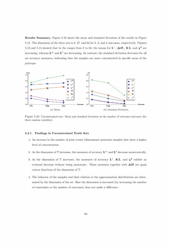
Results Summary. Figure 5.16 shows the mean and standard deviation of the results in Figure
5.15. The dimension of the three sets is 8, 27, and 64 for 2, 3, and 4 outcomes, respectively. Figures
5.13 and 5.14 showed that in the ranges from 2 to 64, the means for L1, |ΔH|, KL, and χ2 are
increasing, whereas L∞ and L2 are decreasing. In contrast, the standard deviation decreases for all
six accuracy measures, indicating that the samples are more concentrated in specific areas of the
polytope.
(a) Mean. (b) Standard Deviation.
Figure 5.16: Unconstrained sets: Mean and standard deviation as the number of outcomes increases (for
three random variables).
5.2.1 Findings in Unconstrained Truth Sets
1. An increase in the number of joint events (dimensions) generates samples that show a higher
level of concentration.
2. As the dimension of T increases, the measures of accuracy L∞ and L2 decrease monotonically.
3. As the dimension of T increases, the measures of accuracy L1, KL, and χ2 exhibit an
eventual decrease without being monotonic. These measures together with ΔH are quasi
convex functions of the dimension of T.
4. The behavior of the samples and their relation to the approximation distributions are deter-
mined by the dimension of the set. How the dimension is increased (by increasing the number
of constraints or the number of outcomes) does not make a difference.
83

5.3 Symmetrically Constrained Multivariate Distributions
In this section, we measure the effects of adding constraints to the truth set T. We consider
two questions: How does adding new constraints affect accuracy? How does changing the existing
constraints affect the accuracy of the distribution approximations? Subsection 5.3.1 addresses the
first question, while Subsections 5.3.2 and 5.3.3 address the second. For simplicity, this section
uses only symmetric information, i.e., all marginal random variables are identically distributed and
binary, and all rank correlations have the same correlation value. However, these results can easily
be extended to random variables with any number of outcomes.
5.3.1 Effects of Increasing the Number of Constraints
Sampling Details. To observe the effects of new constraints on T, the constraints are restricted
to be consistent with the assessments of the discrete uniform distribution (Equation 3.2, marginals
of 12 , pairwise of 1
4 , and three-wise of 18 ). Then, all the constraints are consistent with the center of
T, and all the distribution approximations are equal to the uniform distribution. We start by using
HR to create a collection of 100,000 sampled joint distributions from an unconstrained set with five
binary random variables, and measure the distance to the discrete uniform distribution (Figures
5.17 and 5.18). Next, we add a new constraint (marginal assessments) and observe the changes in
accuracy. This procedure is repeated for pairwise and three-wise constraints. (Results for 3 and
7 binary random variables can be observed in Appendix C, Figures C.9, C.10, and Figures C.11,
C.12, respectively.)
Each column in Figure 5.17 and 5.18 describe the results for a measure of accuracy, while
the rows describe the results for a truth set. For example, the superior row corresponds to the
unconstrained set, and subsequent rows increase the number of constraints downward.
Results. As we add more constrains to T the histograms shift to the left, indicating that the
samples get closer to the uniform distribution. The only exception happens when T becomes
one dimensional (Figure C.9) in which case the samples become distributed uniformly over a line
creating a non-bell-shaped pattern.
84

(a) Unconstrained, L∞. (b) Unconstrained, L
1. (c) Unconstrained, L2.
(d) Marginal, L∞. (e) Marginal, L
1. (f) Marginal, L2.
(g) Pairwise, L∞. (h) Pairwise, L
1. (i) Pairwise, L2.
(j) Three-wise, L∞. (k) Three-wise, L
1. (l) Three-wise, L2.
Figure 5.17: Effects of including new constraints in truth set T. The data are taken for a set thatconsiders 5 binary variables. The unconstrained set uses 1 constraint. The marginal set uses 6constraints. The pairwise set uses 16 constraints. The three-wise set uses 26 constraints.
85

(a) Unconstrained, |ΔH|. (b) Unconstrained, KL. (c) Unconstrained, χ2.
(d) Marginal, |ΔH|. (e) Marginal, KL. (f) Marginal, χ2.
(g) Pairwise, |ΔH|. (h) Pairwise, KL. (i) Pairwise, χ2.
(j) Three-wise, |ΔH|. (k) Three-wise, KL. (l) Three-wise, χ2.
Figure 5.18: Effect of including new constraints in truth set T. The data are taken for a set thatconsiders 5 binary variables. The unconstrained set uses 1 constraint. The marginal set uses 6constraints. The pairwise set uses 16 constraints. The three-wise set uses 26 constraints.
86

A different behavior is exhibited in the case of the dispersion of the samples. As the number
of constraints increases, the collection does not necessarily become more concentrated. This effect
is caused by a tradeoff between the dispersion of the n-content in the interior of T (§3.6), and
the change of geometry of T generated by the new constraint. This accounts for why the variance
may increase or decrease, according to the relation between the dispersion of the n-content and the
geometric shape of T.
Results Summary. Figure 5.19 shows the mean and Figure 5.20 shows the standard deviation of
the results displayed in Figures C.9, C.10; Figures 5.17, 5.18; and Figures C.11, C.12; which pairs
of figures correspond to sets with three, five, or seven binary random variables.
(a) Three Variables. (b) Five Variables.
(c) Seven Variables.
Figure 5.19: Mean results for unconstrained sets (UnC), marginal constrained sets (M), marginal and
pairwise constrained sets (MP), and marginal, pairwise, and three-wise constrained sets (MPT).
Since all the constraints are assessments aligned to the discrete uniform distribution, all
the distribution approximations considered give as a result the discrete uniform distribution. In
this case, the more constrained the truth set, the higher the accuracy of the approximations (the
lower the mean). This result is not surprising because if enough constraints are added, the set T
87
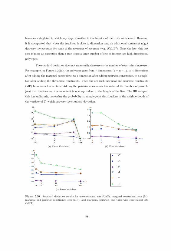
becomes a singleton in which any approximation in the interior of the truth set is exact. However,
it is unexpected that when the truth set is close to dimension one, an additional constraint might
decrease the accuracy for some of the measures of accuracy (e.g. KL,L2). None the less, this last
case is more an exception than a rule, since a large number of sets of interest are high dimensional
polytopes.
The standard deviation does not necessarily decrease as the number of constraints increases.
For example, in Figure 5.20(a), the polytope goes from 7 dimensions (d = n − 1), to 4 dimensions
after adding the marginal constraints, to 1 dimension after adding pairwise constraints, to a single-
ton after adding the three-wise constraints. Then the set with marginal and pairwise constraints
(MP) becomes a line section. Adding the pairwise constraints has reduced the number of possible
joint distributions and the n-content is now equivalent to the length of the line. The HR sampled
this line uniformly, increasing the probability to sample joint distributions in the neighborhoods of
the vertices of T, which increase the standard deviation.
(a) Three Variables. (b) Five Variables.
(c) Seven Variables.
Figure 5.20: Standard deviation results for unconstrained sets (UnC), marginal constrained sets (M),
marginal and pairwise constrained sets (MP), and marginal, pairwise, and three-wise constrained sets
(MPT).
88

5.3.2 Symmetric Marginal Constraints
Sampling Details. We now address the accuracy of the approximations under marginal symmetric
constraints for different values of b (Ap = b). Specifically, we address how the accuracy of the
approximations changes as the marginal assessments change. If X is a binary random variable, then,
we consider marginal assessments with values of P (X = 1) =0.5, 0.6, 0.7, 0.8, and 0.9 and consider
joint distributions with 3, 4, 5, 6, and 7 marginal binary random variables. We start by generating
the truth set Ap = b, p ≥ 0, where b = {b1, b2, . . . , bm}, b1 = b2 = · · · = bm and running HR for
100,000 joint distributions in the case of 3 and 4 marginal random variables, and 200,000 in the case
of 5, 6, and 7 marginal random variables. After the collections are complete, we apply the measures
of accuracy and calculate the mean and standard deviation of each approximation. Because the
number of samples for 6 and 7 random variables does not meet the optimal requirements described
in §3.4.3, we use these results under the caveat that some random noise is being introduced.
Results. Figures 5.21 and 5.22 show the mean and standard deviation for the maximum entropy
(ME), the analytic center (AC), the Chebyshev’s center (ChSC), the maximum volume inscribed
ellipsoid center (MVIE), and the dynamic average sample center (DAC) under the six accuracy
measures. Under all measures, for b1 = 0.5, all approximations have the same accuracy. However,
modifying b1 causes the approximations to become differentiated. This is the first truth set for
which the approximations provide different joint distributions.
ME Findings. In this results the accuracy of ME (blue circle) is consistently lower than most of
the other approximations. This contrast the results in Section 5.1 and the beliefs from the decision
analysis community that hold ME as a good approximations (Bickel and Smith, 2006).
One possible explanation is that for known families of joint distributions, the joint-probability
mass functions (jpmf) are relatively simple. For these models to remain simple requires general
assumptions that reduce the required number of parameters, such as the assumption of having
higher-order relations as independent as possible (maximum entropy). A family of distributions
with lower entropy will result in a jpmf having more parameters to account for all the unspecified
assumptions. In our framework, those assumptions are not required. In fact, we are free to not
assume anything with respect to higher-order assessments; we simply let the geometry of T describe
what is possible, and in that space, maximum entropy is rare.
89

� �� �
�
��
�
�
�
� �
�
�
�
� ��
��
� ��
��
5 6 7 8 9b0.0
0.1
0.2
0.3
0.4Mean
(i) 3 Variables, L∞.
��
��
�
��
�
�
�
� �
�
�
�
� ��
��
� ��
��
5 6 7 8 9b0.0
0.2
0.4
0.6
0.8
1.0
1.2Mean
(ii) 3 Variables, L1.
��
��
�
��
�
�
�
� �
�
�
�
� ��
��
� ��
�
�
5 6 7 8 9b0.0
0.1
0.2
0.3
0.4
Mean
(iii) 3 Variables, L2.
� ��
�
�
� ��
�
�
��
�
�
�
� � ��
�
� � ��
�5 6 7 8 9
b0.0
0.1
0.2
0.3
0.4Mean
(iv) 4 Variables, L∞.
�� � �
�
��
�
�
�
� �
�
�
�
� ��
��
� ��
�
�
5 6 7 8 9b0.0
0.2
0.4
0.6
0.8
1.0
1.2Mean
(v) 4 Variables, L1.
� � ��
�� �
�
�
�
��
�
�
�
� ��
��
� ��
��
5 6 7 8 9b0.0
0.1
0.2
0.3
0.4
Mean
(vi) 4 Variables, L2.
� �
�
��
� ��
�
�
�
� �
�
�
� � � ��
� � � ��
5 6 7 8 9b0.0
0.1
0.2
0.3
0.4Mean
(vii) 5 Variables, L∞.
� � ��
�
��
�
�
�
��
�
�
�
� ��
��
� ��
�
�
5 6 7 8 9b0.0
0.2
0.4
0.6
0.8
1.0
1.2Mean
(viii) 5 Variables, L1.
� �
�
��
� �
�
�
�
�
��
�
�
� � ��
�
� ��
��
5 6 7 8 9b0.0
0.1
0.2
0.3
0.4
Mean
(ix) 5 Variables, L2.
��
�
�
�
�� �
��
�
�
�
�
�� � �� �
� � �� �
5 6 7 8 9b0.0
0.1
0.2
0.3
0.4Mean
(x) 6 Variables, L∞.
� � �
�
�� �
�
�
�
�
��
�
�
� ��
��
� �
�
�
�
5 6 7 8 9b0.0
0.2
0.4
0.6
0.8
1.0
1.2Mean
(xi) 6 Variables, L1.
��
�
�
�
� ��
�
�
�
��
�
�
� � ��
�
� � ��
�5 6 7 8 9
b0.0
0.1
0.2
0.3
0.4
Mean
(xii) 6 Variables, L2.
�
�
�
�
�
�
�� �
��
� �
��
� � � � �5 6 7 8 9
b0.0
0.1
0.2
0.3
0.4Mean
(xiii) 7 Variables, L∞.
��
�
�
�
� �
�
�
�
� �
�
�
�
��
�
��
5 6 7 8 9b0.0
0.2
0.4
0.6
0.8
1.0
1.2Mean
(xiv) 7 Variables, L1.
�
�
�
�
�
��
��
�
��
�
� �� � �
� �5 6 7 8 9
b0.0
0.1
0.2
0.3
0.4
Mean
(xv) 7 Variables, L2.
� ME. � AC � ChSC � MVIE � DAC
Figure 5.21: Mean estimates for truth sets with variables 3 to 7 (part one).
90

� � � � �� �
��
�
��
�� �
� � � � �� � � � �
5 6 7 8 9b�0.5
0.0
0.5
1.0
1.5
Mean
(xvi) 3 Variables, ΔH.
� � � � ��
��
��
� ��
��
� � � � �� � � � �5 6 7 8 9
b0.0
0.5
1.0
1.5
2.0Mean
(xvii) 3 Variables, KL.
� � � �
�
� � � � �
� � � � �� � � � �� � � � �5 6 7 8 9
b0
1
2
3
4
5
6Mean
(xviii) 3 Variables, χ2.
� � � � �� ��
��
�
�
�� �
� � � � �� � � � �
5 6 7 8 9b�0.5
0.0
0.5
1.0
1.5
Mean
(xix) 4 Variables, ΔH.
� � � � �� ��
��
� ��
�
�
� � � � �
� � � ��
5 6 7 8 9b0.0
0.5
1.0
1.5
2.0Mean
(xx) 4 Variables, KL.
� � ��
�
� � � ��
� � ��
�� � � � �� � � � �5 6 7 8 9
b0
1
2
3
4
5
6Mean
(xxi) 4 Variables, χ2.
� � �� �
� ��
��
�
�
��
�
� ��
� �
� �� �
�
5 6 7 8 9b�0.5
0.0
0.5
1.0
1.5
Mean
(xxii) 5 Variables, ΔH.
� � �� �
� �
��
�
��
�
�
�
� � � ��
� ��
��
5 6 7 8 9b0.0
0.5
1.0
1.5
2.0Mean
(xxiii) 5 Variables, KL.
� � �
�
�
� ��
��
�� �
�
�� � � � �� � � � �5 6 7 8 9
b0
1
2
3
4
5
6Mean
(xxiv) 5 Variables, χ2.
� � �
��
� �
� �
�
�
�
� � �
� �� � �
� ��
��
5 6 7 8 9b�0.5
0.0
0.5
1.0
1.5
Mean
(xxv) 6 Variables, ΔH.
� � �
��
� �
�
�
�
�
� �
�
�
� � �� �
� ��
��
5 6 7 8 9b0.0
0.5
1.0
1.5
2.0Mean
(xxvi) 6 Variables, KL.
� � �
�
�
� � � � ��
� �� �� � � � �� � � � �5 6 7 8 9
b0
2
4
6
8
10
12
14
Mean
(xxvii) 6 Variables, χ2.
�
�
�
�
�
�� � �
�
�
�
��
�
� � �� �
5 6 7 8 9b�0.5
0.0
0.5
1.0
1.5
Mean
(xxviii) 7 Variables, ΔH.
�
�
�
�
�
� �
�
�
�
� ��
��
� ��
��
5 6 7 8 9b0.0
0.5
1.0
1.5
2.0Mean
(xxix) 7 Variables, KL.
� � �
�
�
� � � � �� � � � �� � � � �5 6 7 8 9b0
10
20
30
40
50Mean
(xxx) 7 Variables, χ2.
Figure 5.21: Mean estimates for truth sets with variables 3 to 7 (rows). The figures indicatevariation in accuracy due to change in the marginal constraints (part two).
91

��
��
�
��
�
�
�
�
�
�
�
�
� ��
�
�
� ��
�
�
5 6 7 8 9b0.00
0.01
0.02
0.03
0.04
0.05
0.06
0.07SD
(i) 3 Variables, L∞.
�
��
�
�
�
�
�
�
�
��
�
�
�
��
�
�
�
��
�
�
�
5 6 7 8 9b0.00
0.05
0.10
0.15
0.20SD
(ii) 3 Variables, L1.
��
�
�
�
�
�
�
�
�
�
�
�
�
�
� ��
�
�
��
�
�
�
5 6 7 8 9b0.00
0.02
0.04
0.06
0.08
0.10SD
(iii) 3 Variables, L2.
� �
�
�
�
� ��
�
�
�
��
�
�
� � ��
�
� � �
�
�
5 6 7 8 9b0.00
0.01
0.02
0.03
0.04
0.05
0.06
0.07SD
(iv) 4 Variables, L∞.
� �
�
�
�
� �
�
�
�
�
��
�
�
� � ��
�
� ��
�
�
5 6 7 8 9b0.00
0.05
0.10
0.15
0.20SD
(v) 4 Variables, L1.
� �
��
�
� ��
�
�
�
� �
�
�
� � ��
�
� � ��
�
5 6 7 8 9b0.00
0.02
0.04
0.06
0.08
0.10SD
(vi) 4 Variables, L2.
�
�
�
�
��� �
�
�
�
��
�
�� � � �
�� � �
��
5 6 7 8 9b0.00
0.01
0.02
0.03
0.04
0.05
0.06
0.07SD
(vii) 5 Variables, L∞.
��
� �
�
��
�
�
�
�
� �
�
�
� � � �
�
� ��
�
�
5 6 7 8 9b0.00
0.05
0.10
0.15
0.20SD
(viii) 5 Variables, L1.
��
� �
��
� ��
�
�
��
�
�� � � �
��
� ��
�5 6 7 8 9
b0.00
0.02
0.04
0.06
0.08
0.10SD
(ix) 5 Variables, L2.
�
�
�
�
�
��
�
�
�
�
��
�
�
� �
�
� ��� �
��
5 6 7 8 9b0.00
0.01
0.02
0.03
0.04
0.05
0.06
0.07SD
(x) 6 Variables, L∞.
��
�
�
�
� ��
�
�
�
� �
�
�
� ��
� �
� � ��
�5 6 7 8 9
b0.00
0.05
0.10
0.15
0.20SD
(xi) 6 Variables, L1.
�
�
�
�
�
��
�
��
�
��
�
�
� ��
� �� � �� �
5 6 7 8 9b0.00
0.02
0.04
0.06
0.08
0.10SD
(xii) 6 Variables, L2.
�
�
�
�
�
�
�
�
��
�
�
�
�
�
�
� �
��
5 6 7 8 9b0.00
0.01
0.02
0.03
0.04
0.05
0.06
0.07SD
(xiii) 7 Variables, L∞.
�
�
�
�
��
�
�
��
�
�
�
� �� � � � �5 6 7 8 9
b0.00
0.05
0.10
0.15
0.20SD
(xiv) 7 Variables, L1.
�
� �
��
�
��
���
�
�
�
�
� � � � �5 6 7 8 9
b0.00
0.02
0.04
0.06
0.08
0.10SD
(xv) 7 Variables, L2.
� ME. � AC � ChSC � MVIE � DAC
Figure 5.22: Standard deviation estimates for T with variables 3 to 7 (pat one).
92

�
� ��
�
�
� ��
�
�
� ��
�
�� � �
�
�� � �
�
5 6 7 8 9b0.00
0.05
0.10
0.15
0.20
0.25SD
(xvi) 3 Variables, ΔH.
�
� ��
�
�
�
�
�
�
� �
�
�
�
��
��
�
��
�
�
�
5 6 7 8 9b0.00
0.05
0.10
0.15
0.20
0.25
0.30SD
(xvii) 3 Variables, KL.
� � ��
�
� � � � �� � � � �� � � � �� � � � �5 6 7 8 9
b0
1
2
3
4
5
6SD
(xviii) 3 Variables, χ2.
��
� �
�
��
� �
�
��
� �
�
� �� �
�� �
� �
�
5 6 7 8 9b0.00
0.05
0.10
0.15
0.20
0.25SD
(xix) 4 Variables, ΔH.
��
� �
�
��
�
�
�
�
�
�
�
�
� ��
��
� ��
�
�5 6 7 8 9
b0.00
0.05
0.10
0.15
0.20
0.25
0.30SD
(xx) 4 Variables, KL.
� � ��
�
� � � � �� � � � �� � � � �� � � � �5 6 7 8 9
b0
1
2
3
4
5
6SD
(xxi) 4 Variables, χ2.
� �
��
�� �
��
�� �
��
�� �� �
�� ��
�
�
5 6 7 8 9b0.00
0.05
0.10
0.15
0.20
0.25SD
(xxii) 5 Variables, ΔH.
� �
��
�� �
�
�
�
�
�
�
�
�
� �� �
�
� ��
��
5 6 7 8 9b0.00
0.05
0.10
0.15
0.20
0.25
0.30SD
(xxiii) 5 Variables, KL.
� � �
�
�
� � � � ��
� � ��� � � � �� � � � �5 6 7 8 9
b0
1
2
3
4
5
6SD
(xxiv) 5 Variables, χ2.
��
��
�
��
��
�
��
��
�
� �� �
�� �
� �
�
5 6 7 8 9b0.00
0.05
0.10
0.15
0.20
0.25SD
(xxv) 6 Variables, ΔH.
��
��
�
� ��
�
�
�
��
�
�
� � �� �
� ��
��
5 6 7 8 9b0.00
0.05
0.10
0.15
0.20
0.25
0.30SD
(xxvi) 6 Variables, KL.
� � ��
�
� � � � �� � � � �� � � � �� � � � �5 6 7 8 9b0
2
4
6
8
10
12
14
SD
(xxvii) 6 Variables, χ2.
�
�
�
�
�
�
�
�
�
�
�
�
�
�
�
�
��
�
�
5 6 7 8 9b0.00
0.05
0.10
0.15
0.20
0.25SD
(xxviii) 7 Variables, ΔH.
�
�
�
�
�
� �
��
�
�
�
�� �� � � � �
5 6 7 8 9b0.00
0.05
0.10
0.15
0.20
0.25
0.30SD
(xxix) 7 Variables, KL.
� � ��
�
� � � � �� � � � �� � � � �5 6 7 8 9b0
10
20
30
40SD
(xxx) 7 Variables, χ2.
Figure 5.22: Standard deviation estimates for T with variables 3 to 7 (rows). Variation in accuracydue to change in the marginal constraints (part two).
93


The ChSC approximation is not a minimum entropy approximation. However, it serves as
a counterpart to ME by providing a distribution with lower entropy than all other approximations,
and in some cases with less entropy than most of the distributions in the sampled collection as
observed in Figures 5.21(xvi), 5.21(xix), 5.21(xxii), 5.21(xxv), and 5.21(xxviii).
The reduction of T as b1 increases is more pronounced in ChSC than in ME. This effect is
related to the structure of the ChSC approximation observed in Figure 5.26. That 31 of the 32 joint
events have equal probabilities is explained by the attempt to evenly expand a hypersphere inside
the positive hyper-octant with center in T. Then, in the case of symmetric marginal constraints,
a reduction of T as b1 increases makes the set more perpendicular to the closest boundaries of
the positive hyper-octant, providing more room for the hypersphere to expand and improving its
accuracy.
This same behavior affects the variation of the accuracy measures in Figure 5.22, where ME
and ChSC are the two approximations for which the accuracy measures show the largest variation.
Figure 5.26: ChSC changes in b (Ax = b). Figure A presents the full distribution. Figure Bpresents the distributions without the first joint event (ω1) and rescaled. These approximationswere created with 5 binary random variables (32 joint events ω1 to ω32).
Findings on the Most Accurate Approximations. The three approximations that provide the
best accuracy estimates are DAC, AC, and MVIE. Although they have similar accuracy on average,
Figure 5.22 shows that MVIE has more variation in accuracy than the other two. However, when
implemented, MVIE and DAC require a vast amount of memory and numerous iterations, leaving
AC as the best overall alternative. AC provides a simpler and accurate description of the truth set
when the marginal constraints are symmetric. Figure 5.27 shows how each approximation changes
as the marginals (b1) change from 0.5 (front of the cube) to 0.9 (back of the cube), where each
point represents one of the 32 joint events at a specific value of b1.
96

Figure 5.27: From top to bottom, AC, MVIE, and DAC as a function of b (Ax = b). Figures A present
the full distribution. Figures B present the distributions without the first joint event (ω1) and rescaled.
These approximations were created with 5 binary random variables (32 joint events ω1 to ω32).
97

AC has a structure that mimics ME but has a range closer to MVIE (Figures 5.24 and
5.27). The curvature of ME and AC may be attributed to the logarithmic function’s absence
from all other approximations. AC and MVIE may seem strikingly similar, given that the ideas
behind these approximations are so different. However, these similarities became less obvious as
the available information increases.
Finally, as expected, DAC is found to be the most accurate and the most work-intensive
of all the approximations, mostly because it requires use of the JDSIM. Due to lack of computing
resources, the last two sub-figures of Figure 5.27 were calculated running simulations only for
b1 =0.5, 0.6, 0.7, 0.8, and 0.9, giving the impression of a piecewise function. However, these figures
do not represent the approximations’ complete functions, even though they convey some aspects of
those functions.
Percentage of Accuracy. Accuracy can also be expressed as the percentage of the time that one
approximation is better that another. This measure can be observed in Tables 5.5 and 5.6. In these
tables, the first column indicates the number of random variables and the second column indicates
the value of b1 (the values for b1 = 0.5 are omitted since the results are trivial). The rest of the
columns indicate the percentage of the time that a sampled distribution is more accurate than an
alternative. Again the results favor DAC, AC, and MVIE.
For 3 and 4 marginal random variables, the MVIE outperforms the AC. However, increasing
the dimension of the truth set to 5, 6, or 7 marginal random variables makes AC more accurate
than the MVIE. The results show that DAC dominates all other approximations with respect to
greater-accuracy percentage, and ME is dominated by all other approximations.
The values for the MVIE when the jpmf is constructed using 7 marginal random variables
are omitted due to the complexity of the calculations. In particular, the problem requires expo-
nential amounts of memory. Similar problems were found in the simulation procedure for sample
distributions with many random variables. In particular, for 6 and 7 random variables, the sample
size should be close to 1 and 10 million samples, respectively. The actual sample size of 200,000
added random noise to the results.
98

Table 5.5: Percentage of accuracy (i.e. fraction of times one approximation is better than other)for sets with marginal information (b1 =M). For different approximations and number of variables(V= 3, 4, 5).
% of times DAC DAC DAC DAC MVIE MVIE MVIE AC AC ChSC
V M is better than MVIE AC ChSC ME AC ChSC ME ChSC ME ME
3
6 L∞ 47% 43% 53% 47% 58% 55% 60% 52% 48% 50%
6 L1 49% 53% 60% 57% 52% 61% 56% 57% 59% 46%
6 L2 47% 52% 59% 56% 53% 61% 56% 57% 59% 46%
6 KL 47% 50% 59% 54% 53% 61% 55% 57% 57% 46%
6 χ2 46% 45% 63% 50% 50% 65% 52% 61% 53% 42%
3
7 L∞ 45% 64% 55% 72% 59% 59% 68% 50% 76% 60%
7 L1 52% 59% 60% 71% 55% 64% 68% 54% 76% 60%
7 L2 50% 59% 60% 72% 56% 64% 69% 53% 76% 61%
7 KL 49% 59% 60% 71% 56% 65% 68% 54% 76% 59%
7 χ2 50% 56% 64% 71% 54% 69% 68% 58% 76% 57%
3
8 L∞ 45% 65% 55% 82% 61% 59% 80% 48% 87% 74%
8 L1 52% 61% 60% 84% 58% 65% 81% 51% 88% 76%
8 L2 50% 62% 60% 84% 59% 65% 82% 51% 88% 76%
8 KL 49% 62% 60% 84% 58% 65% 81% 52% 88% 75%
8 χ2 51% 61% 65% 86% 57% 70% 84% 56% 90% 77%
3
9 L∞ 44% 67% 54% 91% 64% 57% 90% 45% 94% 87%
9 L1 51% 64% 59% 92% 61% 63% 91% 48% 95% 87%
9 L2 48% 64% 59% 92% 62% 63% 91% 47% 95% 88%
9 KL 47% 64% 59% 93% 61% 63% 92% 48% 96% 88%
9 χ2 48% 63% 64% 96% 61% 68% 95% 52% 98% 92%
4
6 L∞ 55% 54% 77% 44% 38% 76% 44% 76% 44% 29%
6 L1 55% 53% 71% 58% 52% 70% 59% 69% 60% 37%
6 L2 54% 53% 72% 58% 53% 71% 59% 70% 59% 35%
6 KL 54% 53% 72% 58% 53% 71% 58% 70% 59% 36%
6 χ2 54% 53% 77% 53% 49% 77% 53% 76% 54% 30%
4
7 L∞ 52% 50% 77% 73% 57% 82% 69% 73% 75% 55%
7 L1 53% 56% 71% 77% 51% 76% 73% 67% 80% 57%
7 L2 53% 57% 72% 77% 51% 77% 73% 68% 80% 57%
7 KL 53% 57% 73% 78% 51% 78% 74% 69% 81% 55%
7 χ2 56% 54% 79% 77% 48% 84% 72% 76% 80% 50%
4
8 L∞ 53% 53% 77% 93% 57% 83% 91% 72% 94% 82%
8 L1 54% 58% 71% 92% 52% 78% 90% 66% 94% 82%
8 L2 54% 59% 72% 93% 52% 79% 91% 67% 95% 83%
8 KL 54% 59% 74% 93% 52% 79% 91% 69% 95% 79%
8 χ2 58% 56% 80% 94% 48% 85% 92% 75% 96% 78%
4
9 L∞ 50% 59% 76% 100% 63% 79% 100% 65% 100% 98%
9 L1 51% 63% 69% 99% 60% 73% 99% 58% 100% 98%
9 L2 50% 63% 70% 100% 60% 74% 100% 59% 100% 99%
9 KL 50% 63% 71% 100% 60% 75% 100% 62% 100% 97%
9 χ2 54% 59% 79% 100% 56% 82% 100% 69% 100% 99%
5
6 L∞ 41% 50% 84% 43% 61% 82% 37% 84% 45% 24%
6 L1 54% 54% 79% 61% 46% 77% 64% 78% 62% 30%
6 L2 53% 53% 82% 60% 46% 80% 63% 81% 61% 26%
6 KL 53% 54% 82% 61% 46% 79% 64% 81% 62% 28%
6 χ2 51% 52% 88% 57% 52% 86% 59% 87% 57% 22%
5
7 L∞ 66% 53% 85% 86% 35% 90% 83% 85% 87% 56%
7 L1 58% 58% 82% 89% 44% 87% 84% 81% 89% 59%
7 L2 58% 58% 84% 89% 44% 89% 84% 83% 89% 57%
7 KL 58% 57% 85% 91% 44% 89% 85% 84% 91% 54%
7 χ2 62% 54% 91% 90% 38% 94% 84% 90% 89% 46%
5
8 L∞ 64% 54% 84% 100% 30% 92% 97% 86% 99% 85%
8 L1 56% 52% 81% 99% 43% 89% 96% 82% 99% 85%
8 L2 57% 52% 83% 100% 42% 91% 97% 85% 100% 85%
8 KL 58% 56% 85% 100% 43% 91% 96% 86% 99% 77%
8 χ2 66% 58% 91% 100% 34% 95% 97% 92% 99% 76%
5
9 L∞ 51% 51% 82% 100% 43% 86% 100% 75% 100% 99%
9 L1 50% 62% 77% 100% 58% 82% 100% 69% 100% 99%
9 L2 51% 62% 80% 100% 57% 85% 100% 73% 100% 99%
9 KL 53% 63% 81% 100% 56% 85% 100% 76% 100% 99%
9 χ2 57% 56% 90% 100% 49% 92% 100% 86% 100% 100%
99

Table 5.6: Percentage of accuracy (i.e. fraction of times one approximation is better than other)for sets with marginal information (b1 =M). For different approximations and number of variables(V= 6, 7).
% Of times DAC DAC DAC DAC MVIE MVIE MVIE AC AC ChSC
V M is better than MVIE AC ChSC ME AC ChSC ME ChSC ME ME
6
6 L∞ 61% 61% 93% 57% 60% 88% 68% 91% 47% 22%
6 L1 63% 63% 86% 70% 43% 79% 73% 83% 69% 31%
6 L2 60% 64% 93% 68% 43% 87% 71% 91% 67% 22%
6 KL 69% 70% 92% 75% 43% 85% 73% 89% 69% 28%
6 χ2 69% 72% 98% 70% 51% 94% 67% 97% 63% 19%
6
7 L∞ 79% 75% 98% 92% 7% 100% 80% 100% 85% 39%
7 L1 70% 65% 94% 97% 22% 100% 78% 99% 83% 46%
7 L2 71% 66% 98% 94% 20% 100% 78% 100% 84% 39%
7 KL 79% 77% 98% 99% 19% 100% 85% 100% 91% 38%
7 χ2 86% 79% 100% 99% 6% 100% 88% 100% 94% 27%
6
8 L∞ 66% 63% 86% 100% 35% 87% 100% 84% 100% 100%
8 L1 64% 61% 84% 100% 45% 85% 100% 82% 100% 100%
8 L2 68% 57% 86% 100% 45% 87% 100% 83% 100% 100%
8 KL 67% 70% 88% 100% 46% 89% 100% 86% 100% 100%
8 χ2 71% 66% 96% 100% 36% 97% 100% 93% 100% 100%
6
9 L∞ 64% 59% 90% 100% 43% 95% 100% 88% 100% 100%
9 L1 53% 66% 86% 100% 57% 92% 100% 82% 100% 100%
9 L2 58% 65% 90% 100% 55% 95% 100% 87% 100% 100%
9 KL 70% 65% 93% 100% 51% 95% 100% 90% 100% 100%
9 χ2 77% 63% 99% 100% 38% 100% 100% 97% 100% 100%
7
6 L∞ - 75% 81% 89% - - - 51% 99% 63%
6 L1 - 81% 78% 93% - - - 41% 100% 68%
6 L2 - 76% 81% 89% - - - 50% 100% 63%
6 KL - 89% 84% 99% - - - 44% 100% 74%
6 χ2 - 89% 95% 99% - - - 59% 100% 69%
7
7 L∞ - 85% 87% 100% - - - 65% 100% 100%
7 L1 - 99% 85% 100% - - - 57% 100% 100%
7 L2 - 96% 87% 100% - - - 65% 100% 100%
7 KL - 100% 90% 100% - - - 65% 100% 100%
7 χ2 - 97% 97% 100% - - - 82% 100% 100%
7
8 L∞ - 100% 92% 100% - - - 5% 100% 100%
8 L1 - 100% 89% 100% - - - 1% 100% 100%
8 L2 - 100% 92% 100% - - - 5% 100% 100%
8 KL - 100% 95% 100% - - - 24% 100% 100%
8 χ2 - 96% 98% 100% - - - 42% 100% 100%
7
9 L∞ - 53% 85% 100% - - - 84% 100% 100%
9 L1 - 95% 83% 100% - - - 80% 100% 100%
9 L2 - 85% 84% 100% - - - 83% 100% 100%
9 KL - 98% 85% 100% - - - 85% 100% 100%
9 χ2 - 95% 93% 100% - - - 87% 100% 100%
100
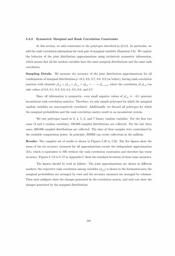
5.3.3 Symmetric Marginal and Rank Correlation Constraints
In this section, we add constraints to the polytopes described in §5.3.2. In particular, we
add the rank correlation information for each pair of marginal variables (Equation 3.9). We explore
the behavior of the joint distribution approximations using exclusively symmetric information,
which means that all the random variables have the same marginal distributions and the same rank
correlation.
Sampling Details. We measure the accuracy of the joint distribution approximations for all
combinations of marginal distributions p =0.5, 0.6, 0.7, 0.8, 0.9 (as before), having rank correlation
matrices with elements ρr1,2 = ρr
1,3 = ρr1,n = ρr
2,3 = · · · = ρrn−1,n, where the correlation of ρr
1,2 can
take values of 0.0, 0.1, 0.2, 0.3, 0.4, 0.5, 0.6, and 0.7.
Since all information is symmetric, even small negative values of ρr1,2 ≈ −0.1 generate
inconsistent rank correlation matrices. Therefore, we only sample polytopes for which the marginal
random variables are non-negatively correlated. Additionally, we discard all polytopes for which
the marginal probabilities and the rank correlation matrix result in an inconsistent system.
We test polytopes based in 3, 4, 5, 6, and 7 binary random variables. For the first two
cases (3 and 4 random variables), 100,000 sampled distributions are collected. For the last three
cases, 200,000 sampled distributions are collected. The sizes of these samples were constrained by
the available computation power. In principle, JDSIM can create collections in the millions.
Results: The complete set of results is shown in Figures 5.28 to 5.32. The five figures show the
mean of the six accuracy measures for all approximations except the independent approximation
(IA), which is equivalent to ME without the rank correlation constraints and therefore has worse
accuracy. Figures C.13 to C.17 in Appendix C show the standard deviation of those same measures.
The figures should be read as follows: The joint approximations are shown in different
markers; the respective rank correlation among variables (ρr1,2) is shown in the horizontal-axes; the
marginal probabilities are arranged by rows and the accuracy measures are arranged by columns.
Then each subfigure show the changes generated by the correlation matrix, and each row show the
changes generated by the marginal distributions.
101

��
��
��
��
��
��
��
��
��
��
��
��
��
��
��
��
� � � � � � � �
� � � � � � � �0 0.1 0.2 0.3 0.4 0.5 0.6 0.7Ρ0.00
0.05
0.10
0.15
0.20
0.25Mean
(i) L∞, p = 0.5
��
��
��
�
�
�
�
�
�
�
�
�
�
�
�
�
�
�
�
�
�
��
��
��
��
� � � � � � � �
��������
0 0.1 0.2 0.3 0.4 0.5 0.6 0.7Ρ0.0
0.2
0.4
0.6
0.8
1.0
Mean
(ii) L1, p = 0.5
�
��
��
�
�
�
�
�
�
�
�
�
�
�
�
�
�
�
�
�
�
�
�
�
�
�
�
�
�
�
��������
��������
0 0.1 0.2 0.3 0.4 0.5 0.6 0.7Ρ0.00
0.05
0.10
0.15
0.20
0.25
0.30Mean
(iii) L2, p = 0.5
�� �
��
��
�
�� �
��
��
�
�� �
��
��
�
�� �
��
��
�
� � � � � � � �� � � � � � � �0 0.1 0.2 0.3 0.4 0.5 0.6 0.7
Ρ0.00
0.05
0.10
0.15
0.20
0.25Mean
(iv) L∞, p = 0.6
�
� ��
�
�
�
�
��
�
�
�
�
�
�
��
�
�
�
�
�
�
��
��
��
��
� � � � � � � �
�� �
�����0 0.1 0.2 0.3 0.4 0.5 0.6 0.7
Ρ0.0
0.2
0.4
0.6
0.8
1.0
Mean
(v) L1, p = 0.6
�
� ��
�
�
�
�
�
��
�
�
�
�
�
�
��
�
�
�
�
�
�
��
�
�
�
�
�
�� �
�����
�� �
�����0 0.1 0.2 0.3 0.4 0.5 0.6 0.7
Ρ0.00
0.05
0.10
0.15
0.20
0.25
0.30Mean
(vi) L2, p = 0.6
��
��
��
�
� ��
��
��
�� �
��
��
�� �
��
��
� � � � � � �� � � � � � �0 0.1 0.2 0.3 0.4 0.5 0.6 0.7
Ρ0.00
0.05
0.10
0.15
0.20
0.25Mean
(vii) L∞, p = 0.7
��
��
�
�
�
��
�
�
�
�
�
��
�
�
�
�
�
��
��
��
�
� � � � � � ��� �
����0 0.1 0.2 0.3 0.4 0.5 0.6 0.7
Ρ0.0
0.2
0.4
0.6
0.8
1.0
Mean
(viii) L1, p = 0.7
�
�
�
�
�
�
�
��
�
�
�
�
�
�
��
�
�
�
�
�
��
�
�
�
�
�� �
����
�������
0 0.1 0.2 0.3 0.4 0.5 0.6 0.7Ρ0.00
0.05
0.10
0.15
0.20
0.25
0.30Mean
(ix) L2, p = 0.7
��
��
�� ��
���
� ��
��� �
��� � � � �� � � � �
0 0.1 0.2 0.3 0.4 0.5 0.6 0.7Ρ0.00
0.05
0.10
0.15
0.20
0.25Mean
(x) L∞, p = 0.8
�
�
�
�
���
�
�
��
��
�
���
��
�� � � � ��� �
��
0 0.1 0.2 0.3 0.4 0.5 0.6 0.7Ρ0.0
0.2
0.4
0.6
0.8
1.0
Mean
(xi) L1, p = 0.8
�
�
�
�
���
�
�
��
��
�
��
��
�
��� �
���
����
0 0.1 0.2 0.3 0.4 0.5 0.6 0.7Ρ0.00
0.05
0.10
0.15
0.20
0.25
0.30Mean
(xii) L2, p = 0.8
��
��
� ��� ��� �� � �� � �
0 0.1 0.2 0.3 0.4 0.5 0.6 0.7Ρ0.00
0.05
0.10
0.15
0.20
0.25Mean
(xiii) L∞, p = 0.9
�
��
�
��
�
��
��
�� � ��� �
0 0.1 0.2 0.3 0.4 0.5 0.6 0.7Ρ0.0
0.2
0.4
0.6
0.8
1.0
Mean
(xiv) L1, p = 0.9
�
�
�
�
��
�
��
�
���
� ����
0 0.1 0.2 0.3 0.4 0.5 0.6 0.7Ρ0.00
0.05
0.10
0.15
0.20
0.25
0.30Mean
(xv) L2, p = 0.9
� UE. � ME. � AC � ChSC � MVIE � DAC
Figure 5.28: Mean estimates for T with 3 binary random variables (part one).
102

��
��
�� � �
��
��
� � � �
��
��
� � � �
��
�� � � � �
� � � � � � � �
� � � � � � � �0 0.1 0.2 0.3 0.4 0.5 0.6 0.7Ρ
�0.4
�0.2
0.0
0.2
0.4
0.6
0.8
Mean
(xvi) ΔH, p = 0.5
�� � � � � �
�
��
�� � � � �
��
�� � � � �
��
� � � � � �
� � � � � � � �� � � � � � � �0 0.1 0.2 0.3 0.4 0.5 0.6 0.7
Ρ0.0
0.5
1.0
1.5
Mean
(xvii) KL, p = 0.5
� � � � � � � �� � � � � � � �
� � � � � � � �
� � � � � � � �� � � � � � � �� � � � � � � �0 0.1 0.2 0.3 0.4 0.5 0.6 0.7
Ρ0
1
2
3
4
5Mean
(xviii) χ2, p = 0.5
��
��
�� � �
�� �
��
� � �
�� �
��
� � �
�� �
� � � � �� � � � � � � �� � � � � � � �0 0.1 0.2 0.3 0.4 0.5 0.6 0.7
Ρ
�0.4
�0.2
0.0
0.2
0.4
0.6
0.8
Mean
(xix) ΔH, p = 0.6
�� � � � �
�
��
� �� � � � �
�� �
� � � � �
�� � � � � � �
� � � � � � � �� � � � � � � �0 0.1 0.2 0.3 0.4 0.5 0.6 0.7
Ρ0.0
0.5
1.0
1.5
Mean
(xx) KL, p = 0.6
� � � � � � � �
� � � � � � � �� � � � � � � �� � � � � � � �� � � � � � � �� � � � � � � �0 0.1 0.2 0.3 0.4 0.5 0.6 0.7
Ρ0
1
2
3
4
5Mean
(xxi) χ2, p = 0.6
� ��
�� � �
� ��
��
� �� �
��
�� �
��
�� � � �� � � � � � �� � � � � � �0 0.1 0.2 0.3 0.4 0.5 0.6 0.7
Ρ
�0.4
�0.2
0.0
0.2
0.4
0.6
0.8
Mean
(xxii) ΔH, p = 0.7
� �
� � ��
�� ��
�� � �
� ��
� � � �� �
� � � � �� � � � � � �� � � � � � �0 0.1 0.2 0.3 0.4 0.5 0.6 0.7Ρ0.0
0.5
1.0
1.5
Mean
(xxiii) KL, p = 0.7
� �
� � � � �
� � � � � � �� � � � � � �� � � � � � �� � � � � � �� � � � � � �0 0.1 0.2 0.3 0.4 0.5 0.6 0.7Ρ0
1
2
3
4
5Mean
(xxiv) χ2, p = 0.7
� ��
� �� �
��
�� ��
��� �
�� �� � � � �� � � � �0 0.1 0.2 0.3 0.4 0.5 0.6 0.7
Ρ
�0.4
�0.2
0.0
0.2
0.4
0.6
0.8
Mean
(xxv) ΔH, p = 0.8
��
��
�� �
��
�� � �� �� � � � �� � � � �� � � � �0 0.1 0.2 0.3 0.4 0.5 0.6 0.7
Ρ0.0
0.5
1.0
1.5
Mean
(xxvi) KL, p = 0.8
� �
� � �
� � � � �� � � � �� � � � �� � � � �� � � � �0 0.1 0.2 0.3 0.4 0.5 0.6 0.7Ρ0
1
2
3
4
5Mean
(xxvii) χ2, p = 0.8
� � �� � �� � �� � �� � �� � �0 0.1 0.2 0.3 0.4 0.5 0.6 0.7Ρ
�0.4
�0.2
0.0
0.2
0.4
0.6
0.8
Mean
(xxviii) ΔH, p = 0.9
�
� �
� � �� � �� � �� � �� � �0 0.1 0.2 0.3 0.4 0.5 0.6 0.7Ρ0.0
0.5
1.0
1.5
Mean
(xxix) KL, p = 0.9
�
�
�
� � �� � �� � �� � �� � �0 0.1 0.2 0.3 0.4 0.5 0.6 0.7Ρ0
1
2
3
4
5Mean
(xxx) χ2, p = 0.9
Figure 5.28: Mean estimates for T with 3 binary random variables. The rank correlation is shownin the x-axes. Each row shows marginal assessments p and each column shows an accuracy measure(part two).
103

��
� � ��
�
�
� � ��
��
��
� � ��
��
��
� � ��
��
��
� � � � � � � �
� � � � � � � �0 0.1 0.2 0.3 0.4 0.5 0.6 0.7Ρ0.00
0.05
0.10
0.15
0.20
0.25Mean
(i) L∞, p = 0.5
� � � � ��
�
�
� ��
�
�
�
�
�
� ��
�
�
�
�
�
� ��
��
�
��
� � � � � � � �
� � ������
0 0.1 0.2 0.3 0.4 0.5 0.6 0.7Ρ0.0
0.2
0.4
0.6
0.8
1.0
Mean
(ii) L1, p = 0.5
��
� � �
�
�
�
� ��
�
�
�
�
�
� ��
�
�
�
�
�
� ��
�
�
�
�
�
� � �� �
���
� � ������
0 0.1 0.2 0.3 0.4 0.5 0.6 0.7Ρ0.00
0.05
0.10
0.15
0.20
0.25
0.30Mean
(iii) L2, p = 0.5
��
� ��
�
�
�
� � ��
��
��
� � ��
��
��
�
� ��
��
��
� � � � � � � �
� � � � � � � �0 0.1 0.2 0.3 0.4 0.5 0.6 0.7Ρ0.00
0.05
0.10
0.15
0.20
0.25Mean
(iv) L∞, p = 0.6
�
�
� ��
�
�
�
� ��
�
�
�
�
�
� ��
�
�
�
�
�
�
��
��
�
��
� � � � � � � �
� � ������0 0.1 0.2 0.3 0.4 0.5 0.6 0.7
Ρ0.0
0.2
0.4
0.6
0.8
1.0
Mean
(v) L1, p = 0.6
�
�
� ��
�
�
�
� ��
�
�
�
�
�
��
�
�
�
�
�
�
�
��
�
�
�
�
�
� � � �����
� � ������0 0.1 0.2 0.3 0.4 0.5 0.6 0.7
Ρ0.00
0.05
0.10
0.15
0.20
0.25
0.30Mean
(vi) L2, p = 0.6
�
�
� �
�
�
�
� � ��
��
�
� ��
��
��
� ��
��
��
� � � � � � �� � � � � � �0 0.1 0.2 0.3 0.4 0.5 0.6 0.7
Ρ0.00
0.05
0.10
0.15
0.20
0.25Mean
(vii) L∞, p = 0.7
�
�
��
�
�
�
�� �
�
�
�
�
��
��
�
�
�
��
��
�
�
�
� � � � � � �
�� �
����0 0.1 0.2 0.3 0.4 0.5 0.6 0.7
Ρ0.0
0.2
0.4
0.6
0.8
1.0
Mean
(viii) L1, p = 0.7
�
�
��
�
�
�
�� �
�
�
�
�
��
��
�
�
�
��
��
�
�
�
� � � ����
�� �
����
0 0.1 0.2 0.3 0.4 0.5 0.6 0.7Ρ0.00
0.05
0.10
0.15
0.20
0.25
0.30Mean
(ix) L2, p = 0.7
�
�
�
�
���
�
�
��
� ��
��
��
��� � � � ��
� � � �0 0.1 0.2 0.3 0.4 0.5 0.6 0.7
Ρ0.00
0.05
0.10
0.15
0.20
0.25Mean
(x) L∞, p = 0.8
�
�
�
�
���
�
�
��
� �
�
�
�
��
�
��� � � ��� �
��
0 0.1 0.2 0.3 0.4 0.5 0.6 0.7Ρ0.0
0.2
0.4
0.6
0.8
1.0
Mean
(xi) L1, p = 0.8
�
�
�
�
���
�
�
��
��
�
�
�
��
�
��� � �
��� �
��
0 0.1 0.2 0.3 0.4 0.5 0.6 0.7Ρ0.00
0.05
0.10
0.15
0.20
0.25
0.30Mean
(xii) L2, p = 0.8
�
�
�
�
�
��
���
��� � �� � �
0 0.1 0.2 0.3 0.4 0.5 0.6 0.7Ρ0.00
0.05
0.10
0.15
0.20
0.25Mean
(xiii) L∞, p = 0.9
�
�
�
�
�
��
���
���
� ����
0 0.1 0.2 0.3 0.4 0.5 0.6 0.7Ρ0.0
0.2
0.4
0.6
0.8
1.0
Mean
(xiv) L1, p = 0.9
�
�
�
�
�
��
���
���
� ����
0 0.1 0.2 0.3 0.4 0.5 0.6 0.7Ρ0.00
0.05
0.10
0.15
0.20
0.25
0.30Mean
(xv) L2, p = 0.9
� UE. � ME. � AC � ChSC � MVIE � DAC
Figure 5.29: Mean estimates for T with 4 binary random variables (part one).
104

��
�
��
� ��
� � �� � �
��
� � ��
��
��
� ��
� � � � �
� � � � � � � �� � � � � � � �0 0.1 0.2 0.3 0.4 0.5 0.6 0.7
Ρ
�0.4
�0.2
0.0
0.2
0.4
0.6
0.8
Mean
(xvi) ΔH, p = 0.5
� �� �
� ��
�� � � � � � ��
� � �� � � � �
� � � � � � � �
� � � � � � � �� � � � � � � �0 0.1 0.2 0.3 0.4 0.5 0.6 0.7
Ρ0.0
0.5
1.0
1.5
Mean
(xvii) KL, p = 0.5
� ��
��
�
�
�
� � � � � � � �� � � � � � � �� � � � � � � �� � � � � � � �� � � � � � � �0 0.1 0.2 0.3 0.4 0.5 0.6 0.7
Ρ0
1
2
3
4
5Mean
(xviii) χ2, p = 0.5
��
�
�� � �
�
� � ��
��
��
� � ��
��
��
�� � � � � � �
� � � � � � � �� � � � � � � �0 0.1 0.2 0.3 0.4 0.5 0.6 0.7
Ρ
�0.4
�0.2
0.0
0.2
0.4
0.6
0.8
Mean
(xix) ΔH, p = 0.6
��
�� � �
�
�� � � � � � �
�
� � � � � � � �
�� � � � � � �
� � � � � � � �� � � � � � � �0 0.1 0.2 0.3 0.4 0.5 0.6 0.7
Ρ0.0
0.5
1.0
1.5
Mean
(xx) KL, p = 0.6
��
�
�
�
�
�
�
� � � � � � � �� � � � � � � �
�� � � � � � �
� � � � � � � �� � � � � � � �0 0.1 0.2 0.3 0.4 0.5 0.6 0.7Ρ0
1
2
3
4
5Mean
(xxi) χ2, p = 0.6
� ��
�� �
�
�� �
��
��
� � � ��
���
�� � � � �
� � � � � � �� � � � � � �0 0.1 0.2 0.3 0.4 0.5 0.6 0.7
Ρ
�0.4
�0.2
0.0
0.2
0.4
0.6
0.8
Mean
(xxii) ΔH, p = 0.7
�
�
��
��
�� � � ��
��
� � � � � � �
� � � � � � �� � � � � � �� � � � � � �0 0.1 0.2 0.3 0.4 0.5 0.6 0.7
Ρ0.0
0.5
1.0
1.5
Mean
(xxiii) KL, p = 0.7
��
�
�
�
��
� � � � � � �� � � � � � �� � � � � � �� � � � � � �� � � � � � �0 0.1 0.2 0.3 0.4 0.5 0.6 0.7
Ρ0
1
2
3
4
5Mean
(xxiv) χ2, p = 0.7
�� �
� �
� ��
��� � �
��
�
�� � �� � � � �� � � � �0 0.1 0.2 0.3 0.4 0.5 0.6 0.7
Ρ
�0.4
�0.2
0.0
0.2
0.4
0.6
0.8
Mean
(xxv) ΔH, p = 0.8
�
�
��
�
� ��
���
� � � ��� � � �� � � � �� � � � �0 0.1 0.2 0.3 0.4 0.5 0.6 0.7
Ρ0.0
0.5
1.0
1.5
Mean
(xxvi) KL, p = 0.8
�
�
�
�
�
� � � � �� � � � �� � � � �� � � � �� � � � �0 0.1 0.2 0.3 0.4 0.5 0.6 0.7Ρ0
1
2
3
4
5Mean
(xxvii) χ2, p = 0.8
� ���
���
���
��� � �� � �0 0.1 0.2 0.3 0.4 0.5 0.6 0.7
Ρ
�0.4
�0.2
0.0
0.2
0.4
0.6
0.8
Mean
(xxviii) ΔH, p = 0.9
�
��
��
�� � �� � �� � �� � �0 0.1 0.2 0.3 0.4 0.5 0.6 0.7
Ρ0.0
0.5
1.0
1.5
Mean
(xxix) KL, p = 0.9
�
�
�
� � �� � �� � �� � �� � �0 0.1 0.2 0.3 0.4 0.5 0.6 0.7Ρ0
1
2
3
4
5Mean
(xxx) χ2, p = 0.9
Figure 5.29: Mean estimates for T with 4 binary random variables. The rank correlation is shownin the x-axes. Each row shows marginal assessments p and each column shows an accuracy measure(part two).
105

�
�
��
� �
�
�� � � �
��
��
� � ��
��
��
� � ��
��
��
� � � � � � � �
� � � � � � � �0 0.1 0.2 0.3 0.4 0.5 0.6 0.7Ρ0.00
0.05
0.10
0.15
0.20
0.25Mean
(i) L∞, p = 0.5
�� � � �
�
�
�
��
��
�
�
�
�
��
�
�
�
�
�
�
� �
�
�
�
�
�
�
� � ������
� �������
0 0.1 0.2 0.3 0.4 0.5 0.6 0.7Ρ0.0
0.2
0.4
0.6
0.8
1.0
Mean
(ii) L1, p = 0.5
��
��
��
�
�
� ��
��
�
�
�
� ��
�
�
�
�
�
� ��
��
��
�
� � � � � � � �
� � ������
0 0.1 0.2 0.3 0.4 0.5 0.6 0.7Ρ0.00
0.05
0.10
0.15
0.20
0.25
0.30Mean
(iii) L2, p = 0.5
�
�
�� �
�
�
�
� � ��
��
�
�
� � ��
��
��
�
� � ��
��
�
� � � � � � � �
� � � � � � � �0 0.1 0.2 0.3 0.4 0.5 0.6 0.7Ρ0.00
0.05
0.10
0.15
0.20
0.25Mean
(iv) L∞, p = 0.6
�
�
� �
�
�
�
�
� ��
�
�
�
�
�
��
�
�
�
�
�
�
�
��
�
�
�
�
�
� � ������
� �������0 0.1 0.2 0.3 0.4 0.5 0.6 0.7
Ρ0.0
0.2
0.4
0.6
0.8
1.0
Mean
(v) L1, p = 0.6
�
�
� ��
�
�
�
� � ��
�
�
�
�
��
��
�
�
�
�
�
��
��
��
�
� � � � � � � �
� � ������0 0.1 0.2 0.3 0.4 0.5 0.6 0.7
Ρ0.00
0.05
0.10
0.15
0.20
0.25
0.30Mean
(vi) L2, p = 0.6
�
�
� �
�
�
�
� ��
��
�
�
� �� �
��
�
��
� ��
��
� � � � � � �� � � � � � �0 0.1 0.2 0.3 0.4 0.5 0.6 0.7
Ρ0.00
0.05
0.10
0.15
0.20
0.25Mean
(vii) L∞, p = 0.7
�
�
�
�
�
�
�
�� �
�
�
�
�
� ��
�
�
�
�
��
�
�
�
�
�
� � � ����
� � �����
0 0.1 0.2 0.3 0.4 0.5 0.6 0.7Ρ0.0
0.2
0.4
0.6
0.8
1.0
Mean
(viii) L1, p = 0.7
�
�
��
�
�
�
� ��
�
�
�
�
� ��
�
�
�
�
��
��
��
�
� � � � � � �
� � �����0 0.1 0.2 0.3 0.4 0.5 0.6 0.7
Ρ0.00
0.05
0.10
0.15
0.20
0.25
0.30Mean
(ix) L2, p = 0.7
�
�
�
�
���
�
�
�� ��
��
�
�
��
�� � � � �� � � � �0 0.1 0.2 0.3 0.4 0.5 0.6 0.7
Ρ0.00
0.05
0.10
0.15
0.20
0.25Mean
(x) L∞, p = 0.8
�
�
�
�
�
��
�
�
�
�
��
�
�
�
�
�
�
��� �
��
�� �
��
0 0.1 0.2 0.3 0.4 0.5 0.6 0.7Ρ0.0
0.2
0.4
0.6
0.8
1.0
Mean
(xi) L1, p = 0.8
�
�
�
�
�
��
�
�
��
��
�
�
�
�
��
��� � � �
�� �
��
0 0.1 0.2 0.3 0.4 0.5 0.6 0.7Ρ0.00
0.05
0.10
0.15
0.20
0.25
0.30Mean
(xii) L2, p = 0.8
�
�
�
�
�
�
��
���
�� � �� � �0 0.1 0.2 0.3 0.4 0.5 0.6 0.7
Ρ0.00
0.05
0.10
0.15
0.20
0.25Mean
(xiii) L∞, p = 0.9
�
�
�
�
�
�
�
�
��
�
��� ����
0 0.1 0.2 0.3 0.4 0.5 0.6 0.7Ρ0.0
0.2
0.4
0.6
0.8
1.0
Mean
(xiv) L1, p = 0.9
�
�
�
�
�
�
��
��
�
�� � ����
0 0.1 0.2 0.3 0.4 0.5 0.6 0.7Ρ0.00
0.05
0.10
0.15
0.20
0.25
0.30Mean
(xv) L2, p = 0.9
� UE. � ME. � AC � ChSC � MVIE � DAC
Figure 5.30: Mean estimates for T with 5 binary random variables (part one).
106

�
�
�
�� � �
�
� �� �
��
��
� ��
��
��
�
��
��
�� � �
� � � � � � � �
� � � � � � � �0 0.1 0.2 0.3 0.4 0.5 0.6 0.7Ρ
�0.4
�0.2
0.0
0.2
0.4
0.6
0.8
Mean
(xvi) ΔH, p = 0.5
��
��
� ��
�� � � � � ��
�
� ��
��
��
�
� ��
��
��
�
� � � � � � � �
� � � � � � � �0 0.1 0.2 0.3 0.4 0.5 0.6 0.7Ρ0.0
0.5
1.0
1.5
Mean
(xvii) KL, p = 0.5
��
�
�
�
�
�
� � � � � � � �
� � � � � � � �
� � � � � � � �� � � � � � � �� � � � � � � �0 0.1 0.2 0.3 0.4 0.5 0.6 0.7
Ρ0
1
2
3
4
5Mean
(xviii) χ2, p = 0.5
�
�
�
�� � �
�
� � ��
��
�
�
� ��
��
��
�
�
��
��
� � �
� � � � � � � �
� � � � � � � �0 0.1 0.2 0.3 0.4 0.5 0.6 0.7Ρ
�0.4
�0.2
0.0
0.2
0.4
0.6
0.8
Mean
(xix) ΔH, p = 0.6
�
�
�� � �
�
�
� � �� �
��
�
� � ��
��
��
�
� ��
��
��
� � � � � � � �
� � � � � � � �0 0.1 0.2 0.3 0.4 0.5 0.6 0.7Ρ0.0
0.5
1.0
1.5
Mean
(xx) KL, p = 0.6
�
�
�
�
�
�
� � � � � � ��
� � � � � � � �
�
� � � � � � �� � � � � � � �� � � � � � � �0 0.1 0.2 0.3 0.4 0.5 0.6 0.7
Ρ0
1
2
3
4
5Mean
(xxi) χ2, p = 0.6
��
�
� � ��
�� �
��
�
�
� � ��
��
�
�
�
� � �� �
� � � � � � �� � � � � � �0 0.1 0.2 0.3 0.4 0.5 0.6 0.7
Ρ
�0.4
�0.2
0.0
0.2
0.4
0.6
0.8
Mean
(xxii) ΔH, p = 0.7
�
�
� ��
�
��
� ��
��
�
�� �
��
��
� �
��
��
�
� � � � � � �� � � � � � �0 0.1 0.2 0.3 0.4 0.5 0.6 0.7
Ρ0.0
0.5
1.0
1.5
Mean
(xxiii) KL, p = 0.7
�
�
�
�
� � � � � � �� � � � � � �
��
� � � � �� � � � � � �� � � � � � �0 0.1 0.2 0.3 0.4 0.5 0.6 0.7Ρ0
1
2
3
4
5Mean
(xxiv) χ2, p = 0.7
�
� �� �
� ��
�
�� � �
��
�
�� � �� � � � ��
� � � �0 0.1 0.2 0.3 0.4 0.5 0.6 0.7
Ρ
�0.4
�0.2
0.0
0.2
0.4
0.6
0.8
Mean
(xxv) ΔH, p = 0.8
�
�
�
�
�
� ��
���
� ��
��
��
��� � � � �� � � � �
0 0.1 0.2 0.3 0.4 0.5 0.6 0.7Ρ0.0
0.5
1.0
1.5
Mean
(xxvi) KL, p = 0.8
�
�
�
� ��
� �� � � � ��
�� � �� � � � �� � � � �0 0.1 0.2 0.3 0.4 0.5 0.6 0.7
Ρ0
1
2
3
4
5Mean
(xxvii) χ2, p = 0.8
��
��
�
��
��
�
�
�� � �� � �0 0.1 0.2 0.3 0.4 0.5 0.6 0.7
Ρ
�0.4
�0.2
0.0
0.2
0.4
0.6
0.8
Mean
(xxviii) ΔH, p = 0.9
�
�
�
�
��
��
���
�� � �� � �0 0.1 0.2 0.3 0.4 0.5 0.6 0.7Ρ0.0
0.5
1.0
1.5
Mean
(xxix) KL, p = 0.9
�
�
��
�� � �� � �� � �� � �0 0.1 0.2 0.3 0.4 0.5 0.6 0.7
Ρ0
1
2
3
4
5Mean
(xxx) χ2, p = 0.9
Figure 5.30: Mean estimates for T with 5 binary random variables. The rank correlation is shownin the x-axes. Each row shows marginal assessments p and each column shows an accuracy measure(part two).
107

�
�
�
�
��
�
�� � � � � �
�
�
� �� �
� �� �
��
� �� �
� �
� � � � � � � �� � � � � � � �0 0.1 0.2 0.3 0.4 0.5 0.6 0.7
Ρ0.00
0.05
0.10
0.15
0.20
0.25Mean
(i) L∞, p = 0.5
�
��
� �
�
�
�
��
��
�
�
�
�
��
�
�
�
�
�
�
� �
�
�
�
�
�
�
� �������
� �������
0 0.1 0.2 0.3 0.4 0.5 0.6 0.7Ρ0.0
0.2
0.4
0.6
0.8
1.0
Mean
(ii) L1, p = 0.5
�
�
�
��
�
�
�
� � � � ��
�
�
� ��
��
�
��
� ��
��
�
��
� � � � � � � �
� � � �� �
� �0 0.1 0.2 0.3 0.4 0.5 0.6 0.7
Ρ0.00
0.05
0.10
0.15
0.20
0.25
0.30Mean
(iii) L2, p = 0.5
�
�
�� �
�
�
�
�
��
� ��
�
�
� � � ��
��
�
�� � �
��
��
� � � � � � � �� � � � � � � �0 0.1 0.2 0.3 0.4 0.5 0.6 0.7
Ρ0.00
0.05
0.10
0.15
0.20
0.25Mean
(iv) L∞, p = 0.6
�
�
�
�
�
�
�
�
�� �
��
�
�
�
��
�
�
�
�
�
�
�
��
�
�
�
�
�
� � ������
� � ������0 0.1 0.2 0.3 0.4 0.5 0.6 0.7
Ρ0.0
0.2
0.4
0.6
0.8
1.0
Mean
(v) L1, p = 0.6
�
�
� � �
�
�
�
�� �
��
�
�
�
�� �
��
��
�
�� �
��
��
�
� � � � � � � �
� � � � ����0 0.1 0.2 0.3 0.4 0.5 0.6 0.7
Ρ0.00
0.05
0.10
0.15
0.20
0.25
0.30Mean
(vi) L2, p = 0.6
�
�
��
�
�
�
��
�
��
�
�
� �� �
�� �
�
�
� ��
� �
� � � � � � �� � � � � � �0 0.1 0.2 0.3 0.4 0.5 0.6 0.7
Ρ0.00
0.05
0.10
0.15
0.20
0.25Mean
(vii) L∞, p = 0.7
�
�
�
�
�
�
�
��
�
�
�
�
�
��
�
�
�
�
�
�
�
�
�
�
�
�
� � �����
� ������
0 0.1 0.2 0.3 0.4 0.5 0.6 0.7Ρ0.0
0.2
0.4
0.6
0.8
1.0
Mean
(viii) L1, p = 0.7
�
�
��
�
�
�
��
�
�
�
�
�
� ��
��
��
�
�
��
��
�
� � � � � � �
� � � �� � �0 0.1 0.2 0.3 0.4 0.5 0.6 0.7
Ρ0.00
0.05
0.10
0.15
0.20
0.25
0.30Mean
(ix) L2, p = 0.7
�
�
�
�
��
�
�
�
�
��
� ��
� �
� ��
� � � � �� � � � �0 0.1 0.2 0.3 0.4 0.5 0.6 0.7Ρ0.00
0.05
0.10
0.15
0.20
0.25Mean
(x) L∞, p = 0.8
�
�
�
�
�
�
�
�
�
��
��
�
�
�
�
�
�
�
�����
�� �
��
0 0.1 0.2 0.3 0.4 0.5 0.6 0.7Ρ0.0
0.2
0.4
0.6
0.8
1.0
Mean
(xi) L1, p = 0.8
�
�
�
�
�
�
�
�
�
��
��
��
��
��
�
� � � � ��� � � �
0 0.1 0.2 0.3 0.4 0.5 0.6 0.7Ρ0.00
0.05
0.10
0.15
0.20
0.25
0.30Mean
(xii) L2, p = 0.8
�
�
�
�
�
�
� � ��
�
�� � �� � �0 0.1 0.2 0.3 0.4 0.5 0.6 0.7Ρ0.00
0.05
0.10
0.15
0.20
0.25Mean
(xiii) L∞, p = 0.9
�
�
��
�
�
�
�
��
�
�����
��
0 0.1 0.2 0.3 0.4 0.5 0.6 0.7Ρ0.0
0.2
0.4
0.6
0.8
1.0
Mean
(xiv) L1, p = 0.9
�
�
�
�
�
�
��
��
�
�� � �� � �0 0.1 0.2 0.3 0.4 0.5 0.6 0.7
Ρ0.00
0.05
0.10
0.15
0.20
0.25
0.30Mean
(xv) L2, p = 0.9
� UE. � ME. � AC � ChSC � MVIE � DAC
Figure 5.31: Mean estimates for T with 6 binary random variables (part one).
108

�
�
�
�� �
��
� � � � ��
�
�
��
��
��
��
��
��
�� � �
� � � � � � � �
� � � � � � � �0 0.1 0.2 0.3 0.4 0.5 0.6 0.7Ρ
�0.4
�0.2
0.0
0.2
0.4
0.6
0.8
Mean
(xvi) ΔH, p = 0.5
�
�
�
�� � �
�� � � � �
��
�
� ��
��
��
�
� ��
��
��
�
� � � � � � � �
� � � � � � � �0 0.1 0.2 0.3 0.4 0.5 0.6 0.7Ρ0.0
0.5
1.0
1.5
Mean
(xvii) KL, p = 0.5
�
�
�
�
�
�
� � � � � � ��
� � � � � � � �
� � � � � � � �
� � � � � � � �� � � � � � � �0 0.1 0.2 0.3 0.4 0.5 0.6 0.7
Ρ0
1
2
3
4
5Mean
(xviii) χ2, p = 0.5
�
�
�
� � ��
�
�� �
� ��
�
�
� ��
��
��
�
��
�
��
� � �
� � �� � � � �
� � �� � � � �0 0.1 0.2 0.3 0.4 0.5 0.6 0.7
Ρ
�0.4
�0.2
0.0
0.2
0.4
0.6
0.8
Mean
(xix) ΔH, p = 0.6
�
�
� �� �
�
��
� �� �
��
�
� � ��
��
��
�� �
��
��
�
� � � � � � � �
� � � � � � � �0 0.1 0.2 0.3 0.4 0.5 0.6 0.7Ρ0.0
0.5
1.0
1.5
Mean
(xx) KL, p = 0.6
�
�
�
��
� � � � � � ��
� � � � � � � �
�� � � � � � �
� � � � � � � �� � � � � � � �0 0.1 0.2 0.3 0.4 0.5 0.6 0.7
Ρ0
1
2
3
4
5Mean
(xxi) χ2, p = 0.6
�
� �
� � � �
��
�
��
�
�
�� �
��
��
�
�
�� �
� �
�� � � � � �
� � � � � � �0 0.1 0.2 0.3 0.4 0.5 0.6 0.7Ρ
�0.4
�0.2
0.0
0.2
0.4
0.6
0.8
Mean
(xxii) ΔH, p = 0.7
�
�
� � �
�
��
��
��
�
�
�� �
��
��
��
��
��
�
� � � � � � �� � � � � � �0 0.1 0.2 0.3 0.4 0.5 0.6 0.7
Ρ0.0
0.5
1.0
1.5
Mean
(xxiii) KL, p = 0.7
�
�
�
� ��
� � ��
� � � � � � �
�
�
� � � � �� � � � � � �� � � � � � �0 0.1 0.2 0.3 0.4 0.5 0.6 0.7
Ρ0
1
2
3
4
5Mean
(xxiv) χ2, p = 0.7
�
�
�� �
� �
�
�
�� � ��
�
�
��
� �� � � � ��� � � �
0 0.1 0.2 0.3 0.4 0.5 0.6 0.7Ρ
�0.4
�0.2
0.0
0.2
0.4
0.6
0.8
Mean
(xxv) ΔH, p = 0.8
�
�
�
�
�
� �
�
�
��
� ��
�
��
��
�� � � � ��� � � �
0 0.1 0.2 0.3 0.4 0.5 0.6 0.7Ρ0.0
0.5
1.0
1.5
Mean
(xxvi) KL, p = 0.8
�
�
�
� ��
��
�� � � �
� �� � �� � � � �� � � � �0 0.1 0.2 0.3 0.4 0.5 0.6 0.7
Ρ0
1
2
3
4
5Mean
(xxvii) χ2, p = 0.8
��
��
�
�
��
�
�
�
�� � �� � �0 0.1 0.2 0.3 0.4 0.5 0.6 0.7
Ρ
�0.4
�0.2
0.0
0.2
0.4
0.6
0.8
Mean
(xxviii) ΔH, p = 0.9
�
�
�
�
�
�
��
���
�� � �� � �0 0.1 0.2 0.3 0.4 0.5 0.6 0.7
Ρ0.0
0.5
1.0
1.5
Mean
(xxix) KL, p = 0.9
�
�
� ��
� � �� ��� � �� � �0 0.1 0.2 0.3 0.4 0.5 0.6 0.7
Ρ0
1
2
3
4
5Mean
(xxx) χ2, p = 0.9
Figure 5.31: Mean estimates for T with 6 binary random variables. The rank correlation is shownin the x-axes. Each row shows marginal assessments p and each column shows an accuracy measure(part two).
109

�
�
�
��
�
�
�
��
� � � ��
�� � �� � � � �
�� �
� �� � �
� � � � � � � �0 0.1 0.2 0.3 0.4 0.5 0.6 0.7Ρ0.00
0.05
0.10
0.15
0.20
0.25Mean
(i) L∞, p = 0.5
�
� �
��
�
�
�
� � � �
�
�
�
�
��
�
�
�
�
�
�
� �
�
�
�
�
�
�
� �������
0 0.1 0.2 0.3 0.4 0.5 0.6 0.7Ρ0.0
0.2
0.4
0.6
0.8
1.0
Mean
(ii) L1, p = 0.5
�
�
�
� ��
�
�� ��
� � �
�
�
� ��
��
��
�
� ��
� ��
��
� � �� � � � �0 0.1 0.2 0.3 0.4 0.5 0.6 0.7
Ρ0.00
0.05
0.10
0.15
0.20
0.25
0.30Mean
(iii) L2, p = 0.5
�
�
�
�
�
�
�
��
�
�� �
�
�
�
�� � �
� � � �
�� � �
� � � �
� � � � � � � �0 0.1 0.2 0.3 0.4 0.5 0.6 0.7Ρ0.00
0.05
0.10
0.15
0.20
0.25Mean
(iv) L∞, p = 0.6
�
�
�� �
�
�
�
�� �
��
�
�
�
�
�
�
�
�
�
�
�
�
�
�
�
�
�
�
�
��������0 0.1 0.2 0.3 0.4 0.5 0.6 0.7
Ρ0.0
0.2
0.4
0.6
0.8
1.0
Mean
(v) L1, p = 0.6
�
�
��
�
�
�
�
�
�
�� �
�
�
�
�� �
��
��
�
�
� ��
��
��
� � � � � � � �0 0.1 0.2 0.3 0.4 0.5 0.6 0.7Ρ0.00
0.05
0.10
0.15
0.20
0.25
0.30Mean
(vi) L2, p = 0.6
� �
��
�
�
�
�
�
��
�
�
��
�
� � � � �
� � �� � � �
� � � � � � �0 0.1 0.2 0.3 0.4 0.5 0.6 0.7Ρ0.00
0.05
0.10
0.15
0.20
0.25Mean
(vii) L∞, p = 0.7
��
��
�
�
�
��
�
�
�
�
�
�
�
�
�
�
�
�
�
� �
�
�
�
�
� � �����
0 0.1 0.2 0.3 0.4 0.5 0.6 0.7Ρ0.0
0.2
0.4
0.6
0.8
1.0
Mean
(viii) L1, p = 0.7
� �
��
�
�
�
�
�
��
�
�
�
�
�
��
��
�
�
� ��
��
�
� � � � � � �0 0.1 0.2 0.3 0.4 0.5 0.6 0.7Ρ0.00
0.05
0.10
0.15
0.20
0.25
0.30Mean
(ix) L2, p = 0.7
�
�
�
�
�
�
�
�
�
�
� �
� � �
��
� � �� � � � �0 0.1 0.2 0.3 0.4 0.5 0.6 0.7Ρ0.00
0.05
0.10
0.15
0.20
0.25Mean
(x) L∞, p = 0.8
�
�
�
�
�
�
�
�
�
�
��
�
�
�
�
��
�
��� �
��
0 0.1 0.2 0.3 0.4 0.5 0.6 0.7Ρ0.0
0.2
0.4
0.6
0.8
1.0
Mean
(xi) L1, p = 0.8
�
�
�
�
�
�
�
�
�
�
� �
��
�
�
�
��
��� � � �
0 0.1 0.2 0.3 0.4 0.5 0.6 0.7Ρ0.00
0.05
0.10
0.15
0.20
0.25
0.30Mean
(xii) L2, p = 0.8
�
�
��
�
�
��
��
�
�� � �0 0.1 0.2 0.3 0.4 0.5 0.6 0.7Ρ0.00
0.05
0.10
0.15
0.20
0.25Mean
(xiii) L∞, p = 0.9
�
�
�
� �
�
��
��
�
����
0 0.1 0.2 0.3 0.4 0.5 0.6 0.7Ρ0.0
0.2
0.4
0.6
0.8
1.0
Mean
(xiv) L1, p = 0.9
�
�
�� �
�
��
��
�
��� �
0 0.1 0.2 0.3 0.4 0.5 0.6 0.7Ρ0.00
0.05
0.10
0.15
0.20
0.25
0.30Mean
(xv) L2, p = 0.9
� UE. � ME. � AC � ChSC � MVIE � DAC
Figure 5.32: Mean estimates for T with 7 binary random variables (part one).
110

�
�
�
�� �
��
� � � ��
��
�
��
��
��
�
�
�
�
��
� ��
�
� �� � � � � �
0 0.1 0.2 0.3 0.4 0.5 0.6 0.7Ρ
�0.4
�0.2
0.0
0.2
0.4
0.6
0.8
Mean
(xvi) ΔH, p = 0.5
�
�
�
� �
��
�
� � � �� �
�
�
��
��
��
��
� ��
��
��
�
� � � � � � � �0 0.1 0.2 0.3 0.4 0.5 0.6 0.7Ρ0.0
0.5
1.0
1.5
Mean
(xvii) KL, p = 0.5
�
�
�
�
�
� � � � � � ��
� � � � � � � �
� � � � �� � �
� � � � � � � �0 0.1 0.2 0.3 0.4 0.5 0.6 0.7Ρ0
1
2
3
4
5Mean
(xviii) χ2, p = 0.5
�
�
�
� � �� �
� � �� �
�
�
�
��
��
��
�
�
�
�
�� �
��
�
� � � � � � � �0 0.1 0.2 0.3 0.4 0.5 0.6 0.7Ρ
�0.4
�0.2
0.0
0.2
0.4
0.6
0.8
Mean
(xix) ΔH, p = 0.6
�
�
� �
��
�
�� � �
� ��
�
�
��
��
��
��
�
��
��
��
�
� � � � � � � �0 0.1 0.2 0.3 0.4 0.5 0.6 0.7Ρ0.0
0.5
1.0
1.5
Mean
(xx) KL, p = 0.6
�
�
�
�
� � � � � � ��
� � � � � � � �
�
� � �� � � �
� � � � � � � �0 0.1 0.2 0.3 0.4 0.5 0.6 0.7Ρ0
1
2
3
4
5Mean
(xxi) χ2, p = 0.6
�
��
�� � �
��
��
�
�
�
�
��
�
��
��
� � ��
� �
� � � � � � �0 0.1 0.2 0.3 0.4 0.5 0.6 0.7Ρ
�0.4
�0.2
0.0
0.2
0.4
0.6
0.8
Mean
(xxii) ΔH, p = 0.7
�
�
��
�
�
��
��
��
�
�
�
�
�
��
��
�
�
� ��
��
�
� � � � � � �0 0.1 0.2 0.3 0.4 0.5 0.6 0.7Ρ0.0
0.5
1.0
1.5
Mean
(xxiii) KL, p = 0.7
�
�
�
� �
� ��
���
�
� � � � �
�
� � � � � �� � � � � � �0 0.1 0.2 0.3 0.4 0.5 0.6 0.7
Ρ0
1
2
3
4
5Mean
(xxiv) χ2, p = 0.7
�
�
�
��
�
�
�
�
�
�
�
�
�
�
�
��
���
� � � �0 0.1 0.2 0.3 0.4 0.5 0.6 0.7
Ρ
�0.4
�0.2
0.0
0.2
0.4
0.6
0.8
Mean
(xxv) ΔH, p = 0.8
�
�
�
�
� �
�
�
�
�
��
�
��
�
�� �
��� � � � �
0 0.1 0.2 0.3 0.4 0.5 0.6 0.7Ρ0.0
0.5
1.0
1.5
Mean
(xxvi) KL, p = 0.8
�
�
�
�
��
��
�
� � �
�� � � �� � � � �0 0.1 0.2 0.3 0.4 0.5 0.6 0.7
Ρ0
1
2
3
4
5Mean
(xxvii) χ2, p = 0.8
�� �
��
��
� ��
�
��� �
0 0.1 0.2 0.3 0.4 0.5 0.6 0.7Ρ
�0.4
�0.2
0.0
0.2
0.4
0.6
0.8
Mean
(xxviii) ΔH, p = 0.9
�
�
�
� ��
��
��
��� � �
0 0.1 0.2 0.3 0.4 0.5 0.6 0.7Ρ0.0
0.5
1.0
1.5
Mean
(xxix) KL, p = 0.9
�
�
�
� �
�� ���
�� � �0 0.1 0.2 0.3 0.4 0.5 0.6 0.7Ρ0
1
2
3
4
5Mean
(xxx) χ2, p = 0.9
Figure 5.32: Mean estimates for T with 7 binary random variables. The rank correlation is shownin the x-axes. Each row shows marginal assessments p and each column shows an accuracy measure(part two).
111


has advantages and disadvantages. For DAC the biggest flaw is the running time of the algorithm,
which constrained us to sample only 200,000 distributions for polytopes constructed using 6 and
7 variables, rather than the more desirable orders of 1,000,000 and 10,000,000, respectively (see
§3.4.3). Large sample sizes can be generated in less than 24 hours, but this is not always sufficient.
The MVIE requires fewer iterations, but each iteration is computationally intensive. Finally, AC
is easy to calculate but behaves erratically for a small number of polytopes (Figure 5.32 third and
fourth rows). The reasons for these behavior are still unknown.
The standard deviation of the accuracy measures for marginal and rank correlation con-
straints can be observed in Appendix C, Figures C.13, C.14, C.15, C.16, and C.17. The standard
deviation corresponds to the principle of contraction and expansion of the truth set, which explains
the increasing and decreasing trend for changes in the rank correlation. Also, for most of the cases,
DAC, AC, and the MVIE provide the lowest standard deviation.
Percentage of Accuracy. In addition to the mean and standard deviation of the accuracy
measures, the percentage of accuracy was calculated. This statistic measures the percentage of time
that a given approximation outperforms another. Tables 5.7, 5.8, 5.9, and 5.10 present the results
for polytopes constructed using 5 binary random variables. The tables show changes in marginal
and rank correlations for all distribution approximations and all measures considered. Values above
50% indicate that the approximation in row one is more accurate than the approximation in row
two, and values below 50% indicate the opposite. Appendix C presents the complete set of results
for 3, 4, 6, and 7 binary random variables in Tables C.10, C.11, C.12, C.13, C.14, C.15, C.16, C.17,
C.18, C.19, C.20, C.21, C.22, C.23, C.24, and C.25.
The overall results show that the approximations in descending order by percentage of
accuracy are DAC, MVIE, AC, ChSC, ME, UE, and IA. This ordering will present a correct
description of the accuracy of the joint approximations, although there are some scenarios for
which the general results do not hold.
Interestingly, AC and ChSC show that in low-dimensional environments (polytopes gener-
ated with 3 binary random variables), ChSC outperforms AC, but as the dimension increases, AC
considerably outperforms ChSC. This suggests that the dimensionality does affect the accuracy of
the ChSC approximations. Because ChSC is a linear function, all of its elements are far from zero.
As the dimension increases, the probability mass needs to be distributed among a larger number
of joint events, creating a joint approximation that is less dispersed and has a larger number of
elements close to zero, which reduces its accuracy.
114

Table
5.7:
Per
centa
ge
of
acc
ura
cy(i
.e.
fract
ion
of
tim
esone
appro
xim
ati
on
isbet
ter
than
oth
er)
for
sets
wit
hsy
mm
etri
cm
arg
inaland
rank
corr
elati
on
info
rmati
on
usi
ng
5bin
ary
random
vari
able
sand
changin
gth
eva
lues
of
p=
0.5
and
ρr 1,2
=0,
0.1,
0.2,
0.3
,0.4
,0.5
,0.6
,and
0.7.
%O
ftim
es
DA
CD
AC
DA
CD
AC
DA
CD
AC
MV
IEM
VIE
MV
IEM
VIE
MV
IEA
CA
CA
CA
CC
hSC
ChSC
ChSC
ME
ME
UE
isbetter
than
MV
IEA
CC
hSC
ME
UE
INA
CC
hSC
ME
UE
IAC
hSC
ME
UE
IAM
EU
EIA
UE
IAIA
pL∞
62%
62%
62%
62%
62%
62%
66%
66%
66%
66%
66%
51%
51%
51%
51%
61%
61%
61%
50%
50%
50%
0.5
L1
52%
52%
52%
52%
52%
52%
49%
50%
50%
50%
50%
47%
47%
47%
47%
46%
46%
46%
50%
50%
50%
ρL2
52%
52%
52%
52%
52%
52%
47%
49%
49%
49%
49%
46%
46%
46%
46%
49%
49%
49%
50%
50%
50%
0K
L52%
52%
52%
52%
52%
52%
47%
49%
49%
49%
49%
46%
46%
46%
46%
100%
100%
100%
50%
50%
50%
χ2
53%
53%
53%
53%
53%
53%
46%
49%
49%
49%
49%
43%
43%
43%
43%
64%
64%
64%
50%
50%
50%
pL∞
51%
50%
56%
61%
74%
97%
56%
56%
61%
75%
97%
56%
62%
75%
97%
49%
74%
90%
74%
98%
74%
0.5
L1
51%
53%
60%
59%
76%
100%
50%
61%
56%
77%
100%
60%
57%
77%
100%
46%
75%
97%
75%
99%
55%
ρL2
50%
52%
62%
60%
76%
100%
51%
63%
58%
78%
100%
62%
59%
77%
100%
46%
76%
94%
75%
100%
56%
0.1
KL
51%
52%
62%
60%
77%
100%
51%
64%
58%
79%
100%
62%
59%
78%
100%
45%
77%
97%
75%
100%
60%
χ2
50%
51%
65%
60%
80%
100%
50%
66%
58%
81%
100%
64%
60%
81%
100%
43%
79%
95%
79%
100%
56%
pL∞
44%
55%
57%
71%
87%
100%
57%
58%
69%
87%
100%
55%
74%
87%
100%
59%
85%
100%
85%
100%
99%
0.5
L1
49%
56%
59%
69%
86%
100%
52%
62%
67%
86%
100%
57%
71%
86%
100%
58%
85%
100%
83%
100%
75%
ρL2
48%
58%
62%
72%
88%
100%
53%
64%
70%
87%
100%
59%
74%
87%
100%
59%
86%
100%
85%
100%
90%
0.2
KL
49%
56%
62%
71%
90%
100%
53%
64%
69%
89%
100%
59%
74%
89%
100%
58%
88%
100%
85%
100%
88%
χ2
52%
54%
66%
71%
92%
100%
51%
68%
69%
92%
100%
63%
74%
92%
100%
56%
90%
100%
88%
100%
87%
pL∞
46%
60%
57%
80%
95%
100%
56%
59%
77%
94%
100%
55%
82%
94%
100%
68%
92%
100%
92%
100%
100%
0.5
L1
49%
58%
59%
76%
94%
100%
52%
62%
74%
93%
100%
57%
78%
93%
100%
66%
92%
100%
91%
100%
96%
ρL2
49%
59%
60%
80%
95%
100%
53%
64%
78%
94%
100%
58%
82%
94%
100%
69%
93%
100%
93%
100%
100%
0.3
KL
49%
59%
62%
79%
96%
100%
53%
64%
77%
96%
100%
58%
82%
96%
100%
67%
95%
100%
93%
100%
99%
χ2
49%
59%
65%
80%
99%
100%
51%
68%
77%
98%
100%
62%
83%
98%
100%
65%
97%
100%
97%
100%
94%
pL∞
46%
57%
58%
86%
98%
100%
56%
60%
83%
98%
100%
55%
87%
98%
100%
76%
98%
100%
98%
100%
100%
0.5
L1
52%
56%
61%
83%
98%
100%
51%
65%
81%
98%
100%
58%
84%
98%
100%
74%
98%
100%
98%
100%
100%
ρL2
51%
58%
63%
86%
98%
100%
52%
67%
84%
98%
100%
60%
88%
98%
100%
77%
98%
100%
98%
100%
100%
0.4
KL
52%
57%
64%
86%
99%
100%
52%
67%
83%
99%
100%
60%
87%
99%
100%
75%
99%
100%
99%
100%
100%
χ2
54%
56%
67%
87%
100%
100%
50%
71%
84%
100%
100%
64%
89%
100%
100%
75%
100%
100%
100%
100%
94%
pL∞
48%
57%
58%
91%
100%
100%
56%
60%
90%
100%
100%
55%
93%
100%
100%
84%
100%
100%
100%
100%
100%
0.5
L1
52%
55%
62%
89%
100%
100%
51%
65%
88%
100%
100%
58%
90%
100%
100%
82%
100%
100%
100%
100%
100%
ρL2
52%
57%
63%
92%
100%
100%
52%
67%
91%
100%
100%
59%
93%
100%
100%
86%
100%
100%
100%
100%
100%
0.5
KL
52%
56%
63%
91%
100%
100%
52%
67%
90%
100%
100%
60%
93%
100%
100%
83%
100%
100%
100%
100%
100%
χ2
54%
54%
67%
93%
100%
100%
50%
71%
91%
100%
100%
63%
94%
100%
100%
83%
100%
100%
100%
100%
89%
pL∞
48%
58%
58%
96%
100%
100%
56%
60%
95%
100%
100%
55%
96%
100%
100%
91%
100%
100%
100%
100%
100%
0.5
L1
51%
56%
61%
94%
100%
100%
51%
65%
92%
100%
100%
58%
94%
100%
100%
89%
100%
100%
100%
100%
100%
ρL2
50%
58%
62%
96%
100%
100%
52%
67%
95%
100%
100%
59%
96%
100%
100%
92%
100%
100%
100%
100%
100%
0.6
KL
52%
57%
63%
95%
100%
100%
52%
67%
94%
100%
100%
59%
96%
100%
100%
90%
100%
100%
100%
100%
100%
χ2
54%
55%
67%
96%
100%
100%
51%
71%
95%
100%
100%
63%
97%
100%
100%
91%
100%
100%
100%
100%
60%
pL∞
53%
62%
55%
99%
100%
100%
60%
56%
99%
100%
100%
51%
100%
100%
100%
99%
100%
100%
100%
100%
100%
0.5
L1
51%
58%
59%
99%
100%
100%
56%
61%
99%
100%
100%
54%
99%
100%
100%
98%
100%
100%
100%
100%
100%
ρL2
50%
59%
61%
99%
100%
100%
57%
63%
99%
100%
100%
54%
100%
100%
100%
99%
100%
100%
100%
100%
100%
0.7
KL
52%
59%
62%
99%
100%
100%
57%
63%
99%
100%
100%
55%
100%
100%
100%
98%
100%
100%
100%
100%
100%
χ2
55%
57%
66%
100%
100%
100%
55%
67%
100%
100%
100%
59%
100%
100%
100%
99%
100%
100%
100%
100%
2%
115

Table
5.8:
Per
centa
ge
of
acc
ura
cy(i
.e.
fract
ion
of
tim
esone
appro
xim
ati
on
isbet
ter
than
oth
er)
for
sets
wit
hsy
mm
etri
cm
arg
inaland
rank
corr
elati
on
info
rmati
on
usi
ng
5bin
ary
random
vari
able
sand
changin
gth
eva
lues
of
p=
0.6
and
ρr 1,2
=0,
0.1,
0.2,
0.3
,0.4
,0.5
,0.6
,and
0.7.
%O
ftim
es
DA
CD
AC
DA
CD
AC
DA
CD
AC
MV
IEM
VIE
MV
IEM
VIE
MV
IEA
CA
CA
CA
CC
hSC
ChSC
ChSC
ME
ME
UE
isbetter
than
MV
IEA
CC
hSC
ME
UE
IAA
CC
hSC
ME
UE
IAC
hSC
ME
UE
IAM
EU
EIA
UE
IAIA
pL∞
48%
54%
80%
49%
49%
49%
61%
78%
60%
60%
60%
81%
37%
37%
37%
20%
20%
20%
50%
50%
50%
0.6
L1
54%
52%
76%
53%
53%
53%
48%
74%
46%
46%
46%
76%
50%
50%
50%
25%
25%
25%
50%
50%
50%
ρL2
53%
52%
78%
52%
52%
52%
49%
76%
47%
47%
47%
78%
50%
50%
50%
23%
23%
23%
50%
50%
50%
0K
L53%
53%
80%
53%
53%
53%
48%
78%
47%
47%
47%
80%
50%
50%
50%
21%
21%
21%
50%
44%
36%
χ2
53%
54%
83%
52%
52%
52%
49%
81%
48%
48%
48%
83%
49%
49%
49%
18%
18%
18%
50%
50%
50%
pL∞
43%
57%
49%
77%
90%
94%
61%
47%
74%
89%
93%
52%
81%
92%
95%
70%
90%
94%
96%
98%
95%
0.6
L1
51%
57%
54%
71%
90%
94%
53%
52%
68%
88%
92%
48%
74%
91%
96%
71%
90%
94%
96%
100%
25%
ρL2
50%
58%
56%
73%
91%
94%
54%
53%
70%
89%
92%
46%
76%
92%
95%
73%
91%
94%
97%
100%
53%
0.1
KL
51%
57%
55%
72%
93%
99%
54%
54%
69%
92%
97%
50%
75%
95%
100%
71%
92%
99%
97%
100%
24%
χ2
52%
56%
56%
73%
96%
100%
53%
55%
70%
94%
98%
51%
77%
96%
100%
71%
95%
100%
98%
100%
20%
pL∞
48%
63%
57%
80%
96%
100%
68%
58%
79%
96%
100%
54%
83%
97%
100%
75%
95%
100%
99%
100%
100%
0.6
L1
48%
59%
60%
78%
96%
100%
56%
63%
77%
95%
100%
53%
81%
97%
100%
73%
95%
99%
99%
100%
48%
ρL2
48%
59%
62%
80%
96%
100%
57%
66%
78%
96%
100%
53%
82%
97%
100%
75%
95%
100%
99%
100%
98%
0.2
KL
49%
59%
63%
80%
97%
100%
57%
65%
78%
97%
100%
58%
83%
98%
100%
71%
97%
100%
99%
100%
53%
χ2
51%
60%
66%
82%
99%
100%
57%
69%
80%
99%
100%
61%
85%
99%
100%
70%
98%
100%
100%
100%
42%
pL∞
51%
55%
58%
81%
98%
100%
54%
61%
80%
98%
100%
57%
82%
98%
100%
74%
98%
100%
99%
100%
100%
0.6
L1
53%
55%
62%
82%
98%
100%
51%
66%
80%
98%
100%
60%
83%
98%
100%
76%
98%
100%
99%
100%
99%
ρL2
52%
57%
63%
83%
98%
100%
53%
68%
82%
98%
100%
61%
84%
98%
100%
78%
98%
100%
99%
100%
100%
0.3
KL
52%
57%
64%
84%
99%
100%
51%
68%
81%
99%
100%
62%
86%
99%
100%
72%
98%
100%
100%
100%
90%
χ2
55%
56%
67%
86%
100%
100%
49%
72%
82%
100%
100%
65%
88%
100%
100%
71%
99%
100%
100%
100%
64%
pL∞
49%
54%
58%
86%
99%
100%
56%
60%
85%
99%
100%
55%
87%
99%
100%
80%
99%
100%
100%
100%
100%
0.6
L1
50%
56%
61%
86%
99%
100%
51%
64%
84%
99%
100%
58%
86%
99%
100%
81%
99%
100%
100%
100%
100%
ρL2
48%
57%
62%
88%
99%
100%
53%
66%
86%
99%
100%
59%
88%
99%
100%
83%
99%
100%
100%
100%
100%
0.4
KL
51%
56%
63%
89%
100%
100%
52%
66%
86%
100%
100%
59%
90%
100%
100%
79%
100%
100%
100%
100%
100%
χ2
53%
55%
66%
89%
100%
100%
50%
70%
87%
100%
100%
63%
91%
100%
100%
78%
100%
100%
100%
100%
74%
pL∞
51%
61%
57%
92%
100%
100%
58%
59%
92%
100%
100%
54%
94%
100%
100%
89%
100%
100%
100%
100%
100%
0.6
L1
51%
57%
61%
92%
100%
100%
53%
64%
92%
100%
100%
57%
93%
100%
100%
89%
100%
100%
100%
100%
100%
ρL2
49%
59%
62%
94%
100%
100%
55%
66%
94%
100%
100%
57%
95%
100%
100%
91%
100%
100%
100%
100%
100%
0.5
KL
51%
58%
63%
94%
100%
100%
54%
66%
93%
100%
100%
58%
95%
100%
100%
88%
100%
100%
100%
100%
100%
χ2
53%
57%
66%
95%
100%
100%
52%
70%
94%
100%
100%
62%
96%
100%
100%
88%
100%
100%
100%
100%
61%
pL∞
50%
58%
56%
96%
100%
100%
59%
58%
96%
100%
100%
52%
97%
100%
100%
94%
100%
100%
100%
100%
100%
0.6
L1
50%
57%
60%
96%
100%
100%
54%
62%
96%
100%
100%
55%
97%
100%
100%
94%
100%
100%
100%
100%
100%
ρL2
49%
59%
61%
97%
100%
100%
56%
64%
97%
100%
100%
55%
98%
100%
100%
96%
100%
100%
100%
100%
100%
0.6
KL
52%
58%
62%
97%
100%
100%
56%
64%
97%
100%
100%
56%
98%
100%
100%
94%
100%
100%
100%
100%
100%
χ2
54%
57%
66%
98%
100%
100%
54%
68%
98%
100%
100%
60%
99%
100%
100%
95%
100%
100%
100%
100%
23%
pL∞
52%
63%
55%
99%
100%
100%
61%
56%
99%
100%
100%
50%
99%
100%
100%
98%
100%
100%
100%
100%
100%
0.6
L1
50%
58%
59%
99%
100%
100%
56%
61%
99%
100%
100%
54%
99%
100%
100%
99%
100%
100%
100%
100%
100%
ρL2
48%
59%
61%
99%
100%
100%
58%
63%
99%
100%
100%
54%
99%
100%
100%
99%
100%
100%
100%
100%
100%
0.7
KL
50%
59%
61%
100%
100%
100%
57%
63%
100%
100%
100%
55%
100%
100%
100%
99%
100%
100%
100%
100%
100%
χ2
52%
57%
65%
100%
100%
100%
55%
67%
100%
100%
100%
58%
100%
100%
100%
100%
100%
100%
100%
100%
0%
116

Table
5.9:
Per
centa
ge
of
acc
ura
cy(i
.e.
fract
ion
of
tim
esone
appro
xim
ati
on
isbet
ter
than
oth
er)
for
sets
wit
hsy
mm
etri
cm
arg
inaland
rank
corr
elati
on
info
rmati
on
usi
ng
5bin
ary
random
vari
able
sand
changin
gth
eva
lues
ofp
=0.
7and
ρr 1,2
=0,
0.1,0
.2,0
.3,0
.4,0
.5,and
0.6
.
%O
ftim
es
DA
CD
AC
DA
CD
AC
DA
CD
AC
MV
IEM
VIE
MV
IEM
VIE
MV
IEA
CA
CA
CA
CC
hSC
ChSC
ChSC
ME
ME
UE
isbetter
than
MV
IEA
CC
hSC
ME
UE
IAA
CC
hSC
ME
UE
IAC
hSC
ME
UE
IAM
EU
EIA
UE
IAIA
pL∞
58%
60%
90%
72%
72%
72%
53%
93%
66%
66%
66%
82%
80%
80%
80%
30%
30%
30%
50%
50%
50%
0.7
L1
55%
63%
88%
76%
76%
76%
57%
92%
69%
69%
69%
79%
84%
84%
84%
33%
33%
33%
50%
50%
50%
ρL2
56%
63%
89%
75%
75%
75%
56%
93%
68%
68%
68%
81%
84%
84%
84%
32%
32%
32%
50%
50%
50%
0K
L56%
63%
90%
75%
75%
75%
56%
93%
68%
68%
68%
83%
84%
84%
84%
28%
28%
28%
50%
50%
50%
χ2
61%
60%
94%
72%
72%
72%
51%
96%
65%
65%
65%
89%
81%
81%
81%
20%
20%
20%
50%
50%
50%
pL∞
43%
63%
86%
80%
94%
98%
59%
82%
75%
92%
97%
88%
82%
95%
98%
6%
99%
100%
99%
100%
100%
0.7
L1
54%
56%
84%
77%
94%
96%
49%
79%
71%
92%
94%
85%
79%
95%
97%
8%
99%
99%
99%
100%
30%
ρL2
53%
58%
85%
79%
94%
97%
51%
81%
73%
92%
96%
87%
81%
95%
97%
6%
100%
100%
99%
100%
100%
0.1
KL
54%
57%
85%
79%
98%
99%
50%
80%
72%
97%
97%
87%
81%
99%
100%
11%
98%
99%
100%
100%
9%
χ2
54%
59%
88%
81%
99%
100%
51%
83%
74%
99%
100%
90%
84%
99%
100%
9%
99%
98%
100%
100%
8%
pL∞
43%
64%
54%
90%
99%
100%
66%
56%
88%
99%
100%
50%
92%
99%
100%
85%
98%
100%
100%
100%
100%
0.7
L1
51%
59%
59%
88%
99%
100%
53%
64%
86%
99%
100%
54%
90%
99%
100%
83%
99%
100%
100%
100%
97%
ρL2
51%
60%
59%
90%
99%
100%
54%
65%
88%
99%
100%
53%
91%
99%
100%
85%
99%
100%
100%
100%
100%
0.2
KL
52%
59%
60%
89%
100%
100%
54%
65%
86%
100%
100%
55%
91%
100%
100%
81%
99%
100%
100%
100%
29%
χ2
53%
59%
62%
90%
100%
100%
53%
67%
87%
100%
100%
57%
92%
100%
100%
82%
100%
100%
100%
100%
17%
pL∞
46%
56%
57%
90%
99%
100%
58%
60%
89%
99%
100%
56%
90%
99%
100%
87%
99%
100%
100%
100%
100%
0.7
L1
51%
55%
61%
89%
99%
100%
51%
64%
88%
99%
100%
58%
89%
99%
100%
86%
99%
100%
100%
100%
100%
ρL2
49%
56%
61%
90%
99%
100%
53%
66%
89%
99%
100%
59%
91%
99%
100%
87%
99%
100%
100%
100%
100%
0.3
KL
51%
55%
63%
91%
100%
100%
52%
66%
88%
100%
100%
60%
91%
100%
100%
84%
100%
100%
100%
100%
90%
χ2
52%
53%
66%
92%
100%
100%
50%
70%
90%
100%
100%
63%
93%
100%
100%
84%
100%
100%
100%
100%
48%
pL∞
50%
58%
57%
93%
100%
100%
57%
59%
92%
100%
100%
54%
93%
100%
100%
91%
100%
100%
100%
100%
100%
0.7
L1
51%
57%
61%
93%
100%
100%
54%
64%
92%
100%
100%
57%
94%
100%
100%
91%
100%
100%
100%
100%
100%
ρL2
52%
59%
63%
94%
100%
100%
55%
66%
93%
100%
100%
58%
94%
100%
100%
92%
100%
100%
100%
100%
100%
0.4
KL
52%
57%
63%
94%
100%
100%
53%
66%
93%
100%
100%
59%
95%
100%
100%
90%
100%
100%
100%
100%
100%
χ2
55%
55%
67%
96%
100%
100%
51%
69%
95%
100%
100%
62%
97%
100%
100%
90%
100%
100%
100%
100%
56%
pL∞
47%
58%
57%
94%
100%
100%
57%
59%
94%
100%
100%
54%
95%
100%
100%
93%
100%
100%
100%
100%
100%
0.7
L1
51%
57%
60%
96%
100%
100%
53%
63%
96%
100%
100%
56%
97%
100%
100%
95%
100%
100%
100%
100%
100%
ρL2
51%
58%
61%
97%
100%
100%
54%
65%
96%
100%
100%
57%
97%
100%
100%
95%
100%
100%
100%
100%
100%
0.5
KL
52%
58%
62%
97%
100%
100%
54%
65%
96%
100%
100%
57%
98%
100%
100%
94%
100%
100%
100%
100%
100%
χ2
54%
56%
66%
98%
100%
100%
52%
69%
97%
100%
100%
61%
98%
100%
100%
94%
100%
100%
100%
100%
35%
pL∞
50%
62%
56%
98%
100%
100%
59%
58%
98%
100%
100%
52%
98%
100%
100%
97%
100%
100%
100%
100%
100%
0.7
L1
50%
58%
61%
99%
100%
100%
54%
63%
99%
100%
100%
56%
99%
100%
100%
99%
100%
100%
100%
100%
100%
ρL2
49%
60%
62%
99%
100%
100%
55%
65%
99%
100%
100%
56%
99%
100%
100%
99%
100%
100%
100%
100%
100%
0.6
KL
50%
59%
63%
100%
100%
100%
55%
65%
100%
100%
100%
57%
100%
100%
100%
99%
100%
100%
100%
100%
100%
χ2
51%
57%
67%
100%
100%
100%
53%
69%
100%
100%
100%
61%
100%
100%
100%
99%
100%
100%
100%
100%
0%
117

Tab
le5.
10:
Per
centa
ge
ofacc
ura
cy(i
.e.
fract
ion
ofti
mes
one
appro
xim
atio
nis
bet
ter
than
other
)fo
rse
tsw
ith
sym
met
ric
marg
inal
and
rank
corr
elati
on
info
rmati
on
usi
ng
5bin
ary
random
vari
able
sand
changin
gth
eva
lues
ofp
=0.
8,0.
9and
ρr 1,2
=0,
0.1
,0.2
,0.3
,0.4
,ρ
r 1,2
=0,
0.1,0
.2re
spec
tivel
y.
%O
ftim
es
DA
CD
AC
DA
CD
AC
DA
CD
AC
MV
IEM
VIE
MV
IEM
VIE
MV
IEA
CA
CA
CA
CC
hSC
ChSC
ChSC
ME
ME
UE
isbetter
than
MV
IEA
CC
hSC
ME
UE
IAA
CC
hSC
ME
UE
IAC
hSC
ME
UE
IAM
EU
EIA
UE
IAIA
pL∞
54%
75%
88%
96%
96%
96%
72%
90%
95%
95%
95%
67%
99%
99%
99%
79%
79%
79%
99%
98%
49%
0.8
L1
51%
79%
86%
97%
97%
97%
76%
89%
96%
96%
96%
61%
100%
100%
100%
82%
82%
82%
50%
50%
50%
ρL2
53%
79%
88%
97%
97%
97%
76%
90%
96%
96%
96%
63%
100%
100%
100%
82%
82%
82%
53%
50%
50%
0K
L52%
79%
89%
96%
96%
96%
75%
91%
95%
95%
95%
66%
100%
100%
100%
77%
77%
77%
60%
0%
0%
χ2
61%
74%
94%
96%
96%
96%
69%
95%
95%
95%
95%
80%
99%
99%
99%
68%
68%
68%
55%
50%
7%
pL∞
49%
50%
86%
81%
98%
100%
46%
84%
79%
97%
100%
85%
80%
98%
100%
4%
100%
100%
100%
100%
100%
0.8
L1
54%
54%
83%
77%
98%
100%
45%
81%
75%
97%
100%
82%
76%
98%
100%
7%
100%
100%
100%
100%
99%
ρL2
53%
52%
85%
79%
98%
100%
47%
83%
77%
97%
100%
84%
78%
98%
100%
5%
100%
100%
100%
100%
100%
0.1
KL
54%
54%
84%
80%
100%
100%
45%
83%
78%
100%
100%
83%
79%
100%
100%
14%
100%
100%
100%
100%
7%
χ2
52%
53%
89%
85%
100%
100%
46%
87%
83%
100%
100%
88%
84%
100%
100%
11%
100%
100%
100%
100%
7%
pL∞
50%
68%
54%
98%
100%
100%
53%
55%
97%
100%
100%
47%
98%
100%
100%
96%
100%
100%
100%
100%
100%
0.8
L1
52%
61%
58%
97%
100%
100%
55%
61%
96%
100%
100%
50%
98%
100%
100%
95%
100%
100%
100%
100%
100%
ρL2
52%
61%
58%
97%
100%
100%
56%
62%
97%
100%
100%
50%
98%
100%
100%
96%
100%
100%
100%
100%
100%
0.2
KL
53%
61%
61%
96%
100%
100%
55%
61%
95%
100%
100%
53%
98%
100%
100%
93%
100%
100%
100%
100%
39%
χ2
54%
61%
64%
97%
100%
100%
55%
64%
96%
100%
100%
56%
99%
100%
100%
94%
100%
100%
100%
100%
17%
pL∞
51%
55%
57%
97%
100%
100%
57%
59%
97%
100%
100%
54%
97%
100%
100%
96%
100%
100%
100%
100%
100%
0.8
L1
51%
57%
61%
96%
100%
100%
54%
63%
96%
100%
100%
56%
97%
100%
100%
95%
100%
100%
100%
100%
100%
ρL2
50%
59%
62%
97%
100%
100%
56%
65%
97%
100%
100%
57%
97%
100%
100%
96%
100%
100%
100%
100%
100%
0.3
KL
52%
58%
63%
97%
100%
100%
55%
65%
96%
100%
100%
58%
97%
100%
100%
94%
100%
100%
100%
100%
100%
χ2
55%
56%
67%
98%
100%
100%
53%
69%
97%
100%
100%
62%
98%
100%
100%
95%
100%
100%
100%
100%
54%
pL∞
51%
59%
57%
98%
100%
100%
58%
59%
98%
100%
100%
53%
98%
100%
100%
97%
100%
100%
100%
100%
100%
0.8
L1
52%
56%
61%
98%
100%
100%
53%
64%
98%
100%
100%
57%
98%
100%
100%
98%
100%
100%
100%
100%
100%
ρL2
51%
58%
62%
98%
100%
100%
54%
65%
98%
100%
100%
57%
98%
100%
100%
98%
100%
100%
100%
100%
100%
0.4
KL
53%
58%
62%
99%
100%
100%
54%
65%
99%
100%
100%
58%
99%
100%
100%
97%
100%
100%
100%
100%
100%
χ2
55%
56%
66%
99%
100%
100%
52%
69%
99%
100%
100%
61%
100%
100%
100%
98%
100%
100%
100%
100%
31%
pL∞
58%
74%
88%
100%
100%
100%
68%
91%
100%
100%
100%
66%
100%
100%
100%
95%
95%
95%
0%
0%
0%
0.9
L1
55%
76%
85%
100%
100%
100%
70%
89%
100%
100%
100%
61%
100%
100%
100%
97%
97%
97%
0%
0%
0%
ρL2
56%
76%
87%
100%
100%
100%
70%
90%
100%
100%
100%
63%
100%
100%
100%
97%
97%
97%
0%
0%
0%
0K
L56%
77%
87%
100%
100%
100%
69%
91%
100%
100%
100%
67%
100%
100%
100%
93%
93%
93%
5%
0%
82%
χ2
65%
71%
94%
100%
100%
100%
61%
96%
100%
100%
100%
81%
100%
100%
100%
94%
94%
94%
13%
100%
94%
pL∞
41%
68%
82%
99%
100%
100%
62%
78%
99%
100%
100%
85%
99%
100%
100%
100%
100%
100%
100%
100%
100%
0.9
L1
53%
59%
78%
99%
100%
100%
53%
74%
98%
100%
100%
81%
99%
100%
100%
100%
100%
100%
100%
100%
100%
ρL2
52%
60%
80%
99%
100%
100%
54%
76%
99%
100%
100%
83%
99%
100%
100%
100%
100%
100%
100%
100%
100%
0.1
KL
52%
60%
80%
98%
100%
100%
54%
76%
97%
100%
100%
83%
99%
100%
100%
100%
100%
100%
100%
100%
11%
χ2
53%
61%
83%
99%
100%
100%
55%
78%
98%
100%
100%
86%
100%
100%
100%
100%
100%
100%
100%
100%
11%
pL∞
49%
61%
57%
99%
100%
100%
57%
59%
99%
100%
100%
54%
99%
100%
100%
99%
100%
100%
100%
100%
100%
0.9
L1
52%
57%
61%
99%
100%
100%
54%
64%
99%
100%
100%
56%
99%
100%
100%
99%
100%
100%
100%
100%
100%
ρL2
51%
60%
62%
99%
100%
100%
56%
66%
99%
100%
100%
57%
99%
100%
100%
99%
100%
100%
100%
100%
100%
0.2
KL
52%
58%
63%
99%
100%
100%
54%
66%
99%
100%
100%
58%
99%
100%
100%
98%
100%
100%
100%
100%
100%
χ2
54%
57%
67%
99%
100%
100%
52%
70%
99%
100%
100%
62%
100%
100%
100%
99%
100%
100%
100%
100%
70%
118

5.3.4 Findings in Symmetrically Constrained Truth Sets
Increasing the Number of Constraints:
1. Increasing the number of constraints increases the mean accuracy of the approximations.
However, the same incase can not be used to predict the behavior of the standard deviation
accuracy of the approximations (e.g. dispersion of the accuracy measures).
Symmetric Marginal Constrained Truth Sets:
1. The most accurate approximation was DAC, followed by AC.
2. The third-most accurate approximation was MVIE. This approximation has nearly the accu-
racy of DAC and AC but shows higher variance.
3. The approximation with the lowest entropy was ChSC. The accuracy of this approximation
was the second worst.
4. The worst approximation was ME, showing its worst performance where the marginals as-
sessments are close to 0.7.
Symmetric Marginal and Rank Correlation Constrained Truth Sets:
1. The most accurate approximation was DAC, followed by AC and MVIE.
2. The worst approximation was UE, followed by ME.
3. The ChSC is an accurate approximation for rank correlation assessments above 0.2 but oth-
erwise has low accuracy in relation to AC, DAC, and MVIE.
5.4 Arbitrarily Constrained Multivariate Distributions
In this section, arbitrary polytopes are created using 3, 4, 5, and 6 binary random variables.
Marginal assessments and rank correlation information are used to generate 20 polytopes for each
of the four sets of binary random variables. For each of the 80 polytopes, we sample a collection of
joint distributions and analyze the accuracy of the approximation distributions. The following two
sections are dedicated to polytopes using arbitrarily selected marginal assessments and arbitrarily
selected marginal and rank correlation assessments.
119

5.4.1 Arbitrary Marginal Constraints
Sampling Details. We observe the accuracy of the proposed approximations for non-symmetric
polytopes with marginal constraints. The polytopes were generated using a uniform random gen-
erator to define the marginal probabilities of the binary random variables used to constraint T. We
generated sample collections of 50,000, 100,000, 200,000, and 400,000 distributions for polytopes
based on 3, 4, 5, and 6 binary random variables, respectively.
Results. The mean accuracy for each polytope, each measure, and each distribution approximation
based on 3 binary random variables, is described in Figure 5.35. Each subfigure describes the results
for one measure, and the different joint approximations are described with different markers (and
colors) for each of the 20 polytopes accommodated along the horizontal-axes. Similar results for 4,
5, and 6 binary random variables are shown in Figures 5.36, 5.37, and 5.38.
Figures 5.35 through 5.38 are consistent with the results taken using symmetric constraints.
As before, ME shows the worst accuracy under all measures considered, and DAC shows the greatest
accuracy. This validates the explanation provided in Figure 5.23. However, it is surprising that
as the dimension of T increases, the accuracy of ME worsens considerably. The explanation of
this effect is given by the sea urchin effect described in Chapter 3: as the volume of T gets more
concentrated, the approximations closer to the extreme points of T suffer a reduction in accuracy.
The results of the simulation show that AC and ChSC have accuracies close to each other,
with slightly better accuracy for AC. However, there is no well-defined rule for the general case.
A similar behavior can be observed for MVIE, which is more accurate than AC or ChSC for low-
dimensions (3 binary random variables) but worsens as the dimension increases. A clear example of
this can be observed in Figure 5.37 polytope 8, which shows that approximations that are typically
accurate can occasionally be inaccurate.
In arbitrary polytopes, it is hard to draw inferences about the “why” of a particular behavior
without considering a large number of instances (1000 polytopes). Therefore, we seek only to
corroborate the findings from sets having symmetric constraints.
120


Percentage of Accuracy. In addition to the mean accuracy, the percentage of accuracy indicates
which approximation provide the most accurate results a larger fraction of the times.
The accuracy comparisons between approximations are shown in Table 5.11, which shows
the aggregated results for all polytopes of equal dimension. For low-dimensional polytopes, the
most accurate approximation is DAC followed by MVIE. However as the dimension increases,
MVIE decreases in accuracy. The accuracy of AC and ChSC increases with respect to MVIE as
dimension increases. The accuracy of AC is somewhat better than that of ChSC, which can be
observed in both the table and figures of this section.
The most significant result can be observed in relation to ME, which has long been consid-
ered a good approximation. However, accuracy comparisons revealed ME to be the least accurate
approximation for all measures in all dimensions. This reflects different philosophies toward treat-
ing unknown information. ME assumes the maximum possible independence wherever the actual
dependence is unknown, whereas DAC allows for the unknown to remain hidden, providing an
approximation that minimizes the Euclidean distance to all other possible approximations in the
collection.
Table 5.11: Percentage accuracy comparisons for asymmetric sets with marginal information forrandom variables V = 3, 4, 5, and 6.
% Of times DAC DAC DAC DAC MVIE MVIE MVIE AC AC ChSC
V is better than MVIE AC ChSC ME AC ChSC ME ChSC ME ME
3
L∞ 51% 53% 56% 61% 52% 56% 62% 55% 64% 60%
L1 51% 53% 56% 62% 52% 56% 62% 54% 65% 61%
L2 51% 53% 56% 63% 52% 56% 63% 53% 66% 61%
ΔH 30% 100% 30% 100% 95% 25% 100% 20% 100% 100%
KL 51% 53% 56% 66% 52% 56% 66% 54% 69% 64%
χ2 51% 52% 57% 67% 51% 57% 66% 57% 70% 64%
4
L∞ 57% 56% 62% 71% 45% 57% 66% 60% 71% 68%
L1 56% 57% 58% 76% 47% 51% 69% 52% 76% 73%
L2 56% 56% 59% 75% 46% 52% 69% 55% 76% 72%
ΔH 10% 90% 15% 100% 100% 30% 100% 15% 100% 100%
KL 57% 57% 63% 81% 50% 57% 76% 60% 82% 76%
χ2 58% 56% 67% 82% 49% 61% 77% 65% 82% 74%
5
L∞ 77% 74% 75% 89% 45% 49% 76% 59% 81% 85%
L1 76% 75% 76% 92% 41% 46% 82% 58% 87% 88%
L2 76% 75% 77% 90% 42% 49% 79% 64% 83% 86%
ΔH 60% 85% 65% 100% 90% 55% 100% 55% 100% 100%
KL 77% 77% 81% 96% 43% 56% 89% 63% 91% 91%
χ2 77% 75% 82% 96% 44% 57% 91% 64% 91% 91%
6
L∞ 83% 81% 81% 94% 33% 33% 85% 52% 89% 87%
L1 87% 84% 85% 97% 32% 30% 95% 51% 98% 97%
L2 86% 83% 84% 96% 33% 30% 88% 54% 96% 95%
ΔH 80% 85% 55% 100% 90% 25% 100% 5% 100% 100%
KL 88% 87% 88% 99% 35% 44% 99% 65% 99% 98%
χ2 87% 85% 89% 99% 37% 58% 98% 74% 98% 97%
125

5.4.2 Arbitrarily Marginal Correlation Constraints
The previous arbitrarily marginal constrained polytopes are extended by adding arbitrary
correlation constraints for 20 polytopes using 3, 4, 5, and 6 binary random variables, for a total of
80 polytopes. To the previous approximations, we add the UE and the IA.
Sampling Details. The constraints for these polytopes were selected by randomly choosing the
marginal probabilities, which creates a polytope by itself, and selecting and arbitrary interior point.
Then, by creating a random direction, an LP was solved to find the farthest extreme point in such
direction, and a distribution was selected at random from the convex hull of the initial interior point
and the extreme distribution. The correlation of these joint distributions varies from independence
to heavily correlated. As before, we generate sample collections of 50,000, 100,000, 200,000, and
400,000 distributions for polytopes based on 3, 4, 5, and 6 binary random variables, respectively.
Results. For clearer presentation, the results are divided into two groups. The first group consists
of UE, IA, ME, and DAC because their scale of accuracy is considerably larger. These results can
be observed in Figure 5.39. The second group includes MVIE, AC, and ChSC and for reference
also includes DAC and ME. These results can be observed in Figures 5.40, 5.41, 5.42, and 5.43.
The results of the first group indicates that the more information an approximation can
process, the more accurate it will be. Then, the most accurate approximation is DAC, followed by
ME, UE, and IA. However, there are scenarios for which the extra information can be misleading (as
in Figure 5.39(x), polytope 20). This results of the first group and those in previous sections suggest
that overall, DAC and ME are the most and second-most accurate distributions, respectively.
The results of the second group indicates that ME is the worst approximation, even though
it is significantly improved by the addition of the rank correlation constraints. The random poly-
topes sampled in this section show that ME is close to all others for low-dimensional polytopes (3
random variables), but worsens faster than other approximations as the dimension increases.
MVIE, AC, and ChSC show similar behavior to the one described in the arbitrarily
marginally constrained polytopes sub-section. MVIE shows the best accuracy after DAC but de-
grades as the dimension of the polytopes increases. AC and ChSC are less accurate but gain
accuracy as the dimension increases. This behavior could be attributed to the geometric shape of
T, for as the dimension increases, the corners of the truth set lose volume exponentially. However
such spaces still affect the shape of MVIE in T, deforming the ellipsoid toward spaces that are hard
to sample due to lack of volume. The results might also be related to the constraints and the sample
size of the collection. Since the values for b (Ap = b) were chosen arbitrarily, some extreme values
might be expected, which might subject the approximations to difficult and uncommon geometries.
In addition, the sample size was set as standard for all polytopes, which might add noise to the
results.
126


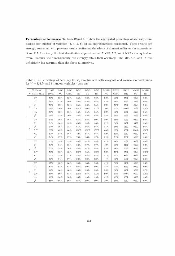
Percentage of Accuracy. Tables 5.12 and 5.13 show the aggregated percentage of accuracy com-
parison per number of variables (3, 4, 5, 6) for all approximations considered. These results are
strongly consistent with previous results confirming the effects of dimensionality on the approxima-
tions. DAC is clearly the best distribution approximation. MVIE, AC, and ChSC seem equivalent
overall because the dimensionality can strongly affect their accuracy. The ME, UE, and IA are
definitively less accurate than the above alternatives.
Table 5.12: Percentage of accuracy for asymmetric sets with marginal and correlation constraintsfor V = 3, 4, 5, and 6 random variables (part one).
% Times DAC DAC DAC DAC DAC DAC MVIE MVIE MVIE MVIE MVIE
V better than MVIE AC ChSC ME UE IN AC ChSC ME UE IN
3
L∞ 50% 52% 50% 55% 90% 99% 52% 48% 55% 90% 99%
L1 50% 52% 50% 55% 85% 93% 52% 50% 55% 85% 93%
L2 50% 52% 50% 55% 86% 95% 52% 50% 55% 86% 94%
ΔH 50% 70% 50% 100% 80% 100% 70% 15% 100% 80% 100%
KL 50% 52% 50% 56% 85% 95% 52% 48% 56% 85% 95%
χ2 50% 52% 50% 56% 85% 95% 52% 49% 56% 85% 95%
4
L∞ 54% 56% 56% 65% 98% 99% 50% 50% 62% 98% 98%
L1 54% 56% 55% 65% 94% 96% 51% 50% 61% 94% 95%
L2 54% 56% 55% 65% 96% 97% 51% 50% 61% 96% 96%
ΔH 35% 65% 60% 100% 100% 100% 60% 65% 95% 100% 100%
KL 53% 57% 56% 72% 95% 97% 52% 51% 69% 96% 96%
χ2 54% 57% 57% 76% 96% 97% 52% 52% 72% 96% 96%
5
L∞ 73% 74% 75% 83% 97% 98% 41% 46% 70% 92% 93%
L1 73% 74% 75% 83% 97% 97% 42% 46% 71% 91% 92%
L2 73% 74% 76% 82% 97% 98% 43% 46% 70% 91% 92%
ΔH 70% 90% 85% 100% 95% 100% 90% 75% 95% 95% 100%
KL 74% 75% 77% 88% 98% 98% 41% 45% 81% 95% 95%
χ2 73% 74% 77% 90% 98% 98% 41% 48% 88% 98% 98%
6
L∞ 87% 85% 86% 94% 98% 99% 41% 38% 81% 96% 96%
L1 87% 87% 87% 96% 99% 99% 38% 37% 87% 98% 99%
L2 86% 86% 86% 95% 99% 99% 38% 36% 84% 97% 97%
ΔH 80% 90% 85% 100% 95% 100% 90% 65% 100% 95% 100%
KL 89% 90% 90% 96% 99% 99% 42% 45% 93% 99% 99%
χ2 88% 88% 90% 97% 99% 99% 39% 50% 93% 99% 99%
133

Table 5.13: Percentage of accuracy for asymmetric sets with marginal and correlation constraintsfor V = 3, 4, 5, and 6 random variables (part two).
% Times AC AC AC AC ChSC ChSC ChSC ME ME UE
V better than ChSC ME UE IN ME UE IN UE IN IN
3
L∞ 48% 55% 92% 100% 55% 90% 99% 89% 100% 87%
L1 48% 55% 86% 94% 55% 85% 93% 83% 95% 65%
L2 48% 55% 87% 96% 55% 86% 94% 83% 98% 57%
ΔH 30% 100% 80% 100% 100% 80% 100% 75% 100% 90%
KL 48% 55% 88% 97% 56% 85% 95% 82% 100% 79%
χ2 48% 55% 88% 98% 56% 85% 95% 82% 97% 80%
4
L∞ 45% 63% 96% 98% 61% 97% 98% 96% 98% 64%
L1 44% 62% 94% 96% 62% 94% 96% 94% 97% 78%
L2 44% 62% 95% 98% 61% 95% 98% 95% 98% 60%
ΔH 35% 100% 100% 100% 100% 100% 100% 100% 100% 85%
KL 44% 69% 96% 99% 68% 95% 98% 94% 100% 72%
χ2 46% 73% 97% 99% 72% 95% 98% 87% 95% 66%
5
L∞ 53% 76% 96% 96% 76% 96% 96% 95% 97% 55%
L1 55% 78% 95% 95% 78% 95% 95% 91% 93% 64%
L2 54% 76% 96% 96% 76% 95% 96% 93% 94% 60%
ΔH 60% 100% 95% 100% 100% 95% 100% 95% 100% 80%
KL 57% 88% 99% 99% 86% 99% 99% 99% 100% 72%
χ2 60% 92% 99% 99% 90% 98% 98% 96% 98% 70%
6
L∞ 50% 88% 96% 96% 87% 96% 96% 96% 96% 46%
L1 46% 94% 99% 99% 94% 99% 99% 99% 100% 52%
L2 47% 91% 97% 98% 91% 98% 99% 98% 98% 28%
ΔH 55% 100% 95% 100% 100% 95% 100% 85% 100% 95%
KL 54% 95% 99% 100% 94% 99% 99% 100% 100% 30%
χ2 64% 95% 99% 100% 94% 98% 99% 99% 100% 29%
5.4.3 Findings in Arbitrarily Constrained Truth Sets
Arbitrarily Marginal Constrained Truth Sets:
1. The most accurate approximation was DAC, followed by AC.
2. The third-most accurate approximation was MVIE. For low-dimensional sets, MVIE is nearly
as accurate as DAC and AC. But as the dimension increases, the difference in accuracy
becomes pronounced.
3. The worst approximation was ME.
Arbitrarily Marginal and Rank Correlation Constrained Truth Sets:
1. Approximations that can process larger amounts of information show better accuracy. Ap-
proximations such as UE and IA that can process only small amounts of information result
in low accuracy approximations.
2. The most accurate approximation was DAC.
3. As dimension increases, MVIE and ME lose accuracy and AC and ChSC gain accuracy.
4. The least accurate approximations were IA, UE, and ME. Among these three, ME showed
the best accuracy.
134

Chapter 6
A New Approach to Decision Analysis
Until now, we have being exploring the accuracy of a joint distribution approximation from
the probability space. In this chapter we observe the accuracy of a joint distribution approximation
from the decision space and its implications in DA. We present two decisions that needs to deal
with probabilistic dependence and provide partial information about the uncertainties.
The first decision is an extension of Bickel et al. (2008). The paper presents a series of
dynamic decisions in the oil industry to optimize the exploration of well-alternatives. The second
decision is taken from Clemen (1996). This is a typical decision model and has being study in
Clemen and Reilly (1999) and Reilly (2000) using different techniques.
6.1 Optimal Sequential Exploration
In this paper we are concern with decisions in which we lack complete information regard-
ing the underlying joint probability distribution. In particular we analyze the optimal exploration
strategy in a deep-water oil and gas exploration program when there is a limited amount of infor-
mation. The problem was originally described in Bickel and Smith (2006), and was solved assuming
the joint probability distribution match the maximum entropy distribution. We extend the analysis
by considering different joint approximation models and apply a new sensitivity analysis procedure
as a significant extension to the original paper. This problem is of particular interest due to the
complexity of the decision and the limited amount of information.
Although the lack of information could stem from an under specification of marginal distri-
butions, we are primarily motivated by underspecification of the probabilistic dependence structure.
Probabilistic dependencies are inherent to many decision environments, including medicine (Chessa
et al., 1999), nuclear power (Cooke and Waij, 1986), environmental policy (Helton, 1993), financial
engineering (Cherubini et al., 2004), critical infrastructure management (Min et al., 2007) and oil
135

exploration (Bickel and Smith, 2006; Bickel et al., 2008). Failure to capture these relationships can
have important and sometimes tragic consequences (Apostolakis and Kaplan, 1981; Smith et al.,
1992). For example, the Space Shuttle Challenger accident was apparently caused, in part, by en-
gineers’ failure to understand the dependency between ambient temperature and o-ring resiliency
(Presidential Commission on the Space Shuttle Challenger Accident, 1986). In finance, the multi-
billion-dollar failure of Long-Term Capital Management stemmed from a failure to properly model
complex dependencies between financial markets (Lowenstein, 2000).
Probabilistic dependence is often ignored because it complicates probability assessments
(Lowell, 1994; Korsan, 1990). Winkler (1982) identified the assessment and modeling of probabilistic
dependence as one of the most important research topics facing decision analysts. He suggested
the development of sensitivity analyses that would identify key dependencies and decision-making
methods that use less than full probabilistic information. Miller (1990) argued, “We need a way to
assess and process dependent probabilities efficiently. If we can find generally applicable methods
for doing so, we could make significant advances in our ability to analyze and model complex
decision problems.” These critical challenges have gone largely unanswered.
In Bickel and Smith (2006) the author make use of the maximum entropy (maxent) method
to generate a single joint distribution with the highest amount of uncertainty (highest entropy)
selected from the set of all possible distributions that are consistent with the given information.
Maxent was pioneered by Jaynes (1957, 1968), and further developed by Ireland and Kullback
(1968), who were the first to approximate a discrete joint distribution given information on the
lower-order component distributions. Lowell (1994) also used maxent to specify a joint distribution
given lower order assessments (e.g., pairwise conditional assessments). More recently, Abbas (2006)
and Bickel and Smith (2006) explored the use of maxent to facilitate the modeling of dependence.
In this paper, we go one step further and perform a new sensitivity analysis procedure that
aloud us to describe the effects of unknown dependence structures in joint probability distributions.
In particular, we create the set of all possible discrete distributions that are consistent with the
available information. We then use a new simulation model described in Chapter 3 to uniformly
sample from this set. Finally, we can evaluate our decision over a collection of joint distributions
that represents a discrete version of the set of all possible joint distributions.
The literature presents other sensitivity procedures that have been developed to explore
136

portions of the set of possible joint distributions. For example, Lowell (1994) developed a sensitivity
analysis procedure to identify important pairwise conditional probability assessments. Clemen and
Reilly (1999) proposed the use of a normal copula, characterized by pairwise correlation coefficients.
They then perturbed the correlation matrix to explore a set of possible joint distributions. This set is
restricted to joint distributions that can be modeled with a normal copula. Reilly (2000) developed a
sensitivity approach that uses synthetic variables based on a pairwise correlation coefficient matrix.
However, our proposed approach is more robust in that it uniformly explores the complete space
of possible joint distribution and can be subject to strict rules or constraints.
The new sensitivity analysis procedure can also be compared to robust procedures such as
maximin or robust optimization (Ben-Tal et al., 2009) to evaluate decisions based on their worst
possible outcomes. We do not directly address these methods. We note, however, that identifying
the worst possible joint distribution is often difficult. Our procedure could be used in a robust
setting to “stress test” decisions.
This paper is organized as follows: §6.1.1 we briefly describe the simulation procedure that
serves as a basis for the rest of the analysis; §6.1.2 lay out the information available to the DM;
§6.1.3 describe how the available information can be coded into a polytope; §6.1.4 test the sampled
collection and present the accuracy measures to be used; §6.1.5 present the decision formulation of
the sequential exploration problem; §6.1.6 show and analyze the results of the optimal sequential
exploration problem. Finally, §6.1.7 conclude and discuss future research.
6.1.1 Joint Distributions Simulation Model
The joint distribution simulation approach (JDSIM) proposed in Chapter 3 samples from
the set of all possible joint distributions that are consistent with the given information. In this
way, it provides not one, but a collection of joint distributions under which the decision can be
evaluated. The procedure begins with the specification of linear constraints on the joint distribution
(e.g., specification of marginal probabilities or pairwise correlations) and the creation of a convex
polytope T, the “truth set,” that matches the given information. By “truth” we mean that any
distribution within this set is consistent with the assessments and therefore could be the “true”
joint distribution.
137

We generate a truth set using the notation described in Chapter 3 to define the following
linear system:
∑ωk∈U
pωk= 1, (6.1a)
∑ωk∈U
ωVir
pωk= q
ωVir
∀ Vi ∈ V, ωVi
r ∈ OVi
, (6.1b)
∑ωk∈U
ωVjs ω
Vir
pωk= q
ωVjs ω
Vir
∀ Vi, Vj ∈ V, ωVi
r ∈ OVi
, ωVj
s ∈ OVj
, (6.1c)
pωk≥ 0, ∀ωk ∈ U. (6.1d)
This truth set is flexible and can integrate more or less information as needed. In this case of study
we limit the information to marginal and pairwise assessments for which equations have being
previously described (Chapter 3).
6.1.2 Optimal Sequential Exploration Information
In Bickel et al. (2008), the Author presents a practical and flexible framework for evaluating
sequential exploration strategies where the exploration prospects are dependent. The paper was
motivated by an oil exploration problem and presents a case where a field with six possible well
locations needs to be developed. Each well location can be wet or dry, meaning there is an oil
deposit or not. The probability of a well being wet is pi. If a well is wet, the expected value of the
success is si. However, if the well is dry, the expected value of failure is fi.
We present a summary of the data in Table 6.1 from Bickel et al. (2008). This Table present
expected values in millions of dollars and represent net present values (NPVs) in the period in which
the well is drilled. The expected value given failure is the expected drilling cost. The expected
value given success is the expected net present value of the hydrocarbon production stream less the
drilling costs, costs of completion, production platforms, etc. These expectations take into account
uncertainty in gas and/or oil prices, reserves, production, drilling costs, and all other uncertainties.
The intrinsic values shown in Table 6.1 are the unconditional expected values: pisi + (1 −pi)fi. In this example, the intrinsic values are all negative, meaning the wells are “out of the
money,” and the company would not choose to drill them if they were considered in isolation.
138
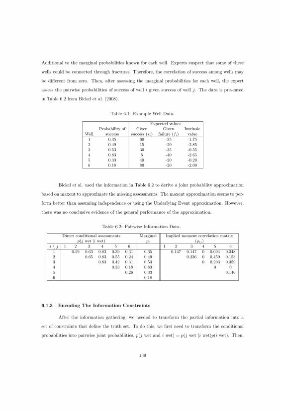
Additional to the marginal probabilities known for each well. Experts suspect that some of these
wells could be connected through fractures. Therefore, the correlation of success among wells may
be different from zero. Then, after assessing the marginal probabilities for each well, the expert
assess the pairwise probabilities of success of well i given success of well j. The data is presented
in Table 6.2 from Bickel et al. (2008).
Table 6.1: Example Well Data.
Expected valuesProbability of Given Given Intrinsic
Well success success (si) failure (fi) value
1 0.35 60 -35 -1.752 0.49 15 -20 -2.853 0.53 30 -35 -0.554 0.83 5 -40 -2.655 0.33 40 -20 -0.206 0.18 80 -20 -2.00
Bickel et al. used the information in Table 6.2 to derive a joint probability approximation
based on maxent to approximate the missing assessments. The maxent approximation seems to per-
form better than assuming independence or using the Underlying Event approximation. However,
there was no conclusive evidence of the general performance of the approximation.
Table 6.2: Pairwise Information Data.
Direct conditional assessments Marginal Implied moment correlation matrixp(j wet |i wet) pi (ρij)
i \ j 1 2 3 4 5 6 1 2 3 4 5 6
1 0.59 0.63 0.83 0.39 0.31 0.35 0.147 0.147 0 0.094 0.2482 0.65 0.83 0.55 0.24 0.49 0.236 0 0.459 0.1533 0.83 0.42 0.31 0.53 0 0.203 0.3594 0.33 0.18 0.83 0 05 0.26 0.33 0.1466 0.18
6.1.3 Encoding The Information Constraints
After the information gathering, we needed to transform the partial information into a
set of constraints that define the truth set. To do this, we first need to transform the conditional
probabilities into pairwise joint probabilities, p(j wet and i wet) = p(j wet |i wet)p(i wet). Then,
139

from Table 6.2 we generate Table 6.3.
Table 6.3: Pairwise Information.
p(j wet and i wet)
i \ j 1 2 3 4 5 6
1 0.2065 0.2205 0.2905 0.1365 0.10852 0.3185 0.4067 0.2695 0.11763 0.4399 0.2226 0.16434 0.2739 0.14945 0.08586
Now we are ready to define the constrains of the truth set. Using the system of Equations
6.1 we can create a polytope Ap = b. Were A is a 22 by 64 matrix of zeros and ones that represent
the 22 constraints of the 64 elements of the joint distribution. The vector b ∈ R22 is the vector that
encode the partial information (marginal and pairwise assessments). In this case, the first element
forces the probabilities to sum to one, the next six elements force the joint distribution to match
the marginal information and the last 15 elements match the elements in Table 6.3.
We define the truth set T ≡ {p | Ap = b, p ≥ 0}. Where the Matrix A and the vector b
are described as follows:
A =
1 1 1 1 1 1 1 1 1 1 1 1 1 1 1 1 1 1 1 1 1 1 1 1 1 1 1 1 1 1 1 1 1 1 1 1 1 1 1 1 1 1 1 1 1 1 1 1 1 1 1 1 1 1 1 1 1 1 1 1 1 1 1 1
1 1 1 1 1 1 1 1 1 1 1 1 1 1 1 1 1 1 1 1 1 1 1 1 1 1 1 1 1 1 1 1 0 0 0 0 0 0 0 0 0 0 0 0 0 0 0 0 0 0 0 0 0 0 0 0 0 0 0 0 0 0 0 0
1 1 1 1 1 1 1 1 1 1 1 1 1 1 1 1 0 0 0 0 0 0 0 0 0 0 0 0 0 0 0 0 1 1 1 1 1 1 1 1 1 1 1 1 1 1 1 1 0 0 0 0 0 0 0 0 0 0 0 0 0 0 0 0
1 1 1 1 1 1 1 1 0 0 0 0 0 0 0 0 1 1 1 1 1 1 1 1 0 0 0 0 0 0 0 0 1 1 1 1 1 1 1 1 0 0 0 0 0 0 0 0 1 1 1 1 1 1 1 1 0 0 0 0 0 0 0 0
1 1 1 1 0 0 0 0 1 1 1 1 0 0 0 0 1 1 1 1 0 0 0 0 1 1 1 1 0 0 0 0 1 1 1 1 0 0 0 0 1 1 1 1 0 0 0 0 1 1 1 1 0 0 0 0 1 1 1 1 0 0 0 0
1 1 0 0 1 1 0 0 1 1 0 0 1 1 0 0 1 1 0 0 1 1 0 0 1 1 0 0 1 1 0 0 1 1 0 0 1 1 0 0 1 1 0 0 1 1 0 0 1 1 0 0 1 1 0 0 1 1 0 0 1 1 0 0
1 0 1 0 1 0 1 0 1 0 1 0 1 0 1 0 1 0 1 0 1 0 1 0 1 0 1 0 1 0 1 0 1 0 1 0 1 0 1 0 1 0 1 0 1 0 1 0 1 0 1 0 1 0 1 0 1 0 1 0 1 0 1 0
1 1 1 1 1 1 1 1 1 1 1 1 1 1 1 1 0 0 0 0 0 0 0 0 0 0 0 0 0 0 0 0 0 0 0 0 0 0 0 0 0 0 0 0 0 0 0 0 0 0 0 0 0 0 0 0 0 0 0 0 0 0 0 0
1 1 1 1 1 1 1 1 0 0 0 0 0 0 0 0 1 1 1 1 1 1 1 1 0 0 0 0 0 0 0 0 0 0 0 0 0 0 0 0 0 0 0 0 0 0 0 0 0 0 0 0 0 0 0 0 0 0 0 0 0 0 0 0
1 1 1 1 0 0 0 0 1 1 1 1 0 0 0 0 1 1 1 1 0 0 0 0 1 1 1 1 0 0 0 0 0 0 0 0 0 0 0 0 0 0 0 0 0 0 0 0 0 0 0 0 0 0 0 0 0 0 0 0 0 0 0 0
1 1 0 0 1 1 0 0 1 1 0 0 1 1 0 0 1 1 0 0 1 1 0 0 1 1 0 0 1 1 0 0 0 0 0 0 0 0 0 0 0 0 0 0 0 0 0 0 0 0 0 0 0 0 0 0 0 0 0 0 0 0 0 0
1 0 1 0 1 0 1 0 1 0 1 0 1 0 1 0 1 0 1 0 1 0 1 0 1 0 1 0 1 0 1 0 0 0 0 0 0 0 0 0 0 0 0 0 0 0 0 0 0 0 0 0 0 0 0 0 0 0 0 0 0 0 0 0
1 1 1 1 1 1 1 1 0 0 0 0 0 0 0 0 0 0 0 0 0 0 0 0 0 0 0 0 0 0 0 0 1 1 1 1 1 1 1 1 0 0 0 0 0 0 0 0 0 0 0 0 0 0 0 0 0 0 0 0 0 0 0 0
1 1 1 1 0 0 0 0 1 1 1 1 0 0 0 0 0 0 0 0 0 0 0 0 0 0 0 0 0 0 0 0 1 1 1 1 0 0 0 0 1 1 1 1 0 0 0 0 0 0 0 0 0 0 0 0 0 0 0 0 0 0 0 0
1 1 0 0 1 1 0 0 1 1 0 0 1 1 0 0 0 0 0 0 0 0 0 0 0 0 0 0 0 0 0 0 1 1 0 0 1 1 0 0 1 1 0 0 1 1 0 0 0 0 0 0 0 0 0 0 0 0 0 0 0 0 0 0
1 0 1 0 1 0 1 0 1 0 1 0 1 0 1 0 0 0 0 0 0 0 0 0 0 0 0 0 0 0 0 0 1 0 1 0 1 0 1 0 1 0 1 0 1 0 1 0 0 0 0 0 0 0 0 0 0 0 0 0 0 0 0 0
1 1 1 1 0 0 0 0 0 0 0 0 0 0 0 0 1 1 1 1 0 0 0 0 0 0 0 0 0 0 0 0 1 1 1 1 0 0 0 0 0 0 0 0 0 0 0 0 1 1 1 1 0 0 0 0 0 0 0 0 0 0 0 0
1 1 0 0 1 1 0 0 0 0 0 0 0 0 0 0 1 1 0 0 1 1 0 0 0 0 0 0 0 0 0 0 1 1 0 0 1 1 0 0 0 0 0 0 0 0 0 0 1 1 0 0 1 1 0 0 0 0 0 0 0 0 0 0
1 0 1 0 1 0 1 0 0 0 0 0 0 0 0 0 1 0 1 0 1 0 1 0 0 0 0 0 0 0 0 0 1 0 1 0 1 0 1 0 0 0 0 0 0 0 0 0 1 0 1 0 1 0 1 0 0 0 0 0 0 0 0 0
1 1 0 0 0 0 0 0 1 1 0 0 0 0 0 0 1 1 0 0 0 0 0 0 1 1 0 0 0 0 0 0 1 1 0 0 0 0 0 0 1 1 0 0 0 0 0 0 1 1 0 0 0 0 0 0 1 1 0 0 0 0 0 0
1 0 1 0 0 0 0 0 1 0 1 0 0 0 0 0 1 0 1 0 0 0 0 0 1 0 1 0 0 0 0 0 1 0 1 0 0 0 0 0 1 0 1 0 0 0 0 0 1 0 1 0 0 0 0 0 1 0 1 0 0 0 0 0
1 0 0 0 1 0 0 0 1 0 0 0 1 0 0 0 1 0 0 0 1 0 0 0 1 0 0 0 1 0 0 0 1 0 0 0 1 0 0 0 1 0 0 0 1 0 0 0 1 0 0 0 1 0 0 0 1 0 0 0 1 0 0 0
b = [1, 0.35, 0.49, 0.53, 0.83, 0.33, 0.18, 0.2065, 0.2205, 0.2905, 0.1365, 0.1085,
0.3185, 0.4067, 0.2695, 0.1176, 0.4399, 0.2226, 0.1643, 0.2739, 0.1494, 0.0858].
140

JDSIM generates a collection of joint probability distributions such that Ap = b and p ≥ 0. This
collection of distributions represents a discrete representation of T.
6.1.4 Sampling From T
We generate a collection of 4 million samples. The collection meet the fair convergence
requirements presented in Chapter 3. That is to say, the dynamic average center (DAC) converges
to a stationary point in the interior of T. The collection took 4 hours of processing time in an
Intel(R) Core(TM)2 Quad CPU Q6700 @ 2.66GHz with 4GB of RAM. The process was run in
Mathematica 8.0.
The collection of joint distributions generated by the HR consist of vectors in R64 located
in a 42 dimensional subspace, making it difficult to observe. Hence, we use different mappings
R64 → R (Equations 6.2) to understand how the sample path is behaving. In this paper we observe
four of such mappings: The maximum absolute differences (L∞ norm), the Euclidean distance
(L2 norm), the Kullback-Leibler divergence (KL) and entropy (H). The first three mappings are
measured with respect to DAC which denotes the center of the collection sampled and converges to
the center of T, while the last mapping is relative to the uncertainty described by each distribution.
L∞n (p,pDAC) = max{|p1 − pDAC1 |, · · · , |pn − pDAC
n |}, (6.2a)
L2n(p,pDAC) =
[n∑
i=1
(pi − pDACi )2
] 12
, (6.2b)
KLn(p||pDAC) =n∑
i=1
pi log
(pi
pDACi
), (6.2c)
Hn(p) =n∑
i=1
pi log pi. (6.2d)
The four different mappings provide one dimensional descriptions of a multidimensional
topography as follows. L∞ norm (6.2a) describes an upper bound for how far two corresponding
elements of two different distributions can be. In specific, it describes how far an element of a
joint distribution can be from the corresponding element at the center of T (DAC). L2 norm (6.2b)
describes the direct distance between the DAC and the sampled distributions. KL (6.2c) measures
141


The dynamic programming model can now be formalized as follows. Let v(w) denote the
continuation value for state w, that is, the expected NPV of future cash flows given that you start
in state w. In this value calculation, we include the expected future value for a successful well (si)
or a failed well (fi) in the period the well is drilled and discount cash flows using a discount factor
δ that corresponds to the time required to drill the well. Recall, that si is the discounted expected
net present value of production, in the period the well is drilled, from a successful well i (including
drilling costs), and (fi) is the expected cost of drilling an unsuccessful well i. If all the wells have
been drilled (i.e., w is a vector of zeros and ones), then v(w) = 0. For earlier states w, the expected
NPV associated with drilling well i is:
vi(w) =μ(w1
i )
μ(w)(si + δv(w1
i )) +μ(w0
i )
μ(w)(fi + δv(w0
i )), (6.4)
The optimal action in state w is to drill the well with the largest v(w) or, if no well has a positive
value, to not drill at all. The optimal continuation value v(w) is max[vi(w), 0], where the maximum
is taken over all available wells and not drilling (0). There is no circularity in this definition of the
value function because one never visits the same state twice; each time you drill a well, its state
changes to either wet or dry.
6.1.6 Optimal Strategies
The optimal strategy describes a drilling policy that indicates wether to drill or not depend-
ing on the state of the previously drilled wells. In our case we can define an optimal strategy for
each joint distribution approximation. In this paper we consider the independence approximation
(IA) which is of common use in practice, the underling event (UE) approximation (Keefer, 2004)
and the maximum entropy approximation as done in Bickel and Smith (2006). Additionally, we
consider the AC, the CHSC, the MVIEC and the DAC approximations and compare the results to
previous approximations.
Figure 6.4 present the optimal strategies for all the joint distribution approximations con-
sidered. These strategies are described as decision trees and must be read sequentially from left
to right. For example, in Figure 6.4(a) the strategy indicates to start drilling well 3, and if the
well is wet (Up), then we should drill well 6, otherwise we stop drilling more wells. In the same
lines, if well 6 is wet, then we drill well 1, otherwise if well 6 is dry, we drill well 2. Additionally,
145

the strategies in Figure 6.4 describe the net present values at each stage of the decision. i.e. the
expected value of each decision at the moment of choosing to drill or not.
(a) ME strategy. (b) DAC strategy. (c) AC strategy.
(d) ChSC strategy. (e) MVIE strategy.
Figure 6.4: Strategies derived from approximation joint distributions.
146

The IA and the UE strategies have been omitted from Figure 6.4, since both strategies are
the same and present a trivial policy (never drill). As recall from Table 6.1, the expected value of
each well independently is negative. Therefore, without any probabilistic dependence, the complete
strategy is the same than the strategy for each particular well. The complete joint probability
distribution approximations are presented in Table 6.4 including the IA/UE approximation.
The ME strategy (Figure 6.4(a)) was previously explore by Bickel and Smith. This strategy
exploit the fact that the ME approximation assumes that all higher order assessments (three wise,
four wise,...) are as close to independent as is aloud by the consistency of the joint distribution. For
example, the pairwise assessments including well 4 show that this well is pairwise independent with
respect to all others. Moreover, the ME approximation assumes that all higher order assessments
are as close to independent as possible. Then, under ME, well 4 is independent and has negative
expected value. The assumptions made by the ME approximation excludes well 4 as a viable drilling
alternative.
The strategy presented by DAC (Figure 6.4(b)) search for a distribution that is the most
conservative representation of the truth set. The DAC approximation does not care about indepen-
dence among wells, but cares about to find the closest approximation to the center of mass of T.
One of the main differences is that the higher order assessments are not as close as independence
as ME assumes. For example, the DAC strategy still considers well 4 to be pairwise independent,
however, the well is not independent of all others. This strategy considers that under some scenarios
well 4 can bring extra revenue.
The AC and the ChSC approximations attempt to find a joint distribution where each
element is as far as possible from zero. In the case of AC, a log-barrier function is used to move
the approximation far from the boundary, in the case of ChSC this same idea is done by means
of expanding a hypersphere with center in T. As with the DAC approximation, the AC and the
ChSC attempt to find a point in the center of the truth set that provide a robust (conservative)
approximation, however, AC and ChSC have the advantage that are invariant with respect to the
collection sampled from T. That is to say, both approximations can be calculated without running
a JDSIM procedure.
Finally, the MVIEC approximate the center of T by assuming it is close to the center of the
ellipsoid with the largest volume inscribed in the truth set. This approximation is also invariant
to the collection sampled, but it is computing intensive do to the number of variables required to
calculate the shape of the hyper ellipse. Empirical observations suggest that the MVIEC and the
147

Table 6.4: Joint Probability Distribution Approximations.
IA/UE ME DAC AC ChSC MVIE1 0.00448 0.03825 0.03957 0.03799 0.03740 0.040592 0.02041 0.03720 0.02523 0.03198 0.03371 0.026063 0.00910 0.02089 0.02507 0.02587 0.02650 0.024554 0.04145 0.02713 0.02947 0.02727 0.02698 0.028685 0.00092 0.00783 0.00280 0.00285 0.00359 0.002736 0.00418 0.00762 0.00510 0.00511 0.00560 0.004697 0.00186 0.00428 0.00298 0.00317 0.00298 0.003038 0.00849 0.00556 0.00610 0.00654 0.00601 0.005979 0.00397 0.00192 0.00113 0.00116 0.00098 0.0011510 0.01810 0.02053 0.02647 0.02358 0.02252 0.0261911 0.00807 0.00167 0.00115 0.00116 0.00098 0.0011512 0.03676 0.02379 0.02785 0.02645 0.02653 0.0288713 0.00081 0.00039 0.00086 0.00085 0.00098 0.0008614 0.00371 0.00421 0.00527 0.00496 0.00481 0.0048715 0.00165 0.00034 0.00089 0.00088 0.00098 0.0008916 0.00753 0.00487 0.00655 0.00671 0.00594 0.0062417 0.00466 0.00441 0.00645 0.00571 0.00498 0.0063718 0.02125 0.00515 0.00674 0.00615 0.00551 0.0061219 0.00947 0.01952 0.01864 0.01988 0.01970 0.0178920 0.04314 0.03045 0.03614 0.03239 0.03246 0.0371821 0.00096 0.00090 0.00212 0.00204 0.00252 0.0021622 0.00435 0.00105 0.00330 0.00315 0.00304 0.0033423 0.00194 0.00400 0.00305 0.00315 0.00298 0.0033024 0.00884 0.00624 0.00774 0.00728 0.00655 0.0078525 0.00414 0.00042 0.00099 0.00100 0.00098 0.0010026 0.01884 0.00540 0.00622 0.00605 0.00563 0.0061427 0.00840 0.00297 0.00112 0.00116 0.00098 0.0011528 0.03826 0.05078 0.03825 0.04271 0.04465 0.0374329 0.00085 0.00009 0.00079 0.00076 0.00098 0.0007930 0.00386 0.00111 0.00345 0.00318 0.00328 0.0034531 0.00172 0.00061 0.00089 0.00089 0.00098 0.0009132 0.00784 0.01040 0.00761 0.00801 0.00829 0.0084333 0.00832 0.02075 0.01677 0.01908 0.01968 0.0162634 0.03791 0.06186 0.08568 0.07744 0.07665 0.0849835 0.01690 0.01170 0.01572 0.01387 0.01407 0.0159036 0.07698 0.04657 0.03679 0.03892 0.03624 0.0363437 0.00170 0.00425 0.00306 0.00319 0.00295 0.0030638 0.00777 0.01267 0.00763 0.00885 0.00838 0.0081439 0.00346 0.00240 0.00355 0.00351 0.00258 0.0034340 0.01577 0.00954 0.01299 0.01288 0.01519 0.0141041 0.00738 0.00128 0.00111 0.00113 0.00098 0.0011142 0.03362 0.04189 0.03895 0.04205 0.04299 0.0394543 0.01498 0.00115 0.00111 0.00112 0.00098 0.0011144 0.06826 0.05011 0.03463 0.03764 0.03951 0.0343345 0.00151 0.00026 0.00091 0.00088 0.00098 0.0008946 0.00689 0.00858 0.00897 0.00842 0.00731 0.0084947 0.00307 0.00023 0.00092 0.00091 0.00098 0.0009248 0.01398 0.01026 0.01473 0.01362 0.01404 0.0150049 0.00866 0.00374 0.00511 0.00515 0.00455 0.0048050 0.03946 0.01340 0.00640 0.00729 0.00777 0.0063751 0.01759 0.01710 0.01340 0.01303 0.01467 0.0143552 0.08012 0.08177 0.07273 0.07789 0.07904 0.0734853 0.00177 0.00077 0.00234 0.00225 0.00228 0.0022954 0.00808 0.00274 0.00431 0.00439 0.00401 0.0046655 0.00360 0.00350 0.00368 0.00358 0.00287 0.0036156 0.01641 0.01675 0.01935 0.01818 0.01858 0.0177457 0.00768 0.00044 0.00097 0.00098 0.00098 0.0009658 0.03499 0.01725 0.00611 0.00717 0.00860 0.0063759 0.01560 0.00319 0.00110 0.00112 0.00098 0.0010960 0.07105 0.16731 0.20293 0.19562 0.19182 0.2026261 0.00157 0.00009 0.00082 0.00079 0.00098 0.0008162 0.00717 0.00353 0.00438 0.00445 0.00443 0.0048863 0.00319 0.00065 0.00094 0.00092 0.00098 0.0009364 0.01455 0.03427 0.02193 0.02370 0.02396 0.02155
148

DAC are close to each other, which explains why both strategies have a similar policy. However,
this is just a conjecture for which no analytic results are known.
6.1.6.1 Accuracy of the Joint Distribution Approximations
Each of the strategies consider so far is directly link to an approximation. The question
now is: How accurate are the approximations with respect to the possible distributions in T? We
answer this question using the JDSIM method described in Chapter 3.
In Bickel and Smith (2006) the authors propose a method to evaluate the accuracy of the
approximations using a simulation procedure proposed by Keefer (2004). However, such simulation
procedure is hard to control and can not be applied to constrained sets. As a result, the accuracy
results provided by Bickel and Smith (2006) are taken over 5,000 arbitrary polytopes (truth sets),
and in each set they test each approximation against one point in the set (the sampled distribution).
Our approach differs in that we only sample distributions from one set defined by the assessed be-
liefs (T). However, we sample 4 million distributions to fully explore the truth set and make a clear
statement about the joint distribution approximations and its accuracy. Recall that in the JDSIM
each sampled joint distribution could be the true distribution, and therefore, any approximation
proposed need to be compared to all the sampled distributions in order to measure its accuracy.
Additionally, we randomly choose 160,000 samples from the 4 million and solve them for the cor-
responding optimal strategies. This process took an average of 20 seconds per distribution, which
make it difficult to solve for the complete sample. However, 160,000 samples from the full collection
can be use as an estimate for the hole sample.
We use four measures of accuracy to evaluate the four approximations: (i) the mean abso-
lute difference between the approximate and sampled joint probabilities, (ii) the maximum absolute
difference in these joint probabilities, (iii) the Euclidean distance, i.e. the length of the straight
line between the approximation and the sampled distributions, and (iv) the KL divergence from
the sampled distribution to the approximation. These error measures are all such that a value of
zero indicates no error and larger values indicate larger errors. Measures (i) and (ii) were used in
Keefer’s analysis; Bickel and Smith, and Abbas considers (i),(ii), and (iv).
Using the sub collection of 160,000 samples for which we solve to optimality, we add two
economic measures in the sequential exploration setting used by Bickel and Smith: (v) the absolute
value of the difference between the optimal expected value given by the sampled probabilities and the
optimal expected value given by the approximate probabilities and (vi) the difference between the
149

expected value given by following the optimal strategy and the expected value given by following the
approximation strategy, with both expected values calculated using the sampled joint probabilities.
We refer to this as the expected value lost.
The error in the value estimate (measure v) is an appropriate error measure if the analysis
is intended to estimate the value of the exploration opportunity, for example, if contemplating
selling or acquiring the exploration opportunity. The expected value lost (measure vi) indicates
how close you come to identifying the optimal exploration strategy.
Table 6.5 shows that for the accuracy measures based in probabilities (i, ii, iii, iv), the best
approximation is DAC, followed by AC, ChSC, MVIEC, ME, UE, IA. The intuition behind these
results can be observed when we consider the information used to create each approximation. It
should not surprise us that the approximation with the least amount of information (IA) provide
the worst results. Notice that in this case both approximations, IA and UE, do not even belong
to the interior of T. Alternatively, the ME distribution does belong to the interior of the truth
set and uses all the information available, which increase its accuracy. However, it fill the missing
Table 6.5: Accuracy Results.
Independent Approx. Maximum Analytic Chebyshev’s Max. Vol. DynamicUnderlying Event Entropy Center Center Ins. Ellip. Average
(IA / UE) (ME) (AC) (ChSC) (MVIEC) (DAC)
i. Mean absolute differenceMean 0.0113 0.0063 0.0054 0.0054 0.0055 0.0054Std dev 0.0008 0.0012 0.0011 0.0011 0.0012 0.0011
ii. Max absolute difference (L∞ Norm)Mean 0.1262 0.0378 0.0294 0.0296 0.0300 0.0294Std dev 0.0189 0.0119 0.0083 0.0083 0.0094 0.0084
iii. Euclidean distance (L2 Norm)Mean 0.1734 0.0815 0.0687 0.0693 0.0701 0.0686Std dev 0.0166 0.0188 0.0159 0.0159 0.0177 0.0159
iv. KL divergenceMean 0.6095 0.2334 0.1802 0.1830 0.1847 0.1795Std dev 0.0649 0.0649 0.0536 0.0533 0.0580 0.0528
v. Absolute error in value estimate ($ million)Mean 17.62 3.22 3.02 3.09 2.36 2.91Std dev 1.18 1.18 1.18 1.18 1.18 1.18
vi. Lost value from approximate policy ($ million)Mean 17.62 4.29 2.95 2.91 3.03 2.91Std dev 1.18 2.16 1.51 1.54 1.72 1.54
150

information by assuming all other assessments should as independent as possible. Approximations
such as AC, ChSC and MVIEC use the same amount of information as ME, but the assumptions
taken in each case varies for each model, which make some approximations better that others in a
case basis. Finally, in addition to the available information, DAC improves its accuracy by using
the information of 4 million sampled joint distributions to fill higher assessment information.
The accuracy measures based on the strategies (v, vi) suggests that the DAC/ChSC and
the MVIE are the best strategies. DAC and ChSC share the lowest lost value from approximate
policy and the MVIE strategy has the lowest absolute error in value estimate followed by DAC.
6.1.6.2 Alternative Strategies
In the previous section we measure the accuracy of four approximations that derive in
four different strategies. However, there are a number of strategies that are not the result of
an approximation distribution, but generated by solving to optimality the sequential exploration
problem using the sampled distributions. In other words, by taking the sub-collection of 160, 000
samples, we can create a collection of 160, 000 strategies (one for each sample). After accounting
for redundancies, we are left with a collection of 82, 205 different strategies, some of which appear
more frequent than others. Figure 6.5 shows the frequencies for each strategy in descending order,
where each dot represents a single strategy.
We observe that a large portion of the strategies have frequency less than ten, and only
ten strategies have frequency above 50, This last group includes the strategies that are optimal
for the largest number of joint distributions sampled in the sub-collection. Then, we can test the
performance of a small group of strategies (the ones with highest frequency) and compare them to
the strategies generated from the approximation distributions. Figure 6.7 shows the nine strategies
for which the frequency is the highest among the sub-collection.
For each of these strategies we evaluate the profit under all 4 million joint distributions in
the original collection sampled from T. The result is a group of 15 strategies (six strategies from the
approximation distributions and nine from the frequencies) that we can evaluate. Tables 6.6 and
6.7 show the mean, standard deviation, minimum and maximum values for the profits generated
by all 15 strategies.
It result is surprising to find that there are strategies that closely match the some of
the approximation joint distributions. This is the case of the fourth strategy (S4) with mean of
$14.42, which outperforms the mean of $13.34 of ME and is close to the mean of $14.71 of DAC.
151

Figure 6.5: Most Common Optimal Strategies.
Table 6.6: Profit Statistics For Full Strategies Based on Approximation Distributions. (in millions)
PMF Approximations
ME AC ChSC MVIE DACMean $ 13.34 $ 14.68 $ 14.71 $ 14.60 $ 14.71Std. Dev. $ 1.55 $ 1.33 $ 1.39 $ 1.63 $ 1.39Min $ 9.26 $ 10.33 $ 9.73 $ 8.86 $ 9.73Max $ 18.22 $ 18.46 $ 18.69 $ 19.03 $ 18.69
Even more, by observing the range [9.9, 20.04], the S4 shows a higher range than the rest of the
strategies consider. Nonetheless, the results from both Tables 6.6 and 6.7 still conclude that the
most profitable strategy in expectation is DAC.
Table 6.7: Profit Statistics For Full Strategies Based on Selected Strategies. (in millions)
High Frequency Full Strategies
1st 2nd 3th 4th 5th 6th 7th 8th 9th
Mean $12.84 $13.27 $13.05 $14.42 $13.46 $12.99 $13.39 $13.04 $13.26St. Dev. $2.14 $1.90 $1.56 $1.69 $1.55 $1.53 $1.61 $1.83 $1.63Min $7.16 $7.03 $8.80 $9.90 $8.17 $7.65 $7.43 $7.26 $7.12Max $18.96 $18.87 $18.68 $20.04 $18.46 $17.82 $18.09 $18.99 $18.32
In Figure 6.6 we can see that some strategies tend to perform better than others a larger
percentage of the time. An advantage of the alternative strategies comes from observing the ro-
bustness of the strategy. In other words, we can observe the fraction of time a strategy outperform
152
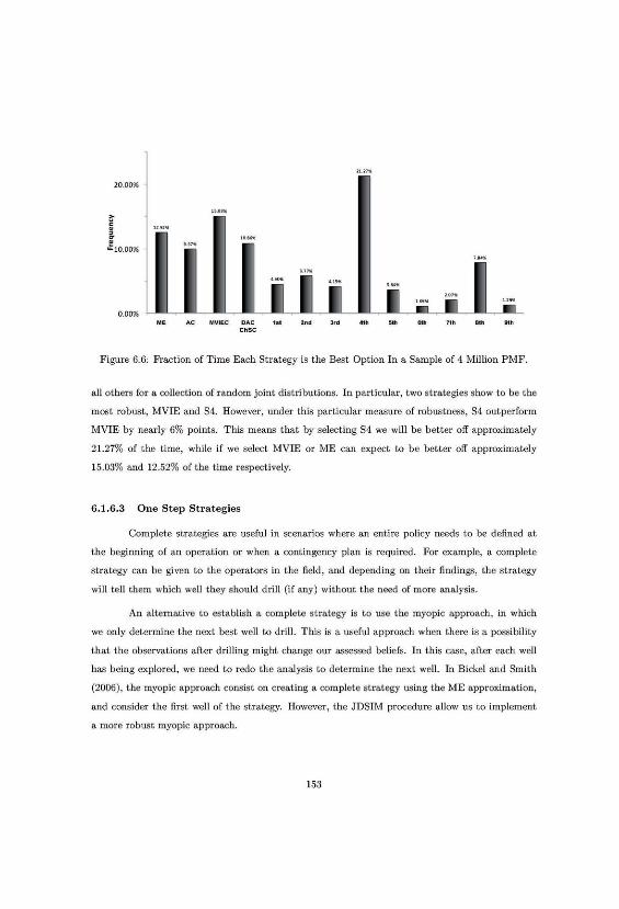

(a) Highest freq. (S1) (b) Second highest freq. (S2) (c) Third highest freq. (S3)
(d) Fourth highest freq. (S4) (e) Fifth highest freq. (S5) (f) Sixth highest freq. (S6)
(g) Seventh highest freq. (S7) (h) Eighth highest freq. (S8) (i) Ninth highest freq. (S9)
Figure 6.7: Strategies With Highest Frequencies.
154


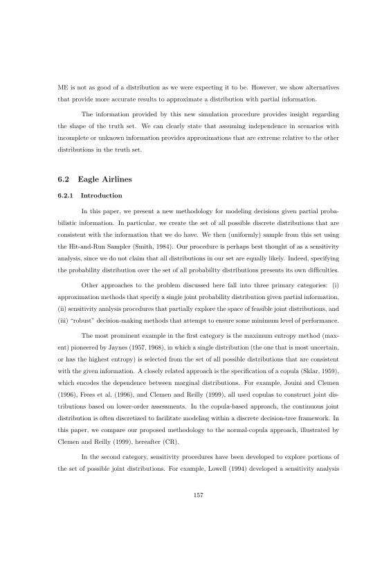
ME is not as good of a distribution as we were expecting it to be. However, we show alternatives
that provide more accurate results to approximate a distribution with partial information.
The information provided by this new simulation procedure provides insight regarding
the shape of the truth set. We can clearly state that assuming independence in scenarios with
incomplete or unknown information provides approximations that are extreme relative to the other
distributions in the truth set.
6.2 Eagle Airlines
6.2.1 Introduction
In this paper, we present a new methodology for modeling decisions given partial proba-
bilistic information. In particular, we create the set of all possible discrete distributions that are
consistent with the information that we do have. We then (uniformly) sample from this set using
the Hit-and-Run Sampler (Smith, 1984). Our procedure is perhaps best thought of as a sensitivity
analysis, since we do not claim that all distributions in our set are equally likely. Indeed, specifying
the probability distribution over the set of all probability distributions presents its own difficulties.
Other approaches to the problem discussed here fall into three primary categories: (i)
approximation methods that specify a single joint probability distribution given partial information,
(ii) sensitivity analysis procedures that partially explore the space of feasible joint distributions, and
(iii) “robust” decision-making methods that attempt to ensure some minimum level of performance.
The most prominent example in the first category is the maximum entropy method (max-
ent) pioneered by Jaynes (1957, 1968), in which a single distribution (the one that is most uncertain,
or has the highest entropy) is selected from the set of all possible distributions that are consistent
with the given information. A closely related approach is the specification of a copula (Sklar, 1959),
which encodes the dependence between marginal distributions. For example, Jouini and Clemen
(1996), Frees et al. (1996), and Clemen and Reilly (1999), all used copulas to construct joint dis-
tributions based on lower-order assessments. In the copula-based approach, the continuous joint
distribution is often discretized to facilitate modeling within a discrete decision-tree framework. In
this paper, we compare our proposed methodology to the normal-copula approach, illustrated by
Clemen and Reilly (1999), hereafter (CR).
In the second category, sensitivity procedures have been developed to explore portions of
the set of possible joint distributions. For example, Lowell (1994) developed a sensitivity analysis
157

procedure to identify important pairwise conditional probability assessments. As discussed above,
CR proposed the use of a normal copula, characterized by pairwise correlation coefficients. They
then perturbed the correlation matrix to explore a set of possible joint distributions. This set is
restricted to joint distributions that can be modeled with a normal copula. Reilly (2000) developed a
sensitivity approach that uses synthetic variables based on a pairwise correlation coefficient matrix.
Finally, in the third category, robust procedures such as maximin or robust optimization
(Ben-Tal et al., 2009) evaluate decisions based on their worst possible outcomes. We do not directly
address these methods. We note, however, that identifying the worst possible joint distribution is
often difficult. Our procedure could be used in a robust setting to “stress test” decisions.
This case of study is organized as follows. §6.2.2 describes a new procedure to generate
joint probability distributions when only partial information is available. §6.2.3 introduces an
illustrative example that we use to demonstrate our approach. §6.2.4 applies our new procedure to
this example. Finally, §6.2.5 concludes and discusses future research directions.
6.2.2 Proposed Approach
The joint distribution simulation approach (JDSIM) samples from the set of all possible
joint distributions that are consistent with the given information. In this way, it provides not one,
but a collection of joint distributions under which the decision can be evaluated.
The procedure described in Chapter 3, begins with the specification of linear constraints on
the joint distribution (e.g., specification of marginal probabilities or pairwise correlations) and the
creation of a convex polytope T, the “truth set,” that matches the given information. By “truth”
we mean that any distribution within this set is consistent with the assessments and therefore could
be the “true” joint distribution.
We illustrate the characterization of T using a simple example with two binary random
variables V1 and V2. This polytope has four joint events (Figure 6.10(a)), whose probabilities must
be positive and sum to one (Figure 6.10(b)). The truth set can be expressed as a hyperplane in four
dimensions or as a full-dimensional polytope in three dimensions (Figure 6.10(c)). We can constrain
T to match marginal assessments such as P (V2) = P1 + P3 = 35 , as shown in Figure 6.10(d). Each
new constraint reduces the dimensionality of T by one. For example, adding a second marginal
constraint reduces T to a one-dimensional line, and adding a correlation constraint reduces T to a
single point.
158


Table 6.9: Ranges and Spearman Correlations for Critical Input Variables.
Fractile Spearman CorrelationsLow Base High
Uncertainty 0.10 0.50 0.90 PL H C OPL $95 $100 $108 1H 500 800 1000 -0.50 1C 40% 50% 60% -0.25 0.5 1O $230 $245 $260 0 0 0.25 1
In order to apply their normal-copula (NC) procedure, CR assumed that the marginal
distributions shown in Table 6.9 are from known families. In particular, they assumed that PL
and H are scaled-beta distributions, C is beta, and O is normally distributed. CR’s parameter
assumptions for each uncertainty are presented in Table 6.10.
Table 6.10: Marginal Distributions For Eagle Airlines.
Uncertainty Distribution Parameters RangePL Scaled beta α = 9, β = 15 [$81.94, $133.96]H Scaled beta α = 4, β = 2 [66.91, 1135.26]C Beta α = 20, β = 20 [0, 1]O Normal μ = 245, σ = 11.72 (−∞, +∞)
With this information, CR proposed a single continuous joint probability density function
(pdf), based on an NC, and discretized it using the Extended Pearson-Tukey (EPT) technique
(Keefer and Bodily, 1983; Pearson and Tukey, 1965). EPT weights the 0.05, 0.50, and 0.95 fractiles
with probabilities of 0.185, 0.630, and 0.185, respectively. CR’s discrete cumulative distribution
function (cdf) for the Expand alternative is shown in Figure 6.12 as a solid black line. This Figure
should be compared to CR’s “discrete approximation” in their Figure 5.
Because CR used EPT, they fixed the probabilities for marginal and conditional distri-
butions, as described above, and solved for the 0.05, 0.50, and 0.95 fractiles. In our simulation
procedure, we fix the values and solve for the probabilities. This approach is helpful for comparing
our procedure to an approximation such as maxent, which is not a function of values and instead
solves for probabilities. Therefore, to better compare our procedure to that of CR, we have dis-
cretized their joint pdf by fixing the marginal values at the 0.05, 0.50, and 0.95 fractiles (using
their pdf assumptions in Table 6.10) and then solving for probabilities using moment matching (see
Appendix D.1). This discrete cdf is shown in Figure 6.12 as the solid gray line. While the two
approaches are not identical, the discretizations are very close. We use the moment matching cdf
in the remainder of the paper.
161

Profit Orig.NC M.M.NC
Mean
Std. Dev.
Inv. Risk
$12,642
$20,275
35.74�
$12,678
$20,265
36.91�
�40 �20 4.2 20 40 60 80 100
Profit
�thousands of $�0�
10�
20�
30�
40�
50�
60�
70�
80�
90�
100�Cumulative Probability
Moment Matching NC cdf
Original CR's NC cdf
Figure 6.12: Eagle Airlines cdf, under original discretization (black) and new discretization (gray).
One potential difficulty with CR’s procedure is that it does not preserve the original pair-
wise correlation assessments. This occurs because the discretization with three points reduces the
possible correlation range, producing a new correlation matrix bounded by [-0.74, 0.74]. Please see
Appendix D.2 for more detail. Table 6.11 presents the correlation matrix implied by CR’s discrete
cdf (the gray line in Figure 6.12). The non-zero correlations have all decreased. Our approach, in
Table 6.11: NC Implied Spearman Correlation Matrix.
PL H C OPL 0.74H -0.38 0.74C -0.19 0.38 0.74O 0 0 0.19 0.74
contrast, preserves the assessed correlations. Of course, the expert would need to understand that
the correlation range is not [-1,1] when they were assessing the correlation between discrete random
variables with only three possible outcomes.
162

6.2.4 Application to Eagle Airlines Decision
In this section, we apply our JDSIM procedure to the Eagle Airlines case. We consider
three information cases. The first case assumes we have information regarding only the marginal
probabilities. The second case includes the previous marginal probabilities and adds information
regarding the rank correlation between PL and H. The final case is equivalent to the original
problem as presented by CR, and includes all the marginal assessments and pairwise correlations.
To facilitate comparison of our results to CR, our JDSIM procedure use the correlations presented
in Table 6.11.
6.2.4.1 Case 1: Given Information Regarding Marginals Alone
We begin by assuming that we have information regarding only the marginal assessments.
To compare our procedure to CR, we also use EPT. In addition to the 0.50 fractile, EPT requires
the 0.05 and 0.95 fractiles, which were not provided by CR. We estimate these fractiles using CR’s
distributional assumptions in Tables 6.9 and 6.10 and present the results in Table 6.12. We now
assume that both the NC and JDSIM methods begin with Table 6.12.
Table 6.12: Fractiles Used in Eagle Airlines Example.
Fractile
Low (l) Base (b) High (h)Uncertainty 0.05 0.5 0.95
PL $93.47 $100 $110.05H 432.92 800 1053.60C 37.14% 50% 62.86%O $225.72 $245 $264.28
Under the NC procedure, we must next assume a particular pdf family for each marginal
distribution and specify a correlation matrix. We use the marginal assessments provided by CR in
Table 6.10. Since we are assuming that dependence information is unavailable, it is unclear how to
specify the correlation matrix. For the benefit of the comparison, and following common practice,
we assume that all correlations are zero. The JDSIM method, in contrast, does not require the
specification of marginal pdf families or a correlation matrix. Rather, we form a polytope that
contains all possible joint distributions matching the marginal assessments given in Table 6.12.
The polytope describing these marginal assessments has 72 dimensions, resulting from 81 joint
probabilities (four random variables with three outcomes each), one constraint that requires the
probabilities to sum to one, and eight constraints to match the marginal assessments (81-1-8=72).
163

The polytope T is defined using Equations (3.1a), (3.1b), and (3.2a). Equations (3.1a) and
(3.1b) constrain the joint probabilities pωk∈ p to sum to one and to be non-negative. Equation
(3.2a) selects subsets of the joint probabilities and constrains their sum to be equal to the marginal
assessments. For example, if we order the random variables as {PL, H, C,O}, each having values
{l, b, h}, there are 81 joint events. Using dot notation, {h, ·, ·, ·} refers to the 27 joint events with PL
equal to 110.05 (the 95th percentile). From the marginal assessments, we know that ph,·,·,· = 0.185,
which defines Equation (6.5). Similar equations can be defined for the remaining 11 marginal
assessments (12 in total). However, four of these constraints are redundant given Equation (3.1a),
reducing the total number of linear constraints to nine.
ph,·,·,· =∑i∈F
∑j∈F
∑k∈F
ph,i,j,k = 0.185, ∀ F ≡ {l, b, h}. (6.5)
We apply the JDSIM procedure to the polytope to create a discrete representation of T by
sampling 10 million discrete joint distributions,1 all of which are consistent with the information
provided by CR. We calculate the mean and standard deviation of profit for each sampled joint
distribution. Additionally, we calculate the frequency with which the Expand alternative yields less
than the Money Market (MM) threshold of $4,200. We refer to this frequency as the “investment
risk.” Based on our 10 million distributions, we calculate frequency distributions for the mean
profit, the standard deviation of profit (Std. Dev.), and the investment risk (Inv. Risk). Table
6.13 shows these percentiles along with their theoretical lower bound (LB) and upper bound (UB),
which we describe shortly. This table should be compared to CR’s Table 5.
Table 6.13: Percentiles for mean profit, standard deviation of profit, and investment risks for JDSIM joint
distributions given only marginal information.
Percentiles
0% 10% 25% 50% 75% 90% 100%
Mean $10,160 $11,667 $11,968 $12,304 $12,637 $12,940 $14,340Std. Dev. $17,300 $21,750 $22,613 $23,576 $24,552 $25,456 $29,580Inv. Risk 19.50% 26.25% 27.65% 29.30% 31.12% 32.79% 40.95%
Statistics
LB μ σ UB
Mean $4,332 $12,303 $496 $21,750Std. Dev. NA $23,591 $1,444 NAInv. Risk 0.00% 29.42% 2.54% 74%
1Run time: Five hours using Mathematica 8 on an Intel CPU [email protected] with 8GB of RAM.
164

The observed mean profit ranges from $10,160 to $14,340, with an average (μ) and standard
deviation (σ) of $12,303 and $496, respectively. The expected profit under the NC is $12,326. Our
observed profit range and the percentiles closely match the results of CR’s sensitivity results (see
their Table 5).
We refer to the 0th and 100th percentiles as “probability bounds” because there could exist
cdfs in T that result in profits outside of this range. However, we did not observe them in 10 million
samples. Since the minimum expected profit that we sampled was $10,160, every simulated joint
distribution had a mean profit greater than the value of the MM alternative. Thus, in this case,
the assessment of probabilistic dependence or differing marginal distributions, which still match
the assessments in Table 6.12, is very unlikely to change the recommendation that Eagle Airlines
should expand (assuming they are risk neutral).
The standard deviations of our sampled cdfs ranged from $17,300 to $29,580, with an
average of $23,641. The standard deviation of profit under the NC is $23,605. On the high end, our
results closely match CR. However, the smallest standard deviations in our sample were larger than
CR’s. We conjecture that this result is related to differences in our discretization procedure and
CR’s marginal/copula assumptions. Referring back to Figure 6.12, we see that our discretization
procedure (fixed values) results in a slightly wider cdf (longer tails) than CR’s approach (fixed
probabilities). Furthermore, their marginal distributions (see Table 6.10) are either normal or close
to normal, implying that they have very thin tails. Likewise, CR modeled dependence with a
normal copula, which also enforces thinner tails. JDSIM is not constrained by these assumptions
and is therefore sampling from distributions that are most likely more spread and contain non-zero
higher moments (e.g., skewness and kurtosis).
Table 6.13 indicates that investment risk, which averaged 29.42%, ranges from 19.50% to
40.95%. While the Expand alternative’s expected profit always exceeds the MM, there may be a
large probability of underperforming this benchmark. This surprisingly large range is driven by
the underlying dependence structure, which highlights the importance of modeling and assessing
dependence. The NC investment risk is 38.05%. The most significant difference between the DAC
and NC cdfs is at the level of individual fractiles–their first two moments are relatively close.
The LB and UB in Table 6.13 were derived from a linear program (LP) described in
Appendix D.3. We provide these hard bounds for the mean profit and investment risk only. De-
termining the minimum and maximum possible standard deviation requires solving an NP-hard
problem, and this was not attempted. The expected-profit LB is $4,332, which is greater than the
165
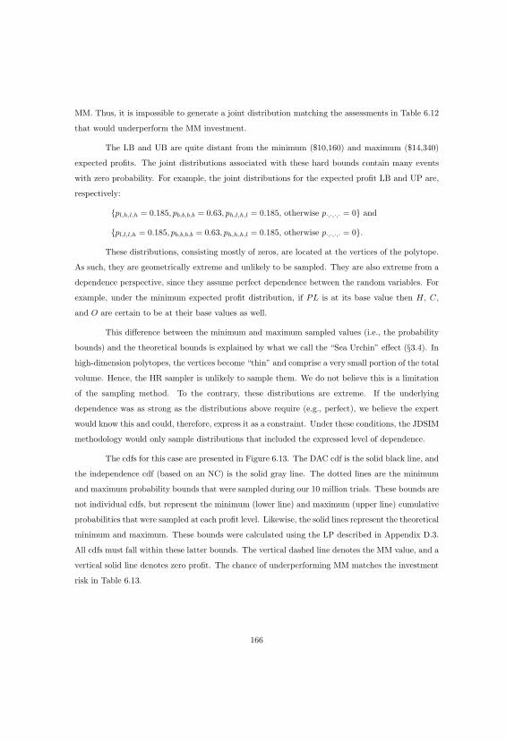
MM. Thus, it is impossible to generate a joint distribution matching the assessments in Table 6.12
that would underperform the MM investment.
The LB and UB are quite distant from the minimum ($10,160) and maximum ($14,340)
expected profits. The joint distributions associated with these hard bounds contain many events
with zero probability. For example, the joint distributions for the expected profit LB and UP are,
respectively:
{pl,h,l,h = 0.185, pb,b,b,b = 0.63, ph,l,h,l = 0.185, otherwise p·,·,·,· = 0} and
{pl,l,l,h = 0.185, pb,b,b,b = 0.63, ph,h,h,l = 0.185, otherwise p·,·,·,· = 0}.
These distributions, consisting mostly of zeros, are located at the vertices of the polytope.
As such, they are geometrically extreme and unlikely to be sampled. They are also extreme from a
dependence perspective, since they assume perfect dependence between the random variables. For
example, under the minimum expected profit distribution, if PL is at its base value then H, C,
and O are certain to be at their base values as well.
This difference between the minimum and maximum sampled values (i.e., the probability
bounds) and the theoretical bounds is explained by what we call the “Sea Urchin” effect (§3.4). In
high-dimension polytopes, the vertices become “thin” and comprise a very small portion of the total
volume. Hence, the HR sampler is unlikely to sample them. We do not believe this is a limitation
of the sampling method. To the contrary, these distributions are extreme. If the underlying
dependence was as strong as the distributions above require (e.g., perfect), we believe the expert
would know this and could, therefore, express it as a constraint. Under these conditions, the JDSIM
methodology would only sample distributions that included the expressed level of dependence.
The cdfs for this case are presented in Figure 6.13. The DAC cdf is the solid black line, and
the independence cdf (based on an NC) is the solid gray line. The dotted lines are the minimum
and maximum probability bounds that were sampled during our 10 million trials. These bounds are
not individual cdfs, but represent the minimum (lower line) and maximum (upper line) cumulative
probabilities that were sampled at each profit level. Likewise, the solid lines represent the theoretical
minimum and maximum. These bounds were calculated using the LP described in Appendix D.3.
All cdfs must fall within these latter bounds. The vertical dashed line denotes the MM value, and a
vertical solid line denotes zero profit. The chance of underperforming MM matches the investment
risk in Table 6.13.
166

We pause here to emphasize the scope and importance of our results. We have sampled 10
million joint distributions from the set of all joint distributions matching the marginal constraints.
In other words, we have sampled from the set of all possible marginal distributions and dependence
structures, rather than a set limited to marginals from particular families (e.g., beta) and whose
dependence structure can be defined with a particular copula (e.g., normal). These 10 million joint
distributions fall within the bounds denoted by the dotted lines. The (NC-based) independence
cdf falls within these bounds, but is rather extreme (relative to the probability bounds) for profits
between -$3,000 and $25,000. The DAC cdf might be thought of as being more representative of
the set of possible joint distributions than is the independence cdf. The DAC and the independence
cdfs differ rather dramatically at a profit level of $4,200, which is the MM benchmark.
Profit NC DAC
Mean
Std. Dev.
Inv. Risk
$12,326
$23,605
38.05�
$12,303
$23,641
29.42�
�40 �20 4.2 20 40 60 80 100
Profit
�thousands of $�0�
10�
20�
30�
40�
50�
60�
70�
80�
90�
100�Cumulative Probability
Theoretical LB
Probability LB
NC cdf
DAC cdf
Probability UB
Theoretical UB
Figure 6.13: Risk profile range given only marginal information, minimum and maximum proba-bility bounds (dashed), theoretical bounds (solid), DAC (black), and NC (gray).
Additionally to DAC, we can also observe in Figure 6.14 the risk profiles for the ME, AC,
ChSC, and MVIE approximations. Notice that ME tend to be closer to the NC, this is given by
the fact that both distributions share high entropy. The NC obtain the high entropy from the
discretization of a normal distribution, which has maximum entropy in continuous space, and ME
is maximum entropy in discrete space. In the other extreme, the ChSC is closet to the probabilistic
lower bounds in the lower portion of the graph and higher in the second one, which produce the
167

lower investment risk among the approximations. Finally, AC and MVIE are closer to DAC, which
suggest that could be used as approximations that are closer to the center of T.
With respect to the profits, we see that in this case the results are close to each other. This
is common in sets where the information is scarce. For example, as we have seeing before, with
no information, all approximations converge to the uniform distribution providing the exact same
results.
Profit ME AC ChSC MVIE
Mean
Std. Dev.
Inv. Risk
$12,326
$23,606
38.05�
$12,320
$23,662
29.14�
$12,318
$23,689
25.35�
$12,320
$23,666
28.38�
�40 �20 0 4.2 20 40 60 80 100
Profit
�thousands of $�0�
10�
20�
30�
40�
50�
60�
70�
80�
90�
100�
Cumulative Probability
Theoretical LB
Probability LB
MVIE cdf
ChSC cdf
AC cdf
ME cdf
Probability UB
Theoretical UB
Figure 6.14: Risk profile range given only marginal information, minimum and maximum probabil-ity bounds (dashed), theoretical bounds (solid), ME (black), AC (gray-dashed), ChSC (gray), andMVIE (black-dotdashed).
6.2.4.2 Case 2: Given Marginals and Only One Rank Correlation
This section analyzes the case where the dependence structure is constrained by a single
pairwise correlation. Specifically, we consider CR’s implied correlation between PL and H, which
is equal to -0.38 (see Table 6.11). We make no assumptions regarding the other five pairwise
correlations. The truth set is generated using Equations (3.1a), (3.1b), (3.2a), and (3.9). As
mentioned in §6.2.4.1, Equations (3.1a), (3.1b), and (3.2a) ensure the sampled points are pmfs
that match the marginal assessments. We add one more constraint (Equation 3.9) to fix the rank
168

correlation between PL and H.
To illustrate Equation 3.9, we describe the construction of one of the 81 coefficients for the
joint events. Using the notation from §3.3, the 50th joint event corresponds to {b, h, b, b} and is
described as ω50 = {PL = $100, H = 1053.6, C = 50%, O = $245}. Equation 3.9 then yields:
Bω50= [Iω50
(PL) × Iω50(H)] =
[p+50(PL), p−50(PL)
] × [p+50(H), p−50(H)
],
Bω50 = [0.815, 0.185] × [1.0, 0.815] .
Then,
V(xy)2 [Bω50 ]
qω+50(PL)qω
+50(H)
=
=(p+
50(PL)p+50(H))2 − (p+
50(PL)p−50(H))2 − (p−50(PL)p+50(H))2 + (p−50(PL)p−50(H))2
P (PL = 100)P (H = 1053.6),
=(0.815 · 1.0)2 − (0.815 · 0.815)2 − (0.185 · 1.0)2 + (0.185 · 0.815)2
0.63 · 0.185= 1.815.
Calculating similar coefficients for all 81 joint events defines Equation (3.9) and yields
0.0342pl,l,·,·
+ 0.185pl,b,·,·
+ 0.3358pl,h,·,·
+ 0.185pb,l,·,·
+ pb,b,·,·
+
1.815pb,h,·,·
+ 0.3358ph,l,·,·
+ 1.815ph,b,·,·
+ 3.2942ph,h,·,·
=ρ
P L,H+ 3
3.
The maximum correlation occurs when the probabilities are pl,b,·,·
= pl,h,·,·
= pb,l,·,·
= pb,h,·,·
=
ph,l,·,·
= ph,b,·,·
= 0, and pl,l,·,·
= 0.185, pb,b,·,·
= 0.63, ph,h,·,·
= 0.185 with a value equal to 0.74, as
was shown in Table 6.11.
We apply the JDSIM procedure to the new polytope and create a discrete representation
of the new truth set by sampling 10 million possible joint distributions using the HR sampler. Each
sampled distribution has marginals equal to 0.185, 0.63, 0.185, of the {l, b, h}, respectively, and
rank correlation ρP L,H
= −0.38. Table 6.14 summarizes our results.
The sampled mean profit ranges from $9,215 to $12,570, with an average value of $10,916
and a standard deviation of $414. The NC expected profit is also $10,916. The distribution of the
mean profit shows that under the new information, the Expand alternative is less attractive than
before. This occurs because the correlation between PL and H is negative; higher prices result in
169
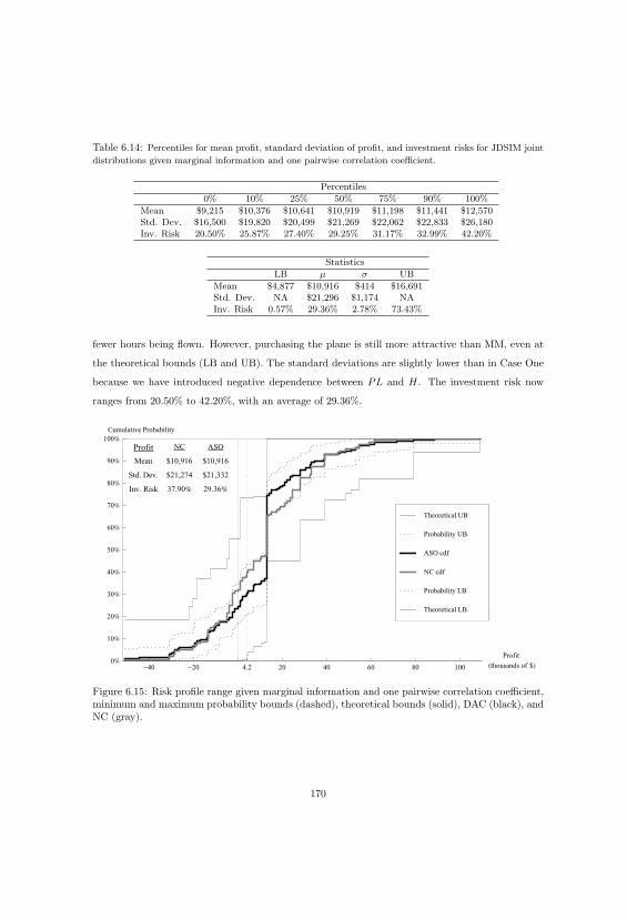
Table 6.14: Percentiles for mean profit, standard deviation of profit, and investment risks for JDSIM joint
distributions given marginal information and one pairwise correlation coefficient.
Percentiles
0% 10% 25% 50% 75% 90% 100%
Mean $9,215 $10,376 $10,641 $10,919 $11,198 $11,441 $12,570Std. Dev. $16,500 $19,820 $20,499 $21,269 $22,062 $22,833 $26,180Inv. Risk 20.50% 25.87% 27.40% 29.25% 31.17% 32.99% 42.20%
Statistics
LB μ σ UB
Mean $4,877 $10,916 $414 $16,691Std. Dev. NA $21,296 $1,174 NAInv. Risk 0.57% 29.36% 2.78% 73.43%
fewer hours being flown. However, purchasing the plane is still more attractive than MM, even at
the theoretical bounds (LB and UB). The standard deviations are slightly lower than in Case One
because we have introduced negative dependence between PL and H. The investment risk now
ranges from 20.50% to 42.20%, with an average of 29.36%.
Profit NC ASO
Mean
Std. Dev.
Inv. Risk
$10,916
$21,274
37.90�
$10,916
$21,332
29.36�
�40 �20 4.2 20 40 60 80 100
Profit
�thousands of $�0�
10�
20�
30�
40�
50�
60�
70�
80�
90�
100�Cumulative Probability
Theoretical LB
Probability LB
NC cdf
ASO cdf
Probability UB
Theoretical UB
Figure 6.15: Risk profile range given marginal information and one pairwise correlation coefficient,minimum and maximum probability bounds (dashed), theoretical bounds (solid), DAC (black), andNC (gray).
170

The cdfs for this case are presented in Figure 6.15. The DAC cdf assumes that ρP L,H
=
−0.38 and all other correlations are unspecified. The NC cdf assumes that ρP L,H
= −0.38 and all
other correlations are zero. As in Case One, the NC cdf is near the probability bounds for profits
of -$3,000 to $25,000. Again, the DAC seems to be more representative than the NC of the set of
possible distributions.
Figure 6.16 shows the results for the rest of the approximations. We see that the information
provided pushed the ChSC closer to AC and MVIEC. These approximations show expected profits
lower than the previous ones. However, are still better positioned with respect to the center of the
truth set. We also observe that that ME and NC share similar shape and statistics values.
The distribution with the lowest investment risk is now MVIEC by a narrow margin, but
it provides close to 10 percent points with respect to ME and NC. This suggest that the probability
of loosing money is lower than what we would expect assuming the high entropy distributions.
Profit ME AC ChSC MVIE
Mean
Std. Dev.
Inv. Risk
$10,910
$21,292
37.90�
$10,905
$21,300
29.10�
$10,901
$21,319
29.09�
$10,905
$21,290
28.18�
�40 �20 0 4.2 20 40 60 80 100
Profit
�thousands of $�0�
10�
20�
30�
40�
50�
60�
70�
80�
90�
100�
Cumulative Probability
Theoretical LB
Probability LB
MVIE cdf
ChSC cdf
AC cdf
ME cdf
Probability UB
Theoretical UB
Figure 6.16: Risk profile range given only marginal information and one pairwise correlation coeffi-cient, minimum and maximum probability bounds (dashed), theoretical bounds (solid), ME (black),AC (gray-dashed), ChSC (gray), and MVIE (black-dotdashed).
171

6.2.4.3 Case 3: Given Information Regarding Marginals and All Rank Correlations
Coeficients
In this section, we adopt all of the information provided by CR and used in their NC
approach. Specifically, we use the marginal assessments from the EPT discretization, given in Table
6.12, and the implied correlations from Table 6.11. The implied correlations are used to make the
comparison to CR as fair as possible. The new polytope is defined using Equations (3.1a), (3.1b),
(3.2a), and (3.9), as illustrated in §6.2.4.1 and §6.2.4.2. To the previous ten constraints (and
the non-negativity constraints), we add five new constraints to fix the values of all the pairwise
correlations, defining a 66-dimensional polytope.
Table 6.15 displays a summary of our 10 million samples of the new polytope using the
HR sampler. The additional constraints have significantly affected the mean profit distribution.
The minimum and maximum sampled mean profits are now $12,448 and $12,910, respectively,
with an average of $12,662 and a standard deviation of $62. The NC expected profit is $12,678.
Additionally, the difference between the theoretical mean profit UB and LB is only $1,222, which is
considerably less than in our previous cases. What little difference there is between mean profits is
due to dependence in the joint distribution that cannot be described by pairwise correlations and
a normal copula.
Table 6.15: Percentiles for mean profit, standard deviation of profit, and investment risks for JDSIMjoint distributions given marginal information and all pairwise correlation coefficients.
Percentiles
0% 10% 25% 50% 75% 90% 100%
Mean $12,448 $12,583 $12,620 $12,662 $12,704 $12,741 $12,910Std. Dev. $18,530 $19,767 $20,063 $20,400 $20,750 $21,051 $22,280Inv. Risk 18.45% 24.63% 25.98% 27.54% 29.18% 30.76% 36.50%
Statistics
LB μ σ UB
Mean $12,049 $12,662 $62 $13.271Std. Dev. NA $20,404 $499 NAInv. Risk 9.55% 27.64% 2.36% 63.72%
The new distribution of the standard deviation of profit ranges from $18,530 to $22,280,
with an average $20,404. The distribution of the investment risk has been shifted towards lower
values (although the LB has increased), with a new range from 18.45% to 36.50%. The average
investment risk is now 27.64%.
172

The bounds for the cdfs when all pairwise correlations are known are shown in Figures 6.17
and 6.18. Both the probability and the absolute boundaries are narrower than before. CR’s NC-cdf
falls slightly outside of the probability bounds for profit values of -$2,000 to $25,000. This suggests
that the NC approach, which specifies a single joint distribution, may not generate an approximation
that is representative of the set of all distributions matching the assessed information.
Profit NC ASO
Mean
Std. Dev.
Inv. Risk
$12,678
$20,265
36.91�
$12,662
$20,410
27.64�
�40 �20 4.2 20 40 60 80 100
Profit
�thousands of $�0�
10�
20�
30�
40�
50�
60�
70�
80�
90�
100�Cumulative Probability
Theoretical LB
Probability LB
NC cdf
ASO cdf
Probability UB
Theoretical UB
Figure 6.17: Risk profile range given marginal information and all pairwise correlation coefficients,minimum and maximum probability bounds (dashed), theoretical bounds (solid), DAC (black) andNC (gray).
We conjecture that the extreme behavior of the NC with respect to the probability bounds
is related to the structure provided by the normal copula. The normal pdf has maximum en-
tropy for a given mean and standard deviation. We suspect that joint distributions formed with
a normal copula are also high in entropy. Indeed, in our case, CR’s NC-cdf and the (Figure
6.18) maximum-entropy cdf (given marginal and all pairwise correlations) are very close to each
other, with a maximum absolute difference among the probabilities of the joint events of 0.0037,
whereas the corresponding difference between NC and DAC is 0.1992. A maxent joint distribu-
tion based on marginals and pairwise correlations will enforce higher-order dependencies that are
as close to independence as possible. This cdf will then tend to be an extreme point within our
truth set. As a simple illustration, assume two identical binary random variables with marginals
of {0.9, 0.1} and unknown correlation. With this information, all the possible distributions are a
convex combination of {0.9, 0, 0, 0.1} and {0.8, 0.1, 0.1, 0}. Hence, T forms a line section with center
173

at {0.85, 0.05, 0.05, 0.05}, whereas maxent is located at {0.81, 0.09, 0.09, 0.01}, close to the second
extreme point.
Profit ME AC ChSC MVIE
Mean
Std. Dev.
Inv. Risk
$12,667
$20,319
36.85�
$12,666
$20,417
27.44�
$12,670
$20,456
23.45�
$12,666
$20,417
27.32�
�40 �20 0 4.2 20 40 60 80 100
Profit
�thousands of $�0�
10�
20�
30�
40�
50�
60�
70�
80�
90�
100�
Cumulative Probability
Theoretical LB
Probability LB
MVIE cdf
ChSC cdf
AC cdf
ME cdf
Probability UB
Theoretical UB
Figure 6.18: Risk profile range given only marginal information and all pairwise correlation co-efficients, minimum and maximum probability bounds (dashed), theoretical bounds (solid), ME(black), AC (gray-dashed), ChSC (gray), and MVIE (black-dotdashed).
The new information has reduce the profits range and reshaped the approximations to the
joint distribution. We are able to observe that, as before, ChSC and ME get closer (or violate)
the probability bounds in opposite sides of the range. Whereas, AC and MVIEC get closer to each
other and to DAC. In this case the approximation with smallest investment risk is ChSC. However,
the approximation with largest expected profit is still the NC.
6.2.4.4 Comparing the Three Information Cases
Figures 6.19(a), 6.19(b), and 6.19(c) compare the pdfs (frequencies) of our sampled ex-
pected profits, standard deviations, and investment risk, respectively. The distribution for Case
One, using only marginal information, is presented as the dotted line filled in white. Case Two,
using marginal information and one pairwise correlation coefficient, is presented as the dashed line
filled in gray. Finally, Case Three, with all marginal information and pairwise correlation assess-
ments, is presented in a solid line filled in black. The vertical lines correspond to the probability
174


bounds for each case mark in dotted (Case One), dashed (Case Two), and solid lines (Case Three).
The range of outcomes for Case One (only marginals) stems from our having not constrained
marginal families or the dependence structure. The addition of a negative correlation between PL
and H, in Case Two, shifted the set of possible profits to the left and narrowed it somewhat.
The specification of all pairwise correlations, in Case Three, constrained the set considerably. The
variability that does exist is related to our marginals’ not having been based on known families
and that higher-order dependencies (beyond pairwise) were not fixed. This indicates that assessing
these higher-order distributions (e.g., all three-way assessments) will not improve the decision.
The investment-risk distributions show less sensitivity to the dependence structure. Al-
though additional constraints had a significant impact on the distribution of expected profit and
the standard deviation of profit, the probability of being less than $4,200 has not changed signifi-
cantly.
6.2.4.5 Decision Robustness
Since we are evaluating the decision (Expand versus MM, in this case) under each simulated
joint distribution, we can test the robustness of each alternative. Specifically, we can determine
in which fraction of our simulated joint distributions each alternative was preferred. As discussed
above, none of our observed distributions results in the MM being the preferred alternative, even
based solely on marginal information. Therefore, to demonstrate the idea of robustness, assume
that Dick Carothers is considering an additional alternative that delivers $11,000 for certain.
Table 6.16 shows the fraction of times that the Expand alternative was optimal for our three
cases (these frequencies can also be estimated directly from Figure 6.19(a)). Given only marginal
assessments, Expand was optimal under 99.56% of simulated pmfs. This dropped to 42.27% given
marginals and that the correlation between PL and H is -0.38. Finally, given marginals and
all pairwise correlations, Expand was optimal (an expected value greater than $11,000) in all 10
million of our simulations (100%). We believe this degree of insight will address a primary concern
held by most decision makers, “Am I making a mistake by choosing this alternative?” and will
thereby increase decision quality and commitment to action. Approaches that posit a single joint
distribution (e.g., copula-based methods) cannot provide this type of feedback.
176

Table 6.16: Percentage of Times the Alternative is Optimal
Information Expand 11K MMMarginal assessments 99.56% 0.44% 0%Marginal and one correlation assessment 42.27% 57.73% 0%Marginal and correlation assessments 100.00% 0% 0%
6.2.5 Final Comments
Both the Joint Distribution Simulation (JDSIM) and the Normal Copula (NC) approaches
propose a method to model probabilities and decisions when only partial probabilistic information
is available. The NC approach assumes a copula in order to specify a single joint probability
distribution. JDSIM, in contrast, explores the set of all joint distributions that match the available
information.
JDSIM provides a flexible and powerful tool to analyze stochastic decision models when
the joint distribution is incompletely specified. The methodology is easy to implement, develops
a collection of joint distributions, and represents a significant extension to previous approximation
models such as the copula-based approach illustrated by CR. We demonstrated the JDSIM proce-
dure with a canonical example based on marginal and pairwise rank correlation coefficients. The
methodology can be extended to more than four random variables, to random variables with more
than three possible outcomes, and to higher-order conditioning such as three-way assessments.
On average, the profit joint distributions produced by JDSIM resulted in expected values
and standard deviations similar to those of NC. The primary difference, in the case examined here,
seems to be differing estimates for particular cumulative probabilities. For example, the NC cdf
produced cumulative probabilities for mid-range profits that were extreme relative to our sample.
This is potentially important in the Eagle Airlines case because this profit range included the value
of the competing alternative. Thus, the two methods might produce very different estimates of
investment risk (the probability of under performing the competing alternative). This being said,
more research needs to be done to better understand if it is possible to faithfully represent the
JDSIM sample with a single joint distribution across a range of applications.
JDSIM’s strength is also a potential weakness, as the decision is not valued or made under
a single distribution, but rather under thousands (possibly millions) of feasible distributions. NC
provides a single, approximate distribution, but, as discussed above, our results suggest that this
approximation may not be representative of the set of possible joint distributions. The accuracy of
the normal copula approach is an open question, but one that could be addressed by comparing it
177

to the JDSIM results.
The information provided by this new simulation procedure provides insight regarding the
shape of the truth set. At this point, we do not claim to know the likelihood of the distributions
in the collection sampled. However, we can clearly state that assuming independence in scenarios
with incomplete or unknown information provides approximations that are extreme relative to the
other distributions in the truth set. This provides yet another example of the importance of not
ignoring dependence.
178

Chapter 7
Future Research
This chapter presents several ideas for future research that build upon the work presented
in this dissertation. These consist of a new sampling procedure named the Randomized Ping-
Pong Sampler, alternative procedures to measure the volume of the relative interior of T (measures
of precision), and different bounds of polyhedra that work as worst cases for the approximation
distributions.
7.1 The Randomized Ping-Pong Sampler
Modifying the HR algorithm can increase the probability of sampling low-probability neigh-
borhoods of T, specifically the areas close to the vertices. The proposed modification could be called
the Randomized Ping-Pong Sampler algorithm. It is designed to force the Markov Chain to select
a new point along the direction of one of the vertices of T with probability p, or a jump along the
direction of the center of T with probability 1− p. When p = 0.5, the algorithm would be expected
to oscillate like a ping-pong ball.
The Randomized Ping-Pong behavior is created by means of two subproblems. The first
one takes a random direction (as with the Hit-and-Run sampler), solves a Linear Program (LP) to
find a vertex, and uses the vertex to create a new point. This problem needs to be solved at each
iteration with probability p, but LPs run efficiently in practice. The second subproblem is to find a
center of T, which would need to be run only once in the initialization. Hence, even if the problem
is difficult, it does not affect the efficiency of the sampling process. The center of T is mainly used
to ensure that as the dimension increases, the sample includes areas of the set that otherwise might
be ignored.
179

Randomized Ping-Pong Sampler Algorithm
1. Select a starting point x0 at the center of T, define α ∈ [0, 0.5], set i = 1 and choose K as the
number of iterations.
2. Generate a random point r in the interval [0, 1].
3. If r < α, go to Step 4. Else, go to Step 5.
4. Perform the following:
(a) Generate the direction di = (x0 − xi)/||x0 − xi||.Find the line set L = T ∩ {x|x = xi + λdi, λ a real scalar}.
(b) Generate a random point xi+1 uniformly distributed over L.
5. Perform the following:
(a) Generate n independent normally distributed random deviates
N = {N1, N2, · · · , Nn} and set ci+1 = N/||N ||.(b) Solve the subproblem:
max ci · vi,
s.t. vi ∈ T.(c) Generate the direction di = (vi − xi)/||vi − xi||.
Find the line set L = T ∩ {x|x = xi + λdi, λ a real scalar}.
(d) Generate a random point xi+1 uniformly distributed over L.
6. If i = K iterations, stop. Otherwise, set i = i + 1 and return to Step 2.
Initializing the algorithm requires defining a center, for which one simple procedure is to
choose the center of the maximum volume ellipsoid inscribed in T. Additionally, other centers
of polyhedra can be used, such as the analytic center (used in interior point algorithms) or the
Chebyshev’s center, which is the farthest point from the boundary of T.
Figures 7.1, 7.2, and 7.3 graphically describe the algorithm in two dimensions. After
defining the center of T and the parameter α, we start with a random point in the interior of the
set (Fig. 7.1(a)). Then, r is randomly chosen and brings about Step 4 if r < α or Step 5 if r ≥ α
(Fig. 7.1(b)).
After choosing r, the algorithm selects between Step 4 and Step 5. If Step 4 is chosen, create the
line L and select a random point uniformly from it (Fig. 7.2(a)-7.2(c)).
180
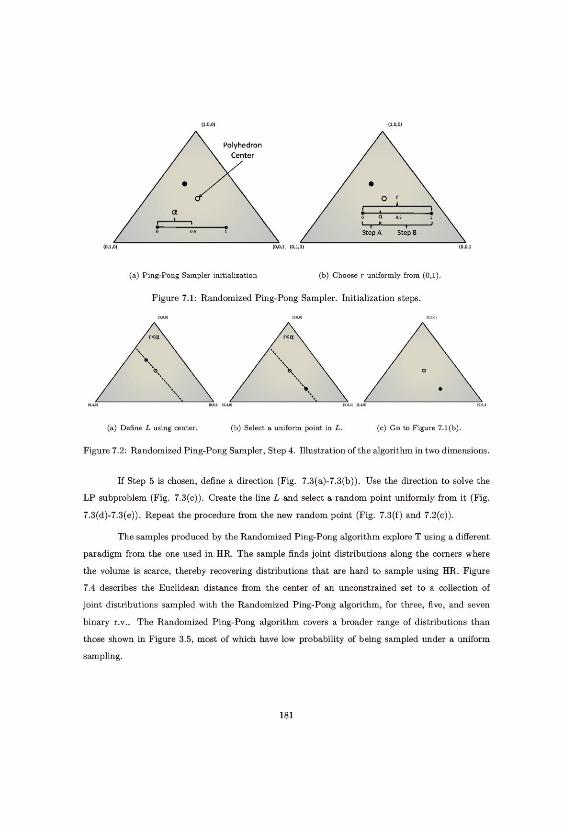


(a) Three Variables. (b) Five Variables. (c) Seven Variables.
Figure 7.5: Randomized Ping-Pong sampler: Norm distance from the center of T, for variousnumbers of binary random variables.
7.2 Measures of Precision
New methods to measure the precision of a truth set T should be developed. The precision
of a set can be characterized by its size. For example, in a small set T, a sampled collection of
distributions taken with the HR sampler will have joint elements close to each other. Then, any
approximation inside T will be close to any element from the sample, and the difference in accuracy
for two approximations will be minimal. However, if T is large, the accuracy of the approximations
will vary significantly.
Because there are many definitions for size of T. We informally define “measure of preci-
sion” as a function f(T) that describes the n-content of a set T.
7.2.1 Volume Ratio
The most intuitive concept to measure the size of a polytope is its relative volume (n-
content). Bertsimas and Tsitsiklis (1997) defined the volume as
Vol(T) =
∫x∈T
dx. (7.1)
Equation (7.1) is zero for every T since the polytope is not full dimensional. However, we
can apply a transformation A such that AT is full dimensional in a new cardinal system with fewer
dimensions. For example, a random variable with three outcomes has a probability distribution
that generates a set T shaped as a triangle with corners in the unit vectors. Then, the 2-content of
T, or cont2(T), is the area of a two-dimensional equilateral triangle(√
32!
).
In general, for an unconstrained joint distribution with n outcomes, contn−1(T) =√
n
(n−1)! ,
which is equivalent to the surface of a hyper-plane that intersects the positive hyper-octant. Kannan
183
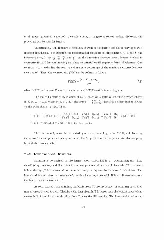
et al. (1996) presented a method to calculate contn−1 in general convex bodies. However, the
procedure can be slow for large n.
Unfortunately, this measure of precision is weak at comparing the size of polytopes with
different dimensions. For example, for unconstrained polytopes of dimensions 3, 4, 5, and 6, the
respective contn(·) are√
32! ,
√4
3! ,√
54! , and
√6
5! . As the dimension increases, contn decreases, which is
counterintuitive. Moreover, making its values meaningful would require a frame of reference. One
solution is to standardize the relative volume as a percentage of the maximum volume (without
constraints). Then, the volume ratio (VR) can be defined as follows:
V R(T) =(n − 1)! contn√
n, (7.2)
where V R(T) = 1 means T is at its maximum, and V R(T) = 0 defines a singleton.
The method described by Kannan et al. is based on a series of concentric hyper-spheres
B0 ⊂ B1 ⊂ · · · ⊂ Br where B0 ⊂ T ⊂ Br. The ratio S1 = V ol(T∩B1)V ol(T∩B0)
describes a differential in volume
on the outer shell of T ∩ B1, Then,
V ol(T) = V ol(T ∩ Br) =V ol(T ∩ Br)
V ol(T ∩ Br−1)· V ol(T ∩ Br−1)
V ol(T ∩ Br−2). . .
V ol(T ∩ B1)
V ol(T ∩ B0)· V ol(T ∩ B0)
V ol(T) = contn(T) = V ol(T ∩ B0) · Sr · Sr−1 . . . S1.
Then the ratio Si ∀i can be calculated by uniformly sampling the set T∩Bi and observing
the ratio of the samples that belong to the set T ∩ Bi−1. This method requires extensive sampling
for high-dimensional sets.
7.2.2 Long and Short Diameters
Diameter is determined by the longest chord embedded in T. Determining this “long
chord” (ChL) precisely is difficult, but it can be approximated by a simple heuristic. This measure
is bounded by√
2 in the case of unconstrained sets, and by zero in the case of a singleton. The
long chord is a standardized measure of precision for a polytopes with different dimensions, since
the bounds are invariant with T.
As seen before, when sampling uniformly from T, the probability of sampling in an area
near a vertex is close to zero. Therefore, the long chord in T is larger than the longest chord of the
convex hull of a uniform sample taken from T using the HR sampler. The latter is defined as the
184

“short chord” (ChS) and describes the largest cord inside a subset of T that encloses most of the
volume.
Then ChS(T) < ChL(T), where the left-hand term disregards the parts of the set where the
volume is negligible, and the right-hand term utilizes all of the set. These values can be estimated
by sampling T using the HR and Randomized Ping-Pong samplers as discussed in the next section.
Once the sample is obtained, we need to find p1 and p2 such that L2n(p1,p2) ≥ L2
n(pi,pj) ∀ i, j.
To find the diameters of the long and short chords is also computer intensive, since we need
to observe the relations among a large series of data points. In future research, we will look for
more efficient ways to achieve this goal. The measures of precision for any truth set could be used
to infer the size of set T.
7.3 Bounds of Polyhedra
After a uniform sample of T has been created, it could be of interest to explore differences
among the sample and the original set to look for extreme or worst cases. This can be done by
exploring the bounds of the polyhedra. Two particular cases of interest are the minimum entropy
distribution and the farthest distribution from an approximation p∗A. Exact values for these bounds
are difficult to calculate, but they can be approximated.
We propose two alternative procedures to find bounds: a sampling method that looks for
extreme points, and one that looks algorithmically for distributions that are not necessarily the
bounds but provide adequate solutions in the ρ-optimality range (Vazirani, 2003). Figure 7.6 shows
the general idea: starting with T, create a sample from T and complement it by looking for possible
bounds for the set.
Previously, we mentioned that T can be evaluated in the geometric space or the information
space. In the geometric space, the objective is to minimize the maximum Euclidean distance from
the center to the boundary of the polyhedron, considering that the choice of center depends on the
model used. In this context, the probability that a distribution is in the neighborhood of { 13 , 1
3 , 13}
is the same as that of its being in the neighborhood of {0, 0, 1}, that is, the vectors inside T are
distributed uniformly.
In contrast, the information space establishes a distribution over T based on the multiplicity
of each joint distribution. When dealing with uncertainty, distributions like { 13 , 1
3 , 13} seem more
natural than distributions like {0.05, 0.05, 0.9}, in agreement with the principle of insufficient reason
185


the matrix represent the axes of the ellipsoid, and the eigenvalues represent the magnitude of the
axes. The problem is to find the maximum geometric distance∏n
i=1 λi of the eigenvectors. The
result yields an ellipse whose major axis (that with the largest eigenvalue) points in a direction that
approximates the location of the vertices that are farthest from the ellipsoid center.
Then the axes of the ellipse can be used to define two directions c and −c, to solve:
max c · x, max −c · x,
s.t. x ∈ T, s.t. x ∈ T.
The LP formulation uses the major axis to find a vertex far from the neighbor of xc. This vertex
can be used as an approximation for a worst-case scenario.
If we use all axes of the ellipsoid, and for each axis solve two LPs, the procedure is equivalent
to creating a box around the ellipsoid and expanding that box to find the farthest vertices in each
direction. In this case, our approximation could be off by at most√∑n
i=1 λ2i )− λmax. This bound
is largest when all lambdas are equal, which makes the bound (√
n − 1) · λ.
The procedure generates an approximation of a worst-case joint distribution with an ap-
proximation factor of (√
n − 1). The approximation factor becomes weaker as the dimensionality
of the set increases, making it less desirable for joint probability distributions with many elements.
However, it is simpler than the heuristic alternative.
7.3.1.2 Heuristic Model
The second alternative consists of a boundary sampling procedure. We use the fact that
the Randomized Ping-Pong algorithm creates at least one extreme point of T at each iteration.
Then we can sample a large number of vertices and observe the one that is the farthest one.
Creating a collection of samples using the Randomized Ping-Pong also defines a set of
randomly selected extreme points. Thus, the problem can be simplified to an evaluation procedure
of the distance to xc for a randomly selected set of extreme points. The use of this heuristic
boundary comes for free when running the Randomized Ping-Pong sampler, and as the number of
iterations increases, the algorithm converges to a global optimum.
The farthest a joint distribution is from the center of T, the easiest is to find it. For a
distribution to be far from the neighborhood of xc some of the active constraints must be as parallel
187

as possible. When solving the sub-problem in Step 3 of the Randomized Ping-Pong sampler, the
range of the vector ci that returns this particular vertex also increases. And since ci is uniformly
distributed on a unit ball, the probability of choosing a given ci increases as the distance of the
resulting vertex from xc increases.
This heuristic reduces to selecting points uniformly from a finite surface divided into sec-
tions of different size. If the points are selected uniformly, in the limit, there will be at least one
point in each section, providing the optimal solution. Moreover, largest sections have largest prob-
ability of being selected, where the largest sections correspond to vertices that are further than
most extreme points. Hence, the heuristic relies in that the worst cases are easier to find than all
other extreme points.
The probability of finding the optimal solution in n iterations is 1 − (1 − p)n, from the
binomial distribution with parameters n and p, where p is the probability of selecting the area that
reaches the optimal solution. The rate to which the probability of finding a solution converges to
one is (1 − p), showing that the rate improves as the optimal vertex gets farther from the center.
7.3.2 Information Space Bounds
In contrast to the geometric space, the information space describes the structure of the
joint events in a jpmf according to the number of bytes required to describe the outcome of the
uncertainties. Entropy can be understood as the expected number of “yes/no” questions that need
to be asked in order to find the outcome of an experiment for some joint distribution. Then,
maximum entropy looks for the distribution in T for which the expected number of questions
required to describe the outcome is as large as possible. In a similar way, minimum entropy looks
for a distribution for which the expected number of questions is the lowest.
Minimum entropy reduces to maximizing a convex function over a convex set, and the
only method to find a global optimizer is true exhaustive search of the vertices in T. However, for
an unconstrained joint distribution, the minimum entropy is given by a distribution of the form
{1, 0, 0, . . . , 0, 0}, showing that entropy is bounded below by zero. Then, a global worst case scenario
can be approximated by finding distributions that share similar characteristics, specifically those
with the largest quantity of zeros.
Unlike maximum entropy, minimum entropy does not necessarily have a unique optimal
solution, e.g., an unconstrained binary distribution has two possible distributions with minimum
entropy {1, 0} and {0, 1}. And the problem became harder as the complexity of T increases.
188

Moreover, the number of optimal solutions increases with the dimension of the set. We propose
two alternatives to provide an approximate solution for the worst case in the information space.
7.3.2.1 Approximation Model
This approximation model looks for distributions with joint probabilities that have a mass
as concentrated as possible. Such distributions are on the extreme points of T and contain the
most zeroes of any distribution. Additionally, of those distributions having the same number
of zeroes, those with the least homogeneous arrangement will have the lowest entropy. These
two characteristics provide distributions with entropy close to the minimum entropy, but under
no circumstances represent necessary or sufficient conditions. We can provide a lower bound for
the minimum entropy. This lower bound can be used to assess the approximation factor of the
worst-case scenario. Then for a distribution P = {p1, p2, · · · , pn}, the entropy function H(P ) =
−∑n
i=1 pi · log pi, and the largest element of P , pmax, we have:
H(P ) ≥ HLB = H(pmax, 1 − pmax) + k · pmax · log k,1
k + 1≤ pmax ≤ 1
k. (7.3)
To find the tightest bound requires only to solve for the largest possible pmax that can exist
in T. This problem is simple and is defined as follows:
max pi, ∀i = {1, 2, . . . , n},s.t. p ∈ T.
Then the minimum entropy approximation problem is described as follows:
HT minn∑
i=1
yi − p2i , (7.4)
s.t. A · p = b, (7.5)
yi − pi ≥ 0, ∀i = 1, . . . , n, (7.6)
pi ≥ 0, ∀i = 1, . . . , n, (7.7)
p = {p1, . . . , pn} ∈ R, y = {y1, . . . , yn} ∈ {0, 1}. (7.8)
Model 7.4 is a non-linear integer programing (NLIP) formulation. Its objective function
minimizes the number of nonzero elements, while the squared term helps to find the most uneven
189
distribution from those with few nonzeros. Constraints 7.5 and 7.7 define the set T, while constraints
7.6 and 7.8 push the elements of the distribution to zero. The solution of this model is a local
optimum, where HT ≥ Hmin ≥ HLB .
7.3.2.2 Heuristic Model
The heuristic model is similar to the one described for the geometric space. Each iteration
of the Randomized Ping-Pong sampler finds a vertex whose entropy then needs to be tested, in
order to ultimately select the distribution with the least entropy.
The convergence rate for the minimum entropy heuristic is worse than that for the max-
imum distance heuristic. However, the convergence rate is bounded by (1 − pmax) ≤ (1 − p) ≤(1 − pmin). In the limit, the heuristic finds the minimum entropy distribution.
The bounds, however, present a different challenge. Lowell (1994) presented the maximum
entropy distribution as a maximization problem of a concave function over a convex set. Hence,
the minimum entropy distribution needs to result from a minimization problem over a concave
function, which means that the solution lies in an extremity of T. Therefore, the minimum entropy
problem is NP-hard and thus requires approximation algorithms. Lin Yuan Kesavan (1998) and
Waterloo (1994) included special cases for which minimum entropy can be efficiently calculated, and
Watanabe (1981) presented a method using pattern recognition to approximate minimum entropy
in special cases. But the general case nonetheless remains a hard problem.
190

Appendix
191

Appendix A
Hit and Run Sampler and Ping-Pong Sampler Plots
The plots replicate the behavior of binary joint distributions seen in Chapter 2 and 7, using distri-
butions with three outcomes.
• Hit and Run: Norm Distance And Histograms For 3, 5, and 7 Variables With 3
Outcomes.
• Ping-Pong: Norm Distance And Histograms For 3, 5, and 7 Variables With 3
Outcomes.
192

Hit and Run: Norm Distance And Histograms For 20000
Samples For 3, 5, and 7 Variables With 3 Outcomes.
(a) Three Variables. (b) Three Variables.
(c) Five Variables. (d) Five Variables.
(e) Seven Variables. (f) Seven Variables.
Figure A.1: Hit and Run: Euclidean norm distance from the center of T to 20,000 sampled distri-butions and histograms. All random variables have three outcomes.
193

Ping-Pong: Norm Distance And Histograms For 20000
Samples For 3, 5, and 7 Variables With 3 Outcomes.
(a) Three Variables. (b) Three Variables.
(c) Five Variables. (d) Five Variables.
(e) Seven Variables. (f) Seven Variables.
Figure A.2: Ping-Pong: Euclidean norm distance from the center of T to 20,000 sampled distribu-tions and histograms. All random variables have three outcomes.
194

Appendix B
Additional Derivations
B.1 Kendall τ
We present the counterpart of the Spearman’s ρ correlation constraint using the Kendall τ
correlation coefficient. As we show, the constraint result in a non linear equation and is therefore
not suitable to be implemented in the HR sample procedure. However, for a sample taken from T,
equation B.5 can be used to measure the dependence structure based on the Kendall τ correlation.
Staring with the copula definition for Kendall τ from Nelsen (2005), we proceed as follows:
4
∫ 1
0
∫ 1
0
CU,V (u, v)dCU,V (u, v) − 1. (B.1)
If variable U has marginal outcomes ωUi index by i = 1, 2, . . . , n, and variable V has marginal
outcomes ωVj indexed by j = 1, 2, . . . , m. We can define a piecewise uniform continues copula using
the intervals IUi = [P (U ≤ ωU
i−1), P (U ≤ ωUi )] and IV
j = [P (V ≤ ωVj−1), P (V ≤ ωV
j )]. To make
the notation more compact we define pUi−1 = P (U ≤ ωU
i−1) and pUi = P (U ≤ ωU
i ) and do the
same for pVi1
and pVi . We also define ΔpU
i = (pUi − pU
i−1) and ΔpVj = (pV
j − pVj−1). Then assuming
(u, v) ∈ Ii,j ≡ IUi × IV
j , we can define CU,V (u, v) ≡ FU,V (u, v) as:
CU,V (u, v) =(u − pU
i−1)(v − pVj−1)
ΔpUi ΔpV
j
pi,j +
i−1Xk=1
(v − pVj−1)
ΔpVj
pk,j (B.2)
+
j−1Xl=1
(u − pUi−1)
ΔpUi
pi,l +
i−1Xk=1
j−1Xl=1
pk,l,
dCU,V (u, v) =pi,j
ΔpUi ΔpV
j
dv du, ∀(u, v) ∈ Ii,j . (B.3)
195

By substituting in equation B.1 and create a partition for all Ii,j we have:
τV,U
+ 1
4=
nXi=1
mXj=1
Z pUi
pUi−1
Z pVj
pVj−1
pi,j
ΔpUi ΔpV
j
"(u − pU
i−1)(v − pVi−1)
ΔpUi ΔpV
j
pi,j
+
i−1Xk=1
(v − pVj−1)
ΔpVj
pk,j +
j−1Xl=1
(u − pUi−1)
ΔpUi
pi,l +
i−1Xk=1
j−1Xl=1
pk,l
#dv du
=
nXi=1
mXj=1
pi,j
ΔpUi ΔpV
j
"pi,j
ΔpUi ΔpV
j
Z pUi
pUi−1
Z pVj
pVj−1
(u − pUi−1)(v − p
Vi−1) dv du
+
i−1Xk=1
pk,j
ΔpVj
Z pUi
pUi−1
Z pVj
pVj−1
(v − pVj−1) dv du +
j−1Xl=1
pi,l
ΔpUi
Z pUi
pUi−1
Z pVj
pVj−1
(u − pUi−1) dv du
+
i−1Xk=1
j−1Xl=1
pk,l
Z pUi
pUi−1
Z pVj
pVj−1
dv du
#
=
nXi=1
mXj=1
pi,j
ΔpUi ΔpV
j
"pi,j(ΔpU
i )2(ΔpVj )2
4ΔpUi ΔpV
j
+
i−1Xk=1
pk,j
ΔpVj
(ΔpVj )2ΔpV
j
2
+
j−1Xl=1
pi,l
ΔpUi
ΔpVj (ΔpU
i )2
2+
i−1Xk=1
j−1Xl=1
pk,lΔpVj Δp
Ui
#
=
nXi=1
mXj=1
pi,j
"pi,j
4+
i−1Xk=1
pk,j
2+
j−1Xl=1
pi,l
2+
i−1Xk=1
j−1Xl=1
pk,l
#.
The step is done by substituting B.2 in B.1 and create a partition based on the Ii,j intervals.
The exchange of integrals an summations in the second step is permitted since summations and
integrals are finite and all its elements are positive. The next two steps solve the integrals and
cancel the redundant terms. The final equation is as follows:
τV,U
=n∑
i=1
m∑j=1
[p2
i,j + 2pi,j
i−1∑k=1
pk,j + 2pi,j
j−1∑l=1
pi,l + 4pi,j
i−1∑k=1
j−1∑l=1
pk,l
]− 1. (B.5)
Equation B.5 is in therms of pi,j to translated in terms of pωkwe need to consider that:
pi,j =∑
ωk∈UU,V
ωUi
ωVj
pωk. (B.6)
Then, we just need to substitute B.6 in B.5 and calculate τV,U
for a given joint distribution.
196
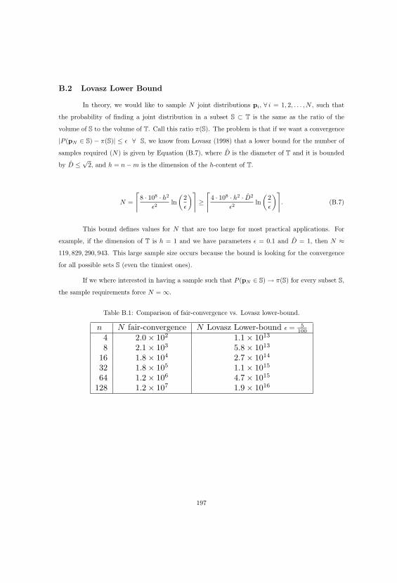
B.2 Lovasz Lower Bound
In theory, we would like to sample N joint distributions pi, ∀ i = 1, 2, . . . , N , such that
the probability of finding a joint distribution in a subset S ⊂ T is the same as the ratio of the
volume of S to the volume of T. Call this ratio π(S). The problem is that if we want a convergence
|P (pN ∈ S) − π(S)| ≤ ε ∀ S, we know from Lovasz (1998) that a lower bound for the number of
samples required (N) is given by Equation (B.7), where D is the diameter of T and it is bounded
by D ≤ √2, and h = n − m is the dimension of the h-content of T.
N =
⌈8 · 108 · h2
ε2ln
(2
ε
)⌉≥
⌈4 · 108 · h2 · D2
ε2ln
(2
ε
)⌉. (B.7)
This bound defines values for N that are too large for most practical applications. For
example, if the dimension of T is h = 1 and we have parameters ε = 0.1 and D = 1, then N ≈119, 829, 290, 943. This large sample size occurs because the bound is looking for the convergence
for all possible sets S (even the tinniest ones).
If we where interested in having a sample such that P (pN ∈ S) → π(S) for every subset S,
the sample requirements force N = ∞.
Table B.1: Comparison of fair-convergence vs. Lovasz lower-bound.
n N fair-convergence N Lovasz Lower-bound ε = 5
100
4 2.0 × 10² 1.1 × 10¹³
8 2.1 × 10³ 5.8 × 10¹³
16 1.8 × 10⁴ 2.7 × 10¹⁴
32 1.8 × 10⁵ 1.1 × 10¹⁵
64 1.2 × 10⁶ 4.7 × 10¹⁵
128 1.2 × 10⁷ 1.9 × 10¹⁶
197

B.3 Symmetric Perturbations
For 2 distributions A and B where A is a uniform distribution with even number of events,
and B is a symmetric perturbation of A. We have:
KLn(B, A) =n∑
i=1
(pBi ) log
(pB
i
pAi
)
=
n∑i=1
(pBi ) log
(pB
i
)−
n∑i=1
(pBi ) log
(pA
i
)
= − H(B) −n2∑
i=1
(pAi + ε) log
(pA
i
)−
n2∑
i=1
(pAi − ε) log
(pA
i
)
=H(A) − H(B) −n2∑
i=1
ε ln
(pA
i
)+
n2∑
i=1
ε log
(pA
i
)=ΔH(B, A).
Given that A is the uniform distribution (pAi = 1
n), and recalling that L1 = ε · n.
KLn(B, A) =
n∑i=1
(pBi ) log
(pB
i
pAi
)
=
n2∑
i=1
(pAi + ε) log
(pA
i + ε
pAi
)+
n2∑
i=1
(pAi − ε) log
(pA
i − ε
pAi
)
=n
2
[(pA
i + ε) log
(pA
i + ε
pAi
)+ (pA
i − ε) log
(pA
i − ε
pAi
)]
=n
2log
[(pA
i + ε
pAi
)(pAi +ε)(
pAi − ε
pAi
)(pAi −ε)
]
=n
2log
[(1 +
ε
pAi
)(pAi +ε)(
1 − ε
pAi
)(pAi −ε)
]
= log
[(1 + n · ε)( 1
n+ε) n
2(1 − n · ε)( 1
n−ε) n
2
]
198

KLn(B, A) = log
[(1 + n · ε) 1+n·ε
2(1 − n · ε) 1−n·ε
2
]
= log
[(1 + n · ε)n·ε+1
2(1 − n · ε)n·ε−1
2
]
= log
[(1 + L1
)L1+12(
1 − L1)L1−1
2
].
Using the logarithmic series expansion of log(1+L1) and log(1−L1), we can approximate KLn(B, A).
KLn(B, A) = log
[(1 + L1
)L1+12(
1 − L1)L1−1
2
]=
∞∑i
(L1)2i
2i(2i − 1) ln(2).
If B is not a symmetric perturbation, we still can make some observations:
KLn(B, A) =n∑
i=1
(pBi ) log
(pB
i
pAi
)
=
n∑i=1
(pBi ) log
(pB
i
)−
n∑i=1
(pBi + pA
i − pAi ) log
(pA
i
)
=H(A) − H(B) −n∑
i=1
(pBi − pA
i ) log
(pA
i
)
=ΔH(B, A) +n∑
i=1
(pAi − pB
i ) log
(pA
i
).
199

Appendix C
Additional Results
• Hypergeometric Family
– Scatterplots for c = 5, n = 3.
– Histograms for c = 5, n = 3.
– Scatterplots for c = 6, n = 8.
– Histograms for c = 6, n = 8.
– Frequency Tables
• Multinomial Family
– Scatterplots for c = 5, n = 3.
– Histograms for c = 5, n = 3.
– Scatterplots for c = 6, n = 8.
– Histograms for c = 6, n = 8.
– Frequency Tables
• Effects Of Increasing The Number OfConstraints
– Histograms for 3 random variables.
– Histograms for 7 random variables.
• Symmetric Sets With Marginal Constraints.
– Tables for 3 random variables (r.v.).
– Tables for 4 random variables.
– Tables for 5 random variables.
– Tables for 6 random variables.
– Tables for 7 random variables.
• Symmetric Sets With Marginal and Rank Cor-relation Constraints.
– Figures of the standard deviation for 3 r.v.
– Figures of the standard deviation for 4 r.v.
– Figures of the standard deviation for 5 r.v.
– Figures of the standard deviation for 6 r.v.
– Figures of the standard deviation for 7 r.v.
– Tables for 3 random variables.Parts 1, 2, 3, and 4.
– Tables for 4 random variables.Parts 1, 2, 3, and 4.
– Tables for 5 random variables.Parts 1, 2, 3, and 4.
– Tables for 6 random variables.Parts 1, 2, 3, and 4.
– Tables for 7 random variables.Parts 1, 2, 3, and 4.
200
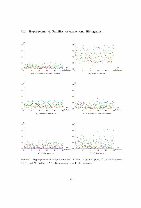
C.1 Hypergeometric Families Accuracy And Histograms.
(a) Maximum Absolute Distance. (b) Total Variation.
(c) Euclidean Distance. (d) Absolute Entropy Difference.
(e) KL Divergence. (f) χ2 Distance.
Figure C.1: Hypergeometric Family: Results for ME (Blue, “@”); ChSC (Red, “ * ”); MVIE (Green,
“ + ”); and AC (Yellow, “ · ”). For c = 5 and n = 3 (100 Samples).
201

(a) Entropy, L∞. (b) Analytic, L
∞. (c) Chebyshev’s, L∞. (d) MVIE, L
∞.
(e) Entropy, L1. (f) Analytic, L
1. (g) Chebyshev’s, L1. (h) MVIE, L
1.
(i) Entropy, Euclidean. (j) Analytic, Euclidean. (k) Chebyshev’s, Euclidean. (l) MVIE, Euclidean.
(m) Entropy, |ΔH|. (n) Analytic, |ΔH|. (o) Chebyshev’s, |ΔH|. (p) MVIE, |ΔH|.
(q) Entropy, KL. (r) Analytic, KL. (s) Chebyshev’s, KL. (t) MVIE, KL.
(u) Entropy, χ2. (v) Analytic, χ2. (w) Chebyshev’s, χ2. (x) MVIE, χ2.
Figure C.2: Hypergeometric Family Histogram Results. From left to right distribution approxima-tions. From Top to bottom measures of accuracy. For c = 5 and n = 3.
202
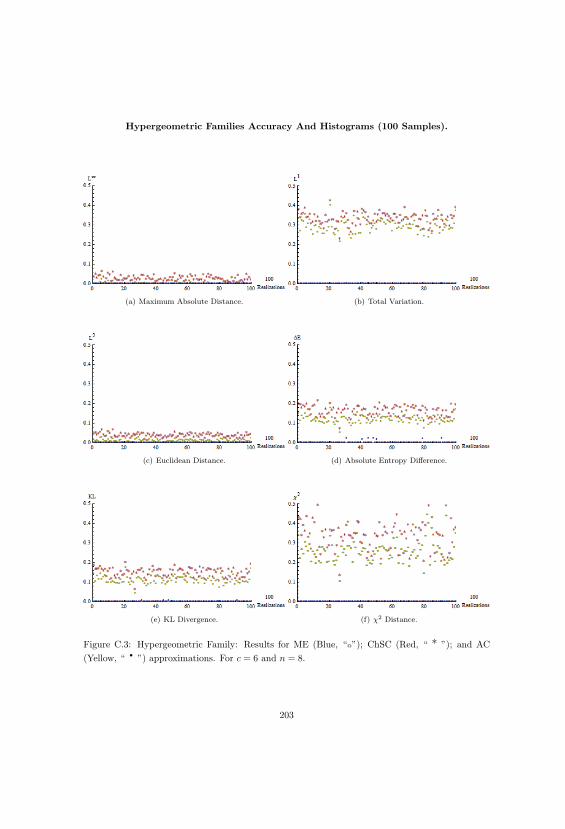
Hypergeometric Families Accuracy And Histograms (100 Samples).
(a) Maximum Absolute Distance. (b) Total Variation.
(c) Euclidean Distance. (d) Absolute Entropy Difference.
(e) KL Divergence. (f) χ2 Distance.
Figure C.3: Hypergeometric Family: Results for ME (Blue, “@”); ChSC (Red, “ * ”); and AC
(Yellow, “ · ”) approximations. For c = 6 and n = 8.
203

(a) Entropy, L∞. (b) Analytic, L
∞. (c) Chebyshev’s, L∞.
(d) Entropy, L1. (e) Analytic, L
1. (f) Chebyshev’s, L1.
(g) Entropy, Euclidean. (h) Analytic, Euclidean. (i) Chebyshev’s, Euclidean.
(j) Entropy, |ΔH|. (k) Analytic, |ΔH|. (l) Chebyshev’s, |ΔH|.
(m) Entropy, KL. (n) Analytic, KL. (o) Chebyshev’s, KL.
(p) Entropy, χ2. (q) Analytic, χ2. (r) Chebyshev’s, χ2.
Figure C.4: Hypergeometric Family Histogram Results. From left to right distribution approxima-tions. From Top to bottom measures of accuracy. For c = 6 and n = 8.
204

Percentage Of Accuracy For The Hypergeometric Distribution.
Table C.1: Approximations And Measures With Parameters c = 5, n = 3.
% Time Is % Time Is % Time Is % Time Is
Approximation Measure The Best The Second Best The Third Best The Worst
Entropy
L∞ 100 0 0 0
L1 100 0 0 0
L2 100 0 0 0
Δ H 100 0 0 0
KL 100 0 0 0
χ2 100 0 0 0
Analytic C
L∞ 0 7 92 1
L1 0 16 83 1
L2 0 11 88 1
Δ H 0 24 75 1
KL 0 22 77 1
χ2 0 41 58 1
ChSC
L∞ 0 93 6 1
L1 0 84 16 0
L2 0 89 11 0
Δ H 0 76 17 7
KL 0 78 18 4
χ2 0 59 22 19
MVIEC
L∞ 0 0 2 98
L1 0 0 1 99
L2 0 0 1 99
Δ H 0 0 8 92
KL 0 0 5 95
χ2 0 0 20 80
Table C.2: Approximations And Measures With Parameters c = 6, n = 8.
Approximation Measure % Time Is The Best % Time Is The Second Best % Time Is The Third Best
Entropy
L∞ 100 0 0
L1 100 0 0
L2 100 0 0
Δ H 100 0 0
KL 100 0 0
χ2 100 0 0
Analytic C
L∞ 0 97 3
L1 0 91 9
L2 0 96 4
Δ H 0 97 3
KL 0 96 4
χ2 0 98 2
ChSC
L∞ 0 3 97
L1 0 9 91
L2 0 4 96
Δ H 0 3 97
KL 0 4 96
χ2 0 2 98
205

C.2 Multinomial Families Accuracy And Histograms.
(a) Maximum Absolute Distance. (b) Total Variation.
(c) Euclidean Distance. (d) Absolute Entropy Difference.
(e) KL Divergence. (f) χ2 Distance.
Figure C.5: Multinomial Family: Results for ME (Blue, “@”); ChSC (Red, “ * ”); MVIE (Green,
“ + ”); and AC (Yellow, “ · ”) approximations. For c = 5 and n = 3.
206

(a) Entropy, L∞. (b) Analytic, L
∞. (c) Chebyshev’s, L∞. (d) MVIE, L
∞.
(e) Entropy, L1. (f) Analytic, L
1. (g) Chebyshev’s, L1. (h) MVIE, L
1.
(i) Entropy, Euclidean. (j) Analytic, Euclidean. (k) Chebyshev’s, Euclidean. (l) MVIE, Euclidean.
(m) Entropy, ΔH. (n) Analytic, ΔH. (o) Chebyshev’s, ΔH. (p) MVIE, ΔH.
(q) Entropy, KL. (r) Analytic, KL. (s) Chebyshev’s, KL. (t) MVIE, KL.
(u) Entropy, χ2. (v) Analytic, χ2. (w) Chebyshev’s, χ2. (x) MVIE, χ2.
Figure C.6: Multinomial Family Histogram Results. From left to right distribution approximations.From Top to bottom measures of accuracy. For c = 5 and n = 3 (100 Samples).
207

Multinomial Families Accuracy And Histograms (100 Samples).
(a) Maximum Absolute Distance. (b) Total Variation.
(c) Euclidean Distance. (d) Absolute Entropy Difference.
(e) KL Divergence. (f) χ2 Distance.
Figure C.7: Multinomial Family: Results for ME (Blue, “@”); ChSC (Red, “ * ”); and AC (Yellow,
“ · ”) approximations. For c = 6 and n = 8.
208

(a) Entropy, L∞. (b) Analytic, L
∞. (c) Chebyshev’s, L∞.
(d) Entropy, L1. (e) Analytic, L
1. (f) Chebyshev’s, L1.
(g) Entropy, Euclidean. (h) Analytic, Euclidean. (i) Chebyshev’s, Euclidean.
(j) Entropy, ΔH. (k) Analytic, ΔH. (l) Chebyshev’s, ΔH.
(m) Entropy, KL. (n) Analytic, KL. (o) Chebyshev’s, KL.
(p) Entropy, χ2. (q) Analytic, χ2. (r) Chebyshev’s, χ2.
Figure C.8: Multinomial Family Histogram Results. From left to right distribution approximations.From Top to bottom measures of accuracy. For c = 6 and n = 8.
209

Percentage Of Accuracy For The Monomial Distribution.
Table C.3: Approximations And Measures With Parameters c = 5, n = 3.
% Time Is % Time Is % Time Is % Time Is
Approximation Measure The Best The Second Best The Third Best The Worst
Entropy
L∞ 99 1 0 0
L1 99 1 0 0
L2 99 1 0 0
Δ H 100 0 0 0
KL 99 1 0 0
χ2 99 1 0 0
Analytic C
L∞ 1 2 95 2
L1 1 3 95 1
L2 1 3 94 2
Δ H 0 15 84 1
KL 1 6 92 1
χ2 1 39 59 1
ChSC
L∞ 0 95 5 0
L1 0 95 4 1
L2 0 95 5 0
Δ H 0 83 15 2
KL 0 91 8 1
χ2 0 58 36 6
MVIEC
L∞ 0 2 0 98
L1 0 1 1 98
L2 0 1 1 98
Δ H 0 2 1 97
KL 0 2 0 98
χ2 0 2 5 93
Table C.4: Approximations And Measures With Parameters c = 6, n = 8.
% Time Is % Time Is % Time Is
Approximation Measure The Best The Second Best The Third Best
Entropy
L∞ 99 1 0
L1 99 1 0
L2 99 1 0
Δ H 97 1 2
KL 99 1 0
χ2 99 1 0
Analytic C
L∞ 1 82 17
L1 1 76 23
L2 1 77 22
Δ H 3 79 18
KL 1 83 16
χ2 1 80 19
ChSC
L∞ 0 17 83
L1 0 23 77
L2 0 22 78
Δ H 0 20 80
KL 0 16 84
χ2 0 19 81
210

C.3 Effects Of Increasing The Number Of Constraints.Effects Of Increasing The Number Of Constraints Part One
(a) Unconst. L∞. (b) Unconst. L
1. (c) Unconst. L2.
(d) Marginal. L∞. (e) Marginal. L
1. (f) Marginal. L2.
(g) Pairwise. L∞. (h) Pairwise. L
1. (i) Pairwise. L2.
(j) Threewise. L∞. (k) Threewise. L
1. (l) Threewise. L2.
Figure C.9: Effects of including new constraints in a truth set T. The data is taken for a setthat considers 3 binary variables. The unconstraint set uses 1 constraint. The Marginal set uses 4constraints. The pairwise set uses 7 constraints. The three-wise set uses 8 constraints.
211

(a) Unconst. ΔH. (b) Unconst. KL. (c) Unconst. χ2.
(d) Marginal. ΔH. (e) Marginal. KL. (f) Marginal. χ2.
(g) Pairwise. ΔH. (h) Pairwise. KL. (i) Pairwise. χ2.
(j) Threewise. ΔH. (k) Threewise. KL. (l) Threewise. χ2.
Figure C.10: Effects of including new constraints in a truth set T. The data is taken for a setthat considers 3 binary variables. The unconstraint set uses 1 constraint. The Marginal set uses 4constraints. The pairwise set uses 7 constraints. The three-wise set uses 8 constraints.
212

Effects Of Increasing The Number Of Constraints Part Two
(a) Unconst. L∞. (b) Unconst. L
1. (c) Unconst. L2.
(d) Marginal. L∞. (e) Marginal. L
1. (f) Marginal. L2.
(g) Pairwise. L∞. (h) Pairwise. L
1. (i) Pairwise. L2.
(j) Threewise. L∞. (k) Threewise. L
1. (l) Threewise. L2.
Figure C.11: Effects of including new constraints in a truth set T. The data is taken for a setthat considers 7 binary variables. The unconstraint set uses 1 constraint. The Marginal set uses 8constraints. The pairwise set uses 29 constraints. The three-wise set uses 64 constraints.
213
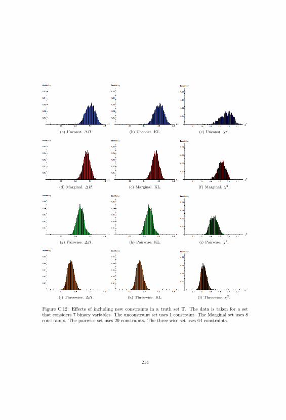
(a) Unconst. ΔH. (b) Unconst. KL. (c) Unconst. χ2.
(d) Marginal. ΔH. (e) Marginal. KL. (f) Marginal. χ2.
(g) Pairwise. ΔH. (h) Pairwise. KL. (i) Pairwise. χ2.
(j) Threewise. ΔH. (k) Threewise. KL. (l) Threewise. χ2.
Figure C.12: Effects of including new constraints in a truth set T. The data is taken for a setthat considers 7 binary variables. The unconstraint set uses 1 constraint. The Marginal set uses 8constraints. The pairwise set uses 29 constraints. The three-wise set uses 64 constraints.
214

C.4 Raw Statistics in Symm. Marginal Constrained Sets.
Symmetric Sets With Marginal Constraints Part One
Table C.5: Accuracy measure statistics for 3 binary variables marginally constrained
Three Variables With Marginals of p = 0.5.
ME L∞
L1
L2 ΔH KL χ2
Mean 0.13483 0.54622 0.22541 0.33667 0.33667 0.44817S.D. 0.04779 0.17924 0.07220 0.19426 0.19426 0.29461Min 0.00734 0.02525 0.01077 0.00067 0.00067 0.00093Max 0.34945 1.39468 0.56951 1.63090 1.63090 2.59473
AC
Mean 0.13483 0.54622 0.22541 0.33667 0.33667 0.44817S.D. 0.04779 0.17924 0.07220 0.19426 0.19426 0.29461Min 0.00734 0.02525 0.01077 0.00067 0.00067 0.00093Max 0.34945 1.39468 0.56951 1.63090 1.63090 2.59473
ChSC
Mean 0.13483 0.54622 0.22541 0.33667 0.33667 0.44817S.D. 0.04779 0.17924 0.07220 0.19426 0.19426 0.29461Min 0.00734 0.02525 0.01077 0.00067 0.00067 0.00093Max 0.34945 1.39468 0.56951 1.63090 1.63090 2.59473
MVIE
Mean 0.13483 0.54622 0.22541 0.33667 0.33667 0.44817S.D. 0.04779 0.17924 0.07220 0.19426 0.19426 0.29461Min 0.00734 0.02525 0.01077 0.00067 0.00067 0.00093Max 0.34945 1.39468 0.56951 1.63090 1.63090 2.59473
DAC
Mean 0.13480 0.54613 0.22537 0.33657 0.33657 0.44799S.D. 0.04777 0.17918 0.07218 0.19426 0.19419 0.29445Min 0.00805 0.02849 0.01258 0.00057 0.00090 0.00126Max 0.34912 1.39332 0.56891 1.63080 1.62687 2.58491
Three Variables With Marginals of p = 0.6.
L∞
L1
L2 ΔH KL χ2
0.12738 0.50316 0.20922 0.29811 0.29811 0.395380.04543 0.16290 0.06721 0.16995 0.16995 0.249610.00725 0.03087 0.01248 0.00094 0.00094 0.001300.35072 1.31034 0.53902 1.50194 1.50194 2.61487
0.12559 0.49615 0.20616 0.29499 0.29071 0.382250.04472 0.15940 0.06581 0.16995 0.16310 0.231670.00725 0.03439 0.01335 -0.00218 0.00098 0.001350.33314 1.25589 0.51567 1.49882 1.36666 2.22531
0.13183 0.51845 0.21546 0.23169 0.31829 0.441940.05435 0.18934 0.07926 0.16995 0.19661 0.297900.00787 0.02922 0.01237 -0.06547 0.00101 0.001410.29999 1.17996 0.48191 1.43553 1.32450 2.01231
0.12510 0.49491 0.20550 0.28541 0.29012 0.382800.04556 0.16206 0.06697 0.16995 0.16417 0.232630.00898 0.03303 0.01430 -0.01175 0.00139 0.001950.31410 1.20511 0.49342 1.48924 1.26180 1.97555
0.12524 0.49442 0.20540 0.28927 0.28927 0.380560.04511 0.15969 0.06605 0.16995 0.16226 0.229140.00943 0.03375 0.01429 -0.00789 0.00154 0.002100.32135 1.21755 0.49948 1.49310 1.27818 1.99151
Three Variables With Marginals of p = 0.7.
ME L∞
L1
L2 ΔH KL χ2
Mean 0.11841 0.45497 0.19176 0.27638 0.27638 0.39948S.D. 0.04906 0.16893 0.07221 0.17522 0.17522 0.30382Min 0.00412 0.01899 0.00822 0.00064 0.00064 0.00089Max 0.33851 1.19043 0.49967 1.50838 1.50838 3.33831
AC
Mean 0.10019 0.39209 0.16339 0.24444 0.21748 0.28755S.D. 0.03777 0.13361 0.05555 0.17522 0.12592 0.18069Min 0.00423 0.02414 0.00879 -0.03130 0.00063 0.00087Max 0.28170 1.03479 0.42755 1.47644 1.12765 1.84165
ChSC
Mean 0.10528 0.41035 0.17075 0.10456 0.24041 0.34964S.D. 0.04799 0.16491 0.06930 0.17522 0.15122 0.25595Min 0.00625 0.02766 0.01118 -0.17118 0.00088 0.00123Max 0.34283 1.22946 0.51185 1.33657 1.25716 2.17363
MVIE
Mean 0.09826 0.38654 0.16058 0.18547 0.21464 0.29003S.D. 0.03973 0.13938 0.05791 0.17522 0.12447 0.18762Min 0.00542 0.02134 0.00974 -0.09027 0.00065 0.00090Max 0.30729 1.11731 0.46295 1.41748 1.00457 1.55146
DAC
Mean 0.09795 0.38437 0.15984 0.21180 0.21180 0.28152S.D. 0.03785 0.13276 0.05513 0.17522 0.12072 0.17556Min 0.00676 0.02589 0.01090 -0.06394 0.00064 0.00089Max 0.29181 1.06080 0.43958 1.44380 1.00053 1.50361
Three Variables With Marginals of p = 0.8.
L∞
L1
L2 ΔH KL χ2
0.11112 0.41058 0.17683 0.27846 0.27846 0.515350.04543 0.14965 0.06575 0.16593 0.16593 0.441330.00304 0.01187 0.00497 0.00027 0.00027 0.000370.26780 0.88085 0.38391 1.16598 1.16598 4.28048
0.06838 0.26737 0.11154 0.19430 0.14538 0.192840.02612 0.09221 0.03850 0.16593 0.08475 0.122530.00403 0.01412 0.00602 -0.08389 0.00046 0.000650.18764 0.67637 0.28114 1.08183 0.66254 1.11941
0.07051 0.27477 0.11435 0.02931 0.15598 0.228690.03170 0.10894 0.04582 0.16593 0.09374 0.162700.00461 0.01712 0.00715 -0.24888 0.00066 0.000920.22176 0.79568 0.33189 0.91684 0.72048 1.29518
0.06566 0.25864 0.10740 0.10852 0.13995 0.189910.02641 0.09254 0.03847 0.16593 0.07906 0.120780.00109 0.00626 0.00228 -0.16967 0.00007 0.000090.19806 0.72090 0.29937 0.99604 0.58323 0.90601
0.06538 0.25712 0.10685 0.13819 0.13819 0.184170.02521 0.08847 0.03671 0.16593 0.07754 0.113870.00215 0.00871 0.00366 -0.14000 0.00017 0.000240.18753 0.68297 0.28368 1.02572 0.58507 0.85818
Three Variables With Marginals of p = 0.9.
ME L∞
L1
L2 ΔH KL χ2
Mean 0.08041 0.28984 0.12572 0.24121 0.24121 0.87143S.D. 0.02641 0.08625 0.03730 0.11861 0.11861 0.89689Min 0.00132 0.00485 0.00206 0.00017 0.00017 0.00023Max 0.16178 0.50381 0.22901 0.79239 0.79239 8.63525
AC
Mean 0.03504 0.13635 0.05698 0.12395 0.07314 0.09699S.D. 0.01344 0.04709 0.01975 0.11861 0.04263 0.06161Min 0.00187 0.00723 0.00332 -0.11710 0.00030 0.00041Max 0.09671 0.34655 0.14364 0.67513 0.33245 0.58519
ChSC
Mean 0.03479 0.13588 0.05650 -0.00548 0.07530 0.11001S.D. 0.01567 0.05395 0.02265 0.11861 0.04472 0.07805Min 0.00102 0.00403 0.00168 -0.24652 0.00006 0.00008Max 0.12062 0.43518 0.18078 0.54571 0.39968 0.74299
MVIE
Mean 0.03269 0.12876 0.05347 0.05024 0.06838 0.09239S.D. 0.01300 0.04561 0.01893 0.11861 0.03823 0.05826Min 0.00104 0.00587 0.00214 -0.19080 0.00009 0.00013Max 0.10877 0.39779 0.16453 0.60142 0.32094 0.52403
DAC
Mean 0.03266 0.12833 0.05333 0.06778 0.06778 0.09018S.D. 0.01252 0.04383 0.01818 0.11861 0.03771 0.05550Min 0.00169 0.00823 0.00311 -0.17326 0.00022 0.00031Max 0.10460 0.38203 0.15807 0.61897 0.29222 0.45628
215

Raw Statistics For Symmetric Sets With Marginal Constraints Part TwoTable C.6: Accuracy measure statistics for 4 binary variables marginally constrained
Four Variables With Marginals of p = 0.5.
ME L∞
L1
L2 ΔH KL χ2
Mean 0.10326 0.60959 0.18628 0.41504 0.41504 0.57825S.D. 0.03320 0.11748 0.03796 0.14290 0.14290 0.24024Min 0.02564 0.18192 0.05369 0.03251 0.03251 0.04613Max 0.27133 1.13834 0.36311 1.11297 1.11297 2.10960
AC
Mean 0.10326 0.60959 0.18628 0.41504 0.41504 0.57825S.D. 0.03320 0.11748 0.03796 0.14290 0.14290 0.24024Min 0.02564 0.18192 0.05369 0.03251 0.03251 0.04613Max 0.27133 1.13834 0.36311 1.11297 1.11297 2.10960
ChSC
Mean 0.10326 0.60959 0.18628 0.41504 0.41504 0.57825S.D. 0.03320 0.11748 0.03796 0.14290 0.14290 0.24024Min 0.02564 0.18192 0.05369 0.03251 0.03251 0.04613Max 0.27133 1.13834 0.36311 1.11297 1.11297 2.10960
MVIE
Mean 0.10326 0.60959 0.18628 0.41504 0.41504 0.57825S.D. 0.03320 0.11748 0.03795 0.14290 0.14290 0.24023Min 0.02563 0.18192 0.05369 0.03251 0.03250 0.04612Max 0.27133 1.13834 0.36311 1.11297 1.11300 2.10951
DAC
Mean 0.10321 0.60946 0.18624 0.41484 0.41484 0.57780S.D. 0.03314 0.11740 0.03792 0.14290 0.14267 0.23945Min 0.02634 0.18733 0.05549 0.03231 0.03476 0.04958Max 0.26849 1.14126 0.36053 1.11277 1.11528 2.07109
Four Variables With Marginals of p = 0.6.
L∞
L1
L2 ΔH KL χ2
0.10264 0.58030 0.18156 0.38441 0.38441 0.532610.03316 0.11695 0.03900 0.13305 0.13305 0.215310.02275 0.15870 0.04871 0.03082 0.03082 0.041500.27012 1.02570 0.33817 1.01482 1.01482 1.93592
0.10030 0.57066 0.17806 0.37726 0.37448 0.515880.03173 0.11448 0.03850 0.13305 0.12888 0.205060.01912 0.14367 0.04460 0.02367 0.03166 0.040940.24591 1.04104 0.32618 1.00767 0.97732 1.86197
0.12235 0.63007 0.20385 0.24205 0.45119 0.686660.04838 0.15687 0.06012 0.13305 0.19018 0.335970.02335 0.17406 0.05367 -0.11154 0.03801 0.053460.27519 1.18928 0.39988 0.87247 1.31573 2.31231
0.10024 0.57028 0.17793 0.37590 0.37425 0.515830.03179 0.11467 0.03866 0.13305 0.12909 0.205570.01943 0.14634 0.04487 0.02231 0.03181 0.041050.24592 1.04496 0.32582 1.00631 0.97572 1.86197
0.10021 0.56976 0.17778 0.37390 0.37390 0.515590.03185 0.11492 0.03885 0.13305 0.12930 0.205780.01977 0.14350 0.04355 0.02032 0.02990 0.038400.24747 1.04305 0.32895 1.00432 0.96946 1.81231
Four Variables With Marginals of p = 0.7.
ME L∞
L1
L2 ΔH KL χ2
Mean 0.12285 0.56422 0.19120 0.38323 0.38323 0.58030S.D. 0.04959 0.14099 0.05479 0.15392 0.15392 0.29392Min 0.02042 0.13858 0.04234 0.02595 0.02595 0.03673Max 0.31862 1.03304 0.39418 1.12777 1.12777 3.13612
AC
Mean 0.08373 0.45758 0.14555 0.30688 0.28485 0.39501S.D. 0.02852 0.09891 0.03494 0.15392 0.09985 0.16213Min 0.01890 0.13020 0.04114 -0.05040 0.02200 0.03041Max 0.22538 0.87573 0.31235 1.05142 0.76385 1.33524
ChSC
Mean 0.10944 0.52264 0.17431 0.04439 0.36269 0.60063S.D. 0.05067 0.15055 0.06130 0.15392 0.15858 0.33156Min 0.01252 0.07112 0.02206 -0.31288 0.00905 0.01257Max 0.31323 1.10271 0.41105 0.78893 1.21351 2.62028
MVIE
Mean 0.08416 0.45638 0.14527 0.24313 0.28669 0.40842S.D. 0.03223 0.10714 0.04000 0.15392 0.10352 0.17874Min 0.01565 0.11441 0.03354 -0.11414 0.01988 0.02617Max 0.24349 0.95023 0.34354 0.98768 0.87986 1.56655
DAC
Mean 0.08283 0.45380 0.14408 0.28254 0.28254 0.39452S.D. 0.02909 0.09964 0.03585 0.15392 0.09862 0.16287Min 0.01699 0.11625 0.03354 -0.07473 0.01896 0.02500Max 0.22342 0.90599 0.32557 1.02708 0.81423 1.41610
Four Variables With Marginals of p = 0.8.
L∞
L1
L2 ΔH KL χ2
0.15280 0.55942 0.21054 0.41817 0.41817 0.857510.04560 0.12770 0.05204 0.15377 0.15377 0.512380.01402 0.09787 0.03042 0.02746 0.02746 0.039360.28293 0.91134 0.35281 1.02725 1.02725 6.75968
0.05818 0.31256 0.10020 0.22998 0.19251 0.270060.01992 0.06996 0.02496 0.15377 0.06980 0.117810.01147 0.07936 0.02456 -0.16073 0.01242 0.016800.14473 0.58690 0.21005 0.83906 0.50069 1.11569
0.07607 0.35761 0.12032 -0.05002 0.24409 0.416920.03585 0.10641 0.04382 0.15377 0.10624 0.238070.01328 0.07723 0.02511 -0.44073 0.01903 0.024360.22040 0.75574 0.29146 0.55906 0.73509 1.70095
0.05823 0.31065 0.09966 0.13670 0.19394 0.282000.02336 0.07767 0.02970 0.15377 0.07249 0.131890.00424 0.02858 0.00895 -0.25400 0.00223 0.003070.17390 0.64902 0.24212 0.74579 0.53727 1.11615
0.05691 0.30794 0.09840 0.19022 0.19022 0.269380.02041 0.07073 0.02587 0.15377 0.06887 0.118960.01377 0.06485 0.02339 -0.20049 0.00564 0.007740.15706 0.61936 0.22435 0.79930 0.49018 1.03395
Four Variables With Marginals of p = 0.9.
ME L∞
L1
L2 ΔH KL χ2
Mean 0.12894 0.43116 0.17169 0.39360 0.39360 2.17852S.D. 0.02261 0.06652 0.02696 0.10901 0.10901 2.18992Min 0.04537 0.16572 0.06414 0.05390 0.05390 0.09628Max 0.19940 0.60674 0.24897 0.81392 0.81392 33.95045
AC
Mean 0.02950 0.15764 0.05058 0.14921 0.09580 0.13215S.D. 0.01036 0.03526 0.01250 0.10901 0.03472 0.05607Min 0.00484 0.03681 0.01062 -0.19050 0.00615 0.00806Max 0.08339 0.31611 0.10863 0.56953 0.31329 0.55574
ChSC
Mean 0.03503 0.17016 0.05640 -0.05363 0.11173 0.18677S.D. 0.01633 0.04899 0.01998 0.10901 0.04603 0.10397Min 0.00641 0.03889 0.01246 -0.39333 0.00951 0.01239Max 0.11103 0.38005 0.14342 0.36669 0.40457 1.01582
MVIE
Mean 0.02769 0.15132 0.04802 0.07259 0.09292 0.13252S.D. 0.01053 0.03535 0.01319 0.10901 0.03347 0.05956Min 0.00489 0.03073 0.01034 -0.26712 0.00508 0.00686Max 0.08778 0.34125 0.12033 0.49291 0.32413 0.66874
DAC
Mean 0.02752 0.15119 0.04792 0.09241 0.09241 0.12994S.D. 0.00993 0.03393 0.01237 0.10901 0.03295 0.05671Min 0.00429 0.02788 0.00892 -0.24729 0.00452 0.00616Max 0.08358 0.33270 0.11647 0.51273 0.30616 0.60998
216

Raw Stat. For Symmetric Sets With Marginal Constraints Part ThreeTable C.7: Accuracy measure statistics for 5 binary variables marginally constrained
Five Variables With Marginals of p = 0.5.
ME L∞
L1
L2 ΔH KL χ2
Mean 0.07249 0.66240 0.14713 0.48525 0.48525 0.70644S.D. 0.01947 0.08348 0.02070 0.10928 0.10928 0.20087Min 0.02516 0.25184 0.05570 0.09122 0.09122 0.09929Max 0.16416 0.96684 0.23241 0.91726 0.91726 1.72842
AC
Mean 0.07249 0.66240 0.14713 0.48525 0.48525 0.70644S.D. 0.01947 0.08348 0.02070 0.10928 0.10928 0.20087Min 0.02516 0.25184 0.05570 0.09122 0.09122 0.09929Max 0.16416 0.96684 0.23241 0.91726 0.91726 1.72842
ChSC
Mean 0.07249 0.66240 0.14713 0.48525 0.48525 0.70644S.D. 0.01947 0.08348 0.02070 0.10928 0.10928 0.20087Min 0.02516 0.25184 0.05570 0.09122 0.09122 0.09929Max 0.16416 0.96684 0.23241 0.91726 0.91726 1.72842
MVIE
Mean 0.07249 0.66240 0.14713 0.48525 0.48525 0.70644S.D. 0.01947 0.08348 0.02070 0.10928 0.10928 0.20086Min 0.02518 0.25184 0.05570 0.09122 0.09121 0.09928Max 0.16418 0.96683 0.23242 0.91726 0.91731 1.72923
DAC
Mean 0.07228 0.66179 0.14696 0.48391 0.48391 0.70309S.D. 0.01935 0.08295 0.02055 0.10928 0.10823 0.19814Min 0.02517 0.25499 0.05574 0.08987 0.09137 0.09989Max 0.16704 0.97397 0.23449 0.91591 0.92660 1.84935
Five Variables With Marginals of p = 0.6.
L∞
L1
L2 ΔH KL χ2
0.08041 0.64619 0.15163 0.46674 0.46674 0.681390.02645 0.09058 0.02583 0.11322 0.11322 0.205320.01706 0.12344 0.02926 0.01940 0.01940 0.027920.20866 0.94929 0.25827 0.90145 0.90145 1.69515
0.07552 0.63180 0.14720 0.45264 0.45049 0.652500.02237 0.08913 0.02518 0.11322 0.10877 0.191560.00984 0.10135 0.02216 0.00530 0.01075 0.015130.17833 0.96252 0.24888 0.88735 0.92705 1.60752
0.12193 0.72370 0.19043 0.22068 0.58280 0.969470.04725 0.12872 0.04940 0.11322 0.18391 0.369720.02130 0.31008 0.06622 -0.22666 0.13105 0.173680.22499 1.13007 0.33192 0.65539 1.33549 2.64987
0.07593 0.63345 0.14763 0.45703 0.45152 0.652990.02279 0.08866 0.02488 0.11322 0.10834 0.190350.00792 0.08748 0.01899 0.00970 0.00954 0.013490.18541 0.95624 0.24515 0.89175 0.90895 1.58001
0.07535 0.63096 0.14704 0.44957 0.44957 0.650690.02223 0.08917 0.02531 0.11322 0.10863 0.190800.01252 0.10928 0.02441 0.00223 0.01218 0.017200.17565 0.97235 0.25037 0.88428 0.95195 1.63698
Five Variables With Marginals of p = 0.7.
ME L∞
L1
L2 ΔH KL χ2
Mean 0.13679 0.66002 0.18925 0.49407 0.49407 0.79982S.D. 0.05064 0.11488 0.04595 0.14134 0.14134 0.30512Min 0.02558 0.26735 0.06421 0.11989 0.11989 0.17261Max 0.28651 1.04497 0.33080 1.06028 1.06028 4.25448
AC
Mean 0.06389 0.49480 0.11895 0.34166 0.33348 0.48548S.D. 0.02265 0.07682 0.02433 0.14134 0.08364 0.15562Min 0.01792 0.15705 0.04110 -0.03251 0.02704 0.03667Max 0.16643 0.83775 0.22026 0.90787 0.71798 1.35700
ChSC
Mean 0.11883 0.60551 0.17037 -0.05189 0.46677 0.86156S.D. 0.04928 0.12492 0.05191 0.14134 0.15319 0.38549Min 0.01845 0.21014 0.04501 -0.42607 0.07799 0.10688Max 0.28625 1.01156 0.34235 0.51432 1.13269 2.70873
MVIE
Mean 0.06547 0.49801 0.12062 0.27779 0.33786 0.50370S.D. 0.02578 0.08507 0.02922 0.14134 0.08832 0.17196Min 0.00782 0.09959 0.02167 -0.09639 0.01785 0.02396Max 0.19326 0.87609 0.24433 0.84400 0.78185 1.40224
DAC
Mean 0.06350 0.49314 0.11848 0.33157 0.33157 0.48229S.D. 0.02258 0.07707 0.02457 0.14134 0.08254 0.15229Min 0.01803 0.15028 0.03886 -0.04261 0.02597 0.03461Max 0.17051 0.83547 0.22191 0.89778 0.71126 1.24376
Five Variables With Marginals of p = 0.8.
L∞
L1
L2 ΔH KL χ2
0.19528 0.68752 0.23914 0.56455 0.56455 1.299410.04490 0.11661 0.04754 0.15420 0.15420 0.659390.08365 0.36192 0.12207 0.16648 0.16648 0.267600.31119 1.01488 0.36051 1.07385 1.07385 7.99695
0.04903 0.35220 0.08769 0.22136 0.23525 0.348880.01851 0.06080 0.02090 0.15420 0.06324 0.125950.01256 0.14568 0.03729 -0.17671 0.04528 0.063890.11549 0.58902 0.17506 0.73065 0.54580 1.06904
0.09136 0.43556 0.12764 -0.16217 0.34056 0.681400.04227 0.10665 0.04532 0.15420 0.12646 0.354500.01173 0.15145 0.03450 -0.56024 0.06644 0.085620.20117 0.74322 0.25038 0.34712 0.82576 2.24795
0.05282 0.35809 0.09110 0.13399 0.24344 0.377030.02500 0.07535 0.02861 0.15420 0.07146 0.152290.01058 0.13100 0.02703 -0.26407 0.03981 0.055410.13917 0.62503 0.19416 0.64329 0.59408 1.22019
0.04896 0.35167 0.08749 0.23318 0.23318 0.342670.01797 0.05852 0.01984 0.15420 0.06019 0.115660.01283 0.15320 0.03659 -0.16489 0.05116 0.072970.11591 0.56933 0.16871 0.74248 0.50387 0.92948
Five Variables With Marginals of p = 0.9.
ME L∞
L1
L2 ΔH KL χ2
Mean 0.17942 0.56225 0.21692 0.56907 0.56907 5.41303S.D. 0.02100 0.05761 0.02370 0.10586 0.10586 4.55807Min 0.09323 0.32094 0.11946 0.20882 0.20882 0.56803Max 0.23446 0.69635 0.27593 0.87649 0.87649 49.73910
AC
Mean 0.02409 0.17333 0.04267 0.15359 0.11518 0.16675S.D. 0.00964 0.02851 0.00996 0.10586 0.02890 0.05326Min 0.00685 0.03806 0.01515 -0.20665 0.00336 0.00439Max 0.07848 0.31661 0.10406 0.46102 0.22713 0.40875
ChSC
Mean 0.03772 0.19919 0.05572 -0.10679 0.14802 0.28483S.D. 0.01936 0.04799 0.02059 0.10586 0.05358 0.15725Min 0.00568 0.07737 0.01737 -0.46703 0.02454 0.04115Max 0.12253 0.40756 0.14995 0.20064 0.43390 1.22346
MVIE
Mean 0.02318 0.16966 0.04163 0.08607 0.11489 0.17293S.D. 0.01089 0.03242 0.01229 0.10586 0.03126 0.06443Min 0.00010 0.00095 0.00021 -0.27418 0.00000 0.00001Max 0.09152 0.34344 0.11788 0.39349 0.26993 0.53751
DAC
Mean 0.02295 0.16961 0.04144 0.11365 0.11365 0.16747S.D. 0.00996 0.02974 0.01087 0.10586 0.02919 0.05642Min 0.00430 0.01982 0.00694 -0.24660 0.00118 0.00157Max 0.08618 0.33218 0.11164 0.42107 0.24141 0.44604
217

Raw Stat. For Symmetric Sets With Marginal Constraints Part FourTable C.8: Accuracy measure statistics for 6 binary variables marginally constrained
Six Variables With Marginals of p = 0.5.
ME L∞
L1
L2 ΔH KL χ2
Mean 0.04767 0.69098 0.11142 0.52996 0.52996 0.80305S.D. 0.01161 0.06077 0.01158 0.08365 0.08365 0.16834Min 0.01106 0.24529 0.03835 0.06961 0.06961 0.09415Max 0.09678 0.90657 0.15131 0.83298 0.83298 1.46521
AC
Mean 0.04767 0.69098 0.11142 0.52996 0.52996 0.80305S.D. 0.01161 0.06077 0.01158 0.08365 0.08365 0.16834Min 0.01106 0.24529 0.03835 0.06961 0.06961 0.09415Max 0.09678 0.90657 0.15131 0.83298 0.83298 1.46521
ChSC
Mean 0.04767 0.69098 0.11142 0.52996 0.52996 0.80305S.D. 0.01161 0.06077 0.01158 0.08365 0.08365 0.16834Min 0.01106 0.24529 0.03835 0.06961 0.06961 0.09415Max 0.09678 0.90657 0.15131 0.83298 0.83298 1.46521
MVIE
Mean 0.04767 0.69098 0.11141 0.52996 0.52996 0.80303S.D. 0.01161 0.06077 0.01158 0.08365 0.08365 0.16834Min 0.01105 0.24540 0.03837 0.06961 0.06966 0.09421Max 0.09678 0.90664 0.15131 0.83298 0.83287 1.46530
DAC
Mean 0.04700 0.68696 0.11066 0.52187 0.52187 0.78255S.D. 0.01146 0.05903 0.01123 0.08365 0.07992 0.15716Min 0.01330 0.25260 0.04094 0.06152 0.07942 0.10810Max 0.09462 0.88391 0.14966 0.82489 0.79832 1.41012
Six Variables With Marginals of p = 0.6.
L∞
L1
L2 ΔH KL χ2
0.06693 0.69707 0.12522 0.54271 0.54271 0.836890.02309 0.06840 0.01803 0.09435 0.09435 0.190120.02048 0.15115 0.03414 0.03094 0.03094 0.046390.14172 0.92423 0.18072 0.86145 0.86145 1.48379
0.05632 0.67235 0.11758 0.51658 0.51002 0.773740.01517 0.06239 0.01545 0.09435 0.08556 0.168970.00740 0.10273 0.01657 0.00481 0.01121 0.015490.10825 0.87593 0.18182 0.83532 0.88124 1.55349
0.12387 0.77780 0.17259 0.17035 0.67547 1.221510.04305 0.09898 0.04042 0.09435 0.16422 0.381540.03395 0.42251 0.08567 -0.34142 0.22115 0.332440.21250 1.05012 0.27717 0.48909 1.30197 2.75889
0.05778 0.67575 0.11862 0.52468 0.51293 0.775820.01608 0.06295 0.01523 0.09435 0.08499 0.165970.00428 0.09266 0.01427 0.01291 0.01031 0.014250.11488 0.86609 0.17752 0.84342 0.86304 1.51869
0.05532 0.66825 0.11661 0.50178 0.50178 0.751180.01492 0.06066 0.01563 0.09435 0.08217 0.156380.01368 0.14252 0.02624 -0.00999 0.02360 0.032900.10499 0.86382 0.18197 0.82052 0.85196 1.41162
Six Variables With Marginals of p = 0.7.
ME L∞
L1
L2 ΔH KL χ2
Mean 0.13396 0.70590 0.17014 0.57215 0.57215 1.00699S.D. 0.04427 0.10019 0.03943 0.12892 0.12892 0.28350Min 0.03528 0.46667 0.09199 0.28110 0.28110 0.42166Max 0.23209 0.98617 0.25935 0.99871 0.99871 2.18777
AC
Mean 0.06046 0.55104 0.10641 0.30221 0.39355 0.60515S.D. 0.02446 0.06930 0.02436 0.12892 0.06985 0.13456Min 0.01580 0.22599 0.03931 0.01116 0.07852 0.10103Max 0.16509 0.79719 0.20786 0.72877 0.63988 1.08699
ChSC
Mean 0.15813 0.72277 0.19467 -0.20909 0.65235 1.44350S.D. 0.04501 0.10364 0.04523 0.12892 0.15518 0.46676Min 0.05964 0.39619 0.08806 -0.50014 0.18956 0.31094Max 0.28852 1.05776 0.32965 0.21746 1.20192 2.99290
MVIE
Mean 0.07045 0.56737 0.11485 0.24349 0.41155 0.65145S.D. 0.02999 0.07966 0.02997 0.12892 0.07721 0.15436Min 0.01012 0.21047 0.03210 -0.04756 0.07551 0.09649Max 0.18427 0.83844 0.22663 0.67005 0.68557 1.17962
DAC
Mean 0.04914 0.52217 0.09689 0.36140 0.36140 0.53010S.D. 0.01701 0.05697 0.01634 0.12892 0.06033 0.10141Min 0.01423 0.32305 0.05190 0.07035 0.12955 0.16761Max 0.13041 0.71499 0.16606 0.78795 0.60765 0.91809
Six Variables With Marginals of p = 0.8.
L∞
L1
L2 ΔH KL χ2
0.26820 0.88013 0.30045 0.83350 0.83350 2.342670.02789 0.07664 0.02954 0.13912 0.13912 0.887650.21474 0.67943 0.24045 0.51544 0.51544 0.894000.34526 1.10852 0.38220 1.28131 1.28131 11.90230
0.03205 0.34262 0.06168 0.28470 0.24246 0.358860.01441 0.03779 0.01116 0.13912 0.03869 0.068610.01037 0.08459 0.01972 -0.03336 0.01042 0.014390.08691 0.48689 0.10639 0.73251 0.38456 0.59871
0.07638 0.41541 0.09915 -0.17734 0.32363 0.636630.02690 0.05763 0.02489 0.13912 0.06100 0.176810.01442 0.22201 0.03962 -0.49540 0.07655 0.132580.12936 0.54808 0.14759 0.27047 0.50609 1.28914
0.03134 0.34249 0.06152 0.21248 0.24197 0.365550.01023 0.03334 0.00886 0.13912 0.03597 0.067930.00220 0.05183 0.00808 -0.10557 0.00749 0.010290.07066 0.45298 0.09082 0.66030 0.36212 0.62365
0.03047 0.33792 0.06043 0.23611 0.23611 0.349500.01149 0.03474 0.00937 0.13912 0.03604 0.064520.00518 0.08948 0.01457 -0.08195 0.01443 0.019950.07706 0.46084 0.09642 0.68392 0.38121 0.65347
Six Variables With Marginals of p = 0.9.
ME L∞
L1
L2 ΔH KL χ2
Mean 0.23114 0.68981 0.26353 0.76366 0.76366 12.71220S.D. 0.01694 0.04519 0.01815 0.10347 0.10347 12.66190Min 0.18707 0.58192 0.21877 0.50138 0.50138 1.46620Max 0.26269 0.79719 0.29936 0.97538 0.97538 172.77814
AC
Mean 0.01747 0.17579 0.03240 0.14023 0.12240 0.18357S.D. 0.00713 0.01979 0.00645 0.10347 0.02177 0.04161Min 0.00605 0.03781 0.01016 -0.12205 0.00388 0.00522Max 0.04105 0.23261 0.05465 0.35196 0.19367 0.32780
ChSC
Mean 0.04055 0.21418 0.05209 -0.15790 0.16668 0.33972S.D. 0.01693 0.03629 0.01650 0.10347 0.04097 0.13072Min 0.01067 0.10933 0.02141 -0.42018 0.03519 0.06220Max 0.08461 0.31799 0.09584 0.05382 0.29850 0.82176
MVIE
Mean 0.01761 0.17419 0.03238 0.08770 0.12313 0.18914S.D. 0.00937 0.02274 0.00870 0.10347 0.02199 0.04508Min 0.00102 0.02016 0.00327 -0.17458 0.00231 0.00312Max 0.04987 0.24706 0.06242 0.29942 0.19928 0.36704
DAC
Mean 0.01699 0.17325 0.03186 0.11988 0.11988 0.17823S.D. 0.00765 0.02049 0.00708 0.10347 0.02023 0.03769Min 0.00456 0.03983 0.00840 -0.14240 0.00572 0.00779Max 0.04407 0.23889 0.05709 0.33160 0.19406 0.32009
218

Raw Stat. For Symmetric Sets With Marginal Constraints Part FiveTable C.9: Accuracy measure statistics for 7 binary variables marginally constrained
Seven Variables With Marginals of p = 0.5.
ME L∞
L1
L2 ΔH KL χ2
Mean 0.02884 0.70191 0.08137 0.55125 0.55125 0.85358S.D. 0.00595 0.04470 0.00690 0.06748 0.06748 0.14537Min 0.00477 0.17046 0.01943 0.03576 0.03576 0.04833Max 0.04634 0.85980 0.10186 0.79736 0.79736 1.32808
AC
Mean 0.02884 0.70191 0.08137 0.55125 0.55125 0.85358S.D. 0.00595 0.04470 0.00690 0.06748 0.06748 0.14537Min 0.00477 0.17046 0.01943 0.03576 0.03576 0.04833Max 0.04634 0.85980 0.10186 0.79736 0.79736 1.32808
ChSC
Mean 0.02884 0.70191 0.08137 0.55125 0.55125 0.85358S.D. 0.00595 0.04470 0.00690 0.06748 0.06748 0.14537Min 0.00477 0.17046 0.01943 0.03576 0.03576 0.04833Max 0.04634 0.85980 0.10186 0.79736 0.79736 1.32808
MVIE
Mean - - - - - -S.D. - - - - - -Min - - - - - -Max - - - - - -
DAC
Mean 0.02677 0.68778 0.07926 0.52047 0.52047 0.76865S.D. 0.00554 0.04127 0.00600 0.06748 0.05510 0.10298Min 0.00794 0.22950 0.02575 0.00497 0.05989 0.08278Max 0.04396 0.83553 0.09685 0.76658 0.71510 1.06711
Seven Variables With Marginals of p = 0.6.
L∞
L1
L2 ΔH KL χ2
0.10436 0.75909 0.13144 0.68065 0.68065 1.243060.03803 0.06260 0.02990 0.11600 0.11600 0.324420.02907 0.57139 0.07443 0.37263 0.37263 0.572550.17855 0.90374 0.19159 0.93252 0.93252 2.06727
0.06607 0.68886 0.10107 0.63267 0.52752 0.801500.03263 0.05570 0.02222 0.11600 0.06357 0.112690.01355 0.42755 0.05833 0.32465 0.23660 0.396870.13625 0.80753 0.15080 0.88455 0.68767 1.09872
0.07466 0.68378 0.10679 0.16552 0.53831 0.908170.03691 0.08307 0.03119 0.11600 0.09932 0.223680.00199 0.06448 0.00721 -0.14250 0.00608 0.008300.14997 0.89815 0.17759 0.41739 0.85039 1.57445
- - - - - -- - - - - -- - - - - -- - - - - -
0.03710 0.62100 0.07824 0.44789 0.44789 0.655470.01488 0.03884 0.00964 0.11600 0.04428 0.084810.01416 0.29349 0.05773 0.13987 0.09290 0.129020.07606 0.75749 0.11333 0.69977 0.61224 1.03324
Seven Variables With Marginals of p = 0.7.
ME L∞
L1
L2 ΔH KL χ2
Mean 0.25710 0.97591 0.27539 1.03916 1.03916 2.16212S.D. 0.02790 0.07475 0.02789 0.14241 0.14241 0.46032Min 0.22025 0.84829 0.23728 0.80271 0.80271 1.43226Max 0.32519 1.18000 0.34240 1.41301 1.41301 3.93052
AC
Mean 0.05361 0.54866 0.08270 0.60587 0.40258 0.59908S.D. 0.02762 0.04477 0.02003 0.14241 0.04560 0.08114Min 0.01772 0.42840 0.05710 0.36941 0.21138 0.26965Max 0.12140 0.69524 0.13512 0.97972 0.54866 0.88104
ChSC
Mean 0.06651 0.53827 0.09040 0.00420 0.42377 0.77956S.D. 0.02530 0.05601 0.02139 0.14241 0.05694 0.16203Min 0.00599 0.19360 0.02220 -0.23225 0.08056 0.10508Max 0.10208 0.65307 0.12083 0.37805 0.57451 1.18127
MVIE
Mean - - - - - -S.D. - - - - - -Min - - - - - -Max - - - - - -
DAC
Mean 0.02816 0.48123 0.06142 0.34794 0.34794 0.51042S.D. 0.01199 0.03058 0.00770 0.14241 0.03446 0.05728Min 0.01193 0.32626 0.04533 0.11148 0.14491 0.18804Max 0.06809 0.58132 0.08716 0.72179 0.46036 0.72335
Seven Variables With Marginals of p = 0.8.
L∞
L1
L2 ΔH KL χ2
0.37009 1.13990 0.39482 1.38460 1.38460 6.043220.01117 0.02786 0.01153 0.06762 0.06762 1.831220.34327 1.02198 0.36705 1.19326 1.19326 3.377880.39706 1.22090 0.42299 1.53707 1.53707 15.24914
0.05747 0.39063 0.07010 0.58656 0.27749 0.410920.01117 0.02288 0.00890 0.06762 0.03079 0.062670.03065 0.24665 0.04736 0.39523 0.08053 0.094620.08445 0.46241 0.09300 0.73903 0.36637 0.60441
0.02394 0.32371 0.04377 0.07383 0.25091 0.424950.01043 0.03172 0.00880 0.06762 0.03960 0.101780.00059 0.01942 0.00221 -0.11751 0.00111 0.001550.05014 0.41908 0.06591 0.22630 0.37662 0.75875
- - - - - -- - - - - -- - - - - -- - - - - -
0.01290 0.29935 0.03562 0.21815 0.21815 0.317590.00344 0.02267 0.00365 0.06762 0.02559 0.045940.00658 0.12600 0.02691 0.02681 0.03014 0.038650.02698 0.38135 0.04823 0.37061 0.30603 0.46909
Seven Variables With Marginals of p = 0.9.
ME L∞
L1
L2 ΔH KL χ2
Mean 0.28588 0.82324 0.31385 1.01351 1.01351 40.40720S.D. 0.01609 0.04252 0.01688 0.10881 0.10881 32.29872Min 0.26624 0.75888 0.29286 0.86241 0.86241 7.70305Max 0.32363 0.92438 0.35240 1.27309 1.27309 253.61681
AC
Mean 0.01456 0.18087 0.02604 0.15437 0.13034 0.19665S.D. 0.00880 0.01547 0.00621 0.10881 0.01541 0.03008Min 0.00521 0.12968 0.01809 0.00326 0.04381 0.05012Max 0.04110 0.22276 0.04371 0.41395 0.17813 0.29940
ChSC
Mean 0.03746 0.21181 0.04480 -0.16385 0.17274 0.37196S.D. 0.01594 0.03470 0.01509 0.10881 0.04077 0.14362Min 0.00098 0.03313 0.00365 -0.31495 0.00640 0.00854Max 0.05703 0.26895 0.06574 0.09573 0.25917 0.71067
MVIE
Mean - - - - - -S.D. - - - - - -Min - - - - - -Max - - - - - -
DAC
Mean 0.01431 0.17299 0.02484 0.11716 0.11716 0.16830S.D. 0.00774 0.01682 0.00582 0.10881 0.01519 0.02431Min 0.00497 0.13004 0.01704 -0.03395 0.04894 0.05580Max 0.03775 0.21385 0.04097 0.37674 0.16437 0.25561
219

C.5 Standard Dev. Marginal and Correlation Symm. Sets.Symmetric Sets Marginal and Correlation Standard Deviation Part One.
�
��
�
�
�
�
�
�
�
�
�
�
�
�
�
�
�
�
�
�
�
�
�
�
�
�
�
�
�
�
�
��������
�
�
�
�
�
�
�
�0 0.1 0.2 0.3 0.4 0.5 0.6 0.7
Ρ0.00
0.01
0.02
0.03
0.04SD
(i) L∞, p = 0.5
�
��
�
�
�
�
�
�
�
�
�
�
�
�
�
�
�
�
�
�
�
�
�
�
�
�
�
�
�
�
�
��������
�
�
�
�
�
�
�
�0 0.1 0.2 0.3 0.4 0.5 0.6 0.7
Ρ0.00
0.05
0.10
0.15
0.20
0.25
0.30SD
(ii) L1, p = 0.5
�
��
�
�
�
�
�
�
�
�
�
�
�
�
�
�
�
�
�
�
�
�
�
�
�
�
�
�
�
�
�
��������
�
�
�
�
�
�
�
�0 0.1 0.2 0.3 0.4 0.5 0.6 0.7
Ρ0.00
0.02
0.04
0.06
0.08
0.10
SD
(iii) L2, p = 0.5
�
��
�
�
�
�
�
�
�
�
�
�
�
�
�
�
�
�
�
�
�
�
�
�
�
�
�
�
�
�
�
��������
�
��
�
�
�
�
�0 0.1 0.2 0.3 0.4 0.5 0.6 0.7
Ρ0.00
0.01
0.02
0.03
0.04SD
(iv) L∞, p = 0.6
�
��
�
�
�
�
�
�
�
�
�
�
�
�
�
�
�
�
�
�
�
�
�
�
�
�
�
�
�
�
�
��������
�
��
�
�
�
�
�0 0.1 0.2 0.3 0.4 0.5 0.6 0.7
Ρ0.00
0.05
0.10
0.15
0.20
0.25
0.30SD
(v) L1, p = 0.6
�
��
�
�
�
�
�
�
�
�
�
�
�
�
�
�
�
�
�
�
�
�
�
�
�
�
�
�
�
�
�
��������
�
��
�
�
�
�
�0 0.1 0.2 0.3 0.4 0.5 0.6 0.7
Ρ0.00
0.02
0.04
0.06
0.08
0.10
SD
(vi) L2, p = 0.6
�
�
�
�
�
�
�
� �
�
�
�
�
�
��
�
�
�
�
�
�
�
�
�
�
�
�
�������
�
��
�
�
�
�0 0.1 0.2 0.3 0.4 0.5 0.6 0.7
Ρ0.00
0.01
0.02
0.03
0.04SD
(vii) L∞, p = 0.7
�
�
�
�
�
�
�
� �
�
�
�
�
�
��
�
�
�
�
�
�
�
�
�
�
�
�
�������
�
��
�
�
�
�0 0.1 0.2 0.3 0.4 0.5 0.6 0.7
Ρ0.00
0.05
0.10
0.15
0.20
0.25
0.30SD
(viii) L1, p = 0.7
�
�
�
�
�
�
�
� �
�
�
�
�
�
��
�
�
�
�
�
�
�
�
�
�
�
�
�������
�
��
�
�
�
�0 0.1 0.2 0.3 0.4 0.5 0.6 0.7
Ρ0.00
0.02
0.04
0.06
0.08
0.10
SD
(ix) L2, p = 0.7
�
�
�
�
��
�
�
�
�
�
�
�
�
��
�
�
�
�������
��
�
�0 0.1 0.2 0.3 0.4 0.5 0.6 0.7
Ρ0.00
0.01
0.02
0.03
0.04SD
(x) L∞, p = 0.8
�
�
�
�
��
�
�
�
�
�
�
�
�
��
�
�
�
�������
��
�
�0 0.1 0.2 0.3 0.4 0.5 0.6 0.7
Ρ0.00
0.05
0.10
0.15
0.20
0.25
0.30SD
(xi) L1, p = 0.8
�
�
�
�
��
�
�
�
�
�
�
�
�
��
�
�
�
�������
��
�
�0 0.1 0.2 0.3 0.4 0.5 0.6 0.7
Ρ0.00
0.02
0.04
0.06
0.08
0.10
SD
(xii) L2, p = 0.8
�
�
�
�
�
�
�
�
��
�
�
���
�
��
0 0.1 0.2 0.3 0.4 0.5 0.6 0.7Ρ0.00
0.01
0.02
0.03
0.04SD
(xiii) L∞, p = 0.9
�
�
�
�
�
�
�
�
��
�
�
���
�
��
0 0.1 0.2 0.3 0.4 0.5 0.6 0.7Ρ0.00
0.05
0.10
0.15
0.20
0.25
0.30SD
(xiv) L1, p = 0.9
�
�
�
�
�
�
�
�
��
�
�
���
�
��
0 0.1 0.2 0.3 0.4 0.5 0.6 0.7Ρ0.00
0.02
0.04
0.06
0.08
0.10
SD
(xv) L2, p = 0.9
� UE. � ME. � AC � ChSC � MVIE � DAC
Figure C.13: Standard Dev. for T with 3 binary random variables (part one).
220

�
�
�
�
�
�
�
�
�
�
�
�
�
�
�
�
�
�
�
�
�
�
�
�
�
�
�
�
�
�
�
�
�
�������
�
�
������
0 0.1 0.2 0.3 0.4 0.5 0.6 0.7Ρ0.00
0.05
0.10
0.15
0.20
0.25
0.30SD
(xvi) ΔH, p = 0.5
�
� � ��
�
�
�
�
�
�
�
�
�
�
�
�
�
�
�
�
�
�
�
�
�
�
�
�
�
�
�
�
�������
�
�
������
0 0.1 0.2 0.3 0.4 0.5 0.6 0.7Ρ0.00
0.05
0.10
0.15
0.20
0.25
0.30
SD
(xvii) KL, p = 0.5
� � � � � � � �� � � � � � � �
� � � � � � � �
� � � � � � � �� � � � � � � �� � � � � � � �0 0.1 0.2 0.3 0.4 0.5 0.6 0.7
Ρ0
1
2
3
4
SD
(xviii) χ2, p = 0.5
�
��
�
�
�
�
�
�
��
�
�
�
�
�
�
��
�
�
�
�
�
�
��
�
�
�
�
�
�� �
�����
�� �
�����0 0.1 0.2 0.3 0.4 0.5 0.6 0.7
Ρ0.00
0.05
0.10
0.15
0.20
0.25
0.30SD
(xix) ΔH, p = 0.6
�
�
��
�
�
�
�
�
��
�
�
�
�
�
�
��
�
�
�
�
�
�
��
�
�
�
�
�
�
� ������
�
�������0 0.1 0.2 0.3 0.4 0.5 0.6 0.7
Ρ0.00
0.05
0.10
0.15
0.20
0.25
0.30
SD
(xx) KL, p = 0.6
�� � � � � � �
� � � � � � � �� � � � � � � �� � � � � � � �� � � � � � � �� � � � � � � �0 0.1 0.2 0.3 0.4 0.5 0.6 0.7
Ρ0
1
2
3
4
SD
(xxi) χ2, p = 0.6
��
�
�
�
�
�
��
�
�
�
�
�
��
�
�
�
�
�
��
�
�
�
�
�
� �
�
����
� �
�
�
���
0 0.1 0.2 0.3 0.4 0.5 0.6 0.7Ρ0.00
0.05
0.10
0.15
0.20
0.25
0.30SD
(xxii) ΔH, p = 0.7
�
�
�
�
�
�
�
��
�
�
�
�
�
��
�
�
�
�
�
�
�
�
�
�
�
�
�������
��
�
����
0 0.1 0.2 0.3 0.4 0.5 0.6 0.7Ρ0.00
0.05
0.10
0.15
0.20
0.25
0.30
SD
(xxiii) KL, p = 0.7
� �
� � � � �
� �� � � � �� � � � � � �� � � � � � �� � � � � � �� � � � � � �0 0.1 0.2 0.3 0.4 0.5 0.6 0.7
Ρ0
1
2
3
4
SD
(xxiv) χ2, p = 0.7
� �
�
�
�
� �
�
�
�
� �
�
�
�
� �
�
�
�� �
�
��
� �
�
�
�0 0.1 0.2 0.3 0.4 0.5 0.6 0.7
Ρ0.00
0.05
0.10
0.15
0.20
0.25
0.30SD
(xxv) ΔH, p = 0.8
�
�
�
�
�
� �
�
�
��
�
�
�
��
�
�
�
�������
����
0 0.1 0.2 0.3 0.4 0.5 0.6 0.7Ρ0.00
0.05
0.10
0.15
0.20
0.25
0.30
SD
(xxvi) KL, p = 0.8
� �
� � �
� �� � �� � � � �� � � � �� � � � �� � � � �0 0.1 0.2 0.3 0.4 0.5 0.6 0.7
Ρ0
1
2
3
4
SD
(xxvii) χ2, p = 0.8
�
��
�
�
��
�
��
��
�� �
���
0 0.1 0.2 0.3 0.4 0.5 0.6 0.7Ρ0.00
0.05
0.10
0.15
0.20
0.25
0.30SD
(xxviii) ΔH, p = 0.9
�
�
�
�
�
�
�
��
�
��
�� ��� �
0 0.1 0.2 0.3 0.4 0.5 0.6 0.7Ρ0.00
0.05
0.10
0.15
0.20
0.25
0.30
SD
(xxix) KL, p = 0.9
�
�
�
� � �� � �� � �� � �� � �0 0.1 0.2 0.3 0.4 0.5 0.6 0.7Ρ0
1
2
3
4
SD
(xxx) χ2, p = 0.9
Figure C.13: Standard Deviation estimates for accuracy measures (Columns) for truth sets with3 binary random variables (part two). The truth set shows rank correlation constrains changes(x-axes) and marginal constrains changes p (rows).
221

Symmetric Sets Marginal and Correlation Standard Deviation Part Two.
�
�
��
�
�
�
�
�
�
�
�
�
�
�
�
�
�
�
�
�
�
�
�
�
�
�
�
�
�
�
�
�
�������
�
�������
0 0.1 0.2 0.3 0.4 0.5 0.6 0.7Ρ0.00
0.01
0.02
0.03
0.04SD
(i) L∞, p = 0.5
�
�
��
�
�
�
�
�� �
�
�
�
�
�
��
�
�
�
�
�
�
��
�
�
�
�
�
�
� � �� �
���
� � ������
0 0.1 0.2 0.3 0.4 0.5 0.6 0.7Ρ0.00
0.05
0.10
0.15
0.20
0.25
0.30SD
(ii) L1, p = 0.5
�
�
� ��
�
�
�
�
��
��
�
�
�
�
��
��
�
�
�
�
��
��
�
��
� � � � � �� �
�� �
�����
0 0.1 0.2 0.3 0.4 0.5 0.6 0.7Ρ0.00
0.02
0.04
0.06
0.08
0.10
SD
(iii) L2, p = 0.5
�
�
��
�
�
�
�
��
��
�
�
�
�
�� �
�
�
�
�
�
�
��
�
�
�
�
�
� � � �����
� � � �����0 0.1 0.2 0.3 0.4 0.5 0.6 0.7
Ρ0.00
0.01
0.02
0.03
0.04SD
(iv) L∞, p = 0.6
�
�
��
�
�
�
�
�� �
�
�
�
�
�
�� �
�
�
�
�
�
�
� ��
�
�
�
�
� � � �����
� � � �����0 0.1 0.2 0.3 0.4 0.5 0.6 0.7
Ρ0.00
0.05
0.10
0.15
0.20
0.25
0.30SD
(v) L1, p = 0.6
�
�
� �
�
�
�
�
�� �
�
�
�
�
�
�� �
�
�
�
�
�
�
� ��
�
�
�
�
� � � � ��� �
� � � �����0 0.1 0.2 0.3 0.4 0.5 0.6 0.7
Ρ0.00
0.02
0.04
0.06
0.08
0.10
SD
(vi) L2, p = 0.6
�
��
�
�
�
�
� � ��
�
�
�
��
� �
�
�
�
��
��
�
�
�
� � � ����
� �� �
���
0 0.1 0.2 0.3 0.4 0.5 0.6 0.7Ρ0.00
0.01
0.02
0.03
0.04SD
(vii) L∞, p = 0.7
�
��
�
�
�
�
� � ��
�
�
�
��
� �
�
�
�
��
��
�
�
�
� � � ����
� � � ����
0 0.1 0.2 0.3 0.4 0.5 0.6 0.7Ρ0.00
0.05
0.10
0.15
0.20
0.25
0.30SD
(viii) L1, p = 0.7
�
��
�
�
�
�
� � ��
�
�
�
� �� �
�
�
�
� �
��
�
�
�
� � � � � ��
� � � ����0 0.1 0.2 0.3 0.4 0.5 0.6 0.7
Ρ0.00
0.02
0.04
0.06
0.08
0.10
SD
(ix) L2, p = 0.7
�
�
�
�
�
�
� �
�
�
�
�
��
�
�
�
��
�
��� �
��
�� �
�0 0.1 0.2 0.3 0.4 0.5 0.6 0.7
Ρ0.00
0.01
0.02
0.03
0.04SD
(x) L∞, p = 0.8
�
��
�
�
�
� �
�
�
�
�
��
�
�
�
��
��� � �
���� �
�0 0.1 0.2 0.3 0.4 0.5 0.6 0.7
Ρ0.00
0.05
0.10
0.15
0.20
0.25
0.30SD
(xi) L1, p = 0.8
�
��
�
�
�
� �
�
�
��
��
�
�
�
��
��� � �
���� �
�0 0.1 0.2 0.3 0.4 0.5 0.6 0.7
Ρ0.00
0.02
0.04
0.06
0.08
0.10
SD
(xii) L2, p = 0.8
�
�
��
�
�
�
���
�
��� ����
0 0.1 0.2 0.3 0.4 0.5 0.6 0.7Ρ0.00
0.01
0.02
0.03
0.04SD
(xiii) L∞, p = 0.9
�
�
��
�
��
���
���
� ��� �
0 0.1 0.2 0.3 0.4 0.5 0.6 0.7Ρ0.00
0.05
0.10
0.15
0.20
0.25
0.30SD
(xiv) L1, p = 0.9
�
�
��
�
��
���
��� � ��
� �0 0.1 0.2 0.3 0.4 0.5 0.6 0.7
Ρ0.00
0.02
0.04
0.06
0.08
0.10
SD
(xv) L2, p = 0.9
� UE. � ME. � AC � ChSC � MVIE � DAC
Figure C.14: Standard Dev. for T with 4 binary random variables (part one).
222

�� �
��
��
�
�� �
��
��
�
�� �
��
��
�
�� �
��
��
�
� � �� � � � �
� � �� � �
��
0 0.1 0.2 0.3 0.4 0.5 0.6 0.7Ρ0.00
0.05
0.10
0.15
0.20
0.25
0.30SD
(xvi) ΔH, p = 0.5
�
�
� ��
�
�
��
� �
��
��
�
�� �
��
�
��
�� �
��
�
��
� � �� � � � �
� � ������
0 0.1 0.2 0.3 0.4 0.5 0.6 0.7Ρ0.00
0.05
0.10
0.15
0.20
0.25
0.30
SD
(xvii) KL, p = 0.5
��
��
�
�
�
�
� � � � � � � �� � � � � � � �� � � � � � � �� � � � � � � �� � � � � � � �0 0.1 0.2 0.3 0.4 0.5 0.6 0.7Ρ0
1
2
3
4
SD
(xviii) χ2, p = 0.5
�� �
�
�
��
�
�� �
�
�
�
�
�
�� �
�
�
�
�
�
�� �
�
��
�
�
� � � �� � �
�
� � � �����
0 0.1 0.2 0.3 0.4 0.5 0.6 0.7Ρ0.00
0.05
0.10
0.15
0.20
0.25
0.30SD
(xix) ΔH, p = 0.6
�
�
�
�
�
�
�
�
�� �
�
�
��
�
�� �
�
�
��
�
�
� ��
�
��
�
� � � � �� � �
� � � �����0 0.1 0.2 0.3 0.4 0.5 0.6 0.7
Ρ0.00
0.05
0.10
0.15
0.20
0.25
0.30
SD
(xx) KL, p = 0.6
� �
�
�
�
�
�
�
� � � � � � � �� � � � � � � ��
� � � � � � �� � � � � � � �� � � � � � � �0 0.1 0.2 0.3 0.4 0.5 0.6 0.7Ρ0
1
2
3
4
SD
(xxi) χ2, p = 0.6
�� �
�
�
�
�
�� �
�
�
�
�
�� �
�
�
�
�
�� �
�
�
�
�
� � � ����
� � � ����
0 0.1 0.2 0.3 0.4 0.5 0.6 0.7Ρ0.00
0.05
0.10
0.15
0.20
0.25
0.30SD
(xxii) ΔH, p = 0.7
�
�
�
�
�
�
�
�� �
�
�
�
�
��
� �
��
�
��
��
��
�
� � � � � � �
�� � �
���0 0.1 0.2 0.3 0.4 0.5 0.6 0.7
Ρ0.00
0.05
0.10
0.15
0.20
0.25
0.30
SD
(xxiii) KL, p = 0.7
� �
�
�
�
�
�
� � � � � � �� � � � � � �� � � � � � �� � � � � � �� � � � � � �0 0.1 0.2 0.3 0.4 0.5 0.6 0.7
Ρ0
1
2
3
4
SD
(xxiv) χ2, p = 0.7
�
��
�
�
�
��
�
�
�
��
�
�
�
��
�
��� �
��
�� �
��
0 0.1 0.2 0.3 0.4 0.5 0.6 0.7Ρ0.00
0.05
0.10
0.15
0.20
0.25
0.30SD
(xxv) ΔH, p = 0.8
�
�
��
�
�
��
�
��
��
�
�
�
�
��
��� � � ��� � �
�0 0.1 0.2 0.3 0.4 0.5 0.6 0.7
Ρ0.00
0.05
0.10
0.15
0.20
0.25
0.30
SD
(xxvi) KL, p = 0.8
��
�
�
�
� � � � �� � � � �� � � � �� � � � �� � � � �0 0.1 0.2 0.3 0.4 0.5 0.6 0.7Ρ0
1
2
3
4
SD
(xxvii) χ2, p = 0.8
�
�
��
�
��
�
��
�
�����
��
0 0.1 0.2 0.3 0.4 0.5 0.6 0.7Ρ0.00
0.05
0.10
0.15
0.20
0.25
0.30SD
(xxviii) ΔH, p = 0.9
�
� �
�
�
�
��
��
��� � ��
� �0 0.1 0.2 0.3 0.4 0.5 0.6 0.7
Ρ0.00
0.05
0.10
0.15
0.20
0.25
0.30
SD
(xxix) KL, p = 0.9
�
�
�
� � �� � �� � �� � �� � �0 0.1 0.2 0.3 0.4 0.5 0.6 0.7Ρ0
1
2
3
4
SD
(xxx) χ2, p = 0.9
Figure C.14: Standard Deviation estimates for accuracy measures (Columns) for truth sets with4 binary random variables (part two). The truth set shows rank correlation constrains changes(x-axes) and marginal constrains changes p (rows).
223

Symm. Sets Marginal and Correlation Standard Deviation Part Three.
�
�
�
�
�
�
�
�
��
��
�
�
�
�
�
�
�
�
�
�
�
�
�
�
�
�
�
�
�
�
���� �
���
��������
0 0.1 0.2 0.3 0.4 0.5 0.6 0.7Ρ0.00
0.01
0.02
0.03
0.04SD
(i) L∞, p = 0.5
�
�
� �
�
�
�
�
� � ��
��
�
�
� � ��
��
��
� � ��
��
��
� � � � � � � �
� � �� �
� ��
0 0.1 0.2 0.3 0.4 0.5 0.6 0.7Ρ0.00
0.05
0.10
0.15
0.20
0.25
0.30SD
(ii) L1, p = 0.5
�
�
� �
�
�
�
�
� � �� �
��
�
� � ��
��
��
�� �
��
��
�
� � � � � � � �� � � � � � � �0 0.1 0.2 0.3 0.4 0.5 0.6 0.7
Ρ0.00
0.02
0.04
0.06
0.08
0.10
SD
(iii) L2, p = 0.5
�
�
�
�
�
�
�
�
�
�
��
�
�
�
�
� � ��
�
�
�
�
�
�
� �
�
�
�
�
� � � �����
� � � �����0 0.1 0.2 0.3 0.4 0.5 0.6 0.7
Ρ0.00
0.01
0.02
0.03
0.04SD
(iv) L∞, p = 0.6
�
�
��
�
�
�
�
�� �
�
�
�
�
�
�� � �
��
��
�
� � ��
��
�
� � � � � � � �
� � � ���� �0 0.1 0.2 0.3 0.4 0.5 0.6 0.7
Ρ0.00
0.05
0.10
0.15
0.20
0.25
0.30SD
(v) L1, p = 0.6
�
�
� �
�
�
�
�
��
��
��
��
� � � ��
��
�
�
� � ��
��
�
� � � � � � � �
� � � � � � � �0 0.1 0.2 0.3 0.4 0.5 0.6 0.7Ρ0.00
0.02
0.04
0.06
0.08
0.10
SD
(vi) L2, p = 0.6
�
�
�
�
�
�
�
�
��
�
�
�
�
�
�� �
�
�
�
�
�
��
�
�
�
� �� �
� ��
�� � �
���0 0.1 0.2 0.3 0.4 0.5 0.6 0.7
Ρ0.00
0.01
0.02
0.03
0.04SD
(vii) L∞, p = 0.7
� � ��
�
�
�
�� �
�
�
�
�
��
��
��
�
�
�
��
��
�
� � � � � � �
� � � �� �
�0 0.1 0.2 0.3 0.4 0.5 0.6 0.7Ρ0.00
0.05
0.10
0.15
0.20
0.25
0.30SD
(viii) L1, p = 0.7
� � ��
�
�
�
�� �
�
�
�
�
�
�� �
��
�
�
�
� ��
��
� � � � � � �
� � � � � � �0 0.1 0.2 0.3 0.4 0.5 0.6 0.7Ρ0.00
0.02
0.04
0.06
0.08
0.10
SD
(ix) L2, p = 0.7
�
�
�
�
�
�
�
�
�
�
� �
� �
�
�
�
��
�
� �� �
���� �
�0 0.1 0.2 0.3 0.4 0.5 0.6 0.7
Ρ0.00
0.01
0.02
0.03
0.04SD
(x) L∞, p = 0.8
�
�
�
�
�
�
�
�
�
�
� ��
��
�
�
��
�� � � � ���� � �
0 0.1 0.2 0.3 0.4 0.5 0.6 0.7Ρ0.00
0.05
0.10
0.15
0.20
0.25
0.30SD
(xi) L1, p = 0.8
�
�
��
�
�
�
��
�
� �� �
�
�
�
� ��
� � � � �� �� � �
0 0.1 0.2 0.3 0.4 0.5 0.6 0.7Ρ0.00
0.02
0.04
0.06
0.08
0.10
SD
(xii) L2, p = 0.8
�
�
��
�
�� �
��
�
�� � �� � �0 0.1 0.2 0.3 0.4 0.5 0.6 0.7
Ρ0.00
0.01
0.02
0.03
0.04SD
(xiii) L∞, p = 0.9
�
�
��
�
���
��
�
�� � �� � �0 0.1 0.2 0.3 0.4 0.5 0.6 0.7
Ρ0.00
0.05
0.10
0.15
0.20
0.25
0.30SD
(xiv) L1, p = 0.9
�
�
��
�
�� � ��
��� � �� � �
0 0.1 0.2 0.3 0.4 0.5 0.6 0.7Ρ0.00
0.02
0.04
0.06
0.08
0.10
SD
(xv) L2, p = 0.9
� UE. � ME. � AC � ChSC � MVIE � DAC
Figure C.15: Standard Dev. for T with 5 binary random variables (part one).
224

� � �� �
��
�
� � ��
��
�
�
� � ��
��
�
�
� � �� �
��
�
� � � � � � ��
� � � � � � ��
0 0.1 0.2 0.3 0.4 0.5 0.6 0.7Ρ0.00
0.05
0.10
0.15
0.20
0.25
0.30SD
(xvi) ΔH, p = 0.5
�
�
�� �
�
�
�
� � ��
��
�
�
� ��
��
��
�
� ��
��
��
�
� � � � � � � �
� � �� � � � �0 0.1 0.2 0.3 0.4 0.5 0.6 0.7
Ρ0.00
0.05
0.10
0.15
0.20
0.25
0.30
SD
(xvii) KL, p = 0.5
��
��
�
�
�
� � � � � � � �� � � � � � � �� � � � � � � �� � � � � � � �� � � � � � � �0 0.1 0.2 0.3 0.4 0.5 0.6 0.7
Ρ0
1
2
3
4
SD
(xviii) χ2, p = 0.5
�� �
��
��
�
�� �
��
�
�
�
�� �
��
�
�
�
� � ��
��
�
�
� � � � � � ��
� � � � � ���
0 0.1 0.2 0.3 0.4 0.5 0.6 0.7Ρ0.00
0.05
0.10
0.15
0.20
0.25
0.30SD
(xix) ΔH, p = 0.6
�
�
�
�
�
�
�
�
�� �
��
��
�
��
��
��
��
�
� � ��
��
�
� � � � � � � �
� � � �� � � �0 0.1 0.2 0.3 0.4 0.5 0.6 0.7
Ρ0.00
0.05
0.10
0.15
0.20
0.25
0.30
SD
(xx) KL, p = 0.6
��
�
�
�
�
� � � � � � � �� � � � � � � �
�� � � � � � �� � � � � � � �� � � � � � � �0 0.1 0.2 0.3 0.4 0.5 0.6 0.7
Ρ0
1
2
3
4
SD
(xxi) χ2, p = 0.6
� � �
�
�
�
�
� � �
�
�
�
�
� � �
�
�
�
�
� � �
��
�
�
� � �� � �
�
� � �����
0 0.1 0.2 0.3 0.4 0.5 0.6 0.7Ρ0.00
0.05
0.10
0.15
0.20
0.25
0.30SD
(xxii) ΔH, p = 0.7
�
�
�
�
�
�
�
� � �
�
�
�
�
� ��
��
��
�
�
��
��
�
� � � � � � �
� � � � � � �0 0.1 0.2 0.3 0.4 0.5 0.6 0.7Ρ0.00
0.05
0.10
0.15
0.20
0.25
0.30
SD
(xxiii) KL, p = 0.7
��
�
�
�
� � � � � � �� � � � � � �
�� � � � � �� � � � � � �� � � � � � �0 0.1 0.2 0.3 0.4 0.5 0.6 0.7
Ρ0
1
2
3
4
SD
(xxiv) χ2, p = 0.7
�
� �
�
�
�
� �
�
�
�
� �
�
�
�
� �
�
�
�� �
��
�� �
��
0 0.1 0.2 0.3 0.4 0.5 0.6 0.7Ρ0.00
0.05
0.10
0.15
0.20
0.25
0.30SD
(xxv) ΔH, p = 0.8
�
�
��
�
�
� �
�
���
��
�
�
�
��
��� � � ��� � � �
0 0.1 0.2 0.3 0.4 0.5 0.6 0.7Ρ0.00
0.05
0.10
0.15
0.20
0.25
0.30
SD
(xxvi) KL, p = 0.8
�
�
�
� � � � �� � � � �� � � � �� � � � �� � � � �0 0.1 0.2 0.3 0.4 0.5 0.6 0.7Ρ0
1
2
3
4
SD
(xxvii) χ2, p = 0.8
�
�
��
�
��
�
��
�
�����
��
0 0.1 0.2 0.3 0.4 0.5 0.6 0.7Ρ0.00
0.05
0.10
0.15
0.20
0.25
0.30SD
(xxviii) ΔH, p = 0.9
�
��
�
�
��
���
�
�� � �� � �0 0.1 0.2 0.3 0.4 0.5 0.6 0.7
Ρ0.00
0.05
0.10
0.15
0.20
0.25
0.30
SD
(xxix) KL, p = 0.9
�
�
� � �� � �� � �� � �� � �0 0.1 0.2 0.3 0.4 0.5 0.6 0.7Ρ0
1
2
3
4
SD
(xxx) χ2, p = 0.9
Figure C.15: Standard Deviation estimates for accuracy measures (Columns) for truth sets with5 binary random variables (part two). The truth set shows rank correlation constrains changes(x-axes) and marginal constrains changes p (rows).
225

Symm. Sets Marginal and Correlation Standard Deviation Part Four.
�
�
��
��
�
�
�
�� �
��
�
�
�
�� �
� �
��
�
�� �
� �
��
�� � � � �
� ���� � � �
� �0 0.1 0.2 0.3 0.4 0.5 0.6 0.7
Ρ0.00
0.01
0.02
0.03
0.04SD
(i) L∞, p = 0.5
�
� � ��
�
�
�
� � � ��
�
��
� � ��
� ��
�
� � ��
� ��
�
� � � � � � � �
� � � � � � � �0 0.1 0.2 0.3 0.4 0.5 0.6 0.7Ρ0.00
0.05
0.10
0.15
0.20
0.25
0.30SD
(ii) L1, p = 0.5
�
� � �� �
��
�� � � � �
��
�� � � � �
� �
�� � � � �
� �� � � � � � � �� � � � � � � �0 0.1 0.2 0.3 0.4 0.5 0.6 0.7
Ρ0.00
0.02
0.04
0.06
0.08
0.10
SD
(iii) L2, p = 0.5
�
�� �
�
�
�
�
�
��
�
�
�
�
�
� ��
��
�
��
�
�
�
��
�
��
� � �� �
�� �
� � �� �
�� �0 0.1 0.2 0.3 0.4 0.5 0.6 0.7
Ρ0.00
0.01
0.02
0.03
0.04SD
(iv) L∞, p = 0.6
��
� �
�
�
�
�
�� �
��
�
��
�� �
��
��
�
�� � �
��
��
� � � � � � � �
� � � � �� � �0 0.1 0.2 0.3 0.4 0.5 0.6 0.7
Ρ0.00
0.05
0.10
0.15
0.20
0.25
0.30SD
(v) L1, p = 0.6
�
�
� ��
�
��
��
��
��
��
� � � � ��
� �
��
� � ��
� �
� � � � � � � �� � � � � � � �0 0.1 0.2 0.3 0.4 0.5 0.6 0.7
Ρ0.00
0.02
0.04
0.06
0.08
0.10
SD
(vi) L2, p = 0.6
�
�
��
�
�
�
�
�
��
�
�
�
� �
� �
��
�
�
�
��
��
�
� �� �
� � �
� �� �
�� �0 0.1 0.2 0.3 0.4 0.5 0.6 0.7
Ρ0.00
0.01
0.02
0.03
0.04SD
(vii) L∞, p = 0.7
��
� �
�
��
��
��
��
�
��
� ��
��
�
�
� ��
��
� � � � � � �
� � � � � � �0 0.1 0.2 0.3 0.4 0.5 0.6 0.7Ρ0.00
0.05
0.10
0.15
0.20
0.25
0.30SD
(viii) L1, p = 0.7
��
� �
��
�
��
� �
��
�
��
� �� � �
�
�
� �� � �
� � � � � � �� � � � � � �0 0.1 0.2 0.3 0.4 0.5 0.6 0.7
Ρ0.00
0.02
0.04
0.06
0.08
0.10
SD
(ix) L2, p = 0.7
�
�
�
�
�
�
�
�
�
�
�
�
� �
�
�
�
��
�
�
�
� ��
��
� ��
0 0.1 0.2 0.3 0.4 0.5 0.6 0.7Ρ0.00
0.01
0.02
0.03
0.04SD
(x) L∞, p = 0.8
��
��
�
� �
�
�
�
��
��
�
�
�
��
�
��� � �
� �� � �
0 0.1 0.2 0.3 0.4 0.5 0.6 0.7Ρ0.00
0.05
0.10
0.15
0.20
0.25
0.30SD
(xi) L1, p = 0.8
��
��
�
� �
��
�
��
� ��
��
� ��
��� � �� �� � �0 0.1 0.2 0.3 0.4 0.5 0.6 0.7
Ρ0.00
0.02
0.04
0.06
0.08
0.10
SD
(xii) L2, p = 0.8
� �
�
� �
�� ��
� �
�� � �� � �0 0.1 0.2 0.3 0.4 0.5 0.6 0.7
Ρ0.00
0.01
0.02
0.03
0.04SD
(xiii) L∞, p = 0.9
� ��
� ��� ��
� ��� � �� � �
0 0.1 0.2 0.3 0.4 0.5 0.6 0.7Ρ0.00
0.05
0.10
0.15
0.20
0.25
0.30SD
(xiv) L1, p = 0.9
� ��
� ��� � �
� ��� � �� � �0 0.1 0.2 0.3 0.4 0.5 0.6 0.7
Ρ0.00
0.02
0.04
0.06
0.08
0.10
SD
(xv) L2, p = 0.9
� UE. � ME. � AC � ChSC � MVIE � DAC
Figure C.16: Standard Dev. for T with 6 binary random variables (part one).
226

� � � � ��
�
�
� � � � ��
�
�
� � � � ��
�
�
� � � � ��
��
� � � � � � � �
� � � � � ���
0 0.1 0.2 0.3 0.4 0.5 0.6 0.7Ρ0.00
0.05
0.10
0.15
0.20
0.25
0.30SD
(xvi) ΔH, p = 0.5
�
��
� � �
�
�� � � � �
��
�
� ��
��
��
�
� ��
��
��
�
� � � � � � � �
� � � � � � � �0 0.1 0.2 0.3 0.4 0.5 0.6 0.7Ρ0.00
0.05
0.10
0.15
0.20
0.25
0.30
SD
(xvii) KL, p = 0.5
��
�
�
�
�
� � � � � � � �� � � � � � � �� � � � � � � �� � � � � � � �� � � � � � � �0 0.1 0.2 0.3 0.4 0.5 0.6 0.7Ρ0
1
2
3
4
SD
(xviii) χ2, p = 0.5
�� �
��
�
�
�
�� �
��
�
�
�
�� �
��
�
�
�
�� �
��
��
�
� � � � � � ��
� � �� � �
��
0 0.1 0.2 0.3 0.4 0.5 0.6 0.7Ρ0.00
0.05
0.10
0.15
0.20
0.25
0.30SD
(xix) ΔH, p = 0.6
�
�
� ��
�
�
�
�� �
��
�
�
�
� � ��
��
��
�
� �� �
��
�
� � � � � � � �
� � � � � � � �0 0.1 0.2 0.3 0.4 0.5 0.6 0.7Ρ0.00
0.05
0.10
0.15
0.20
0.25
0.30
SD
(xx) KL, p = 0.6
��
�
�
�
� � � � � � � �� � � � � � � ��
� � � � � � �� � � � � � � �� � � � � � � �0 0.1 0.2 0.3 0.4 0.5 0.6 0.7Ρ0
1
2
3
4
SD
(xxi) χ2, p = 0.6
�� �
�
��
�
�� �
�
��
�
�� �
�
��
�
� � ��
��
�
� � � �� �
�
� � ��� �
�0 0.1 0.2 0.3 0.4 0.5 0.6 0.7
Ρ0.00
0.05
0.10
0.15
0.20
0.25
0.30SD
(xxii) ΔH, p = 0.7
�
�
�
�
�
�
�
�� �
�
��
�
� � ��
��
�
��
� ��
��
� � � � � � �� � � � � � �0 0.1 0.2 0.3 0.4 0.5 0.6 0.7
Ρ0.00
0.05
0.10
0.15
0.20
0.25
0.30
SD
(xxiii) KL, p = 0.7
��
�
�
� � � � � � �� � � � � � �
�
� � � � � �� � � � � � �� � � � � � �0 0.1 0.2 0.3 0.4 0.5 0.6 0.7Ρ0
1
2
3
4
SD
(xxiv) χ2, p = 0.7
� ��
�
�
� ��
�
�
� ��
�
�
� ��
�
�
� � ���
� � ���
0 0.1 0.2 0.3 0.4 0.5 0.6 0.7Ρ0.00
0.05
0.10
0.15
0.20
0.25
0.30SD
(xxv) ΔH, p = 0.8
� �
�
�
�
� ��
�
���
��
�
�
�
��
���� � ��
� � � �0 0.1 0.2 0.3 0.4 0.5 0.6 0.7
Ρ0.00
0.05
0.10
0.15
0.20
0.25
0.30
SD
(xxvi) KL, p = 0.8
�
�
�
� � � � �� � � � �� � � � �� � � � �� � � � �0 0.1 0.2 0.3 0.4 0.5 0.6 0.7
Ρ0
1
2
3
4
SD
(xxvii) χ2, p = 0.8
��
���
���
���
�� � �� ��
0 0.1 0.2 0.3 0.4 0.5 0.6 0.7Ρ0.00
0.05
0.10
0.15
0.20
0.25
0.30SD
(xxviii) ΔH, p = 0.9
�
�
�
��
��
��
� ��� � �� � �
0 0.1 0.2 0.3 0.4 0.5 0.6 0.7Ρ0.00
0.05
0.10
0.15
0.20
0.25
0.30
SD
(xxix) KL, p = 0.9
�
�
�� �� � �� � �� � �� � �0 0.1 0.2 0.3 0.4 0.5 0.6 0.7
Ρ0
1
2
3
4
SD
(xxx) χ2, p = 0.9
Figure C.16: Standard Deviation estimates for accuracy measures (Columns) for truth sets with6 binary random variables (part two). The truth set shows rank correlation constrains changes(x-axes) and marginal constrains changes p (rows).
227

Symm. Sets Marginal and Correlation Standard Deviation Part Five.
�
�
�
� ��
�
�
�
� �
� �
� ��
�
� �
� ��
��
�
� �
� ��
� ��� �
� � �� �0 0.1 0.2 0.3 0.4 0.5 0.6 0.7
Ρ0.00
0.01
0.02
0.03
0.04SD
(i) L∞, p = 0.5
��
�
� � ��
�
�
�� � �
� ��
��
� � � �� �
��
� �� �
� �
� � � � � � � �0 0.1 0.2 0.3 0.4 0.5 0.6 0.7Ρ0.00
0.05
0.10
0.15
0.20
0.25
0.30SD
(ii) L1, p = 0.5
�
�
�
� � ��
��
� � � �
� � ��
� � � � � � ��
� � � � � � �� � � � � � � �0 0.1 0.2 0.3 0.4 0.5 0.6 0.7Ρ0.00
0.02
0.04
0.06
0.08
0.10
SD
(iii) L2, p = 0.5
�
��
�
��
��
�
��
�
��
��
�� �
�
�� � �
��
� �
� �� �
� � �� � � � �0 0.1 0.2 0.3 0.4 0.5 0.6 0.7
Ρ0.00
0.01
0.02
0.03
0.04SD
(iv) L∞, p = 0.6
� �
��
��
��
� � � ��
��
�
��
� �� �
� �
�
� � �� �
� �
� � � � � � � �0 0.1 0.2 0.3 0.4 0.5 0.6 0.7Ρ0.00
0.05
0.10
0.15
0.20
0.25
0.30SD
(v) L1, p = 0.6
��
��
� �� �
��
� �� �
� �
� � � �� � � �
��
� �� � � �
� � � � � � � �0 0.1 0.2 0.3 0.4 0.5 0.6 0.7Ρ0.00
0.02
0.04
0.06
0.08
0.10
SD
(vi) L2, p = 0.6
�
�
�
� �
�
�
��
�
��
�
�
�
�
��
��
�
�
�
�
� ��
�� � �
� � � �0 0.1 0.2 0.3 0.4 0.5 0.6 0.7Ρ0.00
0.01
0.02
0.03
0.04SD
(vii) L∞, p = 0.7
�
�
�
� ��
�
�� �
�� �
�
��
� ��
� �
�
� ��
� ��
� � � � � � �0 0.1 0.2 0.3 0.4 0.5 0.6 0.7Ρ0.00
0.05
0.10
0.15
0.20
0.25
0.30SD
(viii) L1, p = 0.7
�
�
�
� ��
�
��
�
� ��
�
��
� � � � �
�� �
� � � �� � � � � � �0 0.1 0.2 0.3 0.4 0.5 0.6 0.7Ρ0.00
0.02
0.04
0.06
0.08
0.10
SD
(ix) L2, p = 0.7
�
�
�
��
�
� �
��
�
�
��
�
�
�
�� �
��
� � �0 0.1 0.2 0.3 0.4 0.5 0.6 0.7Ρ0.00
0.01
0.02
0.03
0.04SD
(x) L∞, p = 0.8
��
��
�
�� �
� �
��
�� �
�
�
� � ��� � � �0 0.1 0.2 0.3 0.4 0.5 0.6 0.7
Ρ0.00
0.05
0.10
0.15
0.20
0.25
0.30SD
(xi) L1, p = 0.8
��
�� �
�� �
� �
�
�
� � �
��
� � �� � � � �0 0.1 0.2 0.3 0.4 0.5 0.6 0.7Ρ0.00
0.02
0.04
0.06
0.08
0.10
SD
(xii) L2, p = 0.8
�
�
��
�
��
�
��
�
����0 0.1 0.2 0.3 0.4 0.5 0.6 0.7
Ρ0.00
0.01
0.02
0.03
0.04SD
(xiii) L∞, p = 0.9
�
�
��
�
���
��
�
�� � �0 0.1 0.2 0.3 0.4 0.5 0.6 0.7Ρ0.00
0.05
0.10
0.15
0.20
0.25
0.30SD
(xiv) L1, p = 0.9
�
�
��
�
���
��
�
�� � �0 0.1 0.2 0.3 0.4 0.5 0.6 0.7Ρ0.00
0.02
0.04
0.06
0.08
0.10
SD
(xv) L2, p = 0.9
� UE. � ME. � AC � ChSC � MVIE � DAC
Figure C.17: Standard Dev. for T with 7 binary random variables (part one).
228

�
�� �
�
� ��
�
�� �
�
� ��
�
�� �
�
� ��
�
�� � �
� ��
�� � � �
� ��
0 0.1 0.2 0.3 0.4 0.5 0.6 0.7Ρ0.00
0.05
0.10
0.15
0.20
0.25
0.30SD
(xvi) ΔH, p = 0.5
�
�
�
� �
�
�
��
�� �
�
� ��
��
� ��
��
�
��
� ��
��
�
� �� � � � � �0 0.1 0.2 0.3 0.4 0.5 0.6 0.7
Ρ0.00
0.05
0.10
0.15
0.20
0.25
0.30
SD
(xvii) KL, p = 0.5
��
�
�
�
�
� � � � � � � �� � � � � � � �� � � � � � � �� � � � � � � �0 0.1 0.2 0.3 0.4 0.5 0.6 0.7Ρ0
1
2
3
4
SD
(xviii) χ2, p = 0.5
� � � ��
��
�
� � � ��
�
��
� � � ��
�
��
� � � ��
��
�
� � � � � �� �
0 0.1 0.2 0.3 0.4 0.5 0.6 0.7Ρ0.00
0.05
0.10
0.15
0.20
0.25
0.30SD
(xix) ΔH, p = 0.6
�
�
�
��
��
�
� � � ��
�
��
� �� �
��
� �
�
�� �
� �� �
� � � � � � � �0 0.1 0.2 0.3 0.4 0.5 0.6 0.7Ρ0.00
0.05
0.10
0.15
0.20
0.25
0.30
SD
(xx) KL, p = 0.6
��
�
�
�
� � � � � � � �� � � � � � � �� � � � � � � �� � � � � � � �0 0.1 0.2 0.3 0.4 0.5 0.6 0.7
Ρ0
1
2
3
4
SD
(xxi) χ2, p = 0.6
�
�
�
�� �
�
�
�
�
�� �
�
�
�
�
�� �
�
�
�
�
�� �
�
���� � �
�0 0.1 0.2 0.3 0.4 0.5 0.6 0.7
Ρ0.00
0.05
0.10
0.15
0.20
0.25
0.30SD
(xxii) ΔH, p = 0.7
� �
�
� �
�
�
�
�
�
�� �
�
��
��
��
�
�
� ��
� ��
� � � � � � �0 0.1 0.2 0.3 0.4 0.5 0.6 0.7Ρ0.00
0.05
0.10
0.15
0.20
0.25
0.30
SD
(xxiii) KL, p = 0.7
�
�
�
� � � � � � �� � � � � � �
�� � � � � �� � � � � � �0 0.1 0.2 0.3 0.4 0.5 0.6 0.7
Ρ0
1
2
3
4
SD
(xxiv) χ2, p = 0.7
�
�
�
� �
�
�
�
� �
�
�
�
� �
�
�
�
� �
�
��� �
0 0.1 0.2 0.3 0.4 0.5 0.6 0.7Ρ0.00
0.05
0.10
0.15
0.20
0.25
0.30SD
(xxv) ΔH, p = 0.8
�
�
��
�
�
�
�
� �
��
��
�
��
�� �� � � � �0 0.1 0.2 0.3 0.4 0.5 0.6 0.7
Ρ0.00
0.05
0.10
0.15
0.20
0.25
0.30
SD
(xxvi) KL, p = 0.8
�
�
�
�� � � �� � � � �
�� � � �� � � � �0 0.1 0.2 0.3 0.4 0.5 0.6 0.7
Ρ0
1
2
3
4
SD
(xxvii) χ2, p = 0.8
�
�
��
�
��
�
��
�
��
�
�0 0.1 0.2 0.3 0.4 0.5 0.6 0.7
Ρ0.00
0.05
0.10
0.15
0.20
0.25
0.30SD
(xxviii) ΔH, p = 0.9
�
��
�
�
��
���
�
�� � �0 0.1 0.2 0.3 0.4 0.5 0.6 0.7Ρ0.00
0.05
0.10
0.15
0.20
0.25
0.30
SD
(xxix) KL, p = 0.9
�
�
�
� �� � �� � �� � �0 0.1 0.2 0.3 0.4 0.5 0.6 0.7Ρ0
1
2
3
4
SD
(xxx) χ2, p = 0.9
Figure C.17: Standard Deviation estimates for accuracy measures (Columns) for truth sets with7 binary random variables (part two). The truth set shows rank correlation constrains changes(x-axes) and marginal constrains changes p (rows).
229

C.6
Percentage
OfA
ccuracy
Margin
al,
and
Correla
tio
nInfo
rm
atio
n.
Percentage
OfA
ccuracy.
Sets
Wit
hT
hree
Random
Varia
ble
s,M
argin
al,
and
Correla
tio
nIn
form
atio
nTable
C.1
0:
Perc
enta
ge
ofaccura
cy
for
sets
wit
hm
arg
inaland
rank
corr
ela
tion
info
rmati
on.
We
pre
sent
resu
lts
for
sym
metr
icconst
rain
tsusi
ng
3bin
ary
random
vari
able
s,fo
rall
dis
trib
uti
on
appro
xim
ati
ons
and
accura
cy
measu
res,
while
changin
gth
evalu
es
of
p=
0.5
and
resp
ecti
ve
ρr 1,2
.
%O
ftim
es
DA
CD
AC
DA
CD
AC
DA
CD
AC
MV
IE
MV
IE
MV
IE
MV
IE
MV
IE
AC
AC
AC
AC
ChSC
ChSC
ChSC
ME
ME
UE
isbetter
than
MV
IE
AC
ChSC
ME
UE
IA
AC
ChSC
ME
UE
IA
ChSC
ME
UE
IA
ME
UE
IA
UE
IA
IA
pL∞
50%
50%
50%
50%
50%
50%
50%
50%
50%
50%
50%
50%
50%
50%
50%
0%
0%
0%
48%
52%
54%
0.5
L1
50%
50%
50%
50%
50%
50%
50%
50%
50%
50%
50%
50%
50%
50%
50%
50%
50%
50%
50%
50%
50%
ρL2
50%
50%
50%
50%
50%
50%
50%
50%
50%
50%
50%
50%
50%
50%
50%
50%
50%
50%
50%
50%
50%
0K
L50%
50%
50%
50%
50%
50%
50%
41%
50%
50%
50%
50%
50%
50%
50%
100%
100%
100%
64%
31%
26%
χ2
50%
50%
50%
50%
50%
50%
50%
50%
50%
50%
50%
50%
50%
50%
50%
90%
90%
90%
50%
50%
50%
pL∞
50%
50%
50%
50%
53%
100%
50%
50%
50%
53%
100%
50%
50%
53%
100%
0%
53%
100%
53%
100%
100%
0.5
L1
50%
50%
50%
50%
53%
73%
50%
50%
50%
53%
73%
50%
50%
53%
73%
50%
53%
73%
53%
73%
55%
ρL2
50%
50%
50%
50%
53%
100%
50%
50%
50%
53%
100%
50%
50%
53%
100%
50%
53%
100%
53%
100%
60%
0.1
KL
50%
50%
50%
50%
53%
100%
50%
50%
50%
53%
100%
50%
50%
53%
100%
67%
53%
100%
53%
100%
58%
χ2
50%
50%
50%
50%
53%
100%
50%
50%
50%
53%
100%
50%
50%
53%
100%
82%
53%
100%
53%
100%
59%
pL∞
50%
50%
50%
50%
57%
100%
50%
50%
50%
57%
100%
50%
50%
57%
100%
0%
57%
100%
57%
100%
100%
0.5
L1
50%
50%
50%
50%
57%
100%
50%
50%
50%
57%
100%
50%
50%
57%
100%
50%
57%
100%
57%
100%
64%
ρL2
50%
50%
50%
50%
57%
100%
50%
50%
50%
57%
100%
50%
50%
57%
100%
50%
57%
100%
57%
100%
80%
0.2
KL
50%
50%
50%
50%
57%
100%
50%
50%
50%
57%
100%
50%
50%
57%
100%
83%
57%
100%
57%
100%
71%
χ2
50%
50%
50%
50%
57%
100%
50%
50%
50%
57%
100%
50%
50%
57%
100%
90%
57%
100%
57%
100%
70%
pL∞
50%
50%
50%
50%
60%
100%
50%
50%
50%
60%
100%
50%
50%
60%
100%
0%
60%
100%
60%
100%
100%
0.5
L1
50%
50%
50%
50%
60%
100%
50%
50%
50%
60%
100%
50%
50%
60%
100%
50%
60%
100%
60%
100%
80%
ρL2
50%
50%
50%
50%
60%
100%
50%
50%
50%
60%
100%
50%
50%
60%
100%
50%
60%
100%
60%
100%
100%
0.3
KL
50%
50%
50%
50%
60%
100%
50%
50%
50%
60%
100%
50%
50%
60%
100%
100%
60%
100%
60%
100%
89%
χ2
50%
50%
50%
50%
60%
100%
50%
50%
50%
60%
100%
50%
50%
60%
100%
94%
60%
100%
60%
100%
82%
pL∞
50%
50%
50%
50%
63%
100%
50%
50%
50%
63%
100%
50%
50%
63%
100%
0%
63%
100%
63%
100%
100%
0.5
L1
50%
50%
50%
50%
63%
100%
50%
50%
50%
63%
100%
50%
50%
63%
100%
50%
63%
100%
63%
100%
100%
ρL2
50%
50%
50%
50%
63%
100%
50%
50%
50%
63%
100%
50%
50%
63%
100%
50%
63%
100%
63%
100%
100%
0.4
KL
50%
50%
50%
50%
64%
100%
50%
50%
50%
64%
100%
50%
50%
64%
100%
100%
64%
100%
64%
100%
100%
χ2
50%
50%
50%
50%
64%
100%
50%
50%
50%
64%
100%
50%
50%
64%
100%
96%
64%
100%
64%
100%
94%
pL∞
50%
50%
50%
50%
66%
100%
50%
50%
50%
66%
100%
50%
50%
66%
100%
0%
66%
100%
66%
100%
100%
0.5
L1
50%
50%
50%
50%
66%
100%
50%
50%
50%
66%
100%
50%
50%
66%
100%
50%
66%
100%
66%
100%
100%
ρL2
50%
50%
50%
50%
66%
100%
50%
50%
50%
66%
100%
50%
50%
66%
100%
50%
66%
100%
66%
100%
100%
0.5
KL
50%
50%
50%
50%
68%
100%
50%
50%
50%
68%
100%
50%
50%
68%
100%
100%
68%
100%
68%
100%
100%
χ2
50%
50%
50%
50%
69%
100%
50%
50%
50%
69%
100%
50%
50%
69%
100%
98%
69%
100%
69%
100%
100%
pL∞
50%
50%
50%
50%
70%
100%
50%
50%
50%
70%
100%
50%
50%
70%
100%
0%
70%
100%
70%
100%
100%
0.5
L1
50%
50%
50%
50%
70%
100%
50%
50%
50%
70%
100%
50%
50%
70%
100%
50%
70%
100%
70%
100%
100%
ρL2
50%
50%
50%
50%
70%
100%
50%
50%
50%
70%
100%
50%
50%
70%
100%
50%
70%
100%
70%
100%
100%
0.6
KL
50%
50%
50%
50%
73%
100%
50%
50%
50%
73%
100%
50%
50%
73%
100%
100%
73%
100%
73%
100%
100%
χ2
50%
50%
50%
50%
75%
100%
50%
50%
50%
75%
100%
50%
50%
75%
100%
99%
75%
100%
75%
100%
100%
pL∞
50%
50%
50%
50%
73%
100%
50%
50%
50%
73%
100%
50%
50%
73%
100%
100%
73%
100%
73%
100%
100%
0.5
L1
50%
50%
50%
50%
73%
100%
50%
50%
50%
73%
100%
50%
50%
73%
100%
50%
73%
100%
73%
100%
100%
ρL2
50%
50%
50%
50%
73%
100%
50%
50%
50%
73%
100%
50%
50%
73%
100%
50%
73%
100%
73%
100%
100%
0.7
KL
50%
50%
50%
50%
80%
100%
50%
50%
52%
80%
100%
50%
52%
80%
100%
100%
80%
100%
80%
100%
100%
χ2
50%
50%
50%
50%
84%
100%
50%
50%
50%
84%
100%
50%
50%
84%
100%
100%
84%
100%
84%
100%
100%
230

Table
C.1
1:
Per
centa
ge
ofacc
ura
cyfo
rse
tsw
ith
marg
inaland
rank
corr
elati
on
info
rmati
on.
We
pre
sent
resu
lts
for
sym
met
ric
const
rain
tsusi
ng
3bin
ary
random
vari
able
s,fo
ral
ldis
trib
uti
on
appro
xim
ati
ons
and
acc
ura
cym
easu
res,
while
changin
gth
eva
lues
of
p=
0.6
and
resp
ecti
ve
ρr 1,2
.
%O
ftim
es
DA
CD
AC
DA
CD
AC
DA
CD
AC
MV
IEM
VIE
MV
IEM
VIE
MV
IEA
CA
CA
CA
CC
hSC
ChSC
ChSC
ME
ME
UE
isbetter
than
MV
IEA
CC
hSC
ME
UE
IAA
CC
hSC
ME
UE
IAC
hSC
ME
UE
IAM
EU
EIA
UE
IAIA
pL∞
50%
55%
50%
55%
55%
55%
55%
50%
55%
55%
55%
45%
60%
60%
60%
55%
55%
55%
50%
50%
50%
0.6
L1
50%
55%
50%
55%
55%
55%
55%
50%
55%
55%
55%
45%
60%
60%
60%
55%
55%
55%
50%
50%
50%
ρL2
50%
55%
50%
55%
55%
55%
55%
50%
55%
55%
55%
45%
60%
60%
60%
55%
55%
55%
50%
50%
50%
0K
L50%
55%
50%
55%
55%
55%
55%
50%
55%
55%
55%
45%
60%
60%
60%
55%
55%
55%
40%
64%
68%
χ2
50%
55%
50%
55%
55%
55%
55%
50%
55%
55%
55%
45%
60%
60%
60%
55%
55%
55%
50%
50%
50%
pL∞
50%
51%
50%
53%
57%
100%
51%
50%
53%
57%
100%
49%
54%
58%
100%
53%
57%
100%
59%
100%
100%
0.6
L1
50%
51%
50%
53%
57%
63%
51%
50%
53%
57%
63%
49%
54%
58%
65%
53%
57%
63%
59%
69%
50%
ρL2
50%
51%
50%
53%
57%
67%
51%
50%
53%
57%
67%
49%
54%
58%
73%
53%
57%
67%
59%
85%
66%
0.1
KL
50%
51%
50%
53%
57%
72%
51%
50%
53%
57%
73%
49%
54%
58%
91%
53%
57%
73%
59%
100%
52%
χ2
50%
51%
50%
53%
57%
80%
51%
50%
53%
57%
81%
49%
54%
58%
100%
53%
57%
81%
59%
100%
52%
pL∞
50%
52%
50%
53%
61%
100%
52%
50%
53%
61%
100%
48%
55%
62%
100%
53%
61%
100%
64%
100%
100%
0.6
L1
50%
52%
50%
53%
61%
79%
52%
50%
53%
61%
79%
48%
55%
62%
82%
53%
61%
79%
64%
92%
65%
ρL2
50%
52%
50%
53%
61%
97%
52%
50%
53%
61%
97%
48%
55%
62%
100%
53%
61%
97%
64%
100%
100%
0.2
KL
50%
52%
50%
53%
61%
100%
52%
50%
53%
61%
100%
48%
55%
62%
100%
53%
61%
100%
64%
100%
63%
χ2
50%
52%
50%
53%
61%
100%
52%
50%
53%
61%
100%
48%
55%
62%
100%
53%
61%
100%
64%
100%
59%
pL∞
50%
51%
50%
53%
63%
100%
51%
50%
53%
63%
100%
49%
54%
64%
100%
53%
63%
100%
66%
100%
100%
0.6
L1
50%
51%
50%
53%
63%
100%
51%
50%
53%
63%
100%
49%
54%
64%
100%
53%
63%
100%
66%
100%
100%
ρL2
50%
51%
50%
53%
63%
100%
51%
50%
53%
63%
100%
49%
54%
64%
100%
53%
63%
100%
66%
100%
100%
0.3
KL
50%
51%
50%
53%
64%
100%
51%
50%
53%
64%
100%
49%
54%
65%
100%
53%
64%
100%
67%
100%
83%
χ2
50%
51%
50%
53%
64%
100%
51%
50%
53%
64%
100%
49%
54%
65%
100%
53%
64%
100%
67%
100%
71%
pL∞
50%
50%
50%
52%
66%
100%
50%
50%
52%
66%
100%
50%
53%
66%
100%
52%
66%
100%
68%
100%
100%
0.6
L1
50%
50%
50%
52%
66%
100%
50%
50%
52%
66%
100%
50%
53%
66%
100%
52%
66%
100%
68%
100%
100%
ρL2
50%
50%
50%
52%
66%
100%
50%
50%
52%
66%
100%
50%
53%
66%
100%
52%
66%
100%
68%
100%
100%
0.4
KL
50%
50%
50%
52%
67%
100%
50%
50%
52%
67%
100%
50%
53%
68%
100%
52%
67%
100%
70%
100%
100%
χ2
50%
50%
50%
52%
68%
100%
50%
50%
52%
68%
100%
50%
53%
69%
100%
52%
68%
100%
70%
100%
83%
pL∞
50%
50%
50%
52%
69%
100%
50%
50%
52%
69%
100%
50%
52%
69%
100%
52%
69%
100%
71%
100%
100%
0.6
L1
50%
50%
50%
52%
69%
100%
50%
50%
52%
69%
100%
50%
52%
69%
100%
52%
69%
100%
71%
100%
100%
ρL2
50%
50%
50%
52%
69%
100%
50%
50%
52%
69%
100%
50%
52%
69%
100%
52%
69%
100%
71%
100%
100%
0.5
KL
50%
50%
50%
52%
71%
100%
50%
50%
52%
71%
100%
50%
52%
71%
100%
52%
71%
100%
73%
100%
100%
χ2
50%
50%
50%
52%
73%
100%
50%
50%
52%
73%
100%
50%
52%
73%
100%
52%
73%
100%
74%
100%
96%
pL∞
50%
50%
50%
52%
72%
100%
50%
50%
52%
72%
100%
50%
52%
72%
100%
52%
72%
100%
74%
100%
100%
0.6
L1
50%
50%
50%
52%
72%
100%
50%
50%
52%
72%
100%
50%
52%
72%
100%
52%
72%
100%
74%
100%
100%
ρL2
50%
50%
50%
52%
72%
100%
50%
50%
52%
72%
100%
50%
52%
72%
100%
52%
72%
100%
74%
100%
100%
0.6
KL
50%
50%
50%
52%
76%
100%
50%
50%
52%
76%
100%
50%
52%
76%
100%
52%
76%
100%
78%
100%
100%
χ2
50%
50%
50%
52%
79%
100%
50%
50%
52%
79%
100%
50%
52%
79%
100%
52%
79%
100%
80%
100%
100%
pL∞
50%
50%
50%
52%
75%
100%
50%
50%
52%
75%
100%
50%
52%
75%
100%
52%
75%
100%
76%
100%
100%
0.6
L1
50%
50%
50%
52%
75%
100%
50%
50%
52%
75%
100%
50%
52%
75%
100%
52%
75%
100%
76%
100%
100%
ρL2
50%
50%
50%
52%
75%
100%
50%
50%
52%
75%
100%
50%
52%
75%
100%
52%
75%
100%
76%
100%
100%
0.7
KL
50%
50%
50%
52%
85%
100%
50%
50%
52%
85%
100%
50%
52%
85%
100%
52%
85%
100%
86%
100%
100%
χ2
50%
50%
50%
52%
90%
100%
50%
50%
52%
90%
100%
50%
52%
90%
100%
52%
90%
100%
91%
100%
100%
231

Table
C.1
2:
Per
centa
ge
ofacc
ura
cyfo
rse
tsw
ith
marg
inaland
rank
corr
elati
on
info
rmati
on.
We
pre
sent
resu
lts
for
sym
met
ric
const
rain
tsusi
ng
3bin
ary
random
vari
able
s,fo
ral
ldis
trib
uti
on
appro
xim
ati
ons
and
acc
ura
cym
easu
res,
while
changin
gth
eva
lues
of
p=
0.7
and
resp
ecti
ve
ρr 1,2
.
%O
ftim
es
DA
CD
AC
DA
CD
AC
DA
CD
AC
MV
IEM
VIE
MV
IEM
VIE
MV
IEA
CA
CA
CA
CC
hSC
ChSC
ChSC
ME
ME
UE
isbetter
than
MV
IEA
CC
hSC
ME
UE
IAA
CC
hSC
ME
UE
IAC
hSC
ME
UE
IAM
EU
EIA
UE
IAIA
pL∞
50%
58%
50%
60%
60%
60%
58%
50%
60%
60%
60%
42%
68%
68%
68%
60%
60%
60%
51%
52%
51%
0.7
L1
50%
58%
50%
60%
60%
60%
58%
50%
60%
60%
60%
42%
68%
68%
68%
60%
60%
60%
50%
50%
50%
ρL2
50%
58%
50%
60%
60%
60%
58%
50%
60%
60%
60%
42%
68%
68%
68%
60%
60%
60%
50%
50%
50%
0K
L50%
58%
50%
60%
60%
60%
58%
50%
60%
60%
60%
42%
68%
68%
68%
60%
60%
60%
68%
24%
19%
χ2
50%
58%
50%
60%
60%
60%
58%
50%
60%
60%
60%
42%
68%
68%
68%
60%
60%
60%
50%
50%
50%
pL∞
50%
53%
50%
50%
57%
100%
53%
50%
50%
57%
100%
47%
47%
54%
100%
50%
57%
100%
57%
100%
100%
0.7
L1
50%
53%
50%
50%
57%
70%
53%
50%
50%
57%
70%
47%
47%
54%
65%
50%
57%
70%
57%
70%
72%
ρL2
50%
53%
50%
50%
57%
78%
53%
50%
50%
57%
78%
47%
47%
54%
69%
50%
57%
78%
57%
78%
100%
0.1
KL
50%
53%
50%
50%
57%
100%
53%
50%
50%
57%
100%
47%
47%
54%
88%
50%
57%
100%
57%
100%
59%
χ2
50%
53%
50%
50%
57%
100%
53%
50%
50%
57%
100%
47%
47%
54%
100%
50%
57%
100%
57%
100%
58%
pL∞
50%
53%
50%
56%
65%
100%
52%
50%
56%
65%
100%
48%
59%
67%
100%
56%
65%
100%
71%
100%
100%
0.7
L1
50%
53%
50%
56%
65%
85%
52%
50%
56%
65%
85%
48%
59%
67%
90%
56%
65%
85%
71%
97%
90%
ρL2
50%
53%
50%
56%
65%
92%
52%
50%
56%
65%
92%
48%
59%
67%
100%
56%
65%
92%
71%
100%
100%
0.2
KL
50%
53%
50%
56%
65%
100%
52%
50%
56%
65%
100%
48%
59%
68%
100%
56%
65%
100%
71%
100%
59%
χ2
50%
53%
50%
56%
66%
100%
52%
50%
56%
66%
100%
48%
59%
68%
100%
56%
66%
100%
71%
100%
53%
pL∞
50%
51%
50%
55%
67%
100%
51%
50%
55%
67%
100%
49%
57%
68%
100%
55%
67%
100%
72%
100%
100%
0.7
L1
50%
51%
50%
55%
67%
100%
51%
50%
55%
67%
100%
49%
57%
68%
100%
55%
67%
100%
72%
100%
100%
ρL2
50%
51%
50%
55%
67%
100%
51%
50%
55%
67%
100%
49%
57%
68%
100%
55%
67%
100%
72%
100%
100%
0.3
KL
50%
51%
50%
55%
69%
100%
51%
50%
55%
69%
100%
49%
57%
70%
100%
55%
69%
100%
73%
100%
86%
χ2
50%
51%
50%
55%
70%
100%
51%
50%
55%
70%
100%
49%
57%
71%
100%
55%
70%
100%
74%
100%
67%
pL∞
50%
51%
50%
54%
69%
100%
51%
50%
54%
69%
100%
49%
55%
70%
100%
54%
69%
100%
74%
100%
100%
0.7
L1
50%
51%
50%
54%
69%
100%
51%
50%
54%
69%
100%
49%
55%
70%
100%
54%
69%
100%
74%
100%
100%
ρL2
50%
51%
50%
54%
69%
100%
51%
50%
54%
69%
100%
49%
55%
70%
100%
54%
69%
100%
74%
100%
100%
0.4
KL
50%
51%
50%
55%
72%
100%
51%
50%
54%
72%
100%
49%
55%
73%
100%
54%
72%
100%
76%
100%
100%
χ2
50%
51%
50%
55%
74%
100%
51%
50%
54%
74%
100%
49%
55%
74%
100%
54%
74%
100%
77%
100%
82%
pL∞
50%
50%
50%
54%
72%
100%
50%
50%
54%
72%
100%
50%
54%
72%
100%
54%
72%
100%
76%
100%
100%
0.7
L1
50%
50%
50%
54%
72%
100%
50%
50%
54%
72%
100%
50%
54%
72%
100%
54%
72%
100%
76%
100%
100%
ρL2
50%
50%
50%
54%
72%
100%
50%
50%
54%
72%
100%
50%
54%
72%
100%
54%
72%
100%
76%
100%
100%
0.5
KL
50%
50%
50%
54%
0%
100%
50%
50%
54%
0%
100%
50%
54%
0%
100%
54%
0%
100%
0%
100%
100%
χ2
50%
50%
50%
54%
80%
100%
50%
50%
54%
80%
100%
50%
54%
80%
100%
54%
80%
100%
82%
100%
100%
pL∞
50%
50%
50%
54%
74%
100%
50%
50%
54%
74%
100%
50%
54%
74%
100%
54%
74%
100%
78%
100%
100%
0.7
L1
50%
50%
50%
54%
74%
100%
50%
50%
54%
74%
100%
50%
54%
74%
100%
54%
74%
100%
78%
100%
100%
ρL2
50%
50%
50%
54%
74%
100%
50%
50%
54%
74%
100%
50%
54%
74%
100%
54%
74%
100%
78%
100%
100%
0.6
KL
50%
50%
50%
54%
84%
100%
50%
50%
54%
84%
100%
50%
54%
84%
100%
54%
84%
100%
86%
100%
100%
χ2
50%
50%
50%
54%
89%
100%
50%
50%
54%
89%
100%
50%
54%
89%
100%
54%
89%
100%
91%
100%
100%
232

Table
C.1
3:
Per
centa
ge
ofacc
ura
cyfo
rse
tsw
ith
marg
inaland
rank
corr
elati
on
info
rmati
on.
We
pre
sent
resu
lts
for
sym
met
ric
const
rain
tsusi
ng
3bin
ary
random
vari
able
s,fo
rall
dis
trib
uti
on
appro
xim
ati
ons
and
accu
racy
mea
sure
s,w
hile
changin
gth
eva
lues
ofp
=0.
8,0
.9an
dre
spec
tive
ρr 1,2
.
%O
ftim
es
DA
CD
AC
DA
CD
AC
DA
CD
AC
MV
IEM
VIE
MV
IEM
VIE
MV
IEA
CA
CA
CA
CC
hSC
ChSC
ChSC
ME
ME
UE
isbetter
than
MV
IEA
CC
hSC
ME
UE
IAA
CC
hSC
ME
UE
IAC
hSC
ME
UE
IAM
EU
EIA
UE
IAIA
pL∞
50%
60%
50%
65%
65%
65%
60%
50%
65%
65%
65%
40%
75%
75%
75%
65%
65%
65%
44%
55%
56%
0.8
L1
50%
60%
50%
65%
65%
65%
60%
50%
65%
65%
65%
40%
75%
75%
75%
65%
65%
65%
50%
50%
50%
ρL2
50%
60%
50%
65%
65%
65%
60%
50%
65%
65%
65%
40%
75%
75%
75%
65%
65%
65%
50%
50%
50%
0K
L50%
60%
50%
65%
65%
65%
60%
50%
65%
65%
65%
40%
75%
75%
75%
65%
65%
65%
5%
87%
100%
χ2
50%
60%
50%
65%
65%
65%
60%
50%
65%
65%
65%
40%
75%
75%
75%
65%
65%
65%
20%
49%
80%
pL∞
50%
55%
50%
51%
62%
100%
55%
50%
51%
62%
100%
45%
46%
57%
100%
51%
62%
100%
62%
100%
100%
0.8
L1
50%
55%
50%
51%
62%
84%
55%
50%
51%
62%
84%
45%
46%
57%
74%
51%
62%
84%
62%
85%
100%
ρL2
50%
55%
50%
51%
62%
91%
55%
50%
51%
62%
91%
45%
46%
57%
80%
51%
62%
91%
62%
92%
100%
0.1
KL
50%
55%
50%
51%
62%
100%
55%
50%
51%
62%
100%
45%
46%
58%
100%
51%
62%
100%
63%
100%
64%
χ2
50%
55%
50%
51%
63%
100%
55%
50%
51%
63%
100%
45%
46%
58%
100%
51%
63%
100%
63%
100%
62%
pL∞
50%
53%
50%
59%
69%
100%
53%
50%
59%
69%
100%
47%
61%
72%
100%
59%
69%
100%
78%
100%
100%
0.8
L1
50%
53%
50%
59%
69%
100%
53%
50%
59%
69%
100%
47%
61%
72%
100%
59%
69%
100%
78%
100%
100%
ρL2
50%
53%
50%
59%
69%
100%
53%
50%
59%
69%
100%
47%
61%
72%
100%
59%
69%
100%
78%
100%
100%
0.2
KL
50%
53%
50%
59%
72%
100%
53%
50%
59%
72%
100%
47%
61%
74%
100%
59%
72%
100%
79%
100%
67%
χ2
50%
53%
50%
59%
73%
100%
53%
50%
59%
73%
100%
47%
61%
75%
100%
59%
73%
100%
80%
100%
55%
pL∞
50%
51%
50%
57%
71%
100%
51%
50%
57%
71%
100%
49%
58%
72%
100%
57%
71%
100%
79%
100%
100%
0.8
L1
50%
51%
50%
57%
71%
100%
51%
50%
57%
71%
100%
49%
58%
72%
100%
57%
71%
100%
79%
100%
100%
ρL2
50%
51%
50%
57%
71%
100%
51%
50%
57%
71%
100%
49%
58%
72%
100%
57%
71%
100%
79%
100%
100%
0.3
KL
50%
51%
50%
57%
76%
100%
51%
50%
57%
75%
100%
49%
58%
76%
100%
57%
75%
100%
81%
100%
100%
χ2
50%
51%
50%
57%
78%
100%
51%
50%
57%
78%
100%
49%
58%
78%
100%
57%
78%
100%
82%
100%
79%
pL∞
50%
50%
50%
56%
74%
100%
50%
50%
56%
74%
100%
50%
56%
74%
100%
56%
74%
100%
80%
100%
100%
0.8
L1
50%
50%
50%
56%
74%
100%
50%
50%
56%
74%
100%
50%
56%
74%
100%
56%
74%
100%
80%
100%
100%
ρL2
50%
50%
50%
56%
74%
100%
50%
50%
56%
74%
100%
50%
56%
74%
100%
56%
74%
100%
80%
100%
100%
0.4
KL
50%
50%
50%
56%
80%
100%
50%
50%
56%
80%
100%
50%
57%
81%
100%
56%
80%
100%
85%
100%
100%
χ2
50%
50%
50%
56%
84%
100%
50%
50%
56%
84%
100%
50%
57%
85%
100%
56%
84%
100%
87%
100%
100%
pL∞
50%
62%
50%
70%
70%
70%
62%
50%
70%
70%
70%
38%
82%
82%
82%
70%
70%
70%
82%
84%
51%
0.9
L1
50%
62%
50%
70%
70%
70%
62%
50%
70%
70%
70%
38%
82%
82%
82%
70%
70%
70%
90%
66%
28%
ρL2
50%
62%
50%
70%
70%
70%
62%
50%
70%
70%
70%
38%
82%
82%
82%
70%
70%
70%
90%
66%
28%
0K
L50%
62%
50%
71%
71%
71%
62%
50%
71%
71%
71%
38%
82%
82%
82%
71%
71%
71%
85%
0%
0%
χ2
50%
62%
50%
73%
73%
73%
62%
50%
73%
73%
73%
38%
83%
83%
83%
73%
73%
73%
50%
50%
50%
pL∞
50%
51%
50%
59%
71%
100%
51%
50%
59%
71%
100%
49%
58%
70%
100%
59%
71%
100%
80%
100%
100%
0.9
L1
50%
51%
50%
59%
71%
100%
51%
50%
59%
71%
100%
49%
58%
70%
100%
59%
71%
100%
80%
100%
100%
ρL2
50%
51%
50%
59%
71%
100%
51%
50%
59%
71%
100%
49%
58%
70%
100%
59%
71%
100%
80%
100%
100%
0.1
KL
50%
51%
50%
59%
75%
100%
51%
50%
59%
75%
100%
49%
58%
74%
100%
59%
75%
100%
82%
100%
68%
χ2
50%
51%
50%
59%
77%
100%
51%
50%
59%
77%
100%
49%
58%
77%
100%
59%
77%
100%
83%
100%
60%
pL∞
50%
51%
50%
60%
74%
100%
51%
50%
60%
74%
100%
49%
60%
74%
100%
60%
74%
100%
84%
100%
100%
0.9
L1
50%
51%
50%
60%
74%
100%
51%
50%
60%
74%
100%
49%
60%
74%
100%
60%
74%
100%
84%
100%
100%
ρL2
50%
51%
50%
60%
74%
100%
51%
50%
60%
74%
100%
49%
60%
74%
100%
60%
74%
100%
84%
100%
100%
0.2
KL
50%
51%
50%
60%
81%
100%
51%
50%
60%
81%
100%
49%
61%
82%
100%
60%
81%
100%
88%
100%
100%
χ2
50%
51%
50%
60%
86%
100%
51%
50%
60%
86%
100%
49%
61%
86%
100%
60%
86%
100%
90%
100%
100%
233
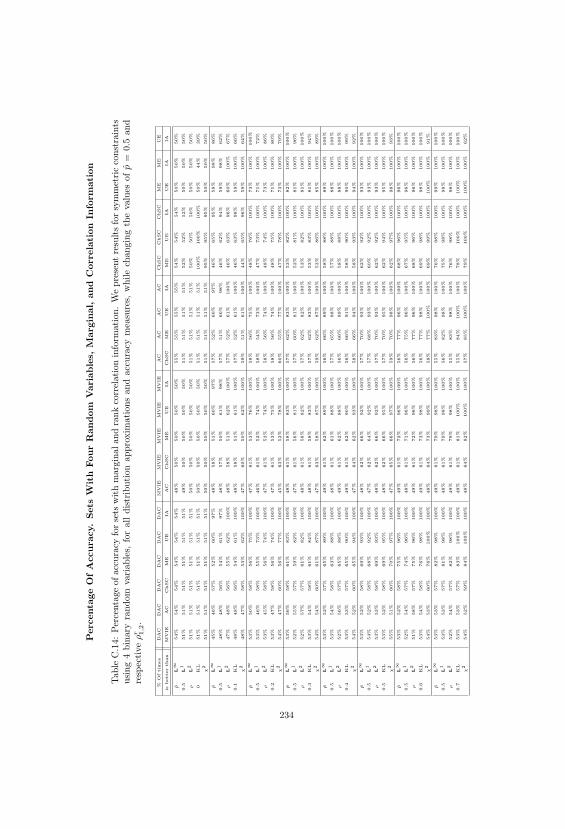
Perc
enta
ge
OfA
ccura
cy.
Sets
Wit
hFour
Random
Vari
able
s,M
arg
inal,
and
Corr
ela
tion
Info
rmati
on
Tab
leC
.14:
Per
centa
geofacc
ura
cyfo
rse
tsw
ith
mar
ginal
and
rank
corr
elat
ion
info
rmat
ion.
We
pre
sent
resu
lts
for
sym
met
ric
const
rain
tsusi
ng
4bin
ary
random
vari
able
s,fo
ral
ldis
trib
uti
on
appro
xim
ati
ons
and
acc
ura
cym
easu
res,
while
changin
gth
eva
lues
of
p=
0.5
and
resp
ecti
ve
ρr 1,2
.
%O
ftim
es
DA
CD
AC
DA
CD
AC
DA
CD
AC
MV
IEM
VIE
MV
IEM
VIE
MV
IEA
CA
CA
CA
CC
hSC
ChSC
ChSC
ME
ME
UE
isbetter
than
MV
IEA
CC
hSC
ME
UE
IAA
CC
hSC
ME
UE
IAC
hSC
ME
UE
IAM
EU
EIA
UE
IAIA
pL∞
54%
54%
54%
54%
54%
54%
48%
50%
50%
50%
50%
55%
55%
55%
55%
54%
54%
54%
50%
50%
50%
0.5
L1
51%
51%
51%
51%
51%
51%
49%
50%
50%
50%
50%
51%
51%
51%
51%
52%
52%
52%
50%
50%
50%
ρL2
51%
51%
51%
51%
51%
51%
50%
50%
50%
50%
50%
51%
51%
51%
51%
50%
50%
50%
50%
50%
50%
0K
L51%
51%
51%
51%
51%
51%
50%
50%
50%
50%
50%
51%
51%
51%
51%
100%
100%
100%
50%
44%
39%
χ2
51%
51%
51%
51%
51%
51%
50%
50%
50%
50%
50%
51%
51%
51%
51%
95%
95%
95%
50%
50%
50%
pL∞
45%
46%
57%
52%
60%
97%
48%
58%
51%
60%
97%
57%
52%
60%
97%
46%
65%
95%
58%
98%
86%
0.5
L1
48%
48%
56%
54%
61%
97%
48%
57%
50%
61%
98%
57%
51%
60%
98%
46%
62%
94%
59%
98%
62%
ρL2
47%
48%
56%
55%
62%
100%
48%
58%
51%
62%
100%
57%
52%
61%
100%
46%
63%
96%
60%
100%
67%
0.1
KL
48%
48%
56%
54%
61%
100%
48%
58%
51%
61%
100%
57%
52%
61%
100%
46%
63%
98%
59%
100%
66%
χ2
48%
47%
58%
53%
62%
100%
47%
60%
50%
62%
100%
59%
51%
61%
100%
44%
65%
96%
59%
100%
64%
pL∞
53%
50%
58%
56%
75%
100%
47%
61%
53%
76%
100%
58%
56%
75%
100%
48%
76%
100%
73%
100%
100%
0.5
L1
53%
46%
58%
55%
73%
100%
46%
61%
52%
74%
100%
58%
54%
73%
100%
47%
73%
100%
71%
100%
72%
ρL2
53%
45%
58%
56%
74%
100%
47%
61%
53%
74%
100%
58%
56%
74%
100%
48%
74%
100%
73%
100%
86%
0.2
KL
53%
47%
58%
56%
74%
100%
47%
61%
53%
75%
100%
58%
56%
74%
100%
48%
75%
100%
71%
100%
80%
χ2
54%
47%
60%
56%
77%
100%
45%
63%
52%
78%
100%
60%
55%
77%
100%
47%
78%
100%
73%
100%
79%
pL∞
53%
56%
58%
61%
83%
100%
48%
61%
58%
83%
100%
57%
62%
83%
100%
53%
82%
100%
82%
100%
100%
0.5
L1
52%
55%
57%
59%
82%
100%
47%
61%
56%
81%
100%
57%
60%
81%
100%
52%
81%
100%
81%
100%
96%
ρL2
52%
57%
57%
61%
82%
100%
48%
61%
58%
82%
100%
57%
62%
82%
100%
53%
82%
100%
81%
100%
100%
0.3
KL
53%
54%
58%
61%
84%
100%
48%
61%
58%
83%
100%
57%
62%
83%
100%
53%
83%
100%
81%
100%
94%
χ2
54%
54%
60%
61%
87%
100%
47%
63%
58%
87%
100%
59%
62%
87%
100%
53%
86%
100%
85%
100%
89%
pL∞
53%
52%
57%
65%
89%
100%
49%
61%
62%
89%
100%
56%
66%
89%
100%
58%
88%
100%
89%
100%
100%
0.5
L1
53%
54%
58%
63%
88%
100%
48%
61%
61%
88%
100%
57%
65%
88%
100%
57%
88%
100%
88%
100%
100%
ρL2
52%
56%
57%
65%
88%
100%
49%
61%
62%
88%
100%
56%
66%
89%
100%
58%
88%
100%
88%
100%
100%
0.4
KL
53%
53%
57%
65%
90%
100%
49%
61%
62%
90%
100%
56%
66%
91%
100%
58%
90%
100%
90%
100%
99%
χ2
54%
52%
60%
65%
94%
100%
47%
64%
62%
93%
100%
58%
66%
94%
100%
58%
93%
100%
94%
100%
92%
pL∞
53%
52%
58%
69%
93%
100%
48%
62%
66%
92%
100%
57%
70%
93%
100%
62%
92%
100%
93%
100%
100%
0.5
L1
54%
52%
58%
68%
92%
100%
47%
62%
64%
92%
100%
57%
68%
93%
100%
60%
92%
100%
93%
100%
100%
ρL2
53%
53%
58%
69%
93%
100%
48%
62%
66%
92%
100%
57%
70%
93%
100%
62%
92%
100%
93%
100%
100%
0.5
KL
53%
52%
58%
69%
95%
100%
48%
62%
66%
95%
100%
57%
70%
95%
100%
62%
94%
100%
95%
100%
100%
χ2
55%
51%
60%
70%
97%
100%
47%
65%
66%
97%
100%
59%
70%
98%
100%
62%
97%
100%
98%
100%
93%
pL∞
53%
52%
58%
75%
96%
100%
49%
61%
72%
96%
100%
56%
77%
96%
100%
68%
96%
100%
96%
100%
100%
0.5
L1
52%
54%
57%
74%
96%
100%
48%
61%
71%
96%
100%
56%
75%
96%
100%
67%
95%
100%
96%
100%
100%
ρL2
51%
58%
57%
75%
96%
100%
49%
61%
72%
96%
100%
56%
77%
96%
100%
68%
96%
100%
96%
100%
100%
0.6
KL
53%
54%
58%
76%
98%
100%
49%
61%
73%
98%
100%
56%
77%
98%
100%
69%
98%
100%
98%
100%
100%
χ2
54%
53%
60%
76%
100%
100%
48%
64%
73%
99%
100%
58%
77%
100%
100%
69%
99%
100%
100%
100%
91%
pL∞
53%
53%
57%
82%
98%
100%
49%
61%
79%
98%
100%
55%
83%
98%
100%
76%
98%
100%
99%
100%
100%
0.5
L1
53%
53%
57%
81%
98%
100%
48%
61%
79%
98%
100%
56%
82%
98%
100%
75%
98%
100%
98%
100%
100%
ρL2
52%
54%
57%
82%
98%
100%
49%
61%
79%
98%
100%
55%
83%
98%
100%
76%
98%
100%
98%
100%
100%
0.7
KL
53%
53%
57%
83%
100%
100%
49%
61%
81%
100%
100%
55%
84%
100%
100%
78%
100%
100%
100%
100%
100%
χ2
54%
52%
59%
84%
100%
100%
48%
64%
82%
100%
100%
57%
85%
100%
100%
79%
100%
100%
100%
100%
62%
234

Table
C.1
5:
Per
centa
ge
ofacc
ura
cyfo
rse
tsw
ith
marg
inaland
rank
corr
elati
on
info
rmati
on.
We
pre
sent
resu
lts
for
sym
met
ric
const
rain
tsusi
ng
4bin
ary
random
vari
able
s,fo
ral
ldis
trib
uti
on
appro
xim
ati
ons
and
acc
ura
cym
easu
res,
while
changin
gth
eva
lues
of
p=
0.6
and
resp
ecti
ve
ρr 1,2
.
%O
ftim
es
DA
CD
AC
DA
CD
AC
DA
CD
AC
MV
IEM
VIE
MV
IEM
VIE
MV
IEA
CA
CA
CA
CC
hSC
ChSC
ChSC
ME
ME
UE
isbetter
than
MV
IEA
CC
hSC
ME
UE
IAA
CC
hSC
ME
UE
IAC
hSC
ME
UE
IAM
EU
EIA
UE
IAIA
pL∞
53%
46%
69%
47%
47%
47%
48%
71%
49%
49%
49%
68%
48%
48%
48%
32%
32%
32%
50%
50%
50%
0.6
L1
53%
50%
68%
51%
51%
51%
48%
70%
49%
49%
49%
67%
51%
51%
51%
34%
34%
34%
50%
50%
50%
ρL2
53%
49%
69%
49%
49%
49%
48%
71%
48%
48%
48%
68%
51%
51%
51%
33%
33%
33%
50%
50%
50%
0K
L52%
48%
69%
49%
49%
49%
48%
71%
48%
48%
48%
68%
49%
49%
49%
33%
33%
33%
50%
47%
45%
χ2
53%
46%
71%
46%
46%
46%
47%
73%
47%
47%
47%
70%
47%
47%
47%
30%
30%
30%
50%
50%
50%
pL∞
45%
61%
47%
66%
78%
90%
56%
48%
63%
75%
86%
41%
67%
79%
92%
65%
76%
88%
82%
97%
96%
0.6
L1
48%
57%
48%
62%
75%
83%
53%
48%
58%
71%
77%
46%
63%
76%
84%
60%
73%
80%
80%
93%
46%
ρL2
48%
57%
46%
64%
76%
86%
53%
49%
60%
73%
81%
45%
65%
77%
87%
62%
74%
83%
81%
95%
71%
0.1
KL
48%
57%
48%
64%
77%
94%
53%
48%
60%
74%
86%
45%
65%
78%
96%
62%
75%
90%
82%
100%
44%
χ2
46%
59%
47%
67%
81%
99%
55%
49%
62%
78%
90%
43%
68%
81%
99%
64%
79%
95%
85%
100%
38%
pL∞
43%
56%
58%
69%
84%
100%
58%
61%
67%
83%
100%
47%
70%
85%
100%
66%
82%
100%
89%
100%
100%
0.6
L1
47%
55%
52%
65%
82%
96%
55%
60%
63%
81%
94%
48%
67%
83%
97%
62%
80%
93%
87%
100%
70%
ρL2
45%
54%
52%
67%
83%
98%
55%
61%
65%
82%
97%
47%
68%
84%
99%
63%
81%
97%
88%
100%
98%
0.2
KL
46%
53%
55%
67%
84%
100%
56%
61%
65%
83%
100%
49%
69%
85%
100%
63%
83%
100%
89%
100%
64%
χ2
44%
54%
58%
70%
88%
100%
58%
63%
68%
87%
100%
49%
72%
89%
100%
65%
86%
100%
92%
100%
56%
pL∞
53%
54%
58%
69%
88%
100%
56%
62%
68%
88%
100%
58%
70%
89%
100%
66%
87%
100%
92%
100%
100%
0.6
L1
52%
53%
58%
66%
87%
100%
53%
61%
65%
87%
100%
54%
67%
88%
100%
63%
86%
100%
91%
100%
100%
ρL2
51%
52%
58%
68%
88%
100%
55%
62%
67%
87%
100%
54%
69%
88%
100%
65%
87%
100%
92%
100%
100%
0.3
KL
53%
53%
58%
69%
90%
100%
52%
62%
66%
89%
100%
57%
70%
90%
100%
62%
89%
100%
93%
100%
87%
χ2
54%
54%
60%
73%
93%
100%
52%
65%
70%
93%
100%
59%
73%
93%
100%
63%
92%
100%
96%
100%
73%
pL∞
53%
59%
58%
72%
92%
100%
48%
62%
71%
91%
100%
57%
73%
92%
100%
68%
91%
100%
94%
100%
100%
0.6
L1
54%
56%
58%
69%
92%
100%
50%
62%
68%
91%
100%
56%
70%
92%
100%
66%
91%
100%
94%
100%
100%
ρL2
53%
58%
58%
71%
92%
100%
51%
62%
70%
91%
100%
56%
72%
92%
100%
67%
91%
100%
94%
100%
100%
0.4
KL
53%
58%
58%
72%
94%
100%
49%
62%
69%
94%
100%
57%
73%
94%
100%
64%
93%
100%
96%
100%
99%
χ2
55%
61%
60%
75%
97%
100%
47%
65%
69%
96%
100%
59%
75%
97%
100%
63%
96%
100%
98%
100%
81%
pL∞
53%
52%
58%
74%
95%
100%
48%
62%
72%
94%
100%
57%
75%
95%
100%
66%
94%
100%
97%
100%
100%
0.6
L1
51%
54%
57%
71%
95%
100%
47%
61%
69%
94%
100%
57%
71%
95%
100%
66%
94%
100%
96%
100%
100%
ρL2
50%
57%
57%
74%
95%
100%
48%
62%
71%
94%
100%
57%
74%
95%
100%
69%
94%
100%
97%
100%
100%
0.5
KL
52%
54%
58%
73%
97%
100%
48%
62%
70%
97%
100%
57%
75%
97%
100%
66%
97%
100%
98%
100%
100%
χ2
54%
53%
60%
74%
99%
100%
47%
64%
71%
99%
100%
59%
76%
99%
100%
66%
99%
100%
100%
100%
85%
pL∞
53%
60%
58%
77%
98%
100%
49%
62%
75%
97%
100%
56%
79%
98%
100%
72%
97%
100%
99%
100%
100%
0.6
L1
52%
56%
57%
76%
98%
100%
48%
61%
74%
97%
100%
56%
77%
98%
100%
71%
97%
100%
99%
100%
100%
ρL2
52%
58%
58%
78%
98%
100%
49%
62%
77%
97%
100%
56%
80%
98%
100%
74%
97%
100%
99%
100%
100%
0.6
KL
53%
54%
58%
79%
99%
100%
49%
62%
76%
99%
100%
56%
80%
99%
100%
72%
99%
100%
100%
100%
100%
χ2
54%
53%
60%
79%
100%
100%
48%
64%
76%
100%
100%
58%
80%
100%
100%
73%
100%
100%
100%
100%
78%
pL∞
53%
53%
58%
85%
99%
100%
49%
62%
83%
99%
100%
56%
86%
99%
100%
81%
99%
100%
99%
100%
100%
0.6
L1
54%
52%
58%
84%
99%
100%
48%
61%
82%
99%
100%
56%
84%
99%
100%
80%
98%
100%
99%
100%
100%
ρL2
53%
53%
58%
86%
99%
100%
49%
62%
84%
99%
100%
56%
86%
99%
100%
82%
99%
100%
99%
100%
100%
0.7
KL
53%
52%
58%
88%
100%
100%
49%
62%
87%
100%
100%
56%
89%
100%
100%
84%
100%
100%
100%
100%
100%
χ2
55%
51%
60%
89%
100%
100%
48%
64%
88%
100%
100%
58%
90%
100%
100%
85%
100%
100%
100%
100%
18%
235

Table
C.1
6:
Per
centa
ge
ofacc
ura
cyfo
rse
tsw
ith
marg
inaland
rank
corr
elati
on
info
rmati
on.
We
pre
sent
resu
lts
for
sym
met
ric
const
rain
tsusi
ng
4bin
ary
random
vari
able
s,fo
ral
ldis
trib
uti
on
appro
xim
ati
ons
and
acc
ura
cym
easu
res,
while
changin
gth
eva
lues
of
p=
0.7
and
resp
ecti
ve
ρr 1,2
.
%O
ftim
es
DA
CD
AC
DA
CD
AC
DA
CD
AC
MV
IEM
VIE
MV
IEM
VIE
MV
IEA
CA
CA
CA
CC
hSC
ChSC
ChSC
ME
ME
UE
isbetter
than
MV
IEA
CC
hSC
ME
UE
IAA
CC
hSC
ME
UE
IAC
hSC
ME
UE
IAM
EU
EIA
UE
IAIA
pL∞
54%
61%
69%
66%
66%
66%
56%
73%
61%
61%
61%
59%
78%
78%
78%
47%
47%
47%
50%
50%
50%
0.7
L1
54%
63%
68%
69%
69%
69%
58%
72%
65%
65%
65%
57%
79%
79%
79%
50%
50%
50%
50%
50%
50%
ρL2
54%
62%
68%
68%
68%
68%
57%
73%
64%
64%
64%
57%
78%
78%
78%
50%
50%
50%
50%
50%
50%
0K
L54%
62%
68%
68%
68%
68%
57%
73%
64%
64%
64%
58%
78%
78%
78%
49%
49%
49%
41%
65%
82%
χ2
56%
60%
72%
66%
66%
66%
55%
77%
61%
61%
61%
62%
76%
76%
76%
45%
45%
45%
41%
50%
59%
pL∞
45%
53%
66%
66%
82%
92%
56%
65%
65%
81%
92%
67%
68%
83%
93%
27%
90%
98%
89%
97%
100%
0.7
L1
49%
54%
66%
64%
80%
86%
52%
64%
63%
79%
85%
67%
66%
81%
87%
30%
89%
96%
88%
95%
60%
ρL2
47%
54%
66%
65%
81%
89%
53%
65%
64%
80%
88%
68%
66%
82%
90%
28%
90%
97%
89%
96%
100%
0.1
KL
45%
53%
66%
66%
86%
96%
54%
65%
64%
84%
93%
67%
67%
87%
97%
31%
90%
100%
92%
100%
30%
χ2
41%
54%
69%
69%
90%
100%
58%
68%
68%
88%
100%
70%
71%
90%
100%
29%
93%
97%
94%
100%
24%
pL∞
46%
62%
47%
76%
90%
100%
57%
58%
72%
89%
100%
44%
77%
91%
100%
71%
88%
99%
96%
100%
100%
0.7
L1
50%
58%
51%
73%
90%
98%
53%
58%
69%
88%
97%
49%
74%
91%
98%
67%
87%
97%
95%
100%
95%
ρL2
49%
59%
50%
74%
90%
99%
53%
58%
70%
88%
99%
48%
76%
91%
99%
69%
88%
98%
96%
100%
100%
0.2
KL
50%
59%
51%
74%
92%
100%
53%
58%
69%
90%
100%
48%
75%
93%
100%
68%
90%
100%
97%
100%
53%
χ2
48%
61%
49%
77%
95%
100%
55%
60%
72%
94%
100%
46%
79%
96%
100%
71%
93%
100%
98%
100%
39%
pL∞
53%
59%
58%
76%
94%
100%
59%
62%
76%
93%
100%
46%
78%
94%
100%
75%
93%
100%
98%
100%
100%
0.7
L1
54%
55%
58%
73%
94%
100%
55%
61%
73%
93%
100%
48%
75%
94%
100%
72%
93%
100%
98%
100%
100%
ρL2
53%
54%
58%
75%
94%
100%
57%
62%
74%
93%
100%
49%
77%
94%
100%
73%
93%
100%
98%
100%
100%
0.3
KL
53%
55%
58%
75%
96%
100%
56%
61%
74%
96%
100%
54%
77%
96%
100%
72%
95%
100%
99%
100%
87%
χ2
54%
57%
60%
79%
98%
100%
59%
64%
77%
98%
100%
56%
81%
98%
100%
75%
98%
100%
99%
100%
61%
pL∞
53%
59%
58%
76%
95%
100%
48%
62%
76%
95%
100%
57%
77%
95%
100%
74%
95%
100%
98%
100%
100%
0.7
L1
52%
56%
58%
74%
95%
100%
51%
61%
73%
95%
100%
56%
75%
95%
100%
72%
95%
100%
98%
100%
100%
ρL2
51%
58%
57%
76%
95%
100%
52%
62%
75%
95%
100%
55%
76%
95%
100%
73%
95%
100%
98%
100%
100%
0.4
KL
53%
58%
58%
77%
97%
100%
49%
62%
75%
97%
100%
56%
78%
98%
100%
72%
97%
100%
99%
100%
100%
χ2
54%
61%
60%
81%
99%
100%
48%
64%
78%
99%
100%
58%
81%
99%
100%
75%
99%
100%
100%
100%
75%
pL∞
53%
52%
58%
79%
97%
100%
49%
62%
78%
97%
100%
56%
79%
97%
100%
77%
97%
100%
99%
100%
100%
0.7
L1
54%
52%
58%
77%
97%
100%
48%
62%
76%
97%
100%
57%
78%
97%
100%
75%
97%
100%
99%
100%
100%
ρL2
53%
53%
58%
79%
97%
100%
49%
62%
78%
97%
100%
56%
79%
97%
100%
76%
97%
100%
99%
100%
100%
0.5
KL
53%
52%
58%
81%
99%
100%
49%
62%
79%
99%
100%
56%
81%
99%
100%
75%
99%
100%
100%
100%
100%
χ2
55%
51%
60%
84%
100%
100%
47%
64%
81%
100%
100%
58%
84%
100%
100%
76%
100%
100%
100%
100%
77%
pL∞
53%
53%
58%
83%
98%
100%
49%
61%
82%
98%
100%
56%
83%
98%
100%
81%
98%
100%
100%
100%
100%
0.7
L1
53%
54%
58%
83%
98%
100%
48%
61%
82%
98%
100%
56%
83%
98%
100%
81%
98%
100%
99%
100%
100%
ρL2
52%
56%
58%
84%
98%
100%
49%
61%
83%
98%
100%
56%
84%
98%
100%
82%
98%
100%
99%
100%
100%
0.6
KL
53%
53%
58%
87%
100%
100%
49%
61%
86%
100%
100%
56%
88%
100%
100%
83%
100%
100%
100%
100%
100%
χ2
55%
52%
60%
89%
100%
100%
48%
64%
87%
100%
100%
58%
90%
100%
100%
84%
100%
100%
100%
100%
34%
236

Table
C.1
7:
Per
centa
ge
ofacc
ura
cyfo
rse
tsw
ith
marg
inaland
rank
corr
elati
on
info
rmati
on.
We
pre
sent
resu
lts
for
sym
met
ric
const
rain
tsusi
ng
4bin
ary
random
vari
able
s,fo
rall
dis
trib
uti
on
appro
xim
ati
ons
and
accu
racy
mea
sure
s,w
hile
changin
gth
eva
lues
ofp
=0.
8,0
.9an
dre
spec
tive
ρr 1,2
.
%O
ftim
es
DA
CD
AC
DA
CD
AC
DA
CD
AC
MV
IEM
VIE
MV
IEM
VIE
MV
IEA
CA
CA
CA
CC
hSC
ChSC
ChSC
ME
ME
UE
isbetter
than
MV
IEA
CC
hSC
ME
UE
IAA
CC
hSC
ME
UE
IAC
hSC
ME
UE
IAM
EU
EIA
UE
IAIA
pL∞
54%
67%
69%
81%
81%
81%
62%
73%
78%
78%
78%
53%
92%
92%
92%
66%
66%
66%
61%
59%
48%
0.8
L1
54%
70%
68%
85%
85%
85%
65%
72%
81%
81%
81%
50%
93%
93%
93%
69%
69%
69%
50%
50%
50%
ρL2
54%
69%
68%
85%
85%
85%
64%
73%
81%
81%
81%
50%
93%
93%
93%
70%
70%
70%
50%
50%
50%
0K
L54%
69%
68%
84%
84%
84%
64%
73%
81%
81%
81%
51%
93%
93%
93%
68%
68%
68%
59%
3%
1%
χ2
57%
67%
73%
85%
85%
85%
62%
78%
80%
80%
80%
56%
94%
94%
94%
65%
65%
65%
50%
50%
50%
pL∞
53%
46%
68%
67%
87%
99%
48%
71%
72%
89%
99%
67%
66%
87%
99%
24%
94%
100%
94%
100%
100%
0.8
L1
53%
51%
67%
66%
86%
95%
47%
70%
70%
88%
96%
66%
65%
86%
95%
29%
94%
99%
93%
99%
100%
ρL2
53%
49%
68%
67%
87%
97%
47%
71%
70%
88%
97%
67%
66%
86%
96%
26%
94%
99%
93%
99%
100%
0.1
KL
53%
48%
67%
68%
92%
100%
48%
71%
72%
93%
100%
66%
67%
92%
100%
32%
96%
100%
97%
100%
29%
χ2
54%
43%
70%
72%
96%
100%
46%
74%
77%
96%
100%
70%
71%
95%
100%
29%
98%
99%
98%
100%
25%
pL∞
45%
63%
49%
82%
95%
100%
59%
58%
80%
94%
100%
42%
84%
96%
100%
79%
94%
100%
99%
100%
100%
0.8
L1
49%
59%
50%
80%
95%
100%
55%
57%
78%
94%
100%
46%
82%
96%
100%
77%
94%
100%
99%
100%
100%
ρL2
49%
60%
49%
81%
95%
100%
56%
58%
79%
94%
100%
45%
83%
96%
100%
78%
94%
100%
99%
100%
100%
0.2
KL
49%
60%
50%
81%
97%
100%
55%
57%
78%
96%
100%
45%
83%
98%
100%
77%
96%
100%
99%
100%
62%
χ2
47%
63%
49%
83%
99%
100%
58%
60%
81%
99%
100%
43%
85%
99%
100%
80%
99%
100%
100%
100%
39%
pL∞
45%
59%
58%
81%
96%
100%
56%
62%
80%
96%
100%
57%
82%
96%
100%
79%
96%
100%
99%
100%
100%
0.8
L1
47%
56%
56%
79%
96%
100%
54%
61%
78%
96%
100%
53%
80%
96%
100%
77%
96%
100%
99%
100%
100%
ρL2
47%
58%
56%
80%
96%
100%
55%
62%
79%
96%
100%
53%
81%
96%
100%
78%
96%
100%
99%
100%
100%
0.3
KL
51%
58%
58%
81%
98%
100%
52%
62%
79%
98%
100%
56%
81%
98%
100%
77%
98%
100%
100%
100%
99%
χ2
53%
61%
60%
84%
100%
100%
51%
64%
82%
100%
100%
58%
84%
100%
100%
80%
100%
100%
100%
100%
72%
pL∞
53%
60%
58%
83%
98%
100%
49%
61%
83%
98%
100%
56%
83%
98%
100%
82%
98%
100%
100%
100%
100%
0.8
L1
54%
57%
58%
82%
98%
100%
49%
61%
82%
98%
100%
56%
82%
98%
100%
81%
98%
100%
100%
100%
100%
ρL2
53%
58%
58%
83%
98%
100%
50%
61%
82%
98%
100%
56%
83%
98%
100%
82%
98%
100%
100%
100%
100%
0.4
KL
53%
54%
58%
85%
100%
100%
49%
61%
84%
99%
100%
56%
86%
100%
100%
82%
99%
100%
100%
100%
100%
χ2
55%
53%
60%
88%
100%
100%
47%
64%
87%
100%
100%
58%
89%
100%
100%
85%
100%
100%
100%
100%
78%
pL∞
54%
71%
69%
92%
92%
92%
66%
73%
91%
91%
91%
49%
98%
98%
98%
83%
83%
83%
57%
13%
12%
0.9
L1
54%
74%
68%
94%
94%
94%
69%
72%
92%
92%
92%
46%
98%
98%
98%
87%
87%
87%
52%
50%
48%
ρL2
55%
73%
69%
94%
94%
94%
68%
73%
93%
93%
93%
46%
98%
98%
98%
87%
87%
87%
51%
46%
24%
0K
L54%
73%
68%
94%
94%
94%
68%
73%
93%
93%
93%
47%
99%
99%
99%
86%
86%
86%
0%
100%
100%
χ2
58%
72%
74%
96%
96%
96%
66%
78%
95%
95%
95%
54%
99%
99%
99%
89%
89%
89%
3%
24%
96%
pL∞
48%
59%
64%
87%
97%
100%
56%
62%
84%
96%
100%
67%
88%
98%
100%
91%
98%
100%
100%
100%
100%
0.9
L1
51%
58%
64%
85%
97%
100%
53%
60%
83%
96%
100%
67%
87%
97%
100%
90%
98%
100%
100%
100%
100%
ρL2
50%
58%
65%
86%
97%
100%
54%
61%
83%
96%
100%
68%
88%
98%
100%
91%
98%
100%
100%
100%
100%
0.1
KL
49%
58%
64%
85%
99%
100%
54%
60%
82%
98%
100%
68%
87%
99%
100%
90%
99%
100%
100%
100%
39%
χ2
47%
60%
67%
88%
100%
100%
56%
63%
85%
100%
100%
70%
90%
100%
100%
92%
100%
100%
100%
100%
28%
pL∞
53%
59%
58%
88%
98%
100%
48%
62%
88%
98%
100%
57%
89%
98%
100%
87%
98%
100%
100%
100%
100%
0.9
L1
54%
56%
58%
87%
98%
100%
52%
61%
87%
98%
100%
55%
88%
98%
100%
86%
98%
100%
100%
100%
100%
ρL2
53%
58%
58%
88%
98%
100%
53%
62%
87%
98%
100%
55%
88%
98%
100%
87%
98%
100%
100%
100%
100%
0.2
KL
53%
58%
58%
88%
100%
100%
50%
62%
87%
100%
100%
56%
89%
100%
100%
86%
100%
100%
100%
100%
100%
χ2
55%
62%
60%
91%
100%
100%
48%
65%
90%
100%
100%
58%
91%
100%
100%
89%
100%
100%
100%
100%
88%
237

Perc
enta
ge
OfA
ccura
cy.
Sets
Wit
hSix
Random
Vari
able
s,M
arg
inal,
and
Corr
ela
tion
Info
rmati
on
Tab
leC
.18:
Per
centa
ge
ofac
cura
cyfo
rse
tsw
ith
mar
ginal
and
rank
corr
elat
ion
info
rmat
ion.
We
pre
sent
resu
lts
for
sym
met
ric
const
rain
tsusi
ng
6bin
ary
random
vari
able
s,fo
ral
ldis
trib
uti
on
appro
xim
ati
ons
and
acc
ura
cym
easu
res,
while
changin
gth
eva
lues
of
p=
0.5
and
resp
ecti
ve
ρr 1,2
.
%O
ftim
es
DA
CD
AC
DA
CD
AC
DA
CD
AC
MV
IEM
VIE
MV
IEM
VIE
MV
IEA
CA
CA
CA
CC
hSC
ChSC
ChSC
ME
ME
UE
isbetter
than
MV
IEA
CC
hSC
ME
UE
IAA
CC
hSC
ME
UE
IAC
hSC
ME
UE
IAM
EU
EIA
UE
IAIA
pL∞
57%
57%
57%
57%
57%
57%
55%
57%
57%
57%
57%
43%
43%
43%
43%
80%
80%
80%
49%
50%
51%
0.5
L1
58%
58%
58%
58%
58%
58%
53%
53%
53%
53%
53%
50%
50%
50%
50%
45%
45%
45%
50%
50%
50%
ρL2
58%
58%
58%
58%
58%
58%
54%
54%
54%
54%
54%
52%
52%
52%
52%
50%
50%
50%
50%
50%
50%
0K
L59%
59%
59%
59%
59%
59%
54%
54%
54%
54%
54%
52%
52%
52%
52%
100%
100%
100%
50%
50%
56%
χ2
58%
58%
58%
58%
58%
58%
55%
55%
55%
55%
55%
55%
55%
55%
55%
64%
64%
64%
48%
50%
53%
pL∞
55%
57%
68%
58%
89%
99%
57%
65%
64%
91%
99%
64%
66%
91%
99%
45%
89%
92%
90%
100%
52%
0.5
L1
59%
58%
70%
66%
89%
100%
50%
70%
62%
91%
100%
69%
64%
91%
100%
45%
88%
98%
88%
100%
41%
ρL2
58%
57%
72%
67%
90%
100%
48%
75%
63%
91%
100%
73%
65%
91%
100%
43%
89%
94%
90%
100%
38%
0.1
KL
59%
59%
73%
68%
91%
100%
48%
76%
62%
92%
100%
74%
64%
92%
100%
41%
90%
99%
90%
100%
51%
χ2
60%
59%
78%
67%
92%
100%
45%
81%
61%
94%
100%
79%
64%
94%
100%
37%
92%
97%
92%
100%
52%
pL∞
57%
57%
71%
84%
99%
100%
61%
62%
84%
99%
100%
59%
87%
99%
100%
70%
98%
100%
96%
100%
98%
0.5
L1
56%
60%
68%
86%
98%
100%
54%
70%
84%
98%
100%
64%
88%
98%
100%
71%
98%
100%
96%
100%
70%
ρL2
56%
60%
73%
89%
99%
100%
53%
74%
87%
99%
100%
68%
90%
99%
100%
72%
99%
100%
98%
100%
90%
0.2
KL
58%
61%
74%
88%
99%
100%
53%
75%
85%
99%
100%
69%
90%
99%
100%
67%
99%
100%
97%
100%
93%
χ2
61%
59%
80%
86%
99%
100%
48%
81%
83%
99%
100%
75%
89%
99%
100%
61%
99%
100%
99%
100%
92%
pL∞
59%
55%
70%
94%
100%
100%
57%
68%
92%
100%
100%
64%
95%
100%
100%
85%
100%
100%
100%
100%
100%
0.5
L1
56%
62%
69%
93%
100%
100%
55%
71%
91%
100%
100%
64%
94%
100%
100%
84%
100%
100%
99%
100%
95%
ρL2
54%
61%
73%
95%
100%
100%
54%
78%
93%
100%
100%
69%
96%
100%
100%
86%
100%
100%
100%
100%
100%
0.3
KL
58%
60%
74%
94%
100%
100%
54%
78%
92%
100%
100%
71%
95%
100%
100%
82%
100%
100%
100%
100%
100%
χ2
61%
56%
80%
93%
100%
100%
48%
83%
91%
100%
100%
77%
95%
100%
100%
77%
100%
100%
100%
100%
97%
pL∞
60%
56%
71%
99%
100%
100%
58%
66%
99%
100%
100%
62%
99%
100%
100%
97%
100%
100%
100%
100%
100%
0.5
L1
53%
61%
65%
99%
100%
100%
58%
67%
99%
100%
100%
60%
99%
100%
100%
96%
100%
100%
100%
100%
100%
ρL2
54%
61%
70%
99%
100%
100%
54%
74%
99%
100%
100%
65%
99%
100%
100%
98%
100%
100%
100%
100%
100%
0.4
KL
57%
61%
71%
99%
100%
100%
54%
75%
99%
100%
100%
66%
99%
100%
100%
94%
100%
100%
100%
100%
100%
χ2
61%
58%
77%
99%
100%
100%
49%
80%
98%
100%
100%
73%
99%
100%
100%
91%
100%
100%
100%
100%
96%
pL∞
64%
62%
76%
99%
100%
100%
42%
78%
100%
100%
100%
75%
100%
100%
100%
98%
100%
100%
100%
100%
100%
0.5
L1
61%
59%
73%
99%
100%
100%
41%
80%
99%
100%
100%
73%
99%
100%
100%
97%
100%
100%
100%
100%
100%
ρL2
61%
59%
74%
99%
100%
100%
38%
86%
100%
100%
100%
79%
100%
100%
100%
98%
100%
100%
100%
100%
100%
0.5
KL
66%
61%
79%
99%
100%
100%
38%
86%
99%
100%
100%
80%
100%
100%
100%
94%
100%
100%
100%
100%
100%
χ2
67%
61%
83%
99%
100%
100%
32%
90%
99%
100%
100%
86%
100%
100%
100%
91%
100%
100%
100%
100%
83%
pL∞
50%
56%
66%
100%
100%
100%
66%
59%
100%
100%
100%
54%
100%
100%
100%
100%
100%
100%
100%
100%
100%
0.5
L1
57%
66%
65%
100%
100%
100%
65%
63%
100%
100%
100%
54%
100%
100%
100%
100%
100%
100%
100%
100%
100%
ρL2
54%
66%
70%
100%
100%
100%
64%
68%
100%
100%
100%
57%
100%
100%
100%
100%
100%
100%
100%
100%
100%
0.6
KL
57%
65%
71%
100%
100%
100%
64%
69%
100%
100%
100%
59%
100%
100%
100%
100%
100%
100%
100%
100%
100%
χ2
54%
59%
78%
100%
100%
100%
58%
77%
100%
100%
100%
67%
100%
100%
100%
100%
100%
100%
100%
100%
14%
pL∞
54%
58%
68%
100%
100%
100%
68%
59%
100%
100%
100%
53%
100%
100%
100%
100%
100%
100%
100%
100%
100%
0.5
L1
59%
67%
67%
100%
100%
100%
66%
63%
100%
100%
100%
53%
100%
100%
100%
100%
100%
100%
100%
100%
100%
ρL2
57%
67%
71%
100%
100%
100%
65%
70%
100%
100%
100%
58%
100%
100%
100%
100%
100%
100%
100%
100%
100%
0.7
KL
60%
67%
71%
100%
100%
100%
65%
71%
100%
100%
100%
60%
100%
100%
100%
100%
100%
100%
100%
100%
100%
χ2
59%
62%
78%
100%
100%
100%
58%
78%
100%
100%
100%
69%
100%
100%
100%
100%
100%
100%
100%
100%
0%
238

Table
C.1
9:
Per
centa
ge
ofacc
ura
cyfo
rse
tsw
ith
marg
inaland
rank
corr
elati
on
info
rmati
on.
We
pre
sent
resu
lts
for
sym
met
ric
const
rain
tsusi
ng
6bin
ary
random
vari
able
s,fo
ral
ldis
trib
uti
on
appro
xim
ati
ons
and
acc
ura
cym
easu
res,
while
changin
gth
eva
lues
of
p=
0.6
and
resp
ecti
ve
ρr 1,2
.
%O
ftim
es
DA
CD
AC
DA
CD
AC
DA
CD
AC
MV
IEM
VIE
MV
IEM
VIE
MV
IEA
CA
CA
CA
CC
hSC
ChSC
ChSC
ME
ME
UE
isbetter
than
MV
IEA
CC
hSC
ME
UE
IAA
CC
hSC
ME
UE
IAC
hSC
ME
UE
IAM
EU
EIA
UE
IAIA
pL∞
59%
53%
63%
60%
60%
60%
31%
58%
71%
71%
71%
61%
70%
70%
70%
43%
43%
43%
27%
46%
63%
0.6
L1
61%
60%
82%
62%
62%
62%
38%
74%
68%
68%
68%
77%
63%
63%
63%
27%
27%
27%
54%
32%
46%
ρL2
59%
59%
86%
60%
60%
60%
40%
75%
69%
69%
69%
79%
63%
63%
63%
26%
26%
26%
35%
29%
43%
0K
L62%
61%
90%
63%
63%
63%
38%
85%
67%
67%
67%
87%
65%
65%
65%
16%
16%
16%
43%
100%
100%
χ2
61%
60%
94%
62%
62%
62%
36%
90%
64%
64%
64%
92%
66%
66%
66%
11%
11%
11%
62%
99%
47%
pL∞
54%
60%
68%
88%
100%
100%
54%
68%
88%
100%
100%
63%
91%
100%
100%
91%
100%
100%
100%
100%
99%
0.6
L1
60%
68%
72%
89%
100%
100%
67%
71%
89%
100%
100%
64%
93%
100%
100%
93%
100%
100%
100%
100%
2%
ρL2
60%
68%
73%
90%
100%
100%
67%
73%
90%
100%
100%
74%
94%
100%
100%
94%
100%
100%
100%
100%
21%
0.1
KL
59%
68%
74%
90%
100%
100%
67%
72%
90%
100%
100%
67%
94%
100%
100%
91%
100%
100%
100%
100%
5%
χ2
56%
64%
74%
89%
100%
100%
63%
72%
89%
100%
100%
67%
94%
100%
100%
89%
100%
100%
100%
100%
7%
pL∞
60%
59%
73%
94%
100%
100%
56%
74%
94%
100%
100%
69%
96%
100%
100%
90%
100%
100%
100%
100%
100%
0.6
L1
60%
62%
72%
93%
100%
100%
59%
77%
93%
100%
100%
62%
96%
100%
100%
88%
100%
100%
100%
100%
13%
ρL2
59%
62%
75%
94%
100%
100%
61%
82%
95%
100%
100%
67%
97%
100%
100%
90%
100%
100%
100%
100%
90%
0.2
KL
60%
61%
76%
94%
100%
100%
57%
83%
93%
100%
100%
77%
96%
100%
100%
80%
100%
100%
100%
100%
28%
χ2
62%
61%
80%
93%
100%
100%
55%
87%
92%
100%
100%
82%
96%
100%
100%
74%
100%
100%
100%
100%
21%
pL∞
60%
51%
74%
90%
100%
100%
46%
75%
85%
100%
100%
73%
88%
100%
100%
82%
100%
100%
100%
100%
100%
0.6
L1
54%
52%
72%
92%
100%
100%
42%
81%
88%
100%
100%
76%
90%
100%
100%
84%
100%
100%
100%
100%
98%
ρL2
54%
51%
74%
92%
100%
100%
40%
86%
88%
100%
100%
79%
90%
100%
100%
85%
100%
100%
100%
100%
100%
0.3
KL
59%
57%
80%
95%
100%
100%
39%
86%
91%
100%
100%
81%
94%
100%
100%
81%
100%
100%
100%
100%
95%
χ2
62%
56%
84%
96%
100%
100%
36%
89%
91%
100%
100%
85%
94%
100%
100%
77%
100%
100%
100%
100%
62%
pL∞
60%
56%
73%
95%
100%
100%
54%
72%
94%
100%
100%
67%
95%
100%
100%
91%
100%
100%
100%
100%
100%
0.6
L1
54%
58%
67%
96%
100%
100%
51%
73%
96%
100%
100%
66%
96%
100%
100%
94%
100%
100%
100%
100%
100%
ρL2
54%
57%
71%
96%
100%
100%
50%
80%
96%
100%
100%
71%
96%
100%
100%
95%
100%
100%
100%
100%
100%
0.4
KL
60%
62%
76%
96%
100%
100%
51%
81%
95%
100%
100%
72%
96%
100%
100%
92%
100%
100%
100%
100%
100%
χ2
64%
60%
84%
96%
100%
100%
44%
87%
95%
100%
100%
80%
96%
100%
100%
90%
100%
100%
100%
100%
66%
pL∞
62%
55%
72%
98%
100%
100%
46%
73%
97%
100%
100%
70%
98%
100%
100%
96%
100%
100%
100%
100%
100%
0.6
L1
55%
58%
69%
99%
100%
100%
48%
75%
99%
100%
100%
69%
99%
100%
100%
98%
100%
100%
100%
100%
100%
ρL2
56%
58%
73%
99%
100%
100%
44%
79%
99%
100%
100%
72%
99%
100%
100%
98%
100%
100%
100%
100%
100%
0.5
KL
58%
60%
74%
99%
100%
100%
44%
80%
99%
100%
100%
73%
99%
100%
100%
96%
100%
100%
100%
100%
100%
χ2
61%
59%
79%
99%
100%
100%
39%
85%
99%
100%
100%
79%
99%
100%
100%
95%
100%
100%
100%
100%
30%
pL∞
58%
56%
70%
100%
100%
100%
60%
65%
100%
100%
100%
60%
100%
100%
100%
100%
100%
100%
100%
100%
100%
0.6
L1
58%
61%
69%
100%
100%
100%
56%
68%
100%
100%
100%
60%
100%
100%
100%
100%
100%
100%
100%
100%
100%
ρL2
59%
62%
72%
100%
100%
100%
56%
74%
100%
100%
100%
64%
100%
100%
100%
100%
100%
100%
100%
100%
100%
0.6
KL
63%
64%
75%
100%
100%
100%
56%
75%
100%
100%
100%
66%
100%
100%
100%
100%
100%
100%
100%
100%
100%
χ2
65%
60%
81%
100%
100%
100%
51%
81%
100%
100%
100%
74%
100%
100%
100%
100%
100%
100%
100%
100%
3%
pL∞
53%
56%
69%
100%
100%
100%
48%
62%
100%
100%
100%
61%
100%
100%
100%
100%
100%
100%
100%
100%
100%
0.6
L1
62%
62%
65%
100%
100%
100%
48%
62%
100%
100%
100%
60%
100%
100%
100%
100%
100%
100%
100%
100%
100%
ρL2
58%
62%
69%
100%
100%
100%
52%
67%
100%
100%
100%
64%
100%
100%
100%
100%
100%
100%
100%
100%
100%
0.7
KL
50%
64%
70%
100%
100%
100%
59%
75%
100%
100%
100%
66%
100%
100%
100%
100%
100%
100%
100%
100%
100%
χ2
45%
62%
76%
100%
100%
100%
59%
83%
100%
100%
100%
73%
100%
100%
100%
100%
100%
100%
100%
100%
0%
239

Table
C.2
0:
Per
centa
ge
ofacc
ura
cyfo
rse
tsw
ith
marg
inaland
rank
corr
elati
on
info
rmati
on.
We
pre
sent
resu
lts
for
sym
met
ric
const
rain
tsusi
ng
6bin
ary
random
vari
able
s,fo
ral
ldis
trib
uti
on
appro
xim
ati
ons
and
acc
ura
cym
easu
res,
while
changin
gth
eva
lues
of
p=
0.7
and
resp
ecti
ve
ρr 1,2
.
%O
ftim
es
DA
CD
AC
DA
CD
AC
DA
CD
AC
MV
IEM
VIE
MV
IEM
VIE
MV
IEA
CA
CA
CA
CC
hSC
ChSC
ChSC
ME
ME
UE
isbetter
than
MV
IEA
CC
hSC
ME
UE
IAA
CC
hSC
ME
UE
IAC
hSC
ME
UE
IAM
EU
EIA
UE
IAIA
pL∞
81%
61%
97%
93%
93%
93%
30%
98%
77%
77%
77%
92%
95%
95%
95%
38%
38%
38%
50%
50%
50%
0.7
L1
82%
72%
95%
96%
96%
96%
37%
98%
80%
80%
80%
90%
97%
97%
97%
49%
49%
49%
50%
50%
50%
ρL2
84%
72%
96%
95%
95%
95%
33%
99%
78%
78%
78%
92%
97%
97%
97%
45%
45%
45%
50%
50%
50%
0K
L85%
70%
99%
95%
95%
95%
30%
99%
74%
74%
74%
97%
97%
97%
97%
12%
12%
12%
50%
24%
10%
χ2
89%
63%
100%
92%
92%
92%
18%
99%
65%
65%
65%
99%
96%
96%
96%
3%
3%
3%
50%
50%
50%
pL∞
56%
60%
96%
90%
100%
100%
58%
94%
88%
99%
100%
97%
91%
100%
100%
0%
100%
100%
100%
100%
100%
0.7
L1
56%
59%
96%
88%
100%
100%
51%
93%
86%
99%
100%
97%
89%
100%
100%
0%
95%
78%
100%
100%
4%
ρL2
56%
61%
96%
89%
100%
100%
52%
94%
87%
100%
100%
98%
90%
100%
100%
0%
100%
100%
100%
100%
100%
0.1
KL
60%
62%
96%
89%
100%
100%
52%
93%
86%
100%
100%
97%
91%
100%
100%
1%
99%
91%
100%
100%
1%
χ2
64%
61%
98%
91%
100%
100%
51%
95%
87%
100%
100%
99%
93%
100%
100%
0%
100%
98%
100%
100%
2%
pL∞
60%
63%
66%
100%
100%
100%
61%
66%
100%
100%
100%
56%
100%
100%
100%
99%
100%
100%
100%
100%
100%
0.7
L1
56%
63%
63%
100%
100%
100%
62%
62%
100%
100%
100%
51%
100%
100%
100%
99%
100%
100%
100%
100%
77%
ρL2
56%
63%
67%
100%
100%
100%
62%
66%
100%
100%
100%
52%
100%
100%
100%
99%
100%
100%
100%
100%
100%
0.2
KL
57%
65%
71%
99%
100%
100%
62%
71%
99%
100%
100%
57%
100%
100%
100%
98%
100%
100%
100%
100%
8%
χ2
57%
62%
77%
100%
100%
100%
59%
76%
100%
100%
100%
65%
100%
100%
100%
96%
100%
100%
100%
100%
4%
pL∞
59%
55%
72%
100%
100%
100%
49%
70%
99%
100%
100%
68%
100%
100%
100%
99%
100%
100%
100%
100%
100%
0.7
L1
54%
59%
71%
99%
100%
100%
47%
75%
99%
100%
100%
70%
99%
100%
100%
98%
100%
100%
100%
100%
100%
ρL2
53%
58%
74%
100%
100%
100%
46%
81%
99%
100%
100%
74%
100%
100%
100%
99%
100%
100%
100%
100%
100%
0.3
KL
59%
59%
76%
100%
100%
100%
44%
82%
98%
100%
100%
76%
99%
100%
100%
94%
100%
100%
100%
100%
92%
χ2
62%
58%
82%
100%
100%
100%
39%
87%
99%
100%
100%
81%
100%
100%
100%
92%
100%
100%
100%
100%
39%
pL∞
58%
58%
72%
100%
100%
100%
62%
64%
100%
100%
100%
59%
100%
100%
100%
100%
100%
100%
100%
100%
100%
0.7
L1
56%
64%
67%
100%
100%
100%
62%
68%
100%
100%
100%
58%
100%
100%
100%
100%
100%
100%
100%
100%
100%
ρL2
55%
65%
72%
100%
100%
100%
61%
74%
100%
100%
100%
62%
100%
100%
100%
100%
100%
100%
100%
100%
100%
0.4
KL
58%
65%
74%
100%
100%
100%
59%
75%
100%
100%
100%
65%
100%
100%
100%
100%
100%
100%
100%
100%
100%
χ2
58%
61%
81%
100%
100%
100%
53%
82%
100%
100%
100%
73%
100%
100%
100%
100%
100%
100%
100%
100%
33%
pL∞
59%
55%
70%
100%
100%
100%
59%
64%
100%
100%
100%
60%
100%
100%
100%
99%
100%
100%
100%
100%
100%
0.7
L1
56%
62%
70%
100%
100%
100%
53%
72%
100%
100%
100%
64%
100%
100%
100%
100%
100%
100%
100%
100%
100%
ρL2
55%
61%
73%
100%
100%
100%
54%
77%
100%
100%
100%
67%
100%
100%
100%
100%
100%
100%
100%
100%
100%
0.5
KL
62%
61%
76%
100%
100%
100%
54%
77%
100%
100%
100%
69%
100%
100%
100%
100%
100%
100%
100%
100%
100%
χ2
64%
58%
81%
100%
100%
100%
49%
83%
100%
100%
100%
76%
100%
100%
100%
100%
100%
100%
100%
100%
4%
pL∞
57%
54%
73%
100%
100%
100%
62%
63%
100%
100%
100%
59%
100%
100%
100%
100%
100%
100%
100%
100%
100%
0.7
L1
60%
63%
66%
100%
100%
100%
58%
63%
100%
100%
100%
57%
100%
100%
100%
100%
100%
100%
100%
100%
100%
ρL2
57%
61%
71%
100%
100%
100%
60%
69%
100%
100%
100%
62%
100%
100%
100%
100%
100%
100%
100%
100%
100%
0.6
KL
57%
64%
73%
100%
100%
100%
60%
72%
100%
100%
100%
63%
100%
100%
100%
100%
100%
100%
100%
100%
100%
χ2
55%
59%
79%
100%
100%
100%
58%
79%
100%
100%
100%
71%
100%
100%
100%
100%
100%
100%
100%
100%
0%
240

Table
C.2
1:
Per
centa
ge
ofacc
ura
cyfo
rse
tsw
ith
marg
inaland
rank
corr
elati
on
info
rmati
on.
We
pre
sent
resu
lts
for
sym
met
ric
const
rain
tsusi
ng
6bin
ary
random
vari
able
s,fo
rall
dis
trib
uti
on
appro
xim
ati
ons
and
accu
racy
mea
sure
s,w
hile
changin
gth
eva
lues
ofp
=0.
8,0
.9an
dre
spec
tive
ρr 1,2
.
%O
ftim
es
DA
CD
AC
DA
CD
AC
DA
CD
AC
MV
IEM
VIE
MV
IEM
VIE
MV
IEA
CA
CA
CA
CC
hSC
ChSC
ChSC
ME
ME
UE
isbetter
than
MV
IEA
CC
hSC
ME
UE
IAA
CC
hSC
ME
UE
IAC
hSC
ME
UE
IAM
EU
EIA
UE
IAIA
pL∞
70%
57%
98%
100%
100%
100%
41%
100%
100%
100%
100%
94%
100%
100%
100%
59%
59%
59%
50%
50%
50%
0.8
L1
69%
64%
98%
100%
100%
100%
46%
100%
100%
100%
100%
92%
100%
100%
100%
65%
65%
65%
50%
50%
50%
ρL2
69%
62%
98%
100%
100%
100%
44%
100%
100%
100%
100%
94%
100%
100%
100%
61%
61%
61%
50%
50%
50%
0K
L69%
73%
99%
100%
100%
100%
42%
100%
100%
100%
100%
97%
100%
100%
100%
46%
46%
46%
50%
50%
50%
χ2
77%
65%
100%
100%
100%
100%
35%
100%
99%
99%
99%
100%
100%
100%
100%
32%
32%
32%
50%
50%
50%
pL∞
58%
43%
88%
87%
100%
100%
32%
86%
81%
96%
100%
87%
85%
99%
100%
1%
100%
100%
100%
100%
100%
0.8
L1
70%
50%
88%
86%
100%
100%
16%
86%
76%
94%
100%
88%
83%
98%
100%
2%
100%
100%
100%
100%
100%
ρL2
64%
47%
89%
87%
100%
100%
18%
87%
79%
95%
100%
88%
84%
98%
100%
1%
100%
100%
100%
100%
100%
0.1
KL
70%
57%
89%
87%
100%
100%
17%
86%
77%
100%
100%
88%
84%
100%
100%
7%
100%
100%
100%
100%
0%
χ2
65%
51%
93%
89%
100%
100%
23%
88%
81%
100%
100%
90%
86%
100%
100%
5%
100%
100%
100%
100%
1%
pL∞
62%
55%
74%
100%
100%
100%
48%
71%
100%
100%
100%
72%
100%
100%
100%
100%
100%
100%
100%
100%
100%
0.8
L1
57%
59%
69%
100%
100%
100%
48%
75%
100%
100%
100%
66%
100%
100%
100%
100%
100%
100%
100%
100%
100%
ρL2
56%
60%
71%
100%
100%
100%
49%
81%
100%
100%
100%
68%
100%
100%
100%
100%
100%
100%
100%
100%
100%
0.2
KL
61%
61%
78%
100%
100%
100%
49%
79%
100%
100%
100%
75%
100%
100%
100%
99%
100%
100%
100%
100%
22%
χ2
64%
59%
82%
100%
100%
100%
46%
83%
100%
100%
100%
80%
100%
100%
100%
98%
100%
100%
100%
100%
11%
pL∞
58%
59%
69%
100%
100%
100%
57%
66%
100%
100%
100%
62%
100%
100%
100%
99%
100%
100%
100%
100%
100%
0.8
L1
57%
61%
68%
100%
100%
100%
47%
72%
100%
100%
100%
65%
100%
100%
100%
100%
100%
100%
100%
100%
100%
ρL2
57%
60%
69%
100%
100%
100%
49%
76%
100%
100%
100%
68%
100%
100%
100%
100%
100%
100%
100%
100%
100%
0.3
KL
58%
64%
74%
100%
100%
100%
52%
76%
100%
100%
100%
68%
100%
100%
100%
100%
100%
100%
100%
100%
100%
χ2
59%
61%
80%
100%
100%
100%
47%
83%
100%
100%
100%
75%
100%
100%
100%
100%
100%
100%
100%
100%
48%
pL∞
59%
59%
72%
100%
100%
100%
61%
67%
100%
100%
100%
61%
100%
100%
100%
100%
100%
100%
100%
100%
100%
0.8
L1
55%
63%
66%
100%
100%
100%
59%
68%
100%
100%
100%
59%
100%
100%
100%
100%
100%
100%
100%
100%
100%
ρL2
56%
62%
71%
100%
100%
100%
57%
73%
100%
100%
100%
63%
100%
100%
100%
100%
100%
100%
100%
100%
100%
0.4
KL
59%
64%
73%
100%
100%
100%
57%
74%
100%
100%
100%
65%
100%
100%
100%
100%
100%
100%
100%
100%
100%
χ2
62%
59%
81%
100%
100%
100%
52%
82%
100%
100%
100%
73%
100%
100%
100%
100%
100%
100%
100%
100%
4%
pL∞
49%
78%
94%
100%
100%
100%
76%
96%
100%
100%
100%
69%
100%
100%
100%
96%
96%
96%
100%
100%
50%
0.9
L1
48%
80%
91%
100%
100%
100%
77%
95%
100%
100%
100%
63%
100%
100%
100%
100%
100%
100%
72%
50%
48%
ρL2
48%
79%
93%
100%
100%
100%
77%
96%
100%
100%
100%
66%
100%
100%
100%
100%
100%
100%
100%
100%
0%
0K
L54%
79%
95%
100%
100%
100%
75%
98%
100%
100%
100%
74%
100%
100%
100%
85%
85%
85%
99%
0%
0%
χ2
61%
74%
100%
100%
100%
100%
67%
100%
100%
100%
100%
95%
100%
100%
100%
88%
88%
88%
100%
99%
0%
pL∞
57%
70%
99%
100%
100%
100%
76%
99%
100%
100%
100%
100%
100%
100%
100%
100%
100%
100%
100%
100%
100%
0.9
L1
57%
66%
98%
100%
100%
100%
66%
98%
100%
100%
100%
99%
100%
100%
100%
100%
100%
100%
100%
100%
100%
ρL2
58%
67%
99%
100%
100%
100%
67%
99%
100%
100%
100%
100%
100%
100%
100%
100%
100%
100%
100%
100%
100%
0.1
KL
58%
68%
99%
100%
100%
100%
66%
99%
100%
100%
100%
100%
100%
100%
100%
100%
100%
100%
100%
100%
0%
χ2
56%
67%
99%
100%
100%
100%
66%
99%
100%
100%
100%
100%
100%
100%
100%
100%
100%
100%
100%
100%
1%
pL∞
61%
53%
69%
100%
100%
100%
59%
66%
100%
100%
100%
61%
100%
100%
100%
100%
100%
100%
100%
100%
100%
0.9
L1
51%
61%
66%
100%
100%
100%
56%
68%
100%
100%
100%
60%
100%
100%
100%
100%
100%
100%
100%
100%
100%
ρL2
50%
61%
70%
100%
100%
100%
55%
75%
100%
100%
100%
65%
100%
100%
100%
100%
100%
100%
100%
100%
100%
0.2
KL
57%
62%
73%
100%
100%
100%
55%
75%
100%
100%
100%
66%
100%
100%
100%
100%
100%
100%
100%
100%
100%
χ2
61%
57%
79%
100%
100%
100%
49%
81%
100%
100%
100%
74%
100%
100%
100%
100%
100%
100%
100%
100%
45%
241

Perc
enta
ge
OfA
ccura
cy.
Sets
Wit
hSeven
Random
Vari
able
s,M
arg
inal,
and
Corr
ela
tion
Info
rmati
on
Tab
leC
.22:
Per
centa
ge
ofacc
ura
cyfo
rse
tsw
ith
marg
inaland
rank
corr
elati
on
info
rmati
on.
We
pre
sent
resu
lts
for
sym
met
ric
const
rain
tsusi
ng
7bin
ary
random
vari
able
s,fo
ral
ldis
trib
uti
on
appro
xim
ati
ons
and
acc
ura
cym
easu
res,
while
changin
gth
eva
lues
of
p=
0.5
and
resp
ecti
ve
ρr 1,2
.
%O
ftim
es
DA
CD
AC
DA
CD
AC
DA
CD
AC
MV
IEM
VIE
MV
IEM
VIE
MV
IEA
CA
CA
CA
CC
hSC
ChSC
ChSC
ME
ME
UE
isbetter
than
MV
IEA
CC
hSC
ME
UE
IAA
CC
hSC
ME
UE
IAC
hSC
ME
UE
IAM
EU
EIA
UE
IAIA
pL∞
-74%
74%
74%
74%
74%
--
--
-44%
68%
54%
44%
71%
58%
0%
44%
21%
27%
0.5
L1
-79%
79%
79%
79%
79%
--
--
-51%
54%
60%
64%
60%
63%
100%
63%
90%
37%
ρL2
-81%
81%
81%
81%
81%
--
--
-52%
52%
61%
52%
88%
63%
52%
63%
0%
37%
0K
L-
82%
82%
82%
82%
82%
--
--
-52%
39%
61%
1%
0%
63%
0%
72%
0%
3%
χ2
-83%
83%
83%
83%
83%
--
--
-51%
49%
62%
32%
30%
71%
0%
72%
0%
18%
pL∞
-75%
78%
71%
100%
100%
--
--
-74%
64%
100%
100%
44%
98%
95%
100%
100%
40%
0.5
L1
-79%
79%
81%
100%
100%
--
--
-72%
78%
100%
100%
47%
98%
99%
96%
98%
39%
ρL2
-75%
78%
80%
100%
100%
--
--
-76%
79%
100%
100%
45%
98%
95%
100%
100%
31%
0.1
KL
-85%
84%
87%
100%
100%
--
--
-76%
79%
100%
100%
42%
98%
100%
100%
100%
71%
χ2
-84%
90%
84%
100%
100%
--
--
-78%
77%
100%
100%
35%
99%
100%
100%
100%
82%
pL∞
-62%
86%
100%
100%
100%
--
--
-80%
100%
100%
100%
98%
100%
100%
97%
100%
100%
0.5
L1
-68%
71%
100%
100%
100%
--
--
-67%
100%
100%
100%
95%
100%
100%
96%
100%
74%
ρL2
-62%
73%
100%
100%
100%
--
--
-79%
100%
100%
100%
98%
100%
100%
100%
100%
97%
0.2
KL
-75%
89%
100%
100%
100%
--
--
-82%
100%
100%
100%
87%
100%
100%
100%
100%
100%
χ2
-73%
94%
100%
100%
100%
--
--
-89%
100%
100%
100%
76%
100%
100%
100%
100%
100%
pL∞
-71%
81%
100%
100%
100%
--
--
-70%
100%
100%
100%
100%
100%
100%
100%
100%
100%
0.5
L1
-82%
80%
100%
100%
100%
--
--
-56%
100%
100%
100%
100%
100%
100%
100%
100%
99%
ρL2
-79%
82%
100%
100%
100%
--
--
-63%
100%
100%
100%
100%
100%
100%
100%
100%
100%
0.3
KL
-85%
86%
100%
100%
100%
--
--
-66%
100%
100%
100%
99%
100%
100%
100%
100%
100%
χ2
-81%
89%
100%
100%
100%
--
--
-81%
100%
100%
100%
96%
100%
100%
100%
100%
100%
pL∞
-78%
81%
100%
100%
100%
--
--
-73%
100%
100%
100%
100%
100%
100%
100%
100%
100%
0.5
L1
-86%
82%
100%
100%
100%
--
--
-64%
100%
100%
100%
100%
100%
100%
100%
100%
100%
ρL2
-84%
83%
100%
100%
100%
--
--
-73%
100%
100%
100%
100%
100%
100%
100%
100%
100%
0.4
KL
-85%
83%
100%
100%
100%
--
--
-75%
100%
100%
100%
100%
100%
100%
100%
100%
100%
χ2
-84%
89%
100%
100%
100%
--
--
-84%
100%
100%
100%
95%
100%
100%
100%
100%
100%
pL∞
-64%
86%
100%
100%
100%
--
--
-73%
100%
100%
100%
100%
100%
100%
100%
100%
100%
0.5
L1
-84%
86%
100%
100%
100%
--
--
-68%
100%
100%
100%
100%
100%
100%
100%
100%
100%
ρL2
-84%
89%
100%
100%
100%
--
--
-73%
100%
100%
100%
100%
100%
100%
100%
100%
100%
0.5
KL
-85%
91%
100%
100%
100%
--
--
-78%
100%
100%
100%
100%
100%
100%
100%
100%
100%
χ2
-81%
95%
100%
100%
100%
--
--
-88%
100%
100%
100%
100%
100%
100%
100%
100%
78%
pL∞
-67%
80%
100%
100%
100%
--
--
-59%
100%
100%
100%
100%
100%
100%
100%
100%
100%
0.5
L1
-78%
80%
100%
100%
100%
--
--
-53%
100%
100%
100%
100%
100%
100%
100%
100%
100%
ρL2
-72%
86%
100%
100%
100%
--
--
-56%
100%
100%
100%
100%
100%
100%
100%
100%
100%
0.6
KL
-86%
86%
100%
100%
100%
--
--
-60%
100%
100%
100%
100%
100%
100%
100%
100%
100%
χ2
-83%
92%
100%
100%
100%
--
--
-72%
100%
100%
100%
100%
100%
100%
100%
100%
0%
pL∞
-64%
79%
100%
100%
100%
--
--
-77%
100%
100%
100%
100%
100%
100%
100%
100%
100%
0.5
L1
-74%
71%
100%
100%
100%
--
--
-61%
100%
100%
100%
100%
100%
100%
100%
100%
100%
ρL2
-72%
72%
100%
100%
100%
--
--
-74%
100%
100%
100%
100%
100%
100%
100%
100%
100%
0.7
KL
-81%
85%
100%
100%
100%
--
--
-75%
100%
100%
100%
100%
100%
100%
100%
100%
100%
χ2
-79%
90%
100%
100%
100%
--
--
-85%
100%
100%
100%
100%
100%
100%
100%
100%
0%
242

Table
C.2
3:
Per
centa
ge
ofacc
ura
cyfo
rse
tsw
ith
marg
inaland
rank
corr
elati
on
info
rmati
on.
We
pre
sent
resu
lts
for
sym
met
ric
const
rain
tsusi
ng
7bin
ary
random
vari
able
s,fo
ral
ldis
trib
uti
on
appro
xim
ati
ons
and
acc
ura
cym
easu
res,
while
changin
gth
eva
lues
of
p=
0.6
and
resp
ecti
ve
ρr 1,2
.
%O
ftim
es
DA
CD
AC
DA
CD
AC
DA
CD
AC
MV
IEM
VIE
MV
IEM
VIE
MV
IEA
CA
CA
CA
CC
hSC
ChSC
ChSC
ME
ME
UE
isbetter
than
MV
IEA
CC
hSC
ME
UE
IAA
CC
hSC
ME
UE
IAC
hSC
ME
UE
IAM
EU
EIA
UE
IAIA
pL∞
-91%
90%
93%
93%
93%
--
--
-87%
71%
71%
71%
15%
15%
15%
47%
54%
88%
0.6
L1
-83%
98%
86%
86%
86%
--
--
-99%
69%
69%
69%
2%
2%
2%
56%
21%
44%
ρL2
-86%
99%
89%
89%
89%
--
--
-99%
68%
68%
68%
1%
1%
1%
28%
25%
38%
0K
L-
88%
99%
91%
91%
91%
--
--
-99%
68%
68%
68%
1%
1%
1%
47%
100%
100%
χ2
-89%
99%
90%
90%
90%
--
--
-99%
69%
69%
69%
1%
1%
1%
66%
100%
46%
pL∞
-68%
80%
97%
100%
100%
--
--
-70%
97%
100%
100%
99%
100%
100%
100%
100%
100%
0.6
L1
-75%
92%
97%
100%
100%
--
--
-85%
97%
100%
100%
97%
100%
100%
100%
100%
1%
ρL2
-76%
92%
97%
100%
100%
--
--
-86%
97%
100%
100%
99%
100%
100%
100%
100%
5%
0.1
KL
-78%
94%
99%
100%
100%
--
--
-92%
97%
100%
100%
85%
100%
100%
100%
100%
5%
χ2
-77%
92%
100%
100%
100%
--
--
-94%
95%
100%
100%
81%
100%
100%
100%
100%
7%
pL∞
-61%
84%
99%
100%
100%
--
--
-81%
99%
100%
100%
97%
100%
100%
100%
100%
100%
0.6
L1
-73%
79%
100%
100%
100%
--
--
-72%
100%
100%
100%
96%
100%
100%
100%
100%
2%
ρL2
-75%
80%
100%
100%
100%
--
--
-77%
100%
100%
100%
97%
100%
100%
100%
100%
91%
0.2
KL
-79%
86%
100%
100%
100%
--
--
-79%
100%
100%
100%
93%
100%
100%
100%
100%
45%
χ2
-78%
91%
100%
100%
100%
--
--
-89%
98%
100%
100%
86%
100%
100%
100%
100%
44%
pL∞
-63%
78%
100%
100%
100%
--
--
-86%
100%
100%
100%
98%
100%
100%
100%
100%
100%
0.6
L1
-67%
79%
100%
100%
100%
--
--
-81%
100%
100%
100%
100%
100%
100%
100%
100%
98%
ρL2
-60%
77%
100%
100%
100%
--
--
-82%
100%
100%
100%
100%
100%
100%
100%
100%
100%
0.3
KL
-85%
90%
100%
100%
100%
--
--
-83%
100%
100%
100%
98%
100%
100%
100%
100%
100%
χ2
-83%
95%
100%
100%
100%
--
--
-88%
100%
100%
100%
93%
100%
100%
100%
100%
96%
pL∞
-68%
85%
100%
100%
100%
--
--
-76%
100%
100%
100%
100%
100%
100%
100%
100%
100%
0.6
L1
-82%
83%
100%
100%
100%
--
--
-69%
100%
100%
100%
100%
100%
100%
100%
100%
100%
ρL2
-81%
82%
100%
100%
100%
--
--
-74%
100%
100%
100%
100%
100%
100%
100%
100%
100%
0.4
KL
-85%
92%
100%
100%
100%
--
--
-76%
100%
100%
100%
100%
100%
100%
100%
100%
100%
χ2
-80%
95%
100%
100%
100%
--
--
-83%
100%
100%
100%
100%
100%
100%
100%
100%
55%
pL∞
-62%
79%
100%
100%
100%
--
--
-65%
100%
100%
100%
100%
100%
100%
100%
100%
100%
0.6
L1
-82%
81%
100%
100%
100%
--
--
-60%
100%
100%
100%
100%
100%
100%
100%
100%
100%
ρL2
-81%
81%
100%
100%
100%
--
--
-65%
100%
100%
100%
100%
100%
100%
100%
100%
100%
0.5
KL
-86%
88%
100%
100%
100%
--
--
-69%
100%
100%
100%
100%
100%
100%
100%
100%
100%
χ2
-85%
92%
100%
100%
100%
--
--
-81%
100%
100%
100%
100%
100%
100%
100%
100%
14%
pL∞
-72%
83%
100%
100%
100%
--
--
-68%
100%
100%
100%
100%
100%
100%
100%
100%
100%
0.6
L1
-77%
81%
100%
100%
100%
--
--
-61%
100%
100%
100%
100%
100%
100%
100%
100%
100%
ρL2
-77%
85%
100%
100%
100%
--
--
-68%
100%
100%
100%
100%
100%
100%
100%
100%
100%
0.6
KL
-82%
88%
100%
100%
100%
--
--
-72%
100%
100%
100%
100%
100%
100%
100%
100%
100%
χ2
-82%
92%
100%
100%
100%
--
--
-82%
100%
100%
100%
100%
100%
100%
100%
100%
0%
pL∞
-61%
76%
100%
100%
100%
--
--
-71%
100%
100%
100%
100%
100%
100%
100%
100%
100%
0.6
L1
-73%
78%
100%
100%
100%
--
--
-66%
100%
100%
100%
100%
100%
100%
100%
100%
100%
ρL2
-71%
79%
100%
100%
100%
--
--
-67%
100%
100%
100%
100%
100%
100%
100%
100%
100%
0.7
KL
-75%
83%
100%
100%
100%
--
--
-70%
100%
100%
100%
100%
100%
100%
100%
100%
100%
χ2
-72%
89%
100%
100%
100%
--
--
-82%
100%
100%
100%
100%
100%
100%
100%
100%
0%
243

Table
C.2
4:
Per
centa
ge
ofacc
ura
cyfo
rse
tsw
ith
marg
inaland
rank
corr
elati
on
info
rmati
on.
We
pre
sent
resu
lts
for
sym
met
ric
const
rain
tsusi
ng
7bin
ary
random
vari
able
s,fo
ral
ldis
trib
uti
on
appro
xim
ati
ons
and
acc
ura
cym
easu
res,
while
changin
gth
eva
lues
of
p=
0.7
and
resp
ecti
ve
ρr 1,2
.
%O
ftim
es
DA
CD
AC
DA
CD
AC
DA
CD
AC
MV
IEM
VIE
MV
IEM
VIE
MV
IEA
CA
CA
CA
CC
hSC
ChSC
ChSC
ME
ME
UE
isbetter
than
MV
IEA
CC
hSC
ME
UE
IAA
CC
hSC
ME
UE
IAC
hSC
ME
UE
IAM
EU
EIA
UE
IAIA
pL∞
-85%
92%
100%
100%
100%
--
--
-80%
100%
100%
100%
100%
100%
100%
100%
100%
0%
0.7
L1
-90%
90%
100%
100%
100%
--
--
-91%
100%
100%
100%
85%
85%
85%
81%
80%
63%
ρL2
-89%
90%
100%
100%
100%
--
--
-94%
100%
100%
100%
99%
99%
99%
100%
100%
0%
0K
L-
90%
94%
100%
100%
100%
--
--
-97%
100%
100%
100%
24%
24%
24%
0%
100%
100%
χ2
-91%
96%
100%
100%
100%
--
--
-97%
100%
100%
100%
8%
8%
8%
0%
0%
100%
pL∞
-100%
85%
93%
100%
100%
--
--
-0%
0%
0%
7%
85%
100%
100%
98%
94%
86%
0.7
L1
-100%
82%
95%
100%
100%
--
--
-0%
0%
3%
8%
90%
100%
100%
100%
100%
100%
ρL2
-100%
89%
93%
100%
100%
--
--
-0%
0%
0%
2%
86%
100%
100%
98%
99%
100%
0.1
KL
-100%
93%
99%
100%
100%
--
--
-0%
0%
100%
94%
82%
100%
100%
100%
100%
2%
χ2
-100%
99%
94%
100%
100%
--
--
-0%
0%
100%
100%
60%
100%
100%
100%
100%
5%
pL∞
-68%
78%
100%
100%
100%
--
--
-74%
100%
100%
100%
100%
100%
100%
100%
100%
100%
0.7
L1
-81%
74%
100%
100%
100%
--
--
-69%
100%
100%
100%
100%
100%
100%
100%
100%
32%
ρL2
-75%
74%
100%
100%
100%
--
--
-71%
100%
100%
100%
100%
100%
100%
100%
100%
100%
0.2
KL
-87%
80%
100%
100%
100%
--
--
-70%
100%
100%
100%
100%
100%
100%
100%
100%
4%
χ2
-85%
87%
100%
100%
100%
--
--
-81%
100%
100%
100%
97%
100%
100%
100%
100%
3%
pL∞
-74%
87%
100%
100%
100%
--
--
-79%
100%
100%
100%
100%
100%
100%
100%
100%
100%
0.7
L1
-85%
84%
100%
100%
100%
--
--
-64%
100%
100%
100%
100%
100%
100%
100%
100%
100%
ρL2
-84%
84%
100%
100%
100%
--
--
-71%
100%
100%
100%
100%
100%
100%
100%
100%
100%
0.3
KL
-85%
92%
100%
100%
100%
--
--
-76%
100%
100%
100%
100%
100%
100%
100%
100%
96%
χ2
-83%
97%
100%
100%
100%
--
--
-86%
100%
100%
100%
100%
100%
100%
100%
100%
20%
pL∞
-67%
86%
100%
100%
100%
--
--
-87%
100%
100%
100%
100%
100%
100%
100%
100%
100%
0.7
L1
-75%
84%
100%
100%
100%
--
--
-81%
100%
100%
100%
100%
100%
100%
100%
100%
100%
ρL2
-71%
86%
100%
100%
100%
--
--
-85%
100%
100%
100%
100%
100%
100%
100%
100%
100%
0.4
KL
-82%
91%
100%
100%
100%
--
--
-87%
100%
100%
100%
100%
100%
100%
100%
100%
100%
χ2
-82%
96%
100%
100%
100%
--
--
-95%
100%
100%
100%
100%
100%
100%
100%
100%
27%
pL∞
-72%
82%
100%
100%
100%
--
--
-88%
100%
100%
100%
100%
100%
100%
100%
100%
100%
0.7
L1
-74%
83%
100%
100%
100%
--
--
-85%
100%
100%
100%
100%
100%
100%
100%
100%
100%
ρL2
-69%
81%
100%
100%
100%
--
--
-89%
100%
100%
100%
100%
100%
100%
100%
100%
100%
0.5
KL
-82%
88%
100%
100%
100%
--
--
-90%
100%
100%
100%
100%
100%
100%
100%
100%
100%
χ2
-82%
94%
100%
100%
100%
--
--
-93%
100%
100%
100%
100%
100%
100%
100%
100%
0%
pL∞
-74%
82%
100%
100%
100%
--
--
-78%
100%
100%
100%
100%
100%
100%
100%
100%
100%
0.7
L1
-82%
79%
100%
100%
100%
--
--
-70%
100%
100%
100%
100%
100%
100%
100%
100%
100%
ρL2
-77%
78%
100%
100%
100%
--
--
-76%
100%
100%
100%
100%
100%
100%
100%
100%
100%
0.6
KL
-86%
88%
100%
100%
100%
--
--
-79%
100%
100%
100%
100%
100%
100%
100%
100%
100%
χ2
-83%
96%
100%
100%
100%
--
--
-88%
100%
100%
100%
100%
100%
100%
100%
100%
0%
244

Table
C.2
5:
Per
centa
ge
ofacc
ura
cyfo
rse
tsw
ith
marg
inaland
rank
corr
elati
on
info
rmati
on.
We
pre
sent
resu
lts
for
sym
met
ric
const
rain
tsusi
ng
7bin
ary
random
vari
able
s,fo
rall
dis
trib
uti
on
appro
xim
ati
ons
and
accu
racy
mea
sure
s,w
hile
changin
gth
eva
lues
ofp
=0.
8,0
.9an
dre
spec
tive
ρr 1,2
.
%O
ftim
es
DA
CD
AC
DA
CD
AC
DA
CD
AC
MV
IEM
VIE
MV
IEM
VIE
MV
IEA
CA
CA
CA
CC
hSC
ChSC
ChSC
ME
ME
UE
isbetter
than
MV
IEA
CC
hSC
ME
UE
IAA
CC
hSC
ME
UE
IAC
hSC
ME
UE
IAM
EU
EIA
UE
IAIA
pL∞
-100%
79%
100%
100%
100%
--
--
-0%
100%
100%
100%
100%
100%
100%
100%
100%
50%
0.8
L1
-100%
79%
100%
100%
100%
--
--
-0%
100%
100%
100%
100%
100%
100%
38%
100%
100%
ρL2
-100%
81%
100%
100%
100%
--
--
-0%
100%
100%
100%
100%
100%
100%
100%
100%
0%
0K
L-
100%
93%
100%
100%
100%
--
--
-3%
100%
100%
100%
100%
100%
100%
100%
0%
0%
χ2
-100%
96%
100%
100%
100%
--
--
-55%
100%
100%
100%
100%
100%
100%
25%
3%
0%
pL∞
-100%
79%
67%
100%
100%
--
--
-6%
0%
47%
100%
21%
100%
100%
100%
100%
100%
0.8
L1
-100%
82%
96%
100%
100%
--
--
-1%
0%
44%
74%
34%
100%
100%
100%
100%
100%
ρL2
-100%
80%
95%
100%
100%
--
--
-3%
0%
42%
89%
22%
100%
100%
100%
100%
100%
0.1
KL
-100%
88%
100%
100%
100%
--
--
-0%
0%
100%
100%
50%
100%
100%
100%
100%
0%
χ2
-100%
95%
99%
100%
100%
--
--
-13%
1%
100%
100%
31%
100%
100%
100%
100%
3%
pL∞
-82%
89%
100%
100%
100%
--
--
-45%
100%
100%
100%
100%
100%
100%
100%
100%
100%
0.8
L1
-83%
86%
100%
100%
100%
--
--
-40%
100%
100%
100%
100%
100%
100%
100%
100%
100%
ρL2
-82%
88%
100%
100%
100%
--
--
-42%
100%
100%
100%
100%
100%
100%
100%
100%
100%
0.2
KL
-87%
91%
100%
100%
100%
--
--
-70%
100%
100%
100%
100%
100%
100%
100%
100%
0%
χ2
-85%
95%
100%
100%
100%
--
--
-80%
100%
100%
100%
100%
100%
100%
100%
100%
0%
pL∞
-71%
87%
100%
100%
100%
--
--
-58%
100%
100%
100%
100%
100%
100%
100%
100%
100%
0.8
L1
-86%
83%
100%
100%
100%
--
--
-53%
100%
100%
100%
100%
100%
100%
100%
100%
100%
ρL2
-87%
86%
100%
100%
100%
--
--
-58%
100%
100%
100%
100%
100%
100%
100%
100%
100%
0.3
KL
-91%
89%
100%
100%
100%
--
--
-62%
100%
100%
100%
100%
100%
100%
100%
100%
100%
χ2
-87%
93%
100%
100%
100%
--
--
-75%
100%
100%
100%
100%
100%
100%
100%
100%
47%
pL∞
-72%
83%
100%
100%
100%
--
--
-75%
100%
100%
100%
100%
100%
100%
100%
100%
100%
0.8
L1
-76%
81%
100%
100%
100%
--
--
-74%
100%
100%
100%
100%
100%
100%
100%
100%
100%
ρL2
-79%
82%
100%
100%
100%
--
--
-76%
100%
100%
100%
100%
100%
100%
100%
100%
100%
0.4
KL
-80%
88%
100%
100%
100%
--
--
-80%
100%
100%
100%
100%
100%
100%
100%
100%
100%
χ2
-81%
95%
100%
100%
100%
--
--
-88%
100%
100%
100%
100%
100%
100%
100%
100%
0%
pL∞
-100%
72%
100%
100%
100%
--
--
-0%
100%
100%
100%
100%
100%
100%
100%
100%
50%
0.9
L1
-100%
75%
100%
100%
100%
--
--
-0%
100%
100%
100%
100%
100%
100%
100%
100%
0%
ρL2
-100%
75%
100%
100%
100%
--
--
-0%
100%
100%
100%
100%
100%
100%
100%
100%
0%
0K
L-
100%
87%
100%
100%
100%
--
--
-0%
100%
100%
100%
100%
100%
100%
100%
0%
0%
χ2
-100%
98%
100%
100%
100%
--
--
-7%
100%
100%
100%
100%
100%
100%
10%
4%
0%
pL∞
-67%
81%
100%
100%
100%
--
--
-77%
100%
100%
100%
100%
100%
100%
100%
100%
100%
0.9
L1
-83%
81%
100%
100%
100%
--
--
-77%
100%
100%
100%
100%
100%
100%
100%
100%
100%
ρL2
-74%
81%
100%
100%
100%
--
--
-77%
100%
100%
100%
100%
100%
100%
100%
100%
100%
0.1
KL
-98%
81%
100%
100%
100%
--
--
-77%
100%
100%
100%
100%
100%
100%
100%
100%
0%
χ2
-98%
84%
100%
100%
100%
--
--
-79%
100%
100%
100%
100%
100%
100%
100%
100%
3%
pL∞
-78%
89%
100%
100%
100%
--
--
-60%
100%
100%
100%
100%
100%
100%
100%
100%
100%
0.9
L1
-80%
78%
100%
100%
100%
--
--
-44%
100%
100%
100%
100%
100%
100%
100%
100%
100%
ρL2
-80%
82%
100%
100%
100%
--
--
-52%
100%
100%
100%
100%
100%
100%
100%
100%
100%
0.2
KL
-88%
91%
100%
100%
100%
--
--
-56%
100%
100%
100%
100%
100%
100%
100%
100%
100%
χ2
-85%
96%
100%
100%
100%
--
--
-79%
100%
100%
100%
100%
100%
100%
100%
100%
43%
245

Appendix D
A New Approach to DA
D.1 Moment Matching Discretization Procedure
CR’s procedure uses EPT to discretize their continuous joint distribution.
Specifically, CR fixed probabilities and then solved for conditional fractiles. This ap-
proach is difficult to compare to the JDSIM procedure, which fixes values and solves
for probabilities. To facilitate comparison, we use a different discretization based on
moment matching. We start by discretizing the marginal distributions using EPT and
fix the values of the 0.05, 0.50, and 0.95 fractiles for all uncertainties. After discretiz-
ing the marginals, we proceed to discretize the conditional distributions using moment
matching to find the respective probabilities (Smith, 1993; Bickel et al., 2011).
The joint probability distribution can be decomposed using Equation (D.1).
P (PL, H, C,O) = P (PL) · P (H|PL) · P (C|PL, H) · P (O|PL, H, C) (D.1)
We start by discretizing P (PL) using EPT and the values of the 0.05, 0.50, and
0.95 fractiles with outcomes $93.47, $100.00, and $110.05, respectively. For these val-
ues, we define the probabilities pPLl , pPL
b , and pPLh as 0.185, 0.63, and 0.185, respectively.
Next, we discretize P (H|PL = $100.00) using the fixed values {432.92, 800, 1053.60}
for H and use moment matching to find the correct probabilities pHl|b, pH
b|b, and pHh|b. To
completely discretize H|PL, we solve Equation (D.2) for the three possible discrete
246

outcomes of PL.
pHl|b + pH
b|b + pHh|b = 1 (D.2a)
432.92 · pHl|b + 800.00 · pH
b|b + 1053.60 · pHh|b = E[H|PL] (D.2b)
(432.92)2 · pHl|b + (800.00)2 · pH
b|b + (1053.60)2 · pHh|b = E[H2|PL] (D.2c)
We discretize P (C|PL, H) using equivalent equations matching E[C|PL, H] and
E[C2|PL, H] and equivalent coefficients based on the fixed values for C to define pCl|.., p
Cb|..
and pCh|... The complete discretization of P (C|PL,H) requires solving a total of nine
moment matching problems, one for each joint outcome of {PL,H}. Finally, a similar
procedure is applied to P (O|PL, H, C), solving a total of 27 moment matching problems.
After discretizing all 39 conditional distributions we apply Equation (D.3) as follows.
P (PL = l,H = b, C = h, O = b) = pPLl · pH
b|l · pCh|l,b · pO
b|l,b,h (D.3)
This alternative discretization fixes the values of the variables and models the
probabilistic dependence using the probabilities of the joint events, which enables
comparison our approach with CR. As shown in Figure 6.12, the two discretizations
are very close.
D.2 Rank Correlation Range in Discrete Distributions
Typically, the rank correlation ρX,Y between two random variables X, Y is per-
ceived to be −1 ≤ ρX,Y ≤ 1, where the correlation between a variable and itself is
defined with the maximum degree of association ρX,X = 1. However, the same concept
only applies to discrete distributions when the number of discrete points tends to infin-
ity. For most discrete distributions ρX,Y is bounded by a scalar |am| < 1. For example,
247

when X and Y have each m equally likely realizations, Mackenzie (1994) proved that
am = 1 − 1m2 . Then, the rank correlation is bounded by −1 + 1
m2 ≤ ρX,Y ≤ 1 − 1m2 and as
the number of realizations increases the limm→∞ |am| = 1.
Unfortunately, the bound presented by Mackenzie is only valid for distributions
with equally likely realizations. In more general scenarios there is not a simple formula
to define the bounds of ρX,Y . However, we know that the maximum association dictates
that P (Y = yi|X = xi) = 1 for every i. For example, in §6.2.4.2 we calculate the
maximum ρPL,H by assigning joint probabilities such that P (PL = l|H = l) = P (PL =
b|H = b) = P (PL = h|H = h) = 1 which results in pl,l,·,·
= 0.185, pb,b,·,·
= 0.63, ph,h,·,·
= 0.185,
with all other probabilities equal to zero. Then, using Equation 3.9 and as shown in
§6.2.4.2, we can calculate ρPL,H = 0.74.
Moreover, since we choose the random variable Y arbitrarily, by setting Y = X
we can calculate ρX,X in the same way we calculate ρX,Y . An example of this is provided
in §6.2.3 Table 6.11. Finally, given that the rank correlation uses P (X) instead of X.
For any variables X,Y , if P (X = xi) = P (Y = yi) for each i, then ρX,X = sup ρX,Y .
D.3 Absolute Bounds for Risk Profiles
The characterization of the truth set can be described as a system of linear
equations Ap = b ∀ p ≥ 0, where A is the matrix of coefficients of Equations (3.1),
(3.2a), and (3.9) and b represents the expert assessments. The decision variable p
has 81 elements, one for each joint outcome of the cdf, and each joint outcome has a
corresponding profit v = {v1, v2, . . . , v81}. Then, for an arbitrary profit u, the LB and
UB of the cdf at u can be calculated using the indicator function 1≤u(vi) = 1 if vi ≤ u
and zero otherwise.
248
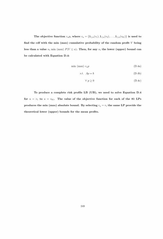
The objective function cup, where cu = {1≤u(v1),1≤u(v2), . . . ,1≤u(v81)} is used to
find the cdf with the min (max) cumulative probability of the random profit V being
less than a value u, min (max) P (V ≤ u). Then, for any u, the lower (upper) bound can
be calculated with Equation D.4:
min (max) cup (D.4a)
s.t. Ap = b (D.4b)
∀ p ≥ 0 (D.4c)
To produce a complete risk profile LB (UB), we need to solve Equation D.4
for u = v1 to u = v81. The value of the objective function for each of the 81 LPs
produces the min (max) absolute bound. By selecting cu = v, the same LP provide the
theoretical lower (upper) bounds for the mean profits.
249

Bibliography
Abbas, A. E. (2006). Entropy methods for joint distributions in decision analysis.
IEEE Transactions on Engineering Management 53(1), 146–159.
Apostolakis, G. and S. Kaplan (1981). Pitfalls in risk calculations. Reliability Engi-
neering 2, 135–145.
Barany, I. and Z. Furedi (1987). Computing the volume is difficult. Discrete and
Computational Geometry 2(1), 319–326.
Ben-Tal, A., L. E. Ghaoui, and A. Nemirovski (2009). Robust Optimization. Princeton,
NJ: Princeton series in Applied Mathematics.
Bertsekas, D. P. (1999). Nonlinear Programming (Second ed.). Athena Scientific.
Bertsimas, D. and J. Tsitsiklis (1997). Introduction to Linear Optimization. Belmont
Mass: Athena Scientific.
Bickel, J. E., L. W. Lake, and J. Lehman (2011, July). Discretization, simulation, and
Swanson’s (inaccurate) mean. SPE Economics and Management 3(3), 128–140.
Bickel, J. E. and J. Smith (2006). Optimal sequential exploration: A binary learning
model. Decision Analysis 3(1), 16–32.
Bickel, J. E., J. E. Smith, and J. L. Meyer (2008). Modeling dependence among
geologic risk in sequential exploration decisions. Reservoir Evaluation and Engi-
neering 3(4), 233–251.
Boyd, S. and L. Vandenberghe (2004). Convex Optimization. Cambridge, UK.: Cam-
bridge University Press.
250
Casella, G. and R. L. Berger (2002). Statistical Inference (Second ed.). Duxbury
Advanced Series. California: Thomson Learning.
Cherubini, U., E. Luciano, and W. Vecchiato (2004). Order Statistics. West Sussex,
England: John Wiley & Sons Ltd.
Chessa, G., R. Dekker, et al. (1999). Correlation in uncertainty analysis for medi-
cal decision making: An application to heart-valve replacement. Medical Decision
Making: an International. 19(3), 276–286.
Clemen, R. T. (1996). Making Hard Decisions. An Introduction To Decision Analysis
(2nd ed.). Duxbury Press.
Clemen, R. T., G. W. Fischer, and R. L. Winkler (2000, August). Assessing depen-
dence: Some experimental results. Management Sci. 46(8), 1100–1115.
Clemen, R. T. and T. Reilly (1999, February). Correlations and copulas for decision
and risk analysis. Management Science 45(2), 208–224.
Cooke, R. M. and R. Waij (1986). Monte Carlo sampling for generalized knowledge
dependence with application to human reliability. Risk Analysis 6(3), 335–343.
Cover, T. M. and J. A. Thomas (2006). Elements of Information Theory (Second
ed.). Wiley Interscience.
David, H. A. (1981). Order Statistics. New York: Wiley.
Deming, W. E. and F. F. Stephan (1940). On a least squares adjustment of a sam-
pled frequency table when the expected marginal totals are known. Ann. Math.
Statist. 11(4), 427–444.
Devroye, L. (1986). Non-Uniform Random Variate Generation. New York: Springer-
Verlag.
251

Devroye, L. and G. Lugosi (2000). Combinatorial Methods in Density Estimation.
New York, NY: Springer-Verlag.
Dyer, M., A. Frieze, and R. Kannan (1995). A random polynomial time algorithm for
approximating the volume of convex bodies.
Frees, E. W., J. Carriere, and E. Valdez (1996, June). Annuity valuation with depen-
dent mortality. The Journal of Risk and Insurance 63(2), 229–261.
Fritz, J. (1948). Extreme problems with inequalities as subsidiary conditions. Inter-
science Studies and Essays, presented to R. Courant on his 60th Birthday, 187–204.
Ghosh, S. and G. Henderson (2001). Chessboard distributions and random vectors
with specified marginals and covariance matrix. Operations Research 50(5), 820–
834.
Ghosh, S. and S. G. Henderson (2003, July). Behavior of the NORTA method for
correlated random vector-generation as the dimension increases. ACM Transactions
on Modeling and Computer Simulation 13(3).
Grant, M. and S. Boyd (2011, April). CVX: Matlab software for disciplined convex
programming, version 1.21. http://cvxr.com/cvx.
Helton, J. C. (1993). Uncertainty and sensitivity analysis techniques for use in perfor-
mance assessment for radioactive waste disposal. Reliability Engineering and System
Safety 42, 327–367.
Howard, R. A. (1966). Decision analysis: Applied decision theory. In D. Hertz and
J. Melese (Eds.), Proceedings of the fourth international conference on operational
research, Wiley Interscience, New York,NY, pp. 55–71.
252

Howard, R. A. (1988, June). Decision analysis: Practice and promise. Management
Science 34(6), 679–695.
Howard, R. A. and J. E. Matheson (2004). The Principles an Applications of Decision
Analysis, Volume 1 of Strategic Decisions Group. SDG.
Howard, R. A. and J. E. Matheson (2005). Influence diagrams. Decision Analysis 2(3),
127–143.
Ireland, C. T. and S. Kullback (1968, March). Contingency tables with given marginals.
Biometrika 55(1), pp. 179–188.
Jaynes, E. T. (1957). Information theory and statistical mechanics. part 1. Physical
Review 106(4), 620–630.
Jaynes, E. T. (1963). Information theory and statistical mechanics. part 3. In G. Uh-
lenbeck. (Ed.), Statistical Physics, pp. 181–218. New York: W. A. Benjamin.
Jaynes, E. T. (1968). Prior probabilities. IEEE Transactions On Systems Science And
Cybernetics 4(3), 227–241.
Jaynes, E. T. (1982). On the rationale of maximum-entropy methods. Proceedings of
the IEEE 70(9), 939–952.
Jimenez, L. and D. Landgrebe (1998, Feb.). Supervised classification in high dimen-
sional space: Geometrical, statistical and asymptotical properties of multivariate
data. IEEE Transactions on Systems, Man, and Cybernetics 28-C (1), 39–54.
Jouini, M. N. and R. T. Clemen (1996, June). Copula models for aggregating expert
opinions. Operations Research 44(3), 444–457.
Kannan, R., L. Lovsz, and M. Simonovits (1996). Random walks and an O*(n5) volume
algorithm for convex bodies. Random Structures and Algorithms Vol 11(Issue 1).
253

Keefer, D. L. (2004). Underlying event model for approximating probabilistic depen-
dence among binary events. IEEE Transactions on Engineering Management 51(2),
173–182.
Keefer, D. L. and S. E. Bodily (1983, May). Three-point approximations for continuous
random variables. Management Science 29(5), 595–609.
Korsan, R. J. (1990). Towards better assessments and sensitivity procedures. In
R. Oliver and J. Smith (Eds.), Influence diagrams, beliefe nets and decision analysis,
pp. 427–454. New York,NY: Wiley & Sons.
Kullback, S. (1967, January). A lower bound for discrimination information in terms
of variation. IEEE Transactions on Information Theory 13(1), 126 – 127.
Kullback, S. (1968). Probability densities with given marginals. The Annals of Math-
ematical Statistics 39(4), 1236–1243.
Kullback, S. and R. A. Leibler (1951). On information sufficiency. The Annals of
Mathematical Statistics 22(1), 79–86.
Lichtenstein, S., B. Fischhoff, and L. D. Phillips (1982). Calibration of probabilities:
The state of the art to 1980. In D. Kahneman and A. Tversky (Eds.), Judgement
under Uncertainty: Heuristics and Biases. Cambridge University Press.
Lin Yuan Kesavan, H. (1998, Aug). Minimum entropy and information measure. Sys-
tems, Man, and Cybernetics, Part C: Applications and Reviews, IEEE Transactions
on 28(3), 488 – 491.
Lovasz, L. (1998). Hit-and-run mixes fast. Mathematical programming 86(3), 443–461.
Lowell, D. G. (1994). Sensitivity to relevance in decision analysis. Ph. D. thesis,
Engineering and Economic Systems, Stanford University, Stanford, CA.
254

Lowenstein, R. (2000). When Genius Failed: The Rise and Fall of Long-Term Capital
Management. New York, NY: Random House.
Mackenzie, G. R. (1994). Approximately Maximum Entropy Multivariate Distribu-
tions With Specified Marginals and Pairwise Correlations. Disertation, University
of Oregon.
McMullen, P. (1970). The maximum number of faces of a convex polytope. Mathe-
matika XVII (2), 179–184.
Miller, A. C. (1990). Towards better assessments and sensitivity procedures by R.
Korsan: Discussion by Allen C. Miller. In R. Oliver and J. Smith (Eds.), Influence
diagrams, belief nets and decision analysis., West Sussex, England. John Wiley &
Sons Ltd.
Min, H.-S. J., W. Beyeler, T. Brown, Y. J. Son, and A. T. Jones (2007). Toward
modeling and simulation of critical national infrastructure interdependencies. IEEE
Transactions on Operations Engineering 39, 57–71.
Nelsen, R. B. (2005). An Introduction to Copulas (Second ed.). Springer Series in
Statistics. Springer.
Ong, H. L., H. C. Huang, and W. Huin (2003). Finding the exact volume of a poly-
hedron. Advances in Engineering Software 34(6), 351–356.
Pearson, E. S. and J. W. Tukey (1965). Approximate means and standard
deviations based on distances between percentage points of frequency curves.
Biometrika 52(3/4), 553–546.
Presidential Commission on the Space Shuttle Challenger Accident (1986). Report of
the Presidential Commission on the Space Shuttle Challenger Accident. Washington,
DC: Hearings of the Presidential Commission on the Space Shuttle.
255

Ravinder, H., D. KLeinmuntz, and J. Dyer. (1988). The reliability of subjective
probabilities obtained through decomposition. Management Science 32(2), 186–
199.
Reilly, T. (2000, Summer). Sensitivity analysis for dependent variables. Decision
Sciences 31(3), 551–572.
Rubin, P. A. (1984). Generating random points in a polytope. Comm. in Statist. -
Simulation and Comput. 13(3), 375–396.
Schmidt, B. K. and T. H. Mattheiss (1977). The probability that a random polytope
is bounded. Mathematics of Operations Research 2(3), 292–296.
Shannon, C. E. (1948). A mathematical theory of communications. Bell Systems
Technical Journal 23(3), 379–423,623–656.
Sklar, A. (1959). Fonctions de repartition a n dimensions et leurs marges. Publ. Inst.
Statist. Univ. Paris(8), 229–231.
Smith, A. E., P. B. Ryan, and J. S. Evans (1992). The effect of neglecting correlations
when propagating uncertainty and estimating the population distribution of risk.
Risk Analysis 12(4), 467–474.
Smith, J. E. (1993). Moment methods for decision analysis. Management Sci-
ence 39(3), 340–358.
Smith, R. L. (1984, Dec). Efficient Monte Carlo procedures for generating points
uniformly distributed over bounded regions. Operations Research 32(6), 1296–1308.
Strichartz, R. S. (2000). The Way of Analysis (Revised ed.). Jones and Bartlett
Mathematics. Toronto Canada: Jones and Bartlett.
256

Thomas, M. U. (1979). A generalized maximum entropy principle. Operations Re-
search 27(6), 1189–1196.
Vandenberghe, L., S. Boyd, and S. Wu. (1998). Determinant maximization with linear
matrix inequality constraints. SIAM J. Matrix Analysis and Applications 19, 499–
533.
Vazirani, V. V. (2003). Approximation Algorithms. New York,NY: Springer.
von Newmann, J. (1963). Various techniques used in connection with random digits,
Volume 5, pp 768-770 of Collected Works. Pergamon Press.
Watanabe, S. (1981). Pattern recognition as a quest for minimum entropy. Pattern
Recognition 13, 381–387.
Waterloo, U. (1994.). On the relationship between variance and minimum entropy. In
Intern. Publ. Univ. Waterloo, Waterloo, Ont., Canada.
Winkler, R. L. (1982). Research directions in decision making under uncertainty.
Decision Sciences 13(4), 517–533.
Ye, Y. (1997). Interior Point Algorithms, Theory and Analysis. New York,NY: Wiley
Interscience.
Zhang, Y. (1999, September). An interior-point algorithm for the maximum-volume
ellipsoid problem. Technical Report TR98-15, Department of Computational and
Applied Mathematics at Rice University, Houston, Tx.
257

Vita
Luis Vicente Montiel Cendejas was born in Mexico City, Mexico, the son of
Q.F.B. Maria Rosa Cendejas and Dr. Luis Isidoro Montiel. He received the Bachelor
of Science degree in Engineering from the Instituto Tecnologico de Monterrey at the
Mexico City Campus (ITESM-CCM). After graduation he work as a strategy consul-
tant before he decided to return to the academic life. In 2003 he moved to Palo Alto,
California and join the Master in Management Science and Engineering Program at
Stanford University. One year later, he continue his studies at Columbia University
in the Financial Engineering department and in 2006 he transfers to the Operations
Research Graduate Program at The University of Texas at Austin. His research in-
terests are in mathematical modeling for optimization under uncertainty with special
interest in decision analysis and simulation learning for optimization.
Permanent address: Operations Research Graduate Program at
The University of Texas at Austin,
Austin, TX 78712, USA, [email protected]
258


Buy your books fast and straightforward online - at one of world’s
fastest growing online book stores! Environmentally sound due to
Print-on-Demand technologies.
Buy your books online at
www.get-morebooks.com
Kaufen Sie Ihre Bücher schnell und unkompliziert online – auf einer
der am schnellsten wachsenden Buchhandelsplattformen weltweit!
Dank Print-On-Demand umwelt- und ressourcenschonend produzi-
ert.
Bücher schneller online kaufen
www.morebooks.deVDM Verlagsservicegesellschaft mbH
Heinrich-Böcking-Str. 6-8 Telefon: +49 681 3720 174 [email protected] - 66121 Saarbrücken Telefax: +49 681 3720 1749 www.vdm-vsg.de