Approximating the Traffic Grooming Problem in Tree and Star Networks
Upload
independentCategory
view
5download
0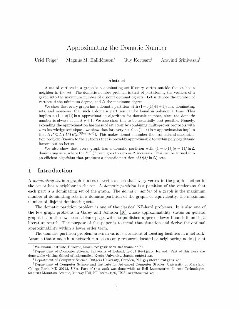
Approximating the Domatic Number
Uriel Feige∗ Magnus M. Halldorsson† Guy Kortsarz‡ Aravind Srinivasan§
Abstract
A set of vertices in a graph is a dominating set if every vertex outside the set has aneighbor in the set. The domatic number problem is that of partitioning the vertices of agraph into the maximum number of disjoint dominating sets. Let n denote the number ofvertices, δ the minimum degree, and ∆ the maximum degree.
We show that every graph has a domatic partition with (1−o(1))(δ+1)/ lnn dominatingsets, and moreover, that such a domatic partition can be found in polynomial time. Thisimplies a (1 + o(1)) lnn approximation algorithm for domatic number, since the domaticnumber is always at most δ + 1. We also show this to be essentially best possible. Namely,extending the approximation hardness of set cover by combining multi-prover protocols withzero-knowledge techniques, we show that for every ǫ > 0, a (1−ǫ) lnn-approximation impliesthat NP ⊆ DTIME(nO(log log n)). This makes domatic number the first natural maximiza-tion problem (known to the authors) that is provably approximable to within polylogarithmicfactors but no better.
We also show that every graph has a domatic partition with (1 − o(1))(δ + 1)/ ln∆dominating sets, where the “o(1)” term goes to zero as ∆ increases. This can be turned intoan efficient algorithm that produces a domatic partition of Ω(δ/ ln∆) sets.
1 Introduction
A dominating set in a graph is a set of vertices such that every vertex in the graph is either inthe set or has a neighbor in the set. A domatic partition is a partition of the vertices so thateach part is a dominating set of the graph. The domatic number of a graph is the maximumnumber of dominating sets in a domatic partition of the graph, or equivalently, the maximumnumber of disjoint dominating sets.
The domatic partition problem is one of the classical NP-hard problems. It is also one ofthe few graph problems in Garey and Johnson [16] whose approximability status on generalgraphs has until now been a blank page, with no published upper or lower bounds found in aliterature search. The purpose of this paper is to mend that situation and derive the optimalapproximability within a lower order term.
The domatic partition problem arises in various situations of locating facilities in a network.Assume that a node in a network can access only resources located at neighboring nodes (or at
∗Weizmann Institute, Rehovot, Israel. [email protected]†Department of Computer Science, University of Iceland, IS-107 Reykjavık, Iceland. Part of this work was
done while visiting School of Informatics, Kyoto University, Japan. [email protected].‡Department of Computer Science, Rutgers University, Camden, NJ. [email protected].§Department of Computer Science and Institute for Advanced Computer Studies, University of Maryland,
College Park, MD 20742, USA. Part of this work was done while at Bell Laboratories, Lucent Technologies,600–700 Mountain Avenue, Murray Hill, NJ 07974-0636, USA. [email protected]
1
itself). Then if there is an essential type of resource that must be accessible from every node (ahospital, a printer, a file, etc.), copies of the resource need to be distributed over a dominatingset of the network. If there are several essential types of resources, each one of them occupies adominating set. If each node has bounded capacity, there is a limit to the number of resourcesthat can be supported. In particular, if each node can only serve a single resource, the maximumnumber of resources supportable equals the domatic number of the graph [15]. We can showhow the general case of larger, possibly non-uniform, capacities can be reduced to the unit case.
We review some elementary facts about dominating sets and domatic partitions, in light ofthe novelty of the problem to many readers. Dominating sets satisfy a monotonicity propertywith regards to vertex additions: if D is a dominating set and D′ ⊃ D, then D′ is also adominating set. This implies that if a graph contains k disjoint dominating sets, then its domaticnumber is at most k; intuitively, the nodes in none of the k sets can be added arbitrarily to thesets to form a proper partition of the vertex set. The domatic number can then be alternativelydefined as the maximum number of disjoint dominating sets. Every graph G satisfies D(G) ≥ 1,and unless G contains an isolated node, D(G) ≥ 2. On the other hand, D(G) ≤ δ+1, where δ isthe minimum degree; the reason being that a node of minimum degree must have some neighbor(or itself) in each of the disjoint dominating sets.
Fujita [14] has studied several greedy algorithms and shown that their performance ratio isno better than (δ+1)/2, for values of δ up to O(
√n). The only other lower bound on D(G) given
in a recent encyclopædic treatment of domination problems [19, 18] is D(G) ≥ ⌈n/(n − δ(G))⌉[39], where n is the number of vertices. This lower bound is relevant only in very dense graphs,since it degenerates to D(G) ≥ 2 when δ(G) ≤ n/2.
Numerous results are known for special classes of graphs. A graph G is said to be domaticallyfull if D(G) = δ(G)+ 1, the maximum possible. Determining if a d-regular graph is domaticallyfull is NP-complete, for any d ≥ 3 [34, 23]. Farber [10] showed nonconstructively that stronglychordal graphs are domatically full. This class contains the classes of interval graphs and pathgraphs. Rao and Rangan [37] then gave a linear time algorithm for interval graphs, and Pengand Chang [32] for strongly chordal graphs. Farber’s theorem turned out to be a special caseof a result of Berge [5] for balanced hypergraphs, and Kaplan and Shamir [21] presented asimple algorithm. They also showed split graphs and bipartite graphs to be NP-hard. Efficientalgorithms are known for partial k-trees, using generic methods [2]. Bonucelli [6] showed thatcircular-arc graphs are NP-hard, while Marathe et al. [28] gave a 4-approximation algorithm.
Let ∆ denote the maximum degree of a given graph. Our main result is a tight bound onthe approximability of the domatic number problem in general graphs. In particular, we give:
(A) An algorithm that finds a domatic partition of size (1−o(1))(δ+1)/ ln n, where the “o(1)”term goes to zero as n increases.
(B) An algorithm that finds a domatic partition of size at least δ/c ln ∆, for some constant c.
(C) A nonconstructive argument showing that the domatic number is at least (1 − o(1))(δ +1)/ ln ∆, where the “o(1)” term goes to zero as ∆ increases. This shows that the value ofthe domatic number can be approximated within a factor of nearly ln ∆.
(D) A bound on the domatic number of random graphs, showing that for most graphs, thedomatic number is at most (1 + o(1))(δ + 1)/ ln ∆, where the “o(1)” term goes to zero asn increases
2
(E) A construction showing that for every ǫ > 0, no polynomial-time algorithm can approxi-mate the problem within a (1−ǫ) ln n factor, unless NP has slightly superpolynomial-timealgorithms (NP ⊆ DTIME(nlog logn)). It also yields a (1 − o(1)) ln ∆–hardness. Theseresults hold even for subclasses of perfect graphs, both bipartite graphs, and a subclass ofchordal graphs called split graphs.
The (1+o(1)) ln n–approximation algorithm is a simple randomized assignment (though careis needed not to lose a factor of two in the analysis), and is derandomized using the method ofconditional probabilities. The results (B) and (C) above use the Lovasz Local Lemma (LLL)[9] as their basic tool. Suitable application of the LLL to our randomized assignment algorithmabove shows that the domatic number is at least (1/3 − o(1))(δ + 1)/ ln ∆; we then refine thisusing a “slow partitioning” scheme, leading to our result that the domatic number is at least(1 − o(1))(δ + 1)/ ln ∆. The O(ln ∆)–approximation algorithm is a constructive version of theLLL, following an approach of Beck [4].
The hardness construction builds on the proof of Feige [11] of similar hardness for the setcover and dominating set problems. In fact, the construction here generalizes the result of[11] in that it shows that it is hard to distinguish between the following two cases: whenthe minimum dominating set is large (and thus the domatic number small), or when thereare many small disjoint dominating sets. This parallels the situation with the archetypicalminimum partitioning problem, graph coloring, where Feige and Kilian [13] showed that it ishard to distinguish between the case when the maximum independent set is small, and when thechromatic number is small. The construction of the current paper, in fact, draws additionallyon the zero-knowledge techniques used in [13].
It is instructive to view our results in a larger context – that of the study of approximationalgorithms in general. It has been empirically observed and further supported by classification ofconstraint satisfaction problems [22] that there seem to be no “natural” maximization problemsapproximable within polylogarithmic factors but no better. Our results provide (to the best ofour knowledge) the first maximization problem with such an approximation behavior, as thedomatic number is a maximization problem approximable within logarithmic factors but nobetter.
Our algorithmic results give absolute ratios, namely bounds in terms of some basic parame-ters of the graph (minimum degree, number of vertices), rather than in terms of the size of theoptimal solution. These are in fact the first nontrivial lower bounds on the size of an optimaldomatic partition for arbitrary δ,∆ such that δ ≥ ln ∆:
D(G) ≥ (1 − o(1)) · δ + 1
ln ∆. (1)
As shown in Section 2.5, this bound is best possible up to lower order terms, for a large rangeof values of δ = δ(n) and ∆ = ∆(n).
In the past, most absolute ratios have been obtained by fairly simple greedy algorithms.Our algorithms are derandomizations of simple randomized algorithms, but their derandomizedversions are not particularly natural, and natural greedy algorithms for the problem attainmuch worse results. It is also interesting that the hardness result gives a “gap location at 1”:namely, it is equally hard to approximately partition graphs that are domatically full. We cangeneralize the problem to partitioning hypergraphs into a maximum number of dominating sets.It corresponds to the maximum number of disjoint transversals of the dual hypergraph. Thehardness results apply without change because graphs are special cases of hypergraphs.
3

The rest of the paper is organized as follows. Section 2 starts with an algorithm that finds adomatic partition into roughly δ/ ln n sets, followed by an algorithm that yields a partition withΩ(δ/ ln ∆) sets. It then proves (1). The section ends with a short proof that the performanceratio of the natural greedy algorithm isO(
√n log n). The hardness reduction is given in Section 3.
2 Approximation algorithms and existential results
This section is devoted to positive results for domatic partitions. Section 2.1 shows algorithmi-cally that D(G) ≥ (1− o(1))(δ+ 1)/ ln n, and also shows that D(G) ≥ (1/3− o(1))(δ+ 1)/ ln ∆.(The two usages of “o(1)” here respectively correspond to n → ∞ and ∆ → ∞.) This secondresult is made algorithmic in Section 2.2, with a loss in the constant factor; the existentiallytight result that D(G) ≥ (1 − o(1))(δ + 1)/ ln ∆ is then shown in Section 2.3. Section 2.4 isdevoted to a short analysis of the natural greedy algorithm for domatic partition.
Notation. Let N(v) denote the set of neighbors of a vertex v in the given graph G, and letN+(v) = v ∪ N(v). Let d(v) = |N(v)| denote the degree of v, and let d+(v) = |N+(v)| =1 + d(v). A partial coloring of G is an arbitrary coloring of an arbitrary subset of the vertices.Given a current partial coloring, define a Boolean variable Av,c to be true if there is no vertexof color c in N+(v), and to be false otherwise. Define [ℓ] to be the set 1, 2, . . . , ℓ.
For an event X, P [X] denotes its probability and E[X] its expectation. Finally, let e denotethe base of the natural logarithm.
2.1 Logarithmic bounds
Theorem 1 Any graph admits a (polynomial-time constructible) domatic partition of size (δ +1)(1 −O(log log n/ log n))/ ln n).
Proof. Independently give each vertex one of ℓ = (δ + 1)/ ln(n lnn) colors at random. For anyvertex-color pair (v, c), P [Av,c] = (1 − 1/ℓ)d
+(v) ≤ e−d+(v)/ℓ ≤ 1/(n ln n). (Note that the events
Av,c are “bad events” for us: if Av,c holds for some pair (v, c), then the coloring is not a domaticpartition; conversely, if none of the events Av,c hold, then every vertex v “sees” every color inN+(v), and we will have a domatic partition. Thus, our focus will be on avoiding all of thesebad events.) Thus, summing over all (v, c) pairs, the expected total number of bad events Av,cis at most ℓ/ ln n. Hence, the expected number of colors that form dominating sets is at least
∑
c
(1 − ℓ (1 − 1/ ln n) =δ + 1
lnn
(
1 − ln lnn+ 1
ln(n lnn)
)
. (2)
The color-classes that do not form dominating sets can all be merged into any one color classthat is a dominating set; thus, we get a domatic partition whose expected number of sets is atleast as large as the r.h.s. of (2).
This randomized argument can be derandomized using the method of conditional probabil-ities (cf. [1]). Number the vertices arbitrarily as v1, v2, . . . , vn, and color the vertices in thisorder (never recoloring a vertex) as follows. Color v1 arbitrarily. Suppose the first j ≥ 1 verticeshave been colored with respective colors c1, c2, . . . , cj ; vertex vj+1 is colored as follows. Letdj+1(v) = |N+(v) ∩ vj+1, vj+2, . . . , vn|. Then, the conditional probability of the bad eventAv,c is given by
P [Av,c|c1, c2, . . . cj ] =
0 if ∃vz ≤ j such that vz ∈ N+(v) and cz = c;
(1 − 1/ℓ)dj+1(v) otherwise.
4

The weight of the current coloring is given by
g(c1, c2, . . . , cj).=∑
v∈V
∑
c
P [Av,c|c1, c2, . . . , cj ];
this is precisely the expected number of pairs (v, c) pairs for which Av,c will hold after coloringall vertices, given the current coloring c1, . . . , cj . In each step j + 1, we choose a color for vj+1
so that the weight of the coloring does not increase. Such a color exists, since g(c1, c2, . . . , cj) isa convex combination of the values g(c1, c2, . . . , cj , cj+1) : cj+1 ∈ [ℓ]:
g(c1, c2, . . . , cj) = (1/ℓ) ·∑
cj+1∈[ℓ]
g(c1, c2, . . . , cj , cj+1).
Then, the total number of colors that are not dominating sets is at most the weight of the finalcoloring, which we ensure is at most the expected number at the outset, or ℓ/ lnn.
We now refine this argument using the LLL to get better bounds when ∆ ≤ n1/3. We statethe symmetric, simpler version of the LLL.
Lemma 2 (LLL [9]) Let p < 1, and let Ei, 1 ≤ i ≤ k be k events such that P[Ei] ≤ p for all i.Suppose there is an integer d such that e · p · (d + 1) ≤ 1, and each event is independent of allbut at most d other events. (More precisely, for each Ei, there is a set Ti of at least k − d − 1other events Ej, such that the conditional probability of Ei given any Boolean combination of theevents in Ti, equals the unconditional probability of Ei.) Then, P[
∧
i Ei] > 0.
Independently color each vertex randomly with one of ℓ = ⌊(δ + 1)/(3 · ln(31/3 · ∆))⌋ colors.For each (v, c) pair, P[Av,c] ≤ (1 − 1/ℓ)d
+(v) ≤ 1/(3 · ∆3). We note that each event Av,c isindependent of all but at most ℓ(1 + d(v) + d(v) · (∆ − 1)) other such events, since vertices ofdistance at least 3 from v are completely irrelevant for v. More precisely, in the notation ofLemma 2, we can take Tv,c to be the set of all events of the form (w, c′), where w is a vertex ata distance of at least 3 from v, and where c′ is any color from [ℓ]: conditioning on any Booleancombination of the events in Tv,c does not influence the colors chosen by vertices in N+(v). Thefollowing lemma now directly follows from the LLL, using the fact that ℓ < ∆ and d(v) ≤ ∆:we set d = ∆3 − 1 and p = 1/(3 · ∆3) in using the LLL.
Lemma 3 Any graph admits a domatic partition of size (1/3 − o(1))δ/ ln ∆, where the “o(1)”term tends to zero as ∆ → ∞.
In Section 2.3, we will refine the above approach by conducting a two-stage partitioning thatattains the tight value of 1−o(1) instead of the value 1/3−o(1) of Lemma 3. However, the abovedirect approach will help us develop a simple algorithmic version of Lemma 3 in Section 2.2. Italso motivates the reason for developing the approach of Section 2.3.
Remark: It is interesting to note that the ∆ in the bound of Lemma 3 cannot be replaced byδ, nor by d, the average degree. Consider, for example, the bipartite graph with 3 · δ verticeson the left side, and
(3·δδ
)
vertices on the right side, with each vertex on the right side connectedto a particular subset of δ vertices in the left side. The domatic number of this graph is two.Indeed, say that there are 3 disjoint dominating sets. One of these sets, S, contains at least δvertices on the left side. There exists a vertex v on the right side all of whose neighbors are inS. Hence, the two remaining sets must both contain the vertex v, a contradiction.
5

A parameter that is intermediate between average and maximum degree is the inductiveness∆∗(G) = maxH⊆G δ(H). It is most notable for giving a tighter upper bound on the chromaticnumber than the maximum degree, as χ(G) ≤ ∆∗(G) + 1 ≤ ∆(G) + 1. The above constructionshows however that ∆∗ cannot replace ∆ in the bound of Lemma 3 on the domatic number.
2.2 O(log ∆)–approximation algorithm
We use an algorithmic version of the LLL due to Beck [4] that derandomizes the probabilisticargument with some loss in the constants. We may assume without loss of generality that G isconnected, since we can treat the connected components separately. Our algorithm has threephases, assigning colors to successively larger fractions of the vertices. After the first phase, eachvertex is either fully satisfied, seeing all colors within its neighborhood, or has at most one-thirdof its neighbors colored. We show that the subgraph induced by nodes that are still active,i.e. either unsatisfied or not yet colored, consists with high probability of only small connectedcomponents, of O(∆6 log n) vertices each. After the second phase, more vertices are colored,with at most two-thirds of the neighbors of yet-unsatisfied vertices being colored. The connectedcomponents induced by active vertices are now of only O(∆7 log log n) size. Then, depending onthe value of ∆, we can either solve each component by exhaustive search, or apply Theorem 1to obtain a full coloring where each vertex is satisfied.
2.2.1 The algorithm
The first phase proceeds as follows. Given a coloring of some of the vertices, call a vertex vdangerous iff:
1. at least δ/3 neighbors of v have been colored, and
2. not all the ℓ colors appear in the neighborhood of v.
Let ℓ = δ/(c ln ∆) for a suitably large constant c. Order the vertices arbitrarily as v1, v2, . . . , vnand process them in this order. When processing vi, we do the following. If vi or one of itsneighbors is dangerous now, we freeze vi; otherwise we assign it one of ℓ colors independentlyat random.
When the process ends, some vertices are colored and some are frozen, and some are dan-gerous and some are not. The vertices that are not dangerous belong to one of two categories:
Good: A good vertex sees all colors in its neighborhood.
Neutral: A neutral vertex v does not see all colors in its neighborhood, but is not dangerous.This can happen only if more than 2/3 of v’s neighbors were frozen.
Thus, we have two orthogonal partitions: colored/frozen, and good/neutral/dangerous.Vertices that are both good and colored do not need to be considered further in the later
phases. Call the other vertices saved, i.e. those that are dangerous, frozen, or neutral. As in [4],we are interested in the maximum size of a connected component of the subgraph induced bysaved vertices, as this bounds the size of the independent subproblems in the next phase. Weshow in Section 2.2.2 that with probability at least 1/2, the largest connected component in thesaved graph has size O(∆6 log n); let us assume that this size bound holds.
Phase two of the algorithm is run separately on each connected component induced by thesaved vertices. Note that each dangerous or neutral vertex v has at least d(v) − δ/3 frozen
6
(i.e., uncolored) neighbors in its connected component. Phase two differs from phase one inthat some of the vertices are colored before we begin. We leave these colors untouched, becausethey may be useful for the vertices that were not saved. We only color the frozen vertices, andagain define the notion of phase-two dangerous, frozen and neutral vertices. Since the number ofvertices we are dealing with now in any connected component is O(∆6 log n), we have essentiallyreplaced n by O(∆6 log n). Thus, analysis similar to that of phase one shows that the connectedcomponents of the newly saved vertices has size at most N = O(∆6(log ∆ + log log n)) withprobability at least 1/4.
In phase three, each dangerous/neutral vertex has at least d(v)−2δ/3 ≥ δ/3 frozen neighborsin its connected component. If ∆ > log log n, we have a domatic partition of the frozen verticesto roughly δ/(3 lnN) parts, via Theorem 1. As lnN = O(log ∆), this is good enough. If ∆ ≤log log n, then we can find a domatic partition of size Ω(δ/ ln ∆) whose existence is guaranteedby Theorem 3, using exhaustive search. Since ∆ ≤ log log n, this only takes time
NO(δ/ ln∆) ≤ (log log n)O((log logn)) ≤ poly(n).
This completes the description of the algorithm.
2.2.2 Analysis of the algorithm
We now show that with probability at least 1/2, the largest connected component in the savedgraph in the first phase, has size O(∆6 log n). This will yield a proof of correctness of ouralgorithm.
Let X(u) be the indicator random variable for vertex u becoming dangerous, and let q =ℓ(1 − 1/ℓ)δ/3.
Lemma 4 Let U = u1, u2, . . . , uk be any set of vertices with pairwise distance at least 3.Then, Pr[X(u1) = X(u2) = · · · = X(uk) = 1] ≤ qk.
Proof. Note that if a vertex v is a neighbor of the set U , then it has a unique neighbor in U sincethe elements of U have pairwise distance at least 3. Let ~a = (a1, a2, . . . , ak) be any sequence ofk colors, and let Si be the random variable denoting the set of the first i nonfrozen neighbors ofU . Let Di(~a) be the event that “for all j = 1, 2, . . . , k, all neighbors of uj in Si avoid color aj”.Thus, Di(~a) is the event that even after processing the first i nonfrozen neighbors of U , each ujin U was missing a particular color aj . In order to let i range all the way up to δk/3, add δk/3dummy vertices just before the last (i.e., highest-numbered) vertex in U . These are considered tobe virtual neighbors of U that are never frozen. Hence, regardless of the freezing process, Di(~a)is defined for all i ≤ δk/3. (We will finally use the fact that if all the uj are dangerous, thenthere is some ~a for which Dδk/3(~a) is true.) We have Pr[D0(~a)] = 1. Now for every i < δk/3,Pr[Di+1(~a)] = Pr[Di(~a)] · (1 − 1/ℓ), because the color of the (i + 1)’st nonfrozen neighbor ofU is chosen at random independent of the previous colors, and independent of which vertex ithappens to be. Hence, Pr[Di(~a)] = (1 − 1/ℓ)i; so, Pr[∃~a : Dδk/3(~a)] ≤ ℓk(1 − 1/ℓ)δk/3 = qk.
As seen above, if all the uj are dangerous, then there is some ~a for which Dδk/3(~a) is true;this completes the proof.
To prove that the largest connected component in the saved graph is “small enough” withreasonable probability, we now show that with reasonable probability the maximum numberof vertices in a spanning tree of such a component is “small”. This is done as follows. By
7
a standard argument, a large connected component contains many vertices with a particularminimum pairwise distance. We first prove that the number of vertices with large pairwisemutual distance which are all saved is “small”. This indirectly bounds the maximum numberof vertices in a connected component as a function of ∆, which is enough for our purposes.
A set of vertices is said to be 7-separated if it is of mutual distance at least 7. A 7-separatedset of k vertices is said to be a bad k-set if, additionally, it becomes connected if we connect allvertices of distance exactly 7. As shown next, the number of such sets in G is at most
n(4∆7)k. (3)
Consider a spanning tree on the set where vertices of distance exactly 7 are connected. Thenumber of distinct ordered rooted trees on k vertices is at most 4k−1. Namely, such a treecan be uniquely represented by ordering the vertices in a lexicographic breadth-first order andattaching two flag bits to each nonroot vertex: whether it has the same parent as the previousvertex in the order, and whether it has a child or not. For each shape of a tree, there are npossibilities of choosing the root, and thereafter at most ∆7 possibilities of choosing each newvertex since we already chose its parent in the tree.
Let Y (u) be the indicator random variable for vertex u becoming saved. To complete ourargument that no connected component of the saved vertices is “large”, we will show:
Lemma 5 For any 7-separated set of vertices v1, v2, . . . , vk,
Pr[Y (v1) = Y (v2) = · · · = Y (vk) = 1] ≤ (2.5∆q)k.
Proof. The following definition will be useful for this proof:
Z(u).= X(u) + (
∑
v∈N(u)
X(v)) +
∑
v∈N(u)
∑
w∈N(v)X(w)
2d(u)/3.
If vertex u is saved, then we have one of three cases: (i) u is dangerous and thus X(u) = 1;or (ii) u has a dangerous neighbor and so
∑
v∈N(u)X(v) ≥ 1; or (iii) u is neutral, so at least2d(u)/3 of its neighbors are frozen, and by the preceding argument it holds for each frozenneighbor v of u that
∑
w∈N(v)X(w) ≥ 1. Therefore, we have the simple but useful observationthat if Y (u) = 1, then Z(u) ≥ 1.
By Markov’s inequality,
Pr[Y (v1) = Y (v2) = · · · = Y (vk) = 1] ≤ Pr[k∏
i=1
Z(vi) ≥ 1] ≤ E[k∏
i=1
Z(vi)]. (4)
Now, using the definition of Z(·) and the linearity of expectation, we can expand E[∏
i Z(vi)] as alinear combination of the terms Pr[X(w1) = X(w2) = · · · = X(wk) = 1]. The main observationis that since the vi have pairwise distance at least 7, the wi have pairwise distance at least 3.Thus, by Lemma 4, any such term has probability at most qk. Thus we get
E[∏
i
Z(vi)] ≤(
q + ∆q +d(u)(∆ − 1)q
2d(u)/3
)k
≤ (2.5∆q)k ,
by first replacing the probability of intersection of events by the product of probabilities, andthen unfolding and reversing the above expansion.
8
Consider now a connected component in the subgraph of G of saved vertices. If its size is k∆6
or more, then it must contain a bad k-set (which is obtained by repeating the procedure of puttinga vertex in the bad k-set and removing all vertices of distance at most 6). Setting the constant cin the expression ℓ = δ/(c ln ∆) large enough, we get that q ≤ ∆−9/10. Set k = log(2n)/ log ∆,and recall (3) and Lemma 5. We get that the probability of existence of a connected componentof the saved vertices with cardinality at least k∆6, is at most (2.5q∆)kn(4∆7)k ≤ 1/2.
Finally, the above Las Vegas algorithm can be derandomized by the approach of pessimisticestimators [35], which is a generalization of the method of conditional probabilities. Briefly, weproceed as follows. As before, we process the vertices one-by-one. Suppose it is currently theturn of vertex v. If v is frozen, we skip over it. Otherwise, we deterministically choose a colorfor it that minimizes the probability of emergence of a large connected component of the savedvertices, using our bounds derived above. Since k = log(2n)/ log ∆, we see from (3) that thenumber of possible bad k-sets to be considered in our analysis above, is bounded by a polynomialin n. Hence, we can write down a pessimistic estimator and choose, in deterministic polynomialtime, a color for vertex v that minimizes the pessimistic estimator.
2.3 Getting the right constant
Our next result improves the value 1/3−o(1) of Lemma 3 to the existentially best-possible valueof 1 − o(1).
Theorem 6 There is a constant a > 0 such that for any graph G with ∆ ≥ 3, D(G) ≥⌊ δ
ln ∆+a ln ln ∆⌋.
The value of D(G) for ∆ ≤ 2 is well-known via a simple case analysis; there is also alinear-time algorithm for the domatic partition problem if ∆ ≤ 2.
Proof. We will assume throughout that ∆ is large enough, i.e., for some absolute constant ∆0,we will assume that ∆ ≥ ∆0. (Indeed, if ∆ ≤ ∆0, the theorem holds by setting a large enough.)For the rest of Section 2.3, any “o(1)” term will denote a function of ∆ alone that goes to zero as∆ increases. We prove the theorem for a being any constant greater than 7, for all large enough∆; this choice of a can be further improved, but we do not attempt this optimization here.
Preprocessing. We preprocess the graph as follows. As long as there is an edge that has bothend-points with degree more than δ, remove such an edge from the graph. At the end of thisprocess, the minimum degree remains at δ, and the maximum degree is at most ∆. We willnow show a lower bound on the domatic number of this preprocessed version, which clearly willyield the same lower bound on the domatic number of the given graph. (This is because thepreprocessing only removes edges from the given graph.) The useful property that now holds isthat for each vertex u, either d(u) = δ, or all neighbors v of u have d(v) = δ.
There are two cases, the first one being simpler.
Case I: δ ≤ ln4 ∆. We assume that δ > ln ∆ + a ln ln ∆, since the theorem is trivially trueotherwise. Define
ℓ =
⌊
δ
ln ∆ + a ln ln ∆
⌋
.
Color each vertex with a random color from [ℓ], independent of all other vertices. We will nowuse the LLL to show that P [
∧
u,c Au,c] > 0, in the same way as we did for Lemma 3. For each
9

(u, c), we have
Pr[Au,c] =
(
1 − 1
ℓ
)d+(u)
≤ e− ln(∆(ln ∆)a)·d+(u)/δ ≤ (∆(ln ∆)a)−1. (5)
Let N2(u) denote the set of vertices at a distance of 0, 1, or 2 from u in G. As in our proofof Lemma 3, each event Au,c depends only on events Av,c′ with v ∈ N2(u); so, it depends on atmost |N2(u)| · ℓ other such events. Our preprocessing step above helps bound |N2(u)| for all u.If d(u) = δ, then |N2(u)| ≤ 1+δ+δ(∆−1). If d(u) > δ, our preprocessing ensures that d(v) = δfor all neighbors v of u; so, |N2(u)| ≤ 1+∆+∆(δ−1). Thus, |N2(u)| ≤ δ∆+1 ≤ ∆ ln4 ∆+1 forall u, since δ ≤ ln4 ∆. So, each Au,c depends on at most O(∆ ln7 ∆) other such events. Recallingthe LLL and (5), we see that P[
∧
u,c Au,c] > 0 as required, since a > 7.
Case II: δ > ln4 ∆. Let ǫ = 1/(ln ∆); define ℓ1 = ⌊ǫ3δ⌋ and ℓ2 = ⌊ln2 ∆/(1 + b(ln ln ∆)/ ln ∆)⌋,where b is any constant larger than 5. We will show the existence of a domatic partition ofsize ℓ1ℓ2, i.e., a coloring of V using ℓ1ℓ2 colors, in such a way that for every vertex u, thereis at least one vertex of each color in N+(u). (Recall that δ > ln4 ∆. By choosing b < 6, forinstance, we can ensure that ℓ1ℓ2 ≥ δ/(ln ∆ + 6 ln ln ∆), for all large enough ∆.) It will beconvenient to view the colors as elements of [ℓ1] × [ℓ2]. We will apply a two-stage coloring: thefirst coloring determines the first components of the vertex-colors, and the second coloring is forthe second components. We can view the first coloring as a coarse partition, which the secondcoloring turns into a fine partition. The primary purpose of the first coloring is to reduce thedependencies sufficiently for our analysis of the second coloring.
The first partitioning is as follows. Color each vertex with a random color from [ℓ1], inde-pendent of all other vertices. For each vertex u and each color c, define X+
u,c to be the subset ofN+(u) that receives color c. We have E[|X+
u,c|] = d+(u)/ℓ1. Let Bu,c be the “bad” event that| |X+
u,c| − d+(u)/ℓ1 | ≥ 3ǫd+(u)/ℓ1. A Chernoff bound shows that
Pr[Bu,c] ≤ 2 · exp(−(9/2 − o(1)) · d+(u)ǫ2/ℓ1) ≤ exp(−(9/2 − o(1)) ln ∆). (6)
Once again, Bu,c is independent of any Boolean combination of events of the form Bv,c′ forvertices v at a distance of 3 or more from u. Thus, each Bu,c “depends” on o(∆3) other suchevents. Recalling (6), the LLL shows that Pr[
∧
u,cBu,c] > 0.Fix a coloring χ1 : V → [ℓ1] which avoids all the events Bu,c. Choose a random color χ2(u) ∈
[ℓ2] for each u, independent of all other vertices; the final color of u is the pair (χ1(u), χ2(u)).Let Bu,c1,c2 be the bad event that there is no vertex of color (c1, c2) in N+(u). We now use theLLL to show that all these bad events can be avoided with positive probability.
For each vertex u and each c ∈ [ℓ1], let N+u,c = v ∈ N+(u) : χ1(u) = c, and define
d+u,c = |N+
u,c|. Since χ1 avoids all the events Bu,c, we have
∀(u, c), (1 − 3ǫ)d+(u)/ℓ1 ≤ d+u,c ≤ (1 + 3ǫ)d+(u)/ℓ1. (7)
Fix an event Bu,c1,c2. First,
Pr[Bu,c1,c2] =
(
1 − 1
ℓ2
)d+u,c1 ≤ e−(1−3ǫ)d+(u)/(ℓ1ℓ2) ≤ (∆(ln ∆)b)−(1−3ǫ) ≤ O((∆(ln ∆)b)−1); (8)
the first inequality here follows from (7). Next, which other events does Bu,c1,c2 depend on?Given S ⊆ V , let N+(S)
.=⋃
v∈S N+(v). Note that Bu,c1,c2 simply says that all elements of
10
N+u,c1 got a χ2(·) value different from c2. Thus, we can check that Bu,c1,c2 only depends on the
events inS(u, c1, c2) = Bv,c′1,c′2 : v ∈ N+(N+
u,c1) and c′1 = c1. (9)
More precisely, we claim that Bu,c1,c2 is independent of any Boolean function of the events lyingoutside S(u, c1, c2); this can be verified by seeing that
N+u,c1 ∩ (
⋃
(v,c′1,c′2): B
v,c′1
,c′26∈S(u,c1,c2)
N+v,c′1
) = ∅.
We now bound |S(u, c1, c2)|, in order to apply the LLL; once again, our preprocessing stepwill be of help. If d(u) = δ, then |N+(N+
u,c1)| ≤ ∆|N+u,c1|; this is at most O(δ∆/ℓ1), by (7). If
d(u) > δ, our preprocessing ensures that |N+(N+u,c1)| ≤ δ|N+
u,c1 |; so, from (7), we again get that
|N+(N+u,c1)| ≤ O(δ∆/ℓ1). Thus, |S(u, c1, c2)| ≤ O(δ∆ℓ2/ℓ1) = O(∆ ln5 ∆). We can now apply
the LLL, using (8) and the facts that: (i) b > 5, and (ii) each bad event Bu,c1,c2 depends on atmost |S(u, c1, c2)| others. This completes the proof.
To see why our two-stage coloring helps, note that the “dependence” |S(u, c1, c2)| in thesecond coloring above is only ∆1+o(1), as compared to the dependence of ∆3+o(1) that we couldget in the direct-coloring approach underlying Lemma 3. The constraint “v ∈ N+(N+
u,c1)” in (9)
saves us a factor of ∆1−o(1), and the constraint “c′1 = c1” saves another factor of ∆1−o(1). Thatthe first-stage coloring eliminates many dependencies in this fashion, is the main idea motivatingthis approach.
It is an open question if a domatic partition of the size guaranteed by Theorem 6 can befound in polynomial time.
2.4 Greedy algorithm
One natural approach to the domatic partition problem is to try to greedily choose small dom-inating sets. The greedy algorithm iteratively pulls out dominating sets from the graph, untilthe remainder is no longer dominating. The dominating sets are found by a standard O(log n)-approximate greedy algorithm [20, 24].
Lemma 7 Suppose D(G) = n/k. Then, the greedy algorithm finds a domatic partition ofΩ(n/(k2 log n)) sets.
Proof. We count how many disjoint dominating sets our algorithm finds before the set of verticesin them intersects at least half of the n/k vertex-disjoint dominating sets in the graph. Duringthis period, there are at least n/(2k) disjoint dominating sets, thus in each step there exists adominating set of size at most 2k and we find one of size at most 2k lnn. Hence, in each step,a vertex from at most 2k lnn different dominating sets is removed. It then requires at least(n/2k)/(2k lnn) steps to halve the original number of dominating sets in the graph.
Since D(G) ≤ n, the approximation ratio is maximized when k ≈√
n/(4 ln n).
Corollary 8 The performance ratio of the greedy domatic partition algorithm is O(√n lnn).
Fujita [14] has shown examples where the performance of this and some other greedy algo-rithms is Ω(
√n).
11
2.5 The domatic number of random graphs
, We now show that the bound (1) is tight for a large range of values of δ = δ(n), by studyingD(G) for suitable random graphs G. Suppose G is drawn from the random graph model G(n, p):i.e., we take n labeled vertices, and put an edge with probability p independently between eachpair of vertices. We will show that with probability 1 − o(1), D(G) ≤ (1 + o(1))δ(G)/ ln ∆(G).(Throughout this section, the “o()” and “ω()” notation refers to n getting large.)
Choose any p = p(n) such that np = (lnn)ω(1) and p = o(1). It is easy to check via aChernoff bound that with probability 1 − o(1), both δ and ∆ will lie in the range (1 ± o(1))npfor our random graph G. Fix any constant ǫ > 0, and let s = ⌊(1 − ǫ) ln(np)/p⌋. We will showthat with probability 1− o(1), any dominating set in G will have size more than s. (Thus, withprobability 1−o(1), we will have D(G) ≤ n/(s+1), completing the proof.) For any given subsetof the vertices S with |S| = s,
Pr[S is a dominating set] = (1 − (1 − p)s)n−s
≤ (1 − e−(1+Θ(p))sp)n−s
≤ (1 − (np)ǫ−1−Θ(p))n−s
≤ e−(n−s)·(np)ǫ−1−Θ(p)
≤ es−(1/p)·(np)ǫ−Θ(p)
= es−(1/p)·(np)ǫ−o(1).
Thus, the probability of existence of a dominating set of size s is at most(
n
s
)
· es−(1/p)·(np)ǫ−o(1) ≤ (ns/s!) · es−(1/p)·(np)ǫ−o(1)= (es/s!) · es lnn−(1/p)·(np)ǫ−o(1)
= o(1);
the bound s lnn = o((1/p) · (np)ǫ−o(1)) follows from the definition of s and from the fact thatnp = (lnn)ω(1).
3 Hardness of approximating the domatic number
We say that a problem is hard to approximate within ratio ρ if having a polynomial time (ran-domized) ρ-approximation algorithm for it would violate some standard hardness assumption,such as P 6= NP. The hardness assumption that we use in this paper is that NP does not have(randomized) algorithms that run in time nO(log logn); for brevity we shall just use the term hardto approximate.
We shall prove the following theorem.
Theorem 9 For every fixed ǫ > 0, it is hard to approximate the domatic number within a ratioof (1 − ǫ) ln |V |.
For this purpose, it is helpful to work with a related but different problem.
Definition 1 A one-sided dominating set in a bipartite graph G(V1, V2, E) is a set of verticesU ⊆ V1 such that for every v ∈ V2 there is some u ∈ U with (u, v) ∈ E. Here it is assumedthat the intended bipartition (V1, V2) is given explicitly as part of the input and that every vertexin V2 has some neighbor in V1. Observe that this problem is merely a reformulation of the wellknown set-cover problem.
12
The one-sided domatic number of a bipartite graph is the maximum number of mutuallydisjoint one-sided dominating sets that the graph contains.
Observe that the dominating set and domatic number problems have a relation similar to the oneof the coloring versus maximum independent problem. A coloring is a packing of independentsets while a domatic partition is a packing of dominating sets.
A related problem is the set cover problem, where a collection of subsets S of a base set U isgiven, and we are to find a minimum cardinality subcollection that contains all elements of U .The set cover packing number is then the maximum number of mutually disjoint set covers. Itis well-known that minimum dominating set, minimum one-sided dominating set and minimumset cover are strongly related, and that lnn is the best approximation ratio for all of them withinlower order terms (details in Section 3.2). The one-sided domatic number problem can be shownto be equivalent to the set cover packing problem in terms of optimization. We are not awareof a similar relationship between one-sided domatic number and domatic number. However, wecan give a reduction that yields the necessary result.
Proposition 10 Let c > 1 and consider bipartite graphs G(V1, V2, E) with |V1| large enough(e.g., |V1| ≥ 4c), |V2| > |V1|c, and the following promise: for some 0 ≤ ǫ ≤ 1 − 1/c and for rand q satisfying rq > (1 − ǫ)|V1| ln |V2| (r and q may depend on the size of G) either
• The size of the smallest one-sided dominating set in G is at least r, or
• The one-sided domatic number of G is at least q.
Note that the two cases for the promise cannot both hold. If it is hard to distinguish whichof the two cases holds, then it is hard to approximate the domatic number within a ratio of(1 − 1/c− ǫ) ln |V |.
The proof of Proposition 10 is given in Section 3.2. The main result of the section is thefollowing theorem, proved in Section 3.5.
Theorem 11 For every ǫ > 0 and every integer c > 0 the two cases of Proposition 10 cannotbe distinguished in (random) polynomial time unless NP has (randomized) algorithms that runin time nO(log logn).
Theorem 9 now follows from Theorem 11 and Proposition 10.
Remark: Theorem 9 implies a ln ∆ hardness of approximation result, for ∆ ≃ nψ for some0 < ψ < 1 which is close to 1. To obtain ln ∆ hardness of approximation results when ∆ is muchsmaller compared to n, simply make many disjoint copies of the graph, increasing n withoutchanging ∆ or the domatic number.
3.1 Overview and intuition
Before presenting the proof of Theorem 11, let us provide some background on proving hardnessof approximation results in general, and how hardness of approximation results were proved forproblems related to domatic number.
A convenient starting point for proving hardness of approximation results is the problem ofMax 3SAT. The input to this problem is a 3CNF formula and the desired output is an assignmentto the variables that satisfies as many clauses as possible. The well known PCP theorem of [3]
13
implies (or in fact, is equivalent to) the following gap: for some ǫ > 0 it is NP-hard to distinguishbetween 3CNF formulas that are satisfiable (which we call yes instances) and 3CNF formulasin which every assignment satisfies at most a (1 − ǫ) fraction of the clauses (which we call noinstances). This hardness result can be extended to a restricted version of Max 3SAT in whichthe input 3CNF formula has the property that each variable appears in exactly 5 clauses. (Thechoice of 5 is arbitrary here. Any other constant greater than 5 would do as well.) We call thisrestricted version Max 3SAT-5.
As noted above, the set cover problem is strongly related to the dominating set problem,which in turn is related to the domatic number problem. Moreover, the one-sided domaticnumber problem is equivalent to the set cover packing problem. Hence our plan for provingTheorem 11 is to take known results regarding the hardness of approximation of set cover, andmodify their proof so that it shows hardness of approximation for the set cover packing problemas well (and hence also for one-sided domatic number). To see more explicitly what needs to bedone, let us first review at a very high level the known result [11] that set cover (and one-sideddominating set) is hard to approximate within a factor of (1 − ǫ) lnn.
The proof in [11] reduces instances of Max 3SAT-5 to instances of one-sided dominating set.The reduction is slightly super polynomial (instances of size n are mapped to instances of sizenO(log logn)) and is a gap reduction in the following sense: yes instances give bipartite graphsthat have small one-sided dominating sets and no instances give graphs all of whose one-sideddominating sets are much larger. To prove hardness of approximation for one-sided domaticnumber, the requirement for no instances does not change, as it already implies a small one-sided domatic number. However, we would like yes instances to give bipartite graphs that havenot just one small one-sided dominating set, but many disjoint small one-sided dominating sets,and hence a large one-sided domatic number.
To achieve this extra property, we invoke an idea used in [13] when proving hardness ofapproximation for chromatic number. In our context, it suffices to change the starting pointof the reduction, from the problem Max 3SAT-5 to the problem Max-3-colorability-5. Thisis the problem of coloring a 5-regular graph with 3 colors, so as to maximize the number ofedges legally colored (see Section 3.3). It also has a gap similar to that of Max 3SAT-5. Theimportant property of Max 3-colorability-5 is that yes instances of it necessarily have many“disjoint” solutions. When these instances are reduced to instances of one-sided dominating set,the resulting bipartite graph has many disjoint small one-sided dominating sets. This implies alarge one-sided domatic number, as required by Theorem 11.
Hence, to complete the proof of Theorem 11, we need to accomplish three things.
1. Introduce the problem of Max 3-colorability-5 and its properties. This is done in Sec-tion 3.3.
2. Give the reduction from Max 3-colorability-5 to one-sided dominating set. This reductionclosely follows the reduction of [11] from Max 3SAT-5 to set cover, except for one smallextra step (vertices on one side of the bipartite graph are duplicated many times, anoperation that was not performed in the reduction to set cover). This reduction is fairlycomplicated, but essentially all complications come from the reduction in [11].
3. Prove the properties of the reduction. This has two parts. One is to show that yes in-stances of Max 3-colorability-5 are reduced to bipartite graphs with high one-sided domaticnumber, which is done in Lemma 17. The other is to show that no instances are reducedto bipartite graphs with only large one-sided dominating sets. This part is not proved
14
in this paper, because the proof in [11] that no instances of Max 3SAT-5 give instanceswith a large set cover, extends virtually without change to our adaptation of the reductionof [11].
Appendix B reviews some of the ingredients of the reduction used in [11] from Max 3SAT-5to set cover, and explains some modifications used in our context. Some of these ingredients areonly used in the analysis of what happens on no instances, and hence do not come into any ofthe proofs in this paper. They are included in the overview only so as to give some indicationon what led to the construction of the reduction. For more details, see [11].
3.2 Domination and one-sided domination
The three problems, minimum dominating set, one-sided dominating set and set cover, areequivalent in the following sense (see e.g., [31]).
Proposition 12 [31] There is a polynomial-time reduction between any of the three problemsdominating set, one-sided dominating set and set cover that preserves the value of the minimumsolution.
Proof. To reduce dominating set to set cover, let V (the set of vertices) become U (the groundset) and let the collection S include the sets N+(v) for every v ∈ V . To reduce set cover toone-sided dominating set, construct a bipartite graph G(V1, V2, E) in which V2 is the ground setU , and the vertices of V1 each represent a set in S. Put an edge (u, v) ∈ E if v ∈ V2 correspondsto an item that is contained in the set that corresponds to the vertex u ∈ V1. Finally, toreduce one-sided dominating set to dominating set make a clique out of all vertices of V1 andlet V = V1
⋃
V2; it is not hard to see that these reductions reserve feasibility of solutions, andin addition it is not hard to see that the size of the minimum dominating set is preserved.
For set cover, let n = |U |. It is known that minimum set cover can be approximated withina ratio of lnn [20, 24], and that for every fixed ǫ > 0, it is hard to approximate it within aratio of (1− ǫ) ln n [11]. By proposition 12, this implies a similar result for one-sided dominatingset, with n = |V2|. For dominating set, it is natural to take n = |V |. Then the approximationratio of lnn trivially applies, but in order to transfer the (1 − ǫ) ln n hardness result from one-sided dominating set to dominating set using the reduction of Proposition 12 we also need thatln |V | ≃ ln |V2|, which holds whenever |V1| ≤ |V2|1+ǫ. It turns out that this is indeed the case inthe construction of [11]. Hence it is known that up to low order terms, lnn is the best possibleapproximation ratio for all three problems.
A proof similar to that of Proposition 12 shows that there is a polynomial-time reductionfrom domatic number (whether one-sided or not) to set cover packing number that preservesthe value of the maximum solution. Likewise, there is a polynomial-time reduction from setcover packing number to one-sided domatic number that preserves the value of the maximumsolution. However, we are not aware of such a reduction from one-sided domatic number todomatic number. Instead, we use the following proposition.
Proposition 13 For every integer k > 0 (where k may be an arbitrary function bounded by apolynomial in the size of the input) there is a transformation mapping a bipartite graph (V1, V2, E)to a graph (V,E′) to domatic number with the following properties:• |V | = |V2| + k|V1| where V1 and V2 are the indicated partition of the graph in the one-sideddomatic number problem; and
15
• For the original problem, let q and r respectively denote the one-sided domatic number and theminimum cardinality of a one-sided dominating set; hence q ≤ |V1|/r. Let p denote the domaticnumber of the new problem. Then kq ≤ p ≤ min[|V |/r, 1 + 2k|V1|/r].
Proof. Let G = (V1, V2, E) be a bipartite graph for which we are interested in computing theone-sided domatic number. Construct a graph G′(V,E′) as follows. V ′
1 =⋃ki=1 V
i1 , where for
every i, V i1 is a copy of V1. V = V ′
1
⋃
V2, which gives |V | = |V2| + k|V1|. For every v ∈ V2,1 ≤ i ≤ k and u ∈ V i
1 , place an edge (u, v) ∈ E′ iff there is an edge (u, v) ∈ E. In addition, allvertices of V ′
1 form a clique.Observe that every one-sided dominating set in G corresponds in a natural way to k mutually
disjoint dominating sets in G′, one on each copy of V i1 . Hence the optimal solution for G can
be copied k times on G′, giving p ≥ kq. (If in addition, V1 has no isolated vertices, then V2 canserve as one more dominating set disjoint from all the others, giving p ≥ kq + 1.)
To upper bound p, let D1, . . . ,Dp be a maximum cardinality collection of disjoint dominatingsets in G′. Similar to the proof of Proposition 12, we can see that we can change maximumdominating set Dj to maximum dominating set D′
j of no larger size, fully contained in V ′1 . As
D′j must dominate V2, we get that |Dj | ≥ |D′
j | ≥ r for all j. Hence p ≤ |V |/r.We now turn to proving the second part of the upper bound, namely, p ≤ 1 + 2k|V1|/r.
This lower bound gives a tighter bound when |V2| ≫ k|V1|. Observe that (Di⋃
Dj)⋂
V ′1 is a
dominating set contained in V ′1 . So suppose we pair up any 2⌊p/2⌋ of the Di’s into ⌊p/2⌋ pairs,
each of which forms a dominating set of size at least r. Then, r⌊p/2⌋ ≤ k|V1|; so, p ≤ 1+2k|V1|/r.
We are now ready to prove Proposition 10.
Proof. Perform the reduction of Proposition 13 with k = |V2|. If the first case holds then thedomatic number of G′ is at most |V |/r. If the second case holds then the domatic numberis at least q|V2|. The ratio between these two values is q|V2|/(|V |/r) = qr|V2|/|V |. We use|V2|/|V | = 1/(|V1| + 1) and qr ≥ (1 − ǫ)|V1| ln |V2| to obtain that the ratio is at least (1 − ǫ −1/|V1|) ln |V2|. Using |V2| > |V1|c and |V1| ≥ 4c we obtain that ln |V2| ≥ (1 − 1/(c + 1/2)) ln |V |.Now Proposition 10 follows assuming that |V1| ≥ 2(c + 1)2.
Remark: The graphs G′ formed in the above reduction are split graphs, which are graphswhose vertex-set can be partitioned into a clique and an independent set. These graphs areboth chordal and complements of chordal graphs, where a graph is chordal if it contains nocycle with four or more vertices as an induced subgraph. Thus, a (1 − o(1)) ln n hardness fordomatic number holds also for split (and thus chordal and co-chordal) graphs. Furthermore, onecan get a similar result for bipartite graphs by the following modification. Instead of making aclique out of V1, we add (δ + 1) vertices and connect them to every node in V1. This affects thedomatic number by at most 1, and the approximability hardness follows.
3.3 The problem Max 3-colorability-5
We now introduce the NP-language that serves as the basis to our reduction.
Definition 2 Max 3-colorability is the problem of coloring the vertices of a graph with threecolors, so as to maximize the number of legally colored edges (edges whose endpoints are coloreddifferently).
16
An NP-witness for 3-colorability is an assignment of colors to the vertices, such that eachedge is legally colored. The witness can be checked in a probabilistic sense, by sampling an edgeat random and checking whether the colors of its two endpoints disagree. The actual names ofthe colors of the vertices play no role because the names of the three colors can be arbitrarilypermuted without changing the legality of the 3-coloring. Hence every NP-witness gives rise tosix different witnesses (depending on the permutation used for the names of the colors), andcycling over the six witnesses, every edge gets its six legal colorings. In our reductions to one-sided dominating set, we shall use this structure of the set of witnesses for 3-colorability in orderto show that if the resulting bipartite graph has a small one-sided dominating set, then in fact ithas many disjoint one-sided dominating sets. We note that the same structure was used in [17]to construct a zero knowledge proof system for NP.
In order to prove a hardness result for Max 3-colorability-5, we relay on the hardness of Max3-colorability and the use of expanders. Call a graph H with some h vertices a (γ, κ)-expanderif for any subset S of the vertices of H with |S| ≤ γh, the number of edges leaving S is atleast κ|S|. For some constant κ > 0 and for any ǫ > 0, there is a h0 such that for all h ≥ h0,there is an explicitly constructible (1/2, κ)-expander with maximum degree at most 6 and withthe number of vertices lying in the range [h, h(1 + ǫ)] [25]. In particular, this implies that forany given integer h, we can construct a (2/3, κ′)-expander with maximum degree at most 6 andwith the number of vertices being some F (h) that satisfies h ≤ F (h) ≤ 2h, for some absoluteconstant κ′ > 0. (We can proceed as follows. If h ≤ h0, where h0 is a sufficiently large constant,just construct any connected h-vertex graph of maximum degree 6. If h > h0, construct a(1/2, κ)-expander with maximum degree at most 6 and with the number of vertices lying in therange [h, 2h], using [25]. It is easy to see that if h0 is large enough, then this has the desiredproperties.)
We will also need the following theorem of [33]:
Theorem 14 ([33]) For some explicit constant ψ < 1, it is NP-hard to distinguish betweengraphs that have a legal 3-coloring (that colors all edges legally), and graphs for which every3-coloring legally colors at most a ψ-fraction of the edges.
Proposition 15 For some explicit constant ψ < 1, it is NP-hard to distinguish between 5-regular graphs that have a legal 3-coloring, and 5-regular graphs for which every 3-coloring legallycolors at most a ψ-fraction of the edges.
Proof. Given a graph G(V,E), we show that it can be modified in polynomial time to a graphG′(V ′, E′) such that: (i) G′ is 5-regular; (ii) |E′| = O(|E|); (iii) G′ is legally 3-colorable iff G is,and (iv) For some constant c > 0 and every 1 ≤ k ≤ |E′|, every 3-coloring of G′ that leaves kedges illegally colored can be transformed in polynomial time to a 3-coloring of G that leaves atmost ck illegally colored edges. We can then invoke Theorem 14.
First, we may assume that every vertex in G has degree at least three. Indeed, suppose werepeatedly remove any vertex of degree at most 2 until the remaining graph G′′ has minimumdegree at least 3. It is easy to see that given any 3-coloring of the vertices of G′′, we can addback the deleted vertices of G and color these added-back vertices in such a way that all theedges incident with them are legally colored. So, we assume that G has minimum degree at least3.
Assume first that all vertices in G have degree at most 13. Then we replace each vertex vby a cluster of d(v) vertices1, where each vertex handles one outgoing edge. (That is, if (v, u)
1Recall that d(v) denotes the degree of vertex v.
17
v2
v1
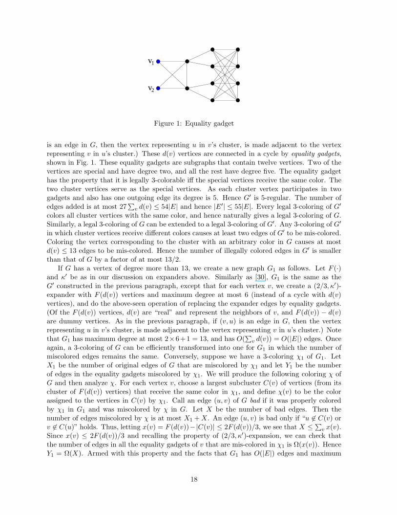
Figure 1: Equality gadget
is an edge in G, then the vertex representing u in v’s cluster, is made adjacent to the vertexrepresenting v in u’s cluster.) These d(v) vertices are connected in a cycle by equality gadgets,shown in Fig. 1. These equality gadgets are subgraphs that contain twelve vertices. Two of thevertices are special and have degree two, and all the rest have degree five. The equality gadgethas the property that it is legally 3-colorable iff the special vertices receive the same color. Thetwo cluster vertices serve as the special vertices. As each cluster vertex participates in twogadgets and also has one outgoing edge its degree is 5. Hence G′ is 5-regular. The number ofedges added is at most 27
∑
v d(v) ≤ 54|E| and hence |E′| ≤ 55|E|. Every legal 3-coloring of G′
colors all cluster vertices with the same color, and hence naturally gives a legal 3-coloring of G.Similarly, a legal 3-coloring of G can be extended to a legal 3-coloring of G′. Any 3-coloring of G′
in which cluster vertices receive different colors causes at least two edges of G′ to be mis-colored.Coloring the vertex corresponding to the cluster with an arbitrary color in G causes at mostd(v) ≤ 13 edges to be mis-colored. Hence the number of illegally colored edges in G′ is smallerthan that of G by a factor of at most 13/2.
If G has a vertex of degree more than 13, we create a new graph G1 as follows. Let F (·)and κ′ be as in our discussion on expanders above. Similarly as [30], G1 is the same as theG′ constructed in the previous paragraph, except that for each vertex v, we create a (2/3, κ′)-expander with F (d(v)) vertices and maximum degree at most 6 (instead of a cycle with d(v)vertices), and do the above-seen operation of replacing the expander edges by equality gadgets.(Of the F (d(v)) vertices, d(v) are “real” and represent the neighbors of v, and F (d(v)) − d(v)are dummy vertices. As in the previous paragraph, if (v, u) is an edge in G, then the vertexrepresenting u in v’s cluster, is made adjacent to the vertex representing v in u’s cluster.) Notethat G1 has maximum degree at most 2×6+1 = 13, and has O(
∑
v d(v)) = O(|E|) edges. Onceagain, a 3-coloring of G can be efficiently transformed into one for G1 in which the number ofmiscolored edges remains the same. Conversely, suppose we have a 3-coloring χ1 of G1. LetX1 be the number of original edges of G that are miscolored by χ1 and let Y1 be the numberof edges in the equality gadgets miscolored by χ1. We will produce the following coloring χ ofG and then analyze χ. For each vertex v, choose a largest subcluster C(v) of vertices (from itscluster of F (d(v)) vertices) that receive the same color in χ1, and define χ(v) to be the colorassigned to the vertices in C(v) by χ1. Call an edge (u, v) of G bad if it was properly coloredby χ1 in G1 and was miscolored by χ in G. Let X be the number of bad edges. Then thenumber of edges miscolored by χ is at most X1 +X. An edge (u, v) is bad only if “u 6∈ C(v) orv 6∈ C(u)” holds. Thus, letting x(v) = F (d(v))−|C(v)| ≤ 2F (d(v))/3, we see that X ≤∑
v x(v).Since x(v) ≤ 2F (d(v))/3 and recalling the property of (2/3, κ′)-expansion, we can check thatthe number of edges in all the equality gadgets of v that are mis-colored in χ1 is Ω(x(v)). HenceY1 = Ω(X). Armed with this property and the facts that G1 has O(|E|) edges and maximum
18
degree 13, we transform G1 into G′ as described in the previous paragraph.
3.4 Preliminaries
Our reduction closely follows that of [11]. The main differences are as follows. (i) The outcomeof the reduction is one-sided dominating set, rather than set cover (which is the same thingtermed differently). (ii) The starting point of the reduction is Max 3-colorability rather thanMax 3SAT. As mentioned earlier, the purpose of this change is to have the reduction applyto one-sided domatic number, rather than just one-sided dominating set. (iii) Every vertex inthe V1 side of the bipartite graph will be duplicated 2l/2 times, where l is a parameter of thereduction. This is a technical condition that seems to be required when we reason about theone-sided domatic number.
To describe the reduction, we recall two notions used in [11].
Definition 3 A (k, l)-Hadamard code is a set of k binary words of length l, where every code-word has Hamming weight l/2 and the Hamming distance between every two codewords is l/2.
There is a simple construction of Hadamard codes when l is a power of 2 and k ≤ l (see,e.g., [27]).
Definition 4 A partition system B(m,L, k, d) has the following properties:• There is a ground set B of m points.• There is a collection of L distinct partitions p1, . . . , pL.• For 1 ≤ i ≤ L, partition pi is a collection of k disjoint subsets whose union is B.• Any cover of the m points by subsets that appear in pairwise different partitions requires atleast d subsets.
The following lemma is proved in [11].
Lemma 16 For every c ≥ 0 and m sufficiently large there is a partition system B(m,L, k, d)whose parameters satisfy the following:• L ≃ (logm)c.• k can be chosen arbitrarily as long as k < lnm
3 ln lnm .• d = (1 − f(k))k lnm, where f(k) → 0 as k → ∞.
Moreover, a random collection of L partitions into k subsets with parameters chosen as abovegives with high probability a partition system with f(k) = 2/k.
The randomized construction can be replaced by a deterministic construction (with a some-what larger value for f(k)) using techniques developed in [29].
The difference from [11]: This reduction is very similar to the one in [11]. Indeed, fora no instance of the NPC language there is no difference at all. In [11] it is proven that a noinstance reduces to a Set-Cover instance with every set-cover being “large”. The only propertyof the intermediate Max 3SAT-5 uses is that the first reduction from a the NPC language to the3-SAT-5 instance, gives a 3SAT-5 instance so that under the best assignment an ǫ fraction of theclauses are unsatisfied. Then, the parallel repetition and the second reduction gives an instanceof the one-sided dominating set problem so that the minimum size of a set-cover is large.
The main difference is in the reduction corresponding to a yes instance of the NPC language.We need to show that the one-sided dominating set instance corresponding to the yes instanceof the NPC problem actually has not only one a “small” one-sided dominating set, but rather“many” vertex-disjoint dominating sets.
19
3.5 The construction
The input to the reduction is a 5-regular graph G(V,E) for which we want to determine whetherit is legally 3-colorable, or whether every 3-coloring of its vertices legally colors at most ψ|E|edges. As noted in Proposition 15, for some explicit ψ < 1 this problem is NP-hard. Thereduction uses the following parameters, which are chosen so that (k, l)-Hadamard codes existand Lemma 16 holds:
• k = l = c log log |V | for some sufficiently large constant c. We assume that l is a powerof 2.
• L = 3l, and m = |V |Θ(l).
The output of the reduction is a bipartite graph G′(V1, V2, E′); when we say “color” below,
we refer to a color-set of 3 colors. The left hand side vertex set V2 is composed of (2|E|)l clustersof vertices, where each cluster contains m vertices. Each left hand side cluster is labeled by asequence of l edges in G and a sequence of l bits; for each i, the ith bit in the bit-sequence denotesone endpoint (vertex) of the ith edge in the edge-sequence. Hence, this sequence of bits can alsobe viewed as a sequence of vertices. The right hand side vertex set V1 is composed of k disjointrays, and each ray is labeled by a codeword of the (k, l)-Hadamard code. Each ray is composedof |V |l/2|E|l/2 clusters, where each cluster contains 6l vertices. Each right hand side clusteris labeled by a sequence of l/2 vertices in G and a sequence of l/2 edges in G. Equivalently,we may merge these two sequences to one sequence of length l, where the codeword of the raycontaining the cluster is used as a selector function specifying the order in which vertices andedges are merged (a vertex when the corresponding bit in the codeword is 0, and an edge whenthe corresponding bit in the codeword is 1). This is called the merged label of a right hand sidecluster. Individual vertices of right hand side clusters are further labeled by a sequence of l/2colors (i.e., a ternary sequence), a sequence of l/2 pairs of distinct colors (i.e., a sequence inbase 6), and a number between 1 and 2l/2. Simple counting shows that for each of the labelingschemes that we defined, the number of available labels is exactly equal to the number of objectsthat need to be labeled.
We say that a left hand side cluster and a right hand side cluster are compatible if theirlabels agree coordinate-wise in the following sense: for coordinate i, if the merged label of theright hand side cluster has an edge, then this is the ith edge in the sequence of edges labelingthe left hand side cluster, and if the merged label has a vertex, then this is the ith vertex inthe sequence of vertices labeling the left hand side cluster. Edges in G′ only connect compatibleclusters (compatibility is necessary but not sufficient, as will be seen shortly). Note that eachleft hand side cluster is compatible with exactly one cluster in each ray. Each right hand sidecluster is compatible with 5l/22l/2 left hand side clusters; the term “5” here arises from the factthat G is 5-regular, and the term “2” follows from the fact that every edge has two end-points.
In order to describe the edge set E′, we use the notion of a partition system. For each lefthand side cluster Cℓ, we have L = 3l partitions with properties as in Definition 4. (Recall thatCℓ has m elements as required by Definition 4.) Each partition is labeled by a sequence of lcolors. This sequence of colors is interpreted as a sequence of colors for the sequence of verticesthat label Cℓ. Note that the same vertex of G may appear several times in the sequence ofvertices that labels Cℓ; we do not require the colors given to this vertex to be the same.
Consider an arbitrary vertex v in a cluster Cr that belongs to ray i. We now describe theset of neighbors that it has in a compatible left hand side cluster Cℓ. Recall that v is labeled
20
by a sequence of l/2 colors and a sequence of l/2 pairs of distinct colors. These colors give ina natural way a coloring for the merged sequence of vertices and edges labeling Cr. The vertexv was also labeled by a number between 1 and 2l/2; this label is ignored when determining theset of neighbors of v (that is, Cr has 2l/2 identical copies of v).
The coloring of the merged sequence of Cr induces in a natural way a coloring for the sequenceof vertices labeling Cℓ. This coloring labels one particular partition p. Vertex v is connected toall vertices (points) of the ith part of partition p (recall that i is the ray to which Cr belongs).This completes the description of E′.
Lemma 17 If G is legally 3-colorable, then the one-sided domatic number of G′ is 6l.
Proof. We first show that G′ has a one-sided dominating set that includes exactly one vertexfrom every right hand side cluster. Consider a sequence of l arbitrary legal 3-colorings of G (thesame legal 3-coloring may appear multiple times in the sequence). Consider now an arbitraryright hand side cluster. It is labeled by a length l merged sequence of vertices and edges. Thesequence of legal 3-colorings induces a coloring on this merged sequence. The cluster containsexactly 2l/2 vertices whose label induces the same coloring. Select one of them arbitrarily to beincluded in the one-sided dominating set.
To show that indeed we have a one-sided dominating set, we need to show that every lefthand side vertex u is covered. Consider the cluster Cℓ to which u belongs. It is labeled by asequence of l edges and a sequence of l vertices. The sequence of legal 3-colorings induces acoloring for the sequence of vertices. This coloring agrees with the name of one partition p. Leti be the part of partition p to which u belongs. Consider the right hand side cluster Cr that iscompatible with Cℓ and belongs to ray i. The vertex selected from Cr necessarily covers u.
We now show that the one-sided domatic number is at least 6l (in fact, it is exactly 6l).Consider an arbitrary legal 3-coloring of G. From it, we can derive 6l distinct length l sequencesof legal 3-colorings, where in each of the l coordinates we put one of the six permutations of thelegal 3-coloring. Each of these sequences gives a one-sided dominating set as described above.We show that these one-sided dominating sets can be chosen to be distinct. This follows fromthe fact that for each sequence of legal 3-colorings and every right hand side cluster, we can have6l/23l/2 equivalence classes of 2l/2 vertices (who differ only in the number they are given in thethird label), and 6l/23l/2 equivalence classes of 2l/2 sequences of colorings (who differ only in theway they color vertices not in the merged sequence of the right hand side cluster). Preservingthe structure of the equivalent classes, we can match the sequences of legal 3-colorings with thevertices of a right hand side cluster.
Lemma 18 If every 3-coloring of G legally colors at most ψ|E| edges, than the smallest one-sided dominating set in G′ is of cardinality at least (1 − o(1))|V1| lnm/6l.
Proof. The proof is essentially identical to that of Lemma 7 in [11] and is omitted.
By making m sufficiently large, we can have lnm ≃ ln |V2|, and the proof of Theorem 11follows.
Acknowledgments
This work appears in preliminary form in [12] and [38].
21

We would like to thank Satoshi Fujita and Mario Szegedy for helpful discussions, and thetwo referees for their helpful comments. The first author is the Incumbent of the Joseph andCelia Reskin Career Development Chair. The research of the first author was supported in partby a Minerva grant. The second author would like to thank Kazuo Iwama at Kyoto Universityfor his hospitality. The last author was supported in part by NSF Award CCR-0208005.
References
[1] N. Alon and J. Spencer. The Probabilistic Method. Wiley, 1992.
[2] S. Arnborg, J. Lagergren, and D. Seese. Easy problems for tree-decomposable graphs.Journal of Algorithms, 12(2):308–340, June 1991.
[3] S. Arora, C. Lund, R. Motwani, M. Sudan, and M. Szegedy. Proof verification and in-tractability of approximation problems. Journal of the ACM 45(3):501–555, 1998.
[4] J. Beck. An algorithmic approach to the Lovasz Local Lemma. Random Structures &Algorithms, 2:343–365, 1991.
[5] C. Berge. Balanced matrices. Math. Programming, 2:19–31, 1972.
[6] M. A. Bonucelli. Dominating sets and domatic number of circular arc graphs. DiscreteAppl. Math., 12:203–213, 1985.
[7] E. J. Cockayne and S. T. Hedetniemi. Towards a theory of domination in graphs. Networks,7:247–261, 1997.
[8] P. Crescenzi and V. Kann. A compendium of NP optimization problems.http://www.nada.kth.se/theory/problemlist.html, 2000.
[9] P. Erdos and L. Lovasz. Problems and results on 3-chromatic hypergraphs and some relatedquestions. In A. Hajnal et al., editor, Infinite and Finite Sets, volume 11 of Colloq. Math.Soc. J. Bolyai, pages 609–627. North Holland, Amsterdam, 1975.
[10] M. Farber. Domination, independent domination, and duality in strongly chordal graphs.Discrete Appl. Math., 7:115–130, 1984.
[11] U. Feige. A threshold of lnn for approximating set cover. J. ACM, 45(2):634–652, 1998.
[12] U. Feige, M. M. Halldorsson, and G. Kortsarz. Approximating the domatic number. InProc. 32nd Ann. ACM Symp. on Theory of Computing, pages 134–143, 2000.
[13] U. Feige and J. Kilian. Zero knowledge and the chromatic number. J. Comput. Syst. Sci.,57:187–199, 1998.
[14] S. Fujita. On the performance of greedy algorithms for finding maximum r-configurations.In Korea-Japan Joint Workshop on Algorithms and Computation (WAAC99), 1999.
[15] S. Fujita, M. Yamashita, and T. Kameda. A study on r-configurations – a resource assign-ment problem on graphs. SIAM J. Disc. Math., 13(2):227–254, 2000.
22
[16] M. R. Garey and D. S. Johnson. Computers and Intractability: A Guide to the Theory ofNP-completeness. Freeman, 1979.
[17] O. Goldreich, S. Micali, and A. Wigderson. Proofs that yield nothing but their validity orall languages in NP have zero-knowledge proofs. J. ACM, 38(3):691–729, 1991.
[18] T. W. Haynes, S. T. Hedetniemi, and P. J. Slater. Domination in Graphs: Advanced Topics.Marcel Dekker, 1998.
[19] T. W. Haynes, S. T. Hedetniemi, and P. J. Slater. Fundamentals of Domination in Graphs.Marcel Dekker, 1998.
[20] D. S. Johnson. Approximation algorithms for combinatorial problems. J. Comput. Syst.Sci., 9:256–278, 1974.
[21] H. Kaplan and R. Shamir. The domatic number problem on some perfect graph families.Inf. Process. Lett., 49(1):51–56, 1994.
[22] S. Khanna, M. Sudan, and D. Williamson. A complete classification of the approximabilityof maximization problems derived from Boolean constraint satisfaction. In Proc. 29th Ann.ACM Symposium on Theory of Computing, pages 11–20, 1997.
[23] J. Kratochvıl. Regular codes in regular graphs are difficult. Discrete Math., 133:191–205,1994.
[24] L. Lovasz. On the ratio of optimal integral and fractional covers. Discrete Math., 13:383–390, 1975.
[25] A. Lubotzky, R. Phillips and P. Sarnak. Ramanujan graphs. Combinatorica, 8:261–277,1988.
[26] C. Lund and M. Yannakakis. On the hardness of approximating minimization problems. J.ACM, 41(5):960–981, 1994.
[27] F. MacWilliams and N. Sloane. The Theory of Error Correcting Codes. North Holland,1983.
[28] M. V. Marathe, H. B. Hunt III, and S. S. Ravi. Efficient approximation algorithms fordomatic partition and on-line coloring of circular arc graphs. Discrete Appl. Math., 64:135–149, 1996.
[29] M. Naor, L. Schulman, and A. Srinivasan. Splitters and near-optimal derandomization. InProc. 36th Ann. IEEE Symp. on Found. of Comp. Sci., pages 182–191, 1995.
[30] C. H. Papadimitriou and Y. Yannakakis. Optimization approximation and complexityclasses. JCSS 43(3): 425-440 (1991)
[31] A. Paz and S. Moran. Nondeterministic polynomial optimization problems and their ap-proximations. Theoretical Comput. Sci., 15:251–277, 1981.
[32] S. L. Peng and M. S. Chang. A simple linear time algorithm for the domatic partitionproblem on strongly chordal graphs. Inf. Process. Lett., 43:297–300, 1992.
23

[33] E. Petrank. The hardness of approximation: Gap location. Comput. Complexity, 4:133–157,1994.
[34] A. Proskurowski and J. A. Telle. Complexity of graph covering problems. Nordic J. Com-puting, 5:173–195, 1998.
[35] P. Raghavan. Probabilistic construction of deterministic algorithms: approximating packinginteger programs. J. Comput. Syst. Sci., 37:130–143, 1988.
[36] R. Raz. A parallel repetition theorem. SIAM J. Comput., 27(3):763–803, 1998.
[37] A. S. Rao and C. P. Rangan. Linear algorithm for domatic number problem on intervalgraphs. Inf. Process. Lett., 33:29–33, 1989.
[38] A. Srinivasan. Domatic partitions and the Lovasz Local Lemma. In Proc. Twelfth ACM-SIAM Symp. on Discrete Algorithms, 2001. To appear.
[39] B. Zelinka. Domatic number and degree of vertices of a graph. Math. Slovaca, 33:145–147,1983.
A Multicoloring version
In the domatic multi-partition problem, we are additionally given an integral weight x : V 7→ Nindicating in how many dominating sets each vertex can appear. The domatic number problemhas x(v) = 1, for each v; the r-Conf problem of [15] has x(v) = r, for each v.
We can reduce the multi-partition problem to the ordinary partition problem. Given a graphG and weight vector x, form a graph G′ as follows. G′ has x(v) copies of each vertex v connectedas a clique. For each edge uv in G, the copies of u and v form a complete bipartite graph inG′. Any minimal dominating set in G′ is also a dominating set in G, and taking one copy ofeach vertex of a dominating set in G also gives a dominating set in G′. Further, a domaticpartition of G′ is in one-to-one correspondence with a multi-partition of G (within the weightconstraints). Thus, the results obtained in this paper for the domatic number problem carryover to the domatic multi-partition problem, replacing δ by minv d(v)x(v) and n by
∑
v x(v).
B Overview of some ingredients from [11]
Parallel repetition of two-prover proof systems: There is a straightforward one-roundtwo-prover proof system for Max 3-colorability-5 that has the following properties: on yes in-stances, the verifier always accepts, and on no instances (when at most a (1− ǫ) fraction of theedges can be legally colored simultaneously) the verifier accepts with probability at most 1−ǫ/2.Give a 5-regular graph G, the proof system proceeds as follows. The verifier sends to the firstprover a random edge in G, and to the second prover a random vertex from that edge. Wecall this vertex the common vertex. It is important that the first prover does not know whichendpoint of the edge is the common vertex, and that the second prover does not know whichedge was received by the first prover. The first prover replies with two different colors (out ofthe three allowable colors) for the two vertices that are the endpoints of the edge. The secondprover replies with a color for the common vertex. The verifier accepts only if the two proversgive the same color to the common vertex. For a yes instance G the two provers can answer
24
according to the global legal 3-coloring and ensure that the verifier accepts with probability 1.For a no instance G, regardless of the strategy of each prover (where a strategy is a functionfrom questions to answers), the acceptance probability is at most 1 − ǫ/2, where probability iscomputed over the random choices of the verifier.
The l-fold parallel repetition of this one-round two-prover proof system is as follows. Theverifier sends to the first prover a tuple of l random edges and to the second prover a tupleof l random vertices, one from each of these edges. Each prover replies with colors to all thevertices that it receives. The verifier accepts if on every one of the l common vertices, the twoprovers agree on the color that they give. It is not hard to see that on yes instances, the proversstill have a strategy that makes the verifier accept with probability 1. The parallel repetitiontheorem [36] shows that on no instances, the verifier accepts with probability at most (1 − ǫ)cl,where c is a constant (that depends on ǫ).
Separating codes and k-provers: To eventually get ≃ lnn hardness of approximation re-sults, two-prover proof systems are extended to k-prover systems in a special way. As in thetwo-prover proof system, the verifier selects l edges at random and a random vertex within eachedge. This gives a total of (2|E|)l possible queries. Each of the k provers is sent some subsetof the l edges and l vertices using the following rule. A (k, l)-Hadamard code is a collection ofk binary words of length l each, for which the Hamming distance between any pair of wordsis “large” (specifically, l/2). With each prover we associate one codeword from the Hadamardcode. The verifier sends to each prover l/2 edges and l/2 vertices, selected according to the 1’sand 0’s in the codeword of the respective prover. Namely, if the ith bit in the code is 1, thenext entry in the query is the respective ith edge (among the l edges in the tuple). If the ithentry is 0, the ith vertex in the vertex tuple is sent. Considering separately two of the provers,the fact that their codewords have a large Hamming distance implies that in many coordinatesone prover will receive an edge while the other prover will receive a vertex on this edge. Thisis similar to the scenario in the two-prover proof system. Intuitively, we may view the k-proverproof system as
(k2
)
correlated two-prover proof systems going on in parallel. It is natural to
have the verifier accept if all(k2
)
proof systems are accepting. The definition of acceptance usedin [11] is more subtle and will not be discussed in this overview.
Next a bipartite graph G′(V1, V2, E′) is built based on this scenario. Specifically, the vertices
in V1 describe the provers/queries schema. The set V1 corresponds to the provers and is parti-tioned into k “rays” V j
1 , 1 ≤ j ≤ k, one ray for each prover. The sets V k1 are further partitioned
into disjoint subsets V j1 (Q), where Q ranges over all the |V |l/2|E|l/2 possible questions that a
prover can receive. On each possible question, the prover must answer with a coloring of thel/2 edges and l/2 vertices received. Thus, the V j
1 (Q) sets are further divided into all possibleanswers. Therefore, there are 3l/2 · 6l/2 points inside V j
1 (Q) in this final division; a point foreach possible coloring of the l/2 vertices and l/2 edges. In addition, for technical reasons, eachpoint (possible answer) of each prover is duplicated 2l/2 times.
Ground sets and random partitions: To determine the structure of V2, some ideas essen-tially due to [26] (and extended in [11]) are used.
The set V2 is partitioned into (2|E|)l ground sets Cℓ, one ground set per each possible query.Each ground set contains m points for m = |V |Θ(l). It is instructive to note the followingasymmetry. Given a query namely a sequence of l edges and l corresponding endpoints for theedges, consider its corresponding ground set in V2. There are exactly k sets V j
1 (Q) that arecompatible with this sequence, one per prover (since the question to the provers is completely
25
determined by the Hadamard code). On the other hand, given a question cluster V j1 (Q), many
possible query-base ground sets in V2 could have caused this question. Indeed, since the questioncontains only l/2 edges and l/2 vertices, this partial information can be completed in 5l/22l/2
ways to give compatible l edges and l vertices. Each vertex sent to this prover has 5 neighborsand thus 5 ways of “completing” this vertex into a (compatible) edge. For each edge sent to thisprover, there are 2 possibilities for which of the two vertices to put in the resulting query.
We use L = 3l random partitions of Cℓ, each partitioning Cℓ into k parts. Consider thel-tuple of vertices in a possible query (namely, the part of the query corresponding to the chosenvertices, one per each edge). Note that the number L = 3l of partitions of each ground setexactly equals the number of possible colorings 3l of the vertices in that query. We can thusform a 1-1 correspondence between the 3l partitionings and the 3-coloring (not necessarily aconsistent one) of the l vertices in the query base. Each partition is now regarded as a coloring,and vice-versa. Recall that a point in the final sub-partition cluster of V1 corresponds to ananswer to the coloring of the query of l/2 edge/vertex pairs. This corresponds to a coloring ofthe l vertices of the cluster Cℓ, hence gives a vertex coloring, and thus a partition of Cℓ. Theedges between the vertices of V1 and V2 are defined as follows. Each vertex (namely, coloring oranswer) v ∈ V j
1 (Q) is connected to the jth part of the partition corresponding to v (as v is acoloring, a partition is also associated with v).
Now, consider the graph G′ resulting from a 3-colorable graph G. We can choose one point(answer) per each question-cluster in V1, so as to cover each Cℓ. Thus all the Cℓ are coveredusing at most k · (2 ·E)l vertices. This will happen if the provers use strategies which are allpart of a global 3-coloring, and this gives a small dominating set. On the other hand, considerthe resulting graph G′ when only 1 − ǫ of the edges of G can be simultaneously legally colored.Because of the parallel repetition which greatly increases the gap, the provers essentially cannotuse a joint strategy. This means that each pair of answers vj ∈ V j
1 (Q), vq ∈ V q1 (Q) chosen,
corresponds to two different colorings. Hence a ground set Cℓ is essentially covered via randomsets each containing m/k random elements of Cℓ. Thus, the number of elements needed in orderto cover Cℓ is roughly k lnm. This gives a total of roughly k · (2 ·E)l ln |V ′| minimum one-sideddominating set for a logarithmic gap.
Zero knowledge and the domatic number: Given the fact that a single “small” one-sideddominating set exists, we can permute the colors (as done in zero-knowledge protocols in orderto “hide” information) to show the existence of “many” disjoint dominating sets, hence a “large”domatic number. Namely, once a 3-coloring of G exists, one gets 6 legal colorings for G. Thisimplies a total of 6l colorings (which can be completed into global coordinatewise-compatiblecolorings) of any l tuple of vertices. The possibility for color permutation was the main reasonfor reducing from a coloring and not a satisfiability problem. Hence, we either get many smalldominating sets which implies a large one-sided domatic number, or any dominating set is large,which gives a a small one-sided domatic number.
26
Copyright © 2022 FDOKUMEN