Approximating the condition and maximum load of an engine ...

Aalto University

School of Electrical Engineering

Isak Frants

Approximating the condition and maximum load of an engine

by comparing engine measurements

School of Electrical Engineering

Master’s Thesis submitted in partial fulfilment of the requirements for the degree of Master

of Science in Technology.

Espoo, 8.9.2016

Supervisor:

Docent, D.Sc. Kai Zenger

Advisor:

M.Sc. Sören Hedvik

Abstract

AALTO UNIVERSITY

SCHOOL OF ELECTRICAL ENGINEERING

ABSTRACT OF THE MASTER’S

THESIS

Author: Isak Frants

Title: Approximating the condition and maximum load of an engine by comparing

engine measurements

School: School of Electrical Engineering

Department: Department of Electrical Engineering and Automation

Professorship: Control Engineering Code: AS-74

Supervisor: Docent, D.Sc. Kai Zenger

Instructor: M.Sc. Sören Hedvik

This thesis discusses how an estimation of an engine’s condition and maximum load can

be calculated from online engine parameter measurements. The calculated engine index is

usable when loading engines, as it enables engines to be loaded more efficiently based on

the actual load capacity. This increases the engines’ total power output, as load reductions

may be avoided.

The purpose of the thesis is to identify the most critical engine parameters needed to

produce a usable index and to develop and test this index. Additionally, the situations and

usability areas where the index is beneficial shall be presented.

The thesis proposes that two indexes shall be calculated by using measurements from the

exhaust gas temperatures, cylinder pressure and turbocharger speed. The indexes express

the engine’s load capacity differently and are assumed to provide various benefits in

situations such as engine diagnostics and control.

Date: 9/8/2016 Language: English Number of pages: 8 +

74

Keywords: estimation, adaptivity, load availability, condition

Abstract (in Swedish)

AALTO-UNIVERSITETET

HÖGSKOLAN FÖR ELEKTROTEKNIK

SAMMANDRAG AV DIPLOMARBETET

Författare: Isak Frants

Titel: Estimering av en motors kondition och maximala last genom kombinering av

mätvärden

Högskola: Högskolan för elektroteknik

Institution: Institutionen för elektronik och automation

Professur: Reglerteknik Kod: AS-74

Övervakare: Docent, TkD Kai Zenger

Handledare: DI Sören Hedvik

I detta arbete kartläggs möjligheterna att räkna ut ett estimat av en motors kondition och

maximala last utgående från motorns mätvärden. Detta motorindex är användbart vid

fördelning av last på motorer, eftersom motorer kan lastas mer effektivt utgående från

motorernas verkliga lastkapaciteter. Detta leder till förbättrad total motoreffekt eftersom

lastreduktioner kan undvikas.

Arbetets syfte är att identifiera de mest kritiska motorparametrarna som krävs för att räkna

ut ett användbart index, samt att utveckla och testa indexet. Utöver detta ska även de

situationer där indexet är användbart kartläggas och presenteras.

Arbetet resulterade i skapandet av två index, vilka använder sig av mätvärden från

avgastemperaturer, cylindertryck och turbons varvtal. Indexen uttrycker mottorns last-

kapacitet på olika sätt och antas därmed ge fördelar i ett flertal situationer såsom motor-

diagnostik och motorreglering.

Datum: 8.9.2016 Språk: engelska Sidantal: 8 + 74

Nyckelord: estimation, adaptivitet, lasttillgänglighet, kondition

iv

Preface

This thesis was conducted at the Engine Performance & Control department during the

spring of 2016 at Wärtsilä, Vaasa. I want to thank Sören Hedvik for offering this

opportunity and for helping out in the process of finding a suitable subject. This work

would not have existed without his efforts. Tommy Dahlberg aided me throughout the

thesis process by pointing me in the right directions, giving helpful advice and

proofreading the thesis. Kai Zenger provided the academic input to this work and

guided me through the finalization process. Many thanks to all of you!

This work would not have been possible to accomplish without a few persons.

Christer Hattar provided exceptional engine performance expertise and answered every

question asked. Jens Vägar gave at numerous times important input to the thesis from a

condition based maintenance point of view. Tom Kaas have developed the adaptive

maps used in the index calculations and commented on my ideas and implementations

several times. These three persons aided vastly in the thesis process and I can only

salute you for taking time to answer my questions!

Various engine experts provided necessary engine technology information and

these were Anders Åberg, Ari Saikkonen, Kimmo Nuormala, Kaj Portin, Niklas Wägar,

Robert Lundström and Thomas Masus. All of these gentlemen provided without

hesitation feedback and answers when needed. Furthermore, around 15 experts have

commented on my ideas and provided support during the development process. Thank

you all for your support, comments and ideas!

The co-operation and communication with everyone mentioned here by name

worked flawlessly, and this is something to emphasize, as this benefit was unfortunately

not always available. Writing a master’s thesis has been an interesting task and I have

acquired greater understanding of engines and their technologies. I am especially proud

of the straightforward workflow, as research and development were conducted one step

at a time and the research questions remained practically unmodified throughout the

project. The thesis is now complete, ending one of the best chapters in my life with

studies in Otaniemi, while starting a new one with new opportunities and possibilities.

Espoo 8.9.2016

Isak Frants

v

Table of contents

Abstract ............................................................................................................................. ii

Abstract (in Swedish) ....................................................................................................... iii

Preface ............................................................................................................................. iv

Table of contents ............................................................................................................... v

Symbols .......................................................................................................................... vii

Abbreviations ................................................................................................................. viii

1 Introduction ............................................................................................................... 1

1.1 Introduction and purpose .................................................................................... 1

1.2 Research questions and limitations .................................................................... 2

1.3 Previous research and outline............................................................................. 2

1.4 Wärtsilä .............................................................................................................. 3

2 Engine technology .................................................................................................... 4

2.1 Wärtsilä engines and their automation ............................................................... 4

2.1.1 Engine overview ......................................................................................... 4

2.1.2 The engine automation system ................................................................... 6

2.1.3 Condition monitoring generally .................................................................. 9

2.1.4 Condition monitoring with Wärtsilä Genius services ................................. 9

2.2 Load sharing and load reduction ...................................................................... 10

2.2.1 The speed/load controller .......................................................................... 10

2.2.2 Load sharing challenges ............................................................................ 11

2.2.3 The load reduction functionality ............................................................... 13

2.2.4 Engine de-rating ........................................................................................ 16

3 Index development .................................................................................................. 19

3.1 Index requirements and assumptions ............................................................... 19

3.1.1 Benefits and usage .................................................................................... 19

3.1.2 Load reduction parameters ........................................................................ 20

3.1.3 Engine performance parameters ............................................................... 23

3.2 Index presentation and calculation ................................................................... 25

3.2.1 Index concepts .......................................................................................... 25

3.2.2 The condition index .................................................................................. 26

3.2.3 The load availability index ....................................................................... 29

3.2.4 Adaptive indexes ....................................................................................... 30

vi

3.3 Parameters included ......................................................................................... 32

4 Index evaluation ...................................................................................................... 35

4.1 The simulation setup ........................................................................................ 35

4.2 The Simulink model ......................................................................................... 37

4.2.1 Model overview ........................................................................................ 37

4.2.2 Inputs ........................................................................................................ 38

4.2.3 Calculations .............................................................................................. 40

4.2.4 Outputs ...................................................................................................... 42

4.2.5 Model usage .............................................................................................. 43

4.3 Test and model configuration ........................................................................... 46

4.4 Results .............................................................................................................. 47

4.4.1 Load and other aspects .............................................................................. 47

4.4.2 High turbocharger speeds ......................................................................... 48

4.4.3 High exhaust gas temperatures ................................................................. 51

4.4.4 High cylinder pressures ............................................................................ 52

4.4.5 History and engine comparison ................................................................ 53

5 Discussion ............................................................................................................... 55

5.1 Index development ........................................................................................... 55

5.2 Adaptivity ......................................................................................................... 57

5.3 Further research ................................................................................................ 59

6 Conclusion .............................................................................................................. 60

References ....................................................................................................................... 61

Appendix A – The data loading script ............................................................................ 64

Appendix B – The simulation and plotting script ........................................................... 66

Appendix C – The script help functions ......................................................................... 71

Appendix D – The C functions ....................................................................................... 73

vii

Symbols

yLR Load reduction setpoint

yM Measured instrument value

yNOM Nominal instrument value

yOFF Difference between measured and nominal instrument value

yREAL Nominal instrument value with offset added

xLOAD Engine load

viii

Abbreviations

CA Charge Air

CI Condition Index

CM Condition Monitoring

CR Common Rail engine

CBM Condition Based Maintenance

CCM Cylinder Control Module

DF Dual Fuel engine

DMP Dynamic Maintenance Planning

EHM Engine Health Management

ESM Engine Safety Module

EFIC Electronic Fuel Injection Control

FAT Factory Acceptance Test

FAKS Fault Avoidance Knowledge System

HT High Temperature

HFO Heavy Fuel Oil

IOM Input Output Module

ISO (1) International Organization for Standardization

ISO (2) Wärtsilä standardized instrument code and description

LAI Load Availability Index

LCP Local Control Panel

LDU Local Display Unit

LT Low Temperature

LHV Lower Heating Value

MCM Main Control Module

PDM Power Distribution Module

PMS Power Management System

SG Spark ignited Gas engine

STM Self-Tuning Map

TC Turbocharger

UNIC Wärtsilä Unified Controls

WSDE Wärtsilä Simulink Development Environment

1 Introduction

This chapter introduces the thesis background, methods and purpose. The research

questions are listed along with the limitations applied to the index development work.

Previous research is discussed at the end of the chapter, followed by a brief presentation

of Wärtsilä.

1.1 Introduction and purpose

Multi-engine control is a wide subject and the thesis will focus on one particular point

of interest of this subject. The topic focus is the optimal loading and sharing of load

between engines, as it has become clear that these could be vastly improved to prevent

potential load reductions. Load reductions are machinery protection functions which

lowers the load on engines to protect them from damage. These are highly disturbing to

the operation because decreased load means less produced electricity or thrust, which is

not a desirable situation for the operator of a power plant or a ship. It should be possible

to share the load in a more preventive way by measuring and analysing the engine’s

ability to increase its load. The load should not necessarily be equally shared and

continuously increased during transients, as this increases the risk for unexpected load

reductions. Instead, engines are monitored and their load availability is calculated, and

only engines which can increase their load can be more heavily loaded. The loading is

performed by the power management system (PMS) in power plants or the auxiliary

system in marine applications. In this way the load is shared between engines according

to their load capacity, and this lowers the risk for load reductions.

The purpose of the thesis is to identify the parameters which can indicate the

load capacity of an engine and to develop an algorithm that describes the engine’s

instantaneous load availability as an index using the statuses of these parameters. The

index defines the operation margin of each engine to the risk zone where potential load

reductions can activate. Many different aspects, such as cylinder knock statuses, various

temperatures and pressures, can be taken into account when defining the risk zone and

these have to be identified and their importance evaluated and weighed. The result of

the thesis is a solution to the problem of how the overall state of an engine can be

calculated in a way that is assumed to be good enough for actual usage in load sharing

and plant load shedding. The main benefit for power plants is economical, as the index

provides the PMS with the engines’ load abilities. This allows ramping up of load on

engines with sufficient load ability fast enough to sell electricity when the price is

beneficial for the plant owner.

Parameters are identified and their importance evaluated in cooperation with

engine performance experts through interviews and discussions. Existing engine

machinery protection and safety specifications clearly specify the properties of the load

reductions and the conditions that must be met before load reductions activate.

Sufficient material for developing the index calculation is received by these two means.

The final index is implemented and tested using real engine data in Simulink. This was

decided to be the best option for testing and demonstration, as other options involved

noticeable time and efforts from application developers. Additionally, it suits well the

purpose of being a proof of concept that demonstrates the benefits of an index that can

indicate the load capacity of an engine. The simulations do not involve load sharing, as

it was seen enough to only demonstrate the index calculation.

2

1.2 Research questions and limitations

It is important to emphasize that not all engine parameters can nor should be included in

the index as the calculations easily become too complex. In fact, only a few parameters

will be taken into account to keep the scope realistic and to develop an index that

actually works instead of being too slow and complex to achieve anything useful. The

simplifications affect the accuracy of the index and its sufficiency will thus have to be

evaluated. Moreover, it is unclear whether one index will be enough or if a group of

indexes with varying complexity is a more preferable solution. It lies within the scope

of this thesis to also explain in which situations it is beneficial and when it is not. The

thesis will hence address the following questions:

Which parameters should at the very least be used by the load capacity index?

Is one index enough or is a group of indexes a better solution?

When and how should the index be used?

The scope of the thesis does not cover any control or demonstrations of load sharing

based on the calculated index. It is only seen as diagnostics of one engine in a static

situation to support other control algorithms. This limitation follows as the work would

otherwise expand uncontrollably and there is a risk of it failing to provide any usable

result at all. The same limitation and reasoning applies to the amount of parameters

taken into account; not all can be integrated and a realistic approach is prioritized to

achieve a working but simplified solution. Such solution can later be expanded and

improved when needed.

1.3 Previous research and outline

Considerable efforts were made to identify previous research about engine load capacity

estimation, load operation margin, load calculation and other similar topics. No paper

was found that discussed the previous topics in a way that would support this thesis

noticeably. Different ways of calculating or estimating the load of an engine can be

found in literature [1-4]. However, no research exist that would discuss estimation or

calculation of an engine’s present load capacity or load margin. The reason for this

could be that the load margin is set by the engine’s safety configuration. Determining

the load margin of engines without a safety system is trivial, as it follows directly from

comparison of the engine’s present load and rated maximum load. No information was

found about engine safety systems similar to the one found on Wärtsilä engines. Hence,

this thesis is the first of its kind in this field and the methods and results here cannot be

compared to any previous research.

The outline of the thesis is as follows. Chapter 1 introduces the reader to the

thesis subject and presents Wärtsilä briefly. Chapter 2 presents the theory needed for the

index development. This includes presentation of the engine automation system and its

functionalities, such as load sharing and load reduction. The index development takes

place in Chapter 3, where the index is derived and the possibilities and requirements are

explained. Index testing is carried out in Chapter 4, where the simulation model, tests

and results are presented. The results are discussed and analysed in Chapter 5, while

Chapter 6 ends the thesis by summarising the work and proposing future research.

3

1.4 Wärtsilä

Wärtsilä was established in 1834, when a sawmill was built in the East of Finland in the

municipality of Tohmajärvi. The diesel engine era started in 1938 when Wärtsilä signed

a licence agreement with Friedrich Krupp Germania Werft AG in Germany. Wärtsilä

started its international era in 1978, when 51 % of the shares in NOHAB diesel business

in Sweden were acquired. The company has continuously evolved during its 182 years

and is now a global corporation and a leading expert in energy solutions in both marine

and power plant segments. Its expertise could clearly be seen during the summer of

2015 when Wärtsilä started manufacturing the new W31 engine. This engine was

announced by the Guinness World Records to be the world’s most efficient 4-stroke

diesel engine. Wärtsilä has in 2015 approximately 18800 employees globally and

approximately 3600 of these work in Finland. These numbers vary from year to year as

Wärtsilä, like many other companies, have employee co-operation negotiations

occasionally. [5],[6],[7]

Wärtsilä is divided into three main sectors: Marine Solutions, Energy Solutions

and Services. The first two were established in July 2015, when the sectors Ship Power

and Power Plant were renamed to better represent the wide range of products and

services which these sectors offer. In rough numbers, 30 % of the personnel work in

Marine Solutions, 10 % in Energy solutions and 60 % in Services. The Service sector

grows as Marine Solutions and Energy Solutions deliver more engines and other

products and solutions to the customers. The sector focuses on customer needs and

offers support, maintenance and service whenever and wherever needed. [8]

4

2 Engine technology

This chapter introduces the theory needed for the index development. The components

of an engine are presented along with the engine automation system that controls and

monitors it. The index describes the engine’s ability to take load and this can be seen as

an indicator of the condition of the engine; its ability to do work. Thus, the existing

engine condition monitoring and its methods and usage are introduced. The load

sharing, the load reduction and de-rating functionalities are explained, as these are

central technologies which affect the engine load.

2.1 Wärtsilä engines and their automation

2.1.1 Engine overview

The main components of an engine are presented here to show what components an

engine consists of and to improve the understanding of the engine automation system

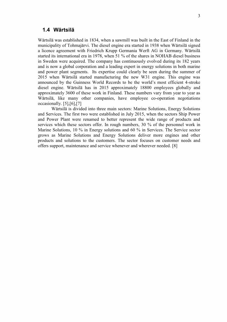
tasks. The presented components are for the in-line W34DF engine which has gas as

well as diesel components. An overview of this dual-fuel (DF) engine can be seen in

Figure 1, followed by brief descriptions of the main components [9].

Figure 1. An in-line engine with some components highlighted. Figure modified from [9].

Engine block

The engine block is the base module for the engine, made in one piece of iron and

designed to absorb the forces from the running engine. The rest of the components are

attached to the engine block.

Crankshaft and main bearings

The crankshaft is the long mechanism beneath the cylinders which converts the linear

motion of the pistons to rotational motion. It is forged in one piece and connected to the

engine block via the main bearings.

5

Connection rod and big end bearings

The connection rods connect the pistons to the crankshaft and the big end bearings are

located between these components.

Cylinder liner, piston and piston rings

The cylinder liner is the cylinder in which the piston moves up and down. The piston is

connected to the connection rod and the piston rings seal the combustion chamber

located above the piston.

Cylinder head

The cylinder head is the top piece of the engine with valves and inlets and outlets for

air, fuel, cooling water and exhaust gases.

Camshaft, camshaft drive and valve mechanism

The camshaft is similar to the crankshaft, but converts rotational motion into linear

motion used by the valve mechanism. The camshaft drive is the gearbox between the

crankshaft and the camshaft.

Fuel system

The main parts of the fuel system are the gas-, the main fuel- and the pilot fuel injection

system which consist of various valves and vents. The fuel gas system and the pilot

injection system are used when the engine is in gas mode. The main fuel oil injection

system and the pilot injection system are in use when the engine is in diesel mode. The

engine is in backup mode if only the main fuel oil injection system is used. The pilot

system is replaced by spark plugs on gas (SG) engines.

Exhaust pipes

The exhaust pipes are made of heat resistant nodular cast iron alloy and connected to the

cylinder head. They are insulated with mineral wool and lead the exhaust gases out from

the engine.

Lubricating oil system

The lubricating oil system provides lubrication and cooling to components such as the

piston and the crankshaft. It consists of two pumps, a valve, filters and a lubricating oil

cooler.

Cooling system

The water cooling system consists of a high (HT) and a low temperature (LT) circuit.

The first one cools cylinder heads and liners and the first stage of the charge air (CA)

cooler. The second one cools the second stage of the CA cooler and the lubricating oil.

Turbocharging and charge air cooling

The turbocharger (TC) produces compressed air that is combined with fuel and injected

into the cylinder. An engine with two cylinder banks, a V-engine, has two turbochargers

and an in-line engine has one. The charge air cooler consists of two stages; a high and a

low temperature stage.

Automation system

The engine automation system is the Wärtsilä Unified Controls (UNIC) and is presented

in Subsection 2.1.2.

6

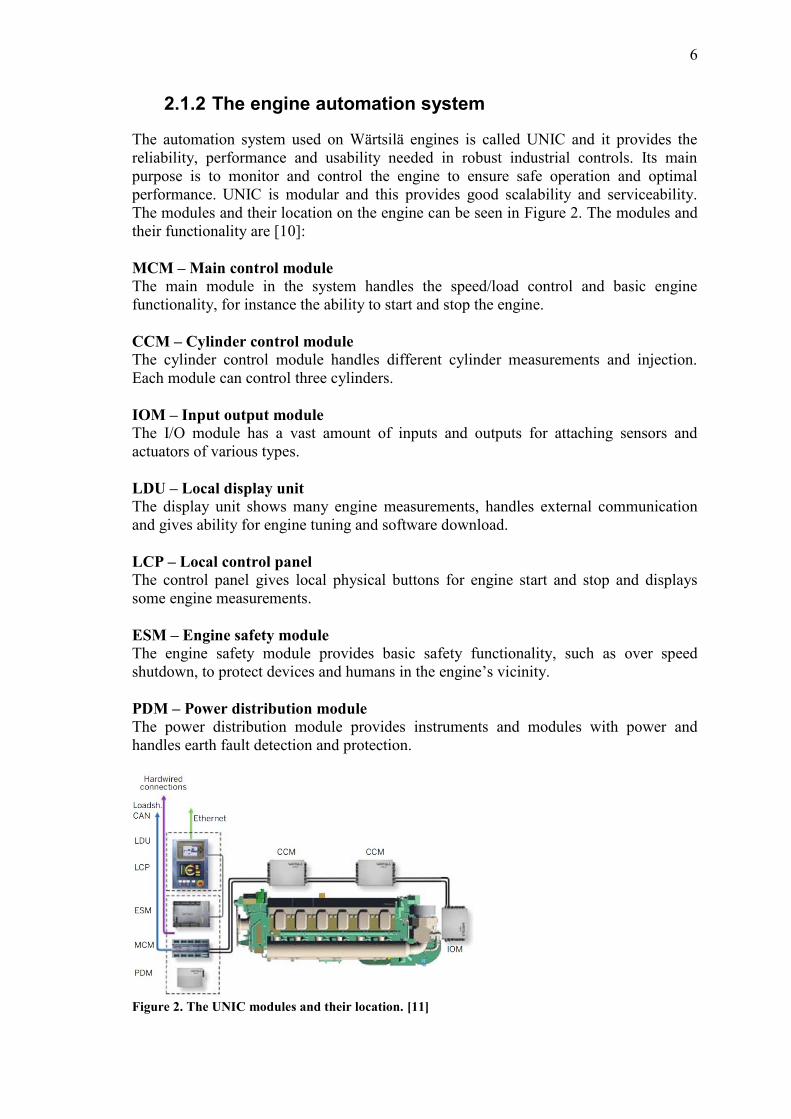
2.1.2 The engine automation system

The automation system used on Wärtsilä engines is called UNIC and it provides the

reliability, performance and usability needed in robust industrial controls. Its main

purpose is to monitor and control the engine to ensure safe operation and optimal

performance. UNIC is modular and this provides good scalability and serviceability.

The modules and their location on the engine can be seen in Figure 2. The modules and

their functionality are [10]:

MCM – Main control module

The main module in the system handles the speed/load control and basic engine

functionality, for instance the ability to start and stop the engine.

CCM – Cylinder control module

The cylinder control module handles different cylinder measurements and injection.

Each module can control three cylinders.

IOM – Input output module

The I/O module has a vast amount of inputs and outputs for attaching sensors and

actuators of various types.

LDU – Local display unit

The display unit shows many engine measurements, handles external communication

and gives ability for engine tuning and software download.

LCP – Local control panel

The control panel gives local physical buttons for engine start and stop and displays

some engine measurements.

ESM – Engine safety module

The engine safety module provides basic safety functionality, such as over speed

shutdown, to protect devices and humans in the engine’s vicinity.

PDM – Power distribution module

The power distribution module provides instruments and modules with power and

handles earth fault detection and protection.

Figure 2. The UNIC modules and their location. [11]

7

The modules are interconnected with a multi-bus cable which includes all the needed

signals in one single cable. These are all doubled for redundancy reasons and include

power supply, engine speed and phase, limp bus and CAN. The two existing CAN

cables are used for communication by interconnected modules. Figure 2 shows the

communication redundancy in UNIC as two CAN cables connect the MCM, CCMs and

IOMs to each other. Both cables are utilized as long as they are available and all CAN

messages are moved to the working cable if the other breaks. An additional CAN cable,

the dedicated load sharing CAN cable, may be installed and used when multiple engines

are connected and the load is shared between them in Isochronous Load Sharing mode.

The external Ethernet communication is available via the LDU module. This

communication link allows UNIC data to be read remotely, from outside the machine

room. [9],[12]

The engines are equipped with instruments which provide UNIC with data and

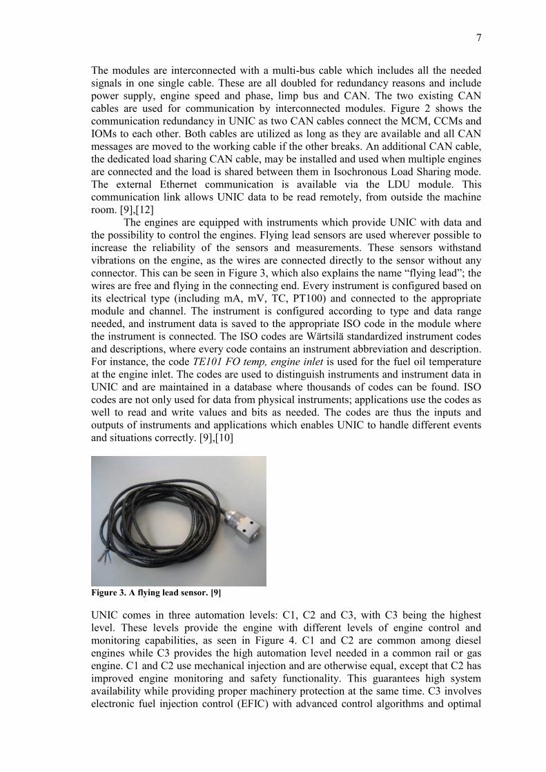
the possibility to control the engines. Flying lead sensors are used wherever possible to

increase the reliability of the sensors and measurements. These sensors withstand

vibrations on the engine, as the wires are connected directly to the sensor without any

connector. This can be seen in Figure 3, which also explains the name “flying lead”; the

wires are free and flying in the connecting end. Every instrument is configured based on

its electrical type (including mA, mV, TC, PT100) and connected to the appropriate

module and channel. The instrument is configured according to type and data range

needed, and instrument data is saved to the appropriate ISO code in the module where

the instrument is connected. The ISO codes are Wärtsilä standardized instrument codes

and descriptions, where every code contains an instrument abbreviation and description.

For instance, the code TE101 FO temp, engine inlet is used for the fuel oil temperature

at the engine inlet. The codes are used to distinguish instruments and instrument data in

UNIC and are maintained in a database where thousands of codes can be found. ISO

codes are not only used for data from physical instruments; applications use the codes as

well to read and write values and bits as needed. The codes are thus the inputs and

outputs of instruments and applications which enables UNIC to handle different events

and situations correctly. [9],[10]

Figure 3. A flying lead sensor. [9]

UNIC comes in three automation levels: C1, C2 and C3, with C3 being the highest

level. These levels provide the engine with different levels of engine control and

monitoring capabilities, as seen in Figure 4. C1 and C2 are common among diesel

engines while C3 provides the high automation level needed in a common rail or gas

engine. C1 and C2 use mechanical injection and are otherwise equal, except that C2 has

improved engine monitoring and safety functionality. This guarantees high system

availability while providing proper machinery protection at the same time. C3 involves

electronic fuel injection control (EFIC) with advanced control algorithms and optimal

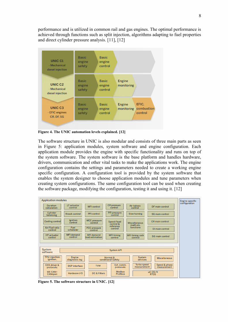
8

performance and is utilized in common rail and gas engines. The optimal performance is

achieved through functions such as split injection, algorithms adapting to fuel properties

and direct cylinder pressure analysis. [11], [12]

Figure 4. The UNIC automation levels explained. [12]

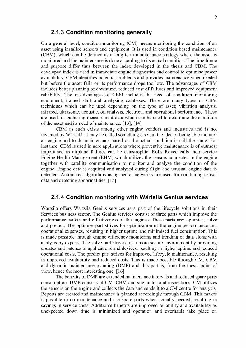
The software structure in UNIC is also modular and consists of three main parts as seen

in Figure 5: application modules, system software and engine configuration. Each

application module provides the engine with specific functionality and runs on top of

the system software. The system software is the base platform and handles hardware,

drivers, communication and other vital tasks to make the applications work. The engine

configuration contains the settings and parameters needed to create a working engine

specific configuration. A configuration tool is provided by the system software that

enables the system designer to choose application modules and tune parameters when

creating system configurations. The same configuration tool can be used when creating

the software package, modifying the configuration, testing it and using it. [12]

Figure 5. The software structure in UNIC. [12]

9

2.1.3 Condition monitoring generally

On a general level, condition monitoring (CM) means monitoring the condition of an

asset using installed sensors and equipment. It is used in condition based maintenance

(CBM), which can be defined as a long term maintenance strategy where the asset is

monitored and the maintenance is done according to its actual condition. The time frame

and purpose differ thus between the index developed in the thesis and CBM. The

developed index is used in immediate engine diagnostics and control to optimise power

availability. CBM identifies potential problems and provides maintenance when needed

but before the asset fails or its performance drops too low. The advantages of CBM

includes better planning of downtime, reduced cost of failures and improved equipment

reliability. The disadvantages of CBM includes the need of condition monitoring

equipment, trained staff and analysing databases. There are many types of CBM

techniques which can be used depending on the type of asset; vibration analysis,

infrared, ultrasonic, acoustic, oil analysis, electrical and operational performance. These

are used for gathering measurement data which can be used to determine the condition

of the asset and its need of maintenance. [13], [14]

CBM as such exists among other engine vendors and industries and is not

invented by Wärtsilä. It may be called something else but the idea of being able monitor

an engine and to do maintenance based on the actual condition is still the same. For

instance, CBM is used in aero applications where preventive maintenance is of outmost

importance as airplane failures can be catastrophic. Rolls Royce calls their service

Engine Health Management (EHM) which utilizes the sensors connected to the engine

together with satellite communication to monitor and analyse the condition of the

engine. Engine data is acquired and analysed during flight and unusual engine data is

detected. Automated algorithms using neural networks are used for combining sensor

data and detecting abnormalities. [15]

2.1.4 Condition monitoring with Wärtsilä Genius services

Wärtsilä offers Wärtsilä Genius services as a part of the lifecycle solutions in their

Services business sector. The Genius services consist of three parts which improve the

performance, safety and effectiveness of the engines. These parts are: optimise, solve

and predict. The optimise part strives for optimisation of the engine performance and

operational expenses, resulting in higher uptime and minimised fuel consumption. This

is made possible through engine efficiency monitoring and trending of data along with

analysis by experts. The solve part strives for a more secure environment by providing

updates and patches to applications and devices, resulting in higher uptime and reduced

operational costs. The predict part strives for improved lifecycle maintenance, resulting

in improved availability and reduced costs. This is made possible through CM, CBM

and dynamic maintenance planning (DMP) and this part is, from the thesis point of

view, hence the most interesting one. [16]

The benefits of DMP are extended maintenance intervals and reduced spare parts

consumption. DMP consists of CM, CBM and site audits and inspections. CM utilizes

the sensors on the engine and collects the data and sends it to a CM centre for analysis.

Reports are created and maintenance is planned accordingly through CBM. This makes

it possible to do maintenance and use spare parts when actually needed, resulting in

savings in service costs. Additional benefits are improved reliability and availability as

unexpected down time is minimized and operation and overhauls take place on

10

scheduled basis. DMP is available for both power plants and marine applications but is

currently more popular in the latter one. [17],[18]

The CM centre data analysis starts when raw data is sent from the sensors

installed on an engine. The engine’s condition is determined through combining

equipment configuration, installation design, liquid inputs and measured parameters.

The parameters are trended and analysed by engine specific algorithms which are built

on the experience of how the engines work. Differences between present and nominal

values are spotted and expertise is provided by human experts who determine the cause

of the differing parameter values. No automatic diagnostic exists and therefore the

algorithms are unable to explain the problem and provide a solution. It is extremely

difficult to integrate human expertise and problem solving skills in an algorithm that

would compare and combine parameters and identify the solution to the engine’s

problem. There are simply too many possible scenarios, parameter combinations and

problems. A Fault Avoidance Knowledge System (FAKS) has existed that could provide

local diagnostic of an engine along with possible problem reasons. This is no longer

used, as engines have evolved and contain too many sensors producing too much data to

take into account. However, the situation is changing and ongoing research with big

data may result in a tool with enough intelligence to provide possible solutions along

with the problem. [19]

These are the difficulties encountered when trying to determine an engine’s

condition or health in such a way that it can be used in the engine automation system.

Many combinations of parameters can be taken into account and this has been seen as

too difficult to do in practice. However, it is should be possible to indicate an engine’s

load ability and that possibility is developed in this thesis. The load capacity is related to

the engine condition and that is why it is realistic to think that the index also gives an

indication of the engine health. The expertise among the CM centre experts and the

collected engine data were vital parts in the index development process. [19]

2.2 Load sharing and load reduction

2.2.1 The speed/load controller

Wärtsilä engines are monitored and controlled by the UNIC automation system. This

system provides the functionality needed to ensure safe and reliable engine operation.

This is not an easy task as engines of various age, type and condition are used in

challenging environments with varying load and speed profiles. UNIC needs to react

sufficiently fast to changes, evaluate the situation and do the right decision within

timeframes of milliseconds. Control challenges are continuously being solved with this

unique system presented in Subsection 2.1.2. One of the most important tasks when

controlling an engine is to control its speed and load level. The speed/load controller

application is the component in UNIC which performs this task. This functionality is

vital to ensure that the engine operates at the correct speed and load in all situations.

Engine load and load sharing are key elements in this thesis and the functionality of the

speed/load controller is hence presented.

The main task of the engine speed/load controller is to keep the engine speed

and load close to the setpoints by controlling the fuel demand. The engine can operate in

three different speed control modes when connected to a busbar: Droop, Isochronous

Load Sharing and True kW. The modes have different properties and are used in various

situations accordingly. Load sharing, the possibility to share load between engines, is

available in the first two modes. Only one mode can be active at a time. [20],[21]

11

Droop mode is the most basic speed mode available and is often used as a backup mode

when Isochronous Load Sharing and True kW are unavailable. No communication takes

place between the engines, as this is handled by the engine-external automation system.

This system controls the frequency of the engines and shares the load between them.

The engine-external automation system is master and the engines are slaves in this

control mode. [20]

Isochronous Load Sharing is utilized in marine applications or in power plants

when running in Island mode i.e. the engines maintain the frequency of the grid on a

small island. It is similar to Droop mode but engines communicate and share the load

independently. The dedicated load sharing CAN bus is used for the communication. The

engines share data including speed reference, load and breaker statuses and each engine

can independently calculate its internal speed reference according to the system load.

The system load is the average engine load of all engines. An engine-external

automation system is still needed that increases or decreases the system load, but the

load balancing between the engines is done by UNIC itself. [20],[22]

True kW is often utilized when an engine or several engines are operating in

parallel with the grid. The grid frequency is maintained by other sources in the grid,

hence the connected engines can decrease or increase their load automatically. Engine

speed is only used for safety in this mode and the load is used as setpoint in the control

loop. The internal load reference is compared to the measured engine load and the error

is the input signal to a controller that controls the fuel demand. No communication takes

place between the engines, as the grid frequency and load demand control the loads of

the engines directly. [21], [22]

2.2.2 Load sharing challenges

Load sharing is needed when several engines are connected to a common load and the

techniques for this were presented in Subsection 2.2.1. Load sharing is challenging as

many types of plant configurations exist with different engine topologies. The engines

may have different type, vendor or condition and the sharing of a varying load is hence

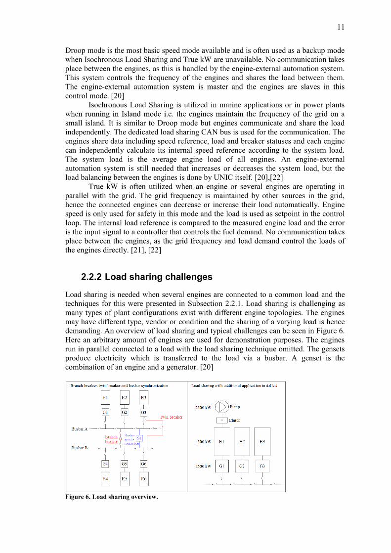
demanding. An overview of load sharing and typical challenges can be seen in Figure 6.

Here an arbitrary amount of engines are used for demonstration purposes. The engines

run in parallel connected to a load with the load sharing technique omitted. The gensets

produce electricity which is transferred to the load via a busbar. A genset is the

combination of an engine and a generator. [20]

Figure 6. Load sharing overview.

12

Challenges in combining engines from different vendors were seen in 2010, when the

immediate need of combining analogue and digital Isochronous Load Sharing

communication was realized. Old non-Wärtsilä engines using analogue communication

had to be combined with new UNIC-controlled engines using digital communication.

The issue was solved by creating a module that translates the analogue signal into a

digital signal and vice versa. Digital Isochronous Load Sharing is superior to analogue,

as it has functionality that cannot be done with an analogue signal. This includes soft

loading, load sharing profiling and busbar synchronisation. Soft loading of an engine

involves utilizing the knowledge of bus and generator breakers statuses and taking

correct decisions of whether to increase or decrease the load of an engine. Load sharing

profiling means that engines are biased according to properties and load. The load is

shared unequally between engines if the load sharing is biased. Busbar synchronization

is marked in Figure 6 in blue and enables the possibility to synchronize frequencies

between two busbars. None of these properties exists with analogue communication, as

this is only an electrical scalar value. An analogue signal has an additional drawback as

signal strength weakens over long distances because of cable resistivity. [20],[21]

The load sharing functionality has existed for a long time, but some challenges

still exist. Figure 6 shows a Branch breaker and a Twin breaker which are challenging

to implement, as they complicate the topology vastly. They could be usable for

redundancy reasons, but are not yet implemented in the load sharing algorithm. Figure 6

shows another issue when an engine is connected simultaneously to two applications,

one being the normal busbar and the other being an arbitrary load, a pump in this case.

Biasing is needed in these cases, as the pump uses some of the engine’s load capacity

and this has to be taken into account when the system load is shared among the engines.

Additionally, attention must be paid to generator capacity not to overload the engine as

the combined rated power of pump and generator can be larger than the rated power of

the engine. [21]

A third issue is seen in marine applications where it is possible to measure

propulsion power easily only when the engine is operating in diesel mode. This issue

affects DF engines, which can operate in gas mode in addition to the diesel mode. SG

engines are not yet used in marine applications. Propulsion power is estimated by

measuring engine fuel consumption, but this is not easily done with gas as fuel. The

issue can be solved by installing equipment for torque measurement. This enables the

ability to calculate the propulsion power in all fuel modes. However, the equipment is

expensive and does not come by default in installations. [21]

Biasing is achieved through four methods; analogue control signal, fixed bias,

mapped bias, and dynamic bias. The first one is used in analogue load sharing or when

manually overriding locally the load sharing balancing. The rest are used in digital load

sharing. Fixed and mapped bias are configuration parameters and the engine-external

automation system shares the load accordingly. Fixed bias is a static scalar value, while

mapped bias is a matrix with two columns, system load and a percentage value, which

allows the engine bias to change according to the system load. Dynamic bias is load

transient shaping, meaning that the bias is shaped according to load transients. The

functionality is achieved by derivation of the system load to find changes, transients,

and by loading engines according to fuel mode. Engines operating in diesel mode are

less sensitive to load changes than engines operating in gas mode. Hence, diesel mode

engines are given positive load offset and gas mode engines are given negative load

offsets to prevent gas engines from tripping into diesel mode. Tripping is not wanted as

gas burns cleaner than diesel and is thus preferred if available. [21]

13

2.2.3 The load reduction functionality

The purpose of the normal and conditional safeties seen in Figure 5 is to protect the

engine from taking damage and alert the operator of issues. This is called machinery

protection and load reduction is one of the actions available when protecting the engine.

Machinery protection works by comparing engine measurements to predefined setpoints

in the software configuration. Actions activate in UNIC if measurements exceed the

setpoints or if values cannot be read due to communication problems or instrument

failures. Activated machinery protection actions are shown locally on the engine’s LDU

and communicated to external systems by using Modbus. The types are [23]:

Start block

A start block prevents the engine from starting. This is vital functionality to not

start an engine with insufficient critical parameters, such as low pre-lube oil

pressure or wrong supply voltage to UNIC modules.

Alarm

An alarm is used to notify the operator that an instrument has exceeded its alarm

level and needs attention. This could be only a minor problem, but the attention

of the operator is needed.

Load reduction

A load reduction lowers the load on the engine to protect it from taking damage.

This can be critical in some situations and the maximum load can hence be

ramped down or reduced in one major step. The action is, depending on the

speed/load mode, either automatic or interactive with the plant.

Shutdown

A shutdown shuts down the engine to protect it from taking damage. An engine

shutdown is needed when a critical problem has been encountered and a load

reduction is not a suitable solution.

Emergency stop

An emergency stop activates when an essential instrument reaches its setpoint.

This cannot be overridden and stops the engine as fast as possible.

Stop

A stop activates when the engine is requested to stop by the operator. This is not

necessarily related to any issues.

Gas trip

Applies to DF engines. A gas trip activates when the conditions for running in

gas mode are no longer met and the engine trips to diesel. The pilot injection

remains activated.

Pilot trip

Applies to DF engines. A pilot trip activates when the conditions for running in

diesel mode are no longer met and the engine trips to backup diesel mode.

Limp

Used mainly on single common rail (CR) main engines. This activates the limp

mode, a very basic engine mode used only in emergency situations. This mode is

activated when the MCM has failed and this allows the CCMs to control basic

engine functionality and to keep the engine running.

14

The load reduction is from a thesis point of view the most interesting action. Three

different load reduction types are used: absolute, adaptive and kW window and their

usage depends on the measurement and on the engine speed/load mode. An absolute

load reduction sets the maximum load to a configurable percentage value and ramps the

engine down towards that value. This type is usually used for various UNIC related

failures. An adaptive load reduction sets the maximum load to a fixed minimum

percentage value and ramps the engine down towards that value. This is usually used

when specific measurements exceed their setpoints. The kW window load reduction is

used in the True kW speed/load mode and corrects the frequency of the engine as

needed. The engine load is ramped down when a load reduction activates and can be

ramped up again when the condition for the load reduction is no longer met. [24]

Engines keep continuously track of their maximum load and this decreases when

a load reduction activates. The maximum load is, depending on the speed/load mode,

used in either UNIC or the engine-external automation system for decreasing the

engine’s actual load. This system is called PMS in power plants and auxiliary system in

marine applications. UNIC itself can decrease the engine’s load in True kW or

Isochronous Load Sharing, while the engine-external automation system handles this in

Droop. There are fundamental differences between the modes how load reductions are

handled and these will be presented here. [21]

UNIC can decrease an engine’s load without compensation from other engines

only in the True kW speed/load mode. The system load, the total load on all engines, is

then lowered. It is possible to lower the load on an engine without compensation as

frequency is maintained by the grid and the load can safely be decreased without

causing power quality issues. The engine’s load reference is lowered when the load

reduction activates and the speed/load controller decreases the fuel demand on the

engine, resulting in a lower load. The engine-external automation system is notified of

the load reduction but there is no need to interfere as UNIC handles the load reduction

itself. The engine-external automation system can handle the load reduction if needed,

but UNIC controls it under normal circumstances. [21],[22]

The situation is different in Isochronous Load Sharing. A load reduction request

is made to the engine-external automation system as the engines cannot decrease the

system load in this mode. This mode can be used on ferries or small islands where the

engines are the main power source. Frequency must be maintained to ensure power

stability in these modes as engines are not connected to a large grid. A load reduction

request is thus made to notify the engine-external automation system that the system

load may need to be decreased. It is important to notice that an engine load can be

decreased by UNIC only if the other engines sharing the same load can compensate by

increasing their load. Otherwise, the engine-external automation system must decrease

the system load. The Isochronous Load Sharing algorithm increases or decreases in both

cases automatically the loads on the engines that are connected to the same load sharing

communication line. This also applies in a load sharing scenario where all engines have

100 % load and a load reduction activates on one engine. Engines will compensate the

load reduction by risk of overloading some engines if the engine-external automation

system does not lower the total system load. This follows as the load itself can’t be

decreased by UNIC, only transferred to other engines. The only possibility in this

scenario is for the engine-external automation system to disconnect some of the power

consumers that create the load on the engines, hence reducing the system load. This is

common on ferries with only a few engines installed, where the principle is used that the

power consumer must be disconnected before the power producer can lower its load.

The load balancing between the engines can after that be processed, as a margin has

been established and some engines can have higher load than other. [21]

15

Load reductions in Droop mode are taken care of by the engine-external automation

system. A load reduction request is sent from the engine with active load reductions and

the system reacts. It uses the engine’s maximum loads and increases or decreases the

loads on the engines as needed by sending speed increase/decrease pulses. The

speed/load controller adjusts the engines’ speed references and the fuel demand is

adjusted accordingly on the affected engines. This lowers the output power on the

engine with a load reduction and increases it correspondingly on other engines. The

total system load stays the same. Alternatively, the engine-external automation system

may first have to lower the system load before balancing the loads between the engines.

The system keeps track of the frequency and compensates this as needed. Loads can

also be biased between engines, even if no load reduction is activated, in both Droop

and Isochronous Load Sharing mode as described in Subsection 2.2.2. [21], [22]

An overview over the differences between how load reductions are handled can

be seen in Table 1. UNIC sends continuously the engine’s maximum available load and,

if needed, a load reduction requests/indication to the engine-external automation system.

Table 1. Overview over how load reductions are handled.

Speed/load

mode

Control loop

setpoint

UNIC Engine-external

automation system True kW

(only used in

power

plants)

Load control Reads the load reference.

The controller sets the

fuel demand accordingly

to maintain given load.

Informs the grid of lowered

system load or compensates

by increasing the load

references on engines

without load reductions.

Isochronous

Load

Sharing

Speed/frequency

control

Shares the system load

according to a give load

reference and maintains a

fixed frequency of the

plant. Loads are shared

equally if possible.

Adjusts speed reference

input and controller sets

fuel demand.

Adjusts system load if

needed.

Droop Speed/frequency

control

Reads speed reference.

The controller sets the

fuel demand to achieve

the given speed, while

using a speed droop curve

to ensure load sharing.

Sends speed INC/DEC

pulses to handle the

frequency. Shares the

system load according to

engine’s maximum load.

Adjusts system load if

needed.

16

2.2.4 Engine de-rating

Wärtsilä engines operating in harsh environments face challenges as ambient conditions

can affect the power output, efficiency and fuel consumption. Engine de-rating is used

to lower the maximum power output of an engine in advance, as the engine’s

performance has been decreased due to external reasons. These plant related reasons are

e.g. ambient temperature, charge air coolant (LT water) temperature and site altitude.

The engine will not be able to produce the power it was designed for and its expected

maximum performance should be lowered. Engine de-rating is done in the engine-

external automation system and is not detected or calculated by UNIC. The ISO 3046-

1:2002 (E) standard is used for combustion engines when measuring engine efficiency

and capacity in reference conditions [25],[26]:

total barometric pressure 100 kPa

air temperature 25 °C

relative humidity 30 %

charge air coolant temperature 25 °C

In comparison, the ambient temperature can reach over 40 °C in e.g. the Middle East

and northern Africa and air pressure is only 85 kPa at 1500 m above sea level. The

engine’s performance may have to be de-rated when conditions outside the reference

ISO standard apply. The de-rating formulas and correction factors will not be shared

here, but can be found in the ISO 3046-1:2002 standard. Ambient temperature and

pressure affect the air density which has a direct impact on the engine’s performance.

High air and LT water temperature increase the charge air temperature and this

increases the risk of e.g. knock on gas engines. High altitude result in lower air pressure

which means that the turbocharger speed must increase to produce sufficient charge air

pressure. This increases the risk of turbocharger problems especially at high loads. High

humidity requires higher LT water temperature to avoid condensation in the charge air

cooler and this leads to higher charge air temperature. These were examples of why

engines are de-rated according to ambient conditions. The derating is done by the

engine-external automation system, resulting in that an engine is not requested higher

power than it can produce. That is the difference between load reductions and engine

de-rating: load reductions protect the engine from breaking by taking engine specific

parameters into account, while de-rating is done preventively by the engine-external

automation system based on external parameters. In practice, the de-rating signal is also

used for lowering the engine load if load reductions activate. The load reduction request

is sent to the engine-external automation system, which lowers the load by de-rating the

engine. The load is set according to whichever is lower, the de-rating level or the load

reference set by UNIC. [9],[25],[26]

The engine-external automation system allows an engine to start only when no

start blocks are active, as mentioned in Subsection 2.2.3. When started, one additional

de-rating rule prevents the engine from ramping up the load too rapidly and that is the

HT water outlet temperature. This limit de-rates the engine especially at cold start, as

the engine cannot be loaded with too cold water. The de-rating exists due to mechanical

reasons, as the HT water cools the cylinder liner and the lube oil cools the piston.

Problems may arise if the HT water is too cold compared to the lube oil temperature, as

this increases the risk that the piston is unable to move due to thermal expansion. This

de-rating rule is being replaced by machinery protection and engines are to be shut

17

down if the difference between lube oil and HT water temperature is too large. Too high

difference is not allowed on an engine, and the de-rating rule becomes obsolete. [26]

The above ambient conditions apply to all engines, but SG and DF engines have

additional gas related criteria. These are valid for SG engines and apply to DF engines

only when running in gas mode. The additional de-rating criteria are [9]:

methane number and charge air temperature

gas feed pressure and lower heating value (LHV)

Detailed information about the relations between minimum and maximum allowed

charge air temperature and methane number or gas feed pressure and LHV can be seen

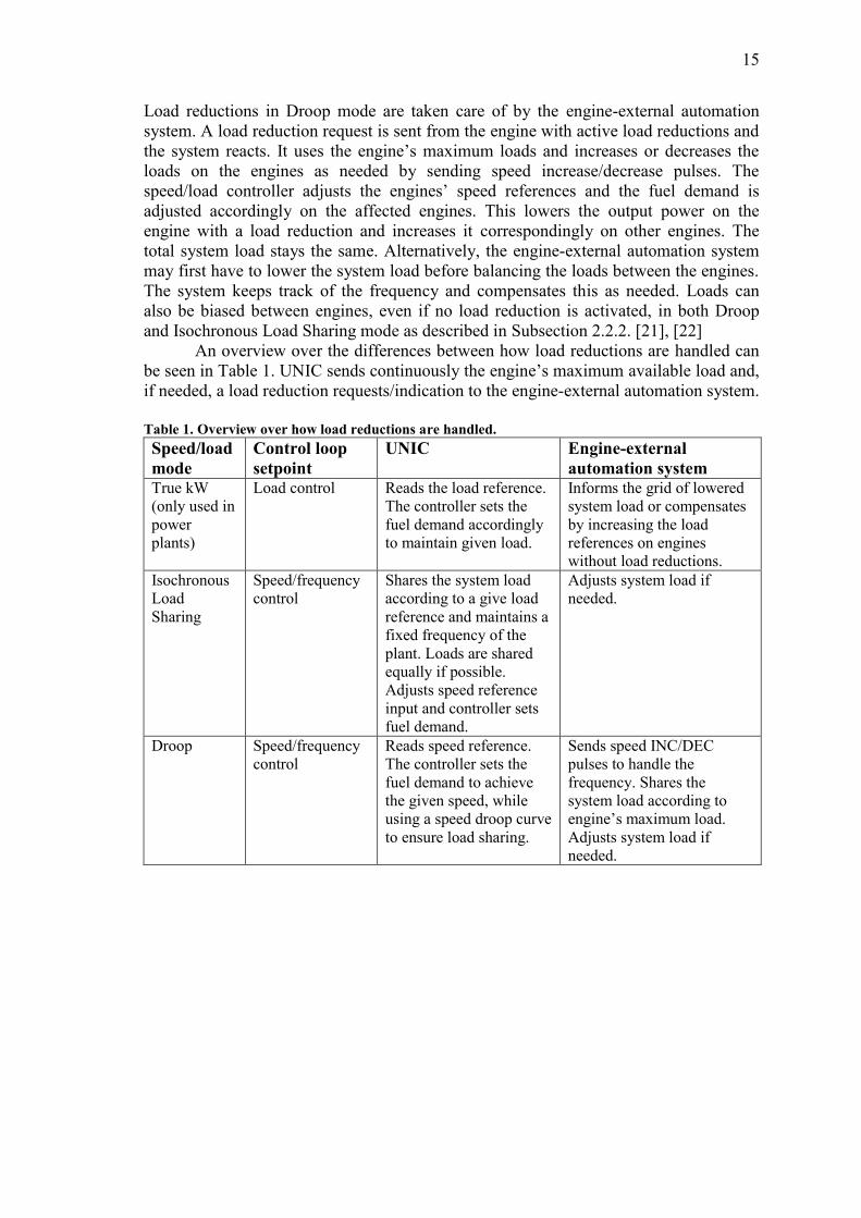
in the W34DF product guide [9]. A low methane number combined with a low charge

air temperature causes a decrease in the maximum engine output as seen in Figure 7. A

low methane number can be compensated up to a certain level by increasing the charge

air temperature. It is currently not supported to measure the methane number

continuously, but ongoing research may change this situation. For now, the methane

number is provided by the operator to the engine-external automation system and is

static until changed manually. [27]

Figure 7. How methane number and charge air temperature affect 34DF de-rating. [9]

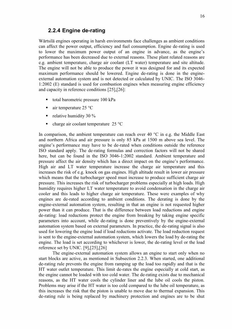
A low gas feed pressure combined with a low LHV cause a decrease in the maximum

engine output as seen in Figure 8. This situation can be improved up to a certain level

by increasing the gas feed pressure. The gas feed from the gas network or gas supply

tank is not connected directly to an engine. A gas regulating valve, safety ventilation

valves and filters are located between the gas feed and the engine. These enable the

monitoring and control capabilities needed to ensure that the gas properties are correct

for the engine combustion process. The engine-external automation system monitors

and controls, together with UNIC to some extent, the gas feed by using the regulating

valves. A certain gas pressure is required at the engine inlet to enable correct proper

mixing of charge air and gas. This sets requirements on the gas feed pressure, and its

minimum value can be calculated by adding the pressure drops over the valves and

filters to the required gas inlet pressure. [27]

18

A low gas feed pressure does not necessarily mean that the gas cannot be used, as the

low pressure can be compensated to some extent. This is achieved by increasing the

duration of the gas injection in the cylinder. This follows quite naturally as a gas supply

with low pressure needs more time to transfer the same amount of gas as a gas supply

with high pressure. The same applies in the situation when gas quality is low due to

pollution of nitrogen. Enough gas for achieving sufficient combustion can be injected

by increasing the injection duration. Due to mechanical reasons, however, the injection

duration cannot be extended indefinitely in these situations. The maximum duration

depends on the gas feed pressure, gas quality and engine. The gas feed pressure is

usually sufficient and drops rarely below the minimum required level. [27]

Figure 8. How gas feed pressure and LHV affect 34DF (480/500 kW/cylinder) de-rating. [9]

The de-rating used to be fixed, meaning that the maximum output of the engine was

lowered permanently if difficult ambient conditions could be met at some point during

the engine’s lifetime. This is not preferable, as the engine’s performance is lowered

even though ambient conditions would be sufficient for the rated engine performance.

Active de-rating was developed to improve the performance of engines by only de-

rating the engines when actually needed. Active de-rating takes ambient conditions into

account and sets the maximum allowed power output on the engine accordingly. This

improves the performance of the engine as the maximum power output is decreased

only when necessary. [9], [26]

The index developed in this thesis cannot directly use the de-rating rules

implemented for an engine. This follows as the de-rating is done by the engine-external

automation system and the de-rated maximum load is not sent to UNIC. The purpose of

the index is not to re-implement the de-rating rules in UNIC, but to take use of engine

measurements and parameters to indicate the engine’s load capacity. The de-rated

maximum load can be sent to UNIC if it turns out necessary. This may not be the case,

as the engine-external automation system handles engine loading, and a more probable

scenario is that UNIC sends the calculated index to this system. The load capacities of

the engines can then be taken into account when defining load references for individual

engines.

19

3 Index development

This chapter presents all aspects, requirements and assumptions that have been

discovered when developing the index. In short, nominal engine parameter values can

be determined by using experts’ experience and formulas along with adaptive

calculations. These nominal values define an engine that operates normally and has

large load capacity. The index should relate the engine’s instantaneous measurements to

the nominal values and to the load reduction setpoints. In this way the index indicates

how normally the engine is operating and how large the load capacity is. The chapter

starts by presenting the index benefits by looking at a few situations where the index is

assumed be beneficial. The most common load reductions are presented to establish a

clear overview over the parameters that can affect the maximum load of an engine.

Finally, the proposed method of calculating the index is derived.

3.1 Index requirements and assumptions

3.1.1 Benefits and usage

The main benefit of a load capacity index is assumed to be that it enables predictive

actions to be made instead of corrective. It would provide the engine-external

automation system with quantitative data about the states of the engines which should

be used in control. Theoretically, the data could be used to increase performance, safety

and power availability on a plant through optimised power management. These

improvements will be discussed by looking at a few situations where the index is

assumed to be beneficial and preferable.

Engine loading and load sharing could be improved if load availability were

known. There is no functionality today that would in a preventive way inform UNIC or

the engine-external automation system that the engine is about to activate a load

reduction. This means that an increased load will be distributed among engines until the

machinery protection activates load reductions. The situation is not desirable as the total

power is unnecessarily decreased, when the engines with activated load reductions

could have been close to their maximum power instead. The index would in this

situation prevent the load reductions from activating by informing the engine-external

automation system not to increase the load any further on engines with low operation

margin. Instead, the load should be transferred to engines which can increase their load

without activation of load reductions. [21], [28]

Especially power plants would benefit from the index when energy is sold on the

energy market in very short time frames. Wärtsilä engines can go from 0 to 100 % load

in < 2 min and this is crucial when selling energy for the next 5 minutes. The index

would in these cases prevent situations where engines with insufficient load capacity are

requested to quickly ramp up. The insufficient load capacity results in the activation of

load reductions and the power plant is unable to produce the energy it sold. This results

in a punishment and the power plant may be forced to pay fees because of its failure.

Instead, engines with sufficient load capacity will be used in these situations. Sold

energy is then produced and this results in profit and not punishment. [28]

The index would be beneficial also in engine diagnostics, as a measurement of

how the engine is performing. Theoretically, the combination of engine parameter

values together with engine load should give information of how close to nominal

operation the engine is and its condition status. This follows as the parameter values can

20

be compared to known nominal values and differences may be noticed as wear and tear

affects the engine. Such general engine condition measurement does not exist and it

could be useful in local engine diagnostics as well as in remote CBM services. [19]

An engine in gas mode trips potentially to diesel mode during transients and that

is why engines operating in diesel mode are preferred during such situations. The main

reason for tripping is cylinder knock issues, and tripping would be less probable if

knock could be prevented effectively. Knock occurs when pockets of the fuel mixture

ignites outside the normal combustion timing window. It is a serious issue that must be

prevented as the engine may otherwise be damaged. Knock is measured by using knock

sensors and cylinder pressure sensors and it is mainly prevented by adjusting the

ignition timing. The knock sensors are piezoelectric sensors which register the

vibrations created by knock, while the pressure sensors detect knock by cylinder

pressure variations. The index would be beneficial in the tripping issue, as it would

prevent the engine from tripping to diesel mode by informing UNIC and the engine-

external automation system of the increased risk of knock. This would, in a load sharing

scenario, be taken into account and the affected engines would be prevented from

tripping as the load would be biased appropriately. [21]

3.1.2 Load reduction parameters

The purpose of the index is to present the engine’s operation margin to the activation of

load reductions. It is necessary to explain when load reductions activate before it is

possible to calculate the index. The load reductions are hence presented to explain how

the machinery protection works, when does an engine trip to diesel and when is the load

reduced. The Engine safety and machinery protection specification specifies the

machinery protection actions with setpoints, delays and other detailed information [23].

This detailed information is not disclosed in this thesis but includes engine modes (e.g.

run, stop and shutdown) and speed/load modes (Droop, Isochronous Load Sharing and

True kW). A machinery protection action activates when the engine is in the correct

mode, the measurement value exceeds the setpoint value and the activation delay has

passed.

The engines have varying requirements of machinery protection based on fuel

type, installation or size. For instance, load reductions are usually preferred over

shutdowns in marine engines, as it is highly undesirable or even hazardous that the

engines shut down on a ship. Shutdowns are more common in power plant installations.

As a result, it is not realistic to take all load reductions specified in the specification into

account, and instead focus on the most common ones. In this way uncommon and

engine- or installation specific load reductions are left out, and the ones used represent

the general situation best. The load reductions used in this thesis were taken from the

Engine safety and machinery protection specification by using a W20V34DF engine as

base. Setpoints and delays are here presented as examples, as these may vary depending

on engine design stage, turbocharger size or some other reason. Load reductions may

also activate when a sensor fails and measurements become unavailable. These are not

included as their statuses are Boolean and were not seen suitable for estimating the

engine load margin.

21

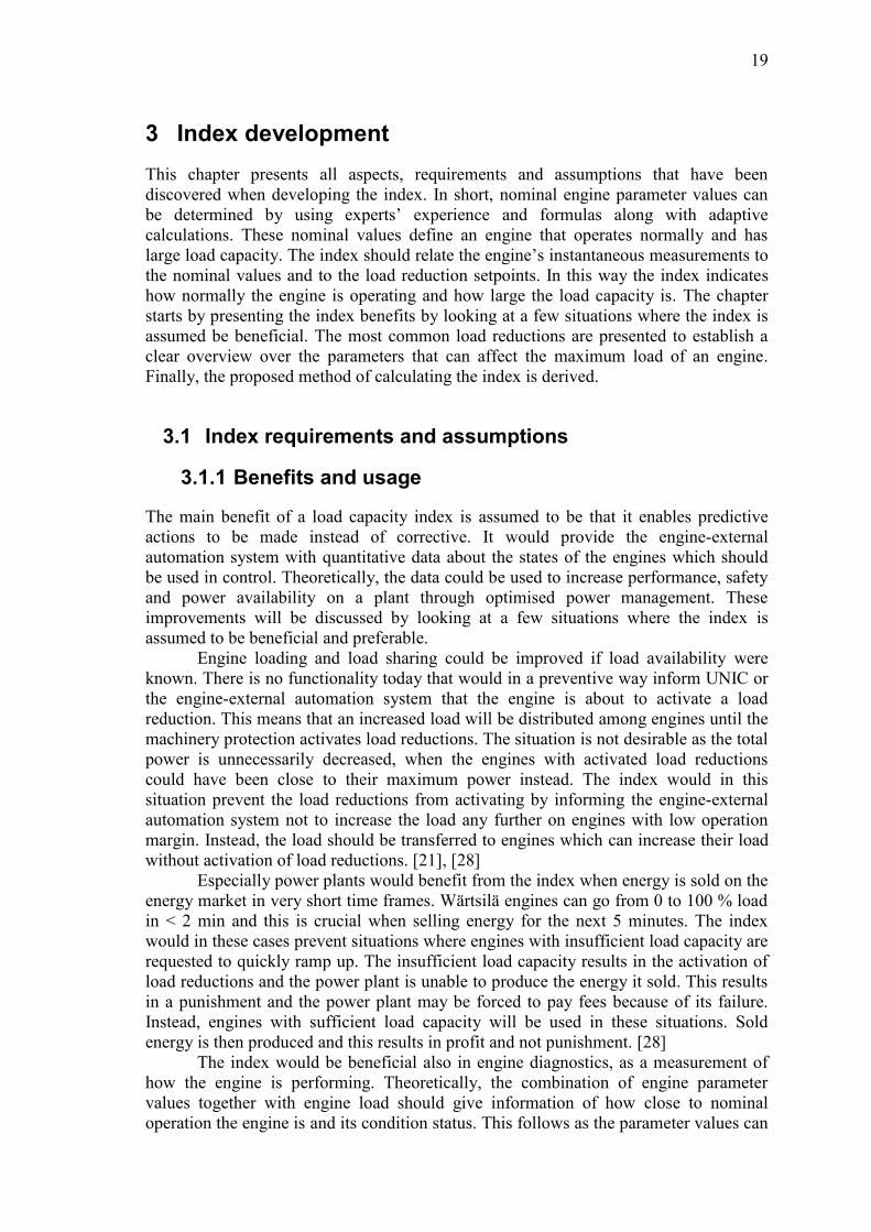
The temperature related load reductions can be seen in Table 2. One of these is more

complicated than the rest and that is the TY5##17# Exhaust gas temperature deviation

load reduction. The double hashtags means the cylinders 01-10 and the single hashtag

means both engine banks, A and B, in a V-engine. This load reduction activates when

any of the exhaust gas temperatures deviates more from the average exhaust gas

temperature than the setpoint ramp slope defines. Activation is possible only when the

average exhaust gas temperature is above 250 °C and the temperature deviation needed

for activation decreases as the average exhaust gas temperature increases.

Lube oil and charge air are the only temperatures measured at engine inlet. The

bearings and liners temperatures are measured inside the engine and the exhaust gas

temperature measurements are done at engine outlet. The HT water temperature is also

measured at engine outlet.

Table 2. Temperature load reductions.

ISO code Description Setpoint Delay Comment

TE201 Lube oil temp, engine inlet 80 °C 5 s High temperature

load reduction.

TE402

TE403

HT water temp, jacket outlet A-

bank

HT water temp, jacket outlet B-

bank

108 °C 5 s High temperature

load reduction.

TE511

TE521

Exhaust gas temp TC A inlet

Exhaust gas temp TC B inlet


load reduction.

TE517

TE527

Exhaust gas temp TC A outlet

Exhaust gas temp TC B outlet


load reduction.

TE5011A

...

TE5101B

Exhaust gas temp, cylinder 01A

...

Exhaust gas temp, cylinder 10B


load reduction.

TY5017A

...

TY5107B

Exhaust gas temp deviation,

cylinder 01A

...

Exhaust gas temp deviation,

cylinder 10B

±110 °C

±70 °C

TY500

[°C]

250

500

10 s High exhaust gas

temperature

deviation from

average.

TE601 Charge air temp, engine inlet 75 °C 5 s High temperature

load reduction.

TE700

...

TE711

Main bearing 00 temp

...

Main bearing 11 temp


load reduction.

TE7011A

...

TE7102B

Liner temp 1, cylinder A01

...

Liner temp 2, cylinder B10


load reduction.

TE7016A

...

TE7106B

Big end bearing temp, cylinder 01A

...

Big end bearing temp, cylinder 10B


load reduction.

Reduced to 80%.

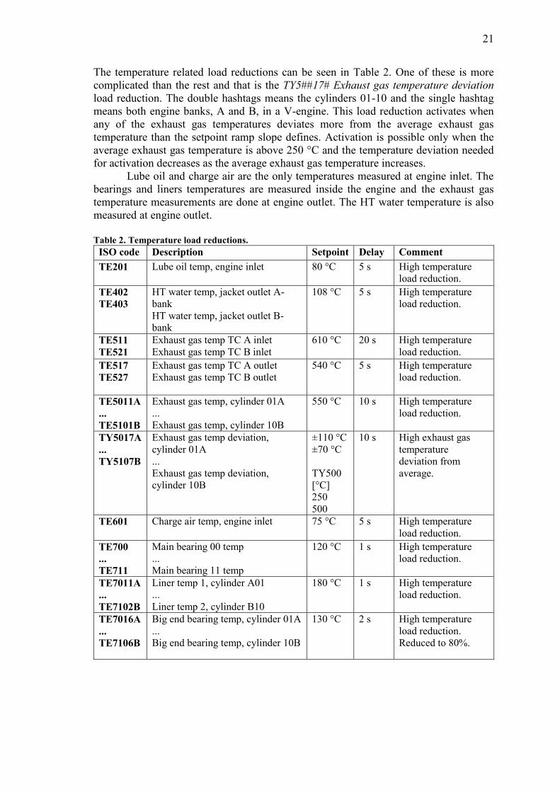
22

The pressure related load reductions can be seen in Table 3. Lube oil and HT water

pressures are measured at engine inlet, while the cylinder pressures are measured inside

the engine.

Table 3. Pressure load reductions.


PT201 Lube oil press, engine

inlet

2,5 bar 5 s Low pressure load reduction.

PT401 HT water press, jacket

inlet

1,6*

(RPM/

Nominal

RPM) bar

5 s Low pressure load reduction.

PT5011A

...

PT5101B

Cylinder pressure,

cylinder A01

...

Cylinder pressure,

cylinder B10

211 bar 0 s High pressure load reduction

The turbocharger related load reductions can be seen in Table 4. The load reductions

activate if the turbocharger speed is above the lower setpoint for more than 5 min or

above the higher setpoint for more than 100 ms. There are two turbochargers on the

engine described as it is a V-engine with two cylinder banks.

Table 4. Turbocharger load reductions.


SE518

SE528

TC A speed

TC B speed

22810

23040

5 min

*)

0,1 s

**)

High turbocharger speed alarm/load

reduction setpoints and delay time

depend on turbocharger model

*) 5 min if speed above alarm limit

**) 0,1 sec if speed above LR limit

The knock related load reductions can be seen in Table 5. Knock is measured by using

piezo and cylinder pressure sensors. The raw data from these sensors is processed by the

Knock control application in UNIC and the data is quantified into knock statuses. The

engine is tuned to be very close to knock to achieve high efficienty. It is up to the

engine expert to tune and decide how the raw data is quantified by changing Knock

control parameters. The knock status is 0 if the engine is free from knock and 1 if the

engine has light knock. Light knock is compensated by the Knock control application by

changing the ignition timing and the main fuel injection demand. However, light knock

may turn into heavy knock if this compensation is unsuccessful. The status for heavy

knock is 2 and the load reduction activates then immediately to protect the engine from

damage. The load reduction is active only in the True kW mode and a gas trip is used in

the other two engine modes. Gas trips change the fuel mode from gas to diesel for a DF

engine.

Table 5. Knock status load reductions.


SEB6014A

...

SEB6104B

Knock status cylinder A1

...

Knock status cylinder B10

Status

= 2

0 s Heavy knock load

reduction.

23

These are the most common load reductions occurring on a DF engine. As was

highlighted, the parameters are measured at different locations on the engine and this

will later restrict their usage in the index calculations. The parameters measured at

engine inlets barely change during load transients and are controlled by the engine-

external automation system. This decreases the amount of information that can be used

for estimating the engine load margin, as the parameters stay close to setpoints, which

usually are static, throughout the entire load range. The internal parameters and the

parameters at engine outlet show different behaviour and can vary greatly depending on

load. This gives information about load availability as parameters correlate with load

and the parameter values and trends may be compared. This load correlation should be

usable by the index and it is to reflect any changes in parameter values that may have an

impact on the load capacity of the engine. [29]

3.1.3 Engine performance parameters

The index describes an engine’s load availability and this would be easy to determine if

the maximum available load of an engine were constant. In that case, a sufficient index

would relate the instantaneous engine load to the engine’s rated load. The rated load

means the designed maximum load and would be the same as the maximum available

load. However, as seen in Subsections 2.2.4 and 3.1.2, de-rating and load reductions

may decrease the engine’s maximum available load to a level lower than the rated load.

The de-rating parameters affect heavily the performance of an engine and are the most

critical engine performance parameters. These must be within allowed ranges for the

engine to operate at maximum performance. Equally important is that load reduction set

points are not reached. The most common load reductions are according to [27], [29]:

high cylinder maximum pressure

high exhaust gas temperature

turbocharger over speed

heavy knock.

These are connected processes as de-rating conditions may affect the load reduction

parameter values and load reduction parameters may additionally be heavily influenced

by the engine load level. For instance, exhaust gas temperatures may increase when the

ambient- or charge air temperature increases, but exhaust gas temperatures increase also

when the engine load increases. This follows as more fuel is combusted in the cylinders.

The charge air temperature is being cooled by the LT water and the LT water

temperature is thus one of the most important engine performance parameters as it

defines directly the charge air temperature. Too high charge air temperature or too low

charge air pressure can lead to knock issues. Too high charge air pressure can lead to

misfiring. High air temperature or low air pressure increase the need of cooling to get

sufficient charge air temperature. The parameters are interconnected and the most

important factors or parameters which affect the load reduction parameters have to be

selected before a realistic index can be calculated. De-rating conditions, load reductions

and engine dynamics make it clear at this stage that a lot can be taken into account when

calculating the index. [27], [30]

24

However, not everything can nor should be taken into account because of complexity,

engine dynamics and mechanical or technical implementations. For instance, it is

important that an engine has enough LT water cooling capacity to cool the charge air

temperature sufficiently at any time instant. This cooling capacity depends on the LT

water temperature and the opening of the LT water regulating valve. The LT water

temperature in turn depends on the speeds of the cooling radiators. An increasing charge

air temperature can be compensated by either increasing the speeds of the cooling

radiators fans or increasing the LT water flow by regulating the LT water regulating

valve. In these cases, either cooler or more water is led to the engine, which decreases

the charge air temperature. UNIC does not control the regulating valve or the speeds of

the radiators in power plants. These are not even measured, as they are completely

controlled by the engine-external automation system in the power plant. Thus, this

information is unavailable and it is not possible to determine the cooling capacity. This

is one example of a situation where engine load capacities may differ because of

external components. Engines with cooling margin can cool more charge air which is

needed when the load increases. An engine without cooling margin cannot increase its

load without increasing its charge air temperature and increasing the risk of knock and

knock load reduction. This cooling margin is zero if the radiator speeds and LT water

flow are close to maximum. Measurements from these components could together with

thermodynamic analysis enable the calculation of the cooling margin on some marine

installations, but this will not be discussed further in this thesis. [27]

The purpose of the index is to determine the load capacity by measuring engine

parameters and estimating the maximum load. As presented in Subsection 2.1.4, the

CBM experts monitor the condition of an engine by gathering measurements and

comparing these to known nominal parameter values. Differences found are analysed

and actions are taken as needed. It was discovered during discussions with the experts

that the nominal parameter values are measured at different engine loads and ambient

temperatures. It was thus possible to get valuable information of how parameters are

expected to change when the engine load changes. Additionally, the nominal values can

be used as reference to define the parameter value zone where the engine is performing

normally. Similarly, the index should indicate when parameter values are located

outside of this region and move towards the region with increased risk of load

reductions. In conclusion, CBM experts brought valuable information to the index

development. Utilizing the knowledge of how parameters change when the load changes

together with the nominal values bring valuable and usable information. [19], [29]

Established at this point is an understanding of where the engine parameter

values should be and where they should not. The engine is operating normally if the

parameter values are close to the nominal values and vice versa; the closer they are to

the load reduction setpoints the worse performance or load availability can be expected.

The index should reflect these situations accordingly. De-rating is done by the engine-

external automation system and is not taken into account by the index, as the purpose of

the index is not to re-implement the de-rating rules. The de-rating parameters are mainly

external and not related to engine components. Additionally, the de-rating information

is presently not sent from the engine-external automation system to the engine. [26]

25

3.2 Index presentation and calculation

3.2.1 Index concepts

It can be concluded when looking at the benefits listed in Subsection 3.1.1 that the index

calculation is far from trivial. The approach is quite broad and the potential situations

where an index would be beneficial are different. Extensive discussions with engine

experts were carried out to better understand what the resulting index actually can

achieve and describe. For instance, should the index be a percentage value that

describes engine condition or should the result go one step further and also offer a

solution of why the engine condition is worse than it should be? How closely related are

the engine condition and engine load availability and which one is more interesting? A

percentage value was seen as a good starting point, as that can be used in diagnostics

and control as such and is useful for humans and for control systems. Additionally, the

index is not a re-implementation of FAKS, the tool that was used by CBM for

diagnosing engines, as that task is too challenging and complicated to integrate into an

engine specific index.

It was decided during the development process that two different approaches of

calculating indexes are realistic enough to be implemented and tested. These approaches

were developed in collaboration with engine experts and may turn out successful. The

proposal is thus that not one but two indexes shall be calculated to enable the benefits

listed in Subsection 3.1.1. The two indexes are named the Condition Index (CI) and the

Load Availability Index (LAI). The two indexes are calculated by combining

instantaneous engine parameter measurements, the load reduction setpoints and the

nominal engine parameter values. Ideally, the nominal parameter values would be the

result of interpolation of the actual measurements. The CBM formulas are used as

reference now for simplicity when deriving the indexes, but these will be replaced later

with interpolated scatter of adaptive measurements which reflect the nominal values of

each engine better than general formulas. The delays used in the machinery protection

are not taken into account when calculating the indexes. It was discussed that the delays

are short, usually < 10 s, and do not add much value to the calculation if only the

margin to the load reduction is interesting. [21],[27],[29]

The two indexes are similar but answer different questions and behave

differently. CI is a measurement of the distance between the load reduction setpoint and

the present parameter value, normalized according to the nominal value range. When

derived it will be seen that CI answers the question “How normally is the engine

operating?”. The LAI is a prediction made with engine measurements and enables the

possibility to predict the load availability. When derived it will be seen that LAI

answers the question “What is the maximum load of the engine?”. These two indexes

will now be derived and explained. Both indexes describe the engine’s load operation

margin, but present it differently. Each has its benefits and they compensate each other

to some extent.

26

3.2.2 The condition index

A load reduction activates when the value of a measurement exceeds the load reduction

setpoint. The task of determining the engine’s operation margin is thus to express the

relation between the present measurement values to the load reduction setpoints. An

indication of how normally the engine is operating is achieved when this relation is

compared to nominal parameter values. The CI development started out by only using

the measurements and the load reduction parameters, as it was not known that nominal

values could be implemented. These were added to the calculations when seen possible

and necessary, and this improved the CI scaling vastly. The proposed method of

calculating the index by using load reduction setpoints, instrument measurements and

nominal values is presented below.

Load reduction setpoints and engine instrument measurements are scalar values.

The relation between two scalar values can be expressed by either subtracting or

dividing the two values. Subtraction of the values gives the relation as the difference

between the values in their original unit. Division of the values gives the relation as a

unitless quotient which easily can be converted to a percentage value. The amount of

units used in UNIC is huge and it is impossible to compare values with different units.

The CI is hence calculated by division as this presents the operation margin for all ISO

codes without using any unit. Additionally, the resulting quotient is less sensitive to

instrument data range sizes. The ranges of the instruments vary considerably and it is

hard to say if a measured value change is small or large without proper scaling. This

scaling is done automatically by division and the result is a value which easily can be

compared between ISO codes.

Four different cases have to be taken into account when calculating the CI.

These depend on whether the load reduction setpoint is positive or negative and if the

instrument value normally is above or below this setpoint. A load reduction is activated

when a value that normally is below a setpoint grows larger than the setpoint and vice

versa. The cases are thus:

1. Instrument value is normally below a positive setpoint

2. Instrument value is normally above a positive setpoint

3. Instrument value is normally below a negative setpoint

4. Instrument value is normally above a negative setpoint

The CI presents the operation margin of an engine to the nearest load reduction. The

appropriate way of scaling the index was decided to be 0-100 %. It was concluded that

the logical behaviour is that 0 % indicates a zero load margin and 100 % indicates a

great distance to the load reduction. The load reduction setpoint has in the first case

been reached and a load reduction activates once its delay has passed.

A first approach on calculating the index for a single ISO code in cases 1 and 4

can be expressed as

𝐶𝐼 = (1 −𝑦𝑀

𝑦𝐿𝑅) ∙ 100 %, (1)

where yM is the measured value of the ISO code and yLR is the load reduction setpoint.

This equation expresses the margin as a percentage value between the ISO code value

27

and its load reduction setpoint. Calculation of the CI in cases 2 and 3 would then be

done by inversing the behaviour of (1) by multiplying with -1:

𝐶𝐼 = (𝑦𝑀

𝑦𝐿𝑅− 1) ∙ 100 %. (2)

These two equations were developed by improving the idea that the operation margin

could be calculated by dividing the ISO code value and the setpoint. Equation (2) is

needed in cases 2 and 3, as it was seen that (1) did not work in these cases. The

equations enables CIs to be calculated and scaled equally for all ISO codes, making

them directly comparable.

The nominal instrument values were then proposed to be integrated in the

calculations. This would make the indexes from different ISO codes more comparable,

as the scaling would be done equally. The index expresses then the distance from the

nominal value to the load reduction setpoint as a percentage value. Again, 0 % means

that this distance is zero while 100 % means that the distance is as long as it should be

when the engine is operating normally. The latter happens when the parameter value is

exactly the nominal value. A second approach of calculating the CI is hence

𝐶𝐼 = (𝑦𝐿𝑅 − 𝑦𝑀

𝑦𝐿𝑅 − 𝑦𝑁𝑂𝑀) ∙ 100 %, (3)

where yNOM is the nominal value of the instrument. It turns out that this equation can be

used for all the cases 1-4 listed above and also when the load reduction setpoint is zero.

The CI will have the same dynamics in all of them, meaning that this is a convenient

way to calculate a compatible and easily comparable index. Comparison shows that (3)

is reduced to (1) when the nominal value is zero and to (2) by additionally multiplying

with -1. The equations were tested with arbitrary values and it was concluded that (3) is

an extended combination of (1) and (2) that scales correctly in all cases 1-4.

Figure 9 shows an example of CI calculation using exhaust gas temperatures.

Exhaust gas temperatures are plotted on the y-axis in degrees Celsius and engine load is

on the x-axis in percentages. The black horizontal line in the figure at 580 °C is the load

reduction setpoint. The blue curve consists of the nominal values and is in this case

made up for demonstration purposes and do not reflect actual nominal temperatures.

The exhaust gas temperatures should be close to this line when the engine is operating

normally. For instance, it can be seen that the temperature should be around 560 °C at

100 % load. The engine has several cylinders and the red dot is the present engine load

and the highest measured exhaust gas temperature from all cylinders. This represents

the worst case and the engine performance is differing from normal operation. The

distance from the blue line is clearly noticeably and the CI is estimated visually by

using (3) as

𝐶𝐼 = (580 − 470

580 − 420) ∙ 100 % ≈ 69 %.

That means that the engine is performing abnormally and the distance to the load

reduction is roughly 2/3 of what it normally is. The CI was later expanded in the

simulations to also incorporate the situation when the highest measured exhaust gas

temperature is below the normal curve. This situation should also be reflected in the CI

as it is an indication of decreased engine performance due to abnormal behaviour. In

this case, the index has grown over 100 % and needs to be inverted. The calculations are

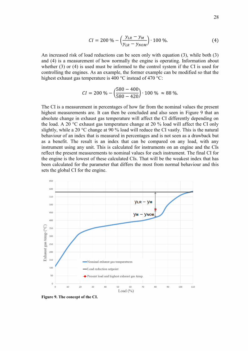
28

𝐶𝐼 = 200 % − (𝑦𝐿𝑅 − 𝑦𝑀

𝑦𝐿𝑅 − 𝑦𝑁𝑂𝑀) ∙ 100 %. (4)

An increased risk of load reductions can be seen only with equation (3), while both (3)

and (4) is a measurement of how normally the engine is operating. Information about

whether (3) or (4) is used must be informed to the control system if the CI is used for

controlling the engines. As an example, the former example can be modified so that the

highest exhaust gas temperature is 400 °C instead of 470 °C:

𝐶𝐼 = 200 % − (580 − 400

580 − 420) ∙ 100 % ≈ 88 %.

The CI is a measurement in percentages of how far from the nominal values the present

highest measurements are. It can then be concluded and also seen in Figure 9 that an

absolute change in exhaust gas temperature will affect the CI differently depending on

the load. A 20 °C exhaust gas temperature change at 20 % load will affect the CI only

slightly, while a 20 °C change at 90 % load will reduce the CI vastly. This is the natural

behaviour of an index that is measured in percentages and is not seen as a drawback but

as a benefit. The result is an index that can be compared on any load, with any

instrument using any unit. This is calculated for instruments on an engine and the CIs

reflect the present measurements to nominal values for each instrument. The final CI for

the engine is the lowest of these calculated CIs. That will be the weakest index that has

been calculated for the parameter that differs the most from normal behaviour and this

sets the global CI for the engine.

Figure 9. The concept of the CI.

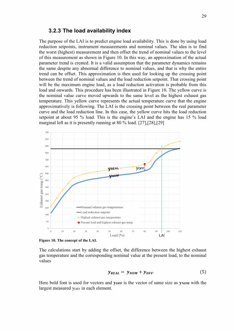
29

3.2.3 The load availability index

The purpose of the LAI is to predict engine load availability. This is done by using load

reduction setpoints, instrument measurements and nominal values. The idea is to find

the worst (highest) measurement and then offset the trend of nominal values to the level

of this measurement as shown in Figure 10. In this way, an approximation of the actual

parameter trend is created. It is a valid assumption that the parameter dynamics remains

the same despite any abnormal difference to nominal values, and that is why the entire

trend can be offset. This approximation is then used for looking up the crossing point

between the trend of nominal values and the load reduction setpoint. That crossing point

will be the maximum engine load, as a load reduction activation is probable from this

load and onwards. This procedure has been illustrated in Figure 10. The yellow curve is

the nominal value curve moved upwards to the same level as the highest exhaust gas

temperature. This yellow curve represents the actual temperature curve that the engine

approximatively is following. The LAI is the crossing point between the real parameter

curve and the load reduction line. In this case, the yellow curve hits the load reduction

setpoint at about 95 % load. This is the engine’s LAI and the engine has 15 % load

marginal left as it is presently running at 80 % load. [27],[28],[29]

Figure 10. The concept of the LAI.

The calculations start by adding the offset, the difference between the highest exhaust

gas temperature and the corresponding nominal value at the present load, to the nominal

values

𝒚𝑹𝑬𝑨𝑳 = 𝒚𝑵𝑶𝑴 + 𝒚𝑶𝑭𝑭. (5)

Here bold font is used for vectors and yOFF is the vector of same size as yNOM with the

largest measured yOFF in each element.

30

The LAI is the result from a lookup of the load reduction setpoint from a map

containing the nominal exhaust gas temperatures with offsets added and matching loads

𝐿𝐴𝐼 = 𝐿𝑜𝑜𝑘𝑢𝑝(𝑦𝐿𝑅, 𝒚𝑹𝑬𝑨𝑳, 𝒙𝑳𝑶𝑨𝑫). (6)

LAI is the x-coordinate of the crossing point between the real temperature curve and the

load reduction line. The load operation margin is expressed as the difference between

the LAI and the actual load

𝐿𝑜𝑎𝑑𝐿𝐸𝐹𝑇 = 𝐿𝐴𝐼 − 𝐿𝑜𝑎𝑑. (7)

This formula works for both absolute load in kW and load measured in percentages.

This follows as the LAI and load can be easily converted to kW by multiplying it with

the engine’s rated load. Equation (7) applies when de-rating is not taken into account.

The equation could be modified if the de-rating information were available to UNIC as

𝐿𝑜𝑎𝑑𝐿𝐸𝐹𝑇 = 𝑀𝐼𝑁(𝐿𝐴𝐼, 𝐿𝑜𝑎𝑑𝐷𝐸𝑅) − 𝐿𝑜𝑎𝑑, (8)

where LoadDER is the present maximum load as determined by de-rating rules. The load

margin is then the difference between the present load and either LAI or LoadDER,

depending on which one is smaller.

LAI is defined as an index 0-100 % and is an approximation of an engine’s

maximum load. This equals to the crossing point between the real parameter curve and

the load reduction line and the index is 100 % if this line cannot be found. Similarly to

the CI, the result is an index that can be compared on any load, with any instrument

using any unit. This is calculated for instruments on an engine and the engine’s final

LAI is the lowest of the calculated indexes. The LAI is based on the idea that the

parameter trend should approximately stay the same, even when a parameter differs

from the nominal value curve. Tests will show how well this works in practice, but

engine experts agreed on that this could be a good enough approximation in many

situations. The LAI in both kW and % could be used by UNIC when controlling the

engine. [22], [29]

3.2.4 Adaptive indexes

The CBM provided general formulas and guidelines are a good starting point when

determining the nominal values for the engine parameters. Their greatest benefit is that

they are not just engine- and fuel specific, but also take external aspects such as

differently sized turbochargers and air temperature into account. However, this benefit

becomes a drawback if the index calculations relied on these formulas only. It is too

complicated to provide specific and up-to-date formulas to UNIC and the formulas are

too general for determining real nominal values. Ambient temperature varies and the

dynamics of engine components change for different reasons such as wear and tear, fuel

quality or lube oil quality. Add to this different ways of operating the engine, ramping

up the load in a fast or slow pace or using the engine as base load or regulating power.

The calculations must be flexible and the nominal values should reflect the changes in

dynamics accordingly. It is then a fact that the nominal values should be adaptively

updated to enable adaptation to the changing environment. This is the only way that

reliable nominal values can be kept up to date without the need for continuously

configuring general formulas for different engine setups. [31]

31

The possibilities for implementing the adaptivity were explored together with engine

automation experts. Wärtsilä uses Simulink and their own development environment,

the Wärtsilä Simulink Development Environment (WSDE), when developing engine

applications. It was a logical choice to use the commonly used tools when implementing

the index calculation, as the ideas and concepts presented in this thesis could end up as

an application developed with the exact same tools. In that case some implementation

work has already been done and time is used more efficiently. Conveniently, a self-

tuning map (STM) has been developed that provides the adaptive functionality needed

for the index calculations. The STM can be found among other function blocks in the

common functions library in WSDE. This library holds many blocks for common

functions used when developing applications. The STM is a result from earlier research

and can be already found in several applications normally used on an engine. The

functionality of the STM and will now be explained along with general information

about how maps work in UNIC applications. [22]

The STM is a one-dimensional vector with pairs of x and y values. The

configurable parameters in the STM are the following [32]:

y_vec_init - y-vector initial values

x_vec - x-vector

x_vec_update - x-vector update width

map_update_gain - y-vector update gain

line_slope_gain - y-vector line slope update gain

vector_size - sizes of the x and y-vectors

enable_train - enable/disable STM updating.

An overview of the functionality can be seen in Figure 11. The x values are used for the

engine load in this thesis. The y values are the corresponding instrument values

measured at different loads. Every x value has an update region and a matching y value

which is updated when the engine load is within the update region. The y value is

updated by increasing or decreasing it by the preconfigured y value gain scaled

according to the line slope. A line slope is used for every y value that approximates the

slope of the curve created by the y values. This is used for weighing y values measured

at different x values and allows values closer to the x points to have greater influence on

the corresponding y values. The line slope is increased or decreased by the line slope

gain based on measurements. The STM is highly configurable as the vector sizes, vector

values, update regions and gains may be configured arbitrarily. [32]

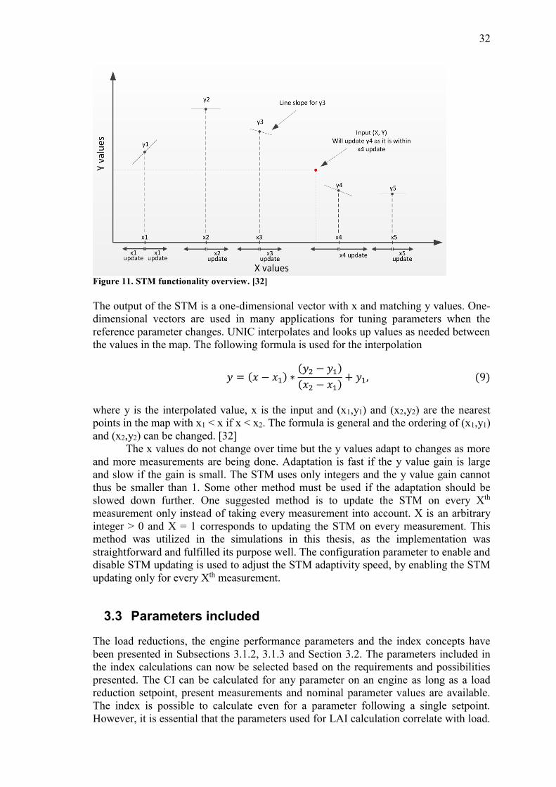
32

Figure 11. STM functionality overview. [32]

The output of the STM is a one-dimensional vector with x and matching y values. One-

dimensional vectors are used in many applications for tuning parameters when the

reference parameter changes. UNIC interpolates and looks up values as needed between

the values in the map. The following formula is used for the interpolation

𝑦 = (𝑥 − 𝑥1) ∗(𝑦2 − 𝑦1)

(𝑥2 − 𝑥1)+ 𝑦1, (9)

where y is the interpolated value, x is the input and (x1,y1) and (x2,y2) are the nearest

points in the map with x1 < x if x < x2. The formula is general and the ordering of (x1,y1)

and (x2,y2) can be changed. [32]

The x values do not change over time but the y values adapt to changes as more

and more measurements are being done. Adaptation is fast if the y value gain is large

and slow if the gain is small. The STM uses only integers and the y value gain cannot

thus be smaller than 1. Some other method must be used if the adaptation should be

slowed down further. One suggested method is to update the STM on every Xth

measurement only instead of taking every measurement into account. X is an arbitrary

integer > 0 and X = 1 corresponds to updating the STM on every measurement. This

method was utilized in the simulations in this thesis, as the implementation was

straightforward and fulfilled its purpose well. The configuration parameter to enable and

disable STM updating is used to adjust the STM adaptivity speed, by enabling the STM

updating only for every Xth measurement.

3.3 Parameters included

The load reductions, the engine performance parameters and the index concepts have

been presented in Subsections 3.1.2, 3.1.3 and Section 3.2. The parameters included in

the index calculations can now be selected based on the requirements and possibilities

presented. The CI can be calculated for any parameter on an engine as long as a load

reduction setpoint, present measurements and nominal parameter values are available.

The index is possible to calculate even for a parameter following a single setpoint.

However, it is essential that the parameters used for LAI calculation correlate with load.

33

This follows as the curve of nominal values does not increase with the increasing load

and will thus not cross the load reduction setpoint line. A parameter that does not

correlate with load will bring no usable information to the calculations. The load

reductions listed in Subsection 3.1.2 can then be discussed from the point of view of

load dependency and real usability. Most of the engine inputs are controlled by external

means and do not correlate with load by definition. They have setpoints and should stay

close to the setpoints despite any load changes. [29],[33]

The LT water cooling system removes heat from the lube oil and charge air.

These are controlled by the engine-external automation system and follow the

temperature setpoints accordingly.

The lube oil cooling system removes heat from bearings and follows LT water

temperature. Lube oil pressure follows its setpoint. The bearings should not be

affected by load changes as long as the lube oil is cooled enough.

The HT water cooling system removes heat from the cylinder liner, cylinder

head and turbocharger. The HT water outlet temperature and input pressure are

controlled by the engine-external automation system and follow the setpoints

accordingly.

It can be concluded that many of the load reduction parameters should by definition

follow a certain setpoint. These can still be used for calculating the CI, but cannot be

used for estimating load capacity with LAI. Additionally, it was concluded that knock

will not be included in the index calculations as knock does not correlate with load.

Knock can occur at any load because of earlier presented reasons. Knock behaviour is

complex and dedicated applications are used for quantifying raw data into knock

statuses. The knock statuses could be used for calculating CI, but it is discussable how

much more information that index gives than simply reading the statuses directly.

Knock is not included in the index calculations because of this fact and the lack of load

correlation. Interesting parameters which correlate with load are:

exhaust gas temperatures

cylinder pressure

TC speed

cylinder liner temperature.

It was decided that these parameters, except the cylinder liner temperature, would be a

good starting point for index calculations. The reason to this is that they are important

performance parameters which correlate with load and the associated load reductions

are commonly activated. That is the situation the index should prevent and these

parameters are a good basic setup for indicating the load capacity of an engine. The

cylinder liner temperature does not usually cause any problem and it was concluded that

it can be neglected for now. The cylinder liner temperature is expected to increase with

load, but much less than the other parameters. Tests showed that the cylinder liner load

reductions never activated and the assumptions were correct. The exhaust gas

temperatures are measured at several points after the engine and these are all heavily

influenced by load and turbocharger speed. The measurement points are directly after

the cylinders, before the TC inlet and after the TC outlet, but some engines do not have

all of these instruments installed. [27],[29],[33]

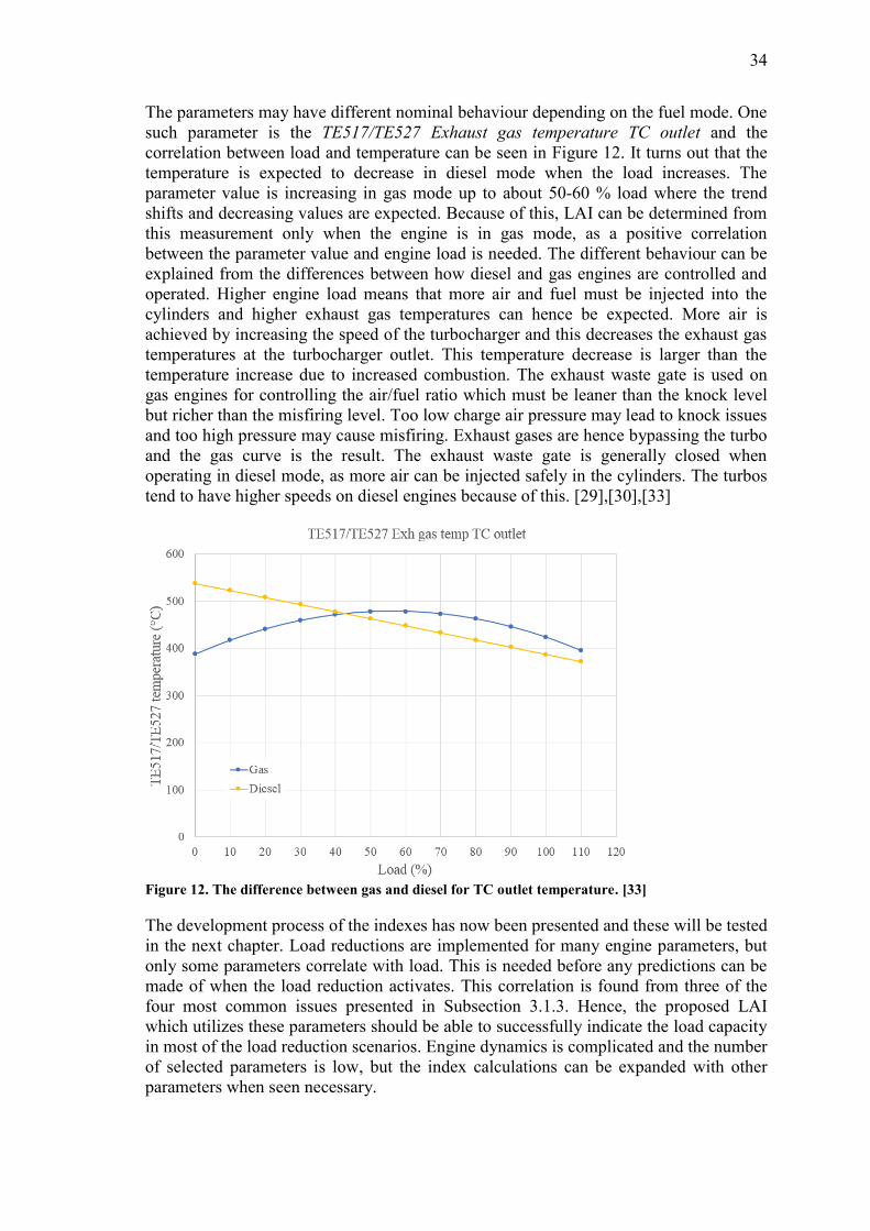
34

The parameters may have different nominal behaviour depending on the fuel mode. One

such parameter is the TE517/TE527 Exhaust gas temperature TC outlet and the

correlation between load and temperature can be seen in Figure 12. It turns out that the

temperature is expected to decrease in diesel mode when the load increases. The

parameter value is increasing in gas mode up to about 50-60 % load where the trend

shifts and decreasing values are expected. Because of this, LAI can be determined from

this measurement only when the engine is in gas mode, as a positive correlation

between the parameter value and engine load is needed. The different behaviour can be

explained from the differences between how diesel and gas engines are controlled and

operated. Higher engine load means that more air and fuel must be injected into the

cylinders and higher exhaust gas temperatures can hence be expected. More air is

achieved by increasing the speed of the turbocharger and this decreases the exhaust gas

temperatures at the turbocharger outlet. This temperature decrease is larger than the

temperature increase due to increased combustion. The exhaust waste gate is used on

gas engines for controlling the air/fuel ratio which must be leaner than the knock level

but richer than the misfiring level. Too low charge air pressure may lead to knock issues

and too high pressure may cause misfiring. Exhaust gases are hence bypassing the turbo

and the gas curve is the result. The exhaust waste gate is generally closed when

operating in diesel mode, as more air can be injected safely in the cylinders. The turbos

tend to have higher speeds on diesel engines because of this. [29],[30],[33]

Figure 12. The difference between gas and diesel for TC outlet temperature. [33]

The development process of the indexes has now been presented and these will be tested

in the next chapter. Load reductions are implemented for many engine parameters, but

only some parameters correlate with load. This is needed before any predictions can be

made of when the load reduction activates. This correlation is found from three of the

four most common issues presented in Subsection 3.1.3. Hence, the proposed LAI

which utilizes these parameters should be able to successfully indicate the load capacity

in most of the load reduction scenarios. Engine dynamics is complicated and the number

of selected parameters is low, but the index calculations can be expanded with other

parameters when seen necessary.

35

4 Index evaluation

This chapter describes the testing of the proposed indexes. The setup with simulations

and real engine data is explained. A Simulink model has been developed and its parts

are presented. The model is configured and executed using MATLAB scripts and

functions and their functionality is explained. The chapter ends with the presentation of

the results from the simulations.

4.1 The simulation setup

It was concluded at an early stage of the index development that the indexes could most

easily be demonstrated in Simulink. This tool is used for application development in

Wärtsilä and it is the logical choice of development tool together with the WSDE

development environment. In this way no real application has to be developed that

would be used on an actual engine. No resources have to be allocated from application

developers or lab engines either, and the daily application development work can

continue normally. Additionally, the benefits of the indexes in engine load sharing can

be demonstrated in Simulink, as multiengine models exist and these may be used for

demonstrating the indexes in a load sharing scenario. This was never implemented, as

the model using real engine data to calculate the indexes was seen as a sufficient

demonstration of the indexes. The load sharing model is suitable when demonstrating

engine control, but this thesis focuses only on the index development.

The index calculations were implemented and tested in a Simulink model using

real engine data from a Wärtsilä power plant [34]. This power plant is connected to the

grid and produces power on a daily basis with its twelve W20V34SG gas engines, each

with a rated output of 9730 kW. This environment has several benefits compared to

tests on lab engines. The power plant has identical engines connected to the grid with a

real power demand. It is challenging to create an equally realistic test setup with only

lab engines in an artificial environment. Thanks to CBM, it was possible to remotely

monitor the engines on the power plant. The power plant’s exact location and other

information will not be disclosed, as this is not essential. However, the ambient

temperature on the location may affect the rate at which load reductions occur and it is

hence presented. The ambient temperature was on average 13 °C, with daily variations

of +- 10 °C. Load reductions were seen that matched the expectations; the most

common load reductions on SG engines are knock, high exhaust gas temperature and

high cylinder pressure. Four engines had more often load reductions than the other six,

thus these were chosen and data for the following parameters were saved for use in the

simulations:

PT5##1# Cylinder pressure, cylinder A01-B10 (20 codes)

TY500 Engine exhaust gas average temperature

TE##1# Exhaust gas temperature, cylinder A01-B10 (20 codes)

TE517 Exhaust gas temperature TC A outlet

TE527 Exhaust gas temperature TC B outlet

SE518 TC A Speed

SE518 TC B Speed

36

The engines did not have any instrument installed for measuring the exhaust gas

temperature at the turbocharger inlets. However, the outlet temperatures were available

and these were chosen along with the normal exhaust gas temperatures. The engines run

on gas and the TC outlet temperatures should thus follow the gas behaviour shown in

Figure 12. Furthermore, data was also saved for six additional codes which were known

to be necessary or could bring usable information. These were

UT793 Engine load

STY196 Engine speed

UP01 De-rating (from PMS)

TE417 LT water temperature

TE601 CA temperature

IB500 Cold cylinder operation

UT703 Engine load is needed for updating the STMs and implementing the index

functionalities. STY196 Engine speed enables the possibility to update the STMs only

when the engine is running at full speed. Measurements should not affect the maps

when the engines stop, are shut down or start, as all parameter values measured in these

engine modes affect the 0 % load element in the STMs. This deforms the curve created

by the STM values unnecessarily. UP01 De-rating is interesting as this contains the de-

rating information from the engine-external automation system. TE417 LT water

temperature and TE601 CA temperature are both important parameters when it comes

to engine performance, hence these can provide useful information in some situations.

IB500 Cold cylinder operation was selected, as this functionality was seen to be in use

on the engines. The cold cylinder operation disables individual cylinders on an engine in

situations such as misfiring or exhaust gas temperature sensor failures. The maximum

power is reduced on the engine when some cylinders are disabled. This is why the code

could be interesting as the maximum load has changed.

The CBM data consisted of measurement of the chosen codes and the lists of

events and alarms which occurred during the timespan chosen. The data sample rate was

1/s and the timespan was chosen to be 30 days from the 1st of March to the 30th of

March. This equals to 3600 * 24 * 30 = 2592000 measurements for one parameter on

one engine. This results in a total of 2592000 * 4 * 51 = 528768000 data points with

four gensets selected with 51 codes each. MATLAB can handle such amount of data

and the script used for importing the data from the CBM .csv-files can be seen in

Appendix A – The data loading script. The script loads data for one genset at a time and

had thus to be run four times. Data from the .csv-files were stored in workspace

variables, which were saved as .mat files as MATLAB can import such almost instantly.

The event and alarm lists contain useful information about different engine events, such

as engine status (start, run, shutdown, load or unload), alarms or load reductions. These

lists enable the possibility to more easily choose specific dates from the data with

interesting events. The four gensets had also been chosen by first filtering load

reductions in Excel in the alarm and event lists from all gensets and this would not have

been possible without the lists.

The sample rate of 1/s is used by CBM as a compromise between up to date

measurements and amount of data that has to be sent to the CM centre. UNIC measures

several quantities on an engine with much faster sample rates, as that is needed when

controlling the engine. Sampling at 1/s is enough for CBM that only follows up how the

engine is performing over time. Cylinder pressure is one of the quantities that has a high

37

sample rate in UNIC. This is needed as the cylinder pressure can change rapidly and

UNIC needs to react fast enough to ensure safe engine operation. Hence, it may turn out

that sample rate is too slow to show the index benefits for the cylinder pressure. The

CBM sample rate was thought to be enough for demonstrating the index benefits for the

exhaust gas temperatures and turbocharger speed, as these have slower dynamics than

the cylinder pressure.

4.2 The Simulink model

4.2.1 Model overview

The simulations were conducted by creating a model with four STMs and feeding these

with the measurement data. Four STMs are needed as four parameters are included in

the simulations; cylinder pressure, exhaust gas temperature, exhaust gas temperature TC

outlet and TC speed. The indexes are calculated from the STM values, the measurement

data and the preconfigured load reduction setpoints as described in Section 3.2. Plots are

used for visualizing the process and demonstrating the usability of the indexes.

Each STM is fed with the average of the measurements, as this was seen as the

logical way of achieving the general behaviour of parameters. TY500 Engine exhaust

gas average temperature is already calculated by UNIC and is available in the CBM

data. The averages for the other three parameters are calculated at the beginning of the

simulation script used for running the simulation model and creating the plots. This

script can be seen in Appendix B – The simulation and plotting script and its help

functions are listed in Appendix C – The script help functions. UNIC takes automatically

sensor failures into account when calculating TY500 by not adding any measurements

from instruments with failures. Averages for the other parameters could be calculated

directly from the data as no severe sensor failures were seen on the four gensets during

the timespan chosen.

The entire simulation model can be seen in Figure 13. The green sub-systems

contain the inputs, the orange sub-systems contain the index calculations with STMs

and the blue sub-system contains the outputs where data is saved to variables. The

orange calculation sub-systems are all identical and interchangeable, and only the inputs

and outputs differ between the parameters. The yellow Real-Time Pacer block is a third-

party Simulink function block used for slowing down the simulations [35]. It enabled

better index evaluation possibilities by allowing the simulations to be slowed down to

almost real time speed. MATLAB runs the simulations as fast as possible without such

block and it is then impossible to analyse the plots on the fly. According to the

developer, setting the Speedup parameter to 1 allows the model to be simulated at real

time. In practice, this behaviour was achieved by setting the parameter to a slightly

higher value ~2. The model can be run at full speed by setting the parameter to Inf, as

this will be the same as not having the Real-Time Pacer block at all. In that case, the

data points from one hour are processed in seconds, making it impossible to see

anything interesting from the plots. The model is discrete with a sample rate of 100 ms.

This was the default WSDE setting and no reason for changing it was seen during the

index evaluation.

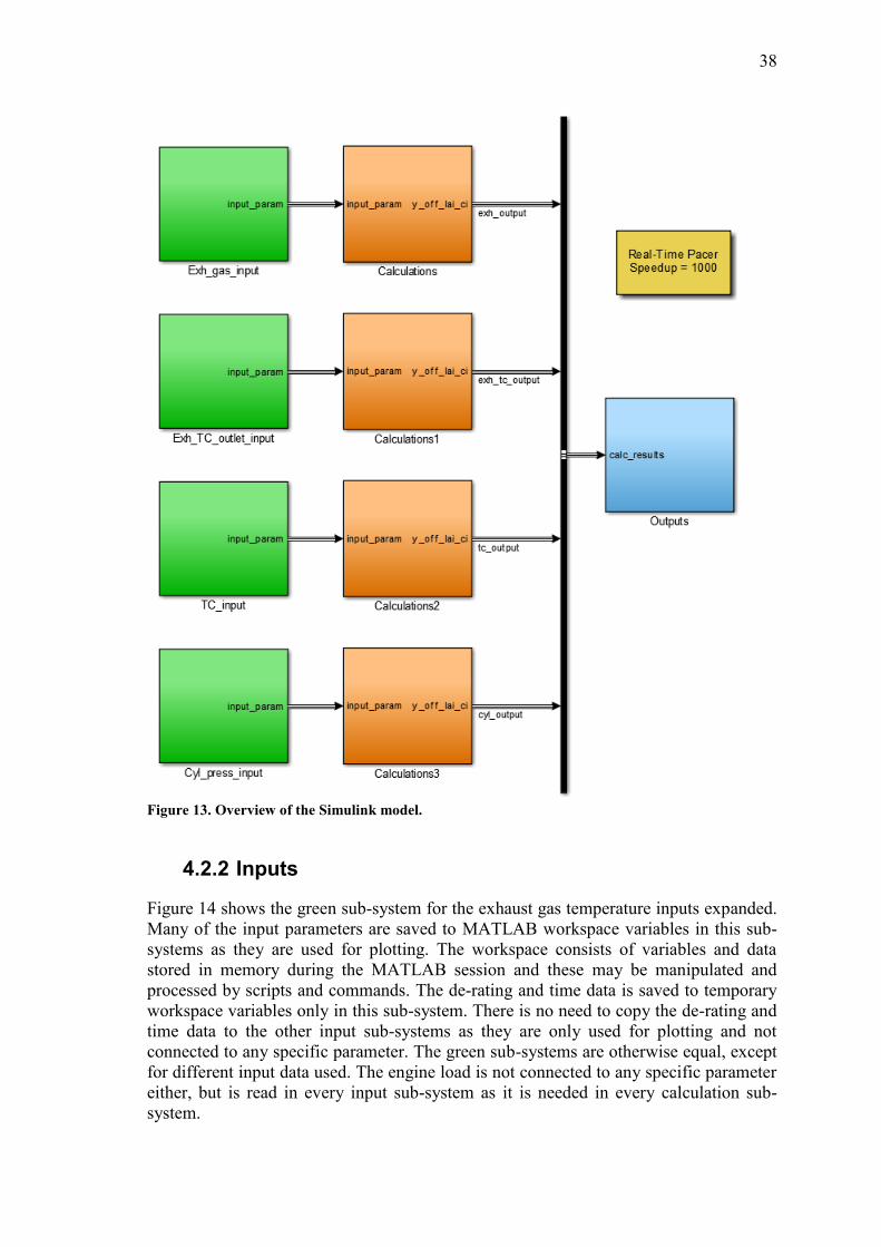
38

Figure 13. Overview of the Simulink model.

4.2.2 Inputs

Figure 14 shows the green sub-system for the exhaust gas temperature inputs expanded.

Many of the input parameters are saved to MATLAB workspace variables in this sub-

systems as they are used for plotting. The workspace consists of variables and data

stored in memory during the MATLAB session and these may be manipulated and

processed by scripts and commands. The de-rating and time data is saved to temporary

workspace variables only in this sub-system. There is no need to copy the de-rating and

time data to the other input sub-systems as they are only used for plotting and not

connected to any specific parameter. The green sub-systems are otherwise equal, except

for different input data used. The engine load is not connected to any specific parameter

either, but is read in every input sub-system as it is needed in every calculation sub-

system.

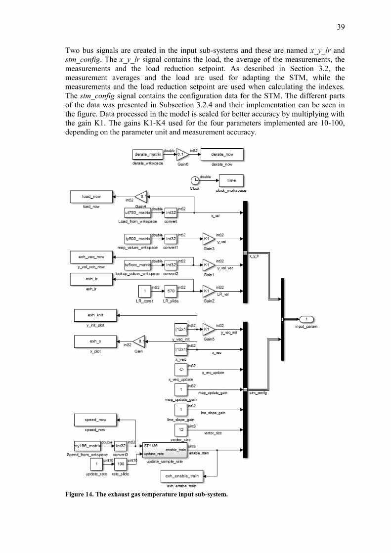
39

Two bus signals are created in the input sub-systems and these are named x_y_lr and

stm_config. The x_y_lr signal contains the load, the average of the measurements, the

measurements and the load reduction setpoint. As described in Section 3.2, the

measurement averages and the load are used for adapting the STM, while the

measurements and the load reduction setpoint are used when calculating the indexes.

The stm_config signal contains the configuration data for the STM. The different parts

of the data was presented in Subsection 3.2.4 and their implementation can be seen in

the figure. Data processed in the model is scaled for better accuracy by multiplying with

the gain K1. The gains K1-K4 used for the four parameters implemented are 10-100,

depending on the parameter unit and measurement accuracy.

Figure 14. The exhaust gas temperature input sub-system.

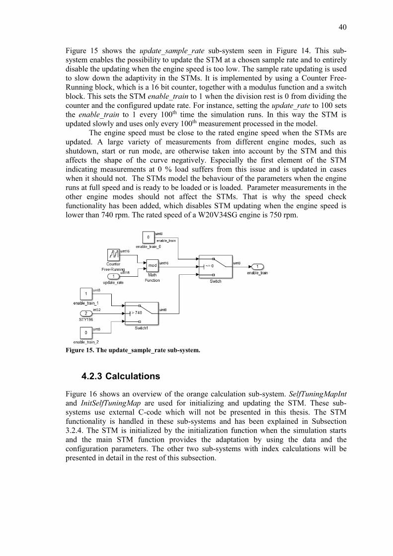
40

Figure 15 shows the update_sample_rate sub-system seen in Figure 14. This sub-

system enables the possibility to update the STM at a chosen sample rate and to entirely

disable the updating when the engine speed is too low. The sample rate updating is used

to slow down the adaptivity in the STMs. It is implemented by using a Counter Free-

Running block, which is a 16 bit counter, together with a modulus function and a switch

block. This sets the STM enable_train to 1 when the division rest is 0 from dividing the

counter and the configured update rate. For instance, setting the update_rate to 100 sets

the enable_train to 1 every 100th time the simulation runs. In this way the STM is

updated slowly and uses only every 100th measurement processed in the model.

The engine speed must be close to the rated engine speed when the STMs are

updated. A large variety of measurements from different engine modes, such as

shutdown, start or run mode, are otherwise taken into account by the STM and this

affects the shape of the curve negatively. Especially the first element of the STM

indicating measurements at 0 % load suffers from this issue and is updated in cases

when it should not. The STMs model the behaviour of the parameters when the engine

runs at full speed and is ready to be loaded or is loaded. Parameter measurements in the

other engine modes should not affect the STMs. That is why the speed check

functionality has been added, which disables STM updating when the engine speed is

lower than 740 rpm. The rated speed of a W20V34SG engine is 750 rpm.

Figure 15. The update_sample_rate sub-system.

4.2.3 Calculations

Figure 16 shows an overview of the orange calculation sub-system. SelfTuningMapInt

and InitSelfTuningMap are used for initializing and updating the STM. These sub-

systems use external C-code which will not be presented in this thesis. The STM

functionality is handled in these sub-systems and has been explained in Subsection

3.2.4. The STM is initialized by the initialization function when the simulation starts

and the main STM function provides the adaptation by using the data and the

configuration parameters. The other two sub-systems with index calculations will be

presented in detail in the rest of this subsection.

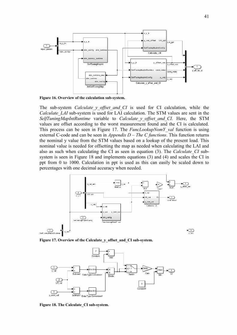
41

Figure 16. Overview of the calculation sub-system.

The sub-system Calculate_y_offset_and_CI is used for CI calculation, while the

Calculate_LAI sub-system is used for LAI calculation. The STM values are sent in the

SelfTuningMapIntRuntime variable to Calculate_y_offset_and_CI. Here, the STM

values are offset according to the worst measurement found and the CI is calculated.

This process can be seen in Figure 17. The FuncLookupNomY_val function is using

external C-code and can be seen in Appendix D – The C functions. This function returns

the nominal y value from the STM values based on a lookup of the present load. This

nominal value is needed for offsetting the map as needed when calculating the LAI and

also as such when calculating the CI as seen in equation (3). The Calculate_CI sub-

system is seen in Figure 18 and implements equations (3) and (4) and scales the CI in

ppt from 0 to 1000. Calculation in ppt is used as this can easily be scaled down to

percentages with one decimal accuracy when needed.

Figure 17. Overview of the Calculate_y_offset_and_CI sub-system.

Figure 18. The Calculate_CI sub-system.

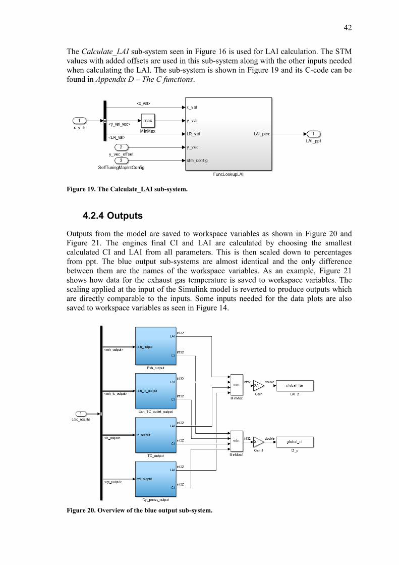
42

The Calculate_LAI sub-system seen in Figure 16 is used for LAI calculation. The STM

values with added offsets are used in this sub-system along with the other inputs needed

when calculating the LAI. The sub-system is shown in Figure 19 and its C-code can be

found in Appendix D – The C functions.

Figure 19. The Calculate_LAI sub-system.

4.2.4 Outputs

Outputs from the model are saved to workspace variables as shown in Figure 20 and

Figure 21. The engines final CI and LAI are calculated by choosing the smallest

calculated CI and LAI from all parameters. This is then scaled down to percentages

from ppt. The blue output sub-systems are almost identical and the only difference

between them are the names of the workspace variables. As an example, Figure 21

shows how data for the exhaust gas temperature is saved to workspace variables. The

scaling applied at the input of the Simulink model is reverted to produce outputs which

are directly comparable to the inputs. Some inputs needed for the data plots are also

saved to workspace variables as seen in Figure 14.

Figure 20. Overview of the blue output sub-system.

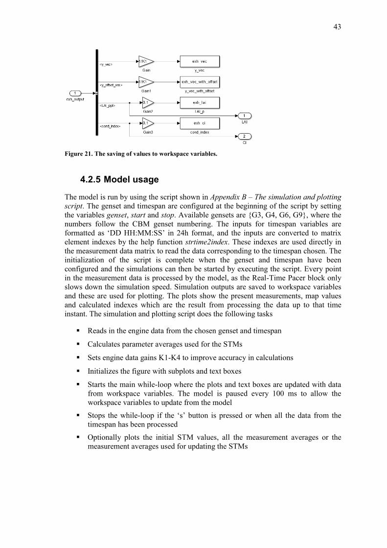
43

Figure 21. The saving of values to workspace variables.

4.2.5 Model usage

The model is run by using the script shown in Appendix B – The simulation and plotting

script. The genset and timespan are configured at the beginning of the script by setting

the variables genset, start and stop. Available gensets are {G3, G4, G6, G9}, where the

numbers follow the CBM genset numbering. The inputs for timespan variables are

formatted as ‘DD HH:MM:SS’ in 24h format, and the inputs are converted to matrix

element indexes by the help function strtime2index. These indexes are used directly in

the measurement data matrix to read the data corresponding to the timespan chosen. The

initialization of the script is complete when the genset and timespan have been

configured and the simulations can then be started by executing the script. Every point

in the measurement data is processed by the model, as the Real-Time Pacer block only

slows down the simulation speed. Simulation outputs are saved to workspace variables

and these are used for plotting. The plots show the present measurements, map values

and calculated indexes which are the result from processing the data up to that time

instant. The simulation and plotting script does the following tasks

Reads in the engine data from the chosen genset and timespan

Calculates parameter averages used for the STMs

Sets engine data gains K1-K4 to improve accuracy in calculations

Initializes the figure with subplots and text boxes

Starts the main while-loop where the plots and text boxes are updated with data

from workspace variables. The model is paused every 100 ms to allow the

workspace variables to update from the model

Stops the while-loop if the ‘s’ button is pressed or when all the data from the

timespan has been processed

Optionally plots the initial STM values, all the measurement averages or the

measurement averages used for updating the STMs

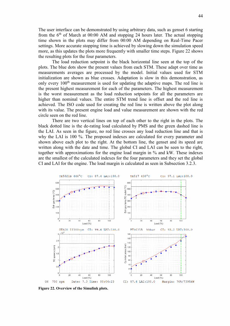
44

The user interface can be demonstrated by using arbitrary data, such as genset 6 starting

from the 6th of March at 00:00 AM and stopping 24 hours later. The actual stopping

time shown in the plots may differ from 00:00 AM depending on Real-Time Pacer

settings. More accurate stopping time is achieved by slowing down the simulation speed

more, as this updates the plots more frequently with smaller time steps. Figure 22 shows

the resulting plots for the four parameters.

The load reduction setpoint is the black horizontal line seen at the top of the

plots. The blue dots show the present values from each STM. These adapt over time as

measurements averages are processed by the model. Initial values used for STM

initialization are shown as blue crosses. Adaptation is slow in this demonstration, as

only every 100th measurement is used for updating the adaptive maps. The red line is

the present highest measurement for each of the parameters. The highest measurement

is the worst measurement as the load reduction setpoints for all the parameters are

higher than nominal values. The entire STM trend line is offset and the red line is

achieved. The ISO code used for creating the red line is written above the plot along

with its value. The present engine load and value measurement are shown with the red

circle seen on the red line.

There are two vertical lines on top of each other to the right in the plots. The

black dotted line is the de-rating load calculated by PMS and the green dashed line is

the LAI. As seen in the figure, no red line crosses any load reduction line and that is

why the LAI is 100 %. The proposed indexes are calculated for every parameter and

shown above each plot to the right. At the bottom line, the genset and its speed are

written along with the date and time. The global CI and LAI can be seen to the right,

together with approximations for the engine load margin in % and kW. These indexes

are the smallest of the calculated indexes for the four parameters and they set the global

CI and LAI for the engine. The load margin is calculated as seen in Subsection 3.2.3.

Figure 22. Overview of the Simulink plots.

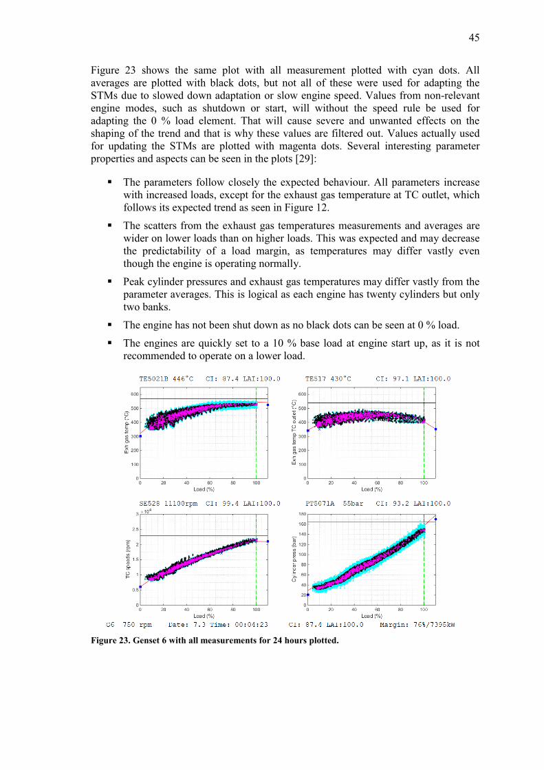
45

Figure 23 shows the same plot with all measurement plotted with cyan dots. All

averages are plotted with black dots, but not all of these were used for adapting the

STMs due to slowed down adaptation or slow engine speed. Values from non-relevant

engine modes, such as shutdown or start, will without the speed rule be used for

adapting the 0 % load element. That will cause severe and unwanted effects on the

shaping of the trend and that is why these values are filtered out. Values actually used

for updating the STMs are plotted with magenta dots. Several interesting parameter

properties and aspects can be seen in the plots [29]:

The parameters follow closely the expected behaviour. All parameters increase

with increased loads, except for the exhaust gas temperature at TC outlet, which

follows its expected trend as seen in Figure 12.

The scatters from the exhaust gas temperatures measurements and averages are

wider on lower loads than on higher loads. This was expected and may decrease

the predictability of a load margin, as temperatures may differ vastly even

though the engine is operating normally.

Peak cylinder pressures and exhaust gas temperatures may differ vastly from the

parameter averages. This is logical as each engine has twenty cylinders but only

two banks.

The engine has not been shut down as no black dots can be seen at 0 % load.

The engines are quickly set to a 10 % base load at engine start up, as it is not

recommended to operate on a lower load.

Figure 23. Genset 6 with all measurements for 24 hours plotted.

46

4.3 Test and model configuration

The alarm and event lists were used to find interesting events, such as load reductions

and alarms, but also to see useful information of how the engines are operated. This

information includes normal events, such as starting, stopping or de-rating, but it is also

possible to see how commonly engines shut down when issues or load reductions occur.

This search resulted in a few situations where the indexes could be useful. Other

situations were discovered by plotting measurements. Shifts in parameter trends could

be discovered and analysed more closely. The Real-Time Pacer was of great help as

simulations could be slowed down vastly, allowing plots to be checked in detail.

The measurement data for the four parameters is multiplied by gains K1-K4

before it is processed in the model. This improves the calculation accuracy, as the data

units are not accurate enough for use in STMs using only integers. The temperatures

(exhaust gas, exhaust gas TC outlet, LT water and CA) are all measured in degrees

Celsius with one decimal accuracy. The turbocharger speed is measured in rpm, while

the cylinder pressure is measured in bars. The smallest gains which were seen to bring

enough accuracy to the calculations were

K1 = 100, used for the exhaust gas temperature

K2 = 100, used for the exhaust gas temperature TC outlet

K3 = 10, used for the TC speed

K4 = 100, used for the cylinder pressure

Increasing the gains further did not improve the accuracy or adaptation in the STMs.

Lower gains were seen to be insufficient, as even minimal STM map and line slope

gains affected the adaptation too excessively. The parameter scaling with K1-K4 affect

only the internal calculations in the model, and it is reverted before the adapted values

from the STMs are saved to workspace variables. In this way the model outputs have

the same units as the inputs.

The load reduction setpoints used in the simulations do not follow the Engine

safety and machinery protection specification [23]. These were not suitable as load

reductions activated on engines at setpoints which differed from the specification. The

reason is that the engines have been configured using older versions of the machinery

protection specification. Additionally, peaks in parameter values might be missing from

the CBM data because of the slow update rate. Especially the cylinder pressure can be

affected by this issue. The setpoints used in simulations corresponded best to the actual

behaviour seen on the engine. Hence, they may differ from the setpoints used in the

engine configurations but are sufficient to demonstrate the indexes.

Fast STM adaptation is problematic as the trend may misshape when the STM

adapts rapidly to differing values on a narrow load range. Because of this, the map and

line slope gains were configured as small as possible which means setting both to 1.

Additionally, the update rate was set to 100, which updates the STMs for every 100th

measurement processed by the model. The x vector update region was set to 8 %,

meaning that the update regions overlap and measurements can affect multiple elements

in the STMs. Sufficient adaptation was achieved with these settings and there were no

reasons to change them throughout the testing process. The last STM configuration

parameters, the initial y values and the x vector, are easily configured as the first

contains the estimated y values used for initializing the STM and the second is the load

vector in percentages.

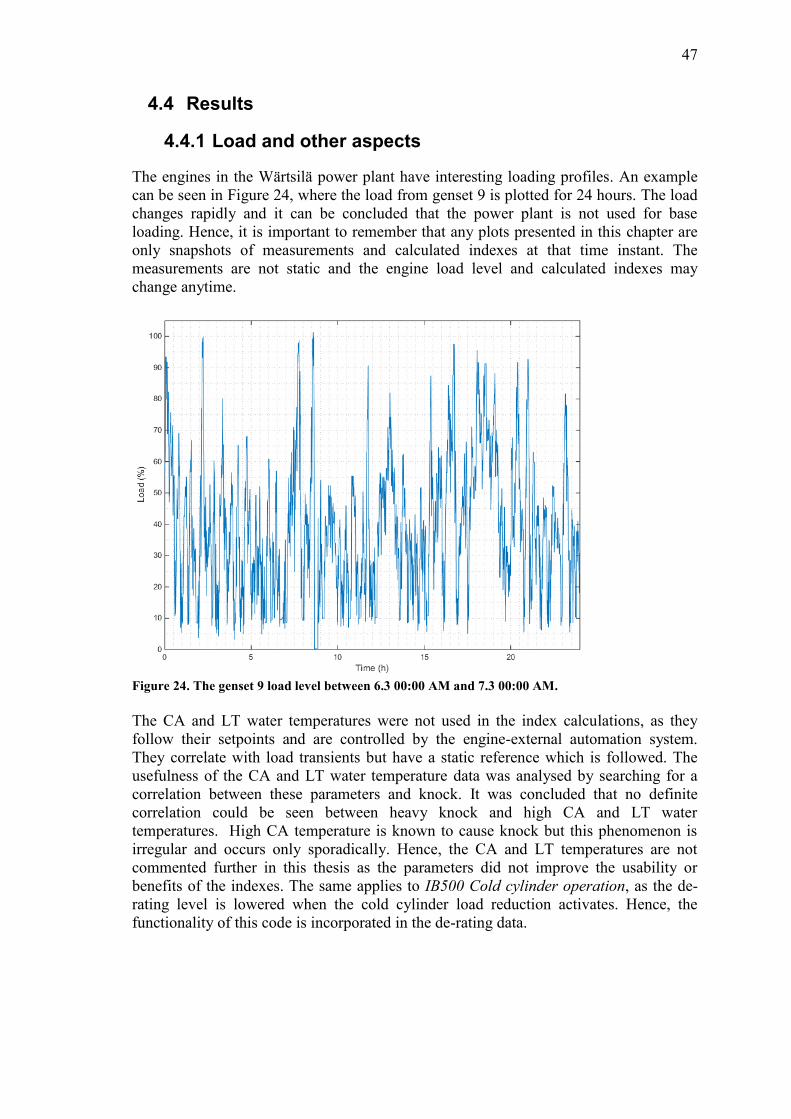
47

4.4 Results

4.4.1 Load and other aspects

The engines in the Wärtsilä power plant have interesting loading profiles. An example

can be seen in Figure 24, where the load from genset 9 is plotted for 24 hours. The load

changes rapidly and it can be concluded that the power plant is not used for base

loading. Hence, it is important to remember that any plots presented in this chapter are

only snapshots of measurements and calculated indexes at that time instant. The

measurements are not static and the engine load level and calculated indexes may

change anytime.

Figure 24. The genset 9 load level between 6.3 00:00 AM and 7.3 00:00 AM.

The CA and LT water temperatures were not used in the index calculations, as they

follow their setpoints and are controlled by the engine-external automation system.

They correlate with load transients but have a static reference which is followed. The

usefulness of the CA and LT water temperature data was analysed by searching for a

correlation between these parameters and knock. It was concluded that no definite

correlation could be seen between heavy knock and high CA and LT water

temperatures. High CA temperature is known to cause knock but this phenomenon is

irregular and occurs only sporadically. Hence, the CA and LT temperatures are not

commented further in this thesis as the parameters did not improve the usability or

benefits of the indexes. The same applies to IB500 Cold cylinder operation, as the de-

rating level is lowered when the cold cylinder load reduction activates. Hence, the

functionality of this code is incorporated in the de-rating data.

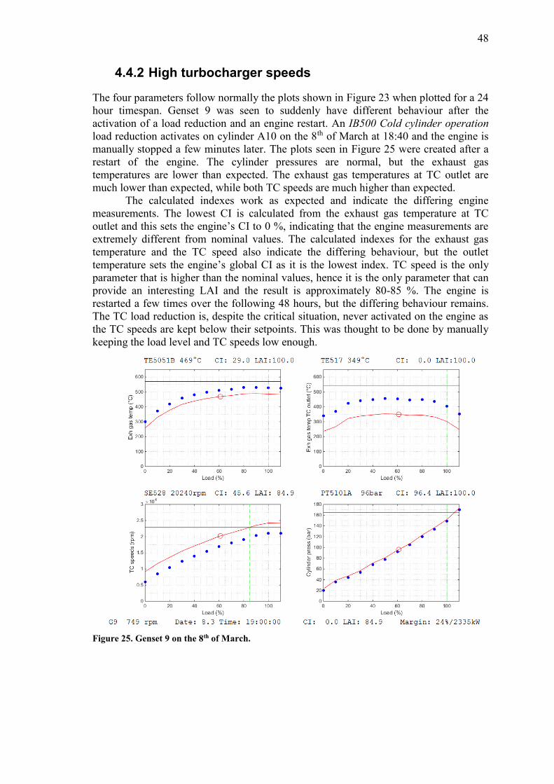
48

4.4.2 High turbocharger speeds

The four parameters follow normally the plots shown in Figure 23 when plotted for a 24

hour timespan. Genset 9 was seen to suddenly have different behaviour after the

activation of a load reduction and an engine restart. An IB500 Cold cylinder operation

load reduction activates on cylinder A10 on the 8th of March at 18:40 and the engine is

manually stopped a few minutes later. The plots seen in Figure 25 were created after a

restart of the engine. The cylinder pressures are normal, but the exhaust gas

temperatures are lower than expected. The exhaust gas temperatures at TC outlet are

much lower than expected, while both TC speeds are much higher than expected.

The calculated indexes work as expected and indicate the differing engine

measurements. The lowest CI is calculated from the exhaust gas temperature at TC

outlet and this sets the engine’s CI to 0 %, indicating that the engine measurements are

extremely different from nominal values. The calculated indexes for the exhaust gas

temperature and the TC speed also indicate the differing behaviour, but the outlet

temperature sets the engine’s global CI as it is the lowest index. TC speed is the only

parameter that is higher than the nominal values, hence it is the only parameter that can

provide an interesting LAI and the result is approximately 80-85 %. The engine is

restarted a few times over the following 48 hours, but the differing behaviour remains.

The TC load reduction is, despite the critical situation, never activated on the engine as

the TC speeds are kept below their setpoints. This was thought to be done by manually

keeping the load level and TC speeds low enough.

Figure 25. Genset 9 on the 8th of March.

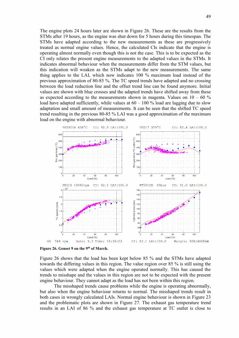
49

The engine plots 24 hours later are shown in Figure 26. These are the results from the

STMs after 19 hours, as the engine was shut down for 5 hours during this timespan. The

STMs have adapted according to the new measurements as these are progressively

treated as normal engine values. Hence, the calculated CIs indicate that the engine is

operating almost normally even though this is not the case. This is to be expected as the

CI only relates the present engine measurements to the adapted values in the STMs. It

indicates abnormal behaviour when the measurements differ from the STM values, but

this indication will weaken as the STMs adapt to the new measurements. The same

thing applies to the LAI, which now indicates 100 % maximum load instead of the

previous approximation of 80-85 %. The TC speed trends have adapted and no crossing

between the load reduction line and the offset trend line can be found anymore. Initial

values are shown with blue crosses and the adapted trends have shifted away from these

as expected according to the measurements shown in magenta. Values on 10 – 60 %

load have adapted sufficiently, while values at 60 – 100 % load are lagging due to slow

adaptation and small amount of measurements. It can be seen that the shifted TC speed

trend resulting in the previous 80-85 % LAI was a good approximation of the maximum

load on the engine with abnormal behaviour.


Figure 26 shows that the load has been kept below 85 % and the STMs have adapted

towards the differing values in this region. The value region over 85 % is still using the

values which were adapted when the engine operated normally. This has caused the

trends to misshape and the values in this region are not to be expected with the present

engine behaviour. They cannot adapt as the load has not been within this region.

The misshaped trends cause problems while the engine is operating abnormally,

but also when the engine behaviour returns to normal. The misshaped trends result in

both cases in wrongly calculated LAIs. Normal engine behaviour is shown in Figure 23

and the problematic plots are shown in Figure 27. The exhaust gas temperature trend

results in an LAI of 86 % and the exhaust gas temperature at TC outlet is close to

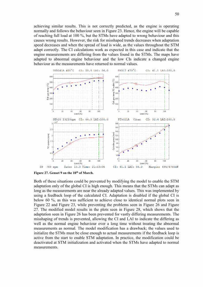
50

achieving similar results. This is not correctly predicted, as the engine is operating

normally and follows the behaviour seen in Figure 23. Hence, the engine will be capable

of reaching full load at 100 %, but the STMs have adapted to wrong behaviour and this

causes wrong results. However, the risk for misshaped trends decreases when adaptation

speed decreases and when the spread of load is wide, as the values throughout the STM

adapt correctly. The CI calculations work as expected in this case and indicate that the

engine measurements are differing from the values found in the STMs. The maps have

adapted to abnormal engine behaviour and the low CIs indicate a changed engine

behaviour as the measurements have returned to normal values.


Both of these situations could be prevented by modifying the model to enable the STM

adaptation only of the global CI is high enough. This means that the STMs can adapt as

long as the measurements are near the already adapted values. This was implemented by

using a feedback loop of the calculated CI. Adaptation is disabled if the global CI is

below 60 %, as this was sufficient to achieve close to identical normal plots seen in

Figure 22 and Figure 23, while preventing the problems seen in Figure 26 and Figure

27. The modified model results in the plots seen in Figure 28, which shows that the

adaptation seen in Figure 26 has been prevented for vastly differing measurements. The

misshaping of trends is prevented, allowing the CI and LAI to indicate the differing as

well as the normal engine behaviour over a long time without treating the abnormal

measurements as normal. The model modification has a drawback; the values used to

initialize the STMs must be close enough to actual measurements if the feedback loop is

active from the start to enable STM adaptation. In practice, the modification could be

deactivated at STM initialization and activated when the STMs have adapted to normal

measurements.

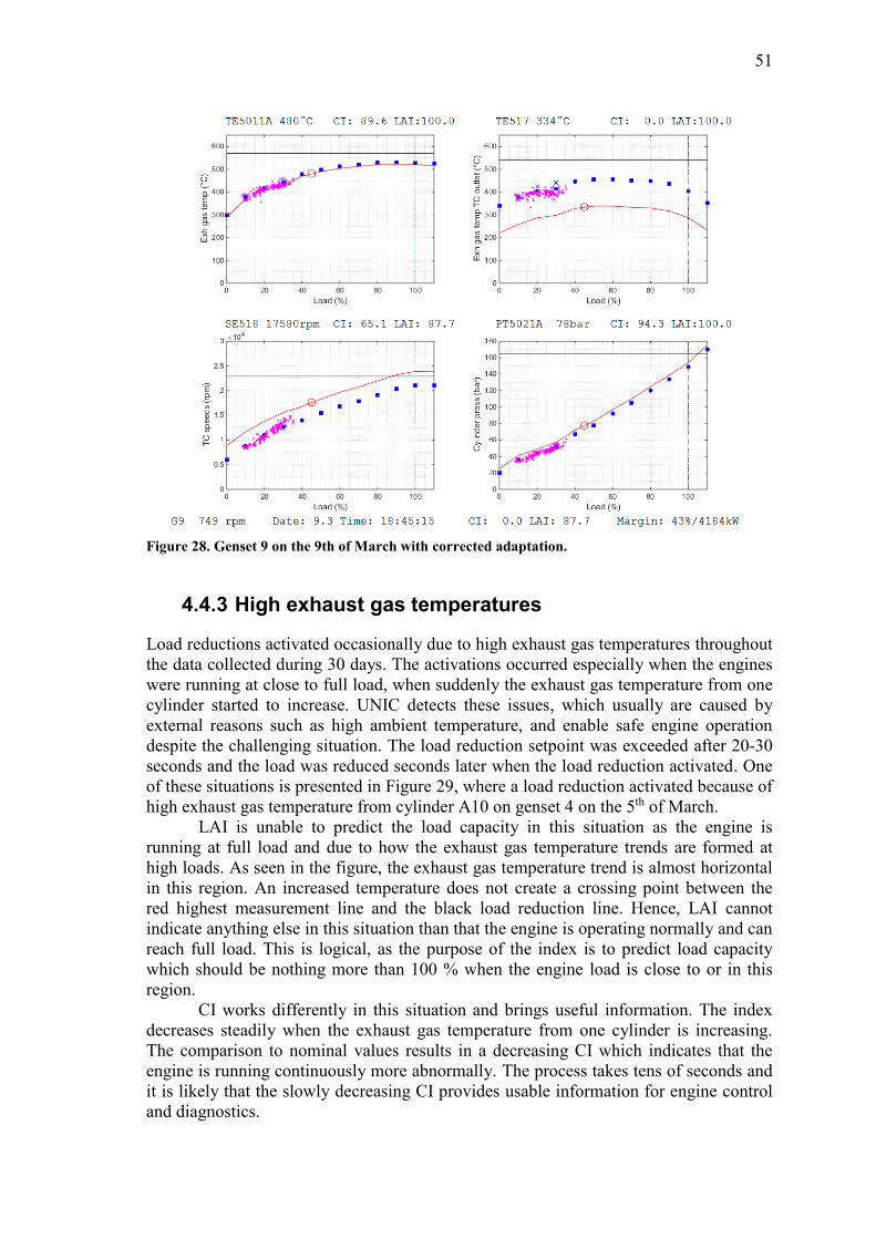
51

Figure 28. Genset 9 on the 9th of March with corrected adaptation.

4.4.3 High exhaust gas temperatures

Load reductions activated occasionally due to high exhaust gas temperatures throughout

the data collected during 30 days. The activations occurred especially when the engines

were running at close to full load, when suddenly the exhaust gas temperature from one

cylinder started to increase. UNIC detects these issues, which usually are caused by

external reasons such as high ambient temperature, and enable safe engine operation

despite the challenging situation. The load reduction setpoint was exceeded after 20-30

seconds and the load was reduced seconds later when the load reduction activated. One

of these situations is presented in Figure 29, where a load reduction activated because of

high exhaust gas temperature from cylinder A10 on genset 4 on the 5th of March.

LAI is unable to predict the load capacity in this situation as the engine is

running at full load and due to how the exhaust gas temperature trends are formed at

high loads. As seen in the figure, the exhaust gas temperature trend is almost horizontal

in this region. An increased temperature does not create a crossing point between the

red highest measurement line and the black load reduction line. Hence, LAI cannot

indicate anything else in this situation than that the engine is operating normally and can

reach full load. This is logical, as the purpose of the index is to predict load capacity

which should be nothing more than 100 % when the engine load is close to or in this

region.

CI works differently in this situation and brings useful information. The index

decreases steadily when the exhaust gas temperature from one cylinder is increasing.

The comparison to nominal values results in a decreasing CI which indicates that the

engine is running continuously more abnormally. The process takes tens of seconds and

it is likely that the slowly decreasing CI provides usable information for engine control

and diagnostics.

52

Figure 29. Exhaust gas temperatures on genset 9 on the 5th of March.

The load reduction has activated in the last plot in Figure 29, where the vertical de-

rating load level has been set by PMS. The engine is almost instantly unloaded to the

de-rating level and the exhaust gas temperatures return to normal as a result from the

decreased load. This de-activates the load reduction and PMS increases the de-rating

load level and ramps up the engine load again over the following minutes.

4.4.4 High cylinder pressures

Figure 23 shows how similar the trends are for the cylinder pressure and the TC speed;

both trends resemble lines and the scatters of average measurements are narrow.

However, the cylinder pressure scatter from all measurements is wider than the average

scatter. It was seen in Subsection 4.4.2 that the indexes worked well when calculated

from the TC speed, as long as adaption was prevented when the engine operated

abnormally. The same should apply to the cylinder pressure, as the trends follow the

same pattern. However, the update rate in CBM data was too slow for achieving as

interesting results for the cylinder pressure as for the other parameters.

Figure 30 shows the parameter plots on genset 3 on the 19th of March. Cylinder

B10 has high exhaust gas temperature and two load reductions activate seconds later.

These are caused by heavy knock and high peak cylinder pressure. The CIs indicate that

the engine is operating abnormally before the load reductions activate, but the index is

insufficient when compared to indexes calculated for the other gensets during the same

time. The measurements from the other engines are similar with even worse behaviour

and higher cylinder peak pressures. Despite that, only genset 3 suffers from load

reductions due to heavy knock and high cylinder peak pressures. The cylinder peak

pressures may vastly differ from the calculated average and the data is not accurate

enough for providing adequate results.

53

The STMs adapt properly to the measurement averages as the scatter of averages is

narrow. The indexes identify situations with abnormally high cylinder peak pressures

when comparing measurements and the STMs, and this results in indications of engine

load availability. However, the data used in the simulations has insufficient update rate

and no plots could be made which appropriately would demonstrate these situations.

The clear similarities to the TC speed trends indicate that the cylinder pressure index

calculations should work similarly well as long as the data has sufficient update rate.


4.4.5 History and engine comparison

Engine diagnostics may be accomplished by comparing adapted parameter values or

calculated indexes between engines or to historical data. For instance, a malfunctioning

engine may be discovered by comparing its adapted values to corresponding data from

other engines. This is possible in the Wärtsilä power plant, where identical engines are

used under the same circumstances and the adapted maps may, together with the

indexes, show how the need of service increases differently on engines. Similarly, the

adapted values may be compared to earlier, known working values which have been

adapted to previously for the same engine. For instance, by comparing the present

adapted values to two months old values or to the initial STM made right after the

Factory Acceptance Test (FAT). This is a collection of tests run on engines before they

are delivered to the customer. It was concluded during index development discussions

that the adapted values and the calculated indexes bring useful diagnostics to CBM

when determining engine service needs. The service need would be easier to determine

by comparing STM values and analysing historical data of index calculations. [19]

As an example, Figure 31 shows a comparison of the STMs for the exhaust gas

temperatures from all four engines, along with a histogram of the CI during the same

timespan. The plots and the histogram were created with data from the same timespan

as in Figure 26. G4 and G6 operated normally while G3 and G9 had different issues.

The engines are plotted according to G3 = blue, G4 = black, G6 = cyan and G9 =

magenta. The trends visualize how the engines are performing when compared to each

other. The G3 measurements are, except for the exhaust gas temperature TC outlet,

54

comparable to the G4 and G6 measurements and are hidden below these if not seen in

the plots. One of the exhaust gas temperature TC outlet sensors has failed on G3 and as

presented earlier, G9 runs abnormally during this timespan and these are the reasons

why their trends differ vastly from the rest. Comparison between adapted values and

indexes results in useful information for CBM or engine experts who perform diagnosis

on an engine.

The histograms are calculated and plotted created by using MATLAB

commands histcounts and bar. The histograms present the occurrences of differently

sized CIs, where the scaling is 0-100 % from left to right. This means that green and

yellow expresses high CIs while blue and violet are low CIs. It can be seen when

inspecting the histograms that G3 and G9 have more frequent occurrences of low CIs

than G4 and G6. Additional interesting numbers may be calculated from the histogram

data, for instance the time in percentages that an engine has had a CI below 50 %. The

results are G3 = 62 %, G4 = 26 %, G6 = 23 % and G9 = 45 %, which together with the

plots of adapted values show how differently the engines operate.

Figure 31. Data comparison for G3, G4, G6 and G9 after 24 hours adaptation.

55

5 Discussion

This chapter highlights the main achievements in the index development process and

discusses the outcome of the thesis. The results from the simulations are analysed and

the answers to the research questions are provided. Finally, proposals for continued

research are presented to highlight development areas not included in the thesis.

5.1 Index development

The purpose of the thesis was to identify the parameters needed to indicate an engine’s

load capacity, and to develop an algorithm which uses the statuses of these parameters

to calculate the engine’s instantaneous load availability as an index. The development

was conducted through interviews with engine experts, resulting in an understanding of

the requirements, possibilities, challenges and benefits of such index. Two indexes were

proposed which would take advantage of the possibilities and be beneficial in several

situations. The following questions were to be addressed in the thesis:

Which parameters should at the very least be used by the load capacity index?

Is one index enough or is a group of indexes a better solution?

When and how should the index be used?

Many engine parameters can be taken into account when calculating an index that

indicates the load capacity of an engine. Extensive discussions with engine experts

together with analysis of power plant data showed that the most frequently occurring

load reductions are caused by cylinder knock, exhaust gas temperatures, cylinder

pressure and turbocharger speed. UNIC is able to detect these issues, possibly caused by

high ambient temperature, insufficient fuel quality or other external reason, and safely

operate and control the engines in these situations, effectively preventing damage to

engines and equipment. External parameters, such as LT water and CA temperature,

affect the performance and load capacity of the engine heavily, but these are usually

controlled by the engine-external automation system and are unavailable in UNIC. It

was concluded that these brought no usable information to the calculations at this stage

of the index development. Instead, research focused on the parameters which usually

cause problems, correlate with load and are controlled and monitored by UNIC. The

parameters integrated in the index demonstration were exhaust gas temperature, exhaust

gas temperature TC outlet, cylinder pressure and turbocharger speed. Knock was,

despite its importance to engine performance, left out from the index calculations, as it

was too complicated to predict and utilize in the same way as the other parameters. The

demonstrated parameters should at the very least be used when calculating the indexes.

Additionally, the exhaust gas temperature TC inlet should be used when available, as it

an important performance parameter which correlates positively with load. Instruments

for this parameter were not installed on the power plant engines and had to be excluded

from the index demonstration. In conclusion, three of the four most important

parameters could be integrated and demonstrated; the proposed indexes should indicate

engine load availability in most situations. The exhaust gas temperatures are then

counted as one parameter and knock is the only important parameter which was

excluded due to complexity and lack of load correlation.

Two indexes were proposed in this thesis which together provide indications of

how normally the engine is operating and the approximated maximum load that the

56

engine can reach. One index was not seen to be enough as the two developed indexes

are similar but they express the relation between nominal and instantaneous engine

measurements differently. Each has its benefits and properties, resulting in varying

usability in different situations. Both indexes are beneficial in engine control and

diagnostics, but the LAI is usable especially in engine control, whereas the CI has

superior properties when performing engine diagnostics. This conclusion was made

after the index evaluations were completed and commented on by engine experts. It is a

valid approximation to assume that the adapted trend is offset according to external

parameters, such as suction air temperature, wear and tear or need of TC washing, and

that the engine’s maximum load or condition can hence be estimated. Adaptive maps

reflect the engine behaviour in the present operating environment and the resulting

parameter trends respond to the actual situation. Parameters may have different nominal

values depending on the fuel mode, and it is a valid assumption that fuel mode specific

adaptive maps must be utilized on DF engines to enable proper index calculation. The

indexes were calculated utilizing measurements and adaptive maps and the results were

seen promising. The indexes worked as expected and engines performing abnormally

could be discovered.

The starting point for this thesis was the US electricity market and the engine

load ramping challenges. Engines should be able to ramp up quickly and indications of

engines failing to do this should be discovered before the actual fail is seen. Only

engines with high load capacity would be loaded to prevent situations where less power

is produced from the power plant than planned. Load reductions should not activate on

any engine and the power plant should be able to produce the right amount of power at

the right time without any issues. The best method for demonstrating the usefulness of

the indexes, especially LAI, would be to use data from a power plant suffering from this

problem. This data was not available and the simulations were conducted with the data

that was available. Engines were reasonably slowly loaded in this data and load

reductions were seldom an issue during the loading. Hence, it was not possible to

demonstrate the usefulness of LAI entirely in the presented loading scenario with the

available setup. The indexes did, however, succeed in demonstrating their usability, but

not up to the extent that could have been possible with data suffering from the issues

which the indexes strive to solve. Manipulation of the data was not seen as an option, as

this last resort solution should be avoided to not modify the data unrealistically.

Furthermore, the data update rate was insufficient for demonstrating the index benefits

for the cylinder pressure. This was a known risk when choosing the data, but the data

benefits exceeded the drawbacks. The data was acquired from identical engines in a real

power plant connected to the grid, and more suitable data for index demonstration is

difficult to find.

The indexes provide quantitatively the condition and maximum load of the

engine which can be used by PMS and/or the load sharing algorithm in UNIC when

controlling the engine. Control can potentially be applied successfully based on the

indexes, but that was out of scope for this thesis. Engine control is conducted on a

millisecond basis and the update rate of the indexes should hence be in the same scale.

Filtering of the signals will additionally be needed, as this can be concluded from how

the indexes are calculated from measurements and trend estimations. Changes in the

measurement values may affect the resulting index values unevenly depending on the

shape of the trend or the load level. As earlier pointed out, the CI varies differently for

the same absolute change in measurement value depending on whether the load level is

low or high. Equally the LAI variations may vary vastly depending on the shape of the

trend and whether the load reduction crossing point could be determined or not. For

instance, a slightly sloping line offset in vertical direction has decreased risk of

57

producing a fluctuating LAI than a curve shaped like the exhaust gas temperature trend.

The slope of the curve is increasingly horizontal at high load and the resulting LAI can

hence vary rapidly when the engine runs at low load. This follows as the exact crossing

point is estimated highly differently depending on the absolute measurement offset.

Filtering of the indexes will hence be needed to ensure that the control signal is not

fluctuating unnecessarily, as such will not result in optimal control or loading of

engines. Proposed at one point during the index development was to demonstrate the

load sharing possibilities by integrating the index functionality in a Simulink model

with two DF engines. It would have been possible to modify the load sharing and

biasing the engines according to load capacity by utilizing the calculated indexes. This

was not realized, as it was seen sufficient to demonstrate the indexes with the Simulink

model developed in the thesis together with real engine data. The load sharing model is

focused on control and it was not seen necessary to provide such simulations.

It was noticed when processing the exhaust gas temperature measurements that

the temperatures where usually lower than expected when ramping up the engine load

and higher when the engine was unloaded. Another discovery was that the exhaust gas

temperatures from individual cylinders differ unequally from the average temperature

on the load range. The difference is largest at low loads and decreases when the load

increases due to cylinder load balancing in UNIC. Both of these temperature behaviours

were normal according to engine experts, but may decrease the usability of the indexes

at load transients as the indexes are calculated from the worst measurements found. The

LAI may indicate a low maximum load either when an engine is quickly unloading or

when the engine is ramping up from a low load because of how the highest exhaust gas

temperature is utilized. The other parameters do not have the same problem, and the

measurement scatters are equally sized on the whole load spectra. [29]

Engines diagnostics may be conducted by comparison of the calculated indexes

or the adapted values in the STMs. This comparison can be performed by comparing

present or historical data for indexes and adapted values for either the same engine or

other engines. Through these means even greater diagnostics possibilities open which

allow improved tools for following up the service need on engines. Also discussed was

the ability to adapt the STMs not just to measurement averages on the same engine, but

also to the averages from the other engines running in the same environment. An even

greater smoothing effect and general parameter behaviour would then be achieved, as

the averages from equal engines following the same system load would be combined.

This demands increased communication between engines and may in practice not be a

suitable option. Especially the CI is suitable in diagnostics, as it is an additional

parameter that provides useful information when distinguishing an engine running

abnormally from an engine operating normally. This follows as CI is a direct

measurement of how normally the engine is operating. It can be calculated for any

parameter, as long as nominal and instantaneous measurements are available along with

the load reduction setpoint. The CBM staff showed great interest in CI, where it may

turn out to be a useful parameter to show how normally the engines operate or have

been operating.

5.2 Adaptivity

It was concluded at an early stage of the index development that the indexes should be

adaptive to provide up-to-date and usable calculation without the need of continuous

configuring. This functionality was possible to add by using the tools available.

Adaptivity results in improved estimation of the nominal values, but the process

58

introduces some challenges. The greatest challenge with adaptivity is to tune the update

rate properly. The adaptivity must be fast enough to show the actual engine behaviour in

the present operating environment, but slow enough to not adapt to wrong

measurements and to prevent misshaping of the parameter trends. Misshaping of the

trends is the greatest challenge to the LAI, while too fast adaptivity as such causes

problems for the CI. The LAI is not able to predict the engine’s maximum load correctly

after a certain amount of time if the adaptivity is fast, as the trend may misshape when

the engine load is kept within a restricted range. Equally, the CI does indicate the

differing engine condition, but this indication weakens as the adaptation progresses.

One possible solution to this problem was proposed and tested in the simulations:

adaptation was prevented when the measurements differed vastly from the adapted

values. This was implemented by using a feedback loop with the calculated CI, which

prevented the engine from adapting to values when the engine behaviour was abnormal.

Only engines with high CIs were allowed to adapt to present measurements. This

improvement was a success and both indexes succeeded in their tasks when the engine

performed abnormally and when it returned to normal operation. It was thought to be a

good starting point to prevent adaptation for all parameters by using the global CI as

input as parameters are highly interconnected on an engine. Alternatively, parameters

may adapt as long as the CI for each parameter is high enough but this was not tested.

The improvement has a major drawback, as the initial values used in the adaptive maps

must be close enough to the measured values. Otherwise adaptation will never occur as

the engine performance is seen as too poor. This could be solved by disabling the CI

effects on adaptation when the engine is operating normally. Furthermore, not only this

setting could be changed when the engine is adapting but also the adaptation rate. It

would be logical to increase the adaptation rate when actually trying to adapt the maps

during FATs or after service has been conducted on the engine. The adaption rate could

then be decreased to prevent the maps from misshaping when the values have adapted,

checked and the engine has been taken into use. Such on-the-fly adaptivity would

provide proper adaptivity throughout the engine’s lifetime.

The adaptivity rate was reduced in the simulations by configuring the gains for

the STMs as small as possible. Furthermore, an adaptivity rate parameter was developed

and set to 100, which updated the maps on every 100th measurement only. The global CI

was also taken into use to prevent adaptation to abnormal values. Successful adaptation

was achieved in the index demonstration with these settings, but the adaptivity rate may

be more challenging to determine on other installations. The timespan for adaptation

must be determined and the weather conditions analysed when configuring the

adaptivity, as the greatest factor when offsetting the trends in vertical directions is the

ambient temperature. This can differ vastly between day and night, from month to

month or when comparing summer to winter. The adaptation must be configured

accordingly for each installation to ensure that the adaptation and index calculations are

conducted as planned. Proposed was also to measure the ambient temperature and to

offset the adapted maps according to the temperature directly. The calculated indexes

would then better reflect the operating environment instantly. This is achieved without

the need of first adapting the maps and risking trend misshaping due to large

temperature deviations or not utilizing the entire load range. The risk of trend

misshaping decreases also as adaptation rate decreases and that is one reason why slow

adaptation is recommended. Adaptation was prevented when the engine speed was

below the rated engine speed to prevent misshaping of trends at the 0 % load element.

This is an important rule that must be implemented in a future index UNIC application

to allow proper adaptation despite various engine modes such as start, stop or shutdown.

59

5.3 Further research

This thesis focused on the development of the load capacity index and did not test nor

discuss thoroughly its implementation in engine control. The acquired possibilities,

challenges and index calculations were presented, enabling the possibility to test the

indexes in optimal engine control and load sharing. This is proposed as the subject of

another research project. Concluded was that the indexes are usable in engine control as

they are scalar values, easily compared and describe an engine’s possibility to be

loaded. Requirements to ensure proper index calculations for engine control are at the

very least sufficient measurement and index update rate along with filtering of the

calculated indexes. Furthermore, continued testing of the indexes is proposed.

Especially recommended is conducting tests with data containing fast ramping of

engines, to better understand how well the LAI works in the US power plant scenario.

Diesel engines should also be tested, as knock is not observed on these engines and the

usefulness of the indexes should improve further. This follows as knock commonly

causes load reductions on SG engines, but was the only parameter which was not

integrated in the index calculations. Similarly, the understanding can be improved of

how usable the CI is in engine diagnostics and service for CBM. Data from other

installations and engine types should be used to thoroughly understand and benefit from

the advantages that the index brings.

Additionally, the idea of a condition or load capacity index may be expanded to

also include the efficiency of an engine. This enables the engine-external automation

system to optimize the usage of different engines according to their thermal efficiencies.

This is beneficial in situations where differently sized engines share a load, as the load

can be shared more efficiently when engines automatically run at speeds with high

thermal efficiency. An efficiency index is challenging to implement as the parameters

needed for it are missing. Engine efficiency is highly dependent on ambient conditions,

temperature of cooling water and lube oil, type of fuel and its heat value, generator

efficiency and other auxiliary systems. Some of these parameters are not available to

UNIC and the engine efficiency is hence not trivial to calculate or estimate. It is thus

proposed that research may be conducted on this topic to determine how and if an

engine efficiency index can be calculated. The index would take known engine

efficiency maps into account and also include important efficiency parameters in its

calculations to provide a usable index which allows engines to run more efficiently if

possible. [19]

60

6 Conclusion

The thesis strived to develop an index that indicates the load capacity of an engine by

using engine measurements. Two indexes were proposed which describe the load

margin of an engine differently. The CI is assumed to be usable especially in engine

diagnostics, while the LAI is superiour in engine control. Three of the four most

common load reduction parameters were integrated in the index calculations, which was

seen as a sufficient amount of parameters at this stage of index development. Knock

was left out due to complexity and lack of load correlation. The indexes are still

assumed to be able to indicate the maximum load and the condition of an engine

successfully in most situations. This was not possible by earlier means and the thesis

results are hence promising, although not completely trouble-free.

The greatest challenges for the two indexes are adaptivity speeds and how to

tune the adaptivity to reflect every situation properly. Additionally, the LAI may

fluctuate vastly depending on the shape of the parameter trend. At the very least, filters

will be needed to produce working and stable indexes. Using the CI as a feedback in the

calculations loop solved most of the issues with adaptiation to abnormal engine

measurements. Further testing with data from other power plants could improve the

understanding of how the adaptivity should be done correctly and how the fluctuations

in index values can be addressed.

The developed indexes corresponds to the requirements and assumptions set at

the beginning of the development process; not all parameters can nor should be

integrated. This thesis started the work of what must, can or should be taken into

account when describing the load operation margin of an engine. Demonstrations show

the importance of adaptive maps of nominal engine parameter measurements and how

vastly these improve index calculations. Engine measurements are additionally

relatively stable, and the interpolated trend represents thus the general situation well. In

conclusion, there is a potential in calculating engine load capacity indexes and the

advantages outnumber the drawbacks.

61

References

[1]. The definition of engine load. SAE J1979 2002/04 p. 23.87 and 23.93.

[2]. Eriksson, L., Nielsen, L., Modeling and Control of Engines and Drivelines. John

Wiley & Sons, 2014, p. 74-76.

[3]. Kao, M., Moskwa, J. J., Engine load and equivalence ratio estimation for control

and diagnostics via nonlinear sliding observer. Proceedings of the American Control

Conference. Baltimore, Maryland. June, 1994, p. 1574-1578.

[4]. Stotsky, A., Eriksson, S., Adaptive Learning Engine Load Estimation. Proceedings

of the 41st IEEE Conference on Decision and Control. Las Vegas, Nevada USA,

December 2002, p. 3712-3717.

[5]. About Wärtsilä. Internet source. Available 18.12.2015:

http://www.wartsila.com/about

[6]. Wärtsilä History. Internet source. Available 18.12.2015:

http://www.wartsila.com/about/history

[7]. Wärtsilä 31 news article. Internet source. Available 18.12.2015:

http://www.wartsila.com/media/news/02-06-2015-new-wartsila-31-engine-achieves-

guinness-world-records-title

[8]. Wärtsilä strategy. Internet source. Available 18.12.2015:

http://www.wartsila.com/about/strategy

[9]. Wärtsilä 34DF product guide. Internet source. Available 22.12.2015:

http://cdn.wartsila.com/docs/default-source/product-files/engines/df-engine/wartsila-

34df-product-guide.pdf

[10]. Wärtsilä UNIC C3 brochure. Internet source. Available 22.12.2015:

http://cdn.wartsila.com/docs/default-source/Service-catalogue-files/Electrical-

Automation-Services/unic-c3-engine-control-system.pdf

[11]. Östman, F. and Kaas, T., Adaptive control – a means for ensuring engine control

quality. Wärtsilä Technical Journal: In Detail. Issue 2, 2009, p. 54-57.

[12]. Pensar, J. and Storbacka, M., UNIC – The reliable solution for robust industrial

controls. Wärtsilä Technical Journal: In Detail. Issue 2, 2007, p. 40-44.

This thesis was possible to accomplish thanks to noticebly efforts from the

following Wärtsilä employees:

Dahlberg Tommy, Hattar Christer, Nuormala Kimmo, Kaas Tom, Saikkonen Ari,

Vägar Jens and Åberg Anders

http://ieeexplore.ieee.org.libproxy.aalto.fi/search/searchresult.jsp?searchWithin=%22Authors%22:.QT.Minghui%20Kao.QT.&newsearch=true

62

[13]. Condition based maintenance generally. Internet source. Available 27.1.2016:

https://www.maintenanceassistant.com/condition-based-maintenance/

[14]. Isermann, R., Fault-Diagnosis Systems – An Introduction from Fault Detection to

Fault Tolerance. Berlin, Springer, 2006.

[15]. Rolls-Royce engine health management. Internet source. Available 27.1.2016:

http://www.rolls-royce.com/about/our-technology/enabling-technologies/engine-health-

management.aspx

[16]. Wärtsilä Genius services. Internet source. Available 7.1.2016:

http://www.wartsila.com/services/lifecycle-solutions/wartsila-genius-services

[17]. Klockars, T. et. al., Making the most of perfect maintenance timing. Wärtsilä

Technical Journal: In Detail. Issue 1, 2011, p. 64-65.

[18]. Wärtsilä DMP and CBM presentation. Internet source. Available 7.1.2016:

http://www.wartsila.com/static/studio/assets/content/ss1/cbm-presentation.pdf

[19]. Interview with Vägar, J. 28.1.2016, 23.3.2016, 2.6.2016.

[20]. Saikkonen, A. and Kaas, T., Analogue isochronous load sharing and UNIC.

Wärtsilä Technical Journal: In Detail. Issue 2, 2012, p. 9-16.

[21]. Interview with Saikkonen, A., 11.1.2016, 9.3.2016.

[22]. Interview with Kaas, T. 3.3.2016, 31.5.2016.

[23]. Engine safety and machinery protection specification rev a. Internal Wärtsilä

document.

[24]. Load Reduction Control v4.1 application description. Internal Wärtsilä document.

[25]. Santoianni, D., Power plant performance under extreme ambient conditions.

Wärtsilä Technical Journal: In Detail. Issue 1, 2015, p. 22-27.

[26]. E-mail conversations with Åberg, A. and Lundström, R. 1.3.2016, 13.6.2016.

[27]. E-mail conversations with Nuormala, K. and Portin, K. 24.2.2016-8.3.2016

[28]. Interview with Dahlberg, T. 2.3.2016, 10.5.2016.

[29]. Interview with Hattar, C. 27.1.2016, 29.3.2016, 26.5.2016

[30]. Interview with Beijar, M. 3.6.2016.

[31]. Interview with Hyvönen, J., Järvi, A., Hattar, C. 23.2.2016.

[32]. Common Functions v8.4 specification. Internal Wärtsilä document.

63

[33]. CBM / Vägar, J., Formulas for determining nominal parameter values at different

engine loads.

[34]. CBM / Masus, T., Engine measurement data from a real power plant.

[35]. Real-Time Pacer for Simulink. Vallabha, G. Internet source. Available 8.6.2016:

http://www.mathworks.com/matlabcentral/fileexchange/29107-real-time-pacer-for-

simulink

64

Appendix A – The data loading script

G_data = zeros(86400*30,53);

filePaths = {'data/BAG031UP01LIM.csv' 'data/SCA031STY196PV.csv' ...

'data/SCA031IB500PV.csv' 'data/SCA031SE518PV.csv' ...

'data/SCA031SE528PV.csv' 'data/SCA031TE517PV.csv' ...

'data/SCA031TE527PV.csv' 'data/SCA031TE471PV.csv' ...

'data/SCA031TE601PV.csv' 'data/SCA031TY500PV.csv' ...

'data/SCA031TE5011APV.csv' 'data/SCA031TE5011BPV.csv' ...










'data/SCA031PT5011APV.csv' 'data/SCA031PT5011BPV.csv' ...









'data/SCA031PT5101APV.csv' 'data/SCA031PT5101BPV.csv'};

fid = fopen('data/SCA031UT793PV.csv');

tline = fgets(fid);

row = 2;

day = str2double(tline(9:10));

second = str2double(tline(12:13)) * 3600 + str2double(tline(15:16)) * 60 +

str2double(tline(18:19));

value = str2double(tline(21:end));

while day < 31

G_data(row,1:3) = [day second value];

tline = fgets(fid);


second = str2double(tline(12:13)) * 3600 + str2double(tline(15:16)) * 60 +

str2double(tline(18:19));

value = str2double(tline(21:end));

row = row + 1;

end

fclose(fid);

id = 1;

65

len = length(filePaths);

while id <= len

fid = fopen(char(filePaths(id)));

tline = fgets(fid);

row = 2;


while day < 31

G_data(row, id + 3) = str2double(tline(21:end));

tline = fgets(fid);


row = row + 1;

end

fclose(fid);

id = id + 1;

end

G_data(1,:) = G_data(2,:);

G_data(1,2) = 0;

66

Appendix B – The simulation and plotting script

%% Reset variables, load data, simulate and plot as long as data

% is found and the key 's' is not pressed

clear;

addpath('RealTime_Pacer','thesis_func')

% Insert genset and start/stop time for fetching data

genset = 'G9';

start = strtime2index('08 19:00:00');

stop = strtime2index('09 18:45:00');

G_data = importdata(strcat('mat_files/',genset,'_all_1-30.mat'));

model_name = 'thesis_demo';

K1 = 100;

K2 = 100;

K3 = 10;

K4 = 100;

% Load data and start the simulation

if strcmp(get_param(model_name,'SimulationStatus'),'stopped')

len = stop - start;

simtime = (0:0.1:len/10)';

ut793_matrix = [simtime G_data(start:stop,3)/9.730];

derate_matrix = [simtime G_data(start:stop,4)/9.730];

sty196_matrix = [simtime G_data(start:stop,5)];

ty500_matrix = [simtime G_data(start:stop,13)];

te5xxx_matrix = [simtime G_data(start:stop,14:33)];

te5x7_avg_matrix = [simtime (G_data(start:stop,9)+G_data(start:stop,10))/2];

te5x7_matrix = [simtime G_data(start:stop,9:10)];

se5x8_avg_matrix = [simtime (G_data(start:stop,7)+G_data(start:stop,8))/2];

se5x8_matrix = [simtime G_data(start:stop,7:8)];

pt5xxx_avg_matrix = [simtime sum(G_data(start:stop,34:53),2)/20];

pt5xxx_matrix = [simtime G_data(start:stop,34:53)];

te601_matrix = [simtime G_data(start:stop,12)];

ib500_matrix = [simtime G_data(start:stop,6)];

te471_matrix = [simtime G_data(start:stop,11)];

clear G_data;

set_param(model_name, 'SimulationCommand', 'start')

set_param(model_name, 'SimulationCommand', 'pause')

pause(1);

end

67

% Create the plot figure and add option to stop simulation by 's' button

mFigure = figure('KeyReleaseFcn', @KeyPress);

set(mFigure,'Position',[200 178 1100 772]);

set(mFigure,'Color', [1 1 1])

fig1 = subplot(2,2,1);




% Create uicontrol for first row of information

mExhTempBox = uicontrol('style','text');

set(mExhTempBox,'FontName','Courier');

set(mExhTempBox,'FontSize',15);

set(mExhTempBox,'Position',[140 730 1100 20])

set(mExhTempBox,'HorizontalAlignment','left')

set(mExhTempBox,'BackgroundColor', [1 1 1])

% Create uicontrol for second row of information

mTurboBox = uicontrol('style','text');

set(mTurboBox,'FontName','Courier');

set(mTurboBox,'FontSize',15);

set(mTurboBox,'Position',[140 370 1100 20])

set(mTurboBox,'HorizontalAlignment','left')

set(mTurboBox,'BackgroundColor', [1 1 1])

% Create uicontrol for third row of information

mTimeBox = uicontrol('style','text');

set(mTimeBox,'FontName','Courier');

set(mTimeBox,'FontSize',15);

set(mTimeBox,'Position',[20 20 1100 20])

set(mTimeBox,'HorizontalAlignment','left')

set(mTimeBox,'BackgroundColor', [1 1 1])

% While simulation is running, update plots

% Pause is needed to update workspace variables

while strcmp(get_param(model_name,'SimulationStatus'),'stopped') ~= 1

set_param(model_name, 'SimulationCommand', 'pause')

% Update plot 1

[exh_max_now,exh_index] = max(exh_vec_now);

plot(fig1,exh_x,exh_vec,'b.','MarkerSize',20)

hold(fig1,'on')

plot(fig1,exh_x,exh_vec_with_offset,'r')

plot(fig1,load_now,exh_max_now,'ro','MarkerSize',10)

plot(fig1,[exh_lai exh_lai],[0 650],'g--','MarkerSize',20)

plot(fig1,[derate_now derate_now],[0 650],'k:','MarkerSize',20)

plot(fig1,[0 110],[exh_lr exh_lr],'k')

grid(fig1, 'minor')

axis(fig1,[0 110 0 650])

xlabel(fig1,'Load (%)')

ylabel(fig1,'Exh gas temp (°C)')

hold(fig1,'off')

% Update plot 2

68

[exh_tc_max_now,exh_tc_index] = max(exh_tc_vec_now);

plot(fig2,exh_tc_x,exh_tc_vec,'b.','MarkerSize',20)

hold(fig2,'on')

plot(fig2,exh_tc_x,exh_tc_vec_with_offset,'r')

plot(fig2,load_now,exh_tc_max_now,'ro','MarkerSize',10)

plot(fig2,[exh_tc_lai exh_tc_lai],[0 650],'g--','MarkerSize',20)


plot(fig2,[0 110],[exh_tc_lr exh_tc_lr],'k')

grid(fig2, 'minor')

axis(fig2,[0 110 0 650])


ylabel(fig2,'Exh gas temp TC outlet (°C)')

hold(fig2,'off')

% Update first row of information

set(mExhTempBox,'String',...

strcat(findCylCode(exh_index,'TE5'),{' '},addSpace(num2str(exh_max_now),3),...

{'°C CI:'},addSpace(num2str(exh_ci,'%.1f'),5),{'

LAI:'},addSpace(num2str(exh_lai,'%.1f'),5),...

{' TE5'}, num2str(exh_tc_index),{'7 '}, addSpace(num2str(exh_tc_max_now),3),...

{'°C CI:'},addSpace(num2str(exh_tc_ci,'%.1f'),5),{'

LAI:'},addSpace(num2str(exh_tc_lai,'%.1f'),5)))

% Update plot 3

[tc_max_now,tc_index] = max(tc_vec_now);

plot(fig3,tc_x,tc_vec,'b.','MarkerSize',20)

hold(fig3,'on')

plot(fig3,tc_x,tc_vec_with_offset,'r')

plot(fig3,load_now,tc_max_now,'ro','MarkerSize',10)

plot(fig3,[tc_lai tc_lai],[0 30000],'g--','MarkerSize',20)


plot(fig3,[0 110],[tc_lr tc_lr],'k')

grid(fig3, 'minor')

axis(fig3,[0 110 0 30000])


ylabel(fig3,'TC speeds (rpm)')

hold(fig3,'off')

% Update plot 4

[cyl_max_now,cyl_index] = max(cyl_vec_now);

plot(fig4,cyl_x,cyl_vec,'b.','MarkerSize',20)

hold(fig4,'on')

plot(fig4,cyl_x,cyl_vec_with_offset,'r')

plot(fig4,load_now,cyl_max_now,'ro','MarkerSize',10)

plot(fig4,[cyl_lai cyl_lai],[0 180],'g--','MarkerSize',20)


plot(fig4,[0 110],[cyl_lr cyl_lr],'k')

grid(fig4, 'minor')

axis(fig4,[0 110 0 180])


ylabel(fig4,'Cylinder press (bar)')

hold(fig4,'off')

% Update second row of information

69

set(mTurboBox,'String',strcat({'SE5'},num2str(tc_index),{'8

'},addSpace(num2str(tc_max_now),5),...

{'rpm CI:'}, addSpace(num2str(tc_ci,'%.1f'),5),{'

LAI:'},addSpace(num2str(tc_lai,'%.1f'),5),...

{' '},findCylCode(cyl_index,'PT5'),{' '},addSpace(num2str(cyl_max_now),3),...

{'bar CI:'}, addSpace(num2str(cyl_ci,'%.1f'),5),{'

LAI:'},addSpace(num2str(cyl_lai,'%.1f'),5)))

% Stop simulation if we are the end

time_temp = floor(time*10 + start);

if time_temp >= stop

set_param(model_name,'SimulationCommand','stop')

end

% Update third row of information

load_left = global_lai(end) - load_now;

kw_left = load_left * 9730 / 100;

set(mTimeBox,'String',strcat({' '},genset,{' '},addSpace(num2str(speed_now),3),{' rpm '},

sec2strtime(time_temp),...

{' CI:'},addSpace(num2str(global_ci(end),'%.1f'),5),{'

LAI:'},addSpace(num2str(global_lai(end),'%.1f'),5), ...

{' Margin:'},addSpace(num2str(load_left),3),...

{'%/'},addSpace(num2str(kw_left),3),{'kW'}))

set_param(model_name, 'SimulationCommand', 'continue')

pause(0.1)

end

hold(fig1,'on')

hold(fig2,'on')

hold(fig3,'on')

hold(fig4,'on')

%% Plot the initial data

plot(fig1,exh_x,exh_init,'bx')

plot(fig2,exh_tc_x,exh_tc_init,'bx')

plot(fig3,tc_x,tc_init,'bx')

plot(fig4,cyl_x,cyl_init,'bx')

%% Plot the data that we have used for adaptation

[exh_load_used,exh_used] = findUsedInSTM(len, exh_enable_train, ut793_matrix,

ty500_matrix);

[exh_tc_load_used,exh_tc_used] = findUsedInSTM(len, exh_tc_enable_train, ut793_matrix,

te5x7_avg_matrix);

[tc_load_used,tc_used] = findUsedInSTM(len, tc_enable_train, ut793_matrix,

se5x8_avg_matrix);

[cyl_load_used,cyl_used] = findUsedInSTM(len, cyl_enable_train, ut793_matrix,

pt5xxx_avg_matrix);

plot(fig1,exh_load_used,exh_used,'m.')

plot(fig2,exh_tc_load_used,exh_tc_used,'m.')

plot(fig3,tc_load_used,tc_used,'m.')

plot(fig4,cyl_load_used,cyl_used,'m.')

70

%% Plot all the averages

plot(fig1,ut793_matrix(:,2)/10,ty500_matrix(:,2),'k.')

plot(fig2,ut793_matrix(:,2)/10,te5x7_avg_matrix(:,2),'k.')

plot(fig3,ut793_matrix(:,2)/10,se5x8_avg_matrix(:,2),'k.')

plot(fig4,ut793_matrix(:,2)/10,pt5xxx_avg_matrix(:,2),'k.')

%% Plot all the measurements

plot(fig1,ut793_matrix(:,2)/10,te5xxx_matrix(:,2:end),'c.')

plot(fig2,ut793_matrix(:,2)/10,te5x7_matrix(:,2:end),'c.')

plot(fig3,ut793_matrix(:,2)/10,se5x8_matrix(:,2:end),'c.')

plot(fig4,ut793_matrix(:,2)/10,pt5xxx_matrix(:,2:end),'c.')

71

Appendix C – The script help functions

function [ result ] = addSpace( str, count )

% addSpace Adds white spaces as needed at start of str.

% Adds until length of str is equal to count

while length(str) < count

str = [' ' str];

end

result = str;

end

function [ result ] = findCylCode(y_val_index, code)

% findCylCode Creates ISO-codes from index = cylinder

% Returns cylinder code and bank

if (y_val_index < 19)

code = strcat(code,'0');

end

if (mod(y_val_index,2) == 1)

result = strcat(code,num2str(floor((y_val_index + 1)/2)),{'1A'});

else

result = strcat(code,num2str(floor((y_val_index + 1)/2)),{'1B'});

end

end

function [y_load_used,y_used] = findUsedInSTM(len, vec_enable_train, ut793_matrix,

y_matrix)

%findUsedInSTM Finds the STM values used based on enable_train status

% Overlow due to simulation speed and stops when time > stopping time

if len < length(vec_enable_train)

vec_enable_train = vec_enable_train(1:(len + 1));

end

% Initialize variables and loop through train, save if we should save

y_load_used = [];

y_used = [];

for i=1:length(vec_enable_train)

if vec_enable_train(i) == 1

y_load_used = [y_load_used ut793_matrix(i,2)/10];

y_used = [y_used y_matrix(i,2)];

end

end

end

function KeyPress(ObjH, EventData)

% KeyPress Stops simulations when 's' is pressed

% 'p' cannot be used for pausing, as the script is paused anyway

model_name = 'thesis_demo';

Key = get(ObjH, 'CurrentCharacter');

switch Key

case 's'

72

set_param(model_name, 'SimulationCommand', 'stop')

% case 'p'

% if strcmp(get_param(model_name,'SimulationStatus'),'running')

% set_param(model_name, 'SimulationCommand', 'pause')

% else

% set_param(model_name, 'SimulationCommand', 'continue')

% end

end

function [ result ] = sec2strtime( time_temp )

% sec2strtime Converts 63 to '01 00:01:03'

% return format is 'Date: D.3 Time: HH:MM:SS'

day = floor(time_temp/86399) + 1;

time_temp = time_temp - (day - 1)*86399;

hour = floor(time_temp/3600);

min = floor(time_temp/60) - hour*60;

sec = time_temp - min*60 - hour*3600;

hour = num2str(hour);

min = num2str(min);

sec = num2str(sec);

if length(hour) == 1

hour = strcat('0',hour);

end

if length(min) == 1

min = strcat('0',min);

end

if length(sec) == 1

sec = strcat('0',sec);

end

result = strcat({'Date: '},num2str(day),{'.3 Time: '},hour,':',min,':',sec);

end

function [ result ] = strtime2index( str )

% strtime2index Converts '01 00:01:03' to 63

% 'DD HH:MM:SS'

sec = str2double(str(10:11));

min = str2double(str(7:8))*60;

hour = str2double(str(4:5))*3600;

days = (str2double(str(1:2)) - 1)*86399;

result = days + hour + min + sec;

end

73

Appendix D – The C functions

#define calcYpol(X_var, xX1, xX2, yY1, yY2) (((X_var - xX1) * (yY2 - yY1)) / (xX2 - xX1) +

yY1 )

#define u16 unsigned short

#define s16 signed short

#define s32 signed long

/****************************************************************************/

/*! \brief Lookup load reduction max load

Looks up the load that corresponds to the load reduction level.

Only maximal load is interesting and that's why we require that x_vec[index] > load

\param load The present load value

\param load_red The present load reduction value

\param y_vec Pointer to the present y value vector

\param pSelfTuningMapConfig Pointer to the self tuning map configuration

*****************************************************************************

/

s32 FuncLookupLAI(s16 load, s32 y_val, s32 load_red, s32 *y_vec,

CSelfTuningMapIntConfigEdit *pSelfTuningMapConfig)

{

u16 index = 0;

s32 temp = 1000;

if (y_val < load_red)

{

for( index = 1; index < pSelfTuningMapConfig->vector_size; ++index )

{

if (pSelfTuningMapConfig->x_vec[index] > load && y_vec[index] > load_red &&

y_vec[index - 1] < load_red)

{

temp = calcYpol(load_red, y_vec[index],y_vec[index - 1],pSelfTuningMapConfig-

>x_vec[index],pSelfTuningMapConfig->x_vec[index - 1]);

break;

}

}

}

else

{

for( index = pSelfTuningMapConfig->vector_size - 2; index > 0; --index )

{

if (y_vec[index + 1] > load_red && y_vec[index] < load_red)

{

temp = calcYpol(load_red, y_vec[index + 1],y_vec[index],pSelfTuningMapConfig-

>x_vec[index + 1],pSelfTuningMapConfig->x_vec[index]);

break;

}

}

}

if (temp <= 0)

{

return 0;

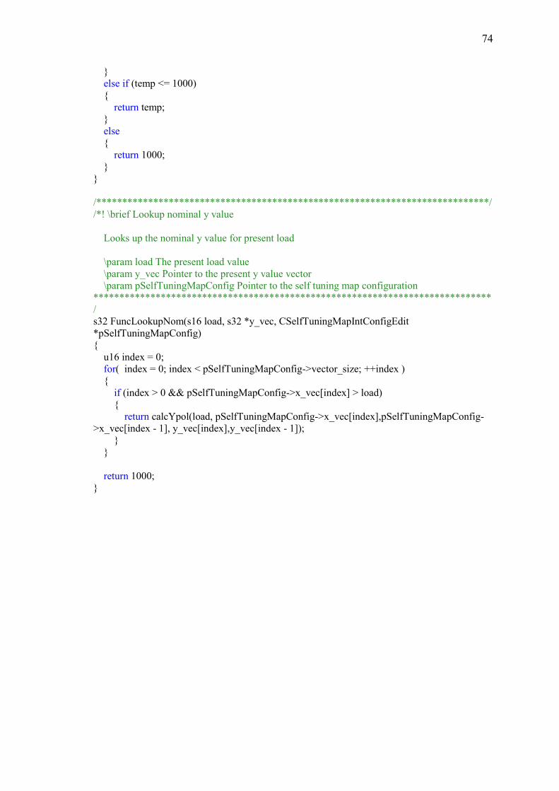
74

}

else if (temp <= 1000)

{

return temp;

}

else

{

return 1000;

}

}

/****************************************************************************/

/*! \brief Lookup nominal y value

Looks up the nominal y value for present load

\param load The present load value

\param y_vec Pointer to the present y value vector

\param pSelfTuningMapConfig Pointer to the self tuning map configuration

*****************************************************************************

/

s32 FuncLookupNom(s16 load, s32 *y_vec, CSelfTuningMapIntConfigEdit

*pSelfTuningMapConfig)

{

u16 index = 0;

for( index = 0; index < pSelfTuningMapConfig->vector_size; ++index )

{

if (index > 0 && pSelfTuningMapConfig->x_vec[index] > load)

{

return calcYpol(load, pSelfTuningMapConfig->x_vec[index],pSelfTuningMapConfig-

>x_vec[index - 1], y_vec[index],y_vec[index - 1]);

}

}

return 1000;

}

Approximating the condition and maximum load of an engine ...

Documents

Transcript of Approximating the condition and maximum load of an engine ...