Applying the MDCT to Image Compression
199
Applying the MDCT to Image Compression Rikus Muller Dissertation presented for the degree of Doctor of Science at Stellenbosch University. Promotors: Prof. B.M. Herbst and Dr. K.M. Hunter March 2009
-
Upload
khangminh22 -
Category
Documents
-
view
0 -
download
0
Transcript of Applying the MDCT to Image Compression

Applying the MDCT to Image Compression
Rikus Muller
Dissertation presented for the degree of Doctor of Science at
Stellenbosch University.
Promotors: Prof. B.M. Herbst and Dr. K.M. Hunter
March 2009

Declaration
By submitting this dissertation electronically, I declare that the entirety of the work
contained therein is my own, original work, that I am the owner of the copyright thereof
(unless to the extent explicitly otherwise stated) and that I have not previously in its
entirety or in part submitted it for obtaining any qualification.
Signature: ........................................ Date: ...................................
Rikus Muller
Copyright c© 2009 Stellenbosch University
All rights reserved

i
Abstract
The replacement of the standard discrete cosine transform (DCT) of JPEG with the
windowed modified DCT (MDCT) is investigated to determine whether improvements
in numerical quality can be achieved. To this end, we employ an existing algorithm
for optimal quantisation, for which we also propose improvements. This involves the
modelling and prediction of quantisation tables to initialise the algorithm, a strategy that
is also thoroughly tested. Furthermore, the effects of various window functions on the
coding results are investigated, and we find that improved quality can indeed be achieved
by modifying JPEG in this fashion.

ii
Opsomming
Die vervanging van JPEG se standaard diskrete kosinus transform (DCT) met die geven-
sterde gemodifiseerde DCT (MDCT) word ondersoek om vas te stel of verbeteringe in
numeriese kwaliteit verkry kan word. Vir hierdie doel maak ons gebruik van ’n bestaande
algoritme vir optimale kwantisering, waarvoor ons ook verbeteringe aanbeveel. Hierdie
verbeteringe behels die modellering en voorspelling van aanvanklike kwantiseringstabelle
vir die algoritme, ’n strategie wat ook deeglik getoets word. Ons ondersoek ook die
uitwerking van verskeie vensterfunksies op die koderingsresultate, en vind dat verbeterde
kwaliteit inderdaad verkry kan word deur JPEG op hierdie manier te modifiseer.

Contents
1 Introduction 1
1.1 Motivation . . . . . . . . . . . . . . . . . . . . . . . . . . . . . . . . . . . . 1
1.2 Quality Measurement . . . . . . . . . . . . . . . . . . . . . . . . . . . . . . 2
1.3 Overview . . . . . . . . . . . . . . . . . . . . . . . . . . . . . . . . . . . . . 3
2 JPEG 5
2.1 Transform Coding . . . . . . . . . . . . . . . . . . . . . . . . . . . . . . . . 5
2.2 Discrete Cosine Transform . . . . . . . . . . . . . . . . . . . . . . . . . . . 6
2.3 Quantisation . . . . . . . . . . . . . . . . . . . . . . . . . . . . . . . . . . . 9
2.4 Huffman Coding . . . . . . . . . . . . . . . . . . . . . . . . . . . . . . . . 12
2.5 Matlab Implementation . . . . . . . . . . . . . . . . . . . . . . . . . . . . . 15
2.6 Improving upon JPEG . . . . . . . . . . . . . . . . . . . . . . . . . . . . . 16
2.6.1 Wavelet Image Compression . . . . . . . . . . . . . . . . . . . . . . 17
2.6.2 Using a Modified Transform . . . . . . . . . . . . . . . . . . . . . . 20
3 The Modified Discrete Cosine Transform (MDCT) 21
3.1 Digital Audio . . . . . . . . . . . . . . . . . . . . . . . . . . . . . . . . . . 21
3.2 Window Functions . . . . . . . . . . . . . . . . . . . . . . . . . . . . . . . 22
iii

CONTENTS iv
3.2.1 The Rectangular Window . . . . . . . . . . . . . . . . . . . . . . . 24
3.2.2 The Sine Window . . . . . . . . . . . . . . . . . . . . . . . . . . . . 25
3.2.3 The Hanning Window . . . . . . . . . . . . . . . . . . . . . . . . . 27
3.2.4 The Kaiser-Bessel Window . . . . . . . . . . . . . . . . . . . . . . . 29
3.3 Overlap-and-add . . . . . . . . . . . . . . . . . . . . . . . . . . . . . . . . 30
3.4 The MDCT . . . . . . . . . . . . . . . . . . . . . . . . . . . . . . . . . . . 33
3.5 Final Note . . . . . . . . . . . . . . . . . . . . . . . . . . . . . . . . . . . . 38
4 Modifying JPEG 39
4.1 Modifications . . . . . . . . . . . . . . . . . . . . . . . . . . . . . . . . . . 39
4.2 What About the Image Boundary? . . . . . . . . . . . . . . . . . . . . . . 42
4.2.1 Padding . . . . . . . . . . . . . . . . . . . . . . . . . . . . . . . . . 42
4.2.2 Wrap-around . . . . . . . . . . . . . . . . . . . . . . . . . . . . . . 44
4.2.3 Hybrid Coefficients . . . . . . . . . . . . . . . . . . . . . . . . . . . 47
4.3 Matlab Implementation . . . . . . . . . . . . . . . . . . . . . . . . . . . . . 52
4.4 A Preliminary Comparison . . . . . . . . . . . . . . . . . . . . . . . . . . . 53
5 QT Design Part 1: Perceptual Coding 56
5.1 Introduction . . . . . . . . . . . . . . . . . . . . . . . . . . . . . . . . . . . 56
5.2 Quality Assessment . . . . . . . . . . . . . . . . . . . . . . . . . . . . . . . 59
5.3 Thresholds . . . . . . . . . . . . . . . . . . . . . . . . . . . . . . . . . . . . 61
5.4 Masking Phenomena and Competing Techniques . . . . . . . . . . . . . . . 63
5.4.1 Luminance Masking . . . . . . . . . . . . . . . . . . . . . . . . . . 64
5.4.2 Contrast Masking . . . . . . . . . . . . . . . . . . . . . . . . . . . . 64
5.4.3 Competing Techniques . . . . . . . . . . . . . . . . . . . . . . . . . 65
CONTENTS v
5.5 Perceptual Coding and the MDCT . . . . . . . . . . . . . . . . . . . . . . 66
6 QT Design Part 2: Optimising Numerical Quality 67
6.1 Introduction . . . . . . . . . . . . . . . . . . . . . . . . . . . . . . . . . . . 67
6.2 Greedy Algorithm . . . . . . . . . . . . . . . . . . . . . . . . . . . . . . . . 69
6.3 Bi-directional Greedy Algorithm . . . . . . . . . . . . . . . . . . . . . . . . 78
6.3.1 Proposed Improvements . . . . . . . . . . . . . . . . . . . . . . . . 83
6.4 Genetic Algorithms . . . . . . . . . . . . . . . . . . . . . . . . . . . . . . . 87
6.4.1 The Fitness Function . . . . . . . . . . . . . . . . . . . . . . . . . . 89
6.4.2 Natural Selection . . . . . . . . . . . . . . . . . . . . . . . . . . . . 90
6.4.3 Genetic Operators . . . . . . . . . . . . . . . . . . . . . . . . . . . 91
6.4.4 Convergence . . . . . . . . . . . . . . . . . . . . . . . . . . . . . . . 94
6.5 C++ Implementation . . . . . . . . . . . . . . . . . . . . . . . . . . . . . . 95
7 Modelling and Predicting Initial Tables 97
7.1 Linear Models . . . . . . . . . . . . . . . . . . . . . . . . . . . . . . . . . . 97
7.2 Prediction Strategy . . . . . . . . . . . . . . . . . . . . . . . . . . . . . . . 100
7.3 C++ Implementation Revisited . . . . . . . . . . . . . . . . . . . . . . . . 118
7.4 Testing the Models . . . . . . . . . . . . . . . . . . . . . . . . . . . . . . . 121
8 Experimental Results 130
8.1 Window Functions . . . . . . . . . . . . . . . . . . . . . . . . . . . . . . . 130
8.2 Compression Results . . . . . . . . . . . . . . . . . . . . . . . . . . . . . . 135
8.3 Conclusions . . . . . . . . . . . . . . . . . . . . . . . . . . . . . . . . . . . 147
8.4 Future Research . . . . . . . . . . . . . . . . . . . . . . . . . . . . . . . . . 147
CONTENTS vi
A Test Images 149
B Source Code 152
B.1 M-files . . . . . . . . . . . . . . . . . . . . . . . . . . . . . . . . . . . . . . 152
B.1.1 JPEG . . . . . . . . . . . . . . . . . . . . . . . . . . . . . . . . . . 152
B.1.2 MJPEG . . . . . . . . . . . . . . . . . . . . . . . . . . . . . . . . . 155
B.2 C++ Implementation . . . . . . . . . . . . . . . . . . . . . . . . . . . . . . 159
C Sensitivity Analysis 181
Bibliography 191

Chapter 1
Introduction
1.1 Motivation
In classical lossy image compression techniques where transform coding is used, the trans-
form is applied to non-overlapping sub-blocks of the image. This is in particular the case
with the lossy modes of JPEG, where a 2D discrete cosine transform (DCT) is applied to
non-overlapping 8× 8 sub-blocks.
Yet it is standard practice to use windowed overlap-and-add transforms, specifically the
windowed modified DCT (MDCT), in audio compression techniques. The reason for
doing so is to mitigate undesirable edge effects, namely the contamination of frequency
components caused by the resulting discontinuities at the boundaries of transform blocks.
While modern transform coding based image compression algorithms (such as JPEG2000)
have eliminated this problem by applying wavelet transforms to entire images, one is still
faced with the question: What if we were to do the same in image compression as is done
in audio compression, replacing the standard DCT with a windowed MDCT?
No investigation into this has been published thus far, therefore the aim of this research
is to thoroughly conduct such an investigation; to give answers to such questions as: Are
there improvements to be gained by modifying JPEG to use a windowed MDCT, and
how would we meaningfully/optimally quantise the resulting frequency components? We
1

CHAPTER 1. INTRODUCTION 2
will refer to this modification as MJPEG. Furthermore, when using overlap-and-add the
transform blocks at image boundaries do not have enough neighbouring blocks to overlap
with during reconstruction; we propose an implementation of MJPEG that efficiently
addresses this issue.
For optimal quantisation we adapt and apply an algorithm, proposed by Fung and Parker
[1] and designed for JPEG, to MJPEG. This algorithm is an improvement on the one by
Wu and Gersho [2] in order to reduce running time. No improvements to the algorithm
by Fung and Parker have since been proposed, with an alternative to the one by Wu and
Gersho instead devised by Ratnakar and Livny [3, 4]. This alternative is known as RD-
Opt. The algorithm by Fung and Parker can, however, still be improved upon to further
reduce running time. A secondary aspect of this dissertation is therefore the proposal of
such improvements. Moreover, the usage of a genetic algorithm to reduce running time
even further is also considered.
Finally, we compare results obtained using MJPEG with optimal quantisation with those
obtained using JPEG with optimal quantisation. These results are generated for four
grayscale images (three of dimensions 256 × 256 and one of dimensions 512 × 512) over
a wide range of compression ratios. With many window functions to choose from when
using an MDCT, the effects on coding performance are also investigated for several window
functions.
1.2 Quality Measurement
In this dissertation we only work with grayscale images, which are m×n matrices of non-
negative integers representing pixels. Since lossy compression gives approximations to the
original images, we would like to measure the quality of such approximations. There are
two distinct approaches to doing this: gauging the perceptual (subjective) quality, and
calculating the numerical (objective) quality. For this dissertation the second approach
is chosen.
The mean-squared-error (MSE) forms the basis for the tradditional objective quality mea-

CHAPTER 1. INTRODUCTION 3
sures. Given an original image I and its approximation I, both of dimensions m× n, the
MSE is defined as
MSE =1
mn
m∑
x=1
n∑
y=1
[I(x, y)− I(x, y)]2. (1.1)
From this, other tradditional measures such as the root-mean-square (RMS) and the peak-
signal-to-noise-ratio (PSNR) can be calculated. The RMS is merely
RMS =√MSE, (1.2)
while the PSNR, measured in decibels (dB), is defined as
PSNR = 10 log10
(peak2
MSE
), (1.3)
where peak is the largest value a pixel can assume. For images of 8-bit precision, this
value is 255, which gives us
PSNR = 10 log10
(2552
MSE
). (1.4)
The PSNR will be the quality measure used throughout this dissertation, and, since all
test images used here are of 8-bit precision, (1.4) will be the formula used to calculate it.
From the two approaches to quality measurement mentioned above, two distinct paradigms
for optimal quantisation emerge: Quantising such that perceptual quality is optimised
(known as perceptual coding) versus quantising such that numerical quality is optimised.
With our choice of quality measure being the PSNR, our approach to optimal quantisation
is within the second paradigm.
1.3 Overview
Since we intend to investigate the replacement of a component (the DCT) of JPEG’s
lossy modes of compression, it is appropriate to dedicate a chapter to some of the basics
of JPEG. This discussion takes place in Chapter 2, and focusses specifically on JPEG’s
sequential mode. We also briefly discuss JPEG’s weaknesses and ways to improve upon
it, such as using wavelet transforms.

CHAPTER 1. INTRODUCTION 4
In Chapter 3 window functions and the overlap-and-add technique are introduced by
explaining the reasons for their usage in audio compression. This culminates in a detailed
discussion of the MDCT.
Chapter 4 explains how JPEG can be modified to use a windowed MDCT. We encounter
the problem pertaining to transform blocks at image boundaries mentioned earlier, and
discuss various strategies that address this issue. The last of these is the one that we
propose, and we describe a Matlab implementation of MJPEG that utilises it. The need
for optimal quantisation arises as a natural consequence at the end of this chapter when
we attempt to meaningfully compare JPEG and MJPEG.
The next two chapters are then devoted to the two paradigms for optimal quantisation
mentioned earlier. Chapter 5 gives an overview of the basics of perceptual coding, pri-
marily those of perceptual image coding. In Chapter 6 the problem of quantising so as to
optimise numerical quality is formalised, and algorithms that attempt to solve this prob-
lem are discussed. In particular, the algorithms designed for JPEG by Wu and Gersho
[2] and Fung and Parker [1] are described, as well as our proposed improvements to the
latter. The basics of genetic algorithms are also described, since an attempt will be made
to further reduce running time with their usage. The chapter ends with a description of
a C++ implementation of the discussed algorithms.
Our proposed improvements to the algorithm by Fung and Parker involves the construc-
tion of initial quantisation tables for the algorithm. Chapter 7 therefore gives a detailed
account of the approach taken to model and predict these initial tables. Our constructed
models are then thoroughly tested on three images for a particular instance of MJPEG,
and the incorporation of a genetic algorithm is also put to the test.
Lastly, in Chapter 8 we compare MJPEG to JPEG, when optimal quantisation is used.
As mentioned earlier, the effects of window functions are also investigated, specifically to
see if a “best” window can be found. This is followed by a discussion of the conclusions
to be drawn from our results, and an outline of possible future research.

Chapter 2
JPEG
JPEG possesses three lossy modes, with the sequential mode being the most popular. For
this reason, our modification of JPEG is specifically applied to this mode, to which we
limit this chapter’s discussion. For details of JPEG’s other modes, we refer the reader
to [5].
2.1 Transform Coding
Lossy JPEG is an example of a transform coding technique and our discussion is therefore
within this framework. Figure 2.1 below gives a classic diagrammatic depiction of this
approach to lossy compression. During the encoding stage, shown in Figure 2.1(a), a
mathematical transformation, known as the forward transform, is applied to an input
signal, yielding an alternate form of it that can be manipulated for compression. The
forward transform is invertible; applying its inverse transform immediately afterward will
give us the original signal back.
5

CHAPTER 2. JPEG 6
ForwardTransform
QuantisationEntropyCoding
Input
Signal
Output
File
(a) Encoding stage
EntropyDecoding
Dequantisat ionInverse
Transform
Output
Signal
Compressed
File
(b) Decoding stage
Figure 2.1: Lossy compression using transform coding
The alternate form of the signal is then manipulated toward greater compressibility by
means of the next stage: quantisation. This stage is where information-loss takes place.
The more information we throw away here, i.e. the more severely we quantise, the more
compression we can achieve. This is known as the quality versus compression trade-off.
In the final stage lossless data compression is applied to the quantised data, a process
conventionally referred to as entropy coding. Various entropy coding algorithms exist;
those employed in image compression are typically Huffman coding or Arithmetic coding.
During this stage the resulting compressed data is written to an output file.
Figure 2.1(b) also shows the decoding stage. Here we undo the actions performed by the
encoder, only in the reverse order. In the absence of quantisation the output signal from
the decoder will be identical to the input signal to the encoder, and this is how lossless
compression can be achieved.
2.2 Discrete Cosine Transform
In the case of JPEG, the forward transform used is the 2D discrete cosine transform
(DCT). Given an image to be compressed, a “level shift” is first performed by subtracting
128 from each pixel value. The image is then partitioned into contiguous 8×8 sub-blocks,

CHAPTER 2. JPEG 7
with the 2D DCT applied to each, in the order left-to-right, top-to-bottom. For such an
8× 8 block, say A, the forward 2D DCT is defined as
F (k, l) =C(k)
2
C(l)
2
8∑
i=1
8∑
j=1
A(i, j) cos
[(2i− 1)(k − 1)π
16
]cos
[(2j − 1)(l − 1)π
16
], (2.1)
k = 1, . . . , 8, l = 1, . . . , 8,
where
C(n) =
1√2, n = 1,
1, otherwise.
The DCT is a mapping into the frequency domain — each block A of 64 numbers in
the spatial domain is associated with a unique block F , consisting of 64 numbers in the
frequency domain. Therefore the numbers F (k, l) are called the frequency components
of A.
Notice that the DCT “rewrites” a matrix A as a linear combination of 64 linearly indepen-
dent matrices, known as the DCT basis functions — discretely sampled cosine functions
of various frequencies. Each entry F (k, l) records the contribution made by its corre-
sponding basis function to the linear combination. As a result, we also refer to the entries
F (k, l) as the DCT coefficients of A. In particular, the first coefficient F (1, 1) is called the
DC coefficient, since it corresponds to the basis function of frequency 0, while the others
are called AC coefficients.
Consider, for example, the first 8×8 block of pixels from the 256×256 Lena image (shown

CHAPTER 2. JPEG 8
in Appendix A) which, after level shifting, gives us
A =
9 8 5 8 10 6 6 4
9 8 5 8 10 6 6 4
10 5 6 6 8 4 2 2
5 5 5 2 6 5 0 -3
1 5 2 2 5 3 4 0
3 5 2 -6 4 3 2 2
3 2 2 2 4 3 0 2
3 4 2 2 3 3 2 0
.
Applying (2.1) to block A, we find that its DCT is, rounded to four decimals,
F =
31.7500 7.1983 -3.1311 7.2608 0.2500 -4.2844 -1.6796 3.0593
14.8539 3.1651 -2.3714 1.2428 3.6567 2.0431 -1.6362 -0.0087
5.6554 -1.0094 0.5732 -0.7337 2.9630 1.6565 -1.1161 -1.8256
-1.0214 -3.7645 2.6375 0.0421 -1.9652 -2.6852 -1.7208 1.0916
-1.2500 0.3573 -2.6692 0.0515 -2.2500 1.0094 -1.8710 -1.2653
-1.5480 1.9691 -1.1503 0.3755 1.3049 -0.1028 3.1041 0.0033
-0.7189 0.8567 2.8839 0.6720 -0.6861 -1.0352 0.9268 1.8997
1.1394 -0.9480 -1.1851 -1.8109 2.5863 2.1821 -0.9581 -1.1044
.
If we were to assign a label to each DCT basis function, say Bk,l (k = 1, . . . , 8, l = 1, . . . 8),
then in terms of the above discussion, matrix A can be written as the following linear
combination
A = (31.75)B1,1 + (7.1983)B1,2 + . . .+ (−1.1044)B8,8.
In other words, by summing the linear combination, A is reconstructed. This is precisely
what the inverse DCT (IDCT) does, which is defined as
A(i, j) =8∑
k=1
C(k)
2
8∑
l=1
C(l)
2F (k, l) cos
[(2i− 1)(k − 1)π
16
]cos
[(2j − 1)(l − 1)π
16
], (2.2)
i = 1, . . . , 8, j = 1, . . . , 8.

CHAPTER 2. JPEG 9
2.3 Quantisation
In JPEG, quantisation is done by dividing each DCT coefficient by a corresponding 8-bit
positive integer stored in a quantisation table (QT) and rounding off. Each integer is
allowed to assume a value between 1 and 255, since we cannot divide by 0. The standard
QT used for grayscale images and the so-called luminance component of colour images is
listed in Table 2.1 below.
16 11 10 16 24 40 51 61
12 12 14 19 26 58 60 55
14 13 16 24 40 57 69 56
14 17 22 29 51 87 80 62
18 22 37 56 68 109 103 77
24 35 55 64 81 104 113 92
49 64 78 87 103 121 120 101
72 92 95 98 112 100 103 99
Table 2.1: The standard JPEG luminance quantisation table
For instance, the quantised version of the block F of frequency components in our example
above will be
Fq =
2 1 0 0 0 0 0 0
1 0 0 0 0 0 0 0
0 0 0 0 0 0 0 0
0 0 0 0 0 0 0 0
0 0 0 0 0 0 0 0
0 0 0 0 0 0 0 0
0 0 0 0 0 0 0 0
0 0 0 0 0 0 0 0
.
Similarly, we dequantise by multiplying quantised coefficients by their corresponding QT

CHAPTER 2. JPEG 10
entries. Thus, in the case of our example, we will have
Fdq =
32 11 0 0 0 0 0 0
12 0 0 0 0 0 0 0
0 0 0 0 0 0 0 0
0 0 0 0 0 0 0 0
0 0 0 0 0 0 0 0
0 0 0 0 0 0 0 0
0 0 0 0 0 0 0 0
0 0 0 0 0 0 0 0
which serves as an approximation to our original F . We see that DCT coefficients that are
quantised to zero cannot be recovered, and the number that meet this fate is determined
by the severity of the quantisation.
The resulting quality versus compression trade-off can be adjusted by multiplying the
standard QT by a scale factor, say α. Many applications obtain α by means of a quality
parameter, say qual, that ranges between 1 and 100, according to the formula
α =
50qual
, 1 ≤ qual ≤ 50,
2− qual
50, 50 < qual ≤ 100.
(2.3)
After multiplying Table 2.1 by α, we round off the entries in the new table and clip
their values between 1 and 255. Notice that the standard QT corresponds to a quality
parameter of qual = 50, and that larger values of qual lead to less severe quantisation,
and vice versa. Returning to our example DCT coefficient block F , let us quantise it with
the QT obtained with qual = 60, namely

CHAPTER 2. JPEG 11
Q =
13 9 8 13 19 32 41 49
10 10 11 15 21 46 48 44
11 10 13 19 32 46 55 45
11 14 18 23 41 70 64 50
14 18 30 45 54 87 82 62
19 28 44 51 65 83 90 74
39 51 62 70 82 97 96 81
58 74 76 78 90 80 82 79
.
This gives us
Fq =
2 1 0 1 0 0 0 0
1 0 0 0 0 0 0 0
1 0 0 0 0 0 0 0
0 0 0 0 0 0 0 0
0 0 0 0 0 0 0 0
0 0 0 0 0 0 0 0
0 0 0 0 0 0 0 0
0 0 0 0 0 0 0 0
where fewer coefficients have indeed been quantised to zero. As a result, its dequantised
counterpart
Fdq =
26 9 0 13 0 0 0 0
10 0 0 0 0 0 0 0
11 0 0 0 0 0 0 0
0 0 0 0 0 0 0 0
0 0 0 0 0 0 0 0
0 0 0 0 0 0 0 0
0 0 0 0 0 0 0 0
0 0 0 0 0 0 0 0
is hopefully a better approximation to the original F .

CHAPTER 2. JPEG 12
2.4 Huffman Coding
JPEG supports two entropy coding techniques: Huffman coding and Arithmetic coding.
Here we discuss the use of Huffman coding, specifically with the predetermined Huffman
tables published in the JPEG standard, since this approach is the easiest to implement
and hence the one most often used. For the more general case of Huffman coding as well
as the use of Arithmetic coding, the reader is referred to [5].
Huffman coding works by replacing a sequence of symbols with codewords of variable
length that are stored in a Huffman table. JPEG uses 2 Huffman tables for the luminance
component of an image (and 2 for the chrominance components, for a total of 4 tables);
one for the coding of DC coefficients and one for the coding of AC coefficients.
As we can see from the quantised coefficients Fq in the previous section’s example, those
corresponding to higher frequencies tend to be zero — therefore the sequence in which
coefficients are encoded is chosen as depicted in Figure 2.2 below. This reordering of
coefficients is termed the zigzag sequence.
Figure 2.2: The zigzag sequence used by JPEG
The benefit of this can be seen from the zigzag reordering, say z, of our second example
Fq, namely

CHAPTER 2. JPEG 13
z = 2 1 1 1 0 0 1 0 0 · · · 0 0 .
We see that this zigzag reordering has resulted in runs of zeroes; in particular we have
a large run of terminating zeroes formed by the higher frequency quantised coefficients.
This is exploited by combining the Huffman coding of AC coefficients with runlength
coding. We now illustrate the procedure by encoding z above. Since our focus is on
JPEG’s sequential mode, the coding is performed via a single pass through the data.
DC coefficients are differentially coded: In order to exploit any correlation between them,
the difference between the current DC coefficient and the one from the previous 8 × 8
block is encoded. In our example we have the very first DC coefficient, whose predecessor
is conventionally chosen as 0, thus the difference to encode is 2.
When encoding a number, an alternative digital representation of integers is used here,
in the form of the pair (category, value). A number’s category is the least number of
bits required to encode it in 1’s complement, while value is the actual encoding (in 1’s
complement). Table 2.2 lists the categories for integers relevant to lossy JPEG.
Category Number
0 0
1 -1, 1
2 -3, -2, 2, 3
3 -7, . . . , -4, 4, . . . , 7
4 -15, . . . , -8, 8, . . . , 15
5 -31, . . . , -16, 16, . . . , 31
6 -63, . . . , -32, 32, . . . , 63
7 -127, . . . , -64, 64, . . . , 127
8 -255, . . . , -128, 128, . . . , 255
9 -511, . . . , -256, 256, . . . , 511
10 -1023, . . . , -512, 512, . . . , 1023
11 -2047, . . . , -1024, 1024, . . . , 2047
Table 2.2: Categories associated with integers where encoding them in 1’s complement

CHAPTER 2. JPEG 14
The codewords in the DC Huffman table are assigned to these categories and can be found
in [5, Table K.3, p.509]. We see that the difference of 2 in our example belongs to category
2, with Huffman code 011, and its representation in 1’s complement is 10; therefore our
first few bits of compressed data are
0 1 1 1 0 .
The runlength/Huffman coding of AC coefficients is done by grouping each non-zero
coefficient with a number indicating how many zeroes preceded it, forming a new symbol
(runlength, number). In the case of our example, the symbols (0, 1), (0, 1), (0, 1) and
(2, 1) are formed.
For encoding, the quantity number is once again represented as (category, value)
(meaning that the information to be conveyed is now of the form (runlength, category,
value)), and Huffman codes are assigned to the pairs (runlength, category). These
codewords constitute the AC Huffman table, shown in [5, Table K.5, p.510]. In our
example, the first symbol was (0, 1) and, according to Table 2.2, its non-zero coefficient
1 belongs to category 1. Hence, we look up the Huffman code for the pair (runlength,
category) = (0, 1), which is 00. With the 1’s complement encoding of 1 simply being 1,
the resulting bit string to add to the output will be 001, and our compressed data stream
is now
0 1 1 1 0 0 0 1 .
Similarly, after encoding the next two non-zero coefficients, we have
0 1 1 1 0 0 0 1 0 0 1 0 0 1
as data stream. The last non-zero coefficient, also a 1, is preceded by a run of two zeroes,
so we look up the Huffman code for the pair (2, 1), which is 11100, and add 111001 to
our example data stream, yielding
0 1 1 1 0 0 0 1 0 0 1 0 0 1 1 1 1 0 0 1 .

CHAPTER 2. JPEG 15
Finally, the run of zeroes terminating the zigzag sequence is grouped together to form
the special symbol end-of-block (EOB). This symbol has the Huffman code 1010, and
subsequently, the complete encoding of z is
0 1 1 1 0 0 0 1 0 0 1 0 0 1 1 1 1 0 0 1 1 0 1 0 .
One more special symbol exists, namely zero-run-length (ZRL), which denotes a run of 16
zeroes. Due to practical restrictions on the size of Huffman tables, the quantity runlength
in the pair (runlength, category) ranges between 0 and 15. In other words, it can only
indicate a (preceding) run of zeroes of length up to 15. Anything longer is broken up
into as many runs of length 16 as necessary, with each encoded by ZRL. Any remaining
zeroes still preceding the non-zero coefficient, i.e. forming a run of length less than 16,
are grouped with the coefficient to form the usual pairing.
2.5 Matlab Implementation
Matlab provides us with a convenient environment in which to access images and ma-
nipulate them. For instance, we can easily calculate the PSNR of an encoding with the
use of matrix subtraction and the built-in sum function. Rather than repeatedly opening
output files (created by a pre-existing implementation of JPEG) in Matlab to do so, it is
much more efficient to just perform the encodings in Matlab as well.
In Appendix B.1.1 implementations of the sequential JPEG encoding and decoding stages,
my jpeg.m and my jpeg dec.m, respectively, are listed. The function my jpeg accepts as
input an m × n image and a QT to quantise it with, and outputs the resulting m × n
matrix, say Y , of quantised DCT coefficients. We can, for example, generate a rescaled
standard JPEG QT with the function jpeg qt.m, which is an implementation of the
approach using a quality parameter mentioned in Section 2.3.
Notice that no output file is generated — we do not need one in order to determine what
its size will be. Since the Huffman codes are known, their lengths (in bits) are also known.
Thus, when parsing through the quantised coefficients the way we normally would when
CHAPTER 2. JPEG 16
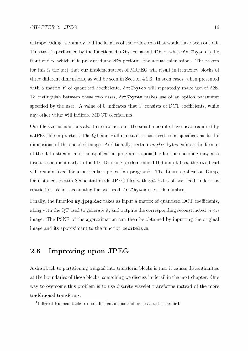
entropy coding, we simply add the lengths of the codewords that would have been output.
This task is performed by the functions dct2bytes.m and d2b.m, where dct2bytes is the
front-end to which Y is presented and d2b performs the actual calculations. The reason
for this is the fact that our implementation of MJPEG will result in frequency blocks of
three different dimensions, as will be seen in Section 4.2.3. In such cases, when presented
with a matrix Y of quantised coefficients, dct2bytes will repeatedly make use of d2b.
To distinguish between these two cases, dct2bytes makes use of an option parameter
specified by the user. A value of 0 indicates that Y consists of DCT coefficients, while
any other value will indicate MDCT coefficients.
Our file size calculations also take into account the small amount of overhead required by
a JPEG file in practice. The QT and Huffman tables used need to be specified, as do the
dimensions of the encoded image. Additionally, certain marker bytes enforce the format
of the data stream, and the application program responsible for the encoding may also
insert a comment early in the file. By using predetermined Huffman tables, this overhead
will remain fixed for a particular application program1. The Linux application Gimp,
for instance, creates Sequential mode JPEG files with 354 bytes of overhead under this
restriction. When accounting for overhead, dct2bytes uses this number.
Finally, the function my jpeg dec takes as input a matrix of quantised DCT coefficients,
along with the QT used to generate it, and outputs the corresponding reconstructedm×nimage. The PSNR of the approximation can then be obtained by inputting the original
image and its approximant to the function decibels.m.
2.6 Improving upon JPEG
A drawback to partitioning a signal into transform blocks is that it causes discontinuities
at the boundaries of those blocks, something we discuss in detail in the next chapter. One
way to overcome this problem is to use discrete wavelet transforms instead of the more
tradditional transforms.
1Different Huffman tables require different amounts of overhead to be specified.

CHAPTER 2. JPEG 17
2.6.1 Wavelet Image Compression
A discrete wavelet transform (DWT), of which the definition and mathematical aspects
are outside the scope of this dissertation, is applied to a signal in its entirety. It is an
example of a filter bank [6]: Given a 1D input signal, say x, the output consists of a
concatenation of a low-pass filtering and high-pass filtering of x. These filterings are each
down-sampled by a factor of 2 before concatenation, so that the output is of the same
length as the input. An illustration of this is shown in Figure 2.3, with L1 denoting
the low-frequency subband and H1 the high-frequency subband. We call this a (1-level)
wavelet decomposition of x.
PSfrag replacements x
DWT
L1 H1
Figure 2.3: A 1-level wavelet decomposition of the signal x
Further levels of decomposition are always applied to the lowest frequency subband; for
example, a 3-level decomposition would proceed as shown in Figure 2.4 below.
PSfrag replacements
x L1
H1H1
H1
L2 H2H2 H3L3
Figure 2.4: A 3-level wavelet decomposition of the signal x, illustrating the repeated
application of the DWT to the lowest frequency subband
In general, subbandsH1, . . . ,Hn represent high-frequency detail extracted from the signal
at successively lower levels of resolution, and Ln represents the remaining low-frequency

CHAPTER 2. JPEG 18
detail. For this reason, such a multi-level decomposition of a signal is also called a multi-
resolution analysis (MRA). Furthermore, the numbers in Ln and H1, . . . ,Hn are called
wavelet coefficients.
In a wavelet image compression technique the first level of decomposition is done by
applying a wavelet transform to the image’s rows, followed by the transform applied to
the columns of the resulting output. This is illustrated in Figure 2.5 below, where we
have labelled the image as I.
PSfrag replacements
I L H
LL1 HL1
LH1 HH1
Figure 2.5: A 1-level wavelet decomposition of an image
Once again, subsequent levels of decomposition are applied to the lowest frequency sub-
band. The second level, for instance, is shown in Figure 2.6. In the case of JPEG2000,
arguably the most well-known wavelet image compression technique, the maximum num-
ber of decomposition levels supported is 32 [6].
PSfrag replacements
LL1 HL1HL1
LH1LH1 HH1HH1
LL2HL2
LH2HH2
Figure 2.6: The second level of wavelet decomposition of an image, obtained from the
first level
An MRA gives us a hierarchy of wavelet coefficients: coefficients in lower frequency sub-
bands are more significant than ones in higher frequency subbands. By encoding coeffi-

CHAPTER 2. JPEG 19
cients in the order of higher significance to lower significance, most significant bit to least
significant bit (known as bit-plane coding), increasingly better approximations to the orig-
inal image are embedded in the output file. Furthermore, by completing the encoding,
lossless compression is achieved2. Lossy compression results by terminating the encoding
when a target file size is reached. This is in contrast to JPEG, where lossless compression
requires its own mode of operation.
Embedded coding gives us the very desirable property of scalability. For example, in-
ternet users with different connection speeds will all be able to view the same sequence
of encoded images in real-time, but at quality levels proportional to their connection
speeds. This is done by transmitting only the first n, say, bytes of each encoding to users
with slower connections, while transmitting the entire encodings to those users with fast
enough connections.
A certain level of embedded coding can also be achieved with JPEG, by selecting either its
progressive mode or its hierarchical mode. In progressive mode, successive approximation
(bit-plane coding), spectral selection (where DCT coefficients are grouped into subbands),
or a mixture of both can be selected. In hierarchical mode, versions of the input image
at various resolutions are obtained via repeated down-sampling. The differences between
these approximations, termed differential images, are then encoded either sequentially or
progressively, depending on the user’s choice.
With so many options to choose from, most users just end up choosing JPEG’s sequential
mode. A further benefit of wavelet image compression techniques is therefore the fact
that all their features are unified under a single coding architecture.
Lastly, each wavelet image compression technique has its own approach to encoding
wavelet coefficients, and it is here that such techniques can differ significantly. This
is however outside the scope of this dissertation, and we refer the reader to the EBCOT
algorithm employed by JPEG2000 [6] and Shapiro’s EZW algorithm [7] as examples of
such differences.
2Provided that an integer-to-integer DWT is used.

CHAPTER 2. JPEG 20
2.6.2 Using a Modified Transform
An alternative approach to dealing with the problem of discontinuities mentioned at
the beginning of this section is to somehow modify the more tradditional transform in
question. As stated in Chapter 1, we investigate the use of the windowed MDCT as
an alternative to the DCT. This approach replaces one component of JPEG with an-
other, meaning that its modes of operation are left more or less unchanged. As such,
the other disadvantages JPEG has compared to wavelet image compression techniques
remain present. We therefore strongly emphasise that this research cannot compete with
such techniques, particularly not JPEG2000, and is not intended to do so.
In the next chapter, the basis for our approach, namely the MDCT, as well as the reasoning
leading up to it, is discussed in detail.

Chapter 3
The Modified Discrete Cosine
Transform (MDCT)
The compression of digital audio provides an ideal background for explaining the use of
the MDCT. Much of this chapter’s discussion will take a cue from the excellent textbook
on the subject by Bosi and Goldberg [8].
3.1 Digital Audio
A digital audio signal is a 1D array of 16-bit numbers, each representing an audio sample.
These samples are obtained by a method known as analogue-to-digital conversion [9], so
called because actual audio is a continuous function of time, and thus an analogue signal.
Due to this continuous nature of audio, digital audio is not played back discretely, but
instead used to reconstruct an analogue signal via digital-to-analogue conversion [9]. One
might immediately be concerned that this reconstructed signal will merely be an ap-
proximation to the original signal that was sampled, i.e. that the information between
samples will not be accurately recovered. Fortunately, the sampling theorem tells us that
we can perfectly reconstruct the original signal, provided that the signal satisfies a certain
requirement, and the sampling rate is high enough.
21

CHAPTER 3. THE MODIFIED DISCRETE COSINE TRANSFORM (MDCT) 22
Before proceeding any further, we first define the Fourier transform (FT) of a function or
analogue signal, say f(t). The FT is the means by which the frequency content of such
signals can be calculated, and is defined as
F (ω) =
∫ ∞
−∞f(t)e−2πiωtdt. (3.1)
Returning now to the sampling theorem, it states that an analogue signal containing
frequency content only up to a finite upper frequency, say Fmax, will be perfectly recon-
structed from discrete samples if the sampling rate, say Fs, satisfies Fs ≥ 2Fmax. We call
such a signal band-limited. When the sampling rate does not meet this condition, aliasing
can occur — contributions made to the original signal by frequencies higher than Fmax
are mistaken for lower frequency contributions in the reconstructed signal.
To ensure that a signal is band-limited, it can be low-pass filtered to cut off all frequency
content above Fmax. With regards to audio signals, they are limited to 22 kHz, because
most human beings cannot hear beyond it. A sampling rate of 44.1 kHz is then used,
both for good measure and historical reasons [9], thereby satisfying the sampling theorem’s
condition.
3.2 Window Functions
Let us now consider an attempt to apply lossy compression to a digital audio signal, using
transform coding in particular. The forward transform shown in Figure 2.1(a) might now
be a 1D time to frequency transform, such as a 1D DCT. As a result, the signal will
again be partitioned into non-overlapping transform blocks. As stated in Section 2.6, this
partitioning causes discontinuities at the edges of those blocks, and we now proceed to
analyse this problem.
Let f(t) denote the original bandlimited signal from which the digital audio signal to be
encoded was obtained, as depicted in Figure 3.1(a). Furthermore, let [0, T ] refer to the
time interval corresponding to the duration of some transform block x.

CHAPTER 3. THE MODIFIED DISCRETE COSINE TRANSFORM (MDCT) 23
PSfrag replacements 0 T
f(t)
t
︸ ︷︷ ︸x
(a) Original audio signal
PSfrag replacements 0 T
f(t)
t
︸ ︷︷ ︸x
(b) Time-limited counterpart
Figure 3.1: Time-limiting resulting from the partitioning of a signal into transform blocks
Notice that by only working with block x, its samples could just as well have been obtained
by sampling the time-limited counterpart of f(t), namely f(t), shown in Figure 3.1(b),
rather than f(t). However, f(t) possesses sharp discontinuities at t = 0 and t = T ; we
CHAPTER 3. THE MODIFIED DISCRETE COSINE TRANSFORM (MDCT) 24
can therefore expect its frequency content to be quite different from that of f(t).
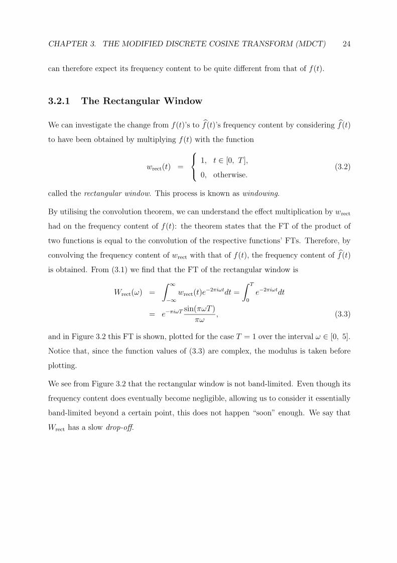
3.2.1 The Rectangular Window
We can investigate the change from f(t)’s to f(t)’s frequency content by considering f(t)
to have been obtained by multiplying f(t) with the function
wrect(t) =
1, t ∈ [0, T ],
0, otherwise.(3.2)
called the rectangular window. This process is known as windowing.
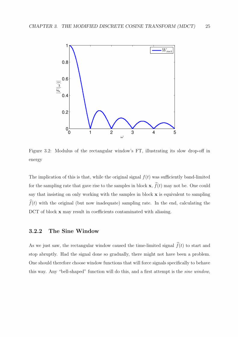
By utilising the convolution theorem, we can understand the effect multiplication by wrect
had on the frequency content of f(t): the theorem states that the FT of the product of
two functions is equal to the convolution of the respective functions’ FTs. Therefore, by
convolving the frequency content of wrect with that of f(t), the frequency content of f(t)
is obtained. From (3.1) we find that the FT of the rectangular window is
Wrect(ω) =
∫ ∞
−∞wrect(t)e
−2πiωtdt =
∫ T
0
e−2πiωtdt
= e−πiωTsin(πωT )
πω, (3.3)
and in Figure 3.2 this FT is shown, plotted for the case T = 1 over the interval ω ∈ [0, 5].
Notice that, since the function values of (3.3) are complex, the modulus is taken before
plotting.
We see from Figure 3.2 that the rectangular window is not band-limited. Even though its
frequency content does eventually become negligible, allowing us to consider it essentially
band-limited beyond a certain point, this does not happen “soon” enough. We say that
Wrect has a slow drop-off.
CHAPTER 3. THE MODIFIED DISCRETE COSINE TRANSFORM (MDCT) 25
0 1 2 3 4 50
0.2
0.4
0.6
0.8
1
PSfrag replacements
ω
|F(ω
)|Wrect
Figure 3.2: Modulus of the rectangular window’s FT, illustrating its slow drop-off in
energy
The implication of this is that, while the original signal f(t) was sufficiently band-limited
for the sampling rate that gave rise to the samples in block x, f(t) may not be. One could
say that insisting on only working with the samples in block x is equivalent to sampling
f(t) with the original (but now inadequate) sampling rate. In the end, calculating the
DCT of block x may result in coefficients contaminated with aliasing.
3.2.2 The Sine Window
As we just saw, the rectangular window caused the time-limited signal f(t) to start and
stop abruptly. Had the signal done so gradually, there might not have been a problem.
One should therefore choose window functions that will force signals specifically to behave
this way. Any “bell-shaped” function will do this, and a first attempt is the sine window,

CHAPTER 3. THE MODIFIED DISCRETE COSINE TRANSFORM (MDCT) 26
given by the formula
wsin(t) =
sin
(πt
T
), t ∈ [0, T ],
0, otherwise.
(3.4)
We of course do not actually window before sampling in practice; the equivalent is to
pointwise multiply the samples in a transform block by a sampled version of the window
function. For a transform block (or discretely sampled signal) consisting of N samples,
the sine window is defined as
wsin(i) = sin
(π(i− 0.5)
N
), i = 1, . . . , N. (3.5)
In Figure 3.3, a sine window of length 32 shown.
0 5 10 15 20 25 300
0.1
0.2
0.3
0.4
0.5
0.6
0.7
0.8
0.9
1
Figure 3.3: A bar-chart depiction of a sine window of length 32
To see how the effect of this window compares to that of wrect, we calculate the FT of
(3.4):
Wsin(ω) =
∫ ∞
−∞wsin(t)e
−2πiωtdt =
∫ T
0
sin
(πt
T
)e−2πiωtdt
= e−πiωT2T cos(πωT )
π(1− (2ωT )2). (3.6)

CHAPTER 3. THE MODIFIED DISCRETE COSINE TRANSFORM (MDCT) 27
In Figure 3.4 this transform is depicted, along with that of the rectangular window,
obtained in the previous subsection.
0 1 2 3 4 50
0.2
0.4
0.6
0.8
1
PSfrag replacements
ω
|F(ω
)|
Wrect
Wsin
Figure 3.4: FTs of the rectangular and sine windows
From this figure we observe that the sine window’s frequency content tends to zero much
faster than that of the rectangular window; any aliasing caused by this window will
thus be significantly less. The so-called main lobe of Wsin is, however, wider than the
one belonging to Wrect. This width is a measure of how accurately we can identify the
amplitudes of specific frequencies, known as frequency resolution: the wider the main lobe,
the poorer the window function’s frequency resolution will be.
3.2.3 The Hanning Window
From (3.4) we see that the sine window happens to have discontinuities in its first deriva-
tive at its end points — an example of a window function which addresses this is the

CHAPTER 3. THE MODIFIED DISCRETE COSINE TRANSFORM (MDCT) 28
Hanning window:
wHan(t) =
0.5
(1− cos
(2πt
T
)), t ∈ [0, T ],
0, otherwise.
(3.7)
Its corresponding definition for discretely sampled signals is given by
wHan(i) = 0.5
(1− cos
(2π(i− 0.5)
N
)), i = 1, . . . , N (3.8)
and, once again, a graphical depiction of one of length 32 is shown in Figure 3.5.
0 5 10 15 20 25 300
0.1
0.2
0.3
0.4
0.5
0.6
0.7
0.8
0.9
1
Figure 3.5: A bar-chart depiction of a Hanning window of length 32
To see if this window is an improvement on wsin, we again calculate the FT, this time of
(3.7), to find
WHan(ω) =
∫ ∞
−∞wHan(t)e
−2πiωtdt =
∫ T
0
0.5
(1− cos
(2πt
T
))e−2πiωtdt
= e−πiωTsin(πωT )
2πω(1− (ωT )2). (3.9)
Figure 3.6 shows the Fourier transforms of all three window functions considered thus far,
with WHan indeed having an even faster drop-off in energy.

CHAPTER 3. THE MODIFIED DISCRETE COSINE TRANSFORM (MDCT) 29
0 1 2 3 4 50
0.2
0.4
0.6
0.8
1
PSfrag replacements
ω
|F(ω
)|Wrect
Wsin
WHan
Figure 3.6: FTs of the rectangular, sine and Hanning windows
The width of its main lobe is, however, even larger than that of Wsin. This means that
one is now faced with a trade-off when selecting a window function: We have to strike a
balance between main lobe width and side lobe energy, or, equivalently, between frequency
resolution and aliasing.
3.2.4 The Kaiser-Bessel Window
A window function that enables us to manipulate the abovementioned trade-off is the
Kaiser-Bessel window. For discretely sampled signals it is defined as
wKB(i) =
I0
(πα
√1−
(i−1−0.5(N−1)
0.5(N−1)
)2)
I0(πα), i = 1, . . . , N, α ≥ 0, (3.10)
where I0 is the 0th order modified Bessel function. The parameter α is the means by
which this manipulation is done: The larger α becomes, the narrower the window’s bell
shape becomes and the faster its side lobe energy drops off, but the poorer its frequency
CHAPTER 3. THE MODIFIED DISCRETE COSINE TRANSFORM (MDCT) 30
resolution is. On the other hand, the smaller α becomes, the more wKB starts to resemble
the rectangular window. In particular, when α = 0, wrect is obtained.
Many other window functions exist, but the two typically used in audio compression
techniques are the sine window and a version of the Kaiser-Bessel window known as the
Kaiser-Bessel Derived (KBD) window1. For example, MPEG AAC makes use of the sine
window and the KBD window with α = 4 and α = 6 [8].
3.3 Overlap-and-add
Utilising a bell-shaped window function unfortunately causes an unwanted side effect:
After windowing and calculating the time-to-frequency transform, we intend to quantise
the resulting transform coefficients. During the decoding process, after dequantising and
inverting the transform, we have to divide (pointwise) by the window function to obtain
an approximation to the original audio samples. In the absence of quantisation this poses
no problem — perfect inversion will take place. However, dividing dequantised transform
coefficients, now containing a quantisation error, will exacerbate that error when dividing
by numbers close to zero. In other words, at the edges of our transform blocks, where
the window function approaches zero, we end up inflating quantisation errors. We need
to remove division by the window function and find another way of recovering the signal
samples.
Let
x = [x1, x2, . . . , xN ]
denote the signal samples in a typical transform block, and
w = [w1, w2, . . . , wN ]
denote the entries in the chosen window function, where N is an even number. Thus,
1We obtain the KBD window by applying the normalisation formula (3.12) listed in the next section
to wKB.

CHAPTER 3. THE MODIFIED DISCRETE COSINE TRANSFORM (MDCT) 31
after windowing, the input to the forward transform is
w ∗ x = [w1x1, w2x2, . . . , wNxN ],
where the symbol “∗” denotes the illustrated pointwise multiplication. In the absence of
quantisation, the output of the inverse transform is again simply w ∗ x, after which we
would have liked to divide by w, as mentioned above. Notice that in the above equation
each wixi is a fraction of the corresponding xi, and if we had an appropriate accompanying
fraction of xi, we could add them together to recover xi.
Overlapping the transform blocks, thus using each sample xi twice, gives us this sec-
ond fraction, as seen in Figure 3.7. Conventionally, in overlap-and-add, windowing is
also applied to the output of the inverse transform, thereby achieving encoding/decoding
symmetry. A window used during encoding is referred to as an analysis window, while
one used during decoding is called a synthesis window, since they are allowed to differ.
Here we will only consider the case of identical analysis and synthesis windows, therefore
the fractions requiring counterparts are now
w2i xi, i = 1, . . . , N.
Transform
Transform
Transform
Window Window Window
PSfrag replacements
x
y
z
Figure 3.7: A graphical depiction of windowed overlap-and-add, with 50% overlap

CHAPTER 3. THE MODIFIED DISCRETE COSINE TRANSFORM (MDCT) 32
Figure 3.7 depicts the specific case of 50% overlap, to which we limit our discussion. The
transform block preceding block x, denoted by y, consists of the N2
samples preceding
block x followed by the first N2
samples of block x. Similarly, the last N2
samples of x
followed by the N2samples succeeding it form the subsequent block, denoted here by z.
Attempting to recover a particular xi, we now overlap the appropriate portion of block x
with the appropriate neighbouring block and add the twice windowed samples together.
In the case of the first half of x we have
w2i xi + w2
N
2+iyN
2+i = w2
i xi + w2N
2+ixi
= xi
(w2i + w2
N
2+i
).
Imposing the restriction
w2i + w2
N
2+i
= 1 (3.11)
on the window function, we ensure that xi is recovered, or, in terms of our previous
discussion, that appropriate fractions of xi are added together. This is known as a perfect
reconstruction requirement. We also arrive at (3.11) when attempting to recover a sample
from the second half of x.
Given any window function, say v, of length N2+ 1, one of length N can easily be con-
structed that satisfies restriction (3.11), using the formula
w(i) =
1
s
√√√√i∑
k=1
v(k) , i = 1, . . . , N2,
1
s
√√√√√N
2+1∑
k=i−N
2+1
v(k) , i = N2+ 1, . . . , N,
(3.12)
where s =
√√√√N
2+1∑
k=1
v(k). We call such a window a normalized window. Notice that the sine
window already satisfies our restriction, due to the trigonometric identity
sin2 x+ cos2 x = 1.
A more general derivation of the perfect reconstruction requirement can be found in [8],
which takes into consideration more general analysis and synthesis windows as well as

CHAPTER 3. THE MODIFIED DISCRETE COSINE TRANSFORM (MDCT) 33
more general overlap lengths. We conclude this section by summarising the encoding and
decoding procedures resulting from the above discussion.
1. Form transform blocks using 50% overlap as suggested by Figure 3.7.
2. Apply a normalized window function to the blocks.
3. Apply a time to frequency mapping to these blocks, resulting in frequency
components.
4. Quantise the frequency components.
5. Entropy code the quantised data.
Algorithm 3.1: Encoding procedure of a basic audio coding technique
1. Decompress entropy coded data, yielding quantised frequency components.
2. Dequantise the frequency components.
3. Apply the inverse transform.
4. Once again, apply the normalized window function.
5. Overlap the resulting data blocks as suggested by Figure 3.7 and add up
corresponding entries.
Algorithm 3.2: Decoding procedure of a basic audio coding technique
3.4 The MDCT
We are faced with one more problem. Recall that in the case of JPEG an 8× 8 block of
pixels is mapped to an 8 × 8 block of frequency components, meaning that the amount
of data to be entropy coded (output of the DCT) is the same as the original amount of
data (input to the DCT). This desirable property is referred to as critical sampling.

CHAPTER 3. THE MODIFIED DISCRETE COSINE TRANSFORM (MDCT) 34
In the case of overlap-and-add (with 50% overlap) described in the previous section, we
have twice as many transform blocks (of the same size) as we would have had without
overlapping. In the process, the amount of data to be compressed has thus doubled, and
critical sampling is lost.
The modified discrete cosine transform (MDCT), invented by Princen and Bradley [10],
overcomes this problem: whereas a standard DCT would map N samples of data to N
new values, the MDCT maps an N -sample block, say x, to a block consisting of N2new
values, say X, as illustrated in Figure 3.8.
ForwardMDCT
InverseMDCT
PSfrag replacements
x
X
x
NN
N2
Figure 3.8: A graphical depiction of the forward and inverse MDCT
Given such an input block
x = [x1, x2, . . . , xN ]
its MDCT X is defined as
X(j) =N∑
i=1
x(i) cos
(2π
N
(i+
N
4− 1
2
)(j − 1
2
)), j = 1, . . . ,
N
2, (3.13)
where we omit the use of windowing for the time being.
The “inverse” transform (IMDCT) then maps X to a block once again consisting of N

CHAPTER 3. THE MODIFIED DISCRETE COSINE TRANSFORM (MDCT) 35
values, say x, as defined by
x(i) =2
N
N
2∑
j=1
X(j) cos
(2π
N
(i+
N
4− 1
2
)(j − 1
2
)), i = 1, . . . , N. (3.14)
We use the term inverse in quotations above, because, by itself, the MDCT is not in-
vertible: x will not be equal to x. Instead, it contains a “scrambled” version of the data
originally contained in x — various samples of x will be added/subtracted forming the
new samples of x. Used in conjunction with overlap-and-add, though, perfect inversion
will take place. We illustrate this for the specific case of transform blocks of length 16,
because our modification of JPEG makes use of them, as will be seen in the next chapter.
For the general derivation of perfect inversion the reader is referred to [10] and [8].
Let x be such a block consisting of 16 samples,
x = a1 a2 a3 a4 b1 b2 b3 b4 c1 c2 c3 c4 d1 d2 d3 d4 (3.15)
or
x = a b c d
for short. Then it is shown in [11] (for the general case of N divisible by 4) that
x = IMDCT(MDCT(x)) =1
2a− br b− ar c+ dr d+ cr , (3.16)
where the subscript r denotes the reversal of a vector, e.g.
ar = a4 a3 a2 a1 ,
and “+” and “ − ” refer to the usual addition and subtraction of vectors, respectively.
For example, the first four entries of x will be
12(a1 − b4)
12(a2 − b3)
12(a3 − b2)
12(a4 − b1) .
We call this phenomenon time-domain aliasing, since it is analogous to the frequency
domain aliasing that we explained earlier. Using 50% overlap, let z be the transform
block succeeding block x, of the form
z = c1 c2 c3 c4 d1 d2 d3 d4 e1 e2 e3 e4 f1 f2 f3 f4 (3.17)

CHAPTER 3. THE MODIFIED DISCRETE COSINE TRANSFORM (MDCT) 36
or
z = c d e f
for short. Now we have that
z = IMDCT(MDCT(z)) =1
2c− dr d− cr e+ fr f + er .
Overlapping the appropriate portions of x and z and adding up gives us
1
2(c+ dr) +
1
2(c− dr) = c
and1
2(d+ cr) +
1
2(d− cr) = d.
Similarly, we recover portions a and b by considering the transform block preceding block
x.
Overlapping and adding has thus resulted in the cancellation of the contaminating signal
portions, with perfect inversion indeed taking place. Consequently, the MDCT is an
example of a time domain aliasing cancellation (TDAC) transform.
We, of course, intend to apply windowing as well, so it remains to show that overlap-and-
add will also simultaneously remove windowing and time domain aliasing. Once again,
let data block x be defined as in (3.15) and let the window function w be given by
w = u1 u2 u3 u4 v1 v2 v3 v4 v4 v3 v2 v1 u4 u3 u2 u1
= u v vr ur , (3.18)
where we now also require the window function to be symmetric. Therefore, restriction
(3.11) can now be written as
u2r + v2 = 1 1 1 1
as well as
v2r + u2 = 1 1 1 1 ,

CHAPTER 3. THE MODIFIED DISCRETE COSINE TRANSFORM (MDCT) 37
where the exponent 2 denotes the pointwise multiplication of a vector with itself. Here
the input to the MDCT will be
w ∗ x = u ∗ a v ∗ b vr ∗ c ur ∗ d ,
and, using (3.16), the output of the IMDCT will be
x = IMDCT(MDCT(w ∗ x))
=1
2u ∗ a− vr ∗ br v ∗ b− ur ∗ ar vr ∗ c+ u ∗ dr ur ∗ d+ v ∗ cr .
Upon decoding, we once again window, yielding
w∗x =1
2u2 ∗ a− u ∗ vr ∗ br v2 ∗ b− v ∗ ur ∗ ar v2
r ∗ c+ vr ∗ u ∗ dr u2r ∗ d+ ur ∗ v ∗ cr .
With the subsequent transform block, z, once again as defined by (3.17), its decoded (and
windowed) version will be
w∗z =1
2u2 ∗ c− u ∗ vr ∗ dr v2 ∗ d− v ∗ ur ∗ cr v2
r ∗ e+ vr ∗ u ∗ fr u2r ∗ f + ur ∗ v ∗ er .
This time overlapping and adding gives us
1
2(v2
r ∗ c+ vr ∗ u ∗ dr) +1
2(u2 ∗ c− u ∗ vr ∗ dr)
=1
2c ∗ (v2
r + u2) +1
2dr(vr ∗ u− vr ∗ u)
=1
2c ∗ 1 1 1 1 =
1
2c
and1
2(u2
r ∗ d+ ur ∗ v ∗ cr) +1
2(v2 ∗ d− v ∗ ur ∗ cr)
=1
2d ∗ (u2
r + v2) +1
2cr(ur ∗ v − ur ∗ v)
=1
2d ∗ 1 1 1 1 =
1
2d.
By now slightly modifying the formula for the IMDCT for the case of windowing —
multiplying by 2 — the desired reconstruction is obtained. Once again, portions a and b
of x are similarly recovered by considering the transform block preceding block x.
CHAPTER 3. THE MODIFIED DISCRETE COSINE TRANSFORM (MDCT) 38
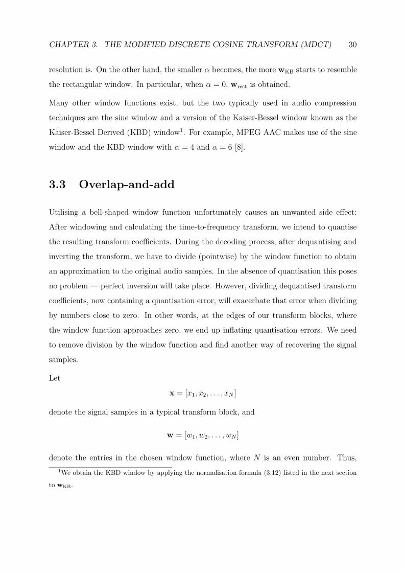
The formulas for the windowed MDCT and IMDCT are now
X(j) =N∑
i=1
w(i)x(i) cos
(2π
N
(i+
N
4− 1
2
)(j − 1
2
)), j = 1, . . . ,
N
2(3.19)
and
x(i) =4
Nw(i)
N
2∑
j=1
X(j) cos
(2π
N
(i+
N
4− 1
2
)(j − 1
2
)), i = 1, . . . , N, (3.20)
respectively, while they remain (3.13) and (3.14) in the absence of windowing.
Lastly, by now using the windowed MDCT in steps 2 and 3 in Algorithm 3.1 (listed in
the previous section), a rough layout of a basic audio coding scheme is formed.
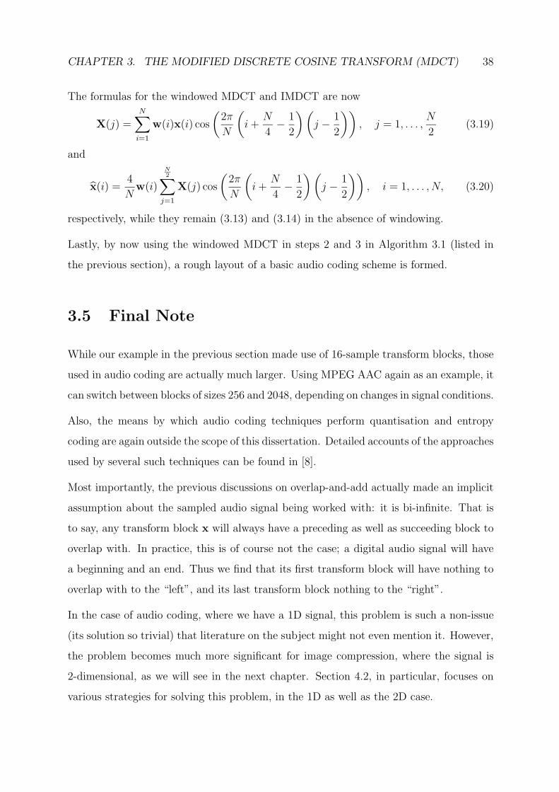
3.5 Final Note
While our example in the previous section made use of 16-sample transform blocks, those
used in audio coding are actually much larger. Using MPEG AAC again as an example, it
can switch between blocks of sizes 256 and 2048, depending on changes in signal conditions.
Also, the means by which audio coding techniques perform quantisation and entropy
coding are again outside the scope of this dissertation. Detailed accounts of the approaches
used by several such techniques can be found in [8].
Most importantly, the previous discussions on overlap-and-add actually made an implicit
assumption about the sampled audio signal being worked with: it is bi-infinite. That is
to say, any transform block x will always have a preceding as well as succeeding block to
overlap with. In practice, this is of course not the case; a digital audio signal will have
a beginning and an end. Thus we find that its first transform block will have nothing to
overlap with to the “left”, and its last transform block nothing to the “right”.
In the case of audio coding, where we have a 1D signal, this problem is such a non-issue
(its solution so trivial) that literature on the subject might not even mention it. However,
the problem becomes much more significant for image compression, where the signal is
2-dimensional, as we will see in the next chapter. Section 4.2, in particular, focuses on
various strategies for solving this problem, in the 1D as well as the 2D case.

Chapter 4
Modifying JPEG
In Chapter 3 we motivated using the windowed MDCT in audio coding. The aim of this
research is to investigate if any improvements in quality can be achieved by doing the
same for image compression. As stated in Chapter 1, we specifically modify JPEG by
replacing the standard DCT with the windowed MDCT, and refer to the modification as
MJPEG.
4.1 Modifications
We would like to retain JPEG’s existing well-defined structure; among others, quantising
8× 8 blocks of frequency components. By extending the 1D case of 16-sample transform
blocks illustrated in Section 3.4 to two dimensions, this is achieved: Given a 16 × 16
block of pixels, we first apply (3.19) to its rows and then to the columns of the resulting
16 × 8 matrix, thereby implementing a 2D windowed MDCT. This transform therefore
maps 16 × 16 transform blocks to 8 × 8 blocks of frequency components. By similarly
using (3.20), the 2D inverse transform will map back to 16 × 16 blocks. This concept is
illustrated in Figure 4.1.
39

CHAPTER 4. MODIFYING JPEG 40
16 x 16 8 x 8 16 x 16
MDCT IMDCT
Figure 4.1: Extending the 1D MDCT to two dimensions in order to obtain 8×8 transform
blocks
By doing this, overlap-adding is also extended to two dimensions, as demonstrated in
Figure 4.2. Notice that each 2D transform block will have eight neighbouring blocks to
overlap with.
Alternatively, one could first apply (3.19) to each row of an entire image, the same way we
would to an audio signal, using 1D transform blocks of length 16. The same is then done to
the columns of the resulting output. In the end, the same matrix, say Y , consisting of 8×8
blocks of frequency components is obtained. To decode, the reverse process is applied —
first each column of Y is inversely transformed using (3.20) and overlap-added, then each
row of the resulting output. Even though both of these implementations yield the same
results, only the latter is compatible with the strategy to be proposed in Section 4.2.3,
and is therefore the implementation we chose.

CHAPTER 4. MODIFYING JPEG 41
PSfrag replacements
1
(a) 1st overlapping block
PSfrag replacements
2
(b) 2nd overlapping block
PSfrag replacements
3
(c) 3rd overlapping block
PSfrag replacements8
(d) 8th overlapping block
Figure 4.2: The extension of overlap-adding to two dimensions, resulting in 8 overlapping
neighbouring blocks for each transform block
By retaining 8 × 8 blocks of frequency components, the overall operation of JPEG is
retained by MJPEG. We can once again use an 8 × 8 quantisation table, form a zigzag
sequence of length 64 from the quantised coefficients, and use the existing Huffman tables
to encode it1.
Lastly, we would also like any given QT to quantise both DCT and MDCT coefficients with
1From (3.19) one can see that no zero-frequency (DC) coefficient is generated by the MDCT. Fortu-
nately, the first coefficient that is generated does still correspond to a low frequency. MJPEG therefore
continues to differentially code these coefficients.
CHAPTER 4. MODIFYING JPEG 42
more or less the same severity. However, due to the differences between the respective
defining equations, MDCT coefficients in an 8 × 8 block are roughly four times larger
than DCT coefficients in an 8×8 block. Our implementation of MJPEG therefore divides
such MDCT coefficients by four before quantisation and multiplies them by four after
dequantisation.
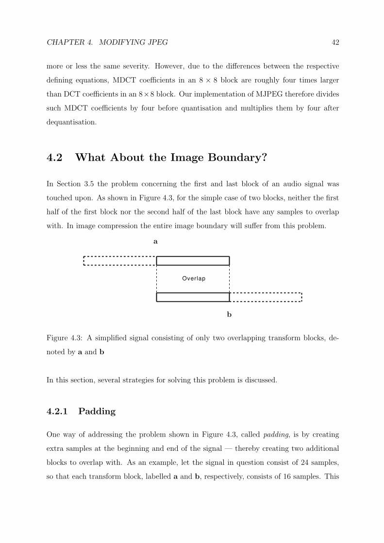
4.2 What About the Image Boundary?
In Section 3.5 the problem concerning the first and last block of an audio signal was
touched upon. As shown in Figure 4.3, for the simple case of two blocks, neither the first
half of the first block nor the second half of the last block have any samples to overlap
with. In image compression the entire image boundary will suffer from this problem.
Overlap
PSfrag replacements
a
b
Figure 4.3: A simplified signal consisting of only two overlapping transform blocks, de-
noted by a and b
In this section, several strategies for solving this problem is discussed.
4.2.1 Padding
One way of addressing the problem shown in Figure 4.3, called padding, is by creating
extra samples at the beginning and end of the signal — thereby creating two additional
blocks to overlap with. As an example, let the signal in question consist of 24 samples,
so that each transform block, labelled a and b, respectively, consists of 16 samples. This

CHAPTER 4. MODIFYING JPEG 43
signal is depicted in Figure 4.4 below.
a︷ ︸︸ ︷
x1 x2 x3 x4 x5 x6 x7 x8 x9 · · · x16 x17 x18 x19 x20 x21 x22 x23 x24
︸ ︷︷ ︸b
Figure 4.4: A 24-sample signal, with overlapping transform blocks a and b consisting of
16 samples each
Since the first 8 samples of a require overlap, the first auxilliary block, say a, will contain
those samples as its second half, leaving us with 8 samples to create for its first half. These
8 samples may be chosen arbitrarily; however, in order to maximise continuity within the
new block, they are chosen as shown in Figure 4.5: Samples x1 to x8 are replicated and
reversed, forming the padded data.
x8 x7 x6 x5 x4 x3 x2 x1 x1 x2 x3 x4 x5 x6 x7 x8
Figure 4.5: Auxilliary block a formed by padding
Clearly these samples will now be recovered during decoding; the additional samples,
whether properly decoded or not, can then be discarded. In a similar fashion, an auxilliary
block, say b, is formed by padding 8 samples at the end of the signal in Figure 4.4.
Notice that, since each of the four transform blocks above (a, a, b, and b) consist of 16
samples, they yield 4 × 8 = 32 frequency components during encoding, 8 more than the
24 samples started with. Padding therefore results in one extra transform block’s worth
of data to store. For audio coding, this is a minuscule amount of overhead, considering
that a typical audio file consists of thousands of transform blocks. The amount is also
fixed — it does not increase with the duration of the audio signal, becoming ever more
negligible as the length of the signal increases.
This solution is immediately applicable to the 2D image compression case as well. Figure
4.6 illustrates the situation that results from this when utilising 2D transform blocks to

CHAPTER 4. MODIFYING JPEG 44
implement the 2D MDCT. The entire image is surrounded by padded data consisting of
replicated pixels.
Padding
BoundaryBlocks Image
ImageBoundary
Figure 4.6: Padding applied to an image, resulting in a significant loss in critical sampling
When using our chosen implementation of the 2D MDCT, only the padding to the left
and right of each image row would consist of replicated pixels. The padding above and
below the columns of the output resulting from applying (3.19) to the rows will be made
up of replicated 1D frequency components. Either way, the amount of padded data is the
same.
The loss in critical sampling is no longer negligible, regardless of the size of the image.
As the size of the image increases, so does the amount of padded data (it does decrease
percentage-wise, relative to the total amount of data to be compressed). This additional
amount, while not drastically large, is still large enough to sabotage competitiveness with
JPEG, which is our main priority.
4.2.2 Wrap-around
Utilising the concept of periodic boundaries, we can devise a solution to the boundary
problem that will maintain critical sampling — we will refer to it as wrap-around. Instead

CHAPTER 4. MODIFYING JPEG 45
of two, only one auxilliary transform block is formed by considering the first N2samples
of a signal as succeeding the last N2samples, where N is the length of a transform block.
When applied to the signal in Figure 4.4, this results in the signal shown in Figure 4.7
below.
a︷ ︸︸ ︷ c︷ ︸︸ ︷
x1 x2 · · · x7 x8 x9 · · · x15 x16 x17 x18 · · · x24 x1 x2 · · · x7 x8
︸ ︷︷ ︸b
Figure 4.7: Periodic extension of the signal in Figure 4.4
Here c denotes the new block formed by letting the first 8 samples (x1 to x8) continue
after the final 8 (x17 to x24). Encoding can then be applied to blocks a, b, and c, in that
order, resulting in 24 frequency components to store. With regards to decoding, samples
x1 to x8 can now be recovered by overlapping and adding the first half and second half
of the respective inverse transforms of blocks a and c’s frequency components. Similarly,
samples x17 to x24 are recovered by overlapping and adding the second half of the inverse
transform of b’s frequency components and the first half of the inverse transform of c’s
frequency components.
Once again, we can readily apply the solution to the 2D case of image compression.
Figure 4.8 illustrates the wrap-around concept in two dimensions, if one were to use 2D
transform blocks. It shows, for instance, that all four corners of an image would overlap,
via wrap-around, with each other. On the other hand, using 1D MDCTs, horizontal
wrap-around will take place in the spatial domain, while vertical wrap-around will take
place in the 1D frequency domain.

CHAPTER 4. MODIFYING JPEG 46
Image
Figure 4.8: Wrap-around extended to two dimensions, illustrating the overlapping of
boundary blocks
Regardless of how we choose to implement the 2D MDCT, the wrap-around technique
causes a problem, as can be seen in Figure 4.7, when examining block c. Roughly speaking,
the concatenated samples sequences [x17, . . . , x24] and [x1, . . . , x8] have nothing to do with
each other. More precisely, the transition from the one to the other causes a sharp
discontinuity in block c, and thus on the signal boundary. The same will also be true of
an image — sharp discontinuities will be formed across the entire image boundary. This,
of course, poses no problem in the absence of quantisation; however, in the presence of
even mild quantisation the problem is severe, forming noticeable lines parallel to each
boundary line of the reconstructed image. An example of this can be seen in Figure
4.9: an MJPEG encoding (with the sine window) of the 256 × 256 Lena image, where
wrap-around in the spatial (pixel) domain was used. Quantisation was done using JPEG’s
standard QT, listed in Table 2.1.
Figure 4.9(a) shows the reconstructed image in its entirety, while Figure 4.9(b) shows an
enlarged portion of it, pointing out the vertical lines that have been formed close to the

CHAPTER 4. MODIFYING JPEG 47
right boundary line.
PSfrag replacements
(a) Reconstructed Image (b) Right Boundary Region
Figure 4.9: Reconstruction of an MJPEG encoding of Lena, where the wrap-around
technique is ultilised
We can neutralise these discontinuities by relaxing the quantisation of the frequency
coefficients in the boundary blocks, but this will also decrease their compressibility. As
was the case with padding, we are left with more data to store than we would prefer, and
competitiveness with JPEG is again compromised.
4.2.3 Hybrid Coefficients
To encode an image’s boundary more efficiently, we need to revisit the inner workings of
the MDCT. Let us again consider our 24-sample signal, reproduced in Figure 4.10 below.

CHAPTER 4. MODIFYING JPEG 48
a︷ ︸︸ ︷ b︷ ︸︸ ︷ c︷ ︸︸ ︷
x1 x2 x3 x4 x5 x6 x7 x8 x9 x10 x11 x12 · · ·
x13 x14 x15 x16 x17 x18 x19 x20 x21 x22 x23 x24
︸ ︷︷ ︸d
︸ ︷︷ ︸e
︸ ︷︷ ︸f
Figure 4.10: Reproduction of the 24-sample signal in Figure 4.4, with 4-sample portions
labelled a to f
Using the notation introduced in Section 3.4, portions of the signal are labelled a,b, . . . , f ,
such that the first transform block consists of portions a to d, and the second consists of
portions c to f. Upon encoding (windowing and performing the MDCT), each transform
block yields 8 frequency components to be (quantised and) stored, say
X1 X2 X3 X4 X5 X6 X7 X8
and
X9 X10 X11 X12 X13 X14 X15 X16
for a total of 16 numbers to store. We thus have space for 8 more numbers. Recall from
Section 3.4 that decoding the above frequency blocks (applying the IMDCT, windowing,
and overlap-adding) yields
u2 ∗ a− u ∗ vr ∗ br v2 ∗ b− v ∗ ur ∗ ar c d v2r ∗ e+ u ∗ vr ∗ fr v ∗ ur ∗ e+ u2
r ∗ f
︸ ︷︷ ︸α
︸ ︷︷ ︸β
where we have used the same notation for the portions of the window function w as in
(3.18), as well additional labels α and β. If we were to store portion a (of Figure 4.10),
consisting of 4 samples, not only would it be trivially recovered, but we would also be
able to recover portion b from either portion α or β. For instance, upon obtaining a and
β, portion a can be reversed, multiplied by portions v and ur (both of which are known),
and the result added to β, giving us
v2 ∗ b− v ∗ ur ∗ ar + v ∗ ur ∗ ar = v2 ∗ b.

CHAPTER 4. MODIFYING JPEG 49
Finally, dividing by v2 results in portion b. Similarly, storing portion f (a further 4
samples) allows us to recover portion e.
In summary, the 24 numbers we now have to store are
x1 x2 x3 x4 X1 · · · X16 x21 x22 x23 x24 .
We apply this strategy to an m× n image as follows.
1. The 1D MDCT incorporating the above approach is first applied to the rows of the
image, resulting in a matrix consisting of an m × (n − 8) interior of 1D frequency
coefficients, and left and right outer strips of original pixel values, each of size m×4.
Such a matrix is depicted in Figure 4.11.
PSfrag replacements
m× 4m× 4
Figure 4.11: First stage output of our proposed MJPEG implementation
2. Since we want the interior to be composed of 8× 8 frequency blocks, we next apply
the 1D MDCT (incorporating the above approach) to the n− 8 interior columns of
this matrix. This gives us the matrix shown in Figure 4.12 below, now also with
a top and bottom strip, each containing 1D frequency coefficients generated in the
previous step. Both strips have dimensions 4×(n−8). Notice that the 8×8 interior

CHAPTER 4. MODIFYING JPEG 50
blocks are the same frequency blocks that would have been obtained using any of
the previous strategies. Hence, normal quantisation can again be applied to them.
PSfrag replacements
m× 4m× 4
4× (n− 8)
4× (n− 8)
Figure 4.12: Second stage output of our proposed MJPEG implementation, containing
outer strips of hybrid coefficients
In order to efficiently encode the image, we also have to apply lossy compression to the
outer strips of Figure 4.12. This means that we would like them to also be in the form of 2D
frequency components. Since the top and bottom strips contain 4 rows of 1D (horizontal)
frequency components, with each row consisting of blocks of length 8, applying a standard
1D DCT to each column results in 4 × 8 blocks of 2D coefficients. Notice that these are
hybrid MDCT/DCT coefficients. To the left and right strips, composed of original pixel
values, we can apply a standard 2D DCT. For convenience, they are partitioned into
(non-overlapping) 4× 4 blocks, to which the 2D DCT is applied.
Each pair of strips now requires its own quantisation table: for the top and bottom strips
we need a 4× 8 table, while the left and right strips need a 4× 4 table. Since our choice

CHAPTER 4. MODIFYING JPEG 51
of quality measure is the PSNR, we can disregard the physical interpretation of frequency
coefficients, and derive the additional QTs from the primary 8 × 8 QT. This is done by
repeatedly downsampling (by averaging adjacent entries) the primary table. For example,
the standard JPEG QT shown in Table 2.1 can be successively downsampled as follows.
First, vertical downsampling provides us with the 4× 8 QT shown in Table 4.1; this table
is then horizontally downsampled to give us the 4× 4 QT shown in Table 4.2.
14 12 12 18 25 49 56 58
14 15 19 27 46 72 75 59
21 29 46 60 75 107 108 85
61 78 87 93 108 111 112 100
Table 4.1: Auxilliary QT obtained by vertically downsampling Table 2.1
13 15 37 57
15 23 59 67
25 53 91 97
70 90 110 106
Table 4.2: Auxilliary QT obtained by horizontally downsampling Table 4.1 above
This approach allows us to avoid the extra overhead of storing the two additional tables
in the output file — we only have to store the primary 8× 8 table. More importantly, it
allows us to apply QT optimisation algorithms designed for JPEG to MJPEG.
In the case of perceptual coding, where the physical meaning of frequency coefficients
is fundamental, one would properly optimise the additional QTs as well, and thus store
them as separate entities in the output file.
These two additional QTs should also quantise their corresponding frequency coefficients
with more or less the same severity as the primary QT does with its corresponding co-
efficients. We therefore multiply the DCT coefficients in the left and right strips by two
before quantisation, since their magnitudes are roughly half as big as those of coefficients
CHAPTER 4. MODIFYING JPEG 52
in 8× 8 DCT blocks. After dequantisation they are divided by two. The 4× 8 blocks of
hybrid coefficients in the top and bottom strips, on the other hand, are left unchanged
because these coefficients are of roughly the same magnitude as coefficients in 8× 8 DCT
blocks.
Finally, entropy coding needs to be applied to these outer strips after quantisation. Just
like the internal 8 × 8 frequency blocks, we form zigzag sequences from the coefficient
blocks in these strips: the 4 × 8 blocks in the top and bottom strips are transformed to
sequences of length 32, while the 4× 4 blocks in the left and right strips are transformed
to sequences of length 16. Once again, we use the standard Huffman tables of JPEG to
encode these zigzag sequences.
4.3 Matlab Implementation
Just like JPEG, we implemented MJPEG in Matlab, specifically making use of the hybrid
coefficients strategy. In Appendix B.1.2 the corresponding m-files are listed, with mjpeg.m
and mjpeg dec.m performing the encoding and decoding, respectively. Once again the
encoder accepts as input an m× n image and a QT to quantise it with, and outputs the
resulting matrix, say Y , of quantised coefficients. To decode, we input Y and the QT
used during encoding to mjpeg dec, which then returns the reconstructed image.
Since we encode by applying the 1D MDCT to the rows and columns of an image sep-
arately, and use the 1D IMDCT in a similar fashion to decode, the auxilliary functions
row enc.m and row dec.m were created. row enc forms transform blocks using 50% over-
lap, windows them, and passes each to the m-file mdct.m, which calculates a transform
block’s 1D MDCT. Similarly, row dec passes blocks of frequency coefficients to the m-file
imdct.m, windows the output, and then performs overlapping and adding. row enc and
row dec are also the m-files where the window function is specified; the versions listed in
Appendix B.1.2 make use of the sine window as an example.
Matlab does not have a built-in implementation of the 1D DCT, required to form the
4 × 8 blocks of hybrid coefficients in the top and bottom strips of matrix Y . Therefore,

CHAPTER 4. MODIFYING JPEG 53
the functions dct1.m and idct1.m were written to perform the necessary calculations.
The extra functionality of dct2bytes and d2b mentioned in Section 2.5 now also becomes
clear: In order to calculate the file size resulting from encoding the three types of coefficient
blocks contained in Y , dct2bytes needs to pass each portion of Y to d2b, one after the
other. For each such portion dct2bytes indicates to d2b the dimensions of the frequency
blocks contained therein by means of an option parameter. d2b then performs the required
calculations accordingly.
4.4 A Preliminary Comparison
In order to compare MJPEG with JPEG, QTs are needed to compress test images. We
could, for instance, adopt the standard JPEG table (together with its rescalings) for
use in MJPEG, having already adopted JPEG’s standard Huffman tables. A comparison
making use of this table is shown in Figure 4.13 below. The 256×256 Lena image was first
JPEG encoded using Table 2.1, resulting in a file size of 7590 bytes. Figure 4.13(a) shows
its reconstruction, which has a PSNR equal to 32.9031 dB. The closest file size resulting
from an MJPEG encoding (with the sine window) is obtained when rescaling Table 2.1
using qual = 51.6. This encoding has a file size of 7596 bytes and a corresponding PSNR
of 33.3762 dB. Its reconstruction is shown in Figure 4.13(b). With a higher PSNR, we
consider MJPEG’s result to be slightly superior to that of JPEG.
These results are, however, not optimal in terms of PSNR. Table 2.1 is the result of
psychovisual experiments conducted on the standard DCT, and should therefore be per-
ceptually optimal for this transform. Hence, the PSNR of Figure 4.13(a) is not necessarily
optimised by this table. Furthermore, rescaled versions of this QT are no longer perceptu-
ally optimal for the DCT, much less numerically. As a result, the PSNR of Figure 4.13(b),
where a different transform (the MDCT) was also used, is most likely also not optimal.

CHAPTER 4. MODIFYING JPEG 54
(a) JPEG encoding: 7590 bytes, 32.9031 dB
(b) MJPEG encoding: 7596 bytes, 33.3762 dB
Figure 4.13: Comparison of JPEG and MJPEG encodings of Lena

CHAPTER 4. MODIFYING JPEG 55
To properly compare MJPEG with JPEG we turn to the design of optimised QTs. This
means that, given an image to compress along with a target file size, we wish to design
a QT that maximises the PSNR for the target file size. As stated in Section 1.2, one
could also design QTs that maximise perceptual quality, or equivalently, minimise visible
distortion — a paradigm known as perceptual coding. While we do not work within this
paradigm, applying it to the MDCT will of course make for an equally interesting avenue
of research. For this reason, we first discuss the basics of perceptual coding in the next
chapter, before discussing our approach of maximising the PSNR in Chapter 6.
Chapter 5
QT Design Part 1: Perceptual
Coding
In this chapter a brief overview of the basic concepts of perceptual coding is presented.
We start by discussing the motivation for this coding paradigm, and describing the way
in which perceptual quality is assessed.
5.1 Introduction
Perceptual coding of both images and audio is motivated by the fact that tradditional
means of gauging the quality of an approximation, such as the PSNR, do not necessarily
correlate well with perceived quality. Given two different encodings of an image (or sound
file), both with the same PSNR, one might be visually (or aurally) indistinguishable from
the original, while the other might exhibit noticeable deterioration. The example shown
in Figure 5.1, though somewhat artificial, illustrates this point.
56

CHAPTER 5. QT DESIGN PART 1: PERCEPTUAL CODING 57
(a) JPEG encoding: 37.8818 dB
(b) Artificially perturbed version: 37.9201 dB
Figure 5.1: Illustration of the shortcomings of the PSNR as a quality measure

CHAPTER 5. QT DESIGN PART 1: PERCEPTUAL CODING 58
Figure 5.1(a) shows the reconstruction of a JPEG encoding of the 256× 256 Lena image,
using qual = 85. It is almost indistinguishable from the original shown in Appendix A,
and has a PSNR equal to 37.8818 dB. By contrast, the image in Figure 5.1(b), while
having a PSNR of 37.9201 dB, has a noticeable difference to the original. It was obtained
by assigning a value of 100 to a block of pixels in Lena’s face. Clearly, the image in
Figure 5.1(a) can be considered visually superior to the one in Figure 5.1(b).
In other words, just because an encoding of an image (or sound file) has a high PSNR,
we cannot assume that it will necessarily be of satisfactory visual (or aural) quality to
an end user. Therefore, instead of maximising the PSNR, perceptual coding attempts to
optimise visual (or aural) quality. In the case of perceptual image coding, this goal is
formalised by the following problem statement:
Given an image to compress, along with a target file size, quantise the fre-
quency components such that the visual quality is maximised (the perceived
error is minimised) for the target file size.
In many applications it is desirable that the encoded image be indistinguishable from the
original (i.e. there is no perceived error). In such a case, we say that the encoding is
transparent and refer to this process as transparent coding. A dual formulation of our
problem statement is then:
Given the requirement of transparent coding, quantise the frequency compo-
nents such that the resulting file size is minimised, or equivalently, minimise
the file size while ensuring that all resulting distortions remain invisible.
Any method that solves either of the above problems is referred to as image dependent,
since it optimises the quality (or file size) of a particular image subject to the file size (or
transparency) constraint. It does so by taking into consideration the characteristics of the
image to be compressed. On the other hand, a technique that generates a quantisation
table to transparently code all images is called image independent— no images are taken
into consideration when calculating the QT. Table 2.1 is an example of a QT generated
by such means.

CHAPTER 5. QT DESIGN PART 1: PERCEPTUAL CODING 59
5.2 Quality Assessment
Having formalised the problem statement above, we still need a method for measuring
visual quality in order to evaluate the performance of competing techniques. The answer
is intuitive: let human observers view the resulting encodings and decide for themselves
how good the images look.
This is done via formal viewing tests: Trained subjects familiar with compression artefacts
evaluate the results under specified viewing conditions using specified display equipment.
This ensures that the process is scientific and that the test results are reproducible. In
each case the viewers are shown both the original version of the image under consideration
as well as a decoding of its compressed form. They then rate the perceived difference
between the two, referred to as an impairment, on a 5-grade impairment scale. This scale
was defined by the International Telecommunication Union, Radiocommunication Bureau
(ITU-R), and is listed in Table 5.1 below, showing the quality assigned to each value.
Value Quality Impairment
5 Excellent Imperceptible
4 Good Perceptible, but not annoying
3 Fair Slightly annoying
2 Poor Annoying
1 Bad Very annoying
Table 5.1: ITU-R 5-grade impairment scale as listed in [8]
Some form of statistical analysis is then applied to the given scores. For instance, the
average of the scores for a particular encoding of an image can be calculated, yielding its
mean opinion score.
When it comes to audio coding, this method of quality assessment has become the official
means of comparing audio coding algorithms. As such, the guidelines for conducting
formal listening tests are much stricter and have been formalised in [12]. Here, instead
of two audio signals, subjects are given three audio signals to listen to, in what is known

CHAPTER 5. QT DESIGN PART 1: PERCEPTUAL CODING 60
as a “double-blind, triple-stimulus with hidden reference” test. Again the original signal,
called the reference, is present and is known as such, but now of the remaining two,
say A and B, one is the encoded version while the other is once again the reference.
Furthermore, neither the listener nor the test administrator knows which is which, hence
the term “double blind”. The listener attempts to identify which of A and B is the copy
of the reference, thereby grading it a 5, and then also grades the quality of the other.
This is done to facilitate a more rigorous statistical analysis. From the above two gradings
the subjective difference grade (SDG) is calculated as
SDG = G1 −G2,
where G1 and G2 are the grades assigned to the encoding and the reference, respectively.
Notice that in the case of non-transparent coding, the SDG will have a negative value when
the listener correctly distinguishes between the reference and the encoding, while yielding
a positive value otherwise. (In the case of transparent coding, listeners will roughly half
of the time incorrectly distinguish between the two signals, but the SDG will in either
case be 0.) Table 5.2, taken from [8], shows the relationship between the 5-grade scale of
Table 5.1 and the SDG.
Impairment ITU-R Grade SDG
Imperceptible 5 0
Perceptible, but not annoying 4 -1
Slightly annoying 3 -2
Annoying 2 -3
Very annoying 1 -4
Table 5.2: Relationship between the 5-grade scale and the SDG
It is then the SDGs to which a more rigorous statistical analysis technique is applied.
Many more details on formal listening tests exist, and a more in-depth discussion can be
found in [8].

CHAPTER 5. QT DESIGN PART 1: PERCEPTUAL CODING 61
5.3 Thresholds
In perceptual coding we utilise studies of human perception in the frequency domain. In
both vision and hearing, human perception is a function of frequency — both the eye and
ear have varying degrees of sensitivity to various frequencies. Figure 5.2, for instance,
depicts what is known as the threshold in quiet in psychoacoustics.
Figure 5.2: Threshold of human hearing as shown in [8]
Such a curve is generated by measuring the amplitude1 at which audio signals of various
frequencies become just noticeable. We observe that the human ear is more sensitive to
mid-range frequencies than very high and very low frequencies. Alternatively, a sensitivity
function, that measures sensitivity as a function of frequency, can be used, and would
behave like a “flipped over” version of the curve above.
In the case of human vision, such sensitivity curves are conventionally used when illus-
trating the sensitivity of the eye to various spatial frequencies. A classic example, taken
from [5], is shown in Figure 5.3, where contrast sensitivity2 is plotted as a function of
spatial frequency.
1The pressure, expressed in decibel units, exerted by sound waves is used to quantify their amplitude.2Contrast refers to the change in intensity of visual input.

CHAPTER 5. QT DESIGN PART 1: PERCEPTUAL CODING 62
Figure 5.3: Classic contrast sensitivity curves for human vision [5]
Three sensitivity curves are shown: one for luminance, and two for so-called chrominance,
since colour can be represented by a luminance and two chrominance components. The
curve depicting luminance contrast sensitivity corresponds to measurements made by
Van Nes and Bouman [13], while the two depicting contrast sensitivity for chrominance
correspond to measurements made by Mullen [14]. From these curves we see that the
eye is most sensitive to low spatial frequencies, and that sensitivity decreases as spatial
frequency increases. Analogously to our discussion of Figure 5.2, the threshold curves for
human vision will be “flipped over” versions of the curves shown in Figure 5.3 above.
In both vision and hearing the concept of thresholds is fundamental — if a signal of a par-
ticular frequency has an amplitude below that frequency’s threshold, it is imperceptible.
Thresholds can also be elevated due to phenomena known as masking, which we discuss
in the next section. These elevated thresholds are referred to as masked thresholds, while
the basic thresholds discussed thus far are sometimes called base thresholds.
Given the concept of thresholds, the achievement of transparent coding now becomes clear:
Frequency components with magnitude below threshold can be discarded (quantised to

CHAPTER 5. QT DESIGN PART 1: PERCEPTUAL CODING 63
zero), since they are redundant. Non-redundant components are quantised such that the
resulting quantisation error is below threshold, rendering it imperceptible.
A very important fact, however, is that the curves shown in Figure 5.3 are not unique.
For each combination of display luminance (the brightness of the display device) and veil-
ing luminance (the brightness of ones surroundings), different sensitivity curves, and thus
different visibility thresholds, will be obtained. The combination of these two luminances
is sometimes called the total luminance. As a result, a perceptual image coder will have
to take into account the total luminance when calculating base thresholds3. By interpo-
lating and extrapolating previous experimental data, Ahumada and Peterson contributed
a model in [15] that does precisely this. It enables us to calculate luminance thresholds
(as a function of frequency) for any realistic value of the total luminance. This model was
then extended to colour components by Ahumada, Peterson and Watson in [16].
Once the base thresholds have been calculated, they can immediately be used to calculate
a QT that will ensure transparent coding. As stated in Section 5.1, such an approach
is called image independent. More sophisticated (image dependent) perceptual coders,
on the other hand, also take advantage of the previously mentioned masking phenomena,
which differ from image to image. By analysing the masking present in an image, such
coders will calculate the masked thresholds from the base thresholds and thereby achieve
better performance. Furthermore, an image dependent perceptual coder will also allow
one to select a desired file size or visual quality.
5.4 Masking Phenomena and Competing Techniques
Masking occurs when the perceptibility of one signal (the maskee) is diminished due to
the presence of another (the masker). In vision, two types of masking exist: luminance
masking and contrast masking.
3This is in contrast to audio coding, where the base thresholds are always calculated from the data
corresponding to Figure 5.2.
CHAPTER 5. QT DESIGN PART 1: PERCEPTUAL CODING 64
5.4.1 Luminance Masking
The model by Ahumada and Peterson mentioned above partially accounts for luminance
masking, since screen brightness and environmental illumination affect the base thresh-
olds. However, various regions of an image to be encoded also have varying brightness.
The thresholds of the frequency components within a transform block will therefore be
elevated by the luminance of that particular block.
Various models for computing this elevation exist. Watson’s DCTune [17, 18, 19], for
instance, uses a transform block’s DC coefficient, denoted by c00, as a measure of its
luminance. The base thresholds, denoted by tij, are then elevated to say tij according to
the model
tij = tij
(c00
c00
)aT
, i = 0, . . . , 7, j = 0, . . . , 7,
where c00 and aT are constants defined in [17, 18, 19].
5.4.2 Contrast Masking
Each transform block in an image is a superposition of components of various frequencies4,
the amplitudes (contributions) of which are given by the output of the chosen transform.
The more prominent of these components, namely those with larger amplitudes (coeffi-
cients), will have a masking effect on the others.
Once again, different models of this phenomenon exist. Both the model used in DCTune
and the improved model in [20, 21] exclude the DC component from contrast masking.
The reason for this is that its masking effect is already taken into account by luminance
masking. Therefore, after applying a luminance masking model, potential maskers are
identified among the AC components. Given such a masker, its coefficient denoted by cM ,
the further elevated threshold, say mij, of a maskee is then calculated as
mij = tij max
(1,
(fcM
tij
)w),
where f and w are parameters defined in [20, 21].
4In the case of the DCT, each transform block is a superposition of the DCT basis functions.

CHAPTER 5. QT DESIGN PART 1: PERCEPTUAL CODING 65
For further examples of masking models, the reader is also referred to [22], [23, 24] and
[25].
5.4.3 Competing Techniques
The way in which masked thresholds are used for quantisation differs from technique to
technique. A distinction can be made between those perceptual coding techniques that
are locally adaptive and those that are not.
Ideally, we would like to quantise each coefficient block using that block’s own masked
thresholds. This means that quantisation adapts from block to block, hence the term
“locally adaptive”. In doing so, we unfortunately no longer have only one quantisation
table, and storing one for each transform block would neutralise any improvements gained.
A locally adaptive technique proposed by Karam and Hontsch [22] addresses this problem
by using linear prediction to predict a block’s QT based on the previous block’s QT as well
as that block’s decoded data. Instead of storing an 8× 8 QT, an 8× 8 table of numbers
needed to initialise the predictive technique is stored in the output file. It also allows the
user to select a desired visual quality, and optimises the quantisation accordingly.
On the other hand, instead of locally adapting, a technique might retain the use of a
single QT. DCTune, for example, “pools” the effects of all masked thresholds, thereby
creating a single QT that minimises an image’s file size for a given visual quality. In the
special case of transparent coding, for instance, all quantisation noise will be below the
pooled masked thresholds, while keeping the file size as small as possible.
Interestingly, the technique by Safranek and Tran [23, 24] is partially locally adap-
tive. Prior to generating a (single) QT, frequency components below their corresponding
masked thresholds are set to zero. This approach is sometimes called a zeroing strategy,
and it allows for improved performance when a single QT is used.
The one thing that image dependent perceptual coders have in common, though, is their
relative ease of calculating QT entries. In each case the perceptual error is measured in
a unit known as the just-noticeable difference (JND). By doing so, the requirement that

CHAPTER 5. QT DESIGN PART 1: PERCEPTUAL CODING 66
the perceptual error of a reconstructed image be smaller than, say ε, is equivalent to
requiring the quantisation error in each frequency component, when converted to JND,
to be smaller than ε. This means that each QT entry can be optimised individually by
searching the set {1, . . . , 255}. Additionally, since quantisation error increases monoton-
ically with the magnitude of an entry, this search can be implemented using a binary
search. This approach is unfortunately not valid when attempting to optimise numerical
(objective) quality, as will be discussed in the next chapter. Consequently, perceptual
coding algorithms have a significant advantage in terms of running time over algorithms
that optimise numerical quality.
Finally, competing perceptual coding techniques can be compared by using the method
of formal viewing tests described in Section 5.2 above. An example of such a comparison
can be found in [22], where Karam and Hontsh’s technique is compared with DCTune.
5.5 Perceptual Coding and the MDCT
Perceptual image coding is typically applied to DCT-based image compression techniques.
Indeed, the threshold model of Ahumada and Peterson, as well as certain models of
masking phenomena, specifically assume the use of the DCT. Therefore, applying this
paradigm to the MDCT would not only involve choosing a perceptual coding technique,
but also the adaptation of these models to this transform. Furthermore, the application
of various perceptual coding techniques to the MDCT could be investigated to see which
performs best. In the end, these results would then be compared with those obtained
for the standard DCT when using the same perceptual coding techniques. Taking into
consideration the fact that all such comparisons would be made by using formal viewing
tests, one can see that this would make for quite an interesting research endeavour.

Chapter 6
QT Design Part 2: Optimising
Numerical Quality
6.1 Introduction
Our approach to optimal quantisation is within the framework of optimising objective
quality. This means that physical interpretations of frequency components can be dis-
carded, and viewing conditions are not taken into consideration. It also means that we
can view our design problem purely from an optimisation theoretical point of view.
A drawback, unfortunately, is that we can no longer “decouple” frequency components as
done in perceptual coding. Requiring that each error in the frequency domain, whether
relative or absolute, be below a certain tolerance ε and optimising the quantisation ac-
cordingly, will not yield the smallest file size for the resulting PSNR (or largest PSNR
for the resulting file size). The reason for this being that different frequency components
contribute differently to the numerical quality of an approximation. Each would require
its own ε, the values of which are unknown a priori. As a result, the optimisation al-
gorithms encountered in this paradigm are often significantly more time-consuming than
67

CHAPTER 6. QT DESIGN PART 2: OPTIMISING NUMERICAL QUALITY 68
those utilised in perceptual coding1.
Additionally, since quantisation takes place in the frequency domain, but the PSNR is
calculated in the spatial domain, an optimisation algorithm would have to completely
decode an image each time a candidate quantisation table is evaluated. This would slow
down running time even further. Therefore a compromise is made: Instead of maximising
the PSNR, the algorithms to be discussed minimise the mean-squared-error (MSE) in the
frequency domain. Given the matrices Y and Ydq of original and dequantised coefficients,
respectively, both of dimensions m× n, this error is defined as
E =1
mn
m∑
x=1
n∑
y=1
[Y (x, y)− Ydq(x, y)]2. (6.1)
Since the DCT is a linear transform, a minimised MSE in the frequency domain corre-
sponds to a minimised MSE in the spatial domain. When rounding to form valid pixels,
this correspondence is no longer exact, but still very good, meaning that a minimised
value of E will also correspond very well to a maximised PSNR.
We are now ready to formalise our optimisation problem:
Let Q = [q1, q2, . . . , q64] denote a quantisation table with entries arranged in
zigzag ordering. Then, given an image to encode and a target file size T (in
bytes), minimise E = E(Q), subject to the constraint
100
( |B(Q)− T |T
)≤ ε, (6.2)
where B denotes the file size (in bytes) obtained by using JPEG’s standard
Huffman tables, explained in Section 2.4.
Notice that constraint (6.2) requires the deviation of the file size from the target to not
exceed ε %. Any candidate Q that satisfies the constraint is called a feasible solution.
Here we choose ε = 0.1. Also, due to our choice to derive the two additional QTs used
1RD-Opt [3, 4] performs such a decoupling by using a statistical analysis of an image’s frequency
components. By doing so, individual binary searches can again be used, but at the cost of achieving
slightly suboptimal results.
CHAPTER 6. QT DESIGN PART 2: OPTIMISING NUMERICAL QUALITY 69
by MJPEG from the primary one, as detailed in Section 4.2, this optimisation problem is
equally applicable to both JPEG and MJPEG.
Due to the rounding that takes place during quantisation, the underlying formula for E as
a function of Q is not differentiable. Hence we cannot apply classic analytical or numerical
methods for solving constrained optimisation problems. Neither does this function possess
continuous behaviour, meaning that algorithms such as Hooke-Jeeves and Nelder-Mead,
which do not attempt numerical differentiation, but do require continuity, are also not
applicable.
The above, coupled with the fact that the independent variables qk (k = 1, . . . , 64) vary
discretely, means that this is a textbook example of a discrete optimisation problem.
In such problems candidate solutions form a finite search space that can, in principle, be
searched through in finite time. The challenge posed by such problems is that the realistic
ones have prohibitively large search spaces.
The search space in our problem is large indeed: with a QT consisting of 64 entries,
each allowed to assume an integer value between 1 and 255, we have 25564 possible QTs.
Searching through such a set is for all intents and purposes impossible.
When all else fails, one can always attempt to solve discrete optimisation problems with
genetic algorithms. They can, however, still be very time-consuming and, fortunately,
alternative approaches are possible for this particular problem. Central to this research
is the greedy algorithm by Wu and Gersho [2], as well as its subsequent improvement by
Fung and Parker [1].
6.2 Greedy Algorithm
The algorithm by Wu and Gersho [2] is a steepest-descent technique that, in light of the
previous discussion, would not seem applicable to our problem. As such, it can only pro-
vide us with approximations to solutions, but given its greedy nature its application makes
intuitive sense. Furthermore, its improvements over QTs such as Table 2.1 are significant,
suggesting that it does indeed yield good approximations to the actual solutions.
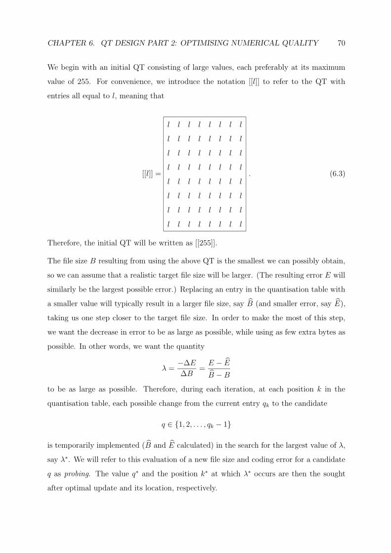
CHAPTER 6. QT DESIGN PART 2: OPTIMISING NUMERICAL QUALITY 70
We begin with an initial QT consisting of large values, each preferably at its maximum
value of 255. For convenience, we introduce the notation [[l]] to refer to the QT with
entries all equal to l, meaning that
[[l]] =
l l l l l l l l
l l l l l l l l
l l l l l l l l
l l l l l l l l
l l l l l l l l
l l l l l l l l
l l l l l l l l
l l l l l l l l
. (6.3)
Therefore, the initial QT will be written as [[255]].
The file size B resulting from using the above QT is the smallest we can possibly obtain,
so we can assume that a realistic target file size will be larger. (The resulting error E will
similarly be the largest possible error.) Replacing an entry in the quantisation table with
a smaller value will typically result in a larger file size, say B (and smaller error, say E),
taking us one step closer to the target file size. In order to make the most of this step,
we want the decrease in error to be as large as possible, while using as few extra bytes as
possible. In other words, we want the quantity
λ =−∆E∆B
=E − E
B −B
to be as large as possible. Therefore, during each iteration, at each position k in the
quantisation table, each possible change from the current entry qk to the candidate
q ∈ {1, 2, . . . , qk − 1}
is temporarily implemented (B and E calculated) in the search for the largest value of λ,
say λ∗. We will refer to this evaluation of a new file size and coding error for a candidate
q as probing. The value q∗ and the position k∗ at which λ∗ occurs are then the sought
after optimal update and its location, respectively.

CHAPTER 6. QT DESIGN PART 2: OPTIMISING NUMERICAL QUALITY 71
At the end of an iteration this optimal update is then made, resulting in a new QT, as
well as new values of the file size B and error E. We repeat these iterations until B is
no longer smaller than the target file size. The pseudocode in Algorithm 6.1 specifies the
algorithm more formally.
Input: Target file size T
initialize QT: Q = [[255]];
calculate B; calculate E;
while B < T doλ∗ = 0;
for k = 1 To 64 do
qq = Q(k);
for q = 1 To qq - 1 do
Q(k) = q;
calculate B; calculate E; λ = E−EB−B
;
if λ > λ∗ then
λ∗ = λ; k∗ = k; q∗ = q; B∗ = B; E∗ = E;
end
end
Q(k) = qq;
end
Q(k∗) = q∗; B = B∗; E = E∗;
end
Algorithm 6.1: The greedy algorithm by Wu and Gersho [2]
In the description of Algorithm 6.1 we have made the assumption that replacing a QT
entry with a smaller value necessarily leads to a reduction in error and an increase in file
size, thus resulting in a positive (and finite) value of λ. Exceptions do however exist and,
while the algorithm is immune to them, some can be exploited to reduce running time.
Let us consider each in turn:

CHAPTER 6. QT DESIGN PART 2: OPTIMISING NUMERICAL QUALITY 72
1. ∆B = 0,−∆E > 0⇒ λ =∞ :
When replacing a QT entry with a smaller one, an encoding sometimes results
that requires the same number of bytes, but has a smaller error than the previous
encoding. The corresponding value of λ, namely ∞, will therefore be judged the
best (assuming the previous best was finite) and no subsequent value of λ (not
even ∞) will be able to beat it. This judgement is appropriate, since the encoding
error is decreased without costing us any bytes. It would therefore be wasteful to
continue probing once a value of∞ is encountered. Even if we compared the values
of −∆E (decrease in error) for each such case in order to find the best “freebie”,
the first occurrence of ∞ will likely be the best. This is so because (a) subsequent
probes within a specific frequency index k will be for larger values of q and cannot
yield larger decreases in E, and (b) subsequent indices k more or less correspond
to higher frequencies due to their zigzag ordering, and probing within them is thus
unlikely to yield larger decreases in E for ∆B = 0.
Instead, upon encountering λ = ∞, we “break” out of the two FOR-loops (having
found the λ∗, q∗, and k∗ we were looking for) and finalise the current iteration.
2. ∆B = 0,−∆E = 0⇒ λ = NaN2:
This situation occurs when the kth coefficient of each frequency block is quantised
to zero by entry qk in the current QT, as well as by the value of q currently being
probed.
When this happens, no further probing is needed for this value of k, since subsequent
(and larger) values of q will also quantise the coefficients involved to zero, and thus
also give us λ = NaN. Therefore, the algorithm can also be modified to break out of
the innermost FOR-loop when λ = NaN is encountered. Note that no programming
language would deem λ = NaN larger than λ∗, meaning that the algorithm still
functions properly when not testing for this case.
2NaN is a special symbol, meaning “not a number”, assigned by certain programming languages to a
number resulting from zero divided by itself.
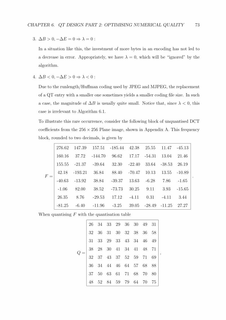
CHAPTER 6. QT DESIGN PART 2: OPTIMISING NUMERICAL QUALITY 73
3. ∆B > 0,−∆E = 0⇒ λ = 0 :
In a situation like this, the investment of more bytes in an encoding has not led to
a decrease in error. Appropriately, we have λ = 0, which will be “ignored” by the
algorithm.
4. ∆B < 0,−∆E > 0⇒ λ < 0 :
Due to the runlength/Huffman coding used by JPEG and MJPEG, the replacement
of a QT entry with a smaller one sometimes yields a smaller coding file size. In such
a case, the magnitude of ∆B is usually quite small. Notice that, since λ < 0, this
case is irrelevant to Algorithm 6.1.
To illustrate this rare occurrence, consider the following block of unquantised DCT
coefficients from the 256× 256 Plane image, shown in Appendix A. This frequency
block, rounded to two decimals, is given by
F =
276.62 147.39 157.51 -185.44 42.38 25.55 11.47 -45.13
160.16 37.72 -144.70 96.62 17.17 -54.31 13.04 21.46
155.55 -21.37 -39.64 32.30 -22.40 33.64 -38.53 26.19
42.18 -193.21 36.84 88.40 -70.47 10.13 13.55 -10.89
-40.63 -13.92 38.84 -39.37 13.63 -6.28 7.86 -1.65
-1.06 82.00 38.52 -73.73 30.25 9.11 3.93 -15.65
26.35 8.76 -29.53 17.12 -4.11 0.31 -4.11 3.44
-81.25 -6.40 -11.96 -3.25 39.05 -28.49 -11.25 27.27
.
When quantising F with the quantisation table
Q =
26 34 33 29 36 30 49 31
32 36 31 30 32 38 36 58
31 33 29 33 43 34 46 49
38 28 30 41 34 41 48 71
32 37 43 37 52 59 71 69
36 34 44 46 64 57 68 88
37 50 63 61 71 68 70 80
48 52 84 59 79 64 70 75
,
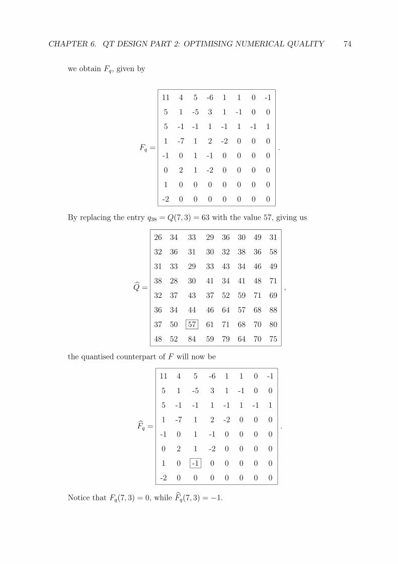
CHAPTER 6. QT DESIGN PART 2: OPTIMISING NUMERICAL QUALITY 74
we obtain Fq, given by
Fq =
11 4 5 -6 1 1 0 -1
5 1 -5 3 1 -1 0 0
5 -1 -1 1 -1 1 -1 1
1 -7 1 2 -2 0 0 0
-1 0 1 -1 0 0 0 0
0 2 1 -2 0 0 0 0
1 0 0 0 0 0 0 0
-2 0 0 0 0 0 0 0
.
By replacing the entry q38 = Q(7, 3) = 63 with the value 57, giving us
Q =
26 34 33 29 36 30 49 31
32 36 31 30 32 38 36 58
31 33 29 33 43 34 46 49
38 28 30 41 34 41 48 71
32 37 43 37 52 59 71 69
36 34 44 46 64 57 68 88
37 50 57 61 71 68 70 80
48 52 84 59 79 64 70 75
,
the quantised counterpart of F will now be
Fq =
11 4 5 -6 1 1 0 -1
5 1 -5 3 1 -1 0 0
5 -1 -1 1 -1 1 -1 1
1 -7 1 2 -2 0 0 0
-1 0 1 -1 0 0 0 0
0 2 1 -2 0 0 0 0
1 0 -1 0 0 0 0 0
-2 0 0 0 0 0 0 0
.
Notice that Fq(7, 3) = 0, while Fq(7, 3) = −1.

CHAPTER 6. QT DESIGN PART 2: OPTIMISING NUMERICAL QUALITY 75
Our somewhat unexpected phenomenon now occurs when we entropy code these
two blocks. The zigzag sequences of Fq and Fq, say z and z, respectively, are (in
truncated form)
z = 11 4 5 · · · -2 0 0 -2 · · · 0 0 0
and
z = 11 4 5 · · · -2 0 -1 -2 · · · 0 0 0 .
The first 36 entries of z and z are identical, ending with the same non-zero AC
coefficient, namely -2. The same contribution to the file size, say p bits, is therefore
made by these entries.
In the case of z, the next two entries are zeroes preceding the subsequent non-zero
coefficient. With this coefficient equal to -2, the symbol (runlength, category) =
(2, 2) is formed, which has a Huffman code of 8-bit length. The contribution made
to the file size by z thus far is now equal to p+ 8 bits.
In the case of z, on the other hand, the 38th entry is equal to -1, with the first
of the abovementioned zeroes now preceding it. The symbol thereby formed is
(runlength, category) = (1, 1), which has a Huffman code that is 4 bits long.
The subsequent entry of -2, no longer preceded by any zeroes is now represented by
(0, 2). The Huffman code for this symbol is 2 bits long. As a result, the first 39
entries of z add p+ 6 bits to the file size, while those of z added p+ 8 bits.
The remaining entries of z and z once again add an equal number of bits to the file
size, meaning that z adds 2 fewer bits to the file size than z.
While some transform blocks from this image do behave in the expected fashion
when making the above change to Q (i.e. add more bits to the file size than before),
most of them yield unchanged quantised coefficients in this particular case, thereby
making the same contribution to the file size before and after changing Q to Q.
The few transform blocks exhibiting the unexpected behaviour illustrated above,

CHAPTER 6. QT DESIGN PART 2: OPTIMISING NUMERICAL QUALITY 76
happen to make more decreased contributions to the file size than the increased
contributions made by the few behaving as expected.
In the end, the number of bits required to encode all quantised coefficients obtained
by using Q is equal to 48041, while the number of bits required when using Q is
equal to 48040. Since storage space is allocated in bytes, the encoding resulting from
using Q has a file size of B = 6006+354 = 6360 bytes, when taking into account the
overhead mentioned in Section 2.5. The encoding resulting from using Q, however,
has a file size of B = 6005 + 354 = 6359 bytes. Consequently, ∆B = B −B = −1.
5. ∆B < 0,−∆E = 0⇒ λ = 0 :
This case is similar to the previous one, with the addition of an (unexpected) oc-
currence of −∆E = 0, similar to that of case 3 above. With λ = 0, it has no effect
on the algorithm.
Algorithm 6.1 is too time-consuming to be implemented in Matlab. Instead, we chose
to implement it in C++, with the program reading in an image’s frequency components
from a mat-file created by Matlab. As an example of the algorithm’s usage, consider its
application to the JPEG encoding of the 256 × 256 Lena image, for the target file size
of 8000 bytes. Starting with the quantisation table Q = [[255]], the initial file size is
B = 1540 bytes, and its corresponding error is E = 375.7444. The first few iterations
yield “freebies”. For instance, the table
Q =
252 255 255 255 255 255 255 255
255 255 255 255 255 255 255 255
255 255 255 255 255 255 255 255
255 255 255 255 255 255 255 255
255 255 255 255 255 255 255 255
255 255 255 255 255 255 255 255
255 255 255 255 255 255 255 255
255 255 255 255 255 255 255 255

CHAPTER 6. QT DESIGN PART 2: OPTIMISING NUMERICAL QUALITY 77
results from the first iteration, where the file size is still B = 1540 bytes but the error is
E = 375.1606.
The second to last table is
Q =
20 23 26 19 23 20 22 20
21 21 20 20 23 27 21 28
21 20 22 25 23 29 27 28
19 19 27 23 22 25 25 39
17 22 22 25 27 32 33 32
20 20 27 25 25 35 35 43
20 26 21 32 24 34 37 33
30 24 35 31 46 42 48 45
with coding file size B = 7980 bytes and error E = 21.5000. This leads to the table
Q =
20 21 26 19 23 20 22 20
21 21 20 20 23 27 21 28
21 20 22 25 23 29 27 28
19 19 27 23 22 25 25 39
17 22 22 25 27 32 33 32
20 20 27 25 25 35 35 43
20 26 21 32 24 34 37 33
30 24 35 31 46 42 48 45
(6.4)
being obtained in the subsequent iteration, where the transition from q2 = Q(1, 2) = 23
to 21 was deemed the most advantageous. The resulting file size is B = 8000 bytes, with
corresponding error E = 21.3941, upon which the algorithm terminates.
Using Matlab, we find that the encoding produced by the final QT above has a PSNR
of 34.8084 dB. By comparison, an encoding of 7995 bytes produced by a rescaling of the
standard JPEG table, using qual = 54.5, has a PSNR of 33.2453 dB. Clearly, the QT
obtained with Algorithm 6.1 is the superior table.
Even when implemented in C++, Algorithm 6.1 still takes too long. The QT in (6.4)

CHAPTER 6. QT DESIGN PART 2: OPTIMISING NUMERICAL QUALITY 78
required roughly 6h15min to obtain when using an Intel Core 2 vPro at 3 GHz. For a
larger target file size this would have taken even longer. Furthermore, the running time is
also proportional to the size of the input image — a 512× 512 image, for example, would
slow things down by a factor of 4.
6.3 Bi-directional Greedy Algorithm
Algorithm 6.1 progresses in only one direction, namely from a file size lower than the
target toward that target, via larger and larger file sizes. However, we could just as easily
have started with an initial QT filled with 1s, and proceeded in the opposite direction. In
other words, by starting with the largest possible file size B and smallest possible error
E, one would now attempt to minimise
λ =∆E
−∆B =E − E
B − B
during each iteration, thereby incurring the smallest increase in error for the largest
decrease in file size. This would continue until the current file size is no longer larger than
the target.
From the above remark we see that both the maximising step in one direction and the
minimising step in the opposite are equally valid. This is the basis for the improved
algorithm proposed by Fung and Parker [1]. Rather than starting with an “extreme”
QT, a more feasible (most likely sub-optimal) initial table is used. The new algorithm
iteratively improves upon this table by probing in the appropriate direction, depending
on whether the current file size is above or below the target. This means that if the
current table yields a file size smaller than the target, the approach used in Algorithm 6.1
is taken: probing smaller QT entries and maximising λ. Otherwise, the dual approach is
taken: probing larger QT entries and minimising λ. The pseudocode for the algorithm is
given in Algorithm 6.2.

CHAPTER 6. QT DESIGN PART 2: OPTIMISING NUMERICAL QUALITY 79
Input: Target file size T and initial table Q
calculate B; calculate E; Rmax =∞; Rmin = 0;
while Rmax > Rmin do
if B < T thenλ∗ = 0;
for k = 1 To 64 do
qq = Q(k);
for q = 1 To qq - 1 do
Q(k) = q; calculate B; calculate E; λ = E−EB−B
;
if λ > λ∗ then
λ∗ = λ; k∗ = k; q∗ = q; B∗ = B; E∗ = E;
end
end
Q(k) = qq;
end
Rmax = λ∗;
elseλ∗ =∞;
for k = 1 To 64 do
qq = Q(k);
for q = qq + 1 To 255 do
Q(k) = q; calculate B; calculate E; λ = E−EB−B
;
if λ < λ∗ And λ > 0 then
λ∗ = λ; k∗ = k; q∗ = q; B∗ = B; E∗ = E;
end
end
Q(k) = qq;
end
Rmin = λ∗;
end
Q(k∗) = q∗; B = B∗; E = E∗;
end
Algorithm 6.2: The bi-directional greedy algorithm by Fung and Parker [1]

CHAPTER 6. QT DESIGN PART 2: OPTIMISING NUMERICAL QUALITY 80
The algorithm keeps track of the most recent maximised and minimised values of λ,
which it stores in Rmax and Rmin, respectively. As long as the algorithm can improve
upon the QT, Rmax will be larger than Rmin. Eventually, this condition ceases to hold,
at which point the algorithm will repeatedly output the same sequence of tables, with a
corresponding sequence of file sizes oscillating about the target file size. For this reason
Rmax ≤ Rmin is used as the stopping condition.
Notice that the interpretations of many of the exceptional cases listed in the previous
section, change when minimising λ in Algorithm 6.2. This is due to the changed order
in which the file sizes and errors are subtracted, where we now expect ∆E and −∆B to
be positive. In particular, the interpretations of cases 1 and 3 will be inverted. Case 3,
now reading (−∆B > 0, ∆E = 0 ⇒ λ = 0), will represent a “freebie”, since the file
size is reduced without incurring any increase in error; in case 1, now reading (−∆B =
0, ∆E > 0 ⇒ λ = ∞), an increased error has not lead to a decrease in file size. Case
1, with λ =∞, will therefore be ignored by the second portion of Algorithm 6.2, and we
could (at first glance) test for case 3 to detect “freebies”.
However, case 4, where λ < 0, and case 5, where λ = 0, now need to be avoided. For this
reason, the additional condition (λ > 0) is used in the second portion of the algorithm,
thereby also potentially throwing away valid “freebies”. Fortunately, no such “freebies”
have ever been observed (we specifically tested for them), so it seems that no harm is
done. Lastly, the interpretation of case 2, where λ = NaN, remains the same, and we can
once again test for it to optimise running time.
We now repeat the search for an optimised QT for the JPEG encoding of Lena, using a
C++ implementation of this algorithm. The JPEG table obtained with qual = 54.5,

CHAPTER 6. QT DESIGN PART 2: OPTIMISING NUMERICAL QUALITY 81
QJ =
15 10 9 15 22 36 46 56
11 11 13 17 24 53 55 50
13 12 15 22 36 52 63 51
13 15 20 26 46 79 73 56
16 20 34 51 62 99 94 70
22 32 50 58 74 95 103 84
45 58 71 79 94 110 109 92
66 84 86 89 102 91 94 90
(6.5)
and used in the previous section, is feasible since it yields an encoding of 7995 bytes. We
thus use it as our initial table. One of the last QTs output before oscillation occurs has
a coding file size of B = 7987 bytes and error E = 21.4616. Thereafter the tables
Q1 =
20 21 26 19 22 20 22 20
21 21 20 20 23 23 21 28
19 20 22 25 23 29 27 29
19 20 25 23 24 25 25 39
17 22 22 25 27 32 33 33
20 20 27 26 33 35 35 43
20 26 23 33 24 34 38 33
23 24 35 32 46 42 48 45
(6.6)
with B = 7995 bytes and E = 21.4199, and
Q2 =
20 21 26 19 22 20 22 20
21 21 20 20 23 23 21 28
19 20 22 25 23 29 27 29
19 17 25 23 24 25 25 39
17 22 22 25 27 32 33 33
20 20 27 26 33 35 35 43
20 26 23 33 24 34 38 33
23 24 35 32 46 42 48 45
(6.7)

CHAPTER 6. QT DESIGN PART 2: OPTIMISING NUMERICAL QUALITY 82
with B = 8012 bytes and E = 21.3333 are obtained, giving us Rmax = 333.8658. Lastly,
the algorithm again outputs Q1, meaning that Rmin is also equal to 333.8658, and it then
terminates. In the absence of the stopping condition, the sequence {Q1, Q2, Q1, . . .} wouldbe generated indefinitely. Algorithm 6.2 is indeed an improvement over Algorithm 6.1,
requiring roughly 2h37min to reach its final sequence of QTs for this particular example.
From such a final sequence, the table with coding file size closest to the target can be
chosen as the final one, but it will not necessarily be feasible. Q1, for instance, while
feasible, could still be tweaked to yield an even closer file size by inspecting the difference
between it and Q2. This difference is between their 4th row, 2nd column entries, where
the transitions from Q1(4, 2) = 20 to Q2(4, 2) = 17, and vice versa, take place. By instead
choosing q12 = 19, the QT
Q =
20 21 26 19 22 20 22 20
21 21 20 20 23 23 21 28
19 20 22 25 23 29 27 29
19 19 25 23 24 25 25 39
17 22 22 25 27 32 33 33
20 20 27 26 33 35 35 43
20 26 23 33 24 34 38 33
23 24 35 32 46 42 48 45
is obtained, which yields an encoding with a file size of 8000 bytes, an error E = 21.3967,
and a PSNR of 34.8085 dB. We can now better compare this table with the one found
with Algorithm 6.1 in the previous section, shown in (6.4). Just as their entries differ only
slightly, their respective encodings also have basically the same PSNR; hence we consider
the two QTs to be equally valid.
We are of course free to start Algorithm 6.2 with any initial table; in particular, were we
to start with the table Q = [[255]], the actions of Algorithm 6.1 would be mimicked and
its output reproduced. Consequently, Algorithm 6.2 is an extension of its predecessor.

CHAPTER 6. QT DESIGN PART 2: OPTIMISING NUMERICAL QUALITY 83
6.3.1 Proposed Improvements
In general, different initial QTs result in slightly different but equally valid optimised
QTs. The running times, however, can be vastly different. The reason for this is the
fact that the number of iterations performed by Algorithm 6.2 is a function of the initial
table. A well chosen initial table could reduce this number by being “close” to a final
sequence of tables in a chronological sense. For instance, each table Qn+1 output by
Algorithm 6.2 is closer to the final sequence than its predecessor Qn, since using Qn+1
as initial table instead of Qn would require one less iteration to reach the final sequence.
The quantisation table
Q =
14 16 18 20 22 24 26 28
16 18 20 22 24 26 28 30
18 20 22 24 26 28 30 32
20 22 24 26 28 30 32 34
22 24 26 28 30 32 34 36
24 26 28 30 32 34 36 38
26 28 30 32 34 36 38 40
28 30 32 34 36 38 40 42
,
for instance, is closer to a final sequence than QJ , shown in (6.5) and used as initial QT in
the example above, was. By instead using Q as initial table and repeating the experiment,
Algorithm 6.2 now requires more or less 1h27min to reach a final sequence of QTs.
Furthermore, the entries in Q are also closer to the entries in the final tables obtained
with it than the entries in QJ are to the entries in Q1 and Q2, shown in (6.6) and
(6.7), respectively. This means that we can significantly reduce the number of candidate
values to probe when using Q, thereby reducing the amount of work done during each
iteration of the algorithm. The same final sequence of QTs can for instance be obtained
by only probing the 20 candidate values above or below each entry during a particular
iteration, depending on the direction being probed in. This reduces the running time to
approximately 17min. If we do the same in the case of QJ , however, the tables Q1 and
Q2 will not be obtained, but an inferior final sequence instead.

CHAPTER 6. QT DESIGN PART 2: OPTIMISING NUMERICAL QUALITY 84
A well chosen initial QT should therefore also minimise the number of values, say w, to
probe in Algorithm 6.2. We will refer to this number as the probing width. Its use is
formally described in Algorithm 6.3, which is a modification of Algorithm 6.2. Note that,
by choosing w = 254, any result obtained with Algorithm 6.2 can be reproduced with
Algorithm 6.3.

CHAPTER 6. QT DESIGN PART 2: OPTIMISING NUMERICAL QUALITY 85
Input: Target file size T , initial table Q and probing width w
calculate B; calculate E; Rmax =∞; Rmin = 0;
while Rmax > Rmin do
if B < T thenλ∗ = 0;
for k = 1 To 64 do
qq = Q(k); qqq = max(qq − w, 1);
for q = qqq To qq - 1 do
Q(k) = q; calculate B; calculate E; λ = E−EB−B
;
if λ > λ∗ then
λ∗ = λ; k∗ = k; q∗ = q; B∗ = B; E∗ = E;
end
end
Q(k) = qq;
end
Rmax = λ∗;
elseλ∗ =∞;
for k = 1 To 64 do
qq = Q(k); qqq = min(qq + w, 255);
for q = qq + 1 To qqq do
Q(k) = q; calculate B; calculate E; λ = E−EB−B
;
if λ < λ∗ And λ > 0 then
λ∗ = λ; k∗ = k; q∗ = q; B∗ = B; E∗ = E;
end
end
Q(k) = qq;
end
Rmin = λ∗;
end
Q(k∗) = q∗; B = B∗; E = E∗;
end
Algorithm 6.3: Proposed improved algorithm utilising a probing width w

CHAPTER 6. QT DESIGN PART 2: OPTIMISING NUMERICAL QUALITY 86
The challenge now becomes choosing an appropriate initial table for an input image and
target file size — one that will allow us to use as narrow a probing width as possible
in order to minimise running time. While Fung and Parker do propose a formula for
calculating initial tables in [1], their tables will often have entries of 255 in high frequency
positions. Based on the discussion above, arriving at properly optimised QTs from such
initial tables would require too much probing. Conversely, using a narrow probing width
in conjunction with an initial QT calculated with the abovementioned formula would yield
an inferior output table.
Instead, we propose an alternative method for calculating initial QTs, with a detailed
account given in the next chapter. Also, an additional performance increase is gained by
using two separate probing widths, one for QT entries in lower frequency positions and one
for entries in higher frequency positions. From our experiments, detailed in Section 7.4,
we found that we could further reduce the probing width for lower frequency entries and
still obtain the same results. For this reason, QT entries are numbered and processed in
zigzag ordering, as formulated in the problem statement in Section 6.1 and the subsequent
descriptions of the greedy algorithms. By doing so, we can easily process lower frequency
entries using their probing width first, followed by higher frequency entries being processed
using their probing width. This partitioning is illustrated in Figure 6.1, where the first
28 entries in zigzag order, constituting the shaded upper triangle, are chosen as the lower
frequency entries.
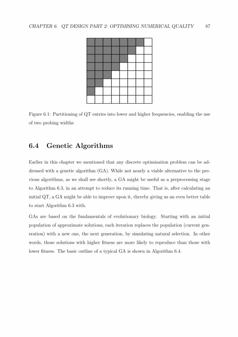
CHAPTER 6. QT DESIGN PART 2: OPTIMISING NUMERICAL QUALITY 87
Figure 6.1: Partitioning of QT entries into lower and higher frequencies, enabling the use
of two probing widths
6.4 Genetic Algorithms
Earlier in this chapter we mentioned that any discrete optimisation problem can be ad-
dressed with a genetic algorithm (GA). While not nearly a viable alternative to the pre-
vious algorithms, as we shall see shortly, a GA might be useful as a preprocessing stage
to Algorithm 6.3, in an attempt to reduce its running time. That is, after calculating an
initial QT, a GA might be able to improve upon it, thereby giving us an even better table
to start Algorithm 6.3 with.
GAs are based on the fundamentals of evolutionary biology. Starting with an initial
population of approximate solutions, each iteration replaces the population (current gen-
eration) with a new one, the next generation, by simulating natural selection. In other
words, those solutions with higher fitness are more likely to reproduce than those with
lower fitness. The basic outline of a typical GA is shown in Algorithm 6.4.
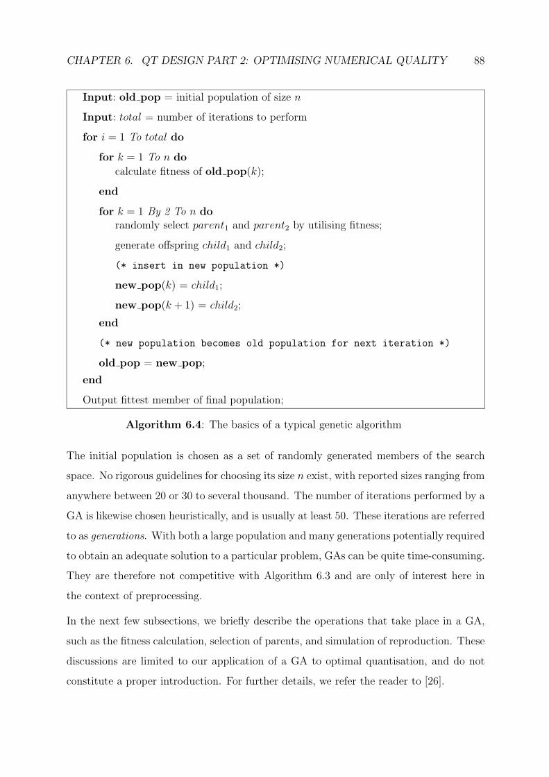
CHAPTER 6. QT DESIGN PART 2: OPTIMISING NUMERICAL QUALITY 88
Input: old pop = initial population of size n
Input: total = number of iterations to perform
for i = 1 To total do
for k = 1 To n do
calculate fitness of old pop(k);
end
for k = 1 By 2 To n dorandomly select parent1 and parent2 by utilising fitness;
generate offspring child1 and child2;
(* insert in new population *)
new pop(k) = child1;
new pop(k + 1) = child2;
end
(* new population becomes old population for next iteration *)
old pop = new pop;
end
Output fittest member of final population;
Algorithm 6.4: The basics of a typical genetic algorithm
The initial population is chosen as a set of randomly generated members of the search
space. No rigorous guidelines for choosing its size n exist, with reported sizes ranging from
anywhere between 20 or 30 to several thousand. The number of iterations performed by a
GA is likewise chosen heuristically, and is usually at least 50. These iterations are referred
to as generations. With both a large population and many generations potentially required
to obtain an adequate solution to a particular problem, GAs can be quite time-consuming.
They are therefore not competitive with Algorithm 6.3 and are only of interest here in
the context of preprocessing.
In the next few subsections, we briefly describe the operations that take place in a GA,
such as the fitness calculation, selection of parents, and simulation of reproduction. These
discussions are limited to our application of a GA to optimal quantisation, and do not
constitute a proper introduction. For further details, we refer the reader to [26].

CHAPTER 6. QT DESIGN PART 2: OPTIMISING NUMERICAL QUALITY 89
6.4.1 The Fitness Function
In a GA the fitness of a candidate solution is a measure of how well it solves the underlying
optimisation problem. This is quantified by using a fitness function, which is always
derived from the function to be optimised, called the object function. In unconstrained
maximisation problems, we can simply use the object function as the fitness function,
while using its negative or inverse as the fitness function in unconstrained minimisation
problems.
Recalling our problem statement in Section 6.1, the function we wish to minimise is the
error E in the frequency domain. If this problem was unconstrained, the fitness f of a
quantisation table Q could for instance be chosen as
f(Q) =1
E(Q).
Our problem is constrained though, so we also have to penalise deviation from constraint
(6.2). If we do not, the table Q = [[1]] (which always yields the smallest error) will always
be deemed the fittest. By virtue of (6.2), a candidate solution Q yielding a file size B will
be penalised if B > 1.001T or B < 0.999T . The deviation (in percentage) is therefore
calculated as
dev(Q) =
100
(B(Q)− 1.001T
1.001T
), B > 1.001T,
100
(0.999T −B(Q)
0.999T
), B < 0.999T,
0 , otherwise.
(6.8)
Using this deviation, a new object function is created, say cost(Q), given by
cost(Q) = E(Q) + c.dev(Q), c > 0. (6.9)
The number c is known as the penalty parameter and is used to ensure proper penalisation
of infeasibility.
For calculating c, the adaptive method proposed in [27] was chosen. During each iteration

CHAPTER 6. QT DESIGN PART 2: OPTIMISING NUMERICAL QUALITY 90
of the GA the current value of c, say ci, is modified for the next generation according to
ci+1 = ci
(BFC
BIC
). (6.10)
Here BFC refers to the lowest cost belonging to a feasible solution (the best feasible
cost), while BIC refers to the lowest cost belonging to an infeasible solution (the best
infeasible cost). As a result, the penalty parameter will be scaled up if deviation from our
constraint is not sufficiently penalised, and down if deviation is over-penalised.
For the initial value of c we use the “interior method” proposed in [27], where an initial
value much higher than the expected proper value is chosen. The value used in our C++
implementation of a GA is 35.
Finally, our fitness function is once again chosen as the inverse of the object function,
meaning that
f(Q) =1
cost(Q). (6.11)
6.4.2 Natural Selection
During a typical iteration of a GA the fitness of each member of the current population
is calculated using the chosen fitness function. As shown in Algorithm 6.4, pairs of these
members are then randomly selected, by utilising their fitness, to reproduce. Several se-
lection methods exist, among others the basic fitness-proportionate method that we chose.
This method is called roulette wheel sampling, and can be implemented by partitioning
the probability interval [0, 1] into n subintervals, where n is the size of the population.
Each member of the population is then assigned its own subinterval, [ak, bk), the width
of which is proportional to that member’s fitness.
In each case the upper limit bk is calculated as
bk =k∑
j=1
f(Qj)
ftot,
where Qj is the jth member of the current generation and ftot is the total fitness
ftot =n∑
j=1
f(Qj).
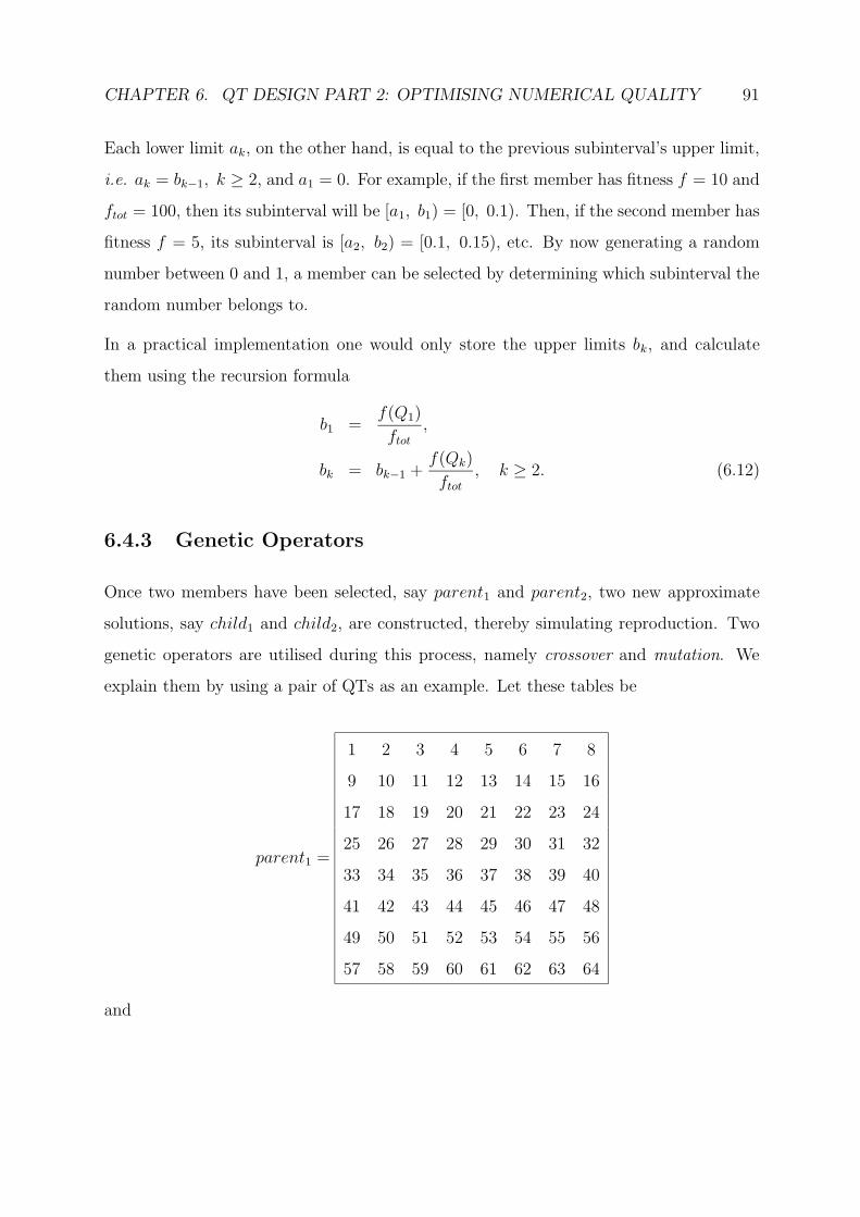
CHAPTER 6. QT DESIGN PART 2: OPTIMISING NUMERICAL QUALITY 91
Each lower limit ak, on the other hand, is equal to the previous subinterval’s upper limit,
i.e. ak = bk−1, k ≥ 2, and a1 = 0. For example, if the first member has fitness f = 10 and
ftot = 100, then its subinterval will be [a1, b1) = [0, 0.1). Then, if the second member has
fitness f = 5, its subinterval is [a2, b2) = [0.1, 0.15), etc. By now generating a random
number between 0 and 1, a member can be selected by determining which subinterval the
random number belongs to.
In a practical implementation one would only store the upper limits bk, and calculate
them using the recursion formula
b1 =f(Q1)
ftot,
bk = bk−1 +f(Qk)
ftot, k ≥ 2. (6.12)
6.4.3 Genetic Operators
Once two members have been selected, say parent1 and parent2, two new approximate
solutions, say child1 and child2, are constructed, thereby simulating reproduction. Two
genetic operators are utilised during this process, namely crossover and mutation. We
explain them by using a pair of QTs as an example. Let these tables be
parent1 =
1 2 3 4 5 6 7 8
9 10 11 12 13 14 15 16
17 18 19 20 21 22 23 24
25 26 27 28 29 30 31 32
33 34 35 36 37 38 39 40
41 42 43 44 45 46 47 48
49 50 51 52 53 54 55 56
57 58 59 60 61 62 63 64
and
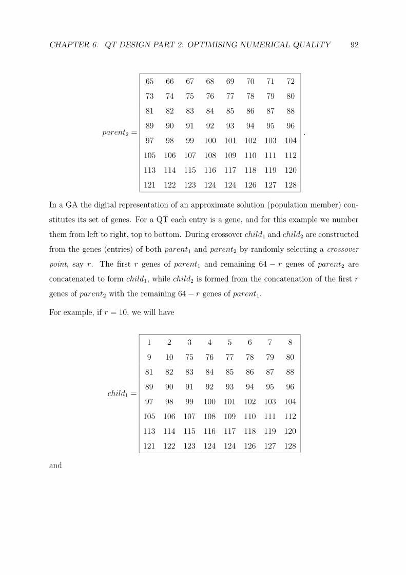
CHAPTER 6. QT DESIGN PART 2: OPTIMISING NUMERICAL QUALITY 92
parent2 =
65 66 67 68 69 70 71 72
73 74 75 76 77 78 79 80
81 82 83 84 85 86 87 88
89 90 91 92 93 94 95 96
97 98 99 100 101 102 103 104
105 106 107 108 109 110 111 112
113 114 115 116 117 118 119 120
121 122 123 124 124 126 127 128
.
In a GA the digital representation of an approximate solution (population member) con-
stitutes its set of genes. For a QT each entry is a gene, and for this example we number
them from left to right, top to bottom. During crossover child1 and child2 are constructed
from the genes (entries) of both parent1 and parent2 by randomly selecting a crossover
point, say r. The first r genes of parent1 and remaining 64 − r genes of parent2 are
concatenated to form child1, while child2 is formed from the concatenation of the first r
genes of parent2 with the remaining 64− r genes of parent1.
For example, if r = 10, we will have
child1 =
1 2 3 4 5 6 7 8
9 10 75 76 77 78 79 80
81 82 83 84 85 86 87 88
89 90 91 92 93 94 95 96
97 98 99 100 101 102 103 104
105 106 107 108 109 110 111 112
113 114 115 116 117 118 119 120
121 122 123 124 124 126 127 128
and

CHAPTER 6. QT DESIGN PART 2: OPTIMISING NUMERICAL QUALITY 93
child2 =
65 66 67 68 69 70 71 72
73 74 11 12 13 14 15 16
17 18 19 20 21 22 23 24
25 26 27 28 29 30 31 32
33 34 35 36 37 38 39 40
41 42 43 44 45 46 47 48
49 50 51 52 53 54 55 56
57 58 59 60 61 62 63 64
.
This particular implementation of crossover is termed single-point crossover, and is the
approach we chose. Other approaches, such as two-point crossover, are explained in [26].
Crossover need not necessarily take place: In general, a crossover probability pc can be
used to determine whether or not crossover takes place. If it does not (i.e. a random
number between 0 and 1 is not smaller than pc), child1 and child2 are chosen as exact
replicas of their parents. Since pc is usually chosen to be at least 0.75, we simply chose
pc = 1 for our implementation.
After child1 and child2 have been created, the mutation operator comes into play. It can
replace a gene in a randomly selected position with a randomly selected new value. To
determine when a mutation takes place, a parameter pm, called the mutation probability,
is used. This number is usually quite small and can for instance be pm = 0.05. If a
random number between 0 and 1 is not smaller than pm, mutation does not take place. In
general, mutation can be applied to each gene with probability pm. Here, for each child
in turn, we apply it only once.
If, for example, child2 above were to undergo a mutation, a random integer between 1
and 64 would be generated to select the gene undergoing the mutation. We would then
generate a random integer between 1 and 255 to determine the new value of the mutated
gene. If the randomly selected gene was at position was 24 and its new value was 200,

CHAPTER 6. QT DESIGN PART 2: OPTIMISING NUMERICAL QUALITY 94
then we would have
child2 =
65 66 67 68 69 70 71 72
73 74 11 12 13 14 15 16
17 18 19 20 21 22 23 200
25 26 27 28 29 30 31 32
33 34 35 36 37 38 39 40
41 42 43 44 45 46 47 48
49 50 51 52 53 54 55 56
57 58 59 60 61 62 63 64
.
In the end, the new members child1 and child2 are placed in a new population that will
replace the current one. For this reason, reproduction is performed n2times per iteration
to obtain a new population of n members.
6.4.4 Convergence
As Algorithm 6.4 suggests, a tradditional stopping condition is not used in a GA. Instead,
the algorithm is run for a large number of generations. Upon termination the fittest
member of the final population will be chosen as the best approximation to the sought
after solution. What happens when convergence takes place, is that all members of the
population will be (roughly) the same. We can therefore inspect the members of the final
population to see whether or not convergence has occurred. If it has not, we can always
“resume” the algorithm, using the final population as the new initial population.
Since each new generation completely replaces the one preceding it, the fittest member
of a particular generation is not necessarily fitter than, or even as fit as, the one from
the previous generation. Rather, it is the average fitness of the population that generally
increases from generation to generation. If we do not wish to lose the fittest member, we
can let it survive: after generating a new population, one can randomly select a member
from it to be replaced by the fittest member from the previous generation. This approach
is called elitism, and we chose to use it in our implementation.

CHAPTER 6. QT DESIGN PART 2: OPTIMISING NUMERICAL QUALITY 95
6.5 C++ Implementation
As we saw in Section 6.3.1, Algorithm 6.3 retains the workings of Algorithms 6.1 and
6.2 as subsets, therefore only its implementation is discussed here. We intend to use the
algorithm to obtain optimised QTs for both JPEG and MJPEG so as to compare results;
hence, two C++ implementations were created. For brevity, only the implementation
for MJPEG, qt m.cc, is listed in Appendix B.2. Its JPEG counterpart, qt.cc, is very
similar.
Each program reads in a mat-file of unquantised frequency components created by Matlab.
Such files are created by applying either my jpeg.m or mjpeg.m (whichever is applicable)
to an image, with quantisation disabled, and saving the output. For instance, qt m will
read in an image’s unquantised MDCT coefficients. These coefficients are stored in the
m× n matrix Y , where m and n are also the dimensions of the original image.
Both programs store their QTs in the same left-to-right, top-to-bottom format as matrix
Y , making quantisation and dequantisation as efficient as possible. In order to still process
QT entries in zigzag ordering, both programs use an array z of indices arranged in this
ordering to reconcile the indexing. In other words, QT entries are now addressed as
Q(z(k)) rather than Q(k) during the main algorithm.
The two probing widths mentioned in Section 6.3.1 are used, with the one used for lower
frequency entries called lo, and the one used for higher frequency entries called hi. To use
these two probing widths, each of the outer FOR-loops of Algorithm 6.3 are separated
into two new ones. The first of these processes the first 28 QT entries using lo, while the
second processes the remaining entries using hi.
As was discussed in Section 6.2, our implementations test for the special cases of λ =∞and λ = NaN in order to break out of the appropriate FOR-loops when necessary. Some
other aspects of note are the functions qdq, dct2bytes, d2b and calc error. Function
qdq performs quantisation and dequantisation (utilising m × n matrices Yq and Ydq);
functions dct2bytes and d2b behave in exactly the same way as their respective Matlab
counterparts; and calc error uses Y and Ydq to calculate the error E defined in (6.1). In

CHAPTER 6. QT DESIGN PART 2: OPTIMISING NUMERICAL QUALITY 96
the case of program qt m the primary QT is also downsampled to form the two auxilliary
QTs before each call to qdq. This task is performed by the function down Q.
Both programs also contain an implementation of our proposed method for calculating
initial QTs. The user can choose, via an input option, whether to directly supply the
main algorithm with such an obtained table (option 0), or to first attempt to improve the
table with a genetic algorithm (option 1). In addition, by choosing option 2, this stage
can be skipped and Algorithm 6.3 will start with an initial table specified in function
init Q. This allows us to generate the output of Algorithms 6.1 and 6.2.
Our implemented genetic algorithm can be found in function ga, which is called after
the construction of an initial population. The adaptive method used for calculating the
penalty parameter, described in Section 6.4.1, relies on the presence of at least one feasible
solution in the initial population. For this reason, before constructing an initial popu-
lation, we ensure the feasibility of our initial QT by prompting the user to make slight
modifications to its entries if it happens to be infeasible. The resulting table, say Q, is
then used to construct an initial population and is also included as a member of that
population. By assuming that Q is a good initial table and subsequently restricting the
search in Algorithm 6.3 with probing widths, the GA’s search space is also reduced. We
therefore generate an initial population by randomly adding or subtracting integer values
from the entries in Q, within the limits set by the probing widths.
As stated in Section 6.4.2, selection is implemented by using roulette wheel sampling;
the function responsible for searching the probability intervals assigned to population
members is find pos. Function mate then performs the crossover and mutation operators
described in Section 6.4.3, and places the resulting offspring in the next generation. Note
that, since the search space is reduced by using probing widths, we also limit the intervals
from which mutated genes are selected accordingly. At the end of each iteration, the
elitist approach mentioned in Section 6.4.4 is employed: the fittest QT from the current
generation survives by replacing a randomly selected QT from the next generation.
Lastly, when the GA has finished, the final generation’s fittest table is chosen as the new
initial QT for Algorithm 6.3.

Chapter 7
Modelling and Predicting Initial
Tables
We saw in the previous chapter that the choice of initial QTs plays a central role in
minimising the running time of Algorithm 6.3. In this chapter we propose a method for
generating good initial tables.
7.1 Linear Models
As we discussed in Section 6.3.1, we would ideally like initial tables to be as “close” as
possible to the optimised tables that will be obtained using them. One aim of doing
so is to hopefully reduce the number of iterations needed by Algorithm 6.3. The other
advantage is the reduction in probing width to be achieved. A good initial table Q should
therefore be “close” to the final table Q in the sense that
||Q− Q||∞ = max1≤k≤64
|qk − qk| (7.1)
should be small. Less formally, we could also say that a good initial table should mimic
the trends of the final table. Looking at the optimised tables shown in Figure 7.1, obtained
for some JPEG encodings of 256× 256 Lena, there indeed seem to be trends to exploit.
97
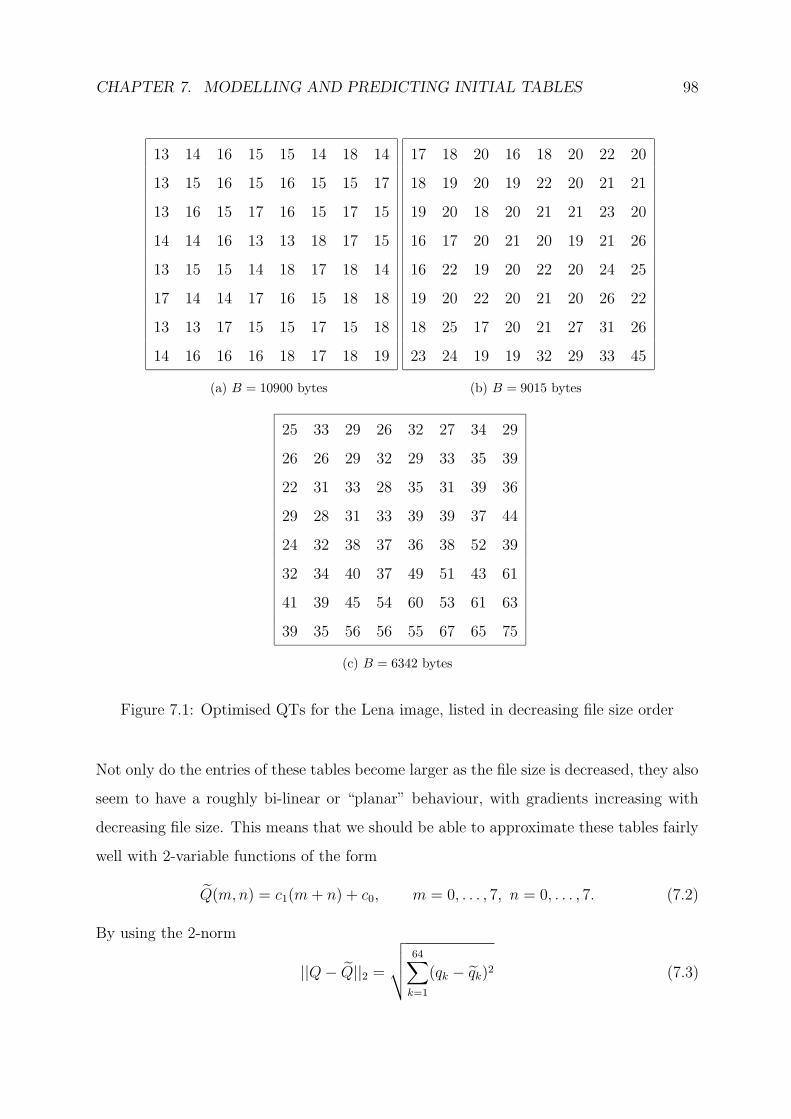
CHAPTER 7. MODELLING AND PREDICTING INITIAL TABLES 98
13 14 16 15 15 14 18 14
13 15 16 15 16 15 15 17
13 16 15 17 16 15 17 15
14 14 16 13 13 18 17 15
13 15 15 14 18 17 18 14
17 14 14 17 16 15 18 18
13 13 17 15 15 17 15 18
14 16 16 16 18 17 18 19
(a) B = 10900 bytes
17 18 20 16 18 20 22 20
18 19 20 19 22 20 21 21
19 20 18 20 21 21 23 20
16 17 20 21 20 19 21 26
16 22 19 20 22 20 24 25
19 20 22 20 21 20 26 22
18 25 17 20 21 27 31 26
23 24 19 19 32 29 33 45
(b) B = 9015 bytes
25 33 29 26 32 27 34 29
26 26 29 32 29 33 35 39
22 31 33 28 35 31 39 36
29 28 31 33 39 39 37 44
24 32 38 37 36 38 52 39
32 34 40 37 49 51 43 61
41 39 45 54 60 53 61 63
39 35 56 56 55 67 65 75
(c) B = 6342 bytes
Figure 7.1: Optimised QTs for the Lena image, listed in decreasing file size order
Not only do the entries of these tables become larger as the file size is decreased, they also
seem to have a roughly bi-linear or “planar” behaviour, with gradients increasing with
decreasing file size. This means that we should be able to approximate these tables fairly
well with 2-variable functions of the form
Q(m,n) = c1(m+ n) + c0, m = 0, . . . , 7, n = 0, . . . , 7. (7.2)
By using the 2-norm
||Q− Q||2 =
√√√√64∑
k=1
(qk − qk)2 (7.3)
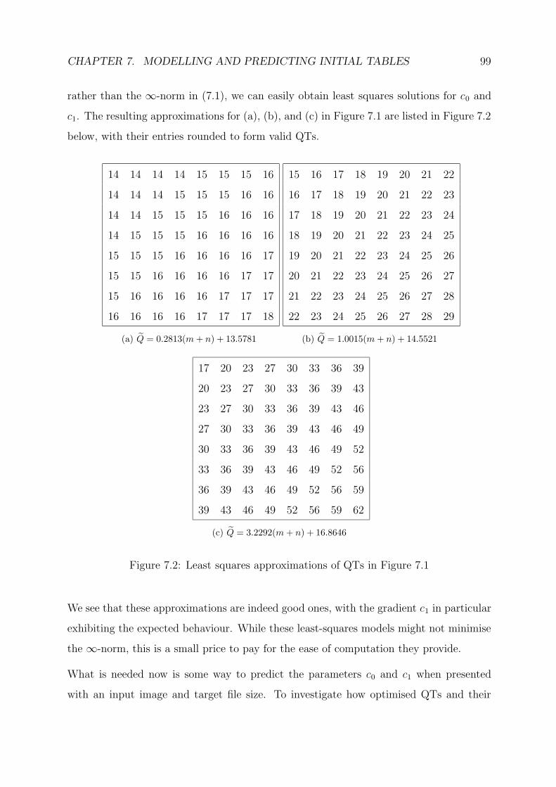
CHAPTER 7. MODELLING AND PREDICTING INITIAL TABLES 99
rather than the ∞-norm in (7.1), we can easily obtain least squares solutions for c0 and
c1. The resulting approximations for (a), (b), and (c) in Figure 7.1 are listed in Figure 7.2
below, with their entries rounded to form valid QTs.
14 14 14 14 15 15 15 16
14 14 14 15 15 15 16 16
14 14 15 15 15 16 16 16
14 15 15 15 16 16 16 16
15 15 15 16 16 16 16 17
15 15 16 16 16 16 17 17
15 16 16 16 16 17 17 17
16 16 16 16 17 17 17 18
(a) Q = 0.2813(m + n) + 13.5781
15 16 17 18 19 20 21 22
16 17 18 19 20 21 22 23
17 18 19 20 21 22 23 24
18 19 20 21 22 23 24 25
19 20 21 22 23 24 25 26
20 21 22 23 24 25 26 27
21 22 23 24 25 26 27 28
22 23 24 25 26 27 28 29
(b) Q = 1.0015(m + n) + 14.5521
17 20 23 27 30 33 36 39
20 23 27 30 33 36 39 43
23 27 30 33 36 39 43 46
27 30 33 36 39 43 46 49
30 33 36 39 43 46 49 52
33 36 39 43 46 49 52 56
36 39 43 46 49 52 56 59
39 43 46 49 52 56 59 62
(c) Q = 3.2292(m + n) + 16.8646
Figure 7.2: Least squares approximations of QTs in Figure 7.1
We see that these approximations are indeed good ones, with the gradient c1 in particular
exhibiting the expected behaviour. While these least-squares models might not minimise
the ∞-norm, this is a small price to pay for the ease of computation they provide.
What is needed now is some way to predict the parameters c0 and c1 when presented
with an input image and target file size. To investigate how optimised QTs and their

CHAPTER 7. MODELLING AND PREDICTING INITIAL TABLES 100
corresponding least-squares models vary for different file sizes and different images, we
stored and analysed the output generated by both qt.cc and qt m.cc for three images.
These images were Lena, Bridge and Plane, all of dimensions 256 × 256 and shown in
Appendix A, and for qt m the sine window was used. In each case the programs were
started with an initial table filled with 1s, made use of a uniform probing width of w = 254,
and were given a target file size of 4000 bytes — thereby mimicking the behaviour of
Algorithm 6.1 in the “opposite” direction. Had we started from the “normal” direction,
with initial tables filled with values of 255, and large target file sizes, many of the optimised
tables corresponding to lower file sizes would have had entries of 255 amongst other two-
digit entries. Our linear model would be a poor fit for such tables. Starting from this
“opposite” direction, on the other hand, results in much better behaved, yet equally valid,
optimised QTs.
7.2 Prediction Strategy
One finding from the analysis mentioned above, is that the parameter c0 (and thus the
first entry of a model) does not necessarily increase monotonically with decreasing file
size. The tables shown in Figures 7.3 and 7.4 below, once again taken from the JPEG
encodings of Lena, and accompanied by their respective models, are an example of this
observation. The same is true of the gradient c1, but we found that the combined effect
of c0 and c1 is always such that the higher frequency entries do increase monotonically
with decreasing file size, in particular those on the co-main diagonal.
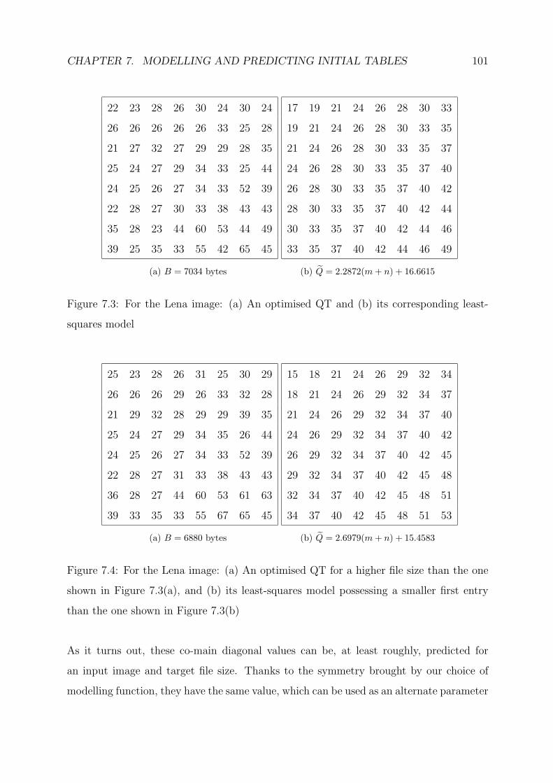
CHAPTER 7. MODELLING AND PREDICTING INITIAL TABLES 101
22 23 28 26 30 24 30 24
26 26 26 26 26 33 25 28
21 27 32 27 29 29 28 35
25 24 27 29 34 33 25 44
24 25 26 27 34 33 52 39
22 28 27 30 33 38 43 43
35 28 23 44 60 53 44 49
39 25 35 33 55 42 65 45
(a) B = 7034 bytes
17 19 21 24 26 28 30 33
19 21 24 26 28 30 33 35
21 24 26 28 30 33 35 37
24 26 28 30 33 35 37 40
26 28 30 33 35 37 40 42
28 30 33 35 37 40 42 44
30 33 35 37 40 42 44 46
33 35 37 40 42 44 46 49
(b) Q = 2.2872(m + n) + 16.6615
Figure 7.3: For the Lena image: (a) An optimised QT and (b) its corresponding least-
squares model
25 23 28 26 31 25 30 29
26 26 26 29 26 33 32 28
21 29 32 28 29 29 39 35
25 24 27 29 34 35 26 44
24 25 26 27 34 33 52 39
22 28 27 31 33 38 43 43
36 28 27 44 60 53 61 63
39 33 35 33 55 67 65 45
(a) B = 6880 bytes
15 18 21 24 26 29 32 34
18 21 24 26 29 32 34 37
21 24 26 29 32 34 37 40
24 26 29 32 34 37 40 42
26 29 32 34 37 40 42 45
29 32 34 37 40 42 45 48
32 34 37 40 42 45 48 51
34 37 40 42 45 48 51 53
(b) Q = 2.6979(m + n) + 15.4583
Figure 7.4: For the Lena image: (a) An optimised QT for a higher file size than the one
shown in Figure 7.3(a), and (b) its least-squares model possessing a smaller first entry
than the one shown in Figure 7.3(b)
As it turns out, these co-main diagonal values can be, at least roughly, predicted for
an input image and target file size. Thanks to the symmetry brought by our choice of
modelling function, they have the same value, which can be used as an alternate parameter

CHAPTER 7. MODELLING AND PREDICTING INITIAL TABLES 102
in (7.2). This means that we can recast our model to look as follows:
Q(m,n) = k1(m+ n− 7) + k0, m = 0, . . . , 7, n = 0, . . . , 7, (7.4)
where k0 will determine the entries on the co-main diagonal, and k1 will have the same
value as c1.
The model in Figure 7.2(a), for example, will be transformed from
Q(m,n) = 0.2813(m+ n) + 13.5781
to
Q(m,n) = 0.2813(m+ n− 7) + 15.5472.
Notice that k0 and k1 have now become the parameters we wish to predict. In this new
form, the gradient k1 can be thought of as a rotation applied about the co-main diagonal
to the table [[k0]], using the notation defined by (6.3). By predicting k0, we would also
be predicting the table [[k0]] to which k1 will be applied. We therefore turn to such
“constant” tables in this endeavour. The hope is that the value k0 for which the table
[[k0]] gives a coding file size closest to the target, will be a good approximation to k0. As a
consequence, k0 has to be restricted to integer values between 1 and 255, since quantising
with floating-point numbers makes no sense when our file size calculations assume the
storage of an 8-bit integer quantisation table in the output file. However, this restriction
also has the benefit of limiting the search to a finite number of candidates.
With k0 now an integer, we can just as well use it as a prediction for the co-main di-
agonal entries instead, to which we will henceforth refer as diag. This will enable us to
approximate (predict) k1: By investigating how k1 varies for each value of diag, a list of
approximate gradients k1 can be maintained and indexed by k0. In other words, upon
obtaining k0 the approximate gradient will be
k1 = list of gradients(k0), (7.5)
making
Q(m,n) = k1(m+ n− 7) + k0, m = 0, . . . , 7, n = 0, . . . , 7 (7.6)

CHAPTER 7. MODELLING AND PREDICTING INITIAL TABLES 103
our predicted initial table.
Let us see how this approach fares when applied to the tables (a), (b) and (c) in Figure 7.1,
using their respective coding file sizes as the target file size T in each case. Firstly, table
(a) has a resulting file size of 10900 bytes, and was approximated by table (a) in Figure
7.2, which has a value of diag equal to 16. By JPEG encoding Lena with the tables
[[1]], [[2]], . . . , [[255]], we find that the table [[16]] gives the closest file size of 10681 bytes.
Therefore k0 = 16. By comparison, the tables [[15]] and [[17]] give file sizes of 11165 bytes
and 10248 bytes, respectively. In general, the sequence of tables [[1]], [[2]], . . . , [[255]] will
result in successively lower file sizes, meaning that the sequence of values
|B(Q)− T |, Q = [[1]], . . . , [[255]]
is convex. Consequently, a golden ratio search can be used to find k0, thereby significantly
reducing the amount of work involved.
Returning to our example, we obtain a value of k0 = 21 for T = 9015 bytes corresponding
to table (b) in Figure 7.1; its approximation has co-main diagonal entries equal to 22, as
we saw in Figure 7.2(b). Lastly, the target file size of 6342 bytes belonging to table (c)
in Figure 7.1 results in k0 = 34, while the actual co-main diagonal values of Figure 7.2(c)
were 39.
The above example gives a snapshot of our findings from analysing the data from the three
test images mentioned earlier. In general, k0 accurately recovers the co-main diagonal up
until roughly diag = 18 for the JPEG encodings, and diag = 16 for the MJPEG encodings,
after which it starts “lagging” behind more and more. This relationship between k0 and
diag is summarised in Table 7.1 below, for the case of the JPEG encodings. It shows, for
each image, the actual values of diag corresponding to values of k0 obtained. The number
of occurrences of each value of diag corresponding to a particular k0 is listed in brackets.

CHAPTER 7. MODELLING AND PREDICTING INITIAL TABLES 104
k0 Lena Plane Bridge
10 10(43), 11(5) 10(46) 10(53)
11 11(40), 12(5) 10(2), 11(41) 10(4), 11(46)
12 12(40), 13(9) 11(1), 12(47) 11(4), 12(39)
13 13(41), 14(6) 12(1), 13(39) 12(5), 13(42)
14 14(35), 15(9) 14(43) 13(3), 14(40)
15 15(27) 14(1), 15(31) 14(3), 15(35)
16 15(1), 16(30), 17(1) 15(1), 16(41) 15(3), 16(41)
17 17(26), 18(2) 17(34), 18(3) 16(3), 17(32)
18 18(31), 19(8) 18(20), 19(2) 18(36), 19(3)
19 19(9), 20(19) 19(27), 20(1) 19(30), 20(7)
20 20(8), 21(16) 20(29), 21(1) 20(24), 21(7)
21 21(3), 22(19) 21(29), 22(4) 21(17), 22(14)
22 22(5), 23(13), 24(5) 22(18), 23(12) 22(15), 23(13)
23 24(10), 25(16) 23(20), 24(4) 23(21), 24(11)
24 25(3), 26(14) 24(21), 25(9) 24(4), 25(23)
25 27(21), 28(1) 25(20), 26(6) 25(3), 26(19)
26 28(21) 26(3), 27(16), 28(4) 26(2), 27(20), 28(10)
27 29(11), 30(11) 28(12), 29(8) 28(7), 29(20)
28 30(8), 31(14) 29(11), 30(13) 29(1), 30(21), 31(7)
29 32(20) 30(2), 31(13), 32(4) 31(6), 32(10), 33(9), 34(1)
30 32(3), 33(8), 34(8) 33(13), 34(5) 34(19), 35(3)
31 34(7), 35(6), 36(5) 34(12), 35(3) 35(17), 36(13)
32 36(15), 37(8) 35(4), 36(14) 36(7), 37(9)
33 37(3), 38(8), 39(6) 36(6), 37(12) 37(7), 38(12)
34 39(15), 40(1) 37(1), 38(12) 38(1), 39(14), 40(4)
35 40(9) 38(5), 39(14), 40(1) 40(11), 41(7), 42(3)
36 40(4), 41(11) 40(18), 41(3) 42(8), 43(5)
Table 7.1: The relationship between k0 and diag for the JPEG encodings of the three
images (continued on next page)

CHAPTER 7. MODELLING AND PREDICTING INITIAL TABLES 105
k0 Lena Plane Bridge
37 42(9), 43(6), 44(3) 41(10), 42(4) 43(5), 44(12), 45(5)
38 44(14) 42(4), 43(12) 45(9), 46(16)
39 45(10) 44(9), 45(4) 46(3), 47(16)
40 45(2), 46(16) 45(3), 46(10), 47(5) 47(1), 48(3), 49(11), 50(2)
41 46(1), 47(10) 47(10), 48(7) 50(14)
42 47(3), 48(9) 48(7), 49(6) 50(1), 51(14), 52(4)
43 49(5), 50(2) 49(3), 50(7) 52(2), 53(8), 54(5)
44 50(9) 50(6), 51(7) 54(9), 55(6)
45 51(5) , 52(5) 51(6) , 52(7) 55(8)
46 52(2), 53(6), 54(6) 52(2), 53(8)
47 54(1), 55(5) 53(1), 54(7), 55(7)
Table 7.1: The relationship between k0 and diag for the JPEG encodings of the three
images (continued)
For both JPEG and MJPEG we chose to limit our linear models to values of diag between
10 and 55. In the case of JPEG, this limits the values of k0 to the set {10, . . . , 47}, asseen in Table 7.1. The reasons for these limits are as follows: On the one hand, models
with co-main diagonal entries of 9 and lower tend to have very small gradients. The
example QT below, taken from the JPEG encodings of Bridge and shown alongside its
least squares model, clearly illustrates this.
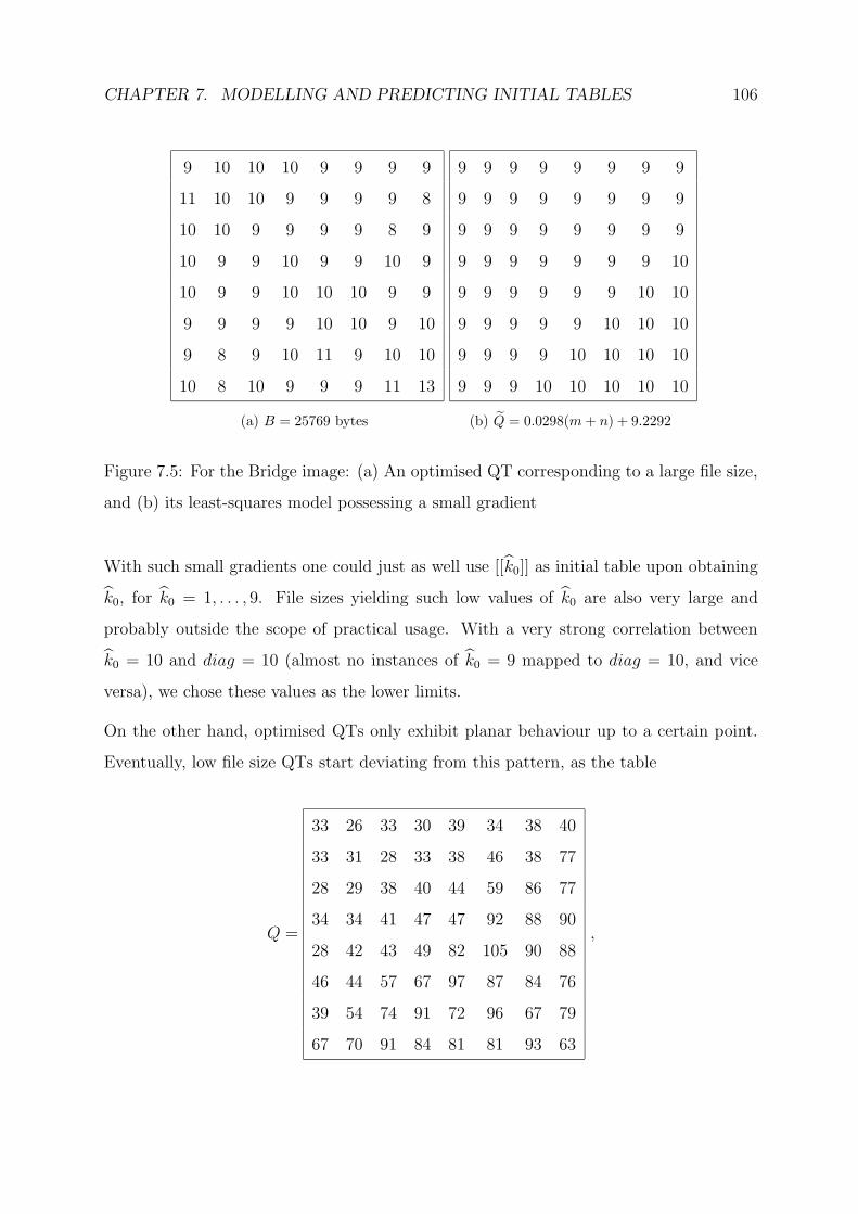
CHAPTER 7. MODELLING AND PREDICTING INITIAL TABLES 106
9 10 10 10 9 9 9 9
11 10 10 9 9 9 9 8
10 10 9 9 9 9 8 9
10 9 9 10 9 9 10 9
10 9 9 10 10 10 9 9
9 9 9 9 10 10 9 10
9 8 9 10 11 9 10 10
10 8 10 9 9 9 11 13
(a) B = 25769 bytes
9 9 9 9 9 9 9 9
9 9 9 9 9 9 9 9
9 9 9 9 9 9 9 9
9 9 9 9 9 9 9 10
9 9 9 9 9 9 10 10
9 9 9 9 9 10 10 10
9 9 9 9 10 10 10 10
9 9 9 10 10 10 10 10
(b) Q = 0.0298(m + n) + 9.2292
Figure 7.5: For the Bridge image: (a) An optimised QT corresponding to a large file size,
and (b) its least-squares model possessing a small gradient
With such small gradients one could just as well use [[k0]] as initial table upon obtaining
k0, for k0 = 1, . . . , 9. File sizes yielding such low values of k0 are also very large and
probably outside the scope of practical usage. With a very strong correlation between
k0 = 10 and diag = 10 (almost no instances of k0 = 9 mapped to diag = 10, and vice
versa), we chose these values as the lower limits.
On the other hand, optimised QTs only exhibit planar behaviour up to a certain point.
Eventually, low file size QTs start deviating from this pattern, as the table
Q =
33 26 33 30 39 34 38 40
33 31 28 33 38 46 38 77
28 29 38 40 44 59 86 77
34 34 41 47 47 92 88 90
28 42 43 49 82 105 90 88
46 44 57 67 97 87 84 76
39 54 74 91 72 96 67 79
67 70 91 84 81 81 93 63
,

CHAPTER 7. MODELLING AND PREDICTING INITIAL TABLES 107
also taken from the JPEG encodings of Bridge, suggests. This table gives a file size of
8442 bytes and has a least squares model with diag = 59. We can see that the largest
entries are no longer confined to only the highest frequencies — they now also show up in
positions slightly below the co-main diagonal. Applying the same models to such tables
would still give us larger and larger gradients, but the resulting approximations would no
longer be satisfactory. With this behaviour tending to occur in tables whose corresponding
models have values of diag larger than 55, we chose to only model up to this point. For
our JPEG models the largest value of k0 to map to diag = 55 was 47, hence the use of it
as a lower limit. Instances of k0 = 47 mapping to values of diag larger than 55 are not
listed in Table 7.1, since they are not applicable, which is why the last two entries in the
third column are empty. Also note that, since the file sizes yielding values of k0 larger
than 47 (and/or values of diag larger than 55) are quite small, they are again probably
outside the scope of practical usage.
As mentioned previously, the correlation between the co-main diagonal values diag and
gradients k1 was also analysed, enabling us to predict approximate gradients k1. For now
these analyses (for both JPEG and sine window MJPEG) are only based on the data
from the Lena image, but have yielded good results as will be seen in Section 7.4. The
findings for the JPEG case are summarised in Table 7.2, where the second column lists
the smallest and largest values k1 assumed for each of the relevant values of diag. The
approximate gradients k1 are then taken as the midpoints of the resulting intervals.
diag Range Approximate gradient k1
10 [0.2723, 0.3170] 0.2946
11 [0.2426, 0.3601] 0.3014
12 [0.2708, 0.3914] 0.3311
13 [0.4018, 0.4896] 0.4457
14 [0.3929, 0.4613] 0.4271
15 [0.2664, 0.4390] 0.3527
16 [0.2589, 0.3021] 0.2805
Table 7.2: The relationship between diag and k1 obtained from the JPEG encodings of
Lena (continued on next page)

CHAPTER 7. MODELLING AND PREDICTING INITIAL TABLES 108
diag Range Approximate gradient k1
17 [0.2813, 0.3780] 0.3297
18 [0.3497, 0.5119] 0.4308
19 [0.5045, 0.7798] 0.6422
20 [0.7545, 0.8259] 0.7902
21 [0.9420, 1.0104] 0.9762
22 [0.9405, 1.0253] 0.9829
23 [1.0298, 1.3170] 1.1734
24 [1.3542, 1.6235] 1.4889
25 [1.6280, 1.8304] 1.7292
26 [1.7932, 1.9152] 1.8542
27 [1.8438, 1.9420] 1.8929
28 [1.8973, 1.9702] 1.9337
29 [1.8884, 2.0551] 1.9718
30 [2.1652, 2.3110] 2.2381
31 [2.1935, 2.3095] 2.2515
32 [2.2693, 2.3542] 2.3118
33 [2.2753, 2.4182] 2.3468
34 [2.6027, 2.7530] 2.6779
35 [2.7098, 2.8750] 2.7924
36 [2.8051, 2.9107] 2.8579
37 [2.9211, 2.9479] 2.9345
38 [2.9137, 3.2262] 3.0700
39 [3.2262, 3.3348] 3.2805
40 [3.0208, 3.2083] 3.1145
41 [3.0744, 3.1458] 3.1101
42 [3.1563, 3.3571] 3.2567
43 [3.4107, 3.5149] 3.4628
Table 7.2: The relationship between diag and k1 obtained from the JPEG encodings of
Lena (continued on next page)
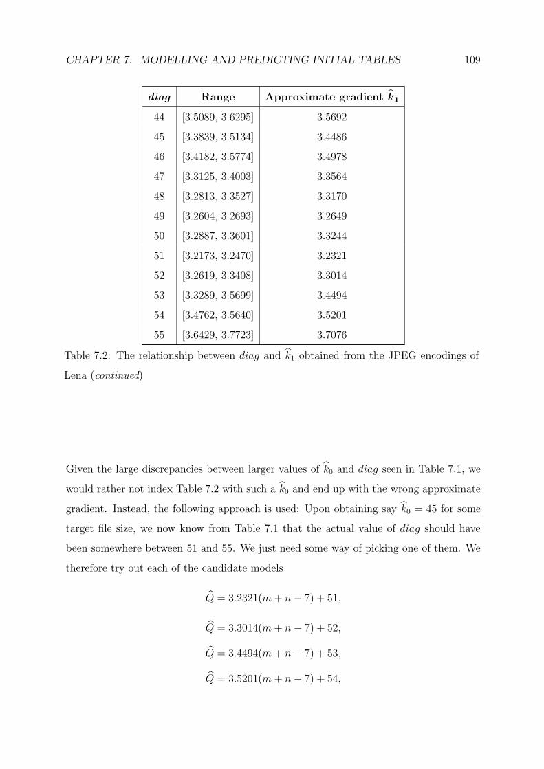
CHAPTER 7. MODELLING AND PREDICTING INITIAL TABLES 109
diag Range Approximate gradient k1
44 [3.5089, 3.6295] 3.5692
45 [3.3839, 3.5134] 3.4486
46 [3.4182, 3.5774] 3.4978
47 [3.3125, 3.4003] 3.3564
48 [3.2813, 3.3527] 3.3170
49 [3.2604, 3.2693] 3.2649
50 [3.2887, 3.3601] 3.3244
51 [3.2173, 3.2470] 3.2321
52 [3.2619, 3.3408] 3.3014
53 [3.3289, 3.5699] 3.4494
54 [3.4762, 3.5640] 3.5201
55 [3.6429, 3.7723] 3.7076
Table 7.2: The relationship between diag and k1 obtained from the JPEG encodings of
Lena (continued)
Given the large discrepancies between larger values of k0 and diag seen in Table 7.1, we
would rather not index Table 7.2 with such a k0 and end up with the wrong approximate
gradient. Instead, the following approach is used: Upon obtaining say k0 = 45 for some
target file size, we now know from Table 7.1 that the actual value of diag should have
been somewhere between 51 and 55. We just need some way of picking one of them. We
therefore try out each of the candidate models
Q = 3.2321(m+ n− 7) + 51,
Q = 3.3014(m+ n− 7) + 52,
Q = 3.4494(m+ n− 7) + 53,
Q = 3.5201(m+ n− 7) + 54,
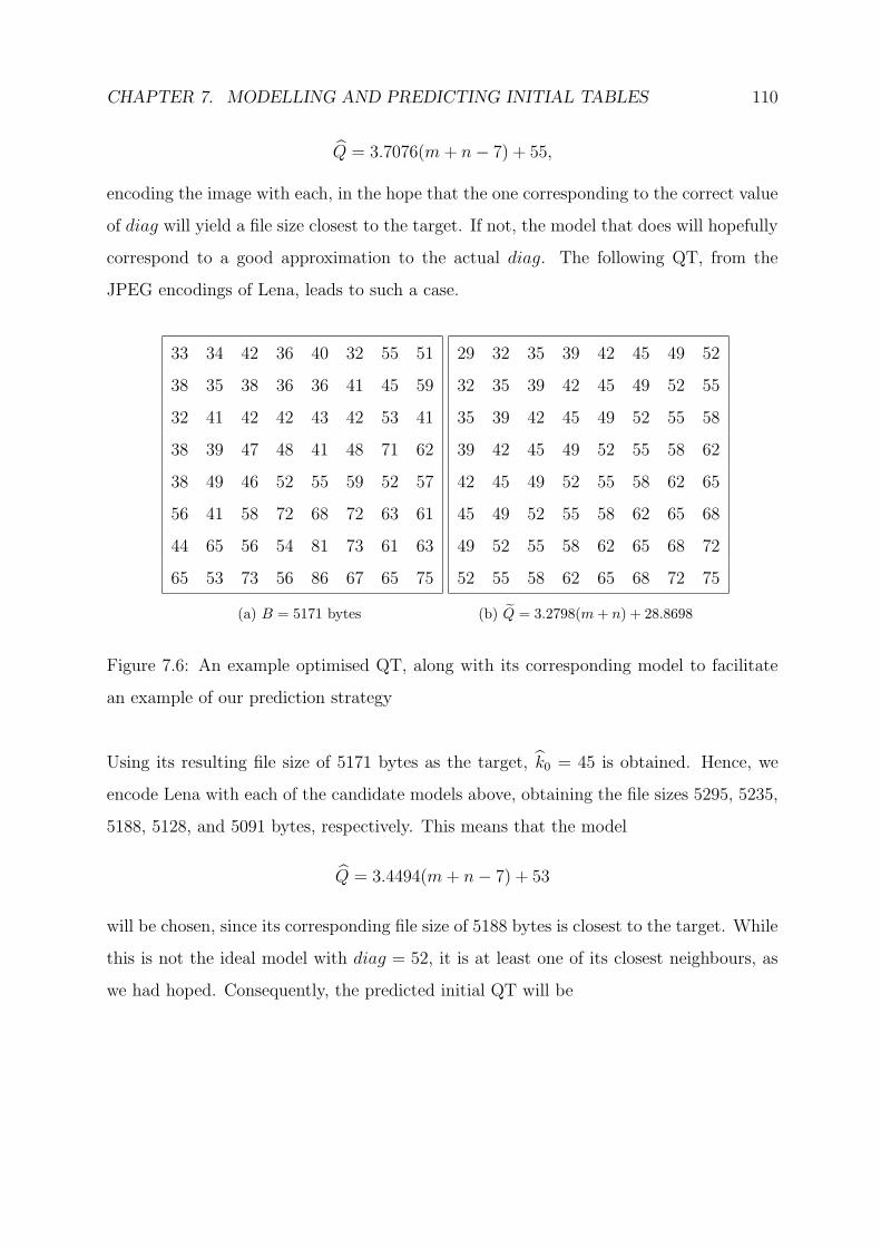
CHAPTER 7. MODELLING AND PREDICTING INITIAL TABLES 110
Q = 3.7076(m+ n− 7) + 55,
encoding the image with each, in the hope that the one corresponding to the correct value
of diag will yield a file size closest to the target. If not, the model that does will hopefully
correspond to a good approximation to the actual diag. The following QT, from the
JPEG encodings of Lena, leads to such a case.
33 34 42 36 40 32 55 51
38 35 38 36 36 41 45 59
32 41 42 42 43 42 53 41
38 39 47 48 41 48 71 62
38 49 46 52 55 59 52 57
56 41 58 72 68 72 63 61
44 65 56 54 81 73 61 63
65 53 73 56 86 67 65 75
(a) B = 5171 bytes
29 32 35 39 42 45 49 52
32 35 39 42 45 49 52 55
35 39 42 45 49 52 55 58
39 42 45 49 52 55 58 62
42 45 49 52 55 58 62 65
45 49 52 55 58 62 65 68
49 52 55 58 62 65 68 72
52 55 58 62 65 68 72 75
(b) Q = 3.2798(m + n) + 28.8698
Figure 7.6: An example optimised QT, along with its corresponding model to facilitate
an example of our prediction strategy
Using its resulting file size of 5171 bytes as the target, k0 = 45 is obtained. Hence, we
encode Lena with each of the candidate models above, obtaining the file sizes 5295, 5235,
5188, 5128, and 5091 bytes, respectively. This means that the model
Q = 3.4494(m+ n− 7) + 53
will be chosen, since its corresponding file size of 5188 bytes is closest to the target. While
this is not the ideal model with diag = 52, it is at least one of its closest neighbours, as
we had hoped. Consequently, the predicted initial QT will be

CHAPTER 7. MODELLING AND PREDICTING INITIAL TABLES 111
Q =
29 32 36 39 43 46 50 53
32 36 39 43 46 50 53 56
36 39 43 46 50 53 56 60
39 43 46 50 53 56 60 63
43 46 50 53 56 60 63 67
46 50 53 56 60 63 67 70
50 53 56 60 63 67 70 74
53 56 60 63 67 70 74 77
.
We use this approach for all values of k0 larger than 18. Instead of using (7.5) and (7.6),
the choice of model described above is made by evaluating
k1 = list of gradients(diag) (7.7)
and
Q(m,n) = k1(m+ n− 7) + diag, m = 0, . . . , 7, n = 0, . . . , 7, (7.8)
for the appropriate candidate values of diag. These candidates are listed in Table 7.3
(formed by condensing the data contained in Table 7.1) for each of the relevant values
of k0.

CHAPTER 7. MODELLING AND PREDICTING INITIAL TABLES 112
k0 diag
19 19, 20
20 20, 21
21 21, 22
22 22, 23, 24
23 23, 24, 25
24 24, 25, 26
25 25, 26, 27
26 26, 27, 28
27 28, 29, 30
28 29, 30, 31
29 30, 31, 32, 33
30 32, 33, 34, 35
31 34, 35, 36
32 35, 36, 37
33 36, 37, 38, 39
34 37, 38, 39, 40
35 38, 39, 40, 41, 42
36 40, 41, 42, 43
37 41, 42, 43, 44, 45
38 42, 43, 44, 45, 46
39 44, 45, 46, 47
40 45, 46, 47, 48, 49, 50
41 46, 47, 48, 49, 50
42 47, 48, 49, 50, 51, 52
43 49, 50, 51, 52, 53, 54
44 50, 51, 52, 53, 54, 55
45 51, 52, 53, 54, 55
46 52, 53, 54, 55
47 53, 54, 55
Table 7.3: Candidate values of diag for each k0 in the case of JPEG
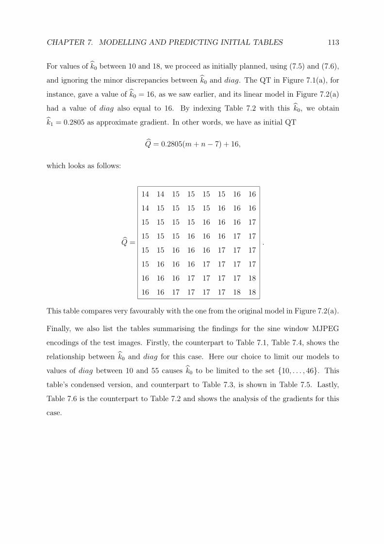
CHAPTER 7. MODELLING AND PREDICTING INITIAL TABLES 113
For values of k0 between 10 and 18, we proceed as initially planned, using (7.5) and (7.6),
and ignoring the minor discrepancies between k0 and diag. The QT in Figure 7.1(a), for
instance, gave a value of k0 = 16, as we saw earlier, and its linear model in Figure 7.2(a)
had a value of diag also equal to 16. By indexing Table 7.2 with this k0, we obtain
k1 = 0.2805 as approximate gradient. In other words, we have as initial QT
Q = 0.2805(m+ n− 7) + 16,
which looks as follows:
Q =
14 14 15 15 15 15 16 16
14 15 15 15 15 16 16 16
15 15 15 15 16 16 16 17
15 15 15 16 16 16 17 17
15 15 16 16 16 17 17 17
15 16 16 16 17 17 17 17
16 16 16 17 17 17 17 18
16 16 17 17 17 17 18 18
.
This table compares very favourably with the one from the original model in Figure 7.2(a).
Finally, we also list the tables summarising the findings for the sine window MJPEG
encodings of the test images. Firstly, the counterpart to Table 7.1, Table 7.4, shows the
relationship between k0 and diag for this case. Here our choice to limit our models to
values of diag between 10 and 55 causes k0 to be limited to the set {10, . . . , 46}. This
table’s condensed version, and counterpart to Table 7.3, is shown in Table 7.5. Lastly,
Table 7.6 is the counterpart to Table 7.2 and shows the analysis of the gradients for this
case.

CHAPTER 7. MODELLING AND PREDICTING INITIAL TABLES 114
k0 Lena Plane Bridge
10 10(44), 11(4) 10(50) 10(44)
11 11(43), 12(10) 10(2), 11(50) 10(5), 11(41)
12 12(32), 13(8) 12(44) 11(7), 12(47)
13 13(31), 14(11) 12(2), 13(41) 12(2), 13(44)
14 14(27), 15(16) 14(38) 13(4), 14(42)
15 15(24), 16(8) 14(3), 15(36) 14(3), 15(32)
16 16(22), 17(11) 15(7), 16(31) 15(3), 16(44)
17 17(18), 18(13) 16(4), 17(29) 16(2), 17(30), 18(1)
18 18(18), 19(13) 18(32) 18(29), 19(4)
19 19(6), 20(19) 18(2), 19(32) 19(26), 20(10)
20 20(7), 21(18) 20(33), 21(4) 20(19), 21(7)
21 21(5), 22(17) 21(20), 22(13) 21(26), 22(9)
22 22(3), 23(13), 24(14) 22(3), 23(20) 22(21), 23(13)
23 24(8), 25(9), 26(11) 24(24), 25(1) 23(15), 24(13)
24 26(4), 27(20) 25(18), 26(8) 24(12), 25(14)
25 27(5), 28(19) 26(15), 27(9) 25(7), 26(25)
26 29(20), 30(2) 27(13), 28(15) 26(3), 27(22)
27 30(19) 28(7), 29(15) 28(20), 29(5)
28 30(3), 31(10), 32(10) 29(5), 30(14) 29(18), 30(15)
29 32(3), 33(10) 30(1), 31(10), 32(6) 30(7), 31(19), 32(1)
30 33(11), 34(9) 33(11), 34(12), 35(4) 32(15), 33(4)
31 34(7), 35(8) 35(8), 36(12) 33(10), 34(18)
32 35(12), 36(3) 36(3), 37(13) 34(1), 35(18), 36(2)
33 36(6), 37(9), 38(5) 37(5), 38(5) 36(15)
34 38(12), 39(4) 38(4), 39(8) 36(2), 37(9), 38(6)
35 39(10), 40(8) 39(12), 40(9) 38(1), 39(17), 40(9)
36 40(7), 41(7), 42(6) 40(12), 41(9), 42(1) 40(12), 41(8)
Table 7.4: The relationship between k0 and diag for the MJPEG encodings of the three
images (continued on next page)

CHAPTER 7. MODELLING AND PREDICTING INITIAL TABLES 115
k0 Lena Plane Bridge
37 42(5), 43(6), 44(9) 42(11), 43(2) 41(6), 42(10), 43(6)
38 44(5), 45(6), 46(6) 43(8), 44(6) 43(2), 44(15), 45(3)
39 46(2), 47(7), 48(6) 44(4), 45(11), 46(6) 45(18)
40 49(11) 46(1), 47(9), 48(3) 46(10), 47(12)
41 49(4), 50(6) 48(12) 47(5), 48(9)
42 50(6), 51(5) 48(3), 49(12), 50(1) 48(7), 49(13)
43 51(5), 52(5) 50(16) 49(7), 50(8)
44 52(8) 51(8) 50(2), 51(5), 52(12)
45 52(2), 53(7) 52(10), 53(7) 52(2), 53(14)
46 53(3), 54(1), 55(4) 53(7), 54(2), 55(6) 54(7), 55(4)
Table 7.4: The relationship between k0 and diag for the MJPEG encodings of the three
images (continued)

CHAPTER 7. MODELLING AND PREDICTING INITIAL TABLES 116
k0 diag
17 17, 18
18 18, 19
19 19, 20
20 20, 21
21 21, 22
22 22, 23, 24
23 23, 24, 25, 26
24 24, 25, 26, 27
25 25, 26, 27, 28
26 26, 27, 28, 29, 30
27 28, 29, 30
28 29, 30, 31, 32
29 30, 31, 32, 33
30 32, 33, 34, 35
31 33, 34, 35, 36
32 34, 35, 36, 37
33 36, 37, 38
34 36, 37, 38, 39
35 38, 39, 40
36 40, 41, 42
37 41, 42, 43, 44
38 43, 44, 45, 46
39 44, 45, 46, 47, 48
40 46, 47, 48, 49
41 47, 48, 49, 50
42 48, 49, 50, 51
43 49, 50, 51, 52
44 50, 51, 52
45 52, 53
46 53, 54, 55
Table 7.5: Candidate values of diag for each k0 in the case of MJPEG
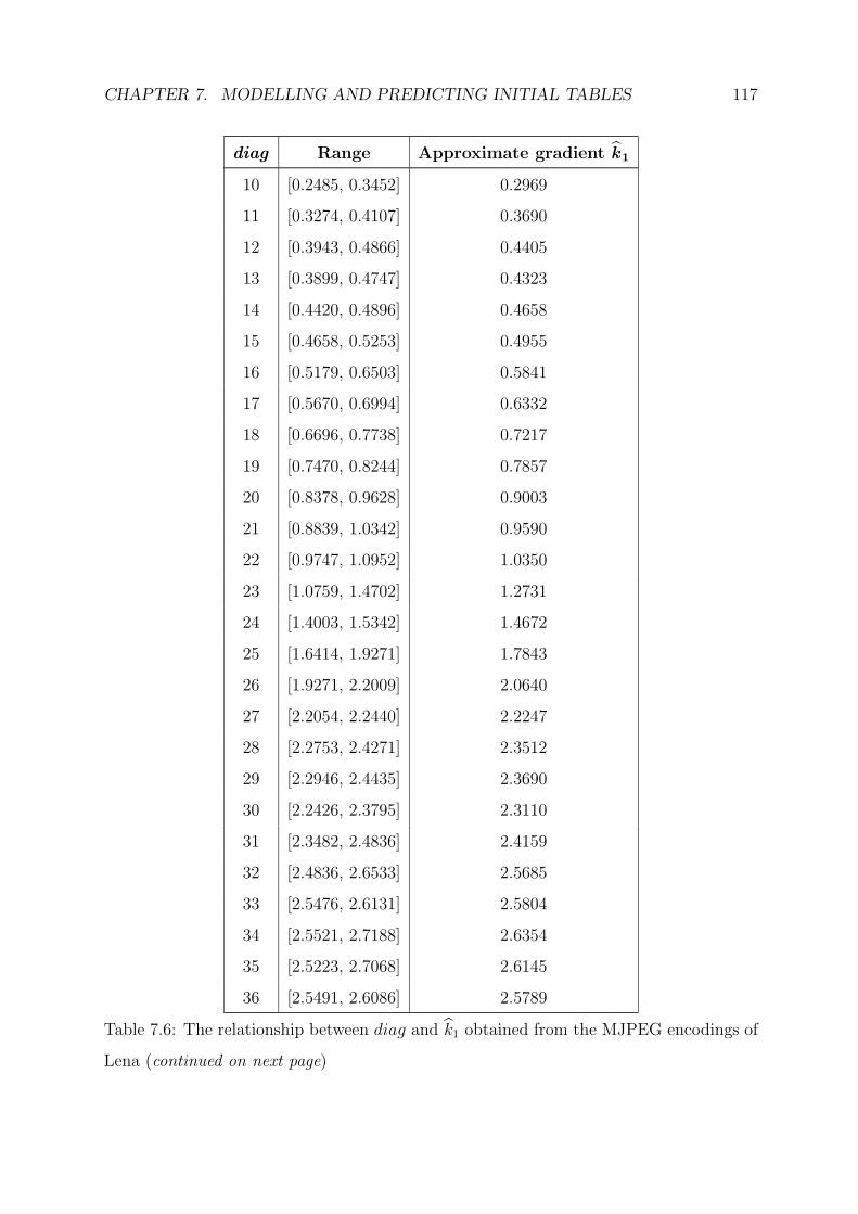
CHAPTER 7. MODELLING AND PREDICTING INITIAL TABLES 117
diag Range Approximate gradient k1
10 [0.2485, 0.3452] 0.2969
11 [0.3274, 0.4107] 0.3690
12 [0.3943, 0.4866] 0.4405
13 [0.3899, 0.4747] 0.4323
14 [0.4420, 0.4896] 0.4658
15 [0.4658, 0.5253] 0.4955
16 [0.5179, 0.6503] 0.5841
17 [0.5670, 0.6994] 0.6332
18 [0.6696, 0.7738] 0.7217
19 [0.7470, 0.8244] 0.7857
20 [0.8378, 0.9628] 0.9003
21 [0.8839, 1.0342] 0.9590
22 [0.9747, 1.0952] 1.0350
23 [1.0759, 1.4702] 1.2731
24 [1.4003, 1.5342] 1.4672
25 [1.6414, 1.9271] 1.7843
26 [1.9271, 2.2009] 2.0640
27 [2.2054, 2.2440] 2.2247
28 [2.2753, 2.4271] 2.3512
29 [2.2946, 2.4435] 2.3690
30 [2.2426, 2.3795] 2.3110
31 [2.3482, 2.4836] 2.4159
32 [2.4836, 2.6533] 2.5685
33 [2.5476, 2.6131] 2.5804
34 [2.5521, 2.7188] 2.6354
35 [2.5223, 2.7068] 2.6145
36 [2.5491, 2.6086] 2.5789
Table 7.6: The relationship between diag and k1 obtained from the MJPEG encodings of
Lena (continued on next page)
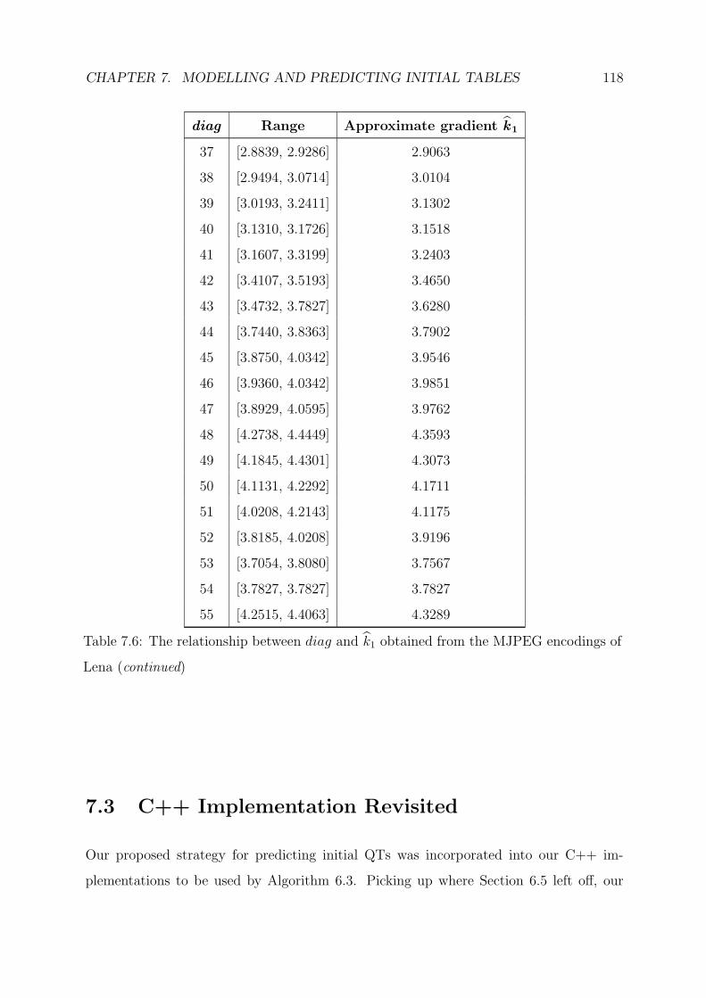
CHAPTER 7. MODELLING AND PREDICTING INITIAL TABLES 118
diag Range Approximate gradient k1
37 [2.8839, 2.9286] 2.9063
38 [2.9494, 3.0714] 3.0104
39 [3.0193, 3.2411] 3.1302
40 [3.1310, 3.1726] 3.1518
41 [3.1607, 3.3199] 3.2403
42 [3.4107, 3.5193] 3.4650
43 [3.4732, 3.7827] 3.6280
44 [3.7440, 3.8363] 3.7902
45 [3.8750, 4.0342] 3.9546
46 [3.9360, 4.0342] 3.9851
47 [3.8929, 4.0595] 3.9762
48 [4.2738, 4.4449] 4.3593
49 [4.1845, 4.4301] 4.3073
50 [4.1131, 4.2292] 4.1711
51 [4.0208, 4.2143] 4.1175
52 [3.8185, 4.0208] 3.9196
53 [3.7054, 3.8080] 3.7567
54 [3.7827, 3.7827] 3.7827
55 [4.2515, 4.4063] 4.3289
Table 7.6: The relationship between diag and k1 obtained from the MJPEG encodings of
Lena (continued)
7.3 C++ Implementation Revisited
Our proposed strategy for predicting initial QTs was incorporated into our C++ im-
plementations to be used by Algorithm 6.3. Picking up where Section 6.5 left off, our

CHAPTER 7. MODELLING AND PREDICTING INITIAL TABLES 119
description is with respect to the program qt m.cc.
First of all, the value k0, represented by the variable kk0, is obtained by evaluating the
file sizes resulting from using tables [[1]], [[2]], . . . , [[255]]. This search is implemented by
using a golden ratio search, and is performed by the function gr. Given that values of k0
are here limited to the set {10, . . . , 46} (as described in the previous section), the program
will exit if kk0 is outside this set.
Next, if kk0 is between 10 and 16, it is directly used to index the list of gradients shown
in Table 7.6. This list is stored in the array gradient, and the obtained approximate
gradient k1 is represented by the variable kk1.
If, on the other hand, kk0 is larger than 17, the function get gradient is called. This
function evaluates candidate models for relevant values of diag and k1, using the approach
described by (7.7) and (7.8). The candidate values of diag listed in Table 7.5 are implicitly
stored in the matrix k2diag by storing the first value of diag corresponding to each k0 in
the matrix’s first row, and the number of candidate values for each k0 in the second row.
Furthermore, to construct each candidate model, the function plane Q is used. The diag
and gradient values eventually decided upon are then stored in kk0 and kk1, respectively.
Lastly, having obtained kk0 and kk1 by either of these two methods, the initial QT is
calculated from them by calling function plane Q.
Notice that, apart from the candidate values of diag listed in Table 7.5, we have also
included additional candidates to consider in k2diag. This ensures that the number of
modifications required to make the initial QT feasible is small. For example, a value
of k0 = 45 will be obtained when inputting the Bridge image’s frequency components
(obtained by using the sine window) to qt m, along with a target file size of 9000 bytes.
Given the choices of diag in Table 7.5 (52 and 53), the values diag = 52 and k1 = 3.9196
will be chosen, resulting in the initial QT

CHAPTER 7. MODELLING AND PREDICTING INITIAL TABLES 120
Q =
25 28 32 36 40 44 48 52
28 32 36 40 44 48 52 56
32 36 40 44 48 52 56 60
36 40 44 48 52 56 60 64
40 44 48 52 56 60 64 68
44 48 52 56 60 64 68 72
48 52 56 60 64 68 72 76
52 56 60 64 68 72 76 79
.
This table yields an encoding with file size B = 8552 bytes and would require many
modifications to become feasible. In order to not destroy the characteristics of the model,
one might subtract a value of 1 from each entry of Q until a file size close enough to
9000 bytes is reached. But then we could just as well have tested the model corresponding
to a slightly lower value of diag instead. The value diag = 50, with corresponding gradient
k1 = 4.1711, for instance, yields the initial QT
Q =
21 25 29 33 37 42 46 50
25 29 33 37 42 46 50 54
29 33 37 42 46 50 54 58
33 37 42 46 50 54 58 63
37 42 46 50 54 58 63 67
42 46 50 54 58 63 67 71
46 50 54 58 63 67 71 75
50 54 58 63 67 71 75 79
,
which results in a much closer coding file size of B = 9004 bytes. For this reason a few
extra candidate values of diag are included in k2diag for each k0.
Of course, these initial QTs do not actually need to be feasible when directly starting
Algorithm 6.3 with one of them (as opposed to first running a genetic algorithm), but we
nevertheless enforce it for two reasons. Firstly, since an initial QT must be feasible when
constructing an initial population for a GA, it makes sense to use the same feasible initial
QT when directly starting Algorithm 6.3, so as to properly compare the running times of

CHAPTER 7. MODELLING AND PREDICTING INITIAL TABLES 121
each approach. Secondly, enforcing feasibility allows us to compare the PSNR obtained
using a feasible initial QT with the PSNR obtained using an optimised QT. This gives us
an additional useful measure of how “close” an initial QT is to an optimal one, and we
utilise it in the next section when testing our models.
7.4 Testing the Models
To investigate how well our models reduce the work needed to be done by Algorithm 6.3,
we tested their MJPEG implementation on the three images Lena, Plane and Bridge. In
particular, these tests were performed for the case of using the sine window. By varying
the target file size, we started Algorithm 6.3 with each obtainable initial QT, running it
for various probing widths in each case. By doing so, we found the smallest values of lo
and hi required to reach the appropriate optimised QTs for each value of diag.
Consider, for example, the data shown in Table 7.7, which is an excerpt from Table C.2
in Appendix C. Here we have the results corresponding to diag = 23 for the Plane image.
diag Widths Widths Widths lo = 1, hi = 1 Initial QT
T (bytes) B (bytes) B (bytes) B (bytes) B (bytes) B (bytes)
PSNR PSNR PSNR PSNR PSNR
23 lo = 4, hi = 10 lo = 3, hi = 10 lo = 4, hi = 5
10346 10343 10346 10346 10347 10350
34.9386 dB 34.9291 dB 34.9325 dB 34.8856 dB 34.7462 dB
Table 7.7: Excerpt from Table C.2, illustrating a sensitivity analysis for the Plane image
when diag = 23
In the first column we list the target file size T used to generate the results, in this case
10346 bytes. For each case we generated a QT using large but equal probing widths
(such as lo = hi = 50) and then decreased them in steps of 5, each time repeating the
experiment. We thereby determined the smallest (multiple of 5) uniform probing width
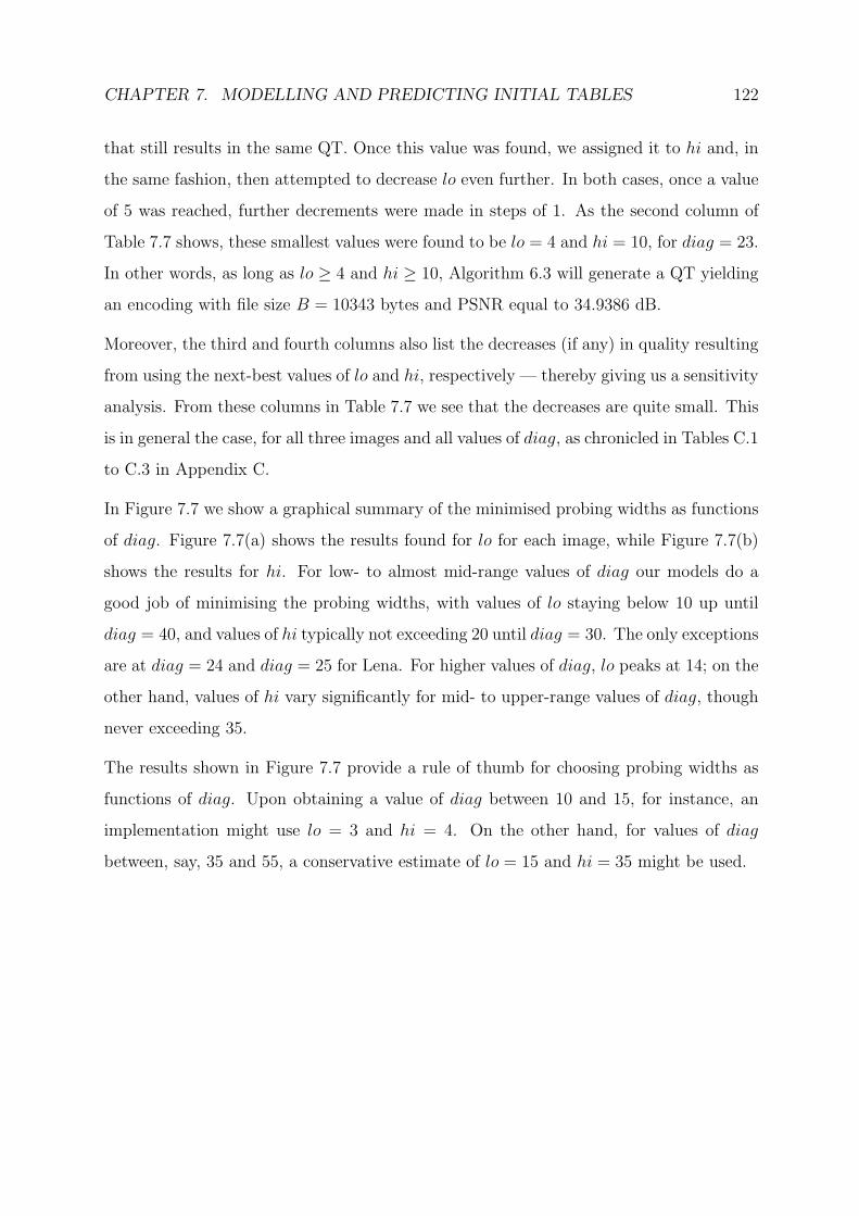
CHAPTER 7. MODELLING AND PREDICTING INITIAL TABLES 122
that still results in the same QT. Once this value was found, we assigned it to hi and, in
the same fashion, then attempted to decrease lo even further. In both cases, once a value
of 5 was reached, further decrements were made in steps of 1. As the second column of
Table 7.7 shows, these smallest values were found to be lo = 4 and hi = 10, for diag = 23.
In other words, as long as lo ≥ 4 and hi ≥ 10, Algorithm 6.3 will generate a QT yielding
an encoding with file size B = 10343 bytes and PSNR equal to 34.9386 dB.
Moreover, the third and fourth columns also list the decreases (if any) in quality resulting
from using the next-best values of lo and hi, respectively — thereby giving us a sensitivity
analysis. From these columns in Table 7.7 we see that the decreases are quite small. This
is in general the case, for all three images and all values of diag, as chronicled in Tables C.1
to C.3 in Appendix C.
In Figure 7.7 we show a graphical summary of the minimised probing widths as functions
of diag. Figure 7.7(a) shows the results found for lo for each image, while Figure 7.7(b)
shows the results for hi. For low- to almost mid-range values of diag our models do a
good job of minimising the probing widths, with values of lo staying below 10 up until
diag = 40, and values of hi typically not exceeding 20 until diag = 30. The only exceptions
are at diag = 24 and diag = 25 for Lena. For higher values of diag, lo peaks at 14; on the
other hand, values of hi vary significantly for mid- to upper-range values of diag, though
never exceeding 35.
The results shown in Figure 7.7 provide a rule of thumb for choosing probing widths as
functions of diag. Upon obtaining a value of diag between 10 and 15, for instance, an
implementation might use lo = 3 and hi = 4. On the other hand, for values of diag
between, say, 35 and 55, a conservative estimate of lo = 15 and hi = 35 might be used.

CHAPTER 7. MODELLING AND PREDICTING INITIAL TABLES 123
10 15 20 25 30 35 40 45 50 550
5
10
15
PSfrag replacements
diag
LenaPlaneBridge
pro
bin
gw
idth
lo
(a) Behaviour of probing width lo
10 15 20 25 30 35 40 45 50 550
5
10
15
20
25
30
35
PSfrag replacements
diag
LenaPlaneBridge
pro
bin
gw
idth
hi
(b) Behaviour of probing width hi
Figure 7.7: Minimised probing widths as functions of diag

CHAPTER 7. MODELLING AND PREDICTING INITIAL TABLES 124
It is also interesting to investigate the results obtained by letting Algorithm 6.3 do the
least amount of work per iteration, i.e. choosing lo = hi = 1. Such a result can be seen
in the fifth column of Table 7.7. We observe that this “short-cut” approach increases the
PSNR from 34.7462 dB (obtained with the feasible initial QT) to 34.8856 dB, more than
half the total increase from 34.7462 dB to the optimal 34.9386 dB. The magnitudes of
increases in PSNR made this way do of course taper off slightly as the required optimal
probing widths increase, but never to the point of insignificance. Once again, these results
are fully documented in Tables C.1 to C.3.
The progression of PSNR values for various probing widths and fixed values of diag can
also be plotted from the rows of the tables in Appendix C, providing us with a graphical
depiction of our sensitivity analysis. Such curves are shown in Figure 7.8 for selected
values of diag in the case of Lena. Data points are calculated by using the best PSNR
corresponding to each value of hi and subtracting the PSNR corresponding to the initial
QT from each. For diag = 12, for instance, shown in Figure 7.8(a), we obtain the first
data point by subtracting 39.2889 dB from 39.4128 dB, giving us the increase in PSNR
resulting from using lo = hi = 1, or equivalently, a uniform probing width of w = 1. The
second data point represents the increase in PSNR obtained by using lo = 2 and hi = 3,
or w = 3, etc. From these curves in Figure 7.8 we see that small increases in PSNR
are generally made from one probing width to the next. Conversely, this means that the
PSNR degrades gracefully as probing widths are reduced beyond their minimal values.

CHAPTER 7. MODELLING AND PREDICTING INITIAL TABLES 125
1 1.5 2 2.5 3 3.5 4 4.5 50.06
0.07
0.08
0.09
0.1
0.11
0.12
0.13
0.14di
ffere
nce
in P
SN
R (d
B)
PSfrag replacements
w
diag = 10diag = 12diag = 15diag = 19
(a) Results for lower-range values of diag
0 5 10 15 20 25 300.1
0.12
0.14
0.16
0.18
0.2
0.22
0.24
diffe
renc
e in
PS
NR
(dB
)
PSfrag replacements
w
diag = 21diag = 22diag = 25diag = 29
(b) Results for mid-range values of diag
Figure 7.8: Sensitivities of PSNR to various probing widths for the Lena image (continued
on next page)

CHAPTER 7. MODELLING AND PREDICTING INITIAL TABLES 126
0 5 10 15 20 25 30 350.05
0.1
0.15
0.2
0.25
0.3di
ffere
nce
in P
SN
R (d
B)
PSfrag replacements
w
diag = 35diag = 39diag = 44diag = 52
(c) Results for upper-range values of diag
Figure 7.8: Sensitivities of PSNR to various probing widths for the Lena image (continued)
Apart from aiding in our sensitivity analysis, the results yielded by the initial QTs shown
in the last column of Tables C.1 to C.3 also serve another purpose. By comparing them
with the results yielded by optimal QTs (shown in the second column), we can gauge
how “close” our initial QTs are to the optimal ones. Figure 7.9 below shows the results
of this analysis, where the differences in obtained PSNR are plotted as a function of diag
for each of the three images. Notice that these differences are generally quite small and
only exceed 0.3 dB in the three instances diag = 26, diag = 27 and diag = 29, for the
Plane image.
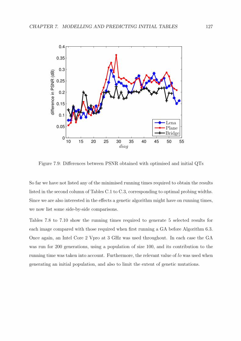
CHAPTER 7. MODELLING AND PREDICTING INITIAL TABLES 127
10 15 20 25 30 35 40 45 50 550
0.05
0.1
0.15
0.2
0.25
0.3
0.35
0.4di
ffere
nce
in P
SN
R (d
B)
PSfrag replacements
diag
LenaPlaneBridge
Figure 7.9: Differences between PSNR obtained with optimised and initial QTs
So far we have not listed any of the minimised running times required to obtain the results
listed in the second column of Tables C.1 to C.3, corresponding to optimal probing widths.
Since we are also interested in the effects a genetic algorithm might have on running times,
we now list some side-by-side comparisons.
Tables 7.8 to 7.10 show the running times required to generate 5 selected results for
each image compared with those required when first running a GA before Algorithm 6.3.
Once again, an Intel Core 2 Vpro at 3 GHz was used throughout. In each case the GA
was run for 200 generations, using a population of size 100, and its contribution to the
running time was taken into account. Furthermore, the relevant value of lo was used when
generating an initial population, and also to limit the extent of genetic mutations.
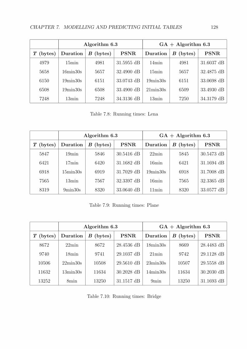
CHAPTER 7. MODELLING AND PREDICTING INITIAL TABLES 128
Algorithm 6.3 GA + Algorithm 6.3
T (bytes) Duration B (bytes) PSNR Duration B (bytes) PSNR
4979 15min 4981 31.5955 dB 14min 4981 31.6037 dB
5658 16min30s 5657 32.4900 dB 15min 5657 32.4875 dB
6150 19min30s 6151 33.0743 dB 19min30s 6151 33.0698 dB
6508 19min30s 6508 33.4900 dB 21min30s 6509 33.4930 dB
7248 13min 7248 34.3136 dB 13min 7250 34.3179 dB
Table 7.8: Running times: Lena
Algorithm 6.3 GA + Algorithm 6.3
T (bytes) Duration B (bytes) PSNR Duration B (bytes) PSNR
5847 19min 5846 30.5416 dB 22min 5845 30.5473 dB
6421 17min 6420 31.1682 dB 16min 6421 31.1694 dB
6918 15min30s 6919 31.7029 dB 19min30s 6918 31.7008 dB
7565 13min 7567 32.3397 dB 16min 7565 32.3365 dB
8319 9min30s 8320 33.0640 dB 11min 8320 33.0577 dB
Table 7.9: Running times: Plane
Algorithm 6.3 GA + Algorithm 6.3
T (bytes) Duration B (bytes) PSNR Duration B (bytes) PSNR
8672 22min 8672 28.4536 dB 18min30s 8669 28.4483 dB
9740 18min 9741 29.1037 dB 21min 9742 29.1128 dB
10506 22min30s 10508 29.5610 dB 23min30s 10507 29.5558 dB
11632 13min30s 11634 30.2028 dB 14min30s 11634 30.2030 dB
13252 8min 13250 31.1517 dB 9min 13250 31.1693 dB
Table 7.10: Running times: Bridge

CHAPTER 7. MODELLING AND PREDICTING INITIAL TABLES 129
From the first row of Table 7.8, for example, we see that the result listed in Table C.1
for diag = 54, using lo = 9 and hi = 35, required roughly 15min to be obtained. By
comparison, roughly 14min were required to obtain an optimised QT when using a GA
prior to Algorithm 6.3, while still using the same probing widths. Since the two approaches
yield two different optimised QTs, the resulting file size and PSNR for each approach are
also listed.
In most cases, unfortunately, the reduction made to the running time of Algorithm 6.3
is outweighed by the running time of the GA, meaning that their combined running
time is longer than that of Algorithm 6.3 by itself. Reducing the number of generations
would reduce the running time of the GA, but could also diminish the quality of the
final population’s fittest member. Conversely, increasing the number of generations could
further reduce the running time of Algorithm 6.3, but would also increase the running
time of the GA. The same is true of a reduction/increase in population size.
Further research would be required to determine the population size and number of gen-
erations that would optimise these trade-offs, and thus the total running time. As such,
the results in the second column of Tables 7.8 to 7.10 are preliminary, although they do
show promise. We discuss this further in Section 8.4, when outlining future research.
Chapter 8
Experimental Results
Now that we have a means to generate good initial tables for Algorithm 6.3, we proceed
to investigate the merits of MJPEG relative to JPEG when using optimised QTs. There
are many window functions to choose from when using the MDCT — the existence of one
yielding results superior to those yielded by all others would be extremely advantageous.
Without it, the user would need to select one by trial-and-error each time an image is to
be compressed. For this reason, we also investigate the effects of several window functions
on the coding results. Notice that, in order to satisfy the perfect reconstruction require-
ment (3.11), all windows (except for the sine window) are subjected to the normalisation
procedure shown in (3.12).
8.1 Window Functions
In addition to the window functions described in Section 3.2, several others exist that are
included in Matlab’s signal processing toolbox. Of these, some are unfortunately defined
to have the value of zero as their first and last entries — an undesirable attribute in the
context of our application, since the first and last samples of transform blocks will play
no role in the MDCT. Consequently, those windows will not yield competitive results,
and have been excluded here. The seven remaining window functions are the Gaussian,
Chebyshev, Triangular, Parzen, Nuttall, Hamming and Blackman-Harris windows; their
130

CHAPTER 8. EXPERIMENTAL RESULTS 131
definitions can be found in their respective built-in Matlab implementations.
Table 8.1 shows a typical set of results obtained when comparing MJPEG using the above
window functions to JPEG. These results were generated for the 256× 256 Bridge image,
using a target file size of T = 22739 bytes. Like the Kaiser-Bessel Derived (KBD) window,
the Gaussian and Chebyshev windows have a parameter determining their shape. In the
definitions provided in the Matlab documentation, the Gaussian window’s parameter is
denoted by a, while that of the Chebyshev window is denoted by r. The optimal value of
each parameter must be found heuristically, involving the repeated use of Algorithm 6.3.
For the particular case shown here, they were found to be roughly α = 1.625, a = 2.9375
and r = 75.
Technique B (bytes) PSNR
Optimised JPEG 22741 37.3789 dB
Sine 22746 37.4207 dB
Hanning 22739 37.4255 dB
KBD (α = 1.625) 22741 37.4236 dB
Gaussian (a = 2.9375) 22738 37.3813 dB
Chebyshev (r = 75) 22739 37.4017 dB
Triangular 22739 37.1221 dB
Parzen 22740 37.2919 dB
Nuttall 22738 37.1943 dB
Hamming 22737 37.2946 dB
Blackman-Harris 22745 37.1886 dB
Table 8.1: Example comparison of coding results yielded by several window functions
with that of JPEG
What is typical about these results is the fact that the seven additional window functions
yield results inferior to those yielded by the three window functions described in Sec-
tion 3.2. Therefore, the comparison of results in the next section does not include these
seven window functions.

CHAPTER 8. EXPERIMENTAL RESULTS 132
As will be seen in the next section, the sine window often outperforms the Hanning and
KBD windows, but unfortunately, as Table 8.1 shows, not always. A question that arises
is whether or not an optimal window function can be designed. Moreover, even if the sine
window consistently outperformed the others, we would still want to know whether or not
an even better one could be designed. This is once again an optimisation problem, only
this time not a discrete one, as described below.
We ideally seek a window function w = [w1, . . . , w16] that maximises the PSNR of all
MJPEG encodings, but to practically solve the problem we can only optimise w for one
encoding at a time. Since MJPEG uses symmetric windows, we can write w as
w = [w1, . . . , w8, w8, . . . , w1], (8.1)
thereby halving the number of independent variables. Furthermore, due to the perfect
reconstruction requirement (3.11), entries w5 to w8 must satisfy
w5 =√
1− w24
w6 =√
1− w23
w7 =√
1− w22
w8 =√
1− w21 . (8.2)
Therefore, only the variables w1 to w4 are independent. Let them be denoted by
x = [w1, w2, w3, w4]. (8.3)
We also require the sequence w1, . . . , w8 to be monotonically increasing — from (8.2) we
conclude that the values of w1 to w4 should not exceed 1√2.
As a result, the optimisation problem reads as follows:
Given a window function specified by x in (8.3), an image’s frequency com-
ponents obtained by using x, and a target file size, maximise the PSNR
= PSNR(x) of the encoding obtained with Algorithm 6.3, subject to
w1 ≤ w2 ≤ w3 ≤ w4
w1, . . . , w4 ∈ [0, 1√2].

CHAPTER 8. EXPERIMENTAL RESULTS 133
With w1 to w4 varying continuously and the PSNR not being differentiable (due to the
rounding involved in quantisation), we attempt to solve this problem using the Nelder-
Mead algorithm. Since the PSNR is also discontinuous as a result of rounding, this
algorithm will eventually break down. Nevertheless, any improvement over results yielded
by the other window functions will do.
The Nelder-Mead algorithm, described in [28], maintains a list of approximate solutions
x1, . . . ,xN+1, whereN is the number of independent variables in the optimisation problem.
These vectors are sorted according to their associated function values, from best to worst.
In our case this sorting will be
PSNR(x1) ≥ PSNR(x2) ≥ PSNR(x3) ≥ PSNR(x4) ≥ PSNR(x5). (8.4)
During each iteration the algorithm will attempt to replace the worst vector xN+1 with
a better one according to formulas and conditions described in [28]. If successful, the
new list of vectors is again sorted, and we proceed to the next iteration. Otherwise, the
convergence breaks down and the algorithm terminates.
For our problem, we used the 256 × 256 Lena image and a target file size of T =
14839 bytes. The initial vectors x1 to x5 were chosen on the boundary of the feasi-
ble region as
x1 = [0, 0, 1√2, 1√
2]
x2 = [0, 0, 0, 1√2]
x3 = [0, 1√2, 1√
2, 1√
2]
x4 = [ 1√2, 1√
2, 1√
2, 1√
2]
x5 = [0, 0, 0, 0].
Here we have numbered the vectors to satisfy (8.4); their respective function values are
PSNR(x1) = 34.6499dB
PSNR(x2) = 34.1350dB
PSNR(x3) = 33.5805dB
PSNR(x4) = 31.9478dB

CHAPTER 8. EXPERIMENTAL RESULTS 134
PSNR(x5) = 31.4014dB.
After several iterations the algorithm eventually broke down. The best vector in the final
list was
x1 = [0.09499651018430, 0.27268735998118, 0.45773112675032, 0.63149105950318]
with PSNR(x1) = 40.2651 dB. Let us refer to the window function constructed from x1,
using (8.1) and (8.2), as the Nelder-Mead1 window.
This window does indeed yield improved results over the sine window for this image and
target file size: While the sine window yields an encoding with a file size of 14840 bytes
and a PSNR of 40.2454 dB, the Nelder-Mead1 window yields an encoding with a file size of
14841 bytes and a PSNR of 40.2651 dB. Moreover, this window consistently outperforms
the sine window for the Lena image, as will be seen in the next section. However, the
Nelder-Mead1 window performs worse than the sine window for the 256× 256 Plane and
512× 512 Peppers (also shown in Appendix A) images, as will also be seen. This means
that the Nelder-Mead1 window is not the best for all images, and that such a best window
does not exist.
To see what an optimised window function for the Plane image (for a particular file size)
would be, we repeated the Nelder-Mead algorithm for this image. The target file size used
was T = 15904 bytes, and the initial vectors x1 to x5 were chosen to be the same as in
the previous experiment. This time the best vector in the final list was
x1 = [0.09917235114230, 0.28849462155593, 0.47112393494117, 0.63470224125757]
with PSNR(x1) = 39.2748 dB. We refer to the window function constructed from this
x1 as the Nelder-Mead2 window. Once again, it improves upon the sine window for the
image and target file size in question. The sine window yields an encoding with a file
size of 15901 bytes and a PSNR of 39.2636 dB, while the Nelder-Mead2 window yields an
encoding with a file size of 15905 bytes and a PSNR of 39.2748 dB.
In the next section we provide a detailed comparison of results obtained using the sine,
Hanning and KBD windows, as well as the Nelder-Mead1 and Nelder-Mead2 windows.
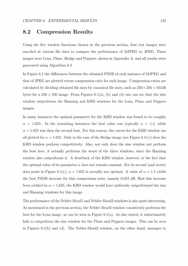
CHAPTER 8. EXPERIMENTAL RESULTS 135
8.2 Compression Results
Using the five window functions chosen in the previous section, four test images were
encoded at various file sizes to compare the performance of MJPEG to JPEG. These
images were Lena, Plane, Bridge and Peppers, shown in Appendix A, and all results were
generated using Algorithm 6.3.
In Figure 8.1 the differences between the obtained PSNR of each instance of MJPEG and
that of JPEG are plotted versus compression ratio for each image. Compression ratios are
calculated by dividing obtained file sizes by canonical file sizes, such as 256×256 = 65536
bytes for a 256 × 256 image. From Figures 8.1(a), (b) and (d) one can see that the sine
window outperforms the Hanning and KBD windows for the Lena, Plane and Peppers
images.
In many instances the optimal parameter for the KBD window was found to be roughly
α = 1.625. In the remaining instances the best value was typically α = 1.5, while
α = 1.625 was then the second best. For this reason, the curves for the KBD window are
all plotted for α = 1.625. Only in the case of the Bridge image (see Figure 8.1(c)) does the
KBD window perform competitively. Also, not only does the sine window not perform
the best here, it actually performs the worst of the three windows, since the Hanning
window also outperforms it. A drawback of the KBD window, however, is the fact that
the optimal value of its parameter α does not remain constant. For its second (and worst)
data point in Figure 8.1(c), α = 1.625 is actually not optimal. A value of α = 1.5 yields
the best PSNR increase for this compression ratio, namely 0.053 dB. Had this increase
been yielded by α = 1.625, the KBD window would have uniformly outperformed the sine
and Hanning windows for this image.
The performance of the Nelder-Mead1 and Nelder-Mead2 windows is also quite interesting.
As mentioned in the previous section, the Nelder-Mead1 window consistently performs the
best for the Lena image, as can be seen in Figure 8.1(a). As also stated, it unfortunately
fails to outperform the sine window for the Plane and Peppers images. This can be seen
in Figures 8.1(b) and (d). The Nelder-Mead2 window, on the other hand, manages to

CHAPTER 8. EXPERIMENTAL RESULTS 136
equal or slightly better the performance of the sine window on most occasions for these
two images. Furthermore, it compares quite well with the Nelder-Mead1 window in the
case of the Lena image, even overtaking it for higher compression ratios. Only in the case
of the Bridge image is the Nelder-Mead1 window the best choice. Here it is only beaten
by the KBD window at the third data point.
Another aspect of note is the fact that optimised MJPEG does not always outperform
optimised JPEG. This can first of all be seen in Figure 8.1(d) for the Peppers image, where
only the results obtained with the sine and Nelder-Mead2 windows are superior to JPEG.
These improvements are also quite small initially. Even worse, from Figure 8.1(b) we see
that the best MJPEG results for the Plane image take a long time to catch up to JPEG.
In Figures 8.2 and 8.3 one can see these results only catching up for high compression
ratios.

CHAPTER 8. EXPERIMENTAL RESULTS 137
4 5 6 7 8 9 100
0.05
0.1
0.15
0.2
0.25
0.3
0.35
compression ratio
diffe
renc
e in
PS
NR
(dB
)
PSfrag replacements
SineHanning
Nelder-Mead1Nelder-Mead2
KBD (α = 1.625)
(a) Window performance: Lena
4 5 6 7 8 9−0.9
−0.8
−0.7
−0.6
−0.5
−0.4
−0.3
−0.2
−0.1
compression ratio
diffe
renc
e in
PS
NR
(dB
)
PSfrag replacements
SineHanning
Nelder-Mead1Nelder-Mead2
KBD (α = 1.625)
(b) Window performance: Plane
Figure 8.1: Comparison of window function performance for each test image (continued
on next page)

CHAPTER 8. EXPERIMENTAL RESULTS 138
2.8 3 3.2 3.4 3.6 3.8 4 4.2 4.4
0.03
0.04
0.05
0.06
0.07
0.08
0.09
compression ratio
diffe
renc
e in
PS
NR
(dB
)
PSfrag replacements
SineHanning
Nelder-Mead1Nelder-Mead2
KBD (α = 1.625)
(c) Window performance: Bridge
4 5 6 7 8 9 10 11 12−0.25
−0.2
−0.15
−0.1
−0.05
0
0.05
0.1
0.15
compression ratio
diffe
renc
e in
PS
NR
(dB
)
PSfrag replacements
SineHanning
Nelder-Mead1Nelder-Mead2
KBD (α = 1.625)
(d) Window performance: Peppers
Figure 8.1: Comparison of window function performance for each test image (continued)

CHAPTER 8. EXPERIMENTAL RESULTS 139
The best results obtained for optimised MJPEG are also plotted in Figure 8.2, along with
the results obtained for optimised and standard JPEG, for each of the four test images.
The MJPEG results shown for the Lena, Plane and Peppers images correspond to those
shown for the Nelder-Mead2 window in Figure 8.1 for each respective image. Those shown
for the Bridge image, on the other hand, correspond to the results shown for the Nelder-
Mead1 window in Figure 8.1(c). Having selected the best window function for each image,
the additional data points in Figure 8.2’s curves were generated to also investigate the
performance of these windows for higher compression ratios. For the sake of interest,
results obtained with standard JPEG are plotted to illustrate the improvements in PSNR
that can be made by using optimal quantisation.
As the curves suggest, even when optimised MJPEG struggles against optimised JPEG,
it eventually yields improved results for higher compression ratios. Since these improve-
ments are initially quite small (or even non-existent in the case of the Plane image), and
therefore difficult to see in Figure 8.2, the corresponding differences in PSNR are plotted
in Figure 8.3 for each image. Notice that improvements of roughly 0.5 dB are achieved
for the Lena and Peppers images at high compression ratios1. Furthermore, even the
differences for the Plane image eventually reach roughly 0.1 dB for a high compression
ratio.
1Higher compression ratios can be achieved for Peppers, since its dimensions are 512× 512.

CHAPTER 8. EXPERIMENTAL RESULTS 140
4 6 8 10 12 14 16 1828
30
32
34
36
38
40
42
compression ratio
PS
NR
(dB
)
JPEGOptimised JPEGOptimised MJPEG
(a) Performance comparison: Lena
3 5 9 11 157 1328
30
32
34
36
38
40
compression ratio
PS
NR
(dB
)
JPEGOptimised JPEGOptimised MJPEG
(b) Performance comparison: Plane
Figure 8.2: Comparison of the best MJPEG results with those of JPEG for each test
image (continued on next page)

CHAPTER 8. EXPERIMENTAL RESULTS 141
2 4 6 8 10 1226
28
30
32
34
36
38
compression ratio
PS
NR
(dB
)
JPEGOptimised JPEGOptimised MJPEG
(c) Performance comparison: Bridge
0 5 10 15 20 25 3029
30
31
32
33
34
35
36
37
38
compression ratio
PS
NR
(dB
)
JPEGOptimised JPEGOptimised MJPEG
(d) Performance comparison: Peppers
Figure 8.2: Comparison of the best MJPEG results with those of JPEG for each test
image (continued)

CHAPTER 8. EXPERIMENTAL RESULTS 142
0 5 10 15 20 25 30−0.5
−0.4
−0.3
−0.2
−0.1
0
0.1
0.2
0.3
0.4
0.5
0.6
compression ratio
diffe
renc
e in
PS
NR
(dB
)
LenaPlaneBridgePeppers
Figure 8.3: Differences in obtained PSNR for optimised MJPEG and optimised JPEG
We lastly also show the decodings corresponding to the last data points of the optimised
JPEG and MJPEG results depicted in Figure 8.2, for each test image. These decod-
ings are shown in Figures 8.4 to 8.7, where subfigure (a) of each depicts the relevant
reconstructed optimised JPEG encoding, and subfigure (b) the relevant reconstructed
optimised MJPEG encoding. In each case, besides possessing a slightly higher PSNR,
the reconstructed MJPEG encodings exhibit fewer blocking artefacts than their JPEG
counterparts. Ringing artefacts, which can occur around prominent edges in an image,
are unfortunately equally visible in both encodings of each image.

CHAPTER 8. EXPERIMENTAL RESULTS 143
(a) JPEG encoding: 4001 bytes, 29.6906 dB
(b) MJPEG encoding with Nelder-Mead2: 4000 bytes, 30.1849 dB
Figure 8.4: Reconstructed low-fidelity encodings of Lena

CHAPTER 8. EXPERIMENTAL RESULTS 144
(a) JPEG encoding: 4504 bytes, 28.8793 dB
(b) MJPEG encoding with NelderMead2: 4503 bytes, 28.9872 dB
Figure 8.5: Reconstructed low-fidelity encodings of Plane

CHAPTER 8. EXPERIMENTAL RESULTS 145
(a) JPEG encoding: 6505 bytes, 26.9080 dB
(b) MJPEG encoding with NelderMead1: 6505 bytes, 27.1197 dB
Figure 8.6: Reconstructed low-fidelity encodings of Bridge

CHAPTER 8. EXPERIMENTAL RESULTS 146
(a) JPEG encoding: 9005 bytes, 29.6165 dB
(b) MJPEG encoding with Nelder-Mead2: 9005 bytes, 30.1167 dB
Figure 8.7: Reconstructed low-fidelity encodings of Peppers
CHAPTER 8. EXPERIMENTAL RESULTS 147
8.3 Conclusions
As stated in Chapter 1, the motivating factor for this research was the question of whether
improvements in PSNR could be gained by replacing JPEG’s standard DCT with a win-
dowed MDCT. As we saw in the previous section, improvements were indeed gained, but
not as significant as one might have hoped.
When it comes to the choice of a window function, we would recommend either the
consistent usage of the Nelder-Mead2 window, or allowing the user to choose between the
Nelder-Mead1 and Nelder-Mead2 windows. One reason for the first option is the fact that
the Nelder-Mead2 window performed consistently well for three of the four test images
considered. The other reason is the fact that it is beneficial to not require the user to
heuristically select a window function.
The Nelder-Mead1 window, on the other hand, performed very well for the Bridge image.
It might therefore be a good idea to include it as a selectable window for cases where the
Nelder-Mead2 window performs poorly. One drawback is of course the fact that an image
would have to be encoded (and decoded) twice so that the user can select the superior
encoding. Another is the fact that an additional parameter would have to be included in
an output file to indicate which window function was utilised.
These drawbacks are not severe though: at worst only one additional byte of overhead
would be added to an output file to signify the choice of window, and one additional
encoding seems a small inconvenience compared to hopefully obtaining the best coding
result each time.
8.4 Future Research
As we saw in Section 7.4, the use of a genetic algorithm in conjunction with Algorithm 6.3
can potentially lead to a reduction in their combined running time. For this to happen
consistently and optimally, however, the optimal choice of population size and number
of generations must still be investigated. Furthermore, our choice of selection scheme,

CHAPTER 8. EXPERIMENTAL RESULTS 148
namely roulette wheel sampling, is very basic. Alternative approaches, such as tournament
selection, exist and sometimes lead to more rapid convergence. An investigation therefore
also needs to be conducted into the optimal choice of selection scheme.
Also, the optimal quantisation results presented in this chapter can be further improved.
While not employed here, the zeroing strategy briefly mentioned in Section 5.4.3 is equally
applicable to both perceptual coding and the optimisation of PSNR. Whereas this strat-
egy is implemented in perceptual coding by setting coefficients that are below their cor-
responding masked thresholds to zero, it is implemented in the alternate paradigm by
setting coefficients to zero that do not contribute enough to objective quality to justify
encoding them. In [29] for instance, Crouse and Ramchandran combined the zeroing of
coefficients with the greedy algorithm of Wu and Gersho [2] (Algorithm 6.1) to achieve
improved results. One could similarly combine a zeroing strategy with Algorithm 6.3,
thereby improving the coding results presented in this chapter.
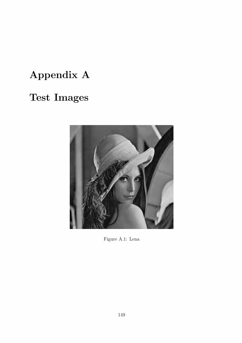
Appendix A
Test Images
Figure A.1: Lena
149

APPENDIX A. TEST IMAGES 150
Figure A.2: Plane
Figure A.3: Bridge
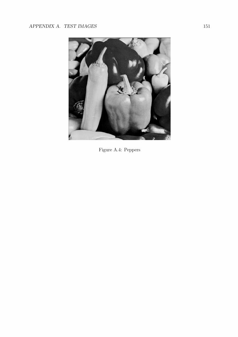
APPENDIX A. TEST IMAGES 151
Figure A.4: Peppers

Appendix B
Source Code
B.1 M-files
B.1.1 JPEG
function Y = my_jpeg(X, Q)
X = double(X); % just in case
[m, n] = size(X);
for k = 1:8:m
for l = 1:8:n
A = X(k:k + 7, l:l + 7) - 128; % level shift
F = dct2(A); % transform
F = round(F./Q); % quantise
Y(k:k + 7, l:l + 7) = F;
end
end
function X = my_jpeg_dec(Y, Q)
[m, n] = size(Y);
for k = 1:8:m
for l = 1:8:n
F = Y(k:k + 7, l:l + 7);
F = F.*Q; % dequantise
A = round(idct2(F) + 128); % inverse transform and level shift
X(k:k + 7, l:l + 7) = A;
end
end
function Q = jpeg_qt(qual)
if qual <= 50
a = 50/qual;
152

APPENDIX B. SOURCE CODE 153
else
a = 2 - qual/50;
end
% luminance quantisation table
Q(1,:) = [16 11 10 16 24 40 51 61];
Q(2,:) = [12 12 14 19 26 58 60 55];
Q(3,:) = [14 13 16 24 40 57 69 56];
Q(4,:) = [14 17 22 29 51 87 80 62];
Q(5,:) = [18 22 37 56 68 109 103 77];
Q(6,:) = [24 35 55 64 81 104 113 92];
Q(7,:) = [49 64 78 87 103 121 120 101];
Q(8,:) = [72 92 95 98 112 100 103 99];
Q = round(a*Q); % scale quantisation table
Q = max(Q, 1); % minimum value is 1
Q = min(Q, 255); % maximum value is 255
function bytes = dct2bytes(Y, opt)
if opt == 0
bytes = d2b(Y, 1);
else
bytes = d2b(Y(5:end-4, 5:end-4), 1);
bytes = bytes + d2b(Y(:, 1:4), 2);
bytes = bytes + d2b(Y(:, end-3:end), 2);
bytes = bytes + d2b(Y(1:4, 5:end-4), 3);
bytes = bytes + d2b(Y(end-3:end, 5:end-4), 3);
end
bytes = bytes + 354;
function bytes = d2b(Y, opt)
if opt == 1 % 8x8 blocks
steps = 8;
max_pos = 64;
offset1 = 7; offset2 = 7;
elseif opt == 2 % 4x4 blocks
steps = 4;
max_pos = 16;
offset1 = 3; offset2 = 3;
else % 4x8 blocks
steps = 8;
max_pos = 32;
offset1 = 3; offset2 = 7;
end
% DC huffman table
hdc = [2 3 3 3 3 3 4 5 6 7 8 9];
% AC huffman table
hac(1,:) = [2 2 3 4 5 7 8 10 16 16];
APPENDIX B. SOURCE CODE 154
hac(2,:) = [4 5 7 9 11 16 16 16 16 16];
hac(3,:) = [5 8 10 12 16 16 16 16 16 16];
hac(4,:) = [6 9 12 16 16 16 16 16 16 16];
hac(5,:) = [6 10 16 16 16 16 16 16 16 16];
hac(6,:) = [7 11 16 16 16 16 16 16 16 16];
hac(7,:) = [7 12 16 16 16 16 16 16 16 16];
hac(8,:) = [8 12 16 16 16 16 16 16 16 16];
hac(9,:) = [9 15 16 16 16 16 16 16 16 16];
hac(10,:) = [9 16 16 16 16 16 16 16 16 16];
hac(11,:) = [9 16 16 16 16 16 16 16 16 16];
hac(12,:) = [10 16 16 16 16 16 16 16 16 16];
hac(13,:) = [10 16 16 16 16 16 16 16 16 16];
hac(14,:) = [11 16 16 16 16 16 16 16 16 16];
hac(15,:) = [16 16 16 16 16 16 16 16 16 16];
hac(16,:) = [16 16 16 16 16 16 16 16 16 16];
[m, n] = size(Y);
bits = 0;
prev = 0; % initial prediction for DC
for k = 1:steps:m
for l = 1:steps:n
A = Y(k:k + offset1, l:l + offset2);
A = zigzag(A, opt);
% trailing zeroes
pos = max_pos;
while (pos ~= 1) & (A(pos) == 0)
pos = pos - 1;
end
% differential DC coding
ddc = A(1) - prev;
category = ceil(log2(abs(ddc) + 1));
bits = bits + hdc(category + 1);
bits = bits + category;
prev = A(1);
if pos == 1
% EOB 1010
bits = bits + 4;
else
% non-zero AC coefficients
index = 2;
count = 0;
while index ~= pos + 1
while A(index) == 0
count = count + 1;
index = index + 1;
% take care of 16 or more zeroes
if count == 16
count = 0;
% ZRL = 11 bits
bits = bits + 11;
end

APPENDIX B. SOURCE CODE 155
end
category = ceil(log2(abs(A(index)) + 1));
bits = bits + hac(count + 1, category);
bits = bits + category;
count = 0;
index = index + 1;
end
% EOB 1010
bits = bits + 4;
end
end
end
bytes = ceil(bits/8);
function psnr = decibels(X, XX)
[m, n] = size(X);
MSE = sum(sum((X - XX).^2))/(m*n);
psnr = 10*log10(65025/MSE);
B.1.2 MJPEG
function Y = mjpeg(X, Q)
X = double(X); % just in case
X = X - 128; % level shift
[m, n] = size(X);
% calculate frequency components
for k = 1:m
f(k,:) = row_enc(X(k,:));
end
for k = 1:(n-8)
F(:,k) = row_enc(f(:,k)’)’;
end
F = F/4;
for k = 1:4:m
left(k:k+3,:) = dct2(X(k:k+3, 1:4));
right(k:k+3,:) = dct2(X(k:k+3, end-3:end));
end
left = 2*left;
right = 2*right;
for l = 1:8:(n-8)
temp = f(1:4, l:l+7);
top(:, l:l+7) = [dct1(temp(:,1)) dct1(temp(:,2))...
dct1(temp(:,3)) dct1(temp(:,4))...
dct1(temp(:,5)) dct1(temp(:,6))...
dct1(temp(:,7)) dct1(temp(:,8))];

APPENDIX B. SOURCE CODE 156
temp = f(end-3:end, l:l+7);
bottom(:, l:l+7) = [dct1(temp(:,1)) dct1(temp(:,2))...
dct1(temp(:,3)) dct1(temp(:,4))...
dct1(temp(:,5)) dct1(temp(:,6))...
dct1(temp(:,7)) dct1(temp(:,8))];
end
% down-sampled quantisation tables
q2(1,:) = round(mean(Q(1:2,:)));
q2(2,:) = round(mean(Q(3:4,:)));
q2(3,:) = round(mean(Q(5:6,:)));
q2(4,:) = round(mean(Q(7:8,:)));
q1(:,1) = round(mean(q2(:, 1:2),2));
q1(:,2) = round(mean(q2(:, 3:4),2));
q1(:,3) = round(mean(q2(:, 5:6),2));
q1(:,4) = round(mean(q2(:, 7:8),2));
% quantise middle (m-8 x n-8)
for k = 1:8:(m-8)
for l = 1:8:(n-8)
F(k:k+7, l:l+7) = F(k:k+7, l:l+7)./Q;
end
end
% quantise left and right (m x 4)
for k = 1:4:m
left(k:k+3, :) = left(k:k+3, :)./q1;
right(k:k+3, :) = right(k:k+3, :)./q1;
end
% quantise top and bottom (4 x n-8)
for l = 1:8:(n-8)
top(:, l:l+7) = top(:, l:l+7)./q2;
bottom(:, l:l+7) = bottom(:, l:l+7)./q2;
end
Y = [top ; F ; bottom];
Y = [left Y right];
Y = round(Y);
function X = mjpeg_dec(Y, Q)
left = Y(:, 1:4);
right = Y(:, end-3:end);
Y(:, 1:4) = [];
Y(:, end-3:end) = [];
top = Y(1:4, :);
bottom = Y(end-3:end, :);
Y(1:4, :) = [];
Y(end-3:end, :) = [];
[m, n] = size(Y);

APPENDIX B. SOURCE CODE 157
% down-sampled quantisation tables
q2(1,:) = round(mean(Q(1:2,:)));
q2(2,:) = round(mean(Q(3:4,:)));
q2(3,:) = round(mean(Q(5:6,:)));
q2(4,:) = round(mean(Q(7:8,:)));
q1(:,1) = round(mean(q2(:, 1:2),2));
q1(:,2) = round(mean(q2(:, 3:4),2));
q1(:,3) = round(mean(q2(:, 5:6),2));
q1(:,4) = round(mean(q2(:, 7:8),2));
% dequantise middle (m x n)
for k = 1:8:m
for l = 1:8:n
Y(k:k+7, l:l+7) = 4*Y(k:k+7, l:l+7).*Q;
end
end
% dequantise left and right (m+8 x 4)
for k = 1:4:(m+8)
left(k:k+3, :) = idct2(0.5*left(k:k+3, :).*q1);
right(k:k+3, :) = idct2(0.5*right(k:k+3, :).*q1);
end
% dequantise top and bottom (4 x n)
for l = 1:8:n
temp = top(:, l:l+7).*q2;
top(:, l:l+7) = [idct1(temp(:,1)) idct1(temp(:,2))...
idct1(temp(:,3)) idct1(temp(:,4))...
idct1(temp(:,5)) idct1(temp(:,6))...
idct1(temp(:,7)) idct1(temp(:,8))];
temp = bottom(:, l:l+7).*q2;
bottom(:, l:l+7) = [idct1(temp(:,1)) idct1(temp(:,2))...
idct1(temp(:,3)) idct1(temp(:,4))...
idct1(temp(:,5)) idct1(temp(:,6))...
idct1(temp(:,7)) idct1(temp(:,8))];
end
% invert
for k = 1:n
F(:,k) = row_dec(Y(:,k)’, top(:,k)’, bottom(:,k)’)’;
end
for k = 1:(m+8)
X(k,:) = row_dec(F(k,:), left(k,:), right(k,:));
end
X = round(X) + 128;

APPENDIX B. SOURCE CODE 158
function f = row_enc(x)
n = length(x);
w = sin(pi*((0:15) + 0.5)/16);
f = [];
for k = 1:8:(n-8)
f = [f mdct(x(k:k+15).*w)];
end
function x = row_dec(f, left, right)
n = length(f);
w = sin(pi*((0:15) + 0.5)/16);
x = zeros(1, n + 8);
for k = 1:8:n
x(k:k+15) = x(k:k+15) + imdct(f(k:k+7)).*w;
end
x(1:4) = left;
x(5:8) = x(5:8) + fliplr(left).*w(5:8).*w(13:16);
x(5:8) = x(5:8)./(w(5:8).^2);
x(end-3:end) = right;
x(end-7:end-4) = x(end-7:end-4) - fliplr(right).*w(1:4).*w(9:12);
x(end-7:end-4) = x(end-7:end-4)./(w(9:12).^2);
function X = mdct(x)
N = length(x); n0 = N/4 + 1/2;
for k = 0:N/2-1
X(k + 1) = sum(x.*cos(2*pi*((0:N-1) + n0)*(k + 0.5)/N));
end
function x = imdct(X)
N = 2*length(X); n0 = N/4 + 1/2;
for n = 0:N-1
x(n + 1) = sum(X.*cos(2*pi*(n + n0)*((0:N/2-1) + 0.5)/N));
end
x = 4*x/N;
function y = dct1(x)
x = x’;
y(1) = 0.5*sum(x)/sqrt(2);
y(2) = 0.5*sum(x.*cos((1:2:7)*pi/8));
y(3) = 0.5*sum(x.*cos((1:2:7)*pi/4));
y(4) = 0.5*sum(x.*cos((1:2:7)*3*pi/8));
y = y’;

APPENDIX B. SOURCE CODE 159
function x = idct1(y)
y = y’;
c = [1/sqrt(2) 1 1 1];
x(1) = sum(c.*y.*cos((0:3)*pi/8));
x(2) = sum(c.*y.*cos((0:3)*3*pi/8));
x(3) = sum(c.*y.*cos((0:3)*5*pi/8));
x(4) = sum(c.*y.*cos((0:3)*7*pi/8));
x = x’;
B.2 C++ Implementation
#include <iostream>
#include <math.h>
#include <time.h>
using std::cout;
using std::cin;
using std::endl;
double target;
const int m = 256;
const int n = 256;
const int lower = 5;
const int upper = 5;
const int pop_size = 100; // size of population
const int total = 200; // number of generations
double Y[m][n]; // frequency components
double Yq[m][n]; // Y quantised
double Ydq[m][n]; // Y dequantised
double zz[64]; // zigzag sequence used in all 3 cases
double gradient[46]; // gradient values, indexed by diag values - 10
int k2diag[2][30]; // corrects kk0 values to diag values, indexed by kk0 - 17
int old_pop[pop_size][64]; // old population
int new_pop[pop_size][64]; // new population
int z[64]; // indices of Q in zigzag ordering
int Q[64]; // quantisation table
int q1[16]; // downsampled 4x4 quantisation table
int q2[32]; // downsampled 4x8 quantisation table
int hdc[12]; // huffman dc
int hac[16][10]; // huffman ac
int kk0; // diag value
double kk1; // gradient value
void show_Q(int* q)
{
int pos;
for (pos = 0 ; pos < 64 ; pos++)
{
if (fmod(pos, 8) == 0)

APPENDIX B. SOURCE CODE 160
{
cout << endl;
}
cout << q[pos] << " ";
}
cout << endl;
}
void mate(int parent1, int parent2, int k)
{
int pos;
double r;
// crossover
r = rand();
r = r/RAND_MAX;
r = round(62*r);
// first portion
for (pos = 0 ; pos <= r ; pos++)
{
new_pop[k][pos] = old_pop[parent1][pos];
new_pop[k + 1][pos] = old_pop[parent2][pos];
}
// second portion
for (pos = int(r) + 1 ; pos < 64 ; pos++)
{
new_pop[k][pos] = old_pop[parent2][pos];
new_pop[k + 1][pos] = old_pop[parent1][pos];
}
// mutation
r = rand();
r = r/RAND_MAX;
if (r < 0.05)
{
r = rand();
r = r/RAND_MAX;
r = round(63*r);
pos = int(r);
r = rand();
r = r/RAND_MAX;
new_pop[k][pos] = new_pop[k][pos] + int(round(2*lower*r - lower));
new_pop[k][pos] = int(fmax(new_pop[k][pos], 1));
new_pop[k][pos] = int(fmin(new_pop[k][pos], 255));
}
r = rand();
r = r/RAND_MAX;
if (r < 0.05)
{
r = rand();
r = r/RAND_MAX;
r = round(63*r);
pos = int(r);
APPENDIX B. SOURCE CODE 161
r = rand();
r = r/RAND_MAX;
new_pop[k + 1][pos] = new_pop[k + 1][pos] + int(round(2*lower*r - lower));
new_pop[k + 1][pos] = int(fmax(new_pop[k + 1][pos], 1));
new_pop[k + 1][pos] = int(fmin(new_pop[k + 1][pos], 255));
}
}
void copy_table(int* q1, int* q2)
{
int k;
for (k = 0 ; k < 64 ; k++)
{
q2[k] = q1[k];
}
}
void update_pop()
{
int k;
for (k = 0 ; k < pop_size ; k++)
{
copy_table(new_pop[k], old_pop[k]);
}
}
int find_pos(double* p, double r)
{
int k = 0;
while (r >= p[k])
{
k++;
}
return k;
}
void down_Q(int* q)
{
// downsample quantisation table
int pos;
for (pos = 0 ; pos < 8 ; pos++)
{
q2[pos] = int(round(double(q[pos] + q[pos + 8])/2));
q2[pos + 8] = int(round(double(q[pos + 16] + q[pos + 24])/2));
q2[pos + 16] = int(round(double(q[pos + 32] + q[pos + 40])/2));
q2[pos + 24] = int(round(double(q[pos + 48] + q[pos + 56])/2));

APPENDIX B. SOURCE CODE 162
}
for (pos = 0 ; pos < 4 ; pos++)
{
q1[pos] = int(round(double(q2[2*pos] + q2[2*pos + 1])/2));
q1[pos + 4] = int(round(double(q2[2*pos + 8] + q2[2*pos + 9])/2));
q1[pos + 8] = int(round(double(q2[2*pos + 16] + q2[2*pos + 17])/2));
q1[pos + 12] = int(round(double(q2[2*pos + 24] + q2[2*pos + 25])/2));
}
}
void qdq(int* q)
{
// quantises and dequantises
int row, column, pos;
// middle
for (row = 4 ; row < m - 4 ; row++)
{
for (column = 4 ; column < n - 4 ; column++)
{
pos = int(8*fmod(row - 4, 8) + fmod(column - 4, 8));
Yq[row][column] = round(Y[row][column]/q[pos]);
Ydq[row][column] = Yq[row][column]*q[pos];
}
}
// left
for (row = 0 ; row < m ; row++)
{
for (column = 0 ; column < 4 ; column++)
{
pos = int(4*fmod(row,4) + column);
Yq[row][column] = round(Y[row][column]/q1[pos]);
Ydq[row][column] = Yq[row][column]*q1[pos];
}
}
// right
for (row = 0 ; row < m ; row++)
{
for (column = n - 4 ; column < n ; column++)
{
pos = int(4*fmod(row,4) + fmod(column,4));
Yq[row][column] = round(Y[row][column]/q1[pos]);
Ydq[row][column] = Yq[row][column]*q1[pos];
}
}
// top
for (row = 0 ; row < 4 ; row++)
{
for (column = 4 ; column < n - 4 ; column++)

APPENDIX B. SOURCE CODE 163
{
pos = int(8*row + fmod(column - 4, 8));
Yq[row][column] = round(Y[row][column]/q2[pos]);
Ydq[row][column] = Yq[row][column]*q2[pos];
}
}
// bottom
for (row = m - 4 ; row < m ; row++)
{
for (column = 4 ; column < n - 4 ; column++)
{
pos = int(8*fmod(row,4) + fmod(column - 4, 8));
Yq[row][column] = round(Y[row][column]/q2[pos]);
Ydq[row][column] = Yq[row][column]*q2[pos];
}
}
}
double calc_error()
{
int row, column;
double E;
E = 0;
for (row = 0 ; row < m ; row++)
{
for (column = 0 ; column < n ; column++)
{
E = E + pow(Y[row][column] - Ydq[row][column], 2);
}
}
return E/(m*n);
}
void zigzag(int row, int column, int opt)
{
switch (opt)
{
case 1 : // 8x8 blocks
zz[0] = Yq[row][column]; zz[1] = Yq[row][column + 1];
zz[2] = Yq[row + 1][column]; zz[3] = Yq[row + 2][column];
zz[4] = Yq[row + 1][column + 1]; zz[5] = Yq[row][column + 2];
zz[6] = Yq[row][column + 3]; zz[7] = Yq[row + 1][column + 2];
zz[8] = Yq[row + 2][column + 1]; zz[9] = Yq[row + 3][column];
zz[10] = Yq[row + 4][column]; zz[11] = Yq[row + 3][column + 1];
zz[12] = Yq[row + 2][column + 2]; zz[13] = Yq[row + 1][column + 3];
zz[14] = Yq[row][column + 4]; zz[15] = Yq[row][column + 5];
zz[16] = Yq[row + 1][column + 4]; zz[17] = Yq[row + 2][column + 3];
zz[18] = Yq[row + 3][column + 2]; zz[19] = Yq[row + 4][column + 1];

APPENDIX B. SOURCE CODE 164
zz[20] = Yq[row + 5][column]; zz[21] = Yq[row + 6][column];
zz[22] = Yq[row + 5][column + 1]; zz[23] = Yq[row + 4][column + 2];
zz[24] = Yq[row + 3][column + 3]; zz[25] = Yq[row + 2][column + 4];
zz[26] = Yq[row + 1][column + 5]; zz[27] = Yq[row][column + 6];
zz[28] = Yq[row][column + 7]; zz[29] = Yq[row + 1][column + 6];
zz[30] = Yq[row + 2][column + 5]; zz[31] = Yq[row + 3][column + 4];
zz[32] = Yq[row + 4][column + 3]; zz[33] = Yq[row + 5][column + 2];
zz[34] = Yq[row + 6][column + 1]; zz[35] = Yq[row + 7][column];
zz[36] = Yq[row + 7][column + 1]; zz[37] = Yq[row + 6][column + 2];
zz[38] = Yq[row + 5][column + 3]; zz[39] = Yq[row + 4][column + 4];
zz[40] = Yq[row + 3][column + 5]; zz[41] = Yq[row + 2][column + 6];
zz[42] = Yq[row + 1][column + 7]; zz[43] = Yq[row + 2][column + 7];
zz[44] = Yq[row + 3][column + 6]; zz[45] = Yq[row + 4][column + 5];
zz[46] = Yq[row + 5][column + 4]; zz[47] = Yq[row + 6][column + 3];
zz[48] = Yq[row + 7][column + 2]; zz[49] = Yq[row + 7][column + 3];
zz[50] = Yq[row + 6][column + 4]; zz[51] = Yq[row + 5][column + 5];
zz[52] = Yq[row + 4][column + 6]; zz[53] = Yq[row + 3][column + 7];
zz[54] = Yq[row + 4][column + 7]; zz[55] = Yq[row + 5][column + 6];
zz[56] = Yq[row + 6][column + 5]; zz[57] = Yq[row + 7][column + 4];
zz[58] = Yq[row + 7][column + 5]; zz[59] = Yq[row + 6][column + 6];
zz[60] = Yq[row + 5][column + 7]; zz[61] = Yq[row + 6][column + 7];
zz[62] = Yq[row + 7][column + 6]; zz[63] = Yq[row + 7][column + 7];
break;
case 2 : // 4x4 blocks
case 3 :
zz[0] = Yq[row][column]; zz[1] = Yq[row][column + 1];
zz[2] = Yq[row + 1][column]; zz[3] = Yq[row + 2][column];
zz[4] = Yq[row + 1][column + 1]; zz[5] = Yq[row][column + 2];
zz[6] = Yq[row][column + 3]; zz[7] = Yq[row + 1][column + 2];
zz[8] = Yq[row + 2][column + 1]; zz[9] = Yq[row + 3][column];
zz[10] = Yq[row + 3][column + 1]; zz[11] = Yq[row + 2][column + 2];
zz[12] = Yq[row + 1][column + 3]; zz[13] = Yq[row + 2][column + 3];
zz[14] = Yq[row + 3][column + 2]; zz[15] = Yq[row + 3][column + 3];
break;
case 4 : // 4x8 blocks
case 5 :
zz[0] = Yq[row][column]; zz[1] = Yq[row][column + 1];
zz[2] = Yq[row + 1][column]; zz[3] = Yq[row + 2][column];
zz[4] = Yq[row + 1][column + 1]; zz[5] = Yq[row][column + 2];
zz[6] = Yq[row][column + 3]; zz[7] = Yq[row + 1][column + 2];
zz[8] = Yq[row + 2][column + 1]; zz[9] = Yq[row + 3][column];
zz[10] = Yq[row + 3][column + 1]; zz[11] = Yq[row + 2][column + 2];
zz[12] = Yq[row + 1][column + 3]; zz[13] = Yq[row][column + 4];
zz[14] = Yq[row][column + 5]; zz[15] = Yq[row + 1][column + 4];
zz[16] = Yq[row + 2][column + 3]; zz[17] = Yq[row + 3][column + 2];
zz[18] = Yq[row + 3][column + 3]; zz[19] = Yq[row + 2][column + 4];
zz[20] = Yq[row + 1][column + 5]; zz[21] = Yq[row][column + 6];
zz[22] = Yq[row][column + 7]; zz[23] = Yq[row + 1][column + 6];
zz[24] = Yq[row + 2][column + 5]; zz[25] = Yq[row + 3][column + 4];
zz[26] = Yq[row + 3][column + 5]; zz[27] = Yq[row + 2][column + 6];
zz[28] = Yq[row + 1][column + 7]; zz[29] = Yq[row + 2][column + 7];
zz[30] = Yq[row + 3][column + 6]; zz[31] = Yq[row + 3][column + 7];
}
}

APPENDIX B. SOURCE CODE 165
double d2b(int opt)
{
int row, column, steps, start_row, stop_row, start_column, stop_column;
int count, pos, max_pos, category, i;
double bits, prev, ddc, bytes;
switch (opt)
{
case 1 : // middle
steps = 8; max_pos = 63; start_row = 4; stop_row = m - 4;
start_column = 4; stop_column = n - 4;
break;
case 2 : // left
steps = 4; max_pos = 15; start_row = 0; stop_row = m;
start_column = 0; stop_column = 4;
break;
case 3 : // right
steps = 4; max_pos = 15; start_row = 0; stop_row = m;
start_column = n - 4; stop_column = n;
break;
case 4 : // top
steps = 8; max_pos = 31; start_row = 0; stop_row = 4;
start_column = 4; stop_column = n - 4;
break;
case 5 : // bottom
steps = 8; max_pos = 31; start_row = m - 4; stop_row = m;
start_column = 4; stop_column = n - 4;
}
bits = 0; prev = 0;
for (row = start_row ; row < stop_row ; row = row + steps)
{
for (column = start_column ; column < stop_column ; column = column + steps)
{
zigzag(row, column, opt);
// trailing zeros
pos = max_pos;
while ((pos != 0) && (zz[pos] == 0))
{
pos--;
}
// differential DC coding
ddc = zz[0] - prev;
category = int(ceil(log2(fabs(ddc) + 1)));
bits = bits + hdc[category];
bits = bits + category;
prev = zz[0];
if (pos == 0)
{
bits = bits + 4; // EOB 1010
}

APPENDIX B. SOURCE CODE 166
else
{
// non-zero AC coefficients
i = 1;
count = 0;
while (i != pos + 1)
{
while (zz[i] == 0)
{
count++;
i++;
// more than 16 zeros
if (count == 16)
{
count = 0;
bits = bits + 11; // ZRL contributes 11 bits
}
}
category = int(ceil(log2(fabs(zz[i]) + 1)));
bits = bits + hac[count][category - 1];
bits = bits + category;
count = 0;
i++;
}
bits = bits + 4; // EOB 1010
}
}
}
bytes = ceil(bits/8);
return bytes;
}
double dct2bytes()
{
double bytes;
bytes = d2b(1) + d2b(2) + d2b(3) + d2b(4) + d2b(5); // middle left right top bottom
bytes = bytes + 354; // overhead
return bytes;
}
void ga()
{
// Genetic Algorithm
double c = 35; // penalty parameter
double best = 0; // best fitness in final population
double bfc; // best feasible cost
double bic; // best infeasible cost
double B, E, dev, cost;
double fitness[pop_size];
double prob[pop_size];

APPENDIX B. SOURCE CODE 167
double tot_fitness;
double r;
int iter, k, index, parent1, parent2;
for (iter = 1 ; iter <= total ; iter++)
{
bfc = INFINITY;
bic = INFINITY;
tot_fitness = 0;
// calculate cost and fitness
for (k = 0 ; k < pop_size ; k++)
{
down_Q(old_pop[k]);
qdq(old_pop[k]);
E = calc_error();
B = dct2bytes();
// calculate deviation from constraint
if (B > 1.001*target)
{
dev = 100*(B - 1.001*target)/(1.001*target);
}
else if (B < 0.999*target)
{
dev = 100*(0.999*target - B)/(0.999*target);
}
else
{
dev = 0;
}
cost = E + c*dev;
fitness[k] = 1/cost;
tot_fitness = tot_fitness + fitness[k];
if (dev == 0)
{
if (cost < bfc)
{
bfc = cost;
index = k;
}
}
else if (cost < bic)
{
bic = cost;
}
}
// update c
c = c*bfc/bic;
cout << "c = " << c << endl;

APPENDIX B. SOURCE CODE 168
// calculate probability interval
prob[0] = fitness[0]/tot_fitness;
for (k = 1 ; k < pop_size ; k++)
{
prob[k] = prob[k - 1] + fitness[k]/tot_fitness;
}
// generate new population
for (k = 0 ; k < pop_size ; k = k + 2)
{
r = rand();
r = r/RAND_MAX;
parent1 = find_pos(prob, r);
r = rand();
r = r/RAND_MAX;
parent2 = find_pos(prob, r);
mate(parent1, parent2, k);
}
// retain best solution
r = rand();
r = r/RAND_MAX;
r = round((pop_size - 1)*r);
copy_table(old_pop[index], new_pop[int(r)]);
cout << "best = " << bfc << endl;
show_Q(old_pop[index]);
update_pop();
}
// final population
// calculate cost and fitness
for (k = 0 ; k < pop_size ; k++)
{
down_Q(old_pop[k]);
qdq(old_pop[k]);
E = calc_error();
B = dct2bytes();
// calculate deviation from constraint
if (B > 1.001*target)
{
dev = 100*(B - 1.001*target)/(1.001*target);
}
else if (B < 0.999*target)
{
dev = 100*(0.999*target - B)/(0.999*target);
}
else
{
dev = 0;
}
cost = E + c*dev;
fitness[k] = 1/cost;

APPENDIX B. SOURCE CODE 169
if (fitness[k] > best)
{
best = fitness[k];
index = k;
}
}
copy_table(old_pop[index], Q);
}
void fill_Q(int q)
{
// fills Q with a constant value
int pos;
for (pos = 0 ; pos < 64 ; pos++)
{
Q[pos] = q;
}
}
void plane_Q()
{
// evaluates plane function using values of kk0 and kk1 ; fills in Q
int row, column;
for (row = 0 ; row < 8 ; row++)
{
for (column = 0 ; column < 8 ; column++)
{
Q[8*row + column] = int(round(kk1*(row + column - 7))) + kk0;
}
}
}
int gr()
{
// golden ratio search
double r = 1 - (sqrt(5) - 1)/2;
int w = 255;
int L = 1; int R = 255;
int a, b;
double B, fL, fR, fa, fb, best;
fill_Q(L);
down_Q(Q);
qdq(Q);
B = dct2bytes();
fL = fabs(B - target);

APPENDIX B. SOURCE CODE 170
fill_Q(R);
down_Q(Q);
qdq(Q);
B = dct2bytes();
fR = fabs(B - target);
a = L + int(floor(r*w));
fill_Q(a);
down_Q(Q);
qdq(Q);
B = dct2bytes();
fa = fabs(B - target);
b = R - int(floor(r*w));
fill_Q(b);
down_Q(Q);
qdq(Q);
B = dct2bytes();
fb = fabs(B - target);
while (w > 3)
{
if (fa < fb)
{
// discard RHS
R = b; fR = fb;
b = a; fb = fa;
w = R - L + 1;
a = L + int(floor(r*w));
fill_Q(a);
down_Q(Q);
qdq(Q);
B = dct2bytes();
fa = fabs(B - target);
}
else
{
// discard LHS
L = a; fL = fa;
a = b; fa = fb;
w = R - L + 1;
b = R - int(floor(r*w));
fill_Q(b);
down_Q(Q);
qdq(Q);
B = dct2bytes();
fb = fabs(B - target);
}
}
best = fmin(fmin(fL, fR), fa);
if (fL == best)
{
return L;
}
else if (fR == best)

APPENDIX B. SOURCE CODE 171
{
return R;
}
else
{
return a;
}
}
void get_gradient()
{
// determines value of kk0 and kk1
double B, dev, best_dev;
int best_diag;
int num, count;
count = 1;
num = k2diag[1][kk0 - 17]; // number of values to consider
kk0 = k2diag[0][kk0 - 17]; // first new value of kk0
cout << "testing " << kk0 << endl;
kk1 = gradient[kk0 - 10];
plane_Q();
down_Q(Q);
qdq(Q);
B = dct2bytes();
dev = fabs(B - target);
best_dev = dev;
best_diag = kk0;
while (count < num)
{
kk0++; // try next value
cout << "testing " << kk0 << endl;
kk1 = gradient[kk0 - 10];
plane_Q();
down_Q(Q);
qdq(Q);
B = dct2bytes();
dev = fabs(B - target);
if (dev < best_dev)
{
best_dev = dev;
best_diag = kk0;
}
count++;
}
kk0 = best_diag;
kk1 = gradient[kk0 - 10];
}

APPENDIX B. SOURCE CODE 172
void init_Q()
{
// manually specify quantisation table
Q[0] = 255; Q[1] = 255; Q[2] = 255; Q[3] = 255;
Q[4] = 255; Q[5] = 255; Q[6] = 255; Q[7] = 255;
Q[8] = 255; Q[9] = 255; Q[10] = 255; Q[11] = 255;
Q[12] = 255; Q[13] = 255; Q[14] = 255; Q[15] = 255;
Q[16] = 255; Q[17] = 255; Q[18] = 255; Q[19] = 255;
Q[20] = 255; Q[21] = 255; Q[22] = 255; Q[23] = 255;
Q[24] = 255; Q[25] = 255; Q[26] = 255; Q[27] = 255;
Q[28] = 255; Q[29] = 255; Q[30] = 255; Q[31] = 255;
Q[32] = 255; Q[33] = 255; Q[34] = 255; Q[35] = 255;
Q[36] = 255; Q[37] = 255; Q[38] = 255; Q[39] = 255;
Q[40] = 255; Q[41] = 255; Q[42] = 255; Q[43] = 255;
Q[44] = 255; Q[45] = 255; Q[46] = 255; Q[47] = 255;
Q[48] = 255; Q[49] = 255; Q[50] = 255; Q[51] = 255;
Q[52] = 255; Q[53] = 255; Q[54] = 255; Q[55] = 255;
Q[56] = 255; Q[57] = 255; Q[58] = 255; Q[59] = 255;
Q[60] = 255; Q[61] = 255; Q[62] = 255; Q[63] = 255;
}
int main(int argc, char* argv[])
{
double x, E, B, dev, nu_E, nu_B, lambda, best_lambda, best_E, best_B, Rmax, Rmin;
int row, column, pos, q, qq, qqq, best_pos, best_q, k;
if (argc != 3)
{
cout << "Must specify target file size and GA option" << endl;
exit(1);
}
// read in frequency components
FILE* pic = fopen("lena_m2.mat", "r");
fseek(pic, 184, SEEK_SET);
for (column = 0 ; column < n ; column++)
{
for (row = 0 ; row < m ; row++)
{
fread(&x, 8, 1, pic);
Y[row][column] = x;
}
}
// initialize random number generator and get target file size
srand(time(NULL));
target = atoi(argv[1]);
// enter indices in z
APPENDIX B. SOURCE CODE 173
z[0] = 0; z[1] = 1; z[2] = 8; z[3] = 16;
z[4] = 9; z[5] = 2; z[6] = 3; z[7] = 10;
z[8] = 17; z[9] = 24; z[10] = 32; z[11] = 25;
z[12] = 18; z[13] = 11; z[14] = 4; z[15] = 5;
z[16] = 12; z[17] = 19; z[18] = 26; z[19] = 33;
z[20] = 40; z[21] = 48; z[22] = 41; z[23] = 34;
z[24] = 27; z[25] = 20; z[26] = 13; z[27] = 6;
z[28] = 7; z[29] = 14; z[30] = 21; z[31] = 28;
z[32] = 35; z[33] = 42; z[34] = 49; z[35] = 56;
z[36] = 57; z[37] = 50; z[38] = 43; z[39] = 36;
z[40] = 29; z[41] = 22; z[42] = 15; z[43] = 23;
z[44] = 30; z[45] = 37; z[46] = 44; z[47] = 51;
z[48] = 58; z[49] = 59; z[50] = 52; z[51] = 45;
z[52] = 38; z[53] = 31; z[54] = 39; z[55] = 46;
z[56] = 53; z[57] = 60; z[58] = 61; z[59] = 54;
z[60] = 47; z[61] = 55; z[62] = 62; z[63] = 63;
// fill in huffman tables
hdc[0] = 2; hdc[1] = 3; hdc[2] = 3; hdc[3] = 3; hdc[4] = 3; hdc[5] = 3;
hdc[6] = 4; hdc[7] = 5; hdc[8] = 6; hdc[9] = 7; hdc[10] = 8; hdc[11] = 9;
hac[0][0] = 2; hac[0][1] = 2; hac[0][2] = 3; hac[0][3] = 4; hac[0][4] = 5;
hac[0][5] = 7; hac[0][6] = 8; hac[0][7] = 10; hac[0][8] = 16; hac[0][9] = 16;
hac[1][0] = 4; hac[1][1] = 5; hac[1][2] = 7; hac[1][3] = 9; hac[1][4] = 11;
hac[1][5] = 16; hac[1][6] = 16; hac[1][7] = 16; hac[1][8] = 16; hac[1][9] = 16;
hac[2][0] = 5; hac[2][1] = 8; hac[2][2] = 10; hac[2][3] = 12; hac[2][4] = 16;
hac[2][5] = 16; hac[2][6] = 16; hac[2][7] = 16; hac[2][8] = 16; hac[2][9] = 16;
hac[3][0] = 6; hac[3][1] = 9; hac[3][2] = 12; hac[3][3] = 16; hac[3][4] = 16;
hac[3][5] = 16; hac[3][6] = 16; hac[3][7] = 16; hac[3][8] = 16; hac[3][9] = 16;
hac[4][0] = 6; hac[4][1] = 10; hac[4][2] = 16; hac[4][3] = 16; hac[4][4] = 16;
hac[4][5] = 16; hac[4][6] = 16; hac[4][7] = 16; hac[4][8] = 16; hac[4][9] = 16;
hac[5][0] = 7; hac[5][1] = 11; hac[5][2] = 16; hac[5][3] = 16; hac[5][4] = 16;
hac[5][5] = 16; hac[5][6] = 16; hac[5][7] = 16; hac[5][8] = 16; hac[5][9] = 16;
hac[6][0] = 7; hac[6][1] = 12; hac[6][2] = 16; hac[6][3] = 16; hac[6][4] = 16;
hac[6][5] = 16; hac[6][6] = 16; hac[6][7] = 16; hac[6][8] = 16; hac[6][9] = 16;
hac[7][0] = 8; hac[7][1] = 12; hac[7][2] = 16; hac[7][3] = 16; hac[7][4] = 16;
hac[7][5] = 16; hac[7][6] = 16; hac[7][7] = 16; hac[7][8] = 16; hac[7][9] = 16;
hac[8][0] = 9; hac[8][1] = 15; hac[8][2] = 16; hac[8][3] = 16; hac[8][4] = 16;
hac[8][5] = 16; hac[8][6] = 16; hac[8][7] = 16; hac[8][8] = 16; hac[8][9] = 16;
hac[9][0] = 9; hac[9][1] = 16; hac[9][2] = 16; hac[9][3] = 16; hac[9][4] = 16;
hac[9][5] = 16; hac[9][6] = 16; hac[9][7] = 16; hac[9][8] = 16; hac[9][9] = 16;
hac[10][0] = 9; hac[10][1] = 16; hac[10][2] = 16; hac[10][3] = 16; hac[10][4] = 16;
hac[10][5] = 16; hac[10][6] = 16; hac[10][7] = 16; hac[10][8] = 16; hac[10][9] = 16;
hac[11][0] = 10; hac[11][1] = 16; hac[11][2] = 16; hac[11][3] = 16; hac[11][4] = 16;
hac[11][5] = 16; hac[11][6] = 16; hac[11][7] = 16; hac[11][8] = 16; hac[11][9] = 16;
hac[12][0] = 10; hac[12][1] = 16; hac[12][2] = 16; hac[12][3] = 16; hac[12][4] = 16;
hac[12][5] = 16; hac[12][6] = 16; hac[12][7] = 16; hac[12][8] = 16; hac[12][9] = 16;
hac[13][0] = 11; hac[13][1] = 16; hac[13][2] = 16; hac[13][3] = 16; hac[13][4] = 16;
hac[13][5] = 16; hac[13][6] = 16; hac[13][7] = 16; hac[13][8] = 16; hac[13][9] = 16;
hac[14][0] = 16; hac[14][1] = 16; hac[14][2] = 16; hac[14][3] = 16; hac[14][4] = 16;
hac[14][5] = 16; hac[14][6] = 16; hac[14][7] = 16; hac[14][8] = 16; hac[14][9] = 16;
hac[15][0] = 16; hac[15][1] = 16; hac[15][2] = 16; hac[15][3] = 16; hac[15][4] = 16;
hac[15][5] = 16; hac[15][6] = 16; hac[15][7] = 16; hac[15][8] = 16; hac[15][9] = 16;

APPENDIX B. SOURCE CODE 174
if (atoi(argv[2]) == 2)
{
// go directly to main algorithm
init_Q();
goto L1;
}
// fill in gradient values
gradient[0] = 0.2969; gradient[1] = 0.3690;
gradient[2] = 0.4405; gradient[3] = 0.4323;
gradient[4] = 0.4658; gradient[5] = 0.4955;
gradient[6] = 0.5841; gradient[7] = 0.6332;
gradient[8] = 0.7217; gradient[9] = 0.7857;
gradient[10] = 0.9003; gradient[11] = 0.9590;
gradient[12] = 1.0350; gradient[13] = 1.2731;
gradient[14] = 1.4672; gradient[15] = 1.7843;
gradient[16] = 2.0640; gradient[17] = 2.2247;
gradient[18] = 2.3512; gradient[19] = 2.3690;
gradient[20] = 2.3110; gradient[21] = 2.4159;
gradient[22] = 2.5685; gradient[23] = 2.5804;
gradient[24] = 2.6354; gradient[25] = 2.6145;
gradient[26] = 2.5789; gradient[27] = 2.9063;
gradient[28] = 3.0104; gradient[29] = 3.1302;
gradient[30] = 3.1518; gradient[31] = 3.2403;
gradient[32] = 3.4650; gradient[33] = 3.6280;
gradient[34] = 3.7902; gradient[35] = 3.9546;
gradient[36] = 3.9851; gradient[37] = 3.9762;
gradient[38] = 4.3593; gradient[39] = 4.3073;
gradient[40] = 4.1711; gradient[41] = 4.1175;
gradient[42] = 3.9196; gradient[43] = 3.7567;
gradient[44] = 3.7827; gradient[45] = 4.3289;
// fill in k2diag values
// first value to consider
k2diag[0][0] = 17; k2diag[0][1] = 18; k2diag[0][2] = 19; k2diag[0][3] = 20;
k2diag[0][4] = 21; k2diag[0][5] = 22; k2diag[0][6] = 23; k2diag[0][7] = 24;
k2diag[0][8] = 25; k2diag[0][9] = 26; k2diag[0][10] = 28; k2diag[0][11] = 29;
k2diag[0][12] = 30; k2diag[0][13] = 32; k2diag[0][14] = 33; k2diag[0][15] = 34;
k2diag[0][16] = 35; k2diag[0][17] = 36; k2diag[0][18] = 38; k2diag[0][19] = 39;
k2diag[0][20] = 40; k2diag[0][21] = 41; k2diag[0][22] = 42; k2diag[0][23] = 44;
k2diag[0][24] = 46; k2diag[0][25] = 47; k2diag[0][26] = 49; k2diag[0][27] = 49;
k2diag[0][28] = 50; k2diag[0][29] = 51;
// number of values to consider
k2diag[1][0] = 2; k2diag[1][1] = 3; k2diag[1][2] = 3; k2diag[1][3] = 3;
k2diag[1][4] = 4; k2diag[1][5] = 5; k2diag[1][6] = 6; k2diag[1][7] = 6;
k2diag[1][8] = 6; k2diag[1][9] = 6; k2diag[1][10] = 6; k2diag[1][11] = 6;
k2diag[1][12] = 6; k2diag[1][13] = 6; k2diag[1][14] = 6; k2diag[1][15] = 6;
k2diag[1][16] = 6; k2diag[1][17] = 7; k2diag[1][18] = 8; k2diag[1][19] = 8;
k2diag[1][20] = 8; k2diag[1][21] = 9; k2diag[1][22] = 8; k2diag[1][23] = 7;
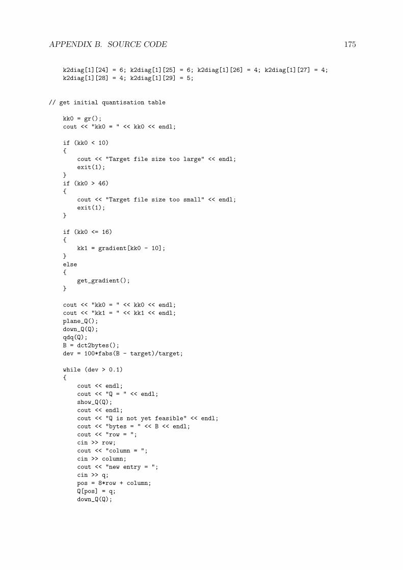
APPENDIX B. SOURCE CODE 175
k2diag[1][24] = 6; k2diag[1][25] = 6; k2diag[1][26] = 4; k2diag[1][27] = 4;
k2diag[1][28] = 4; k2diag[1][29] = 5;
// get initial quantisation table
kk0 = gr();
cout << "kk0 = " << kk0 << endl;
if (kk0 < 10)
{
cout << "Target file size too large" << endl;
exit(1);
}
if (kk0 > 46)
{
cout << "Target file size too small" << endl;
exit(1);
}
if (kk0 <= 16)
{
kk1 = gradient[kk0 - 10];
}
else
{
get_gradient();
}
cout << "kk0 = " << kk0 << endl;
cout << "kk1 = " << kk1 << endl;
plane_Q();
down_Q(Q);
qdq(Q);
B = dct2bytes();
dev = 100*fabs(B - target)/target;
while (dev > 0.1)
{
cout << endl;
cout << "Q = " << endl;
show_Q(Q);
cout << endl;
cout << "Q is not yet feasible" << endl;
cout << "bytes = " << B << endl;
cout << "row = ";
cin >> row;
cout << "column = ";
cin >> column;
cout << "new entry = ";
cin >> q;
pos = 8*row + column;
Q[pos] = q;
down_Q(Q);

APPENDIX B. SOURCE CODE 176
qdq(Q);
B = dct2bytes();
dev = 100*fabs(B - target)/target;
}
cout << endl;
cout << "Q is now feasible" << endl;
if (atoi(argv[2]) == 1)
{
// feasible Q is first member of old_pop
copy_table(Q, old_pop[0]);
// fill in rest of old_pop
for (k = 1 ; k < pop_size ; k++)
{
for (pos = 0 ; pos < 64 ; pos++)
{
x = rand();
x = x/RAND_MAX;
old_pop[k][pos] = Q[pos] + int(round(2*lower*x - lower));
old_pop[k][pos] = int(fmax(old_pop[k][pos], 1));
old_pop[k][pos] = int(fmin(old_pop[k][pos], 255));
}
}
cout << "Q = " << endl;
show_Q(Q);
cout << endl;
cout << "Running Genetic Algorithm" << endl;
ga();
}
L1:
cout << "initial table = " << endl;
show_Q(Q);
// quantise and dequantise Y
down_Q(Q);
qdq(Q);
// calculate error
E = calc_error();
cout << "Error = " << E << endl;
// calculate bytes
B = dct2bytes();
cout << "bytes = " << B << endl;
// main algorithm
Rmax = INFINITY; Rmin = 0;
while (Rmax > Rmin)
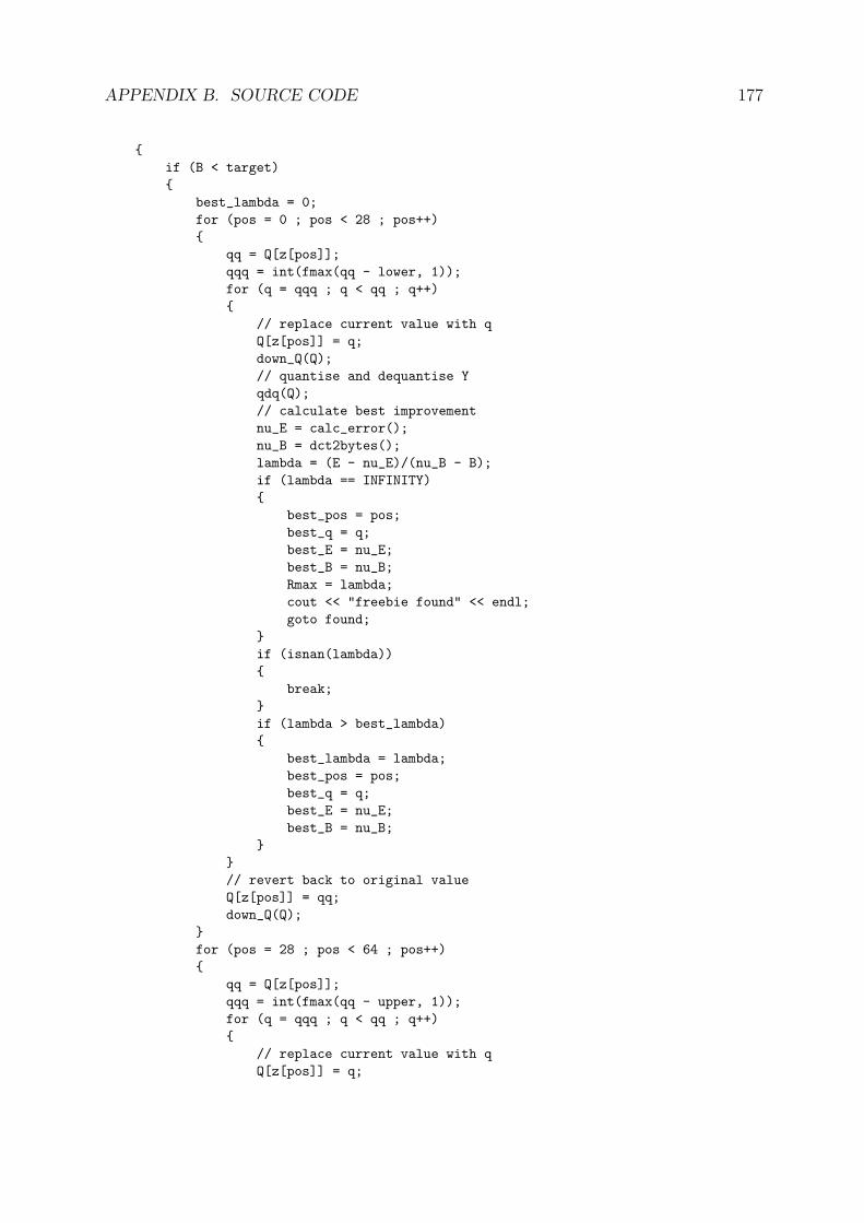
APPENDIX B. SOURCE CODE 177
{
if (B < target)
{
best_lambda = 0;
for (pos = 0 ; pos < 28 ; pos++)
{
qq = Q[z[pos]];
qqq = int(fmax(qq - lower, 1));
for (q = qqq ; q < qq ; q++)
{
// replace current value with q
Q[z[pos]] = q;
down_Q(Q);
// quantise and dequantise Y
qdq(Q);
// calculate best improvement
nu_E = calc_error();
nu_B = dct2bytes();
lambda = (E - nu_E)/(nu_B - B);
if (lambda == INFINITY)
{
best_pos = pos;
best_q = q;
best_E = nu_E;
best_B = nu_B;
Rmax = lambda;
cout << "freebie found" << endl;
goto found;
}
if (isnan(lambda))
{
break;
}
if (lambda > best_lambda)
{
best_lambda = lambda;
best_pos = pos;
best_q = q;
best_E = nu_E;
best_B = nu_B;
}
}
// revert back to original value
Q[z[pos]] = qq;
down_Q(Q);
}
for (pos = 28 ; pos < 64 ; pos++)
{
qq = Q[z[pos]];
qqq = int(fmax(qq - upper, 1));
for (q = qqq ; q < qq ; q++)
{
// replace current value with q
Q[z[pos]] = q;

APPENDIX B. SOURCE CODE 178
down_Q(Q);
// quantise and dequantise Y
qdq(Q);
// calculate best improvement
nu_E = calc_error();
nu_B = dct2bytes();
lambda = (E - nu_E)/(nu_B - B);
if (lambda == INFINITY)
{
best_pos = pos;
best_q = q;
best_E = nu_E;
best_B = nu_B;
Rmax = lambda;
cout << "freebie found" << endl;
goto found;
}
if (isnan(lambda))
{
break;
}
if (lambda > best_lambda)
{
best_lambda = lambda;
best_pos = pos;
best_q = q;
best_E = nu_E;
best_B = nu_B;
}
}
// revert back to original value
Q[z[pos]] = qq;
down_Q(Q);
}
Rmax = best_lambda;
}
else
{
best_lambda = INFINITY;
for (pos = 0 ; pos < 28 ; pos++)
{
qq = Q[z[pos]];
qqq = int(fmin(qq + lower, 255));
for (q = qq + 1 ; q <= qqq ; q++)
{
// replace current value with q
Q[z[pos]] = q;
down_Q(Q);
// quantise and dequantise Y
qdq(Q);
// calculate minimal degradation
nu_E = calc_error();
nu_B = dct2bytes();
lambda = (nu_E - E)/(B - nu_B);

APPENDIX B. SOURCE CODE 179
if (isnan(lambda))
{
break;
}
if ((lambda < best_lambda) && (lambda > 0))
{
best_lambda = lambda;
best_pos = pos;
best_q = q;
best_E = nu_E;
best_B = nu_B;
}
}
// revert back to original value
Q[z[pos]] = qq;
down_Q(Q);
}
for (pos = 28 ; pos < 64 ; pos++)
{
qq = Q[z[pos]];
qqq = int(fmin(qq + upper, 255));
for (q = qq + 1 ; q <= qqq ; q++)
{
// replace current value with q
Q[z[pos]] = q;
down_Q(Q);
// quantise and dequantise Y
qdq(Q);
// calculate minimal degradation
nu_E = calc_error();
nu_B = dct2bytes();
lambda = (nu_E - E)/(B - nu_B);
if (isnan(lambda))
{
break;
}
if ((lambda < best_lambda) && (lambda > 0))
{
best_lambda = lambda;
best_pos = pos;
best_q = q;
best_E = nu_E;
best_B = nu_B;
}
}
// revert back to original value
Q[z[pos]] = qq;
down_Q(Q);
}
Rmin = best_lambda;
}
// update quantisation table
found:
Q[z[best_pos]] = best_q;

APPENDIX B. SOURCE CODE 180
down_Q(Q);
show_Q(Q);
B = best_B;
E = best_E;
cout << "bytes = " << B << endl;
cout << "Error = " << E << endl;
}
return 0;
}

Appendix C
Sensitivity Analysis
diag Widths Widths Widths lo = 1, hi = 1 Initial QTT (bytes) B (bytes) B (bytes) B (bytes) B (bytes) B (bytes)
PSNR PSNR PSNR PSNR PSNR10 lo = 1, hi = 2
14839 14840 14840 1482640.2454 dB 40.2451 dB 40.1679 dB
11 lo = 2, hi = 3 lo = 1, hi = 3 lo = 2, hi = 214057 14058 14057 14059 14059 14064
39.7846 dB 39.7812 dB 39.7931 dB 39.7708 dB 39.7069 dB12 lo = 2, hi = 4 lo = 1, hi = 4 lo = 2, hi = 3
13461 13463 13463 13464 13461 1345439.4207 dB 39.4162 dB 39.4151 dB 39.4128 dB 39.2889 dB
13 lo = 2, hi = 2 lo = 1, hi = 212664 12664 12665 12664 12659
38.8768 dB 38.8687 dB 38.8626 dB 38.7605 dB14 lo = 1, hi = 2
11788 11790 11791 1178438.2526 dB 38.2497 dB 38.1301 dB
15 lo = 3, hi = 3 lo = 2, hi = 3 lo = 2, hi = 211403 11401 11401 11403 11404 11408
37.9621 dB 37.9621 dB 37.9578 dB 37.9418 dB 37.8744 dB16 lo = 3, hi = 4 lo = 2, hi = 4 lo = 3, hi = 3
10717 10715 10715 10714 10718 1072137.4314 dB 37.4341 dB 37.4365 dB 37.4087 dB 37.3230 dB
17 lo = 3, hi = 4 lo = 2, hi = 4 lo = 3, hi = 310468 10466 10469 10468 10469 10474
37.2367 dB 37.2350 dB 37.2380 dB 37.2205 dB 37.1463 dB18 lo = 4, hi = 4 lo = 3, hi = 4 lo = 3, hi = 3
10311 10311 10313 10313 10313 1030837.1028 dB 37.1095 dB 37.1097 dB 37.0921 dB 36.9705 dB
19 lo = 5, hi = 5 lo = 4, hi = 5 lo = 4, hi = 49897 9903 9900 9897 9897 9904
36.7720 dB 36.7677 dB 36.7569 dB 36.7353 dB 36.6461 dB20 lo = 4, hi = 5 lo = 3, hi = 5 lo = 4, hi = 4
9521 9520 9521 9522 9521 952636.4327 dB 36.4289 dB 36.4350 dB 36.4079 dB 36.3228 dB
Table C.1: Results obtained for Lena (continued on next page)
181
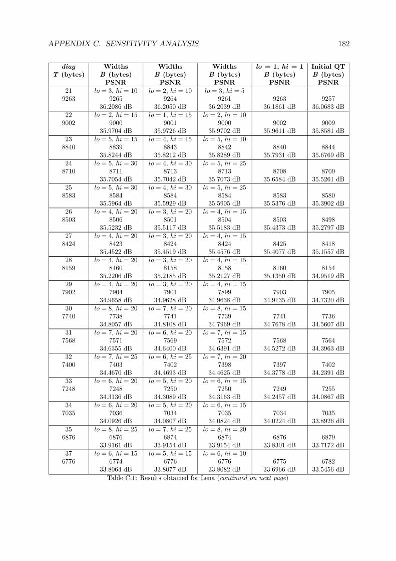
APPENDIX C. SENSITIVITY ANALYSIS 182
diag Widths Widths Widths lo = 1, hi = 1 Initial QTT (bytes) B (bytes) B (bytes) B (bytes) B (bytes) B (bytes)
PSNR PSNR PSNR PSNR PSNR21 lo = 3, hi = 10 lo = 2, hi = 10 lo = 3, hi = 5
9263 9265 9264 9261 9263 925736.2086 dB 36.2050 dB 36.2039 dB 36.1861 dB 36.0683 dB
22 lo = 2, hi = 15 lo = 1, hi = 15 lo = 2, hi = 109002 9000 9001 9000 9002 9009
35.9704 dB 35.9726 dB 35.9702 dB 35.9611 dB 35.8581 dB23 lo = 5, hi = 15 lo = 4, hi = 15 lo = 5, hi = 10
8840 8839 8843 8842 8840 884435.8244 dB 35.8212 dB 35.8289 dB 35.7931 dB 35.6769 dB
24 lo = 5, hi = 30 lo = 4, hi = 30 lo = 5, hi = 258710 8711 8713 8713 8708 8709
35.7054 dB 35.7042 dB 35.7073 dB 35.6584 dB 35.5261 dB25 lo = 5, hi = 30 lo = 4, hi = 30 lo = 5, hi = 25
8583 8584 8584 8584 8583 858035.5964 dB 35.5929 dB 35.5905 dB 35.5376 dB 35.3902 dB
26 lo = 4, hi = 20 lo = 3, hi = 20 lo = 4, hi = 158503 8506 8501 8504 8503 8498
35.5232 dB 35.5117 dB 35.5183 dB 35.4373 dB 35.2797 dB27 lo = 4, hi = 20 lo = 3, hi = 20 lo = 4, hi = 15
8424 8423 8424 8424 8425 841835.4522 dB 35.4519 dB 35.4576 dB 35.4077 dB 35.1557 dB
28 lo = 4, hi = 20 lo = 3, hi = 20 lo = 4, hi = 158159 8160 8158 8158 8160 8154
35.2206 dB 35.2185 dB 35.2127 dB 35.1350 dB 34.9519 dB29 lo = 4, hi = 20 lo = 3, hi = 20 lo = 4, hi = 15
7902 7904 7901 7899 7903 790534.9658 dB 34.9628 dB 34.9638 dB 34.9135 dB 34.7320 dB
30 lo = 8, hi = 20 lo = 7, hi = 20 lo = 8, hi = 157740 7738 7741 7739 7741 7736
34.8057 dB 34.8108 dB 34.7969 dB 34.7678 dB 34.5607 dB31 lo = 7, hi = 20 lo = 6, hi = 20 lo = 7, hi = 15
7568 7571 7569 7572 7568 756434.6355 dB 34.6400 dB 34.6391 dB 34.5272 dB 34.3963 dB
32 lo = 7, hi = 25 lo = 6, hi = 25 lo = 7, hi = 207400 7403 7402 7398 7397 7402
34.4670 dB 34.4693 dB 34.4625 dB 34.3778 dB 34.2391 dB33 lo = 6, hi = 20 lo = 5, hi = 20 lo = 6, hi = 15
7248 7248 7250 7250 7249 725534.3136 dB 34.3089 dB 34.3163 dB 34.2457 dB 34.0867 dB
34 lo = 6, hi = 20 lo = 5, hi = 20 lo = 6, hi = 157035 7036 7034 7035 7034 7035
34.0926 dB 34.0807 dB 34.0824 dB 34.0224 dB 33.8926 dB35 lo = 8, hi = 25 lo = 7, hi = 25 lo = 8, hi = 20
6876 6876 6874 6874 6876 687933.9161 dB 33.9154 dB 33.9154 dB 33.8301 dB 33.7172 dB
37 lo = 6, hi = 15 lo = 5, hi = 15 lo = 6, hi = 106776 6774 6776 6776 6775 6782
33.8064 dB 33.8077 dB 33.8082 dB 33.6966 dB 33.5456 dB
Table C.1: Results obtained for Lena (continued on next page)

APPENDIX C. SENSITIVITY ANALYSIS 183
diag Widths Widths Widths lo = 1, hi = 1 Initial QTT (bytes) B (bytes) B (bytes) B (bytes) B (bytes) B (bytes)
PSNR PSNR PSNR PSNR PSNR38 lo = 7, hi = 35 lo = 6, hi = 35 lo = 7, hi = 30
6667 6667 6668 6668 6667 666233.6782 dB 33.6745 dB 33.6755 dB 33.5571 dB 33.4058 dB
39 lo = 7, hi = 35 lo = 6, hi = 35 lo = 7, hi = 306508 6508 6508 6510 6509 6503
33.4900 dB 33.5007 dB 33.4824 dB 33.3657 dB 33.2580 dB40 lo = 7, hi = 35 lo = 6, hi = 35 lo = 7, hi = 30
6377 6377 6377 6375 6379 637333.3299 dB 33.3370 dB 33.3337 dB 33.2355 dB 33.1112 dB
41 lo = 11, hi = 35 lo = 10, hi = 35 lo = 11, hi = 306304 6306 6303 6306 6305 6305
33.2503 dB 33.2484 dB 33.2545 dB 33.1244 dB 33.0098 dB42 lo = 6, hi = 35 lo = 5, hi = 35 lo = 6, hi = 30
6260 6260 6262 6262 6259 626233.1920 dB 33.2034 dB 33.1994 dB 33.1037 dB 32.9432 dB
43 lo = 7, hi = 35 lo = 6, hi = 35 lo = 7, hi = 306193 6193 6192 6193 6190 6190
33.1211 dB 33.1201 dB 33.1204 dB 33.0059 dB 32.8594 dB44 lo = 6, hi = 35 lo = 5, hi = 35 lo = 6, hi = 30
6150 6151 6148 6153 6151 614733.0743 dB 33.0624 dB 33.0722 dB 32.9700 dB 32.7913 dB
45 lo = 12, hi = 35 lo = 11, hi = 35 lo = 12, hi = 306056 6056 6056 6058 6056 6052
32.9580 dB 32.9569 dB 32.9617 dB 32.8752 dB 32.7030 dB46 lo = 9, hi = 35 lo = 8, hi = 35 lo = 9, hi = 30
5940 5939 5938 5942 5941 594032.8278 dB 32.8259 dB 32.8251 dB 32.7364 dB 32.5864 dB
47 lo = 9, hi = 35 lo = 8, hi = 35 lo = 9, hi = 305859 5862 5861 5860 5856 5863
32.7413 dB 32.7271 dB 32.7282 dB 32.6394 dB 32.4889 dB48 lo = 14, hi = 35 lo = 13, hi = 35 lo = 14, hi = 30
5840 5842 5840 5839 5843 584232.7077 dB 32.7082 dB 32.7071 dB 32.6174 dB 32.4459 dB
49 lo = 8, hi = 35 lo = 7, hi = 35 lo = 8, hi = 305658 5657 5660 5658 5658 5656
32.4900 dB 32.4927 dB 32.4906 dB 32.4151 dB 32.2707 dB50 lo = 9, hi = 35 lo = 8, hi = 35 lo = 9, hi = 30
5549 5549 5549 5548 5549 554632.3637 dB 32.3641 dB 32.3640 dB 32.2455 dB 32.1367 dB
51 lo = 10, hi = 35 lo = 9, hi = 35 lo = 10, hi = 305448 5447 5449 5449 5449 5446
32.2268 dB 32.2376 dB 32.2345 dB 32.1325 dB 31.9864 dB52 lo = 8, hi = 35 lo = 7, hi = 35 lo = 8, hi = 30
5216 5218 5218 5216 5218 522031.9223 dB 31.9299 dB 31.9215 dB 31.8341 dB 31.7472 dB
53 lo = 9, hi = 35 lo = 8, hi = 35 lo = 9, hi = 305106 5108 5104 5108 5106 5106
31.7650 dB 31.7678 dB 31.7792 dB 31.6692 dB 31.6148 dB
Table C.1: Results obtained for Lena (continued on next page)

APPENDIX C. SENSITIVITY ANALYSIS 184
diag Widths Widths Widths lo = 1, hi = 1 Initial QTT (bytes) B (bytes) B (bytes) B (bytes) B (bytes) B (bytes)
PSNR PSNR PSNR PSNR PSNR54 lo = 9, hi = 35 lo = 8, hi = 35 lo = 9, hi = 30
4979 4981 4977 4977 4979 497631.5955 dB 31.5888 dB 31.5892 dB 31.4953 dB 31.4324 dB
Table C.1: Results obtained for Lena (continued)
diag Widths Widths Widths lo = 1, hi = 1 Initial QTT (bytes) B (bytes) B (bytes) B (bytes) B (bytes) B (bytes)
PSNR PSNR PSNR PSNR PSNR10 lo = 1, hi = 2
17157 17159 17162 1717140.0746 dB 40.0840 dB 40.0195 dB
11 lo = 2, hi = 2 lo = 1, hi = 215904 15901 15909 15907 15919
39.2636 dB 39.2660 dB 39.2652 dB 39.1971 dB12 lo = 1, hi = 2
15464 15466 15465 1546538.9686 dB 38.9785 dB 38.8582 dB
13 lo = 2, hi = 3 lo = 1, hi = 3 lo = 2, hi = 214392 14389 14395 14394 14394 14387
38.2095 dB 38.2098 dB 38.2111 dB 38.1959 dB 38.1417 dB14 lo = 3, hi = 3 lo = 2, hi = 3 lo = 2, hi = 2
14016 14018 14016 14016 14014 1402137.9440 dB 37.9377 dB 37.9377 dB 37.9255 dB 37.8460 dB
15 lo = 3, hi = 4 lo = 2, hi = 4 lo = 3, hi = 313164 13164 13163 13163 13165 13161
37.3267 dB 37.3288 dB 37.3303 dB 37.3128 dB 37.2064 dB16 lo = 3, hi = 5 lo = 2, hi = 5 lo = 3, hi = 4
12890 12892 12893 12893 12892 1288137.1232 dB 37.1231 dB 37.1213 dB 37.1094 dB 36.9651 dB
17 lo = 3, hi = 10 lo = 2, hi = 10 lo = 3, hi = 512300 12300 12303 12298 12299 12307
36.6536 dB 36.6485 dB 36.6465 dB 36.6302 dB 36.5301 dB18 lo = 3, hi = 5 lo = 2, hi = 5 lo = 3, hi = 4
11744 11744 11746 11745 11744 1174436.1948 dB 36.1825 dB 36.1908 dB 36.1807 dB 36.0884 dB
19 lo = 4, hi = 4 lo = 3, hi = 4 lo = 3, hi = 311395 11395 11395 11395 11396 11404
35.8913 dB 35.8913 dB 35.8913 dB 35.8732 dB 35.7922 dB20 lo = 4, hi = 4 lo = 3, hi = 4 lo = 3, hi = 3
11131 11134 11131 11129 11131 1113435.6635 dB 35.6561 dB 35.6497 dB 35.6293 dB 35.5265 dB
21 lo = 4, hi = 5 lo = 3, hi = 5 lo = 4, hi = 410745 10746 10744 10746 10744 10742
35.2977 dB 35.2886 dB 35.2974 dB 35.2720 dB 35.1813 dB
Table C.2: Results obtained for Plane (continued on next page)

APPENDIX C. SENSITIVITY ANALYSIS 185
diag Widths Widths Widths lo = 1, hi = 1 Initial QTT (bytes) B (bytes) B (bytes) B (bytes) B (bytes) B (bytes)
PSNR PSNR PSNR PSNR PSNR22 lo = 4, hi = 10 lo = 3, hi = 10 lo = 4, hi = 5
10505 10506 10506 10505 10508 1050635.0820 dB 35.0807 dB 35.0850 dB 35.0322 dB 34.9395 dB
23 lo = 4, hi = 10 lo = 3, hi = 10 lo = 4, hi = 510346 10343 10346 10346 10347 10350
34.9386 dB 34.9291 dB 34.9325 dB 34.8856 dB 34.7462 dB24 lo = 5, hi = 5 lo = 4, hi = 5 lo = 4, hi = 4
10099 10098 10098 10102 10099 1009834.7350 dB 34.7299 dB 34.7307 dB 34.6676 dB 34.5145 dB
25 lo = 4, hi = 5 lo = 3, hi = 5 lo = 4, hi = 49947 9947 9948 9949 9945 9945
34.5924 dB 34.5860 dB 34.5912 dB 34.5316 dB 34.3365 dB26 lo = 5, hi = 15 lo = 4, hi = 15 lo = 5, hi = 10
9806 9807 9805 9805 9808 979934.4666 dB 34.4600 dB 34.4628 dB 34.4012 dB 34.1586 dB
27 lo = 7, hi = 10 lo = 6, hi = 10 lo = 5, hi = 59608 9609 9607 9606 9606 9607
34.2916 dB 34.2796 dB 34.2818 dB 34.1863 dB 33.9619 dB28 lo = 7, hi = 10 lo = 6, hi = 10 lo = 5, hi = 5
9314 9313 9313 9315 9315 930834.0187 dB 34.0200 dB 34.0161 dB 33.9351 dB 33.7317 dB
29 lo = 5, hi = 20 lo = 4, hi = 20 lo = 5, hi = 159226 9225 9226 9224 9227 9225
33.9416 dB 33.9459 dB 33.9399 dB 33.8426 dB 33.5783 dB30 lo = 7, hi = 30 lo = 6, hi = 30 lo = 7, hi = 25
8853 8853 8852 8855 8852 885333.5802 dB 33.5748 dB 33.5832 dB 33.5133 dB 33.3150 dB
31 lo = 6, hi = 25 lo = 5, hi = 25 lo = 6, hi = 208689 8688 8688 8692 8690 8694
33.4168 dB 33.4131 dB 33.4153 dB 33.3391 dB 33.1584 dB32 lo = 5, hi = 15 lo = 4, hi = 15 lo = 5, hi = 10
8540 8540 8541 8539 8540 854333.2718 dB 33.2580 dB 33.2618 dB 33.1482 dB 33.0094 dB
33 lo = 6, hi = 15 lo = 5, hi = 15 lo = 6, hi = 108319 8320 8317 8321 8320 8325
33.0640 dB 33.0551 dB 33.0612 dB 32.9461 dB 32.8107 dB34 lo = 7, hi = 30 lo = 6, hi = 30 lo = 7, hi = 25
8106 8106 8105 8104 8107 811232.8597 dB 32.8596 dB 32.8561 dB 32.7579 dB 32.6145 dB
35 lo = 4, hi = 20 lo = 3, hi = 20 lo = 4, hi = 157881 7879 7882 7882 7881 7879
32.6401 dB 32.6295 dB 32.6374 dB 32.5312 dB 32.4026 dB36 lo = 5, hi = 25 lo = 4, hi = 25 lo = 5, hi = 20
7740 7741 7741 7741 7740 774232.5103 dB 32.5097 dB 32.5112 dB 32.4058 dB 32.2680 dB
37 lo = 6, hi = 20 lo = 5, hi = 20 lo = 6, hi = 157706 7704 7705 7707 7705 7707
32.4714 dB 32.4776 dB 32.4722 dB 32.3725 dB 32.2147 dB
Table C.2: Results obtained for Plane (continued on next page)

APPENDIX C. SENSITIVITY ANALYSIS 186
diag Widths Widths Widths lo = 1, hi = 1 Initial QTT (bytes) B (bytes) B (bytes) B (bytes) B (bytes) B (bytes)
PSNR PSNR PSNR PSNR PSNR38 lo = 8, hi = 20 lo = 7, hi = 20 lo = 8, hi = 15
7565 7567 7567 7564 7565 756632.3397 dB 32.3316 dB 32.3365 dB 32.2226 dB 32.0789 dB
39 lo = 9, hi = 20 lo = 8, hi = 20 lo = 9, hi = 157337 7336 7338 7337 7334 7338
32.1127 dB 32.1063 dB 32.1158 dB 32.0184 dB 31.8930 dB40 lo = 9, hi = 20 lo = 8, hi = 20 lo = 9, hi = 15
7233 7235 7233 7234 7234 723232.0258 dB 32.0254 dB 32.0107 dB 31.8999 dB 31.7739 dB
41 lo = 9, hi = 20 lo = 8, hi = 20 lo = 9, hi = 157142 7142 7140 7144 7141 7140
31.9298 dB 31.9233 dB 31.9257 dB 31.7743 dB 31.6551 dB42 lo = 9, hi = 25 lo = 8, hi = 25 lo = 9, hi = 20
7031 7032 7030 7030 7032 703231.8140 dB 31.8154 dB 31.8124 dB 31.6391 dB 31.5497 dB
43 lo = 9, hi = 25 lo = 8, hi = 25 lo = 9, hi = 206918 6919 6920 6919 6918 6920
31.7029 dB 31.7013 dB 31.7009 dB 31.5870 dB 31.4594 dB44 lo = 9, hi = 30 lo = 8, hi = 30 lo = 9, hi = 25
6840 6839 6839 6840 6840 683631.6230 dB 31.6141 dB 31.6195 dB 31.5051 dB 31.3690 dB
45 lo = 9, hi = 20 lo = 8, hi = 20 lo = 9, hi = 156755 6755 6757 6757 6756 6757
31.5233 dB 31.5334 dB 31.5281 dB 31.4201 dB 31.2799 dB46 lo = 9, hi = 25 lo = 8, hi = 25 lo = 9, hi = 20
6623 6623 6625 6622 6622 662831.3844 dB 31.3824 dB 31.3840 dB 31.2923 dB 31.1486 dB
47 lo = 9, hi = 25 lo = 8, hi = 25 lo = 9, hi = 206534 6535 6535 6534 6534 6538
31.2896 dB 31.2919 dB 31.2894 dB 31.1657 dB 31.0355 dB49 lo = 8, hi = 25 lo = 7, hi = 25 lo = 8, hi = 20
6421 6420 6420 6423 6420 641731.1682 dB 31.1694 dB 31.1682 dB 31.0396 dB 30.8816 dB
50 lo = 8, hi = 25 lo = 7, hi = 25 lo = 8, hi = 206286 6286 6285 6289 6286 6281
31.0317 dB 31.0273 dB 31.0265 dB 30.8961 dB 30.7621 dB51 lo = 9, hi = 25 lo = 8, hi = 25 lo = 9, hi = 20
6100 6101 6101 6099 6100 610330.8228 dB 30.8262 dB 30.8209 dB 30.6801 dB 30.5947 dB
52 lo = 12, hi = 30 lo = 11, hi = 30 lo = 12, hi = 255955 5957 5955 5955 5955 5955
30.6633 dB 30.6668 dB 30.6610 dB 30.5373 dB 30.4477 dB53 lo = 14, hi = 30 lo = 13, hi = 30 lo = 14, hi = 25
5847 5846 5848 5848 5847 584430.5416 dB 30.5395 dB 30.5353 dB 30.4061 dB 30.3323 dB
Table C.2: Results obtained for Plane (continued)

APPENDIX C. SENSITIVITY ANALYSIS 187
diag Widths Widths Widths lo = 1, hi = 1 Initial QTT (bytes) B (bytes) B (bytes) B (bytes) B (bytes) B (bytes)
PSNR PSNR PSNR PSNR PSNR10 lo = 2, hi = 2 lo = 1, hi = 2
25200 25198 25203 25201 2522039.1426 dB 39.1328 dB 39.1437 dB 39.0200 dB
11 lo = 2, hi = 2 lo = 1, hi = 223776 23775 23775 23775 23791
38.1606 dB 38.1454 dB 38.1454 dB 38.0644 dB12 lo = 3, hi = 3 lo = 2, hi = 3 lo = 2, hi = 2
23200 23200 23202 23202 23197 2321137.7483 dB 37.7503 dB 37.7503 dB 37.7519 dB 37.6089 dB
13 lo = 2, hi = 4 lo = 1, hi = 4 lo = 2, hi = 322080 22082 22075 22082 22084 22094
36.9383 dB 36.9266 dB 36.9417 dB 36.9246 dB 36.8556 dB14 lo = 2, hi = 3 lo = 1, hi = 3 lo = 2, hi = 2
21416 21420 21420 21413 21420 2142236.4666 dB 36.4752 dB 36.4656 dB 36.4570 dB 36.3522 dB
15 lo = 3, hi = 4 lo = 2, hi = 4 lo = 3, hi = 320633 20634 20637 20632 20628 20630
35.9281 dB 35.9299 dB 35.9203 dB 35.9069 dB 35.8157 dB16 lo = 4, hi = 4 lo = 3, hi = 4 lo = 3, hi = 3
20070 20073 20076 20076 20076 2006035.5671 dB 35.5684 dB 35.5684 dB 35.5493 dB 35.3665 dB
17 lo = 4, hi = 4 lo = 3, hi = 4 lo = 3, hi = 319426 19423 19425 19424 19427 19407
35.1241 dB 35.1320 dB 35.1314 dB 35.1078 dB 34.9382 dB18 lo = 3, hi = 15 lo = 2, hi = 15 lo = 3, hi = 10
18533 18536 18530 18534 18535 1854234.5156 dB 34.5140 dB 34.5149 dB 34.5059 dB 34.4017 dB
19 lo = 4, hi = 15 lo = 3, hi = 15 lo = 4, hi = 1018029 18028 18032 18029 18028 18013
34.1848 dB 34.1878 dB 34.1875 dB 34.1563 dB 34.0434 dB20 lo = 3, hi = 10 lo = 2, hi = 10 lo = 3, hi = 5
17416 17417 17419 17417 17414 1742333.7853 dB 33.7908 dB 33.7888 dB 33.7609 dB 33.6773 dB
21 lo = 3, hi = 10 lo = 2, hi = 10 lo = 3, hi = 516824 16824 16824 16823 16822 16829
33.4110 dB 33.4033 dB 33.4081 dB 33.3904 dB 33.3028 dB22 lo = 3, hi = 10 lo = 2, hi = 10 lo = 3, hi = 5
16328 16329 16327 16328 16328 1633033.0948 dB 33.0945 dB 33.0979 dB 33.0623 dB 32.9790 dB
23 lo = 3, hi = 10 lo = 2, hi = 10 lo = 3, hi = 515951 15954 15952 15954 15952 15953
32.8579 dB 32.8577 dB 32.8627 dB 32.8270 dB 32.7277 dB24 lo = 5, hi = 10 lo = 4, hi = 10 lo = 5, hi = 5
15688 15690 15691 15691 15690 1567832.6890 dB 32.6820 dB 32.6871 dB 32.6572 dB 32.4897 dB
25 lo = 4, hi = 15 lo = 3, hi = 15 lo = 4, hi = 1015358 15360 15360 15361 15358 15354
32.4709 dB 32.4706 dB 32.4719 dB 32.4493 dB 32.2726 dB
Table C.3: Results obtained for Bridge (continued on next page)

APPENDIX C. SENSITIVITY ANALYSIS 188
diag Widths Widths Widths lo = 1, hi = 1 Initial QTT (bytes) B (bytes) B (bytes) B (bytes) B (bytes) B (bytes)
PSNR PSNR PSNR PSNR PSNR26 lo = 5, hi = 10 lo = 4, hi = 10 lo = 5, hi = 5
14991 14990 14990 14991 14993 1498632.2428 dB 32.2420 dB 32.2418 dB 32.2285 dB 32.0404 dB
27 lo = 5, hi = 10 lo = 4, hi = 10 lo = 5, hi = 514600 14598 14599 14597 14601 14599
32.0002 dB 31.9979 dB 31.9956 dB 31.9744 dB 31.8195 dB28 lo = 4, hi = 10 lo = 3, hi = 10 lo = 4, hi = 5
14192 14191 14193 14190 14191 1419131.7487 dB 31.7511 dB 31.7442 dB 31.7050 dB 31.5712 dB
29 lo = 6, hi = 10 lo = 5, hi = 10 lo = 5, hi = 513971 13973 13971 13971 13972 13968
31.6133 dB 31.6120 dB 31.6024 dB 31.5727 dB 31.3894 dB30 lo = 6, hi = 10 lo = 5, hi = 10 lo = 5, hi = 5
13515 13516 13517 13514 13515 1351531.3203 dB 31.3249 dB 31.3108 dB 31.2743 dB 31.1450 dB
31 lo = 6, hi = 10 lo = 5, hi = 10 lo = 5, hi = 513252 13250 13251 13251 13249 13251
31.1517 dB 31.1521 dB 31.1523 dB 31.1172 dB 30.9512 dB32 lo = 5, hi = 10 lo = 4, hi = 10 lo = 5, hi = 5
12836 12836 12835 12836 12837 1283830.9172 dB 30.9113 dB 30.8992 dB 30.8491 dB 30.7461 dB
33 lo = 6, hi = 10 lo = 5, hi = 10 lo = 5, hi = 512530 12530 12530 12529 12530 12533
30.7309 dB 30.7259 dB 30.7089 dB 30.6710 dB 30.5557 dB34 lo = 6, hi = 25 lo = 5, hi = 25 lo = 6, hi = 20
12315 12316 12318 12312 12316 1232130.6110 dB 30.6126 dB 30.6098 dB 30.4998 dB 30.4091 dB
35 lo = 9, hi = 20 lo = 8, hi = 20 lo = 9, hi = 1511932 11935 11933 11935 11930 11928
30.3820 dB 30.3813 dB 30.3835 dB 30.2781 dB 30.1846 dB36 lo = 6, hi = 15 lo = 5, hi = 15 lo = 6, hi = 10
11632 11634 11633 11632 11631 1163530.2028 dB 30.2019 dB 30.2018 dB 30.1077 dB 29.9998 dB
37 lo = 5, hi = 20 lo = 4, hi = 20 lo = 5, hi = 1511482 11484 11483 11480 11481 11484
30.1227 dB 30.1050 dB 30.1222 dB 30.0434 dB 29.9193 dB38 lo = 7, hi = 15 lo = 6, hi = 15 lo = 7, hi = 10
11209 11205 11208 11212 11212 1121229.9593 dB 29.9608 dB 29.9568 dB 29.8811 dB 29.7610 dB
39 lo = 7, hi = 15 lo = 6, hi = 15 lo = 7, hi = 1011000 11002 11000 11001 11003 11002
29.8518 dB 29.8456 dB 29.8316 dB 29.7500 dB 29.6408 dB40 lo = 6, hi = 30 lo = 5, hi = 30 lo = 6, hi = 25
10745 10745 10747 10747 10744 1075129.7046 dB 29.7000 dB 29.6943 dB 29.5746 dB 29.4891 dB
41 lo = 6, hi = 30 lo = 5, hi = 30 lo = 6, hi = 2510506 10508 10506 10506 10506 10505
29.5610 dB 29.5608 dB 29.5605 dB 29.4155 dB 29.3434 dB
Table C.3: Results obtained for Bridge (continued on next page)

APPENDIX C. SENSITIVITY ANALYSIS 189
diag Widths Widths Widths lo = 1, hi = 1 Initial QTT (bytes) B (bytes) B (bytes) B (bytes) B (bytes) B (bytes)
PSNR PSNR PSNR PSNR PSNR42 lo = 6, hi = 20 lo = 5, hi = 20 lo = 6, hi = 15
10358 10360 10361 10360 10357 1035629.4686 dB 29.4656 dB 29.4713 dB 29.3565 dB 29.2620 dB
43 lo = 7, hi = 20 lo = 6, hi = 20 lo = 7, hi = 1510207 10208 10207 10206 10209 10215
29.3804 dB 29.3752 dB 29.3726 dB 29.2582 dB 29.1901 dB44 lo = 7, hi = 20 lo = 6, hi = 20 lo = 7, hi = 15
10069 10071 10070 10071 10069 1006529.2920 dB 29.2990 dB 29.3052 dB 29.1843 dB 29.0908 dB
45 lo = 7, hi = 30 lo = 6, hi = 30 lo = 7, hi = 259909 9907 9910 9907 9910 9906
29.2006 dB 29.2164 dB 29.2072 dB 29.0955 dB 29.0054 dB46 lo = 7, hi = 25 lo = 6, hi = 25 lo = 7, hi = 20
9740 9741 9738 9742 9741 973629.1037 dB 29.1135 dB 29.1009 dB 29.0113 dB 28.8878 dB
47 lo = 7, hi = 25 lo = 6, hi = 25 lo = 7, hi = 209550 9551 9551 9549 9550 9548
28.9928 dB 28.9902 dB 28.9884 dB 28.8778 dB 28.7747 dB48 lo = 8, hi = 20 lo = 7, hi = 20 lo = 8, hi = 15
9472 9471 9471 9473 9472 947128.9471 dB 28.9500 dB 28.9391 dB 28.8431 dB 28.7284 dB
49 lo = 8, hi = 20 lo = 7, hi = 20 lo = 8, hi = 159150 9147 9152 9153 9148 9147
28.7371 dB 28.7406 dB 28.7406 dB 28.6529 dB 28.5747 dB50 lo = 9, hi = 30 lo = 8, hi = 30 lo = 9, hi = 25
8987 8988 8986 8986 8988 898728.6499 dB 28.6329 dB 28.6457 dB 28.5466 dB 28.4533 dB
51 lo = 9, hi = 25 lo = 8, hi = 25 lo = 9, hi = 208672 8672 8674 8673 8673 8672
28.4536 dB 28.4360 dB 28.4580 dB 28.3292 dB 28.2591 dB
Table C.3: Results obtained for Bridge (continued)

Bibliography
[1] Hei Tao Fung and Kevin J. Parker. Design of image-adaptive quantization tables for JPEG. Journal
of Electronic Imaging, 4(2):144–150, 1995.
[2] Siu-Wai Wu and Allen Gersho. Rate-constrained picture-adaptive quantization for JPEG baselinecoders. In IEEE International Conference on Acoustics, Speech and Signal Processing, volume 5,pages 365–368, 1993.
[3] Viresh Ratnakar and Miron Livny. RD-OPT: An efficient algorithm for optimizing DCT quantizationtables. In Data Compression Conference, pages 332–341, 1995.
[4] Viresh Ratnakar and Miron Livny. RD-OPT: An efficient algorithm for optimizing DCT quantiza-tion. IEEE Transactions on Image Processing, 9(2):267–270, 2000.
[5] William B. Pennebaker and Joan L. Mitchell. JPEG: Still Image Data Compression Standard. VanNostrand Reinhold, New York, 1993.
[6] Tinku Acharya and Ping-Sing Tsai. JPEG2000: Standard for Image Compression. Wiley-Interscience, New Jersey, 2005.
[7] Jerome M. Shapiro. Embedded image coding using zerotrees of wavelet coefficients. IEEE Transac-
tions on Signal Processing, 41:3445–3459, 1993.
[8] Marina Bosi and Richard E. Goldberg. Introduction to Digital Audio Coding and Standards. Springer,New York, 2003.
[9] Ken C. Pohlmann. Principles of Digital Audio. McGraw-Hill, New York, 1995.
[10] John P. Princen and Alan Bernard Bradley. Analysis/synthesis filter bank design based on timedomain aliasing cancellation. IEEE Transactions on Accoustics, Speech, and Signal Processing,ASSP-34(5):1153–1161, 1986.
[11] Chi-Min Liu and Wen-Chieh Lee. A unified fast algorithm for cosine modulated filter banks incurrent audio coding standards. Journal of the Audio Engineering Society, 47:1061–1075, 1999.
[12] International Telecommunications Union, Radiocommunications Sector, Geneva. Methods for the
Subjective Assessment of Small Impairments in Audio Systems Including Multichannel Sound Sys-
tems, 1997. BS.1116 (rev. 1).
[13] Floris L. Van Nes and Maarten A. Bouman. Spatial modulation transfer in the human eye. Journal
of the Optical Society of America, 57(3):401–406, 1967.
[14] Kathy T. Mullen. The contrast sensitivity of human colour vision to red–green and blue–yellowchromatic gratings. Journal of Physiology, 359:381–400, 1985.
[15] Albert J. Ahumada and Heidi A. Peterson. Luminance-model-based DCT quantization for colorimage compression. In SPIE conference on Human Vision, Visual Processing, and Digital Display
III, volume 1666, pages 365–374, 1992.
[16] Albert J. Ahumada Heidi A. Peterson and Andrew B. Watson. An improved detection model forDCT coefficient quantization. In SPIE conference on Human Vision, Visual Processing, and Digital
Display IV, volume 1913, pages 191–201, 1993.
190
BIBLIOGRAPHY 191
[17] Andrew B. Watson. DCTune: A technique for visual optimization of DCT quantization matricesfor individual images. Society for Information Display Digest of Technical Papers, XXIV:946–949,1993.
[18] Andrew B. Watson. Visually optimal DCT quantization matrices for individual images. In Data
Compression Conference, pages 178–187, 1993.
[19] Andrew B. Watson. DCT quantization matrices visually optimized for individual images. In SPIE
conference on Human Vision, Visual Processing, and Digital Display IV, volume 1913, pages 202–216, 1993.
[20] Albert J. Ahumada Andrew B. Watson, Alan Gale and Joshua A. Solomon. DCT basis functionvisibility: Effects of viewing distance and contrast masking. In SPIE conference on Human Vision,
Visual Processing, and Digital Display IV, pages 99–108, 1994.
[21] Andrew B. Watson Joshua A. Solomon and Albert J. Ahumada. Visibility of DCT basis functions:Effects of contrast masking. In Data Compression Conference, pages 361–370, 1994.
[22] Ingo Hontsch and Lina J. Karam. Adaptive image coding with perceptual distortion control. IEEE
Transactions on Image Processing, 11(3):213–222, 2002.
[23] Trac Duy Tran and Robert Safranek. A locally adaptive perceptual masking threshold model forimage coding. In Proceedings of the IEEE International Conference on Acoustics, Speech and Signal
Processing, volume 4, pages 1882–1885, 1996.
[24] Trac Duy Tran. A locally adaptive perceptual masking threshold model for image coding. Master’sthesis, Massachusetts Institute of Technology, 1994.
[25] S. J. P. Westen, R. L. Lagendijk, and J. Biemond. Optimization of JPEG color image coding using ahuman visual system model. In SPIE conference on Human Vision and Electronic Imaging, volume2657, pages 370–381, 1996.
[26] Melanie Mitchell. An Introduction to Genetic Algorithms. The MIT Press, Massachusetts, 1996.
[27] M. H. Afshar and M. A. Marino. A parameter-free self-adapting boundary genetic search for pipenetwork optimization. Computational Optimization and Applications, 37:83–102, 2007.
[28] C. T. Kelly. Iterative Methods for Optimization. Society for Industrial and Applied Mathematics,Philadelphia, 1999.
[29] Matthew Crouse and Kannan Ramchandran. Joint thresholding and quantizer selection for transformimage coding: entropy-constrained analysis and applications to baseline JPEG. IEEE Transactions
on Image Processing, 6(2):285–297, 1997.