Applied Statistics using PAST - part 2

DISTRIBUTIONS

Dr. Efthymia Nikita

Athens 2013

The concept of distribution

Histograms of large samples give us a qualitative picture of the way in which the sample values are distributed around the mean or the median.

Therefore, they allow us to gain a rather intuitive notion of the concept of distribution.

For example consider the following two samples: The one on the left presents the wall thickness of pots (in mm) and the one on the right the lengths of metal knives (in cm) from an archaeological site.

19.7122.8226.3325.4329.8319.3519.1721.5920.1022.02

14.2821.8921.7618.9820.6425.1019.0924.3626.9422.32

17.3718.0017.8721.9621.3724.3022.0316.3221.8114.01

18.1821.2016.8022.2724.4223.7117.3416.3019.2024.00

23.6021.0014.5025.8017.6028.0016.0022.209.9015.00

16.5024.6017.6016.6027.4016.2039.0013.5022.2032.00

13.1010.7016.2020.0015.008.3024.4016.7019.8014.20

11.0018.2014.2013.5019.7012.4013.1018.108.7019.90


Histograms of the samples with wall thickness data (left) and knife length data

(right) with 10 classes (bins)


We observe that the values of the two samples are not distributed in the same way. In other words, the two samples exhibit different distributions.

In the case of the wall thickness data, the sample values appear to be symmetrically distributed around the mean, while the distribution of the knife length data is asymmetric.


Therefore, distribution is the way in which the values of a sample are dispersed around the mean or median and it is visualized primarily using histograms, provided that the sample sizes are large.

Experimental and theoretical studies have demonstrated that there are many different distributions.

The curve that passes from the upper surface of the histogram columns is called distribution curve.


Basic distributions NORMAL DISTRIBUTION, Ν(μ,σ2)

This is one of the most important distributions since many statistical tests require that the data follows it in order for the results to be valid.

A sample or a population is normal if the histogram is symmetric, bell-shaped, under the condition that the sample is large. In addition, 68% of the values should lie within one standard deviation (σ) of the mean (μ), 95% of the values within 2 standard deviations and 99.7% of the values should lie within 3 standard deviations of the mean.

Normal distribution histogramBasic distributions

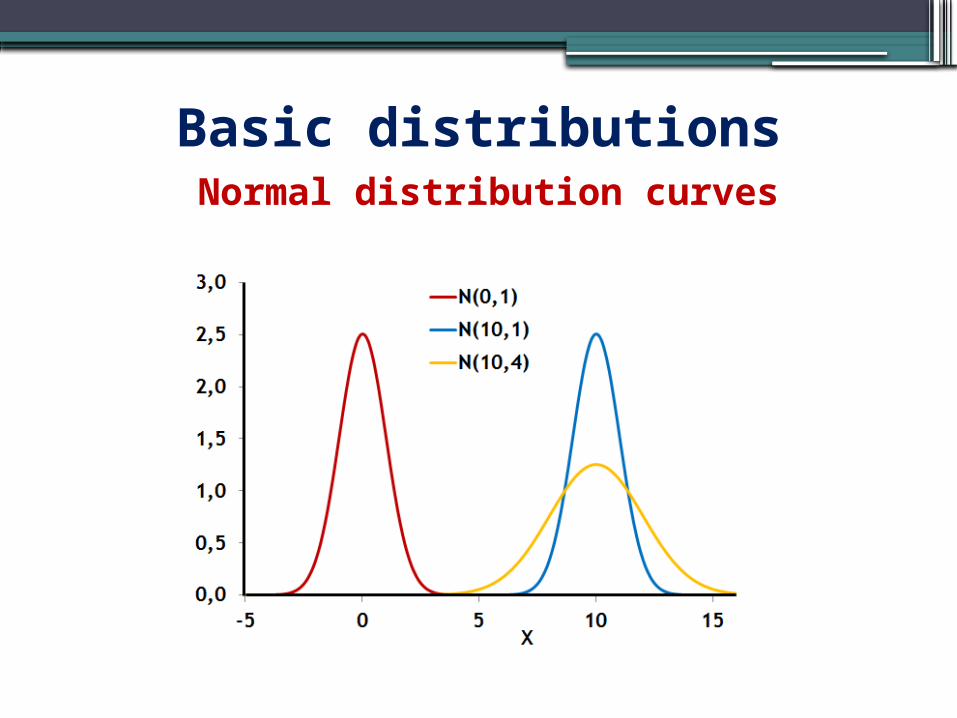
Normal distribution curvesBasic distributions

Basic distributions STANDARD NORMAL DISTRIBUTION, Ν(0,1)

It is the normal distribution when the mean value is equal to 0 (μ = 0) and the standard deviation equal to 1 (σ = 1).

BINOMIAL DISTRIBUTION

It is characteristic of samples with two possible outcomes with probabilities p and q = 1 - p, respectively.

For example, in archaeology it is used in cases where we study the presence or absence of a disease in the skeletal remains of a population.

Basic distributions

Binomial distribution curvesBasic distributions

Distribution curves (N, p), where N is the sample/population size and p

the probability

Note that as N increases, the distribution curves tend to be similar to the normal distribution curves (Central Limit Theorem).

There are many artificial distributions, i.e. distributions that do not appear in real samples but in samples that are created after various mathematical transformations of the values of real samples.

These distributions are used extensively in Inferential Statistics.

Other distributions

Student or t distribution The Student or t distribution is used in many statistical tests, particularly in order to define confidence intervals and in comparing the mean values of two samples.

Other distributions

Student or t distribution curvesOther distributions

Graphs of the Student distribution when ν = 1, 2, 4, . When ν = it becomes identical to the

standard normal distribution

ν=1

ν=

The student distribution has the name Student for the following reason:

Fun fact

William Gosset (1876-1937) worked for the Guinness brewery when he studied this distribution. The Irish brewery did not allow him to publish his results so he used the nickname ‘student’ since at the time he was studying at university.

Chi-square distribution

Other distributions

Graphs of the χ2 distribution when ν = 3, 5 and 10

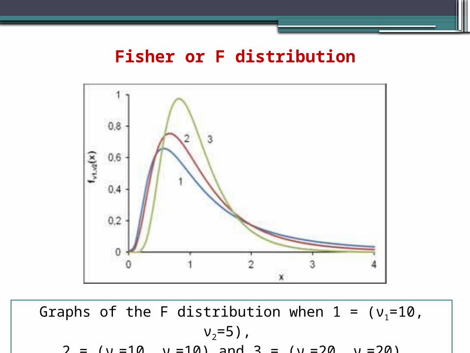
Graphs of the F distribution when 1 = (ν1=10, ν2=5),

2 = (ν1=10, ν2=10) and 3 = (ν1=20, ν2=20)

Fisher or F distribution

BASIC PRINCIPLES OF INFERENTIAL STATISTICS

Dr. Efthymia Nikita

Athens 2013

Statistical hypotheses We often have to make a decision relating

to: Comparing the characteristics of the

material culture among two or more archaeological sites and drawing conclusions about the life style, the cultural contacts and the impact of the natural environment.

Comparing the artifacts from different contexts within a site in order to examine different uses of the space.

Comparing the results obtained by different methods in order to test their validity.

Statistical hypotheses In all these cases we formulate certain statistical hypotheses and subsequently we run analyses in order to see which hypothesis will be accepted and at what price.

However, the statistical hypotheses we can use and test are specific and depend on the type of problem we are examining.

We CANNOT use any hypothesis that comes to our mind.

The null hypothesis In every problem we select the statistical hypotheses that have already been proposed for the study of that specific problem.

In every problem we formulate two hypotheses, the null hypothesis, Η0, and the alternative hypothesis, Η1.

In principle the null hypothesis proposes that any difference among two or more samples is due to random factors, that is, there is no specific factor that differentiates the samples.

The null hypothesis Example 1. We want to examine if a sample is normal (follows the normal distribution). The hypotheses we state are:

Η0: The sample comes from a normal populationH1: The sample does not come from a normal

population

Testing the null hypothesis In order to test the null hypothesis:

First, we define a level that is called significant level, it is symbolized with α, and expresses the largest probability with which we accept to make a mistake when we reject a valid null hypothesis.

Subsequently we calculate the p-value. When this value is smaller than the significant level, we reject the null hypothesis.

Significant level As mentioned previously, this is the largest probability with which we accept to falsely reject a valid null hypothesis.

The values we most often use are α = 0.05 or α = 0.01.

This means that the probability to reject a valid null hypothesis is 5% when α = 0.05 and 1% when α = 0.01.

p-value When the p-value is smaller than α, the null hypothesis is rejected. The smaller the p-value in comparison to the significant level, the more confident we can be that our decision to reject the null hypothesis is correct.

Reject, DON’T accept! The statistical tests can only reject the null hypothesis. Also, as we have mentioned, when we reject the null hypothesis there is α % chance that it is actually valid.

However, if the results of our analyses do not allow the rejection of the null hypothesis at a significant level α, then we DO NOT accept it, because we cannot assess the danger of having made a mistake!

Parametric and non-parametric tests

The statistical tests may be parametric or non-parametric.

Parametric tests require the data to follow the normal distribution.

Non parametric tests do not require any assumptions concerning the distribution of the data.

An interesting differentiation between parametric and non-parametric tests is that in non-parametric tests we do not analyze the raw data but rather we analyze ranks or runs of data.

If Δ = (x1, x2, ..., xm) is a random sample with quantitative data, we call rank of value xi the number ri of sample data that are smaller than or equal to xi.

For example, sample Δ = (0.12, 0.09, 0.11, 0.10) is turned into Δ = (4, 1, 3, 2).


Runs consist of symbols that belong to two types. For example:

+ + + - + - - + + + + + - - - The sample data is easily transformed to runs if each value that is smaller than the median is symbolized with + and each value larger than the median is symbolized with -


For instance, sample Δ = (4.12, 4,09, 4.11, 4.10, 4.15, 4.23, 4.09) is transformed to:

- + + - - + and the statistical analysis is performed on the above data or on the equivalent:

0 1 1 0 0 1


These tests include Bootstrap methods and Permutations. The general principle is the following:

1. The software creates a user-defined number of samples (Ν >1000) with values drawn from the original samples.

2. Subsequently, it compares these new samples and obtains a p-value.

Monte-Carlo tests

The Monte-Carlo tests, Bootstrap and Permutations, can be used as alternatives of the parametric and non-parametric tests.

They are mostly used as alternatives to parametric tests when we have doubts as to whether our samples conform to the prerequisites of parametric tests.

They are usually employed as alternatives to non-parametric tests when we are dealing with small sample sizes.

Monte-Carlo tests

What type of test should I prefer?

Parametric tests are more robust than the non-parametric ones. However, we need to be certain that the necessary preconditions for parametric tests apply.

If there are doubts on whether parametric tests can be applied, e.g., some samples follow the normal distribution but others don’t, it is best to use both types of tests, parametric and non-parametric.

In all cases it is advisable to run Monte-Carlo tests complementarily, if this is an option.

In cases where the various tests give contradictory results, we make the final decision by taking into consideration all the data.

Let’s sort things out… The steps we follow in every statistical test are the following: 1. We define the null hypothesis and the

alternative hypothesis. 2. We define the level of significance, usually

α = 0.05.3. We calculate the p-value.4. If the p-value ≤ α, the null hypothesis is

rejected with α error probability. 5. If the p-value > α, the null hypothesis is

retained, but without knowing the probability of error. For this reason, only if the sample size is large, can we accept the null hypothesis with some certainty.

TESTS OF NORMALITY

Dr. Efthymia Nikita

Athens 2013

Normality tests All parametric statistical tests require the sample data to follow the normal distribution. In other words, it is essential that the populations from which the samples were derived, follow the normal distribution.

So, the normality tests are the first and most important tests to run in order to analyze the data properly.

In such tests the null hypothesis and the alternative hypothesis are:

Η0: The sample comes from a normal populationΗ1: The sample does not come from a normal

population The principal statistical tests for normality apply the Shapiro-Wilk and Anderson-Darling criteria, of which the former is considered more robust.

They are both non-parametric tests (obviously!!!)

Normality tests

PAST uses both criteria (as well as the Jarque-Bera, which is rather weak) in order to calculate the p-value.

When the p-value is larger that α = 0.05, we accept that the samples do not deviate from the normal distribution, whereas when the p-value is smaller than α = 0.05, we reject the null hypothesis, that is, we accept that the sample is not normal.

Normality tests

Normality tests with PAST - Exercise 5

Examine if the samples with the base diameter for the pots found in two archaeological sites, A and B (file ‘exercise 4’) follow the normal distribution.

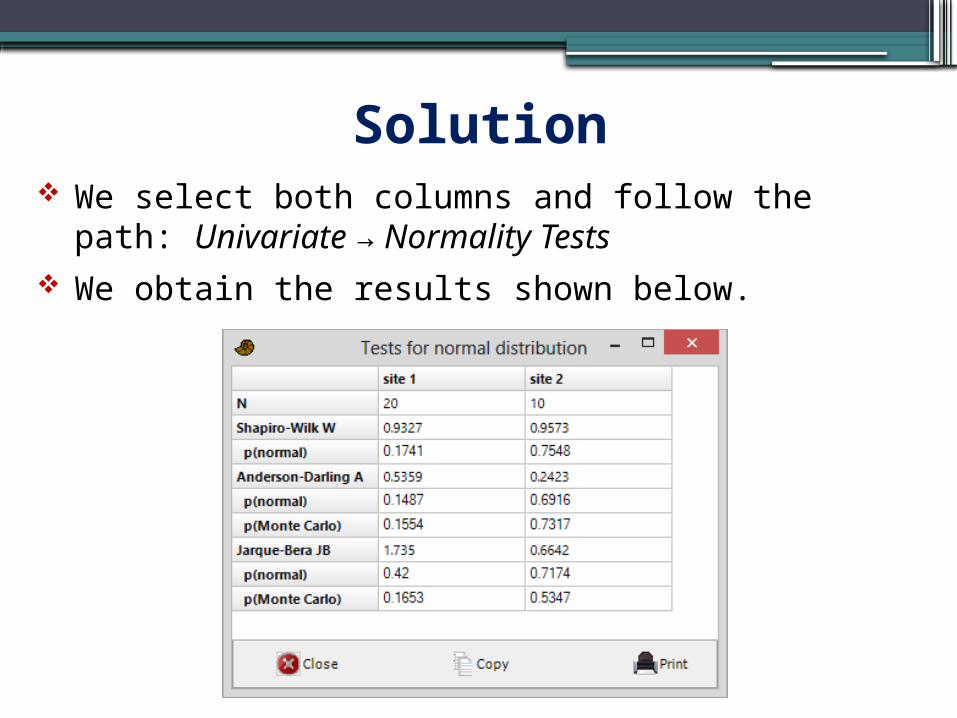
Solution We select both columns and follow the path: Univariate → Normality Tests

We obtain the results shown below.

Interpretation We observe that the p-values in PAST are denoted simply by p.

All tests give p-values larger than 0.05.

Therefore, we cannot reject the null hypothesis, that is, we accept that the samples do not appear to deviate significantly from normality.

This means that these samples can be further analyzed using parametric tests.

Exercise 6 The file ‘exercise 6’ contains the lengths (in cm) of metal knives from an archaeological site.

Examine whether the sample follows the normal distribution.

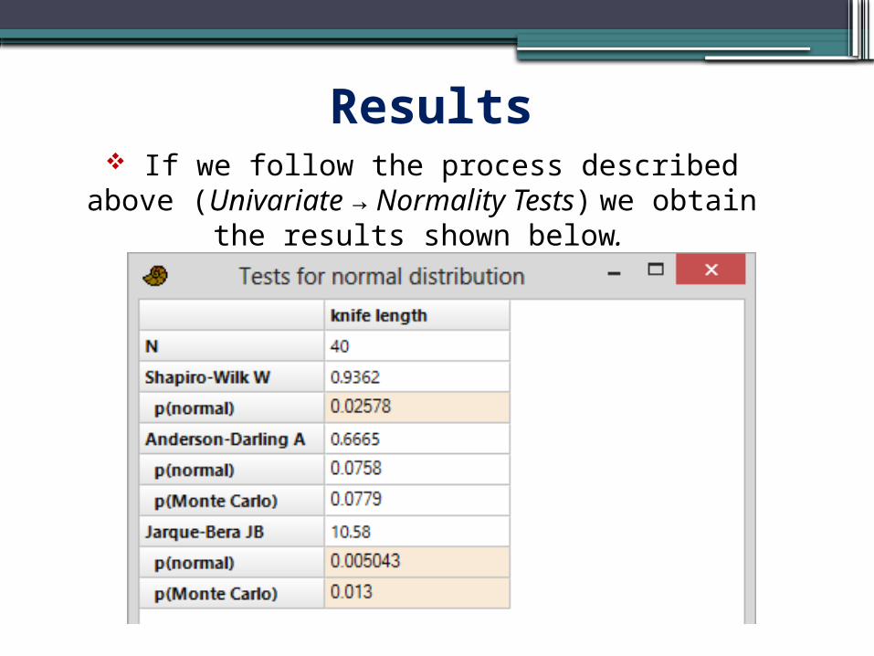
Results If we follow the process described

above (Univariate → Normality Tests) we obtain the results shown below.

We observe that the Shapiro-Wilk criterion has a p-value = 0.026 < 0.05. In contrast, the Anderson-Darling criterion gives a p-value = 0.08 > 0.05. However, as mentioned, this criterion is less robust than the Shapiro-Wilk and therefore we may accept that the sample deviates from normality.

Results

General observation Even though small deviations from normality should not discourage us from applying parametric tests, in cases where we are not certain if a parametric or a non-parametric test is more suitable, it is advisable to use them both as well the corresponding Monte-Carlo tests.

Applied Statistics using PAST - part 2

Documents

Transcript of Applied Statistics using PAST - part 2