Application of serial-and parallel-projection methods to correlation-filter design

Application of serial- and parallel-projectionmethods to correlation-filter design

Tuvia Kotzer, Joseph Rosen, and Joseph Shamir

We describe generalized projection procedures for the design of arbitrary filter functions for correlators.More specifically, serial and parallel implementations of projection-based algorithms are employed. Thenovelty of this procedure lies in its generality and its ability to handle wide varieties of constraints by thesame procedure. The procedure is demonstrated by the design of filters for the 4-f linear correlator, thephase-extraction correlator, and variants thereof. The filters are subject to a variety of constraints,including rotation-invariant pattern recognition and class discrimination. Examples are given to showthe versatility, flexibility, and applicability of the design process to a variety of pattern-recognitiontasks. Satisfactory results are also obtained because of the combination with the special nonlinearcorrelators proposed for pattern recognition.

1. Introduction

Pattern-recognition 1PR2 systems are usually de-signedwith specific requirements. Examples of theserequirements are rotation invariance, scale invari-ance, and tilt invariance. Various dedicated proce-dures were proposed in the past, such as circularharmonic component1 1CHC2 filters and CHC phase-only filters2 1CHC POF’s2 for rotation-invariant PR,the Fourier–Mellin transform3 for scale-invariant PR,position determination,4 etc. The underlying charac-teristic of the above approaches is that they assume, apriori, a predefined structure for the filter. From asystems point of view, a generalized procedure for thedesign of arbitrary reference functions for correlatorsis desirable, without an a priori limiting structure.In this paper we show how such requirements can

be handled by general-purpose procedures. Thepower of the algorithms lie in 1a2 their simplicity, and1b2 the fact that the solutions are not confined to apredetermined structure, which leaves more flexibil-ity to arrive at not only better solutions, but also at

When this work was performed the authors were with theDepartment of Electrical Engineering, Technion, Israel Institute ofTechnology, Haifa 32000, Israel. T. Kotzer is now with the Algo-rithm Division, IMETRTIX, P.O. Box 1165, Rehovot 76110, Israel.J. Rosen is now with the Department of Applied Physics, Califor-

nia Institute of Technology, Pasadena, California.Received 14 December 1994; revised manuscript received 21

March 1995.0003-6935@95@203883-13$06.00@0.

r 1995 Optical Society of America.

solutions that were not previously considered possiblebecause of a, perhaps mistaken, a priori confinementof the solution. The purpose of the paper is thustwofold: 1a2 introduce, review, and enhance somenew concepts in the design of optical PR systems 1forlinear and nonlinear systems2, and 1b2 demonstratethe applicability of projection-based methods for theachievement of superior performance in the above PRsystems under a wide and quite stringent range ofrequirements.The algorithms we employ are parallel and serial

versions of the projection-onto-constraint sets 1POCS’s2method: when the serial-projection method5,6 is ap-plicable we employ it; otherwise we employ the re-cently introduced parallel-projectionmethod,7–9 basedon Ref. 10, which may be employed for both linear-correlator 1LC2 systems as well as non-LC systems,such as the phase-extraction correlator11 1PEC2 and itsvariants. In Section 2, after some preliminary defini-tions, we describe the parallel- and the serial-projectionmethods and their characteristics. In Sec-tion 3 we design filters by a parallel version of POCS,for both the PEC and the 4-f LC. In Section 4 weinvestigate rotation-invariant filtering, based on theCHC1 filter and introduce some energy measuresaccording to which we can establish a fair criterion forcomparison between PEC-based correlators and simi-lar LC’s. In Section 5, based on CHC decompositiontheory and its application in Section 4, we design, bythe serial-POCS method, special rotation-invariantfilters to detect a class of objects that maintain thenarrow, high-intensity, correlation peaks typical ofthe PEC. Conclusions are given in Section 6.

10 July 1995 @ Vol. 34, No. 20 @ APPLIED OPTICS 3883

2. Background

A. Serial Projections

Given a Hilbert space H , a distance function d on H ,and a closed convex set 1CCS2 C in H , projection fromH onto Cwith respect to the distance function d is anoperation P that associates to every element h [ H

the 1unique2 element h8 in C closest to h, where ‘‘close’’is measured by d:

P1h2 5 h8

if and only if h8 [ C and infy[C

d1 y, h2 5 d1h8, h2;

112

1projected vectors are henceforth marked by a prime2.Usually d is derived from the prevailing Hilbert-spacestructure,

d1h, h82 5 6h 2 h86H [ e 0h1x2 2 h81x2 02dx. 122

If the sets Ci are closed with respect to d and areconvex, the projection element exists and is unique.If the sets are not convex, procedures exist for deter-mining the 1unique2 projection.12Sometimes the projection operation is modified to

admit relaxation. For instance, P may be replacedby the relaxed operator Pl defined by

Pl1h2 5 P1h2 1 l3P1h2 2 h4, 132

where l is a real relaxation parameter with 0l 0 , 1.Given N CCS’s, Ci, i 5 1, . . . , N, Ci , H , with a

nonempty intersectionC0 5 >i51N Ci, we can associate a

separate relaxed projection Pi,li with each set Ci andcorresponding projection Pi. To obtain an element inC0 we iterate the composed operator T, defined by,

T 5 PN,lNPN21,lN21

· · · P1,l1, 142

by using the following algorithm:

Algorithm 1: Given an arbitrary initial functionh01x2,

hk11 5 T1hk2, k $0. 152

For any arbitrary initial function h0 we ensure thatthe infinite sequence 5h0, h1, h2, . . .6 generated byalgorithm 1 converges weakly13 to an element in C0,provided all projections are performed with respect tothe same distance function14 and that all the N setsare CCS’s 1in finite dimension, e.g., H 5 Cn, weak andstrong convergence are the same2. If some of the Nsets are not convex, we are assured of a monotonicnonincrease of some error function along the iterates,provided N # 2. If N . 2 this is not guaranteed,even if only one set is not convex.

3884 APPLIED OPTICS @ Vol. 34, No. 20 @ 10 July 1995

B. Parallel Projection

We start by defining generalized weighted, L2, norm-squared distance functions, with weightWi:

di1h1, h22[ 6H1 2 H26Wi

2

[ e2`

`

0H11u2 2 H21u2 02Wi1u2du h1, h2 [ H ,

162

where Wi1u2 is an essentially positive and essentiallybounded weighting function, and uppercase lettersdenote the Fourier transform 1FT2 of the lowercasefunctions, e.g., Hi1u2 [ F 5hi1x26. We also define a costfunctional:

J1h22 [ oi51

N

bidi3PCidi 1h2, h4

5 oi51

N

bi6 F 5PCidi 1h26 2 F 5h66Wi

2 , 172

where bi . 0 attributes an importance to the projec-tion, PCi

di 1h2 denotes the projection of h onto the set Ci

with respect to the distance function di, i.e.,

PCidi 1h2 5 h8 if and only if inf

h1[Cidi1h1, h2 5 di1h8, h2,

h8 [ Ci. 182

We also denote by Pi,li the relaxed projections, asabove 3where we omit the superscript 1?2di for brevity4.If the sets Ci are closed with respect to di and convex,the projection element exists and is unique. If thesets are not convex, procedures exist for determiningthe 1unique2 projection.12 With these definitions wecan state the parallel-projection algorithm in its space1time2 representation, generating the sequence of suc-cessive estimates 5h0, h1, . . . ,6. Although the algo-rithm operates in an infinite-dimensional Hilbertspace as well,7,15 we assume finite dimension 1as it isimplemented on a digital computer2.

Algorithm 2, space domain: Given an arbitrary ini-tial function h01x2, calculate,

vik111x2 [ Pi,l3hk1x24, for all i 5 1, 2, . . . , N, 19a2

hk111x2 5 F215oi51

N

biWi1u2 F 5vik1161u2

oi51

N

biWi1u2 6 , 19b2

where F and F 21 denote the FT and its inverse,respectively. For an equivalent frequency represen-tation, see Ref. 16.A detailed mathematical justification of this algo-

rithm is provided in Refs. 15 and 16, which is briefly

reviewed in appendix A. Here we note only thatiterates generated by this parallel algorithm convergeweakly to C0, provided that all sets are CCS’s and l [121, 12, and that the individual projections may bedefined with respect to different distance functions, incontrast to the serial algorithm. Also, even if some,or all, of the sets are nonconvex, the cost function J isnonincreasing along the iterates, provided that l [10, 12, assuring us of improved estimates along theiterates. This holds for an arbitrary number of sets,as opposed to the serial algorithm in Subsection 2.A.

C. Correlator and Related Definitions

Using one-dimensional notation for brevity, we definethe correlation between an input function f 1x2 and areference 1filter2 function h1x2 by

F1x2 5 F215NlE F 5 f 1x26FNlE F 5h1x26F6 1102

where Nl is a, possibly nonlinear, operator defined by

Nl5R1u26 5 0R1u2 0lexp3iw1u24,

R1u2 5 0R1u2 0exp3iw1u24, 0 # l # 1. 1112

We further define fp1x2 and hp1x2 by fp1x2 [ F 215Nl50

E F 5 f 1x26F6, hp1x2 [ F 215Nl50E F 5h1x26F6, which corre-spond to the phase parts of the functions f 1x2 and h1x2,respectively.With these definitions, we are in a position to state

the following three correlators that are considered inthis work:

LC:

F1x2 5 h1x2 f 1x2. 1122

PEC:

F1x2 5 hp1x2 fp1x2. 1132

Generalized PEC 1GPEC2:

F1x2 5 h1x2 fp1x2, 1142

Other degrees of nonlinearity, 1monitored by l2 can betried as well, leading to nonlinear correlators similarto the nonlinear joint transform correlator,17–19 asindicated in Ref. 20. Also, note that both the PECand the GPEC are nonlinear correlation systems.In the rest of the paper we employ the serial- and

the parallel-projection methods for the design offilters for the LC, the PEC, and the GPEC. This isperformed subject to a variety of demands 1con-straints2 including class discrimination and class rec-ognition with rotation invariance. We note that theserial POCS has already been applied successfully tothe design of filters that are both rotation and shiftinvariant, as well as having a predetermined, limitedscale range for which the response is constant too.21This was possible because of the flexibility of themethod. The optical implementations of the various

PEC’s and other non-LC’s11,18–20,22 and LC’s21 weregiven elsewhere and are not repeated here, for brev-ity.

3. Applications

Throughout the following sections, we use variousprojection algorithms to design filters for optical LCand non-LC systems. In the design process theconstraints are basically composed of discriminationand peak energy 1amplitude2 constraints. Noise con-straints, e.g., noise robustness, can be easily incorpo-rated into the design process as well, at least for theparallel algorithm, as shown in Ref. 7 1in Ref. 7 thenoise is taken into account for image-restorationpurposes and the idea is similar for PR purposes2.Our interest here is concerned mainly with non-LC

systems like the PEC and the GPEC that providebetter discrimination than the LC and are barelyaffected by noise up to a certain level. Moreover, itwas shown in Ref. 20 that the presence of noiseactually assisted in the case of multiple-object inputs.Thus, for brevity, noise problems are not consideredfurther, nor is shift invariance, which was demon-strated in Refs. 11 and 20.

A. Class Discrimination by a Linear Correlator

For a class-discrimination problem we define a train-ing set consisting of two classes. The class to bedetected is placed in a region of spaceR1, and the classto be rejected is situated in the regionR2. The task isto design a filter, h, such that

112 Its correlation with a given input function, f,will satisfy some correlation constraint C1. Namely,in the detection region, R1, the correlation peaks willbe larger than some predetermined value T1, whereasin the rejection region, R2, the correlation will belower than some predetermined value T2. If thecomplete training set is presented simultaneouslyover the input plane, then R1 corresponds to regionsin the correlation plane that correspond to the posi-tions of objects to be detected, whereas the regions R2represent the location of objects to be rejected andempty regions surrounding the correlation peaks inR1. During the learning stage the correlation peak isassumed to be contained in a single pixel. Becausethis is physically not possible, some of the peakenergy will leak out into neighboring pixels, constitut-ing the background that should be below T2. Also, T1and T2 are appropriately chosen threshold values toprovide sufficient discrimination 1at least T1@T22 aswell as sufficient energy in the peak 1high absolutevalue of T12. The appropriate values will depend onthe specific application and the level of similaritybetween both classes.

122 Its FT, F 5h6, corresponds to a passive element1C22.

132 It should have finite support, say 32a, a41C32.

Any filter h that satisfies all three constraints above isconsidered a solution. More specifically, the con-


straints are given by the following definitions:

C1 [ 5h 0 1h f 21 j2 [ C1, ;j6, 115a2

C1 [ 5F1 j2 0 0F1 j2 0 # T2, for j [ R2;

Fre1 j2 $ T1 and Fim1 j2 5 0, for j [ R16,

115b2

C2 [ 5h 0 0 F 5h1 j26 0 # 16, 115c2

C3 [ 5h 0h1 j2 5 0, for j 32a, a4; a . 06, 115d2

where

F1 j2 [ 1h f 21 j2, F1 j2 [ Fre1 j2 1 iFim1 j2;

Fre1 j2 5 Re5F1 j26, Fim1 j2 5 Im5F1 j26.

Actually, the measured quantity is 0F 02 and not itsimaginary or real values. However, the constraint,0F1 j2 02 $ const. is not a convex constraint set andconvergence is then not guaranteed. This is not thecase for C2, where the constraint is 0I1 j2 0 # const.Thus with our choice, C1, C1, C2, and C3 are CCS’s.Projections onto C2, C3 with respect to the distance

function given by Eq. 162 with unity weighting3Wi1u2 5 1, i 5 2, 32, i.e., the Euclidean norm, aresimple and are given by

PC2d2 5h1x26 5 F

215H81u26,

where

H81u2 5 5H1u2 if 0H1u2 0 # 1

exp3iwH1u24 otherwise,

PC3d3 5h1x26 5 5h1x2 if x [ 12a, a2

0 otherwise, 1162

where H1u2 5 F 5h1x26 5 0H1u2 0exp3iwH1u24. Unfor-tunately, projection ontoC1 with respect to the Euclid-ean norm is complicated and is a typical constraineddeconvolution problem in itself.14,16To perform the projection onto C1 easily we follow

the idea proposed in Ref. 14. We perform the projec-tion onto C1, with respect to the distance functioninduced by a weighted norm squared, with the appro-priate weighting given by W11m2 [ 0 F 3 f 1 j24 02 5

0F1m2 02:

d11H1,H22 5 omW11m2 0H11m2 2 H21m2 02

5 oj0 F 2153W11m241@261 j2 3h11 j2 2 h21 j24 02.

1172


This careful choice of the weighting function resultsin a simple projection, viz.,

E F 215V16 5F

v1 [ PC1d1 1h2, where V11m2 5

F 5F81 j261m2

F1m2,

F81 j2

5 5T2 exp3iwF1 j24, if j [ R2 and 0F1x2 0 . T2

F1 j2, if j [ R2 and 0F1 j2 0 # T2

T1, if j [ R1 and Fre1 j2 , T1

Fre1 j2, if j [ R1 and Cre1 j2 $ T1

F1 j2, otherwise

,

where

F1 j2 5 0F1 j2 0exp31iwF1 j24

5 F215H1m2F1m26 5 h1 j2 f 1 j2. 1182

For details see Ref. 16.Algorithm 2 allows projections with respect to

several different distance functions, and, therefore,projecting different quantities in domains where boththe constraint set and the distance function aresimple is possible 1see Ref. 14, Section VI2; hence itis employed for this filter synthesis task. The se-quence 5hk6k50

` generated by algorithm 2 convergesto a function in C0, satisfying all constraints,and is given by 3see Eqs. 19a2 and 19b24 hk111 j2 5 F 215Hk111m26, where

Hk111m2 5F 5PC1

d1E F 215Hk6F61m2W11m2 1 F 5PC2d2E F 215Hk6F61m2 1 F 5PC3

d3E F 215Hk6F61m2

W11m2 1 1 1 1, 1192

and where d1 is given by Eq. 1172, a zero-relaxationparameter 1l 5 02 is employed, and d21h1, h22 5d31h1, h22 5 6h1 2 h26 1the Euclidean norm2.In one of our simulation experiments we started

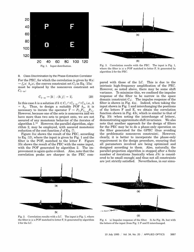
from a filter h such that h C1, h [ C2, hC3. Figure 1 shows the input distribution.The task is to detect the letter F and reject all

others. Figure 21a2 shows the correlation distribu-tion with a LC, where the filter is a POF23 matched tothe letter F. Fig. 21b2 shows the correlation distribu-tion with the filter generated by algorithm 2. Theimprovement in both recognition and discriminationis obvious.In the case of the GPEC, for which the correlation is

given by F1x2 [ h1x2 fp1x2, we may employ theserial-projection algorithm 1POCS2 with equal ease.This was already treated in Ref. 14 and is notdiscussed here.

B. Class Discrimination by the Phase-Extraction Correlator

For the PEC, for which the correlation is given by F1x2[ fp1x2 hp1x2, the convex constraint set C2 in Eq. 115a2must be replaced by the nonconvex constraint setC22nc:

C22nc [ Eh 0 0 F 5h1 j26 0 5 1F. 1202

In this case h is a solution if h[C1 >C22nc >C3, i.e., h5 hp. Thus, to design a suitable POF hp, it isnecessary to iterate the operator T [ PC1PC22nc

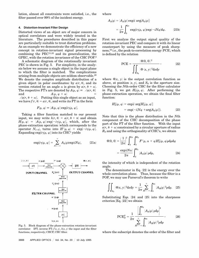
PC3.However, because one of the sets is nonconvex and wehave more than two sets to project onto, we are notassured of any monotonic behavior of the iterates ofalgorithm 1.12 However, the parallel algorithm, algo-rithm 2, may be employed, with assured monotonicreduction of the cost function J of Eq. 172.Figure 31a2 shows the result of the PEC, according

to Eq. 1132, where the input is given by Fig. 1 and thefilter is the POF, matched to the letter F. Figure31b2 shows the result of the PEC with the same input,with the POF generated by algorithm 2. The im-provement is again quite evident. Also, note that thecorrelation peaks are sharper in the PEC com-

Fig. 1. Input distribution.

Fig. 2. Correlation results with a LC. The input is Fig. 1, wherethe filter is 1a2 a POFmatched to letter F, 1b2 generated by algorithm2 for the LC.

pared with those of the LC. This is due to theintrinsic high-frequency amplification of the PEC.However, as noted above, there may be some shiftvariance. To minimize this, we confined the impulseresponse of the filter to be narrow in the spacedomain 1constraint C32. The impulse response of thefilter is shown in Fig. 41a2. Indeed, when taking theinput shown in Fig. 1 and interchanging the positionsof the letters F and E, we obtain the correlationfunction shown in Fig. 41b2, which is similar to that ofFig. 31b2 1when noting the interchange of letters2,demonstrating approximate shift invariance. We alsonote that another approach for the design of filtersfor the PEC may be to do a phase-only operation onthe filter generated for the GPEC 1thus avoidingthe problematic nonconvex constraint2. However,clearly, it is better to incorporate the phase-onlyrequirement in the design procedure, ensuring thatall parameters involved are being optimized anddesigned according to them. Also, naturally, theparallel-projection algorithm is stopped after a finitenumber of iterations 3basically when J1h2 is consid-ered to be small enough4 and thus not all constraintsare 1yet2 strictly satisfied. Nevertheless, in our simu-

Fig. 3. Correlation results with the PEC. The input is Fig. 1,where the filter is 1a2 a POF matched to letter F, 1b2 generated byalgorithm 2 for the PEC.

Fig. 4. 1a2 Impulse response of the filter. 1b2 As Fig. 3b, but withthe letters of the input 1from Fig. 12 F and E interchanged.


lation, almost all constraints were satisfied, i.e., thefilter passed over 99% of the incident energy.

4. Distortion-Invariant Filter Design

Distorted views of an object are of major concern inoptical correlators and were widely treated in theliterature. The procedures described in this paperare particularly suitable to treat distortion problems.As an example we demonstrate the efficiency of a newconcept in rotation-invariant signal processing bycombining the PEC11,22 and its generalization, theGPEC, with the rotation invariance of the CHC POF.2A schematic diagram of the rotationally invariant

PEC is shown in Fig. 5. For simplicity, in the analy-sis below we assume a single object in the input planeto which the filter is matched. The complicationsarising frommultiple objects are seldom observable.20We denote the complex amplitude distribution of agiven object 1in polar coordinates2 by a1r, u2, and itsversion rotated by an angle a is given by a1r, u 1 a2.The respective FT’s are denoted by A1r, w2 ; F 5a1r, u26and A1r, w 1 a2 5

F 5a1r, u 1 a26. Putting this single object as an input,we have f 1r, u2 5 a1r, u2, and write its FT in the form

F1r, w2 ; 0A1r, w2 0exp3ig1r, w24.

Taking a filter function matched to our presentinput, we may write h1r, u2 5 a1r, u 1 p2 and obtainH1r, w2 5 0A1r, w2 0exp32ig1r, w24, which, after thephase-extraction operation 1which corresponds to theoperator Nl502, turns into H81r, w2 5 exp32ig1r, w24.Expanding exp3ig1r, w24 into its CHC1 yields

exp3ig1r, w24 5 oN52`

`

AN1r2exp1iNw2, 121a2

Fig. 5. Block diagram of the phase-extraction rotation-invariantcorrelator: IFT, inverse FT; f 1x, y2, h1x, y2 the input and the filterfunctions, respectively; CHCF, CHC filter.


where

AN1r2 5 0AN1r2 0exp5i arg3AN1r246

51

2p e0

2p

exp3ig1r, w24exp12iNw2dw. 121b2

First we analyze the output signal quality of therotation-invariant PEC and compare it with its linearcounterpart by using the measure of peak sharp-ness,24 i.e., the peak-to-correlation energy 1PCE2, whichis defined by the relation

PCE 50F10, 02 02

eeS0

0F 1x, y2 02dxdy

, 1222

where F1x, y2 is the output correlation function asabove, at position 1x, y2, and S0 is the aperture size.Choosing the Nth-order CHC for the filter calculatorin Fig. 5, we get H8N1r, w2. After performing thephase-extraction operation, we obtain the final filterfunction:

H9N1r, w2 5 exp5i arg3H8N1r, w246

5 expA2i5Nw 1arg3AN1r246B. 1232

Note that this is the phase distribution in the Nthcomponent of the CHC decomposition of the phasepart of the FT of the filter function. With the inputa1r, u 1 a2 constrained by a circular aperture of radiusR0 and using the orthogonality of CHC’s, we obtain

F10, 02 5 1 12p22 e

0

2p e0

R0

F81r, a 1 w2H9N1r, w2rdrdw

5exp1iNa2

2p e0

R0

0AN1r2 0rdr, 1242

the intensity of which is independent of the rotationangle.The denominator in Eq. 1222 is the energy over the

whole correlation plane. Thus, because the filter is aPOF, we may use Parseval’s theorem to write

eeS0

0F1x, y2 02dxdy 51

2p oM52`

` e0

r0

0AM1r2 02rdr. 1252

Substituting Eqs. 1242 and 1252 into the sharpnesscriterion 3Eq. 12224we obtain

PCENP 5

1

2p

3e0

R0

0AN1r2 0rdr42

oM52`

` e0

r0

0AM1r2 02rdr

, 1262

where the subscript denotes the order of the filter and

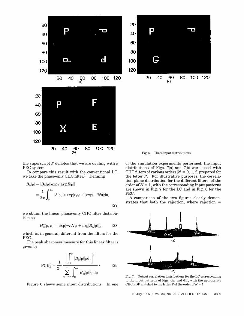
Fig. 6. Three input distributions.

the superscript P denotes that we are dealing with aPEC system.To compare this result with the conventional LC,

we take the phase-only CHC filter.2 Defining

BN1r2 5 0BN1r2 0exp5i arg3B1r246

51

2p e0

2p

0A1r, u2 0exp3ig1r, u24exp12iNu2du,

1272

we obtain the linear phase-only CHC filter distribu-tion as

H9N1r, w2 5 expA2i5Nw 1 arg3BN1r246B, 1282

which is, in general, different from the filters for thePEC.The peak sharpness measure for this linear filter is

given by

PCENL 5

1

2p

3e0

r0

0BN1r2 0rdr42

om52`

` e0

r0

0Bm1r2 02rdr

. 1292

Figure 6 shows some input distributions. In one

of the simulation experiments performed, the inputdistributions of Figs. 71a2 and 71b2 were used withCHC filters of various orders 1N 5 0, 1, 22 prepared forthe letter P. For illustrative purposes, the correla-tion-plane distribution for the different filters, of theorder ofN 5 1, with the corresponding input patternsare shown in Fig. 7 for the LC and in Fig. 8 for thePEC.A comparison of the two figures clearly demon-

strates that both the rejection, where rejection 5

Fig. 7. Output correlation distributions for the LC correspondingto the input patterns of Figs. 61a2 and 61b2, with the appropriateCHC POFmatched to the letter P of the order ofN 5 1.


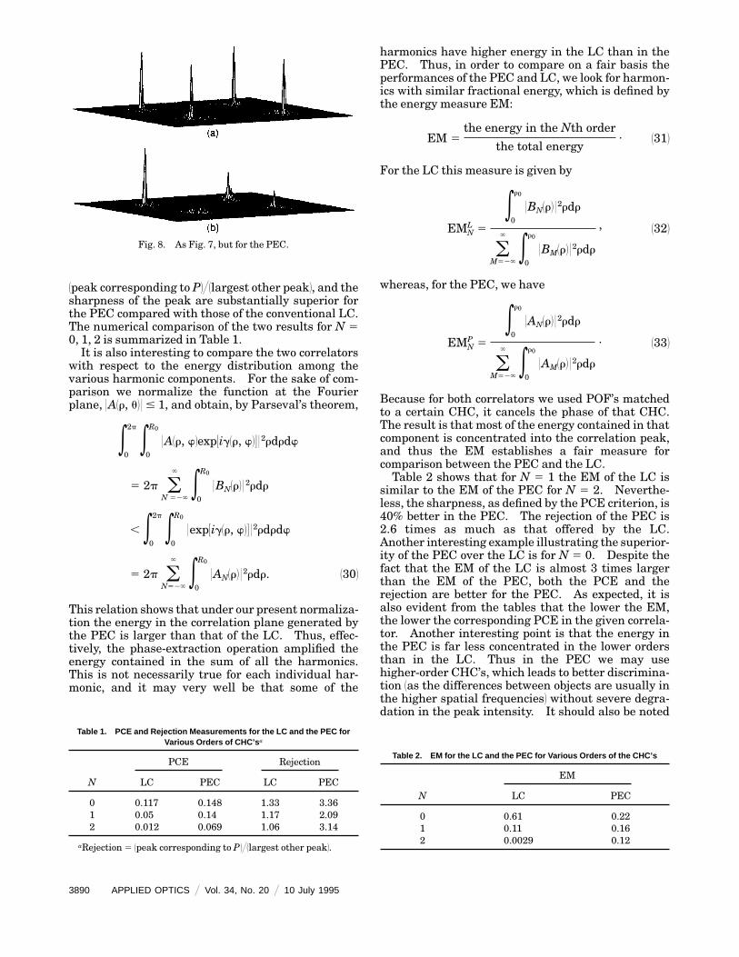
1peak corresponding to P2@1largest other peak2, and thesharpness of the peak are substantially superior forthe PEC compared with those of the conventional LC.The numerical comparison of the two results for N 50, 1, 2 is summarized in Table 1.It is also interesting to compare the two correlators

with respect to the energy distribution among thevarious harmonic components. For the sake of com-parison we normalize the function at the Fourierplane, 0A1r, u2 0 # 1, and obtain, by Parseval’s theorem,

e0

2p e0

R0

0A1r, w2exp3ig1r, w24 02rdrdw

5 2p oN 52`

` e0

R0

0BN1r2 02rdr

, e0

2p e0

R0

0exp3ig1r, w24 02rdrdw

5 2p oN52`

` e0

R0

0AN1r2 02rdr. 1302

This relation shows that under our present normaliza-tion the energy in the correlation plane generated bythe PEC is larger than that of the LC. Thus, effec-tively, the phase-extraction operation amplified theenergy contained in the sum of all the harmonics.This is not necessarily true for each individual har-monic, and it may very well be that some of the

Fig. 8. As Fig. 7, but for the PEC.

Table 1. PCE and Rejection Measurements for the LC and the PEC forVarious Orders of CHC’s a

N

PCE Rejection

LC PEC LC PEC

0 0.117 0.148 1.33 3.361 0.05 0.14 1.17 2.092 0.012 0.069 1.06 3.14

aRejection 5 1peak corresponding to P2@1largest other peak2.


harmonics have higher energy in the LC than in thePEC. Thus, in order to compare on a fair basis theperformances of the PEC and LC, we look for harmon-ics with similar fractional energy, which is defined bythe energy measure EM:

EM 5the energy in the Nth order

the total energy. 1312

For the LC this measure is given by

EMNL 5

e0

r0

0BN1r2 02rdr

oM52`

` e0

r0

0BM1r2 02rdr

, 1322

whereas, for the PEC, we have

EMNP 5

e0

r0

0AN1r2 02rdr

oM52`

` e0

r0

0AM1r2 02rdr

. 1332

Because for both correlators we used POF’s matchedto a certain CHC, it cancels the phase of that CHC.The result is that most of the energy contained in thatcomponent is concentrated into the correlation peak,and thus the EM establishes a fair measure forcomparison between the PEC and the LC.Table 2 shows that for N 5 1 the EM of the LC is

similar to the EM of the PEC for N 5 2. Neverthe-less, the sharpness, as defined by the PCE criterion, is40% better in the PEC. The rejection of the PEC is2.6 times as much as that offered by the LC.Another interesting example illustrating the superior-ity of the PEC over the LC is for N 5 0. Despite thefact that the EM of the LC is almost 3 times largerthan the EM of the PEC, both the PCE and therejection are better for the PEC. As expected, it isalso evident from the tables that the lower the EM,the lower the corresponding PCE in the given correla-tor. Another interesting point is that the energy inthe PEC is far less concentrated in the lower ordersthan in the LC. Thus in the PEC we may usehigher-order CHC’s, which leads to better discrimina-tion 1as the differences between objects are usually inthe higher spatial frequencies2 without severe degra-dation in the peak intensity. It should also be noted

Table 2. EM for the LC and the PEC for Various Orders of the CHC’s

N

EM

LC PEC

0 0.61 0.221 0.11 0.162 0.0029 0.12

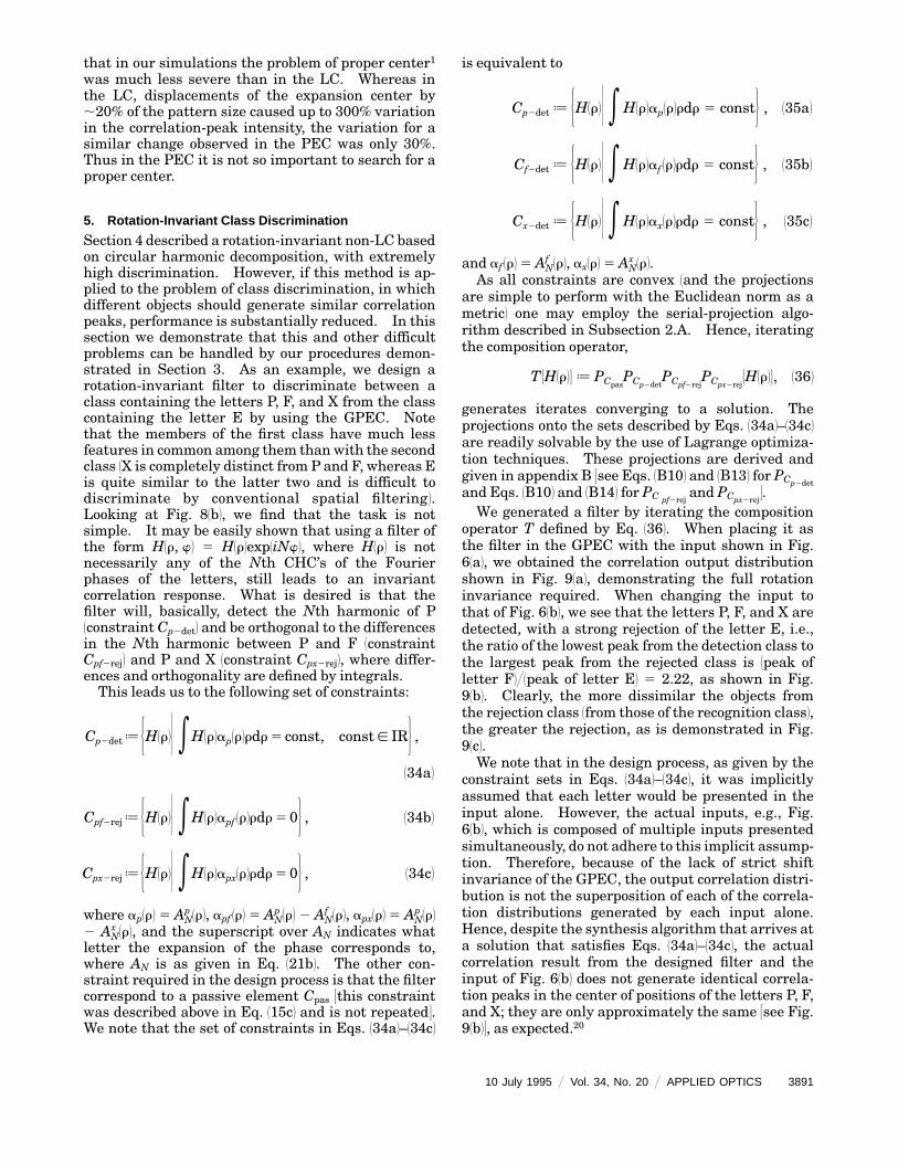
that in our simulations the problem of proper center1was much less severe than in the LC. Whereas inthe LC, displacements of the expansion center by,20% of the pattern size caused up to 300% variationin the correlation-peak intensity, the variation for asimilar change observed in the PEC was only 30%.Thus in the PEC it is not so important to search for aproper center.

5. Rotation-Invariant Class Discrimination

Section 4 described a rotation-invariant non-LC basedon circular harmonic decomposition, with extremelyhigh discrimination. However, if this method is ap-plied to the problem of class discrimination, in whichdifferent objects should generate similar correlationpeaks, performance is substantially reduced. In thissection we demonstrate that this and other difficultproblems can be handled by our procedures demon-strated in Section 3. As an example, we design arotation-invariant filter to discriminate between aclass containing the letters P, F, and X from the classcontaining the letter E by using the GPEC. Notethat the members of the first class have much lessfeatures in common among them thanwith the secondclass 1X is completely distinct from P and F, whereas Eis quite similar to the latter two and is difficult todiscriminate by conventional spatial filtering2.Looking at Fig. 81b2, we find that the task is notsimple. It may be easily shown that using a filter ofthe form H1r, w2 5 H1r2exp1iNw2, where H1r2 is notnecessarily any of the Nth CHC’s of the Fourierphases of the letters, still leads to an invariantcorrelation response. What is desired is that thefilter will, basically, detect the Nth harmonic of P1constraint Cp2det2 and be orthogonal to the differencesin the Nth harmonic between P and F 1constraintCpf2rej2 and P and X 1constraint Cpx2rej2, where differ-ences and orthogonality are defined by integrals.This leads us to the following set of constraints:

Cp2det[ 5H1r20 eH1r2ap1r2rdr 5 const, const[ IR6 ,134a2

Cpf2rej[ 5H1r20 eH1r2apf 1r2rdr 5 06 , 134b2

Cpx2rej[ 5H1r20 eH1r2apx1r2rdr 5 06 , 134c2

where ap1r2 5 ANp 1r2, apf 1r2 5 AN

p 1r2 2 ANf 1r2, apx1r2 5 AN

p 1r22 AN

x 1r2, and the superscript over AN indicates whatletter the expansion of the phase corresponds to,where AN is as given in Eq. 121b2. The other con-straint required in the design process is that the filtercorrespond to a passive element Cpas 3this constraintwas described above in Eq. 115c2 and is not repeated4.We note that the set of constraints in Eqs. 134a2–134c2

is equivalent to

Cp2det [ 5H1r20 e H1r2ap1r2rdr 5 const6 , 135a2

Cf2det [ 5H1r20 e H1r2af 1r2rdr 5 const6 , 135b2

Cx2det [ 5H1r20 e H1r2ax1r2rdr 5 const6 , 135c2

and af 1r2 5 ANf 1r2, ax1r2 5 AN

x 1r2.As all constraints are convex 1and the projections

are simple to perform with the Euclidean norm as ametric2 one may employ the serial-projection algo-rithm described in Subsection 2.A. Hence, iteratingthe composition operator,

T5H1r26 [ PCpasPCp2det

PCpf2rejPCpx2rej

5H1r26, 1362

generates iterates converging to a solution. Theprojections onto the sets described by Eqs. 134a2–134c2are readily solvable by the use of Lagrange optimiza-tion techniques. These projections are derived andgiven in appendix B 3see Eqs. 1B102 and 1B132 for PCp2detand Eqs. 1B102 and 1B142 for PC pf2rej

and PCpx2rej4.

We generated a filter by iterating the compositionoperator T defined by Eq. 1362. When placing it asthe filter in the GPEC with the input shown in Fig.61a2, we obtained the correlation output distributionshown in Fig. 91a2, demonstrating the full rotationinvariance required. When changing the input tothat of Fig. 61b2, we see that the letters P, F, and X aredetected, with a strong rejection of the letter E, i.e.,the ratio of the lowest peak from the detection class tothe largest peak from the rejected class is 1peak ofletter F2@1peak of letter E2 5 2.22, as shown in Fig.91b2. Clearly, the more dissimilar the objects fromthe rejection class 1from those of the recognition class2,the greater the rejection, as is demonstrated in Fig.91c2.We note that in the design process, as given by the

constraint sets in Eqs. 134a2–134c2, it was implicitlyassumed that each letter would be presented in theinput alone. However, the actual inputs, e.g., Fig.61b2, which is composed of multiple inputs presentedsimultaneously, do not adhere to this implicit assump-tion. Therefore, because of the lack of strict shiftinvariance of the GPEC, the output correlation distri-bution is not the superposition of each of the correla-tion distributions generated by each input alone.Hence, despite the synthesis algorithm that arrives ata solution that satisfies Eqs. 134a2–134c2, the actualcorrelation result from the designed filter and theinput of Fig. 61b2 does not generate identical correla-tion peaks in the center of positions of the letters P, F,and X; they are only approximately the same 3see Fig.91b24, as expected.20


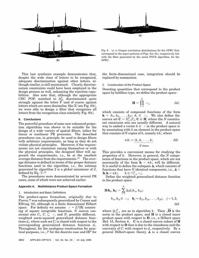
Fig. 9. 1a2–1c2 Output correlation distributions for the GPEC thatcorrespond to the input patterns of Figs. 61a2–61c2, respectively, butwith the filter generated by the serial POCS algorithm, for theGPEC.

This last synthesis example demonstrates that,despite the wide class of letters to be recognized,adequate discrimination against other letters, al-though similar, is still maintained. Clearly, discrimi-nation constraints could have been employed in thedesign process as well, enhancing the rejection capa-bilities. Also note that, although the appropriateCHC POF, matched to AN

P , discriminated quitestrongly against the letter F 1and of course againstletters which are more dissimilar, like X2 3see Fig. 81b24,we were able to design a filter that recognizes allletters from the recognition class similarly 3Fig. 91b24.

6. Conclusions

The powerful procedure of some new enhanced projec-tion algorithms was shown to be suitable for thedesign of a wide variety of spatial filters, either forlinear or nonlinear PR processes. The describedprocedures can, in principle, be used to design filterswith arbitrary requirements, as long as they do notviolate physical principles. Moreover, if the require-ments are not consistent among themselves or withthe physical principles, the designed filter will ap-proach the requirements, i.e., be at the smallestaverage distance from the requirements.15 The aver-age distance is defined in terms of the proper distancefunctions used in the algorithm, i.e., the solutiongenerated by algorithm 2 is a global minimizer of J,defined by Eq. 172.15The procedures were demonstrated by several PR

cases, some of which were not achieved earlier.

Appendix A. Multidistance Product-Space Formalism

1. Introduction and Basic Definitions

The product-space formalism, originally due toPierra,25 was subsequently generalized by Censor andElfving 3104, although in a finite dimensional Hilbertspace. For definity we assume H 5 L21IR2 consist-ing of square integrable functions, N convex con-straint sets Ci, Ci # H , and N, possibly different,weighted norm-squared generalized distance func-tions di, where each set Ci is closed with respect to thecorresponding generalized distance function di.Throughout, for the analogous construction for prac-tical purposes, i.e., l2 for the discrete case and IRN for


the finite-dimensional case, integration should bereplaced by summation.

2. Construction of the Product Space

Denoting quantities that correspond to the productspace by boldface type, we define the product space:

H [ pi51

N

H i, 1A12

which consists of compound functions of the formh 5 1h1, h2, . . . , hN2, hi [ H i. We also define theconvex set C [ pi51

N Ci; C [ H, where the N constitu-ent constraint sets are usually different. A naturalway to embed a vector h [ H in the product space isby associating with h an element in the product spacethat consists ofN copies of h, namely t1h2, where

t1h2 Z 1h, h, . . . , h2. 1A226

N times

This provides a convenient means for studying theproperties of h. However, in general, the N compo-nents of functions in the product space, which are notnecessarily of the form h 5 t1h2, will be different.It is useful to define the subspace D, which consists offunctions that have N identical components, i.e., D 5

5h 0h 5 t1h2; h [ >i51NH i6.

Define the weighted generalized distance functionin the product space:

D1h1, h22 5 oi51

N

bidi1h1i, h2i2;

h1i,h2i [ H i; hj[ 1hj1,hj2, . . . , hjN2, j5 1, 2,

1A32

where 5bi6i51N are as in algorithm 2. Then ŒD is the

norm in the product space, and H is a closed innerproduct space with respect to D, i.e., a Hilbert space1Ref. 15, Section 42. C is a closed convex subset of Hwith respect toD that is due to the closedness and theconvexity of Ci with respect to di, respectively. By ageneral Hilbert-space theory, D is a closed convex

subset of H with respect to D as well, in fact, a closedlinear subspace 1Ref. 15, Section 42.Using this formalism, one may define a projection

in the product space onto an arbitrary set S, closedwith respect toD, as follows. h8 [ S is the projectionof h onto S, denoted by

PSD1h2 5 h8 if and only if

infh1[S

D1h1, h2 5 D1h8, h2. 1A42

If S is C 1or D2 then the projection onto C 1or D2 existsand is unique because of the closedness and convexityof the sets.26It follows from Eq. 1A32 that, for any h [ H ,

infh1[C

D3h1, t1h24 5 oi51

N

bi3 infh1i[Ci

di1h1i, h24. 1A52

Using Eqs. 1A52 and 182 it is not difficult to derive anexplicit expression for a projection in the productspace onto C 1see Lemma 4.1 in Ref. 102. This isobtained when parallel projections are performed onthe individual sets Ci, i.e.,

PCD3t1h24 5 3PC1

d1 1h2, PC2d2 1h2, . . . , PCN

dN 1h24. 1A62

The projectionPDD can be expressed in a similar way

with the relation 1see Lemma 4.2 in Ref. 10 and thederivation in Sections 3 and 4 in Ref. 152

h8 5 PDD1h2 if and only if h8 5 t1h82

where =h1D 3t1h12, h4 0h15h8 5 0. 1A72

This leads to

h8 5 t1h82, where h8 [ F215oi51

N

biWi1u2Vi1u2

oi51

N

biWi1u2 6 .Here =h1 denotes the gradient.

3. Projections onto Nonconvex Sets

Define the relaxed projection operators by

PC,l1h2 [ PC1h2 1 l3h 2 PC1h24. 1A82

We have the following theorem, which is from Leviand Stark, Ref. 12, p. 934:

Theorem 1: Given a Hilbert space H with an innerproduct 7h1, h28, h1, h2 [ H . Let C1, C2 be two closedsubsets of H , not necessarily convex, with relaxedprojection operators given by T1 [ TC1,l11h2, T2 [TC2,l21h2, respectively. Then a recursion of the form

hk11 [ T13T21hk24; k $ 0, 1A92

has the property that the summed-distance error

functional, J, given by

J1h2 [ oi51

2

6h 2 PCi1h26, 1A102

where 6·6 is the appropriate norm in the Hilbertspace H , is nonincreasing for any l1, l2 in theinterval 30, 14.Now consider the following algorithm:

Algorithm 3: Initialization: Let h0 [ t1h02, h0 [ H

arbitrary.Iterative step: given the function hk [ t1hk 2, calcu-late

vk11 5 PC,lD 1hk2,

and then, set

hk11 5 PDD1vk2, 1A112

where PC,lD 1h2[ PC

D1h2 1 l3h 2 PCD1h24.

This algorithm performs two alternating opera-tions in the product space: a relaxed projection ontoC and a projection onto D. Even if all sets Ci are notconvex 1implying thatC is not convex2, in any event, inthe product space we have only two sets: C and D.Thus we may apply the theorem of Levi and Stark,12cited above, in the product space, where the Hilbertspace is H, the distance function is the norm in theproduct space ŒD, and the appropriate summed-distance error functional in the product space is

J1h2 [ 5D3PCD1h2, h461@2 1 5D3PD

D1h2, h461@2. 1A122

Because it can easily be shown that algorithms 2 and3 are equivalent and that hk generated by algorithm 3is equal to t1hk2, where hk is the sequence generated byalgorithm 2, we have the following corollary.

Corollary 2: The functional J1hk2 given by Eq. 172,which is equal to J1hk2 given by Eq. 1A122, is 1monotoni-cally nonincreasing2 convergent along the iterates ofthe respective algorithm 2, i.e., 5J1hk26k$0 is a conver-gent sequence, for any sequence 5hk6k$0 generated byalgorithm 2, irrespective of the sets Ci being convex ornot. Moreover, if all sets Ci are convex, then C isconvex, and if >i51

N Ci is nonempty then C > D isnonempty, and hence hk converges to C0.

Appendix B. Some Specific Projections

Below we develop the projections onto the sets givenby Eqs. 134a2–134c2. Define the distance function by

d23H1r2, H81r24

5 e0

`

53Hr1r2 2 H8r1r242 1 3Hi1r2 2 H8i1r24

26rdr, 1B12

which is just the Euclidean norm.


Let

A 5 e0

`

3Hr1r2 fr1r2 2 Hi1r2 fi1r24rdr, 1B22

B 5 e0

`

3Hr1r2 fi1r2 1 Hi1r2 fr1r24rdr, 1B32

where the subscripts r and i denote the real andimaginary parts, respectively:

H1r2 5 Hr1r2 1 iHi1r2; H81r2 5 H8r1r2 1 iH8i1r2,

f 1r2 5 fr1r2 1 ifi1r2. 1B42

Writing the constraints of Eqs. 1342 in full yieldsrequirements of the following form:

e0

`

3H8r1r2 fr1r2 2 H8i1r2 fi1r24rdr 5 0,

e0

`

3H8r1r2 fi1r2 1 H8i1r2 fr1r24rdr 5 0 1B52

for Cpf2rej and Cpx2rej;

e0

`

3H8r1r2 fr1r2 2 H8i1r2 fi1r24rdr $T1,

e0

`

3H8r1r2 fi1r2 1 H8i1r2 fr1r24rdr 5 0 1B62

for Cp2det.We note that the functional form of the require-

ments in Eqs. 1B52 and 1B62 are similar. Therefore wedevelop the projection onto Cp2det first and then arriveby inspection at the projection onto Cpf2rej and Cpx2rej.Rewriting the requirement of Eqs. 1B62 yields

g1r2 5 e0

`

3H8r1r2 fr1r2 2 H8i1r2 fi1r24rdr 2 1T1 1 j2 5 0,

1B72

q1r2 5 e0

`

3H8i1r2 fr1r2 1 H8r1r2 fi1r24rdr 5 0, 1B82

where we introduce the surplus variable j, which isconfined by j $ 0.To determine the projection we must minimize Eq.

1B12. By defining =T 1≠@≠H8r, ≠@≠H8i2, then, withthe above notation, the Lagrange requirement be-comes 3remembering that our task is to minimize Eq.1B12 subject to the requirements given by Eqs. 1B72and 1B824,

=d21H, H82 5 l=g 1 µ=q. 1B92

Performing the necessary derivatives given by the


= operator in Eq. 1B92 and applying Eqs. 1B72 and 1B82yield

H8r 1r2 5 Hr1r2 1lfr1r2 1 µfi1r2

2, 1B10a2

H8i1r2 5 Hi1r212lfi1r2 1 µfr1r2

2. 1B10b2

To determine l, µ, we substitute Eqs. 1B10a2 and1B10b2 into Eqs. 1B72 and 1B82 to find the l, µ valuesthat satisfy the necessary constraints. After somealgebra we finally arrive at

l 5221A 2 T1 2 j2

E, 1B11a2

µ 522B

E,

E 5 e0

`

0 f 1r2 02rdr. 1B11b2

Substituting the values of l, µ from Eqs. 1B112 intoEqs. 1B102 and minimizing Eq. 1B12 yield

d1H, H82 5 minl2 1 µ2

4E. 1B122

Thus l is the value that will minimize l2 subject to theconstraint that j $ 0. µ is given by Eq. 1B11b2. Todetermine l, we examine two cases:

1a2 A # T1.In this case, l2, as given by Eq. 1B11a2, is a monotonicincreasing function of j for j $ 0, l2 attaining itsminimum with j 5 0, l 5 221A 2 T12@E.

1b2 A . T1.In this case we may choose j 5 A 2 T1 and l 5 0.Hence we have

l 5 0, if A . T1

l 5121T1 2 A2

Eif A #T1

, 1B13a2

µ 522B

E. 1B13b2

Thus, finally, PCp2det3H1r24 5 H81r2 is given by Eqs. 1B102,

with l, µ given by Eqs. 1B132, where the values of Aand B are determined by Eqs. 1B22 and 1B32 and f 1r2 5ap1r2.By analogy we identify that PCpf2rej

, PCpx2rejfollows

the same analysis with T1 5 0 and j 5 0; hence we get

l 522A

E, 1B14a2

µ 522B

E. 1B14b2

Thus finally Ppf2rej3H1r24 5 H81r2 and Ppx2rej3H1r24 5 H81r2are given by Eqs. 1B102 with l, µ given by Eqs. 1B142,where the values of A and B are determined by Eqs.1B22 or 1B32 and f 1r2 5 apf 1r2 or f 1r2 5 apx1r2 for Ppf2rej andPpx2rej, respectively.

This work was performed within the TechnionAdvanced Opto-Electronics Center established by theAmerican Technion Society, NewYork.

References1. Y. Hsu, H. H. Arsenault, and G. April, ‘‘Rotation invariant

digital pattern recognition using circular harmonic expan-sion,’’ Appl. Opt. 21, 4012–4015 119822.

2. J. Rosen and J. Shamir, ‘‘Circular harmonic phase filter forefficient rotation invariant pattern recognition,’’ Appl. Opt. 27,2895–2899 119882.

3. D. Casasent and D. Psaltis, ‘‘New optical transforms forpattern recognition,’’ Proc. IEEE 65, 77–84 119772.

4. M. Fleisher, U. Mahlab, and J. Shamir, ‘‘Target locationmeasurement by optical correlators: a performance crite-rion,’’ Appl. Opt. 31, 230–235 119922.

5. J. Rosen and J. Shamir, ‘‘Application of the projection-onto-constraint-sets algorithm for optical pattern recognition,’’ Opt.Lett. 16, 752–754 119912.

6. J. Rosen, ‘‘Learning in correlators based on projections ontoconstraint sets,’’ Opt. Lett. 18, 1183–1185 119932.

7. T. Kotzer, N. Cohen, and J. Shamir, ‘‘Image reconstruction by anovel parallel projection onto constraint sets method,’’ EEPub. 919 1Dept. of Electrical Engineering, Technion—IsraelInstitute of Technology, Haifa, June 19942.

8. T. Kotzer, N. Cohen, J. Shamir, and Y. Censor, ‘‘Multi-distance,Multi-projection, parallel projection method,’’ presented at theInternational Conference on Optical Computing-OC94, Edin-burgh, Scotland, August, 1994.

9. T. Kotzer, N. Cohen, and J. Shamir, ‘‘Signal synthesis andreconstruction by projection methods in a hyper space,’’ pre-sented at the Annual Meeting of the Optical Society ofAmerica, Dallas, Tex., October 1994.

10. Y. Censor and T. Elfving, ‘‘A multiprojection algorithm usingBregman projections in a product space,’’ Numerical Algo-rithms 8, 221–239 119942.

11. T. Kotzer, J. Rosen, and J. Shamir, ‘‘Phase extraction patternrecognition,’’ Appl. Opt. 31, 1126–1137 119922.

12. A. Levi and H. Stark, ‘‘Image restoration by the method of

generalized projections with application to restoration frommagnitude,’’ J. Opt. Soc. Am.A 1, 932–943 119842.

13. D. C. Youla and H. Webb, ‘‘Image restoration by the method ofconvex projections: part 1—theory,’’ IEEE Trans. Med. Imag.TMI-1, 81–94 119822.

14. T. Kotzer, N. Cohen, and J. Shamir, ‘‘Extended and alterna-tive projections onto convex constraint sets: theory andapplications,’’ EE Pub. 900, 1Dept. of Electrical Engineering,Technion—Israel Institute of Technology, Haifa, November19932.

15. T. Kotzer, N. Cohen, and J. Shamir, ‘‘A projection algorithm forconsistent and inconsistent constraints,’’ EE Pub. 920 1Dept. ofElectrical Engineering, Technion Israel Institute of Technol-ogy, Haifa, August 19942.

16. T. Kotzer, N. Cohen, J. Shamir, and Y. Censor, ‘‘Summeddistance error reduction of simultaneous multiprojections andapplications,’’ EE Pub. 909 1Dept. of Electrical Engineering,Technion—Israel Institute of Technology, Haifa, Israel,August19942.

17. B. Javidi, ‘‘Nonlinear joint power spectrum based opticalcorrelation,’’ Appl. Opt. 28, 2358–2367 119892.

18. B. Javidi and J. Wang, ‘‘Binary nonlinear joint transformcorrelation with median and subset thresholding,’’ Appl. Opt.30, 967–976 119912.

19. W. B. Hahn and D. L. Flannery, ‘‘Design elements of binaryjoint transform correlation and selected optimization tech-niques,’’ Opt. Eng. 31, 896–905 119922.

20. T. Kotzer, J. Rosen, and J. Shamir, ‘‘Multiple-object input innonlinear correlation,’’ Appl. Opt. 32, 1919–1932 119932.

21. E. Silvera, T. Kotzer, and J. Shamir, ‘‘Adaptive pattern recogni-tion with rotation, scale and shift invariance,’’ Appl. Opt. 34,1891–1900 119952.

22. J. Rosen, T. Kotzer, and J. Shamir, ‘‘Optical implementation ofphase extraction pattern recognition,’’ Opt. Commun. 83,10–14 119912.

23. J. L. Horner and P. D. Gianino, ‘‘Phase only matched filtering,’’Appl. Opt. 23, 812–816 119842.

24. B. V. K. V. Kumar, W. Shei, and C. Hendrix, ‘‘Phase onlymatched filters with maximally sharp correlation peaks,’’ Opt.Lett. 15, 807–809 119902.

25. G. Pierra, ‘‘Decomposition through formalization in a productspace,’’ Math. Prog. 28, 96–115 119842.

26. N. I. Akhiezer and I. M. Glazman, Theory of Linear Operatorsin Hilbert Space 1Ungar, NewYork, 19612, Vol. I.


Application of serial-and parallel-projection methods to correlation-filter design

Documents

Transcript of Application of serial-and parallel-projection methods to correlation-filter design