Session #: 1426

Application of Mathcad” Software in Performing Uncertainty Analysis Calculations to FacilitateLaboratory Instruction

M. H. Hosni, H. W. Coleman, W. G. SteeleKansas State UniversityA.Jniversity of Alabama in Huntsville/Mississippi State University

ABSTRACTUncertainty analysis is a technique for determining an estimate for the intend about a reported result

within which the true result is expected to lie with a certain degree of confidence. The uncertainty analysis is anextremely usefid tool for all phases of an experimental program from the initiaJ planning (general uncertaintyanalysis) to detailed design, debugging, testing, and data analysis (detailed uncertainty analysis).

The main objective of this article is to describe how Mathcad@ software maybe used to facilitateuncertainty analysis calculations in undergraduate laboratory instruction. This objective is accomplished byperforming general uncertainty analysis calculations for several example problems using Mathcad”. Theseexamples show how quick uncertainty analysis calculations using Mathcad@ during the planning phase of anexperiment may assist students to select appropriate measurement equipment. Furthermore, an example ofdetailed uncertainty analysis is presented to investigate the contributions of the elemental bias and precisionerror sources, obtain estimates of the bias and precision limits for each measured variable, and illustrate how themeasurement errors propagate into the experimental result.

INTRODUCTIONUncertainty analysisl is a technique for determining an estimate for the interval about a reported result

within which the true result is expected to lie with a certain degree of confidence. The uncertainty analysis is anextremely usefil tool for all phases of an experimental program from the initial planning (general uncertaintyanalysis) to detailed design, debugging, testing, and data analysis (detailed uncertainty analysis).

The undergraduate laboratory experience usually includes experimentation with several previouslydesigned experiments using various measurement equipment. For instance, a group of students is assigned toan experimental setup to obtain forced convection data for a heated horizontal cylinder placed in the testsection of a wind tunnel. The students measure the amount of power supplied to the cylinder, surfacetemperature of the heated cylinder, air temperature, surrounding temperatures, air velocity, etc. using varioustransducers via either manual or automated data acquisition system. Upon completion of data collectio~ theheat transfer coefficient for the cylinder is determined and compared with the available empirical correlations.The experimental results are expected to be reported with uncertainty limits due to the measurement errorsassociated with each transducer or measurement equipment. The uncertainty limits for experimental results areestimated by pefiorming detailed uncertainty analysis calculations. In some laboratory experiments, thestudents may perform general uncertainty analysis to select appropriate measurement equipment apriori toexperimentation. In either case, the students are required to quantifi the measurement uncertainties and

$iii:} 1996 ASEE Annual Conference Proceedings‘?+,~yHL:.

Page 1.81.1

estimate the interval about the reported result within which the true result is expected to lie with a certaindegree of cordldence using uncertainty analysis techniques.

The students are faced with understanding the objectives of the laboratory experiment, details of theexperimental setup (transducers, wiring, measurement equipment, etc.), experimental procedures (operation ofdifferent components) and perilorming uncertainty analysis. The experimental uncertainty analysis is animportant part of experimentation. However, occasionally students become so immersed in the many details ofthe uncertainty analysis that the overall objective of the experiment is forgotten.

The main objective of this article is to describe how Mathcad” software2 may be used to facilitateuncertainty analysis calculations in undergraduate laboratory instruction. This objective is accomplished byperforming general uncertainty analysis calculations for several example problems using Mathcad” andpresenting a comparison with the manual analysis. These examples show how quick uncertainty analysiscalculations using Mathcad” during the planning phase of an experiment may assist students to selectappropriate measurement equipment. Furthermore, an example of detailed uncertainty analysis is presented toinvestigate the contributions of the elemental bias error sources, obtain estimates of the bias and precision limitsfor each measured variable, and illustrate how the errors propagate into the experimental result.

UNCERTAINTY ANALYSISLaboratory instruction is one of the most important components of the engineering education.

Experimentation and reporting of results are major parts of the laboratory experience. In a laboratory, studentsseek an experimental answer to a question. Depending upon the complexity of the question, a single or manyphysical variables are measured and the results are determined. This process may require application of varioustransducers and measurement equipment that individually or combined provide experimental data that maybeused to deduce the result. However, experimentation is not just data collection. Students are expected to learnand master a systematic approach to experimentation by dividing the experimental program (i.e., the process ofobtaining the desired result) into different phases such as planning, design, constructio~ debugging, execution,data analysis, and reporting of results. There are not sharp divisions between these phases and it is expected toproceed with several phases simultaneously in an iterative manneq however, the concept of dividing anexperimental program into different phases provides the students with a clear and logical direction. In theplanning phase, the students evaluate the applicability of various approaches in finding an answer to thequestion being addressed (i.e., the result). The general uncertainty analysis will be most helpful in this phase ofthe experimental plan. The detailed uncertainty analysis procedure is very usefil in the desig~ constructio~debugging, data analysis, and reporting phases of an experiment. It is through the detailed uncertainty analysisthat the students will investigate the contributions of the elemental bias (fixed) error sources due to differenttransducers and measurement instruments, obtain estimates of the bias and precision limits for each measuredvariable, and learn how these errors propagate into the experimental result.

To facilitate the uncertainty calculations and enhance understanding of this important experimentationtool, application of Mathcada software as an effective instructional tool is described herein.

GENERAL UNCERTAINTY ANALYSISIn the planning phase, general uncertainty analysis is used to determine whether a particular experiment

is feasible, which measurements are more important than others, which techniques may provide more reliableresults, etc. Thus, the behavior of the experimental result as a fimction of the uncertainties in the measured

?$!iiia} 1996 ASEE Annual Conference Proceedings‘.@llHllc.’

Page 1.81.2

variables is being investigated. At this stage, estimated uncertainties are assigned to measured variables andproperties obtained from reference sources and an overall uncertainty for the result is obtained. No equipmentis selected or purchased yet, but the calculations establish the feasibility of the experiment.

Consider a general case in which an experimental result, r, is a iimction of J variables zx~ = mq, q 3 , . . . . . . . . , XJ) (1)

Equation (1) is called the data reduction equation. The uncertainty in the result is given by

u, = [(~ UX,)2+(2C- UX2)2 + . . . . ..+(~ u-,; ]1’2

1 ax2 J(2)

where U~ is the uncertainty in the result and the Ux are the uncertainties in the measured variables X,. Thed,, ilr—” is called an “absolute sensitivity coefficient”; it represents a partial derivative of the result with respect

axl

to the measured variableX1. In equation (2), it is assumed that the measured variablesXi are independent of

each other and that the uncertainties in the measured variables are also independent of one another.

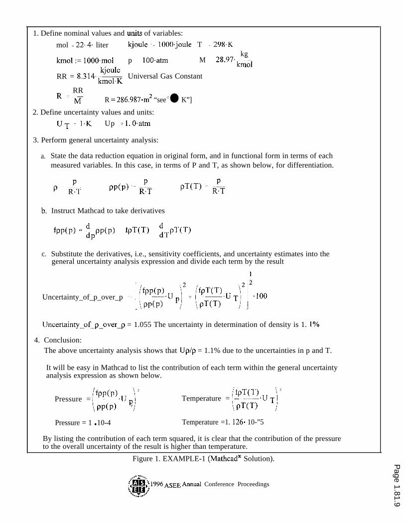
For instance, the students are asked to experimentally determine the density of air (p ) in a pressurizedtank and the conditions are such that the equation of state of an ideal gas ( p = P/R T) is applicable. The% thedetermination of air density (p) depends on the evaluation of the pressure (P), temperature (T), and the gasconstant (R). It is not necessary to measure the gas constant since it is available with great accuracy inreference sources3, thus, the air pressure and temperature are the quantities to be measured in the laboratory.The students know that there are uncertainties (measurement errors) associated with each measured variables,however, the key question for them is, how do these uncertainties in the individual variables propagatethrough the akzta reduction equation (governing equation) into the result? The following examples of generaluncertainty analysis during the planning phase of the experiment show the flexibility on estimating uncertaintiesfor measured variables and the propagation of these uncertainties into the experimental result.

Example Problem -1A pressurized air tank is stored in a laboratory where the nominal ambient temperature is 27 “C. The air

temperature is measured using a sensor with an uncertainty of 1 “C and the uncertainty in pressure measurementis 10/o. Evaluate the uncertainty in determining the air density using the equation of state for an ideal gas.

A. SoIution (Manual Analvsi&The data reduction equation is

~‘ = R T

The uncertainty expression becomes

up = [(: UJ2 +(3&J2 +(&T)2]1’2

The partial derivatives areap 1—=—ap RT

(3)

(4)

(5)

$!iia-’} 1996 ASEE Annual Conference Proceedings‘.+,yyHl’,$

Page 1.81.3

*=_ PaR R 2T

ap P—= ——aT R T2

(6)

(7)

Substitution of the partial derivatives into (4) gives

up ‘ [(+T UP)2 +(= UR)2 + (= UT)2]1’2R 2T R T2

Dividing the uncertainty expression (8) by the data reduction equation (3) givesu U2U2 u 2 1/2

Q = [(;) +(;) +(;) 1P

(8)

(9)

Values for the variables areT=27”C+273=300KU== 1 “C (=1 K)up/p = 0.01UR = 0 . 0

The uncertainty in ~ i.e. U~, is assumed negligible since the gas constant is available in reference sources with agreat degree of certainty. Substitution of the numerical values in (9) gives the uncertainty in the air density

uJp=o.oll = 1.1%The analysis presented for the above example problem shows the necessary steps in a general uncertaintyanalysis. The analysis for this simple problem is straightforward, however, manual evaluation of the derivativesand repeated calculations for more complex problem can become tedious. Application of Mathcad@ foruncertainty analysis of complex problems provides the convenience and the flexibility to facilitate laboratoryinstruction by reducing the difficulty of calculations (i.e., taking derivatives) and increasing the speed inrepeating computations.

B. Solution (USim.z Mathcad@~The step-by-step solution procedure using Mathcad@ is given in Figure 1. Mathcad@ provides the

flexibility to pefiorm repeated calculations and show the results at various intermediate steps. As shown inFigure 1, the uncertainty contributions from pressure and temperature terms are presented separately. It is clearthat the contribution due to the pressure is much larger than temperature. This step illustrates the utility ofuncertainty analysis in identi~ng the more sensitive measurement variables with which special care must betaken. Suppose we want to reduce the uncertainty of the result (density) to 0.50A. Then, we can vruy theestimated uncertainty in temperature measurement, pressure measurement, or both. Reducing the uncertaintyin temperature measurement alone will not satis~ our requirement since setting it even to zero reduces theuncertainty in density to 10/o. Thus, acquiring more expensive temperature measurement device for betteraccuracy is unnecessary. By improving the pressure measurement and reducing its uncertainty to 0.3°/0, theuncertainty in density reduces to O. S”/O. The key point in this exercise is to show how the students may vary theuncertainties in each measured variables as they select proper transducers based on manufacturers’specifications apriori to purchasing the transducers. It also illustrates how quickly and conveniently the valuesof measured variables and associated uncertainties maybe varied in Mathcad@ and obtain accurate results. TheMathcad@ flexibility in allowing to enter measured values in different system of units (i.e. English or S1) asobtained from different measurement equipment is an added convenience.

?$ii&) 1996 ASEE Annual Conference Proceedings‘.J~y&lll’,?

Page 1.81.4

Example Problem -2A client needs to determine the behavior of the convective heat transfer from a heated circular cylinder

of finite length that will be immersed in an air flow whose velocity might range from 1 to 100 rnhec. Theexpected convective heat transfer coefficient for these velocities range up to 1000 W/m2 “C. The cylinder tubeto be tested is 152 mm long with a diameter of 25.4 mm and a wall thickness of 1.27 mm. The primary case ofinterest is for an air temperature of about 25 ‘C with the cylinder at about 45 ‘C. The cylinder is made ofaluminum, for which the specific heat has been found from a table as 903 J/kg ‘C at 300 K. The mass of thetube has been measured as 0.020 kg. The client wants to know the convective heat transfer coefficient (h)within 5°A and must be assured that “h” can be determined within 10°/0 before fimding for the experiment willbe allocated.

The two experimental techniques being considered for determining the heat transfer coefficient in thisexample problem are a steady-state and a transient technique, respectively. The heat transfer from the cylinderby radiation or conduction is assumed negligible in this initial analysis.

The data reduction equation for the steady-state technique is

h =w

nDL( T- T.)

For a given air velocity, the convective heat transfer coefficient h is determined by measuring the electricalpower W, the cylinder diameter D and length L, and the temperatures of the cylinder surface T and the airstream T,.

The data reduction equation for a transient technique ish= Mc

n~DL

(lo)

(11)

The convective heat transfer coefficient h for a given air velocity is determined by using the cylinder mass M,specific heat c, diameter D and length L, and the time constant z. In this approach, the cylinder is heated until itreaches a temperature TO and then the power is switched off. The time constant ~ is defined as the time takenfor the cylinder temperature T to change 63 .2V0 of the way from TO to T..

A, Steady State Solution (Manual Analvsis);The uncertainty expression for the steady-state technique is

Uh = [(@# Jwf+( &D; +(guL; +(guT; +($2 1/2

U’1’a ) 1a

For this analysis, assume that the temperature difference (T-T~ will be measured directly. Therefore, theuncertainty expression simplifies as

Uh = [(-&w)2 +(% UD)2 +($ UL)2 + ( $T‘A*)21“2

(12)

(13)

Students are expected to estimate the uncertainties in W,uncertainties:

U~ = 0.025 mmU== 0.25 mm

D, L, and AT. Assume the following measurement

?$iiik} 1996 ASEE Annual Conference Proceedings‘.,.,yyHl’:

Page 1.81.5

u~= = 0.25 “C and 0.5 ‘CUW=0.5 Wand 1.OW

Manual evaluation of the partial derivatives, substitution into(13) and determination of the uncertainty forseveral h values are presented elsewhere and will not be repeated here. However, general uncertainty analysisusing Mathcad@ is presented herein.

B. Steady State SoIution (using Math-m.

The steady-state solution using Mathcad@ is presented in Figure 2.

A. Transient Solution (Manual Analvsis);The uncertainty expression for the transient technique is

U, = [(~u~)’ ‘($Uc)’ ‘(~ U.: ‘(~ ‘.)’ +(&.)’1”2 (14)

The uncertainties in ~ c, D, L, and T need to be estimated. Uncertainties in D and L are the same as thoseused in the steady-state analysis. Let us use the following measurement uncertainties in this analysis:

U~ = 0.025 mmU~ = 0.25 mmU~ = 0.0001 KgUJC = 1 . 0 %Uz = 5, 10, and 20 msec

Manual evaluation of the partial derivatives, substitution into (14) and determination of the uncertainty arepresented elsewhere and will not be repeated here. However, Mathcadm evaluations are presented herein.

B. Transient SoIution (using Mathcad@);The transient solution using Mathcad@ is presented in Figure 3.

DETAILED UNCERTAINTY ANALYSISThe detailed uncertainty analysis4 is very usefil in the design, construction, debugging, data analysis,

and reporting phases of an experimental program. This approach is more complex than the general uncertaintymethod since the bias and precision components of uncertainty are considered separately.

The elemental bias limits from all sources for each measured variable are combined using RSS to obtaina resultant bias limit for that variable. For the ith variable influenced by biases from M significant elementalerror sources, the resultant bias limit is calculated by

B, = [ (Bl); + (13i): +...... + (Bf)’J” (15)

The precision limit, Pi, for each variable, ~, is estimated from multiple readings of the variable overthe appropriate time period or from previous experince.

Once the bias and precision limits for each variable have been estimated, the bias and precision limits forthe experimental result are found from the uncertainty analysis expressions (16) and (17), respectively, whichassume no correlated bias or precision uncertainties and incorporates the large sample assumption as discussedin Coleman and Steele (1995)4.

>C..g. f,,,

.s~~ -,) 1996 ASEE Annual C’onfcrencx Proceedings

‘.,,,plpj

Page 1.81.6

B,=[( -&BJ2 +(A B2)2+ . . . ..+( ~BJ)2 ]1’2

1 ax2 Jand

P, = [(-& PJ2+(~ P 2)2 +..... +( &PJ)2 ]1’2

1 2 J

(16)

(17)

The bias component (B, ) is a fixed error that may in some instances be reduced by calibration. Theprecision component (1?, ) is a variable error that may be reduced by averaging repeated measurements takenover an appropriate time period. The uncertainty in the result is then given

u, = [B: +P; ]1’ 2 (18)

The uncertainty U, gives 95% coverage of the true value when the bias and precision contributions areestimated for a 95°A confidence level. In practice, dividing each term in expressions (16), (17) and(18) by theresult may sometimes result in simplifications, and the uncertainty results are expressed in percentages as shownin Figure 4.

Example Problem -3The changes in air velocity in an exhaust duct of a manufacturing plant is being monitored. To

speci~ what magnitude of changes in the measured velocity should be viewed as a drifi in the operatingpoint of the system, one must know the range of velocity measurements expected if the system is operatingat a “steady” set point. Analyze the system and estimate the expected range of velocity readings at a pointin the duct exit plane using the measurement system described below.

The measurement system consists of a Pitot tube mounted in the exit plane of the duct, an analogdifferential pressure gauge with a range of O to 2 in. of water and a least scale division of 0.05 in. of water,a thermometer with a least scale division of 1 “C, and a barometer with a least scale division of 1 mm Hg.The normal operating temperature and pressure are given as 300 K and 760 mm Hg, respectively. Thenominal dynamic pressure measured by the differential pressure gauge is 1.5 in. H20.

The Pitot tube senses both stagnation pressure and static pressure, and these are fed into thedifferential pressure gauge. The gauge then indicates the dynamic pressure, Ap, which is the differencebetween stagnation and static pressures.

The air velocity is given by

where the air density p is calculated from the ideal gas relation

y_‘=RT

Substituting (20) into (19), gives the data reduction equation

V=( 2R TAp 112

P)

(19)

(20)

(21)

fx’,.:} 1996 ASEE Annual Conference Proceedings

‘..+,RT~,<

Page 1.81.7

This data reduction equation is used for the detailed uncertainty analysis. The estimates for error sourcesare required apriori. The elemental uncertainties are presented and used in the detailed uncertaintyanalysis in Figure 4.

SUMMARY AND CONCLUSIONSThe uncertainty analysis calculations for the example problems presented in this article show that

regardless of the complexity of the data reduction equation, Mathcada software maybe used quiteeffectively as an instructional tool. The convenience in taking derivatives of the data reduction equation,the flexibility in allowing graphical presentation of results, the capability in checking the accuracy of unitsfor various measured variables, and the convenience of repeating calculations are the usefhl features of theMathcad” software for uncertainty analysis. These features may enhance students interest in laboratoryexperimentation and facilitate learning. The students are expected to benefit from reduced analysis time bydevoting more time to understand the importance of uncertainty analysis in all phases of an experimentalprogram.

REFERENCES1. Coleman, II. W. and Steele, W. G., 1989, Experimentation and Uncertainty Analysis for Eng”neers,

John Wiley & sons, Inc. New York.2. Mathcad is a technical calculation software developed and marketed by MathSoft, Inc.3. Tables of Thermal Properties of Gases, U.S. National Bureau of Standards Circular 564, 1955.4. Coleman, H.W. and Steele, W. G., 1995, Engineering Application of Experimental Uncertainty

Analysis, AIAA J., Vol. 33, No. 10, pp. 1888-1896.

AUTHORS’ AFFILIATIONSDR. M. H. HOSNI is the Director of the Engineering Institute for Environmental Research and anAssociate Professor of Mechanical Engineering at Kansas State University, Manhattan, KS 66506.

DR. H. W. COLEMAN is an Eminent Scholar in Propulsion and Professor of Mechanical Engineering atthe University of Alabama in Huntsville, Huntsville, AL 35899.

DR. W. G. STEELE is a Professor and Head of Mechanical Engineering at Mississippi State University,Mississippi State, MS 39762.

f&?,.,) 1996 ASEE Anilual Conference P1-(xxcclings

‘..,,~TQL;<

Page 1.81.8

1. Define nominal values and units of variables:

mol = 22” 4“ liter kjoule - 1000”joule T = 298*K

krnol := 1000”mol p 100”atm Mkjoule

RR = 8.314.&rK Universal Gas Constant

RRR=m R =286.987*m2 “see-2 ● K”]

kg

28”97”kmoi

2. Define uncertainty values and units:

UT ~~ 1*K Up .- l. O.atm

3. Perform general uncertainty analysis:

a.

b.

c.

State the data reduction equation in original form, and in functional form in terms of eachmeasured variables. In this case, in terms of P and T, as shown below, for differentiation.

p ,. .R:T PP(P) “ ~pT pT(T) -= RPT

Instruct Mathcad to take derivatives

fPP(P) “ +PP(P) fpT(T) ~-TpT(T)

Substitute the derivatives, i.e., sensitivity coefficients, and uncertainty estimates into thegeneral uncertainty analysis expression and divide each term by the result

Uncertainty_of_p_over_p ~-l(f5:f”upr’rJ::i”uTrl;”100

Uncertainty_of_p_over_p = 1.055 The uncertainty in determination of density is 1. l?ko

4. Conclusion:The above uncertainty analysis shows that Up/p = 1.1% due to the uncertainties in p and T.

It will be easy in Mathcad to list the contribution of each term within the general uncertaintyanalysis expression as shown below.

()fpp(p).u 2

Pressure = -——PP(P) p ()fpT(T) 2

Temperature = -- –— “UTpT(T)

Pressure = 1 ● 10-4 Temperature =1. 126s 10-”5

By listing the contribution of each term squared, it is clear that the contribution of the pressureto the overall uncertainty of the result is higher than temperature.

Figure 1. EXAMPLE-1 (Mathcad@ Solution).

{62’&~ 1996 ASEE Annual Conference Proceedings‘.,,,yyy’j.

Page 1.81.9

1. Define nominal values and units of variables:

2.4.watt

4.9.watt

12.watt

24. watt

49. watt

121.watt

243 watt

2. Define uncertainty

U A T z0.5. K

()

0.5.wattUw .1 .O.watt

L =0.152.m

D “= 0.0254. m

AT ~ 20. K

i ‘=0..6

i represents the number of nominal values for power W.

The power matrix corresponds to the range of potential h values upto 1000 W/m2 ‘C

values and units:

U D = ().ozs.mm UL -0.zs.mm

j =0..1 j represents the number of uncertainty limits to be used for power W.

3. General uncertainty analysis according to the data reduction equation:

a. State the data reduction equation in original form, and in functional form in terms of each measured variables.

Wi Wi Wi

~ ‘---- hAT(AT) hD( D) hL(L) hW(W)w

z.DLAT TC. D.L.AT n. D.L. AT TC. D.LAT n. D. L.AT

b. Instruct Mathcad to take derivatives

fhW( W) = :whW( W) fhD(D) = :=hD( D) fhAT(AT) :AThAT(AT)

c. Substitute the derivatives, i.e., sensitivity coefficients, and uncertainty estimates into the general uncertaintyanalysis expression

12

.100

The results of Uh /h for UA~ = 0.50 ‘C are presented below. Uh vectors show the Uh\h in % for 0.5 W and 1,0 Wuncertainty estimates in power measurements. The hW(W i ) vector shows the corresponding convectivecoefficients (h).

Uh=

5.W 1.OW

21 41.7-

10.5 20.6

4.9 8.7

3.3 4.9

2.7 3.2

2.5 2.6

2.5 2.5

I 9.9kgsec 3K ‘ I

20.2.kg.see” 3. K-’

%%%$-l202. kg. sec 3.K 1

498.8 .kg. sec-3K

1. 103.kg. sec 3. K-

Figure 2. EXAMPLE-2 (Mathcad@ Solution).

.c,.~ .,,,

.@; 1996 ASEE Annual Conference Proceedings‘Jyyy’::.

Page 1.81.10

The figure below is a plot of uh /h versus h values for both 0.5 W and 1.0 W uncertainties estimates in power

measurement for UAT = 0.5 K.

40 I I I

UA~= 0.5 K30 --

qL

z

20

\

10 J\

< - . . . _ _ ——0 I T–

100 200 300 400h (W/m2.C)

And the results of uncertainty analysis for UL~ = 0.25 “C are:

U A T z0.25. K

“iJ=[(5w”uwJ’(f ~~”uDJ’-(:::”u’r’(::: #}”u’Tr ‘“’00

0.5. W I.e. w‘W(wi)

20.9 41.7

- ,~,,

9.9.kg. sec 3.K 1

10.3 20.4 20.2. kg.sec K4.4 8.4 49.5. kg.sec K

u’. 2.4 4.498.9. kg.sec K“

1.6 2.4202. kg.sec” K

1.3 1.5

1.3 1.3 498.8 kg.sec- .K-

1.10 .kg.sec- .K -

40

U~~ = 0.25 K30 --

<L

s

20

\

10 J\\ _ _ _ _

0100 200 300 400

4. Conclusion:h (W/m2.C)

The uncertainties of 0.5 watt and 1.0 watt in the power measurement are adequate at higher values of h (>100 W/m2.k)lbut do not satisfy the requirements at low and moderate h values. The uncertainty in the power measurement is thedominant uncertainty (for the assumption made in this analysis) in the low and moderate h range, and would have to bereduced below 0.5 watt for the requirement of about 5% uncertainty in h to be met.

Figure 2. EXAIVIPLE-2 (Mathcadw Solution Continued).

~“hxli’}. 1996 ASEE Annual Conference Proceedings;:,~ly...:.

Page 1.81.11

i 0..6

1. Define nominal values and units of variables:

M =0.02.kgjoule

c :=903 --- ---kg.K

D 25.4mm L 152.mm

149,0. sec

74.4sec

29.8. sec

Tz 14.9. sec

7.4. sec

3. O.sec

1.5. sec

The time constant matrix corresponds to the range of potential h values up to 1000 W/m2. ‘C.

2. Define uncertainty values and units of variables:

1UM =0.0001. kg Uc ‘ C“mo u D ‘ o.ozs.mm uL ‘o.zsmm

[)

0.05. sec

uT’ - O.lO. sec j 0..20.20. sec

3. General uncertainty analysis based on the data reduction equation:

a. State the data reduction equation in original form, and in functional form in terms of each measured variables,

MChi ;= ‘“c hM( M) ~= --—- hc(c) = .-”:.C-..~.D.L.~i ~.D.L.~i n. D.L~i

hD(D) : ❑ -+’;;-; hL(L) ~= ;-;;-; h+) := ~;. . . . . . . .

I I

b. Instruct Mathcad to take derivatives

fiM(M) =&hM(M) fhC(C) =$chc(c) tk~(z) -= :;h~(~)

fhD(D) ~= :DhD(D) fhL(L) =: LhL(L)

c. Substitute the derivatives, i.e., sensitivity coefficients, and uncertainty estimates into the general uncertaintyanalysis expression

,

1

‘hj:=[(t;:;JuM~+~~uc~+[~uDr*~~yJuLr+~u7J[100

.- –...Figure 3. EXAMPLE-2 (Mathcadw Solution).

<’~g~~ 1996 ASEE A~~u~l Conference Proceedings‘Jll&.:.

Page 1.81.12

0.05.sec O.1.sec 0.2. sec h~(~i)

4

Uh=

1.1 1.1 1.1

1.1 1.1 1.2

1.1 1.2 1.3

1.2 1.3 1.8

1.3 1.8 2.9

2 3.5 6.8

3.5 6.8 13.4

M20.013 .kg. sec K

49.966 .kg. sec K

99.932 .kg.sec .K-

201.214 kg.sec-3K 1

12

8

4

0

-------.

-- ---- -----_- —- -.= =--1 I I I200 400 600 800 I 000

h (W/m2.C)

Conclusion:For the conditions and estimates used in this analysis, the transient technique will meet the requirements if thetime constant can be measured with an acceptable uncertainty.

Figure 3. EXAMPLE-2 (Mathcad@ Solution Continued).

?fi!iia-’} 1996 ASEE Annual Conference Proceedings‘.,,,~ycllll+:?.

Page 1.81.13

1. Define nominal values and units of variables:

mol “=22.4 .liter ~ , 28.97.-! In_H20 -112.62.43. 144. psimol

1joule

mm_Hg – - .in_HgRR z 8.314. ---- -- Universal Gas Constant

25.4mol. K

Ap 1.51 n_H20

~=R: R =0.029 kgm”K 1 P 760.mm_Hg

T =300. K

?. Define uncertainty values and units for elemental bias sources:

Differential pressure gauge:

B_Ap_o = 0.05 ~ In_H20 zeroth order bias limit

Pitot tube:

B_Ap_l “= 0.015. 1n_H20 bias limit for installation

Barometer:

BI_o 2. O.mm_Hg zeroth order bias limit

Thermometer:

13_T_o “= 2.O.K zeroth order bias limit

1. Perform detailed uncertainty analysis:

a. Determine bias limits for measurements of individual variables1

lAP = [ [B_Ap_o)2 I- (B_AP_I)2] 2

B_Ap = 0.052 ”In_H20 Bias limit for Ap

b. Estimate precision limits for measurements of individual variables using previous experienceswith the system:

P_Ap : = 0.061. In_H20 Precision limit for Ap

P~_o = 0.25. mm_Hg zeroth order precision limit

P_T_o :=0,5K zeroth order precision limit

c. State the data reduction equation in original form, and in functional form in terms of eachmeasured variables.

1 I

()

2 2“ . 2. R.T.Ap

P ()V P ( P ) ~ 2:-R;:*P

Figure 4. EXAMPLE-3 (Mathcad@ Solution).

{hid-’} 1996 ASEE Annual Conference Proceedings‘.,+,~yRL,~

Page 1.81.14

I

d. Instruct Mathcad to take derivatives

fvP(P) = :-pVP(P) fVAp (Ap) d VAp (Ap)dAp

fVT(T) ~TVT(T)

e. Substitute the derivatives, i.e., sensitivity coefficients, and bias estimates into the uncertaintyanalysis expression and divide by the result

Bias_V_over_V = 1.777 Thus, the bias limit for the velocity is 1.8%

f. Substitute the derivatives, i.e., sensitivity coefficients, and precision estimates into the uncertaintyanalysis expression and divide by the result

1.

( fVP( P)2

Precision_V_over_V z)(

fVT(T)— ~ PJ_o tVP(P)

_...p_T_O]2+[:::#P_AP]2 ‘.100VT(T)

Precision_V_over_V = 2.035 Thus, the precision limit for the velocity is 2?k0

g. Calculate the uncertainty in the result using the bias and precision limits1

U_V_over_V = [ ( Bias_V_over_V )2 t ( precision_V_over_V)2 ] 2 U_V_over_V = 2.701

4. Conclusion:The above detailed uncertainty analysis shows that Uv/v = 2.7%

Figure 4. EXAMPLE-3 (Mathcad” Solution Continued).

~’ ,.~ ,,,,

@H~ 1996 ASEE Annual Conference Proceedings‘..*,EI:B,:

Page 1.81.15