applied sciences

Article

Application of Machine Learning to Include Honking Effect inVehicular Traffic Noise Prediction

Daljeet Singh 1,*, Antonella B. Francavilla 2 , Simona Mancini 3 and Claudio Guarnaccia 2,*

�����������������

Citation: Singh, D.; Francavilla, A.B.;

Mancini, S.; Guarnaccia, C.

Application of Machine Learning to

Include Honking Effect in Vehicular

Traffic Noise Prediction. Appl. Sci.

2021, 11, 6030. https://doi.org/

10.3390/app11136030

Academic Editor:

Sławomir K. Zielinski

Received: 5 May 2021

Accepted: 25 June 2021

Published: 29 June 2021

Publisher’s Note: MDPI stays neutral

with regard to jurisdictional claims in

published maps and institutional affil-

iations.

Copyright: © 2021 by the authors.

Licensee MDPI, Basel, Switzerland.

This article is an open access article

distributed under the terms and

conditions of the Creative Commons

Attribution (CC BY) license (https://

creativecommons.org/licenses/by/

4.0/).

1 Department of Mechanical Engineering, Thapar Institute of Engineering and Technology, Patiala 147004, India2 Department of Civil Engineering, University of Salerno, 84084 Fisciano, Italy; afrancavilla@unisa.it3 Department of Information Engineering, Electric Engineering and Applied Mathematics,

University of Salerno, 84084 Fisciano, Italy; smancini@unisa.it* Correspondence: daljeet.singh@thapar.edu (D.S.); cguarnaccia@unisa.it (C.G.)

Featured Application: Machine learning techniques are calibrated on a dataset of sound levelsin urban areas in India, with relevant honking occurrences. The best model chosen will improvethe prediction of road traffic noise in similar cases, with respect to standard models that neglectthe effects of honking.

Abstract: A vehicular road traffic noise prediction methodology based on machine learning tech-niques has been presented. The road traffic parameters that have been considered are traffic volume,percentage of heavy vehicles, honking occurrences and the equivalent continuous sound pressurelevel. Leq A method to include the honking effect in the traffic noise prediction has been illustrated.The techniques that have been used for the prediction of traffic noise are decision trees, randomforests, generalized linear models and artificial neural networks. The results obtained by using thesemethods have been compared on the basis of mean square error, correlation coefficient, coefficient ofdetermination and accuracy. It has been observed that honking is an important parameter and con-tributes to the overall traffic noise, especially in congested Indian road traffic conditions. The effectsof honking noise on the human health cannot be ignored and it should be included as a parameter inthe future traffic noise prediction models.

Keywords: road traffic noise; honking; machine learning; prediction; modelling

1. Introduction

The number of vehicles on the roads has been increasing exponentially, both in de-veloping and developed countries. The reasons are consumerism, reduced prices, financeoptions, competition and the requirement of faster and convenient transport. An inevitableoutcome of this continuous production and buying of these vehicles, especially the privateones, has been an increase in the noise and air pollution levels due to the hard trafficcongestion, especially in critical areas of the cities [1–3]. The effects of air pollution arewell known to the general public. To address the problem of environmental pollution,many predictive models and experimental studies have been developed for the trafficmanagement as efficient solution to reduce vehicle journey times and, consequently, envi-ronmental impact. For instance, in [4], carbon dioxide (CO2) emissions and unnecessaryfuel consumption are addressed in the framework of route management for autonomousvehicles in urban areas. Conversely, there is a relatively lesser awareness of the harm-ful effects of traffic noise on the human population. Some of the adverse effects [5–8]include sleep disturbance, speech interference, annoyance, cardio-vascular effects and lossof fertility. In rare cases, such as with traffic policemen who are exposed to high soundpressure levels and long-term road traffic noise, hearing loss has also been observed [9].As for the prediction of traffic volumes and the adoption of traffic management strategiesto reduce noise pollution levels, a lot of research has been done on the effects of noise

Appl. Sci. 2021, 11, 6030. https://doi.org/10.3390/app11136030 https://www.mdpi.com/journal/applsci

Appl. Sci. 2021, 11, 6030 2 of 16

on human health [10,11]. Traffic noise prediction models play a very important role notonly in the design and modification of road and traffic infrastructure [12] but also in theassessment of the noise level, based on certain critical parameters. Different types of trafficnoise prediction models include country or region-specific models like the “Federal High-way Administration model” (FHWA, USA), the “UK Calculation of Road Traffic Noise”(CoRTN, UK), the “Acoustical Society of Japan Road Traffic Noise model” (ASJ, Japan) andthe “Richtlinien für den Lärmschutz an Straben” (RLS-90, Germany). A critical review ofthe most used models can be found in [13–16]. Other categories of models include staticand dynamic, stochastic and deterministic and artificial intelligence or machine learningbased models [17–22]. In particular, several applications to traffic noise prediction can befound in literature, for instance [23–27], in which the authors adopt artificial intelligencetechniques, such as artificial neural networks (ANN) and genetic algorithms (GA).

In most recent studies, hybrid models combining systems of ANN and fuzzy inter-ference systems (FIS) (i.e., adaptive neuro fuzzy inference system—ANFIS) have beendeveloped too [28]. Other hybrid models are represented by the integration between timeseries analysis techniques and ANN [29].

The different parameters that are generally considered in these models are trafficvolume (number of vehicles per unit of time), percentage of heavy vehicles, averagespeed of vehicles, tyre–road interaction, building height, road width and gradient etc.One parameter that has generally been not considered and is quite prevalent in the Indianroad conditions is honking noise.

The relevance of the honking in the Indian scenario has been demonstrated in severalstudies. In [30], for example, it is reported how the expansion of the transportation industryin the city of Nagpur led to an increment of 5–6 dBA in noise level, 4–6 times in honkingand 1.7 times in traffic volume.

The Indian roads traffic conditions are quite different because of the size of the popu-lation, topography of the roads, vehicle types and conditions, driving habits and culture.Because of the congested traffic conditions and anxious drivers, the effect of honking onthe overall traffic noise and its effects on the drivers, pedestrians, cyclists, traffic policepersonnel, nearby shopkeepers and residents needs to be considered. In this heterogeneouscomposition of traffic, horn events get to increase noise level (Lden) up to 0.5–13 dBAcompared to homogenous traffic conditions [31]. Therefore, the prediction models usedfor homogenous traffic conditions are not applicable in this heterogeneous context. Thus,to increase the accuracy of noise prediction models, considering honking is required.

Some models considering honking have been developed by using regression modeland statistical analysis [32], others by introducing a factor for horn correction, with respectof level of service (LOS), in traffic noise models such as CRTN, FHWA, and RLS 90 [31].

In the present work, an attempt has been made to include the honking effect in thetraffic noise prediction model developed using machine learning methods. In particular,four different techniques have been selected, calibrated and tested on a case study exper-imental dataset collected in Patiala city, India. A comparison of these techniques on thebasis of criteria of mean square error, correlation coefficient, coefficient of determinationand accuracy has also been presented.

2. Materials and Methods2.1. Dataset and Sites Description

The data used in this paper has been collected on the busy urban roads of the Patialacity in India (Figure 1). Besides the equivalent continuous sound pressure level (Leq),the data collection included the parameters traffic volume (Q), percentage of heavy vehicles(P) and total honking occurrences (H) that have been used to calibrate and test the machinelearning models. These parameters have been collected manually using videography atfive different identified sites, highlighted in Figure 1, on the basis of congestion, presence ofhonking noise and proximity to resident population. For each video, the numbers of light

Appl. Sci. 2021, 11, 6030 3 of 16

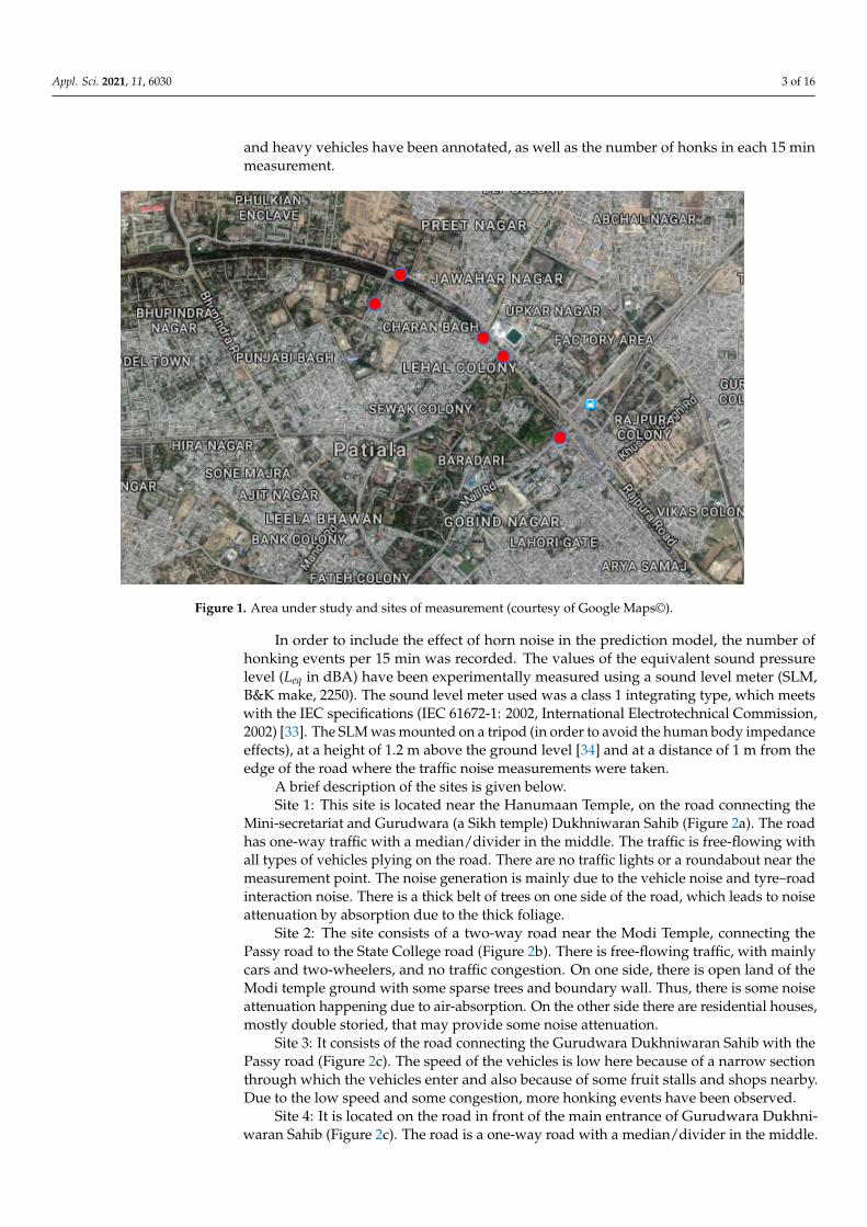
and heavy vehicles have been annotated, as well as the number of honks in each 15 minmeasurement.

Appl. Sci. 2021, 11, x FOR PEER REVIEW 3 of 17

chine learning models. These parameters have been collected manually using videogra-phy at five different identified sites, highlighted in Figure 1, on the basis of congestion, presence of honking noise and proximity to resident population. For each video, the num-bers of light and heavy vehicles have been annotated, as well as the number of honks in each 15 min measurement.

Figure 1. Area under study and sites of measurement (courtesy of Google Maps©).

In order to include the effect of horn noise in the prediction model, the number of honking events per 15 min was recorded. The values of the equivalent sound pressure level (Leq in dBA) have been experimentally measured using a sound level meter (SLM, B&K make, 2250). The sound level meter used was a class 1 integrating type, which meets with the IEC specifications (IEC 61672-1: 2002, International Electrotechnical Commission, 2002) [33]. The SLM was mounted on a tripod (in order to avoid the human body imped-ance effects), at a height of 1.2 m above the ground level [34] and at a distance of 1 m from the edge of the road where the traffic noise measurements were taken.

A brief description of the sites is given below. Site 1: This site is located near the Hanumaan Temple, on the road connecting the

Mini-secretariat and Gurudwara (a Sikh temple) Dukhniwaran Sahib (Figure 2a). The road has one-way traffic with a median/divider in the middle. The traffic is free-flowing with all types of vehicles plying on the road. There are no traffic lights or a roundabout near the measurement point. The noise generation is mainly due to the vehicle noise and tyre–road interaction noise. There is a thick belt of trees on one side of the road, which leads to noise attenuation by absorption due to the thick foliage.

Site 2: The site consists of a two-way road near the Modi Temple, connecting the Passy road to the State College road (Figure 2b). There is free-flowing traffic, with mainly cars and two-wheelers, and no traffic congestion. On one side, there is open land of the Modi temple ground with some sparse trees and boundary wall. Thus, there is some noise attenuation happening due to air-absorption. On the other side there are residential houses, mostly double storied, that may provide some noise attenuation.

Site 3: It consists of the road connecting the Gurudwara Dukhniwaran Sahib with the Passy road (Figure 2c). The speed of the vehicles is low here because of a narrow section

Figure 1. Area under study and sites of measurement (courtesy of Google Maps©).

In order to include the effect of horn noise in the prediction model, the number ofhonking events per 15 min was recorded. The values of the equivalent sound pressurelevel (Leq in dBA) have been experimentally measured using a sound level meter (SLM,B&K make, 2250). The sound level meter used was a class 1 integrating type, which meetswith the IEC specifications (IEC 61672-1: 2002, International Electrotechnical Commission,2002) [33]. The SLM was mounted on a tripod (in order to avoid the human body impedanceeffects), at a height of 1.2 m above the ground level [34] and at a distance of 1 m from theedge of the road where the traffic noise measurements were taken.

A brief description of the sites is given below.Site 1: This site is located near the Hanumaan Temple, on the road connecting the

Mini-secretariat and Gurudwara (a Sikh temple) Dukhniwaran Sahib (Figure 2a). The roadhas one-way traffic with a median/divider in the middle. The traffic is free-flowing withall types of vehicles plying on the road. There are no traffic lights or a roundabout near themeasurement point. The noise generation is mainly due to the vehicle noise and tyre–roadinteraction noise. There is a thick belt of trees on one side of the road, which leads to noiseattenuation by absorption due to the thick foliage.

Site 2: The site consists of a two-way road near the Modi Temple, connecting thePassy road to the State College road (Figure 2b). There is free-flowing traffic, with mainlycars and two-wheelers, and no traffic congestion. On one side, there is open land of theModi temple ground with some sparse trees and boundary wall. Thus, there is some noiseattenuation happening due to air-absorption. On the other side there are residential houses,mostly double storied, that may provide some noise attenuation.

Site 3: It consists of the road connecting the Gurudwara Dukhniwaran Sahib with thePassy road (Figure 2c). The speed of the vehicles is low here because of a narrow sectionthrough which the vehicles enter and also because of some fruit stalls and shops nearby.Due to the low speed and some congestion, more honking events have been observed.

Site 4: It is located on the road in front of the main entrance of Gurudwara Dukhni-waran Sahib (Figure 2c). The road is a one-way road with a median/divider in the middle.

Appl. Sci. 2021, 11, 6030 4 of 16

The traffic volume is very high as the vehicles arrive from different sections of the city andconverge here to pass through this bottle-neck section and then go to Mini-secretariat roador the Sirhind road. There is a large number of heavy vehicles passing through this sectionas the vehicles coming from bus stand or other areas move out of the city using this road,to reach the Sirhind road and then subsequently to the national highway. On one side thereis the Gurudwara Sahib main premises and the outer boundary wall, and on the other side,there are shops. High traffic noise levels are observed here due to the large traffic volumeas well as honking.

Site 5: The site is situated near the Patiala Bus stand (Figure 2d). A lot of cars,two wheelers and three wheelers pass through this section. The speed of the vehicles islow due to the traffic congestion, as people come here to pick and drop passengers at thebus stand. This also leads to the highest number of horns/honking events observed heregiving rise to high noise levels.

A description of the data collected at the above sites, with some statistical analysisand insights into the same is presented below.

The data was collected for 10 days at each site, with 15 min time span, so a datasetof 50 days has been obtained for all the five sites. A resume of the data main statistics isreported in Table 1, while the full dataset is reported in Appendix A.

Appl. Sci. 2021, 11, x FOR PEER REVIEW 4 of 17

through which the vehicles enter and also because of some fruit stalls and shops nearby. Due to the low speed and some congestion, more honking events have been observed.

Site 4: It is located on the road in front of the main entrance of Gurudwara Dukhni-waran Sahib (Figure 2c). The road is a one-way road with a median/divider in the middle. The traffic volume is very high as the vehicles arrive from different sections of the city and converge here to pass through this bottle-neck section and then go to Mini-secretariat road or the Sirhind road. There is a large number of heavy vehicles passing through this section as the vehicles coming from bus stand or other areas move out of the city using this road, to reach the Sirhind road and then subsequently to the national highway. On one side there is the Gurudwara Sahib main premises and the outer boundary wall, and on the other side, there are shops. High traffic noise levels are observed here due to the large traffic volume as well as honking.

Site 5: The site is situated near the Patiala Bus stand (Figure 2d). A lot of cars, two wheelers and three wheelers pass through this section. The speed of the vehicles is low due to the traffic congestion, as people come here to pick and drop passengers at the bus stand. This also leads to the highest number of horns/honking events observed here giving rise to high noise levels.

A description of the data collected at the above sites, with some statistical analysis and insights into the same is presented below.

The data was collected for 10 days at each site, with 15 min time span, so a dataset of 50 days has been obtained for all the five sites. A resume of the data main statistics is reported in Table 1, while the full dataset is reported in Appendix A.

(a)

(b)

Figure 2. Cont.

Appl. Sci. 2021, 11, 6030 5 of 16Appl. Sci. 2021, 11, x FOR PEER REVIEW 5 of 17

(c)

(d)

Figure 2. localization of the identified sites, respectively site 1 (a), site 2 (b), site 3 and 4 (c), site 5 (d).

Table 1. Resume of the main statistics of data and parameters used in the calibration and testing of the models. All the features have been measured with 15 min time span.

Mean Standard De-viation

Median Min Max

Traffic volume in 15 min (Q) [veh] 633.8 341.2 583 216 1377 Percentage of heavy vehicles (P) [%] 1.36 1.42 0.5 0 3.8

Total honking occurrences in 15 min (H) [counts] 218.0 88.9 227 90 406

Equivalent continuous sound level (Leq) [dBA] 74.7 3.4 75 68 79.7

2.2. Bivariate Correlation Analysis A bivariate correlation analysis has been performed in R software framework [35].

Results are reported in Figure 3, in which traffic volume (Q), heavy vehicle percentage (P), total honking occurrences (H) and measured equivalent continuous sound pressure level (Leq) are reported with bivariate scatter plots below the diagonal, histograms on the diag-onal and the Pearson correlation above the diagonal. A high correlation (0.90) is found between Leq and traffic volume, as expected since the main noise sources in the measure-ment sites are the vehicles. A significant (0.65) correlation is found between Leq and P, as well as between Leq and H.

Figure 2. Localization of the identified sites, respectively site 1 (a), site 2 (b), site 3 and 4 (c), site 5 (d).

Table 1. Resume of the main statistics of data and parameters used in the calibration and testing of the models. All thefeatures have been measured with 15 min time span.

Mean Standard Deviation Median Min Max

Traffic volume in 15 min (Q) [veh] 633.8 341.2 583 216 1377Percentage of heavy vehicles (P) [%] 1.36 1.42 0.5 0 3.8

Total honking occurrences in 15 min (H) [counts] 218.0 88.9 227 90 406Equivalent continuous sound level (Leq) [dBA] 74.7 3.4 75 68 79.7

2.2. Bivariate Correlation Analysis

A bivariate correlation analysis has been performed in R software framework [35].Results are reported in Figure 3, in which traffic volume (Q), heavy vehicle percentage(P), total honking occurrences (H) and measured equivalent continuous sound pressurelevel (Leq) are reported with bivariate scatter plots below the diagonal, histograms onthe diagonal and the Pearson correlation above the diagonal. A high correlation (0.90)is found between Leq and traffic volume, as expected since the main noise sources in themeasurement sites are the vehicles. A significant (0.65) correlation is found between Leqand P, as well as between Leq and H.

Appl. Sci. 2021, 11, 6030 6 of 16Appl. Sci. 2021, 11, x FOR PEER REVIEW 6 of 17

Figure 3. Scatter plot of traffic volume (Q), heavy vehicles percentage (P), honking occurrences (H) and measured contin-uous equivalent levels (Leq), with bivariate scatter plots below the diagonal, histograms on the diagonal and the Pearson correlation above the diagonal.

It is interesting to notice that the heavy vehicle percentage, that is usually imple-mented in the most common road traffic noise models, being recognized as an important parameter of the phenomenon, correlates with the noise levels similarly to the total honk-ing occurrences, that is practically always neglected. In the authors’ opinions, this means that, at least in the five test sites and in all the sites with similar features, the honking events cannot be ignored when designing and calibrating an effective traffic noise model.

2.3. Machine Learning Methodologies The traffic noise prediction models were developed using four machine learning

methods in R software [35], namely decision trees (DT), random forests (RF) [36], gener-alized linear models (GLM) and artificial neural networks (ANN) [24,25]. These methods have been implemented in the ‘Rattle’ (R) software [37] which is open source and has a GNU (general public license).

The different machine learning methodologies used in the present work are briefly described below: (i). Decision Trees (DT) [18]: These methodologies are employed in machine learning

applications where an analysis of the data is required. They use a structure which resembles a flow chart as they are based on deterministic data structures and used in classification problems. At the top of the tree, there is a root node and the branches represent the tests that are done and the leaves denote the results of the tests. The rpart( ) function builds a decision tree model. A decision tree works by splitting nodes into sub-nodes. The parameter MinSplit describes the minimum number of members that a node should have before the split is attempted. MaxDepth indicates the maxi-mum depth or length of the tree, starting from the root node up to the leaf node. MinBucket parameter specifies the minimum number of entities that a leaf node can have. The default value is generally one-thirds of the MinSplit value.

(ii). Random Forests (RF) [36]: In this approach, groups of decision trees are created. This is an ensemble method, which can be used for regression, classification and other tasks. They avoid over-fitting, which can be a drawback in the decision tree method, by making random decision forests. The observations are used as input for each tree

Figure 3. Scatter plot of traffic volume (Q), heavy vehicles percentage (P), honking occurrences (H) and measuredcontinuous equivalent levels (Leq), with bivariate scatter plots below the diagonal, histograms on the diagonal and thePearson correlation above the diagonal.

It is interesting to notice that the heavy vehicle percentage, that is usually imple-mented in the most common road traffic noise models, being recognized as an importantparameter of the phenomenon, correlates with the noise levels similarly to the total honkingoccurrences, that is practically always neglected. In the authors’ opinions, this means that,at least in the five test sites and in all the sites with similar features, the honking eventscannot be ignored when designing and calibrating an effective traffic noise model.

2.3. Machine Learning Methodologies

The traffic noise prediction models were developed using four machine learning meth-ods in R software [35], namely decision trees (DT), random forests (RF) [36], generalizedlinear models (GLM) and artificial neural networks (ANN) [24,25]. These methods havebeen implemented in the ‘Rattle’ (R) software [37] which is open source and has a GNU(general public license).

The different machine learning methodologies used in the present work are brieflydescribed below:

(i). Decision Trees (DT) [18]: These methodologies are employed in machine learningapplications where an analysis of the data is required. They use a structure whichresembles a flow chart as they are based on deterministic data structures and used inclassification problems. At the top of the tree, there is a root node and the branches rep-resent the tests that are done and the leaves denote the results of the tests. The rpart( )function builds a decision tree model. A decision tree works by splitting nodes intosub-nodes. The parameter MinSplit describes the minimum number of members thata node should have before the split is attempted. MaxDepth indicates the maximumdepth or length of the tree, starting from the root node up to the leaf node. Min-Bucket parameter specifies the minimum number of entities that a leaf node can have.The default value is generally one-thirds of the MinSplit value.

(ii). Random Forests (RF) [36]: In this approach, groups of decision trees are created.This is an ensemble method, which can be used for regression, classification and othertasks. They avoid over-fitting, which can be a drawback in the decision tree method,by making random decision forests. The observations are used as input for each treeand the most common outcome is used as the final output. As the errors are cancelled

Appl. Sci. 2021, 11, 6030 7 of 16

out, a more accurate prediction is obtained using this method. The randomForest( )function is used for the implementation of the random forests. Breiman (2001) [36]introduced the idea of random sampling of variables at each node as the tree is beingbuilt. He also introduced the bagging concept for the sampling [38] in which randomsamples are chosen for the training dataset for each tree. It helps in making the modelrobust to noise and outliers. The parameter ntree specifies the number of trees built inthe Random Forests model.

(iii). Linear Models: Generalized linear models (GLM) make use of and combine differenttypes of regression, e.g., linear and logarithmic [39]. They take care of different typesof distribution like the log-linear and log-odds, as the response is not always linearand might not follow a normal distribution.

(iv). Neural Networks [40]: Artificial neural networks (ANN) are similar in working tothe human brain which uses neurons (connections of nodes) for the learning tasks.The process involves the assignment of weights to the inputs and activation functionsfor getting the desired outputs. There are different layers in a neural network likean input layer, a hidden layer (which performs non-linear transformations of theinputs) and an output layer of neurons. The function neuralnet( ) is used to build aneural network model in R software [35]. The parameter hlayers is used to specify thenumber of hidden layer nodes or neurons in the NN architecture. MaxNWts sets themaximum limit of the number of weights that can be used in the model. The maxitparameter defines the maximum number of iterations to be done during the training.

The values of the training hyperparameters for the different methods have been takenbased on experience and literature survey and are briefly given below.

For the decision trees, the value of MinSplit used is 20, MaxDepth 30 and MinBucket7. The type of random forest used in RF is regression. The number of trees is 500 andthe number of variables tried at each split is 1. The sampling type is bagging. In theneural networks, the number of hidden layer nodes or neurons is 10 with one hidden layer,epochs 150 and the batch size is 8. The activation function used is Sigmoid, dropout rate is0.2, number of units is 30 and the learning rate is 0.01. The optimizer used is Grid Search.Some of the values, along with names of modules, are given in Table 2.

Table 2. Machine Learning Methods Used [41].

Model Method Name of Module Input Parameters and Values

Decision Trees rpart Rpart MinSplit = 20, MaxDepth = 30, MinBucket = 7

Random Forests rf randomForest ntree = 500, sampling = bagging

Linear Models lm glm None

Neural Networks neuralnet Neuralnet hlayers = 10, MaxNWts = 10,000, maxit = 100

2.4. Perfomance Metrics

The results obtained by using the methods described above were compared on the ba-sis of the criteria of correlation coefficient (r), coefficient of determination (R2), mean squareerror (MSE) and accuracy, briefly resumed in this subsection.

2.4.1. Correlation Coefficient (r)

The correlation coefficient (r) is a measure of a linear correlation between two setsof data. In particular, it measures the closeness of the points in a scatter plot to the linearregression obtained on the basis of the input data. This parameter can be evaluated asfollows [42]:

r =Cov (X, Y)√

s2xs2

y

(1)

Appl. Sci. 2021, 11, 6030 8 of 16

where Cov (X, Y) is the covariance and s2x and s2

y are the sample variance for X and Y.Obviously, a coefficient of correlation close to 1 indicates a strong linear correlation while acoefficient r close to 0 suggests a little correlation between the investigated parameters.

2.4.2. Coefficient of Determination (R2)

The coefficient of determination R2 provides the percentage variation in Y explained byX-variable. It is the square of the coefficient of correlation (r) therefore it is a measurementused to explain how much variability of one factor can be caused by its relationship toanother related factor. When the coefficient of determination is equal to 1, the regressionline fits all the sample data [42].

2.4.3. Mean Squared Error (MSE)

MSE is a measure of the difference between the measured and the predicted values.It is a sample standard deviation of the differences between the observed values and thosepredicted by the model. These are called residuals when the differences are calculated forthe sample (called in-sample) points, that were used to make the model and predictionerrors when the calculations are done for out-of-sample data points. It is calculated as [42]:

MSE =∑n

i=1(bi−ai)2

n(2)

where, a is the observed value, b is the predicted value and n is the number of sampledata points.

2.4.4. Accuracy

The accuracy is defined in percentage as the mean of the number of the differencesbetween the predicted and the observed values of the dependent variable, that fall withina given range e (i.e., within an acceptable error) [28,41]. It can be calculated as follows:

Acc = 100n

n∑

i=1ci

ci =

{1, if abs(bi−ai) ≤ e0, otherwise

(3)

where, b is the predicted value of dependent variable, a is the observed value of dependentvariable, e is the acceptable value of error and n is the total number of samples.

The results obtained are presented in the subsequent section.

3. Results and Model Comparison

The results obtained by using the four machine learning models are compared onthe basis of r, R2, MSE and accuracy. The above relation has been used for an accuracy of±1 dBA. The values of the different criteria for the four models are shown in Table 3.

Table 3. Comparison of results for the prediction models in the training phase.

Machine Learning Method r R2 MSE[dBA]

Accuracy (±1 dBA)[%]

Decision Trees(DT) 0.935 0.876 0.884 68

Random Forests(RF) 0.987 0.975 0.413 94

Generalized Linear Model(GLM) 0.974 0.949 0.616 82

Neural Networks(ANN) 0.974 0.949 0.616 82

Appl. Sci. 2021, 11, 6030 9 of 16

It is seen that random forests performs better than other models in the training phase,in the criteria of r, R2, MSE and accuracy. The value of MSE is 0.413 for rf which is thelowest and the value of accuracy is 94% (for ±1 dBA) which is the highest among allother models.

However, for a proper comparison, a testing dataset check was performed, in order toavoid overfitting.

In order to meet this objective, the dataset was split into 70/30 as training and testingdata, respectively. Following the training, using the 70% data, the models were tested onthe testing dataset (30%). This was done 10 times (ten-fold cross validation) for the bestperforming model in order to check the stability and robustness of the model. The resultsobtained from the testing dataset show that the generalized linear model (GLM) performsbetter on the considered criteria, as seen in the Table 4.

Table 4. Comparison of results for the prediction models (testing dataset).

Machine Learning Method r R2 MSE[dBA]

Accuracy (±1.0 dBA)[%]

Decision Trees(DT) 0.797 0.636 1.780 40.0

Random Forests(RF) 0.955 0.913 0.797 60.0

Generalized Linear Model(GLM) 0.965 0.933 0.666 80.0

Neural Networks(ANN) 0.959 0.921 0.717 73.3

As seen in Table 4, the value of mean square error is the lowest (0.666) for the gener-alized linear model (GLM) and the accuracy is highest (80.0%). The values of MSE andaccuracy obtained with neural networks are 0.717 and 73.3% respectively. Random forestsand neural networks might give better results for bigger datasets but for the present case,GLM has outperformed the other models.

Results of the models’ predictions plotted versus measured equivalent levels in thevalidation and training datasets are shown in Figure 4. It is easy to see that apart fromdecision trees (DT) that in 4 points is very far from the measured Leq, all the models’results are gathered almost close to the bisector, meaning a general effectiveness of theproposed models. When the measured Leq are around 70 dBA (site 2), the models have thebest performances. This site is characterized by absence of heavy vehicles and honkingfrequencies lower than in the other sites. Data above 78 dBA are related to site 4, in whichthe traffic flows are higher than in the other sites.

A scatter plot between the measured and predicted values of Leq for the four methodsis shown in Figure 5.

A ten-fold cross validation was also performed for the best performing model, GLM andthe results are shown in Figure 6. A general stability of the results is observed, confirmingthe goodness of the model and the suitability to be used in such applications, on noise datathat includes a relevant contribution from honking.

Appl. Sci. 2021, 11, 6030 10 of 16Appl. Sci. 2021, 11, x FOR PEER REVIEW 10 of 17

Figure 4. Scatter plot of the models’ predictions versus measured equivalent levels in the training dataset. The black solid line is the bisector and is used as a guide for the eye, to easily identify overestimation and underestimation of the models.

A scatter plot between the measured and predicted values of Leq for the four methods is shown in Figure 5.

Figure 4. Scatter plot of the models’ predictions versus measured equivalent levels in the trainingdataset. The black solid line is the bisector and is used as a guide for the eye, to easily identifyoverestimation and underestimation of the models.

Appl. Sci. 2021, 11, x FOR PEER REVIEW 10 of 17

Figure 4. Scatter plot of the models’ predictions versus measured equivalent levels in the training dataset. The black solid line is the bisector and is used as a guide for the eye, to easily identify overestimation and underestimation of the models.

A scatter plot between the measured and predicted values of Leq for the four methods is shown in Figure 5.

Appl. Sci. 2021, 11, x FOR PEER REVIEW 11 of 17

Figure 5. Scatter plots between measured and predicted values of Leq.

A ten-fold cross validation was also performed for the best performing model, GLM and the results are shown in Figure 6. A general stability of the results is observed, con-firming the goodness of the model and the suitability to be used in such applications, on noise data that includes a relevant contribution from honking.

Figure 5. Scatter plots between measured and predicted values of Leq.

Appl. Sci. 2021, 11, 6030 11 of 16

Appl. Sci. 2021, 11, x FOR PEER REVIEW 11 of 17

Figure 5. Scatter plots between measured and predicted values of Leq.

A ten-fold cross validation was also performed for the best performing model, GLM and the results are shown in Figure 6. A general stability of the results is observed, con-firming the goodness of the model and the suitability to be used in such applications, on noise data that includes a relevant contribution from honking.

Appl. Sci. 2021, 11, x FOR PEER REVIEW 12 of 17

Figure 6. A ten-fold cross validation for r, R2, MSE and accuracy for the generalized linear model (GLM).

4. Discussion The results reported in Section 3 inspire interesting discussions and allow to draw

some preliminary conclusions. Looking at the scatter plot reported in Figure 4, it is easy to see that, apart from deci-

sion trees (DT), some points underestimate the measured Leq and all the models’ results are gathered almost close to the bisector, meaning a general effectiveness of the proposed models. When the measured values of Leq are around 70 dBA (site 2), the models have the best performance. This site is characterized by the absence of heavy vehicles and honking occurrences lower than in the other sites.

Data above 78 dBA are also associated with good performances of the models. These points are related to site 4, in which the traffic volumes are higher than in the other sites.

Finally, the larger dispersion is observed in the middle range of noise levels. In this range basically all the models produce results that are different with respect to the ob-served noise levels. There is not a clear pattern of overestimation or underestimation, meaning that these errors are basically random for all the models. Only the data com-prised in the range 77–78 dBA seems to show a general underestimation of the models. These points belong to site 5, in which the highest mean honking occurrences has been observed.

In order to highlight the importance of the honking inclusion in the models, a simu-lation without the honking parameter has been performed on the same dataset, both in training and testing phases. Results of the performance metrics without honking are re-ported in Tables 5 and 6.

Figure 6. A ten-fold cross validation for r, R2, MSE and accuracy for the generalized linear model (GLM).

4. Discussion

The results reported in Section 3 inspire interesting discussions and allow to drawsome preliminary conclusions.

Looking at the scatter plot reported in Figure 4, it is easy to see that, apart fromdecision trees (DT), some points underestimate the measured Leq and all the models’ resultsare gathered almost close to the bisector, meaning a general effectiveness of the proposedmodels. When the measured values of Leq are around 70 dBA (site 2), the models have thebest performance. This site is characterized by the absence of heavy vehicles and honkingoccurrences lower than in the other sites.

Data above 78 dBA are also associated with good performances of the models. Thesepoints are related to site 4, in which the traffic volumes are higher than in the other sites.

Finally, the larger dispersion is observed in the middle range of noise levels. In thisrange basically all the models produce results that are different with respect to the observednoise levels. There is not a clear pattern of overestimation or underestimation, meaningthat these errors are basically random for all the models. Only the data comprised in therange 77–78 dBA seems to show a general underestimation of the models. These pointsbelong to site 5, in which the highest mean honking occurrences has been observed.

In order to highlight the importance of the honking inclusion in the models, a simu-lation without the honking parameter has been performed on the same dataset, both intraining and testing phases. Results of the performance metrics without honking arereported in Tables 5 and 6.

Appl. Sci. 2021, 11, 6030 12 of 16

Table 5. Comparison of results for the prediction models in the training phase (without consider-ing honking).

Machine Learning Method r R2 MSE[dBA]

Accuracy (±1 dBA)[%]

Decision Trees(DT) 0.933 0.871 0.902 64

Random Forests(RF) 0.978 0.957 0.526 82

Generalized Linear Model(GLM) 0.904 0.818 1.182 40

Neural Networks(ANN) 0.904 0.818 1.182 40

Table 6. Comparison of results for the prediction models (testing dataset) without considering honking.

Machine Learning method r R2 MSE[dBA]

Accuracy (±1.0 dBA)[%]

Decision Trees(DT) 0.798 0.637 1.781 40.0

Random Forests(RF) 0.955 0.913 0.809 66.7

Generalized Linear Model(GLM) 0.880 0.774 1.291 46.7

Neural Networks(ANN) 0.880 0.774 1.291 46.7

Comparing with results reported in Tables 3 and 4, it can be noticed that the inclusionof honking in the modeling leads to an overall improvement of the performance metrics.The DT model seems to be not sensible to honking, since the metrics are basically constantwith and without honking inclusion, both in training and testing phases. RF in testingdataset keeps r and R2 basically constant, the accuracy has a little increase from 60.0% to66.7%, but MSE increases from 0.797 dBA to 0.809 dBA. The other two models, namely GLMand ANN, converge to similar predictions and, consequently, to equal performance metrics.They exhibit a worsening of all the selected metrics when honking is not considered. SinceGLM was the best performing model in the training dataset with honking, it is evident thatthe inclusion of this parameter leads to a better prediction of noise levels in the presentedapplication. When honking is not included, the MSE of GLM increases from 0.666 dBA to1.291 dBA and the GLM accuracy gets worse, lowering from 80% to 46.7%.

Regarding the cross validation of GLM, the ten-fold cross validation results reportedin Figure 6 shows a general stability. This confirms the goodness of the model and the suit-ability to be used in such applications, on noise data that includes a relevant contributionfrom honking.

Although the dataset is sufficient for the present study, a bigger dataset with a greaterspread across different times of the year and more sites can be prepared and utilized in afuture study. A limitation of the present study, in fact, is that the models are region-specific,since they are based on the data collected at the specific sites identified for the assessment.

The number of input parameters is limited to three in the present work (i.e., traffic vol-ume Q, percentage of heavy vehicles P and total honking occurrences H). In a future work,this number can be expanded including more parameters like speed of vehicles, differenttypes of vehicles (e.g., two-wheelers, three-wheelers etc.) and acceleration-deceleration ofvehicles, etc. Furthermore, an assessment of the actual increase in the noise level (in dBA)due to honking can be made and the effect of the duration of the different types of hornsused on different vehicles needs to be studied.

Appl. Sci. 2021, 11, 6030 13 of 16

5. Conclusions

A traffic noise prediction approach using machine learning methods has been pre-sented, which considers the parameter of honking noise. Horn noise contributes signif-icantly to the overall road traffic noise in Indian road traffic conditions as well as otherregions in the Indian sub-continent. Therefore, there is a need to pay attention to thisimportant parameter while developing traffic noise models. An approach to include theeffect of honking noise by considering the honking occurrences as a parameter has beenillustrated with the help of a case study of the Patiala city in India. A preliminary multivari-ate analysis of the dataset showed that the presence of honking cannot be neglected in thecases under study. A relevant correlation with the continuous equivalent level was found.This correlation was equal to the one found between noise levels and percentage of heavyvehicles, that is a parameter commonly implemented in standard road traffic noise models.

The models developed were compared using the criteria of r, R2, mean square errorand accuracy. It is seen that the generalized linear model (GLM) and artificial neuralnetworks (ANN) are the best performing models, with GLM doing slightly better thanANN on the considered criteria.

A simulation without honking parameter inclusion has been performed, to assessits contribution on the models’ performances. Results showed that including honkingleads to an improvement of the prediction, in particular for GLM, i.e., the model that bestperformed in the testing phase.

Also, a ten-fold cross validation has been done for the best performing model (GLM) tocheck the robustness of the developed model, showing an excellent stability of the technique.

It can be concluded that the machine learning approach can be used to develop trafficnoise prediction models, including honking as a parameter, with considerable accuracy.The effect of changing the traffic parameters on the overall traffic noise can be assessedwith the help of these models, without the actual need of experiments using the sound levelmeter or other equipment. Thus, the policy makers and administration can take suitablesteps for noise abatement, which would be beneficial for the health and well-being of allthe involved stakeholders.

Future developments of this research will be aimed at the calibration and testing ofthe presented models on more data, coming from different sites and with different trafficconditions, in order to enlarge the possible applications to other scenarios. Furthermore,the inclusion of further parameters, such as speed of vehicles, different types of vehicles(e.g., two-wheelers, three-wheelers etc.) and acceleration-deceleration regimes, will be apossible development of the methodology presented.

Author Contributions: Conceptualization, D.S.; methodology, D.S. and C.G.; software, D.S.; vali-dation, D.S., A.B.F., S.M. and C.G.; formal analysis, D.S., A.B.F., S.M. and C.G.; investigation, D.S.,A.B.F., S.M. and C.G.; resources, D.S., A.B.F., S.M. and C.G.; data curation, D.S., A.B.F., S.M. and C.G.;writing—original draft preparation, D.S.; writing—review and editing, D.S., A.B.F., S.M. and C.G.;visualization, A.B.F. and S.M.; supervision, D.S. and C.G. All authors have read and agreed to thepublished version of the manuscript.

Funding: This research received no external funding.

Data Availability Statement: The data presented in this study are available in Appendix A.

Acknowledgments: The authors are thankful to the Noise and Vibration laboratory, Mechanical Engi-neering Department, Thapar Institute of Engineering and Technology, Patiala, for the equipment andother support during the execution of this work. Also, the authors are thankful to Civil EngineeringDepartment, University of Salerno for providing infrastructure and computational facilities.

Conflicts of Interest: The authors declare no conflict of interest.

Appl. Sci. 2021, 11, 6030 14 of 16

Appendix A

The dataset obtained in the measurement sites described in the paper and adopted inthis study is reported in the table below. It can be used for scientific purposes, citing thesource of the data and referring to this paper.

Table A1. Full dataset containing traffic volumes (Q), percentage of heavy vehicles (P), total honkingoccurrences in 15 min (H) and continuous equivalent sound level (Leq) for all the measurements, inall the sites.

ProgressiveNumber

TrafficVolume (Q)

[veh]

Percentage ofHeavy Vehicles

(P) [%]

Total HonkingOccurrences(H) [Counts]

ContinuousEquivalent

Sound Level(Leq) [dBA]

Site 1 1 570 3.3 110 74.02 582 2.2 135 74.63 574 3.7 112 74.54 576 2.8 118 74.75 585 1.7 267 74.46 589 2.5 249 74.97 572 3.4 128 75.18 584 1.3 175 74.59 593 2.4 191 74.310 597 1.5 231 75.0

Site 2 11 216 0.0 126 69.912 241 0.0 102 70.013 238 0.0 110 69.714 239 0.0 102 69.515 220 0.0 106 68.016 230 0.0 115 69.317 226 0.0 100 69.518 244 0.0 123 70.219 219 0.0 93 68.620 246 0.0 90 69.8

Site 3 21 513 0.0 363 76.522 423 0.6 293 73.023 419 0.7 316 75.024 505 0.4 322 75.225 464 0.6 330 76.026 463 0.2 278 72.227 450 0.5 267 72.828 422 0.1 161 72.329 433 0.2 210 72.530 369 0.8 135 72.0

Site 4 31 1092 3.8 204 78.732 1315 3.7 209 79.733 1143 3.4 205 78.934 1141 3.6 210 78.535 1350 3.3 232 79.536 1169 3.5 257 78.837 1344 3.2 229 79.138 1090 3.2 268 78.539 1279 3.7 237 79.340 1377 3.1 279 79.7

Appl. Sci. 2021, 11, 6030 15 of 16

Table A1. Cont.

ProgressiveNumber

TrafficVolume (Q)

[veh]

Percentage ofHeavy Vehicles

(P) [%]

Total HonkingOccurrences(H) [Counts]

ContinuousEquivalent

Sound Level(Leq) [dBA]

Site 5 41 657 0.5 406 78.042 663 0.5 229 75.143 687 0.4 351 77.244 686 0.5 368 77.445 671 0.4 257 75.746 689 0.4 273 76.147 688 0.4 345 77.448 680 0.5 360 77.849 675 0.5 299 76.650 690 0.4 225 75.5

References1. Moshammer, H.; Panholzer, J.; Ulbing, L.; Udvarhelyi, E.; Ebenbauer, B.; Peter, S. Acute Effects of Air Pollution and Noise from

Road Traffic in a Panel of Young Healthy Adults. Int. J. Environ. Res. Public Health 2019, 16, 788. [CrossRef]2. Gieseke, J.; Gerbrandy, G.J. Report on the Inquiry into Emission Measurements in the Automotive Sector; Committee of Inquiry into

Emission Measurements in the Automotive Sector, European Parliament: Brussel, Belgium, 2017.3. Pascale, A.; Fernandes, P.; Guarnaccia, C.; Coelho, M.C. A study on vehicle Noise Emission Modelling: Correlation with air

pollutant emissions, impact of kinematic variables and critical hotspots. Sci. Total Environ. 2021, 787, 147647. [CrossRef]4. Zambrano-Martinez, J.L.; Calafate, C.T.; Soler, D.; Lemus-Zúñiga, L.G.; Cano, J.C.; Manzoni, P.; Gayraud, T. A centralized

route-management solution for autonomous vehicles in urban areas. Electronics 2019, 8, 722. [CrossRef]5. Babisch, W. Stress hormones in the research on cardiovascular effects of noise. Noise Health 2003, 5, 1. [PubMed]6. World Health Organization. Environmental Noise Guidelines for the European Region; World Health Organization Regional Office for

Europe UN City: Copenhagen Ø, Denmark, 2018.7. Banerjee, D. Research on road traffic noise and human health in India: Review of literature from 1991 to current. Noise Health

2012, 14, 113.8. Silva, L.T.; Oliveira, I.S.; Silva, J.F. The impact of urban noise on primary schools. Perceptive evaluation and objective assessment.

Appl. Acoust. 2016, 106, 2–9. [CrossRef]9. Win, K.N.; Balalla, N.B.P.; Lwin, M.Z.; Lai, A. Noise-Induced Hearing Loss in the Police Force. Saf. Health Work 2015, 6, 134–138.

[CrossRef] [PubMed]10. Rice, C. CEC joint research on annoyance due to impulse noise: Laboratory studies. In Proceedings of the Fourth International

Congress on Noise as A Public Health Problem, Turin, Italy, 21–25 June 1983; Volume 2, pp. 1073–1084.11. Frei, P.; Mohler, E.; Röösli, M. Effect of nocturnal road traffic noise exposure and annoyance on objective and subjective sleep

quality. Int. J. Hyg. Environ. Health 2014, 217, 188–195. [CrossRef]12. Singh, D.; Nigam, S.P.; Agrawal, V.P.; Kumar, M. Modelling and Analysis of Urban Traffic Noise System Using Algebraic Graph

Theoretic Approach. Acoust. Aust. 2016, 44, 249–261. [CrossRef]13. Steele, C. A critical review of some traffic noise prediction models. Appl. Acoust. 2001, 62, 271–287. [CrossRef]14. Garg, N.; Maji, S. A critical review of principal traffic noise models: Strategies and implications. Environ. Impact Assess. Rev. 2014,

46, 68–81. [CrossRef]15. Quartieri, J.; Mastorakis, N.E.; Iannone, G.; Guarnaccia, C.; D’Ambrosio, S.; Troisi, A.; Lenza, T.L. A Review of Traffic Noise

Predictive Models. In Recent Advances in Applied and Theoretical Mechanics, Proccedings of the Conference Applied and TheoreticalMechanics, Puerto de la Cruz, Tenerife, Spain, 14–16 December 2009; WSEAS Press: Athens, Greece, 2009; pp. 72–80.

16. Guarnaccia, C. Advanced Tools for Traffic Noise Modelling and Prediction. WSEAS Trans. Syst. 2013, 12, 121–130.17. Kumar, K.; Parida, M.; Katiyar, V.K. Road traffic noise prediction with neural networks–A review. Int. J. Optim. Control 2012,

2, 29–37. [CrossRef]18. Quinlan, J.R. Induction of decision trees. Mach. Learn. 1986, 1, 81–106. [CrossRef]19. Eliseeva, E.; Hubbard, A.E.; Tager, I.B. An application of machine learning methods to the derivation of exposure-response curves

for respiratory outcomes. In U.C. Berkeley Division of Biostatistics Working Paper Series; University of California: Berkeley, CA, USA,2013; p. 309. Available online: http://biostats.bepress.com/ucbbiostat/paper309 (accessed on 1 May 2013).

20. Iannone, G.; Guarnaccia, C.; Quartieri, J. Noise Fundamental Diagram deduced by traffic dynamics. In Recent Researches inGeography, Geology, Energy, Environment and Biomedicine, Proceedings of the 4th WSEAS International Conference on EMESEG’11, CorfùIsland, Greece, 14 July 2011; WSEAS Press: Athens, Greece, 2011; pp. 501–507.

Appl. Sci. 2021, 11, 6030 16 of 16

21. Quartieri, J.; Mastorakis, N.E.; Iannone, G.; Guarnaccia, C. Cellular automata application to traffic noise control. In Proceedingsof the 12th WSEAS International Conference on Automatic Control, Modelling and Simulation (ACMOS’10), Sicily, Italy,29–31 May 2010; pp. 299–304.

22. Graziuso, G.; Mancini, S.; Guarnaccia, C. Comparison of single vehicle noise emission models in simulations and in a real casestudy by means of quantitative indicators. Int. J. Mech. 2020, 14, 198–207. [CrossRef]

23. Cammarata, G.; Cavalieri, S.; Fichera, A. A neural network architecture for noise prediction. Neural Netw. 1995, 8, 963–973.[CrossRef]

24. Kumar, P.; Nigam, S.P.; Kumar, N. Vehicular traffic noise modeling using artificial neural network approach. Transp. Res. Part CEmerg. Technol. 2014, 40, 111–122. [CrossRef]

25. Givargis, S.; Karimi, H. A basic neural traffic noise prediction model for Tehran’s roads. J. Environ. Manag. 2010, 91, 2529–2534.[CrossRef]

26. Gündogdu, Ö.; Gökdag, M.; Yüksel, F. A traffic noise prediction method based on vehicle composition using genetic algorithms.Appl. Acoust. 2005, 66, 799–809. [CrossRef]

27. Rahmani, S.; Mousavi, S.M.; Kamali, M.J. Modeling of road-traffic noise with the use of genetic algorithm. Appl. Soft Comput.2011, 11, 1008–1013. [CrossRef]

28. Singh, D.; Upadhyay, R.; Pannu, H.S.; Leray, D. Development of an adaptive neuro fuzzy inference system based vehicular trafficnoise prediction model. J. Ambient Intell. Hum. Comput. 2021, 12, 2685–2701. [CrossRef]

29. Guarnaccia, C.; Quartieri, J.; Tepedino, C. A hybrid predictive model for acoustic noise in urban areas based on time seriesanalysis and artificial neural network. In AIP Conference Proceedings; AIP Publishing LLC: Melville, NY, USA, 2017; Volume 1836,p. 020069.

30. Thakre, C.; Laxmi, V.; Vijay, R.; Killedar, D.J.; Kumar, R. Traffic noise prediction model of an Indian road: An increased scenario ofvehicles and honking. Environ. Sci. Pollut. Res. Int. 2020, 27, 38311–38320. [CrossRef] [PubMed]

31. Kalaiselvi, R.; Ramachandraiah, A. Honking noise corrections for traffic noise prediction models in heterogeneous trafficconditions like India. Appl. Acoust. 2016, 111, 25–38. [CrossRef]

32. Sharma, A.; Bodhe, G.L.; Schimak, G. Development of a traffic noise prediction model for an urban environment. Noise Health2014, 16, 63–67. [CrossRef]

33. IEC 61672-1: 2002. Electroacoustics—Sound level meters—Part 1: Specifications; International Electrotechnical Commission: Geneva,Switzerland, 2002.

34. ISO 362-1: 2015. Measurement of Noise Emitted by Accelerating Road Vehicles—Engineering Method—Part 1: M and N Categories;International Organization for Standardization: Geneva, Switzerland, 2015.

35. R Core Team. R: A Language and Environment for Statistical Computing; R Foundation for Statistical Computing: Vienna, Austria,2014. Available online: http://www.R-project.org/ (accessed on 3 May 2021).

36. Breiman, L. Random forests. Mach. Learn. 2001, 45, 5–32. [CrossRef]37. Williams, G. Rattle: A Data Mining GUI for R. R J. 2009, 1, 45–55. [CrossRef]38. Breiman, L. Bagging Predictors. Mach. Learn. 1996, 24, 123–140. [CrossRef]39. Nelder, J.A.; Wedderburn, R.W.M. Generalized linear models. J. R. Stat. Soc. A 1972, 135, 370–384. [CrossRef]40. Riedmiller, M.; Braun, H. A direct adaptive method for faster backpropagation learning: The RPROP algorithm. In Proceedings

of the IEEE International Conference on Neural Networks, New Jersey, NJ, USA, 28 March–1 April 1993; pp. 586–591.41. Singh, D.; Nigam, S.P.; Agrawal, V.P.; Kumar, M. Vehicular traffic noise prediction using soft computing approach.

J. Environ. Manag. 2016, 183, 59–66. [CrossRef]42. Spiegel, M.R.; Stephens, L.J. Theory and Problems of Statistics, 3rd ed.; Schaum’s Outline Series; McGraw-Hill: New York, NY,

USA, 1999.