Celestial Mechanics and Dynamical Astronomy manuscript No.(will be inserted by the editor)

P. Di Lizia · R. Armellin · M. Lavagna

Application of high order expansions of two-pointboundary value problems to astrodynamics

Received: date / Accepted: date

Abstract Two-point boundary value problems appear frequently in space trajectory design. Aremarkable example is represented by the Lambert’s problem, where the conic arc linking twofixed positions in space in a given time is to be characterized in the frame of the two-body prob-lem. Classical methods to numerically solve these problems rely on iterative procedures, whichturn out to be computationally intensive in case of lack of good first guesses for the solution.An algorithm to obtain the high order expansion of the solution of a two-point boundary valueproblem is presented in this paper. The classical iterative procedures are applied to identify areference solution. Then, differential algebra is used to expand the solution of the problem aroundthe achieved one. Consequently, the computation of new solutions in a relatively large neighbor-hood of the reference one is reduced to the simple evaluation of polynomials. The performancesof the method are assessed by addressing typical applications in the field of spacecraft dynamics,such as the identification of halo orbits and the design of aerocapture maneuvers.

Keywords two-point boundary value problem, differential algebra, halo orbit, aerocapture.

1 Introduction

Two-point boundary value problems (TPBVP) appear frequently in space trajectory design whensolving a system of ODE with boundary conditions on both sides of the integration interval(Armellin and Topputo 2006). A typical example is the classical Lambert’s problem, in which aconic arc linking two fixed positions in a given time is to be identified in the frame of the two-bodyproblem. Such a problem can be solved by means of efficient semi-analytical algorithms, since ananalytic solution is available in the case of Kepler’s problem (Battin 1993). Even optimal space-craft control problems are reduced to TPBVP within the framework of indirect methods (Brysonand Ho 1975): the full system of equations, made up by the states and the Lagrange multipliersdynamics, must be solved for initial and final conditions derived by problem requirements. Thishighlights the relevance of the TPBVP in spacecraft dynamics and the wide applicability of therelated methods and algorithms.

P. Di Lizia, R. Armellin, and M. LavagnaDipartimento di Ingegneria Aerospaziale, Politecnico di MilanoVia La Masa, 34 – 20156, Milano, ItalyE-mail: dilizia, armellin, lavagna@aero.polimi.it

2

TPBVP are usually solved by means of numerical methods belonging to one of the follow-ing two classes: shooting schemes, simple and multiple, or difference methods, according to thestandard classification of Stoer and Bulirsch (1993). Methods belonging to the first class reducethe boundary value problem to several initial value problems to be solved within each subin-terval. Such methods can reach effective convergence but are highly sensitive to intermediateinitial conditions when the subintervals become large. The second class methods are based onthe discretization of first-order ODE over an appropriate grid. The resulting finite-dimensionalproblem, satisfying both the defects, resulting by the discretization process, and the boundaryconditions, is solved.

Methods belonging to these two classes have different performances in terms of accuracy,robustness, and computational efficiency, but they share the common feature of delivering a so-lution valid only for the considered set of boundaries constraints and parameters. On the otherhand, a method capable of solving TPBVP for sets of boundary conditions and parameters wouldbe desirable for example when searching for families of periodic orbits, like in the restricted threebody problem, or during the early design of interplanetary trajectories or space maneuvers. Theattainment of this noticeable task has recently been faced by Guibout and Scheeres (2006a).More specifically, the approach relies on the theory of canonical transformations and their gen-erating functions for Hamiltonian systems: canonical transformations are able to solve boundaryvalue problems between Hamiltonian coordinates and momenta for a single flow field. The maindifficulty of the previous approach is finding the generating function via the solution of theHamilton-Jacobi equation. This problem was solved by Guibout and Scheeres by expanding thegenerating function in power series of its arguments.

Differential algebraic (DA) techniques (Berz 1999b) are proposed in this work as a valuabletool to develop an alternative approach to answer the previous requirements, whose applicabilityis not limited to Hamiltonian systems. Differential algebra serves the purpose of computing thederivatives of functions in a computer environment. More specifically, by substituting the classicalimplementation of real algebra with the implementation of a new algebra of Taylor polynomials,any function f of v variables is expanded into its Taylor series up to an arbitrary order n. DAtechniques are effectively used to represent the dependency of the computed quantities on thedesign parameters by means of high order Taylor polynomials. Moreover, the resulting Taylorpolynomials can be manipulated to gain explicit representations of the constraint manifolds ofthe TPBVP in terms of Taylor polynomials. This enables the expansion of the TPBVP solutionabout an available reference solution. The resulting Taylor polynomials can be evaluated for newsolutions of the original TPBVP, so avoiding the multiple run of classical iterative procedures.Some hints about the analogy between the approach proposed in this work and the method ofgenerating functions are supplied in Di Lizia (2008b).

The paper is organized as follows. A brief introduction to differential algebra is given in Sect.2. Being at the basis of the proposed methods, the possibility of expanding the flow of ODE ispresented in Sect. 3. The algorithm for the high order expansion of the solution of TPBVP isillustrated in Sect. 4. The application of the algorithm to the identification of families of haloorbits and to the design of aerocapture maneuvers is addressed in Sect. 5.

2 Differential Algebra

DA techniques find their origin in the attempt to solve analytical problem by an algebraic ap-proach (Berz 1999b). Historically, the treatment of functions in numerics has been based on thetreatment of numbers, and the classical numerical algorithms are based on the mere evaluationof functions at specific points. DA techniques are based on the observation that it is possible toextract more information on a function rather than its mere values. The basic idea is to bringthe treatment of functions and the operations on them to the computer environment in a similarway as the treatment of real numbers. Referring to Fig. 1, consider two real numbers a and b.

3

a, b ∈ R a, b ∈ FP

a× b

× ⊗

a⊗ b

T

T

f, g

f × g

× ⊗

T

T

F,G

F ⊗G

Fig. 1 Analogy between the floating point representation of real numbers in a computer environment(left figure) and the introduction of the algebra of Taylor polynomials in the differential algebraic frame-work (right figure).

Their transformation into the floating point representation, a and b respectively, is performed tooperate on them in a computer environment. Then, given any operation × in the set of real num-bers, an adjoint operation ⊗ is defined in the set of FP numbers such that the diagram in figurecommutes1. Consequently, transforming the real numbers a and b in their FP representation andoperating on them in the set of FP numbers returns the same result as carrying out the operationin the set of real numbers and then transforming the achieved result in its FP representation.In a similar way, suppose two sufficiently regular functions f and g are given. In the frameworkof differential algebra, the computer operates on them using their Taylor series expansions, Fand G respectively. Therefore, the transformation of real numbers in their FP representation isnow substituted by the extraction of the Taylor expansions of f and g. For each operation in thefunction space, an adjoint operation in the space of Taylor polynomials is defined such that thecorresponding diagram commutes; i.e., extracting the Taylor expansions of f and g and operatingon them in the function space returns the same result as operating on f and g in the originalspace and then extracting the Taylor expansion of the resulting function. The straightforwardimplementation of differential algebra in a computer allows to compute the Taylor coefficientsof a function up to a specified order n, along with the function evaluation, with a fixed amountof effort. The Taylor coefficients of order n for sums and product of functions, as well as scalarproducts with reals, can be computed from those of summands and factors; therefore, the setof equivalence classes of functions can be endowed with well-defined operations, leading to theso-called truncated power series algebra (Berz 1986; Berz 1987).

Similarly to the algorithms for floating point arithmetic, the algorithm for functions followed,including methods to perform composition of functions, to invert them, to solve nonlinear systemsexplicitly, and to treat common elementary functions (Berz 1991; Berz 1999). In addition to thesealgebraic operations, also the analytic operations of differentiation and integration are introduced,so finalizing the definition of the DA structure. The differential algebra sketched in this sectionwas implemented by M. Berz and K. Makino in the software COSY-Infinity (Berz and Makino2006).

3 High Order Expansion of ODE Flow

The differential algebra introduced in the previous section allows to compute the derivatives ofany function f of v variables up to an arbitrary order n, along with the function evaluation.This has an important consequence when the numerical integration of an ODE is performed bymeans of an arbitrary integration scheme. Any explicit integration scheme is based on algebraicoperations, involving the evaluations of the ODE right hand side at several integration points.

1 The diagram commutes approximately in practice, due to truncation errors.

4

Therefore, carrying out all the evaluations in the DA framework allows differential algebra tocompute the arbitrary order expansion of the flow of a general ODE initial value problem.

Without loss of generality, consider the scalar initial value problem

x = f(x)x(ti) = xi.

(1)

Replace the point initial condition xi by the DA representative of its identity function, [xi] =x0

i + δxi, where x0

i is the reference point for the expansion. If all the operations of the numericalintegration scheme are carried out in the framework of differential algebra, the Taylor expansionof the solution with respect to the initial condition is obtained at each step. As an example,consider the forward Euler’s scheme

xk = xk−1 + ∆t · f(xk−1) (2)

and analyze the first integration step, i.e.,

x1 = x0 + ∆t · f(x0), (3)

where x0 = xi. Substitute the initial value with [x0] = [xi] = x0

i + δxi in (3) for

[x1] = [x0] + ∆t · f([x0]). (4)

If the function f is evaluated in the DA framework, the output of the first step, [x1], is theTaylor expansion of the solution x1 at t1 with respect to the initial condition about the referencepoint x0

i . The previous procedure can be inferred through the subsequent steps until the lastintegration step is reached. The result at the final step is the n-th order Taylor expansion of theflow of the initial value problem (1) at the final time tf . Thus, the expansion of the flow of adynamical system can be computed up to order n with fixed amount of effort.

The previous DA-based numerical integrators pave the way to numerous practical applica-tions, some of them being addressed in the remaining of this work. A first example is presentedhereafter pertaining the propagation of errors on initial conditions. The Taylor polynomials re-sulting from the use of DA-based numerical integrators expand the solution of the initial valueproblem (1) with respect to the initial condition. Thus, at each integration step, the dependenceof the solution xk on the value of the initial condition xi is available in terms of a polynomialmap Mxk

(δxi), where δxi is the displacement of the initial condition xi from the reference valuex0

i . Suppose now the reference value x0i represents a nominal initial condition for a dynamical

system, and assume some error δxi occurs between the actual initial condition xi and the nominalone. The evaluation of the Taylor polynomial Mxk

(δxi) readily supplies the new solution xk attime tk corresponding to the displaced initial condition. More precisely, the Taylor polynomialMxk

(δxi) delivers a Taylor approximation of the new solution xk, whose accuracy depends onthe expansion order n and the size of the displacement δxi. The main advantage of the DA-basedintegrator is that the new solution is obtained by means of the evaluation of a polynomial, soavoiding a new numerical integration corresponding to the displaced initial condition. Moreover,the same Taylor polynomial can be used to identify the solution corresponding to any error δxi.Consequently, if many values of δxi are to be processed, multiple simple polynomial evaluationscan be efficiently performed in place of multiple intensive numerical integrations.

The results of the application of the previous procedure are illustrated in the following ex-ample. The dynamics of an object moving in the solar system is integrated in the framework ofthe two body problem:

r = v

v = − µr3 r,

(5)

5

−3 −2.5 −2 −1.5 −1 −0.5 0 0.5 1

−1.5

−1

−0.5

0

0.5

1

1.5

x [AU]

y [A

U]

(a)

−1 −0.5 0 0.5 1−2

−1.8

−1.6

−1.4

−1.2

−1

−0.8

−0.6

x [AU]

y [A

U]

exact

1−st order

2−nd order

5−th order

(b)

Fig. 2 (a) Propagation of a box of initial positions in the two-body problem using the 5-th orderexpansion of the flow of the associated ODE; (b) accuracy analysis on one of the resulting boxes.

where r and v are the object position and velocity vectors respectively, and µ is the Sun gravita-tional parameter. The nominal initial conditions are set such that the object starts moving fromthe pericenter of an elliptic orbit, lying on the ecliptic plane (see the dotted line in Fig. 2a). Thepericenter radius is 1 AU, whereas the magnitude of the initial velocity is selected to have a re-sulting orbit of eccentricity 0.5. A DA-based 8-th order Runge–Kutta–Fehlberg (RKF78) schemeis used to expand the solution of the ODE (5) along one revolution of the resulting orbit. A boxof initial positions 0.01 AU on each side is considered and its evolution is investigated. Giventhe bijectivity of the flow of (5), the boundary points of the initial uncertainty box propagateinto boundary points of the corresponding solution set at each integration time. Consequently,the evolution of the initial box is studied by evolving its boundary. Based on the previous ob-servation, a uniform sampling of the boundary of the initial box is performed; for each sample,the displacement with respect to the nominal initial conditions is computed and the polynomialmaps obtained by means of the DA-based integrator are evaluated. In this way, for each integra-tion time, the evolved box can be readily plotted by means of mere polynomial evaluations. Theevolved box is reported in Fig. 2a corresponding to 10 integration times uniformly distributedover the orbital period, using a 5-th order expansion of the flow of the ODE in (5). The timerequired by COSY-Infinity for the computation of the 5-th order map is about 0.38 s on a 2 GHzIntel Core Duo MacBook running Mac OS X.

The accuracy of the Taylor expansion of the flow is better highlighted in Fig. 2b. Focusing on aparticular integration time, the exact propagated box is reported (solid line), which is based on amultiple point-wise integration of the samples. The propagated boxes obtained by the evaluationof the polynomial maps representing the flow of the ODE in (5) are then plotted for comparison,corresponding to different expansion orders. The figure shows that an accurate representation ofthe flow is already achieved using a 5-th order expansion of the flow.

It is worth noting that methods to obtain high order expansion of the flow of ODE have beenalready explored in detail by Griffith et al. (2004) and Park and Scheeres (2006 and 2007). Theseauthors have shown the potentials of these techniques by applying them to the development ofhigh order methods for the solution of relevant space-related problems such as low-thrust Mars-Earth transfers, spacecraft targeting in two-body and Hill three-body dynamics, and trajectoryestimation in the circular restricted three body problem. It has to be stressed that their approachfirstly requires to derive the ODE for the so-called state transition tensors and secondly tointegrate them along with the reference solution. On the other hand, it is not required to writeany additional set of ODE within the differential algebra approach, being the arbitrary highorder expansion of the flow a straightforward result of the implemented algebra. Furthermore,map derivation, integration, and inversion are embedded operations that allow the development

6

of complex algorithms, like those presented in Di Lizia et al. (2008a) and in the followings, in asimple and elegant manner.

4 High Order Expansion of the Solution of TPBVP

As already stated in Sect. 1, besides the considerable opportunity of expanding the flow of ODEpresented in the previous section, an application of DA techniques useful in the framework ofspace trajectory design is analyzed: the high order Taylor expansion of the solution of a TPBVParound a reference solution.

Suppose the dynamics of a point mass is described by the generic system of v first-orderequations

x = f(x, t), (6)

and suppose v appropriate boundary conditions are supplied, whose general non-linear form is

g(x(ti), x(tf )) = 0, (7)

where ti and tf are the initial and final integration time respectively. Equations (6) and (7)together form a TPBVP. Suppose now a simpler form of the boundaries (7) is of interest. Inparticular, assume they reduce to fixing the value of m components of the initial state vector andv−m components of the final state vector, with m < v. Suppose Ci is the set of indexes identifyingthe constrained components of the initial state vector, and Fi is the set of the remaining indexesthat indicates the free components of the same vector. The set Ci contains m indexes, whereasFi is made up of the remaining v − m indexes. Similarly, suppose Cf and Ff are the sets ofindexes that identify the fixed and free components of the final state vector, respectively. Theset Cf now contains v −m elements, whereas Ff is made up by the remaining m indexes. Giventhe introduced notation, the v boundaries (7) assume the simpler form

xCi= xCi

xCf= xCf

,(8)

where xCi= xCi

(ti) and xCf= xCf

(tf ). The original TPBVP has been reduced to the problemof solving (6) together with the v appropriate boundaries (8).

Several techniques are available in the literature to solve the previous problem for assigned xCi

and xCf, as the simple and multiple shooting schemes or difference methods (Stoer and Bulirsch

1993). This means that, given xCiand xCf

, the previous techniques allow the computation of the

free components of the state vector at ti that solve the TPBVP, which will be indicated as x0

Fi.

The solution is then uniquely identified by the initial state vector, given by the combination ofxCi

and x0

Fi. For the sake of a clearer notation, and without loss of generality, this combination

is indicated as a simple concatenation in the followings; i.e.,

x0

i =

(

xCi

x0

Fi

)

. (9)

Assume now a reference solution x0i is available and suppose the Taylor expansion of the

solution of the TPBVP with respect to a set of parameters p is of interest, where p can containeither components of the constrained subset of the initial state, xCi

, or dynamical model param-eters. Differential algebra can effectively serve the purpose of identifying the Taylor expansion.Indicate with p0 the reference value of p used to identify x0

i and initialize both xFiand p as DA

variables. This means the variations

xFi= x0

Fi+ δxFi

p = p0 + δp.(10)

7

are considered.Using the techniques introduced in Sect. 3, expand the solution of equation (6) with respect

to the initial conditions to obtain the map(

xCf

xFf

)

=

(

x0

Cf+ δxCf

x0

Ff+ δxFf

)

=

(

x0

Cf

x0

Ff

)

+

(MxCf

MxFf

) (

δxFi

δp

)

, (11)

where x0

Cfand x0

Ffare the constant part of the map; i.e., the reference solution flowing from x0

i

under the ODE in (6).Subtract the constant part from (11) for

(

δxCf

δxFf

)

=

(MxCf

MxFf

) (

δxFi

δp

)

, (12)

extract MxCffrom (12), and consider the map

(

δxCf

δp

)

=

(

MxCf

Ip

) (

δxFi

δp

)

, (13)

which is built by concatenating MxCfwith the identity map for δp.

Using suitable polynomials inversion techniques (Berz 1999b), the map in (13) can now beinverted to obtain

(

δxFi

δp

)

=

(

MxCf

Ip

)

−1 (

δxCf

δp

)

. (14)

The previous map relates the displacement of the free components of the initial state vector δxFi

and of the parameters δp from their reference values (x0

Fiand p0) to the displacement of the

constrained components of the final state vector (δxCf) from its nominal value (x0

Cf) and again

δp. Given any displacement δxCfof the constrained components of the final state xCf

from their

reference values x0

Cfand any displacement δp of the parameters p from their reference values p0,

the map in (14) delivers the correction δxFito x0

Fito obtain the corresponding solution of the

TPBVP. In other words, the map in (14) is a Taylor expansion of the solution of the TPBVP withrespect to both xCf

and p, which could be profitably used in case of uncertain final boundaryconditions, as in the problem of chasing a moving target. For the applications addressed in thispaper, the aim is that of finding the value of xFi

the point mass must have to meet the desiredxCf

at the given time tf . Thus, the boundary condition

xCf= x0

Cf+ δxCf

= xCf(15)

must be normally imposed. To this aim, note that x0

Cf= xCf

, as x0

i is a solution of the TPBVP.

Consequently, (15) reduces toδxCf

= 0. (16)

Substituting (16) into (14) yields

(

δxFi

δp

)

=

(

MxCf

Ip

)

−1 (

0

δp

)

. (17)

Extract the first v − m components of the map in (17), which will be indicated as

δxFi= MxFi

(δp). (18)

The map in (18) delivers the desired Taylor expansion of the solution of the TPBVP with respectto the parameters in p: given any displacement δp of p from the reference value p0, the simple

8

evaluation of the polynomials in (18) supplies the correction δxFito x0

Fito obtain the new value

of xFithe point mass must have to reach xCf

at time tf .

It is worth observing that a possible alternative approach to solve the previous problem couldhave consisted of solving the TPBVP for the new parameters value p = p0 + δp using classicaltechniques. However, a significant disadvantage characterizes this approach: a new TPBVP mustbe solved for each assigned δp, which involves running through the iterative procedures beneaththe classical TPBVP solvers. Each iterative procedure is able to deliver one solution, whosevalidity is limited to the corresponding δp. Consequently, the classical TPBVP solvers shouldbe applied for each new assigned δp value. The Taylor expansion of the TPBVP supplies aneffective alternative method to solve the previous problem. First of all, analytical information isgained, which can supply a valuable insight on the underlying dynamics. Moreover, for any newδp, the simple evaluation of polynomials suffices to obtain the new value of xFi

, so avoiding theuse of iterative algorithms. Nevertheless, the polynomial relation between xFi

and δp given by(18) is accurate up to the order of the DA-based computation.

Before assessing the performances of the algorithm on applications of interest to spacecraftdynamics, additional notes must be supplied pertaining the existence of the inverse map in (14).The algorithm for map inversion is based on the work of Berz (1999b). More specifically, theinversion of polynomials is reduced to the solution of an equivalent fixed point problem. Thisproblem can be readily solved with a fixed amount of effort in the DA setting through a multipleevaluation of the associated fixed point operator. However, the procedure to obtain the fixed pointoperator relies on the computation of the inverse of the linear part of the map to be inverted.Consequently, the existence of the relations in (14) and (17) is invalidated when the linear partof the map in (13) is singular. The occurrence of such singularities in the solution of TPBVPhas been analyzed in detail in the past by Guibout and Scheeres (Guibout and Scheeres 2004;Guibout and Scheeres 2006b). In particular, it has been shown that these singularities representthe presence of multiple solutions to the TPBVP through a given point. A classical example ofthis situation in spacecraft dynamics is the solution of the Lambert’s problem (see Battin 1993)over a 180-deg transfer, where an infinite number of solutions exists, associated to the lack ofuniqueness of the transfer plane.

It is worth observing that the introduced DA-based algorithm aims at expanding the solutionof a TPBVP in Taylor series about a reference solution already available to the user; i.e., itaddresses the high order Taylor expansion of the solution of the associated relative TPBVP. Thus,the map in (13) is singular only in the presence of multiple solutions of the relative TPBVP.More specifically, if the TPBVP for the computation of the reference solution is singular becauseof lack of uniqueness, the user can eliminate the singularity by forcing the selection of oneparticular solution. This solution can then be used as reference solution for the Taylor expansionof the associated relative TPBVP. For the sake of completeness, as already stated by Guiboutand Scheeres (2004), the presence of such singularity can be overcome for well posed dynamicalproblems by a suitable selection of the variables with respect to which the expansion of thesolution of the relative TPBVP is made. In fact there always exists a choice of these variablespreventing the occurrence of the singularity. However, the problem of singularities does not affectthe applications illustrated in the remaining of this paper.

5 Application to Spacecraft Dynamics

The performances of the technique introduced in the previous section are assessed in the follow-ings in the frame of spacecraft dynamics. Two applications are investigated: the identificationof the family of halo orbits around the Lagrangian point L1 of the Earth–Moon system and thedesign of an aerocapture maneuver for different values of entry velocity and drag coefficient.

9

m1 m2 x

y

L1 L2L3

L4

L5

Fig. 3 Lagrangian points.

5.1 Families of halo orbits

Given two point masses m1 and m2, the restricted three body problem (RTBP) studies themotion of a third point mass m3, whose dynamics is affected by, but does not affect, m1 and m2,which are called the primaries (Thurman and Worfolk 1996). Consequently, the primaries movealong conic arcs. A particular case of RTBP is the CRTBP, where the primaries are assumed tomove along a circular orbit. In this framework, the synodic reference frame is usually introducedthat is centered at the center of mass of the primaries and rotates with them at the correspondingconstant angular velocity, with axis x always aligned with the primaries line, axis y perpendicularto x and lying on the orbital plane of the primaries, and axis z selected to form a right-handedcoordinate system with x and y. Then, a normalization process is usually performed to obtaindimensionless coordinates and parameters. To this aim, the lengths are normalized with thedistance between the primaries, time is normalized so that the angular velocity of the primariesis one, and the masses are scaled by the sum of the primaries masses. After normalization in thesynodic reference frame, the equations of motion for m3 in the CRTBP are

x − 2y = Ωx

y + 2x = Ωy

z = Ωz,

(19)

with

Ω =1

2(x2 + y2) +

1 − µ

r1

+µ

r2

, (20)

where µ = m1/(m1 + m2), and r1 and r2 denote the distances of m1 and m2 from the center ofmass of the system. The second order ODE in (19) can be reduced to the system of first orderODE

x = vx

y = vy

z = vz

vx = 2y + Ωx

vy = −2x + Ωy

vz = Ωz,

(21)

10

which will be indicated asX = f(X) (22)

in the followings, where X = (x, y, z, vx, vy, vz) is the state vector.The CRTBP, expressed by (22), has five equilibrium points, reported in Fig. 3, called La-

grangian or libration points. All the equilibrium points lie in the (x,y)-plane. Two of them, namedL4 and L5, form equilateral triangles with the primaries, whereas the remaining points (L1, L2

and L3) lie on the x-axis and are called the collinear libration points.A growing interest has recently characterized the identification and use of periodic solutions

about the collinear libration points (Bernelli et al. 2004). Among them, the so called halo orbitsappear to be the most promising, as far as practical applications are concerned. Halo orbits arethree-dimensional periodic orbits around the collinear libration points. They differ from planarperiodic solutions, like Lyapunov orbits, because the motion is not forced to lie on the x,y-plane,as an out-of-plane component is gained. Given the constant relative position of the orbit withrespect to the primaries, halo orbits are particularly suitable for either relay satellites or sciencemissions, like space telescopes.

The procedure to compute halo orbits deserves a more detailed analysis. By analyzing equa-tions (22), halo orbits are recognized to be symmetric with respect to the (x,z)-plane (Thurmanand Worfolk 1996). This entails the perpendicularity of the halo orbits to the aforementionedplane. Let now a halo orbit be characterized by its intersection with the (x,z)-plane. Thus, if apoint in phase space is given by X = (x, y, z, vx, vy, vz), then a halo orbit can be specified by(x, 0, z, 0, vy, 0) and the orbital period T , as y = 0 to specify intersection with the (x,z)-planeand vx = vz = 0 to satisfy the symmetry condition. The previous observation eases the numericalcomputation of halo orbits. Suppose that the orbit only crosses the (x,z)-plane in two points.Then the second point will be halfway around. We can then use the symmetry of the problemto generate the entire orbit from the half of the orbit lying to one side of the (x,z)-plane. Thecomputation of the halo orbit is reduced to identifying the values of x, z, and vy at the firstintersection with the (x,z)-plane, which will be indicated by xi, zi, and vyi

, and the value of theperiod T such that, by flowing the initial state Xi = (xi, 0, zi, 0, vyi

, 0) under (22) from t = 0 tot = T/2, the resulting final condition is the next intersection with the (x,z)-plane. By reason ofthe perpendicularity condition, the final state must have the form Xf = (xf , 0, zf , 0, vyf

, 0); i.e.,the final constraints

yf = 0

vxf= 0

vzf= 0

(23)

must be satisfied. Apparently, identifying halo orbits is reduced to a TPBVP. However, unlikethe formalism presented in Sect. 4, the final integration time tf = T/2 is here unknown. It isconvenient in this case to change the time scale by setting t = τ T , where τ is the new independentvariable. The dynamical system (22) is then extended to

dX

dτ= T f (X)

ds

dτ= 0,

(24)

with the initial condition s(0) = si = T for the adjoint variable s. The integration of (22) in theunknown time interval t ∈ [0, T/2] is now reduced to the integration of (24) in the known timeinterval τ ∈ [0, 1/2]. With the time scale change introduced above, the computation of the haloorbit is reduced to a TPBVP with the formalism of Sect. 4. More specifically, the dynamicalsystem is governed by the set of ODE in (24). The sets of the constrained and free componentsof the initial state vector are:

xCi= (yi, vxi

, vzi) xFi

= (xi, zi, vyi, si), (25)

11

0.82

0.84

0.86 −0.050

0.05

−0.03

−0.02

−0.01

0

0.01

0.02

0.03

yx

z

(a)

0.82 0.825 0.83 0.835 0.84 0.845 0.85 0.855 0.86−0.03

−0.02

−0.01

0

0.01

0.02

0.03

x

z

(b)

Fig. 4 An Az = 10000 km L1 halo orbit. (a) A three-dimensional view; (b) the (x,z) view.

whereas, the same sets for the final state read

xCf= (yf , vxf

, vzf) xFf

= (xf , zf , vyf, sf ). (26)

Both xCiand xCf

are constrained to satisfy xCi= 0 and xCf

= 0. Computing a halo orbitis reduced to identifying xFi

which results to a final state Xf satisfying the final constraintsxCf

= 0. Apparently, the problem is not well-defined, as four design variables are available inxFi

to satisfy the three constrains xCf= 0. This is expected because the solution is not unique,

as a family of halo orbits exist, which can be parameterized by the value of one of the elementsin xFi

. The classical choice is selecting the out-of-plane amplitude zi = Az of the halo orbit asparameter: a different unique halo orbit corresponds to each assigned Az , which can be computedsolving the corresponding TPBVP. Thus, the set of free components of the initial state vectorreduces to xFi

= (xi, vyi, si).

Figure 4 illustrates a halo orbit around the Lagrangian point L1 in the Earth-Moon CRTBPwith an out-of-plane amplitude of 10000 km. The orbit is computed using a classical simpleshooting algorithm. The first guess for the associated iterative procedure is supplied by thethird order approximation of the equations of motion about the Lagrangian point derived by thesemi-analytical formulation of Richardson (1980). (For further details about the procedure seeThurman and Worfolk 1996).

It is straightforward noticing that a different TPBVP must be solved for each assigned Az ,which involves running through the iterative procedures of the classical TPBVP solvers. A moreefficient solution to the previous problem is represented by the identification of an explicit alge-braic relation between xFi

and the parameter Az : for each assigned Az , the simple evaluationof the algebraic relations would deliver the set xFi

corresponding to the associated halo orbit.A significant step toward the identification of such explicit relation is already represented bythe aforementioned Richardson’s semi-analytical formulation, which relies on the application ofthe Lindstedt-Poincare method to deal with a third order approximation of the dynamics ofthe CRTBP about the collinear libration points. An effective arbitrary order application of theLindstedt-Poincare method was implemented and used by the group of researchers in Barcelona(Masdemont 2005; Gomez and Mondelo 2001; Gomez et al. 2000; Jorba and Masdemont 1999).Besides supplying an effective mean to explicitly compute the invariant tori contained in thecenter manifold of the RTBP, the previous technique showed remarkably advantages in the qual-itative study of the dynamics around the collinear libration points.

A different approach is proposed in this work, which relies on the use of DA techniques. Asthe identification of halo orbits has been reduced to the solution of a TPBVP, the basic idea istaking advantage of the algorithm introduced in Sect. 4. More specifically, suppose a referencehalo orbit is available, corresponding to a reference amplitude A0

z, which is identified by the

12

0.82 0.83 0.84 0.85 0.86 −0.050

0.05−0.04

−0.03

−0.02

−0.01

0

0.01

0.02

0.03

0.04

yx

z

(a)

0.82 0.83 0.84 0.85 0.86 0.87−0.04

−0.03

−0.02

−0.01

0

0.01

0.02

0.03

0.04

x

z

(b)

Fig. 5 The Taylor representation of the family of halo orbits around L1 in the interval Az ∈ [6000, 14000]km. (a) A three-dimensional view; (b) the (x,z) view.

values of the free components of the initial state vector x0

Fi. The algorithm is used to obtain an

arbitrary order expansion of the solution of the associated TPBVP about the reference one, withrespect to Az . Consequently, the role of the parameter p in the algorithm is here played by Az

and the result of the algorithm is the map

δxFi= MxFi

(δAz). (27)

Given any assigned value of δAz = Az −A0z, the simple evaluation of the polynomials in (27) de-

livers the corrections δxFito x0

Fifor the value of xFi

corresponding to the halo orbit of amplitudeAz. Moreover, as for the Lindstedt-Poincare method, the further advantage of the availabilityof analytical information must be highlighted, which can be manipulated and effectively used insubsequent design phases.

The performances of the algorithm are assessed in the followings, taking the halo orbit in Fig.4 as reference solution. A RKF78 time integration scheme, with relative and absolute tolerancesequal to 10−14, is used to obtain a 18-th order expansion of the TPBVP with respect to Az.The resulting map is reported in Appendix and the time required for its computation is about1255.29 s on a 2 GHz Intel Core Duo MacBook running Mac OS X. The computational timelowers to 596.03 s if the integration tolerances are relaxed to 10−12. Then, the expansion is usedto obtain the family of halo orbits reported in Fig. 5, which are characterized by an out-of-planeamplitude Az ∈ [6000, 14000] km; i.e., Az = A0

z ± 4000 km, where the halo orbit correspondingto A0

z is plotted in bold.As already pointed out in Sect. 4, (27) is a Taylor expansion of the solution of the TPBVP.

Consequently, it is worth assessing the accuracy with which the TPBVP is solved, which suppliesan important insight on the validity of the resulting maps. To this aim, for each Az in theinterval [6000, 14000] km, the Taylor expansions in (27) are used to compute the xFi

that solvesthe corresponding TPBVP. Then, the new initial conditions are flown from τ = 0 to τ = 1/2using again the RKF78 integrator. The accuracy of the Taylor expansion of the solution isthen evaluated as the absolute error on the fulfillment of the final constraints xCf

= 0. Inparticular, the maximum norm of xCf

is reported in Fig. 6 in normalized units as a function of the

displacement δAz of Az from the reference value A0z . The comparison of the curves corresponding

to different expansion orders indicates that the 18-th order polynomial representation ensures amaximum error below 10−10 in the whole interval Az ∈ [6000, 14000] km. As expected, the erroris maximum at the boundary of the interval, whereas it tends to decrease toward the center,where the minimum level of 10−14 is reached, which is related to the tolerance set for the RKF78integrations. The accuracy can be further improved using higher order expansions. For the sake

13

−4000 −3000 −2000 −1000 0 1000 2000 3000 400010

−14

10−12

10−10

10−8

10−6

10−4

||xC

f|| ∞

δ Az [km]

3−rd order

9−th order

18−th order

Fig. 6 Accuracy of the Taylor representation of the family of halo orbits in the interval Az ∈[6000, 14000] km in terms of the fulfillment of the final constraint xCf

= 0.

0.82 0.83 0.84 0.85 0.86 −0.050

0.05

−0.04

−0.02

0

0.02

0.04

yx

z

(a)

−8000−6000−4000−2000 0 2000 4000 6000 8000 1000010

−15

10−10

10−5

100

||xC

f|| ∞

δ Az [km]

3−rd order

9−th order

18−th order(b)

Fig. 7 The Taylor representation of the family of halo orbits around L1 in the interval Az ∈ [1000, 20000]km. (a) A three-dimensional view; (b) error on the fulfillment of the final constraint xCf

= 0.

of completeness, it is worth reporting that the times required for the computation of the 3-rdand 9-th order expansions are 0.10 s and 7.80 s, respectively, on the same machine used to obtainthe 18-th order representation.

Even if the Taylor representation of the halo orbits is not considered sufficiently accurateoutside the interval Az ∈ [6000, 14000] km, it can be profitably used to obtain very accurate firstguesses for classical TPBVP solvers aimed at identifying the corresponding halo orbits. This isconfirmed in Fig. 7a, where the Taylor representation is used to illustrate the family correspondingto the wider interval Az ∈ [1000, 20000] km. The accuracy analysis reported in Fig. 7b showsthat the 18-th order expansion has a maximum error of about 10−5 in the extended interval. Itis worth observing that the error of the 18-th order expansion in the outer region of the intervalis greater than the error corresponding to the 9-th order expansion. This is representative of thefact that the Taylor series do not converge in those regions. Nevertheless, given the relativelysmall error, they can be used as first guesses for the TPBVP. Moreover, once a new referencesolution is available outside the validity interval, a new expansion of the solution of the TPBVPcan be computed using the algorithm introduced in Sect. 4, so gaining a new polynomial map,widening the domain of validity of the available Taylor representations.

5.2 Aerocapture at Mars

The second application, which focuses on an aerocapture maneuver at Mars, has the main roleof showing the versatility of the proposed algorithm as it can be applied to any kind of dy-

14

namics. Aerocapture is a state-of-the-art technology considered to reduce the cost of planetaryexploration. This technique, firstly proposed by Cruz et al. (1979), allows the reduction of fuelcost for planetary insertion by using atmospheric drag to decrease the total orbital energy of thevehicle. The aerocapture is designed to aerodynamically decelerate a spacecraft from hyperbolicapproach to a captured orbit within a single pass through the atmosphere with no propulsionexploitation. Once the vehicle enters the atmosphere, bank angle modulation is used to safelyremain within the flight corridor, preventing skip-out or planetary impact. Propulsion is used forattitude control and periapsis raise only.

The dynamical model adopted here is the one derived by Vinh et al. (2000) to carry outan analytical guidance law, and later modified by Armellin and Lavagna (2008) to address theproblem of aerocapture multidisciplinary optimization. The variables of interest are the vehicleradius, velocity, and flight path angle as the goal is limited to the achievement of a closed orbitwith the apogee on the 200 × 200 km target orbit, neglecting three-dimensional details. Theresulting dynamical model is made up by a set of three differential equations

y = −√

βrey sin γ

x = εy + 2δex√βre

sinγ

γ = ε2

(

CL

CD

)

cosσ + cos γ√βre

(1 − δex),

(28)

indicated in the followings asX = f(X), (29)

in which the state vector X = (y, x, γ) consists in the dimensionless altitude and velocity, andthe vehicle flight path angle. In these equations, CL and CD are the lift and drag coefficients andσ is the bank angle, defined as the angle between the lift vector an the plane described by thelocal vertical and the velocity vector. The independent variable is the dimensionless arc length lthat replaces the time t by

dl =

√

β

re

vdt. (30)

The altitude is nondimensionalized with

y =ρ

ρe

= e−βh, (31)

in which the altitude h is relative to the planet’s atmosphere boundary, h < 0 means the vehicle iswithin the atmosphere. It is important to note that a simple exponential model for the planetarydensity ρ = ρee

−βh is considered, being β the inverse scale height of the atmosphere, whoseboundary is fixed for Mars at 100 km of altitude. With the concerned speed, the followingexpression is used

x = ln(ve

v

)2

. (32)

The remaining required non-dimensional parameters are defined by

ε =

√

β

re

ρeSCD

m, (33)

δ =µ/re

v2e

, (34)

in which S is the aerodynamic reference surface, m is the vehicle mass, and µ the gravitationalparameter of the planet.

15

In the previous equations, the e subscript refers to properties at the atmosphere’s boundary.In particular, the value of ve is determined by the Vis -Viva equation,

1

2v2

e − µ

re

=1

2v2

∞, (35)

once the incoming velocity in the planets sphere of influence v∞ is know. A nominal value of 5km/s is considered here, corresponding to ve = 7.0384 km/s. Consequently, the initial values ofy and x are known from the entry condition in the planetary sphere of influence, whereas theentire final state is univocally defined if exit trajectory is designed to have the apogee lying on thetarget orbit and a constraint on the ∆v required for the orbital circularization is set (Armellinand Lavagna 2008).

In order to pose the aerocapture trajectory problem as a TPBVP, the same number of differ-ential equations and boundary conditions are required, thus two differential equations must beadded to the system (28). For this purpose, the arc length is scaled as l = Tτ where τ belongsto the interval [0, 1], and T is the unknown final arc length, which is an unknown constant. Oneadditional differential equation is then ds

dτ= 0 with s(0) = si = T as initial condition for the

adjoint variable s. Furthermore, if a constant bank angle control law is considered, the differentialequation dσ

dτ= 0 can be used to match the number of equations and the number of boundary

conditions. The constant bank angle approximation represents the simplest control law that canbe adopted, as far as the achievement of the three-dimensional final orbit is not of concern. Inthis work-frame the complete set of equations in the new independent variable τ is

dX

dτ= T f(X)

ds

dτ= 0

dσ

dτ= 0

(36)

This set of equations is suitable to define a TPBVP in which

xCi= (yi, xi) xFi

= (γi, si, σi), (37)

andxCf

= (yf , xf , γf ) xFf= (sf , σf ). (38)

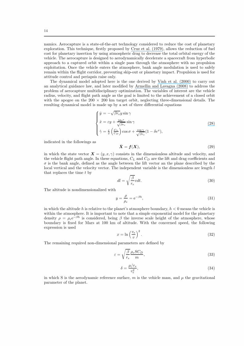
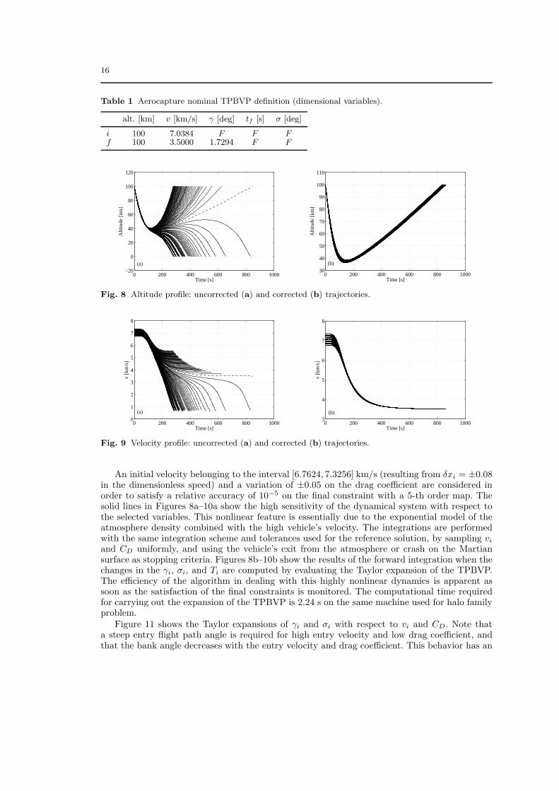
The numerical values used for the reference solution are βre = 390.2652, ε = 2.1835× 10−4,δ = 2.4767 × 10−1, CD = 6.8962× 10−1, and CL = −2.2304× 10−1. The TPBVP is completelydefined by Table 1, in which the data are given for the corresponding dimensional variables,being i and f the initial and final state respectively, and F the free variables. Note that theselected values for the final velocity and flight path angle limit the ∆v for the periapsis raise toonly 52.5865 m/s. The reference solution is showed in Figures 8a–10a by the dashed line and it ischaracterized by σ = 59.6096 deg and lasts 848.7132 s. This solution is obtained by applying theliner multi-point method described in Armellin and Topputo (2006) and assessed by a forwardintegration with a RKF78 scheme with absolute and relative tolerance of 10−12. The secondorder solution developed by Vinh et al. (2000) is used as first guess in order to facilitate theconvergence of the method.

The algorithm of Sect. 2 is now applied to obtain the expansion of the solution of the TPBVPwith respect to atmosphere entry velocity and vehicle drag coefficient. It is important to stressthat, differently from the halo orbit case, the parameter vector p includes a state variable and asystem design parameter (i.e., CD). This feature is of particular interest when dealing with theearly maneuver design as it allows the achievement of a deep insight into the dynamical systemat hand, and the identification and definition of key design parameters.

16

Table 1 Aerocapture nominal TPBVP definition (dimensional variables).

alt. [km] v [km/s] γ [deg] tf [s] σ [deg]

i 100 7.0384 F F Ff 100 3.5000 1.7294 F F

0 200 400 600 800 1000−20

0

20

40

60

80

100

120

Time [s]

Alti

tude

[km

]

(a)

0 200 400 600 800 100030

40

50

60

70

80

90

100

110

Time [s]

Alti

tude

[km

]

(b)

Fig. 8 Altitude profile: uncorrected (a) and corrected (b) trajectories.

0 200 400 600 800 10000

1

2

3

4

5

6

7

8

Time [s]

v [k

m/s

]

(a)

0 200 400 600 800 10003

4

5

6

7

8

Time [s]

v [k

m/s

]

(b)

Fig. 9 Velocity profile: uncorrected (a) and corrected (b) trajectories.

An initial velocity belonging to the interval [6.7624, 7.3256] km/s (resulting from δxi = ±0.08in the dimensionless speed) and a variation of ±0.05 on the drag coefficient are considered inorder to satisfy a relative accuracy of 10−5 on the final constraint with a 5-th order map. Thesolid lines in Figures 8a–10a show the high sensitivity of the dynamical system with respect tothe selected variables. This nonlinear feature is essentially due to the exponential model of theatmosphere density combined with the high vehicle’s velocity. The integrations are performedwith the same integration scheme and tolerances used for the reference solution, by sampling vi

and CD uniformly, and using the vehicle’s exit from the atmosphere or crash on the Martiansurface as stopping criteria. Figures 8b–10b show the results of the forward integration when thechanges in the γi, σi, and Ti are computed by evaluating the Taylor expansion of the TPBVP.The efficiency of the algorithm in dealing with this highly nonlinear dynamics is apparent assoon as the satisfaction of the final constraints is monitored. The computational time requiredfor carrying out the expansion of the TPBVP is 2.24 s on the same machine used for halo familyproblem.

Figure 11 shows the Taylor expansions of γi and σi with respect to vi and CD. Note thata steep entry flight path angle is required for high entry velocity and low drag coefficient, andthat the bank angle decreases with the entry velocity and drag coefficient. This behavior has an

17

0 200 400 600 800 1000−30

−25

−20

−15

−10

−5

0

5

10

Time [s]

γ [d

eg]

(a)

0 200 400 600 800 1000−10

−8

−6

−4

−2

0

2

Time [s]

γ [d

eg]

(b)

Fig. 10 Flight path angle profile: uncorrected (a) and corrected (b) trajectories.

0.64 0.66 0.68 0.7 0.72 0.74

6.7

6.8

6.9

7

7.1

7.2

7.3

7.4

γi [deg]

CD

v i [km

/s]

−9.15

−9.1

−9.05

−9

−8.95

−8.9

−8.85

−8.8

(a)

0.64 0.66 0.68 0.7 0.72 0.74

6.7

6.8

6.9

7

7.1

7.2

7.3

7.4

σi [deg]

CD

v i [km

/s]

57.5

58

58.5

59

59.5

60

60.5

61

61.5

(b)

Fig. 11 Corrections in the initial flight path angle (a) and bank angle (b) as a function of CD and vi.

intuitive explanation. For a given drag coefficient, an higher entry velocity results in a greaterdemanded energy loss that can be achieved by flying deeper in the atmosphere and by increasingthe maneuver duration. This can be obtained by adopting a steeper entry and by increasing thecentripetal contribution of the lift acting on the bank angle (note that as CL is negative, the liftis aligned with the nadir direction when σ = 0). On the other hand, for a chosen entry velocity,an increase of the drag coefficient promotes the energy loss, thus a shallower entry is allowed andlower bank angle is required to avoid an early skip from the atmosphere.

6 Conclusions

This work investigated the benefits that DA techniques can bring to space trajectory design. Thepossibility of expanding the flow of a general ODE with respect to the initial conditions up toan arbitrary order was described. The resulting Taylor expansions represent a valuable mean tocarry out high order sensitivity analyses on dynamical systems. The Taylor expansion of the flowwas shown to be profitable in the framework of TPBVP. Using appropriate inversion techniques,the expansion of the flow is used to gain explicit representations of the constraint manifolds ofa TPBVP in terms of Taylor polynomials. Thus, a high order expansion of the solution of theTPBVP with respect to any parameter about an available reference solution is obtained. Thealgorithm has been applied to the identification of the family of halo orbits around the librationpoint L1 of the Earth–Moon CRTBP. In particular, once a reference halo orbit is available, theidentification of the contiguous halo orbits is reduced to the simple evaluation of polynomials,so avoiding the multiple run of intensive iterative procedures. The versatility of the proposedalgorithm was shown by applying it also to a completely different dynamical system, like the one

18

describing the aerocapture maneuver. The possibility of expanding the solution of the TPBVPwith respect to both state variables and system parameters was here demonstrated to bringpotential benefits when dealing with the early design of maneuvers. Ongoing work is devoted tocope with the optimal control problem of continuously propelled space trajectories, which canbe reduced to a TPBVP in the framework of indirect methods.

Acknowledgments

We are indebted to Prof. Martin Berz and Kyoko Makino for having introduced us to differentialalgebra, for all the interesting discussions, and for giving us the opportunity of using COSY-Infinity, without which this work could not have been done. We are also grateful to FrancescoTopputo for the support in dealing with CRTBP dynamics.

Appendix

The polynomial map resulting from the application of the algorithm introduced in Sect. 4 tothe identification of the family of L1 halo orbits in the Earth–Moon CRTBP is reported in thissection. As already pointed out in Sect. 5, the halo orbits are parameterized based on the valueof the out-of-plane amplitude Az. Given a reference halo orbit corresponding to an assignedreference A0

z, the algorithm is able to deliver the explicit relation between the free componentsof the initial state vector xFi

= (xi, vyi, T ) and Az in terms of the arbitrary order polynomial

mapδxFi

= MxFi(δAz), (39)

where δAz = Az − A0z and δxFi

is the correction to be supplied to the reference x0

Fito identify

the value of xFifor the halo orbit of amplitude Az. Referring to the reference halo orbit reported

in Fig. 4, Fig. 12 illustrates the resulting 18-th order Taylor polynomials for each component ofxFi

. More specifically, the map is reported in normalized units. For each polynomial, the firstcolumn lists the coefficients of the Taylor expansions, whereas the second column shows thecorresponding order. As the polynomials are monovariate expansions, the order coincides withthe associated exponent for the expansion variable. The polynomials reported in Fig. 12 refer toa map

δxFi= MxFi

(δAz), (40)

where the variable Az = 0.001 Az is introduced to suitably rescale the resulting polynomials, soavoiding numerical problems associated to the representation of the coefficients in the computerenvironment.

References

1. Armellin, R. and Lavagna, M.: Multidisciplinary Optimization of Aerocapture Maneuvers. Journalof Artificial Evolution and Applications, 2008, Article ID 248798, 13 pages (2008).

2. Armellin, R., Topputo, F.: A sixth-order accurate scheme for solving two-point boundary valueproblems in astrodynamics. Celestial Mechanics and Dynamical Astronomy, 96, 289–309 (2006).

3. Battin, R.H.: An Introduction to the Mathematics and Methods of Astrodynamics, Revised Edition.AIAA Education Series, Providence (1993).

4. Bernelli Zazzera, F., Topputo, F., and Massari, M.: Assessment of Mission Design Including Uti-lization of Libration Points and Weak Stability Boundaries. Final Report, ESTEC Contract No.18147/04/NL/MV (2004).

5. Berz, M.: The new method of TPSA algebra for the description of beam dynamics to high orders.Technical Report AT-6:ATN-86-16, Los Alamos National Laboratory (1986).

19

COEFFICIENT EXPONENT

0.8233989468774330 0

0.2439065278188019E-04 1

0.9603816377931132E-05 2

0.1081901214732030E-05 3

-0.8720728004249879E-08 4

-0.3815669619030723E-08 5

0.2137595025652236E-09 6

0.4114236239120348E-11 7

-0.1168909463191024E-11 8

0.5075351459660132E-13 9

0.2652561281432105E-14 10

-0.4201027652659181E-15 11

0.1215583232584160E-16 12

0.1265455705892179E-17 13

-0.3727736848627907E-18 14

0.4133416474469995E-19 15

0.1616290913929191E-18 16

0.8848723509976703E-18 17

0.6964388034282895E-18 18

COEFFICIENT EXPONENT

0.1368527787979750 0

0.3782078297117446E-02 1

0.2714781099125496E-03 2

-0.1441704193880840E-04 3

-0.5431994648518032E-07 4

0.4177605236243339E-07 5

-0.2054503521218269E-08 6

-0.4716027806707428E-10 7

0.1158930851900079E-10 8

-0.4760643620493138E-12 9

-0.2685460674919819E-13 10

0.4041516220219051E-14 11

-0.1114957958306015E-15 12

-0.1225882652819771E-16 13

0.3713900442549058E-17 14

-0.3993594507613108E-18 15

-0.1671557082256560E-17 16

-0.9319060348658749E-17 17

-0.7198834952638262E-17 18

xi vyi T

COEFFICIENT EXPONENT

2.747520156118796 0

0.1692536149285003E-02 1

0.1448019913127069E-03 2

-0.3322762232198235E-05 3

-0.1398077146111032E-06 4

0.8795275007661261E-09 5

-0.1336724794353381E-09 6

-0.4384400521688138E-11 7

0.4294856065180787E-12 8

-0.1370128395293440E-13 9

-0.1216982637789168E-14 10

0.1257933246082722E-15 11

0.5074874216682234E-19 12

-0.1893828266682122E-17 13

-0.1098681514396162E-17 14

-0.3199291345154227E-17 15

-0.5271519621695668E-17 16

-0.1030523637730787E-16 17

-0.6084353362279186E-17 18

Fig. 12 18-th order expansion of the solution of the TPBVP for the identification of the family of L1

halo orbit in the Earth–Moon CRTBP: polynomials maps corresponding to each component of the vectorxFi

= (xi, vyi, T ).

6. Berz, M.: The method of power series tracking for the mathematical description of beam dynamics.Nuclear Instruments and Methods A258, 431 (1987).

7. Berz, M.: High-Order Computation and Normal Form Analysis of Repetitive Systems. Physics ofParticle Accelerators, Volume AIP 249, 456 (1991).

8. Berz, M.: Differential Algebraic Techniques. Handbook of Accelerator Physics and Engineering, M.Tigner and A. Chao (Eds.), World Scientific (1999a).

9. Berz, M.: Modern Map Methods in Particle Beam Physics. Academic Press (1999b).10. Berz, M., and Makino, K.: COSY INFINITY version 9 reference manual, MSU Report MSUHEP-

060803, Michigan State University, East Lansing, MI 48824 (2006).11. Bryson, A.E., Ho, Y.C.: Applied Optimal Control. Hemisphere Publishing Co., Washigton (1975).12. Cruz, M.I.: The Aerocapture Vehicle Mission Design Concept. Joint Propulsion Conference, AIAA

paper 79-0893 (1979).13. Di Lizia, P.: Robust Space Trajectory and Space System Design using Differential Algebra. Ph.D.

dissertation, Politecnico di Milano (2008a).14. Di Lizia, P., Armellin, R., Ercoli-Finzi, A., and Berz, M.: High-order robust guidance of interplan-

etary trajectories based on differential algebra, Journal of Aerospace Engineering, Sciences andApplications, 1, 43–57, (2008b).

15. Griffith, T.D., Turner, J.D., Vadali, S.R., and Junkins, J.L.: Higher Order Sensitivities for SolvingNonlinear Two-Point Boundary-Value Problems. AIAA/AAS Astrodynamics Specialist Conferenceand Exhibit, Providence, Rhode Island, August 16–19, (2004).

16. Gomez, G., Jorba, A., Masdemont, J., Simo, C.: Dynamics and Mission Design near LibrationPoints–Volume III: Advanced Methods for Collinear Points. World Scientic (2000).

17. Gomez, G., and Mondelo, J.M.: The Dynamics around the Collinear Equilibrium Points of theRTBP. Physica D, 157, 283–321 (2001).

18. Guibout, V., and Scheeres, D.J.: Solving Relative Two-Point Boundary Value Problems: SpacecraftFormulation Flight Transfers Application. Journal of Guidance, Control, and Dynamics, 27, 693–704 (2004).

19. Guibout, V., and Scheeres, D.J.: Solving Two Point Boundary Value Problems Using GeneratingFunctions: Theory and Applications to Astrodynamics. Modern Astrodynamics, Elsevier Astrody-namics Series (P. Gurfil, ed.), Academic Press (2006a).

20. Guibout, V., and Scheeres, D.J.: Spacecraft Formation Dynamics and Design. Journal of Guidance,Control, and Dynamics, 29, 121–133 (2006b).

21. Jorba, A., and Masdemont, J.: Dynamics in the Center Manifold of the Collinear Points of theRestricted Three Body Problem. Physica D, 132, 189–213 (1999).

20

22. Masdemont, J.J.: High order expansions of invariant manifolds of libration point orbits with appli-cations to mission design. Dyn. Sys.: An Int. J., 20, 59–113 (2005).

23. Park, R.S. and Scheeres, D.J.: Nonlinear Mapping of Gaussian Statistics: Theory and Application toSpacecraft Trajectory Design. Journal of Guidance, Control and Dynamics, 29, 1367–1375, (2006).

24. Park, R.S. and Scheeres, D.J.: Nonlinear Semi-Analytic Methods for Trajectory Estimation. Journalof Guidance, Control and Dynamics, 30, 1668–1676, (2007).

25. Richardson, D.L.: Analytic construction of periodic orbits about the collinear points. CelestialMechanics, 22, 241–253 (1980).

26. Stoer, J. and Bulirsch R.: Introduction to Numerical Analysis, Springer, New York (1993).27. Thurman, R., and Worfolk, P.A.: The geometry of halo orbits in the circular restricted three body

problem. Technical Report GCG95, Geometry Center, University of Minnesota (1996).28. Vinh, N.X., Johnson, W.R., and Longusky J.M.: Mars Aerocapture Using Bank Modulation. In Col-

lection of technical papers AIAA/AAS Astrodynamics Specialist Conference, Denver, CO, August14–17, (2000).