Application of binary classifiers to filter transactions on the financial market
41
Running head: FILTERING TRADING SYSTEM TRANSACTIONS 1 Application of binary classifiers to filter transactions on the financial market Andrzej Endler Quants Technologies S.A. ,ul.Getta Żydowskiego 16,98-220 Zduńska Wola, Poland [email protected]
-
Upload
independent -
Category
Documents
-
view
2 -
download
0
Transcript of Application of binary classifiers to filter transactions on the financial market
Running head: FILTERING TRADING SYSTEM TRANSACTIONS 1
Application of binary classifiers to filter transactions
on the financial market
Andrzej Endler
Quants Technologies S.A. ,ul.Getta Żydowskiego 16,98-220 Zduńska Wola, Poland

FILTERING TRADING SYSTEM TRANSACTIONS 2
Abstract
One of the key problems relating to concluding transactions on financial markets is the
definition of whether or not, in given market conditions, we should conclude a specific
transaction. This problem applies to all transactions irrespective of whether they are
concluded in a discretionary manner by a person, or by the appropriate software. The subject
of research presented in this document was practical verification of the hypothesis that the use
of filters composed of classifiers independent of the main algorithm of the strategy may
improve the characteristics of this strategy. This means constructing an additional filter,
independent of the main logic and algorithm of the strategy, either allowing the transaction to
be conducted or not. The strategy being examined is a real strategy used in trading in shares
on the American market. Many various classifiers based on various algorithms, as well as sets
of classifiers composed of them, were examined.
As a consequence of this research interesting results were obtained, noticeably improving the
various characteristics of an automatic strategy for which the filters had been created. The
research confirmed the justification for using classifiers as a filter for transactions for the
automatic strategy under examination.
Keywords: Data Mining, Classification, Classifiers, Trading Systems, Stocks, Filtering transactions, Data mining techniques, real-world applications

FILTERING TRADING SYSTEM TRANSACTIONS 3
Application of binary classifiers to filter transactions
on the financial market
The objective of this study is to present the results of research relating to the use of binary
classifiers to filter transactions of the existing automatic trading strategy on the American
shares market. As will be indicated at a later stage in this paper, the use of such classifiers
may bring very positive results which clearly improve the characteristics of the trading
strategy.
1. Introduction
Many studies have been devoted to various methods of anticipating the returns on financial
markets using various Data Mining methods. For example (AL-RADAIDEH, ASSAF,
&ALNAGI, 2013) discusses the use of decision trees for this purpose, (Soni, 2010) in his
paper presents literature devoted to use of neural networks to anticipate returns on the shares
market. There are considerably fewer works devoted to the application of methods of learning
and classification for additional filtering of automatic strategy principles. (Varutbangkul,
2013) discusses the use of decision trees to filter signals in six simple ‘traditional’ trading
systems. Most often, in available studies simple, somewhat ‘academic’ trading strategies are
used, such as intersection of moving averages, and not ‘real-life’, more complicated strategies
actually used on the financial market. The aim of my study is to present the research for
which the input data was taken from a strategy applied ‘live’ on the American shares market.
FILTERING TRADING SYSTEM TRANSACTIONS 4 Automatic systems analyse market data, and then with the use of an implemented
algorithm take a decision on the purchase or sale of given financial assets e.g. shares. Such
systems base their operating principles on extremely varied algorithms based on the classical
technical analysis, or various types of data analysis, including the use of statistical tools and
data exploration. Most frequently a set of input data is checked, for which the conditions are
defined which – if they are satisfied – make the system take up a certain market position.
Next, the position is managed in accordance with the assigned algorithm and finally closed
with either a profit or a loss.
The problem of a good system (somewhat simplified of course) involves in fact
finding a system with a positive expected value of the transaction and at the same time trading
as often as possible. An ideal situation is a presence of as great a volume as possible of
transactions and, in addition, only profit-making ones, however such situations practically do
not exist in conditions of real market trading.
I decided to examine whether it was possible to ‘improve’ the existing system
operating on the market so as to improve its characteristics by eliminating those transactions
which did not bring any profit, and at the same time by preserving the maximum possible
volume of transactions which resulted in earing a profit. I narrowed the task down to the
problem of binary classification. Transactions which achieved a profit were included in one
class (positive class), and those which did not achieve a profit into another class (negative
class).
Usually, every automatic strategy already contains some type of filters in the form of
e.g. trend filters based on moving averages or similar. However, we want to find additional
variables /attributes, not dependent on the main logic of the strategy. Obviously, we do not
know what variables, e.g. price or derivative indices, are significant and how to define this
filter.
FILTERING TRADING SYSTEM TRANSACTIONS 5 The strategy which is the source of data on transactions is described in chapter 2. The
first step was to prepare the data for all assets present in the transactions, which I will be
discussing in chapter 3. The next step was the selection of attributes which will constitute
good input data for the classifiers. The choice of attributes will be discussed in chapter 4. In
chapter 5 I will present the choice of classifiers found to be the most suitable for our data. In
chapter 6 I will describe the construction of sets of classifiers used later on for research, and
chapter 7 sets out the procedure for this research. Finally, in chapter 8 I will set out the results
of research of individual classifiers and their groups, and in chapter 9 I am applying models
obtained for filtering automatic strategy transactions. Chapter 10 contains brief conclusions
and suggestions for further studies.
2. Strategy for which we define filters
The strategy for which we define filters admitting/eliminating transactions is a trading
strategy on the American shares market. The strategy opens the position at the opening of the
stock exchange session if the defined conditions are satisfied, mainly if a considerable
deviation between the opening price and the closing price (a gap) occurs. The strategy is
trading only on the “long” side, taking up a position in the opposite direction to the gap,
expecting it to decrease. The time spent on the market is fairly short and amounts to an
average of 20 minutes.
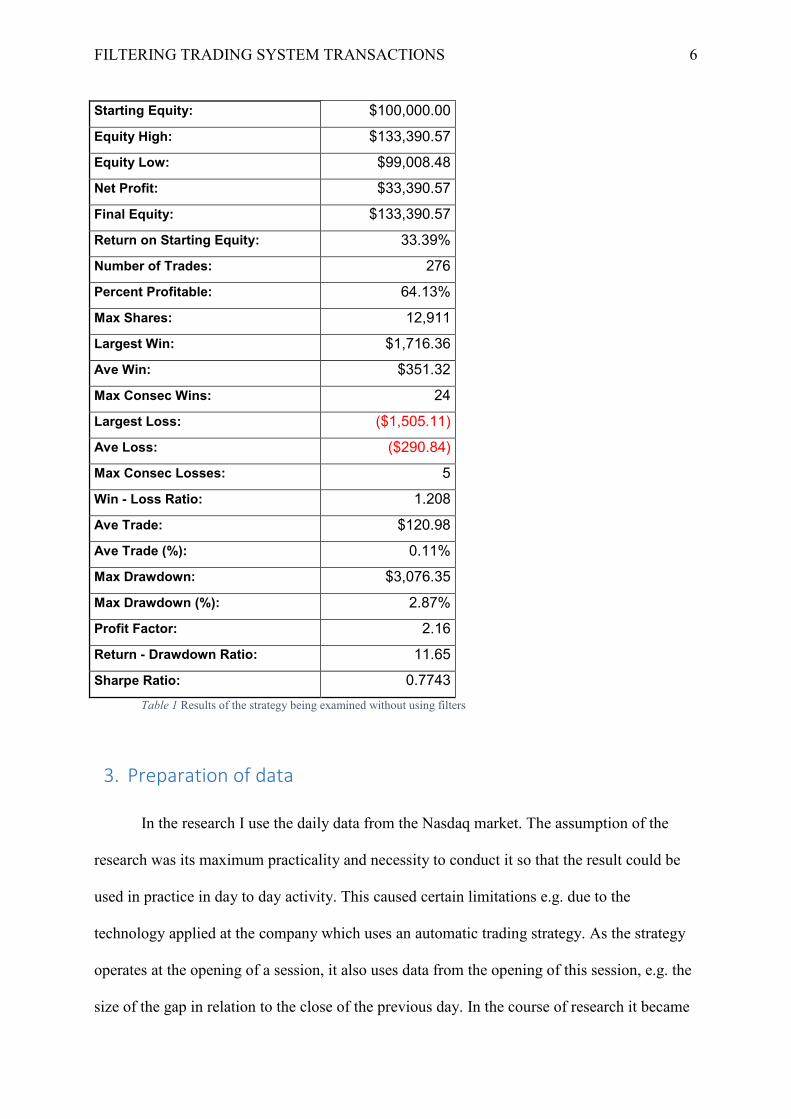
The results set out in the table below are results of the backtest strategy from February
2009 to April 2014. A commission of 0.005$ on share was included. The strategy is used to
trade on the Nasdaq market on a composite basket of 95 assets, using 33.33% of the capital
available at any given moment for each transaction.
FILTERING TRADING SYSTEM TRANSACTIONS 6
Starting Equity: $100,000.00
Equity High: $133,390.57
Equity Low: $99,008.48
Net Profit: $33,390.57
Final Equity: $133,390.57
Return on Starting Equity: 33.39%
Number of Trades: 276
Percent Profitable: 64.13%
Max Shares: 12,911
Largest Win: $1,716.36
Ave Win: $351.32
Max Consec Wins: 24
Largest Loss: ($1,505.11)
Ave Loss: ($290.84)
Max Consec Losses: 5
Win - Loss Ratio: 1.208
Ave Trade: $120.98
Ave Trade (%): 0.11%
Max Drawdown: $3,076.35
Max Drawdown (%): 2.87%
Profit Factor: 2.16
Return - Drawdown Ratio: 11.65
Sharpe Ratio: 0.7743 Table 1 Results of the strategy being examined without using filters
3. Preparation of data
In the research I use the daily data from the Nasdaq market. The assumption of the
research was its maximum practicality and necessity to conduct it so that the result could be
used in practice in day to day activity. This caused certain limitations e.g. due to the
technology applied at the company which uses an automatic trading strategy. As the strategy
operates at the opening of a session, it also uses data from the opening of this session, e.g. the
size of the gap in relation to the close of the previous day. In the course of research it became
FILTERING TRADING SYSTEM TRANSACTIONS 7
evident that due to the required speed of the system’s reaction and other technical conditions,
I had to limit myself only to the data at the close of the previous day (not taking into account
the data from the opening of the session). Creating models, making calculations and
classifications took place in the period between sessions.
As I did not know what attributes (variables) actually conveyed the information
allowing to increase the probability of a successful transaction, I decided to use a large group
of technical analysis indices, prices, sales volumes and their values shifted in time (delayed)
and differences. Data on values and indices for stock market indices and gold, oil and
American bonds were added as potential indicators defining the state of the market. In total
there were 39,886 attributes. All attributes were numeric attributes – continuous ones. All data
was subject to the ‘Z’ transformation (by subtracting the average and dividing by the standard
deviation) for time windows of a period of 100 days. I carried out a simple data cleansing
removing all observations with an undefined value. After completing all data cleansing
operations, I was left with 551 transactions / observations on 89 assets.
4. Selection of significant variables
Due to the very substantial number of attributes it was necessary to select the
significant attributes. I tried to select those attributes by applying 3 methods:
a) Random forest
b) Tree from the C5.0 algorithm
c) Rough Sets – reduct
I carried out an assessment of the behaviour of individual sets of parameters by
comparing the results of classifications for several selected classification methods – C5.0,
SVM Radial Basis Function kernel and Naive Bayes. As a result of conducting many tests for

FILTERING TRADING SYSTEM TRANSACTIONS 8
various numbers of attributes and methods of defining significant variables, I decided to use
attributes defined by the random forest (10,000 trees). For the purposes of further
examination, I assumed the first 60 variables from the list sorted by the significance of
variables provided by this model. In the future it is worth considering using various sets of
variables/attributes and creating sets of classifiers with various sets of input data. An
interesting fact relating to the selected variables is that a large part of them constitute
variables which are derivatives of indices, gold, oil and bonds – that is, variables defining the
state of the market in general and not the price of the asset itself.
5. Selecting classifiers
My next step was to examine the behaviour of various types of classifiers towards the
data. I selected parameters for each classifier using the Cross Validation procedure 10, and
then averaged out the results obtained. I chose parameters of the model maximizing the F
coefficient. In the examination I used the caret package (Kun et al., 2014) and other R
packages (R Core Team, 2014) described in chapter 11.
I checked a total of 76 various classifiers, defining for each one the average parameters
of classification quality for my data. The results are presented in the following diagrams, and
detailed values for individual classifiers in appendix 1.

FILTERING TRADING SYSTEM TRANSACTIONS 9
Figure 1. Recall of classifiers being tested.
Figure 2. Precision of classifiers being tested.
FILTERING TRADING SYSTEM TRANSACTIONS 10
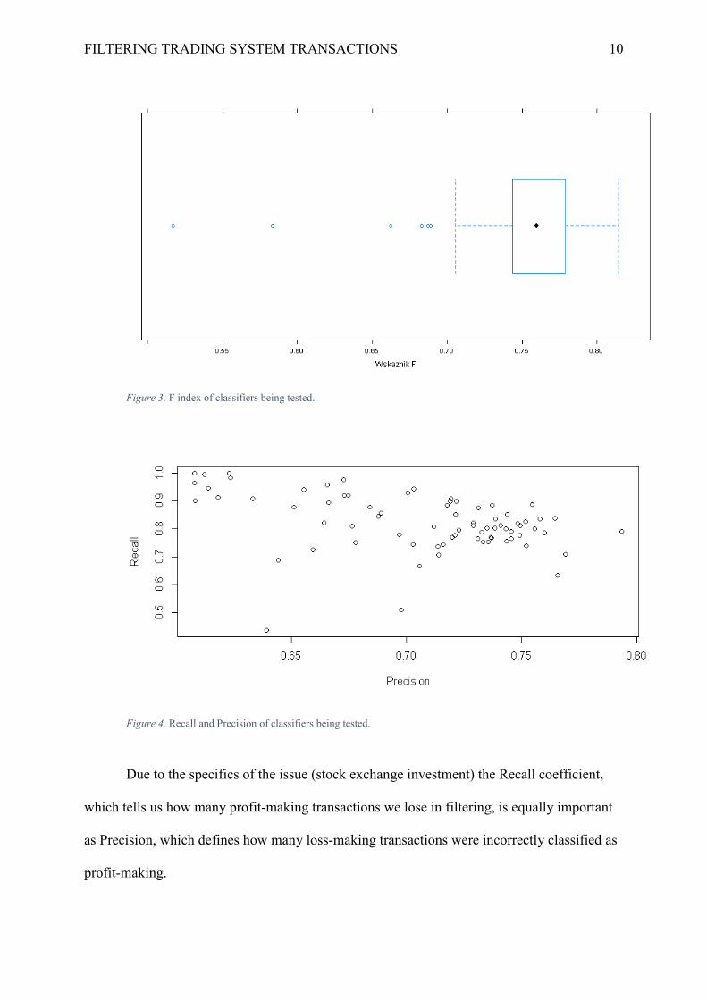
Figure 3. F index of classifiers being tested.
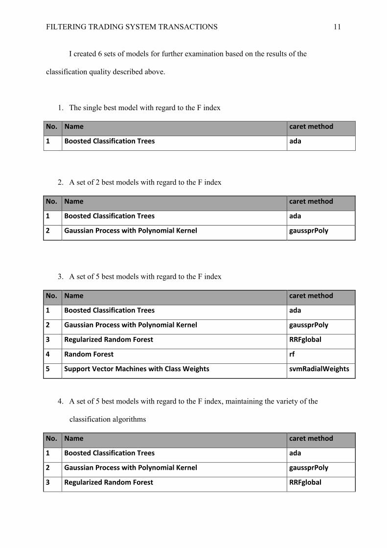
Figure 4. Recall and Precision of classifiers being tested.
Due to the specifics of the issue (stock exchange investment) the Recall coefficient,
which tells us how many profit-making transactions we lose in filtering, is equally important
as Precision, which defines how many loss-making transactions were incorrectly classified as
profit-making.
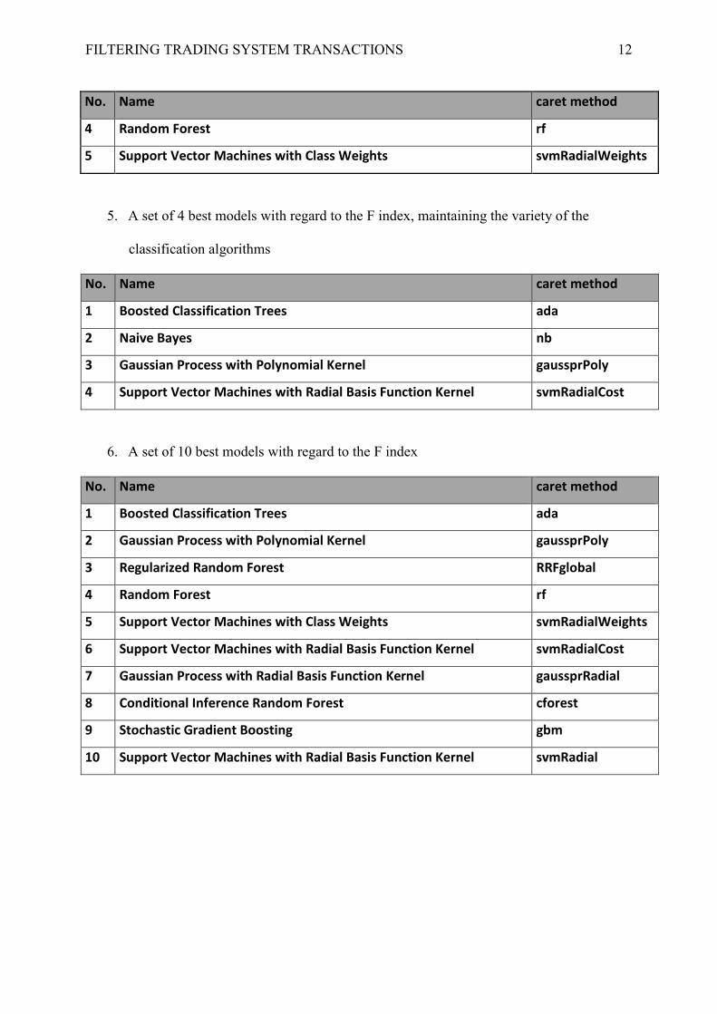
FILTERING TRADING SYSTEM TRANSACTIONS 11 I created 6 sets of models for further examination based on the results of the
classification quality described above.
1. The single best model with regard to the F index
No. Name caret method
1 Boosted Classification Trees ada
2. A set of 2 best models with regard to the F index
No. Name caret method
1 Boosted Classification Trees ada
2 Gaussian Process with Polynomial Kernel gaussprPoly
3. A set of 5 best models with regard to the F index
No. Name caret method
1 Boosted Classification Trees ada
2 Gaussian Process with Polynomial Kernel gaussprPoly
3 Regularized Random Forest RRFglobal
4 Random Forest rf
5 Support Vector Machines with Class Weights svmRadialWeights
4. A set of 5 best models with regard to the F index, maintaining the variety of the
classification algorithms
No. Name caret method
1 Boosted Classification Trees ada
2 Gaussian Process with Polynomial Kernel gaussprPoly
3 Regularized Random Forest RRFglobal
FILTERING TRADING SYSTEM TRANSACTIONS 12
No. Name caret method
4 Random Forest rf
5 Support Vector Machines with Class Weights svmRadialWeights
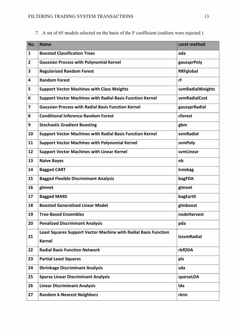
5. A set of 4 best models with regard to the F index, maintaining the variety of the
classification algorithms
No. Name caret method
1 Boosted Classification Trees ada
2 Naive Bayes nb
3 Gaussian Process with Polynomial Kernel gaussprPoly
4 Support Vector Machines with Radial Basis Function Kernel svmRadialCost
6. A set of 10 best models with regard to the F index
No. Name caret method
1 Boosted Classification Trees ada
2 Gaussian Process with Polynomial Kernel gaussprPoly
3 Regularized Random Forest RRFglobal
4 Random Forest rf
5 Support Vector Machines with Class Weights svmRadialWeights
6 Support Vector Machines with Radial Basis Function Kernel svmRadialCost
7 Gaussian Process with Radial Basis Function Kernel gaussprRadial
8 Conditional Inference Random Forest cforest
9 Stochastic Gradient Boosting gbm
10 Support Vector Machines with Radial Basis Function Kernel svmRadial
FILTERING TRADING SYSTEM TRANSACTIONS 13
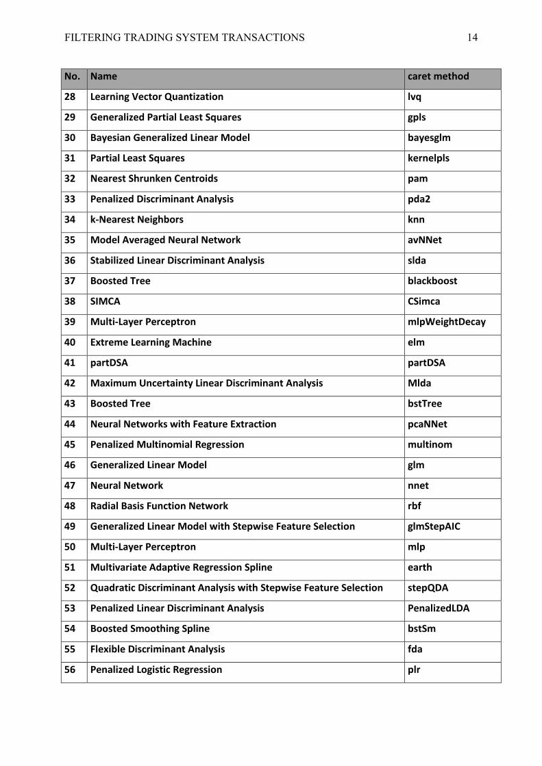
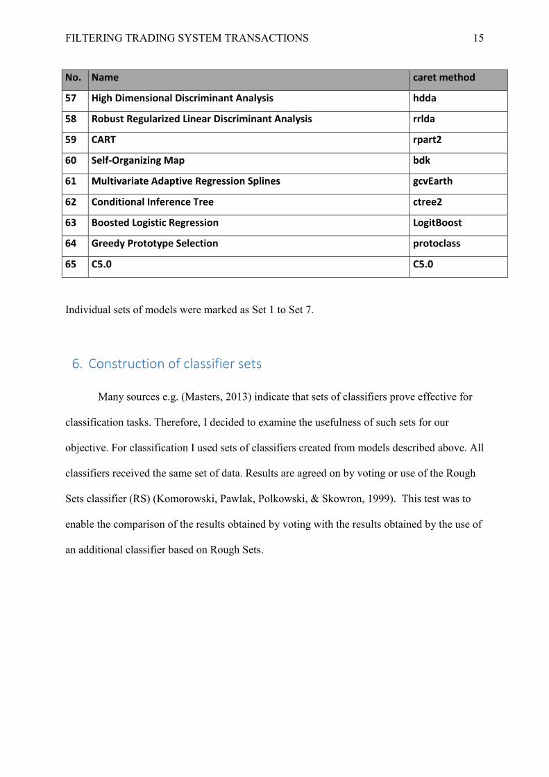
7. A set of 65 models selected on the basis of the F coefficient (outliers were rejected )
No. Name caret method
1 Boosted Classification Trees ada
2 Gaussian Process with Polynomial Kernel gaussprPoly
3 Regularized Random Forest RRFglobal
4 Random Forest rf
5 Support Vector Machines with Class Weights svmRadialWeights
6 Support Vector Machines with Radial Basis Function Kernel svmRadialCost
7 Gaussian Process with Radial Basis Function Kernel gaussprRadial
8 Conditional Inference Random Forest cforest
9 Stochastic Gradient Boosting gbm
10 Support Vector Machines with Radial Basis Function Kernel svmRadial
11 Support Vector Machines with Polynomial Kernel svmPoly
12 Support Vector Machines with Linear Kernel svmLinear
13 Naive Bayes nb
14 Bagged CART treebag
15 Bagged Flexible Discriminant Analysis bagFDA
16 glmnet glmnet
17 Bagged MARS bagEarth
18 Boosted Generalized Linear Model glmboost
19 Tree-Based Ensembles nodeHarvest
20 Penalized Discriminant Analysis pda
21 Least Squares Support Vector Machine with Radial Basis Function
Kernel lssvmRadial
22 Radial Basis Function Network rbfDDA
23 Partial Least Squares pls
24 Shrinkage Discriminant Analysis sda
25 Sparse Linear Discriminant Analysis sparseLDA
26 Linear Discriminant Analysis lda
27 Random k-Nearest Neighbors rknn
FILTERING TRADING SYSTEM TRANSACTIONS 14
No. Name caret method
28 Learning Vector Quantization lvq
29 Generalized Partial Least Squares gpls
30 Bayesian Generalized Linear Model bayesglm
31 Partial Least Squares kernelpls
32 Nearest Shrunken Centroids pam
33 Penalized Discriminant Analysis pda2
34 k-Nearest Neighbors knn
35 Model Averaged Neural Network avNNet
36 Stabilized Linear Discriminant Analysis slda
37 Boosted Tree blackboost
38 SIMCA CSimca
39 Multi-Layer Perceptron mlpWeightDecay
40 Extreme Learning Machine elm
41 partDSA partDSA
42 Maximum Uncertainty Linear Discriminant Analysis Mlda
43 Boosted Tree bstTree
44 Neural Networks with Feature Extraction pcaNNet
45 Penalized Multinomial Regression multinom
46 Generalized Linear Model glm
47 Neural Network nnet
48 Radial Basis Function Network rbf
49 Generalized Linear Model with Stepwise Feature Selection glmStepAIC
50 Multi-Layer Perceptron mlp
51 Multivariate Adaptive Regression Spline earth
52 Quadratic Discriminant Analysis with Stepwise Feature Selection stepQDA
53 Penalized Linear Discriminant Analysis PenalizedLDA
54 Boosted Smoothing Spline bstSm
55 Flexible Discriminant Analysis fda
56 Penalized Logistic Regression plr
FILTERING TRADING SYSTEM TRANSACTIONS 15
No. Name caret method
57 High Dimensional Discriminant Analysis hdda
58 Robust Regularized Linear Discriminant Analysis rrlda
59 CART rpart2
60 Self-Organizing Map bdk
61 Multivariate Adaptive Regression Splines gcvEarth
62 Conditional Inference Tree ctree2
63 Boosted Logistic Regression LogitBoost
64 Greedy Prototype Selection protoclass
65 C5.0 C5.0
Individual sets of models were marked as Set 1 to Set 7.
6. Construction of classifier sets
Many sources e.g. (Masters, 2013) indicate that sets of classifiers prove effective for
classification tasks. Therefore, I decided to examine the usefulness of such sets for our
objective. For classification I used sets of classifiers created from models described above. All
classifiers received the same set of data. Results are agreed on by voting or use of the Rough
Sets classifier (RS) (Komorowski, Pawlak, Polkowski, & Skowron, 1999). This test was to
enable the comparison of the results obtained by voting with the results obtained by the use of
an additional classifier based on Rough Sets.
FILTERING TRADING SYSTEM TRANSACTIONS 16
custom Klasyfikatory
...
Voting
Classifier 1 Classifier 2 Classifier 3 Classifier n
Classifier RoughSets
Results
Data
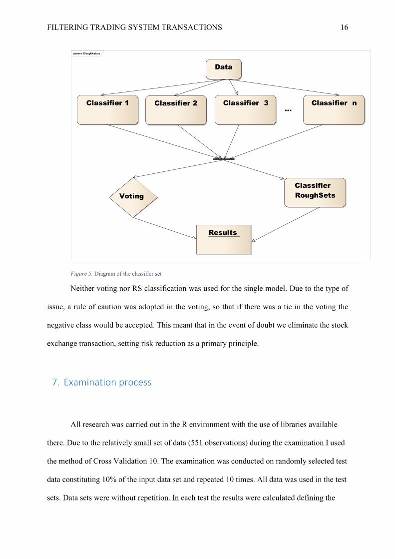
Figure 5. Diagram of the classifier set
Neither voting nor RS classification was used for the single model. Due to the type of
issue, a rule of caution was adopted in the voting, so that if there was a tie in the voting the
negative class would be accepted. This meant that in the event of doubt we eliminate the stock
exchange transaction, setting risk reduction as a primary principle.
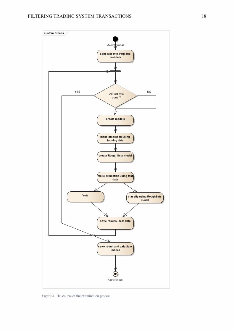
7. Examination process
All research was carried out in the R environment with the use of libraries available
there. Due to the relatively small set of data (551 observations) during the examination I used
the method of Cross Validation 10. The examination was conducted on randomly selected test
data constituting 10% of the input data set and repeated 10 times. All data was used in the test
sets. Data sets were without repetition. In each test the results were calculated defining the
FILTERING TRADING SYSTEM TRANSACTIONS 17
classification quality. Models were trained on sets containing 90% of data. After creating all
models for a given sequence, the prediction was carried out for this data, which constituted a
training set for the Rough Set based classifier used to resolve conflicts between classifiers.
The results of the classification then created an initial set of the classified data containing 551
observations, which were compared with the known set. The indices defining the
classification quality are calculated on the basis of this data.
FILTERING TRADING SYSTEM TRANSACTIONS 18
custom Proces
ActivityFinal
sav e result and calculate indices
sav e results - test data
classify using RoughSets model
Vote
make prediction using test data
create Rough Sets model
make prediction using training data
create models
Split data into train and test data
ActivityInitial
All test setsdone ?
YES NO
Figure 6. The course of the examination process
FILTERING TRADING SYSTEM TRANSACTIONS 19
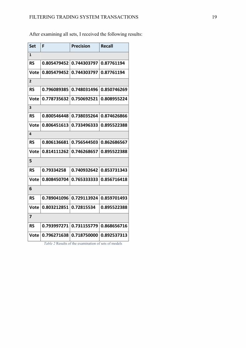
After examining all sets, I received the following results:
Set F Precision Recall
1
RS 0.805479452 0.744303797 0.87761194
Vote 0.805479452 0.744303797 0.87761194
2
RS 0.796089385 0.748031496 0.850746269
Vote 0.778735632 0.750692521 0.808955224
3
RS 0.800546448 0.738035264 0.874626866
Vote 0.806451613 0.733496333 0.895522388
4
RS 0.806136681 0.756544503 0.862686567
Vote 0.814111262 0.746268657 0.895522388
5
RS 0.79334258 0.740932642 0.853731343
Vote 0.808450704 0.765333333 0.856716418
6
RS 0.789041096 0.729113924 0.859701493
Vote 0.803212851 0.72815534 0.895522388
7
RS 0.793997271 0.731155779 0.868656716
Vote 0.796271638 0.718750000 0.892537313
Table 2 Results of the examination of sets of models
FILTERING TRADING SYSTEM TRANSACTIONS 20
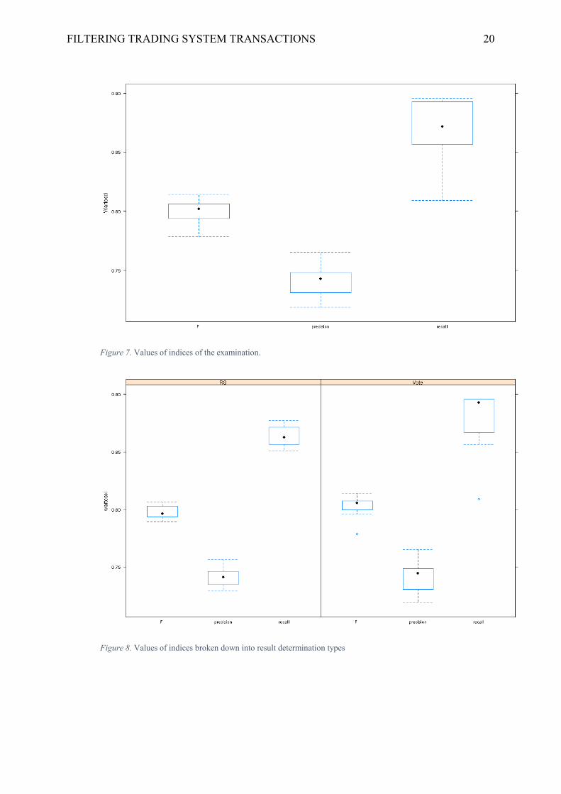
Figure 7. Values of indices of the examination.
Figure 8. Values of indices broken down into result determination types
FILTERING TRADING SYSTEM TRANSACTIONS 21
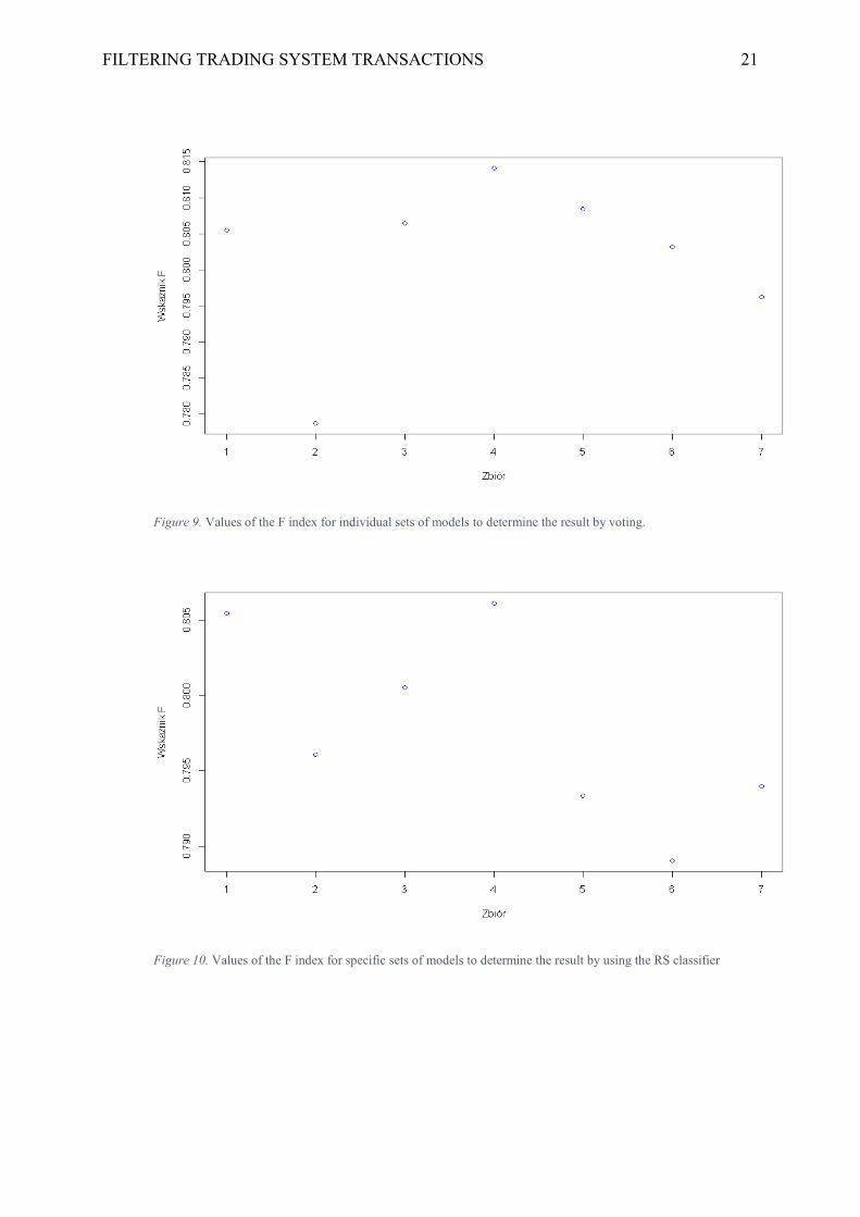
Figure 9. Values of the F index for individual sets of models to determine the result by voting.
Figure 10. Values of the F index for specific sets of models to determine the result by using the RS classifier

FILTERING TRADING SYSTEM TRANSACTIONS 22
7.1. Conclusions drawn from examining various classifiers
The research conducted shows that the best results were achieved for model set no. 4
where the results were determined by voting. Use of the RS classifier does not significantly
improve results, however it changes their characteristics slightly. Further (in relation to set 4)
increase of the number of classifiers in the set does not improve the results. It should be
added, however, that the results for various sets are similar, there are no significant
differences.
For further research I selected set 4, comprising 5 classifiers.
8. Application of the chosen set of models to filter transactions in the
automatic strategy
In the next step I used the selected models to filter transactions in the automatic
strategy. I carried out two tests. The first uses the Cross Validation procedure leaving 10 test
transactions for the set of classifiers described above (set 4). In the second test I used a single
model with the best parameters (set 1 described above) and used the backtest procedure.
Initially half of the data was used as a training set with a test on a single observation, which in
the next step was included in the training set, increasing it etc.
8.1. Application of filters using a set of classifiers (set 4)
Due to the relatively small amount of data I used the method of leaving 10 transactions
for the test set, and treated the remainder as a training set. The data was downloaded in
FILTERING TRADING SYSTEM TRANSACTIONS 23
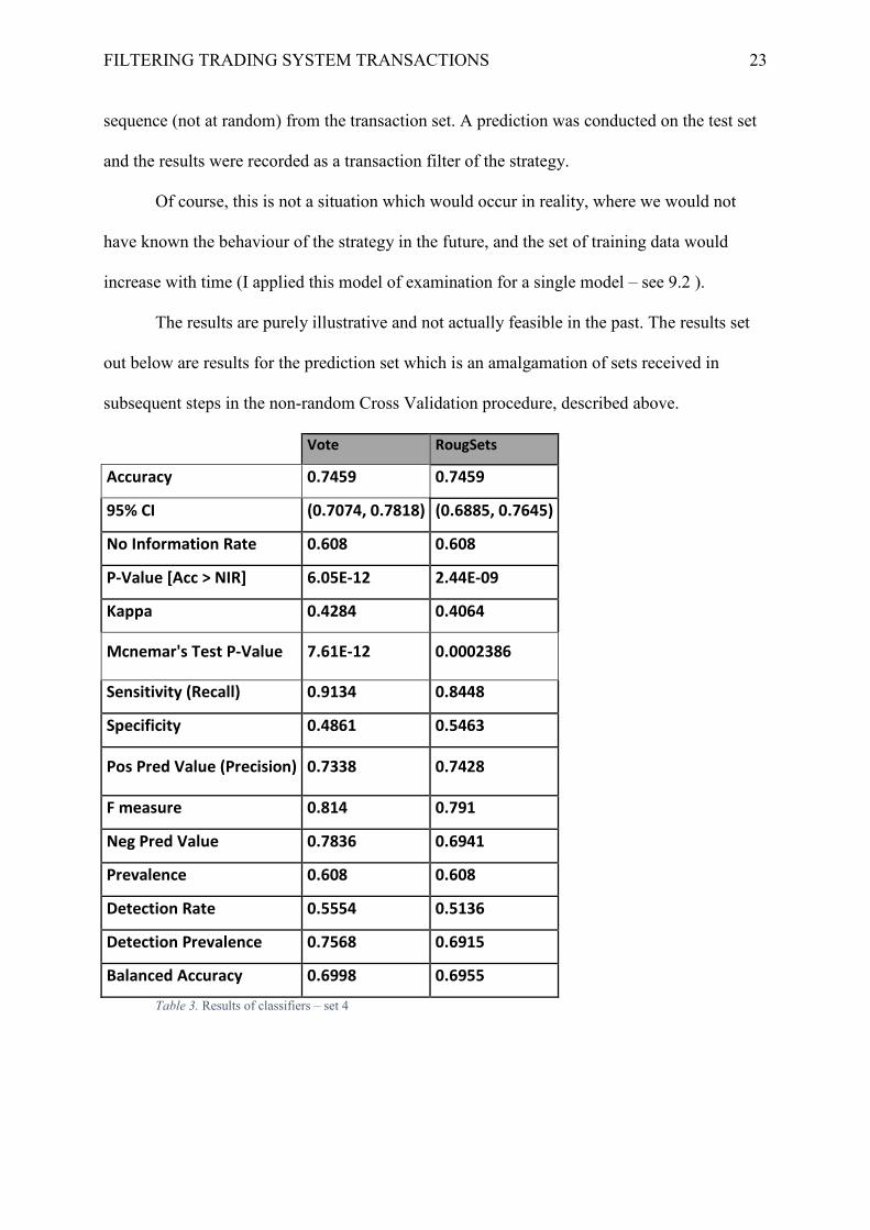
sequence (not at random) from the transaction set. A prediction was conducted on the test set
and the results were recorded as a transaction filter of the strategy.
Of course, this is not a situation which would occur in reality, where we would not
have known the behaviour of the strategy in the future, and the set of training data would
increase with time (I applied this model of examination for a single model – see 9.2 ).
The results are purely illustrative and not actually feasible in the past. The results set
out below are results for the prediction set which is an amalgamation of sets received in
subsequent steps in the non-random Cross Validation procedure, described above.
Vote RougSets
Accuracy 0.7459 0.7459
95% CI (0.7074, 0.7818) (0.6885, 0.7645)
No Information Rate 0.608 0.608
P-Value [Acc > NIR] 6.05E-12 2.44E-09
Kappa 0.4284 0.4064
Mcnemar's Test P-Value 7.61E-12 0.0002386
Sensitivity (Recall) 0.9134 0.8448
Specificity 0.4861 0.5463
Pos Pred Value (Precision) 0.7338 0.7428
F measure 0.814 0.791
Neg Pred Value 0.7836 0.6941
Prevalence 0.608 0.608
Detection Rate 0.5554 0.5136
Detection Prevalence 0.7568 0.6915
Balanced Accuracy 0.6998 0.6955
Table 3. Results of classifiers – set 4
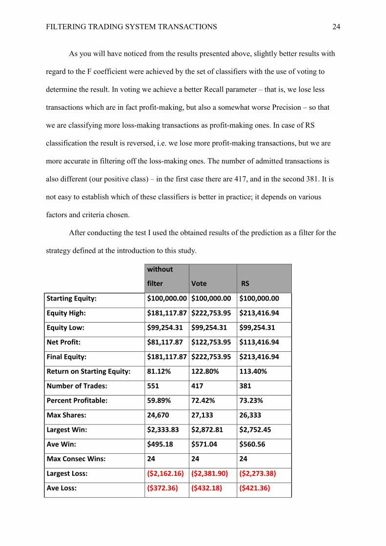
FILTERING TRADING SYSTEM TRANSACTIONS 24 As you will have noticed from the results presented above, slightly better results with
regard to the F coefficient were achieved by the set of classifiers with the use of voting to
determine the result. In voting we achieve a better Recall parameter – that is, we lose less
transactions which are in fact profit-making, but also a somewhat worse Precision – so that
we are classifying more loss-making transactions as profit-making ones. In case of RS
classification the result is reversed, i.e. we lose more profit-making transactions, but we are
more accurate in filtering off the loss-making ones. The number of admitted transactions is
also different (our positive class) – in the first case there are 417, and in the second 381. It is
not easy to establish which of these classifiers is better in practice; it depends on various
factors and criteria chosen.
After conducting the test I used the obtained results of the prediction as a filter for the
strategy defined at the introduction to this study.
without
filter Vote RS
Starting Equity: $100,000.00 $100,000.00 $100,000.00
Equity High: $181,117.87 $222,753.95 $213,416.94
Equity Low: $99,254.31 $99,254.31 $99,254.31
Net Profit: $81,117.87 $122,753.95 $113,416.94
Final Equity: $181,117.87 $222,753.95 $213,416.94
Return on Starting Equity: 81.12% 122.80% 113.40%
Number of Trades: 551 417 381
Percent Profitable: 59.89% 72.42% 73.23%
Max Shares: 24,670 27,133 26,333
Largest Win: $2,333.83 $2,872.81 $2,752.45
Ave Win: $495.18 $571.04 $560.56
Max Consec Wins: 24 24 24
Largest Loss: ($2,162.16) ($2,381.90) ($2,273.38)
Ave Loss: ($372.36) ($432.18) ($421.36)
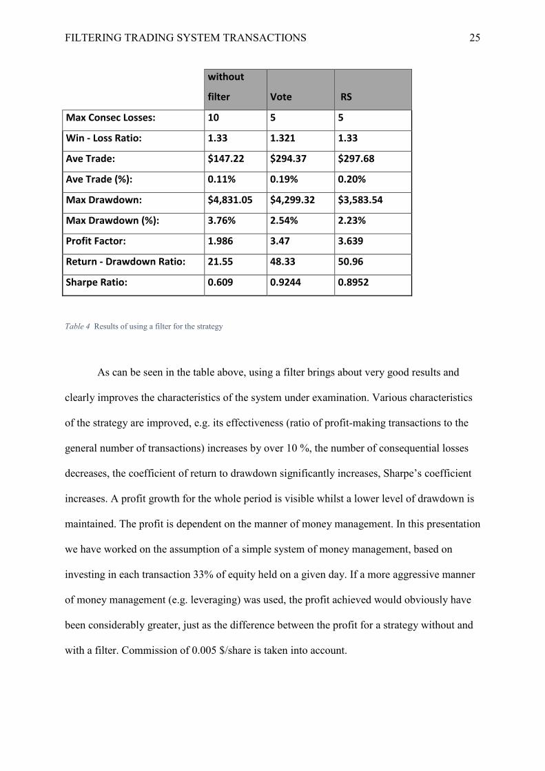
FILTERING TRADING SYSTEM TRANSACTIONS 25
without
filter Vote RS
Max Consec Losses: 10 5 5
Win - Loss Ratio: 1.33 1.321 1.33
Ave Trade: $147.22 $294.37 $297.68
Ave Trade (%): 0.11% 0.19% 0.20%
Max Drawdown: $4,831.05 $4,299.32 $3,583.54
Max Drawdown (%): 3.76% 2.54% 2.23%
Profit Factor: 1.986 3.47 3.639
Return - Drawdown Ratio: 21.55 48.33 50.96
Sharpe Ratio: 0.609 0.9244 0.8952
Table 4 Results of using a filter for the strategy
As can be seen in the table above, using a filter brings about very good results and
clearly improves the characteristics of the system under examination. Various characteristics
of the strategy are improved, e.g. its effectiveness (ratio of profit-making transactions to the
general number of transactions) increases by over 10 %, the number of consequential losses
decreases, the coefficient of return to drawdown significantly increases, Sharpe’s coefficient
increases. A profit growth for the whole period is visible whilst a lower level of drawdown is
maintained. The profit is dependent on the manner of money management. In this presentation
we have worked on the assumption of a simple system of money management, based on
investing in each transaction 33% of equity held on a given day. If a more aggressive manner
of money management (e.g. leveraging) was used, the profit achieved would obviously have
been considerably greater, just as the difference between the profit for a strategy without and
with a filter. Commission of 0.005 $/share is taken into account.
FILTERING TRADING SYSTEM TRANSACTIONS 26 The strategy which uses classifiers with determination by voting is somewhat more
‘aggressive’, involves more transactions, a larger drawdown, more consequential losses. The
strategy which uses classifiers with determination by the RS classifier is more conservative,
operates less frequently and has a better ratio of profit-making transaction to the general
number of transactions. However, the results do not vary significantly.
8.2. Application of filters in the backtest convention for the
single model
Due to slight differences between the results of individual sets of models I decided to
check the behaviour of strategies for the simplest, single model from the ada package (Culp,
Johnson, & Michailidis, 2012) (Boosted Classification Trees). The research was conducted in
a manner considerably closer to reality. The first 265 transactions of the strategy (half of the
available data) were treated as a training set and then the classifier was activated on the next
data record (transaction), in the next step the training set increased by one record (to 276), and
the next record was included in the tests etc. until the end of the set of strategy transactions.
This means that the training set increased with each transaction. At every step, an examination
referred to above was carried out, i.e. new model parameters were selected.
The results again confirmed a considerable advantage of using a classifier for the
strategy. The results obtained are clearly better than those achieved by the strategy without a
classifier. Commission of 0.005 $ per share was taken into consideration . The results for the
strategy without and with a filter are set out below (there is no division into Vote and RS with
regard to the single model, and no mechanism of result determination is used ).
FILTERING TRADING SYSTEM TRANSACTIONS 27
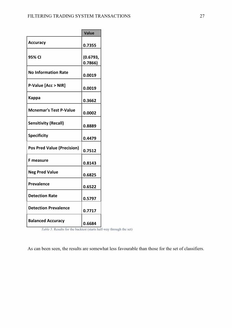
Value
Accuracy 0.7355
95% CI (0.6793, 0.7866)
No Information Rate 0.0019
P-Value [Acc > NIR] 0.0019
Kappa 0.3662
Mcnemar's Test P-Value 0.0002
Sensitivity (Recall) 0.8889
Specificity 0.4479
Pos Pred Value (Precision) 0.7512
F measure 0.8143
Neg Pred Value 0.6825
Prevalence 0.6522
Detection Rate 0.5797
Detection Prevalence 0.7717
Balanced Accuracy 0.6684
Table 5. Results for the backtest (starts half-way through the set)
As can been seen, the results are somewhat less favourable than those for the set of classifiers.
FILTERING TRADING SYSTEM TRANSACTIONS 28
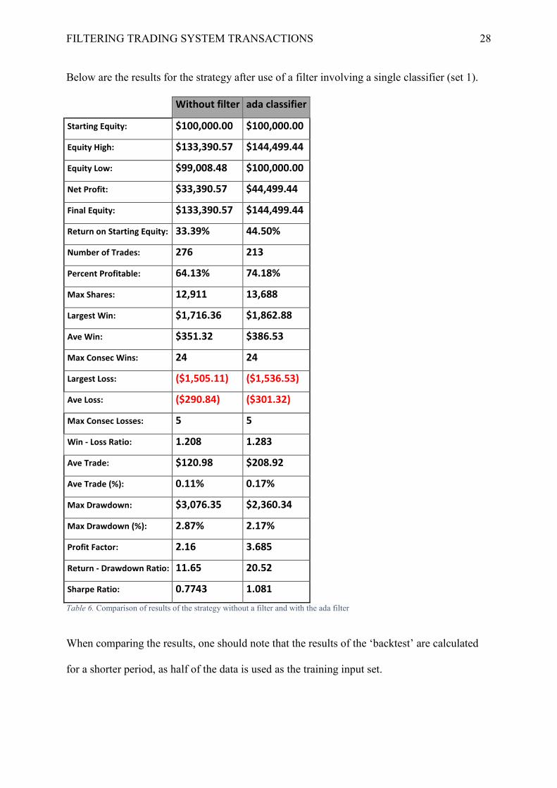
Below are the results for the strategy after use of a filter involving a single classifier (set 1).
Without filter ada classifier
Starting Equity: $100,000.00 $100,000.00
Equity High: $133,390.57 $144,499.44
Equity Low: $99,008.48 $100,000.00
Net Profit: $33,390.57 $44,499.44
Final Equity: $133,390.57 $144,499.44
Return on Starting Equity: 33.39% 44.50%
Number of Trades: 276 213
Percent Profitable: 64.13% 74.18%
Max Shares: 12,911 13,688
Largest Win: $1,716.36 $1,862.88
Ave Win: $351.32 $386.53
Max Consec Wins: 24 24
Largest Loss: ($1,505.11) ($1,536.53)
Ave Loss: ($290.84) ($301.32)
Max Consec Losses: 5 5
Win - Loss Ratio: 1.208 1.283
Ave Trade: $120.98 $208.92
Ave Trade (%): 0.11% 0.17%
Max Drawdown: $3,076.35 $2,360.34
Max Drawdown (%): 2.87% 2.17%
Profit Factor: 2.16 3.685
Return - Drawdown Ratio: 11.65 20.52
Sharpe Ratio: 0.7743 1.081
Table 6. Comparison of results of the strategy without a filter and with the ada filter
When comparing the results, one should note that the results of the ‘backtest’ are calculated
for a shorter period, as half of the data is used as the training input set.
FILTERING TRADING SYSTEM TRANSACTIONS 29
9. Final conclusions
This research has proved the great advantage of using binary classifiers to filter
transactions of the system under examination. The research brought very good results and
should be continued.
In the future it is worth considering the use of additional attributes and methods, which
may enable even better results to be achieved. One could, for example, consider the method of
selecting classifiers with regard to their accuracy on the training data which is similar to that
examined (e.g. because of the cosine similarity). In other words, a classifier might be selected
at a given moment which was the most suitable one for similar data in the past (Masters,
2013).
It should also be established how often the models should be taught on new data, and
also whether to continue adding new data (increasing the training set with time), or to use the
flexible time window for training data.
An important aspect is the model’s ability to adapt to the changing market – and
therefore in the production framework, besides selection of model parameters (e.g. with each
transaction), also periodical selection of significant attributes and perhaps even control of
model effectiveness should be taken into account.
10. Calculations
All computations and graphics in this paper have been obtained using R version 3.1.0
(R Core Team, 2014) using packages: ada (Culp et al., 2012), arm (Gelman & Su, 2014),
blotter (Carl & Peterson, 2014), bst (Wang, 2013),C50 (Kuhn, Weston, & Quinlan, 2014, p.
50), caTools (Tuszynski, 2014), chron(James & Hornik, 2014), class (Venables & Ripley,
FILTERING TRADING SYSTEM TRANSACTIONS 30
2002), compiler (R Core Team, 2014), earth (S. M. D. from mda:mars by T. Hastie &
wrapper, 2014), elmNN (Gosso, 2012), extraTrees (Simm & Abril, 2013),
FinancialInstrument (Carl et al., 2012), foreach (Analytics & Weston, 2014), gbm (Ridgeway,
2013), glmnet (Simon, Friedman, Hastie, & Tibshirani, 2011), gpls (Ding, n.d.), HDclassif
(Bergé, Bouveyron, & Girard, 2012), HiDimDA(Silva, 2012), ipred (Peters & Hothorn,
2013), kernlab (Karatzoglou, Smola, Hornik, & Zeileis, 2004), klaR (Weihs, Ligges, Luebke,
& Raabe, 2005), kohonen(Wehrens & Buydens, 2007), lattice (Sarkar, 2008),
MASS(Venables & Ripley, 2002), mboost(Hothorn, Buehlmann, Kneib, Schmid, & Hofner,
2013),mda (Leisch, Hornik, & Ripley, 2013),nnet (Venables & Ripley, 2002),
nodeHarvest(Meinshausen, 2013), pamr(T. Hastie, Tibshirani, Narasimhan, & Chu, 2013),
partDSA(Molinaro, Olshen, Lostritto, Ryslik, & Weston, 2014),party (Hothorn, Hornik, &
Zeileis, 2006), penalizedLDA (Witten, 2011), PerformanceAnalytics (Carl & Peterson,
2013), pls (Mevik, Wehrens, & Liland, 2013), plyr (Wickham, 2011), pracma (Borchers,
2014), proxy (Meyer & Buchta, 2014), quantmod (Ryan, 2013), quantstrat (Carl, Peterson,
Ulrich, & Humme, 2014), randomForest (Liaw & Wiener, 2002), rknn (Li, 2013), RoughSets
(Riza et al., 2014), rpart (Therneau, Atkinson, & Ripley, 2014), rrcovHD (Todorov, 2013),
RRF (Deng, 2013), rrlda (Gschwandtner, Filzmoser, Croux, & Haesbroeck, 2012), RSNNS
(Bergmeir & Benítez, 2012), RWeka (Hornik, Buchta, & Zeileis, 2009), sda (Ahdesmaki,
Zuber, Gibb, & Strimmer, 2014), SDDA (Bioinformatics & Stone, 2010), sparseLDA
(Clemmensen & Kuhn, 2012), stats (R Core Team, 2014), stepPlr (Park & Hastie, 2010),
TTR (Ulrich, 2013), xts (Ryan & Ulrich, 2014)
FILTERING TRADING SYSTEM TRANSACTIONS 31
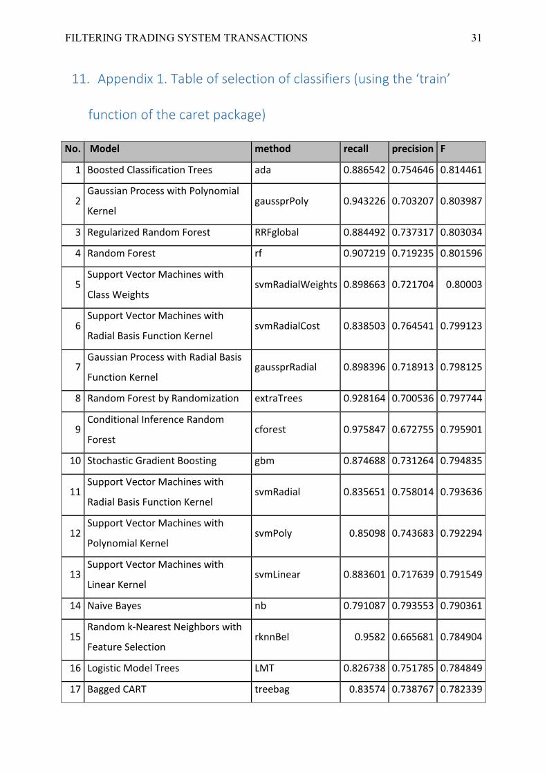
11. Appendix 1. Table of selection of classifiers (using the ‘train’
function of the caret package)
No. Model method recall precision F
1 Boosted Classification Trees ada 0.886542 0.754646 0.814461
2 Gaussian Process with Polynomial
Kernel gaussprPoly 0.943226 0.703207 0.803987
3 Regularized Random Forest RRFglobal 0.884492 0.737317 0.803034
4 Random Forest rf 0.907219 0.719235 0.801596
5 Support Vector Machines with
Class Weights svmRadialWeights 0.898663 0.721704 0.80003
6 Support Vector Machines with
Radial Basis Function Kernel svmRadialCost 0.838503 0.764541 0.799123
7 Gaussian Process with Radial Basis
Function Kernel gaussprRadial 0.898396 0.718913 0.798125
8 Random Forest by Randomization extraTrees 0.928164 0.700536 0.797744
9 Conditional Inference Random
Forest cforest 0.975847 0.672755 0.795901
10 Stochastic Gradient Boosting gbm 0.874688 0.731264 0.794835
11 Support Vector Machines with
Radial Basis Function Kernel svmRadial 0.835651 0.758014 0.793636
12 Support Vector Machines with
Polynomial Kernel svmPoly 0.85098 0.743683 0.792294
13 Support Vector Machines with
Linear Kernel svmLinear 0.883601 0.717639 0.791549
14 Naive Bayes nb 0.791087 0.793553 0.790361
15 Random k-Nearest Neighbors with
Feature Selection rknnBel 0.9582 0.665681 0.784904
16 Logistic Model Trees LMT 0.826738 0.751785 0.784849
17 Bagged CART treebag 0.83574 0.738767 0.782339
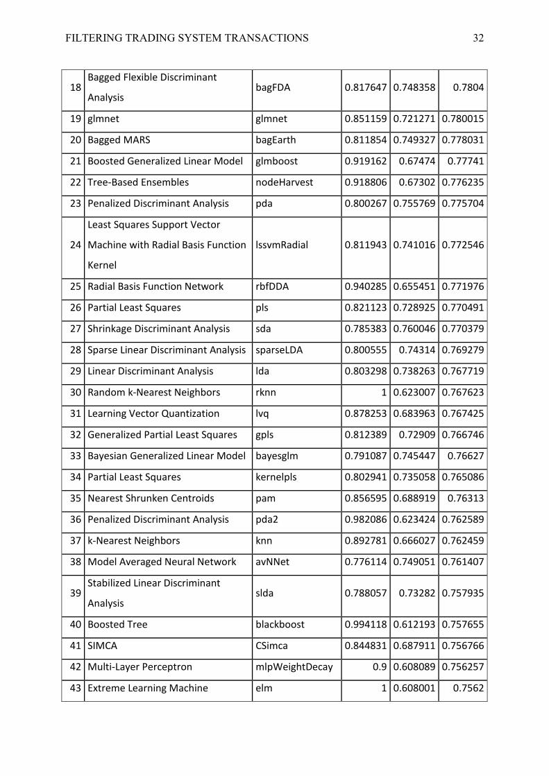
FILTERING TRADING SYSTEM TRANSACTIONS 32
18 Bagged Flexible Discriminant
Analysis bagFDA 0.817647 0.748358 0.7804
19 glmnet glmnet 0.851159 0.721271 0.780015
20 Bagged MARS bagEarth 0.811854 0.749327 0.778031
21 Boosted Generalized Linear Model glmboost 0.919162 0.67474 0.77741
22 Tree-Based Ensembles nodeHarvest 0.918806 0.67302 0.776235
23 Penalized Discriminant Analysis pda 0.800267 0.755769 0.775704
24
Least Squares Support Vector
Machine with Radial Basis Function
Kernel
lssvmRadial 0.811943 0.741016 0.772546
25 Radial Basis Function Network rbfDDA 0.940285 0.655451 0.771976
26 Partial Least Squares pls 0.821123 0.728925 0.770491
27 Shrinkage Discriminant Analysis sda 0.785383 0.760046 0.770379
28 Sparse Linear Discriminant Analysis sparseLDA 0.800555 0.74314 0.769279
29 Linear Discriminant Analysis lda 0.803298 0.738263 0.767719
30 Random k-Nearest Neighbors rknn 1 0.623007 0.767623
31 Learning Vector Quantization lvq 0.878253 0.683963 0.767425
32 Generalized Partial Least Squares gpls 0.812389 0.72909 0.766746
33 Bayesian Generalized Linear Model bayesglm 0.791087 0.745447 0.76627
34 Partial Least Squares kernelpls 0.802941 0.735058 0.765086
35 Nearest Shrunken Centroids pam 0.856595 0.688919 0.76313
36 Penalized Discriminant Analysis pda2 0.982086 0.623424 0.762589
37 k-Nearest Neighbors knn 0.892781 0.666027 0.762459
38 Model Averaged Neural Network avNNet 0.776114 0.749051 0.761407
39 Stabilized Linear Discriminant
Analysis slda 0.788057 0.73282 0.757935
40 Boosted Tree blackboost 0.994118 0.612193 0.757655
41 SIMCA CSimca 0.844831 0.687911 0.756766
42 Multi-Layer Perceptron mlpWeightDecay 0.9 0.608089 0.756257
43 Extreme Learning Machine elm 1 0.608001 0.7562
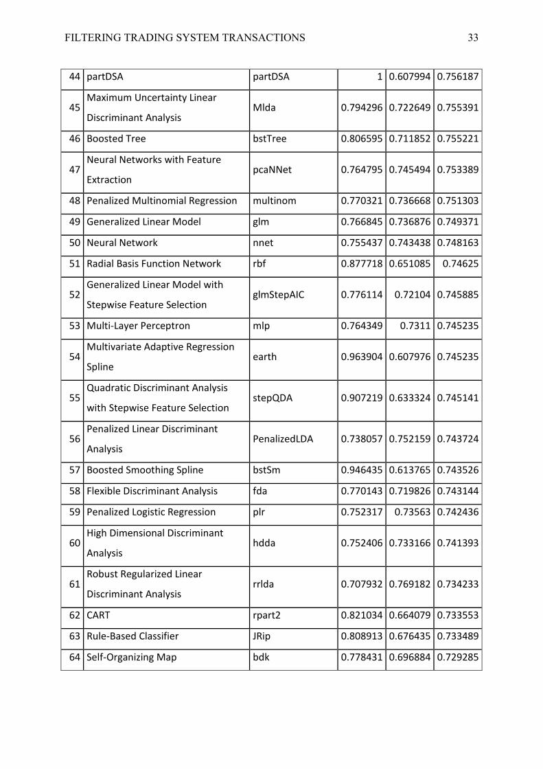
FILTERING TRADING SYSTEM TRANSACTIONS 33
44 partDSA partDSA 1 0.607994 0.756187
45 Maximum Uncertainty Linear
Discriminant Analysis Mlda 0.794296 0.722649 0.755391
46 Boosted Tree bstTree 0.806595 0.711852 0.755221
47 Neural Networks with Feature
Extraction pcaNNet 0.764795 0.745494 0.753389
48 Penalized Multinomial Regression multinom 0.770321 0.736668 0.751303
49 Generalized Linear Model glm 0.766845 0.736876 0.749371
50 Neural Network nnet 0.755437 0.743438 0.748163
51 Radial Basis Function Network rbf 0.877718 0.651085 0.74625
52 Generalized Linear Model with
Stepwise Feature Selection glmStepAIC 0.776114 0.72104 0.745885
53 Multi-Layer Perceptron mlp 0.764349 0.7311 0.745235
54 Multivariate Adaptive Regression
Spline earth 0.963904 0.607976 0.745235
55 Quadratic Discriminant Analysis
with Stepwise Feature Selection stepQDA 0.907219 0.633324 0.745141
56 Penalized Linear Discriminant
Analysis PenalizedLDA 0.738057 0.752159 0.743724
57 Boosted Smoothing Spline bstSm 0.946435 0.613765 0.743526
58 Flexible Discriminant Analysis fda 0.770143 0.719826 0.743144
59 Penalized Logistic Regression plr 0.752317 0.73563 0.742436
60 High Dimensional Discriminant
Analysis hdda 0.752406 0.733166 0.741393
61 Robust Regularized Linear
Discriminant Analysis rrlda 0.707932 0.769182 0.734233
62 CART rpart2 0.821034 0.664079 0.733553
63 Rule-Based Classifier JRip 0.808913 0.676435 0.733489
64 Self-Organizing Map bdk 0.778431 0.696884 0.729285
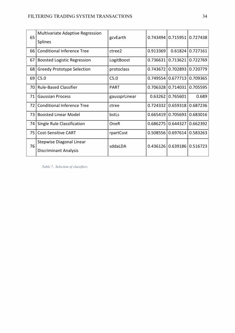
FILTERING TRADING SYSTEM TRANSACTIONS 34
65 Multivariate Adaptive Regression
Splines gcvEarth 0.743494 0.715951 0.727438
66 Conditional Inference Tree ctree2 0.913369 0.61824 0.727161
67 Boosted Logistic Regression LogitBoost 0.736631 0.713621 0.722769
68 Greedy Prototype Selection protoclass 0.743672 0.702893 0.720779
69 C5.0 C5.0 0.749554 0.677713 0.709365
70 Rule-Based Classifier PART 0.706328 0.714031 0.705595
71 Gaussian Process gaussprLinear 0.63262 0.765601 0.689
72 Conditional Inference Tree ctree 0.724332 0.659318 0.687236
73 Boosted Linear Model bstLs 0.665419 0.705693 0.683016
74 Single Rule Classification OneR 0.686275 0.644327 0.662392
75 Cost-Sensitive CART rpartCost 0.508556 0.697614 0.583263
76 Stepwise Diagonal Linear
Discriminant Analysis sddaLDA 0.436126 0.639186 0.516723
Table 7.. Selection of classifiers
FILTERING TRADING SYSTEM TRANSACTIONS 35
12. References
Ahdesmaki, M., Zuber, V., Gibb, S., & Strimmer, K. (2014). sda: Shrinkage Discriminant
Analysis and CAT Score Variable Selection. Retrieved from http://CRAN.R-
project.org/package=sda
AL-RADAIDEH, Q. A., ASSAF, A. A., & ALNAGI, E. (2013). PREDICTING STOCK
PRICES USING DATA MINING TECHNIQUES.
Analytics, R., & Weston, S. (2014). foreach: Foreach looping construct for R. Retrieved from
http://CRAN.R-project.org/package=foreach
Bergé, L., Bouveyron, C., & Girard, S. (2012). HDclassif: An R Package for Model-Based
Clustering and Discriminant Analysis of High-Dimensional Data. Journal of
Statistical Software, 46(6), 1–29.
Bergmeir, C., & Benítez, J. M. (2012). Neural Networks in R Using the Stuttgart Neural
Network Simulator: RSNNS. Journal of Statistical Software, 46(7), 1–26.
Bioinformatics, C., & Stone, G. (2010). SDDA: Stepwise Diagonal Discriminant Analysis.
Retrieved from http://CRAN.R-project.org/package=SDDA
Borchers, H. W. (2014). pracma: Practical Numerical Math Functions. Retrieved from
http://CRAN.R-project.org/package=pracma
Carl, P., Eddelbuettel, D., Ryan, J., Ulrich, J., Peterson, B. G., & See, G. (2012).
FinancialInstrument: Financial Instrument Model Infrastructure for R. Retrieved from
http://CRAN.R-project.org/package=FinancialInstrument
Carl, P., & Peterson, B. G. (2013). PerformanceAnalytics: Econometric tools for performance
and risk analysis. Retrieved from http://CRAN.R-
project.org/package=PerformanceAnalytics
FILTERING TRADING SYSTEM TRANSACTIONS 36
Carl, P., & Peterson, B. G. (2014). blotter: Tools for transaction-oriented trading systems
development. Retrieved from http://R-Forge.R-project.org/projects/blotter/
Carl, P., Peterson, B. G., Ulrich, J., & Humme, J. (2014). quantstrat: Quantitative Strategy
Model Framework. Retrieved from http://R-Forge.R-project.org/projects/blotter/
Clemmensen, L., & Kuhn, contributions by M. (2012). sparseLDA: Sparse Discriminant
Analysis. Retrieved from http://CRAN.R-project.org/package=sparseLDA
Culp, M., Johnson, K., & Michailidis, G. (2012). ada: ada: an R package for stochastic
boosting. Retrieved from http://CRAN.R-project.org/package=ada
Deng, H. (2013). Guided Random Forest in the RRF Package. arXiv:1306.0237.
Ding, B. (n.d.). gpls: Classification using generalized partial least squares.
Gelman, A., & Su, Y.-S. (2014). arm: Data Analysis Using Regression and
Multilevel/Hierarchical Models. Retrieved from http://CRAN.R-
project.org/package=arm
Gosso, A. (2012). elmNN: Implementation of ELM (Extreme Learning Machine ) algorithm
for SLFN ( Single Hidden Layer Feedforward Neural Networks ). Retrieved from
http://CRAN.R-project.org/package=elmNN
Gschwandtner, M., Filzmoser, P., Croux, C., & Haesbroeck, G. (2012). rrlda: Robust
Regularized Linear Discriminant Analysis. Retrieved from http://CRAN.R-
project.org/package=rrlda
Hastie, S. M. D. from mda:mars by T., & wrapper, R. T. U. A. M. F. utilities with T. L. leaps.
(2014). earth: Multivariate Adaptive Regression Spline Models. Retrieved from
http://CRAN.R-project.org/package=earth
Hastie, T., Tibshirani, R., Narasimhan, B., & Chu, G. (2013). pamr: Pam: prediction analysis
for microarrays. Retrieved from http://CRAN.R-project.org/package=pamr
FILTERING TRADING SYSTEM TRANSACTIONS 37
Hornik, K., Buchta, C., & Zeileis, A. (2009). Open-Source Machine Learning: R Meets Weka.
Computational Statistics, 24(2), 225–232. doi:10.1007/s00180-008-0119-7
Hothorn, T., Buehlmann, P., Kneib, T., Schmid, M., & Hofner, B. (2013). mboost: Model-
Based Boosting, R package version 2.2-3. Retrieved from http://CRAN.R-
project.org/package=mboost.
Hothorn, T., Hornik, K., & Zeileis, A. (2006). Unbiased Recursive Partitioning: A
Conditional Inference Framework. Journal of Computational and Graphical Statistics,
15(3), 651–674.
James, D., & Hornik, K. (2014). chron: Chronological Objects which Can Handle Dates and
Times. Retrieved from http://CRAN.R-project.org/package=chron
Karatzoglou, A., Smola, A., Hornik, K., & Zeileis, A. (2004). kernlab – An S4 Package for
Kernel Methods in R. Journal of Statistical Software, 11(9), 1–20.
Komorowski, J., Pawlak, Z., Polkowski, L., & Skowron, A. (1999). Rough sets: A tutorial.
Rough Fuzzy Hybridization: A New Trend in Decision-Making, 3–98.
Kuhn, M., Weston, S., & Quinlan, N. C. C. code for C. 0 by R. (2014). C50: C5.0 Decision
Trees and Rule-Based Models. Retrieved from http://CRAN.R-
project.org/package=C50
Kun, M., Weston, S., Williams, A., Keefer, C., Engelhardt, A., Cooper, T., … Wing, J.
(2014). caret: Classification and Regression Training. Retrieved from
http://CRAN.R-project.org/package=caret
Leisch, S. original by T. H. & R. T. O. R. port by F., Hornik, K., & Ripley, B. D. (2013).
mda: Mixture and flexible discriminant analysis. Retrieved from http://CRAN.R-
project.org/package=mda
Li, S. (2013). rknn: Random KNN Classification and Regression. Retrieved from
http://CRAN.R-project.org/package=rknn
FILTERING TRADING SYSTEM TRANSACTIONS 38
Liaw, A., & Wiener, M. (2002). Classification and Regression by randomForest. R News,
2(3), 18–22.
Masters, T. (2013). Assessing and Improving Prediction and Classification (1 edition.).
CreateSpace Independent Publishing Platform.
Meinshausen, N. (2013). nodeHarvest: Node Harvest for regression and classification.
Retrieved from http://CRAN.R-project.org/package=nodeHarvest
Mevik, B.-H., Wehrens, R., & Liland, K. H. (2013). pls: Partial Least Squares and Principal
Component regression. Retrieved from http://CRAN.R-project.org/package=pls
Meyer, D., & Buchta, C. (2014). proxy: Distance and Similarity Measures. Retrieved from
http://CRAN.R-project.org/package=proxy
Molinaro, A., Olshen, A., Lostritto, K., Ryslik, G., & Weston, S. (2014). partDSA:
Partitioning using deletion, substitution, and addition moves. Retrieved from
http://CRAN.R-project.org/package=partDSA
Park, M. Y., & Hastie, T. (2010). stepPlr: L2 penalized logistic regression with a stepwise
variable selection. Retrieved from http://CRAN.R-project.org/package=stepPlr
Peters, A., & Hothorn, T. (2013). ipred: Improved Predictors. Retrieved from http://CRAN.R-
project.org/package=ipred
R Core Team. (2014). R: A Language and Environment for Statistical Computing. Vienna,
Austria: R Foundation for Statistical Computing. Retrieved from http://www.R-
project.org/
Ridgeway, G. (2013). gbm: Generalized Boosted Regression Models. Retrieved from
http://CRAN.R-project.org/package=gbm
Riza, L. S., Janusz, A., Cornelis, C., Herrera, F., Slezak, D., & Benitez, J. M. (2014).
RoughSets: Data Analysis Using Rough Set and Fuzzy Rough Set Theories. Retrieved
from http://CRAN.R-project.org/package=RoughSets
FILTERING TRADING SYSTEM TRANSACTIONS 39
Ryan, J. A. (2013). quantmod: Quantitative Financial Modelling Framework. Retrieved from
http://CRAN.R-project.org/package=quantmod
Ryan, J. A., & Ulrich, J. M. (2014). xts: eXtensible Time Series. Retrieved from
http://CRAN.R-project.org/package=xts
Sarkar, D. (2008). Lattice: Multivariate Data Visualization with R. New York: Springer.
Retrieved from http://lmdvr.r-forge.r-project.org
Silva, A. P. D. (2012). HiDimDA: High Dimensional Discriminant Analysis. Retrieved from
http://CRAN.R-project.org/package=HiDimDA
Simm, J., & Abril, I. M. de. (2013). extraTrees: ExtraTrees method. Retrieved from
http://CRAN.R-project.org/package=extraTrees
Simon, N., Friedman, J., Hastie, T., & Tibshirani, R. (2011). Regularization Paths for Cox’s
Proportional Hazards Model via Coordinate Descent. Journal of Statistical Software,
39(5), 1–13.
Soni, S. (2010). Applications of ANNs in Stock Market Prediction: A Survey.
Therneau, T., Atkinson, B., & Ripley, B. (2014). rpart: Recursive Partitioning and
Regression Trees. Retrieved from http://CRAN.R-project.org/package=rpart
Todorov, V. (2013). rrcovHD: Robust multivariate Methods for High Dimensional Data.
Retrieved from http://CRAN.R-project.org/package=rrcovHD
Tuszynski, J. (2014). caTools: Tools: moving window statistics, GIF, Base64, ROC AUC, etc.
Retrieved from http://CRAN.R-project.org/package=caTools
Ulrich, J. (2013). TTR: Technical Trading Rules. Retrieved from http://R-Forge.R-
project.org/projects/ttr/
Varutbangkul, E. (2013). Integrating Traditional Stock Trading Systems: A Data Mining
Approach.
FILTERING TRADING SYSTEM TRANSACTIONS 40
Venables, W. N., & Ripley, B. D. (2002). Modern Applied Statistics with S (Fourth.). New
York: Springer. Retrieved from http://www.stats.ox.ac.uk/pub/MASS4
Wang, Z. (2013). bst: Gradient Boosting. Retrieved from http://CRAN.R-
project.org/package=bst
Wehrens, R., & Buydens, L. M. C. (2007). Self- and Super-organising Maps in R: the
kohonen package. J. Stat. Softw., 21(5). Retrieved from
http://www.jstatsoft.org/v21/i05
Weihs, C., Ligges, U., Luebke, K., & Raabe, N. (2005). klaR Analyzing German Business
Cycles. In D. Baier, R. Decker, & L. Schmidt-Thieme (Eds.), Data Analysis and
Decision Support (pp. 335–343). Berlin: Springer-Verlag.
Wickham, H. (2011). The Split-Apply-Combine Strategy for Data Analysis. Journal of
Statistical Software, 40(1), 1–29.
Witten, D. (2011). penalizedLDA: Penalized classification using Fisher’s linear discriminant.
Retrieved from http://CRAN.R-project.org/package=penalizedLDA

FILTERING TRADING SYSTEM TRANSACTIONS 41