ORIGINAL ARTICLE

J For Res (2005) 10:113–123 © The Japanese Forest Society and Springer-Verlag Tokyo 2005DOI 10.1007/s10310-004-0116-9

Kazuhiro Aruga · John Sessions · Abdullah E. Akay

Application of an airborne laser scanner to forest road design with accurateearthwork volumes

Received: March 8, 2004 / Accepted: August 3, 2004

K. Aruga (*)Department of Forest Science, Faculty of Agriculture, UtsunomiyaUniversity, 350 Mine, Utsunomiya 321-8505, JapanTel. �81-28-649-5537; Fax �81-28-649-5545e-mail: aruga@cc.utsunomiya-u.ac.jp

J. SessionsDepartment of Forest Engineering, College of Forestry, OregonState University, Corvallis, USA

A.E. AkayForest Engineering Department, Faculty of Forestry,Kahramanmaras Sutcu Imam University, Kahramanmaras, Turkey

Abstract In this study we developed a forest road designprogram based on a high-resolution digital elevation model(DEM) from a light detection and ranging (LIDAR)system. After a designer has located the intersection pointson a horizontal plane, the model first generates the horizon-tal alignment and the ground profile. The model preciselygenerates cross-sections and accurately calculatesearthwork volumes using a high-resolution DEM. Themodel then optimizes the vertical alignment based on con-struction and maintenance costs using a heuristic techniqueknown as tabu search. As the distance between cross-sections affects the accuracy of earthwork volume calcula-tions, the results were examined by comparing them withthe exact earthwork volume calculated by the probabilisticMonte Carlo simulation method. The earthwork volumescalculated by the Pappus-based method were similar tothose calculated by the Monte Carlo simulation when thedistance between cross-sections was within 10m. The modelwas applied to a high-resolution DEM from the LIDAR ofCapitol Forest in Washington State, USA. The model gen-erated a horizontal alignment, length 827m, composed offive horizontal curves. We examined the number of gradechange points. The results indicated that tabu search foundthe best solution ($61.42/m) with five grade change points.This was composed of two vertical curves that almostfollowed the ground profile. As the accuracy of a high-resolution DEM from LIDAR increases, the model would

become a useful tool for a forest road designer because iteliminates or at least reduces the time-consuming process ofroad surveys.

Key words Forest road design · Airborne laser scanner ·Monte Carlo simulation · Pappus-based method · Tabusearch

Introduction

An airborne laser scanner is a remote sensing technologythat is increasingly being used to map forested terrain. Thismapping technology utilizes a light detection and ranging(LIDAR) system. LIDAR was developed over 20 years agoand has since been improved. LIDAR has the ability tocreate much more accurate elevation and terrain maps inthe presence of a forest canopy than pre-existing sourcescan, due to a small-diameter laser beam footprint belowtens of centimeters in size.

Considering a forestry application of a LIDAR system,Chung et al. (2004) developed a method for optimizingcable logging layouts using a heuristic network algorithm.The model evaluates the logging feasibility of alternativecable corridors based on a digital elevation model (DEM)developed from LIDAR and GIS (geographic informationsystem) data. Coulter et al. (2002) first applied a high-reso-lution DEM from LIDAR to forest road design for linearroad segments. Akay (2003) then developed a 3-D forestroad alignment optimization model, TRACER, using ahigh-resolution DEM from LIDAR. After a designer hasdetermined the initial alignment by locating intersectionpoints and grade change points on a 3-D graphic interface,the model automatically generates horizontal and verticalcurves, and cross-sections, and calculates construction,maintenance, and transportation costs. The model then op-timizes vertical alignments based on manually selectedgrade change points using simulated annealing (Dowsland1993) while minimizing earthwork allocation costs usinglinear programming (Mayer and Stark 1981).

114

The program can generate cross-sections precisely andcalculate earthwork volumes on straight roadways accu-rately using a high-resolution DEM. However, the modelcannot calculate earthwork volumes for curved roadwaysaccurately because it uses the average end-area method toestimate earthwork volumes. The average end-area methodis commonly used for straight roadways, but tends to over-estimate the volume. The prismoidal method provides amore precise volume calculation for linear profiles. Easa(1992a) developed a modified prismoidal method for com-puting volumes of straight roadways with nonlinear groundprofiles.

For a curved roadway, the existing method of volumecomputation is analogous to the average end-area methodfor straight sections. The method is based on Pappus’ theo-rem, which states that the volume of the solid formed byrotating a plane figure about an axis in its plane equals thearea of the figure multiplied by the length of the path tracedout by the centroid of the figure. Based on this theorem, theearthwork volume is computed approximately as the aver-age of the volumes resulting from rotating the areas of thetwo cross-sections (Kato 1951).

We proposed the new model combined with the methodbased on Pappus’ theorem in order to calculate earthworkvolumes for curved roadways more accurately. The model isalso combined with the vertical alignment optimizationtechnique proposed by Aruga et al. (2005). The model com-bined with this technique can optimize vertical alignmentwhile changing heights of grade change points as well as theplacement of grade change points. The earlier study con-cluded that the examination of the placement of gradechange points improved solution quality (Aruga et al. 2005).The present study first describes details of forest road de-sign in the model. We then apply the model to a high-resolution DEM from a LIDAR of Capitol Forest inWashington State, USA, and discuss the solution quality ofvertical alignments optimized by the model. Finally, wediscuss the distance between cross-sections, which affectsthe accuracy of earthwork volumes, by comparing themwith the probabilistic method to calculate the exactearthwork volume using the Monte Carlo simulation pro-posed by Easa (2003).

Forest road design

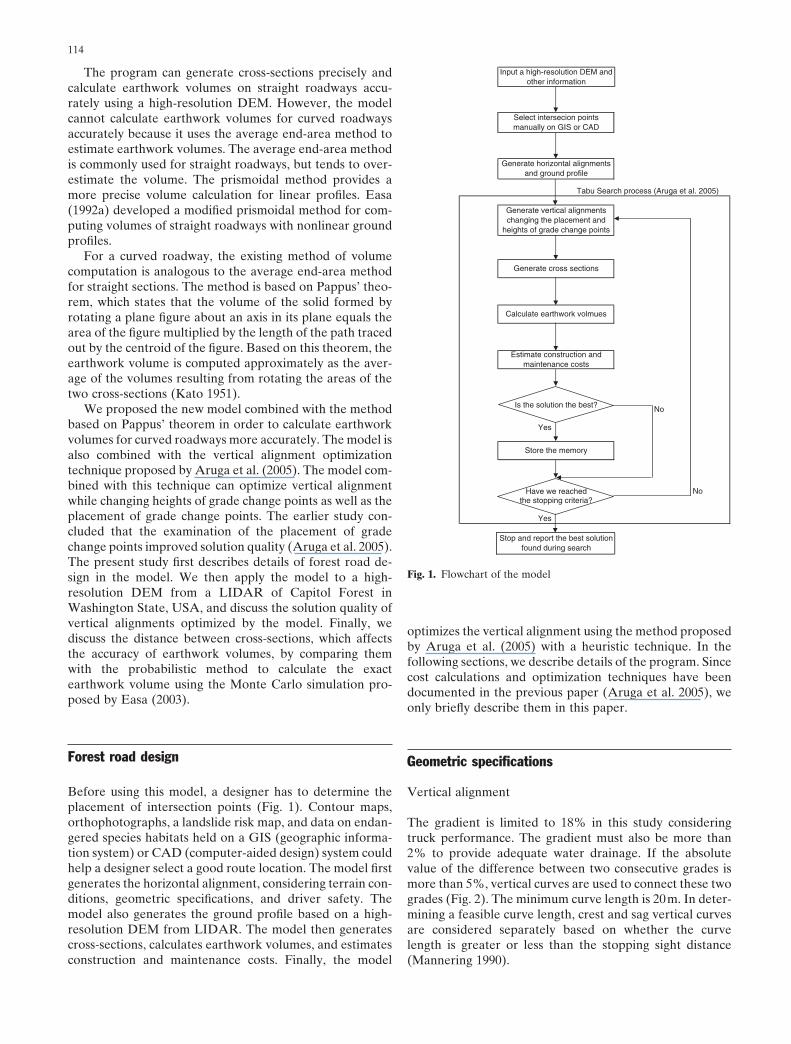
Before using this model, a designer has to determine theplacement of intersection points (Fig. 1). Contour maps,orthophotographs, a landslide risk map, and data on endan-gered species habitats held on a GIS (geographic informa-tion system) or CAD (computer-aided design) system couldhelp a designer select a good route location. The model firstgenerates the horizontal alignment, considering terrain con-ditions, geometric specifications, and driver safety. Themodel also generates the ground profile based on a high-resolution DEM from LIDAR. The model then generatescross-sections, calculates earthwork volumes, and estimatesconstruction and maintenance costs. Finally, the model

optimizes the vertical alignment using the method proposedby Aruga et al. (2005) with a heuristic technique. In thefollowing sections, we describe details of the program. Sincecost calculations and optimization techniques have beendocumented in the previous paper (Aruga et al. 2005), weonly briefly describe them in this paper.

Geometric specifications

Vertical alignment

The gradient is limited to 18% in this study consideringtruck performance. The gradient must also be more than2% to provide adequate water drainage. If the absolutevalue of the difference between two consecutive grades ismore than 5%, vertical curves are used to connect these twogrades (Fig. 2). The minimum curve length is 20m. In deter-mining a feasible curve length, crest and sag vertical curvesare considered separately based on whether the curvelength is greater or less than the stopping sight distance(Mannering 1990).

Tabu Search process (Aruga et al. 2005)

No

Yes

No

Yes

Stop and report the best solution found during search

Input a high-resolution DEM and other information

Select intersecion points manually on GIS or CAD

Generate vertical alignments changing the placement and

heights of grade change points

Generate cross sections

Is the solution the best?

Generate horizontal alignments and ground profile

Have we reachedthe stopping criteria?

Calculate earthwork volmues

Estimate construction and maintenance costs

Store the memory

Fig. 1. Flowchart of the model

115

SV

tV

g f Gd

dr

d

r

� ��3 6 2 3 6

2

2. .( )( ) (1)

where Sd is the stopping sight distance (m), Vd is the designspeed (e.g. 30km/h), tr is the perception-reaction time(2.5s), g is the gravity (9.81m/s2), fr is the braking/tractivecoefficient (e.g. 0.5), and G is the road grade (decimal). Theappropriate value of road grade at a vertical curve wherethe grade keeps changing is not explicitly suggested by theAmerican Association of State Highway and Transporta-tion Officials (AASHTO 1994). In this study, the road gradefor two different road sections is taken as their averagevalue. On one-lane, two-directional roads, the stoppingsight distance is approximately twice the stopping sight dis-tance for a two-lane road, because both drivers must safelystop their vehicles.

The length of the crest vertical curve is calculated basedon the stopping sight distance. When the stopping sightdistance is greater than curve length,

L Sh h

Av d

d o� �

�2

100 2 22( )

D

(2)

when the stopping sight distance is less than the curvelength,

LA S

h hv

d

d o

��

D2

2

100 2 2( ) (3)

where Lv is the length of vertical curve (m), A∆ is the alge-braic difference in grades (percent), hd is the height ofdriver’s eye above road way surface (1.05m), and ho is theheight of object above roadway surface (0.15m). The lengthof a sag curve is calculated based on the stopping sightdistance as well. When the stopping sight distance is greaterthan the curve length,

L SH S

Av dd

� ��

2200 tanb( )

D(4)

and, when the stopping sight distance is less than the curvelength,

LA S

H Svd

d

��

D2

200 tanb( ) (5)

where H is the head light height (0.6m) and � is the upwardangle of the headlight beam (1°).

Horizontal alignment

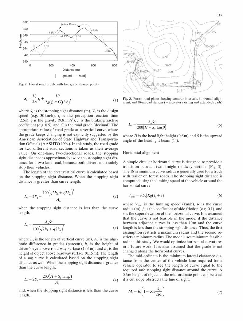
A simple circular horizontal curve is designed to provide atransition between two straight roadway sections (Fig. 3).The 18m minimum curve radius is generally used for a truckwith trailer on forest roads. The stopping sight distance iscomputed using the limiting speed of the vehicle around thehorizontal curve.

V Rg f elimit s� �3 6. ( ) (6)

where Vlimit is the limiting speed (km/h), R is the curveradius (m), fs is the coefficient of side friction (e.g. 0.1), ande is the superelevation of the horizontal curve. It is assumedthat the curve is not feasible in the model if the distancebetween adjacent curves is less than 10m and the curvelength is less than the stopping sight distance. Thus, the firstassumption restricts a maximum radius and the second re-stricts a minimum radius. The model uses minimum feasibleradii in this study. We would optimize horizontal curvaturesin a future work. It is also assumed that the grade is notchanged along the horizontal curves.

The mid-ordinate is the minimum lateral clearance dis-tance from the center of the vehicle lane required for avehicle operator to see the length of curve equal to therequired safe stopping sight distance around the curve. A0.6m height of object at the mid-ordinate point can be usedif a cut slope obstructs the line of sight.

M RSRs v

d

v

� �12

cosÊËÁ

ˆ¯̃ (7)

340

342

344

346

348

350

352

0 200 400 600 800Distance (m)

Hei

ght (

m)

ground road

–2.2%

3.2%–2.6%

–5.3%

Vertical Curve

2.0%

2.7%

Fig. 2. Forest road profile with five grade change points

Fig. 3. Forest road plane showing contour intervals, horizontal align-ment, and 30-m road stations (� indicates existing and extended roads)

116

where Ms is the mid-ordinate (m) and Rv is the design curveradius minus the half of the road width (m). This conditionassumes that there is little or no vertical curvature on thehorizontal curve.

If cut slope height is higher than the height of object, themodel lays back the cut slope from road edge to the driver’sline of sight to provide the minimum safe stopping distance.In order to layback the cut slope, the horizontal distancefrom each point to the line of sight, Mp(m) is computed.

M RS R

S Rp vd v

d v s

� ��

12

2

cos

cos( )

( )Ê

ËÁ

ˆ

¯˜q (8)

where

q q qs

c d v

CL� �

�D S R2

(9)

where θ is the intersection angle (radian), Dc is the horizon-tal distance from the beginning point of the curve to eachpoint of the curve (m), and CL is the curve length (m).

Curve widening must provide adequate lane width forthe off-tracking of design and critical vehicles, such as logtrucks, tractor trailer trains, and logging equipment. Ontwo-lane roads, curve widening is designed for each lane.On one-lane roads, curve widening is usually designed onthe inside of curves. The off-tracking equation has beendeveloped to compute off-tracking of tractor trailer trainsand a stinger-type log truck (Cain and Langdon 1982).

OT e� � � � � �R R LR

L2 2 1 0 015

1800 216( ) Ê

ËÁˆ¯̃

ÊËÁ

ˆ¯̃

exp . .q

p(10)

Where OT is the total vehicle off-tracking (m) and Le is theeffective vehicle length (m). The effective vehicle length fora lowboy tractor-trailer combination is:

L L L Le � � �12

22

32 (11)

where L1 is the wheelbase of the tractor (e.g. 4.72m), L2 isthe distance from fifth wheel to center of rear duals of thefirst trailer (e.g. 0.30m), and L3 is the distance from fifthwheel to center of rear duals of the second trailer (e.g.11.67m). The USFS preconstruction handbook (USDA1987) recommends a straight line taper transition to thewidened curve beginning before the curve and ending afterthe curve (Table 1).

Turnouts are designed for one-lane, two directionalroads to facilitate vehicle passage. A maximum turnout in-tervisible distance is 300m in common practice (AASHTO

1994). The turnout should be at least 3m in width and 15mlong, with a 7.5-m transition at each end.

Earthwork volume

Cross-sections

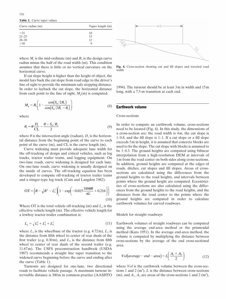
In order to compute an earthwork volume, cross-sectionsneed to be located (Fig. 4). In this study, the dimensions ofa cross-section are: the road width is 4m, the cut slope is1 :0.8, and the fill slope is 1 :1. If a cut slope or a fill slopeexceeds 5m in height, it is assumed that concrete blocks areused to fix the slope. The cut slope with blocks is assumed tobe 1 :0.3. The ground heights are computed using bilinearinterpolation from a high-resolution DEM at intervals of1m from the road center on both sides along cross-sections.In addition, ground heights are computed at the edges ofroads, ditches, cut slopes and fill slopes. Areas of cross-sections are calculated using the differences from theground heights to the road heights, and intervals betweenpoints where the ground height are computed. Eccentrici-ties of cross-sections are also calculated using the differ-ences from the ground heights to the road heights, and thedistances from the road center to the points where theground heights are computed in order to calculateearthwork volumes for curved roadways.

Models for straight roadways

Earthwork volumes of straight roadways can be computedusing the average end-area method or the prismoidalmethod (Kato 1951). In the average end-area method, thevolume is computed by multiplying the distance betweencross-sections by the average of the end cross-sectionalarea.

Vol average end area LA A

� � ��( ) Ê

ËÁˆ¯̃

1 2

2 (12)

where Vol is the earthwork volume between the cross-sec-tions 1 and 2 (m3), L is the distance between cross-sections(m), and A1, A2 are areas of the cross-sections 1 and 2 (m2),

Table 1. Curve taper values

Curve radius (m) Taper length (m)

�21 1821–25 1526–30 12�30 9

Fig. 4. Cross-section showing cut and fill slopes and traveled roadwidth

117

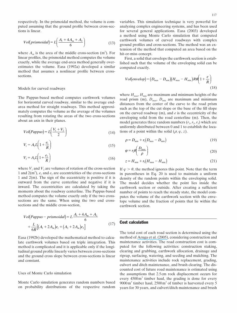
respectively. In the prismoidal method, the volume is com-puted assuming that the ground profile between cross-sec-tions is linear.

Vol prismoidal LA A A( ) Ê

ËÁˆ¯̃

�� �1 24

6m

(13)

where Am is the area of the middle cross-section (m2). Forlinear profiles, the prismoidal method computes the volumeexactly, while the average end-area method generally over-estimates the volume. Easa (1992a) developed a similarmethod that assumes a nonlinear profile between cross-sections.

Models for curved roadways

The Pappus-based method computes earthwork volumesfor horizontal curved roadway, similar to the average end-area method for straight roadways. This method approxi-mately computes the volume as the average of the volumesresulting from rotating the areas of the two cross-sectionsabout an axis in their planes.

Vol Pappus LV V( ) Ê

ËÁˆ¯̃

��1 2

2 (14)

V A LeR1 1

11� �ÊËÁ

ˆ¯̃ (15)

V A LeR2 2

21� �ÊËÁ

ˆ¯̃ (16)

where V1 and V2 are volumes of rotation of the cross-section1 and 2(m3), e1 and e2 are eccentricities of the cross-sections1 and 2(m). The sign of the eccentricity is positive if it isoutward from the curve centerline and negative if it isinward. The eccentricities are calculated by taking themoments about the roadway centerline. The Pappus-basedmethod computes the volume exactly only if the two cross-sections are the same. When using the two end cross-sections and the middle cross-section,

Vol Pappus prismoidal LA A A

LR

A A e A A e

� �� �

� � � �

( )

( ) ( )[ ]

1 2

1 1 2 2

46

62 2

m

m m

(17)

Easa (1992b) developed the mathematical method to calcu-late earthwork volumes based on triple integration. Thismethod is complicated and it is applicable only if the longi-tudinal ground profile linearly varies between cross-sectionsand the ground cross slope between cross-sections is linearand constant.

Uses of Monte Carlo simulation

Monte Carlo simulation generates random numbers basedon probability distributions of the respective random

variables. This simulation technique is very powerful foranalyzing complex engineering systems, and has been usedfor several general applications. Easa (2003) developeda method using Monte Carlo simulation that computedearthwork volumes of curved roadways with complexground profiles and cross-sections. The method was an ex-tension of the method that computed an area based on thehit-or-miss concept.

First, a solid that envelops the earthwork section is estab-lished such that the volume of the enveloping solid can becomputed exactly.

Vol envelop D D H H ReR

( ) ( )( ) ÊËÁ

ˆ¯̃

� � � �max min max min q 1

(18)

where Hmax, Hmin are maximum and minimum heights of theroad prism (m), Dmax, Dmin are maximum and minimumdistances from the center of the curve to the road prismsuch as the top of the cut slope or the base of the fill slopeon the curved roadway (m), and e is the eccentricity of theenveloping solid from the road centerline (m). Then, themodel generates three random numbers (r1, r2, r3) which areuniformly distributed between 0 and 1 to establish the loca-tions of a point within the solid (r, �, z).

r � � �D r D Dmin max min1( ) (19)

j qr

� rD

2maxÊ

ËÁˆ¯̃ (20)

z H r H H� � �min max min3( ) (21)

If � � θ, the method ignores this point. Note that the termin parentheses in Eq. 20 is used to maintain a uniformdensity of the random points within the enveloping solid.The model decides whether the point lies inside theearthwork section or outside. After creating a sufficientnumber of points to reach the steady state, the model com-putes the volume of the earthwork section with the enve-lope volume and the fraction of points that lie within theearthwork section.

Cost calculation

The total cost of each road section is determined using themethod of Aruga et al. (2005), considering construction andmaintenance activities. The road construction cost is com-puted for the following activities: construction staking,clearing and grubbing, earthwork allocation, drainage andriprap, surfacing, watering, and seeding and mulching. Themaintenance activities include rock replacement, grading,culvert and ditch maintenance, and brush clearing. The dis-counted cost of future road maintenance is estimated usingthe assumptions that 2.5cm rock displacement occurs forevery 4500m3 timber haul, the grading is done for every9000m3 timber haul, 2500m3 of timber is harvested every 5years for 30 years, and culvert/ditch maintenance and brush

118

clearing are done every 5 years. The annual interest rate is1%. In the model, the objective function takes the followingform:

MinT C MC � � 0 (22)

where TC � the total cost, C � the construction cost, andM0 � the discounted maintenance cost.

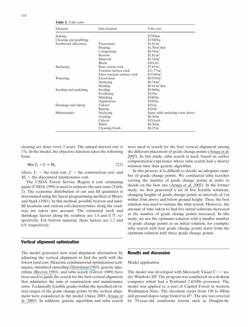
The USDA Forest Service Region 6 cost estimatingguide (USDA 1999) is used to estimate the unit costs (Table2). The economic distribution of cut and fill quantities isdetermined using the linear programming method of Mayerand Stark (1981). In this method, possible borrow and land-fill locations and various soil characteristics along the road-way are taken into account. The estimated swell andshrinkage factors along the roadway are 1.4 and 0.75, re-spectively. For borrow material, these factors are 1.2 and0.9, respectively.

Vertical alignment optimization

The model generates new road alignment alternatives byadjusting the vertical alignment to find the path with thelowest total cost. Heuristic combinatorial optimization tech-niques, simulated annealing (Dowsland 1993), genetic algo-rithms (Reeves 1993), and tabu search (Glover 1989) havebeen used to guide the search for the best vertical alignmentthat minimizes the sum of construction and maintenancecosts. Technically feasible grades within the specified eleva-tion ranges of the grade change points of the vertical align-ment were considered in the model (Akay 2003; Aruga etal. 2005). In addition, genetic algorithm and tabu search

were used to search for the best vertical alignment amongthe different placement of grade change points (Aruga et al.2005). In this study, tabu search is used, based on earliercomputational experience where tabu search had a shortersolution time than genetic algorithm.

In this process, it is difficult to decide an adequate num-ber of grade change points. We conducted tabu searchesvarying the number of grade change points in order todecide on the best one (Aruga et al. 2005). In the formerstudy, we first generated a set of five feasible solutions,changing heights of grade change points at intervals of 1mwithin 10m above and below ground height. Then, the bestsolution was used to initiate the tabu search. However, theamount of time taken to find five initial solutions increasedas the number of grade change points increased. In thisstudy, we use the optimum solution with a smaller numberof grade change points as an initial solution, for example,tabu search with four grade change points starts from theoptimum solution with three grade change points.

Results and discussion

Model application

The model was developed with Microsoft Visual C�� un-der Windows XP. The program was conducted on a desktopcomputer which had a Pentium4 2.4GHz processor. Themodel was applied to a part of Capitol Forest in westernWashington State. The elevation varies from 150 to 400mand ground slopes range from 0 to 45°. The site was coveredby 70-year-old coniferous forests such as Douglas-fir,

Table 2. Unit costs

Element Sub-element Unit cost

Staking $778/kmClearing and grubbing $3700/haEarthwork allocation Excavation $1.61/m3

Hauling $1.30/m3/kmCompacting $0.58/m3

Borrow $1.81/m3

Disposal $0.10/m3

Block $161/m2

Surfacing Base course rock $7.85/m3

Traction surface rock $11.77/m3

Finer traction surface rock $15.69/m3

Watering Excavation $0.078/m3

Surfacing $0.34/m3

Hauling $0.41/m3/kmSeeding and mulching Seeding $9.90/ha

Fertilizing $12/haMulching $240/haApplication $550/ha

Drainage and riprap Culvert $25/mRiprap $10/m3

Maintenance Surfacing Same with surfacing costs aboveGrading $0.30/mCulvert $15/eachDitch $0.20/mCleaning brush $0.25/m

119

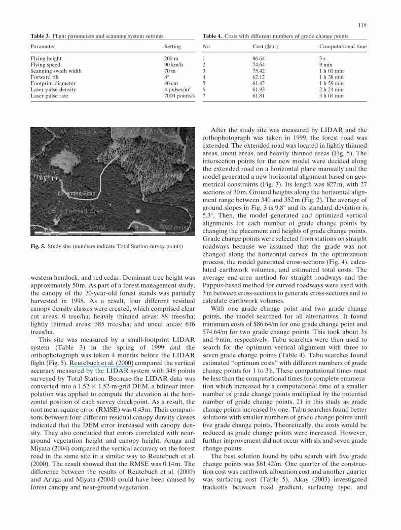
western hemlock, and red cedar. Dominant tree height wasapproximately 50m. As part of a forest management study,the canopy of the 70-year-old forest stands was partiallyharvested in 1998. As a result, four different residualcanopy density classes were created, which comprised clearcut areas: 0 tree/ha; heavily thinned areas: 88 trees/ha;lightly thinned areas: 385 trees/ha; and uncut areas: 616trees/ha.

This site was measured by a small-footprint LIDARsystem (Table 3) in the spring of 1999 and theorthophotograph was taken 4 months before the LIDARflight (Fig. 5). Reutebuch et al. (2000) compared the verticalaccuracy measured by the LIDAR system with 348 pointssurveyed by Total Station. Because the LIDAR data wasconverted into a 1.52 � 1.52-m-grid DEM, a bilinear inter-polation was applied to compute the elevation at the hori-zontal position of each survey checkpoint. As a result, theroot mean square error (RMSE) was 0.43m. Their compari-sons between four different residual canopy density classesindicated that the DEM error increased with canopy den-sity. They also concluded that errors correlated with near-ground vegetation height and canopy height. Aruga andMiyata (2004) compared the vertical accuracy on the forestroad in the same site in a similar way to Reutebuch et al.(2000). The result showed that the RMSE was 0.14m. Thedifference between the results of Reutebuch et al. (2000)and Aruga and Miyata (2004) could have been caused byforest canopy and near-ground vegetation.

After the study site was measured by LIDAR and theorthophotograph was taken in 1999, the forest road wasextended. The extended road was located in lightly thinnedareas, uncut areas, and heavily thinned areas (Fig. 5). Theintersection points for the new model were decided alongthe extended road on a horizontal plane manually and themodel generated a new horizontal alignment based on geo-metrical constraints (Fig. 3). Its length was 827m, with 27sections of 30m. Ground heights along the horizontal align-ment range between 340 and 352m (Fig. 2). The average ofground slopes in Fig. 3 is 9.8° and its standard deviation is5.3°. Then, the model generated and optimized verticalalignments for each number of grade change points bychanging the placement and heights of grade change points.Grade change points were selected from stations on straightroadways because we assumed that the grade was notchanged along the horizontal curves. In the optimizationprocess, the model generated cross-sections (Fig. 4), calcu-lated earthwork volumes, and estimated total costs. Theaverage end-area method for straight roadways and thePappus-based method for curved roadways were used with3m between cross-sections to generate cross-sections and tocalculate earthwork volumes.

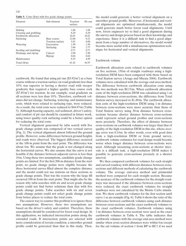
With one grade change point and two grade changepoints, the model searched for all alternatives. It foundminimum costs of $86.64/m for one grade change point and$74.64/m for two grade change points. This took about 3sand 9min, respectively. Tabu searches were then used tosearch for the optimum vertical alignment with three toseven grade change points (Table 4). Tabu searches foundestimated “optimum costs” with different numbers of gradechange points for 1 to 3h. These computational times mustbe less than the computational times for complete enumera-tion which increased by a computational time of a smallernumber of grade change points multiplied by the potentialnumber of grade change points, 21 in this study as gradechange points increased by one. Tabu searches found bettersolutions with smaller numbers of grade change points untilfive grade change points. Theoretically, the costs would bereduced as grade change points were increased. However,further improvement did not occur with six and seven gradechange points.

The best solution found by tabu search with five gradechange points was $61.42/m. One quarter of the construc-tion cost was earthwork allocation cost and another quarterwas surfacing cost (Table 5). Akay (2003) investigatedtradeoffs between road gradient, surfacing type, and

Table 3. Flight parameters and scanning system settings

Parameter Setting

Flying height 200 mFlying speed 90 km/hScanning swath width 70 mForward tilt 8°Footprint diameter 40 cmLaser pulse density 4 pulses/m2

Laser pulse rate 7000 points/s

Fig. 5. Study site (numbers indicate Total Station survey points)

Table 4. Costs with different numbers of grade change points

No. Cost ($/m) Computational time

1 86.64 3 s2 74.64 9 min3 75.42 1 h 01 min4 62.12 1 h 38 min5 61.42 1 h 59 min6 61.93 2 h 24 min7 61.81 3 h 01 min

120

earthwork. He found that using pit run ($3.92/m3) as a basecourse without a traction surface on road gradients less than10% was superior to having a shorter road with steepergradients that required a higher quality base course rock($7.85/m3) for traction. In our example, road gradients onall sections were less than 10%. Therefore, earthwork vol-umes did not change. Surfacing, watering, and maintenancecosts, which were related to surfacing type, were reduced.As a result, the total costs were reduced to $44.97/m (Table5). Although bearing capacity, soil sediment, driver’s safety,and comfort of pit run should be examined in future work,using lower quality rock surfacing could be a better optionfor reducing the total costs.

Vertical alignment generated by tabu search with fivegrade change points was composed of two vertical curves(Fig. 2). The vertical alignment almost followed the groundprofile. However, some differences between ground heightsand roads were observed. The biggest difference occurredat the 100-m point from the start point. The difference wasabout 4m. We assume that the grade is not changed alongthe horizontal curves. We also assume that the curve is notfeasible if the distance between adjacent curves is less than10m. Using these two assumptions, candidate grade changepoints are limited. For the first 200-m distance from the startpoint, no grade change points were eligible because thethree horizontal curves filled almost the complete distanceand the model could not use stations on these sections asgrade change points. That was the reason why the large filloccurred 100-m from the start point. That might also be thereason why tabu searches with six and seven grade changepoints could not find better solutions than that with fivegrade change points. Tabu searches with six and sevengrade change points could not select grade change pointsfrom better places to reduce the total costs.

The easiest way to counter this problem is to ignore thesetwo assumptions. However, these two assumptions arebased on the driver’s safety and comfort. Therefore, theseassumptions should be considered for forest road design. Inthis application, we indicated intersection points along theextended roads. If intersection points are selected withmore consideration of terrain condition, a smoother groundprofile could be generated than that in this study. Then,

the model could generate a better vertical alignment on asmoother ground profile. Moreover, if horizontal and verti-cal alignments are optimized simultaneously, the modelcould generate much better forest road alignments. Untilnow, forest engineers try to find a good alignment duringthe survey and design process based on their knowledge andexperience. Since it is a difficult task to find a good align-ment from a large number of alternatives, the model wouldbecome more useful with a simultaneous optimization tech-nique for horizontal and vertical alignments.

Earthwork volume

Earthwork allocation costs related to earthwork volumeson five sections, 150m of straight roadways using a high-resolution DEM have been compared with those based onTotal Station survey (Aruga and Miyata 2004). Earthworkvolumes were calculated with the average end-area method.The difference between earthwork allocation costs usingthe two methods was $0.13/m. When earthwork allocationcosts of the high-resolution DEM was calculated using 1-mdistance between cross-sections, the difference from TotalStation survey increased to $1.49/m. The earthwork alloca-tion costs of the high-resolution DEM using 1-m distancebetween cross-sections were more accurate than those ofTotal Station survey using 30-m distance between cross-sections because shorter distance between cross-sectionscould represent actual ground profiles and cross-sectionsmore precisely. Therefore, the effect of distance betweencross-sections on earthwork volumes was larger than that ofquality of the high-resolution DEM in this site, whose aver-age error was 0.14m. In other words, even with good datafrom a high-resolution DEM or from ground survey,earthwork volume estimates for road design would becomeworse when longer distance between cross-sections wereused. Although measuring cross-sections at shorter inter-vals is a difficult task, a high-resolution DEM makes itpossible to generate cross-sections precisely at a shorterinterval.

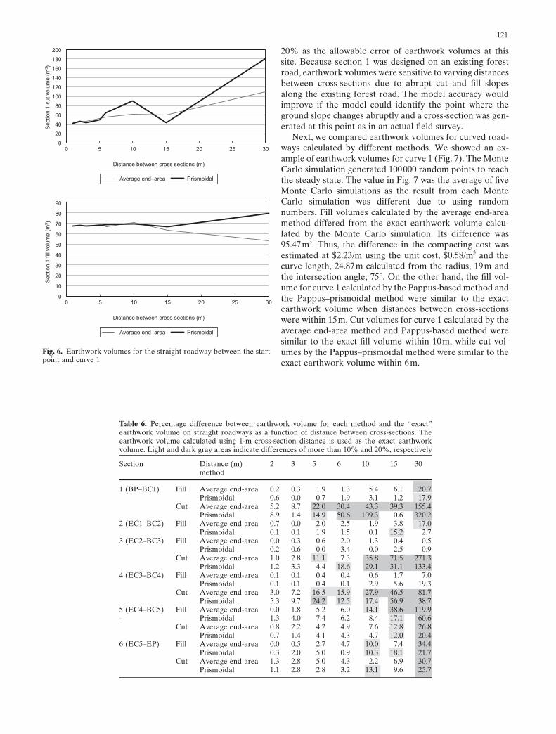
We then compared earthwork volumes for each straightand curved roadway with different distances between cross-sections and different methods of calculating the earthworkvolume. The average end-area method and prismoidalmethod were compared for each straight section. Becausethe accuracy of the earthwork volumes for the straight road-ways was increased if the distances between cross-sectionswere reduced, the exact earthwork volumes for straightroadways were not calculated by the Monte Carlo simula-tion. We show earthwork volumes for the first section untilcurve 1 as an example (Fig. 6). Table 6 shows the ratio of thedifference between earthwork volumes using each distancebetween cross-sections and the exact earthwork volumes tothe exact earthwork volumes. Earthwork volumes using1-m distance between cross-sections were used as the exactearthwork volumes in Table 6. The table indicates thatearthwork volumes with the average end-area method weresimilar when cross-section distances were within 6m exceptfor the cut volume of section 1 from BP to BC1 if we used

Table 5. Costs ($/m) with five grade change points

Element Sub-element Traction Pit runsurface

Staking 1.06 1.06Clearing and grubbing 8.29 8.29Earthwork allocation 16.01 16.01Surfacing Base course 12.60 6.21

Traction surface 5.81 0.00Watering Excavation 1.99 1.99

Surfacing 3.66 2.77Seeding and mulching 0.71 0.71Drainage and riprap Culvert 2.90 2.90

Riprap 0.04 0.04Maintenance 8.35 4.99

Total ($/m) 61.42 44.97

121

20% as the allowable error of earthwork volumes at thissite. Because section 1 was designed on an existing forestroad, earthwork volumes were sensitive to varying distancesbetween cross-sections due to abrupt cut and fill slopesalong the existing forest road. The model accuracy wouldimprove if the model could identify the point where theground slope changes abruptly and a cross-section was gen-erated at this point as in an actual field survey.

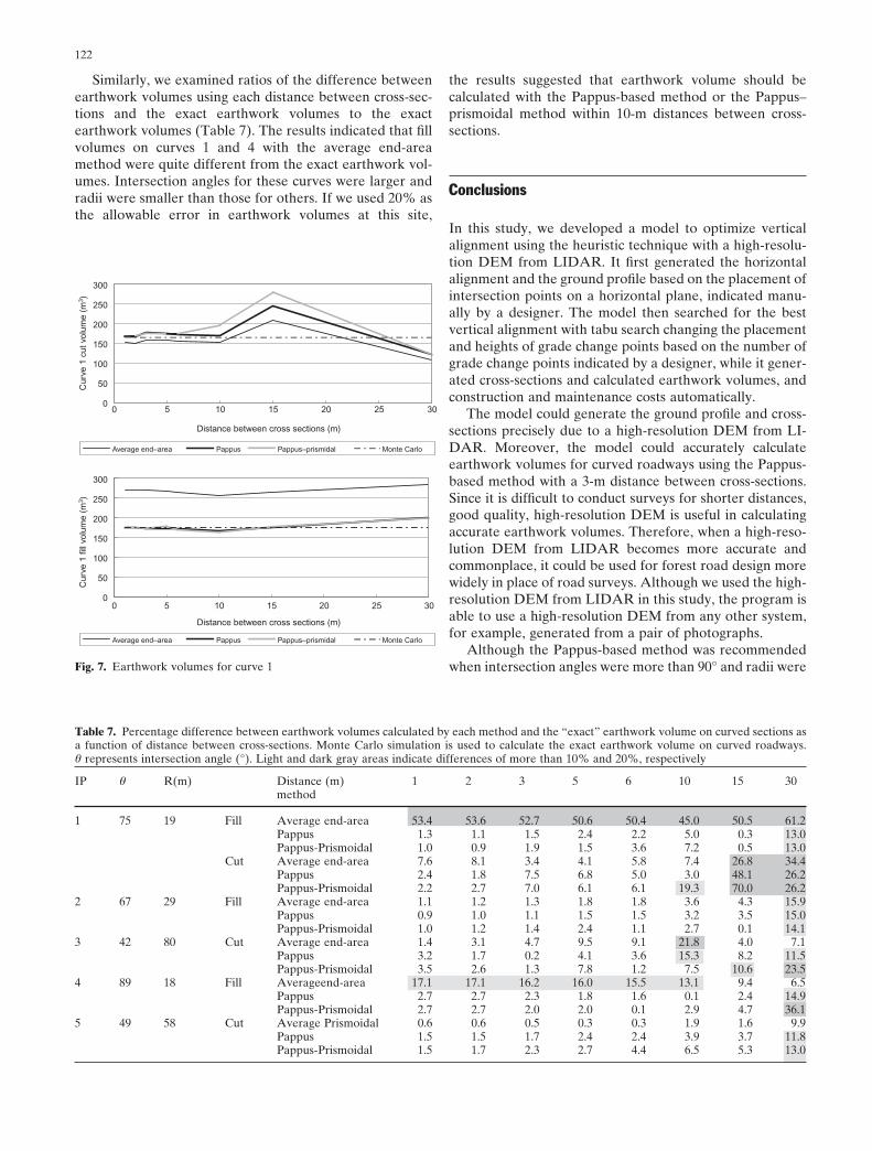
Next, we compared earthwork volumes for curved road-ways calculated by different methods. We showed an ex-ample of earthwork volumes for curve 1 (Fig. 7). The MonteCarlo simulation generated 100000 random points to reachthe steady state. The value in Fig. 7 was the average of fiveMonte Carlo simulations as the result from each MonteCarlo simulation was different due to using randomnumbers. Fill volumes calculated by the average end-areamethod differed from the exact earthwork volume calcu-lated by the Monte Carlo simulation. Its difference was95.47m3. Thus, the difference in the compacting cost wasestimated at $2.23/m using the unit cost, $0.58/m3 and thecurve length, 24.87m calculated from the radius, 19m andthe intersection angle, 75°. On the other hand, the fill vol-ume for curve 1 calculated by the Pappus-based method andthe Pappus–prismoidal method were similar to the exactearthwork volume when distances between cross-sectionswere within 15m. Cut volumes for curve 1 calculated by theaverage end-area method and Pappus-based method weresimilar to the exact fill volume within 10m, while cut vol-umes by the Pappus–prismoidal method were similar to theexact earthwork volume within 6m.

Distance between cross sections (m)

200

180

160

Sec

tion

1 cu

t vol

ume

(m3 )

140

120

100

80

60

40

20

00 5 10 30252015

0 5 10 30252015

90

80

70

Sec

tion

1 fil

l vol

ume

(m3 )

60

50

40

30

20

10

0

Average end–area Prismoidal

Distance between cross sections (m)

Average end–area Prismoidal

Fig. 6. Earthwork volumes for the straight roadway between the startpoint and curve 1

Table 6. Percentage difference between earthwork volume for each method and the “exact”earthwork volume on straight roadways as a function of distance between cross-sections. Theearthwork volume calculated using 1-m cross-section distance is used as the exact earthworkvolume. Light and dark gray areas indicate differences of more than 10% and 20%, respectively

Section Distance (m) 2 3 5 6 10 15 30method

1 (BP–BC1) Fill Average end-area 0.2 0.3 1.9 1.3 5.4 6.1 20.7Prismoidal 0.6 0.0 0.7 1.9 3.1 1.2 17.9

Cut Average end-area 5.2 8.7 22.0 30.4 43.3 39.3 155.4Prismoidal 8.9 1.4 14.9 50.6 109.3 0.6 320.2

2 (EC1–BC2) Fill Average end-area 0.7 0.0 2.0 2.5 1.9 3.8 17.0Prismoidal 0.1 0.1 1.9 1.5 0.1 15.2 2.7

3 (EC2–BC3) Fill Average end-area 0.0 0.3 0.6 2.0 1.3 0.4 0.5Prismoidal 0.2 0.6 0.0 3.4 0.0 2.5 0.9

Cut Average end-area 1.0 2.8 11.1 7.3 35.8 71.5 271.3Prismoidal 1.2 3.3 4.4 18.6 29.1 31.1 133.4

4 (EC3–BC4) Fill Average end-area 0.1 0.1 0.4 0.4 0.6 1.7 7.0Prismoidal 0.1 0.1 0.4 0.1 2.9 5.6 19.3

Cut Average end-area 3.0 7.2 16.5 15.9 27.9 46.5 81.7Prismoidal 5.3 9.7 24.2 12.5 17.4 56.9 38.7

5 (EC4–BC5) Fill Average end-area 0.0 1.8 5.2 6.0 14.1 38.6 119.9- Prismoidal 1.3 4.0 7.4 6.2 8.4 17.1 60.6

Cut Average end-area 0.8 2.2 4.2 4.9 7.6 12.8 26.8Prismoidal 0.7 1.4 4.1 4.3 4.7 12.0 20.4

6 (EC5–EP) Fill Average end-area 0.0 0.5 2.7 4.7 10.0 7.4 34.4Prismoidal 0.3 2.0 5.0 0.9 10.3 18.1 21.7

Cut Average end-area 1.3 2.8 5.0 4.3 2.2 6.9 30.7Prismoidal 1.1 2.8 2.8 3.2 13.1 9.6 25.7

122

the results suggested that earthwork volume should becalculated with the Pappus-based method or the Pappus–prismoidal method within 10-m distances between cross-sections.

Conclusions

In this study, we developed a model to optimize verticalalignment using the heuristic technique with a high-resolu-tion DEM from LIDAR. It first generated the horizontalalignment and the ground profile based on the placement ofintersection points on a horizontal plane, indicated manu-ally by a designer. The model then searched for the bestvertical alignment with tabu search changing the placementand heights of grade change points based on the number ofgrade change points indicated by a designer, while it gener-ated cross-sections and calculated earthwork volumes, andconstruction and maintenance costs automatically.

The model could generate the ground profile and cross-sections precisely due to a high-resolution DEM from LI-DAR. Moreover, the model could accurately calculateearthwork volumes for curved roadways using the Pappus-based method with a 3-m distance between cross-sections.Since it is difficult to conduct surveys for shorter distances,good quality, high-resolution DEM is useful in calculatingaccurate earthwork volumes. Therefore, when a high-reso-lution DEM from LIDAR becomes more accurate andcommonplace, it could be used for forest road design morewidely in place of road surveys. Although we used the high-resolution DEM from LIDAR in this study, the program isable to use a high-resolution DEM from any other system,for example, generated from a pair of photographs.

Although the Pappus-based method was recommendedwhen intersection angles were more than 90° and radii were

Distance between cross sections (m)

Distance between cross sections (m)

Pappus–prismidalAverage end–area Pappus

300

Cur

ve 1

cut

vol

ume

(m3 )

Cur

ve 1

fill

volu

me

(m3 )

250

200

150

100

50

0

300

250

200

150

100

50

0

Monte Carlo

Pappus–prismidalAverage end–area Pappus Monte Carlo

0 5 10 30252015

0 5 10 30252015

Similarly, we examined ratios of the difference betweenearthwork volumes using each distance between cross-sec-tions and the exact earthwork volumes to the exactearthwork volumes (Table 7). The results indicated that fillvolumes on curves 1 and 4 with the average end-areamethod were quite different from the exact earthwork vol-umes. Intersection angles for these curves were larger andradii were smaller than those for others. If we used 20% asthe allowable error in earthwork volumes at this site,

Table 7. Percentage difference between earthwork volumes calculated by each method and the “exact” earthwork volume on curved sections asa function of distance between cross-sections. Monte Carlo simulation is used to calculate the exact earthwork volume on curved roadways.θ represents intersection angle (°). Light and dark gray areas indicate differences of more than 10% and 20%, respectively

IP θ R(m) Distance (m) 1 2 3 5 6 10 15 30method

1 75 19 Fill Average end-area 53.4 53.6 52.7 50.6 50.4 45.0 50.5 61.2Pappus 1.3 1.1 1.5 2.4 2.2 5.0 0.3 13.0Pappus-Prismoidal 1.0 0.9 1.9 1.5 3.6 7.2 0.5 13.0

Cut Average end-area 7.6 8.1 3.4 4.1 5.8 7.4 26.8 34.4Pappus 2.4 1.8 7.5 6.8 5.0 3.0 48.1 26.2Pappus-Prismoidal 2.2 2.7 7.0 6.1 6.1 19.3 70.0 26.2

2 67 29 Fill Average end-area 1.1 1.2 1.3 1.8 1.8 3.6 4.3 15.9Pappus 0.9 1.0 1.1 1.5 1.5 3.2 3.5 15.0Pappus-Prismoidal 1.0 1.2 1.4 2.4 1.1 2.7 0.1 14.1

3 42 80 Cut Average end-area 1.4 3.1 4.7 9.5 9.1 21.8 4.0 7.1Pappus 3.2 1.7 0.2 4.1 3.6 15.3 8.2 11.5Pappus-Prismoidal 3.5 2.6 1.3 7.8 1.2 7.5 10.6 23.5

4 89 18 Fill Averageend-area 17.1 17.1 16.2 16.0 15.5 13.1 9.4 6.5Pappus 2.7 2.7 2.3 1.8 1.6 0.1 2.4 14.9Pappus-Prismoidal 2.7 2.7 2.0 2.0 0.1 2.9 4.7 36.1

5 49 58 Cut Average Prismoidal 0.6 0.6 0.5 0.3 0.3 1.9 1.6 9.9Pappus 1.5 1.5 1.7 2.4 2.4 3.9 3.7 11.8Pappus-Prismoidal 1.5 1.7 2.3 2.7 4.4 6.5 5.3 13.0

Fig. 7. Earthwork volumes for curve 1

123

less than 20m (Japan Forest Road Association 2003), itmight be necessary to use Pappus-based method at smallerintersection angles and larger radii than the recommendedvalues. The distance between cross-sections was 3m in thisstudy. Shorter distances result in more accurate earthworkvolumes, but longer computational times. Since allowableerrors and the distance to calculate earthwork volume accu-rately may differ from site to site, a designer should exam-ine the distance by comparing the exact volume calculatedby the Monte Carlo simulation. Although the Monte Carlosimulation was not combined with the model because of itslonger computation time, it could be useful to calculate acomplex area or volume.

The model was applied to a high-resolution DEM fromLIDAR at Capitol Forest in Washington State, USA. Tabusearch found the best solution with five grade change points,$61.42/m. During the application, we found several limita-tions of the current program. One was that tabu searcheswith six and seven grade change points could not find bettersolutions than that with five grade change points. Anotherwas that some large differences between ground and roadheights were observed. Since those limitations are coun-tered by optimizing horizontal and vertical alignments si-multaneously, we would improve the model by including anew feature that finds the best horizontal and vertical align-ment automatically.

Acknowledgments LIDAR data were provided by the USDA ForestService, PNW Research Station, Resource Management and Produc-tivity Program. Orthophotograph is courtesy of the Washington StateDepartment of Natural Resources, Resource Mapping Section. Weexpress our thanks to USDA Forest Services researchers, Mr. SteveReutebuch, Mr. Robert McGaughey, Dr. Ward Carson, and Universityof Washington Professor Edwin Miyata who provided LIDAR data,helped to handle LIDAR data, and guided the site. We also express ourbest regards to Washington State Department of Natural Resourceswho provided the orthophotograph and let us use the site.

Literature cited

AASHTO (1994) A policy on geometric design of highways andstreets. American Association of State Highway and TransportationOfficials, Washington, DC

Akay AE (2003) Minimizing total cost of construction, maintenance,and transportation costs with computer-aided forest road design.PhD thesis, Oregon State University, Corvallis, OR

Aruga K, Miyata ES (2004) Application of airborne laser scanner toforest road survey (in Japanese). J Jpn For Eng 19:49–54

Aruga K, Sessions J, Akay AE (2005) Heuristic planning techniquesapplied to forest road profiles. J For Res 10:83–92

Cain C, Langdon JA (1982) AE guide for determining minimum roadwidth on curves for single-lane forest roads. Engineering field notes,vol 14, USDA Forest Service, Washington, DC

Chung W, Sessions J, Heinimann HR (2004) An application of a heu-ristic network algorithm to cable logging layout design. J For Eng15:11–24

Coulter ED, Chung W, Akay AE, Sessions J (2002) Forest roadearthwork calculations for linear road segments using a highresolution digital terrain model generated from LIDAR data. In:Proceedings of the first international precision forestry symposium.University of Washington College of Forest Resources, Seattle, WA,USA, pp 125–129

Dowsland KA (1993) Simulated annealing. In: Reeves C (ed) Modernheuristic techniques for combinatorial problems. Wiley, New York,pp 20–69

Easa SM (1992a) Modified prismoidal method for nonlinear groundprofiles. J Survey Land Inform Syst 52:13–19

Easa SM (1992b) Estimating earthwork volumes of curved roadways:mathematical model. J Transport Eng 118:834–849

Easa SM (2003) Estimating earthwork volumes of curved roadways:simulation model. J Survey Eng 129:19–27

Glover F (1989) Tabu search: part I. ORSA J Comput 1:190–206Japan Forest Road Association (2003) Forest road handbook (in

Japanese). Japan Forest Road Association, TokyoKato S (1951) Forestry civil engineering (in Japanese). Sangyotosho,

TokyoMannering FL (1990) Principles of highway engineering and traffic

analysis. Wiley, New YorkMayer R, Stark R (1981) Earthmoving logistics. ASCE J Const Div

107(CO2):297–312Reeves C (1993) Genetic algorithms. In: Reeves C (ed) Modern heuris-

tic techniques for combinatorial problems. Wiley, New York, pp151–196

Reutebuch SE, Ahmed KM, Curtis TA, Petermann D, Wellander M,Froslie M (2000) A test of airborne laser mapping under varyingforest canopy. In: Proceedings of the ASPRS national convention,Washington, DC

USDA Forest Service (1987) Road preconstruction handbook. Forestservice handbook No. 7700.56

USDA Forest Service (1999) Cost estimating guide for road construc-tion, region 6. USDA, Portland, OR, USA