


sustainability and new digital trends for heavy haul - UIC ...
Upload
khangminh22Category
view
3download
0

EARTHW ORK HAUL AND
OVERHAUL
INCLUDING
ECONOMIC DISTRIBUT ION
J. C . Le FISH
Member American Society ofCivil Engineers; Member American RailwayEngineering Association; Sometime, DivisionEngineer, LakeShore
and Michigan Southern Railway; Professor ofRailroadEngineering , Leland Stanford JuniorWuivem
'
ty .
F I R S T E D I T I ON
FIRST THOUSAND
NEW Y ORK
JOHN W ILEY a: SONS
LONDON : CHAPMAN HALL, LIMITED1 9 13S


PREFACE
THIS b ook presents answers to all questions on computation
of overhaul and on theuse of them ass curve in planning dis
tribution,which have arisen during an experience covering a
wide range of conditions .
Part I is planned to servefive classes of men : railroad engi
neers, railroad contractors,computers, students, and teachers .
Engineers responsible for overhaul computation may beaidedin selecting a method of computation by reading Sections 47 55 ,146 and 203 ; and can obtain uniform results by merely direct
ing their subordinates to follow theinstructions given in Chapter
VI or Chapter VII for the selected method.
Computers , having been directed to use a given method of
computing overhaul , will find in either Chapter VI or ChapterVII a comp leteplan of procedureunder themethod.
Railroad contractors about to subm it bids on work involvingoverhaul
,will find the descriptions of bases and methods of
computation of overhaul , given in Chapters V ,VI
,and VII, a
ready means of com ing to a definite understanding with rail
road engineers as to the way in which the overhaul is to be
computed.
Students of overhaul , in school or out , will find in ChaptersI—V a full presentation of each of the elements of overhaul
computation . The beginner is advised to proceed at once to
compute theoverhaul for some simplecase sim ilar to that shown
in Fig . 1 9 , by Method IV (Sections 89 studying the refer
emees under each step no more than may benecessary to execute
the step intelligently . A working knowledge of the essentials
and routine of onemethod thus acquired furnishes the groundwork necessary for the most profitable study of other portions
of the book .

iv PREFACE
Men called upon from time to time,in class - room or offi ce
,
to give instruction in overhaul computation ,will find Part I a
treatise from which portions can be selected to fulfi ll require
ments for a course short or long according to the timeavailable
for the subject . The fact that the writer is entitled to fullmembership in this class may be taken as a guaranty that the
teacher ’s interests have not been overlooked herein .
Part II is devoted to theelements of theproblem of economic
distribution,and presents a thorough treatment of the solution
o f this problem by theuse of them ass curve.
The attention of thosewho are familiar with thep reviously
p rinted m atter bearing on haul and overhaul is directed to
Sections 2—9 (swell and distribution) ; 1 5
—19 (concerning the
:mass curve) ; 43 , 44 (crosshaul) Chapter VI (data and solution
o f a simple overhaul problem ,by each of eight methods) ; Chap
ter VII (data and solution of complex overhaul problem from
practice, by each of fivemethods) ; Fig . 36 (statement of over
h aul computed by various methods) ; and nearly all of Part II.
Thewriter’
s indebtedness to the published matter on over
h aul , especially to the Proceedings,1906 , of the American
Railway Engineering Association,will be apparent to thewell
informed. The drawings , with one or two exceptions , have
b een prepared by Messrs . N . M . Halcombe and A . C . Sand
strom ,at present studying civ il engineering in Stanford Uni
versity . Mr . Sandstrom has taken a lively interest in the text
as well ; and his criticism s and suggestions at m any points have
caused desirable changes in and additions to the original manu
script .
The writer will be glad to receive suggestions for the im
provement of any part of the book , from those to whom it does
no t proveentirely satisfactory .
J. C . L . FISH.
STANFORD UNIVERSITY,CALIFORNIA
May 20, 19 1 2 .
TA BLE OF CONTENTS
PART I
HAUL AND OVERHAUL
CHAPTER I
CONSIDERATIONS PRELIMINARY To THE COMPUTATION or HAUL
This chapter shows the necessity of adopting an ideal distribution,instead of
the actual, as a basis of computing haul or overhaul ; that , under some common
conditions, any prediction of swell of material must be subject to considerableuncertainty ; and gives a method for determining them ost reasonableswell- factorsin thosecases wherefield measurements for exact determination areno t available.
PAGEHaul definedDistribution ofmaterial
, actual and assumed; simplecase
Distribution ofmaterial,actual and assumed ; complex case
Swell and shrinkage.
Swell of two ormorematerials depends upon the thoroughness ofm ixing
Swell increment ; swell ratio ; swell- factorEquating - factor
Determination of swell- factor ; simple case.
Determination of swell- factor ; complex case
CHAPTER II
THE MASS CURVE
This chapter sets forth the principles of construction and interpretation of the
mass curve; describes thehorizontal and theobliquebalancing line; and discussestheeffect of drafting
- errors on results obtained from themass curve.
IO .
I I .
1 2 .
1 3 .
Construction ofmass curveor prOfileof quantitiesCharacteristics of themass curve.
Thehorizontal balancing line.
Theob liquebalancing line

TABLE OF CONTENTS
PAGE
Relation between haul and mass- curve area when the mass curveplo tted from cut - vo lumes and equated fill—vo lumes
Relation between haul and mass—curve area when the mass curveplo tted from fill- volumes and equated cut—volumes
Lim it oferror in a distanceplo t ted o r sealed
Lim it oferror in area dueto errors in distance
Scale of ordinates for themass curvePlotting themass curve
CHAPTER III
LIMITS AND CENTER OF MASS OF A BODY OF MATERIAL
This chap ter describes how ,b y eye, by arithmetic , and by mass curve, to de
t erminethelim its of a body ofmaterial in cut or in fill from given conditions ; and
how to determine the center of volume or mass of such body . (Figs. 19 , 2 1 , 2 1a,
and 24 facep .
20 .
2 I .
2 2 .
23 .
PAGELim it of a fill made from a given body of cut : arithmetical solution ;
mass—curve solut ion ; so lution by inspection
Center ofmass of a singleprismo id
Center of mass of a series of prismoids . Arithmetical solution
Center ofmass of a series ofprism oids . Mass—curveso lution
CHAPTER IV
CENTER OF GRAVITY'In this chapter are described eight methods (so - called) of finding the center of
gravity of a body ofmaterial,ranging from theroughly approximate to thepracti
cally exact , and using the eye, arithmetic, or the mass curve. All themethods
are applied to the sameproblem ,namely ,
finding the center of gravity of the cut
between 9 co and 1 2 28 of Fig . 1 9 (facing p .
Relation between center of gravity and haulCenter of gravity of a singleprismoid .
Center of gravity of a series ofprismoids .
Method I. Center of gravity determined by eyeMethod II. Center ofgravity assumed to lieat themid—pointMethod III. Series ofprismoids treated as a singleprismoid
Method IV . Center of gravity assumed to lie at the center of mass .
Arithmetical solution .
Method V . Center of gravity assumed to lie at the center of mass.
Mass- curve solution .
Method VI. Center of gravity of each prismoid assumed to lie at its
mid-
point . Arithmetical solut ion .

0 .
TABLE OF CONTENTS Vll
PAGE33 . Useeither measured or equated fill- vo lumes in computing by moments
(MethodsVIand VIII, Secs. 3 2 and 3 5 ) thestation ofcenter ofgrav ityof series offil l prismoids.
34. Method VII. Center of gravity ofeach prismoid assumed to lieat its
mid-
point . Mass- curve solution .
3 5 . MethodVIII. Thetruecenter ofgravity
CHAPTER V
OVERHAUL,FREE HAUL
,AND CROSSHAUL
In this chapter overhaul is defined ; a digest of American practicein computing
overhaul is given ; the American Railway Engineering Asso ciation’s Specification,
which is used as the basis for all the problem s worked in this book, is presented ;and threemethods by eye, by arithmetic
,and by mass curve of determining
free- haul limits are explained. Crosshaul is discussed; and eight methods of
computing overhaul are characterized. (Fig . 19 faces p . 96 ; Fig . 36, p . 67 ; Fig .
38 , p.
Definitions
Basis o f overhaul computation: review of current practice in America .
American Railway Engineering Association basis of computing overhaulInterpretation of bases (A) and (B) of Section 3 7Free- haul limits : arithmetical solution
Free- haul lim its : mass- curve so lution .
Free- haul lim its : by eye
Crosshaul and its effect on to tal haulCrosshaul within free—haul limits : its efiect on overhaulLimit oferror in to tal cost ofoverhaul dueto error in computed position
of center of gravity .
Statement of overhaul .
Methods of computing overhaulMethod I
Method II
Method III
Method IV
Method V
Method VI
Method VII
Method VIII
CHAPTER VI
OVERHAUL COMPUTED FOR THE SIMPLE CASE or FIG . 19
In this chapter theoverhaul ofFig . 1 9 is computed by each of theeight methods
of computing overhaul , the work under each method being laid out in formal
steps and in detail. Theresults arepresented in Fig. 36 on thelines which begin

viii TABLE OF CONTENTS
with A . Finally the results are compared in Section 146 . This chapter is
intended to serve thecomputer of overhaul as a guide in his computations. The
following chapter is Similar to this, but the problem there solved is complex .
(Fig. 1 9 faces p . 96 ; Fig . 36 faces p .
56 . Preliminary remarks .
Overhaul in Fig. 19 computed by Method I
(In Method I center ofgravity and all limits aredetermined by eye.)
5 7 . Step 1 . Data .
58 . Step 2 . Distribution ofmaterial .
59 . Step 3 . Swell- factor and equating - factor .
60. Step 4. Limits of bodies ofmaterial6 1 . Step 5 . Lim its of freehaul .
6 2 . Step 6 . Centers of gravity .
63 . Step 7 . Averagehaul- distance.
64. Step 8 . Averageoverhaul-distance65 . Step 9 . Theoverhaul66 . Step 10 . Statement of overhaul .
Overhaul in Fig. 19 computed by Method II
(InMethod II center ofgravity of body of cut or fill is assumed to lieat center
of length . Limits are computed by arithmetic.)
6 7 . Step 1 . Data
68 . Step 2 . Distribution ofmaterial
69 . Step 3 . Swell and equating - factors
70. Step 4 . Equateeach station—volume of fill to volume in place7 1 . Step 5 . Lim its of bodies ofmaterial7 2 . Step 6 . Limits of freehaul .
73 . Step 7 . Centers of gravity .
74. Step 8 . Averagehaul- distance.
75 . Step 9 . Averageoverhaul—distance76 . Step 1 0 . Theoverhaul7 7 . Step 1 1 . Statement of overhaul
Overhaul in Fig. 19 computed by Method III
(In Method III center of gravity of body of cut or fill is determined by com
puting its distance from center of length . Limits are computed b y arithmetic .)PAGE
78 . Step 1 . Data . 76
79 . Step 2 . Distribution ofmaterial 77
80 . Step 3 . Swell and equating—factors . 77
8 1 . Step 4 . Equateeach station- volumeof fill to volume in place 7 7
82 . Step 5 . Limits of bodies ofmaterial 77

83 .
84 .
85 .
86 .
8 7 .
88 .
Step
Step
Step
Step
Step 10 .
Step 1 1 .
\O
OO
\IO\
TABLE OF CONTENTS ix
Limits of freehaul
Centers of gravity .
Averagehaul- distanceAverage overhaul -distance
TheoverhaulStatement of overhaul .
Overhaul in Fig. 19 computed by Method IV
(InMethod IV center of gravity of cut or fill is assumed to lieat its center of
vo lume, and is computed by arithmetic. Limits are computed by arithmetic. )
Data
Distribut ion ofmaterialSwell and equating—fac torsEquateeach station- vo lumeof fill to vo lume in placeLimits of bodies ofmaterialLimits of freehaul .
Centers of gravity .
Averagehaul- distanceAverageoverhaul-distanceTheoverhaulStatement of overhaul .
Overhaul in Fig. 19 computed by Method V
(In Method V center of gravity of body of cut or fill is assumed to lie at its
center of volume,and is determined by mass curve. Limits are determined by
mass curve.)
Data
Distribution ofmaterial
Swell and equating- factors
Equateeach station- vo lumeof fill to volume in placePlo t themass curve.
Limits of bodies ofmaterialLim its of free haulCenters of gravityAveragehaul—distanceAverage overhaul- distanceTheoverhaulStatement of overhaul .
Overhaul of Fig. 1 9 computed by Method VI
(In Method VI the center of gravity of a body of cut or fill is computed, arith
metically , by themethod of moments ; thecenter ofgrav ity ofeach station- volum e

X TABLE OF CONTENTS
b eing assumed to lie at its center of length . The limits are computed by arith
metic .)
1 1 2 . Step I
1 13 . Step 2
1 14 . Step 3
1 15 . Step 4
1 16 . Step 5 .
1 1 7 . Step 6
1 18 . Step 7
1 19 . Step 8
1 20 . Step 9
1 2 1 . Step 1 0
1 2 2 . Step I I
Data .
Distribution ofmaterial
Swell and equating—factorsEquateeach station- volumeof fill to vo lumein placeLimits of bodies ofmaterialLimits of freehaul .
Centers of gravity .
Averagehaul-distance.
Averageoverhaul- distanceTheoverhaul
Overhaul of F ig. 1 9 computed by Method VII
(In Method VII the center o f gravity of each body of cut or fill is computed,
b y means of the mass curve, by the method of moments. All limits aredeter
mined by them ass curve.)
Data
Distribution ofmaterial
Swell and equating- factors .
Equateeach station- volumeof fill vo lumePlot themass curveLimits of bodies ofmaterialLimits of freehaul .
Centers of gravity .
Averagehaul—distanceAverageoverhaul—distanceTheoverhaulStatement of overhaul
Overhaul of Fig. 19 computed by Method V] II
(InMethod VI I I thecenter of gravity of each cut or fill is found by themethod
o f moments, using arithmetic,the center of grav ity of each station- vo lume being
found by computing its distance from the center of length . All limits are com
puted by arithm etic .)
1 35 .
1 36 .
1 3 7 .
1 38 .
1 39 .
1 40 .
Step
Step
Step
Step
Step
Step ON
UI
A
CN
N
H Data
Distribution ofmaterialSwell and equating - factors
Equateeach station- volumeof fill to volumein placeLim its of bodies ofmaterial .
Limits of freehaul
TABLE OF CONTENTS X1
PAGE1 41 . Step 7 . Centers of gravity .
142 . Step 8 . Averagehaul- distance1 43 . Step 9 . Averageoverhaul - distance
144 . Step 10 . The overhaul1 45 . Step 1 1 . Statement of overhaul .
Comparison ofMethods and Results
1 46 . The foregoing results compared
CHAPTER VII
OVERHAUL COMPUTED FOR THE COMPLEX CASE or FIG. 38
In this chapter Methods I, IV ,V
,VI
,and VII of overhaul computation are
applied ,one after ano ther
,to thecomplex problem of Fig . 3 8 . The steps in each
”method are formally stated. The results are presented in Fig . 36 on the lines
b eginning with“B
,and compared in Section 203 . This chapter, like the pre
ceding , aim s to serveas a working guide to the computer. (Fig . 36 faces p. 67 ;
Figs. 36a, 3 7 , and 38 facep .
1 47 . Preliminary
Overhaul of Fig. 38 computed by Method I
(InMethod I center of gravity and all limits aredetermined by eye.)
1 48 . Step 1 . Data .
1 49 . Step 2 . Distribution ofmaterial
1 50 . Step 3 . Free—haul lim its and o ther limits of bodies ofmaterial1 5 1 . Step 4 . Centers of gravity .
1 5 2 . Step 5 . Averagehaul-distance1 53 . Step 6 . Average overhaul-distance1 54 . Step 7 . Vo lumes of bodies of overhauled material1 5 5 . Step 8 . Theoverhaul1 56 . Step 9 . Statement of overhaul
Overhaul of Fig. 38 computed by Method IV
(In Method IV center of gravity of cut or fill is assumed to lieat its center of
vo lume,and is computed by arithmflic. Limits are computed by arithmetic
Data
Distribution ofmaterial .
Determination of swell- factors and of thevolumes of theseveral bodies of cut and fill .
Lim its of bodies ofmaterial .
Equateeach station- volumeof fill to volume in placeLimits of freehaul .

1 63 .
1 64 .
1 65 .
1 66 .
1 67 .
Step 7 .
Step 8 .
Step 9 .
Step 10 .
Step 1 1 .
TABLE OF CONTENTS
Centers ofgravity .
Averagehaul—distancesAverageoverhaul- distancesTheoverhaulStatement of overhaul .
Overhaul of Fig. 38 computed by Method V
(In Method V center of gravity of body of cut or fill is assumed to lieat its:
center of volume, and is determined by mass curve. Limits are determined by
mass curve.)
Data .
Distribution ofmaterial
Determination of swell—factors and of the volumes of the
several bodies of cut and fillEquateeach station—vo lumeof fill to volume in placePlo t themass curve.
Limits of bodies ofmaterialLimits of freehaul
Centers of gravity .
Averagehaul- distancesAverageoverhaul—distancesThe overhaulStatement of overhaul
Overhaul of F ig. 38 computed by Method VI
(In Method VI thecenter of gravity of a body of cut or fill is computed, arith
metically ,by themethod of moments
,thecenter of gravity of each station- volume
being assumed to lie at its center of length . The limits are computed by arith
metic.)
180.
1 8 1 .
182 .
183 .
184 .
1 85 .
1 86 .
187 .
188 .
189.
190.
Step 1 .
Step 2 .
Step
StepStep
Step
Step
Step
Step
Step 10.
Step 1 1 .
O
N
Q
Q
UI
-h
Data
Distribution ofmaterial3 . Determination of swell - factors and of volumes of the several
bodies of cut and fillLimits of bodies ofmaterialEquateeach station - volumeoffill to volumein placeLimits of freehaulCenters ofgrav ity
Averagehaul-distancesAverageoverhaul-distancesTheoverhaulStatement of overhaul .

TABLE OF CONTENTS xiii
Overhaul of Fig. 38 computed by Method VII
(InMethod VII the center of gravity of each body of cut or fill , is computed,
b y means of themass curve, by themethod of moments. All limits are deter
mined by themass curve.)
Step 1 .
Step 2 . Distribution ofmaterialStep 3 . Determination of swell- factors and of volumes of the several
cuts and fills
Step 4. Equateeach station—vo lumeoffill to volumein placeStep 5 . Plo t themass curveStep 6 . Limits of bodies ofmaterialStep 7 . Limits of freehaul
Step 8 . Centers of gravityStep 9 . Averagehaul-distancesStep 1 0. Averageoverhaul—distancesStep 1 1 . TheoverhaulStep 1 2 . Statement of overhaul
Comparison ofMethods and Results.
The foregoing results compared
PART II
ECONOMIC DISTRIBUTION OF MATERIAL ALONG THE PROFILE
CHAPTER VIII
PRELIMINARY CONSIDERATIONSThis chapter discusses the
fi
efiect of swell on planning distribution, and limit ofprofitable haul ; and states theprinciple of economic distribution.
204 . Swell- factor. Problems of past and futurehaul compared
.2o5 . Cut - volumes must beequated to fill- volumes206 . Limiting distancewhen thereis no freehaul207 . Limiting distancewhen there is freehaul
208. Principleof economic distribution
CHAPTER IX
ECONOMIC BALANCING LINE FOR MASS CURVE PLOTTED FROM CUT- VOLUMES ANDEQ UATED FILL- VOLUMES
,OR FROM CUT- VOLUMES AND FILL- VOLum s
WHEN SWELL- FACTOR IS UNITYThis chapter discusses the application of theprinciple of economic distribution
to each of several typical forms of mass curve, progressing from the simple to thecomplex. All themass curves of this chapter areassumed to beplotted from pay

xiv TABLE OF CONTENTS
yards , that is, from yards in place. All themass curves of the following chapter
are assumed to be plo tted from yards of swelled material. Otherwise the two
chapters are similar. (Figs. 50—603. face p .
Note
Economic balancing linefor simple loopEconom ic balancing linefor corrugated loopEconom ic balancing linefor two long loops separated by a short loop .
Economic balancing linefor mass curvewith onesag and onehump .
Economic continuous balancing line for mass curvewith two sags and
two humps
Continuous balancing linev s. broken balancmg lineWhen thebaseline15 theeconomic balancing lineExamples Ofeconom ic balancing lines .
Practical useOfmass curve in planning distribution
CHAPTER X
ECONOMIC BALANCING LINE FOR MASS CURVE PLOTTED FROM FILL- VOLUMES ANDEQ UATED CUT-VOLUMES
This chapter discusses the application of theprinciple of economic distributionto each of several typical form s ofmass curve, progressing from the simple to thecomplex. Themass curves here represent cubic yards of swelled material
,while
themass curves of thepreceding chapter represent cubic yards in place.
PAGENote
Econom ic balancing line for simple loopEconomic balancing line for corrugated loopEconomic balancing lineformass curvewith two long loops separated bya short loop
Econom ic balancing lineformass curvewith onesag and onehump .
Economic balancing linefor mass curvewith two sags and two humps.
W hen swell- factors are all equalPractical useofmass curve in plannmg distribution
EARTHW ORK HAUL ANDOVERHAUL
PART I
CHAPTER I
CONSIDERATIONS PRELIMINARY TO COMPUTATION OF HAUL
This chapter shows the necessity of adopting an ideal distribution,instead of
the actual, as a basis of computing haul or overhaul ; that , under some common
conditions, any prediction Of swell of material must be subject to considerableuncertainty ; and gives a method for determ ining themost reasonableswell factorsin thosecases wherefield measurements for exact determ ination areno t available.
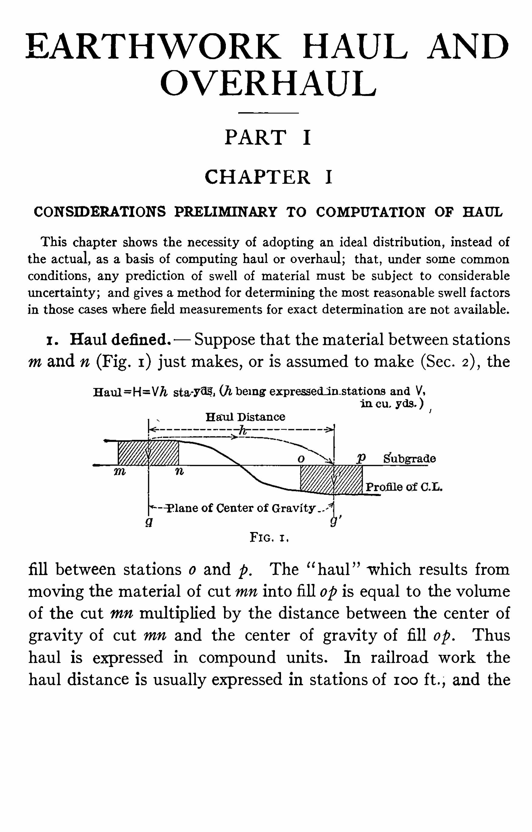
1 . Haul defined. Supposethat them aterial between stations
m and n (Fig . 1 ) just m akes , or is assumed to make (Sec . the
Hau1=H=Vh sta-yds, (It being expressedjns tat ions and V.in cu. yds. )
1
Hau l Distance
-P.1aneof Center of Gravity __
FIG . I .
fill between stations 0 and p . The haul which results from
moving thematerial of cut mn into fill op is equal to thevolum e
of the cut mn multiplied by the distance between the center of
gravity of cut mn and the center Of gravity of fill op. Thus
haul is expressed in compound units . In railroad work the
haul distance is usually expressed in stations of 100 ft . and the

2 EARTHWORK HAUL AND OVERHAUL
volume in cubic yards . Hence the customary unit of haul is
the station - yard (hereafter written sta the haul resulting
from hauling 1 c .y . Of m aterial a distance Of 1 sta . So 50 sta
yds. is the result Of hauling 1 c .y . 50 stas . ; 50 c.y . 1 sta . ; or
c .y . 4 stas . ; and so on .
Let V volume in the cut mn .
V’ volume in thefill op.
g station and plus of the center Of gravity of thecut mu .
g' station and plus of the center of gravity of the fill op.
h g’
g haul distance distance (stations) betweenthe center of gravity of the fill and the center of
grav ity Of the cut .
H thehaul (sta—yds) .Then
H Vh (not V’h,unless V’
V) . (I)So
,then
,to ascertain the haul resulting from transporting a
given body Ofm aterial from a given position in a cut to a given
position in a fill, wemust (I ) ascertain the volume of the givenbody Of material in place (that is, in its original position inthe cut) ; and (2) find the position Of the center of gravity of
that body of material in place and the position Of the center
of gravity Of the same body of material after it is hauled to
the fill. The reader is supposed to be fam iliar with earthwork
measurements and volume computation . For reasons which willappear later , methods of determining center Of gravity
—
are de
ferred,to be taken up after attention has been given to the dis
tribution and swell of m aterial,and to them ass curve.
2 . Disposition of material, actual and assumed ; simple case.
In some cart- work the cut and fill,starting at the grade
point, are carried forward in Opposite directions simultaneously
and with full cross- section, as shown in Figs . 2 and 1 2 . Suc
cessive slabs across the cut are broken down,and hauled and
dumped over theend of thefill where thematerial of each slab
forms another slab on the end face of the fill. Under such

4 EARTHWORK HAUL AND OVERHAUL
In Short,in computing haul wedeal with thefill as if it werean
ideal cart—fill. The position of the ideal, separating transverse
plane is found by themethod given in Sec . 20 .
Again,let us consider the case of a cut m ade in the following
m anner (Fig . A steam - shovel starting near n,m akes a cut
ting to thevicinity of o,and then backs up to n . This process
is repeated until all them aterial is rem oved from cut no . The
steam—Shovel is served by two trains . Part of the time both
trains haul m aterial to onefill, part of the time to theother , and
still a third part Of the time one train hauls to fill mn and the
other train to fill op, according to the varying conditions on the
FIG . 3 .
work . In this case it is evidently impracticable to find the
position of thecenter Of gravity Of the space originally occupied
by them aterial hauled to the left,or to find theposition of the
center of gravity Of thespaceoriginally occupied by thematerial
hauled to the right . Theonly practicablemethod of computing
thehaul in cases heretypified is to substitute for this purpose an
ideal cart- cut for the steam—Shovel cut ; that is, wem ust assume
that a transverseplane, as ab , separates that portion of the cut
from which m aterial was hauled to the right,from that portion
from which thematerial was hauled to the left .
3 . Disposition of material : actual and assumed ; complex
case.
— Fig . 4 shows by arrows the ideal distribution of the
m aterial,assuming that the m aximum haul does not exceed
thedistance of profitablehaul (Secs . 206,
Fill ab is m ade
from the adjacent material be. There is m ore than enough
material in cc to makethefill ef, so fill of ismadefrom de, leaving

COMPUTATION OF HAUL 5
a surp lus of m aterial , cd. Fill gh takes all them aterial from cut
fg. The surplus cd is hauled to hi and the rem ainder i] of fill giis made frOm jk .
I DEAL D I STRIBUT I ONOF
MATERIAL BY CARTS—NO CROSS HAULFIG . 4.
If thework be done by carts,thedistribution of thematerial
will norm ally be the ideal indicated. The order in which the
parts of thework are attacked is of no signifi cance. Wemight
start a cart gang at b,a second at e
,a third at g, and a fourth at
j, sim ultaneously ,and put a gang on d after the roadbed was
completed between d and h ; or , wemight haveonly one gang to
takeup the cuts in any order , except that the cut cd would not
ordinarily be taken out till the roadbed from d to h had beencompleted, and so on .
C d d’
ANOTHER D I STRIBUT I ON—NO CROSS HAUL
FIG. 5 .
The disposition indicated above is called ideal because thereis no crosshaul (Sec. 43) and thehaul (Sec. 1 ) is a minim um .
The profile Of Fig . 4 is repeated in Figs . 5 and 6 . Fig . 5
shows a little variation from Fig . 4 . It is plain that the two

6 EARTHWORK HAUL AND OVERHAUL
figures indicate the same amount Of haul (sta HoweverFig . 4 , and not 5 , shows the normal disposition for carts .
In Fig . 6 thereis a surplus of m aterial at the left and a deficitat the right . Supposefx hauled to fy , causing a surplus at dw ,
which results in hauling dw to zh . Fig . 6 indicates m ore haul
(sta -
yds.) than does Fig . 4, for in Fig . 6 we have crosshaul between y and x .
D I STRIBUT I ON SHOW ING CROSS HAUL AT a: y
FIG. 6 .
Now if thework be done by contract,and the contractor be
directed to dispose of the m aterial as indicated by arrows inFig . 6
,the hau l Should be calculated on the basis of the dis
tribution therein indicated by the arrows ; however , if the
contractor,having been directed to dispose of the m aterial as
indicated by the arrows in Fig . 4 , should for his own reasons
make thedisposition as indicated in Fig . 6,then thehaul should
be calculated on the assumption that them aterial was hauled as
indicated by the arrows in Fig . 4 . This applies whether xy is
less than the free- haul distance (Secs . 40 , 44) or not .
If thefills bemadeby dumping from trestles we have in this
case (Fig . 6) not only thecrosshaul above indicated but also the
crosshaul pointed out in the examples Of the preceding section .
4. Swell and shrinkage. Theact of excavating thematerial
of a cut causes them aterial to expand in volume, because Of the
separating Of the parts . W hen them aterial is dumped in the
fill there is usually some reduction of the increased volume, due
to theconsolidation of theparts . SeeGillette’s “Earthwork and
Its Cost,
”
pp . I I—I8 ; Gillette
’s Rock Excavation ,”
pp . 8—1 1 ;

COMPUTATION OF HAUL 7
Manual ” of the Am . Ry . Engrg . Assoc,1 9 1 1 , p . 35 ; Webb
’
s
Railroad Construction ,
”
pp . 1 14—1 18
,Arts . 96 , 97 ; Prelini
’
s
Earth and Rock Excavation , pp . 3 28—33 1 .
Uniform unm ixed m aterial , as sand, or clay , or loam , or
sandstone,etc .
,handled in a uniform way, under uniform con
ditions,may beexpected to have a constant relative change Of
PURE MATERIALS
FIG . 6a.
volume,due to excav ation
,hauling
,and dumping . After the
m aterial is placed in the fill its volume decreases , as a rule, for
somemonths or years . Fills Of uniform unm ixedm aterial , m ade
under uniform conditions,in a uniform way
,may be expected,
with continuing uniform conditions,to contract with ageaccord
ing to the same law . The foregoing with regard to uniform
unm ixed materials applies as well to uniform mixtures of difier
ent materials. By observation it is possible to make out a
schedulelikethat abovefor material which is placed in fills of like
dimensions . The accompanying schedule, it will be observed,

8 EARTHWORK HAUL AND OVERHAUL
is for fil ls of oneheight only . For fills Of another height it would
benecessary to makea corresponding similar schedule. Perhaps
fiv e such schedules would be sufficient for heights of fill running
up to 100 feet . These five schedules would give data for cases
Of unm ixed m aterials only . The foregoing,taken in connec
tion with the following section and with the further fact thatm ixtures of endless variety aremet in practice, will account forthehesitancy Of writers to givehard—and—fast rules for predicting swell.
5 . Swell of two or more materials depends on thoroughnessof mixing . Fig . 7 shows a layer of 1000 c .y . Of unm ixed earth
Earth ( swell facto r :
ub g'rade
So lid Rock ( swell factior=
2000c .y .
30000.y . Profi le
MATERIALS KEPT SEPARATE
FIG . 7 .
lying over 2000 c .y . Of unmixed solid rock . Fig . 8 shows thesame cut . The earth is Supposed to occupy the same space in
(swell factor=1 .0)
Subg radeSoli Rock swell facto r=1.5)2000c .y.
3000c.y. Profi
MATERIALS UNI FORMLY MIXEDFIG. 8 .
the fill as in the cut,that is
,the earth is supposed neither to
swell nor shrink . The solid rock is supposed to swell so that1 c.y . of cut makes 1% c .y . of fill.

COMPUTATION OF HAUL 9
Fig . 7 Shows theresult of keeping the rock and earth separatewhen m aking the excavation and fill . The total fil l measures
4000 c .y . The total cut is 3000 c .y . Hence in Fig . 7 the in
crease ih the volume of them aterial of the cut when deposited
Earth
Sub s-
Hide
Mix tureofMaterialsnot Uniform
F ILL MADE BY CARTS DUMPING OVER THE ENDFIG . 9 .
in thefill is 1000 c.y . ; that is, the swell ratio of the cut taken as
a whole is (Sec .
Fig . 8 shows the eflect of placing in the fill thematerial Of
the cut , uniform ly m ixed. The 1 000 c .y . Of voids in the m ass
of broken rock is precisely filled with the 1000 c.y . of earth .
ub g rad‘
e
EILL MADE IN LAYERS
FIG . 10.
Hencein Fig . 8 thefill measures 3000 c.y . Hence thematerial
from thefill occupies the same total space as it occupied in the
cut . In Fig . 8,then
,wehaveneither swell nor shrinkage in the
grading as a whole.
It may be objected that Figs . 7 and 8 Show extreme cases
which are not to be expected in practice. They do show the
lim iting cases : in Fig . 7 wehaveno mixture; in Fig . 8 a complete
mixture. Cases in practice, then, will be of some degree of

IO EARTHWORK HAUL AND OVERHAUL
mix ture,or
,rather
,of various degrees of mixture
,approaching
the one lim it or the other , depending on theplant and methods
used (seeFigs . 9 , 10, Thepoint m adehere is that it is not
usually possible to predict with close approxim ation the swell
of a cut composed Of two or more materials,even if we know
the swell ratio of each of the component m aterials .
caoss sscrnonTHROUGH FILL
MADE BY DUMPING
Profileof Fill FROMTEMPORARY TRESTLESub grade mpleted
FIG. I I .
6 . Swell increment ; swell ratio ; swell factor . The Swell
increment ” of a body of m aterial is theincreasein bulk resulting
from Shifting the m aterial from its original position to a fill.Swell increment is usually expressed in cubic yards . If thereis shrinkage
,the increment is negative.
Let C volum e of a given body of m aterial in place,(that is, in the cut before being disturbed) .
F volume Of the same body of m aterial after
deposit in fill ;swell increment ;
swell increment;swell ratio
volume In place5 swell factor .
Then the swell increment is
i F C.
The swell ratio is
The Swell factor is
1 + r.

1 2 EARTHWORK HAUL AND OVERHAUL
are made to full section as the work proceeds . At any time
during the progress Of this work it is easy to cross- section the
cut and thefill as far as completed at that time, and thus Obtain
the volume of the cut and of the fill, and from these the Swell
factor . The cut is cross—sectioned at the end of them onth for
the m onthly estim ate, and if the extra work of cross - section
ing the fill is doneat that time, them ost accuratedata for com
puting the swell factor are had at m inimum expense.
east o f Carl:Cut in Prog ress
Subgrade
End o fF IIIID
VOLUME READ I LY MEASURED IN PLACEAND IN FILL
FIG . 1 2 .
In many cases,however
,thefill is not carried forward at full
height and width,but in such m anner that the work of cross
sectioning would take considerable time more time often
than could be given without providing an extra force for the
surveying party .
Again,a fill may be composed of materials brought from two
or m ore cuts and deposited in such m anner as to interm ingle the
m aterials from the different sources . For example, the output
Of two steam —shovels,working in two cuts
,say
,one Of clay and
the other of solid rock ,may beused to widen the samefill. In
such a case it is impracticable to measure the volume of that
portion Of the fill which comes from either cut .
Finally , of two trains serving a steam—shovel, one may be
dumping on onefill and theother on another fill. If thematerial
going to each fill bedeposited in well- defined position so as to bereadily cross - sectioned we can, by counting the num ber of carloads going to each fill, and multiplying by the average carload

COMPUTATION OF HAUL 13
in cubic yards , obtain approxim ately thevolume of cut hauledto each fill. And then, by measuring thefills , we can computean approximate swell- factor . If
, however, in this case,either
train add an irregular layer to a ragged fill previously m ade in
part from another cut, it will be im practicable to Obtain cross
sections during the progress Of the work which will give satis
factory swell factors .
Themethod of determ ining the swell factor in these complex
cases will begiven in thenext section .
9 . Determination of swell factor ; complex case. When the
w ork of grading a stretch of railroad is so carried on that it is
Swell Fact ors
A djusted s1
Givenz-Cuts and Fills b alanceb etween‘
m'and
‘n‘
ADJUSTMENT OF ESTIMATEDSWELL FACTORS
FIG. 1 3 .
impracticable to take such cross—sections as will enable one to
computedirectly the swell factor for any single cut or part of a
cu t,we have to resort to estim ating the swell factor of each cut
(or part of cut) and so adjusting the estimated swell factors asto m ake them harmonize with the fact (ascertained by crosssectioning all the cuts and fil ls of the stretch in question after
they are completed) that so m any (total) cubic yards of cut
havem ade so many (total) cubic yards of fill .
Let us illustrate. Referring to Fig . 13 let us assume that the
grading has been completed and that between thepoints m and n
the cuts precisely m ake the fills ; in other words , the cuts and
fills balance between m and n . Let it be assumed that during
the progress of the work it has been impracticable tomake
I4 EARTHWORK HAUL AND OVERHAUL
measurements from which to obtain the swell factor of any
singlecut or any part of a cut . Required to determinethe swell
factor for each Of the cuts of the series .
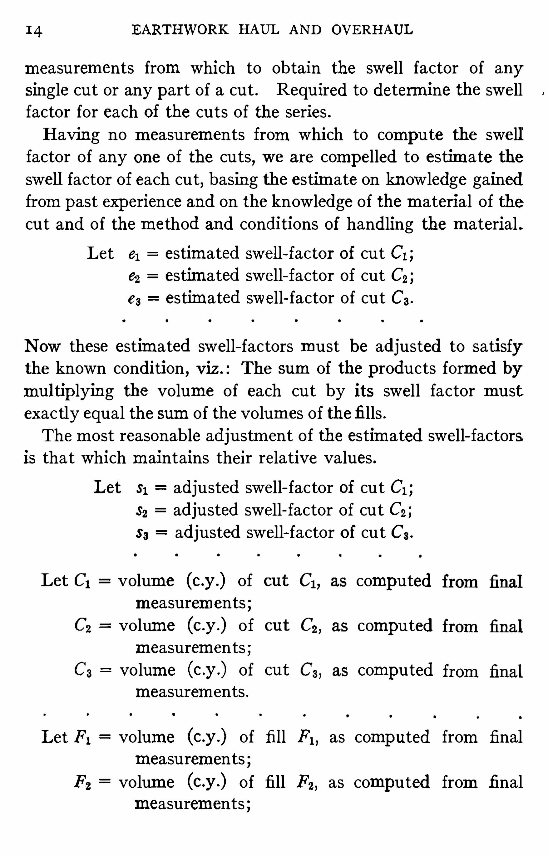
Having no measurements from which to compute the swellfactor of any one of the cuts, we are compelled to estim ate the
swell factor of each cut, basing theestim ateon knowledge gainedfrom past experienceand on theknowledgeof thematerial of thecut and of themethod and conditions Of handling thematerial .
Let cl estimated swell~factor Of cut C1 ;e2 estim ated swell- factor of cut C2 ;ea estim ated swell- factor of cut C3 .
Now these estim ated swell- factors must be adjusted to satisfythe known condition
,v iz . : The sum of theproducts formed by
multiplying the volume of each cut by its swell factor mustexactly equal thesum of thevolumes of thefills .
Them ost reasonableadjustment of theestim ated swell- factorsis that which maintains their relative values .
Let $1 adjusted swell- factor Of cut C1 ;32 adjusted swell- factor of cut C2 ;3 3 adjusted swell- factor Of cut C3 .
volume of computedmeasurements ;
volume of computedmeasurements
volume of computedmeasurements .
Let F , volume of fill PI, as computed from finalmeasurements
F2 volume of fill F2, as computed from finalmeasurements

COMPUTATION OF HAUL 1 5
F3 volume of fill F3 , as computed from final
measurements .
Now if thefactors areadjusted so as tomaintain thesamerelative
values,we have
kz, say ;
k3 , say ;
say ;
whence,
5 3 7335 1,
From theknown condition that the cuts and fills balance,
have
C13 1 + 025 2 “I‘ Csss + C55 5 FI +F2+
which by substitutions from eq . 7 becomes
Solving this equation for s1 we have
F1 + 172 + F 3 + Fe
Having the value of $1, the values of $2, 83 , S4, are com
puted by eq . 7 .
The foregoing method Of fixing upon the swell factors for the
several cuts may be divided for convenient use into the follow
ing steps
Step 1 . Estimate the swell factors e1, e2, ea, for the cuts
C1, C2, C3, respectively.

16 EARTHWORK HAUL AND OVERHAUL
Compute
3 . Compute the adjusted swell - factor for
Step 4 . Compute the adjusted swell- factor for each of
remaining cuts :
Swell Factors
Estimated—éAdiusted
Meas ’d.V o lts
Cuts and Fills b alancebetween‘m
‘and
b
rt‘
EXAMPLE OF ADJUSTMENT OF SWELL FACTORS
FIG. 14 .
To illustratewe turn to the following example. Referring
Fig. 14 : The grading between m and n has been completed.
Thefinal measurements of cuts C1, C2, C3 and fills F1, F2, F 3 , F4have been made; and from thesemeasurements have been com
puted thevolumes shown in Fig. 14 .
Step 1 . According to the best available judgment the swell

COMPUTATION OF HAUL I 7
ratios have been estimated to be as follows : swell ratio of cutC1, of C2, and of C3 , Hence
Estimated swell- factor of cut C1 is clEstimated swell- factor of cut C2 is 82Estim ated swell—factor Of cut C3 is e;,
Step 2 . By theuse of eq . 1 1,and a slide- rule. the following
multipliers are computed
kg
Step 3 . The adjusted swell - factor for cut C1 is (eq . 1 2)F1 F2 F 3 F4
C1 Czkz Cake
6270 2 268 6 1 1
9642 5056 (07 92) 4643 (09 1 7)
Step 4. The adjusted swell - factors for the remaining cuts are
computed by eq . 1 3 .
32 k25 1 X
5 3 k351 X
To check the foregoing computations this test is applied
The sum of the products formed by multiplying each cut
volume by its swell—factor m ust equal the sum Of the corre
sponding fill- volumes
,that is
,
C15 1 C252 “I“ C33 3 F1 F2 + F 3 + F4
C131 9642 x
0282 5056 X
C333 4643 X
C131 C232 C3s3
PI + F2 + F 3 + F4
Discrepancy 16

1 8 EARTHWORK HAUL AND OVERHAUL
Thus the test is met ; the work checks ; the discrepancy of
1 6 c .y .,which due to using the slide- rule
,is negligible;
Theuncertainty in theestimated swell - factors is usually such
as to perm it the use of the slide- rule in making all
putations of this section .
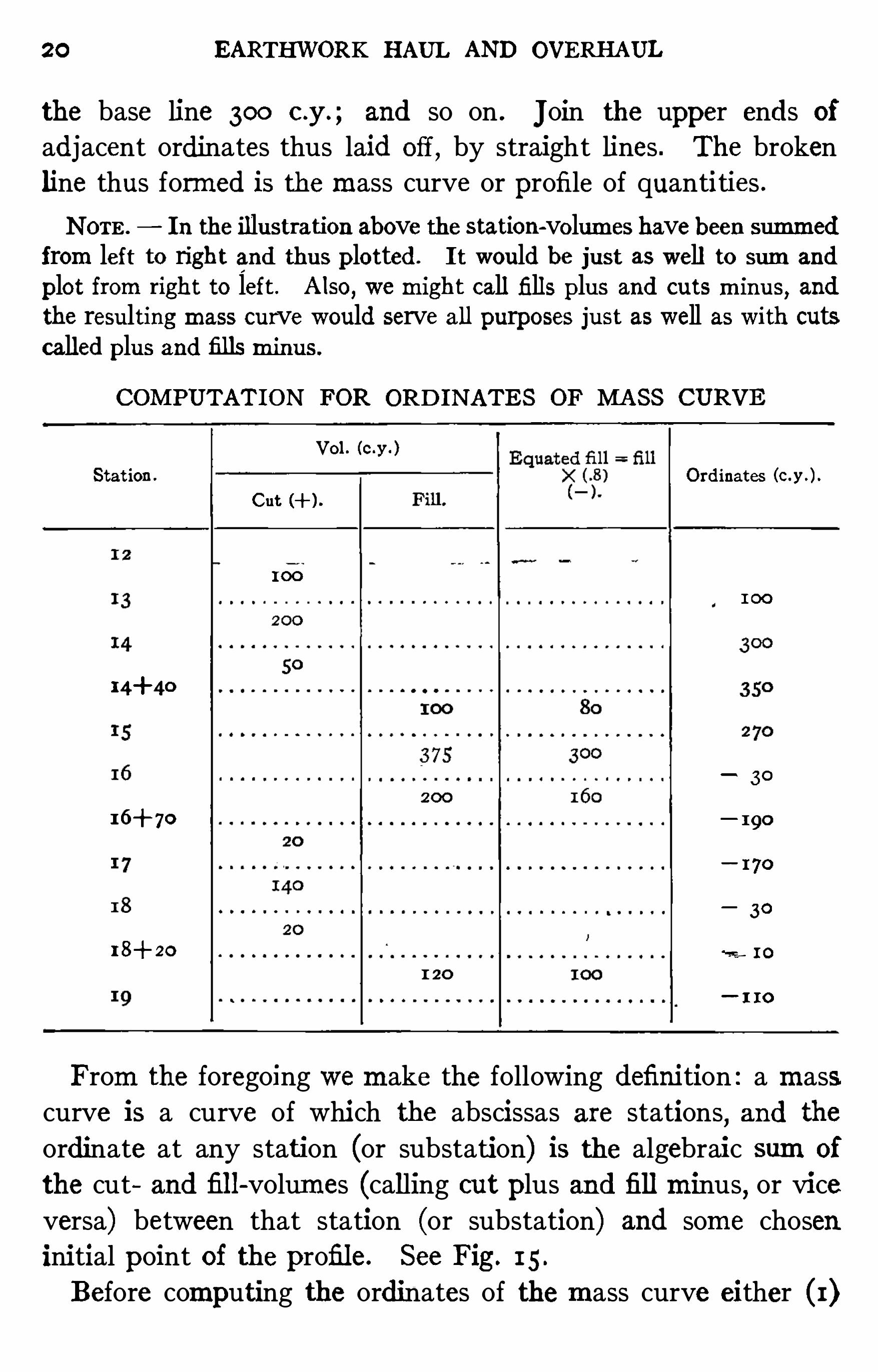
20 EARTHWORK HAUL AND OVERHAUL
the base line 300 c .y . ; and so on . Join the upper ends of
adjacent ordinates thus laid Off,by straight lines . The broken
line thus formed is themass curve or profile of quantities .
NOTE. In theillustration abovethestation- volumes havebeen summed
from left to righ t and thus plotted. It would bejust as well to sum and
plot from righ t to left . Also , wemigh t call fills plus and cuts minus, and
the resulting mass curvewould serveall purposes just as well as with cutscalled plus and fills minus.
COMPUTATION FOR ORDINATES OF MASS CURVE
Vol.
Stat ion. Ordinates
Cut
100
1 00
l 4+4o
200
— 190
— 1 70
1 8+ 20 —2 10
" " I IO
From the foregoing wemake the following definition : a masscurve is a curve of which the abscissas are stations
,and the
ordinate at any station (or substation) is the algebraic sum of
the cut and fill- volumes (calling cut plus and fill minus, or viceversa) between that station (or substation) and some choseninitial point Of theprofile. See Fig. 1 5 .
Before computing the ordinates of them ass curve either (I)


2 2 EARTHWORK HAUL AND OVERHAUL
the cut - volumes for the several station - intervals must bemulti
plied by their proper swell- factors (Sec . or (2) thefill- volumesfor the several station - intervals must be equated to volume in
place (Sec . (See exception to this statement in Sec .
If the grading has been completed and the volume computed
from final measurements , then thefill- volumes should beequated
to volume in place, and the equated fill- volumes used with the
cut—volumes in computing ordinates Of the m ass curve; but if
thegrading has no t been completed,or has not been started
,the
cut - volumes must bemultiplied by theproper Swell - factors before
the ordinates of them ass curve are computed,and the swelled
cut - volumes used with the fill- volumes to Obtain the ordinates .
W hen there are both cut and fill in any station - interval as in
side- hill work theexcess Of the one over the other is used as
an increment (positive or negative as the casemay be) in com
puting m ass- curve ordinates .
1 1 . Characteristics of the mas s curve.
— A study of Fig . 1 5
will show the truth of the following statements :
W ithin the limits of a single cut them ass curve rises from left
to right . W ithin the limits of a Singlefill them ass curve falls
from left to right . Hencein passing from left to right from cut
to fill we have at the gradepoint a m aximum ordinate for the
m ass curve; and in passing from left to right from fill to cut we
have at the gradepoint a minimum ordinate.
NOTE — Had thevolumes been summed from righ t to left in the com
putation for ordinates, the resulting mass curve would rise from righ t to
left instead of from left to righ t within the range of a single cut . If cuts
had been reckoned m inus and fills plus, while retaining the left - to - right
summation,themass curvewould Slopedownward from left to right within
the range of'
a single cut .
The algebraic difference between the ordinates of any two
stations which lie between a m aximum point Of them ass curveand an adjacent minimum point, represents theyardagebetween
the two stations .

THE MASS CURVE 23
Theslopeof themass curveis steepest at stations of greatest
v olumes . See Fig . 38 where both mass curve and profile. are
drawn to scale.
Other characteristics Of them ass curve are given in Secs . I 2,
I3 , 14, 1 5 .
1 2 . The horizontal balancing line. The mass curve in
Fig . 1 5 is plotted from cut - volumes and equated fill- volumes .
Any horizontal linedrawn to cut off a loop Of such a m ass curve
cuts the curvein two points between which the cut will precisely
m ake the fill. Thus the horizontal line NO cuts the curve at
N and 0. Between N and O the cut just m akes thefill . Such
a line is called a “balancing line.
”
Under the given conditions
of plotting them ass curve of Fig. 1 5 , a loop above thebalancingline indicates forward hauling
,and a loop below the balancing
line indicates backward hauling . See Figs . 50—60 .
It is evident that all balancing lines are horizontal for a m ass
curvewhich is plotted from cut - volumes and equatedfill- volumes
or from fill—volumes and equated swelled) cut - volumes .
When them ass curve is plotted from cut - volumes and actual
fill- volumes a balancing linewill be Oblique if them aterial from
the cut either swells or shrink s . See Sec . 1 3 .
The horizontal balancing line only is used in theproblem s of
this book .
13 . The ob lique balancing line.
— Fig . 1 6 shows the profile
of a cut and fil l. Let it be assumed that them aterial of the cut
swells,and that the cut just makes the fill . The mass curve
below theprofile is plotted from the cut - volumes and actual fillvolumes thevolumes in fill havenot been equated to volumes
in place. Thus the total fill- volume I’I is greater than the
total cut - volume AA ’. Where the m ass curve is thus plotted
without first equating the fill- volumes to volumes in place, or
equating the cut—volumes to fill- volumes , the balancing linewill
be a horizontal line only when the equating - factor is unity
only when them aterial of the cut neither Shrinks nor swells .

24 EARTHWORK HAUL AND OVERHAUL
The balancing lines in Fig . 16 are oblique. The balancing
linewhich passes through A passes also through I, because be
tween a and i'
the cut just makes thefill.
Produce the line AI to meet at N the horizontal line EN
drawn through thehighest point E Of themass curve. Each of
the lines BE, CG,
DF radiating from N cuts themass curve in
two points and is approximately a balancing line.
Sub g rade
Mass Curve
Balancing
OBLIQ UE BALANC ING LINE
FIG. 1 6 .
It is the practice of some engineers to plot the m ass curvefrom theunequated cut and fill—volumes and to use
,therefore
,the
Oblique balancing line. An example of the use of the oblique:
balancing lineis given in an article,by Mr. S. B . Fisher
, printedin the Engineering News, Jan . 3 1 , 189 1 , under the title
“Esti
m ating Overhaul in Earthwork byMeans of theProfile of Quan
tities .
” Mr. Fisher further explained the Obliquebalancing linein a letter printed in theEngineering News, Feb . 7 , 189 1 . Both
articleand letter are reprinted in Gillette’s “Earthwork and Its
Cost,”
pp . 2 1 7—2 25 ; and in Proceedings
,American Railway
Engineering Association , vol . 7 , 1 906 , pp . 381—385 .
14. Relation between haul and mass- curve area when the
mass curve is plotted from cut - volumes andequated fill- v olumes.
— Them ass curve of Fig. 1 5 is plotted from cut- volumes and

THE MASS CURVE 25
equated fill- volumes . The area lying between the balancing
lineand thecorresponding loop of them ass curve is themeasure
of the haul (Sec. 1 ) involved in m aking t he cut and fill between
the extremities of the loop . Thus the balancing line NO cuts
themass curve at N and O,and cuts off the loop NPO. The
area of the loop NPO is a measure Of the haul performed in
making thefill between p and o from the cut between it and p .
The extreme haul- distance for thematerial between it and o is
no NO ; and thevolumeof cut up is equal to PP’
(to scale)equals equated fill—volume between p and 0.
To convert thearea NPO into haul (sta -
yds.) multiply theareaNP0 (in square inches) by the product formed by multiplyingthe stations represented by one horizontal inch of paper by the
number of cubic yards represented by onevertical inch of paper .
Let Y number of cubic yards represented by one inch Of
ordinate;number Of feet represented by one inch Of abscissa ;haul area in square inches ;haul in station—yards represented by one square
inch Of area .
The area , A ,Of the loop NPO measured with theplanimeter,
is sq . in . For Fig . 1 5 , Y 200 c .y .,and S 200 ft . Hence
the haul is
H AH1 X x 200 1 1 20 sta -
yds.
1 5 . Relation between haul and mass - curve area when mass
curve is plotted from fill - volumes and equated cut—volumes.
In Fig. 1 7 the cut is just sufficient to m ake thefill. Thevolume
of the cut is C c .y .
,and the swell - factor is s. Thevolumeof the

26 EARTHWORK HAUL AND OVERHAUL
fill is F c .y . Then C F4, and Cs F,where q is the
equating—factor of the fill (Sec.
First,wewill reduce the station - volumes of fill to volumes in
placeby multiplying each station - volumeby q, and construct the
mass curve above theprofile, using thecut - volumes and equated
\\Mass Curvebased on
Q cut v o ls. and equatedfill v ols .
Haul—Area ABD
ofileC.L.
BaseLine
FIG . 1 7 .
fill- volumes . Now them aximum ordinateof them ass curveABD
is C (to scale) ; and the area of them ass curveABD represents
the haul . Thehaul involved in the grading is
H (areaABDin sq . in .) Ii Y sta-
yds.
Next , let us equate the station—volumes of cut to fill- volumes
by multiplying each station - volume of cut by the swell - factor s ;then plot them ass curveA
’B
’D’ below theprofile, using thefill
Volumes and equated cut—volumes . In this m ass curvethemaxi
mum ordinate is equal (to scale) to Cs F . Now for every

28 EARTHWORK HAUL AND OVERHAUL
the 2 - in. scratch . In other words,we know that theremay be,
due to lack of precision in placing the m ark B ,an error of as
much as in . in theposition of B . Thus the resulting error
in theplotted distanceAB may beas much as 7 3—3 in . in .
If the two errors areeach in . and both outward,then the
distance between m ark A and mark B is in . If the two
errors are each in. and both inward, the distance between
A and B is in . And if the two errors are
equal but one is inward while the other is outward,the two
errors cancel and the distance from m ark A to m ark B is just2 in .
I
In general,ifin placing thezero scratch of the scaleagainst
a mark and if in placing a m ark on the paper against a given
scratch on the scale weare subject to an error of e in .
,then the
limit of error in any distancewhich we lay off at oneapplication
of the scale is 2 e.
The statements above apply as well to the work of scaling adistance from a drawing . Therefore when a distance is scaledfrom a drawing the scaled distance is subject to an error whichis the resultant of theerrors of plotting and of scaling . Hencethe limit of error E in a scaled distance
,due to thelimit of error
in placing a scratch of the scale against a mark , is
E 4 ein .
If one inch of paper represents S feet
E 4 65 ft . (1 6)
Example. A draftsman lays off on paper a distanceAB on thescaleof1 in. 400 ft . We scale thedistanceAB and find it to be 87 5 ft . What
is the lim it '
oi error in the 875 ft . if in plo t ting and in scaling there is a
possib leerror of in. in placing a scratch of the scaleagainst a mark on
the paper? The answer is
E 4 65 4 400
1 7 . Lim it of error in area dueto errors in distance. Suppose
the true dimensions of the rectangle ABCD (Fig . 18) are d

THE MASS CURVE 29
inches by a inches . Suppose that in scaling the dimensions
from thedrawing wem ake an error E in each,so that we come
to have d + E and a + E asthe dimensions of the rec
tangle. The true area of the
rectangle is da . The area ob
tained by use of the scaled di dzmensions is (d E) (a E)da dE dE E2. IgnoringE2
, which is relatively small ‘i
(da dE dE) da, (dE
dB) , is the lim it of error
in area , due to the error E ineach dimension . If E
’is the limit of error in area
,due to E
,
the limit of error in distance,we have
E’
E (d (1) sq . in .
,
whereE,d, and a are in inches .
If each inch of paper represents S feet, then each square inchof paper represents 5
2 square feet,
and E’
E (d a) S2 sq . ft . (18)
Substituting for E its value (eq . 1 5) in term s of e (the limit oferror in placing a scratch of thescaleagainst a mark on thepaper) ,eq . 18 becomes
E’
4 e(d a) 52 sq . ft . (1 9)
If thevertical scale of the rectangle is 1 in . Y c .y .
,and the
horizontal scaleis 1 in . 5 ft .
,then 1 sq . in . of paper represents Y
i sta-
yds. of haul,
100
E’
4 e(d a) Y sta-
yds.
Example. A mass curveis drawn with vertical scaleof 1 in . 1000 c.y .,
and horizontal scale of 1 in . 400 ft . A rectangular area representinghaul is scaled. The horizontal dimension appears to be in . ; and the

30 EARTHWORK HAUL AND OVERHAUL
vertical,
in. Theresulting haul is H A Y (eq . 14a) X 1 .5
X4—0—9 x 1000 sta-
yds. If in plo tting and scaling themass curve100
the limit of error in placing a scratch of the scale against a mark on the
paper was in .,what is theresul ting limit oferror in the sta-
yds.?
Theanswer is E’
4 6 (d+ a) YS
4 1000599
1 264100 100
sta-
yds.
W e have been considering the limiting error . It should bebornein m ind that limiting errors in drafting areinfrequent
,and
that theerrors areas likely to bepositiveas negative, and therefore tend to neutralize one another .
18 . Scale of ordinates for m as s curve.
— We may say.
that
anything less than —inch distanceon a profileis inappreciable.
Hence,for a scaleof 1 in . 100 c .y . less than c .y . is negligible;
for 1 in . 1000 c .y . less than 5 c .y . is negligible; for 1 in.
5000 c .y . less than 2 5 c .y . is negligible; and so on . The larger
the scale the less the uncertainty,due to thedrawing itself
,in
the results obtained through theuse of themass curve. On the
other hand,the larger the scale the greater the required width
(top to bottom ) of thepaper on which them ass curve is drawn .
The choice of scale for the ordinates of the mass curve in any
given casewill depend (1 ) on thearithmetic sum of them aximum
positive ordinate and m aximum negative ordinate of the curve;
(2) on the horizontal scale used ; (3) on the uncertainty of the
data upon which theordinates are computed ; (4) on the desired
accuracy of the results to be obtained from the use of themass
curve; and (5) on the convenient maximum top- to - bottom
dimension of the paper .
When drawing a m ass curve for cuts and fills of great volume,the scale used for the ordinates is usually a compromise. In
any case the scale should be no larger than necessary to keeptheerrors from the use of them ass curvewell within the limits
of error in the data upon which the computed ordinates are

THE MASS CURVE 3 1
based. W ith great volumes the limit of error in the data iscomparatively great owing to theirregular manner of excavating
and depositing them aterial (Secs . 2, 3 ,
19 . Plotting the mass curve. Them ass curve is m ost con
veniently plotted and used when plotted on profilepaper of the
samehorizontal scaleas theprofileof thelineunder consideration .
For“PlateA ”
profilepaper (20 horizontal rulings to theinch) ,them ass curve ordinates
,
—provided the scale used therefor is
200 or 2000 or c .y . to the inch,
arem ost readily plotted
in them anner of plotting points on theprofile. For“PlateB
profile paper (30 horizontal lines to the inch) , and for a scale of
300 ,or 3000 or c .y . to the inch for ordinates
,the m ass
curve points arem ost quickly plotted in them anner of plotting
profilepoints . Under other conditions them ass - curveordinates
arem ost conveniently laid off by means of theengineers ’ scale,
ignoring the horizontal rulings of the profile paper . When the
engineers ’ scale is to beused instead of the rulings of theprofile
paper in laying off the ordinates of them ass curve, the scale of
ordinates should,for convenience
,be one of the following : 100
,
1 000,
or c .y . to the inch ; 200,2000 or c .y .
to the inch ; 300, 3000 ,or to the inch ; 400 , 4000,
or
to theinch ; 500, 5000, or to theinch ; or 600,6000
,
or c .y . to the inch .
When plotting themass curveand drawing lines by means of
which to obtain results from it,keep the pencil as sharp as a
needle. The 6 - H pencil is best if theeyes of theplotter and the
light are good ; otherwise use a 4- H pencil although this will
require frequent sharpening , and the lines will rub somewhat .
Sharpen thepencil to a long conepoint on emery paper , andpolish
the point on a piece of detail paper . Repolish the point after
drawing each foot or two of line; and theknifeand emery paper
will have to beused only occasionally . The importanceof draw
ing thefinest lines and m aking the finest points in all graphical
computation must be fully appreciated by the draftsman ;
EARTHWORK HAUL AND OVERHAUL
otherwise second- class work result . Secs . 1 6 and
For the sake of convenience useml: of one color for ascending
segments of a m ass curve, and ink of another color for descend
segrnents ; or , use a full line for the one, and a broken
for the other,as shown in Fig. 1 5 .

CHAPTER III
LIMITS AND CENTER or MASS or A BODY or MATERIAL
This chapter describes how, by eye, by arithmetic,and by mass curve, to deter.
mine the limits of a body ofmaterial in cut or in fill from given conditions; andhow to determine thecenter of volume or mass of such body . (Figs. 19 , 2 1 , zra,and 24 facep .
20. Limit of a fill made from a given b ody of material .
Fig. 19 . Let it be assumed that the m aterial between sta .
‘
9
and the gradepoint (sta . 13 75) is to beused to m ake a por
tion of the adjacent fill . Further let it be assumed that thematerial swells 25% (swell ratio and that the station
volumes areas entered on thelower part of Fig. 19 . Theproblemis to find thepoint on theprofile to which them aterial between 9and 13 75 will make thefill .
(a) Arithmetical solution . The total yardagebetween stas . 9
and 13 75 is 1 280 . Tabulate the stations of fill and the
corresponding station- volumes . See the tabulation below . In
the third column enter the equated fill- volumes . (The swellratio being the swell—factor is 5 , and theequating- factor
is, therefore, II
TS(seeSecs . 6
, Next,fill out thefourth
column by entering oppositeeach station thesum of equated fill
volumes between that station and the gradepoint, sta . 13 75 .
Now looking at the summ ation colum n ,we see that the 1 280
c .y . of material will fill to a point between stas . 18 and 1 9 . The
fill to sta . 1 8 requires 1 140 c .y .
,leaving a surplus of 1 280 1 140
140 c.y . to fill beyond sta . 1 8 .
Assuming that the cross - sectional area of the fill is uniform
between 18 and 19 , the (equated) volume of the fill is140
c.y . per running foot . At this rate it will require;

34 EARTHWORK HAUL AND OVERHAUL
running feet of fill beyond sta . 18 to useup the140 c.y . of surplus
m aterial . Thus 1 8 25 is the limit of thefill which the given
cut will m ake. (We have assumed that the end of the fill is
bounded by a plane of cross—section , i.e.
,that thefill is m ade of
full section as far as it goes .)
(b) Mass- curvesolution. The lower portion of Fig. 19 shows
themass curveAGDE corresponding to theprofile. The base
line of themass curveis AB ,and A is theorigin at sta . 9 . The
o rdinateat sta . 10 is 500 c .y . ; at sta . 1 1, 500 300 800 c .y . ;
at sta . 1 2,800 200 1000 c .y . ; at sta. 13 , 1000 200
1 200 c.y . ; at sta . 1 3 75 , 1 200 80 1 280 c.y . ; at sta . 14,
1 280 20 1 260 c .y . ; at sta. 1 5 , 1 260 1 20 1 140 c.y . ;
and so on . The ordinate at sta . 1 9 is 420 c.y .
To find thelimit of thefill m adeby thecut , 9 00 to 13 75 .
Through thepoint of them ass curve at sta . 9 draw a horizontal
to intersect the right half of the m ass curve. The point of
intersection is the limit of the fill. Thus through the point A
draw the horizontal AB (which is the base line in this case)intersecting them ass curve at B . B marks the right- hand limit
of thefill,and is thepoint sought . By scaling theplus, wefind
that B lies at sta . 1 8 24 .

36 EARTHWORK HAUL AND OVERHAUL
ev idently the center of mass lies between themid- section of mn
and sta . m .
For thework of computing haul and overhaul it is customary
to assume that the center of mass of a singleprismoid of a
station - volume or substation - volume) lies m idway between the
end sections of theprismoid.
22 . Center of mass of a series of prism oids . Arithmetical
solution .
— Let m,n,o,p, 9 (Fig . 20) be consecutive stations
(or stations and substations) along theprofile.
Subgrade
CENTER OF MASS.
FIG. 20.
If all the prismoids are of uniform cross—sectional area then
the center of m ass of the series of prism oids , mn ,no
,op, pg, lies
midway between stas . m and 9. There are,of course, other
exceptional conditions under which the center of m ass will lie
m idway between theextreme stations of the series .
Sometimes thecenter of mass is assumed to bemidway between
theextremestations even in thosecases (most frequent) in which
the center of m ass is known to be actually eccentric (that is, tolie on one side or the other of themid-
point) .
The general method of finding the center of m ass of a series
of prismoids is m ade clear in the following example
Example. Fig . 2 1 Show s station - vo lumes between stas. 9 and 1 2 28.
To find the center ofmass of this series ofprism oids weproceed as fo llowsFind thes um of the volumes of the prismoids 1056 c .y . The half sumis 5 28 c.y . Then find thesum of thevolumes from sta. 9 up to each station.
(This wo rk is shown in tabular form .)

LIMITS AND CENTER OF MASS 3 7
Stat ion. Vo lum e. Summ at ion
1 000
1056 c .y .
find that between sta. 9 and sta. 1 0 the summation volume is lessthan one- half the to tal volume (5 28) o f the series of prismoids ; and that
between sta. 9 and sta. 1 1 the summation volume is greater than one- halfthe to tal volume of the series. Plainly , then, the center of mass of the
series of prismoids lies somewhere between stas. 10 and 1 1 . The center of
mass of the series lies 28 c .y . (so to speak) to therigh t of sta. 10 . Now in
passing from 10 to 1 1 wepass 300 c .y .
,which (assuming that the prism oid
10—1 1 is of uniform cross- sectional area) is at the rate of 3 c .y .
per running foo t . To pass over the 28 c.y .
,then
,wemust go
2311 ft .
from sta. 10 towards sta. 1 1 . Thus we find the center ofmass of the series
ofprismoids is at sta. 10
Evidently the result will be the same if we carry the computation from
the o ther end: sta. 1 2 28 ; thus
The tabulation shows that in passing from 1 2 28 to 1 1 the to tal intervening volume is 256 which is less than 5 28 (the half- to tal volume) ; and

3 8 EARTHWORK HAUL AND OVERHAUL
that in passing from 1 2 28 to 10 the total intervening volume is 556which is greater than the 5 28 . Wepass 300 c .y . in moving over the 100 ft .
between 1 1 and 10,or at the rate of 3 c .y . per running foo t (as
suming the prismoid 1 1—10 to be of uniform cross- sectional area) . To
come to thecenter of themass of theseries ofprismoids we-must movefrom
ft .,which b rings us to
s ta. 1 1 sta. 10 Thus thesameresult is ob tainedwhetherwe start from oneend or the o ther. In practice the computations shouldb emade from oneend and then the resul t checked by computing from the
o ther.
23 . Center of mass of a series of prismoids . Two mass- curves olutions. (a) Common mass- curve solution . Using the data
s h own in Fig . 2 1 which represents a profile, weproceed as follows :Construct them ass curve (Secs . 10 and 20) for thestation—vol
"
lumes lying between stas . 9 and 1 2 28 . Themaximum ordinateis C
’C (2) Mark thepoint C
” which bisects the ordinateC’C.
(3) Through C"draw a horizontal linecutting them ass curveAC
at somepoint M . (4) Thestation and plus of M is now read as
zs ta. 10 10,which is the center of m ass of the series of pris
m oids. This result differsby ft . from that found in thepreceding section .
AS the horizontal scale of profile paper is 1 in . 400 ft .,the
uncertainty in theposition of the center of mass , as found by the
use of them ass curve,is
,in general
,not less than 4 ft . (Sec .
The results found by thealgebraic and graphical methods in any
c ase should substantially agree.
(b) Another mass - curve solution . The following method of
finding the center of m ass is taken from a letter by Mr. T . S.
Russell to Engineering News . The letter appeared in the issue
o fMarch 14, 1 89 1 , under thecaption“TheCalculation of Over
haul ” ; was reprinted in Gillette’s “Earthwork and Its Cost ,
”
pp . 2 14—2 1 7 ; and reprinted again in Proceedings of American
Railway Engineering Association,vol . 7 pp . 386
—389 .
The profile and“first ” m ass curve of Fig . 2 1a are the same

LIMITS AND CENTER OF MASS 39
as theprofile and m ass curve of Fig . 2 1 . Now,in Fig . 2 i a
, plot
a “second m ass curve,C
’MA ’
,for the same cut ac
,taking the
origin at C’and plotting from right to left . The ordinate at
sta . 1 2 is 56 c .y . ; at sta . 1 1, 56 200 256 c .y . ; at sta . 10
,
256 300 556 c .y . ; at sta . 9 , 556 500 1056 c .y . Call
thepoint of intersection of thefirst and second m ass curves , M .
Thevertical Mm contains the center of m ass of the cut ac . By
scaling,M is found to be 10 ft . to theright of sta . 10 ; hence, the
center of m ass of cut ac lies at sta . 10 10 . This is the same
as theresult found in Sec . 23 ; though ,owing to errors of plotting
and scaling,such agreement is not to be regularly expected. See
Secs . 16,1 7 .

CHAPTER IV
CENTER OF GRAVITY
In this chapter are described eigh t methods (so—called) of finding the center of
gravity ofa body o fmaterial,ranging from theroughly approximateto thepracti
cally exact , and using theeye, arithmetic, or themass curve. All themethods are
applied to the same problem ,namely ,
finding the center of gravity of the cut
between 9 00 and 1 2 28 of Fig . (Figs. 1 9 , 2 1 , 2 1a, and 24 facep .
24. Relation b etween haul and center of gravity. Wehave
seen (Sec. 1 ) that one of the two factors of haul is the distancebetween the center of gravity of a body of m aterial in cut and
the center of gravity of the same body of m aterial in fill. To
find the distance factor we shall first find the position of each
center of gravity . Methods of finding the position of the
center of gravity of a body of m aterial are presented in the
following sections .
25 . Center of gravity of single prismoid . In m ost cases itserves every requirement to assume that the center of gravity
lies at the center of length of the prism oid. For example, the
center of gravity of theprismoid lying between stas . 1 2 and 13
(Fig . 2 2) may be assumed to be at 1 2 50 . In rare cases it
may be thought that the foregoing assumption will not give
satisfactory results,and in such cases the true center of gravity
of each single prism oid (station or substation - volume) is determined in the following m anner .
Let A 12 cross—sectional area at sta . 1 2 ;
A 13 cross - sectional area at sta . 1 3 .
It is plain that the true center of gravity of prism oid 1 2—13
lies between sta . 1 2 50 and the station having the larger area .
Thus,as A 12 is greater than A 13 (as shown in thefigure) , thecenter
of gravity lies to the left of sta . 1 2 50 .
40

CENTER OF GRAVITY 41
Let x the horizontal distance between the true center of
gravity and themid-
point of the prismoid ;l station - interval (length of prismoid) ;V volume of prismoid.
An_ 1
27 V
where A , and An_1 are the cross - sectional areas at the two
adjacent stations . (See Allen’s “Railroad Curves and Earth
work,
”
pp . 1 92—1 93 , for derivation of this formula
,and Ray
m ond’s Railroad Field Geometry,
”
p . 222, eq .
Center of Grav ity
Sub gra
CENTER OF GRAVITY OF SINGLE PRISMOID
FIG . 2 2 .
Ifwe substitute for V in eq . 2 1 its value 1l, wehave
1 n Ari - 1
)
A,,
X
(See Searles Engineers ’ Field Book, p . 244 , eq .
Example. In Fig . 2 2,Am 200 sq . ft .
,and A 13 1 50 sq . ft . Length
ofprismoid 1 2—13 is 100 ft . Therefore thecenter ofgravity of theprismoid
lies to one sideof themid- section the distance
1 50ft .
’
62 4
and since thearea at sta. 1 2 is greater than thearea at sta. 1 3 , the center of
grav ity lies on the left of themid- section. Hence the center of gravity liesat (sta. 1 2 50) ft . sta. 1 2

42 EARTHWORK HAUL AND OVERHAUL
For theerror in overhaul resulting from the use of the center of length
instead of thecenter of gravity of theprismoid, seeSec . 146 .
26 . Center of gravity of a series of prismoids.
— Eight
methods of finding the center of gravity of a series of pris
m oids will begiven ranging from roughly approxim ate to closely
approxim ate. Themethods will be illustrated, in the followingsections , by application to one of the profiles of Figs . 1 9 , 2 1
,
24 . See column s 6 and 1 0,Fig. 36 , for center of gravity deter
mined by each of theeight methods .
2 7 . Meth od 1. Center of gravity determined b y eye. This
method serves for rough estim ates and rough check on results
obtained by other methods . The center of gravity of the cut
(Fig . 1 9) between sta . 9 and sta . 1 2 28 appears to be at about
sta . 1 0 60 . The person who finds the center of gravity by
inspection of theprofilemust beignorant of the computed center
of gravity ; otherwise his result will be biased and of no value.
28 . Method II. Center of gravity assumed to lie at the
center of length . W hen the profile of the cut (or fill) is praetically symmetrical about a central vertical line, the center of
gravity may ,for rough estim ates and checks , be assumed to lie
at the center of length . Though the cut,sta . 9 to sta . 1 2 28
(Fig . 1 9) lacks symmetry ,we use it for an example for this
method. Thecenter of length lies at sta . 9 [(sta . 1 2 28)
(sta . 9 sta . 9 1 64 sta . 10 64 .
29 . Meth od III. Series of prism oids treated as a single
prismoid. W hen the area of cross - section increases (or de
creases) with practical regularity as we pass from the initial to
the final station of the series of prism oids , a rough determination
of the position of the center of gravity of the series can bem ade
by considering the series as a single prismoid and applying to
this prism oid themethod given in Sec. 2 5 (center of gravity ofsingle prismoid) .Apply this method to the series of prismoids (Fig . 19) lying
between stas . 9 and 1 2 28 . The mid—point of the series is

44 EARTHWORK HAUL AND OVERI-LAUL
of a body of material when themass curve is straight betweenthe terminal stations of that body .
3 2 . Method VI. Center of gravity of each prismoid assumed
to lie at its mid-
point . Arithmetical solution.— This method,
one of the standard methods used in computing pay quantities ,is as follows : Fig. 23 . Let m,
n,o,p be consecutive stations
Profile
Sub grade
(or substations) along theprofile. Let the center of gravity of
each prismoid beassumed to lieat its center of length (except forthis assumption, this method is exact) . Let V1 , V2, V3 ,
bethe respectivevolumes of theprismoids , mn, no, op,Taking m as a center of moments
Themoment of V1 about m is VI
Themoment of V2 about m is Va
Themoment of V3 about m is V3 +no
The distance (stas .) from the center of moments (m,in this
case) to the center of gravity of the series is
sum of themoments about m (sta-
yds.)(23)
sum of thevolumes
Applying this method to the out between stas . 9 and 1 2 28
(Fig . 1 9) wemakethe computations below.

CENTER OF GRAVITY 45
MOMENTS ABOUT STATION 9
V vo lume a lever- arm Va m omentStat ion.
(c .y (stas. (sta-
yds.
1056 c .y . 1 3 76 sta-
yds .
Average lever- arm distance from sta. 9 t o! stas .
center of gravity of series of prismo ids
Hencestation of center of gravity (sta . 9 00) stas.sta . 10
As a check on the computations abovewemay find the center
of gravity by taking moments about the other extreme station,
1 2 28 .
MOMENTS ABOUT STATION 1 2
V vo lume a lev er - arm Va m omentStat ion.
(stas . ) (sta- y ds .)
To tals 1056 c .y . 2088 sta-
yds .
Average lever - arm distance from sta. 1 2 28
to center of gravity of series of prism oids lyingbetween stas . 1 2 28 and 9 00 .
Hence station of center of gravity is (sta . 1 2 28)stas . sta . 10 (check) .
NOTE . The two tabular form s ab ove may be comb ined in one with
sav ing of spaceand time. SeeSec. 1 18 .
stas .
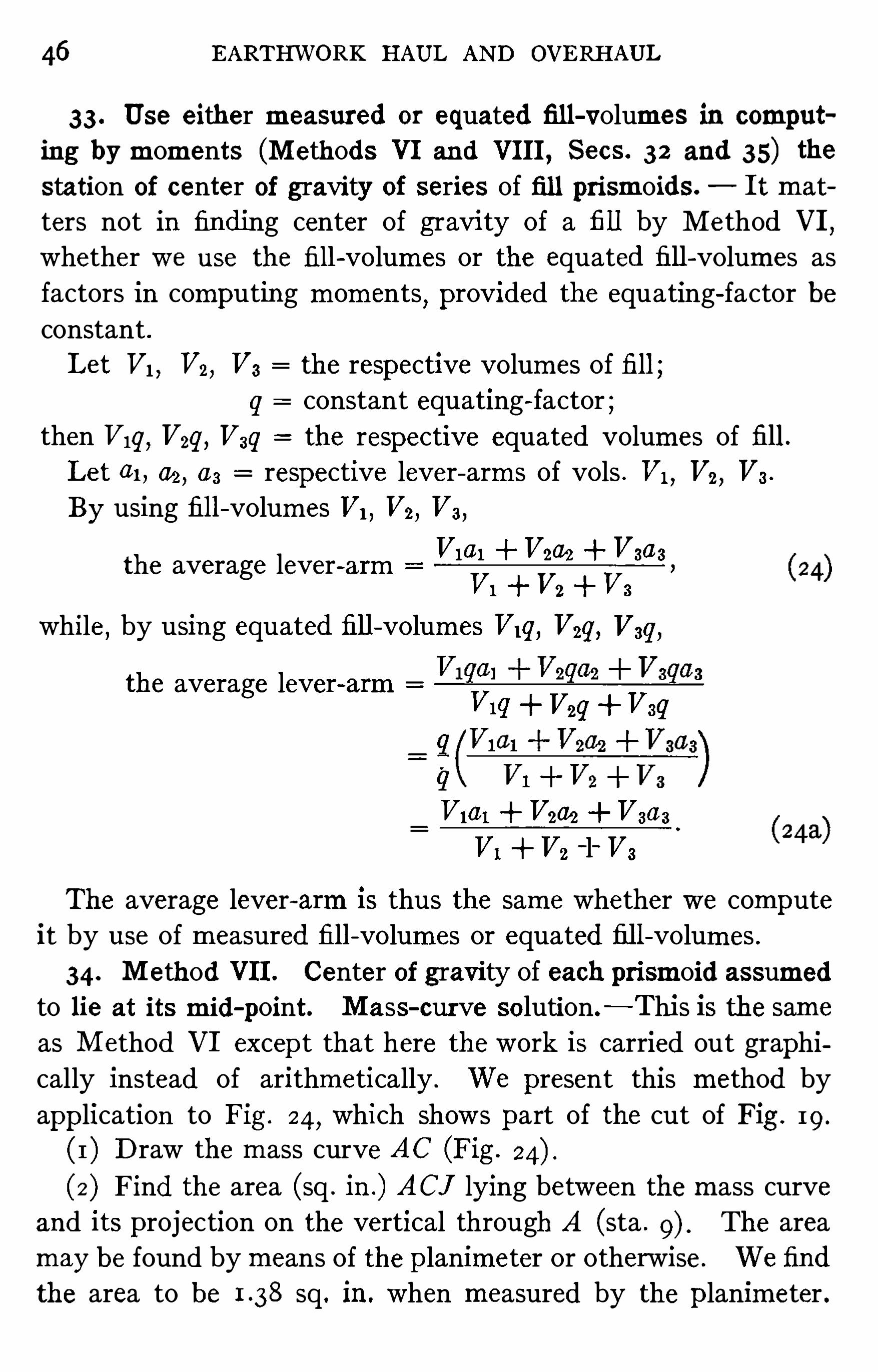
46 EARTHWORK HAUL AND OVERHAUL
33 . Use either measured or equated fill- volumes in comput
ing by moments (Methods VI and VIII, Secs . 3 2 and 3 5) the
station of center of gravity of series of fill prism oids. It mat
ters not in finding center of gravity of a fill by Method VI,whether we use the fill—volumes or the equated fill- volumes as
factors in computing moments , provided theequating - factor be
constant .
Let VI, V2, V3 the respectivevolumes of fill ;
q constant equating—factor ;then V19, V29, Vsq the respective equated volumes of fill.
Let al , a2, a3 respective lever- arm s of vols . V1, V2, V3 .
By using fill—volumes VI, V2, V3 ,
V101 V202 V303,
V1 V2 V3
while, by using equated fill—volumes VI9, V29, Vaq,
the average lever - arm
the average lever- armVig V2? Vsq
V101 V204 V303
V1 V2 “l“ V3
The average lever—arm is thus the samewhether we computeit by use of measured fill- volumes or equated fill- volumes .
34. Method VII. Center of gravity of each prismoid assumedto lie at its m id-
point . Mass- curve so lution.— This is thesame
as Method VI except that here thework is carried out graphically instead of arithmetically . We present this method by
application to Fig . 24 , which shows part of the cut of Fig . 19 .
(1 ) Draw them ass curveAC (Fig .
(2) Find the area (sq . in .) AC] lying between them ass curveand its projection on the vertical through A (sta . The areamay be found by means of theplanimeter or otherwise. Wefind
the area to be sq. in. when measured by the planimeter .

CENTER OF GRAVITY 47
(3) Multiply the area AC] (sq . in .) by the sta-
yds. repre
sented by 1 sq . in. of paper (Sec. obtaining the total haul
H . H 1000 x 1380 sta-
yds.
(4) Divide H by total volume obtained by scaling
o rdinateCC’
) of prism oids lying between stas . 9 and 1 2
obtaining the distance from sta . 9 out to the center of gravity
of the series of prismoids . Distance stas .
Hence the center of gravity of the series of prismoids is at
(sta . 9 00) stas . sta . 10
Otherwise
(1 ) Draw themass curveAC.
(2) Find area AC] in square inches .
(3) DivideAC] by CC’
(inches) , and multiply by thenumberof horizontal feet per inch of paper , thus obtaining thedistance
from sta . 9 to the center of gravity of thevolume lying between
stas . 9 and 1 2 29 .
The same result would be obtained if we dealt with the area
ACC’
instead of the area AC],except that with the area ACC
’
the resulting distance would be that between sta . 1 2 29 and
the center of gravity of the series of prismoids lying between
stas . 1 2 29 and 9 . Thus the planimeter gives the area
ACC’ sq . in . ThereforeH X 500 X
2 13 1 sta—yds . Hence thedistance from 1 2 29 to the center of
grav ity of the series of prismoids iiiir stas . Hence
the center of gravity of the series of prism oids lies at (sta . 1 2
stas . 10 The discrepancy between the
Thepracticableway of determ ining volume, when using a given mass curve,is to scale an ordinate; and for this reason we havehere used thevalue 1064 c.y .
o f CC determined by scaling, no twithstanding we canno t haveforgo tten that CC’
was plo tted to represent 1 05 6 c .y .
TThepoint c, Fig . 24 , is the left - hand lim it of the free- haul distance shown in
Fig . 19 . In Sec. 40 it is found by arithmetic that c lies at sta. 1 2 28 ; while in
Sec. 41 it is found, by the useof themass curve, that C lies at sta. 1 2 29 ; and
this accounts for the fact that sometimes we speak of the cut 9 00 to 1 2 28,
and at other times of cut 9 00 to 1 2 29 .

48 EARTHWORK HAUL AND OVERHAUL
two results comes from the errors involved in taking off the
areas . The larger the scale of ordinates for the m ass curve,the smaller will be thediscrepancy . SeeSecs . 1 6
,1 7 , 1 8 .
3 5 . Meth od VIII. The true center of gravity — This method
is the same as Method VI except that in the former we locate
the true center of grav ity of each prismoid by the method
given in Sec . 25 ; whereas in the latter we took themid-
point
of each prismoid for its center of gravity .
From Sec . 25 , eq . 2 2,the distance in feet between themid
point and the center of gravity of a prismoid is
sum of end areas (sq . ft .)
T0 illustrate,let us apply this method to theseries of prism oids
lying between stas . 9 and 1 2 28 of Fig . 1 9 .
COMPUTATION FOR POSITION OF CENTER OF GRAVITY OF
EACH PRISMOID
lDiff.
l lengt h Aa
end Sumdof Stat ion of Stat ion of
Station. of pbe‘
gv
gen
eDiff
l
6center of center of
mo ld (sq . ft .)areas .
area
c
ls .
Sum en
fgth
prism o id . grav it y .
0 2
1 00 0 3 1 6 7
1 00 O O
1 2 28
NOTE .
—To compute the stations of the centers of gravity of thepris
moids,is over and above thework required in the less exact Method VI.
o+so
104-
50 Io+4s
1 2+ I4

CENTER OF GRAVITY 49
MOMENTS ABOUT STATION 9 00
Station of center V v ol . of pris Va m omentStat ion.
of grav it y . m old (sta
To tals 1056 c .y . 1344 sta-
yds .
The average lever- arm distance of center
of gravity of the series of prism o ids from stas .
sta. 9 00 .
Hence,center of gravity of the series of prism oids lies at
sta . 9 sta . 10
Check this result by taking m oments ab out 1 2 28 .
MOMENTS ABOUT STATION 1 2 28
Stat ion of center V v ol . ofpris m omentStat ion.
of gravity . m oid (CAL ) . (sta
To tals 1056 c .y . 2 1 1 9 sta-
yds .
The average lever- arm = distance from center
of gravity of the series of prism o ids t o sta . stas .
1 2 28 .
Hence the center of gravity of the series of prism oids is at
(sta . 1 2 28) stas . sta . 10 (check) .

CHAPTER V
OVERHAUL, FREE HAUL, AND CROSSHAUL
In this chapter, overhaul is defined; a digest ofAmerican practicein computingoverhaul is given; theAmerican Railway Engineering Asso ciation’
s Specification,
which is used as thebasis for all the prob lems worked in this b ook, is presented ;and threemethods— by eye, by arithmetic, and by mass curve— of determiningfree- haul limits are explained. Crosshaul is discussed; and eight methods of
computing overhaul arecharacterized. (Fig . 19 faces p. 96 ; Fig. 36, p . 6 7 Fig .
3 8 , p .
3 6 . Definitions.— In some contracts for railroad grading it
is stipulated that the contractor shall bepaid so much per cubic
yard for excavating, hauling , and dumping , regardless of the
distancewhich them aterial is hauled ; in others , that a certain
price shall be paid per cubic yard for excavating , hauling , and
dumping , for all material hauled less than a specified distance,and that an extra sum shall be paid for each cubic yard which
is hauled a distance in excess of the specified distance. It is
specified that to determinethenumber of cubic yards of m aterial
excavated,hauled
,and dumped, thematerial shall bemeasured
in its original condition ; in other words , payment is on thebasis
of cubic yards of m aterial in place.
The“specified distance aboveis called thefree~haul distance.
The distancein excess of the specified distance aboveis called
theoverhaul distance. The extra sum ” aboveis themoney paidfor hauling a cubic yard the overhaul distance. By overhaul
price is usually meant theprice stipulated for hauling one cubic
yard a distanceof onestation (100 Overhaul is theproduct
of the number of cubic yards hauled, by the average overhaul
distance. Theoverhaul distanceis usually expressed in stations
of 100 ft .,and accordingly the overhaul is expressed in station~
yards . SeeSec. 1 .

5 2 EARTHWORK HAUL AND OVERHAUL
or some of the m aterial is hauled beyond the freelimit .
This method basis] is called the free average haul ,applicable, however , only to cuts with overhauls . [SeeSec . 39 for an interpretation of basis
(C) All cuts , them aterial from which is disposed of withinthe free—haul limit[s] are left out of consideration en
tirely . A t all other cuts them aterial in the cut requiredto balance them aterial in thenearest fill or fills is determinedwith in the free—haul lim it[s] ; in other words , a stripequal to the free- haul limit free—haul distance] is cutout of theprofile in such a way that the cut balances thefill within the limit[s] of this strip . This balanced material within the free- haul strip is not taken into account .
All other material that is clearly hauled m ore than the
free—haul limit free—haul distance] is taken into ac
count,the average haul[distance] ofeach individual mass
determined,and the average total haul[distance] estab
lished accordingly . The free- haul[distance] is deductedfrom the average total haul[distance] , and the balancerepresents the overhaul[distance] applicable to the totalyardage of such parts of cuts as are hauled beyond the
free limit[s] .This method basis] is called the free straight haul , asit eliminates consideration of absolutely all m aterial thatis hauled less than the free limit free haul distance] .
[Basis (C) is used throughout the following pages Of thisbook . See Sec . 38 ]
Replies to the circular letter above were received from 1 24
members of theA ssociation , connected with 75 railroads . Basis
(A) was preferred by 4 mem bers ; basis (B) , by 2 1 ; basis (C) ,by 54 ; and 4 members preferred other bases ; while3 7 membersomitted the overhaul clause from the contract .
As to the free- haul distance: 3 2 members preferred 500 ft . ;
1 6,1000 ft . ; 4 , 400 ft . ; 4 , 300 ft . ; 3 , 700 ft . ; 3 , 600 ft . ; 3 , 200
ft . ; 2,100 ft . ; 2
,200—500 ft . ; 2
,200
—1000 ft . ; 2
, 500—1 000
ft . ; one each,1 50 meters ; 2 50 meters ; 800 ft . ; 1 500 ft . ; and
500—1 200 ft . See Proceedings
,American Railway Engineering

OVERHAUL , FREE HAUL,AND CROSSHAUL 53
Association,vol . 7 pp . 429
—43 1 , from which the foregoing
facts are taken .
38 . Basis of overhaul computation recommended by AmericanRailway Engineering As sociation . In June, 1906 , theAssocia
tion adopted by letter ballot the following alternate optional
overhaul - clause which is virtually basis (C) presented above.
On pp . 26 and 27 of theManual (edition of 19 1 1 ) of theAssociation will be found
,incorporated in Specifications for theForm a
tion of theRoadway,
”
the following clauses on overhaul :
48 . Unless otherwise specified, it is distinctly understoodthat the contract price per cubic yard covers any haulfound necessary
,and that there shall be no allowance
m ade for any so - termed overhaul .
ALTERNATE OPTIONAL OVERHAUL CLAUSE
(The following alternate optional overhaul clause is recom
mended to[be substitutedfor clauseNo . 48 of theSpecifica
tions for theFormation of theRoadway in all cases whereit
is desired to allow overhaul .)
48- a. No payment shall bem ade for hauling m aterial whenthe length of haul does not exceed the limit of free haul
free- haul distance] , which Shall be ft .
The lim its of freehaul shall bedeterm ined by fixing on the
profile two points oneon each sideof theneutral grade
point one in excavation and the other in embankment ,such that thedistancebetween them shall equal the specified free- haul limit free- haul distance] and theincludedquantities of excavation and em bankment balance. All
haul on m aterial beyond this free- haul limit free- hauldistance] shall be estimated and paid for on the basis ofthe following method of computation, v iz
All m aterial within the limit[s] of this free haul Shall beeliminated from further consideration .
Thedistance between the center of gravity of therem ainingmass of excavation and center of gravity of the resultingembankment
,less the limit of free- haul less the free
haul distance] , as above specified, shall be the length of

54 EARTHWORK HAUL AND OVERHAUL
overhaul the overhaul distance] ; and the compensation to be rendered therefor shall bedetermined by multiplying the yardage in the rem aining m ass , as abovedescribed,
by the length of the overhaul by the
overhaul distance] . Payment of the same shall be. byunits of one cubic yard hauled one hundred (100) feet .
Where material is obtained from borrow pits alongside theembankment and runways are constructed
,the haul
[distance] shall be determined by the distance the teamnecessarily travels . The overhaul on m aterial thushauled Shall be determined by multiplying the yardageso hauled by one- half the round distance m ade by the
team less the free- haul distance. The runways shall beestablished by the engineer .
Sub gra
OVERHAUL: BASIS A AND BASIS 8FIG. 25 .
It will beseen that theoverhaul clauseaboveis basis (C) given
in Sec. 3 7 .
All directions given in this book for the computation of over
haul assume that the overhaul clause “48a” next above is the
basis of computation .
For the various methods of computing overhaul on this Amer
ican Railway Engineering Association basis,see Sec. 47 .
39 . Interpretation of basis (A) and basis (B) . Although
neither basis (A) nor (B) of Sec . 37 will beused in this book, the
following interpretation is given to m ake clear the differences
between the three bases cited and to enable the inexperienced
computer to compute overhaul by either (A) or (B) if that isdesired.

OVERHAUL,FREE HAUL ,
AND CROSSHAUL 55
Let us apply basis (A) for the overhaul of Fig. 25 , in which
the arrows indicate the distribution of the m aterial . It is assumed that cut C1 precisely m akes thefill F1 ; cut C2 thefill F2 ;and so on .
Let C1, C2, volumes of bodies C1, C2,respectively, of cut ;
h; distance (in stations) between the center
of gravity of cut C1 and center of gravity
Of fill F1 ;
hz distance (in stations) between the center
of gravity of cut C2 and center of grav
ity of fill F2, and so on ;
f free—haul distance in stations ;0A overhaul (sta-
yds.) computed on basis (A) ;OB overhaul (sta-
yds .) computed on basis (B) .
Then according to the rules under basis (A) (Sec .
If someof them aterial of every cut is hauled farther than thefree- haul distance
,theoverhaul will be the samewhen computed
on basis (B) as when computed on basis (A) . But suppose that
all of them aterial of cuts C4 and Cs—Ceis disposed of within thefree- haul distance; then the overhaul computed on basis (A)will be the same as before, but computed on basis (B) will be
Q + Q + Q—fim+ a+ ai (m
Observe that if oneportion of a cut, as portion C2 of cut C1‘ C2—C3
(Fig. is hauled farther than the free- haul distance,all other
portions of the cut come into the computation whether they are
hauled farther than the free- haul distance or no t .
40. Free- haul limits : arithmetical method. This method is
presented by application to a particular case. In Fig . 1 9 the

5 6 EARTHWORK HAUL AND OVERHAUL
free- haul distance is assumed to be 300 ft . The swell ratio is
assumed to be To fix the free- haul limits in this casewe
take the following steps :1 . Equate the fill—volumes (given in Fig . 1 9) to volumes in
place (Sec. (The equated fill - volumes are entered on the
profile.) In the succeeding steps weuse theequated fill - volumes
along with the cut - volumes .
2 . We take stas . 1 2 and 1 5 as trial free- haul limits . This
gives 80 200 280 c .y . of cut and 20 1 20 140 c .y . of
fill . Therefore between stas . 1 2 and 1 5 , cut exceeds fill by280 140 140 c .y . ; and wemust shift the 300- ft . free- hauldistance to the right (toward the fill) some distance, x ,
say,in
order to decrease the cut and increase the fill to a point wherethe cut and fill between the limits just balance.
3 . The v olume per running foot between stas . 1 2 and 13 is
iig 2 c.y . (average) ; and between stas . 1 5 and 1 6 is
3 c .y . (average) . Therefore if we shift the 300 - ft . free- hauldistance one foot to the right wedecrease the 280 c .y . of cut by
2 c .y .
,and increase the 140 c.y . of fill by 3 c .y . Hence for each
foot of shift toward the right the difference,140 c.y .
,between
cut and fill - volumes is decreased by 2 3 5 c.y . Therefore
to reduce the difference to zero to m ake the cut and fill bal
ance— wemust Shift the 300- ft . free- haul distance to the right
a distance equal to x 1439 28 ft . Thus we find that the
free~haul limits are at stas . 1 2 28 and 1 5 28 .
If the trial limits had been taken as Stas . 1 3 and 1 6 we shouldhave reached the same result . In such casewe Should have:
Cut 80 c .y . ; fill 20 1 20 300 440 c .y . Fill is in
excess by 440 80 360 c.y . Thereforewe shift the free- hauldistance to the left a distancex ’ 34
39
72 ft . ; and this placesthefree- haul limits finally at stas . 1 2 28 and 1 5 28
,as before.
4 1 . Free- haul limits : mass- curve method. This graphical
method of fixing upon the limits of free haul is always usedwhen themass curve is used for computing overhaul ; and may

OVERHAUL, FREE HAUL, AND CROSSHAUL 5 7
beused when the overhaul is computed arithmetically . In the
following it is assumed that them ass curveis to serveno purposeother than finding the free- haul limits .
Below theprofile, Fig . 26,draw a base linebelow which to lay
off mass—curve ordinates . To a convenient scale lay Oflbelow
FIG . 26 .
— Limits of FreeHaul.
the base line at each station in cut the total cubic yards of cut
lying between that station and thegradepoint , c, of theprofile.
Connect theplotted points , two and two , by straight lines , thus
forming a mass curve with origin at the grade point . In like
manner lay off below the base line at each station in fill the total
cubic yards of equated fill lying between that station and the
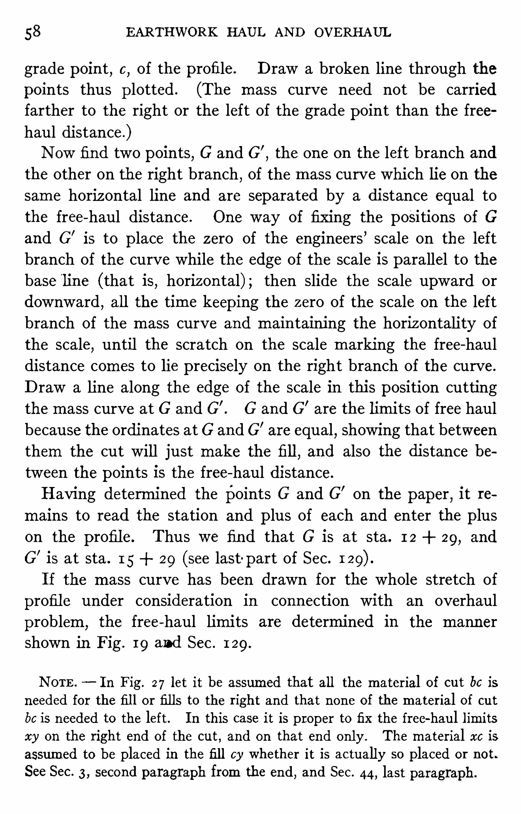
58 EARTHWORK HAUL AND OVERHAUL
gradepoint , e, of theprofile. Draw a broken line through the
points thus plotted. (The mass curve need not be carried
farther to the right or the left of the gradepoint than the free
haul distance.)Now find two points , G and G
’
,the oneon the left branch and
the other on the right branch ,of them ass curvewhich lieon the
same horizontal line and are separated by a distance equal to
the free- haul distance. One way of fixing the positions of G
and G’is to place the zero of the engineers ’ scale on the left
branch of the curvewhile theedge of the scale is parallel to the
baseline (that is, horizontal) ; then slide the scale upward or
downward,all the time keeping the zero of the scale on the left
branch of the m ass curve and m aintaining the horizontality of
the scale,until the scratch on the scalem arking the free- haul
distance comes to lieprecisely on the right branch of the curve.
Draw a line along the edge of the scale in this position cutting
them ass curve at G and G’
. G and G’are thelimits of freehaul
becausetheordinates at G andG’areequal
,showing that between
them the cut will just m ake the fill,and also the distance be
tween thepoints is the free—haul distance.
Having determined the points G and G’ on the paper , it re
m ains to read the station and plus of each and enter the plus
on the profile. Thus we find that G is at sta. 1 2 29 , and
G’is at sta . 1 5 29 (see last'part of Sec.
If the m ass curve has been drawn for the whole stretch of
profile under consideration in connection with an overhaul
problem ,the free—haul limits are determined in the m anner
shown in Fig . 19 and Sec . 1 29 .
NOTE. In Fig . 2 7 let it be assumed that all the material of out be isneeded for thefill or fills to the righ t and that none of thematerial of cutbeis needed to the left . In this case it is proper to fix the free- haul limitsxy on the right end of the cut , and on that end only . Thematerial xc isassumed to beplaced in the fill cy whether it is actually so placed or not .
SeeSec. 3 , second paragraph from theend, and Sec. 44, last paragraph .

60 EARTHWORK HAUL AND OVERHAUL
both directions over the same identical part of the line. The
nature of crosshaul is clearly shown in Figs . 28 to 3 1 .
V o l‘s —_V
Swell Factors 3b
Distance
SHOW ING CROSSHAUL
FIG . 28 .
SHOW ING NO CROSSHAUL
FIG . 29 .
Let it be assumed that the volume of fill a volume of fill
c V c .y . Let s, be the swell - factor of cut b and sd be theswell
factor Of cut d. Then it will takeS
zcy . from cut b to m ake V
b
c .y . of fill and1—1c .y . from cut d to m akeV c .y . of fill .
d
Assume that there are VbK
c .y . of m aterial in cut b and3 b
of m aterial in cut d.
d
Now if, as shown by arrows in Fig . 28,V, c .y . is hauled from
b to c, and Vd c .y . is hauled from d to a,the resulting haul is
5 28 17 5176 Vd da
+ Q + Q +d
5 4 Sd se

OVERHAUL ,FREE HAUL, AND CROSSHAUL 6 1
If,on the contrary
,Vb is hauled from b to a
,and Vd is hauled
from d to c,as indicated by the arrows in Fig. 29 , the resulting
haul isVbab Vdcd
Sub g rade
ICrosshaul dis tance
”
ISHOW ING CROSSH
’AUL
FIG . 30 .
V o l ’s —V-bV
Swell Factors Sir“
SHOWING NO GROSSHAUL
FIG . 3 1 .
Hence excess haul due to the crosshaul is
s — s V (”
5+ i—d
)5 d sd
V + 2
— V be + ab (29)«Yd
It is evident that 3 23 E gg may in somecases be negative, that
is,under some conditions of distance and Swell
,crosshauling
may actually result in minimum haul .

62 EARTHWORK HAUL AND OVERHAUL
For the special case in which the two swell - factors are equal ,
so thatI I
i say,eq . 29 reduces to
E gg—H29
= V <For the special casein which each of the swell—factors is unity,
s 1,and eqs . 29 and 30 reduce to
Egg E gg 2 bCV .
SHOWING NO CROSSHAUL
FIG . 3 2 .
SHOWING GROSSHAUL
FIG . 33 .
Looking at eqs. 30 and 3 1 , we see that when the two swell
factors are equal,whether they are each equal to unity or not
,
crosshauling increases,never diminishes
,the total haul .
From one point of view all crosshauling with the exception
noted under eq . 29 is unnecessary hauling and therefore a waste
of effort,time
,and m oney ; but often the conditions of thework
are such that some crosshauling gives an Operating advantage
which more than offsets theextra cost due to the crosshauling .
This is peculiarly the case in steam - Shovel work .
It is quite possible to underestim ate the extra cost due to
crosshauling . A casein point which has come to the author’s
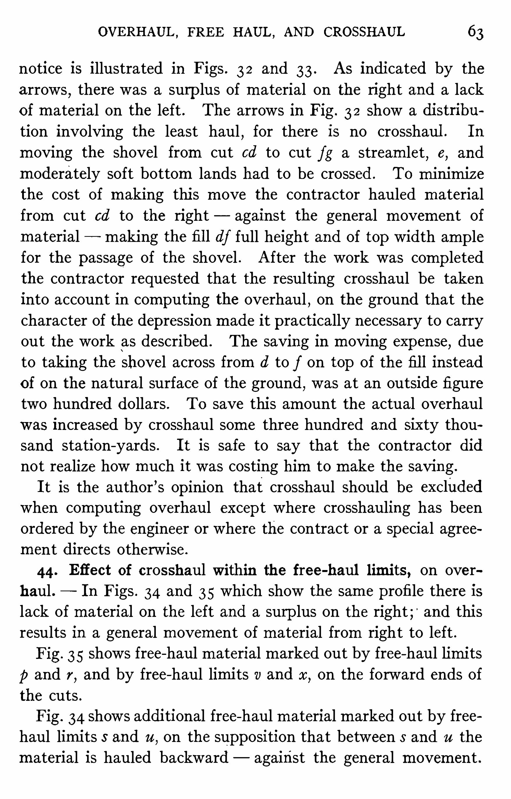
OVERHAUL,FREE HAUL,
AND CROSSHAUL 63
notice is illustrated in Figs . 3 2 and 33 . As indicated by the
arrows,therewas a surplus of material on the right and a lack
Ofm aterial on the left . The arrows in Fig . 3 2 Show a distribu
tion involving the least haul,for there is no crosshaul . In
m oving the shovel from cut cd to cut fg a stream let , e, and
m oderately soft bottom lands had to be crossed. To minimize
the cost of m aking this m ove the contractor hauled m aterial
from cut cd to the right against the general m ovement of
m aterial m aking thefill df full height and of top width ample
for the passage of the shovel . After the work was completed
the contractor requested that the resulting crosshaul be takeninto account in computing the overhaul , on theground that the
character of thedepression m adeit practically necessary to carry
out thework as described. The saving in moving expense, due
to taking the shovel across from d to f on top of the fill instead
of on thenatural surface of theground,was at an outsidefigure
two hundred dollars . To save this amount the actual overhaul
was increased by crosshaul some threehundred and Sixty thou
sand station—yards . It is safe to say that the contractor did
not realizehow much it was costing him to m ake the sav ing .
It is the author ’s opinion that crosshaul should be excliIded
when computing overhaul except where crosshauling has been
ordered by theengineer or where the contract or a special agree
ment directs otherwise.
44. Efiect of crosshaul W ithin the free- haul limits, on over
haul . In Figs . 34 and 3 5 which Show the sameprofile there is
lack of m aterial on the left and a surplus on the right and this
results in a general movement of m aterial from right to left .
Fig . 3 5 Shows free- haul m aterial m arked out by free- haul limits
p and r,and by free- haul limits 1) and x
,on the forward ends of
the cuts .
Fig . 34 shows additional free- haul m aterial m arked out by free
haul limits 5 and u,on thesupposition that between s and u the
material is hauled backward against the general movement .

64 EARTHWORK HAUL AND OVERHAUL
Let C, designate the body of cut st ; C of cut yz ; Fb , of fill
tu ; and Fd, of fill no . Thedistribution in the two figures is the
same except for this
In Fig . 3 5 , cut Cc m akes fil l F
and cut Ca m akes fill F b ;whilein Fig . 34, cut Cc
m akes fill F b ;and cut Ca m akes fill Fd .
There is no crosshaul in Fig . 3 5 . In Fig . 34 there is crosshaulbetween s and u . Theeffect of this crosshaul on the total haulis Shown in the preceding section . Now what is the effect of
crosshaul within the free—haul limits s and u,on the ov erhaulD
Let a be the center of gravity of cut Ca ; b , of fill F b ; c,of cut
C and d,of fill Fd .
Fills Fb and Ed have the same volume V,say .
Let C volume of cut C
C volume of cut Ca ;
s swell - factor of cut C
s swell - factor of cut Ca ;
f free- haul distance;034 total overhaul on volumes Cc and C,
in Fig . 34 ;
035 total overhaul on volumes C, and C,in Fig . 3 5 .
0
Q
0
9
I
Let all distances beexpressed in stations of 1 00 ft .
ThenV
and Cc
V
so sc
In Fig . 34 the overhaul on CCis nothing
,because them aterial
is all dumped within thefree- haul distance. Theoverhaul on Ca
isC, (ad f) . Hencethetotal overhaul on CC and C, in Fig . 34 is
034 Ca (ad — f)
1,
a. so
so so
and ad ab be+ cd.

OVERHAUL,FREE HAUL
, AND CROSSHAUL 65
In Fig. 35 the overhaul on C, is
C, (cd — f) V
and the overhaul on C,is
Ca (ab — f) V
-f
f= freehaul distance
SHOWING CROSSHAUL W ITHIN FREEHAUI. LIMITS
FIG. 34.
f=£reehaul distance
SHOW ING NO CROSSHAUL
FIG . 35 .
Hence the total overhaul on C, and CO in Fig. 35 is
035 V “Z:
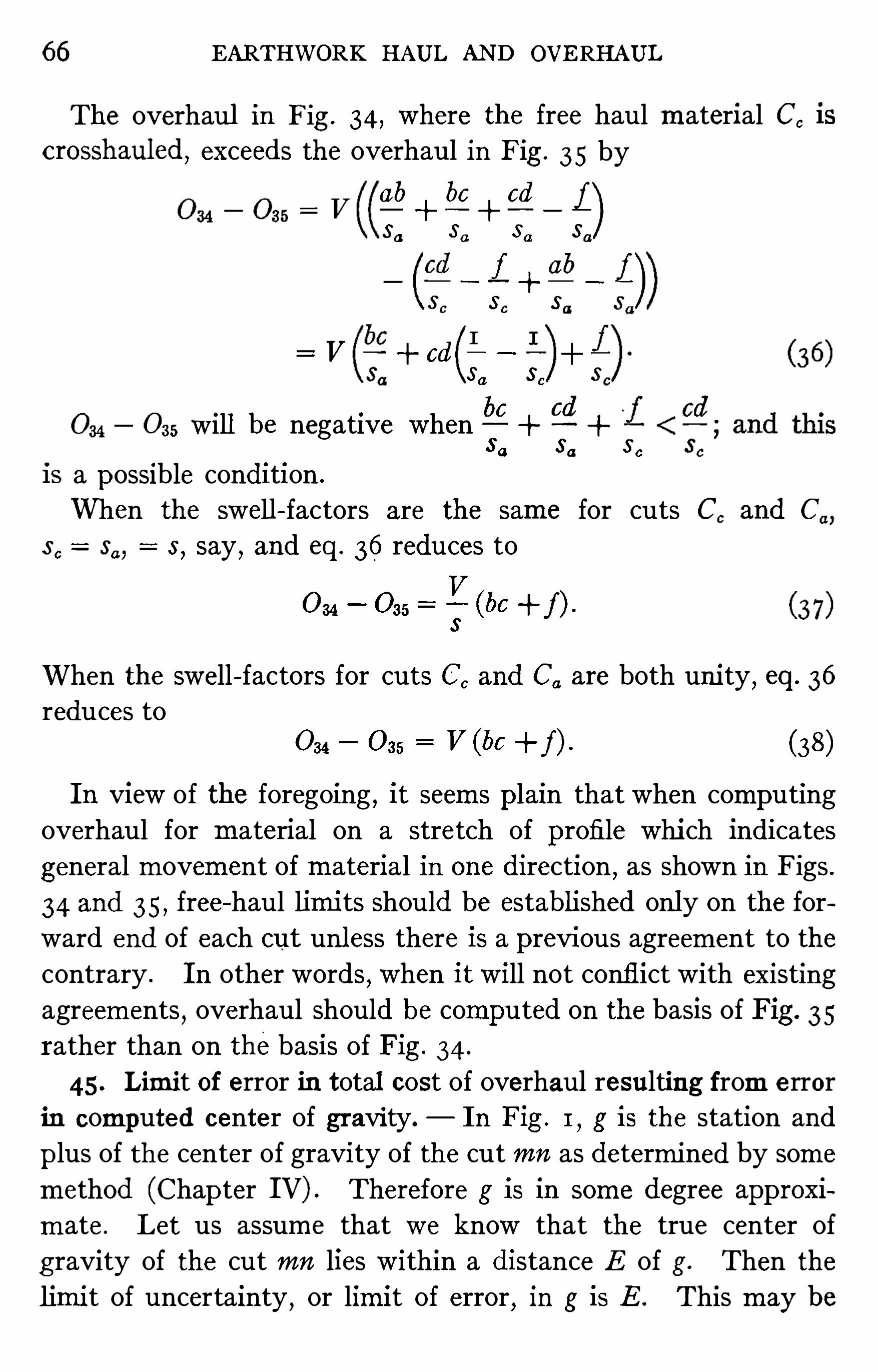
66 EARTHWORK HAUL AND OVERHAUL
The overhaul in Fig . 34 , where the free haul material C,
crosshauled, exceeds the overhaul in Fig . 3 5 by
E+E+o
_ qso so so so
s, s
V cdso SC 8
be ed035 W ill be negative when
3 a 5 a 3 e
a possible condition .
When the swell - factors are the same for cuts C, and C
s , s, , s,say
,and eq . 36 reduces to
034 035 +f)
W hen the swell - factors for cuts C, and C, are both unity , eq . 36
reduces to
In View of the foregoing , it seem s plain that when computing
overhaul for m aterial on a stretch of profile which indicates
general movement of m aterial in onedirection,as shown in Figs .
34 and 35 , free—haul limits should beestablished only on the for
ward end of each out unless there is a previous agreement to the
contrary . In other words,when it will not conflict with existing
agreements,overhaul should becomputed on thebasis of Fig. 3 5
rather than on thebasis of Fig . 34 .
45 . Limit of error in total cost of overhaul resulting from error
in computed center of gravity. In Fig . 1, g is the station and
plus of the center of gravity of the cut mn as determined by some
method (Chapter IV) . Therefore g is in some degree approxi
mate. Let us assume that we know that the true center of
gravity of the cut mn lies within a distanceE of g. Then thelimit of uncertainty
,or lim it of error
,in g is E. This may be

68 EARTHWORK HAUL AND OVERHAUL
$1 . Ob serve that wedo no t say that theresult , 3562 .50, is in error
to theamount of $1 . The fact is we canno t know what is theactual errorin the resul t . We know only that the error due to the cause stated lies
somewherebetween $1 and 81 . Wedo know,however
,that in many
cases in practice theerror in theascertained position of the two centers of
gravity is as likely to be positive as negative; and hence in the long run
these errors tend to neutralize one another.
46 . Statement of overhaul . — A fter the overhaul has been
computed,thenext step is to m akea statement of overhaul for
the use of interested parties . This statement concerning the
overhaul on any body of m aterial should give not only the
amount Of the overhaul but also sufficient data to enable one to
locate quickly and exactly on theprofile the lim its and center of
gravity of that body of m aterial both in cut and in fill,and to
check readily the overhaul . It is believed that the form of
statement given in Fig . 36 satisfies every requirement ; and
that no one of the columns of the form can be omitted without
inconvenience.
47 . Methods of overhaul computation . The overhaul com
putations which appear in the following pages are all based
on the overhaul clause recommended by theAmerican Railway
Engineering Association . See Sec . 38 .
NOTE .
—The overhaul clause is referred to in this b ook as the BASIS
of overhaul computation rather than as theMETHOD of computation,in
order that the latter term may be free to be applied to each of the severalways
—some arithm etical
,some graphical, ranging in accuracy from the
roughly approximate to the closely approximate which aredescribed and
illustrated in the following pages.
Each of the following methods of computing overhaul on the
American Railway Engineering Association basis , corresponds to
one of the methods given in Chapter IV for determining the
center of gravity . Each method of computing overhaul takes
its number from the number of the method therein used to
determine the center of gravity .


OVERHAUL,FREE HAUL
,AND CROSSHAUL 69
Methods of Computing Overhaul
48 . Meth od I. The center of gravity of each body of over
hauled material in cut and in fill is determined by eye (Sec. 27)directly on the profile. The lim its of any body of material
overhauled and the limits of free haul are likewise determinedby eye (Sec . Method I is applied in Chapter VI (Secs . 57
66) to theprofile of Fig . 1 9 , and in Chapter VII (Secs . 148—1 56)
to the profile of Fig . 38 .
49 . Method II. The center of gravity of each body of over
hauled m aterial is assumed to lie at the center Of length of that
body . See Sec . 28 . The lim its of each body of m aterial are
determined by eye (Sec . 20 (c)) or by arithmetic (Sec . 20
Thelimits of freehaul aredeterm ined by eye (Sec . 42) or by arithmetic (Sec . This method of computing overhaul is given
in Chapter VI (Secs . 67-
77) by application to the profile ofFig . 19 .
50. Method III.
— The center of gravity of each body of
overhauled m aterial is determined by computing its distancefrom the center of length (Sec . The limits of bodies of
m aterial are found by arithmetic (Sec . 20 Thelimits of free
haul are determ ined by arithmetic (Sec . The details of
this method of overhaul computation are illustrated in Chapter
VI (Secs . 78—88) by application to theprofile of Fig . 19 .
5 1 . Meth od IV .
— Thecenter of gravity of each body ofmaterial
overhauled is assumed to lieat its center of m ass, and is found by
arithmetic . SeeSec . 30 . Thelimits of bodies of m aterial arefound
by arithmetic (Sec . 20 Lim its of freehaul aredetermined
by arithmetic (Sec . Method IV is illustrated in detail in
Chapter VI (Secs . 89—99) by application to theprofileof Fig . 1 9 ,
and in Chapter VII (Secs . 1 5 7—1 67) to theprofile of Fig . 38 .
52 . Method V.
- The m ass curve is used. The center of
gravity of each body of m aterial overhauled is assumed to lie
at its center of m ass . See Sec . 3 1 . The limits of bodies of
material are determined by themass curve (Sec . 20 The

7 0 EARTHWORK HAUL AND OVERHAUL
limits of free haul are determined by themass curve (Sec.
This method of computing overhaul is applied in Chapter VI
(Secs . 100—1 1 1 ) to the profile of Fig . 1 9 , and in Chapter VII
(Secs . 168— 1 79) to the profile of Fig. 38 .
A full description of this method,based on Sec . 3 1 (a) is given
inMolitor andBeard’s Manual for Resident Engineers , pp . 57~
6 1,and reprinted in Proceedings , American Railway Engineering
A ssociation,vol . 7 pp . 40 1
—403 . Thesamemethod, based
on Sec . 3 1 (b) , is given in Engineering News, March 14, 189 1 ,
pp . 2 54, 255 (reprinted in Proceedings , American Railway EngineeringAssociation
,vol . 7 pp . 386 in a contribution
byMr. T . S. Russell who gives credit for themethod to Mr . R . P.
B ruer .
5 3 . Method VI.
— Arithm etical computation . The center«of gravity of each prismoid is assumed to lie at the middle of
its length . The center of gravity of each body of overhauled
material is determined by the method of m oments (Sec .
T he limits of bodies of material are determined by arithmetic
(Sec . 20 The limits of free haul are found by arithmetic
(Sec . This method of computing overhaul is applied in
C hapter VI (Secs . 1 1 2—1 2 2) to the profile of Fig . 1 9 , and in
Chapter VII (Secs . 1 80—190) to theprofile of Fig . 38 .
54. Method VII. The m ass curve is used. The center
o f gravity of each prismoid is assumed to lie at its center of
length . The center of gravity of each body of material over
h auled is found by themethod of moments applied graphically
by means of them ass curve. SeeSec . 34 . The lim its of bodies
o fmaterial aredetermined by them ass curve (Sec . 20 The
limits of freehaul arefound by them ass curve (Sec . Method
VII is given in detail in Chapter VI (Secs . 1 23—1 34) through its
application to theprofile of Fig . 1 9 , and in Chapter VII (Secs .
1 9 1—202) to theprofile of Fig . 38 .
55 . Method VIII.
—Arithmetical computation . The center
o f gravity of each prismoid is found by computing its distance

OVERHAUL,FREE HAUL
,AND CROSSHAUL 7 I
from the center of length of the volume. The center of gravity
of each body of overhauled m aterial is determined by the
method of m oments (Sec. The limits of bodies of ma
terial are found by arithmetic (Sec . 20 The limits of free
haul are determined by arithmetic (Sec . This method of
computing overhaul is applied in Chapter VI (Secs . 135—145) to
theprofile of Fig. 19 .

CHAPTER VI
OVERHAUL COMPUTED FOR THE SIMPLE CASE OF FIG. 19
In this chapter theoverhaul ofFig . 1 9 is computed by each of theeight methods
of computing overhaul ; the work under each method being laid out in formalsteps, and in detail. Theres
'
ults arepresented in Fig . 36 on the lines which beginwith
“A
,and compared in Sec. 146 . This chap ter is intended to serve thecom
puter who has cho sen one of the eigh t methods of compu ting overhaul (Secs.
48—5 as a guide in his computations. The following chapter is Similar to this,
but theproblem there so lved is complex . (Fig . 19 faces p . 96 ; Fig . 36 , p .
56 . Preliminary remark s — Each of the eight methods of
computing overhaul , stated in the preceding chapter , is appliedin turn to the simple case presented by the profile of Fig . 19 .
The first step in the computation of overhaul , by whatever
method of computation, is to gather all thedata bearing on the
problem in hand. Thedata for the overhaul problem of Fig . 19
are given in Step 1 of each method following .
A comparison of the results obtained by the several methods
applied to theparticular problem of Fig . 19 , is madein Sec. 146 .
Overhaul of Fig. 1 9 Computed by Method I
(In Method I center of gravity and all limits aredeterm ined by eye.)
5 7 . Step 1 . Data. W e are given the following informa
tion :
(1 ) We are given the profile, . Fig . 1 9 .
(2) The volume of each station and substation as computed
from the notes of final cross - sections is given in Fig . 1 9 .
3) Them aterial between 9 00 and thegradepoint (13 75)was used to makefill of full section from thegradepoint toward
the right as far as them aterial would go .
72

74 EARTHWORK HAUL AND OVERHAUL
center of gravity of that body in cut and the center of gravityof the same body in fill.
Center of gravity of fill (Sec . 62) sta . 1 7 10 .
Center of gravity of cut (Sec . 62) sta . 10 60.
I
I
Average haul - distance stas .
64. Step 8 . Average overhaul - distance. This is equal to
theaveragehaul—distance less the free—haul distance.
Averagehaul - distance (Sec . 63 ) 6 . 50 stas .
Free- haul distance (Sec . 5 7 stas .
Overhaul distance 3 . 50 stas .
65 . Step 9 . The overhaul . The overhaul resulting frommoving them aterial of cut
, 9 00 to 1 2 50,to fill
,1 5 50
to 18 20,is equal to the volume of the said cut multiplied by
the overhaul distance. The volume of the cut, 9 00 to 1 2
50 ,is about 1 100 c .y . (Fig . The overhaul distance for this
volume is stas . (Sec . The overhaul 1 100 X
3850 sta-
yds.
66 . Step 10. Statement of overhaul . When overhaul isfound by Method I
,it may not beworth while to m ake as com
plete a statement of it as that shown in Fig . 36 . Nevertheless
some orderly record of thework should be kept . If a series of
computations is worth making , it seem s worth the trouble to
m ake a digest of the results . In order to permit a convenient
comparison of the result of each Step by the present method,with theresults of the corresponding Steps of the other methods
of computing the overhaul of Fig . 1 9 , a complete statement of
the overhaul just computed is entered in Fig . 36 on lineA—I.
Overhaul ofFig. 1 9 Computed by Method II
(In Method II center of gravity of body of cut or fill is assumed to lieat center
of length . Limits are computed by arithmetic.)
67 . Step 1 . Data. W earegiven the following information
(1 ) Wearegiven theprofile, Fig . 1 9 .

OVERHAUL COMPUTED FOR FIG . 19 75
(2) The volume of each station and substation as computed
from thenotes of final cross - sections is given in Fig . 19 .
(3) Thematerial between 9 00 and thegradepoint 13 75)was used to m akefill of full section from thegradepoint toward
the right as far as thematerial would go .
(4) Theswell - factor for thematerial of thecut is given as 5 .
5) The free- haul distance is given as 300 ft .
68 . Step 2 . Distrib ution of material . See Sec . 67
69 . Step 3 . Swell and equating- factors. The swell - factor
is 5 . Theequating - factor is therefore;
(Sec .
70. Step 4. Equate each station- vo lume of fill to volume in
place. Each station - volumeof fill ismultiplied by theequating
factor (Sec . The resulting volumes in placeareentered on
Fig . 19 .
7 1 . Step 5 . Limits of b odies of material . The limits of the
cut are 9 00 and 1 3 75 (Sec . 67 The left—hand limit
of thefill is at the grade point 13 75 . The right - hand limitof the fill m ade from the material of the cut is found by the
arithmetical method of Sec . 20 where for this particular casethe right - hand limit of the fill is computed to be 18 25 .
72 . Step 6 . Limits of free h aul. The free—haul limits aredetermined by themethod of Sec . 40 where for this profile thelimits were computed to be 1 2 28 and 1 5 28 . See Sec. 40
for the details of the computation .
73 . Step 7 . Centers of gravity. Centers of grav ity are
determined by Method II,Sec . 28
,in which it is assumed that
the center of gravity of a body of m aterial lies at them id—pointof that body . Thecenter of gravity of thecut
, 9 00 to 1 2 28,
was found in Sec . 28 to lieat 10 64 . The center of gravity ofthe fill
,1 5 28 to 1 8 25 , is found by this method to lie at
(sta . 1 5 28) [(sta . 1 8 25) (sta . 1 5 (sta.
1 5 28) sta . 16

76 EARTHW ORK HAUL AND OVERHAUL
74. Step 8 . Average haul - distance The averagehaul- dis
tance for the m aterial between 9 00 and 1 2 28 is the dis
tance between the center of gravity of cut, 9 00 to 1 2 28
,
and the center of gravity of thefil l, 1 5 28 to 18 2 5 .
Center of gravity of fill (Sec . 73) sta . 1 6
Center of gravity of cut (Sec . 73 ) sta . 10 + 64 .
Averagehaul - distance stas .
75 . Step 9 . Average overhaul- distance. This is equal to
the averagehaul—distance less the free- haul distance.
Averagehaul - distance (Sec . 74) stas .
Free—haul distance (Sec . 67 3 . stas .
Overhaul distance 5 stas .
76 . Step 1 0. The overh aul . The overhaul on them aterial
of cut, 9 00 to 1 2 28
,is equal to the volume of that cut
multiplied by the overhaul distance. The volume of the cut
is 1 056 c .y . (Fig . The overhaul distance is stas .
(Sec . 7 Therefore the overhaul 1056 X 5 3300
sta -
yds.
77 . Step 1 1 . Statement of overhaul . — A full statement of
the overhaul just computed is entered on lineA—II, Fig . 36 .
Overhaul of Fig. 19 Computed by Method III
(In Method III center of gravity of body of cut or fill is determined by com
puting its distance from center of length . Limits are computed by arithmetic .)
78 . Step 1 . Data. Wearegiven the following inform ation
(1 ) W earegiven theprofile, Fig . 1 9 .
(2) The volume of each station and substation as computed
from thenotes of final cross—sections is given on Fig . 1 9 .
3) Thematerial between 9 00 and thegradepoint (1 3+ 75)was used to m akefill of full section from thegradepoint toward
the right as far as them aterial would go .

OVERHAUL COMPUTED FOR FIG .19 77
(4) Theswell - factor for thematerial of the cut is given as 5 .
5) The free- haul distance is given as 300 ft .
79 . Step 2 . Distribution of material . SeeSec. 78
80. Step 3 . Swell and equating - factors .
— The swell - factor
is 5 (Sec 78 Theequating - factor is therefore
(Sec .
8 1 . Step 4. Equate each station- volume of fill to volume in
place.
— Each station - volume of the fill is multiplied by the
equating—factor (Sec . The resulting volumes in place
are entered in parentheses on Fig . 1 9 .
82 . Step 5 . Limits of b odies of material . — The limits of
the out are 9 + 00 and 1 3 7 5° (Sec . 78 The left- hand
lim it of the fill is at the grade point 1 3 75 . The right - hand
limit of the fill m ade from them aterial of the cut is found by
the arithmetical method of Sec . 20,where for this casethe right
h and limit of the fill is computed to be at 18 25 .
83 . Step 6 . Limits of free haul . The free- haul limits are
determined by the method of Sec . 40 ,where for this case the
lim its were computed to be 1 2 28 and 1 5 28 .
84 . Step 7 . Centers of gravity . UseMethod III, Sec . 29 .
In Sec . 29 the center of gravity of cut , 9 00 to 1 2 28 , was
computed to lie at 10 (See Sec . 29 for the details ofthe computation . ) The computation for the center of gravity
of fill, 1 5 28 to 18 2 5 , is m ade thus : The m id-
point is at
(sta . 1 5 28) [(sta . 1 8 2 5 ) (sta . 1 5 1 6
Area of section at 1 5 28 is 1 0 2 sq . ft . The area of thesection at 18 2 5 is 180 sq . ft . (Fig . The length Of the
body of fill is (sta . 18 2 5) (sta . 1 5 28) 297 ft . Com
putex 332 ft . Thecenter of grav ity sought
lies x feet to the right of the m id-
point , that is, at (sta .
16 sta . 16

78 EARTHWORK HAUL AND OVERHAUL
85 . Step 8 . Average haul- distance. The average h aul
distance for the m aterial between 9 00 and 1 2 28 is the
distance between the center of gravity of cut , 9 00 to 1 2 28 ,
and the center of gravity of thefill, 1 5 28 to 1 8 25 .
Center of gravity of fill (Sec . 84) sta . 1 6
Center of gravity of cut (Sec . 84) sta . 10
Averagehaul - distance 5 stas .
86 . Step 9 . Average overhaul - distance. Theaverageover
haul - distance is equal to the averagehaul - distance less the free
haul distance.
Averagehaul—distance (Sec . 85) stas .
Free- haul distance (Sec . 78 stas .
Average overhaul - distance 3 . 53 5 stas .
87 . Step 10. The overh aul . The overhaul on them aterial
of cut, 9 + 00 to 1 2 28
,is equal to thevolume of that m aterial
multiplied by its overhaul distance. The volume of the cut is1 056 c .y . (Fig . The average overhaul - distance isstas . (Sec . Thus the overhaul 1056 x 3730
sta -
yds .
88 . Step 1 1 . Statement of overhaul . The comp lete statement of theoverhaul just computed is entered in Fig . 36 on line
A—III.
Overhaul of Fig. 19 Computed by Method IV
(In Method IV center of gravity of body of cut or fill is assumed to lie at
its center of volume,and is computed by arithmetic. Limits are computed by
arithmetic .)
89 . Step 1 . Data . Wearegiven the following information :
( 1 ) W e are given theprofile, Fig . 1 9 .
(2) The volume of each station and substation as computedfrom the notes of final cross - sections is given on Fig . 1 9 .
(3) Them aterial between 9 00 and thegradepoint (1 3 75)was used to m akefill of full section from thegradepoint toward
theright as far as thematerial would go .

OVERHAUL COMPUTED FOR FIG .1 9 79
(4) Theswell—factor for thematerial of thecut is given as 5 .
5) The free—haul distanceis given as 300 ft .
90. Step 2 . Distrib ution of material . SeeSec. 89
9 1 . Step 3 . Swell and equating—factors. The swell - factor
is 5 (Sec . 89 Theequating - factor is thereforeI
(Sec .
I 2
92 . Step 4. Equate each station - volume of fill to volume in
place. Each station - volumeof fill ismultiplied by theequating
factor (Sec . Theresulting volumes in placeareentered
in Fig . 1 9 .
93 . Step 5 . Limits of b odies of material. — The limits of
the cut are 9 00 and 13 75 (Sec . 89 The left—hand
limit of the fill is at the gradepoint 1 3 75 . The right—hand
limit of thefill m ade from thematerial of the cut is found by the
arithmetical method of Sec . 20,where for this case the right
hand lim it of thefill is computed to be at 18 25 .
94. Step 6 . Limits of free haul . The free- haul limits are
determ ined by the method of Sec . 40 ,where for this case the
limits of freehaul were computed to be 1 2 28 and 1 5 28 .
95 . Step 7 . Centers of gravity.
— UseMethod IV , Sec. 30,
where it is assumed that the center of grav ity lies at the center
of m ass . In Sec . 30 it was computed that the center of grav ity
of cut, 9 00 to 1 2 28
,lies at 1 0 By the same
method the center of gravity of fill, 1 5 28 to 1 8 2 5 , is foundto lie at 1 7 03 .
96 . Step 8 . Average haul - distance. The average haul
distance for the material of cut , 9 00 to 1 2 28,is the dis
tancebetween thecenter of gravity of that cut and the center of
grav ity of fill,1 5 28 to 18 2 5 .
Center of gravity of fill (Sec . 95) sta . 1 7 03 .
Center of grav ity of cut (Sec . 95) sta . 10
Averagehaul - distance stas .

80 EARTHWORK HAUL AND OVERHAUL
97 . Step 9 . Average overhaul- distance.
— This is equal tothe average haul - distance less the free—haul distance.
Averagehaul - distance (Sec. 96) stas .
Free- haul distance (Sec . 89 stas .
Averageoverhaul - distance stas .
98 . Step 10. The overhaul . The overhaul on thematerialof cut
, 9 00 to 1 2 28,is equal to thevolumeof that m aterial
multiplied by its averageoverhaul - distance. Thevolumeof them aterial is 1056 c .y . (Fig . The average overhaul - distanceis stas . (Sec . Therefore the overhaul 1056 X
4 1 57 sta-
yds .
99 . Step 1 1 . Statement of overhaul . — A full statement ofthe overhaul just computed is entered on lineA—IV ,
Fig . 36 .
Overhaul of Fig. I9 Computed by Method V
(In Method V center of gravity of body of cut or fill is assumed to lie at its
center of vo lume,and is determ ined by mass curve. Limits are determined by
mass curve.)
100. Step 1 . Data .
— We are given the following informa
tion :
( 1 ) W e are given theprofile, Fig . 1 9 .
(2) The volume of each station and substation as computedfrom the notes of final cross—sections is given on Fig . 1 9 .
(3) Them aterial between 9 00 and thegradepoint (1 3 75)was used to m akefill of full section from thegradepoint toward
the right as far as them aterial would go .
(4) The swell - factor for them aterial of thecut is given as 5 .
5) The free- haul distance is given as 300 ft .
101 . Step 2 . Distrib ution of m aterial . See Sec . 100
102 . Step 3 . Swell and equating—factors .
- Theswell—factor
is 5 (Sec . 100 Theequating—factoris therefore
(Sec .

82 EARTHWORK HAUL AND OVERHAUL
to 1 2 29 , and, by scale, lies at 10 10 . M’is the center of
gravity of the fill , 1 5 29 to 1 8 24 , and lies , by scale,at
1 7 05 .
108 . Step 9 . Averagehaul - distance. Theaveragehaul - dis
tance for them aterial of cut, 9 00 to 1 2 29 , is thedistance
between the center of gravity of that m aterial and the center of
grav ity of thefill,1 5 29 to 18 24 .
Center of gravity of fill (Sec . 107) sta . 1 7 05 .
Center of gravity of cut (Sec . 107) sta . 10 10 .
Averagehaul - distance stas .
109 . Step 10. Average overhaul - distance This is equal to
the average haul- distance less the free—haul distance.
Average haul - distance (Sec . 1 08) 5 stas .
Free- haul distance (Sec. 100 stas .
Average overhaul - distance stas .
1 10. Step 1 1 . The overhaul . Theoverhaul on them aterial
of cut, 9 00 to 1 2 29 , is equal to thevolumeof that m aterial
multiplied by its averageoverhaul - distance. Thevolume of the
cut was found by scaling the ordinate CC’ to be 1064 c.y . (Of
coursein this particular case it would have been easy to find the
exact volume, 1056 c.y .,which was originally used in plotting
the ordinateCC See footnoteto Sec. 34 , p . Theaverage
overhaul- distance is 5 (Sec . Therefore the overhaul is
1064 x 4202 station—yards .
1 1 1 . Step 1 2 . Statement of overhaul . The complete state
ment of the overhaul computed above is entered in Fig . 36 on
lineA—V .
Overhaul of Fig. 19 Computed by Method VI
(In Method VI the center of gravity of a body of cut or fill is computed arith
metically by themethod ofmoments ; thecenter of gravity ofeach station- volumebeing assum ed to lie at its center of length . The limits are computed by arith
metic.)

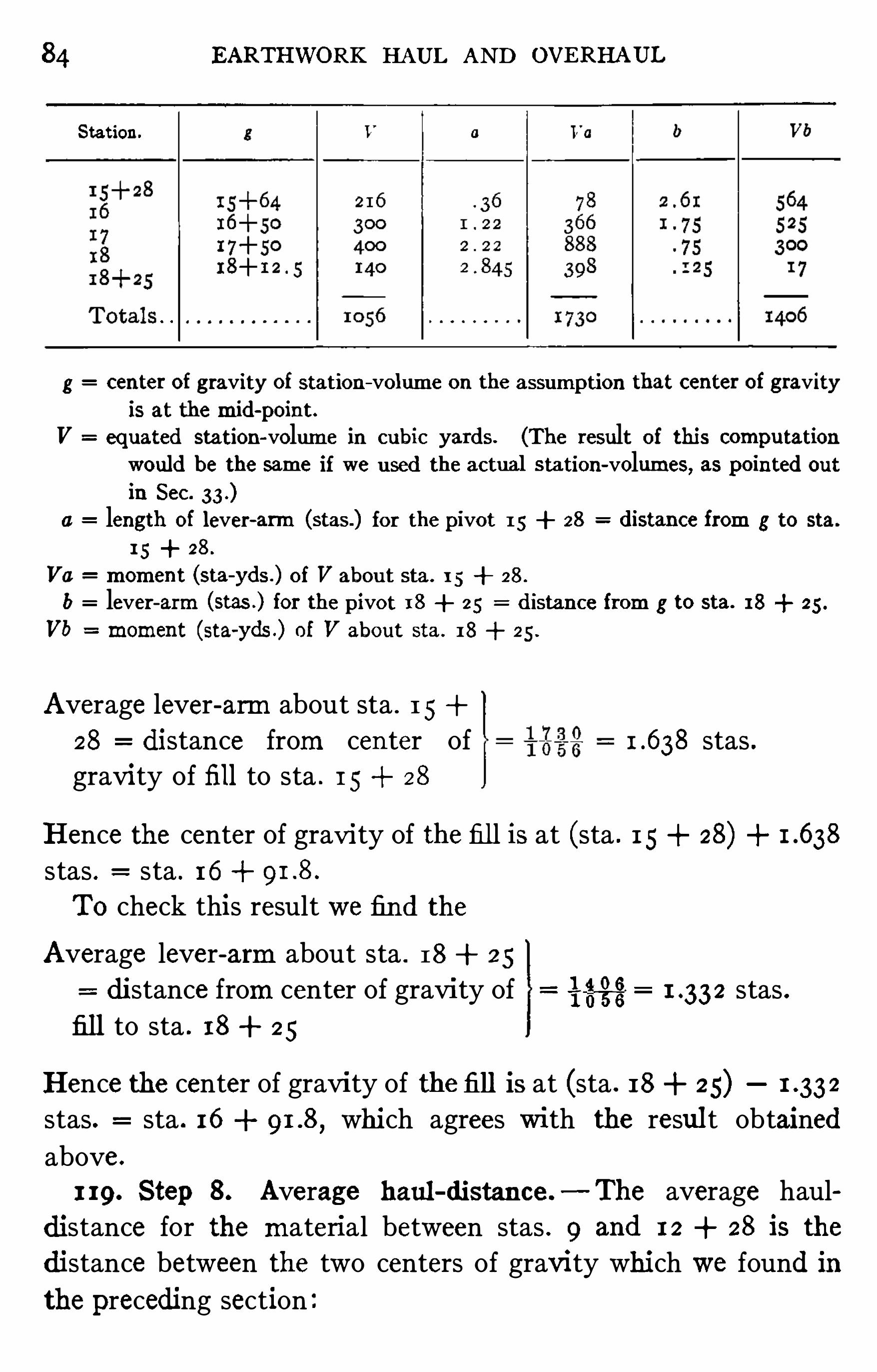
84 EARTHWORK HAUL AND OVERHAUL
Station.
g center of gravity of station—volumeon theassumption that center ofgravityis at themid-
point .
V equated station- volume in cubic yards. (The result of this computation
would be thesame if we used theactual station- volumes, as pointed out
in Sec.
a length of lever- arm (stas.) for thepivo t 1 5 28 distancefrom g to sta.
1 5 28 .
Va moment (sta-
yds . ) of V about sta. 1 5 28 .
b lever- arm (stas .) for thepivo t 1 8 25 distancefrom g to sta. 18 25 .
Vb moment (sta-
yds .) of V about sta. 1 8 25 .
Averagelever - arm about sta . 1 5
28 distance from center of stas .
gravity of fill to sta . 1 5 28
Hence the center of gravity of thefill is at (sta . 1 5 28)stas . sta . 1 6
To check this result wefind the
Average lever- arm about sta . 1 8 2 5
distancefrom center of gravity of gfig stas .
fill to sta . 18 25
Hencethecenter of gravity of thefill is at (sta . 1 8 25) 3 2
stas . sta . 16 which agrees with the resul t obtained
above.
1 19 . Step 8 . Average haul - distance.—The average haul
distance for the material between stas . 9 and 1 2 28 is the
distance between the two centers of grav ity which we found in
thepreceding section

86 EARTHWORK HAUL AND OVERHAUL
1 2 2 . Step 1 1 . Statement of overhaul . — The statement of
the overhaul just computed is given on lineA—VI of Fig . 36 .
Overhau l of Fig. 1 9 Computed by Method VII
(InMethod VII thecenter of gravity of each body of cut or fill is computed by
means of the mass curve by the method of moments. All limits aredetermined
b y the mass curve.)
1 23 . Step 1 . Data.
— W e are given the following informa
(1 ) Wearegiven theprofile, Fig . 1 9 .
(2) The volume of each station and substation as computed
from thenotes of final cross - sections is given on Fig . 1 9 .
(3) Them aterial between 9 00 and thegradepoint (1 3 + 75)was used to m akefill of full section from the gradepoint towardthe right as far as them aterial would go .
(4) The swell - factor for them aterial of the cut is given as 5 .
5) The free- haul distance is given as 300 ft .
124. Step 2 . Distrib ution of material . See Sec. 1 23
1 2 5 . Step 3 . Swell and equating- factors. Theswell - factor
is 5 (Sec . 1 23 Thereforetheequating - factor is
(Sec .
1 26 . Step 4 . Equate each station- vo lume of fill to volume in
place. Multiply each station~v olumeof thefil l by theequating
factor (See. 1 2 Theresulting volumes in placeareenteredin Fig . 19 .
1 2 7 . Step 5 . Plot the m as s curve. The m ass curve is
plotted from cut~v o lumes and equated fill—volumes in themanner
explained in Sec . 1 0 . In Fig . 1 9 sta . 9 00 is taken as the
origin of them ass curve.
1 28 . Step 6 . Limits of b odies of material . The left—handlimit of the cut is given as 9 00. Wefind theright—hand lim it
of the fill by them ass—curvemethod of Sec . 20 . Through A
9 00 on them ass curve draw a horizontal to meet the right
slopeof thecurveat somepoint B . Thehorizontal,thus drawn ,

OVERHAUL COMPUTED FOR FIG. 19 87
h appens, in this case, to coincide with the base line. B is the
right- hand lim it of the fill m ade from thematerial of the cut,
9 00 to 13 75 . By means of the engineer’s scale we find
that B is at 1 8 24. (If theplus of B had been estim ated by
eye, it would probably havebeen taken as 25 ft . instead of 24 ft .)The plus , 24 ft . , is now recorded in proper position on them ass
curve in Fig. 19 .
129 . Step 7 . Limits of free haul . The free—haul distance
is given as 300 it . By themass - curv emethod of Sec. 4 1 wefind
that a horizontal line 300 ft . long which has its extrem ities,C
and D,on the curvemust have one extremity at sta . 1 2 29
and theother at sta . 1 5 29 . These two stations are the free
haul limits . (The plus of each limit was scaled in this case
Theposition of C was found to be 1 2 30 and that of D,1 5
28 . As the two limits must be just 300 ft . apart, a compromise
was m ade on theplus of 29 ft .)130. Step 8 . Centers of gravity . Thecenters of gravity are
found by Method VII, Sec . 34 , thus : Draw a vertical through
C cutting AB at C’. Wemeasure the area ACC’
A with a pla
nimeter andfind it to be sq . in. (This area may be com
puted from thedimensions of the component trapezoids .) Sinceone square inch Of paper represents 2 x 500 1000 sta—yds .
,
the area ACC’A represents x 1000 2 13 1 sta-
yds . of
haul . The ordinate CC is found, by scaling,to represent
1064 c .y . (SeeSec. Thus thedistance from thecenter of
gravity, E, of thecut AC to the right—hand limit ; C, Of the cut is
ordinateCC’
(in cubic
stas .
E’
, likeC,is at sta . 1 2 29
EE’
2
ThereforeE, the center of gravity of cut,sta . 9 to sta . 1 2 29 , is at sta . 10

88 EARTHWORK HAUL AND OVERHAUL
Similarly we find that the distance between the left - hand
limit,D
,of fill DB and the center of gravity
,F
,of that fill
,is
ordinateDD’
(in cubic yards)
3559, stas .
F’
,likeD
,is at sta . 1 5 29
FF’
1 67
ThereforeF,thecenter of gravity of fillDB
,is at sta . 1 6 96 .
13 1 . Step 9 . Average haul- distance The average haul
distance for them aterial of the cu t,sta . 9 00 to sta . 1 2 29 ,
is the distance between E,the center of gravity of this cut
,and
F,the center of gravity of the corresponding fill, stas . 1 5 29
to 1 8 24 . From Sec . 1 30 wehave
E at sta . 10
F at sta . 1 6
Average haul- distance EF stas .
1 3 2 . Step 10. Average overhaul—distance. The average
overhaul- distance for the m aterial in the out between stas . 9
and 1 2 29 is equal to the average haul- distance less the free
haul distance.
Averagehaul- distance (Sec . 1 3 1 )Free- haul distance (Sec . 1 23
Average overhaul - distance stas .
The average overhaul—distance is evidently equal to EE’
plus
FF’
,also . SeeFig . 1 9 .
133 . Step 1 1 . The overhaul . Theoverhaul on thematerial
m ov ed from cut AC to fill DB is equal to thefi
v olume of cut AC
multiplied by the average overhaul- distance. Volume of cut
is 1064 c .y . (Sec . 1 30) and the average overhaul- distance is
stas . (Sec . Thereforetheoverhaul 1064 X
3907 sta—yds.

90 EARTHWORK HAUL AND OVERHAUL
1 36 . Step 2 . Distribution of material . SeeSec. 13 5
13 7 . Step 3 . Swell and equating- factors. Theswell - factor
is 5 (Sec . 135 Theequating—factor is thereforeI
(Sec .
1 38 . Step 4. Equateeach station- volume of fill to volume in
place. Wemultiply each station—volumeof fill by theequatinga
factor (Sec. The equated fill - volumes have been
entered on Fig . 1 9 .
1 39 . Step 5 . Limits of b odies of material .
— The limits of
the out are 9 00 and 13 75 (Sec . 135 The left - hand
limit of thefill is 13 75 . The right - hand limit of thefillm adefrom them aterial of the cut is found by thearithmetical method
of Sec . 20 . It was found in Sec . 20 that the right—hand lim it of
the fill is 1 8 25 .
140. Step 6 . Limits of free haul . The free- haul limits are
determined by themethod of Sec . 40 . In Sec. 40 the free—haul
lim its for Fig . 1 9 were found to be stas . 1 2 28 and 1 5 28 .
141. Step 7 . Centers of gravity. UseMethodVIII,Sec. 3 5 .
By this method the center of gravity of thecut , to
was found to lie at 10 Applying the samemethod to
find the center of gravity of thefill, 1 5 28 to 18 25 , wehavethe following computations :
COMPUTATION FOR CENTER OF GRAVITY OF EACH STATION
BODY
Station
2042042 70
348
l length (ft .) ofprismoid (station body) ;A end area (sq .
x distance (ft ) from mid-
po int to center of gravity of prism oid.

OVERHAUL COMPUTED FOR FIG .19 9 1
COMPUTATION OF MOMENTS
Station.
g center of gravity of station body , as computed above.
V equated station- volume in cubic yards. (The res ult of this computation
would be the same if we used the actual fill- vo lumes instead of the
equated (Sec.
a length of lever- arm (stas.) for pivot at sta. 1 5 28 distance from
center of gravity of station body to sta. 1 5 28 .
Va moment (sta. yds.) of station- volumeabout sta. 1 5 28 .
b length of lever- arm (stas.) for pivo t at sta. 18 25 distance from
center of gravity of station body to sta. 1 8 25 .
Vb moment (sta-
yds.) of the station- volumeabout sta. 18 25 .
Average lever - arm about sta . 1 5 28
distance from center of gravity stas .
of fill to sta . 1 5 28
Hencethecenter of gravity of thefill is at (sta . 1 5 28) 1 .653
stas . sta . 1 6
To check this result wefind the
Average lever- arm about sta . 1 8 + 25
distance from center of grav ity stas .
of fill to sta . 1 8 25
Hencethecenter of gravity of thefill is at (sta . 1 8 25) 1 .3 1 6
stas . sta . 1 6 (check within ft .)142 . Step 8 . Average haul- distance. The average haul
distance for them aterial of the cut, 9 00 to 1 2 28
,is the
distance between the center of gravity of that material and the
center of gravity of thefill,1 5 28 to 1 8 25 .
Center of gravity of fill (Sec . 14 1 ) sta . 1 6
Center of grav ity of cut (Sec . 14 1 ) sta . 1 0
Averagehaul - distance stas .
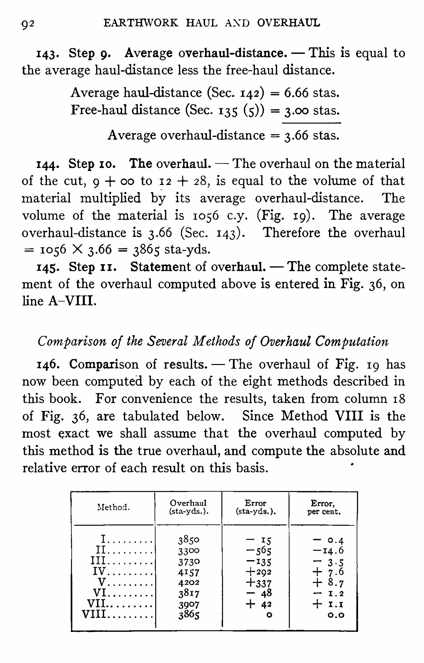
1
9 2 EARTHWORK HAUL AND OVERHAUL
143 . Step 9 . Average overhaul- distance. This is equal to
the averagehaul- distance less the free—haul distance.
Averagehaul - distance (Sec. 142) stas .
Frec- haul distance (Sec . 1 3 5 stas .
Average overhaul - distance stas .
144. Step 10. Theoverhaul . Theoverhaul on thematerial
of the cut, 9 00 to 1 2 28
,is equal to the volume of that
m aterial multiplied by its average overhaul - distance. The
volume of the material is 1056 c .y . (Fig. The averageoverhaul- distance is (Sec . Therefore the overhaul
1056 X 3865 sta-
yds .
145 . Step 1 1 . Statement of overh aul . The complete state
ment of the overhaul computed above is entered in Fig . 36 , on
lineA—VIII.
Comparison of theSeveral Methods of Overhaul Computation
146 . Comparison of results.
— The overhaul of Fig . 1 9 has
now been computed by each of the eight methods described inthis book . For convenience the results
,taken from column 1 8
of Fig . 36, are tabulated below . Since Method VIII is the
m ost exact we shall assum e that the overhaul computed by
this method is the true overhaul , and computethe absoluteandrelativeerror of each resul t on this basis .

94 EARTHWORK HAUL AND OVERHAUL
to obtain more or less discordant results by Method V . Any
difference between theresult obtained by MethodV and that byMethod IV is due to thoseerrors which occur in plotting and scal
ing themass curve. Let us seewhat is them aximum possibleerror in the result
,as found by the m ass curve. If the total
possible error in plotting a distance is inch,and the total
possible error in scaling a distance is the same,them aximum
resultant error in the yardage,as scaled from the m ass curve
,
is X 500 10 c .y . So the volume of the overhauled material
,scaling 1064 c .y .
,may be as sm all as 1064 10 1054 ,
or as great as 1064 10 1074 ; and the distance overhauled,
scaling stas .,may be as little as X
stas .,or as much as stas . Therefore
the true overhaul (true taking Method IV as the standard) maybe as little as 1054 X 4079 sta-
yds.
,or as much as 1074 X
43 28 sta-
yds. That the result, 4202 sta—yds.
,which has
been obtained by Method V is so near the result from MethodIV —
so far within the extremes computed above— is due to
the fact that of the several errors m ade in plotting and scaling,
some havebeen negative and somepositive, and the two kinds
of error largely neutralize each other . It is because errors of
graphical work are as lik ely to bepositive as negative, and very
large errors are rare, that the actual resultant error in the
overhaul for onebody of m aterial computed by them ass curve
is seldom so large as the computed lim it of error ; and that the
error in the sum of several item s of overhaul thus computed is
generally insignificant . SeeSec . 203 .
Method VI gives a result in error by and this result,
too,is determined by the assmnptions relative to the position
of the center of grav ity of each station—volume upon which the
method is based. The judgment of the computer has no effect
on the result . The error obtained is a true measure of the
accuracy of themethod under the conditions of thegiven profile.
Method VII differs from Method VI only as Method V differs

OVERHAUL COMPUTED FOR FIG .19 95
from Method IV ; Methods VIandVIIare based on theassumption that the center of gravity and center of length of a station
volumearecoincident , but thecomputations of thelatter method
are performed graphically (using the m ass curve) , and of the
former,arithmetically . Hence the error in the result obtained
by Method VII is not a true measure of the accuracy of the
method.
In the foregoing,it has been assumed that the result
, 3865
sta-
yds . of overhaul Obtained by the use of Method VIII,is
without error because of the refined process of determining the
center of gravity of a given body of m aterial . Wemust remem
b er,however
,that the lim its of each body of m aterial aredeter
m ined,in this method as in II
,III
,IV
,VI
,on the assumption
that thevolumeper running foot , of a station solid, is constant ;and in the case of the problem of Fig . 1 9 this is not true. It is
believed that because of the uncertainties as to swell and dis
tribution,the lim its of error in the cross - sectioning
,and because
of the sm all cost of one station - yard of haul,and of the extra
w ork involved in computing overhaul by that method, the use
of Method VIII will not be justified except under extraordinary
conditions .
To sum up : The percentage errors in the results Obtained by
Methods II,III
,IV , VI, and VIII Show the true relative accu
racies of thosemethods for all profiles sim ilar to that of Fig . 1 9 .
For bodies of m aterial of other shapes the relative accuracies
will be different .
The percentage of error in the result obtained by Method Iis dependent entirely upon the skill and judgment of the com
puter . If,when about to compute by some one of the m ore
accuratemethods theoverhaul for thevarious bodies of m aterial
along a given profile, the computer will take the trouble to
computefirst by eye (Method I) the overhaul on each body and
m akea record thereof,hewill havea rough check on the correct
ness of the later results obtained by them ore accuratemethod

96 EARTHWORK HAUL AND OVERHAUL
and at the same time he will have an opportunity to find the
percentage of error in each of the results obtained by eye, and
thus find approxim ately his limit of error in the use of that
method.
Theerror in the resul t obtained by Method V is a resultant of
the error obtained by Method IV and the errors incidental to
plotting and scaling them ass curve, and the latter errors depend
upon the skill of thedraftsm an and the scale of them ass curve.
In the sameway,Method VII gives an error in any case, which
is the resultant of the error com ing from Method VI and the
errors of plotting and scaling them ass curve. See Sec . 203 for
comments on results obtained for the overhaul of Fig. 38 .
It is suggested that the engineer who is responsible for the
selection of a method for computing overhaul on an extensive
piece of earthwork , apply Methods IV , V ,VI
,and VII to a few
of those bodies of overhauled m aterial for which the four
methods may be expected to giVe them ost widely differing re
sults,and select for the computation of the rem aining overhaul
that method which,while giving satisfactorily precise results ,
requires the least work . When time permits , Methods V and
VII serve as excellent checks on Methods IV and VI respec
tively . The engineer will usually be compelled by lack of time
to useMethod I to check the overhaul computed by sub ordi
nates by some one of them oreexact methods .


CHA PTER VII
OVERHAUL COMPUTED FOR THE COMPLEX CASE OF FIG . 38
In this chapter Methods I, IV , V , VI, and VII of overhaul computation are
applied, oneafter ano ther, to the complex problem of Fig . 38 . The steps in each
method are formally stated. The results are presented in Fig . 36 on the linesbeginning with “B , and compared in Sec . 203 . This chapter, like thepreceding ,is designed to serve as a working guide to the computer as so on as the method
has been selected. (Fig. 36 faces page 67 ; Figs. 36a, 3 7 , and 38 facepage
147 . Each of the overhaul computation methods , I, IV ,V
,
VI, and VII (Secs . 47—5 will be applied in this chapter to the
complex overhaul problem presented by theprofile of Fig . 38 .
It will be observed that the problem of Fig . 38 differs from
that of Fig. 1 9 in two points : (1 ) In Fig . 38 thereare four dis
tinct bodies of m aterial overhauled,whilein Fig. 1 9 there is but
one. (2) Thework of determining swell and equating—factors
and distribution of material was simple in Fig . 1 9 , but is com
parativ ely complicated in Fig. 38 . After we have determinedthe swell and equating - factors and thedistribution of material
,
for the case of Fig . 38 , we shall find that the further steps of
determining limits,centers of gravity
,etc .
,are littlem ore than
repetition of the corresponding steps taken in Chapter VI for
Fig . 1 9 .
To conform to good practice, wefirst m akeready for thecorn
putations by gathering all the available data . All the data for
the overhaul problem in hand are given in Sec . 148 , which isStep I of Method I, and are repeated in Sec . 1 5 7 .
The results obtained by thedifferent methods of computation
will be recorded in Fig . 36 , and compared in Sec. 203 .
9 7

98 EARTHWORK HAUL AND OVERHAUL
Overhaul of Fig. 38 Computed by Method I
(In Method I center of gravity and all limits aredetermined by eye.)
148 . Step 1 . Data.—We have the following data bearing
on the distribution of m aterial between t1 and t17 in Fig . 37
which shows a sm all- scale copy of theprofile of Fig . 38 .
(1 ) All thegrading was donewith a steam - shovel plant .
(2) Volumes computed from final measurements areas follows
The volumes tabulated above are shown on Fig. 37 ; and the
v olumes station by station are shown on Fig . 38 .
(3) The grading was performed in this order : (a) The shovel
went first to cut t14t16 . The excavated material was hauled in
both directions , m aking all of fill t16t17 and nearly all of fill tutu .
After completing this cut (b) the shovel m oved to tn and made
a cutting to tg , sending part of them aterial to the right, com
pleting fill tutu ; part to fill tstg ; and a third part to fill t4h .
W ithout completing cut tgllz (c) theShovel moved to t8 andmadea cutting from t, to t7 , sending the m aterial to fill t4t7 . The
shovel then turned around and m ade a cutting from t7 to ts,
sending the m aterial to fill l4iq . This work completed the cut
mg . (d) The shovel m oved to t, and completed the cut tgtm,
sending a part of the m aterial to fill tgtg enough to complete
that fill and therem ainder of them aterial to fill t4tq . (e) The
Shovel then turned around and m oved to t4 , and excavated cut
tzt4, a part of the m aterial making the entire fill tl lg , and the
rem ainder completing fill t4t7 .
(4) From diary and daily car records thenumber of car - loads
h auled from out tgtlg to fill t4t, was ascertained. From them onthly

IOO EARTHWORK HAUL AND OVERHAUL
of the profile that this would require all the m aterial of theadjacent cut back as far as 8 1 70 . The limits of bodies ofm aterial which appeared to beoverhauled havebeen entered inFig . 36 on lines B—I— 1
, 3 , 4 . (Such form al record may be considered superfluous in practice for thedetails of rough estim ates
of overhaul . The details areentered here to permit compari
sons to be m ade between the various methods of computing
overhaul .)1 5 1 . Step 4. Centers of gravity . The center of grav ity of
each body of cut and of fill overhauled was picked out by eye
(Sec . For example, the center of gravity of cut , 76 80
to 8 1 70 ,appeared to the estim ator to be at 78 90 . (To
m ake the best estim ate of the position of the center of gravity
of a body of cut or of fill,theprofile to the right and to the left
of that body should be concealed from view whilem aking the
estim ate. ) The centers of gravity, determ ined by eye, have
been entered in Fig . 36 , on lines B - I—1, 3 , 4 .
1 5 2 . Step 5 . Average haul—distance. The average haul
distance for a body of overhauled m aterial is the distance from
its center of gravity in cut to its center of gravity in fill. Thus
the average haul - distance for the m aterial of cut , 76 80 to
8 1 70 ,is the distance between sta . 78 90 (column 6) and
sta . 63 50 (colum n or stas . ,which is entered in
column 1 1 .
1 53 . Step 6 . Average overhaul - distance.
— Theaverageover
haul - distance for any body of overhauled m aterial is equal
to the average haul- distance for that body less the free- haul
distance. The free- haul distance is given as 1 000 ft . (Sec . 148
Thus the average overhaul- distance for the m aterial of
cut, 76 80 to 8 1 70 ,
is equal to (taken from column 1 1 )less 10 stas .
,which is entered in colum n 1 2 .
1 54. Step 7 . Volumes of b odies of overhauled material .
If the station - volumes along theprofile aregiven ,thevolume of
each body of overhauled m aterial may be found by summ ing

OVERHAUL COMPUTED FOR FIG . 38 10 1
thestation - volumes that constitute that body . In this way the
volumes recorded in colum n 1 5 , lines B—I—1 , 3 , 4 ,were found.
If the station—volumes arenot included with thedata , they may
beestim atedwith thehelp of earthwork tables or a yardagescale.
1 5 5 . Step 8 . The overhaul . - The overhaul on a body of
material is equal to the volume (in place) of that m aterial mul
tiplied by its averageoverhaul - distance. For example, theover
haul on thematerial of cut, 76 80 to 8 1 70 ,
is equal to
(taken from colum n 1 5 , Fig . 36 , line B—I-
4) multiplied by
(taken from column 1 2) sta-
yds.
,which is entered in
column 1 8 .
1 56 . Step 9 . Statement of overhaul . The full statement
of the overhaul just estim ated for the profile, Fig . 38 , is given
on the upper set of lines B—I—1 , 3 , 4 , Fig . 36 . The lower set of
lines B—I—1, 3 , 4 shows results obtained by a second estim ator .
Overhaul of Fig. 38 Computed by Method IV
(In Method IV center of gravity of body of cut or fill is assumed to lie at its
center of volume, and is computed by arithmetic . Limits are computed by
arithmetic .)
1 5 7 . Step 1 . Data — We have the following data bearing on
the distribution of m aterial between t1 and t17 in Fig . 3 7 whichshows a sm all—scale copy of theprofile of Fig . 38 :
(1 ) All the grading was donewith a steam - Shovel plant .
(2) Volumes computed from final measurements areas follows
The volumes tabulated above are shown on Fig . 3 7 ; and the
volumes station by station are shown on Fig . 38 .
(3) The grading was performed in this order : (a) The shovel

1 02 EARTHWORK HAUL AND OVERHAUL
went first to cut t14t16 . The excavated m aterial was hauled in
both directions , m aking all of fill t16t17 and nearly all of fill tut“.
A fter completing this cut (b) the Shovel moved to tu and m ade
a cutting to tg , sending part of the m aterial to the right , com
pleting fill tu tu ; part to fill tstg ; and a third part to fil l t4t7 .
W ithout completing cut lgllg (c) the shovel moved to t8 and m adea cutting from lg to h ,
sending the m aterial to fil l t4t7 . The
shovel then turned around and m ade a cutting from A to lg,
sending the m aterial to fill t4ty. This work completed the cut
h tg . (d) The shovel m oved to lg and completed the cut tgllz,sending a part of them aterial to fill tstg enough to complete“
that fill and the remainder of them aterial to fill t4t7 . (e) Theshovel then turned around and moved to t4, and excavated cut
tzt4 , a part of the m aterial m aking the entire fill tl tz, and the
remainder completing fill t4h .
(4) From diary and daily car records the number of car - loads
hauled from out tgtm to fill fit; was ascertained. From them onthly
estimates and car records the average car—load (cubic yards in
p lace) was computed. In this way it was computed that 5000
c .y . (in place) of cut tgtm went to fill t4t7 .
5) From field diaries and car records it appeared that 1400 c .y .
(in place) went from out t9 l12 to fill tu tu .
(6) Swell . Cut t14t16 had a uniform swell . The 1400 c .y .
hauled from cut tgtm to fill t12t14 had no Swell . The m aterial
h auled to fill tgtg had a uniform swell . The m aterials making
,fills tl tz and t4ty had the same swell . These swells were based on
the judgment of thosewho watched theprogress of the grading .
NO measurements had been made from which the swell of any
o ne body of m aterial could bedirectly computed.
(7) Free- haul distance is 1000 ft . (Contract )
(8) The American Railway Engineering Association basis of
computing overhaul is to be used. (Instructions )1 58 . Step 2 . Distrib ution ofmaterial . Thedata Show that
t he distribution of them aterial was complex (Secs . 1, It
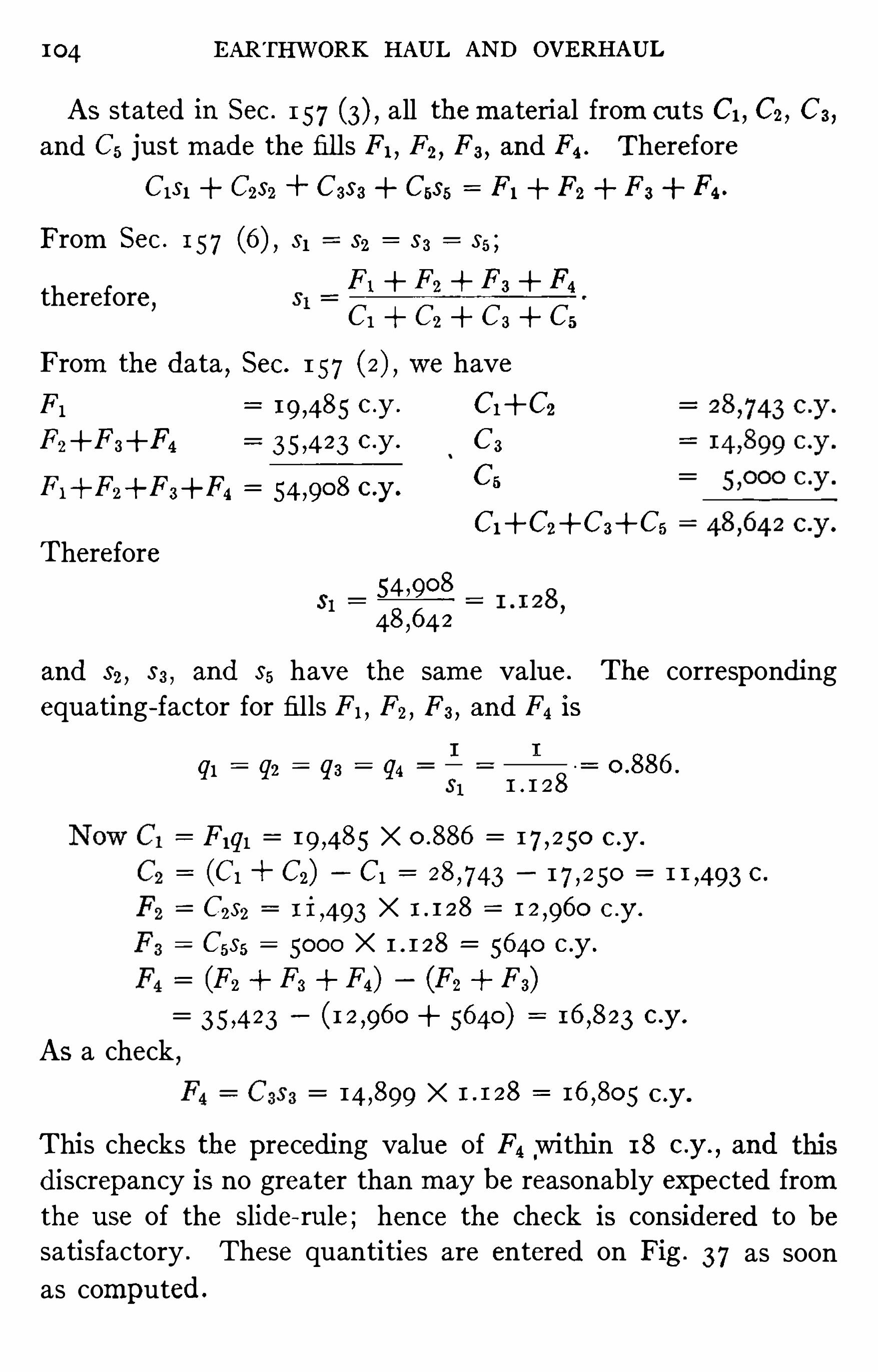
104 EARTHWORK HAUL AND OVERHAUL
As stated in Sec . 1 57 all them aterial from cuts C1 , C2, C3 ,and C5 just m ade the fills F 1 , F2, F 3 , and F4 . Therefore
C13 1 C252 “I" C35 3 C585 F 1 “I" F2 “I“ F 3 "I“ F4 .
From Sec . 1 5 7 s1 sz s3 s5 ;
C1 + C2 + C3 + C5
From the data,Sec. 1 57 we have
therefore,
PI c .y . C1+C2
F2+F 3+F4 c .y . C3
F 1+F2+F 3+F4 c .y .
Cs
C1+C2+C3+C5Therefore
and $2, s3 , and s5 have the same value. The corresponding
equating—factor for fil ls F 1 , F2, F 3 , and F4 is
QI Q2 Q 3 Q4
F 191 X c .y .
(C1 “I“ C2) C1 1 7 12 50 C
C252 1 i,493 X c .y .
C5s5 5000 X 5640 c .y .
(F. P3 + F4> (112 + F 3)
5640) c .y .
As a check
X c .y .
This checks the preceding value of F4 within 1 8 c .y .
, and
discrepancy is no greater than may be reasonably expected from
the use of the slide—r ule; hence the check is considered to besatisfactory . These quantities are entered on Fig . 37 as soon
as computed.

OVERHAUL COMPUTED FOR FIG . 38 105
The swell - factor for cut C6 is unity (Sec . 1 5 7 therefore
F, Case 1400 X 1 1400 c .y .
C4 (C4 C5 Cs) (C5 Ce)
(5000 1400) c .y .
Theequating—factor for fill F 5 is 95 g: gigéThe volume of fill F7 (F6 F7) F6 1400
C -y
Theequating- factors for fil ls F7 and F8 are found thus : Fromthedata
,Sec. 1 57 and the foregoing computations wehave
F797“I‘ F898 C7 C8 ,
q’(F7 + Fs) + 4600)
0 78 °
07 F747 X 0 - 753 c y
Cs ma 4600 X 0 - 753 cr
c .y .
This value of C7 C3 differs from (the volumeStep 1 by 3 yards . This
‘
is a close agreement .
The swell- factors of cuts C7 and C8 are
I I
97 98 0 - 753
Having entered on the profile, Fig . 3 7 , all these computedvolumes
,swell - factors
,and equating
- factors,we are ready for
the next Step .
160. Step 4. Limits of b odies of material . Figs . 37 and 38 .
There is no division plane in fill F1 . The position of division
plane t, which limits cut C1 on theright is found thus : W e have
found that C1 c .y . ; by themethod given in Sec . 20,
wefind that in passing from tz (sta . 14 1 2) to sta . 1 7
wehavea total volumeof and that in passing from t; to

106 EARTHWORK HAUL AND OVERHAUL
1 8 we have a total of 56 13 c .y .
Hence theright- hand lim it t3 of cut C1 must liebetween 1 7+ 30 . 5
and 1 8 05 . 5 . Now between these two stations thevolumeper
running foot
.8(sta . 18 - (sta . 1 7 4
.
7574 C Y
Therefore ta lies to the right of 1 7 a distance
74 8ft . Therefore the div ision plane be
tween cut C1 and cut C2 lies at
t», (sta . 1 7 sta . 1 7
(To check this result wecomputethedistancefrom sta . 1 8 05 . 5
back to t3 : t;, to 1 8 There74 -8
fore the station of ta is (sta . 18 sta .
This agrees with the preceding result . As the com putations
were performed with the Slide- rule a discrepancy of some tenths
of a foot is to be expected, and the precise agreemen t here isaccidental .)The details of the computations performed to ascertain the
station and plus of each o f theother division -
planes are om itted.
The results of the computations are tabulated below .
POSITIONS OF DIVISION PLANES.
Substation volumes .
Division plane. Stat ion and plus .
On the left . On the righ t .
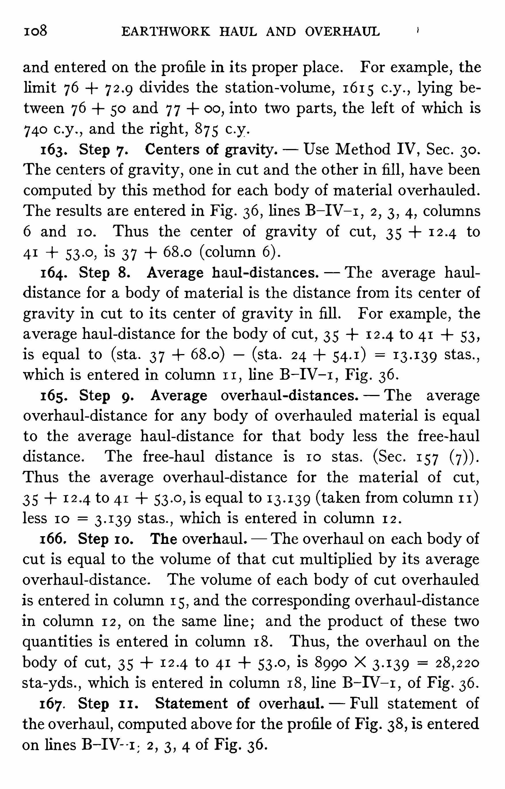
108 EARTHWORK HAUL AND OVERHAUL
and entered on theprofilein its proper place. For example, the
lim it 76 divides the station—volume,1 6 1 5 c .y .
,lying be
tween 76 50 and 77 00,into two parts, the left of which is
740 c .y .
,and the right
,875 c .y .
163 . Step 7 . Centers of gravity. UseMethod IV , Sec . 30 .
The centers of gravity,onein cut and theother in fill
,havebeen
computedby this method for each body of m aterial overhauled.
Theresults areentered in Fig . 36 , lines B—IV—r,2, 3 , 4 , columns
6 and 10 . Thus the center of gravity of cut, 3 5 to
4 1 is 3 7 (colum n164. Step 8 . Average h aul - distances.
— The average hauldistance for a body of m aterial is thedistance from its center of
gravity in cut to its center of gravity in fill. For example, theaveragehaul - distance for thebody of cut
, 35 to 4 1 53 ,
is equal to (sta . 3 7 (sta . 24 stas .
which is entered in column 1 1,line B—IV—r , Fig . 36 .
1 65 . Step 9 . Average overhaul - distances. The averageoverhaul - distance for any body of overhauled m aterial is equal
to the average haul - distance for that body less the free- haul
distance. The free- haul distance is 10 stas . (Sec . 1 57
Thus the average overhaul—distance for the m aterial of cut,
3 5 to 4 1 is equal to (taken from colum n 1 1 )less 1 0 stas .
,which is entered in colum n 1 2 .
1 66 . Step 10. Theoverh aul . Theoverhaul on each body of
cut is equal to the volume of that cut m ultiplied by its averageoverhaul - distance. The volume of each body of cut overhauledis entered in column 1 5 , and the corresponding overhaul- distancein column 1 2
,on the same line; and the product of these two
quantities is entered in column 18 . Thus,the overhaul on the
body of cut , 35 to 4 1 is 8990 X
sta -
yds .
,which is entered in column 1 8
,lineB—IV— r
,of Fig . 36 .
167 . Step 1 1 . Statement of overhaul. Full statement of
theoverhaul,computed abovefor theprofileof Fig. 38 , is entered
on lines B—IV -
1 . 2, 3 , 4 of Fig . 36 .

OVERHAUL COMPUTED FOR FIG . 38 109
Overhaul of Fig. 38 Computed by Method V
(In Method V center of gravity of body of cut or fill is assumed to lie at its
center of volume, and is determined by mass curve. Limits are determined b y
mass curve.)
1 68 . Step 1 . Data. Read Sec. 1 5 7 .
169 . Step 2 . Distrib ution of material . SeeSec . 1 58 .
1 70. Step 3 . Determination of swell - factors and volumes of
the several b odies of cut and fill. Read Sec . 1 59 .
1 7 1 . Step 4. Equate each station- volume of fill to volume in
place. SeeSec . 1 6 1 . Equated fill- volum es only areused with
thecut- volumes throughout the rem aining steps of this Method.
1 72 . Step 5 . Plot themass curve. The origin of them ass
cur've was taken above the profile at sta . 10 08,Fig . 38 .
The cut- volumes are considered positive and the fill—volumes
negative. The ordinate at each station is the algebraic sum
of the station- volumes lying between that station and 10 08 .
Theincrement to them ass curvefor a station - interval which con
tains both cut and fill, is theexcess of theoneover theother . In
Fig . 38 the horizontal scale of the profile and m ass curve is
1 in . 400 ft . ; thevertical scale of theprofile is 1 in . 20 ft . ;
and thevertical scaleof them ass curveis 1 in . c .y .
NOTE .
— The original drawing for this mass curvewas made on a rollof cross- section paper , 10 X 10 to the inch ; and the scales were 1 in.
100 ft .,horizontal, and 1 in . 2 500 c .y .
, vertical. The results given inthefollowing Steps were ob tained from the original draw ing .
1 73 . Step 6 . Limits of b odies of material .
— The base line
of this m ass curve is the balancing line. The points at which
the m ass curve cuts the balancing line m ark the limits of the
bodies of cut and fill . These points are noted and the plus of
each is scaled off and entered on them ass curve. Thus there
are div ision planes at stas . 1 7 64 ,23 44 , 54 94 , 58 1 2
,
and 8 1 24 . Also the horizontal drawn through the summit
o f themass curveat sta. 41 53 , is a balancing line, which ,by

1 10 EARTHWORK HAUL AND OVERHAUL
cutting themass curve,gives us division planes at stas . 24 02
,
4 1 53 , and 5 2 98 .
1 74. Step 7 . Limits of free haul . Find the lim its of free
haul by themethod of Sec . 41 . The plus of each lim it of free
haul is scaled and entered on the m ass curve. The free- haul
limits determined by this method are
Stas . and
1 75 . Step 8 . Centers of gravity. The center of gravity of"
each body of m aterial is found in cut and in fill by Method V,
Sec . 3 1 . Thus the center of gravity of cut , 3 5 1 2 to 41 53 ,
is found to be at 3 7 66,which is entered in column 6
,line
B—V—1,Fig . 36 . Centers of gravity thus determined are indi
cated above them ass curve, on Fig . 38 , by theprefix CM .
”
176 . Step 9 . Average haul - distances . The average haul
distance for a body of m aterial is thedistance from its center of
gravity in cut to its center of gravity in fill . Thus the averagehaul - distance for the body of cut
, 3 5 1 2 to 41 53 , is equal
to (sta . 37 66) (sta . 24 + 53) stas .
,which is re
corded in column 1 1,lineB—V—r , Fig . 36 .
1 77 . Step 10. Average overhaul - distances . The averageoverhaul - distance for any body of overhauled m aterial is equal
to the average haul - distance for that body less the free- haul
distance. The free—haul distance is 10 stas . (Sec . 148
Thus the average overhaul - distance for the m aterial of cut,
3 5 1 2 to 41 53 , is equal to (taken from column 1 1 )less 10 stas .
,which is recorded in column 1 2 .
1 78 . Step 1 1 . The overhaul . The overhaul on each body
of cut is equal to thevolumeof that cut multiplied by its average
haul—distance. The volume of each body of cut overhauled is
entered in column 1 5 , and the corresponding average overhaul
distance in column 1 2 on the same line; and the product of

I I 2 EARTHWORK HAUL AND OVERHAUL
colum n 6 ; for thefills , in column 10 . The computations m ade
to find the position of the center of gravity of the body of cut
lying between stas . 76 and 8 1 are given below .
Stat ion.
o o o o o o o o o o o o o
g center of gravity of station - volumeon assumption that center of gravity liesat themid-
point .
V station—volume in cubic yards.
a length in stations, of lever- arm distance from each mid-
point, in turn,to
the center of m oments,sta. 76 00 .
Va moment (station-
yards) of V about sta. 76 00 .
b lever- arm length ,in stations distancefrom each mid-
point , in turn,to the
center ofmoments,sta. 82 00 .
Vb moment (station-
yards) of V about sta. 8 2 00.
Average lever—arm about sta . 76
00 distance from center of stas .
gravity of cut to sta . 76 00
Hence the center of gravity of the cut,sta . 76 72 to sta . 8 1
is at (sta . 76 00) stas . sta . 78 This
result may be checked in the following way .
Average lever—arm about sta . 82
00 distance from center ofgravity of cut to sta . 82 00
Hencethecenter of gravity of the cut,sta . 76 72 to sta . 8 1
is at (sta . 82 00) stas . sta . 78 (check) .
This result , sta . 78 is entered in column 6,lineB—VI—4,
stas .

OVERHAUL COMPUTED FOR FIG . 38 1 13
Fig . 36 . The other centers of gravity were computed in like
manner,and entered on lines B—VI
,in column s 6 and 10,
Fig . 36 .
NOTE 1 .
—The computer who found the results ab ove, mul tiplied and
divided in thelong way . Ano ther computer, using the 10- inch slide- rule
,on
thesamedata found the sum of column Va to be and of column Vb,
and found the center ofgravity from moments Va to beat 78 90,
and from moments Vb , at 78
NOTE 2 . It will be ob served that in the computation ab ove,thecenter
of moments was arb itrarily taken at 76 00 instead of 76 which
is the left lim it of theb ody ofmaterial under consideration,because of the
greater ease thereby afforded in making the sub tractions to ob tain lengthsof lever- arm s
,co lum n a. For the same reason the center of moments for
thecheck computations was taken at 8 2 00 rather than at 8 1
187 . Step 8 . Average haul - distances . We have already
entered in Fig . 36 , lines B—VI— r,2, 3 , 4 , the center of grav ity of
each body of cut overhauled, and the center of gravity of the
corresponding body of fill . Thedistancebetween thetwo centers
of grav ity entered on the same line is the average haul- distancefor the body of cut
,the lim its of which appear on that line, and
is entered in column 1 1 on thesam e line. Thus theaveragehaul
distance for the body of cut lying between the lim its 5 2
and 5 2 is (sta . 5 2 (sta . 42
stas .
188 . Step 9 . Average overhaul - distances . The averageoverhaul - distance for each body of cut is equal to the averagehaul- distance of the body less the free- haul distance (1000 feet
in this case) . The average overhaul- distance for each body of
cut is entered in column 1 2,Fig . 36 .
189 . Step 10. The overhaul . — The volume of each body
of cut is entered in colum n 1 5 , Fig . 36 ; and the corresponding
overhaul , which is the product of the volume by the averageoverhaul- distance, is entered in column 1 8 .
190. Step 1 1 . Statement of overhaul . Lines B—VI—r,2, 3 ,
4 , of Fig . 36 , now constitute a full statement of the overhaul on

1 14 EARTHWORK HAUL AND OVERHAUL
the material represented by the profile of Figs . 3 7 and 38 , as
computed by Method VI.
Overhaul of Fig. 38 Computed by Method VII
(In Method VII the center of gravity of each body of cut or fill is computed
by means of themass curve by themethod ofmoments. All limits aredeterm ined
b y themass curv e. )
1 9 1 . Step 1 . Data. Read Sec . 1 57 .
192 . Step 2 . Distrib ution of material . Read Sec . 1 58 .
193 . Step 3 . Determination of the swell - factors and thevol
umes of the several b odies of cut and fill . Read Sec . 1 59 .
194. Step 4. Equate each station—volume of fill to volume in
place. Read Sec . 1 6 1 . Equated fill- volumes only areused with
cut—volumes throughout the rem aining Steps of this Method.
195 . Step 5 . Plot themass curve. Theorigin for them ass
curvewas taken above theleft end of theprofile at sta . 10+08,
Fig . 38 . The cut- volumes are reckoned positive and the fill
volum es negative. Theordinate at each station is the algebraic
sum. of the station- volumes lying between that station and
sta . 10 08 . In Fig. 38 the horizontal scale of theprofile andof them ass curve is 1 inch 400 feet ; the vertical scale of the
profile is 1 inch 20 feet ; and the vertical scale of the m ass
curve is 1 inch c .y .
NOTE.
— The o riginal drawing for this mass curvewas made on a roll ofcross- section paper, 10 X 1 0 to the inch ; and the scales were: horizontal
,
1 inch 100 feet ; vertical, 1 inch 2 500 c .y . The results given in thefollowing Steps were ob tained from the original draw ing .
196 . Step 6 . Limits of b odies of material . The base lineof this m ass curve is a balancing line. Thepoints at which the
m ass curvecuts thebalancing line, m ark the limits of thebodies
of cut and of fill. These points are noted and the plus of each
is scaled off and entered on the m ass curve. Thus there are
division planes at stas . 1 7 64 ; 23 44 ; 54 94 ; 58 1 2 ;
8 1 24 . A lso thehorizontal drawn through the summit of the
mas s curve at 41 53 is a balancing line, which ,by cutting the

1 1 6 EARTHWORK HAUL AND OVERHAUL
202 . Step 12 . Statement of overhaul . The complete state
ment of theoverhaul on theprofile Shown in Figs . 36a, 3 7 , ascomputed by Method VII, is given on lines B—VII— r
,2, 3 , 4 of
Fig . 36 .
Comparison ofResults
203 . The foregoing results compared. The results obtainedin this chapter are clearly set forth in Fig . 36 , and are readily
compared. However,to save the time of the reader the results
have been retabulated in three different ways below . MethodVIII, the most accurate of all , was not applied to Fig . 38 ,
because of the labor involved . So in the comparisons of Tab les
I and II the results obtained by Method VI, which methodstands second in point
’
of accu racy (Sec . are considered to
be true results .
Referring to Table I. The errors in the results of Method I,
in which the lim its and centers of grav ity aredeterm ined by eyedirectly from theprofile, range from 1 3% to approxi
m ately . Observe that the error in the total overhaul is only
about less than as is to be expected because theerror
in the sum of several estim ates will always be sm aller than thelargest error of the component estim ates . In Fig . 36 are shown
the results Obtained by two men separately applying Method I.
The group of results that we have not copied into the following
tables has decidedly sm aller errors than those copied. How
ever,a third estimator m ight obtain results in error by more
than It should be stated here that theprofile of Fig . 38
presents extremely unfavorable conditions for determining over
haul by Method I,because Of the fact that cuts (Fig . 36a) t2t4,
tgtlz, t14t16 , and fills t4t7 , tstg , t15t17 , wereon steep hillsides . The fair
results obtained by this , by far the quickest , method of com
puting overhaul , seem to indicate that it has decided value for
m aking rough estim ates of overhaul , whether for checking over
haul computed by some m ore accurate method or for prelimi
nary studies ; or,under proper conditions , for m aking monthly

OVERHAUL COMPUTED FOR FIG . 38 1 1 7
estimates of overhaul . The best results from this method are
to be expected from onewho is familiar with the ground along
theprofile, and with oneof them ore accuratemethods of over
haul computation . For rem arks on acquiring skill in theuse of
Method I,see Sec . 146 .
TABLE I
Errors in the overhaul ofFig . 38 computed b y Methods I, IV , V , VI, VII,
grouped b y Methods . Overhaul computed b y Meth od VI is taken as the
true overhaul .
Method.
R i
ggsgénetgrorI
to +5 25
to
to
7 13 25NOTE . Overhaulcomputed b yMethod VI istaken as thetrue o verhaul ,in this tab le.
t o

1 18 EARTHWORK HAUL AND OVERHAUL
In Method IV the computations are all m ade by arithm etic ;in Method V ,
by the m ass curve; but in both the center of
volume is taken as the center of gravity . On the individual
bodies theerror ranges from zero to approxim ately ; but
the error of the total is only about On this particular
profile theerrors due to assum ing that center of gravity lies at
center of volum e,are all of one sign ,
and therefore cum ulative.
Of course the Sign of the error for any given body of m aterial
depends upon the Shape of that body .
In Table II the results obtained by the several Methods for
each body of m aterial are grouped together .
TABLE II
Errors in theOverhaul of Fig . 38 computed b y Meth ods I, IV , V , VI, VII,
grouped b y b odies of o verhauled m aterial . Overhaul computed b y Meth odVI is taken as the t rue overhaul .
Body of o verhaule
ldIr
\Inate
Metgtgt
c
ii
gncom
Overhaul (sta Error (sta Error (per cent ) .r1a o .
In TableIII all theoverhaul quantities obtained bym ass curve
are so arranged as to bring out clearly the range of errors which

1 20 EARTHWORK HAUL AND OVERHAUL
obtained for body No . 4 by this large- scalem ass curve, is about
while the limit of error for the smaller body,No . 1
,is about
this on the assumption that all errors of plotting and
scaling are of m axim um Size and of such sign as no t to perm it
cancellation in summ ing them . Thus the sm all errors actually
obtained are sm all because errors of m aximum size are not
frequent and m oreover tend to cancel in the sum m ation . The
larger the scale the sm aller the error to be expected.
W hen we consider the uncertainty in thevolumes obtained by
cross - sectioning irregular cuts and fills,and in the swell- factors
,
and,further
,remem ber that the actual distribution of m aterial
must be replaced by an assumed distribution before we can
proceed with the computation of overhaul , the use of them ass
curve,when due regard is paid to the scale, seem s , even for the
method of m oments , to be fully justified.
In any case the choice of method will be influenced by the
quality of thedata supplied to , and the time at the disposal of,the com puter , the use to which the results are to be put , and
finally by theprevious training and experience of the computer .


1 22 EARTHWORK HAUL AND OVERHAUL
from month to m onth ,say as he obtains additional data on
swell from the grading in progress . Of course when any un
expected condition of m aterial is found in thework of grading ,the side slopes as well as theestim ated swell - factors may require
modification . Suppose that the original plan of distribution
of m aterial along the profilewas based on quantities computed
from an assumed side slope of 1 1 in cut and of 1 in fill.
If at theend of the first m onth ,say
,of grading it is found that
them aterial is such as to m ake it wise to change the side slopes
in oneor m oreplaces to such an extent as to m akea considerable
change in theestim ated yardage on which the original plan was
based,the engineer Should revise the plan of distribution ,
usingv olume estim ates based on the revised side slopes . Other con
ditions m ay arise which m ake it impracticable to carry out in
every detail the best possible original plan of distribution . For
example, heavy and continued floods may m ake it impossible
to build a bridge in time to permit the passage of m aterial as.
planned ; or delay in purchaseof a pieceof land for right- oi—way,
wastebank,or borrow pit may prevent carrying out some detail
of theoriginal plan of disposition of m aterial ; or some condition
not developed by the investigations preliminary to them akingof the plan of distribution may even require a change of alinement or of grade which will upset the original plan of distri
bution,at least in part . The nature of the m aterial in each
proposed excavation can be (though seldom is) determined with
all requisite accuracy by borings or test pits ; but even then no
exact estim ate of resulting swell can be m ade,for the reasons
stated in Secs . 2 and 3 . The frequent checking and occasional
revision of theplan of distribution takes much time, but is never
theless imperative from the standpoint of economy . See Pro
ceedings , American Railway Engineering Association,vol . 7
PP 4 14—421
205 . Cut - volumes must be reduced to fill - volumes. In
planning the distribution of thematerial along the profile it is.

PRELIMINARY CONSIDERATIONS I 23
first necessary to convert thecut - volumes into swelled v olumes
by multiplying each cut- volume by its estim ated swell- factor .
We cannot equatefill- volumes to volumes in place at this point ;for until theplanning is completed and we havedetermined thedistribution of m aterial we do not know from what cut or part
of a out any given fill or part of fill is going to be m ade, and
thereforedo not know what equating- factor to use in any given
Estimated Swell Factors
rofileC.L.
Sub grade
FIG . 40 .
case. For example, in planning thedistribution of them aterial
shown in Fig . 40 we can say at once that every yard of cut C1will m akes1 yards of fill wherever it may bedeposited, and that
thewholeof cut C1 willm akeC1s, yards of fill whether them aterial
be all dum ped in one body or scattered in both fills . On the
contrary it will takemore or fewer yards in place to m ake fillF1 according to the cut from which them aterial is taken
,and
so for fill F2.
A fter the p lanning is completed we know where them aterial
for each fil l is to come from and can then compute the proper
equating—factor,and finally reduce all volumes to volumes in
place.
When theengineer has no reliabledata to the contrary hewill
adopt unity as the swell—factor, that is, assume that a yard of
cut will make a yard of fill, for theexcellent reason that by so
doing the computations are reduced to a minimum .
206 . Limiting distance limit of profitab lehaul when there
is no freehaul. The lim iting distance often called limit of

1 24 EARTHWORK HAUL AND OVERHAUL
profitable haul— is discussed in this Section from the stand
point of the contractor and of the owner who does his own
grading . Cost,in this section
,means cost to the contractor
,or
to an owner who does h is own grading . For a discussion of
lim iting distance from the standpoint of the owner when the
grading is to be done under an overhaul contract see Sec . 207 .
The cost of grading , per cubic yard, is composed of (1 ) costof excavating and loading ; (2) cost of hauling ; and (3) cost of
dumping . The cost of hauling , only ,increases with thedistance
of hauling .
Referring to Fig . 4 1 and assum ing for them oment that thereis no swell of m aterial : W e can excavatea cubic yard of m aterial
at m ,haul it to n
,and place it in the fill
,at a cost of K cents
,
say . Or , we can excavate the cubic yard at m and throw it to
one side waste it and excavate another cubic yard along
siden and place it in thefill at n borrow a yard at n at a
cost of K ’ cents,say . Now the
useful results are the same in1 both cases ; by each plan a yard
Dq of excavation is m ade at m and
a yard of fill is m ade at n . AS
suming that the cost of excav at
ing ,loading
,and dumping is constant , which of the two is the
m oreeconom ical plan? Evidently when m and n are very near
together the first plan is the cheaper ; and when m and n are
very far apart the second plan is the cheaper . There is,then
,
somedistancebetween m and n within which the cut- to - fill plan ,
and beyond which the waste- and—borrow plan ,is the m ore
economical . This particular distancewe shall call the“limiting
distance,
”and designate by p .
Wehave so far in this section assumed a swell- factor of unity
for the m aterial wasted and the m aterial borrowed. In the
following derivation of a form ula for limiting distance this as
sumption is omitted.
FIG . 41 .

1 26 EARTHWORK HAUL AND OVERHAUL
is made at n. The total cost of 1 c .y . of excavation at m and
c .y . of fill at n,
if effected by hauling from out to fill K Th ;
if effected by waste and borrow ,W B
Evidently it is cheaper to haul from out to fill instead of wasting
and borrowing,so long as the haul distance
,h,is such as to m ake
K + Th < W + Bs
(4 1 )b
It is cheaper to waste and borrow than to haul from out to fill,
when thehaul distance,h,is such as to m ake
K + Th > W + B (42)
Both plans areequally econom ical when the haul distance, h, is
such as to m ake
K + Th = W + B (43)
That value of h which reduces the inequalities of eqs. 41 and 42
to theequality of eq . 43 is the lim iting distancewhich wecall p .
Thus the limiting distance, when there is no free haul , is
If sm s, , that is if the swell of the two m aterials is the same,eq . 44 becomes
Looking at eq . 44 we see that the limiting distance increases
with decreasing haul price, T ;with increasing cost of borrowing , B ;with increasing cost of wasting , W ;
with decreasing cost of excavating and dumping , K ;with increasing swell - factor , sm ; and
with decreasing swell - factor , sb .

PRELIMINARY CONSIDERATIONS I 2 7
W hen estim ating the cost of wasting a yard of m aterial the
necessary haul distance for wastemust be taken into account .
Unless there is room for this waste on the right - of- way the landrequired for thewastedum ps must bepurchased or the right to
waste on private lands must be acquired ; and the cost of such
land or right, per yard of waste, is a part of W . For a given cost
of such land or right,thegreater thenum ber of yards to bewasted
the less will be the cost per yard arising from cost of land or
right . Sometim es the conditions are such that no land in the
immediate vicinity of them aterial to bewasted is availableand
then the cos t of wasting is increased by the longer haul distance,
as well as by lhe cost of the land .
When estim ating the cost of a yard of borrow wehave to take
into account the cost of excavating them aterial which is avail
able within a m inimum distance. If the nearest availablema
terial is solid rock we naturally look farther for m aterial which
can beexcavated at a cost enough sm aller than that of excav at
ing solid rock to m ore than offset the increased cost of hauling .
(Solid rock as borrow has some points in its favor : it m akes a
fill of first quality ; and it has a high swell - factor which means
that one yard of solid rock will m akem ore fill than oneyard of
m aterial which is m ore cheaply excavated.) In some cases the
m aterial for borrow - is not available on the right- of—way,and it
becomes necessary to buy lands for borrow pits or to buy theright to borrow material from private lands . The cost of theland or right , per cubic yard of borrow ,
is a part of the total cost
of a yard of borrow .
It is important to bear in m ind that thedesirability of a piece
of land for borrow or for wastedepends somewhat on its eleva
tion with respect to subgrade, on theintervening topography, on
the character of the grading plant used, and on the quantity of
waste or borrow contemplated. Further,the desirability of a
pieceof land for borrow will depend on thehorizontal and vertical
dimensions of thebody of m aterial which it is desired to borrow,
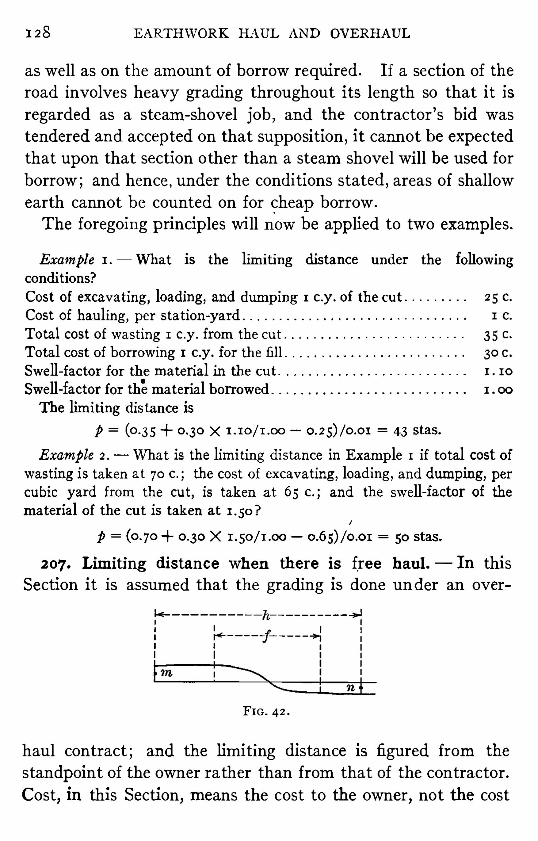
1 28 EARTHWORK HAUL AND OVERHAUL
as well as on the amount of borrow required. If a section of the
road involves heavy grading throughout its length so that it is
regarded as a steam - shovel job,and the contractor ’s b id was
tendered and accepted on that supposition ,it cannot beexpected
that upon that section other than a steam shovel will beused for
borrow ; and hence,under the conditions stated, areas of shallow
earth cannot b e counted on for cheap borrow .
The foregoing principles will now be applied to two examples .
Example 1 . What is the lim iting distance under the followingconditions?
Cost of excavating , loading, and dum ping 1 c.y . of thecut
Cost of hauling , per station-
yard
Total cost of wasting 1 c .y . from thecut
To tal cost of b orrowing 1 c.y . for thefill
Swell - factor for thematerial in the cut
Swell - factor for thismaterial b orrowedThe lim iting distance is
p X 43 stas.
Example2 . What is thelimiting distance in Example 1 if to tal cost ofwasting is taken at 70 c. ; thecost of excavating, loading , and dumping, percubic yard from the cut
,is taken at 65 c. ; and the swell- factor of the
material of the cut is taken at
p X 50 stas.
207 . Lim iting distance when there is free haul . — In this
Section it is assumed that the grading is done under an over
_> I
FIG . 42 .
haul contract ; and the lim iting distance is figured from the
standpoint of theowner rather than from that of thecontractor .
Cost, in this Section , means the cost to the owner , not the cost

1 30 EARTHWORK HAUL AND OVERHAUL
The limiting distance is
p X 3 stas .
‘
Example 2 . What is the limiting distancein Example 1 if thematerialfrom the cut canno t be wasted with a haul distance shorter than 800 ft .?
Under thechanged conditions W K TM K 5 T
5
and p X 3 stas.
208 . Principle of economic distrib ution . Other things being
equal,that is them ost economical distribution of m aterial along
the profile, which result in m inimum total haul (staThe application of this principle is m ade by means of them ass
curve to some special cases in the following chapters . In Chapter IX it is throughout assumed that them ass curve is plotted
(1 ) from actual cut - volumes and actual fill- volumes,the cuts
having each a swell - factor of 1 ; or (2) from actual cut—volumes
and equated fill—volumes . In Chapter X it is assumed through
out that them ass curve is plotted from actual fill—volumes andequated swelled) cut—volumes .
NOTE . Under someconditions o f grading it is no t on thewholeeconomical to adhere strictly to a plan of distribution which involves minimumhaul. This point is discussed in Note3 , Sec. 213 , which see.

CHAPTER IX
ECONOMIC BALANCING LINES FOR MASS CURVES PLOTTEDFROM
CUT- VOLUMES AND EQUATED FILL—VOLUMES, OR FROM
CUT- VOLUMES AND FILL—VOLUMES WHENSWELL- FACTOR IS UNITY
This chapter discusses the application of theprinciple of economic distributionto each of several typical forms ofmass curve, progressing from thesimple to thecomplex . All the mass curves of this chapter are assumed to be plotted frompay yards, that is, from yards in place. All themass curves of thefollowing chapter areassumed to beplotted from yards of swelled material. Otherwise the two
chapters are similar. Figs. 50—60a face page 146 .
209 . Note.— It is important to bear in mind that , because
every mass curvein this chapter (1 ) represents grading in whichthere is neither swell nor shrinkage
,or (2) isplotted from actual
cut - volumes andequatedfill—volumes,the balancing linein every
case must be horizontal,and haul haul - area multiplied by
VS
100(see Sec.
For theeconomic balancing line for mass curve, plotted from
fill- volumes and equated cut- volumes,seeChapter X .
It is, of course, necessary_to useestim ated volumes of cut and
of fill in thework of planning distribution .
2 10. Economic balancing line for the simpleloop. Between
two adjacent zero ordinates of the m ass curve thedistance be
tween which is not greater than the lim iting distance, the base
line is the economic balancing line, provided no adjacent looplying on thesamesideof the base line is nearer than the lim iting
distance.
Let it be assumed that the profile mo , Fig. 43 , represents a
self- contained stretch of earthwork . Let thecut mn beassumed
to contain just suffi cient m aterial to make the fill no. This is13 1

1 3 2 EARTHWORK HAUL AND OVERHAUL
indicated by them ass curvewhich rises from M to N and then
descends returning to thebase line at 0. Let M0benot greater
MO is Economic Balancing Line
FIG. 43 .
than the lim iting distance (Secs . 206 and In this caseMO,
the base line, is theeconomic balancing line.
M'
0’
is theEco nomic Balancing LineFIG. 43a.
AreaMNO is themeasureof thehaul (sta-
yds.) involved in the
grading , that is, thehaul is proportional to this area (Sec.

1 34 EARTHWORK HAUL AND OVERHAUL
which results from using the base lineas a balancing line, can be
diminished only by raising the balancing line; and raising the
balancing line introduces waste and borrow which under the
conditions named is not econom ical .
(2) Assume that MU is greater than p ,the limiting distance.
Then the economic balancing line is M1U1 so placed that
M 1U1 p, prov idedM1U1 does not touch the curve at any point
between M1 and U1 .
(3) Draw the horiz ontal M2Q2U2 tangent at Q2 to the lowest
sag in them ass curve. Draw M3U3 to cut the m ass curve at
two points only between M3 and U3 . The two intermediate
points areQ 3 andOs’
.
Assume that M2U2 is greater than p . This case falls under
Sec . 2 10 or Sec . 2 1 2 .
2 12 . Economic balancing line for two long loops separated b y
a short loop. In Secs . 2 10 and 2 1 1 it has been shown that the
base line is,under lim iting conditions
,the econom ic balancing
line for a single isolated loop , whether simple or corrugated.
If the m ass curve in question contains two closely adjacent
loops on the same sideof thebase line, as in Fig. 45 , thework of
finding the econom ic balancing line is m ore complex .
It is assumed that AC and EG,Fig . 45 , areeach less than p ,
the limiting distance. The econom ic balancing line for loopABC
,when that loop is considered by itself , is thebase lineAC.
So,too
'
,the base lineEG is the econom ic balancing line for loop
EFG when that loop is considered apart from the rest of the
m ass curve.
Now let us consider at one time thewholem ass curvebetween
A and G. Adopting the balancing line AG results in the dis
tribution indicated by the arrows in Fig . 45a: cut ab makes fill
bc ; cut dem akes fill cd; cut ef m akes filljg. The total haul is
represented by the sum of the areas ABC,CDE
,and EFG.
Next , let us Shift thebalancing line to a higher position , A’G’
In thus raising the balancing lineweeffect threechanges : (1 ) We

ECONOMIC BALANCING LINES FOR MASS CURVES
decrease the total haul - area by thesum of thetwo strips AA’C’C
and EE’G’G
,and this decreaseis an advantage; (2) we increase
the total haul- area by the strip CC’E
’E ; and this is a dis
advantage; and (3) we introducewaste between A and A’
,and
borrow between G and G’
; and this is a disadvantage. Thedis
tribution resulting from the balancing line A ’G’is shown by
[f A’ p ,A'G" is t heeconomic b alancing line
FIGS. 45 (middle) , 45a (upper) , 45b (lower) .
arrows in Fig. 45b . W hether or not it is economical
thebalancing line above thebase linedepends upon the
between theadvantageof decreasing thehaul (sta -
yds .)corresponding disadvantage of introducing waste and
If A’G’is so drawn as to make
A’C’
E’G’
C’E
’ p,
A’C
’E
’G
’
C’E
’ p,

1 36 EARTHWORK HAUL AND OVERHAUL
Where p is the limiting distance; then A ’
G’is the economic
balancing line. This may be shown as followsIf we drop the balancing line A ’
G’
(so drawn as to producethe equality abovewritten) , the yard at A
’ goes to C’
,giving a
haul A’C’ sta -
yds . theyard at E’ goes to G’
,giving a haul
E’
G’ sta -
yds . ; thetotal haul for thetwo yards being A’
C’
E’
G’
s ta-
yds.
If we raise thebalancing line aboveA ’G’
,theyard at E’ goes
t o C’
, giv ing a haul E’
C’ sta-
yds . The yard at A ’is wasted
,
and the yard at G’
must be borrowed,thus giving a haul of E’
C’
plus a yard of waste plus a yard of borrow ,and this is equiv a
lent to haul E’
C’ p
,since one yard of wasteplus oneyard of
borrow is equivalent to one yard hauled a distance1) (Secs . 206
and Since by assumption A’
C’
E’
G’
C’E
’ p it is
p lain that it is a m atter of indifferencewhether wehaul theyard
a t A’ to C’
and theyard at E’ to G’
,or haul the yard at E’ to
‘C’
,and waste the yard at A ’
and borrow a yard for G’
Now if we raise the balancing line one cubic yard (to scale)above A ’
G’ to the position A
’G’
AI/CI/
+ El /G/ l
< Gl lE
/ l
+ P, (49)
which m eans that it is cheaper to haul theyard at A” to C and
haul the yard at E” to G”
,than to haul the yard at E” to C”
,
waste the yard at A”
,and borrow the yard for G”
. On the
o ther hand,if we lower the balancing line by one cubic yard
(to scale) from A’O
’ to
Al l /CH I
+ El l lG/ l /
CINE
/ l l p, (50)
which means that it is cheaper to haul the yard at E to C’
waste the yard at A’
and borrow the yard for G” than to
haul theyard at A to C”and haul theyard at E to G’
2 13 . Economic b alancing line for a mas s curve of one sag
and onehump . Fig . 46 shows a self- contained section of earth
w ork . The m ass curve shows that the cut is not sufficient to
completeeither of the two fills . It is assumed that thenecessary

138 EARTHWORK HAUL AND OVERHAUL
consideration we shall find that neither AB nor CD is theeco
nomic balancing line for this m ass curve.
Draw by trial thebalancing lineLMN so as to m akeLM =MNLMN is theeconomic balancing line. Using this balancing line
,
the cut to the left of m m akes thefill to l ; and the resulting haulis measured by thearea LCM . Thecut to the right of m m akes
the fill to n ; and the resulting haul is measured by the area
MBN The total haul with this balancing lineis thus measured
by total area,LCM MBN We now go on to show that this
total area is a minimum .
If we raise the balancing lineLMN slightly say a distancet the right- hand haul—area is decreased by the strip above
MN ; but the left- hand haul - area is at the same time increasedby the longer strip aboveLM ; and the net result of raising thebalancing line the slight distance
,t,is to increase the total haul
area . Ev idently by raising the balancing line step by stepa distance t each time the strip added at each step to the
left—hand haul - area is longer than the corresponding strip taken
away from the right - hand area . This m eans that any position
of the balancing line aboveLMN involves m ore haul - area,and
thereforem ore haul , than the balancing lineLMN
Again,try the effect on haul- area of lowering the balancing
line from the position LMN By dropping LMN a sm all dis
tance,t,thehaul - area on the left is decreased by the strip lying
below LM but at the same time the longer strip below MN is
added to the haul- area on the right . Hence the net result of
lowering the balancing lineby the sm all distance t is an increase
in the total haul - area . If wego on lowering the balancing line
step by step ,each successive step increases theright—hand haul
area m ore than it decreases the left—hand haul - area . Thus it
appears that any position of the balancing line below LMN
involves m ore haul - area , and therefore more haul , than LMN
To sum up . The balancing line LMN is so drawn (by trial)that the two segm ents , LM andMN , areequal . Any balancing

ECONOMIC BALANCING LINES FOR MASS CURVES
line, aboveor below LMN involves more haul- area , and there
foremore haul , than LMN T herefore LMN is the economic
balancing line.
MNTPP
If LM=MN,LN is theEconom ic Balancing Line
FIG. 46a.
NOTE 1 .
—Ano ther way of stating the proposition ab ove is: for theconditions shown in Fig . 46 , the position of theeconomic division point inthe cut is that which makes the extreme haul - distances equal . Thus the
proposition is stated by Mr. GeorgeH . Tinker who gavean algeb raic proofof it in Engineering News, 190 1 , v ol. 45 , p . 82 .
NOTE 2 . Thesameproposition applies , of course, in thecaseofa profile
which shows a fill lying between two cuts either one of which is sufficient
to make thecompletefill . Thus in Fig . 46a, LMN which is so drawn as to
makeLM MN,is theeconom ic b alancing line.
NOTE 3 . Fig . 46 . Thedivision point m of thecut has been so locatedas to give the least to tal haul . If thematerial in the cut is no t divided at
m therewill beunnecessary haul . Now,under some conditions of grading
it is no t economical, on thewhole, to elim inate all such unnecessary haul.For example, if thematerial is movedwith carts
,and hauling against grade
is more expensive than with the grade, by reason of the steepness of the
gradeor thepresenceofwater in theup -
gradecut , it will beunwiseto adhereto the plan of dividing the cut precisely at m . Again, if the cut is taken

140 EARTHWORK HAUL AND OVERHAUL
out by means of a steam—shovel plant theeconom ical working of that plant
will probab ly requirewide departure from the plan of distribution whichinvolves theleast haul perhaps even to theextent ofhauling all of thecutin onedirection if thetopography at oneend of thecut permits alow gradeforthehauling track while the topography at the o ther end requires an excessivegrade.
Thefact that in practice it is often w ise to depart more or less from the
plan which involves the least haul is not an argument against making such
plan. It is sound engineering to makesuch plan ofdistribution and departfrom it only in so far as good reasons for so do ing present themselves.
2 14. Economic continuous b alancing line for a mass curve
with two sags and two humps . Fig . 47 shows a profileof a self
Borrow
N0
0]; O
II
P/l
TheEconomic Continuous B alancing Line is LP fif LM NOMN OP; b u t t heBro ken Balancing LineLN N”P” is the'
Economic Balancing Linein th is Case
FIG . 47 .
contained stretch of earthwork ; that is, no m aterial is moved
past a or f. Them ass curve, drawn below the profile, shows
that there is m orefill than cut . Material to the amount repre
sented by theordinateFF ’must beborrowed. Let it beassumed
that borrow is as readily got at one part of the profile as at
another .
The lineLP , drawn by trial so as to m ake
LM NO MN OP, (5 1 )
is the economic continuous balancing line for this mass curve,

142 EARTHWORK HAUL AND OVERHAUL
not so . Fig . 48 shows a mass curve for which LP ,so drawn as
to m ake LM NO MN OP ,is the econom ic balancing
line. If we break LP at N ,and shift each part , regardless of
theother , to obtain a minimum total haul - area for each part , we
find that LN must be lowered to the position L’N for which
L’M’ M’
N and NP must be raised to the position N’P
’
for which N’’O
”
O”P
”. But this shifting of the two parts
ABaseLine2 F
,
TheEconomic Cont inuousBalancing LineLP is theEconomicBalancing Linein this Case
FIG . 48 .
causes them to overlap between N andN’
and such overlapping
is inadmissible. In the case shown in Fig . 48 the continuous
economic balancing lineis therefore theeconomic balancing line.
It may be stated as a general rule that the continuous economic
balancing line is theeconom ic balancing lineexcept when it can
be broken into parts and each part , considered by itself , shiftedto theposition of least haul without an overlapping of theparts .
2 16 . W hen the base line is the economic balancing line.
In Fig . 49 , which represents a m ass curve constru cted on thebase
lineAD,let it beassumed that thelength of each of thesegments
into which the base lineis cut by them ass curve is not greater
than thelimiting distance, 1) (Secs . 206 and Them ass curve
shows that the cuts and fills balancebetween the two points A
and D. Let it be assumed that no m aterial is to bemoved past
A or D. Let it be assum ed, further , that
AB + CD ~ BC < p

ECONOMIC BALANCING LINES FOR MASS CURVES
Under the foregoing conditions the economic balancing lineis the base lineAD. This is true because to raise or lower thebalancing lineAD or any part thereof is to introducewasteand
b orrow ; and under the given conditions waste and borrow are
not economical .
Mass Curve
AB> P CD> P
TheBaseLineis theEconom ic Balancing Line
FIG . 49 .
2 1 7 . Examples of economic balancing lines. It is assumed
that the conditions are such that no m aterial will bemoved past
either end of theprofile in any of thefigures (folding plate, page
1 46) to which reference is m ade in this section . Each profile is
accompanied by its m ass curve.
On each m ass curve theeconomic balancing lineis represented
b y a full , heav y line and is designated by two or m ore of the
letters L,M
,N
,L
’
,M’
,N
’.
The economic distribution of m aterial , corresponding to the
economic balancing line, is indicated by arrows on the profile.
The figures are given in pairs ; the first figure of each pair
shows them ass curve above thebaseline; the second shows the
m ass curve below the base line. The two figures of each pair
p resent the same problem as far as determining the econom ic
balancing line.
In every casep lim iting distance (Secs . 206 and
Fig. 50. Theprofile shows a cut only . There is no fill into
which them aterial of the cut m ay bedumped ; hence theentire
cut must bewasted. This condition is clearly reflected in the
m ass curve, which , rising from start to finish, precludes a balanc
ing line. Fig. 50a shows a fill thematerial for which must be
b orrowed.

144 EARTHWORK HAUL AND OVERHAUL
Fig. 5 1 . Herewehavea cut and a fill. The cut ab ismore
than sufficient to m ake thefill bm . Hence thereis waste. This
condition is shown by the fact that the right extremity of the
m ass curve lies above thebase line. Draw a horizontal through
M to meet them ass curve at L . If LM is not greater than p,
the lim iting distance,LM is the econom ic balancing line. As
sum ing that LM 31> p , draw the vertical Ll . The portion lb of
the cut just m akes the fill bni . The portion c l of the cut is
wasted. This is the econom ical distribution of the m aterial,
and is indicated by arrows on theprofile. In Fig . 5 1a we have
the foregoing conditions reversed : the fill ab is larger than the
cut bin,so that thefill d l is borrowed
,and fill lb takes theentire
cut,bm .
Fig . 52 . The right extrem ity,C
,of the m ass curve lies at
a distance CC’ above the base line, which means that waste to
the am ount of CC’
(to scale) cannot be avoided. We drewthrough C thehorizontal CA ’
meeting the left slope of them ass
curve at A ’
. We scaled the distance A ’
C and found it to be
greater than p,the limiting distance. Therefore A ’
C cannot
be theeconom ic balancing line. Next we raised the balancing
line to theposition LM such that LM p . LM is theeconomic
balancing line. Hence the econom ic distribution : cut lb m akes
fill bni ; cut d l is wasted ; and fill me is borrowed. In Fig. 5 2a
we have a similar case, except that the fill is larger than the
cut . Hence borrowing to the am ount CC’
(to scale) cannot be
avoided. A'C is greater than p ; therefore A
’
C is not the eco
nomic balancing line. Theeconom ic balancing linein this figure
is LM so drawn as to m ake LM\
= p . The arrows show the
economic distribution .
Fig. 53 . Here the cut balances thefill . That is to say,the
material of the cut is just sufficient to m ake the fill. This con
dition is shown by them ass curvewhich begins and ends on the
base line. It is assumed that thebase line intercept , LM ,is no t
greater than the limiting distance. In this case theeconom ic

146 EARTHWORK HAUL AND OVERHAUL
Hereeconomy requires that we break the balancing lineA ’N
’ at
M ,and raise the left- hand portion to theposition L
’M’ such that
L’M’ p . L
’M’
,MN is the econom ic balancing line. The
arrows indicate the econom ic distribution . The same rem arks
apply to Fig . 5 7a.
Fig. 5 8 . Here,as in Figs . 56 and 5 7 , there is a fill lying be
tween two cuts . Draw a horizontal through D,the right - hand
end of them ass curve,cutting them ass curveat B ’
and B”
. As
sum ethatB ” D is greater than B ’B
’B
’B
’D is not theeconom ic
balancing line. Draw thehorizontal LM so as to m ake the two
intercepts , LM andMN ,equal . Assuming that neither LM nor
MN is greater than the limiting distance, LMN is the eco
nom ic balancing line. Fig . s8a shows a cut lying between two
fills but theproblem of determ ining theeconomic balancing lineis the same as in Fig . 58 .
Fig. 59 . The conditions hereare like thoseof Fig . 58 , except
that here we find on drawing a horizontal LN so as to m ake
LM MN ,that both LM andMN aregreater than p
,the limit
ing distance. Hence,LMN is here not the econom ic balancing
line. Econom y requires us to break thebalancing lineLMN at
M ; raise the left portion to theposition L’M such that L” M ”
p ; and lower the right portion to thepositionM’N
’ such that
M’
N’ p . The broken balancing lineL” M ”
,M’N
’is theeco
nom ic balancing line. Fig . soa presents the sameproblem .
Fig . 60 . Here again we have a fill lying between two cuts .
Thefill in this case,however
,is greater than the combined cuts
,
and this means unavoidable borrow . Draw through N’
,the
right end of them ass curve,a horizontal cutting thecurveatM ’
.
Assuming that neither LM,the base line intercept , nor M
’N
’is
greater than p,the lim iting distance
,the broken balancing line
LM,M’N
’is theeconom ic balancing line. Fig . 60a shows a cut
lying between two fills , the cut being more than suffi cient to
make thefills,so that thereisunavoidablewaste. Theproblem
of Fig . 60a is thesameas that of Fig . 60 .


CHAPTER X
ECONOMIC BALANCING LINE FOR MASS CURVE PLOTTEDFROM FILL- VOLUMES AND EQUATED CUT- VOLUMES
This chapter discusses the application of theprinciple of econom ic distributionto each of several typical forms of mass curve
, progressing from the simple to thecomplex . Themass curves here represent cubic yards of swelled material ; whilethemass curves of thepreceding chapter represent cubic yards in place.
2 19 . Note.
— Every m ass curve in this chapter is plottedfrom the estim ated fill- volumes and equated estim ated cut
volumes . This means that each station - volume of cut was
multiplied by its estim ated swell—factor , and the resulting swelledvolumes werecombined with theestimated fill- volumes to obtain
the ordinates to them ass curve.
For econom ic balancing lines for m ass curves plotted fromcut- volumes and equated fill—volumes
,and for m ass curves
p lotted from fill- volumes and cut- volumes of unity swell see
Chapter IX .
2 20. Economic b alancing line for simple loop .
— The base
line,Fig . 62 , is the econom ic balancing line provided AC is no t
greater than the lim iting distance; and the
(55)
where s swell- factor for cut ab ; Y cubic yards per inch of
o rdinate; and S feet per horizontal inch of themass curve.
If AC is greater than p ,the economic balancing line is A
’C’
s o placed that A
’C’ p ; and the total haul (5) (area A
’BC
’
)
YS sta -
yds ; but in this caseAA’is wasted and CC is borrowed.
TOO

ECONOMIC BALANCING LINE FOR MASS CURVE 149
well Factors
Sub grade
FIG . 62 .
2 2 1 . Economic balancing linefor corrugated Icon— Referringto Fig 63 : Let s1 and 52 be the swell - factors of cuts C1 and C2respectively . AE is the base lineof them ass curve. Draw the
horizontal A2Ez to touch the sag at C . Draw the horizontal
fs— Swell Factors—
1
Sub g rade
FIG. 63 .
A 1E1 between AzEz and the base line. Draw A 3E3 aboveA2
to cut the sag at C’and C
”
Now if AzEz is less than p , thelimiting distance the problem of determining the economic
balancing line is the same as if the loop were simple (Sec .

I50 EARTHWORK HAUL AND OVERHAUL
But if AgEz is greater than p, the problem of determining the
econom ic balancing line comes under Sec. 22 2 , which see.
222 . Economic balancing line for two long loops separated
by a short loop. Fig . 64 . A t first glance the base line seem s
Swell Factors
BaseLine
FIG . 64.
’ to be theeconomic balancing line, provided neither LN nor QU
is greater than 17 , the limiting distance.
Let W total cost of wasting 1 c.y . in place at l, less X1 ;
B total cost of borrowing 1 c.y . in place at u ;K 1 cost of excavating and dumping 1 c .y . (in p lace) of
thematerial of cut 1 ;K 2 cost of excavating and dumping 1 c.y . (in place) of
thematerial of cut 2 ;$1 swell- factor of cut 1 ;52 swell- factor of cut 2 ;Sb swell- factor of m aterial for borrow at u ;T cost per station- yard of haul cost of hauling 1 c.y .
(in place) 100 ft .
W ith thebase lineas balancing line thedistribution is as follows
material of cut lm m akes fill mn ;material of cut oq makes fill no ;material of cut qr makes fill ru .

1 5 2 EARTHWORK HAUL AND OVERHAUL
Let $1 swell- factor of cut 1 ;$2 swell - factor of cut 2 ;Y cubic yards represented by one inch of ordinate'
S feet represented by onehorizontal inch of m ass curve.
Remember that the ordinates of the m ass curve are m ade up
from fill- volumes and equated cut - volumes .
Swell Facto rs
3 1 3 2
Sub gr
LMN is theEconomic Balancing Lineif LM MNt ooFormeaning of hp h g, 223
FIG. 65 .
Draw thehorizontal LMN so as to m ake
LM MN
3 1 82
LMN is the econom ic balancing line. This may be shown as
follows
If we raise the balancing lineLMN a small distance t to the
position L’M N we add to the area MCN a strip MM
’N
’
N of
which the length is (MN MN h ,say ; and
this means an increase of (MN h )S
i f—i sta—yds . of haul .2
(Secs . 14 and But at thesame timewe take away from the

ECONOMIC BALANCING LINE FOR MASS CURVE 1 53
haul- area LBM the strip LL’M M of which the length is
% (LM L’M’
) LM hz, say ; and this means a decrease of
(LM ho) g sta -
yds . of haul . If we let H’
net in
crease in haul which results from raising the balancing linefrom the position LMN to the position we have
H’= (MN h1) (EM he)
MN LM
52 8 1
therefore$1 100
Thus we find that this increase,H
’
,in the total haul , due to
raising thebalancing linethesm all distancet, is positive. There
fore it is not economical to raise the balancing line above the
position LMN
Again : If we lower the balancing line a small distance t, to
theposition L’M N we add to the haul - area LEM the strip
LL” M” M
,the length of which is —é(LM L
” M ”
) LM h3 ,
say ; and this increases thehaul by (LM h3) And at
the same timewe take away from the haul - area MCN the stripMM”
N”N ,
the length of which is % (MN M ”N
”
) = MN h4 ,
say,thus decreasing the total haul - area by (MN
1
1
22sta—yds. Let H net increase in haul resulting from this
lowering of the balancing line. Then
H (LM h.) 5 5 — (MN h4)100
13 £ 9 sta-
yds .
,
IOO
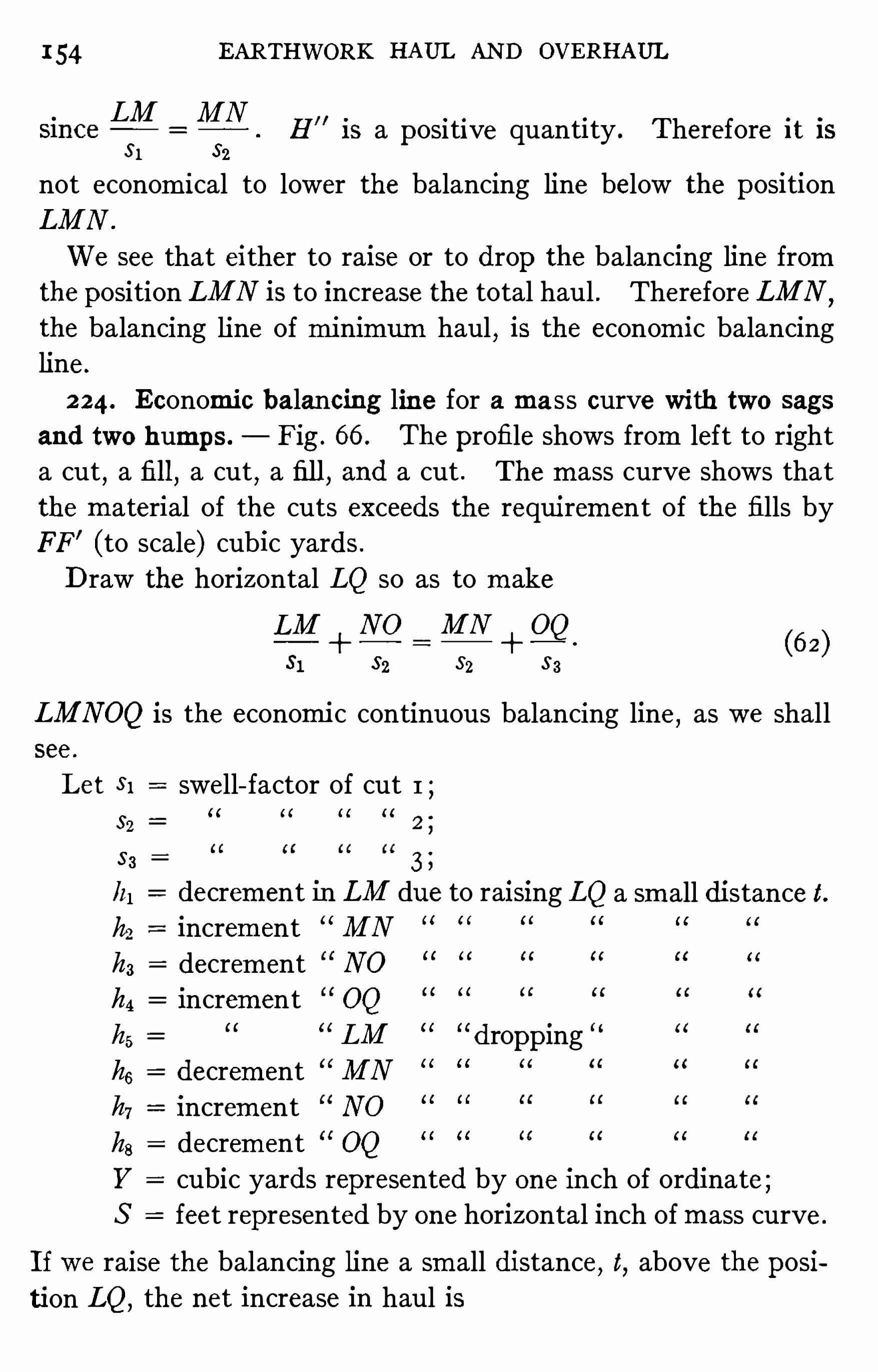
1 54 EARTHWORK HAUL AND OVERHAUL
LM MN
5 1 52
not econom ical to lower the balancing line below the position
LMN
We see that either to raise or to drop the balancing line from
theposition LMN is to increase the total haul . ThereforeLMNthe balancing line of minimum haul
,is the econom ic balancing
line.
2 24. Economic balancing line for a mass curve with two sags
and two humps. Fig . 66 . Theprofile shows from left to right
a cut,a fill
,a cut
,a fill
,and a cut . Them ass curve shows that
the m aterial of the cuts exceeds the requirement of the fills byFF
’
(to scale) cubic yards .
Draw the horizontal LQ so as to m ake
LM+NG MN
+O_ Q
. (62)$1 $2 52 S3
H is a positive quantity . Therefore it is
LMNOQ is theeconomic continuous balancing line, as we shallsee.
Let sl swell- factor of cut 1 ;( i N ( l
$2
3 3 3 ;
111 decrement in LM dueto raising LQ a sm all distancet.h increment MN u cc
A
ha decrement NO
h4 increment OQhf, LM “
dropping
he decrement MN
h7 increment NO
kg decrement OQY cubic yards represented by oneinch of ordinate;S feet represented by onehorizontal inch of m ass curve.
Ifwe raise thebalancing line a sm all distance, l, above theposi
tion LQ ,thenet increase in haul is

1 56 EARTHWORK HAUL AND OVERHAUL
LM N0 MN Q _0
$1 82 $2 $ 3
the balancing linebelow theposition LQ increases thehaul .
Wefind that the haul is increased whether we raise or lower
the balancing line from the position LQ ,which means that LQ
is the economic continuous balancing line.
In Sec . 2 1 5 it is shown that the continuous economic balancing
line is not in every case theeconomic balancing line. Sometimes
theform of them ass curveis such as to m akeit possibleto reduce
the haul resulting from the balancing lineLQ by breaking that
line at N. Theprinciple brought out in Sec . 2 1 5 applies here.
2 25 . W hen swell - factors are all equal. If the swell- fac
tors of any section of this chapter each be replaced by 1, the
section will reduce to the corresponding section of thepreceding
chapter . For example, eq . 62 will then becomeeq . 5 1 . More
over , if the swell- factors of any section of this chapter be given
a uniform value other than 1,the section will become about
as simple as the corresponding section of the preceding chapter .
W ith this changeeq . 62,for example, will reduce to eq . 5 1 .
226 . Practical use of mass curve in planning distrib ution.
The work of p lanning distribution with m ass curve basedon equal swell - factors is little greater than with mass curve
based on the comm on swell—factor 1 (Sec . 1 On thecontrary,
the additional work required with mass curve based on unequal
swell - factors is considerable. However,it is not often that
data pertaining to future swell and yardage is so reliable as to
justify the adoption of unequal swell- factors in planning dis
tribution . In the m ajority of cases the engineer will use the
swell—factor 1 for all thecuts involved in onedistribution problem ;and in most of thecases in which thedata will warrant deviating
from the swell—factor 1,will be justified in adopting some other
uniform swell - factor .
So H is positive, and dropping

INDEX(References areto pages.)
Adjustment of swell- factors, 13 .
A llen, C. Frank, 41 .
American Railway Engineering Association, iv .
abstract ofoverhaul practice, 5 1 .
basis of overhaul computation, 53 , 54, 68.
center ofmass, 38.
Committeeon Roadway , 5 1 .
economic balancing line,free- haul distance, American practice, 5 2.
“Manual ” of recommended practice, 7 , 53 .
ob liquebalancing line, 23 .
overhaul clause, 53 .
overhaul computation, Method V, 70.
“Proceedings,
” iv, 5 1 , 70.
Review ofLiteratureofOverhaul , ” 5 1 .
revision of plan of distribution,1 22 .
specifications for roadway , 53 .
Area, cross- section, 40, 48 , 90.
error, 28 .
mass curve, 24, 25 , 46 , 87 .
Arithmetical computation,center ofgravity , 42-
44, 48, 75 , 77 , 1 1 1 .
center ofmass, 36, 79 , 108 .
free- haul limits, 55 , 75 , 7 7 , 79, 8 1 , 90, 107 , 1 1 1 .
limits of bodies ofmaterial, 33 , 7 5 , 7 7 , 79 , 83 , 90, 105, 1 1 1 .
moments, 44, 49, 70, 7 1 , 84 , 9 1 , 1 1 2 .
overhaul, 69—7 1 , 76, 78, 80, 85 , 9 2 , 108, 1 1 3 .
Average, haul- distance, 73 .
overhaul-distance, 74.
Balancing line, base line, 142 .
broken,141 , 156 .
continuous, 141 , 1 56 .
corrugated loop , 133 , 149 .
economic, 13 1—1 56 .
examples (Figs. 50—60a) , 143 , 146 .
horizontal, 23 .
ob lique, 23 .
onesag and onehump, 136, 1 5 1 .

1 58 INDEX
Balancing line, simpleloop ,13 1 , 148 .
two long loops separated b y short loop , 1 34, 1 50.
two sags and two humps, 140, 1 54.
Base lineofmass curve,19 .
economic balancing linewhen,142 .
Basis of overhaul computation, Amer. Ry . Eng. Ass’n.
,
(A) , (B) , methods of freeaveragehaul, 5 1 , 5 2 , 54.
(C) , method of free straight haul, 5 2 , 53 .
distinguished from Method, 54, 68.
interpretation , 54 .
review of American practice, 5 1 .
Beard, E. J . , 70.
Berg, W alter G . , 5 1 .
Borrow,1 24
—130.
co st,1 27 .
land for,1 2 7 .
Bruer, R . P., 70.
Cart - cut,actual and ideal
,2—6 .
Center of gravity ,arithmetic (Methods II, III, IV ,
VIII) , 42—44, 48, 69 ,7s, 7 7 , 79 , 83 . 108 , 1 1 1 .
as for singleprismoid (Method III) , 42 , 69 , 7 7 .
center of length (Method II) , 42 , 69 , 75 .
center ofmass (Methods IV, V) , 43 , 69 , 79 , 81 , 108, 1 10.
cut , 42—49 .
determ ined readily or with difficulty , 3 , 4.
eye (Method I) , 42 , 69 , 73 , 100.
—49 .
haul,1, 40 .
mass curve (Methods V ,VII) , 43 , 46 , 69 , 70 , 81 , 87 , 1 10, 1 1 5 .
methods I—VIII, 42
—49 .
moments, arithmetic (Methods VI, VIII) , 44, 49 , 70, 83 , 1 1 1 .
mass curve (Method VII) , 46 , 70, 87 , 1 1 5 .
singleprismoid, 40, 4 1 , 48 , 90 .
series of prismoids, 42—49 .
true, 40 , 41 , 48 , 90, 9 1 .
Center of length ,center of gravity , 42 , 69 , 75 .
center ofmass, 3 5 , 36 .
Center of mass,arithmetic
, 3 5 , 36 , 43 , 69 , 79 , 108 .
center of gravity , 43 , 69 , 79 , 8 1 , 108 , 1 1 0.
mass curve, 38 , 43 , 69 , 8 1 , 1 10.
singleprismoid, 3 5 .
series of prismoids, 36 , 38 , 43 , 79 , 8 1 , 1 08, 1 10.
Center of volume (sameas Center ofmass) .

I 60 INDEX
Economic balancing line,two long loops separated by oneshort loop ,
two sags and two humps, 140, 1 54.
Economnc distribut ion,1 2 1—1 56 .
principle, 1 30.
Engineering Netos , 24 , 38 , 70 ,1 39 .
Engineers’Field Book ,
”
Searles, 41 .
Equating factor, 1 1 , 73 , 103 .
Error, area, 28 .
cost o f overhaul, 66 .
distanceplo tted or scaled,27 .
overhaul , 92 , 1 1 6 , 1 1 9 .
Estimating overhaul (Method I) , 69 , 72 , 98.
Eyedetermination ,center of gravity , 42 , 69 ,
free- haul limits, 59 , 73 , 99 .
limits of bodies of niaterial, 3 5 , 73 , 99 .
overhaul (Method I) , 69, 7 2 , 98 .
Facto r,adjusted, 1 3—1 8 .
determination of,1 1 - 1 8
, 73 , 1 03—1 05 .
equating-
3 1 1 , 73 , 1 03—105 .
estimated, 13 103—105 , 1 2 1 , 1 23, 1 56 .
swel-l 10,1 3 , 103
—105 , 1 2 1 , 1 23 , 1 56 .
1 page
facing
c c c c c c c
facing

INDEX 1 61
page 1 20
50—60a facing
1 35
IS7
Fill,actual replaced by ideal, 2—6 , 98, 99 .
center of gravity (seealso Center of gravity) , 40—49 .
center ofmass (seealso Center ofmass) , 35—49 .
limits (seealso Limits) , 33—35~trestle, 3 .
- volume actual volumeof a b ody of fill .
widening, 3 .
Fisher, S. B . ,24.
Freeaveragehaul, (A) and (B) , 5 1 , 5 2 .
Free- haul distance, American practice, 5 2 .
defined, 50 .
Free- haul limits,arithmetic
, 5 5 , 75 , 107 .
at only oneend of cut when, 6 , 58 , 59 , 66.
defined , 53 .
eye, 59 , 73. 99
mass curve, 56 , 8 1 , 1 10.
Freestraight haul , (C) , 5 2 .
Gillette, H. P.
,6,24, 38 .
Gravity center (seealso Center of gravity) , 40—49 .
Halcom be, N . M .,iv .
Haul,area ofmass curve, 24—2 7 , 87 , 89 , 1 1 5 .
arithmetic,1, 44 , 49 , 84, 1 1 2 .
center of gravity , 1 , 40.
cross 3—6
, 59 , 63 .
freeaverage, 5 1 , 5 2 , 54.
free straight , 5 2 , 53 .
least,no t always economical, 130 , 1 39 .
limit of profitable, 1 23 , 1 28 .
mass curve, 24, 2 5 , 46 , 87 , 89 , 1 1 5 .
minimum,no t always economical, 1 30, 139 .
over (seealso Overhaul) , 50.

1 62 INDEX
Haul, unit of, 2 .
Haul- distance, 1 , 2 .
average, 73 .
Ideal cart - cut, 3—6 .
Increment,swell 10.
In-
placevolume, 2 .
Inspection,center of gravity , 42 , 69 , 73 , 100 .
free—haul limits, 59 , 73 , 99 .
limits of bodies ofmaterial, 35 , 73 , 99 .
overhaul (Method I) , 69 , 7 2 , 98 .
Least haul not always economical, 130, 1 39 .
Limiting distance, with free haul , 1 28 .
without freehaul , 1 23 .
Limit of error,area
,28 .
cost of overhaul,66 .
distanceplot ted or scaled,2 7 .
overhaul, 9 2 , 1 16 .
Limit of profitablehaul, with freehaul, 1 28.
without freehaul, 1 23 .
Limits of body ofmaterial,arithmetic
, 33 , 75 ,
eye, 3 5 , 73 ; 99'
mass curve, 34 , 8 1 , 109 .
Limits of freehaul, arithmetic, 55 , 75 , 107 .
defined, 53 .
eye, 59 , 73 , 99
mass curve, 56 , 8 1 , 1 10.
on only oneend of cut when,6, 58 , 59 , 66 .
Manual of recommended practice, Amer. Ry . Eng.
Manual for Resident Engineers,”
by Molitor and BeardMass
,center of (seealso Center of mass) , 35—39 .
Mass curve, area and haul , 24, 25 , 46 , 87 .
balancing line (seealso Balancing line) , 23 , 13 1—1 56 .
base line, 19—2 1 , 142 .
center of gravity (seealso Center of gravity) , 43 , 46.
center ofmass (seealso Center ofmass) , 38.
characteristics, 2 2 .
construction of,19 .
defined, 20.
free- haul limits, 56 .
limits of bodies, 34 .
moments, 46 , 87 , 1 1 5 .
plotting , 3 1 , 8 1 , 109 .

1 64 INDEX
Overhaul , interpretation of bases (A) and (B) , 54 .
mass—curvemethods :V ,69 , 80 , 109 ; VII, 70, 86 ,
methods of computing, I—VIII, 68
—7 1 .
moments, arithmetic, 70, 84 , 9 1 , 1 1 2 .
mass curve, 87 , 1 1 5 .
of Fig . 19 , Methods I—VIII, 7 2—96 .
of Fig . 38 , Methods I, IV—VII, 97—1 20.
results, 9 2 , 1 16 , and Fig. 36 facing 67 .
statement,68 and Fig. 36 .
true, 92 , 1 16 .
Place, volume in,2 .
Plan of distribution,economic, 1 2 1
—1 56.
making , 130,147 , 1 56 .
mass curve,1 3 1
—1 56 .
must berevised, 1 2 1 .
Plo tting, mass curve, 109.
errors of, 2 7 .
Prelini, Charles, 7 .
Principleof economic distribution,130 .
Prismo id, center of gravity (seealso Center ofgravity) , 40.
center ofmass (seealso Center ofmass) , 3 5 .
definition, 3 5 .
Prismoids,center ofgravity ofseries (seealso Center ofgravity) , 42-
49.
center ofmass (seealso Center ofmass) , 36—39 .
Pro ceedings,”American Railway Engineering Association, 38, 5 1 , 70.
Profileof quantities, 1 9 .
Profitablehaul , limit of, 1 23 , 1 28 .
Ratio , swell 10 .
“Railroad Curves and Earthwork, by Allen, 41 .
Raymond, W . G . , 41 .
“Railroad Construction,
b y Webb, 7 .
Reineker, F .,141 .
Results of overhaul computation,Fig. 36 facing 67 .
compared, 9 2 , 1 16 .
Rock Excavation, by Gillette, 6 .
Russell, T . S., 38 , 70.
Sandstrom ,A . C.
,iv .
Scale of ordinates for mass curve, 30.
Scaling , errors of, 2 7 .
Searles, W . H.
, 41 .
Shrinkage, 6 .
factor,10 .

INDEX 1 65
Slide- rule,1 7 , 1 8 , 104, 106 , 1 13 .
Specifications, 53 .
Statement of overhaul, 68 and Fig . 36 .
Station- volume vo lume of a single prismoid.
Steam - shovel, 4, 1 2 , 98 .
Sub station~v olume volumeof a« singleprismo id leSs than
Swell, 6 .
depends on thoroughness ofmixing, 8 .
examples of, 1 03 .
factor (seealso Swell-factor) , 10 .
increment , 10 .
not uniform ,6—10 .
ratio , 1 0 .
Swell- factor, 10.
adjnstr-nent , 1 3—18 .
estimated,1 3—1 8 1 21
,
determination 1 1—18, 73 , 103
- 105 .
Tables : I, 1 1 7 ; II, 1 1 8 ; III, 1 19 .
Tinker,GeorgeH .
,1 39 .
T restlefill, 3 .
True, center of gravity , 40 , 41 , 48 , 90, 9 1 .
overhaul, 70 ,
89 , 9 2 , 1 16 .
Unit of haul, 1 .
Vo lume,cut volume in place.
equated cut vo lume in place X swell- factor.
equated fill volumeof fill x equating factor.
fi-ll actual volumeofa body of fill .in place, 2 .
station volumeof a singleprismoid.
sub station vo lume. of prismoid less than 100 ft . long.
swelled cut volume in place swell- factor.
W aste, 1 24—130 .
suitable land for, 1 27 .
Webb,Walter Loring , 7 .
W idening fill, 2 .
Yardage, v'
olume in cubic yards.


B IRKMIRE— Arch itectural Iron and Steel . 8 v o .
Com pound Riv eted Girders as Ap p lied in Buildings . 8 v o ,
Planning and Const ruct ion o f High Offi ce Buildings . 8v o .
Skeleton Construct ion in Buildings . 8 v o ,B RIGGS— Modern Am erican Scho o l BuildingsBYRNE— Inspect ion of Materials and W o rkmanship Em p loyed in Co nst ruo
t io n 16m o .
CARPENTER— Heat ing and Vent ilating of Buildings . 8 v 0 ,
CORTHELL— Allowable Pressure on Deep Foundat ions 12m 0 ,
ECKEL— Building St ones and C lay s 8 v o
F REITAG - Arch itectural Engineering .
Fire Prevent ion and Fire Pro tec tion 16m o , m or . ,
F irepro ofing of Steel Buildings 8 v o
GERHA RD— Gulde t o Sanitary Inspect ions 12m o ,
Mo dern Bath s and Bath Houses 8v o ,
Sanitat ion of Public Bu ildings . l 2m o ,
Theat re Fires and Panics 12m o
The W ater Supp ly , Sewerage and Plumbing o f Modern Cit y Buildings ,
8 v o ,
GREENE— Elements of Heat ing and Vent ilat ion 8v o ,
JOHNSON— Stat ics b y Algebraic and Grap h ic Meth ods 8 v o ,
KELLAWAY— HOW t o Lay Out Suburban Hom e Gro unds. Sv o ,
KIDDER— Arch itect s'and Builders' Po cket—bo ok 16m o , m or . ,
MERRILL— Stones fo r Bu ilding and Deco ration 8 v o ,
MONCKTON— St air - building 4t o ,
PATTON— Pract ical Treat ise on Fo undat ions 8 v o ,
PEA BODY— Naval Architect ure 8 v 0 ,
R ICE— Co ncrete- block Manufac ture 8 v o ,
RICHEY— Handbook fo r Superin tendent s o f Const ruct io n l o , m o r . ,Building Fo rem an’
s Po cket Bo ok and Ready Reference 16m o , m or . ,Building Mech anics' Ready Reference Series :Carpenters
'and W o odworkers' Edit ion 16m o , m or
Cement W o rkers' and Plasterers ’
Edit ion . . 16m o , rno r
Plumbers ’
. Steam - Fit ters'
, and Tinners‘
Edit ion 16m o , m o r
Stone and Brick - m asons'Edit ion . 16m o , m o r . ,
RIBS— Building St ones and Clay Product s . 8 v o ,
SA BIN— House Paint ing (Glazing , Paper Hanging and W h itew ashing ) . 12m o ,
SIEBERT and B l o om — Modern St o ne cu t ting and Masonry 8 v o ,
SNOW— Principal Species of W ood “ Sv o ,
W AIT— Engineering and Arch itectural Jurisp rudence 8 v o ,
Sheep ,
Law o f Cont racts . 8v o ,
Law o f Operat io ns Prelim inary t o Const ruct ion in Engineering and
Arch itecture .
Sheep ,
W iLSON— Air Conditioning 12m o ,
W ORCESTER and ATKINSON— Sm all Ho sp itals , Establishment and Mainte
nance, Suggest ions for Ho spital Arch itecture, w ith Plans fo r a Sm all
Ho spital 12m o ,
ASSAY ENG .
BE'
r’
rs— Lead Refining b y Elect ro lysis 8 v o ,
FLETCHER— Pract ical Inst ructions in Quant itat ive Assay ing w ith the B lowp ipe 16m o , m o r. ,
FURMAN and PARDOE— Manual of Prac tical Assay ing 8 v o ,
LODGE— No tes on Assaying and Metallurgical Labo rat o ry Experim ents . 8 y o ,
Low— Technical Meth ods of Ore Analy sis . 8 v o ,
MILLER— Cyanide Process 12m o ,
Manual of Assay ing 12m o ,
MINEr— Product ion o f Alum inum and it s‘
Industrial Use. (W ALDO ) . 12m o ,
PRICE and MEADE— The Technical Analy sis of Brass and the Non - Ferrous
Allo ys 12m o ,
RICK E’
I'
TS and MILLER— No tes on Assay ing . 8 v o ,
ROBINE and LENGLEN— Cyanide Indust ry . (LE CLERC .) . 8v o ,
SEAMON— Manual for Assayers and Chem ists Sm all 8v o ,
2
00
03
05
0)
c01
MH
H
OO
OD
W
H
i»
i»
lO
th
W
N

ASTRONOMY .
COMSTOCK— Field Astronom y for EngineersC RA IG—Azim uth
CRANDALL— Text - bo ok on Geodesy and Least SquaresDOOLITTLE— Treatise on Pract ical Astronom yHAYFORD— Text - bo ok of Geodet ic A stronom yHOSMER— A zirnuth
Text - book on Practical AstronomyMERRIMAN— Element s of Precise Surv eying and GeodesyMICHIE and HARLOW— Practical Ast ronom yRUST— Ex—meridian Alt itude, Azimuth and Star - Finding TablesW HITE— Elements of Theo retical and Descrip tiv eAstronom y
BIOLOGY .
COHNHEIM— Enzymes 12m o .
*1
DAVENPOR r— St atist ical Meth ods with Special Reference t o Bio logicalVariat ion 16m o , m o r . 1
EFFRONT and PRESCOTT— Enzymes and Their App licat ions 8 v o , 3
EULER and POPE— General Chem istry of the Enzymes 8 v o ,
*3
MAST— Ligh t and Beh avior of Organism s 8 v o ,
*2
PRESCOTT and W INSLow— Elem ent s of W ater Bacterio logy , w ith Special
Reference to Sanitary W ater Analy sis 12m o , 1
W ARD and W HIPPLE— F resh water Bio logy (In Press )W HIPPLE— The Microscopy of Drinking W ater SW ) , 3
W INSLow— The Sy stemat ic Relationship of the Co ccacem . . Small 8 y o , 2
CHEMISTRY .
A BDERHALDEN— Ph y sio lo gical Chem ist ry in Thirt y Lectures . (HALL and
DEFREN ) 8 v o ,
* 5
A BEGQ —Theo ry ofElect ro ly tic Disso ciation . (VON ENDE .) 12m o ,
*1
ALEXEY EFF— General Princip les of Organic Sy n theses . 3
ALLEN— Exercises in General Chem ist ry , Lo o se Leaf Labo rato ry Manual .
Oblong 4t o , paper ,
*1
Tables fo r Iron Analy sis . 8 v o , 3
ARMSBY— Princip les of Anim al Nu trition 8 y o , 4
A RNOLD— Com pendium of Chem ist ry . (MANDEL . ) Sm all 8 v c , 3
A SSOCIATION OF STATE AND NATIONAL FOOD AND DAIRY DEPARTMENTS ,
Hartfo rd Meet ing , 1906 8 v o , 3
Jamest own Meet ing , 1907 8v o , 3
AUSTEN— No tes fo r Chem ical Studen ts . 12m o , 1
B ERNADOU— Srnokeless Powder — Nit ro - cellulo se, and Theo ry of the Cellu
lose Mo lecule 12m o , 2
B ILTz— Introduct ion to Inorganic Chem ist ry . (HA LL and PHELAN ) 12m o ,
Laborat o ry Meth ods of Inorganic Chem ist ry . (HALL and BLANCHARD .
8 v o , 3
B INGHAM and W HITE— Laboratory Manual of Inorganic Chem ist ry 12m o ,
* 1
BLANCHARD - Synthet ic Inorganic Chem ist ry . 12m o ,
* 1
BOTTLER— Germ an and American Varnish Making . Small 8v o ,
*3
BROWNE—Handbo ok of Sugar Analy sis . 8 v o ,
*6
Sugar Tables fo r Laborat o ry Use . . 8 v o ,
* l
BROWNING—In troduct iDn t o t he Rarer Elements . 8 v o ,
* 1
B RUNSW IG —Explo sives. (MUNROE and KIBLER) Sm all 8v o ,
*3
CLAASSEN— Beet - sugar Manufacture. (HALL and 8v o ,
*3
CLA SSEN— Quant itativeAnaly sis b y Elect rolysis . (HALL .) (In Press .)
3
CORN— Indicat o rs and Test - papers . 12m o ,
Tests and Reagen t s . 8 v a,
COOPER— Const itut ional Analy sis b y Ph y sico - chem ical Met h ods (Ino rganic) ,(In Press .)
DANNEEL— Elec trochem istry . (MERRIAM .) 12mo ,
DANNERTH— Meth ods of Text ile Chem ist ry . 12m o ,
DUI-IEM— Therm o dynam ics and Chem ist ry . (BURGESS .) . 8 v o .
EISSLER— Modern High Exp lo sives . 8 v o .
EK ELEY— Laboratory Manual of Ino rganic Chem ist ry 12m o ,
FLETCHER— Pract ical Instructions in Quant itativ e Assay ing w ith the Blowp ipe 16m o m or . ,
FOWLER— SewageW o rks Analy ses 12m o ,
FRESENIUS— Manual of Qualit at ive Chem ical Analy sis . . 8 v o ,
Manual of Qualit ative Chem ical Analysis . Part I Descrip t ive.
(W ELLs .) 8 v o ,
Quantitat ive Chem ical Analy sis . (COHN .) 2 vo ls 8v o ,
W hen So ld Separately , Vo l . I , 56 . Vo l . II, $8 .
FUERTEs— W ater and Public Health 12m o ,
FULLER— Qualitat iv e Analy sis of Medicinal Preparat ions 12m o ,
FURMAN and PARDOE— Manual of Practical Assay ing . . 8 v o ,
GETMAN— Exercises in Ph y sical Chemistry 12m o ,
G ILL— Gas and Fuel Analy sis for Engineers 12m o ,
GOOCH— Meth ods in Chem ical Analy sis . . 8v o ,
and BROWN ING— Out lines of Qualitat ive Ch em ical Analysis . Sm all 8v o .
GROTENF ELT— Prlnciples of Modern Dairy Practice. 12m o ,
GROTH— Int roduct ion t o Chem ical Cry stallograp h y . (MA RSHALL . ) 12m o ,
HAMMARSTEN— Text—bo ok of Phy siological Chem istry . (MANDEL .) . 8 v o ,
HANAUSEK — Microscopy of Technical Product s . (W INTON . ) . 8 v o ,
HASKINS— Organic Chem ist ry 12m o ,
HERRICK— Denatu red o r Indust rial Alcoh ol . . 8v o ,
H INDs— Inorganic Chem istry 8 v o ,
Laborato ry Manual fo r Student s 12m o ,
HOLLEMAN— Labo rat o ry Manual of Organic Chem istry fo r Beginners .
(W ALKER .) 12m o ,
Text - book of Inorganic Chem ist ry . (COOPER .) . 8 v o ,
Text - bo ok of Organic Chem istry . (W ALKER AND 8 v o ,
(EK ELEY ) Labo rat o ry Manual t o A ccom pany Ho llem an’
s Text - bo ok o f
Inorganic Chem ist ry . 12m o ,
HOLLEY— Analy sis o f Paint and Varnish Products . Small , 8v o ,
Lead and Zinc Pigm ent s Sm all 8 v o ,
HOPKINS— Oil chem ist s’
Handbook 8v o ,
JACKSON— Direct ions for Labo rato ry W o rk in Ph y sio logical Chem istry . 8v o ,
JOHNSON— Rap id Meth ods fo r t he Chem ical Analy sis of Special Steels , Steel
m aking Alloy s and Graph ite . Sm all 8 v o ,
LANDAU ER— Spectrum Analy sis . 8 v o ,
LASSAR - COHN— Applicat ion of Som e General React ions t o Invest igat ions inOrganic Chem istry . (TINGLE .) 12m o ,
LEACH— Fo od Inspect ion and Analysis 8 v o ,
LOB— Elect rochem istry of Organic Com p ounds . .8 v o ,
LODGE— No tes on A ssaying and Metallu rgical Laborato ry Experiments . 8 v o ,
Low— Technical Method of Ore Analy sis . . 8 v o ,
LOWE— Paint for Steel Structures 12m o ,
LUNGE— Techno - chemical Analysis. (COHN .) 12m o ,
MCKAY and LARSEN— Princip les and Practice of Bu t ter- m aking . . 8 v o .
MAIRE— Modern Pigment s and their Vehicles . 12m o ,
MANDEL— Handbo ok fo r Bio chem ical Laboratory . ,12m o
MARTIN— Laborat o ry Guide to Qualitat iveAnaly sis w ith theBlowpipe. 12mo ,
MASON— Exam inat ion of W ater . (Chem ical and Bacterio logical . . 12m o ,
W ater- supp ly . (Considered Principally from a Sanitary Standpo int .)8v o ,
MATHEWSON— First Principles of Chem ical Theory 8 v o ,
MATTHEWS— Laborat ory Manual of Dyeing and Textile Chem ist ry 8 y o ,
Text ile Fibres 8 v o
MEYER— Determ inat ion of Radicles in Carbon Compounds. (TINGLE .
Third Edit ion . 12m o ,
MILLER— CyanidePro cess . . 12m o ,
Manual of Assaying . 12mo ,
00
03
n
i»
H
O
H
MH
i—‘wwflb
1+
th
os
e-
1a
va
r-t
i
00
00
25
00
00
00
00
50
00
00
00
50
50
50
00
00
25
00
25
00
25
00
00
00
00
00
00
00
50
50
00
50
00
00
25
00
00
00
50
00
00
00
00
00
50
00
50
60
25
00
00
50
00
25
00
00

CIVIL ENG INEERING .
BRIDGES AND ROOFS , HYDRAULICS , MATER IALS OF ENGINEER
ING . RAILWAY ENGINEERING .
AMERICAN C IVIL ENGINEERS ’
POCKET BOOK. (MANSFIELD MERRIMAN ,
Edit or in chief. . ,16m o m o r. 5
B AKER— Engineers'
Surveying Inst rum ents 12m o , 3
B IXBY— Grap hical Com puting Table Paper 19 5 X241 inches , 0
BREED and HOSMER— Princip les and Pract ice of Survey ing .
Vo l . 1 . Elem entary Surv ey ing . 8V0. 3
Vo l. II. Higher Surv eying 8 v o , 2
BURR— Ancient and Modern Engineering and the Isthm ian Canal . 8 v o ,
*3
COMSTOCK— Field Astronom y fo r Engineers . 8 v o , 2
CORTIIELL— A llowable Pressure on Deep Foundat ions 12m o ,
*1
CRANDALL— Text - bo ok on Geodesy and Least Squares 8 v o , 3
DAVIS —Elev at ion and Stadia Tables . 8VO , 1
ELLIOTT— Engineering fo r Land Drainage. 12m o , 2
F IEBEGER— Treat ise on Civil Engineen'
ng . . 8 v o ,
' *5
FLEMER— Ph ot o t o pograph ic Met h ods and Instrument s 8 v o , 5
FOLWELL— Sewerage. (Designing and Maintenance.) 8v o , 3
F REITA c—Architectural Engineen'
ng 8 v o , 3
HAUCH and R ICE— Tables of Quant it ies fo r Prelim inary Est im ates . 12m o ,
*1
HAYFORD— Text—book of Geodet ic A st ronom y 8 v o 3
HERINGr—Ready ReferenceTables (Conversion Fact o rs ) . 16m o , m o r 2
HOSMER— A zimuth . 16m o , m or 1
Text - bo ok on Pract ical Ast ronom y . 8 v o ,
*2
HOWE— Retaining W alls for Earth . . 12m o 1
IVES— Adjustment s of the Engineer'
s Transit and Level 16m o , b ds*0
IVES and HILTs— Problem s in Surveying , Railro ad Surveying and Geod
m o r . , 1
JOHNSON (J . B .) and SMITH— Theo ry and Pract ice of Survey ing . Sm all 8v o ,
*3
JOHNSON (L . J .)— Stat ics b y Algebraic and Graph ic Met h ods 8v o , 2
K INNICUTT , W INSLOW and PRATT— Sewage Disp osal 8 v o ,
*3
MAHAN— Descrip t ive Geometry 8v o ,
* 1
MERRIMAN— Elem ent s of Precise Survey ing and Geo desy 8 v o 2
MERRIMAN and BROOKS— Handbo ok for Surveyo rs 16m o , m or 2
NUGENT— Plane Survey ing . 8 v o , 3
OGDEN— Sewer Construct ion . 8 v o , 3
Sewer Design 12m o , 2
OGDEN and CLEVELAND— Pract ical Meth ods of Sewage Dispo sal fo r Resideuces , Ho tels , and Inst itut ions . . 8 v o ,
*1
PARSONS— Dispo sal o f Municip al Refu se. . 8 v o , 2
PATTON— Treatise on Civ il Engineering 8v o , half leather , 7
R EED— To pographical Draw ing and Sketch ing 4to , 5
RIEMER— Shaft - sinking under Difficul t Co nditions . (CORN ING and PEELE . )8v o , 3
SIEBERT and BIGGIN— Modern Stone- cu tt ing and Masonry 8v o , 1
SMITH— Manual of Top ographical Draw ing . (MCMILLAN . ) 8 v o , 2
SO PER— Air and Ventilatio n of Subway s . 12m o 2
TRACY— Exercises in Survey ing 12m o , m o r *1
Plane Survey ing . 16m o , m o r 3
VENA BLE— Garbage Crem at o ries in Am erica 8 v o , 2
Methods and Devices for Bacterial Treatment of Sewage . 8. v ,o 3
W AIT— Engineen ng and Architectural Jurisprudence 8 v o , 6
Sheep , 6
Law of Contract s . 8 v o , 3
Law of Operations Prelim inary to Co nstructio n in Engineeri ng and
Arch itecture. . 8 v o , 5
Sheep , 5
W ARREN— Stereo t o rny— Problem s in St one- cut ting . . 8 v o , 2
W ATERBURY —Vest - Po cket Hand- bo ok of Mathemat ics for Engineers .
2£x 5 i inches , m o r*1
Enlarged Edit ion , Including Tables . m or*1
W EBB— Pro b lem s in the Use and Adjustment of Engineering Inst rument s .
16m o m o r . , 1
W ILSON— Top ographic , Trigonometric and Geodetic Survey ing 8 y o , 3
6
00
00
25
00
50
50
50
25
00
00
00
00
00
50
25
00
50
00
00
25
25
50
50
00
00
50
50
00
50
00
00
50
00
50
00
00
50
50
50
00
00
00
00
00
50
00
00
50
50
00
50
25
50

BRIDGES AND ROOFS.
B ISHOP— St ructural Det ails of Hip and V alley Oblong large 8v 0 . 7 5
BOLLER— Pract ical Treatise on t he Const ruct ion of Iron Highw ay Bridges8 y o , 2
Thames River Bri dge Oblong paper ,
*5
BURR and FALK— Design ahd Const ruction of Metallic Bridges. . . 8v o , 5
Influence Lines fo r Bridge and R o o f Com p utat ions . 8 v o , 3
DU BOIS— Mechanics of Engineering . Vo l . II Sm all 4t o . 10
FOSTER— Treat ise on W o oden Trest le Bridges 4t o , 5
FOWLER— Ordinary Foundat ions . 8 v o , 3
G REENE— Arches in W o od , Iron and St one 8 v o , 2
Bridge Trusses 8V0 , 2
R oof Trusses 8v o , 1
GRIMM— Secondary Stresses in Bridge Trusses 8 v o , 2
HELLER— Stresses in Structures and the A ccom pany ing Deform at ions . . 8 v o , 3
HOWE— Design of Simp leRoof- t russes in W o od and Steel 8 y o , 2
Symmetrical Masonry Arches 8 v o , 2
Treat ise on Arches 8v o , 4
HUDSON— Deflect ions and Statically Indeterm inate Stresses . . Sm all 4to ,
*3
Plate Girder Design . 8v o ,
*1
JACOBY— St ructural Details , o r Elem ent s of Design in Heav y Fram ing . 8v o ,
*2
JOHNSON , BRYAN and TURNEAURE— Theo ry and Prac tice in theDesigning of
Modern Fram ed Structu res . New Edition .
Part I. St resses in Sim p le St ructu res . Sv o ,
*3
Part II. Statically Indeterm inate St ructures and Secondary St resses
8 y o , 4
MERRIMAN and JACOBY— Text - bo ok on Ro ofs and B ridgesPart I. Stresses in Sim ple Trusses
Part II. Graph ic Statics
Part III. Bridge Design .
Part IV . Higher St ructures
RICKER— Design and Construct ion of R o ofs
SONDERICK ER— Grap h ic Stat ics , w ith A pplications t o Trusses ,
Arches
W ADDELL- De Pont ib us , Po cket: book fo r Bridge Engineers .
Specifications for Steel BridgesHYDRAULICS.
BARNES— Ice Form at ion . 8 v o , 3
BAzIN— Experim ent s up on the Cont ract ion of the Liquid Vein Issuing froman Orifice. (TRAUTW INE . ) . 8v o , 2
BOVEY— Treat ise on Hydraulics . 8v o , 5
CHURCH— Diagram s o f Mean Velocit y of W ater in Open Channels .
Oblo ng 4 to , paper , 1
Hydraulic Mo t ors 8v o , 2
Mech anics of Fluids (Being Part IV of Mech anics of Engm eering ) . . 8 v o 3
COFFIN— Graph ical Solut ion of Hy draulic Problem s . . 16m o , m o r 2
PLATHER— Dy nam om eters . and the Measurem ent of Power 12m o , 3
FOLWELL— W ater- supp ly Engineering . . 8 v o , 4
FRIzELL— W ater—p ower 8 v o , 5
FUERr Es— W ater and Public Health . 12m o , 1
FULLER— Dom estic W ater Supplies fo r t he Farm . 8 v o *1
GANGU ILLET and KUTTER— General F o rm u la fo r theUniform Flow Of W ater
in R ivers and Other Ch annels . (HERING and TRAUTW INE . . 8 v o , 4
HA ZEN— Clean W ater and How t o Get It . Small 8 v o , 1
Filt rat ion of Public W ater- supp lies . 8v o , 3
HA ZELHURST— Towers and Tanks fo r W ater- w orks . 8 v o , 2
HERSCHEL— 115 Experiment s on the Carrying Capacity of Large, Riveted ,
Met al Conduits . Sv o , 2
HOYT and GROVER— River Discharge 8v o , 2
HUBBARD and K IERSTED—W ater - Wo rks Managem en t and Maintenance, 8 v o , 4
LYNDON— Development and Electrical Dist ribut ion of W ater Power 8 v o ,
*3
MASON— W ater - supp ly . (Considered Principally from a Sanitary St and
p o int .. 8v o , 4
MERRIMAN— Elements of Hydraulics . 12m o ,
* 1
Treatise on Hydraulics. 9th Edit ion , Rewrit ten . 8 v o ,
*4
7

MOLITOR— Hy draulics of Rivers , W eirs and Sluices
MORRISON and BRODIE— High Masonry Dam Design . 8v o ,
*1
SCHUYLER— Reserv oirs fo r Irrigat ion , W ater—pow er , and Domest ic W ater
supply . Second Edit ion , Rev ised and Enlarged Large 8v o , 6
THOMA S and W ATT— Im pro v ement of Rivers . 4to ,
*6
TURNEAURE and RUSSELL— Public W ater- supplies . . 8 v o , 5
W EGMANN— Design and Const ruct ion o f Dam s . 6th Ed enlarged. . . 4to ,
*6
W ater Supp ly of t he City o f New Yo rk from 16 5 8 t o . 4t o , 10
W HIPPLE— Value Of PureW ater Sm all 8 v o , 1
W ILLIAMS and HAZEN— Hydraulic Tables . 8y o , 1
W ILSON— Irrigat ion Engineering . 8 v o , 4
W OOD—Turbines 8v o , 2
MATERIALS OF ENGINEERING.
BAKER— Roads and Pavem ents 8v o , 5 00
Treat ise on Masonry Construction . 8v o , 5 00
BLACK— United States Public W orks . Oblong 4to , 5 00
BLANCHARD— Bitum inous Surfaces and Bitum inous Pav ements . (1n Preparation .)and DROWNE— Highway Engineering , as Presented at t he Second
Internat ional Road Congress , Brussels , 19 10 . 8 v o ,
*2 00
Text - book on Highway Engineering (In Press . )BOTTLER— Germ an and Am erican Varnish Making . . Sm all 8v o ,
*3 50
BURR— Elasticit y and Resist ance of the Materials of Engineering 8v o , 7 5 0
BYRNE— Highw ay Const ruc t ion 8v o , 5 00
Inspect ion of theMaterials and W o rkm anshipEm p lo yed In Constructio n .
16m o , 3 00
CHURCH— Mechanics of Engineering 8y o , 6 00
Mechanics of So lids (Being Parts I, II, III of Mechanics of Engineer
ing ) 4 50
Mechanics of Fluids (Being Part IV of Mechanics of Engineering) . 8 v o , 3 00
DU BOIS— Mechanics of Engineering :
V o l . I. Kinem at ics . Statics , Kinet ics Sm all 4t o , 7E50Vo l . II. The Stresses in Framed Structures , St rength o f Materials and
Theo ry of Flexures Sm all 4t o , 10 00
ECKEL— Building Stones and Clay s . 8 y o ,
*3 00
Cement s , Limes , and Plasters . 8 v o ,
*6 00
FOWLER— Ordinary F oundat ions 8 v o , 3 50
FULLER and JOHNSTON— App lied MechanicsVo l . I. Theo ry of Stat ics and Kinet ics (In Press .)Vol . II. Strengt h of Materials (In Preparation .)
GREENE— St ructural Mechanics . 8v o ,
*2 50
HOLLEY— Analy sis of Paint and Varnish Product s . Sm all 8 v o ,
*2 50
Lead and Zinc Pigment s Sm all 8v o ,
*3 00
HU BBARD— Dust Prevent ives and,Road Binders 8 v o ,
*3 00
JOHNSON (J . B . ) —Maten‘
als of Construct ion Large 8v o , 6 00
KEEP— Cast Iron 8v o , 2 50
KING— Element s of theMech anics of Materials and of Power of Transm is
sion . 8v o ,
*2 50
LAN ZA— App lied Mechanics 8 y o , 7 50
LOWE— Paint s for Steel Structures 12m o , 1 00
MA IRE— Modern Pigment s and their Veh icles 12m o , 2 00
M AURER— Technical Mechanics 8 v o , 4 00
MERRILL— Stones for Building and Deco ration 8 v o , 5 00
MERRIMAN— Mechanics of Materials 8v o , 5 00
Strengt h of Materials 12m o ,
*1 00
METCALF— Steel . A Manual fo r Steel- users 12m o , 2 00
MORRISON— Highw ay Engineering 8 v o , 2 50
MURDOCK— Streng th of Materials 12m o ,
*2 00
PATTON— Pract ical Treat ise on Foundat ions 8v o , 5 00
R ICE— Concrete Blo ck Manufacture 8 v o , 2 00
R ICHARDSON— Modern Asph alt Pav emen tI
8v o 3 00
R ICHEY— Building Fo rem an's Po cket Bo ok and Ready Reference. l 6m o .m o r 5 00
Cement W o rkers' and Plasterers’
Edition (Building Mechanics' ReadyReference Series) . 16m o , m or
Handbo ok fo r Superintendents o f Co nstruct ion 16m o , m or
Stoneand Brick Masons'
Edit ion (Building Mechanics'Ready ReferenceSeries) 16m o , m or . ,
*1 5 0

DRAW ING .
BARR and W OOD— Kinematics of Machinery . 8 v o .BARTLETT— Mechanical Draw ing . Th ird Edit ion 8v o
Abridgment of the Second Editio n . 8 v o
and JOHNSON— Engineering Descrip t iv e Geom et ry . 8 v o ,B ISHO P—“ St ruc tural Details of Hip and Valley Rafters . Oblo ng large 8 v oBLESSING and DARLING— Descrip tiv e Geomet ry . . 8 v o ,
Elem en ts of Drawing 8 y o ,
COOLIDGE— Manual of Draw ing . 8 v o , p aper ,
and FREEMAN— Element s of General Drafting fo r Mechanical Eng ineersOblo ng 4to ,
DURLEY— Kinem atics of Machines 8 v c ,
EMCH— Introduct ion t o Pro jective Geometry and its App licatio n . . 8 v o ,
F RENCH and IVES— Stereo t om y ” 8 v o ,
HILL— Text bo ok on Shades and Shadow s , andPerspectiv e 8 v o ,
JAMISON Advanced Mechanical Draw ing 8 y o ,
Element s of Mech anical Draw ing 8 v o ,
JONES- MachineDesign :Part I. Kinem atics of Mach inery 8 v o
Part II. Fo rm , St rengt h , and Propo rt ions o f Part s 8 y o ,KIMBALL and BARR— Mach ine Design . 8 y o ,
MACCO RD— Elem ent s of Descrip t iv e Geom et ry 8 v o ,Kinem at ics ; o r , Practical Mechanism . 8 v o ,
Mechanical Draw ing 4 to ,
Velo cit y Diagram s 8 v o
MCLEOD— Descrip t ive Geomet ry Sm all 8 v o ,
MAHAN— Descript ive Geomet ry and Stone- cut ting . 8 v o ,
Industrial Draw ing . (THOMPSON .) . 8v o ,
MOVER— Descrip t iv e Geom et ry 8 y o ,
R EED— Topo graphical Draw ing and Sketch ing 4to ,
R EID— Mechanical Draw ing . (Elem entary and Advanced.) 8 v o ,
Text - bo o k ofMechanical Draw ing and Elem entary Mach ineDesign 8 v o ,
ROBINSON— Princip les ofMechanism 8 v o ,
SCHW AMB and MERRILL— Elem ent s o f Mechanism 8 y o ,
SMITH (A . W .) and MARX— Mach ine Design 8 v o
(R . S.)— Manual Of To p o graph ical Draw ing . (MCMILLAN . ) 8 v o ,
T ITSW ORTH— Elem ent s o f Mechanical Draw ing Oblo ng largesy o ,
W ARREN— Elem ent s o fDescrip tiv eGeometry , Sh ado ws , and Perspec t iv e.8 v o ,
Elem ents o f Mach ine Construct ion and Draw ing . . 8v o ,
Elem ent s of Plane and So lid Free- hand Geom etrical Drawing 12m o ,
General Problem s of Shades and Shadows . 8 v o ,
Manual OfElementary Problem s in t heLinear Perspect ive o f Fo rm s and
Shadow s 12m o ,
Manual ofElem entary Pro ject ion Draw ing . 12m o ,
Plane Problem s in Elementary Geom etry 12m o ,
W EISBACH—~Kinem at ics and Power of Transm issio n . (HERRMANN and
KLEIN .) 8 v o ,
W ILSON . (H. M .
— Topograph ic , Trigonometric and Geodetic Surv ey ing . 8 v o ,
(V . T . ) Descrip tive Geometry “ 8 v o ,
F ree- hand Let tering 8 v o ,
Free- h and Perspective 8 v o ,
W OOLF—Elementary Course in Descrip tive Geomet ry Large 8 y o ,
ELECTRICITY AND PHYSICS.
ABEGG—Theory of Electrolyt ic Disso ciation . (VON ENDE .) 12m o ,
ANDREWS— Hand—bo ok fo r Street Railway Engineers . . 3 X5 inches , m o r . ,
ANTHONY and BALL— Lecture—no tes on t he Theory of Electrical Measurements 12m o ,
and BRACKETT— Text - book of Ph y sics (MAG IE . ) Small 8v o ,BEN JAMIN— Histo ry of Elect ricity . 8 v o ,B ETTS— Lead Refining and Electro ly sis 8 y o
BURGESS and LE CHATELIER— Measurement o f High Temperatures . Th ird
Edit ion
C L ASSEN— Quant itativeAnaly sis b y Elect ro ly sis. (HALI (In Press .)
10

COLLINS— Manual of W ireless Teleg rap hy and Teleph on y 12mo ,
*31 50
C REHORE and SQ UIER— Po larizing Pho t o - ch ro nograph . 8 v o , 3 00
DA NNEEL— Elect rochem ist ry . 12m o*1 25
DAWSON Eng ineering and Elect ric Tract io n Po cket - bo ok . . l o , m o r 5‘
00
DOLEZALEK — Theory of the Lead Accum ulato r (Sto rage Bat tery ) . (VONENDE . ) 12m o , 2 50
DUHEM— Therm odynam ics and Chem istry . (BURGESS . ) 8 v o , 4 00
FLATHER— Dy nam ometers , and t he Measurement o f Po wer 12m o , 3 00
GETMAN— Introduct ion t o Ph ysical Science 12m o ,
*1 50
G ILBERT— De Magnete. (MOTTELAY .) 8v o , 2 50
HANCHETT— Alternat ing Curren ts . i 12m o ,
*1 00
Ready Reference Tables (Con v ersion Fac tors) . . 16m o , m o r . , 2 5 0
HO BART and ELLIS— High - speed Dynam o Electric Mach inery 8 v o ,
*6 00
HOLMAN— Precision o'
i Measurements . 8 v o , 2 00
Telesco pe- Mirror - scale Method . Adjustment s , and Tests . . Large 8 v o , 0 7 5
HUTCHINSON— High - Efiiciency Elect rical Illum inant s and Illum ination .
Sm all 8 y o ,
*2 50
JONES— Electric Ignit ion for Combustion Mot ors . . Sv o ,
*4 00
K ARAPETOFF— Experim ental Electrical Eng ineen'
ng
Vo l. I. . 8v o ,
"3 5 0
Vo l . II . 8 v o ,
*2 50
K INZBRUNNE 8 v o , 2 00
KOCH— Mathem atics of App lied Elect ric it y Small 8 v o ,
"3 00
LANDAUER— Spectrum Analy sis. 8 v o , 3 00
LAUFEER— Elect rical Inju ries 16 1110 ,
*0 50
LOB— Elect ro chem ist ry of Organic Com po unds . (Lo RENz. ) 8 y o , 3 00
LYNDON— Dev elopm ent and Elect rical Distrib u tion of W ater Power . . . 8 v o ,
*3 00
LYONS— Treatise on Elect rom agnetic Phenom ena. Vo ls . I and II, 8 v o , each ,
*6 00
MARTIN— Measurement of Induction Sh ocks . 12m o ,
* 1
MIcm E— Element s of W aveMo tion Relat ing t o Sound and Lig h t . . 8 v o .
*4 00
MORGAN— Ph y sical Chem istry fo r Elect rical Engineers . 12m o ,
*1 50
No RRIs— In troduct ion t o the Study of Elect rical Engineer ing . . 8 v o *2 50
PARSHALL and HO BART— Elect ric MachineDesign 4 to , half m o r*12 50
REAGAN— Locom o t ives : Simp le, Com pound , and Elec tri Small 8 v o , 3 5 0
RODENHAUSER and SCHOENAW A— Elect ric Furnaces in t he Iron and Steel
Industry (VOM BAU R .) ( In Press . )ROSENBERG— Elect rical Engineering . (HALDANE GEE— K INZERUNNER . ) . Sv o ,
*2 00
RYAN— Design of Electrical Machinery :
Vol . I. Direct Current Dynam o s . 8 y o ,
*1 50
Vo l. II. Alternat ing Current Transfo rmers 8 y o ,
*1 50
Vol. III. Alternators , Synch ronous Mo t ors , and Ro tary Conv erters .
8 v o ,
*1 5 0
SCHAPPER— Laborat ory Guide for Students in Ph y sical Chemistry . 12m o , 1 00
TILLMAN— Elementary Lessons in Heat . . Sv o ,
* l 50
TIMBIE— Answers to Problem s in Elements of Elec tricit y . 12m o , Paper ,
*0 25
Elements of Electricit y Sm all 8 v o ,
*2 00
Essentials of Electricit y . 12m o ,
*1 25
TORY and PITCHER— Manual of Laborat o ry Ph ysics Small 8 v o , 2 00
ULKE— Modern Elect ro ly tic Co p per Refining 8 v o , 3 00
W ATERS—Commercial Dynamo Design 8 v o ,
*2 00
LAW .
BRENNAN— Hand- book of Useful Legal Info rmation fo r B usiness Men16m o , m o r
*5
DAVIS— Elements of Law 8 v o ,
*2
Treat ise on the Military Law of United States . 8 v o ,
*7
DUDLEY— Milit ary Law and the Procedure of Court s martial Small 8 v o ,
*2
MANUAL FOR COURTS MARTIAL 16m o , m o r . , 1
W AIT— Engineering and Architectural Jurisprudence . 8 v o , 6
Sheep , 6
Law of Cont ract s .. 8v o . 3
Law o f Operat ions Prelim inary t o Co nstruction in Engineering and
Architecture.. 8 v 0 , 5
Sheep , 5

MATHEMATICS.
BAKER—. Elliptic Funct io ns . Sv o .
BRIGGS— Elements o f Plane Analy tic Geometry . . 12m o ,
BUCHANAN— Plane and Spherical Trigonomet ry . 8 v o ,
BYERLY— Harm onic Functions . 8 v o .
CHA NDLER— Elements of t he Infinitesim al Calculus l 2m o ,
COFEIN— Vect o r Analy sis . 12m o ,
COMPTON— Manual of Logarithm ic Com putations 12m o ,
DICKSON— Co llege Algebra Sm all 8 v o ,
Introduct ion t o t he Theory of A lgebraic Equat ions Sm all 8 v o ,
EMCH— Int roduction t o Pro jective Geomet ry and its Ap plicat ion . . 8 v o .
F ISKE— Funct ions of a Co mp lex Variable . 8 v o ,
HALSTED— Elem en tary Synt het ic Geom et ry . 8 v o ,
Element s of Geomet ry . 8 v o ,
Ratio nal Geometry 12m o ,
Synthet ic Pro jective Geometry 8 v o ,
HANCOCK— Lec tures on the Theo ry of Elliptic Functions 8 y o ,
HYDE— Grassmann'
5 Space Analy sis . 8 v o ,
JOHNSON (J . B .) Th ree- p lace Logarithm ic Tables : Vest p ocket size, paper ,
100 co pieS ,
Mounted on heav y cardboard , 8 X10 inches ,
10 Cop ies ,
(W . W .) Abri dged Editions of Difierent ial and Integral Calcu lus.
Sm all 8 y o , 1 v o l
Curve Tracing in Cartesian Co—o rdinates . 12mo ,
Difieren tial Equations . 8 v o .
Elementary Treatise on Diff erential Calculus Small 8 v o ,
Elementary Treat ise on the Internal Calculus Small 8 y o .
Theoretical Mech anics 12m o ,
Theory of Erro rs and the Method of Least Squares 12m o ,
Treatise o n Difierential Calculus . Sm all 8 v o ,
Treat ise on t he Integral Calculus Sm all 8 v o ,
Treat ise on Ordinary and Partial Different ial Equatio ns . . Small 8 y o ,
K ARAPE’
I‘
OFF— Engineering App licat ions of Higher Mathem at ics :
Part I. Problem s on Mach ine Design . Sm all 8y o ,
KOCH— Mat hemat ics of App lied Elect ricit y Sm all 8 v o ,
LAPLACE— Ph ilo sop h ical Essay on Probabilit ies . (TRUSCOTT and EMORY . )12m o ,
LE MESSURIER— K ey t o Professor W . W . Johnson's Difierent ial Equat io ns .
Sm all 8 y o ,
LUDLow— Logarithm ic and Trigonomet ric Tables . 8 v o ,
and BASS— Element s of Trigonometry and Logarithm ic and Other
Tables 8 v o ,
Trigonomet ry and Tables published separately . Each ,
MACFARLANE— Vect or Analy sis and Quaternio ns . . 8 v o ,
MCMAHON— Hyperbo lic Functions 8 v o ,
MANNING—Irrat ional Numbers and their Represent ation b y Sequences and
Series 12mo ,
MARSH— Industrial Mat hem atics . Sm all 8 v o ,
MATHEMATICAL MONOGRA PHS . Edited b y MANSF IELD MERRIMAN and
RO BERT S. W OODWARD Octav o , each ,
No . 1 . Hist ory of Modern Mathem at ics , b y DAVID EUGENE SMITH.
No . 2. Sy nthetic Pro jectiv e Geometry , b y GEORGE BRUCE HALSTED .
No . 3 . Determ inan t s , b y LAENAS GIFFORD W ELD .
NO . 4 . Hyperbolic Funct ions , b y JAMES MCMAHON .
No . 5 . Harm onic Funct ions , b y W ILLIAM E. BYERLY .
No . 6 . Grassm ann'
s Space Analy sis , b y EDWARD W . HYDE .
No . Probabilit y and Theory of Errors , b y RO BERT S . W OODWARD .
NO . 8 . Vecto r Analysis and Quaternio ns . b y ALEXANDER MACF ARLANE.
No . 9 . Differential Equat ions , b y W ILLI 1M W OOLSEY JOHNSON .
No . 10. The So lu tio n o f Equatio ns , b y MANSFIELD MERRIMAN .
No . 11 . Funct ions o f a Com p lex Variable, b y THOMAS S . FISKE .
MAURER— Technical Mech anicsMERRIMAN— Met hod of Least Squares .
Solu t ion of EquationsMo RITz— Elements of Plane Trigonometry
High School Edit ion
n»
woo
oo
e-
oo
p-u-a
wi-n
m
11»
o*3
1*2
1

MACCORD— Kinemat ics ; or Pract ical Mechanism 8v o ,
Mech anical Drawing . 4to ,
Velo cit y Diagram s . 8 v o ,
MACFA RLAND— Standard Reduct ion Facto rs fo r Gases . 8v o ,
MAHAN— Indu stn'
al Draw ing . (THOMPSON .) . 8 v o ,
MEHRTENS— Gas Engine Theo ry and Design Sm all 8v o ,
OBERG—Handbo ok of Sm all To o ls Sm all 8v o , wwmu
wlem
PARSHALL and HO BART— Elect ric Mach ine Design . . Small 4 to , half leather ,
*12
PEELE— Com pressed Air Plant . Second Edit ion , Revised and Enlarged . 8 v o ,
POOLE— Calo rific Power of Fuels . 8 v o ,
PORTER— Eng ineering Rem iniscences , 18 5 5 t o 1882 . 8v o ,
REID— Mechanical Drawing . (Elementary and Adv anced ) . . 8 v o ,
Text—bo ok ofMech anical Draw ing and Elementary Mach ineDesign . 8v o ,
R ICHARDS— Com p ressed Air 1 12m o ,
R OBINSON— Princip les of Mechanism . 8 v o ,
SCHW AMB and MERRILL— Element s of Mechanism . 8 v o ,
SMITH (O .)— Press—w o rking of Metals . . 8v o ,
(A . W .) and MARX— Mach ine Design 8v o ,
SOREL— Carburet ing and Com bust ion in Alcoh ol Engines . (W OODWARD andPRESTON . ) . Sm all 8v o ,
STONE— Practical Testing of Gas and Gas Meters . 8 v o ,
THURSTON— Animal as a Mach ine and Prim e Mot or , and the Law s o f
Energetics 12m o ,
Treat ise on Frict ion and Lo st W ork in Mach inery and Mill W ork . . 8 v o ,
TILLSON— Com p leteAutom obile Inst ruct o r 16m o ,
TITSWORTH— Element s of Mechanical Draw ing Oblong 8v o ,
W ARREN— Element s of Mach ine Const ruct ion and Draw ing 8v o
W ATERBURY— Vest Pocket Hand - bo ok of Mat hem at ics fo r Engineers .
25X5 3 inches m or
Enlarged Edition , Including Tables m or
W EISBACH— Kinem at ics and t he Power of Transm ission . (HERRMANNKLEIN .) 8 v o ,
Mach inery o f Transm ission and Governo rs. (HERRMANN— KLEIN .) . 8 v o ,
WOOD— Turbines 8y o ,
MATERIALS OF ENGINEERING .
BOTTLER— Germ an and Am erican Varnish Making . (SAB IN . ) . Sm all 8 v o ,BURR— Elast icit y and Resist ance of t he Materials o f Eng ineering 8 v o ,
CHURCH— Mech anics of Engineering 8 v o ,
Mech anics o f So lids (Being Parts I, II, III of Mechanics o fEngineering) .8 v o ,
FULLER and JOHNSTON— Applied MechanicsV o l. I. Theo ry of Stat ics and Kinet ics (In Press.)V o l. .II. Strength of Materials . (In Preparation.)
GREENE— Structural Mechanics 8 v o ,
HOLLEY— Analy sis of Paint and Varnish Pro duct s Small 8 v o ,
Lead and Zinc Pigment s Sm all 8 v o ,
JOHNSON (C . M .)— Rap id Meth ods fo r the Chem ical Analy sis of Special
Steels , Steel - m aking Allo y s and Graph ite . Sm all 8v o ,
(J . B .) Materials of Const ruct ion 8v o ,KEEP—Cast Iron 8 v o ,KING —Element s of the Mechanics of Materi als and of Power o f Trans
m ission 8v o ,
LAN ZA— Ap plied Mech anics . . 8 v o ,
LOWE— Paint s for Steel Str uctures 12m o ,
MA IRE— Modern Pigm ent s and their Veh icles 12m o
MARTIN— Text - Bo ok of Mech anics :Vol. I. Statics .
Vo l. II. Kinem atics and Kinet icsVol . III. Mech anics of Materials
Vol . IV . App lied Stat ics
MAU RER— Technical Mechanics .
MERRIMAN— Mechanics of Materials
St rength of Materials
METCALF— Steel . A Manual for Steel - users
MURDOCIc— Strength of Materials .
*3
3*3*2
co
mmon-l
o:
00
00
[0
01
01
*3

SAnIN— Industrial and Artist ic Tech nology of Paint and Varnish . . 8 v o ,
SMITH (A . W .
— Materials of Mach ines 121110 ,
(H . E .
— St reng t h of Material . 12m o ,
THURSTON— Materials of Engineering 3 vols . , 8 y o ,
Part I. Non m etallic Materials of Engineering 8 y o ,
Part II. Iron and Steel 8 v o ,
Part III. A Treat ise o n Brasses , Bronzes , andOther Alloy s and their
Const ituent s . . ,8 v oW ATERBURY— Labo rato ry Manual fo r Test ing Materials of Const ruction.
12m o ,
W OOD (DE V .)— Elem ent s of Analy tical Mechanics 8 v o ,
Treatise on the Resistance of Materials and an Appendix on the Preser
vation of Timber . 8 v o ,
(M . P. ) Rust less Coat ings . Co rrosion and Elect ro ly sis of Iro n andSteel 8 y o ,
STEAM- ENGINES AND BOILERS.
ABRAHAM— Steam Econom y in the Sugar Fact ory . (BAYLE .) (In Press.)B ERRY— Tem perature- ent ropy Diagram . Th ird Edit ion Revised and En
larged ” 12m o ,
CARNOT— ReflectiOns on the Mo tive Power of Heat . (THURSTON . 12m o ,
CHASE— Art of Pat tern Making ” 12m o ,
CREIGHTON— Stearn - engine and o ther Heat Mo tors. 8 y o ,
DAWSON Engineering and Elect ric Tractio n Pocket bo o k . 16m o , m o r
GEBHARDT— Steam Power Plant Engineering 8 v o ,
GOSS— Lo com o tivePerform ance 8 v o ,
HEMENWA Y— Indicator Pract ice and Steam - engine Econom y . 12m o ,
HIRSHFELD and BARNARD— Heat Power Engineering . 8 v o ,
HUTTON— Heat and Heat - engines . 8v o ,
Mechanical Engineering of Power Plant s 8 v o ,
KENT— Steam Bo iler Economy . 8 v o ,
KING— Steam Engineering (In Press. )KNEASS— Pract ice and Theory of the Injector 8 v o ,
MACCORD— Slide- valv es 8 y o ,
MEYER— Modern Locom ot ive Const ruct ion 4to ,
MILLER ,BERRY , and R ILEY— Problem s in Therm ody nam ics 8 v o , paper ,
MOYER— Stearn Turbines . 8 v o ,
PEA BODY— Manual of the Steam—engine Indicat or 12m o ,
Tables of the Properties o f Steam and Other Vap ors and Tem perature
Ent rop y Table . 8v o ,
Therm ody nam ics of the Steam - engine and Other Heat - engines. . 8 v o ,
Therm ody nam ics of th e Steam Turbine . 8 v o ,
Valve- gears for Steam - engines . 8v o ,
and MILLER— Steam - bo ilers . 8v o ,
PERKINS— Int roduct ion to General Th erm ody nam ics 12m o ,
PU PIN— Therm odynam ics Of Rev ersible Cycles in Gases and Saturated
Vap ors . (OSTERBERG . ) 12m o ,
REAGAN— Locom o t ives : Sim p le, Com pound , and Elect ric . New Edit io n .
Sm all 8 y o ,
SINCLAIR— Lo com ot ive EngineRunning and Managem ent 12m o ,
SMART— Handbo ok of Engineering Laborat ory Pract ice. . 12m o ,
SNOW— Steam—bo iler Practice.. 8v o ,
SPANGLER— No tes on Therm odynam ics . . 12m o ,
Valve- gears 8 y o ,
GREENE and MARSHALL— Elements of Steam - engineering 8 v o ,
THOMAS— Steam turbines 8v o
THURSTON— Manual of Steam - bo ilers , t heir Designs , Construction , and
Operat ion 8v o ,
Manual of t he Steam - engine .. 2 vo ls 8 v o ,
Part 1. Hist o ry , Structure. and Theory . 8v o ,
Part II. Design , Const ruct ion . and Operat ion 8y o ,
W EHRENFENN IG—Analy sis and Softening of Bo iler Feed - water. (PATTER
SON .) 8 y o ,
W EISBACH— Heat , Steam , and Steam - engines. (DU BOIS .) 8 v o ,
W HI’
I‘
HAM— Steam - engine Design 8v o ,
W o o o —Therm ody nam ics , Heat Mo tors and Refrigerating Machines . . 8v o ,
$3 00
lP
Ol
O‘
U‘
lO
CH
O
Cfl
CflN
P—‘N
mp
o
o
wi-i
H
p
mwmy-a
H
P
U‘
CJ‘
fli
03
03
0
0!
“hos
te
l—400
10
59
0:

MECHANICS PURE AND APPLIED.
CHURCH— Mechanics ofEngineering . 8v o ,
Mechanics o f Solids (Being Parts I, 11 , IIIo f Mechanics o f Engineering ) .8 y o ,
Mechanics of F luids (Being Part IV of Mech anics o f Engineering) . 8 v o ,
Mechanics o f Internal W o rk 8v o ,
No tes and Exam p les in Mechanics 8 y o ,
DANA— Text bo ok of Element ary Mechanics fo r Co lleges and Schoo ls 12m o
DU B OIs— Elementary Princip les of Mechanics :Vo l . I. K inem at ics
Vo l. II. Statics .
Mechanics of Engineering . Vo l . I
V o l . II
FULLER and JOHNSTON— Applied Mech anicsVo l. 1. Theory of Statics and K inet ics (In Press . )V o l. II. St reng th of Materials (In Preparation .)
GREENE— St ructural Mech anics 8v o ,
HARTMANN— Element ary Mech anics for Engineering Student s 12m o ,
JAMES— Kinem at ics of a Po int and the Rat io nal Mechanics of a Particle.
Sm all 8v o ,
JOHNSON (W . W .) Theo retical Mech anics . 12m o ,KING— Element s of t he Mechanics of Materials and of Power o f Trans
m ission . 8v o ,
K O'
I‘
I CAMP— Exercises for the App lied Mechanics Labo rato ry , Lo o se Leaf
Labo rat ory Manual . Oblong 4to , paper ,
LAN ZA— Applied Mechanics . . 8v o
MARTIN— Text Bo ok of MechanicsVol. I. Stat ics
V o l . II. Kinem atics and Kinet icsV ol . III. Mech anics of Materials
V ol . IV . Applied Stat ics .
MAU RER— Technical MechanicsMERRIMAN— Elements of Mechanics
Mech anics of Materials .
MICHIE— Element s of Analy tical MechanicsROBINSON— Princip les of MechanismSAN BORN— Mech anics Problem s
SCHW AMB and MERRILL— Element s of MechanismW OOD—Element s o f Analy t ical Mechanics
Principles of Elementary Mechanics
MEDICAL.
A BDERHALDEN—Physiological Chem istry in Th irty Lectures. (HALL andDEFREN .) . 8 v o ,
VON BEHRiNo—Suppression of Tuberculo sis . (Bo lduan ) 12m o ,BOLDUAN— Irnm une Sera 12m o ,BORDET— Studies in Immunit y . (GAY .) . 8v o ,
CHA PIN— The Sources and Modes of Infect ion m all 8 y o ,
COHNHEIM— Enzymes 12m o ,
DAVENPORT— St atistical Meth ods w ith Special Reference to Bio logical Variat ions 16m o , m o r .
EFFRONT— Enzymes and Their App licat ions . (PRESCOTT . . . 8 v o ,
EHRLICH— Studies on Imm unity . (BOLDUAN . . 8 v o ,
EULER— General Chem istry of the Enzymes (POPE . . 8 v o ,
F ISCHER— Neph ritis Small 8v o ,
Oedem a 8v o ,
Phy sio logy of Alimentation Small 8 y o ,
DE FURSAC— Manual of Psy ch iatry . (ROSANOFF and COLLINS .) Sm all 8v o ,
FULLER— Qualitat iveAnaly sis of Medicinal Preparat ions . . 12m o ,
HAMMARSTEN— Text—bo ok on Ph y sio logical Chem ist ry . . 8 v o ,
JACKSON Directions fo r Laboratory W o rk in Ph y sio lo gical Chem istry 8v o ,
LASSAR - COHN— Praxis of Urinary Analy sis . . 12m o ,
LAUFF ER—Elect rical Injuries . 16m o ,
MANDEL—Hand- book for theBio - Chem ical Labo rat ory . . 12m o ,
16

DUDLEY— Military Law and the Pro cedure of Court s- m artial . Small 8v o ,
*2
DURAND—Resistance and Propulsion of Ship s 8 v o , 5
DYER— I-Iandb ook of Ligh t Artillery 12m o ,
*3
EISSLER— Modern High Explo siv es . 8 v o . 4
F IEBEGER—Text - bo ok on Field Fo rtificat ion . Small 8 v o ,
*2
HAMILTON and BOND— The Gunner'
s Catechism . . 18m o , 1
HOFF~—Elementary Naval Tact ics . 8 v o ,
*1
INGA LLs— Handbook of Problem s in Direct Fire 8 y o , 4
Interior Ballistics . 8 v o ,
*3
LISSAK— Ordnance and Q unnery . . 8 v o ,
*6
LUDLow— Logarithm ic and Trigonomet ric Tables *1
LYONS —Treat ise on Elect romagnet ic Phenomena. Vols . I. and II 8v o . each ,
*6
MAHAN— Permanent Fort ifications. (MERCUR) 8 v c , half m o r . ,*7
MANUAL F_0R COURTS - MA RTIAL 16mo , m or 1
MERCUR— At tack of Fo rt ified Places
Elem ent s of the Art of W ar . 8v o .
*4
NIXON— Adjutant s ’ Manual 24m o , 1
PEA BODY- Naval Architecture 8v o , 7
Propellers 8 v o , 1
PHELPS- Pract ical Man'
ne Surveying 8v o ,
*2
PUTNAM— Nautical Chart s 8v o , 2
RUST— Ex -meridian A lt itude, Azimuth and Star- Finding Tables 8v o , 5
SELKIRK— Catechisrn o f Manual of Guard Duty . 24m o ,*0
SHARPE— Art of Subsist ing Arm ies in W ar 18mo , m o r 1
TAYLOR— Speed and Power of Sh ip s. 2 vo ls . Text 8v o , p lates oblong 4to ,*7
TUPES and POOLE— Manual of Bay onet Exercise and Musketry Fencing .
241110, leather ,*0
W EAVER— Milit ary Explosives . 8 v o ,
*3
W OODHULL— Military Hygiene for Ofiicers of theLine. Small 8v o ,*1
MINERALOGY .
BROWNING—Introduct ion t o Rarer Elem ents 8 v o ,*1
BRUSH— Manual of Determ inativeMineralogy . (PENF IELD .) 8 v o ,
I
4
BUTLER~—Po cket Hand—bo ok of Blow pipe Analysis 16 1110 ,*0
Po cket Hand- bo ok of Minerals . 16mm m o r . , 3
CHESTER— Catalogue of Minerals . . 8v o , paper , 1
Cloth , 1
CRANE— Gold and Silver . 8v o ,
*5
DANA— First Appendix to Dana's New Sy stem o fMineralogy . Large8v o , 1
Second Appendix t o Dana’
s New System of Mineralogy . Large 8y o , 1
Manual of Mineralogy . (FORD . ) . . 12m o ,*2
Minerals, and Ho w t o Study Them 12mo , 1
Sy stem of Mineralo gy . Large 8 v o , half leather , 12
Text - boo k of Mineralogy . 8v o , 4
DOUGLAS- Untechnical Addresses on Technical Sub ject s 12m o , 1
EAKLE— Mineral Tables . 8v o , 1
ECKEL— Building Stones and Clays . 8v o ,
*3
GOESEL— Minerals and Metals : A Reference Book 16m o , m or . , 3
GRO'
I‘
H— TheOptical Propert ies of Cry stals . UACK SON . ) 8v o ,
*3
Introduct ion to Chem ical Crystallo graph y . (MARSHALL ) 12m o , 1
HAYES— Handbo ok for Field Geologists . IGm o m o r. ,
*1
IDDiNc s— Igneous Rocks 8v c , 5
R o ck Minerals 8v o , 5
JOHANNSEN— Determ ina’cion ofRock- fo rm ing Minerals in Thin Sect ions , 8 y o ,
W ith Thum b Index , 5
LEWIS— Determinat iveMineralogy Small 8v o ,*1
MARTiN— Laboratory Guidet o Qualitat iveAnaly sis w it h theBIOW p ipe.12m o ,
*0
MERRILL— Non- metallic Minerals : Their Occurrence and Uses 8y o , 4
Stones for Building and Decoration 8y o , 5
PENF IELD— Notes on Determ inative Mineralogy and Record of MineralTests . 8v o . paper ,
*0
Tables of Minerals , Including the Use of Minerals and Stat istics of
Domestic Production . 8v o , 1
PIRSSON— Rocks and Rock Minerals . 121110 *2
RIa lm s—Synopsis of Mineral Characte 12mo , mor *1
50
00
00
00
00
00
50
00
00
00
00
00
50
50
00
00
00
50
25
50
00
00
50
50
50
50
00
50
50
00
7 5
00
00
25
00
00
50
00
50
50
00
00
25
00
00
50
25
50
00
00
00
50
60
00
00
50
00
50
25

RIEs— Building Stones and Clay Products . 8v o ,
Clay s : Their Occurrence, Propert ies and Uses 8 y o ,
*5
and LEIG l-ITON— Histo ry of t he Clay working Industry of the United
States . . 8 v o ,
*2
R OWE— Pract ical Mineralogy Sim p lified . 12m o ,
*1
TILLMAN— Text - bo ok of Im port an t Minerals and R ocks 8v o ,
*2
W A SHINGTON— Manual of the Chem ical Analy sis of Rocks 8v o , 2
MINING .
B EA RD —Mine Gases and Explosions Small 8v o ,
*3
B RUNSW IG— Explo siv es . (MUNROE and K IBLER .) Ready Fall , 19 12
CRANE— Gold and Silver . 8y o ,
*5
Index of Mining Engineering Literature, Vo l . I . 8v o -1
8v o , m or* 5
Vol . II . 8v o ,
*3
8 y o , m o r . ,
*4
Ore Mining Methods . 8 v o ,
*3
DANA and SAU NDERS— R o ck Drilling . 8v o ,
*4
DOUGLAS— Untech nical Addresses on Technical Subject s . 12m o , 1
EISSLER— Modern High Exp lo siv es . 8y o , 4
G ILBERT, W IGHTMAN and SAUNDERS— Subw ay s andTunnels of New Yo rk .
8v o ,
*4
GOESEL— Minerals and Metals : A ReferenceBo ok 16m o , m or . , 3
IHLSENG— Manual of Mining . . 8v o , 5
ILEs— Lead Sm elting . 12m o ,*2
PEELE— Com pressed A ir Plant . 8 v o ,
*3R IEMER— Shaft Sinking under Difficult Condit ions . (CORNING and PEELE .)
8v o , 3
W EAVER—Military Exp lo sives 8v o ,
*3
W ILSON— Hy draulic and Placer Mining 12m o , 2
Treat ise on Pract ical and Theo retical Mine Vent ilatio n 12m o , 1
SANITARY SCIENCE.
ASSOCIA TION OF STATE AND NATIONAL FOOD AND DAIRY DEPARTMENTS ,
Hartford Meet ing , 1906 8v o , 3
Jamest own Meeting , 1907 8 v o , 3
BASHO RE— Out lines of Pract ical Sanitat ion 12m o ,
* 1
Sanitat io n o f a Count ry House 12m o , 1
Sanitation of Recreat ion Camps and Parks 12m o , 1
FOLWELL— Sewerage. (Designing , Construct ion , and Maintenance ) . 8v o , 3
W ater - supp ly Engineering 8 v o , 4
FOWLER— SewageW orks Analy ses . 12m o , 2
FUERTES— W ater—filtrat ion W orks 12m o , 2
GERHARD— Guide t o Sanitary Inspect ions . 12m o , 1
Modern Bat hs and Bath Houses . .
'
8 v o ,
*3
Sanit at ion of Public Buildings . 12m o , 1
TheW ater Supp ly , Sewerage, and Plumbing of Modern City Buildings .
8 v o ,
*4
HA ZEN— Clean W ater and How t o Get It Sm all 8y o , 1
Filt ration of Public W ater—supp lies . . 8v o , 3
K INN ICUTT , W INSLOW and PRATT— Sew age Disp osal 8v o ,
*3
LEACH— Inspect ion and Analy sis of Food w ith Special Reference to State
Contro l . Sv o , 7
MASON— Exam ination of W ater . (Chem ical and Bacterio lo gical . ) . 12m o , 1
W ater- supp ly . (Considered p rincip ally from a Sanit ary Standpo int . )8 y o , 4
MERRIMAN— Elements of Sanitary Engineering . 8v o ,
*2
OGDEN— Sewer Construct ion . . 8 v o , 3
Sewer Design . 12m o , 2
OGDEN and CLEVELAND— Pract ical Meth ods of Sewage Disp o sal for Residences , Ho tels and Inst itut ions . Sy o ,
*1
PARSONS—Disp osal of Municipal Refuse . 8v o , 2
19
00
00
50
25
00
00
00
00
25
00
00
00
00
50
50
50
00
50
00
00
50
25
00
00
00
00
50
00

PRESCOTT and W INSLOW— Elem ents of W ater Bacterio logy , w ith Special
Reference to Sanit ary W ater Analy sis 12m o .
PRICE— Handbook on Sanitat ion 12m o ,
R ICHARDS— Conserv at ion b y Sanitation . . 8 v o ,
Co st of Cleanness 12m o ,
Co st o f Food . A Study in Dietaries 12m o ,
Co st of Liv ing as Modified b y Sanitary Science 121110
Cost of Shelter . 12m o ,
Laboratory No tes on Industrial W ater Analy sis 8v o ,
R ICHARDS and W OODMAN— Air , W ater , and Fo od from a Sanitary Stand
p oint 8v o ,
R ICHEY— Plumbers', Steam fit ters , and Tinners' Editio n (Building Mechan
ics’
Ready Reference Series) . 16m o , m or
RIDEAL— Disinfection and the Preservation of Fo od . 8 v o ,
SOPER— Air and Ven t ilation of Subw ay s . 12m o ,
TURNEAURE and RUSSELL— Public W ater - supp lies 8y o ,
VENA BLE— Garbage Crem at ories in Am erica 8v o ,
Method and Dev ices fo r Bacterial Treatment of Sewage 8v o ,
W ARD and W HIPPLE— Freshwater Bio logy (In Press . )W HIPPLE— Microscop y o f Drinking - water . 8 v o .
Typh o id Fever Small 8v o ,
Value of PureW ater Small 8 v o ,
MISCELLANEOUS.
BURT— Railway Station Serv ice 12m o ,
CHA PIN— How to Enam el 12m o ,
EMMONS—Geo logical Guide- book of t he Ro cky Mountain Excursion o f the
Internat ional Congress of Geo lo gist s Large 8 v o ,
FERREL— Popular Treat ise on t heW inds . 8 v o ,
F ITZGERALD— Bost on Mach inist 18m o ,
FRITZ- Autobiograph y of Jo hn . . 8 v o ,
GANNETT— Stat istical Abst ract of t he W o rld 24m o ,
GREEN— Elem entary Hebrew Gramm ar . 12m o ,
HA INES— American Railway Management . 12m o ,
HANAUSEK— The Microscopy _of Technical Product s . (W INTON .) . 8 v o ,
JACOBS— Bet terment Briefs . A Co llection of Published Papers on Organ
ized Industrial Efficiency . 8 v o ,
METCALFE— Co st of Manufactures , andtheAdm inistrat ion of W o rksh op s .
8 v o ,
PARK HURsr— Applied Meth ods of Scient ific Management 8 v o'
,
PUTNAM— Naut ical Ch art s 8 v o ,
R ICKETTS— Histo ry of Rensselaer Po ly technic Institute. 1824—1894 .
Sm all 8 v o ,
ROTCH and PALMER— Chart s of the Atm osphere for Aeronaut s and Aviato rs.
Oblong 4t o ,
ROTHERHAM— E rnph asised New Testament Large 8v o ,
RU ST— Ex Meridian Alt itude, Azim u th and Star finding Tables 8 v o ,
STANDAGE— Deco rat ion of W oo d , Glass , Metal , et c 12m o ,
W ESTERMAIER— Com pendium of General Bo tany . (SCHNEIDER ) 8y o ,
W INSLOW— Element s of Applied Microscop y . 12m o ,
2
*2*1
U‘
N
H
O
N
P—‘QH
00
5*2
2
3
Copyright © 2022 FDOKUMEN