Application of active electrodecompensation to perform continuousvoltage-clamp recordings with sharpmicroelectrodes

J F Gómez-González1,2, A Destexhe1 and T Bal1

1Unit for Neurosciences, Information and Complexity (UNIC), UPR-3293 CNRS, F-91198 Gif-sur-Yvette,France2Department of Industrial Engineering, La Laguna University, E-38071 La Laguna, Tenerife, Spain

E-mail: jfcgomez@ull.edu.es

Received 2 July 2014, revised 15 August 2014Accepted for publication 19 August 2014Published 23 September 2014

AbstractObjective. Electrophysiological recordings of single neurons in brain tissues are very common inneuroscience. Glass microelectrodes filled with an electrolyte are used to impale the cellmembrane in order to record the membrane potential or to inject current. Their high resistanceinduces a high voltage drop when passing current and it is essential to correct the voltagemeasurements. In particular, for voltage clamping, the traditional alternatives are two-electrodevoltage-clamp technique or discontinuous single electrode voltage-clamp (dSEVC).Nevertheless, it is generally difficult to impale two electrodes in a same neuron and the switchingfrequency is limited to low frequencies in the case of dSEVC. We present a novel fullycomputer-implemented alternative to perform continuous voltage-clamp recordings with a singlesharp-electrode. Approach. To reach such voltage-clamp recordings, we combine an activeelectrode compensation algorithm (AEC) with a digital controller (AECVC). Main results. Weapplied two types of control-systems: a linear controller (proportional plus integrative controller)and a model-based controller (optimal control). We compared the performance of the twomethods to dSEVC using a dynamic model cell and experiments in brain slices. Significance.The AECVC method provides an entirely digital method to perform continuous recording andsmooth switching between voltage-clamp, current clamp or dynamic-clamp configurationswithout introducing artifacts.

Keywords: microelectrode, voltage clamp, dSEVC, AEC

1. Introduction

The intracellular recording of the membrane potential (Vm) isat the basis of several electrophysiological techniques, such asvoltage-clamp, current-clamp and dynamic-clamp. In manycases such as in vivo recordings, high electrode resistance andcapacitance must be used, and this fact introduces limitations,which may cause significant measurement errors [1, 2]. Atthis moment, there are three possible techniques that try toovercome these problems, two-electrode voltage-clamp andcontinuous or discontinuous single-electrode voltage clamp.The first one is useful but difficult to apply in the intact brain,

while the other techniques are applicable to both in vitro andin vivo. Continuous single-electrode voltage-clamp (cSEVC)is only possible with low-resistance patch electrodes, and thediscontinuous method (dSEVC) has high frequency limita-tions (dSEVC is carried out by hardware in commercialsystems like Axoclamp series (Molecular Devices, SiliconValley, CA, USA) and consequently could severely limit thetemporal resolution of the recording. The SEC series (NPIelectronic GmbH, Tamm, Germany), however, has no suchlimitation but was found noisier than our digital solution.These problems are accentuated with the fact that the time-

Journal of Neural Engineering

J. Neural Eng. 11 (2014) 056028 (17pp) doi:10.1088/1741-2560/11/5/056028

1741-2560/14/056028+17$33.00 © 2014 IOP Publishing Ltd Printed in the UK1

constant of electrode response could change and increaseduring the experiments.

Motivated by the need for high precision recordings withfine temporal resolution for dynamic-clamp applications,Brette and colleagues [3] developed a computer-aided tech-nique called active electrode compensation (AEC). The AECconsists of a real time correction of the recorded membranepotential in the current-clamp mode based on a computationalmodel of the electrode [4, 5]. It was shown to provide veryaccurate recordings in both in vitro and in vivo experiments.

In AEC, the whole system kernel, K, is determined bywhite noise current injection which has a small effect on themembrane and a large effect on the electrode. The systemkernel is composed of the electrode kernel and the membranekernel. The membrane responds approximately as a first orderlow-pass linear filter (i.e. RC circuit). The AEC takesadvantage of the fact that the time constant of the electrode ismuch smaller than that of the membrane, and therefore can beidentified and subtracted from the full kernel, K, leading to anaccurate estimation of the membrane kernel, Km, [3]. Thetime constant, τm, and resistance, R, of the membrane can bedetermined after this subtraction, hence the membrane kernel,Km, is expressed as, Km= (R/τm)exp(−t/τm). Once this is done,the membrane voltage can be corrected in real time byremoving the electrode effect by deconvolution.

In this study, we propose to extend the AEC technique tovoltage-clamp recordings (AEC voltage clamp—AECVC).We have tested two methods to control the real membranevoltage using the corrected membrane potential calculated bythe AEC algorithm when a single high resistance electrode isused in electrophysiological recordings. The control methodsthat we have used are based on the proportional-integralcontroller (PI) and on the optimal control theory (OP) [6]. Wealso compare the AECVC with other techniques, such as thediscontinuous single electrode V-clamp [7]. The results showthat the AECVC provides a better temporal resolution.Moreover, because AECVC is performed in current-clamp,and is based on a software algorithm, it can be easily extendedto more complicated experimental protocols where it is pos-sible to smoothly switch between voltage-clamp anddynamic-clamp.

2. Materials and methods

2.1. Electrical model of cell membrane

The stationary model of a cell membrane can be representedby a resistor, a capacitor and a current supply; all of themconnected in parallel. This is the configuration of theCLAMP-1U model cell unit, provided with AxoClampamplifiers (Molecular Devices) that is used to test theexperimental setup. Here, a direct current is injected acrossthe RC model to emulate the resting potential of the cell. Thismeans that the current is constrained to keep the membraneresting potential at −60 mV (1.2 nA for the 50MΩ , resistanceof the model cell). In addition, to simulate non-steady statesituations, like for example during synaptic perturbations (i.e.,

conductance variations), the current injected by the amplifieris modulated as a function of the membrane voltage.

In the same way, we have used an equivalent mathe-matical RC model for theoretical developments and mathe-matical simulations as described previously. In this case, also,it is possible to emulate variation of conductance or currentacross the membrane by modulating the current supply.

2.2. Voltage clamp using AEC

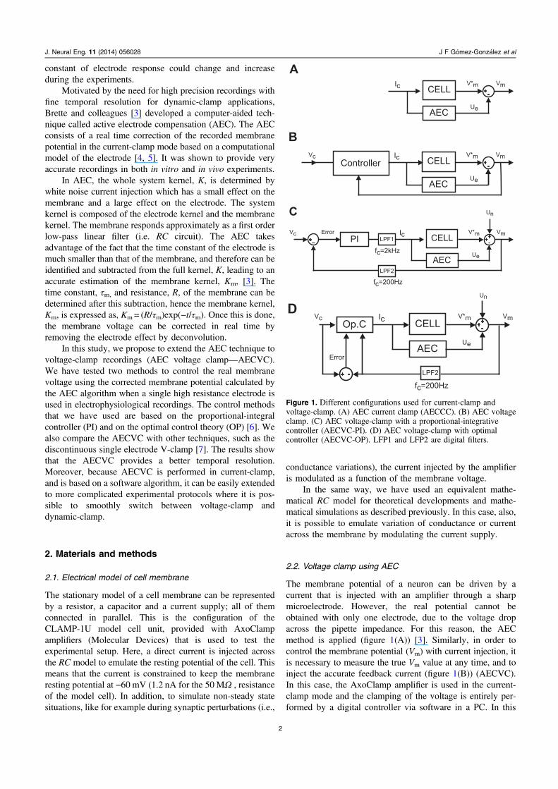
The membrane potential of a neuron can be driven by acurrent that is injected with an amplifier through a sharpmicroelectrode. However, the real potential cannot beobtained with only one electrode, due to the voltage dropacross the pipette impedance. For this reason, the AECmethod is applied (figure 1(A)) [3]. Similarly, in order tocontrol the membrane potential (Vm) with current injection, itis necessary to measure the true Vm value at any time, and toinject the accurate feedback current (figure 1(B)) (AECVC).In this case, the AxoClamp amplifier is used in the current-clamp mode and the clamping of the voltage is entirely per-formed by a digital controller via software in a PC. In this

Figure 1. Different configurations used for current-clamp andvoltage-clamp. (A) AEC current clamp (AECCC). (B) AEC voltageclamp. (C) AEC voltage-clamp with a proportional-integrativecontroller (AECVC-PI). (D) AEC voltage-clamp with optimalcontroller (AECVC-OP). LFP1 and LFP2 are digital filters.

2

J. Neural Eng. 11 (2014) 056028 J F Gómez-González et al

work, two controllers were tested: proportional-integrativecontroller (PI) and model-based controller design (optimalcontroller) (figures 1(C) and (D)).

2.3. Mathematical model of the experimental setup

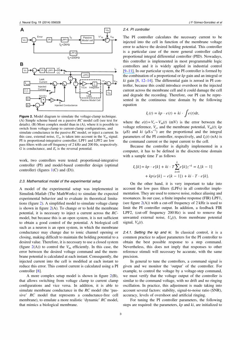
A model of the experimental setup was implemented inSimulink-Matlab (The MathWorks) to simulate the expectedexperimental behavior and to evaluate its theoretical limita-tions (figure 2). A simplified model to simulate voltage clampis shown in figure 2(A). To change or to hold the membranepotential, it is necessary to inject a current across the RC-model, but because this is an open system, it is not sufficientto obtain a good control of the potential. A biological cellsuch as a neuron is an open system, in which the membraneconductance may change due to ionic channel opening orclosing, making difficult to maintain the holding potential to adesired value. Therefore, it is necessary to use a closed system(figure 2(A)) to control the Vm efficiently. In this case, theerror between the desired voltage command and the mem-brane potential is calculated at each instant. Consequently, theinjected current into the cell is modified at each instant toreduce this error. This control current is calculated using a PIcontroller [8].

A more complex setup model is shown in figure 2(B),that allows switching from voltage clamp to current clampconfigurations and vice versa. In addition, it is able tosimulate membrane conductance in the RC model (the ‘pas-sive’ RC model that represents a conductance-free cellmembrane), to emulate a more realistic ‘dynamic’ RC model,that mimics a biological membrane.

2.4. PI controller

The PI controller calculates the necessary current to beinjected into the cell in function of the membrane voltageerror to achieve the desired holding potential. This controlleris a particular case of the more general controller calledproportional integral differential controller (PID). Nowadays,this controller is implemented in most programmable logiccontrollers and it is widely applied in industrial control[9–11]. In our particular system, the PI controller is formed bythe combination of a proportional or kp gain and an integral orki gain [8, 12–14]. The differential gain is zeroed in PI con-troller, because this could introduce overshoot in the injectedcurrent across the membrane cell and it could damage the celland degrade the recording. Therefore, our PI can be repre-sented in the continuous time domain by the followingequation

∫= ⋅ + ⋅I t kp e t ki e t t( ) ( ) ( )d ,c

where the e(t) =Vc−Vm(t) (mV) is the error between thevoltage reference, Vc, and the membrane potential, Vm(t); kp(μS) and ki (μS s−1) are the proportional and the integralparameters of the PI controller, respectively, and Ic(t) (nA) isthe command current or the input current to the cell.

Because the controller is digitally implemented in acomputer, it has to be defined in the discrete-time domainwith a sample time T as follows

∑= ⋅ + ⋅ = −

+ − − + ⋅ ⋅=

−I k kp e k ki T e k z I k

kp e k e k ki T e k

[ ] [ ] [ ] [ 1]

( [ ] [ 1]) [ ].k

kk

c

0

c

On the other hand, it is very important to take intoaccount the low pass filters (LPFs) in all controller imple-mentation. They are used to remove noise, reduce aliasing andresonances. In our case, a finite impulse response (FIR) LPF1,(see figure 2(A)) with a cut-off frequency of 2 kHz is used tolimit the PI controller output. In addition, a feedback FIRLPF2, (cut-off frequency 200 Hz) is used to remove theunwanted external noise, Un(t), from membrane potentialsignal, Vn(t).

2.4.1. Setting the kp and ki. In classical control, it is acommon practice to adjust parameters for the PI controller toobtain the best possible response to a step command.Nevertheless, this does not imply that responses to otherreference stimuli will necessary be accurate, with the sameprecision.

In general to tune the controllers, a command signal isgiven and we monitor the ‘output’ of the controller. Forexample, to control the voltage by a voltage-step command,we must verify that the voltage output of the controller issimilar to the command voltage, with no drift and no ringingoscillation. In practice, this adjustment is made taking intoaccount several factors: stability, signal-to-noise ratio (SNR),accuracy, levels of overshoot and artificial ringing.

For tuning the PI controller parameters, the followingsteps are required: the parameters, kp and ki, are initialized to

Figure 2. Model diagram to simulate the voltage-clamp technique.(A) Simple scheme based on a passive RC model cell (see text fordetails). (B) More complex model than in (A), where it is possible toswitch from voltage-clamp to current-clamp configurations, andsimulate conductance in the passive RC model, or inject a current. Inthis case, external noise, Un, is taken into account in the Vm signal.PI is proportional-integrative controller; LPF1 and LPF2 are lowpass filters with cut-off frequency of 2 kHz and 200 Hz, respectively.G is conductance, and Er is the reversal potential.

3

J. Neural Eng. 11 (2014) 056028 J F Gómez-González et al

small values (i.e. kp= 0.01 μS, ki = 0.01 μS s−1), then a squarewave of voltage is applied. At that moment the voltage is notyet controlled, then kp is increased until the clamped voltagefollows the square wave, without overshoot. In the case thatthe detected voltage is too noisy, the kp can be reduced,followed by a reduction of ki. We found that noise reductionis acceptable when the deseeded SNR is high enough to detectthe synaptic current transients without introducing artefacts.(e.g. SNR is around 69 for the voltage trace in the figure 4(A),where SNR is defined as the ratio between the signal meanand the standard deviation.) In addition, it should be notedthat when the SNR becomes too small, the system becomesunstable and could damage the cell.

2.5. Model-based controller design (optimal controller)

The optimal control theory is a time domain technique tocontrol and to determinate the state trajectories for a dynamicsystem over a period of time to minimize a performance (cost)function [6, 12, 13]. In other words, having defined the per-formance function, the best control signal over time may befound by minimizing this function.

The formulation of an optimal control problem requiresthe following: (a) a mathematical model of the system to becontrolled, (b) a specification of the performance function, (c)a specification of all boundary conditions on states, andconstrains to be satisfied by states and controls, and (d) astatement of what variable are free.

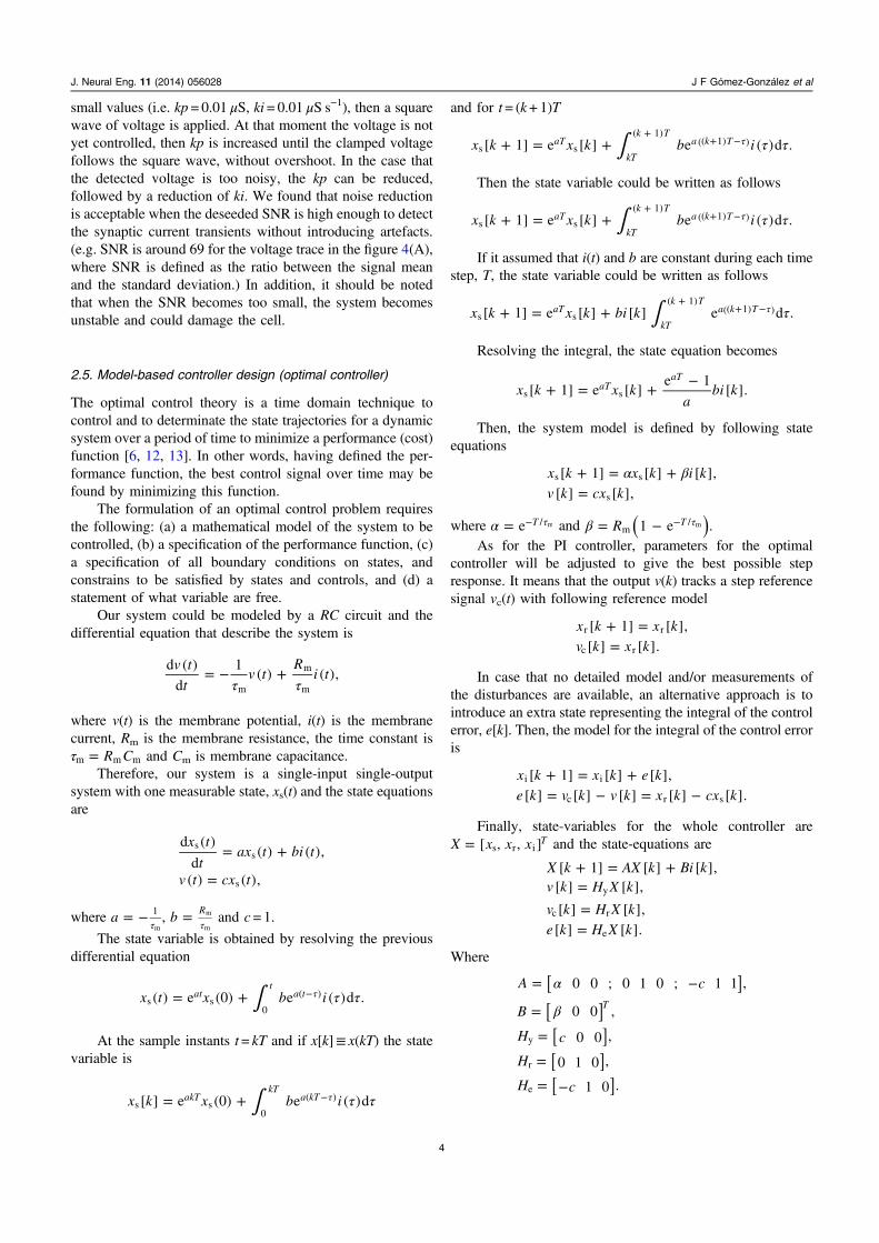
Our system could be modeled by a RC circuit and thedifferential equation that describe the system is

τ τ= − +v t

tv t

Ri t

d ( )

d

1( ) ( ),

m

m

m

where v(t) is the membrane potential, i(t) is the membranecurrent, Rm is the membrane resistance, the time constant isτ = R Cm m m and Cm is membrane capacitance.

Therefore, our system is a single-input single-outputsystem with one measurable state, xs(t) and the state equationsare

= +

=

x t

tax t bi t

v t cx t

d ( )

d( ) ( ),

( ) ( ),

ss

s

where = −τ

a 1

m, =

τb

Rm

mand c= 1.

The state variable is obtained by resolving the previousdifferential equation

∫ τ τ= + τ−x t x b i( ) e (0) e ( )d .att

a ts s

0

( )

At the sample instants t= kT and if x[k]≡ x(kT) the statevariable is

∫ τ τ= + τ−x k x b i[ ] e (0) e ( )dakTkT

a kTs s

0

( )

and for t= (k+ 1)T

∫ τ τ+ = + τ+

+ −x k x k b i[ 1] e [ ] e ( )d .aT

kT

k Ta k T

s s

( 1)(( 1) )

Then the state variable could be written as follows

∫ τ τ+ = + τ+

+ −x k x k b i[ 1] e [ ] e ( )d .aT

kT

k Ta k T

s s

( 1)(( 1) )

If it assumed that i(t) and b are constant during each timestep, T, the state variable could be written as follows

∫ τ+ = + τ+

+ −x k x k bi k[ 1] e [ ] [ ] e d .aT

kT

k Ta k T

s s

( 1)(( 1) )

Resolving the integral, the state equation becomes

+ = + −x k x k

abi k[ 1] e [ ]

e 1[ ].aT

aT

s s

Then, the system model is defined by following stateequations

α β+ = +=

x k x k i k

v k cx k

[ 1] [ ] [ ],[ ] [ ],s s

s

where α = τ−e T / m and β = − τ−( )R 1 e .Tm

/ m

As for the PI controller, parameters for the optimalcontroller will be adjusted to give the best possible stepresponse. It means that the output v(k) tracks a step referencesignal vc(t) with following reference model

+ ==

x k x k

v k x k

[ 1] [ ],[ ] [ ].

r r

c r

In case that no detailed model and/or measurements ofthe disturbances are available, an alternative approach is tointroduce an extra state representing the integral of the controlerror, e[k]. Then, the model for the integral of the control erroris

+ = += − = −

x k x k e k

e k v k v k x k cx k

[ 1] [ ] [ ],[ ] [ ] [ ] [ ] [ ].i i

c r s

Finally, state-variables for the whole controller are=X x x x[ , , ]Ts r i and the state-equations are

Α Β+ = +===

X k X k i kv k H X k

v k H X k

e k H X k

[ 1] [ ] [ ],[ ] [ ],

[ ] [ ],[ ] [ ].

y

c r

e

Where

α

β

= −

=

=

=

= −

[ ][ ]

[ ][ ][ ]

A c

B

H c

H

H c

0 0 ; 0 1 0 ; 1 1 ,

0 0 ,

0 0 ,

0 1 0 ,

1 0 .

T

y

r

e

4

J. Neural Eng. 11 (2014) 056028 J F Gómez-González et al

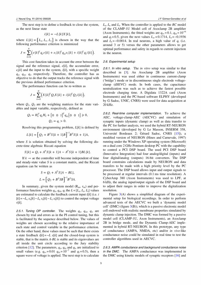
The next step is to define a feedback to close the system,as the next linear state

= −i k L k X k[ ] [ ] [ ],

where ⎡⎣ ⎤⎦=L k L L L[ ] , ,s r i is chosen in the way that thefollowing performance criterion is minimized

∑= + +=

( )J e k q e k e k q e k i k q i k[ ] [ ] [ ] [ ] [ ] [ ] .k

NT T T

0e i ei i i

This cost function takes in account the error between thesignal and the reference signal, e[k], the accumulate error,ei[k] and the input to the system, i[k], with a specific weightqe, qei, qi, respectively. Therefore, the controller has asobjective to do that the output tracks the reference signal withthe previous defined performance criterion.

The performance function can be re-written as

∑= +=

( )J X k Q X k i k Q i k[ ] [ ] [ ] [ ] ,k

NT T

0

1 2

where Q1, Q2 are the weighting matrices for the state vari-ables and input variable, respectively, defined as

= + ⩾[ ] [ ]Q H q H q0 0 1 0 0 1 0,T T1 e e e ei

= >Q q 0.2 i

Resolving this programming problem, L[k] is defined by

⎡⎣ ⎤⎦Β Β Β Α= + + +−

L k Q S k S k[ ] [ 1] [ 1] ,T T2

1

where S is solution obtained by solving the following dis-crete-time algebraic Riccati equation

Α Α Α Β= + + − +S k Q S k S k L k[ ] [ 1] [ 1] [ ].T T1

If → ∞k the controller will become independent of timeand steady-state value S is a constant matrix, and the Riccatiequation can be written as

Α Α Β= + −S Q S L[ ],T1

⎡⎣ ⎤⎦Β Β Β Α= +−

L Q S S .T T2

1

In summary, given the system model (Rm, τm) and per-formance function weights qe, qei, qi the L = [Ls, Lr, Li] valuesare estimated to calculate the feedback current input i[k] (i.e. i[k] =−Ls xs[k]− Lr xr[k]− Li xi[k]) to control the output voltagev[k].

2.5.1. Tuning OP controller. The weights qe, qei, qi, arechosen by trial and errors as in the PI control tuning, but thisis facilitated by the sequence described below. The values ofweights are chosen according to the relative importance ofeach state and control variable in the performance criterion.On the other hand, these values must be such that there existsa state feedback i[k] =−L x[k] and the closed-loop system isstable, that is the matrix A-BL is stable and its eigenvalues areall inside the unit circle according to the Jury stabilitycriterion [12]. The parameters, qe, qei and qi, are initialized tosmall values (e.g. qe, = 0.01 qei = 10

−7 and qi = 0.5), then asquare wave of voltage is applied. The next step is to calculate

Ls, Lr and Li. When the controller is applied to the RC modelof the CLAMP-1U Model cell of Axoclamp 2B amplifier(Axon Instruments), the fitted weights are qe, = 0.1, qei = 10

−6

and qi = 0.5, given the next values Ls, = 0.1714, Lr =−0.1936and Li =−0.0014. In real neurons, a high value of qi (i.e.around 3 or 5) versus the other parameters allows to getoptimal performance and safety in regards to current injectionin the neuron.

2.6. Experimental setup

2.6.1. In vitro setup. The in vitro setup was similar to thatdescribed in [3]. An Axoclamp 2B amplifier (AxonInstruments) was used either in continuous current-clamp(‘bridge’) mode or in discontinuous single electrode voltage-clamp (dSEVC) mode. In both cases, the capacitanceneutralization was such as to achieve the fastest possibleelectrode charging time. A Digidata 1322A card (AxonInstruments) and the PC-based software ELPHY (developedby G Sadoc, UNIC, CNRS) were used for data acquisition at20 kHz.

2.6.2. Real-time computer implementation. To achieve theAEC, voltage-clamp-AEC (AECVC) and simulation ofsynaptic inputs (dynamic clamp) as well as data transfer tothe PC for further analysis, we used the hybrid RT-NEURONenvironment (developed by G Le Masson, INSERM 358,Université Bordeaux 2; Gérard Sadoc, CNRS [15]), amodified version of NEURON (Hines and Carnevale, 1997)running under the Windows XP operating system (Microsoft)on a dual core 2 GHz Pentium desktop PC with the capabilityto control a PCI DSP board. The used PCI DSP board(Innovative Integration) had four analog/digital (inputs) andfour digital/analog (outputs) 16-bit converters. The DSPboard constrains calculations made by NEURON and datatransfers to be made with a high priority level by the PCprocessor. The DSP board allows input and output signals tobe processed at regular intervals (0.1 ms time resolution). ACyberAmp 380 (Axon Instruments) was used to LPF, at6 kHz, the analog input/output signals of the DSP board andto adjust their ranges in order to improve the digitalizationresolution.

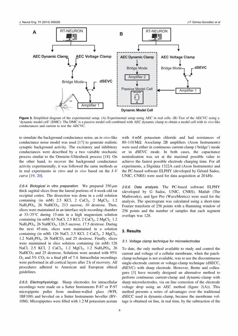
Figure 3(A) shows a simplified diagram of the experi-mental setup for biological recordings. In order to performadvanced tests of the AECVC we built a ‘dynamic modelcell’ (DMC) (figure 3(B)), which is a passive electronic modelcell endowed with realistic membrane properties simulated bydynamic clamp injection. The DMC was formed by a passivemodel cell (CLAMP-1U, Axon Instruments), an Axoclamp2B in bridge mode, and the Dynamic Clamp-AEC imple-mented in hybrid RT-NEURON. In this prototype, any typeof conductance (AMPA, NMDA, etc) and/or in vivo-likeconductance noise could be simulated in real time to test thecontroller algorithms used in AECVC.

2.6.3. AMPA conductance and background conductance noisein the DMC. The AMPA conductance was implemented inthe DMC using kinetic models of synaptic receptors [16] and

5

J. Neural Eng. 11 (2014) 056028 J F Gómez-González et al

to simulate the background conductance noise, an in vivo-likeconductance noise model was used [17] to generate realisticsynaptic background activity. The excitatory and inhibitoryconductances were described by a two variable stochasticprocess similar to the Ornstein–Uhlenbeck process [18]. Onthe other hand, to recover the background conductanceactivity experimentally, it was followed the same methods asin real experiments in vitro and in vivo based on the I–Vcurve [19, 20].

2.6.4. Biological in vitro preparation. We prepared 350 μmthick sagittal slices from the lateral portions of 4-week-old ratoccipital cortex. The dissection was done in a cold solutioncontaining (in mM) 2.5 KCl, 2 CaCl2, 2 MgCl2, 1.2NaH2PO4, 26 NaHCO3, 213 sucrose, 10 dextrose. Then,slices were maintained in an interface style recording chamberat 33–35°C during 15 min in a high magnesium solutioncontaining (in mM) 63 NaCl, 2.5 KCl, 2 CaCl2, 2 MgCl2, 1.2NaH2PO4, 26 NaHCO3, 126.5 sucrose, 17.5 dextrose. Duringthe next 45 min, slices were maintained in a solutioncontaining (in mM) 126 NaCl, 2.5 KCl, 2 CaCl2, 2 MgCl2,1.2 NaH2PO4, 26 NaHCO3 and 25 dextrose. Finally, sliceswere maintained in slice solution containing (in mM) 126NaCl, 2.5 KCl, 2 CaCl2, 1.2 MgCl2, 1.2 NaH2PO4, 26NaHCO3 and 25 dextrose. Solutions were aerated with 95%O2 and 5% CO2 to a final pH of 7.4. Intracellular recordingswere performed in all cortical layers after 2 h of recovery. Allprocedures adhered to American and European ethicalguidelines.

2.6.5. Electrophysiology. Sharp electrodes for intracellularrecordings were made on a Sutter Instruments P-87 or P-97micropipette puller from medium-walled glass (WPI,1BF100) and beveled on a Sutter Instruments beveller (BV-10M). Micropipettes were filled with 1.2M potassium acetate

with 4 mM potassium chloride and had resistances of80–110MΩ. Axoclamp 2B amplifiers (Axon Instruments)were used either in continuous current-clamp (‘bridge’) modeor in dSEVC mode. In both cases, the capacitanceneutralization was set at the maximal possible value toachieve the fastest possible electrode charging time. For allexperiments, a Digidata 1322A card (Axon Instruments) andthe PC-based software ELPHY (developed by Gérard Sadoc,UNIC, CNRS) were used for data acquisition at 20 kHz.

2.6.6. Data analysis. The PC-based software ELPHY(developed by G Sadoc, UNIC, CNRS), Matlab (TheMathworks), and Igor Pro (WaveMetrics) were used for theanalysis. The spectrogram was calculated using a short-timeFourier transform of 256 points with a Hamming window of256 points and the number of samples that each segmentoverlaps was 128.

3. Results

3.1. Voltage clamp technique for microelectrodes

To date, the only method available to study and control thecurrent and voltage of a cellular membrane, when the patch-clamp technique is not available, was to use the discontinuoussingle-electrode current or voltage-clamp technique (dSECC,dSEVC) with sharp electrode. However, Brette and collea-gues [3] have recently designed an alternative method toperform continuous current-clamp and dynamic-clamp withsharp microelectrodes, via on line correction of the electrodevoltage drop using an AEC method (figure 2(A)). Thismethod presents a series of advantages over the traditionaldSECC used in dynamic-clamp, because the membrane vol-tage is obtained on line, in real time, by the subtraction of the

Figure 3. Simplified diagram of the experimental setup. (A) Experimental setup using AEC in real cells. (B) Test of the AECVC using a‘dynamic model cell’ (DMC). The DMC is a passive model cell combined with AEC dynamic clamp to obtain a model cell with in vivo-likeconductances and current to test the AECVC.

6

J. Neural Eng. 11 (2014) 056028 J F Gómez-González et al

calculated electrode voltage to the given voltage for theelectrophysiology amplifier in ‘bridge’ mode. As AEC allowsto determinate the transfer function of the electrode [3], thevoltage across the electrode, Ue, is determined as the con-volution of the injected current, i.e., and the electrode kernelKe, therefore the membrane potential is given as follows

= − = − ⊗V t V t U V t K I t( ) ( ) ( ) ( ).m r e r e e

Since the voltage of the membrane of the cell is measurederror-free when using AEC, it is then possible to accuratelycontrol its value through the current injection across themicroelectrode. However, in this case, it is necessary toimplement a control system that changes the injected currentinto the cell in real time, such that the membrane voltagefollows the desired set value (figure 2(B)). Two differentmethods to control the membrane voltage are presented in thisarticle: (a) the proportional-integral controller (PI controller),which is a feedback controller that drives the system using theerror, defined as the difference between the membrane voltageand the desired set value, and the accumulated error asinformation inputs to the controller (figure 2(C)); (b) theoptimal controller (OP controller), that attempt to find thecontrol variables that best achieve some criteria minimizingthe cost function of the system (figure 2(D)).

3.2. Comparison of voltage clamp techniques

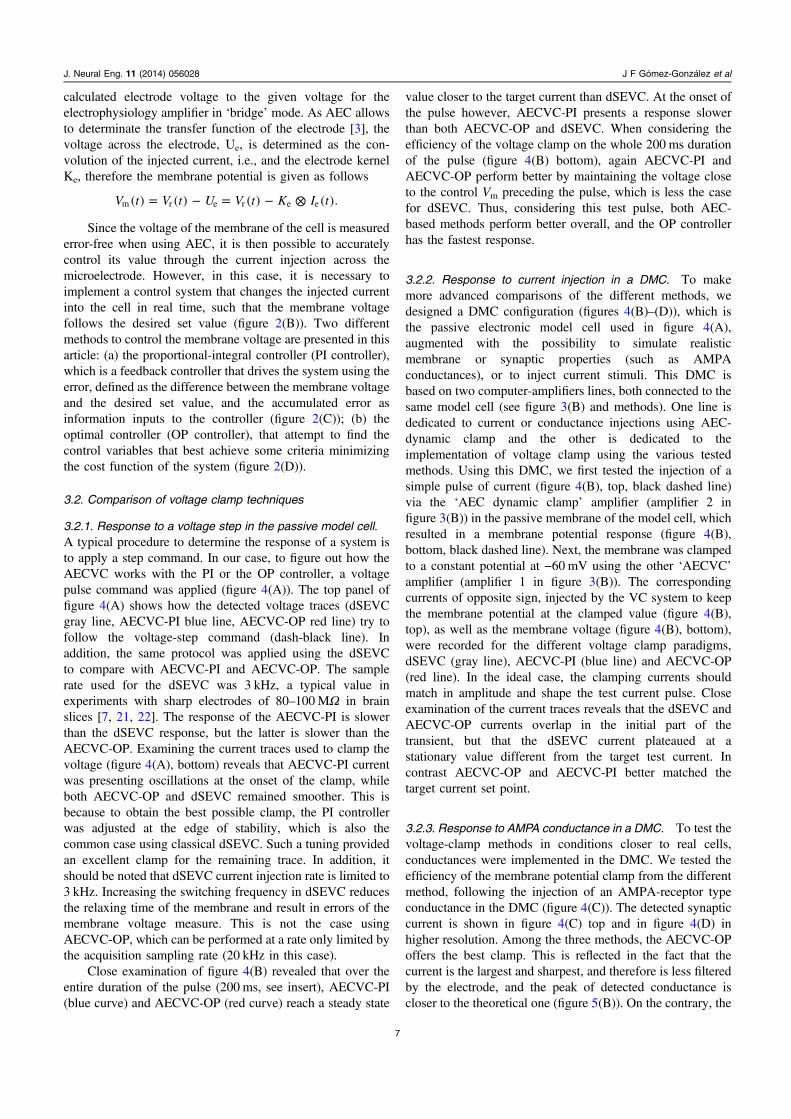
3.2.1. Response to a voltage step in the passive model cell.A typical procedure to determine the response of a system isto apply a step command. In our case, to figure out how theAECVC works with the PI or the OP controller, a voltagepulse command was applied (figure 4(A)). The top panel offigure 4(A) shows how the detected voltage traces (dSEVCgray line, AECVC-PI blue line, AECVC-OP red line) try tofollow the voltage-step command (dash-black line). Inaddition, the same protocol was applied using the dSEVCto compare with AECVC-PI and AECVC-OP. The samplerate used for the dSEVC was 3 kHz, a typical value inexperiments with sharp electrodes of 80–100MΩ in brainslices [7, 21, 22]. The response of the AECVC-PI is slowerthan the dSEVC response, but the latter is slower than theAECVC-OP. Examining the current traces used to clamp thevoltage (figure 4(A), bottom) reveals that AECVC-PI currentwas presenting oscillations at the onset of the clamp, whileboth AECVC-OP and dSEVC remained smoother. This isbecause to obtain the best possible clamp, the PI controllerwas adjusted at the edge of stability, which is also thecommon case using classical dSEVC. Such a tuning providedan excellent clamp for the remaining trace. In addition, itshould be noted that dSEVC current injection rate is limited to3 kHz. Increasing the switching frequency in dSEVC reducesthe relaxing time of the membrane and result in errors of themembrane voltage measure. This is not the case usingAECVC-OP, which can be performed at a rate only limited bythe acquisition sampling rate (20 kHz in this case).

Close examination of figure 4(B) revealed that over theentire duration of the pulse (200 ms, see insert), AECVC-PI(blue curve) and AECVC-OP (red curve) reach a steady state

value closer to the target current than dSEVC. At the onset ofthe pulse however, AECVC-PI presents a response slowerthan both AECVC-OP and dSEVC. When considering theefficiency of the voltage clamp on the whole 200 ms durationof the pulse (figure 4(B) bottom), again AECVC-PI andAECVC-OP perform better by maintaining the voltage closeto the control Vm preceding the pulse, which is less the casefor dSEVC. Thus, considering this test pulse, both AEC-based methods perform better overall, and the OP controllerhas the fastest response.

3.2.2. Response to current injection in a DMC. To makemore advanced comparisons of the different methods, wedesigned a DMC configuration (figures 4(B)–(D)), which isthe passive electronic model cell used in figure 4(A),augmented with the possibility to simulate realisticmembrane or synaptic properties (such as AMPAconductances), or to inject current stimuli. This DMC isbased on two computer-amplifiers lines, both connected to thesame model cell (see figure 3(B) and methods). One line isdedicated to current or conductance injections using AEC-dynamic clamp and the other is dedicated to theimplementation of voltage clamp using the various testedmethods. Using this DMC, we first tested the injection of asimple pulse of current (figure 4(B), top, black dashed line)via the ‘AEC dynamic clamp’ amplifier (amplifier 2 infigure 3(B)) in the passive membrane of the model cell, whichresulted in a membrane potential response (figure 4(B),bottom, black dashed line). Next, the membrane was clampedto a constant potential at −60 mV using the other ‘AECVC’amplifier (amplifier 1 in figure 3(B)). The correspondingcurrents of opposite sign, injected by the VC system to keepthe membrane potential at the clamped value (figure 4(B),top), as well as the membrane voltage (figure 4(B), bottom),were recorded for the different voltage clamp paradigms,dSEVC (gray line), AECVC-PI (blue line) and AECVC-OP(red line). In the ideal case, the clamping currents shouldmatch in amplitude and shape the test current pulse. Closeexamination of the current traces reveals that the dSEVC andAECVC-OP currents overlap in the initial part of thetransient, but that the dSEVC current plateaued at astationary value different from the target test current. Incontrast AECVC-OP and AECVC-PI better matched thetarget current set point.

3.2.3. Response to AMPA conductance in a DMC. To test thevoltage-clamp methods in conditions closer to real cells,conductances were implemented in the DMC. We tested theefficiency of the membrane potential clamp from the differentmethod, following the injection of an AMPA-receptor typeconductance in the DMC (figure 4(C)). The detected synapticcurrent is shown in figure 4(C) top and in figure 4(D) inhigher resolution. Among the three methods, the AECVC-OPoffers the best clamp. This is reflected in the fact that thecurrent is the largest and sharpest, and therefore is less filteredby the electrode, and the peak of detected conductance iscloser to the theoretical one (figure 5(B)). On the contrary, the

7

J. Neural Eng. 11 (2014) 056028 J F Gómez-González et al

current from the dSEVC method presents a smaller peak andoscillations due to the low sampled-and-hold switchingfrequency.

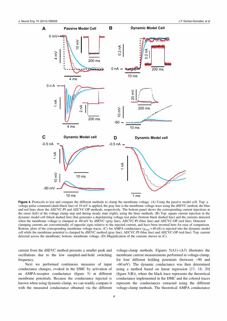
Next we performed continuous measures of inputconductance changes, evoked in the DMC by activation ofan AMPA-receptor conductance (figure 5) at differentmembrane potentials. Because the conductance injected isknown when using dynamic-clamp, we can readily compare itwith the measured conductance obtained via the different

voltage-clamp methods. Figures 5(A1)–(A3) illustrates themembrane current measurements performed in voltage-clamp,for four different holding potentials (between −90 and−60 mV). The dynamic conductance was then determinedusing a method based on linear regression [17, 18, 20](figure 5(B)), where the black trace represents the theoreticalconductance implemented in the DMC and the colored tracesrepresent the conductances extracted using the differentvoltage-clamp methods. The theoretical AMPA conductance

Figure 4. Protocols to test and compare the different methods to clamp the membrane voltage. (A) Using the passive model cell. Top: avoltage pulse command (dash-black line) of 10 mV is applied, the gray line is the membrane voltage trace using the dSEVC method, the blueand red lines show the AECVC-PI and AECVC-OP methods, respectively. The bottom panel shows the corresponding current injections atthe onset (left) of the voltage clamp step and during steady state (right), using the three methods. (B) Top: square current injection in thedynamic model cell (black dashed line) that generates a depolarizing voltage test pulse (bottom black dashed line) and the currents detectedwhen the membrane voltage is clamped at –60 mV by dSEVC (gray line), AECVC-PI (blue line) and AECVC-OP (red line). Detectedclamping currents are conventionally of opposite signs relative to the injected current, and have been inverted here for ease of comparison.Bottom: plots of the corresponding membrane voltage traces. (C) An AMPA conductance (gmax = 40 nS) is injected into the dynamic modelcell while the membrane potential is clamped by dSEVC method (gray line), AECVC-PI (blue line) and AECVC-OP (red line). Top: currentdetected across the membrane; bottom: membrane voltage. (D) Magnification of the currents shown in (C).

8

J. Neural Eng. 11 (2014) 056028 J F Gómez-González et al

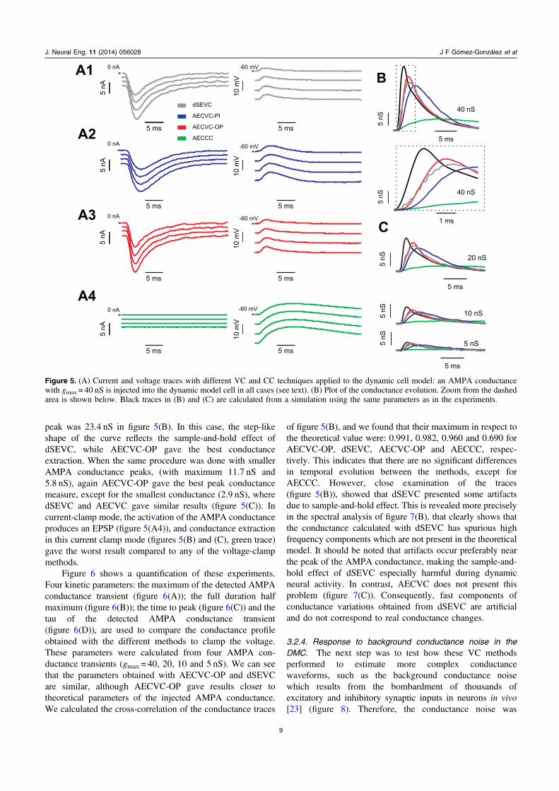
peak was 23.4 nS in figure 5(B). In this case, the step-likeshape of the curve reflects the sample-and-hold effect ofdSEVC, while AECVC-OP gave the best conductanceextraction. When the same procedure was done with smallerAMPA conductance peaks, (with maximum 11.7 nS and5.8 nS), again AECVC-OP gave the best peak conductancemeasure, except for the smallest conductance (2.9 nS), wheredSEVC and AECVC gave similar results (figure 5(C)). Incurrent-clamp mode, the activation of the AMPA conductanceproduces an EPSP (figure 5(A4)), and conductance extractionin this current clamp mode (figures 5(B) and (C), green trace)gave the worst result compared to any of the voltage-clampmethods.

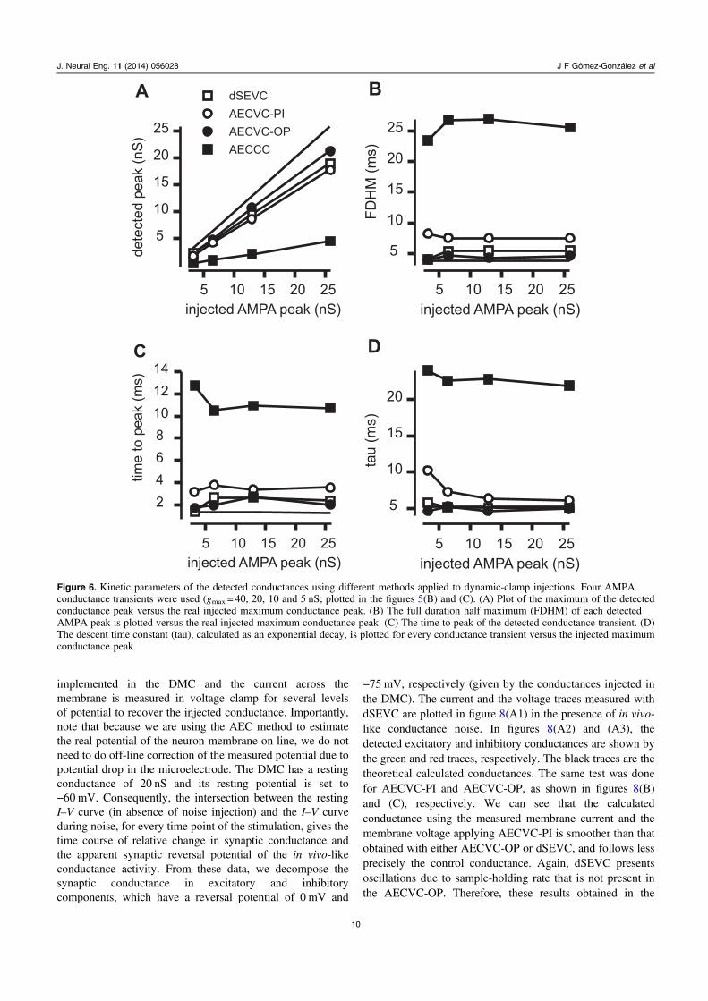
Figure 6 shows a quantification of these experiments.Four kinetic parameters: the maximum of the detected AMPAconductance transient (figure 6(A)); the full duration halfmaximum (figure 6(B)); the time to peak (figure 6(C)) and thetau of the detected AMPA conductance transient(figure 6(D)), are used to compare the conductance profileobtained with the different methods to clamp the voltage.These parameters were calculated from four AMPA con-ductance transients (gmax = 40, 20, 10 and 5 nS). We can seethat the parameters obtained with AECVC-OP and dSEVCare similar, although AECVC-OP gave results closer totheoretical parameters of the injected AMPA conductance.We calculated the cross-correlation of the conductance traces

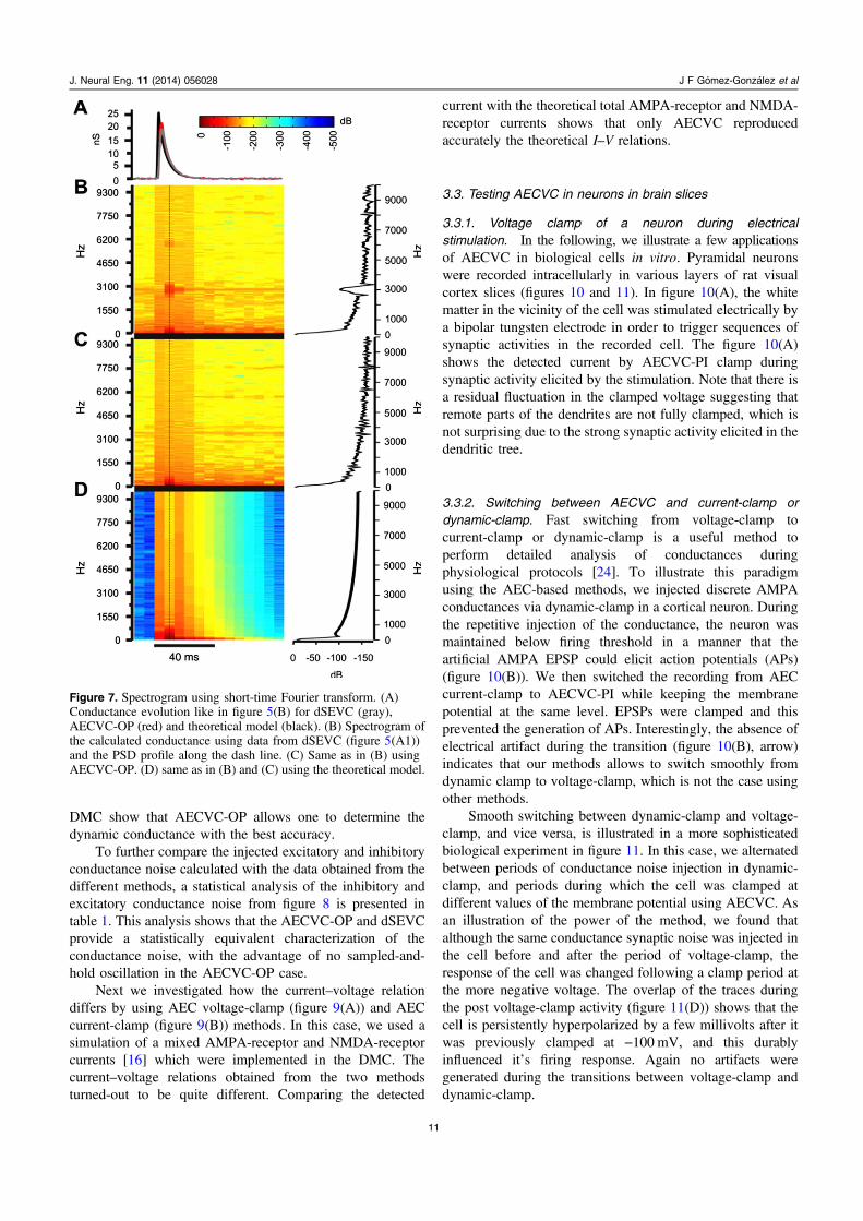
of figure 5(B), and we found that their maximum in respect tothe theoretical value were: 0.991, 0.982, 0.960 and 0.690 forAECVC-OP, dSEVC, AECVC-OP and AECCC, respec-tively. This indicates that there are no significant differencesin temporal evolution between the methods, except forAECCC. However, close examination of the traces(figure 5(B)), showed that dSEVC presented some artifactsdue to sample-and-hold effect. This is revealed more preciselyin the spectral analysis of figure 7(B), that clearly shows thatthe conductance calculated with dSEVC has spurious highfrequency components which are not present in the theoreticalmodel. It should be noted that artifacts occur preferably nearthe peak of the AMPA conductance, making the sample-and-hold effect of dSEVC especially harmful during dynamicneural activity. In contrast, AECVC does not present thisproblem (figure 7(C)). Consequently, fast components ofconductance variations obtained from dSEVC are artificialand do not correspond to real conductance changes.

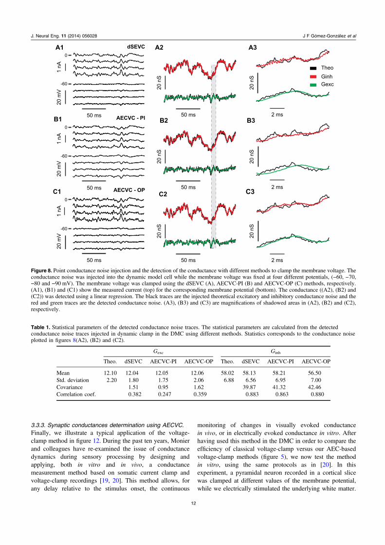
3.2.4. Response to background conductance noise in theDMC. The next step was to test how these VC methodsperformed to estimate more complex conductancewaveforms, such as the background conductance noisewhich results from the bombardment of thousands ofexcitatory and inhibitory synaptic inputs in neurons in vivo[23] (figure 8). Therefore, the conductance noise was

Figure 5. (A) Current and voltage traces with different VC and CC techniques applied to the dynamic cell model: an AMPA conductancewith gmax = 40 nS is injected into the dynamic model cell in all cases (see text). (B) Plot of the conductance evolution. Zoom from the dashedarea is shown below. Black traces in (B) and (C) are calculated from a simulation using the same parameters as in the experiments.

9

J. Neural Eng. 11 (2014) 056028 J F Gómez-González et al

implemented in the DMC and the current across themembrane is measured in voltage clamp for several levelsof potential to recover the injected conductance. Importantly,note that because we are using the AEC method to estimatethe real potential of the neuron membrane on line, we do notneed to do off-line correction of the measured potential due topotential drop in the microelectrode. The DMC has a restingconductance of 20 nS and its resting potential is set to−60 mV. Consequently, the intersection between the restingI–V curve (in absence of noise injection) and the I–V curveduring noise, for every time point of the stimulation, gives thetime course of relative change in synaptic conductance andthe apparent synaptic reversal potential of the in vivo-likeconductance activity. From these data, we decompose thesynaptic conductance in excitatory and inhibitorycomponents, which have a reversal potential of 0 mV and

−75 mV, respectively (given by the conductances injected inthe DMC). The current and the voltage traces measured withdSEVC are plotted in figure 8(A1) in the presence of in vivo-like conductance noise. In figures 8(A2) and (A3), thedetected excitatory and inhibitory conductances are shown bythe green and red traces, respectively. The black traces are thetheoretical calculated conductances. The same test was donefor AECVC-PI and AECVC-OP, as shown in figures 8(B)and (C), respectively. We can see that the calculatedconductance using the measured membrane current and themembrane voltage applying AECVC-PI is smoother than thatobtained with either AECVC-OP or dSEVC, and follows lessprecisely the control conductance. Again, dSEVC presentsoscillations due to sample-holding rate that is not present inthe AECVC-OP. Therefore, these results obtained in the

Figure 6. Kinetic parameters of the detected conductances using different methods applied to dynamic-clamp injections. Four AMPAconductance transients were used (gmax = 40, 20, 10 and 5 nS; plotted in the figures 5(B) and (C). (A) Plot of the maximum of the detectedconductance peak versus the real injected maximum conductance peak. (B) The full duration half maximum (FDHM) of each detectedAMPA peak is plotted versus the real injected maximum conductance peak. (C) The time to peak of the detected conductance transient. (D)The descent time constant (tau), calculated as an exponential decay, is plotted for every conductance transient versus the injected maximumconductance peak.

10

J. Neural Eng. 11 (2014) 056028 J F Gómez-González et al

DMC show that AECVC-OP allows one to determine thedynamic conductance with the best accuracy.

To further compare the injected excitatory and inhibitoryconductance noise calculated with the data obtained from thedifferent methods, a statistical analysis of the inhibitory andexcitatory conductance noise from figure 8 is presented intable 1. This analysis shows that the AECVC-OP and dSEVCprovide a statistically equivalent characterization of theconductance noise, with the advantage of no sampled-and-hold oscillation in the AECVC-OP case.

Next we investigated how the current–voltage relationdiffers by using AEC voltage-clamp (figure 9(A)) and AECcurrent-clamp (figure 9(B)) methods. In this case, we used asimulation of a mixed AMPA-receptor and NMDA-receptorcurrents [16] which were implemented in the DMC. Thecurrent–voltage relations obtained from the two methodsturned-out to be quite different. Comparing the detected

current with the theoretical total AMPA-receptor and NMDA-receptor currents shows that only AECVC reproducedaccurately the theoretical I–V relations.

3.3. Testing AECVC in neurons in brain slices

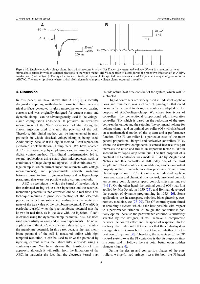
3.3.1. Voltage clamp of a neuron during electricalstimulation. In the following, we illustrate a few applicationsof AECVC in biological cells in vitro. Pyramidal neuronswere recorded intracellularly in various layers of rat visualcortex slices (figures 10 and 11). In figure 10(A), the whitematter in the vicinity of the cell was stimulated electrically bya bipolar tungsten electrode in order to trigger sequences ofsynaptic activities in the recorded cell. The figure 10(A)shows the detected current by AECVC-PI clamp duringsynaptic activity elicited by the stimulation. Note that there isa residual fluctuation in the clamped voltage suggesting thatremote parts of the dendrites are not fully clamped, which isnot surprising due to the strong synaptic activity elicited in thedendritic tree.

3.3.2. Switching between AECVC and current-clamp ordynamic-clamp. Fast switching from voltage-clamp tocurrent-clamp or dynamic-clamp is a useful method toperform detailed analysis of conductances duringphysiological protocols [24]. To illustrate this paradigmusing the AEC-based methods, we injected discrete AMPAconductances via dynamic-clamp in a cortical neuron. Duringthe repetitive injection of the conductance, the neuron wasmaintained below firing threshold in a manner that theartificial AMPA EPSP could elicit action potentials (APs)(figure 10(B)). We then switched the recording from AECcurrent-clamp to AECVC-PI while keeping the membranepotential at the same level. EPSPs were clamped and thisprevented the generation of APs. Interestingly, the absence ofelectrical artifact during the transition (figure 10(B), arrow)indicates that our methods allows to switch smoothly fromdynamic clamp to voltage-clamp, which is not the case usingother methods.

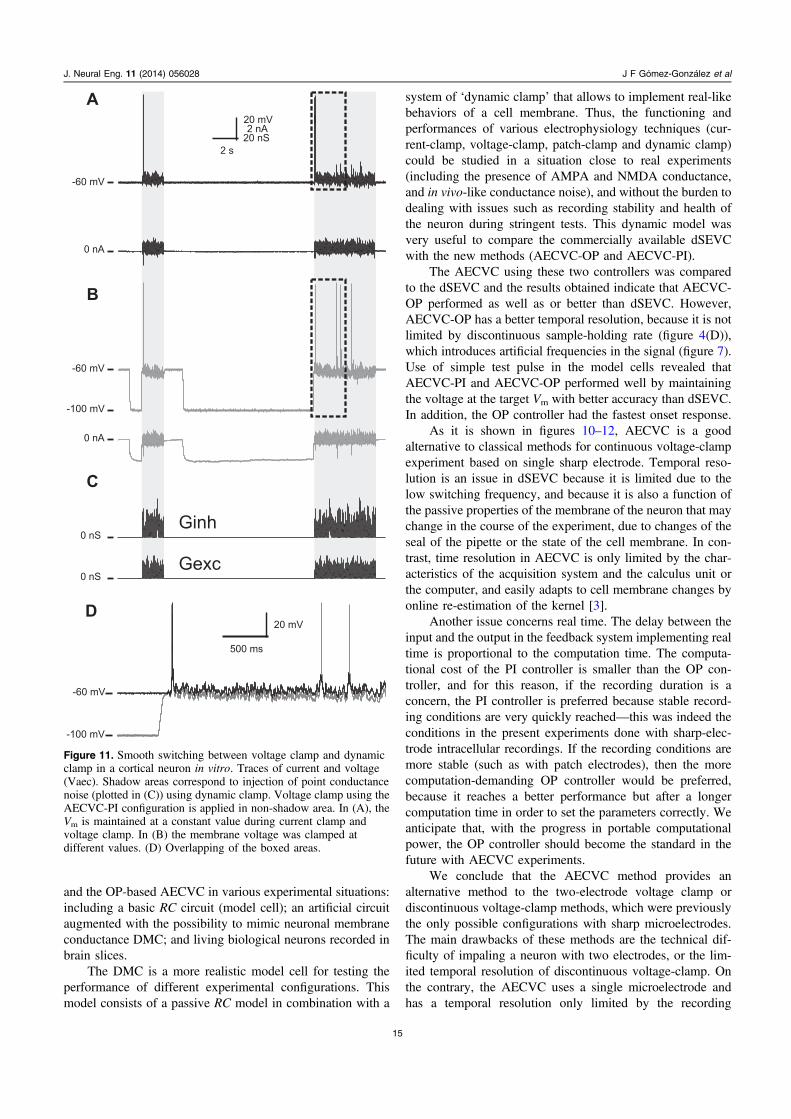
Smooth switching between dynamic-clamp and voltage-clamp, and vice versa, is illustrated in a more sophisticatedbiological experiment in figure 11. In this case, we alternatedbetween periods of conductance noise injection in dynamic-clamp, and periods during which the cell was clamped atdifferent values of the membrane potential using AECVC. Asan illustration of the power of the method, we found thatalthough the same conductance synaptic noise was injected inthe cell before and after the period of voltage-clamp, theresponse of the cell was changed following a clamp period atthe more negative voltage. The overlap of the traces duringthe post voltage-clamp activity (figure 11(D)) shows that thecell is persistently hyperpolarized by a few millivolts after itwas previously clamped at −100 mV, and this durablyinfluenced it’s firing response. Again no artifacts weregenerated during the transitions between voltage-clamp anddynamic-clamp.

Figure 7. Spectrogram using short-time Fourier transform. (A)Conductance evolution like in figure 5(B) for dSEVC (gray),AECVC-OP (red) and theoretical model (black). (B) Spectrogram ofthe calculated conductance using data from dSEVC (figure 5(A1))and the PSD profile along the dash line. (C) Same as in (B) usingAECVC-OP. (D) same as in (B) and (C) using the theoretical model.

11

J. Neural Eng. 11 (2014) 056028 J F Gómez-González et al

3.3.3. Synaptic conductances determination using AECVC.Finally, we illustrate a typical application of the voltage-clamp method in figure 12. During the past ten years, Monierand colleagues have re-examined the issue of conductancedynamics during sensory processing by designing andapplying, both in vitro and in vivo, a conductancemeasurement method based on somatic current clamp andvoltage-clamp recordings [19, 20]. This method allows, forany delay relative to the stimulus onset, the continuous

monitoring of changes in visually evoked conductancein vivo, or in electrically evoked conductance in vitro. Afterhaving used this method in the DMC in order to compare theefficiency of classical voltage-clamp versus our AEC-basedvoltage-clamp methods (figure 5), we now test the methodin vitro, using the same protocols as in [20]. In thisexperiment, a pyramidal neuron recorded in a cortical slicewas clamped at different values of the membrane potential,while we electrically stimulated the underlying white matter.

Figure 8. Point conductance noise injection and the detection of the conductance with different methods to clamp the membrane voltage. Theconductance noise was injected into the dynamic model cell while the membrane voltage was fixed at four different potentials, (−60, −70,−80 and −90 mV). The membrane voltage was clamped using the dSEVC (A), AECVC-PI (B) and AECVC-OP (C) methods, respectively.(A1), (B1) and (C1) show the measured current (top) for the corresponding membrane potential (bottom). The conductance ((A2), (B2) and(C2)) was detected using a linear regression. The black traces are the injected theoretical excitatory and inhibitory conductance noise and thered and green traces are the detected conductance noise. (A3), (B3) and (C3) are magnifications of shadowed areas in (A2), (B2) and (C2),respectively.

Table 1. Statistical parameters of the detected conductance noise traces. The statistical parameters are calculated from the detectedconductance noise traces injected in dynamic clamp in the DMC using different methods. Statistics corresponds to the conductance noiseplotted in figures 8(A2), (B2) and (C2).

Gexc Ginh

Theo. dSEVC AECVC-PI AECVC-OP Theo. dSEVC AECVC-PI AECVC-OP

Mean 12.10 12.04 12.05 12.06 58.02 58.13 58.21 56.50Std. deviation 2.20 1.80 1.75 2.06 6.88 6.56 6.95 7.00Covariance 1.51 0.95 1.62 39.87 41.32 42.46Correlation coef. 0.382 0.247 0.359 0.883 0.863 0.880

12

J. Neural Eng. 11 (2014) 056028 J F Gómez-González et al

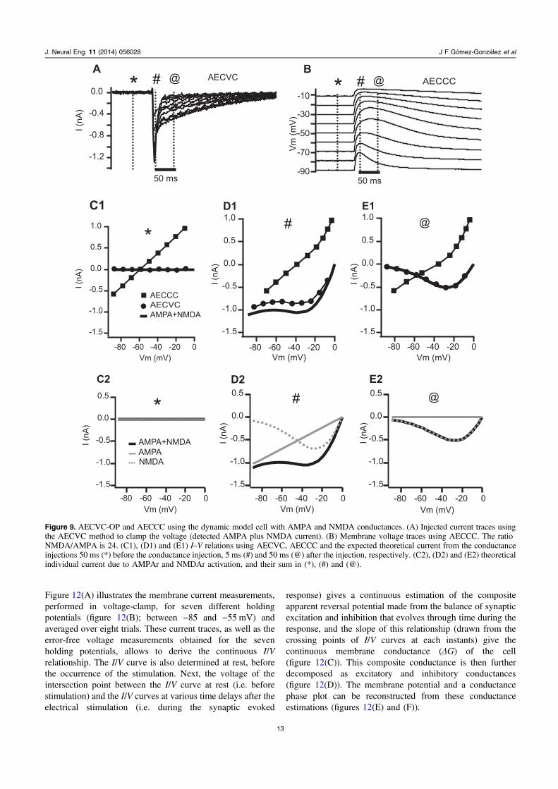
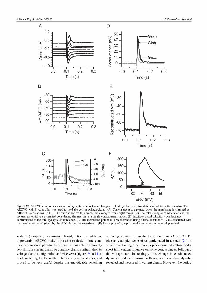
Figure 12(A) illustrates the membrane current measurements,performed in voltage-clamp, for seven different holdingpotentials (figure 12(B); between −85 and −55 mV) andaveraged over eight trials. These current traces, as well as theerror-free voltage measurements obtained for the sevenholding potentials, allows to derive the continuous I/Vrelationship. The I/V curve is also determined at rest, beforethe occurrence of the stimulation. Next, the voltage of theintersection point between the I/V curve at rest (i.e. beforestimulation) and the I/V curves at various time delays after theelectrical stimulation (i.e. during the synaptic evoked

response) gives a continuous estimation of the compositeapparent reversal potential made from the balance of synapticexcitation and inhibition that evolves through time during theresponse, and the slope of this relationship (drawn from thecrossing points of I/V curves at each instants) give thecontinuous membrane conductance (ΔG) of the cell(figure 12(C)). This composite conductance is then furtherdecomposed as excitatory and inhibitory conductances(figure 12(D)). The membrane potential and a conductancephase plot can be reconstructed from these conductanceestimations (figures 12(E) and (F)).

Figure 9. AECVC-OP and AECCC using the dynamic model cell with AMPA and NMDA conductances. (A) Injected current traces usingthe AECVC method to clamp the voltage (detected AMPA plus NMDA current). (B) Membrane voltage traces using AECCC. The ratioNMDA/AMPA is 24. (C1), (D1) and (E1) I–V relations using AECVC, AECCC and the expected theoretical current from the conductanceinjections 50 ms (*) before the conductance injection, 5 ms (#) and 50 ms (@) after the injection, respectively. (C2), (D2) and (E2) theoreticalindividual current due to AMPAr and NMDAr activation, and their sum in (*), (#) and (@).

13

J. Neural Eng. 11 (2014) 056028 J F Gómez-González et al

4. Discussion

In this paper, we have shown that AEC [3], a recentlydesigned computing method—that corrects online the elec-trical artifacts generated in glass micropipettes when passingcurrents and was originally designed for current-clamp anddynamic-clamp—can be advantageously used in the voltage-clamp configuration (AECVC). It provides an error-freemeasurement of the ‘true’ membrane potential during thecurrent injection used to clamp the potential of the cell.Therefore, this digital method can be implemented in mostprotocols in which classical voltage-clamp is being used.Additionally, because it is a digital method, it can replace theelectronic implementation in amplifiers. We have adaptedAEC to voltage-clamp by employing a software-implementeddigital control method. This digital implementation led toseveral applications using sharp glass micropipettes, such ascontinuous voltage-clamp (as opposed to discontinuous vol-tage-clamp in which current injections alternate with voltagemeasurements), and programmable smooth switchingbetween current-clamp, dynamic-clamp and voltage-clamp,paradigms that were not possible using current methods.

AEC is a technique in which the kernel of the electrode isfirst estimated (using white noise injection) and the recordedmembrane potential is then corrected online in real time. Thistechnique requires a prior identification of the electrodeproperties, which are subtracted, leading to an accurate esti-mate of the true value of the membrane potential. The AEC isparticularly useful when the true membrane potential must beknown in real time, as in the case with the injection of con-ductances using the dynamic-clamp technique. AEC has beenused successfully in vitro and in vivo experiments. The novelapplication of the AEC, which we introduce here, is to controlthe membrane potential. In this case, because the real mem-brane potential of the cell is measured online with hightemporal resolution, it can be used to drive the potential byinjecting current across the intracellular electrode using acontrol-system. We have shown the feasibility of thisapproach, although it will suffer from the limitations of theAEC, in particular the fact that the electrode kernel may

include natural fast time constant of the system, which will besubtracted.

Digital controllers are widely used in industrial applica-tions and thus there was a choice of paradigms that couldpresumably be used to design a controller adapted to thepurpose of AEC-voltage-clamp. We chose two types ofcontrollers: the conventional proportional plus integrativecontroller (PI), which is based on the reduction of the errorbetween the output and the setpoint (the command voltage forvoltage-clamp), and an optimal controller (OP) which is basedon a mathematical model of the system and a performancefunction. The PI controller is a particular case of the moregeneral proportional, integral and derivative controllers (PID),where the derivative components is zeroed because this partincreases the noise and this is an important factor to take inaccount in voltage-clamp technique. The first proposal of apractical PID controller was made in 1942 by Ziegler andNichols and this controller is still today one of the mostsimple and robust controllers, in addition, another importantproperty is that it controls uncertain processes. Some exam-ples of application of PI/PID controller in industrial applica-tions are: water and chemical flow control, tank level control,temperature control, motor speed control, ship steering, etc[9–11]. On the other hand, the optimal control (OP) was firstapplied by MacDonald in 1950 [25], and Bellman developedthe concept of dynamic programming in 1953 [26]. Someapplications are in aerospace, robotics, bioengineering, eco-nomics, medicine, etc [27–29]. The OP control system aimedat obtaining a system which is the best possible with respectto a performance criterion. Although, the controller is par-tially optimal because the performance criterion is arbitrarilyselected by the designer, it will achieve a compromisebetween the control effort and the speed of response. On thecontrary, the traditional PID assumes that the control-systemconfiguration is known but it is not known whether it is thebest control system [30]. Therefore, the advantage of the OPcontrol system over the PI controller is that its response timeis shorter and it follows the set point better upon suddenchanges (figure 4).

During the design and comparison phases of the con-trollers, we performed stringent tests for both the PI-based

Figure 10. Single-electrode voltage clamp in cortical neurons in vitro. (A) Traces of current and voltage (Vaec) in a neuron that wasstimulated electrically with an external electrode in the white matter. (B) Voltage trace of a cell during the repetitive injection of an AMPAconductance (bottom trace). Through the same electrode, it is possible to injected conductances in AEC-dynamic clamp configuration or inAECVC. The arrow tip shows where switch from dynamic clamp to voltage clamp occurred smoothly.

14

J. Neural Eng. 11 (2014) 056028 J F Gómez-González et al

and the OP-based AECVC in various experimental situations:including a basic RC circuit (model cell); an artificial circuitaugmented with the possibility to mimic neuronal membraneconductance DMC; and living biological neurons recorded inbrain slices.

The DMC is a more realistic model cell for testing theperformance of different experimental configurations. Thismodel consists of a passive RC model in combination with a

system of ‘dynamic clamp’ that allows to implement real-likebehaviors of a cell membrane. Thus, the functioning andperformances of various electrophysiology techniques (cur-rent-clamp, voltage-clamp, patch-clamp and dynamic clamp)could be studied in a situation close to real experiments(including the presence of AMPA and NMDA conductance,and in vivo-like conductance noise), and without the burden todealing with issues such as recording stability and health ofthe neuron during stringent tests. This dynamic model wasvery useful to compare the commercially available dSEVCwith the new methods (AECVC-OP and AECVC-PI).

The AECVC using these two controllers was comparedto the dSEVC and the results obtained indicate that AECVC-OP performed as well as or better than dSEVC. However,AECVC-OP has a better temporal resolution, because it is notlimited by discontinuous sample-holding rate (figure 4(D)),which introduces artificial frequencies in the signal (figure 7).Use of simple test pulse in the model cells revealed thatAECVC-PI and AECVC-OP performed well by maintainingthe voltage at the target Vm with better accuracy than dSEVC.In addition, the OP controller had the fastest onset response.

As it is shown in figures 10–12, AECVC is a goodalternative to classical methods for continuous voltage-clampexperiment based on single sharp electrode. Temporal reso-lution is an issue in dSEVC because it is limited due to thelow switching frequency, and because it is also a function ofthe passive properties of the membrane of the neuron that maychange in the course of the experiment, due to changes of theseal of the pipette or the state of the cell membrane. In con-trast, time resolution in AECVC is only limited by the char-acteristics of the acquisition system and the calculus unit orthe computer, and easily adapts to cell membrane changes byonline re-estimation of the kernel [3].

Another issue concerns real time. The delay between theinput and the output in the feedback system implementing realtime is proportional to the computation time. The computa-tional cost of the PI controller is smaller than the OP con-troller, and for this reason, if the recording duration is aconcern, the PI controller is preferred because stable record-ing conditions are very quickly reached—this was indeed theconditions in the present experiments done with sharp-elec-trode intracellular recordings. If the recording conditions aremore stable (such as with patch electrodes), then the morecomputation-demanding OP controller would be preferred,because it reaches a better performance but after a longercomputation time in order to set the parameters correctly. Weanticipate that, with the progress in portable computationalpower, the OP controller should become the standard in thefuture with AECVC experiments.

We conclude that the AECVC method provides analternative method to the two-electrode voltage clamp ordiscontinuous voltage-clamp methods, which were previouslythe only possible configurations with sharp microelectrodes.The main drawbacks of these methods are the technical dif-ficulty of impaling a neuron with two electrodes, or the lim-ited temporal resolution of discontinuous voltage-clamp. Onthe contrary, the AECVC uses a single microelectrode andhas a temporal resolution only limited by the recording

Figure 11. Smooth switching between voltage clamp and dynamicclamp in a cortical neuron in vitro. Traces of current and voltage(Vaec). Shadow areas correspond to injection of point conductancenoise (plotted in (C)) using dynamic clamp. Voltage clamp using theAECVC-PI configuration is applied in non-shadow area. In (A), theVm is maintained at a constant value during current clamp andvoltage clamp. In (B) the membrane voltage was clamped atdifferent values. (D) Overlapping of the boxed areas.

15

J. Neural Eng. 11 (2014) 056028 J F Gómez-González et al

system (computer, acquisition board, etc). In addition,importantly, AECVC make it possible to design more com-plex experimental paradigms, where it is possible to smoothlyswitch from current-clamp or dynamic-clamp configuration tovoltage-clamp configuration and vice versa (figures 9 and 11).Such switching has been attempted in only a few studies, andproved to be very useful despite the unavoidable switching

artifact generated during the transition from VC to CC. Togive an example, some of us participated in a study [24] inwhich maintaining a neuron at a predetermined voltage had ashort-term critical influence on some conductances, followingthe voltage step. Interestingly, this change in conductancedynamics induced during voltage-clamp could—only—berevealed and measured in current clamp. However, the period

Figure 12. AECVC continuous measure of synaptic conductance changes evoked by electrical stimulation of white matter in vitro. TheAECVC with PI controller was used to hold the cell in voltage-clamp. (A) Current traces are plotted when the membrane is clamped atdifferent Vm as shown in (B). The current and voltage traces are averaged from eight traces. (C) The total synaptic conductance and thereversal potential are estimated considering the neuron as a single-compartment model. (D) Excitatory and inhibitory conductancecontributions to the total synaptic conductance. (E) The membrane potential is reconstructed using a time constant of 19 ms calculated withthe membrane kernel given by the AEC during the experiment. (F) Phase plot of synaptic conductance versus reversal potential.

16

J. Neural Eng. 11 (2014) 056028 J F Gómez-González et al

of transition between the clamping modes were lost due to theartifact produces when switching modes in the amplifier. Thiscontributed to our motivation to realize a digital voltage-clamp methodology. Indeed, as shown in figures 10 and 11 ofthe present study, there are no switching artifacts at thetransition from the various clamp types. This is possiblebecause the switching is done digitally, without any hardwaremodification. An additional advantage is that conductanceextraction could be done directly, by a method based on linearregression [20], without processing the data to remove theelectrode effects in measurements (figure 12), because AECbased methods measure the real membrane voltage on line.

In conclusion, we have shown here that the AECVC tech-nique, regardless of the controller used is a useful tool for elec-trophysiological study of single neurons in vitro. This techniqueis an alternative to DCC, enabling true continuous records in thevoltage-clamp mode with sharp electrodes. The type of controllerused is critical, and determines the precision and stability of theentire system. Therefore, future research could aim at improvingor testing faster controllers. AECVC could be used in electro-physiological studies in intact brains in vivo, since high-resistancemicroelectrodes are used in these types of experiments. Finally,AECVC could be adapted to the patch clamp technique, eitherin vivo or in dendritic recordings, which typically also requirehigh-resistance patch electrodes. For this however, it will benecessary to specifically adapt the AEC kernel to the desiredpatch pipette characteristics before using it in AECVC [3].

Acknowledgments

This work was supported by CNRS, the ANR (HR-Cortex,Complex-V1) and the EU (BrainScales, FP7-269921). Wethank Sébastien Béhuret for his help during the experimentsand Romain Brette, Yves Fregnac, Cyril Monier and ZuzannaPiwkowska for helpful discussions during this project.

References

[1] Sala F and Sala S 1994 Sources of errors in different single-electrode voltage-clamp techniques: a computer simulationstudy J. Neurosci. Methods 53 189–97

[2] Williams S R and Mitchell S J 2008 Direct measurement ofsomatic voltage clamp errors in central neurons Nat.Neurosci. 11 790–8

[3] Brette R, Piwkowska Z, Monier C, Rudolph-Lilith M,Fournier J, Levy M, Fregnac Y, Bal T and Destexhe A 2008High-resolution intracellular recordings using a real-timecomputational model of the electrode Neuron 59 379–91

[4] Rossant C, Fontaine B, Magnusson A K and Brette R 2012 Acalibration-free electrode compensation methodJ. Neurophysiol. 108 2629–39

[5] Rossert C, Straka H, Glasauer S and Moore L E 2009Frequency-domain analysis of intrinsic neuronal propertiesusing high-resistant electrodes Front. Cell. Neurosci. 3 25

[6] Boltyanski V G and Poznyak A S 2012 Linear quadratic optimalcontrol The Robust Maximum Principle (Systems and Control,Foundations and Applications vol 22) ed V G Boltyanski andA S Poznyak (Boston, MA: Birkhaüser) pp 71–118

[7] Finkel A S and Redman S 1984 Theory and operation of asingle microelectrode voltage clamp J. Neurosci. Methods11 101–27

[8] Ogata K 2010 Modern Control Engineering (EnglewoodCliffs, NJ: Prentice-Hall)

[9] Bennett S 1984 Nicholas Minorsky and the automatic steeringof ships IEEE Control Syst. Mag. 4 10–5

[10] Proudfoot C G, Gawthrop P J and Jacobs O L R 1983 Self-tuning PI control of a pH neutralisation process IEE Proc. D130 267–72

[11] Zhang G 2000 Speed control of two-inertia system by PI/PIDcontrol IEEE Trans. Ind. Electron. 47 603–9

[12] Phillips C L and Nagle H T 1995 Digital Control SystemAnalysis and Design (Englewood Cliffs, NJ: Prentice-Hall) 704

[13] Xue D, Chen Y and Atherton D P 2007 Linear FeedbackControl. Analysis and Design with Matlab (Philadelphia,PA: Society for Industrial and Applied Mathematics) p 370

[14] Ziegler J G and Nichols N B 1942 Optimum settings forautomatic controllers Trans. ASME 64 9

[15] Sadoc G, Masson G L, Fountry B, Franc Y L, Piwkowska Z,Dextexhe A and Bal T 2009 Re-creating in vivo-like activityand investigating the signal transfer capabilities of neurons:dynamic-clamp applications using real-time neuron Dyn.-Clamp Princ. Appl. 287 320

[16] Destexhe A, Mainen Z F and Sejnowski T J 1994 An efficientmethod for computing synaptic conductances based on akinetic model of receptor binding Neural Comput. 6 14–8

[17] Destexhe A, Rudolph M, Fellous J M and Sejnowski T J 2001Fluctuating synaptic conductances recreate in vivo-likeactivity in neocortical neurons Neuroscience 107 13–24

[18] Uhlenbeck G E and Ornstein L S 1930 On the theory of thebrownian motion Phys. Rev. 36 823–41

[19] Borg-Graham L J, Monier C and Fregnac Y 1998 Visual inputevokes transient and strong shunting inhibition in visualcortical neurons Nature 393 369–73

[20] Monier C, Fournier J and Fregnac Y 2008 In vitro and in vivomeasures of evoked excitatory and inhibitory conductancedynamics in sensory cortices J. Neurosci. Methods 169323–65

[21] Mulloney B 2003 During fictive locomotion, graded synapticcurrents drive bursts of impulses in swimmeret motorneurons J. Neurosci. 23 5953–62

[22] Wang J H and Kelly P T 1997 Attenuation of paired-pulsefacilitation associated with synaptic potentiation mediatedby postsynaptic mechanisms J. Neurophysiol. 78 2707–16

[23] Destexhe A, Rudolph M and Pare D 2003 The high-conductance state of neocortical neurons in vivo Nat. Rev.Neurosci. 4 739–51

[24] Tscherter A, David F, Ivanova T, Deleuze C, Renger J J,Uebele V N, Shin H S, Bal T, Leresche N and Lambert R C2011 Minimal alterations in T-type calcium channel gatingmarkedly modify physiological firing dynamics J. Physiol.589 1707–24

[25] McDonald D 1950 Nonlinear techniques for improving servoperformance Proc. National Electronics Conf. vol 6pp 400–21

[26] Bellman R 1954 The theory of dynamic programming Bull.Am. Math. Soc. 60 503–15

[27] Herman L and Papic I 2010 Optimal control of reactive powercompensators in industrial networks Proc. 14th Int. Conf. onHarmonics and Quality of Power (ICHQP) pp 1–6

[28] Matsui N and Kurokawa F 2012 An improved model-basedcontroller for power turbine generators on grid system ofshipboard IEEE Trans. Ind. Appl. 48 1237–42

[29] Slate J B and Sheppard L C 1982 Automatic control of bloodpressure by drug infusion IEE Proc. A 129 639–45

[30] Shinners S M 1998 Advanced Modern Control System Theoryand Design (New York: Wiley-Interscience) p 607

17

J. Neural Eng. 11 (2014) 056028 J F Gómez-González et al