Application Insight Through Performance Modeling

Gabriel MarinDepartment of Computer Science

Rice UniversityHouston, TX 77005mgabi@cs.rice.edu

John Mellor-CrummeyDepartment of Computer Science

Rice UniversityHouston, TX 77005johnmc@cs.rice.edu

Abstract

Tuning the performance of applications requires under-standing the interactions between code and target archi-tecture. This paper describes a performance modeling ap-proach that not only makes accurate predictions about thebehavior of an application on a target architecture for dif-ferent inputs, but also provides guidance for tuning by high-lighting the factors that limit performance in each section ofa program. We introduce two new performance metrics thatestimate the maximum gain expected from tuning differentparts of an application, or from increasing the number ofmachine resources. We show how this metric helped iden-tify a bottleneck in the ASCI Sweep3D benchmark where thelack of instruction-level parallelism limited performance.Transforming one frequently executed loop to amelioratethis bottleneck improved performance by 16% on an Ita-nium2 system.

1 Introduction

Accurate performance models of applications can beused to understand how their performance scales under dif-ferent conditions, pinpoint sources of inefficiency, identifyopportunities for tuning, guide mapping of application com-ponents to a collection of heterogeneous resources, or pro-vide input into the design of architectures. Building accu-rate models of application performance is difficult becauseof the large number of variables that affect the executiontime, including algorithmic factors, program implementa-tion details, architecture characteristics, and input data pa-rameters. Moreover, these factors interact in complex ways,making it difficult to understand what limits the perfor-mance for each section of the code. Hardware counters,present on all modern microprocessors, provide a low over-head solution for observing resource utilization during anapplication’s execution. While they can provide insight onhow resources (e.g., time) are being expended for a given

input size and target architecture, they cannot provide esti-mates of how execution time will change if we change theproblem size or the type and number of resources in thearchitecture. Also, they cannot directly pinpoint programsections that will benefit most from code transformations.

In this paper, we describe an approach for measuring andmodeling application characteristics independent of the un-derlying architecture. We use the resulting models to under-stand features of the application that limit its performanceand we explore how the application maps onto a target ar-chitecture to identify resources that limit performance dueto a high level of contention. We show that our application-centric modeling technique can provide insight into appli-cations that hardware counter based tools alone cannot.

Our goal is to answer questions about an application’sperformance. Is the program slow because of a costly algo-rithm? Does the program have insufficient instruction-levelparallelism? Is there a mismatch between the type and num-ber of resources provided on the target machine and the typeof resources required by the most frequently executed loopsof the application? Is the application bandwidth starved, oris it limited by the memory latency? How much memoryhierarchy bandwidth is needed to fully utilize the executionunits if we could perfectly prefetch all data?

We introduce two new performance metrics that enableus to pinpoint sections of the application that have insuffi-cient instruction-level parallelism or poor memory balance,and sections that have a high level of instruction parallelismand might benefit from an attached accelerator (e.g., anFGPA). In addition, our modeling technique may be usedto inform the design process for future architectures aboutwhich high-level architectural changes would most benefitthe application.

The rest of the paper is organized as follows. Section 2introduces our modeling framework and motivates our de-sign decisions. Section 3 describes our approach for gaininginsight into application performance bottlenecks. Section 4presents case studies in which we use our models to analyzethe ASCI Sweep3D benchmark and LANL’s Parallel Ocean

Object

Code

Binary

Analyzer

•Control flow graph

•Loop nesting

•Instructiondependences

•BB instruction mix

Static Analysis

Binary

Instrumenter

Instrumented

Code

Execute

• BB & Edge Counts

• Memory Reuse Distance

• Communication Volume & Frequency

Dynamic

Analysis

Architecture

neutral model

Scalable Models

Modeling

Program

Evaluate

IR code

Architecture

Description

Performance

Prediction

for Target

Architecture

Cross Architecture Models

Modulo

Scheduler

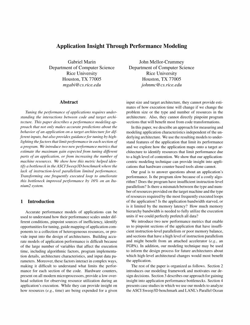
Figure 1. Modeling framework diagram.

Program (POP). Section 5 identifies related work in the areaof performance modeling and prediction. Section 6 presentsour conclusions and plans for future work.

2 The Modeling Framework

We use static and dynamic analysis of binaries as thebasis for performance modeling and prediction. Becausewe analyze and instrument object code, our tools are lan-guage independent and naturally handle applications withmodules written in different languages. In addition, binaryanalysis works equally well on optimized code; we do notneed our own optimizer to predict performance of optimizedcode. Finally, it is easier to predict performance of a mix ofmachine instructions with predictable latencies than to es-timate the execution cost of high-level language constructs.Working on binaries, however, has its own drawbacks. First,the tool’s portability is limited by the binary analysis libraryit uses. This is mitigated by the fact that we measure andmodel application characteristics that are machine indepen-dent, and then we use these models to predict performanceon arbitrary RISC-like architectures. Second, certain high-level information is lost when the source code is translatedto low-level machine code, while other information requiresmore thorough analysis to extract.

Figure 1 shows an overview of our modeling framework.There are four main functional components: static analy-sis, dynamic analysis, an architecture neutral modeling tool,and a modulo-scheduler for cross-architecture performanceprediction. Most of the components of our modeling frame-work are described in detail elsewhere [9]. In section 3,we describe our modulo-scheduler and other extensions thatprovide insight into applications and reveal performancebottlenecks. To provide context for that work, we brieflydescribe the components of our framework.

The static analysis subsystem shown in Figure 1 is nota standalone application but rather a component of everyprogram in our toolkit. We employ static analysis to re-cover high-level program information from application bi-

naries, including reconstruction of the control flow graph(CFG) for each routine and identifying natural loops andloop nesting in each CFG using interval analysis [15]. Otheruses of static analysis involve understanding and modelingaspects of the application that are important for its perfor-mance but are independent of execution characteristics, e.g.,the instruction mix in loop bodies, as well as dependenciesbetween instructions that limit instruction-level parallelism(ILP). Understanding memory dependencies within loopsfrom machine code is a particularly difficult problem thatwe tackle by computing symbolic formulae that character-ize the access pattern of each memory reference, a processthat is described in more detail elsewhere [10].

Often, many important characteristics of an application’sexecution behavior can only be understood accurately bymeasuring them at run time using dynamic analysis. Ourtoolkit uses binary rewriting to augment an application tomonitor and log information during execution. To under-stand the nature and volume of computation performed byan application for a particular program input, we collect his-tograms indicating the frequency with which particular con-trol flow graph edges are traversed at run time. To under-stand an application’s memory access patterns, we collecthistograms of the reuse distance [4]—the number of uniquememory locations accessed between a pair of accesses toa particular data item—observed by each load or store in-struction. These measures quantify key characteristics ofan application’s behavior upon which performance depends.By design, these measures are independent of architecturaldetails and can be used to predict the behavior of a programon an arbitrary RISC-like architecture.

Collecting dynamic data for large problem sizes can beexpensive. To avoid this problem, we construct scalablemodels of dynamic application characteristics. These mod-els, parameterized by problem size or other input parame-ters, enable us to predict application behavior and perfor-mance for data sizes that we have not measured [9, 10].

To compute cross-architecture performance predictions,we combine information gathered from static analysis anddynamic measurements of execution behavior. We then mapthis information onto an architectural model constructedfrom a machine description file. This process has two steps.First, we predict the program’s memory hierarchy behaviorby translating memory reuse distance models into predic-tions of cache miss counts for each level of the memory hi-erarchy on the target architecture. We predict capacity andcompulsory misses directly from the reuse distance mod-els and estimate conflict misses using a probabilistic strat-egy [10]. Second, we predict computation costs by identi-fying paths in each routine’s CFG and their associated fre-quencies, and mapping instructions along these paths ontothe target architecture’s resources using a modulo instruc-tion scheduler. This process is described in section 3.1.

3 Understanding Performance Bottlenecks

In our previous work [9, 10] we validated our approachby successfully predicting memory hierarchy behavior andexecution time of several scientific codes, including theASCI Sweep3D benchmark [1] and several NAS bench-marks, on different architectures for a large range of inputsizes. In this section, we show how models can provide in-sight into applications and reveal performance bottlenecks.The cornerstone of this analysis is our modulo-scheduler,which maps a sequence of generic instructions with theircorresponding data dependencies to a collection of hetero-geneous resources, in accordance with a mapping functionbetween instructions and resources, and with the objectivefunction of minimizing the schedule length. The next sec-tions describe the functionality and design of our scheduler.

3.1 Scheduler front end

To understand the cost of a program’s computation on atarget architecture, we start by identifying paths in the CFGof each routine and computing their associated frequenciesfrom basic block and edge frequency counts collected dur-ing dynamic analysis. For nested loops, we work from theinside out, each loop being represented by a special Inner-Loop instruction in its parent scope. Once a loop is sched-uled, we also compute information about its registers thatare live across the loop boundaries. Such information isused to compute the proper register dependencies betweena loop and instructions in its parent scope. In addition, in-ner loops and function calls act as fence instructions in ourschedules; they prevent instruction reordering across them.

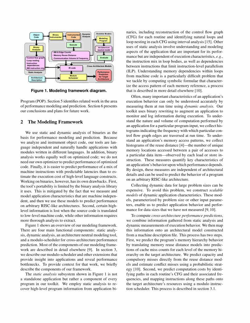
As seen in Figure 1, the scheduler works on an interme-diate representation (IR) of the code. We found the mostflexible format for the IR is a dependence graph, in whichnodes represent generic instructions and edges represent de-pendences between instructions. Figure 2(b) shows the de-pendence graph for the innermost loop of routinecomputeshown in Figure 2(a).1 Using such an intermediate repre-sentation has two main benefits. First, it isolates the sched-uler from the binary analysis library underneath, making itportable to a different run-time system. We need to provideonly a front end that translates machine code into the IR byidentifying all schedule dependencies among instructions.Second, the scheduler can be used to analyze sequences thatinclude higher-level operations (i.e. FFT or dot product op-erations) if the machine description provides units whichcan execute such instructions, and if the front end recog-nizes such operations and includes them as nodes in the IR.

In our implementation, we defined a set of generic RISCinstruction classes and our front-end translates SPARC ma-

1To reduce clutter, the graph does not include the loop control arith-metic and the loop branch instruction.

voidcompute(int size, double* A, double c1){int i, j;for (j=0 ; j<size ; ++j)

for (i=0 ; i<size-1 ; i+=1){A[(i+1)*size+j] =

A[(i+1)*size+j] +c1 * A[(i)*size+j];

}}

(a)

(b) (c)

Figure 2. (a) Sample source code; (b) IR forthe inner most loop; (c) IR after replacementrules and edge latencies are computed.

chine instructions into the intermediate representation. Wedefined a machine description language (MDL) that must beused to model the target architecture. The architecture de-scription at a minimum must define the number and type ofexecution units, and the resources required by each genericinstruction on that architecture. Instead of providing the en-tire grammar of our MDL, we illustrate the most importantlanguage constructs with snippets from our description ofthe Itanium2 architecture [8].

3.2 Machine description language

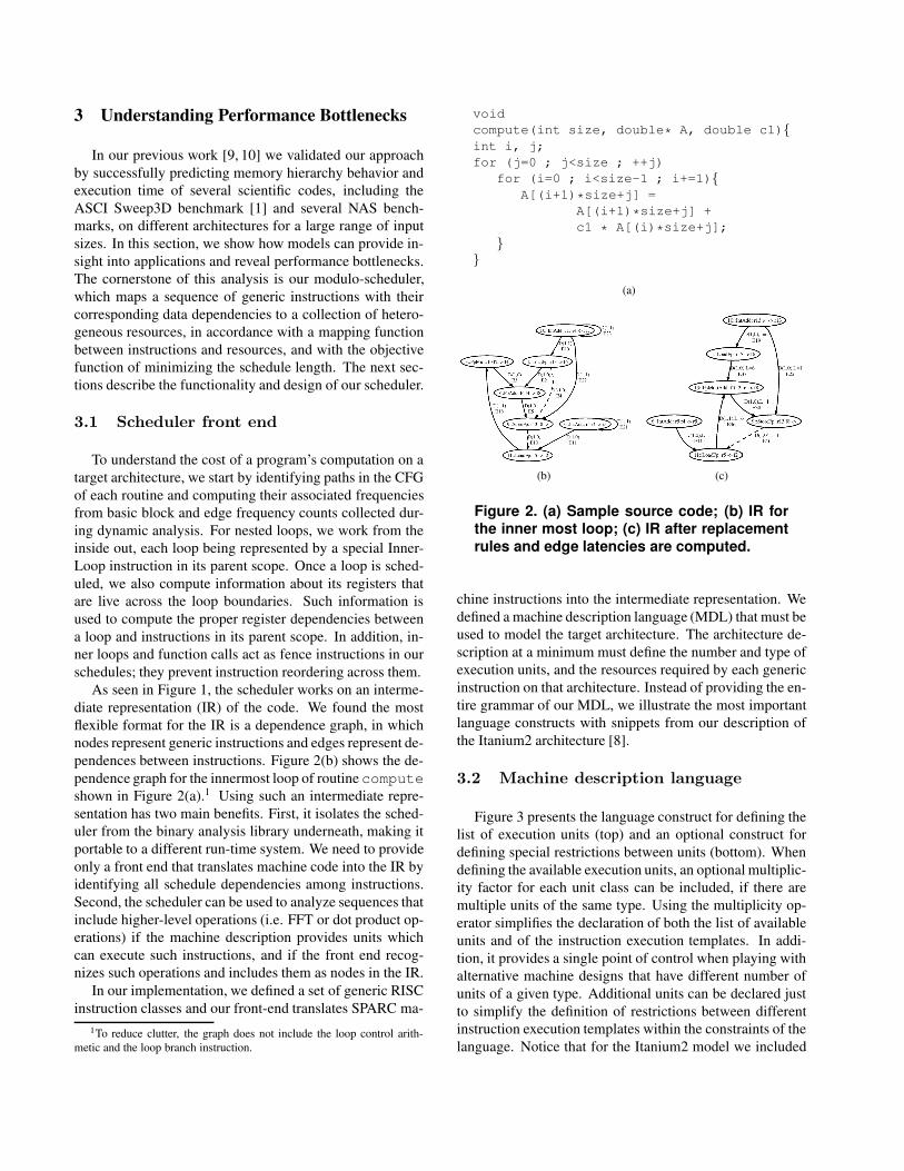
Figure 3 presents the language construct for defining thelist of execution units (top) and an optional construct fordefining special restrictions between units (bottom). Whendefining the available execution units, an optional multiplic-ity factor for each unit class can be included, if there aremultiple units of the same type. Using the multiplicity op-erator simplifies the declaration of both the list of availableunits and of the instruction execution templates. In addi-tion, it provides a single point of control when playing withalternative machine designs that have different number ofunits of a given type. Additional units can be declared justto simplify the definition of restrictions between differentinstruction execution templates within the constraints of thelanguage. Notice that for the Itanium2 model we included

List of execution units (EU):

CpuUnits = U_Alu*6, U_Int*2, U_IShift,U_Mem*4, U_PAlu*6, U_PSMU*2,U_PMult, U_PopCnt, U_FMAC*2,U_FMisc*2, U_Br*3,I_M*4, I_I*2, I_F*2, I_B*3;

Special restrictions between EUs:

Maximum 1 from U_PMult, U_PopCnt;Maximum 6 from I_M, I_I, I_F, I_B;

Figure 3. MDL constructs for defining the ex-ecution units and restrictions between units.

Instruction execution templates:

Instruction LoadFp template =I_M + U_Mem, NOTHING*5;

Instruction StoreFp template =U_Mem[2:3](1)+I_M[2:3](1);

Instruction replacement rules:

Replace FpMult $fX, $fY -> $fZ +FpAdd $fZ, $fT -> $fD with

FpMultAdd $fX, $fY, $fT -> $fD;

Replace StoreFp $fX -> [$rY] +LoadGp [$rY] -> $rZ with

GetF $fX -> $rZ;

Figure 4. MDL constructs for declaring in-struction execution templates (top) and in-struction replacement rules (bottom).

also a list of issue ports in addition to the execution units.Using the convention that each instruction template mustdeclare the use of one issue port of proper type in additionto one or more execution units, we can restrict the numberand type of instructions that can be issued in the same cycle.For example, to model the six issue width of the Itanium2processor, the second restriction rule in Figure 3 specifiesthat at most six issue ports can be used in any given cycle.

Figure 4 presents examples of instruction execution tem-plates and instruction replacement rule declarations. An in-struction template defines the latency of an instruction, andthe type and number of execution units used in each cycle.The first instruction template in Figure 4 represents the mostcommon format of template declaration, thus the shortest. Itapplies to instructions that execute on fully pipelined sym-metric execution units. On Itanium2, floating-point loadscan be issued to any of the four memory units, and have aminimum latency of six cycles when data is found in the L2cache. Thus, one LoadFp instruction is declared to needone issue port of type I M and one execution unit of type

U Mem in the first clock cycle, plus five additional clockcycles in which it does not conflict with the issue of anyinstruction. NOTHING is a keyword which specifies thatno execution unit is used. Instruction templates can makeuse of the multiplicity operator to specify consecutive clockcycles that require the same type and number of resources.The second template in Figure 4 shows the extended formof declaring an execution template which is needed in caseof asymmetric execution units. While floating-point loadscan execute on any of the four memory type units, stores canexecute only on the last two units. Thus, this template usesthe optional range operator in square brackets to specify asubset of units of a given type, and the count operator be-tween round parentheses to specify how many units of thattype are needed. Instructions can have associated multipleexecution templates, possibly with different lengths.

Instruction replacement rules, presented in the bottomhalf of Figure 4, are an important type of language con-struct used to translate sequences of instructions from theinstruction set of the input architecture, into functionallyequivalent sequences of instructions found on the target ar-chitecture. We introduced the replacement construct to ac-count for slight variations in the instruction set of differ-ent architectures. For example, the SPARC architecturedoes not have a multiply-add instruction, while Itanium2does. Moving data between general-purpose and floating-point registers is accomplished on SPARC by a save fol-lowed by a load from the same stack location using regis-ters of different types. Itanium2 provides two instructionsfor transferring the content of a floating-point register to ageneral-purpose register and back. In addition, the IA-64instruction set does not include the following type of in-structions: integer multiply, integer divide, floating-pointdivide, and floating-point square root. Floating-point divideand square root operations are executed in software using asequence of fully pipelined instructions. The integer mul-tiply and divide operations are executed by translating theoperands to floating-point format, executing the equivalentfloating-point operations, and finally transferring the resultback into a fixed-point register. In our Itanium2 architec-ture description, we provide replacement rules for all thesetype of instructions. Figure 2(c) presents the dependencegraph for loop i of the code shown in Figure 2(a) after thereplacement rules were applied. One multiply and one addinstructions were replaced with a single multiply-add.

The final two constructs are shown in Figure 5. By-pass latency rules are used to specify different latenciesthan what would normally result from the instruction exe-cution templates for certain combinations of source instruc-tion type, dependence type, and sink instruction type. Thetwo bypass rules shown in Figure 5 refer to control depen-dences. For example the second rule specifies that a branchor function call instruction can be issued in the same cycle

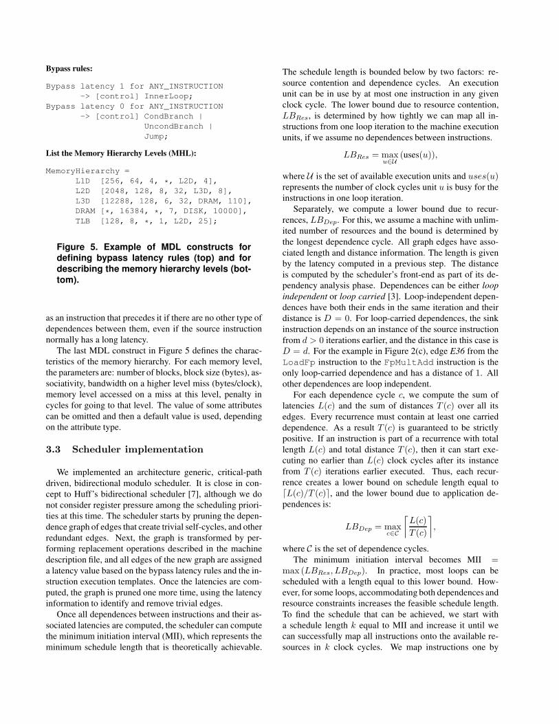
Bypass rules:

Bypass latency 1 for ANY_INSTRUCTION-> [control] InnerLoop;

Bypass latency 0 for ANY_INSTRUCTION-> [control] CondBranch |

UncondBranch |Jump;

List the Memory Hierarchy Levels (MHL):

MemoryHierarchy =L1D [256, 64, 4, *, L2D, 4],L2D [2048, 128, 8, 32, L3D, 8],L3D [12288, 128, 6, 32, DRAM, 110],DRAM [*, 16384, *, 7, DISK, 10000],TLB [128, 8, *, 1, L2D, 25];

Figure 5. Example of MDL constructs fordefining bypass latency rules (top) and fordescribing the memory hierarchy levels (bot-tom).

as an instruction that precedes it if there are no other type ofdependences between them, even if the source instructionnormally has a long latency.

The last MDL construct in Figure 5 defines the charac-teristics of the memory hierarchy. For each memory level,the parameters are: number of blocks, block size (bytes), as-sociativity, bandwidth on a higher level miss (bytes/clock),memory level accessed on a miss at this level, penalty incycles for going to that level. The value of some attributescan be omitted and then a default value is used, dependingon the attribute type.

3.3 Scheduler implementation

We implemented an architecture generic, critical-pathdriven, bidirectional modulo scheduler. It is close in con-cept to Huff’s bidirectional scheduler [7], although we donot consider register pressure among the scheduling priori-ties at this time. The scheduler starts by pruning the depen-dence graph of edges that create trivial self-cycles, and otherredundant edges. Next, the graph is transformed by per-forming replacement operations described in the machinedescription file, and all edges of the new graph are assigneda latency value based on the bypass latency rules and the in-struction execution templates. Once the latencies are com-puted, the graph is pruned one more time, using the latencyinformation to identify and remove trivial edges.

Once all dependences between instructions and their as-sociated latencies are computed, the scheduler can computethe minimum initiation interval (MII), which represents theminimum schedule length that is theoretically achievable.

The schedule length is bounded below by two factors: re-source contention and dependence cycles. An executionunit can be in use by at most one instruction in any givenclock cycle. The lower bound due to resource contention,LBRes, is determined by how tightly we can map all in-structions from one loop iteration to the machine executionunits, if we assume no dependences between instructions.

LBRes = maxu∈U

(uses(u)),

where U is the set of available execution units and uses(u)represents the number of clock cycles unit u is busy for theinstructions in one loop iteration.

Separately, we compute a lower bound due to recur-rences, LBDep. For this, we assume a machine with unlim-ited number of resources and the bound is determined bythe longest dependence cycle. All graph edges have asso-ciated length and distance information. The length is givenby the latency computed in a previous step. The distanceis computed by the scheduler’s front-end as part of its de-pendency analysis phase. Dependences can be either loopindependent or loop carried [3]. Loop-independent depen-dences have both their ends in the same iteration and theirdistance is D = 0. For loop-carried dependences, the sinkinstruction depends on an instance of the source instructionfrom d > 0 iterations earlier, and the distance in this case isD = d. For the example in Figure 2(c), edge E36 from theLoadFp instruction to the FpMultAdd instruction is theonly loop-carried dependence and has a distance of 1. Allother dependences are loop independent.

For each dependence cycle c, we compute the sum oflatencies L(c) and the sum of distances T (c) over all itsedges. Every recurrence must contain at least one carrieddependence. As a result T (c) is guaranteed to be strictlypositive. If an instruction is part of a recurrence with totallength L(c) and total distance T (c), then it can start exe-cuting no earlier than L(c) clock cycles after its instancefrom T (c) iterations earlier executed. Thus, each recur-rence creates a lower bound on schedule length equal to�L(c)/T (c)�, and the lower bound due to application de-pendences is:

LBDep = maxc∈C

⌈L(c)T (c)

⌉,

where C is the set of dependence cycles.The minimum initiation interval becomes MII =

max (LBRes, LBDep). In practice, most loops can bescheduled with a length equal to this lower bound. How-ever, for some loops, accommodating both dependences andresource constraints increases the feasible schedule length.To find the schedule that can be achieved, we start witha schedule length k equal to MII and increase it until wecan successfully map all instructions onto the available re-sources in k clock cycles. We map instructions one by

one, in an order determined by a dynamic priority functionthat tracks how much of each recurrence is still not sched-uled. We use limited backtracking and unscheduling of op-erations already scheduled when the algorithm cannot con-tinue. The full details on the implementation of this step arebeyond the scope of this paper.

3.4 Performance analysis extensions

So far, we have described the steps of a fairly standardmodulo-scheduling algorithm. Our implementation has itsstrengths and weaknesses. A strength of the scheduler isthat it can be applied to different scheduling scenarios. Aweakness of the scheduler is that it ignores some architec-tural details, such as register pressure or branch miss pre-diction. It is adequate for our purposes because we want topredict a lower bound (though not too loose) on achievableperformance, and to understand what sections of code maybenefit from transformations or from additional executionunits. A modulo-scheduler offers us this insight because wecan attribute each clock cycle of the resulting schedule to aparticular cause.

When we compute the minimum initiation interval of theschedule, if LBDep ≥ LBRes, we consider that LBDep

clock cycles of each loop iteration are due to applicationdependences. If, on the other hand, the bound due to re-source contention is greater, we know also which unit wasdetermined to have the highest contention factor.2 If multi-ple units have the same contention factor, the first unit de-fined in the machine description file is selected. In suchcases we say LBRes clock cycles of each iteration are dueto resource bottlenecks, and we refine this cost further bythe type of unit that is causing the most contention.

In the next step of the algorithm, we try to find an ac-tual feasible schedule length that takes into account bothinstruction dependences and resource contention. Everytime we increase the schedule length, we determine whatresource, either execution unit or restriction rule, preventedthe scheduler from continuing. The way this schedulingstep is implemented, the algorithm does not try to sched-ule an instruction in a clock cycle that breaks dependences.Therefore, the scheduler fails when there is no executiontemplate that does not conflict with resources already allo-cated or with one of the optional restriction rules for anyof the valid issue cycles. This additional scheduling costfor each iteration is counted separately as scheduling extracost. Again, we refine this cost further by the unit type thatwas the source of contention.

We compute the execution costs in a bottom-up fashion,from the innermost loops to routines and to the entire pro-

2Because the machine model may contain optional restriction rules be-tween units, if one of the rules is determined to cause the most contention,then the cost is associated with that rule

gram, aggregating costs for each of the categories describedabove. At the end of this process, we have not only a pre-diction of instruction schedule time for the entire program,each routine and each loop, but also the attribution of exe-cution cost to the factors that contribute to that cost.

Performance monitoring hardware on most modern ar-chitectures can provide insight into resource consumptionon current platforms. Our performance tool can providesuch insight for future architectures, at a much lower costthan cycle accurate simulators. However, we realized thatwhat is lacking in current performance tools, is a way topoint the application developer, or an automatic tuning sys-tem for that matter, to those sections of code that can benefitthe most from program transformations or from additionalmachine resources. Just because a loop accounts for a sig-nificant fraction of execution time, it may not be wastingissue slots. It may actually have good instruction and mem-ory balance with respect to the target architecture with littleroom for improvement. We need to focus on loops that arefrequently executed but also use resources inefficiently.

3.5 New performance metrics

One of the steps in the scheduling algorithm is the com-putation of the minimum initiation interval. For this, twolower bounds on the schedule length are computed. LBRes

represents the lower bound due to resource contention, andis computed assuming no schedule dependences betweeninstruction. Let S be the computation cost computed by thescheduler when both instruction dependences and resourceconstraints are considered. We define the metric maximumgain achievable from increased ILP as MaxGainILP =S − LBRes. This metric represents exactly what its nameimplies. If total computation cost is S, and the cost achiev-able with the same set of machine resources if we removedall data dependences in loops is LBRes, then the maximumwe can expect to gain from transforming the code to in-crease ILP, is S −LBRes. If the code’s performance is lim-ited by the number and type of machine resources, that is ifS = LBRes, there is nothing that can be gained from trans-forming the code, unless we rewrite the code using differentinstructions that require different resources.

LBDep represents the lower bound due to dependencecycles, and is computed assuming unlimited number ofmachine resources. We define the metric maximum gainachievable from additional resources as MaxGainRes =S − LBDep. The name of this metric is self explanatory.No matter how many execution units we add to a machine,the execution cost of the code cannot be lower than LBDep

unless we also apply code transformations. For loops with-out recurrences, LBDep of N iterations is equal to the exe-cution cost of one iteration from start to finish, independentof N . With an unlimited number of machine resources, and

with no carried dependences, all iterations can be executedin parallel in the time taken by a single iteration. However,we do not apply the same idea to outer loops or loops withfunction calls. As we explained in Section 3.2, inner loopsand function calls act as fence instructions, so they create atleast a recurrence on themselves.

Each of these two metrics gives an estimate of the per-formance increase possible by modifying only one variableof the equation in isolation. At an extreme, if we removedall dependences and we assumed an infinite number of re-sources, we could execute a program in one cycle. But thisis too unrealistic to be of any use in practice. As with otherperformance data we compute, we aggregate these two met-rics in a bottom-up fashion up to the entire program level.To explore this data, we output all metrics in XML format,and use the hpcviewer user interface [11] that is part ofHPCToolkit [12].

4 Case Studies

In this section, we briefly illustrate how to analyze andtune an application using these new performance metrics.We study two applications. Sweep3D [1] is a 3D Carte-sian geometry neutron transport code benchmark from theDOE’s Accelerated Strategic Computing Initiative. As abenchmark, this code has been carefully tuned already, sothe opportunities for improving performance are slim. TheParallel Ocean Program (POP) [2] is a climate modelingapplication developed at Los Alamos National Laboratory.This is a more complex code with the execution cost spreadover a large number of routines. We compiled both codeson a Sun UltraSPARC-II system using the Sun WorkShop 6update 2 FORTRAN 77 5.3 compiler, and the optimizations:-xarch=v8plus -xO4 -depend -dalign -xtypemap=real:64.

For Sweep3D, we used our toolkit to collect edge fre-quency data and memory reuse distance information for acubic mesh size of 50x50x50 and 6 time steps without fix-up code. For POP, we collected data for the default bench-mark size input. Then, we processed collected data with ourmodulo-scheduler using a machine model of the Itanium2architecture, and produced performance databases in XMLformat for each of the codes. In the next two sections welook at each code on turn.

4.1 Analysis of Sweep3D

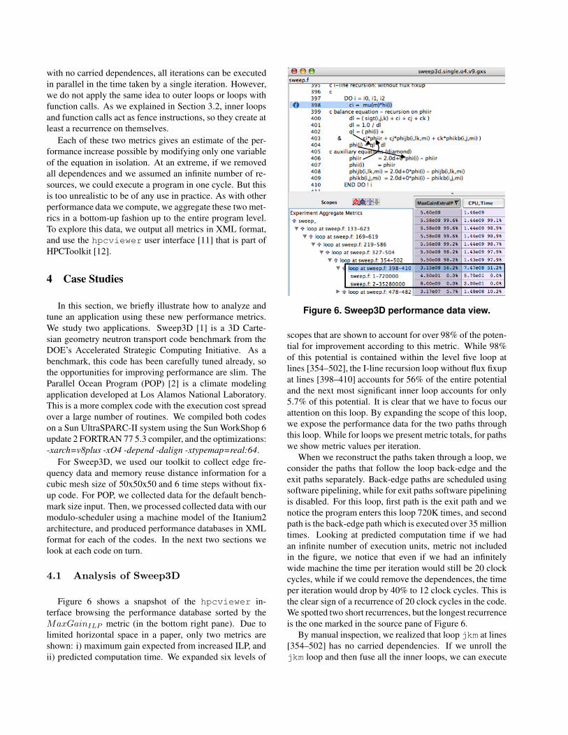
Figure 6 shows a snapshot of the hpcviewer in-terface browsing the performance database sorted by theMaxGainILP metric (in the bottom right pane). Due tolimited horizontal space in a paper, only two metrics areshown: i) maximum gain expected from increased ILP, andii) predicted computation time. We expanded six levels of

Figure 6. Sweep3D performance data view.

scopes that are shown to account for over 98% of the poten-tial for improvement according to this metric. While 98%of this potential is contained within the level five loop atlines [354–502], the I-line recursion loop without flux fixupat lines [398–410] accounts for 56% of the entire potentialand the next most significant inner loop accounts for only5.7% of this potential. It is clear that we have to focus ourattention on this loop. By expanding the scope of this loop,we expose the performance data for the two paths throughthis loop. While for loops we present metric totals, for pathswe show metric values per iteration.

When we reconstruct the paths taken through a loop, weconsider the paths that follow the loop back-edge and theexit paths separately. Back-edge paths are scheduled usingsoftware pipelining, while for exit paths software pipeliningis disabled. For this loop, first path is the exit path and wenotice the program enters this loop 720K times, and secondpath is the back-edge path which is executed over 35 milliontimes. Looking at predicted computation time if we hadan infinite number of execution units, metric not includedin the figure, we notice that even if we had an infinitelywide machine the time per iteration would still be 20 clockcycles, while if we could remove the dependences, the timeper iteration would drop by 40% to 12 clock cycles. This isthe clear sign of a recurrence of 20 clock cycles in the code.We spotted two short recurrences, but the longest recurrenceis the one marked in the source pane of Figure 6.

By manual inspection, we realized that loop jkm at lines[354–502] has no carried dependencies. If we unroll thejkm loop and then fuse all the inner loops, we can execute

0.5

0.6

0.7

0.8

0.9

1

1.1

1.2

1.3

0 20 40 60 80 100 120 140 160 180 200

Mesh Size

Tra

nsfo

rmed

/ O

rig

inal

Execution Time

L2 Misses

L3 Misses

TLB Misses

Retired Instructions

Retired NOPS

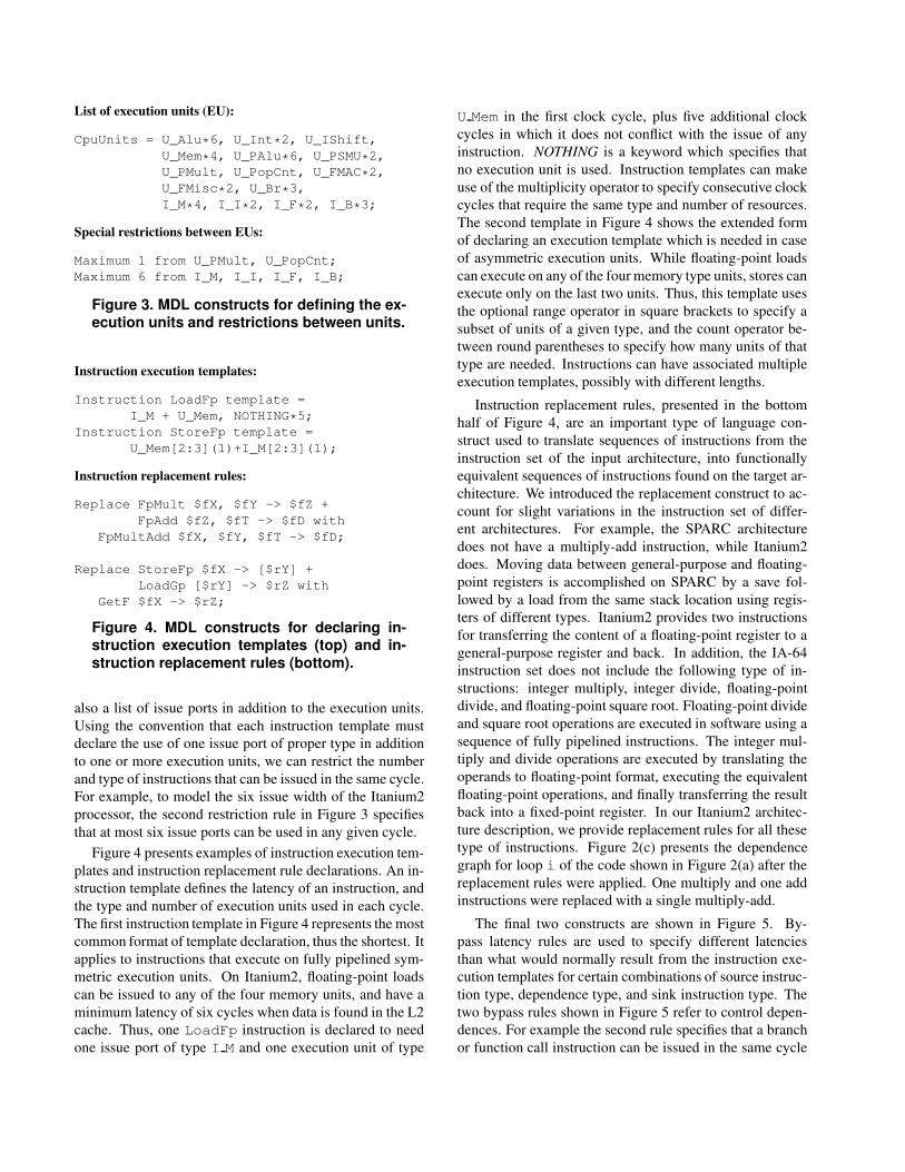
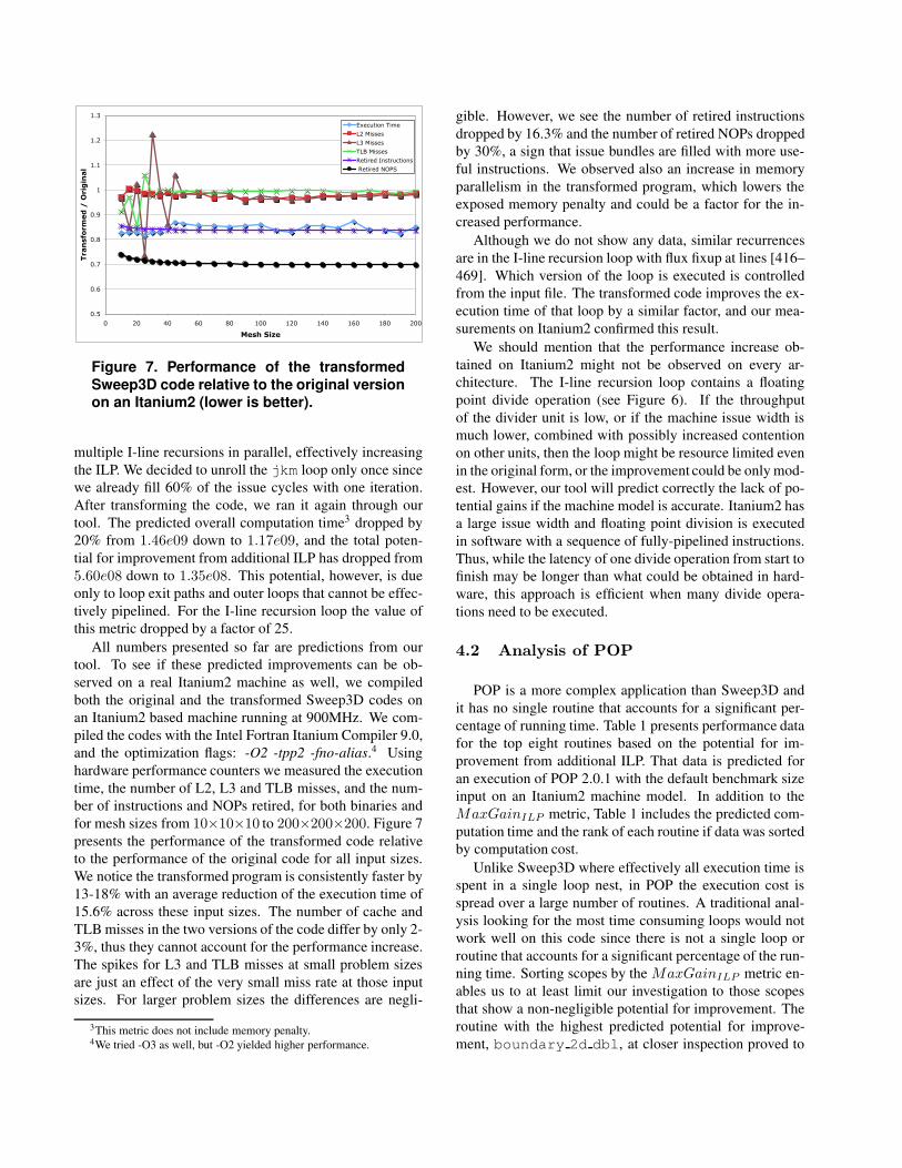
Figure 7. Performance of the transformedSweep3D code relative to the original versionon an Itanium2 (lower is better).

multiple I-line recursions in parallel, effectively increasingthe ILP. We decided to unroll the jkm loop only once sincewe already fill 60% of the issue cycles with one iteration.After transforming the code, we ran it again through ourtool. The predicted overall computation time3 dropped by20% from 1.46e09 down to 1.17e09, and the total poten-tial for improvement from additional ILP has dropped from5.60e08 down to 1.35e08. This potential, however, is dueonly to loop exit paths and outer loops that cannot be effec-tively pipelined. For the I-line recursion loop the value ofthis metric dropped by a factor of 25.

All numbers presented so far are predictions from ourtool. To see if these predicted improvements can be ob-served on a real Itanium2 machine as well, we compiledboth the original and the transformed Sweep3D codes onan Itanium2 based machine running at 900MHz. We com-piled the codes with the Intel Fortran Itanium Compiler 9.0,and the optimization flags: -O2 -tpp2 -fno-alias.4 Usinghardware performance counters we measured the executiontime, the number of L2, L3 and TLB misses, and the num-ber of instructions and NOPs retired, for both binaries andfor mesh sizes from 10×10×10 to 200×200×200. Figure 7presents the performance of the transformed code relativeto the performance of the original code for all input sizes.We notice the transformed program is consistently faster by13-18% with an average reduction of the execution time of15.6% across these input sizes. The number of cache andTLB misses in the two versions of the code differ by only 2-3%, thus they cannot account for the performance increase.The spikes for L3 and TLB misses at small problem sizesare just an effect of the very small miss rate at those inputsizes. For larger problem sizes the differences are negli-

3This metric does not include memory penalty.4We tried -O3 as well, but -O2 yielded higher performance.

gible. However, we see the number of retired instructionsdropped by 16.3% and the number of retired NOPs droppedby 30%, a sign that issue bundles are filled with more use-ful instructions. We observed also an increase in memoryparallelism in the transformed program, which lowers theexposed memory penalty and could be a factor for the in-creased performance.

Although we do not show any data, similar recurrencesare in the I-line recursion loop with flux fixup at lines [416–469]. Which version of the loop is executed is controlledfrom the input file. The transformed code improves the ex-ecution time of that loop by a similar factor, and our mea-surements on Itanium2 confirmed this result.

We should mention that the performance increase ob-tained on Itanium2 might not be observed on every ar-chitecture. The I-line recursion loop contains a floatingpoint divide operation (see Figure 6). If the throughputof the divider unit is low, or if the machine issue width ismuch lower, combined with possibly increased contentionon other units, then the loop might be resource limited evenin the original form, or the improvement could be only mod-est. However, our tool will predict correctly the lack of po-tential gains if the machine model is accurate. Itanium2 hasa large issue width and floating point division is executedin software with a sequence of fully-pipelined instructions.Thus, while the latency of one divide operation from start tofinish may be longer than what could be obtained in hard-ware, this approach is efficient when many divide opera-tions need to be executed.

4.2 Analysis of POP

POP is a more complex application than Sweep3D andit has no single routine that accounts for a significant per-centage of running time. Table 1 presents performance datafor the top eight routines based on the potential for im-provement from additional ILP. That data is predicted foran execution of POP 2.0.1 with the default benchmark sizeinput on an Itanium2 machine model. In addition to theMaxGainILP metric, Table 1 includes the predicted com-putation time and the rank of each routine if data was sortedby computation cost.

Unlike Sweep3D where effectively all execution time isspent in a single loop nest, in POP the execution cost isspread over a large number of routines. A traditional anal-ysis looking for the most time consuming loops would notwork well on this code since there is not a single loop orroutine that accounts for a significant percentage of the run-ning time. Sorting scopes by the MaxGainILP metric en-ables us to at least limit our investigation to those scopesthat show a non-negligible potential for improvement. Theroutine with the highest predicted potential for improve-ment, boundary 2d dbl, at closer inspection proved to

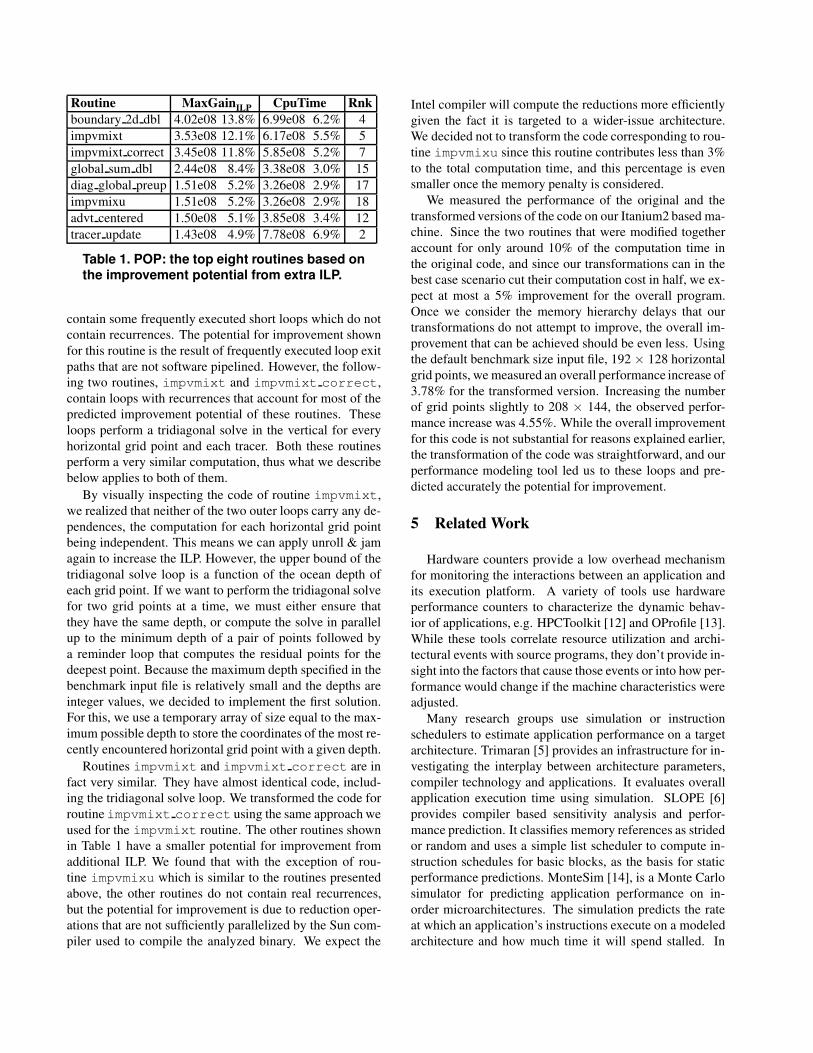
Routine MaxGainILP CpuTime Rnkboundary 2d dbl 4.02e08 13.8% 6.99e08 6.2% 4impvmixt 3.53e08 12.1% 6.17e08 5.5% 5impvmixt correct 3.45e08 11.8% 5.85e08 5.2% 7global sum dbl 2.44e08 8.4% 3.38e08 3.0% 15diag global preup 1.51e08 5.2% 3.26e08 2.9% 17impvmixu 1.51e08 5.2% 3.26e08 2.9% 18advt centered 1.50e08 5.1% 3.85e08 3.4% 12tracer update 1.43e08 4.9% 7.78e08 6.9% 2

Table 1. POP: the top eight routines based onthe improvement potential from extra ILP.

contain some frequently executed short loops which do notcontain recurrences. The potential for improvement shownfor this routine is the result of frequently executed loop exitpaths that are not software pipelined. However, the follow-ing two routines, impvmixt and impvmixt correct,contain loops with recurrences that account for most of thepredicted improvement potential of these routines. Theseloops perform a tridiagonal solve in the vertical for everyhorizontal grid point and each tracer. Both these routinesperform a very similar computation, thus what we describebelow applies to both of them.

By visually inspecting the code of routine impvmixt,we realized that neither of the two outer loops carry any de-pendences, the computation for each horizontal grid pointbeing independent. This means we can apply unroll & jamagain to increase the ILP. However, the upper bound of thetridiagonal solve loop is a function of the ocean depth ofeach grid point. If we want to perform the tridiagonal solvefor two grid points at a time, we must either ensure thatthey have the same depth, or compute the solve in parallelup to the minimum depth of a pair of points followed bya reminder loop that computes the residual points for thedeepest point. Because the maximum depth specified in thebenchmark input file is relatively small and the depths areinteger values, we decided to implement the first solution.For this, we use a temporary array of size equal to the max-imum possible depth to store the coordinates of the most re-cently encountered horizontal grid point with a given depth.

Routines impvmixt and impvmixt correct are infact very similar. They have almost identical code, includ-ing the tridiagonal solve loop. We transformed the code forroutine impvmixt correct using the same approach weused for the impvmixt routine. The other routines shownin Table 1 have a smaller potential for improvement fromadditional ILP. We found that with the exception of rou-tine impvmixu which is similar to the routines presentedabove, the other routines do not contain real recurrences,but the potential for improvement is due to reduction oper-ations that are not sufficiently parallelized by the Sun com-piler used to compile the analyzed binary. We expect the

Intel compiler will compute the reductions more efficientlygiven the fact it is targeted to a wider-issue architecture.We decided not to transform the code corresponding to rou-tine impvmixu since this routine contributes less than 3%to the total computation time, and this percentage is evensmaller once the memory penalty is considered.

We measured the performance of the original and thetransformed versions of the code on our Itanium2 based ma-chine. Since the two routines that were modified togetheraccount for only around 10% of the computation time inthe original code, and since our transformations can in thebest case scenario cut their computation cost in half, we ex-pect at most a 5% improvement for the overall program.Once we consider the memory hierarchy delays that ourtransformations do not attempt to improve, the overall im-provement that can be achieved should be even less. Usingthe default benchmark size input file, 192 × 128 horizontalgrid points, we measured an overall performance increase of3.78% for the transformed version. Increasing the numberof grid points slightly to 208 × 144, the observed perfor-mance increase was 4.55%. While the overall improvementfor this code is not substantial for reasons explained earlier,the transformation of the code was straightforward, and ourperformance modeling tool led us to these loops and pre-dicted accurately the potential for improvement.

5 Related Work

Hardware counters provide a low overhead mechanismfor monitoring the interactions between an application andits execution platform. A variety of tools use hardwareperformance counters to characterize the dynamic behav-ior of applications, e.g. HPCToolkit [12] and OProfile [13].While these tools correlate resource utilization and archi-tectural events with source programs, they don’t provide in-sight into the factors that cause those events or into how per-formance would change if the machine characteristics wereadjusted.

Many research groups use simulation or instructionschedulers to estimate application performance on a targetarchitecture. Trimaran [5] provides an infrastructure for in-vestigating the interplay between architecture parameters,compiler technology and applications. It evaluates overallapplication execution time using simulation. SLOPE [6]provides compiler based sensitivity analysis and perfor-mance prediction. It classifies memory references as stridedor random and uses a simple list scheduler to compute in-struction schedules for basic blocks, as the basis for staticperformance predictions. MonteSim [14], is a Monte Carlosimulator for predicting application performance on in-order microarchitectures. The simulation predicts the rateat which an application’s instructions execute on a modeledarchitecture and how much time it will spend stalled. In

contrast, our work uses both static and dynamic analysisto provide application-centric performance feedback usefulfor tuning in addition to computing predictions of memoryhierarchy and execution behavior.

6 Conclusions and Future Plans

This paper describes a performance modeling approachthat can guide tuning by highlighting the factors that limitperformance at points in a program. We describe two newperformance metrics that can pinpoint sections of code withthe highest potential for improvement from increased in-struction level parallelism or from additional machine re-sources. These metrics can be directly computed by amodulo-scheduler. We presented a machine description lan-guage (MDL) that can model the main architecture char-acteristics affecting instruction scheduling and instructionlatencies, and a modulo-scheduler targeted to such a ma-chine model. The MDL’s replacement rules are essential forproducing accurate cross-architecture predictions. Apply-ing our approach to the ASCI Sweep3D benchmark usingan Itanium2 machine model, we found a loop with high po-tential for improvement from additional ILP. Transformingthe loop increased overall application performance by 16%on an Itanium2-based platform. Applying our approach toPOP, we identified routines with poor ILP and correctly pre-dicted the potential for improving them. Transforming thecode to increase ILP yielded 4% better performance.

This paper explores only one of the possible applicationsof these metrics. We are currently studying how to applythese and other metrics to understand which sections of acode could benefit from acceleration using an FPGA. Ourfuture plans call for exploring how to extend our reuse dis-tance based analysis of memory access patterns to identifyhow to improve memory hierarchy performance by apply-ing loop transformations such as fusion and tiling.

7 Acknowledgments

This work is supported in part by the National Sci-ence Foundation under Cooperative Agreement No. CCR-0331654, the Department of Energy (DOE) Office of Sci-ence Cooperative Agreement No. DE-FC02-06ER25762,and DOE under Contract Nos. 03891-001-99-4G, 74837-001-03 49, 86192-001-04 49, and/or 12783-001-05 49 fromthe Los Alamos National Laboratory. Experiments wereperformed on equipment purchased with support from In-tel and the National Science Foundation under Grant No.EIA-0216467.

References

[1] The ASCI Sweep3D Benchmark Code. DOE Ac-celerated Strategic Computing Initiative. http://www.llnl.gov/asci benchmarks/asci/limited/sweep3d/asci sweep3d.html.

[2] The Parallel Ocean Program (POP). http://climate.lanl.gov/Models/POP.

[3] R. Allen and K. Kennedy. Optimizing Compilers for Mod-ern Architectures: A Dependence-Based Approach. MorganKaufmann Publishers Inc., San Francisco, CA, USA, 2002.

[4] B. Bennett and V. Kruskal. LRU Stack Processing. IBMJournal of Research and Development, 19(4):353–357, July1975.

[5] L. N. Chakrapani, J. Gyllenhaal, W. W. Hwu, S. A. Mahlke,K. V. Palem, and R. M. Rabbah. Trimaran: An Infrastructurefor Research in Instruction-Level Parallelism. Lecture Notesin Computer Science, 3602:32–41, 2005.

[6] P. C. Diniz and J. Abramson. SLOPE: A Compiler Ap-proach to Performance Prediction and Performance Sensi-tivity Analysis for Scientific Codes. CyberinfrastructureTechnology Watch: Special Issue on HPC Productivity,2(4B), Nov. 2006.

[7] R. A. Huff. Lifetime-Sensitive Modulo Scheduling. In PLDI’93: Proceedings of the ACM SIGPLAN 1993 Conference onProgramming Language Design and Implementation, pages258–267, New York, NY, USA, 1993. ACM Press.

[8] Intel Corporation. Intel Itanium2 Processor Reference Man-ual for Software Development and Optimizations, 2003.

[9] G. Marin and J. Mellor-Crummey. Cross-Architecture Per-formance Predictions for Scientific Applications Using Pa-rameterized Models. In Proceedings of the Joint Interna-tional Conference on Measurement and Modeling of Com-puter Systems, pages 2–13. ACM Press, June 2004.

[10] G. Marin and J. Mellor-Crummey. Scalable Cross-Architecture Predictions of Memory Hierarchy Responsefor Scientific Applications. In Proceedings of the LosAlamos Computer Science Institute Sixth Annual Sympo-sium, Santa Fe, NM, USA, Oct. 2005. http://lacsi.rice.edu/symposium/symposiumdownloads/lacsi 2005/papers/pap108.pdf.

[11] J. Mellor-Crummey. Using hpcviewer to BrowsePerformance Databases, Feb. 2004. http://www.hipersoft.rice.edu/hpctoolkit/tutorials/Using-hpcviewer.pdf.

[12] J. Mellor-Crummey, R. J. Fowler, G. Marin, and N. Tallent.HPCVIEW: A Tool for Top-down Analysis of Node Per-formance. The Journal of Supercomputing, 23(1):81–104,2002.

[13] The OProfile website. http://oprofile.sourceforge.net/docs.

[14] R. Srinivasan and O. Lubeck. MonteSim: A MonteCarlo Performance Model for In-order Microachitectures.SIGARCH Computer Architecture News, 33(5):75–80, 2005.

[15] R. E. Tarjan. Testing Flow Graph Reducibility. Journal ofComputer and System Sciences, 9:355–365, 1974.