Available online at www.sciencedirect.com

www.elsevier.com/locate/eswa

Expert Systems with Applications 34 (2008) 2436–2443

Expert Systemswith Applications

Applicability of feed-forward and recurrent neural networksto Boolean function complexity modeling

Azam Beg a,*, P.W. Chandana Prasad b, Ajmal Beg c

a College of Information Technology United Arab Emirates University, United Arab Emiratesb Faculty of Information Systems and Technology, Multimedia University, Malaysia

c SAP Australia Brisbane, Australia

Abstract

In this paper, we present the feed-forward neural network (FFNN) and recurrent neural network (RNN) models for predicting Bool-ean function complexity (BFC). In order to acquire the training data for the neural networks (NNs), we conducted experiments for alarge number of randomly generated single output Boolean functions (BFs) and derived the simulated graphs for number of min-termsagainst the BFC for different number of variables. For NN model (NNM) development, we looked at three data transformation tech-niques for pre-processing the NN-training and validation data. The trained NNMs are used for complexity estimation for the Booleanlogic expressions with a given number of variables and sum of products (SOP) terms. Both FFNNs and RNNs were evaluated against theISCAS benchmark results. Our FFNNs and RNNs were able to predict the BFC with correlations of 0.811 and 0.629 with the bench-mark results, respectively.� 2007 Elsevier Ltd. All rights reserved.

Keyword: Machine learning; Feed-forward neural network; Recurrent neural network; Bias; Biological sequence analysis; Motif; Sub-cellular localization;Pattern recognition; Classifier design

1. Introduction

In the past several decades, very large scale integration

(VLSI) has followed the Moore’s Law (Moore, 1975) thathad predicted doubling of transistor on a chip every year.Constant miniaturization of circuit has increased the com-plexity of VLSI design many folds. These VLSI designs candirectly benefit from optimal representation of a circuit assets of BFs (Bryant, 1986). BFs find applications in areassuch as combinational logic verification (Mahk, Wang,A, Brayton, & Sangiovanni-Viicentelli, 1988), sequential-machine equivalence (Coudert, Berthec, & Madre, 1989),logic optimization of combinational circuits (Muroga,Kambayashi, Lai, & Culliney, 1989), test pattern genera-tion (Breuer & Friedman, 1976), timing verification in the

0957-4174/$ - see front matter � 2007 Elsevier Ltd. All rights reserved.

doi:10.1016/j.eswa.2007.04.010

* Corresponding author. Tel.: +971 50 583 6872; fax: +971 3 7626309.E-mail addresses: abeg@uaeu.ac.ae (A. Beg), m2160062@mmu.edu.my

(P.W. Chandana Prasad), ajmal.beg@bigpond.com (A. Beg).

presence of false paths (Mc Geer & Brayton, 1989), andsymbolic simulation (Cho, 1988).

BF representation has a direct influence on the compu-tation time and space requirements of digital circuits andmost of the problems in VLSI/CAD designs can be formu-lated in terms of Boolean functions. The efficiency of anymethod used depends on the complexity of Boolean func-tions (Breuer & Friedman, 1976). Research on the com-plexity of BFs in non-uniform computation models isnow part of one of the most interesting and importantareas in theoretical computer science (Breuer & Friedman,1976; Cho, 1988; Mc Geer & Brayton, 1989). Rapidincrease in the design complexity and the need to reducetime-to-market have resulted in a need for CAD tools thatcan help make important design decisions early in thedesign process. Area complexity is one of the most impor-tant criteria that have to be taken into account while mak-ing these decisions. However, to be able make thesedecisions early, there is a need for methods to estimate

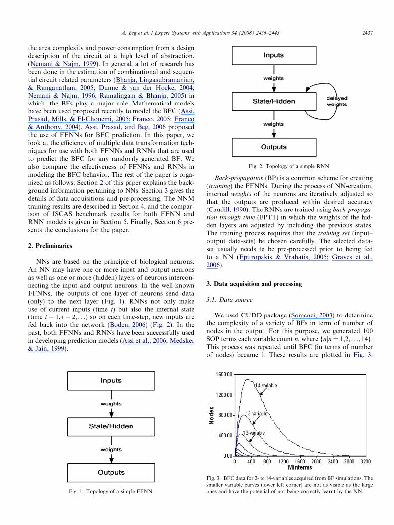
Fig. 2. Topology of a simple RNN.

A. Beg et al. / Expert Systems with Applications 34 (2008) 2436–2443 2437

the area complexity and power consumption from a designdescription of the circuit at a high level of abstraction.(Nemani & Najm, 1999). In general, a lot of research hasbeen done in the estimation of combinational and sequen-tial circuit related parameters (Bhanja, Lingasubramanian,& Ranganathan, 2005; Dunne & van der Hoeke, 2004;Nemani & Najm, 1996; Ramalingam & Bhanja, 2005) inwhich, the BFs play a major role. Mathematical modelshave been used proposed recently to model the BFC (Assi,Prasad, Mills, & El-Chouemi, 2005; Franco, 2005; Franco& Anthony, 2004). Assi, Prasad, and Beg, 2006 proposedthe use of FFNNs for BFC prediction. In this paper, welook at the efficiency of multiple data transformation tech-niques for use with both FFNNs and RNNs that are usedto predict the BFC for any randomly generated BF. Wealso compare the effectiveness of FFNNs and RNNs inmodeling the BFC behavior. The rest of the paper is orga-nized as follows: Section 2 of this paper explains the back-ground information pertaining to NNs. Section 3 gives thedetails of data acquisitions and pre-processing. The NNMtraining results are described in Section 4, and the compar-ison of ISCAS benchmark results for both FFNN andRNN models is given in Section 5. Finally, Section 6 pre-sents the conclusions for the paper.

2. Preliminaries

NNs are based on the principle of biological neurons.An NN may have one or more input and output neuronsas well as one or more (hidden) layers of neurons intercon-necting the input and output neurons. In the well-knownFFNNs, the outputs of one layer of neurons send data(only) to the next layer (Fig. 1). RNNs not only makeuse of current inputs (time t) but also the internal state(time t � 1, t � 2, . . .) so on each time-step, new inputs arefed back into the network (Boden, 2006) (Fig. 2). In thepast, both FFNNs and RNNs have been successfully usedin developing prediction models (Assi et al., 2006; Medsker& Jain, 1999).

Fig. 1. Topology of a simple FFNN.

Back-propagation (BP) is a common scheme for creating(training) the FFNNs. During the process of NN-creation,internal weights of the neurons are iteratively adjusted sothat the outputs are produced within desired accuracy(Caudill, 1990). The RNNs are trained using back-propaga-tion through time (BPTT) in which the weights of the hid-den layers are adjusted by including the previous states.The training process requires that the training set (input–output data-sets) be chosen carefully. The selected data-set usually needs to be pre-processed prior to being fedto a NN (Epitropakis & Vrahatis, 2005; Graves et al.,2006).

3. Data acquisition and processing

3.1. Data source

We used CUDD package (Somenzi, 2003) to determinethe complexity of a variety of BFs in term of number ofnodes in the output. For this purpose, we generated 100SOP terms each variable count n, where {njn = 1,2, . . ., 14}.This process was repeated until BFC (in terms of numberof nodes) became 1. These results are plotted in Fig. 3.

Fig. 3. BFC data for 2- to 14-variables acquired from BF simulations. Thesmaller variable curves (lower left corner) are not as visible as the largeones and have the potential of not being correctly learnt by the NN.

2438 A. Beg et al. / Expert Systems with Applications 34 (2008) 2436–2443

We observed that BFC increases as the number of min-terms (product terms) increases until it reaches a peak cor-responding to the maximum complexity. Beyond the peak,the min-terms tend to simplify and BFC declines andreaches a final value of zero.

3.2. Rationale for data pre-processing

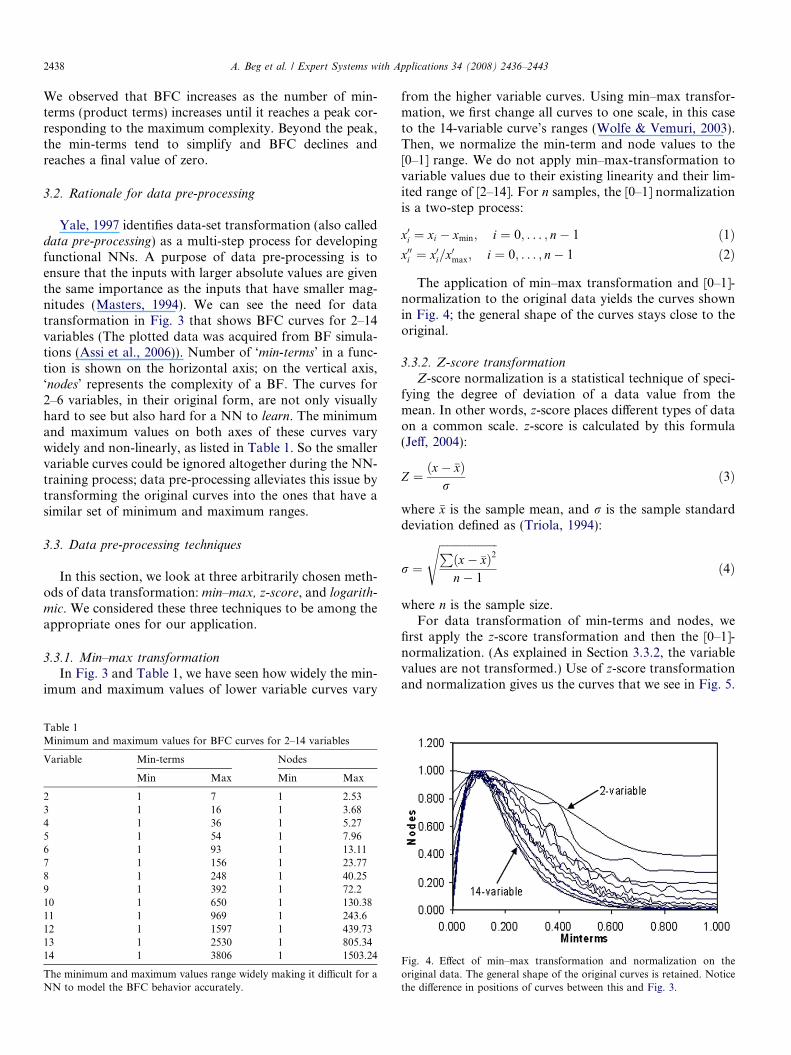
Yale, 1997 identifies data-set transformation (also calleddata pre-processing) as a multi-step process for developingfunctional NNs. A purpose of data pre-processing is toensure that the inputs with larger absolute values are giventhe same importance as the inputs that have smaller mag-nitudes (Masters, 1994). We can see the need for datatransformation in Fig. 3 that shows BFC curves for 2–14variables (The plotted data was acquired from BF simula-tions (Assi et al., 2006)). Number of ‘min-terms’ in a func-tion is shown on the horizontal axis; on the vertical axis,‘nodes’ represents the complexity of a BF. The curves for2–6 variables, in their original form, are not only visuallyhard to see but also hard for a NN to learn. The minimumand maximum values on both axes of these curves varywidely and non-linearly, as listed in Table 1. So the smallervariable curves could be ignored altogether during the NN-training process; data pre-processing alleviates this issue bytransforming the original curves into the ones that have asimilar set of minimum and maximum ranges.

3.3. Data pre-processing techniques

In this section, we look at three arbitrarily chosen meth-ods of data transformation: min–max, z-score, and logarith-

mic. We considered these three techniques to be among theappropriate ones for our application.

3.3.1. Min–max transformationIn Fig. 3 and Table 1, we have seen how widely the min-

imum and maximum values of lower variable curves vary

Table 1Minimum and maximum values for BFC curves for 2–14 variables

Variable Min-terms Nodes

Min Max Min Max

2 1 7 1 2.533 1 16 1 3.684 1 36 1 5.275 1 54 1 7.966 1 93 1 13.117 1 156 1 23.778 1 248 1 40.259 1 392 1 72.210 1 650 1 130.3811 1 969 1 243.612 1 1597 1 439.7313 1 2530 1 805.3414 1 3806 1 1503.24

The minimum and maximum values range widely making it difficult for aNN to model the BFC behavior accurately.

from the higher variable curves. Using min–max transfor-mation, we first change all curves to one scale, in this caseto the 14-variable curve’s ranges (Wolfe & Vemuri, 2003).Then, we normalize the min-term and node values to the[0–1] range. We do not apply min–max-transformation tovariable values due to their existing linearity and their lim-ited range of [2–14]. For n samples, the [0–1] normalizationis a two-step process:

x0i ¼ xi � xmin; i ¼ 0; . . . ; n� 1 ð1Þx00i ¼ x0i=x0max; i ¼ 0; . . . ; n� 1 ð2Þ

The application of min–max transformation and [0–1]-normalization to the original data yields the curves shownin Fig. 4; the general shape of the curves stays close to theoriginal.

3.3.2. Z-score transformation

Z-score normalization is a statistical technique of speci-fying the degree of deviation of a data value from themean. In other words, z-score places different types of dataon a common scale. z-score is calculated by this formula(Jeff, 2004):

Z ¼ ðx� �xÞr

ð3Þ

where �x is the sample mean, and r is the sample standarddeviation defined as (Triola, 1994):

r ¼

ffiffiffiffiffiffiffiffiffiffiffiffiffiffiffiffiffiffiffiffiffiPðx� �xÞ2

n� 1

sð4Þ

where n is the sample size.For data transformation of min-terms and nodes, we

first apply the z-score transformation and then the [0–1]-normalization. (As explained in Section 3.3.2, the variablevalues are not transformed.) Use of z-score transformationand normalization gives us the curves that we see in Fig. 5.

Fig. 4. Effect of min–max transformation and normalization on theoriginal data. The general shape of the original curves is retained. Noticethe difference in positions of curves between this and Fig. 3.

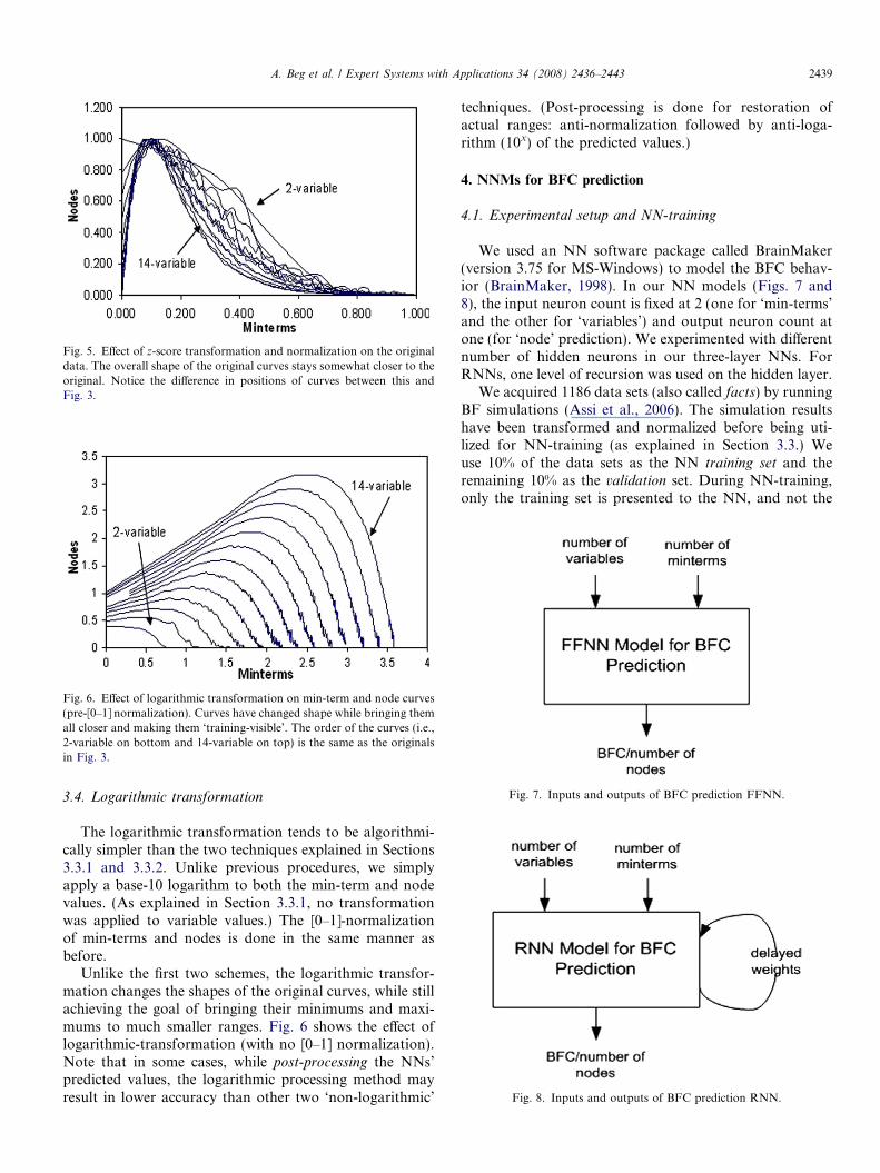
Fig. 5. Effect of z-score transformation and normalization on the originaldata. The overall shape of the original curves stays somewhat closer to theoriginal. Notice the difference in positions of curves between this andFig. 3.

Fig. 6. Effect of logarithmic transformation on min-term and node curves(pre-[0–1] normalization). Curves have changed shape while bringing themall closer and making them ‘training-visible’. The order of the curves (i.e.,2-variable on bottom and 14-variable on top) is the same as the originalsin Fig. 3.

Fig. 7. Inputs and outputs of BFC prediction FFNN.

Fig. 8. Inputs and outputs of BFC prediction RNN.

A. Beg et al. / Expert Systems with Applications 34 (2008) 2436–2443 2439

3.4. Logarithmic transformation

The logarithmic transformation tends to be algorithmi-cally simpler than the two techniques explained in Sections3.3.1 and 3.3.2. Unlike previous procedures, we simplyapply a base-10 logarithm to both the min-term and nodevalues. (As explained in Section 3.3.1, no transformationwas applied to variable values.) The [0–1]-normalizationof min-terms and nodes is done in the same manner asbefore.

Unlike the first two schemes, the logarithmic transfor-mation changes the shapes of the original curves, while stillachieving the goal of bringing their minimums and maxi-mums to much smaller ranges. Fig. 6 shows the effect oflogarithmic-transformation (with no [0–1] normalization).Note that in some cases, while post-processing the NNs’predicted values, the logarithmic processing method mayresult in lower accuracy than other two ‘non-logarithmic’

techniques. (Post-processing is done for restoration ofactual ranges: anti-normalization followed by anti-loga-rithm (10x) of the predicted values.)

4. NNMs for BFC prediction

4.1. Experimental setup and NN-training

We used an NN software package called BrainMaker(version 3.75 for MS-Windows) to model the BFC behav-ior (BrainMaker, 1998). In our NN models (Figs. 7 and8), the input neuron count is fixed at 2 (one for ‘min-terms’and the other for ‘variables’) and output neuron count atone (for ‘node’ prediction). We experimented with differentnumber of hidden neurons in our three-layer NNs. ForRNNs, one level of recursion was used on the hidden layer.

We acquired 1186 data sets (also called facts) by runningBF simulations (Assi et al., 2006). The simulation resultshave been transformed and normalized before being uti-lized for NN-training (as explained in Section 3.3.) Weuse 10% of the data sets as the NN training set and theremaining 10% as the validation set. During NN-training,only the training set is presented to the NN, and not the

Fig. 11. FFNN model predictions for 8 variables.

2440 A. Beg et al. / Expert Systems with Applications 34 (2008) 2436–2443

validation set. We started with the NN learning rate of 0.1and then adjusted it down in increments of 0.01 as thetraining progressed. The initial weights were randomlyset. A total of 72 different configurations of NN were usedto collect the data on FFNN and RNN learnability. We set1000 epochs as the training limit because we found that theproperly converging NNs would provide maximum accu-racy well before the 1000-epoch limit.

In our experiments, the logarithmic transformationyielded the best training and validation accuracy for bothFFNN and RNN models. For FFNNs, the raw data (usingno transformation) provided an average training accuracyof 90.8% and average validation accuracy of 90.0%. Whilethe logarithmic transformation provided training and vali-dation accuracies of 98.8% and 99.1%, respectively. Theaverage RNN training accuracy with no-transformationwas 81.5% and the average validation accuracy was78.4%. The logarithmic transformation improved the train-ing and validation accuracies to 91.9% and 92.5%, respec-tively. Note that the prediction accuracy for every NNconfiguration was calculated by taking the average of threedifferent training sessions, in order to alleviate the potentialof local minima.

Fig. 10. Average prediction accuracy vs. number of neurons in RNN.Twelve seemed to be an optimum neuron count.

Fig. 12. FFNN model predictions for 14 variables.

Fig. 9. Average training accuracy vs. number of neurons in FFNN.Maximum accuracy showed with up 18 neurons in the NN.

Figs. 9–12 depict the comparison for experimentalresults with FFNN and RNN predictions for 8 and 14 vari-ables respectively. It can be inferred that the NNMs canprovide a very good approximation of the BFC. The effectof total neuron count on FFNN and RNN training accu-racy is shown in Figs. 13 and 14. The accuracy of FFNNpeaked out at 18 neurons; further increase in neuron counthad an adverse effect on the accuracy (Fig. 13). Whereas,RNN accuracy flattened out 12 neurons; any increasebeyond this size did not provide any appreciable gains inaccuracy (Fig. 14).

Fig. 13. RNN model predictions for 8 variables.

Fig. 14. RNN model predictions for 14 variables.

A. Beg et al. / Expert Systems with Applications 34 (2008) 2436–2443 2441

5. Benchmark results and discussion

Training of NNM with the experimental data has an up-front once-only cost, and then the NNM can be quicklyrun (within a few milliseconds or less) to predict the com-plexity of various functions with different number of vari-ables and min-terms. Running the NNMs is generallyfaster than simulations, especially when larger benchmarksare involved. (The experimental results were obtained on aPentium IV machine with 512 MB RAM running on Linuxenvironment). The ISCAS benchmark circuit (Hansen,Yalcin, & Hayes, 1999) validation results for CUDD,FFNN and RNN are tabulated in Table 2. The ISCASbenchmarks are sets of multi-input compound Booleanexpressions, but the randomly generated BFs used for theexperiments were single-output SOP expressions, thereforethe benchmark functions were split into multiple single-output expressions, and then expanded directly to SOPterm. Each ISCAS benchmark produced a collection ofSOP expressions. For each of these expressions, the nodecount was computed using the CUDD package.

For each variable count, the curve of node count againstterm count is similar in shape to the Poisson (derivative ofGaussian) curve, starting at zero, rising to a single peak,and then tailing off to zero slowly as the term count goesto infinity. The curves are almost similar geometrically.To increase the comparability of the data, each node countwas divided by the peak node count for the given variablecount. For 3–14 variables the peak node counts were(empirically determined to be): 4, 5, 8, 13, 23, 40, 73, 135,244, 445, 816, and 1498, respectively. Variables 1 and 2were ignored, because they do not have enough impacton the output results.

In Table 2, each data record contains the benchmarkcircuit name, number of circuits, actual node count, andFFNN/RNN predictions. For each benchmark (and forthe total collection) the number of circuits, the meandifference between actual node count and FFNN andRNN predictions, the mean and standard deviation ofthe differences, and the correlation of the two scores ofactual-FFNN and actual-RNN were computed (seeTable 2).

For some benchmarks, lack of variation made the corre-lation meaningless. But, for the complete set of 267 circuits,the FFNN correlation coefficient of about 0.811 is verysignificant, the chances of getting this assuming the mea-sures are actually uncorrelated is less that 1 in a million:firm evidence of a significant relation between the two mea-sures. The non-zero mean difference would be correctablewithin the model, and may reflect a small scaling or incre-menting is required. The non-zero standard deviation ismore significant, indicating, in informal terms, that themodel predicts within about 15% of the actual value, mostof the time. Given the correlation coefficient, near 0.811,and that the model is predicting the average value of thenode count (which is liable to considerable deviation) themodel is judged to have passed a non-trivial test of itsrelevance.

RNN was only able to produce a correlation coefficientof about 0.629. It can be inferred from these results that theFFNN is a better model on prediction of the complexityif the input data range is known. Although the bench-mark circuits considered had up to 47 inputs, no outputdepended on more than 14 of those inputs. The circuitsfor all outputs were measured. It was observed that theterm-variable count combinations were almost all to theleft of the peak complexity, and thus still in region of log-arithmic complexity. So, empirically the most importantpart of the model is the logarithmic rise, and it was thispart that has been validly tested by the benchmark circuitanalysis. This part of the model also has the strongest the-oretical grounding. Due to the above factor, one of theimportant consideration is what is the largest variableshould be for which these curves need to be generated inorder to justify the similarity of the FFNN and RNN mod-els for benchmarks. It is obvious that curves are going to bemore difficult to generate for larger number of variablesbecause of the lack of sample product terms that can beextracted from the benchmarks. Luckily, these are reasonswhy, this is not a problem so that considering variablesmaximum up to 14 is sufficient.

6. Conclusions

In this research, we proposed BFC prediction using twotypes of NNs, i.e., FFNN and RNN. The results from ourexperiments demonstrated the capabilities of NNs, whichproduce the close match for the theoretical results derivedfor the ISCAS benchmark circuits with a correlation of0.811 and 0.629 for FFNN and RNN, respectively. It canbe concluded that the FFNN model is more efficient onworking with randomly generated BFs producing a closermatch with the theoretical results. Advantages of both ofthese models are that each one of them is a single integratedmodel for different number of variables and number ofproduct terms. Our NNMs were capable of providing use-ful clues about the complexity of the final design, whichcould lead to a great reduction in time complexity for di-gital circuit’s designs. In light of the results, we conclude

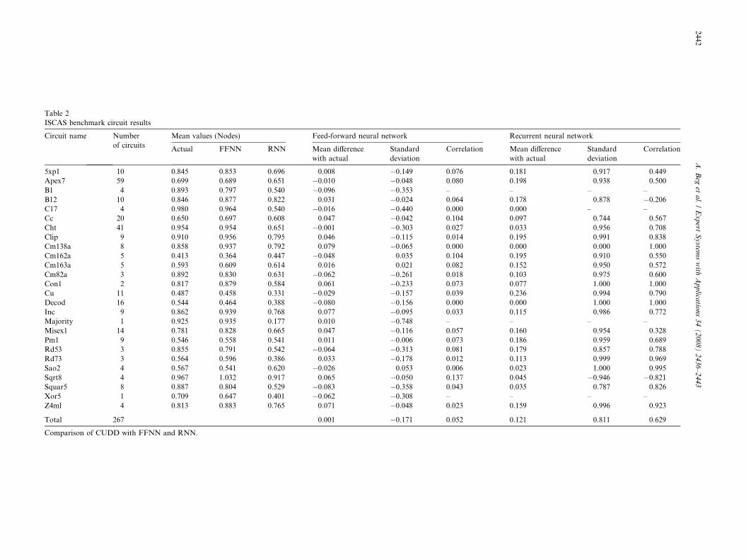
Table 2ISCAS benchmark circuit results

Circuit name Numberof circuits

Mean values (Nodes) Feed-forward neural network Recurrent neural network

Actual FFNN RNN Mean differencewith actual

Standarddeviation

Correlation Mean differencewith actual

Standarddeviation

Correlation

5xp1 10 0.845 0.853 0.696 0.008 �0.149 0.076 0.181 0.917 0.449Apex7 59 0.699 0.689 0.651 �0.010 �0.048 0.080 0.198 0.938 0.500B1 4 0.893 0.797 0.540 �0.096 �0.353 – – – –B12 10 0.846 0.877 0.822 0.031 �0.024 0.064 0.178 0.878 �0.206C17 4 0.980 0.964 0.540 �0.016 �0.440 0.000 0.000 – –Cc 20 0.650 0.697 0.608 0.047 �0.042 0.104 0.097 0.744 0.567Cht 41 0.954 0.954 0.651 �0.001 �0.303 0.027 0.033 0.956 0.708Clip 9 0.910 0.956 0.795 0.046 �0.115 0.014 0.195 0.991 0.838Cm138a 8 0.858 0.937 0.792 0.079 �0.065 0.000 0.000 0.000 1.000Cm162a 5 0.413 0.364 0.447 �0.048 0.035 0.104 0.195 0.910 0.550Cm163a 5 0.593 0.609 0.614 0.016 0.021 0.082 0.152 0.950 0.572Cm82a 3 0.892 0.830 0.631 �0.062 �0.261 0.018 0.103 0.975 0.600Con1 2 0.817 0.879 0.584 0.061 �0.233 0.073 0.077 1.000 1.000Cu 11 0.487 0.458 0.331 �0.029 �0.157 0.039 0.236 0.994 0.790Decod 16 0.544 0.464 0.388 �0.080 �0.156 0.000 0.000 1.000 1.000Inc 9 0.862 0.939 0.768 0.077 �0.095 0.033 0.115 0.986 0.772Majority 1 0.925 0.935 0.177 0.010 �0.748 – – – –Misex1 14 0.781 0.828 0.665 0.047 �0.116 0.057 0.160 0.954 0.328Pm1 9 0.546 0.558 0.541 0.011 �0.006 0.073 0.186 0.959 0.689Rd53 3 0.855 0.791 0.542 �0.064 �0.313 0.081 0.179 0.857 0.788Rd73 3 0.564 0.596 0.386 0.033 �0.178 0.012 0.113 0.999 0.969Sao2 4 0.567 0.541 0.620 �0.026 0.053 0.006 0.023 1.000 0.995Sqrt8 4 0.967 1.032 0.917 0.065 �0.050 0.137 0.045 �0.946 �0.821Squar5 8 0.887 0.804 0.529 �0.083 �0.358 0.043 0.035 0.787 0.826Xor5 1 0.709 0.647 0.401 �0.062 �0.308 – – – –Z4ml 4 0.813 0.883 0.765 0.071 �0.048 0.023 0.159 0.996 0.923

Total 267 0.001 �0.171 0.052 0.121 0.811 0.629

Comparison of CUDD with FFNN and RNN.

2442A

.B

eget

al.

/E

xp

ertS

ystem

sw

ithA

pp

licatio

ns

34

(2

00

8)

24

36

–2

44

3

A. Beg et al. / Expert Systems with Applications 34 (2008) 2436–2443 2443

that the NNMs proposed in this work could be a valuabletool for exploring the complex computational capabilitiesof BFCs.

References

Assi, A., Prasad, P. W. C., & Beg, A. (2006). Modeling the complexity ofdigital circuits using neural networks. WSEAS Transactions on Circuits

and Systems, 810–820.Assi, A., Prasad, P. W. C., Mills, B., & El-Chouemi, A. (2005). Empirical

analysis and mathematical representation of the path length complex-ity in binary decision diagrams. Journal of Computer Science, 2(3),236–244.

Bhanja, S., Lingasubramanian, K., & Ranganathan, N. (2005). Estimationof switching activity in sequential circuits using dynamic Bayesiannetworks. In Proceedings of VLSI design (pp. 586–591).

Boden, M. (2006). A guide to recurrent neural networks and backprop-agation. <http://www.itee.uq.edu.au/~mikael/papers/rn_dallas.pdf>.

BrainMaker (1998). User’s guide and reference manual (7th ed.). CaliforniaScientific Software Press.

Breuer, M. A., & Friedman, A. D. (1976). Diagnosis and reliable design of

digital systems. Computer Science Press.Bryant, R. E. (1986). Graph-based algorithm for Boolean function

manipulation. IEEE Transactions on Computers, 35, 677–691.Caudill, M. (1990). AI expert: Neural network primer. Miller Freeman

Publications.Cho, K. (1988). Test pattern generation for combinational and sequential

MOS circuits by symbolic F&T simulation. PhD thesis. CarnegieMellon University.

Coudert, O., Berthec, C., & Madre, J. (1989). Verification of sequentialmachines using Boolean function vectors. In IMEC-IFIP international

workshop on applied formal methods for correct VLSI design.Dunne, P. E., & van der Hoeke, W. (2004). Representation and

complexity in Boolean games. In Proceedings of the 9th European

conference on logics in artificial intelligence (pp. 347–350). Springer-Verlag.

Epitropakis, M. G., & Vrahatis, M. N. (2005). Timely communications:Root finding and approximation approaches through neural networks.ACM SIGSAM Bulletin, 39(4).

Franco, L. (2005). Role of function complexity and network size in thegeneralization ability of feedforward networks. In Lecture Notes inComputer Science. Computational intelligence and bioinspired systems:

eighth international workshop on artificial neural networks. IWANN

2005. v3512 (pp. 1–8).Franco, L., & Anthony, M. (2004). On a generalization complexity

measure for Boolean functions, IEEE Conference on Neural Net-

works. In Proceedings on 2004 IEEE international joint conference on

neural networks (pp. 973–978).Graves, A., Fernandez S., Gomez F., & Schmidhuber J. (2006). Connec-

tionist temporal classification: labeling unsegmented sequence datawith recurrent neural networks. In Proceedings of the 23rd international

conference on machine learning, ICML ’06, June 2006.Hansen, M., Yalcin, H., & Hayes, J. P. (1999). Unveiling the ISCAS-85

Benchmarks: A Case Study in Reverse Engineering. IEEE Transactions

on Design and Test, 16, 72–80.Jeff, (2004). What’s a Z-Score and Why Use it in Usability Testing?

<http://www.measuringusability.com/z.htm> (website).Mahk, S., Wang, A, Brayton, R., & Sangiovanni-Viicentelli, A. (1988).

Logic verification using binary decision diagrams in a logic synthesisenvironment. In Proceedings in international conference on CAD

(pp. 6–9).Masters, T. (1994). Signal and image processing with neural networks. John

Wiley & Sons, Inc.McGeer, P., & Brayton, R. (1989). Efficient algorithms for computing the

longest viable path in a combinational network. In Proceedings of the

26th design automation conference (pp. 561–567).Medsker, L., & Jain, L. (1999). Recurrent neural networks: Design and

applications. CRC Press.Moore, G. E. (1975). Progress in digital integrated electronics. IEEE

IEDM, 11–13.Muroga, S., Kambayashi, Y., Lai, H., & Culliney, J. (1989). The

transduction method-design of logic networks based on permissiblefunctions. IEEE Transactions on Computers, 38, 1404–1424.

Nemani, M., & Najm, F. N. (1996). High-level power estimation and thearea complexity of Boolean functions. Proceeding of IEEE interna-

tional symposium on low power electronics and design, 329–334.Nemani, M., & Najm, F. N. (1999). High-level area and power estimation

for VLSI circuits. IEEE Transaction on Computer Aided Design of

Integrated Circuits and Systems, 18(6), 697–713.Ramalingam, N., & Bhanja, S. (2005). Causal probabilistic input

dependency learning for switching model in VLSI circuits. InProceedings of the ACM great lakes symposium on VLSI (pp. 112–115).

Somenzi, F. (2003). CUDD: CU Decision Diagram Package. <ftp://vlsi.colorado.edu/pub/>.

Triola, M. (1994). Elementary stastictics (6th ed.). Addison-WesleyPublishing Co.

Wolfe, G., & Vemuri, R. (2003). Extraction and use of neural networkmodels in automated synthesis of operational amplifiers. IEEE

Transactions on Computer-Aided Design of Integrated Circuits and

Systems, 22(2), 198–212.Yale, K. (1997). Preparing the right data for training neural networks.

IEEE Spectrum, 34(3), 64–66.