Appendix C Mass Balance Modeling Analysis - Passaic River ...
197
Appendix C Mass Balance Modeling Analysis Appendix C: Mass Balance Modeling Analysis Lower Eight Miles of the Lower Passaic River 2014
-
Upload
khangminh22 -
Category
Documents
-
view
3 -
download
0
Transcript of Appendix C Mass Balance Modeling Analysis - Passaic River ...
Appendix C
Mass Balance Modeling Analysis
Appendix C: Mass Balance Modeling Analysis Lower Eight Miles of the Lower Passaic River 2014

LOWER EIGHT MILES OF THE LOWER PASSAIC RIVER APPENDIX C: MASS BALANCE MODELING ANALYSIS
TABLE OF CONTENTS
1 Introduction .......................................................................................................... 1-1
2 Overview of the Fate and Transport analysis ...................................................... 2-1
2.1 Contaminant Mass Balance Considerations for the Lower Passaic River ... 2-3
2.2 Forecasting Contaminant Concentrations in Surface Sediments ................. 2-4
3 Empirical Mass Balance for the Lower Passaic River ......................................... 3-1
3.1 General Summary of Model ......................................................................... 3-1
3.2 Model Formation ......................................................................................... 3-5
3.3 Identifying Contaminants for Inclusion in EMB Model .............................. 3-9
3.4 Best Estimate Scenario .............................................................................. 3-11
3.5 Sensitivity Analysis of SWO Concentrations and Solids Constraint ........ 3-12
3.6 Monte Carlo Analysis of Uncertainty and Variability in Contaminant
Concentrations ....................................................................................................... 3-13
3.7 Model Performance Evaluation ................................................................. 3-14
3.8 Model Limitation ....................................................................................... 3-15
4 Modeling Results ................................................................................................. 4-1
4.1 EMB Model Solids Balance Results: Best Estimate Scenario and Uncertainty
4-1
4.2 EMB Model Contaminant Fate and Transport ............................................ 4-2
4.3 Evaluation of EMB Model Performance ..................................................... 4-9
4.4 Sensitivity Analysis ................................................................................... 4-10
4.5 Assessment of the Cooperating Parties Group (CPG) 2008-2009 Data .... 4-11
5 Forecasting Contaminant Concentrations ............................................................ 5-1
5.1 Development of Concentration Half Times for the Excess Passaic River
Sediment Burden ...................................................................................................... 5-3
5.2 Forecasts of Sediment Concentrations for FFS Remedial Alternatives ..... 5-10
5.3 Incorporation of the CPG 2008-2009 Data ................................................ 5-22
6 Summary .............................................................................................................. 6-1
Appendix C: Mass Balance Modeling Analysis Lower Eight Miles of the Lower Passaic River 2014
i

6.1 Summary of EMB Results ........................................................................... 6-1
6.2 Summary of Contaminant Forecast Results ................................................. 6-2
7 Acronyms ............................................................................................................. 7-1
8 References ............................................................................................................ 8-1
Appendix C: Mass Balance Modeling Analysis Lower Eight Miles of the Lower Passaic River 2014
ii
LOWER EIGHT MILES OF THE LOWER PASSAIC RIVER APPENDIX C: MASS BALANCE MODELING ANALYSIS
LIST OF TABLES
Table 3-1 EMB Model Optimization Parameters
Table 3-2 Additional Parameters Used for EMB Model Evaluation
Table 3-3 Average Resuspension (Lower Passaic River) Concentrations for
Selected Contaminants (0-6 inch Surface Sediment Samples)
Table 3-4 Newark Bay Northern End and Southern End Average Concentrations
for Selected Contaminants
Table 3-5 Upper Passaic River Recently-Deposited Surface Sediment
Concentrations for Selected Contaminants
Table 3-6 Tributary Average Concentrations for Selected Contaminants
Table 3-7 Average CSO and SWO Concentrations for Selected Contaminants
Table 3-8 Average Lower Passaic River Recently-Deposited (Be-7 Bearing)
Sediment Concentrations for Selected Contaminants
Table 4-1 Contaminant Burden Attributed to Resuspension
Table 4-2 Summary of Solids Contribution Results for Best Estimate Scenarios
Table 4-3 Summary of Solids Contribution Results for SWO Sensitivity Scenarios
Table 4-4 Summary of Solids Contribution Results for Relaxed Solids Constraint
Sensitivity Scenarios
Table 4-5 Comparison of 2008 Tributary and Dundee Dam Measured Surface
Sediment Concentrations with Monte Carlo Simulated Model Inputs
Table 5-1 Comparison of the Average 1980s Concentrations and 2005 Surface
Sediment Concentrations for Selected Contaminants
Table 5-2 Contaminant Half Times for “Excess Concentration” in Lower Passaic
River Sediments Based on High Resolution Cores from 2005 and
Surface Samples in 2007
Table 5-3a Reduction in Best Estimate Forecasted Surface Sediment Concentrations
in 2059 relative to 2017
Appendix C: Mass Balance Modeling Analysis Lower Eight Miles of the Lower Passaic River 2014
iii

Table 5-3b Best Estimate Forecasted Surface Sediment Concentrations in 2017 and
2059
Appendix C: Mass Balance Modeling Analysis Lower Eight Miles of the Lower Passaic River 2014
iv

LOWER EIGHT MILES OF THE LOWER PASSAIC RIVER APPENDIX C: MASS BALANCE MODELING ANALYSIS
LIST OF FIGURES
Figure 3-1 Sources of Model for the Lower Passaic River Empirical Mass Balance
Figure 3-2 Relationship between Average Contaminant Concentration and Standard
Error for the Recently-Deposited Sediments in the Main Stem Lower
Passaic River
Figure 3-3 Cluster Analysis for PAHs
Figure 3-4 Cluster Analysis for Metals
Figure 4-1 Best Estimate of Relative Solids Contribution to the Lower Passaic
River Estimated by the EMB Model
Figure 4-2 Fractional Contribution for Solids (Results from Monte Carlo Analysis
and Best Estimate Solution)
Figure 4-3 Source Concentration and Mass Balance for 2,3,7,8-TCDD
Figure 4-4 Source Concentration and Mass Balance for Total Tetra-dioxins
Figure 4-5 Source Concentration and Mass Balance for Total PCBs
Figure 4-6 Source Concentration and Mass Balance for Benzo[a]pyrene
Figure 4-7 Source Concentration and Mass Balance for Fluoranthene
Figure 4-8 Source Concentration and Mass Balance for 4,4’-DDE
Figure 4-9 Source Concentration and Mass Balance for gamma-Chlordane
Figure 4-10 Source Concentration and Mass Balance for Copper
Figure 4-11 Source Concentration and Mass Balance for Chromium
Figure 4-12 Source Concentration and Mass Balance for Mercury
Figure 4-13 Source Concentration and Mass Balance for Lead
Figure 4-14 Source Concentration and Mass Balance for Iron
Figure 4-15 Source Concentration and Mass Balance for Total Organic Carbon
Figure 4-16 Dieldrin Contribution to the Lower Passaic River
Figure 4-17 Phenanthrene Contribution to the Lower Passaic River
Figure 4-18 Evaluation of EMB Model Performance
Appendix C: Mass Balance Modeling Analysis Lower Eight Miles of the Lower Passaic River 2014
v
Figure 5-1 Excess 2,3,7,8-TCDD Concentration vs. Approximate Year of
Deposition
Figure 5-2 Excess Mercury Concentration vs. Approximate Year of Deposition
Figure 5-3 Excess Lead Concentration vs. Approximate Year of Deposition
Figure 5-4 Excess Copper Concentration vs. Approximate Year of Deposition
Figure 5-5 Excess 4,4’-DDE Concentration vs. Approximate Year of Deposition
Figure 5-6 Excess gamma-Chlordane Concentration vs. Approximate Year of
Deposition
Figure 5-7 Excess Dieldrin Concentration vs. Approximate Year of Deposition
Figure 5-8 Excess Total PCBs Concentration vs. Approximate Year of Deposition
Figure 5-9 Excess High Molecular Weight PAH Concentration vs. Approximate
Year of Deposition
Figure 5-10 Excess Low Molecular Weight PAH Concentration vs. Approximate
Year of Deposition
Figure 5-11 2,3,7,8-TCDD Best Estimates of Trajectories for 0-6 inch Biologically
Active Layer
Figure 5-12 Mercury Best Estimates of Trajectories for 0-6 inch Biologically Active
Layer
Figure 5-13 Lead Best Estimates of Trajectories for 0-6 inch Biologically Active
Layer
Figure 5-14 Copper Best Estimates of Trajectories for 0-6 inch Biologically Active
Layer
Figure 5-15 4,4’-DDE Best Estimates of Trajectories for 0-6 inch Biologically
Active Layer
Figure 5-16 gamma-Chlordane Best Estimates of Trajectories for 0-6 inch
Biologically Active Layer
Figure 5-17 Total PCB Best Estimates of Trajectories for 0-6 inch Biologically
Active Layer
Figure 5-18 HMW PAH Best Estimates of Trajectories for 0-6 inch Biologically Active Layer
Appendix C: Mass Balance Modeling Analysis Lower Eight Miles of the Lower Passaic River 2014
vi
LOWER EIGHT MILES OF THE LOWER PASSAIC RIVER
APPENDIX C: MASS BALANCE MODELING ANALYSIS
LIST OF ATTACHMENTS
Attachment A Monte Carlo Methodology for Uncertainty Analysis on the EMB
Model and Forecast Trajectories
Attachment B Estimating the Common Half Time for Legacy Sediments in
Lower Passaic River
Attachment C Derivation of the Trajectories
Appendix C: Mass Balance Modeling Analysis Lower Eight Miles of the Lower Passaic River 2014
vii
1 INTRODUCTION
This appendix describes the Empirical Mass Balance (EMB) modeling analysis
developed to support the Focused Feasibility Study (FFS) of the lower eight miles of the
Lower Passaic River1. It encompasses sources to and receptors present in the tidal portion
of the river, from River Mile (RM2) 0 to RM17.4, to provide a more complete
understanding of contaminant fate and transport. The appendix is composed of the
following chapters in addition to the introduction:
• Chapter 2, Overview of the Fate and Transport Conceptual Analysis: provides an
overview of the contaminant fate and transport conceptual models.
• Chapter 3, Empirical Mass Balance Model for the Lower Passaic River: describes the
EMB model established for the river, which is designed to characterize the fate and
transport of contaminants in the Lower Passaic River.
• Chapter 4, Empirical Mass Balance Model Results: presents the results of the EMB
for contaminants and solids.
• Chapter 5, Forecasting Contaminant Concentrations: presents the forecast
concentrations of contaminants in Lower Passaic River surface sediment based on the
EMB results.
• Chapter 6, Summary: summaries the results of the EMB and future forecast of
contaminant concentrations.
• Chapter 7, Acronyms: defines the acronyms used in this appendix.
• Chapter 8, References: lists the references used in this appendix.
Appendix A (Data Evaluation Reports) and Appendix C (Mass Balance Modeling
Analysis) contain elements previously discussed in the Draft Comprehensive Conceptual
1 Throughout this appendix, the term “Lower Passaic River” is used to refer to the tidal portion of the Passaic River, from Dundee Dam to the river mouth at Newark Bay (RM0 to RM17.4). The term “lower 8 miles” refers to the FFS Study Area, from RM0 to RM8.3. The term “Upper Passaic River refers to the freshwater portion of the Passaic River above Dundee Dam. 2 The FFS uses the “River Mile” (RM) system developed by the United States Army Corps of Engineers (USACE), which follows the navigation channel of the Lower Passaic River. The Data Evaluation Reports (Appendix A), Empirical Mass Balance (Appendix C) and Lower Passaic River-Newark Bay model (Appendix B) were initially developed at the beginning of the 17-mile Remedial Investigation and Feasibility Study (RI/FS), and thus follow a RM system developed for that RI/FS, which follows the geographic centerline of the river. RM0 is defined by an imaginary line between two marker lighthouses at the confluence of the Lower Passaic River and Newark Bay: one in Essex County just offshore of Newark and the other in Hudson County just offshore of Kearny Point. River miles then continue upriver to the Dundee Dam (RM17.4). The two RM systems are about 0.2 miles apart.
Appendix C: Mass Balance Modeling Analysis Lower Eight Miles of the Lower Passaic River 2014 1-1

Site Model (Malcolm Pirnie, 2008). A contractor-led independent peer review of this
document was conducted from May 31 through July 7, 2008. As a result of this peer
review several changes were made and were incorporated into Appendices A and C:
• A Monte Carlo technique was used to estimate uncertainty in the empirical mass
balance and the prediction of future sediment concentrations under various
remedial scenarios. The results were incorporated into Appendix C.
• Additional sampling events were conducted in 2008 to collect a set of low
resolution cores above RM8 and a set of suspended solids samples from the CSOs
and SWOs to address acknowledged data gaps. Also, in addition to the use of
Monte Carlo analysis to estimate uncertainties, the discussion of the high
resolution core dating assignments was expanded and refined. The results were
incorporated into Appendices A and C.
Appendix C: Mass Balance Modeling Analysis Lower Eight Miles of the Lower Passaic River 2014 1-2

2 OVERVIEW OF THE FATE AND TRANSPORT ANALYSIS
For the FFS, two separate model-based examinations of contaminant transport were
conducted. This Appendix presents one of these examinations, called the EMB Model,
which used an empirical receptor modeling approach to simultaneously examine the
particle-borne concentrations of a broad suite of contaminants and other compounds to
establish the magnitude of each contaminant contribution from each of the major sources
to the estuary. Appendix B3 presents the other examination, the Lower Passaic River-
Newark Bay Model, which used a mechanistic modeling approach, incorporating
hydrodynamic and sediment transport modeling results while modeling various
contaminants on an individual basis.
In this Appendix, the goal of the modeling was to infer contaminant contributions from
various sources, and to use this result to empirically forecast future concentrations under
different remedial alternatives. To do this for the Lower Passaic River, a “receptor”
modeling approach was undertaken. Receptor models are empirically-based, focus on the
behavior at the receptor site, and infer contributions from different sources based on
multivariate measurements taken at the receptor site and likely sources.
Receptor models have been widely used in the field of air pollution [e.g., United States
Environmental Protection Agency (USEPA) Chemical Mass Balance (CMB) Model
(Watson et al., 2004)] as tools for identification of pollutant sources and evaluation of
their relative contributions. Recently, receptor models have also been applied to sediment
sites that are contaminated with polychlorinated biphenyl (PCB), polychlorinated
dibenzodioxin/furan (PCDD/F), and polycyclic aromatic hydrocarbon (PAH) compounds.
Examples of these sediment contamination sites include: the Fox River in Wisconsin (Su
et al., 2000), San Francisco Bay in California (Johnson et al., 2000), the Ashtabula River
in Ohio (Imamoglu et al., 2002), Lake Calumet in Chicago (Bzdusek et al., 2004), and
Tokyo Bay and Lake Shinji in Japan (Ogura et al., 2005). The objectives of the receptor
3 This appendix makes extensive use of cross references to direct the reader to the sources of the analyses and conclusions incorporated in this appendix.
Appendix C: Mass Balance Modeling Analysis Lower Eight Miles of the Lower Passaic River 2014 2-1

model are to determine the number of sources contributing to the system, the contaminant
composition of each source, and the relative contribution of each source to the receptor
site.
For the FFS, the receptor model described here will focus on explaining the contaminant
concentrations in recently-deposited sediments [i.e., Beryllium-7 (Be-7)4 -bearing
sediment] in the Lower Passaic River. Recently-deposited sediments integrate the various
sources to the Lower Passaic River water column, as well as internal river processes that
affected these sediments when they were deposited during the prior six to twelve month
period. Because the source compositions are known and data are available to determine
their contaminant composition, the non-negative constrained contaminant mass balance
approach is used. This approach used in the analysis follows a recent application of the
USEPA CMB model that was combined with Monte Carlo techniques5, to account for
uncertainty and variability in the data (Ogura et al., 2005). A detailed description of the
Monte Carlo analysis methodology and how it was used to account for uncertainties in
source and receptor compositions is given in Attachment A.
The following sections describe the empirical modeling analyses that were incorporated
in the development of the Conceptual Site Model (CSM) to gain insight into some of the
important environmental processes occurring in the Lower Passaic River. The analyses
performed included: Contaminant Mass Balance for the Lower Passaic River and
Development of a Mass Balance Forecast Model to forecast contaminant concentrations
for the Lower Passaic River.
4 Be-7 is a naturally occurring, particle-reactive radioisotope with a short half-life (53 days). The presence of Be-7 in surface sediments suggests that the associated solids were deposited on the sediment bed within the last 6 months (termed “recently-deposited surface sediments”) prior to collection. 5 Monte Carlo is an analytical technique where a large number of simulations are run, using randomly selected quantities from a specified distribution for each variable, and the output then reviewed and evaluated to determine which values are the most likely. In this Monte Carlo simulation, the concentrations of contaminants in the sources and receptor are generated randomly from defined distributions, and the mass balance calculation is repeated many times with different randomly determined data to allow statistical conclusions to be drawn.
Appendix C: Mass Balance Modeling Analysis Lower Eight Miles of the Lower Passaic River 2014 2-2

2.1 Contaminant Mass Balance Considerations for the Lower Passaic River
Contaminants are transmitted through the environment by a variety of processes,
including advection and dispersion, as both dissolved constituents and adsorbed
constituents of particles. The contaminants themselves also undergo alterations due to
environmental processes such as adsorption to and desorption from particles and
degradation through microbial respiration. Contaminant fate and transport analysis
attempts to understand the effects of these processes either through mechanistic or
empirical means. For the FFS, both means were used to provide two lines of evidence on
which to base decisions. The mechanistic contaminant fate and transport model is
presented in Appendix B. The EMB model, a semi-empirical formulation presented here,
evaluates the relative contributions of the important boundary conditions [the Upper
Passaic River, Newark Bay, tributaries, Combined Sewer Overflows/Stormwater Outfalls
(CSOs/SWOs) and resuspended legacy sediment acting as sources to the recently
depositing sediments (i.e., Be-7-bearing sediment)]. Note that the term “resuspension of
legacy sediment” represents all the net sediment transfer processes from the bed of the
Lower Passaic River that will affect recently-deposited sediment, including:
resuspension, porewater exchange, and bioturbation. The EMB model for the Lower
Passaic River is developed in Chapter 3, with results and conclusions provided in Chapter
4.
The following tasks were conducted to prepare and solve the EMB model:
• A contaminant mass balance equation was developed to determine the relative
contribution of each external source of fine-grained solids and associated
contaminants (Upper Passaic River, tributaries, CSOs/SWOs, and Newark Bay) to the
recently-deposited (Be-7-bearing) sediments of the Lower Passaic River.
• An empirically-based receptor model was selected to solve the mass balance
equations for the relative contributions of the known sources to the receptor. The
model combines a non-negative constrained contaminant mass balance with
sensitivity analysis simulations to address variability and uncertainty in the source
characterizations.
Appendix C: Mass Balance Modeling Analysis Lower Eight Miles of the Lower Passaic River 2014 2-3

• The solids contribution from the tributaries and point discharges were further
constrained using their watershed areas to ensure that their model-estimated solids
contributions do not exceed their watershed solids carrying capacity.
• Contaminant parameters from the available datasets were subjected to a cluster
analysis to identify independent contaminants that were uniquely associated with the
sources. The Lower Passaic River accumulates solids that originate from several
sources. In order for the EMB model to decipher the contribution of these sources to
the receptor sediments, independent parameters must be identified and applied in the
model. Independent parameters are contaminants that have independent sources, or
different fate and transport processes, or both. The combination of contaminants
selected for analysis must provide a unique pattern for each of the various sources in
order for a unique solution to be obtained by the model.
• A total of 22 parameters were used in the model. Of these, 13 were directly used in
model optimization to determine the solids contributions. The remaining nine were
used to further evaluate the model performance.
• Model performance was evaluated using a normalized mean error defined as the
difference between the predicted and the observed, normalized to the observed
receptor concentration for each parameter.
• Uncertainties in source and receptor composition and spatial variability in
contaminant concentrations were accounted for through a Monte Carlo analysis.
2.2 Forecasting Contaminant Concentrations in Surface Sediments
Using the results of the EMB model, a two-layer single box model was developed for use
in forecasting Lower Passaic River contaminant concentrations in sediment. This is
described in Chapter 5. The average surface concentrations for various contaminants in
the 0 to 6 inch sediment layer of the Lower Passaic River were empirically forecast under
the four remedial alternatives being evaluated in the FFS using a numerical model
combined with a stochastic simulation. The forecasting formulation aggregates the river
section between RM2 to RM12 as a two-layer single box model consisting of a water
column where mixing of particles from external sources and resuspension occurs, and a
Appendix C: Mass Balance Modeling Analysis Lower Eight Miles of the Lower Passaic River 2014 2-4

mixed-layer surface sediment bed to which particle deposition from the water column
occurs. The rationale for using the single aggregate representation of this river section
follows from observations of recently-deposited sediments which show little longitudinal
variation in concentrations from RM2 to RM12 (see Data Evaluation Report No. 4 in
Appendix A ). Note that there are concentration gradients at either end of this river
section representing mixing zones with Upper Passaic River solids (i.e., from RM12 to
RM17.4) and Newark Bay solids (from RM0 to RM2), each with relatively low
contaminant concentrations. Furthermore, although the 1995 Tierra Solutions (TSI)
surface sediment data (see Data Evaluation Report No. 1 in Appendix A) indicate
significant spatial variability in surface contaminant concentrations in the river, this
variability (as well as other sources of variability) were accounted for stochastically by a
Monte Carlo simulation approach, providing an estimate of the distribution of future
contaminant concentrations in the river bed. The forecasting analysis integrated results
from the EMB model (Section 3.0), observed surface sediment concentrations (Data
Evaluation Report No. 4 in Appendix A), current contaminant compositions of external
sources (Data Evaluation Report No. 2 in Appendix A), and historical trends of
contamination from dated sediment cores (Data Evaluation Report No. 3 in Appendix A).
Appendix C: Mass Balance Modeling Analysis Lower Eight Miles of the Lower Passaic River 2014 2-5
3 EMPIRICAL MASS BALANCE FOR THE LOWER PASSAIC
RIVER
3.1 General Summary of Model
Understanding the various contaminant inputs to the river is essential to determining the
effectiveness of remedial strategies. For this reason, it is necessary to establish the
importance of each potential source of contaminants to the Lower Passaic River. The
EMB model was developed to estimate the magnitude of the tributaries, CSOs/SWOs,
Newark Bay, and Upper Passaic River as contaminant sources relative to the
resuspension of legacy sediments and their associated contaminant inventory (Figure 3-
1), in order to aid decision-making regarding the remedial alternatives being evaluated in
the FFS.
As part of the process to evaluate alternatives, the FFS requires an estimation of the post-
remediation contaminant concentrations for each alternative. The FFS also requires an
estimation of the potential risk from exposure to these future contaminant concentrations.
Before post-remediation surface sediment concentrations can be predicted, the current
conditions in the river must be understood and the relative contaminant burden currently
delivered from each source to the Lower Passaic River must be quantified. As shown on
Figure 3-1, the recently-deposited sediment concentrations in the Lower Passaic River are
derived from some combination of several sources, which can be represented with the
following contaminant mass balance equation for each contaminant (i) (Equation 3-1):
total
iRSP
iCSO
iSWOR
iR
iSR
iNB
iDDi
surface SMMMMMMMC ++++++
= /23 Equation 3-1
Where
Cisurface: contaminant i concentration in the Lower Passaic River surface sediments
Appendix C: Mass Balance Modeling Analysis Lower Eight Miles of the Lower Passaic River 2014 3-1

MiDD: contaminant i mass derived from the Upper Passaic River (The subscript
DD is a reference to the Dundee Dam, the structure that divides the Lower
and Upper Passaic Rivers.)
MiNB: contaminant i mass derived from Newark Bay
MiSR: contaminant i mass derived from Saddle River
Mi3R: contaminant i mass derived from Third River
Mi2R/SWO: contaminant i mass derived from Second River and the SWOs
MiCSO: contaminant i mass derived from the CSOs
MiRSP: contaminant i mass derived from sediment resuspension
STotal: total sediment mass load deposited in the Lower Passaic River
Note that the phrasing “derived from” indicates that the mass contribution comes from a
specific source, but not all of the mass delivered by these sources is deposited on the
surface of the sediment bed of the Lower Passaic River. Equation 3-1 represents the
recently-deposited surface sediments of the Lower Passaic River as a combination of the
solids and contaminant mass originating from various sources. Based on this contaminant
mass balance, a receptor6-type model was developed where the total contaminant mass
present in the sediments of the receptor (i.e., the recently-deposited, Be-7-bearing
sediments in the Lower Passaic River) is the sum of the mass contributions from the
individual sources. For a fixed number of sources (p), the receptor observation of the ith
contaminant (i = 1, 2 …, j) is modeled as a linear combination of sources’ contaminant
species as presented in Equation 3-2. (Equation 3-2 is an algebraic manipulation of
Equation 3-1 where the contaminant mass from each source is represented by a
concentration and a solids fraction.)
∑=
+=p
jiijji XfY
1ε Equation 3-2
6 The term “receptor” is used throughout Chapter 3 of this appendix to refer to the concentrations in sediments depositing on the river bottom (i.e., recently -deposited sediments). This receptor represents the integration of the various external and internal loads. This term is not the same as the risk assessment definition of the term, as used elsewhere in the FFS.
Appendix C: Mass Balance Modeling Analysis Lower Eight Miles of the Lower Passaic River 2014 3-2

Where
Yi: receptor concentration for the ith contaminant concentration
Xij: the ith contaminant concentration for the jth source
fi: fraction of solids contributed by the jth source to the receptor
ei: error associated with the concentration of the ith contaminant
p: number of sources
Note that the term fi represents the fraction of solids by the ith source to the Be-7-bearing
sediments (i.e., the receptor). Given that there are seven possible sources, there are then
seven fi terms. The regression process solves for these seven fi terms by optimizing the fi
values and minimizing the residual error term ei. The EMB model is designed to be
solved simultaneously for the contaminant burden of the ith contaminant species for each
jth source, assuming that the model parameters are independent. The following premises
were considered in the design of the EMB model:
• The number of sources is known and includes the Upper Passaic River (above
Dundee Dam), Saddle River, Third River, Second River, CSOs, SWOs, resuspension
of legacy sediments within the Lower Passaic River, and Newark Bay. Contaminant
inputs from atmospheric deposition and groundwater have been determined to be
negligible [See Data Evaluation Report No. 2 in Appendix A].
• Because the SWO samples were collected from points below the high-tide mark,
solids collected from the SWOs represent a mixture of river-originated solids and
SWO-originated solids. Since the data from the SWO samples were compromised by
the intrusion of Lower Passaic River sediments into the SWOs, the contribution from
Second River and the SWOs was combined as a single term in the model and the
contaminant characteristics of both were based on samples taken in Second River (see
Data Evaluation Report No. 2 in Appendix A for a discussion of SWO data quality).
Second River was deemed to be representative of SWO discharges into the Passaic
River, because the Second River drains a highly-urbanized watershed that is fed
primarily by storm water collection systems. A sensitivity analysis simulation was
conducted to evaluate the impact of the SWO concentrations on model results.
Appendix C: Mass Balance Modeling Analysis Lower Eight Miles of the Lower Passaic River 2014 3-3
• The nature of the sources is known, and the available data represents the current
average composition of all these sources. In most instances, those sources are
characterized by samples collected at or near their discharge points to the Lower
Passaic River. The source characteristics for resuspension of Lower Passaic River
sediments were represented by the surface concentrations from the 1995 TSI
dataset. The 1995 TSI dataset is considered representative of the contaminant
signature of the net transfer of sediment from the bed to the water column through
mechanisms such as erosion, bioturbation, and other resuspension processes.
Although the surface sediment concentration in the 1995 TSI data sets were used
to define the resuspension signature for the EMB model, this analysis does not
assume that erosion is limited to the surface sediments only. The concentrations
of most of the contaminants analyzed in the EMB model vary by several orders of
magnitude in the 1995 TSI surface sediment data (see Data Evaluation Report No
4 in Appendix A). For example, surface concentrations of 2,3,7,8-
tetrachlorodibenzo-p-dioxin (2,3,7,8-TCDD) vary by four orders of magnitude
(see Data Evaluation Report No. 4 in Appendix A). This variability likely
represents the range of concentrations of sediments that are resuspended into the
water column, which is incorporated into the EMB model through a Monte Carlo
analysis. Note that median surface sediment contaminant concentrations have not
changed much between 1995 to 2012 (see Temporal and Spatial Trends sections
of Data Evaluation Report No. 4 in Appendix A). Furthermore, the 1995
Remedial Investigation (RI) program was designed to follow a systematic (i.e.,
unbiased) sampling scheme. Sediment cores were collected from multiple
transects spaced at quarter mile intervals, with three cores along each transect (see
Figure 2.1-1 of Data Evaluation Report No. 4 in Appendix A).
• The model focuses on the movement of solids; therefore, it tracks the contaminant
species associated with the solids. Since the modeled compounds are primarily
hydrophobic contaminants, dissolved-phase concentrations (and the processes
impacting dissolved-phase concentrations) are relatively small and are not addressed
by the model.
Appendix C: Mass Balance Modeling Analysis Lower Eight Miles of the Lower Passaic River 2014 3-4

• The contaminant species included in the mass balance do not react with each other
and can be added linearly.
• The EMB model system is over-determined [there are 13 parameters (twelve
contaminants plus Total Organic Carbon (TOC), see Table 3-1) and 7 equations],
meaning that the number of sources is less than or equal to the number of
contaminant species. Because it is over-determined, several physical constraints were
applied to guide the model solution (see sections 3.2.1, 3.5, and 4.4).
• The source profiles [i.e., the relative proportion of the 13 parameters (see Table 3-1)
in each source] are linearly independent of each other, and any contaminant
transformations or losses that occur between the source and receptor are not
considered. Only contaminants that aid in differentiating among the sources (i.e.,
make the sources independent) were selected for the modeling analysis.
• Uncertainties in the measurement of contaminants and spatial variability are
addressed through a Monte Carlo simulation approach.
Once the receptor solids and source solids were characterized, statistically independent
parameters were identified (see Section 3.3) and the average concentrations of these
parameters were used as inputs to the EMB model. The output of the EMB model
quantifies the relative contribution of the contaminant burden and solids load from each
source to the recently-deposited (Be-7-bearing) Lower Passaic River sediment. The fate
and transport implications of the model output were then described qualitatively for each
contaminant. This modeling approach, which was used to describe the contaminant
burden of the river under current conditions, was also used to provide insight to the
application of the mechanistic model described in Appendix B.
3.2 Model Formation
3.2.1 Function and Constraints / Assumptions and Limitations
The receptor model was formulated following the principles described in Section 3.1 and
using Equations 3-1 and Equation 3-2. The linear equations generated from Equation 3-2
were solved simultaneously using a least square solution to determine the fraction of the
Appendix C: Mass Balance Modeling Analysis Lower Eight Miles of the Lower Passaic River 2014 3-5

contaminant burden (i.e., the contaminant flux) contributed by each source to the Lower
Passaic River. This solution was achieved by establishing an objective function as
defined by Soonthornnonda and Christensen (2008) below (Equation 3-3):
( ) ( ){ }∑
∑
∑
=
=
=
+
−
=n
ip
jijijik
p
jijji
XerfYer
XfYQ
1
1
22
2
12
.... Equation 3-3
Where:
Q2: weighted sum of squares differences between predicted and observed
receptor concentrations
Yi: concentration in Lower Passaic River surface sediment for the ith
contaminant
fj: fraction of solids contributed by the jth source to the Lower Passaic River
Xij: ith contaminant concentration from the jth source
p: number of sources
n: number of contaminant species (assuming that n > p)
r.e.k: relative error or uncertainty and spatial variability in Yi.
r.e.i: relative error or uncertainty and spatial variability in Xij.
To optimize the fj values, the objective is to choose the fj values so as to minimize the
value of Q2. According to Soonthornnonda and Christensen (2008), these relative errors
can be characterized by the standard error of the measurements for each contaminant and
Equation 3-3 reduces to an expression used by Ogura et al., (2005) given by:
2
1 1
2 1∑ ∑= =
−=
n
i
p
jijji
i
XfYQσ
Equation 3-4
Where:
Appendix C: Mass Balance Modeling Analysis Lower Eight Miles of the Lower Passaic River 2014 3-6
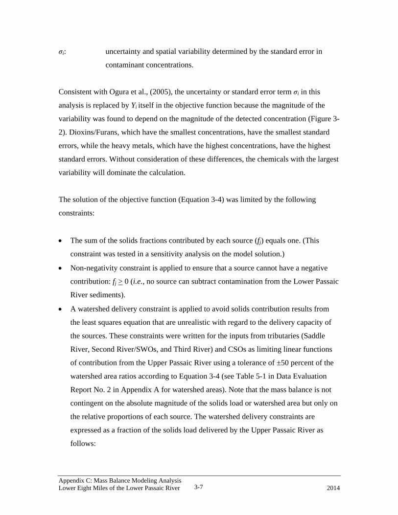
σi: uncertainty and spatial variability determined by the standard error in
contaminant concentrations.
Consistent with Ogura et al., (2005), the uncertainty or standard error term σi in this
analysis is replaced by Yi itself in the objective function because the magnitude of the
variability was found to depend on the magnitude of the detected concentration (Figure 3-
2). Dioxins/Furans, which have the smallest concentrations, have the smallest standard
errors, while the heavy metals, which have the highest concentrations, have the highest
standard errors. Without consideration of these differences, the chemicals with the largest
variability will dominate the calculation.
The solution of the objective function (Equation 3-4) was limited by the following
constraints:
• The sum of the solids fractions contributed by each source (fj) equals one. (This
constraint was tested in a sensitivity analysis on the model solution.)
• Non-negativity constraint is applied to ensure that a source cannot have a negative
contribution: fj > 0 (i.e., no source can subtract contamination from the Lower Passaic
River sediments).
• A watershed delivery constraint is applied to avoid solids contribution results from
the least squares equation that are unrealistic with regard to the delivery capacity of
the sources. These constraints were written for the inputs from tributaries (Saddle
River, Second River/SWOs, and Third River) and CSOs as limiting linear functions
of contribution from the Upper Passaic River using a tolerance of ±50 percent of the
watershed area ratios according to Equation 3-4 (see Table 5-1 in Data Evaluation
Report No. 2 in Appendix A for watershed areas). Note that the mass balance is not
contingent on the absolute magnitude of the solids load or watershed area but only on
the relative proportions of each source. The watershed delivery constraints are
expressed as a fraction of the solids load delivered by the Upper Passaic River as
follows:
Appendix C: Mass Balance Modeling Analysis Lower Eight Miles of the Lower Passaic River 2014 3-7
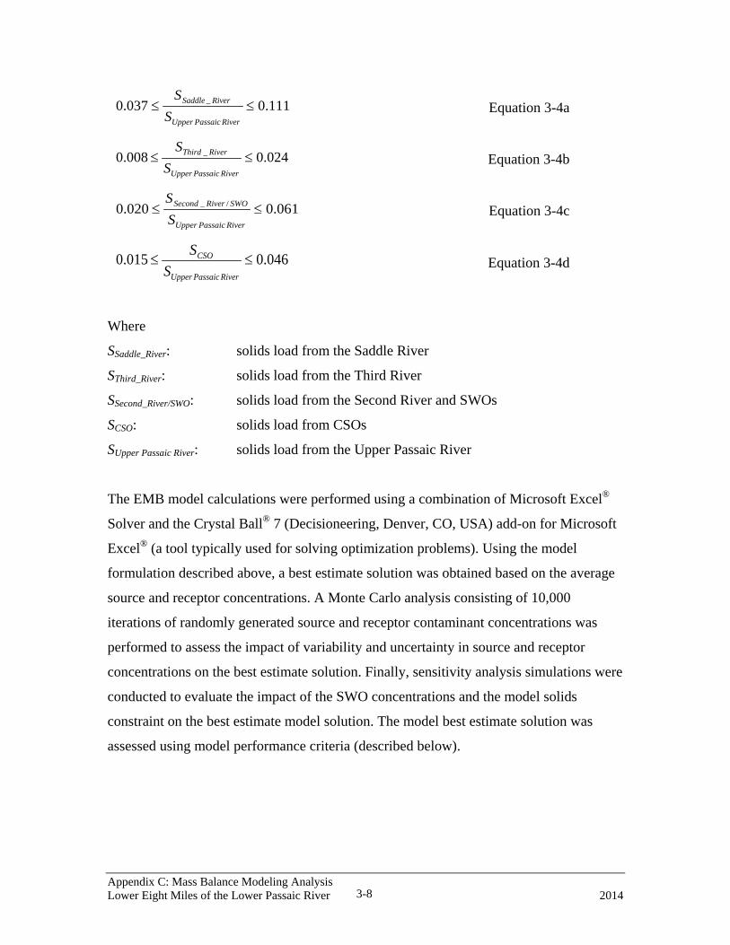
111.0037.0 _ ≤≤RiverPassaicUpper
RiverSaddle
SS
Equation 3-4a
024.0008.0 _ ≤≤RiverPassaicUpper
RiverThird
SS
Equation 3-4b
061.0020.0 /_ ≤≤RiverPassaicUpper
SWORiverSecond
SS
Equation 3-4c
046.0015.0 ≤≤RiverPassaicUpper
CSO
SS
Equation 3-4d
Where
SSaddle_River: solids load from the Saddle River
SThird_River: solids load from the Third River
SSecond_River/SWO: solids load from the Second River and SWOs
SCSO: solids load from CSOs
SUpper Passaic River: solids load from the Upper Passaic River
The EMB model calculations were performed using a combination of Microsoft Excel®
Solver and the Crystal Ball® 7 (Decisioneering, Denver, CO, USA) add-on for Microsoft
Excel® (a tool typically used for solving optimization problems). Using the model
formulation described above, a best estimate solution was obtained based on the average
source and receptor concentrations. A Monte Carlo analysis consisting of 10,000
iterations of randomly generated source and receptor contaminant concentrations was
performed to assess the impact of variability and uncertainty in source and receptor
concentrations on the best estimate solution. Finally, sensitivity analysis simulations were
conducted to evaluate the impact of the SWO concentrations and the model solids
constraint on the best estimate model solution. The model best estimate solution was
assessed using model performance criteria (described below).
Appendix C: Mass Balance Modeling Analysis Lower Eight Miles of the Lower Passaic River 2014 3-8
3.3 Identifying Contaminants for Inclusion in EMB Model
The Lower Passaic River accumulates solids that originate from several sources. In order
for the EMB model to decipher the contribution of these sources to the receptor
sediments, independent parameters must be identified and applied in the model.
Independent parameters are contaminants that have independent sources and/or different
fate and transport processes. Note that in the special case where a contaminant is not
independent of another contaminant, but together they form a fingerprint that can be used
to distinguish the sources, the two contaminants can be considered in the analysis. The
combination of contaminants selected for analysis must provide a relatively unique
pattern for each of the various sources in order for a unique solution to be obtained by the
model. Contaminants were selected from each of the compound classes, including:
dioxins/furans, PCBs, PAHs, pesticides, and metals. The individual contaminants chosen
are as follows:
• For dioxin/furan compounds, 2,3,7,8-TCDD and total tetrachlorodibenzodioxin
(Total TCDD) were selected. Although they are not independent parameters, both
were included because their ratio is an important tracer for Lower Passaic River
solids throughout the New York-New Jersey Harbor Estuary (Chaky, 2003).
• For PCBs, the data for the external sources were reported on a congener basis.
However, because the TSI 1995 data was reported on an Aroclor basis, the sum of
PCB Aroclors was selected to represent PCBs.
• For PAHs, the contaminants were selected based on the results of cluster analysis
performed on PAH mass fractions. Clustering is the partitioning of a dataset into
subsets, or “clusters,” where the data in each subset share some common trait. The
PAH cluster analysis yielded three different clusters (Figure 3-3). The two
independent PAHs selected from two of the clusters as contaminants with unique
sources or fate and transport processes consist of Benzo(a)pyrene (from the green
group in Figure 3-3) and Fluoranthene (from the blue group in Figure 3-3). The
third cluster was not included because it contained mostly 2- and 3-ring PAH
compounds, which likely have significant dissolved phase concentrations and may
Appendix C: Mass Balance Modeling Analysis Lower Eight Miles of the Lower Passaic River 2014 3-9
not be conservative particle tracers. Note that the EMB model focuses on particle-
bound contaminants.
• For pesticides, the selected compounds were limited by data availability and
difference in analytical techniques. In the TSI 1995 data set only Total DDx7
compounds were reported for the DDT group of compounds. In Newark Bay, only
dichlorodiphenyldichloroethylene (DDE) was consistently detected in the
sediments. Therefore, 4,4’-dichlorodiphenyldichloroethylene (4,4’-DDE) was
selected for the EMB model. In addition, gamma-Chlordane was selected because
dated sediment cores indicated that there has been little or no change in sediment
concentration over time and thus provides a good check on the model (See Data
Evaluation Report No. 3 in Appendix A).
• For the metals, cluster analysis was used to separate them into four different
clusters (Figure 3-4). Four metals were selected (chromium, copper, lead and
mercury), one from each cluster, as contaminants with unique sources or fate and
transport processes.
In addition to the above contaminants, the contaminant normalizers iron and TOC were
included to account for variability in particle size and organic carbon content of the
sediment. These normalizers helped to reduce the variability in the concentrations of
sediments and suspended solids (see Data Evaluation Report No. 4 in Appendix A).
The EMB model was designed to solve simultaneous mass balance equations for various
parameters by optimization. Thirteen parameters (eleven contaminants plus iron and
TOC) were directly used in the model for optimization (Table 3-1).
In addition to the list of 13 optimized parameters, another nine parameters were selected
for further EMB model evaluation (Table 3-2). This additional EMB model evaluation
was done by: 1) using model-optimized solids contributions to predict the concentrations
of the nine additional parameters in recently-deposited sediment of the Lower Passaic
7 Total DDx refers the sum of the 4,4’-dichlorodiphenyldichloroethane (4-4’-DDD), 4,4’-dichlorodiphenyldichloroethylene (4,4’-DDE) and 4,4’- Dichlorodiphenyltrichloroethane (4,4’-DDT) concentrations in a sample.
Appendix C: Mass Balance Modeling Analysis Lower Eight Miles of the Lower Passaic River 2014 3-10

River, and 2) comparing the predicted concentrations to the observed values for these
parameters.
3.4 Best Estimate Scenario
The sources and the receptor used in the EMB model are shown in Figure 3-1. For
completeness, a brief description of each source and the receptor is provided here along
with their respective concentrations used for the model parameters. The concentrations of
these parameters represent the best estimates for the various sources/receptor; the
application of these concentrations in the EMB model is called the best estimate scenario.
• Resuspension of the FFS Study Area legacy sediments was represented by the
average surface concentrations from the 1995 TSI dataset (i.e., 0-6 inches surface
sediment from RM1 to RM7). The average contaminant concentrations for the
resuspension signature are summarized in Table 3-3.
• Newark Bay was characterized by a northern and southern region. Average
contaminant concentrations for these regions are shown in Table 3-4; however, the
Newark Bay end member is represented by the northern region in the base case
simulation given its proximity to the Lower Passaic River. The surface sediment (0-6
inch) samples used to delineate the Newark Bay end member were from the 2005
Phase 1 and 2007 Phase 2 RI study by TSI. Only surface sediments (0-6 inches) at
depositional locations in the channel were considered (see Data Evaluation Report
No. 2 in Appendix A for discussion).
• The Upper Passaic River was characterized by four Be-7-bearing surface sediment
samples (only two of these were analyzed for organic contaminants), four Be-7-
bearing dated sediment core tops, and the suspended solids from two sediment traps.
These samples were collected between 2005 and 2008. The average contaminant
concentrations for the Upper Passaic River are summarized in Table 3-5.
• Tributary concentrations were based on averages from several recently-deposited
surface sediment samples and sediment trap samples obtained during the 2007/2008
sampling event. The average contaminant concentrations for the tributaries are
summarized in Table 3-6. Water column suspended sediment samples were removed
Appendix C: Mass Balance Modeling Analysis Lower Eight Miles of the Lower Passaic River 2014 3-11
from the population before the calculation of the statistics because these water
column samples represent a snap-shot at the time of collection (a few hours), and may
not be representative of average conditions. Indeed, several of them were reported to
have unusually high concentrations of many of the contaminants (possibly reflecting
rain event-driven peaks in contaminant concentrations). The exception is Second
River, where sediment and water column suspended sediment samples were used.
These water column suspended sediment samples did not show the variability
observed in other surface water samples and there were not enough sediment samples
to calculate meaningful statistics from sediment alone.
• The CSO and SWO data were based on water column suspended sediment samples
taken at the outfalls of several CSO and SWO locations (Table 3-7). The SWO
samples were determined not to be representative of the contribution of SWOs to the
contaminant loads in the river and they were not used in the base case model
simulation (see Section 3.2 for a discussion of the data quality from the SWO
samples).
• The recently-deposited Lower Passaic River surface sediments are the receptor in the
model. They were characterized by recently-deposited sediments, including core tops
from the 2005 high resolution cores and Be-7 surface sediment samples from the
2007/2008 sampling event. Data Evaluation Report No. 4 in Appendix A shows that
most contaminants have relatively constant iron-normalized concentrations from
RM2 to RM12, but these ratios often vary at the two ends of the study area. For this
reason, only data for samples between RM2 and RM12 were used in the model. The
average concentrations are listed in Table 3-8.
3.5 Sensitivity Analysis of SWO Concentrations and Solids Constraint
The base estimate scenario described above used the best estimates of the concentrations
for the various parameters for the sources/receptor in the EMB model. However, because
the SWOs were not sampled at a location above the influence of the Lower Passaic River,
the data from the SWO samples were compromised by the intrusion of Lower Passaic
River sediments into the SWOs. Therefore, the contributions from Second River and the
SWOs were combined in the model and the contaminant characteristics of both were
Appendix C: Mass Balance Modeling Analysis Lower Eight Miles of the Lower Passaic River 2014 3-12
based on samples taken in Second River only (see Section 3.2 for a discussion of SWO
data quality). The Second River was deemed to be representative of SWO discharges into
the Passaic River, because the Second River drains a highly-urbanized watershed that is
fed primarily by storm water collection systems. To assess the impact of this premise on
the best estimate solution, a model scenario was conducted that separated the SWO from
the Second River, with the SWO contaminant profile represented by the average of the
compromised SWO data. The solids and contaminant contributions obtained from this
sensitivity scenario were compared with the corresponding results from the best estimate
solution.
The second sensitivity analysis performed was to assess the impact of the solids
constraint on the best estimate solution. The solids constraint states that the sum of the
solids fractions from the various sources in the objective function (Equation 3-4) equals
one. Because of differences in the particle size distribution from the various sources, the
sum of the solids fractions may not necessarily be equal to one. This constraint was tested
in a sensitivity analysis and the model solution was compared to the results for the best
estimate scenario.
3.6 Monte Carlo Analysis of Uncertainty and Variability in Contaminant
Concentrations
The best estimate scenario described above used the best estimates of the concentrations
for the various parameters for the sources and receptor in the EMB model; however to
account for uncertainties and variability in source and receptor compositions, a Monte
Carlo sampling approach was used to develop 10,000 iterations of the input parameters
and the EMB model was optimized for each set of input parameters (i.e., 10,000
optimized solutions were obtained). The objective of the Monte Carlo analysis was to
develop confidence bounds in the EMB model-estimated solids balance and contaminant
fate and transport deduced from the solids balance by accounting for uncertainties in
source and receptor composition, and in the spatial variability in parameter
concentrations. Detailed description of the Monte Carlo simulation approach is given in
Appendix C: Mass Balance Modeling Analysis Lower Eight Miles of the Lower Passaic River 2014 3-13

Attachment A. In brief, the Monte Carlo simulation approach was used to develop the
10,000 iterations of the input parameters as follows:
• For the external sources and the receptor concentrations, a bounded normal
distribution defined by the mean, standard deviation, minimum, and maximum of
each parameter in each source term and receptor was used to perform the Monte
Carlo simulation.
• For resuspension, a bootstrap8 method was used to simulate the 10,000 iterations
of the contaminant concentrations in resuspended sediment since the 1995 TSI
data are neither normal nor log-normal.
• The correlations amongst the parameters for each source and receptor were
examined to verify that the 10,000 iterations of parameter profiles represent the
contaminant inter-dependencies.
As stated previously, 10,000 iterations were used to create 10,000 optimized model
estimates of the solids concentrations. Those 10,000 estimates of the solids contributions
were used to developed confidence levels of the solids contribution and the sources
parameter contributions to the Lower Passaic River.
3.7 Model Performance Evaluation
Model-optimized receptor concentrations for the 13 optimized parameters and model-
predicted receptor concentrations for the nine additional contaminants were evaluated for
the best estimate scenario using a statistical indicator called the normalized mean error
(NME). The NME is defined as the difference between the predicted and the observed,
normalized to the observed receptor concentration for each parameter (Equation 3-5):
measured
measuredel
CCCNME −
= mod Equation 3-5
8 Bootstrap is a powerful Monte Carlo method that re-samples the original sample set with replacement to generate a distribution of sample's statistics. It is a non-parametric method.
Appendix C: Mass Balance Modeling Analysis Lower Eight Miles of the Lower Passaic River 2014 3-14

where,
Cmodel = Parameter-specific concentration estimated
by the model
Cmeasured = Parameter-specific concentrations measured
in the Lower Passaic River
The NME expresses the bias in model predictions and observations, and gives an
indication of overestimation (NME >0) or underestimation (NME <0) for each
contaminant.
3.8 Model Limitation
Receptor models are inferential in nature, meaning that they infer the contributions from
different sources based on multivariate measurements collected at the receptor site.
Because the models infer rather than predict, they cannot be used directly to estimate
future changes in the system under certain conditions. For example, while the model
indicates that a fraction of the Lower Passaic River bottom sediments is composed of
Newark Bay sediments, the model cannot predict how the Newark Bay contribution will
change after the Newark Bay channel is deepened.
Appendix C: Mass Balance Modeling Analysis Lower Eight Miles of the Lower Passaic River 2014 3-15

4 MODELING RESULTS
This chapter discusses the EMB model solids balance results and the fate and transport of
contaminants deduced from the solids balance in the Lower Passaic River. The EMB
model calculations were performed for the best estimate scenario and a Monte Carlo
analysis was included to assess the uncertainty in model estimates. In addition, two
sensitivity analysis scenarios were performed to assess the sensitivity of the model result
to the inclusion of compromised SWO sample results and to the use of tributary solids
constraints included in the model. The model results for the best estimate scenario form
the basis for the solids balance and contaminant fate and transport in the river. The results
of the Monte Carlo analysis were used to account for uncertainties and spatial variability
on the best estimate model results, and these uncertainties were expressed as confidence
levels on the best estimate solution. The Monte Carlo analysis also provided a median
estimate based on the 10,000 iterations which was also compared to the best estimate
scenario.
4.1 EMB Model Solids Balance Results: Best Estimate Scenario and
Uncertainty
Thirteen parameters [Table 3-1; copper, chromium, mercury, lead, gamma-Chlordane,
4,4’-DDE, 2,3,7,8 TCDD, Total TCDD, Total PCB, benzo(a)pyrene, fluoranthene, iron,
and TOC] were optimized in the model to determine the solids balance. The model was
then used to predict the receptor concentrations for the remaining nine parameters in
Table 3-2 to evaluate its performance (see Section 4.3 below). Note that while iron and
TOC are not contaminants, they are generally important in the transport of fine particles
and associated contaminants. In particular, the inclusion of iron and TOC in the EMB
model is an indirect means of normalizing the various source terms to their fine-grained
sediment content. Therefore, the EMB model focuses on those sediments that contain and
transport the majority of the contaminant burden.
Appendix C: Mass Balance Modeling Analysis Lower Eight Miles of the Lower Passaic River 2014 4-1

Uncertainties in the model solution were developed from the Monte Carlo analysis based
on confidence intervals (5th and 95th percentiles) of the 10,000 optimized solutions. The
results of the EMB model optimization of the 10,000 Monte Carlo iterations are
presented later in this discussion as box and whisker plots which depict the median
solution plus the 5th, 25th, 75th and 95th percentiles of the 10,000 iterations. The best
estimate solution was also added to the plots.
The EMB model solids balance results are shown in Figure 4-1 based on best estimates of
the concentrations of contaminants. The best estimate solution indicates that resuspended
solids account for about 48 percent of the total solids in recently-deposited (Be-7-
bearing) sediments in the Lower Passaic River. Newark Bay and the Upper Passaic River
account for about 14 percent and 32 percent, respectively, of the solids delivered to the
Lower Passaic River. The tributaries, CSO and SWO together contribute about 6 percent
of the solids. Uncertainties in these solids fraction estimates derived from the Monte
Carlo iterations (Figure 4-2) indicate that resuspension accounted for about 28 to 65
percent, Upper Passaic River accounted for about 13 to 49 percent, Newark Bay
accounted for less than 1 to 44 percent, and all the other sources together contribute
between 2 and less than 12 percent. The relatively high contribution of solids from
resuspension translates to a high resuspension contribution (33 percent or higher) of the
contaminant burden (Table 4-1) in recently-deposited (Be-7-bearing) sediments.
4.2 EMB Model Contaminant Fate and Transport
The EMB model solids balance results presented above (Section 4.1) lead to further
discussion of the fate and transport of contaminants in the Lower Passaic River. The fate
and transport discussions are based on the mass balance outputs showing the distribution
of the contaminant flux among the sources and a comparison of average contaminant
concentrations used to characterize each source. This section is divided into two sub-
sections: (1) fate and transport of parameters examined and optimized in the EMB model,
and (2) inferred fate and transport of additional parameters. The results for the best
estimate scenario and the associated Monte Carlo-based uncertainty are presented for the
contaminants examined in the EMB model. Only the best estimate scenario is presented
Appendix C: Mass Balance Modeling Analysis Lower Eight Miles of the Lower Passaic River 2014 4-2
for fate and transport of additional contaminants, since these contaminants were not part
of the Monte Carlo analysis.
4.2.1 Fate and Transport of Contaminants Optimized in the EMB Model
2,3,7,8-TCDD and Total TCDD Mass Balances
The upper panel of Figure 4-3a presents a box and whisker plot of the 2,3,7,8-TCDD
concentration for each source with a solid line (marked “Target Concentration9”)
representing the average 2,3,7,8-TCDD concentration in recently-deposited (Be-7-
bearing) sediments in the Lower Passaic River (from RM2 to RM12). The first striking
feature is that external sources alone (the Upper Passaic River, the tributaries, the
CSO/SWOs, and Newark Bay) cannot explain the measured 2,3,7,8-TCDD concentration
in the river. Note that the 2,3,7,8-TCDD concentrations from the upland external sources
(the Upper Passaic River, the tributaries, the CSO/SWOs) are approximately two orders
of magnitude less than the measured concentration in the recently-deposited (Be-7-
bearing) surface sediments. Northern Newark Bay is approximately one order of
magnitude lower, likely due to the impacts of the Lower Passaic River on this water
body. Consequently, another source of 2,3,7,8-TCDD is necessary to achieve a closed
contaminant mass balance. The only other source that could explain the target
concentrations in the Lower Passaic River is the resuspension of legacy sediments. The
mass balance calculated for 2,3,7,8-TCDD, shown on Figure 4-3a bottom panel and
Figure 4-3b, indicates that resuspension accounts for about 87 to 100 percent, with a best
estimate of 97 percent of the 2,3,7,8-TCDD observed in recently-deposited sediments in
the Lower Passaic River.
Similar results were observed for Total TCDD (Figure 4-4a,b); however, for Total
TCDD, the relative difference between the measured concentration in the Lower Passaic
River and the concentrations in the external sources is less than the corresponding
difference observed for 2,3,7,8-TCDD. The Total TCDD concentration difference among
the upland external sources is only about one order of magnitude, as opposed to two
9 “Target concentration” represents the average contaminant concentration in recently-deposited (Be-7-bearing) sediments in the Lower Passaic River between RM2 and RM12.
Appendix C: Mass Balance Modeling Analysis Lower Eight Miles of the Lower Passaic River 2014 4-3
orders of magnitude for 2,3,7,8-TCDD. Even though the variation is much less, sediment
resuspension is still necessary to achieve a closed contaminant mass balance. While all
external sources account for about 1 to 28 percent with a best estimate of 8 percent of the
Total TCDD mass balance, sediment resuspension accounts for 76 to 97 percent with a
best estimate of ~ 92 percent of the contaminant mass.
The Newark Bay contribution to the Lower Passaic River dioxin contaminant burden
ranges from less than 1 percent to 13 percent for 2,3,7,8-TCDD, with a best estimate of 3
percent. For Total TCDD, Newark Bay contribution ranges from less than 1 percent to 21
percent, with a best estimate of 5 percent. The concentrations of these contaminants in the
river surface sediments are greater than the reported concentrations in the bay. These
results indicate that the Lower Passaic River is a source of contamination to the bay.
Total PCB Mass Balance
The fate and transport of Total PCBs is influenced by sediment resuspension (Figure 4-
5a, b). The Total PCB concentration in Newark Bay is about two times lower than the
Lower Passaic River concentration and the Upper Passaic River concentration is about
three times lower than the Lower Passaic River concentration. These concentration
patterns in the source signatures indicate a dominant resuspension contribution of Total
PCBs to the Lower Passaic River with a best estimate of about 81 percent and a range of
59 to 90 percent. Upper Passaic River is the most important external source of total PCB
contamination to the Lower Passaic, with a best estimate of 11 percent (range of 4 to 22
percent of the overall mass), while the Newark Bay contributes about 7 percent (range of
less than 1 to 25 percent) of the overall mass.
PAH Mass Balance
In the model, benzo[a]pyrene (Figure 4-6a, b) and fluoranthene (Figure 4-7a, b) represent
the PAH contaminant compounds directly optimized by the model. For both of these
compounds, the average PAH concentration in the Upper Passaic River is higher
(approximately 1.5 times) than the Lower Passaic River average PAH concentration. The
tributaries, the CSOs/SWOs and the 1995 surface sediment concentrations are
Appendix C: Mass Balance Modeling Analysis Lower Eight Miles of the Lower Passaic River 2014 4-4

comparable to the measured PAH concentration in the 2005-2007 Be-7-bearing
sediments in the Lower Passaic River. The Newark Bay average PAH concentration is
about two times smaller than the Lower Passaic River concentration. Because the average
PAH concentration in the Upper Passaic River is higher than the target concentration
(Lower Passaic River) and the other sources have similar PAH concentration, the
contribution of the Upper Passaic PAH to the Lower Passaic PAH contamination is larger
than any other compounds used in the mass balance. The Upper Passaic River
contribution ranges from 27 to 70 percent for benzo[a]pyrene, with a best estimate of 53
percent and for fluoranthene from 24 to 64 percent with a best estimate of 47 percent.
Resuspension of the historical inventory accounts for about 39 percent (range of 17 to 58
percent) of the PAH contaminant burden of the Lower Passaic River. Newark Bay’s PAH
contribution range from less than 1 percent to 30 percent, with a best estimate of
approximately 6 percent.
Although higher PAH concentrations were observed in the tributaries and CSOs,
comparable to observations in the Upper Passaic River, the relatively small solids
contributions from the tributaries and CSOs limits their combined contribution to less
than 17 percent.
Pesticides Mass Balance
The average 4,4’-DDE concentration in the Upper Passaic River is roughly four times
lower than the measured concentration in the Lower Passaic River (Figure 4-8a, b). The
4,4’-DDE concentration in Newark Bay is slightly lower than the concentration in the
Lower Passaic River. The average 4,4’-DDE concentration of the 1995 surface sediment
source is only slightly higher than the 2005-2007 Be-7-bearing sediments in the Lower
Passaic River (approximately 30 percent higher). While the Second and Third River 4,4’-
DDE concentration overlaps with measured 4,4’-DDE in the 2005-2007 Be-7-bearing
sediments in the Lower Passaic River, the limited solids load from these tributaries
cannot account for the 4,4’-DDE mass in the river. The resuspension of the historical
inventory contributes between 52 to 88 percent of the 4,4’-DDE mass in the Lower
Passaic River, with a best estimate of 78 percent. Newark Bay contributes about 8 percent
Appendix C: Mass Balance Modeling Analysis Lower Eight Miles of the Lower Passaic River 2014 4-5
of 4,4’-DDE mass (range of less than 1 to 34 percent) and the Upper Passaic River
contributes about 10 percent (range of 4 to 21 percent). The combined contribution from
tributaries SWOs and CSOs range from 1 to 10 percent, with a best estimate of about 4
percent.
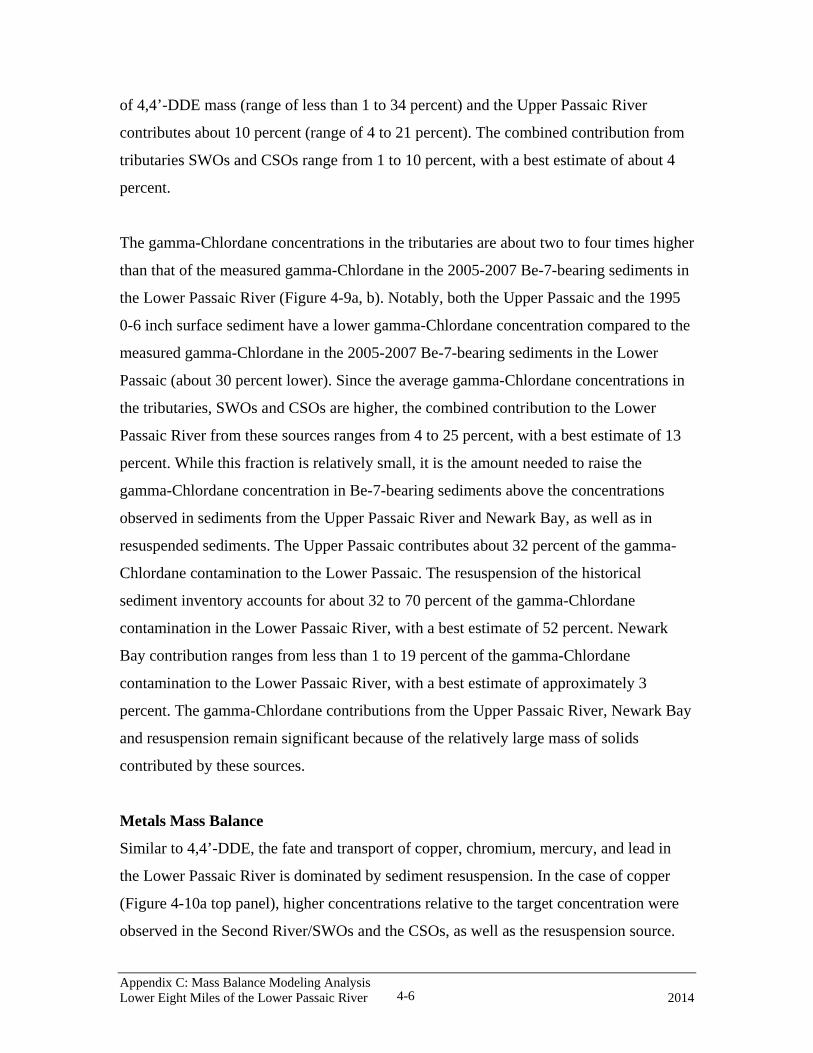
The gamma-Chlordane concentrations in the tributaries are about two to four times higher
than that of the measured gamma-Chlordane in the 2005-2007 Be-7-bearing sediments in
the Lower Passaic River (Figure 4-9a, b). Notably, both the Upper Passaic and the 1995
0-6 inch surface sediment have a lower gamma-Chlordane concentration compared to the
measured gamma-Chlordane in the 2005-2007 Be-7-bearing sediments in the Lower
Passaic (about 30 percent lower). Since the average gamma-Chlordane concentrations in
the tributaries, SWOs and CSOs are higher, the combined contribution to the Lower
Passaic River from these sources ranges from 4 to 25 percent, with a best estimate of 13
percent. While this fraction is relatively small, it is the amount needed to raise the
gamma-Chlordane concentration in Be-7-bearing sediments above the concentrations
observed in sediments from the Upper Passaic River and Newark Bay, as well as in
resuspended sediments. The Upper Passaic contributes about 32 percent of the gamma-
Chlordane contamination to the Lower Passaic. The resuspension of the historical
sediment inventory accounts for about 32 to 70 percent of the gamma-Chlordane
contamination in the Lower Passaic River, with a best estimate of 52 percent. Newark
Bay contribution ranges from less than 1 to 19 percent of the gamma-Chlordane
contamination to the Lower Passaic River, with a best estimate of approximately 3
percent. The gamma-Chlordane contributions from the Upper Passaic River, Newark Bay
and resuspension remain significant because of the relatively large mass of solids
contributed by these sources.
Metals Mass Balance
Similar to 4,4’-DDE, the fate and transport of copper, chromium, mercury, and lead in
the Lower Passaic River is dominated by sediment resuspension. In the case of copper
(Figure 4-10a top panel), higher concentrations relative to the target concentration were
observed in the Second River/SWOs and the CSOs, as well as the resuspension source.
Appendix C: Mass Balance Modeling Analysis Lower Eight Miles of the Lower Passaic River 2014 4-6

Copper concentrations in the other sources were less than the average target
concentration. Given that the solids contribution from the Second River and CSOs are
insignificant relative to the resuspension contribution, a mass balance for copper would
need a significant resuspension contribution to explain the high target concentration. This
is confirmed by the model-estimated copper budget (Figure 4-10a bottom panel and
Figure 4-10b), which shows that resuspension accounts for 72 percent of the contaminant
burden (range of 45 to 85 percent), while Newark Bay, the Upper Passaic and CSOs
account for 12 percent (range of less than 1 to 40 percent), 14 percent (range of 5 to 25
percent) and 1 percent (range of less than 1 to 6 percent), respectively.
The relative concentrations of chromium (Figure 4-11a top panel) and mercury (Figure 4-
12a top panel) in the various sources show higher or comparable average concentrations
in Newark Bay and resuspension sources and lower concentrations for other sources,
relative to the target concentrations. A mass balance for these metals can only be
obtained by a large resuspension contribution to explain the target concentrations. This
observation is confirmed by the best estimate and Monte Carlo mass balance results for
chromium (Figure 4-11a bottom panel) and mercury (Figure 4-12a bottom panel).
Resuspension of sediment accounts for approximately 74 percent of chromium and
approximately 75 percent of mercury, both with a range between 44 and 88 percent. Both
chromium and mercury also have similar contributions from Newark Bay and the Upper
Passaic River, with respective values of 15 and 10 percent for chromium and 14 and 11
percent for mercury.
Average concentrations of lead from the various sources are shown in the top panel of
Figure 4-13a. Lead concentrations are higher in the Second River/SWOs, CSOs and the
resuspension source, relative to the average target concentration in the Lower Passaic
River. Because the solids contribution from the Second River/SWO and CSOs are
relatively small, a significant resuspension input is needed to explain the observed target
concentration. The mass balance calculated for lead (Figure 4-13b, bottom panel)
indicates a best estimate of 71 percent resuspension contribution to the overall lead
burden in recently-deposited (Be-7-bearing) sediments, with an uncertainty range of 48 to
Appendix C: Mass Balance Modeling Analysis Lower Eight Miles of the Lower Passaic River 2014 4-7

83 percent. The best estimates of the lead contributions from Newark Bay and the Upper
Passaic River are about 7 and 19 percent, respectively, while the tributaries, SWO and
CSOs contribute a combined 3 percent.
Iron and TOC Balance
Average source concentrations for iron indicate higher iron concentrations and, by
association, higher fractions of fine particles in Newark Bay and the Lower Passaic River
sediments relative to the other sources (Figure 4-14a top panel). The resulting mass
balance (Figure 4-14a bottom panel) indicates between 29 to 72 percent, with a best
estimate of 54 percent of the iron in Be-7-bearing sediments originating from
resuspension. The iron contribution from Newark Bay ranges from less than 1 to 52
percent, with a best estimate of approximately 18 percent. The Upper Passaic River
contributes a best estimate of 24 percent (range of 9 to 43 percent) of the iron burden to
the target area.
Unlike iron, which indicates an appreciable Newark bay contribution, TOC in Newark
Bay is low relative to other sources (Figure 4-15a, top panel). The TOC mass balance
indicates a best estimate resuspension contribution of 72 percent to the TOC burden in
the Lower Passaic River, with a range of 48 to 83 percent (Figure 4-15a bottom panel).
4.2.2 Inferred Fate and Transport Model for contaminants
Two contaminant mass balances could not be fully quantified in the EMB model due to
data gaps/limitations and the degree of particle affinity of any given contaminant. For
example, dieldrin was generally not detected in the Phase 1 Newark Bay dataset, thus
only the Phase 2 data with some detected values were used and an inferred best estimate
mass balance was developed for dieldrin.
Furthermore, because Low Molecular Weight (LMW) PAHs may be affected by
dissolved phase concentrations as well as other contaminant degradation processes, they
were not explicitly included in the EMB model. However, the best estimate EMB model
solids balance was used to calculate a mass balance for phenanthrene, used as a surrogate
Appendix C: Mass Balance Modeling Analysis Lower Eight Miles of the Lower Passaic River 2014 4-8
for LMW PAH compounds. A summary of the inferred best estimate mass balances is as
follows:
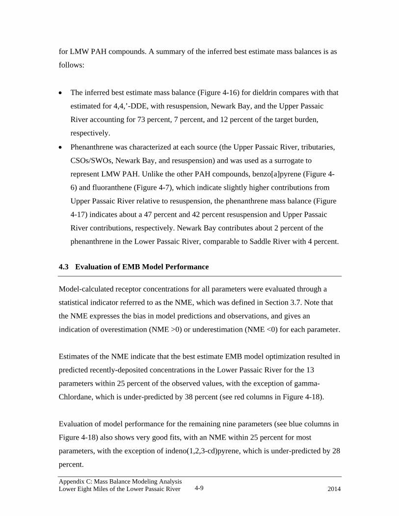
• The inferred best estimate mass balance (Figure 4-16) for dieldrin compares with that
estimated for 4,4,’-DDE, with resuspension, Newark Bay, and the Upper Passaic
River accounting for 73 percent, 7 percent, and 12 percent of the target burden,
respectively.
• Phenanthrene was characterized at each source (the Upper Passaic River, tributaries,
CSOs/SWOs, Newark Bay, and resuspension) and was used as a surrogate to
represent LMW PAH. Unlike the other PAH compounds, benzo[a]pyrene (Figure 4-
6) and fluoranthene (Figure 4-7), which indicate slightly higher contributions from
Upper Passaic River relative to resuspension, the phenanthrene mass balance (Figure
4-17) indicates about a 47 percent and 42 percent resuspension and Upper Passaic
River contributions, respectively. Newark Bay contributes about 2 percent of the
phenanthrene in the Lower Passaic River, comparable to Saddle River with 4 percent.
4.3 Evaluation of EMB Model Performance
Model-calculated receptor concentrations for all parameters were evaluated through a
statistical indicator referred to as the NME, which was defined in Section 3.7. Note that
the NME expresses the bias in model predictions and observations, and gives an
indication of overestimation (NME >0) or underestimation (NME <0) for each parameter.
Estimates of the NME indicate that the best estimate EMB model optimization resulted in
predicted recently-deposited concentrations in the Lower Passaic River for the 13
parameters within 25 percent of the observed values, with the exception of gamma-
Chlordane, which is under-predicted by 38 percent (see red columns in Figure 4-18).
Evaluation of model performance for the remaining nine parameters (see blue columns in
Figure 4-18) also shows very good fits, with an NME within 25 percent for most
parameters, with the exception of indeno(1,2,3-cd)pyrene, which is under-predicted by 28
percent.
Appendix C: Mass Balance Modeling Analysis Lower Eight Miles of the Lower Passaic River 2014 4-9

4.4 Sensitivity Analysis
Uncertainties in source and receptor compositions and spatial variability in parameter
concentrations were incorporated into the model solution through the Monte Carlo
analysis described above. This section presents the result of additional analysis performed
to assess the impact of compromised SWO contaminant concentrations (Table 4-3) and
the model solids constraint (Table 4-4). The sensitivity results are discussed below.
Impact of Stormwater Data
The impact of compromised SWO data was evaluated by performing a model simulation
using separate source compositions for Second River and the SWOs (the SWO
contribution was separated from the Second River, with the SWO contaminant profile
represented by the average of the compromised SWO data). The results of this scenario
were not significantly different relative to the best estimate scenario (Tables 4-2 and 4-3,
respectively). As expected, the use of the SWO data as an individual source did not affect
the model calculations, most likely, because the SWOs, like the other tributaries, are
minor solids contributors.
Impact of Model Solids Constraint
The best estimate solution, which was simulated using a solids constraint which required
that the total solids fraction should be one, was redone without this constraint. There were
slight differences between the best estimate solution (Table 4-2) and the relaxed solids
constraint scenario (Table 4-4). In general, the differences were within the uncertainty
estimated by the best estimate scenario of the Monte Carlo analysis. When the solids
constraint was relaxed, the model predicted the solids fractions with an error of 8 percent,
a value within the variability inherent in the contaminant measurements. The agreement
between these two scenarios suggests that the contaminants profiles provide adequate
constraint on the mass balance, as well as a strong mathematical basis to track the
sediment types that are mostly associated with the contamination.
Appendix C: Mass Balance Modeling Analysis Lower Eight Miles of the Lower Passaic River 2014 4-10
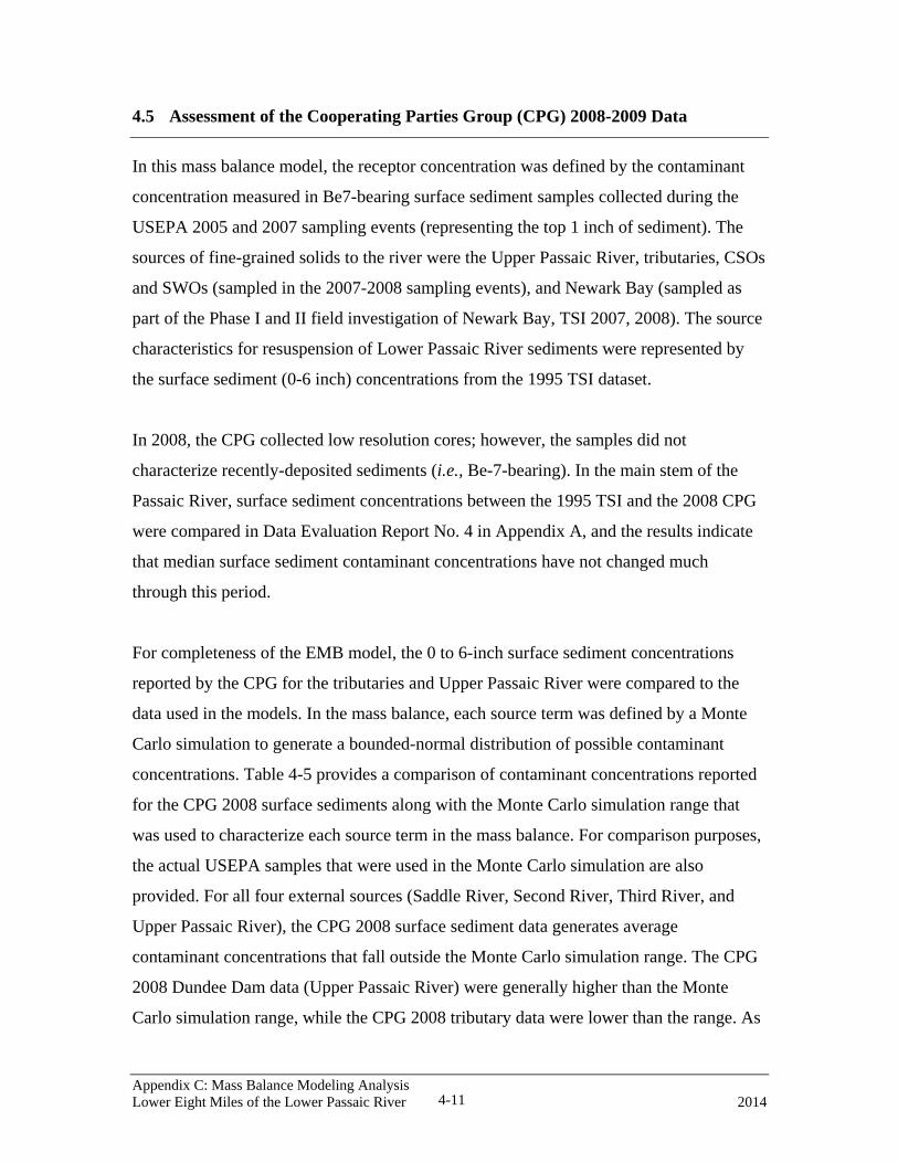
4.5 Assessment of the Cooperating Parties Group (CPG) 2008-2009 Data
In this mass balance model, the receptor concentration was defined by the contaminant
concentration measured in Be7-bearing surface sediment samples collected during the
USEPA 2005 and 2007 sampling events (representing the top 1 inch of sediment). The
sources of fine-grained solids to the river were the Upper Passaic River, tributaries, CSOs
and SWOs (sampled in the 2007-2008 sampling events), and Newark Bay (sampled as
part of the Phase I and II field investigation of Newark Bay, TSI 2007, 2008). The source
characteristics for resuspension of Lower Passaic River sediments were represented by
the surface sediment (0-6 inch) concentrations from the 1995 TSI dataset.
In 2008, the CPG collected low resolution cores; however, the samples did not
characterize recently-deposited sediments (i.e., Be-7-bearing). In the main stem of the
Passaic River, surface sediment concentrations between the 1995 TSI and the 2008 CPG
were compared in Data Evaluation Report No. 4 in Appendix A, and the results indicate
that median surface sediment contaminant concentrations have not changed much
through this period.
For completeness of the EMB model, the 0 to 6-inch surface sediment concentrations
reported by the CPG for the tributaries and Upper Passaic River were compared to the
data used in the models. In the mass balance, each source term was defined by a Monte
Carlo simulation to generate a bounded-normal distribution of possible contaminant
concentrations. Table 4-5 provides a comparison of contaminant concentrations reported
for the CPG 2008 surface sediments along with the Monte Carlo simulation range that
was used to characterize each source term in the mass balance. For comparison purposes,
the actual USEPA samples that were used in the Monte Carlo simulation are also
provided. For all four external sources (Saddle River, Second River, Third River, and
Upper Passaic River), the CPG 2008 surface sediment data generates average
contaminant concentrations that fall outside the Monte Carlo simulation range. The CPG
2008 Dundee Dam data (Upper Passaic River) were generally higher than the Monte
Carlo simulation range, while the CPG 2008 tributary data were lower than the range. As
Appendix C: Mass Balance Modeling Analysis Lower Eight Miles of the Lower Passaic River 2014 4-11

discussed above (and presented in Table 4-5), this difference is likely associated with
sampling depths that represent different physical/contaminant regimes. Above Dundee
Dam, 0 to 6 inches of silty sediment is likely characterizing deeper legacy sediments, so
higher sediment concentrations are expected; whereas on the sandy tributaries, a 0 to 6-
inch sample is likely capturing the underlying sand, which reduces the overall sample
concentration. For the two tributaries with higher 2,3,7,8-TCDD concentrations than used
in the model analysis, these stations are likely to be impacted by tidal transport of Lower
Passaic River sediments into the tributaries during low flow periods. Consequently, the
existing contaminant mass balance does not need any modification since the CPG 2008
sampling event was not designed to characterize the source term or solids transported
from these sources to the river, and in some cases may be impacted by solids from the
Lower Passaic River itself.
Appendix C: Mass Balance Modeling Analysis Lower Eight Miles of the Lower Passaic River 2014 4-12
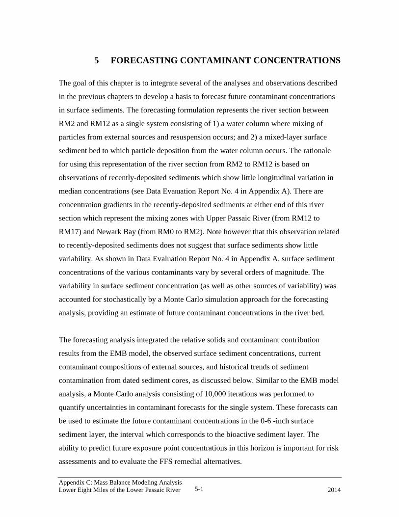
5 FORECASTING CONTAMINANT CONCENTRATIONS
The goal of this chapter is to integrate several of the analyses and observations described
in the previous chapters to develop a basis to forecast future contaminant concentrations
in surface sediments. The forecasting formulation represents the river section between
RM2 and RM12 as a single system consisting of 1) a water column where mixing of
particles from external sources and resuspension occurs; and 2) a mixed-layer surface
sediment bed to which particle deposition from the water column occurs. The rationale
for using this representation of the river section from RM2 to RM12 is based on
observations of recently-deposited sediments which show little longitudinal variation in
median concentrations (see Data Evaluation Report No. 4 in Appendix A). There are
concentration gradients in the recently-deposited sediments at either end of this river
section which represent the mixing zones with Upper Passaic River (from RM12 to
RM17) and Newark Bay (from RM0 to RM2). Note however that this observation related
to recently-deposited sediments does not suggest that surface sediments show little
variability. As shown in Data Evaluation Report No. 4 in Appendix A, surface sediment
concentrations of the various contaminants vary by several orders of magnitude. The
variability in surface sediment concentration (as well as other sources of variability) was
accounted for stochastically by a Monte Carlo simulation approach for the forecasting
analysis, providing an estimate of future contaminant concentrations in the river bed.
The forecasting analysis integrated the relative solids and contaminant contribution
results from the EMB model, the observed surface sediment concentrations, current
contaminant compositions of external sources, and historical trends of sediment
contamination from dated sediment cores, as discussed below. Similar to the EMB model
analysis, a Monte Carlo analysis consisting of 10,000 iterations was performed to
quantify uncertainties in contaminant forecasts for the single system. These forecasts can
be used to estimate the future contaminant concentrations in the 0-6 -inch surface
sediment layer, the interval which corresponds to the bioactive sediment layer. The
ability to predict future exposure point concentrations in this horizon is important for risk
assessments and to evaluate the FFS remedial alternatives.
Appendix C: Mass Balance Modeling Analysis Lower Eight Miles of the Lower Passaic River 2014 5-1

This chapter is divided into two major sections: “Development of Concentration Half
Times10 for the Excess Passaic River Sediment Burden” and “Forecasts of Sediment
Concentrations for FFS Remedial Alternatives.” The first section describes the results of
an analysis which uses the dated sediment cores to examine the decline in contaminant
concentrations over time. As part of this analysis, baseline contaminant levels in the
external upland sources are subtracted from the Lower Passaic River sediment
concentrations observed in the dated cores, yielding the component of the annual
contaminant burden that is due to loads “internal” to the Lower Passaic River. This is also
referred to as the “excess sediment burden.” Nearly all internal contaminant loads present
in the Lower Passaic River can be attributed to legacy sediment resuspension. It is
essential to quantify the internal burden since it represents the contamination that would
be controlled by a remedial action performed on the Lower Passaic River. Using the
observed decline of this burden over time, the rate of concentration decrease can be
described by a first-order exponential decay curve with an estimated half time based on
the rate of the natural recovery process (i.e., the time it takes for the concentrations in
depositing sediment to decline by half as a result of these processes). Once the half times
for the different contaminants were determined, regression analysis was used to compare
the contaminant-specific half times and determine a single half time for the excess
sediment burden in the Lower Passaic River.
In the second section, the half times developed from the dated sediment core
chronologies for the internal resuspension load were used, together with the results of the
EMB model, to forecast future concentrations in the bioactive sediment layer. The
forecast calculations were made for the best estimate scenario using average contaminant
concentrations and other model inputs, and uncertainties were quantified by Monte Carlo
analysis. These forecasts are made for the FFS Remedial Alternatives, including: No
10 The use of the term “half time” in this sense is not to imply decay or destruction of 2,3,7,8-TCDD over time, akin to the decay of a radionuclide. Rather, the term here is used to express a rate for the decline of 2,3,7,8-TCDD concentrations in the solids accumulating at each coring location. Specifically, the half time is the time required for the 2,3,7,8-TCDD concentration to decline to half of its current value. The processes that affect the decline are multifold, including many of the fluxes and processes that occur in an urban estuary. The “half time” expression is just a means to encompass these processes and note their net effect on concentration through time.
Appendix C: Mass Balance Modeling Analysis Lower Eight Miles of the Lower Passaic River 2014 5-2
Action (Alternative 1), Deep Dredging with Backfill (Alternative 2), Capping with
Dredging for Flooding and Navigation (Alternative 3), and Focused Capping with
Dredging for Flooding (Alternative 4). Detailed description of these alternatives is
provided in Chapter 4 of the FFS Report.
5.1 Development of Concentration Half Times for the Excess Passaic River
Sediment Burden
The dated sediment core profiles for the Lower Passaic River and the Upper Passaic
River at Dundee Dam describe the chronologies of contaminant concentrations in the
sediment. By careful selection of the coring locations and radionuclide dating of the
sediment layers, the time-dependence of contaminant concentrations can be discerned. As
discussed in Data Evaluation Report No. 3 in Appendix A these sediment records are a
proxy for contaminant concentrations on suspended matter in the water column at the
time of deposition. Because tidal mixing integrates suspended matter and the associated
contaminant loads over distances of several miles, each dated sediment core records the
relative intensity of loads as they are deposited on the river bottom in its vicinity.
To the extent that the core records yield regular variations over time (e.g., a steady
decline in contaminant concentrations from depth to the surface), the trends in the core
chronologies can be extrapolated and used as a basis to estimate future conditions in the
absence of remediation. Essentially, the rate of contaminant concentration decline
documented by the core implies a rate of recovery for the river’s sediments in the absence
of any marked changes in loads or processes. In most instances, these loads and processes
(e.g., the integration of a large watershed area) are difficult to change or redirect without
major intervention.
The dated sediment cores document the impacts of internal and external loads to annual
deposition, the equivalent of the annual Be-7-bearing sediment deposits. In order to
forecast future impacts of legacy sediment-related loads, it is first necessary to
distinguish the component of the water column-based sediment record (i.e., the dated
Appendix C: Mass Balance Modeling Analysis Lower Eight Miles of the Lower Passaic River 2014 5-3
sediment cores) that is due to legacy sediment resuspension from that which is due to
external loads.
The EMB model, presented in Chapters 3 and 4, used available field data to represent the
contaminant sources associated with sediment flux from each of the major tributaries, the
CSOs/SWOs, Newark Bay, and the Upper Passaic River. The EMB model also used the
1995 surface sediment data to estimate the conditions of the internal contaminant source:
the resuspension of legacy sediments. After balancing the loads from all the sources with
the known conditions of recently-deposited (Be-7-bearing) sediment, the EMB model
produced a set of fractions describing the solids contribution from each of the sources.
These fractions can be used to separate the loads measured in the dated sediment cores
into the contributions from each source, which is necessary to identify which portion of
the contaminant load will be controlled by remediation. The underlying premise of this
approach is that the relative solids contributions from each of the solids sources to annual
deposition as recorded in the cores has remained constant over for the historical period
examined. This is for the period 1980 to 2005 as described below.
5.1.1 Natural Recovery Processes Occurring in the Lower Passaic River
Natural recovery processes are likely occurring in the Lower Passaic River and impacting
some contaminant concentrations over time. These trends are observed in the dated
sediment core profiles presented in Data Evaluation Report No. 3 in Appendix A, with
concentrations declining from the 1980s to 2005 for some contaminants. Table 5-1
summarizes the average 1980s concentrations for some of the contaminants and
compares these values to the average 2005 surface sediment concentrations.
The observed concentration decline may be due to multiple factors, including: natural
recovery processes (such as mixing and burial) and the elimination of direct discharges,
the combination of which curtailed the contaminant load over time. For this analysis,
only sediment samples dated from 1980 and later were included. Based on the dated
cores, this period was inferred to represent natural recovery-type reductions in
Appendix C: Mass Balance Modeling Analysis Lower Eight Miles of the Lower Passaic River 2014 5-4

concentration more than reductions caused by the elimination of direct contaminant
discharges. These natural reductions are assumed to continue into the future.
5.1.2 Data Available for Estimating the Half Times and Developing the
Trajectories
Each of the sources and the data available to quantify the decline in concentrations over
the last three decades are described herein:
• Lower Passaic River – There are five high resolution sediment cores collected in
2005 that document the characteristics of fine-grained suspended solids over time,
representing 12 miles of the Lower Passaic River and providing a basis for an
analysis of sediment contaminant concentrations as they change through time (see
Data Evaluation Report No. 3 in Appendix A).
• Upper Passaic River – One of the high resolution cores taken from Dundee Lake in
2005 by scientists from Rensselaer Polytechnic Institute (RPI) contains sufficient data
to describe the trend in contaminant concentrations in the Upper Passaic River over
the last 30 years. This core is presented in Figures 3-1, 3-2, 3-5 and 3-6 in Data
Evaluation Report No. 2 in Appendix A. With the exception of PAHs and dieldrin,
the detected contaminants have had relatively constant concentrations in the
suspended sediments above Dundee Dam since about 1990. Previous to that time,
there were elevated contaminant concentrations in the core segments and, by
inference, in the contemporaneous suspended solids transported over the dam. PAHs
and dieldrin appeared to decline in concentration until about 1990, when the trend
reversed and concentrations began to increase again. In addition, data from several
core tops, surface sediment samples, and sediment traps collected in 2007-2008 were
used to estimate the current average concentration on suspended sediment (Be-7
bearing).
• Newark Bay – No known high resolution cores exist to quantify
depositional/contaminant chronologies in the Newark Bay sediments for the post-
1990 period. The surface sediment samples from 2005 indicate a spatial gradient for
many of the contaminants from south to north, but there is no information on
temporal change in sediment concentrations. The EMB model used the five northern
Appendix C: Mass Balance Modeling Analysis Lower Eight Miles of the Lower Passaic River 2014 5-5

samples (see Table 3-4) to define the Newark Bay end member for use in the model.
The trajectory calculations also used these northern samples to calculate the Newark
Bay component.
• Tributaries – There are no temporal data available to determine the changes of
sediment contaminant concentrations over time in the Saddle River, Second River or
Third River.
• CSO/SWOs – There are no temporal data available to determine the changes of
contaminant concentrations over time in the releases from either the CSOs or the
SWOs.
To determine the temporal changes in the internal (resuspension) Lower Passaic River
contribution to the total contaminant load, each of the external sources was quantified and
subtracted from the total concentration, using the solids fractions obtained from the EMB
model results.
In the absence of information to the contrary, the tributaries and the CSO/SWO
components were assumed to have constant contaminant concentrations from the 1980s
to the end of the trajectory forecast. Since the EMB model found that the combined
sediment contributions from these sources were less than 5 percent of the entire sediment
load in the river, their contribution is small enough to warrant an assumption of this
nature without materially affecting the outcome of the trajectory forecasts.
The Upper Passaic River contribution was defined by a linear interpolation of
concentration versus time between each core segment from the RPI core (see Data
Evaluation Report No. 3 in Appendix A). After the last data point on that core (2005) and
through the end of the trajectory forecasts, the Upper Passaic component was assumed to
be constant. The constant concentration was an average of the core tops from two RPI
cores (one previously mentioned) and two Malcolm Pirnie cores collected early in 2007,
as well as a number of surface sediment and sediment trap samples from the 2007/2008
sampling program.
Appendix C: Mass Balance Modeling Analysis Lower Eight Miles of the Lower Passaic River 2014 5-6

The remaining two components are the Lower Passaic River resuspension component and
the Newark Bay component. Given the close link between these two water bodies and the
lack of a Newark Bay core to separately track fine-grained suspended matter from the
Bay, there is no way to separate their rates of decline. As a result, both contributions are
assumed to decline at the same rate. Therefore, when calculating the rate of decline, the
portion of the total contaminant load remaining after subtraction of the Upper Passaic
River, tributary, and CSO/SWO loads is defined as the “excess load”.
The assumption that Newark Bay concentrations are declining at a similar rate to the
Lower Passaic River sediments is rational, and perhaps conservative, given that the
northern end of Newark Bay is the end member used in the EMB model. Data Evaluation
No. 2 in Appendix A discusses the evidence to support the premise that 70 percent of the
dioxin load in Newark Bay is derived from the Lower Passaic River. Since so much of
the sediment dioxin load in Newark Bay originates from the river, it is appropriate to
assume that the rates of concentration decline are similar. For other contaminants, the
Lower Passaic River’s contribution to Newark Bay is probably much less due to other
sources. However, in these instances, the Newark Bay concentrations at the southern end
of the Bay are used as the “base” for the Newark Bay contribution (i.e., northern Newark
Bay concentrations are not permitted to decline below this concentration). Thus for those
contaminants with a strong north-to-south gradient in Newark Bay (suggesting an
important Lower Passaic River contribution), the large difference between the ends of the
bay is allowed to decline at the rate observed for the Lower Passaic River. For those
contaminants with a shallow or no gradient, the concentration on Newark Bay solids
delivered to the Lower Passaic River remains essentially constant over time.
5.1.3 Calculating the Half Times
Figures 5-1 through 5-10 show the excess concentration, obtained by subtracting the
products of each upland source’s concentration (based on averages of available data) and
solids fraction (from the EMB model) from the concentrations assigned to each slice of
the five high-resolution cores from the Lower Passaic River. The resulting datasets were
fitted to a first-order exponential decay curve as described above. While the exact
Appendix C: Mass Balance Modeling Analysis Lower Eight Miles of the Lower Passaic River 2014 5-7

mechanism(s) and rate of decline for this excess concentration are not specifically
known, the results clearly indicate a decline for most contaminants. The choice of a first
order decay process is consistent with the expected processes affecting most
contaminants in this system, specifically dispersion, bioturbation, diffusion, and
degradation. For each of these processes, the rate at which they occur is linearly
dependent on the contaminant concentrations (e.g., the higher the concentration, the
higher their rates of dispersion, diffusion, and degradation). The basic first-order decay
equation is presented as Equation 5-1 below.
tot eCC λ−= Equation 5-1
Where
Ct: excess sediment concentration at a given time
Co: excess sediment concentration at the initial time
λ: exponential decay parameter
t: time
Moreover, the exponential decay parameter (λ) is related to the half time (Equation 5-2),
or the estimated time for the contaminant concentration to decrease by half:
λ)2ln(
=halft Equation 5-2
Where
thalf : time estimated for the 1980 concentration to decline by half
The regression fits of the exponential regression lines, coefficient of determination of the
fits (R2), confidence interval of the half times, and the level of significance of the
regression are included in Figures 5-1 through 5-10. The fits of the exponential regression
lines were shown to be statistically significant (P<0.05) for all of the parameters except
Appendix C: Mass Balance Modeling Analysis Lower Eight Miles of the Lower Passaic River 2014 5-8

gamma-Chlordane and the sum of High Molecular Weight (HMW) PAHs. For these two
contaminants, the confidence intervals, especially the upper interval, cannot be estimated.
Further, one contaminant, dieldrin, was shown to have an increasing, statistically
significant trend. An increasing trend cannot be explained by the geochemical constructs
inherent in this analysis, so dieldrin was not forecast.
Forecasting the future behavior of LMW PAHs was not performed due to the inability of
the EMB model to balance the contribution of the various sources to the Lower Passaic
River for these contaminants, which may indicate that their fate and transport is not
strictly tied to fine-grained sediments. However, the measured trend of LMW PAH
concentrations from the dated sediment cores, which is declining with a half time of
about 63 years (Figure 5-10) provides an indication of sediment recovery for LMW
PAHs.
The individual contaminant-specific half times and associated confidence intervals for all
contaminants are listed in Table 5-2. Note that these are not true half times for the
contamination in the Lower Passaic River; rather, they are half times for the portion of
the contamination that is attributable to resuspension in the Lower Passaic River and
input from Newark Bay (“excess concentration”). This is the only portion that is assumed
to be declining exponentially. Comparison of the confidence intervals of 2,3,7,8-TCDD,
total PCB, 4,4’-DDE, mercury, lead, copper, and gamma-Chlordane shows significant
overlap suggesting a common exponential decline for the excess sediment burden in the
Lower Passaic River. To estimate this common half time for the excess sediment burden,
a first-order regression model was developed incorporating the excess contaminant
concentrations for multiple contaminants and their estimated time of deposition in the
Lower Passaic River. Details of this regression analysis are described in Attachment B.
The results of the analysis indicate a common average half time of approximately 35
years for the excess sediment burden. The 95 percent confidence interval for this
common half time is from 27 to 48 years. Although only seven contaminants were
included in the model, this result also applies to other particle-reactive contaminants in
the Lower Passaic River that have a significant resuspension source term.
Appendix C: Mass Balance Modeling Analysis Lower Eight Miles of the Lower Passaic River 2014 5-9
5.2 Forecasts of Sediment Concentrations for FFS Remedial Alternatives
This section describes the process to determine the best-estimate, post-remediation
contaminant concentrations and associated uncertainties in surface sediments for the
following four alternatives:
• No Action (Alternative 1)
• Deep Dredging with Backfill (Alternative 2)
• Capping with Dredging for Flooding and Navigation (Alternative 3)
• Focused Capping with Dredging for Flooding (Alternative 4)
For each alternative listed, post-remediation surface sediment concentrations were
forecast for the contaminants listed in Table 5-1. All of the remedial alternatives listed
above include the 200,000 cubic yards of sediment removed behind a coffer dam under
the Tierra Removal Phases 1 and 2 (see FFS Report Section 4.0 for more information).
However, this removal action was not explicitly included in the empirical trajectory
forecast for the following reasons:
• Surface sediment concentrations for 2,3,7,8-TCDD in the Tierra Removal Phase 1
and 2 areas compare to the range of values reported for other locations within the
FFS Study Area. This observation also applies to other contaminants. Thus
inclusion of these values does not affect the mean concentration estimates or the
associated statistics used in the model.
• Because the removal occurred within confinement, release of extremely high
concentration in the deeper sediment layers in Tierra Removal Phase 1 and 2
areas is not anticipated.
• The forecast trajectory model represented the surface sediments in the FFS Study
as a single system represented by the average. Excluding the post-dredging
anticipated concentrations of approximately zero in the spatially small Tierra
Removal Phase 1 and 2 areas does not affect the average sediment concentrations
used to represent the legacy sediments in the model or the variability in
concentrations represented in the Monte Carlo simulation.
Appendix C: Mass Balance Modeling Analysis Lower Eight Miles of the Lower Passaic River 2014 5-10

5.2.1 Overview of Remedial Alternatives
Alternative 1 - No Action – Although the No Action Alternative involves no active
remedial technologies, natural recovery processes (e.g., mixing and burial) may be at
work to reduce contaminant concentrations in sediments over a period of interest.
Alternative 2 – Deep Dredging with Backfill – This active remedial alternative specifies
removal of the fine-grained sediments present in the FFS Study Area, bank to bank, by
dredging. The intent of Alternative 2 is to remove as much contaminated fine sediment as
practicable between RM0 and RM8.3. Dredging outside the Tierra Removal Phase 1 and
2 areas would begin in March 2018 and all activities will be completed in October 2028,
and backfill placement will be completed in July 2029. The release of sediments and
contaminants during the dredging process is not represented in the empirical forecast
model.
Alternative 3 – Capping with Dredging for Flooding and Navigation – This active
remedial alternative specifies a combination of dredging and capping, bank to bank, of
the fine-grained sediments present in the FFS Study Area. The intent of Alternative 3 is
to sequester the contaminated sediments under an engineered cap, while dredging enough
material to limit flooding that might be caused by the installation of a cap and to
accommodate current and projected future use of the federal navigation channel from
RM0.0 to RM2.2. Dredging outside the Tierra Removal Phase 1 and 2 areas would begin
in March 2018 and will be completed in November 2022. Backfill and cap placement
activities will be completed in December 2022. The release of sediments and
contaminants during the dredging processes is not represented in the empirical forecast
model.
Alternative 4 – Focused Capping with Dredging for Flooding – This active remedial
alternative specifies a combination of dredging and capping of discrete areas of fine-
grained sediments that add up to about one-third of the river bottom in the FFS Study
Area. Dredging outside the Tierra Removal Phase 1 and 2 areas would begin in March
2018 and all activities will be completed in February 2020. Final cap placement is
Appendix C: Mass Balance Modeling Analysis Lower Eight Miles of the Lower Passaic River 2014 5-11

anticipated to be completed in March 2020. It was assumed that one-third of the area will
be remediated. The release of sediments and contaminants during the dredging processes
is not represented in the empirical forecast model.
5.2.2 Assumptions for the Active Remediation Alternatives
The methodology used to derive the trajectory forecasts are presented in detail in
Attachment C. In order to forecast contaminant concentrations in surface sediments after
active remediation (Alternatives 2 to 4), several assumptions were needed:
• From 1995 to the end of 2017, the concentration trends for the contaminants for all
alternatives will continue to follow an exponential decline based on the half time
values provided in Table 5-2 and estimated from contaminant histories obtained from
the high-resolution cores. Beyond 2017, only the No Action alternative will continue
this trend through the end of the trajectory analysis.
• For Alternatives 2, 3, and 4, a linear reduction in surface sediment concentration
during the implementation of the remedy is assumed between the value in 2017 and
the anticipated value at the end of the remedy. For Alternatives 2 and 3, surface
sediment concentrations declined linearly from the value in 2017 to zero in 2029 and
2022, respectively. For Alternative 4, surface sediment concentrations declined
linearly by one-third from the value in 2017 to 2020.
• After remediation is complete, the impact of any remedy on resuspension is
proportional to the fraction of fine-grained sediment area addressed by the remedy.
This premise is based on the observation that the majority of the contaminant burden
is associated with fine-grained sediments. Thus the reduction in the resuspension
contribution declines directly with the reduction in fine-grained sediment surface
area. Therefore, for Alternatives 2 and 3, remediation of sediments from RM0 to
RM8.3 results in a 75 percent reduction in the sediments and contaminants available
for resuspension (e.g., erosional silt areas) over the entire 17 miles of the Lower
Passaic River. The exception to this is 2,3,7,8-TCDD. Because 2,3,7,8-TCDD is not
found in the sediments above RM12 to an appreciable degree, the availability of
2,3,7,8-TCDD contaminated fine-grained sediment for resuspension is reduced by 88
percent (see the formula derivation in Attachment C).
Appendix C: Mass Balance Modeling Analysis Lower Eight Miles of the Lower Passaic River 2014 5-12

• The average sedimentation rate (0.27 inches/year) remains unchanged by the remedy.
• Following remediation, surface sediment concentrations in unremediated areas will
continue to decline exponentially with the same half time values provided in Table 5-
2. This assumption does not account for any reductions in the flux of contaminants
carried into the unremediated areas after the remediation of the lower eight miles. It
also does not account for any remediation from RM8.3 to RM17.4 that might be
planned by the Cooperating Parties Group (CPG). This assumption would tend to
underestimate the benefits of remediating the lower eight miles.
• Initially, after remediation, the resuspension contribution from the capped or
backfilled areas will be zero, due to the designed resistance to erosion or the use of
sand as backfill. However, over time, it is anticipated that fine-grained sediments will
settle on the cap, recreating the current sediment texture (i.e., a fine-grained area that
is capped with coarse sand will, over time, become covered with fine-grained
sediments again). Thus, the volume resuspended from the remediated areas was
allowed to linearly increase each year until a full 6-inch biologically active layer has
been developed on top of the remediated area. Assuming 0.27 in/year of
sedimentation this is calculated to take 22 years. After the 22-year period,
resuspension from the remediated area will be at the same rate as for any other fine-
grained area in the river.
• No decline in concentrations in the Upper Passaic River, the tributaries, or the
CSO/SWOs will occur at any time in the future. Concentrations of Newark Bay
suspended matter delivered to the Lower Passaic River will reduce exponentially
(with the half times listed in Table 5-2) towards the level currently measured in the
Be-7 bearing sediment at the southern end of the bay. Thus, the surface sediment
concentrations in the Lower Passaic River will asymptotically approach the level of
contamination represented by the combination of these external sources.
The final premise listed above refers to a “floor” or baseline value for each trajectory.
Although the Newark Bay source is assumed to be dropping exponentially, it is not
reasonable to assume that it will reach undetectable levels for most contaminants within
the time period analyzed without remediation efforts. This analysis assumes that the
Appendix C: Mass Balance Modeling Analysis Lower Eight Miles of the Lower Passaic River 2014 5-13
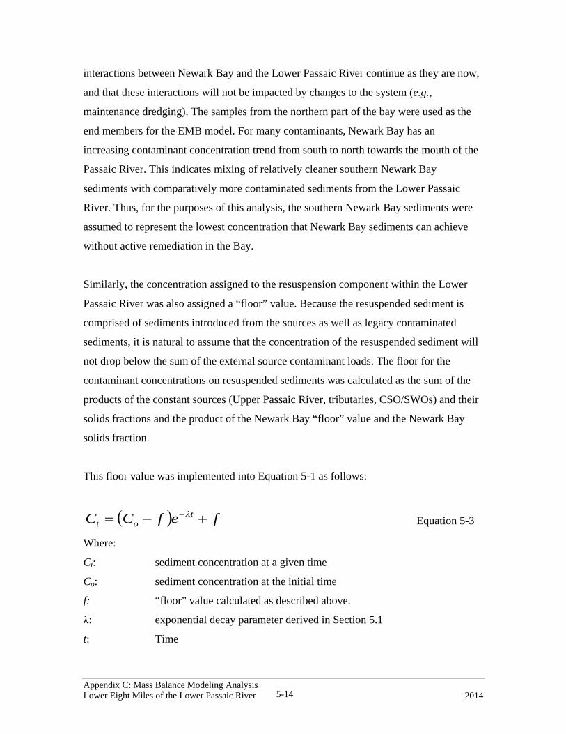
interactions between Newark Bay and the Lower Passaic River continue as they are now,
and that these interactions will not be impacted by changes to the system (e.g.,
maintenance dredging). The samples from the northern part of the bay were used as the
end members for the EMB model. For many contaminants, Newark Bay has an
increasing contaminant concentration trend from south to north towards the mouth of the
Passaic River. This indicates mixing of relatively cleaner southern Newark Bay
sediments with comparatively more contaminated sediments from the Lower Passaic
River. Thus, for the purposes of this analysis, the southern Newark Bay sediments were
assumed to represent the lowest concentration that Newark Bay sediments can achieve
without active remediation in the Bay.
Similarly, the concentration assigned to the resuspension component within the Lower
Passaic River was also assigned a “floor” value. Because the resuspended sediment is
comprised of sediments introduced from the sources as well as legacy contaminated
sediments, it is natural to assume that the concentration of the resuspended sediment will
not drop below the sum of the external source contaminant loads. The floor for the
contaminant concentrations on resuspended sediments was calculated as the sum of the
products of the constant sources (Upper Passaic River, tributaries, CSO/SWOs) and their
solids fractions and the product of the Newark Bay “floor” value and the Newark Bay
solids fraction.
This floor value was implemented into Equation 5-1 as follows:
( ) fefCC tot +−= −λ
Equation 5-3
Where:
Ct: sediment concentration at a given time
Co: sediment concentration at the initial time
f: “floor” value calculated as described above.
λ: exponential decay parameter derived in Section 5.1
t: Time
Appendix C: Mass Balance Modeling Analysis Lower Eight Miles of the Lower Passaic River 2014 5-14
In this way, the concentration of surface sediments approaches f, instead of 0 as given by
Equation 5-1.
5.2.3 Calculation of the Best Estimate Trajectories
As described in the previous section, half times were calculated for each of the
contaminants of concern listed in Table 5-1 by subtracting out the portions of the total
concentration from the high resolution cores that were attributable to the Upper Passaic
River, the tributaries, or the CSOs and SWOs. The exponential line fit through the data,
then, represented the reduction in contaminant concentration due to natural recovery
processes occuring in the Lower Passaic River and Newark Bay.
Using the average concentrations for each of the sources and the half time calculated
from the high resolution cores, a natural recovery (no action) trajectory for annual
deposition (equivalent to the Be-7-bearing sediment deposited in a given year) was fit
through the concentrations for each source.
The EMB model was an optimization routine that systematically searched for the best set
of solids contribution fractions that would balance the mass of each contaminant from
each source. It was an over-constrained set of 13 equations with 7 unknowns. Because of
modeling assumptions, simplifications to the system, and variations or errors in data sets,
the optimization routine was not able to find a solution that perfectly balanced all 13
parameters. As explained in Chapter 4, the fit was good for most of the parameters. In the
case of gamma-Chlordane, the fit was not as good, resulting in an error of 38 percent.
Because of this lack of fit, the summation of the gamma-Chlordane contributions from
each of the sources did not match the data collected in the main stem of the river between
RM2 and RM12 during the 2007 sampling effort or the core tops from the 2005 high
resolution cores. For most of the contaminants, model prediction yielded a sufficiently
small NME that the contaminant trajectories passed through the concentration range
represented by the 2005-2007 data. For gamma-Chlordane however, the trajectory fell
significantly below the recent data points, and each source concentration was artificially
Appendix C: Mass Balance Modeling Analysis Lower Eight Miles of the Lower Passaic River 2014 5-15

increased by the percent error from the EMB model to bring the trajectory up to match
the measured data.
As discussed above for the active remedial alternatives, treatment of the river bottom is
expected to prevent resuspension of contaminated sediment. However, these treatments
would also initially prevent resuspension of any sediment on the cap or backfill. Because
the cap or backfill will be composed of clean sand and, in the case of a cap, may be
armored in certain areas to prevent erosion due to high velocities, this assumption would
apply for the early part of the remedy’s design life. As time goes on, the river is expected
to deposit silt particles on the top of the cap or backfill. These particles are then available
for resuspension and mixing with other sources from the river. The amount of silt
available for resuspension within the remediated area would increase from zero at the
time of installation to a maximum level, at which point the resuspension from the
remediated area would match the resuspension from unremediated areas.
In the calculation of these trajectories, it was assumed that the rate of resuspension from
the remediated area would match that of unremediated areas once a 6-inch layer of
sediment had been re-deposited on top of the capped or backfilled area. This layer would
be biologically and physically active, and was assumed to be a vertically mixed surface
layer. At a sedimentation rate of 0.27 inches per year on average, it would take 22 years
for this layer to reach an average depth of 6 inches. For simplicity, the amount of
resuspension on the cap or backfill was assumed to increase linearly from 0 to the level of
the unremediated areas during this 22- year period. Since the remediation is assumed to
be completed in 2029 (Alternative 2), 2022 (Alternative 3) and 2020 (Alternative 4), the
newly re-deposited layer would be 6 inches thick by the years 2051, 2045 and 2042,
respectively.
Since the calculations allow the remediated areas to eventually contribute to the
resuspended sediment load in the river, it is necessary to estimate the concentration of the
contaminants in this resuspended sediment. This material is derived from the upper 6
inches of the capped or backfilled surface. The contaminant concentrations in this layer
Appendix C: Mass Balance Modeling Analysis Lower Eight Miles of the Lower Passaic River 2014 5-16
initially would be zero, since the cap or backfill is assumed to be free of contaminants.
This concentration would not be added to the river in the first year since the material
would be designed to largely remain in place. As the remediated surface begins to
accumulate sediments from the water column, it becomes more subject to resuspension.
The concentration of contaminants in sediments resuspending from the remediated areas
was calculated assuming that the upper 6 inches represents a mix of newly-deposited
sediment and the cap or backfill material. Thus, in the second year, the upper 6 inches
would equal on average 5.73 inches of clean cap or backfill material and 0.27 inches of
deposited sediment. The contaminant concentration of this layer would be the volumetric
average of the concentration on the newly deposited 0.27 inches of sediment and the 5.73
inches of clean material. Continuing this process, in the third year the contaminant
concentration in the upper 6 inches would be a volumetric average of 5.73 inches of
mixed cap or backfill material (from the previous year) with a concentration equal to that
calculated the second year and 0.27 inches of newly-deposited material with a
concentration equal to the forecast Be-7-bearing surface sediment concentration from the
previous year. In each case, the two concentrations are mixed proportional to the
thicknesses mentioned. This composite concentration was then applied to any
resuspension occurring from the remediated areas for that year.
For the purposes of the risk analysis and for comparison of the remediation alternatives, it
is most appropriate to compare the effects of the remediation on the upper 6 inches of
sediment instead of simply the recently-deposited (Be-7-bearing) sediment. This is
because the upper 6 inches represents what is typically considered the biologically active
layer and thus represents the exposure point concentration for most biota. For the No
Action alternative, the mean sediment concentration over the upper six inches of
sediment can be estimated by averaging the annual sediment deposition for the previous
22 years as characterized by the dated sediment cores. When the upper 6-inch layer
concentration for each of the contaminants is estimated in this way for the year 1995, all
of the contaminant concentrations estimated from the dated sediment cores (except Total
PCBs) fall within two standard errors of the mean value from the TSI 1995 surface
sediment (0-6 in) dataset.
Appendix C: Mass Balance Modeling Analysis Lower Eight Miles of the Lower Passaic River 2014 5-17
The 1995 TSI dataset does not report concentrations for all the PCB congeners, so the
Total PCB concentration was estimated as the sum of the Aroclors. This differs from
other samples in the 2005 and 2007/2008 sampling events, which report all of the
congeners, and the Total PCB as a sum of congeners. These two sums are not always
analogous. A regression analysis between Aroclor and congener-based total PCB
estimates using 2005 to 2010 data indicated that Total PCBs by Aroclor was biased low
by 25 percent (see Data Evaluation Report No 5 in Appendix A). Despite this difference,
the Total PCB concentrations estimated by the EMB model agreed to within 2 percent of
the measured data.
Assuming that the concentration trends observed for the past 25 years will continue into
the future, surface sediment concentrations from 2005 to 2059 were forecast for the
annual deposition (equivalent to the Be-7-bearing sediments deposited each year) for
each contaminant following Equation 5-4. These concentrations were then used to
estimate the exposure concentrations in the 0-6 inch biologically active layer of sediment
using the process outlined in Attachment B. The placement of sand material to construct
a sub-aqueous cap or to backfill after dredging is assumed to temporarily restrict fine-
grained sediment resuspension, as described above. Given the many unknowns associated
with remedial construction sequence for the various alternatives, no attempt has been
made to predict short-term consequences during implementation, such as resuspension
during dredging; these short-term impacts are incorporated into the mechanistic model
(Appendix B) and addressed in the FFS. During the remediation, a linear reduction in
surface sediment concentration is assumed between the value in 2017 and the anticipated
value at the end of the remedy. After completion of each remedy, for the purposes of
long-term forecasts, it has been assumed that all benefits of remediation are realized in
the final year of the typical remedial alternative construction period (2029, 2022, or 2020
for Alternatives 2, 3, and 4, respectively). The following equation integrates the spatial
extent of remediation and the processes affecting the 0 to 6 inch layer:
Appendix C: Mass Balance Modeling Analysis Lower Eight Miles of the Lower Passaic River 2014 5-18
( )( )( ) ( ) RSP
ii
RSP
capRSPRSPREM fcb
fCfcb
bcCdbCfC
−−+
−−
+−−= ∑
11111
Equation 5-4
Where:
CREM: new recently-deposited (Be-7-bearing) sediment concentration following
remediation in 2029, 2022, or 2020 for Alternatives 2, 3, and 4, respectively.
CRSP: contaminant concentration for resuspending sediment (top six inch average)
Ccap: contaminant concentration on top of the cap or backfill (top six inch average)
Ci: contaminant concentration on incoming sediment from source, i
i: subscript representing all sediment sources other than resuspension
fRSP: fraction of solids associated with resuspension
fi: fraction of solids associated with source, i
b: fraction of fine-grained sediment area impacted by placement of cap or backfill
material
c: ratio of resuspension occurring in remediated areas per unit area to that in
unremediated areas
d: adjustment for fine-grained sediment area not impacted by remediation and not
contaminated with dioxin (this value is zero for all contaminants other than
dioxin.)
5.2.4 Calculation of the Trajectory Uncertainties
The best estimate trajectory calculations described above used the best estimates, or
averages of all the concentrations and other inputs needed, for the trajectory forecast
calculations. The uncertainties in best estimate trajectories were determined by Monte
Carlo simulation for 2,3,7,8-TCDD, Total PCB, 4,4’-DDE, mercury, lead, copper, and
gamma-Chlordane. Detailed description of the Monte Carlo analysis, which was
composed of 10,000 iterations of randomly-generated input values to the trajectory
calculation, is provided in Attachment A. The 10,000 Monte Carlo-generated inputs to
the contaminant forecasts calculations include:
• Randomly generated contaminant inputs to the EMB model;
• Optimized EMB model solids balance output;
Appendix C: Mass Balance Modeling Analysis Lower Eight Miles of the Lower Passaic River 2014 5-19
• Randomly-generated half times using the confidence bounds and a normal
distribution assumption;
• Randomly-generated sedimentation rates developed using bootstrap analysis of
the difference between the 1989 and 2007 bathymetric surfaces; and
• Randomly-generated estimates of the depth of the sediment mixed layer between
10 and 20 cm.
Uncertainties in the contaminant forecasts developed from the Monte Carlo analysis were
based on the confidence interval (5th, 25th, 75th and 95th percentiles) of the 10,000
optimized solutions.
5.2.5 Best Estimate Trajectory for the No Action Alternative (Alternative 1)
Assuming that the concentration trends observed for the past 25 years will continue into
the future, concentrations in the 0-6 inch surface sediment layer from 1995 to 2059 were
forecast for each contaminant following the procedure outlined in Attachment B. This
procedure assumes that the exponential decline noted in the combination of Lower
Passaic River (internal resuspension) source and the Newark Bay source continues at the
same rate noted for the last three decades. It also assumes that the “constant” sources
(Upper Passaic River, tributaries, and CSO/SWOs) remain constant for the period of
model simulation. The best estimate No Action Alternative concentration forecast is
calculated using Equation 5-3 for Newark Bay and the resuspension term. All other
sources are added in as constants. The best estimate No Action forecasts are presented in
part A of Figures 5-11 through 5-17 (e.g., Figure 5-11A) and Figure 5-18. Table 5-3
presents the percent reduction in forecast concentration in 2059 relative to 2017 level
before the active remedies are to be implemented.
Part A of Figures 5-11 through 5-17 and Figure 5-18 also show the mean concentration
reported in the 1995 TSI surface sediment dataset (red point). The error bars indicate two
standard errors above and below the mean. The estimated concentration for the 0-6 inch
biologically active zone is within this envelope in every case (see discussion on gamma-
Chlordane adjustment above).
Appendix C: Mass Balance Modeling Analysis Lower Eight Miles of the Lower Passaic River 2014 5-20
These results indicate that 2,3,7,8-TCDD surface sediment concentrations are forecast to
decline by 59 percent (from 0.5 to 0.2 µg/kg) from 2017 to 2059 under No Action. For
the other contaminants, the decline is 50 percent or less (Table 5-3a for percentages and
Table 5-3b for the concentrations). The relatively larger decline in 2,3,7,8-TCDD
compared to other contaminants is because the external sources (e.g., Upper Passaic
River, tributaries, CSOs/SWOs) are not significant contributors of 2,3,7,8-TCDD to the
sediments of the Lower Passaic River. Contaminants like gamma-Chlordane and PAHs,
which have seen no appreciable decline in the last 25 years, are not predicted to decline at
all over the time period of the forecast. The smaller reductions seen for metals, DDE, and
PCBs indicate that significant sources of these contaminants exist in the Upper Passaic
River or Newark Bay. Although significant concentrations may exist in the tributaries or
the CSO/SWOs, their small solids contribution prevents them contributing a large mass
of hydrophobic contaminant to the Lower Passaic River.
5.2.6 Best Estimate Trajectory for Alternatives 2 to 4.
The other remediation alternatives involve dredging and capping/backfill described in
Section 5.2.1. The forecast concentrations in the 0-6 inch layer are shown as orange lines
for Alternative 2, green lines for Alternative 3, and purple lines for Alternative 4 on part
A of Figures 5-11 through 5-17 and Figure 5-18. The percent reductions in forecast
concentrations in 2059 relative to 2017 for each Alternative are tabulated in Table 5-3.
Overall, the trajectory results indicate that Alternative 4, the focused capping remedy,
provides much less reduction in future concentrations compared to Alternatives 2 and 3.
About a 90 percent reduction in 2,3,7,8-TCDD surface sediment concentrations was
estimated by 2059 for Alternatives 2 and 3 (from 0.5 to approximately 0.04 µg/kg), as
compared to about 70 percent for Alternative 4. The increase in surface sediment
concentrations after the implementation of the remedy shown in the figures follows from
infilling of sediments over the remediated areas from the external sources as well as
sediments upriver of the FFS Study Area.
Appendix C: Mass Balance Modeling Analysis Lower Eight Miles of the Lower Passaic River 2014 5-21
5.2.7 Trajectory Uncertainties
Uncertainty in trajectory forecasts for contaminant concentrations in the bioactive layer
included using the uncertainty analysis developed for the EMB model combined with
additional variability in the distributions developed for the remaining parameters used in
the forecast model (e.g., “excess” contaminant half times, mixed layer thickness,
sediment deposition rate). Parts B, C, and D of Figures 5-11 through 5-17 present the
uncertainty in trajectory forecasts as confidence bounds associated with best estimate,
predicted future contaminant concentrations. The most significant finding from the
uncertainty analysis is that by 2059 there will be no statistical significant difference
between No Action (Alternative 1) and Alternative 4. In addition, Alternatives 2 and 3
are not different from each other by 2059. However, there is a statistically significant
difference between Alternatives 2 and 3 versus Alternatives 1 and 4.
5.3 Incorporation of the CPG 2008-2009 Data
The CPG 2008 and 2009 datasets were not available at the time that the Mass Balance
Forecast Model analysis was performed. The CPG 2008 and 2009 datasets provide an
opportunity to confirm the forecast Lower Passaic River surface sediment concentrations
that were presented in the previous sections. In Parts B, C, and D of Figures 5-11 through
5-17, the mean and two standards errors of the measured CPG 2008 and CPG 2009
surface sediment concentrations were added to the Monte Carlo trajectory results. For the
contaminants examined, the simulated 2008, and 2009 distributions of the mean surface
sediment concentrations fall within the uncertainty of the measurements, except for the
simulated 2009 mercury concentration distribution (which plots on the border of the
uncertainty range). This agreement between the model forecast and the new CPG data
provides a rough validation of the model and the original forecast.
Appendix C: Mass Balance Modeling Analysis Lower Eight Miles of the Lower Passaic River 2014 5-22

6 SUMMARY
This appendix describes the EMB modeling analysis developed to support the FFS of the
lower eight miles of the Lower Passaic River. It consists of an EMB model designed to
characterize the fate and transport of contaminants in the Lower Passaic River, as well as
a semi-empirical model used to forecast the concentrations of contaminants in Lower
Passaic River surface sediment for the FFS remedial alternatives. The summary of the
observations are provided below.
6.1 Summary of EMB Results
• Resuspension of legacy sediments represented the single largest contributor of
solids to recently-deposited sediments, accounting for 28 to 65 percent of the
recent deposition with a best estimate of 48 percent. The Upper Passaic River
accounted for about 13 to 49 percent of recently-deposited solids, with a best
estimate of 32 percent. Newark Bay accounted for less than 1 to 44 percent, with
a best estimate of 14 percent. All the other sources together contribute between 2
and less than 12 percent.
• The mass balance calculated for 2,3,7,8-TCDD, indicates that resuspension
accounts for about 87 to 100 percent, with a best estimate of 97 percent of the
2,3,7,8-TCDD observed in recently-deposited sediments in the Lower Passaic
River.
• Resuspension contribution of Total PCBs to the Lower Passaic River ranges from
59 to 90 percent with a best estimate of about 81 percent. Upper Passaic River is
the most important external source of Total PCB contamination to the Lower
Passaic, with a best estimate of 11 percent (range of 4 to 22 percent of the overall
mass), while Newark Bay contributes about 7 percent (range of less than 1 to 25
percent) of the overall mass.
• External inputs of PAHs are very important to the PAH mass balance for the
system. The Upper Passaic River contribution for benzo[a]pyrene was estimated
as 53 percent (ranging from 27 to 70 percent) and for fluoranthene the estimate
was 47 percent (ranging from 24 to 64 percent). Resuspension of the historical
Appendix C: Mass Balance Modeling Analysis Lower Eight Miles of the Lower Passaic River 2014 6-1
inventory accounts for about 39 percent (ranging from 17 to 58 percent) of the
PAH contaminant burden of the Lower Passaic River. Newark Bay’s PAH
contribution ranges from less than 1 percent to 30 percent, with a best estimate of
approximately 6 percent. Although higher PAH concentrations were observed in
the tributaries and CSOs, comparable to concentrations in the Upper Passaic
River, the relatively small solids contributions from the tributaries and CSOs
limits their combined contribution to less than 17 percent.
• For 4,4’-DDE, resuspension of the historical inventory contributes between 52 to
88 percent of the mass in recently-deposited sediments, with a best estimate of 78
percent. Newark Bay contributes about 8 percent of 4,4’-DDE mass (ranging from
less than 1 to 34 percent) and the Upper Passaic River contributes about 10
percent (ranging from 4 to 21 percent). The combined contribution from
tributaries SWOs and CSOs range from 1 to 10 percent, with a best estimate of
about 4 percent.
• Similar to 4,4’-DDE, the fate and transport of copper, chromium, mercury, and
lead in the Lower Passaic River is dominated by sediment resuspension.
• Overall, the EMB Model identifies the sediments of the Lower Passaic River as
an important source of all contaminants of concern and the single most important
source of 2,3,7,8-TCDD to the entire Lower Passaic River.
6.2 Summary of Contaminant Forecast Results
• Surface sediment concentrations of 2,3,7,8-TCDD are forecast to decline by 59
percent from 2017 to 2059 under No Action. For the other contaminants, the
decline is less than 48 percent. The relatively larger decline in 2,3,7,8-TCDD
compared to other contaminants is because the external sources (e.g., Upper
Passaic River, tributaries, CSOs/SWOs) are not significant contributors of 2,3,7,8-
TCDD to the sediments of the Lower Passaic River.
• The forecasts for Alternatives 2 and 3 show a significant decline over time for
most contaminant concentrations when compared to No Action. About a 90
percent reduction in 2,3,7,8-TCDD surface sediment concentrations was
Appendix C: Mass Balance Modeling Analysis Lower Eight Miles of the Lower Passaic River 2014 6-2
estimated by 2059 for Alternatives 2 and 3. Sediment 2,3,7,8-TCDD
concentrations, which originate largely from an internal source (resuspension), are
most dramatically reduced by Alternatives 2 and 3. Contaminants such as PAHs,
which have a significant external source, are impacted immediately upon
remediation, but the improvement wanes as contaminated sediments from external
sources are deposited on top of the remediated area and subsequently may
resuspend and continue mixing with the river’s solids load.
• The surface sediment contaminant concentrations after implementation of
Alternatives 2 and 3 are not statistically different from each other by 2059 for the
contaminants forecast.
• The trajectory results indicate that by 2059 there will be no statistically significant
difference between No Action (Alternative 1) and the focused remedy
(Alternative 4). Alternative 4 does not provide the sustained reduction in future
concentrations estimated for Alternatives 2 and 3.
Appendix C: Mass Balance Modeling Analysis Lower Eight Miles of the Lower Passaic River 2014 6-3
7 ACRONYMS
2,3,7,8-TCDD 2,3,7,8-Tetrachlorodibenzo-p-dioxin
4,4’-DDE 4,4’-dichlorodiphenyldichloroethylene
Be-7 Beryllium-7
CMB Chemical Mass Balance
CPG Cooperating Parties Group
CSM Conceptual Site Model
CSO Combined Sewer Overflow
DDE Dichlorodiphenyldichloroethylene
DDT Dichlorodiphenyltrichloroethane
EMB Empirical Mass Balance
FFS Focused Feasibility Study
HMW High Molecular Weight
LMW Low Molecular Weight
µg/kg micrograms per kilogram
mg/kg milligram per kilogram
NME Normalized Mean Error
PAH Polycyclic Aromatic Hydrocarbon
PCB Polychlorinated Biphenyl
PCDD/F Polychlorobenzodioxin/furan
ppb parts per billion
R2 coefficient of determination of regression line fits
RI Remedial Investigation
RM River Mile
RPI Rensselaer Polytechnic Institute
SWO Stormwater Outfall
TOC Total Organic Carbon
Total DDx the sum of the 4,4’-dichlorodiphenyldichloroethane (4-4’-DDD),
4,4’-dichlorodiphenyldichloroethylene (4,4’-DDE) and 4,4’-
Dichlorodiphenyltrichloroethane (4,4’-DDT) concentrations
Appendix C: Mass Balance Modeling Analysis Lower Eight Miles of the Lower Passaic River 2014 7-1
Total TCDD Total Tetrachlorodibenzodioxin
TSI Tierra Solutions, Inc.
USEPA United State Environmental Protection Agency
Appendix C: Mass Balance Modeling Analysis Lower Eight Miles of the Lower Passaic River 2014 7-2

8 REFERENCES
Bzdusek, P.A., E.R. Christensen, A Li, and Q Zou. 2004. “Source Apportionment of
Sediment PAHs in Lake Calumet, Chicago: Application of Factor Analysis with
Nonnegative Constraints”. Environmental Science Technology. 38(1): 97-103.
Chaky, D.A. 2003. “Polychlorinated Biphenyls, Polychlorinated Dibenzo-p-Dioxins and
Furans in the New York Metropolitan Area; Interpreting Atmospheric Deposition and
Sediment Chronologies.” PhD Thesis, Rensselaer Polytechnic Institute (Troy, NY).
August 2003.
Imamoglu, I., K. Li and E.R. Christensen. 2002. “Modeling Polychlorinated Biphenyl
Congener Patterns and Dechlorination in Dated Sediments from the Ashtabula River,
Ohio, USA.” Environmental Toxicology and Chemistry. 21(11): 2283–2291.
Johnson, G.W., W.M. Jarman, C.E. Bacon, J.A. Davis, R. Ehrlich and R.W. Risebrough.
2000. “Resolving Polychlorinated Biphenyl Source Fingerprints in Suspended Particulate
Matter of San Francisco Bay”. Environmental Science and Technology. 34(4):552-559.
Ogura, I., M. Gamo, S. Masunaga and J. Nakanishi. 2005. “Quantitative Identification of
Sources of Dioxin-Like Polychlorinated Biphenyls in Sediments by a Factor Analysis
Model and a Chemical Mass Balance Model Combined with Monte Carlo Techniques”.
Environmental Toxicology and Chemistry. 24(2): 277–285.
Soonthornnonda, P. and E.R. Christensen. 2008. “Source Apportionment of Pollutants
and Flows of Combined Sewer Wastewater”. Water Research, Volume 42, Issues 8-9,
pp1989-1998.
Su, M., E.R. Christensen, J.F. Karls, S. Kosuru, I. Imamoglu. 2000. “Apportionment of
Polycyclic Aromatic Hydrocarbon Sources in Lower Fox River, USA, Sediments by a
Appendix C: Mass Balance Modeling Analysis Lower Eight Miles of the Lower Passaic River 2014 8-1
Chemical Mass Balance Model.” Environmental Toxicology and Chemistry. 19(6):
1481–1490.
Watson, J.G., et al., 2004. “Protocol for Applying and Validating the CMB Model for
PM2.5 and VOC.” Prepared for the Office of Air Quality Planning & Standards,
Emissions, Monitoring & Analysis Division. EPA-451/R-04-001. Available online:
http://www.epa.gov/scram001/models/receptor/CMB_Protocol.pdf. Last accessed:
December 30, 2013.
Appendix C: Mass Balance Modeling Analysis Lower Eight Miles of the Lower Passaic River 2014 8-2

Appendix C: Mass Balance Modeling Analysis Lower Eight Miles of the Lower Passaic River 2014
TABLES
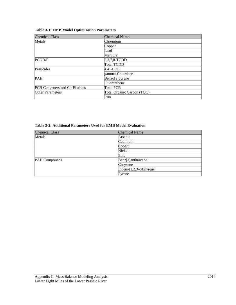
Appendix C: Mass Balance Modeling Analysis 2014
Lower Eight Miles of the Lower Passaic River
Table 3-1: EMB Model Optimization Parameters
Chemical Class Chemical Name
Metals Chromium
Copper
Lead
Mercury
PCDD/F 2,3,7,8-TCDD
Total TCDD
Pesticides 4,4’-DDE
gamma-Chlordane
PAH Benzo[a]pyrene
Fluoranthene
PCB Congeners and Co-Elutions Total PCB
Other Parameters Total Organic Carbon (TOC)
Iron
Table 3-2: Additional Parameters Used for EMB Model Evaluation
Chemical Class Chemical Name
Metals Arsenic
Cadmium
Cobalt
Nickel
Zinc
PAH Compounds Benz[a]anthracene
Chrysene
Indeno[1,2,3-cd]pyrene
Pyrene
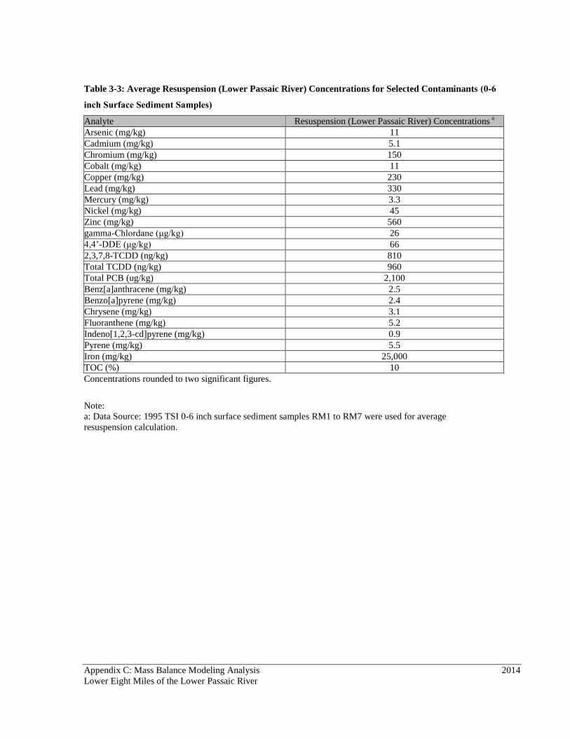
Appendix C: Mass Balance Modeling Analysis 2014
Lower Eight Miles of the Lower Passaic River
Table 3-3: Average Resuspension (Lower Passaic River) Concentrations for Selected Contaminants (0-6
inch Surface Sediment Samples)
Analyte Resuspension (Lower Passaic River) Concentrations a
Arsenic (mg/kg) 11
Cadmium (mg/kg) 5.1
Chromium (mg/kg) 150
Cobalt (mg/kg) 11
Copper (mg/kg) 230
Lead (mg/kg) 330
Mercury (mg/kg) 3.3
Nickel (mg/kg) 45
Zinc (mg/kg) 560
gamma-Chlordane (μg/kg) 26
4,4’-DDE (μg/kg) 66
2,3,7,8-TCDD (ng/kg) 810
Total TCDD (ng/kg) 960
Total PCB (ug/kg) 2,100
Benz[a]anthracene (mg/kg) 2.5
Benzo[a]pyrene (mg/kg) 2.4
Chrysene (mg/kg) 3.1
Fluoranthene (mg/kg) 5.2
Indeno[1,2,3-cd]pyrene (mg/kg) 0.9
Pyrene (mg/kg) 5.5
Iron (mg/kg) 25,000
TOC (%) 10
Concentrations rounded to two significant figures.
Note:
a: Data Source: 1995 TSI 0-6 inch surface sediment samples RM1 to RM7 were used for average
resuspension calculation.
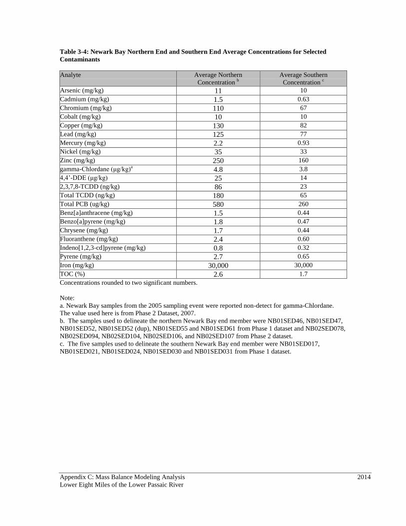
Appendix C: Mass Balance Modeling Analysis 2014
Lower Eight Miles of the Lower Passaic River
Table 3-4: Newark Bay Northern End and Southern End Average Concentrations for Selected
Contaminants
Analyte Average Northern
Concentration b
Average Southern
Concentration c
Arsenic (mg/kg) 11 10
Cadmium (mg/kg) 1.5 0.63
Chromium (mg/kg) 110 67
Cobalt (mg/kg) 10 10
Copper (mg/kg) 130 82
Lead (mg/kg) 125 77
Mercury (mg/kg) 2.2 0.93
Nickel (mg/kg) 35 33
Zinc (mg/kg) 250 160
gamma-Chlordane (μg/kg)a 4.8 3.8
4,4’-DDE (μg/kg) 25 14
2,3,7,8-TCDD (ng/kg) 86 23
Total TCDD (ng/kg) 180 65
Total PCB (ug/kg) 580 260
Benz[a]anthracene (mg/kg) 1.5 0.44
Benzo[a]pyrene (mg/kg) 1.8 0.47
Chrysene (mg/kg) 1.7 0.44
Fluoranthene (mg/kg) 2.4 0.60
Indeno[1,2,3-cd]pyrene (mg/kg) 0.8 0.32
Pyrene (mg/kg) 2.7 0.65
Iron (mg/kg) 30,000 30,000
TOC (%) 2.6 1.7
Concentrations rounded to two significant numbers.
Note:
a. Newark Bay samples from the 2005 sampling event were reported non-detect for gamma-Chlordane.
The value used here is from Phase 2 Dataset, 2007.
b. The samples used to delineate the northern Newark Bay end member were NB01SED46, NB01SED47,
NB01SED52, NB01SED52 (dup), NB01SED55 and NB01SED61 from Phase 1 dataset and NB02SED078,
NB02SED094, NB02SED104, NB02SED106, and NB02SED107 from Phase 2 dataset.
c. The five samples used to delineate the southern Newark Bay end member were NB01SED017,
NB01SED021, NB01SED024, NB01SED030 and NB01SED031 from Phase 1 dataset.
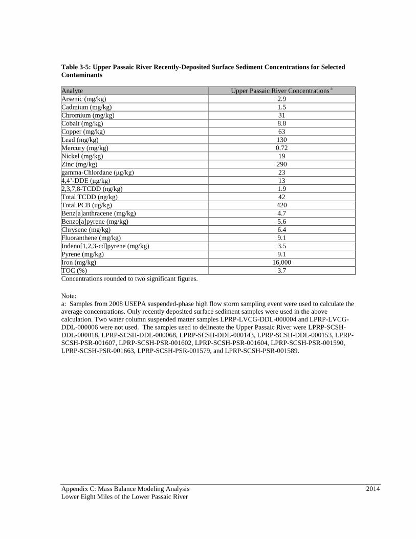
Appendix C: Mass Balance Modeling Analysis 2014
Lower Eight Miles of the Lower Passaic River
Table 3-5: Upper Passaic River Recently-Deposited Surface Sediment Concentrations for Selected
Contaminants
Analyte Upper Passaic River Concentrations a
Arsenic (mg/kg) 2.9
Cadmium (mg/kg) 1.5
Chromium (mg/kg) 31
Cobalt (mg/kg) 8.8
Copper (mg/kg) 63
Lead (mg/kg) 130
Mercury (mg/kg) 0.72
Nickel (mg/kg) 19
Zinc (mg/kg) 290
gamma-Chlordane (μg/kg) 23
4,4’-DDE (μg/kg) 13
2,3,7,8-TCDD (ng/kg) 1.9
Total TCDD (ng/kg) 42
Total PCB (ug/kg) 420
Benz[a]anthracene (mg/kg) 4.7
Benzo[a]pyrene (mg/kg) 5.6
Chrysene (mg/kg) 6.4
Fluoranthene (mg/kg) 9.1
Indeno[1,2,3-cd]pyrene (mg/kg) 3.5
Pyrene (mg/kg) 9.1
Iron (mg/kg) 16,000
TOC (%) 3.7
Concentrations rounded to two significant figures.
Note:
a: Samples from 2008 USEPA suspended-phase high flow storm sampling event were used to calculate the
average concentrations. Only recently deposited surface sediment samples were used in the above
calculation. Two water column suspended matter samples LPRP-LVCG-DDL-000004 and LPRP-LVCG-
DDL-000006 were not used. The samples used to delineate the Upper Passaic River were LPRP-SCSH-
DDL-000018, LPRP-SCSH-DDL-000068, LPRP-SCSH-DDL-000143, LPRP-SCSH-DDL-000153, LPRP-
SCSH-PSR-001607, LPRP-SCSH-PSR-001602, LPRP-SCSH-PSR-001604, LPRP-SCSH-PSR-001590,
LPRP-SCSH-PSR-001663, LPRP-SCSH-PSR-001579, and LPRP-SCSH-PSR-001589.
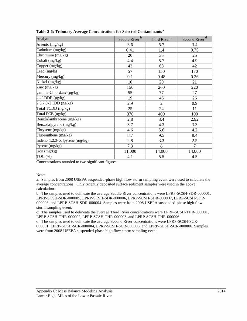
Appendix C: Mass Balance Modeling Analysis 2014
Lower Eight Miles of the Lower Passaic River
Table 3-6: Tributary Average Concentrations for Selected Contaminants a
Analyte Saddle River b
Third River c
Second River d
Arsenic (mg/kg) 3.6 5.7 3.4
Cadmium (mg/kg) 0.41 1.4 0.75
Chromium (mg/kg) 20 35 25
Cobalt (mg/kg) 4.4 5.7 4.9
Copper (mg/kg) 43 68 42
Lead (mg/kg) 57 150 170
Mercury (mg/kg) 0.1 0.48 0.26
Nickel (mg/kg) 10 20 21
Zinc (mg/kg) 150 260 220
gamma-Chlordane (μg/kg) 55 77 27
4,4’-DDE (μg/kg) 19 46 26
2,3,7,8-TCDD (ng/kg) 2.9 2 0.9
Total TCDD (ng/kg) 25 24 11
Total PCB (ug/kg) 370 400 100
Benz[a]anthracene (mg/kg) 2.8 3.4 2.92
Benzo[a]pyrene (mg/kg) 3.7 4.3 3.3
Chrysene (mg/kg) 4.6 5.6 4.2
Fluoranthene (mg/kg) 8.7 9.5 8.4
Indeno[1,2,3-cd]pyrene (mg/kg) 2.8 3.3 2.5
Pyrene (mg/kg) 7.3 8 7
Iron (mg/kg) 11,000 14,000 14,000
TOC (%) 4.1 5.5 4.5
Concentrations rounded to two significant figures.
Note:
a: Samples from 2008 USEPA suspended-phase high flow storm sampling event were used to calculate the
average concentrations. Only recently deposited surface sediment samples were used in the above
calculation.
b: The samples used to delineate the average Saddle River concentrations were LPRP-SCSH-SDR-000001,
LPRP-SCSH-SDR-000005, LPRP-SCSH-SDR-000006, LPRP-SCSH-SDR-000007, LPRP-SCSH-SDR-
000003, and LPRP-SCSH-SDR-000004. Samples were from 2008 USEPA suspended-phase high flow
storm sampling event.
c: The samples used to delineate the average Third River concentrations were LPRP-SCSH-THR-000001,
LPRP-SCSH-THR-000002, LPRP-SCSH-THR-000003, and LPRP-SCSH-THR-000006.
d: The samples used to delineate the average Second River concentrations were LPRP-SCSH-SCR-
000001, LPRP-SCSH-SCR-000004, LPRP-SCSH-SCR-000005, and LPRP-SCSH-SCR-000006. Samples
were from 2008 USEPA suspended-phase high flow storm sampling event.
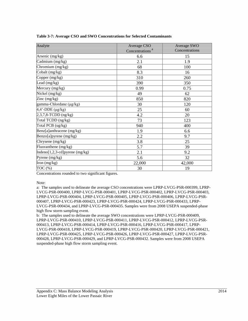
Appendix C: Mass Balance Modeling Analysis 2014
Lower Eight Miles of the Lower Passaic River
Table 3-7: Average CSO and SWO Concentrations for Selected Contaminants
Analyte Average CSO
Concentrations a
Average SWO
Concentrations
Arsenic (mg/kg) 6.6 15
Cadmium (mg/kg) 2.1 1.9
Chromium (mg/kg) 68 100
Cobalt (mg/kg) 8.3 16
Copper (mg/kg) 310 260
Lead (mg/kg) 390 350
Mercury (mg/kg) 0.99 0.75
Nickel (mg/kg) 49 62
Zinc (mg/kg) 850 820
gamma-Chlordane (μg/kg) 30 120
4,4’-DDE (μg/kg) 25 60
2,3,7,8-TCDD (ng/kg) 4.2 20
Total TCDD (ng/kg) 73 123
Total PCB (ug/kg) 940 400
Benz[a]anthracene (mg/kg) 1.9 6.6
Benzo[a]pyrene (mg/kg) 2.2 9.7
Chrysene (mg/kg) 3.8 25
Fluoranthene (mg/kg) 5.7 39
Indeno[1,2,3-cd]pyrene (mg/kg) 2.1 9.2
Pyrene (mg/kg) 5.6 32
Iron (mg/kg) 22,000 42,000
TOC (%) 30 19
Concentrations rounded to two significant figures.
Note:
a: The samples used to delineate the average CSO concentrations were LPRP-LVCG-PSR-000399, LPRP-
LVCG-PSR-000400, LPRP-LVCG-PSR-000401, LPRP-LVCG-PSR-000402, LPRP-LVCG-PSR-000403,
LPRP-LVCG-PSR-000404, LPRP-LVCG-PSR-000405, LPRP-LVCG-PSR-000406, LPRP-LVCG-PSR-
000407, LPRP-LVCG-PSR-000423, LPRP-LVCG-PSR-000424, LPRP-LVCG-PSR-000433, LPRP-
LVCG-PSR-000434, and LPRP-LVCG-PSR-000435. Samples were from 2008 USEPA suspended-phase
high flow storm sampling event.
b: The samples used to delineate the average SWO concentrations were LPRP-LVCG-PSR-000409,
LPRP-LVCG-PSR-000410, LPRP-LVCG-PSR-000411, LPRP-LVCG-PSR-000412, LPRP-LVCG-PSR-
000413, LPRP-LVCG-PSR-000414, LPRP-LVCG-PSR-000416, LPRP-LVCG-PSR-000417, LPRP-
LVCG-PSR-000418, LPRP-LVCG-PSR-000419, LPRP-LVCG-PSR-000420, LPRP-LVCG-PSR-000421,
LPRP-LVCG-PSR-000425, LPRP-LVCG-PSR-000426, LPRP-LVCG-PSR-000427, LPRP-LVCG-PSR-
000428, LPRP-LVCG-PSR-000429, and LPRP-LVCG-PSR-000432. Samples were from 2008 USEPA
suspended-phase high flow storm sampling event.
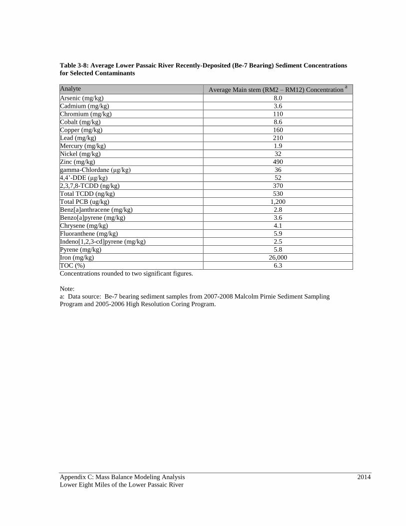
Appendix C: Mass Balance Modeling Analysis 2014
Lower Eight Miles of the Lower Passaic River
Table 3-8: Average Lower Passaic River Recently-Deposited (Be-7 Bearing) Sediment Concentrations
for Selected Contaminants
Analyte Average Main stem (RM2 – RM12) Concentration a
Arsenic (mg/kg) 8.0
Cadmium (mg/kg) 3.6
Chromium (mg/kg) 110
Cobalt (mg/kg) 8.6
Copper (mg/kg) 160
Lead (mg/kg) 210
Mercury (mg/kg) 1.9
Nickel (mg/kg) 32
Zinc (mg/kg) 490
gamma-Chlordane (μg/kg) 36
4,4’-DDE (μg/kg) 52
2,3,7,8-TCDD (ng/kg) 370
Total TCDD (ng/kg) 530
Total PCB (ug/kg) 1,200
Benz[a]anthracene (mg/kg) 2.8
Benzo[a]pyrene (mg/kg) 3.6
Chrysene (mg/kg) 4.1
Fluoranthene (mg/kg) 5.9
Indeno[1,2,3-cd]pyrene (mg/kg) 2.5
Pyrene (mg/kg) 5.8
Iron (mg/kg) 26,000
TOC (%) 6.3
Concentrations rounded to two significant figures.
Note:
a: Data source: Be-7 bearing sediment samples from 2007-2008 Malcolm Pirnie Sediment Sampling
Program and 2005-2006 High Resolution Coring Program.

Appendix C: Mass Balance Modeling Analysis 2014
Lower Eight Miles of the Lower Passaic River
Table 4-1: Contaminant Burden Attributed to Resuspension
Analyte Percent of Contaminant Burden in Recently Deposited
Sediments Attributed to Resuspension and Confidence Interval
Chromium ≈ 74 (44 to 88)
Copper ≈ 72 (45 to 85)
Lead ≈ 71 (48 to 83)
Mercury ≈ 75 (43 to 88)
gamma-Chlordane ≈ 52 (32 to 70)
4,4’-DDE ≈ 78 (52 to 88)
2,3,7,8-TCDD ≈ 97 (87 to 100)
Total TCDD ≈ 92 (76 to 97)
Total PCB ≈ 81 (59 to 90)
Benzo[a]pyrene ≈ 33 (17 to 52)
Fluoranthene ≈ 40 (21 to 58)
Iron ≈ 54 (29 to 72)
TOC ≈ 72 (48 to 83)

Appendix C: Mass Balance Modeling Analysis 2014
Lower Eight Miles of the Lower Passaic River
Table 4-2: Summary of Solids Contribution Results for Best Estimate Scenarios
Solids and Analytes Resuspension Newark Bay Upper Passaic
River
Saddle
River
Second River / Storm
Water Outfall
Third
River
Combined Sewer
Overflow
Solids 48% 14% 32% 4% 1% 1% 0.5%
Copper 72% 12% 14% 1% 0.4% 0.3% 1%
Chromium 74% 15% 10% 1% 0.4% 0.3% 0.3%
Iron 54% 18% 24% 2% 1% 1% 0.5%
Mercury 75% 14% 11% 0.2% 0.2% 0.2% 0.2%
Lead 71% 7% 19% 1% 1% 0.5% 1%
gamma-Chlordane 52% 3% 32% 8% 2% 2% 1%
4,4’-DDE 78% 8% 10% 2% 1% 1% 0.3%
2,3,7,8-TCDD 97% 3% 0.1% 0.03% 0.003% 0.004% 0.005%
Total TCDD 92% 5% 3% 0.2% 0.03% 0.04% 0.07%
Total PCB 81% 7% 11% 1% 0.1% 0.3% 0.4%
Benzo(a)pyrene 33% 7% 53% 4% 2% 1% 0.3%
Fluoranthene 40% 5% 47% 5% 2% 1% 0.4%
TOC 72% 5% 17% 2% 1% 1% 2%

Appendix C: Mass Balance Modeling Analysis 2014
Lower Eight Miles of the Lower Passaic River
Table 4-3: Summary of Solids Contribution Results for SWO Sensitivity Scenarios
Solids and Analytes Resuspension Newark Bay Upper Passaic
River
Saddle
River
Second
River
Third
River
Storm Water
Outfall
Combined
Sewer Overflow
Solids 47% 17% 31% 3% 0% 1% 1% 0%
Copper 69% 14% 13% 1% 0% 0% 2% 1%
Chromium 70% 18% 9% 1% 0% 0% 1% 0%
Iron 51% 22% 22% 2% 0% 0% 2% 0%
Mercury 72% 17% 10% 0% 0% 0% 0% 0%
Lead 69% 9% 18% 1% 0% 0% 2% 1%
gamma-Chlordane 50% 3% 30% 8% 0% 2% 7% 1%
4,4’-DDE 76% 10% 10% 2% 0% 1% 2% 0%
2,3,7,8-TCDD 96% 4% 0% 0% 0% 0% 0% 0%
Total TCDD 91% 6% 3% 0% 0% 0% 0% 0%
Total PCB 79% 8% 11% 1% 0% 0% 0% 0%
Benzo(a)pyrene 33% 8% 51% 4% 0% 1% 3% 0%
Fluoranthene 37% 6% 43% 5% 0% 1% 7% 0%
TOC 70% 6% 16% 2% 0% 1% 3% 2%

Appendix C: Mass Balance Modeling Analysis 2014
Lower Eight Miles of the Lower Passaic River
Table 4-4: Summary of Solids Contribution Results for Relaxed Solids Constraint Sensitivity Scenarios
Solids and Analytes Resuspension Newark Bay Upper Passaic
River
Saddle
River
Second River / Storm
Water Outfall
Third
River
Combined Sewer
Overflow
Solids 42% 20% 32% 4% 2% 1% 0%
Copper 65% 18% 14% 1% 1% 0% 1%
Chromium 65% 23% 10% 1% 0% 0% 0%
Iron 46% 27% 23% 2% 1% 0% 0%
Mercury 67% 21% 11% 0% 0% 0% 0%
Lead 65% 12% 19% 1% 2% 1% 1%
gamma-Chlordane 48% 4% 33% 9% 2% 3% 1%
4,4’-DDE 72% 13% 11% 2% 1% 1% 0%
2,3,7,8-TCDD 95% 5% 0% 0% 0% 0% 0%
Total TCDD 89% 8% 3% 0% 0% 0% 0%
Total PCB 76% 10% 12% 1% 0% 0% 0%
Benzo(a)pyrene 30% 11% 53% 4% 2% 1% 0%
Fluoranthene 36% 8% 47% 5% 3% 1% 0%
TOC 67% 8% 18% 2% 1% 1% 2%

Appendix C: Mass Balance Modeling Analysis Lower Eight Miles of the Lower Passaic River 2014
Page 1 of 2
Table 4‐5: Comparison of 2008 Tributary and Dundee Dam Measured Surface Sediment Concentrations with Monte Carlo Simulated Model Inputs
Second River Third River Saddle River
Contaminant
Units
Monte Carlo
Model Simulated Range of Possible
Concentrations
USEPA 2008 Surface Grab (0‐1 inch) and Sediment Trap
CPG 2008 Surface Results
(Measured 0 6
Monte Carlo
Model Simulated Range of Possible
Concentrations
USEPA 2008 Surface Grab (0‐1
inch) and Sediment Trap
CPG 2008 SurfaceResults
(Measured 0‐6 inches)
Monte Carlo
Model Simulated Range of Possible
Concentrations
USEPA 2008 Surface Grab (0‐1 inch) and
Sediment Trap
CPG 2008 Surface Results (Measured 0‐6 inches)
Average ± Standard
Deviation (Range) Count = 4
Average ± Standard Deviation (Range) Count = 3 (PCBs,
Metals, PAHs, Pesticides) Count = 2
(Dioxins)
Average ± Standard Deviation
(Range) Count = 3
Average ± Standard Deviation (Range)
Count = 4
Average ± Standard Deviation (Range)
Count = 4 (Dioxins, PCBs, PAHs, Pesticides) Count = 6
(Metals)
Average ± Standard Deviation (Range)
Count = 3
2,3,7,8‐TCDD ng/kg 0.1 to 1.8 0.92 ± 0.98 (0.1 to 1.8)
4.2 ± 5.9 (0.030 to 8.3) 1.7 to 2.4
2.0 ± 0.35 (1.7 to 2.5)
48 ± 83 (0.062 to 144) 1.2 to 6.7
2.9 ± 2.6 (1.2 to 6.7)
0.075 ± 0.039 (0.033 to 0.11)
Total TCDD ng/kg 3 to 22.8 11 ± 8.4
(3.0 to 23) 3.1 ± 3.2
(0.89 to 5.4) 13.3 to 30.7 24 ± 7.8
(13 to 31) 31 ± 54
(0.040 to 93) 18.7 to 34 25 ± 6.8
(19 to 34) 1.6 ± 1.2
(0.37 to 2.7)
Total PCB mg/kg 0 to 0.2 0.10 ± 0.054
(0.043 to 0.17) 0.034 ± 0.023
(0.011 to 0.056) 0.1 to 1 0.40 ± 0.43 (0.12
to 1.0) 0.092 ± 0.12
(0.0032 to 0.23) 0 to 1.1 0.37 ± 0.51
(0.050 to 1.1) 0.10 ± 0.076
(0.038 to 0.19)
Mercury mg/kg 0.1 to 0.5 0.26 ± 0.15
(0.097 to 0.46) 0.90 ± 0.045 (0.051 to
0.14) 0.3 to 0.7 0.48 ± 0.19 (0.29
to 0.67) 0.18 ± 0.13
(0.085 to 0.32) 0.1 to 0.2 0.10 ± 0.038
(0.063 to 0.17) 0.12 ± 0.11
(0.033 to 0.24)
Chromium mg/kg 18.2 to 40.9 25 ± 11
(18 to 41) 11 ± 1.6
(9.3 to 12) 27.2 to 42.9 35 ± 6.5
(27 to 43) 29 ± 14
(13 to 37) 14.8 to 36.5 20 ± 8.4
(15 to 37) 21 ± 7.9
(13 to 29)
Benzo[a]pyrene ug/kg 792 to 7,089 3,300 ± 2,700 (790 to 7,100)
220 ± 150 (70 to 370) 3,810 to 4,930
4,300 ± 500 (3,800 to 4,900)
1,300 ± 1,300 (0.018 to 2,600) 2,600 to 4,799
3,700 ± 1,100 (2,600 to 4,800)
1,100 ± 420 (670 to 1,500)
Fluoranthene ug/kg 1,770 to 17,599 8,400 ± 6,900
(1,800 to 18,000) 400 ± 350 (75 to 770)
8,220 to 11,099
9,500 ± 1,400 (8,200 to 11,000)
2,800 ± 3,100 (1.9 to 6,100) 5,832 to 11,499
8,700 ± 3,200 (5,800 to 12,000)
1,500 ± 1,400 (90 to 2,800)
4,4'‐DDE ug/kg 6.6 to 54.7 26 ± 20
(6.6 to 55) 4.2 ± 3.7
(1.6 to 8.5) 35 to 60.1 46 ± 11
(35 to 60) 15 ± 14
(0.12 to 28) 12.7 to 28 19 ± 6.8
(13 to 28) 4.7 ± 1.5
(3.7 to 6.4)
gamma-Chlordane ug/kg 12.1 to 54.2
27 ± 19 (12 to 54)
3.4 ± 0.91 (2.4 to 4.1) 33.9 to 139
77 ± 45 (34 to 140)
31 ± 28 (0.21 to 55) 31.7 to 77.6
55 ± 23 (32 to 78)
12 ± 1.0 (11 to 13)
Notes: 1. The nondetect values are presented as half the detection limit. 2. Dundee Dam samples are repeated for completeness. 3. CPG 2008 2,3,7,8‐TCDD values are presented corrected using the correction factor. 4. CPG 2008 and 2009 uses lab generated sum of PCB congeners. Measured average surface sediment concentration is higher than the simulated concentration range Measured average surface sediment concentration is less than the simulated concentration range
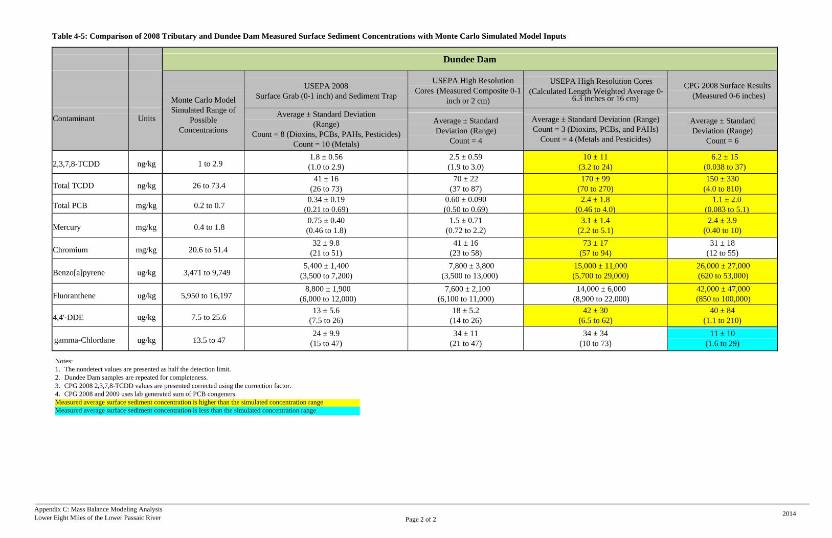
Appendix C: Mass Balance Modeling Analysis Lower Eight Miles of the Lower Passaic River 2014
Page 2 of 2
Table 4‐5: Comparison of 2008 Tributary and Dundee Dam Measured Surface Sediment Concentrations with Monte Carlo Simulated Model Inputs
Dundee Dam
Contaminant
Units
Monte Carlo Model Simulated Range of
Possible Concentrations
USEPA 2008 Surface Grab (0‐1 inch) and Sediment Trap
USEPA High Resolution Cores (Measured Composite 0‐1
inch or 2 cm)
USEPA High Resolution Cores (Calculated Length Weighted Average 0‐
6.3 inches or 16 cm) CPG 2008 Surface Results
(Measured 0‐6 inches)
Average ± Standard Deviation (Range)
Count = 8 (Dioxins, PCBs, PAHs, Pesticides) Count = 10 (Metals)
Average ± Standard Deviation (Range)
Count = 4
Average ± Standard Deviation (Range) Count = 3 (Dioxins, PCBs, and PAHs)
Count = 4 (Metals and Pesticides)
Average ± Standard Deviation (Range)
Count = 6
2,3,7,8‐TCDD ng/kg 1 to 2.9 1.8 ± 0.56 (1.0 to 2.9)
2.5 ± 0.59 (1.9 to 3.0)
10 ± 11 (3.2 to 24)
6.2 ± 15 (0.038 to 37)
Total TCDD ng/kg 26 to 73.4 41 ± 16
(26 to 73) 70 ± 22
(37 to 87) 170 ± 99
(70 to 270) 150 ± 330
(4.0 to 810)
Total PCB mg/kg 0.2 to 0.7 0.34 ± 0.19
(0.21 to 0.69)0.60 ± 0.090 (0.50 to 0.69)
2.4 ± 1.8 (0.46 to 4.0)
1.1 ± 2.0 (0.083 to 5.1)
Mercury mg/kg 0.4 to 1.8 0.75 ± 0.40 (0.46 to 1.8)
1.5 ± 0.71 (0.72 to 2.2)
3.1 ± 1.4 (2.2 to 5.1)
2.4 ± 3.9 (0.40 to 10)
Chromium mg/kg 20.6 to 51.4 32 ± 9.8
(21 to 51) 41 ± 16
(23 to 58) 73 ± 17
(57 to 94) 31 ± 18
(12 to 55)
Benzo[a]pyrene ug/kg 3,471 to 9,749 5,400 ± 1,400
(3,500 to 7,200) 7,800 ± 3,800
(3,500 to 13,000) 15,000 ± 11,000 (5,700 to 29,000)
26,000 ± 27,000 (620 to 53,000)
Fluoranthene ug/kg 5,950 to 16,197 8,800 ± 1,900
(6,000 to 12,000) 7,600 ± 2,100
(6,100 to 11,000) 14,000 ± 6,000
(8,900 to 22,000) 42,000 ± 47,000 (850 to 100,000)
4,4'‐DDE ug/kg 7.5 to 25.6 13 ± 5.6
(7.5 to 26) 18 ± 5.2
(14 to 26) 42 ± 30
(6.5 to 62) 40 ± 84
(1.1 to 210)
gamma-Chlordane ug/kg 13.5 to 47 24 ± 9.9
(15 to 47) 34 ± 11
(21 to 47) 34 ± 34
(10 to 73) 11 ± 10
(1.6 to 29)
Notes: 1. The nondetect values are presented as half the detection limit. 2. Dundee Dam samples are repeated for completeness. 3. CPG 2008 2,3,7,8‐TCDD values are presented corrected using the correction factor. 4. CPG 2008 and 2009 uses lab generated sum of PCB congeners. Measured average surface sediment concentration is higher than the simulated concentration range Measured average surface sediment concentration is less than the simulated concentration range
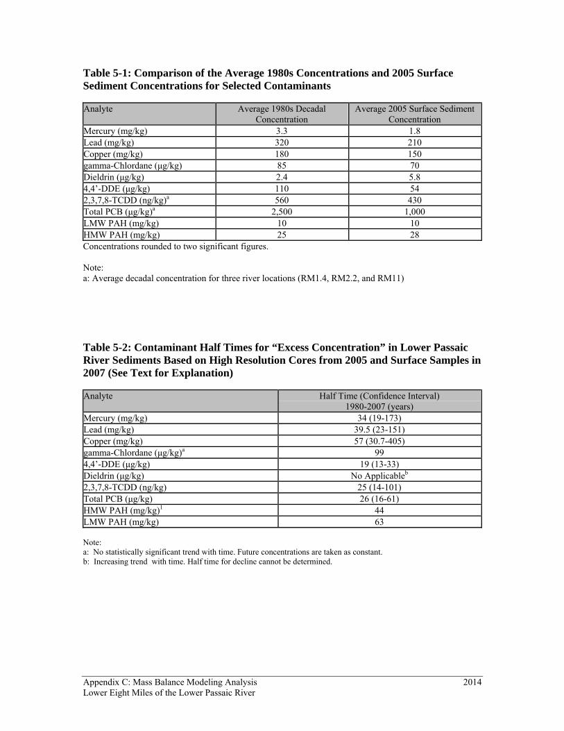
Appendix C: Mass Balance Modeling Analysis 2014 Lower Eight Miles of the Lower Passaic River
Table 5-1: Comparison of the Average 1980s Concentrations and 2005 Surface Sediment Concentrations for Selected Contaminants Analyte Average 1980s Decadal
Concentration Average 2005 Surface Sediment
Concentration Mercury (mg/kg) 3.3 1.8 Lead (mg/kg) 320 210 Copper (mg/kg) 180 150 gamma-Chlordane (μg/kg) 85 70 Dieldrin (μg/kg) 2.4 5.8 4,4’-DDE (μg/kg) 110 54 2,3,7,8-TCDD (ng/kg)a 560 430 Total PCB (μg/kg)a 2,500 1,000 LMW PAH (mg/kg) 10 10 HMW PAH (mg/kg) 25 28 Concentrations rounded to two significant figures. Note: a: Average decadal concentration for three river locations (RM1.4, RM2.2, and RM11)
Table 5-2: Contaminant Half Times for “Excess Concentration” in Lower Passaic River Sediments Based on High Resolution Cores from 2005 and Surface Samples in 2007 (See Text for Explanation) Analyte Half Time (Confidence Interval)
1980-2007 (years) Mercury (mg/kg) 34 (19-173) Lead (mg/kg) 39.5 (23-151) Copper (mg/kg) 57 (30.7-405) gamma-Chlordane (μg/kg)a 99 4,4’-DDE (μg/kg) 19 (13-33) Dieldrin (μg/kg) No Applicableb 2,3,7,8-TCDD (ng/kg) 25 (14-101) Total PCB (μg/kg) 26 (16-61) HMW PAH (mg/kg)1 44 LMW PAH (mg/kg) 63 Note: a: No statistically significant trend with time. Future concentrations are taken as constant. b: Increasing trend with time. Half time for decline cannot be determined.
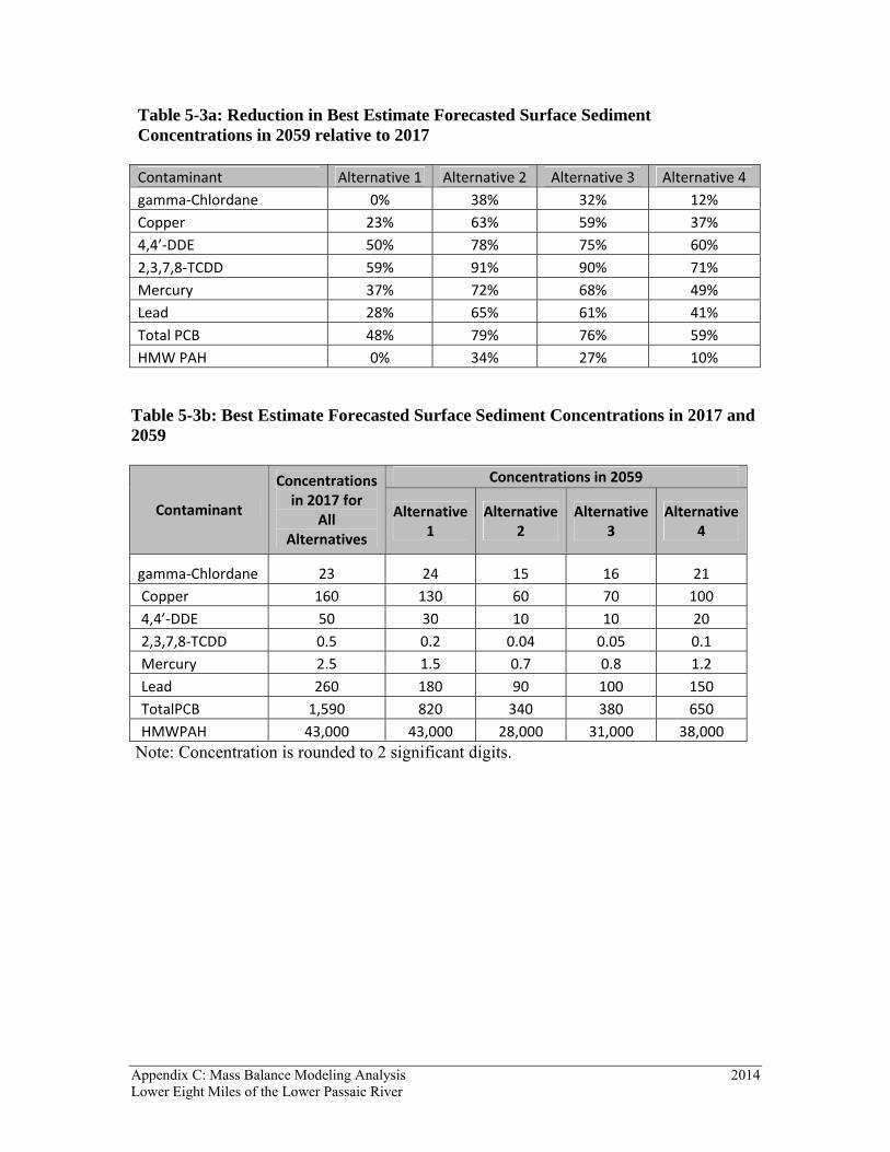
Appendix C: Mass Balance Modeling Analysis 2014 Lower Eight Miles of the Lower Passaic River
Table 5-3a: Reduction in Best Estimate Forecasted Surface Sediment Concentrations in 2059 relative to 2017 Contaminant Alternative 1 Alternative 2 Alternative 3 Alternative 4 gamma‐Chlordane 0% 38% 32% 12% Copper 23% 63% 59% 37% 4,4’‐DDE 50% 78% 75% 60% 2,3,7,8‐TCDD 59% 91% 90% 71% Mercury 37% 72% 68% 49% Lead 28% 65% 61% 41% Total PCB 48% 79% 76% 59% HMW PAH 0% 34% 27% 10%
Table 5-3b: Best Estimate Forecasted Surface Sediment Concentrations in 2017 and 2059
Contaminant
Concentrations in 2017 for
All Alternatives
Concentrations in 2059
Alternative 1
Alternative 2
Alternative 3
Alternative 4
gamma‐Chlordane 23 24 15 16 21 Copper 160 130 60 70 100 4,4’‐DDE 50 30 10 10 20 2,3,7,8‐TCDD 0.5 0.2 0.04 0.05 0.1 Mercury 2.5 1.5 0.7 0.8 1.2 Lead 260 180 90 100 150 TotalPCB 1,590 820 340 380 650 HMWPAH 43,000 43,000 28,000 31,000 38,000
Note: Concentration is rounded to 2 significant digits.

Appendix C: Mass Balance Modeling Analysis Lower Eight Miles of the Lower Passaic River 2014
FIGURES
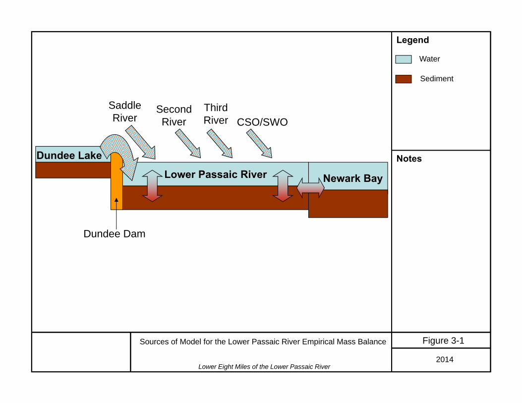
Lower Eight Miles of the Lower Passaic River2014
Figure 3-1Sources of Model for the Lower Passaic River Empirical Mass Balance
Legend
Notes
Lower Passaic River Newark Bay
Dundee Lake
SaddleRiver
SecondRiver
ThirdRiver CSO/SWO
Water
Sediment
Dundee Dam

Lower Eight Miles of the Lower Passaic River2014
Figure 3-2Relationship between Average Contaminant Concentration and Standard Error for the Recently-Deposited Sediments in the Main Stem
Lower Passaic River
R² = 0.98
1.E‐05
1.E‐04
1.E‐03
1.E‐02
1.E‐01
1.E+00
1.E+01
1.E+02
1.E+03
1.E+04
1.E+05
1.E+06
1.E+07
1.E‐05 1.E‐04 1.E‐03 1.E‐02 1.E‐01 1.E+00 1.E+01 1.E+02 1.E+03 1.E+04 1.E+05 1.E+06 1.E+07 1.E+08
Standard Error (ppb
)
Average Concentration (ppb)
PCDD/F
PCB
OCP
PAH
Metals
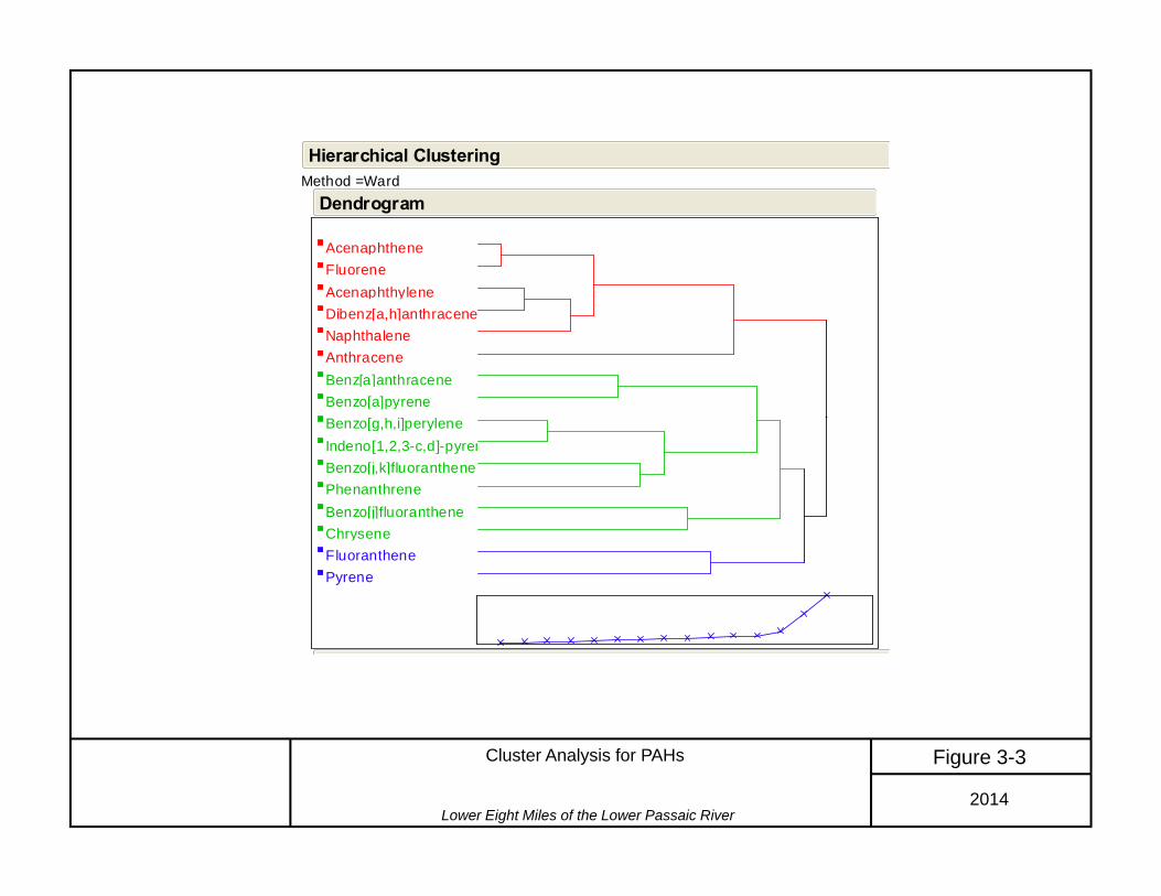
Lower Eight Miles of the Lower Passaic River2014
Figure 3-3Cluster Analysis for PAHs
Method = Ward
Acenaphthene
Acenaphthylene
AnthraceneBenz[a]anthraceneBenzo[a]pyreneBenzo[g,h,i]perylene
Benzo[j,k]fluoranthene
Benzo[j]fluorantheneChrysene
Dibenz[a,h]anthracene
Fluoranthene
Fluorene
Indeno[1,2,3-c,d]-pyrene
Naphthalene
Phenanthrene
Pyrene
Dendrogram
Hierarchical Clustering
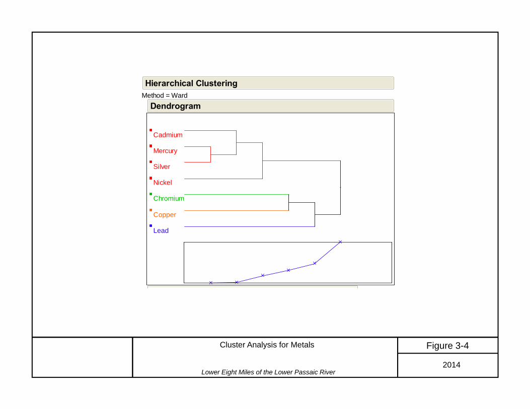
Lower Eight Miles of the Lower Passaic River2014
Figure 3-4Cluster Analysis for Metals
Method = Ward
Cadmium
Chromium
Copper
Lead
Mercury
Nickel
Silver
Dendrogram
Hierarchical Clustering

Lower Eight Miles of the Lower Passaic River
Figure 4‐1Best Estimate of Relative Solids Contribution to the Lower Passaic River Estimated by the EMB Model
Legend
Upper Passaic River
Saddle River
Second River/SWO
Third River
CSO
Newark Bay Northern EndResuspension (LowerPassaic River)
2014
Resuspension (Lower Passaic River)
48%
Newark Bay14%
Upper Passaic River32%
Saddle River4%
Third River1%
Second River / SWO1%CSO0%CSO0.5%

Lower Eight Miles of the Lower Passaic River
Figure 4‐2Fractional Contribution for Solids(Results from Monte Carlo Analysis and Best Estimate Solution)
Legend
95th Percentile
5th Percentile
50th Percentile
25th Percentile
75th PercentileBest Estimate *
0.0
0.1
0.2
0.3
0.4
0.5
0.6
0.7
0.8
0.9
1.0
Resuspen
sion
New
ark B
ay
Upp
er Passaic River
Sadd
le River
Second
River/SWO
Third
River
CSO
Fractio
nal C
ontribution
Notes:*: Best Estimate representsMass Balance estimates using average input valuesfor source profiles.
5th, 25th, 50th, 75th and 95thpercentiles are based onMass Balance results for the 10,000 iterations in MonteCarlo Analysis.
2014

Lower Eight Miles of the Lower Passaic River 2014
Figure 4-3aSource Concentration and Mass Balance for 2,3,7,8-TCDD
Legend
Notes
Legend
*: Second River Results are used to represent the SWOs. (see Appendix F)
Source Concentration of 2,3,7,8-TCDDMaximum
Minimum
Median25% quartile
75% quartile
Outliers
Mean ± 2 standarderrors
Upper Passaic River
Saddle River
Second River/SWO
Third River
CSO
Newark Bay Northern EndResuspension (LowerPassaic River)
Best Estimate Mass Balance for 2,3,7,8-TCDD
Average
0.0001
0.001
0.01
0.1
1
10
100
Upp
er P
assa
ic R
iver
Sad
dle
Riv
er
Third
Riv
er
Sec
ond
Riv
er/S
WO
*
CS
O
New
ark
Bay
N
orth
ern
End
1995
0-6
inch
S
urfa
ce S
edim
ent
2,3,
7,8-
TCD
D C
once
ntra
tion
(ug/
kg)
Lower Passaic RiverTarget Concentration(RM2 to 12)
Resuspension (Lower Passaic River)
97%
Newark Bay3%
Upper Passaic River0.1%
Saddle River0.03%
Third River0.004%
Second River / SWO0.003%
CSO0.005%

Lower Eight Miles of the Lower Passaic River
Figure 4‐3bFractional Contribution for 2,3,7,8‐TCDD(Results from Monte Carlo Analysis and Best Estimate Solution)
Legend
95th Percentile
5th Percentile
50th Percentile
25th Percentile
75th PercentileBest Estimate *
Notes:*: Best Estimate representsMass Balance estimates using average input valuesfor source profiles.
5th, 25th, 50th, 75th and 95thpercentiles are based onMass Balance results for the 10,000 iterations in MonteCarlo Analysis.0.0
0.1
0.2
0.3
0.4
0.5
0.6
0.7
0.8
0.9
1.0
Resuspen
sion
New
ark B
ay
Upp
er Passaic River
Sadd
le River
Second
River/SWO
Third
River
CSO
Fractio
nal C
ontribution
2014

Lower Eight Miles of the Lower Passaic River 2014
Figure 4-4aSource Concentration and Mass Balance for Total Tetra-dioxins
Legend
Notes
Legend
*: Second River Results are used to represent the SWOs. (see Appendix F)
Source Concentration of Total Tetra-dioxinsMaximum
Minimum
Median25% quartile
75% quartile
Outliers
Mean ± 2 standarderrors
Upper Passaic River
Saddle River
Second River/SWO
Third River
CSO
Newark Bay Northern EndResuspension (LowerPassaic River)
Best Estimate Mass Balance for Total Tetra-dioxins
Average
0.001
0.01
0.1
1
10
100
Upp
er P
assa
ic R
iver
Sad
dle
Riv
er
Third
Riv
er
Sec
ond
Riv
er/S
WO
*
CS
O
New
ark
Bay
Nor
ther
n E
nd
1995
0-6
inch
S
urfa
ce S
edim
ent
Tota
l Tet
ra-d
ioxi
ns C
once
ntra
tion
(ug/
kg)
Lower Passaic RiverTarget Concentration(RM2 to 12)
Resuspension (Lower Passaic River)
92%
Newark Bay5%
Upper Passaic River3%
Saddle River0.2%
Third River0.04%
Second River / SWO0.03%
CSO0.07%
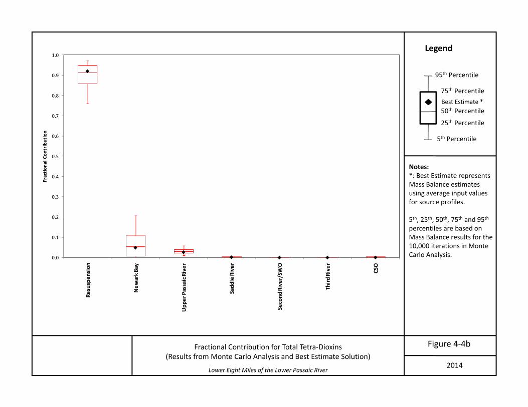
Lower Eight Miles of the Lower Passaic River
Figure 4‐4bFractional Contribution for Total Tetra‐Dioxins(Results from Monte Carlo Analysis and Best Estimate Solution)
Legend
95th Percentile
5th Percentile
50th Percentile
25th Percentile
75th PercentileBest Estimate *
Notes:*: Best Estimate representsMass Balance estimates using average input valuesfor source profiles.
5th, 25th, 50th, 75th and 95thpercentiles are based onMass Balance results for the 10,000 iterations in MonteCarlo Analysis.0.0
0.1
0.2
0.3
0.4
0.5
0.6
0.7
0.8
0.9
1.0
Resuspen
sion
New
ark B
ay
Upp
er Passaic River
Sadd
le River
Second
River/SWO
Third
River
CSO
Fractio
nal C
ontribution
2014

Lower Eight Miles of the Lower Passaic River 2014
Figure 4-5aSource Concentration and Mass Balance for Total PCBs
Legend
Notes
Legend
*: Second River Results are used to represent the SWOs. (see Appendix F)
Source Concentration of Total PCBsMaximum
Minimum
Median25% quartile
75% quartile
Outliers
Mean ± 2 standarderrors
Upper Passaic River
Saddle River
Second River/SWO
Third River
CSO
Newark Bay Northern EndResuspension (LowerPassaic River)
Best Estimate Mass Balance for Total PCBs
Average
10
100
1,000
10,000
100,000
Upp
er P
assa
ic R
iver
Sad
dle
Riv
er
Third
Riv
er
Seco
nd R
iver
/SW
O*
CS
O
New
ark
Bay
Nor
ther
n En
d
1995
0-6
inch
Su
rface
Sed
imen
t
Tota
l PC
Bs
(ug/
kg)
Target Concentration Lower Passaic Average Surface Sediment (RM2 to 12)
Resuspension (Lower Passaic River)
81%
Newark Bay7%
Upper Passaic River11%
Saddle River1%
Third River0.3%
Second River / SWO0.1%
CSO0.4%

Lower Eight Miles of the Lower Passaic River
Figure 4‐5bFractional Contribution for Total PCBs(Results from Monte Carlo Analysis and Best Estimate Solution)
Legend
95th Percentile
5th Percentile
50th Percentile
25th Percentile
75th PercentileBest Estimate *
Notes:*: Best Estimate representsMass Balance estimates using average input valuesfor source profiles.
5th, 25th, 50th, 75th and 95thpercentiles are based onMass Balance results for the 10,000 iterations in MonteCarlo Analysis.0.0
0.1
0.2
0.3
0.4
0.5
0.6
0.7
0.8
0.9
1.0
Resuspen
sion
New
ark B
ay
Upp
er Passaic River
Sadd
le River
Second
River/SWO
Third
River
CSO
Fractio
nal C
ontribution
2014

Lower Eight Miles of the Lower Passaic River 2014
Figure 4-6aSource Concentration and Mass Balance for Benzo[a]pyrene
Legend
Notes
Legend
*: Second River Results are used to represent the SWOs. (see Appendix F)
Source Concentration of Benzo[a]pyreneMaximum
Minimum
Median25% quartile
75% quartile
Outliers
Mean ± 2 standarderrors
Upper Passaic River
Saddle River
Second River/SWO
Third River
CSO
Newark Bay Northern EndResuspension (LowerPassaic River)
Best Estimate Mass Balance for Benzo[a]pyrene
Average
100
1,000
10,000
100,000
Upp
er P
assa
ic R
iver
Sad
dle
Riv
er
Third
Riv
er
Sec
ond
Riv
er/S
WO
*
CSO
New
ark
Bay
Nor
ther
n En
d
1995
0-6
inch
S
urfa
ce S
edim
ent
Benz
o[a]
pyre
ne C
once
ntra
tion
(ug/
kg)
Lower Passaic RiverTarget ConcentrationRM2 to 12
Resuspension (Lower Passaic River)
33%
Newark Bay7%
Upper Passaic River53%
Saddle River4%
Third River1%
Second River / SWO2%
CSO0.3%

Lower Eight Miles of the Lower Passaic River
Figure 4‐6bFractional Contribution for Benzo[a]pyrene(Results from Monte Carlo Analysis and Best Estimate Solution)
Legend
95th Percentile
5th Percentile
50th Percentile
25th Percentile
75th PercentileBest Estimate*
Notes:*: Best Estimate representsMass Balance estimates using average input valuesfor source profiles.
5th, 25th, 50th, 75th and 95thpercentiles are based onMass Balance results for the 10,000 iterations in MonteCarlo Analysis.0.0
0.1
0.2
0.3
0.4
0.5
0.6
0.7
0.8
0.9
1.0
Resuspen
sion
New
ark B
ay
Upp
er Passaic River
Sadd
le River
Second
River/SWO
Third
River
CSO
Fractio
nal C
ontribution
2014

Lower Eight Miles of the Lower Passaic River 2014
Figure 4-7aSource Concentration and Mass Balance for Fluoranthene
Legend
Notes
Legend
*: Second River Results are used to represent the SWOs. (see Appendix F)
Source Concentration of FluorantheneMaximum
Minimum
Median25% quartile
75% quartile
Outliers
Mean ± 2 standarderrors
Upper Passaic River
Saddle River
Second River/SWO
Third River
CSO
Newark Bay Northern EndResuspension (LowerPassaic River)
Best Estimate Mass Balance for Fluoranthene
Average
100
1,000
10,000
100,000
Upp
er P
assa
ic R
iver
Sad
dle
Riv
er
Third
Riv
er
Seco
nd R
iver
/SW
O*
CSO
New
ark
Bay
Nor
ther
n E
nd
1995
0-6
inch
Su
rface
Sed
imen
t
Fluo
rant
hene
Con
cent
ratio
n (u
g/kg
)
Lower Pasaic RiverTarget ConcentrationRM2 to 12
Resuspension (Lower Passaic River)
40%
Newark Bay5%
Upper Passaic River47%
Saddle River5%
Third River1%
Second River / SWO2%
CSO0.4%

Lower Eight Miles of the Lower Passaic River
Figure 4‐7bFractional Contribution for Fluoranthene(Results from Monte Carlo Analysis and Best Estimate Solution)
Legend
95th Percentile
5th Percentile
50th Percentile
25th Percentile
75th PercentileBest Estimate *
Notes:*: Best Estimate representsMass Balance estimates using average input valuesfor source profiles.
5th, 25th, 50th, 75th and 95thpercentiles are based onMass Balance results for the 10,000 iterations in MonteCarlo Analysis.0.0
0.1
0.2
0.3
0.4
0.5
0.6
0.7
0.8
0.9
1.0
Resuspen
sion
New
ark B
ay
Upp
er Passaic River
Sadd
le River
Second
River/SWO
Third
River
CSO
Fractio
nal C
ontribution
2014

Lower Eight Miles of the Lower Passaic River 2014
Figure 4-8aSource Concentration and Mass Balance for 4,4’-DDE
Legend
Notes
Legend
*: Second River Results are used to represent the SWOs. (see Appendix F)
Source Concentration of 4,4’-DDEMaximum
Minimum
Median25% quartile
75% quartile
Outliers
Mean ± 2 standarderrors
Upper Passaic River
Saddle River
Second River/SWO
Third River
CSO
Newark Bay Northern EndResuspension (LowerPassaic River)
Best Estimate Mass Balance for 4,4’-DDE
Average
1
10
100
1,000
Upp
er P
assa
ic R
iver
Sad
dle
Riv
er
Third
Riv
er
Sec
ond
Riv
er/S
WO
*
CS
O
New
ark
Bay
N
orth
ern
End
1995
0-6
inch
S
urfa
ce S
edim
ent
4,4'
-DD
E C
once
ntra
tion
(ug/
kg) Lower Passaic River
Target ConcentrationRM2 to 12
Resuspension (Lower Passaic River)
78%
Newark Bay8%
Upper Passaic River10%
Saddle River2%
Third River1%
Second River / SWO1%
CSO0.3%
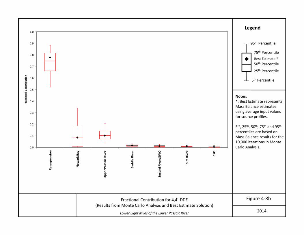
Lower Eight Miles of the Lower Passaic River
Figure 4‐8bFractional Contribution for 4,4’‐DDE(Results from Monte Carlo Analysis and Best Estimate Solution)
Legend
95th Percentile
5th Percentile
50th Percentile
25th Percentile
75th PercentileBest Estimate *
Notes:*: Best Estimate representsMass Balance estimates using average input valuesfor source profiles.
5th, 25th, 50th, 75th and 95thpercentiles are based onMass Balance results for the 10,000 iterations in MonteCarlo Analysis.0.0
0.1
0.2
0.3
0.4
0.5
0.6
0.7
0.8
0.9
1.0
Resuspen
sion
New
ark B
ay
Upp
er Passaic River
Sadd
le River
Second
River/SWO
Third
River
CSO
Fractio
nal C
ontribution
2014

Lower Eight Miles of the Lower Passaic River 2014
Figure 4-9aSource Concentration and Mass Balance for gamma-Chlordane
Legend
Notes
Legend
*Second River Results are used to represent the SWOs. (see Appendix F)+Robinson (2002)
Source Concentration of gamma-ChlordaneMaximum
Minimum
Median25% quartile
75% quartile
Outliers
Mean ± 2 standarderrors
Upper Passaic River
Saddle River
Second River/SWO
Third River
CSO
Newark Bay Northern EndResuspension (LowerPassaic River)
Best Estimate Mass Balance for gamma-Chlordane
Average
Resuspension (Lower Passaic River)
52%
Newark Bay3%
Upper Passaic River32%
Saddle River8%
Third River2%
Second River / SWO2%
CSO1%
1
10
100
1,000
Upp
er P
assa
ic R
iver
Sadd
le R
iver
Third
Riv
er
Seco
nd R
iver
/SW
O*
CS
O
New
ark
Bay
Nor
ther
n En
d+
1995
0-6
inch
Su
rface
Sed
imen
t
Chl
orda
ne (g
amm
a) (u
g/kg
)
Lower Passaic RiverTarget ConcentrationRM2 to 12
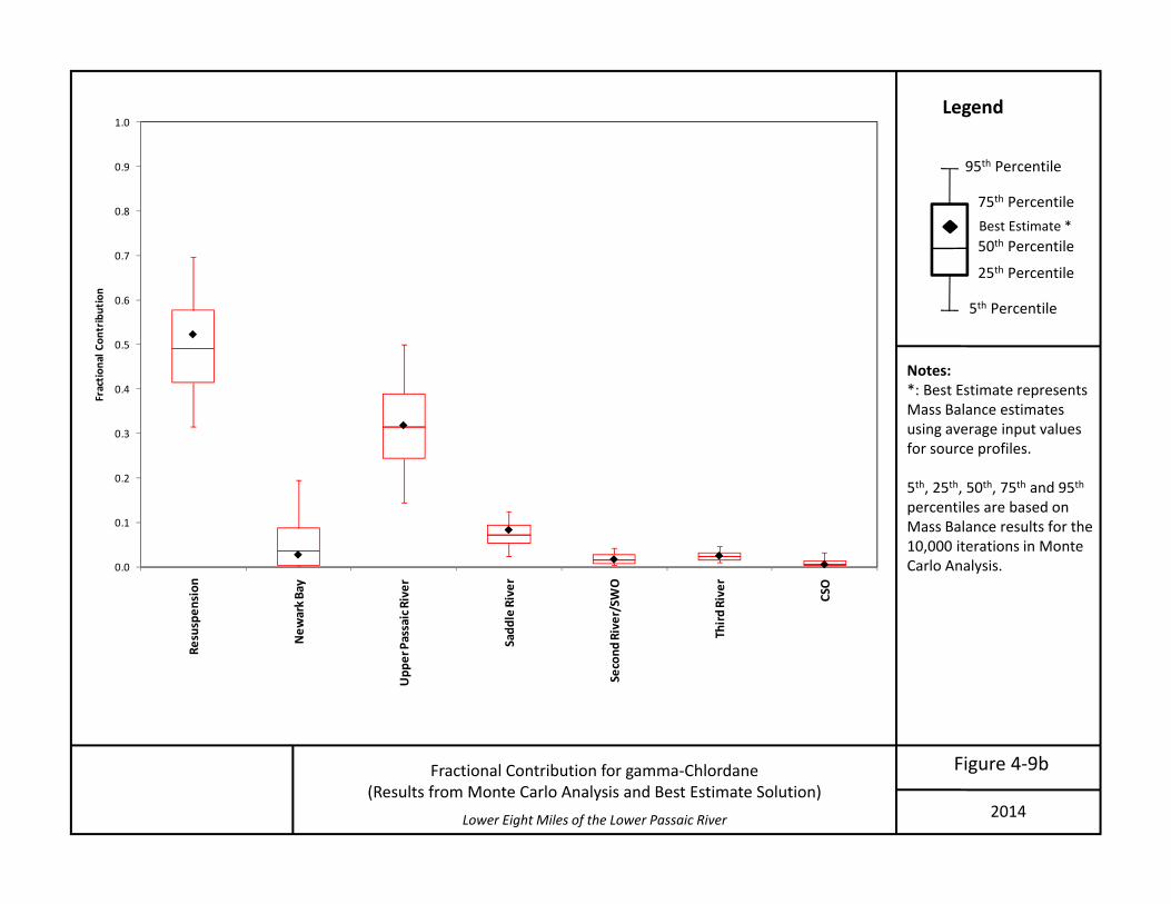
Lower Eight Miles of the Lower Passaic River
Figure 4‐9bFractional Contribution for gamma‐Chlordane(Results from Monte Carlo Analysis and Best Estimate Solution)
Legend
95th Percentile
5th Percentile
50th Percentile
25th Percentile
75th PercentileBest Estimate *
Notes:*: Best Estimate representsMass Balance estimates using average input valuesfor source profiles.
5th, 25th, 50th, 75th and 95thpercentiles are based onMass Balance results for the 10,000 iterations in MonteCarlo Analysis.0.0
0.1
0.2
0.3
0.4
0.5
0.6
0.7
0.8
0.9
1.0
Resuspen
sion
New
ark B
ay
Upp
er Passaic River
Sadd
le River
Second
River/SWO
Third
River
CSO
Fractio
nal C
ontribution
2014
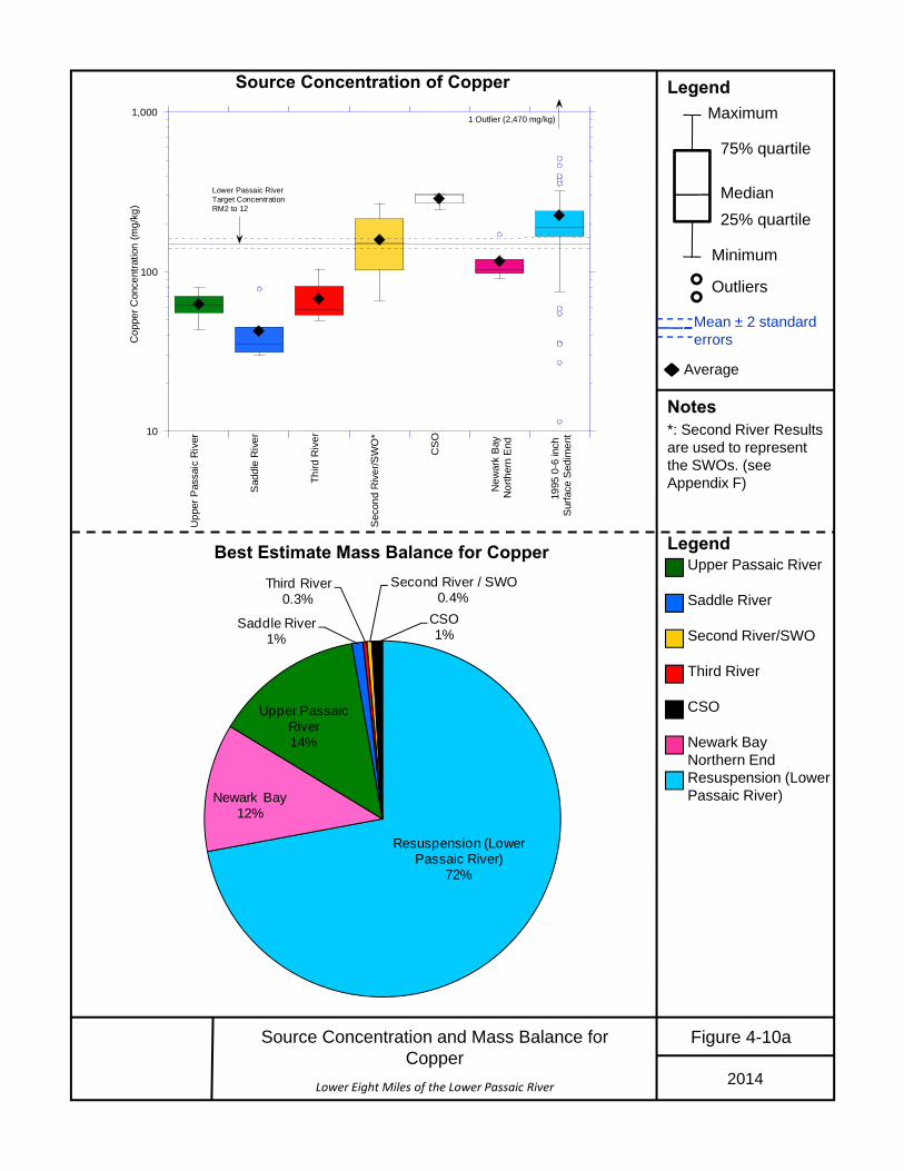
Lower Eight Miles of the Lower Passaic River 2014
Figure 4-10aSource Concentration and Mass Balance for Copper
Legend
Notes
Legend
*: Second River Results are used to represent the SWOs. (see Appendix F)
Source Concentration of CopperMaximum
Minimum
Median25% quartile
75% quartile
Outliers
Mean ± 2 standarderrors
Upper Passaic River
Saddle River
Second River/SWO
Third River
CSO
Newark Bay Northern EndResuspension (LowerPassaic River)
Best Estimate Mass Balance for Copper
Average
10
100
1,000
Upp
er P
assa
ic R
iver
Sad
dle
Riv
er
Third
Riv
er
Sec
ond
Riv
er/S
WO
*
CS
O
New
ark
Bay
N
orth
ern
End
1995
0-6
inch
S
urfa
ce S
edim
ent
Cop
per C
once
ntra
tion
(mg/
kg)
Lower Passaic RiverTarget ConcentrationRM2 to 12
1 Outlier (2,470 mg/kg)
Resuspension (Lower Passaic River)
72%
Newark Bay12%
Upper Passaic River14%
Saddle River1%
Third River0.3%
Second River / SWO0.4%
CSO1%

Lower Eight Miles of the Lower Passaic River
Figure 4‐10bFractional Contribution for Copper(Results from Monte Carlo Analysis and Best Estimate Solution)
Legend
95th Percentile
5th Percentile
50th Percentile
25th Percentile
75th PercentileBest Estimate *
Notes:*: Best Estimate representsMass Balance estimates using average input valuesfor source profiles.
5th, 25th, 50th, 75th and 95thpercentiles are based onMass Balance results for the 10,000 iterations in MonteCarlo Analysis.0.0
0.1
0.2
0.3
0.4
0.5
0.6
0.7
0.8
0.9
1.0
Resuspen
sion
New
ark B
ay
Upp
er Passaic River
Sadd
le River
Second
River/SWO
Third
River
CSO
Fractio
nal C
ontribution
2014

Lower Eight Miles of the Lower Passaic River 2014
Figure 4-11aSource Concentration and Mass Balance for Chromium
Legend
Notes
Legend
*: Second River Results are used to represent the SWOs. (see Appendix F)
Source Concentration of ChromiumMaximum
Minimum
Median25% quartile
75% quartile
Outliers
Mean ± 2 standarderrors
Upper Passaic River
Saddle River
Second River/SWO
Third River
CSO
Newark Bay Northern EndResuspension (LowerPassaic River)
Best Estimate Mass Balance for Chromium
Average
10
100
1,000
Upp
er P
assa
ic R
iver
Sad
dle
Riv
er
Third
Riv
er
Sec
ond
Riv
er/S
WO
*
CS
O
New
ark
Bay
N
orth
ern
End
1995
0-6
inch
Su
rface
Sed
imen
t
Chr
omiu
m C
once
ntra
tion
(mg/
kg)
Lower Passaic RiverTarget ConcentrationRM2 to 12
1 Outlier (7.9 mg/kg)
Resuspension (Lower Passaic River)
74%
Newark Bay15%
Upper Passaic River10%
Saddle River1%
Third River0.3%
Second River / SWO0.4%
CSO0.3%

Lower Eight Miles of the Lower Passaic River
Figure 4‐11bFractional Contribution for Chromium(Results from Monte Carlo Analysis and Best Estimate Solution)
Legend
95th Percentile
5th Percentile
50th Percentile
25th Percentile
75th PercentileBest Estimate*
Notes:*: Best Estimate representsMass Balance estimates using average input valuesfor source profiles.
5th, 25th, 50th, 75th and 95thpercentiles are based onMass Balance results for the 10,000 iterations in MonteCarlo Analysis.0.0
0.1
0.2
0.3
0.4
0.5
0.6
0.7
0.8
0.9
1.0
Resuspen
sion
New
ark B
ay
Upp
er Passaic River
Sadd
le River
Second
River/SWO
Third
River
CSO
Fractio
nal C
ontribution
2014

Lower Eight Miles of the Lower Passaic River 2014
Figure 4-12aSource Concentration and Mass Balance for Mercury
Legend
Notes
Legend
*: Second River Results are used to represent the SWOs. (see Appendix F)
Source Concentration of MercuryMaximum
Minimum
Median25% quartile
75% quartile
Outliers
Mean ± 2 standarderrors
Upper Passaic River
Saddle River
Second River/SWO
Third River
CSO
Newark Bay Northern EndResuspension (LowerPassaic River)
Best Estimate Mass Balance for Mercury
Average
0.01
0.1
1
10
100
Upp
er P
assa
ic R
iver
Sad
dle
Riv
er
Third
Riv
er
Sec
ond
Riv
er/S
WO
*
CS
O
New
ark
Bay
N
orth
ern
End
1995
0-6
inch
S
urfa
ce S
edim
ent
Mer
cury
Con
cent
ratio
n (m
g/kg
) Lower Passaic RiverTarget ConcentrationRM2 to 12
Resuspension (Lower Passaic River)
75%
Newark Bay14%
Upper Passaic River11%
Saddle River0.2%
Third River0.2% Second River / SWO
0.2%CSO0.2%
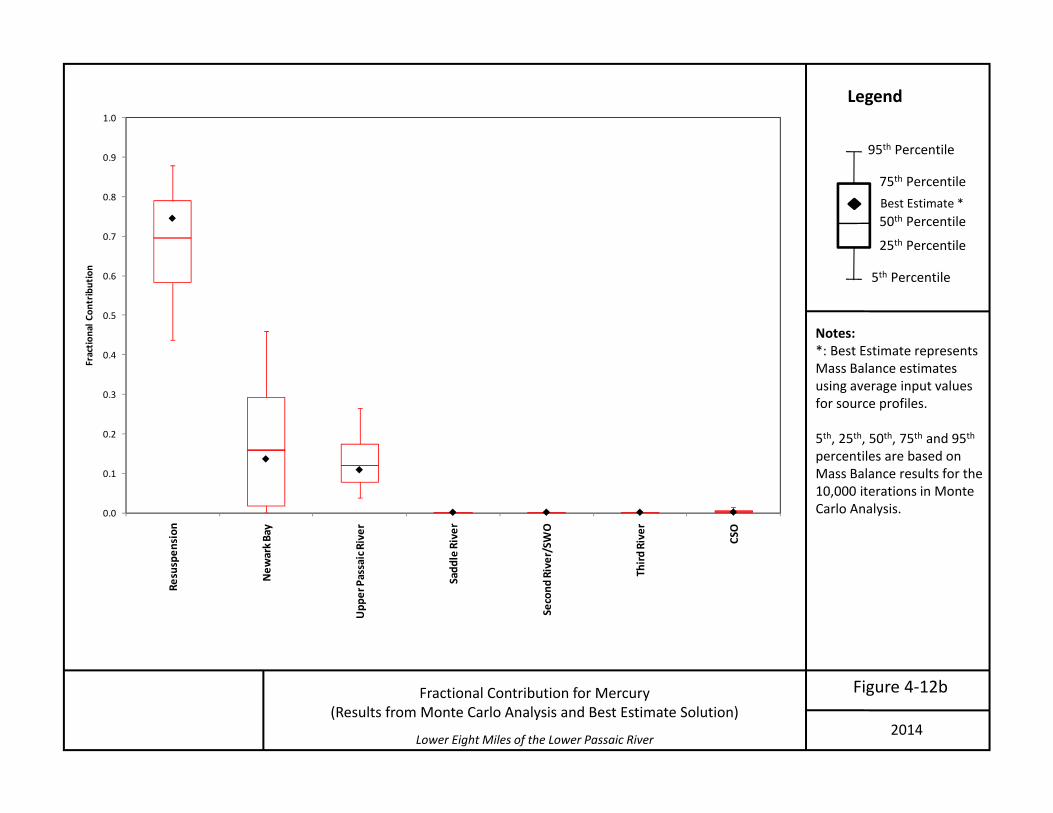
Lower Eight Miles of the Lower Passaic River
Figure 4‐12bFractional Contribution for Mercury(Results from Monte Carlo Analysis and Best Estimate Solution)
Legend
95th Percentile
5th Percentile
50th Percentile
25th Percentile
75th PercentileBest Estimate *
Notes:*: Best Estimate representsMass Balance estimates using average input valuesfor source profiles.
5th, 25th, 50th, 75th and 95thpercentiles are based onMass Balance results for the 10,000 iterations in MonteCarlo Analysis.0.0
0.1
0.2
0.3
0.4
0.5
0.6
0.7
0.8
0.9
1.0
Resuspen
sion
New
ark B
ay
Upp
er Passaic River
Sadd
le River
Second
River/SWO
Third
River
CSO
Fractio
nal C
ontribution
2014

Lower Eight Miles of the Lower Passaic River 2014
Figure 4-13aSource Concentration and Mass Balance for Lead
Legend
Notes
Legend
*: Second River Results are used to represent the SWOs. (see Appendix F)
Source Concentration of LeadMaximum
Minimum
Median25% quartile
75% quartile
Outliers
Mean ± 2 standarderrors
Upper Passaic River
Saddle River
Second River/SWO
Third River
CSO
Newark Bay Northern EndResuspension (LowerPassaic River)
Best Estimate Mass Balance for Lead
Average
10
100
1,000
Upp
er P
assa
ic R
iver
Sad
dle
Riv
er
Third
Riv
er
Seco
nd R
iver
/SW
O*
CSO
New
ark
Bay
N
orth
ern
End
1995
0-6
inch
Su
rface
Sed
imen
t
Lead
Con
cent
ratio
n (m
g/kg
)
Lower Passaic RiverTarget ConcentrationRM2 to 12
2 Outliers (4.4 mg/kg, 5.6 mg/kg)
Resuspension (Lower Passaic River)
71%
Newark Bay7%
Upper Passaic River19%
Saddle River1%
Third River0.5%
Second River / SWO1%CSO1%

Lower Eight Miles of the Lower Passaic River
Figure 4‐13bFractional Contribution for Lead(Results from Monte Carlo Analysis and Best Estimate Solution)
Legend
95th Percentile
5th Percentile
50th Percentile
25th Percentile
75th PercentileBest Estimate *
Notes:*: Best Estimate representsMass Balance estimates using average input valuesfor source profiles.
5th, 25th, 50th, 75th and 95thpercentiles are based onMass Balance results for the 10,000 iterations in MonteCarlo Analysis.0.0
0.1
0.2
0.3
0.4
0.5
0.6
0.7
0.8
0.9
1.0
Resuspen
sion
New
ark B
ay
Upp
er Passaic River
Sadd
le River
Second
River/SWO
Third
River
CSO
Fractio
nal C
ontribution
2014

Lower Eight Miles of the Lower Passaic River 2014
Figure 4-14aSource Concentration and Mass Balance for Iron
Legend
Notes
Legend
*: Second River Results are used to represent the SWOs. (see Appendix F)
Source Concentration of IronMaximum
Minimum
Median25% quartile
75% quartile
Outliers
Mean ± 2 standarderrors
Upper Passaic River
Saddle River
Second River/SWO
Third River
CSO
Newark Bay Northern EndResuspension (LowerPassaic River)
Best Estimate Mass Balance for Iron
1,000
10,000
100,000
Upp
er P
assa
ic R
iver
Sad
dle
Riv
er
Third
Riv
er
Sec
ond
Riv
er/S
WO
*
CS
O
New
ark
Bay
N
orth
ern
End
1995
0-6
inch
S
urfa
ce S
edim
ent
Iron
Con
cent
ratio
n (m
g/kg
)
Lower Passaic RiverTarget ConcentrationRM2 to 12
Average
Resuspension (Lower Passaic River)
54%
Newark Bay18%
Upper Passaic River24%
Saddle River2%
Third River1%
Second River / SWO1%
CSO0.5%

Lower Eight Miles of the Lower Passaic River
Figure 4‐14bFractional Contribution for Iron(Results from Monte Carlo Analysis and Best Estimate Solution)
Legend
95th Percentile
5th Percentile
50th Percentile
25th Percentile
75th PercentileBest Estimate*
Notes:*: Best Estimate representsMass Balance estimates using average input valuesfor source profiles.
5th, 25th, 50th, 75th and 95thpercentiles are based onMass Balance results for the 10,000 iterations in MonteCarlo Analysis.
0.0
0.1
0.2
0.3
0.4
0.5
0.6
0.7
0.8
0.9
1.0
Resuspen
sion
New
ark B
ay
Upp
er Passaic River
Sadd
le River
Second
River/SWO
Third
River
CSO
Fractio
nal C
ontribution
2014
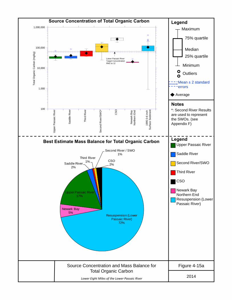
Lower Eight Miles of the Lower Passaic River 2014
Figure 4-15aSource Concentration and Mass Balance for Total Organic Carbon
Legend
Notes
Legend
*: Second River Results are used to represent the SWOs. (see Appendix F)
Source Concentration of Total Organic CarbonMaximum
Minimum
Median25% quartile
75% quartile
Outliers
Mean ± 2 standarderrors
Upper Passaic River
Saddle River
Second River/SWO
Third River
CSO
Newark Bay Northern EndResuspension (LowerPassaic River)
Best Estimate Mass Balance for Total Organic Carbon
100
1,000
10,000
100,000
1,000,000
Upp
er P
assa
ic R
iver
Sad
dle
Riv
er
Third
Riv
er
Seco
nd R
iver
/SW
O*
CS
O
New
ark
Bay
N
orth
ern
End
1995
0-6
inch
S
urfa
ce S
edim
ent
Tota
l Org
anic
Car
bon
(mg/
kg)
Lower Passaic RiverTarget ConcentrationRM2 to 12
Average
Resuspension (Lower Passaic River)
72%
Newark Bay5%
Upper Passaic River17%
Saddle River2%
Third River1%
Second River / SWO1%
CSO2%

Lower Eight Miles of the Lower Passaic River
Figure 4‐15b
2014
Fractional Contribution for Total Organic Carbon(Results from Monte Carlo Analysis and Best Estimate Solution)
Legend
95th Percentile
5th Percentile
50th Percentile
25th Percentile
75th PercentileBest Estimate *
Notes:*: Best Estimate representsMass Balance estimates using average input valuesfor source profiles.
5th, 25th, 50th, 75th and 95thpercentiles are based onMass Balance results for the 10,000 iterations in MonteCarlo Analysis.
0.0
0.1
0.2
0.3
0.4
0.5
0.6
0.7
0.8
0.9
1.0
Resuspen
sion
New
ark B
ay
Upp
er Passaic River
Sadd
le River
Second
River/SWO
Third
River
CSO
Fractio
nal C
ontribution

Lower Eight Miles of the Lower Passaic River
Figure 4‐16
2014
Dieldrin Contribution to the Lower Passaic River
Legend
Upper Passaic River
Saddle River
Second River/SWO
Third River
CSO
Newark Bay Northern EndResuspension (LowerPassaic River)
Resuspension (Lower Passaic River)
73%
Newark Bay7%
Upper Passaic River12%
Saddle River5%
Third River1%
Second River / SWO1%
CSO1%

Lower Eight Miles of the Lower Passaic River
Figure 4‐17
2014
Phenanthrene Contribution to the Lower Passaic River
Legend
Upper Passaic River
Saddle River
Second River/SWO
Third River
CSO
Newark Bay Northern EndResuspension (LowerPassaic River)
Resuspension (Lower Passaic River)
47%
Newark Bay2%
Upper Passaic River42%
Saddle River4%
Third River1%
Second River / SWO2%
CSO2%
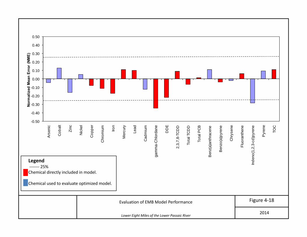
Lower Eight Miles of the Lower Passaic River
Figure 4‐18Evaluation of EMB Model Performance
-0.50
-0.40
-0.30
-0.20
-0.10
0.00
0.10
0.20
0.30
0.40
0.50
Ars
enic
Cob
alt
Zinc
Nic
kel
Cop
per
Chr
omiu
m
Iron
Mer
cury
Lead
Cad
miu
m
Chl
orda
ne
DD
E
2,3,
7,8-
TCD
D
Tota
l TC
DD
Tota
l PC
B
Ben
z(a)
anth
race
ne
Ben
zo(a
)pyr
ene
Chr
ysen
e
Fluo
rant
hene
Inde
no(1
,2,3
-cd)
pyre
ne
Pyr
ene
TOC
Norm
aliz
ed M
ean
Erro
r (N
ME)
Legend‐‐‐‐‐‐‐ 25%Chemical directly included in model.
Chemical used to evaluate optimized model.
2014
gam
ma-
Chl
orda
ne
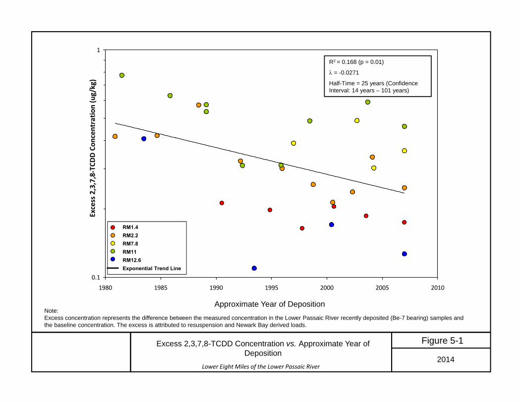
Lower Eight Miles of the Lower Passaic River2014
0.1
1
1980 1985 1990 1995 2000 2005 2010
Deposition Year
Excess 2,3,7,8‐TCD
D Con
centratio
n (ug/kg)
Figure 5-1Excess 2,3,7,8-TCDD Concentration vs. Approximate Year of Deposition
Note:Excess concentration represents the difference between the measured concentration in the Lower Passaic River recently deposited (Be-7 bearing) samples and the baseline concentration. The excess is attributed to resuspension and Newark Bay derived loads.
R2 = 0.168 (p = 0.01)
= -0.0271
Half-Time = 25 years (Confidence Interval: 14 years – 101 years)
RM1.4 RM2.2RM7.8RM11RM12.6Exponential Trend Line
Approximate Year of Deposition
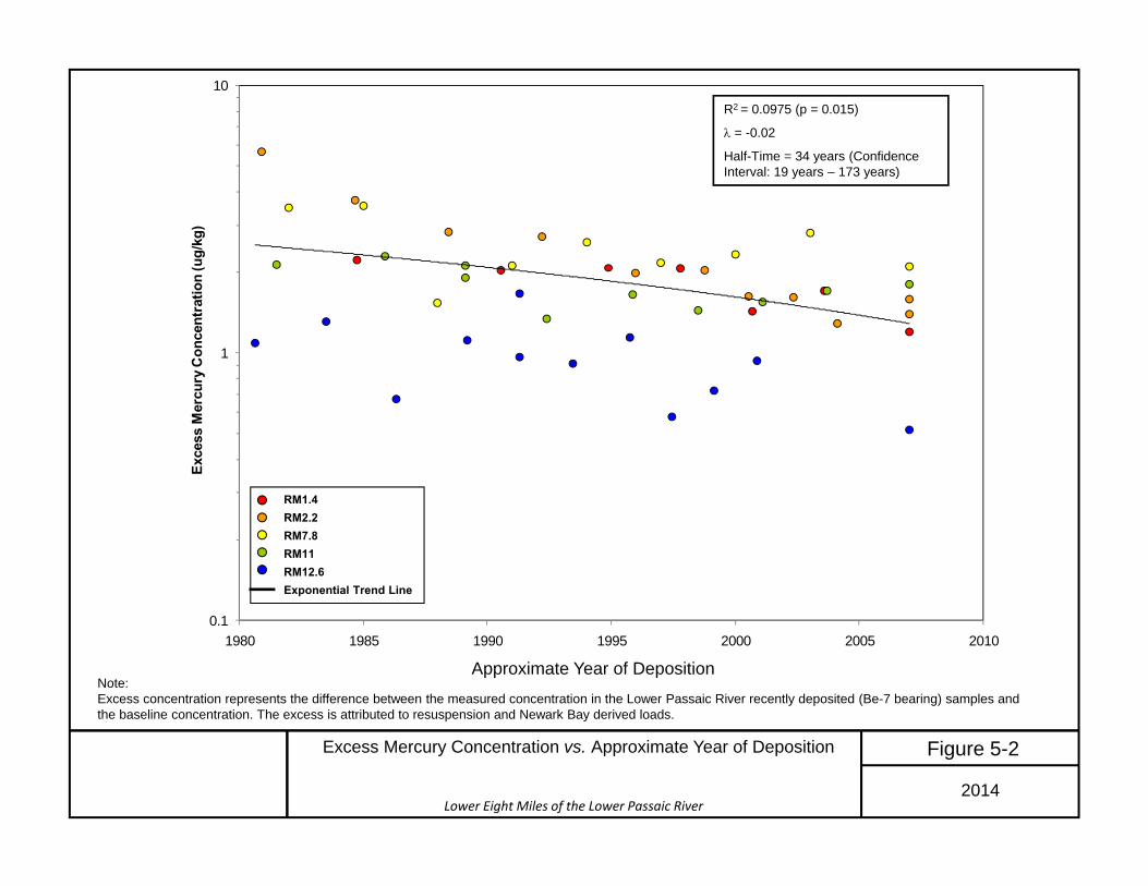
Lower Eight Miles of the Lower Passaic River2014
Figure 5-2Excess Mercury Concentration vs. Approximate Year of Deposition
Note:Excess concentration represents the difference between the measured concentration in the Lower Passaic River recently deposited (Be-7 bearing) samples and the baseline concentration. The excess is attributed to resuspension and Newark Bay derived loads.
RM1.4 RM2.2RM7.8RM11RM12.6Exponential Trend Line
0.1
1
10
1980 1985 1990 1995 2000 2005 2010
Exce
ss M
ercu
ry C
once
ntra
tion
(ug/
kg)
R2 = 0.0975 = -0.0201Half -Life = 34 years
Approximate Year of Deposition
RM1.4 RM2.2RM7.8RM11RM12.6Exponential Trend Line
R2 = 0.0975 (p = 0.015)
= -0.02
Half-Time = 34 years (Confidence Interval: 19 years – 173 years)

Lower Eight Miles of the Lower Passaic River2014
Figure 5-3Excess Lead Concentration vs. Approximate Year of Deposition
Note:Excess concentration represents the difference between the measured concentration in the Lower Passaic River recently deposited (Be-7 bearing) samples and the baseline concentration. The excess is attributed to resuspension and Newark Bay derived loads.
10
100
1000
1980 1985 1990 1995 2000 2005 2010
Exce
ss L
ead
Con
cent
ratio
n (u
g/kg
)
R2 = 0.116 = -0.0175Half -Life = 40 years
Approximate Year of Deposition
RM1.4 RM2.2RM7.8RM11RM12.6Exponential Trend Line
R2 = 0.116 (p <0.01)
= -0.0175
Half-Time = 39.5 years (Confidence Interval: 23 years – 151 years)
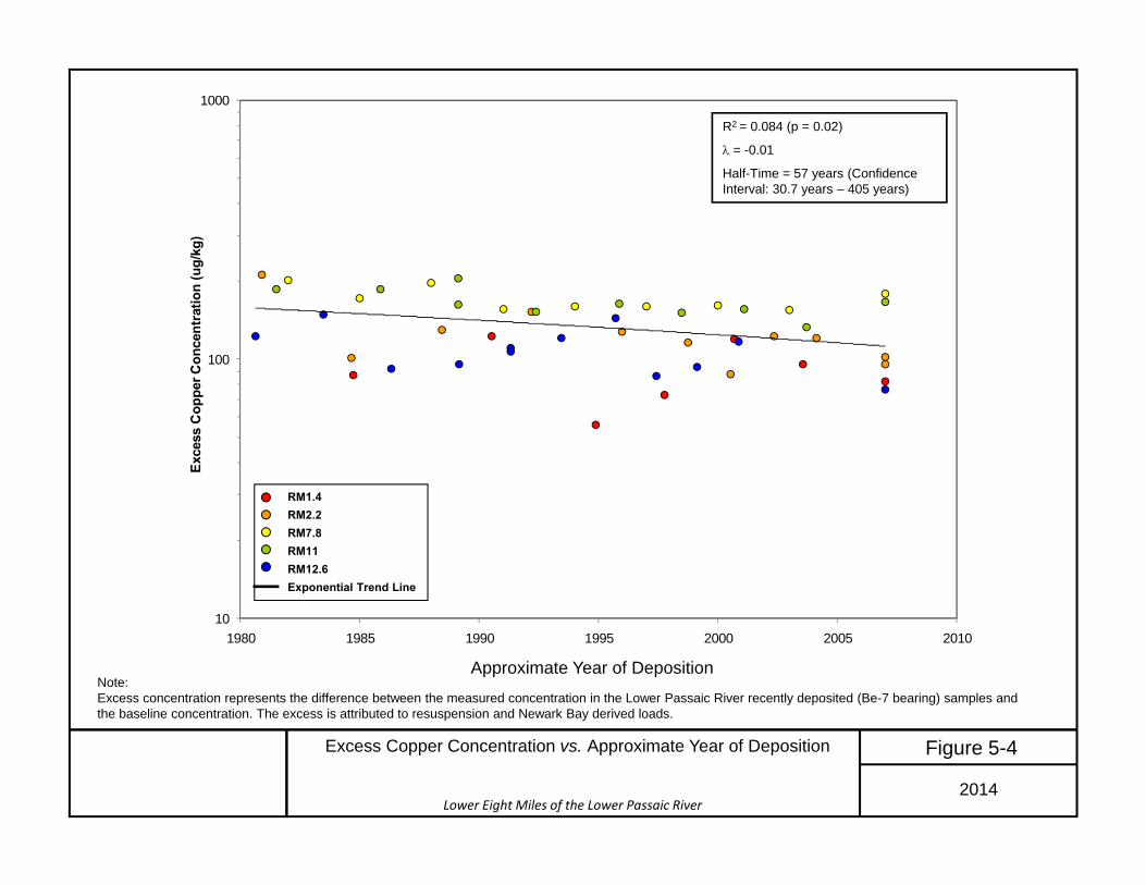
Lower Eight Miles of the Lower Passaic River2014
Figure 5-4Excess Copper Concentration vs. Approximate Year of Deposition
Note:Excess concentration represents the difference between the measured concentration in the Lower Passaic River recently deposited (Be-7 bearing) samples and the baseline concentration. The excess is attributed to resuspension and Newark Bay derived loads.
10
100
1000
1980 1985 1990 1995 2000 2005 2010
Exce
ss C
oppe
r Con
cent
ratio
n (u
g/kg
)
R2 = 0.0837 = -0.0122Half -Life = 57 years
Approximate Year of Deposition
RM1.4 RM2.2RM7.8RM11RM12.6Exponential Trend Line
R2 = 0.084 (p = 0.02)
= -0.01
Half-Time = 57 years (Confidence Interval: 30.7 years – 405 years)

Lower Eight Miles of the Lower Passaic River2014
10
100
1,000
1980 1985 1990 1995 2000 2005 2010
Deposition Year
Excess 4,4'‐D
DE Co
ncen
tration (ug/kg)
Figure 5-5Excess 4,4’-DDE Concentration vs. Approximate Year of Deposition
Note:Excess concentration represents the difference between the measured concentration in the Lower Passaic River recently deposited (Be-7 bearing) samples and the baseline concentration. The excess is attributed to resuspension and Newark Bay derived loads.
R2 = 0.407 (p < 0.01)
= -0.036
Half-Time = 19 years (Confidence Interval: 13 years – 33 years)
RM1.4 RM2.2RM7.8RM11RM12.6Exponential Trend Line
Approximate Year of Deposition

Lower Eight Miles of the Lower Passaic River2014
Figure 5-6Excess gamma-Chlordane Concentration vs. Approximate Year of Deposition
Note:Excess concentration represents the difference between the measured concentration in the Lower Passaic River recently deposited (Be-7 bearing) samples and the baseline concentration. The excess is attributed to resuspension and Newark Bay derived loads.
1
10
100
1980 1985 1990 1995 2000 2005 2010
Exce
ss g
amm
a-C
hlor
dane
(tra
ns) C
once
ntra
tion
(ug/
kg)
R2 = -0.0116 = -0.00701Half -Life = 99 years
Approximate Year of Deposition
RM1.4 RM2.2RM7.8RM11RM12.6Exponential Trend Line
R2 = -0.01 (p = 0.44)
= -0.007
Half-Time = 99 years
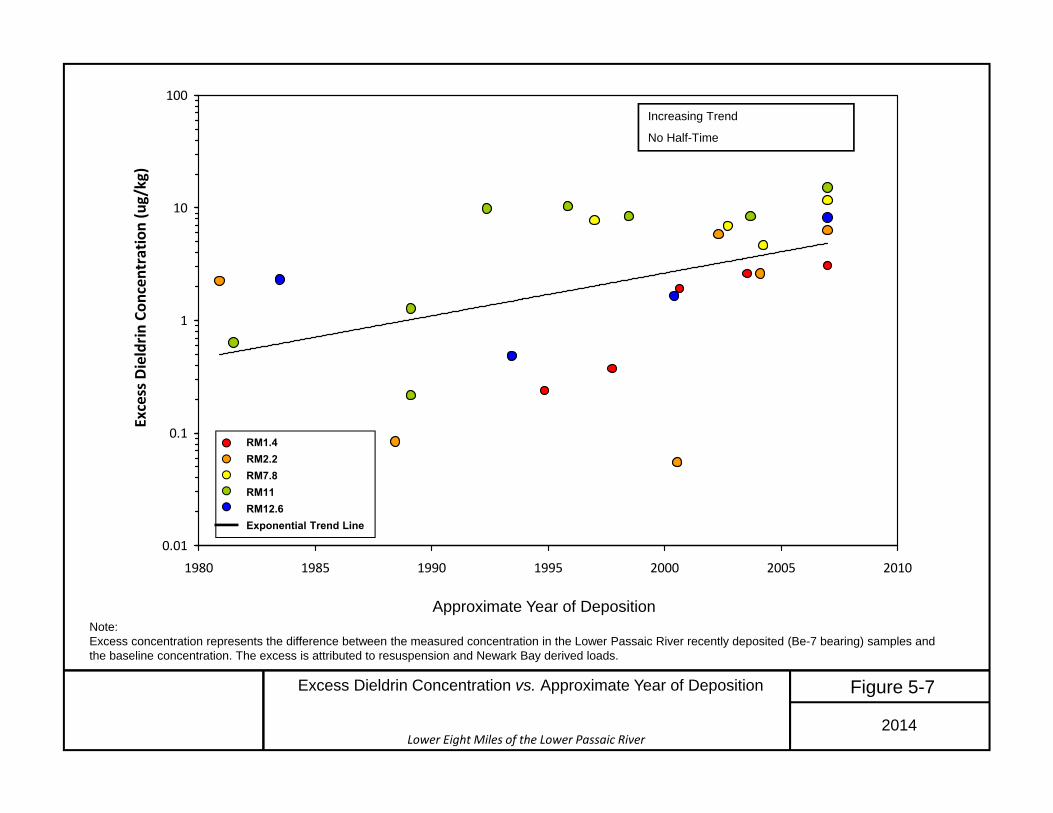
Lower Eight Miles of the Lower Passaic River2014
0.01
0.1
1
10
100
1980 1985 1990 1995 2000 2005 2010
Deposition Year
Excess Dieldrin
Con
centratio
n (ug/kg)
Figure 5-7Excess Dieldrin Concentration vs. Approximate Year of Deposition
Note:Excess concentration represents the difference between the measured concentration in the Lower Passaic River recently deposited (Be-7 bearing) samples and the baseline concentration. The excess is attributed to resuspension and Newark Bay derived loads.
Increasing Trend
No Half-Time
RM1.4 RM2.2RM7.8RM11RM12.6Exponential Trend Line
Approximate Year of Deposition

Lower Eight Miles of the Lower Passaic River2014
100
1,000
10,000
1980 1985 1990 1995 2000 2005 2010
Deposition Year
Excess Total PCB
Con
centratio
n (ug/kg)
Figure 5-8Excess Total PCBs Concentration vs. Approximate Year of Deposition
Note:Excess concentration represents the difference between the measured concentration in the Lower Passaic River recently deposited (Be-7 bearing) samples and the baseline concentration. The excess is attributed to resuspension and Newark Bay derived loads.
R2 = 0.25 (p < 0.01)
= -0.027
Half-Time = 26 years (Confidence Interval: 16 years – 61 years)
RM1.4 RM2.2RM7.8RM11RM12.6Exponential Trend Line
Approximate Year of Deposition
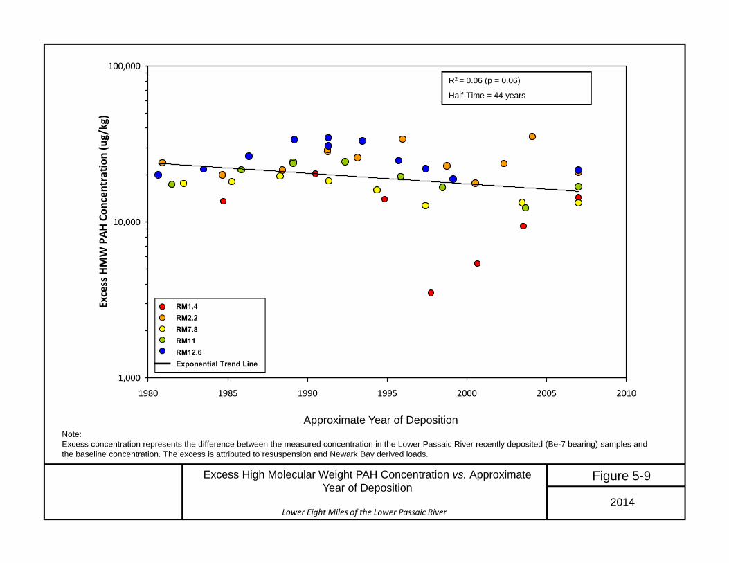
Lower Eight Miles of the Lower Passaic River2014
1,000
10,000
100,000
1980 1985 1990 1995 2000 2005 2010
Deposition Year
Excess HMW PAH
Con
centratio
n (ug/kg)
Figure 5-9Excess High Molecular Weight PAH Concentration vs. Approximate Year of Deposition
Note:Excess concentration represents the difference between the measured concentration in the Lower Passaic River recently deposited (Be-7 bearing) samples and the baseline concentration. The excess is attributed to resuspension and Newark Bay derived loads.
R2 = 0.06 (p = 0.06)
Half-Time = 44 years
RM1.4 RM2.2RM7.8RM11RM12.6Exponential Trend Line
Approximate Year of Deposition

Lower Eight Miles of the Lower Passaic River2014
Figure 5-10Excess Low Molecular Weight PAH Concentration vs. Approximate Year of Deposition
Note:Excess concentration represents the difference between the measured concentration in the Lower Passaic River recently deposited (Be-7 bearing) samples and the baseline concentration. The excess is attributed to resuspension and Newark Bay derived loads.
R2 = 0.19
Half-Time = 25 years
RM1.4 RM2.2RM7.8RM11RM12.6Exponential Trend Line
1,000
10,000
1980 1985 1990 1995 2000 2005 2010
LMW PAH M
easure Con
centration
(ug/kg)
Mid Year
R2 = 0.082 Half‐Life = 63 years
Note that the concentration is not the excess concentration, but the measured concentration for each core
Approximate Year of Deposition
RM1.4 RM2.2RM7.8RM11RM12.6Exponential Trend Line
R2 = 0.07 (p = 0.04)
Half-Time = 63 years

2014Lower Eight Miles of the Lower Passaic River
Figure 5-11a2,3,7,8-TCDD Best Estimates of Trajectories for 0-6 inch Biologically Active Layer
Legend
NoteBest Estimate represents trajectory results using average input values for all parameters.
Alternative 4
Alternative 3
Alternative 2
Alternative 1
1995 TSI Data Set
1995 TSI Dataset
Mean
+ 2 Standard Errors
- 2 Standard Errors
0.001
0.01
0.1
1
10
1990 2000 2010 2020 2030 2040 2050 2060
2,3,
7,8-
TC
DD
Con
cent
ratio
n (u
g/kg
)
Year
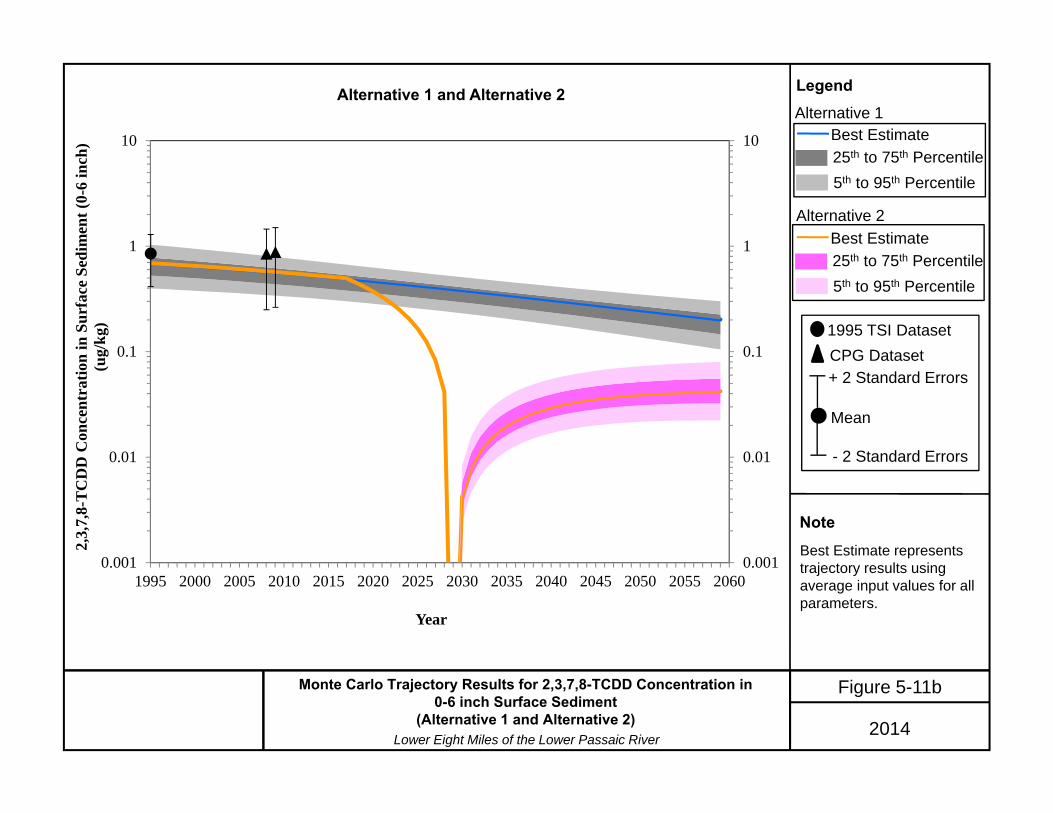
2014Lower Eight Miles of the Lower Passaic River
0.001
0.01
0.1
1
10
0.001
0.01
0.1
1
10
1995 2000 2005 2010 2015 2020 2025 2030 2035 2040 2045 2050 2055 2060
2,3,
7,8-
TC
DD
Con
cent
ratio
n in
Sur
face
Sed
imen
t (0-
6 in
ch)
(ug/
kg)
Year
Figure 5-11bMonte Carlo Trajectory Results for 2,3,7,8-TCDD Concentration in 0-6 inch Surface Sediment
(Alternative 1 and Alternative 2)
Alternative 1 and Alternative 2 LegendAlternative 1
Alternative 2
NoteBest Estimate represents trajectory results using average input values for all parameters.
25th to 75th Percentile5th to 95th Percentile
Best Estimate
25th to 75th Percentile5th to 95th Percentile
Best Estimate
1995 TSI DatasetCPG Dataset
Mean
+ 2 Standard Errors
- 2 Standard Errors
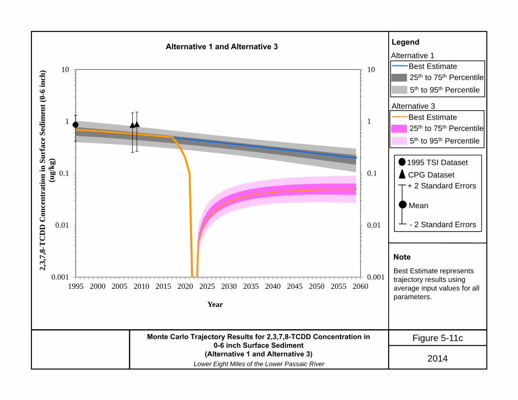
2014Lower Eight Miles of the Lower Passaic River
Figure 5-11cMonte Carlo Trajectory Results for 2,3,7,8-TCDD Concentration in 0-6 inch Surface Sediment
(Alternative 1 and Alternative 3)
Alternative 1 and Alternative 3 LegendAlternative 1
Alternative 3
NoteBest Estimate represents trajectory results using average input values for all parameters.
25th to 75th Percentile5th to 95th Percentile
Best Estimate
25th to 75th Percentile5th to 95th Percentile
Best Estimate
1995 TSI DatasetCPG Dataset
Mean
+ 2 Standard Errors
- 2 Standard Errors
0.001
0.01
0.1
1
10
0.001
0.01
0.1
1
10
1995 2000 2005 2010 2015 2020 2025 2030 2035 2040 2045 2050 2055 2060
2,3,
7,8-
TC
DD
Con
cent
ratio
n in
Sur
face
Sed
imen
t (0-
6 in
ch)
(ug/
kg)
Year
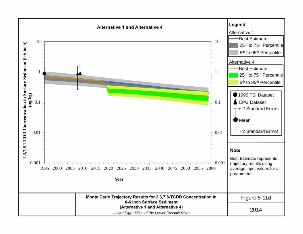
2014Lower Eight Miles of the Lower Passaic River
Figure 5-11dMonte Carlo Trajectory Results for 2,3,7,8-TCDD Concentration in 0-6 inch Surface Sediment
(Alternative 1 and Alternative 4)
Alternative 1 and Alternative 4 LegendAlternative 1
Alternative 4
NoteBest Estimate represents trajectory results using average input values for all parameters.
25th to 75th Percentile5th to 95th Percentile
Best Estimate
25th to 75th Percentile5th to 95th Percentile
Best Estimate
1995 TSI DatasetCPG Dataset
Mean
+ 2 Standard Errors
- 2 Standard Errors
0.001
0.01
0.1
1
10
0.001
0.01
0.1
1
10
1995 2000 2005 2010 2015 2020 2025 2030 2035 2040 2045 2050 2055 2060
2,3,
7,8-
TC
DD
Con
cent
ratio
n in
Sur
face
Sed
imen
t (0-
6 in
ch)
(ug/
kg)
Year

2014Lower Eight Miles of the Lower Passaic River
Figure 5-12aMercury Best Estimates of Trajectories for 0-6 inch Biologically Active Layer
Legend
NoteBest Estimate represents trajectory results using average input values for all parameters.
1995 TSI Dataset
Mean
+ 2 Standard Errors
- 2 Standard Errors
Alternative 4
Alternative 3
Alternative 2
Alternative 1
1995 TSI Data Set
0.1
1
10
1990 2000 2010 2020 2030 2040 2050 2060
Mer
cury
Con
cent
ratio
n (m
g/kg
)
Year
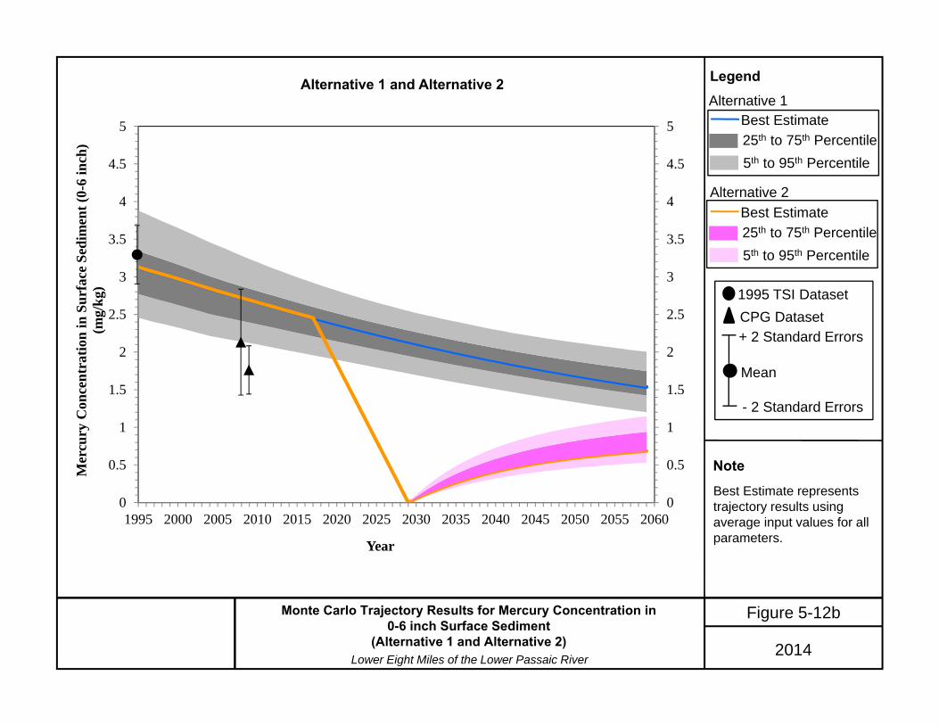
2014Lower Eight Miles of the Lower Passaic River
Figure 5-12bMonte Carlo Trajectory Results for Mercury Concentration in 0-6 inch Surface Sediment
(Alternative 1 and Alternative 2)
Alternative 1 and Alternative 2 LegendAlternative 1
Alternative 2
NoteBest Estimate represents trajectory results using average input values for all parameters.
25th to 75th Percentile5th to 95th Percentile
Best Estimate
25th to 75th Percentile5th to 95th Percentile
Best Estimate
1995 TSI DatasetCPG Dataset
Mean
+ 2 Standard Errors
- 2 Standard Errors
0
0.5
1
1.5
2
2.5
3
3.5
4
4.5
5
0
0.5
1
1.5
2
2.5
3
3.5
4
4.5
5
1995 2000 2005 2010 2015 2020 2025 2030 2035 2040 2045 2050 2055 2060
Mer
cury
Con
cent
ratio
n in
Sur
face
Sed
imen
t (0-
6 in
ch)
(mg/
kg)
Year
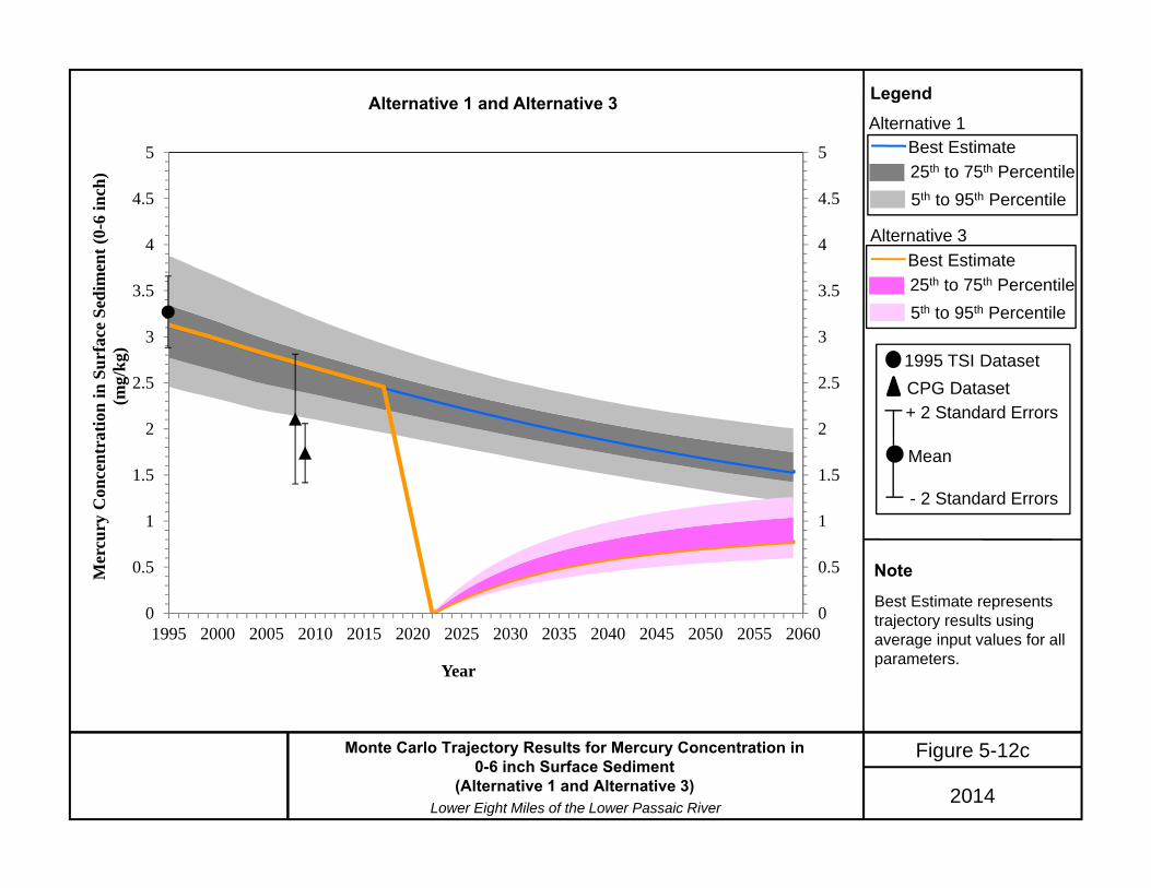
2014Lower Eight Miles of the Lower Passaic River
Figure 5-12cMonte Carlo Trajectory Results for Mercury Concentration in 0-6 inch Surface Sediment
(Alternative 1 and Alternative 3)
Alternative 1 and Alternative 3 LegendAlternative 1
Alternative 3
NoteBest Estimate represents trajectory results using average input values for all parameters.
25th to 75th Percentile5th to 95th Percentile
Best Estimate
25th to 75th Percentile5th to 95th Percentile
Best Estimate
1995 TSI DatasetCPG Dataset
Mean
+ 2 Standard Errors
- 2 Standard Errors
0
0.5
1
1.5
2
2.5
3
3.5
4
4.5
5
0
0.5
1
1.5
2
2.5
3
3.5
4
4.5
5
1995 2000 2005 2010 2015 2020 2025 2030 2035 2040 2045 2050 2055 2060
Mer
cury
Con
cent
ratio
n in
Sur
face
Sed
imen
t (0-
6 in
ch)
(mg/
kg)
Year

2014Lower Eight Miles of the Lower Passaic River
Figure 5-12dMonte Carlo Trajectory Results for Mercury Concentration in 0-6 inch Surface Sediment
(Alternative 1 and Alternative 4)
Alternative 1 and Alternative 4 LegendAlternative 1
Alternative 4
NoteBest Estimate represents trajectory results using average input values for all parameters.
25th to 75th Percentile5th to 95th Percentile
Best Estimate
25th to 75th Percentile5th to 95th Percentile
Best Estimate
1995 TSI DatasetCPG Dataset
Mean
+ 2 Standard Errors
- 2 Standard Errors
0
0.5
1
1.5
2
2.5
3
3.5
4
4.5
5
0
0.5
1
1.5
2
2.5
3
3.5
4
4.5
5
1995 2000 2005 2010 2015 2020 2025 2030 2035 2040 2045 2050 2055 2060
Mer
cury
Con
cent
ratio
n in
Sur
face
Sed
imen
t (0-
6 in
ch)
(mg/
kg)
Year

2014Lower Eight Miles of the Lower Passaic River
Figure 5-13aLead Best Estimates of Trajectories for 0-6 inch Biologically Active Layer
Legend
NoteBest Estimate represents trajectory results using average input values for all parameters.
1995 TSI Dataset
Mean
+ 2 Standard Errors
- 2 Standard Errors
Alternative 4
Alternative 3
Alternative 2
Alternative 1
1995 TSI Data Set
10
100
1,000
1990 2000 2010 2020 2030 2040 2050 2060
Lea
d C
once
ntra
tion
(mg/
kg)
Year

2014Lower Eight Miles of the Lower Passaic River
Figure 5-13bMonte Carlo Trajectory Results for Lead Concentration in 0-6 inch Surface Sediment
(Alternative 1 and Alternative 2)
Alternative 1 and Alternative 2 LegendAlternative 1
Alternative 2
NoteBest Estimate represents trajectory results using average input values for all parameters.
25th to 75th Percentile5th to 95th Percentile
Best Estimate
25th to 75th Percentile5th to 95th Percentile
Best Estimate
1995 TSI DatasetCPG Dataset
Mean
+ 2 Standard Errors
- 2 Standard Errors
0
50
100
150
200
250
300
350
400
0
50
100
150
200
250
300
350
400
1995 2000 2005 2010 2015 2020 2025 2030 2035 2040 2045 2050 2055 2060
Lea
d C
once
ntra
tion
in S
urfa
ce S
edim
ent (
0-6
inch
)(m
g/kg
)
Year

2014Lower Eight Miles of the Lower Passaic River
Figure 5-13cMonte Carlo Trajectory Results for Lead Concentration in 0-6 inch Surface Sediment
(Alternative 1 and Alternative 3)
Alternative 1 and Alternative 3 LegendAlternative 1
Alternative 3
NoteBest Estimate represents trajectory results using average input values for all parameters.
25th to 75th Percentile5th to 95th Percentile
Best Estimate
25th to 75th Percentile5th to 95th Percentile
Best Estimate
1995 TSI DatasetCPG Dataset
Mean
+ 2 Standard Errors
- 2 Standard Errors
0
50
100
150
200
250
300
350
400
0
50
100
150
200
250
300
350
400
1995 2000 2005 2010 2015 2020 2025 2030 2035 2040 2045 2050 2055 2060
Lea
d C
once
ntra
tion
in S
urfa
ce S
edim
ent (
0-6
inch
)(m
g/kg
)
Year

2014Lower Eight Miles of the Lower Passaic River
Figure 5-13dMonte Carlo Trajectory Results for Lead Concentration in 0-6 inch Surface Sediment
(Alternative 1 and Alternative 4)
Alternative 1 and Alternative 4 LegendAlternative 1
Alternative 4
NoteBest Estimate represents trajectory results using average input values for all parameters.
25th to 75th Percentile5th to 95th Percentile
Best Estimate
25th to 75th Percentile5th to 95th Percentile
Best Estimate
1995 TSI DatasetCPG Dataset
Mean
+ 2 Standard Errors
- 2 Standard Errors
0
50
100
150
200
250
300
350
400
0
50
100
150
200
250
300
350
400
1995 2000 2005 2010 2015 2020 2025 2030 2035 2040 2045 2050 2055 2060
Lea
d C
once
ntra
tion
in S
urfa
ce S
edim
ent (
0-6
inch
)(m
g/kg
)
Year
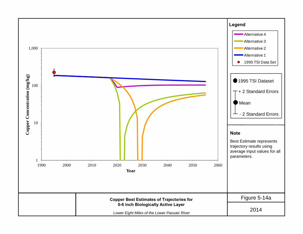
2014Lower Eight Miles of the Lower Passaic River
Figure 5-14aCopper Best Estimates of Trajectories for 0-6 inch Biologically Active Layer
Legend
NoteBest Estimate represents trajectory results using average input values for all parameters.
1995 TSI Dataset
Mean
+ 2 Standard Errors
- 2 Standard Errors
Alternative 4
Alternative 3
Alternative 2
Alternative 1
1995 TSI Data Set
1
10
100
1,000
1990 2000 2010 2020 2030 2040 2050 2060
Cop
per
Con
cent
ratio
n (m
g/kg
)
Year

2014Lower Eight Miles of the Lower Passaic River
Figure 5-14bMonte Carlo Trajectory Results for Copper Concentration in 0-6 inch Surface Sediment
(Alternative 1 and Alternative 2)
Alternative 1 and Alternative 2 LegendAlternative 1
Alternative 2
NoteBest Estimate represents trajectory results using average input values for all parameters.
25th to 75th Percentile5th to 95th Percentile
Best Estimate
25th to 75th Percentile5th to 95th Percentile
Best Estimate
1995 TSI DatasetCPG Dataset
Mean
+ 2 Standard Errors
- 2 Standard Errors
0
50
100
150
200
250
300
0
50
100
150
200
250
300
1995 2000 2005 2010 2015 2020 2025 2030 2035 2040 2045 2050 2055 2060
Cop
per
Con
cent
ratio
n in
Sur
face
Sed
imen
t (0-
6 in
ch)
(mg/
kg)
Year

2014Lower Eight Miles of the Lower Passaic River
Figure 5-14cMonte Carlo Trajectory Results for Copper Concentration in 0-6 inch Surface Sediment
(Alternative 1 and Alternative 3)
Alternative 1 and Alternative 3 LegendAlternative 1
Alternative 3
NoteBest Estimate represents trajectory results using average input values for all parameters.
25th to 75th Percentile5th to 95th Percentile
Best Estimate
25th to 75th Percentile5th to 95th Percentile
Best Estimate
1995 TSI DatasetCPG Dataset
Mean
+ 2 Standard Errors
- 2 Standard Errors
0
50
100
150
200
250
300
0
50
100
150
200
250
300
1995 2000 2005 2010 2015 2020 2025 2030 2035 2040 2045 2050 2055 2060
Cop
per
Con
cent
ratio
n in
Sur
face
Sed
imen
t (0-
6 in
ch)
(mg/
kg)
Year

2014Lower Eight Miles of the Lower Passaic River
Figure 5-14dMonte Carlo Trajectory Results for Copper Concentration in 0-6 inch Surface Sediment
(Alternative 1 and Alternative 4)
Alternative 1 and Alternative 4 LegendAlternative 1
Alternative 4
NoteBest Estimate represents trajectory results using average input values for all parameters.
25th to 75th Percentile5th to 95th Percentile
Best Estimate
25th to 75th Percentile5th to 95th Percentile
Best Estimate
1995 TSI DatasetCPG Dataset
Mean
+ 2 Standard Errors
- 2 Standard Errors
0
50
100
150
200
250
300
0
50
100
150
200
250
300
1995 2000 2005 2010 2015 2020 2025 2030 2035 2040 2045 2050 2055 2060
Cop
per
Con
cent
ratio
n in
Sur
face
Sed
imen
t (0-
6 in
ch)
(mg/
kg)
Year
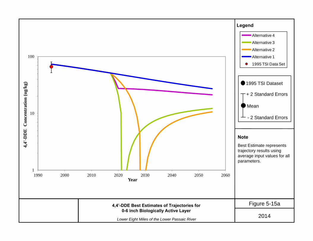
2014Lower Eight Miles of the Lower Passaic River
Figure 5-15a4,4’-DDE Best Estimates of Trajectories for 0-6 inch Biologically Active Layer
Legend
NoteBest Estimate represents trajectory results using average input values for all parameters.
1995 TSI Dataset
Mean
+ 2 Standard Errors
- 2 Standard Errors
Alternative 4
Alternative 3
Alternative 2
Alternative 1
1995 TSI Data Set
1
10
100
1990 2000 2010 2020 2030 2040 2050 2060
4,4'
-DD
E C
once
ntra
tion
(ug/
kg)
Year

2014Lower Eight Miles of the Lower Passaic River
Figure 5-15bMonte Carlo Trajectory Results for 4,4’-DDE Concentration in 0-6 inch Surface Sediment
(Alternative 1 and Alternative 2)
Alternative 1 and Alternative 2 LegendAlternative 1
Alternative 2
NoteBest Estimate represents trajectory results using average input values for all parameters.
25th to 75th Percentile5th to 95th Percentile
Best Estimate
25th to 75th Percentile5th to 95th Percentile
Best Estimate
1995 TSI DatasetCPG Dataset
Mean
+ 2 Standard Errors
- 2 Standard Errors
0
20
40
60
80
100
120
0
20
40
60
80
100
120
1995 2000 2005 2010 2015 2020 2025 2030 2035 2040 2045 2050 2055 2060
4,4'
-DD
E C
once
ntra
tion
in S
urfa
ce S
edim
ent (
0-6
inch
)(u
g/kg
)
Year

2014Lower Eight Miles of the Lower Passaic River
Figure 5-15cMonte Carlo Trajectory Results for 4,4’-DDE Concentration in 0-6 inch Surface Sediment
(Alternative 1 and Alternative 3)
Alternative 1 and Alternative 3 LegendAlternative 1
Alternative 3
NoteBest Estimate represents trajectory results using average input values for all parameters.
25th to 75th Percentile5th to 95th Percentile
Best Estimate
25th to 75th Percentile5th to 95th Percentile
Best Estimate
1995 TSI DatasetCPG Dataset
Mean
+ 2 Standard Errors
- 2 Standard Errors
0
20
40
60
80
100
120
0
20
40
60
80
100
120
1995 2000 2005 2010 2015 2020 2025 2030 2035 2040 2045 2050 2055 2060
4, 4
'-DD
E C
once
ntra
tion
in S
urfa
ce S
edim
ent (
0-6
inch
)(u
g/kg
)
Year

2014Lower Eight Miles of the Lower Passaic River
Figure 5-15dMonte Carlo Trajectory Results for 4,4’-DDE Concentration in 0-6 inch Surface Sediment
(Alternative 1 and Alternative 4)
Alternative 1 and Alternative 4 LegendAlternative 1
Alternative 4
NoteBest Estimate represents trajectory results using average input values for all parameters.
25th to 75th Percentile5th to 95th Percentile
Best Estimate
25th to 75th Percentile5th to 95th Percentile
Best Estimate
1995 TSI DatasetCPG Dataset
Mean
+ 2 Standard Errors
- 2 Standard Errors
0
20
40
60
80
100
120
0
20
40
60
80
100
120
1995 2000 2005 2010 2015 2020 2025 2030 2035 2040 2045 2050 2055 2060
4,4'
-DD
E C
once
ntra
tion
in S
urfa
ce S
edim
ent (
0-6
inch
)(u
g/kg
)
Year

2014Lower Eight Miles of the Lower Passaic River
Figure 5-16agamma-Chlordane Best Estimates of Trajectories for 0-6 inch Biologically Active Layer
Legend
NoteBest Estimate represents trajectory results using average input values for all parameters.
1995 TSI Dataset
Mean
+ 2 Standard Errors
- 2 Standard Errors
Alternative 4
Alternative 3
Alternative 2
Alternative 1
1995 TSI Data Set
1
10
100
1990 2000 2010 2020 2030 2040 2050 2060
Gam
ma-
Chl
orda
ne C
once
ntra
tion
(ug/
kg)
Year

2014Lower Eight Miles of the Lower Passaic River
Figure 5-16bMonte Carlo Trajectory Results for gamma-Chlordane Concentration in 0-6 inch Surface Sediment
(Alternative 1 and Alternative 2)
Alternative 1 and Alternative 2 LegendAlternative 1
Alternative 2
NoteBest Estimate represents trajectory results using average input values for all parameters.
25th to 75th Percentile5th to 95th Percentile
Best Estimate
25th to 75th Percentile5th to 95th Percentile
Best Estimate
1995 TSI DatasetCPG Dataset
Mean
+ 2 Standard Errors
- 2 Standard Errors
0
5
10
15
20
25
30
35
40
0
5
10
15
20
25
30
35
40
1995 2000 2005 2010 2015 2020 2025 2030 2035 2040 2045 2050 2055 2060Gam
ma-
Chl
orda
ne C
once
ntra
tion
in S
urfa
ce S
edim
ent (
0-6
inch
)(u
g/kg
)
Year
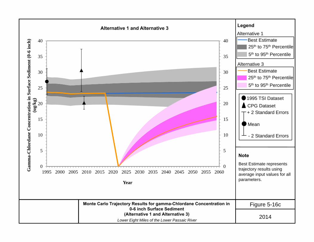
2014Lower Eight Miles of the Lower Passaic River
Figure 5-16cMonte Carlo Trajectory Results for gamma-Chlordane Concentration in 0-6 inch Surface Sediment
(Alternative 1 and Alternative 3)
Alternative 1 and Alternative 3 LegendAlternative 1
Alternative 3
NoteBest Estimate represents trajectory results using average input values for all parameters.
25th to 75th Percentile5th to 95th Percentile
Best Estimate
25th to 75th Percentile5th to 95th Percentile
Best Estimate
1995 TSI DatasetCPG Dataset
Mean
+ 2 Standard Errors
- 2 Standard Errors
0
5
10
15
20
25
30
35
40
0
5
10
15
20
25
30
35
40
1995 2000 2005 2010 2015 2020 2025 2030 2035 2040 2045 2050 2055 2060Gam
ma-
Chl
orda
ne C
once
ntra
tion
in S
urfa
ce S
edim
ent (
0-6
inch
)(u
g/kg
)
Year
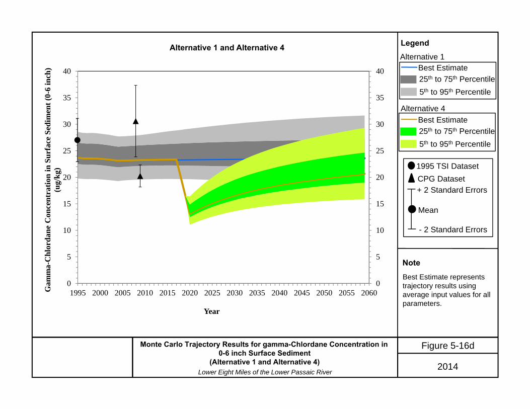
2014Lower Eight Miles of the Lower Passaic River
Figure 5-16dMonte Carlo Trajectory Results for gamma-Chlordane Concentration in 0-6 inch Surface Sediment
(Alternative 1 and Alternative 4)
Alternative 1 and Alternative 4 LegendAlternative 1
Alternative 4
NoteBest Estimate represents trajectory results using average input values for all parameters.
25th to 75th Percentile5th to 95th Percentile
Best Estimate
25th to 75th Percentile5th to 95th Percentile
Best Estimate
1995 TSI DatasetCPG Dataset
Mean
+ 2 Standard Errors
- 2 Standard Errors
0
5
10
15
20
25
30
35
40
0
5
10
15
20
25
30
35
40
1995 2000 2005 2010 2015 2020 2025 2030 2035 2040 2045 2050 2055 2060Gam
ma-
Chl
orda
ne C
once
ntra
tion
in S
urfa
ce S
edim
ent (
0-6
inch
)(u
g/kg
)
Year
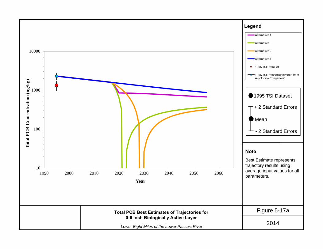
2014Lower Eight Miles of the Lower Passaic River
Figure 5-17aTotal PCB Best Estimates of Trajectories for 0-6 inch Biologically Active Layer
Legend
NoteBest Estimate represents trajectory results using average input values for all parameters.
1995 TSI Dataset
Mean
+ 2 Standard Errors
- 2 Standard Errors
Alternative 4
Alternative 3
Alternative 2
Alternative 1
1995 TSI Data Set
1995 TSI Dataset (converted from Aroclors to Congeners)
10
100
1000
10000
1990 2000 2010 2020 2030 2040 2050 2060
Tota
l PC
B C
once
ntra
tion
(ug/
kg)
Year

2014Lower Eight Miles of the Lower Passaic River
Figure 5-17bMonte Carlo Trajectory Results for Total PCB Concentration in 0-6 inch Surface Sediment
(Alternative 1 and Alternative 2)
Alternative 1 and Alternative 2 LegendAlternative 1
Alternative 2
NoteBest Estimate represents trajectory results using average input values for all parameters.
25th to 75th Percentile5th to 95th Percentile
Best Estimate
25th to 75th Percentile5th to 95th Percentile
Best Estimate
1995 TSI DatasetCPG Dataset
Mean
+ 2 Standard Errors
- 2 Standard Errors
0
500
1000
1500
2000
2500
3000
0
500
1000
1500
2000
2500
3000
1995 2000 2005 2010 2015 2020 2025 2030 2035 2040 2045 2050 2055 2060
Tota
l PC
B C
once
ntra
tion
in S
urfa
ce S
edim
ent (
0-6
inch
)(u
g/kg
)
Year

2014Lower Eight Miles of the Lower Passaic River
Figure 5-17cMonte Carlo Trajectory Results for Total PCB Concentration in 0-6 inch Surface Sediment
(Alternative 1 and Alternative 3)
Alternative 1 and Alternative 3 LegendAlternative 1
Alternative 3
NoteBest Estimate represents trajectory results using average input values for all parameters.
25th to 75th Percentile5th to 95th Percentile
Best Estimate
25th to 75th Percentile5th to 95th Percentile
Best Estimate
1995 TSI DatasetCPG Dataset
Mean
+ 2 Standard Errors
- 2 Standard Errors
0
500
1000
1500
2000
2500
3000
0
500
1000
1500
2000
2500
3000
1995 2000 2005 2010 2015 2020 2025 2030 2035 2040 2045 2050 2055 2060
Tota
l PC
B C
once
ntra
tion
in S
urfa
ce S
edim
ent (
0-6
inch
)(u
g/kg
)
Year

2014Lower Eight Miles of the Lower Passaic River
Figure 5-17dMonte Carlo Trajectory Results for Total PCB Concentration in 0-6 inch Surface Sediment
(Alternative 1 and Alternative 4)
Alternative 1 and Alternative 4 LegendAlternative 1
Alternative 4
NoteBest Estimate represents trajectory results using average input values for all parameters.
25th to 75th Percentile5th to 95th Percentile
Best Estimate
25th to 75th Percentile5th to 95th Percentile
Best Estimate
1995 TSI DatasetCPG Dataset
Mean
+ 2 Standard Errors
- 2 Standard Errors
0
500
1000
1500
2000
2500
3000
0
500
1000
1500
2000
2500
3000
1995 2000 2005 2010 2015 2020 2025 2030 2035 2040 2045 2050 2055 2060
Tota
l PC
B C
once
ntra
tion
in S
urfa
ce S
edim
ent (
0-6
inch
)(u
g/kg
)
Year

2014Lower Eight Miles of the Lower Passaic River
Figure 5-18HMW PAH Best Estimates of Trajectories for 0-6 inch Biologically Active Layer
Legend
NoteBest Estimate represents trajectory results using average input values for all parameters.
Alternative 4
Alternative 3
Alternative 2
Alternative 1
1995 TSI Data Set
1995 TSI Dataset
Mean
+ 2 Standard Errors
- 2 Standard Errors
1,000
10,000
100,000
1990 2000 2010 2020 2030 2040 2050 2060
HM
W P
AH
Con
cent
ratio
n (u
g/kg
)
Year

Appendix C: Mass Balance Modeling Analysis Lower Eight Miles of the Lower Passaic River 2014
ATTACHMENTS
ATTACHMENT A
MONTE CARLO METHODOLOGY FOR UNCERTAINTY ANALYSIS
ON THE EMB MODEL AND FORECAST TRAJECTORIES

Attachment A: Monte Carlo Methodology for Uncertainty Analysis on EMB Model and Forecasts Trajectory.
1.0 Introduction
Environmental systems generally have several sources of uncertainties, and these uncertainties are not only due to a lack of proper measurements, but also due to the randomness inherent in real ecosystems. Incorporating these uncertainties into the modeling process could potentially result in providing useful information that can aid in decision-making.
The EMB model best estimate scenario assumed average values for all model inputs in determining the solids contribution, fate and transport of chemicals, as well as the forecast of future surface sediment concentrations under various remedial scenarios. To incorporate uncertainties in model parameters, a Monte Carlo1 sampling approach was used to develop 10,000 iterations of each input. These 10,000 inputs were optimized in the EMB model and the optimized results were carried through the trajectory forecast calculations. A combination Microsoft Excel® Solver and the Crystal Ball® 7 (Decisioneering, Denver, CO, USA) add-on for Microsoft Excel® (a tool typically used for solving optimization problems), was used to perform this analysis. The objective of the uncertainty analysis was to provide an insight into the level of confidence in the model estimates for the best estimate scenario. This attachment presents the detailed methodology for the Monte Carlo analysis for the EMB model and Trajectory forecasts.
2.0 Methodology The following stages were involved in the uncertainty analysis of the solids and contaminant mass balances, and contaminant forecasts presented in the Appendix C: (a) characterization of uncertainties in EMB model input chemical profiles, (b) estimation of the uncertainty in EMB model optimized outputs resulting from the uncertainty in chemical profiles, and (c) characterization of the uncertainties in model forecast resulting from uncertainties in the input profiles, EMB model outputs of solids contribution, decay of excess contaminant concentrations (lambda), and depth of resuspension reservoir/mixed layer (uncertainty propagation). A schematic diagram illustrating the Monte Carlo methodology is given in Figure A-1 and detailed description is presented below.
1 Monte Carlo simulation is categorized as a sampling method in which the trails or realizations are randomly generated from probability distributions to simulate the process of sampling from an actual population.
Attachment A: Monte Carlo Methodology for Uncertainty Analysis 2014 On the EMB Model and Forecasts Trajectory A-1 Lower Eight Miles of the Lower Passaic River

2.1 Uncertainties in EMB Model chemical input profiles Thirteen chemicals (copper, chromium, mercury, lead, gamma-Chlordane, 4,4’-DDE, 2,3,7,8 TCDD, Total TCDD, Total PCB, benzo(a)pyrene, fluoranthene, iron, and TOC) were optimized in the EMB model to determine the solids balance. The uncertainties in the concentrations of these 13 chemicals for the external sources, and the resuspension source were defined by parametric and non-parametric statistics, respectively. These are described below.
2.1.1 External Sources and Receptor Profiles The observed concentrations for the 13 chemicals for the external sources (Upper Passaic River, Newark Bay, Saddle River, Second River/SWO, Third River, and CSOs) were generally normally distributed. For each external source and the receptor, a bounded normal distribution defined by the mean, standard deviation, minimum, and maximum of each chemical was used to perform Monte Carlo simulation in Crystal Ball® 7. In performing these Monte Carlo simulations, it was important to maintain the relationship amongst the variables. Therefore, for each source, the correlation matrix was also specified in Crystal Ball® 7 to ensure that the 10,000 iterations of chemical profile represented the variability, inter-dependencies, and uncertainty for each external source and the receptor. Figure A-2a though A-2g presents the statistical distributions of chemical concentrations for the 13 chemicals optimized in the EMB model, for the external sources and the receptor.
2.1.2 Resuspension Source Profiles The chemical profiles for the resuspension source were generated based on the TSI 1995 observations. The concentrations of each chemical in this data were neither normal nor log-normal distributed. None of the complex parametric distributions in Crystal Ball® 7 could adequately fit the data set. Therefore, to create the 10,000 iterations of concentrations for the resuspension source profile, a non-parametric simulation method called a bootstrap2 was used.
The basic bootstrap approach uses Monte Carlo sampling to generate an empirical estimate of the sampling distribution of interest. In the bootstrap method, the 1995 data set was treated as the population and a Monte Carlo-style procedure was conducted on it to 10,000 iterations of the mean of the 13 chemicals optimized. This was done as follows:
2 Bootstrap is a powerful Monte Carlo method that re-samples the original sample set with replacement to generate a distribution of sample's statistics. It is a non-parametric method.
Attachment A: Monte Carlo Methodology for Uncertainty Analysis 2014 On the EMB Model and Forecasts Trajectory A-2 Lower Eight Miles of the Lower Passaic River

1. The original sample locations, totaling 92 from the 1995 TSI data set were assumed to define the population of data set in surface sediments for resuspension. Note that in performing this analysis, TSI Location 246 was removed from the data set because the PAH concentrations at this location were not representative of PAH values generally reported in the 1995 TSI data set.
2. The original locations were re-sampled with replacement to generate a bootstrap sample of size 91. This creates a bootstrap data set of the same size as the original, excluding Location 246. By re-sampling the locations rather than each chemical independently, the correlations amongst the chemicals were maintained. Note that this bootstrap sample set may include some sample numbers in the original sample several times, and at the same time other sample numbers may be excluded.
3. Using the chemical concentrations for the locations selected in the 91 bootstrap samples, the average concentration for each chemical was calculated.
4. Steps 2 and 3 were repeated 10,000 times to generate the empirical distribution of the resuspension source profile (Figure A-2h).
The 10,000 average concentrations generated for each chemical via bootstrap for resuspension were used along with the 10,000 iterations for the external sources and receptor to represent the uncertainty in the inputs for EMB model optimization.
2.2 Estimation of uncertainty in EMB Model Output A Microsoft Excel® macro3, which calls the SOLVER routine, was developed to perform the EMB model optimization with the aim of determining the relative solids contributions from the various sources and the mass balance for the chemicals optimized. The macro was used to solve the 10,000 optimizations using the 10,000 iterations of the sources and receptor generated by the Monte Carlo simulation. The results of the optimization run were used to understand the uncertainty in the relative source contributions and chemical mass balance for the Lower Passaic River. The 10,000 EMB model optimized results were also used as input to the trajectory forecast calculations.
3 A Microsoft Excel® macro is a set of instructions written in Visual Basic programming language for Application that can be triggered by a keyboard shortcut, toolbar button or an icon in a spreadsheet. Macros are used to eliminate the need to repeat the steps of common tasks over and over.
Attachment A: Monte Carlo Methodology for Uncertainty Analysis 2014 On the EMB Model and Forecasts Trajectory A-3 Lower Eight Miles of the Lower Passaic River

2.3 Uncertainties in Trajectory Forecast Uncertainties in forecasted chemical concentrations were defined by the results of 10,000 iterations of forecasted values. The chemicals forecasted included: 2,3,7,8-TCDD, mercury, copper, lead, 4,4’-DDE, Total PCB, and gamma-Chlordane. Four remedial alternatives were considered including: No Action (Alternative 1), Deep Dredging with Backfill (Alternative 2), Capping with Dredging for Flooding and Navigation (Alternative 3), and Focused Capping with Dredging for Flooding (Alternative 4). Complete descriptions of these alternatives are provided in FFS Chapter 4 and the assumptions made in the trajectories are given in Appendix C. Forecasting the future concentrations of chemicals under the various remedial scenarios required inputs of (i) chemical concentrations, (ii) solids contributions for the various sources determined by the EMB model optimization, (iii) decay of excess contaminant concentrations (lambda; λ), net sedimentation rate, and (iv) the depth of the sediment mixed layer. Uncertainties in these inputs were defined as follows:
1. Uncertainties in the chemical concentrations were defined by the 10,000 iterations used as inputs to the EMB model optimizations (Figure A-2). For each forecast calculation, the source and receptor profiles were represented by the Monte Carlo generated values as described in Section 2.1 above.
2. Uncertainties in solids contribution from the various sources were obtained from the uncertainty in the solids contributions determined by the EMB model optimization results. This was implemented by using the 10,000 solids contribution results from the EMB model.
3. Uncertainties in decay of excess sediment contamination were defined by the regression between the natural logarithm of the excess concentrations versus time (see Figure C-5-1 to C-5-10 in Appendix C). Using the slope (λ), standard error, and confidence bounds from the regressions, 10,000 iterations of λ were simulated using Monte Carlo sampling from bounded normal distributions (Figure A-3). Note: 𝐻𝑎𝑙𝑓 𝑡𝑖𝑚𝑒 = ln (0.5) 𝜆⁄
4. Uncertainties in the sedimentation rates were generated by bootstrap analysis of the differences between the 1989 and 2007 bathymetric surfaces (Figure A-4).
5. The uncertainties in depth of the sediment mixed layer were generated by 10,000 random numbers between 10 cm to 20 cm in Microsoft Excel®. Note that Microsoft Excel®’s random number generates uniform distributions of the parameter of interest (Figure A-5).
The Microsoft Excel® spreadsheets designed to perform forecast calculations using the best estimate for all inputs were modified to perform the calculations for the 10,000 iterations through
Attachment A: Monte Carlo Methodology for Uncertainty Analysis 2014 On the EMB Model and Forecasts Trajectory A-4 Lower Eight Miles of the Lower Passaic River
a macro. For each iteration, the macro reads the input values of chemical concentrations, λ, sediment deposition rate and mixed layer depth, updates the forecast spreadsheet with these values, and then saves the results of the forecast calculation for all the remedial scenarios.
3.0 Results Uncertainties in the EMB model solution and trajectory forecasts were defined by the confidence interval (5th and 95th percentiles) of the 10,000 optimized solutions. All the results are presented and discussed in Appendix C.
Attachment A: Monte Carlo Methodology for Uncertainty Analysis 2014 On the EMB Model and Forecasts Trajectory A-5 Lower Eight Miles of the Lower Passaic River
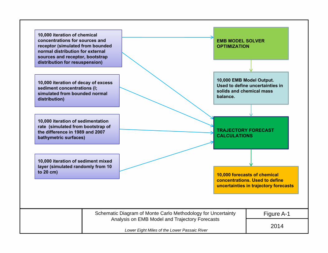
Lower Eight Miles of the Lower Passaic RiverSeptember 2008
Figure A-1Schematic Diagram of Monte Carlo Methodology for Uncertainty Analysis on EMB Model and Trajectory Forecasts
2014
10,000 iteration of chemical concentrations for sources and receptor (simulated from bounded normal distribution for external sources and receptor, bootstrap distribution for resuspension)
10,000 iteration of decay of excess sediment concentrations (l; simulated from bounded normal distribution)
10,000 iteration of sedimentation rate (simulated from bootstrap of the difference in 1989 and 2007 bathymetric surfaces)
10,000 iteration of sediment mixed layer (simulated randomly from 10 to 20 cm)
10,000 EMB Model Output. Used to define uncertainties in solids and chemical mass balance.
EMB MODEL SOLVER OPTIMIZATION
TRAJECTORY FORECAST CALCULATIONS
10,000 forecasts of chemical concentrations. Used to define uncertainties in trajectory forecasts
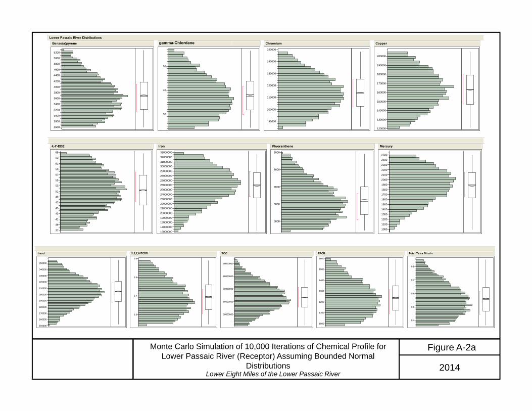
Lower Eight Miles of the Lower Passaic River2014
Figure A-2aMonte Carlo Simulation of 10,000 Iterations of Chemical Profile for Lower Passaic River (Receptor) Assuming Bounded Normal
Distributions
2600
2800
3000
3200
3400
3600
3800
4000
4200
4400
4600
4800
5000
5200
Benzo(a)pyrene
30
40
50
trans-Chlordane
90000
100000
110000
120000
130000
140000
150000
Chromium
120000
130000
140000
150000
160000
170000
180000
190000
200000
Copper
Lower Passaic River Distributions
37
39
41
43
45
47
49
51
53
55
57
59
61
63
65
4,4'-DDE
16000000
17000000
1800000019000000
20000000
21000000
2200000023000000
24000000
25000000
2600000027000000
28000000
29000000
3000000031000000
32000000
33000000
Iron
5000
6000
7000
8000
9000
Fluoranthene
1000
1100
1200
1300
1400
1500
1600
1700
1800
1900
2000
2100
2200
2300
2400
2500
Mercury
150000
160000
170000
180000
190000
200000
210000
220000
230000
240000
250000
Lead
0.3
0.4
0.5
0.6
2,3,7,8-TCDD
50000000
60000000
70000000
80000000
90000000
TOC
1000
1100
1200
1300
1400
1500
1600
TPCB
0.4
0.5
0.6
0.7
0.8
Total Tetra Dioxin
gamma-Chlordane

Lower Eight Miles of the Lower Passaic River2014
Figure A-2bMonte Carlo Simulation of 10,000 Iterations of Chemical Profile for Newark Bay Assuming Bounded Normal Distributions
700
900
1100
1300
1500
1700
1900
2100
2300
2500
2700
2900
3100
Benzo(a)pyrene
3
4
5
6
7
8
9
10
11
12
13
trans-Chlordane
90000
100000
110000
120000
130000
140000
150000
160000
Chromium
90000
100000
110000
120000
130000
140000
150000
160000
170000
180000
190000
Copper
Newark Bay Distributions
10
20
30
40
50
4,4'-DDE
24000000
25000000
26000000
27000000
28000000
29000000
30000000
31000000
32000000
33000000
34000000
35000000
36000000
37000000
38000000
39000000
Iron
2000
3000
4000
Fluoranthene
2000
3000
4000
Mercury
80000
90000
100000
110000
120000
130000
140000
150000
160000
170000
180000
190000
200000
Lead
0.04
0.05
0.06
0.07
0.08
0.09
0.1
0.11
0.12
0.13
2,3,7,8-TCDD
20000000
30000000
40000000
50000000
TOC
400
500
600
700
800
TPCB
0.10.110.120.130.140.150.160.170.180.190.2
0.210.220.230.240.250.260.270.280.29
Total Tetra Dioxin
gamma-Chlordane

Lower Eight Miles of the Lower Passaic River2014
Figure A-2cMonte Carlo Simulation of 10,000 Iterations of Chemical Profile for Upper Passaic River Assuming Bounded Normal Distributions
4 0 0 0
5 0 0 0
6 0 0 0
7 0 0 0
8 0 0 0
9 0 0 0
B e n z o (a )p y re n e
2 0
3 0
4 0
tra n s-C h l o rd a n e
2 0 0 0 0
3 0 0 0 0
4 0 0 0 0
5 0 0 0 0
C h ro m iu m
5 0 0 0 0
6 0 0 0 0
7 0 0 0 0
8 0 0 0 0
C o p p e r
U p p e r P a ssa ic D istr ib u tio n s
8
10
12
14
16
18
20
22
24
26
4,4 '-D D E
130 000 00140 000 00
150 000 00160 000 00170 000 00
180 000 00190 000 00
200 000 00210 000 00220 000 00
230 000 00
I ro n
600 0
700 0
800 0
900 0
100 00
110 00
120 00
130 00
140 00
150 00
160 00
F lu o ra n th e n e
5 006 007 00
9 001 0001 1001 200
1 4001 5001 6001 700
M e rcu ry
90000
100000
110000
120000
130000
140000
150000
160000
Lead
0.001
0.0012
0.0014
0.0016
0.0018
0.002
0.0022
0.0024
0.0026
0.0028
2,3,7,8-TCDD
30000000
40000000
50000000
60000000
70000000
TOC
300
400
500
600
700
TPCB
0.03
0.04
0.05
0.06
0.07
Tota l Tetra Dioxin
gamma-Chlordane

Lower Eight Miles of the Lower Passaic River2014
Figure A-2dMonte Carlo Simulation of 10,000 Iterations of Chemical Profile for Saddle River Assuming Bounded Normal Distributions
260028003000320034003600380040004200440046004800
B e n z o (a )p yre n e
40
50
60
70
tra n s-C h lo rd a n e
150001700019000
2100023000
250002700029000
3100033000
3500037000
C h ro m iu m
30000
40000
50000
60000
70000
C o p p e r
S a d d le R ive r D istrib u tio n s
1 3
1 5
1 7
1 9
2 1
2 3
2 5
2 7
4 ,4 '-D D E
9 0 0 0 0 0 0
1 0 0 0 0 0 0 0
1 1 0 0 0 0 0 0
1 2 0 0 0 0 0 0
1 3 0 0 0 0 0 0
1 4 0 0 0 0 0 0
1 5 0 0 0 0 0 0
1 6 0 0 0 0 0 0
1 7 0 0 0 0 0 0
1 8 0 0 0 0 0 0
I ro n
6 0 0 0
7 0 0 0
8 0 0 0
9 0 0 0
1 0 0 0 0
1 1 0 0 0
F lu o ra n th e n e
7 0
8 0
9 0
1 0 01 1 0
1 2 0
1 3 0
1 4 0
1 5 01 6 0
1 7 0
M e rc u ry
40000
50000
60000
70000
80000
90000
Le a d
0.002
0.003
0.004
0.005
0.006
2,3,7,8-TCDD
30000000
40000000
50000000
60000000
70000000
80000000
TO C
100200
300400500
600700
800900
1000
1100
TP CB
0.019
0.021
0.023
0.025
0.027
0.029
0.031
0.033
Tota l Te tra Diox in
gamma-Chlordane
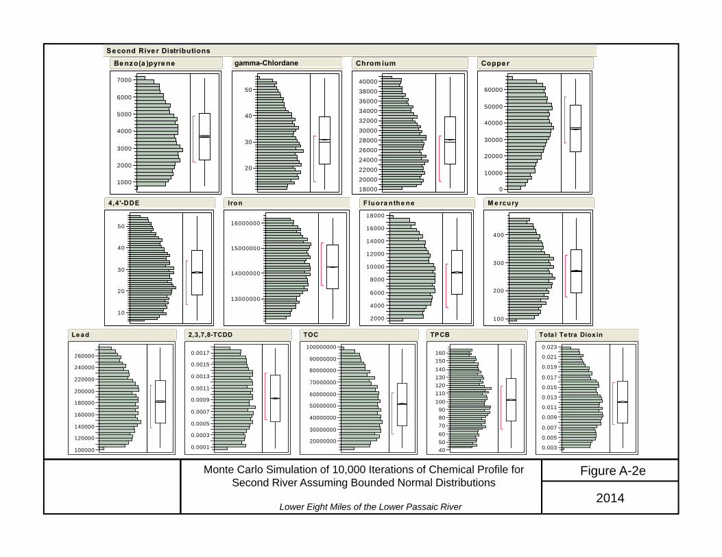
Lower Eight Miles of the Lower Passaic River2014
Figure A-2eMonte Carlo Simulation of 10,000 Iterations of Chemical Profile for Second River Assuming Bounded Normal Distributions
1000
2000
3000
4000
5000
6000
7000
Be nzo(a )pyre ne
20
30
40
50
tra ns-Chlorda ne
180002000022000240002600028000300003200034000360003800040000
Chrom ium
0
10000
20000
30000
40000
50000
60000
Coppe r
Se cond Rive r Distributions
10
20
30
40
50
4,4'-DDE
13000000
14000000
15000000
16000000
Iron
2000
4000
6000
8000
10000
12000
14000
16000
18000
Fluora nthe ne
100
200
300
400
M e rcury
100000
120000
140000
160000
180000
200000
220000
240000
260000
Le ad
0.0001
0.0003
0.0005
0.0007
0.0009
0.0011
0.0013
0.0015
0.0017
2,3,7,8-TCDD
20000000
30000000
40000000
50000000
60000000
70000000
80000000
90000000
100000000
TOC
405060708090
100110120130140150160
TPCB
0.003
0.005
0.007
0.009
0.011
0.013
0.015
0.017
0.019
0.021
0.023
Tota l Te tra Diox in
gamma-Chlordane
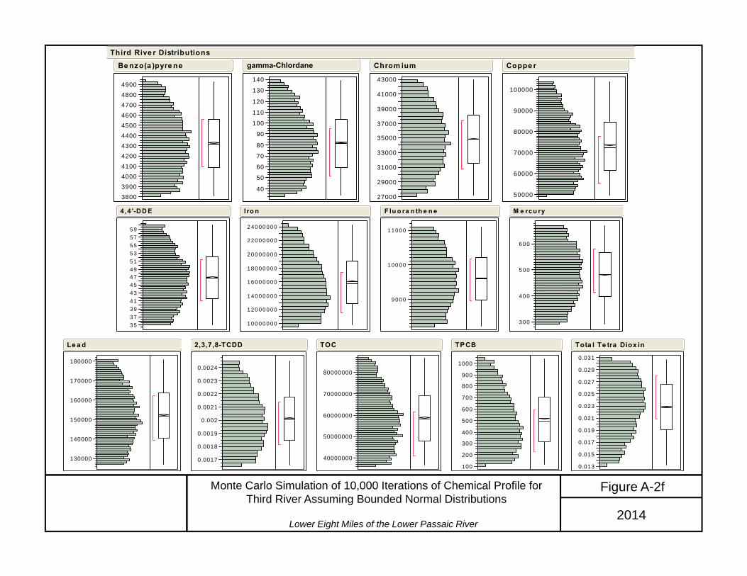
Lower Eight Miles of the Lower Passaic River2014
Figure A-2fMonte Carlo Simulation of 10,000 Iterations of Chemical Profile for Third River Assuming Bounded Normal Distributions
380039004000410042004300440045004600470048004900
Be nzo(a )pyre ne
40
50
60
70
80
90
100
110
120
130
140
tra ns-Chlorda ne
27000
29000
31000
33000
35000
37000
39000
41000
43000
Chrom ium
50000
60000
70000
80000
90000
100000
Coppe r
Third Rive r Distributions
3 53 73 94 14 34 54 74 95 15 35 55 75 9
4 ,4 '-D D E
1 00 0 00 00
1 20 0 00 00
1 40 0 00 00
1 60 0 00 00
1 80 0 00 00
2 00 0 00 00
2 20 0 00 00
2 40 0 00 00
I ro n
9 00 0
1 00 0 0
1 10 0 0
F lu o ra n th e n e
3 00
4 00
5 00
6 00
M e rcu ry
130000
140000
150000
160000
170000
180000
Le a d
0.0017
0.0018
0.0019
0.002
0.0021
0.0022
0.0023
0.0024
2,3,7,8-TCDD
40000000
50000000
60000000
70000000
80000000
TOC
100
200
300
400
500
600
700
800
900
1000
TPCB
0.013
0.015
0.017
0.019
0.021
0.023
0.025
0.027
0.029
0.031
Tota l Te tra Diox in
gamma-Chlordane
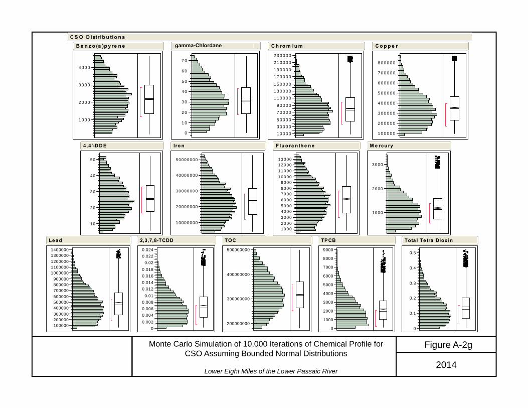
Lower Eight Miles of the Lower Passaic River2014
Figure A-2gMonte Carlo Simulation of 10,000 Iterations of Chemical Profile for CSO Assuming Bounded Normal Distributions
1 0 0 0
2 0 0 0
3 0 0 0
4 0 0 0
B e n z o (a )p y re n e
0
1 0
2 0
3 0
4 0
5 0
6 0
7 0
tra n s-C h lo rd a n e
1 0 0 0 03 0 0 0 05 0 0 0 0
7 0 0 0 09 0 0 0 0
1 1 0 0 0 01 3 0 0 0 01 5 0 0 0 0
1 7 0 0 0 01 9 0 0 0 0
2 1 0 0 0 02 3 0 0 0 0
C h ro m iu m
1 0 0 0 0 0
2 0 0 0 0 0
3 0 0 0 0 0
4 0 0 0 0 0
5 0 0 0 0 0
6 0 0 0 0 0
7 0 0 0 0 0
8 0 0 0 0 0
C o p p e r
C S O D istr ib u tio n s
10
20
30
40
50
4,4 '-D D E
10000000
20000000
30000000
40000000
50000000
I ro n
100020003000400050006000700080009000
10000110001200013000
F lu o ra n th e n e
1000
2000
3000
M e rcu ry
100000200000300000400000500000600000700000800000900000
10000001100000120000013000001400000
Lead
00.0020.0040.0060.008
0.010.0120.0140.0160.018
0.020.0220.024
2,3,7,8-TCDD
200000000
300000000
400000000
500000000
TOC
0
1000
2000
3000
4000
5000
6000
7000
8000
9000
TPCB
0
0.1
0.2
0.3
0.4
0.5
Tota l Te tra Diox in
gamma-Chlordane

Lower Eight Miles of the Lower Passaic River2014
Figure A-2hBootstrap Simulation of 10,000 Iterations of Chemical Profile for Resuspension Source Based on 1995 TSI 0-6 inch Data (TSI Location
246 Excluded)
2 0 0 0
3 0 0 0
4 0 0 0
B e n z o (a )p y re n e
1 9
2 1
2 3
2 5
2 7
2 9
3 1
3 3
3 5
tra n s-C h lo rd a n e
1 2 0 0 0 0
1 3 0 0 0 0
1 4 0 0 0 0
1 5 0 0 0 0
1 6 0 0 0 0
1 7 0 0 0 0
1 8 0 0 0 0
1 9 0 0 0 0
C h ro m iu m
1 7 0 0 0 0
1 9 0 0 0 0
2 1 0 0 0 0
2 3 0 0 0 0
2 5 0 0 0 0
2 7 0 0 0 0
2 9 0 0 0 0
3 1 0 0 0 0
3 3 0 0 0 0
3 5 0 0 0 0
3 7 0 0 0 0
C o p p e r
R e su sp e n sio n D istr ib u tio n s
5 0
6 0
7 0
8 0
9 0
4 ,4 '-D D E
2 2 0 0 0 0 0 0
2 3 0 0 0 0 0 0
2 4 0 0 0 0 0 0
2 5 0 0 0 0 0 0
2 6 0 0 0 0 0 0
2 7 0 0 0 0 0 0
I ro n
4 0 0 0
5 0 0 0
6 0 0 0
7 0 0 0
8 0 0 0
9 0 0 0
1 0 0 0 0
F lu o ra n th e n e
2 6 0 0
2 8 0 0
3 0 0 0
3 2 0 0
3 4 0 0
3 6 0 0
3 8 0 0
4 0 0 0
4 2 0 0
M e rcu ry
270000280000290000300000310000320000330000340000350000360000370000380000390000
Lead
0.3
0.5
0.7
0.9
1.1
1.3
1.5
1.7
1.9
2,3,7,8-TCDD
80000000
90000000
100000000
110000000
120000000
TOC
1400
1600
1800
2000
2200
2400
2600
2800
3000
3200
TPCB
0.4
0.6
0.8
1
1.2
1.4
1.6
1.8
2
Tota l Te tra Diox in
gamma-Chlordane
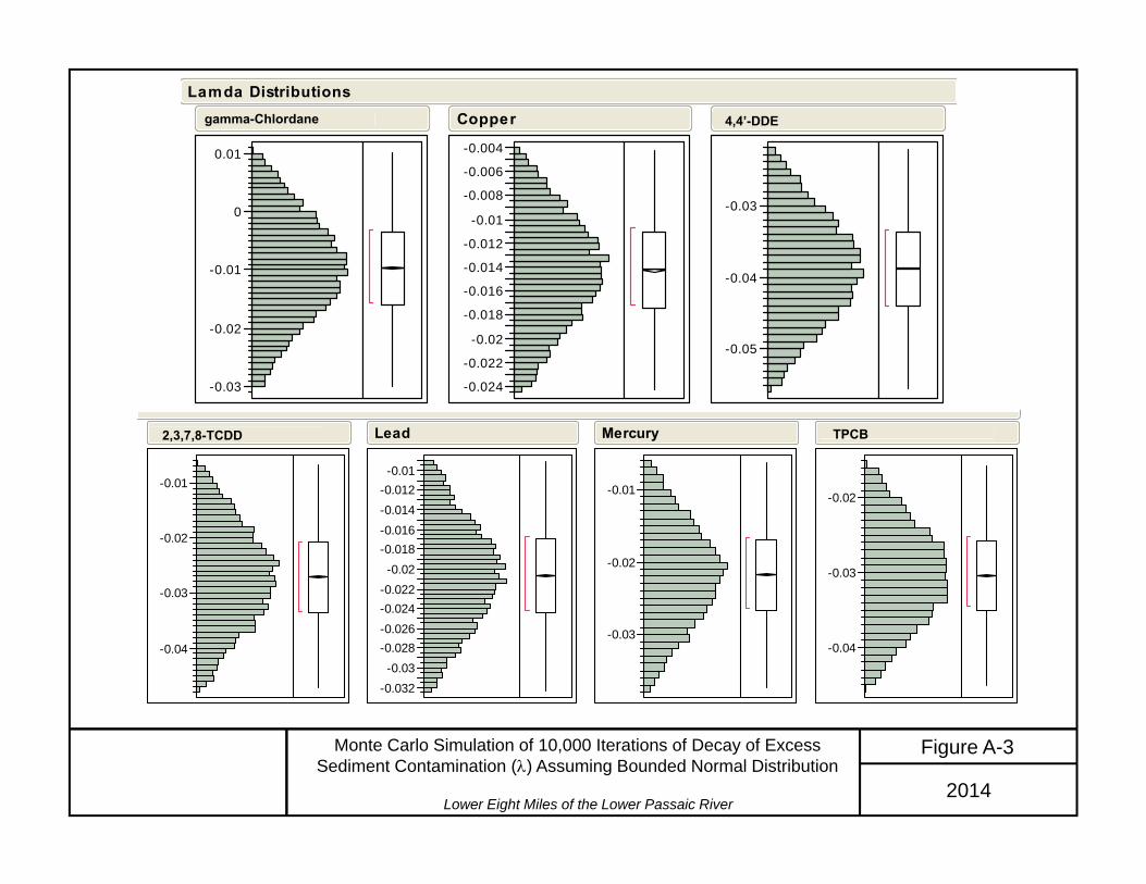
Lower Eight Miles of the Lower Passaic River2014
Figure A-3Monte Carlo Simulation of 10,000 Iterations of Decay of Excess Sediment Contamination () Assuming Bounded Normal Distribution
-0.03
-0.02
-0.01
0
0.01
Chlordane
-0.024
-0.022
-0.02
-0.018
-0.016
-0.014
-0.012
-0.01
-0.008
-0.006
-0.004
Copper
-0.05
-0.04
-0.03
DDE
Lamda Distributions
-0.04
-0.03
-0.02
-0.01
Diox
-0.032-0.03
-0.028-0.026-0.024-0.022-0.02
-0.018-0.016-0.014-0.012-0.01
Lead
-0.03
-0.02
-0.01
Mercury
-0.04
-0.03
-0.02
PCB
gamma-Chlordane 4,4’-DDE
2,3,7,8-TCDD TPCB

Lower Eight Miles of the Lower Passaic River2014
Figure A-4Bootstrap Simulation of 10,000 Iterations of Net Sediment Rate Based on the Differences Between the 1989 and 2007 Bathymetric Surfaces
0.25
0.26
0.27
0.28
0.29
0.3
0.31
0.32
0.33
Net Sediment Rate (in/yr)

Lower Eight Miles of the Lower Passaic River2014
Figure A-5Simulation of 10,000 Depth of Mixed Layer Based on Random Variation Between 10 and 20 cm
10
11
12
13
14
15
16
17
18
19
20
Depth(cm)
ATTACHMENT B
ESTIMATING THE COMMON HALF TIME FOR LEGACY SEDIMENTS
IN LOWER PASSAIC RIVER

Attachment B: Estimating the Common Half Time for Legacy Sediments in Lower Passaic River.
1.0 Summary
A first-order regression model was applied to the excess chemical concentrations1 and estimated time of deposition in the Lower Passaic River in order to determine a common half-time for legacy contaminated sediments. The data used in the model came from high resolution cores collected in the Lower Passaic River, and concentrations observed for the external sources. The chemicals included in the model were: gamma-Chlordane, 2,3,7,8-TCDD, Total PCB, 4,4’-DDE, mercury, lead, and copper. The results of the analysis indicate a common decay process2
for these sediments at an average half time of approximately 35 years. The 95 percent confidence interval for this common half time is from 27 to 48 years. Although only seven chemicals were included in the model, this result also applies to other particle reactive contaminants in the Lower Passaic River that have a significant resuspension source term.
2.0 Objectives • Determine whether the chemical specific decay rates or half times on the excess
concentrations are similar (i.e., no significant difference amongst them). • Estimate the common decay rate for the excess concentrations in legacy sediment in the
Lower Passaic River, along with the associated confidence interval.
3.0 Methods • The chemicals included in the analysis were: gamma-Chlordane, 2,3,7,8-TCDD, Total
PCB, 4,4’-DDE, mercury, lead, and copper. • High-resolution core and external source data were used in the analysis. For the high
resolution cores, data were limited to segments with approximate years from 1980 to 2007.
• A multiple-regression analysis was conducted to determine the similarities and differences amongst the half times of the various chemicals. This model combined the excess concentrations and time of deposition for all the chemicals. In addition, it included indicator variables for the chemical type and allowed for interaction effects between deposition time and chemical type. The first-order regression model used was:
1 Excess chemical concentrations were defined as the Lower Passaic River sediment concentrations less the concentrations from the external sources. 2 The term decay is used here to quantify the net processes that result in the decline of chemical concentrations over time as observed in the high resolution cores. Attachment B: Estimating the Common Half Time for 2014 Legacy Sediments in Lower Passaic River B-1 Lower Eight Miles of the Lower Passaic River
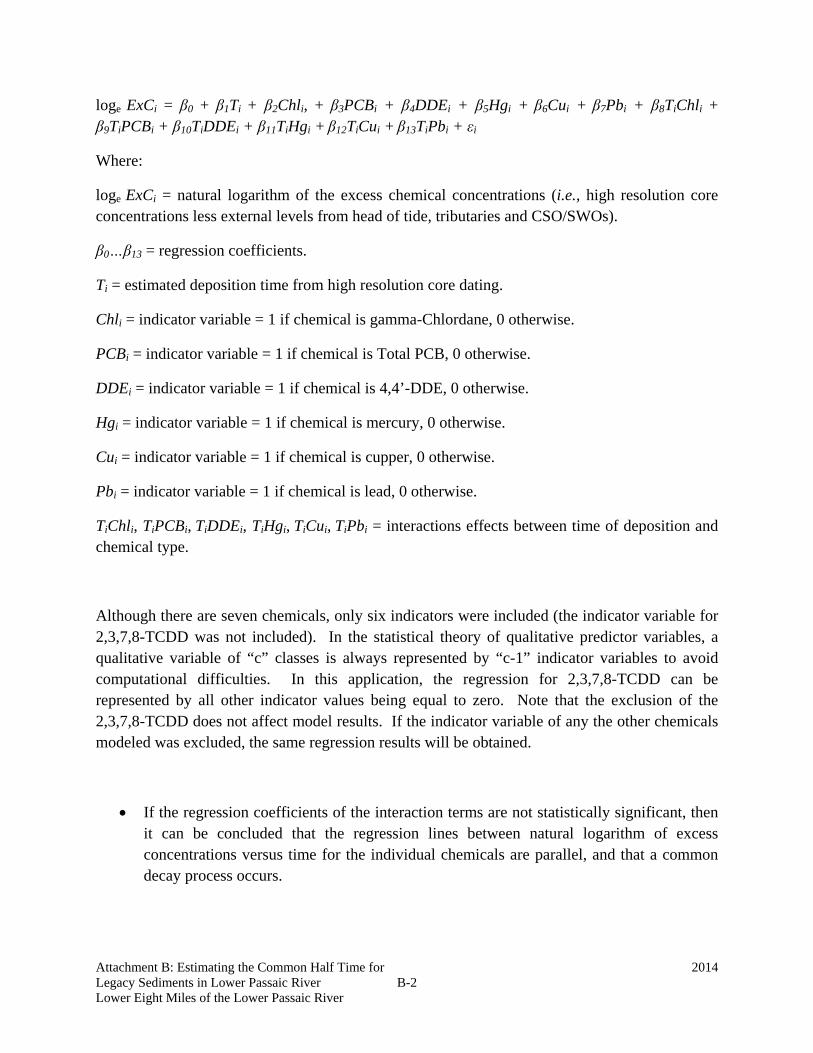
loge ExCi = β0 + β1Ti + β2Chli, + β3PCBi + β4DDEi + β5Hgi + β6Cui + β7Pbi + β8TiChli + β9TiPCBi + β10TiDDEi + β11TiHgi + β12TiCui + β13TiPbi + εi
Where:
loge ExCi = natural logarithm of the excess chemical concentrations (i.e., high resolution core concentrations less external levels from head of tide, tributaries and CSO/SWOs).
β0…β13 = regression coefficients.
Ti = estimated deposition time from high resolution core dating.
Chli = indicator variable = 1 if chemical is gamma-Chlordane, 0 otherwise.
PCBi = indicator variable = 1 if chemical is Total PCB, 0 otherwise.
DDEi = indicator variable = 1 if chemical is 4,4’-DDE, 0 otherwise.
Hgi = indicator variable = 1 if chemical is mercury, 0 otherwise.
Cui = indicator variable = 1 if chemical is cupper, 0 otherwise.
Pbi = indicator variable = 1 if chemical is lead, 0 otherwise.
TiChli, TiPCBi, TiDDEi, TiHgi, TiCui, TiPbi = interactions effects between time of deposition and chemical type.
Although there are seven chemicals, only six indicators were included (the indicator variable for 2,3,7,8-TCDD was not included). In the statistical theory of qualitative predictor variables, a qualitative variable of “c” classes is always represented by “c-1” indicator variables to avoid computational difficulties. In this application, the regression for 2,3,7,8-TCDD can be represented by all other indicator values being equal to zero. Note that the exclusion of the 2,3,7,8-TCDD does not affect model results. If the indicator variable of any the other chemicals modeled was excluded, the same regression results will be obtained.
• If the regression coefficients of the interaction terms are not statistically significant, then it can be concluded that the regression lines between natural logarithm of excess concentrations versus time for the individual chemicals are parallel, and that a common decay process occurs.
Attachment B: Estimating the Common Half Time for 2014 Legacy Sediments in Lower Passaic River B-2 Lower Eight Miles of the Lower Passaic River

4.0 Results Table B-1 presents the regression output for the first order model described above. A statistically significant model was obtained (p < 0.001 from Analysis of Variance results). The most important finding from this regression analysis is that the interaction terms are not significant (p > 0.05). Therefore, the individual chemical regressions are parallel and there is a common decay process for the legacy contaminated sediments in the Lower Passaic River. This legacy sediment represents the resuspension source that is the dominant contribution for most chemicals. Note that the residuals of this regression satisfy the regression assumptions of normality and homogeneity of variance.
Given that a common decay process exist for the Lower Passaic River excess legacy chemical concentrations, a second regression run was conducted to estimate the common decay rate and corresponding half time. For this regression run, the interaction terms which are not statistically significant were dropped from the regression equation. Table B-2 and Figure B-1 present the results for this reduced regression output. This reduced model and all the regression coefficients are statistically significant (p < 0.0001), and the chemical specific regressions lines are approximately parallel. The residuals of this reduced regression satisfy the regression assumptions of normality and homogeneity of variance. The regression coefficient for the time of deposition (β1) under the reduced regression model, which represents the common decay rate is -0.02 (Table B-2). This common decay rate corresponds to a half time of approximately 35 years. Using the standard error and t-values from Table B-2 for β1, the 95 percent confidence interval for β1 is -0.026 to -0.014. The corresponding common half time confidence interval is 27 to 48 years.
Attachment B: Estimating the Common Half Time for 2014 Legacy Sediments in Lower Passaic River B-3 Lower Eight Miles of the Lower Passaic River

Table B-1: Regression results with interaction terms
Attachment B: Estimating the Common Half Time for 2014 Legacy Sediments in Lower Passaic River B-4 Lower Eight Miles of the Lower Passaic River
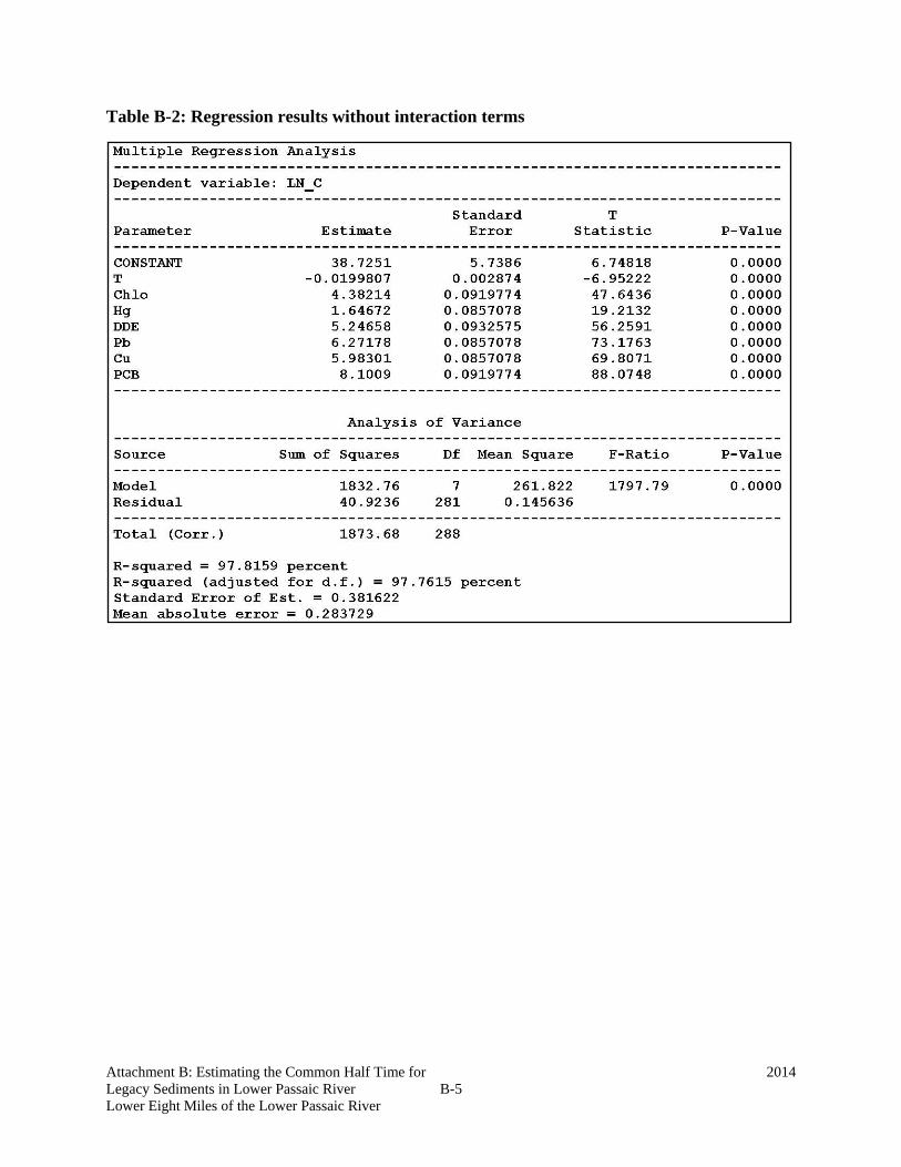
Table B-2: Regression results without interaction terms
Attachment B: Estimating the Common Half Time for 2014 Legacy Sediments in Lower Passaic River B-5 Lower Eight Miles of the Lower Passaic River
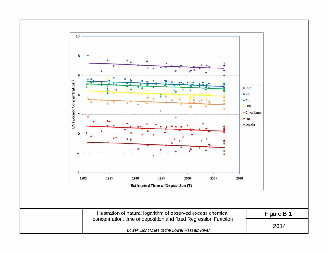
Lower Eight Miles of the Lower Passaic River 2014
Figure B-1Illustration of natural logarithm of observed excess chemical concentration, time of deposition and fitted Regression Function
ATTACHMENT C
DERIVATION OF THE TRAJECTORIES

Attachment C: Derivation of the Trajectories The EMB model and the trajectory calculations are based on the assumption that the contaminant load in the Lower Passaic River is carried to the river on the incoming suspended sediment and that the masses contributed by each source are additive. Based on this assumption, we can develop a mass balance equation for each contaminant like Equation C-1.
CSOCSORRRRSRSRDDDDNBNBRSPRSPTT SCSCSCSCSCSCSCSC ++++++= 2233 Equation C-1
where CT = contaminant concentration on recently deposited sediment (Be-7 bearing) CRSP = contaminant concentration on resuspended sediment within the Lower
Passaic River CNB = contaminant concentration on sediment entering from Newark Bay CDD = contaminant concentration on sediment entering over Dundee Dam (from
the Upper Passaic River) CSR = contaminant concentration on sediment entering from Saddle River C3R = contaminant concentration on sediment entering from Third River C2R = contaminant concentration on sediment entering from Second River and
SWOs CCSO = contaminant concentration on sediment entering from CSOs ST = total solids load in the Lower Passaic River SRSP = total solids load from resuspension within the Lower Passaic River SNB = total solids load delivered from Newark Bay SDD = total solids load delivered over Dundee Dam (from the Upper Passaic
River) SSR = total solids load delivered from Saddle River S3R = total solids load delivered from Third River S2R = total solids load delivered from Second River and SWOs SCSO = total solids load delivered from CSOs If we define fi as the fraction of the total solids load in the Lower Passaic River originating with source, i, we can rewrite Equation C-1 as follows:
CSOCSORRRRSRSRDDDDNBNBRSPRSPLPR fCfCfCfCfCfCfCC ++++++= 2233 Equation C-2
where CLPR = concentration of recently deposited sediment in the Lower Passaic River fRSP = fraction of the Lower Passaic River solids load originating as
resuspension within the river fNB = fraction of the Lower Passaic River solids load originating in Newark
Bay fDD = fraction of the Lower Passaic River solids load originating in the Upper
Passaic River fSR = fraction of the Lower Passaic River solids load originating in the Saddle
River
Attachment C: Derivation of Trajectory C-1 2014 Lower Eight Miles of the Lower Passaic River

f3R = fraction of the Lower Passaic River solids load originating in the Third River
f2R = fraction of the Lower Passaic River solids load originating in the Second River or the SWOs
fCSO = fraction of the Lower Passaic River solids load originating in the CSOs The purpose of the EMB model was to find the best set of fractions for each of the solids sources to balance Equation C-2 for all of the contaminants of concern. The mechanics of the EMB model and the model results are described in more detail in Appendix F of the FFS. Table C-1 below shows the resulting fractions for each source based on the best solution to Equation C-2. Table C-1: EMB Results – Fractional Contributions of Solids from each Source Solids source Percent contribution Resuspension 47.8% Newark Bay 13.5% Upper Passaic River 32.3% Saddle River 3.6% Third River 0.5% Second River and SWOs 1.3% CSOs 0.3% In order to project the contaminant concentrations in the river (CLPR), we need to examine the past behavior of each component of the contaminant loads. In order to avoid including any effects of turning off sources, we will only examine the contaminant histories back to 1980. There is no data available to quantify the past behavior of any of the tributaries or the CSOs and SWOs. Since these sources represent less than 5 percent of the total solids load, they cannot represent a significant portion of any contaminant load. Thus, their future trajectories are not important to this process and we will assume they are constant. An understanding of the past behavior of sediment concentrations in the Upper Passaic River is based on a single high-resolution core from Dundee Lake, which was extracted by scientists at Renssalaer Polytechnic Institute (RPI) and analyzed by the USEPA. This core is described in more detail in Data Evaluation Report No. 3 - Contaminant History as Recorded in the Sediments in Appendix A. For all of the contaminants to be projected except HMW PAHs, the Dundee Lake sediments generally decreased in concentration from 1980 to about 1985 or 1990. After 1990 all contaminants (except HMW PAHs) are generally constant. We can use this information to project the Upper Passaic River component into the future as a constant source. For HMW PAHs, the concentrations seem to decrease from 1980 to the mid 1990s and then they begin to increase. That increase may continue in the future, but for the purposes of this analysis, we will assume a constant concentration from 2005 into the future. This means that the trajectory analysis may be under-predicting the HMW PAHs concentrations in the future.
Attachment C: Derivation of Trajectory C-2 2014 Lower Eight Miles of the Lower Passaic River
The Upper Passaic River component of the Lower Passaic River sediments is not assumed to have been constant in the past, however. The data points from the RPI Core were linearly interpolated to provide a concentration for each year from 1980 to 2005 and the actual measured values were used in the analysis. Newark Bay and the resuspension term are both assumed to be declining, but without any specific information on either source, they cannot easily be separated. Therefore, both were assumed to decay exponentially with the same half time (time required for the concentration to drop by 50 percent). The half time was calculated by separating the constant sources and the Dundee Dam source from the total concentrations reported on the dated high resolution cores from the Lower Passaic River according to the following equation:
CSOCSORRRRSRSRDDDDHRCEX fCfCfCfCfCCC −−−−−= 2233 Equation C-3
where CEX = “excess” concentration (originating from Newark Bay and resuspension) CHRC = concentration reported on the high resolution cores The concentrations for the tributaries and the CSOs were based on averages from the measurements taken during the 2007/2008 sampling events. The concentration for the Upper Passaic River was based on a linear interpolation of data from the dated RPI core from Dundee Lake. The resulting data was fit to an exponential decay curve, defined by Equation C-4.
toeCtC λ−=)( Equation C-4
where C(t) = concentration at time, t Co = concentration at t = 0 λ = decay coefficient t = time The half time of the decay curve can be calculated from the decay coefficient as shown in Equation C-5.
( )λ
21ln
21 =t Equation C-5
where t1/2 = half time for the exponential decay curve The next step is to calculate the concentrations of sediments from each source into the future. For the constant sources (tributaries and SWOs) and the Upper Passaic River, this is easy. These sources are assigned the average concentration from recent sediment samples from 2005 throughout the length of the trajectory. Newark Bay and resuspension contributions must be calculated using the decay rate defined above. Attachment C: Derivation of Trajectory C-3 2014 Lower Eight Miles of the Lower Passaic River
Equation C-4 shows that the limit of the concentration as time approaches infinity is zero. Although we are assuming an exponential decay for Newark Bay, we do not expect the Newark Bay sediment concentrations to reach zero. The EMB model used the northern samples from Newark Bay as the end members. Most contaminants show an increasing trend in concentration from the south to the north end of the bay, probably indicating mixing with Passaic River sediments. For this analysis, we assume that the Newark Bay sediments will never drop below the level recently measured in the southern samples in Newark Bay. This floor value is implemented as shown in Equation C-5, which forces the concentration to approach CFloor as time approaches infinity.
( ) ( )[ ] ( )Floor
tFloorNBNB CeCCtC +−= −− 20052005 λ Equation C-5
where CFloor = minimum concentration on Newark Bay sediments as defined by southern
samples There is also a floor value associated with the resuspended sediment concentrations. Because the resuspending sediment is actually the reworking of old sediment, its concentration cannot drop beneath a floor which is defined as the sum of all other sources. Equation C-6 shows the calculation of the floor for any contaminant. The southern Newark Bay sediments were again used to define the Newark Bay contribution.
CSORRSRDDNB
CSOCSORRRRSRSRDDDDNBNBFloor ffffff
fCfCfCfCfCfCC+++++
+++++=
23
2233 Equation C-6
where CFloor = minimum concentration on resuspended sediments Similar to Equation C-5, the resuspension concentration was calculated using Equation C-7. The 2005 concentration, CRSP(2005) was assigned based on the average concentration measured in the 1995 TSI surface samples.
( ) ( )[ ] ( )Floor
tFloorRSPRSP CeCCtC +−= −− 20052005 λ Equation C-7
where CFloor = minimum concentration on resuspended sediments as defined in Equation C-
6 When all of the components had been projected into the future, Equation C-2 was used to sum them up and predict the future concentration and construct the No Action (Alternative 1) trajectory. Constructing trajectories for the remediation options (Alternatives 2, 3 and 4) involved more manipulations of the data. We can simplify Equation C-2 to Equation C-8 by defining:
Attachment C: Derivation of Trajectory C-4 2014 Lower Eight Miles of the Lower Passaic River

∑ +++++= CSOCSORRRRSRSRDDDDNBNBii fCfCfCfCfCfCfC 2233
Equation C-8
Because the volume of solids contributed by resuspension and the characteristics of those solids change with remediation, we define the remediated concentration of surface sediments in the Lower Passaic River using Equation C-9.
∑+= iiRSPRSPREM fCfCC ''' Equation C-9
where CREM = Lower Passaic River surface concentrations after remediation C’RSP = contaminant concentration on resuspended sediments after remediation f’RSP = fraction of solids originating as resuspension after remediation f’i = fraction of solids originating with source, i, after remediation Using the definition of f, we can convert Equation C-9 to Equation C-10.
T
ii
T
RSPRSPREM S
SCS
SCC''
'' ∑+= Equation C-10
where S’RSP = solids load contributed from resuspension after remediation Si = solids load contributed from source, i S’T = solids load in the Lower Passaic River after remediation We define the following variables: a = the unremediated fraction of the erosional silt areas of the river bed b = the remediated fraction of the erosional silt areas of the river bed a = 1-b c = the amount of resuspension occurring in the remediated areas per unit area as a
fraction of the resuspension occurring in unremediated areas per unit area Using these definitions, we can define the solids load from resuspension after remediation according to Equation C-11.
( ) ( )( )cbSaSS RSPRSPRSP +=' Equation C-11 The first term on the right-hand side of the equation represents the resuspension occurring in the unremediated areas of the river, while the second term includes the resuspension occurring in the remediated areas of the river. This equation can be simplified to Equation C-12.
∑+= iiRSPRSPLPR fCfCC
Attachment C: Derivation of Trajectory C-5 2014 Lower Eight Miles of the Lower Passaic River
( )( )cbSS RSPRSP −−= 11' Equation C-12 The total solids load in the river after remediation can be defined by Equation C-13.
RSPRSPTT SSSS '' +−= Equation C-13 By plugging Equation C-13 into Equation C-12 and simplifying, we get Equation C-14.
( )( )cbSSS RSPTT −−= 1' Equation C-14 We can simplify Equation C-14 further by using the definition for fRSP.
( )( )[ ]T
TRSPTT S
ScbSSS −−= 1'
( )( )( )cbfSS RSPTT −−= 11' Equation C-15 The concentration of the resuspending sediment after remediation is defined by Equation C-16.
( ) ( )( )bca
cbCaCC capRSP
RSP +
+=' Equation C-16
where Ccap = concentration of sediment resuspending from remediated areas As described in Appendix C of the FFS and the Data Evaluation Reports, there is no appreciable dioxin contamination above RM12, so the fraction of solids eliminated by remediating is not the same as the fraction of dioxin mass isolated by remediating. To account for this issue, we define a new variable d, as the difference between a and the fraction of dioxin mass isolated by remediating. For all other contaminants, d will remain zero. This addition to Equation C-16 yields Equation C-17.
( ) ( )( )bca
cbCdaCC capRSP
RSP +
+−=' Equation C-17
where d = the difference between the fraction of solids eliminated by remediating and
the fraction of dioxin mass isolated by remediating Equation C-17 reduces to Equation C-18 using the definition of a.
( ) ( )( )( )cb
cbCdbCC capRSP
RSP −−+−−
=11
1' Equation C-18
Attachment C: Derivation of Trajectory C-6 2014 Lower Eight Miles of the Lower Passaic River
The final equation for the remediated concentration of suspended sediment in the Lower Passaic River can then be developed by substituting Equations C-12, C-15 and C-18 into Equation C-10 as shown in Equation C-19.
( ) ( )( )( ) ( )( )[ ]
( )( )( ) ( )( )( )cbfSfC
cbfS
cbScb
cbCdbC
CRSPT
ii
RSPT
RSPcapRSP
REM −−+
−−
−−
−−+−−
= ∑1111
1111
1
Equation
C-19
Through additional simplification and remembering the definition of fRSP and fi, Equation C-19 can be converted to Equation C-20.
( ) ( )( )( )( )( ) ( )( )cbf
fCcbf
cbCdbCfC
RSP
ii
RSP
capRSPRSPREM −−
+−−
+−−= ∑
11111
Equation C-20
The calculation of Ccap is based on the assumption that there is a 6-inch biologically active zone that is well-mixed and available for resuspension. The average annual sedimentation rate was determined to be 0.27 inches. Based on this data, we can estimate that it takes 22 years to build up a 6-inch layer in the remediated area. Ccap can then be calculated by assuming 5.73 inches have the same concentration as Ccap the previous year and 0.27 inches have the same concentration as the newly deposited sediment (CREM) the previous year. The two pieces are assumed to be completely mixed and Ccap can be calculated as shown in Equation C-21.
( ) ( ) ( )[ ]1121
221
−−+= tREMtcaptcap CCC Equation C-21
where t = time (in years) Equation C-21 is also used to calculate the average concentration in the upper six inches of the sediment in the remediated areas. For the No Action Alternative, the average concentration in the upper six inches is estimated in much the same way, except the 1995 value is estimated as the average of the previous 22 years of Be-7 bearing sediment concentrations. The final necessary calculation is c, which is defined as the amount of resuspension occurring in the remediated areas per unit area as a fraction of the resuspension occurring in unremediated areas per unit area. During remediation, resuspension is assumed to decline linearly until remediation is complete. For Alternatives 2 and 3, immediately after remediation, c is assumed to be zero since the cap or backfill will be made up of sand particles, too large to be suspended under normal hydrodynamic conditions. However, as time passes, more and more sediment will be deposited in the remediated area. At some point, resuspension in the river is assumed to reach the level it had before remediation. For purposes of this analysis, we assume that this level will be reached once the river has deposited a full 6-inch biologically active layer. Using the average annual deposition rate
Attachment C: Derivation of Trajectory C-7 2014 Lower Eight Miles of the Lower Passaic River
of 0.27 inches, this point will be reached 22 years after remediation. For simplicity, the value of c is assumed to move linearly from a value of zero just after remediation is complete (i.e., 2029 for Alternative 2, 2022 for Alternative 3) to a value of one in the year 2051 for Alternative 2 and 2044 for Alternative 3. For Alternative 4, the mixing described in Equation C-21 is also used to calculate the concentration in the upper 6-inch biologically active zone for the unremediated areas below RM8.3. The area averaged concentration across both remediated and unremediated areas was then calculated by assuming one-third of the area below RM8.3 was remediated.
Attachment C: Derivation of Trajectory C-8 2014 Lower Eight Miles of the Lower Passaic River