ANTIRANDOM TESTING: GETTING THE MOST OUT OF BLACK-BOX TESTING*

Yashwant K. Malaiya Computer Science Dept.

Colorado State University Fort Collins, CO 80523

malaiya@cs .colost at e.edu

ABSTRACT

Random testing is a well known concept that re- quires that each test is selected randomly regardless of the test previously applied. This paper introduces the concept of antirandom testing. In this testing strategy each test applied is chosen such that its total distance from all previous tests is maximum. Two distance measures are defined. Procedures to construct anti- random sequences are developed. A checkpoint encod- ing scheme is introduced that allows automatic gener- ation of efficient test cases. Further developments and studies needed are identified.

1 Introduction

Exhaustive testing of software is infeasible except for very small programs [I, 21. Achieving 100% test coverage using a specific measure does not assure that all defects have been found [4, 51. Obtaining total coverage itself may be hard; 85% branch coverage is often used as a target. The testing time, often a sig- nificant fraction of the overall development time, is always limited. The testers thus have the challenging task of making testing as efficient as possible, since the cost of remaining defects in the released code can be very high.

Here we consider black-box testing where only the external specifications are used to obtain test suites. No implementation specific information is assumed to be known. Often software testing is termed random

*This research was supported by a BMDO funded project monitored by ONR

[3, 6, 71. By definition, in random testing the val- ues of the inputs in each test are selected randomly, regardless of the previous tests applied. Random test- ing and its variations have been extensively used and studied for hardware systems.

Random testing avoids the problem of determinis- tic test generation that requires structural information about the program to be processed for generating each test. Available evidence suggests that random testing may be a reasonable choice for obtaining a moderate degree of confidence; however, it becomes very ineffi- cient when the residual defect density becomes low [6].

Random testing does not exploit some informa- tion that is available in black-box testing environment. This information consists of the previous tests applied. If an experienced tester is generating tests by hand, he would select each new test such that it covers some part of the functionality not yet covered by tests al- ready generated. The objective of this paper is to formally define an approach that uses this informa- tion and to propose schemes that may allow such test generation to be done automatically. We term this approach antirandom testing, since selection of each test explicitly depends on the tests already obtained. The problem of generating antirandom sequences is first considered for boolean inputs. to make each new test as different as possible, we use Hamming distance and Cartesian distance as measures of difference. In general, the input variables for a program can be num- bers, characters as well as data structures. Here we also present an approach to efficiently encode the in- put space spanned by such variables into binary. This allows binary antirandom sequences to be decoded into actual inputs.

86 1071-9458/95 $4.00 Q1995 IEEE

Test data selection has been regarded as an im- portant part of testing software [8, 9, 10, 111. Re- searchers have identified valuable guidelines for select- ing test data. We can divide ithe input space into multi-dimensional subdomains such that the software responds to all the points within the same subdomain in a similar way. Both experience and intuitive reason- ing would suggest that a significant fraction of faults would tend to occur at the boundary values. Also since the program behavior for the different points within such a subdomain is likely to be strongly cor- related, testing for just a single internal point in the subdomain may be adequate in many cases. Testing for boolean conditions is discussed in [13, 141. Au- tomated test generation has been considered by some researchers [14, 151. The problem of reducing the number of tests by limiting the total number. of combi- nations to be considered by using orthogonal arrays is given in [16, 171. This approach, although not consid- ered here, can be used in conjunction with the scheme proposed here. One major difference between the two approaches is that antirandom tlesting will test for all input interactions provided sufficient test vectors are applied. It is thus applicable for ultra-high reliability software also.

There can be two possible test scenarios. For large systems, testing would have to be terminated long be- fore it has exhausted all combinations. In this case antirandom testing would attempt to probe well dis- tributed points, resulting in higher defect finding ca- pability. There may be some cases (e.g. unit testing) where exhaustive testing in some sense may be possi- ble (perhaps in terms of equivalence partitioning). In such cases, antirandom testing is likely to find defects sooner, thus reducing the overall test and debugging time.

The next section introduces amd explains the basic concepts used. It also considers the problem of gener- ating binary antirandom test sequences. In the third section, we consider automated testing of software. A checkpoint encoding scheme is introduced th,at reduces the general problem of testing software to generation of antirandom test sequences. Further experimental and theoretical work needed is identified in the sec- ond and the third section as well as in the concluding

section.

2 Binary Antirandom Sequences

Here we start with formal definitions of the terms used and then examine construction of antirandom se- quences. We assume that the input variables are all binary. Definition: Antirandom test sequence (ATS) is a test sequence such that a test ti is chosen such that it satisfies some criterion with respect to all tests t o , t l , ... ti-1 applied before. Definition: Distance is a measure of how different two vectors ti and t j are. Here we use two measures of distance defined below. Definition: Hamming Distance (HD) I181 is the number of bits in which two binary vectors differ. It is not defined for vectors containing continuous values. Definition: Cartesian Distance (CD) between two vectors, A = ( U N , U N - 1 , . . A I , UO} and B = { b ~ , b ~ - l , .. .b l , uo} is given by:

CD(A, E ) =

d(a~ - bN)’ + ( ~ N - I - bN-1)’ + .. + (a0 - bo)’ (1) If all the variables in the two vectors are binary, then equa-

tion 1 can be written as:

C D ( A B) = J l a ~ - b N l + ( ~ N - I - bN-iI+ .. + b o - bo1

Example 1: Consider a pair of vectors: A = (0000} B = (1010) Then HD(A,B) = 2 and CD(A,B) = 1/2 0

Definition: Total Hamming Distance (THD) for any vector is the sum of its Hamming distances with respect to all previous vectors. Definition: Total Cartesian Distance (TCD) for any vector is the sum of its Cartesian distances with respect to all previous vectors. Definition: Maximal Distance Antirandom Test Sequence (MDATS) is a test sequence such that each test t i is chosen to make the total distance be- tween ti and each of to,tl ... t i -1 maximum, i.e.

i -1

TD(ti ) = D(ti , t j ) (3) j =O

87

is maximum for all possible choices of t i . We will use Hamming distance and Cartesian distance to con- struct MHDATSs and MCDATSs.

Example 2: Consider the partial binary test sequence to= {O,O,O,O} and tl= {l,l,l,l}. To construct a 3- test MHDATS, t2 can be any one of the remaining 14 vectors. Both sequences are valid MHDATSs: to= 0 0 0 0 to= 0 0 0 0 t 1 = l l l l tl= 1 1 1 1 t z = 0 0 0 1 t2= 0 0 1 1

For the first sequence THD(t2) = 1 + 3 = 4. For the second sequence also THD(t2) = 2 + 2 = 4.

However, the first sequence is not a MCDATS like the second. For the first sequence TCD(t2) = &+a = 2.732, and for the second TCD(t2) = fi + J"i = 2.828. U

For black-box testing, we have no structural in- formation available about the actual implementation. Using maximal distance criterion, every time we at- tempt to find a test vector as different as possible from all previously applied vectors. The antirandom test- ing scheme thus attempts to keep testing as efficient as possible. In this approach we are using the hypothesis that if two input vectors have only a small distance between them then the sets of faults encountered by the two is likely to have a number of faults in com- mon. Conversely, if the distance between two vectrs is large, then the set of faults detected by one is likely to contain only a few of the faults detected by the other.

If testing is less than exhaustive, then MDAT (max- imum distance antirandom testing) is likely to be more efficient than either random or pseudorandom testing. This is likely to be the case for all practical systems. Even when exhaustive testing is feasible, MDAT is likely to detect the presence of bugs earlier.

When some structural information is available, it is possible to enhance MDAT using educated guesses, just as random testing can be enhanced by using weighted random testing. However, only black-box testing is considered here. A simple but computation- ally expensive procedure may be specified in this way.

Procedure 1. Construction of a MHDATS (MCDATS):

Step 1. For each of N input variables, assign an arbi- trarily chosen value to obtain the first test vector. As discussed below this does not result in any loss of generality.

Step 2. To obtain each new vector, evaluate the THD (TCD) for each of the remaining combinations

with respect to the combinations already chosen and choose one that gives maximal distance. Add it to the set of selected vectors.

Step 3. Repeat step 2 until all 2N combinations have been used. 0

This procedure uses exhaustive search. As we will see later, the computational complexity can be greatly reduced.

To illustrate the process of generating MDATS, we consider in detail the generation of a complete se- quence for three binary variables.

Example 3: For a system, the inputs {x,y,z} can be either 0 or 1. We will illustrate the generation of MHDATS using a cube with each node representing one input combination.

Let us start with the input {O,O,O}. This does not result in any loss of generality. As we will see later, the polarity of any variable can be inverted. The next vector t l of the MHDTS is obviously {l , l , l} with THD(t1) = 3. At this point, the situation is shown in Fig. l a , where the input combinations already cho- sen are marked.

As can be visually seen, a symmetrical situation ex- ists now. Any vector chosen would have HD = 1 from one of the past chosen vectors and HD = 2 from the others. If we allow the variables to be reordered, then without any loss of generality we have the following choices. t o = {O,O,O} ti= {l,l,l}; THD = 3 t 2 = {O, l ,O}; THD = 3 OT tz = {l,O,l}; THD = 3

Let us consider the first choice. After t 2 = {O,l,O}, the clear choice for t 3 is { l , O , l } a t the opposite corner of the cube. The situation now is shown in Fig. lb .

11

110 py'l 000 001 llofjjl 000 001 1 001

101 100 100 I

a b. C.

Figure 1: Construction of 3-bit MHDATS

Again a symmetrical situation exists. Any one of the remaining vectors have the same relationship with the set of vectors already chosen. Let us pick {1,0,0} as t 4 . The next vector t 5 then hm to be { O , l , l } at the opposite corner of the cube. We can again choose any one of two remaining vectors as shown in Fig. IC. Let us choose t6 = { l , l , O } which leaves t7 = {O,O,l}. The

88

complete MHDTS obtained here is given its sequence 1 in Table 1. 13

Table 1: 3-bit MHDTS (Example 3) lTestlxyz ITHD ?m

0 1 1

1.7320 2!.4142 4.146 4.8284 6.5604 7.2426

In this example, it is easy to see that with our cho- sen vectors for to, t l and the two choices for t z , we could have constructed 16 distinct MHDATSs using all of the later choices available. We can verify that all of these are also MCDATSs.

A large number of experiments with construction of MHDATSs and MCDATSs have been done. Based on these, the following results can be stated. Definition: If a sequence B is obtained by rleordering the variables of sequence A, then B is a variable- order-variant (VOV) of A. Theorem 1: If a sequence B is variable-order-variant of a MHDATS (MCDATS) A, then B is also a MH- DATS (MCDATS).

The theorem follows from the fact that Haimming or Cartesian distance is independent of how the variables are ordered.

Example 4: The sequence A below is both a MH- DATS and a MCDATS. The sequence B constructed by switching the second and the third columns is also both MHDATS and MCDATS, as can be verified cal- culating THD and TCD values for all optiolns for t l , t 2 and t 3 .

Sequence A Sequence B t o = 0 0 0 0 0 0 0 0 t 1 = 1 1 1 1 1 1 1 1 t 2 = 1 0 1 0 1 1 0 0 t 3 = 0 1 0 1 0 0 1 1 U

Definition: If a binary sequence B is obtained by changing the polarity (i.e. inverting all the values) of one or more variables of a sequence A, then B is termed a polarity-varknt of A. Theorem 2: If a sequence B is a polarity-variant of a MHDATS (MCDATS) A, then B is also IMHDATS (MCDATS).

The theorem follows from the fact that for a pair of vectors the distance remains the same, if the same

89

set of variables in both are complemented.

Example 5: The sequence B below is obtained by complementing the second and the fourth variables. It can be seen that both are MHDATSs and MCDATSs. Sequence A Sequence B t o= 0 0 0 0 0 1 0 1 t 1 = 1 1 1 1 1 0 1 0 t z = 1 0 1 0 1 1 1 1 t 3 = 0 1 0 1 0 0 0 0 0

Theorem 3: A MHDATS (MCDATS) will always contain complementary pair of vectors, i.e. t z k will always be followed by t 2 k + l which is complementary for all bits in t 2 k where k = 1 ,2 , . . .. Proof: The first two vectors to and t l will always be a complementary pair. Below we will show that if the vectors t o , t l , ..., t 2 k - 1 are complementary pairs, then the vectors t 2 k and t 2 k + l will also be a complementary pair. Thus t 2 and t 3 , hence t 4 and t 5 , etc. will all be complementary paris.

Let us assume a MHDATS contains an even number of vectors, t o , t l . . . t 2 k - 2 , t 2 k - 1 , such that a vector with an odd subscript is a complement of the preceding vector. Let us now assume that a vector t 2 k is found such that its total Hamming (Cartesion) distance from all of t o , ... t 2 k - 1 is maximal.

If we change the polarity of all the variables, we get the sequence . . . t 2 k - 2 , t 2 i - l , t 2 k I where fi in- dicates complement of t i . By Theorem 2 , this is also a MHDATS (MCDATS). Now since 6 = t o ,

= t l etc., the partial sequence f o , & . . . t 2 ; 2 , t 2 k - 1

contains the same vectors as t o , t l ... t 2 k - z 1 t 2 k - 1 but in a different order. Thus t 2 k has the same total Hamming (Cartesian) distance as t 2 k with respect to

Now after having constructed the MHDATS (MC- DATS) t o , t l , . . . t 2 k - 2 , t 2 k - l 1 t 2 k I the addition of t2;+1

= t 2 k will keep it a MHDATS (MCDATS) because: 1. t i k provides the maximal total HD (CD) with

respect to { t o , t l . . & k - 2 , t 2 k - 1 ) .

2. t i k also provides the maximal HD (CD) with re- o spect to t 2 k . QED.

h t l ~ . * t 2 k - 2 , t Z k - I .

So far we have assumed the construction of MH- DATSs (MCDATS) using exhaustive evaluation of all the remaining vectors. Thus for a vector containing N variables, the computation will require evaluation of {1+(2N-1) + (zN-2) + ... 4 + 3 + 2 + 0 ) distances to obtain a complete sequence. Using the above property, the number of evaluations is reduced to (1 + 0 + (2N- 2) + 0 + (2N - 4) + ... 4 + 0 + 0 + 0) distances. That may still represent a prohibitive amount of computa-

tion in situations when N is large. We will next con- sider incremental construction of complete MHDATSs and MCDATSs.

Procedure 2. Expansion of MHDATS (MC- DATS): Step 1. Start with a complete MHDATS of N vari- ables, X N - I , X ~ r - 2 , . . .XI, Xo. Step 2. For each vector t i , i = 0 , 1, ... ( 2 N - 1 ) , add an additional bit corresponding to an added variable X N , such that ti has the maximum total HD (CD with respect to all previous vectors. A

We have extensively experimented with this proce- dure. We have two major observations. 1. It is always possible to extend a MHDATS (MC- DATS) by adding one more variable using Procedure 2. A formal proof for this is being sought. 2 . The column added is a function of columns already included. We are attempting to identify this function such that it does not vary for different values of N and can be used in a simple way.

To illustrate additional aspects of constructing an- tirandom sequences, let us consider the following ex- ample.

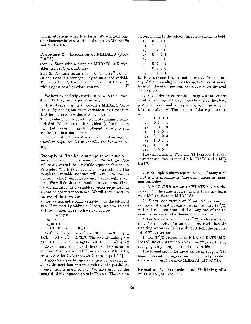
Example 6: Here let us attempt to construct a 4- variable antirandom test sequence. We will use Pro- cedure 2 to extend the %variable sequence obtained in Example 3 (Table 1) by adding an extra column. The complete 4-variable sequence will have 16 vectors as opposed to the %variable sequence we have with 8 vec- tors. We will do the construction in two parts. First, we will augment the 3-variable/8 vector sequence into a 4-variable/8 vector sequence. We will then construct the rest of the 8 vectors. a, Let us append a forth variable w to the lefthand side. If we start by adding a ‘0’ to t o , we have to add a ‘1’ to t l , then for t 2 we have two choices.

w x y z t o = 0 0 0 0 t 1 = 11 1 1

t z = 0 0 1 0 o r t 2 = 1 0 1 0 With the first choice we have THD = 1 + 3 = 4 and

TCD = l/i + a = 2.7320. The second choice gives us THD = 2 + 2 = 4 again, but TCD = f i + f i = 2.8284. Since the second choice would generate a sequence that is a MCDATS as well as a MHDATS, let us use i t for t z . The vector t 3 then is (0 1 0 1).

Using Cartesian distance as a criterion, we can con- struct the next four vectors similarly. the partial se- quence then is given below. We have used up the complete 3 bit sequence given in Table I. The column

corresponding to the added variable is shown in bold. to 0 0 0 0 tl 1 1 1 1 t 2 1 0 1 0 t 3 0 1 0 1 t 4 1 1 0 0 t 5 0 0 1 1 t 6 0 1 1 0 t 6 1 0 0 1

b. Now a symmetrical situation exists. We can use any of the remaining vectors for t s ; however, it would be useful if certain patterns are repeated for the next eight vectors.

Our extensive experimentation suggests that we can construct the rest of the sequence by taking the above partial sequence and simply changing the polarity of leftmost variable w. The last part of the sequence then is:

t 8 1 0 0 0 t g 0 1 1 1 t 1o 0 0 1 0 tll 1 1 0 1 t 1 2 0 1 0 0 t i 3 1 0 1 1 t14 1 1 1 0 t 1 5 0 0 0 1

The calculation of TCD and THD proves that the 16-vector sequence is indeed a MCDATS and a MH- DATS. O

The Example 6 above represents one of many such construction experiments. The observations are sum- marized below.

1. A MCDATS is always a MHDATS but not vice versa. For the same number of bits there are fewer valid MCDATSs than MHDATSs.

2. When constructing an N-variable sequence, a symmetrical situation exists, when the first ( 2 N / 2 ) vectors have been obtained, i.e. any one of the re- maining vectors can be chosen as the next vector.

3. For N-variables, the first ( z N / 2 ) vectors are such that if the polarity of a variable is reversed, then the resulting vectors ( 2 N / 2 ) are distinct from the original set of P / 2 ) vectors.

4. For 2 N / 2 vectors of an N-bit MCDATS (MH- DATS), we can obtain the rest of the 2 N / 2 vectors by changing the polarity of one of the variables.

The formal proofs for these are being sought. The above observations suggest an incremental procedure to construct an N-variable MHDATS (MCDATS).

Procedure 3. MHDATS (MCDATS):

Expansion and Unfolding of a

Step 0. Start with a complete (N-1) variable MH- DATS (MCDATS) with 2N-1 vectors.

Step 1. Expand by adding a v,ariable using Proce- dure 2. We now have the first (2”‘/2) vectors; needed.

Step 2. Complement one of tlhe columns and ap- pend the resulting vectors to first set of vectors ob- tained in Step 1. Here, it woulld be convenient to

0 complement the variable added in Step 1.

N The procedure requires %.f = ZN-’ bits to be

evaluated.

In many cases we would like to obtain an antiran- dom sequence involving a large number of variables. Instead of incrementally expanding and unfolding, can we concatenate m N-bit antirandom sequences to ob- tain a m x N bit antirandom sequence with 2” vectors? Can we obtain the rest of (2m*N -- 2 * N ) vectors in an algorithmic manner to create the complete sequence? Consider the following example.

Example 7: Let us concatenate two copies of the 3- bit antirandom sequence to obtain the following 6 bit sequence. t o 0 0 0 0 0 0 t l 1 1 1 1 1 1 t 2 0 1 0 0 1 0 t 3 1 0 1 1 0 1 t 4 1 0 0 1 0 0 t 5 0 1 1 0 1 1 t 6 1 1 0 1 1 0 t 7 0 0 1 0 0 1

An evaluation shows this to be a MHDATS but not a MCDATS. We can easily see that for a MCDATS, the vector t 2 should have an equal number oi’ones and zeroes. 0

Our experiments suggest that such concatenation should retain the maximal HD property. We need to obtain a formal proof for this. We also need to obtain an algorithmic method to obtain wide MCDATSs and to obtain the rest of the (2“ - 2 N ) vectors. It is our conjecture that it should be possible by using polarity variants of the component arrays.

In some applications it may be possible to order and partition the set of variables! into group of size p, such that effect of variables in one group is disjoint (or nearly disjoint) to the variables in all other groups. In this case, all we need to do is to apply an p-variable antirandom sequence to each group in parallel. This can considerably reduce the test application time.

3 Checkpoint Encoding

In a general case, the inputs can be numbers, al- phanumeric characters as well as data structures com- posed using them. In such cases also we would like to maximize the effectiveness of testing. It is possible for one to define ‘distance’ and use them for constructing antirandom sequences in such cases also.

Example 8: Let us consider two real variables x and y which can range from 0 to 1. The following then is a MCDATS.

0 0 1 1 0.5 0.5

However, defining ‘distance’ can be difficult for data structures. Also for a program, the input variables can be of different types and ranges, which will make construction of antirandom sequences extremely hard. We here propose an encoding approach which will con- vert the problem to constructing binary antirandom sequences. The approach is based on domain and partition analysis and the concepts of equivalence partitioning, revealing subdomains [ll] and ho- mogeneous subdomains [19]. The technique par- tially encodes an input into binary, such that sample points desired can be obtained by automatic transla- tion.

These sample points, termed checkpoints here, are strategically selected such that they are likely to span most types of variations in the program behavior with respect to each input. To illustrate the approach let us consider this simple example. For convenience, we use a square bracket (”[,, or ”I”) to indicate inclu- sion of the endpoint and a parenthesis (”(” or ”)”) to indicate exclusion.

For testing, it is important to test for illegal input values because the program must respond correctly to those inputs, as we see in the following example. The range of illegal values should be regarded as one or more additional equivalent partitions.

Example 9: Consider a continuous input variable c which can range from xman to xmaz, with the end Val- ues included. A value outside of [emin, zmaz] is illegal (Figure 2). Let us call all the values of x such that emin < c < cmaz internal points. Let us assume that the program under test either works correctly or incorrectly for all internal points. We can thus use the following checkpoint encoding scheme as shown in Table 2.

91

- Illega1 Illegal

xrmn X m a X

Encoded Binary

0 0

0 1 1 0 1 1

Value of x randomly chosen value in the illegal range xmin

xmax a randomly chosen internal point

0

In general encoding can take several considerations into account based on specifications and the fault hy- pothesis used.

1. Some fraction of all input values applied should be illegal.

2. Many defects may be associated with bound- ary values. They may not be detected when ”typical” values are used for testing. Some defects may require testing points closest to the boundary on both sides.

3. A legal range of values can often be partitioned into subdomains, such that each subdomain exercises a somewhat different (but not necessarily disjoint) part of the functionality. Thus one can use a fault hypoth- esis that exercising only one such subdomain, defects corresponding to other subdomains may not be trig- gered. 4. With black-box testing, specifications may not

reveal the reasons which would suggest a subdomain should have been further partitioned. Thus there may be a need to sample a few randomly chosen points within a subdomain. In practice, some information about the software structure can be useful for proper identification of subdomains.

5. If some inputs are more critical, there may be a reason to use a larger number of samples for that input. This can be done by using more bits to encode that input.

Let us now see an example that illustrates some of the above considerations.

Example 10: Consider a continuous input variable x which is valid in the range [- a, b]. Let us assume the program may respond differently in subdomains [-a, 0) and (0, b]. In addition, we also wish to sample the function with a couple of values each within both [-a, 01 and (0 , b].

Here we can use the checkpoint encoding scheme shown in Table 3. It attempts to ensure that the spe-

cial cases (boundary and illegal values) are generated early and the adjacent internal points are also adjacent in the Hammine: distance sense. ”

Table 3: Encoding scheme for Example 10 [Encoded 1

Binary 1 0 1 0 0 0 1 0 0 1 1 0 0 1 0 0 1 1 0 1 1 1 1 1

Value of x randomly chosen in the illegal range -a randomly chosen in (-a, -a/2] range randomly chosen in (-a/2, 0) range 0 randomly chosen in (0, b/2) range randomly chosen in [b/2, b) range b

U

After we have encoded all the inputs using binary variables, the problem is simply reduced to that of generating binary antirandom sequences. If the input variable I, j = 0,1, ... M where M is the total number of inputs, is encoded using Cj bits, the binary vectors would be C,”=,Cj bits wide. Notice that the tests generated by this scheme will include common com- binations, likely to be encountered most often during operational use as well as special combinations which have higher error revealing capability.

The proposed scheme, as illustrated in Figure 3, combines the benefit of checkpoint encoding with an- tirandom testing. Once the Checkpoint encoding defi- nition (CED) has been obtained, the tests can be gen- erated automatically. The antirandom vectors gen- erated are translated using the CED. When needed, the random value generator will generate a random value of an input, which may be a single number or a data structure. The advantage of randomization is that when a subdomain for an input variable is en- countered several times, each time a different value is likely to be generated. This would require that the seed values be altered during each access.

The computational requirements of the blocks in- cluded in the Checkpoint Encoded Antirandom test- ing (CEAR) scheme are very light. Thus it may not be necessary to record the set of tests before they are applied. The GEAR and the software under test may run together, a test being used right after it is gen- erated. The GEAR scheme may be implemented to make the test-suite generated either repeatable or non- repeatable. The first option would be suitable if a fixed regression testing test-suite is desired.

We must discuss a very important tradeoff. Many defects can be associated with boundary conditions. Such a condition can be subdomain boundary for a

92

U; ..I .........,.. .. .......... .... ......... I . , . , .......... ... ......... ..... ........ .......

Field Array Size

Element values

F points to

Figure 3: Proposed CEAR scheme with encoded anti- random vectors.

” Bits bO

b3, b2 ,b l

b5,b4

single input variable or a combination of such bound- aries for several input variables. On the other hand, in normal operation, much of the tiime only internal val- ues will occur. Thus the field failure rate may depend more on the faults associated with the values which are not boundary conditions.

In terms of the checkpoint eiicoding scheme, the question can be stated in this ‘way. For each vari- able that is part of the input space, how many check- points should represent ‘common’ values, and how many should be boundary values? We perhaps re- quire a considerable amount of experimental data be- fore we can obtain definite guidelines for answering this question. If we can be certain that there are no unidentified subdomain boundaries (that wild however require examining the software implementation), we could assume that each internal1 subdomain is a re- vealing subdomain, and thus it needs to be sampled only once. For very small software systems, it may be possible to exhaustively test for all boundary val- ues combinations along with a reasonable number of common combinations. However, for a general sys- tem, guidelines for making optimal choices cannot be offered at this time.

Example 11: As a more complete example of check- point encoding, let us consider the FIND program by Hoare (Figure 4). Testing of its FORTRAN version was examined by DeMillo et al. [8]. It takes as an input an integer array A with size N 2 1 and an array index F, 1 L F L N . The program rearranges the array such that all elements to the left of .A(F) have values no larger than A(F), and all elements to the right are no smaller.

The subdomains are identified below; the special cases are marked with an asterisk.

Array size: 1, 2 and greater than two Element values:

all positive, all 0, all negative, illegal (containing non-integers), mixed.

F points to: first element , a middle element, last element outside (illegal)

Array status: 1. elements randomly ordered 2. elements already ordered as needed 3. elements in order reverse of case 2 4. elements all equal

In order to encode the checkpoints efficients, we may want to separate special cases and consider them separately. For example When the array size is 1, the choices for F and array staus do not make sense. Sim- ilarly the case when all elememnts are 0 may also be considered separately. Separating such cases, we may use the encoding scheme suggested in Table 4. It can be called a ”field encoding scheme” because each field of a few bits is encoded separately.

Table 4: Encodine: scheme for Examde 11 -

valuc - 0 1 000 001 010 rest 00 01 10 11 00 01 10 11

We have thus used eight variz

Significance 2 > 2 all positive all negative illegal mixed first element a middle element last element illegal randomly ordered already ordered reverse ordered all eaual

les for encoding. A - partial nine vector 8-bit antirandom sequence is shown in Table 5. It should be noticed that the first 8 rows are formed by concatenation of two partial 4-bit an- tirandom sequences. It is possible to use some multi- bit combinations across several fields to specify special cases.

Notice that all the individual choices have occurred in the first eight vectors, but to apply all possible com- binations allowed by the encoding scheme, 28 vectors would be needed. 0

93

Table 5: A part lb7 6blb5 b4

1 1 1 1 1 0 1 0 0 1 0 1 1 1 0 0 0 1 1 0 0 0 1 1 0 1 1 0 1 0 0 1 1 0 0 0

ijl 1 1 0 0

0 0 1 1

0 1 1 0 1 0 0 1 0 1 1 1

It can be seen that the

tl &bit sequence m

resulting combinations are consistent with the findings and recommendations of DeMillo et al. [SI. They suggest use of illegal as well as special values in addition to the usual values. If additional testing time is available] the coding scheme above should be modified to allow a larger number of normal combinations.

SUBROUTINE FIND(A,N,F) C C FORTRAN VERSION OF HOARE'S FIND C PROGRAM (DIRECT TRANSLATION OF C THE ALGOL 60 PROGRAM FOUND IN C HOARE'S "PROOF OF FIND" ARTICLE C IN CACM 1971).

INTEGER A(N) ,N,F INTEGER M,NS,R,I,J,W M= 1 NS=N

R=A(F) I=M J=NS

10 IF(M.GE.NS) GOTO 80

20 IF(1.GT.J) GOTO 60 30 IF(A(1I.GE.R) GOTO 40

I=I+i GOTO 30

40 IF(R.GE.A(J)) GOTO 50 J=J-I GOTO 40

50 IF(1.GT.J) GOTO 20 C C COULD HAVE CODED GO TO 60 DIRECTLY C -DIDN'T BECAUSE THIS REDUNDANCY C IS PRESENT IN HOARE'S ALGOL C PROGRAM DUE TO THE SEMANTICS OF C THE WHILE STATEMENT. C

W=A(I) A(I)=A) J) A(J)=W

I=I+I J=J-1 GOTO 20

NS=J GOTO 10

M= I GOTO 10

80 RETURN END

Figure 4. FIND program from [8].

60 IF(F.GT.J) GOTO 70

70 IF(1.GT.F) GOTO 80

4 Conclusion and Future Work

We have presented a black-box approach that at- tempts to maximize the test effectiveness by keeping tests as different as possible from each other. The scheme provides formalization of a concept that is intuitively attractive. Unlike coding theory or ran- dom/pseudorandom testing, this is a new approach that requires further theoretical and experimental in- vestigations. Some of the theoretical challenges are identified in the paper. We need to experimentally evaluate and refine the techniques for well known benchmark programs for comparison and characteri- zation as well as for larger systems. The proposed technique needs to be compared with existing white- box and random testing approaches. Techniques that allow application of this approach to large software systems need to be be developed and studied. The checkpoint encoding scheme proposed here converts the test generation requirement to a binary problem. It also has the advantage of explicitly enumerating the checkpoints which is vital to keep testing efficient.

5 Acknowledgements

I would like to thank A. Jayasumana and S. Jand- hyala for suggestions and discussions on this topic.

References

[1] B. Beizer, Software Testing Techniques] Second Edition, Van Nostrand Reinhold, 1990.

[2] G. Meyers, Art of Software Testing, John Wiley & Sons, 1979.

94

Y.K. Malaiya and S. Yang, ”The coverage prob- lem for random testing,” Proc. Int. Test Conf., Oct. 1984, pp. 237-242.

Y.K. Malaiya, N. Li, R. Kai:cich, and B. Skibbe, ”The relationship between test coverage and reli- ability,” Proc. ISSRE, Nov. 1994, pp. 186-195.

W.E. Wong, J.R. Horgan, S. London and A.P. Mathur, ”Effect of test set si:ze and block coverage on the fault detection effectiveness,” Proc. ISSRE, NOV. 1994, pp. 230-238.

Y.K. Malaiya, A. von Mayrhauser and P.K. Sri- mani, ”An examination of fault exposure ratio,” IEEE Tans. Software Engineering, Vol. 19, No. 11, NOV. 1993, pp. 1087-1094.

S. Seth, V. Agrawal and H. Farhat, ”A statistical theory of digital circuit testability,” IElEE Trans. Comp., Apr. 1990, pp. 582-586.

R.A. DeMillo, R.J. Lipton and F.G. Sayward, ”Hints on test data selection: Help for the prac- ticing programmer,” IEEE Computer, Apr. 1978, pp. 34-41.

Lee White and Edward Cohen, ”A domain strat- egy for computer program testing,” IEEE Trans. Software Engineering, May 1980, pp. 247-257.

[lo] W.E. Howden, ”The theory and practice of func- tional testing,” IEEE Software, Sept. 1985, pp. 6-17.

[ll] E.J. Weyuker and B. Jeng, ”Analyzing partition testing strategies,” IEEE Trans. Software Engi- neering, July 1991, pp. 702-711.

[12] R. Hamlet and R. Taylor, ” Partition testing does not inspire confidence,” Proc. 2nd Work. Soft. Testing, Verification and Analysis, July 1988, pp. 206-215.

[13] K.C. Tai, ”Condition based software testing strategies,” Proc. COMPSAC ’90, Oct. 1990, pp. 564-569.

[14] E. Weyuker, T. Goradia andl A. Singh, ”‘Automat- ically generating test data from a boolean speci- fication,” IEEE Trans. Soft Eng., May 1994, pp. 353-363.

[15] A. von Mayrhauser, J . Walls and R. Miraz, ”Test- ing applications using dom<ain based testing and sleuth,” Proc. ISSRE, Nov. 1994, pp. 206-215.

[16] R. Mandl, ”Orthogonal Latin square: An appli- cation of experiment design to compiler testing,” Comm. ACM, Oct. 1985, pp. 1054-1058.

[17] D.M. Cohen, S.R. Dalal, A. Kajla and G.C. Patton, ”The automatic efficient test generator (AETG) system,” Proc. ISSRE, Nov. 1994, pp.

[18] W.R. Hamming, ”Error detecting and error cor- recting codes,” Bell Sys. Tech. Journal, Apr. 1950,

303-309.

pp. 147-160.

[19] J.D. Musa, ”Operational Profiles in Software Reliability Engineering,” IEEE Software, March 1993, pp. 14-32.

95