(D01•v.

owz

ANSTO/E697

O

PARTICLE INDUCEDX-RAY EMISSION

by

' DAVID D. COHEN

AUGUST 1991

ISBN 642 59912 2ISSN 1030-7745

AUSTRALIAN NUCLEAR SCIENCE AND TECHNOLOGY ORGANISATION

LUCAS HEIGHTS RESEARCH LABORATORIES

PARTICLE INDUCED X-RAY EMISSION

BY

DAVID D COHEN

ABSTRACT

The accelerator based ion beam technique of Particle Induced X-ray

Emission (PIXE) is discussed in some detail. This report pulls togetherall major reviews and references over the last ten years and reports on

PIXE setups, applications, sensitivities, artifacts and costing.

National Library of Australia card number and ISBN 0 642 59912 2

The following descriptions have been selected from the INIS Thesaurusto describe the subject content of this report for information retrievalpurposes. For further details please refer to IAEA-INIS-12 (INIS: Manualfor Indexing) and IAEA-INIS-13 (INIS: Thesaurus) published in Vienna bythe International Atomic Energy Agency.

Accelerators; Ansto; efficiency; emission; filter; ion beam; particleinduced; interactions; PIXE; photons; protons; sensitivity; Si(Li)detectors; spectrum; technique; vacuum; Van de Graaff; X-rays; X-rayenergy; X-ray yield.

EDITORIAL NOTE

The Australian Nuclear Science and Technology Organisationreplaced the Australian Atomic Energy Commission on 27April 1987. Reports issued after April 1987 have theprefix Ansto with no change of the symbol (E, M, S or C)or numbering sequence.

CONTENTS

Page No

1. INTRODUCTION 1

2. ION BEAM INTERACTIONS 1

3. PIXE SENSITIVITY 3

4. PIXE YIELDS 7

5. PIXE SYSTEMS 8

5.1 Vacuum PIXE 9

5.2 External PIXE 10

5.3 Si(Li) Detectors 10

5.4 Electronics 11

5.5 Filters 11

5.6 Spectrum Artifacts 12

6. SUMMARY OF PIXE OPERATING CONDITIONS 13

7. PIXE APPLICATIONS 14

8. PIXE AND OTHER TECHNIQUES 17

9. PIXE COSTS 18

10. CONCLUSION 20

11. REFERENCES 20

1. INTRODUCTION

Particle Induced X-ray Emission or FIXE became popular in the mid 1970'sfollowing an excellent review on the analytical applications of FIXE byJohansson and Johansson [1]. As early as 1970 it had been demonstrated byJohansson et al [2] that a combination of X-ray excitation by protons anddetection by a Si(Li) detector was a powerful multielemental surfaceanalysis method of high sensitivity. It was not until the advent of thecommercial Si(Li) detector late in the 1970's and early 1980's that thePIXE explosion took off. FIXE now has a world wide following with many

small accelerator laboratories operating their own analytical facilities.There are currently over 100 laboratories in more than 30 differentcountries throughout the world operating PIXE systems. These tend to be onaccelerators with terminal voltages between 1 and 5 MV (2 to 3 MV most

popular) using mainly proton bombardment of a host of different targetmaterials.

The very broad range of applications of the PIXE technique have beenadequately summarised by the proceedings of 3 of the last 5 InternationalConferences on PIXE and its Analytical Applications [3-5]. They coverareas as diverse as aerosol pollution studies, mining, geological,archaeological, art and biomedical applications. The technique of using

light ion beams from accelerators to induce X-rays characteristic of thesurface being bombarded has been adequately reviewed over the years [6-10]and will not be treated in depth here.

The aim of this brief report is to bring together key references and data

on PIXE and to discuss PIXE in vacuum and using external beams and to talkabout the advantages, limitations, costs and types of studies that may beundertaken using an accelerator based ion beam technique such as PIXE.

2. ION BEAM INTERACTIONS

When a. light ion such as a proton or helium ion from an acceleratorinteracts with an atom in the target material several reaction processesare possible. Some of these are shown in Fig. 1. Ion interactions with a

target atom electron cloud produce ionisation (electron ejection) andsubsequent photon emission. Nuclear interactions may scatter the incoming

ion, produce gamma rays and/or other product particles. Ion interactionswith several target atoms may break chemical bonds, produce light or UV,sputter atoms from the surface itself or, if the target has its owncrystalline structure, even channel the incoming ion. The result of allthese processes is the ion loses energy in the target material.

-1-

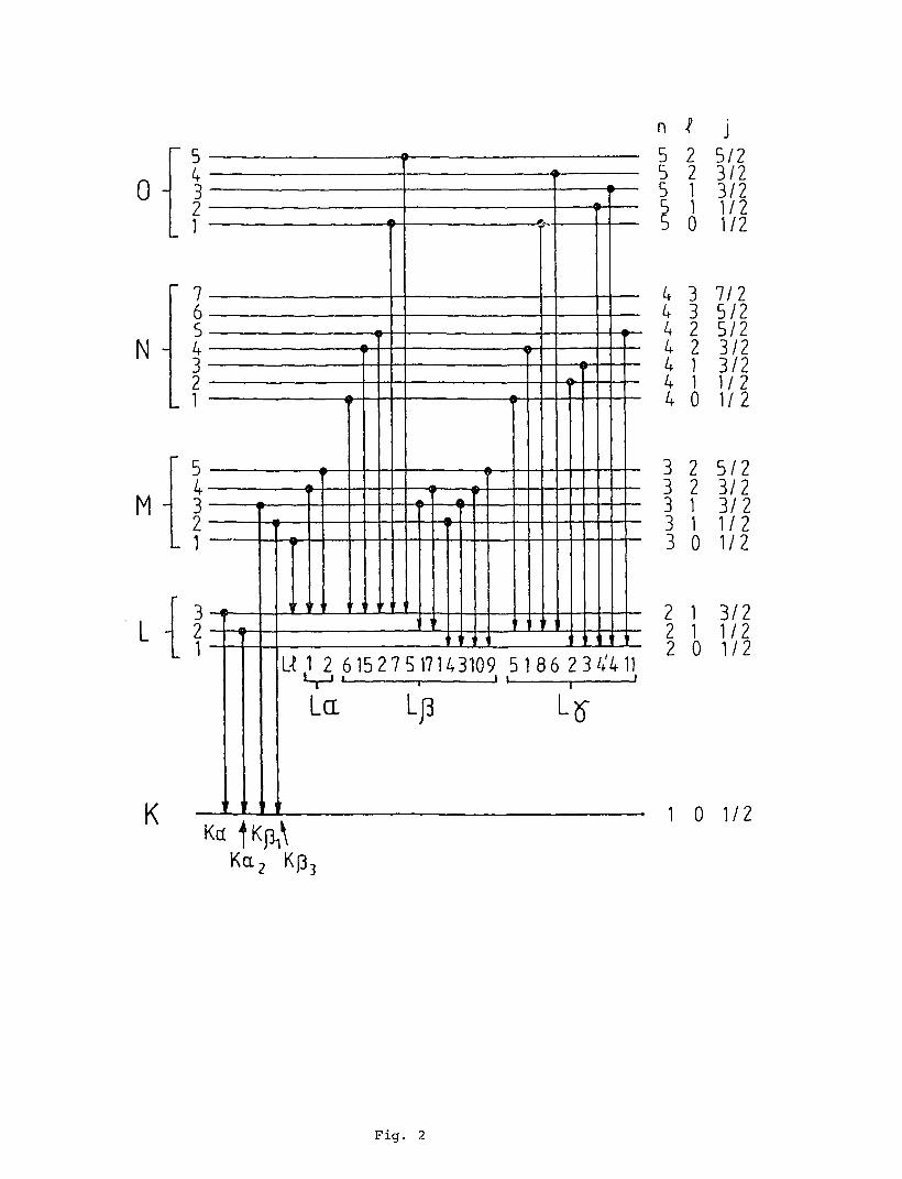
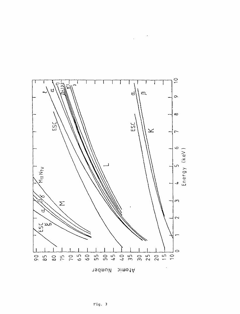
The PIXE technique utilizes the ion energy loss process of inner shellionisation of the target atom. Electrons ejected from the K or L shell bythe Coulomb interaction of the fast moving ion have their vacancies filledby other outer electron transitions into these shells and an X-ray photonis emitted to carry off the excess energy. The allowable X-raytransmissions for initial vacancies in the K and L shell of the targetatom are shown in Fig. 2. Using the conventional Siegbahn notation theseare generally referred to as Kalpha, Kbeta or Lalpha, Lbeta and LgammaX-ray transitions depending in which shell the original vacancy occurred.Fig. 3 shows the typical X-ray energies for K, L and M shell X-rays versus

target atomic number. Each target has a unique K,L or M X-ray signatureand these X-ray energies fall into discreet bands, increasing

monotonically with energy. For PIXE systems M X-rays are typically lowenergy (1-3 keV), L intermediate energy (1-20 keV) and K X-rays highenergy (1-30 keV).

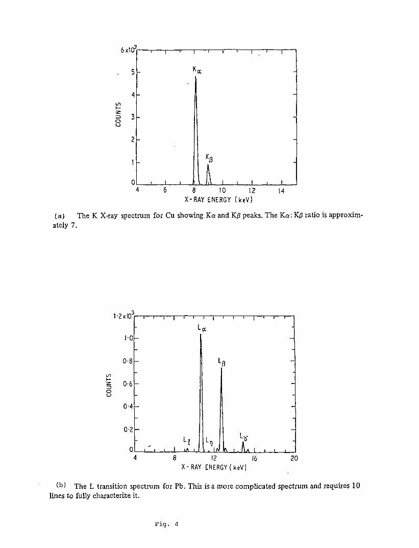
The X-ray signals produced by ion bombardment generate a uniquefingerprint for that element. Figs. 4a and b show the K and L shell

fingerprints of pure Cu and Pb targets respectively. These spectra weretaken using a standard energy dispersive Si(Li) detector system discussedfurther below and they demonstrate the basic principle of the PIXEtechnique. That is the X-ray energy specifies the element present in thetarget and the number of X-rays produced specifies the amount of thatelement in the target. For targets containing several elements a detectionsystem with sufficient resolution to detect each elemental signature isrequired.

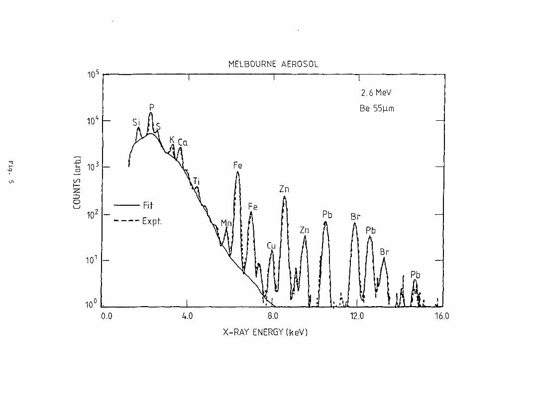
A typical PIXE detection system may operate over the X-ray energy range 1-

40 keV, and hence be capable of detecting K, L or M light X-rays. Fig. 5is an X-ray spectrum obtained by the bombardment of 2.6 MeV protons onto athin aerosol filter paper sample. It contains X-rays from many elementsand several different X-ray bands. The filter paper sample had air drawn

through it for several hours and the spectrum shows K X-rays for selectedelements from Si to Br and L X-rays for Pb. This spectrum was acquired

after just a few minutes of accelerator running time and shows X-ray peaks

for a dozen different elements varying in height over 5 orders ofmagnitude. It represents elemental concentrations of a few percent byweight for Si to a few micrograms per gram for Cu and clearly demonstratesthe power of the PIXE analytical technique. The increased backgroundaround 2 keV is secondary electron Bremsstrahlung background produced bydeceleration of electrons generated by the ion in the target. Thisbackground falls by 2 orders of magnitude between 1 and 4 keV, beingessentially zero above 8 keV. The lack of background in the X-ray regionabove several keV is the reason for the high sensitivity of PIXE comparedto other X-ray analytical techniques.

-2-

3. FIXE SENSITIVITY

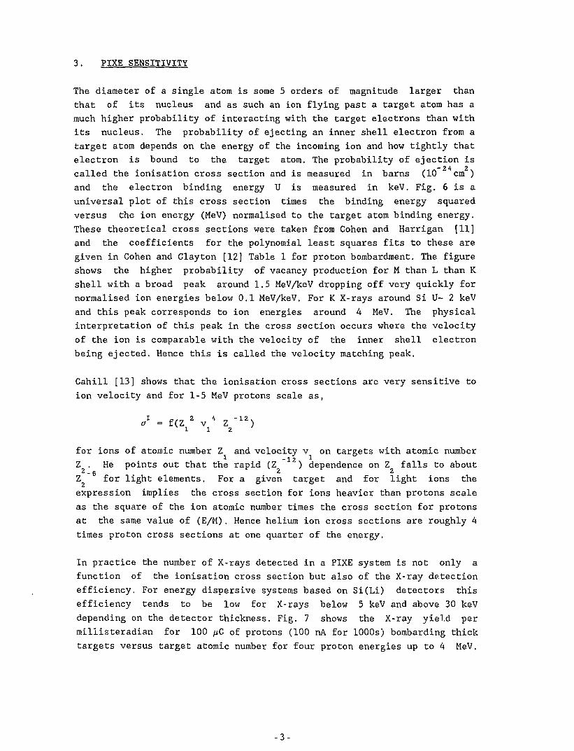
The diameter of a single atom is some 5 orders of magnitude larger thanthat of its nucleus and as such an ion flying past a target atom has amuch higher probability of interacting with the target electrons than withits nucleus. The probability of ejecting an inner shell electron from atarget atom depends on the energy of the incoming ion and how tightly thatelectron is bound to the target atom. The probability of ejection is

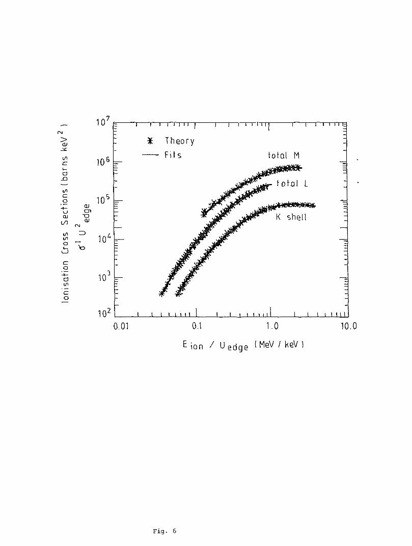
"24 2called the ionisation cross section and is measured in barns (10 cm )and the electron binding energy U is measured in keV. Fig. 6 is auniversal plot of this cross section times the binding energy squaredversus the ion energy (MeV) normalised to the target atom binding energy.These theoretical cross sections were taken from Cohen and Harrigan [11]and the coefficients for the polynomial least squares fits to these aregiven in Cohen and Clayton [12] Table 1 for proton bombardment. The figureshows the higher probability of vacancy production for M than L than Kshell with a broad peak around 1.5 MeV/keV dropping off very quickly fornormalised ion energies below 0.1 MeV/keV. For K X-rays around Si U- 2 keVand this peak corresponds to ion energies around 4 MeV. The physicalinterpretation of this peak in the cross section occurs where the velocity

of the ion is comparable with the velocity of the inner shell electronbeing ejected. Hence this is called the velocity matching peak.

Cahill [13] shows that the ionisation cross sections are very sensitive toion velocity and for 1-5 MeV protons scale as,

for ions of atomic number Z and velocity v on targets with atomic number1 - 12 ^Z . He points out that the rapid (Z ) dependence on Z falls to about

2 _ g 2 2Z for light elements. For a given target and for light ions theexpression implies the cross section for ions heavier than protons scale

as the square of the ion atomic number times the cross section for protonsat the same value of (E/M) . Hence helium ion cross sections are roughly 4times proton cross sections at one quarter of the energy.

In practice the number of X-rays detected in a FIXE system is not only afunction of the ionisation cross section but also of the X-ray detectionefficiency. For energy dispersive systems based on Si (Li) detectors thisefficiency tends to be low for X-rays below 5 keV and above 30 keV

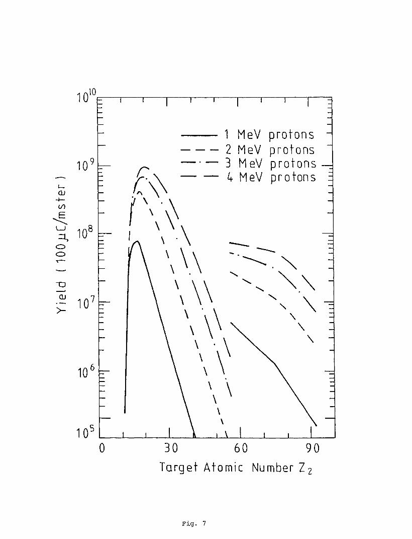
depending on the detector thickness. Fig. 7 shows the X-ray yield permillisteradian for 100 p,C of protons (100 nA for 1000s) bombarding thicktargets versus target atomic number for four proton energies up to 4 MeV.

-3-

The K shell X-rays cover the target atomic number range from 10 to 60 andthe L shell from 50 to 90. For 4 MeV the K shell yield peak around 10counts/100 /jC/msr for targets between Ca and Zn, this is typical for mostFIXE systems. The sharp low target atomic number cutoff below Z =10 isproduced by low detection efficiency for K X-rays below 2 keV and theslower high target atomic number roll off above Z =40 for K and 90 for Lis produced by the smaller ionisation cross sections for these moretightly bound inner shell electrons.

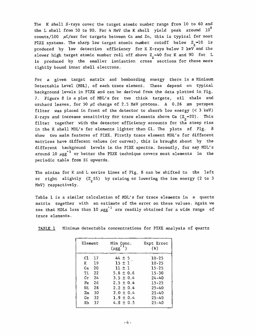
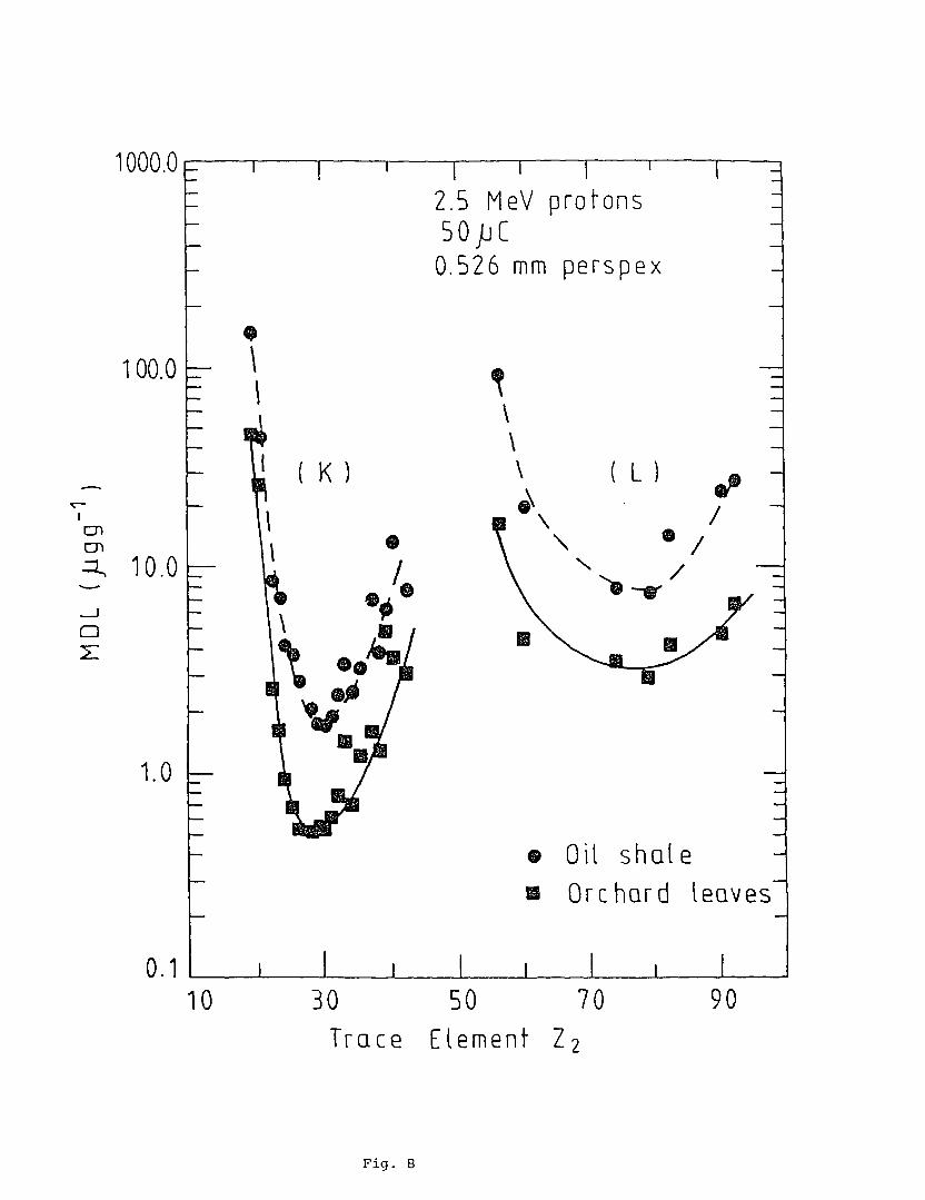
For a given target matrix and bombarding energy there is a MinimumDetectable Level (MDL), of each trace element. These depend on typicalbackground levels in FIXE and can be derived from the data plotted in Fig.7. Figure 8 is a plot of MDL's for two thick targets, oil shale andorchard leaves, for 50 p.C charge of 2.5 MeV protons. A 0.26 mm perspex

filter was placed in front of the detector to absorb low energy (< 3 keV)X-rays and increase sensitivity for trace elements above Ca (Z =20). Thisfilter together with the detector efficiency accounts for the steep risein the K shell MDL's for elements lighter than Cl. The plots of Fig. 8show two main features of PIXE. Firstly trace element MDL's for differentmatrices have different values (or curves), this is brought about by thedifferent background levels in the PIXE spectra. Secondly, for say MDL'saround 10 /igg or better the PIXE technique covers most elements in the

periodic table from Si upwards.

The minima for K and L series lines of Fig. 8 can be shifted to the leftor right slightly (Z ±5) by raising or lowering the ion energy (2 to 3

2MeV) respectively.

Table 1 is a similar calculation of MDL's for trace elements in a quartzmatrix together with an estimate of the error on these values. Again wesee that MDLs less than 10 jigg are readily obtained for a wide range of

trace elements.

TABLE 1 Minimum detectable concentrations for PIXE analysis of quartz

Element

ClKCaTiCrFeNiZnGeRb

17192022242628303237

Min Cone.

44 ± 515 ± 1 '11 ± 15.8 ± 0.63.5 ± 0.42.5 ± 0.42.2 ± 0.42.0 ± 0.41.9 ± 0.44.8 ± 0.5

Expt Error

10-2510-2515-2515-3024-4015-2525-4025-4025-4025-40

-4-

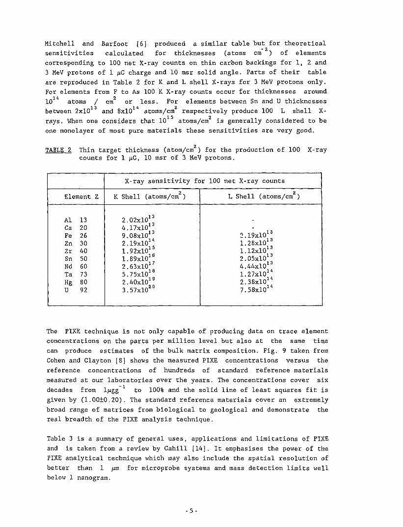
Mitchell and Ear foot [6] produced a similar table but for theoreticalsensitivities calculated for thicknesses (atoms cm ) of elementscorresponding to 100 net X-ray counts on thin carbon backings for 1, 2 and3 MeV protons of 1 y.C charge and 10 msr solid angle. Parts of their tableare reproduced in Table 2 for K and L shell X-rays for 3 MeV protons only.For elements from F to As 100 K X-ray counts occur for thicknesses around

1 / O

10 atoms / cm or less. For elements between Sn and U thicknessesbetween 2xl013 and SxlO1'1 atoms/cm2 respectively produce 100 L shell X-

rays. When one considers that 10 atoms/cm is generally considered to beone monolayer of most pure materials these sensitivities are very good.

TABLE 2 Thin target thickness (atom/cm ) for the production of 100 X-raycounts for 1 /zC, 10 msr of 3 MeV protons.

Element Z

Al 13Ca 20Fe 26Zn 30Zr 40Sn 50Nd 60Ta 73Hg 80U 92

X-ray sensitivity for 100 net X-ray counts

K Shell (atoms/cm )

2.02xl013

4.17x109.08xl013

2. 19x10* *1.92xl015

1.89x102.63xl017

5.75xl018

2.40xl019

3.57xl02°

L Shell (atoms/cm )

_

2.19xl013

1.28xl013

1.12xl013

2.05xl013

4.44xl013

1. 27x10* *2. 38x10* A

7.58xl01A

The P1XE technique is not only capable of producing data on trace elementconcentrations on the parts per million level but also at the same time

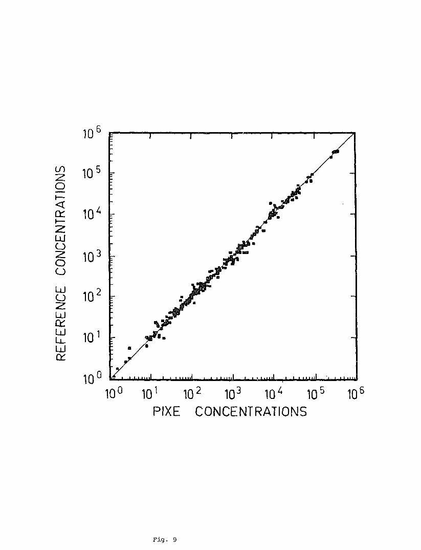
can produce estimates of the bulk matrix composition. Fig. 9 taken fromCohen and Clayton [8] shows the measured PIXE concentrations versus the

reference concentrations of hundreds of standard reference materialsmeasured at our laboratories over the years. The concentrations cover six

decades from Ipgg to 100% and the solid line of least squares fit is

given by (1.00±0.20). The standard reference materials cover an extremelybroad range of matrices from biological to geological and demonstrate thereal breadth of the PIXE analysis technique.

Table 3 is a summary of general uses, applications and limitations of PIXEand is taken from a review by Cahill [14]. It emphasises the power of thePIXE analytical technique which may also include the spatial resolution of

better than 1 pm for microprobe systems and mass detection limits wellbelow 1 nanogram.

-5-

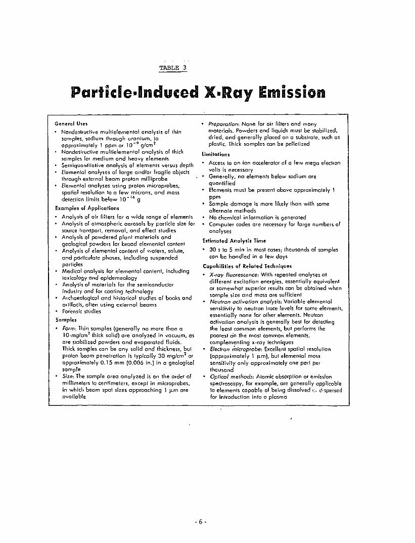
TABLE 3

Particle-Induced X-Ray Emission

General Uses

• Nondestructive mullielemenlal analysis of ihinsamples, sodium through uranium, loapproximately 1 ppm or 10" g/cm

• Nondestructive mullielemenlal analysis of thicksamples for medium and heavy elements

• Semiquanlilalive analysis of elements versus depth• Elemental analyses of large and/or fragile objects

through external beam proton milliprobe

• Elernenlal analyses using proton microprobes,spatial resolulion lo a few microns, and mass

detection limits below 10"'* g

Examples of Applications

• Analysis of air fillers for a wide range of elements

• Analysis of atmospheric aerosols by particle size forsource transport, removal, and effect studies

• Analysis of powdered plant materials and

geological powdets for broad elemental content

• Analysis of elemental content of waters, solute,

and parliculale phases, including suspendedparticles

• Medical analysis for elemental conlenl, including

toxicology and epidemeology• Analysis of materials for the semiconductor

industry and for coaling technology

• Aichaeological and historical studies of books andartifacts, often using external beams

• Forensic studies

Samples

• Form-. Thin samples (generally no more than a

10-mg/cm5 thick solid) are analyzed in vacuum, as

are stabilized powders and evaporated fluids.

Thick samples can be any solid and thickness, but

proton beam penetration is typically 30 mg/cm7 or

approximately 0.15 mm (0.006 in.) in a geologicalsample

• Size: The sample area analyzed is on the order of

millirnelers to centimeters, except in microprobes,in which beam spot sizes approaching 1 (im are

available

• Preparation: None for air fillers and manymaterials. Powders and liquids must be stabilized,

dried, and generally placed on a substrate, such asplastic. Thick samples can be pellelized

limitations

• Access lo an ion accelerator of a few mega electron

volls is necessary

• Generally, no elements below sodium are

quantified• Elements must be present above approximately 1

ppm

• Sample damage is more likely than with some

alternate methods• No chemical information is generated

• Computer codes are necessary for large numbers of

analyses

Estimated Analysis Time

• 30 s lo 5 min in most cases; thousands of samples

can be handled in a few days

Capabilities of Related Techniques

• X-ray fluorescence: With repealed analyses atdifferent excitation energies, essentially equivalent

or somewhat superior results can be obtained whensample size and mass ore sufficient

• Neutron activation analysis: Variable elementalsensitivity lo neutron Irace levels for some elements,

essentially none for olher elemenls. Neulron

aclivalion analysis is generally best for delecting

the least common elemenls, but performs the

poorest on the most common elemenls,complementing x-ray techniques

• Electron microprcbe: Excellent spatial resolulion

(approximalely 1 p.m), but elemenlal mass

sensitivity only approximalely one part per

thousand• Optical methods: Atomic absorption or emission

speclroscopy, for example, are generally applicablelo elemenls capable of being dissolved <'., Aspersedfor introduction into a plasma

- 6 -

4. FIXE YIELDS

Since the range of charged particles in matter is limited PIXE is asurface technique only. For example, 3 MeV protons in C or Si have rangesof 65 and 95 microns respectively, while for 3 MeV alphas these ranges areonly 9 and 12 microns respectively. Hence for bulk analysis using PIXE onemust be certain that the target is homogeneous or at least that the firstfew microns of the surface are representative of the bulk of the material.This problem is further enhanced by two facts (i) the ion loses energyalong its path and hence the X-ray production falls dramatically with

depth into the target, (ii) the emerging X-rays are absorbed by thetarget. A good rule of thumb is that 90% of the total X-ray yield isusually produced in the first quarter of the ion range in the material[7,8].

Thin targets are defined as those for which ion energy losses and X-rayabsorption effects are negligible, say less than 5%. Thick targets areusually those for which the incident ion is completely stopped and thecalculated yields for these require integration over ion energy loss andemergent X-ray absorption. Expressions for yields for both thin and thick

targets have been discussed at length elsewhere [8,9,12] and will not bereproduced here. Several papers [6,8,12,15] and the references thereinhave discussed in detail the data bases necessary to compute these X-rayyields for known concentrations of trace elements in known matrices.

Computer codes have been written by a variety of laboratories to not onlyanalyse the peak areas of PIXE spectra [9,16,17] but also convert theseareas to concentrations [17].

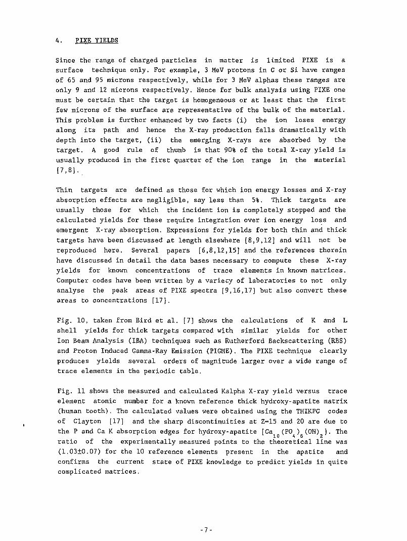
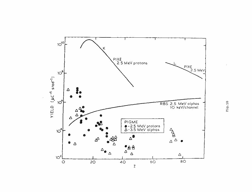
Fig. 10, taken from Bird et al. [7] shows the calculations of K and Lshell yields for thick targets compared with similar yields for other

Ion Beam Analysis (IBA) techniques such as Rutherford Backscattering (RBS)and Proton Induced Gamma-Ray Emission (PIGME). The PIXE technique clearly

produces yields several orders of magnitude larger over a wide range oftrace elements in the periodic table.

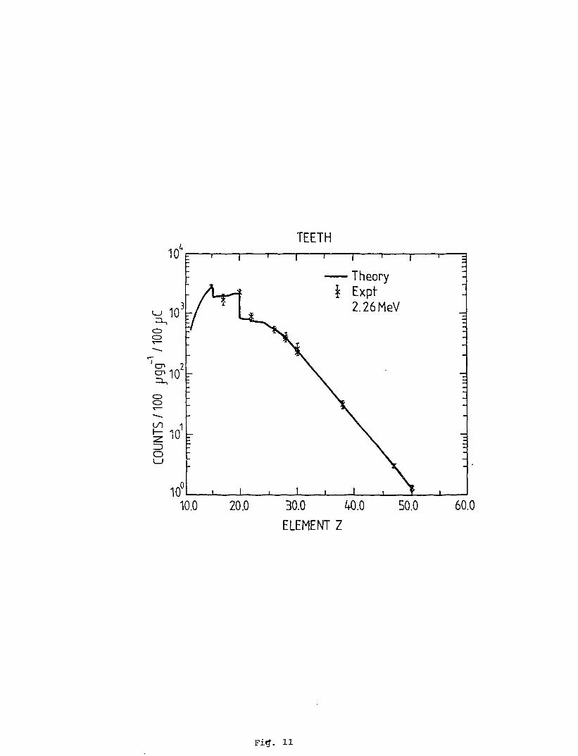
Fig. 11 shows the measured and calculated Kalpha X-ray yield versus trace

element atomic number for a known reference thick hydroxy-apatite matrix(human tooth). The calculated values were obtained using the THIKPC codes

of Clayton [17] and the sharp discontinuities at Z=15 and 20 are due tothe P and Ca K absorption edges for hydroxy-apatite [Ca (PO ) (OH) ]. The

ratio of the experimentally measured points to the theoretical line was(1.03±0.07) for the 10 reference elements present in the apatite andconfirms the current state of PIXE knowledge to predict yields in quitecomplicated matrices.

-7-

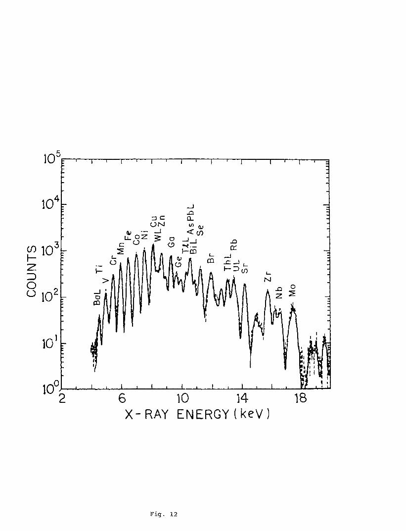
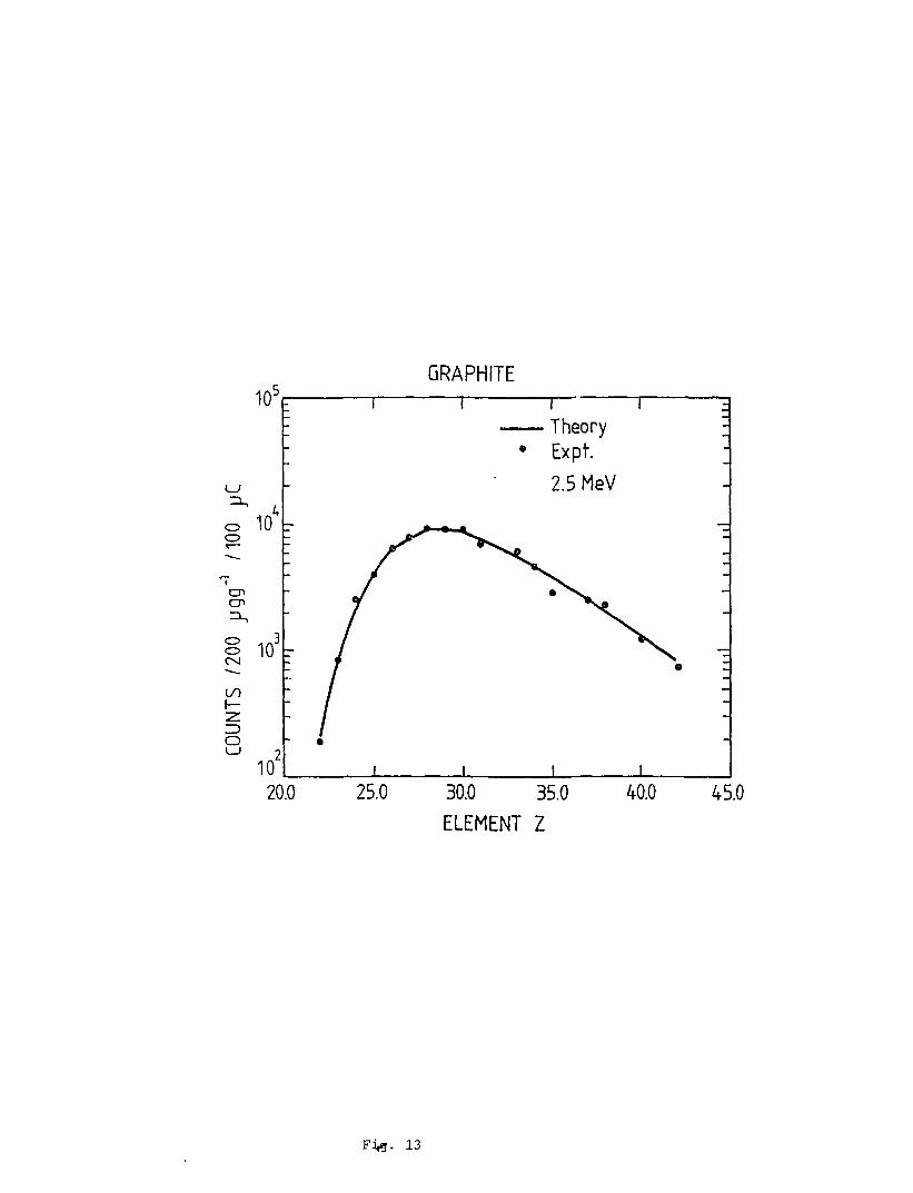
Similar techniques also work for many trace elements in a simple matrix.For example, Fig. 12 is a PIXE spectrum for over 40 elements in a graphitematrix [18], each with a nominal concentration of around 200 pgg . Thespectrum was accumulated using 2.5 MeV protons, 1.5mm thick perspex filterin front of the detector with a. solid angle of 1.34 msr. The solid curveis a fit to the data (dashed curve) using the PIXAN package of Clayton[17]. The measurement took less than 20 minutes. The theoretical yieldsobtained are compared with the experimental values in Fig. 13 and for

elements between Ti and Sr differ by an average of less than 6% from thereference values.

These figures show that both thin and thick target PIXE calculations, andhence data bases [12,15], have reached such a degree of sophisticationthat X-ray yields for trace elements can now be predicted at the 5% levelfor an extremely diverse range of known target matrices. Further evidencefor this is given by Maenhaut and Raemdonck [19] who measured a set ofaccurate thin film standards and compared this with absolute theoreticalcalculations. They found an individual element could be analysed with an

accuracy of better than 4% for elements from Na to Sn.

The main advantage of having reliable data bases to produce reliable yieldcurves for a given matrix is that a single external or internal standardcan be used to normalise this yield curve to the experimental results andhence produce yields for most elements across the periodic table. Forexample, if the yield curve for Fig. 11 is normalised to the known valueof Ca in apatite (39.9 wt%) to give the experimentally measured value of

the number of X-rays in the Ca Kalpha peak then Kalpha yields for allother elements from Z=10 to 50 can be obtained. This then would be

normalising to the internal Ca standard in apatite and reduces alluncertainties associated with charge collection, detection efficiency and

solid angle. This procedure is practised by many laboratories in varying

forms, often uncommon elements such as Y or Sr are used in known amountsto spike powdered samples before pressing into a solid target. The X-rayyield results are then normalised to the known Kalpha yields from theseinternal standards.

5. PIXE SYSTEMS

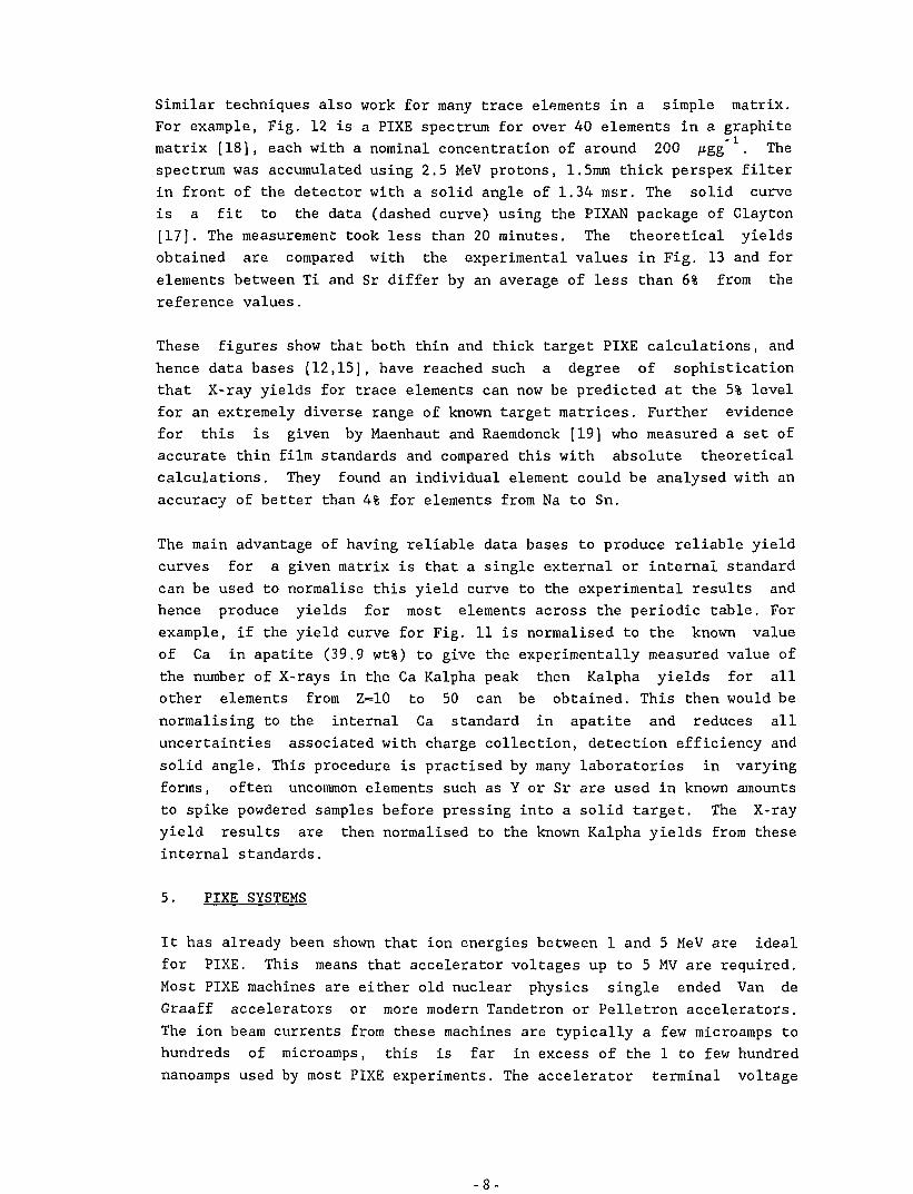
It has already been shown that ion energies between 1 and 5 MeV are idealfor PIXE. This means that accelerator voltages up to 5 MV are required.

Most PIXE machines are either old nuclear physics single ended Van deGraaff accelerators or more modern Tandetron or Pelletron accelerators.The ion beam currents from these machines are typically a few microamps tohundreds of microamps, this is far in excess of the 1 to few hundrednanoamps used by most PIXE experiments. The accelerator terminal voltage

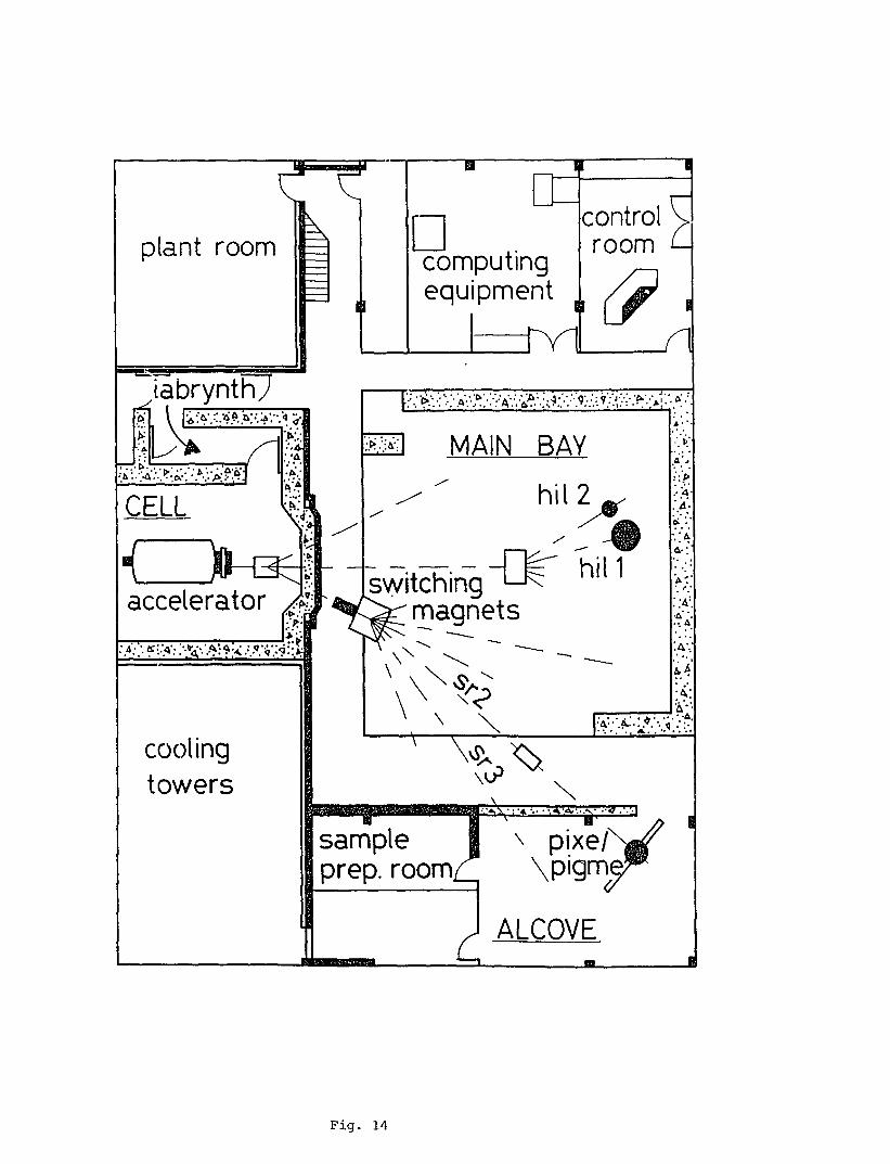
is usually stabilised to a few keV or better and the excess ion currentsreduced by beam transport through bending magnets, quadrupoles andapertures. Fig. 14 is a floor plan of the 3 MV Van de Graaff acceleratorat Lucas Heights. The accelerator and the main analysing magnet arecontained in a concrete block house or cell for radiation shielding. Thisis really only necessary when deuteron beams which produce neutrons areused. For protons radiation levels only become significant near the ionsource and adjacent to the accelerator tank and shielding is not usually a

problem. The analysing magnet can switch the ion beam down 3 legs into themain bay. The centre and right legs have switching magnets on them. Sothere are about 11 different legs operating at the present time. The mainPIXE/PIGME system is located in a low noise (electronic) background areacalled the Alcove adjacent to our clean sample preparation room. Typicallywe would run 2.5 MeV protons, 10 /jA, 10mm diameter beams onto the beam

stop before the analysing magnet in the cell. This produces about 2 /jA,5mm diameter beam spot after the switching magnet in the main bay and with

quadrupole defocusing and selected apertures we can dial up anything froma 1 mm diameter 1 nA beam spot to an 8mm several hundred nanoamp spot.

Currently there are 3 different FIXE systems operating on our accelerator,one for batch analysis of many targets, one miniprobe (50pm) system fordetailed analysis of individual targets and one external beam system forlarge targets unable to be placed in vacuum.

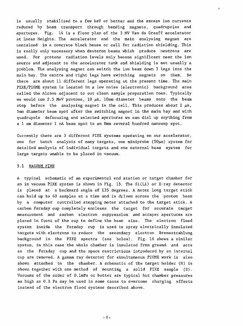
5.1 VACUUM FIXE

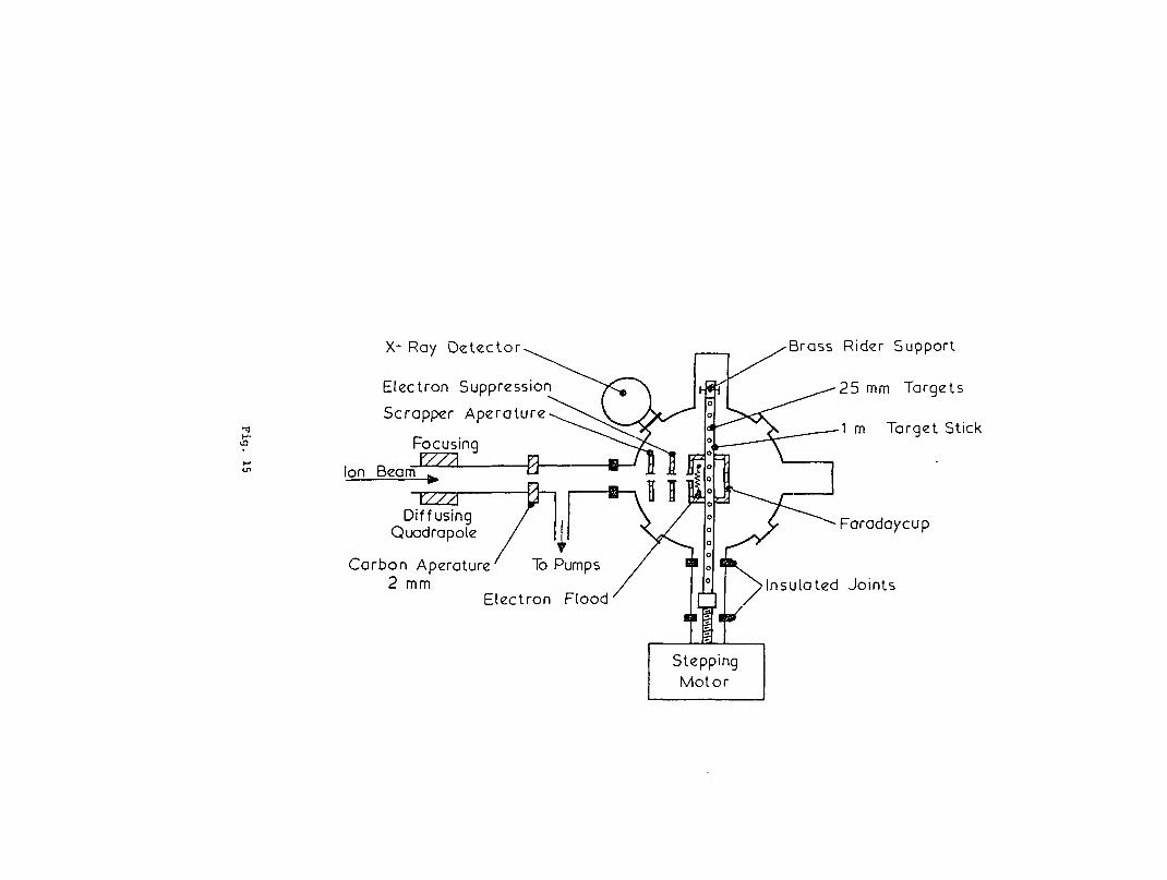
A typical schematic of an experimental end station or target chamber foran in vacuum FIXE system is shown in Fig. 15. The Si(Li) or X-ray detectoris placed at a backward angle of 135 degrees. A meter long target stickcan hold up to 60 samples at a time and is driven across the proton beamby a computer controlled stepping motor attached to the target stick. Acarbon Faraday cup completely encloses the target for accurate target

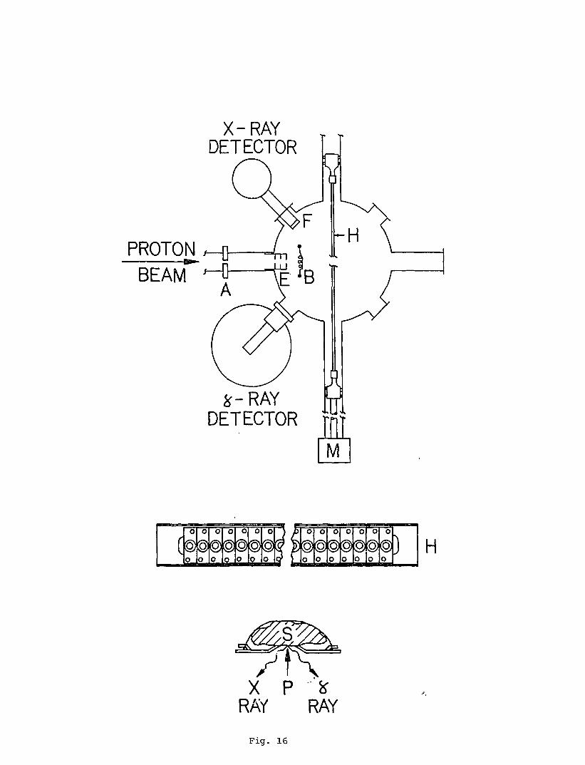
measurement and carbon electron suppression and scraper apertures areplaced in front of the cup to define the beam size. The electron floodsystem inside the Faraday cup is used to spray electrically insulatedtargets with electrons to reduce the secondary electron Bremsstrahlungbackground in the FIXE spectra (see below). Fig. 16 shows a similarsystem, in this case the whole chamber is insulated from ground and actsas the Faraday cup and the space restrictions introduced by an internalcup are removed. A gamma ray detector for simultaneous PIGME work is alsoshown attached to the chamber. A schematic of the target holder (H) isshown together with one method of mounting a solid PIXE sample (S).Vacuums of the order of O.lmPa or better are typical but chamber pressuresas high as 0.1 Pa may be used in some cases to overcome charging effectsinstead of the electron flood systems described above.

-9-

5.2 EXTERNAL PIXE

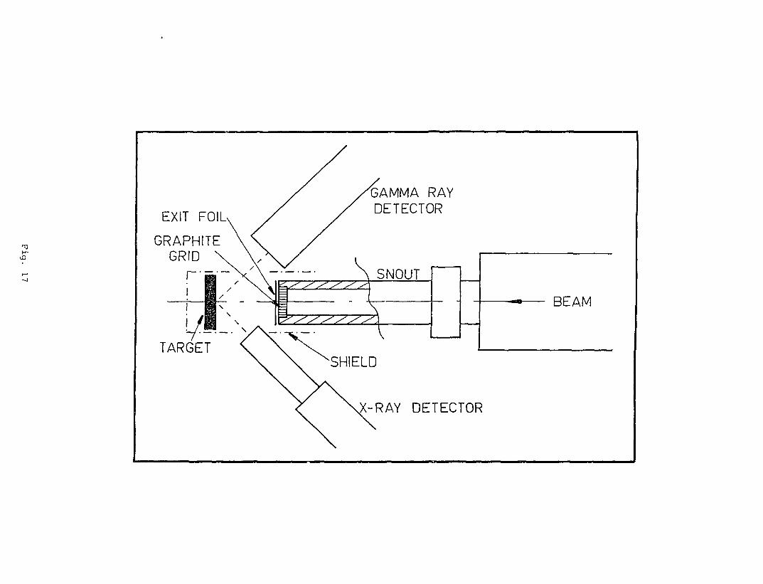
Some targets are either too big or too delicate to place in a vacuumsystem. For these the ion beam may be brought out into air or a heliumatmosphere through a thin foil, usually Kapton or Ni. External systems areto be discussed by others at this meeting and will not be treated indetail here. Fig. 17 is a schematic of a typical external beam PIXE. Theexit foil is Kapton resting on a perforated graphite support whichtransmits 50% of the beam. The target can be placed within a couple ofcms. of the exit window.

Care should be taken with radiation from external beams. Contact with the

skin will produce radiation burns from Mrad proton doses. X-ray and gammaray fluxes can be high from the air and exit foils. Hundreds of mrads afew cms. from the exit windows are possible and care should be taken notto irradiate the eyes or other body parts.

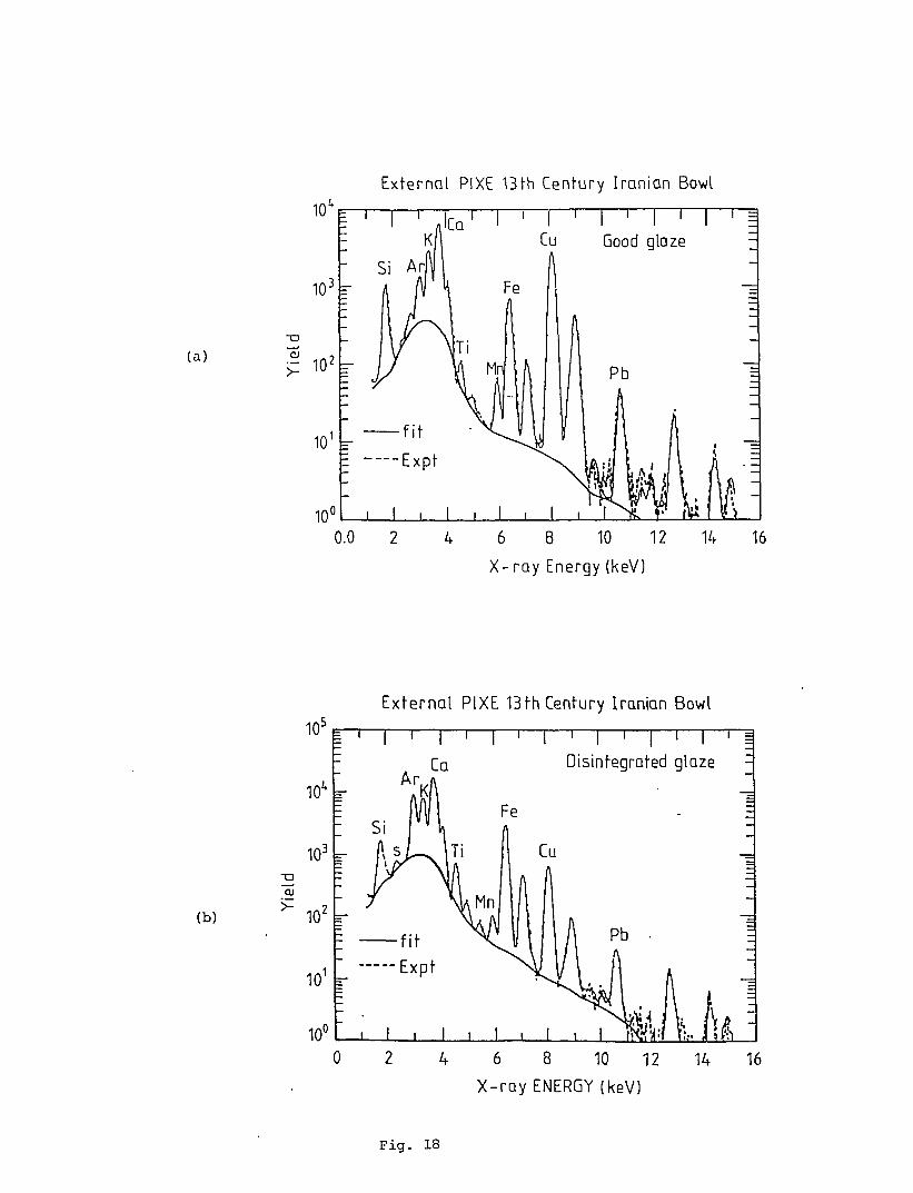
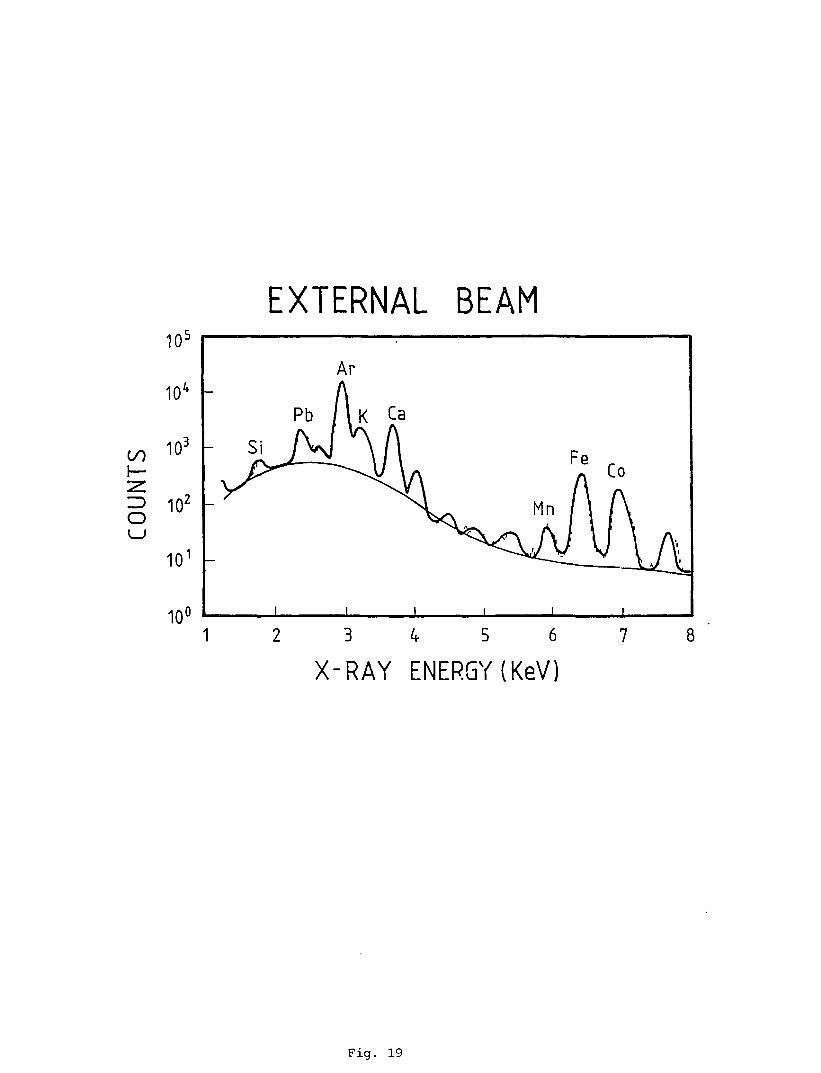
Beryllium extraction windows should never be used as the neutron (p,n)reaction produces prolific numbrfrs of neutrons at PIXE energies. Fi s. 18and 19 show typical external beaK PIXE spectra for an investigation ofglaze on a large Iranian bowl and the pigments in a 17th century Italianpainting. The Argon peak around 3 keV is a typical feature of externalPixe spectra in air.

5.3 SifLi) DETECTORS

X-rays are virtually always measured with energy dispersive Si(Li)detector systems. The use of these semiconductor detectors rests on the

principle of absorption of photons through ionisation which occurs whenenergetic electron produced via the photo-electric effect loses its

energy. The photo electron creates many electron-hole pairs in the Si(Li)crystal and a bias applied across the crystal sweeps out the charge to the

corresponding electrode. This charge pulse is amplified and its height isproportional to the total energy deposited in the crystal detector. The

energy required to generate an electron hole pair in Si is only about 3.8eV at liquid nitrogen temperatures (77°K). The keV X-rays will generate

large numbers of hole pairs which yield excellent statistics formeasurement of the size of the charge pulse. Finally since the mobility of

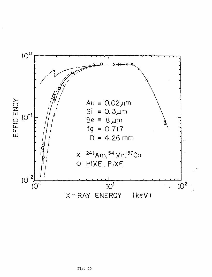
these charge carriers (electrons) is high most are collected and theSi(Li) detector has good resolution, typically 150 eV at 6 keV or (AE/E)approximately 2.5%. These ideas and principles have been thoroughlydiscussed by Woldseth [20]. A comprehensive Si(Li) detector efficiencymodel has been presented by Cohen [21] covering the energy range 3-60 keV.

-10-

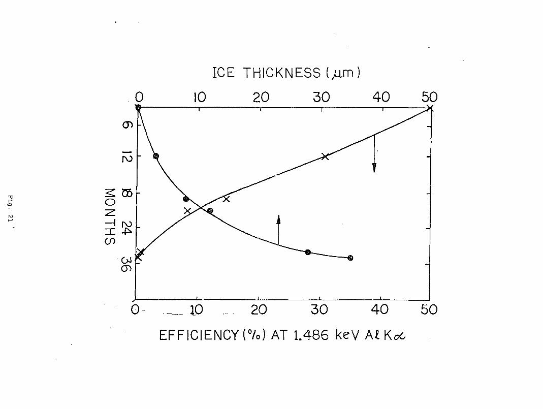
Fig. 20 shows the efficiency of a typical Si(Li) detector with a thin 8/jmBe window as a function of X-ray energy. The experimental measurementswere taken using X-ray standard sources and by measuring X-rays from knownPIXE and HIXE targets. Clearly below 3 keV the efficiency as calculatedfrom the manufacturer's specifications overestimates the experimentalresults. The detector crystals are held at 77°K and it was shown by Cohen[22] that this discrepancy was due to an ice buildup on the front face ofthe detector with a thin Be window. Ice thicknesses of between 10-20pmwere common and easily removed by warming up the crystal (to 50°C) andpumping the cryostat for a few days. This buildup is present in most thinwindowed detectors and increases in thickness with time. Measurements ofthis low energy efficiency degradation with time are given in Fig. 21.Over 36 months the ice thickness grew from 1 or 2 m to 50/jm at whichpoint the detector was "sweating" so much it would not hold liquidnitrogen and the cryostat had to be pumped. For this range of icethickness the efficiency of this detector for the Al Kalpha X-ray droppedfrom 35% to zero.

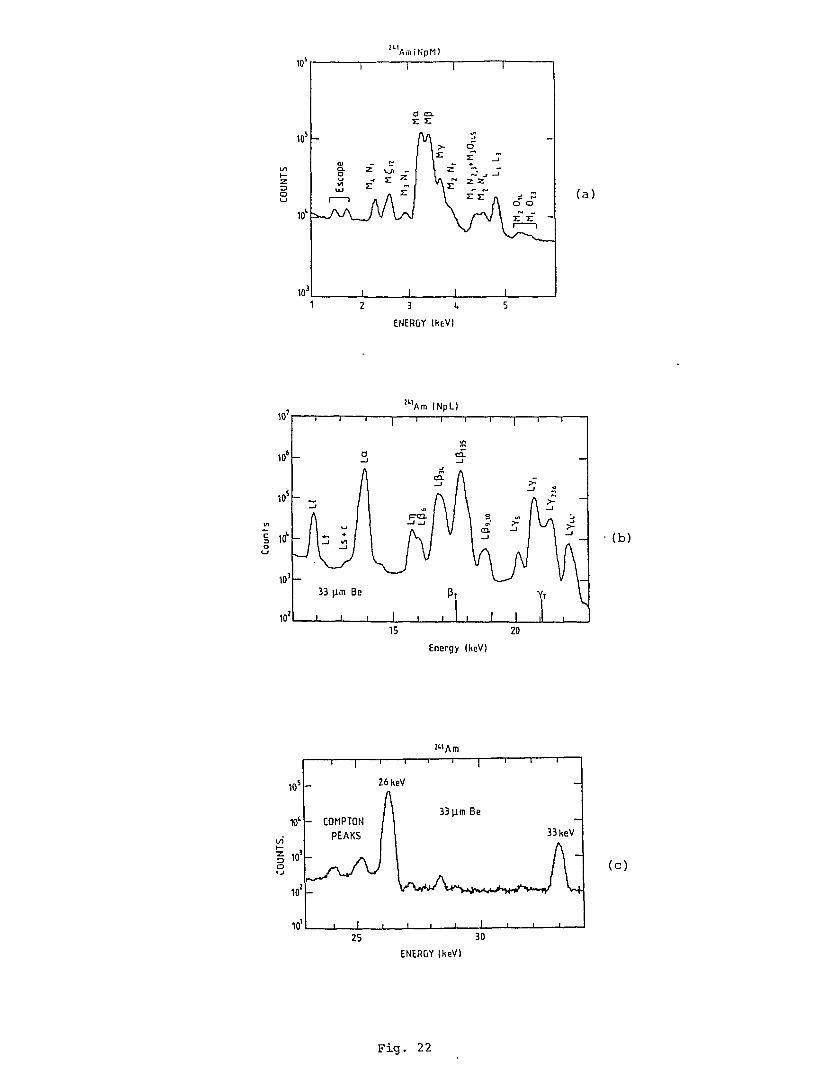
A simple technique to measure the thickness of ice build up on the frontface of detectors has been described by Cohen [8,22] together with a full

description of useful X-rays from Am-241 source for detector efficiencycalibration. Figure 22 shows the X-ray spectrum from an Am-241 source andthe 20 or so X-ray lines that can be used to calibrate Si(Li) detectorefficiencies over the energy range 2-30 keV. The M X-ray lines areparticularly sensitive to ice buildup.

5.4 ELECTRONICS

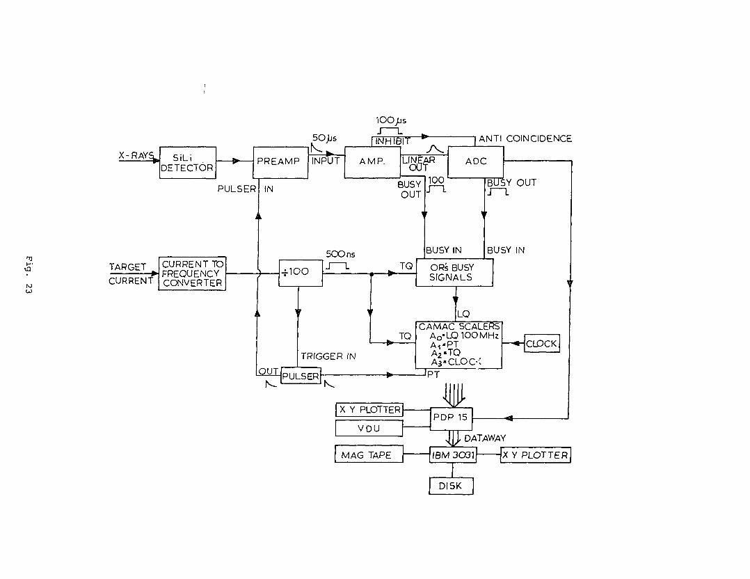
The signals from the Si(Li) detector are amplified, fed into an ADC andcomputing system for analysis. A typical block diagram for theelectronic setup of a PIXE system is shown in Fig. 23. Logic busy signalsare used to gate the ADC's deadtime and to adjust the spectrum live times.

The inhibit signal from the main amplifier is used in the anticoincidenceinput of the ADC to reject pileup pulses in the spectrum. Spectrum run

times are determined by the total accumulated charge on the target. Thisis monitored by a current to frequency converter and the total number ofpulses from this is used to drive an external start/stop clock for the runtimes.

5.5 FILTERS

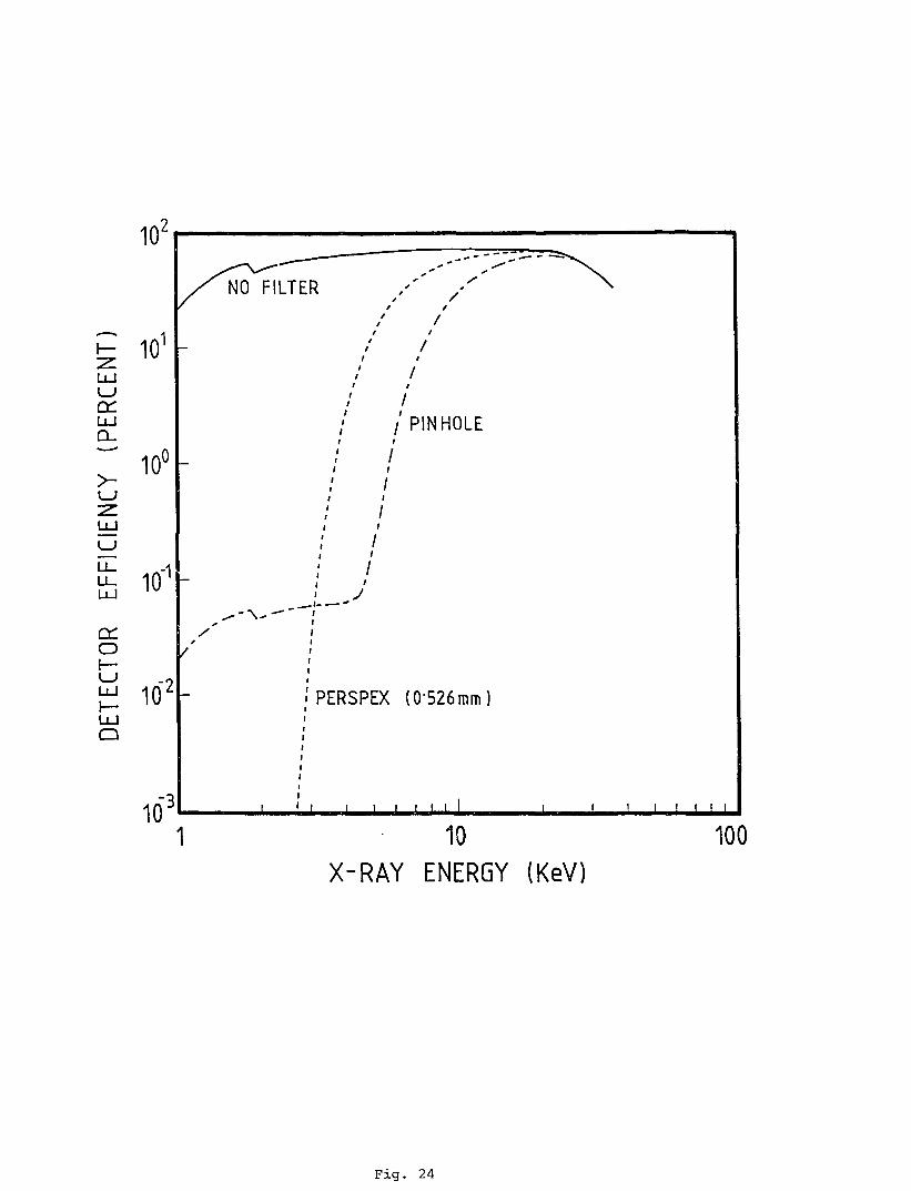
Shaping the detector efficiency to suit the count rate into various peaks

in a PIXE spectrum is a common way of optimising the system to give thebest sensitivities in the shortest times.

-11-

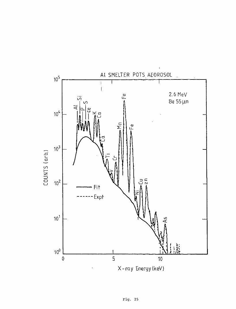
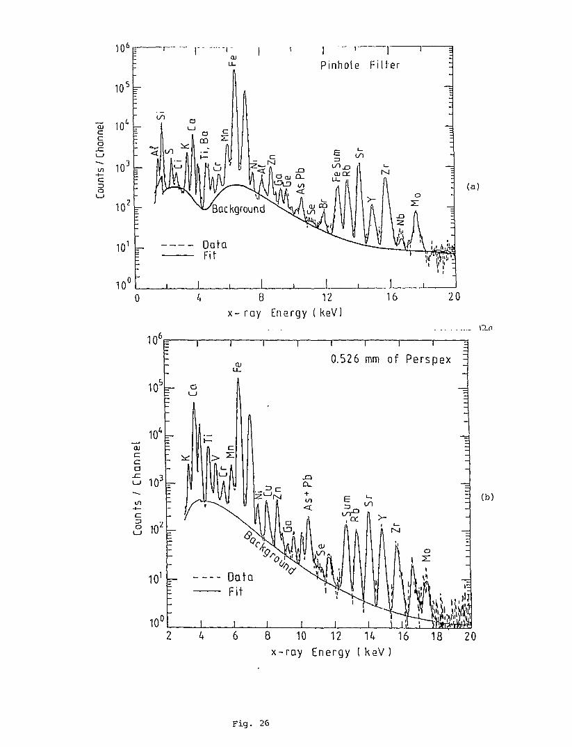
If the spectrum contains mainly light elements whose K X-rays lie below 10keV then generally minimal filtering is used providing the Be windowthickness is sufficient to completely stop the scattered proton beam. Ifthe spectrum contains high count rates into high energy X-rays with onlytrace elements in the lower energy regions then several hundreds ofmicrons of Mylar or Perspex filter may be used. Many spectra however havesignificant count rates across the energy region and pinhole or funnyfilters are used. The effect on efficiency of these 3 types of filters isshown in Fig. 24. The pinhole filter is a 2mm Perspex filter with a 70pmpinhole through its centre to allow a small fraction of the lower energyX-rays through. Figs. 25 to 27 show the effects of such filters on PIXEspectra. Fig. 25 is the spectrum from 2.6 MeV protons on an aerosol filterpaper taken near Al smelter pots. The 55pm Be was used to just stop thescattered protons. Clearly the filter paper contains lots of Al, Si, P, Sand Fe with trace elements of Zn and As. No X-rays are detected above 10keV. Fig. 26 shows the effects of pinhole and Perspex filters on 2.5 MeVproton PIXE spectra, for a USGS oil shale reference standard sample. The

Perspex filter completely removes the light element X-rays. Fig. 26

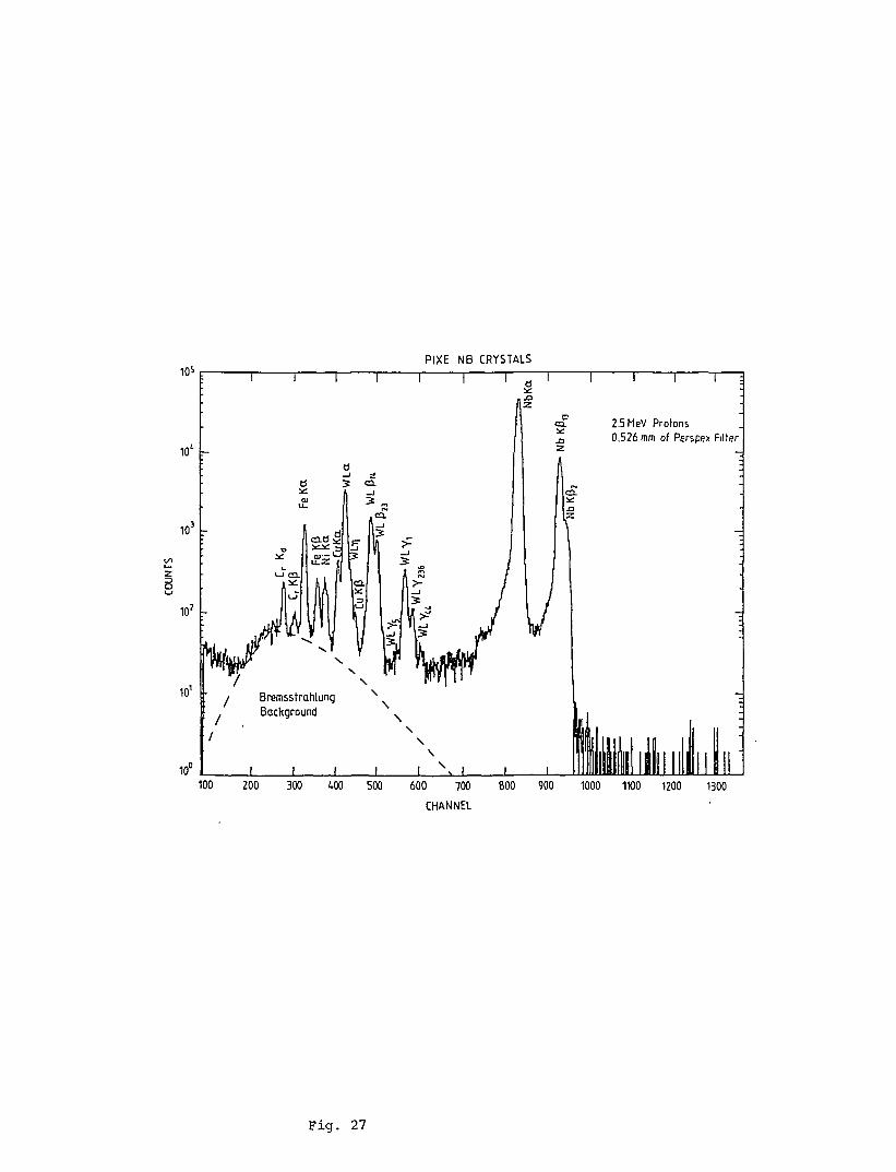
demonstrates the use of a pinhole filter when both light elements like Aland heavier elements like Zr and Mo are wanted. Fig. 27 shows the spectrumfrom a pure Nb crystal cut with a W saw. Here 0.526 mm of Perspex wereused to reduce the Bremsstrahlung background in the region up to channel300 (6 keV) and the trace amounts of W are clearly seen.

Thin metal foil filters may also be used when particular peaks rather thanwhole regions of the spectrum need to be reduced. This is done by

selecting a foil thickness (just a few microns) whose K edge energy liesjust below that for the Kalpha line of the peak whose count rate must bereduced. For example 12pm of Cr filter will reduce the count rate into theFe Kalpha peak by 98.5% but only reduced the adjacent elements Mn Kalpha

and Cu Kalpha by 47.5% and 90% respectively.

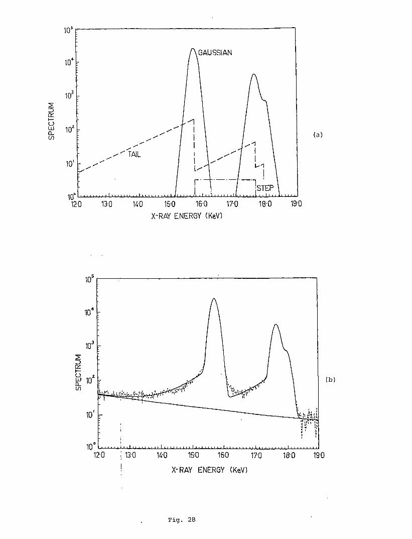
5.6 SPECTRUM ARTIFACTS

We have already shown many experimental PIXE spectra which have beenfitted by programs such as the PIXAN package of Clayton [17], see forexample Figs. 25 and 26. These fits assume some knowledge of the spectralresponse of your detection system. Peaks shapes are basically Gaussianwith low energy steps and tails as shown in Fig. 28a. These steps andtails are typically 2 to 3 orders of magnitude smaller than the primary

amplitude and are produced by inefficient charge collection in thedetector. If the amplitude and slope of these are allowed to vary in the

fitting routines then excellent fits like those shown in Fig. 28b areobtained. This is a PIXE spectrum for a pure thick Sr sample taken fromRef. [8]. The amplitude of these steps and tails is both energy and countrate dependent.

-12-

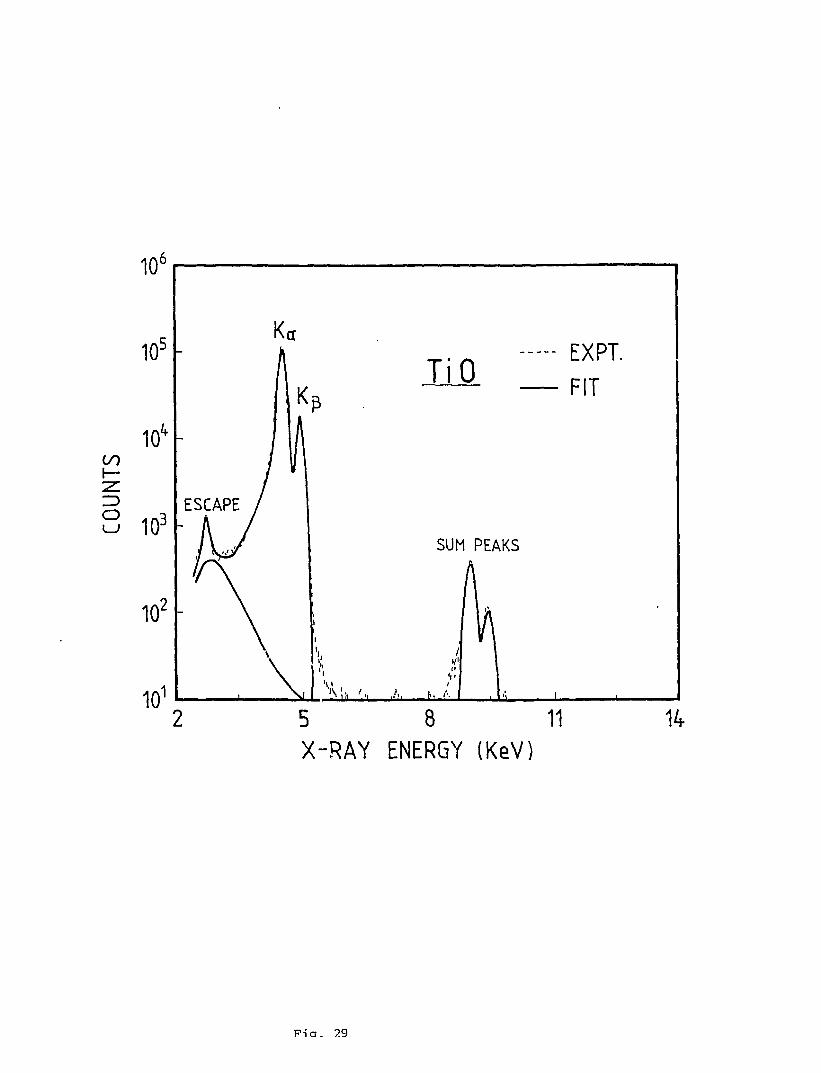
Fig. 29 is the PIXE spectrum from a pure Ti target and clearly shows twomore spectrum artifacts, namely the lower energy escape peak and sum peakswhich occur at approximately twice the energy of the primary peak. For agiven element the escape peak is a constant fraction (few percent of theprimary peak amplitude and is not count rate dependent. It is produced bythe escape of Si Kalpha X-rays from the detector crystal. The escape peakenergy is always 1.74 keV lower than the primary X-ray energy from whichit originates. Each X-ray peak will have its associated escape peak.

j

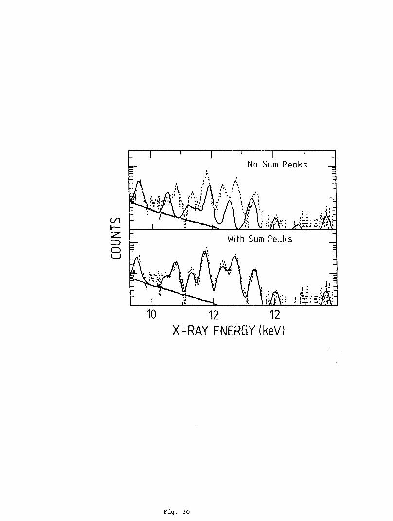
The sum peak, at twice the primary peak energy, is produced by the nonzero pulse pair resolution time of the detector electronic system (usually0.5 ps). Pulses arriving in the detector within this time interval are notcounted as two pulses but as one with twice the energy. Clearly the peakheight of this pulse is count rate dependent but in most typical systemsit is around 3 orders of magnitude smaller than the primary peak. Againeach primary peak can sum with itself and every other peak in the system.Hence for n X-ray peaks there are (n+l)n/2 sum peaks at the sum energy ofeach peak. For high count rates (>5kHz) into many element peaks thiseffect could seriously hamper the analysis of real trace element peakswhich overlap with them. Fig. 30, taken from Ref. [8], shows the 10 to 14keV region of a sample containing 6% Cr and 6% Fe. The top curve showsPIXAN fits without sum peaks and the bottom curve shows superior fitsobtained by including the 10 sum peaks for the 4 Cr and Fe Kalpha andKbeta peaks between 10.8 keV and 14 keV. The peaks for Br K alpha and betaat 11.9 and 13.3 keV and the Rb Kalpha at 13.4 keV can still be accuratelyextracted by the PIXAN package after inclusion of these sum peaks.

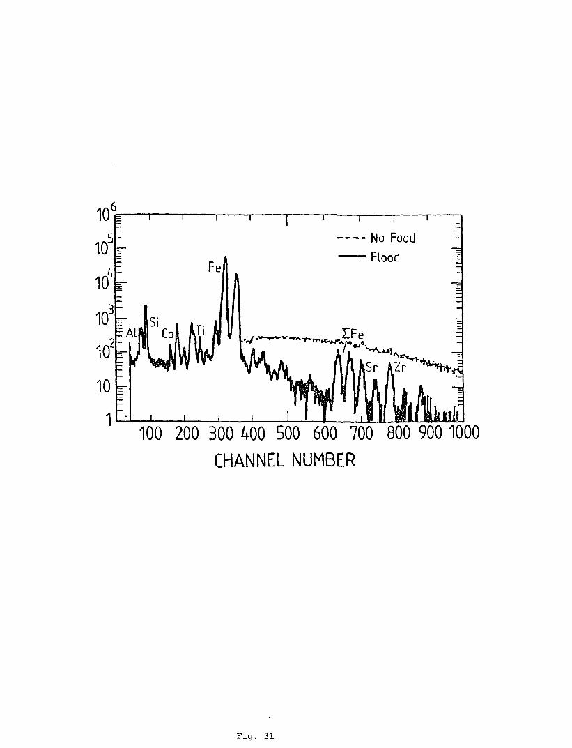
One further gross artifact that often appears in the PIXE spectrum forelectrically insulated targets is an increased Bremsstrahlung backgroundextending in some instances all the way out to several 10's of keV. Fig.

31 taken from Ref. [7] shows the PIXE spectra for a Motupure potterysample. The dashed line shows the effects of charging of the insulated

sample and the solid line shows the effective reduction of this backgroundby flooding the target with electrons from a heated carbon filament.Clearly the sensitivity for the elements in the region around Sr and Zr isdramatically improved.

6. SUMMARY OF PIXE OPERATING CONDITIONS

Typical PIXE operating conditions are given in Table 4 for a nonmicroprobe system.

-13-

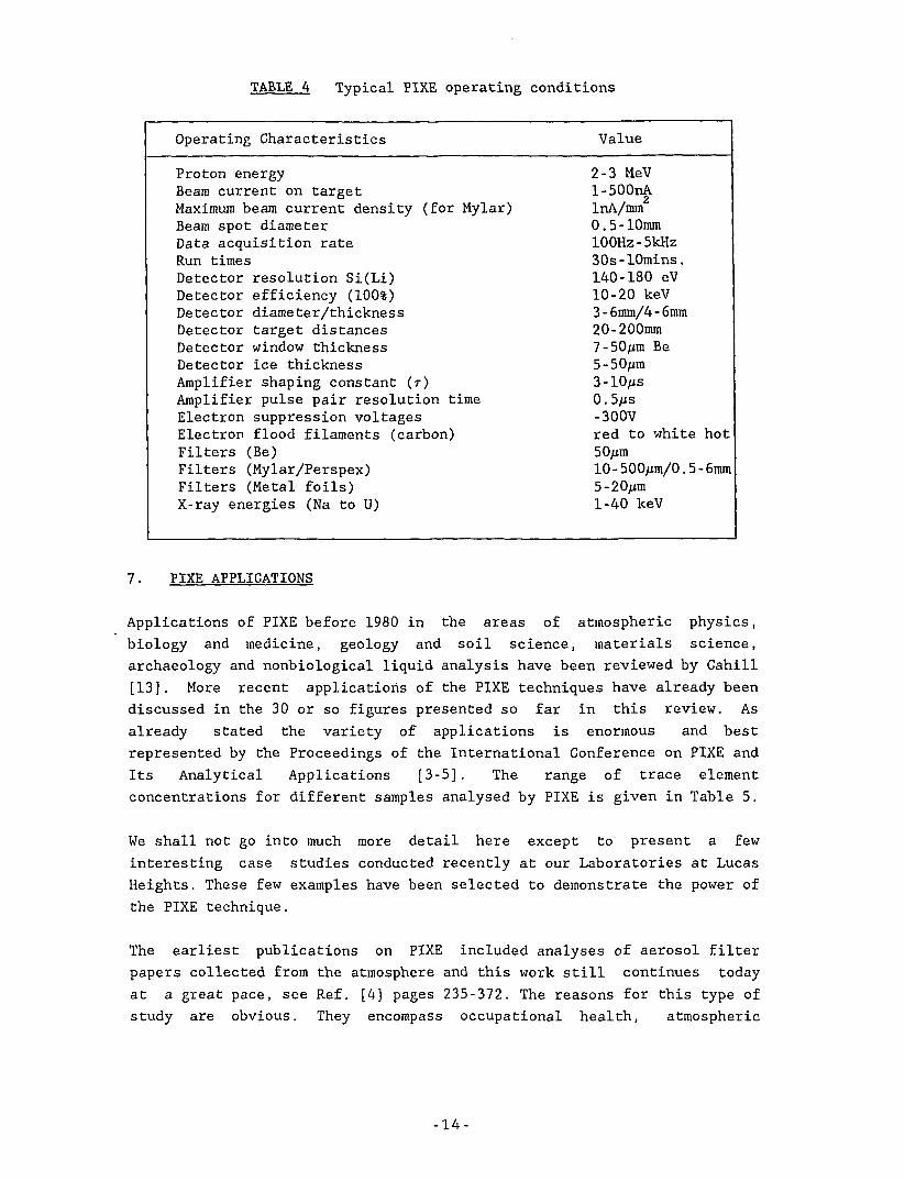
TABLE 4 Typical FIXE operating conditions

Operating Characteristics Value

Proton energy 2-3 MeVBeam current on target l-500nAMaximum beam current density (for Mylar) InA/mmBeam spot diameter 0.5-10mmData acquisition rate 100Hz-5kHzRun times 30s-10mins.Detector resolution Si(Li) 140-180 eVDetector efficiency (100%) 10-20 keVDetector diameter/thickness 3-6mm/4-6mmDetector target distances 20-200mmDetector window thickness 7-50/jm BeDetector ice thickness 5-50/imAmplifier shaping constant (r) 3-10/jsAmplifier pulse pair resolution time 0.5/*sElectron suppression voltages -300VElectron flood filaments (carbon) red to white hotFilters (Be) 50/imFilters (Mylar/Perspex) 10-500/jm/0.5-6mmFilters (Metal foils) 5-20/jmX-ray energies (Na to U) 1-40 keV

7. FIXE APPLICATIONS

Applications of PIXE before 1980 in the areas of atmospheric physics,biology and medicine, geology and soil science, materials science,archaeology and nonbiological liquid analysis have been reviewed by Cahill[13]. More recent applications of the PIXE techniques have already beendiscussed in the 30 or so figures presented so far in this review. Asalready stated the variety of applications is enormous and bestrepresented by the Proceedings of the International Conference on PIXE and

Its Analytical Applications [3-5], The range of trace elementconcentrations for different samples analysed by PIXE is given in Table 5.

We shall not go into much more detail here except to present a fewinteresting case studies conducted recently at our Laboratories at LucasHeights. These few examples have been selected to demonstrate the power ofthe PIXE technique.

The earliest publications on PIXE included analyses of aerosol filterpapers collected from the atmosphere and this work still continues today

at a great pace, see Ref. [4] pages 235-372. The reasons for this type ofstudy are obvious. They encompass occupational health, atmospheric

-14-

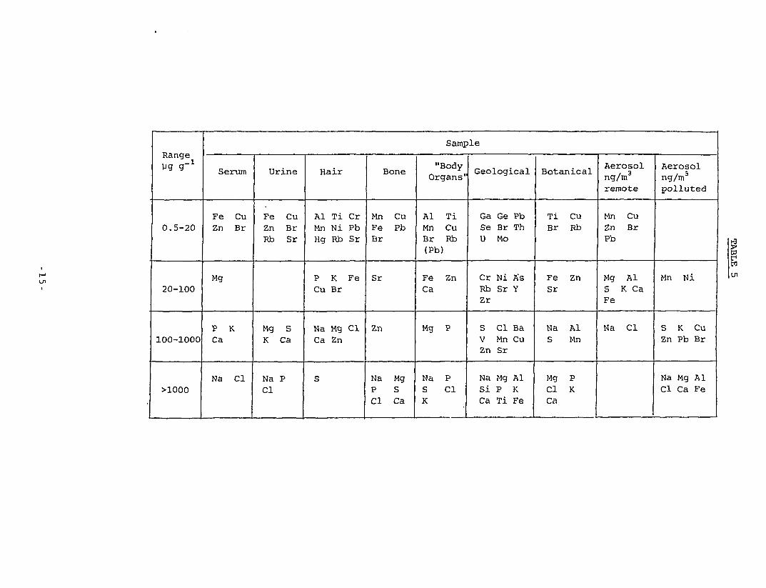
Rangeug g"1

0.5-20

20-100

100-1000

>1000

Sample

Serum

Fe CuZn Br

Mg

P KCa

Na Cl

Urine

Fe CuZn BrRb Sr

Mg SK Ca

Na PCl

Hair

Al Ti CrMn Ni PbHg Rb Sr

P K FeCu Br

Na Mg ClCa Zn

S

Bone

Mn CuFe PbBr

Sr

Zn

Na MgP SCl Ca

"BodyOrgans'

Al TiMn CuBr Rb(Pb)

Fe ZnCa

Mg P

Na PS ClK

Geological

Ga Ge PbSe Br ThU Mo

Cr Ni AsRb Sr YZr

S Cl BaV Mn CuZn Sr

Na Mg AlSi P KCa Ti Fe

Botanical

Ti CuBr Rb

Fe ZnSr

Na AlS Mn

Mg PCl KCa

Aerosolng/m3

remote

Mn CuZn BrPb

Mg AlS K CaFe

Na Cl

Aerosolng/m3

polluted

Mn Ni

S K CuZn Pb Br

Na Mg AlCl Ca Fe

IM

•visibility, acid rain, soil erosion and ecological effects. FIXE cancontribute to these studies despite the very small masses collected onfilter papers.

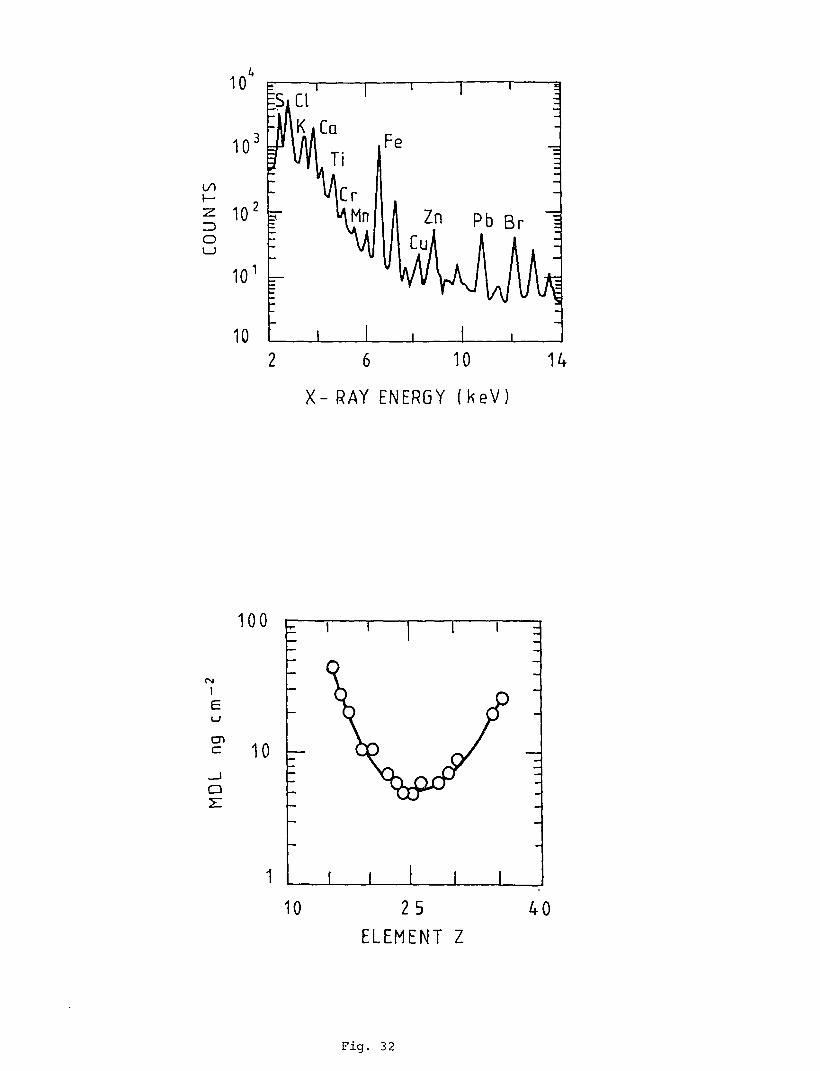
There are over 20 elements present at the 0.1% level or less in an averageurban air sample. Fig. 32 shows a typical PIXE spectrum obtained for anurban aerosol filter paper after just a few minutes of machine runningtime. The MDL's in nanograms per unit area of filter paper versus trace

element atomic number, calculated for typical aerosol filter samples are_ 2

also shown. Values of a few ngcm are readily obtainable for elementsfrom Ca to Zn. Cahill [5] reports on large scale aerosol monitoringprograms which extend across the whole of North America, containing morethan 50 sampling stations, and generating tens of thousands of PIXEsamples a year.

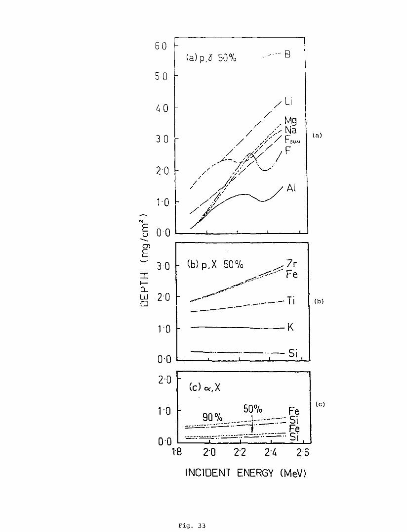
Duerden et al [23] have reported a combination of ion beam techniques toanalyse desert varnish cover on rock surfaces from western NSW inAustralia. Desert varnish is a naturally occurring shiny dark colouredthin (5 to 200 /*m) silicate clay mineral layer, containing Ca, Ti, K, P,mS and Na, which occur on fine-grained iron bearing rocks. Younger varnishmay contain higher ratios of (Ca+K) to Ti than older varnish. Measurementof this varnish layer on or near rock bearing aboriginal carvings may beable to better date these artifacts. In this study X-rays induced byprotons and helium ions were used as well as the PIGME and RBS techniquesin an attempt to distinguish trace elements both in the varnish and thesubstrate rock.

X-ray and gamma ray yields were calculated as functions of incident ion

energy as a function of sample depth. Fig. 33a shows proton depth in thej>

sample (in mg/cm') for 50% contribution to the gamma ray yield for various

light trace elements between Li and Mg. Similar calculations are shown forPIXE and HIXE for elements from Si upwards and for ion energies between

1.8 and 2.6 MeV in Figs. 33b and c. By varying the incident ion and itsenergy the varnish composition was measured for depths of around 20pm for

protons but only 1 or 2 urn for helium ions and differences between thevarnish cover and its underlying rock were easily distinguished.

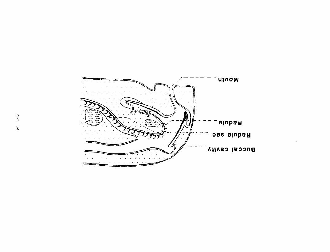
One of the main strengths of the PIXE system is its ability to analyse

very small samples. Kim et al [24] report on a quantitative PIXE study formeasuring elemental composition of teeth, on the radula, of limpets. Fig.34 shows the cross section of a limpet's mouth parts. The radula about 70mm long contains the teeth, each of which is only about 300 pm long and 30pm wide. The teeth have different stages of development andbiomineralisation depending on their position along the radula, later

stage teeth may contain up to 65% Fe. Teeth from several radulae at

-16-

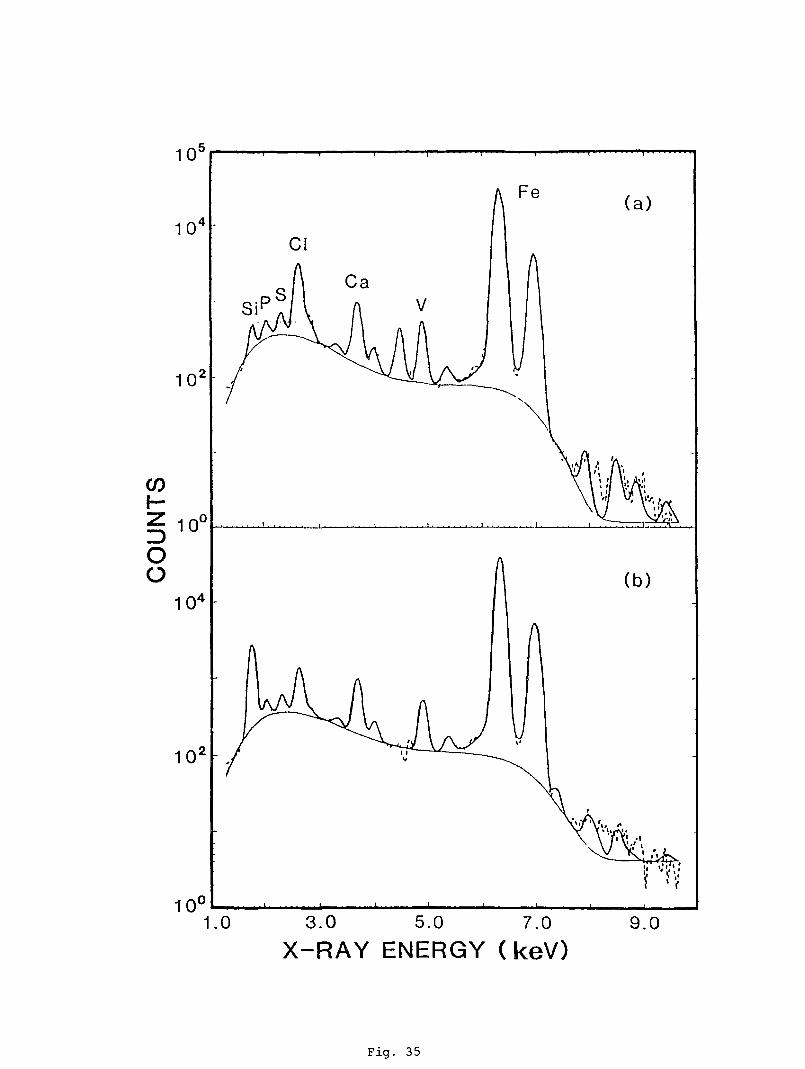
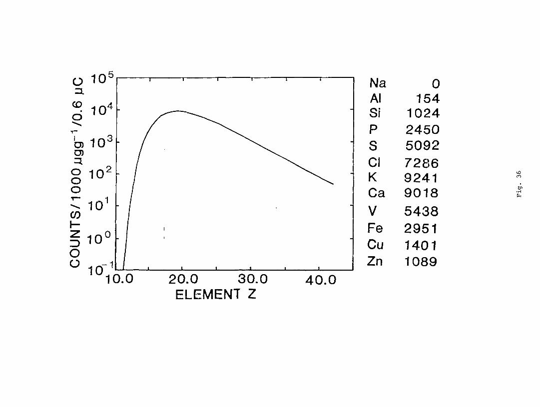
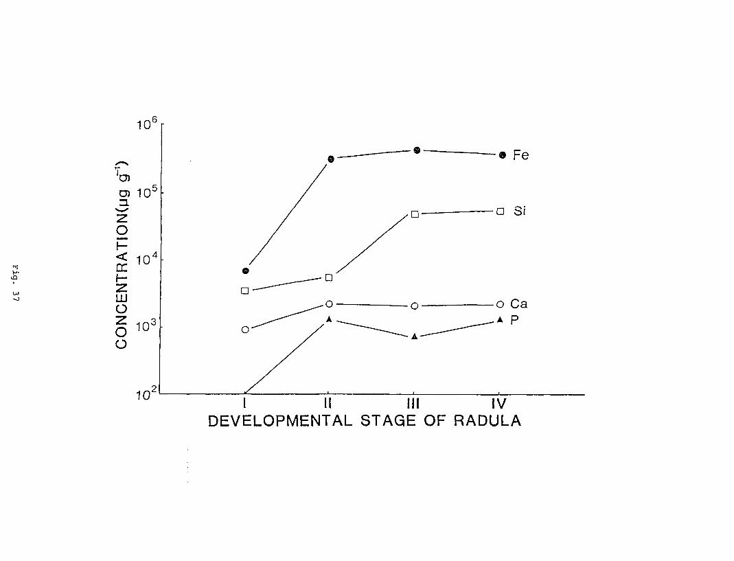
similar stages of development were extracted, powdered, spiked with a Vinternal standard and pressed into pellets containing less than 1 mg ofsample. Fig. 35 shows the PIXE spectra for two samples from differentstages of development containing different amounts of Si. PIXE allowedelemental composition along the radula to be followed quantitatively. Thecalculated Kalpha yield curves for trace elements from Al to Zr are shownin Fig. 36. The concentrations of selected elements for four stages ofmineralisation are shown in Fig. 37. The Fe concentration varies from lessthan 10 mgg to over 65% along the radula an extremely high Fe contentfor a biological system.

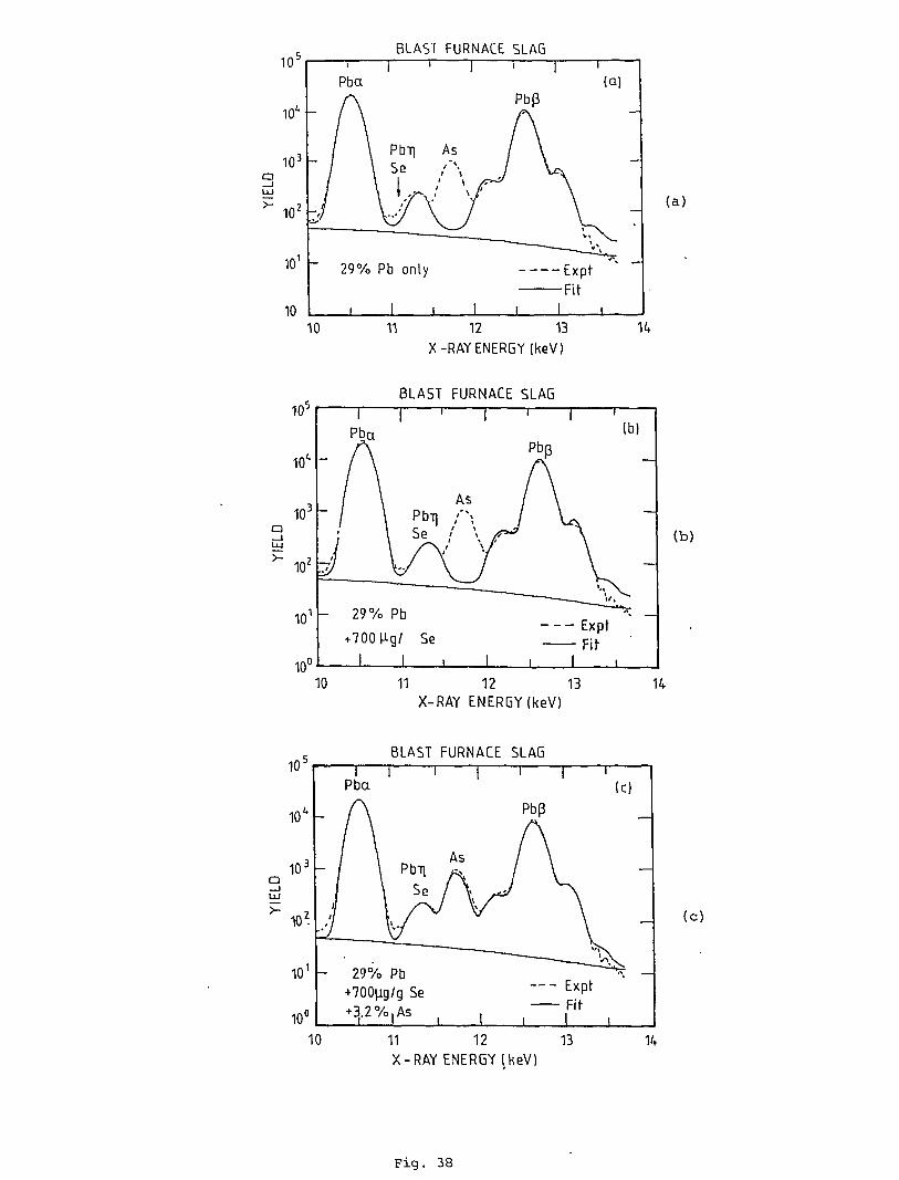
The multielement analysis capability of PIXE is also another of itsstrengths. X-ray peaks from up to 40 elements (see Fig. 12) can beanalysed in one spectrum simultaneously. However this many peaks can alsointerfere with other smaller peaks that may be of interest. An exampleof this is shown in Figs. 38a to c, which shows the PIXE spectrum from analuminium blast furnace slag over the X-ray energy range 10 to 14 keV. Theslag contains 29% Pb and the analysis required concentrations for Se andAs to be extracted. The Pb Lalpha and Leta lines interfere with As Kalphaand Se Kalpha lines respectively. Using the PIXAN analysis package wefirst included Se (Fig. 38b) and then As (Fig. 38c). The fits (solidcurves) become progressively closer to the experiment (dashed curves)

•M 1

eventually providing estimates of 700 gg for Se and 3.2% As in thepresence of 29% Pb. Calculations show that MDL's for Se and As were 200pgg and 1500 pgg respectively in the presence of 29% Pb.

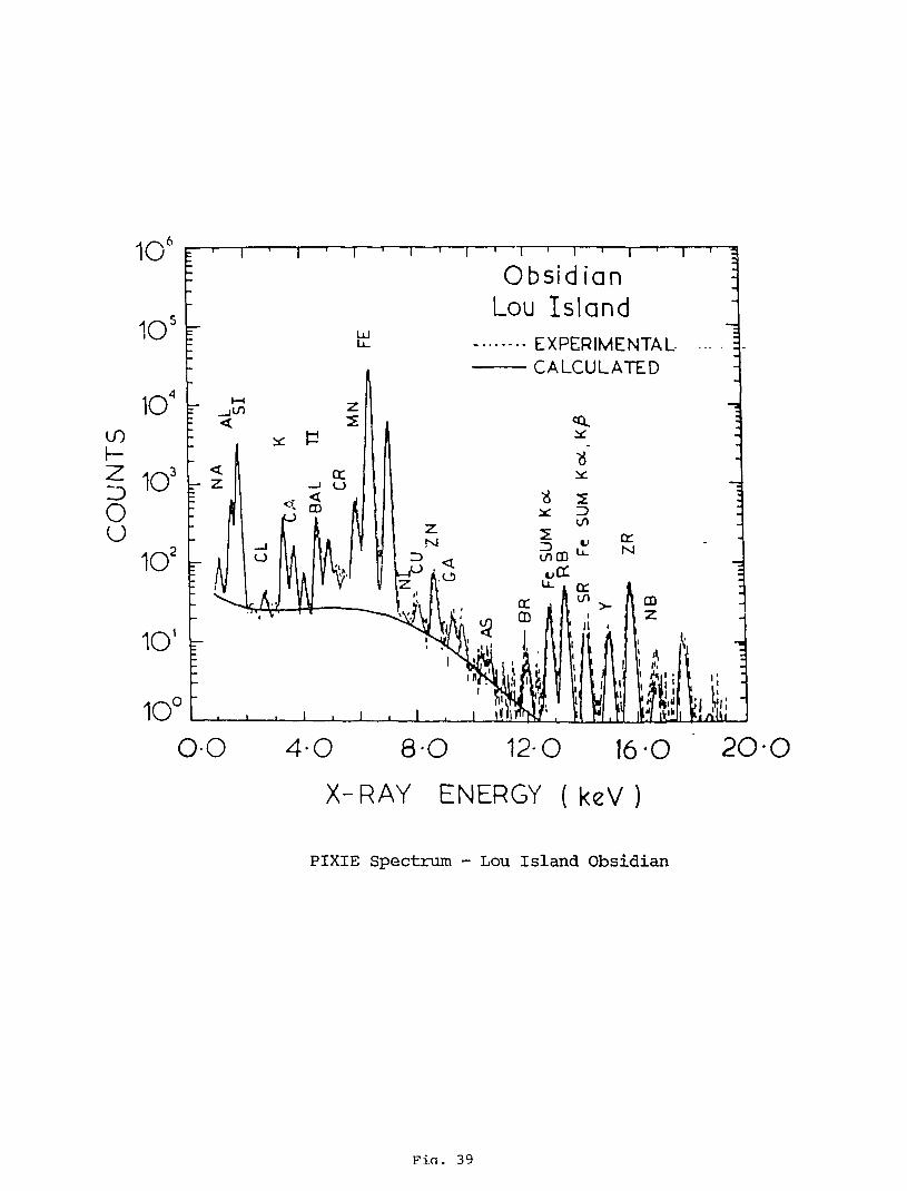
The multielemental capabilities of PIXE have also been applied extensivelyat Lucas Heights to the fingerprinting of tens of thousands of obsidian

glass samples [7]. Fig. 39 shows the PIXE spectrum, taken with a pinholefilter, of Lou Island obsidian glass. Elements from Na to Zr are clearly

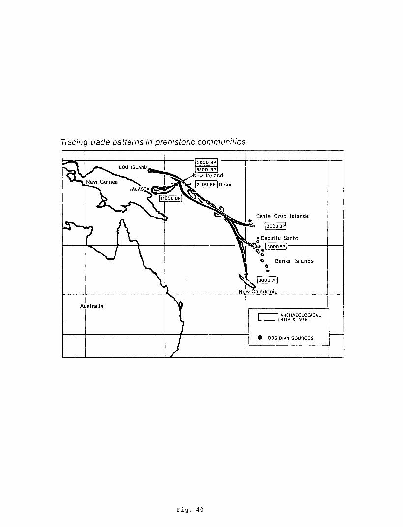
visible. Fingerprints have been obtained for all known obsidian sourcesfrom Australia, New Zealand and the South Pacific region as well as manyartifacts from Melanesia, New Zealand and neighbouring islands. The onlysample preparation was an ultrasonic wash in benzene. The analysis of

artifacts and source obsidian has enabled archaeologists to establish

trade patterns between natives in New Britain as early as 11000 BP andover distances of 400 km, including significant water crossings as earlyas 6800 BP. By 3500 BP, prime quality obsidian was extensively distributed

over 3500 km of the Melanesian Island chain from the Admiralty Islands toVanuatu (New Hebrides), see Fig. 40.

8. PIXE AND OTHER TECHNIQUES

The principles, instrumentation and methodological aspects of other

techniques competing with PIXE have been very thoroughly reviewed in an

-17-

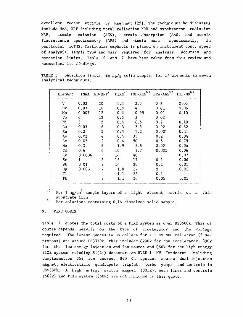
excellent recent article by Maenhaut [25]. The techniques he discussesinclude NAA, XRF including total reflection XRF and synchrotron radiationXRF, atomic emission (AES), atomic absorption (AAS) and atomicfluorescence spectrometry (AFS) and atomic mass spectrometry, inparticular ICPMS. Particular emphasis is placed on instrument cost, speedof analysis, sample type and mass required for analysis, accuracy anddetection limits. Table 6 and 7 have been taken from this review andsummarises its findings.

TABLE 6 Detection limits, in /*g/g solid sample, for 17 elements in sevenanalytical techniques.

Element INAA EB-XRF3

VCrMnFeNiCuZnAsSeMoCdInSnSbHgTlPb

0.030.030.001630.030.30.030.030.30.60.000610.010.003

201612125654256

887

8

> PIXEa)

1.30.80.60.50.40.30.30.40.41.9101416141.01.11.1

ICP-AESb }

3.540.9536.53.51.235505.51.7401720172530

ETA-AASb 3

0.20.010.010.020.20.020.0010.20.50.020.003

0.10.120.10.05

ICP-MSb)

0.030.060.10

0.100.320.210.040.790.040.060.070.060.050.02

0.05

a)

b)

9.

'g

For 1 rag/cm sample layers of a light element matrix on a thinsubstrate film.For solutions containing 0.1% dissolved solid sample.

PIXE COSTS

Table 7 quotes the total costs of a PIXE system as over US$500k. This of

course depends heavily on the type of accelerator and the voltagerequired. The latest quotes in US dollars for a 1 MV NEC Pellatron (2 MeV

protons) are around US$350k, this includes $200k for the accelerator, $90kfor the low energy injection and ion source and $60k for the high energyPIXE system including Si(Li) detector. An HVEE 1 MV Tandetron includingduoplasmatron 358 ion source, 860 Cs sputter source, dual injectionmagnet, electrostatic quadrupole triplet, turbo pumps and controls isUS$880k, A high energy switch magnet ($35K), beam lines and controls($62k) and PIXE system ($60k) are not included in this quote.

-18-

The HVEE 3MV AN2500 Van de Gra?.ff accelerator only with RF ion source wasquoted at US$535k. High energy beamlines, chambers and switching magnetsare extra.

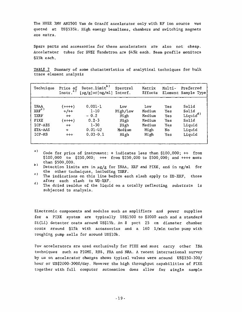
Spare parts and accessories for these accelerators are also not cheap.Accelerator tubes for HVEE Tandetron are $45k each. Beam profile monitors$15k each.

TABLE 7 Summary of some characteristics of analytical techniques for bulktrace element analysis

Technique

INAAXRF°TXRFPIXEICP-AESETA-AASICP-MS

Price of Detec. limitInstr.a) [/ig/g]or[ng/ml]

(-H-H-) 0.001-1+/-H- 1-10++ - 0.2

/ i | | i \ n 07i i i r i i \j * £ J++ 1-30+ 0.01-02-H-+ 0.03-0.1

SpectralInter f.

LowHigh/LowHighHighHighMediumHigh

MatrixEffects

LowMediumMediumMediumMediumHighHigh

Multi-Element

YesYesYesYesYesNoYes

PreferredSample Type

SolidSolidLiquidd 5

SolidLiquidLiquidLiquid

a)

b)

c)

d)

Code for price of instrument: + indicates less than $100,000; ++ from$100,000 to $250,000; +++ from $250,000 to $500,000; and -H-H- morethan $500,000.Detection limits are in Mg/g for INAA, XRF and PIXE, and in ng/ml forthe other techniques, including TXRF.The indications on this line before each slash apply to ED-XRF, thoseafter each slash to WD-XRF.The dried residue of the liquid on a totally reflecting substrate issubjected to analysis.

Electronic components and modules such as amplifiers and power suppliesfor a PIXE system are typically US$1500 to $2000 each and a standard

Si(Li) detector costs around US$15k. An 8 port 25 cm diameter chambercosts around $15k with accessories and a 160 1/min turbo pump withroughing pump sells for around US$10k.

Few accelerators are used exclusively for PIXE and most carry other IBAtechniques such as PIGME, RBS, FRA and NRA. A recent international survey

by us on accelerator charges shows typical values were around US$150-300/hour or US$2000-3000/day. However the high throughput capabilities of PIXEtogether with full computer automation does allow for single sample

-19-

charges to be as low as $20/sample. However a more realistic range appearsto be $30 to $70 per sample depending on the number of elements requiredand the levels at which they occur.

10. CONCLUSION

Johansson [5] in his summary of the 5th International Conference on FIXEand Its Applications points out that a PIXE spectrum looks the same as itdid 20 years ago, since detector resolutions have not improvedsignificantly and protons of a few MeV still give the best overallperformance. The thing that has improved is our knowledge of all thedetails of PIXE and the PIXE procedure. An accuracy and precision of a fewpercent for thick target PIXE as well as thin targets can now be achieved.PIXE is now a standard world-wide accelerator based analytical technique.

The author acknowledges that a lot of the data presented here was obtainedby many others in the Ansto IBA group over the last 15 years.

11. REFERENCES

[1] S.A.E. Johansson and T.B. Johansson,Nucl. Instr. and Methods, 137(1976)473.

[2] T.B. Johansson, R. Akselsson and S.A.E. Johansson,Nucl. Instr. and Methods, 64(1970)141.

[3] Proceedings of 3rd Int. Conf. on PIXE and Its Analytical Applications,Heidleberg, July, 1983, Nucl. Instr. and Methods, 63(1984)1-711.

[4] Proceedings of 4th Int. Conf. on PIXE and Its Analytical Applications,

Florida, June, 1986, Nucl. Instr. and Methods, B22(1987)1-484.

[5] Proceedings of 5th Int. Conf. on PIXE and Its Analytical Applications,Amsterdam, August, 1989, Nucl. Instr. and Methods, B49(1990)1-589.

[6] "Particle Induced X-ray Emission Analysis Application to AnalyticalProblems", I.V. Mitchell and K.M. Barfoot, Nucl. Science Applications,

1(1981)99-162.

[7] "Ion Beam Techniques in Archaeology and the Arts", J.R, Bird, P.

Duerden and D.J. Wilson, Nucl. Science Applications, 1(1983)357.

[8] "Ion Induced X-ray Emission", D.D. Cohen and E. Clayton in Ion Beamsfor Materials Analysis (Academic Press, New York, 1989) eds. J.R. Birdand J.S. Williams p209-260.

-20-

[9] "A Novel Technique for Elemental Analysis" (Wiley, New York, 1988)S.A.E. Johansson and J.L. Campbell.

[10] "Principles and Applications of High Energy Ion Beams" eds. F. Watt

and G.W. Grime, 1987, Adam Hilger, Bristol.

[11] D.D. Cohen, M.H. Harrigan, Atomic Data Nucl. Data Tables, 33(1985)255.

[12] D.D. Cohen and E. Clayton, Nucl. Instr. and Methods, B22(1987)59.

[13] T.A. Cahill, Ann. Rev. Nucl. Part. Sci., 30(1980)211.

[14] "Particle Induced X-ray Emission", T.A. Cahill, Metals MaterialsCharacterisation Handbook, 9th edition, vol.10, American Society for

Metals, 1985, p!02.

[15] D.D. Cohen, Nucl. Instr. and Methods, B49(1990)1.

[16] J.L. Campbell et al, Nucl. Instr. and Methods, B14(1986)204.

[17] E. Clayton, PIXAN Package, AAEC Report No. M113(1986).

[18] E. Clayton, Nucl. Instr. and Methods, 191(1981)567.

[19] W. Maenhaut and H. Raemdonck, Nucl. Instr. and Methods, Bl(1984)123.

[20] R. Woldseth, X-ray Energy Spectroraetry, published by Kevex Corp, USA(1973).

[21] D.D. Cohen, Nucl. Instr. and Methods, 178(1980)481.

[22] D.D. Cohen, X-ray Spectrometry, 16(1987)237.

[23] P. Duerden, D.D. Cohen, D. Dragovich and E. Clayton, Nucl. Instr. and

Methods, B15(1986)643.

[24] K.S. Kim, D.D. Cohen, J. Webb and D.J. Macey, Nucl. Instr. andMethods, B22(1987)227.

[25] W. Maenhaut, Nucl. Instr. and Methods, B49(1990)518.

-21-

FIGURE CAPTIONS

Figure 1. Ion beam interactions with solid targets,

Figure 2. Allowable K and L shell X-ray transitions for aninitial vacancy in the K and L shell.

Figure 3. X-ray energy bands versus target atomic number. ESCcorresponds to the escape peak energies for theprimary alpha X-ray.

Figure 4. (a) The K shell spectrum of pure Cu; (b) The L shellspectrum of pure Pb.

Figure 5. Typical FIXE spectrum for 2.6 MeV protons on anaerosol filter paper taken from an urban area nearMelbourne.

Figure 6. K, L and M shell ionisation probabilities versusnormalised ion energy. Taken from Ref.[8].

Figure 7. Calculated X-ray yield /100 jjC/msr for thick targets

and various proton energies.

Figure 8. Measured minimum detectable limits for 2.5 MeVprotons on NBS standard reference materials.

Figure 9. Comparison of Reference concentrations versus

measured PIXE concentrations covering six decades ofconcentration.

Figure 10. Comparison of yields/jjC/sr for PIXE, PIGME, RBS andNRA. Taken from Ref.[7].

Figure 11. The K alpha yield for an apatite matrix withoutfilter as a function of trace element atomic numberfor 2.26 MeV protons 0.06 msr.

Figure 12. The PIXE spectrum from a sample containing over 40elements at the 200 /ig g"1 in a graphite matrix. Thefigure shows 26 elements in the range 4 to 20 keV,for 100 pC of 2.5 MeV protons with 1.5 mm perspexfilter.

Figure 13. The trace element K alpha X-ray yields for a graphitematrix for 2.5 MeV protons and solid angle of 1.34

msr.

Figure 14. Floor plan of the Lucas Heights 3 MV Van de Graaffaccelerator.

Figure 15. Schematic of a typical PIXE target chamber.

Figure 16. Schematic of a typical PIXE/PIGME system with targetholder (H) and sample mount (S).

Figure 17. Schematic of a typical external PIXE/PIGME systemshowing window and graphite grid support.

Figure 18. Typical external beam PIXE spectra for 2.5 MeVprotons on an Iranian bowl for two different spots on

its surface.

Figure 19. External beam PIXE spectrum of 17 century Italian

painting. Blue pigments are identified by thepresence of Co, Si and K.

Figure 21. Variation of Si(Li) detector efficiency with time dueto ice buildup on the detector front face.

Figure 22. PIXE spectrum from an Am source (a) M lines; (b) Llines; and (c) Gamma rays.

Figure 23. Electronic block diagram of a typical PIXE setup.

Figure 24. The effect of 3 types of filter on the detector

efficiency of a PIXE system.

Figure 25. Aerosol filter paper PIXE spectrum for 2.6 MeV

protons with a 55 urn Be filter.

Figure 26. Typical PIXE spectra for (a) 2 mm thick 70 /jm holecarbon filter; (b) Same sample for 0.526 mm ofperspex.

Figure 27. PIXE spectrum from pure Nb crystals cut with tungstensaw.

Figure 28. (a) Typical Si(Li) spectral response for a SiLidetector; (b) Fits by the PIXAN package of Clayton

[17] to pure thick Sr K X-rays.

Figure 29. Typical PIXE spectrum for pure Ti target showing

escape peak and sum peaks.

Figure 30. Sum peak contributions for a mineral sample

containing high concentrations of Cr and Fe.

Figure 31. PIXE spectrum from an obsidian ^lass sample taken at2.5 MeV with a pin hole filter showing the effect offlooding the target with electrons.

Figure 32. Typical PIXE aerosol spectrum and corresponding MDLcurve for 2.5 MeV protons.

Figure 33. The depth reached in a desert varnish sample for 50%contribution to the yield for (a) PIGME; (b) FIXE;and (c) HIXE.

Figure 34. Baccal cavity and mouth parts of the limpet PatellaVulgata.

Figure 35. PIXE spectra from two different stages of Limpet

radula development.

Figure 36. Calculated PIXE yields for limpet teeth versus target

trace element atomic number.

Figure 37. A plot of the elemental concentrations along thelimpet radula representing various stages ofmineralisation.

Figure 38. PIXE spectra for blast furnace slag containing 29%Pb. The dashed curves are the experimental data andthe solid curves are the fits using the PIXAN packageof Clayton. (a) no As or Se (b) Pb and 700 pgg"1 ofSe (c) As 3.2% and Se.

Figure 39. PIXE spectrum of obsidian glass taken for 2.5 MeV

protons and using a pinhole filter.

Figure 40. Map of island groups to the north of Australiashowing native trade patterns as determined byobsidian analysis.

NUCLEAR REACTION PRODUCTS(ions, v--rays, neutrons)

k. -' • A

SPUTTERED ATOMS

INCIDENTION BEAM

LIGHT, UV, etc.

SCATTERED IONS

CHANNELLED IONS

>* DECAY

Fig. 1

543

765

M i21

21

KKd

U 1 2 61527517143109 5 1 8 6 2 3 4'4 11S-11—La Lj3

555

44444

33333

221

0

322110

22

0

J5/23 / 23/21 / 21/2

7 / 25 / 2

3 /23 /21 / 21 / 2

5 / 23 / 23 / 21 / 21 /2

2 1 3/22 1 1/22 0 1/2

1 0 1/2

Fig. 1

CNJ

Fig. 3

6X103

. 5

4LO

1 30

2

1

0

1 l '

K

_

-

-

-

i i > i i i

oc

-

-

-

, M 1 i 1 i !

8 10 12

X - R A Y ENERGY ( k e V )

14

(a) The K X-ray spectrum for Cu showing Ka and K0 peaks. The Ka: K0 ratio is approxim-ately 7.

oo

XIU

1-0

0-8

0-6

0-4

0-2

0

i i i l i i

L

- , L <1 1 1 1 LA 1

1 | i l i | ' i r

(X

L

L1

fl

-

-

y -rv . .A* i , , ,

8 12 16

X - R A Y ENERGY ( k e V )

20

(k) The L transition spectrum for Pb. This is a more complicated spectrum and requires 10lines to fully characterize it.

Fig. 4

MELBOURNE AEROSOL

10-

10' Si

_O 3

10

10'

101

I

2.6MeV

Be

Pb

Br

Pb

• IW. M

0.0 4.0 8.0 12.0 16.0

X-RAY ENERGY (keV)

10' I I 1 I I I I(M

o»j£

</>c:i_a

cr

OJi/)

LOa

c:o

c:o

QJen

TDQJ

10

10'

10'0.01

Theo ry

F i t s

I I I I I I I I

t o t a l M

0.1 1.0

ion / U e d g e ( MeV / keV ]

10.0

Fig. 6

io'

10

<D

00

E

10s

TD

~OJ - .710

10

10

i r i r

1 MeV protons2 MeV protons

— 4 MeV protons E

0 30 60 90

Target A tom ic Number Z 2

Fig. 7

1000.0 p

100.0 - \

Ienen

10.0

a

1.0

0.1

2.5 MeV protonsS O j U C

0.526 mm p e r s p e x

10

( K )

Oil shale

Orcha rd leaves"

30 50 70

T r a c e E lement 22

90

Fig. 8

10b

g 105

o

104

10

10

10

UJO

ooUJoUJ

UJLL.LJ

10 0

10° 101 102 103 10"1 105 106

PIXE CONCENTRATIONS

Fig. 9

10.10

10C

in

O ©

10Q_JLU

O 20

PIXE2.5 MeV protons L

PIXE2.5 MeV

RBS 2.5 MeV alphas1O keV/channel

PIGME®-2.5 MeV protonsA-3.5 MeV alphas

4O 60 8O

OH

C7>

TEETH

TheoryExpt-2.26MeV

10.0 20.0 30.0 40.0

ELEMENT Z

10

10'

£10'z:

8,o2

10'

10°

\~

6 10 14 18X - R A Y E N E R G Y ( k e V )

Fig. 12

10-

LJ

10

enen

°™3

1020.0

GRAPHITE

TheoryExph2.5 MeV

25.0 30.0 35.0

ELEMENT Z

40.0 45.0

. 13

<controlroomplant room computing

equipment

iabrynthy

MAIN BAY

hiMsyvitchingaccelerator *? magnets

coolingtowers

pixe/\pigm

ALCOVE

Pig. 14

X- Ray Detector

Electron Suppression

Scrapper Aperature

Ion Beam

FocusingY77A

\///\Diffusing

Quadrapole

Carbon Aperature2 mm

Electron Flood

Brass Rider Support

25 mm Targets

1 m Target Stick

Faradaycup

Insulated Joints

X-RAYDETECTOR

PROTON _flBEAM

&-RAYDETECTOR •U:

II

Fig. 16

EXIT FOIL

GRAPHITEGRID

GAMMA RAYDETECTOR

X-RAY DETECTOR

BEAM

(a)

External PIXE 13th Century Iranian Bowl

T

Cu Good glaze

6 8 1 0 1 2 1 4

X - r a y Energy (keV)

16

(b)

External PIXE 13th Century Iranian Bowl

-acu

Disintegrated glaze

10' r

102 4 6 8 10 12

X-ray ENERGY (keV)

16

Fig. 18

105

104

103

§ 1°2

10°

EXTERNAL BEAM

SiFe

2 3 4 5 6

X-RAY ENERGY(KeV)

Co

8

Fig. 19

10o

o

LJ

10-2

i—i—r

D = 4.26mm

10o

x 24lAm,54Mn,57CoO HIXE. PIXE

to1

X - R A Y ENERGY (keV)10'

Fig. 20

ICE THICKNESS

0 10 20 30 40

EFFICIENCY (%) AT 1.486 keV A*

z13o (a )

2 3 t

ENERGY (heV)

10'-

10'

- • (b)

15 20

Energy (hcV)

2" Am

i i i I 1 1 110'

(c)

ENERGY IkeV)

Fig. 22

1OO/JS

row

ANTI COINCIDENCE

X-RAY^

TARGET

CURRENT

CURRENT TOFREQUENCYCONVERTER

UJ

UJQ_

LJZUJ

LJ

cro

10'

10L

10 III

_l-I

//PINHOLE

LU[—QJQ

10 '• PERSPEX (0-526mm)

10

10X-RAY ENERGY (KeV)

100

Fig. 24

C3

l/lh-ZIDO

10-Al SMELTER POTS AEOROSOL

I

10"

101

10U

2.6 MeVBe 55|im

5 10

X-ray Energy(keV)

Fig. 25

_ Data

(a)

10/, 8 12

x- ray Energy ( keV)

01

i i i i

0.526 mm of Perspex :

o

10

(b)

2 4 8 10 12 14 16 18 20x- ray Energy ( keV )

Fig. 26

PIXE NB CRYSTALS

2.5 MeV Protons0.526 mm of Perspex Filter

200 300 WO 500 600 700 800 900 1000 1X)0 1200 1300

CHANNEL

Fig. 27

10*

o:

£CO

10J

10'TAIL

GAUSSIAN

(a)

1Q° I . . . i . . . . i I i i i i i i i . i I i i i . . . . i i I J i!i i I i i 1 i I i i I i I )i i i i . i i i i I I i i 1 i I I I i

12-0 13-0 14-0 15-0 16-0 170 18-0 19-0

X-RAY ENERGY (KeV)

12-0 j 13-0 14-0 1&0 1&0 1701 X-RAY ENERGY (KeV)

(b)

18-0 19-0

Fig. 28

10-

8 103ESCAPE

K;T iO

SUM PEAKS

ML'. , A

EXPT.

FIT

5 8 11X-RAY ENERGY (KeV)

14

Pia. 29

No Sum Peaks —

With Sum PeaksOUJ

10 12 12X-RAY ENERGY (keV)

Fig. 30

No Food

Flood

100 200 300 400 500 600 700 800 900 1000

CHANNEL NUMBER

Pig. 31

oLJ

2 6 10 14

X - R A Y ENERGY ( k e V )

100

csi

01c 10

10

I i

2 5

ELEMENT Z

40

Fig. 32

60 -

50 -

4 0

3 0

2-0

VO

§ 0-0

50%

en

3-0

§ 2-0

1-0

o-o2-0

1-0

(b)p,X 50%, Fe

Ti

K

o-o

(c)o,,X

50%90 % . ....i...- Fe

SiFe

(a)

(b)

(c)

18 2-0 2-2 2-4 2-6

INCIDENT ENERGY (MeV)

Fig. 33

T)—I.

0 ejnpey

068

icr

10'

COh-

10o

Oo

104

Cl

(a)

(b)

1.0 3.0 5.0 7.0

X-RAY ENERGY (keV)9.0

Fig. 35

o 10

O)

10

CO

§10°o

10.0 20.0 30.0ELEMENT Z

40.0

NaAlSiPSClKCa

VFeCuZn

0154

1024245050927286924190185438295114011089

"0H-

OJ

9 Fe

I II III IVDEVELOPMENTAL STAGE OF RADULA

BLAST FURNACE SLAG

1010 11 12 13

X-RAY ENERGY (keV)

(a)

BLAST FURNACE SLAG

11 12 13X-RAY ENERGY (keV)

(b)

10"BLAST FURNACE SLAG

o_iUJ

>•

10:

10

10°

Pba

h 29% Pb+700|ig/g Se

(0Pbp

I10 11 12 13

X - R A Y ENERGY I keV)14

(c)

Fig. 38

I ' I ' I '—IObsidian

Lou IslandEXPERIMENTALCALCULATED

10

O-O 4-O 8-O 12-O 16-O

X-RAY ENERGY ( keV )

PIXIE Spectrum - Lou Island Obsidian

2O-0

Fin. 39

Tracing trade patterns in prehistoric communities

Santa Cruz Islands

SOOOBP

Pig. 40

APPENDIX A

USEFUL PIXE DATA

K Shell

Line Energies, Fluorescence yields and Emission Rates

Energy (keV) Relative IntensityKoc = 100

Elt Z Kabs Kai K£i K£z UK K£i K£z

Na 11 1.072 1.041 0.023Mg 12 1.305 1.253 0.030Al 13 1.559 1.486 0.039Si 14 1.838 1,736 1.839 0.050 2.7P 15 2.142 2.013 2.139 0.063 4.3S 16 2.472 2.307 2.464 0.078 5.9Cl 17 2.822 2.621 2.816 0.097 8.2Ar 18 3.202 2.955 3.190 0.118 10.5K 19 3.607 3.312 3.589 0.140 11.7

Ca 20 4.038 3.690 4.012 0.163 12.8Sc 21 4.496 4.088 4.460 0.188 13.1Ti 22 4.965 4.508 4.931 0.214 13.4V 23 5.465 4.949 5.426 0.243 13.5Cr 24 5.989 5.411 5.946 0.275 13.5Mn 25 6.540 5.894 6.489 0.308 13.5Fe 26 7.112 6.398 7.057 0.340 13.5Co 27 7.709 6.924 7.648 0.373 13.5Ni 28 8.333 7.471 8.263 0.406 13.5Cu 29 8.979 8.040 8.904 0.440 13.7

Zn 30 9.659 8.630 9.570 0.474 13.8Ga 31 10.368 9.241 10.263 0.507 14.3Ge 32 11.104 9.874 10.980 0.535 14.7As 33 11.868 10.530 11.724 0.562 15.2Se 34 12.658 11.207 12.494 0.589 15.7Br 35 13.474 11.907 13.289 13.467 0.618 15.8 1.1Rb 37 15.201 13.373 14.959 15.183 0.667 16.0 1.7Sr 38 16.105 14.140 15.833 16.082 0.690 16.0 2.0Y 39 17.037 14.931 16.735 17.013 0.710 16.3 2.2

Zr 40 17.998 15.744 17.665 17.967 0.730 16.6 2.4Nb 41 18.986 16.581 18.619 18.949 0.747 16.8 2.6Mo 42 20.002 17.441 19.610 19.962 0.765 17.0 2.7Tc 43 21.054 18.325 20.615 21.002 0.780 17.3 2.8Ru 44 22.118 19.233 21.653 22.070 0.794 17.5 2.9Rh 45 23.224 20.165 22.720 23.169 0.808 17.7 3.0Pd 46 24.350 21.121 23.815 24.295 0.820 17.9 3.1Ag 47 25.514 22.101 24.938 25.452 0.831 17.9 3.3Cd 48 26.711 23.106 26.091 26.639 0.843 17.8 3.5In 49 27.940 24.136 27.271 27.856 0.853 18.1 3.6

Sn 50 29.200 25.191 28.481 29.104 0.862 18.5 3.7Sb 51 30.491 26.271 29.721 30.388 0.870 18.5 3.7I 53 33.169 28.607 32.289 33.036 0.884 18.9 4.0Ba 56 37.441 32.062 36.372 37.251 0.902 19.2 4.5

L SHELL LINE ENERGIES (keV)

EJlt

ZRLNBLMDLRULRHLPPLAGLCDLINLSNLSBLTELJLCSLBALLALCELPRLNPLSMLEULGDLTBLPYLHDLERLTHLYBLLULHFLTALUILRELOSLIRLPTLAULHGLTLLPBLBILRALTHLPALUL

Z

40414244454647484950515253555657585V606263646566676869707172737475767778798081828388909192

Loti

2.0402.1662.2932.5582.6962.8362.9643. 1333.2863.4433.6043.7963.9374 ,28<<>4.4654 .6504. 8395.0335.2295.635S.8456 .0566.2726.49-1)6.7196.9477.1797.4147.6547.8986.1458.39«,8.6518.9109.1749.4419.7129.98710.26710.55410.83712.33812.96713.28813.612

L£

1 .7921 .9022.0152.2522.3762.5032.6332.7672.90-1!3.0443.1883.3353.4843.7943.9534.1244.2674.4524.6324.9945.1765.3615.5465.7425.9426.1526.3416.5446.7526.9587.1727.3867.6027.8218.0408.2676.4938.7208.9529.1839.41910.62011.11711.36411.616

Ln1 .B761 .9962.1202.3822.5192.6602.6062.9563.1123.2723.4363.6053.7804 . 1414 .3304.5244.7314.9355. 1455.5885.8166.0496.2836.5336.7877.0577.3087.5797.8566.1 388.4278.7239.0269.3359.6499.9730.30710.64910.99211 .34711 .71013.6614 .5074.9445.397

LBi

2.1242.2572.3942.6832.8342.9903. 3.503.3163.4873.6623.8434 .0294.2214 .6194.8275 .0415.2615.4885.7216.2046.4556.7126. 9777.2467.5247.8098. 1008.4008.7089.0219.3429.67110.00810.35410.70611 .06911 . 44011 .82112.21112.61213.02115.23316. 19916,69917.217

LB2

2.2192. 3672.5182.8353.0013.1713.3473.52B3.7133.9044.1004 .3014.5074.9355.1565.3835.6125.8496.0856.5866.8427. 1027.3657 .6347.9108.1888.4678.7579.0479.3469.6509.960

10.27411O.59710.91911 .24911 .58311 .92212.27012.62112.97814.83915.62116,02216.425

LB3

2.2012.3342.4732.7632.9153.0723.2343.4013.5723.7503.9324 .1204.3134.7164.9265.1435.3645.5915.8286.3176. 57O6.8307.0957.3697.6507.9388.2298.5358.8459,1629.4869.817

10.15810.50910.86611 .23311 .6081 1 .99312.38812.79113.20815.44216.42336.92717.452

LB4

2. 1872.3192.4552.7712. 8903.0453.2033.3673.5353.7083.8864.0694.2574 .6494 .8515.0615.2765.4975.7216. 1956.43B6.6866.9397.2037.4707.7448.0248.312B.6058.9049.2119.5249.8451O. 17410.5O910.85211 .20311 .56111 .92913.01312.68914.74515.64016.10116.573

LBs

6.711<5.P757.2367.5087.8048.0618.3498.6398.9389.2399 . 5539.87310.19910.53010.86911 .20911 .55911 .91412.27512.64112.30413.39315.37516.21116.63417.067

LB62.1712.3122.4552.7632.9223.0873.2553.4293.6083.7923.9794.2734.3704.7804.9935.2115.4335.65<?5.8926.3696.6166.8667.1157.3697.6347.9088.1768.4558.7369.0219.3149.6109.90910.21510.52310.84011 .15811 .48011 .81012.14112.47914.23414.97315.34315.723

LYl

2.3022.4612.6232.9643.1433.3283.5193.7163.9204 .1304.3474.57O4. BOO5.2795.5305.7886.0516. 3216.6017. 1777.4797.7848. 100B.4178.7469.0879.4249.78810. 14210.51410.89311 .28411 .68312.09312.51012.94013.37913.82814 .28913.37015.24517.84518.97919.56520. 164

,LY2

2.5022.6632.8303.1803.3633.5533.7433.9514 .1604.3764.5994.8285.0655.5415.7966.0596.3246.5976.8827.4657.7668.0868.3968.7139.0499.3849.72810.08810.45810.83211 .21511 .60612.00812.42012.64013.26813.70714. 16014.62314 .76215.58018.17619.30219.8692O. 481

^Y3

5.5525.8086.0736.3406.6156.9007.4857.7958. 1048.4228.7529.0869.4299.77B10.14110.50910.88911 .27611 .67212,08012.49812.92213.35913,80714 .J6214 .73415.20015.70818.35419.50320.09420,709

LYU

4 .2364 . 4634 .6964.936S. 1845. 7025.9726.2516.5276.8147. 1067.7128.0298.3548.6839.0189.3739 . 72110.08310.45810.84011 .23811 .64312.06112.49012.92113.36613.82614 .29714 .77615.26915.76516.29219.08120.2892O. 87921 .559

LY5

2.2552 .4062.5632 .8913 . 0643.2433 . 4283.6193.8154.0184 .2284.4434 .6655. 1285.3705.6205.8746. 1356.4056 .9677.2557 .5537.8528. 1658.4808.S129 . 1439.4849.84110. 19910.56910.94711 .3321 1 .72812. 13212.55012.97213.40813.85014 .30514.77117.27118.36118.92519.5O4

LY6

7. 3067.6137.9248.2458.5748.9039.2539.6069.975

10.34110.73111 .12911 .53711 . 95412.38312.81813.26913.72814.19614.68415.17615.68318.41119.59620.21220.839

13

60 70 80ATOMIC NUMBER Z

L Subshell

Fluorescence Yields and Coster-Kronig Transitions Rates

ui <J2 U3 f 2 3 f '1 3

2830323436384042444648

50525456586062646668

70727476788082848688

90929496

0000

.0000000

0000000000

0000000000

0000

.0014

.0018

.0024

.0032

.0041

.0051

.0068

.010

.012

.014

.018

.037

.041

.046

.052

.058

.064

.071

.079

.089

.100

.112

.128

.147

.130

.114

.107

.112

.122

.134

.146

.161

.176

.205

.228

0.00860.0110.0130.0160.0200.0240.0280.0340.0400.0470.056

0.0650.0740.0830.0960.1100.1240.1400.1580.1780.200

0.2220.2460.2700.2950.3210.3470.3730.4010.4290.456

0.4790.4670.4640.479

0.00930.0120.0150.0180.0220.0260.0310.0370.0430.0490.056

0.0640.0740.0850.0970.1110.1250.1390.1550.1740.192

0.2100.2310.2550.2810.3060.3330.3600.3860.4110.437

0.4630.4890.5140.539

0.3000.2900.2800.2800.2700.2700.2600.1000.1000.1000.100

0.1700.1800.1900.1900.1900.1900.1900.1900.1900.190

0.1900.1800.1700.1600.1400.1300.1200.1100.1000.090

0.0900.0800.0500.040

0.550.540.530.520.520.520.520.610.610.600.59

0.270.280.280.280.290.300.300.300.300.30

0.290.280.280.390.500.560.580.580.580.58

0.570.570.560.55

0.0280.0260.0500.0760.1000.1170.1320.1410.1480.1510.155

0.1570.1550.1540.1530.1530.1520.1500.1470.1430.140

0.1380.1350.1330.1280.1240.1200.1160.1110.1100.108

0.1080.1670.1980.200

0.00010.00010.00010.00010.0001

0.00030.00030.00040.00050.00060.00070.00080.00100.00120.0014

0.00180.00230.00280.00290.00280.00300.00350.00420.00520.0064

0.00780.00970.01300.0160

0.00920.01160.01420.01740.02150.02590.03130.03650.04290.04880.0575

0.06710.07710.08810.10030.11440.12880.14340.16000.18000.2010

0.22100.24310.27080.29340.31810.34480.37180.39630.42190.4475

0.47610.50340.52780.5565

0.00890.01130.01380.01740.02220.02700.03210.03920.04640.05440.0647

0.07500.08550.09610.11080.12700.14300.16090.18080.20290.2269

0.25100.27720.30390.33100.35890.38700.41480.44380.47420.5032

0.52900.54870.56580.5868

0.00930.0120.0150.0180.0220.0260.0310.0370.0430.0490.056

0.0640.0740.0850.0970.1110.1250.1390.1550.1740.192

0.2100.2310.2550.2810.3060.3330.3600.3860.4110.437

0.4630.4890.5140.539

3

70 80

ATOMIC NUMBER Z

100

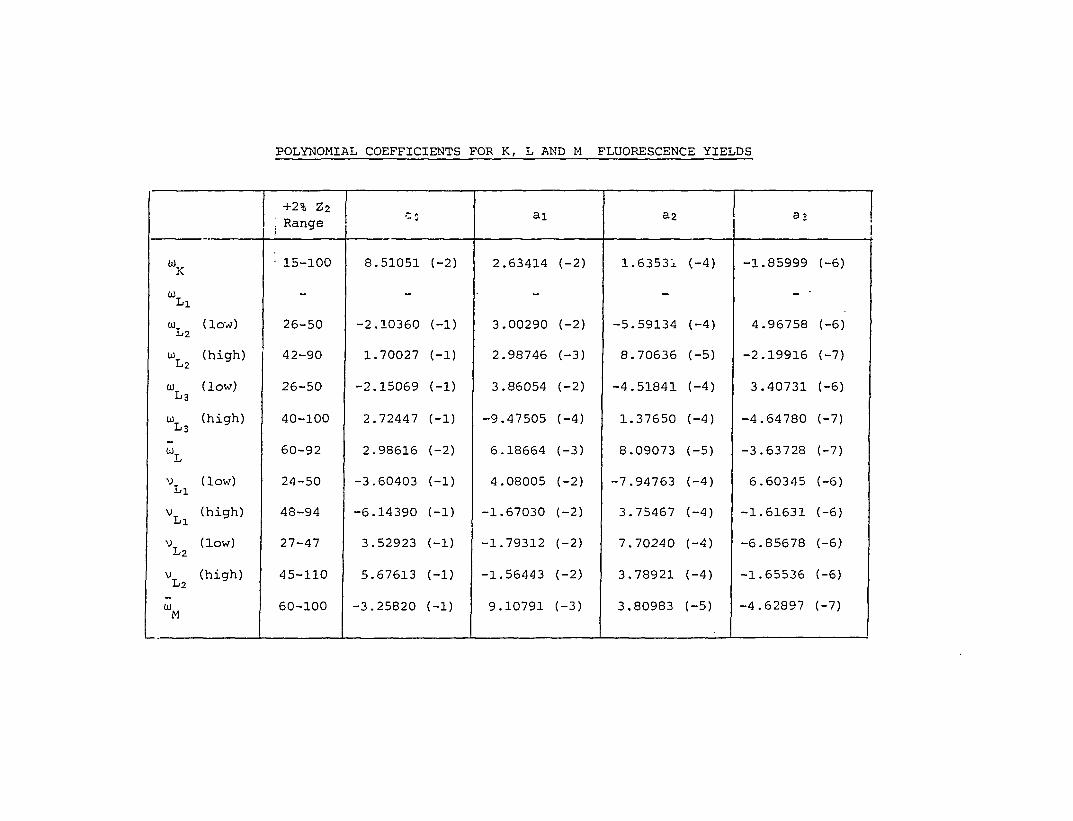
POLYNOMIAL COEFFICIENTS FOR K, L AND M FLUORESCENCE YIELDS

WK

wLI

ui (low)L2

u (high)1*2

a) (low)L3

u) (high)

"Lv (low)LI

v (high)

v. (low)La

v (high)L2

"M

+2% Z2j Range

1 15-100

-

26-50

42-90

26-50

40-100

60-92

24-50

48-94

27-47

45-110

60-100

--0

8.51051 (-2)

-

-2.10360 (-1)

1.70027 (-1)

-2.15069 (-1)

2.72447 (-1)

2.98616 (-2)

-3.60403 (-1)

-6.14390 (-1)

3.52923 (-1)

5.67613 (-1)

-3.25820 (-1)

ai

2.63414 (-2)

•

3.00290 (-2)

2.98746 (-3)

3.86054 (-2)

-9.47505 (-4)

6.18664 (-3)

4.08005 (-2)

-1.67030 (-2)

-1.79312 (-2)

-1.56443 (-2)

9.10791 (-3)

aa

1.63531 (-4)

-

-5.59134 (-4)

8.70636 (-5)

-4.51841 (-4)

1.37650 (-4)

8.09073 (-5)

-7.94763 (-4)

3.75467 (-4)

7.70240 (-4)

3.78921 (-4)

3.80983 (-5)

93

-1.85999 (-6)

- '

4.96758 (-6)

-2.19916 (-7)

3.40731 (-6)

-4.64780 (-7)

-3.63728 (-7)

6.60345 (-6)

-1.61631 (-6)

-6.85678 (-6)

-1.65536 (-6)

-4.62897 (-7)

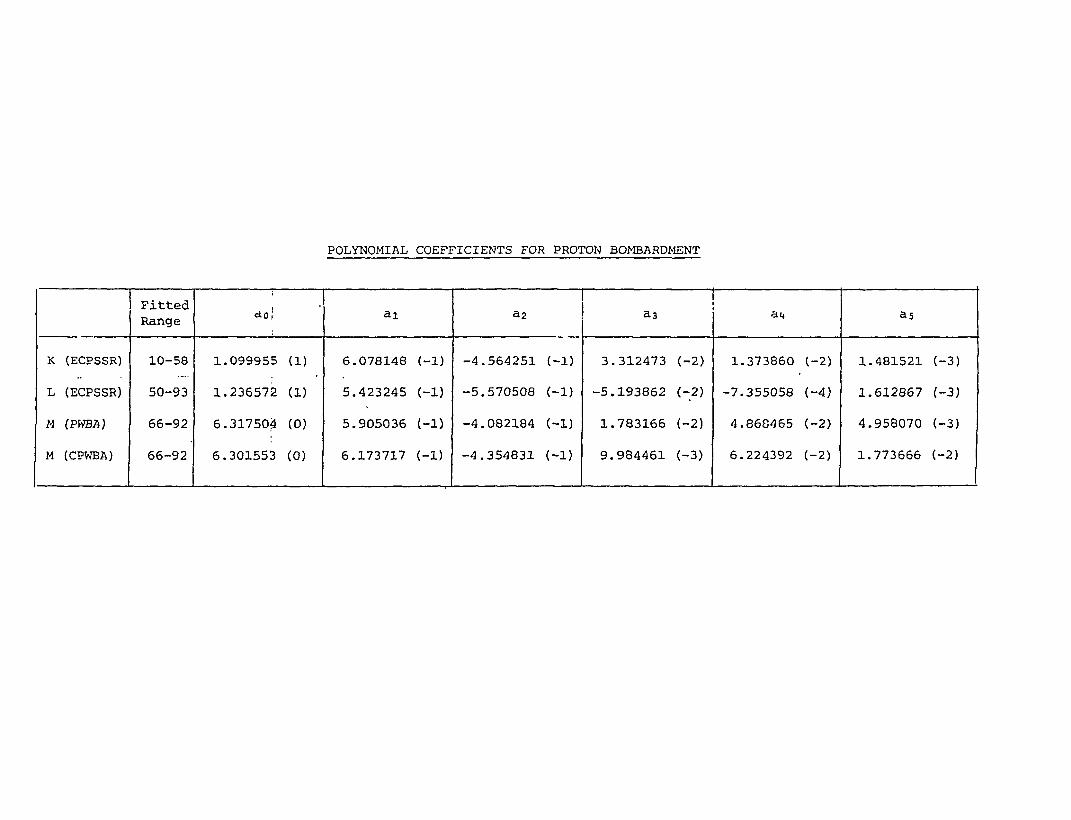
POLYNOMIAL COEFFICIENTS FOR PROTON BOMBARDMENT

K (ECPSSR)

L (ECPSSR)

M (PWBA)

M (CPWBA)

FittedRange

10-58

50-93

66-92

66-92

i

rioj

1.099955 (1)

1.236572 (1)

6.317504 (0)

6.301553 (0)

ai

6.078148 (-1)

5.423245 (-1)

5.905036 (-1)

6.173717 (-1)

a2

-4.564251 (-1)

-5.570508 (-1)

-4.082184 (-1)

-4.354831 (-1)

a-3

3.312473 (-2)

-5.193862 (-2)

1.783166 (-2)

9.984461 (-3)

ai.

1.373860 (-2)

-7.355058 (-4)

4.86S465 (-2)

6.224392 (-2)

as

1.481521 (-3)

1.612867 (-3)

4.958070 (-3)

1.773666 (-2)

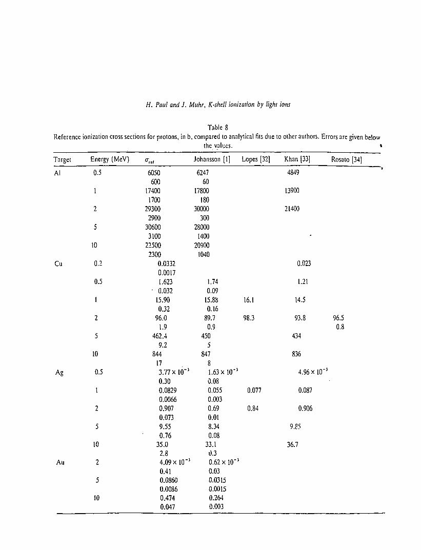
H. Paul and J. Muhr, K-shell ionization by light ions

Table 8Reference ionization cross sections for protons, in b, compared to analytical fits due to other authors. Errors are given below

the values. «

Target

Al

Cu

Ag

Au

Energy (MeV)

0.5

1

2

5

10

0.2

0.5

1

2

5

10

0.5

1

2

5

10

2

5

10

*•«!

6050600

174001700

293002900

306003100

225002300

0.03320.00171.623

• 0.03215.900.32

96.01.9

462.49.2

844173.77 x 10"3

0.300.08290.00660.9070.0739.550.76

35.02.84.09 x lO ' 3

0.410.08600.00860.4740.047

Johansson [ I ] Lopes [32] Khan [33) Rosato [34]

6247 484960

17800 13900180

30000 21400300

280001400

209001040

0.023

1.74 1.210.09

15.88 16.1 14.50.16

89.7 98.3 93.8 96.50.9 0.8

450 4345

847 83681.63 x l O " 3 4.96 x lO ' 3

0.080.055 0.077 0.0870.0030.69 0.84 0.9060.018.34 9.850.08

33.1 36.70.30.62 x 10'3

0.030.03150.00150.2640.003

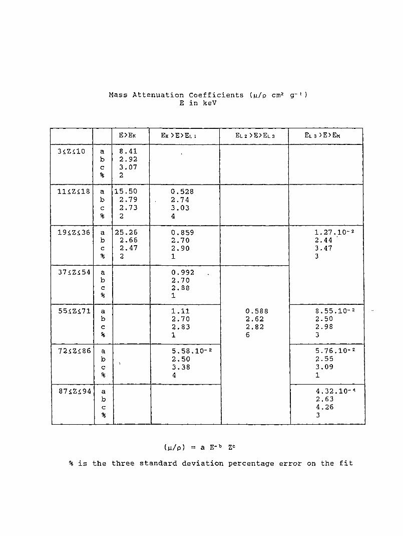
Mass Attenuation Coefficients (w/p cm2 g~ ' )E in keV

3iZilO

HiZilS

19iZ436

371Z154

55SZS71

72SZS86

871ZS94

abc%

abc%

abc%

abc%

abc%

abc%

abc%

E>E K

8.412.923.072

15.502.792.732

25.262.662.472

\

EK > E > E L i

0.5282 .743.034

0.8592.702.901

0.9922 .702.881

1.112.702.831

5.58.10-2

2.503.384

E L 2 > E > E L a

0.5882.622.826

E L G > E > E M

1.27.10-22 . 4 43.473

8.55.10-22.502.983

5.76.10-2

2.553.091

4. 32. 10-"2.634 .263

(M/P) = a E-b Z<=

% is the three standard deviation percentage error on the fit

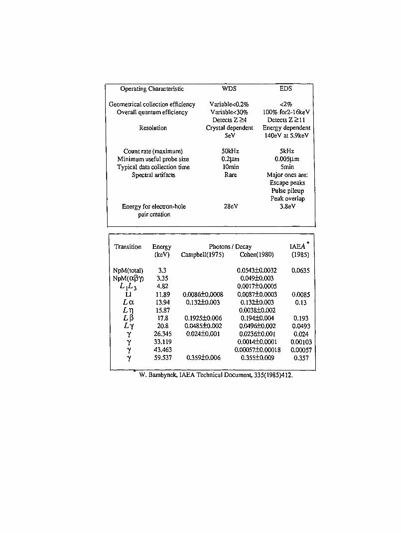
Operating Characteristic

Geometrical collection efficiencyOverall quantum efficiency

Resolution

Count rate (maximum)Minimum useful probe sizeTypical data collection time

Spectral artifacts

Energy for electron-holepair creation

WDS

Variable<0.2%Variable<30%Detects Z >4

Crystal dependent5eV

50kHz0.2|lmlOminRare

28eV

EDS

<2%100% for2-16keV

Detects Z>11Energy dependent140eV at 5.9keV

5kHz0.005|lm

5minMajor ones are:Escape peaksPulse pileupPeak overlap

3.8eV

Transition

NpM(total)NpM(ttpY)

L,L3LI

LaL7]LpLYYYYY

Energy(keV)

3.33.354.8211.8913.9415.8717.820.8

26.34533.11943.46359.537

Photons / DecayCampbell(1975)

0.0086±0.00080.132±0.003

0.1925±0.0060.0485±0.0020.024±0.001

0.359±0.006

Cohen(1980)

0.0543±0.00320.049+0.003

0.0017+0.00050.0087±0.00030.132±0.0030.0038±0.0020.194±0.0040.0496+0.0020.0236±0.0010.0014±0.0001

0.00057+0.000180.355±0.009

IAEA*(1985)

0.0635

0.00850.13

0.1930.04930.024

0.001030.000570.357

W. Bambynek, IAEA Technical Document, 335(1985)412.