1

Anomaly detection through Probabilistic Support Vector Machine Classification

- Part I -

Vasilis A. Sotiris

Department of Mathematics PhD Candidate in Applied Mathematics and Scientific Computation

University of Maryland, College Park, MD vsotiris@math.umd.edu

Michael Pecht

Department of Mechanical Engineering Director of the Center for Advanced Life Cycle Engineering (CALCE)

University of Maryland, College Park, MD pecht@calce.umd.edu

Abstract

Probabilistic Support Vector Machine Classification (PSVC) is a real time detection and prediction algorithm that is used to overcome assumptions regarding the distribution of the data. Its classification output is complemented with a probabilistic cost function and incorporates a degree of uncertainty in its predictions. Computationally, this algorithm is fast because it performs the classification using only a fraction of the original data.

This project investigates the use of support vector machines (SVMs) to detect anomalies and isolate faults and failures in electronic systems. The output of the SV Classifier is calibrated to posterior probabilities thus improving the classical SVM deterministic predictor model to a more flexible probabilistic “soft” predictor model. This result is desirable because it is anticipated to reduce the false alarm rate in the presence of outliers and allow for more realistic interpretation of the system health. This report also investigates the use of a linear principal component decomposition (PCA) of the input data into two lower dimension subspaces in order to decouple competing failure modes in the system parameters and uncover hidden degradation features. The SV classification is then used in the two extracted orthonormal subspaces to determine a predictor model for each subspace respectively. A final decision function is constructed with the joint output of the two predictor models. The approach is tested on simulated and real data and the results are compared to the popular LibSVM software.

This project will attempt to address some present issues in health monitoring of electronic systems: a) reduction of false negative alarms in the training stage b) reduction false positive alarms in the training stage c) identify hidden degradation of system parameters and d) investigate the presence of intermittent faults in healthy system performance.

Introduction

With increasing functional complexity of on-board autonomous systems, there is now an increasing demand for early system level health assessment, fault diagnostics, and prognostics. In the presence of high complexity and remote inaccessibility, the health of electronic parts and systems is difficult to monitor, diagnose and predict. Due to the micro scale packaging and material properties of the integrated components on electronic systems, performance and physics of failure (PoF) models are still uncommon and or intractable in application. There is a need for a fast and dependable way to detect when these systems are degrading, or have sustained a fault or failure that is critical. Also there is a need to predict their remaining useful life. In the absence of sustainable PoF models, a data driven approach in the machine learning framework is suitable for the first task, that of anomaly detection.

A critical part of detection and in general health monitoring is the management of false and positive alarms. Decisions made by the algorithm will not always be ideally 100% accurate, and

2

management of this accuracy is important. False alarms occur in the training and in the evaluation stage. In the training stage, the algorithm uses the training data to construct the predictor model, a model that will function as a decision boundary, inside of which incoming new observations will be classified as positive/healthy and outside of which negative/abnormal. Note that a negative classification is not necessarily unhealthy, but is at least abnormal. The diagnosis of health will need to consider other factors including further knowledge of the system itself. In the training stage, false alarms occur when some training data are misclassified; theoretically all training data should belong to the positive class. In the evaluation stage, the algorithm classifies new observations against the predictor model constructed in the training stage. Here false alarms refer to the algorithms generalization ability to correctly classify data for the system it was training on. High false alarm rates can be indicative of bad training or indeed an unhealthy system.

Existing approaches to health monitoring are more rudimentary and include the use of (1) built-in devices such as canaries and fuse devices that fail earlier than the host product to provide advance warning of failure; (2) monitoring and reasoning of parameters, such as shifts in performance parameters, progression of defects, that are precursors to impending failure; and (3) modeling stress and damage in electronics utilizing exposure conditions (e.g., usage, temperature, vibration, radiation) coupled with physics–of–failure (PoF) models to compute accumulated damage and assess remaining life [1], [2]. Traditional univariate analyses analyze each parameter separately whereas an SVM approach evaluates the data as a whole, trying to differentiate or characterize the mixture of information without necessarily requiring all the system parameters. This is especially true when working with complex electronic systems, where hundreds of signals can coexist in the sample and it is very difficult to identify every single contributor to the final system output. The SVM approach will take advantage of the overlapping sensitivities and process the information generated by these sensors to improve the resolution and accuracy of the analysis, be much more economical and easier to build.

Methodology

An important consideration for this work is to design a detection algorithm that can be used in real time, which means that it has to be fast and robust. A main focus is to process high dimensional and correlated parameter information fast without compromising the original information. For this, a Karhunen-Loev decomposition is used to compress the training data into two lower dimensional distributions; one that estimates the maximum variance and the other the error in the Karhunen-Loev model selection [6]. The compressed data will retain most of the original information and provide insight to the variance of the system, which can be used to detect anomalies, which is anticipated to enhance the interpretation of the SVM output.

3

PCA ModelR kxm

Residual ModelR lxm

PCA Model Decision boundary

Residual Model Decision boundary

D2(y2)

Posterior ClassProbabilities

p

0

1

0D(x)

-1 +10

1

0D(x)

-1 +1

0

1

0D(x)

-1 +1

Posterior ClassProbabilities

p

Probabilitymatrix

Probabilitymatrix

HealthDecision

Trending of jointprobability distributions

Joint Probabilities

BaselinePopulationDatabase

Input space R nxm

Training data

PCA

D1(y1)

New Observation∈ R 1xm

SVC

SVC

PCA SVCProbabilityModel

Figure 1 – Algorithm flow chart

Figure 1 illustrates the approach methodology. The multivariate training data X ∈ Rnxm where n is

the number of observations and m the number of parameters. The Karhunene-Loev, or otherwise known as Principal component analysis (PCA), decomposes the signal into two orthonormal subspaces, the model [S] and the residual [R] subspaces. The distribution of the projected data in the model subspace is used to estimate the maximum variance in the original parameters and the distribution on the residual is used to test the fit of the model to the data. Greater variance in the residual distribution is an indication of a poorly chosen model subspace. In addition, the residual subspace is anticipated to uncover hidden behaviors in the system degradation by highlighting abnormal variation in parameters that are overshadowed by dominant ones.

The two resulting distributions are then used as the training stage for the SV classifier, which constructs two predictor models D1(y1) and D2(y2) for each distribution respectively. The “training” of the SV classifier is an important part of this work, and is further discussed in the implementation section of this report. For now, these predictor models are constructed by using the given PCA output from two subspaces and a distribution of negative class data. One class classifiers would be more appropriate in this situation where negative class data (representing faulty behavior) are not available. A soft decision boundary can be constructed by fitting the training data with a likelihood function that maps SVM output to posterior probabilities. In the evaluation stage, a new observation is processed through the same algorithmic steps; it is projected onto the model and residual subspaces and classified with the SVM predictor model. The new observation will be classified twice and with two probabilities. The joint class probability from the two subspaces will in the end be used for the decision classification.

Support vectors produce an uncalibrated value that is not a probability. By constructing the classifier to produce a posterior probability P(class|input) the predictor model can benefit from an uncertainty to each prediction and give realistic interpretations for the classification output. The soft decision boundary can reduce the number of false alarms in both the training and evaluation stage by accepting new observations inside the SVM predictor boundary and also within the soft boundary. The issue of hidden degradation can be addressed with the PCA decomposition of the input space, where the residual subspace can uncover parameters that are overshadowed by dominantly varying ones.

Principal Component Analysis

Subspace decomposition into Principal Components can be accomplished using singular value decomposition of matrix the input data X [3] [4]. The SVD of data matrix X, is expressed as X=USVT, where S=diag(s1,…,sm) ∈ Rnxm, and s1>s2>…>sm. The two orthogonal matrices U and V are called the left

4

and right eigen matrices of X. Based on the singular value decomposition, the subspace decomposition of X is expressed as:

Trrr

Tsssrs VSUVSUXXX +=+= (1)

The two orthogonal matrices U and V are called the left and right eigen matrices of X. The signal

space Ss is defined by the PCA model and the residual subspace Sr is taken as the residual space. The diagonal Ss are the singular values { s1,…,sk }, and { sk+1,…,sm } belong to the diagonals of Sr. The set of orthonormal vectors Us=[u1,u2,…,uk] form the bases of signal space Ss. SVD is employed as a matrix algebra tool to perform the projection required for the subspace decomposition of the signal. The original data is decomposed into three matrices, U, S and V, where matrix U contains the transpose of the covariance eigenvectors. The original data X is projected onto the signal subspace as defined by the PCA model. It is furthermore desirable to use the SVD because we can express the projection in terms of existing information, that is: the eigenvectors of the covariance of the original data X.

y

x

u

v

Vp

v-pu

O

y

x

u

v

Vp

v-pu

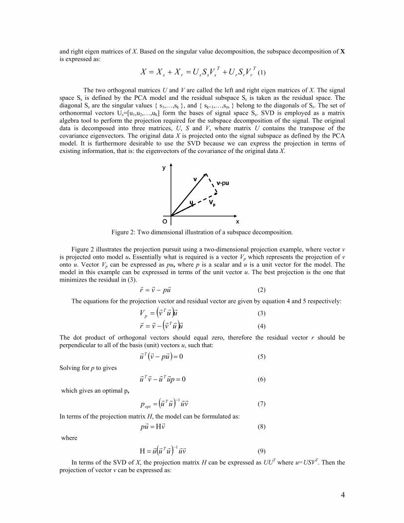
O Figure 2: Two dimensional illustration of a subspace decomposition.

Figure 2 illustrates the projection pursuit using a two-dimensional projection example, where vector v

is projected onto model u. Essentially what is required is a vector Vp which represents the projection of v onto u. Vector Vp can be expressed as pu, where p is a scalar and u is a unit vector for the model. The model in this example can be expressed in terms of the unit vector u. The best projection is the one that minimizes the residual in (3).

upvr rrr−= (2)

The equations for the projection vector and residual vector are given by equation 4 and 5 respectively:

( )uuvV Tp

rrr= (3)

( )uuvvr T rrrrr−= (4)

The dot product of orthogonal vectors should equal zero, therefore the residual vector r should be perpendicular to all of the basis (unit) vectors u, such that:

( ) 0=− upvu T rrr (5)

Solving for p to gives

0=− puuvu TT rrrr (6)

which gives an optimal p,

( ) vuuup Topt

rrrr 1−= (7)

In terms of the projection matrix H, the model can be formulated as: vup rr

Η= (8)

where

( ) vuuuu T rrrrr 1−=Η (9)

In terms of the SVD of X, the projection matrix H can be expressed as UUT where u=USVT. Then the projection of vector v can be expressed as:

5

vUUV Tp = (10)

and the residual vector as:

( )vUUIr T−= (11) The projection matrix Ps onto the signal subspace is therefore given by:

Tsss UUP = (12)

The residual subspace is the orthogonal complement of the signal subspace and the projection of the original data onto it can be expressed as

sr PIP −= (13) Any vector x can be represented by a summation of two projection vectors from subspaces Ss and Sr.

xPIxPXXX ssrsrr )( −+=+= (14)

Support Vector Machines The training data (xi,yi) in each subspace, x ∈ Xm, an the class yi ∈ {+1,-1}, i=1,…,n can be

separated by the hyperplane decision function D(x) with appropriate w and b. The classification problem can be states as:

min!½ ( ||w||2 ) = ½ wTw (15)

s.t. y(xi) = sign [ wTxi + b] – 1 ≥ 0 (16) where w = [w1,…,wn]T is the weight vector of the hyperplane and x = [x1,…xn]T the training data. Therefore, training data x with yi = +1 will fall into D(x) > 0 while the others with yi = - 1 will fall into D(x) < 0. The separating hyperplane will function as the predictor model and is chosen to maximize the distance between the two classes, a distance called the margin M = 2 / ||w||, called the objective function. The objective function is penalized by adding an error term ξ to the optimization equation:

∑=

+=n

ii

T CwwbwD12

1),,( ξξ (17)

where C is the margin penalty parameter that determines the trade-off between the maximization of the margin and minimization of the classification error, and therefore the false alarm rate.

Support Vector Machine Training

The training stage of the SVM is critical. With negative class data (fault information) the task is relatively easy because the boundaries between negative and positive class is given and a separation boundary can be computed. In cases where system faults and especially failures are absent, training becomes an issue. Whereas in the two class approach the training strategy is to generate an artificial negative class based on human knowledge of system performance, the alternative one – class training approach is investigated in this project. In the one – class training approach, data from the known positive class are “converted” to negative class points. Logically these points should be chosen as the outliers of the positive class, in other words, the task is to find the boundary of the positive class training data.

In one – class training one seeks to intelligently find areas of low data density in the training data to assign the negative class. In this project we investigate the use of statistical decision theory to infer data sufficient statistics such as the mean and variance and in such the data with associated maximum likelihood for the negative class. Computational approaches using Kmeans, or Centroid Clustering will also be investigated1.

1 One – class training will be developed as part II of this project

6

Posterior Probabilities

One way of producing posterior probabilities for the SV classifier output D is to fit a sigmoid function S [7] around it. An MLE estimate of its parameters optimizes the function to better fit the distribution of the support vectors generated by SVM. The density function that best prescribes this probability is the likelihood function computed based on the knowledge of the decision function values D(xi).

x1

x2

D(x)

D(x)

Figure 3 – Maximum Likelihood Estimate of posterior class probabilities

The likelihood function illustrated in Figure 3 (right) is a result of the maximum likelihood estimate (MLE) of the parameters a and b in:

( ) ( )( )bxaDbaDfyP

++≡≈+=

exp11),,(1 (18)

where the probability of the class prediction (in this case being +1) is given by a parametric model f which is a function of D, and the parameters a and b. So, the above equation says that the probability that a data point x is positively (normal) classified is defined by an inverse exponential function [7]. The parameters a and b in (18) are found by minimizing the negative log likelihood of the training data:

( )∑=

−−+−=n

iiiiiba

ptptF1,

)1log()1()log(min (19)

( )bxaDp

ii ++=

)(exp11

21+

= ii

yt

The minimization of (19) can be performed using any number of optimization algorithms. Each prediction will be given as two probabilities for each subspace prediction, a total set of four probabilities. The joint probabilities from the two predictors (model and residual) are used to formulate a final probabilistic prediction.

Implementation

One of the main motivations in designing a detection algorithm is its generality; that is to be suitable for a broad range of applications regardless of the data type or system purpose. For this, its online computational performance characteristics are important factors in programming the algorithm into stand alone software/tools, which should be able to perform on a standard dual processor PC with 2.2 GHz. A proof of concept will be performed using Matlab in (.m) and (.mex) files. A C based code will be attempted for the final tool. For the proof of concept, the quadratic programming solution to the quadratic optimization problem will be addressed with existing matlab/C code available in LibSVM and other matlab

7

based SVM code. Singular value decomposition will be used for computations of matrix inverses and eigenanalysis. A complexity analysis of the algorithm will be provided and a discussion of potential improvements noted. The tool will be called CALCEsvm.

Platt [7] uses a Levenberg-Marquardt (LM) algorithm to solve (19). The LM method was originally designed for solving nonlinear least-squares problems. As an iterative procedure, at the kth step, this method solves (19) to obtain a direction δk and moves the solution from zk to zk+1=zk+δk if the function is sufficiently decreases. Here Hk is an approximation of the Hessian of the least-square problem, I is the identity matrix and zk the sequence of iteration vectors.

)()( kkkk zFIH −∇=+ δλ (20)

It can be proven that the MLE optimization that (5) is convex [8] which allows for the use of more

efficient numerical optimization techniques such as Newton’s method with a backtracking line search, which are fast and robust.

Testing and Validation

The Center for Advanced Life Cycle Engineering (CALCE) at University of Maryland has extensive experimental data for electronic parts and systems under accelerated condition testing. The testing plan will utilize two data sets:

a) A simulation of training data for a multivariate system with non-uniformly scaled parameter distributions to simulate physically different measurements. The test data is identical to the training data, but with artificially injected faults. The injected faults will also differ in degree, where one parameter will be subjected to gross changes in variance while other parameters will be subjected to finer changes in variance and other still to just Gaussian noise ~ N(0,σ2) and the remaining will be unchanged.

b) Experimental data for training and experimental data with faults and failures. The experimental data includes intermittent faults and failures as part of the training and evaluation stage. The output of the algorithm will be tested against the LibSVM software output on four categories: a) false negative and false positive alarm rate for training stage b) False negative and false positive alarm rate for the evaluation stage.

c) Accuracy and timeliness in detecting known faulty periods, including intermittent faults d) Computation time. Data will generally be stored in (.mat) or excel files.

8

Midterm Results

In the first part of the project, SVM and PCA were combined and tested against a simulated data set. The training data X ∈ R3x374 consist of three parameters (chosen for visualization purposes), and n = 374 observations. The test data t consists of three parameters and only 9 observations. Each row in the data matrix X is considered an observation in time. An outlier in T is artificially injected (Table 1) at the fourth observation, the remaining observations were taken out of the distribution of the positive class.

-2-1

01

2

-4

-2

0

2-5

0

5

10

XY

Z

Figure 4 – Raw data

-4 -3 -2 -1 0 1 2 3 4-4

-2

0

2

4

6

8

PC

2

PC1

Negative class

Figure 5 – Distribution of data on Model space

-4 -2 0 2 4 6 8-3

-2

-1

0

1

2

3

PC1

PC

2

Figure 6 – Distribution of data on residual space

-4 -3 -2 -1 0 1 2 3 4-4

-2

0

2

4

6

8

PC1

PC

2

Abnormal Test point

Figure 7 – SVM prediction boundary

The application of the algorithm at this point, without the MLE optimization uses the PCA output

to train the SVM. Then the output of the SVM is tested against known faults, i.e., the injected outlier in the test data set. Both the model and residual space were chosen to be two dimensional. With the appropriate number of negative class data the algorithm does a good job at identifying the outlier. The current state of the algorithms calls for a user defined number of negative class data points to look for. This task in itself is a bottleneck in the analysis because a selection of too few negative class data points causes a larger proportion of positive misclassification (that is estimating healthy when in fact the data is unhealthy) and a selection of too many negative class data points causes a larger proportion of positive misclassification (estimating unhealthy when in fact the data is healthy). For the purpose of part I of this project the size of the negative class is chosen based on the user input only. For later analysis the plan is to optimize the size of the negative class by minimizing the volume within the SVM generated boundary. This should

9

theoretically converge to an optimum size for the negative class population. This optimization will be designed as part of the one – class training module. Table 1 shows the results of the analysis on the simulated data. The first three columns show the test data where the fourth row highlights the outlier. The fourth column shows the results of the classification prediction of the SVM on the model and residual spaces respectively. Both outputs detect the presence of the outlier, as indicated in the fourth row.

Table 1 - Test Data with one outlier and prediction results

X Y Z Prediction on Model Space

Prediction on Residual Space

3.14439 21.42006 42.25756 -1 -1 2.524949 23.41016 6.106023 -1 -1 2.255137 20.06534 38.8432 -1 -1

7.7 21.94482 3.382264 +1 +1 2.515579 23.16903 3.858731 -1 -1 0.781046 22.91557 12.18433 -1 -1 0.564716 23.96737 37.2265 -1 -1 2.028987 20.68384 17.43634 -1 -1 0.576191 23.15583 42.13435 -1 -1

Summary

In part I of the project, PCA and SVM were successfully integrated and used to detect outliers in a simulated data set. The preliminary results are promising and show that the algorithm can accurately detect anomalies in non Gaussian data. Concerns exist regarding the one – class training stage of the algorithm, in which the negative class data are generated based on outlying positive class data. The method for selection of both the size and actual data points for the negative class is still in question. Currently, the user specifies the size of the negative class and the actual points that represent it are chosen based on the sum of the second norm distances of each data point to each of their neighbors. The cross space detection results will be further investigated and the posterior probabilities, as discussed, used to compute the joint classification probabilities. It is anticipated that the trend of these joint class probabilities can be used to predict the future system performance.

In Part II of the project, the plan is to develop the one – class training algorithm, compute the

maximum likelihood of the sigmoid parameters a and b, implement the joint class probability model and design a performance tracker to tabulate and compare the performance characteristics of CALCEsvm with LibSVM. In terms of the data, get access to experimental data on tested electronic systems from CALCE and run both tools on the same data. Additionally the CALCEsvm will be compared against the Classical hard classifier SVM to compare and find potential improvements or benefits in using the probabilistic approach.

10

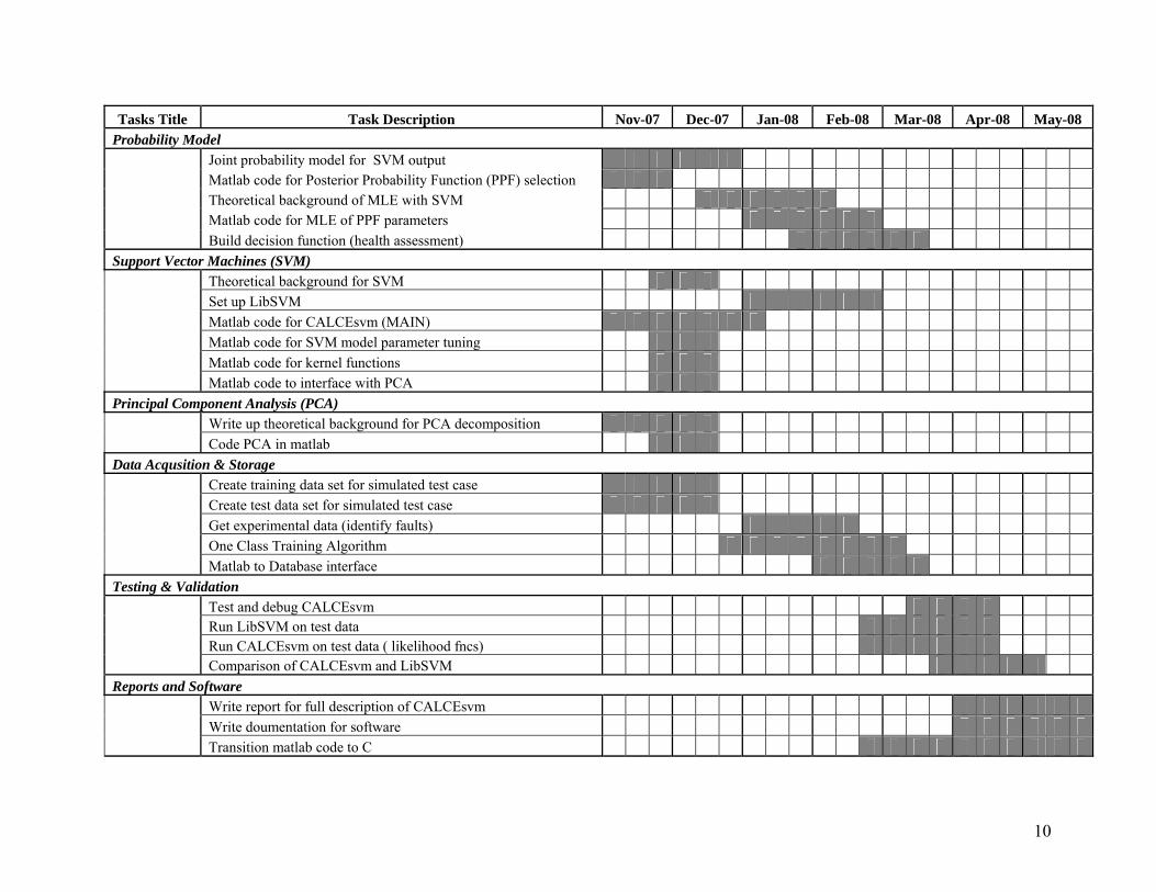
Tasks Title Task Description Nov-07 Dec-07 Jan-08 Feb-08 Mar-08 Apr-08 May-08 Probability Model

Joint probability model for SVM output Matlab code for Posterior Probability Function (PPF) selection Theoretical background of MLE with SVM Matlab code for MLE of PPF parameters

Build decision function (health assessment) Support Vector Machines (SVM)

Theoretical background for SVM Set up LibSVM Matlab code for CALCEsvm (MAIN) Matlab code for SVM model parameter tuning Matlab code for kernel functions

Matlab code to interface with PCA Principal Component Analysis (PCA)

Write up theoretical background for PCA decomposition Code PCA in matlab Data Acqusition & Storage

Create training data set for simulated test case Create test data set for simulated test case Get experimental data (identify faults) One Class Training Algorithm

Matlab to Database interface Testing & Validation

Test and debug CALCEsvm Run LibSVM on test data Run CALCEsvm on test data ( likelihood fncs)

Comparison of CALCEsvm and LibSVM Reports and Software

Write report for full description of CALCEsvm Write doumentation for software

Transition matlab code to C

11

Bibliography [1] G. Jie, N.Vichare, T. Tracy, M. Pecht, “Prognostics Implementation Methods for Electronics”, 53rd Annual

Reliability & Maintainability Symposium (RAMS), Florida, 2007 [2] Vichare, N. and Pecht, M.; “Prognostics and Health Management of Electronics,” IEEE Transactions on

Components and Packaging Technologies, Vol. 29, No. 1, March 2006. pp. 222–229 [3] Haifeng Chen, Guofei Jiang, Cristian ungureanu and Kanji Yoshihira, 2005, “Failure Detection and Localization

in Component Based Systems by Online Tracking”, KDD, August 2005, Chicago Illinois [4] Jun Liu, Khiang-Wee Lim, Rajagopalan Srinivasan and Xuan-Tien Doan, 2005, “ On-Line Process Monitoring

and Fault Isolation Using PCA”, IEEE 2005 [5] C. J.C. Burges, “A Tutorial on Support Vector Machines for Pattern Recognition”, Data Mining and Knowledge

Discovery, 2, 121–167 (1998) [6] J. A. K. Suykens, T. Van Gestel, J. Vandewalle, and B. De Moor, “A Support Vector Machine Formulation to

PCA Analysis and Its Kernel Version”, IEEE Transactions on Neural Networks, 14, 2, 2003 [7] J.C. Platt, “Probabilistic outputs for Support Vector Machines and Comparisons to Regularized Likelihood

Methods”, March 6, 1999 [8] H.T Lin, C.J. Lin, R.C. Weng, “A Note on Platt’s Probabilistic Outputs for Support Vector Machines”, Machine

Learning, 68 , 3, 267 – 276, 2007