ANNUAL REPORT INFORME ANUAL - IATTC
271
ANNUAL REPORT of the Inter-American Tropical Tuna Commission 1991 INFORME ANUAL dela Comision Interamericana del Atlin Tropical La Jolla, California 1992
-
Upload
khangminh22 -
Category
Documents
-
view
0 -
download
0
Transcript of ANNUAL REPORT INFORME ANUAL - IATTC
ANNUAL REPORT of the
Inter-American Tropical Tuna Commission
1991
INFORME ANUAL dela
Comision Interamericana del Atlin Tropical
La Jolla, California
1992

CONTENTS - INDICE
ENGLISH VERSION - VERSION EN INGLES
Page
INTRODUCTION. . . . . . . . . . . . . . . . . . . . . . . . . . . . . . . . . . . . . . . . . . . . . . . . . . . .. 7
COMMISSION MEETINGS. . . . . . . . . . . . . . . . . . . . . . . . . . . . . . . . . . . . . . . . . . .. 8
ADMINISTRATION 11
Budget 11
Financial statement 11
INTER-AGENCY COOPERATION 11
VISITING SCIENTISTS AND STUDENTS 12
FIELD STATIONS 13
PUBLICATIONS 13
THE FISHERy 14
Statistics of catches and landings 14
The eastern Pacific Ocean tuna fleet 15
REGULATION OF THE FISHERY '" 17
RESEARCH 18
Tuna and bilJfish biology 18
Tuna-dolphin investigations 44
STATUS OF THE TUNA STOCKS IN 1991 AND OUTLOOK FOR 1992 51
Yellowfin 51
Skipjack , 65
Northern bluefin 69
Bigeye 74
Black skipjack 77
FIGURES AND TABLES - FIGURAS Y TABLAS 79

VERSION EN ESPANOL - SPANISH VERSION
Pagina
INTRODUGCION 183
REUNIONES DE LA COMISION 184
ADMINISTRACION 187
Presupuesto 187
Informe financiero 187
COLABORACION ENTRE ENTIDADES AFINES 187
CIENTIFICOS Y ESTUDIANTES EN VISITA 188
OFICINAS REGIO~ALES 189
PUBLICACIONES 190
LA PESQUERIA 190
Estadisticas de capturas y desembarcos 190
La flota atunera del Oceano Pacifico oriental 192
REGLAMENTACION DE LA PESQUERIA 194
LA INVESTIGACION 194
Biologia de los tunidos y picudos 194
Investigaciones atun-delfin _ 223
CONDICION DE LOS STOCKS DE ATUNES EN 1991 Y PERSPECTIVAS PARA 1992 230
Aleta amarilla 230
Barrilete 245
Aleta azul del norte 250
Patudo , 254
Barrilete negro 258
APPENDIX 1 - ANEXO 1
STAFF - PERSONAL 259
APPENDIX 2 - ANEXO 2
RESOLUTION PASSED AT INTERGOVERNMENTALMEETING
RESOLUCION APROBADO EN EL REUNION
INTERGUBERNA:vI:ENTAL 264
APPENDIX 3 - ANEXO 3
FINANCIAL STATEMENT - DECLARACION FINANCIERA 267
APPENDIX 4 - ANEXO 4
PUBLICATIONS - PUBLICACIONES 271


COMMISSIONERS OF THE INTER-AMERICAN TROPICAL TUNA COMMISSION AND THEIR PERIODS OF SERVICE FROM ITS
INCEPTION IN 1950 UNTIL DECEMBER 31, 1991
LOS COMISIONADOS DE LA COMISION INTERAMERICANA DEL ATUN TROPICAL YSUS PERIODOS DE SERVICIO DESDE LA FUNDACION
EN 1950 HASTAEL 31 DE DICIEMBRE DE 1991
COSTA RICA Virgilio Aguiluz... .Jose L. Cardona-Cooper....... Victor Nigro Fernando Flores B....... Milton H. L6pez G _.. . . Eduardo Beeche T.. '" Francisco Thrun Valls.. Manuel Freer.......... G.briel. Mye" RDdolfo Saenz 0.. .. .. . Manuel Freer .Jimenez . Carlos P. Vargas Stew," Heigold Stuart . . . . . . . . . . . . . .. Herbert Nanni Echandi. . . . . . ..... 1990
UNITED STATES OF AMERICA
.1950-1965 . .1950-1979
1950-1969 1958-1977 1965-1977 1969-1971
.1971·1977 .. .1977-1979
1977-1979 .. 1977-1979
. .... 1989·1990 . 1989-1990
. .. 1990
Lee F. Payne............... Milton C. James. Gordon W. Sloan............... John L. Kask . .. . .. .. .. .. John L. Farley.... Arnie J. Suomela. RDbert L. Jones. Eugene D. Bennett. . . . . . . J. Laurence McHugh.. . John G. Driscoll. Jr. . . William H. Holmstrom. . . . . . . Donald P Loker. .. . .. . .. . .. . .. William M. Thrry.. Steven K SChanes......... Robert C. Macdonald. . . . . . . Wilv.n G. Van Campen .. . . . . Jack Gorby. .. .. . .. Glen H. Copeland. Wymberley Com. . Henry R. Beasley. . Mary L. Walker. . .
PANAMA Miguel A. Corro. . . . . Domingo A. Diaz. Walter Myers, .Jr.... .Juan L. de Obarrio Richard Eisenmann. Gabriel Galindo. . . . . . Harmodio Alias, .Jr.... RDberto Novey........ Carlos A. Lopez Guevara. Dora de Lanzner... .... Camilo Quintero _.. _.... Arquimedes Franqueza.... Federico Humbert, Jr. . . . Carolina T. de Mouritzen. .Jaime Valdez... Carlos ArellallO L.. . Luis E. Rodriguez.. Armando Martinez. . . . Carlos E. Icaza E........ .. Dalva H. Arospmena M............. -Jesus A. Correa G. Jorge Lymberopulos.. . Carlos E. Icaza E.. Jose Antonio leaza . .. .. .. .. . .. . .. Roy E. Cardoze . . . .
. .. 1950-19611 .. .. 1950-1951
..195]·1957 . ... 19-52
..1953-1956
. . 1957-1959 . 1958·19652 . 1950-19683 . 1960-1970
. 1962·19754 . 1966-1973
.. 1969-1976 . ... 1970-19735 . .. 1973-1974
. 1973· . .. 1974-1976
. 1975. . 1976-1977
. ..... 1977-1988 . .. 1986. . 1988
. . 1953-1957 . 195,'l-1957 .1!l.5R-1957
1958-1980 . ... 1958-1960
1958-1960 . . 1961-1962
. ... 1961-1962 ..1962-1971 .1963-1972
'" 196il-1972 . ... 1972-1974
. . 1972·1974 . .. 1974-1985 . .. 1974·1985 . . 1980-1983 . .1980·1984
. .. 1984-1988 1985-1988
. .. 1988-1990 . 1989
. .. 1989 . . 1990-1991
. .. 1990-1991 . 1990·
Jorge Lymberopulos. . ... 1991· .Juan Antonio Varela.. 1991
ECUADOR Ce:;ar Raza ..... 1961-1962 Enrique Ponce y Cabro ..... " .1961-1963 Pedro Jose Artota . . ... 1961-1962 Eduardo Burneo . .1961-1965 Hector A. Chiriboga . ....... 196.1-19G6 Francisco Baquerizo .. , ... 1963 Vicente Tarnariz A . . .. 1964-19G5 Wilson Vela H . .. 19G6-1968 Luis Pareja P . '" 1966-1968 Vinicio Reyes E , . . 1966·19G8
MEXICO Rodolfo Ramirez G '" 1964·1966 Manro Cardenas F 1964-1968 Hector Chapa Saldana 1964-1968 Maria Emilia Tellez B. . . . . . . . .Juan Luis Cifuentes L................ Alejandro Cervantes D........ Amin Zanlf M..................... Arturo Diaz R.. . .. . . . .. . . . .. -Joaquin Mercado F.. . . . . . . . .. . . . . . . Pedro Mercado S.. . Fernando Castro y Castro. . . . . . . . . .
CANADA Emerson Gennis , .. Alfred W. H. Needler .. E. Blyth Young . Leo E. Labrosse . Robert L. Payne . G. Ernest Waring. S. 1I'0el Tibbo . James S. Bec-kett . :IIichael Hunter _ .
JAPAN Tomonari Matsmhita , Sboichi Masuda . f'U1mhiko Suzuki . Seiya Nishida . Kunio ¥oHezawa. . Harunori Kaya ... Micbia Mizoguchi. Miebihiko Junihiro. Thtsuo Saito Thshio Isogai Susumu Akiyama Ryuiehi'Thnabe
. ..
. .
Satoshi Moriya . Yamato Veda Takehisa Nogami .. Kazuo Shima .. Shigenobu Kato ... Kouji Imamura, , Koichiro Seki .. .. . .
FRANCE Serge Garache . RDbert Letaconnoux.. Rene Thibaudau . Maurice Fourneyron . Dominique Piney . Daniel Silvestre .
JliICARAGVA Gilberto Bergman Padilla Antonio Flores Mana. . Jose B. Godoy.......... Odavio Gutierrez D..... Jar.1il V,TOZ E. . . . . . . . . . Abelino Aro,tegui Valladares. . . . . Sergio Martinez Casco. .
VANUATU Ricbard Carpenter .
. 1964-1971 . 1967·1970
. 1960·1978 . 1968-1970
. 1970-1978 . 1970-1977 . 1970-1975
. 197.5-1977
. .. 196819G9 · .1968-1972
.. .19G8-19~]
· 1970-1972 .. 1970-1974 .. 1970-1976
.. 1970-1977 · 1977-1984 .1981-1984
.1971-197R . .. 1971-1985
1971-1972 1972-1974
· . 1973-1979 . ... 1974-1976
1976-1977 .1979-1980
. .... 1979-1988 · 1980-1988
. ... 1984-1986 '" . 1984-1985 . .. 1985-1987
.... 1985. 1986-1989
.. 1987·1989 · . 1989·1991 .1989
.. 1991
.. ........ 19731983 .1973-1983 .1976-1977 · 1980-1987
..1984.1990
1973-1980 . 1973·1978
1976·1980 .1977·1980 . 1977-1985
. 1985-1988 1988
.1991Doresthy Kennetb . 1991
1 Deceased in service AprilJO. 1961 1 Muri6 en t:iervicio activo ellO de abril de 1961 2 Deceased in service April 26, 1965 2 Muzi6 en servicio activo e126 de abri1 de 1965 3 Deceased in service December 18. 19G8 3 Muri6 en servicio activo ell8 de diciembre de 1968 4 Deeeased in service May 5, 1973 4 Muri6 en servicio activu el5 de mayo de 1973 5 Deceased in service October 16, 1975 5 Muri6 en servicio activo e116 de octubre de 1975


ANNUAL REPORT OF THE I~TER-AMERICAN TROPICAL TUNA COMMISSION, 1991
INTRODUCTION
The Inter-American Tropical Tuna Commission operates under the authority and direction of a convention originally entered into by Costa Rica and the United States. The convention, which came into force in 1950, is open to adherence by other governments whose nationals fish for tropical tunas in the eastern Pacific Ocean. Under this provision Panama adhered in 1953, Ewador in 1961, Mexico in 1964, Canada in 1968, Japan in 1970, and France and Nicaragua in 1973. Ecuador withdrew from the Commission in 1968, Mexico in 1978, Costa Rica in 1979, and Canada in 1984. Costa Rica re-adhered to the convention in 1989, and Vanuatu joined the Commission in 1990.
The principal duties of the Commission under the convention are (1) to study the biology of the tunas and related species of the eastern Pacific Ocean with a view to determining the effects that fishing and natural factors have on their abundance and (2) to recommend appropriate conservation measures so that the stocks of fish can be maintained at levels which will afford maximum sustainable catches.
In 1976 the Commission's duties were broadened to address problems arising from the tunadolphin relationship in the eastern Pacific Ocean. As its objectives it was agreed that, "the Commi::>sion should strive [1] to maintain a high level of tuna production and also [2] to maintain porpoise stocks at or above levels that assure their survival in perpetuity, [3] with every reasonable effort being made to avoid needless or careless killing of porpoise;' The specific areas of involvement were to be (1) monitoring population sizes and mortality incidental to fishing through the collection of data aboard tuna purse seiners, (2) aerial surveys and dolphin tagging, (3) analyses of indices of abundance of dolphins and computer simulation studies, and (4) gear and behavioral research and education.
To carry out these missions, the Commission is required to conduct a ,,~de variety of investigations at sea, in ports where tunas are landed, and in the laboratory. The research is carried out by a permanent, internationally-recruited research and support staff selected and employed by the Director (Appendix 1), who is directly responsible to the Commission.
The scientific program is now in its 41st year. The results of its research are published by the Commission in its Bulletin series in English and Spanish, its two official languages. Reviews of each year's operations and activities are reported upon in its Annual Report, also in the two languages. Other studies are published in the Commission's Special Report series and in books, outside scientific journals, and trade journals.
7

8 TUNA COMMISSION
COMMISSION MEETINGS
A technical meeting was convened in La Jolla, California, USA, on January 14·15, 1991, to elaborate the details of an international program for the conservation of the dolphin populations affected by the fishery for tunas in the eastern Pacific Ocean. Dr. James Joseph, Director of the IATTe, served as Chail1nan. Representatives of Colombia, Costa Rica, Ecuador, EI Salvador, Mexico, l\icaragua, Panama, Spain, the United States, Vanuatu, and Venezuela attended the meeting, as did observers from Italy, New Zealand, the Commission ofthe European Communities, the Food and Agriculture Organization of the United Nations, and the Organizaci6n Latinoamericana de Desarrollo Pesquero. Observers from 10 non-governmental organizations, the American Cetacean Society, Association Robin des Bois, the Center for Marine Conservation, the Committee for Humane Legislation, the Earth Island Institute, Friends of Animals, Greenpeace, the Porpoise Rescue Foundation, the Whale and Dolphin Conservation Society, and the Windstarl Foundation also attended.
The follo\'i1ng agenda was adopted: 1. Opening of the meeting 2. Election of officers 3. Adoption of agenda 4. Areview of the 1990 tuna fishery in the eastern Pacific
a. Tunas b. Dolphins
5. A review of action taken at the 48th meeting of the IATTC and the Intergovernmental Meeting held in San Jose, Costa Rica, in September 1990
6. Alternatives for limiting and reducing the incidental mortality of dolphins 7. Aprogram to increase observer coverage to 100 percent 8. Programs to improve existing fishing gear and techniques with regard to reducing dolphin
mortality and to develop alternate fishing methods with a view to eliminating dolphin mortality induced by fishing
9. Programs to achieve the highest standards of performance in preventing dolphin mortality by the intel11ational fleet operating in the eastern Pacific
10. Requirements for implementation of the program a. Administrative b. Fiscal
11. Recommendations 12. Other business 13. Adjournment The IATTe staff presented abackground paper, Technical Aspects of an International Program
for the Conservation of the Dolphin Populations Mfected by the Fishery for Tropical Tunas in the Eastern Pacific Ocean, which was discussed by the attendees.
The technical meeting was followed by an intergovernmental meeting on January 16-18, at which representatives of the various governments discussed the same subject. Staff members of the IATTC provided technical advice to the participants. Aresolution (Appendix 2), calling for expansion of the intemational observer program and further research in methods of fishing for tunas which do not involve dolphins, was passed at the meeting.
The Commission held its 49th meeting in Tokyo, Japan, on June 18-20, 1991. ~lr. Koji Immamura of Japan served as Chairman. Representatives of all seven member governments attended the meeting, as did observers from Chile, Colombia, Ecuador, Mexico, Peru, Senegal, Spain, Taiwan, the Union of Soviet Socialist Republics, Venezuela, the European Economic Community (EEC), the Forum Fisheries Agency, Greenpeace, and ~he International Whaling Commission.

9 ANNUAL REPORT 1991
. The following agenda was adopted: 1. Opening of meeting 2. Adoption of agenda 3. Review of current tuna research 4. The 1990 fishing year 5. Status of tuna stocks 6. Review of Tuna-Dolphin Program 7. Recommendations for 1991 8. Recommended research program and budget for FY 1992-1993 9. An update of activities concerning arrangements for tuna management in the eastern Pacific
10. Status of a Protocol to the Convention establishing the Inter-American Tropical Tuna Commission
11. Place and date of next meeting 12. Election of officers 13. Other business 14. Adjournment The following actions were taken by the Commission: (1) Aresolution inviting the Depositary Government, the United States, to initiate procedures
to amend the Commission's Convention to make it easier for eligible nations to join the Commission and to enable international organizations, such as the EEC, to join it, was passed. This resolution reads as follows:
Noting that the procedure for adherence to the Convention between the United States ofAmerica and the Republic of Costa Rica for the Establishment of an Inter-American Tropical Tuna Commission (hereinafter referred to as the "Convention") set forth in Article V, paragraph 3 thereof has been giving rise to difficulties to the efforts of eligible governments desiring to adhere to the Convention;
Noting that Intergovernmental Economic Integration Organizations may have transferred to them by their member states competence over the matters governed by the Convention;
Desiring that Article V, paragraph 3 of the Convention be amended, in particular, to facilitate the adherence of eligible governments to the Convention and to enable such eligible organizations mentioned in paragraph 2above to adhere to the Convention;
The Inter-American Tropical Tuna Commission, ther~fore, resolves to invite the Depositary Government of the Convention to take the necessary steps as appropriate to initiate formal procedures necessary to amend the relevant Articles of the Convention.
(2) The nations with coastlines bordering the eastern Pacific Ocean (EPO), and other nations whose vessels fish for tunas in the EPO with purse seines, were invited to contribute to efforts to reduce or eliminate the mortalities of dolphins in the fishery for tunas, as expressed in the following resolution:
The Inter-American Tropical Tuna Commission, at its 49th Meeting, held in Tokyo, Japan, on June 18·20, 1991.
Noting the resolution from the Intergovernmental Meeting held in San Jose, Costa Rica, in September 1990, calling for the establishment of an international program to reduce dolphin mortality caused by the tuna purse-seine fishery in the eastern Pacific Ocean to insignificant levels approaching zero, coupled with research to improve the efficiency of existing fishing gear and techniques in reducing dolphin mortality and develop alternative fishing methods which do not involve intentional setting on dolphins, and identifying the Inter-American Tropical Tuna Commission as the most appropriate entity to coordinate the technical aspects of the program;
Further noting the resolution from the Intergovernmental Meeting held in La Jolla, California,
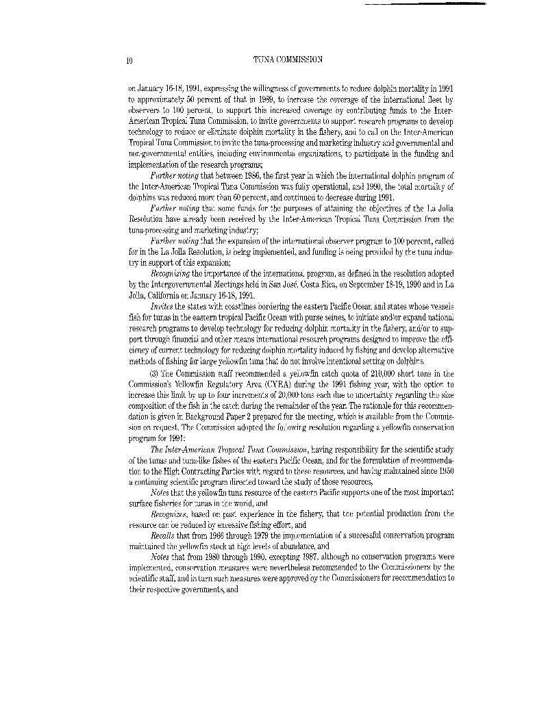
10 TUNA COMMISSION
on Janua!'y 16-18, 1991, expressing the willingness of governments to reduce dolphin mortality in 1991 to approximately 50 percent of that in 1989, to increase the coverage of the international fleet by observers to 100 pereent, to support this increased coverage by contributing funds to the InterAmerican Tropical Tuna Commission, to invite governments to support research programs to develop technology to reduce or eliminate dolphin mortality in the fishery, and to call on the Inter-American Tropical Tuna Commission to invite the tuna-processing and marketing industry and governmental and non-governmental entities, including environmental organizations, to participate in the funding and implementation of the research programs;
Further not~ng that between 1986, the first year in which the international dolphin program of the Inter-American Tropical Tuna Commission was fully operational, and 1990, the total mortality of dolphins was reduced more than 60 percent, and continued to decrease during 1991.
Further noting that some funds for the purposes of attaining the objectives of the La Jolla Resolution have already been received by the Inter-American Tropical Tuna Commission from the tuna-processing and marketing industry;
Fwiher noting that the expansion of the international observer program to 100 percent, called for in the La Jolla Resolution, is being implemented, and funding is being provided by the tuna industry in support of this expansion;
Recognizing the importance of the international program, as defined in the resolution adopted by the Intergovernmental Meetings held in San Jose, Costa Rica, on September 18·19,1990 and in La Jolla, California on January 16-18, 1991.
Invites the states with coastlines bordering the eastern Pacific Ocean and states whose vessels fish for tur.as in the eastern tropical Pacific Ocean with purse seines, to initiate andlor expand national research programs to develop technology for reducing dolphin mortality in the fishery, andlor to support through financial and other means international research programs designed to improve the efficiency of current technology for reducing dolphin mortality induced by fishing and develop alternative methods of fishing for large yellowfin tuna that do not involve intentional setting on dolphins.
(3) The Commission staff recommended a yellowfin catch quota of 210,000 ShOlt tons in the Commission's Yellowfin Regulatory Area (CYRA) during the 1991 fishing year, with the option to increase this limit by up to four increments of 20,000 tons each due to uncertainty regarding the size composition of the fish in the catch during the remainder of the year. The rationale for this reeommen· dation is given in Background Paper 2prepared for the meeting, which is available fmm the Commission on request. The Commission adopted the following resolution regarding a yellowfin conservation program for 1991:
The Inter-American Tropical Tuna Commission, having responsibility for the scientific study of the tunas and tuna-like fishes of the eastern Pacific Ocean, and for the formulation of recommendation to the High Contracting Parties with regard to these resources, and having maintained since 1950 a continuing scientific program directed toward the study of those resources,
Notes that the yellowfin tuna resource of the eastern Pacific supports one of the most important surface fisheries for tunas in the world, and
Recognizes, based on past experience in the fishery, that the potential production from the resource can be reduced by exeessive fishing effort, and
Recalls that from 1966 through 1979 the implementation of a successful conservation program maintained the yellowfin stock at high levels of abundance, and
Notes that from 1980 through 1990, excepting 1987, although no conservation programs were implemented, conservation measures were nevertheless recommended to the Commissioners by the scientific staff, and in turn such measures were approved by the Commissioners for recommendation to their respective governments, and
11 ANNUAL REPORT 1991
Observes that, at current levels of abundance and at current fleet capacity, the stock of yellowfin can be over-exploited,
Concludes that a limitation on the catch of yellowfin tuna should be implemented during 1991. The Inter-American Tropical Tnna Commission therefore recommends to the High Contract
ing Parties that an annual quota of210,OOO short tons should be established for the 1991 calendar year on the total catch of yellowfin tuna from the CYRA (as defined in the resolution adopted by the Commission on May 17,1962), and that the Director should be authorized to increase this limit by no more than four successive increments of 20,000 short tons each if he concludes from examination of available data that such increases will offer no substantial danger to the stocks, and
Finally recommends that all member states and other interested states work diligently to achieve the implementation of such a yellowfin conservation program for 1991.
(4) The Commission agreed to aproposed budget of $4,423,824 for the 1992-1993 fiscal year. (5) The Commission agreed that its next meeting would be held in La Jolla, California, USA, in
late Mayor June 1992. (6) The Commission elected Mr. Herbert Nanne Echandi of Costa Rica and the head of the
Nicaraguan delegation as Chairman and Secretary, respectively, of the next meeting of the IATTC.
ADMINISTRATION
BUDGET
At its 46th meeting, held in Paris, France, on May 10-12, 1989, the Commission unanimously approved the budget for the 1990-1991 fiscal year, submitted by the Director, in the amount of $3,706,020. However the final amount received from the member nations during the 1990-1991 fiscal year was $3,204,882, a shortfall of $501,138 relative to the amount which was recommended and approved. As a consequence, some planned research had to be limited.
FINANCIAL STATEMENT
The Commission's financial accounts for fiscal year 1990-1991 were audited by Peat, Marwick, Mitchell and Co. Summary tables of its report are shown in Appendix 3of this report.
INTER·AGENCY COOPERATION
During 1991 the scientific staff continued to maintain close contact with university, governmental, and private research organizations and institutions on the local, national, and international level. This contact enabled the staff to keep abreast of the rapid advances and developments taking place in fisheries research and oceanography throughout the world. Some aspects of these relationships are described below.
The Commission's headquarters are located on the campus of Scripps Institution of Oceanography, University of California, La Jolla, California, one of the major world centers for the study of marine science and the headquarters for state and federal agencies involved in fisheries, oceanography, and ancillary sciences. This situation provides the staff an excellent opportunity to maintain frequent contact \\ith scientists of these organizations. Dr. Richard B. Deriso of the IATTC staff shared teach· ing responsibilities with Dr. George Sugihara of Scripps Institution of Oceanography for a course entitled Quantitative Theory of Populations and Communities, given at that institution during the fall quarter of 1991.
The cordial and productive relationships which this Commission has enjoyed with the Comisi6n
12 TUNA COMMISSION
Permanente del Pacffico Sur (CPPS), the Food and Agriculture Organization (FAO) of the United Nations, the International Commission for the Conservation of Atlantic Tunas (ICCAT), the Organizacion Latinoamericana de Desarrollo Pesquero (OLDEPESCA), the South Pacific Commission (Spe), and other international bodies have continued for many years. For example, three staff members attended a meeting of the FAO Expert Consultation on Interactions of Pacific Ocean Tuna Fisheries, sponsored by FAO, at Noumea, New Caledonia. They prepared four background papers for that meeting. One of them served as Chairman of the working group on eastern Pacific yellowfin and Cochairman of the working group on skipjack. Another served as Chairman of the working group on northern bluefin and as one of the rapporteurs of the working group on North Pacific albacore. The third served as one of the rapporteurs of the working group on northern bluefin.
Also during 1991, the Commission maintained close working relationships "With fishery agencies of its member countries, as well as similar institutions in many non-member countlies in various parts of the world. For example. a workshop on bluefin tunas, sponsored jointly by the IATTC and the Australian Fisheries Service, was held in La Jolla on May 25-31, 1990. Its purpose was to discuss and report on the strengths and weaknesses of stock assessment techniques used on bluefin stocks in the Pacific, Indian, and Atlantic Oceans and the Mediterranean Sea. The proceedings of that meeting were published as an lATTC Special Report in 1991. Dr. Martin A. Hall of the IATTC staff has served as a member of the U.S. National Academy of Sciences Committee on Reducing Porpoise Mortality from 'lUna Fishing since October 1989. Since 1977 the lATTC staff has been training observers for placement aboard tuna vessels to collect data on abundance, mortality, and other aspects of the biology of dolphins. Government organizations, educational institutions, and industry representatives from the various countries involved have cooperated fully in the training and placement of these observers. Over the years scientists and students from many countries have spent several weeks or months at the Commission's headquarters in La Jolla, learning new research methods and conducting research utilizing IATTC data files. The visitors whose stays amounted to 2weeks or more are listed in the section entitled VISITING SCIENTISTS AND STUDENTS. Also. IATTC scientists have often rendered assistance with research on fisheries for tunas or other species to scientists of other countries while on duty travel to those countries, and occasionaliy have travelled to other countries for the specific purpose of assisting with their research programs.
The establishment by the Commission of a research facility in Panama, described in the section entitled FIELD STATIONS, is giving the staff the opportunity to work more closely with Panamanian fisheries personnel. The presence of Commission scientists at this laboratory has made it possible to provide assistance to local scientists in the implementation of research projects on species other than tunas, e.g. snappers. Considerable progress has been made in the snapper program; this subject is discussed in the section entitled Snapper resource studies.
VISITING SCIENTISTS AND STUDENTS
Dr. Hideki Nakano, an employee of the :--rational Research Institute of Far Seas Fisheries, Shimizu, Japan, completed a temporary assignment in La Jolla on February 28, 1991, and returned to Japan. He spent a year working with IATTC staff members on the longline fishery for tunas and billfishes in the eastern Pacific Ocean and on various aspects of the biology of Pacific billfishes.
Mr. Arvid K. Beltestad, an employee of the Institute of Fishery Technology Research, Bergen, Norway, completed a temporary assignment at IATTC headquarters in La Jolla on June 25, 1991, and returned to Norway. Mr. Beltestad, an expert on fishing gear, spent 9 months conducting his own research on tuna purse-seining gear and methods.
Mr. Michel Goujon, a former student at the Ecole Nationale Superieure Agronomique de Rennes, Rennes, France, completed a 16-month assignment at the IATTC headquarters in La Jolia, on

13 ANNUAL REPORT 1991
August 16, 1991, and returned to France. While at La Jolla he collaborated with IATTC staff members on computer simulations to estimate the potential effects of cessation of sets on dolphin-associated tunas on the fishery and worked independently on a study of the tuna fisheries of Clipperton Island and French Polynesia.
Dr. Arne BjQlrge, a biologist from the Ministry of the Environment of Norway, began a 2 1/2month stay at IATTC headquarters in La Jolla on December 11, 1991. Dr. Bj0rge conducted his own research on marine mammals and discussed research projects with IATTC and U.S. NMFS biologists.
Dr. Thomas Munroe, U.S. National Marine Fisheries Service Systematics Laboratory, Washington, D.C., spent the period of July 1-20 at the Achotines Laboratory, where he collected fishes in nearshore waters as part of a project to describe the herrings and anchovies of the Panama Bight.
Mr. Simon Thorrold, an employee of the Australian Institute of Marine Science, Thwnsville, Queensland, spent the period of July l-August 6 at the Achotines Laboratory, where he collaborated with IATTC scientists in the use of light traps to catch late-larval and early·juvenile scombrids.
Mr. Michael G. Hinton of the IATTC staff commenced a 7-week assignment with the };ational Research Institute of Far Seas Fisheries in Shimizu, Japan, on November 20, 1991. While there he worked with Dr. Hideki Nakano of that organization on studies of billfishes.
FIELD STATIONS
The Commission maintains field offices in Manta, Ecuador; Ensenada, Baja California, and Mazatlan, Sinaloa, Mexico; Panama, Republic of Panama; Trujillo, Peru; Terminal Island, California, and Mayaguez, Puerto Rico, U.S.A.; and Cumana, Venezuela. The scientists and technicians stationed at these offices collect landings statistics, abstract the logbooks of tuna vessels to obtain catch and effort data, measure fish and collect other biological data, and assist with the training and placement of observers aboard vessels participating in the Commission's tuna-dolphin program. This work is carried out not only in the above-named ports, but also in other ports in Colombia, Costa Rica, Ecuador, Mexico, Panama, Peru, Puerto Rico, and Venezuela, which are visited periodically by these employees.
In addition, the Commission maintains a laboratory at Achotines Bay, just west of Punta Mala on the Azuero Peninsula of Panama. The Achotines Laboratory is used principally for studies of the early life history of tunas. Such studies are of great importance, as acquisition of knowledge of the life history of tunas prior to recruitment into the fishery would eliminate much of the uncertainty which cUlTently exists in the staff's assessments of the condition of the various stocks of tunas. The Commission plans to enlarge the laboratory facilities so that there will be adequate space for investigators from other agencies, such as Panama's Direcci6n General de Recursos Marinos, the University of Pan· ama, etc.
PUBLICATIONS
The prompt and complete publication of research results is one of the most important elements of the Commission's program of scientific investigations. By this means the member governments, the scientific community, and the public at large are currently informed of the research findings of the IATTC staff. The publication of basic data, methods of analysis, and conclusions afford the opportunity for critical review by other scientists, ensuring the soundness of the conclusions reached by the IATTC staff, as well as enlisting the interest of other scientists in the Commission's research. By the end of 1991 the IATTC staff had published 130 Bulletins, 39 Annual Reports, 7Special Reports, 5books, and 369 chapters and articles in books and outside journals. The contributions by staff members published during 1991 are listed in Appendix 4ofthis report.
14 TUNA COMMISSION
THE FISHERY
STATISTICS OF CATCHES AND LANDINGS
The IATTC staff is concerned principally with the eastern Pacific Ocean (EPO), defined as the area between the mainland of North, Central, and South America and 150°W:
Statistical data from the Commission's field stations are continuously being collected and processed. As a result, estimates of fisheries statistics v,ith varying degrees of accuracy and precision are available. Because it may require ayear or more to obtain some final information, and because the staff has been updating the data for earlier years, the annual statistics reported here are the most current, and supersede earlier reported statistics. The weights are reported in short tons.
Annual estimates of the catches of the various species of tunas and other fishes landed by vessels of the EPO tuna fleet (see next section) are shown in Table 1. This table includes only the catches by sUlface gear, except that Japanese longline catches of yellowfin, Thunnus albacares, in the Commission's Yellowfin Regulatory Area (CYRA, Figure 1) are included. The catch data for yellowfin in the CYRA and skipjack, Katsuwonus pelamis, and bluefin, Thunnus thynnus, in the EPO are essentially complete except for insignificant catches of all three species made by the sport and artisanal fisheries, and insignificant catches of skipjack and blueiin by the longline fishery. The western Pacific and Atlantic Ocean catch data in Table 1are not total catch estimates for those waters because data for vessels which had not fished in the EPO during the year in question are not included. Also, substantial amounts of yellowfin taken by longlines in the EPO outside the CYRA and large amounts of bigeye, Thunnus obes1Ls, taken by longlines in the EPO are not included in Table 1; those catches are included in Tables 24 and 30, however.
There were no restrictions on fishing for tunas in the EPO during the 1979-1990 period, so the statistics for 1991 are compared to those of 1979-1990. During this period there was a major EI Nino that began in late 1982 and persisted until late 1983. The catch rates in the EPO were low during the EI Nino, which caused a shift of fishing effort from the eastern to the western Pacific, and fishing effort remained relatively low during 1984-1986.
The average yellowfin catch in the CYRA during the 1979-1990 period was 202.0 thousand tons (range: 91.4 to 294.7). The preliminary estimate of the 1991 yellowfin catch in the CYRA is 237.5 thousand tons. During the 1979-1990 period the yellowfin catch from the area between the CYRA boundary and 1500 Whas averaged 28.5 thousand tons (range: 13.5 to 51.3). The preliminary estimate of the yellowfin catch from this area for 1991 is 21.5 thousand tons. The estimated 1991 yellowfin catch from the EPO, 259.0 thousand tons, is well below the maximum 317.8 thousand tons taken in 1989, though it does exceed 1979-1990 average, 230.5 thousand tons.
The average annual distribution of logged catches of yellowfin by purse seiners in the EPO during the 1979-1990 period is shown in Figure 2, and a preliminary estimate for 1991 is shown in Figure 3. As fishing conditions change throughout the year, the areas of greatest catches vary. The catch of yellowfin during the first quarter of 1991 was generally restricted to regions inside the CYRA, primarily in nearshore areas and along the Inter-Tropical Convergence Zone. Additionally, good fishing occurred offshore at about 90S to 11oS between 800 W and 90°W. During the second quarter the nearshore catches continued, with areas of high catch occurring near the coast between about lOON and 23°l\. The catches during the second quarter increased in offshore areas between about 5°N and 15°N from 1200 Wto 140°W. The catches during the third quarter were fairly uniformly distributed between about 6°N and I5°N from 84°W to I40oW, with some areas of high catches near the coast, particulaJ'!y near the southern tip of Baja California. DUling the fourth quarter fishing was again taking place primarily within the CYRA in a distIibution much like that observed during the first

15 ANNUAL REPORT 1991
quarter, except that the fishing remained good around the tip of Baja California. During the 1979-1990 period the skipjack catch in the EPO averaged 94.3 thousand tons (range:
54.5 to 145.5). The preliminary estimate of the skipjack catch in the EPO in 1991 is 71.3 thousand tons. The average annual distribution of catches of skipjack by purse seiners in the EPO during the
1979-1990 period is shown in Figure 4, and a preliminary estimate for 1991 is shown in Figure 5. As in 1990, the skipjack catches in 1991 were concentrated in two areas: between about 5°8 and WON from the coast to 900W; and further south between about 10°8 to 15°8 from 800Wto 85aW.
'While yellowfin and skipjack comprise the most significant portion of the catch made in the EPO, bluefin, bigeye, albacore, Thunnus alalunga, black skipjack, Euthynnus lineatus, bonito, Sarda orientalis, and other species contribute to the overall harvest in this area. The total catch of these other species in the EPO was about 8.4 thousand tons in 1991, as compared to the 1979-1990 average of 18.1 thousand tons (range: 8.2 to 32.7). The estimated catch of all species in the EPO in 1991 was about 338.8 thousand tons.
Tuna vessels fishing in the EPO occasionally fish in other areas in the same year. In 1991 various vessels which were part of the EPO tuna fleet also fished in the western Pacific andlor in the Atlantic and Caribbean. The 1979·1990 median catch by these vessels in the western Pacific was about 8.0 thousand tons (range: 0.3 to 83.6), and in the Atlantic and Caribbean about 8.5 thousand tons (range: 0.5 to 17.3). The maximum catches made in other areas by vessels of the EPO tuna fleet were made in 1983, the year of the lowest total catch in the EPO (18G.4 thousand tons) since 1960 (173.6 thousand tons). Preliminary estimates indicate that the 1991 total catches in these areas by vessels of the EPO tuna fleet were about 1.8 thousand tons in the western Pacific and 9.0 thousand tons in the Atlantic and Caribbean.
The 1990 and preliminary 1991 catches in the EPO, by flag, and landings of fish caught in the EPO, by country, are given in Tables 2 and 3. The landings are fish unloaded during a calendar year, regardless of the year of catch. The country of landing is that in which the fish were unloaded from the fishing vessel or, in the case of transshipments, the country which received the transshipped fish. In 1991 92 percent of the EPO yellowfin catch of 259.0 thousand tons was made in the CYRA, with Mexican-, Venezuelan-, Ecuadorian-, and U.S.-flag vessels harvesting 42,16, 12, and 11 percent, respectively, of the total EPO catch.
Preliminary landings data indicate that of the 350.8 thousand tons landed in 1991,96.8 thousand tons (28 percent) were landed in Mexico. The landings to Ecuador (55.5 thousand tons; 16 percent) and Venezuela (45,4 thousand tons, 12 percent) were next in terms of magnitude. Other countries with significant landings oftunas caught in the EPO included the United States, Costa Rica, and Spain. It is important to note that when final information is available, the landings currently assigned to various countries may change due to exports from storage facilities to processors in other nations.
Under the terms of the convention which established the Inter-American Tropical 'funa Commission, monitoring the condition of the stocks of tunas and other species taken in the EPO by tuna fisheries is the primary objective of the Commission's research. Taking into consideration the extensive movements of the tunas, the mobility of the vessels of the tuna fleets of various nations, and the international nature of the tuna trade, statistics on the catch and effort from the EPO must be viewed in the light of global statistics. The estimated global catches of tunas and related species for 1990, the most recent year for which data are available, are presented in Figures 6 and 7. An overview of the catches of the principal market species of tunas during 1975-1990 by oceans appears in Figure 8.
THE EASTERN PACIFIC TUNA FLEET
The IATTC staff maintains records of gear. flag, and fish·cal'l'ying capacity for most of the

16 TUNA COMMISSION
vessels which fish for yellowfin, skipjack, or bluefin tuna in the EPO. Records are not maintained for Far East-flag longline vessels, nor for sport-fishing vessels and small crait such as canoes or launches. The EPO surface fleet described here includes vessels which have fished all or part of the year in the EPO for yellmdin, skipjack, or bluefin.
The owner's or builder's estimates of the vessel carrying capacities are used until landing records indicate that revision of these is appropriate. The vessels are grouped, by carrying capacity, into the following size classes for reporting purposes: class 1, less than 51 tons; class 2, 51-100 tons; class 3,101-200 tons; class 4, 201-300 tons; class 5, 301·400 tons; and class 6, more than 400 tons. (These are not to be confused with the eight size groups used for calculation of the catch per ton of carrying capacity in the section entitled Catch per ton ofcarrying capacity.) Except for longliners and miscel· laneous small vessels mentioned in the previous paragraph, all vessels which fished in the EPO during the year are included in the annual estimates of the size of the surface fleet.
Until about 1960 fishing for tunas in the EPO was dominated by baitboats operating in the more coastal regions and in the vicinity of offshore islands. During the late 1950s and early 1960s most of the larger baitboats were converted to purse seiners, and by 1961 the EPO surface fleet was dominated by these vessels. During the 1961-1991 period the number of baitboats decreased from about 100 to 20, and the capacity decreased from about 10 thousand to 2 thousand tons. During the same period the number of purse seiners increased from about 125 to 170, and the capacity increased from about 30 thousand to 135 thousand tons. The peak in numbers and capacity of purse seiners occurred during the 1978-1981 period, when the number of these vessels ranged from 247 to 268 and the capacity from 181 to 185 thousand tons (Table 4).
The construction of new and larger purse seiners, which began during the mid-1960s, resulted in an increase in the fleet capacity from 46.3 thousand tons in 1966 to 184.6thousa:1d tons in 1976. During the 1977-1981 period the fleet capacity remained fairly stable, increasing by only about 1.6 thousand tons. During this period the construction of new vessels continued, but the new capacity was offset by losses due to sinkings and vessels leaving the fishery. In 1982 the fleet capacity declined by 16.2 thousand tons as vessels were deactivated or left the EPO to fish in other areas, primarily the western Pacific. This trend continued through 1983 as the catch rates in the EPO declined, due primarily to anomalous ocean conditions during 1982-1983. During 1983 the fleet capacity declined by 28.8 thousand tons, and in 1984 it declined an additional 25.4 thousand tons. The fleet capacity in 1984, about 116.5 thousand tons, was the lowest it had been since 1971. In 1985, however, due primarily to the return of vessels from the western Pacific, the capacity increased to about 129.7 thousand tons. In 1986 the fleet capacity decreased slightly to about 124.5 thousand tons. During 1987 several vessels were activated, and others returned to the EPO fishery from the western Pacific, causing the fleet capacity to increase to 146.0 thousand tons. This trend continued in 1988, resulting in a fleet capacity of 151.4 thousand tons. This was the greatest fleet capacity observed since 1982. In 1989 the fleet capacity dropped to about 136.6 thousand tons. In 1990 the fleet capacity remained about the same, 137.6 thousand tons. This fleet capacity was not present in the EPO through the entire year, however. In the spring of 1990 the U.S. tuna canning industry adopted a policy of not purchasing tunas caught in association with dolphins (U.S. canners' dolphin-safe policy). This caused many of the U.S.-flag vessels fishing in the EPO to leave the fishery and enter the fisheries in the Atlantic or western Pacific. The U.S. canners maintained their dolphin-safe policy through 1991, and there was a continuing decrease in U.S.-flag vessels fishing in the EPO.
The 1990 and preliminary 1991 data for numbers and carrying capacities of surface-gear vessels of the EPO tuna fleet are shown in Table 5. The EPO tuna fleet was dominated by vessels operating under the Mexican, U.S., and Venezuelan flags during both 1990 and 1991, with about 80 percent of the total capacity of the fleet flying the flags of these nations. The Mexican-flag fleet was the largest in

17 ANNUAL REPORT 1991
both years, with about 35 to 40 percent of the annual total capacity. Venezuela-flag vessels comprised about about 15 to 20 percent of the fleet in 1990 and 1991. In 1990 the U.S.-flag fleet included 29 large purse seiners, but following adoption of the U.S. canners' dolphin-safe policy, this number decreased to only 13 in 1991. It is expected that the U.S.-flag fleet will further decrease if the canners continue that policy in 1992. The U.S. canners' policy does not appear to have significantly affected the sizes of the other fleets operating in the EPO. The majority of the total capacity of the EPO tuna fleet consists of purse seiners with capacities of over 400 tons. This group of vessels comprised about 92 percent of the total fishing capacity operating in the EPO in both 1990 and 1991.
The average, minimum, and maximum tons of fleet capacity at sea (CAS) by month for the EPO during 1979·1990, and the 1991 values, are shown in Figure 9. These monthly values are the averages of the CAS estimates given in weekly reports prepared by the IATTC staff. The values for the 1979-1990 period were chosen for comparison with those of 1991 because the earlier years, when regulations were in effect, had somewhat different temporal distributions of effort due to restriction of yellowfin fishing in the CYRA. Overall, the 1991 CAS values are significantly reduced from the 1979-1990 average. This reduction is attributed to the reduction in the number of U.S.-flag vessels participating in the fishery due to the U.S. canners' dolphin-safe policy previously discussed.
REGULATION OF THE FISHERY
During past years catch quotas for yellowfin tuna for the Commission's Yellowfin Regulatory Area (CYRA, Figure 1) have been recommended by the IATTC staff and variously adopted in Commission resolutions and implemented by the countries participating in the fishery. Quotas for 1966 through 1979 were adopted and implemented. Agreement on a quota for 1979 was reached so late that it was ineffective, however. At its 37th meeting, held in October 1979, the Commission was unable to arrive at an agreement concerning ayellowfin conservation program for 1980; it subsequently agreed to a quota of 165,000 short tons, with provisions to increase it at the discretion of the Director, but the quota was not implemented. At the 38th through 43rd meetings the IATTC staff recommended quotas of 160,000 tons for 1981 and 1982, 170,000 tons for 1983, 162,000 tons for 1984, 174,000 tons for 1985, and 175 thousand tons for 1986, with provisions for increases by the Director based on findings of the staff regarding the status of the stock. These quotas were adopted, but not implemented. At the 44th meeting, due to special circumstances which resulted in unusually great abundance of yellowfin in the eastern Pacific Ocean, the IATTC staff did not recommend aquota for 1987, but emphasized that catch quotas would almost certainly be necessary in the future. At its 45th through 47th meetings the staff recommended quotas of 190,000 tons for 1988, 220,000 tons for 1989, and 200,000 tons for 1990, with provisions for increases by the Director based on findings of the staff regarding the status of the stock. These quotas were adopted, but not implemented. At its 49th meeting, held in June 1991, the staff recommended a quota of 210,000 tons, with the option to increase the limit by four increments of 20,000 tons each. The quota was again adopted (see resolution on pages 10·11), but not implemented.
It has not been demonstrated to date that there is a need for conservation measures for the other species of tunas harvested in the EPO.

18 TUNA COMMISSION
RESEARCH
TUNA ANO BILLFISH BIOLOGY
Annual trends in catch per unit ofeffort (CPUE)
Catch per days fishing (CPDF) and catch per standard days fishing (CPSDF) are used by the IATTC staff as indices of apparent abundance and as general measures of fishing success. The data are obtained from logbook records supplied by most of the vessels which fish for tunas in the eastern Pacific Ocean (EPO). The data which do not meet certain criteria for species composition and accuracy are eliminated from consideration before proceeding with the calculations. During the 1950s, when most of the catch was taken by baitboats, catch and CPDF data for baitboats of different size classes were standardized to calculate the CPSDF for Class-4 baitboats (vessels with capacities of 201-300 short tons of frozen tuna). Later, when most of the baitboats were converted to purse seiners, the catch and CPDF data for purse seiners were standardized to calculate the CPSDF for Class-3 purse seiners (vessels with capacities of 101 to 200 tons). The next steps, as smaller vessels were replaced by larger ones, were calculation of the CPSDF for Class-6 purse seiners (vessels with capacities of more than 400 tons) and finally calculation of the CPDF for Class-6 purse seiners, ignoring the data for the smaller vessels. The CPDF and CPSDF may be influenced by such factors as spatial and temporal changes in fishing strategy, distribution of effort, vulnerability of the fish to capture, and market demand for different species or sizes of fish. Some of these changes have been estimated and adjusted for, and others, such as those due to environmental conditions, are assumed to average out over the long tenn.
CPUE data for 1959-1991 for yellowfin and skipjack combined are shown in the top panel of Figure 10. The data for 1968-1991 are CPDF data for Class-6 purse seiners. Those for 1959-1967 are CP8DF data for Class-4 baitboats, multiplied by 2.82 to adjust for the fact that Class-6 purse seiners are about 2.82 times as efficient as Class-4 baitboats. The adjustment factor of 2.82 was calculated from CPDF data for yellowfin and skipjack combined for Class-6 purse seiners and Class-4 baitboats fishing in the same area-time strata during the 1965-1974 period, when there were sufficient numbers of both types of vessels in the fishery. Because the 1968-1991 data are CPDF data for Class-6 vessels and those for 1959-1967 are adjusted to the equivalent of CPDF for Class-6 vessels, they will henceforth be referred to as CPDF data.
The total catches ofyellowfin and skipjack taken by all surface gear east of 1500 Wcombined for each year were divided by the CPDF for both species for unregulated trips to estimate the total effort in Class-6 purse-seine days. These estimates of total effort were divided into the total catch of yellowfin and the total catch of skipjack to obtain the CPOF for each species separately. These are shown in the middle and bottom panels of Figure 10.
Yidlowfin
The preliminary CPDF value of 15.2 tons per day for 1991 is the second greatest on record, exceeded only by that for 1986 (16.3 tons per day). During the 1959-1972 period the CPDF ranged from about 9 to 14 tons per day, with lows in 1959, 1962, and 1971 and highs in 1960, 1968, and 1969. Begilming in 1973, the CPOF began to decline, reaching a low of 4.9 tons in 1982. Since then there has been aremarkable recovery. The fishery has changed considerably since the 1960s, however, so caution should be used in compming the data for the earlier years with those for the more recent ones. The principal problem is caused by the fact that the baitboat fishery operates relatively near shore and almost entirely north of 15°N, whereas the purse-seine fishery operates also far offshore and as far south as about 20°8. The values in Figure 10 differ somewhat from those in Table 24 because the values

19 ANNUAL REPORT 1991
in the figure were obtained by a procedure involving the total catches of yellowfin and skipjack by the surface fishery, as explained above, whereas those in the table were obtained by dividing the logged yellowfin catch by purse seiners by the logged effort by purse seiners.
Skipjack
During the 1959-1968 period the CPDF for skipjack averaged about 10 tons per day, ''lith a high of 16.0 tons in 1967 and a low of 5.5 tons in 1960 (Figure 10). During the late 1960s many small purse seiners were replaced by larger ones which found it more profitable to fish in areas where yellowfin were more abundant and skipjack less so, which resulted in lower CPDF values for skipjack. During the 1969-1991 period the average CPDF was about 4tons per day, with a high of 7.5 tons in 1971 and lows of 2.4 tons in 1972 and 1973. The 1991 value of 4.2 tons per day is a little above the average for recent years. As is the case for yellowfin, caution should be used in comparing the data for earlier and later years. In addition to the probable bias caused by the fact that the effort was directed more toward yellowfin and less toward skipjack during the more recent years, there is the problem caused by the restricted range of the baitboat fishery mentioned in the yellowfin section above.
Catch per ton of carrying capacity
The eastern Pacific Ocean (EPO) tuna fleet's total catch per ton of carrying capacity (CPTCC) provides an index of trends in annual relative gross income for vessel size groups. To provide more detail in this index than would be available if the Commission's historical six classes of vessel capacity classification were used, the following size groups have been identified: 1, <301 tons; 2, 301-400 tons; 3, 401-600 tons; 4, 601-800 tons; 5, 801-1000 tons; 6,1001-1200 tons; 7,1201-1400 tons; and 8, >1400 tons.
CPTCC estimates for 1980-1991 period are presented in Table 6 for the EPO and for all ocean fishing areas from which vessels of the EPO tuna fleet harvested fish, by size group, area, and species. Yellowfin and skipjack contribute the most to the CPTCC for the larger vessels, while other species, which include other tunas as well as miscellaneous fishes, make up an important part of the CPTCC of the smaller vessels in many years. In earlier years, and in years when the majority of the EPO tuna fleet exerts most of its fishing effort in the EPO, the CPTCCs for the EPO and all ocean fishing areas are nearly the same. During the 1980-1990 period the pooled CPTCC in the EPO for all vessels and all species averaged 2.5 tons of fish per ton of carrying capacity, with a range of 1.7to 3.2; for yellowfin it averaged 1.7tons, with a range of 0.9 to 2.4; and for skipjack it averaged 0.7 tons, with a range of 0.5 to 0.9. The preliminary estimates for 1991 are 3.0,2.3, and 0.6 tons for all species, yellowfin, and skipjack, respectively.
Standardization ofyellowfin catch rates
An alternative to catch per day's fishing (CPDF) as an index of relative annual yellowfin abundance is described in IATTC Bulletin, Vol. 19, No.3. With the alternative index, each observation of catch rate is defined as the tons of yellowfin caught in a set divided by the hours of searching since the last set. In order to estimate the average abundance over each entire year and the entire eastern Pacific Ocean, the data are weighted such that each 5-degree quadrangle-month receives a weight proportional to the surface area of ocean in it and each hour of searching receives approximately equal weight within a 5-degree quadrangle-month. Then a generalized linear model is used to estimate the annual variation in the catch rates, independent of trends in vessel efficiency, environmental conditions, and modes of fishing.
Data exist for many factors which could conceivably influence the yellowfin catch rates. The following factors were investigated, using data from 1970-1985: vessel speed and capacity, whether the

20 TUNA COMMISSION
vessel had ahelicopter, whether it had sonar, net length and depth, vessel captain, sea-surface temperature, wind speed and direction, location and time of fishing, set type (school, dolphin, or floating object), and whether skipjack were also caught. After the factors which did not have important effects were eliminated, the model included the effects of year, vessel speed, search classification, season-area, and the interaction between search classification and season-area. Search classification Cfable 7) is based on set types and whether skipjack were caught. Season-area is described in Figure 11. The year effects are the annual differences in catch rates not attributable to the other variables in the model. They serve as indices of abundance, standardized by the other variables.
As shown in Figure 12, the trend of the indices has both differences from and similarities to the trend for CPDF. The indices from the linear model do not have the large fluctuations during 1970-1974 that CPDF has; however, they both show a sharp decline in 1975 and asharp recovery in 1976. Both the decline in 1976-1982 and the increase during 1983-1986 are more gradual for the indices from the linear model. It appears that when the fishery switches from fishing for dolphin-associated fish to fishing for fish associated with floating objects, as it did during 1974-1982, CPDF underestimates yellowfin abundance, and that when the fishery switches back to dolphin-set fishing, as it did during 1985-1991, CPDF overestimates the abundance.
Size composition of the catch
Length-frequency samples are the basic source of data used in estimating the size and age composition of the various species of fish in the landings. This information is necessary to obtain agestructured estimates of the population for various purposes, including age-structured population modelling. The results of age-structured population modelling can be used to estimate recruitment, which can be compared to spawning biomass and oceanographic conditions. Also, the estimates of mortality obtained from age-structured population modelling can be used, in conjunction with growth estimates, for yield-per-recruit modelling. The results of such studies have been reported on in several IATTC Bulletins and in all of its Annual Reports since 1954.
Routine data collection
Length-frequency samples of yellowfin, skipjack, northern bluefin, bigeye, and black skipjack from purse-seine and baitboat catches made in the eastern Pacific Ocean (EPa) are collected by IATTC personnel at ports oflanding in Ecuador, Mexico, Panama, Peru, the USA (California and Puerto Rico), and Venezuela. The catches of yellowfin and skipjack were first sampled in 1954, and sampling has continued to the present.
The staff collected and processed 634 yellowfin, 238 skipjack, 4 bluefin, 23 bigeye, and 5 black skipjack samples from the 1991 catch. Most of these were 50-fish samples. For both yellowfin and skipjack, the length-frequency samples are stratified by market-measurement areas (Figure 13), month, and gear. Sampling within each stratum is done in two stages, with aboat "unit" (usually awell or pair of wells) as the first stage and individual fish as the second stage. The units within strata are sampled randomly, and fish selected randomly from each sampled unit are individually measured. The total number of fish in each length group in a sampled unit is estimated by dividing the total catch, in weight, in the unit by the average weight of sampled fish in the unit and then multiplying this quotient by the fraction of the sampled fish in that length group. The stratum totals, in numbers of fish, for each length group are obtained by summing the totals for each sampling unit and multiplying this total by the ratio of the weight of the logged catch of the stratum to the sum of the weights of the sampled units. The quarterly and annual totals are obtained by summing the data for all the sampled strata for the quarter or year in question. The quarterly and annual average weights are obtained by summing over all the length groups in the quarterly or annual estimates and dividing this sum into the sum of
21 ANNUAL REPORT 1991
the weights of the catches for all the sampled strata. Figure 14 consists of histograms showing the estimated tons ofyellowfin caught in the market
measurement areas of the CYRA (all areas except 10 and 11 in Figure 13) in 1991. The areas are arranged approximately from north (top) to south (bottom) in the figure. In Areas 1, 8, 4, 5, and 6more than 50 percent of the catch, by weight, was less than 100 em in length, and the largest modal groups occurred below 100 em. In Areas 2, 7, and 13 the opposite was the case. Approximately 64 percent of the catch was made in Areas 4and 5.
Histograms showing the estimated tons of yellowfin caught in the entire CYRA for each year of the 1986-1991 period appear in Figure 15. In 1991 the average weight of yellowfin caught in the CYRA was 25.1 pounds (11.4 kg). This is 2.1 pounds (1.0 kg) more than the average of the weights for 19861990.
Figure 16 consists of histograms showing the estimated tons of yellowfin caught in the area between the CYRA boundary and 1500 W(Areas 10 and 11 of Figure 13) for each year of the 1986-1991 period. The most prominent modal group of the 1991 distribution was between 130 and 140 em. The average weight for 1991, 47.6 pounds (21.6 kg), was 20.1 pounds (9.1 kg) less than the average of the 1986-1990 weights, and is the lowest annual average weight since 1983. In 1991, as in previous years, the catch from the area west of the CYRA had a greater proportion of large fish than did the CYRA catch. In the CYRA approximately 46 percent of the catch, by weight, was 100 em or greater in length, while in the area west of the CYRA 82 percent of the catch was 100 em or greater in length.
Histograms showing the estimated tons of skipjack caught in the market-measurement areas of the EPO in 1991 appear in Figure 17. The data for the four northernmost Areas (1, 2, 4, and 8) have been combined due to low catches in all of them. Approximately 9percent of the 1991 catch was taken in these four areas. In contrast, Areas 5and 6had 25 and 46 percent of the catch, respectively. In these two areas most of the fish caught were between about 35 and 70 em. Each area had one dominant modal group, located approximately between 40 and 60 em.
Figure 18 consists of histograms showing the estimated tons of skipjack caught in the entire EPO for each year of the 1986-1991 period. In 1991 the average weight of skipjack caught in the EPO was 6.1 pounds (2.8 kg). This is 1.5 pounds (0.7 kg) less than the average of the 1986-1990 annual values, and is the lowest annual average weight since 1983.
Northern bluefin are caught off California and Baja California from about 23°N to 35°N, with most of the catch occurring during May through October. In 1991 the area in which bluefin were caught extended from 26°N to 33°N, and nearly all of the catch was made during the June-August period. The 1991 catch of 462 tons was the lowest since the 1930s. Histograms showing the estimated tons of bluefin caught for each year of the 1986-1991 period appear in Figure 19. The 1991 distribution has two modes, the larger at 64-66 cm and the smaller at 84-86 em. In 1991 no fish larger than 110 cm were measured.
The surface catch of bigeye is incidental to that of yellowfin and skipjack, and the total catch ('fable 1) and number of length-frequency samples are much less than those for yellowfin and skipjack. Accurate estimates of the weight of bigeye in sampling units are often lacking, so individual samples have not been weighted by the estimated numbers of fish in the units sampled. Figure 20 consists of histograms showing the estimated surface catch of bigeye in the EPO for each year of the 1986-1991 period.
Annual length-frequency distributions of black skipjack measured during 1986-1991 are shown in Figure 21. The catch of black skipjack is incidental to the catches of yellowfin and skipjack, and most of it is discarded or not sold through the usual processors, so no attempt has been made to estimate catch by size intervals.

22 TUNA COMMISSION
Vertical mixing offrozen yellowfin tuna in apurse-seine well
The two-stage sampling model used by the IATTC staff in its length-frequency sampling program includes the implicit assumption that the fish from a single month-area stratum are collected at random from the well(s). In previous tests, sequential sampling of all fish in a well indicated that this assumption is reasonable, provided that the contents of the well represent a single set. If the contents of the well is made up of fish from several sets, however, it is not clear how the variables that affect vertical mixing may also affect the usual 50-fish sample. Several variables are introduced during the loading process, including the size of the well, the number of sets used to fill it, the volumes of fish for the individual sets, the temperature and salinity of the brine, and the loading strategy. The last category has several components, including the effects of replacing superchiUed sea water with brine of a different density, whether the fish are placed directly into various depths of brine, and whether the brine level is raised or lowered before and after the sets. Mter the fish are placed into awell, additional variation in vertical mixing can occur through load instability, changes in temperature or salinity, and particularly by the unloading strategy, i.e., floating the fish out through the well head or manually unloading the fish from a brine-drained well.
In order to study the mechanisms of vertical mixing and its possible effects on sampling, two IATTC staff members of the Ensenada, Mexico, field office opportunistically tagged 128 yellowfin from seven different sets as the fish were being placed into a 65-ton well of the purse seiner Maria Fernanda. Numbered tags of fabric-backed vinyl were attached to the caudal peduncles of the fish with plastic cable ties. In port, the fish were removed from the well by filling it with brine and floating them to the surface. The unloading sequence of the 128 tagged fish was monitored to compare the order of removal and the reverse order of entry. .
A runs test was used to determine whether the tagged fish were randomly mixed in the well. Each tagged fish, as it was unloaded, was assigned to one of two groups, depending on whether it had been caught in Sets 1-3 or 4-7. The actual number of runs for the two groups, 41, was much less than expected (64.8), indicating that the unloading sequence was significantly clumped. As further evidence of the lack of overall randomness, the sequence of sets to which the fish belonged during the unloading process was significantly correlated (I' = 0.32) with the reverse order of sets during entry. Mter recovering about 36 tagged fish, however, the order of sets during loading and unloading was no longer correlated. To determine how this situation occurred, it is helpful to examine the unloading sequence of the individual tagged fish.
The deviation of the actual tag number from its expected value during unloading is shown in Figure 22, based on the assumption that no mixing occurred. Although the first 13 fish unloaded adhered closely to the order in which they were added to the top of the well, thereafter, and up to the 72nd fish, the tag numbers for the majority of fish were almost always below their expected values. The most likely explanation for this is that the unloaders penetrated deeper and deeper into the center of the well, rather than removing the frozen and interlocking fish in horizontal layers. This interpretation is supported by the fact that, when the well was about half empty, the 57th and 58th tagged fish recovered were from the first set placed in the well. Mter the 72nd fish, the bulk of the tag numbers were greater than expected. This suggests that fish tagged during the latter part of the loading were falling away from the sides of the well and the sides of the shaft created by the unloaders before becoming easily available to them.
Firm conclusions cannot be drawn from studying a single well, but the following observations seem reasonable if fish are floated out of a well: (1) if the last set loaded is relatively large, a standard sample from the top of the well is likely to be representative of that set; (2) the probability of collecting a sample from a specific set diminishes with the volume of the well unloaded; (3) the second observa

23 ANNUAL REPORT 1991
tion, and the fact that the sets were uncorrelated after the 36th fish, suggests that vertical mixing increases with depth. A sample taken near the bottom of the well would therefore be more likely to represent the length frequencies of all the fish in the well.
In order to gain more information on the complex mechanisms involved in vertical mixing, further studies should focus on the effects of different loading and unloading strategies used by vessels of the purse-seine fleet.
Weight-length relationships ofyellowfin and skipjack
When analyzing fisheries data, it is often necessary to convert the catch in weight to catch in numbers of fish. Therefore, the total weight of the catch in a stratum is divided by the estimated average weight of fish in a sample caught in that stratum. Since it is much easier to measure a fish than it is to weigh it, the weight of each sampled fish is estimated, using a previously-determined relationship between weight and length for the species in question.
The IATTC staff initiated a length-sampling program for tunas in 1954, and began systematically collecting data from landings made at ports along the Pacific coast of the Americas and in Puerto Rico. As early as 1959, the IATTC staff determined that there was significant variability in the weightlength relationship when comparing samples from different areas (IATTC Bulletin, Vol. 3, No.7), but these differences have generally been ignored. Also, the early studies were based ,on samples taken primarily from baitboat- and purse seine-caught fish between 40 and 100 cm in length which were captured inshore or near offshore islands and banks. Since 1968, the fishery has included substantial catches made far offshore, with many fish greater than 100 cm in length. During the early 1980s, a study based on a sample of 196 fish revealed that there were differences between the weight-length relationships of fish caught inshore and offshore.
In 1990, a study was initiated to obtain further information on the effects of area, time, and type of school on the weight-length relationship. This study includes measurements made on about 9,000 yellowfin 25 to 170 cm in length and about 3,500 skipjack 30 to 80 cm in length, collected from May 1990 to December 1991. The sampling was performed opportunistically with purse seine-caught fish landed at Ensenada and Mazatlan, Mexico, and Mayaguez, Puerto Rico. During the unloading process the lengths of brine-frozen fish were measured to the nearest millimeter with a 2-m wooden caliper, and each fish was weighed with a digital platform scale (300-pound capacity, with accuracy of plus or minus 0.1 pound). The wells were categorized, and samples of yellowfin andlor skipjack were obtained if the well contained fish from a known area, month, and school type (fish associated with dolphins, fish associated with floating objects, or fish associated only with other fish). Whenever possible, the sampling was done on fish from trips which were accompanied by IATTC observers; 41 percent of all samples came from such trips. If the vessel did not have an IATTC observer, information from the vessel bridge logbook was used to determine the area, month, and school type, but only after it had been determined that the likelihood that the data were accurate was high. On each day that samples were taken the calipers were tested and adjusted, if necessary, and each scale was calibrated to 0 and 50 pounds 'with the aid of calibration weights, for the purpose of reducing the sampling bias.
Since several investigators have suggested that the weight-length relationships of males and females are different, a separate study to investigate this is underway. Partially-thawed yellowfin and skipjack are being measured and weighed at canneries when the fish are cut open, so that the sex can be determined. The methods being used to measure and weigh the fish and record the information are the same as those used for the frozen fish, described above. So far, 464 yellowfin (253 males and 211 females) and 129 skipjack (69 males and 60 females) have been sampled, with 85 percent of the samples coming from boats with IATTC observer data.

24 TUNA COMMISSION
Computer simulation studies
Spatial model for yellowfin tuna production in the eastern Pacific Ocean
The spatial model described in arecent paper (U.S. Nat. Mar. Fish. Serv., Fish. Bull., 87 (2): 353362) has been fitted to catch and effort data for yellowfin tuna in the eastern Pacific Ocean. Within each I-degree area the population is modelled, using a symmetrical production model (IATTC Bulletin, Vol. 1, No.2; Vol. 2, No.6). Fish are allowed to diffuse from each I-degree area to adjacent areas, and thus throughout the region modelled.
There are some areas within the eastern Pacific Ocean that consistently yield greater catches of fish. These are also areas of high primary production. It is hypothesized that the catches of tunas are elevated in these areas because the amounts of forage are greater there. If so, then the biomass of fish would tend to grow faster in those areas, but this is not enough to explain the variation in catches over the region.
The results of tagging experiments indicate that tunas disperse rapidly. If these dispersion rates are used as constants of diffusion (U.S. Nat. Mar. Fish. Serv., Fish. Bull., 87 (2): 353-362) in a model, the abundance of the fish is shown to be almost uniform within the area. If the diffusion coefficient is allowed to vary, however, variations in abundance that are of the same order as the spatial variation in catch rates can be simulated with an average diffusion coefficient within the range of estimated values.
The I-degree areas which consistently yield high catch rates were classified separately from the rest of the region. Aparameter representing carrying capacity was fitted for each of these two classes of I-degree areas. A single parameter represented the intrinsic growth rate for every I-degree area, and another determined the overall rate of diffusion. Local diffusion was everywhere proportional to the degree of saturation of the local carrying capacity.
The average rate of diffusion estimated by fitting the model to the catch data is similar to the estimates derived from tagging estimates. The growth rate of the population estimated by the spatial model is somewhat less than that estimated using the simple, spatially-aggregated model, while the total carrying capacity of the area is somewhat greater for the spatial model than for the simple model.
Prediction of the effect of elimination of sets on tunas associated with dolphins on the catches ofyellowfin tuna in the eastern Pacific Ocean
With recent legislation restricting the mortality of dolphins incidental to tuna seining and increasing preference by consumers for "dolphin safe" tuna, it has become of interest to know how much the catch of yellowfin tuna in the eastern Pacific Ocean might be reduced by the elimination of sets on dolphin-associated fish. (For the sake of brevity, sets on dolphin-associated fish will henceforth be referred to as dolphin sets and fishing for such fish will be referred to as dolphin fishing.) One method of prediction was discussed in the IATTC Annual Report for 1990. Four additional methods are presented here. All of the methods require estimates of fishing effort and catchability coefficients for both dolphin-associated and non-dolphin-associated fish. The second method uses the annual ratios of the exploitation rates predicted if all fishing effort were directed toward non-dolphin-associated fish to the exploitation rates observed when the fishing effort is directed toward both dolphin-associated and non-dolphin-associated fish. The third method involves the use of age structure and monthly agespecific catchability coefficients by fishing mode (dolphin and non-dolphin fishing). The fourth method estimates the reduction in yield per recruit which might arise from the fishery switching from the older fish commonly associated with dolphins, which usually average about 40 to 50 pounds (18 to 23 kg), to younger fish which seldom associate with dolphins, which usually average about 10 to 15 pounds

25 ANNUAL REPORT 1991
(5 to 7 kg) (IATTC Annual Report for 1990, Figure 69). The fIfth method involves the use of a production model applied to estimates of what the catches on yellowfin would have been if there had been no dolphin sets during the last 20 years.
The exploitation-rate method of predicting yellowfin catches in a purse-seine fishery without dolphin sets is based on the assumption that depletion is important within years, but that the catch of any given year has no effect on the size of the population of fish in the subsequent year. The first step of the method is to estimate the average catchability coefficients for both the observed mixture of fishing modes and non-dolphin fishing only as
where qo = mean catchability coefficient for yellowfin observed in the mixed-mode fishery during
1980-1988,
qn = mean catchability coefficient for non-dolphin-associated yellowfin during 1980-1988,
Yo = mean catch (in weight) of all yellowfin by monitored vessels during 1980-1988,
Yn = mean catch (in weight) of non-dolphin-associated yellowfin by monitored vessels during 1980-1988,
fo = mean fishing effort by monitored vessels during 1980-1988,
fn = mean fishing effort by monitored vessels leading to non-dolphin sets during 1980-1988 and,
B = average of the mean annual biomasses during 1980-1988, estimated from cohort analysis.
The annual fishing effort by mode of fishing was estimated by assigning all of the searching effort preceding each set to that set. Then the values of catch and effort were summed separately for each year for dolphin and non-dolphin sets. Next, the instantaneous annual fishing and total mortality rates and the exploitation rates for each year were estimated by
Foi = qoEoi and Fpi == qnEoi,
Zoi = Foi + M and Zpi == Fpi + M, and
uoi = (FoilZoJ (1 - e-Zoi) and upi == (FpilZpJ (l - e-ZpiJ,
where Foi is the observed and Fpi is the predicted instantaneous a~ual fishing mortality during year i if all purse-seine effort, Eoi, is directed at non-dolphin sets and M is the average instantaneous annual natural mortality of 0.80. The total effort by purse seiners is estimated to be
where Yoi is the total catch taken by all purse seiners in year i. The predicted yellowfin catch when all of the effort is directed at non-dolphin sets is

26 TUNA COMMISSION
The results obtained by this method are shown in Table 8, Column B. These can be compared with the catches from the observed mixture of fishing modes in Column A.
The third method uses age-specific monthly catchability coefficients by fishing mode, and allows the future population structure to be affected by the previous catches. First, age-specific catchabilities for each month, m, were estimated in amanner similar to that described above by
where Cnmj i? the estimated total non-dolphin purse-seine catch in numbers of fish of semi-annual age group j and Enm is the estimated total purse-seine effort on non-dolphin-associated yellowfin. The total catches in numbers of fish are estimated by cohort analysis. Beginning with the population structure in January 1980, estimated from cohort analysis, predictions of what the catches of each semiannual age group of fish during each month would have been if no dolphin sets had been made are estimated by
where Mj is the age-specific instantaneous annual natural mortality, estimated by using 0.8 for males and a variable rate for females obtained from sex-specific growth-rate and sex-ratio data. The resulting natural mortalities are the averages for the two sexes weighted by the numbers of fish of each sex. The yield in weight is estimated by
rpmj = ~W(j)Cpmj, j
where WW is the mean weight of age-j yellowfin. The next month's abundance of semi-annual age group j is predicted to be
except for the months of recruitment when Nm+l,j is set equal to the historical recruitment, previously estimated for that time period by cohort analysis. Also, each January the semi-annual age groups graduate as follows
where the subscript 1refers to January and 0to the previous December. The results obtained with this method are shown in Table 8, Column C. The results obtained when the catchability coefficients are set to their 1980-1988 quarterly averages are shown in Column Dof the same table. The data indicate that the catchability coefficients increased during the late 1980s.
The fourth method is based on yield per recruit. Since sets on yellowfin associated with dolphins produce larger fish, on the average, than sets on yellowfin not associated with dolphins, the mean age of entry would be expected to be reduced, changing the yield per recruit. The yield in weight of fish

27 ANNUAL REPORT 1991
first recruited at time tis t+a_ .
Yt = E Wdm) Ct (m), m=t
where m = time in months, a = maximum age, Ct(m) = estimated catch, in numbers, during month m, of fish first recruited at time t, and Wt(m) = average weight of fish of age m - t + to, where to is the age of recruitment.
The yield per recruit is Yt/Nt(t), where Nt(t) is the initial number of recruits. The catches during each month are calculated by
For the observed mixture of fishing modes
Ft(m) = qot(m)Eo(m) and
Zt(m) =Ft(m) + A!t(m)
where
Ft(m) = instantaneous fishing mortality during month m for fish recruited at time t, qot(m) = observed catchability coefficient during month m ofyellowfin recruited at time t, and Mdm) = average instantaneous natural mortality of yellowfin of age m - t + to.
For the scenario involving fishing only for fish not associated with dolphins
Ft(rn) = qnt(m)Eo(m) and
Zt(m) = Ft(m) +Mt(m)
The last two columns of Table 8 show that, with the average recruitment for 1980-1988, the average catch of yellowfin would be reduced from 213 to 153 thousand tons.
Finally, a symmetrical production model (IATTC Bulletin, Vol. 1, No.2; Vol. 2, No.6) can be fitted to each of the following time series of catches: (1) the actual catches; (2) those generated using the catchability coefficients from cohort analysis; (3) those generated as in (2), but assuming that all fish had been caught in association with dolphins; and (4) those generated as in (2), but assuming that no fish had been caught in association with dolphins. The catches for 1980-1988 used in the fourth series of data are shown in Table 8, Column C. Those for 1971-1979 (not shown) were also obtained with a cohort analysis, using the average quarterly catchability coefficients for 1980-1988.
The parameters of the symmetrical production model are: q, catchability coefficient; K, carrying capacity of the environment; r, intrinsic rate of growth of the population. The residuals obtained after fitting the model to each series for ranges of parameter values are shown in Figure 23. The minima for the first and second series occur with similar values of rand qK, the maximum catch per unit of effort, which suggests that the same parameters of the symmetrical model fit both the actual catches and
28 TUNA COMMISSION
those generated using the observed mix of fishing. The data in Table 9suggest that fishing exclusively for dolphin-associated fish would have increased the catches during the periods in question by about 10 percent, while taking no fish associated with dolphins would have reduced those catches by approximately one third. This reduction is reflected in the parameters of the model which would give the best fit to the data.
For any value of r, the value of qK that minimizes the residual error in each of the four series can be found. Apattern emerges for the case of fishing only for fish not associated with dolphins: the minimizing value of qK in this case is about 30 to 40 percent less than that for the case of mixed fishing. The reduction in qK while r remains constant suggests a proportional reduction in yield at any level of effort. An equivalent change in the optimal parameters in the case of fishing only for fish associated with dolphins is not clear; this is simply due to the insensitivity of the model to relatively small changes in catches. The results obtained by fixing qK and minimizing with r do not suggest any trend; r seems to be independent of fishing mode.
Obviously, the prediction of what the tuna catches would be without dolphin sets depends on the assumptions used in the model. Depending on whether the exploitation-rate method or the agestructured method is used, the average catch of yellowfin could range from 61 (Table 8, Column B) to 77 (Table 8, Column C) percent of the observed catch. In addition, the methods presented here do not provide for the possible effects of reduction in effort, fishing area, or average age of fish caught, all of which could reduce the predicted catches even further.
In addition, the IATTC staff has begun working on a model which incorporates yellowfin movements and purse-seine fleet dynamics.
Modelling ofneet dynamics
The IATTC staff is modelling the dynamics of the purse-seine fishery for tunas in the eastern Pacific Ocean to obtain a better understanding of the relationship between fishing effort and abundance of the tuna and dolphin stocks and to predict the possible consequences of changes in the way the fleet operates. The processes under study are mainly short·term responses to conditions in the fishery, such as changes in searching behavior and in preference for certain species.
The main sources of data are the logbook and tuna-dolphin observer data bases, which contain information on the characteristics of the individual vessels and the spatial distribution of effort for each trip. The rest of the data will be obtained from interviews with the vessel captains. An initial exploratory analysis of the data bases has been carried out to identify patterns in the distribution of effort. The results of this analysis, together with information on the physical characteristics of the vessels, will be used to investigate whether groups of vessels with similar harvesting patterns exist. This classification may facilitate the estimation of the parameters required in the model.
The model includes individual vessels, each belonging to one of the groups previously identified. Each boat has specific attributes which determine its unique searching behavior. These attributes include preferred areas, targeting of effort toward one or more species, probability of detecting a school and making a successful set on it, lowest catch rate deemed acceptable in an area, and other factors that could be relevant for the fishing strategy. It is a common practice for boats to associate with small numbers of other boats in what are knovm as "code groups:' whose members exchange information daily about fishing conditions. Th explore the effects of cooperation among fishermen, structures similar to code groups will be included in the model.
The movement rules in the model are simple, and dependent on local fishing conditions and on the information available from other boats in the code group. Each boat explores sequentially in its set of preferred areas until it or another member of the code group finds a good fishing area. A random search period then begins in the good fishing area, which ends when the catch rates fall below a certain

29 ANNUAL REPORT 1991
critical value due to the effect of local depletion, or until a much better area is found by another member of the code group. Gear interaction is included indirectly in the model through increased local depletion due to fishing.
This approach to the modelling of fishing effort should improve the staffs estimates of the relative abundance of the tuna and dolphin stocks by identifying potential sources of bias. It can also provide a way to predict the consequences of drastic changes in the fishery, such as those which could result from the cessation of dolphin-associated fishing. To achieve that, this model would be coupled with other models representing the dynamics of the stocks under exploitation. Afirst version of such a model has already been developed by the staff and described in the IATTe Annual Report for 1990, page 22.
Reproductive biology ofyellowfin
Knowledge of the reproductive biology of yellowfin tuna is important for understanding the population dynamics of this species. Various aspects of the reproductive biology of yellowfin, including spatial and temporal variability in spawning, size and age at maturity, and spawning frequency, are still not well known. There is also a need to determine whether there is diversity with respect to reproductive characteristics of fish in different parts of the eastern Pacific Ocean (EPO). Research on yellowfin reproductive biology should contribute to an understanding of the dynamics of spawning and recruitment and make it possible to evaluate the effect of fishing on the reproductive potential of the population.
From September 1987 through October 1989, a large-scale sampling program was conducted to obtain information on size-specific reproductive characteristics of yellowfin throughout the EPO. The objectives are: (1) to classify by reproductive status the yellowfin of both sexes, by size, season, and area, in order to define, by size, the duration, peak intensity, and locations of spawning; (2) to determine the lengths and ages of yellowfin at sexual maturity, and to establish predictive regression equations for the proportions of mature fish within areas; (3) to determine the spawning frequencies of yellowfin within areas; (4) to determine the batch fecundity (number of eggs produced per spawning) of yellowfin at various lengths within areas and estimate the annual fecundity within areas; and (5) to establish the relationships between these reproductive characteristics and climatic and oceanic phenomena, by area.
Three types of samples have been taken for these studies. The at-sea samples were collected in nearly all areas of the EPO in which tuna vessels carrying observers have caught yellowfin. The primary cannery samples, taken at Ensenada, Baja California, and Terminal Island, California, include only fish caught north of 17°N. The supplementary cannery samples, collected at Ensenada and at Mayaguez and Ponce, Puerto Rico, include fish caught in two area·time strata in which spawning peaks of yellowfin are believed to occur. The supplementary cannery samples included otoliths, to be used for age determination, as well as gonads.
Processing of yellowfin gonads (ovaries and testes) continued during 1991. All of the 15,336 tissue samples collected at sea and preserved in lO-percent neutral buffered Formalin have been proc· essed for histological slides. Each of these slides will be examined microscopically to identify the stages of oogenesis in females or spermatogenesis in males. This will provide an accurate assessment of the reproductive status of each fish. In addition, all ovaries from the fish sampled at sea were saved, and processing of these samples for gonosomatic indices (ratios of gonad weight to estimated fish weight), measurements of the oocyte diameters, and identification of residual hyaline oocytes was completed during 1991. Ovaries were selected during this processing for fecundity determinations.
The histological classification, with light microscopy, of the ovarian and testicular tissues, to describe the reproductive states of individual fish and to estimate the batch fecundity, will continue during 1992.

30 TUNA COMMISSION
Food ofjuvenile yellowfin
The stomach contents of 301 juvenile yellowfin tuna caught in the nearshore waters off Colombia, Costa Rica, Ecuador, and Panama by purse-seine vessels have been examined. The samples, which came from fish which ranged from 254 to 462 mm in length, were collected at sea by IATTC observers aboard tuna vessels during the period of November 1987-September 1988.
Most of the fish were caught in schools containing fish of a wide range of sizes associated with floating debris ("logs"). Juvenile yellowfin are seasonally abundant in these waters, which are areas of high primary productivity as a result of upwelling, particularly at the Costa Rica Dome and in the Panama Bight, and input of terrestial organic material from runoff. This productivity serves as a base for a rich assemblage of micronekton forage organisms.
Forty-nine percent of the stomachs examined were empty. This percentage is greater than the percentage of empty stomachs observed in previous studies of baitboat-and purse seine-caught yellowfill (IATTC Bulletin, Vol. 7, No.5; IATTC Annual Report for 1978). The empty stomachs were distributed fairly evenly across the size range of fish sampled.
An Index of Relative Importance (lRI) was calculated for the three major food categories, crustaceans, cephalopods, and fishes, by
IRI = (%N + %W)%F
where N = number of individuals, W= total weight, and F = frequency of occurrence for the category in question. Crustaceans were the most numerous and most frequently-occurring prey group, but fishes, primarily lanternfish (Myctophidae), dominated in weight (Figure24). Crustaceans had the highest IRI value (70 percent of the summed IRIs), followed by cephalopods and fishes (15 percent each).
The dominant crustaceans in the samples werepostlarval stomatopods of the family Squillidae. They were also the single most important food item,by numbers and frequency of occurrence, found in the stomachs. Of the 3,030 food items enumerated, 1,937 were stomatopod postlarvae, 64 percent of the total. The juvenile yellowfin at times gorged themselves on stomatopods, with the stomach of one fish containing over 230 postlarvae. The stomatopod postlarvae were small, however, the total lengths averaging approximately 15 mm from the rostral spike to the edge of the telson. Due to their low average body weight (0.05 gper individual) and their advanced stage of digestion, their overall weight represented only 22 percent of the total weight of all food items.
An ommastrephid squid, Dosidicus gigas, was the dominant cephalopod, accounting for approximately 52 percent by number and 73 percent by weight of all cephalopods encountered. As noted in other studies of the food of yellowfin, the cephalopods were well represented by number and frequency of occurrence, but their importance by weight was low because in most cases the soft tissue had been digested, and only the beaks were present in the stomachs. Of the 424 cephalopods encountered, only 17 were whole specimens, mostly D. gigas and Onychoteuthis sp.
The fishes category was dominated, by numbers, weight, and frequency, by lanternfish, particularly Myctophum aurolaternatum and Hygophum sp.
These results indicate that small crustaceans were an important component of the diet of these juvenile yellowfin. Previous studies, e.g. IATTC Bulletin, Vol. 7, No.5, indicate that fishes and larger crustaceans, e.g. red crabs, Pleuroncodes planipes, were more important in the diet of larger yellowfin.
Fish-aggregating devices (FADs) project
In connection with attempts to develop alternative fishing methods for tunas in the eastern

31 ANNUAL REPORT 1991
Pacific Ocean (EPO), the IATTC initiated in 1987 a research program to study the association of juvenile yellowfin ness than about 80 em) and skipjack tunas with floating objects of various kinds, mainly trunks and branches of trees, but also algae, dead animals, various kinds of man-made objects, and other floating matter. Most natural floating objects originate from rivers which flow into the ocean from the Pacific coasts of southern Mexico, Central America, Colombia, and Ecuador_ Most of these drift northward along the coast of Central America, and are then carried westward by currents and winds toward the ocean areas along WON, where fishing on dolphin-asociated schools of yellowfin is prevalent. The fauna associated with this floating debris is varied, and includes many groups other than tunas (lATIC Annual Report for 1989: 27). Dolphins do not usually show an affinity for floating objects in the EPO, so this form of fishing rarely, if ever, results in incidental mortality of dolphins.
Fishing for tunas associated with fish-aggregating devices (FADs), which takes advantage of the tunas' natural affinity for floating objects, is common in many parts of the world. However, this technique has not been used on a commercial scale in the tuna fishery in the EPO. There are many types of FADs, most of them used in artisanal fisheries; usually they involve deploJing a submerged attraction device (generally palm fronds or something similar, but also baitfish, man-made devices, and chemicals or lights) on aline attached to a raft or buoy anchored in shallow water. Experimental work with drifting FADs in the EPO has not been carried out, despite the fact that many purse-seine fishermen routinely attempt to enhance the attractiveness of floating logs by attaching ropes, netting, andlor dead fish to them. One of the main problems with this fishing technique in the EPO is that most of the tunas caught in association ~ith floating objects are small, and of less commercial value than the larger fish which are associated with dolphins. Nonetheless, there are certain areas and seasons in which at least some large tunas have been caught in association with floating objects (IATTC Annual Report for 1989: Figure 25).
In late 1990 the IATTC staff, in collaboration with staff members of the U.S. National Marine Fisheries Service (NMFS), and with financial support from Bumble Bee Seafoods, Inc., initiated a project to investigate the use of drifting FADs in the EPO. The objective of this project is to evaluate the potential of FADs in attracting and aggregating large (more than about 80 cm) yellowfin and bigeye tuna in areas where they are usually associated with dolphins, or in areas where naturally-occurring floating objects are scarce. Since dolphins are seldom attracted to floating objects, it is hoped that FADs will enhance fishing opportunities by supplementing or replacing catches of dolphin-associated tunas, and thus reduce dolphin mortalities incidental to purse-seine fishing operations.
The cooperation of all vessels of the EPO tuna fleet in reporting sightings of FADs and success of fishing in their vicinity is vital to the success of the project. This information is, of course, made available to all vessels of the fleet.
The purpose of the project is to determine the effectiveness and feasibility of various FAD designs, treating as separate entities the surface section of the device, which keeps the FAD afloat, and the underwater part, which includes various means of attracting fish, including rope and plastic arrays, lights, and chemicals.
Preliminary deployments
Preliminary to this FAD project, the NMFS and IATTC acquired 50 proprietary Sea Kites (underwater attracting devices made of fiberglass rods and nylon canvas), and loaned them to tuna vesseIR for deployment in the EPO. The results of these studies are summarized in the IATTC Annual Report for 1990: Sea Kites at several depths attracted sharks, dorado Coryphaena spp.), forage fish, and sea birds.
In early 1991, the NMFS and IATTC deployed two FADs with satellite transmitters in the EPO
32 TUNA COMMISSION
to assess the durability, drift rates and patterns, and ease of locating the FADs. The FADs were designed and built by Coastal and Offshore Pacific Corporation, Walnut Creek, California. The FAD design is shown in Figure 25. The first of the two FADs was deployed on January 4, 1991, at 9°00' N88°31'W. One set was made on this FAD on January 30,1991, at 8°32' N-93°0l 'W, capturing 15 tons of yellowfin (size not reported) and 10 tons of frigate and/or bullet tuna (Auxis spp.). Sharks, dorado, forage fish, and sea birds were also associated with the FAD. Another set was made on this FAD on April 11, 1991, at 10032'N-118°18'W, capturing 7tons of mixed 4- to 8-pound (2- to 4-kg) yellowfin and skipjack, 10 tons of black skipjack, and 1ton of Auxis spp. Sharks, wahoo (Acanthocybium solandri), forage fish, and sea birds were also associated with the FAD, which drifted westward along lOON during this period, and had drifted more than 3,000 11m (5,556 km) when it ceased transmitting in early July at l1054'N-137°24'W.
The second FAD was deployed on February 2, 1991, at 11°21' N-90035'W. Its last transmitted position was at 12°44' N-89OS3'W on March 4, 1991. It is not known whether it stopped transmitting due to radio failure or due to destruction or disintegration of the entire FAD. The FAD first drifted in a westerly direction, then turned north, and then turned northeast. It was heading east toward the coast of Nicaragua prior to its last transmitted position. There were no sets reported on fish associated with this FAD.
Offshore deployment
Thirty additional FADs were deployed during <Tuly. The deployment and subsequent monitoring and recovery is a joint project ""~th the Universidad Nacional Aut6noma de Mexico (UNAM) and the Mexican navy. The 30 FADs, in 10 groups of 3units each, were deployed offshore in the area between 9°N and lION and between 121°W and 124°W (Figure 26) by the Mexican navy vessel Altair. These FADs are of four different designs; some are surface units only, while others are surface units with underwater arrays up to 50 fathoms (91 m) deep. The components of each FAD are described in Table 10, and the various FAD types are shown in Figure 27. They are equipped with various tracking and locating devices. One FAD in each group is equipped with a satellite transmitter, which enables the FAD's position to be pinpointed to within 1 km (0.6 mile); the other two FADs in the group are equipped with selective-calling (Sel-Call) medium-wave radio buoys, which operate only when activated by afishing vessel's signal generator. These buoys can be tracked by vessels at distances up to 200 km (108 nm). Several FADs are also fitted with radar reflectors andlor flashing lights that activate at night. The baUe"ies furnishing power to the electronic equipment on the FADs are expected to last at least 10 months.
During 1991 the positions and directions and rates of drift of these FADs were monitored at the NMFS Southwest Fisheries Science Center in La Jolla. California. This information was provided on a daily basis to vessel managers and to IATTC offices in Latin America, and also transmitted in English and Spanish by NMFS radio station KHU in San Diego, California, and by a radio station in Ensenada, Mexico.
Several sightings of and sets on these FADs haVE been reported. Generally, they appear to be in good condition, despite several hurricanes, and reports indicate that all observed FADs have accumulated fauna to some degree. By the end of the year, four sets had been reported, with a total catch of 18 tons of yellowfin, 14 tons of skipjack, 13 tons of black skipjack, and 8 tons of Auxis spp. In a set reported in mid-August, the captain sighted a school of medium-sized yellowfin which he estimated at 15 tons; however, most of the school evaded the net by swimming under the boat before pursing, and less than 1 ton was actually caught. The accumulation of associated species, including medium- to large-sized dorado, marlin (Istiophoridae), wahoo, sharks, triggerfish (Balistidae), and small forage fish, and the recent sightings of tunas associated with the FADs, are encouraging.
33 ANNUAL REPORT 1991
Of the 10 satellite transmitter-equipped FADs deployed, 9 were still transmitting positions at the end of 1991. Seven satellite FADs drifted north and east after deployment to about 12°N-ll0°W: The other three drifted north to about 14°N and west to about 130°W: By mid-October, however, all the eastward-drifting FADs had reversed direction, and by December all the transmitting satellite FADs were drifting westward between WON and 15°N and between 118°W and 1500W(Figure 28). As these drift patterns were taking the FADs out of the fishing grounds, the vessels were asked to retrieve any that they encountered. Four Sel-Call radio buoys that were either attached to a FAD or were part of a FAD were retrieved by tuna vessels in 1991. The salvageable parts of the retrieved FADs, such as the electronic components, will be used in the second phase of this project, which is scheduled for 1992.
Seasonal patterns ofskipjack tuna cohorts in the eastern and central Pacific Ocean
Analyses oflength-frequency samples of skipjack caught in the eastern Pacific Ocean (EPO) and in the vicinity of Hawaii were performed to determine (1) if seasonal recruitment patterns occur in either area and, if so, (2) if there are similarities in the patterns observed in the two areas. Skipjack spawn in all months of the year in the central equatorial Pacific, and seasonally in the northern hemisphere around the Hawaiian Islands and in the southern hemisphere around the Marquesas Islands. It is not known whether the fish caught in these and nearby areas represent fish from dominant seasonal cohorts or from cohorts of varying strength which are distributed more or less uniformly throughout the year. In areas where the spawning is seasonal, these analyses allow comparisons with arriving cohorts which are the products of spawning that occurred during different times of the year. For example, if the dominant cohort of the catch coincides with the local peak spawning period, then spawning from elsewhere may not contribute significantly to the local fishable stock. If the converse is true, however, the fishable stock is likely to be less dependent on local spawning activity. This information should provide a better understanding of the possible relationships between fish caught in the different areas.
The first step in the analysis was to create monthly estimates of the length frequencies of fish caught in each stratum by weighting the samples according to the catches for the strata. For the Hawaiian data, this entailed weighting the length-frequency samples by the total catches '.tithin size groups for each month. In the EPO, the strata were defined by 5-degree quadrangles, months, and purse-seine set types (sets on fish associated with floating objects and fish associated only with other fish). The length-frequency samples within these strata were weighted by the corresponding catches. Three sets of monthly length frequencies were estimated for the EPO, one for all catches made north of WON, one for all catches made south of WON, and one for the entire EPO.
The next step was to convert the length frequencies to proportions at age. Because of uncertainties in the length-age relationships for skipjack, an initial reference age group with a mean of 40 cm was established. Subsequent age groups were established relative to this initial age group, thereby avoiding assumptions about the true ages of the fish. This method allows direct comparisons with the growth rates estimated from tagging data. Areparameterization of the von Bertalanffy growth equation (Canad. Jour. Fish. Aquatic Sci., 37 (9): 1337-1351) was adapted for this problem as
where Jla =mean length at age a, Sfirst = mean length at age for first age gTOUp considered,
34 TU~A COMMISSION
Slast = mean length at age for last age group considered, p =Brody growth coefficient =e-K (K =von Bertalanffy growth parameter), a = age in years, Ea = error term [N(O, Va)l, and Va = age-specific variance.
The term month adjusts the age in years by the increment (or decrement) needed to match the tested recruitment month of the first age class (that which has a mean length of 40 em). For example, if the hypothesis is that the recruitment of 40-cm fish occurs primarily during June, then the possible ages for length samples collected in March would be 0.75, 1.75, and 2.75 years and would fit the data accordingly. The expectation maximization algorithm was used to estimate the proportion at age, given the distribution oflengths at age (Amer. Fish. Soc., Trans., 116 (2): 232-243). The model fit to the data was compared for individual months of the year and over a range of growth rates.
The results from this analysis suggest a strong seasonal recruitment pattern for each area considered. Likelihood (lack-of-fit) profiles over different growth rates and recruitment months indicate similarities among areas within the EPa, but differences between EPa and Hawaiian skipjack (Figure 29). On the average, the best fit of annual age groups occurred when the first age group (which has a mean length of 40 em) entered the fishery between November and February. For the Hawaiian data, however, this size group entered the fishery between March and May. This leads to formulation of alternative hypotheses about skipjack population structure in the eastern and central Pacific.
Th test the validity of the estimation procedure, an age-structured population was simulated with monthly recruitments. Sampling from the simulated populations followed a size-based multinomial process. The following recruitment scenarios were analyzed:
1. recruitment continuous and constant during all months of the year; 2. recruitment continuous and constant during all months of the year, but with one month
producing 5times as many recruits as the average for the other months; 3. recruitment continuous and constant during all months of the year, but with one month
producing 10 times as many recruits as the average for the other months; 4. recruitment continuous and constant during all months of the year, but with one month
producing 5 times as many recruits as the average and another producing 10 times as many recruits as the average for the other months. These two months are set 6months apart.
The results from this phase of the study show that the months with above-average recruitment can be distinguished from the other months, even when there were two peak months in each year.
Possible misidentification ofbigeye tuna in the eastern Pacific Ocean
Bigeye and yellowfin tuna are similar in appearance, so it is possible that they are sometimes misidentified, which would produce errors in some the data collected by the IATTC staff. It is more likely that bigeye are identified as yellowfin than the reverse, as yellowfin are far more abundant in the catches. The IATTC staff uses at least three sources of information to estimate the tonnage and size distribution of bigeye caught by surface gear in the eastern Pacific Ocean (EPa). These include entries in vessel logbooks, unloading weights supplied by canneries, and identification of bigeye by field personnel who collect length-frequency samples during the unloading of fishing vessels. The IATTC employees who sample the fish during unloading are not able to examine the livers of the fish, which provide the best means of distinguishing bigeye from yellowfin. Instead, they must rely on external features of bigeye, which include the relatively greater length of the pectoral fins, the downward curving tip of this fin in fresh individuals, and the greater depth of the body, relative to the length of the fish, between the first dorsal and pelvic fins. Since bigeye and yellowfin must often be identified quickly during unloading, experience in detecting these differences is crucial to the process. It is important to determine whether bigeye are misidentified as yellowfin and, if so, to what extent. Data

35 ANNUAL REPORT 1991
collected as part of another project provided a unique opportunity to examine these questions. During 1987-1989, observers aboard U.S. purse seiners collected yellowfin gonads for a study of
the reproduction of yellowfin. These observers had received special training to enable them to identify and reject bigeye by external characters. Prior to collecting the gonads, however, the observers were required to confirm the identity of the fish by examining their livers. The logbooks of the observers recorded catches of 51 tons of bigeye and 18,910 tons of other tunas in log and schoolfish sets during the period of April 7, 1987, through September 12, 1989. It was determined from landings data that U.S purse seiners without specially·trained observers aboard caught 246.2 tons of fish recorded as bigeye and 93,668.4 tons of fish recorded as other tunas in log and schoolfish sets during the same period. The ratios of bigeye to other tunas, 0.0027 for the vessels with observers and 0.0026 for those without observers, are nearly the same, so it does not appear that the bigeye catch by U.S. vessels is either underestimated or overestimated by the current methods of evaluation.
Although U.S. and non-U.S. vessels fish in the same areas in the EPO, the effort by U.S. vessels is concentrated north of the equator to agreater extent than that of the vessels of other nations. The catches of bigeye tend to be greater in the vicinity of the Galapagos Islands and elsewhere south of the equator. Therefore, it is not surprising that the ratio of bigeye to other tunas for non-U.S. vessels in the same set type-time strata, 0.0066, is about twice that for the U.S. vessels. However, since the same sources of information are used to estimate the landings for both segments of the fishery, there is no reason to suspect that the bigeye catches are underestimated or overestimated for the purse-seine fleet as a whole.
Longline studies
Dr. Hideki Nakano, an employee of the National Research Institute of Far Seas Fisheries, Shimizu, Japan, spent most of 1990 and the first two months of 1991 at the IATTC headquarters in La Jolla, where he worked with IATTC staff members on several projects.
One of these is a study of the Japanese longline fishery of the eastern Pacific Ocean during the 1981-1987 period. It includes analyses of trends in fishing effort and in catch and abundance of the various species of fish; distribution of the fishing grounds by area and quarter; maturity and size composition of the fish; the deep longline fishery, which is directed chiefly at bigeye tuna; and interaction between the surface and longline fisheries for yellowfin. (Similar studies for the 1956-1980 period have been carried out previously by Japanese and IATTC scientists and published in the IATTe's Bulletin series.)
In addition, Dr. Nakano worked with an IATTC staff member on a study of the standardization of longline hook rates for bigeye and yellowfin tunas.
Athird study, on the biology of the billfishes, is described in the next section.
BillflSh research
General biology and relationships to the environment
Billfishes, which are particularly important to the recreational and tuna longline fisheries, are taken incidentally by the purse-seine fisheries for tunas in the Atlantic, Pacific, and Indian Oceans. Basic data on the biology of the billfishes, including information necessary for managing them, is currently lacking. As the billfishes share the habitat of tunas and are taken by the smface and subsur· face fisheries for tunas, it is appropriate that the IATTC and other organizations involved in tuna research also conduct research on the billfishes. Billfishes are highly migratory, so it is necessary that research on Pacific billfishes include the entire Pacific Ocean, rather than just part of it. Accordingly, a joint research program of the IATTC and the National Research Institute of Far Seas Fisheries (NRIFSF) of Japan, to investigate the biology of the billfishes, was initiated in 1991. These studies are focusing on the relationship ofthe billfishes to their environment, and on estimation of the status of the stocks of marlins and sailfish relative to fishing. Data for the recreational, longline, and purse-seine
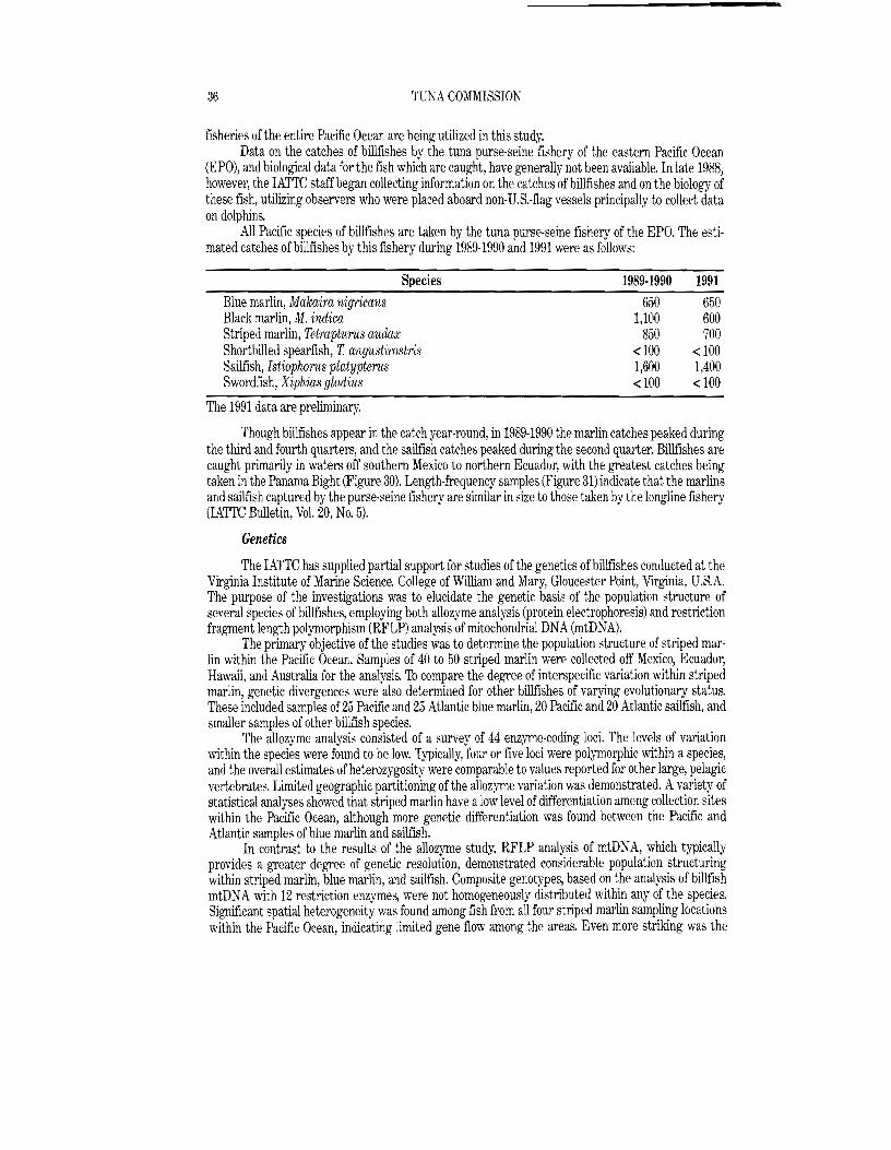
36 TCNA COMMISSION
fisheries of the entire Pacific Ocean are being utilized in this study. Data on the catches of billfishes by the tuna purse-seine fishery of the eastern Pacific Ocean
(EPO), and biological data for the fish which are caught, have generally not been available. In late 1988, however, the IATTC staff began collecting information on the catches of billfishes and on the biology of these fish, utilizing observers who were placed aboard non-U.S.-flag vessels principally to collect data on dolphins.
All Pacific species of billfishes are taken by the tuna purse-seine fishery of the EPO. The estimated catches of billfishes by this fishery during 1989-1990 and 1991 were as follows:
Species 1989·1990 1991 Blue marlin, Makaira nigricans 650 650 Black marlin, M. indica 1,100 600 Striped marlin, Tetraptnrus audax 850 700 Shortbilled spearfish, T angustirostris <100 <100 Sailfish, Istiophorus platypterus 1,600 1,400 Swordfish, Xiphias gladius <100 <100
The 1991 data are preliminary.
Though billfishes appear in the catch year-round, in 1989-1990 the marlin catches peaked during the third and fourth quarters, and the sailfish catches peaked during the second quarter. Billfishes are caught primarily in waters off southern Mexico to northern Ecuador, with the greatest catches being taken in the Panama Bight (Figure 30). Length-frequency samples (Figure 31) indicate that the marlins and sailfish captured by the purse-seine fishery are similar in size to those taken by the longline fishery (IATTC Bulletin, Vol. 20, No.5).
Genetics
The IATTC has supplied partial support for studies of the genetics of billfishes conducted at the Virginia Institute of Marine Science, College of William and Mary, Gloucester Point, Virginia, U.S.A. The purpose of the investigations was to elucidate the genetic basis of the population structure of several species of billfishes, employing both allozyme analysis (protein electrophoresis) and restriction fragment length polymorphism (RFLP) analysis of mitochondrial DNA (mtDNA).
The primary objective of the studies was to determine the population structure of striped marlin within the Pacific Ocean. Samples of 40 to 50 striped marlin were collected off Mexico, Ecuador, Hawaii, and Australia for the analysis. To compare the degree of interspecific variation within striped marlin, genetic divergences were also determined for other billfishes of varying evolutionary status. These included samples of 25 Pacific and 25 Atlantic blue marlin, 20 Pacific and 20 Atlantic sailfish, and smaller samples of other billfish species.
The allozyme analysis consisted of a survey of 44 enzyme-coding loci. The levels of variation within the species were found to be low. Typically, four or five loci were polymorphic within a species, and the overall estimates of heterozygosity were comparable to values reported for other large, pelagic vertebrates. Limited geographic partitioning of the allozyme variation was demonstrated. Avariety of statistical analyses showed that striped marlin have a low level of differentiation among collection sites within the Pacific Ocean, although more genetic differentiation was found between the Pacific and Atlantic samples of blue marlin and sailfish.
In contrast to the results of the allozyme study, RFLP analysis of mtDNA, which typically provides a greater degree of genetic resolution, demonstrated considerable population structuring within striped marlin, blue marlin, and sailfish. Composite genotypes, based on the analysis of billfish mtDNA with 12 restriction enzymes, were not homogeneously distributed \\>ithin any of the species. Significant spatial heterogeneity was found among fish from all four striped marlin sampling locations within the Pacific Ocean, indicating limited gene flow among the areas. Even more striking was the

37 ANNUAL REPORT 1991
degree of genetic differentiation between the Pacific and Atlantic populations of blue marlin and sailfish. For both species, much greater genetic variation was found within the Atlantic samples than within the Pacific samples. The results suggest that the Pacific and Atlantic populations of both species were isolated at one time, but have recently experienced some limited gene flow. The marked genetic differences found for the Atlantic and Pacific populations of blue marlin and sailfish contrast sharply with the results obtained from similar studies of tunas.
Early life history studies
For many years fisheries scientists have believed that the abundance of fish of any year class is determined principally during the early life history (egg, larval, andlor early-juvenile) stages. Although decades of research have provided considerable information on the populations of adult tunas, relatively little is known about the early life history stages and the factors which affect their recruitment to the exploitable stocks. In the eastern Pacific Ocean fishermen seldom catch tunas less than about 30 em in length, so samples of fish in that size range are not readily available. These considerations motivated the IATTC to establish a research facility at Achotines Bay in the Republic of Panama dedicated to the study of the early life histories of tunas.
Achotines Bay is located on the southern coast of the Azuero Peninsula in the Los Santos province of Panama (Figure 32). The continental shelf is quite narrow at this location, with the 200-m (109-fathom) depth contour occurring only 6 to 10 km (3 to 5nm) from shore. This provides the scientists working there with ready access to oceanic waters where some species of tunas spawn during every month of the year. The annual range of sea-surface temperature in these waters is approximately 21° to 29°C (70° to 84OF). Achotines Bay provides seawater suitable for holding live tunas in the laboratory. The proximity of the research station to the study area provides a low-cost altel11ative to a large research vessel, and improves sampling flexibility and spontaneity.
The IATTe's early life history research program involves laboratory and field studies aimed at gaining insight into the recruitment process and the factors that affect it. Previous research on recruitment of fishes suggests that both abiotic factors, such as temperature, salinity, and local circulation, and biological factors, such as feeding and predation, can affect recruitment. As pre-recruit survival is probably controlled by a combination of these factors, a recruitment research program must address the interaction between the biological system and the physical environment. This section describes the studies conducted at the Achotines Laboratory and the La Jolla laboratory to elucidate information on mOltaIity, growth, and the influence of the environment on the biology of larval and early-juvenile tunas.
Much of the early work at the Achotines Laboratory was concentrated on developing methods of capturing, transferring, and maintaining live scombrids in captivity. Late-larval and early-juvenile scombrids (8 to 35 mm standard length, SL) are captured for laboratory studies and other research projects by nightlighting from a skiff. The specimens are attracted to a bright underwater light at night, collected by dipnet, and transported to the laboratory. Th date, yellowfin andlor bigeye tuna (hereafter in this section referred to as Thunnns spp.); black skipjack tuna, Euthynnus lineatus; frigate andlor bullet tuna, Auxis thazard andlor A. rochei (hereafter in this section referred to as Auxis spp.; sierra, Scomberomorus sierra; chub mackerel, Scomber japonicu,s: and striped bonito, Sarda orientalis, have been captured and held in the laboratory. (Early-juvenile yellowfin and bigeye cannot be distinguished on the basis of morphological, meristic, osteological, or pigmentation characters; identification by electrophoretic means is described in a recent paper (U.S. Nat. Mar. Fish. Serv., Fish. BulL, 86 (4): 835-838). Larval and early-juvenile Auxis thazard and A. rochei have been distinguished by minor differences in pigmentation, body depth, and gill raker counts, but the identifications are ambiguous.) Research at the laboratory has focused on black skipjack, Auxis spp., and sierra, the most abundant scombrids in nearshore waters.
Low to moderate numbers of scombrid late larvae (late notochord flexion and post-flexion stages) and eady juveniles were taken by nightlighting during the first half of 1991. For the fourth
38 TUNA COMMISSION
consecutive year, high densities of black skipjack and Auxis spp. were present in the waters at the shelf break and continental slope south of the Azuero Peninsula during July and August. Large numbers (several hundred per night) of black skipjack were captured during late July and early August. The circulation patterns seem to retain late-larval scombrids in the slope and littoral waters during this portion of the rainy season. Low to moderate numbers of black skipjack, Attxis spp., and sierra were taken from mid-August to mid-September. The catches of black skipjack were low in October and early November despite intense sampling effort. Due to poor weather, followed by arrival of the offshore trade winds, only two nightlighting trips were made from mid-November through the end of December, and no scombrids were taken.
In 1991, as in 1990, moderate numbers (up to several dozen per night) of Thunnus spp. late larvae were collected off the Azuero Peninsula from mid-June to mid-July. In addition, moderate numbers of Thunnus spp. were captured during September. The sea-surface temperatures during these periods ranged from about 28.0° to 29.5°C (82.5° to 85.0°F). It is not known where these pulses of Thunnus spp. late larvae originate, but it is suspected that spawning occurs offshore and the larvae are carried onshore by the currents.
Development of improved husbandry techniques and the addition of supplements to the diet of juvenile black skipjack in the laboratory have resulted in more rapid growth and greater survival rates than previously attained. Sixteen black skipjack (14-20 mm 8L) captured during mid- to late November 1990 grew to 230-280 mm 8L by the end of March 1991. Transferring the early juveniles to 15- or 21foot (4.6- or 6.4-m) diameter tanks with 20-30 other fish of the same size and supplementing the regular diet of mollies (Poeciliidae) with minced beef liver appeared to increase the survival and feeding efficiency. Some of these fish became sexually mature in captivity (see Maturation of black skipjack in captivity).
The experimental aquaria at the Achotines Laboratory were re-configured during late 1991 in preparation for experiments on the effects of food concentration and water temperature on the growth and survival of late-larval and early-juvenile black skipjack. Twelve 330-L (87-gal) fiberglass tanks were plumbed in sets of three tanks each with chilling and heating equipment. Two sets receive heated seawat€r and two receive chilled seawater. The tanks will have uniform lighting, water exchange, and aeration. The system was tested and a trial experiment was conducted. Poor nightlighting conditions prevented the initiation of the experiments during 1991, however.
Sampling with light traps
During July and early August, a field sampling program was conducted to examine the distribution and abundance of late-larval and early-juvenile scombrids in the waters off the Azuero Peninsula. Mr. Simon Thorrold, a visiting scientist from the Australian Institute of Marine Science (AIMS), collaborated with IATTC scientists in the study. Automated light traps, designed and fabricated by AIMS, were used to study the nighttime vertical distribution of young scombrids. Another objective of the study was to compare the catches made by light traps to the catches made by nightlighting.
The light traps were deployed at the surface and at depths of 10 and 20 m(5 1/2 and 11 fathoms) on 21 dates. The catches oflate-larval scombrids were rather low. Atotal of 32 scombrids was collected: 14 black skipjack (8.5 to 15.0 mm SL), 13 Thunnus spp. (8.5 to 12.8 mm 8L), and 5 Auxis spp. (9.0 to 11.0 mm SL). The scombrids were caught only in the traps deployed at the surface. The approximate effort at each depth was: surface -64.5 hours; 10 m-34.0 hours; 20 m-46.5 hours.
The data are limited, but they seem to indicate that at night the late larvae and early juveniles are restricted to the upper depth strata of the mixed layer. These results will be compared to depth distribution data for larvae obtained with the Tucker trawl (see Ichthyoplankton and oceanographic studies).
The light traps and nightlight were used simultaneously on seven dates (Thble 11). Low numbers of late larvae were captured by both gear types on four dates, and the catches taken by nightlighting greatly exceeded those taken by the light traps on three dates. Visual observations indicated that,
39 ANNUAL REPORT 1991
when late larvae were abundant in the surface waters, they would approach the light traps in small schools, but would not enter the traps in great numbers. It was clear that young scombrids were initially strongly attracted to the traps. It is possible that zooplankton, which are also attracted to the traps, may provide an additional stimulus for young scombrids to enter the traps to prey on them. The zooplankton densities during the sampling period (July and early August) may have been insufficient to attract large numbers of scombrids into the traps. It may be possible to test the effect of high zooplankton densities on scombrid catches by light traps during the dry season (December-April), when the zooplankton densities are usually higher. In contrast, the nightlight apparently provides a stronger stimulus to attract late larvae and juveniles, perhaps due to a broader light field. The greater catches by nightlighting also reflect the greater vulnerability of late larvae to capture by dipnet once they are observed in the light field. The IATTC's nightlighting method, though somewhat subjective because of variable sea conditions and skill levels of the different collectors, appears to provide a reasonably good general index of relative abundance oflate-larval and early-juvenile scombrids.
Maturation of black skipjack in captivity
Five black skipjack which had been captured by nightlighting on November 14-16, 1990, at lengths of about 16 to 22 mm were still alive in mid-September 1991 in a 6.4-m (21-foot) diameter pool containing 30,000 L(8,000 gal) of seawater at the Achotines Laboratory. The pool had to be drained for repairs, so the fish were sacrificed for measurement of their muscle temperatures. These fish, four males and one female, were found to be sexually mature. They ranged in fork length from 290 to 366 mm, smaller than the smallest mature female (400 mm) found in aprevious study (IATTC Bulletin, Vol. 19, No.2) of approximately 6,000 wild-caught black skipjack. In an attempt to induce fertilization, milt from two of the males and several hundred eggs from the female were mixed 'A~th seawater in laboratory glassware, gently aerated, and held at two different temperatures. Although some of the eggs were hydrated and about 1mm in diameter, none appeared to have been fertilized. The milt contained active sperm, and motility continued for almost a week in refrigerated samples.
These fish had spent 305 to 307 days in captivity at the Achotines Laboratory. This is believed to be the longest time any scombrid has been held in captivity beginning at an early life stage, and the first known case of such fish attaining sexual maturity. The early juveniles were fed wild plankton during the first week in captivity, followed by chopped fish supplemented with beef liver and vitamin C.
Nutritional condition oflarval and juvenile scombrids
A study of the nutritional condition and rates of starvation in larval and early-juvenile scombrids collected during the rainy season (May to November) of 1988, described in the IATTC Annual Report for 1990, was nearly completed in 1991. Amanuscript describing this work was in preparation at the end of the year.
Age and growth studies
The age and gro\\th of 218 black skipjack tuna, ranging in size from 5.7 to 20.3 mm SL, were analyzed, using growth increments counted in their sagittae (the largest of the three pairs of otoliths). All the specimens were collected by nightlighting 3.5 to 6.5 nm off the coast of Panama near the IATTC's Achotines Laboratory between December 1987 and February 1989. The methodologies for preparation of the specimens and sagittae for the study are described in the IATTC Annual Report for 1989.
Immersion experiments conducted during 1990 demonstrated that increments are deposited at daily intervals on the sagittae of late-larval and early-juvenile black skipjack (IATTC Annual Report
40 TUNA COMMISSION
for 1990). Based upon these findings, ages were assigned to the 218 fish, and the length-age relationship was used to estimate the average growth rate (0.70 mm/d; Figure 33).
The growth of the sagitta, determined from measurements of the radius of the rostrum (the anterior-most projection of the sagitta), is directly proportional to the somatic growth in standard length for fish in the indicated size range (Figure 34). This close relationship suggests that the width of any increment is a measure of the instantaneous growth. Therefore, individual growth histories can be determined by back-calculation of size at age, using measurements of the increment widths.
Separate linear regressions for the length-age data were calculated for the fish collected in July and August, during the rainy season, and in January and February, during the dry (upwelling) season (Figure 35). These could not be compared statistically because their variances were not homogeneous (P<0.005). For fish older than 14 days, the variance was significantly greater (P<0.02) for the rainy season. For fish 8 to 14 days old, however, the variances were homogeneous for the two seasons (P>0.20), so linear regressions were fitted to the two truncated sets of data (Figure 35). Although the growth rate was greater during the rainy season (0.90 ± 0.11 mm/d) than during the dry season (0.70 ± 0.13 mm/d), the difference between the regression coefficients was not significant (ANCOVA, FO.05(1),1,37 = 1.18, P>0.20). The common regression coefficient and growth rate were 0.84 mm/d. The mean daily growth rates for fish older than 14 days were also compared for the two seasons. The mean daily gTowth rates for the older fish during the rainy and dry seasons were 0.82 and 0.85 mm/d, respectively. These rates were also similar for the two seasons (to.05(2),23 = 0.903, P>0.20), with a common mean of 0.83 mm/d. The greater variability in the growth of the older individuals during the rainy season may be due to a change in the diet preference of the older individuals and/or to patchiness or changes in the abundance of certain types of food organisms.
The data for seasonal growth comparisons are limited. More larvae, including those collected with a Tucker trawl, and juveniles will be analyzed for possible differences in growth between the two seasons.
Ichthyoplankton and oceanographic studies
In 1991, a change was made in the gear and procedures for sampling the ichthyoplankton off the southern coast of the Azuero Peninsula. ATucker trawl, an opening-closing sampling device with the ability to catch larvae at discrete depth strata, replaced the bongo net used in previous surveys to obtain information on the day-night patterns of vertical distribution of scombrid larvae in relation to temperature, salinity, oxygen, and light intensity in the water column.
The trawl was specially fabricated with a mouth area of about 0.6 m2for use on asmall research boat. It was made with 335-i!m mesh blue-green netting, and equipped with a temperature-depth logger for recording the water temperature and depth of the net during the tow. A small net with 73-i!m mesh and a mouth area of 0.014 m2 was nested inside the trawl to collect microzooplankton simultaneously. The microzooplankton samples will be studied to characterize the forage organisms which are available to larval scombrids.
The ability of scombrid larvae to search for food particles is based largely on visual detection. Therefore, the level of ambient light at depth is important when estimating the feeding incidence and efficiency of scombrid larvae. Aphotosynthetically-available radiation (PAR) sensor has been added to the CTDO (a device which simultaneously measures the conductivity (salinity), temperature, depth, and oxygen level of the water) for determination of light levels in the water column during the ichthyoplankton and oceanographic surveys.
The Tucker trawl was used in 1991 during 45 ichthyoplankton cruises. The samples were taken at Station MSB (Figure 32) during the daytime hours of approximately 10 a.m. to 3p.m. and during the

41 ANNUAL REPORT 1991
nighttime hours of approximately 9 p.m. to 3 a.m. During eight of the cruises, samples were taken on consecutive day-night periods. Based on results from a previous phase of the program, sampling with the Tucker trawl was conducted exclusively at Station MSB. The earlier sampling was done with a bongo net at least monthly at 14 stations along three transects extending from Punta Mala, Achotines Bay, and Morro Puercos (Figure 32), and this sampling indicated that the abundance of larval scombrids was consistently higher at Station MSB than at the other stations. Also, the Punta Mala transect (Figure 32) was the only transect at which all five taxa of scombrids, black skipjack, Auxis spp., Thunnus spp., sierra, and striped bonito, occurred in the net samples, and the densities of scombrids at this transect were an order of magnitude greater than those at the other transects.
The sampling protocol for the ichthyoplankton surveys is as follows. Two replicate tows with the Tucker trawl are made at five depth strata: 0-5, 5-20, 20-40,40-60, and 60-80 m(0-3,3-11,11-22,22-33, and 33-44 fathoms). The samples collected at the three shallower strata are preserved by two different methods, in accordance with how they are to be utilized. The samples to be used in studies of nutritional condition are preserved in Bouin's solution, while those to be used in studies of age and growth and of feeding ecology are preserved in 95-percent ethanol. A codend splitter, placed between the net and its two codends, was developed to divide the sample from a single tow into two approximatelyequal portions during the tow. The samples collected at the two deeper strata are not split, and are preserved in 5-percent Formalin solution, as are the microzooplankton samples from all the strata. CTDO casts are made to depths as gYeat as 100 m(55 fathoms) immediately before and after the trawl tows. Weather, ambient light intensity, water clarity, and sea state are recorded at the time of the casts.
Fish-aggregating device
Afish-aggregating device (FAD), built at the Achotines Laboratory, was deployed off the southern coast of the Azuero Peninsula on April 18, 1991. Its position is 7°20.16' N-8001O.02'W, just west of Frailes del Sur. The FAD has been attracting juvenile and adult fishes. Trolling near the FAD has resulted in the capture of adult yellowfin, black skipjack, wahoo (Acanthocybium solandri), dorado (Coryphaena hippurlis), and several species of Carangidae. Juvenile carangids, rainbow runners (Elagatis bipinnulata), and sergeant majors (Abudefduf troschelli), measuring about 3 to 25 cm (1 to 10 inches) in length, were observed by divers to be aggregating and feeding around the FAD.
Mullet brood stock
Efforts continued during 1991 to refine methods for inducing spawning in a captive brood stock of white mUllet, Mugil curema, at the Achotines Laboratory. The mullet are being reared to produce larvae to feed to young tunas in the laboratory. Several hundred mullet, 100 to 150 mm SL, were captured with beach seines and gill nets in local waters and placed in two saltwater ponds to supplement the brood stock. Preparations were made to transfer several dozen large female mullet into a 15foot (4.6-m) diameter laboratory tank. These females will be exposed to a reduced photoperiod regime to stimulate oocyte development. Then, slow-release hormone pellets will be implanted intramuscularly to accelerate gonadal development.
Snapper resource studies
The IATTC staff is conducting a cooperative project with scientists from Panama's Direcci6n General de Recursos Marinos (DGRM) to study some commercially-important coastal fishes in the Los Santos province of Panama. The purpose of the project is to provide some fundamental information on the biology and potential catches of these species. Recent industrialization, principally through

42 TUNA COMMISSION
improved arrangements for processing and export of the catches, and the possible entry of larger vessels into the fishery make acquisition of estimates of the potential yields desirable. A sampling program was implemented in 1986 to survey and assess the resources of snappers (family Lutjanidae), and other coastal fishes. Catch, effort, length. and weight data are being collected daily by DGRM biologists. These basic data will provide information on species composition, size compositions, condition factors, catches per unit of effort using alternative gear configurations, and seasonal vmiability of the above. The fishery lands primarily Lutjanus peru. Other species caught in smaller quantities include L. guttatus, L. argentiventris, L. jordani, L. novemfasciatus, L. aratus, L viridis, L. inermis, L. colorado, and Hoplopagrus giintheri. The first three species comprise over 90 percent of the catch in the Los Santos Province. The data are being analyzed and a report is being prepared by a DGRM biologist stationed at the Achotines Laboratory.
In 1991, preparations continued to initiate a tagging program for the most common snappers caught in the fishery. Snappers were caught by hook and line and transferred to four 3.7-m (12-ft) diameter tanks at the Achotines Laboratory for preliminary tagging experiments. The experiments will assess the feasibility of using anewly-developed visible-implant (VI) tag in future full-scale tagging experiments in the field. In addition, the rates of growth and tag shedding will be measured. Several tagging locations on the fish were tested in attempts to position the VI tags so they are visible externally, will not impede the fish's movements and behavior, and will not be subject to loss during capture with hooks. The experiments were not initiated during 1991 because of problems acquiring enough Lutjamts pe'yu for a statistically-valid experiment and mortality in captivity from infections and possi· ble nutritional deficiencies. Changes in procedures resulted in reduced mortality, and by the end of 1991 there were 31 L. peru alive in three tanks at the Achotines Laboratory.
Oceanography and tuna ecology
El Nino episodes of the second halfof the 20th century
There have been 20 El Nino episodes during the 20th century, including two very strong events, one in 1925-1926 and one in 1982-1983. The El Nino of 1982-1983 was the strongest and most extensive warm-water event recorded in the eastern tropical Pacific (ETP) so far this century. It had a duration of 18 to 24 months, during which the sea-surface temperatures (SSTs) reached more than 6°C (14.4°F) above normal in Ecuadorian and Peruvian coastal waters. As a result, many forms of sea life were affected for more than 2years over most ofthe eastern Pacific Ocean (EPO). Prior to the International Geophysical Year (IGY) of 1957-1958, El Nino was not widely known, except in the tropics, to be a frequent environmental event. During the IGY, however, a strong El Nino developed, with severe effects on bird life and fisheries in the ETP, especially along the coasts of Ecuador and Peru. This episode was well documented in the extensive data collected during the IGY. From 1955 to date, including the IGY, there have been eight El Nino episodes of varying degrees of intensity, and all have been better documented than those of the first half century.
Today El Nino is better understood as just one manifestation of abnormal patterns in the global atmospheric and oceanic circulations, leading to deeper-than-normal thermocline and mixed layer depths (MLDs), above-normal S8Ts, and above-normal sea levels in the ETP. These are related to significant modifications in the ocean currents, which result from weakening of the surface v.~nds in the tropical Pacific. The height of the sea level and the depth of the thermocline in the ETP are inversely correlated ",ith the strength of the easterly winds over the tropical Pacific. An important measure of the strength of the tropical wind circulation is the Southern Oscillation Index (SOIl, which is the difference between the standardized sea-surface pressure at Darwin, Australia (12°S) and at Tahiti (17°8). There is also a marked decrease in the nutrients in the upper mixed layer of the sea, leading to a depletion of forage, and probably a redistribution of food by the altered ocean currents.
43 ANNUAL REPORT 1991
'lbday there is worldwide interest in and continuous monitoring of the global atmospheric and oceanic conditions which may lead to El Nino events in the EPO and unusual weather and ocean conditions in other regions. Data on several observed environmental factors have been shown during the past three or four decades to be useful for detecting the onset of EI Nino episodes. In Figure 36 are shown the mean annual departures from normal of four frequently-monitored environmental parameters that indicate the status of atmospheric and oceanic conditions in the ETP, especially in regard to the warm (El Nino) or cold (anti-EI Nino) episodes during most of the second half of the 20th century (1955-1991). The data for the figure were obtained from climatological records compiled by the Climate Diagnostics Center, U.S. National Weather Service, and the governments of Ecuador and Peru.
In some years, as El Nino conditions develop, the SOl (Figure 36, Panel A) becomes negative for 6 months to 1 year. This is usually associated with weakening of the easterly surface winds in the tropics. Subsequently, the sea levels and SSTs begin rising in the ETP (Figure 36, Panels B and C). During an El Nino event the rainfall becomes intense at times, with an average annual accumulation of 50 to 75 mm (2 to 3 inches) above normal at Guayaquil, Ecuador, for example (Figure 36, Panel D). In some years the El Nino episode may be weak and of short duration, as it was in 1969 when the sea level and SST anomalies were small and the rainfall was near normal. In contrast, as shown in Figure 36, the strong El Nino episodes of 1957-1958 and 1972-1973 were characterized by large anomalies. The very strong EI Nino of 1982-1983 was preceded by several years of negative SOls and above-normal sea levels along the coasts of Ecuador and Peru. As a result, the EI Nino episode developed quickly after mid-1982, and the positive SST anomalies expanded rapidly. During 1983 the average sea level was 15.2 em (6 inches) above normal, the average SST was 6°C (14.4°F) above normal, and the accumulated annual rainfall at Guayaquil and surrounding coastal areas was 292 mm (11.5 inches) above normal.
El Nino episodes of the early 1990s
As the final decade of the 20th century began, the strong anti-EI Nino which occurred during 1988 and 1989 came to an end, marked by near-normal SSTs over most of the ETP during the first quarter of 1990. During the second quarter of 1990, however, in the offshore region along the equator between 900 W and 110°W, above-normal SSTs indicated that upwelling was weak. The SSTs were normal, or slightly above normal, at coastal stations of Peru.
During the ftrst and second quarters of 1990 the MLD and the thermocline became deeper than normal, the sea level rose in the coastal areas of central and South America, and the SOl became negative, reflecting weaker-than-normal surface wind circulation. During the third quarter, however, these emironmenta1 parameters returned to near-normal again and the El Nino development ceased. By the end of 1990 the El Nino had returned: the thermocline deepened by 10 to 20 m(5 to 11 fathoms), and there was agradual rise in sea level to above normal once again. The SOl become negative also, as it had earlier in the year. However, SST anomalies more than 1°C (1.8°F) above normal occurred only in a few small areas along the equator east of 1500W
The warming trend over the ETP that began in 1990 continued during the fIrst and second quarters of 1991. Because there had been agradual and prolonged warming in the upper mixed layer of the equatorial part (5°N to 100 S) of the ETP, the heat content above the thermocline had become great enough during the fIrst quarter of 1991 to trigger El Nino conditions, provided that the SOl remained negative during most of 1991. During the first quarter of 1991 the average SOl was -0.5 (Figure 36, Panel D). The ocean conditions were similar to those during the fourth quarter of 1990, i.e., the sea level was slightly above normal and the thermocline was about 20 m(11 fathoms) deeper than normal in the equatorial area east of 140°W. The SSTs were above normal over most of the ETP. During the second cuarter of 1991 slowly-developing EI Nino conditions prevailed west of the Galapagos Islands in the equatorial part of the ETP. The SST anomaly pattern for June 1991 in Figure 37 shows the mid
44 TUNA COMMISSION
year warming along the equator between 900 Wand 130°W, where the SSTs were 2° to 3°C (3.6° to 5.2°F) above normal. The rapid increase in the SSTs indicated amarked decrease in upwelling of cooler sub-surface water, which usually is most pronounced during the second and third quarters of the year. It can also be seen in Figure 37 that the development of El Nino conditions had not yet affected the coastal region of South America or the ETP north of lOON. By the end of the second quarter of 1991 it appeared that the El Nino would expand eastward to the coast and reach peak intensity before the end of the year.
By the middle of the third quarter, however, the development of EI Nino conditions came to an apparent halt. The SOl increased from -1.5 in May to -0.5 during the first half of the third quarter, indicating a slight strengthening of the surface winds over the southern tropical Pacific. The sea level became normal along much of the coast of South America, and the thermocline moved upward closer to the surface in equatorial waters. During this period, the U.S National Oceanic and Atmospheric Administration had reported that volcanic dust from the eruption of Mount Penatubo in the Philippines had been circling the earth in the stratosphere above the tropics and sub-tropics, causing a slight reduction in the amount of heat from the sun reaching the earth. This could be another factor contributing to the reduced rate of poleward expansion of the El Nino during the third quarter.
During the first part of the fourth quarter of 1991 the SSTs were more than 1°C above normal across nearly all of the equatorial part of the ETP, and several areas with SSTs more than 2°C above normal appeared along the equator. The SOl decreased to -1.2 (Figure 36, Panel D) between October and November. During the same period the sea level rose to several centimeters above normal at Baltra Island, one of the Galapagos Islands, and also from La Libertad, Ecuador, to Callao, Peru. In addition, the thermocline descended again to approximately 40 m (22 fathoms) deeper than normal along the equator east of 115°W. During this quarter the El Kino was beginning to affect the west coast of the Americas from Ecuador to northern Chile, where the SSTs were more than 1°C above normal.
By the end of the fourth quarter of 1991 there were no indications from the monitored environmental parameters that the El Nino was going to dissipate during the first quarter of 1992. The SST anomaly pattern for December 1991 (Figure 38) suggests that the EI Nino had strengthened in the offshore region along the equator. At the same time, however, the coastal region of Peru and northern Chile experienced, for the first time in 1991, SSTs of 1° to 3°C above normal. This suggests that the EI Nino may have reached a peak in development during the austral summer of 1991-1992, especially in the coastal region. By the end of the fourth quarter there was no evidence that this EI Nino had expanded north of WON. There remains a question, however, concerning whether there will be a northward expansion to the coasts of Central America and Mexico of this warm-water episode before the end of the 1991-1992 austral summer. If EI Nino conditions do not extend northward beyond lOON before the end of the first quarter of 1992, it is likely that the tuna fishing activity in the Commission's Yellowfin Regulatory Area (Figure 1) north of lOON will be no more affected in 1992 than it was during 1991. Additional information concerning the effects of EI Nino events on the tuna fisheries in the eastern Pacific Ocean is given in the IATTC Annual Reports for 1987 through 1990.
TUNA-DOLPHIN INVESTIGATIONS
The Commission's responsibilities include investigation of the problems arising from the tunadolphin relationship in the eastern Pacific Ocean (EPO), as described on page 7.
Data collection
In 1991, observers from the IATTC Tuna-Dolphin Program accompanied 237 fishing trips by purse seiners in the EPO. Twenty-three carryovers (trips which started in late 1990 and were com

45 ANNUAL REPORT 1991
pleted in early 1991) brought the total number of such trips for 1991 to 260, all of them aboard Class-6 vessels (capacity >400 short tons) operated under the jurisdictions of Colombia, Ecuador, Honduras, Mexico, Panama, the United States, Vanuatu, and Venezuela.
U.S. vessels also carried observers from the dolphin program conducted by the U.S. National Marine Fisheries Service (NMFS). These observers accompanied another 26 trips made by U.S.-flag vessels, and the two programs thus sampled a combined total of 286 trips, or approximately 60 percent of international fleet trips. This is the greatest percent coverage of trips in the 13 years in which the IATTC has been involved in this program. The coverage of non-U.S. fleet trips was almost 57 percent, also a sampling high. The sampling coverage of Class-6 seiners of the international fleet is summarized in Table 12.
The IATTC sampled approximately 36 percent of the trips of Mexican-flag vessels during 1991. Late in the year the Mexican government initiated its own national observer program. The IATTC and the NMFS provided logistical support to Mexico in initiating its program, which began sampling the Mexican fleet in December. Mexico has mandated 100-percent fleet coverage in 1992, with the IATTC program to continue to place observers on one-third of the trips and the national program to place observers on the other two-thirds.
Throughout the year Ecuador, Panama, and the United States had 100-percent coverage programs in place. The actual coverage of U.S. Class-6 vessels was 90 percent, due to the fact that one vessel did not have a U.S. government permit to fish on dolphin-associated tunas, and thus was not required to carry an observer on any of its trips. Vanuatu increased its fleet coverage to 100 percent early in the year, and Venezuela did the same in September. Cyprus and Spain each had a vessel which made one unobserved trip in the eastern Pacific, and Peru had one vessel which made two such trips.
A portion of the funding for the observer program was contributed by the Associazione Nazionale Conservieri Ittici e delle Tonnare (ANCIT) ofItaly.
"Dolphin-safe" certificates
In 1990, the IATTC began providing "dolphin-safe" certificates to purse-seine vessels which carried IATTC observers whose data verified the fact that no dolphins had been intentionally chased or encircled during that fishing trip. These certificates are issued only at the request of vessel management. In 1991, the IATTC issued 67 of these certificates to vessels under the jurisdictions of Colombia, Ecuador, Panama, Vanuatu, and Venezuela. The U.S. NMFS issued similar certificates to U.S. vessels which had met the requirements.
Statements ofparticipation
During 1991, the IATTC staff was asked to provide, upon request by vessels which have been participating in the international observer program at the coverage levels agTeed upon by their governments and the IATTC, a certificate to that effect. This "Statement of Participation" can also state that the vessel is equipped with all the dolphin safety equipment recommended by the IATTC and that the IATTC staff has verified the proper alignment and condition of the vessel's dolphin safety panel during a trial set. Between September 1991 and the end of the year, 31 statements were issued to vessels of the international fleet.
Training
Five courses for training observers in the collection of data aboard tuna vessels were held in Colombia, Mexico, Panama, and Venezuela during 1991 ('fable 13). The attendees were instructed in the identification of marine mammals, tunas, turtles, and seabirds, requirements and procedures for data collection, methods for estimating the sizes of herds of marine mammals, fishing gear and operations, and shipboard protocol and safety.

46 TUNA COMMISSION
The course in Colombia was conducted at the request of the Colombian government, under the auspices of the Asociacisn Nacional de Industriales de Colombia. It was coordinated by Dr. Martha Bernal de Mosquera, deputy director of the Fishery Production section of the Ministry of Agriculture.
Gear program
Agenerous contribution for the gear program was received from ANCIT.
Services
During 1991 the gear program staff conducted dolphin safety panel (DSP) alignments and inspections of dolphin rescue gear aboard 24 vessels from Colombia, Mexico, and Vanuatu. The standard DSP consists of two strips of 1 1/4-inch (3.2-cm) mesh, made of 24-thread nylon twine, which replace part of the 4 1/4-inch (10.S-cm) mesh adjacent to the corkline; dolphins are less likely to get their snouts entangled with the finer mesh when being released from the net. In order to check the alignment of the DSP, a trial set is made, during which an IATTC employee observes the performance of the net from an inflatable raft during backdown. He transmits his observations, comments, and suggestions to the vessels's captain, and attempts are made to resolve any problems which may arise. Afterward, a report is prepared for the vessel owner or manager. This report contains a summary of the IATTC employee's observations and, if necessary, suggestions for improving the vessel's dolphin safety gear and/O!' procedures.
The IATTC also offers other services to help individual vessels and fleets reduce dolphin mortality. Publications and video tapes on the subject are available at IATTC field offices. Trip analyses, detailed reports of observed fishing trips, are prepared upon request and, after the required authorizations are obtained, sent to the vessel owners to allow them to assess the performance of the vessels and captains.
Dolphin safety panel modification
A U.S. tuna boat owner and captain has been working on a modification of the DSP that may help reduce dolphin entanglement due to net canopies and collapses in the backdown channel area. His concept is to replace sections of the 1 1/4-inch mesh DSP with sections designed to allow dolphins which are forced into contact with the net to pass easily through the net wall, while still providing enough of a visual barrier for tunas to prevent their escape. The designer is working in conjunction with a company which makes purse seines in developing a prototype that they hope to begin testing in 1992. Staff members of the IATTC and the Porpoise Rescue Foundation have been involved in early discussions about the modification.
Workshops
Three workshops on reducing dolphin mortality were held during 1991 (Table 14). These workshops are intended not only for vessel captains, who are directly in charge of fishing operations, but also for other crew members and for administrative personnel responsible for vessel equipment and maintenance. Fishern1en who attend the workshops are presented with certificates of attendance.
Mortality estimation
The total incidental mortality estimates for 1991 are shown in Table 15. They represent a reduction of 4S percent with respect to 1990. Two factors control the level of mortality, the number of sets on fish associated with dolphins and the average mortality per set (MPS). The number of sets on fish associated with dolphins declined by about 10 percent and the average MPS declined by about 40 percent relative to 1990. Improvements in performance of the captains and crews were obviously the
47 ANNUAL REPORT 1991
major reason for the 48-percent reduction in the total mortality of dolphins. There are a number of factors which affect the mortality rates. These were examined, using the
data base for non-U.S. vessels. The data for U.S vessels were not combined with those for the other vessels because the portion of the international fleet which was U.S. vessels has changed during recent years. Some of the factors which affect the mortality rates are:
Proportion of night sets: This proportion declined from 8.0 percent in 1990 to 6.5 percent in 1991. Still, as the mortality rates during night sets are several times those during day sets, nearly 17 percent of the mortality occurred during night sets.
Proportion of sets with net collapses: This proportion declined from 31.3 percent in 1990 to 26.5 percent in 1991. Almost half of the total mortality occurred during sets with net collapses.
Proportion of sets with net canopies: This proportion declined from 25.0 percent in 1990 to 18.2 percent in 1991. Almost 65 percent of the mortality occurred during sets with net canopies.
Average number of dolphins left in the net after backdown: This number decreased from 2.9 in 1990 to 1.7 in 1991, shows that the procedures used to release the dolphins from the net improved.
Average number of dolphins encircled: This number decreased from 582 in 1990 to 549 in 1991. This is another area in which the fleet is showing improvement. The fishermen were able to encircle fewer dolphins without reducing the average catch of yello'NlIn tuna per dolphin set (16.6 tons in 1990 versus 16.8 tons in 1991). The decrease in the number of dolphins encircled is at least partly the result of the fishermen's increased skill in separating the dolphins which "carry tuna" from those which do not before setting.
Relationship between mortality and abundance
The best way to assess the impact of the fishery on the various dolphin stocks is to bring together information on the mortality and abundance of each stock. The most recent estimates of the absolute abundances of the various dolphin stocks affected by the fishery are those calculated by Mr. Paul Wade and Dr. Timothy Gerrodette of the U.S. NMFS, recently submitted to the International Whaling Commission. The estimates from that paper and the mortality figures for 1991 are shown in Table 16. The incidental mortalities for all stocks are less than 1percent of their population sizes. As the most conservative estimate of the net recruitment rate currently used is 2percent, it is likely that the stocks affected by the fishery are already recovering from the higher mortalities of earlier years.
Estimation of relative abundance
To monitor the possible effects of incidental mortality on the sizes of dolphin stocks, estimates of their abundance have been made, usually by applying line transect methodology to data collected from tuna vessels, research vessels, or both. In recent years, the U.S. NMFS has carried out a series of cruises on research vessels for the purpose of estimating trends in the abundances of the major dolphin stocks. IATTC staff members have analyzed data gathered by observers placed on board tuna purse seiners. The tuna-vessel data provide a large data base at no additional cost, 'Nith regular coverage of a substantial portion of the area occupied by the dolphin stocks. However, due to the nature of the fishing operations, the assumptions necessary for line-transect sampling to yield unbiased estimates of absolute abundance are often violated. Procedures were therefore developed to obtain estimates as insensitive as possible to those violations (see IATTC Annual Report for 1987). However, since these procedures are unlikely to remove all biases, the estimates should be treated as estimates of the relative abundances of the stocks, rather than as estimates of their absolute abundances.
48 TUNA COMMISSION
The relative abundance index for any given stock is obtained from an estimate of the herd encounter rate, an estimate of the average herd size, an estimate of the area of distribution of the stock in question, and an adjustment factor (derived from a model fitted to the sightings data) that accounts for herds that are not detected. Th reduce biases, separate geographical stratification schemes are applied for the estimation of each of the components of the estimator. A non·parametric procedure (bootstrap) is applied to estimate the variances, using data for individual fishing trips as resampling units.
The underlying trends in abundance are estimated by smoothing the series of estimates. This smoothing reduces the effect of extreme estimates (outliers) on the estimation of the trends, and improves the overall precision by incorporating more information in the estimation of each year's index. Since the numbers of dolphins are unlikely to vary greatly in successive years, smoothed esti· mates which combine information from neighboring years are a better indicator of change, and the resulting confidence intervals are more precise.
Smoothed confidence intervals are computed by combining the smoothing and bootstrap procedures. After obtaining abootstrap estimate for agiven stock for each year, the estimates are smoothed across years. This procedure is repeated 79 times, and for each year the 6th-smallest and 6th-largest smoothed estimates provide approximate 85-percent confidence limits. The sequence of medians of the smoothed bootstrap estimates is used as the "best" estimate of the trend. The smoothing procedure does not perform well on the first and last points of the series, so therefore smoothed estimates are not given for the first and last years in the series for each stock. Assessments of the performances of other smoothing methods are currently in progress.
The numbers of nautical miles of searching effort by tuna vessels with observers on board and the numbers of sightings made during these searching periods in 1991 are shown in Table 17. The relative abundance indices for 1991 are shown in Table 18. The estimates of the underlying trends for each of the main stocks associated ¥lith tunas in the EPa are shown in Figures 39-46. Since the stock boundaries and stock identities are uncertain for the northern and southern stocks of the offshore spotted dolphin, estimates were also made after pooling the data for both stocks. The broken horizontal lines in these plots correspond to the upper and lower 85-percent confidence limits for the 1990 relative abundance index. The years for which the entire confidence interval lies outside the region between the broken horizontal lines show relative abundance indices which are significantly different from those for 1990.
Spotted dolphin
It appears that the northern stock of the spotted dolphin has remained stable over the last few years (Figure 39). The figure suggests a slight apparent decrease after 1986, but no significant differences are detected over that period, and the estimate for 1991, being close to the 1990 estimate, supports the assessment that the population has exhibited little, if any, change during recent years.
For the southern stock, the 1991 estimate is similar to those of 1989 and 1990, giving support to the hypothesis that the low indices obtained for the 1984-1988 period were not indicative of a real decline in abundance (Figure 40).
Apossible explanation for the recent trends seen in both stocks is that there have been large movements of dolphins across the assumed boundary between the northern and southern stocks. If such movements are common, it is possible that they would have caused apparent simultaneous increases in the northern stock and decreases in the southern stock during the mid-1980s. For this reason, it is preferable to assess them as if they were a single stock. The results of this analysis (Figure 41) suggest that the two stocks taken together have exhibited almost no change in recent years.

49 ANNUAL REPORT 1991
Spinner dolphin
The results for the eastern stock of the spinner dolphin suggest that it has been stable during the last few years (Figure 42). With the exception of a high estimate for 1988, the unsmoothed indices for the last five years are in the range of 360 to 380 thousand animals, similar to the levels estimated for the late 1970s. Acomparison with earlier estimates indicates that there is some evidence that the 1990 smoothed estimate is lower than the smoothed estimate for 1976.
There have been no significant changes for the whitebelly stock during the last decade (Figure 43). The smoothed estimates suggest that there was a slight decline after 1986, although this is not statistically significant, and a significant decline with respect to the levels during the 1976-1978 period. It is possible that the estimates for this stock are affected to some extent by the El Nino phenomenon; the unsmoothed estimate for 1991 is less than the average index for the mid-1980s, but similar to the estimates for the very strong El Nino of 1982-1983.
Common dolphin
There is evidence, after the addition of the 1991 estimate, of a decline for the northern stock of the common dolphin with respect to the late 1970s and early 1980s (Figure 44). The 1990 index is significantly lower than the estimates for the 1977-1982 period. In particular, the 1991 estimate is considerably lower than the estimates for the previous years, mainly as aresult of avery low encounter rate (Table 18). There are several possible explanations for this result.
The first possibility is that the low 1991 estimate is the result of a large decline in the population. However, the incidental mortality for this stock has been low relative to the total population size and, since 1989, consistently less than 0.2 percent of the best available estimates of absolute abundance. It seems unlikely, therefore, that the population has been affected by high incidental mortality.
The second possibility is that the low 1991 estimate is the result of a change in fishing patterns. If, during 1991, the fishermen directed their effort in the area to fishing for tunas not in association with dolphins, the observer would have been less likely to be aware of these sightings, even including those made close to or on the trackline, which would cause a downward bias in the relative abundance indices. However, if the fishermen's effort directed toward dolphin-associated fish is measured by the ratio of the number of dolphin sets to the total number of sets, it would appear that fishing in association with dolphins was more common in the area during 1991 than during the previous years. Therefore, there seems to be little support for the hypothesis that changes in fishing pattel11s account for the low estimate of 1991.
Athird possibility is that a shift in the distribution of the stock occurred during 1991. The study area, as defined for these analyses, does not include the entire range of the northel11 common dolphin. Common dolphins are frequently sighted as far north as 35°N. Therefore, movements within the range of the stock could affect the relative abundance indices. There is some evidence that such movements occurred during 1991. The results from an aerial survey and preliminary results from a ship survey carried out by the U.S. NMFS along the coast of Southern California indicate that the abundance of common dolphins during 1991 was an order of magnitude greater than during previous years. Environmental data with which to carry out a comprehensive analysis of the conditions in the habitat of the northern common dolphin are not yet available for 1991. The only information available at this time is sea-surface temperature (SST) measurements taken by observers at the time of sets made on tunas associated with dolphins. These data indicate that the SSTs were about 1.5°C (2.7°F) greater during 1991 than during previous years (Table 19). This could indicate a northward extension of the range of the common dolphin, which prefers cooler waters. If a change in the distribution of the northel11

50 TUNA COMMISSION
common dolphin is the main reason for the low 1991 estimate, it would be difficult to modify the IATTC staffs current procedures to take this into account. Extending the area in which the stock is presumed to occur, as was done previously to adjust for a similar problem affecting estimates for the southern stock of offshore spotted dolphins, would not be effective in this case, as tuna purse seiners rarely operate in the area north of 300 N. If the change in distribution persists for more than one year, the estimated underlying trend would indicate that the population is declining rapidly, as appeared to be the case for the southern stock of the offshore spotted dolphin before 1989. Inclusion of environmental variables in the estimation procedures, currently underway as part of a revision of the methods, will probably improve the relative abundance indices for this and other stocks.
The estimated trend for the central stock of common dolphins indicates stable abundance since the early 1980s, after a decline during the late 1970s (Figure 45). The index for 1991 is similar to those for the previous years.
Data for the southern stock are sparse, making the trends in abundance difficult to assess (Figure 46). There are no significant differences among the estimates for the entire time series.
Effect of "dolphin-safe" fishing trips
The possible consequences of recent changes in the fishery were also analyzed. In 1990, several U.S. tuna canners announced that they would no longer accept tuna caught in association with dolphins; this became known as the "dolphin-safe" policy. At the same time, some countries in the region passed legislation banning the encirclement of dolphins. Vessels affected by these policies were required to carry an observer who could certify that the tuna were not caught in association with dolphins. As a consequence, during 1991 the observer coverage for these vessels was much greater than the coverage for the fleet as a whole. Therefore, a substantial proportion of the basic data available for abundance estimation was contributed by "dolphin-safe" trips. The inclusion of fishing trips during which no sets were made on dolphin-associated fish can cause a bias toward low estimates in two different ways. First, as the vessels are not encircling dolphins, the observers are less likely to be aware of herds of dolphins sighted by the crew. Second, the best areas for fishing for tunas not associated with dolphins do not always coincide 'With the areas in which searching traditionally takes place when fishing for tunas associated with dolphins. Achange in the distribution of effort toward the best non-dolphin areas can cause a change in the bias with respect to previous years, especially for stocks for which spatial stratification is not possible (southern stock of the offshore spotted dolphin and northern and southern stocks of the common dolphin).
To assess the importance of this effect, fishing trips without sets in association with dolphins were deleted from the data base, and new estimates of the abundances of the various stocks were obtained from the reduced data base CTable 20). Apaired I-test was carried out on the logarithm of the estimates of abundance before and after removing the data for the "dolphin-safe" fishing trips. The result indicates that there is no evidence of bias due to the inclusion of "dolphin-safe" trips (t5 = -1.30; P>0.22).
Age and maturity ofdolphins
Biologists participating in a joint project sponsored by the IATTe, the U.S. NMFS, and the Chicago Zoological Society have found changes in the layering patterns in the teeth of dolphins which appear to be correlated with the process of sexual maturation. This project is part of a study which has been conducted over the last 21 years on free-ranging bottlenose dolphins, Tursiops truncatus, near Sarasota, Florida. The reproductive histories of these dolphins are known from observational studies that have recorded the birth of calves to marked females and from capture-and-release studies that have measured reproductive hormone levels from blood samples.
51 ANNUAL REPORT 1991
After removal from the dolphins, the teeth are decaleified, cut into thin sections, and stained with hematoxylin to make the layers more distinct. The area in which the layering pattern changes, termed the transition zone, is formed over a 2- or 3-year period. The transition zone generally includes of the following features: (1) a dark-staining layer which is more distinct than the preceding and succeeding layers, (2) a thinning of the layers, and (3) a change in coloration of the stained layers. The transition zone generally begins at about 8to 10 years of age. Prior to that time the males and females have low levels of reproductive hormones and the females have not been recorded with calves. During and after the time that the transition zone is laid down, the reproductive hormone levels are higher and some of the females have been recorded to have their first calves.
Previous workers have suggested that this layering pattern is correlated with parturition. This hypothesis was not borne out by this study because: (1) the pattern was seen in both males and females, and (2) the pattern was not seen in the teeth of older females at ages when the females were known to have given birth.
This technique could prove valuable for studying life-history trends in eastern Pacific dolphins. For example, it might be possible to examine the teeth of older animals which matured during the early days of the purse-seine fishery, prior to the collection of life-history data in the mid-1970s. If a density-dependent response to exploitation has occurred, it may be revealed from a comparison of the average age of sexual maturity calculated from animals that matured in the 1960s versus those that matured more recently. This method has the additional advantage that it does not require sample sizes as large as those required by other techniques which do not involve examination of the teeth.
The sexual maturity of bottlenose dolphins, based on observations of births of first calves and the occurrence of transition zones, typically occurs at 7to 10 years. The estimates of the average age at sexual maturity of spotted dolphins caught incidentally in the purse-seine fishery are higher (10 to 12 years), which is contrary to what was expected, as bottlenose dolphins live longer than spotted dolphins. These unexpected results could be due to bias introduced by the use of this method or bias in the collection of samples of spotted dolphins from the purse-seine fishery, or the expectations could be based on faulty assumptions about the dynamics of dolphin populations.
STATUS OF THE TUNA STOCKS IN 1991 AND OUTLOOK FOR 1992 The convention establishing the Inter-American Tropical Tuna Commission states that its prin
cipal duties are to study the biology of the tunas and related species of the eastern Pacific Ocean (EPO) to determine the effects that fishing and natural factors have on their abundance and, based on these studies, to recommend appropriate conservation measures so that the stocks of fish can be maintained at levels which will allow maximum catches on a sustained basis. To fulfill this responsibility, a broad program of research involving biological and oceanographic studies and the acquisition and interpretation of detailed statistics of catch and effort of vessels fishing in the EPO is carried out by the Commission's staff. In keeping with these responsibilities, background papers are prepared to inform the Commissioners of the staff's current assessment of the status of the tuna resources of the EPO. The information in these background papers is reprinted in this Annual Report, with minor changes, to make it available to the general public.
YELLOWFIN
Yellowfin is the most important species taken by the surface fishery for tunas in the EPO. A variety of age-structured and production models has been used by the IATTC staff to assess the effect that fishing has had on the abundance of yellowfin in the EPO and to determine the present condition of the resource.
52 TUNA COMMISSION
Age-structured models
Age·structured models make use of data on recruitment and on the growth and mortality of individual fish. Estimates of these parameters are obtained from analyses of length-frequency and otolith data from the fish in the catches, supplemented by tag return data and other data of various types. The IATTC staff has collected data on the size composition of the fish in the catches of yellowfm in the eastern Pacific Ocean (EPO) since 1954, and in addition has had access to the corresponding data collected during 1951-1954 by the California Department of Fish and Game. The otoliths were collected during 1977-1979, and the analyses were carried out during the early 1980s. Tagging was conducted principally from 1955 to 1981, and analyses of these data are still in progress.
Biomass analyses
Age-structured biomass analyses performed by the IATTC staff have produced information concerning the abundance and mortality of fish of individual cohorts which has been highly useful for stock assessment. (A cohort consists of all the fish recruited to the fishery at the same time, such as the X73 cohort, which reached a length of 30 cm in about November of that year, first entered the fishery in small numbers during the first half of 1974, and contributed to it significantly for the first time during the second half of that year, and the Y73 cohort, which reached a length of 30 cm in about May of 1973, first entered the fishery in small numbers during the second half of that year, and contributed to it significantly for the first time during the first half of 1974.) As a first step, the fish in the catch must be assigned to cohorts. Then estimates are made of the numbers of fish of each cohort at the time of recruitment and at various intervals thereafter and of the numbers which are caught and which die during each interval. The information needed for these calculations includes the numbers and average weights of fish of each cohort in the catch, an estimate of the natural mortality rate (or estimates of a series of rates if the natural mortality is not constant for the fish of different ages), and an estimate of the fishing mortality rate for at least one catch interval for each cohort. These are called the "initiating" rates of fishing mortality. All of these estimates are obtained from analyses of catch statistics and length-frequency, weight-length, and sex ratio data. The results of these analyses are not as accurate as desired because, although fish of different cohorts can be easily distinguished from one another when they are young, this becomes increasingly difficult as they grow older, so older fish are probably often assigned to the wrong cohorts. Thus not only are the estimates of the catches of fish of each cohort less accurate than desired, but the estimates of the mortality rates are somewhat crude. Specifically, an estimate of 0.8 for the instantaneous annual rate of natural mortality (M) is used for all ages of males. For females, M is assumed to be 0.8 for the first 30 months in the fishery and then to increase linearly to about 6.5 at 80 months. (In practice, it varies somewhat among cohorts.) Also, the catchability of the fish varies according to age, area, season, weather, and other circumstances, the gro~th rates vary, and the times of recruitment vary. All of these introduce "noise;' and possibly bias as well, into the calculations.
The estimated average populations of fish of the various cohorts, in numbers of fish, are shown in Table 21. For the X68 cohort, for example, there was an average of 23,667,000 O-year-olds during the last quarter of 1968, and the population of that cohort during the first, second, third, and fourth quarters of 1969 averaged 19.38, 15.76, 12.53, and 9.40 million fish, respectively (1969 rows, I column). In 1970 the average populations of 2-year-olds of that cohort during the first through fourth quarters were 6.30, 3.76, 2.84, and 2.15 million fish, respectively (1970 rows, II column), and so on. The average numbers of 0-, 1-,2-,3-,4-,5-, and 6-year-olds of the seven Xcohorts (1968, 1967, 1966, 1965, 1964, 1963, and 1962) during the last quarter of 1968 were 23.67, 9.18, 2.26, 0.61, 0.13, 0.06, and 0.02 million, respectively (1968, last row). The table is read the same way for the Y cohorts as for the X cohorts, except that the Ycohort first appears during the second quarter of the year.

53 ANNUAL REPORT 1991
Estimates of the numbers of recruits for each cohort for 1967-1991 are listed in Table 22. The estimates for 1991 are preliminary and subject to change, however. This is because the recruits have been exposed to the fishery for less than one year, and if their vulnerability to capture was above or below average the recruitment would have been over- or underestimated. The same is true, to a lesser extent, for the estimates for 1990. The averages of the initial recruitments (Columns 2-4) are 39 million for the X cohort and 47 million for the Y cohort; the averages of the average populations during the month of recruitment (Columns 5-7) are 37 million for the Xcohort and 45 million for the Ycohort. The variability (ratio of the largest to the smallest estimate) among years is roughly the same for the X cohort (3.10) and the Ycohort (3.00), and that for the combined data (2.68) indicates an inverse relationship (not necessarily significant) for the two cohorts. The recruitment has been variable, but the average for 1978-1991 has exceeded that for 1967-1977. There appears to have been an upward trend in recruitment over the last 20 years or so, the initial recruitment averaging about 64, 73, and 98 million fish during the 1967-1975, 1976-1982, and 1983-1991 periods, respectively (Figure 47). It could be argued, however, that this is due to chance variation, especially for the 1973-1991 period, when the initial recruitment has averaged about 86 million fish.
The numbers of fish in Table 21 were converted to weights, using data on the average weights of fish of different sizes (Table 23) to calculate the estimated average annual biomass (total weight averaged over four quarters) for each cohort. Different initiating rates of fishing mortality were estimated for the months during which different cohorts were last exploited, depending on fluctuations in effort from season to season. In addition, for purposes of comparison, calculations were made for all cohorts with initiating rates greater and less than those considered to be the best estimates. Some tuning of these initiating rates was done to obtain a better comparison of the cohort biomass estimates (Figure 57, bottom panel) to the other estimated trends in abundance (Figure 57, top and middle panels). The estimates of biomass shown in Figure 48 were calculated using monthly values. It is easy to see the relative strengths of the various cohorts from this figure. For example, the recruitment of X84 and Y84 cohorts combined was about average (Table 22) and their biomass (Figure 48, cross-hatched) was greatest at age 2. These cohorts were not fished heavily until 1987, when they were 2years old (Figure 49). The initial recruitment of the X72 and Y72 cohorts combined (Figure 48, diagonal lines), on the other hand, was below average (Table 22), and after the Y-cohort fish were fished heavily as age-I fish in 1973 (Figure 49) their biomass was relatively low (Figure 48) in the succeeding years.
In Figure 50 are shown the average annual biomass estimates for 1967 through 1991 for all fish regardless of age and for "large fish" (all X- and Y-cohort fish which had been in the fishery more than 17 months). During 1967-1971 the total biomass averaged about 365 thousand short tons. This was comprised of a large proportion of older fish resulting from recruitment during 1965-1967 which were exploited lightly as young fish. Below-average recruitment, coupled with increasing exploitation rates during 1969-1972, resulted in a decline in the biomass of the older fish from 1969 to 1973. The lesser biomass of older fish persisted through 1974, whereas the abundance of smaller fish increased in 1974 as a result of an extremely large 1973 year class. That year class accounted for most of the increase in biomass oflarge fish in 1975 and 1976. The greatest catch of yellowfin in the history of the fishery prior to 1986 was made during 1976. Below-average recruitment during 1975 and 1976, coupled with heavy exploitation of young fish from 1973 to 1982, resulted in the biomass of both young and old fish decreasing until 1982, when it reached the lowest level observed in the recent history. Although the 1977 recruitment was well above average, exceeded only by those of 1973, 1987, and 1988, so many of these fish (and those of the 1978 recruitment) were captured as 1- and 2-year-olds that they did not contribute heavily to the fishery in 1981 or 1982. The recruitment was below average from 1979 through 1982, about average from 1983 through 1985, and above average from 1986 through 1991. The biomass increased in 1983, due primarily to lesser fishing effort, and increased greatly in 1984 and 1985, due to

54 TUNA COMMISSION
increased recruitment and reduced fishing on young fish. Since then, based on cohort analyses, it has increased slowly.
The annual catches of fish of the X and Y cohorts, and of both cohorts combined, during 19671991, are shown in Figures 49 and 51. In Figure 49 each panel contains the catches of fish of the same cohort in different years, whereas in Figure 51 each panel contains the catches of fish of different cohorts in the same year.
Comparison of Figures 48 (annual estimates of the biomass of the Xand Y cohorts), 50 (annual estimates of the total biomass and the biomass of large fish), and 51 (catches during each year by age) reveals the changes which have taken place in the age composition of the population and the catch. During the 1970s, when the fishing effort was high, fewer and fewer individuals survived to reach the larger sizes. The fishing effort was reduced in 1982, 1983, and 1984, which permitted many fish which would have been caught while young to grow larger. The total contributions of the combined Xand Y cohorts from 1967 through 1986 (Figure 49) ranged from 148 thousand tons for the 1976 cohort to 374 thousand tons for that of 1973, with an average for the 20 groups of 219 thousand tons. If the Y73 cohort had not been fished so heavily during its first year the catches for that cohort would have been even greater. Division of these combined cohort catches by the corresponding initial estimates of recruitment (Table 22) gives yield-per-recruit estimates for each combined cohort (Figure 52) which varied from 4.8 to 7.5 pounds, (2.2 to 3.4 kg). The initial recruitment varied from 49 million to 120 million fish (Table 22), averaging 72 million fish, producing an average yield pel' recruit of 6.1 pounds (2.8 kg).
Yield-per-recruit analyses
In addition to age-structured biomass analyses, yield-per-recruit analyses have been used by the IATTC staff. When the fish of a cohort are young the total weight increases because the growth in weight of the individual fish is rapid, while the losses to the cohort due to natural mortality are moderate. Later, as the fish grow older, their growth rate becomes slower, while the natural mortality continues to be about the same, Thus the losses to the total weight due to natural mortality at that time are greater than the gains due to growth, and there is a net loss to the total weight. Eventually the cohort disappears. The ideal way to obtain the maximum yield in weight from a cohort of fish (assuming, for this discussion, that this is the object of management) would be to harvest each fish just before it died a natural death. This is not possible, of course. The next best alternative would be to harvest all the survivors at the age or size at which the loss to the total weight by natural mortality exactly balances the gain to it by growth (the "critical age" or "critical size"). This is possible for some animals, such as oysters or clams which are exposed at low tide and can be easily harvested at that time. When the manager of a bed of oysters or clams surveys it at frequent intervals and removes the individuals which have reached the critical size he is exerting an infinite amount of fishing effort on the animals which have reached that size. It is obvious that this alternative is not practical for most species offish,
Intuitively, it seems that if the second alternative is not possible harvesting should begin on fish which have not yet reached the critical size. This is the third alternative, and the only practical one for most species of fish. It is assumed, for the moment, that the size at entry (i.e. the size of the smallest fish caught) can be efficiently controlled. If the fishing effort is high a size at entry only slightly less than the critical size would be selected, most of the fish caught would be close to the critical size and age, and the yield would be almost as great as under the second alternative. If the fishing effort is lower a size at entry considerably below the critical size would be selected, the fish caught would exhibit a wider range of sizes and ages, and the yield would be considerably less than it would under

55 ANNUAL REPORT 1991
the second alternative (but still the maximum possible without increasing the effort). It may not be possible, however, to control efficiently the size at entry. If so, the only way to
manage the fishery is to control the effort. If the size at entry is greater than the critical size unlimited effort can be permitted, but if the size at entry is less than the critical size restriction of the effort may increase the yield.
So far it has not been mentioned that at least some of the individuals ofacohort must be allowed to spawn at least once before they are harvested. If spawning occurs well before the fish reach the critical size there is probably no danger from this standpoint, but if spa\!ming does not occur until after the fish have reached the critical size, and the fishing effort is high, there is a possibility that the number of spawners would be so reduced that the recruitment in subsequent years would be reduced. Therefore a fishing strategy designed to produce the maximum yield per recruit will not necessarily produce the maximum yield. If the fishing pattern has an impact on the future recruitment, the maximum yield will be obtained by controlling the fishing to optimize the cohort size and yield per recruit simultaneously. This will be discussed in more detail later. (It should not be assumed, however, that a modest reduction in spawners would reduce the recruitment in subsequent years, as this does not appear to be the case for most species of fish.) The yield-per-recruit model, as described here, does not take into account the possibility of changes in recruitment, but this is an integral part of production models, which will be discussed later.
Also, it has not been mentioned that the growth of the individual fish may be slower, or the natural mortality may be greater, when apopulation of fish is dense than when it is less dense. Accordingly, the loss due to harvesting of some fish at less than the critical size may be at least partially compensated for by faster growth and/or lesser natural mortality of the remaining fish. In addition. if the growth or natural mortality rates are affected by population density the critical size and age ~~II
vary according to population density. This is another complication not taken into account in the yieldper-recruit model as described here, but it is automatically compensated for in production models.
Proceeding now to yellowfin in the EPO, the estimates of growth and natural mortality obtained by the IATTC staff are not as reliable as desired, but the critical size is estimated to be roughly 119 cm (75 pounds or 34 kg). Most fish caught by the baitboat fishery are considerably smaller than this. As most of the tuna fleet converted from bait to purse-seine fishing in the late 1950s and early 1960s the average size of the fish in the catch increased, many of them being approximately equal to or greater than the critical size. The average annual catch of yellowfin by smface gear increased considerably during the period after the conversion to purse seining, averaging about 105 thousand tons for 19611970, as compared to 84 thousand tons for 1951-1960. The offshore expansion of the fishery during the mid- and late 1960s was an important factor in these greater catches, but the increase in the average size of the fish caught was also partially responsible for the increased catches.
The objective of management specified by the IATTC convention is to obtain the average maximum sustainable yield (AMSY). The maximum yield per recruit is equivalent to the AMSY, provided recruitment is independent of the number of spawners, as discussed above. The estimated yields per recruit produced by different combinations of size at entry and fishing effort for two different time periods are shown in Figure 53. (Fishing effort will be discussed in more detail in the section entitled Production models.) Various combinations of fishing effort and size at entry give various yields per recruit, which are indicated by the curved lines. The calculations are based upon the growth-in-weight data shown in Table 23, coefficients of fishing mortality obtained from estimating the biomass as described in the subsection entitled Biomass analyses, and estimates of the coefficients of natural mortality given in that subsection. During the 1978-1982 period the fishing effort was directed more or less equally at small, medium, and large fish, whereas during the 1985-1987 period the effort was
56 TUNA COMMISSION
directed most at large fish and least at small ones. During 1988 the size distribution was similar to those during 1978-1982, containing a mixture of small, medium, and large fish, but during the 19891991 period the fishery again concentrated on larger fish. The effects of this shift can be seen in the age-frequency histograms in Figure 51. The values on the horizontal scales of Figure 53 are multiples of the fishing effort during the years in question, i.e. 0.2, 1.0, and 2.0 represent values about one flfth of, equal to, and twice the average effort values for the respective time periods. With an infinite amount of effort the optimum size at entry would be 75 pounds (34 kg), the critical size, and the yield per recruit would be 10.1 pounds (4.6 kg). The sizes at entry which would produce the maximum yields per recruit for various multiples of fishing effort are shown in Figure 53 as dashed curves. These are called eumetric fishing curves. For the 1978-1982 case, it can be seen in the upper panel of Figure 53 that if the effort were to increase to about 1.5 times the 1978-1982 level and the size at entry to about 35 pounds (15.9 kg) the yield per recruit would increase from about 4.8 pounds (2.2 kg) to about 8.7 pounds (3.9 kg). For the 1985-1989 case (Figure 53, lower panel) the yield per recruit would increase from about 6.7 pounds (3.0 kg) to about 9.0 pounds (4.1 kg).
The above description contains the implicit assumption that alteration of the size at entry does not change the areal distribution of the fishing effort. This assumption would be justified if the fishery operated as follows. At first, when the size at entry was low, the vessels would search for schools of fish, finding some containing small fish and some containing large fish, and setting on both. Later, when the size at entry was increased, the vessels would search in the same manner as before, but would set only on the schools containing large fish. Hence the effort directed toward large fish would be the same in the second period as in the first. However, it is likely that if for any reason the size at entry for yellowfin were increased there would be a tendency for the fishermen to search less in the area-time strata containing mostly small fish and more in those containing mostly large fish, so the fishing effort on the large fi~h would probably increase. In general, this would tend to increase the yield per recruit more than indicated in Figure 53. It appears that this has happened in recent years.
The total yield is the product of the estimates of the yield per recruit and recruitment. For example, the yield per recruit (with fishing mortality equivalent to a multiplier of 1), determined from the lower edge of Figure 53, is about 4.8 pounds (2.2 kg) for the 1978-1982 period and about 6.7 pounds (3.0 kg) for the 1985-1989 period. From the biomass analyses (pages 52-54) it was determined that the annual average yield per recruit was 6.2 pounds (2.8 kg) for 1967-1991 (Figure 52, bottom panel). The yields obtainable with these yields pel' recruit and an initial recl1litment of 89 million fish, the average for 1977-1991. are as follows:
Period Yield per recruit Recruitment Yield (thousands (pounds) (millions of fish) oftons)
1978-1982 4.8 89 214 1985-1989 6.7 89 298 1967-1991 6.3 89 280
The yield with the size-specific fishing mortality pattern of 1985-1989 is 39 percent greater than that with the pattern of 1978-1982. It was pointed out in previous Annual Reports of the IATTC that a shift of fishing effort from smaller to larger fish would increase the yields per recl1lit and catches. Such a shift did occur, and this resulted in increased catches during 1985, 1986, and 1987. The fishery took more smaller fish in 1988, however, and then returned to catching larger fish in 1989, 1990, and 1991 (Figure 15). As can be seen in Figure 52, bottom panel, the yield per recruit decreased in 1988 and then increased in 1989, 1990, and 1991. The yield per recruit within a year (Figure 52, bottom panel) is highly correlated ",ith the average weight caught (Figure 54) within that year (Figure 55).
57 ANNUAL REPORT 1991
Production models
Production models, in contrast to age-structured models, make use of data on the population as a whole, rather than on individual fish. When a population of fish has not been exposed to a fishery it is at the maximum size that the environment permits. Lack of food, lack of suitable living space, presence of predators, etc., prevent the population from growing beyond that maximum. When, over the long run, gains to the population by recruitment and growth are balanced by losses due to natural mortality the population is said to be in equilibrium. There may be years of especially favorable environmental conditions when the population is greater than average and years of especially poor environmental conditions when the population is less than average, but these can often be ignored when looking at long-term trends.
Ifone or more fishing boats began to fish on the population the catch per unit of effort (catch per day of searching, for example), which is assumed to be proportional to the size of the population, would initially be relatively high, as the population would be at its maximum. The gains to the population would still be due to recruitment and growth, but the losses to the population would be due not only to natural mortality, but also to fishing mortality. Thus the population would be reduced. In response to the reduction in population the rates of recruitment, growth, andlor natural mortality would change, the gains from the first two exceeding the losses from the third. If the boats stopped fishing this net gain would cause the population to increase gradually to its original size. As the population approached that size the rates of recruitment, growth, andlor natural mortality would gradually approach their previous levels until they were the same as before the fishery began. The population would thus be restored to equilibrium at its maximum size. If the boats continued to fish at the same rate, however, the population would eventually come into equilibrium with different rates of recruitment, growth, andlor natural mortality and a population size which was less than the original population size. The catch per unit of effort (CPUE) would still be proportional to the population size. If there were only a few boats the population size would be only slightly reduced and the CPUE would be relatively high, but if there were many boats the population would be considerably reduced and the CPUE would be much lower.
The total catch would be the product of the CPUE and the total effort. If the fishing effort were relatively low, modest increases in effort would more than offset the corresponding decreases in CPUE, resulting in greater catches, but at greater levels of effort such would not be the case. At some intermediate level of effort the product would be at its maximum. If the objective of management is to obtain the average maximum sustainable yield (AMSY) of fish (which is the objective stated in the IATTC's convention) the fishing effort should be maintained at that level. If the object is maximum profit the effort should be somewhat less (assuming that the price remains constant), and if the object is maximum employment of fishermen the effort should be somewhat greater. If the effort is less than whatever optimum is selected, the population is said to be underfished, and if the effort is greater than that optimum, the population is said to be overfished.
It is easiest to consider the interrelationships of effort, catch, and CPUE at equilibrium conditions, but it must be recognized that such conditions are rarely present. For example, if the population is at equilibrium near its maximum and the effort is suddenly increased the CPUE will gradually decrease for a period before a new equilibrium point with a lesser CPUE is reached. The catches will be greater during the period of transition than at the new point of equilibrium. Likewise, if the population is at equilibrium at a low level and the effort is suddenly decreased the CPUE will gradually increase for a period before a new equilibrium point is reached with agreater CPUE. The catches will be less during the period of transition than at the new point of equilibrium.
It is appropriate at this point to examine the applicability and usefulness of production models for the yellowfin resource of the EPO. The previous discussion has dealt with "a population of fish!'

58 TUNA COMMISSION
Production models are not applicable unless the amount of interchange between the fish in the area of study and adjacent areas is relatively low. The extent of interchange of yellowfin between the CYRA and the area outside the CYRA (Figure 56) has been studied, and the results are discussed in previous Annual Reports of the IATTC. Prior to 1990, production modelling was done only for the CYRA, but, as mentioned on page 48 of the IATTC Annual Report for 1989, the staff has decided to carry out analyses based on the assumption that the catches made in the EPa (east of 150°W) come from a single stock. Limited data indicate that the mixing of fish between the EPa and the area to the west of 1500 Wis not extensive.
Assuming that production models are applicable, that fact can be detected only if (1) there are catch, effort, and CPUE data available for a wide range of levels of fishing effort, preferably including periods of both underfishing and overfishing, and (2) the perturbations caused by fluctuations in environmental conditions are not so great as to mask the changes in apparent abundance caused by fluctuations in fishing effort. It will be seen below that data are available for a wide range of levels of fishing effort. The effects of environmental conditions have been studied and reviewed in previous Annual Reports of the IATTC. As far as could be determined, these effects usually balanced out over fairly short periods of time, so it was decided that they could be ignored without invalidating the use of the model.
Effort has been mentioned, but so far no mention has been made of the fact that there are different kinds of effort, i.e., baitboat, purse-seine, and longline effort, and effort by different sizes of vessels. In most cases the different kinds of effort data cannot simply be combined to obtain a value of the total effort. There are two alternatives. First, the data for only one type of gear, ordinarily the most prevalent one, can be considered. This will be called the standard type. The total catch by all types of gear, divided by the CPUE for the standard type, provides an estimate for the total effort in units of the standard type. Second, the efficiency of each type of gear relative to that of the standard type can be estimated, and the standardized effort for each type can then be obtained by adjusting the raw effort data by the proper factors. Then the raw effort data for the standard type of gear and the standardized effort data for the other types can be summed to obtain the total standardized effort. The IATTC staff has used the first alternative and various combinations of the first and second alternatives. Unstandardized and standardized effort have been measured in days of fishing and standardized days of fishing, respectively, and the corresponding CPUEs have been referred to as catch per day's fishing (CPDF) and catch per standardized day's fishing (CPSDF). In this section only effort estimated by dividing the total yellowfin catch by the yellowfin CPDF of unregulated Class-6 purse seiners (greater than 400 tons capacity) is used except in the searching-time model (Figure 57, middle pane]), which will be discussed in the next paragraph.
The CPDF values for 1967-1991 are shown in the top panel of Figure 57. In the middle panel of that figure is shown an index of abundance for 1970-1991 based on a "searching-time" model (IATTC Bulletin, Vol. 19, No.3) which is similar to the CPDF model. Biomass indices of the abundance of yellowfin, derived from the cohort analyses described previously, are shown in the bottom panel of the figure. The trends for all three indices are similar, although the cohort index indicates greater abundance relative to 1970 than do the other two. Two of the indices show the population increasing from 1985 to 1986, decreasing from 1986 to 1987, and then remaining at about the same level. The other shows it increasing from 1984 to 1985 and then increasing more slowly from 1985 to 1991.
The CPDF data shown in Table 24 and Figure 57, top panel, indicate that the abundance of yellowfin in 1986 was the greatest for any year of the 1967-1986 period, and since then has stabilized at a level slightly less than that of 1986. The increase was expected, due to the low catches in 1982, 1983, and 1984 which permitted the population to increase, and the decline from 1986 to 1987 was also expected, due to the large catches during 1986 and 1987. The CPDFs for 1984-1991 have been even

59 ANNUAL REPORT 1991
greater than expected, however. This was probably caused by (1) above-average recruitment, (2) the fact that, due to the lower demand for skipjack and small yellowfin, less of the effort was expended in areas where these are most abundant, and (3) the larger average size of yellowfin taken, which resulted in a greater yield per recruit. With reference to point (2), it should be noted that the searching time model (Figure 57, middle panel) includes an adjustment for the effect of fishing in areas where skipjack occur.
The symmetrical production model, described below, was first applied with baitboat catch, effort, and CPUE data for the inshore area (Figure 56) for the period of 1934-1955, which included a wide range of effort on the underfishing side of the curve. Those data indicated that, within the ranges of fishing effort for which information was available, the population conformed to the model. In 1960 and 1961, for the first time, the effort was greater than optimum, and the population responded in the ensuing years with lower CPUEs and catches, which gave further indication that the model was applicable.
Prior to the mid-1960s the fishery was pursued only in the inshore portion of the EPa and in the vicinity of a few offshore islands and banks. During the mid- and late 1960s, however, the fishing fleet began to increase in size and extended its operations much further offshore. The inshore, offshore, and far offshore areas are termed Areas AI, A2, and A3, respectively, in Figure 56. If the interchange of fish among these three areas is instantaneous the AMSY of the three areas combined would be the same as that of Area Al alone, but if there is no interchange the AMSY of the three areas combined would be the sum of the individual AMSYs of the three areas. Studies have shown that there is relatively slow interchange offish among the three areas, so the AMSY for AI, A2, and A3 combined is greater than that for Area AI, but less than the sum of the individual AMSYs for AI, A2, and A3. These studies have been described in more detail in previous Annual Reports of the IATTe.
As mentioned previously, data which encompass awide range of effort are required to establish the AMSY and the corresponding effort and CPUE values. In 1968, after it had become apparent that the estimate of the AMSY calculated for Area Al was not applicable to the entire CYRA, the Commissioners authorized the staff to undertake an experimental overfishing program so that an estimate of the AMSY for the CYRA could be obtained as quickly as possible. This was necessary because the effort had been relatively constant during the few years since the offshore expansion of the fishery had begun. When levels of effort in excess of optimum were reached the catch would be reduced, or at least would fail to increase. Then the effort could be reduced to increase the catch eventually (assuming that it had previously been reduced), and so on, until a sufficiently good estimate of the AMSY was obtained. This takes quite a bit of time, however, due to the fact that the population does not respond instantly to changes in the fishing effort, and also because pertmbations caused by environmental factors tend to make interpretation of the results more difficult. The experimental overfishing program remained in effect through 1979.
Regression techniques are used to obtain estimates of the parameters in the production models, using observed catch and effort data for a number of years. One of these parameters is an estimate of the population biomass at the beginning of the first year. The population biomass at the beginning of the second year is estimated by using the model, the catch in the first year, and the other parameter estimates. This process is continued sequentially for the remaining years. Estimates of the average population biomass for each year are obtained similarly.
With production models, it is important to remember that the growth (positive or negative) of a population is determined by three factors, growth (due to growth of individual fish and to recruitment), natural loss, and catch. In any given year the catch is fixed, so whether the population increases or decreases is determined by its size at the beginning of the year. If, for any reason, natural factors cause the population to decrease more than predicted by the model, the predicted value for the beginning of

60 TUNA COMMISSION
the next year will be greater than the actual value. This overestimation ,,@ continue until, for some reason, the population grows more rapidly than predicted by the model. The opposite would be the case if the population at first grows more rapidly than predicted by the model. There is a fundamental difference between underestimation and overestimation, however. When the population growth is less than expected the catches will be reduced and the model ,,~ll predict changes which are less than the real changes. The catches will continue to be less than expected, but a catastrophic outcome will not be predicted. When the population is greater than expected the catches will be greater than expected, and the model will predict declines in the population which are greater than the actual changes. If large catches occur in several successive years the model may predict a complete collapse of the population even when it is at a safe level. This phenomenon is the result of the sequential process employed by the IATTC staff, and it probably manifested itself during the 1984-1991 period.
In the years previous to 1987 the estimation had been done without adjustments to compensate for the sequential nature of the estimation process, but by then, as explained in the preceding paragraph, it seemed necessary to make some sort of adjustment. The adjustment used to obtain the 1987 estimates was accomplished by interrupting the sequence of population estimates at 1985, and reestimating the biomass by dividing the observed CPUE for 1985 by the estimate of the coefficient of catchability. This seemed like a reasonable adjustment, given that all three estimators shown in Figure 57 were high for 1985. The new procedure had minimal impact on the estimates of the parameters, but a great impact on the estimate of the 1987 population size. In recent years two fits have been estimated, one for the 1968-1983 period and another for the period from 1984 to the most recent year for which data are available.
Two analyses for the CYRA based on production models were discussed in the IATTC Annual Reports for 1986, 1987, and 1988. One of these employed the logistic or symmetrical model, for which it is assumed that the equilibrium relationship between catch and CPUE is linear. The other employed the generalized stock production model, for which the equilibrium relationship between catch and CPUE need not be linear. For both of these only the effort data, estimated by dividing the total catch by the CPDF for Class-6 vessels, were used. For both of the fits the coefficient of catchability, q, was set equal to 0.000039, the estimate obtained previously with data for 1968-1982, implying that the catchability of the fish of the various ages has not changed with time. The data for these two curves are as follows:
Maximum sustainable yield Sum of squares Fit m q in thousands of tons (x 10-9)
1 2.0 0.000039 174 2.224 2 0.8 0.000039 178 3.330
rn is a parameter which controls the shape of the curve; 2 makes it symmetrical, values less than 2 make it skewed to the right, and values greater than 2make it skewed to the left. The sum of squares is a measure of the goodness of fit ofthe points to the curve, lower values of the sum of squares indicating better fits and vice versa.
Based on production model analyses employing data for 1968-1985, it was stated in the IATTC Annual Report for 1985 that to bring the CYRA stock to its optimum size the 1986 CYRA catch should not exceed 224 thousand tons. However, because some estimates indicated a lesser amount than this, the 1986 maximum quota for the CYRA was set at 205 thousand tons. The catch in the CYRA in 1986 was 253 thousand tons, and yet the indices of abundance did not show a decline during 1986. It was shown previously that this unexpected increase in production was due to increased recruitment and

61 ANNUAL REPORT 1991
yield per recruitment. Fluctuations in recruitment and changes in age-specific fishing mortality have always created difficulties in applying the results of production model analysis. As has already been stated, the recruitment was high during 1983-1989, and probably 1990 and 1991 as well, and these high levels of recruitment, coupled with changes in age-specific fishing mortality, make short-term reliance on production model analyses alone misleading. For example, adding the 1986 and 1987 data to the 1968-1985 data base and re-estimating the production model parameters made little change in the estimates of AMSY and optimum effort, and over the long term both the symmetrical and asymmetrical models, with the adjustment discussed above, described the average potential production from the stock fairly well. When the data for 1988 were added, however, the need for a different explanation was obvious. The catch for 1988 was so great that the model predicted a population crash and extremely low CPUEs in early 1989. This, obviously, did not happen.
During the three periods mentioned on page 53 the estimated initial recruitments, average weights, yields per recruit, potential yields, and annual catches for the EPa were as follows:
Period Initial Average weight Yield per Potential Observed recruitment Ihs (kg) recruit yield catch
(millions of fish) (pounds) (1000 tons) (1000 tons)
1967-1975 64 24.4 (11.1) 6.8 218 184 1976-1982 73 14.7 (6.7) 5.3 193 212 1983-1991 98 24.1 (10.9) 6.5 318 269
Since the observed catches during the first two periods were about the same (although for different reasons), fitting the production models to catch and effort data for 1968-1984 can be accomplished without complications. As both the recruitment and the yield per recruit increased during the last period, however, it has become impossible to explain the relationship between catch and effort by assuming that the population parameters remain constant. Accordingly, the data for the EPa have been fit with two different sets of parameters, one for the data for 1968-1983 and one for the data for 1984-1991 (Figures 58 and 59, top panels). The results are as follows:
Maximum sustainable yield Sum of squares Period m q in thousands oftons (x 10.9)
1968-1983 2.0 0.000027 211 1.7680 1968-1983 0.8 0.000027 200 1.9000
1984-1991 2.0 0.000039 322 0.3943 1984-1991 0.8 0.000039 328 0.3891
The predicted yields for the 1984-1991 period seem too high, based on the yield-per·recruit modelling, but only eight years of data are available, and only the last seven contribute to the fitting. The symmetrical model (rn =2.0) seems to give a better fit (Figure 58), but the asymmetrical model with rn =0.8 (Figure 59) gives a smaller sum of squares for the latter period. The yield-per-recruit model indicates that the asymmetrical model should be more appropriate.
In the lower panels of Figures 58 and 59 the observed CPDFs are compared to the expected CPDFs computed from the model itself, using values for rn of 2.0 and 0.8 and data for two different time periods. It can be seen that they correspond fairly well, on the average, over the series of years shown. In specific years there are wide divergences, however, particularly for rn = 0.8. The reason for
62 TUNA COMMISSION
this is that the production models are essentially regression models which assume average conditions, and cannot reflect the effects of large, short-term changes in recruitment or age-specific mortality.
Status of the stock during 1991 and considerations for 1992
Cohort analysis provides estimates of the number and weight of fish of each age group in the fishery at the beginning of 1992, and also provides the basis for estimating the catch in 1992, provided certain assumptions regarding the numbers of fish recruited, the fishing effort, and the age-specific fishing mortality during 1992 are fulfilled. The recruitments during 1991 and 1992 have been assumed to be above average and the fishing effort and age-specific fishing mortality during 1992 to be equal to that for 1991. It should be noted that the effort in 1991 was substantially less than that during 19871990 (Figures 58 and 59). The results indicate that the catch during 1992 will be about the same as that during 1991, i.e. about 272 thousand tons. If the fishery reverts to catching primarily smaller fish, however, as was the case during 1978-1982 and, to a lesser extent, during 1988, the 1992 catch, with effort at the 1991 level, will decrease. If the recruitment during 1991 and 1992 proves to be average or below average the 1992 catch will be less than predicted, of course.
The yield-per-recruit analyses have demonstrated that the yield per recruit is about 34 percent greater when the vessels concentrate on larger fish, as during 1985-1989, than when they direct their efforts more toward smaller fish, as during 1978-1982. The yields per recruit for two different patterns of age-specific fishing mortality are shown in Figure 60. The solid and dashed curves were computed from the age-specific fishing mortalities observed during 1978-1982 and 1985-1989, respectively.
The effects of two different levels of recruitment, those for 1985-1989 ("high") and 1967-1989 ("average"), combined with the age-specific fishing mortality of 1985-1989, are shown in Figure 61. The yield with high recruitment is about 26 percent greater than that with average recruitment..
The combined effects of high recruitment and age-specific fishing mortality similar to that of 1985-1989 versus average recruitment and age-specific fishing mortality similar to that of 1978-1982 are shown in Figure 62. In this instance the yield in the first case exceeds that for the second case by about 60 percent with multipliers of fishing effort greater than 0.50.
Production models for which the parameters were estimated with the 1968-1983 data indicate that the stock of yellowfin would be reduced to zero by the beginning of 1990, due to the large catches made during 1985-1989. These models allow for virtually no catch during 1990, 1991, or 1992. Obviously, these estimates are not representative of conditions in the fishery. As noted above, agestructured analyses demonstrate that major changes in age-specific fishing mortality and recruitment have occurred during recent years, and these have caused the production from the stock to be much greater than predicted by the model parameters for 1968-1983. If it is assumed that the data for the most recent years represent current conditions in the fishery, and the parameters of the production model are re-estimated as described previously, the expected catches correspond much more closely to the observed catches Gower panels of Figures 58 and 59). The re-estimated parameters of the model predict that the equilibrium catch for 1992, with the reduced effort level of 1991, should be approximately 300 thousand tons. As the stock size is predicted to be somewhat greater than optimum, the 1992 catch could exceed 300 thousand tons without decreasing the stock size below the optimum. With this reduced level of effort, the CPDF should be about 16 tons.
It is estimated that the recruitment has fluctuated by afactor of about 3, and over the observed range of data for the fishery it does not appear to be related to the stock size (Figure 63). This adds to the difficulties in making short-term predictions with production models. If the predictions from this model are to be improved it is necessary to use information about the recruitment. It would be best to be able to predict the recruitment a year or two in advance. One of the reasons that the Commission's laboratory at Achotines, Panama, was established was to obtain information which will make it possible
63 ANNUAL REPORT 1991
to predict the recruitment of yellowfin, but the necessary information will not be available in the near future. As was reported in the IATTC Annual Report for 1985, fluctuations in recruitment have seemed to be related to major changes in the ocean environment. The estimates of recruitment derived from the cohort analyses and presented in Table 22 show positive anomalies in recruitment in 1970, 1973, and 1977. These increases in recruitment were preceded by El Nino conditions in 1969, 1972, and 1976. On the basis of this relationship, it was not unexpected that there would be an increase in recruitment following the strong 1982-1983 El Nino, and indeed there was. Another El Nino, weaker and less widespread, occurred during 1986-1987. Thus from 1982 through 1987 the waters in the EPO were generally warmer then normal. The recruitment during the 1983-1989 period was the greatest on record for a 7-year period. During 1988 and 1989 strong anti-El Nino conditions prevailed in the EPO, but the recruitment was above average in 1989, and probably 1990 and 1991 as well. Accordingly, there is now less evidence supporting the hypothesis that El Nino events are at least partly responsible for above-average recruitments than there was in 1990.
In summary, evaluating the effect of fishing on the abundance and yield of yellowfin in the EPO is difficult. Using the production models alone provides tenuous results, so the staff has combined the results of three different models, cohort, yield-per-recruit, and production, to arrive at what are believed to be the most reasonable conclusions. However, the predictive capability of such analyses is subject to a high level of error, so the staff is continuing to explore alternative analytical techniques to arrive at the best estimates possible of the productivity of the yellowfin stock.
The abundance of yellowfin is determined by three factors, recruitment, size composition of the catch, and total catch (which is afunction of effort).
With regard to the first factor, at this time it appears that recruitment is determined solely by natural factors, though it is conceivable that in the future it may be shown that very high fishing mortality or some other factor, such as severe pollution, could reduce the recruitment.
Proceeding now to the second factor, it is theoretically possible to alter the size composition of the catch. This latter point has been made on numerous occasions, but no recommendations have been made for protecting the smaller fish. However, the catches of small fish were relatively low during 1985-1987 and 1989-1991, as was pointed out previously. This change in size composition of the catch was due, at least in part, to lesser demand for small fish, and there is no assurance that this situation will continue. In fact, restrictions on the catching of tunas in association with dolphins could cause a major increase in the catch of small fish. As mentioned earlier, the catch of smaller fish was greater in 1988 than during 1985-1987 or 1989-1991. There are several methods which could be used to reduce the catches of small fish. First, the fishing effort could be reduced. Second, a minimum size limit could be set. Third, if small fish are predominant in certain areas during certain seasons fishing in those areas at those times could be restricted. Fourth, assuming that a system of annual closures could be reinstituted, the opening date of the season could be shifted so as to reduce the amount of fishing during some period when small fish are most abundant in the catch.
With regard to the first approach, it has been pointed out that reduced fishing during the 19821984 period increased the average size of the fish in the population, which increased its productivity. Further decreases in effort would probably not increase the catch, however, unless the size composition of the stock became severely altered by heavy fishing on smaller fish.
With regard to the second approach, analyses of size composition data show that in general there is ahigh incidence of small fish mixed with larger fish and of skipjack mixed with small yellowfin. This would make the problem of protecting small yellowfin difficult because these might be caught in large numbers by vessels attempting to catch skipjack and larger yellowfin. If these small yellowfin could not be landed they would be thrown back into the sea dead, and the yield per recruit would be decreased, rather than increased.

64 TUNA COMMISSION
With regard to the third approach, the elimination of tuna fishing in areas where small yellowfin are most abundant would probably increase the yield per recruit of yellowfin, provided the fleet was able to operate successfully in large-fish areas, but the decrease in catches of skipjack would probably exceed the increase in catches of yellowfin, since skipjack are most abundant in the areas where small yellowfin are most abundant.
With regard to the fourth approach, it does not appear as though shifting the opening date of the season would be beneficial. During the earlier years of the period during which annual closures were in effect, when most of the fishing effort took place during the first half of the year, only small catches were made of Y-cohort fish entering the fishery for the first time at about 1.5 to 4.5 pounds (0.7 to 2.0 kg) during the second half of the year. It was thought that this was due mostly to the lack of vulnerability of the fish of this group to the fishery. During the later years, however, there was heavy fishing during the second half of the year, and the catches of the entering Y-cohort fish increased substantially. Therefore, the benefits of shifting the season may not be as great in protecting the younger fish as originally thought.
The staff cannot recommend any of the above measures at this time because the effect of such regulations on the actual catches (not landings) of small fish cannot be predicted.
With regard to the third factor, the IATTC staff has recommended only catch quotas (Table 24) for regulation of the fishery. The quotas have been for the CYRA, or portions of it. When the quota was filled, or it appeared that it would be filled by vessels which were at sea prior to the closure date, vessels which were subject to the quota were permitted to fish for species other than yellowfin, and to land incidentally-caught yellowfin amounting to up to 15 percent of their total catch of tunas. Accordingly, e harvest of skipjack was not curtailed by the quotas for yellowfin.
The foregoing analyses demonstrate that the stock ofyellowfin in the EPa is somewhat greater than the optimum level. If the effort is directed mostly toward fish associated with dolphins, as during 1989-1991, and the effort remains at about the 1991 level, the CPUE during 1992 should be about 16 tons per day, as it was in 1991. If the fishery is directed entirely toward small fish during the second half of 1992 the average size of the fish in the catch will decrease, resulting in a substantial decrease in the yield per recruit. Dividing an estimated 1992 catch in the EPa of 272 thousand tons by the average recruitment for 1983-1991 of 98 million fish gives a yield per recruitment of 5.6 pounds (2.5 kg). The average size of the fish caught when there was no fishing directed at dolphin-associated fish would be about 10 pounds or 4.5 kg (Figure 64). The yield per recruitment for 1O-pound fish can be seen in Figure 55 to be about 4.4 pounds (2.0 kg). With 98 million recruits in the EPa and a yield per recruitment of 4.4 pounds the catch would be about 216 thousand tons. Since the fleet has fished mostly for tunas associated with dolphins during the first half of 1992, the catch for the entire year, with no effort directed toward dolphin-associated fish during July-December, would be about 244 thousand tons. However, if fishing for tunas associated with dolphins is eliminated, there will probably be a substantial reduction in the area in which fishing takes place. During the 1976-1982 period, when there was reduced fishing for dolphin-associated fish, the recruitment averaged 73 million fish, which is 74 percent of the 98 million recruits estimated for 1983-1991. If there were no fishing on fish associated with dolphins during the second half of 1992 the catch would be about 202 thousand tons for the entire EPO. It is possible that the situation will be somewhere between the two extremes, that is fishing for dolphin-associated fish during the second half of the year will be reduced, but not eliminated. Therefore, at the 1991 level of effort, the catch in the EPa during 1992 should be in the 202- to 272-thousandton range, depending on the extent to which the fishermen direct their effort toward fish associated with dolphins.
Ifproduction models are used to estimate the condition of the stock and predict future catches, it can be surmised from Figures 58 and 59 that the production could stay at about 250 to 300 thousand

65 ANNUAL REPORT 1991
tons if the effort continues at the 1991 level and the vessels continue to direct most of their effort toward dolphin-associated fish. If, however, the fleet directs a greater portion of its effort toward fish not associated with dolphins the catch for the EPO, according to the production model, would decrease to about 150 to 200 thousand tons. This decrease might take about 2 years to manifest itself fully. (It should be noted, however, that production models have not been fitted to a series of data for a fishery which does not include sets on fish associated with dolphins.)
Two important points must be kept in mind regarding a recommendation for a quota on the catch of yellowfin. First, the area to which the quota would apply would be the CYRA, even though the fish of the CYRA and the portion of the EPO outside the CYRA now appear to belong to a single stock. Second, the amount will depend greatly upon the size composition of the fish in the catch.
In regard to the first point, in the portion of the EPO outside the CYRA the average size of the fish in the catch is near the critical size, and therefore optimum in terms of maximizing the yield per recruit. Accordingly, limits on the catch are not necessary for that area.
In regard to the second point, it is not known to what extent the fishery for dolphin-associated fish will be curtailed. Such being the case, if a quota is set it should be sufficiently low to accommodate the possibility that there is little or no fishing for dolphin-associated fish during the second half of 1992, with allowance for increments compatible 'with the possibility that the fishery for dolphin-associated fish will continue as during the second half of 1991. Specific recommendations for regulations were presented at the 50th Meeting of the Commission, held in 1992.
SKIPJACK
The world catches of skipjack have exceeded those of any other species of tuna for many years. The proportions of the world catches of the principal market species (skipjack, yellowfin, bigeye, albacore, and northern and southern bluefin) which were skipjack were 45, 44, 49, 45, and 45 percent in 1986, 1987, 1988, 1989, and 1990, respectively. In the Pacific Ocean 51, 47, 54, 48, and 49 percent of the catches in 1986, 1987, 1988, 1989, and 1990, respectively, were skipjack. The world catches of skipjack by area are shown in Figure 65. It is apparent that the catches in the Pacific are much greater than those in the Atlantic and Indian Oceans and that the catches in the western and central Pacific are much greater than those in the eastern Pacific Ocean (EPO). The catches in the EPO, except for those of the 1975-1981 period, which were greater, have remained at about the same level during the 19611991 period, while those of the other areas have greatly increased.
Substantial fisheries for skipjack occur in the northeastern Pacific near Baja California, the Revillagigedo Islands, and Clipperton Island and in the southeastern Pacific near Central America, northern South America, Cocos Island-Brito Bank, and the Galapagos Islands. The area of very warm water off southern Mexico which separates the two areas is usually nearly devoid of skipjack, but in some years, such as 1956, the distribution of skipjack has been continuous from north to south. The fishery for skipjack in the EPO tends to take place closer to shore than that for yellowfin, but in recent years greater portions of the skipjack catches have been made further offshore. In the central Pacific there are lesser fisheries for skipjack near the Hawaiian Islands and French Polynesia (the Marquesas, Tuamotu, and Society Islands). Further to the west, near Fiji, Indonesia, Japan, New Zealand, Papua New Guinea, the Philippines, the Solomon Islands, and many other islands, there are more substantial fisheries for skipjack.
The catch of skipjack in the EPO varies considerably from year to year (Figure 66). During the late 1950s large catches of skipjack were made south of 50 S, and from the late 1950s to the early 1970s large catches of this species were made close to shore off Ecuador and northern Peru. During the early 1970s, however, the center of abundance of the southeastern group seemed to shift to waters off Colombia and Central America, and then during the early 1980s it seemed to shift back to Colombia and
66 TUNA COMMISSION
Ecuador. In 1991 substantial catches were made off northern South America (Figure 5). The size compositions of skipjack samples taken in the EPa during 1986 through 1991 are
shown in Figure 18. Differences among years are apparent; the fish were smaller during 1988 and 1991 than during the other years.
Population structure
It is of fundamental importance to determine whether the skipjack occurring in the Pacific Ocean belong to one or more than one subpopulation and, if the latter is the case, where the different subpopulations occur and how their distributions vary with time and age. This problem has been studied by various methods, including analyses of catch statistics, life history, tagging, and biochemical genetic data. Research in these fields has been conducted by many organizations, including the IATTC, the South Pacific Commission (SPCl, the U.S. National Marine Fisheries Service (NMFS), and various organizations in Japan. The research results pertinent to a solution to this problem were examined at a workshop of fisheries biologists and population geneticists sponsored by the SPC in 1980, and the conclusions reached at that meeting were discussed in detail in the IATTC Annual Report for 1984. In summary, there are two principal hypotheses for skipjack in the Pacific Ocean. The separate subpopulation hypothesis states that there are two or more genetically-distinct subpopulations of skipjack in the Pacific Ocean, and the clinal hypothesis states that separate subpopulations of skipjack do not exist in the Pacific Ocean, but there is isolation by distance, i.e. the probability of any two fish interbreeding is an inverse function of their distance from one another. It was concluded at the workshop that the available data did not favor either the clinal or the separate subpopulation hypothesis.
The IATTC Annual Report for 1984 includes a discussion of the population structure of skipjack in the EPa and their relationship with those in the rest of the Pacific. Tagging has shown that there is little mixing of fish between the northern Mexico and northern South America-Central America areas. The catches of skipjack in the northeastern and southeastern areas are moderately well correlated with one another, however, although in some years, for example 1970, the catch has been above average in one area and below average in the other (Figure 66). Examination of all the available data leads to the conclusion that the skipjack of northern Mexico and northern South America-Central America are parts of a single group inhabiting an arc-shaped area with its tips at those two areas, and that the fish at the ends of the distribution mix at least to some extent on the spawning grounds of the central and/or western Pacific.
During the late 1970s and early 1980s the IATTC staff conducted research on the chemical composition of vertebrae of tunas, using proton-induced x-ray emission spectroscopy, to estimate the amount of mixing among fish of different areas, The results of this work have been published in IArTC Annual Reports and in the Collective Volume of Scientific Papers, International Commission for the Conservation of Atlantic Tunas, Vol. 24. The rationale behind this technique is that different ocean areas have different chemical, physical, and biological properties which influence the chemical makeup of the hard parts of the fish. Unfortunately, however, stock structure analysis using this technique is expensive and technically difficult. Also, interpretation of the results is difficult because the processes governing the elemental composition of the hard parts are not well understood.
The IATTC, in cooperation with scientists at the University of Washington, has been involved in a study of an alternative method of detecting natural markers on the otoliths of tunas. The method tested, which employs an energy-dispersive x-ray detector attached to a scanning electron microscope, is non-destructive and hence suited for examination of elemental patterns at different periods of afish's growth. The technique is inexpensive, and has been applied to species other than tunas with some success. After conducting some preliminary experiments with yellowfin, a study of skipjack microconstituents was carried out, using otoliths from fish of various sizes collected from off Baja California,

67 ANNUAL REPORT 1991
Hawaii, and Fiji. Regular patterns of strontium and calcium concentrations were found in fish from all areas. These patterns coincided with specific zones of the otolith associated with early growth (focus), mid-life growth (mid-region), and most recent growth (outer extremity).
Discriminant function analyses of the elemental concentrations in the early-growth zone showed that (1) the fish from Baja California and Hawaii were similar and (2) the fish from Fiji were different from those from Baja California and Hawaii. The results for the fish from Baja California and Hawaii can be interpreted in two ways. These fish may have (1) all originated in the same spawning area or (2) originated in different areas, but the method is not powerful enough to detect whatever differences there are. Increasing the sample size would increase the likelihood of detecting differences between those two areas, if they exist. The overall results are consistent with those obtained from genetic studies, which have shown similarities between fish from the eastern and central Pacific and differences between these fish and fish from the western Pacific.
The recruitment patterns of skipjack in the EPO and in the vicinity of Hawaii have been investigated, using length-frequency data for fish caught in these areas. Models were developed to examine seasonal variation in recruitment among areas at a standard size. Comparisons were made among fish from Hawaii and the northern and southern EPO (north and south of WON) to determine whether they had hatched at the same time. The results indicate that the spawning which contributes to the southern EPO fishery occurs 1 to 2 months earlier than the spawning which contributes to the northern EPO fishery and 5 to 6 months earlier than the spawning which contributes to the Hawaiian fishery. Skipjack are known to spawn over periods of several months, and even throughout the year in some areas, so the patterns observed here suggest at least two hypotheses concerning the population structure of skipjack in the EPO and Hawaii. The separate population hypothesis states that the skipjack in these three areas spawn at different times of the year and do not mix extensively at other times. The panmictic hypotheses states that the skipjack caught in these areas are the result of north-south movement of a single population which spawns over an extended period. The results from studies of movement of tagged fish, genetics, and microconstituents of otoliths favor the latter hypothesis.
Abundance, availability, and vulnerability to capture
An examination of the effects of environmental conditions on the abundance, availability, and vulnerability to capture of skipjack in the EPO has recently been published in IATTC Bulletin, Vol. 19, No.6. One study involves analysis of the relationship between the apparent abundance of skipjack in their second year of life in the EPO and (1) the average sea-surface temperature in the area of the Pacific Ocean between 135°W and 1800 with sea-surface temperatures exceeding 82°F (27.8°C), and (2) the wind-mixing index (the cube of the average wind speed, which is roughly proportional to the degree of mixing caused by wind in the upper layers of the ocean) in this area.
The first analysis was performed because there is a high positive correlation between the concentration of skipjack larvae in zooplankton net tows and temperature, and it was reasoned that more spawning or greater survival of the eggs and/or larvae might occur in warmer years. The second was performed because the survival of skipjack larvae may depend upon the degree of mixing of the upper layers of the ocean. Investigations conducted at the U.s. NMFS Southwest Fisheries Science Center in La Jolla indicate that in the California Current concentrations of food suitable for first-feeding larval anchovies tend to occur in aggregations and well-defined layers. Mixing disrupts the layering and disperses the food organisms, so that many of the larvae are unable to obtain sufficient food for survival. It appears that strong year classes of anchovies are associated with weak winds during the larval stages, and vice versa. It was thought that this effect might also occur in the skipjack spawning areas of the central Pacific. There was asignificant relationship between skipjack abundance and sea-surface temperature, and a highly-significant correlation between skipjack and the wind-mixing index, with

68 TUNA COMMISSION
this index accounting for 46 percent of the variability in the apparent abundance of skipjack in the EPO in their second year of life.
In addition, investigations of the possible relationship between the apparent abundance of skipjack in their second year of life in the EPO and the strength of the eastward-flowing North Equatorial Countercurrent were conducted. If skipjack use this current in their migration it would be expected that young fish would be carried to the EPO in greater than average numbers when the current is stronger and in less than average numbers when it is weaker. No significant correlation was found, however, between skipjack abundance and indices of current speed.
On the whole, the results of the IATTC staffs attempts to relate the apparent abundance of skipjack with environmental conditions suggest that this relationship is complex and not obvious. Some of the problem might be resolved if biological and statistical studies could be made for the entire population unit(s) which contribute(s) to the EPO fishery, instead of the portion of it (01' them) which inhabit(s) the EPO during part of the life span. Usable catch, effort, and catch per unit of effort (CPUE) data are available for some parts of the Pacific population unit(s), but not for others. Also, there is the problem ofseparating the catches of fish of the population unit(s) which contribute(s) to the EPO fishery from those which do not.
Age-structured models
The yield-per-recruit approach to age-structured modelling has been discussed earlier in this report for yellowfin. The skipjack and yellowfin populations in the EPO are somewhat different, however. The natural attrition of yellowfin consists only of natural mortality, whereas that for skipjack consists of both natural mortality and emigration to the central and westel'l1 Pacific. The combined annual rate of natural mortality and emigration for skipjack is estimated from length-frequency and tagging data to be roughly 75 to 90 percent per year, as compared to approximately 55 percent for the natural mortality of yellowfin.
Length-frequency and tag retul'l1 data have been used to estimate the rate of growth of skipjack. As compared to yellowfin, it is much more difficult to follow the progressions of modal groups because the modal lengths vary so erratically from month to month. Recruitment from the central Pacific and emigration in the opposite direction is obviously largely responsible for this, but it also appears that the vulnerability of groups of fish of different sizes varies considerably from month to month within the EPO. Thgging data are also useful in this respect, although most of the retUl'l1s are from fish which have been at liberty only short periods of time, and thus are of limited value. Two recently-completed studies (IATTC Bulletin, Vol. 19, Nos. 4 and 6) furnish estimates of the linear growth rates and the parameters of the von Bertalanffy growth equation which are proving useful for studies of age-structured models.
The yields per recruit for skipjack with various combinations of natural attrition (natural mortality plus emigration), fishing effort, and size at entry are shown in Figure 67. The IATTC staffs estimates of age-specific fishing mortality for 1986-1987, growth, and natural attrition have been inte.grated to obtain the calculations which form the basis for this figure. The sources of the growth-inweight data were as follows:
Computation
growth in length
weight-length relationship
24 cm
logw
Equation
per year
= 3.33610gl- 8.250
Source
IATTC Bulletin, Vol. 19, No.6
IATTC BUlletin, Vol. 4, No.2

69 ANNUAL REPORT 1991
Instantaneous annual rates of natural attrition of 1.5 (about 78 percent) and 2.0 (about 86 percent) were used. The values in the horizontal scale are multiples of the fishing effort, i.e. 0.5, 1.0, and 2.0 represent effort values half of, equal to, and twice the actual effort values for 1986-1987. Various combinations of fishing effort and size at entry give various yields per recruit, which are indicated by curved lines. For example, if the size at entry is fixed at 40 cm (about 2.7 pounds or 1.2 kg) the J~eld per recruit with a multiplier of 1is about 1.58 pounds (0.72 kg) in the upper panel and about 0.85 pounds (0.39 kg) in the lower panel. In the upper panel sizes at entry of about 40 cm with amultiplier of 1or about 48 cm with a multiplier of 2 to 3 would produce the maximum yield per recruit. In the lower panel the yields per recruit are greatest with sizes at entry of 30 cm or less. In general, fishing effort considerably greater or ages at entry considerably less than has been the case so far in the EPO would be required to reduce the yield per recruitment. This is because the losses to the total weight of a cohort of fish by natural mortality and emigration exceed the gains to it by growth, even when the fish are less than 50 cm long and presumably growing rapidly.
Production models
Production models, based on indices of abundance of the fish, have been described earlier in this report for yellowfin. It was pointed out that models of this type are not applicable unless the fish in question belong to a discrete population, i.e. there is relatively little interchange between the fish in the area under consideration, in this case the EPO, and those in other areas where the species in question is exploited, or the exchange rates among subpopulations are known. Neither of these requirements is met, as tagging has demonstrated interchange of fish of the eastern, central, and western Pacific Ocean (Figure 68), but the exchange rates are not known. Most of the skipjack caught in the EPO are taken relatively near the coast, and most of these are apparently the result of spawning in the central and/or western Pacific, which may also supply skipjack to the offshore portions of the EPO, the central Pacific, and the western Pacific. Thus the amounts caught in the EPO may be determined by either the abundance of juveniles hatched in the central and/or western Pacific or the portion of juveniles in that or those areas which migrate to the EPO. In the absence of definition of the population being exploited, production modelling is of little or no value for skipjack in the EPO fishery.
Considerations for 1992
The yield-per-recruit model does not indicate any need for the management of skipjack. This model, with a natural attrition value of 2.0, indicates that the maximum yield per recruit from adolescent skipjack in the EPO can be obtained by fishing the individuals over about 30 cm in length as hard as possible. Conceivably this could reduce the recruitment in subsequent years, but this seems unlikely from what is known of the spawning behavior and population structure.
It is reasonably certain that skipjack are underfished in the EPO and that this situation will continue in the foreseeable future. Nevertheless it is important, for at least two reasons, to learn more about this species and its relationships with the environment. First, such knowledge may make it possible to predict the abundance of skipjack in the EPO several months ahead of time, which would be of great value to the fishing industry. Second, knowledge of the environmental conditions favorable to the existence of skipjack, coupled with understanding of the dynamic processes of the ocean, could make it possible to predict where and when skipjack are likely to be caught, which should increase the efficiency of the fishing fleet.
NORTHERN BLUEFIN
Northern bluefin occur in both the Atlantic and Pacific Oceans. The world and Pacific Ocean

70 TUNA COMMISSION
catches of northern bluefin are much less than those of skipjack, yellowfin, bigeye, or albacore, but the fishery is still of considerable economic value. The annual catches of nOlthern bluefin in the Pacific Ocean for the 1951-1991 period are shown in Figure 69. Surface gear accounts for the majority of the catches in both the eastern Pacific Ocean (EPO) and the western Pacific Ocean (WPO). In the WPO the catches were well above average during 1978-1983, about average during 1984-1987, and below average during 1988-1990. In the EPO the catches were poor during 1980-1984, a little below average during 1985 and 1986, and poor during 1987-1991.
In the EPO nearly all of the catch is made by purse seiners fishing relatively close to shore off California and Baja California. The fishing season typically extends from late May to mid-October, although sporadic catches are made in other months. The 1991 catch of about 462 tons was the lowest since the early 1930s. In 1991 bluefin were caught between 26°N and 27°N during June and between 27°N and 33°N during July and August. None were caught during January-Mayor SeptemberDecember.
The staff of the IATTC has been studying bluefin on a modest scale since 1973. Prior to 1979 staff members collected logbook data and measured samples of fish caught by purse seiners in the EPO to determine their length compositions. Since 1979, however, more has been done. In 1979 a review of information pertinent to stock assessment of this species was prepared (IATTC Internal Report 12). Also, data on the surface catches of bluefin in the EPO by area, date, vessel size class, size of school, type of school, etc., were assembled, analyzed, and published in 1982 in IATTC Bulletin, Vol. 18, No.2. A scientist from the Far Seas Fisheries Research Laboratory (FSFRL) (now the National Research Institute of Far Seas Fisheries (NRIFSF)), Shimizu, Japan, spent the period of September 1988-January 1989 at the IATTC headquarters in La Jolla, where he collaborated with an IATTC staff member in studies of bluefin. Some of the results of these studies were published in IATTC Bulletin, Vol. 20, No. 1. A workshop on bluefin tuna, sponsored jointly by the IATTC and the Australian Fisheries Service, was held in La Jolla, California, in May 1990. Its purpose was to discuss and report on the strengths and weaknesses of stock assessment techniques used on bluefin stocks in the Pacific, Indian, and Atlantic Oceans and the Mediterranean Sea. The proceedings of the meeting were published as Special Report 7ofthe IATTC.
Length-frequency histograms of the bluefin caught in the EPO during 1986-1991 are shown in Figure 19. Exceptionally large fish, weighing 230 to 1010 pounds (105 to 460 kg) were caught during October-December of 1986, 1988, and 1989. The total weights of the large fish were small, but these fish were of considerable economic value, as immediately after they were caught most of them were flown to Japan, where high prices are paid for fresh bluefin.
Bluefin were tagged in the EPO in 1958 and 1979-1980 by the IATTC and in 1962-1968 by the U.S. Bureau of Commercial Fisheries (now the U.S. National Marine Fisheries Service), the California Department of Fish and Game (CDFG), and the Mission Bay Research Foundation. Tagging of bluefin in the WPO was canied out by IATTC employees who were stationed in Japan intermittently during 1980-1982 and by employees of the FSFRL during 1980-1988. The release and recapture data are summarized in Tables 25 and 26, and the results of the experiments are discussed in IATTC Bulletin, Vol. 20, No. 1.
Analysis of the data for the fish released and recaptured in the EPO indicates seasonal northsouth movement, with the fish being furthest north during July-October and furthest south during May-June. Ten returns of fish released in the EPO and recaptured in the WPO have been obtained, all from fish which were at liberty more than 22 months.
The fish released and recaptured in the WPO, like those released and recaptured in the EPO, tended to move northward in the spring and summer and southward in the fall and winter. The migrations from the WPO to the EPO are of particular interest. Some year classes, e.g. those of 1983 and

71 ANNUAL REPORT 1991
1984, produced large numbers of migrants and others did not. The best catches during the 1980s in the EPO were made in 1985 and 1986, and these consisted mostly of age-2 fish of the 1983 and 1984 year classes. (In this report fish in their first year of life are referred to as O-year-olds, age-O fish, or fish 0 years of age, fish in their second year of life are referred to as 1-year-olds, age-I fish, or fish 1year of age, and so on.)
Life history and relationships between (lSh of the WPO and the EPO
The information in this section is presented as background necessary for understanding the section on stock assessment which follows it.
Spawning of bluefin in the Pacific Ocean is knO\Vll to occur only in the vicinity of Japan. Some fish apparently remain their entire lives in the WPO. Others migrate to the EPO, mostly, or perhaps entirely, during their first or second years of life. Those which migrate during their first year are exposed to the summer and fall troll fisheries for small bluefin and other species off Japan before beginning their journey to the EPO in the fall or winter. Those which migrate during their second year are also exposed to the winter troll fishery and other fisheries which take place in the vicinity of Japan before beginning their journey to the EPO in the spring, summer, or fall. The migrants, after crossing the ocean, are fished by purse seiners off California and Baja California.
Fish less than about 100 cm in length, which make up the bulk of the EPO catch, mayor may not leave the EPO each fall or winter. Bluefin of that size are seldom caught in the EPO during NovemberApril, which might indicate that they have left that region. They probably do not go all the way to the WPO, however, as the minimum time at liberty observed for a tagged fish released in the EPO and recaptured in the WPO was 674 days; if most of them migrated to the WPO each fall or winter and back to the EPO each spring some would probably have been recaptured in the WPO in the winter or early spring after less than about 100 to 150 days at liberty. Also, the energy costs of making such a long migration are so high that it would probably not be feasible for a fish to make two such migrations each year for several years.
After a sojourn in the EPO, which mayor may not be interrupted by temporary visits to the central Pacific or the WPO, the survivors return to the WPO, where, presumably, they eventually spawn. The length of the sojourn in the EPO is not known, but the results of recent age-composition studies seem to indicate that most of the fish begin their return trip to the WPO before reaching 3 years of age. It is virtually certain, however, that some fish stay in the EPO at least 2 years, as fish tagged in the EPO have been recaptured there after as long as 2years at liberty. Fish of at least 6or 7 age groups are caught in the EPO, so it is possible that some fish stay in that region for at least 5 or 6 years.
Large fish are occasionally caught in the EPO, especially in the vicinity of Guadalupe Island, Mexico, and the Channel Islands, off Southern California. The largest of these are almost certainly over 10 years old. These have not necessarily resided in the EPO since they were about 11/2 to 2years old. They may have arrived for the first time shortly before they were caught, or they may have made more than one round trip across the Pacific. It seems unlikely that all the large fish could spawn in the WPO each year, however, as some have been caught in the EPO during the spawning season.
Stock assessment
The staff of the IATTC is concerned about the poor catches of bluefin in the EPO and WPO in some years, and particular attention is being given to the poor catches in the EPO during 1980-1984 and 1987-1991. These could be due to (1) a decrease in the overall abundance of fish greater than about 60 cm in length caused by heavy exploitation of fish in their first year of life off Japan, (2) reduced fishing effort in the EPO, (3) a decrease in vulnerability to capture of the fish which have migrated to

72 TUNA COMMISSION
the EPO, and/or (4) a decrease in the availability of bluefin in the EPO (i.e. a decrease in the proportion of the population which has migrated to the EPO or'a shorter average sojourn in the EPO of the fish which have made that migration).
In regard to Point 1above, data compiled by the NRIFSF for the age composition of the catch of bluefin during 1966-1986 by Japanese vessels Crable 27) indicate that there has not been a decline in the catches of fish older than age-O nor an increase in the proportion of age-O to older fish, which seems to rule out the first possibility.
Proceeding now to Point 2, the numbers of smaller purse seiners, which previous to the late 1970s had been responsible for most of the bluefin catches in the EPO, declined during the late 1970s and the 1980s. The catch and effort data should be examined in such a way that it can be determined to what extent the decline in the catches is due to declines in effort by vessels of various sizes. Accordingly, for the area north of 23°N and the May-October periods for 1975 through 1987, tabulations were made of (a) the tons of bluefin caught, (b) the numbers of purse-seine sets, (c) the proportions of those sets which caught bluefin, (d) the tons of bluefin caught per successful bluefin set, and (e) the percentages of bluefin caught off Mexico and the United States. Virtually all of the bluefin catches are made north of 23°N, and the great majority are made during the May-October period. The 1975-1987 period includes years of normal and below-normal catches. Some results obtained from manipulation of these data are shown in Figure 70. The greatest decline has been for catch (except for Class-2 and -3 vessels). (The vessel size classes, based on their carrying capacities, are as follows: 1, less than 51 tons; 2, 51-100 tons; 3,101-200 tons; 4, 201-300 tons; 5,301-400 tons; 6, more than 400 tons.) The numbers of sets have declined by about 50 percent for Class-3, -4, and -5 vessels, while the average catches per successful bluefin set have remained about the same. The proportions of the sets which caught bluefin were greater in 1985 and 1986 than in the other years with average to better-than-average bluefin catches, 1975-1979. The proportions of the catches taken off Mexico and the United States remained about the same for each vessel size class during the period under consideration. In summary, the amounts of bluefin caught per successful set stayed about the same, but the numbers of sets on bluefin decreased. From these data it appears that most of the decrease in catches of bluefin is due to declining effort andlor lesser vulnerability to capture (Point 3below) or availability (Point 4below) of this species.
In regard to Point 3, the distribution of bluefin in the EPO seems to have changed during this century. Prior to 1930 they were caught only off California. During the 1930-1947 period they were caught off both California and Baja California, but greater catches were made off California in most years. From 1948 to the present most of the catch has been made off Baja California. Fishermen based in California seem to direct more of their effort toward bluefin than do those based in Mexico, so the shift in distribution appears to have decreased the vulnerability of bluefin to capture. This shift took place well before the 1980s, however, so it does not appear that it is the cause of the poor catches during that decade.
Proceeding finally to Point 4, age composition data (Table 27) have been assembled by the staffs of the NRIFSF and the IATTe. Correlation coefficients were calculated for 10 pairs of data (Table 28, upper panel), using the data in Table 27. Three of these were significant at the 5-percent level. The numbers of age-2 fish in the EPO and WPO are negatively correlated (Test 6), indicating that the poor catches in the EPO could be due at least partly to greater-than-normal proportions of the total population failing to migrate from the WPO to the EPO. The catches of age-1 and -2 fish in the EPO are positively correlated (Test 7), indicating that the catch of age-2 fish in the EPO can be predicted, albeit poorly, from the catch of age-I fish in the EPO one year previously. The catches of age-O and -I fish in the WPO are highly correlated (Test 8), indicating that the catch of age-I fish in the WPO can be predicted from the catch of age-O fish in the WPO one year previously.

73 ANNUAL REPORT 1991
The coefficient of correlation for the catches of age-O fish in the WPO and the catches of age-2 fish in the EPO two years later is 0.386 (TItble 28, Test 2). Although this relationship is not significant at the 5-percent level, it may indicate that the catch of age-2 fish in the EPO is related to recruitment two years previously, assuming that the catch of age-O fish in the WPO is a valid index of recruitment. Since the catch of age-2 fish in the EPO appears to be related to the recruitment two years previously (Test 2) and the catch of age-2 fish in the WPO in the same year (Test 6), a multiple comlation coefficient was calculated (Test 11). The resulting coefficient of multiple determination was highly significant, indicating that 55.6 percent (0.7462 x 100) of the variation of the catches of age-2 fish in the EPO is explained by (1) a positive relationship to recruitment in the WPO and (2) a negative relationship to the catch of age-2 fish in the WPO. Since the catches of age-2 fish make up the majority of the catch by weight in the EPO in most years, recruitment and emigration from the WPO appear to have major influences on the total catches in the EPO.
In general, the results of the analysis of the catch-at-age data tend to support the tentative conclusion from the studies of the tagging data that variations in the proportions of fish which migrate from the WPO to the EPO are at least partly responsible for variations in catches in the EPO.
A yield-per-recruit analysis has been carried out, using the data in TItble 29. The following assumptions were made: (1) the fish are hatched on May 16; (2) they are recruited to the fishery on July 1 of the same year at a length of 15 cm; (3) they attain a length of 223 cm on their 15th birthday, at which time they disappear from the fishery. The 223-cm value comes from an estimate of the asymptotic length given in IATTC Bulletin, Vol. 20, No.1, TItble 5. The annual coefficient of natural mortality was set at 0.2 and 0.3 and the annual coefficients of fishing mortality were set at 1.0 for periods of substantial catches, 0.0 for periods of zero or very low catches, and 0.5 for periods of transition. It was assumed that the fish either begin a west-east migration during their first year of life and then begin an east-west migration during their third year of life (Option 1) or begin a west-east migration during their second year oflife and then begin an east-west migration during their third year oflife (Option 2). Graphs showing the yields per recruit possible with different ages of entry into the fishery, and with three multipliers of the vectors of fishing effort, are shown in Figure 71. Because the values of the natural and fishing mortality, especially the latter, are little more than guesses, the results of these analyses should not be taken literally. Nevertheless, it appears that increasing the age at entry into the fishery to about 21/2 years (90-100 em) would maximize the overall yields (i.e. the catches in both the WPO and EPO) of fish which migrate to the EPO.
The above information suggests at least three high-priority research items. The first is further studies of population structure. The tentative conclusion that there is a single major population from which different proportions migrate to the EPO in different years (IATTC Bulletin, Vol. 20, No.1, page 18) needs further investigation. If this conclusion is confirmed, attempts should be made to determine what oceanographic conditions influence the migration offish from the WPO to the EPO. Also, it would be of great interest to know if the bluefin hatched in the Sea of Japan are genetically distinct from those which are hatched south of Japan. Further knowledge might be obtained from biochemical genetic studies, but such studies could be time-consuming and expensive to carry out. The second is chemical analysis of the micro-constituents ofthe otoliths of bluefin. The rationale for this approach is that different ocean areas have different physical, chemical, and biological properties which influence the chemical makeup of the otoliths. Accordingly, analysis of the otoliths of an individual fish could reveal which ocean areas it had inhabited at various stages of its life, and analyses of the otoliths of samples offish collected each year in the WPO and the EPO could give far more information on transPacific migration than can tagging data. The third is further study of catch, length-frequency, and age data for the WPO and EPO fisheries and analysis of these on a Pacific-wide basis. As mentioned above, scientists of the NRIFSF have recently assembled data on the age composition of bluefin caught in the

74 TUNA COMMISSION
WPO during 1966-1986. The IATTC staff is currently carrying out such studies for the EPO. Later, if time and fiscal resources permit, NRIFSF and IATTC scientists will probably work together on the data for the entire Pacific.
BIGEYE
Data on the catches of bigeye in the Pacific Ocean are given in Table 30. The combined surface and subsurface catches of this species in the eastern Pacific Ocean (EPO) during recent years have been about the same as those of skipjack, but substantially less than those of yellowfm (Table 1). Bigeye are caught mostly by longlines. During the early 1950s there was little longline fishing in the EPO, and hence the catches of bigeye in that area were low. During the mid-1950s, however, Japanese longline vessels began to fish in the EPO, and the catches of bigeye increased. Accordingly, this species has been given more attention by the IATTC staff. During the 1963-1991 period five Japanese scientists from the National Research Institute of Far Seas Fisheries (NRIFSF; formerly the Far Seas Fisheries Research Laboratory) have spent time in La Jolla working with IATTC scientists on the Japanese longline fishery for bigeye and related species in the EPO.
The estimated catches of bigeye by surface gear in the EPO increased during the late 1960s and the 1970s, and then declined after 1981 (Table 30). The increases were apparently due to two factors. First, the actual catches probably increased because there have been no regulations for this species, which in some instances caused fishermen to seek out bigeye in preference to yellowfin, as the latter were subject to regulation in a considerable portion of the EPO during the latter part of each year of the 1966-1979 period. Concurrently with this, the fishermen's skill in catching bigeye probably increased. Second, the statistics collected after the mid-1960s are more accurate. Bigeye and yellowfin caught by the surface fishery bring the same price to the fishermen, so bigeye have often been reported as yellowfin. Since the advent of regulations, however, the two species have more often been reported separately, and in locations where they are not there has been better coverage by IATTC employees, who estimate the proportions of the two species in mixed landings. Arecent study (pages 34-35) indicates that bigeye were not misidentified as yellowfin during the 1987-1989 period.
The IATTC staff's studies of surface-caught bigeye have consisted principally of recording and processing catch and effort data from information on weights of fish unloaded and logbook records, collection of length-frequency data from fish unloaded at canneries, and analysis of these data. In addition, during the 1959-1978 period 611 surface-caught bigeye were tagged, and 15 of these have been recaptured.
The distributions of the surface catches of bigeye in the EPO, averaged over the 1981-1987 period, are shown in Figure 72. This information was obtained from logbook data collected by the IATTC staff. The greatest catches were made off northern South America and offshore west of South and Central America. Bigeye were caught off Baja California and California during the third quarter.
Length-frequency data for bigeye caught by purse seiners in the EPO during 1986-1991 and measured by IATTC staff members are shown in Figure 20. About half the catch by weight is made up of fish less than 100 cm in length.
An analysis of the surface fishery for bigeye in the EPO has recently been completed by scientists from the NRIFSF and the IATTe. It was shown that there is considerable overlap in the lengths of bigeye taken by the surface and longline fisheries. About 64 percent of the catch of bigeye is taken in unassociated schools, 29 percent in schools associated with floating objects, and the rest in schools associated with whales, sharks, and dolphins. During the 1971-1986 period the average catch per successful set of bigeye was 23 tons (22 and 28 tons for unassociated schools and floating-object schools, respectively). The percentages of bigeye caught which were in pure schools (not mixed with other
75 ANNUAL REPORT 1991
species of commercially-important fish) were as follows: unassociated schools, 76; floating-object schools, 28.
The distributions of the catches per unit of effort of bigeye by Japanese longliners in the EPO, averaged over the 1981-1987 period, are shown in Figure 73. The hook rates (numbers of fish caught per 100 hooks) of bigeye were high in most of the EPO except the area north of 5°N and east of 125°W. The greatest hook rates were recorded (1) between Ecuador and 1200Wand 10°8 and 5°N throughout the year, (2) northeast of Hawaii between 200 N and 33°N and 122°Wand 1400Wduring the first and fourth quarters, and (3) off southern Peru and northern Chile between 18°8 and 25°8 and 800 Wand 900Wduring the third and fourth quarters.
In the north equatorial region, between the equator and 8°N, where there was heary fishing effort, the hook rates were relatively low during the second half of the year, especially in the western part of this region. In the south equatorial region, between the equator and 15°8, however, the hook rates were relatively high in the western part of the region throughout the year.
The distribution of effort did not coincide well with the areas of greatest hook rates of bigeye, even though bigeye was the most important species offish caught by Japanese longliners. For example, heavy concentrations of effort are apparent in equatorial waters (8°N to 15°8 and west of 110°W), but the hook rates of bigeye in this area were not particularly high. Furthermore, although the hook rates for bigeye were fairly high northeast of Hawaii and off southern Peru and northern Chile, not much effort was exerted in these areas. This may be because in the equatorial region bigeye could be caught throughout the year and the fish tended to be large, whereas in the higher latitudes the occurrence of bigeye was more seasonal and the fish tended to be smaller.
Astudy utilizing general linear models to standardize the hook rates of bigeye in the EPO was nearly completed during 1991. The effects of years, seasons, areas, and depths of fishing were considered, and all were found to have significant effects on the hook rates.
Length-frequency data for bigeye caught by longlines in the area delineated in Figure 74 during 1981-1987 are shown in Figure 75. Most of the fish in the catch ranged from about 90 to 170 em in length. The length compositions varied considerably from year to year. The proportions of smaller fish were greatest during 1982 and 1986, and those of larger fish were greatest during 1983 and 1984.
In general, there are two approaches to the analysis of the effects of fishing on a population of fish, age-structured modelling and production modelling. These models are described in detail in the section of this report dealing with yellowfin.
Age-structured models
The yield-per-recruit model, a type of age-structured model, gives information on the yield pel' recruit to be expected with different combinations of size at entry and fishing effort. The input consists of length-at-age or weight-at-age data and natural mortality data. Both of these, especially natural mortality, are difficult to estimate. Nevertheless, the yields per recruit of bigeye at various combinations of length at entry and fishing effort (F) were calculated. The length-at-age data were obtained from an equation for the growth of bigeye which appears in IATTC Bulletin, Volume 11, Number 2. Trial values ofthe coefficient of natural mortality (M) of 0.4 and 0.6, on an annual basis, were used. The value of 0.4 is approximately equal to the estimate of 0.361 given in Report of the Nankai Regional Fisheries Research Laboratory, No. 25, pages 91-103. The value of 0.6 is somewhat greater than an estimate of 0.477 derived by the method given in Journal du Conseil, Vol. 39, No.2, pages 175-192. The results with lengths at entry of 40 em (4 pounds or 2kg), 60 em (12 pounds or 5kg), 90 em (38 pounds 01'
17 kg), 120 em (87 pounds or 40 kg), and 150 em (167 pounds or 76 kg) and annual values of F of 0.0 to 1.6, are shown in Figure 76. In every case the yields per recruit were least with a length at entry of 150
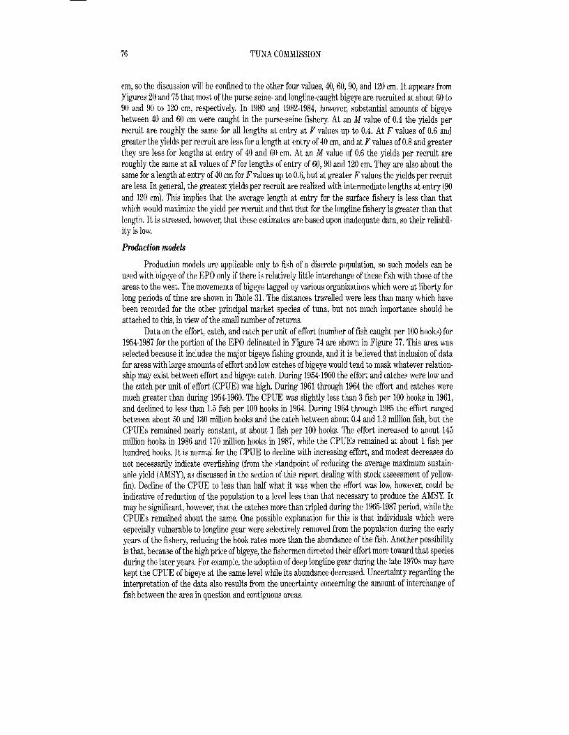
76 TUNA COMMISSION
em, so the discussion will be confined to the other four values, 40, 60, 90, and 120 em. It appears from Figures 20 and 75 that most of the purse seine- and longline-caught bigeye are recruited at about 60 to 90 and 90 to 120 em, respectively. In 1980 and 1982-1984, however, substantial amounts of bigeye between 40 and 60 em were caught in the purse-seine fishery. At an M value of 0.4 the yields per recruit are roughly the same for all lengths at entry at F values up to 0.4. At F values of 0.6 and gTeater the yields per recruit are less for a length at entry of 40 em, and at Fvalues of 0.8 and greater they are less for lengths at entry of 40 and 60 em. At an M value of 0.6 the yields per recruit are roughly the same at all values of F for lengths of entry of 60, 90 and 120 em. They are also about the same for a length at entry of 40 em for Fvalues up to 0.6, but at greater F values the yields per recruit are less. In general, the greatest yields per recruit are realized with intermediate lengths at entry (90 and 120 em). This implies that the average length at entry for the surface fishery is less than that which would maximize the yield per recruit and that that for the longline fishery is greater than that length. It is stressed, however, that these estimates are based upon inadequate data, so their reliability is low.
Production models
Production models are applicable only to fish of a discrete population, so such models can be used with bigeye of the EPa only if there is relatively little interchange of these fish with those of the areas to the west. The movements of bigeye tagged by various organizations which were at liberty for long periods of time are shown in Table 31. The distances travelled were less than many which have been recorded for the other principal market species of tuna, but not much importance should be attached to this, in view of the small number of returns.
Data on the effort, catch, and catch per unit of effort (number of fish caught per 100 hooks) for 1954·1987 for the portion of the EPa delineated in Figure 74 are shown in Figure 77. This area was selected because it includes the major bigeye fishing grounds, and it is believed that inclusion of data for areas with large amounts of effort and low catches of bigeye would tend to mask whatever relationship may exist between effort and bigeye catch. During 1954-1960 the effort and catches were low and the catch per unit of effort (CPUE) was high. During 1961 through 1964 the effort and catches were much greater than during 1954-1960. The CPUE was slightly less than 3 fish per 100 hooks in 1961, and declined to less than 1.5 fish per 100 hooks in 1964. During 1964 through 1985 the effort ranged between about 50 and 130 million hooks and the catch between about 0.4 and 1.3 million fish, but the CPUEs remained nearly constant, at about 1 fish per 100 hooks. The effort increased to about 145 million hooks in 1986 and 170 million hooks in 1987, while the CPUEs remained at about 1 fish per hundred hooks. It is normal for the CPUE to decline with increasing effort, and modest decreases do not necessarily indicate overfishing (from the standpoint of reducing the average maximum sustainable yield (AMSY), as discussed in the section of this report dealing with stock assessment of yellowfin). Decline of the CPUE to less than half what it was when the effort was low, however, could be indicative of reduction of the population to a level less than that necessary to produce the AMSY. It may be significant, however, that the catches more than tripled during the 1965-1987 period, while the CPUEs remained about the same. One possible explanation for this is that individuals which were especially vulnerable to longline gear were selectively removed from the population during the early years of the fishery, reducing the hook rates more than the abundance of the fish. Another possibility is that, because of the high price of bigeye, the fishermen directed their effort more toward that species during the later years. For example, the adoption of deep longline gear during the late 1970s may have kept the CPUE of bigeye at the same level while its abundance decreased. Uncertainty regarding the interpretation of the data also results from the uncertainty concerning the amount of interchange of fish between the area in question and contiguous areas.

77 ANNUAL REPORT 1991
BLACK SKIPJACK
Black skipjack, although they constitute only a minor part of the total landings of tunas caught in the eastern Pacific Ocean, are of considerable commercial importance in a number of Latin American countries. Furthermore, they represent a resource of significant magnitude, which will be more heavily exploited as the demand for tuna increases. Accordingly, it is prudent to learn as much as possible about this species.
The present knowledge of black skipjack comes mainly from vessel logbook data, data on the weights of fish unloaded at canneries, stomachs, gonads, and measurements of fish taken at canneries, physiological data gathered on one tagging cruise, gonads collected for histological studies on tagging cruises, larval surveys directed primarily at other species, recapture data for black skipjack tagged incidentally to yellowfin and skipjack, and current studies at the IATTC's Achotines Laboratory.
Data on the landings of black skipjack by tuna bQats during 1961-1991 are listed in Table 1. These data include only the fish which are landed. Additional amounts are known to have been caught but not landed, and these are not included in the statistics. Estimates of amounts of black skipjack discarded at sea by purse-seine vessels during the 1986-1991 period range from about 6to 11 thousand tons per year. Black skipjack are also caught by small boats based in Latin America, for which data are not obtained. Therefore the actual catches are greater than those recorded in the table. The areas of the 1980-1983 catches by vessels from which logbook data were obtained are shown in Figure 78.
An analysis of the weight-length relationships of black skipjack is given in IATTC Internal Report 17. Some observations on the swimming performance, body temperatures, and gastric evacuation times of black skipjack were made on a tagging cruise conducted in 1981, and an analysis of the results was published in an outside journal in 1984. A total of 1,502 black skipjack have been tagged, and 107 of these have been recaptured. Information on the movements and growth of black skipjack, as determined from these data, are given in the IATTC Annual Report for 1982.
Information on the areas and duration of spawning, size at sexual maturity, sex ratios, fecundity, and spawning frequency was recently published in IATTC Bulletin, Vol. 19, No.2. The measurement of reproductive potential is of primary importance with respect to the dynamics of fish populations, since it is abasic determinant of productivity. Furthermore, since the amount of fish of catchable size available to the fishery is largely dependent on the success of spawning and survival during the earliest stages of life, studies of this nature can yield information of potential value for predictive purposes. In addition, large numbers of larval and juvenile black skipjack, along with those of other species of scombrids (tunas and mackerels) have been collected, particularly off Central America and near the entrance to the Gulf of California.
The larvae and juvenile data, tagging data, and logbook data provide indices of abundance of black skipjack relative to the other species of scombrids. It appears, on the basis of this information, that the potential annual production of this species is far greater than the present levels of landings.
A considerable amount of work on black skipjack is currently being conducted at the IATTC laboratories at Achotines Bay, Panama, and La Jolla. These studies are summarized in the section of this report entitled Early life history studies.


79 ANNUAL REPORT 1991
100 80140
4040
20 20
EXPERIMENTAL AREA 2 OPEN DURING' 976· '979 ZONA EXPERIMENTAL 2
ABIERTA DURANTE '976 . '979
/ o/mo EXPERIMENTAL AREA'
OPEN DURING '976· '979 ZONA EXPERIMENTAL'
ABIERTA DURANTE '976· '979
EXPERIMENTAL AREA' OPEN DURING '973· '979
ZONA EXPERIMENTAL'
20 ABIERTA DURANTE' 973 • '979 20
C'-,
EXPERIMENTAL AREA 3 OPEN DURING '978· '979 ZONA EXPERIMENTAL 3
ABIERTA DURANTE '978· '979
40 L..----'--1,--4Lo,-------'---.L--.L-,----1.J."'"o---'------L----'---10--l0--.L---'----~--=8'-:0-----'---'--~-----'40 2
FIGURE 1. The Commission's Yellowfin Regulatory Area (CYRA).
FIGURA 1. Area Reglamentaria de la Comisi6n para eJ Aleta Amarilla (ARCAA).

~ 160 140 130 120 110 100 90 80 70
~
30 30CIJ ~ 600 TONS
@ 100 - 499 TONS
l o 26 - 99 TONS
1 - 24 TONS
20 20 ,00'
oo@oo 0" 0 0000
· ." coQOO@OO •• 0000 0000000000
"<> 0 00000" 000000 · '000<>000000
• "" 0" "000
10 I[ :g~~oo 10 >-3
~ · " " "oaa . ooocQOO@@@@@@@@@O@@OOoOOcoQOOOOOOO Z
· ." 000000000000000000000000000000000000 ~
· "" "" 0000 <> 000000000000" <> 0000" "000000 · 000000000000000000000000000000000000 o
ooocoa@aoocooooooooooocoooooooooooooooooo<>ooo<>oooooooooooooo<>ooooo@@ooo
• <> 0 <> <> " a " " <> " 0 " <> <> " <> " " " 0 "00" " 0 0 O@OO " 000 ~ o " <> <> a " <> <> " " " " <> <> "<> <> " <> " " 0000 Os 0 " <> 0 U\SIV U V U(£" • " ~ " n <> " 0 <> 0 <> 0 <> "" """ 0 0 0 O@O" o >-<
D w · 00<>" <> "000<>000000"<>0 000000000 " w
<>" 0000 <>00000"""""" 000" <>" O@@OO >-< 0000000000000000000000000000 0(2)
r Q
o Z"""", 'OOO,OOOOOOO@OO@\
<> 000000 0 0 0 0000000 0 00
""""00000""" Q <> 00" " "0" "" ""
oooooo@aOQoQ
oooooooo@@a@@@ooo10 ooooO@@@@@@@@@O 10
",,'000@@@@@@, ~
CI CI 0 CI oOOO@@@OCl o Uv VyOOOOOOy
r " <I CI <I <1000 <I <I
<I <I <I <I <10<1 <Il 00<>
... 20 20
160 140 130 120 110 100 90 80 70
FIGURE 2. Average annual catches of yellowfin in the EPa during 1979-1990 for all purse-seine trips for which usable logbook data were obtained.
FIGURA 2. Capturas medias anuales de atun aleta amarilla en el OPO durante 1979-1990 de todos los viajes de barcos cerqueros de los que se obtuvieron datos de bitacora utilizables.

150 140 130 120 110 100 90 80 70
3°1 0::
00· ~
-130o ~ 500 TONS
@ 100 - 499 TONS
0 25 - 99 TONS
1 - 24 TONS
"I EFFORT, NO CATCH
" 0 -j 20ESFUERZO SIN CAPTURA
"I z ~
10 Z ~
t""" ::>::l
o@c o@ooooo@@@oo@ggg:g:g~~gg~~~~gg~~~~o trjcO 0000 ·oaoQ@@oO@o@o@oo@@OO@@@@@@OO .0 ""0o@OOO @@O OO@@O OOOo@@@o@oO@O@O@·@OQOOO
0 ·000 c@ooOOO .o@ooooOO 0o ~ 00" , c oO'<§8'o Qo. 00 ::>::l <> • 0 0 >-3
O@OOOO<> 00 ooo@@o
0
ooo@ ~• 000
00000" O@@@OQ.Q 0·0 ~
OQ.@@ooo·oo· >--' 00· ·OOO@OoO
<> 0 0" OO@O oo@aQoOOoo
o·@@o@<>10 ~ @@o 0 \ -I 10o " 0000 o o·
oooo@ooo 00 0
~-, I
20 I J"-------"---- ~
150 140 130 120 110 100 90 80 70
FIGURE 3. Catches of yellowfin in the EPO in 1991 for all purse-seine trips for which usable logbook data were obtained. CDFIGURA 3. Capturas de atlin aleta amarilla en el OPO en 1991 de todos los viajes de barcos cerqueros de los que se obtuvieron datos de bitacora utilizables. >--'
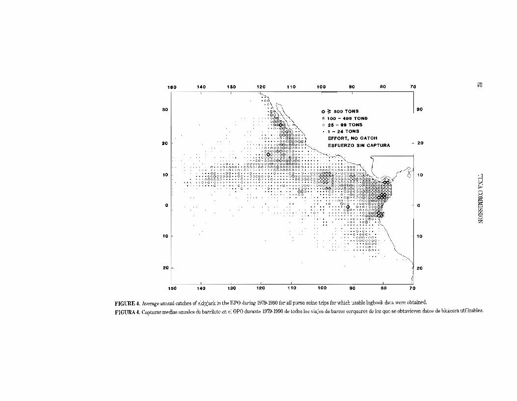
~ 150 1..0 180 120 110 100 90 80 70
·0 ·0
80 80o ~ 500 TONS
@ 100 - "88 TONS
o 26 - 98 TONS
1 - 2.. TONS 000 ",.
00· EFFORT, NO CATCH O@@20 20000 ,,"-.:, ESFUERZO SIN CAPTURA
. oOoOOOO@O@OO""'" <>OOOO@@OOOOoa ..
00 aOOoooo@OOOoo, 'oooOOOOOOOOO@OO<>'" ."
." oOOoOOOO@@O@@O@O<><>"""'" . C 000"'" ooooooooo@aooo@@@oo<>" .. "",,· .... <>" ...
. QoooOoOOOooOOOOoOOoQOO@OOOOOOOO"QOOOQ,,<>OoooooQOQ· <>" '000000000"<>000000<>0000000000<> '<>0<>00000 0 00 0 000 00
" " .. 00 " " .. 00 " " 0 .... " 0 " " " " " " " 0 " " " .. 00 .. " 0 " " 000 a@@@o 0 " 00000 000 t.10 ooooOO@OOOOOooQOooOOOoOoOooaoooO@OOOOOOOO@@@@@OOOOO@@OO 10 >-3<>000000000000000000000<>000<> aoooooOOOOOOOO@@@O@OOOOO@@@O c:: " .. 0 " 0 " 0 " .... <> " " " " 0 " " D " " " " " " " <> " <> " " .. " .. " " <> " 00 O@@O@OO 0 0 0 000 " ..... o'c 00-'''''''' -00"''''
D
""" ... "." 0000"" 00000 oQoooa@ao@@@@ooo s;:. 0 ". . 00"'" ." .. 00000"" <> oO@@OOOO@O@OOO
-@@oeo ooooOOooeOOOOOO ()nonGO oooOon Ooo@OOO
e e e e e e e O@ e 000 000000 0 0 000 000 00 @OO e 0000 ~ o o >-<
e : : : 0 ;g~ 0 ~ ; ~ ; U1 ·0· 0000000 eo_ 000 U1
00000000 _ 000@ 0000000 000 0 o
000 00@0- Z
- 00000000 - 00000000010 0000 0 00 0 10
- 000000000- 0000000
00 00@0 0 00000000 0
20 20
150 140 130 120 110 100 90 80 70
FIGURE 4. Average annual catches of skipjack in the EPO during 1979-1990 for all purse-seine trips for which usable logbook data were obtained.
FIGURA 4. Capturas medias anuales de barrilete en el OPO durante 1979-1990 de todos los viajes de barcos cerqueros de los que se obtuvieron datos de bitacora utilizables.
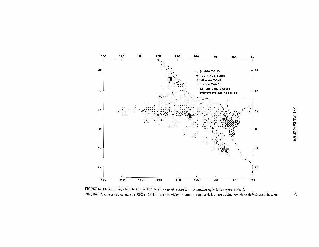
150 140 130 120 110 100 90 80 70
30 30o ~ 500 TONS~\.~\
I
@ 100 - 499 TONS o~~ o 25 - 99 TONS . . 0" OO~.@ 00
1 - 24 TONS
EFFORT, NO CATCH20
·0' ·0· ESFUERZO SIN CAPTURA
20 " o@
.@. O@O •
o . (I (I" .. ~ .
• " <> 00" "" @ o
DO" ." ". 0 <> 0" ~
00' "" .. " . """ @ " .. 0 ""10 o O@@oO oooOOooOO@O -00 OOO@O 000.(100 0000· 10 Z ·0 0<> OoooQ@lo . @@@@o@~oo.o 0"<>0 <>O'OO@O~' Z
@o DO@ oo@6 @oO@@OO@O 000 ODO@OOO@O@<>·@OOO. 0" . " . D (I. 000· .... 00" @@O"'''O@@' 0•
-0- 'O@"" '@OQ <>@o" O@@@@O ~
" . ·0· "." " t"" 00- '00_" QOO@OO§lo·Q ::0
. OO@' ." ... " 0 '@O' ·0· trJ
"'0On" o@o ·0·0· " . o o 00
@ ~
o· >-'"0 . (I 0 0•
. o@OO' .". ~
>-'
O@O" "0 '@O@O'
0<100· .@@@o .10 10
,og~~~ . . 0" 000D
00
,or _, , J~
150 140 180 120 110 100 90 80 70
FIGURE 5. Catches of skipjack in the EPO in 1991 for all purse-seine trips for which usable logbook data were obtained.
FIGURA 5. Capturas de barrilete en el OPO en 1991 de todos los viajes de barcos cerqueros de los que se obtuvieron datos de bitacora utilizables. "'" 00

~
PRINCIPAL MARKET SPECIES - ESPECIES COMERCIALES PRIMARIAS 65.4%
SKIPJACK - BARRILETE I I 1,366
YELLOWFIN - ALETA AMARILLA I I 1,087
BIGEYE -PATUDO CJ 284
ALBACORE-ALBACORA CJ 2561 N. BLUEFIN - ALETA AZUL N. 0
32~S. BLUEFIN - ALETA AZUL S. 0 17 TOTAL 3,042
SECONDARY MARKET SPECIES - ESPECIES COMERCIALES SECUNDARIAS 25.6%
SEERFISHES . SIERRAS I I 538 >-:l
215 c::::BULLET TUNAS - MELVAS CJ LONGTAIL - TONGOL 180 ~0 Q
BLACK SKIPJACKS - BARRILETES NEGROS 0 161 o
BONITOS - BONITOS 0 90 ~ ......D wOTHERS - OTRAS I 6 w TOTAL 1,190 <5 z
BILLFISHES - PICUDOS 3.5%
SWORDFISH· PEZ ESPADA 0 85 --= -:J ISTIOPHORIDS - AGUJAS 0 77 TOTAL 162
UNSPECIFIED TUNAS AND BILLFISHES - ATUNES Y PICUDOS NO ESPECIFICADOS 258 ~
ALL SPECIES - TODAS LAS ESPECIES 4,652
FIGURE 6. World catches of tunas and tuna-like species in 1990, in thousands of short tons.
FIGURA 6. Capturas mundiales de atunes y especies afines en 1990, en miles de toneladas cortas.

_~ "_ 0'
-~
~
---~ ~=
PACIFIC OCEAN OCEANO PACIFICO
CATCH CAPTURAI~'INDIAN OCEAN SKIPJACK 976-v
BARRILETEOCEANO INDICa YELLOWFIN 714
CAPTURA ALETA AMARILLA SKIPJACK 241
CATCH ~~;,,~~
BIGEYE 165 BARRILETE PATUDO YELLOWFIN 198 ALBACORE 136ALETA AMARILLA ALBACORA BIGEYE W47 N. BLUEFIN 7PATUDO \J ALETA AZUL N. ALBACORE 44 5S. BLUEFINALBACORA
ALETA AZUL S. S. BLUEFIN 11 TOTAL 2,003ALET A AZUL S.
I
I TOTAL 541
FIGURE 7. Catches of the principal market species of tunas in 1990, in thousands of short tons.
FIGURA 7. Capturas de las especies de atunes comerciales principales en 1990, en miles de toneladas cortas.
o
ATLANTIC OCEAN OCEANO ATLANTICa ~r
ZCATCH z
CAPTURA SKIPJACK 147 §2
t""BARRILETE ~
tr:I '"0
YELLOWFIN 175 ALETA AMARILLA 0
BIGEYE 72 ~ ......PATUDO ~
~ ALBACORE 76 ALBACORA
N. BLUEFIN 25 ALETA AZUL N.
S. BLUEFIN 2 ALETA AZUL S.
I TOTAL 497
00
"'"'

86 TUNA COMMISSION
600 INDIAN OCEAN - OCEANO INDICa 600
400 400
200 200 (/)
(/) « I-« a 0 II:0 0iI <.)I-
w 600 ATLANTIC OCEAN - OCEANO ATLANTICa (/):2 «600(/) e « « 0 400 ...J « 400 UJ
Z-' w 0 Z 200 I-
2000 UJl e w 0 (/)
(/) 0
UJ ...J
~ 1800 2000 :EPACIFIC OCEAN - OCEANO PACIFICO ~ I
1800 (/)(/) 1600 ZZ 00 I 1600 ~ g 1400
II: a: I 1400 ~ w 1200 (/):2 LL 0 1200 15
1000 (/)
0 Z
(/)
1000 ~ « «800(/) (/) ~ ::J8000 0 I J:600I- I-
600
400 400
200 200
Ol.-l_.-J..._--L_L---l_.-J..._--'--_L----.J_---'-_--'--_...L-_L-_L----L_....I....JO 1975 1980 1985 1990
FIGURE 8. Catches of the principal market species oftunas.
FIGURA 8. Capturas de las especies de atunes comerciales principales.
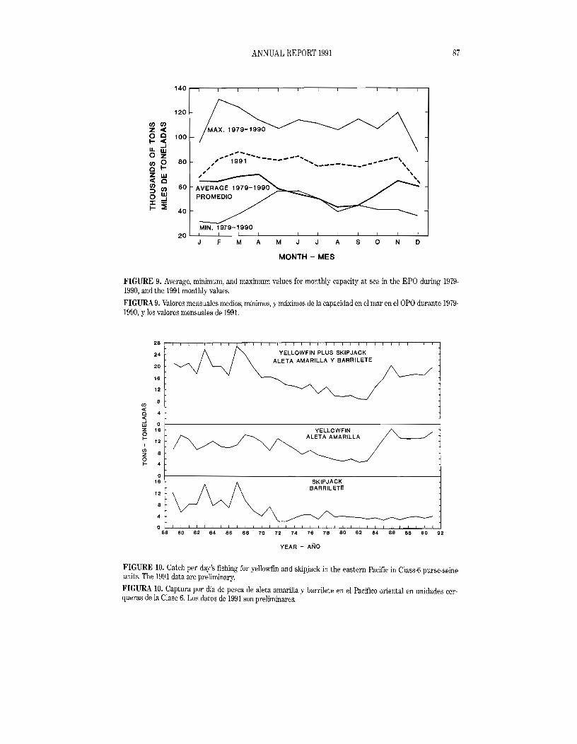
87
120
ANNUAL REPORT 1991
140 ~-~----r--"""'----'------'----,---.---,---r--r--,-,
(/)(/) Z 001( MAX. 1979-1990 o a 100 I :s u. w ,.,.. ... -.. ..- ...o Z
", 1991 ------- "...... .... ............, (/)0 80 a I , / '----------',,Z W , ,001( a , (/) (/) 60 ::J W o ...J
~ ~ 40
MIN. 1979-1990
J F M A M J J A s N D
MONTH - MES
FIGURE 9. Average, minimum, and maximum values for monthly capacity at sea in the EPa during 19791990, and the 1991 monthly values.
FIGURA 9. Valores mensuales medios, minimos, y maximos de la capacidad en el mar en el OPO durante 19791990, y los valores mensuales de 1991.
28
YELLOWFIN PLUS SKIPJACK ALETA AMARILLA Y BARRILETE
24
20
16
12
8 en <C 0 4 <C -' 0U.I Z 16 YELLOWFIN 0 ALETA AMARILLAI
12 I
en 8
0 z I- 4
0 16 SKIPJACK
BARRILETE 12
8
4
0 58 60 62 84 66 68 70 72 74 76 78 80 82 84 86 88 90 92
YEAR - ANO
FIGURE 10. Catch per day's fishing for yellowfin and skipjack in the eastern Pacific in Class-6 purse-seine units. The 1991 data are preliminary.
FIGURA 10. Captura por dia de pesca de aleta amarilla y barrilete en el Pacifico oriental en unidades cerqueras de la Clase 6. Los datos de 1991 son preliminares.

88 TUNA COMMISSION
150 140 130 110 100 90 80 70
30
20 1~APR-SEP
16. OCT-MAR
10
°r---------------l.------,.-.....l..-F
10 1. JAN-FEB 2. MAR-OCT 3. NOV-DEC
20
150 140 130 120 110 100 90
FIGURE 11. Season-area strata used to standardize the catch rates of all sizes of yellowfin combined.
FIGURA 11. Estratos de temporada-area usados para estandardizar las tasas de captura de aleta amarilla de todas tallas combinadas.
18
« i5 a: 16 0 n. I/)
« 14 c « ..J w 12 Z 0 l-I 10
> « c a: 8
w 0I/) Z
6
0 I
4 70 72 74 76 78 80 82 84 86 88 90 92
YEAR - AND
FIGURE 12. Comparison of annual indices of yellowfin abundance. The solid line is the index from the generalized linear model, with the 22-year mean set equal to the 2-year mean CPDF, and the vertical bars are the approximate 95-percent confidence limits. The dashed line is the index most commonly used, CPDF for vessels with greater than 400 tons carrying capacity. The data for 1991 are incomplete.
FIGURA 12. Comparaci6n de los indices anuales de abundancia del aleta amarilla. La linea continua representa el indice del modelo lineal generalizado, con el promedio de 22 aiios fijado igual a la CPDP media de 2 aiios, y las barras verticales los limites de confianza de 95% aproximados. La linea de trazos representa el indice de uso mas frecuente, CPDP de barcos de mas de 400 toneladas de capacidad de acarreo. Los datos de 1991 son incompletos.
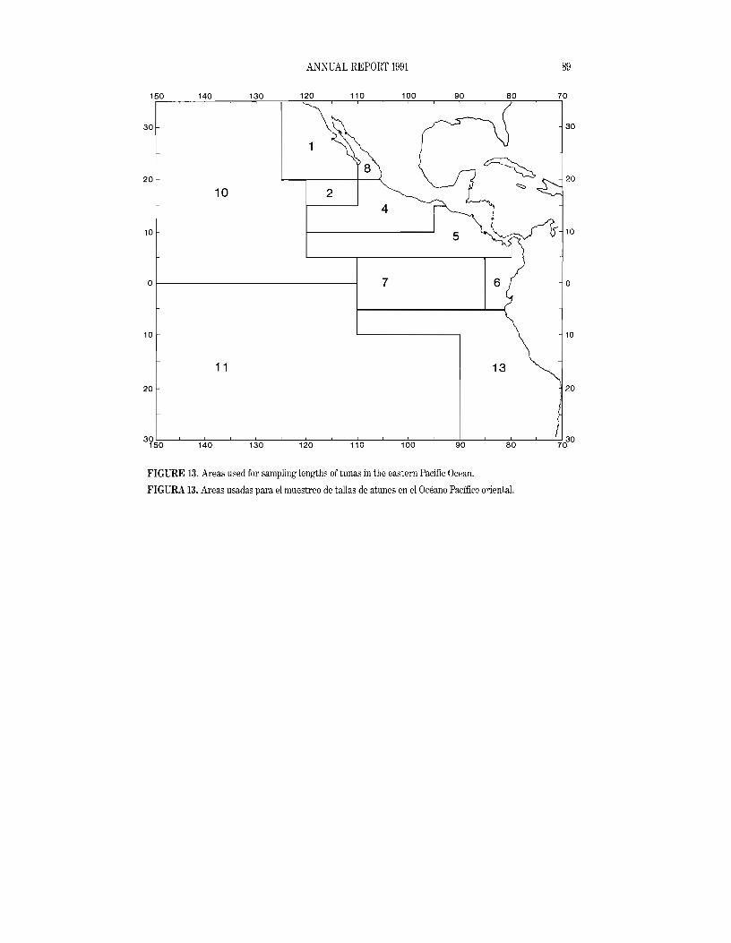
89 ANNUAL REPORT 1991
150 140 130 120 110 100 70
30 30
1
8 20 20
10 2 4
10 105
o1-------------------1 7
10 10
11 13
20 20
3~5~0c----'----:-14;-;Oo------'----:;1-;:3-;::-0---'----1~2::00c-----'-----;1-;-10;:;------'----,1,-!O::OOc-----'----g;:!:0:;-------'-----;;a';:;0----'------::
FIGURE 13. Areas used for sampling lengths of tunas in the eastern Pacific Ocean.
FIGURA 13. Areas usadas para el muestreo de tallas de atunes en el Oceano Pacifico oriental.

90 TUNA COMMISSION
10
CI)
« I-a: 0 ()
5
0
5
0
AREA 1
11.8 LB - 5.4 KG
AREA 8
28.1 LB - 12.7 KG
CI)
« 0 « -J UJ Z 0 I-
5
0
30
25
AREA 4
35.2 LB - 16.0 KG
AREA 2
49.6 LB - 22.5 KG
UJ 0 20
CI)
0 I-Z UJ ()
15
10
5
CI)
Z 0 I-
I-a: 0 I CI)
0
10
5
0
10 AREA 6
11.8 LB - 5.4 KG
AREA 5
22.5 LB - 10.2 KG
li0 5
CI) 0 w a: 0 Z ::::> I
0
5
0
5
0
20 40 60 80 100 120 140 160 180 200
LENGTH IN CENTIMETERS - TALLA EN CENTIMETROS
FIGURE 14. Estimated yellowfin catch by 2-cm intervals for the market measurement areas of the CYRA in 1991. The values in the upper right corners of the panels are average weights.
FIGURA 14. Captura estimada de aleta amarilla en las zonas de medici6n en el ARCAA en 1991, por intervalos de 2 em. El valor en la esquina superior derecha de cada recuadro representa el peso promedio.

91 ANNUAL REPORT 1991
1986 6 27.1 LB - 12.3 KG(J)
« 4I0:
2o o
o(J)
« 1987
« o 6
22.0 LB - 10.0 KG -I 4W Z
2o I
oW o 1988
6(J) 17.1 LB - 7.8 KG W -I 4 :2
2 (J)
Z o o 1989 l 4 25.2 LB - 11.4 KG I 0: 2o I (J) o
1990u. 6o 23.7 LB - 10.8 KG
(J) 4o z
2« (J)
:::> 01--~""""""-l..llli..1J...l..l..Ll..LU-l..lll..LU-l..llLJ...LJ-l..lll..LU-l..llLJ...LJ-l..llLJ...LJ.ll.LLJ...LJ...LLLl..1..1..1-'='--------i
o 1991I 4I- 25.1 LB - 11.4 KG
2
OI---.-....c<:j-l..ll.L+.J..l~l..LU+U-l.l..f-I-l..llf-l-Ul.Lf-lJ...!l.1-l..ll.L+.J..l...l.Ll-LJ...LJ+U-l.l..f-I...LLLf-l-U=poC.....jF----.-----i
20 40 60 80 100 120 140 160 180 200
LENGTH IN CENTIMETERS - TALLA EN CENTIMETROS
FIGURE 15. Estimated yellowfin catch by 2-cm intervals in the CYRA. The values in the upper right corners of the panels are average weights.
FIGURA 15. Captura estimada de aleta amarilla en el ARCAA, pOl' intervalos de 2 em. El valor en la esquina superior derecha de cada recuadro representa el peso pl'omedio.

92 TUNA COMMISSION
30 ,----,---,---,-----r--,-------,--,------,-----,,-----,-----r--,-------,--,------.----.----,---,
25 1986
77.0 LB - 34.9 KG C/) 20 <t: I 15 0:
10o ()
5 C/) 0f- --I~~=cD::!=D=_...d:!1.llJ..l..l.Ll..Ll..Llli.lill.l.lllJ..l..l.Llli.lll.tIJ.........<t: o 198715<t: -' 83.1 LB - 37.7 KG w 10 z o 5 I- 0f---- ...c=d::J:1..LJUl.1..l:LDUl.1..Ll..lJUl.1..Ll..lJL.Lll.Ll..lJUl.1..Ll..lJUl.1.l...Cb -----1 W 1988o 10
58.6 LB - 26.6 KGC/) 5o
I 0f---- -----1~LD..J:i.l...t:u....uUl.1..Ll..lJUl.1..Ll..lJL.Lll.L1..LJL.Lll.L1..LJUl.1..L1..LJ...LLL.L1..LJ~
Z W 198925 () 60.3 LB - 27.4 KG
20 C/)
15Z o 10lI 5 0: 0f---o .L1..LJ...D...L.L1..LJ-="""-J...LLL.L1..LJ...LLL.L1..LJ...LLL.L1..LJ...LLL~...LLLJ...J..J..J...LLL.L..U.J-=--------i
I 1990 C/) 25
59.6 LB - 27.0 KG LL 20o
15 C/)
o 10 W 0: 5 o Of-__----d:b=<=:J..llJ..l..l.Ll..Ll..Lll.ll.LLU..LllJLlll.lli.lill.l.LLU..LllJLlll.llllIJ...... ---jZ :::> 1991 I 10 47.6 LB - 21.6 KG
5
ol-----,-----..,....--9=l::H:I:!=fJ'£q:a:cq:Ilt.d.jJJJ..LjJ..W+W-4-Ul.l+J..l.L4lilltut¥L-,------r-r--J
20 40 60 80 100 120 140 160 180 200
LENGTH IN CENTIMETERS - TALLA EN CENTIMETROS
FIGURE 16. Estimated yellowfin catch by 2-cm intervals in the area between the CYRA boundary and 150°W. The values in the upper left corners of the panels are average weights.
FIGURA 16. Captura estimada de aleta amarilla en la zona entre ellimite del ARCAA y 150°W; por intervalos de 2 em. El valor en la esquina superior izquierda de cada recuadro representa el peso promedio.

93 ANNUAL REPORT 1991
4
AREAS 1,2,4, AND 8 2en 5.7 LB - 2.6 KG
« I-
0 0 0::
AREA 5 0 4 5.9 LB - 2.7 KGen « 0 2 « -' w 0z 0 AREA 6 I- 10 6.0 LB - 2.7 KG W 0
8en 0 I- eZ W
0 4
en Z 2 0 I-
0I-0:: AREA 7 0 I 2 5.6 LB - 2.5 KG en LL 00 en AREA 13 0 2 7.2 LB - 3.3 KG w 0:: 0 0 Z AREA 10 ::::> I 11.0 LB - 5.0 KG2
0 20 25 30 35 40 45 50 55 60 65 70 75 80 85 90
lENGTH IN CENTIMETERS - TAllA EN CENTIMETROS FIGURE 17. Estimated skipjack catch by I-ern intervals for selected market measurement areas of the eastern Pacific Ocean in 1991. The values in the upper right corners of the panels are average weights.
FIGURA 17. Captura estimada de barrilete en areas de medici6n seleccionadas del Oceano Pacifico oriental en 1991, par intervalos de 1 ern. El valor en la esquina superior derecha de cada recuadro representa el peso promedio.

94 TUNA COMMISSION
(j)
« f a: o ()
(j)
« o « --I w Z o f-W o (j) W --I
~
(j)
z o f-
f a: o I (j)
ll.. o (j)
o z « (j) ::J o I f
3 1986
2 7.9 LB - 3.6 KG
1
o 1987
2 7.1 LB - 3.2 KG
1
o 1988
4 6.4 LB - 2.9 KG
3
2
1
o 1989
3 8.1LB-3.7KG
2
o 1990
3
2
8.5 LB - 3.9 KG
1
01-- =i..L.l-'-'-L.L..L.L..U.-'-'-L.L..L.L..U.-LJ...JL.L..L.LJ....L-'--'--J--L.L.LJ....L.J....L..I...L..L.'----__--i
1991 2 6.1 LB - 2.8 KG
1
o 20 25 30 35 40 45 50 55 60 65 70 75 80 85 90
LENGTH IN CENTIMETERS - TALLA EN CENTIMETROS FIGURE 18. Estimated skipjack catch by I-em intervals in the eastern Pacific Ocean. The values in the upper left corners of the panels are average weights.
FIGURA 18. Captura estimada de barrilete en el Oceano Pacifico oriental, par intervalos de 1 em. El valor en la esquina superior izquierda de cada recuadro representan el peso promedio.
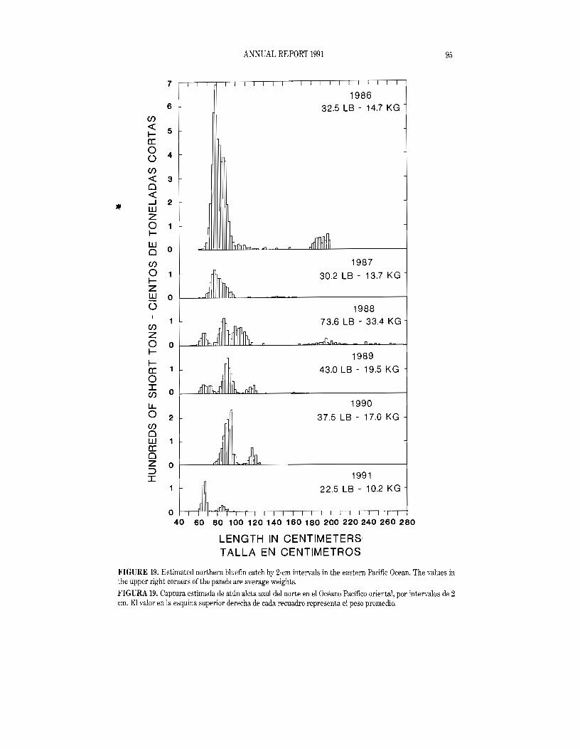
95 ANNUAL REPORT 1991
7
1986 6 32.5 LB - 14.7 KG
CJ)
« le:
5
0 () 4
CJ)
« 3 0 «
11 .....J UJ
2
Z 0 IUJ 0 CJ)
0 I
0 l 1987
30.2 LB - 13.7 KG z UJ 0 () 1988
CJ) 73.6 LB - 33.4 KG
Z 0 0 I
1989 I-e: 1 43.0 LB - 19.5 KG 0 I CJ) 0
u.. 1990 0 2 37.5 LB - 17.0 KG CJ)
0 w e: 0 z :::> I
0 1991
22.5 LB - 10.2 KG
0 I I I
40 60 80 100 120140 160180200220240260280
LENGTH IN CENTIMETERS TALLA EN CENTIMETROS
FIGURE 19. Estimated northern bluefin catch by 2-cm intervals in the eastern Pacific Ocean. The values in the upper right corners of the panels are average weights.
FIGURA 19. Captura estimada de attin aleta azul del norte en el Oceano Pacifico oriental, por intervalos de 2 em. El valor en la esquina superior derecha de cada recuadro representa el peso promedio.

96 TUNA COMMISSION
1986 100 67.7 LB - 30.7 KG
50
Of-__---,---:c-=-::~fl..l.JL.U.LLLUl.lllJ.LlJ.l.ilJLl.lll.llllillJ.LlJ.l.ilJLl.llil_l.lL _____j
1987 50 67.5 LB - 30.6 KG
o 1988
(j) 50 60.8 LB - 27.6 KG « ~ Of-- """""-':bd:b---....ccl..ll-l.l..LLLU-l.l..Lll1l-l.l..LLLUJ:::l.LLLUi.O..LLUil..LllUl.l.L ---l a: 1989o
100() 51.8 LB -23.5 KG (j) 50« o Of-__--d:1l:l:::l::hIl:il:r::l...t:l:cl..ili1illl..WLilLW1Uil1WlllJ..1.J:I::d1rL..D. ~ « 1990.....J w 300 61.3 LB - 27.8 KGZ o 250 ~
200(j)
Z 150o
~ 100
~ a:
50o I (j) Of--_~....LLJ...rr]::l..ill..l.lJ...Lill..l.lJ...Lill..l..lJ..l.lll..l.lJ..l.lll..l..lJil..LLLU-l.l..LL.LUi.l..LLLlL_ ---l
1991 250 90.5 LB - 41.0 KG
200
150
100
50
Of----,-----.-....o=:p:u:Q:>-O>oCf'>==I.fi.ll.l..j-Ul.l.J-'LULj...Lil.J.t.l.lJ.lfl..l.l.l.jf-U-l-4.lll..lflJ:1.Ii--,---,----j
20 40 60 80 100 120 140 160 180 200
LENGTH IN CENTIMETERS - TALLA EN CENTIMETROS
FIGURE 20. Estimated bigeye catch by 2-cm intervals in the eastern Pacific Ocean. The values in the upper left corners ofthe panels are average weights.
FIGURA 20. Captura estimada de patudo en el Oceano Pacifico oriental, por intervalos de 2 cm. El valor en la esquina superior izquierda de cada recuadro representa el peso promedio.

__
97 ANNUAL REPORT 1991
15 r---r-----,-------.-----,----,----,---r---,---r
1986 N= 27210
5
o 1987
N= 110610
5 ill....,
OI--__~_.LLL.LL-LLJ_l....LLLl_.LLL.LL_LLJ:::I:.L~« I 1988Z ill N = 1639o 5cr: o CL o
1989 I Z N= 516
5ill o cr: ill o Q..
1990 N =7910
5
Oi- --LL_---"---'--.L-LLLLl---'--.LLLLLl---'--.L-'------__-i
1991 N=184
5
Oi--,-----,l:::L.L.L.j-LLl....l...f--LLL..Lj---'--.L-LLf-l-l---'--.L+.t:=---.------.--
20 25 30 35 40 45 50 55 60 65 70
LENGTH IN CENTIMETERS TALLA EN CENTIMETROS
FIGURE 21. Annual length-frequency distributions of black skipjack caught in the eastern Pacific Ocean.
FIGURA 21. Distribuci6n anual de la frecuencia de talla del barrilete negro capturado en el Oceano Pacifico oriental.
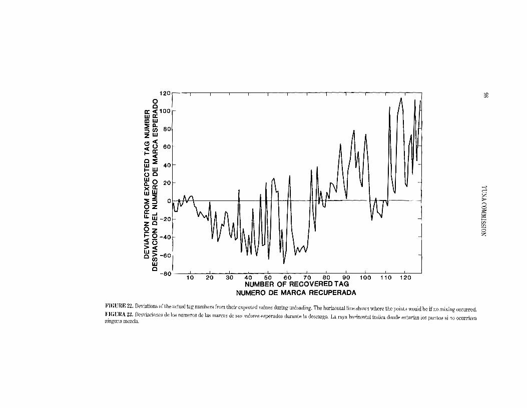
120 1 I I I I I I I I I I I I '-"" 00
o o
II: < 100 wo: mw ~ g,ZW
80
< ~ 0 60
'1- II:c(
fiJ::E 40 I-W 00 W 0ll.a:X wW::E
20 >-3c::
::E:::>OZ
~
(') o
D:...J ~
LL. W -20 ~
ZO Qz I- 0c(- -40 -0><we > -60
(J)
UJ. UJ. >-;
o Z
W 0_80 1 I
10 I
20 I
30 I
40 I
50 I
60 I
70 I
80 I
90 I
100 I
110 I
120 NUMBER OF RECOVERED TAG
NUMERO DE MARCA RECUPERADA
FIGURE 22. Deviations of the actual tag numbers from their expected values during unloading. The horizontal line shows where the points would be if no mixing occurred.
FIGUHA 22. Desviaciones dc los numeros de las marcas de sus valol'es esperados durante la descarga. La raya horizontal indica donde estarian los puntas si no ocurriera ninguna mezcla.

99 ANNUAL REPORT 1991
OBSERVED MIX OF FISHINGACTUAL CATCH DATA COMBINACIONES DE PESCA OBSERVADOS DATOS DE CAPTURA REAL
DOLPHIN FISHING ONLY NON-DOLPHIN FISHING ONLY PESCA CON DELFINES SOLAMENTE PESCA SIN DELFINES SOLAMENTE
FIGURE 23. Residual sums of squares for the fitting of the symmetrical production model to: (A) actual catch data; (B) catches generated using catchability coefficients obtained from a cohort analysis; (C) catches generated as in (B), but assuming all fish were caught in association with dolphins; and (D) catches generated as in (B), but assuming no fish were caught in association with dolphins.
FIGl.:RA 23. Sumas de cuadrados residuales para el ajuste del modelo simetrico de produccion a: (A) datos reales de captura; (B) capturas generadas usando coeficientes de capturabilidad obtenidos de un analisis de cohortes; (C) capturas generadas de la misma forma que en (B), pero suponiendo que todos los peces fueron capturados en asociaci6n con delfines; y (D) capturas generadas de la misma forma que en (B), pero suponiendo que ningUn pez fue capturado en asociaci6n con delfines.

>-'o ga:a: W 75
W::::E , 70.4 i INDICES OF RELATIVE IMPORTANCE ::::Ez CRUSTACEA INDICES DE IMPORTANCIA RELATIVA ~ ~ 60
CRUSTACEA 6561 (70.1%)
m:::>
>-Q. m W 45 CEPHALOPODA 1418 (15.2%) ~..,
FISHES-PECES 1376 (14.7%)z< ~ ~ 30
Wa: w O Q. ~ 15 1--17.8
Q. C11.8~ >-3
0----- ~
~O oFISHES o::I:C/) is:C!JW PECES is:-------------:-~:::~
Z
.......- Q. 15 enWa: en .......;:0 o I 25.8 ' Z>-Q.m W 30
-, 40.5~<
z~
W Z 45 OW a:O
60 I'~==L=----------:-------W a:Q.O Q. I I 68.2 I A" " I
PERCENT FREQUENCY OF OCCURRENCE FREQUENCIA PORCENTUAL DE OCURRENCIA
FIGURE 24. Composition of the food of juvenile yellowfin by major categories.
FIGURA 24. Composici6n del alimento de aletas amarillas juveniles, por categorias principales.

102 TUNA COMMISSION

FADs 1,2,3 FADs 4,5,6 FADs 7,10,11 FADs 12,13,14
GROUP 1 GROUP 2 GRO:~_ _// Gr±=--# ~b ~ ~~:l3 FJ%:/ /''\Jf ' t4~ ~ ~ y~, f: ~~
1-~ T/} ~ }-<ii ~ 'LA ~ "k! d"'l r~ ~, :~5 FATH/BAZ
>• ~25 FATH/BRZ ~ Z • -~O FATH/BRZ Z
§2FADs 18,19,20 FADs 21,22,23 FADs 24,25,26 FADs 27,28,29 FADs 30,31,32 t""
GROUP 6 qJ GROUP 10 ::0GROUP 7 ,~ G'O"" '"00" ""cI{--,--V V i otr1
~
....... ~= ~J(lJ <;:> <;:> .......
xL ht~ a: ~I~ k~
~ ~
~FATH/BAZ~ -12 FATH/BRZ
~
~FATH/BAZN ~ FATH/BRZI
FIGURE 27. FADs deployed by the U.S. NMFS and the lATTC during July 1991. ....... FIGURA 27. Balsas FAD puestas en uso por el NMFS y la CIAT en julio de 1991. ~

104 TUNA COMMISSION
150 145 140 135 130 125 120 115
JULY 22 - OCTOBER 31, 1991
15
10
5 L.---:-1-=-5o::----1-.L4--:-5---1,-'4-o---1~3'-:5:----.,..13~0:------:-1-:-25::-----:-1-':-2-0------,-1-.L::------J15 11 05
150 145 140 135 130 125 120 115 110 20 20
NOVEMBER 1 - DECEMBER 31, 1991
,. 15 15
@ 11~11 ® ,.
~. 11 11
10 10 11
5 L.--,-15-':-O-----,-l-.L4-=-5---1..J.4-0---1c:3:-::5:----1::-:3'-:O:-----:-12~S:-----:-12~O:------:-1.':..lS=----J11 OS
FIGURE 28. Drift patterns of FADs tracked by satellite during July-October and November-December 1991.
FIGURA 28. Derivas de balsas FAD rastreadas por satelite durante julio-octubre y noviembre-diciembre de 1991.

EPO NORTH OF 100 N -OPO AL NORTE DE 100 N EPO SOUTH OF 1CON - OPO AL SUR DE 1CON HAWAII .
1 .......... .. . C ./<C C 0.9 l- I:J . -m I p;... m /
Z<C 0.8 ~ Z . ~o t""'
0: ~
Ma. 0.7 1-' / "U oI ~
I-'C X ~
I-'o 0.6 1-;" ". o -J:
..'.'... ..... ...J . .0.5 . 'W ~ -. :...J ......: .0.4 I I I I ! I I I I ! ! I I ••.•••••I I I I I I I I I I ! I I
1 3 5 7 9 11 1 3 5 7 9 1 1
MONTH-MES FIGURE 29. Likelihood (Iack-of-fit) profiles for three areas, showing differences in recruitment patterns of cohorts of skipjack in the eastern and central Pacific.
FIGURA 29. Perfiles de verosimilitud (falta de ajuste) correspondientes a tres areas, senalando las diferencias en el reclutamiento de cohortes de barriletes en el Pacifico I-'
~oriental y central.
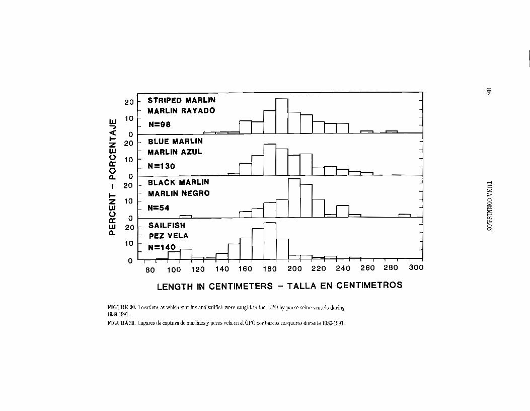
LENGTH IN CENTIMETERS - TALLA EN CENTIMETROS
FIGURE 30. Locations at which marlins and sailfish were caught in the EPa by purse-seine vessels during 1989-1991.
FIGURA 30. Lugares de captura de marlines y peces vela en el OPO par barcos cerqueros durante 1989-1991.

107 ANNUAL REPORT 1991
140 130 120 110 100 90 80 70 30 ,------,-----,-----;:-,,---,r-------,----,-----r-------, 30
STRIPED MARLIN - MARLIN RAY ADO
o ~ @ 20-49200
~ 50-199 o 10-19
20 20 o < 10
10 10 o
o '--- --'--- ----'- L-- --'--- ----"__----'---=--'-- _
140 130 120 110 100 90 80
140 130 120 110 100 90 80 70 30 , BLUE MARLIN
0 ~ 200
- MARLIN AZUL
@ 20-49
30
~ 50-199 0 10-19
20 0 < 10
20 0 - - - - -- -
0 0 0 00 0 10 10
0 @(@) (@)@(@)
0 0 140 130 120 110 100 90 80 70
FIGURE 31. Length frequencies of marlins and sailfish caught in the EPa by purse-seine vessels during 1989-1991.
FIGURA 31. Frecuencias de talla de marlines y peces vela capturados en el OPO por barcos cerqueros durante 1989-1991.

108 TUNA COMMISSION
140 130 120 110 100 90 80 70 30 30, BLACK MARLIN - MARLIN NEGRO
~ 200 @ 20-49OJ (@) 50-199 0 10-19
20 20 0 < 10
0 0 ------~.
0 0 0
10 10
@ © 0
0
0 0140 130 120 110 100 90 80 70
140 130 120 110 100 90 80 70 30 30 , SAILFISH - PEZ VELA
• ~ 200 @ 50-99
0 (@) 100-199 0 10-49
20 20 0 < 10
0
0 0
10 10
JI
0
140 130 120 110 100 90 80
FIGURE 31. (continued)
FIGURA 31. (continuacion)

109 ANNUAL REPORT 1991
25" 20' 15' 10' 55' 50'
40' 40'
35' 35'
PACIFIC OCEAN 30' 30'
25' 25'
20' 20'
15' 15'
10' 10'
1000m 5' 5'
MORRO PUERCOS TRANSECT
7° 2000m r3000m
PAS
55' 55'
50' 50'
25' 20' 15' 10' 55' 50'
FIGURE 32, Location of Achotines Bay, Panama, The Achotines Laboratory is located on the east side of the bay, The dots on the transects represent sampling stations,
FIGURA 3,2. Ubicaci6n de la Bahia de Achotines, Panama, EI laboratorio esta situado al borde este de la bahia. Los puntos en los transectos representan estaciones de muestreo.

110 TUNA COMMISSION
a: 22
« 0 Z «
20 y= 2.01 + 0.70 X
n= 218 0
I(J) W 18
« 0 ....J ....J «
16 0 0 0
I~
::E 14 \fo
00
0 0
~ 12 0
:I: I 0 <!l Z 0 0
W ....J
0a: « 0 z « I(J)
16 18 20 22 24
ESTIMA TED AGE IN DAYS - EDAD ESTIMADA EN DIAS
FIGURE 33. Relationship between standard length and age estimated from otolith (sagitta) increment counts of 218 larval and early-juvenile black skipjack tuna collected in nearshore waters adjacent to the Achotines Laboratory. The line was fitted to the data by weighted least-squares regression.
FIGURA 33. Relaci6n entre talla estandar y edad estimada a partir del conteo de los incrementos de los otolitos (sagitas) de 218 barriletes negTos lanrales y juveniles tempranos capturados en aguas costeras cerca del Laboratorio de Achotines. Se ajust6 la linea a los datos mediante regresi6n de cuadrados minimos ponderados.
22 a: A« Y = 3.26 + 0.08 x0 020Z ,2 =0.845« I n= 218(J) 18W 0
« 0 ....J ....J 16 0 « I 0 0 ~ 14::E ~ :I: 12 I<!l Z 10W ....J
0a: 8 « 0 z 6« I(J)
4 20 40 60 80 100 120 140 160 180 200 220
ROSTRUM RADIUS (JLm) RADIO DEL ROSTRO
FIGURE 34. Linear least-squares relationship between standard length and otolith (sagitta) rostrum radius for 218 larval and early-juvenile black skipjack tuna collected in nearshore waters adjacent to the Achotines Laboratory.
FIGURA 34. Relacion de cuadrados minimos lineal entre talla estandar y radio del rostro del otolito (s:igita) correspondiente a 218 barriletes negros larvales y juveniles tempranos capturados en aguas costeras cerca del Laboratorio de Achotines.
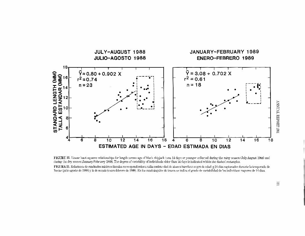
JULY-AUGUST 1988 JANUARY-FEBRUARY 1989 JULIO-AGOSTO 1988 ENERO-FEBRERO 1989
18. iii iii' .... ...... Y= 0.80 + 0.902 X Y =3.08 + 0.702 X -~- .-----.,
~ ~1e r2 =0.74 I • I r2 =0.61 • I 1-~ n=23 n=18 r---I-·;::I:- • I. • I
• I ... I I ·.11-a: 14 I 1 • • I· I
I • ICJ« ..1 • 1•~ I • 1 I I
I I.1 • Iffi~12-1« I.. I I I! .J ~ I. III Z C 1- 10
I· I ZL ... ~Ja: (I) • • §2
• t""«W ::0
C « 8 t:r:I Z-l •• o '"D
«-I ~ I- « e >-' <r:>(1)1- <r:> >-'
44 6 8 1'0 1'2 14 1'e 1'8 4 6 8 10 12 18
ESTIMATED AGE IN DAYS - EDAD ESTIMADA EN DIAS
FIGURE 35. Linear least-squares relationships for length versus age of black skipjack tuna 14 days or younger collected during the rainy season (July-August 1988) and during the dry season (January-February 1989). The degree of variability of individuals older than 14 days is indicated within the dashed rectangles.
FIGURA35. Relaciones de cuadrados minimos lineales correspondientes a talla contra edad de atunes barrilete negro de edad :$14 dias capturados durante la temporada de lIuvias Gulio-agosto de 1988) y la de sequia (enero-febrero de 1989). En los cuadrangulos de trazos se indica el grado de variabilidad de los individuos mayores de 14 dias.
>-' ...... >-'

112 TUNA COMMISSION
1.5 SOUTHERN OSCILLATION I INDEX - INDICE D~ OSCILACION DEL SUR I I I : I1.0 i :: I0.5 I I I0
-0.5
-1.0
-1.5 A I I I I 114
SEA-LEVEL ANOMALIES - ANOMALIAS DEL NIVEL DEL liAR12 I I i I 10 I I I Ien en
a: 0 8 l- I- 6 I I W a: I : I: W W I::;: ::;: 4 t= t= 2Z ZWw 000
-2
-4
-6
§ 0 3.0 I/) ~ 2.0 W enW 0 1.0
!5 ~ 0 f----++=""-,.-----o~_A""--fl~_++'\_-_f="'_::__;7-=FF"':4-___j"+\_-='C9 ~ !5 -1.0
f--......----------'-----'--------'---+-------;.-..,:.,..-=c:----r------'--1 125
I/) en a:o w 0:
100
75 I IWw ;l ::;: oJ oJ::! ~ ::;:
50
25
o HC-'--P-"'--'.;~-25
-50 I
I I I
I I I I
I I I
I I I
I I I
VERY STRONG MODERHE WEAK STRONG MODERATE VERY STRONG MODERATE MODERATE
MUY FUERTE MODER ADO DEBIL FUERTE MODER ADO MUY FUERTE MODERADO MODER ADO
(20 MO) (121'0) (6 MO) (151'0) (12 MOl (221'0) (131'0) I! ! !
55 60 65 70 75 8D 85 90
YEAR -AND
FIGURE 36. Time sections of the annual averaged anomalies (departures from 10ng-tel111 normals) of four computed parameters: Panel A, the Southern Oscillation Index; Panel B, annual average sea level based on sea levels at three coastal stations, (1) Baltra Island, Galapagos Islands, (2) La Libertad, Ecuador, anti (3) Callao, Peru; Panel C, annual anomalies averaged from SSTs at four Peruvian coastal stations (Thlara, Chicama, Chimbote, and Callao); and Panel D, accumulated annual average rainfall at Guayaquil, Ecuador. EI Nino periods are indicated by vertical dashed lines, with their strengths at the bottom.
FIGURA 36. Secciones de tiempo de las anomalias (desviaciones del nivel nOl1nal a largo plazo) anuales medias de cuatro parametros computados: Recuadro A, el Indice de Oscilaci6n del Sur; Recuadro B, el nivel del mar medio anual basado en el nivel medido en tres estaciones costeras en (1) Baltra, (Islas Galapagos), (2) La Libertad (Ecuador), y (3) Callao (Peru); Recuadro C, anomalias anuales promediadas de las TSM en cuatro estaciones costeras en Peru (Thlara, Chicama, Chimbote, y Callao); y Recuadro D, precipitaci6n media anua acumulada en Guayaquil (Ecuador). Se indican los periodos de El Nino con lineas verticales de trazos, con I fuerza anotada al pie.
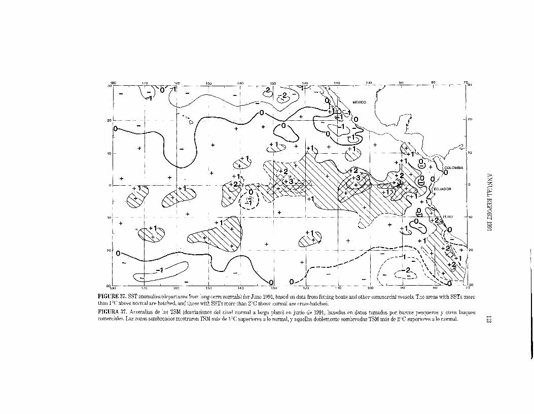
'F 150 140 120 110 100 90 80
30l--------l°
20 f---- -----1 20\Jz 1
+ 10 10
p;..+ Z
0 z $: t"""' ::e t:zj '"d 0
10 10 ~
.......+ <0 <0 .......
r I ;-1
3~80 170 160 90
FIGURE 37. SST anomalies (departure8 from long-term nonnals) for June 1991, based on data from fishing boats and other commercial vessels. The areas with SSTs more th:m laC above normal are hatched, and those with SSTs more than 2°e above normal are cross-hatched.
FIGURA 37. Anomalias de las TSM (desviaciones del nive! normal a largo plazo) en junio de 1991, basadas en datos tomados por barcos pesqueros y otros buques .......comerciales. Las zonas somhreados mostraron TSM mas de 1°C superiores a 10 normal, y aquellas doblemente sombreadas TSM mas de 2°e superiores a 10 normal. ....... "'"
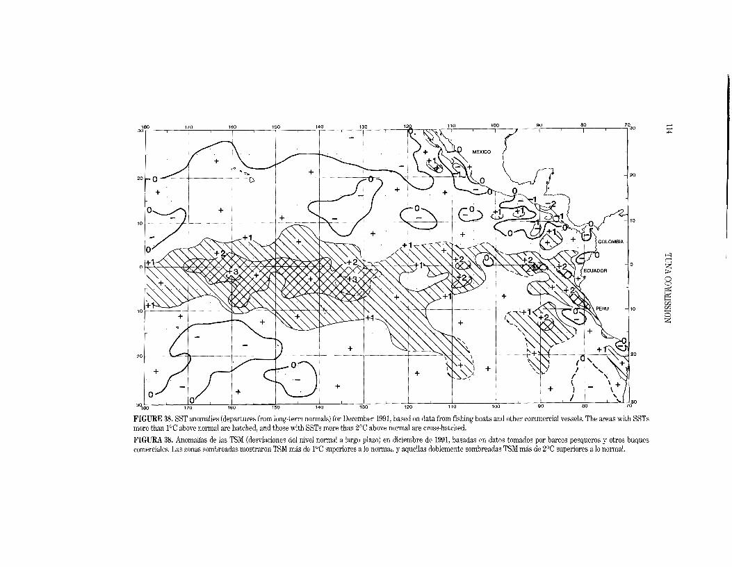
...3ci~O l~O 1~O l~O lio 1~O 12J\ [Q~ \0 11° 1~0 7 91° 8f I 7°30 ...
200..-0 ~
+
10
20
+
30
1 ....
20
+ r-I
+ I -~----- 10
I
>-'l
o c:: z ~
n o is: is: en w10 23 z
+
+ + +
180 170 130 120 110 100 90
FIGURE 38. SST anomalies (departures from long-term normals) for December 1991, based on data from fishing boats and other commercial vessel& The areas ""ith SSTs more than 1°C above normal are hatched, and those with SSTs more than 2°C above normal are cross-hatched.
FIGURA 38. Anomalias de las TSM (desviaciones del nivel normal a largo plazo) en diciembre dc 1991, basadas en datos tornados POl' barcos pesqueros y otros buques comerciales. Las zonas sombreadas mostraron IBM mas de 1°C superiores a 10 normal, y aquellas doblemente sombreadas T8M mas de 2°C supcriores a 10 normal.

115 ANNUAL REPORT 1991
8000
(j) 7000
~(j) < w C/) -I 6000
5~ :I: <c> 5000 w j::u< ~""'''''''''''zuJ 4000
~< :::l (3 3000In Z
<a:.
:::O~-;C__'~'::;;-',~:~:~~;:;~~:::< < w 0 > z 2000j:: :::l <In-1< oW 1000a:.
0 74 76 78 80 82 84 86 88 90 92
YEAR - ANO
FIGURE 39. Smoothed trends in abundance of the northern offshore stock of spotted dolphin in the eastern Pacific Ocean. The broken lines indicate the approximate 85-percent confidence limits. The horizontal lines correspond to the 85-percent confidence limits for the 1990 estimate.
FIGURA 39. Tendencias suavizadas en la abundancia del stock norteiio del delfin manchado en el Oceano Pacifico oriental. Las lineas de trazos indican los limites de confianza aproximados de 85%. Las lineas horizontales corresponden a los limites de confianza aproximados de 85% de la estimaci6n de 1990.
2500
(j) 0,... ~ ~ 2000 C/) -I
5~ :1:<C>j:: 1500
o
W U
< -I
Z W < a:.
~ :~ 1000 In :Z< ,< w~ > :::1j::1n:5 -< 500 t wa:.
OL-l.-_----l__---'--__...l-__.L-_----'__--L.__...L__.L-_----'----'
74 76 78 80 82 84 86 88 90 92
YEAR - ANO
FIGURE 40. Smoothed trends in abundance of the southern offshore stock of spotted dolphin in the eastern Pacific Ocean. The broken lines indicate the approximate 85-percent confidence limits. More details are given in the title for Figure 39.
FIGURA 40. Tendencias suavizadas en la abundancia del stock sureiio de altamar del delfin manchado en el Oceano Pacifico oriental. Las lineas de trazos indican los limites de confianza aproximados de 85%. Vel' leyenda de la Figura 39 para mayor detalle.
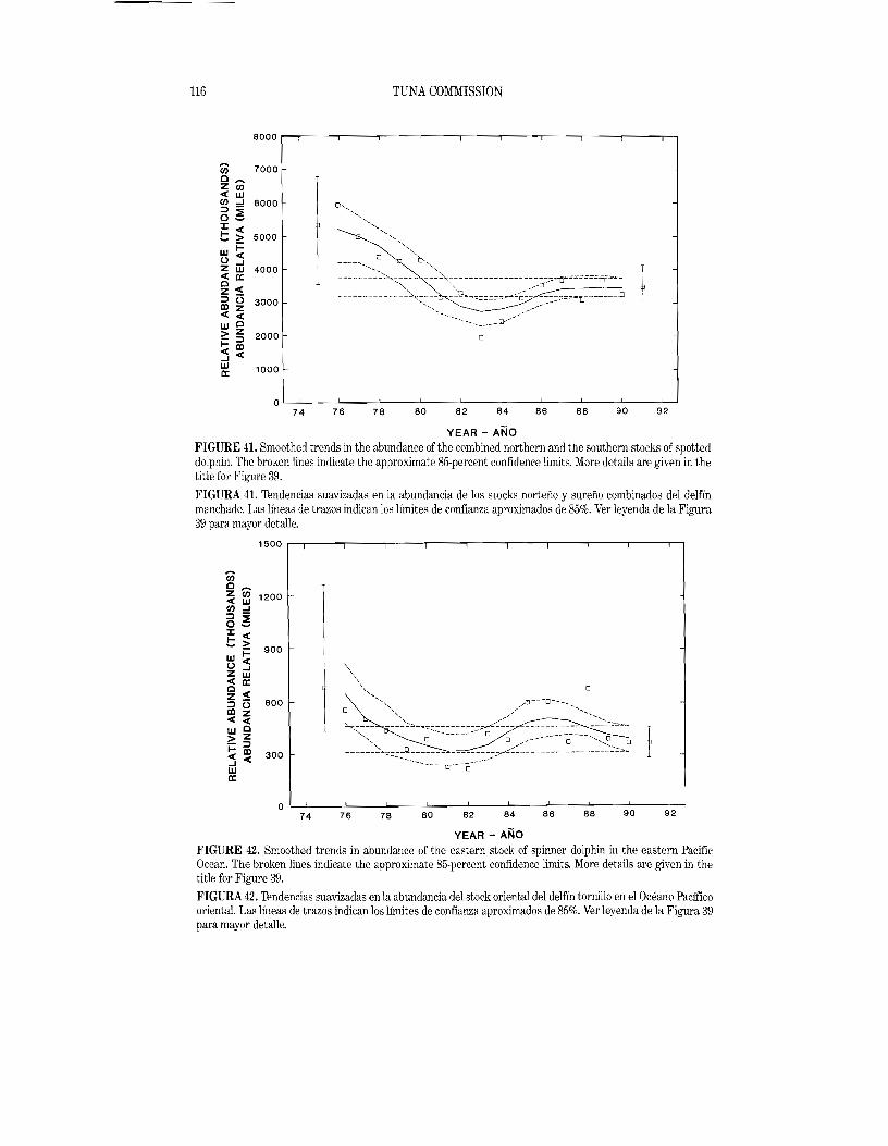
116 TUNA COMMISSION
8000
en 7000 C Z en« w 00 ....I 6000 ::J 0 ~ :x: C «
> 5000 i=
W «u ....I Z W 4000« a: c z « ::J 0 3000ID Z« «
0 Z
w > ::J 2000 oi=« ID
«....I W 1000a:
0 74 76 78 80 82 84 86 88 90 92
YEAR - ANO FIGURE 41. Smoothed trends in the abundance ofthe combined nOlthern and the southern stocks of spotted dolphin. The broken lines indicate the approximate 85-percent confidence limits. More details are given in the title for Figure 39.
FIGURA 41. Tendencias suavizadas en la abundancia de los stocks norteno y sureno combinados del delfin manchado. Las lineas de trazos indican los limites de confianza aproximados de 85%. Vel' leyenda de la Figura 39 para mayor detalle.
1500
en c z en 1200« w 00....1 ::J o~ :x: «C>
i= 900 w «u ....IZ W« a:c z « ::J 0 600 ID Z« « w 0
z> ::Ji=« ID« 300
....I wa:
o 74 76 78 80 82 84 86 88 90 92
YEAR - ANO FIGURE 42. Smoothed trends in abundance of the eastern stock of spinner dolphin in the eastern Pacific Ocean. The broken lines indicate the approximate 85-percent confidence limits. More details are given in the title for Figure 39.
FIGURA 42. Tendencias suavizadas en la abundancia del stock oriental del delfin tornillo en el Oceano Pacifico oriental. Las lineas de trazos indican los limites de confianza aproximados de 85%. Vel' leyenda de la Figura 39 para mayor detalle.

117
1200
ANNUAL REPORT 1991
1500 ,--...,..----r-----,-----,---,---,------.,---,---...,.---I""]
gOO
1 600
300 o
o 74 7S 78 80 82 84 86 88 gO 92
YEAR - ANO FIGURE ,13. Smoothed trends in abundance of the whitebelly stock of spinner dolphin in the eastern Pacific Ocean. The broken lines indicate the approximate 85-percent confidence limits. More details are given in the title for Figure 39.
FIGURA 43. Tendencias suavizadas en la abundancia del stock panza blanca del delfin tornillo en el Oceano Pacifico oriental. Las lineas de trazos indican los limites de confianza aproximados de 85%. Ver leyenda de la Figura 39 para mayor detalle.
1000 ,---,---,-----,------,,----;----,---,----,---,----..,..,
Ci) c z Ci.i 800< w (J) ..J :::> 0 ~ CJ:
><
SOO w i=
<<.> ..Jz W< a: c z <
400 lD Z :::> C3 < < cw z>i= :::>
lD 200< <..J Wa:
o L .L----'-S---7-'-8---8...i--------'82--------'8--:-4--....8'--S----'8'--8---=-9'=-0---::9'::2---J 7 4 7 0
YEAR - ANO
FIGURE 4,1. Smoothed trends in abundance of the northern stock of common dolphin in the eastern Pacific Ocean. The broken lines indicate the approximate 85-percent confidence limits. More details are given in the title for Figure 39.
FIGURA 44. Tendencias suavizadas en la abundancia del stock norteno del delfin comun en el Oceano Pacifico oriental. Las lineas de trazos indican los limites de confianza aproximados de 85%. Ver leyenda de la Figura 39 para mayor detalle.
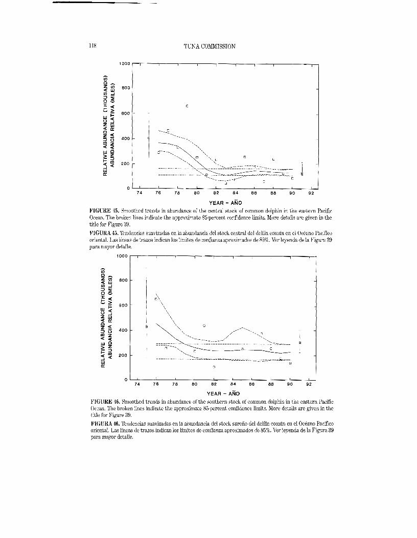
118 TUNA COMMISSION
1000 r-~--'------,------r-----r-----r---r--.,....---...,---,--,
U1 O~ zrn 800« w rn ..J
6~ J: « oc> 600 w i= ()«zuJ « cr ~«
400:::l 13 m z « « WO > zi= ::> « m 200 ..J « w a: r
OL--.l..-_----L__-L__--'-__'--_-----l.__-L__-'-__'--_-----l.......J
74 76 78 80 82 84 86 88 90 92
YEAFl - AND FIGURE 45. Smoothed trends in abundance of the central stock of common dolphin in the eastern Pacific Ocean. The broken lines indicate the approximate 85-percent confidence limits. More details are given in the title for Figure 39.
FIGURA 45. Tendencias suavizadas en la abundancia del stock central del delfin comun en el Oceano Pacifico oriental. Las lineas de trazos indican los limites de confianza aproximados de .':5%. Vel' leyenda de la Figura 39 para mayor detalle.
1000 r-~--,----r_----r--___r-----r----,-----,---...,---.,.--,
(j) 0 Z Ci) 800« w rn ..J :::l 0 ~ J: «C > 600i=w «() ..JZ W « cr 0 z «
400:::l 13 m z« «
0w 1z> ::Ji= m 200« «..J w cr
O'--'-----'----'----'--_'--_----L__-'-__-'-__'--_--'-.......J 74 76 78 80 82 84 86 88 90 92
YEAR - AND
FIGURE 46. Smoothed trends in abundance of the southern stock of common dolphin in the eastern Pacific Ocean. The broken lines indicate the approximate 85-percent confidence limits. More details are given in the title for Figure 39.
FIGURA 46. Tendencias suavizadas en la abundancia del stock surefio del delfin comun en el Oceano Pacifico oriental. Las lineas de trazos indican los limites de confianza aproximados de 85%. Vel' leyenda de la Figura 39 para mayor detalle.

130
en w 120o w a.. w 110 c en w 100z o ...J ::! 90
~
~ Z I z
:I: 80 fi2 t:-'(/') ;0u:: t'J '"1:170IJ.. oo ~
(/') >-"
60 = z ;:::o :J ...J
50 ~
40
30 66 68 70 72 74 76 78 80 82 84 86 88 90 92
YEAR - ANO
FIGURE 47. Estimated initial recruitments of yellowfin in the eastern Pacific Ocean, with the average recruitments for 1967-1975,1976-1982, and 1983-1990. >-"FIGURA 47. Reclutamientos iniciales estimados del alela amarilla en el Oceano Pacifico oriental, con los reclutamientos medias de 1967-1975, 1976-1982, Y1983-1990. >-"
=
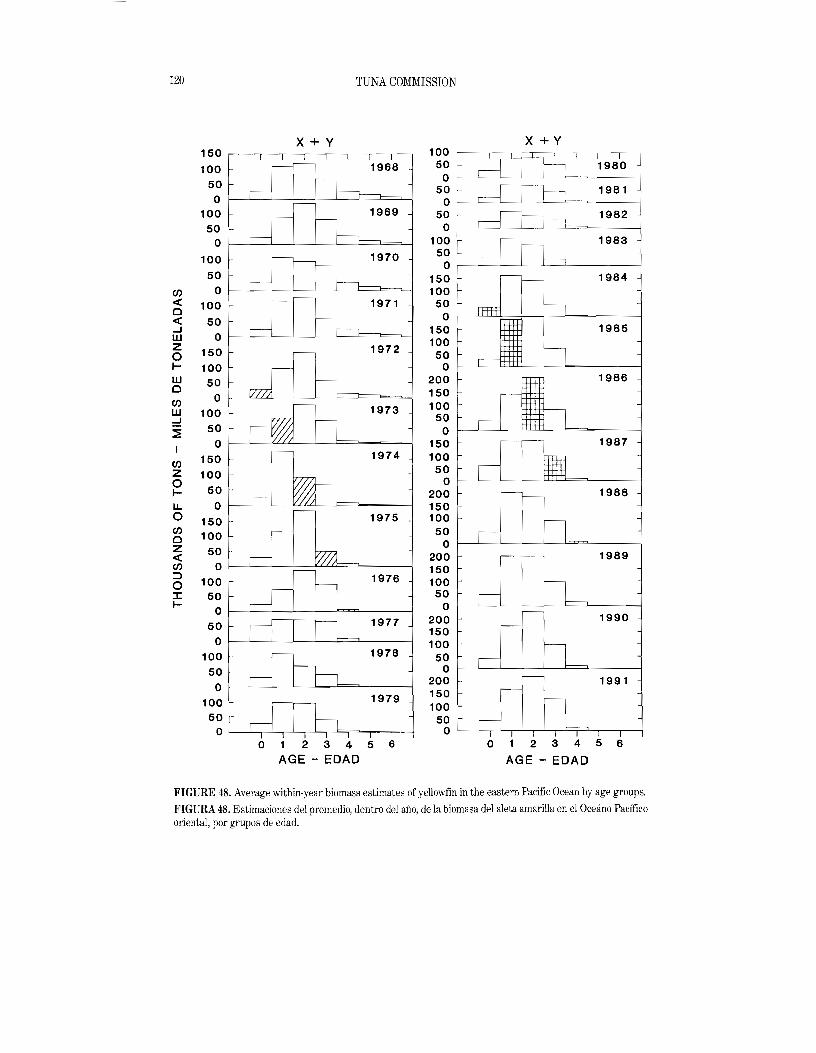
__
120
I
TUNA COMMISSION
X+Y
:~~ ~~'_' "96'. 1 5~Ld~1 ~jI
100 1969
5~ ~~===--1
o 1-----.L----l_l---L L-_t:::===-------1
100 ~ 1970 50 I
(J) o « o 100 1971
« 50 ...J w Z 150o I 100 W 50o
o(J) W 100 ...J
50 ~ o f---'-
150(J) Z 100 o 50l-LL. o o 150 (J)
100o z 50« o 1-J-----l_-'--_iLLLL==(J) ~
1972
1973
1974
1975
, 1976100o
J: 50 I-
OI---L----l_-'-----L_b=~______1
197750 Of--'--L--'--L-----'=="---------I
1978100 50 Of---'--L----L--"---'==~---
1501979100 100 50 50 o L----J....~_'_____,---L~-"--.----.c==;=~r_~I--j o
o 1 2 3 4 5 6
AGE - EDAD
x + Y
1~g ~ rJ:E I ~~I
5~r~1981 50 r- 1982
'~~ f~_----l_.L-J_ 1_9_8_3___
150 1984 100
1:~ ~ 1985 100 t
50 01--L_=~~-~------1
200 150 100
5~ 150 100 50 o
200 150 100 50
o 200 150 100 50 o
200 150 100
50 o
200
1986
_c::=l--=IIL.-----b=__--1
1987
1988
f--'--_L-_L_L-----"=~__---I
1989
1990
1991
123 4 5 6
AGE - EDAD
FIGURE 48. Average within-year biomass estimates of yellowfin in the eastel11 Pacific Ocean by age groups.
FIGURA 48. Estimaciones del promedio, dentro del ano, de la biomasa del aleta amarilla en el Oceano Pacifico oriental, par grupos de edad.
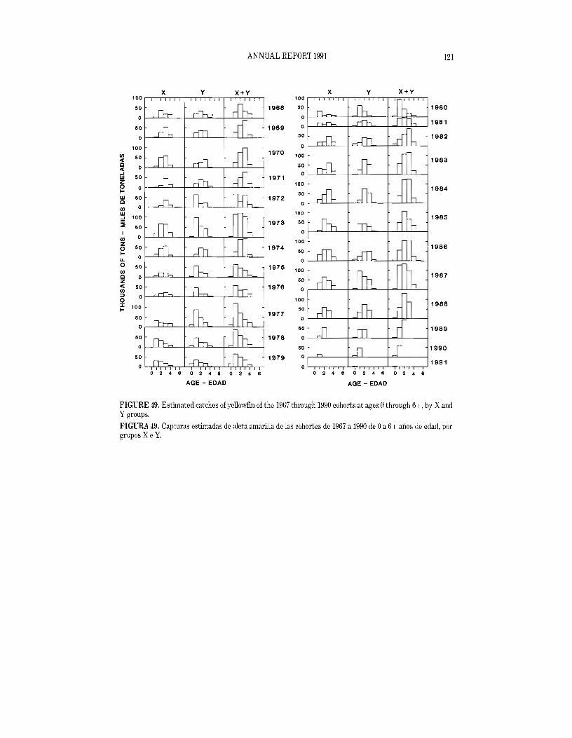
121 ANNUAL REPORT 1991
x Y X+Y x Y X+Y 100 r,-nrrrrrr---.rr,..,.--r-,--rr.--r-nrn 100 r-r-nrrTTTT--rTTTTT1-rT;+;T1-rrn
50 1968 50 1980 o ~_.=i...l....L-'--+----'-J-J.-'-''---i_..J....l--,=LL---1 ol--L.<:==>---t-=--'-=---+-9=,"""P--i
o 1-L.C:L.l:J.-+.......L..L.J......,-r--LL="''------1 19 8 1 50 1969 50o ~_"""'L..Ll.-+---'---LLL---+---'--W---'---'----1 1982 01--.l....LJ-J.--'-----t-=--'-'--'---+-=-.L.L-'--'---i100
1970til 10050« 1983 Q 50 ~ 01--.l....L..I-J.-L---t---,--,-w---+---'-.L.L-'--'---iW 50 1971Z 100o 1984I 50 W 50 1972 Q 01--.l....LJ-J.--'-----t--'--'-L-'=~-+---'-.L.L-'--'---i
til W 100 ::! 100 1985 ~ 1973 50
50 Ol---=..L...l--'---+.......--'-L-'=~-+---'-.L-L..I-J._I o ~_.L-L-'--'---'----+"""'..J....l--'-_+""-J==!-'----1til 100Z
50 1974 1986o 50l o ~_.L-L..J...J::::L--+----'-::LI--'-_-+--'-LL=----1 LL of--.l....L..L...l-L---+-=--'-'--'=~-+-=-.L.L.J....J.--i
o 50 1975 100 Q o ~_.d.....J...J::::L--+"""'..J....l--'---_-+-..L..JLL=---i 1987til
50 « 1976 o I-LL.L..L.L--t-='-LL-'=-_j-=LLL..L.L-_ Z
50 til :::l o !-_.c::L.L..J::>-+--L=l=---+---l--WL....L'----1o 100
1988 ~ 100 50
197750 o I-LL.L.L--t-...L.L.L.L--r--~i-"----1
Ol--.L-L-'--'--'--+-=...L.l---'---f-'::::J....JLLLL--i 50 1989 50 1978 ol---=--'------t---'--'-'-----+-........L-L---i
o !-_L..LL.J::>-+=-L..L.b...--+--=i-LLL'----1 50 1990 50 1979 o 1-=----t-.=i...L---j-=LL--
1991 o L,-Y-r.y,"-r-lr'-y,.y,..........,.-I-Y,-l,-YT'r-r-l o L..,r.-rr,....,......--'"T"TT-r-r-nr'-.....-rrrrr
024602460246 024602460246
AGE - EDAD AGE - EDAD
FIGURE 49. Estimated catches ofyellowfin of the 1967 through 1990 cohorts at ages 0 through 6+, by Xand Y groups.
FIGURA 49. Capturas estimadas de aJeta amarilla de las cohortes de 1967 a 1990 de 0 a 6+ arios de edad, por grupos X e Y.

600 ...... ~
ALL FISH 550 TODOS LOS PECES
(/) c:( 5000 c:( ...J w 450Z 0 IW 400 0 LARGE FISH (/) w 350 PECES GRANDES ...J
:il >-3 c:::::300I z :>
Z (/)
250 8 0 ~
l- ~
LL. En 0 rn200 .....,
o(/) Z0 Z 150c:( en ::)
0 100 ::r: I
50
J6 68 70 72 74 76 78 80 82 84 86 88 90 92
YEAR - ANO
FIGURE fiO. Average biomass estimates of yellowfin in the eastern Pacific Ocean for all fish and for larger fish only.
FIGURA 50. Estimaciones de la biomasa media del aleta amarilla en el Oceano Pacifico oriental correspondientes a todos los peces y a los peces mayores solamente.
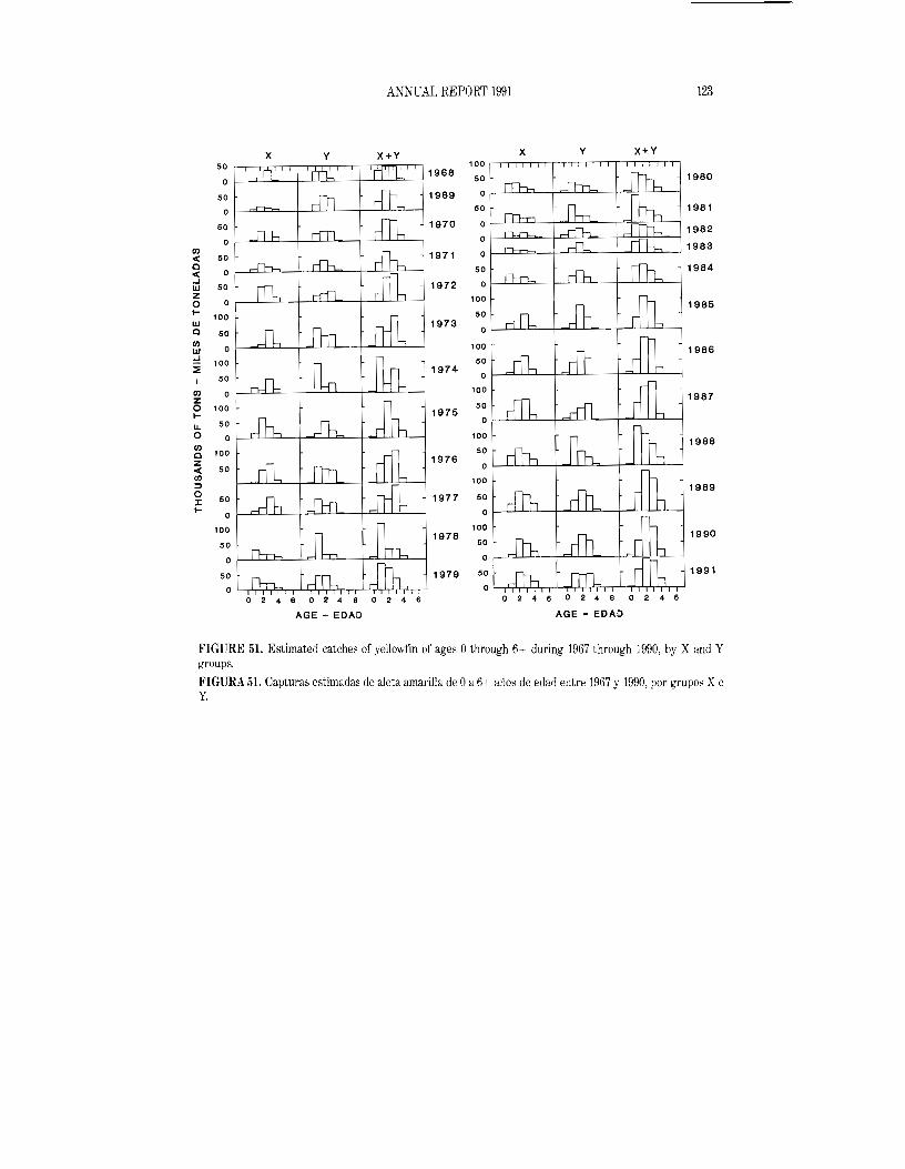
123 ANNUAL REPORT 1991
x Y X+Y x Y X+Y 50 ,..-,,,rrrrrr-rrr-rrTT-r-rrrTffiITT" 1 9 6 8 100 r-r""rrrr"rrrTTT,-rTTTTT"Tl
of--.....cLJ.,~+....L..L.!=L---+----'--L-<~____j 50 1980 of--.L.L.LX:l....-+='---LLb....-i~=;---LL'----j50 1969
ol-==-t-LU---L--t-----'U-l-=----j 50 1981
50 1970 o f--.L.L-'--J....L..--+-='-...l...J-'-~-t-'=',=~:;--'-----, 198 2 oI-L.I=L.I='----+-':::iJ--LJ~__+_=:::J=i...LJ~of---'--.L..L-'----+....L..L.L'----+----'--L-<~____j
(/l o f--.L.l:==--+....LL...l='-----j_LLL='----j 1983< 50 1971 a < of---=-.L.l:"-+....L..L.L'=--\-----'~=;__'L-----' 50 1984 ...J
ol-.L..L-'--"~-+---'--'--J.--'-_+---'--JL.L=-_W 50 1972
oZ o!----L.L.L-'----+...LJLL'----+-----l.-J...-C--L-<____j 100
1985I100 50
w 1973a o f--.L..L.L.l:~+.....L.L.L~-i.--J....L..L.L'----j50 (/l
w of-....cLL-'----+.....L.LL'----+........--L-<~____j 100 1986::! 100 50:;: 1974 ol-.d....LL-L-+=Ll-..LL----\--='LLLLL50
(/l 100 z 1987 o 100 50 I- 1975
50 of--.L.L-"-l-L-+....d-LJLL_--j-'-'--L.L.->....L_U.
o Of---L..L...Ll....l..--t........--L.l...>=L---t-''"'--J.....L-L.L.--j 100
:g 1988'00 50
z 1976 50 of--LL.L.LJ.-.+.....L.LLb....-\..........L-''-'-'---I<
(/l 100::l
o 1989 J: 50 1977 50 I- o 1-.LL.LL-L-+....Ll-..Lb..---j_LLL..LL.---j
100 100 1978 1990
50 50
of--LLLl=o....---!-,d-LL:'--__+--=':::"-,-='------j 01--d....LL...L-+...d..w-l..~+=L~:-'-_
50 1979 50 1991
oL,lhYT'-rr--Ll?,JW'r-r-r"--Y-rY-r"?..-J oL..,-'T1,,.!,J.,.J-...,J--.J.rYfi,...,....L..-r'-rY-r.y..,,.--' 024602460246 0246 0 2460246
AGE - EDAD AGE - EDAD
FIGURE 51. Estimated catches of yellowfin of ages 0 through 6+ during 1967 through 1990, by X and Y groups.
FIGURA 51. Capturas estimadas de aleta amarilla de 0 a 6+ aJ10S de edad entre 1967 y 1990, por grupos X e Y.

......8 s:::
7 ..........
6
5
en 8 < Y COHORT - COHORTE Y a: ~ 7 ...J
I >-36 c::::en z;:....C Z 5 n :::> ~
>-<~ 8 w ~
X AND Y COHORTS COMBINED w 23COHORTES X E Y COMBINADAS7 z
6
5
4' , I , , , I I , , I I , , I I I I I , I , , I , I I
66 68 70 72 74 76 78 80 82 84 86 88 90 92 YEAR - ANO
FIGURE 52. Yields per recruit of yellowfin. The top and middle panels contain data for the 1967 through 1986 cohorts caught during different years (equivalent to Figure 49), whereas the bottom panel contains data for fish of different cohorts caught during 1967 through 1990 (equivalent to Figure 51).
FIGURA 52. Rendimientos pOI' recluta del aleta amarilla. Los datos en los dos recuadros superiores corresponden a las cohortes de 1967 a 1986 capturadas en distintos aiios (equivalente a la Figura 49), mientras que los datos en el recuadro inferior corresponden a peces de distintas cohortes capturados entre 1967 y 1990 (equivalente a la Figura 51).
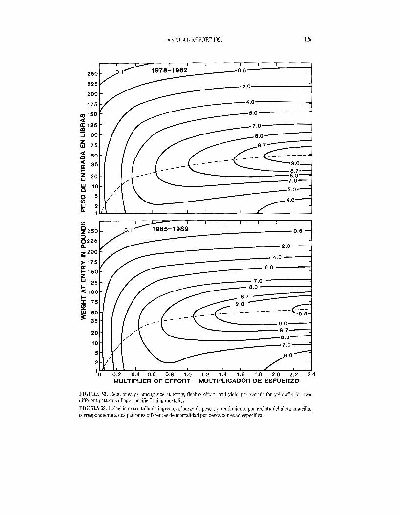
125 ANNUAL REPORT 1991
1978-1. ~9~8~2_----0.5250
225 __----2.0------~
200 __----4.0------......."d175
__---5.0---~--~C/J 150 -<a: 125 __-- 7.0---------1 In :J 100 8.0
W 75 7
-< 50a -<
Z
_-------ES
35 • ~ a: ----z 20W W 100
50 C/JW 2 ~
1I
C/J
~250 0.1 ~=-::.=_-----_---0.5
::::> 0225 ~ __----------2.0----i ~200
__----------: 4.0 ---1>175 a: __------ 6.0 -----I ~ 150
7.0 -------.:::1W 125 ~ ~__--- 8.0 ---------\ -< 100 . ~ ::t: ~
;:W 50
35
20 __________---8.0--..., 10
/ ~_------7.0---""I5 I
2 I
I
10 0.2 0.4 0.6 0.8 1.0 1.2 1.4 1.6 1.8 2.0 2.2 2.4
MULTIPLIER OF EFFORT MULTIPLICADOR DE ESFUERZO
FIGURE 53. Relationships among size at entry, fishing effort, and yield per recruit for yello'.'fin for two different patterns of age-specific fishing mortality.
FIGURA 53. Relaci6n entre talla de ingreso, esfuerzo de pesca, y rendimiento por recluta del aleta amarilla, correspondiente ados patrones diferentes de mortalidad por pesca por edad especifica.

15
126 TUNA COMMISSION
35
30 (J)
0 (J)
< IX: CD ..J
25
20
~ < IX:
10~
0 ..J
I ~
(J) I 0 Z :::> 0 a.
15
10 5
(J)
~ < IX: ~ 0 ~
5 ~
~6 68 70 72 74 76 78 80 82 84 86 88 90 92
YEAR - ANO FIGURE 54. Average weights of yellowfln caught in the eastern Pacific Ocean.
FIGURA 54. Peso promedio de aletas amarillas capturados en el Oceano Pacifico oriental.
8r-----....,....----~---....,....----r_---.....,...----r_---....,
• (/) <0:
(/)!!!ll:
O...J 7Zz6 UJ
Cl.<O: zl-3 I-() 5UJ ll: Ir 6 ()IrWa ll:Cl. Ira WICl. zOW ul ~ s -0>-z
W ll:
4 SL-----1LO----1LS----2LO----2Ls----aLo----aLs-------l40
AVERAGE WEIGHT IN POUNDS - PESO PROMEDIO EN LIBRAS
FIGURE 55. Relationship between yield per recruit and average weight at capture for yellowfln in the eastern Pacific Ocean.
FIGURA 55. Relacion entre el rendimiento por recluta y el peso media de captura del aleta amarilla en el Oceano Pacifico oriental.

150
ANNUAL REPORT 1991 127
'50 '40 130 120 110 100 90 80 70 40 ,....------,--------,-----,..---.------.----------.--------,-----r-----,40
o INSHORE CYRA - CERCA A lA COSTA EN EL ARCAA (A 1)
[2] OFFSHORE CYRA - MAR AFUERA EN El ARCAA (A2)
o OUTSIDE CYRA - FUERA OEl ARCAA (A3)
30 30
20 r----------120
10
O.
10
20
30 '-- .l.- -'-- ---'- ..l- ---' -'-''-"'-'-"'-.L....'-'''--.L-'-''~_'
140 130 120 110 100 90 80
FIGURE 56. The eastern Pacific Ocean, showing the historical areas of the fishery for yellowfin, AI, the more recently fished areas within the CYRA, A2, and the area outside the CYRA, A3.
FIGURA 56. El Oceano Pacifico oriental. Se indican las zonas hist6ricas de pesca de aleta amarilla (All, las zonas de pesca mas recientes en el ARCAA (A2), y la zona fuera del ARCAA (exterior) (A3).

00
< >0 25
<a: 00 20 a: 0. W'" 150.< a ~~ 10
OW I- Z 50
I 0
x~
W~
1.00< ~o
ZWi 0.8 0 ~: 0.6 00 Z W 0.4 :::)QIDa<;: 0.2
0.0
"'0 ~ ~ 500 1-< LL. ~ 400 Oz o 0 30001Z W<0 200
0f1) :::) W 100 O~
:I:~ 0I
CPDF (CLASS-6 VESSELS) CPDP (BARCOS DE LA CLASE 6)
SEARCHING TIME TIEMPO DE BUSQUEDA
COHORT BIOMASS BIOMASA DE LA COHORTE
66 68 70 72 74 76 78 80 82 84
YEAR - ANO
FIGURE 57. Three indices of abundance ofyellowfin in the eastern Pacific Ocean.
FIGURA 57. Tres indices de la abundancia del aleta amarilla en el Oceano Pacifico oriental.
...... ""
>-3 c:::: S; n o ~ ...... en rn (3 Z
86 88 90 92

129 ANNUAL REPORT 1991
350 r--·...,...-T"""~-""T""'--,-"'T'"---,I.--...,...-T"""-,--"T"""'l~-""T""'--,.----r-,,---,,-,-r--,-r----,
~ q=O.oOOO39 (LATE - TARDE) 90 89••88 AMSY=322000 (LATE) ~ q=O.oooo27 (EARLY - .S6.......,'ta;------ ............RPMS -J 300 r- TEMPRANO),. ... .... UJ ~ I-UJ
250 IQrn" ~ 200 I
I rn z 150o lll. o
100 rn Q z -<
///
"",. .... , ../(~JH .76 .......... ,
",// 85 "" -",·.74 75 " '" ·73 • .77 ,
.79 , .72 _------------- 78 .81 ~
".70.......... .80 / ..."'''.84 .............
,," .69",,'" .......... , , ~... .71 .82.....
I ...... ,/68."" ,
/ /' .83 AMSY=211000(EARLY) " I ,/ RPMS
I '"
I /
'"'"
I "," ~ 50 - /,,/ o :I: II- I""
1/ I I I I I I
00L-~2-....L4--6L--....L.8-..110-...J121...--11..4-1.L6-....L18--20L--2.L.2-2.L4-~26:---21..8-3J..O-..J.32-....I34--38.L...--38..L.......J40
EFFORT IN THOUSANDS OF DAYS - EZFUERZO EN MILES DE DIAS
20
18
16
rn 14 -<Q -< 12 -J UJ Z
10 0 II
8 rn z 0 6
4
2
0
I
68
EXPECTED (LATE) ESPERADO CTARDE)
~I.-"-
..., \ \
\ \ \ \ \ \ \ \ \ \
EXPECTED (EARLY) \ ESPERADO (TEMPRANO) \
\ \
84 86 88 90 92
FIGURE 58. Relationships between effort and catch for the yellowfin fishery in the eastern Pacific Ocean during 1968·1990, for the logistic (symmetrical) model with m set at 2.0 (upper panel), and observed and predicted values of the CPDF (lower panel).
FIGURA 58. Relacion entre el esfuerzo y la captura en la pesqueria del aleta amarilla en el Oceano Pacifico oriental durante 1968·1990, segdn el modelo logistico (simetrico) con m fijado en 2.0 (recuadro superior), y valores de CPDP observados y predichos (recuadro inferior).

130 TUNA COMMISSION
350 r--,---r-__r---r-.,......---,-...,--.,......-,.-...,--r---r--r-__r---r-'T"""---.-...,...-..-----.en 89 I I I I
~ 86 92-~~!-----------_:5 300 q=0.000039 (LATE-TARDE) • _-- ·87AMSY:328000 (LATE)
-~ q=0.OOOO27T~~~~~~O) "..,/;.- RPMS 76
o " @ •~ ;; 85 W 250 /. C ".
74• j5 77en ;/ 73 • W / 72 78 81 -I ". • •S1 200 ,," 70 _----------------_ I / • .,.",. .....-- -80--
en I 69 .... -.... .84 AMSY =200000 (EARLY) z /........ RPMSe 150 / 68 /'" .71 .82 LL. I}I' o / ,/ .83 en 100 I" C I ' z ,I < I /en II5 50 1/ J: 1/ ~ P
I I I I I I I I0L-..J-._.L---'-_..l....--L_...J....--1_...J...._.L---.l.._.L---'-_...l..---1_....L.._l...--l.._.L---L_..J o 2 4 8 8 10 12 14 16 18 20 22 24 26 28 30 32 34 38 38 40
EFFORT IN THOUSANDS OF DAYS - EZFUERZO EN MILES DE DIAS
18
18
EXPECTED (LATE).... ... ... ' en 14 ESPERADO (TARDE) ..,<C I
I< 12 I..J IW
~ 10 ,I ~
I 8 ,/ '\
I \ t/'J \ Z / \
\e 6 -' \ \
4 ~\ EXPECTED (EARLY)
\ \
2 ESPERADO(TEMPRANO) \ \
o ~7.......-::'::-'-..............~:-'- ......................--1L-......................--1L-.L-.......---L:-'-I-.....L.......l..--1~92
FIGURE 59. Relationships between effort and catch for the yellowfin fishery in the eastern Pacific Ocean during 1968-1990, for the generalized stock production (asymmetrical) model with m set at 0.8 (upper panel), and observed and predicted values of CPDF (lower panel).
FIGURA 59. Relaci6n entre el esfuerzo y la captura en la pesqueria del aleta amarilla en el Oceano Pacifico oriental durante 1968-1990, seg"lin el modelo generalizado de producci6n del stock (asimetrico) con m fijado en 0.8 (recuadro superior), y valores de CPDP observados y predichos (recuadro inferior).

--------------------- ---------
131 ANNUAL REPORT 1991
1985-1989 FISHING MORTALITY 1985-1989 MORTALIDAD POR PESCA
(]J
~ 6 (]Jell 0:]Zz :::Ow
12;0; S Z:::of=...J-v:::ow <I: c: 4 Uc:Wo <I:c<I: 0 1978-1982 FISHING MORTALITY Weo..z 1978-1982 MORTALIDAD POR PESCA Ow m~ 5=0 z 2
w c:
~.LOO--O..l.2-S--0..l.5-0--0.J...7S---1.1..00--,...J.2'-:S--'-'.S~0--'-:.7~5----:-2.':..00::----:2"'::.2:-5---'2.50
MULTIPliER OF EFFORT - MULTIPLICADOR DEL ESFUERZO
FIGURE 60. Yields per recruit for age-specific mortality rates of 1978-1982 and 1985-1989.
FIGURA 60. Rendimientos por recluta correspondientes a las tasas de mortalidad por edad especifica de 1978-1982 y 1985-1989.
400 r-----,r----,---r---r---,---.---,---,---~-___,
1985-1989 FISHING MORTALITY AND HIGH RECRUITMENT (1985-1989) 3S0 1985-1989 MORTALIDAD POR PESCA Y RECLUTAMIENTO ALTO(1985-19891
(f) /.",...,,-----------(f) ,S 300 / --z .~ / -O-~ / ----~~ I -------_is i~ 2S0 (f) LU o Cl ~ U)
~ ~~ 200 o :~ IZ f- LU
~ f2 1S0
I I
I I
I I I IIIIIII
1985-1989 FISHING MORTALITY AND AVERAGE RECRUITMENT (1967-1989) 1985-1989 FISHING MORTALIDAD POR PESCA Y RECLUTAMIENTO PROMEDIO ...JZ
w~ ;;:::~
~~ 100 UJ 0:
(1967-1989)
I so
~.!:::OO'-----'0::-!.2"'S----;O:-!S"'-0----"0*.75,,----71."'OO,----"".2!:.,S---,,:-!.S"'O---,,,-!.7"'S----;2,-!;.O.,,-O----,,2*.2;-S-~2.S0
MULTIPLIER OF EFFORT - MULTIPLICADOR DEL ESFUERZO
FIGURE 61. Yields for high and average recruitments and age-specific fishing mortality similar to that of 1985-1989.
FIGURA 61. Rendimientos correspondientes a reclutamientos elevados y medios, y mortalidad por pesca por edad especifica similar a aquella del perfodo 1985-1989.

132 TUNA COMMISSION
400
1985-1989 FISHING MORTALITY AND HIGH RECRUITMENT (1985-1989) 350
1985-1989 MORTALIDAD POR PESCA Y RECLUTAMIENTO ALTO (1985-1989)
<{ ",..-----------..{fJ ---------
3000UJ<{Z-J
Z ---OW I- 0 ---2501l..1Ow UJO OUJ Zw<{-J 200UJ:::):2 OzIw 1 0 150~I-OZ -Ji±! W:2
1978-1982 FISHING MORTALITY AND AVERAGE RECRU ITMENT (1967-1989) >=0Z 100 1978-1982 MORTALIDAD POR PESCA Y RECLUTAMIENTOPROMEDIO(1967-1989) w ce
O........---'-----'------'-----l..------'------''-----.l..----'-----'--_....J 0.00 0.25 0.50 0.75 1.00 1.25 150 1.75 2.00 2.25 250
MULTIPLIER OF EFFORT - MULTIPLICADOR DEL ESFUERZO
FIGURE 62. Yields for average recruitment and age-specific fishing mortality similar to that of 1978-1982 and for high recruitment and age-specific mortality similar to that of 1985-1989.
FIGURA 62. Rendimientos correspondientes al reclutamiento normal y mortalidad por pesca por edad especifica similar a aquella de 1978-1982, y al reclutamiento elevado y mortalidad por edad especifica similar a aquella de 1985-1989.
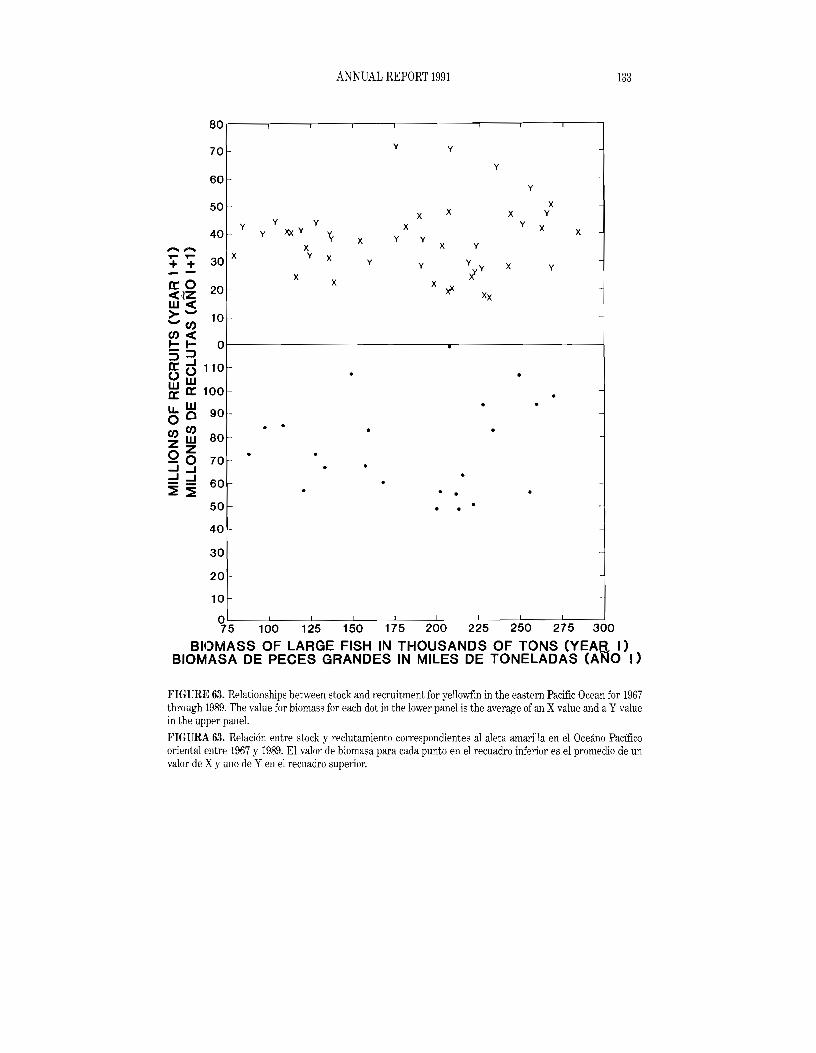
133 ANNUAL REPORT 1991
80
70 y y
y
60 y
50 x x x
x y
-40
y y
y y ~Y
x Y x
x y y
x y
y x x
~ ~
+ T- -erO <C1ZUJ<C >-en
30 _x
20
10
x
y x
x
y y
x J1..
y
I y
Xx
x y
en<c t-t 05=>5 d 110
UJ ~ er 100 LLUJ 0°enC/)zUJ
90
eO r OZ-0 ..J..J
70 ..J..J
60 ~~
50
40
30
20
10
o I I
75 100 125 150 175 200 225 250 275 300
BIOMASS OF LARGE FISH IN THOUSANDS OF TONS (YEAR I) BIOMASA DE PECES GRANDES IN MILES DE TONELADAS (ANO I)
FIGURB 63. Relationships between stock and recruitment for yellowfin in the eastern Pacific Ocean for 1967 through 1989. The value for biomass for each dot in the lower panel is the average of an X value and a Y value in the upper panel.
FIGURA 63. Relaci6n entre stock y reclutamiento correspondientes al aleta amarilla en el Oceano Pacifico oriental entre 1967 y 1989. El valor de biomasa para cada punto en el recuadro inferior es el promedio de un valor de Xy uno de Y en el recuadro superior.

"-'
70~
"""
~30 "'"
60 """- WITH DOLPHINS
25 en0
rn 50 < ~
« V a: C'a: ~ m 20 0\-I~ ::!:::i 40 ~ '""'3I CI zrn
~C 15 en Q
~ 30 ~ 0 c:( rs::
rs::0 SCHOOLFISH a: ena.. (!J if)CARDUMENES NO ASOCIADOS >-<10 0 0 20 l- I'.. ::::! z
~
,--- ......... 510 I- ---",--- ,/ ..... _-............... -----' WITH LOGS CON OBJETOS FLOTANTES
I I ! ! 1 I ! ! J I I ! J ! I I ! t I !06'8 '0
70 72 74 76 78 80 82 84 86 88
YEAR - ANO
FIGURE 64. Average weights of dolphin-associated fish, log-associated fish, and "schoolfish" (fish associated only with other fish).
FIGURA 64. Peso promedio de peces asociados con delfines, con objetos flotantes, y no asociados (asociados solamente con otros peces).

135 ANNUAL REPORT 1991
1960 1965 1970 1975 1980 1985 1990 200
200
100 100
(/) 0 0«
900 (/)~ WESTERN AND CENTRAL PACIFIC 800 «e: PACIFICO OCCIDENTAL Y CENTRAL I-I- e:w 8000
700 ~ U (/)
(/)« 0 700 ~ « ..J 600 «
..JW Z 600 ~ 0 0I-- 500 I-W 500 w0 0 (/) 400 (/)w ..J 400 ~ ~ ~ I 300 I
(/) 300 (/) Z Z0 0I-- 200 200 I-~ I-e: e: I- 100 100 0 W J: ~ (/)
u. u. 0 0 0 0 (/) ATLANTIC AND INDIAN OCEANS 400 (/)0 0OCEANOS ATLANTICO E INDICO Z Z « 300 « (/) 300 (/) :::> :::> 0 0 J: 200 J: I-- 200 I-
100 ~ 100
0P960 1965 1970 1975 1980 1985 1990
YEAR - ANO
FIGURE 65. Catches of skipjack in the eastern Pacific Ocean, central and western Pacific Ocean, and Atlantic and Indian Oceans.
FIGURA 65. Capturas de barrilete en el Oceano Pacifico oriental, central y occidental, y en los Oceanos Athintico e Indica.
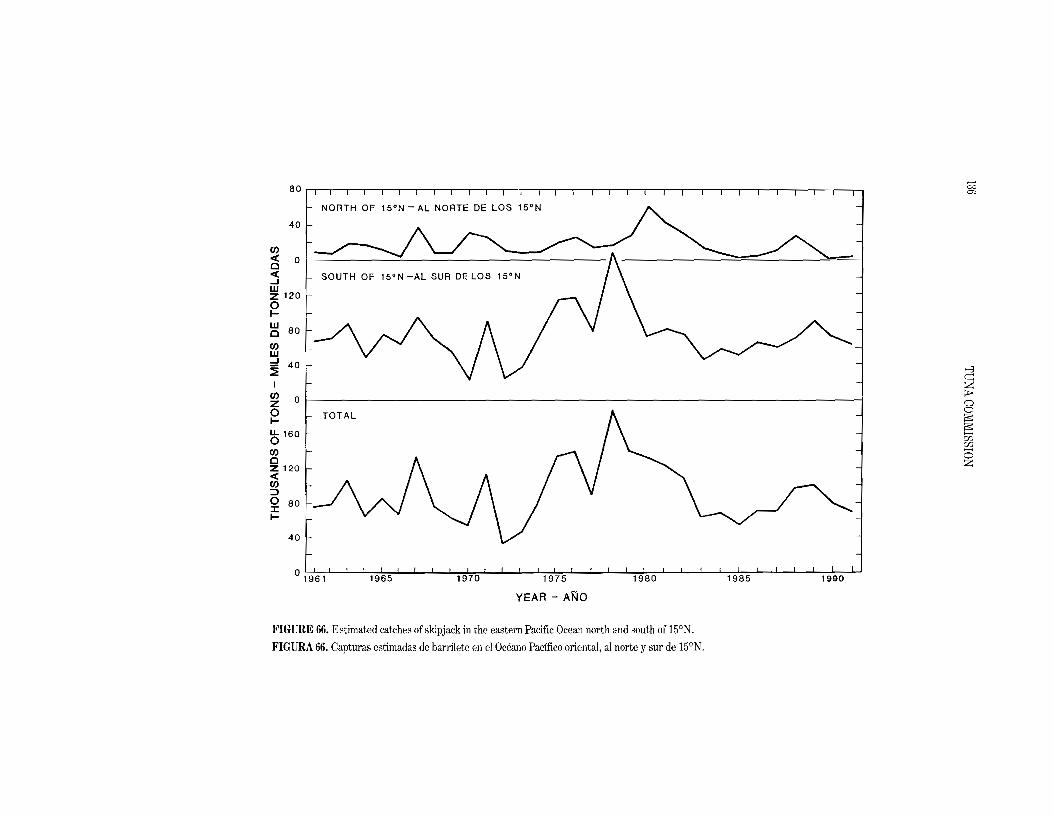
80 I I I , I , I I ii' I 'I i I I , i I I I' I I, I I I >~
NORTH OF 15°N AL NORTE DE LOS 15° N
40
en « 00 « ...J W Z 120 0 I
~ 80
en w :::! 40 ~
I
en z 0
0 I
~ 160
~ 120 I « en ::> o 80 J: I
TOTAL
A
V V
1\ ~ ..."c::: z ;J> ("")
0 ~
~-UJ UJ-0 z
40
YEAR - AND
FIGURE 66. Estimated catches of skipjack in the eastern Pacific Ocean north and south of 15°N.
FIGURA 66. Capturas estimadas de barrilete en el Oceano Pacifico oriental, al norte y sur de 15°N.
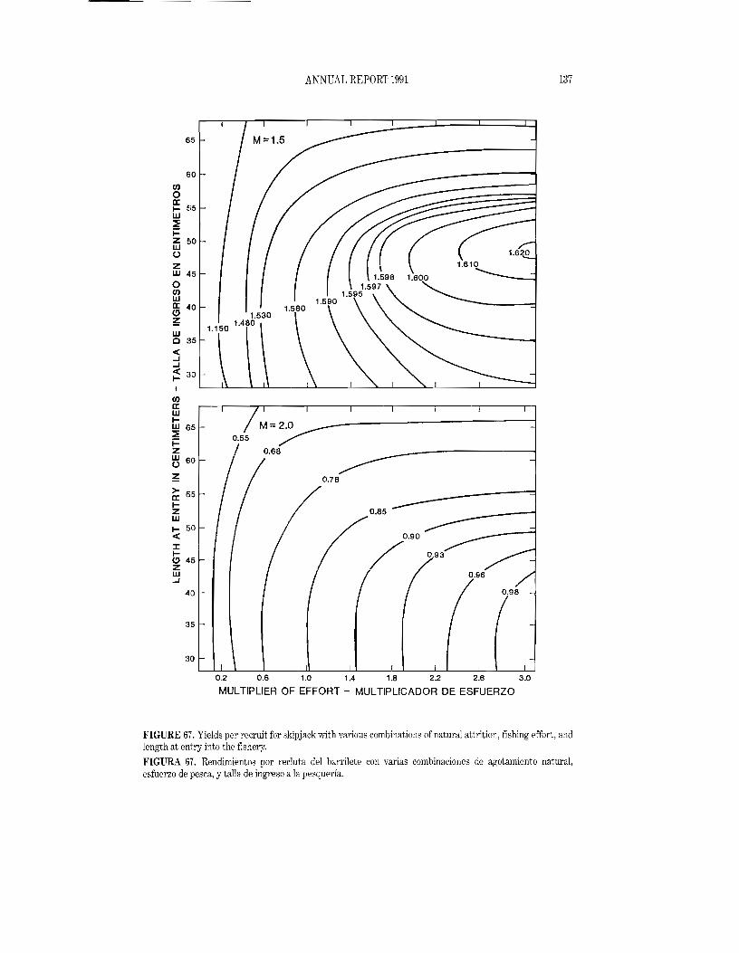
137 ANNUAL REPORT 1991
65
60
en 0 a: I- fj5 W ~ ~ Z 50 W 0 Z W 45 0 en wa:: 40 C' ~ w a 35 4( oJ oJ 4( '10l-I
en a: w IW 65 ~ 0.55 ~ Z W 600
~ 0.78
> 55a:: I-z 0.85 W
I- 50 c( 0.90 J: I- 0.93 ~ 45 Z W ...J
40 0.98
:l5
30
0.2 0.6 1.0 1.4 1.8 2.2 2.6 3.0
MULTIPLIER OF EFFORT - MULTIPLICADOR DE ESFUERZO
FIGURE 67. Yields per recruit for skipjack with various combinations of natural attrition, fishing effort, and length at entry into the fishery.
FIGURA 67. Rendimientos pOI' recluta del bal'rilete con varias combinaciones de agotamiento natural, esfuerzo de pesca, y talla de ingreso a la pesquel'ia.
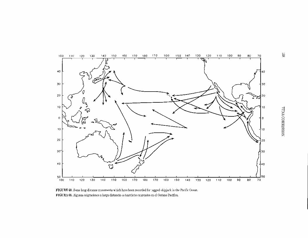
110 120 130 140 150 160 170 180 170 160 150 140 130 120 110 100 90 80 70 ~
100 I II ill iI I I I i j I I I I \"'-. I , I I I I
40
30 30
o ~ • " 411(20 20• ~~
10 It 10 '""":3 c::::"~
o 0 Q""" 0 ~
~
Uft Z
>-<~<D-' -~ en10 en 25 Z
20 20
30'
40
50 ! , ! I ! I I 1 I ! I ! I ! ", 50I I I I
100 110 120 130 140 150 160 170 180 170 160 150 140 130 120 110 100 90 80 70
FIGURE 68. Some long-distance movements which have been recorded for tagged skipjack in the Pacific Ocean.
FIGURA 68. Algunas migraciones a larga distancia de barriletes marcados en el Oceano Pacifico.
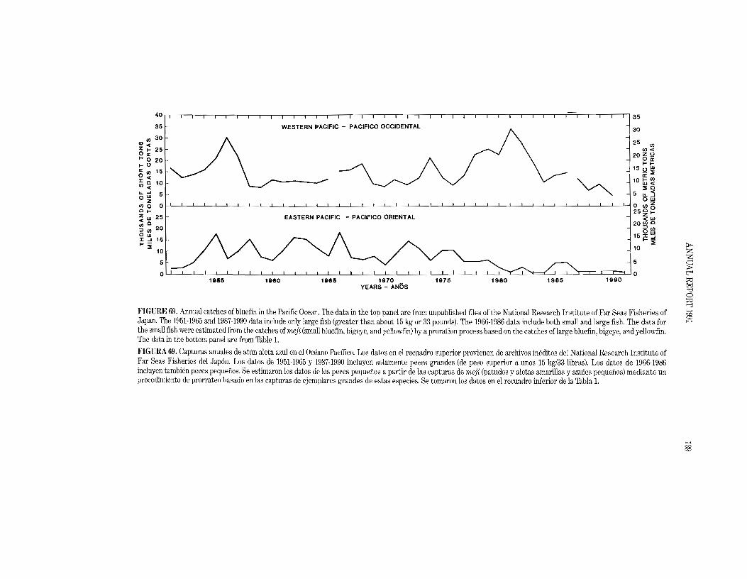
:l ',,,,,,,,~,;,,~, ;.c:,,; -~.;.,;o ~cc~,,;,..: ' , , , , , '1\', , , , , , , , , '~ : en 30 25 m
~~25 J ~ 20~~I- 0 20 f- lI- 0 15 () ~
D: en 15 a: o < '\.. -"". 10 tu ~
;J; 0 10 V" "" ~ cU.~5 5~~
o Z 0 lJ) Z en 0 0 25 c ~ 01- Z Z w 25 EASTERN PACIFIC - PACIFICO ORIENTAL ;;'i ~
<0 W~
en 20 0 (J)
:J en 15 J: W
~ ~ ~ :: 1\ /\ ~ 1\ ~ _ 10 f- ~
Z Z
5 5 §2 t-<
11115 11180 11185 ~
trJ "0 o ~
FIGURE 69. Annual catches of bluefin in the Pacific Ocean. The data in the top panel are from unpublished files of the National Research Institute of Far Seas Fisheries of >-'
"" >-'Japan. The 1951-1965 and 1987-1990 data include only large fish (greater than about 15 kg or 33 pounds). The 1966-1986 data include both small and large fish. The data for "" the small fish were estimated from the catches of me.ii (small bluefin, bigeye, and yellowfin) by a proration process based on the catches of large bluefin, bigeye, and yellowfin. The data in the bottom panel are from Table 1.
FIGURA 69. Capturas anuales de attin aleta azul en el Oceano Pacifico. Los datos en el recuadro superior provienen de archivos ineditos del National Research Institute of Far Seas Fisheries del Japon. Los datos de 1951-1965 y 1987-1990 incluyen solamente peces grandes (de peso superior a unos 15 kg/33 libras). Los datos de 1966-1986 incluyen tambien peces pequeiios. Se estimaron los datos de los peces pequeiios a partir de las capturas de meji (patudos y aletas amarillas y azules pequeiios) mediante un procedimiento die' prorrateo basado en las capturas de ejemplares grandes de estas especies. Se tomaronlos datos en el recuadro inferior de la Tabla 1.
>-' = ""
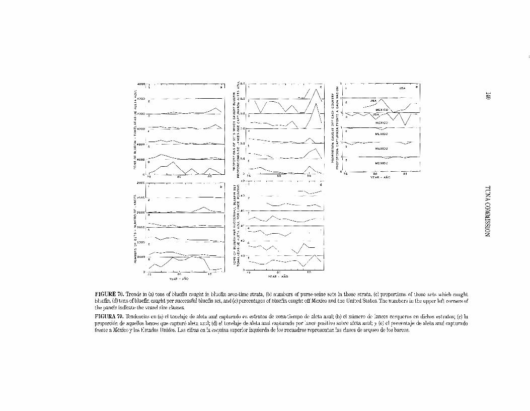
4000~-'-------'--'-----'~~~ 0~5 ~~--.-~~,---,---,-~-.-~~~
.000 f,- "~-;-j ...... :!3I 2 I
I,000E-~I lv~7i:, MEXICO
• - - - I \ 1 1 ........4000 --------- I 051~.-------=-----==-~ 7
MEXICOI'0.51~----- /'5-.·~~
to MEXICO"OOI~----= 'r-=.000~1 0516~- .. h- MEX::--~0~1 ~l o 80 85
YEAR - ANO
~ a ' >-3'~_. I ~~ ~
d
l'2000 r _80 85
b
I .01 ol~7580 75
~ ~ .0 l 1 Z ~ Q. I 2 _ >~200T--- __ j ~
-J (")
~ ~ --------~l o ::J ...,! 40
W tL ....-_ ~ .......-~2000~. ~:5 3~ ~ ~~ ~
u ~ >-< w~~ w" ~ 2000 1-4.-- ~ ~
~
~~.O~;:~~ . o• ~~
~ ~.o 5 ./'-..~2oool=I~-=.--z
I ~ ~ -------~ 'V
~~-j ~~J6---~!2000~1 5~ I~ I r- t-- I !,
.0 o I !, 85 o I " " ' 75 80/5 85
YEAR - ANa YEAR - ANa
FIGURE 70. Trends in (a) tons of bluefin caught in bluefin area-time strata, (b) numbers of purse-seine sets in those strata, (c) proportions of those sets which caught bluefin, (d) tons of bluefin caught pel' successful bluefin set, and (e) percentages of bluefin caught off Mexico and the United SLates. The numbers in the upper left corners of the panels indicate the vessel size classes.
FIGURA 70. Tendencias en (a) el tonelaje de aleta azul capturado en estratos de zona-tiempo de aleta azul; (b) el numero de lances cerqueros en dichos estratos; (c) la proporci6n de aquellos lances que captur6 aleta azul; (d) el tonelaje de aleta azul capturado pOl' lance positivo sobre aleta azul; y (e) el porcentaje de aleta azul capturado frente a Mexico y los Estados Unidos. Las cifras en la esquina superior izquierda de los recuadros representan las clases de arqueo de los barcos.

30 1ofI) i I .-._._.-.:::i: iii Iii ,...._._._.-..... ...... OPTION 2, M=0.2OPTION 1, M =0.2« ... I I
roC< .';--------..... .... ... I ·;-------- . ..... /_4/ .......... rr
f/i l'- /-/ i "" :::i: " 20 . .........
/ . ...<0 / r J .................~2.0 I .............. · ..... 2.0
"a: ...J .-' ............. 1.0i ' ......... 1.0 0:::':: . 0.5 .... '0.5 -,Z .-.1 ~ W 10 /Z< /-~
~::J_...J ::J()a:W() a: 0' ~
Wa:W a: ' §2201-----~------------Z
a: 0a. t:-<Cl~ OPTION 1, M=0.3 OPTION 2, M = ~::----- 0.3t·_·_·_·_·:.: .... "'-'-'--_._-, trJ0.0 "02 ' o -1'~"'----2 -"'r' ---- Q:.. ... ------ -- ......... ............... Pl. ...wW ......-. ........... ...... ...................>= ~ 10 ~/ ....../ • ..J "'_ __ 2 0
..... ----..: ...... · .... ·-.2.0C / 1'-' ~ i ------_1:0
~
Z ----- 1.0 ./.W 0.5 / / 0.5 a:
0' I I I I I I I I I I I
o 1 2 3 4 5 6 7 8 9 10 11 0 1 2 3 4 5 6 7 8 9 10 11
AGE AT ENTRY IN YEARS - EDAD DE ENTRADA EN ANOS
FIGURE 71. Yield-per-recruit curves for northern bluefin, based on the data in Thble 29. The values, 0.5, 1.0, and 2.0, represent multipliers of the vectors of fishing mortality shown in Thble 29. The horizontal portions of the curves are caused by the lack of fishing effort during these periods.
FIGURA 71. Curvas de rendimiento pOl' recluta correspondientes al aleta azul del norte, basadas en los datos de la Thbla 29. Los valores de 0.5, 1.0, y 2.0 representan multiplicadores de los vectores de mortalidad pOl' pesca presentados en la Thbla 29. Las porciones horizontales de las curvas resultan de la falta de esfuerzo de pesca en esos ......periodos. ...... "'"
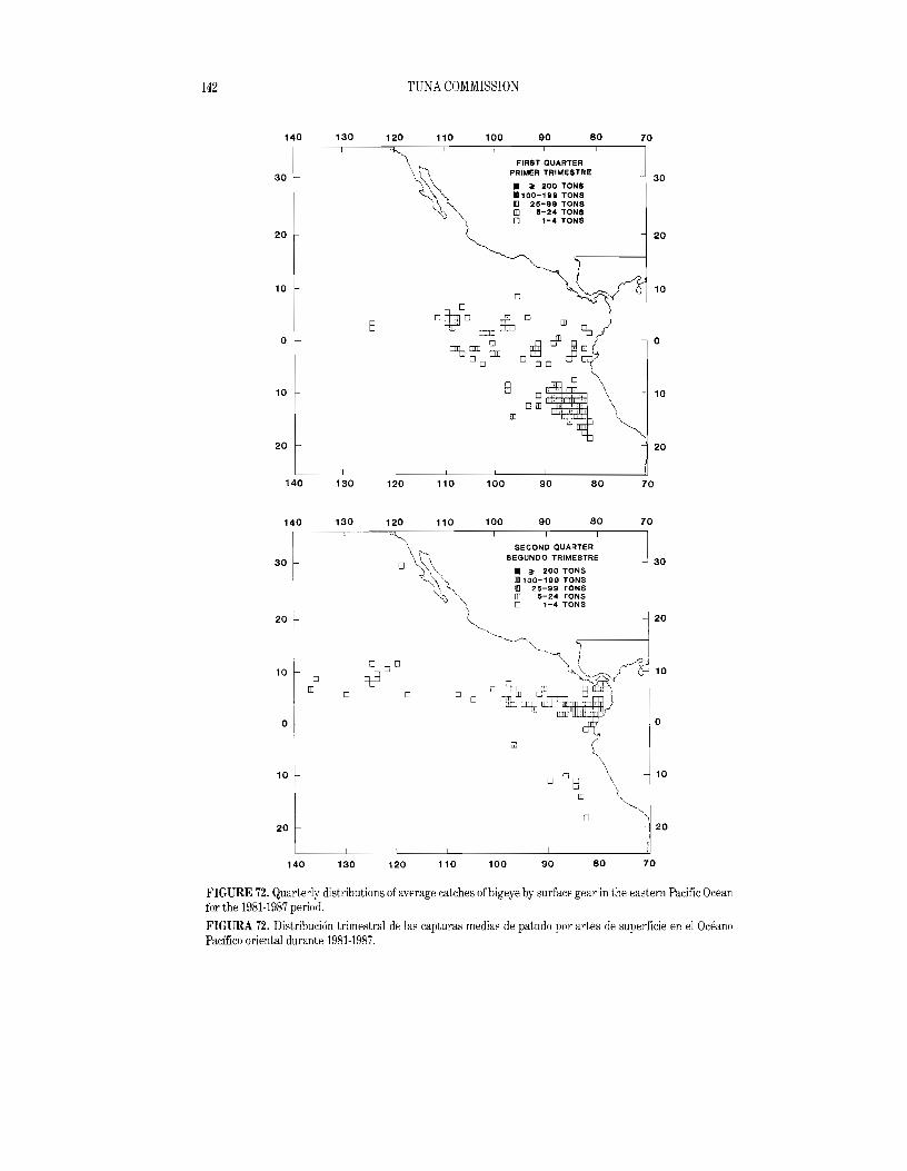
142 TUNA COMMISSION
140 130 120 110 100 90 80 70
30
20
~ FIRST QUARTER
PRIMER TRIMESTRE
• ~ 200 TONS • ,00-,88 TONS IIIl 28-99 TONS ill 8-24 TONS 0 1-4 TONS
30
20
10 10
o B
o
10 10
20 20
140 130 120 110 100 90 80 70
140
I 30 ~
I
"I 10 ~ OJO
o ~ I
10 r
20 r 140
130
o
130
120 110 100 90 80 70
7080
o
90100110
o
~ SECON~ QUARTER I \ \~ SEGUNDO TRIMESTRE '
o ~~\" • ? 200 ~·132°0JJl100-199 TONS all 25-99 TONSTONS OJ 5-24 TONS o 1-4 TONS
~, l ·~L11"
o 0 D~ ~ ~ J arm o
L J"120
o 0oED u
FIGURE 72. Quarterly distributions of average catches of bigeye by surface gear in the eastern Pacific Ocean for the 1981-1987 period.
FIGURA 72. Distribuci6n trimestral de las capturas medias de patudo pOl' artes de superficie en el Oceano Pacifico oriental durante 1981-1987.

143 ANNUAL REPORT 1991
140
I
"r20
130 120 110\1 Cc~
100 90 801 THIRD QUARTER
TERCER TRIMESTRE
• ~ 200 TONS II 100-199 TONS ill 25-99 TONS IIJ 5-24 TONS 0 1-4 TONS
70
l30
I" 10 0
0 DO
III o~~Bm~" 0 0
o a III em IB::P
10 rna
10
20 20
140 130 120 110 100 90 80 70
140 130 120 110 100 90 80 70
FOURTH QUARTER CUARTO TRIMESTRE 30 30
• ~ 200 TONS II 100-199 TONS ill 25-99 TONS rn 5-24 TONS 0 1-4 TONS
20 ~ 20
10 10 ~~~ 0 0~t:ol¥ca, ~o\ - 10
20:: ~ 140 130 120 110 100 90 80 70
FIGURE 72. (continued)
FIGURA 72. (continuacion)

144 TUNA COMMISSION
c-::-_--'l:;.4"'-o_--'lCOT3"'o__.:..:12r-'o'-----_-'-1-;.:10"----_--'l"i0.::.0__--'9,=-0 8TO~ _ _',7040
FIRST QUARTER PRIMER TRIMESTRE
30> 1.5• <.m [] <. P
o
20
o
10
20 20
30 30
40'------'-'-~---'_,____--'-::---____:_'_::_--.,-J-::~~__='=-~---7;:--~;; 150 140 130 120 110 100 90 80
4d c-:~50"----'-14;:i 0"___--".::;~"-0--.:..:12r-'i 0'-----_...:.'.;-)O"----_--":.:;O"-O~~ .::9FO T8 0'-----_---'-7040
SECOND QUARTER SEGUNDO TRIMESTRE
30 = ~iIP •m >(. 1.51.5
30
•• 0 {~ri
~ml ' .. : ::0 20
10
o
10
20 20
30
40i_~~L' ~---'------'-------:-'-i=--~-:-:_,____~----:';:-~~=-___'___; 150 140 130 120 110 100 90 80
FIGURE 73. Quarterly distributions of the average hook rates (numbers of fish per 100 hooks) of bigeye by longline vessels in the eastern Pacific for the 1981-1987 period.
FIGURA 73. Distribuci6n trimestral de las tasas medias de captura (mimero de peces por 100 anzuelos) de patudo por barcos palangreros en el Pacifico oriental en el perfodo de 1981-1987.

145 ANNUAL REPORT 1991
'10 100 90 80 70 40
THIRD QUARTER TERCER TRIMESTRE
30> '.5•ID <= 1.5 0 <= 1
0
20
10
0
10
20 20
30
J q" 150 140 130 120 110 100 90 80
100 90 80 70"0 40
FOURTH QUARTER CUARTO TRIMESTRE
• 30> 1.5 ID <= 1.5 0 (= 1
0
20
o
10
20
30
o
4?SLO---14.L0,-------'--'3-0---12'-0---1.Ll0---'--'0-,-0---9'-0---8""0,...-----''-::'
FIGURE 73. (continued)
FIGURA 73. (continuaci6n)

TUNA COMMISSION146
20 20
10r-----------------........
o o
10 10
20,.....------------....... 20
30 30
40L..-_-J...__....L...__...l...-__...l...-__L..-_---J__.......J._----l......J 40 150 140 130 120 110 100 90 80 70
FIGURE 74. Area from which the data used for Figures 75 and 77 were collected.
FIGURA 74. Area en la que se tomaron los datos usados en las Figuras 75 y 77.
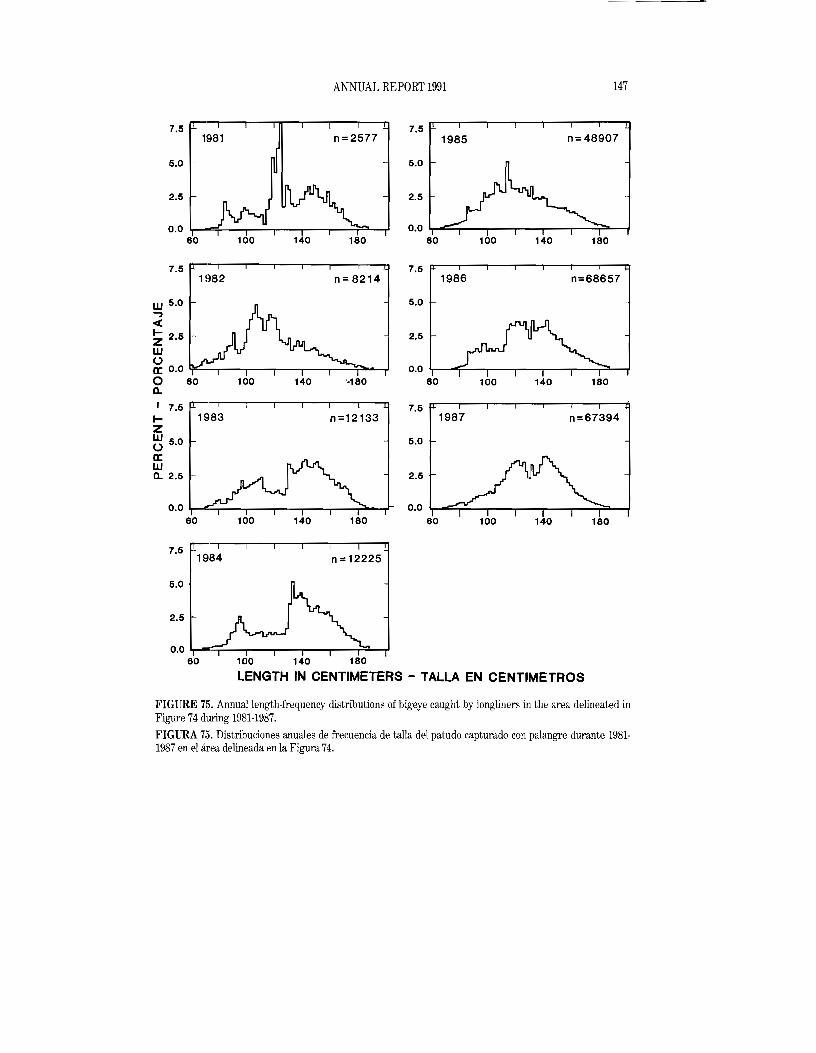
147 ANNUAL REPORT 1991
7.5 7.5 1985 n=48907
5.0 5.0
2.5 2.5
o.0 I,--.....,,~-.-----.--------,.--------,r__--=;=----,J 0.0 60 100 140 180 60 100 140 180
7.5 7.5 1982 n = 8214 1986 n=68657
W 5.0 5.0 ..., <C ~ 2.5 2.5
W <.>CC 0.0 ¥'-,--.-----,--.--------,r__-'i?-......... 0.0 o 60 100 140 '-180 60 100 140 180 c.. I 7.5 n---r--,--,--.------,r__-.----~ 7.5
I- 1983 n=12133 1987 n=67394 Z w 5.0<.> 5.0
CC W c.. 2.5 2.5
0.0 'r-"""-,--,--,--,---,.------,r..:>w--,r 0.0 ...""""r--r--r--,--r--r=-~
60 100 140 180 60 100 140 180
7.5 1984 n = 12225
5.0
2.5
0.0 ........~~----,r__--,r__--,----r----r=----,J
60 100 140 180
lENGTH IN CENTIMETERS - TAllA EN CENTIMETROS
FIGURE 75. Annual length-frequency distributions of bigeye caught by longliners in the area delineated in Figure 74 during 1981-1987.
FIGURA 75. Distribuciones anuales de frecuencia de talla del patudo capturado con palangre durante 19811987 en el area delineada en la Figura 74.

148 TUNA COMMISSION
50 ~---r----"""----",,------"'----"""----""------""'---
(/) M=0.4 <0: m 40 ...J 120 __ Z W .----=: --'------.::::-:-;;:=--. 90 t < 30 .:::=:-...J ::J
:~: ._. 60 _._U
0:
~
o
20
.~ '-'-'~'--a. o 10 [I:.f ._.~.-t Z W ~ o .-.--'--'---' o z W 0:
I 25 ~------------------------~ (/) o Z M=0.6 90 ::J
a. ~.---'--'~:---
020 <::.:--: 60Z .,e::::::--':?' . !:: ~~.::J1510: U w tf.:(::7· '-'--.~ ..-a: 0: 10 1w
o ...J
a.
5 :~. ~ . _--'"""1~W
>- --'--.-.--.~ __---.J~L_ ..l...___----L __1. ...L__-.Jo \C"",=:=:::-=....._- ____1. ,
0.2 0.4 0.6 0.8 1.0 1.2 1.4 1.6 COEFFICIENT OF FISHING MORTALITY
COEFICIENTE DE MORTALiDAD POR PESCA
FIGURE 76. Estimated yields per recruit of bigeye with various combinations of fishing mortality and lengths at entry for annual natural mortality rates of 0.4 and 0.6.
FIGURA 76. Estimacion del rendimiento por recluta del patudo con distintas combinaciones de mortalidad por pesca y talla de ingreso cOl'l'espondientes a tasas anuales de mortalidad natural de 0.4 y 0.6.

00 1.8iii .... ""} i i I i I i .. ,....:A
W OOZ Z 0 1.6 O...J ~ ~ 1.4
~ Z 1.2 ZW
J: ~ 1 000-W >U. (l, 0.8 Z
Zu. w0 ~ 00.6 !=O tJjJ:< ""Cl o~ a: 0.4 ~
......<
~ , if; ......
~ ' , ,() <a. 0.2 , O
0""- MY J J I , o 40 80 120 160
EFFORT IN MILLIONS OF HOOKS ESFUERZO POR MILLONES DE ANZUELOS
FIGURE 77. Relationship between estimated longline catch and effort for bigeye in the portion of the eastern Pacific Ocean delineated in Figure 74 for the 1954-1987 period. The fine lines denote CPUEs in numbers of fish per 100 hooks.
FIGURA 77. Relaci6n entre el esfuerzo y la captura palangrera estimada de patudo en el area delineada en la Figura 74 durante el periodo de 1954-1987. Las lineas finas denotan la CPUE en numero de peces pOI' 100 anzuelos. ......
<'E

150
30
TUNA COMMISSION
120 110 'DO 90 80 -~~-'-------'---T----r--30
• "'00 TONS n ~O - 99 TONS 1980 : "'~g ~O~: TONS 1981 IIJI 25 - 49TONS In 25 49TONS
20 III
[I) o
5 - 24TONS 1 4TONS o III
o 5 - 24TONS 1 4 TONS
20
o o r:fl1 00 o
III '0 o 10
o o o
L- "- '-- '-- "--'-_ 10'0
,---,:-;-,-,----,------,,-----,----, 30
• "'00 TONS• ~ 10Q TONS I1J 50-99TONS1982o 50 - 99 TONS 1983
IIIJ 25 - 49TONSnIl 25 - 49 TONS III 5-24TONSill 5 - 24TONS o o 1 - 4TONS20 U 1- 4TQNS 20
o
'0 10
o o
'0 12'--0----IILO-----IOLO----9~0-----,L-J--' 10'20 110 100 90 80
FIGURE 78. Logged purse-seine catches of black skipjack in the eastern Pacific Ocean during 1980-1983.
FIGURA 78. Capturas cerqueras de barrilete negro registradas en el Oceano Pacifico oriental en 1980-1983.

-- --
TABLE 1. Estimated catches, in short tons, by the eastern Pacific tuna fleet. The abbreviations used in the table are as follows: YFT, yellowfin; SKJ, skipjack; BET, bigeye; BFT, bluefin; BEP, bonito; ALB, albacore; BKJ, black skipjack; MISC, other species including sharks, other tunas, and miscellaneous fishes; CYRA, Commission's Yellowfin Regnlatory Area; outside, area between the CYRA and 150°W. The 1991 data are preliminary. Additional information concerning this table is given in the text. TABLA 1. Capturas estimadas, en toneladas cortas, logradas por laflota atunera del Pacifico oriental. En la tabla se usan las signientes abreviaturas: YFT: aleta amarilla; SKJ: barrilete; BET: patudo; BFT: aleta azul; BEP: bonito; ALB: albacora; BKJ: barrilete negro; MISC: otras especies, incluyendo tiburones, otros tlinidos, y peces diversos; ARCAA: Area de Regnlacion de la Comision para el Aleta Amarilla; exterior: zona entre el ARCAA y 150°W. Los datos de 1991 son preliminares. En el texto se ofrece mayor informacion sobre esta tabla.
CYRA Outside Pacific Ocean east of 1500W Year ARCAA Exterior Oceano Pacifico al este de 1500W Ano YFT YFT YFT SKJ BET BFT BEP ALB BKJ MISe Tbtal 1961 115,682 0 115,682 75,468 235 8,968 3,205 2,670 0 236 206,464 1962 87,158 0 87.158 78,256 362 12,421 3,576 1,292 0 193 183,258 1963 72,136 0 72,136 105,333 83 13,527 3,442 3,773 0 265 198,559 1964 101,390 0 101,390 65,322 75 10,161 7,387 3,672 5 248 188,260 1965 90,167 0 90,167 86,194 130 7,592 4,464 710 18 171 189,446 1966 91,513 0 91,513 66,669 294 17,523 4,911 2,140 10 465 183,525
;J;>1967 90,116 0 90,116 132,999 1,834 6,491 11,072 4,133 0 127 246,772 Z1968 114,500 1,207 115,707 78,385 2,821 6,587 8,772 4,955 0 138 217,365 Z 1969 126,898 19,217 146,115 65,109 635 7,635 3,252 3,246 0 1 225,993 ~ 1970 142,425 30,680 173,105 61,752 1,469 4,372 5,223 4,935 0 29 250,885 t'"' 1971 113,886 22,758 136,644 115,432 2,830 9,215 10,581 2,745 6 67 277,520 ~
M1972 152,897 44,768 197,665 36,826 2,468 14,714 9,781 5,326 662 404 267,846 '"d 1973 177,985 49,506 227,494 48,450 2,181 11,845 8,670 2,553 1,845 391 303,429 0
~
1974 191,606 40,988 232,594 86,862 980 6,192 4,888 5,272 4,125 1,087 342,000 >-3 ......
1975 176,044 47,729 223,773 136,540 4,104 10,563 18,561 3,672 564 305 398,082 = <0 ......1976 210,468 50,829 261,297 139,070 11,229 11,735 4,815 4,115 1,681 1,463 435,405 1977 202,409 17,792 220,201 95,169 7,777 6,033 12,428 2,163 1,608 2,148 347,527 1978 183,995 16,037 200,032 187,185 12,911 5,948 5,332 1,923 2,383 888 416,602 1979 194,973 15,177 210,150 145,531 8,302 6,744 1,988 361 1.509 1,375 375,960 1980 146,480 29,638 176,118 143,761 16,998 3,239 6,736 661 4,057 1,050 352,620 1981 174,691 26,545 201,236 131,846 11,124 1.201 6,523 830 2,108 1,113 355,981 1982 118,722 20,079 138,801 108,782 4,524 3,472 2,339 610 1,475 862 260,865 1983 91,397 13,482 104,879 64,049 3,594 940 4,221 503 1,363 1,885 181,434 1984 142,325 18,186 160,511 66,746 6,453 972 3,873 5,899 734 1,087 246,275 1985 216,235 24,075 240,310 54,456 4,996 4,469 3,973 955 328 590 310,077 1986 252,951 42,688 295,639 70,005 2,182 5,604 540 198 656 1,256 376,080 1987 274,911 26,616 301,527 68,608 850 1,097 3,417 54 948 1,829 378,330 1988 294,716 22,941 317,657 94,137 1,161 1,569 10,535 178 1.573 2,760 429,570 1989 267,218 51,944 319,162 102,468 1,621 1.289 13,332 1 1,845 1,882 441,599 1990 250,645 51,074 301,719 80,908 5,232 1.682 15,331 203 1,089 1,281 407,445 ......
......1991 237,531 21,507 259,038 71,305 4,008 462 1,378 908 575 1,161 338,835 <:.n

...... TABLE 1. (continued) "" ['0)
TABLA 1. (continuacion)
Western Pacific Atlantic and Caribbean Year Total, all areas and speciesPacifico occidental Atlantico y CaribeAno Total, todas las zonas y especies
YFT SKJ MISC YFT SKJ BET MISC
1961 0 0 0 14 llJ 0 0 206,589 1962 0 0 0 0 0 0 0 183,258 1963 0 0 0 14 1,827 0 2,985 203,385 1964 0 0 0 0 4,361 0 3,159 195,780 1965 0 0 0 50 173 0 1,390 191,059 1966 0 0 0 0 4 0 124 183,653 1967 0 0 0 1,252 542 0 858 249,424 1968 0 0 0 7,371 4,213 17 0 228,966 1969 0 0 0 20,243 5,202 163 0 251,601 >-3
~
1970 0 227 0 10,321 13,094 215 1,790 276,532 Z::.-1971 0 0 0 4,595 20,156 649 1.820 304,740 ("}
1972 0 0 0 14,158 14,797 234 1,094 298,129 0 ~1973 0 0 0 4,248 25,494 125 746 334,041 ~ 1974 35 0 0 6,528 21,693 957 178 371,391 en
1975 0 363 0 15,884 8,310 74 909 423,622 rn >-<
1976 247 5,435 2 2,509 2.842 43 469 446.952 0 Z1977 157 6,822 4 8,821 7,054 365 130 370,880
1978 24 8,050 44 11,474 9,381 274 369 446,218 1979 0 4,826 0 3,491 3,097 234 659 388,267 1980 351 6,062 0 5,540 4,269 222 32 369,096 1981 5,369 6,603 0 4,401 5,047 141 186 377,428 1982 6,106 13,402 66 5,502 3,277 380 243 289,841 1983 27,930 55,325 390 10,269 6,742 0 276 282,366 1984 5.877 17,971 537 7,696 5,934 3 193 284,486 1985 991 5,368 7 7,851 4,096 0 49 328.439 1986 4,321 5,341 0 1,068 1,767 9 15 388,601 1987 1,532 3,427 54 1.009 2,428 26 107 389,914 1988 772 2,102 556 334 202 0 0 433,537 1989 0 0 269 2,957 1,762 0 2 446,588 1990 2.247 9,708 484 2,923 1,957 69 7 424,838 1991 252 1,544 0 5,252 3,733 0 39 349,655
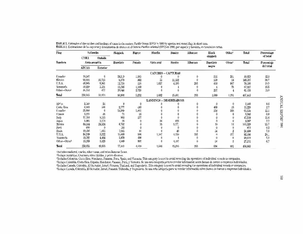
TABLE 2. Estimates of the catches and landings of tunas in the eastern Pacific Ocean (EPO) in 1990 by species and vessel flag, in short tons. TABLA 2. Estimaciones de las capturas y desembarcos de atunes en el Oceano Pacifico oriental (OPO) en 1990, por especie y bandera, en toneladas cortas.
Flag Yellowfin
CYRA Outside
Skipjack Bigeye B1uefin Bonito Albacore Black skipjack
Other! Total Percentage of total
Bandera Aleta amarilla
ARCAA Exterior
Barrilete Patudo Aleta azul Bonito Albacora Barrilete negro
Otras1 Total Porcentaje del total
Ecuador Mexico U.S.A. Venezuela Other-Otros2
19,587 93,691 49,985 49,228 38,154
0 35,715 9,361 5,521
477
28,519 8,379
12,718 11,246 20,046
1,385 362 116
1,149 2,220
CATCHES CAPTURAS 0 0
55 11,132 1,627 4.195
0 4 0 0
0 0
203 0 0
251 159 418
4 257
281 14
907 75 4
50,023 149,507 79,530 67,227 61,158
12.3 36.7 19.5 16.5 15.0
Thtal
Africa Costa Rica Ecuador France Italy Japan Mexico Peru Spain U.S.A. Venezuela Other-Otros3
250,645
2,548 6,940
25,998 3,221
37,764 5,001
68,144 680
19,456 56,249 18,765 13,269
51,074
24 586
0 38
8,515 3,174
24.524 0
1,835 3,222 4,464 3,423
80,908
8 2,777
33,269 71
903 26
6,702 193
7,035 15,609 5,879 4,969
5,232
0 490
1,861 16
137 0 0 0
44 596 498 997
1,682 15,331
LANDINGS DESEMBARCOS 0 0 0 0 0 0 0 0 0 0
38 823 55 5,771 0 0 0 40
1,587 4,150 0 4 0 4,497
203
0 0 0 0 0 0 0 0 0
203 0 0
1,089
0 409 158
0 0 0
19 0
54 0 0
54
1,281
0 18
268 0 0 0
14 0 2
577 0 2
407,445
2,580 11,220 61,554 3,346
47,319 9,062
105,229 873
28.466 82,193 29,610 27,211
0.6 2.7
15.1 0.8
11.6 2.2
25.7 0.2 7.0
20.1 7.2 6.7
>Z Z §Z r-< ~
tr:l "'CI 0
~
...... <0 <0 ......
Thtal 258,035 49,805 77,441 4,639 1,680 15,285 203 694 881 408,663
1Includes mackerel, sharks, other tunas, and miscellaneous fishes. lIncluye macarelas, tiburones, otros tunidos, y peces diversos. 2Includes Colombia, Costa Rica, Honduras, Panama, Peru, Spain, and Vanuatu. This category is used to avoid revealing the operations of individual vessels or companies. 2Incluye Colombia, Costa Rica, Espana, Honduras, Panama, Peru, y Vanuatu. Se usa esta categoria para no revelar informacion sobre faenas de barcos 0 empresas individuales. 3Includes Canada, Colombia, El Salvador, Israel, Panama, Thailand, and Yugoslavia. This category is used to avoid revealing the operations of individual vessels or companies. 3Incluye Canada, Colombia, El Salvador, Israel, Panama, Tailandia, y Yugoslavia. Se usa esta categoria para no revelar informacion sobre faenas de barcos 0 empresas individuales.
...... 01
"""
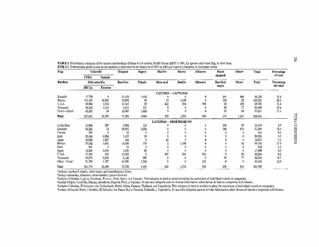
,..... ~
TABLE 3. Preliminary estimates of the catches and landings oftunas in the eastern Pacific Ocean (EPO) in 1991, by species and vessel flag, in short tons. TABLA 3. Estimaciones preliminares de las capturas y desembarcos de atunes en el OPO en 1991 pOI' especie y bandera, en toneladas cortas. Flag Yellowfin Skipjack Bigeye Bluefin Bonito Albacore Black Otherl Total Percentage
skipjack of totalCYRA Outside
Bandera Aleta amarilla Barrilete Patudo Aleta azul Bonito Albacora Barrilete Otrasl Total Porcentaje negro del total
ARCAA Exterior
CATCHES - CAPTURAS Ecuador 17,780 0 21,475 1,932 0 0 0 281 658 42,126 12.4 Mexico 111,563 16,521 13,805 66 10 1,168 0 156 32 143,321 42.3 U.S.A. 20,884 1.811 14,147 28 452 204 908 25 306 38,765 11.4 Venezuela 45,022 3,141 6,811 327 0 0 0 30 77 55,408 16.4 Other-Otros2 42,282 34 15,067 1,655 0 6 0 83 88 59,215 17.5
>-3Thtal 237,531 21,507 71,305 4,008 472 1,378 908 575 1,161 338,835 ~
Z ;.>
Costa Rica 15,964 397 3,004 113 0 0 0 309 29 19,816 5.6 0Q
Ecuador 24,342 74 28,005 2,354 0 0 0 162 612 55,549 15.8 ~
France 399 0 16 0 0 0 0 0 0 415 0.1
LANDINGS - DESEMBARCOS
~
EnItaly 20,144 6,694 1,157 30 0 0 0 0 0 28,025 8.0 en Japan 10,528 1,537 164 3 23 0 0 0 0 12,255 3.5 25 Mexico 79,342 5.605 10,430 179 2 1,168 0 6 32 96,764 27.6 Z Peru 201 0 18 0 0 0 0 0 0 219 0.1 Spain 12.236 3,896 1,329 28 0 0 0 0 0 17,489 5.0 U.S.A. 17,483 222 13,032 2 437 204 814 0 60 32,254 9.2 Venezuela 33.374 3,286 5,122 693 0 0 0 29 77 42,581 12.1 Other-Otros3 31,766 1,797 10,485 1,244 0 0 121 0 0 45,413 12.9
Thtal 245,779 23,508 72,762 4,646 462 1,372 935 506 810 350,780
1Includes mackerel, sharks, other tunas, and miscellaneous fishes. IIncluye macarelas, tiburones, otros tunidos, y peces diversos. 2Includes Colombia. Cyprus, Honduras, Panama, Peru. Spain, and Vanuatu. This category is used to avoid revealing the operations of individual vessels or companies. 2Incluye Chipre, Colombia, Espaiia, Honduras, Panama, Peru, y Vanuatu. Se usa esta categoria para no revelar informacion sobre faenas de barcos 0 empresas individuales. 3Includes Colombia, El Salvador, the Netherlands, North Africa, Pananla, Thailand, and Yugoslavia. This category is used to avoid revealing the operations of individual vessels or companies. 3Incluye Africa del Norte, Colombia, El Salvador, los PaUles Bajos, Panama, Tailandia, yYugoslavia. Se usa esta categoria para no revelar informacion sobre faenas de barcos 0 empresas individuales.

----
155 ANNUAL REPORT 1991
TABLE 4. Numbers and carrying capacities, in short tons, of vessels of the eastern Pacific tuna fleet. Bolicheras are small pill'se seiners with limited ranges. Information for 1950·1960 is given in Table 4of the IATTC Annual Report for 1988. The data for 1991 are preliminary. TABLA 4. l\limero y capacidad de acarreo, en toneladas cortas, de los barcos de la flota atuncra del Pacifico oriental. Las bolicheras son cerqueros pequefios con radio de accion limitado. En la Tabla 4 del Informe Anual de la C1AT de 1988 se presentan las datos de 1950·1960. Los datos de 1991 son preliminares.
Year Seiners Baitboats Bolicheras Trollers 'futaJ
No. 'funs No. 'funs No. 'funs No. 'funs No. 'funs
Aiio Cerqueros De camada Bolicheras Curricanes 'futal
'!io. 'fun. No. 'fun. No. 'fun. No. 'fun. No. 'fun.
19i11 124 30,011 93 10,510 1 25 0 0 218 40,546 1962 130 33,945 89 6,725 27 675 0 0 246 41,345 1963 141 39.834 108 5,964 18 450 3 55 270 46,30:3 1964 134 40.307 88 4,712 3 65 0 0 225 45.084 1965 146 42,283 109 5,777 17 395 7 182 279 48,637 1966 126 39.869 113 6,217 140 2 29 248 46,255 1967 122 40,221 108 5,862 8 170 0 0 238 46,253 1968 139 50,613 89 5.743 4 100 2 24 234 56,480 1969 149 57,008 69 1.957 4 95 :J 71 225 62,131 1970 162 67,508 49 4.302 0 0 9 177 220 71,987 1971 185 88,770 102 5,569 6 150 66 1,514 359 96,003 1972 206 112,361 108 6,707 4 100 74 1.946 392 121,114 1973 216 131.910 106 6,856 3 75 28 729 353 139,570 1974 230 146,990 111 7,766 4 110 7 150 352 155,016 1975 249 163,766 102 7,403 4 105 9 181 364 171,455 1976 250 176,469 99 7,071 4 115 38 909 391 184,564 1977 250 178,8Ii3 79 5,436 3 87 37 953 371 185,289 1978 262 180,781 68 5,044 9 272 50 1,303 389 187,400 1979 268 183,673 4,) 3,979 14 405 5 112 332 188,169 1980 258 184,647 46 3,838 12 355 4 106 320 188,840 1981 247 183,729 39 3,063 3 72 2 55 291 186,919 1982 221 167,780 36 2.713 2 60 4 131 263 170,684 1983 199 137,842 52 3,470 12 300 8 244 271 141,856 1984 165 113,168 40 3,055 0 0 9 232 214 116,455 1985 175 127,272 25 2,424 0 0 1 14 201 129,710 1986 165 122,564 17 1,939 0 0 0 0 183 124,50:3 1987 177 143,765 29 2,237 0 0 0 0 206 146,002 1988 185 148,227 36 3,081 0 0 3 70 224 151,378 1989 178 133,678 30 2,951 0 0 1 11 209 136,640 1990 172 135,552 24 2,016 0 0 0 0 196 137,568 1991 150 116,665 22 1,883 0 0 0 0 172 118,548

156 TUNA COMMISSION
TABLE 5. Estimates of the numbers and carrying capacities in short tons of vessels (exclusive of longliners and miscellaneous small vessels) operating in the EPO in 1990 and 1991 by flag, gear, and size class. Each vessel is included in the totals for each flag under which it fished during the year, but is included only once in the fleet total. Therefore the totals for the fleet may not equal the sums of the individual flag entries. The data for 1990 are preliminary. (PS ~ pmse seiner; BB ~ baitboat) TABLA 5. Estimaciones del mimero de barcos que pescaron en el OPO en 1990 y 1991 (sin incluir palangreros y barcos pequenos diversos), y capacidad de acarreo de los mismos, en toneladas cortas, pOl' bandera, arte de pesca, y clase de arqueo. Se incluye cada barco en los totales de cada bandera bajo la cual pesc6 durante el ano, pero solamente una vez en el total de la flota; pOl' consiguiente, los totales de las flotas no son necesariamente iguales a las sumas de las banderas individuales. Los datos de 1990 son preliminares. (PS =cerquero; BB =barco de camada)
Flag Gear Size class - Clase de arqueo Capacity Bandera Arte 2 3 4 5 6 Total Capacidad
1990 NUMBER NUMERO Colombia PS 1 1 Costa Rica PS 1 1 Ecuador PS 2 6 10 6 2 8 34 9,185
BB 7 7 192 Honduras PS 1 1 * Mexico PS
BB 2 8
2 48 52 11
50,753 1,292
Panama PS 1 6 7 * Peru PS 1 1 Spain PS 1 1 USA PS 12 29 46 32.134
BB 4 6 532 Vanuatu PS 10 11 * Venezuela PS 24 24 28,610 Others-Otras* PS 22 21.697
All flags- PS 2 18 17 6 6 123 172 'Thdas las BB 8 7 9 24 banderas All gear 10 25 26 6 6 123 196
CAPACITY - CAPACIDAD All flags- PS 80 1,572 2,401 1,389 2,242 127,868 135,552 'Thdas las BB 232 577 1,207 2,016 banderas All gear 312 2.149 3,608 1,389 2,242 127,868 137,568
1991 NUMBER - NUMERO Colombia PS 2 2 Cyprus PS 1 1 Ecuador PS 2 5 10 2 7 33 8,825
BB 6 6 162 Honduras PS 1 1 Mexico PS 4 2 43 49 46,445
BB 8 9 1,094 Panama PS 1 2 3 6 2,739 Peru PS 1 1 * Spain PS 2 2 USA PS 5 4 13 23 14,814
BB 5 1 7 627 Vanuatu PS 10 11 Venezuela PS 21 21 24,798 Others-Otras* PS 24 21,783
All flags- PS 2 10 19 9 6 104 150 'Thdas las BB 7 6 9 22 banderas All gear 9 16 28 9 6 104 172
CAPACITY - CAPACIDAD Allflags- PS 80 952 2,614 2,169 2,242 108,608 116,665 'Thdas las BB 202 492 1,189 1.883 banderas All gear 282 1,444 3,803 2,169 2,242 108,608 118,548
*Asterisks indicate data pooled to avoid revealing the operations of individual vessels or companies. *Los asteriscos indican datos combinados para evitar revelar las actividades de barcos 0 empresas individuales.

---
157 ANNUAL REPORT 1991
TABLE 6. Catches per ton of carrying capacity by vessel size group for the EPO purse-seine fleet, by species, in the EPO and in all ocean fishing areas (OFA). The size groups, by capacity in short tons, are as follows: 1, <301; 2, 301-400; 3, 401-600; 4, 601-800; 5, 801-1000; 6,1001-1200; 7, 1201-1400; 8, >1400. The abbreviations for the species are as follows: YFT, yellowfin; SKJ, skipjack; All, all species reported. The 1991 data are preliminary. TABLA 6. Captura por tonelada de capacidad de acarreo y por clase de arqueo de la flota cerquera del OPO, por especie, en el OPO y en todas las zonas pesqueras oceanicas (All OFA). Las clases de arqueo, por capacidad en toneladas cortas, son las siguientes: 1, <301; 2, 301-400; 3, 401-600; 4, 601-800; 5, 801-1000; 6, 1001-1200; 7, 1201-1400; 8, >1400. Las abreviaturas de las especies son: YFT: aleta amarilla; SKJ: barrilete. La abreviatura ''All'' en la columna de "Especie" indica todas las especies informadas. Los datos de 1991 son preliminares.
Size group and catch area
Year Species 1 2 3 4 5 6 7 8 Total
EPO All EPO All EPO All EPO All EPO All EPO All EPO All EPO All EPO All
Clase de arqueo yzona de captura
!\itO Espl,cie 3 4 6 7 8 Total
OPO All OPO All OPO All OPO All OPO All OPO All OPO All OPO All OPO All
1980 YF'T 0.8 0.8 1.1 1.1 0.9 0.9 1.2 1.2 0.6 0.6 0.9 1.0 1.1 1.1 0.8 0.9 0.9 1.0 SKJ 0.5 0.5 0.9 0.9 0.8 0.8 1.0 1.0 0.4 0.4 0.8 0.8 0.9 1.0 0.6 0.7 0.7 0.8 All 2.2 2.2 2.3 2.3 1.8 1.8 2.2 2.2 U 1.2 1.8 1.9 2.1 2.2 1.5 1.7 1.8 1.9
1981 YI'T 1.1 1.1 1.2 1.2 0.9 0.9 1.3 1.3 1.0 1.0 1.2 1.2 1.0 1.2 0.6 0.7 1.1 1.1 SKJ 1.0 1.0 1.1 \.1 0.7 0.7 0.9 0.9 0.4 0.4 0.7 0.7 0.6 0.8 0.4 0.6 0.7 0.7 All 3.0 3.0 2.6 2.6 1.6 1.7 2.2 2.2 1.5 1.5 1.9 2.0 1.7 2.0 1.0 1.4 1.9 2.0
1982 YFT 0.8 0.8 0.8 0.8 0.7 0.7 0.7 0.7 0.6 0.7 0.9 1.0 0.9 0.9 0.7 0.9 0.8 0.9 SKJ 1.9 1.9 1.3 1.3 0.7 0.7 0.6 0.6 0.4 0.5 0.5 0.6 0.7 0.7 0.2 0.7 0.6 0.7 All 3.3 3.3 2.5 2.5 1.5 1.5 1.3 1.3 1.0 1.2 1.5 1.7 1.6 1.7 0.9 1.8 1.5 1.7
1983 YFT 1.2 1.2 1.0 1.0 0.7 0.7 0.7 0.7 0.8 1.0 0.7 1.1 0.6 0.8 0.3 0.9 0.7 1.0 SKJ 1.7 1.7 0.9 0.9 0.5 0.5 0.4 0.4 0,4 0.5 0.3 1.0 0.3 0.9 0.1 0.9 0.4 0.9 All 3.7 3.7 2.0 2.0 1.2 1.2 1.1 1.1 1.3 1.5 1.0 2.1 0.9 1.7 0,3 1.8 1.2 1.9
1984 YFT 1.8 1.8 1.9 1.9 1.2 1.2 1.7 1.7 1.5 1.6 1.4 1.6 1.0 1.1 0.2 0.6 1.4 1.5 SKJ 1.9 1.9 1.6 1.6 0.7 0.7 0.6 0.6 05 0.6 0.4 0.8 0.3 0.6 0.3 0.6 0.6 0.8 All 5.0 5.0 3.9 3.9 2.0 2.0 2.3 2.3 2,2 2.3 2.0 2.5 1.3 1.7 0.6 1.2 2.1 2.4
1985 YFT 1.4 1.4 1.1 1.1 1.2 1.2 1.6 1.6 1.4 1.6 2.1 2.1 2.1 2.1 1.3 1.6 1.9 1.9 SKJ 2.1 2.2 1.5 1.5 0.3 0.3 0.4 0.4 0.1 0.1 0.3 0.4 0.1 0.1 1.0 1.1 0.4 0.5 All 4.7 4.7 3.0 3.0 1.9 1.9 2.1 2.1 1.5 1.8 2.4 2.6 2.2 2.3 2.4 2.7 2.4 2.5
1986 YFT 2.0 2.0 1.8 1.8 1.5 1.5 2.0 2.0 2.0 2.0 2.5 2.6 2.6 2.7 2.1 2.1 2.4 2.4 SKJ 2.4 2.4 2.0 2.0 0.6 0.6 0.5 0.5 0.5 0.5 0.4 0.5 0.1 0.2 0.9 0.9 0.6 0.6 All 5.3 5.3 4.3 4.3 2.4 2.4 2.5 2.5 2.5 2.5 3.0 3.1 2.8 3.0 3.0 3.0 3.0 3.1
1987 YFT 2.0 2.0 2.1 2.1 1.2 1.4 1.8 1.8 1.4 1.5 2.2 2.3 2.4 2.4 1.1 1.4 2.1 2.1 SKJ 2.0 2.0 3.2 3.2 1.2 1.5 0.6 0.6 0.5 0.6 0.3 0.3 0.2 0.2 0.3 0.6 0.4 0.5 All 5.0 5.0 5.4 5.4 2.4 2.9 2.4 2.4 2.0 2.1 2.5 2.6 2.6 2.7 1.4 2.0 2.6 2.7
1988 YFT 2.8 2.8 3.3 3.3 1.9 1.9 2.2 2.2 1.5 1.5 2.1 2.2 2.1 2.1 1.1 1.2 2.1 2.1 SKJ 1.7 1.7 1.4 1.4 0.8 0.8 0.6 0.6 0.5 0.5 0.5 0.5 0.6 0.6 0.2 0.5 0.6 0.6 All 5.7 5.7 5.4 5.4 2.8 2.8 3.0 3.0 2.0 2.1 2.7 2.7 2.7 2.7 1.3 1.7 2.8 2.8
1989 YFT 1.7 1.7 2.4 2.4 1.9 1.9 2.0 2.0 1.5 1.5 2.5 2.5 2.6 2.6 1.4 1.7 2.3 2.3 SKJ 1.9 1.9 2.3 2.3 1.3 1.3 0.7 0.7 0.8 0,8 0.6 0.6 0.5 0.5 0.6 0.9 0.7 0,7 All 4.3 4.3 5.9 5.9 3.4 3.4 3.1 3.1 2.5 2.5 3.1 3.2 3.1 3.1 2.0 2.6 3.2 32
1990 YFT 2.0 2.0 2.3 2.3 1.2 1.2 1.5 1.5 1.1 1.1 2.6 2.6 2.3 2.4 1.8 2.0 2.2 2.2 SKJ 2.4 2.4 2.2 2.2 1.2 1.2 0.6 0.6 0.4 0.4 0,5 0.6 0.2 0.5 0.4 0.4 0.6 0.7 All 5.6 5.6 5.5 5.5 2.9 2.9 2.6 2.6 1.7 1.7 3.1 3.2 2.5 2.8 2.2 2.4 2.9 3.1
1991 YFT 2.0 2.0 3.3 3.3 1.1 1.3 1.8 1.8 1.5 1.5 2.5 2.5 2.6 2.7 1.3 1.5 2.2 2.3 SKJ 1.8 1.8 1.4 1.4 0.9 1.0 0.8 0.8 0.5 0.5 0.4 0.5 0.3 0.3 0.5 0.6 0.6 0.6 All 4.2 4.2 5.0 5.0 2.2 2.6 2.8 2.8 2.0 2.1 2.9 3.0 2.9 3.0 1.8 2.1 2.9 3.0
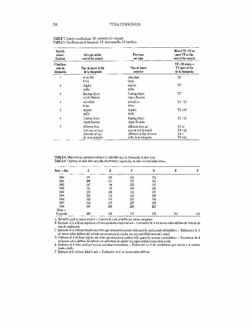
158 TUNA COMMISSION
TABLE 7. Search classifications. YF: yellowfin; SJ: skipjack. TABLA 7. Clasificaciones de bUsqueda. YF: aleta amarilla; SJ: barrilete.
Search Mixed YF t SJ or c1assi- Set type at the Previous pure YF at the
fication end of the search set type end ofthe search
Clasifica- YFtSJ mixto 0
cion de Tipo de lance al fin Tipo de lance YF puro al fin blisqueda de la blisqueda anterior de la blisqueda
schoolfish schoolfish YF brisa brisa dolphin dolphin YF delf!n delf!n floating object floating object YF objeto flotante objeto flotante schoolfish schoolfish YF+SJ brisa brisa dolphin dolphin YF+SJ delf!n delf!n floating object floating object YF+SJ objeto flotante objeto flotante different from different from set YFor previous set type type at end of search YFtSJ diferente al tipo diferente al tipo de lance YFo de lance anterior al fin de la bUsqueda YF+SJ
TABLE 8. Observed and predicted catches of yellowfin tuna, in thousands of short tons. TABLA 8. Capturas de atlin aleta amarilla observadas y esperadas, en miles de toneladas cortas.
Year-ArlO A B C D E F
1980 187 123 142 174 1981 209 141 167 161 1982 147 94 122 132 1983 114 91 106 108 1984 170 100 113 137 1985 250 112 145 186 1986 315 173 212 185 1987 314 176 267 215 1988 333 233 293 252
Mean-Promedio 226 138 174 172 213 153
A Yellowfin catch by purse seiners - Captura de aleta amarilla por barcos cerqueros B Estimate of Awithout dolphin sets from exploitation-rate method - Estimacion de A sin lances sobre delfines del metodo de
tasa de explotacion C Estimate of Awithout dolphin sets from age-structured method with monthly and annual catchabilities - Estimacion de A
sin lances sobre delfines del metoda con estructura de edades con capturabilidad mensual y anual D Estimate of Awithout dolphin sets from age·structured method with quarterly average catchabilities - Estimacion de A
sin lances sobre delfines del metodo con estructura de edades con capturabilidad trimestral media E Estimate of Afrom yield per recruit and mean recruitment - Estimacion de A del rendimiento por recluta y el recluta
miento medio F Estimate of E without dolphin sets - Estimaci6n de E sin lances sabre delfines

159 ANNUAL REPORT 1991
TABLE 9. 'lbtal catches of yellowfin during two periods and total catches of yellowfin during those periods obtained by three simulations. TABLA 9. Capturas totales de aleta amarilla durante dos periodos y capturas totales de aleta amarilla durante esos periodos obtenidas pOl'tres simulaciones.
1971-1988 1975-1988 'lbns x 106
Percentage of Line 1
Sum of squares x 106
'lbns x 106
Percentage of Line 1
Sum of squares x 106
1971-1988 1975-1988 Thneladas
x 106
Porcentaje de Linea 1
Sumade cuadrados
x 106
'lbneladas x 106
Porcentaje de Linea 1
Sumade cuadrados
x 106
Actual catch -Captura real 4.051 100.0 3.214 100.0
Predicted catch -Captura esperada
Mixed fishing -Pescamixta 4.075 100.6 2.22 3.27] 101.8 1.85
Dolphin only Con delfines solamente 4.473 110.4 3.71 3.271 110.4 3.05
Non-dolphin only Sin delfines solamente 2.690 66.4 4.87 2.221 68.8 3.54
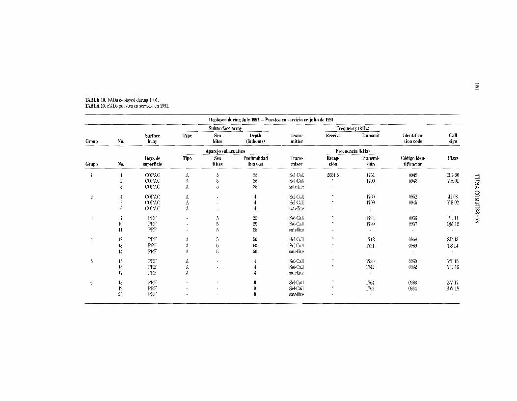
>-'
8
TABLE 10. FADs deployed during 1991. TABLA 10. FADs puestos en servicio en 1991.
Deployed during July 1991 - Puestos en servicio en julio de 1991
Group No. Surface
buoy Type
Subsurface array Sea
kites Depth
(fathoms) Transmitter
Frequency (kHz) Receive Transmit Identifica
tion code Call sign
Grupo No. Boyade
superficie Tipo
Aparejo subacwitico Sea Profundidad
Kites (brazas) Transmisor
Frecuencia (kHz) Recep- Transmi· cion sion
Codigo identificacion
Clave
2
3
1 2 3
4 5 6
7 10 11
COPAC COPAC COPAC
COPAC COPAC COPAC
PRF PRF PRF
A A A
A A A
5 5 5
5 5 5
25 25 25
4 4 4
25 25 25
Sel-Call Sel-Call satellite
Bel-Call Sel-Call satellite
Sel-Call Sel-Call satellite
2331.5
"
1751 1700
1769 1709
1793 1799
0949 0943
0952 0945
0956 0957
HG06 VA01
JI08 YB02
PL 11 QM 12
>-3 cj Z ~
(") 0 ~
~
>-< UJ UJ
0 Z
4 12 13 14
PRF PRF PRF
A A A
5 5 5
50 50 50
Sel-Call Sel-Call satellite
1712 1721
0958 0969
SR 13 TS 14
5 15 16 17
PRF PRF PRF
A A A
4 4 4
Sel-Call SE'I-Call satellite
" 17:30 1742
0960 0962
VT15 YU16
6 18 19 20
PRF PRF PRF
0 0 0
Sel-Call Sel-Call satellite
" 1764 1763
0963 0964
ZV 17 BW18

TABLE 10. (continued) TABLA 10. (continuacion)
Subsurface array Frequency (kHz) Surface Type Sea Depth Trans- Receive Transmit Identifica- Call
Group No. buoy kites (fathoms) rnitter ti(mcode sign
Aparejo sllbacuatico Frecllencia (kHz) Boyade Tipo Sea Profundidad Trans- Recep- Transrni- Codigo iden- Clave
Grupo No. superficie kites (brazas) rnisor cion sion tificacion >Z7 21 FG B 5 50 Sel-Call 2331.5 1727 0947 BD04 Z22 FG B 5 50 Sel-Call 1760 0950 IH07 §223 FG B 5 50 satellite t"" ::cI
8 24 FG 5 25 Sel-Call 1736 0948 EF05 tr:I '1;125 FG 5 25 Sel·Call 1718 0946 ZC03 0
26 FG 5 25 satellite q ...... <09 27 RADIO 5 50 Sel-Call " 1772 0965 EX 19 <0 ......28 RADIO 5 50 Sel-Call 1784 0967 HY20
29 RADIO 5 50 satellite
10 30 RADIO B 3 11 Sel·Call 1787 0954 OKlO 31 RADIO B 3 11 Sel-Call 1778 0953 MJ09 32 RADIO B 3 11 satellite
Deployed during early 1991- Puestos en servicio a principios de 1991
8 COPAC A 4 satellite 9 COPAC A 4 satellite
...... g:
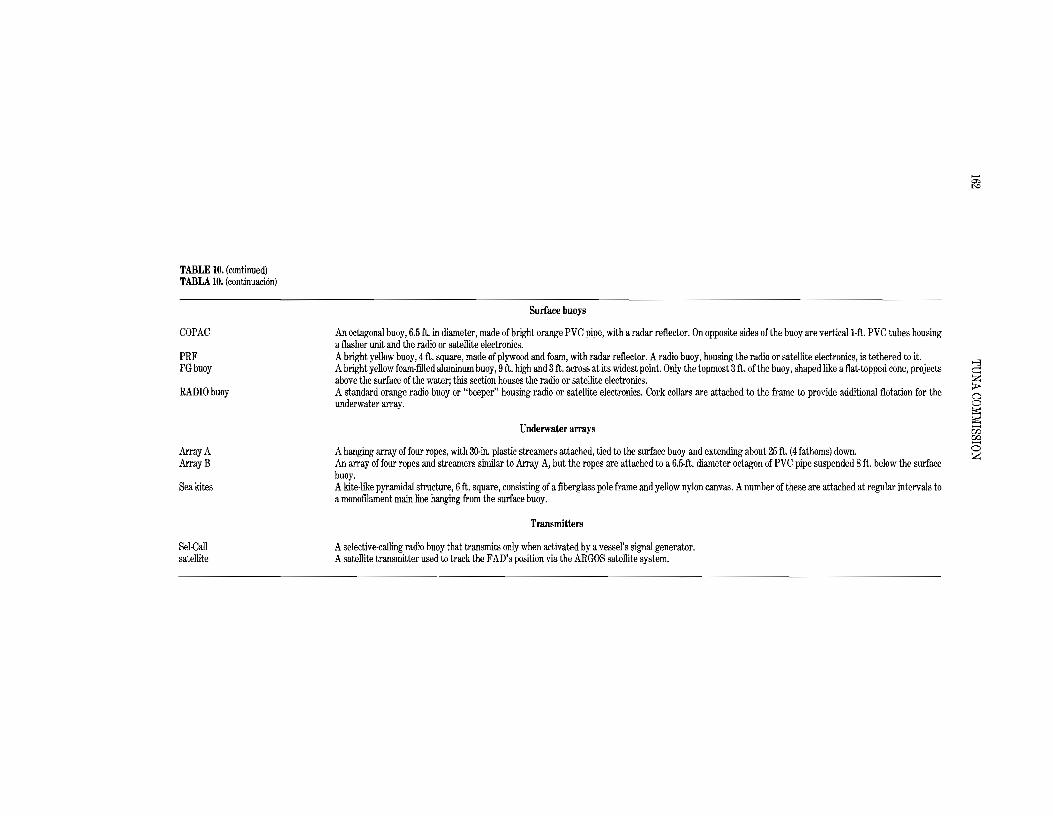
...... ~
TABLE 10. (continued) TABLA 10. (continuaci6n)
Surface buoys
COPAC An octagonal buoy, 6.5 ft. in diameter, made of bright orange PVC pipe, with a radar reflector. On opposite sides of the buoy are verticall-ft. PVC tubes housing a flasher unit and the radio or satellite electronics.
PRF FG buoy
Abright yellow buoy, 4ft. square, made of plywood and foam, with radar reflector. Aradio buoy, housing the radio or satellite electronics, is tethered to it. Abright yellow foam-fIlled aluminum buoy, 9ft. high and 3ft. across at its widest point. Only the topmost 3ft. of the buoy, shaped like aflat-topped cone, projects >-3
c:::: above the surface ofthe water; this section houses the radio or satellite electronics. ~ RADIO buoy A standard orange radio buoy or "beeper" housing radio or satellite electronics. Cork collars are attached to the frame to provide additional flotation for the underwater array.
(") o ~
Underwater arrays en w
Array A ArrayB
Ahanging array of four ropes, with 3O-in. plastic streamers attached, tied to the surface buoy and extending about 25 ft. (4 fathoms) down. An array of four ropes and streamers similar to Array A, but the ropes are attached to a 6.5-ft. diameter octagon of PVC pipe suspended 8 ft. below the surface
(5 Z
buoy. Sea kites Akite-like pyramidal structure, 6ft. square, consisting of a fiberglass pole frame and yellow nylon canvas. Anumber of these are attached at regular intervals to
a monofilament main line hanging from the surface buoy.
Transmitters
Sel-Call Aselective-calling radio buoy that transmits only when activated by a vessel's signal generator. satellite Asatellite transmitter used to track the FAD's position via the ARGOS satellite system.

TABLE 10. (continued) TABLA 10. (continuacion)
Boyas de Superficie
CaPAC Boya octagonal, diametro 2m, fabricado de tubo de PVC de color naranja brillante, con reflector de radar. La luz intermitente y el equipo de radio 0 transmisor a satelite estan montados en tubos de PVC verticales cortos en dos puntos opuestos de la boya.
PRF Boya cuadrada de color amarillo brillante, 1.25 mx 1.25 m, fabricado de espuma de plastica ymadera, con reflector de radar. Lleva amarrada una radioboya con el >Zequipo electronico. Z
BoyaFG Boya de aluminio de color amarillo brillante, Ileno de espuma, 3mde alto y de 1m de ancho mayor. Solamente el tercio superior de la boya, de forma conica, flota §2encima de la superficie del agua; en esta seccion esta el equipo electronico. t:-<
RADIOboya Radioboya comun, color naranja, con equipo electronico. Lleva dos collares de corcho para flotacion adicional para el aparejo subacuatico. ::0 M
:5Apar~osSubacuaticos
~
......Aparejo A 4sogas, con banderillas de plastico de 75 em de largo, atadas ala boya de superficie; longitud 7m. ~ ......
la boya de superficie. "Sea Kites" Estructura piramidal, 2mx2m, de lona de nylon amarillo cubriendo un armazon de varillas de fibra de vidrio. Se sujetan varios de estos a intervalos regulares a
una linea de monofilamento suspendido de la boya de superficie.
Aparejo B 4sogas con banderillas, similares al Aparejo A, excepto que las sogas estan atadas aun octagono de tubo de PVC, de 2mde diametro, suspendido 2.5 mdebajo de
Transmisores Sel-Call Radioboya de transmision selectiva, activada por el generador de seiiales de un barco. satellite Transmisor a satelite usado para rastrear al FAD mediante el sistema de satelite ARGOS.
...... 85
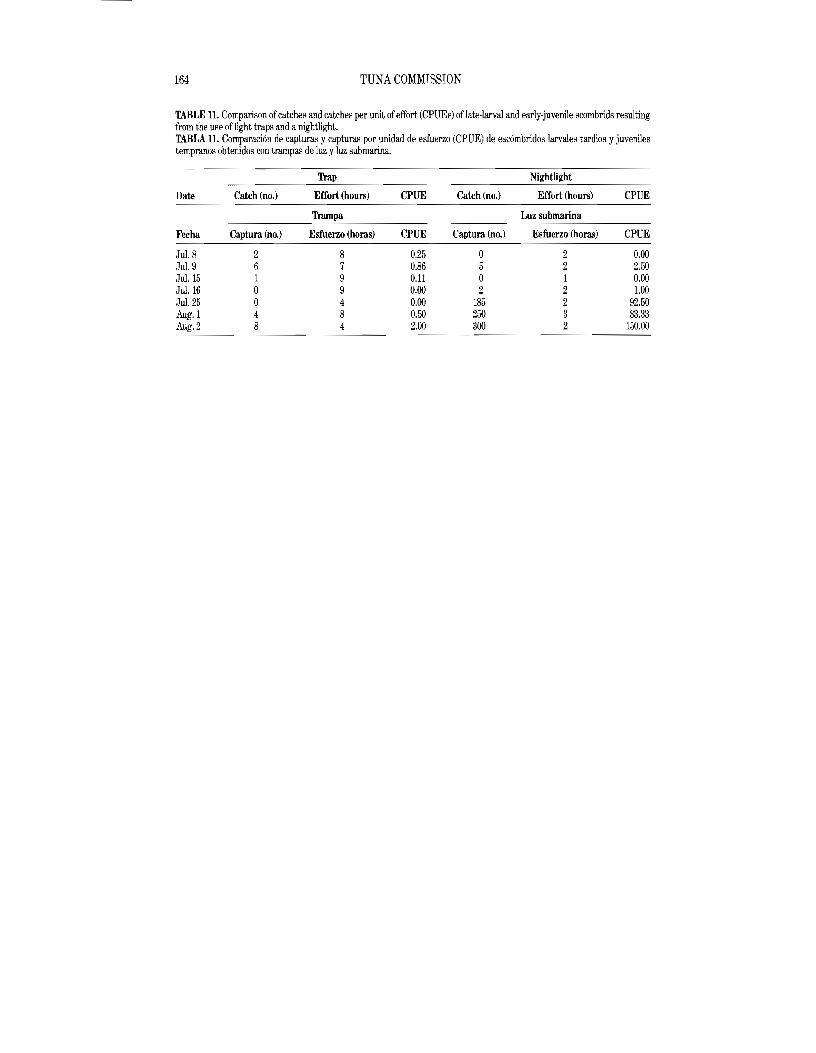
164 TUNA COMMISSION
TABLE 11. Comparison of catches and catches per unit of effort (CPUEs) oflate-Iarval and early-juvenile scombrids resulting from the use of light traps and a nightlight. TABLA 11. Comparaci6n de capturas y capturas por unidad de esfuerzo (CPUE) de esc6mbridos larvales tardios y juveniles tempranos obtenidos con trampas de luz y luz submarina.
Trap Nightlight
Date Catch (no.) Effort (hours) CPUE Catch (no.) Effort (hours) CPUE
Trampa Luz submarina
Fecha Captura (no.) Esfuerzo (horas) CPUE Captura (no.) Esfuerzo (horas) CPUE
Jul. 8 2 8 0.25 0 2 0.00 Jul. 9 6 7 0.86 5 2 2.50 Jul.15 1 9 0.11 0 1 0.00 Jul.16 0 9 0.00 2 2 1.00 Jul. 25 0 4 0.00 185 2 92.50 Aug. 1 4 8 0.50 250 3 83.33 Aug. 2 8 4 2.00 300 2 150.00
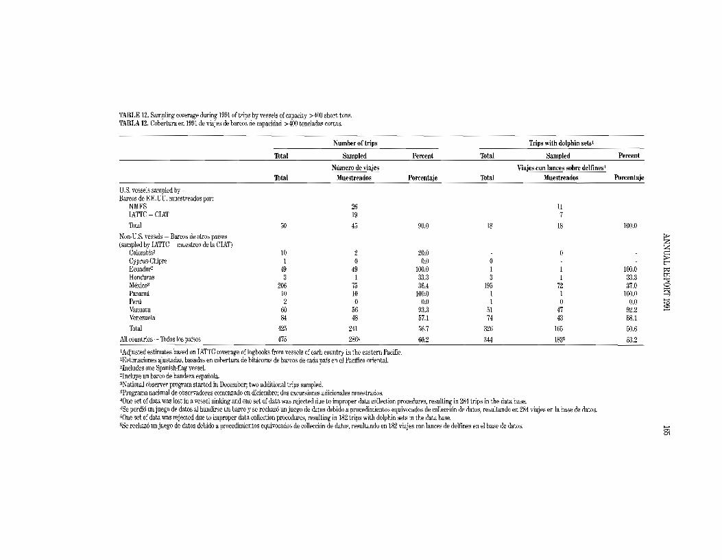
TABLE 12. Sampling coverage during 1991 of trips by vessels of capacity >400 short tons. TABLA 12. Cobertura en 1991 de viajes de barcos de capacidad >400 toneladas cortas.
Number of trips Trips with dolphin sets'
Thtal Sampled Percent Thtal Sampled Percent
Numero de viajes Viajes con lances sobre delfines1
Thtal Muestreados Porcentaje Thtal Muestreados Porcentaje
U.S. vessels sampled by -Barcos de EE.UU. muestreados por:
NMFS 26 11 IATTC-CIAT 19 7 Thtal 50 45 90.0 18 18 100.0
Non-U.S. vessels - Barcos de otros paises >Z(sampled by IATTC - muestreo de la CIAT) Z
Colombia2 10 2 20.0 o ~ Cyprus-Chipre 1 0 0.0 o t"" Ecuador2 49 49 100.0 1 1 100.0 ;0
MHonduras 3 1 33.3 3 1 33.3 "lj
Mexic03 206 75 36.4 195 72 37.0 0
Panama 10 10 100.0 1 1 100.0 ~
......Peru 2 0 0.0 1 o 0.0 <:<::> <:<::>
Vanuatu 60 56 93.3 51 47 92.2 ...... Venezuela 84 48 57.1 74 43 58.1 Thtal 425 241 56.7 326 165 50.6
All countries - Thdos los paises 475 2864 60.2 344 1835 53.2
1Adjusted estimates based on IATTC coverage of logbooks from vessels of each country in the eastern Pacific. lEstimaciones ajustadas, basadas en cobertura de bitacoras de barcos de cada pais en el Pacifico orientaL 2Includes one Spanish-flag vesseL 2Incluye un barco de bandera espanola. 3National observer program started in December; two additional trips sampled. 3Programa nacional de observadores comenzado en diciembre; dos excursiones adicionales muestrados. 40ne set of data was lost in a vessel sinking and one set of data was rejected due to improper data collection procedures, resulting in 284 trips in the data base. 4Se perdi6 un juego de datos al hundirse un barco y se rechaz6 un juego de datos debido a procedimientos equivocados de collecci6n de datos, resultando en 284 viajes en la base de datos. sOne set of data was rejected due to improper data collection procedures, resulting in 182 trips with dolphin sets in the data base. 5Se rechaz6 unjuego de datos debido a procedimientos equivocados de collecci6n de datos, resultando en 182 viajes con lances de delfines en el base de datos. ......
~

166 TUNA COMMISSION
TABLE 13. Training sessions held for observers during 1991. TABLA 13. Cursos de capacitaci6n de observadores durante 1991.
Dates Location Number of attendees
Fechas Sede Numero de asistentes
February 25-March 13 March 11-22 May 21-June 5 September 16-27 December 2-17
Panama. (R.P.) Cumana, Venezuela Buenaventura, Colombia Cuman:!, Venezuela Ensenada, Mexico
3 8
22 25 8
Total 66
TABLE 14. Dolphin mortality workshops sponsored by the IATTC during 1991. TABLA 14. Talleres subre la mortalidad de delfines auspiciados por la CIAT en 1991.
Date
Fecha
.January 8 June 11 August 8
Location
Sede
Ensenada, Mexico Ensenada, Mexico Ensenada, Mexico
Captains
Capitanes
15 7 6
Attendees Others
Asistentes Otras
41 15 11
Total
'lbtal
56 22 17
Total 28 67 95
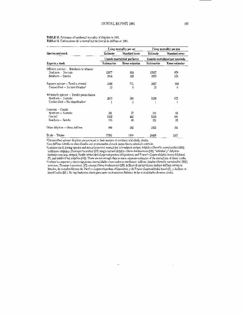
167 ANNUAL REPORT 1991
TABLE 15. Estimates of incidental mortality of dolphins in 1991. TABLA 15. Estimaciones de la mortalidad incidental de delfines en 1991.
Using mortality per set Using mortality per ton Species and stock Estimate Standard error Estimate Standard error
Usando mortalidad POl' lance Usando mortalidad POl' tonelada Especie y stock Estimaci6n Error estlindar Estimaci6n Error estlindar
Offshore spotted - Manchado de altamar Northern -- Norteno 12977 934 13537 978 Southern _. Sureno 1014 122 1023 125
Eastern spinner '!brnillo oriental 5866 771 5927 808 Unidentified No identificados1 13 6 13 6
Whitebelly spinner '!brnillo panza blanca Northern _. Norteno 2973 598 3136 673 Unidentified No identificados1 1 1 1 1
Common - Comun Northern _. Norteiio 161 57 141 64 Central 3182 442 3515 491 Southern - Sureiio 115 30 121 33
Other dolphins - Otros delfines 990 182 1025 191
'!btals '!btales 27292 1439 28439 1537
lUnidentified spinner doiphins are prorated to their eastern or northern whitebelly stocks. 1Los delfines tornillo no identificados son prorrateados al stock panza blanca oriental 0 norteiio. 2Includes the following species and stocks (observed mortalities in brackets): striped dolphins (Stenella coernleoalba) [305J; bottlenose dolphins (Tursiops trnncatus) [57J; rough-toothed dolphins (Steno bredanensis) [29J; "whitebelly" dolphins (includes common, striped, Pacific whitesided (Lagenorhynchus obliquidens), and Fraser's (Lagenodelphis hosei) dolphins) [7], and unidentified dolphins [83]). There are not enough data to make separate estimates of the mortalities of these stocks.
2Incluye las especies y stocks siguientes (mortalidades observados en corchetes): delfines listados (Stenella coernlealba) [305J; tursiones (Tursiops trnncatus) [57]; estenos (Steno bredanensis) [29J; delfines de panza blanca (incluye delfines comunes, listados, de costados blancos del Pacifico (Lagenorhynchus obliquedens), y de Fraser (Lagenodelphis hosei) [7], y delfines no identificados [83]). No hay bastantes datos para hacer estimaciones distintos de las mortalidades de estos stocks.

168 TUNA COMMISSION
TABLE 16. Estimates of average population abundance for 1986·1990, of incidental mortality during 1991, and of the percentage of the population that suffered mortality due to purse·seine fishing for tunas. TABLA 16. Estimaciones de abundancia promedio de poblaci6n para 1986·1990, de mortalidad incidental en 1991, y del porcentaje de la poblaci6n que sufri6 mortalidad debido ala pesqueria cerquera de attin.
Stock Population Incidental Percent abundance mortality mortality
Stock Abundancia de la Mortalidad Mortalidad poblacion incidental porcentual
Northeastern spotted - Manchado del nordeste 738.100 .1
Western and/or southern spotted -Manchado del oeste y/o sureno 1,299,300 .1
All spotted (except coastal)-Thdos los manchados (con excepci6n de costeros) 2,037,400 14,000 0.69
Eastern spinner - Thrnillo oriental 632,700 5,900 0.93
Whitebelly spinner - Thrnillo panza blanca 1,020,100 2,940 0.29
]I;orthern common - Comtin norteno 477,000 122 0.03
Central common - Comun central 415,600 3,150 0.76
Southern common - Comtin sureno 2,211.500 113 0.01
Other dolphins - Otros delfines2 2,729,100 1,045 0.04
Thtal 9,523,400 27,270 0.29
lThe incidental mortalities for the individual stocks of offshore spotted dolphin will be recalculated in accordance \Iith the proposed new stock boundaries.
lLas mortalidades para los stocks individuales de delfines manchados de alta mar seran recalculados de acuerdo con los nuevos limites propuestas para los stocks.
2"Other dolphins" includes striped dolphin, bottlenose dolphin, the coastal stock of spotted dolphin, Fraser's dolphin, rough· toothed dolphin, and Risso's dolphin (Grampus griseus).
2"Otros delfines" incluyen delfines listados, tursiones, el stock costero de delfin manchado, delfines de Fraser, estenos. y delfines de Ri6So (GmmJlUs griseus).
TABLE 17. Numbers of sightings, areas in which stocks occur, and searching effort, 1991. TABLA 17. Numero de observaciones, areas donde los stocks ocurren, y esfuerzo de bUsqueda, 1991.
Species and stock Numbers of Areas of stocks Searching effort sightings (1,000 mn) (1,000 nm)
Especie y stock Numerode Area del stock Esfuerzo de observaciones (1000 ron) btisqueda
(1000 mn)
Offshore spotted - Manchado de altamar Northern - Norteno 2605 3796.6 340.1 Southern - SureJio 112 1414.5 35.4
Spinner - Thmillo Eastem - Oriental 853 2267.1 319.4 Whitebelly - Panza blanca 382 4194.9 248.3
Common - Comtin Northem - Norteno 39 615.3 55.7 Central 388 2186.8 260.4 Southem - Sureno 115 842.4 62.6

TABLE 18. Estimates ofrelative abundances of dolphins for 1991. The bootstrap standard errors are given in parentheses. The asterisks indicate unidentified spinner herds prorated between the eastern and whitebelly stocks. TABLA 18. Estimaciones de la abundancia relativa de los delfines en 1991. Los valores en parentesis son los errores estandar del procedimiento de "bootstrap." Los asteriscos indican manadas de tornillos no identificados prorrateados entre los stocks oriental y panza blanca.
Effective Encounter Average Number Number Number half-width rate herd of of of
of strip (herds/ size herds dolphins dolphins Species and stock (nm) 1,000 nm) (OOOs) (OOOs) (OOOs)
Medioancho Tasa de Tamaiio Numero Numero Numero efectivo encuentro mediode de de de
de la banda (manadas/ manada manadas delfines delfines Especie y stock (mn) 1,000 mn) (OOOs) (OOOs) (OOOs)
~Northern offshore spotted 3.55 8.60 543.7 4601 2502 ZManchado a1tamar del norte (0.18) (0.50) (35.7) (355) (268) Z Southern offshore spotted 3.21 3.15 952.5 695 662 ~
L'Manchado altamar del sur (0.51) (0.36) (109.5) (132) (149) ::0 I?J
Northern and southern 3.52 7.06 658.1 5218 3434 "'CI Del norte y del sur (0.18) (0.38) (37.0) (405) (332) 0
~
Eastern spinner 3.59 3.46 332.6 1093 363 358* ...... Thrnillo del este (0.27) (0.26) (26.3) (120) (49) (65) '"" ~
Whitebelly spinner 3.61 2.92 255.6 1691 432 425* Thrnillo de panza blanca (0.38) (0.31) (24.7) (266) (91) (71)
Eastern whitebelly, and unidentified 3.68 4.26 267.1 2932 783 Del este, de panza blanca, y sin identificaci6n (0.19) (0.37) (17.6) (282) (96)
Northern common 1.7:) 0.70 775.1 125 97 Camtin del norte (0.35) (0.16) (185.5) (33) (41)
Central common 2.08 0.72 333.2 379 126 Comtin central (0.37) (0.07) (65.5) (70) (39)
Southern common 1.53 1.83 606.1 504 305 Comun del sur (0.22) (0.41) (85.6) (136) (79)
...... 0>
'""

170 TUNA COMMISSION
TABLE 19. Thtal numbers of observed sets, percentages of observed sets which were in association with dolphins, and average sea-surface temperatures (SSTs) recorded during dolphin sets in the stock area corresponding' to the northern stock of the common dolphin. TABLA 19. ilftirneros totales de lances observados, porcelltajes de lances observados asociados con delfines, y promedios de las temperaturas superficiales del mar (TSM) registrados durante lances de delfines en el area del stock norteno del delfin comtin.
Year Thtal numbers Percentages of Average SSTs of sets dolphin sets (degrees Celsius)
Ano Numeros totales Porcentajes de TSMs promedios de lances lances con delfines (grados Celsius)
1987 1293 59 23.10 1988 2515 37 23.14 1989 1882 45 23.76 1990 1325 54 23.05 1991 1485 71 24.65

TABLE 20. Estimates of relative abundances of dolphins for 1991 obtained after removing the data for trips with no dolphin sets. TABLA 20. Estimaciones de la abundancia relativa de delfines en 1991, obtenidas tras descartar viajes en los que no efectuaron lances sobre delfines.
Effective Encounter Average Number Number half-width rate herd of of
of strip (herds/ size herds dolphins Species and stock (nm) 1,000 nm) (OOOs) (OOOs) ;p
Z Medioancho Thsa de Thmaiio Ntimero Ntimero Z
efectivo encuentro medio de de de ~
de la banda (manadas/ manada manadas delfines r'
Especies y stock (mn) 1,000 mn) (OOOs) i:'J(OOOs) ;0
>-0Offshore spotted - Manchado de altamar 0
Northern - Norteiio 3.82 8.39 533.0 4167 2221 q ......Southern - Sureiio 3.50 3.85 1050.9 780 819 ~ ......
Spinner - Thrnillo Eastern - Oriental 4.05 3.43 378.9 961 364 Whitebelly - Panza blanca 3.69 2.68 266.9 1522 406
Common - Comun Northern - Norteiio 1.44 0.70 850.7 150 128 Central 2.14 1.00 566.7 510 289
...... -"J ......

172 TUNA COMMISSION
TABLE 21. Estimated average numbers of yelJowfin in the eastern Pacific Ocean, in thousands, for the X and Y cohorts during the 1967 through 1991 seasons. TABLA 21. Estimaciones del mimero promedio de aletas amarillas en el Oceano Pacifico oriental, en miles de peces, para las cohortes XeYentre 1967 y 1991.
Year Quarter XCohort - Cohorte X YCohort - Cohorte Y
Aoo Trimestre 0 I II III IV V VI 0 II III IV V VI 1967 1 0 14419 8310 1198 393 106 49 0 18066 2784 733 205 69 33
2 0 11805 5738 902 277 83 40 37416 12838 1710 505 147 55 27 3 0 8984 3995 686 200 65 33 30633 8217 1333 357 112 45 22 4 21009 7207 3165 504 148 52 27 25079 6528 1035 250 87 36 18
1968 1 0 17201 5688 2373 362 112 42 0 20500 5091 777 179 69 30 2 0 14076 3878 1184 244 87 34 25309 15254 3487 533 128 55 24 3 0 11479 2833 834 173 69 28 20721 9663 2469 363 97 44 20 4 23667 9182 2258 609 128 55 23 16945 7612 1923 256 75 36 16
1969 1 0 19377 7027 1791 411 97 44 0 13645 5426 1254 177 59 29 2 0 15760 4927 1369 246 75 36 27242 9007 3241 603 124 48 24 3 0 12530 3869 1042 172 59 29 22304 6246 2465 381 95 38 20 4 27218 9403 3064 723 125 47 24 18259 4638 1851 237 74 31 16
1970 1 0 22284 6301 2191 465 95 38 0 14668 2976 1270 157 58 25 2 0 18238 3757 1269 229 74 31 2(;869 10513 1720 737 103 47 20 3 0 14789 2840 872 152 58 25 21998 7163 1325 460 78 37 17 4 34665 11445 2152 56:3 107 4(; 21 17994 5313 988 285 61 30 14
1971 1 0 28378 8296 1576 359 81 37 0 14430 3822 653 153 48 25 2 0 23059 5707 1172 226 61 30 27624 9994 2322 408 105 38 20 3 0 18506 4454 848 157 48 25 22617 7440 1736 271 79 31 17 4 19886 14210 3517 529 110 38 20 18514 5863 12(;8 149 62 25 14
1972 1 0 16281 10650 2222 305 78 31 0 14652 408.3 680 80 49 20 2 0 13312 6578 1065 173 59 25 36871 10839 2860 314 47 38 17 3 0 10808 4901 729 84 47 21 30187 7851 2173 156 31 31 14 4 16817 8699 3504 454 45 37 17 24713 6194 1587 70 24 25 11
1973 1 0 13769 6936 2430 222 32 30 0 1945(; 4257 1061 41 19 20 2 0 10982 5191 1298 104 25 24 68941 9353 2594 577 26 15 17 3 0 8843 4133 913 56 20 20 56444 5261 1927 258 17 12 14 4 4(;972 7043 32.'13 447 30 16 16 45879 3673 1451 82 13 10 11
1974 1 0 38457 5387 2003 229 17 13 0 339(;0 2558 969 23 10 8 2 0 31242 4089 1122 139 13 10 29101 18394 1737 (;29 13 8 7 3 0 25011 3291 763 55 11 8 23823 10143 1325 307 9 6 5 4 36764 19509 2557 448 22 8 7 18602 7251 975 145 7 5 4
1975 1 0 30089 12924 1739 271 11 7 0 14620 5120 670 78 5 4 2 0 23947 8674 1003 132 7 5 :36986 10768 3559 377 28 4 3 3 0 17996 6196 607 49 5 4 :30193 8097 2429 192 11 3 3 4 17375 13406 4601 347 19 4 4 24108 13484 1598 83 6 2 2
1976 1 0 14221 9936 299(; 207 11 3 0 16160 4984 1099 32 5 2 2 0 11513 5938 1995 89 6 3 28536 9342 3760 628 13 4 2 3 0 8891 4203 1248 31 5 2 23329 5643 2354 238 9 3 1 4 18777 6410 3209 687 15 4 2 18609 3824 1434 76 6 2 1

173 ANNUAL REPORT 1991
TABLE 21. (continued) TABLA 21. (continuaci6n)
XCohort- Cohorte X YCohort - Cohorte YYear Quarter Ano Trimestre 0 I II III IV V VI 0 I II III IV V VI
1977 1 0 15293 4850 2324 259 9 3 0 13929 2693 1032 34 5 2 2 0 12109 3183 1515 152 6 3 69666 8012 1886 698 23 4 2 3 0 9320 2210 671 57 5 2 56693 4613 1097 252 12 3 1 4 34335 6733 1554 303 15 4 2 43582 3213 772 75 7 2 1
1978 1 0 27965 4919 1171 174 9 3 0 29044 2337 555 32 5 2 2 0 19591 3349 744 113 6 3 42531 13648 1585 377 18 4 2 3 0 12208 2494 504 54 5 2 34119 7993 1177 226 10 3 1 4 39612 8919 1784 284 14 4 2 25755 5773 843 79 4 3 1
1979 1 0 32402 5961 1286 151 7 :J 0 16715 4039 516 39 2 2 2 0 24352 3937 767 87 5 3 40076 9713 2244 334 23 2 2 3 0 16531 3018 493 35 4 2 31868 6014 1540 174 13 2 1 4 30239 9421 2259 314 22 3 2 20541 4129 1036 113 10 1 1
1980 1 0 24251 6248 1627 160 9 2 0 13604 3080 584 51 6 2 0 16941 3206 1186 75 3 2 42635 7385 2296 370 16 2 3 0 10043 2279 821 31 2 2 34446 4662 1577 182 7 1 4 22106 6710 1679 544 16 2 26610 3404 1093 100 4 1
1981 1 0 17819 4775 1177 300 10 0 19216 2593 797 51 2 1 2 0 12763 3080 811 133 4 31347 11176 1815 521 15 1 1 3 0 7757 2072 536 63 4 25366 5737 1308 226 8 1 0 4 24063 4170 1386 309 42 3 19374 3377 820 140 5 1 0
1982 1 0 19281 2577 989 174 10 2 0 13089 2135 555 41 3 1 2 0 12656 1752 671 100 5 2 39268 8269 958 369 21 3 1 3 0 7702 1333 440 50 4 2 31013 5205 686 180 13 2 1 4 31699 5386 1044 249 24 2 21259 4026 445 93 7 2 0
1983 1 0 25770 4081 818 77 6 0 15094 3262 268 20 2 2 0 19628 2982 612 28 3 42005 10360 2529 147 7 2 3 0 13539 2272 404 13 2 34237 7683 1779 80 5 1 4 40064 10068 1743 264 8 1 27251 6131 981 42 3 1
1984 1 0 32495 8124 1340 123 5 0 21484 4833 590 18 2 1 2 0 25490 6193 983 55 3 39097 16566 3349 345 8 1 1 3 0 17976 4880 654 18 2 31766 12780 2358 148 2 1 1 4 41515 12419 3677 352 6 2 25870 9613 1517 58 1 1 0
1985 1 0 33988 9532 2697 140 2 0 21071 7155 923 20 1 1 2 0 27185 7404 1771 56 1 34516 16415 4897 448 7 1 1 3 0 21843 5354 1062 16 1 28021 12892 3217 171 2 1 1 4 40663 16877 4061 577 4 1 22780 10103 2061 55 1 0 0
1986 1 0 33103 10361 2974 296 2 1 0 17335 7688 1273 24 1 0 2 0 26779 7365 1822 95 1 0 39491 13326 5088 594 7 1 0 3 0 21232 5887 1020 21 1 0 32128 9669 3331 167 3 1 0 4 51423 16431 4661 527 7 1 0 24364 6351 2211 54 2 0 0

174 TUNA COMMISSION
TABLE 21. (continued) TABLA 21. (continuaci6n)
Year Quarter XCohort - Cohorte X YCohort - Cohorte Y
Aim Trimestre 0 I II III IV V VI 0 I II III IV V VI
1987 1 0 41835 12530 3515 279 4 1 0 18284 4670 1441 16 0 2 0 33342 8616 2108 155 2 1 75892 13154 3007 838 5 0 3 0 25115 6322 1181 57 1 0 61914 10082 2044 318 2 0 4 51056 16756 4086 610 19 1 0 49824 7898 1400 141 1 0
1988 1 0 41698 12221 2936 331 5 1 0 37604 6038 987 43 0 2 0 32722 8305 1996 117 2 1 54308 21994 4449 574 6 0 3 0 23881 6106 1338 39 1 0 44343 15443 3321 295 1 0 4 52176 17135 4228 814 14 1 0 35380 10768 2118 147 0 0
1989 1 0 42691 12292 3085 442 5 1 0 27861 7437 1390 68 0 0 2 0 33482 8580 1998 210 2 1 50428 20879 5317 806 25 0 0 3 0 25501 5889 1259 89 1 0 41217 16069 3661 369 16 0 0 4 43186 18352 4040 722 34 1 0 33025 12067 2431 151 11 0 0
1990 1 0 35253 13682 2762 323 15 1 0 26065 9076 1527 32 8 0 2 0 28089 9463 1824 167 9 0 48475 18757 6061 887 10 6 0 3 0 21968 6536 1244 78 7 0 39661 13074 4118 391 6 5 0 4 48558 17148 4787 759 44 6 0 31000 9837 2895 191 3 4 0
1991 1 0 39707 13323 3523 377 28 4 0 22160 7530 1787 70 2 3 2 0 31039 9332 2465 183 19 4 49309 14726 5329 1066 28 3 3 0 24388 6515 1557 71 12 3 40288 10612 3833 592 3 2 4 48550 18967 4772 1004 46 9 2 31998 7667 2910 376 1 2

175 ANNUAL REPORT 1991
TABLE 22. Estimated recruitment, in thousands of fish, of the Xand Y cohorts, and of the Xand Ycohorts combined. The initial estimates correspond to the numbers of fish at the beginning of the first month in the first year that they reach alength of 30 em (November for the Xgroup and May for the Y group). The average estimates correspond to the average numbers alive during that first month; these numbers are the same as those in Table 1. TABLA 22. Reclutamiento estimado, en miles de peces, de las cohortes X e Y, y de las cohortes X e Y combinadas. Las estimaciones iniciales corresponden al numero de peces al principio del primer mes del primer ano en el cual alcanzaron una talla de 30 em (noviembre para el grupo Xy mayo para el grupo Y). Las estimaciones medias corresponden al numero medio vivo durante ese primer mes; estas cantidades son identicas a aquellas en la Tabla 1.
Initial- Inicial Average - Promedio
Year - Aiio X Y XtY X Y XtY
1967 21717 38677 60394 21009 37416 58425 1968 24465 26162 50627 23667 25309 48976 1969 28136 28161 56297 27218 27242 54460 1970 35833 27774 63607 34665 26869 61534 1971 20557 28555 49112 19886 27624 47510 1972 17384 38114 55498 16817 36871 53688 1973 48555 71264 119819 46972 68941 115913 1974 38007 30082 68089 36764 29101 65865 1975 17961 38233 56194 17375 36986 54361 1976 19430 29498 48928 18777 28536 47313 1977 35492 72014 107506 34335 69666 104001 1978 40950 44043 84993 39612 42531 82143 1979 31259 41451 72710 30239 40076 70315 1980 22851 44078 66929 22106 42635 64741 1981 24881 32409 57290 24063 31347 55410 1982 32779 40597 73376 31699 39268 70967 1983 41414 43429 84843 40064 42005 82069 1984 42914 40435 83349 41515 39097 80612 1985 42033 35680 77713 40663 34516 75179 1986 53183 40822 94005 51423 39491 90914 1987 52778 78451 131229 51056 75892 126948 1988 53938 56151 110089 52176 54308 106484 1989 44642 52127 96769 43186 50428 93614 1990 50207 50109 100316 48558 48475 97033 1991 50186 50971 101157 48550 49309 97859
Average - Promedio 38763 46926 85689 37495 45389 82884
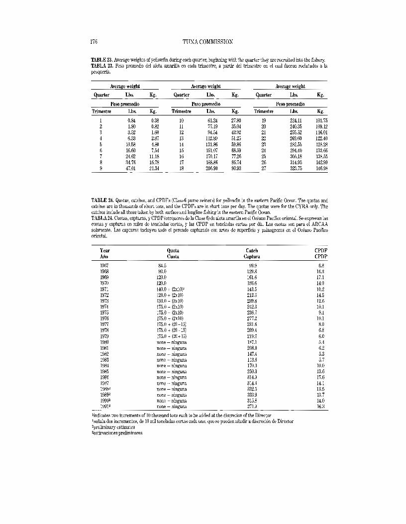
176 TUNA COMMISSION
TABLE 23. Average weights of yellowfm during each quarter, beginning with the quarter they are recruited into the fishery. TABLA 23. Peso promedio del aleta amarilla en cada trimestre, a partir del trimestre en el cual fueron reclutados a la pesqueria.
Average weight Average weight Average weight
Quarter Lbs. Kg. Quarter Lbs. Kg. Quarter Lbs. Kg.
Peso promedio Peso promedio Peso promedio Trimestre Lbs. Kg. Trimestre Lbs. Kg. Trimestre Lbs. Kg.
1 0.84 0.38 10 61.24 27.80 19 224.11 101.75 2 1.80 0.82 11 77.19 35.04 20 240.35 109.12 3 3.52 1.60 12 94.54 42.92 21 255.52 116.01 4 6.33 2.87 13 112.89 51.25 22 269.60 122.40 5 10.58 4.80 14 131.86 59.86 23 282.55 128.28 6 16.60 7.54 15 151.07 68.59 24 294.40 133.66 7 24.62 lLl8 16 170.17 77.26 25 305.18 138.55 8 34.76 15.78 17 188.86 85.74 26 314.95 142.99 9 47.01 21.34 18 206.90 93.93 27 323.75 146.98
TABLE 24. Quotas, catches, and CPDFs (Class-6 purse seiners) for yello\\1in in the eastern Pacific Ocean. The quotas and catches are in thousands of short tons, and the CPDFs are in short tons per day. The quotas were for the CYRA only. The catches include all those taken by both surface and longline fishing in the eastern Pacific Ocean. TABLA 24. Cuotas, capturas, y CPDP (cerqueros de Ia Clase 6) de aleta amarilla en el Oceano Pacifico oriental. Se expresan las cuotas y capturas en miles de toneladascortas, y las CPDP en toneladas cortas por dia. Las cuotas son para el ARCAA solamente. Las capturas incluyen todo el pescado capturado con artes de superficie y palangreras en el Oceano Pacifico oriental.
Year Quota Catch CPDF AiIO Cuota Captura CPDP
1967 84.5 99.9 6.8 1968 93.0 129.8 16.3 1969 120.0 161.6 17.1 1970 120.0 186.6 14.0 1971 140.0 + (2xlO)1 143.5 10.2 1972 120.0 + (2xl0) 212.3 14.5 1973 130.0 + (3xlO) 239.8 12.6 1974 175.0 + (2xl0) 242.3 10.1 1975 175.0 + (2xlO) 236.7 9.1 1976 175.0 + (2xlO) 277.2 10.1 1977 175.0 + (20 +15) 231.6 8.0 1978 175.0 + (20+ 15) 209.4 6.8 1979 175.0 + (20+ 15) 219.7 6.0 1980 none - ninguna 187.1 5.4 1981 none - ninguna 208.0 6.2 1982 none - ninguna 147.4 5.3 1983 none - ninguna 113.6 5.7 1984 none - ninguna 170.0 10.0 1985 none - ninguna 250.3 13.6 1986 none - ninguna 314.9 17.6 1987 none - ninguna 314.4 14.1 19882 none - ninguna 332.5 13.5 19892 none - ninguna 333.9 13.7 19902 none - ninguna 315.8 14.0 19912 none - ninguna 271.9 16.3
lindicates two increments of 10 thousand tons each to be added at the discretion of the Director lseiiala dos incrementos, de 10 mil toneladas cortas cada uno, que se pueden aJiadir a discreci6n de Director 2preliminary estimates 2estimaciones preliminares
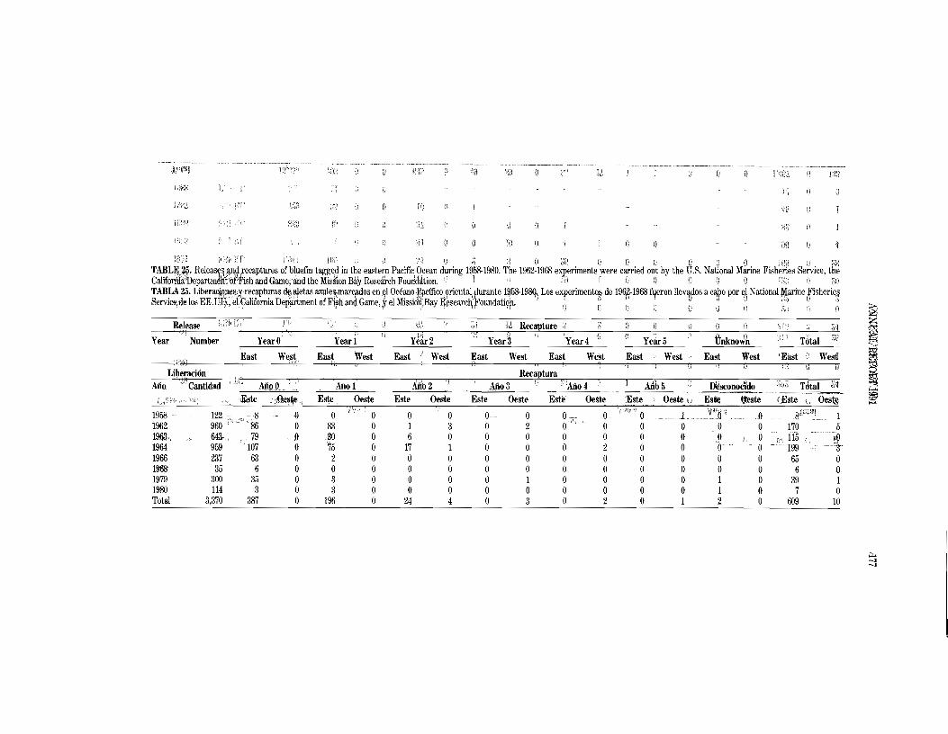
J},l-rq IJ FP l'J ~i\ o 10, 0 n 13:1
\) 42 IJ
(/ G (j il
() TO (l (I'I o ()f! i
i ;) :J 0 il(! 0 () II \) U (j j(!8 U ');.( TABL~J\i. Release~,an4,~ecaptures ofbluefm tagg~d in the eastern Pacific Ocean during 1958-1980. The 1962-1968 experiments were carried out by the U.S. National Marine Fisheries Service, the Califori\i~';Departm~1ft uf'Fish and Game; and the Misilion Bay ReseM-ch Found~tion. 1 Ii) T 0 !J 0 ,1 I)
TABLA.. 25. LiberaGi.q~~!,y,recaPturas dll fIIetas azule~... marci!dos en~l Oceano EjiCifico.,Oriental.(!urante 1~58-198(j, Los experimentQS. de 196~-1968 fljeron llev~dos a cWo pOl' eJ National Marine Fisheries Service;delos EE.U,q;.;elCalifornia DeIiill"tment ofFl~h and'Game,~ el Missiori,Bay R~searc~Foundati?n. I . ;1 ': ; I I, ) :,!) \) S
: '., ' .; .! \) ~I (} \1 {, 0 tz:Release 'J :.'il; ;,/ r~ Recapture :! :; () 0 u 0 I: :; Ii: IJ iN ~ Year , Number Year 0 Yead Ye~r2 J Year3 'rear4 0 n Year 5 tJnknowit :{i I Tb1aIW
I ~
te"
'V" East We~t East West E~W~ ~ast West East West East West East West 'East (I West"
~ ..... 1958 8 0 0 0 0 0 0 0 0.,- 00 1 0 1 1962 86 0 83 0 1 3 0 2 0 .' 0 0 0 0 0 170 19&'L 79 030 0 6 0 0 0 0 0 0 000 115 1964 107 0 75 0 17 1 0 0 0 2 0 0 '0 .., 0 199 1966 63 0 2 0 0 0 0 0 0 0 0 0 0 0 65 o 1968 6 00 00 00 00 00 00 06 ,.~
1979 35 0 3 0 0 0 0 1 0 0 0 0 1 0 39 1 1980 3 03 00 00 00 00 01 07 o Total 387 0 196 0 24 4 0 3 0 2 0 1 2 0 609 10
~
::l
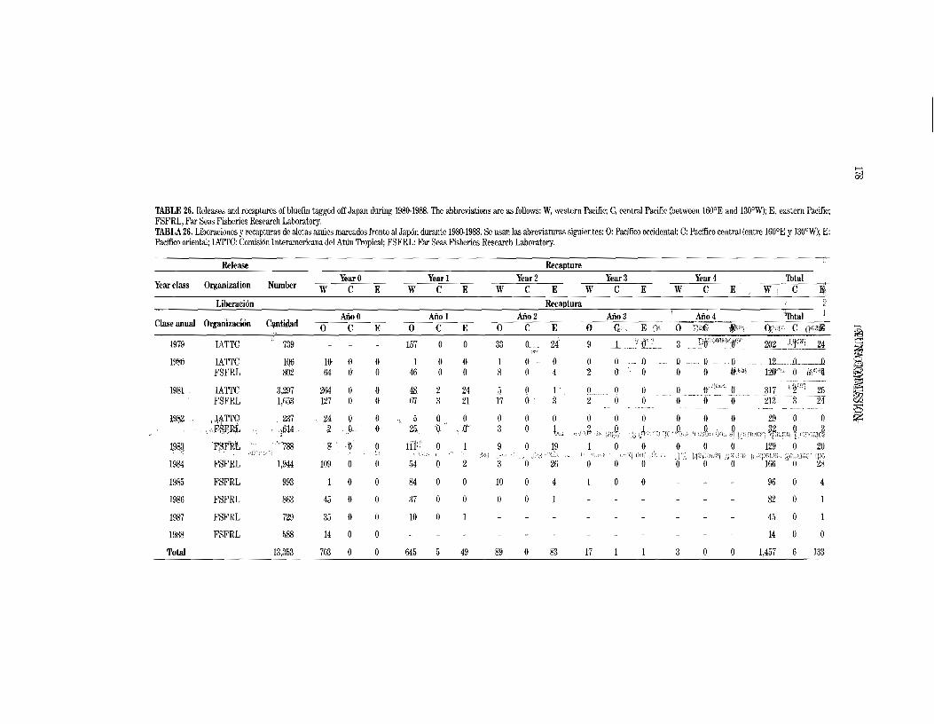
>-'
til
TABLE 26. Releases and recaptures of bluefin tagged off Japan during 1980·1988. The abbreviations are as follows: W, western Pacific; C, central Pacific (between 1600 E and 130°W); E, eastern Pacific; FSFRL, Far Seas Fisheries Research Laboratory. TABLA 26. Liberaciones y recapturas de aletas azules marcados frente aJ Jap6n durante 1980·1988. Se usan las abreviaturas siguientes: 0: Pacifico occidental; C: Pacifico central (entre 1600 E y 130°W); E: Pacifico oriental; IATTe: Comisi6n Intcramericana del Attin Tropical; FSFRL: Far Seas Fisheries Research Laboratory.
Release Recapture VearO Vearl Year 2 Vear3 Year 4 'lbtal
Vear class Organization Number W C E W C E W C E W C E W C E W C J¥i Liberaci6n Recaptura ?
Ano 0 Ano 1 ADo 2 Afto3 ~ ... ADo 4 ~tal
Clase anual OrganlzaciOn C~nt:idad 0 CEO CEO CEO ri' E- . 0 Eg~ ~8i, Q"\', C Ob2J: § 1979 IATTC 739 157 o o 33 0., 24 9 L .1 1'L2 3 ..!!6'i~!llJnri':~ .~LL~~'Il_..M 'CO:
~
1986 IATTC 11)6 10 {) o 1 o 0- 1 0 O.(). 0 0 0 0 -0. 12__ JL ..~,Jl
FSFRL 802 04 tl o 46 o o 8 0 42 0 0 0 0 11,S8\ tID"" 0 M£211 ~
1981 IATTC 3,297 204 o o 48 2 24 fi o l' () o o o oFSFRL 1,653 127 o o 67 3 21 17 o 3 2 o o o 0"- ~ o
~9~ lJiTTO 237 24 0 0 ;; 0 o o o o o o o o 0 29 0 o ~
. ,WSFRL 1614 290 2Sti 3 o
198;1 ~FRt 788 S iJ li'F 0 9 o w o o o 0 129 0 20 ~ J' "'! ., fi:le:}JGt;!B>, CpG
1984 FSFRL 1,944 109 0 0 54 0 2 o 26 o o '0' 166 28
1985 FSFRL 993 o o 84 o o 10 o 4 o o 96 0 4
1986 FSFRL 863 45 0 o 37 o o o o 82 0
1987 FSFRL 729 35 0 o 10 o 45 0
1988 FSFRL 588 14 0 o 14 0 o Total 13,353 703 0 o 045 5 49 89 o 83 17 3 o o 1,457 6 133

179 ANNUAL REPORT 1991
TABLE 27. Estimated numbers of bluefin, in thousands, caught in the western and eastern Pacific Oceans. TABLA 27. Numero estimado de a1etas azules, en miles, capturados en el Oceano Pacifico occidental y oriental.
Western Pacific Ocean Eastern Pacific Ocean
Year class 0 1 2 1 2
Oceano Pacifico occidental Oceano Pacifico oriental Clase anual 0 1 2 1 2
1958 17 47 1959 24 298 1960 577 450 1961 990 529 1962 501 202 1963 982 288 1964 91 333 715 1965 266 3 622 308 1966 1270 461 1 97 155 1967 3607 964 78 416 311 1968 2300 371 48 290 256 1969 2970 378 2 13 556 1970 1938 443 15 366 1971 3316 682 20 458 1972 498 124 28 810 407 1973 4875 1403 46 163 529 1974 3953 676 96 439 173 1975 1277 222 61 483 211 1976 1784 698 151 50 94 1977 2542 478 98 473 457 1978 5091 1452 119 161 225 1979 2088 611 180 118 60 1980 2810 605 200 6 88 1981 1975 785 139 281 69 1982 665 213 44 28 42 1983 1362 421 49 35 272 1984 2417 757 61 117 369 1985 2046 760 40 62 1986 1470 16 47
TABLE 28. Correlations for various combinations of catches of bluefin. WPO and EPO stand for western and eastern Pacific Ocean, respectively. TABLA 28. Correlaciones para varias combinaciones de capturas de a1eta azul. WPO = Oceano Pacifico occidental; EPO =
Oceano Pacifico oriental.
Correlation Degrees of freedom r
Correlacion Grados de libertad r
1. WPO, age 0, versus EPO, age 1 18 -0.069 2. WPO, age 0, versus EPO, age 2 18 0.386 3. WPO, age 1, versus EPO, age 1 18 -0.306 4. WPO, age 1, versus EPO, age 2 18 0.D78 5. WPO, age 2, versus EPO, age 1 18 -0.278 6. WPO, age 2, versus EPO, age 2 18 -0.463* 7. EPO, age 1, versus EPO, age 2 18 0.418 8. WPO, age 0, versus WPO, age 1 18 0.843** 9. WPO, age 0, versus WPO, age 2 17 0.174
10. WPO, age 1, versus WPO, age 2 18 0.344
11. EPO, age 2,versus WPO, age 0, 15 0.746** and WPO, age 2
* significant at 5-percent level **significant at I-percent level

------
...... ~
TABLE 29. Growth, weight-length, and fishing mortality data used for estimation of yields per recruit of northern bluefin. TABLA 29. Datos de crecimiento, peso-talla, y mortalidad de pesca usados para estimaci6n de rendimientos por recluta de atun aleta azul norteno.
Age in years Equation Units of measurement Source
Edad en anos Ecuaci6n Unidades de medir Fuente
Growth - Crecimiento 0.1250·1.0037 Lt20.001 = 5810.001 + (Ltl0.001 - 5810.00l)eO.01184(t2 - t1) millimeters, days IATTC Bull., Vol. 20, No.1 1.0037-5.0000 Lt = 564 + 0.70911t millimeters, days IATTC Bull., Vol. 20, No.1 5.0000-15.0000 Lt = 1595 + 63.500M millimeters, years linear interpolation
Weight-length - Peso-talla >-3
0.1250-0.6250 w =(2.87819 x 10⁻⁹)[3.33350 millimeters, kilograms IATTC Spec. Rep., No.7 c::: ~ 0.6250-15.0000 w= (1.92917 x 10⁻⁷)[2.79464 millimeters, pounds lATTC Spec. Rep., No.7 (") o
Fishing mortality - Mortalidad de pesca ~
First-year migrants - Emigrantes del ano primero ~ ....... w~arO ~ar1 Year 2 Years 3 and 4 Year 5 Subsequent years w
Aiio 0 Aiio 1 Aiio2 Aiios3y4 Aiio5 Aiios siguentes o zMay 16.-Jun. 30 0.0 Jan.-Jun. 0.0 Jan.-Mar. 0.0 Jan.-Dec. 0.0 Jan.1-Mav 15 0.5 Jan.-Dec. 1.0 .luI. 0.5 Jul.-Sep. 1.0 Apr.-Jun. 0.5 May 16-Dec. 31 1.0 Aug.-Sep. 1.0 Oct.-Dec. 0.5 Jul.-Sep. 1.0 Oct.-Dec. 0.5 Oct.-Dec. 0.5
Second-year migrants - Emigrantes del ano segundo Year 0 Year 1 Year 2 Years 3and 4 Year 5 Subsequent years AiioO Aiio 1 Aiio2 Alios 3y 4 Aiio5 Alios siguentes
May 16-Jun. 30 0.0 Jan.-Sep. 1.0 Jan.·Mar. 0.0 Jan.-Dec. 0.0 Jan. I-May 15 0.5 Jan.-Dec. 1.0 .luI. 0.5 Oct.-Dec. 0.5 Apr.-Jun. 0.5 May 16-Dec. 31 1.0 Aug.·Dec. 1.0 Jul.·Sep. 1.0
Oct.-Dec. 0.5

181 ANNUAL REPORT 1991
TABLE 30. Annual catches of bigeye, in short tons, by all gear in the Pacific Ocean and by swface and longline gear in the eastern Pacific Ocean. The 1991 data are preliminary. TABLA 30. Capturas anuales de patudo, en toneladas cortas, logradas por todas las artes en el Oceano Pacifico, y por artes de superficie y palangre en el Oceano Pacifico oriental. Los datos de 1991 son preliminares.
Year
Ano
1954 1955 1956 1957 1958 1959 1960 1961 1962 1963 1964 1965 1966 1967 1968 1969 1970 1971 1972 1973 1974 1975 1976 1977 1978 1979 1980 1981 1982 1983 1984 1985 1986 1987 1988 1989 1990 1991
Eastern Pacific Ocean
Surface Longline
Oceano Pacifico oriental
de superficie
303 129 44 75
256 165 202 235 361
83 75
130 294
1,834 2,820
635 1,469 2,829 2,467 2,181
981 4,104
11,228 7,777
12,912 8,303
16,999 11,124 4,522 3,593 6,539 4,996 2,137
850 1,161 1,621 5,232 4,008
palangre
2,187 2,459 3,271
13,175 14,389 16,231 25,562 72,942 63,503 89,677 56,889 37,346 42,175 43,716 43,072 63,631 40,519 34,902 43,006 61,170 48,669 54,762 61,348 81,333 82,015 75,098 78,928 54,951 50,632 63,775 50,285 62,874 84,487 99,049
Thtal Pacific Ocean,all gear
Thtal Oceano Pacifico, todas las artes
92,900 75,700 85,000 87,900 73,900 87,900 83,800 74,700 98,000 98,400 98,533
112,895 139,500 158,718 129,986 138,908 133,931 111,445 119,919 122,169 113,136 136,605 165,568 165,897 133,003 141,032 149,633

TABLE 31. Data on tagged bigeye at liberty long periods of time (from IATTC Special Report, 2: page 259). The lengths are given in centimeters and the distances in nautical miles. TABLA 31. Datos de petudos en libertad durante largos periodos (del Informe Especial N° 2de la CIAT; pagina 259). Se expresan las tallas en centimetros y las distancias en millas miuticas. .......
00 t-:l
Release Recapture Distance Days free Direction Reference
Area Date Length Area Date Length
Liheracion Recaptura Distancia Diasen Direccion Referencia
Area Fecha Talla Area Fecha Talla Iihertad
300 59'N- Jan. 31, 122.3 32°41' N- Nov. 24, 126.8 785 298 82
l7l°I4'W 1955 155°57'W 1955
300 59'N- Jan. 31, 109.0 29°50'N- Feb.2, 127.5 348 368 259 2
l7lo14'W 1955 117°50'W 1956
32°59'N- May 31. 82 29°15' N- Nov. ll, llO-ll5 540 530 >-3 255 2 C
Z143°19'E 1958 133°45'E 1959 ~
n 32°59'N- May 31, 81 35°27'N- Jan. 17, ll9 182 597 0
~324 2 ~
143°19'E 1958 141 °10' E 1960 en en
3°18'N- May 6. 80 2°12' S- Jan. 13, ? 664 253 23 ll7 IATTC, Z
900 50'W 1967 81°01'W 1968 unpublished
3°18' N- May 12, 50 4°32'N- Jun. 18. 128.0 1,020 769
274 3 900 50'W 1967 107°50'W 1969
Cairns, 1986 Gilbert ca. 2,000 31 mos. ca. 45 4 Australia Islands
Cairns, 1986 Line ca. 3,600 43 mos. ca. 60 Australia Islands
Cairns, 1986 Solomon ca. 1,500 ca. 1,650 ca. 45 4 Australia Islands
1. Pacif. Sci., 10 (2): 236. 2. Nankai Reg. Fish. Res. Lab., Rep., 25: 75-80. 3. IATTC, Ann. Rep., 1969: 28. 4. Austral. Fish., 51 (6): 24.

INFORME ANUAL DE LA COMISION INTERAMERICANA DEL ATUN TROPICAL, 1991
INTRODUCCION
La Comisi6n Interamericana del Atun Tropical funciona bajo la autoridad y direcci6n de un convenio suscrito originalmente pOl' Costa Rica y los Estados Unidos de America. El convenio, vigente desde 1950, esta abierto a la afilia- ci6n de cualquier pais cuyos ciudadanos pesquen atunes tropicales en el Oceano Pacifico oriental. Bajo esta estipulaci6n, la Republica de Panama se afili6 en 1953, Ecuador en 1961, Mexico en 1964, Canada en 1968, Jap6n en 1970, y Francia y Nicaragua en 1973. Ecuador se retir6 de la Comisi6n en 1968, Mexico en 1978, Costa Rica en 1979, y Canada en 1984. Costa Rica se adhiri6 de nuevo al Convenio en 1989, y Vanuatu se hizo miembro de la Comisi6n en 1990.
Las obligaciones principales de la Comisi6n bajo el Convenio son (1) estudiar la biologia de los atunes y especies afines en el Oceano Pacifico oriental para determinar los efectos de la pesca y los factores naturales sobre su abundancia, y (2) recomendar las medidas de conservaci6n apropiadas para que los stocks de peces puedan mantenerse a niveles que permitan capturas maximas sostenibles.
En 1976 se ampliaron las obligaciones de la Comisi6n para abarcar los problemas ocasionados porIa relaci6n atun-delfin en el Oceano Pacifico oriental. Los objetivos acordados en torno a esta cuesti6n son: "[1] mantener la producci6n atunera a un alto nivel; [2] mantener las poblaciones de delfines aniveles 0 sobre niveles que garanticen su supervivencia aperpetuidad; [3] trabajar en cuanto sea posible para evitar la muerte innecesaria 0 pOI' descuido de los delfines en las maniobras de pesca". Los puntos especificos de participaci6n son: (1) vigilar la magnitud de las poblaciones y la mortalidad incidental a la pesca, mediante la toma de datos a bordo de embarcaciones atuneras de cerco; (2) realizar reconocimientos aereos y marcado de delfines; (3) analizar los indices de abundancia de los delfines; y (4) proceder al entrenamiento e investigaci6n sobre las artes de pesca y el comportamiento de los delfines.
Para cumplir con estos objetivos, la Comisi6n debe efectuar un amplio programa de estudios en el mar, en los puertos donde se desembarca el atun, y en ellaboratorio. Dichos estudios son llevados a cabo pOI' un equipo internacional permanente de investigadores y tecnicos (Anexo 1), contratados pOI' el Director, quien responde directamente ante la Comisi6n.
El programa cientifico se encuentra en su cuadragesimoprimer ano. Los resultados de las investigaciones son publicados en ingIes y espanol, los dos idiomas oficiales, en la serie de Boletines de la Comisi6n. En un Informe Anual, asimismo bilingee, se describen las actividades realizadas en el ano en cuesti6n. Se publican otros estudios en la serie de Informes Especiales de la Comisi6n, en libros, revistas cientificas externas, yen publicaciones comerciales.

184 COMISION DEL ATUN
REUNIONES DE LA COMISION
Se convoc6 una reuni6n tecnica en La Jolla, California, EE.UU., el14 y 15 de enero de 1991, para profundizar los detalles de un programa internacional para la conservaci6n de las poblaciones de delfines afectadas porIa pesca de atunes en el Oceano Pacifico oriental. EI Dr. James Joseph, Director de la CIAT, presidi6 sobre la reuni6n, a la cual asistieron representantes de Colombia, Costa Rica, Ecuador, El Salvador, Espana, los Estados Unidos, Mexico, Nicaragua, Panama, Vanuatu, y Venezuela, y tambien observadores de Italia, Nueva Zelandia, la Comunidad Econ6mica Europea, la Organizaci6n de las Naciones Unidas para la Agricultura y la Alimentaci6n, y la Organizaci6n Latinoamericana de Desarrollo Pesquero. Asistieron asimismo observadores de 10 organizaciones no gubernamentales siguientes: American Cetacean Society, Association Robin des Bois, Center for Marine Conservation, Committee for Humane Legislation, Earth Island Institute, Friends of Animals, Greenpeace, Porpoise Rescue Foundation, \Vbale and Dolphin Conservation Society, y Windstart Foundation.
Se aprob6 la agenda siguiente: 1. Apertura de la reuni6n 2. Nombramiento de funcionarios 3. Aprobaci6n de la agenda 4. Repaso de la pesqueria atunera del Pacifico oriental en 1990:
a. Atunes b. Delfines
5. Repaso de las acciones tomadas en la XLVIII Reuni6n de la CIAT y la Reuni6n Intergu. bernamental celebrada en San Jose, Costa Rica, en septiembre de 1990.
6. Alternativas para limitar y reducir la mortalidad incidental de los delfines. 7. Un programapara aumentar la cobertura pOl' los observadores aI100%. 8. Programas para mejorar las artes y tecnicas de pesca actuales en cuanto a la reducci6n de la
mortalidad de los delfines y para desarrollar metodos alternativos de pesca con miras a eliminar la mortalidad de delfines causada porIa pesca.
9. Programas para lograr los mas altos niveles de desempeilo en cuanto a la prevenci6n de la mortalidad de los delfines poria flota internacional que opera en el Pacifico oriental.
10. Requerimientos para la ejecuci6n del programa: a. Administrativos b. Fiscales
11. Recomendaciones 12. Otros asuntos 13. Clausura Cientificos de la CIAT presentaron un documento tecnico, Aspectos Tecnicos de un Programa
Internacional para la Conservaci6n de las Poblaciones de Delfines Mectadas porIa Pesca de Atunes Tropicales en el Oceano Pacifico Oriental, sobre la cual se hicieron comentarios.
Esta reuni6n fue seguida los dias 16 a 18 de enero pOl' una reunion inter- gubernamental, en la cuallos representantes de los distintos gobiernos discu- tieron el mismo tema. Miembros del equipo de la CIAT proporcionaron asesoria tecnica a los participantes. La reuni6n aprob6 una resoluci6n (Anexo 2) sobre la ampliaci6n del programa internacional de observadores y la profundizaci6n de la investigaci6n de metodos de pescal' atunes sin involucrar a los delfines.
La Comisi6n celebr6 su XLIX Reuni6n en 'Ibkio (Jap6n). del 18 al20 de junio de 1991, con el Sr. Koji Imamura como Presidente. Asistieron representantes de los siete gobiernos miembros, asi como observadores de Colombia, Chile, Ecuador, Espana, Mexico, Peru, Senegal, Taiwan, la Union de Reptiblicas Socialistas Sovieticas, Venezuela, la Comisi6n Ballenera Internacional, la Comunidad Eco
185 INFORME ANUAL 1991
n6mica Europea (CEE), la Forum Fisheries Agency, y Greenpeace. Se aprob61a agenda siguiente: L Apertura de la reuni6n 2. Aprobaci6n de la agenda 3. Examen de la investigaci6n atunera actual 4. El ano pesquero 1990 5. Condici6n de los stocks de atunes 6. Examen del Programa Atun-Delffn 7. Recomendaciones para 1991 S. Programa de investigaci6n y presupuesto recomendado para el AF 1992-1993 9. Consideraci6n de un Protocolo al Convenio estableciendo la Comisi6n Interamericana del
Atun Tropical 10. Fecha y sede de la pr6xima reuni6n 11. Nombramiento de funcionarios 12. Otros asuntos 13. Clausura La Comisi6n tom61as acciones siguientes: (1) Aprob6 una resoluci6n invitando al Gobierno Depositario, los Estados Unidos, a iniciar las
gestiones para enmendar el Convenio de la Comisi6n para facilitar la adhesi6n de naciones elegibles a la Comisi6n y para permitir la adhesi6n de organizaciones internacionales, tal como la CEE. El texto de la resoluci6n es como sigue:
Notanda que el procedimiento para la adhesi6n a la Convenci6n entre los Estados Unidos de Norte America yla Republica de Costa Rica para el establecimiento de la Comisi6n Interamericana del Atun Tropical (de aquf en mas Hamada la "Convenci6n") presentado en el Art. V, Parrafo 3, ha creado dificultades a los esfuerzos de gobiernos elegibles para adherirse ala Convenci6n;
Notando que organizaciones intergubernamentales de integraci6n econ6mica puedan haber recibido, transferido pOl' sus estados miembros, competencias sobre los asuntos gobernados porIa Convenci6n;
Deseando que el Articulo V, parrafo 3 de la Convenci6n sea enmendado, en particular, para facilitar la adhesi6n de gobiernos elegibles ala Convenci6n y para capacitar a las organizaciones elegibles mencionadas en el parrafo 2para adherirse a la Convenci6n;
La Comisi6n Interamericana del Atlin Tropical, por 10 tanto, res'uelve invitar al Gobierno Depositario de la Convenci6n para que tome los pasos necesarios que fueren apropiados para iniciar los procedimientos formales necesarios para enmendar los Artfculos relevantes de la Convenci6n.
(2) Se invit6 a las naciones con costas bordeando el Oceano Pacifico oriental (OPO), y a otras naciones cuyas embarcaciones pescan atunes en el OPO con redes de cerco, a contribuir a los esfuerzos pOl' reducir 0 eliminar la mortalidad de delfines en la pesca atunera, de acuerdo con la resoluci6n siguiente:
La Comisi6n Interamericana del Atun Tropical, en su XLIX Reuni6n, celebrada en Tokio, Jap6n, dellS a 20 de junio de 1991:
Notando la resoluci6n de la Reuni6n Intergurbernamental celebrada en San Jose, Costa Rica, en septiembre de 1990, Ia cuaI recomend6 estabIecer un programa internacionaI para reducir Ia mortalidad de los delfines causada porIa pesca atunera can red de cerco en el Oceano Pacifico oriental a niveles insignificantes cercanos a cera, junto con investigaciones para nejorar las artes y tecnicas de pesca actuales con respecto a la reducci6n de la mortalidad de los delfines y desarrollar metodos aIternativos de pesca que no impIiquen lances intencionales sobre delfines, e identific6 a la Comisi6n Interamericana del Atun Tropical como la entidad mas adecuada para coordinar los aspectos tecnicos del programa;
186 COMISION DEL ATUN
Notando ademas la resolucion de la Reunion Intergubernamental celebrada en La Jolla, California, del 16 al18 de enero de 1991, la cual expresa la voluntad de los gobiernos de reducir la mortalidad de delfines en 1991 a un 50% del nivel de 1989, ampliar la cobertura de la flota internacional pOl' observadores al 100%, apoyar esta cobertura ampliada mediante la contribucion de fondos a la Comision Interamericana del Atun Tropical, invitar a los gobiernos a apoyar programas de investigacion para desarrollar tecnologfa para reducir 0 eliminar la mortalidad de los delfines en la pesqueria, y exhortar a la Comision Interamericana del Atun Tropical a invitar a la industria de procesamiento y comercializacion de atun yaentidades gubernamentales yotras, incluidas las organizaciones ambientalistas, a participar en el financiamiento y ejecucion de dichos programas de investigacion;
Notando ademas que entre 1986, ano en el cual el programa internacional de delfines de la Comision Interamericana del Atun Tropical fue ejecutado plenamente, y 1990, la mortalidad total de los delfines se redujo en mas de un 60%, y sigue disminuyendo en forma significativa en 1991;
Notando ademas que algunos de los fondos para la realizacion de los objetivos de la Resolucion de La Jolla ya han sido recibidos porIa Comision Interamericana del Atun Tropical de la industria de procesamiento y comercializacion de atun;
Notando ademds que la ampliacion al100% del pl'ograma internacional de obsel'vadores, recomendada en la Resolucion de La Jolla, esta siendo realizada, y que la industria atunera esta proporcionando fondos para apoyar dicha ampliacion;
Reconociendo la importancia del programa internacional, tal como se definio en la resolucion adoptada pOl' la Reunion Intergubernamentalllevada a cabo en San Jose, Costa Rica, los dias 18 y 19 de septiembre de 1990 en La Jolla los dias 16 aIlS de enero de 1991,
Invita a los paises cuyas costas bordean el Oceano Pacifico oriental y a las naciones cuyas embarcaciones pescan atunes con redes de cerco en el Oceano Pacifico oriental, a iniciar y/o ampliar programas nacionales de investigacion para desarrollar tecnologfa para reducir la mortalidad de los delfines en la pesqueria, y/o apoyar con medios financieros 0 de otro tipo a los programas internacionales de investigacion ideados para mejorar el desempeno de la tecnologfa actual para la reduccion de la mortalidad de los delfines ocasionada porIa pesca y desarrollar metodos alternativos de pesca de atunes aleta amarilla grandes que no impliquen lances intencionales sobre delfines.
(3) EI personal de la Comision recomendo una cuota de captura de aleta amarilla de 210,000 toneladas cortas en el Area de Reglamentacion de la Comision para el Aleta Amarilla (ARCAA) en el ano pesquero 1991, con la opcion de aumentar dicho limite pOI' hasta cuatro incrementos de 20,000 toneladas cada uno, debido a la incertidumbre acerca de la composicion pOI' talla del pescado en la captura durante el resto del ano. En el Documento Ne 2 preparado para la reunion se presentan las razones pOI' esta recomendacion. La Comision aprobO la resolucion siguiente con respecto a un programa de conservacion de aleta amarilla en 1991:
La Comisi6n Interamericana del Atun Tropical, teniendo la responsabilidad del estudio cientifico de los atunes yespecies afines del Oceano Pacifico Oriental, y la formulacion de recomendaciones a las Altas Partes Contratantes con respecto al manejo de dichos recursos y habiendo mantenido desde 1950 un programa cientifico ininterrumpido dedicado al estudio de dichas especies,
Observa que el atun aleta amarilla del Pacifico Oriental constituye un recurso que sostiene auna de las pesquerias de atunes con artes de superficie mas importantes del mundo, Y
Reconoce, con base en la experiencia previa en esta pesqueria, que existe la posibilidad de reducir la produccion potencial delrecurso si el esfuerzo de pesca es excesivo;
Tiene presente que el cumplimiento satisfactorio del programa de conservacion entre 1966 y 1979 mantuvo los stocks de aleta amarilla, y
Observa que de 1980 a 1990, excepto 1987, a pesar de no haberse establecido un programa de
187 INFORME ANUAL 1991
conservaci6n, el personal cientifico de la Comisi6n recomend6 medidas de conservaci6n a los Delega· dos, quienes a su vez transmitieron estas recomendaciones a sus gobiernos respectivos, y
Observa que, a los niveles actuales de abundancia y al nivel actual de capacidad de la flota, es posible sobreexplotar el stock de aleta amarilla,
Concluye que se deberia implementar una limitaci6n de la captura del aleta amarilla en 1991. La Comisi6n Interamericana del Atun Tropical recomienda por 10 tanto a las Altas Partes
Contratantes que se establezca una cuota anual para el ano civil 1991 de 210,000 toneladas cortas para la captura total del atun aleta amarilla del ARCAA, tal como se definiera en la resoluci6n adoptada por la Comisi6n el17 de mayo de 1962, y que se autorice al Director a aumentar este limite pOI' un maximo de cuatro incrementos de 20,000 toneladas cortas cada uno, si el anaJisis de los datos disponibles Ie lleva ala conclusi6n que estos incrementos no perjudicarian el stock de forma sustancial, y
&comienda finalmente que todas las naciones miembros y demas naciones interesadas hagan 10 posible pOI' logl'ar el cumplimiento de tal programa de conservaci6n del atun aleta amarilla en 1991.
(4) La Comisi6n aprob6 un presupuesto recomendado de US$4,423,824 para el ano financiero 1992-1993.
(5) La Comisi6n acord6 que su pr6xima reunion tendria lugar en La Jolla, California (EE.UU.) a fines de mayo 0 en junio de 1992.
(6) La Comisi6n eligi6 al Ing. Herbert Nanne Echandi de Costa Rica yaljefe de la delegaci6n de Nicaragua como Presidente y Secretario, respectivamente, de la pr6xima reuni6n de la CIAT.
ADMINISTRACION
PRESUPUESTO
En la cuadragesimasexta reuni6n, celebrada del 10 al12 de mayo de 1989 en Paris (Francia), la Comisi6n aprob6 unanimamente el presupuesto de $US 3,706,020 presentado pOI' el Director para el ano fiscal 1990-1991. Sin embargo, la cantidad aportada pOI' los paises miembros en dicho ano fue $US 3,204,882, 0 $US 501,138 menos que la suma recomendada y aprobada. A consecuencia de esto, se tuvieron que limitar algunos proyectos programados.
INFORME FINANCIERO
El estado de cuentas de la Comisi6n para el ano fiscal 1990-1991 fue comprobado pOI' Peat, Marwick, Mitchell and Co. En el Anexo 3 del presente informe se presentan las tablas compendiadas del informe de los mismos.
COLABORACION ENTRE ENTIDADES AFINES
Durante 1991 el equipo de investigadores continu6 desarrollando vinculos estrechos con organi· zaciones e instituciones investigativas universitarias, gubernamentales, y privadas a nivel local, nacional, e internacional. Esta reciprocidad permite que los investigadores se mantengan al corriente de los avances y el desarrollo actual en la investigacion pesquera y oceanografica mundial. A conti· nuaci6n se describen algunos aspectos de dichas relaciones.
Las oficinas principales de la Comisi6n se encuentran en los terrenos del Scripps Institution of Oceanography de la Universidad de California en La Jolla, California, uno de los principales centros mundiales de ciencias marinas ysede de varias agencias federales yestatales de pesca, oceanografia, y ciencias afines. Esta situacion fomenta un contacto frecuente entre los investigadores de la CIAT y los cientificos de estas entidades. El Dr. Richard B. Deriso comparti6 con el Dr. George Sugihara, del

188 COMISION DEL ATUN
Scripps Institution of Oceanography, la enseiianza de un curso titulado "Quantitative Theory of Populations and Communities" [Thorla Cuantitativa de Poblaciones y Comunidades] dada en dicha institucion en otoiio de 1991.
Durante muchos aiios se han mantenido relaciones cordiales y productivas con la Comision Internacional para la Conservacion del Atun Atlantico (CICAA), la Comision Permanente del Pacifico Sur (CPPS), la Organizacion de las Naciones Unidas para la Agricultura y la Alimentacion (FAO), la Organizacion Latinoamericana de Desarrollo Pesquero (OLDEPESCA), la South Pacific Commission (SPC), y otros organismos internacionales. Por ejemplo, tres miembros del personal de la CIAT asistieron a una reunion de la Asesoria Experta de la FAa sobre las Interacciones de las Pesquerias de Atun en el Oceano Pacifico, patrocinada por la FAa, en Noumea (Nueva Caledonia), para la cual prepararon cuatro documentos. Uno actuo como Presidente del grupo de trabajo sobre el aleta amarilla del Pacifico oriental y Co-presidente del grupo de trabajo sobre el barrilete, otro como Presidente del grupo de trabajo sobre el aleta azul del norte y uno de los relatores del grupo de trabajo sobre la albacora del Pacifico norte, y el tercero como uno de los relatores del grupo de trabajo sobre el aleta azul del norte.
Durante 1991, la Comision continu6 su estrecha colaboraci6n con agencias pesqueras de naciones afiliadas ala CIAT y con organismos similares de diversos paises no afiliados. Por ejemplo, del 25 al 31 de mayo de 1990 se celebr6 en La Jolla un taller sobre los atunes aleta azul, auspiciado conjuntamente por la CIAT y el Australian Fisheries Service. EI objetivo de la reuni6n fue discutir e informar sobre los puntos fuertes y debiles de las tecnicas de evaluaci6n de los stocks usadas para los stocks de los Oceanos Atlantico; Pacifico, e Indico y del Mar Mediterraneo. Las aetas de la reunion fueron publicadas como un Informe Especial en 1991. Desde octubre de 1989 e1 Dr. Martin Hall ha servido como miembro del Comite sobre la Reducci6n de la Morta1idad de los Delfines en la Pesca Atunera de la Academia Naciona1 de Ciencias de los Estados Unidos. Desde 197710s investigadores de la CIAT han capacitado observadores para la toma de datos a bordo de barcos atuneros sobre la abundancia, 1a mortalidad, y otros aspectos de la biologia de los delfines. Diversas organizaciones gubernamentales e instituciones educativas, asi como representantes del sector industrial, han colaborado activamente en el entrenamiento y embarque de estos observadores. Atraves de los aiios, cientificos y estudiantes de muchos paises han visitado la oficina principal de la Comisi6n, permaneciendo durante varias semanas 0 meses, aprendiendo nuevos metodos de investigaci6n 0 utilizando los datos de la CIAT para sus estudios. En la secci6n titulada CIENTIFICOS Y ESTUDIANTES EN VISITA se enumeran aquellos cuyas visitas duraron mas de 2 semanas. Asimismo, cientificos de la CIAT que viajan a otros paises por razones profesionales con frecuencia ayudan a los cientificos de aquellos paises con sus investigaciones relacionadas ala pesca del atun, y de vez en cuando viajan al extranjero con e1 prop6sito especifico de prestar ayuda en tales programas investigativos.
Ellaboratorio de investigaci6n de la CIAT en la Republica de Panama, descrito en la secci6n titulada OFICINAS REGIONALES, permite una colaboraci6n mas estrecha entre los investigadores de la CIAT yel personal de las agencias pesqueras panameiias. Los cientificos de la Comisi6n en dicho laboratorio han ayudado a cientificos locales con proyectos de investigacion fuera del campo de los tunidos, sobre los pargos, por ejemplo. Se han logrado importantes avances en este tema, que se analizan en la secci6n titulada Estudios del recurso de pargo.
CIENTIFICOS YESTUDIANTES EN VISITA
El Dr. Hideki Nakano, del National Research Institute of Far Seas Fisheries en Shimizu (Japan), completo su visita a La Jolla el 28 de febrero de 1991, y volvi6 al Jap6n. Pasa un aiio colaborando con cientificos de la CIAT en un estudio de la pesca de atunes y picudos con palangre en el

189 INFORME ANUAL 1991
Oceano Pacifico oriental y en distintos aspectos de la biologia de los picudos del Pacifico. EI Sr. Arvid K. Beltestad, del Institute of Fishery Technology Research en Bergen (Noruega),
quien estuvo estudiando las artes y metodos de pesca con red de cerco en la oficina de la CIAT en La Jolla desde septiembre de 1990, completo su tarea el25 de junio de 1991, y regreso a Noruega.
EI Sr. Michel Goujon, antiguo alumno del Ecole Nationale Superieure Agronomique de Rennes en Rennes (Francia), completo una visita de 16 meses a La Jolla el16 de agosto de 1991, y volvio a Francia. Durante su estancia en La Jolla colaboro con miembros del personal en simulaciones en computadora para estimar los efectos potenciales sobre la pesqueria de cesar de hacer lances sobre atunes asociados con delfines y trabajo independientemente en un estudio de las pesquerias de atunes en la Isla Clipperton y la Polinesia Francesa.
EI Dr. Arne Bjorge, biologo del Ministerio del Ambiente de Noruega, comenzo una visita de diez semanas a la oficina principal de la CIAT en La Jolla el 11 de diciembre de 1991. Realizo sus propias investigaciones sobre los mamiferos marinos y discutio proyectos de investigacion con biologos de la CIAT y el NMFS.
EI Dr. Thomas Munroe, del Laboratorio de Sistematica del National Marine Fisheries Service de los Estados Unidos en Washington, D.C., paso el periodo dell al20 de julio en el Laboratorio de Achotines, donde colecto peces en las aguas costeras como parte de un proyecto para describir los arenques yanchoas del Golfo de Panama.
EI Sr. Simon Thorrold, del Instituto Australiano de Ciencias Marinas de 'Ibwnsville, Queens· land, paso el periodo dell de julio al 6 de agosto en el Laboratorio de Achotines, donde colaboro con cientificos de la CIAT en el uso de trampas de luz para la captura de escombridos larvales tardios y juveniles primarios.
EI Sr. Michael G. Hinton, miembro del personal de la CIAT, comenzo una asignacion de 7 semanas con el National Research Institute of Far Seas Fisheries en Shimizu (Japon) el20 de noviembre de 1991. Durante su visita alli trabajo con el Dr. Hideki Nakano de dicha institucion en estudios de picudos.
OFICINAS REGIONALES
La Comision mantiene oficinas regionales en Manta (Ecuador); Terminal Island, California, y Mayaguez, Puerto Rico, (EE.UU); Ensenada, Baja California, y Mazatlan, Sinaloa (Mexico); Panama (Republica de Panama); Trujillo (Peru); y Cumana (Venezuela). Los cientificos y tecnicos alii radicados obtienen estadisticas de los desembarcos, recopilan las bitacoras de los barcos atuneros para obtener datos de captura y esfuerzo, toman medidas y demas datos biologicos de los peces, y colaboran en la capacitacion y embarque de los observadores que acompaiian a los barcos que participan en el programa atun-delfin de la Comision. Este trabajo no s610 se lleva a cabo en los puertos arriba nombrados, sino que tambien se efectua en otros puertos de Colombia, Costa Rica, Ecuador, Mexico, Panama, Peru, Puerto Rico, y Venezuela, visitados periodicamente por el personal de las oficinas regionales.
La Comisi6n mantiene ademas un laboratorio en la Republica de Panama, situado en la Bahia de Achotines, al oeste de Punta Mala en la Peninsula de Azuero. Dicho laboratorio se emplea principalmente para estudios de las primeras etapas del ciclo vital de los atunes. Estos estudios son muy importantes, ya que informaci6n sobre el cicio vital de los atunes antes de su reclutamiento a la pesqueria servira para eliminar, en gran medida, la incertidumbre en las evaluaciones de la condicion de los diversos stocks de tlinidos. La Comisi6n piensa ampliar las instalaciones dellaboratorio para poder acomodar a investigadores de otras agencias, como por ejemplo personal de la Direcci6n General de Recursos Marinos de Panama, la Universidad de Panama, etc.

190 COMISION DEL ATUN
PUBLICACIONES
La publicacion pronta y completa de los resultados de la investigacion es uno de los elementos mas importantes del programa cientifico de la Comision. POl' este medio los gobiernos miembros, la comunidad cientifica, y el publico en general se mantienen informados de los resultados de las investigaciones realizadas pOl' los cientificos de la CIAT. La publicacion de datos basicos, metodos de amilisis, y las conclusiones resultantes permiten que otros investigadores evaluen y critiquen los estudios, 10 que sirve para verificar la validez de los resultados logndos pOl' el personal de la CIAT y al mismo tiempo despertar el interes de otros investigadores en dicha labor. A fines de 1991 el personal de la CIAT habia publicado 130 Boletines, 39 Informes anuales, 6 Informes Especiales, 5libros, y 371 capitulos y articulos en libros y revistas externas. En el Anexo 4 del presente informe se enumeran las contribuciones del equipo de investigadores publicadas durante 1991.
LA PESQUERIA
ESTADISTICAS DE CAPTURAS YDESEMBARCOS
EI area de interes principal para el personal de la CIAT es el Oceano Pacifico oriental (OPO), definido como la zona entre ellitoral de las Americas y 1500 W
Los datos estadisticos obtenidos en las oficinas regionales de la Comisi6n son recopilados y procesados de forma continua. Se obtienen asi estimaciones de estadisticas pesqueras de diversos grados de exactitud y precision. Ya que se puede tardar un ano 0 mas en obtener cierta informacion definitiva, y ya que se ha ido actualizando los datos de anos anteriores, las estadisticas anuales aqui presentadas son las mas actuales, y reemplazan a aquellas publicadas anteriornlente. Los tonelajes se expresan en toneladas cortas.
En la Tabla 1se presentan estimaciones anuales de la captura de distintas especies de atunes y especies afines desembarcadas porIa flota atunera del OPO (vel' secci6n siguiente). Se incluyen solamente las capturas con artes de superficie, mas las capturas de aleta amarilla, Thunnus albacares, logradas poria flota palangrera japonesa en el Area de Regulacion de la Comision para el Aleta Amarilla (ARCAA, Figura 1). Los datos de captura del aleta amarilla en el ARCAA y del barrilete Katsuwonus pelamis, y aleta azul, Thunnus thynn1(s, en el OPO son casi completos, salvo las canti· dades minimas de las tres especies capturadas pOl' barcos de pesca deportiva y artesanal, y las capturas insignificativas de barrilete y aleta azullogradas poria pesca palangrera. Los datos de captura del Oceano Pacifico occidental y el Oceano Atlantico senalados en la Tabla 1no son estimaciones de la captura total en dichas zonas puesto que no incluyen datos de embarcaciones que no pescaron en el OPO durante el ano en cuesti6n. La Tabla 1 no incluye las capturas sustanciales de aleta amarilla logradas con palangre en el OPO fuera del ARCAA, ni tampoco las grandes cantidades de patudo, Thunnus obesus, capturado porIa pesca palangrera en el OPO; seincluyen esas capturas en las Tablas 24 y 30.
No se impusieron restricciones sobre la pesca de atunes en el OPO entre 1979 y 1990, YpOl' 10 tanto se comparan las estadisticas de 1991 con aquellas de 1979-1990. Durante este periodo ocurri6 un importante evento de El Nino, que comenz6 hacia fines de 1982 y persisti6 hasta fines de 1983. Las tasas de captura en el OPO fueron bajas durante este Nino, 10 cual causo un traslado del esfuerzo de pesca del Pacifico oriental al occidental, y el esfuerzo permaneci6 relativamente bajo durante 19841986.
La captura media de aleta amarilla en el ARCAA en el periodo 1979-1990 fue 202.0 mil toneladas (rango: 91.4 a294.7). La estimaci6n preliminar de la captura de aleta amarilla en el ARCAA en 1991 es

191 INFORME ANUAL 1991
de 237.5 mil toneladas. Durante 1979-1990 la captura media de aleta amarilla en el area entre ellfmite del ARCAAy 1500 Wfue 28.5 mil toneladas (rango: 13.5 a 51.3). La estimacion preliminar de la captura de aleta amarilla en este area en 1991 es de 21.5 mil toneladas. La captura estimada de aleta amarilla en el OPO en 1991,259.0 mil toneladas, es bien inferior al valor anual maximo registrado en 1989 (317.8 mil toneladas), aunque si supera al promedio de 1979-1990 de 230.5 mil toneladas.
En la Figura 2 se ilustra la distribucion media anual de las capturas de aleta amarilla registra· das en el OPO en 1979-1990, y en la Figura 3 una estimaci6n preliminar para 1991. Las areas de mayor captura varian de acuerdo con cambios en las condiciones de pesca durante el ano. La captura de aleta amarilla en el primer trimestre de 1991 fue generalmente limitada a regiones dentro del ARCAA, la mayoria de elias cerca de la costa ya 10 largo de la Zona de Convergencia Intertropical. La pesca fue buena tambien en alta mar desde 9°8 hasta 11°8 entre 800Wy 90°W. Durante el segundo trimestre continuaron estas capturas costeras, con areas de captul'as altas cerca dellitoral entre WON y 23°N. En este trimestre aumentaron las capturas de altamar entre 5°N y 15°N desde 1200Whasta 140°W. Las capturas en el tercer trimestre se vieron distribuidas de forma bastante uniforme entre 6°N y 15°N desde 84°W basta 1400 W, con algunas zonas de alta captura cerca de la costa, especialmente cerca de la punta sur de Baja California. Durante el cuarto trimestre la distribuci6n de la pesca fue similar a la del primer trimestre, con la mayoria de la captura lograda dentro del ARCAA, excepto que la pesca sigui6 buena cerca de la punta de Baja California.
Entre 1979 y 1990 la captura media de barrilete en el OPO fue 94.3 mil toneladas (rango: 54.5 a 145.5). La estimaci6n preliminar de la captura de barrilete en el OPO en 1991 es 71.3 mil toneladas.
En la Figura 4se ilustra la distribuci6n media anual de las capturas cerqueras de barrilete en el OPO en 1979-1990, yen la Figura 5una estimaci6n preliminar para 1991. Al igual que en 1990, en 1991 las capturas de barrilete estuvieron concentradas en dos areas: entre 5°8 y WON desde la costa basta 900 W, y mas al sur entre 10°8 y 15°8 desde 800 Wbasta 85°W.
El aleta amarilla y barrilete forman la mayor parte de la captura total del OPO, pero el aleta azul, patudo, albacora (Thunnus alalunga), barrilete negro (Euthynnus lineatus), bonito (Sarda orientalis), y otras especies contribuyen tambien. La captura total de estas otras especies en el OPO fue de unas 8.4 mil toneladas en 1991, comparado con el promedio de 1979-1990 de 18.1 mil toneladas (rango: 8.2 a 32.7). La captura estimada de todas especies en el OPO en 1991 fue de unas 338.8 mil toneladas.
Los barcos atuneros que pescan en el OPO pescan de vez en cuando en otras zonas en el mismo ano. En 191H varios barcos que formaban parte de la flota del OPO pescaron tambien en el Pacifico occidental y/o en el Atlantico y Caribe. En 1979-1990 la captura mediana lograda pol' estos barcos en el Pacifico occidental fue unas 8.0 mil toneladas (rango: 0.3 a 83.6), y en el Atlantico y Caribe unas 8.5 mil toneladas (rango 0.5 a 17.3). Las capturas maximas realizadas en otras zonas pOl' barcos de la flota atunera del OPO fueron logradas en 1983, aflO en el cual se registr6 la captura mas baja en el OPO (180.4 mil toneladas) desde 1960 (173.6 mil toneladas). Las estimaciones preliminares indican que las capturas totales de 1991 en esas zonas pOl' barcos de la flota atunera del OPO se cifraron en unas 1.8 mil toneladas en el Pacifico occidental y9.0 mil toneladas en el Atlantico y Caribe.
En la Tablas 2y 3se detallan las capturas en el OPO, clasificadas pOl' bandera, y los descargues de pescado capturado en el OPO, clasificados pOl' pais, correspondientes a 1990 y a estimaciones preliminares para 1991. Los descargues representan pescado descargado en el ano civil, sin tener en cuenta el ana en que fue capturado. El pais de descargue es aquel en el cual se descarg6 el pescado del barco, 0 en el caso de trasbordos, el pais que recibio el pescado trasbordado. En 1991 e192% de las 259.0 mil toneladas de aleta amarilla capturadas en el OPO provinieron del ARCAA. Barcos mexicanos, venezolanos, ecuatorianos, y estadounidenses fueron responsables del 42%, 16%, 12%, Y11%, respectivamente, de la captura total del OPO.
Datos preliminares de descargue sefialan que de las 350.8 mil toneladas descargadas en 1991,

192 COMISION DEL ATUN
96.8 mil toneladas (28%) fueron descargadas en Mexico; Ie siguen Ecuador (55.5 mil toneladas; 16%) y Venezuela (45.4 mil toneladas; 12%). Otros paises con descargues significativos de atunes capturados en el OPO incluyeron Costa Rica, Espana, ylos Estados Unidos. Cabe destacar que cuanda se disponga de informaci6n final, es posible que se asignen algunos descargues a paises diferentes, debido a la exportaci6n de pescado almacenado aplantas procesadores en otros paises.
Bajo las estipulaciones del Convenio que estableci6 la Comisi6n Interamericana del Atun TJ'opical, el objetivo principal de las investigaciones de la Comisi6n es vigilar la condici6n de los stocks de atunes y otras especies capturadas poria pesca atunera del OPO. 'Ibmando en cuenta los movimientos extensos de los atunes, la movilidad de los barcos de las f10tas atuneras de los distintos paises, y el cal'acter intemacional del comercio del atun, las estadisticas de captura y esfuerzo del OPO deben ser vistas ala luz de las estadisticas mundiales. En las Figuras 6y 7 se presentan las capturas mundiales estimadas de atunes y especies afines en 1990, el ano mas reciente para el cual se dispone de datos. En la Figura 8 se ilustran las capturas de las principales especies comerciales de atunes en 1975-1990, pOl' oceano.
LA FLOTA ATUNERA DEL PACIFICO ORIENTAL
El personal de la CIAT mantiene registros del arte de pesca, bandera, y capacidad de acarreo de la mayoria de los barcos que pescan atunes aleta amarilla, barrilete, 0 aleta azul en el OPO. No se mantienen registros de los barcos palangreros de bandera de paises de Lejano Oriente, ni de barcos de pesca deportiva ni embarcaciones pequenas tales como canoas ylanchas. La f10ta del OPO aqui descrita incluye barcos que pescaron aleta amarilla, barrilete, 0 aleta azul en el OPO durante el ano entero 0 parte del mismo.
Se usan las estimaciones de capacidad del armador 0 astillero del barco a menos de que los registros de descargue indiquen que sea apropiado revisarlas. Para los registros se dividen los barcos pOl' capacidad de acarreo en las si- guientes clases: Clase 1, menos de 51 toneladas cortas; Clase 2, 51100 tone-ladas; Clase 3,101-200 toneladas; Clase 4, 201-300 toneladas; Clase 5, 301- 400 toneladas; y Clase 6, mas de 400 toneladas. (No se deben confundir estas c1ases con los ocho grupos de tamano usados para calcular la captura pOl' tonelada de capacidad de acarreo en la secci6n titulada Captum por tonelada de capacidad de acarreo.) Con la excepci6n de los palangreros ylas embarcaciones pequenas miscelaneas descritas en el parrafo anterior, se incluyen todos los barcos que pescaron en el OPO durante el mio en las estimaciones anuales del tamano de la f10ta de superficie.
Hasta aproximadamente 1960 predominaron en la pesca de atunes en el OPO los barcos de camada, que operaban en las zonas costeras y cerca de islas de altamar. Hacia fines de los anos 50 y a principios de los 60, la mayoria de los barcos de camada grandes fueron convertidos ala pesca con red de cerco, yen 1961 barcos de este tipo formaban la mayor parte de la f10ta de superficie del OPO. Entre 1961 y 1991 el mimero de barcos de camada se redujo de unos 100 a 20, y la capacidad disminuyo de unas 10 mil aunas 2mil toneladas. En el mismo periodo el numero de cerqueros aument6 de unos 125 a 170, y la capacidad subio de unas 30 mil a casi 135 mil toneladas. Tanto elmimero como la capacidad alcanzaron un maximo durante 1978-1981, cuando el mimero de barcos oscil6 entre 247 y 268, y la capacidad entre 181 y 185 mil toneladas (Tabla 4).
La construcci6n de nuevos cerqueros de mayor tamano, que comenz6 a mediados de los aiios 60, result6 en un aumento en la capacidad de la f10ta de 46.3 mil toneladas en 1966 a 184.6 mil toneladas en 1976. Entre 1977 y 19811a capacidad permaneci6 bastante estable, aumentando en tan s610 unas 1.6 mil toneladas, Se prosigui6 la construcci6n de barcos nuevos durante este periodo. pero la capacidad adicional se vi6 compensada pOl' perdidas ocasionadas pOl' barcos que se hundieron 0que abandonaron la pesqueria. En 1982 ocurri6 una reducci6n de 16.2 mil toneladas en la capacidad de la flota, debido al

193 INFORME ANUAL 1991
retiro de barcos 0 a su traslado a otras zonas de pesca, principalmente el Pacifico occidental. Esta tendencia continu6 en 1983 a medida que disminuyeron las tasas de captura en el OPO, principalmente a raiz de las condiciones oceanicas an6malas de 1982-1983. En 19831a capacidad de la flota se redujo en 28.8 mil toneladas, y en 1984 se redujo en 25.4 mil toneladas mas; en aquel ano alcanz6 el nivel mas bajo desde 1971, unas 116.5 mil toneladas. No obstante, en 1985 aument6 a unas 129.7 mil toneladas, debido principalmente al regreso de barcos del Pacifico occidental, pero en 1986 volvi6 areducirse ligeramente a unas 124.5 mil toneladas. Durante 1987 se reactivaron varios barcos, y otros regresaron del Pacifico occidental al OPO a pescar, 10 cual result6 en un aumento en la capacidad de la flota a unas 146.0 mil toneladas. Esta tendencia continuo en 1988, resultando en una capacidad de la flota de 151.4 mil toneladas, la mayor observada desde 1982 (Thbla 4). En 1989 la capacidad de la flota disminuy6 a unas 136.6 mil toneladas, y en 1990 permaneci6 aproximadamente igual, en 137.6 mil toneladas. En 1990, empero, esta capacidad no estuvo presente en el OPO durante el ano entero. En la primavera de 1990 la industria enlatadora de los Estados Unidos decidi6 no comprar mas el atlin capturado en asociaci6n con delfines (conocida como la pesca "sin delfines"). Esto !lev6 a que muchas de las embarcaciones de bandera de los Estados Unidos que pescaban en el OPO abandonaran el area y se fueran a pescar en el Atlantico 0 el Pacifico occidental. Las enlatadoras mantuvieron esta politica en 1991, y el nlimero de barcos estadounidenses pescando en el OPO sigui6 disminuyendo.
En la Thbla 5se presentan los datos finales de 1990 y preliminares de 1991 del nlimero y capacidad de acarreo de barcos de arte de superficie de la flota atunera del OPO. Predominaron en ambos anos barcos de bandera mexicana, estadounidense, y venezolana, que juntos formaron un 80% de la capacidad total de la flota. En ambos anos ]a flota mas grande fue la mexicana, con entre 35 y40% de la capacidad total anual; la venezolana form6 entre el15 y e120% del total en ese periodo. En 1990 la flota de los Estados Unidos incluia 29 barcos cerqueros grandes, pero tras la adopci6n de la politica de pesca "sin delfines;' disminuy6 a solamente 13 barcos en 1991. Se espera que esta flota seguira disminuyendo si las empresas enlatadoras mantienen esta pillitica en 1992, la cual no parece haber afectado significativamente el tamano de las demas flotas nacionales faenando en el OPO. La mayoria de la capacidad total de la flota atunera del OPO consiste de embarcaciones cerqueras de mas de 400 toneladas de capacidad de acarreo. En 1990 y 1991 el 93% de la capacidad total que pesc6 en el OPO consisti6 de barcos de este tipo.
En la Figura 9 se presentan los valores medios, minimos, y maximos mensuales del tonelaje de capacidad en el mar (CEM) en el OPO durante 1979- 1990, junto con los de 1991. Los valores mensuales son los promedios de los valores de las estimaciones de la CEM publicadas en el informe semanal preparado por por el personal de1a CIAT. Se escogieron los valores de 1979- 1990 para comparar con los de 1991 porque los anos anteriores, en los cuales regian reglamentaciones, muestran distribuciones temporales del esfuerzo algo diferentes, a raiz de la restricci6n de la pesca del aleta amarilla en el ARCAA. En general, los valores de la CEM en 1991 son significativamente inferiores a los valores medios de 1979-1990, fen6meno atribuido ala reducci6n en el nlimero de barcos estadounidenses participando en la pesqueria que resulta de la politica de pesca "sin delfines" arriba comentada.

194 COMISION DEL ATUN
REGLAMENTACION DE LA PESQUERIA
En anos anteriores, los investigadores de la CIAT han recomendado cuotas de captura del attin aleta amarilla en el Area de Reglamentacion de la Comision para el Aleta Amarilla (ARCAA, Figura 1), y estas han sido aprobadas en las resoluciones de la Comision y puestas en practica pOI' las naciones que participan en la pesqueria. Entre 1966 y 1979 se aprobaron y pusieron en vigor cuotas anuales, pero se tard6 tanto en llegar a un acuerdo sobre la cuota para 1979 que no tuvo efecto. En la XXXVII Reunion de la CIAT, celebrada en octubre de 1979, no se lleg6 a un acuerdo sobre el programa de conservacion del attin aleta amarilla para 1980. Posteriormente se acord6 una cuota de 165,000 toneladas cortas, con una clausula que autorizaba un aumento a discrecion del Director de la CIAT; sin embargo, la cuota no entro en vigencia. En las proximas seis reuniones se recomendaron las cuotas siguientes: 160,000 toneladas en 1981 y 1982, 170,000 toneladas en 1983, 162,000 toneladas en 1984, 174,000 toneladas en 1985, y 175,000 toneladas en 1986, con incrementos facultativos a discrecion del Director, con base en los resultados de los analisis de la condicion del stock. Dichas cuotas fueron aprobadas pero no entraron en vigor. En la XLIV Reunion, debido a circunstancias especiales que resultaron en una abundancia extraordinariamente elevada de aleta amarilla en el Pacifico oriental, no se recomendo una cuota para 1987, pero se destaco que una cuota de captura seria muy probablemente necesaria en el futuro. En la XLV Reunion y las dos reuniones siguientes se recomendal'on cuotas de 190 mil toneladas para 1988, 220,000 toneladas para 1989, y 200,000 toneladas para 1990, con la posibilidad de incrementos facultativos basados en los resultados de las investigaciones sobre la condicion del stock. Se aprobaron estas cuotas, pel'o no se pusieron en vigor. En la XLIX Reunion, celebrada en junio de 1991, se recomendo una cuota de 210 mil toneladas, con cuatro incrementos opcionales de 20 mil toneladas cada uno. De nuevo, se aprobo la cuota (vel' resolucion en las paginas 186-187), pero no se puso en vigor.
Nose ha demostrado, hasta la fecha, la necesidad de aplicar medidas de conservacion a otras especies de ttinidos explotados porIa pesca en el OPO.
LA INVESTIGACION
BIOLOGIA DE LOS TUNIDOS YPICUDOS
Tendencias anuales en la captura por unidad de esfuerzo (CPUE)
Los investigadores de la Comision usan la captura pOI' dia de pesca (CPDP) y la captura pOl' dia estandar de pesca (CPDEP) como indices de abundancia aparente y tambien como una medida general del exito de la pesca. Se obtienen los datos de los registros de bitacora de la mayoria de las embarcaciones que pescan attin en el Oceano Pacifico oriental (OPO). Los datos que no satisfacen ciertos criterios de exactitud y composicion pOI' especies son eliminados antes de realizar los calculos. Durante los alios 50, cuando predominaban los barcos de camada, se estandardizaban los datos de captura y de la CPDP de los barcos de camada de las distintas clases de arqueo para calcular la CPDEP de barcos de camada de la Clase 4 (con capacidad de 201-300 toneladas cortas de attin congelado). Posteriormente, cuando la mayor paJte de las embarcaciones fueron adaptadas ala pesca con red de cerco, se estandardizaron los datos de captura y de CPDP de los barcos cerqueros para calcular la CPDEP de cerqueros de la Clase 3 (de 101 a 200 toneladas de capacidad). Amedida que se fueron reemplazando los barcos pequelios con embarcaciones mas grandes, se procedio a calcular la CPDEP de cerqueros de la Clase 6 (de mas de 400 toneladas de capacidad) y finalmente la CPDP de cerqueros de la Clase 6, omitiendo

195 INFORME ANUAL 1991
datos correspondientes a barcos mas pequelios. La CPDP y la CPDEP pueden verse afectadas por ciertos factores, tales como los cambios temporales ygeograficos en la estrategia pesquera, la distribuci6n del esfuerzo, y la vulnerabilidad de los peces a la captura. Se han estimado algunos de estos cambios y se han hecho los ajustes necesarios; con otros, por ejemplo aquellos provocados pOl' condiciones ambientales, se supone que se compensan a la larga.
Los datos combinados de la CPUE de aleta amarilla ybarrilete durante el periodo 1959-1991 se selialan en el recuadro superior de la Figura 10. Los datos del periodo 1968-1991 son datos de CPDP de barcos cerqueros de la Clase 6; los del periodo 1959-1967 son datos de CPDEP de barcos de carnada de la Clase 4, multiplicados pOI' 2.82 para compensar pOI' el hecho de que los cerqueros de la Clase 6 son aproximadamente 2.82 veces mas eficientes que los barcos de carnada de la Clase 4. Se calcul6 este factor de ajuste de 2.82 apartir de datos de CPDP de aleta amarilla y barrilete combinados correspondientes acerqueros de la Clase 6ybarcos de carnada de la Clase 4que pescaron en los mismos estratos de area-tiempo entre 1965 y 1974, periodo en el cual habia una cantidad suficiente de ambos tipos de barcos en la pesqueria. Puesto que los datos del periodo de 1968-1991 son datos de CPDP de barcos de la Clase 6y aquellos de 1959-1967 fueron ajustados al equivalente de la CPDP de embarcaciones de la Clase 6, de ahora en adelante se denominaran datos de CPDP.
Para estimar el esfuerzo total en dias cerqueros de embarcaciones de la Clase 6, se dividieron las capturas totales en cada alio de aleta amarilla ybarrilete combinados al este de 1500 WporIa CPDP de ambas especies en viajes no regulados. A continuaci6n se dividieron las capturas totales de aleta amarilla y de barrilete pOI' estas estimaciones del esfuerzo total para obtener la CPDP de cada especie pOI' separado, selialadas en el recuadro central e inferior de la Figura 10.
Aleta amarilla
El valor preliminar de la CPDP en 1991, 15.2 toneladas/dia, es inferior s6lamente al de 1986 (16.3 toneladas/dia). Durante el periodo de 1959-1972la CPDP oscil6 entre 9y 14 toneladas/dia, alcanzando valores minimos en 1959, 1962, Y1971, Ymaximos en 1960, 1968, Y1969. A partir de 1973 la CPDP comenz6 a disminuir, llegando a un valor minimo de 4.9 toneladas en 1982, momento a partir del cual comenz6 a recuperarse notablemente. Sin embargo, la pesqueria ha cambiado mucho desde los alios 60, por 10 que se debe proceder con cautela al comparar datos de alios precedentes con los de alios mas recientes. El problema principal se debe a que la pesca con carnada tiene lugar relativamente cerca de la costa y casi exclusivamente al norte de 15°N, mientras que la pesca cerquera es tanto costera como de altura y opera hasta aproximadamente 200 S. Los valores de la Figura 10 son ligeramente diferentes a aquellos de la Thbla 24 porque los valores de la figura se obtuvieron a partir de datos de capturas totales de aleta amarilla y barrilete porIa pesqueria superficial, explicado arriba, mientras se obtuvieron los en la tabla por medio de dividir la captura apuntada de aleta amarilla pOI' embarcaciones cerqueras pOI' el esfuerzo apuntado pOI' embarcaciones cerqueras.
Barrilete
Durante el periodo de 1959-1968 la CPDP media del barrilete fue de aproximadamente 10.0 toneladas diarias, con un maximo de 16.0 toneladas en 1967 y un minimo de 5.5 toneladas en 1960 (Figura 10). Afines de la decada de 1960 muchos cerqueros pequeiios fueron reemplazados por otros mas grandes, para los cuales era mas rentable pescar en zonas de mayor abundancia de aleta amarilla y menor abundancia de barrilete, produciendose asi valores de CPDP de barrilete reducidos. Durante el periodo 1969-1991, la CPDP media fue de unas 4toneladas diarias, con un maximo de 7.5 toneladas en 1971 y minimos de 2.4 toneladas en 1972 y 1973. El valor de 1991 de 4.2 toneladas/dia es un poco superior al promedio de los liltimos aiios. Al igual que en el caso del aleta amarilla, se debe proceder con cautela al comparar datos mas antiguos con datos mas recientes. Ademas del probable sesgo
196 COMISION DEL ATUN
causado pOl' el hecho de que en anos recientes el esfuerzo se dirigi6 en mayor medida ala pesca de aleta amarilla y en menor medida a la del barrilete, se debe considerar el problema creado pOl' al alcance restringido de la pesca con camada, senalado en la secci6n arriba sobre aleta amarilla.
Captum por tonelada de capacidad de acarreo
La captura pOI' tonelada de capacidad de acarreo (CPTCA) de la flota en el Oceano Pacifico oriental (OPO) proporciona un indice de las tendencias en el ingreso anual bruto relativo correspondiente alas distintas clases de arqueo. Para lograr mas detalle en este indice de 10 que proporcionan las seis clases de arqueo usadas tradicionalmente pOl' la Comisi6n para clasmcar los barcos, se identm· caron las clases de arqueo siguientes: 1) <301 toneladas; 2) 301·400 toneladas; 3) 401-600 toneladas; 4) 601-800 toneladas; 5) 801·1000 toneladas; 6) 1001-1200 toneladas; 7) 1201-1400 toneladas; y 8) >1400 toneladas.
En la Tabla 6se presentan las estimaciones del CPTCA en 1980-1991 correspondientes al OPO y a todas las areas oceanicas de pesca en las cuales barcos de la flota atunera del OPO capturaron pescado, pOl' clase de arqueo, area, y especie. La CPTCA de los barcos mayores consiste principalmente de aleta amarilla ybarrilete, mientras que otras especies, entre elias otros atunes y peces miscelaneos, forman una parte importante de la CPTCA de los barcos mas pequenos en muchos anos. En anos anteriores, yen aquellos anos cuando la mayoria de la flota del OPO ejerce la mayoria de su esfuerzo pesquero dentro del OPO, las CPTCA del OPO y de todas las areas oceanicas de pesca son casi iguales. Durante el periodo de 1980·1990, el promedio de la CPTCA combinada de todos los barcos y todas las especies en el OPO fue de 2.5 toneladas de pescado pOI' tonelada de capacidad de acarreo (rango: 1.7a 3.2); para el aleta amarilla, el promedio fue 1.7 toneladas (rango: 0.9 a 2.4), y para el barrilete, 0.7 toneladas (rango: 0.5 a 0.9). Las estimaciones preliminares para 1991 son 3.0, 2.3, y 0.6 toneladas para todas las especies, aleta amarilla, y barrilete, respectivamente.
Estundardizacion de las tasas de captum de uleta amarilla
En el Boletin de la CIAT, Vol. 19, N° 3se describe una altemativa a la captura pOl' dia de pesca (CPDP) como indice de la abundancia anual relativa del aleta amarilla. Con el indice altemativo se define cada observaci6n de la tasa de captura como el tonelaje capturado en un lance dividido pOl' las horas de bUsqueda desde ellance anterior. Para estimar la abundancia media para el ano entero y el Oceano Pacifico oriental entero se ponderan los datos de tal forma que cada cuadrangulo de 5°-mes recibe una ponderaci6n proporcional al area superficial de oceano que contiene y cada hora de busqueda recibe igual ponderaci6n dentro de un cuadrangulo de 5°·mes. Se utiliza entonces un modelo lineal generalizado para estimar la variaci6n anual en las tasas de captura independiente de las tenden· cias en la eficacia del barco, las condiciones ambientales, y el modo de pesca.
Existen datos sobre muchos factores que pudieran posiblemente inflnir sobre las tasas de cap· tura de aleta amarilla. Se investigaron los factores siguientes, utilizando datos de 1970·1985: la capacidad yvelocidad del barco, si el barco llevaba 0 no un helic6ptero, si llevaba 0 no equipo sonar, la longitud y profundidad de la red, el capitan, la temperatura de la superficie del mar, la velocidad y direcci6n del viento, ellugar y hora de la pesca, el tipo de lance (cardumen no asociado ("brisa"), delfin, u objeto flotante), y si se captur6 tambien barrilete. Una vez eliminados aquellos factores que no ejercian un efecto importante, el modelo incluia los efectos de ano, velocidad del barco, clasmcaci6n de la busqueda, temporada-area, y la interacci6n entre clasmcaci6n de blisqueda y temporada-area. Se basa la clasmcaci6n de busqueda (Tabla 7) en tipos de lance y tambien si se capturaron barrilete. En la Figura 11 se describe temporada·area. Los efectos de ano son las diferencias anuales en las tasas de captura no atribuibles a las demas variables en el modelo. Sirven de indices de abundancia estandardizados pOI' las demas variables.

197 INFORME ANUAL 1991
Tal como se muestra en la Figura 12, la tendencia de los indices es al mismo tiempo diferente y similar a la tendencia para CPDP. Los indices del modelo lineal no seflala las grandes fluctuaciones de 1970-1974 seflalada por la CPDP; sin embargo, ambos indican una reducci6n precipitada en 1975 y una recuperaci6n marcada en 1976. La reducci6n en 1976-1982 y el aumento de 1983-1986 son mas paulatinos en los indices del modelo lineal. Parece que cuando se cambia de lances sobre delfines a lances sobre objetos flotantes, tal como hizo la flota en 1974-1982, la CPDP subestima la abundancia del aleta amarilla, mientras que la sobreestima cuando cambia de nuevo a lances sobre delfines, tal como ocurri6 durante 1984-1991.
Composicion de talla de fa captura
Las muestras de frecuencia de talla son la fuente basica de datos usados para estimar la composici6n por talla y edad de las distintas especies de peces en los descargues. Esta informaci6n es necesaria para obtener estimaciones de las poblaciones estructuradas por edad, usadas para varios prop6sitos, entre ellos el modelado de las poblaciones con estructura de edades. Los resultados de dicho modelado pueden ser usados para estimar el reclutamiento, que puede ser comparado con la biomasa reproductora y las condiciones oceanograficas. Ademas, las estimaciones de mortalidad obtenidas a partir del modelado pueden ser usadas, en conjunto con las estimaciones del crecimiento, para el modelado del rendimiento por recluta. Los resultados de estudios de este tipo han sido descritos en diversos Boletines de la CIAT y en todos los Informes Anuales desde 1954.
Toma rutinaria de datos
Las muestras de frecuencia de talla de aleta amarilla, barrilete, patudo, aleta azul, y barrilete negro capturados por barcos cerqueros y de carnada en el Oceano Pacifico oriental (OPO) son tomadas por personal de la CIAT en puertos de desembarco en Ecuador, los Estados Unidos (California y Puerto Rico), Mexico, Panama, Peru, y Venezuela. El muestreo de las capturas de aleta amarilla y barrilete por personal de la CIAT fue iniciado en 1954, y continua actualmente.
De la captura de 1991 se tomaron y procesaron 634 muestras de aleta amarilla, 238 de barrilete, 4de aleta azul, 23 de patudo, y 5 de barrilete negro. La mayoria de estas muestras fueron de 50 peces. Se estratifican las muestras de frecuencia de talla de aleta amarilla y barrilete por zonas de medici6n (Figura 13), mes, y arte de pesca. Se divide el muestreo de cada estrato en dos etapas: en la primera, se toman muestras de una "unidad" del barco (generalmente una 0 dos bodegas), y en la segunda se muestrean peces individuales. Se muestrean al azar las unidades dentro de cada estrato, y se miden individualmente peces seleccionados al azar de cada unidad muestrada. Para estimar el numero total de peces de cada grupo de talla en la unidad muestreada se divide el peso total de la captura en la unidad por el peso promedio de los peces muestreados en la unidad; a continuaci6n se multiplica este cociente por la fracci6n de peces muestreados en ese grupo de talla. Se obtienen los totales de cada estrato, expresados en numero de peces, para cada grupo de talla sumando los totales de cada unidad muestreada y multiplicando el resultado por la raz6n del peso de la captura registrada en ese estrato a la suma del peso de las unidades muestreadas. Los totales trimestrales y anuales se obtienen sumando los datos de todos los estratos muestreados en el trimeste 0 ano en cuesti6n. Se obtiene el peso prome· dio anual y trimestral al dividir la suma del peso de las capturas de todos los estratos muestreados por la suma de todos los grupos de talla en las estimaciones trimestrales y dividiendo este suma en el suma de los pesos de las capturas para todos los estratos muestreados.
La Figura 14 consiste de histogramas del tonelaje estimado de aleta amarilla eapturado en 1991 en las areas de medici6n del ARCAA (todas las areas excepto 10 y 11 en la Figura 13). En la figura, las areas se presentan en un orden aproximado de norte (arriba) a sur (abajo). En las Areas 1, 8, 4, 5, Y6 mas del 50% de la captura, en peso, consisti6 de peces de talla inferior a los 100 ern, y los grupos

198 COMISION DEL ATUN
modales mayores ocurrieron amenos de dicha talla. En las Areas 2, 7, Y13 ocurri610 contrario. EI64%, aproximadamente, de la captura fue lograda en las Areas 4y 5.
En la Figura 15 se muestran histogramas del tonelaje estimado de aleta amarilla capturado en el ARCAA entero durante cada ano del periodo 1986-1991. En 1991 el peso promedio del aleta amarilla capturado en el ARCAA fue 11.4 kg (25.1libras), peso 1.0 kg (2.11ibras) superior al promedio de los pesos de 1986-1990.
La Figura 16 consiste de histogramas del tonelaje estimado de aleta amarilla capturado en la zona entre ellimite del ARCAA y 1500WGas Areas 10 y 11 en la Figura 13) en cada ano del periodo 1986-1991. El grupo modal mas prominente de la distribuci6n de 1991 ocum6 entre los 130 y 140 em. El peso promedio de 1991, 21.6 kg (47.61ibras), fue 9.1 kg (20.11ibras) inferior al promedio de los pesos de 1986·1990, yes el peso promedio anual mas bajo desde 1983. En 1991, al igual que anos anteriores, la captura proveniente del area al oeste del ARCAA contuvo una mayor proporci6n de peces grandes que la captura del ARCAA. En el ARCAA un 46% de la captura, en peso, midi6 100 em 0mas, mientras que en la zona al oeste del ARCAA un 82% de la captura midi6 100 em 0 mas.
En la Figura 17 se presentan histogramas del tonelaje estimado de barrilete capturado en las areas de medici6n en el OPO durante 1991. Se combinaron los datos de las cuatro areas mas nortenas (1,2, 4, Y8), debido a las bajas capturas en ellas logradas, que juntas formaron un 9% de la captura de 1991. En contraste, en las Areas 5y 6se logr6 e125% y 46%, respectivamente, de la captura total. En estas dos areas la mayoria del pescado midi6 entre 35 y70 em, yel grupo modal dominante en cada area ocurri6 entre los 40 y 60 em, aproximadamente.
La Figura 18 consiste de histogramas del tonelaje estimado de barrilete capturado en el Oceano Pacifico oriental en cada ano del periodo 1986-1991. En 1991 el peso promedio del barrilete capturado en el OPO fue 2.8 kg (6.1 libras), 0.7 kg (1.51ibras) inferior al promedio de los valores de 1986-1990 y el peso promedio anual mas bajo desde 1983.
El aleta azul del norte es capturado frente a California y Baja California entre 23°N y 35°N, aproximadamente, principalmente entre mayo y octubre. En 1991 fue capturado entre 26°N y 33°N, y casi toda la captura fue lograda entre junio yagosto. La captura en 1991, 462 toneladas, fue la mas baja desde los anos 30. Se muestran en la Figura 19 histogramas del tonelaje estimado de aleta azul capturado en cada ano del periodo 1986-1991. La distribuci6n de 1991 presenta dos modas, la mayor a los 64-66 em y la menor a los 84-86 em. En 1991 no se midi6 ningtin pez de mas de 110 em de talla.
La captura de superficie de patudo es incidental a la de aleta amarilla ybarrilete (Tabla 1), y la captura total y la cantidad de muestras de frecuencia de talla es muy inferior a las del aleta amarilla y barrilete. Con frecuencia se carece de estimaciones precisas del peso del patudo en las unidades de muestreo; pOl' consiguiente, no se ponderan las muestras individuales pOl' el numero estimado de peces en la unidad muestreada. La Figura 20 consiste de histogramas de la captura estimada de patudo en el OPO en cada ano del periodo 1986-1991.
En la Figura 21 se presentan las distribuciones anuales de frecuencia de talla de barriletes negros medidos durante 1986-1991. La captura de barriletes negros es incidental a aquella del aleta amarilla y barrilete, y gran parte de ella es desechada 0 vendida a procesadores aparte del comercio usual, y pOl' 10 tanto no se ha intentado estimar la captura pOl' intervalos de talla.
Mezcla vertical de atunes aleta amarilla congelados en las bodegas
El modelo de dos etapas usado pOl' el personal de la CIAT en el programa de muestreo de frecuencia de talla incluye la suposici6n implicita que los peces de un solo estrato de mes-area son tornados de la(s) bodega(s) al azar. En pruebas previas, el muestreo secuencial de todos los peces en una bodega senal6 que esta suposici6n es razonable, siempre que una bodega contenga pescado proveniente de un solo lance. Si contiene pescado de varios lances, empero, no es claro c6mo las variables que

199 INFORME ANUAL 1991
afectan la mezcla vertical podrian tambien afectar la muestra normal de 50 peces. Se introducen varias variables durante la carga del pescado, entre ellas el tamaiio de la bodega, el mimero de lances necesarios para llenarla, el volumen de pescado de lances individuales, la temperatura y salinidad de la salmuera, y la estrategia de carga. Esta ultima categoria incluye varios componentes, entre ellos los efectos de sustituir agua salada superrefrigerada con salmuera de distinta densidad, si los peces son colocados directamente en distintas profundidades de salmuera, y si se alza 0 baja el nivel de la salmuera antes y despues de los lances. Una vez cargado el pescado en la bodega, puede ocurrir una variaci6n adicional en la mezcla vertical a causa de inestabilidad de la carga, cambios en la temperatura osalinidad, yparticularmente la estrategia de descarga, es decir, flotando el pescado porIa boca de la bodega 0 vaciando la salmuera de la bodega y descargandola a mano.
Afin de estudiar los mecanismos de la mezcla vertical y sus efectos posibles sobre el muestreo, dos tecnicos de la oficina regional de la CIAT en Ensenada (Mexico) marcaron oportunisticamente 128 aletas amari1las de 7lances distintos mientras los peces estaban siendo cargados en una bodega de 65 toneladas de capacidad del cerquero Maria Fernanda. Se fijaron marcas de vinilo y tela al pedunculo caudal de los peces con ataduras de cable plastico. En el puerto se descarg6 el pescado llenando la bodega con salmuera yflotandolos a la superficie. Se observ61a secuencia de descarga de los 128 peces marcados para comparar el orden en que salieron con aquel en que fueron cargados.
Se us6 una prueba de raehas para determinar si los peces marcados fueron mezclados al azar en la bodega. En la descarga, cada pez marcado fue asignado auno de dos grupos, de acuerdo con si habia sido capturado en los lances 1-3 0 4-7. EI numero de rachas para los dos grupos (41) fue muy inferior a 10 esperado (64.8), seiialando que la secuencia de descarga estaba agrupada significativamente. Un indicio adicional de que el proceso no es generalmente aleatorio fue que la secuencia de lances a los cuales correspondian los peces durante la descarga estaba altamente correlacionado (I' = 0.32) con el orden inverso de carga de los lances. Sin embargo, tras recuperar unos 36 peces marcados, el orden de los lances durante la carga y descarga ces6 de estar correlacionado. Para averiguar el porque de esta situacion, es util examinar la secuencia de descarga de peces marcados individuales.
En la Figura 22 se ilustra la desviacion del numero de marca real del valor esperado durante la descarga, basada en la suposicion de que no ocurrio ninguna mezcla. Los 13 primeros peces descargados siguieron fielmente el orden en el cual fueron aiiadidos a la bodega, pero subsecuentemente, y hasta el pez mimero 72, el numero de marca de la mayoria de los peces fue casi consistentemente inferior al valor esperado. La causa mas probable de este fen6meno es que los descargadores no sacaron el pescado congelado en capas horizontales sino que penetraron a mayor profundidad en el centro de la pila de pescado en la bodega. Esta interpretacion se ve apoyada pOl' el hecho que, cuando la bodega estaba ya medio vacia, los peces 57 y 58 recuperados eran del primer lance cargado en la bodega. Apartir del pez 72, los numeros de la mayoria de las marcas eran mas altos de 10 esperado. Esto sugiere que los peces cargados hacia el fin de la carga de la bodega se estaban separando de las bobinas congeladoras y cayendo en el hoyo inicial creado pOl' los descargadores, de donde fueron descargados.
No se pueden formal' conclusiones firmes del estudio de una sola bodega, pero las observaciones siguientes parecen razonables si se descarga el pescado pOl' flotacion: (1) si la cantidad de pescado del ultimo lance cargado es relativamente grande, una muestra estandar tomada de la parte de arriba de la bodega sera probablemente tipica de ese lance; (2) la probabilidad de obtener una muestra de un lance especifico disminuye con el volumen de la bodega descargada; (3) esta segunda observacion, junto con el hecho de que los lances no estuvieron correlacionados a partir del pez 36, sugiere que la mezcla vertical aumenta con la profundidad. Una muestra tomada hacia el fondo de la bodega tendria pOl' 10 tanto una mayor probabilidad de representar la frecuencia de talla de todos los peces en la bodega.
A fin de obtener mayor informacion sobre los mecanismos complejos implicados en la mezcla

200 COMISION DEL ATUN
vertical, se concentraran los estudios futuros en los efectos de las distintas estrategias de carga y descarga usados pOl' los barcos de la flota cerquera.
Relaciones peso-talla del aleta amarilla y barrilete
Al analizar los datos de las pesquerias, es a menudo necesario convertir la captura en peso a captura en mimero de peces. Para esto se divide el peso total de la captura en un estrato pOl' el peso medio estimado de los peces en una muestra capturada en ese estrato. Ya que es mucho mas facil mediI' un pez que pesarlo, se estima el peso de cada pez muestreado, usando una relaci6n, determinada anteriormente, entre el peso y la talla de la especie en cuesti6n.
El personal de la CIAT inici6 un programa de muestreo de talla en 1954, y comenz6 a tomar datos de forma sistematica de pescado descargado en puertos dellitoral Pacifico de las Americas y en Puerto Rico. Ya en 1959 se determino que existia una variabilidad significativa en la relaci6n talla-peso al comparar muestras de distintas areas (Boletin de la CIAT, Vol. 3, N° 7), pero en general se ha hecho caso omiso a estas diferencias. Ademas, los estudios iniciales se basaron en muestras tomadas primordialmente de pescado de talla entre 40 y 100 em capturado pOl' barcos de carnada y cerqueros cerca de la costa 0 de Islas y bancos de altura. Desde 1968, la pesqueria incluye capturas sustanciales realizadas muy lejos de la costa, con muchos peces de mas de 100 em de largo. A principios de los alios 80, un estudio basado en una muestra de 196 peces descubri6 que existian diferencias entre la relaci6n tallapeso de peces capturados cerca de la costa y la de aquellos capturados en alta mar.
En 1990 se inici6 una investigaci6n para obtener mayor informaci6n sobre los efectos de area, tiempo, y tipo de cardumen sobre la relaci6n talla-peso. Este estudio incluye mediciones de unos 9,000 aletas amarillas, de talla entre 25 y 170 em, y unos 3,500 barriletes de entre 30 y 80 em de talla, realizadas entre mayo de 1990 y diciembre de 1991. El muestreo fue realizado oportunisticamente con peces capturados con redes de cerco y descargados en Ensenada y Mazatlan (Mexico) y Mayaguez (Puerto Rico). Durante el descargue se midi61a talla de los peces, congelados con salmuera, al milimetro mas cercano con un calibre de madera de 2 m, y cada uno fue pesado en una bascula digital de plataforma de 300 libras de capacidad y de una precisi6n de ±0.11ibras. Se categorizaron las bodegas, y se tomaron muestras de aleta amarilla y/o barrilete si la bodega contenia peces provenientes de un area, mes, y tipo de cardumen (asociado con delfines, con objeto flotante, 0 no asociado) conocidos. En todo caso posible, se tomaron muestras capturadas en viajes acompaliados pOl' un observador de la CIAT; el41%de las muestras satisficieron esta condici6n. Si el barco no llevo un observador de la CIAT en el viaje en cuesti6n, su us6 la informaci6n en el cuaderno de bitacora del barco para determinar el area, mes, y tipo de cardumen, pero solamente si se pudo comprobar que existia una alta probabilidad de que dicha infol1naci6n fuera correcta. En cada dfa de muestreo se comprob6 la precisi6n de los calibres, y se ajustaron en caso necesario, y se calibr6 cada bascula a 0y 50 libras con pesos de calibracion, para asi reducir el sesgo de muestreo.
Ya que varios investigadores han sugerido que la relaci6n talla-peso es diferente para machos y hembras, se esta realizando un estudio separado para investigar esta hip6tesis. Se estan midiendo y pesando aletas amarillas y barriletes parcialmente descongelados al momento del primer corte en las plantas enlatadoras, para permitir determinar el sexo. Los metodos usados para mediI' y pesar los peces y registrar ]a informacion son identicos a aquellos usados para los peces congelados, arriba descritos. Hasta la fecha han sido muestreados 464 aletas amarillas (253 machos y 211 hembras) y 129 barriletes (69 machos y 60 hembras); el 85% de las muestras provienen de viajes acompaliados pOl' observadores de la CIAT.

201 INFORME ANUAL 1991
Estudios de simulacion en computadora
Modelo espacial de la produccion de atlin aleta amarilla en el Oceano Pacifico oriental
El modelo espacial descrito en un trabajo reciente (U.S. Nat. Mar. Fish. Serv., Fish. Bull., 87 (2): 353-362) ha sido ajustado a datos de captura y esfuerzo del atun aleta amarilla en el Oceano Pacifico oriental. Se modela la poblaci6n en cada area de 10
, usando un modelo simetrico de producci6n (Boletin de la CIAT, Vol. 1, N° 3; Vol. 2, N° 6). Se permite a los peces difundirse de cada area de l O a areas adyacentes, y por 10 tanto par toda la regi6n modelada.
Hay ciertas areas dentro del Oceano Pacifico oriental que producen consistentemente capturas mayores de pescado. Estas areas son tambien areas de alta producci6n primaria. Se propone que las capturas de atunes son elevadas en estas areas porque contienen una mayor cantidad de alimento. De ser asi, la biomasa de peces tenderia a crecer con mayor rapidez en esas areas, pero eso es insuficiente para explicar la variaci6n en las capturas sobre la regi6n.
Los resultados de experimentos de marcado indican que los atunes se dispersan rapidamente. Si se usan estas tasas de dispersi6n como constantes de difusi6n (U.S. Nat. Mar. Fish. Serv., Fish. Bull., 87(2): 353-362), la abundancia de los peces resulta ser casi uniforme en el area. Sin embargo, si se permite variar al coeficiente de difusi6n, se pueden simular las variaciones en abundancia del mismo orden que la variaci6n espacial de las tasas de captura con un coeficiente medio de difusi6n dentro del rango de los valores estimados.
Las areas de 10 que producen consistentemente tasas de captura elevadas fueron clasificadas aparte del resto de la regi6n. Para cada una de estas dos clases de area de lO se ajust6 un parametro representando la capacidad de soporte. Se represent6 la tasa de crecimiento intrinseco correspon· diente a cada area de 10 con un solo parametro, y la tasa general de difusi6n con otro. Se asumi6 la difusi6n local en toda la regi6n ser proporcional al grado de saturaci6n de la capacidad de soporte local.
La tasa media de difusi6n estimada a partir del ajuste del modelo a los datos de captura es similar a las estimaciones derivadas de las estimaciones de marcado. La tasa de crecimiento de la poblaci6n estimada por'el modelo espacial es algo inferior aaquella estimada con el modelo sencillo con agregaci6n espacial, mientras que la capacidad de soporte total del area es algo mayor con el modelo espacial que con el sencillo.
Prediccion de los posibles efectos sobre las capturas de atlin aleta amarilla en el Oceano Pacifico oriental de la eliminacion de lances sobre atunes asociados con delfines
Con la legislaci6n reciente que limita la mortalidad de delfines incidental a la pesca de atunes con red de cerco, y con la popularidad creciente de atun "sin delfines:' resulta interesante saber por cuanto se reduciria la captura de atunes aleta amarilla en el Oceano Pacifico oriental can la eliminaci6n de lances sobre atunes asociados con delfines. (Para mayor brevedad, de ahora en adelante en esta secci6n se referira a la pesca de atunes asociados con delfines y a los lances sobre los mismos como pesca con delfines y lances sobre delfines.) En el Informe Anual de la CIAT de 1990 se present6 un metodo de predicci6n, y en este informe se presentan cuatro metodos adicionales. Thdos los metodos requieren estimaciones del esfuerzo de pesca y los coeficientes de capturabilidad de peces asociados con delfines yno asociados con delfmes. El segundo metoda usa los cocientes anuales entre las tasas de explotaci6n predichas si todo el esfuerzo de pesca fuera dirigido hacia peces no asociados con delfines y aquellas observadas cuando el esfuerzo es dirigido hacia peces asociados con delfines y no asociados con delfines. El tercer metodo usa la estructura de edades y los coeficientes de capturabilidad mensuales especificos por edad y por modo de pesca (con y sin delfines). En el cuarto metodo se estima la reducci6n en el rendimiento por recluta que resultaria si la pesqueria cambiara de los peces mayores

202 COMISION DEL ATUN
generalmente asociados con delfines, que en promedio pesan unos 18 a 23 kg (40 a 50 libras), a peces mas j6venes que raramente se asocian con delfines, y que suelen pesar unos 5 a 7 kg (10 a 15 libras) (Informe Anual de la CIAT de 1990: Figura 69). EI quinto metodo usa un modelo de producci6n aplicado a las estimaciones de 10 que hubieran sido las capturas de aleta amarilla si no se hubieran realizado lances sobre delfines en los ultimos 20 anos.
EI metoda de tasas de explotaci6n para predecir las capturas de aleta amarilla en una pesqueria sin lances sobre delfines se basa en el concepto de que la depleci6n es importante dentro de anos, pero que la captura de un ano dado no afecta el tamano de la poblaci6n en el ano subsiguiente. EI primer paso del metodo consiste en estimar los coeficientes medios de capturabilidad de la combinaci6n observada de modos de pesca y de la pesca sin delfines solamente, como
donde
go = coeficiente medio de capturabilidad de aleta amarilla observado en la pesqueria de modo mixto durante 1980-1988,
gn = coeficiente medio de capturabilidad de aleta amarilla no asociado con delfines durante 1980-1988,
Yo =captura media (en peso) de aleta amarilla total por barcos observados durante 1980-1988,
Yn = captura media (en peso) de aleta amarilla no asociado con delfines pOl' barcos observados durante 1980-1988,
fo =esfuerzo de pesca medio pOI' barcos observados durante 1980-1988,
fn = esfuerzo de pesca medio pOl' barcos observados que conduce a lances sobre peces no asociados con delfines durante 1980-1988, y
B =promedio de las biomasas anuales medias de aleta amarilla durante 1980-1988, estimadas a partir de analisis de cohortes.
Se estim6 el esfuerzo de pesca anual pOI' modo de pesca mediante la asignaci6n de todo el esfuerzo de blisqueda que precedi6 cada lance a ese lance. A continuaci6n se sumaron pOl' separado los valores de captura y esfuerzo para cada ano correspondientes a lances con y sin delfines, entonces se estimaron las tasas de mortalidad por pesca instantanea actual y total, y las tasas de explotaci6n para cada ano mediante
Foi = qoEoi and Ppi = qnEoi,
Zoi = Poi + Mand Zpi = Fpi + M, and
uoi = (PoilZoJ (1 - e-Zoi) andupi = (FpilZpiJ (l - e-Zpi),
donde Foi es la mortalidad por pesca anual instantanea observada y flJJ.i la predicha durante el ano i si todo el esfuerzo cerquero, Eoi, es dirigido hacia lances sin delfines y M es la mortalidad natural anual

203 INFORME ANUAL 1991
instantanea media de 0.80. Be estima que el esfuerzo total por barcos cerqueros es
donde Yai es la captura totallograda por todos los barcos cerqueros en el ano i. La captura de aleta amarilla predicha cuando todo el esfuerzo es dirigido hacia lances sin delfines es
En la Tabla 8, Columna B, se presentan los resultados obtenidos con este metodo; se pueden comparar con las capturas de las combinaciones observadas de modalidades de pesca en la Columna A.
EI tercer metodo usa coeficientes mensuales de capturabilidad especificos por edad por modo de pesca, y permite que la estructura de la poblaci6n futura sea afectada por las capturas previas. En primer lugar, se estim6 la capturabilidad especifica por edad para cada mes, m, de forma similar a aquella arriba descrita mediante
donde Gnmj es I~ captura cerquera sin delfines total estimada, en mimero de peces, del grupo de edad semianual j, y Enm el esfuerzo cerquero total estimado sobre aletas amarillas no asociados con delfines. Be estiman las capturas totales en mimero de peces por medio de un analisis de cohortes. Comenzando con la estructura de la poblaci6n en enero de 1980, estimado a partir del anaIisis de cohortes, se estiman predicciones de 10 que hubiera sido la captura lograda de cada grupo de edad semianual en cada mes si no se hubieran realizado lances sobre delfines mediante
Gpmj = [(NmjflnmjEorrJ1(qnmjEom+ Mj)] [1- e-(qmnjEom +Mj)],
donde Mj es la mortalidad natural anual instantanea especifica por edad, estimada usando 0.8 para machos y una tasa variable para hembras , obtenida de datos de tasas de crecimiento especificas por sexo y proporciones de sexos. Las mortalidades naturales resultantes son los promedios correspondientes a los dos sexos ponderados par el mimero de peces de cada sexo. Be estima el rendimiento en peso mediante
}rpmj = ~W(j)Gpmj, J
donde W0) es el peso medio de aletas amarillas de edadj. Be predice que la abundancia del grupo de edad semianualJ' en el mes siguiente sera
excepto en el mes de su reclutamiento, cuando se fija Nm+l,j igual al reclutamiento hist6rico, estimado previamente para ese periodo mediante un analisis de cohortes. Ademas, cada enero los grupos de edad semianuales pasan al pr6ximo grupo de la forma siguiente:
NIJ'+2 = NoJ'e-(qnojEoO + Mj)" ,
204 COM1SION DEL ATUN
donde el subindice 1se refiere al enero y el subindice 0al diciembre anterior. En la Tabla 8, Columna C, se presentan los resultados obtenidos con este metodo. En la Columna Dde la misma tabla se presentan los resultados obtenidos con los coeficientes de capturabilidad fijados en los promedios trimestrales de 1980-1988. Los datos indican que los coeficientes de capturabilidad aumentaron en los liltimos alios de la decada de los 80.
El cuarto metoda se basa en el rendimiento pOl' recluta. Ya que los lances sobre aletas amarillas asociados con delfines suelen producir pescado mas grande, en promedio, que aquellos sobre aletas amarillas no asociados con delfines, se esperaria que la edad de ingreso media se reduciria, cambiando as! el rendimiento pOl' recluta. El rendimiento en peso de peces reclutados inicialmente en el momento t es
t+a_ _ Yt = E Wt(m)Ctr'm),
m=t
donde m = el tiempo en meses, a =la edad maxima, CtCm) = la captura estimada, en numero de peces, durante el mes m, de peces reclutados
inicialmente en el momenta t, Y Wt(rn) =peso promedio de peces de edad m - t + to, donde to es la edad de reclutamiento.
El rendimiento pOl' recluta es Yt/Nt(t), donde Nt(t) es el numero inicial de reclutas. Se calculan las capturas en cada mes mediante
Para la combinaci6n de modos de pesca observada
Ft(m) = qotCm)Eo(m) and
Zt(m) = Ft(m) Mt(m)T
donde Ft(m) =mortalidad pOl' pesca instantanea durante el mes m de peces reclutados en el momenta
t, qot(m)) = coeficiente de capturabilidad observado durante el mes m de peces reclutados en el
momentot, y A1t(mj = mortalidad natural instantanea media de aletas amarillas de edad m - t + to.
Para el escenario en el cual se pescan solamente peces no asociados con delfines
Ff{m) = qnt(m)Eo(m) and
Zt(rn) = Ft(m) +Mt(m)
Las dos ultimas columnas de la Tabla 8 selialan que, con el reclutamiento medio de 1980-1988, la captura media de aleta amarilla seria reducida de 213 a 153 mil toneladas.
Finalmente, un modelo de producci6n simetrico (Boletin de la CIAT, Vol. 1, N° 3, YVol. 2, N° 6) puede ser ajustado a cada una de las series de tiempo de capturas siguientes: (1) las capturas reales; (2)

205 INFORME ANUAL 1991
aquellas generadas con los coeficientes de capturabilidad del amilisis de cohortes; (3) aquellas generadas en (2), pero suponiendo que todo el pescado fue captw'ado en asociaci6n con delfines; y (4) aquellas generadas en (2), pero suponiendo que ninguna parte del pescado fue capturado en asociaci6n con delfines. En la Tabla 8, Columna Cse presentan las capturas de 1980-1988 usadas en la cuarta serie de datos. Aquellas de 1971-1979 (no presentadas) fueron igualmente obtenidas a partir de un amilisis de cohortes, usando los coeficientes capturabilidad trimestrales medios de 1980-1988.
Los parametros del modelo de producci6n simetrico son: q, coeficiente de capturabilidad; K, capacidad de soporte del ambiente; r, tasa intrinseca de crecimiento de la poblaci6n. En la Figura 23 se ilustran los residuales obtenidos tras ajustar el modelo a cada serie para rangos de valores de los parametros. Los minimos de la primera y segunda serie occurren con valores similares de r y qK, la captura maxima pOl' unidad de esfuerzo, sugeriendo que los mismos parametros del modelo simetrico se ajustan a las capturas reales y a aquellas generadas usando las combinaciones de modos de pesca observadas. Los datos en la Tabla 9 sugieren que pescar peces asociados con delfines exclusivamente aumentaria las capturas durante los periodos en cuesti6n en un 10%, mientras que no pescarlos las reduciria en un 30%, aproximadamente. Esta reducci6n se ve reflejada en los parametros del modelo que brindaria el mejor ajuste a los datos.
Para cualquier valor de r, es posible calcular el valor de qK que minimiza el error residual en cadauna de las cuatro series. Aparece un efecto regular en el caso de la pesca de peces no asociados con delfines so]amente: el mejor valor de qK en este caso es un 30 a 40% menor que aquel del caso de de pesca mixta. La reducci6n de qK mientras r permanece constante sugiere una reducci6n proporcional del rendimiento con cualquier nive] de esfuerzo. Un cambio equivalente de los parametros 6ptimos en el caso de pesca con delfines solamente no es claro; se debe sencillamente a la falta de sensibilidad del modelo a cambios relativamente pequeiios en las capturas. Los resultados obtenidos al fijar qK y minimizar con r no sugieren ninguna tendencia; r parece ser independiente del modo de pesca.
Obviamente, la predicci6n de 10 que serian las capturas de atun sin lances sobre delfines depende de las suposiciones usadas en el modelo. BegUn si se usa el metodo de tasas de explotaci6n 0
aquel con estructura de edades, la captura media de aleta amarilla puede variaI' de 61% (Tabla 8, Columna B) a 84% (Tabla 8, Columna C) de la captura observada. Ademas, los metodos presentados aqui no proveen pOl' los efectos posibles de reducci6n de esfuerzo, area de pescar, 0 edad promedial de peces capturados, todos de los cuales podrian reducir las capturas predictadas aun mas.
Adicionalmente, se ha comenzado a elaborar un modelo que incorpora los desplazamientos del aleta amarilla y la dinamica de la flota cerquera.
Modelado de la dinamica de la !lota
Los illvestigadores de la CIAT estan modelando la dinamica de la pesqueria de atunes con red de cerco en el Oceano Pacifico oriental para lograr una mayor comprensi6n del vinculo entre el esfuerzo de pesca y la abundancia de los stocks de atunes y de]fines y para pronosticar las consecuencias posibles de cambios en la forma en que opera la flota. Los procesos estudiados son principalmente reacciones acorto plazo acondiciones ellia pesqueria, tal como cambios en el comportamiento de busqueda y en la preferencia pOl' ciertas especies.
Las fuentes principales de datos son las bases de datos de bitacora y de los observadores del programa atun-delfin, que contienen informaci6n sobre las caracteristicas de los barcos individuales y la distribuci6n espacial del esfuerzo en cada viaje. Be obtelldra el resto de los datos en entrevistas con capitanes de barcos. Be realiz6 un analisis inicial exploratorio de las bases de datos para identificar patrones en la distribuci6n del esfuerzo. Be usaran los resultados de este analisis, junto con informacion sobre las caracteristicas fisicas de los barcos, para investigar si existen grupos de barcos que suelen

206 COMISION DEL ATUN
pescar de forma similar. Esta clasificacion podria faciJitar la estimacion de los panimetros necesarios para el modelo.
EI modelo induye barcos individuales, cada uno asignado a uno de los grupos previamente identificados. Cada barco tiene atributos especificos que determinan su comportamiento de blisqueda individual. Dichos atributos incluyen areas preferidas, direccion del esfuerzo hacia una 0mas especies, la probabilidad de detectar un cardumen y realizar un lance positivo sobre el mismo, la tasa de captura minima aceptable en una cierta area, y demas factores que podrian ser relevantes para la estrategia de pesca. Es comun en la pesqueria que barcos se asocian en grupos pequenos, conocidos como "grupos de codigo;' cuyos miembros intercambian informacion a diario sabre las condiciones de pesca. A fin de explorar los efectos de esta cooperacion entre pescadores, se incluinin en el modelo estructuras similares a estos grupos de codigo.
Las reglas de movimiento del modelo son sencillas, y dependen de las condiciones de pesca locales yde la informacion disponible de otros barcos en el grupo de codigo. Cada barco explora secuencialmente en su conjunto de areas preferidas hasta que el u otro miembro de su grupo de codigo encuentra un buen area de pesca. Entonces comienza en ese area un periodo de blisqueda aleatoria, que termina cuando las tasas de captura caen por debajo de un cierto valor critico debido al efecto de deplecion local 0 hasta que otro miembro del grupo de codigo encuentra un area mucho mejor. La interaccion entre artes de pesca en el modelo esta incluida de forma indirecta, mediante el incremento de la deplecion local debido ala pesca.
Este enfoque al modelado del esfuerzo de pesca deberia mejorar las estimaciones del personal de la CIAT de la abundancia relativa de los stocks de atunes y delfines mediante la identificacion de fuentes potenciales de sesgos. Puede asimismo proporcionar un metodo para predecir las consecuencias de cambios drasticos en la pesqueria, tales como los que pudieran resultar del cese de la pesca de atunes asociados con delfines. Para eso se unma este modelo con otros que representaran la dinamica de los stocks explotados. Una primera version de un modelo de este tipo, desarrollado pOl' el personal, es descrito en la pagina 193 del Informe Anual de la CIAT de 1990.
Biologia reproductora del uleta amarillu
Un conocimiento de la biologia reproductora del atun aleta amarilla es importante para la comprension de la dinamica poblacional de esta especie. Se ignoran todavia varios aspectos de dicha biologia, entre e110s la variabilidad espacial y temporal del desove, la talla y la edad de madurez sexual, y la frecuencia del desove. Es tambien necesario determinar si existe una diversidad con respecto a las caracteristicas reproductoras de peces de distintas partes del Pacifico oriental. Es probable que la investigacion de la biologia reproductora del aleta amarilla contribuya a una comprension de la dinamica del desove y el reclutamiento, y haga posible la evaluaci6n del efecto de la pesca sobre el potencial reproductor de la poblaci6n.
Desde septiembre de 1987 hasta octubre de 1989, se realiz6 un programa de muestreo a fin de obtener informaci6n sobre las caracteristicas reproductoras del aleta amarilla especificas por talla en el Pacifico oriental entero. Los objetivos especificos son: (1) clasificar por estado reproductor los aletas amarillas de ambos sexos, por talla, estacion del ano, y area, a fin de definir, por taIla, la duracion, intensidad maxima, y lugar del desove; (2) determinar la ta11a yedad de maduracion sexual de los aletas amariIlas, y establecer ecuaciones de regresion predictoras de las proporciones de peces maduros dentro de areas; (3) determinar la frecuencia de desove de aletas amarillas dentro ele areas; (4) determinar la fecundidad por camada (nlimero ele huevos producielo por desove) de aletas amarillas de distintas tallas dentro de areas y estimar la fecundidad anual dentro de areas; y (5) establecer las relaciones entre estas caracteristicas reproductivas y los fen6menos climaticos y oceanicos, por area.
Se han tomado tres tipos de muestras para estos estudios. Las muestras tomadas en el mar

207 INFORME ANUAL 1991
fueron tomadas en casi todas las areas del Oceano Pacifico oriental en las cuales barcos atuneros con tecnicos cientificos a bordo han capturado aleta amarilla. Las muestras primarias provenientes de plantas enlatadoras, tomadas en Ensenada (Baja California) y Terminal Island (California), incluyen solamente peces capturados al norte de 17eN. Las muestras suplementarias de las enlatadoras, tomadas en Ensenada yen Mayaguez y Ponce (Puerto Rico), incluyen peces capturados en dos estratos de areatiempo en los cuales se cree que ocurren los picos del desove del aleta amarilla. Dichas muestras suplementarias incluyeron los otolitos, que se usaran para la determinaci6n de la edad, y tambien las g6nadas.
En 1991 se continu6 la preparaci6n de las muestras de g6nadas (ovarios y testiculos) de aleta amarilla. 'Ibdas de las 15,336 muestras tomadas en el mar y conservadas en fonnol neutro al10% han sido preparadas para el analisis histol6gico. Se examinara con microscopio cada una de las muestras para identificar la etapa de ovogenesis en las hembras y de espermatogenesis en los machos, 10 cual proporcionara una evaluaci6n exacta del estado reproductor de cada pez. Se guardaron tambien los ovarios de todos los peces muestreados en el mar, y durante 1991 se complet6 e] procesamiento de los mismos para obtener indices gonosomaticos (proporci6n del peso de las g6nadas con respecto al peso estimado del pez), mediciones del diametro de los ovocitos, e identificaci6n de los ovocitos hialinos l'esiduales. Durante este procesamiento se seleccionaron ovarios para determinaciones de la fecundidad.
En 1992 se continuara la clasificaci6n histol6gica, con microscopia de luz, de los tejidos de testiculos y ovarios, a fin de describir la condici6n reproductora de peces individuales y estimar la fecundidad pOl' camada.
Alimento de aletas amarillas juveniles
Se examin6 el contenido de los est6magos de 301 atunes aleta amarilla juveniles capturados en aguas costeras de Colombia, Costa Rica, Ecuador, y Panama pOl' barcos cerquel'Os. Las muestras, provenientes de peces de talla entre 254 y 462 mm, fueron tomadas en el mar pOl' observadores de la CIAT a bordo de barcos atuneros entre noviembre de 1987 y septiembre de 1988.
Casi todos los peces fueron capturados en cardtimenes que contenian peces de tallas muy variadas asociados con objetos flotantes. Aletas amarillas juveniles son abundantes en ciertas temporadas en estas aguas, de alta productividad primaria como resultado del afloramiento, especialmente en el Domo de Costa Rica yen la Bahia de Panama, y el aporte de material organico terrestre pOl' los rios. Esta productividad sirve como base para una rica aglomeraci6n de organismos micronect6nicos.
El 49% de los est6magos examinados estaban vacios. Este porcentaje de est6magos vados es mayor a aquel observado en estudios previos de aletas amarillas captul'ados con palangres y redes de cerco (Boletin de la CIAT, Vol. 7, N° 5; Informe anual de la CIAT de 1978). Los est6magos vados estuvieron distribuidos de forma bastante uniforme pOl' el rango de tallas de los peces muestreados.
Se calcul6 un Indice de Importancia Relativa (lIR) para las tres categorias principales de alimento, crustaceos, cefal6podos, ypeces:
lIR == (%N +%P)%F
donde N == ntimero de individuos, P == peso total, y F == frecuencia de ocurrencia de la categoria en cuesti6n. Los crustaceos fueron los mas numerosos y el grupo de presas de ocurrencia mas frecuente, pero los peces, principalmente peces linterna (Myctophidae), dominaron en peso (Figura 24). Los crustaceos presentaron el valor de IIR mas elevado (70% de los lIR sumados), seguidos pOl' los cefal6podos y peces (15% cada uno).
Los crustaceos dominantes en las muestras fueron estomat6podos postlarvales de la familia Squillidae. Eran tambien el alimento mas importante, en ntimero yfrecuencia de ocurrencia, encontra
208 COMISION DEL ATUN
dos en los est6magos. De los 3,030 articulos de alimento enumerados, 1,937 (64% del total) fueron estomat6podos postlarvales. A veces los aletas amarillas juveniles se saciaban de estomat6podos; el est6mago de un pez contenia mas de 230 postlarvas. Sin embargo, las postlarvas de estomat6podo eran pequeiios, can una talla total media de unos 15 mm del pico rostral al borde del telson. Araiz de su bajo peso medio (0.05 gpOl' individuo) y 10 avanzado de la digesti6n, su peso total representaba solamente el 22% del peso total del alimento.
Un calamar ommastrefido, Dosidicus gigas, era el cefalopodo dominante, representando e152% del mimero y 73% del peso de todos los cefa16podos encontl'ados. Tal como se nota en otros estudios del alimento del aleta amarilla, los cefalopodos estuvieron bien representados en numero yfrecuencia de ocurrencia, pero su importancia en peso fue baja porque en la mayoria de los casos el tejido blando habia sido digerido, y en los est6magos estaban presentes solamente los picos. De los 424 cefalopodos encontrados, solamente 17 eran especimenes enteros, principalmente D. gi.ga.q y Onychoteuthis sp.
La categoria de peces fue dominada en mimero, peso, y frecuencia, pOl' peces linterna, particularmente Myctophwm aurolaternatum y Hygophum sp.
Estos resultados indican que los crustaceos pequeiios son un componente importante de la dieta de estos aletas amarillas juveniles. Estudios anteriores, pOl' ejemplo el Boletin de la CIAT Vol. 7, N" 5, indican que peces y crustaceos mayores (cangrejos rojos, Pleuroncodes planipes, y otros) eran mas importantes en la dieta de los aletas amarillas mas grandes.
Progecto de balsas pam agregar peces
En relaci6n con esfuerzos pOl' desarrollar metodos alternativos para pescar atunes en el Oceano Pacifico oriental (OPO) la CIAT inicio en 1987 un programa de investigaci6n para estudiar la asociaci6n de atunes aleta amarilla juveniles (de menos de 80 cm) ybarrilete con objetos f10tantes de varios tipos, principalmente troncos y ramas de arboles, pero tambien algas, animales muertos, distintos tipos de objetos antropogenicos, y demas material flotante. Esta asociaci6n parece estar vinculada con la alimentacion y la orientaci6n. La mayoria de los objetos f10tantes naturales provienen de rios que desembocan en el oceano dellitoml pacifico del SUI' de Mexico, America Central, Colombia, y Ecuador. La mayoria de estos objetos derivan hacia el norte a 10 largo de la costa de Centroamerica, y luego son llevados hacia el oeste pOl' las corrientes y los vientos hacia las areas oceanicas a 10 largo de lOON, donde predomina la pesca de cardlimenes de aletas amarillas asociados con delfines. La fauna asociada con estos objetos f10tantes es diversa, e incluye muchos grupos aparte de atunes (Informe Anual de la CIAT de 1989: 210-211). Los delfines no demuestran generalmente una afinidad pOl' los objetos flotantes en el OPO, y pal' 10 tanto esta forma de pesca no resulta en mortalidad incidental de los mismos.
La pesca de atunes asociadas can balsas para agregar peces (conocidos porIa sigla FAD, de Fish-Aggregating Devices), que aprovecha la afinidad natural de los atunes pOl' los objetos f1otantes, es comtin en muchas partes del mundo. Sin embargo, esta tecnica no ha sido usada aescala comercial en la pesqueria atunera del OPO. Existen muchos tipos de FAD, la mayoria de ellos usados en pesquerias artesanales; suelen consistir de un dispositivo de attracci6n sumergido (generalmente hojas de palmera aun arbol 0 similar, pero tambien peces de carnada, aparejos artificiales, y medios quimicos 0
luces) en un cabo sujetado a una balsa 0 boya anclada en aguas someras. No se han realizado trabajos experimentales con balsas a la deriva en el OPO, a pesar de que muchos pescadores procuran rutinariamente aumentar el poder de atracci6n de objetos flotantes al agregarles sogas, malla, y/o peces muertos. Uno de los problemas principales can esta tecnica de pesca en el OP~ es que la mayoria de los atunes capturados en asociacion con objetos f10tantes son pequeiios, y de valor comercial inferior a los atunes mas grandes asociados con delfines. :'J"o obstante, en ciertas areas y temporadas se capturan pOl' 10 menos algunos atunes grandes en asociaci6n con objetos f10tantes (Informe Anual de la CIAT de 1989: Figura 25).

209 INFORME ANUAL 1991
Hacia fines de 1990 los investigadores de la CIAT, en colaboraci6n con miembros del personal del National Marine Fisheries Service (NMFS) de los Estados Unidos, y con apoyo financiero de la empresa Bumble Bee Seafoods, Inc., iniciaron un proyecto para investigar el uso de balsas ala deriva en el OPO. EI objetivo del proyecto es evaluar el potencial de las balsas para atraer y agregar atunes aleta amarilla grandes (de mas de 80 cm) y patudos en areas donde generalmente se encuentran asociados con delfines, 0 en areas donde escasean los objetos flotantes de origen natural. Ya que es poco comun que los delfines sean atraidos a los objetos flotantes, se espera que las balsas incrementen las oportunidades de pesca al suplementar 0 reemplazar las capturas de atunes asociados con delfines, y asi reduzcan la mortalidad de delfines incidental a las operaciones de pesca con red de cerco.
La cooperaci6n de todos los barcos de la flota atunera del OPO en reportar observaciones de las balsas y el exito de la pesca cerca de los mismos es esencial para el exito del proyecto. La informaci6n es, naturalmente, puesta a disposici6n de todos los barcos de la flota.
EI objetivo del proyecto es determinar la eficacia y viabilidad de distintos diseiios de balsas, considerando como entidades separadas la secci6n de superficie, que mantiene la balsa a ras de agua, y la secci6n subsuperficial, que incluye varios medios para atraer peces, entre ellos sogas, aparejos de plastico, luces, y medios quimicos.
Experimentos preliminares
Como etapa preliminar aeste proyecto, el NMFS y la CIAT adquirieron 50 Sea Kites, 0 cometas marinos, aparejos de atracci6n subacuaticos fabricados de varillas de fibra de vidrio y tela de nylon, y los pusieron a disposici6n de barcos atuneros para ser usados en la pesqueria del OPO. Los resultados de estos estudios se resumen en el Informe Anual de la CIAT de 1990: los cometas a varias profundidades atrajeron tiburones, dorados (Coryphaena spp.), peces de camada, y aves marinas.
Aprincipios de 1991, el NMFS y la CIAT pusieron a la deriva en el OPO dos balsas con transmisores a satelite, a fin de evaluar la durabilidad, velocidades y patrones de deriva, y la facilidad de localizar las mismas. Las balsas fueron diseiiadas y fabricadas pOl' Coastal y Offshore Pacific Corporation, de Walnut Creek, Califomia. Se ilustra el diseiio en la Figura 25. La primera balsa fue botada al agua el4 de enero de 1991, en 9°00'N-88°31'W. Se realiz6 un lance sobre la misma el dia 30 del mismo mes, en 8°32'N-93°01'W, en el eual se capturaron 15 toneladas de aleta amarilla (cuya talla no fue reportada) y 10 toneladas de melvas (Auxis spp.). Tambien estuvieron asociados con la balsa tiburones, dorado, peces de camada, y aves marinas. Se realiz6 otro lance sobre la balsa el11 de abril de 1991, en 10°32' N-118°18'W, en el cual se capturaron 7toneladas of aleta amarilla ybarrilete de entre 2y4kg (4 Y8libras), 10 toneladas de barrilete negro, y 1tonelada de melvas. Tambien estuvieron asociados con la balsa tiburones, petos (Aeanthocybium solandri), peces de camada, y aves marinas. Deriv6 hacia el oeste a10 largo de lOON durante este periodo, y en total se desplaz6 mas de 3,000 millas nauticas (5,556 km) antes de cesar de transmitir aprincipios de julio en 11°54' N-137°24'w.
La segunda balsa fue botada al agua el 2 de febrero de 1991, en 11°21' N.90°35' W. La Ultima posici6n transmitida fue 12°44'N-89°53'W el4 de marzo siguiente. Se ignora si ces6 de transmitir como resultado de un fallo del transmisor 0 a causa de la destrucci6n 0 disintegraci6n de la balsa entera. Al principio deriv6 hacia el oeste, despues hacia el norte, y finalmente hacia el noreste. Se dirigia al este hacia la costa de Nicaragua antes de cesar de transmitir. No se reportaron lances sobre peces asociados con esta balsa.
Experimentos en alta mar
En julio se pusieron a la deriva 30 balsas adicionales. Su puesta en uso, y el rastreo y reeuperaci6n subsecuentes forman parte de un proyecto conjunto con la Universidad Nacional Aut6noma de Mexico (UNAM) y la marina mexicana. Estas 30 balsas, en 10 grupos de 3 unidades eada uno, fueron

210 COMISION DEL ATUN
botadas al agua en el area entre 9°N y11oN y entre I21°W Y124°W (Figura 26) pOl' el barco Altair de la Marina mexicana. Estas balsas son de cuatro disenos diferentes; algunos consisten de aparejos de superficie solamente, mientras que otros son unidades de superficie con aparejos subacuaticos de hasta 50 brazas (91 m) de profundidad. En la Tabla 10 se detallan los componentes de cada balsa, y en la Figura 27 de ilustran los distintos tipos de balsas. Estan dotadas de varios aparatos de rastreo y localizacion. Una balsa en cada grupo esta equipada con un transmisor a satelite, que permite fijar su posici6n con una precision de 1 km (0.6 millas); las otras dos balsas en el grupo llevan radioboyas de onda media de llamada selectiva (Sel-Call), que funcionan solamente al ser activadas pOl' el generador de senales de un barco pesquero. Estas pueden ser detectadas pOI' barcos a distancias de hasta 200 km (108 nm). Varias balsas llevan tambien reflectores de radar y/o luces intermitentes que se activan de noche. Se espera que las baterias que alimentan el equipo electronico en las balsas duren pOI' 10 menos 10meses.
Durante 1991 las posiciones, direcciones, y velocidad de deriva de las balsas fueron monitoreadas desde el Southwest Fisheries Science Center del NMFS en La Jolla, California. La informaci6n fue proporcionada a diario a los armadores de barcos y a las oficinas de la CIAT en America Latina, y tambien transmitida en espanol y en ingles porIa emisora KHU del NMFS en San Diego (California) y pOI' una emisora en Ensenada (Mexico).
Se han reportado varias observaciones y lances sobre estas balsas. Se han reportado en buenas condiciones generales, a pesar de varios huracanes, y los informes indican que todas las balsas observadas han acumulado fauna en alglin grado. Al fin del ano se habian reportado cuatro lances, con una captura total de 18 toneladas of aleta amarilla, 14 de barrilete, 13 de barrilete negro, y 8de melvas. En un lance reportado a mediados de agosto, el capitan avist6 un cardumen de aletas amarillas de talla mediana que estim6 en unas 15 toneladas, pero la mayoria de los atunes evadieron la red nadando bajo el barco antes de cerraI' el fondo de la red, y se capturo menos de una tonelada. Son alentadores la acumulacion de especies asociadas, que incluye dorados medianos y grandes, marlines (Istiophoridae), petos, tiburones, peces puerco (Balistidae), y peces de carnada pequenos, y observaciones recientes de atunes asociados con las balsas.
De las 10 balsas equipadas con transmisor a satelite, 9 seguian transmitiendo su posici6n a fines de 1991. Siete de estas 10 se desplazaron hacia el norte y este hasta aproximadamente 12°N-110oW; las tres otras derivaron al norte hasta aproximadamente 14°N y al oeste hasta 1300 W A mediados de octubre, sin embargo, todas las que se dirigian hacia el este habian cambiado de direcci6n, y a principios de diciembre todas las que seguian transmitiendo iban hacia el oeste entre lOON y 15°N Yentre 118°W y 1500 W(Figura 28). Debido a que estas trayectorias de deriva estaban llevando a las balsas fuera de las areas de pesca, se les pidi6 a los barcos recobrar cualquier balsa que encontraran. Cuatro radioboyas Sel-Call sujetadas a balsas 0 que formaron parte de una balsa fueron recuperadas pOl' barcos atuneros en este ano. Las partes utilizables de las balsas recuperadas, tales como los componentes electr6nicos, seran usadas en la segunda fase del proyecto, prevista para 1992.
Variaciones estacionales en las cohortes del atun barrilete en el Pacifico oriental y central
Se realizaron amilisis de muestras de frecuencia de talla de atunes barrilete capturados en el Oceano Pacifico oriental (OPO) y cerca de Hawaii para determinar: (1) si el reclutamiento muestra una relaci6n con la temporada en una u otra area y, de ser asi, (2) si existen similitudes en el reclutamiento observado en las dos areas. EI barrilete desova en todos los meses del ano en el Pacifico ecuatorial central, y solamente en ciertas temporadas en el hemisferio norte alrededor de las islas de Hawaii y en el hemisferio sur alrededor de las Islas Marquesas. Se ignora si los peces capturados en estas areas y areas adyacentes provienen de cohortes dominantes 0 de cohortes de distinta fuerza que estan distri

211 INFORME ANUAL 1991
buidas de manera mas 0 menos uniforme durante el ano. En areas donde el desove es estacional, estos analisis permiten comparaciones con cohortes entrantes que son el producto de desoves que ocurrieron en distintas epocas del ano. POl' ejemplo, si la cohorte dominante de la captura coincide con el penodo de desove maximo local, entonces el desove de otras partes podria no contribuir de forma significativa al stock local explotable. Si ocurre 10 contrario, empero, el stock explotable sera probablemente menos dependiente de la actividad de desove local. Esta informaci6n deberia llevar a una comprensi6n mejor de las relaciones posibles entre peces capturados en distintas areas.
EI primer paso en el analisis fue creal' estimaciones mensuales de las frecuencias de talla de los peces capturados en cada estrato mediante la ponderaci6n de las muestras de acuerdo con las capturas en los estratos. Para los datos de Hawaii, esto implic6 ponderar las muestras de frecuencia de talla pOl' la captura total en cada grupo de talla en cada mes del ano. En el OPO se definen los estratos pOl' cuadrangulos de cinco grados, mes, y tipo de lance cerquero Gances sobre peces asociados con objetos flotantes ylances sobre "brisas", acardumenes no asociados). Se ponderaron las muestras de frecuencia de talla dentro de estos estratos pOl' las capturas correspondientes. Se estimaron tres conjuntos de frecuencias de talla mensuales para el OPO, correspondientes a las capturas realizadas al norte de lOeN, al sur de lOeN, y en el OPO entero.
EI pr6ximo paso consisti6 en convertir las frecuencias de talla en proporciones pOl' edad. Araiz de las incertidumbres en la relaci6n de talla· edad del barrilete, se defini6 un grupo de edad inicial de referencia can una talla media de 40 em. Se establecieron grupos de edad mayor apartir de este grupo inicial, evitando asi la necesidad de hacer suposiciones acerca de la edad real de los peces. Este metoda permite comparaciones directas can las tasas de crecimiento estimadas a partir de los datos de marcado. Una reparametrizaci6n de la ecuaci6n de crecimiento de von Bertalanffy (Canad. Jour. Fish. Aquat. ScL, 37 (9): 1337-1351) fue adaptada para este prop6sito de esta forma
((month, - 1) )
lla =Sftrst + (Slo" - Sft"t) 1- pa + 12 + f.a (
1- pN
donde lla =talla media a edad a,
Sfirst = talla media a edad del primer grupo de edad considerado, Slast =talla media a edad del ultimo grupo de edad considerado, p = coeficiente de crecimiento de Brody = e-K (K = parametro de crecimiento de von Berta·
lanffy), a =edad en anos, f.a = termino de error [N(O, Va)], y Va =varianza especifica pOl' edad.
EI termino month ajusta la edad en anos pOl' el incremento (0 decremento) necesario para equivaler al mes de reclutamiento comprobado de la primera clase de edad (aquella con una talla media de 40 em). POl' ejemplo, si la hip6tesis es que el reclutamiento de peces de 40 em ocurre principalmente en junio, entonces las edades posibles correspondientes a la distribuci6n de tallas de marzo sena 0.75, 1.75, y 2.75 anos y se ajustaria a los datos en conformidad con esto. Se seleccion6 el algoritmo de esperanzamaximizaci6n (EM) para estimar la proporci6n pOl' edad, dada la distribuci6n de tallas pOl' edad (Amer. Fish. Soc., Trans., 116 (2): 232-243). EI ajuste de estos datos al modelo fue comparado para meses individuales del ana y pOl' el rango entero de tasas de crecimiento.
Los resultados de este analisis sugieren una fuerte variaci6n estacional del reclutamiento en las areas consideradas. Perfiles de probabilidad (falta de ajuste) en distintas tasas de crecimiento y meses
212 COMISION DEL ATUN
de reclutamiento indican similitudes entre areas dentro del OPO, pero diferencias entre los barriletes del OPO y de Hawaii (Figura 29). En promedio, el mejor ajuste de grupos de edad anuales ocurrio cuando la primera clase de edad (con una talla media de 40 em) ingreso ala pesqueria entre noviembre y febrero. En los datos de Hawaii, empero, este grupo de talla ingreso a la pesqueria entre marzo y mayo. Esto lleva a la formulacion de hipotesis alternativas sobre la estructura de la poblacion de barriletes en el Pacificio oriental y central.
Para comprobar la validez del procedimiento de estimacion, se simulo una poblacion estructurada pOl' edad con reclutamientos mensuales. El muestreo de las poblaciones simuladas siguio un procedimiento multinomial basado en la talla. Se analizaron las siguientes posibilidades:
1. reclutamiento continuo y constante durante todos los meses del ano; 2. reclutamiento continuo y constante durante todos los meses del ano, pero con un mes que
produce 5veces el promedio de los demas meses; 3. reclutamiento continuo y constante durahte todos los meses del ano, pero con un mes que
produce 10 veces el promedio de los demas meses; 4. reclutamiento continuo y constante durante todos los meses del ano, pero con un mes que
produce 5 veces y otro que produce 10 veces el promedio de los demas meses. Estos dos meses estaban separados pOl' un semestre.
Los resultados de esta fase del estudio demostraron que los meses con recluta- miento superior al promedio pueden ser distinguidos de los demas, aun cuando ocurren dos meses pico en cada ano.
Posible misidentificaci6n de atunes patudo en el Oceano Pacifico oriental
Los atunes patudo y aleta amarilla son muy parecidos, y es pOl' 10 tanto posible que sean misidentificados de vez en cuando, 10 cual produciria errores en algunos de los datos reunidos pOl' el personal de la CIAT. Es mas probable que los patudos sean identificados como aletas amarillas que 10 contrario, ya que la segunda especie es mucho mas abundante en las capturas. El personal de la CIAT usa pOl' 10 menos tres fuentes de informacion para estimar el tonelaje y la distribucion de tallas del patudo capturado con arte de superficie en el Oceano Pacllco oriental (OPO). Estas incluyen registros en los cuadernos de bitacora de los barcos, pesos descargados suministrados pOl' las enlatadoras, e identificacion de patudos pOl' representantes en el muelle que toman muestras de frecuencia de talla durante la descarga de barcos pesqueros. Los empleados de la CIAT que muestrean el pescado durante la descarga no pueden examinar el higado de los peces, la mejor manera de distinguir el patudo del aleta amarilla; tienen que usaI' las caracteristicas externas del patudo, que incluyen la longitud relativamente mayor de las aletas pectorales, el extremo curvo hacia abajo de las mismas en especimenes frescos, yla mayor profundidad del cuerpo, en relacion a la talla del pez, entre las aletas primera dorsal y pelvica. Ya que es amenudo necesario identificar a los patudos y aletas amarillas con rapidez durante la descarga, es critica la experiencia en la deteccion de estas diferencias. Es importante determinar si los patudos son misidentificados como aletas amarillas y, de ser asi, en cual grado. Datos tomados como parte de otro proyecto brindaron una oportunidad unica para examinar estas cuestiones.
Durante 1987-1989 observadores a bordo de barcos cerqueros estadounidenses colectaron gonadas de aletas amarillas para un estudio de la reproduccion de la especie. Fueron capacitados en la identificacion del patudo con base en caracteristicas externas, y se les requirio verificar su identificacion de los peces mediante la examinacion del higado antes de extraer las gonadas. Los registros de estos observadores senalaron capturas de 51 toneladas de patudo y 18,910 toneladas de otros atunes en lances sobre brisas y objetos f10tantes entre el 7 de abril de 1987 y el12 de septiembre de 1989. Se determino a partir de los datos de descargue que en e1 mismo periodo cerqueros estadounidenses sin estos observadores especialmente entrenados a bordo capturaron 246.2 toneladas registradas como de patudo y93,668.4 toneladas registradas como de otros atunes en lances sobre objetos f10tantes ybrisas. La proporcion de patudo a otros atunes (0.0027 para los barcos con observadores y0.0026 para aquellos sin) son casi igua1es, pOl' 10 cual parece que la captura de patudo pOl' barcos estadounidenses no es ni sobreestimada ni subestimada pOl' los metodos de evaluacion actuales.

213 INFORME ANUAL 1991
Barcos de los Estados Unidos y de otras naciones pescan en las mismas areas del OPO, pero el esfuerzo de los barcos estadounidenses esta concentrado al norte de la lfnea ecuatorial en grado mucho mayor que aquel de los barcos de otras naciones. Las capturas de patudo suelen ser mayores cerca de las Islas Galapagos y al sur de la lfnea ecuatorial. Noes pOl' 10 tanto sorprendente que la proporci6n de patudo a otros atunes correspondiente a los barcos de las otras naciones en los mismos estratos de tipo de lance-periodo, 0.0066, es aproximadamente dos veces aquella de los barcos estadounidenses. Sin embargo, ya que se usan las mismas fuentes de informaci6n para estimar las descargas de ambos segmentos de la pesqueria, no hay razones pOI' sospechar que las capturas de patudo sean subestimadas 0sobreestimadas para la flota cerquera entera.
Estudios de palangre
El Dr. Hideki Nakano, del National Research Institute of Far Seas Fisheries en Shimizu (Jap6n), pas6la mayor parte de 1990 ylos dos primeros meses de 1991 en la oficina principal de la CIAT en La Jolla, donde colabor6 con investigadores de la CIAT en varios estudios.
Uno de estos es un estudio de la pesqueria palangrerajaponesa en el Oceano Pacifico oriental en el periodo de 1981-1987. Incluye analisis de las tendencias en la captura, el esfuerzo, y la abundancia, la distribuci6n de las zonas de pesca pOI' area y trimestre, la madurez y composici6n pOI' talla de los peces, la pesqueria con palangre profundo, dirigida principalmente hacia el atun patudo, Yla interacci6n entre las pesquerias de superficie y palangrera del atun aleta amarilla. (Estudios similares del periodo de 1956-1980 han sido realizados previamente pOl' cientificos japoneses y de la CIAT y publicados en la serie de Boletines de la CIAT.)
El Dr. Nakano trabaj6 tambien con un investigador de la CIAT en un estudio de la estandardizaci6n de las tasas de captura con palangre de atunes patudo y aleta amarilla.
En la pr6xima secci6n se describe un tercer estudio, sobre los picudos.
Estudios de picudos
Biologia general y relaciones al ambiente
Los picudos, peces de importancia particular para las pesquerias de atunes recreacional ypalangrera, son capturados incidentalmente en las pesquerias atuneras con red de cerco en los Oceanos Atlantico, Pacifico, e Indico. Actualmente se carece de datos basicos sobre la biologia de los picudos, inclusive la informaci6n necesaria para su manejo. Ya que los picudos comparten el habitat de los atunes y son capturaods en las pesquerias superficiales y subsuperficiales de los mismos, es apropiado que la CIAT y otras organizaciones involucradas en la investigaci6n de los atunes realicen tambien investigaciones sobre los picudos. Los picudos son altamente migratorios, y es pOI' 10 tanto necesario que la investigacion de los picudos del Pacifico incluya el Oceano Pacifico entero, y no solamente parte del mismo. Consecuentemente, en 1991la CIAT y el National Research Institute of Far Seas Fisheries (NRIFSF) del Jap6n iniciaron un programa conjunto para investigar la biologia de los picudos. Estos estudios se enfocan en la relaci6n entre los picudos y su ambiente, y en la estimaci6n de la condici6n de los stocks de marlines y peces vela en relaci6n a la pesca. En el estudio se utilizan datos de las pesquerias recreacionales, palangreras, y cerqueras del Oceano Pacifico entero.
Generalmente no se ha dispuesto de datos sobre las capturas de los picudos en la pesqueria cerquera atunera del Oceano Pacifico oriental (OPO) ni de datos bio16gicos de los peces capturados. A fines de 1988, sin embargo, el personal de la CIAT comenz6 a reunir informaci6n sobre las capturas de picudos yla biologia de los mismos, atraves de los observadores asignados abarcos de banderas aparte de la estadounidense principalmente para tomar datos sobre delfines.
Thdas las especies de picudos del Pacifico son capturadas en la pesqueria atunera cerquera del OPO. Las capturas estimadas de picudos en esta pesqueria durante 1989-1990 y 1991 fueron las siguientes:

214 COMISION DEL ATUN
Especie 1989·1990 1991
Marlin azul, Makaira nigricans 650 650 Marlin negro, M. indica 1,100 600 Marlin rayado, Tetrapturus audax 850 700 Marlin trompa corta, T. angustirostris <100 <100 Pez vela, Istiophorus platypterus 1,600 1,400 Pez espada, Xiphias gladius <100 <100
Los datos de 1991 son preliminares. Los picudos aparecen en las capturas durante todo el ano, pero en 1989-1990 las capturas de
marlines fueron maximas durante el tercer y cuarto trimestre, y las de peces vela en el segundo. Los picudos son capturados primordialmente en aguas entre el sur de Mexico y el norte del Ecuador, y las capturas mayores son logradas en el Golfo de Panama (Figura 30). Muestras de frecuencia de talla (Figura 31) indican que los marlines y peces vela capturados en la pesqueria con red de cerco son de talla similar a aquellos capturados con palangre (Boletin de la CIAT, Vol. 20, N° 5).
Genetica
La CIAT subvencion6 en parte estudios de la genetica de los picudos realizados en el Virginia Institute of Marine Science, College of William and Mary, Gloucester Point, Virginia, EE. UU. EI objetivo de la investigaci6n fue elucidar la base genetica de la estructura de la poblaci6n de varias especies de picudos, usando analisis de alozimas (electroforesis de proteinas) y amilisis del polimorfismo de la longitud del fragmento restrictivo (RFLP, 0 restriction fragment length polymorphism) de ADN mitocondrial (mtDNA).
EI objetivo principal del estudio fue determinar la estructura de la poblaci6n del marlin rayado en el Oceano Pacifico. Se tomaron muestras de 40 a 50 ejemplares de la especie en Australia, Ecuador, Hawaii, y Mexico. Afin de comparar el grado de variaci6n interespecifica del marlin rayado, se determinaron las divergencias geneticas de otros picudos de distintas condiciones evolutivas. Se realiz6 esto mediante el analisis de muestras de marlin azul, 25 del Pacifico y 25 del Atlantico, y de pez vela, 20 del Pacifico y 20 del Atlantico, ymuestras mas pequefias de otras especies de picudos.
El analisis de alozimas consisti6 de un estudio de 44 sitios de codificaci6n de enzimas. Se descubri6 que los niveles de variaci6n dentro de las especies eran bajos. Tipicamente, cuatro 0 cinco sitios eran polim6rficos en una especie, y las estimaciones generales de heterozigosis fueron comparables a los valores reportados para otros vertebrados pelagicos grandes. Se comprob6 una separaci6n geografica limitada de la variaci6n de las alozimas. Varios analisis estadisticos demostraron que el marlin rayado tiene un bajo nivel de diferenciaci6n entre lugares de colecci6n en el Oceano Pacifico, aunque si se descubri6 una diferenciaci6n genetica mayor entre las muestras del Pacifico y del Atlantico del marlin azul y el pez vela.
A diferencia de los resultados del estudio de alozimas, el analisis de RFLP del mtDNA, que tipicamente proporciona una mayor grado de resoluci6n genetica, demostr6 una estructuraci6n considerable de la poblaci6n del marlin rayado, el marlin azul, y el pez vela. Genotipos compuestos, basados en el analisis de mtDNA de picudos con 12 enzimas de restricci6n, no estuvieron distribuidos de forma homogenea en ninguna de las especies. Se descubri6 una heterogeneidad espacial significativa entre peces de los cuatro puntos de muestreo de marlin rayado en el Oceano Pacifico, indicando un flujo de genes limitado entre las areas. Thdavia mas notorio fue el grado de diferenciaci6n genetica entre las poblaciones de marlines azules y peces vela en el Athintico y el Pacifico. Para ambas especies, se encontr6 una variaci6n genetica mucho mayor en las muestras del Atlantico que en las del Pacifico. Los resultados sugieren que las poblaciones de los dos oceanos estuvieron aisladas en otros tiempos, pero que recientemente ha ocurrido un flujo de genes limitado. Las diferencias geneticas marcadas descubiertas en las poblaciones atlanticas y pacificas del marlin azul y el pez vela se contrastan marcadamente con los resultados obtenidos de estudios similares de atunes.

215 INFORME ANUAL 1991
Estudios del cicio vital temprano
Desde hace ya muchos anos los bi6logos pesqueros creen que la fuerza de una clase anual se ve determinada principalmente durante las etapas tempranas del ciclo vital (huevo, larva, y/o juvenil primario). Decadas de investigaci6n han descubierto una cantidad considerable de informaci6n sobre las poblaciones de atunes adultos, pero se sabe relativamente poco acerca de las etapas tempranas del ciclo vital y los factores que afectan el reclutamiento de los juveniles a los stocks explotables. En el Oceano Pacifico oriental los pescadores no suelen capturar atunes de talla inferior a los 30 cm, y pOI' 10 tanto no se dispone de muchas muestras de peces de ese tamano. Estas consideraciones motivaron a la CIAT a establecer en la Bahia de Achotines, en la Republica de Panama, una facilidad de investigaci6n dedicado al estudio del ciclo vital temprano de los atunes.
La Bahia de Achotines esta situada en la punta sur de la Peninsula de Azuero en la Provincia de Los Santos, Republica de Panama (Figura 32). La plataforma continental es bastante estrecha en este lugar: el contorno de 200 metros (109 brazas) se encuentra a entre 6y 10 km (3 a 5millas nauticasl del litoral. Este fen6meno les proporciona a los cientificos del laboratorio un acceso facil a aguas oceanicas donde desovan algunas especies de atunes en cada mes del ano. EI rango anual de la temperatura superficial del mar va de los 21° a los 29°C. La Bahia de Achotines brinda una fuente de agua salada adecuada para mantener atunes vivos en ellaboratorio. La proximidad dellaboratorio al area de estudio ofrece una alternativa menos costosa que un buque de investigaci6n, y permite una mayor flexibilidad y espontaneidad en el muestreo.
EI programa de la CIAT de investigaci6n de las etapas tempranas del ciclo vital incluye estudios de laboratorio y de campo ideados para lograr un mayor conocimiento del procedimiento de reclutamiento y de los factores que 10 afectan. Investigaciones anteriores del reclutamiento de los peces sugieren que tanto los factores abi6ticos (temperatura, salinidad, circulaci6n local, etc.) como los biol6gicos (alimentaci6n, predaci6n, etc.) pueden afectar el reclutamiento. Ya que la supervivencia antes del reclutamiento es controlada probablemente pOI' una combinaci6n de estos factores, un programa de investigaci6n del reclutamiento debe tomar en cuenta la interacci6n entre el sistema biol6gico y el ambiente fisico. En esta secci6n se describen los estudios realizados en los laboratorios de Achotines y La Jolla para profundizar la informaci6n sobre la mortalidad, el crecimiento, y la influencia del ambiente fisico sobre la biologia de los atunes larvales y juveniles tempranos.
Gran parte del trabajo realizado en el Laboratorio de Achotines en los primeros anos fue dedicado a desarrollar metodos de capturar, trasladar, ymantener vivos en cautiverio alos esc6mbridos. Se capturan escombridos larvales tardios y juveniles tempranos (de talla estandar (TEl de entre 8 y 35 mm) para los experimentos de laboratorio y otros proyectos de investigaci6n de noche, usando una luz submarina suspendida de una lancha. La luz atrae a los peces, que se capturan con un salabre y se trasladan vivos al laboratorio. Rasta la fecha se han capturado y mantenido vivos en el laboratorio atunes aleta amarilla y/o patudo (denominados Thunnus spp. de ahora en adelante en esta secci6n); atunes barrilete negro, Euthynnus lineatus; melvas, Auxis thazard y/o A. rochei (denominados Auxis spp. de ahora en adelante en esta seccion); sierras, Scomberomorus sierra; macarelas, Scomber japonicus; y bonitos del Pacifico, Sarda orientalis. (Es imposible en esta etapa del ciclo vital distinguir los aletas amarillas de los patudos usando caracteres morfol6gicos, meristicos, osteol6gicos, 0 de pigmentacion; en un trabajo reciente (U.S. Nat. Mar. Fish. Servo Bull., 86 (4):835-838) se describe la identificaci6n pOI' electroforesis. Se pueden distinguir Auxis thazard y A. rochei larvales y juveniles tempranos a partir de diferencias menores en la pigmentaci6n, la profundidad del cuerpo, y el conteo de las branquiespinas, pero las identificaciones son ambiguas.) Las investigaciones en ellaboratorio se han enfocado en el barrilete negro, Auxis spp., y las sierras, los esc6mbridos mas abundantes en las aguas costeras.
Durante el primer semestre de 1991 se capturaron de noche con luz artificial cantidades de bajas a moderadas de esc6mbridos larvales tardios (en etapas de flexi6n tardia ypostflexi6n del notocordiol y juveniles tempranos. POI' cuarto ano consecutivo, estuvieron presentes densidades elevadas de atunes barrilete negro y Auxis spp. en las aguas del borde de la plataforma continental y de la pendiente continental al sur de la Peninsula de Azuero durante julio y agosto. A fines de julio y principios de

216 COMISION DEL ATUN
agosto se capturaron gTandes cantidades (varios centenares cada noche) de barriletes negros. Parece que la circulaci6n retiene a los esc6mbridos larvales tardios en las aguas de la pendiente y del litoral durante esta porci6n de la temporada de lluvias. Entre mediados de agosto y mediados de septiembre se capturaron cantidades de bajas a moderadas de barriletes negros, Auxis spp., y sierras. Las capturas de barriletes negros fueron bajas en octubre y a principios de noviembre a pesar de un esfuerzo intensivo de muestreo. A raiz del mal tiempo, seguido porIa llegada de los vientos alisios terrales, se realizaron solamente dos viajes de captura nocturna entre mediados de noviembre y fines de diciembre, y no se capturaron esc6mbridos.
En 1991, al igual que en 1990, fueron colectadas cantidades moderadas (hasta varias docenas pOl' noche) de Thunnus spp. larvales tardios frente a la Peninsula de Azuero entre mediados de junio y mediados de julio. Se capturaron tambien cantidades moderadas de Thunnus spp. durante septiembre. La temperatura superficial del mar durante esos periodos oscil6 entre 28.0° y 29.5°C (82.5° Y85.0°F). Se ignora el origen de estos pulsos de Thunnus spp. larvales tardios, pero se sospecha que el desove ocuna lejos de la costa y que las larvas son transportadas hacia la costa pOl' las corrientes.
Avances en las tecnicas de cria y el aiiadir suplementos ala dieta de barriletes negros juveniles en ellaboratorio han resultado en un crecimiento mas rapido y tasas de supervivencia mas elevadas. Dieciseis baniletes negros (TE 14-20 mm) capturados de mediados a fines de noviembre de 1990 crecieron a una TE 230-280 mm a fines de marzo de 1991. El traslado de los juveniles primarios a tanques de 4.6 6 6.4 m de diametro con de 20 a 30 otros peces del mismo tamaiio y el suplemento de la dieta regular de pececillos (Poeciliidae) con higado de buey picado parece haber mejorado la supervivencia y la eficacia de la alimentaci6n. Algunos de estos peces alcanzaron la madurez sexual en cautiverio (vel' Maduraci6n del barrilete negro en cautiverio).
Los acuarios experimentales en el Laboratorio de Achotines fueron reconfigurados hacia fines de 1991 en preparaci6n para experimentos sobre los efectos de concentraci6n de alimento y temperatura del agua sobre el crecimiento y supervivencia de barriletes negros larvales tardios y juveniles tempranos. Se conectaron en grupos de tres doce tanques de fibra de vidrio de 330 litros (87 galones) de capacidad, cada uno con equipo de refrigeraci6n y calefacci6n. Dos grupos reciben agua de mar calentada y dos agua de mar refrigerada. La iluminaci6n, intercambio de agua, y aeraci6n de los tanques sera unum'me. Se comprob6 el sistema y se realiz6 un experimento de prueba, pero las malas condiciones para la captura nocturna prohibieron el inicio de los experimentos durante 1991.
Muestreo con trampas de luz
Durante julio y principios de agosto, se realiz6 un programa de muestreo de campo para examininar la distribuci6n y abundancia de esc6mbridos larvales tardios y juveniles tempranos frente a la Peninsula de Azuero. El Sr. Simon Thorrold, cientifico del Instituto Australiano de Ciencias Marinas (AIMS), colabor6 con cientificos de la CIAT en el estudio. Se usaron trampas de luz automaticas, diseiiadas y fabricadas pOl' AIMS, para estudiar la distribuci6n vertical nocturna de esc6mbridos juveniles. Otro objetivo del estudio fue comparar las capturas realizadas pOl' las trampas de luz con aquellas logradas con luz submarina.
Se ubicaron las trampas de luz en la superficie ya profundidades de 10 y 20 m(5 1/2 y 11 brazas) en 21 ocasiones. Las capturas de esc6mbridos larvales tardios fueron algo bajas. En total se capturaron 32 esc6mbridos, 14 barriletes negro (TE 8.5 a 15.0 mm), 13 Thunnus spp. (TE 8.5 a 12.8 mm), y5Auxis spp. (TE 9.0 a 11.0 mm). Los esc6mbridos fueron capturados solamente en las trampas en la superficie. El esfuerzo aproximado a cada profundidad fue: superficie - 64.5 horas; 10 m-34.0 horas; 20 m- 46.5 horas.
Los datos son limitados, pero parecen indicar que de noche las larvas tardias y juveniles tempranos estan restringidos a los estratos superiores de la capa de mezcla. Se compararan estos resultados con los datos de distribuci6n pOl' profundidad de las larvas obtenidos con la red de Tucker (vel' Estudios de ictioplancton y oceanogrcincos).
En siete ocasiones se usaron las trampas de luz y la luz submarina simultaneamente ('labia 11). En cuatro ocasiones ambas artes capturaron cantidades bajas de larvas tardias, y en tres ocasiones las

217 INFORME ANUAL 1991
capturas logradas con la luz submarina fueron mucho mayores que las de las trampas de luz. Observaciones visuales indicaron que, cuando las larvas tardias abundaban en las aguas de supemcie, se acercarlan a la trampas en cardumenes pequenos, pero no entrarlan en elias en grandes cantidades. Es bien claro que los esc6mbridos j6venes sienten una fuerte atracci6n pOl' las trampas. Es posible que el zooplancton, tambien atraido a las trampas, pueda brindar un estimulo adicional al hacer que los esc6mbridos j6venes entren a las trampas para comerlo. Es posible que la densidad del zooplancton durante el perlodo de muestreo Gulio y principios de agosto) haya sido insuficiente para atraer a grandes cantidades de esc6mbridos a las trampas. Pudiera ser posible comprobar el efecto de densidades elevadas de zooplancton sobre las capturas de esc6mbridos con trampas de luz durante la temporada de sequia (diciembre- abril), cuando la densidad del zooplancton suele ser mayor. En contraste, el estimulo de atracci6n de la luz submarina es aparentemente mayor para las larvas tardias y juveniles, debido quiza a que el area iluminada sea mayor. Las capturas mayores obtenidas con la luz submarina reflejan tambien la mayor vulnerabilidad de las larvas tardias ala captura con salabardo una vez observadas en el area iluminada. El metodo de luz submarina de la CIAT es algo sujetivo, debido a la variabilidad de las condiciones en el mar y la pericia de los operadores, pero parece resultar en un indice general relativamente bueno de la abundancia relativa de los esc6mbridos larvales tardios y juveniles tempranos.
Maduraci6n del barrilete negro en cautiverio
Cinco barriletes negros capturados con luz submarina entre el14 yel16 de noviembre de 1990, con tallas de captura de entre 16 y 22 mm, seguian vivos a mediados de septiembre de 1991 en un tanque de 6.4 mde diametro que contiene 30,000 L de agua de mar en el Laboratorio de Achotines. Se tuvo que vaciar el tanque, y se sacrificaron los peces para medir la temperatura de los musculos. Se descubri6 que los peces, cuatro machos yuna hembra, eran sexualmente maduros. La talla furcal de los mismos, entre 290 y 366 mm, es inferior a aquella de la hembra madura mas pequena (400 mm) descubierta en un estudio previo (Boletin de la CIAT Bulletin, Vol. 19, N° 2) de unos 6,000 barriletes negros capturados en el oceano. En un intento de inducir fertilizaci6n, se mezclaron en frascos de laboratorio esperma de los machos y varios centenares de huevos de la hembra con agua de mar, se gase6 suavemente, y se mantuvo ados temperaturas distintas. Aunque algunos de los huevos estaban hidratados y de 1 mm de diametro, ninguno parecia haber sido fertilizado. La esperma contenia espermatozoas activas, y motilidad persisti6 casi una semana en muestras refrigeradas.
Estos peces habian pasado entre 305 y 307 dias en cautiverio en el Laboratorio de Achotines. Se cree que esto representa el periodo de cautiverio mas largo para cualquier esc6mbrido comenzando en una etapa temprana del ciclo vital, y el primer caso conocido en que uno de estos peces alcanz6 la madurez sexual. Los juveniles tempranos fueron alimentados con plancton salvaje durante la primera semana de cautiverio, y posteriormente con pescado picado suplementado can higado de buey y vitamina C.
Condici6n nutritiva de los esc6mbridos larvales y juveniles
Un estudio de la condici6n nutritiva y tasas de inanici6n de esc6mbridos larvales y juveniles tempranos colectados durante la temporada de lIuvias (mayo a noviembre) de 1988, descrito en el informe Anual de la CIAT de 1990, fue casi completado en 1991. Al fin del ano se estaba preparando un manuscrito sabre este trabajo.
Estudios de edad y crecimiento
Se analizaron la edad y el crecimiento de 218 atunes barrilete negro, de TE entre 5.7 y 20.3 mm, usando conteos de los incrementos de crecimiento en las sagitas Oos mas grandes de las tres parejas de otolitos). Todos los especimenes fueron capturados de noche con luz artificial a entre 3.5 y 6.5 millas

218 COMISION DEL ATUN
miuticas de la costa de Panama cerca del Laboratorio de Achotines de la CIAT entre diciembre de 1987 y febrero de 1989. En el Informe Anual de la CIAT de 1989 se describe la metodologia de la preparaci6n de los especimenes y sagitas para el estudio.
Experimentos de inmersi6n realizados en 1990 demostraron que los incrementos son depositados a intervalos diarios en las sagitas de barriletes negros larvales tardios y juveniles tempranos (Informe Anual de la CIAT de 1990). Con base en esto, se asignaron edades a los 218 peces, y se us6 la relaci6n talla-edad para estimar la tasa media de crecimiento diario (0.70 mm/d; Figura 33).
EI crecimiento de las sagitas, determinado a partir de mediciones del radio del rostro (la proyecci6n mas anterior de la sagita), es directamente proporcional al crecimiento somatico en talla estandar en el rango de tallas indicado (Figura 34). Esta relaci6n estrecha sugiere que el ancho de cualquier incremento es una medida del crecimiento instantaneo. POl' consiguiente, es posible determinar la historia del crecimiento de un individuo mediante elretrocalculo de la talla en edad, usando mediciones del ancho de los incrementos.
Se calcularon regresiones lineales separadas para los datos de talla-edad de los peces colectados en julio y agosto, durante la temporada de lluvias, y enero y febrero, durante la temporada de sequia (afloramiento) (Figura 35). No fue posible compararlos estadisticamente porque sus varianzas no eran homogeneas (P <0.005). En el casu de la temporada de lluvias, la varianza fue significativamente mayor (P>0.02) para los peces de mas de 14 dias de edad. Sin embargo, para los peces de entre 8y 14 dias de edad las varianzas fueron homogeneas para las dos temporadas (P>0.20), y pOl' 10 tanto se ajustaron regresiones lineales a los dos subconjuntos truncados de datos (Figura 35). A pesar de que la tasa de crecimiento fue mayor durante la temporada de lluvias (0.90 ± 0.11 mm/d) que durante la temporada de sequia (0.70 ± 0.13 mm/d), la diferencia entre los coeficientes de regresi6n no fue significativa (ANCOVA, FO.05(1),1,37 = 1.18, P>0.20). EI coeficiente de regresi6n comun fue 0.84 mm/d. Se compar6 tambien entre las dos temporadas el crecimiento diario medio de peces de mas de 14 dias de edad; fue 0.82 mm/d y 0.85 mm/d en las temporadas de lluvias y de sequia, respectivamente. Estas tasas fueron asimismo similares para las dos temporadas (to.05(2),23 = 0.903, P>0.20), con un promedio comun de 0.83 mm/d. La mayor variabilidad en el crecimiento de individuos de mayor edad durante la temporada de lluvias podria ser debida a un cambio en las preferencias dieteticas de los individuos mayores y/o a irregularidad 0 cambios en la abundancia de ciertos tipos de organismos alimenticios.
Los datos para comparaciones de crecimiento pOl' temporada son limitados. Se analizaran mas larvas, incluso aquellas tomadas durante el tercel' trimestre con la red de Tucker, y juveniles para examinar diferencias posibles en el crecimiento entre las dos temporadas.
Estudios de ictioplancton y oceanogrrificos
En 1991 se realizaron cambios en el equipo y los procedimientos usados para muestrear el ictioplancton frente a la costa sur de la Peninsula de Azuero. Un red de arrastre tipo Tucker, capaz de ser abierta y cerrada bajo el agua y pOl' 10 tanto muestrear a estratos discretos de profundidad, reemplaz6 la red de bongo usada en muestreos anteriores para obtener informaci6n sobre las diferencias entre la distribuci6n vertical nocturna y diurna de los esc6mbridos larvales con respecto a la temperatura, la salinidad, el oxigeno, y la intensidad de la luz en la columna de agua.
Se fabric6 una red especial con una apertura de 0.6 m2 para permitir usarla en un barco de investigaci6n pequeno. Fue fabricada de malla de 335 J.lm de color azul-verdoso, y equipada con un dispositivo que registra la temperatura del agua y la profundidad de la red durante el arrastre. Se insert6 en esta red una red subsidiaria, de malla de 73J.lm y de 0.014 m2 de apertura, para colectar microzooplancton simultaneamente. Se estudiaran las muestras de microzooplancton para caracterizar los organismos disponibles a los esc6mbridos larvales como alimento.
La capacidad de blisqueda de particulas de alimento de las larvas de esc6mbridos se basa princi
219 INFORME ANUAL 1991
palmente en la detecci6n visual. Es pOl' 10 tanto importante el nivel de luz ambiental pOl' profundidad para la estimaci6n de la incidencia y eficacia de alimentaci6n de estos organismos. Se ha aiiadido un sensor de radiaci6n utilizable para la fotosintesis al CTDa (aparato que mide simultaneamente la conductividad (salinidad), temperatura, profundidad, y nivel del oxigeno del agua) para determinar el nivel de luz en la columna de agua durante los muestreos ictioplanct6nicos y oceanograficos.
Durante 1991 se completaron 45 viajes de muestreo de ictioplancton con la red de Tucker. Las muestras fueron tomadas en la estaci6n MSB (Figura 32) de dia entre aproximadamente las 1000 y 1500 horas y de noche entre aproximadamente las 2100 y 0300 horas. Durante ocho de estos viajes se tomaron muestras en periodos diumos y noctumos consecutivos. Basado en los resultados de una fase previa del programa, se realiz6 el muestreo con el red de Tucker exclusivamente en la estaci6n MSB. Se hizo el muestreo anterior con un red de bongo pOl' 10 menos una vez al mes en 14 estaciones en tres transectos que se extienden desde Punta Mala, la Bahia de Achotines, y Morro Puercos (Figura 32) y este muestreo indic6 que la abundancia de esc6mbridos larvales fue consistentemente mas elevada en la estaci6n MSB que en las otras estaciones. Tambien, el transecto de Punta Mala (Figura 32) fue el linico donde ocurrieron todos los cinco generos taxa de esc6mbridos, barrilete negro, Auxis spp., Thunnus spp., sierra, y bonito mono, en los muestreos de red, y las densidades de esc6mbridos en este transecto fueron un orden de magnitud mayores que aquellas de los otros dos.
EI protocolo de los muestreos de ictioplancton es como sigue. Se realizan dos rastreos replicados con la red de Tucker en cinco estratos de profundidad: 0-5,5-20,20-40,40-60, y 60-80 m(0-3, 3-11,11-22, 22-33, Y33-44 brazas). Se conservan las muestras obtenidas en los tres estratos mas someros pOl' dos metodos distintos, de acuerdo con la manera en que se seran utilizadas. Se conservan en fijador de Bouin las muestras que seran utilizadas en investigaciones de condici6n nutritiva, mientras se preservan en etanol al 95% las muestras que seran utilizadas en investigaciones de edad y crecimiento y de la ecologia de alimentaci6n. Se desarro1l6 un separador de copos, puesto entre la red y sus dos copos, para dividir la muestras de un solo arrastre en dos partes de tamaiio mas 0 menos igual durante el arrastre. Nose dividen las muestras recogidas en los dos estratos mas profundos, y se las preserva en una soluci6n de formol aI5%, como en el caso de las muestras microzooplanct6nicas de todos los estratos. Se realizan lances de CTDa a profundidades de hasta 100 m(55 brazas) inmediatamente antes y despues de los arrastres. Se registra las condiciones meteorol6gicas, la intensidad de la luz ambiental, la claridad del agua, y el estado del mar en el momento de los lances.
Roga para agregar peces
Un boya para agregar peces, construida en el Laboratol'io de Achotines, fue sembrada frente a la costa sur de la Peninsula de Azuero el18 de abril de 1991, en 7°20.16' N-80°10.02' W, justo a] oeste de la isla Frailes del Sur. Ha estado atrayendo peces juveniles y adultos. La pesca con cebo cerca de la boya result6 en la captura de ejemplares adultos de aleta amarilla, barrilete negro, peto (Acanthocybium solandri), dorado (Coryphaena hippurus), y varias especies de Carangidae. Carangidos, salmones (Elagatis bipinnulata), y chopas Abud~fduf troschelli juveniles, de talla entre 3 y 25 cm, agregados y alimentadose alrededor de la boya, fueron observados pOI' buzos.
Programa de mugiles reproductores
Durante 1991 se continuaron esfuerzos pOI' inducir el desove en un stock cautivo de mligiles blancos, Mugil curema, en el Laboratorio de Achotines. Se estan cl'iando los mligiles para producir larvas para alimental' atunes juveniles en ellaboratorio. Val'ios centenares de mligiles, de TE entre 100 y 150 mm, fueron capturados con jabegas y redes agalleras en aguas locales y trasladados a unos estanques de agua salada para suplementar el stock de reproductores. Se hicieron los preparativos para trasladar varias docenas de mligiles hembras grandes a un tanque de 4.6 m de diametro en el

220 COMISION DEL ATUN
laboratorio, donde senin sometidos a un regimen de fotoperiodo reducido para estimular el desarrollo de los ovocitos. Subsecuentemente se implantaran pelotillas de hormonas de disoluci6n en los musculos para acelerar el desarrollo de las g6nadas.
Estudios del recurso de pargo
EI personal de la CIAT esta realizando un proyecto cooperativo con cientificos de la Direcci6n General de Recursos Marinos (DGRM) panamena para estudiar algunas especies de peces costeros de importancia comercial en la Provincia de Los Santos de la Republica de Panama. El objetivo de este proyecto es obtener datos fundamentales sobre la biologla y capturas potenciales de estas especies. La industrializaci6n reciente, principalmente relacionada con el perfeccionamiento del procesamiento y exportaci6n de las capturas, y el posible ingreso de embarcaciones de mayor tamano a la pesqueria, hacen que sea deseable contar con estimaciones del rendimiento potencial. En abrH de 1986 se inici6 un programa de muestreo para estudiar y evaluar los recursos de pargo (familia Lutjanidae) y otras especies costeras. Biologos de la DGRM toman datos a diario sobre la captura, el esfuerzo, la talla, y el peso. Estos datos basicos proporcionaran informaci6n sobre la composici6n pOl' especie, composici6n pOl' talla, factores de condici6n, captura pOl' unidad de esfuerzo (CPUE) usando distintas configuraciones de las artes de pesca, y variaciones estacionales de todos estos. La especie mas importante descargada porIa pesqueria es Lutjanus peru; otras especies, capturadas en cantidades menores, incluyen L. guttatus, L. argenti1lentris, 1. jordani, 1. novemfo,sciatus, L. arntus, 1. viridis, L. inermis, L. colorado, y Hoplopagrus gunthe1'i. Las tres primeras especies forman mas del 90% de la captura en la Provincia de Los Santos. Un bi610go de la DGRM trabajando en el Laboratorio de Achotines esta realizando un analisis de los datos ypreparando un informe.
En 1991 se continuaron preparativos para iniciar un programa de marcado de los pm'gos capturados con mayor frecuencia en la pesqueria. Se capturaron pargos y se trasladaron a cuatro depositos de 3.7 m de diametro en el Laboratorio de Achotines para experimentos preliminares de marcado. Dichos experimentos evaluaran si es factible usaI' una marca de implantacion visible (IV), recien desarrollada, en experimentos de marcado agran escala en el mar. Se mediran tambien las tasas de perdida de marcas y de crecimiento. Se probaron varios puntos del cuerpo para las marcas a fin de ubicar las marcas de tal forma que fueran visibles desde fuera, que no impidieran el comportamiento y movimiento del pez, y que no se pierdan durante la captura con anzuelo. Nose iniciaron los experimentos durante 1991 a raiz de problemas con la adquisicion de suficientes Lutjanus peril para un experimento estadisticamente valido y de mortalidad causada pOl' infecciones y posibles deficiencias nutritivas. Cambios en los procedimientos llevaron a una reducci6n de la mortalidad, y al fin de 1991 habian 31 1. peru vivos en tres depositos en el Laboratorio de Achotines.
Oceanografia y ecologia de los atunes
El'entos de El Nino en la segunda mitad del siglo XX
Durante el siglo XX han ocurrido 20 eventos de agua calida, llamados EI Nino, en el Pacifico oriental tropical (POT). Dos de estos, los de 1925-1926 y1982-1983, fueron muy fuertes. El de 1982-1983, el mas fuerte y mas extenso del siglo, duro entre 18 y 24 meses, durante los cuales las temperaturas superficiales del mar ('ISM) alcanzaron un nivel mas de 6°C (14.4°F) superior al normal en las aguas costeras del Ecuador y Peru. Como resultado, muchos organismos marinos fueron afectados durante mas de 2anos en la mayor parte del Oceano Pacifico oriental (OPO). Antes del Ailo Geofisico Internacional (AGI) de 1957-1958, EI Nino no era ampliamente conocido (excepto en areas tropicales) como evento ambiental frecuente, pero en ese ano se desarrollo un Nino fuerte, con efectos severos sobre las aves marinas y las pesquerias en el POT, especialmente en los litorales de Ecuador y Peru. Este
221 INFORME ANUAL 1991
episodio fue bien documentado en los datos extensos colectados durante el AGI. Desde 1955 han ocurrido ocho eventos de El Nino de distintos grados de intensidad, y todos ellos fueron mejor documentados que aquellos de la primera mitad del siglo.
Oceanogmf(a y ecologia de los atunes
Eventos de EI Nino en la segunda mitad del siglo XX
Durante el siglo XX han ocurrido 20 eventos de agua calida, llamados El Nino, en el Pacifico oriental tropical (POT). Dos de estos, los de 1925-1926 y 1982-1983, fueron muy fuertes. El de 1982·1983, el mas fuerte y mas extenso del siglo, dur6 entre 18 y 24 meses, durante los cuales las temperaturas superficiales del mar (TSM) alcanzaron un nivel mas de 6°C (14.4°F) superior al normal en las aguas costeras del Ecuador y Peru. Como resultado, muchos organismos marinos fueron afectados durante mas de 2 anos en la mayor parte del Oceano Pacifico oriental (OPO). Antes del Ano Geofisico Internacional (AGI) de 1957-1958, El Nino no era ampliamente conocido (excepto en areas tropicales) como evento ambiental frecuente, pero en ese ano se desarro1l6 un Nino fuerte, con efectos severos sobre las aves marinas y las pesquerias en el POT, especialmente en los litorales de Ecuador y Peru. Este epi80dio fue bien documentado en los datos extensos colectados durante el AGI. Desde 1955 han ocurrido ocho eventos de El Nino de distintos grados de intensidad, y todos ellos fueron mejor documentados que aquellos de la primera mitad del siglo.
Actualmente El Nino es mejor comprendido como solamente una manifestaci6n de patrones anormales en las circulaciones atm08fericas y oceanicas globales, conduciendo en el POT a termoclinas y capas de mezcla de profundidad anormalmente grande, y a TSM y niveles del mar anormalmente elevadas. Estos fen6menos estan vinculados a cambios significativos en las corrientes oceanicas, que resultan de una reducci6n de la fuerza de los vientos de superficie en el Pacifico tropical. El nivel del mar y la profundidad de la termoclina en el POT estan correlacionados inversamente con la fuerza de 108 vientos de oriente sobre el Pacifico tropical. Una medida importante de la fuerza de la circulaci6n de los vientos tropicales es el Indice de Oscilaci6n del Sur (lOS), la diferencia entre la presi6n a nivel del mar (PNM) estandardizada en Darwin, Australia (12°S) y en Tahiti (17°S). Ocurre tambien una reducci6n marcada en los nutriente8 en la capa de mezcla superior del mar, llevando a una depleci6n del alimento, y probablemente a una redistribuci6n del alimento pOl' las corrientes oceanicas cambiadas.
Existe actualmente en todo el mundo un interes en las condiciones atmosfericas y oceanicas globales que podrian llevar a un evento de El Nino en el OPO y en condiciones meteorol6gicas y oceanicas atipicas en otras regiones, y todas estas condiciones son vigiladas de forma continua. En las tiltimas tres 0cuatro decadas se ha demostrado que datos sobre varios factores ambientales observados pueden ser titiles para detectar el comienzo de estos eventos. En la Figura 36 se ilustran las desviaciones anuales medias de los valores normales de cuatro parametros ambientales frecuentemente vigilados que senalan el estado de las condiciones atmosfericas y oceanicas en el POT, especialmente con respecto a eventos calidos (El Nino) 0 frios (anti-EI Nino) durante la mayor parte de la segunda mitad del siglo XX (1955-1991). Los datos de la figura provienen de registros climatol6gicos compilados pOl' el Climate Diagnostics Center del National Weather Service de los Estados Unidos y los gobiernos de Ecuador y Peru.
En algunos anos, a medida que se desarrollan las condiciones de EI Nifio, el lOS (Figura 36, Recuadro A) se vuelve negativo durante entre 6meses y un ano. Esto esta generalmente asociado con una reducci6n de la fuerza de los vientos superficiales de oriente en los tr6picos. Subsecuentemente, el nivel del mar y las TSM comienzan a ascender en el POT (Figura 36, Recuadros By C). Durante un Nino la precipitaci6n se hace a veces intensa, con una acumulaci6n anual media de entre 50 y 75 mm mas de 10 normal en Guayaquil, Ecuador, pOl' ejemplo (Figura 36, Recuadro D). En algunos anos el

222 COMISION DEL ATUN
episodio de El Nino puede ser debil y de carta duraci6n, como en 1969, POl' ejemplo, cuando las anomalias del mvel del mar y las 'ISM fueron pequenas y la precipitaci6n casi normal. En contraste, los eventos de EI Nino fuertes de 1957-1958 y 1972·1973 fueron caracterizados pOl' anomalias grandes (Figura 36). El Nino muy fuerte de 1982-1983 fue precedido pOl' varios anos de IOS negativos y niveles del mar superiores a10 normal en la costa de Ecuador yPeru. Como resultado, el episodio de EI Nino se desarro1l6 con rapidez a partir de mediados de 1982, y las anomalias positivas de las 'ISM se ampliaron velozmente. Durante 1983 el mvel del mar medio fue 15.2 em superior al normal, la 'ISM media fue 6°C (14.4°F) superior al normal, y la precipitaci6n anual acumulada en Guayaquil fue 292 mm mayor que la normal.
Eventos de El Nino de principios de los anos 90
Al comenzar la ultima decada del siglo XX, termin6 el anti-EI Nino fuerte de 1988 y 1989, destacado pOl' 'ISM casi normales en la mayor parte del POT durante el primer trimestre de 1990. Durante el segundo trimestre de 1990, sin embargo, en la region de alta mar a 10 largo de la linea ecuatorial entre 900W y 1l00W, las 'ISM superiores a 10 normal senalaron que el afloramiento era debil. Las TSM eran normales, 0ligeramente par encima de 10 normal, en estaciones costeras en Peru.
Durante los dos primeros trimestres de 1990 la profundidad de la capa de mezcla (PCM) y la termoclina se hicieron mayores que de costumbre, el nivel del mar ascendi6 en las areas costeras de America Central y del Sur, y el IOS se volvi6 negativo, reflejando una circulaci6n de los vientos de superficie mas debil que de costumbre. Durante el tercer trimestre, empero, estos parametros ambientales volvieron a casi su nivel normal y ces6 el desarrollo del Nino. Al fin del a1io El NiJio habia vuelto; la termoclina estaba a una profundidad de 10 a20 mmayor, y el nivel del mar ascendi6 paulatinamente a un nivel superior al normal. EI IOS tambien se hizo negativo, al igual que al principio del ano. No obstante, ocurrieron anomalias positivas de las 'ISM de mas de 1°C solamente en unas pocas areas en la linea ecuatorial al este de 150°W.
La tendencia de calentamiento en el POT que comenz6 en 1990 continu6 durante los dos primeros trimestres de 1991. Debido al calentamiento gradual y prolongado en la capa superior de mezcla en la parte ecuatorial (de 5°N a 100S) del POT, el contenido de calor pOl' encima de la termoclina se habia hecho suficientemente grande durante el primer trimestre de 1991 para contribuir a condiciones de EI Nino, siempre que el IOS permaneciera negativo durante la mayor parte de 1991. Durante el primer trimestre de 1991 el IOS medio fue -0.5 (Figura 36, Recuadro D). Las condiciones oceanicas fueron similares a aquellas del cuarto trimestre de 1990, es decir, el nivel del mar fue ligeramente superior al normal y la termoclina estuvo a una profundidad unos 20 mmayor que de costumbre en el area ecuatorial al este de 140°W. Las 'ISM fueron superiores que de costumbre en la mayor parte del POT. Durante el segundo trimestre de 1991 condiciones de desarrollo lento de un Nino prevalecieron al oeste de las Islas Galapagos en la parte ecuatorial del POT. Las anomalias de las 'ISM en junio de 1991 (Figura 37) senalan el calentamiento a mediados del ano a 10 largo de la linea ecuatorial entre 900Wy
130°W; donde las TSM fueron de 2° a 3°C superiores a 10 normal. La rapida subida de las 'ISM indic6 una reducci6n marcada en el afloramiento de agua subsuperficial mas fna, generalmente mas pronunciada durante el segundo y tercer trimestre del ano. En la Figura 37 se puede tambien vel' que el desarrollo de las condiciones de El Nino todavia no habian afectado la regi6n costera de Sudamerica ni el POT al norte de WON. Al fin del segundo trimestre de 1991 parecia que el NiJio se extendena hacia el este a la costa yalcanzar su intensidad maxima antes del fin del ano.
A mediados del tercer trimestre, empero, el desarrollo del Nino pareci6 cesar. El IOS ascendi6 de -1.5 en mayo a ·0.5 durante la primera mitad del tercer trimestre, indicando una leve intensificaci6n de los vientos de superficie sobre el Pacifico tropical del sur. EI nivel del mar volvi6 al normal en gran
223 INFORME ANUAL 1991
parte del litoral de Sudamerica, y la termoclina ascendio hacia la superficie en aguas ecuatoriales. Durante este periodo el National Oceanic and Atmospheric Administration de los Estados Unidos inform6 que polvo volcanico en la estratosfera sobre la zona tropical y subtropical, proveniente de la erupcion del Monte Penitubo en las Filipinas, habia llevado a una leve reducci6n en la cantidad de calor solar que llega a la superficie terrestre. Esto podria ser otro factor contribuyendo a la reducci6n en la expansion hacia el norte y sur del Nino durante el tercer trimestre.
Durante el cuarto trimestre de 1991, las TSM fueron mas de 1°C superiores al nivel normal en casi toda la regi6n ecuatorial del POT, y a 10 largo de la linea ecuatorial aparecieron varias areas con TSM mas de 2°C superiores a10 normal. EI lOS descendi6 a -1.2 (Figura 36, Recuadro D) entre octubre y noviembre. Durante el mismo perfodo el nivel del mar ascendi6 a varios centfmetros pOl' arriba de su nivel normal en Baltra, una de las Islas Galapagos, y tambien entre La Libertad (Ecuador) y Callao (Peru). Ademas, la termoclina volvio a descender a una profundidad aproximadamente 40 m(22 brazas) mayor de 10 normal a 10 largo de la linea ecuatorial al este de 115°W. Durante este trimestre el Nino comenz6 a afectar allitoral occidental de Sudamerica entre Ecuador y el norte de Chile, donde las TSM fueron mas de 1°C superiores a10 normal.
Al fin del cuarto trimestre los parametros ambientales observados no indicaban que EI Nino se disiparia durante el primer trimestre de 1992. Las anomalias de las TSM en diciembre de 1991 (Figura 38) sugieren que el Nino habia arreciado en la region de alta mar a 10 largo de la linea ecuatorial. Al mismo tiempo la region costera de Peru y el norte de Chile occurieron, pOl' primera vez en 1991, TSM de 1° a 3°C superiores a 10 normal. Esto sugiere que el Nino pueda haber alcanzado su desarrollo maximo durante el verano austral de 1991-1992, especialmente en la region costera. Al fm del cuarto trimestre no existfa evidencia de que este Nino se hubiera extendido al norte de WON. Sin embargo, queda sin resolver la cuesti6n de que si este episodio de agua calida se ampliara hacia el norte, allitoral de Mexico y America Central, antes de terminal' el verano austral de 1991-1992. Si las condiciones de EI Nino no se extienden hacia el norte mas alla de WON antes de terminal' el primer trimestre de 1992, es probable que la pesqueria atunera en el Area Regulatoria de la Comision de Aleta Amarilla (Figura 1) al norte de dicha latitud no se yea mas afectada pOl' este Nino en 1992 que en 1991. En los Informes Anuales de la CIAT de 1987 a 1990 se presenta informacion adicional acerca de los efectos de los eventos de EI Nino sobre la pesca de atun en el Oceano Pacifico oriental.
INVESTIGACIONES ATUN·DELFIN
Las responsabilidades de la Comision incluyen la investigacion de los problemas ocasionados pOl' la relacion atun-delfin en el Oceano Pacifico oriental, descritos en la pagina 183.
1bma de datos
En 1991 observadores de la CIAT zarparon en 237 viajes de pesca en el OPO a bordo de cerqueros de la clase 6(capacidad >400 toneladas cortas) con bandera de Colombia, Costa Rica, Ecuador, Espana, los Estados Unidos, Honduras, Mexico, Panama, Vanuatu, y Venezuela. En el ano fueron observados 260 viajes, 23 de ellos iniciados en 1990 y completados a principios de 1991.
Observadores del National Marine Fisheries Service (NMFS) acompanaron a 26 viajes de bal" cos estadounidenses. El total de 286 viajes cubiertos pOl' los dos programas, 0casi e160% de los viajes emprendidos porIa flota internacional, es el mayor porcentaje de cobertura de los 13 anos del programa de la CIAT. EI nivel de cobertura de los viajes de la flota no estadounidense, 57%, constituyo tambien un nuevo record. En la Tabla 12 se resume la cobertura de cerqueros de la Clase 6de la flota internacional.
Durante el ano la CIAT cubri6 un 36% de los viajes de la flota mexicana. Hacia fines del ano el

224 COM1SION DEL ATUN
gobierno mexicano inici6 su propio programa nacional de observadores, para el cual la CIAT y el NMFS proporcionaron apoyo logistico. EI programa nacional comenz6 a muestrear la flota mexicana en diciembre, con observadores en dos barcos. Mexico ha establecido cobertura al 100% para 1992; la CIAT continuara asignando observadores a un tercio de los viajes y el programa nacional a los otros dos tercios.
Durante el ano entero Ecuador, los Estados Unidos, y Panama mantuvieron programas de cobertura por observadores all00%. La cobertura real de cerqueros estadounidenses de la clase 6fue 90%, debido a que un barco carecia de un permiso oficial para pescar atunes asociados con delfines y por 10 tanto no lIev6 observador en ninguno de sus viajes. Vanuatu ampli6 la cobertura de su flota al 100% en los primeros meses del ano, y Venezuela hizo igual en septiembre. Un barco chipriota hizo un viaje sin observador en el Pacifico oriental, y un barco peruano hizo dos.
Certificados de pesca "sin delfines"
En 1990 la CIAT comenz6 a proveer certificados de pesca "sin delfines" a aquellos barcos que lIevaron un observador de la CIAT cuyos datos constarian que no se realizaron lances intencionales sobre atunes asociados con delfines. En 1991 la CIAT emiti6 67 de estos certificados a barcos de Colombia, Ecuador, Espana, Panama, Vanuatu, y Venezuela. EI NMFS estadounidense otorg6 certificados similares a barcos estadounidenses que cumplieron con los requisitos.
Constancias de participaci6n
Durante 1991 se solicit6 ala CIAT emitir certificados que constaran que un barco participaba en el programa internacional de observadores al nivel de cobertura acordado por el gobierno del pais de registro y la CIAT. Estas "Constancias de Participaci6n:' emitidas a pedido de la embarcaci6n en cuesti6n, puede tambien certificar que el barco esta dotado de todo el equipo de protecci6n de delfines recomendado por la CIAT yque tecnicos de la CIAT han verificado el alineamiento correcto y condici6n del pano de protecci6n de delfines en la red durante un lance de prueba. Entre septiembre de 1991 y el fin del ano se emitieron 31 de estas constancias a barcos de la flota internacional.
Capacitaci6n
Durante 1991 se impartieron cinco cursos de capacitaci6n de observadores para la toma de datos a bordo de barcos atuneros ('labIa 13). Los asistentes fueron instruidos en la identificaci6n de atunes y mamiferos marinos, tortugas, y aves marinas, los requerimientos y procedimientos para la toma de datos, la estimaci6n del tamano de las manadas de mamiferos marinos, el equipo ylas faenas de pesca, y el protocolo yla seguridad a bordo del barco.
EI curso en Colombia se imparti6 a petici6n del gobierno colombiano, con el auspicio de este y la Asociaci6n Nacional de Industriales de Colombia. La coordinaci6n del curso estuvo a cargo de la Dra. Martha Bernal de Mosquera, Subdirectora de Producci6n Pesquera del Ministerio de Agricultura.
Programa de artes de pesca
Una contribuci6n generosa para el programa del artes de pesca se recibi6 de ANCIT.
Servicios
Durante 1991 el personal del programa de artes de pesca particip6 en alineaciones del pano de protecci6n de delfines (PPD) y revisiones del equipo de protecci6n de delfines en 24 barcos de la flota internacional, con banderas de Colombia, Mexico, y Vanuatu. Un PPD normal consiste de dos panos de malla de 1 1/4 pulgadas (3.2 cm), fabricada de cordel de nylon de 24 hilos, que sustituyen parte de la malla de 41/4 pulgadas (l0.8 cm) adyacente a la linea de corchos; la probabilidad de que los delfines se
225 INFORME ANUAL 1991
em'eden en esta malla fina es mucho menor. Para verificar la alineaci6n del PPD, se realiza un lance de prueba, durante el cual un tecnico de la CIAT observa el desempeiio de la red durante el retroceso desde una balsa inflable. Transmite sus observaciones, comentarios, y sugerencias al capitan del barco por radio, y se procura resolver cualquier problema que surja. Posteriormente, se prepara un informe para el armador 0 administrador del barco, en el cual se resumen los comentarios del tecnico de la CIAT y, en caso necesario, las recomendaciones para mejorar el equipo de protecci6n de delfines del barco y/o la forma de usarlo.
La CIAT ofrece ademas otros servicios para ayudar a barcos individuales y f10tas a reducir la mortalidad de delfines. En las oficinas regionales de la CIAT se pueden obtener publicaciones y cintas video sobre el tema. A petici6n, y siempre que se disponga de las autorizaciones necesarias, se preparan Analisis de crucero, informes detallados sobre viajes de pesca observados, que se envian a los armadores para permitirles evaluar el desempeiio de barcos y capitanes.
Modificacion del patio de proteccion de delfines
El armador y capitan de un barco atunero estadounidense ha estado trabajando en una modificaci6n del PPD que podria reducir el enmallamiento de delfines debido a abultamientos 0 colapsos de la red en el area del canal de retroceso. Su idea es reemplazar secciones del PPD de malla de 1 1/4 pulgadas con secciones diseiiadas para permitir a los delfines que entren en contacto con la malla pasar facilmente por la pared de la red, pero al mismo tiempo formar una barrera visual suficiente para evitar que se escapen los atunes. Esta trabajando en conjunto con una empresa fabricadora de redes de cerco para desarrollar un prototipo que esperan poder comenzar a probar a principios de 1992. Miembros del personal de la CIAT y del Porpoise Rescue Foundation estuvieron involucrados en la discusiones iniciales sobre la modificaci6n.
Seminarios
En 1991 se celebraron tres seminarios sobre la reducci6n de la mortalidad de los delfines (Tabla 14). Dichos seminarios estan ideados no solamente para los capitanes de los barcos, encargados de las faenas de pesca, sino tambien para los otros tripulantes y para el personal administrativo responsable del equipo y mantenimiento del barco. Se presenta un certificado de participaci6n a todos los pescadores que asisten a estos seminarios.
Estimacion de la mortalidad
En la Tabla 15 se presentan estimaciones de la mortalidad incidental total de delfines en 1991. Representan una reducci6n de 48% con respecto a 1990. Dos factores controlan el nivel de mortalidad: el mimero de lances sobre atunes asociados con delfines y la mortalidad por lance (MPL) media. El mimero de lances sobre peces asociados con delfines disminuy6 en un 10%, y la MPL media en un 40% con respecto a 1990. Mejoras en el desempeiio de los capitanes y tripulantes fueron obviamente la causa principal de la reducci6n de 48% en la mortalidad total de delfines.
Hay varios factores que afectan las tasas de mortalidad. Se examinaron estos, usando la base de datos de barcos no estadounidenses. No se combinaron los datos de los barcos de Estados Unidos con aquellos de los demas barcos a raiz de que la porci6n de la flota internacional formada por barcos de ese pais ha disminuido en los tiltimos aiios. Algunos de los factores que afectan las tasas de mortalidad son:
Proporci6n de lances nocturnos: Esta proporci6n disminuy6 de 8.0% en 1990 a 6.5% en 1991. No obstante, ya que la tasa de mortalidad en estos lances es varias veces mayor que la de los lances diurnos, casi e117% de la mortalidad ocurri6 en lances nocturnos.
Proporci6n de lances con colapsos de la red: Esta proporci6n disminuy6 de 31.3% en 1990 a 26.5% en 1991. Casi la mitad de la mortalidad total ocurri6 durante lances con colapsos de la red.

226 COMISION DEL ATUN
Proporci6n de lances con abultamientos de la red: Esta proporci6n disminuy6 de 25.0% en 1990 a 18.2% en 1991. Casi e165% de la mortalidad ocurri6 durante lances con abultamientos de la red.
Ntimero medio de delfines que permanecian en la red despues del retroceso: Este ntimero disminuy6 de 2.9 en 1990 a 1.7 en 1991, que indica que procedimientos usados para liberal' a los delfines de la red mejoraron.
Ntimero medio de delfines cercados: Este ntimero disminuy6 de 582 en 1990 a 549 en 1991. Esta es otra area en la cualla flota demuestra avances. Los pescadores lograron cercar menos delfines sin reducir la captura media de attin aleta amarilla pOl' lance sobre delfines (16.6 toneladas en 1990 versus 16.8 toneladas en 1991). La reducci6n en el ntimero de delfines cercados resulta al menos parcialmente de la mayor pericia de los pescadores en separar a los delfines que "llevan attin" de los que no antes de comenzar ellance.
ReLacion entre mortalidad y abundancia
La mejor manera de evaluar el efecto de la pesqueria sobre los distintos stocks de delfines es reunir informaci6n sobre la mortalidad y abundancia de cada stock. Las estimaciones mas recientes de la abundancia absoluta de los stocks de delfines afectados porIa pesqueria son aquellas calculadas pOl' Paul Wade y Timothy Gerrodette, del NMFS de los Estados Unidos, remitidas recientemente a la Comisi6n Ballenera Internacional. En la Tabla 16 se presentan las estimaciones de ese trabajo y las cifras de mortalidad de 1991. La mortalidad incidental de todos los stocks representan menos dell%de la poblaci6n total. Ya que la estimaci6n mas conservadora de la tasa de reclutamiento neta actualmente en uso es 2%, es probable que los stocks afectados porIa pesqueria ya se esta recuperando de las mortalidades mas elevadas de aii.os anteriores.
Estimacion de La abundancia reLativa
Afin de estimar los efectos posibles de la mortalidad incidental sobre los tamaii.os de los stocks de delfines, se prepararon estimaciones de su abundancia, generalmente mediante la aplicaci6n de metodologia de transectos lineales a datos tornados en barcos atuneros, barcos de investigaci6n, 0
ambos. En aii.os recientes, el NMFS de los Estados Unidos ha realizado una serie de cruceros en barcos de investigaci6n con el prop6sito de estimar las tendencias en la abundancia de los stocks principales de delfines. Investigadores de la CIAT analizaron datos reunidos pOl' observadores a bordo de barcos cerqueros atuneros. Los datos de los barocs atuneros brindan una base de datos amplia sin costo adicional, con cobertura regular de una porci6n sustancial del area ocupada pOl' los stocks de delfines. Sin embargo, debido al caracter de las operaciones de pesca, los supuestos necesarios para que el muestreo con transectos lineales produzca estimaciones insesgadas de abundancia absoluta se yen frecuentemente violadas. Se desarrollaron pOl' 10 tanto procedimientos para obtener estimaciones con el menor grado de sensibilidad posible a estas violaciones (vel' Informe Anual de la CIAT de 1987). Sin embargo, ya que es poco probable que estos procedimientos eliminen todos los sesgos, se debe considerar a las estimaciones como estimaciones de las abundancias relativas de los stocks, y 110 como estimaciones de sus abundancias absolutas.
Se obtiene el indice de abundancia relativa de un stock dado de la estimaci6n de la tasa de encuentro de manadas, una estimaci6n del tamaii.o medio de las manadas, una estimaci6n del area de distribuci6n del stock en cuesti6n, y un factor de ajuste (derivado de un modelo ajustado alos datos de avistamientos) que toma en cuenta las manadas que no son detectadas. Afin de reducir los sesgos, se aplican estratificaciones geograficas separadas para la estimaci6n de cada uno de los componentes del estimador. Se usa un procedimiento no parametrico (de bootstrap) para estimar las varianzas, usando datos de viajes de pesca individuales como unidad de remuestreo.

227 INFORME ANUAL 1991
Las tendencias subyacentes en la abundancia son estimadas mediante la suavizaci6n de la serie de estimaciones. Esta suavizaci6n reduce el efecto de las estimaciones extremas (valores atipicos) sobre la estimaci6n de las tendencias, y mejora la precisi6n general al incorporar mas informaci6n en la estimaci6n del indice de cada ano. Ya que es poco probable que el mimero de delfines vane mucho en anos sucesivos, estimaciones suavizadas que combinan informaci6n de anos vecinos son un indicador mejor de cambios, y los intervalos de confianza resultantes son mas precisos.
Se computan los intervalos de confianza suavizados mediante la combinaci6n de procedimientos de suavizaci6n y de bootstrap. Tras obtener una estimaci6n de bootstrap para un stock dado para cada ano, se suavizan las estimaciones a traves de anos. Se repite este procedimiento 79 veces, y para cada ano las seis estimaciones suavizadas mas pequenas y las seis mas grandes producen limites de confianza de 85% aproximados. Se usa la secuencia de medianas de las estimaciones de bootstrap suavizadas como la "mejor" estimaci6n de la tendencia. El procedimiento de suavizaci6n no produce un buen resultado en el primer y ultimo puntos de la serie, y por 10 tanto no se presentan estimaciones suavizadas para el primer y ultimo ano de la serie para cada stock. Se estan realizando actualmente evaluaciones del desempeno de otros metodos de suavizaci6n.
En la Tabla 17 se detallan el numero de millas nauticas de esfuerzo de bUsqueda por barcos atuneros con observadores a bordo y el numero de observaciones realizadas durante esos penodos de bUsqueda en 1991. En la Tabla 18 se presentan los indices de abundancia relativa de 1991. En las Figuras 39-46 se ilustran las estimaciones de las tendencias subyacentes para cada uno de los stocks principales asociados con atunes en el OPO. Ya que existe incertidumbre acerca de los limites geograficos e identidad de los stocks norteno y sureno del delfin manchado de altamar, se realizaron estimaciones tambien tras combinar los datos de ambos stocks. Las lineas horizontales de trazos en los graficos cOl'responden a los limites de confianza de 85% superior e inferior del indice de abundancia relativa de 1990. Los anos para los cuales el intervalo de confianza entero yace afuera de la regi6n entre las lineas horizontales de trazos tienen indices de abundancia relativa significativamente diferentes a aquellas de 1990.
Delfin manchado
Parece que el stock norteno del delfin manchado ha permanecido estable en los ultimos anos (Figura 39). La figura sugiere una ligera reducci6n aparente despues de 1986, pero no se detectan diferencias significativas en ese periodo, y la estimaci6n de 1991, parecida a la de 1990, apoya la evaluaci6n de que la poblaci6n ha mostrado poco 0 ninglin cambio en anos recientes.
En el caso del stock sureno, la estimaci6n de 1991 es similar a aquellas de 1989 y 1990, apoyando la hip6tesis de que los indices bajos obtenidos para el periodo de 1984-1988 no eran indicativos de una reducci6n real en la abundancia (Figura 40).
Una explicaci6n posible de las tendencias recientes observadas en ambos stocks es que han ocurrido desplazamientos grandes de delfines a traves del limite supuesto entre los stocks norteno y sureno. Si desplazamientos de este tipo son comunes, es posible que hayan causado aumentos simultaneos aparentes en el stock norteno y disminuciones en el sureno a mediados de los anos 80. Es por 10 tanto preferible evaluarlos como si fueran un solo stock. Los resultados de este analisis (Figura 41) sugieren que los dos stocks juntos no han mostrado casi ninglin cambio en los ultimos anos.
Delfin tornillo
Los resultados para el stock oriental del delfin tornillo sugieren que ha sido estable durante los ultimos anos (Figura 42). Con la excepci6n de una estimaci6n elevada para 1988, los indices no suavizados de los t\ltimos cinco anos caen entre 360 y 380 miles de animales, nivel similar a aquellos estimados para los fines de la decada de los 70. Una comparaci6n con estimaciones anteriores indica que existe
228 COMISION DEL ATUN
alguna evidencia de que la estimaci6n suavizada de 1990 es inferior a aquella de 1976. No han ocurrido cambios significativos en el stock panza blanca durante la ultima decada
(Figura 43). Las estimaciones suavizadas sugieren que ocurri6 una ligera disminuci6n despues de 1986, aunque no estadisticamente significativa, y una reducci6n significativa con respecto a los niveles del periodo de 1976-1978. Es posible que las estimaciones para este stock esten afectadas en cierto grado pOl' el fen6meno de El Nino; la estimaci6n no suavizada de 1991 es inferior al indice medio de mediados de los anos 80, pero similar a las estimaciones de El Nino muy fuerte de 1982-1983.
Delfin comun
Existe evidencia, tras anadir la estimaci6n de 1991, de una reducci6n en el stock norteno del delfin comun con respecto a fines de los anos 70 y principios de los 80 (Figura 44). El indice de 1990 es significativamente inferior a las estimaciones del periodo de 1977-1982. En particular, la estimaci6n de 1991 es considerablemente inferior a las estimaciones de los anos previos, principalmente como resultado de una tasa de encuentro muy baja (Tabla 17). Existen varias explicaciones posible para este resultado.
La primera posibilidad es que la estimaci6n baja de 1991 sea el resultado de una disminuci6n importante de la poblaci6n. Sin embargo, la mortalidad incidental de este stock ha sido baja con respecto al tamano total de la poblaci6n y, desde 1989, consistentemente inferior al 0.2% de la mejor estimaci6n disponible de abundancia absoluta. Parece pOl' 10 tanto poco probable que la poblaci6n haya sido afectada pOl' una mortalidad incidental elevada.
La segunda posibilidad es que la estimaci6n baja de 1991 resulte de un cambio en las modalidades de pesca. Si durante 1991 los pescadores dirigieron sus esfuerzos en el area hacia la pesca de atunes no asociados con delfines, seria menos probable que el observador se enterara de avistamientos de delfines, incluidos aquellos realizados en 0 cerca de la linea de derrota, 10 cualllevaria a un sesgo negativo en los indices de abundancia relativa. Sin embargo, si se mide el esfuerzo de pesca dirigido hacia peces asociados con delfines porIa proporci6n del numero total de lances que se realiz6 sobre delfines, entonces parece que la pesca en asociaci6n con delfines fue mas comun en el area durante 1991 que durante los anos anteriores. Parece pOl' 10 tanto que existe poco apoyo ala hip6tesis de que cambios en la pesqueria explican la estimacion baja de 1991.
Una tercera posibilidad es que ocurri6 un cambio en la distribuci6n del stock durante 1991. El area de estudio, tal como se define para estos analisis, no incluye toda el area de distribuci6n del delfin comun norteno. Delfines comunes son vistos a menudo en 35°N. POI' consiguiente, desplazamientos dentro del area de distribuci6n del stock podrian afectar los indices de abundancia relativa. Existen algunos indicios de que ocurrieron desplazamientos de este tipo durante 1991. Los resultados de un estudio aereo y los resultados preliminares de un estudio realizado a bordo de un barco pOl' el NMFS de los Estados Unidos a 10 largo de la costa del sur de Alta California indican que la abundancia del delfin comun durante 1991 fue un orden de magnitud mayor que la obtenida en un estudio previo. Thdavia no se dispone de datos ambientales de 1991 con los cuales realizar un analisis comprehensivo de las condiciones del habitat del delfin comun norteno. La unica informaci6n actualmente disponible es de la temperatura superficial del mar (TSM) medida pOl' observadores en el momento del lance sobre atunes asociados con delfines. Estos datos indican que las TSM fueron unos 1.5°C (2.7°F) mas altos durante 1991 que durante anos previos (Tabla 19). Esto podria indicar una extensi6n hacia el norte de la distribuci6n del delfin comun, que prefiere aguas mas frias. Si un cambio en la distribuci6n del delfin comun norteno es la raz6n principal de la estimaci6n baja de 1991, seria dificil modificar los procedimientos actuales usados pOl' los investigadores de la CIAT para tomar en cuenta esta posibilidad. Extender el area en el cual se supone ocurre el stock, tal como se hizo para ajustar pOl' un problema similar que afectaba las estimaciones en el caso del stock surefio del delfin manchado de altamar, no
229 INFORME ANUAL 1991
seria eficaz en este caso, ya que rara vez pescan los cerqueros atuneros en el area al norte de 30oN. Si persiste el cambio en la distribuci6n durante mas de un ano, la tendencia subyacente estimada indicaria que la poblaci6n esta disminuyendo rapidamente, tal como pareci6 ocurrir en el caso del stock surefio del delfin manchado de altamar antes de 1989. La inclusion de variables ambientales en los procedi· mientos de estimacion, actualmente en desarrollo como parte de una revision de los metodos, mejorara probablemente los indices de abundancia relativa para este y otros stocks.
La tendencia estimada para el stock central del delfin comtin indica una abundancia estable desde principios de los afios 80, tras una reduccion a fines de la decada anterior (Figura 45). El indice de 1991 es similar a aquellos de los afios anteriores.
Los datos para el stock surefio son escasos, dificultando la evaluacion de las tendencias en la abundancia (Figura 46). No existen diferencias significativas entre las estimaciones de la serie entera.
Efecto de viajes de pesca "sin delfines"
Se analizaron tambien las consecuencias posibles de cambios recientes en la pesqueria. En 1990, varias empresas enlatadoras de attin en los Estados Unidos anunciaron que ya no aceptarian attin capturado en asociacion con delfines; decision que se conoce como la politica "sin delfines:' SimuM· neamente, algunos paises de la region aprobaron legislacion prohibiendo cereal' delfines. Se requirio que los barcos afectados pOl' estas decisiones llevaran un observador que pudiera constar que el attin no fue capturado en asociacion con delfines. Como consecuencia, durante 1991 el nivel de cobertura de estos barcos pOl' observadores fue mucho mayor que para la flota en general. POl' consiguiente, una proporcion sustancial de los datos basicos disponibles para la estimacion de la abundancia provino de viajes "sin delfines:' La inclusion de viajes de pesca durante los cuales no se realizaron lances sobre atunes asociados con delfines puede causal' una sesgo hacia estimaciones bajas de dos formas distintas. En primer lugar, ya que los barcos no cercan delfines, el observador r.~ne menor probabilidad de estar al tanto de manadas de delfines observadas porIa tripulacion. En segundo lugar, las mejores areas para la pesca de atunes no asociados con delfines no coinciden siempre con las areas en las cuales se busca tradicionalmente al pescar atunes asociados con delfines. Un cambio en la distribucion del esfuerzo hacia las mejores areas de pesca no asociada con delfines puede causar un cambio en el sesgo con respecto a afios anteriores, especialmente para los stocks para los cuales es imposible una estratifi· cacion espacial (stock surefio del delfin manchado de altamar y los stocks nortefio y surefio del delfin comtin).
Afin de evaluar la importancia de este efecto, se eliminaron de la base de datos todos los viajes sin lances en asociacion con delfines, y se obtuvieron nuevas estimaciones de la abundancia de los distintos stocks de la base de datos reducida (Tabla 20). Se realizo un prueba de t emparejada sobre el logaritmo de las estimaciones de abundancia antes y despues de eliminar los datos de los viajes "sin delfines:' El resultado indica que no existe evidencia de un sesgo ocasionado porIa inclusion de viajes "sin delfines" (t5 = - 1.30; P>0.22).
Edad y madurez de delfines
Biologos participando en un proyecto conjunto patrocinado poria CIAT, el NMFS, y la Sociedad Zoologica de Chicago han descubierto cambios en la formacion de las capas en los dientes de delfines que parecen estar correlacionados con la maduracion sexual. Este proyecto es parte de un estudio que se ha estado realizando a traves de los tiltimos 21 afios con delfines Tursiops truncatus salvajes en Sarasota, Florida (EE.UU.). Se conoce la historia reproductiva de estos delfines gracias a estudios observacionales que han registrado el nacimiento de cachorros a hembras marcadas y estudios de captura ymarcado que han medido los niveles de hormonas reproductivas en muestras de sangre.
Tras extraer los dientes de los delfines, se cortan en secciones finas, se descalcifican, y se tifien

230 COMISION DEL AT UN
con hematoxilina para hacer destacar las capas. El area con las capas modificadas, denominada la zona de transicion, es formada a 10 largo de un periodo de 2 03 alios. Incluye generalmente las caracteristicas siguientes: (1) una capa de tinte oscuro mas notoria que la anterior y la posterior, (2) un adelgazamiento de las capas, y (3) un cambio en la coloracion de las capas teliidas. La zona de transicion suele comenzar a la edad de 8 a 10 alios. A edades menores ambos sexos tienen niveles de hormonas reproductivas bajas y no se han registrado hembras con cachorros. Durante y despues del periodo de formacion de la zona de transicion, los niveles de hormonas reproductivas son mas elevadas y algunas hembras han sido registradas con su primer cachorro.
Otros investigadores han sugerido que esta configuracion de capas esta correlacionada con el parto. Esta hipotesis no se ve confirmada pOl' este estudio, ya que (1) se observo el cambio en las capas en machos y hembras, (2) no se observo en los dientes de hembras de mayor edad a edades a las cuales se sabia que habian dado a luz,
Esta tecnica podria ser de valor en el estudio de tendencias en el ciclo vital de los delfines del Pacifico oriental. POl' ejemplo, podrfa ser posible examinar los dientes de animales de mayor edad que maduraron durante los primeros alios de la pesqueria con red de cerco, antes del comienzo de la toma de datos del cicIo vital a mediados de los alios 70. Si es que ha ocurrido una reaccion dependiente de la densidad a la explotacion, es posible que sea expuesta mediante una comparacion de la edad media de madurez sexual calculada de animales que maduraron en los alios 60 con los que maduraron mas recientemente. Este metodo brinda la ventaja adicional de que no requiere muestras tan grandes como las que requieren las tecnicas que no involucran la examinacion de los dientes.
La maduracion sexual de los delfines T1trsiops, estimada a partir de observaciones de los primeros cachorros y la ocurrencia de zonas de transicion, ocurre tipicamente de 7a 10 alios. Las estimaciones de la edad media de maduracion sexual de delfines manchados capturados incidentalmente en la pesqueria cerquera son mas elevadas (de 10 a 12 alios), contrario a 10 que se esperaba, ya que la longevidad de los Tursiops es mayor que la de los delfmes manchados. Estos resultados inesperados podrian ser debidos a sesgos introducidos pOl' el uso de este metodo 0 en la toma de muestras de delfines manchados de la pesqueria cerquera, 0 es posible que las expectativas se basen en suposiciones erroneas acerca de la dinamica de las poblaciones de delfines.
CONDICION DE LOS STOCKS DE ATUNES EN 1990 YPERSPECTIVAS PARA 1991
El Convenio que establecio la Comision Interamericana del Atun Tropical manifiesta que las responsabilidades principales de la Comision son estudiar la biologfa de los atunes y especies afines del Oceano Pacifico oriental (OPO) para determinar los efectos de la pesca y de los factores naturales sobre la abundancia de los mismos y, con base en estos estudios, recomendar medidas apropiadas de conservacion para mantener a los stocks de peces a niveles que permitan capturas maximas sostenidas. Para cumplir con esta obligacion, el personal de la Comision realiza un amplio programa de de investigacion que abarca estudios biologicos y oceanograficos y la toma y analisis de estadisticas detalladas de captura y esfuerzo de los barcos que pescan en el Pacifico oriental. De acuerdo con estas responsabilidades, se preparan documentos informativos para informal' a los Comisionados de la evaluacion actual del personal de la Comision de la condicion de los recursos atuneros en el OPO. En el presente Informe Anual se reproduce la informacion en dichos documentos, con cambios menores, para ponerlo al alcance del publico en general.
ALETA AMARILLA
EI aleta amarilla es la especie mas importante capturada poria pesquerfa atunera de superficie en el OPO. EI personal de la CIAT ha usado varios modelos con estructura de edades y de produccion

231 INFORME ANUAL 1!}91
para evalual' el efecto de la pesca sobre la abundancia del aleta amarilla en el OPO y determinar la condicion actual del recurso.
Modelos con estructura de edades
Los modelos con estructura de edades utilizan datos sobre el reclutamiento y sobre el crecimiento y mOltalidad de peces individuales. Las estimaciones de estos parametros se obtienen mediante el analisis de datos de frecuencia de talla y de los otolitos de los peces en la captura, complementados con datos de marcas devueltas y demas datos de varios tipos. Los investigadores de la CIAT han recopilado datos sobre la composicion de tallas de aletas amarillas capturados en el Oceano Pacifico oriental (OPO) desde 1954, y han tenido acceso a datos analogos recopilados pOI' el California Department of Fish and Game durante el periodo 1951-1954. Los otolitos fueron coleccionados entre 1977 y 1979, Yse realizaron los analisis a principios de los anos 80. La gran mayoria del marcado fue llevada a cabo entre 1955 y 1981, Yse continua el analisis de los datos resultantes.
Analisis de la biomasa
Los estudios de la biomasa con estructura de edades realizados pOI' los investigadores de la CIAT han producido informacion sobre la abundancia y mortalidad de peces de cohortes individuales muy util para la evaluacion del stock. (Una cohorte consiste de todos los peces reclutados a la pesqueria al mismo tiempo: pOI' ejemplo, los peces de la cohorte X73 alcanzaron una talla de unos 30 em en noviembre de 1973, ingresaron inicialmente a la pesqueria en pequenas cantidades durante el primer semestre de 1974, y contribuyeron a ella de forma significativa pOl' primera vez durante el segundo semestre de ese ano; la cohorte Y73, que alcanzolos 30 em en mayo de 1973, ingreso ala pesqueria pOl' primera vez en pequenas cantidades en el segundo semestre del mismo ano, y contribuyo significativamente a la pesqueria pOI' primera vez en el primer semestre de 1974.) EI primer paso consiste en asignar a los peces a la cohorte adecuada. Acontinuacion se calculan estimaciones del numero de peces en cada cohorte al momento de reclutamiento y a varios intervalos subsiguientes, y tambien del numero que es capturado y que muere durante cada intervalo. La informacion necesaria para realizar estos calculos incluye la cantidad y peso promedio de los peces de cada cohorte en la captura, una estimaci6n de la tasa de mortalidad natural (0 estimaciones de una serie de tasas si la mortalidad natural no es constante para peces de distintas edades), y una estimacion de la tasa de mortalidad pOI' pesca correspondiente a pOl' 10 menos uno de los intervalos de captura de cada cohorte. Estas se denominan tasas "de inicid' de la mortalidad pOI' pesca. 'Ibdos estas estimaciones se obtienen de los analisis de las estadisticas de captura, y de los datos de la frecuencia de talla, peso-talla, y proporcion de sexos. Los resultados de estos analisis no tienen la precision deseada porque, aunque es facil distinguir los peces de una cohorte cuando son jovenes, esto se hace mas y mas dificil a medida que envejecen, y pOl' consecuencia es probable que se asignen a menudo a cohortes incorrectas. POl' 10 tanto no solo son menos precisas de 10 deseable las estimaciones de las capturas de los peces de cada cohorte, sino que las estimaciones de las tasas de mortalidad son algo imprecisas. Especificamente, se usa una tasa anual instantanea de mortalidad natural (M) de 0.8 para machos de cualquier edad. Para las hembras, se supone que Mes 0.8 para los primeros 30 meses en la pesqueria, y que subsecuentemente aumenta de forma lineal hasta llegar a 6.5 a los 80 meses. (En realidad, varia bastante entre cohortes.) Ademas, la capturabilidad de los peces varia con la edad, area, temporada del ano, condiciones meteorol6gicas, y otras circunstancias, y las tasas de crecimiento y el momento de reclutamiento tambien varian. Todo esto crea interferencia y produce tambien posiblemente un sesgo en los calculos.
En la Tabla 21 se presentan las poblaciones medias estimadas de las distintas cohortes, expresadas en numero de peces. En el caso de la cohorte X68, pOl' ejemplo, el numero medio de peces de edad 0 en el ultimo trimestre del 1968 fue 23,667,000, y la poblacion de la cohorte durante el primer, segundo,

232 COMISION DEL ATUN
tercer, y cuarto trimestre de 1969 fue en promedio 19.38, 15.76, 12.53, Y9.40 millones de peces, respectivamente (filas de 1969, columna I). En 1970, el promedio de la poblaci6n de peces de 2alios de edad de la misma cohorte del primer al cuarto trimestre fue 6.30, 3.76, 2.84, y 2.15 millones de peces, respectivamente (filas de 1970, columna II), y asi sucesivamente. El promedio del mimero de peces de 0, 1,2, 3, 4, .5, y 6alios de edad de las siete cohortes X(1968, 1967, 1966, 1965, 1964, 1964, y 1962) durante el ultimo trimestre de 1968 fue de 23.67, 9.18, 2.26, 0.61, 0.13, 0.06, y 0.02 millones, respectivamente (1968, ultima fila). Se presentan los valores para las cohortes Y de igual forma, excepto que estas aparecen pOl' primera vez durante el segundo trimestre del alio.
En la Tabla 22 se presentan las estimaciones del numero de reclutas de cada cohorte en el periodo 1967-1991. Las estimaciones de 1991 son preliminares y estan sujetas a cambios, debido a que los reclutas han estado expuestos a la pesca menos de un alio, y si su vulnerabilidad a la captura fue superior 0 inferior al promedio, entonces el reclutamiento habria sido sobreestimado 0 subestimado. Ocurre 10 mismo, si bien en grado menor, con las estimaciones de 1990. Los promedios de los reclutamientos iniciales (columnas 2-4) son 39 millones para la cohorte X y 47 millones para la cohorte Y; el promedio de la poblaci6n media durante el mes de reclutamiento (columnas 5-7) es 37 millones para la cohone Xy 45 millones para la cohorte 1. La variabilidad (el cociente de la estimaci6n mas grande ala mas pequelia) entre alios es aproximadamente igual para la cohorte X(3.10) y la cohorte Y (3.00), y aquella de los datos combinados (2.68) indica una relaci6n inversa (no necesariamente significativa) para las dos cohortes. El reclutamiento ha sido variable, pero el promedio de 1978-1991 ha superado aquel de 1967-1977. Parece que fue ascendiente la tendencia en el reclutamiento en los 20 ultimos alios, con un reclutamiento inicial medio de unos 64, 73, y 99 millones de peces durante los periodos de 19671975, 1976-1982, Y1983-1991, respectivamente (Figura 47). Se podria sin embargo postular que esto se debe a una variaci6n aleatoria, especialmente en el periodo 1973-1991, cuando el reclutamiento inicial medio fue unos 86 millones de peces.
Los numeros de peces en la Tabla 21 fueron convertidos a pesos, usando los datos del peso promedio de los peces de distintas tallas (Tabla 23), para calcular la biomasa anual media estimada (peso total promediado sobre cuatro trimestres) de cada cohorte. Se estimaron tasas de mortalidad pOl' pesca de inicio distintas para los meses en los cuales se explotaron pOl' ultima vez las distintas cohortes, de acuerdo can las fluctuaciones del esfuerzo de temporada a temporada. Ademas, para permitir una comparaci6n, se hicieron los calculos para todas las cohortes con tasas de inicio superiores 0 inferiores a aquellas que se consideran ser las mejores estimaciones. Se ajustaron estas tasas para lograr una comparaci6n mejor de las estimaciones de la biomasa de las cohortes (Figura 57, recuadro inferior) con las demas tendencias estimadas de la abundancia (Figura 57, recuadros superior y central). Se calcularon las estimaciones de la biomasa (Figura 48) usando valores mensuales. En esta figura es facil verla fuerza relativa de las varias cohortes. POl' ejemplo, el reclutamiento de las cohortes X84 y Y84 combinadas fue mas 0 menos normal (Tabla 22) y su biomasa (Figura 48, sombreado doble) alcanz6 su maximo a la edad de 2alios. Estas cohortes no fueron explotadas de forma intensiva hasta 1987, cuando tenian 2 alios de edad (Figura 49). En cambio, el reclutamiento inicial de las cohortes X72 y Y72 combinadas (Figura 48, rayas diagonales) fue inferior al promedio (Tabla 22), y despues de la pesca intensiva de los peces de la cohorte Yala edad de 1alio en 1973 (Figura 49), su biomasa fue relativamente baja (Figura 48) en los aflos subsiguientes.
En la Figura 50 se presentan las estimaciones de la biomasa anual media correspondientes al periodo de 1967-1991, correspondientes a todos los peces de todas edades y a "peces grandes" (todos los peces de ambas cohortes presentes en la pesqueria durante mas de 17 meses). El promedio de la biomasa total en el periodo 1967-1971 fue de unas 365 mil toneladas cortas. Consistia de una gran proporci6n de peces mas viejos, procedentes del reclutamiento de 1965-1967 y poco explotados en su juventud. El reclutamiento inferior al promedio, junto con el aumento de la explotaci6n durante el
233 INFORME ANUAL 1991
periodo 1969-1972, provoc6 una reducci6n de la biomasa de peces mas viejos de 1969 a 1973. Permaneci6 baja hasta 1974, mientras que la abundancia de peces mas pequelios aument6 en ese alio a raiz de una generaci6n anual extremadamente numerosa en 1973, la cual produjo la mayor parte del aumento en la biomasa de peces grandes en 1975 y 1976. La mayor captura anual de aleta amarilla en la historia de la pesqueria antes de 1986 fue la de 1976. EI reclutamiento inferior al promedio de 1975 y 1976, junto con la explotaci6n fuerte de peces j6venes entre 1973 y 1982, provocaron una reducci6n en la biomasa de peces j6venes y viejos, alcanzando en 1982 el nivel mas bajo observado en alios recientes. Aunque el reclutamientos de 1977 fue bien superior al promedio (fue superado solamente por aquellos de 1973, 1987, y 1988), la captura de estos peces (y de aquellos del reclutamiento de 1978) a 1y2alios de edad fue tan elevada que impidi6 que estas generaciones contribuyeran mayormente ala pesca en 1981 y 1982. El reclutamiento fue inferior al promedio desde 1979 hasta 1982, aproximadamente normal de 1983 a 1985, y superior al promedio desde 1986 hasta 1991. La biomasa aument6 en 1983, debido principalmente a la disminuci6n del esfuerzo de pesca en ese alio, y se increment6 mucho en 1984 y 1985 gracias al aumento del reclutamiento y a la reducci6n de la pesca de peces j6venes. Desde entonces ha aumentado paulatinamente.
En las Figuras 49 y 51 se presentan las capturas anuales de peces de las cohortes X e Y, y de ambas cohortes combinadas, durante el periodo 1967-1991. En la Figura 49 cada recuadro incluye las capturas de peces de una sola cohorte en diferentes alios, mientras que en la Figura 51 cada recuadro incluye las capturas de peces de distintas cohortes en un solo alio.
Los cambios ocurridos en la composici6n por edad de la poblaci6n yla captura se yen bien claros si se comparan las Figuras 48 (estimaciones anuales de la biomasa de las cohortes X e Y), 50 (estimaciones anuales de la biomasa total y de peces grandes), Y51 (capturas anuales, clasificadas por edad). En los alios setenta, cuando el esfuerzo de pesca era elevado, sobrevivian cada vez menos peces hasta alcanzar un tammio grande. La reducci6n en el esfuerzo en 1982, 1983, y 1984 permiti6 el desarrollo de muchos peces que anteriormente hubieran sido capturados de j6venes. La contribuci6n total de las cohortes Xe Ycombinadas en el periodo de 1967-1986 (Figura 49) fluctlian de las 148 mil toneladas de la cohorte de 1976 a las 374 mil toneladas de la de 1973, con un promedio de 219 mil toneladas para los 20 grupos. De no haber sido explotada tan intensamente la cohorte Y73 durante su primer alio, las capturas correspondientes hubieran sido todavia mayores. Al dividir las capturas de estas cohortes combinadas por las estimaciones del reclutamiento iniciales correspondientes (Tabla 22) se producen estimaciones del rendimiento por recluta para cada cohorte combinada (Figura 52) que oscilan entre 2.2 y 3.4 kg (4.8 y 7.5Iibras). EI reclutamiento inicial vari6 entre 49 y 120 millones de peces (Tabla 22), con un promedio de 72 millones, y produjo un rendimiento por recluta medio de 2.8 kg (6.1libras).
Analisis de rendimiento por recluta
Ademas de los analisis de la biomasa con estructura de edades, se usa tambien el modelo de rendimiento por recluta. Cuando los peces de una cohorte son j6venes, el peso total aumenta debido al rapido crecimiento en peso de los peces individuales, mientras que las perdidas por mortalidad natural son leves. Amedida que envejecen los peces, se reduce su tasa de crecimiento, mientras que la mortalidad natural permanece mas 0 menos igual, y en consecuencia la disminuci6n del peso total ocasionada por la mortalidad natural en ese periodo es superior al incremento por crecimiento, yel peso total sufre una perdida neta. Eventualmente, la cohorte desaparece. La forma ideal de obtl'mer el maximo rendimiento en peso de una cohorte de peces (suponiendo, para los fines de este estudio, que ese es el prop6sito de la administraci6n de la especie) seria de capturar cada pez justo antes de su muerte por causas naturales, situaci6n imposible de lograr. La mejor alternativa seria capturar a los peces cuando alcancen la edad 0 talla a la cual la perdida en el peso total ocasionada por la mortalidad natural compensa exactamente la ganancia debida al crecimiento ("edad critica" 0 "talla critica"). Esto es

234 COMISION DEL ATUN
factible en el caso de algunos moluscos, como las ostras y las almejas, que quedan expuestos al bajar la marea y pueden ser capturadas facilmente en ese momento. 8i se vigila constantemente un banco de moluscos, y se recogen con frecuencia aque110s ejemplares que han alcanzado la ta11a crftica, se esta ejerciendo un esfuerzo pesquero infinito sobre los organismos que han alcanzado dicha ta11a. Es obvio que esto no es factible para la mayoria de las especies marinas.
8i tampoco es factible esta segunda altemativa, entonces la intuici6n nos sugiere que la pesca deberfa comenzar pOl' aque110s peces que todavfa no han alcanzado la ta11a critica. Esta es la tercera altemativa, y es la unica factible para la mayorfa de las especies de peces. 8e supone, pOl' ahora, que la ta11a de ingreso (es decir, la talla de los peces mas pequelios capturados) puede ser controlada eficaz, mente. 8i el esfuerzo de pesca es intenso, se seleccionaria una ta11a de ingreso s6lo ligeramente inferior a la ta11a critica, la mayorfa de los peces capturados serfan de edad y ta11a cercanas a nivel critico, y el rendimiento seria casi tan elevado como con la segunda altemativa. 8i el esfuerzo de pesca es menos intenso, se seleccionaria una ta11a de ingreso muy inferior a la critica, el rango de ta11a y edad de los peces capturados seria mas amplio, y el rendimiento serfa bien inferior a 10 que se podria lograr con la segunda opci6n (pero continuaria representando el maximo posible sin incremento del esfuerzo).
No obstante, es posible que no se pueda controlar la ta11a de ingreso eficazmente. En tal caso, la unica manera de administrar la pesqueria es mediante el control del esfuerzo. 8i la ta11a de ingreso es superior a la ta11a critica, se puede permitir un esfuerzo ilimitado, pero si es inferior, limitar el esfuerzo podria aumentar el rendimiento.
Cabe mencionar que es necesario permitir que algunos miembros de una cohorte se reproduz· can pOl' 10 menos una vez antes de ser capturados. 8i los peces desovan mucho antes de alcanzar la ta11a crftica, la poblaci6n probablemente no se vera afectada; sin embargo, si el desove ocurre despues de que los peces hayan alcanzado la talla critica, yel esfuerzo de pesca es intenso, es posible que el numero de reproductores se reduzca al grado de repercutir negativamente en el reclutamiento de alios subsi· guientes. En consecuencia, una estrategia de pesca orientada a lograr el rendimiento pOl' recluta maxi· mo no producira necesariamente un rendimiento maximo. 8i la forma de pescar influye en elrecluta· miento futuro, se lograra el rendimiento maximo mediante un control de la pesca que optimize la magnitud de la cohorte y el rendimiento pOl' recluta en forma simultanea: esta posibilidad sera anali· zada en deta11e mas adelante. (No obstante, esto no significa que una leve reducci6n del numero de reproductores disminuiria el reclutamiento en aflos subsiguientes, puesto que esta situaci6n no parece presentarse en la mayorfa de las especies de peces). El modelo de rendimiento pOl' recluta aquf descrito no considera la posibilidad de cambios en el reclutamiento. pero esto sf forma parte de los modelos de producci6n, analizados mas adelante.
Cabe selialar ademas que un aumento en la densidad de una poblaci6n de peces puede 11evar a una reducci6n en el crecimiento de individuos 0un aumento en la mortalidad natural. POI' consiguiente, es posible que la perdida pOl' captura de algunos peces de ta11a inferior a la crftica sea compensada, al menos parcialmente, pOl' el crecimiento mas rapido y/o la morialidad natural inferior del resto de los peces. Ademas, si la densidad de la poblaci6n influye en las tasas de crecimiento y de mortalidad natural, esto modificara la ta11a y la edad criticas de manera correspondiente. El modelo de rendi· miento pOl' recluta aqui descrito no toma en cuenta esta dificultad, pero se compensa en fOlma auto· matica en los modelos de producci6n.
En el caso del aleta amarilla del OPO, las estimaciones del crecimiento y de la mortalidad natural obtenidas pOl' los investigadores de la CIAT serian idealmente mas confiables, pero se estima la ta11a crftica en aproximadamente 119 cm (34 kg 0 75 libras). La mayoria de los peces capiurados porIa pesca con camada son bastante mas pequelios. Afines de los alios cincuenta yprincipios de los sesenta, cuando la mayor parte de la flota atunera cambi6 de la pesca con camada a la pesca con red de cerco, se increment6la ta11a promedio de los peces capturados: muchos de e110s eran de ta11a igual 0 superior a la

235 INFORME ANUAL 1991
critica. La captura anual media lograda pOl' las artes de superficie tambien aument6 de forma marcada despues de la conversi6n a la pesca cerquera, cifrandose en unas 105 mil toneladas entre 1961 y 1970, en comparaci6n con unas 84 mil toneladas en 1951-1960. La expansi6n de la pesqueria hacia alta mar a mediados yfines de los alios sesenta fue un factor importante en este incremento de las capturas, pero tambien influy6 el aumento en la talla promedio de los peces capturados.
EI objetivo de la administraci6n estipulado en el convenio de la CIAT es obtener el rendimiento promedio maximo sostenible (RPMS). EI rendimiento maximo pOl' recluta es equivalente al RPMS, siempre que el reclutamiento sea independiente del mimero de reproductores, como se indic6 anterior· mente. En la Figura 53 se presentan las estimaciones del rendimiento pOl' recluta que resultan de varias combinaciones de talla de ingreso y esfuerzo de pesca, correspondientes ados epocas diferentes. (EI esfuerzo de pesca se analizara mas detalladamente en la secci6n titulada ModeLos de produccion.) Las diversas combinaciones del esfuerzo de pesca y de la talla de ingreso producen diferentes rendi· mientos pOl' recluta, selialadas pOl' las lineas curvas. Los calculos se basan en los datos de crecimiento en peso sefialados en la Tabla 23, los coeficientes de mortalidad pOl' pesca obtenidos del analisis de la biomasa descrito en la subsecci6n titulada AnciLisis de La biomasa, y las estimaciones de los coefi· cientes de mortalidad natural presentadas en esa subsecci6n. Durante el periodo 1978-1982 el esfuerzo de pesca se aplic6 en casi igual proporci6n a peces pequefios, medianos, y grandes, mientras que durante el periodo de 1985-1987 el esfuerzo de pesca se orient6 en mayor medida hacia peces grandes y en menor medida hacia peces pequefios. Durante 19881a distribuci6n de tallas fue similar a las de 19781982, comprendiendo una mezcla de peces grandes, medianos, y pequefios, pero durante el periodo de 1989-1991 la pesca enfoc6 de nuevo en los peces mas grandes. Los efectos de este cambio pueden observarse en los histogramas de frecuencia de edad en 'Ia Figura 51. Los valores en las escalas horizontales de la Figura 53 son mliltiplos del esfuerzo de pesca durante los afios mencionados, es decir, 0.2, 1.0, Y2.0 representan valores de aproximadamente la quinta parte de, igual a, yel doble del promedio de los valores del esfuerzo durante los periodos correspondientes. Si se aplicara una cantidad infinita de esfuerzo, la talla de ingreso 6ptima seria 34 kg (75 libras) (la talla critical, y el rendimiento pOl' recluta 4.6 kg (lO.1libras). Las tallas de ingreso que producirian los rendimientos maximos pOl' recluta para diversos mliltiplos del esfuerzo de pesca, sefialadas pOl' lineas curvas en la Figura 53, se denominan curvas pesqueras eumetricas. Para el periodo 1978-1982, se puede vel' en el primer recuadro de la Figura 53 que si el esfuerzo aumentara a un nivel 1.5 veces superior al de 1978-1982 y la talla de ingreso a unas 35 libras (15.9 kg), el rendimiento pOl' recluta ascenderia de unas 4.8 libras (2.2 kg) a unas 8.7libras (3.9 kg). Para el periodo 1985-1989 (Figura 53, recuadro inferior), el rendimiento pOl' recluta aumentaria de aproximadamente 6.7libras (3.0 kg) a 9.0 libras (4.1 kg).
La descripci6n anterior supone, pOl' implicaci6n, que la alteraci6n de la talla de ingreso no modifica la distribuci6n pOl' area del esfuerzo de pesca, suposici6n que se veria justificada si la pesqueria operara como se sefiala a continuaci6n. Al principio, cuando la talla de ingreso es baja, los barcos encontrarian algunos cardlimenes de peces pequefios y otros de peces grandes, y realizarian lances sobre ambos tipos. Posteriormente, cuando la talla de ingreso es mayor, los barcos realizarian lances solamente sobre cardlimenes con peces grandes. POl' consiguiente, el esfuerzo dirigido hacia peces grandes en el segundo periodo seria igual que en el primero. Sin embargo, es probable que si la talla de ingreso del aleta amarilla aumentara pOl' alglin motivo, los pescadores tenderian a disminuir la bUsqueda en estratos de tiempo-area con preponderancia de peces pequefios y la intensificarian en aque1I0s en que predominaran los peces grandes, aumentando probablemente el esfuerzo de pesca aplicado a peces grandes. En general, esto tenderia a incremental' el rendimiento pOl' recluta en mayor medida que 10 indicado en la Figura 53, y parece que esto es 10 que ha ocurrido en los liltimos afios.
EI rendimiento total es el producto de las estimaciones del rendimiento pOl' recluta y el reclutamiento. POI' ejemplo, el rendimiento pOl' recluta (con una mortalidad pOl' pesca equivalente a un multi

236 COMISION DEL ATUN
plicador de I), determinado a partir del extremo inferior de la Figura 53, es aproximadamente 2.2 kg (4.8Iibras) en 1978-1982 y3.0 kg (6.7Iibras) en 1985-1989. Apartir de los amilisis de la biomasa (paginas 231-233), se estableci6 que Ie rendimiento pOl' recluta anual medio fue 2.8 kg (6.2Iibras) en el periodo de 1967-1991 (Figura 52, tercer recuadro). Los rendimientos obtenibles con estos rendimientos pOl' recluta y un reclutamiento inicial de 89 millones de peces, el promedio de 1977-1991, son como sigue:
Periodo Rendimiento pOl' Reclutamiento Rendimiento (miles recluta (libras) (millones de peces) de toneladas cortas)
1978-1982 4.8 89 214 1985-1989 6.7 89 298 1967-1991 6.3 89 280
Elrendimiento con la mortalidad pOl' pesca especifica pOl' talla de 1985-1989 es un 39% mayor que con aquella de 1978-1982. En Informes Anuales de la CIAT anteriores se senal6 que el cambio de orienta· ci6n del esfuerzo de pesca de peces pequenos a peces grandes provocaria un aumento delrendimiento pOl' recluta yde las capturas. Ocurri6 un cambio de ese tipo, y result6 en un aumento en las capturas en 1985, 1986, Y1987. Sin embargo, en 1988 se capturaron mas peces de menor talla, y en 1989, 1990, y 1991 volvi6 acapturar peces mas grandes (Figura 15). Tal como se puede vel' en el tercel' recuadro de la Figura 52, elrendimiento pOl' recluta disminuy6 en 1988 y luego aument6 en 1989, 1990, y 1991. EI rendimiento pOl' recluta en un ano (Figura 52, tercerrecuadro) esta altamente cOl'l'elacionado con el peso medio capturado (Figura 54) en ese ano (Figura 55).
Modelos de producci6n
Los modelos de producci6n, a diferencia de los modelos con estructura de edades, se basan en datos de la totalidad de la poblaci6n y no de especimenes individuales. Una poblaci6n de peces que no ha sido expuesta a la pesca esta a la magnitud maxima permitida pOl' las condiciones ambientales; su mayor desarrollo se ve impedido pOl' los predadores, pOl' falta de alimento 0 de espacio vital adecuado, etc. Se dice que la poblaci6n esta en equilibrio cuando el incremento pOl' reclutamiento ycrecimiento es compensado a la larga pOl' las perdidas causadas porIa mortalidad natural. Es posible que la magnitud de la poblaci6n sea superior al promedio en anos de condiciones ambientales particularmente favorabIes, e inferior al mismo en otros, pero generalmente se puede hacer caso omiso de estas condiciones al analizar las tendencias a largo plazo.
Si una 0 mas embarcaciones pesqueras comenzaran a explotar la poblaci6n, la captura pOl' unidad de esfuerzo (pOl' ejemplo, la captura pOl' dia de btisqueda), que se supone ser proporcional a la magnitud de la poblaci6n, seria bastante elevada al principio, ya que la poblaci6n estaria en su punto maximo. EI incremento de la poblaci6n seguiria siendo debido alreclutamiento y crecimiento, pero las perdidas se deberian no s610 a la mortalidad natural sino tambien a la mortalidad pOl' pesca, y pOl' consiguiente disminuiria la poblaci6n. En reacci6n a esta disminuci6n, las tasas de reclutamiento, crecimiento, y/o mortalidad natural cambiarian, y la ganancia lograda pOl' los dos primeros factores excederia la perdida provocada pOl' el ultimo. Si se dejara de pescar, la ganancia neta haria que la poblaci6n recuperara paulatinamente su magnitud original. A medida que la poblaci6n se aproximase a esa magnitud, las tasas de reclutamiento, crecimiento, y/o mortalidad natural volverian gradualmente a los niveles anteriores, hasta acabar iguales a 10 que eran antes de comenzar la pesca. En esta forma, la poblaci6n recuperaria el equilibrio en su magnitud maxima. Sin embargo, si se continuara a pescar al mismo nivel, la poblaci6n llegaria eventualmente a equilibrarse, pero con diferentes tasas de reclutamiento, crecimiento, y/o mortalidad natural, y seria de magnitud inferior a la original. La captura pOl' unidad de esfuerzo (CPUE) seguiria siendo proporcional a la magnitud de la poblaci6n. Si hubieran

237 INFORME ANUAL 1991
pocos barcos explotando el recurso, la magnitud de la poblaci6n se reduciria levemente yla CPUE seria relativamente elevada, perc si hubieran muehos, la poblaci6n se reduciria considerablemente y la CPUE seria mucho menor.
La captura total seria el produeto de la CPUE y el esfuerzo total. Si el esfuerzo de pesea fuera relativamente bajo, un incremento moderado del esfuerzo compensaria de sobra la reducci6n correspondiente de la CPUE y produciria capturas mayores, perc esto no sueederia si el nivel de esfuerzo fuera mas elevado. En algtin nivel intermedio de esfuerzo el producto se encontraria en su punta maximo. Si el objetivo de la administraei6n es obtener un rendimiento promedio maximo sostenible (RPMS) de peces (meta estipulada en el convenio de la CIAT), el esfuerzo de pesca deberia mantenerse a ese nivel. Si el objetivo es obtener una gananeia maxima, el esfuerzo deberia ser algo menor (suponiendo un precio eonstante), y si es lograr el mayor empleo posible de pescadores, deberia ser algo mayor. Si el esfuerzo es inferior al grado 6ptimo seleccionado, se dice que la poblaci6n esta subexplotada, mientras que si el esfuerzo es mayor al6ptimo, se afmna que la poblaci6n esta sobreexplotada.
Es mas faeil analizar la interrelaci6n entre el esfuerzo, la captura, y la CPUE en condiciones de equilibrio, pero es necesario reconocer que rara vez se presentan estas condiciones. Por ejemplo, si la poblaci6n se eneuentra en equilibrio cerca de su punta maximo y subitamente se incl'ementa el esfuerzo, la CPUE disminuira paulatinamente durante un tiempo hasta aleanzar un nuevo punta de equilibrio con una CPUE menor. Durante el periodo de transici6n las capturas seran mayores que en el nuevo punto de equilibrio. De manera similar, si la poblaci6n se encuentra en equilibrio a un nivel bajo y el esfuerzo disminuye repentinamente, la CPUE aumentara gradualmente durante un tiempo antes de alcanzar un nuevo punto de equilibrio con una CPUE mayor. Durante el periodo de transici6n las capturas seran menores a las que se lograran en el nuevo punto de equilibrio.
Es oportuno examinar ahora la aplicabilidad yutilidad de los modelos de producci6n para el atun aleta amarilla del OPO. El analisis anterior examin6 "una poblaci6n de peces". Los modelos de producci6n no son aplicables a menos de que haya poco intercambio entre los peces del area de interes y las areas adyacentes. Se ha estudiado el grado de intercambio de aleta amarilla entre el ARCAA yla zona que 10 rodea (Figura 56), y se analizaron los resultados en Informes Anuales anteriores de la CIAT. Antes de 1990 se realiz6 el modelado de producci6n solamente para el ARCAA, perc (tal como se explica en la pagina 233 del Informe Anual de la CIAT de 1989) se decidi6 realizar analisis basados en la suposici6n de que las capturas realizadas en el OPO (al este de 150°W) provienen de un solo stock. Datos limitados indican que no oeune una mezcla amplia de peces entre el OPO y el area al este de 150°W.
Suponiendo que los modelos de producci6n sean aplicables, este hecho puede advertirse s610 si: (1) existen datos de captura, esfuerzo, y CPUE de un amplio rango de niveles de esfuerzo de pesea, que de preferencia incluyan periodos de subexplotaci6n y sobreexplotaci6n, y (2) las perturbaciones causadas por la fluctuaci6n de las condiciones ambientales no alcanzan a ocultar los cambios en la abundancia aparente provocados por las variaciones en el esfuerzo de pesca. Se observara mas adelante que si existen datos sobre un amplio rango de niveles de esfuerzo de pesca. Los efectos de las condiciones ambientales tambien se analizaron en Informes Anuales de la CIAT anteriores. Rasta donde se ha podido establecer, estos efectos suelen compensarse en periodos relativamente cortos, y se decidi6 no tomarlos en cuenta pues no afectaban la eficacia del modelo.
Se ha hecho referencia al esfuerzo de pesca sin especificar que existen distintos tipos de esfuerzo, concretamente, los que ejercen las embarcaciones cerqueras, palangreras, y de carnada, mas las variaciones correspondientes a distintas capacidades de acarreo. En la mayoria de los casos, no es posible obtener el valor del esfuerzo total por medio de la simple combinaci6n de los distintos tipos de datos sabre el esfuerzo. Ray dos metodos para calcularlo. En el primero se consideran exclusivamente los datos conespondientes a un solo tipo de arte de pesca, generalmente la predominante, denominada
238 COM1SION DEL ATUN
clase estandar. La captura total de todos los tipos de arte, dividida porIa CPUE de la clase estandar, proporciona una estimacion del esfuerzo total en unidades de la clase estandar. En el segundo se estima la eficacia de cada clase de arte con relacion a la de la clase esbindar, y entonces se calcula el esfuerzo estandardizado de cada clase pOl' medio del ajuste de los datos del esfuerzo no reducidos pOl' los factores apropiados. El esfuerzo total estandardizado se deriva de la suma de los datos no reducidos del esfuerzo del arte estandar y los datos estandardizados del esfuerzo de las demas artes. Los investigadores de la CIAT han utilizado el primer metodo y varias combinaciones de ambos metodos. Se ha medido el esfuerzo no estandardizado y estandardizado en dias de pesca y en dias estandardizados de pesca, respectivamente, y las CPUE correspondientes han sido sefialadas como captura pOl' dia de pesca (CPDP) y captura pOl' dia estandardizado de pesca (CPDEP). En esta seccion solo se utiliza el esfuerzo estimado a partir de la division de la captura total de aleta amarilla porIa CPDP de aleta amarilla de los cerqueros no reglamentados de la clase 6 de arqueo (de mas de 400 toneladas de capacidad), salvo en el caso del modelo de tiempo de busqueda (Figura 57, segundo recuadro), analizado en el proximo panafo.
En el recuadro superior de la Figura 57 se sefialan los valores de la CPDP correspondientes al periodo de 1967-1991. En el segundo recuadro de la figura se presenta un indice de la abundancia para 1970-1991 basado en el modelo de "tiempo de busqueda" (Boletin de la CIAT, Vol. 19, N° 3), similar al modelo de CPDP. En el recuadro inferior se presentan los indices de la biomasa de la abundancia del aleta amarilla, derivados del analisis de cohortes descrito anteriormente. Las tendencias de los tres indices son similares, aunque el indice de cohortes indica una abundancia relativa a 1970 mayor que los demas. Dos de los indices sefialan que la poblacion aumento en 1985 y 1986, disminuyo en 1986 y 1987, Y permanecio a ese nivel; el tercero indica que aumento subitamente en 1984 y 1985 Ymas lentamente desde 1985 hasta 1991.
Los datos de CPDP sefialados en la Tabla 24 y el recuadro superior de la Figura 57 indican que la abundancia del aleta amarilla en 1986 fue la mas alta del periodo de 1967-1986, y que desde entonces ha permanecido estable a un nivelligeramente inferior a aquel de 1986. En vista de las escasas capturas en 1982, 1983, Y1984, que permitieron el aumento de la poblacion, este incremento de la abundancia era de esperar, como tambien 10 era la disminucion de 1986 a 1987, ocasionada pOl' las grandes capturas durante 1986 y 1987. Sin embargo, las CPDP de 1984-1991 han sido mas altas que 10 previsto, 10 cual se debe probablemente a (1) un reclutamiento superior al promedio, (2) una reduccion del esfuerzo en las zonas de mayor abundancia de banilete, a raiz de la disminucion de la demanda de barrilete y atun aleta amarillo pequeno, y (3) la mayor talla promedio del aleta amarilla capturado, que produjo un rendimiento pOl' recluta mas elevado. En cuanto al punto (2), cabe mencionar que el modelo de tiempo de bUsqueda (Figura 57, segundo recuadro) incluye un ajuste para el efecto producido porIa pesca en las zonas de mayor abundancia de barrilete.
EI modelo simetrico de produccion, descrito a continuacion, se aplico primero con los datos de captura, esfuerzo, y CPUE de los barcos de camada en el Area Al (Figura 56) en el periodo de 19341955, que abarcaban un ampJio rango de esfuerzo allado de la curva correspondiente a la subexplotacion. Dichos datos indicaban que, dentro del rango de esfuerzo de pesca incluido, la poblacion se conformaba al modelo. En 1960 y 1961 el esfuerzo fue mayor al nivel optimo pOl' primera vez, y la poblacion reacciono en afios subsiguientes, provocando capturas y CPUE inferiores, 10 que sirvio para una mayor confirmacion de la aplicabilidad del modelo.
Antes de mediados de los afios sesenta solo se pescaba en la parte del OPO cercana a la costa, y alrededor de algunas islas ybancos de altamar. Amediados y fines de esa decada comenz6 a incrementarse la flota pesquera, y el esfuerzo de pesca se extendi6 a una distancia mucho mayor de la costa. En la Figura 56 se ilustran tres areas, denominadas AI, A2, y A3, que representan respectivamente la extension original de la pesqueria, el resto del ARCAA., y el resto del Oceano Pacifico oriental. Si el
239 INFORME ANUAL 1991
intercambio de peces entre estas tres areas es instantaneo, el RPMS de las tres zonas combinadas sena igual al del Area Al solamente, pero si no hay intercambio, el RPMS de las tres areas combinadas sena la suma de los RPMS individuales de las tres areas. Estudios descritos detalladamente en Informes Anuales anteriores de la CIAT indican que el intercambio de peces entre las tres areas es relativamente lento; pOl' 10 tanto, el RPMS de AI, A2, y A3 combinadas es superior al del Area AI, pero inferior a la suma de los RPMS individuales de AI, A2, yA3. En los Informes Anuales anteriores de la CIAT se describieron estos estudios en mayor detalle.
Thl como se mencion6 anteriormente, es necesario contar con datos que abarquen un amplio rango de esfuerzo para estimar el RPMS y los valores correspondientes del esfuerzo y la CPUE. En 1968, una vez que se hizo evidente que la estimaci6n del RPMS calculada para el Area Al no era aplicable al ARCAA entero, los Comisionados autorizaron a los investigadores a emprender un pro· grama experimental de sobrepesca con el objeto de obtener, 10 antes posible, una estimaci6n del RPMS del ARCAA. Esto fue necesario puesto que el esfuerzo habia sido relativamente constante durante los escasos anos transcurridos desde la extensi6n de la pesca hacia alta mar. Al sobrepasar los niveles 6ptimos del esfuerzo, la captura se reduciria, 0al menos no aumentaria. Se podria entonces reducir el esfuerzo para aumentar eventualmente la captura (suponiendo que esta se hubiera reducido anteriormente) y asi sucesivamente, hasta obtener una estimaci6n suficientemente precisa del RPMS. Sin embargo, esto requiere de bastante tiempo, ya que la poblaci6n no reacciona instantaneamente a los cambios en el esfuerzo de pesca, y tambien porque las perturbaciones causadas pOl' los factores ambientales dificultan aun mas la interpretaci6n de los resultados. El programa experimental de sobrepesca permaneci6 vigente hasta 1979.
Se utilizan tecnicas de regresi6n para obtener estimaciones de los parametros de los modelos de producci6n, usando datos de esfuerzo y captura en varios anos. Uno de estos parametros es una estimaci6n de la biomasa de la poblaci6n al principio del primer ano. Se estima la biomasa de la poblaci6n al principio del segundo ano a partir del modelo, la captura en el primer ano, y las demas estimaciones de los parametros, y asi sucesivamente en los demas anos. Se usa el mismo metoda para estimar la biomasa anual media de la poblaci6n.
Es importante tener en cuenta al aplicar un modelo de producci6n que el crecimiento de una poblaci6n, tanto positivo como negativo, se ve determinado pOl' tres factores: crecimiento (debido al crecimiento de peces individuales y al reclutamiento), perdidas naturales, y captura. La captura es un parametro fijo en un ano dado, y pOl' 10 tanto la magnitud de la poblaci6n al principio del ano es 10 que determina si la poblaci6n aumenta 0disminuye. Si pOl' alguna raz6n los factores naturales provocan una reducci6n mayor ala que predice el modelo, entonces el valor predicho para el ano siguiente superara al valor real, yesta sobreestimaci6n seguira hasta que algo cause que la poblaci6n crezca con una rapidez mayor a la que predice el modelo. Sucederia 10 contrario si al principio creciera la poblaci6n a un paso mayor al predicho. Sin embargo, existe una diferencia fundamental entre la subestimaci6n y la sobreestimaci6n. Si el crecimiento de la poblaci6n es inferior a la predicci6n, las capturas seran menores, y el modelo predira cambios menores que los reales. Las capturas seguiran siendo inferiores a10 esperado, pero no se predira un resultado catastr6fico. En cambio, si la poblaci6n supera la magnitud predicha, las capturas tambien seran superiores a 10 esperado, y el modelo predira reducciones en la poblaci6n mayores que las reales. Si se realizan capturas grandes en varios anos seguidos, entonces es posible que el modelo prediga la desaparici6n de la poblaci6n, aun cuando esta sea de una magnitud que prevenga este riesgo. Esta situaci6n resulta del procedimiento secuencial utilizado pOl' el personal de la CIAT, Y parece que ocurri6 en el periodo de 1984-1991.
En anos anteriores a 1987 se llev6 a cabo la estimaci6n sin ajustes para compensar pOl' el caractel' secuencial del procedimiento de estimaci6n pero, tal como se explica en el parrafo anterior, pareci6 entonces necesario incluir alglin tipo de ajuste. Se 10gr6 el ajuste usado para calcular las estimaciones
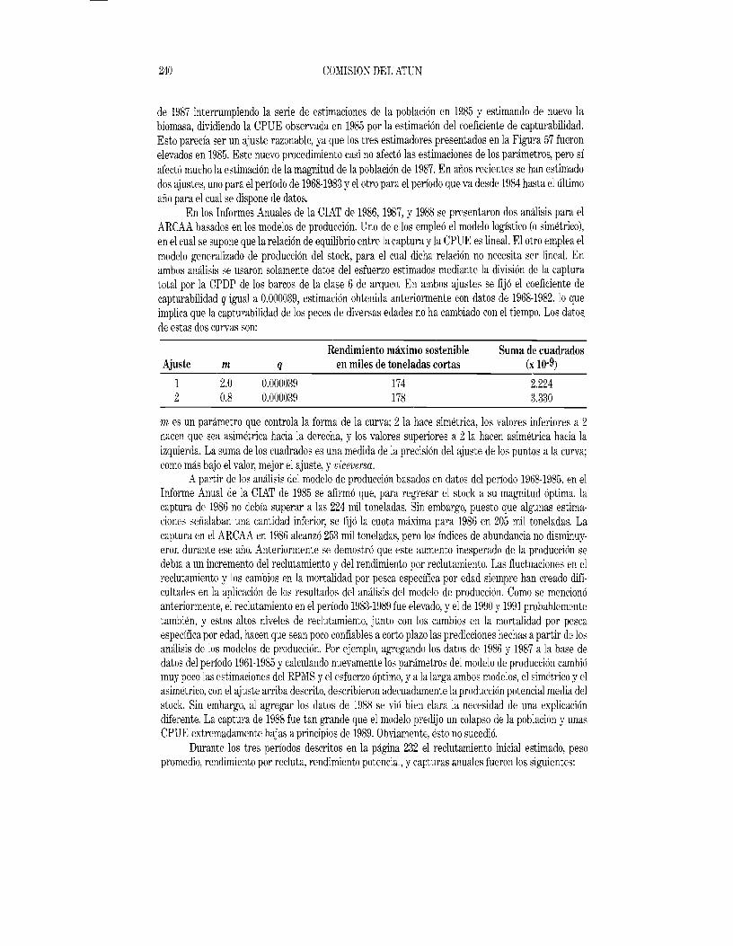
240 COMISION DEL ATUN
de 1987 interrumpiendo la serie de estimaciones de la poblacion en 1985 y estimando de nuevo la biomasa, dividiendo la CPUE observada en 1985 por la estimacion del coeficiente de capturabilidad. Esto parecia ser un ajuste razonable, ya que los tres estimadores presentados en la Figura 57 fueron elevados en 1985. Este nuevo procedimiento casi no afect6 las estimaciones de los panimetros, pero si afecto mucho la estimaci6n de la magnitud de la poblacion de 1987. En anos recientes se han estimado dos ajustes, uno para el periodo de 1968-1983 y el otro para el periodo que va desde 1984 hasta el ultimo ano para el cual se dispone de datos.
En los Informes Anuales de la CIAT de 1986, 1987, y 1988 se presentaron dos amilisis para el ARCAA basados en los modelos de producci6n. Uno de e110s emple6 el modelo logistico (0 simetrico), en el cual se supone que la relaci6n de equilibrio entre la captura yla CPUE es lineal. El otro emplea el modelo generalizado de produccion del stock, para el eual dicha relaci6n no neeesita ser lineal. En ambos amilisis se usaron solamente datos del esfuerzo estimados mediante la divisi6n de la eaptura total por la CPDP de los barcos de la clase 6 de arqueo. En ambos ajustes se fijo el coeficiente de capturabilidad q iguaJ a 0.000039, estimaci6n obtenida anteriormente con datos de 1968-1982,10 que implica que la capturabilidad de los peees de diversas edades no ha cambiado con el tiempo. Los datos. de estas dos eurvas son:
Rendimiento maximo sostenible Suma de cuadrados Ajuste m q en miles de toneladas cortas (x 10-9)
1 2.0 0.000039 174 2.224 2 0.8 0.000039 178 3.330
m es un parametro que controla la forma de la curva; 2 la haee simetrica, los valores inferiores a 2 hacen que sea asimetrica hacia la derecha, y los valores superiores a 2 la hacen asimetrica hacia la izquierda. La suma de los cuadrados es una medida de la precision del ajuste de los puntos a la curva; como mas bajo el valor, mejor el ajuste, y viceversa.
Apartir de los analisis del modelo de producci6n basados en datos del periodo 1968-1985, en el Informe Anual de la CIAT de 1985 se afirm6 que, para regresar el stock a su magnitud 6ptima, la captura de 1986 no debia superar a las 224 mil toneladas. Sin embargo, puesto que algunas estima· ciones senalaban una cantidad inferior, se fijo la cuota maxima para 1986 en 205 mil toneladas. La captura en el ARCAA en 1986 alcanzo 253 mil toneladas, pero los indices de abundancia no disminuy· eron durante ese ano. Anteriormente se demostr6 que este aumento inesperado de la produccion se debia a un incremento del reclutamiento y del rendimiento por reclutamiento. Las fluctuaciones en el reclutamiento y los cambios en la mortalidad por pesca especifica por edad siempre han ereado difi· cultades en la aplicaei6n de los resultados del analisis del modelo de producci6n. Como se mencion6 anteriormente, el reclutamiento en el periodo 1983-1989 fue elevado, y el de 1990 y 1991 probablemente tambien, y estos altos niveles de reclutamiento, junto con los cambios en la mortalidad por pesca especifica por edad, hacen que sean poco confiables a corto plaza las predicciones hechas a partir de los analisis de los modelos de producci6n. Por ejemplo, agregando los datos de 1986 y 1987 a la base de datos del periodo 1961-1985 y calculando nuevamente los parametros del modelo de producci6n cambi6 muy poco las estimaciones del RPMS yel esfuerzo 6ptimo, y ala larga ambos modelos, el simetrico y el asimetrico, con el ajuste arriba descrito, describieron adecuadamente la produccion potencial media del stock. Sin embargo, al agregar los datos de 1988 se vi6 bien clara la necesidad de una explicaci6n diferente. La captura de 1988 fue tan grande que el modelo predijo un colapso de la poblaci6n y unas CPUE extremadamente bajas a principios de 1989. Obviamente, esto no sucedi6.
Durante los tres periodos deseritos en la pagina 232 el reclutamiento inicial estimado, peso promedio, rendimiento por recluta, rendimiento potencial, y capturas anuales fueron los siguientes:
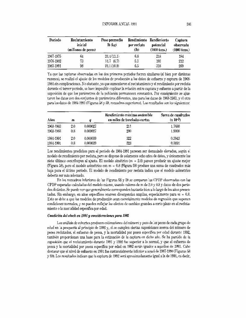
241 INFORME ANUAL 1991
Periodo Reclutamiento Peso promedio Rendimiento Rendimiento Captura inicial lb (kg) porrecluta potencial observada
(millones de peces) (lb) (1000 tons.) (1000 tons.)
1967-1975 64 24.4 (11.1) 6.8 218 184 1976-1982 73 14.7 (6.7) 5.3 193 212 1983-1991 98 24.1 (10.9) 6.5 318 269
Ya que las capturas observadas en los dos primeros periodos fueron similares (si bien por distintas razones), se realiz6 el ajuste de los modelos de producci6n a los datos de esfuerzo y captura de 19681984 sin complicaciones. No obstante, ya que aumentaron el reclutamiento y el rendimiento por recluta durante el tercer periodo, se hace imposible explicar la relaci6n entre captura y esfuerzo a partir de la suposici6n de que los panimetros de la poblaci6n permanecen constantes. Por consiguiente se ajustaron los datos con dos conjuntos de parametros diferentes, uno para los datos de 1968-1983, y el otro para los datos de 1984-1991 (Figuras 58 y 59, recuadros superiores). Los resultados son los siguientes:
Rendimiento maximo sostenible Suma de cuadrados Mios m q en miles de toneladas cortas (x 10-9)
1968-1983 2.0 0.000027 211 1.7680 1968-1983 0.8 0.000027 200 1.9000
1984-1991 2.0 0.000039 322 0.3943 1984-1991 0.8 0.000039 328 0.3891
Los rendimientos predichos para el periodo de 1984-1991 parecen ser demasiado elevados, seglin el modelo de rendimiento por recluta, pero se dispone de solamente ocho alios de datos, y linicamente los siete liltimos contribuyen al ajuste. EI modelo simetrico (m = 2.0) parece producir un ajuste mejor (Figura 58), pero el modelo asimetrico con m = 0.8 (Figura 59) produce una suma de cuadrados mas baja para el ultimo periodo. El modelo de rendimiento por recluta indica que el modelo asimetrico deberia ser mas adecuado.
En los recuadros inferiores de las Figuras 58 y 59 se comparan las CPDP observadas con las CPDP esperadas ca1culadas del modelo mismo, usando valores de m de 2.0 y 0.8 y datos de dos periodos distintos. Se puede ver que generalmente corresponden bastante bien a10 largo de los alios presentados. Sin embargo, en anos especificos ocurren divergencias amplias, especialmente para m = 0.8. Esto se debe a que los modelos de producci6n sean esencialmente modelos de regresi6n que suponen condiciones normales, y no pueden reflejar los efectos de cambios grandes a corto plazo en el reclutamiento 0 la mortalidad especifica por edad.
Condicion del stock en 1991 y consideraciones para 1992
Los analisis de cohortes producen estimaciones del numero y peso de los peces de cada grupo de edad en la pesqueria al principio de 1992 y, si se cumplen ciertas suposiciones acerca del numero de peces reclutados, el esfuerzo de pesca, y la mortalidad por pesca especifica por edad durante 1992, tambien proporcionan una base para la estimaci6n de la captura en dicho ano. Se ha partido de la suposici6n que el reclutamiento durante 1991 y 1992 fue superior a 10 normal, y que el esfuerzo de pesca y la mortalidad por pesca especifica por edad en 1992 seran iguales a aquellos de 1991. Cabe destacar que el nivel de esfuerzo en 1991 fue sustancialmente inferior a aquel de 1987-1990 (Figuras 58 y 59). Los resultados indican que la captura de 1992 sera aproximadamente igual a la de 1991, es decir,
242 COMISION DEL ATUN
unas 272 mil toneladas. Sin embargo, si la pesqueria se dedica nuevamente a la captura de peces de menor talla, tal como ocurri6 en el peliodo 1978-1982 y, en menor grado, en 1988, la captura de 1992, con el esfuerzo al nivel de 1991, disminuira. Claro que si el reclutamiento de 1991 y 1992 resulta ser igual 0inferior al promedio, la captura de 1992 sera inferior a 10 predicho.
Los analisis del rendimiento pOl' recluta han demostrado que dicho rendimiento es un 34% mayor cuando los barcos dirigen su esfuerzo hacia peces grandes, tal como hicieron en 1985-1989, que cuando 10 concentran en peces pequenos, tal como ocurri6 en 1978-1982. En la Figura 60 se ilustran los rendimientos pOl' recluta correspondientes ados pautas diferentes de mortalidad pOl' pesca especifica pOl' edad. Las curvas continua y de trazos fueron calculadas a partir de las mortalidades pOl' pesca especificas pOl' edad observadas durante 1978-1982 y 1985-1989, respectivamente.
En la Figura 61 se presentan los efectos de dos niveles distintos de reclutamiento, de 1985-1989 ("elevado") y de 1967-1989 ("promedio"), combinados con la mortalidad pOl' pesca especifica pOl' edad de 1985-1989. EI rendimiento con un reclutamiento elevado es un 26% mayor que con reclutamiento promedio.
En la Figura 62 se presentan los efectos combinados de reclutamiento elevado y mortalidad pOI' pesca especifica pOl' edad similar a aquella de 1985-1989 versus reclutamiento normal y mortalidad pOl' pesca especifica pOl' edad similar a aquella de 1978-1982. En este caso el rendimiento de la primera combinaci6n supera a aquel de la segunda pOl' un 60% con multiplicadores del esfuerzo de pesca superiores al 0.50.
Los modelos de producci6n para los cuales se estimaron los parametl'os con los datos de 19681983 pl'edicen que el stock de aleta amarilla se reduciria a cera a principios de 1990, a l'aiz de las capturas grandes logradas durante 1985-1989. Estos modelos permiten una captura casi nula en 1990, 1991,0 1992. Obviamente estas estimaciones no son representativas de las condiciones en la pesqueria. Tal como se indica arriba, los analisis con estructura de edades demuestran que han ocurrido cambios mayores en la mortalidad pOl' pesca especifica pOl' edad y el reclutamiento en los ultimos alios, y que estos han causado que la producci6n del stock sea mucho mayor que 10 predicho pOl' los parametros del modelo de 1968-1983. Si se supone que los datos de los anos mas recientes representan las condiciones actuales en la pesqueria, y se estiman de nuevo los parametros del modelo de producci6n de la forma descrita anteriormente, entonces las capturas esperadas corresponden mucho mejor a las observadas (recuadros inferiores de las Figuras 58 y 59). Los parametros nuevamente estimados del modelo predicen que la captul'a de equilibrio de 1992, con el nivel de esfuerzo reducido de 1991, seria aproximadamente 300 mil toneladas. Ya que se predice que la magnitud del stock sera algo mayor al nivel6ptimo, la captura de 1992 podria superar las 300 mil toneladas sin l'educir el stock a un nivel inferior al6ptimo. Con este nivel de esfuerzo reducido, la CPDP seria unas 16 toneladas.
Se estima que el reclutamiento ha fluctuado pOl' un factor de 3, aproximadamente, y que no parece tener relaci6n con la magnitud del stock dentro del rango de datos de pesca observados (Figura 63). Esta situaci6n dificulta aun mas la elaboraci6n de pron6sticos a corto plazo con modelos de producci6n. Para mejorar las predicciones obtenidas apartir de este modelo es necesario utilizar informaci6n sobre el reclutamiento. Lo mas conveniente seria efectuar pron6sticos con uno 0 dos anos de anticipaci6n. El Laboratorio de la CIAT en Achotines, Republica de Panama, se cre6, en parte, para obtener informaci6n que permita realizar pron6sticos sobre el reclutamiento de aleta amarilla, pero no se obtendra informacion util en el futuro inmediato. Tal como se sena16 en el Informe Anual de la CIAT de 1985, las fluctuaciones en el reclutamiento parecen estar vinculadas con cambios importantes en el medio oceanico. Las estimaciones del reclutamiento derivadas de los analisis de las cohortes y presentadas en la Tabla 22 indican que existieron anomalias positivas en el reclutamiento de 1970, 1973, Y 1977. Estos incrementos del reclutamiento fueron precedidos pOl' condiciones de EI Nino en 1969, 1972, Y1976. A partir de esta correlaci6n se esperaba un incremento del reclutamiento despues del Nino

243 INFORME ANUAL 1991
fuerte de 1982-1983, y, efectivamente, asi fue. En 1986-1987 ocurri6 otro Nino, de menor intensidad y extensi6n; las aguas del OPO fueron pOl' 10 tanto mas calidas que de costumbre desde 1982 hasta 1987. EI reclutamiento del periodo 1983-1989 fue el mayor jamas registrado en un periodo de 7anos. Durante 1988 y 1989 prevalecieron en el OPO condiciones fuertes delllamado "anti-EI Nino," pero el reclutamiento fue superior a 10 normal en 1989, y probablemente en 1990 y 1991 tambien. Hay pOl' 10 tanto ahora menos evidencia que en 1990 para apoyar la hip6tesis de que los eventos de EI Nino sean al menos parcialmente responsables de los reclutamientos anormalmente elevados.
En resumen, la evaluaci6n del efecto de la pesca sobre la abundancia y rendimiento del aleta amarilla en el OPO presenta dificultades. EI uso exclusivo de los modelos de producci6n arroja resultados tenues, yen consecuencia se han combinado los resultados de tres modelos diferentes (rendimiento porrecluta, cohortes, yproducci6n) para lIegar a10 que se cree ser las conclusiones mas acertadas. Sin embargo, la capacidad de pron6stico de estos analisis esta sujeta a un margen de error considerable, y se prosigue pOl' 10 tanto la exploraci6n de tecnicas analiticas alternas para lIegar a las mejores estimaciones posibles de productividad del stock de aleta amarilla.
La abundancia del aleta amarilla se ve determinada pOl' tres factores: el reclutamiento, la composici6n de la captura, y la captura total (una funci6n del esfuerzo).
Con respecto al primer factor, parece actualmente que el reclutamiento es determinado exclusivamente pOl' factores naturales, aunque es posible que en el futuro se demuestre que pudiera ser reducido pOl' una mortalidad pOl' pesca muy elevada u otros factores, tal como una contaminaci6n severa.
En cuanto al segundo factor, es posible modificar la composici6n de talla de la captura, al menos te6ricamente. Se ha hecho hincapie en esta posibilidad en multiples ocasiones, pero no se han formulado recomendaciones para la protecci6n de los peces de menor talla. Sin embargo, y como se senal6 anteriormente, las capturas de peces pequeilos fueron relativamente bajas durante 1985-1987 y 19891991. Esta modificaci6n de la composici6n de talla de la captura se debe, al menos parcialmente, ala reducci6n de la demanda de peces pequenos, pero es imposible preyer la duraci6n de esta situaci6n. De hecho, la restricci6n de la captura de atunes asociados con delfines pudiera resultar en un gran aumento en la captura de peces pequenos. Tal como se mencion6 anteriormente, la captura de peces pequenos fue mayor en 1988 que en 1985-1987 0 1989-1991. Hay varias maneras de reducir la captura de peces pequenos: 1) reducir el esfuerzo de pesca; 2) fijar una talla minima; 3) limitar la pesca en las zonas y las temporadas en que predominan los peces pequenos; 4) suponiendo que fuera posible restablecer el sistema anual de clausura, modificar la fecha de apertura de la temporada, para asi reducir la cantidad de pesca durante el periodo de abundancia maxima de peces pequenos en la captura.
En cuanto a la primera opci6n, se ha senalado que la reducci6n de la pesca durante el periodo 1982-1984 produjo un incremento en la talla promedio de los peces de la poblaci6n, 10 que aument6 su productividad. Sin embargo, una disminuci6n adicional del esfuerzo probablemente no produciria un aumento de la captura, a menos de que la composici6n de talla del stock fuera modificado de forma importante porIa pesca intensiva de peces pequenos.
En cuanto ala segunda opci6n, los analisis de los datos de composici6n de talla indican que, pOl' 10 general, las capturas suelen consistir de mezclas de peces pequenos y gl-andes, y de aletas amarillas pequenos y barriletes. Esto dificultaria la protecci6n del aleta amarilla pequeno, ya que es posible que sean capturados en grandes cantidades pOl' barcos que intentan capturar aletas amarillas grandes y barriletes. Si no se permitiera la descarga de los peces pequenos, se arrojarian al mar, ya muertos, y el rendimiento pOl' recluta se reduciria en lugar de aumentar.
En cuanto ala tercera opci6n, la eliminaci6n de la pesca de atunes en areas de mayor abundancia del aleta amarilla pequeno serviria quizas para incremental' el rendimiento pOl' recluta de esta
244 COIvIISION DEL ATUN
especie, siempre que la flota pudiera pescar con buen exito en areas donde hay peces de mayor talla, pero la reducci6n de las capturas de barrilete probablemente sena mayor que el aumento de las capturas de aleta amarilla, ya que el barrilete es mas abundante en esas zonas donde se encuentran los aletas amarillas pequenos en mayor cantidad.
En cuanto a la cuarta opci6n, no parece que la modificaci6n de la fecha de apertura de la temporada produzca el beneficio deseado. Durante los primeros anos del periodo en que rigieron las vedas anuales, cuando la mayor parte del esfuerzo de pesca se ejercia en el primer semestre del ano, s610 se obtenian pequenas capturas de los peces de la cohorte Yque ingresaban pOl' primera vez ala pesqueria con un peso de 0.7 a 2.0 kg (1.5 a 4.51ibras) en el segundo semestre del ano. Se crey6 que esto se debia fundamentalmente a la falta de vulnerabilidad ala pesca de los peces de esta cohorte. Sin embargo, en anos posteriores, la pesca fue intensa durante el segundo semestre del ano, y la captura de peces de la cohorte Y entrante aument6 substancialmente. En consecuencia, es posible que la modificaci6n de la temporada no proteja a los peces mas j6venes al grado esperado.
Actualmente, no se puede recomendar ninguna de las medidas anteriores, puesto que no es posible predecir el efecto de tal reglamentaci6n sobre la captura real (no el descargue) de peces pequenos.
En cuanto al tercer factor, el personal de la CIAT ha recomendado solamente cuotas de captura (Tabla 24) para reglamentar la pesqueria. Las cuotas rigieron en el ARCAA, 0parte del mismo. Una vez alcanzada la cuota de aleta amarilla, 0 cuando parecia que seria alcanzada pOl' barcos en el mar antes de la fecha de clausura, se permitia a aquellas embarcaciones que estaban sujetas a la cuota pescar otras especies, y descargar aletas amarillas capturados incidentalmente hasta un limite del 15% de su captura total de atunes. POl' consiguiente, la captura de barrilete no fue reducida pOl' las cuotas de aleta amarilla.
Los amilisis precedentes demuestran que el tamafio del stock de aleta amarilla en el OPO es algo mayor al 6ptimo. Si se dirige el esfuerzo principalmente hacia peces asociados con delfines, tal como ocurri6 en 1989-1991, y el esfuerzo permanece alrededor del nivel de 1991, la CPUE durante 1992 deberia ser unas 16 toneladas diarias, al igual que en 1991. Si la pesca es dirigida exclusivamente hacia peces pequenos durante el segundo semestre de 1992, el peso pl'omedio de los peces en la captura disminuira, provocando una reducci6n sustancial en el rendimiento pOl' recluta. Dividiendo la captura estimada de 1992 en el OPO (272 mil toneladas) pOl' el reclutamiento medio de 1983-1991 (98 millones de peces) produce un rendimiento pOl' reclutamiento de 2.5 kg (5.6libras). El peso promedio de los peces capturados sin pesca dirigida hacia peces asociados con delfines seria unos 4.5 kg 0 10 libras (Figura 64). Ell'endimiento pOl' reclutamiento para peces de este peso es unos 2.0 kg (4.4. libras) (Figura 55). Con 98 millones de reclutas en el OPO y un rendimiento pOl' reclutamiento de 2.0 kg, la captura sena unas 209 mil toneladas. Ya que la flota ha pescado principalmente atunes asociados con delfines durante el primer semestre de 1992, la captura del ano entero, sin esfuerzo dirigido hacia peces asociados con delfines entre julio y diciembre, seria unas 244 mil toneladas. No obstante, si se elimina la pesca de atunes asociados con delfines, el area de pesca se vera probablemente reducida de forma sustancial. Durante el periodo de 1976-1982, en el cual se redujo la pesca de atunes asociados con delfines, el reclutamiento medio fue 73 millones de peces, el 74% de los 98 millones estimados para el periodo de 1983-1991. Si ni se pescaran atunes asociados con delfines durante el segundo semestre de 1992, la captura sena aproximadamente 202 mil toneladas en el OPO entero. Es posible que la realidad caiga entre estos dos extremos, es decir que la pesca de atunes asociados con delfines sera reducida durante el segundo semestre del ano, pero no eliminada. POl' consiguiente, al nivel de esfuerzo de 1991, la captura en el OPO en 1992 caera entre 202 y 272 mil toneladas, segUn la proporci6n del esfuerzo dirigido hacia peces asociados con delfines.
Si se usan los modelos de producci6n para estimar la condici6n del stock y predecir las capturas
245 INFORME ANUAL 1991
Muras, se puede deducir a partir de las Figuras 58 y 59 que la produccion podria pel1llanecer alrededol' de las 250 a 300 mil toneladas si el esfuerzo continua al nivel de 1991 y si se continua dirigiendo la mayoria del esfuerzo hacia peces asociados con delfines. Sin embargo, si la flota dirigiera una mayor porcion del esfuerzo hacia peces no asociados con delfines, la captura del OPO seglin el modelo de produccion, se reduciria a unas 150 a 200 mil toneladas. Esta reduccion pudiera tardar unos 2 alios en manifestarse completamente. (Cabe destacar, sin embargo, que los modelos de produccion no han sido aplicados a una serie de datos de una pesqueria que no incluye lances sobre delfines.)
Se deben tomar en cuenta dos puntos importantes acerca de la recomendacion de una cuota de captura para el aleta amarilla. En primer lugar, el area abarcada poria cuota seria el ARCAA, pese a que los peces del ARCAA yuna porcion del OPO fuera del ARCAA parecen ahora pertenecer a un solo stock y, en segundo, la cantidad dependera mucho de la composicion de talla de los peces en la captura.
Con respecto al primer punto, en la porcion del OPO fuera del ARCAA la talla promedio de los peces en la captura es cercana a la critica, y pOl' 10 tanto optima en cuanto a la maximizacion del rendimiento pOl' recluta. No es pOl' 10 tanto necesario limitar la captura en dicha area.
En cuanto al segundo punto, se ignol'a en cual grado se limitara la pesca de peces asociados con delfines. En vista de esto, cualquier cuota que se imponga deberia ser suficientemente baja como para acomodar la posibilidad que se reduzca 0 abandone la pesca de atunes asociados con delfines en el segundo semestre de 1992, y tambien pel1llitir incrementos compatibles con la posibilidad de que dicho tipo de pesca continue al igual que en el periodo correspondiente en 1991. Durante la quincuagesima Reunion de la Comision, celebrada en junio de 1992, se presentaron recomendaciones especificas para la reglamentacion de la pesca.
BARRILETE
Las capturas mundiales del barrilete han superado las de las otras especies de atunes desde hace muchos alios. La proporcion de barrilete en las capturas mundiales de las especies de mayor importancia comercial (barrilete, aleta amarilla, patudo, albacora, y aleta azul del norte y del sur) fue 45%,44%,49%,45%, y 45% en 1986, 1987, 1988, 1989, y 1990, respectivamente. En el Oceano Pacifico el barrilete fOl1llo un 51%, 47%, 54%, 48% Y49% de la captura en 1986, 1987, 1988, 1989, Y1990, respectivamente. En la Figura 65 se presentan las capturas mundiales de barrilete, divididas pOl' zonas. Es evidente que las capturas en el Oceano Pacifico son muy superiores a las del Oceano Atlantico 0 Indico, y que las capturas en la parte central y occidental del Pacifico son mucho mas elevadas que las del Pacifico oriental. Las capturas en el Pacifico oriental pel'manecieron aproximadamente al mismo myel desde 1961 hasta 1991, con excepcion del incremento en el periodo 1975-1981; en cambio las capturas de otras zonas han aumentado marcadamente.
Existen pesquerias sustanciales de barrilete en el Oceano Pacifico nordeste cerca de Baja California, las Islas Revillagigedo, y la Isla Clipperton, y en el Oceano Pacifico sudeste cerca de America Central, el norte de Sudamerica, la Isla de Cocos-Banco de Brito, y las Islas Galapagos. La zona de aguas calidas a la altura de Mexico meridional que separa estas dos regiones generalmente carece de barrilete, pero en algunos alios, como sucedi6 en 1956, la distribuci6n de barrilete ha sido continua de norte a sur. La pesca de barrilete en el OPO tiene lugar mas cerca dellitoral que la del aleta amarilla, pero en los illtimos alios ha aumentado la proporci6n de barrilete capturado mar afuera. En el Oceano Pacifico central se explota el barrilete en menor escala cerca de las islas de Hawaii y la Polinesia Francesa Oas Islas Marquesas, Tuamotu, y Sociedad). Hacia el oeste, cerca de Fiji, las Filipinas, Indonesia, Jap6n, Papua Nueva Guinea, Nueva Zelandia, las Islas Salom6n, etc., se explota el barrilete en fOl1lla mas significativa.
La captura de barrilete en el OPO varia considerablemente de un alio a otro (Figura 66). Afines de la decada de los cincuenta se obtuvieron grandes capturas de barrilete al sur de 50 S, y desde
246 COMISION DEL ATUN
entonces hasta principios de los alios setenta se lograron grandes capturas de la especie cerca de la costa, a la altura de Ecuador y el norte de Peru. Sin embargo, aprincipios de la decada de los setenta, el centro de abundancia del grupo del sudeste se traslad6 aparentemente alas aguas frente a Colombia y America Central, regresando nuevamente hacia Colombia y Ecuador a principios de la decada de los ochenta. En 1991 se lograron capturas sustanciales frente al norte de Sudamerica (Figura 5).
En la Figura 18 se ilustra la composici6n de talla de las muestras de barrilete tomadas en el OPO entre 1986 y 1991. Son evidentes las diferencias entre los alios; los peces fueron mas pequelios en 1988 y 1991 que en los otros alios.
Estructura de la poblacion
Es de importancia fundamental establecer si el barrilete que en el Oceano Pacifico forma parte de una sola subpoblacion 0 de varias subpoblaciones, y en este ultimo caso, determinar en cuales areas ocurren las distintas subpoblaciones e investigar las variaciones de la distribucion con el tiempo y la edad. Se han usado varios metodos para estudiar este problema, entre ellos el analisis de las estadisticas de captura, el ciclo vital, el marcado, y los datos geneticos bioquil11icos. Diversas organizaciones, entre ellas la CIAT, la South Pacific Commission (SPC), el National Marine Fisheries Service (NMFS) de los EE.UU., y varias entidades japonesas han estudiado estos temas. Los resultados y recomendaciones de estos estudios se analizaron en una reunion de trabajo patrocinada porIa SPC en 1980, ala que asistieron biologos pesqueros y especialistas en genetica de poblacion; las conclusiones de esa reunion fueron analizadas a fondo en el Informe Anual de la CIAT de 1984. En resumen, existen dos hipotesis principales sobre el barrilete del Oceano Pacifico: (1) la hipotesis de la subpoblacion separada, que afirma que en el Oceano Pacifico existen al menos dos subpoblaciones de barrilete geneticamente distintas; (2) la hip6tesis de gradaci6n (0 clinal), que sostiene que no existen subpoblaciones separadas de barrilete en el Oceano Pacifico, sino que hay aislamiento pOl' distancia: es decir, la probabilidad de hibridizacion de dos peces dados es una funcion inversa de la distancia entre los dos. Enla reunion de trabajo se concluy6 que la informacion disponible no permite decidir a favor de una u otra de las dos hipotesis.
EI Informe Anual de la CIAT de 1984 contiene un analisis de la estructura de poblacion del barrilete en el OPO, y su relacion con las poblaciones en el resto del Pacifico. EI marcado ha demostrado que ocurre poca mezcla de peces entre la zona del norte de Mexico y la del norte de SudamericaCentroamerica. Existe una correlacion moderada entre las capturas de barrilete de la zona nordeste y sudeste, sin embargo, pero en ocasiones, como sucedio en 1970, la captura es superior al promedio en una zona e inferior al promedio en la otra (Figura 66). Un examen de los datos disponibles lleva a la conclusi6n que el barrilete del norte de Mexico y el de Sudamerica-Centroamerica parece formal' parte de un solo grupo que habita una zona en forma de arco cuyos extrel110S se encuentran en esas dos zonas; los peces que se encuentran en los extremos de la distribucion se mezclan, en cierta medida, en las zonas de desove del Pacifico central ylo occidental.
Hacia fines de los alios 70 y a comienzo de los 80 el personal de la CIAT realizo investigaciones de la composicion quimica de las vertebras de los atu- nes, usando espectroscopia de emision de rayos X inducida pOl' protones para estimar la cantidad de mezcla entre peces de distintas areas. Se han publicado los resultados de este estudio en Informes Anuales de la CIAT y en el Volumen Colectivo de Trabajos Cientificos de la Comision Internacional para la Conservacion del Atun Atlantico, Vol. 24. EI uso de esta tecnica se basa en el hecho de que las distintas areas del oceano l11uestran caracteristicas quimicas, fisicas, y biologicas que afectan la composicion quimica de las partes duras de los peces. Desgraciadamente, el analisis de la estructura de los stocks con este metodo es caro y presenta dificultades tecnicas. La interpretacion de los datos es asimismo dificil, debido a que no se entienden bien los procesos que rigen la composici6n elemental de las partes duras.
247 INFORME ANUAL 1991
En colaboraci6n con cientificos de la Universidad de Washington, la ClAT realiz6 un estudio de un metodo alterno de detectar marcas naturales en las partes duras de los atunes. EI metoda investigado, que usa un detector de rayos Xdispersores de energia (energy-dispersing X-ray detector, 0 EDS) unido a un microscopio electr6nico de barrida, no destruye la muestra, y es pOl' 10 tanto adecuado para el estudio de la composici6n elemental en distintas etapas del crecimiento del pez. La tecnica es barata, y ha dado bastante exito con otras especies de peces. Tras unos experimentos preliminares con aletas amarillas, se realiz6 un estudio de los microconstituyentes del barrilete, usando otolitos de peces de varias tallas capturados frente a Baja California, Hawaii, y Fiji. Se encontraron concentraciones de estroncio y calcio en distribuciones regulares en los peces de todas las areas. Estas distribuciones coincidieron con zonas especificas del otolito asociadas con el crecimiento temprano (foco), de media vida (regi6n media), y mas reciente (extremo exterior).
Analisis de funci6n discriminante de las concentraciones elementales en la zona de crecimiento temprano senalaron que (1) los peces de Baja California y Hawaii eran similares y (2) que los peces de Fiji eran diferentes de los de Baja California y Hawaii. Los resultados de los peces de Baja California y Hawaii pueden ser interpretados de dos maneras. Dichos peces podrian haber (1) originado todos en el mismo area de desove 0 (2) originado en distintas areas, pero el metodo no tiene la potencia necesaria para distinguir las diferencias que pudieran existir. Un aumento en el tamane de la muestra mejoraria la probabilidad de detectar diferencias entre las dos areas, si es que existen. Los resultados generales son consistentes con aquellos obtenidos de etudios geneticos, que han demostrado similitudes entre peces del Pacifico oriental ycentral y diferencias entre estos peces ypeces del Pacifico occidental.
Se investig6 el reclutamiento del barrilete en el OPO y cerca de Hawaii, usando datos de frecuencia de talla de peces capturados en esas areas. Se desarrollaron modelos para examinar la variaci6n estacional en el reclutamiento entre areas a una talla estandar. Se compararon peces de Hawaii y del norte y del sur del OPO (al norte y al sur de WON) a fin de determinar si fueron criados al mismo tiempo. Los resultados indican que el desove que contribuye ala pesqueria del sur del OPO ocurre de 1 a 2 meses antes de aquel que contribuye ala pesqueria del norte del OPO y de 5a 6 meses antes de aquel que contribuye a la pesqueria de Hawaii. Se sabe que el barrilete desova en periodos de varios meses, yhasta durante el ano entero en algunas areas, ypOI' 10 tanto las distribuciones aqui observadas sugieren pOI' 10 menos dos hip6tesis sobre la estructura de la poblaci6n de barrilete en el OPO y Hawaii. La hip6tesis de poblaciones separadas mantiene que los barriletes en estas tres areas desovan en distintas epocas del ano yno se mezclan extensivamente en otras epocas. Las hip6tesis panmicticas afmnan que el barrilete capturado en estas areas resultan de un desplazamiento de norte a sur de una sola poblaci6n que deova durante un periodo extendido. Los resultados de estudios de los desplazamientos de peces marcados, geneticos, y de microconstituyentes de otolitos apoyan esta segunda hip6tesis.
Abundancia, disponibilidad, y vuLnembilidad a La captum
En el Boletin de la ClAT, Vol. 19, N° 6, se public6 un examen de los efectos de las condiciones ambientales sobre la abundancia, disponibilidad, y vulnerabilidad a la captura del barrilete en el OPO. En uno de estos estudios se analiza la relaci6n entre la abundancia aparente de barrilete en su segundo ano de vida en el OPO y(1) el promedio de la temperatura de la superficie del mar ('ISM) en la parte del Oceano Pacifico comprendida entre los 135e y los 1800Wcon 'ISM superiores a los 27.8°C (82°F); y (2) el indice de mezcla pOI' viento (el cubo de la velocidad promedio del viento, aproximadamente proporcional al grado de mezcla causado pOI' el viento en las capas superiores del oceano) en esta zona.
Se efectu6 el primer analisis en vista de la alta correlaci6n positiva entre la temperatura y la concentraci6n de larvas de barrilete capturadas en redes de zooplancton de arrastre, 10 cual permite pensar que puede ocurrir un mayor desove 0 supervivencia de huevos y/o larvas en los anos mas

248 COMISION DEL ATUN
calidos. El segundo analisis se realiz6 porque es posible que la supervivencia de las larvas de barrilete dependa del grado de mezc!a de las capas superiores del oceano. Investigaciones realizadas en el Southwest Fisheries Science Center del NMFS en La Jolla indican que en la Corriente de California el alimento apto para las larvas de anchoa en sus primeras alimentaciones suele concentrarse en grupos y estratos bien definidos. La mezc!a deshace los estratos y dispersan los organismos alimenticios, de modo que muchas de las larvas no pueden obtener alimento suficiente para sobrevivir. Aparentemente, las generaciones fuertes de anchoas adultas estan asociadas can vientos debiles durante la etapa larval, y viceversa, y se crey6 que pudiera ocurrir 10 mismo en las zonas de desove del barrilete en el Pacifico central. Se descubrio una correlaci6n significativa entre la abundancia del barrilete y la TSM, y una correlacion altamente significativa entre el barrilete y el indice de la mezc!a del viento, ya que este indice es responsable del 46% de la variabilidad en la abundancia aparente del barrilete en el OPO en su segundo ana de vida.
Se han realizado ademas investigaciones para determinar si existe una relacion entre la abundancia aparente del barrilete en el OPO en su segundo ana de vida y la fuerza de la Contracorriente Ecuatorial del Norte que fluye hacia el este. Si el barrilete usa esta corriente en su migracion se esperaria que la cantidad de peces j6venes transportados al OPO seria mayor cuando la corriente es mas fuerte y menor cuando es mas debil. Sin embargo, no se encontro una correlacion significativa entre la abundancia del barrilete y los indices de la velocidad de la corriente.
En general, los resultados obtenidos par los investigadores de la CIAT, en sus intentos par relacionar la abundancia aparente del barrilete can las condiciones ambientales, indican que esta relaci6n es compleja y sutil. Parte del problema podria quizas ser resuelto si se pudieran realizar estudios biologicos y estadisticos de toda la unidad (0 de todas las unidades si hay mas de una) de la poblaci6n que contribuye ala pesca en el OPO, en lugar de analizar tan s6lo la parte que habita el OPO durante parte de su cicIo vital. Se cuenta can datos utilizables sabre la captura, el esfuerzo y la captura par unidad de esfuerzo (CPUE) para tan s6lo algunas partes de la unidad (0 unidades) de la poblacion del Pacifico. La separacion de las capturas de peces de la unidad (0 unidades) de la poblacion que contribuye(n) ala pesca en el OPO de aquella(s) que no contribuye(n) constituye un problema adicional.
Modelos con estructura de edades
En una secci6n anterior de este informe se analiz6 el concepto de rendimiento par recluta aplicado a modelos can estl1lctura de edades para el aleta amarilla. Sin embargo, las poblaciones de barrilete y aleta amarilla del OPO son alga diferentes. EI agotamiento natural del aleta amarilla se debe s6lo ala mortalidad natural, mientras que el del ba1111ete se debe tambien ala emigraci6n al Pacifico central y occidental. A partir de los datos de frecuencia de talla y del marcado, se calcula que la tasa anual combinada de mortalidad natural y emigracion del barrilete es de aproximadamente 75 a 90%, en comparacion can e155% de la mortalidad natural del aleta amarilla.
Se han usado los datos de frecuencia de talla y de devoluci6n de marcas para estimar la tasa de crecimiento del barrilete. Es mucho mas dificil seguir la progresi6n de los grupos modales para esta especie que para el aleta amarilla, ya que la talla modal varia de un mes a otro de forma muy erratica. Evidentemente, la causa principal de esto radica en el rec!utamiento de peces del Pacifico central y la emigraci6n en direcci6n opuesta, pero ademas parece que la vulnerabilidad de grupos de peces de distintas tallas varia considerablemente de un mes a otro en el OPO. Los datos del marcado son tambien titiles en este respecto, aunque su valor se ve limitado par el hecho de que la mayoria de los peces recapturados permanecieron poco tiempo en libertad. Dos estudios recien completados (Boletin de la CIAT, Vol. 19, Nos. 4 y 6) proporcionan estimaciones de las tasas lineales de crecimiento y de los parametros de la ecuaci6n de crecimiento de von Bertalanffy, y estas estan probando ser titiles en los estudios de modelos can estl1lctura de edades.
249 INFORME ANUAL 1991
En la Figura 67 se presentan los rendimientos por recluta del barrilete correspondientes a varias combinaciones de agotamiento natural (la mortalidad natural mas la emigraci6n), esfuerzo de pesca, y talla de ingreso. Para obtener los calculos que forman la base de esta figura se integraron las estimaciones de los investigadores de la CIAT de la mortalidad por pesca especifica para cada edad durante 1986-1987, el crecimiento, yel agotamiento natural. Las fuentes de los datos sobre crecimiento en peso son las siguientes:
Crecimiento en talla Ecuacion Fuente
Crecimiento en talla 24 cm/ano Boletin de la CIAT: Vol. 19, N° 6
Relaci6n logw =3.33610g1 - 8.250 Boletin de la CIAT: Vol. 4, N° 2 peso-talla
Se usaron tasas anuales instantaneas de agotamiento natural de 1.5 (un 78%) y 2.0 (un 86%). Los valores en la escala horizontal son los mLiltiplos del esfuerzo de pesca, es decir, 0.5, 1.0, y 2.0 representan los valores del esfuerzo la mitad de, igual a, y el doble de los valores reales del esfuerzo de 19861987. Distintas combinaciones del esfuerzo de pesca y de la talla de ingreso rinden rendimientos por recluta distintos, indicados por lineas en curvas. Por ejemplo, si se fija la talla de ingreso en 40 em (unos 1.2 kg/2.7libras) el rendimiento por reeluta con un multiplicador de 1es aproximadamente 0.72 kg (1.58 libras) en el recuadro superior y 0.39 kg (0.85 libras) en el inferior. En el recuadro superior se produciria el rendimiento por recluta maximo con una talla de ingreso de unos 40 em con un multiplicador de 1, y de unos 48 em con un multiplicador de 2a 3. En el recuadro inferior son maximos los rendimientos por recluta a una talla de ingreso de 30 em 0 menos. En general, se tendria que ejercer un esfuerzo de pesca mucho mayor al actual, 0 tener una edad de ingreso mucho menor que la actual, para pescar por exceso la poblaci6n en el sentido de rendimiento por recluta. Esto se debe a que la perdida en el peso total de una cohorte de peces, por mortalidad natural y emigraci6n, excede su incremento por crecimiento, aLin cuando los peces midan menos de 50 em y esten supuestamente creciendo con rapidez.
Modelos de producci6n
En una secci6n anterior de este informe se describieron los modelos de producci6n, basados en los indices de abundancia de los peces, en relaci6n al aleta amarilla. Se senal6 que los modelos de este tipo no tienen validez a menos que los peces pertenezcan auna poblaci6n diferenciada, es decir una en la cual haya relativamente poco intercambio entre los peces que habitan la zona estudiada (en este caso, el OPO) y aquellos de otras zonas en las que se explota la especie en cuesti6n, 0 los indices de intercambio entre las subpoblaciones de la cual sean conocidas. No se satisface ninguno de estos requisitos, ya que el marcado ha demostrado que existe intercambio de peces del Oceano Pacifico oriental, central, y occidental (Figura 68), pero se ignoran las tasas de intercambio. La mayor parte de la captura de barrilete en el OPO es realizada bastante cerca de la costa, y aparentemente la mayor parte de esta captura proviene de los desoves en el Pacifico central y/o occidental, desoves que tambien pueden abastecer a las regiones de alta mar del OPO, central, y occidental. En consecuencia, es posible que la captura en el OPO este determinada por la abundancia de los juveniles nacidos en el Pacifico central y/o occidental, apor la abundancia de los juveniles en esa zona 0 zonas que migran al OPO. Afalta de una definici6n de la poblaci6n explotada, el modelado de producci6n tiene poco 0 hasta ningLin valor para el barrilete pescado en el OPO.
Considemciones pam 1992
EI modelo de rendimiento por recluta no senala que sea necesario controlar la pesca del barri
250 COMISION DEL ATUN
lete. A un valor de agotamiento natural de 2.0, este modelo indica que se puede obtener el maximo rendimiento pOl' recluta del barrilete adolescente del OPO mediante la pesca intensiva de ejemplares de mas de 30 cm. Aunque podria pensarse que esto reduciria el reclutamiento en alios subsiguientes, los conocimientos actuales sobre el desove y la estructura de la poblaci6n indican que es poco probable que asi suceda.
Se puede afmnar con bastante seguridad que el barrilete ha sido subexplotado en el OPO, y que esta situaci6n no cambiara en el futuro inmediato. No obstante, es importante adquirir mayores conocimientos sobre esta especie y su relaci6n con el ambiente, en particular pOl' las dos razones siguientes. En primer lugar, es posible que estos conocimientos permitan pronosticar, con varios meses de anticipaci6n, la abundancia de barrilete en el OPO, 10 cual seria muy valioso para la industria pesquera. En segundo lugar, es posible que un conocimiento de las condiciones ambientales favorables para la existencia del barrilete, junto con la noci6n de los procesos dinamicos del oceano, permita pronosticar los lugares y momentos en que existe mayor probabilidad de capturar barrilete, 10 cual aumentaria la eficacia de la flota pesquera.
ALETA AZUL DEL NORTE
EI aleta azul del norte ocurre en el Oceano Atlantico y en el Pacifico. Las capturas mundiales y del Pacifico son mucho menores que las del barrilete, aleta amarilla, patudo, y albacora; sin embargo, la pesqueria es de valor econ6mico considerable. En la Figura 69 se presentan las capturas anuales del attin aleta azul en el Oceano Pacifico durante el periodo de 1951-1991. Las artes de superficie obtienen la mayoria de las capturas tanto en el Oceano Pacifico oriental (OPO) como en el occidental. Las capturas en el Pacifico occidental fueron bien superiores al promedio durante 1978-1983, medias durante 1984-1987, e inferiores al promedio durante 1988-1990; las del OPO fueron pobres durante 1980-1984, ligeramente inferiores al promedio en 1985 y 1986, Ypobres durante 1987-1991.
En el OPO casi toda la captura es lograda pOl' barcos cerqueros que pescan bastante cerca de la costa de Alta y Baja California. La temporada de pesca se extiende tipicamente desde fines de mayo hasta mediados de octubre, aunque tambien se efectuan capturas esporadicas en otros meses. La captura en 1991, unas 462 toneladas, fue la mas baja desde los principios de los anos 30. En 1991 se capturaron aletas azules entre 26°N y 27°N en junio y entre 27°N y 33°N en julio y agosto. No se captur6 ninguno entre enero y mayo y entre septiembre y diciembre.
EI personal de la CIAT estudia el atlin aleta azul en modesta escala desde 1973. Antes de 1979, se obtenian datos de bitacora y se median muestras de peces capturados pOl' embarcaciones cerqueras en el OPO para determinar la composicion de talla, pero a partir de esc alio se intensificaron los estudios. En 1979, se preparo un an:Hisis de los datos referentes a la evaluacion de los stocks de esta especie (Informe Interno 12 de la CIAT). Asimismo, en 1982, los datos sobre la captura de superficie de aleta azul en el OPO pOl' area, fecha, clase de arqueo, tamalio del cardumen, tipo del mismo, etc., fueron recopilados, analizados, y publicados en el Eoletin de la CIAT, Vol. 18, NOe 2. Un investigador del Far Seas Fisheries Research Laboratory (FSFRL) (ahara el National Research Institute of Far Seas Fisheries (NRIFSF)) en Shimizu (Japon) trabajo en la oficina principal de la CIAT desde septiembre de 1988 hasta enero de 1989, colaborando can cientificos de la Comision en estudios del aleta azul. Algunos de los resultados de estos estudios fueron publicados en 1991 en el Eoletin de la CIAT, Vol. 20, N° 1. En mayo de 1990 se celebro en La Jolla, California, un taller sabre el aleta azul, patrocinado conjuntamente porIa CIAT yel Australian Fisheries Service. El objetivo de la reunion era comentar e informal' sabre los puntas fuertes y debiles de las tecnicas de evaluacion de stocks usadas para los stocks de aletas azules de los Oceanos Pacifico, Indico, y Athintico, y el Mar Mediterraneo. Las aetas del taller fueron publicadas como el Informe Especial Ne 7de la CIAT.
251 INFORME ANUAL 1991
En la Figura 19 se presentan histogramas de la frecuencia de talla del aleta azul capturado en el OPO en 1986-1991. Entre octubre y diciembre de 1986, 1988, y 1989 se capturaron peces de tamano extraordinariamente grande (pesando entre 105 y 460 kg/230 y 1010 libras). EI peso total de estas capturas no fue muy grande, pero los peces poseian gran valor economico, ya que inmediatamente despues de su captura se les transporto por avion al Japon, donde se pagan precios muy altos por aleta azul fresco.
Aletas azules fueron marcados en el OPO por la CIAT en 1958 y 1979-1980 y por el Bureau of Commercial Fisheries (ahora el National Marine Fisheries Service) de los Estados Unidos, el California Department of Fish and Game (CDFG), y el Mission Bay Research Foundation en 1962-1968. Aletas azules en el Pacifico occidental fueron marcados por cientificos de la CIAT trabajando en el Japon en 1980-1982 y del FSFRL entre 1980 y 1988. En las Thblas 25 y 26 se resumen los datos de liberacion y recaptura, y en el Boletin de la CIAT Vol. 20, Nu 1, se discuten los resultados de los experimentos.
Amilisis de los datos de los peces liberados y recapturados en el OPO indican desplazamientos estacionales de norte al sur, alcanzando los peces su punto mas norteno en julio-octubre y mas sureno durante mayo yjunio. Se han obtenido diez devoluciones de peces liberados en el OPO y recapturados en el Pacifico occidental, todas de los cuales permanecieron mas de 22 meses en libertad.
Los peces marcados y liberados en el Pacifico occidental, al igual que aquellos en el OPO, solian desplazarse hacia el norte ella primavera y verano y hacia el sur en el otono e inviemo. Las migraciones del Pacifico occidental al oriental son de interes especial. Algunas clases anuales, por ejemplo aquellas de 1983 y 1984, produjeron grandes cantidades de migrantes, yotras no. Las mejores capturas de la decada de los 80 en el OPO fueron logradas en 1985 y 1986, y consistieron principalmente de peces de edad 2 de las clases anuales de 1983 y 1984. (En el presente informe se refiere a los peces en su primer ano de vida como de 0anos de edad 0 de edad 0, aquellos en su segundo ano de vida como de 1 ano de edad 0 de edad 1, y asi sucesivamente.)
El cicio vital y la relacion entre peces del Pacifico occidental y oriental
La informacion presentada en esta seccion es fundamental a la comprension de la seccion siguiente sobre la evaluacion del stock.
La unica zona del Oceano Pacifico donde se sabe que ocurre el desove es en las inmediaciones del Jap6n. Aparentemente, algunos peces permanecen toda su vida en el Pacifico occidental. Otros migran al OPO, principalmente 0 quizas exclusivamente durante el primer 0 segundo ano de vida. Los que se desplazan durante el primer ano se encuentran expuestos a la pesca de arrastre (sedal con anzuelo y cebo) veraniega y otonal dirigida sobre atunes aleta azul pequenos y otras especies frente al Jap6n antes de empezar su viaje al OPO en el otono 0 inviemo. Los que se desplazan en el segundo ano de vida se encuentran ademas expuestos a la pesca de arrastre invemal y demas formas de pesca que se practican en las inmediaciones del Jap6n, antes de comenzar su viaje al OPO en la primavera, el verano, o el otono. Despues de atravesar el oceano, los peces migrantes son pescados por barcos cerqueros frente a Alta y Baja Califomia.
No esta ni confirmada ni refutada la hip6tesis que peces de talla inferior a unos 100 em, que forman la mayor parte de la captura del OPO, abandonen el Pacifico occidental cada otono 0 inviemo. Es poco comun capturar un aleta azul de ese tamaIio en el OPO entre noviembre yabril, 10 cual pudiera indicar que hayan abandonado la regi6n. Sin embargo, es poco probable que recorran la distancia entera al Pacifico occidental, ya que el periodo minimo de libertad observado para un pez marcado liberado en el OPO y recapturado en el Pacifico occidental es de 674 dias; si la mayoria de ellos migrara al Pacifico occidental cada otono 0 inviemo, y regresara al OPO cada primavera, entonces seria probable que se hubiera recapturado algunos de ellos en el Pacifico occidental en el inviemo 0 primavera al cabo de menos de unos 100 0 150 mas en libertad. Ademas, los gastos energeticos de realizar una
252 COMISION DEL ATUN
migraci6n tan larga son tan elevados que probablemente no seria factible para un pez efectuar dos migraciones tales pOl' alio durante varios alios seguidos.
Tras una estadia en el OPO, que pudiera 0no ser interrumpida pOl' visitas al Pacifico central u occidental, los sobrevivientes regresan al Pacifico occidental, donde presuntamente desovan eventualmente. No se sabe cminto tiempo permanecen en el OPO, pero los resultados de estudios recientes de la composici6n pOl' edades parecen indicar que la mayoria de los peces regresa al al Pacifico occidental antes de alcanzar los tres alios de edad. Sin embargo, es casi seguro que algunos peces permanecen en el OPO al menos 2alios, ya que peces marcados en el OPO han sido recapturados alli mismo despues de haber estado hasta 2alios en libertad. En el OPO se capturan peces de pOl' 10 menos 667grupos de edad, y es POl' consiguiente posible que algunos peces permanezcan alli pOl' 10 menos 566alios.
De vez en cuando se capturan peces grandes en el OPO, especialmente cerca de la Isla Guadalupe (Mexico) y las Islas Channel (Alta California). Los mas grandes tienen casi seguramente mas de 10 alios de edad, pero no han vivido necesariamente en el OPO desde alcanzar la edad de al10 y medio 0 dos alios, aproximadamente. Es posible que hayan llegado alIi pOl' primera vez poco antes de ser capturados, 0 que hayan cruzado el Pacifico en ambas direcciones mas de una vez. Parece sin embargo poco probable que todos los peces grandes pudieran desovar en el Pacifico occidental cada alio, ya que se han capturado algunos en el OPO durante la temporada de desove.
Evaluacion del stock
La escasa captura de aleta azul en el OPO y occidental en algunos alios preocupa a los investigadores de la CrAT, y se ha prestado especial atenci6n a las escasas capturas en el OPO durante 19801984 y 1987-1991. Estas pudieran ser debidas a (1) una disminuci6n en la abundancia total de peces de mas de unos 60 cm de talla, causada porIa fuerte explotaci6n de peces en el primer alio de vida cerca del Jap6n, (2) una reducci6n del esfuerzo pesquero en el OPO, (3) una disminuci6n en la vulnerabilidad a la captura de aquellos peces que migraron al OPO, y/o (4) una reducci6n en la disponibilidad del aleta azul en el OPO (es decil~ una reducci6n en la proporci6n de la poblaci6n que migr6 al OPO 0una estadia mas corta en dicha zona de aquellos peces que si realizaron la migraci6n).
Con respecto a la primera posibilidad, datos compilados pOl' el NRIFSF sobre 1a composici6n pOl' edad de la captura de aletas azules 10grada pOl' barcos japoneses durante 1966-1986 (Thbla 27) indican que no ha ocurrido una reducci6n en las capturas de peces mayores de edad 0, ni tampoco un aumento en la proporci6n de peces de edad 0 a la de peces mayores, 10 cual parece eliminar esta hip6tesis.
En cuanto a la segunda posibilidad, a partir de fines de los alios 70 se ha ido reduciendo la cantidad de barcos cerqueros menores, que anteriormente habian sido responsables de la mayoria de las capturas de aletas azules en el OPO. Se deberian estudiar los datos de esfuerzo y captura de una forma que permitiera determinar hasta cual punto la reducci6n en las capturas se debe a la disminuci6n del esfuerzo de barcos de varias capacidades. POl' 10 tanto se entablaron los siguientes datos correspondientes a la zona al norte de 23°N y el periodo de mayo a octubre para 1975 a 1987: (a) tonelaje de aleta azul capturado; (b) mimero de lances cerquel'Os; (c) porci6n de los lances que captur6 aleta azul; (d) tonelaje de aleta azul capturado pOl' lance positivo; y (e) porcentaje de aleta azul capturado frente a Mexico y los Estados Unidos. Se logran casi todas las capturas de aleta azul al norte de 23°N, y la gran mayoria de elIas entre mayo y octubre. El periodo de 1975 a 1987 incluye alios can capturas normales y subnormales. En la Figura 70 se presentan algunos de los resultados obtenidos. La mayor disminuci6n ocurri6 en las capturas (con la excepci6n de los barcos de en las clases de arqueo 2 y 3). (Las clases de arqueo de los barcos, basadas en su capacidad de acarreo, son las siguientes: 1, menos de 51 toneladas; 2, 51-100 toneladas; 3, 101-200 toneladas; 4, 201-300 toneladas; 5, 301-400 toneladas; 6, mas de 400 toneladas.) El mimero de lances realizados pOl' barcos de las clases 3, 4, y 5 disminuy6 en un 50%,
253 INFORME ANUAL 1991
mientras que la captura media por lance positivo sobre aletas azules permaneci6 mas 0 menos igual. La proporci6n de lances que captur6 aletas azules fue mayor en 1985 y 1986 que en los otros alios con capturas de aleta azul medias 0 superiores al promedio, 1975-1979. La proporci6n de las capturas lograda frente a Mexico y los Estados Unidos permaneci6 mas 0 menos igual para cada clase de arqueo durante el periodo en cuesti6n. En resumen, la cantidad de aleta azul capturado por lance positivo permaneci6 mas 0 menos igual, pero el mimero de lances sobre la especies disminuy6. Estos datos indican que la mayor parte de la disminuci6n en las capturas de aleta azul se debe a una reducci6n del esfuerzo y/o de la vulnerabilidad a la captura (tercera posibilidad, abajo) 0 disponibilidad (cuarta posibilidad, abajo) de esta especie.
En cuanto a la tercera posibilidad, la distribuci6n del aleta azul en el OPO parece haber cambiado en este siglo. Antes de 1930 eran capturados solamente frente a Alta California. Entre 1930 y 1947 fueron capturados frente a Alta y Baja California, pero en la mayoria de los alios las capturas frente a Alta California fueron mayores. Desde 1948 se ha logrado la mayoria de la captura frente a Baja California. Los pescadores basados en los Estados Unidos parecen dirigir una mayor proporci6n de su esfuerzo de pesca hacia el aleta azul que aquellos basados en Mexico, ypor 10 tanto el cambio en la distribuci6n parece haber reducido la vulnerabilidad de la especie ala captura. Sin embargo, el cambio tuvo lugar mucho antes de la decada de los 80, por 10 cual no parece que sea la causa de las capturas pobres en esa decada.
Pasando finalmente a la cuarta posibilidad, el personal de la NRIFSF y la CIAT han reunido datos de composici6n por edad (labIa 27). Se calcularon coeficientes de correlaci6n para 10 parejas de datos (Tabla 28, recuadro superior), usando los datos en la Tabla 27. Tres de estos fueron significativos al nivel de 5%. El mimero de peces de edad 2 en el Pacifico oriental y occidental esta correlacionado negativamente (Prueba 6), 10 cual indica que las capturas pobres en el OPO podrian ser debidas, al menos parcialmente, a que una proporci6n de la poblaci6n total mayor a 10 normal no migrara del Pacifico occidental al oriental. Las capturas de peces de edad 1y 2 en el OPO estan correlacionadas positivamente (Prueba 7), 10 cual indica que la captura de peces de edad 2 en el OPO puede ser pre· dicha, aunque no muy bien, a partir de la captura de peces de edad 1 en el OPO un alio antes. Las capturas de peces de edad 0y 1en el Pacifico occidental estan altamente correlacionadas (Prueba 8), 10 cual indica que la captura de peces de edad 1en el Pacifico occidental puede ser predicha a partir de la captura de peces de edad 0en e! Pacifico occidental un alio antes.
EI coeficiente de correlaci6n de las capturas de peces de edad 0 en el Pacifico occidental y las capturas de peces de edad 2 en el OPO dos alios despues es 0.386 (Tabla 28, Prueba 2). Apesar de que esta relaci6n no es significativa al nivel de 5%, es posible que indique que la captura de peces de edad 2 en el OPO este vinculada al reclutamiento de dos alios antes, suponiendo que la captura de peces de edad 0 en el Pacifico occidental sea un indice valido del reclutamiento. Ya que la captura de peces de edad 2 en el OPO parece estar relacionado con el reclutamiento de dos alios antes (Prueba 2) y la captura de peces de edad 2 en el Pacifico occidental en el mismo alio (Prueba 6), se calcu16 un coefi· ciente de correlaci6n multiple (Prueba 11). EI coeficiente de determinaci6n multiple resultante fue altamente significativo, indicando que un 55.6% (0.7462 x 100) de la variaci6n de las capturas de peces de edad 2en el OPO es explicado por (1) una relaci6n positiva al reclutamiento en el Pacifico occidental y (2) una relaci6n negativa a la captura en el Pacifico occidental. Ya que la mayor parte de la captura en peso del OPO enla mayoria de los alios consiste de peces de edad 2, el reclutamiento y la emigraci6n del Pacifico occidental parecen ejercer influencias importantes sobre las capturas totales en el OPO.
En general, los resultados del amilisis de edad de captura tienden a apoyar la conclusi6n tentativa de los estudios de datos de marcado que las variaciones en las porciones de peces que migran del Pacifico occidental al OPO son por 10 menos parcialmente responsables de las variaciones en las capturas en el OPO.

254 COMISION DEL ATUN
Se ha llevado a cabo un amilisis de rendimiento por recluta, usando los datos en la Tabla 29. Se usaron los siguientes supuestos: (1) los peces fueron criados el 16 de mayo; (2) fueron reclutados ala pesqueria ell de julio del mismo ano auna talla de 15 em; (3) alcanzan una talla de 223 em al cnmplir los 15 anos, en cual momento desaparecen de la pesqueria. El valor de 223 em se basa en una estimaci6n de la talla asint6tica publicada en el Boletin de la CIAT, Vol. 20, N" 1, Tabla 5. Se fij6 el coeficiente anual de mortalidad natural en 0.2 y 0.3 Ylos coeficientes anuales de mortalidad por pesca en 1.0 para periodos de capturas importantes, 0.0 para periodos de capturas nulas 0 muy bajas, y 0.5 para periodos de transicion. Se supuso que los peces comienzan una migraci6n de oeste aeste en su primer ano de vida y luego una de este a oeste en su tercer ano (Opci6n 1), 0 sino que comienzan una migracion de oeste a este en su segundo ano de vida y luego una de este a oeste en su tercer ano (Opci6n 2). En la Figura 71 se presentan graficos que demuestran los rendimientos por reeluta posibles con distintas edades de ingreso a la pesqueria, y con tres multiplicadores del vector de esfuerzo de pesca. Ya que los valores de mortalidad natural y por pesca, y especialmente el segundo, son esencialmente conjeturas, no se deberian tomar literalmente los resultados de estos analisis. No obstante, parece que un aumento de la edad de ingreso a la pesqueria aunos 2.5 anos (90-100 em) maximizaria el rendimiento total (es decir, las capturas en el Pacifico occidental y oriental) de los peces que migran al OPO.
Esta informaci6n sugiere al menos tres temas de investigaci6n de alta prioridad. El primero es mas estudios de la estructura de las poblaciones. Hace falta una investigaci6n mas a fondo de la conclusi6n tentativa que existe una sola poblaci6n principal de la cual porciones variables migran al OPO en diferentes anos (Boletin de la CIAT, Vol. 20, N" 1, pagina 87). Si se confirma esta conclusi6n, se deberian hacer esfuerzos para determinar cuales condiciones oceanograficas influyen sobre la migracion de peces del Pacifico occidental al oriental. Seria tambien de interes saber si los aletas azules criados en el Mar del Jap6n son geneticamente distintos de los que se crian al sur del Japon. Se obtendrla posiblemente mayor informaci6n de estudios geneticos bioquimicos, pero estos serian probablemente caros y de larga duraci6n. EI segundo es un analisis quimico para los micro-componentes de los otolotos de aleta azul. La exposici6n razonada por este acercamiento es que diferentes areas oceanicas tienen caracteristicos fisicos, quimicos, y biologicos diferentes que influyen la composici6n quimica de los otolitos. Por 10 tanto, analisis de los otolitos de un pez individual podria revelar cuales areas oceanicas donde el pez habia ocupado en las varias etapas de su vida, y amilises de los otolitos de muestreos de peces recogidos cada ano en el Oceano Pacifico occidental y oriental podria dar mucha mas informacion sobre migraci6n trans-Pacifico que puede dar datos de marcaci6n. EI tercer es mayor estudio de los datos de captura, frecuencia de talla, y edad de las pesquerias del Pacifico occidental y oriental, y un analisis de estos enfocado en el Pacifico entero. Tal como se comenta mas arriba, cientificos del NRIFSF han recopilado recientemente datos sobre la composicion por edades de aletas azules capturados en el Pacifico occidental entre 1966 y 1986. El personal de la CIAT esta trabajando actualmente en un analisis similar del OPO. Posteriormente, si se dispone del tiempo y los medios financieros necesarios, cientificos del NRIFSF y la CIAT colaboraran en un estudio de los datos del Pacifico entero.
PATUDO
En la Tabla 30 se presentan datos sobre las capturas de patudo en el Oceano Pacifico. Las capturas de esta especie en el Oceano Pacifico oriental (OPO) logradas por todas artes en anos recientes fueron muy parecidas a las de barrilete, pero marcadamente inferiores alas de aleta amarilla (Tabla 1). Se captura el patudo principalmente con palangre. Al principio de los anos 50 se practicaba muy poca pesca con palangre en el OPO, y las capturas eran por consiguiente bajas. Sin embargo, a mediados de la misma decada, barcos japoneses comenzaron a pescar en esta zona, y las capturas de

255 INFORME ANUAL 1991
patudo aumentaron, y pOl' 10 tanto los investigadores de la CIAT han prestado mayor atenci6n a la especie. Entre 1963 y 1991 cinco cientificos japoneses del National Research Institute of Far Seas Fisheries (NRIFSF; antes el Far Seas Fisheries Research Laboratory) han venido a La Jolla a colaborar con cientificos de la CIAT en estudios de la pesca palangrera japonesa del patudo y especies afines en el OPO.
Las capturas estimadas de patudo pOI' las artes epipehigicas en el OPO aumentaron hacia fines de los anos 60 y en los anos 70, y disminuyeron a partir de 1981 (Tabla 30). EI aumento en las capturas se debio evidentemente ados factores. En primer lugar, la captura del patudo no esta reglamentada, 10 cual pudo haber causado un aumento en las capturas reales, ya que los pescadores habrian preferido en algunos casos pescar esta especie y no el aleta amarilla, debido a que la captura de este ultimo estuvo controlada en una regi6n considerable del OPO durante la ultima parte de cada ano entre 1966 y 1979. SimuItaneamente, la pericia de los pescadores en capturar patudo probablemente mejoro. En segundo lugar, las estadisticas recogidas despues del medio de los anos 60 son mas precisas. Se paga el mismo precio a los pescadores pOl' el patudo y el aleta amarilla capturados con artes de superficie, y pOl' 10 tanto las capturas de patudo han sido registradas frecuentemente como capturas de aleta amarilla. No obstante, desde que se promulgaron las reglamentaciones se registran con mas frecuencia las dos especies pOI' separado, y en las localidades donde no se hace asi se ha aumentado la cobertura de descargues pOl' parte de los empleados de la CIAT, quienes estiman las proporciones de las dos especies en descargues mixtos. Una investigacion reciente (paginas 212-213) indica que no se identificaron erroneamente los patudos como aleta amarilla durante el periodo entre 1987 y 1989.
Los estudios de los investigadores de la ClAT sobre el patudo capturado pOl' artes epipelagicas han consistido principalmente en (1) anotar y procesar los datos de captura y esfuerzo basados en los cuadernos de bitacora y la informacion sobre el peso descargado, (2) la toma de datos de frecuencia de talla en las plantas enlatadoras, y (3) el analisis de estos datos. Ademas, durante el periodo 1959-1978 se marcaron 611 patudos capturados pOl' artes epipelagicas, y se han recapturado 15 de estos.
En la Figura 72 se presentan las distribuciones de la captura de superficie de patudo en el OPO, promediadas para el periodo de 1981 a 1987. La informacion proviene de datos de bitacora recopilados pOl' el personal de la ClAT. Las capturas mayores fueron logradas frente al norte de Sudamerica y en alta mar al oeste de Centro y Sudamerica. Durante el tercer trimestre se capturo patudo frente a Baja y Alta California.
En la Figura 20 se presentan datos de frecuencia de talla de patudos capturados pOl' barcos cerqueros en el OPO entre 1986 y 1991 Ymedidos pOI' empleados de la ClAT. Aproximadamente la mitad de la captura, pOl' peso, consiste de peces de talla inferior a los 100 em.
Los investigadores del NRIFSF y la ClAT terminaron recientemente un analisis de la pesca epipelagica de patudo en el OPO. Se descubrio que existe una sobreposici6n considerable en las tallas de patudos capturados porIa pesca palangrera y de superficie. Un 64% de la captura de patudo se obtiene en cardumenes no asociados, un 29% en cardumenes asociados con objetos f1otantes, y el resto en cardumenes asociados con ballenas, tiburones, y delfines. Durante el periodo de 1971 a 1986, el promedio de captura de patudo pOl' lance positivo fue de 23 toneladas (22 y 28 toneladas, respectivamente, en cardumenes no asociados y en cardumenes asociados con objetos f1otantes). Se captur6 un 76% del patudo capturado en cardtimenes puros (que no estan mezclados con otras especies de impor· tancia comercial) en cardumenes no asociados, y un 28% en cardumenes asociados con objetos flotantes.
En la Figura 73 se presentan las distribuciones de la captura de patudo pOI' unidad de esfuerzo lograda pOl' palangreros japoneses en el OPO, promediadas para el periodo de 1981 a 1987. Las tasas de captura pOl' anzuelo (numero de peces capturados pOl' 100 anzuelos) fueron elevadas en la mayor parte del OPO, excepto en la zona al norte de 5°N y al este de 125°W: Las tasas de captura mas elevadas
256 COMISION DEL ATUN
fueron registradas (1) entre 1200W y el Ecuador desde 100 S hasta 5°N durante todo el ano, (2) al nordeste de Hawaii entre 200 Ny 33°N desde 122°W hasta 1400Wdurante el primer y cuarto trimestre, y(3) frente al sur del Peru y el norte de Chile entre 18°S y 25°S desde 800 Whasta 900 Wdurante el tercer y cuarto trimestre.
En la regi6n ecuatorial del norte, entre la linea ecuatorial y 8°N, donde se aplic6 un fuerte esfuerzo de pesca, las tasas de captura pOl' anzuelo fueron relativamente bajas durante el segundo semestre del ano, especialmente en la parte occidental de esta regi6n. En cambio, en la regi6n ecuatorial del sur, entre la linea ecuatorial y 15°S, las tasas de captum fueron relativamente elevadas en la parte occidental de la regi6n durante todo el ano.
La distribuci6n del esfuerzo no coincide bien con las zonas con las tasas mas elevadas de captura de patudo pOl' anzuelo, a pesar de que fue la especie mas importante capturada pOl' los palangreros japoneses. POl' ejemplo, es aparente una fuerte concentraci6n de esfuerzo en aguas ecuatoriales (8°N a 15°S y al oeste de 110°W), pero las tasas de captura pOl' anzuelo de patudo en esta zona no fueron particularmente elevadas. Ademas, aunque las tasas de captura pOl' anzuelo fueron bastante elevadas al nordeste de Hawaii y frente al sur del Peru y el norte de Chile, no se aplic6 mucho esfuerzo en esas zonas. Puede ser que esto se deba a que en la regi6n ecuatorial se pudo capturar el patudo durante todo el ano y los peces fueron generalmente grandes, mientras que mas al norte y mas al sur la presencia del patudo fue mas estacional, y los peces solian ser mas pequenos.
Durante 1991 casi se complet6 un estudio usando modelos lineales generalizados para estandardizar las tasas de captum de patudo en el OPO. Se consideraron ano, temporada, area, yprofundidad de pesca, y se descubri6 que todos tenian un efecto significativo sobre la tasa de captura.
Se presentan en la Figura 75 los datos de frecuencia de talla del patudo capturado con palangre durante 1981-1987 en la zona delineada en la Figura 74. La mayorfa de los peces capturados median entre unos 90 y 170 em. La composici6n de talla varia considerablemente de ano a ano. Las proporciones de peces mas pequenos alcanzaron un maximo durante 1982 y 1986, y aquellas de peces mas grandes durante 1983 y 1984.
En general, se usan dos metodos para analizar los efectos de la pesca sobre una poblaci6n de peces: el modelo con estructura de edades, y el modelo de producci6n. Estos modelos son descritos en detalle en la secci6n del presente informe sobre el aleta amarilla.
Modelos con estructum de edades
EI modelo de rendimiento pOl' recluta (un tipo de modelo con estructura de edades) suministra infonnaci6n sobre el rendimiento pOl' recluta que puede esperarse con varias combinaciones de esfuerzo de pesca y tamanos de ingreso. EI modelo se basa en datos sobre la talla ala edad 0 el peso ala edad y la mortalidad natural. Ambos, especialmente la mortalidad natural, son dificiles de estimar. Se calcul6 no obstante el rendimiento pOl' recluta de patudo con respecto a varias combinaciones de esfuerzo de pesca (F) y de talla de ingreso. Los datos sobre la talla a la edad se obtuvieron seglin una ecuaci6n de crecimiento de patudo presentada en el Boletin de la CIAT (Vol. 11, N° 2). Se usaron valOl'es anuales experimentales del coeficiente de mortalidad natural (M) de 0.4 y0.6. EI valor de 0.4 es aproximadamente igual a la estimaci6n de 0.361 publicado en el Informe del Laboratorio Regional de Nankai de Investigaciones Pesqueras J Ne 25, paginas 175-192. En la Figura 76 se presentan los resultados, con tallas de ingreso de 40 em (2 kg 0 4Iibras), 60 em (5 kg 0 12libras), 90 em (17 kg 0 38Iibras), 120 em (40 kg 0 87 libras), y 150 em (76 kg 0 167libras) y valores de F de 0.0 a 1.6. En cada easo, el rendimiento pOl' recluta fue minimo a una talla de ingreso de 150 em, asi que el estudio se limitara alos otros euatro valores, 40, 60, 90, Y120 em. Seglin las Figuras 20 y 75, parece que la mayoria del patudo eapturado pOl' eerqueros y palangreros se recluta a una talla de unos 60 a 90 em y 90 a 120 em, respectivamente. Sin embargo, en 1980 y 1982·1984 se capturaron en la pesca eerquera grandes canti

257 INFORME ANUAL 1991
dades de patudo entre los 40 y 60 em. Con un valor de Mde 0.4, el rendimiento pOl' recluta es aproximadamente igual para todas las tallas de ingreso con valores de F hasta 0.4. Avalores de F de 0.6 0mas, el rendimiento pOl' recluta es menor para una talla de ingreso de 40 em, y a valores de F de 0.8 0mas es menor para una talla de ingreso de 60 em. Con un valor de M de 0.6, el rendimiento pOl' recluta es aproximadamente igual a todos valores de F para tallas de ingreso de 60, 90 Y120 em. Es asimismo aproximadamente igual para una talla de ingreso de 40 em con valores de F hasta 0.6, pero con valores mayores de F el rendimiento pOl' recluta es menor. En general, se obtienen los rendimientos pOl' recluta mayores con tallas de ingreso intermedias (90 y 120 em). Esto siguifica que la talla de ingreso promedio para la pesca de superficie es inferior a aquella que lograria un rendimiento pOl' recluta maximo, y que aquella de la pesca palangrera es superior a esa talla. Sin embargo, se recalca que estas estimaciones se basan en datos inadecuados, asi que son poco confiables.
Modelos de producci6n
Los modelos de producci6n pueden ser aplicados solamente a peces de poblaciones separadas; en consecuencia, s6lo se pueden usaI' para el patudo del OPO si hay relativamente poco intercambio entre estos peces y aquellos de las zonas mas el oeste. En la Tabla 31 se detallan los movimientos de patudos marcados pOl' varias organizaciones que permanecieron en libertad durante periodos largos. Las distancias recorridas son inferiores a aquellas registradas para las otras especies de atunes de importancia comercial, pero no se debe exagerar el significado de esto, dada la escasez de las devoluciones.
En la Figura 77 se presentan los datos del esfuerzo, la captura y la captura pOl' unidad de esfuerzo (cantidad de peces capturados pOl' cien anzuelos) correspondientes a 1954-1987, en la parte del OPO delineada en la Fignra 74. Se escogi6 esta zona porque incluye las zonas principales de pesca de patudo, y se cree que la inclusi6n de datos de zonas con grandes cantidades de esfuerzo y pocas capturas de patudo ocultaria la posible relaci6n entre el esfuerzo y la captura de patudo. En 1954-1960, el esfuerzo y la captura fueron bajos, y la captura pOl' unidad de esfuerzo (CPUE) elevada. De 1961 a 1964, el esfuerzo y la captura fueron muy superiores a los de 1954-1960. En 1961la CPUE fue ligeramente inferior a3peces pOl' 100 anzuelos, yen 1964 se redujo amenos de 1.5 peces pOl' 100 anzuelos. De 1964 a 1985 el esfuerzo fluctu6 entre 50 y 130 millones de anzuelos, y la captura entre 0.4 y 1.3 millones de peces, pero la CPUE permaneci6 aproximadamente constante, cerca de 1pez pOl' 100 anzuelos. El esfuerzo aument6 a unos 145 millones de anzuelos en 1986 y 170 millones en 1987, mientras que la CPUE permaneci6 alrededor de 1pez pOl' 100 anzuelos. Es normal que la CPUE disminuya al aumentar el esfuerzo, y una pequeila reducci6n no indica necesariamente una pesca excesiva (desde el punto de vista de reducir el rendimiento promedio maximo sostenible (RPMS), como se informa en la secci6n sobre el avaltio de stock del aleta amarilla en el presente informe). Sin embargo, la reducci6n de la CPUE a menos de la mitad de 10 que era cuando el esfuerzo era bajo puede indicar una reducci6n de la poblaci6n a un nivel inferior al necesario para producir el RPMS. No obstante, puede resultar significativo el hecho de que las capturas se hayan mas que triplicado en el periodo 1965·1987, mientras que las CPUE permanecieron casi iguales. Una explicaci6n posible seria que aquellos individuos especialmente vulnerables a las artes palangreras hayan sido extraidos selectivamente de la poblaci6n durnate los primeros ailos de la pesqueria, reduciendo asi las tasas de captura mas que la abundancia de los peces. Otra posibilidad es que, debido al precio elevado del patudo, los pescadores dirigieron su esfuerzo mas hacia esa especie en los Iiltimos ailos. POI' ejemplo, es posible que el mayor empleo de las artes palangreras de profundidad a fines de los ailos setenta haya mantenido la CPUE del patudo al mismo nivel mientras se reducia su abundancia. El desconocimiento actual sobre los niveles de intercambio de peces entre la zona analizada y las zonas adyacentes contribuye tambien ala incertidumbre en la interpretaci6n de los datos.

258 COMISION DEL ATUN
BARRILETE NEGRO
EI barrilete negro forma solamente una muy pequena parte de los descargues de atunes capturados en el Oceano Pacifico oriental, pero tiene bastante importancia comercial en varios paises latinoamericanos. Forma ademas un recurso de magnitud importante, que probablemente sera explotado mas fuertemente a medida que aumente la demanda de attin. POl' consiguiente, es prudente obtener todo conocimiento posible sobre esta especie.
Los conocimientos actuales del barrilete negro provienen principalmente de los datos de bitacora de los barcos, de datos sobre los pesos de peces descargados en las enlatadoras, de est6magos, g6nadas, y mediciones de peces obtenidas en las enlatadoras, de g6nadas recolectadas en cruceros de marcado para estudios histol6gicos, de estudios de larvas (orientados principalmente a otras especies), de datos de recaptura de barriletes negros marcados incidentalmente cuando se marca aleta amarilla 0
barrilete, y de estudios actuales en el Laboratorio de la CIAT en Achotines. En la Tabla 1se presentan los datos sobre los descargues de barrilete negro pOl' barcos atuneros
de 1961 a 1991. Estos datos incluyen s610 el pescado descargado; se sabe que se capturan cantidades mayores, pero como no se descargan, no se incluyen en las estadisticas. Las estimaciones de cantidades de barriletes negros devueltos al mar pOl' barcos cerqueros durante el periodo entre 1986 y 1991 se extienden de aproximadamente 6 hasta 11 miles de toneladas pOl' ano. Ademas, esta especie es capturada pOl' pequenos barcos con base en Latinoamerica, de los cuales no se obtienen datos. Las capturas reales son asi superiores a las indicadas en la tabla. En la Figura 78 se presentan las zonas de captura de 1980 a 1983 de barcos de los que se obtuvieron datos de bitacora.
En ellnforme lnterno 17 de la CIAT se presenta un analisis de la relaci6n peso-talla del barrilete negro. En un crucero de marcado, realizado en 1981, se hicieron algunas observaciones sobre la habilidad natatoria, la temperatura del cuerpo, y el tiempo requerido para la evacuaci6n gastrica; el analisis de los resultados fuese publicado en una revista cientffica en 1984. En total han sido marcados 1,502 barriletes negTos, 107 de los cuales han sido recapturados. En el Informe Anual de la CIAT de 1982 se presentan datos sobre los desplazamientos y crecimiento del barrilete negro, determinados a partir de estos datos.
Se publicaron recientemente en el Boletin de la CIAT, Vol. 19, N° 2, datos sobre las areas y la duraci6n del desove, la talla de madurez sexual, la proporci6n de sexos, la fecundidad, y la frecuencia del desove. EI calculo del potencial reproductivo es de importancia primordial con respecto a la dinamica de poblaciones de los peces, ya que es un detel1ninante basico de la productividad. Ademas, ya que la cantidad de peces de tamano capturable disponible a la pesca depende en gran parte del exito del desove y de la sobrevivencia durante los primeros estadios del ciclo vital, los estudios de este tipo pueden producir informaci6n de valor potencial para realizar pronosticos. Ademas, se han capturado grandes cantidades de larvas yjuveniles de barrilete negro y de otras especies de esc6mbridos (atunes y caballas), en particular frente a America Central y cerca de la desembocadura del Mar de Cortez.
Los datos sobre larvas y juveniles, junto con los datos de marcado y de bitacora, proporcionan los indices de abundancia del barrilete negro con relaci6n a las demas especies de esc6mbridos. Esta informaci6n parece indicar que la produccion anual potencial de esta especie es muy superior a los niveles actuales de descargue.
Actualmente se estan realizando estudios extensivos del barrilete negro en ellaboratorio de la CIAT en Achotines (Panama) y en La Jolla. Se resumen dichos estudios en la secci6n del presente infol1ne titulada Estudios del ciclo vital temprano.

259 ANNUAL REPORT 1991
APPENDIX 1- ANEXO 1 STAFF* - PERSONAL*
DIRECTOR
James Joseph, Ph.D. (University of Washington)
SCIENTIFIC - CIENTIFICO
Chief Scientists - Cientificos Dirigentes
Richard B. Deriso, Ph.D. (University of Washington) Tuna-billfish Program - Programa Atun-picudo
Martin A. Hall, Ph.D. (University of Washington) Tuna-dolphin Program - Programa Atlln-delfin
Senior Scientists - Cientificos Principales
Pablo R. Arenas, Ph.D. (University of Washington) Biology - Biologia
William H. Bayliff, Ph.D. (University of Washington) Biology - Biologia
David A. Bratten, B.S. (San Diego State University) Biology - Biologia
Michael G. Hinton, M.S. (University of Washington) Biology: statistics - Biologia: estadistica
Daniel Margulies, Ph.D. (University of Maryland) - BiologiaBiology
Robert J. Olson, Ph.D. (University of Wisconsin) Biology - Biologia
Michael D. Scott, Ph.D. (University of California at Los Angeles) Biology - Biologia
Patrick K. Thmlinson, B.S. (Humboldt State University) Biology: population dynamics - Biologia: dim\mica de poblaciones
Alexander Wild, Ph.D. (University of British Columbia) Biology - Biologia
Associate Scientists - Cientificos Asociados
Alejandro A. Anganuzzi, Lie. (Universidad Nacional de Mar del Plata) Biology: population dynamics - Biologia: dinamica de poblaciones
Thomas P. Calkins, B.S. (University of Washington) Biology - Biologia
Edward H. Everett, B.A. (San Jose State University) Biology: statistics - Biologia: estadistica

260 TUNA COMMISSION
Terry J. Foreman, M.S. (San Diego State University) Biology - Biologia
Marco A. Garcia, Lie. (Universidad de Oriente) Biology: mathematics - Biologia: matematica
Robert R. Lauth, M.S. (University of Washington) Biology - Biologia
(Achotines, Panama) (to October 15 - hasta el15 de octubre)
Cleridy E. Lennert, M.S. (University of California at San Diego) Biology: mathematics - Biologia: matematica (from August 1 - desde 1de agosto)
Richard J. Lindsay, B.S. (Long Island University) Biology - Biologia
Milton F. Lopez, B.S. (University of Rhode Island) Computer science - Ciencia de computadoras
Ashley J. Mullen, B.A. (University of Warwick) Biology: mathematics - Biologia: matematica
Richard G. Punsly, M.S. (University of Washington) Biology: population dynamics - Biologia: dinamica de poblaciones
Kurt M. Schaefer, M.S. (San Diego State University) Biology - Biologia
Vernon P. Scholey, B.S. (University of Washington) Biology - Biologia
(Achotines, Panama)
Gayle VerSteeg, B.S. (Iowa State University) Computer programmer - Programadora de computadoras
Assistant Scientists - Cientificos Auxiliares
Ernesto Altamirano Nieto, B.S. (Universidad Autonoma de Baja California) Biology - Biologia
Armando Enrique Carrasco Arevalo, B.S. (University of West Florida) Biology: statistics - Biologia: estadistica
(Cumana, Venezuela)
Adrian Celaya Ortega, B.S. (Universidad Autonoma de Baja California Sur) Biology: statistics - Biologia: estadistica
(Mazatlan, Mexico)
Richard K. Childers, B.S. (Humboldt State University) Biology: statistics - Biologia: estadistica
(Manta, Ecuador) (to June 12 - hasta el12 de junio)

261 ANNUAL REPORT 1991
Alvin Delgado Martinez, Lic. (Universidad de Oriente) Biology: statistics - Biologia: estadistica
(Cumami, Venezuela)
Leonardo Garcia, Lic. (Universidad de Guayaquil) Biology: statistics - Biologia: estadistica
(Manta, Ecuador)
Pablo X. Guerrero Verduga, Lic. (Universidad de Guayaquil) Biology: statistics - Biologia: estadistica
(Manta, Ecuador)
Craig F. Heberer, B.S. (Humboldt State University) Biology: statistics - Biologia: estadistica
(Mayaguez, Puerto Rico)
Alberto Morales Yanez, B.S. (Universidad Autonoma de Baja California) Biology - Biologia
(Ensenada, Mexico)
Hideki Nakano, Ph.D. (Hokkaido University) Biology - Biologia (to February 28 - hasta el28 de febrero)
Elizabeth A. Palmer, B.S. (California State Polytechnic University) Biology: statistics - Biologia: estadistica
(San Pedro, California)
Eric E. Pedersen, B.S. (Humboldt State University) Biology: statistics - Biologia: estadistica
(Ensenada, Mexico)
Andris Purmalis, B.S. (University of Michigan) Biology: statistics - Biologia: estadistica
(Panama, R.P.)
Lesly Rodriguez, Lic. (Universidad Nacional Aut6noma de Nicaragua) Biology - Biologia
Osvaldo A. Silva, Ict. Pis. (Instituto de Altos Estudios de la Tecnica en la Industria y Economia Pesquera, Astrakhan, USSR) Biology: statistics - Biologia: estadistica
(Panama, R.P.)
John H. Stadler, M.S. (University of Washington) Biology - Biologia
(Achotines, R.P.) (from September 30 - desde el30 de septiembre)
Enrique Urena Portales, B.S. (Universidad Aut6noma de Baja California) Biology: statistics - Biologia: estadistica
Nicholas W Vogel, B.A. (University of California at Santa Barbara) Biology - Biologia

262 TUNA COMMISSION
Jeanne B. Wexler, B.S, (Humboldt State University) Biology - Biologia
TECHNICAL - TECNICO
Javier Barandianin, B.A.C (Universidad de Puerto Rico) Waterfront contact: laboratory technician - Representante en el muelle:
tecnico de laboratorio
Sharon A. Booker Data secretary - Secretaria de datos
Joanne E. Boster Statistical technician - Tecnica en estadistica
Laura J. Bowling Data secretary - Secretario de datos
Jesus Mario Budria Gracia Maintenance supervisor Supervisor de mantenimiento
(Achotines, Panama)
Julio Carranza Waterfront contact: laboratory technician - Representante en el muelle:
tecnico de laboratorio (Coishco, Peru)
Nannette Y. Clark Statistical technician - Tecnica en estadistica
Yolanda Covington Data assistant - Asistente de datos (from September 23 - desde el23 de septiembre)
Juan A. Gracia, J.D. (Universidad Cat6lica de Puerto Rico) Waterfront contact: laboratory technician - Representante en el muelle:
tecnico de laboratorio (Mayaguez, Puerto Rioo)
Julio Cesar Guevara Quintana Waterfront contact: laboratory technician - Representante en el muelle:
tecnico de laboratorio (Panama, R.P.)
Kenton J. Heldoorn, B.S. (University of California at San Diego) Laboratory technician - Tecnico de laboratorio
Manuel R. lnclan Waterfront contact: laboratory technician - Representante en el muelle:
tecnico de laboratorio (Ensenada, Mexico)

263 ANNUAL REPORT 1991
Ronald E. Keefe Draftsman - Dibujante tecnico (to December 13 - hasta 13 de diciembre)
Janet E. Vallette, B.A. (San Diego State University) Data assistant Asistente de datos (to September 30 - hasta el30 de septiembre)
ADMINISTRATIVE ADMINISTRATIVO
Lydia M. Avila Bilingual secretary - Secretaria bilingiie (to August 31 - hasta e131 de agosto)
Marisa Chocano Bilingual secretary - Secretana bilingiie (from September 23 - desde e123 de septiembre)
Berta~. Juarez Bilingual secretary to the Director - Secretaria bilingiie del Director
Daniel R. Lilly, B.S. (Marquette University) Administrative assistant - Ayudante administrativo
Nicholas J. Webb, B.A. (University of York) Translator - Traductor
*All staff members at La Jolla unless otherwise noted
*Thdos en La Jolla. a menos que se indique 10 contrario

264 TUNA COMMISSION
APPENDIX 2- ANEXO 2 INTERGOVERNMENTAL RESOLUTION
The Governments participating in the intergovernmental meeting in La Jolla, California on January 16-18, 1991:
RECALLING the resolution of the intergovernmental meeting held in San Jose, Costa Rica in September 1990;
FURTHER RECALLING the agreement at that meeting to develop a program which includes 100% observer coverage, the maximum reduction of the incidental mortality of dolphins, and the implementation of research programs;
NOTING the commitment of the United States representative to use best efforts to seek amendment of the embargo provisions of the Marine Mammal Protection Act;
EXPRESS THEIR WILLINGNESS to use best efforts to achieve the following objectives:
1. Each purse seine vessel greater than 400 short tons carrying capacity fishing for yellowfin tuna in the eastern tropical Pacific Ocean should have on board a qualified observer from an international organization.
2. Each country should contribute or ensure that each vessel in its fleet contributes the sum of $10 per vessel ton carrying capacity per annum to the IATTC for the purpose of implementing the international observer program.
3. In order to implement enhanced research efforts to develop alternative fishing techniques and to improve existing techniques, the IATTe should invite the tuna processing and marketing industry, and governmental and nongovernmental entities including environmental organizations, to participate in the research program and the financing thereof. The IATTC will maintain contacts with international organizations conducting research in tuna fisheries in the eastern Pacific.
4. The observer program shall be fully funded by May 1and fully implemented by July 1, 1991.
5. Each country should support research programs that identify, develop and transfer alternative techniques that do not involve intentional setting on dolphins, while fully utilizing the yellowfin tuna resources in the eastern tropical Pacific Ocean. To this end, they shall pursue national and international research programs including but not limited to the following investigations:
- Attraction of large yellowfin tuna to floating objects and location of tuna schools by electronic and acoustical devices; and
- Capture of large yellowfin tuna through an understanding of the association of tuna and dolphin in order to separate them or to capture the tuna when they are naturally disassociated from dolphin.
6. Each country should implement a program having the objective of reducing dolphin mortalities by its flag vessels in 1991 to a level approximately 50 percent below the 1989 level of dolphin mortality.
The countries shall pursue national and international programs including research and training to improve existing fishing technology to reduce dolphin mortality.
7. The governments will continue their consultations and negotiations to develop and implement a dolphin conservation program for 1992 and thereafter, including an equitable program to reduce dolphin mortality associated Thith purse seine fisheries to insignificant levels approaching zero.
265 ANNUAL REPORT 1991
RESOLUCIONINTERGUBERNAMENTAL
Los gobiernos participantes en la reuni6n intergubernamental celebrada en La Jolla, California, del 16 al18 de enero de 1991:
TENIENDO EN CUENTA la resoluci6n de la reuni6n intergubernamental celebrada en San Jose, Costa Rica, en septiembre de 1990:
TENIENDO EN CUENTA TAMBIEN que en dicha reuni6n se acord6 desarrollar un programa que incluiria cobertura pOl' observadores allOO%, la reducci6n maxima de la mortalidad incidental de los delfines, y la ejecuci6n de programas de investigaci6n;
NOTANDO el compromiso del representante de los Estados Unidos de America de hacer 10 posible pOl' lograr enmiendas relacionadas con las medidas de embargo establecidas en la Ley de Protecci6n de Mamiferos Marinos;
EXPRESAN SU BUENA VOLUNTAD pOl' hacer los mejores esfuerzos posibles pOl' lograr los objetivos siguientes:
1. Cada embarcaci6n cerquera de capacidad de acal'l'eo mayor de 400 toneladas cortas pescando atunes aleta amarilla en el Oceano Pacifico oriental tropical debera llevar a bordo un observador calificado de una organizaci6n internacional durante cada viaje.
2. Cada pais debera contribuir 0 asegurar que cada embarcaci6n en su flota contribuya con la cantidad de $ US 10 pOl' tonelada de acarreo del barco pOl' ano a la CIAT con el prop6sito de instrumental' el programa internacional de observadores.
3. Para la ejecuci6n de los esfuerzos ampliados de investigaci6n para desarrollar tecnicas alternativas de pesca y perfeccionar las tecnicas actuales, la CIAT debera invitar a la industria procesadora y vendedora del atun, asi como a las entidades gubernamentales y no gubernamentales, incluyendo las organizaciones ambientalistas y otras, a participar en el fmanciamiento del programa de investigaci6n. La CIAT mantendra contactos con otros organismos internacionales que investiguen la pesca del atun en el Oceano Pacifico oriental.
4. El programa de observadores debera ser completamente financiado antes dell de mayo de 1991 y plenamente ejecutado antes dell de julio de 1991.
5. Cada pais apoyara programas de investigaci6n para identificar, desal'l'ollar, y transferir tecnicas de pesca alternativas que no impliquen lances intencionales sobre delfines, pero que al mismo tiempo aprovechen plenamente el recurso de atun del Oceano Pacifico oriental tropical. Con estos prop6sitos, proseguiran programas de investigaci6n nacionales e internacionales que incluyan pero que no esten limitados a las investigaciones siguientes:
- La atracci6n de los atunes aleta amarilla gJ'andes a los objetos flotantes y la ubicaci6n de los atunes con aparatos electr6nicos y acusticos; y
- La captura de los atunes aleta amarilla grandes mediante la adecuada comprensi6n de la asociaci6n entre estos atunes y los delfines a fin de separarlos, 0 cuando los atunes se encuentren separados en forma natural de los delfines.
6. Cada pais debera ejecutar un programa con el objetivo de reducir la mortalidad de delfines ocasionada pOl' su flota nacional en 1991 a un nivel aproximado del 50% pOl' debajo del nivel de mortalidad de delfines del ano 1989.
Los paises buscaran establecer programas nacionales e internacionales que incluyan investiga

266 TUNA COMMISSION
eion y eapaeitaeion para mejorar las teeno10gias pesqueras existentes para redueir 1a mortalidad de delfines.
7. Los gobiernos eontinuaran sus consultas ynegoeiaciones eon e1 objeto de desarrollar e instrumental' un programa para la conservacion del delfin para el ano 1992 y anos subsiguientes, incluyendo un programa equitativo para reducir 1a mortalidad de de1fines asociada a la pesqueria de los barcos eel'queros a niveles insignifieantes que se aproximen a cero.

APPENDIX 3- ANEXO 3
INTER·AMERICAt~ TROPICAL TUNA COMMISSION - COMISION INTERAMERICANA DEL ATUN TROPICAL Balance Sheet, September 30, 1991
Balance General, 30 de Septiembre de 1991
Assets - Activo Current assets - Activo circulante
Cash - Efectivo Accounts receivable - Cuentas por cobrar Employee advances - Anticipos a los empleados Deposits and other assets - Depositos y otro activo
Total current assets - Activo total circulante
Real property, at cost - Propiedad raiz, al costo
Liabilities and fund balances - Pasivo y balance de los fondos
Current liabilities - Pasivo circulante
Accounts payable - Cuentas por pagar Accrued expenses - Gastos acumulados
Total current liabilities - Pasivo total circulante
Fund balance - Balance de los fondos General fund - Fondo general Real property fund - Fondo propiedad raiz Restricted fund - Fondo restringido
Total fund balance - Balance total de los fondos
$784,047 19,203
154,604 M19
959,473 z ~
325,775 z ~ 1,285,248 t""' ~
i:'j '"0 0 ~
>-3 ...... <0 <0....
67,058 280,684
347,742
520,325 325,775 91,406
937,506 0> ""
$1,285,248 --0

INTER-AMERICAN TROPICAL TUNA COMMISSION - COMISION INTERAMERICANA DEL ATUN TROPICAL Statement of Revenue and Expenses for the Year Ended Septemher 30, 1991 - iSS ""
Declaracion de Ingresos y Gastos Correspondiente al Ailo Fiscal Que Termina el30 de Septiembre de 1991
Revenue - Ingresos Government contributions for joint expenses - Contribuciones de los gobiernos a los gastos combinados
United States of America - Estados Unidos de America Japan - JapOn France - Francia Panama - Panama Costa Rica Nicaragua Vanuatu
Thtal contributions - Contribuciones totales
Contract revenue - Ingresos por contrato Interest income - Ingresos por interes Other revenue - Otros ingresos
Thtal revenue - Ingreso total
Expenses - Gastos Salaries - Sueldos Observer costs - Gastos para los observadores Contract expenditures - Gastos para los contratos Employee benefits - Beneficios laborales Materials and supplies - Materiales y suministros Travel- Viajes Rent and utilities - Alquiler y servicios publicos Printing and postage - Imprenta yfranqueo Insurance and taxes - Seguros e impuestos Legal and professional- Leg-ales y profesionales Miscellaneous-Miscelanea
Thtal expenses - Gastos totales
Excess of revenue over expenses - Exceso de gastos sobre ingresos
$2,958,000 138,551 107,331
1,000
3,204,882 >-3 ~ z
1,001,582 ;J>
42,357 00
~31,409 ~
W4,280,230 w 5 z
1,709,583 439,602 418,719 287,804 237,150 219,685 88,182 84,651 23,518 19,254 23,958
3,552,106
$ 728,124

INTER-AMERICAN TROPICAL TUNA COMMISSION - COMISION INTERAMERICANA DEL AWN TROPICAL Statements of Changes in Fund Balances for the Year Ended September 30, 1991
Declaraci6n de Cambios en el Balance de los Fondos Correspondiente al Ano Fiscal que Termina el30 de Septiembre de 1991
Real property Restricted General fund - fund- fund >
Fondo Fondo Fondo z z g~n~ra! _ (l!'ollie!la~ raiz restri!1gldo Total §2
t""' ~Balance at September 30, 1989 trJ
Balance hasta el 30 de septiembre de 1989 $ 55,270 325,775 381,045 '1:1 0
~ Excess of expenditures over revenues ...... <C>
Exceso de gastos sobre ingresos (171,633) (171,663) ~
Balance (deficiency) at September 30, 1990 Balance (deficit) hasta el30 de septiembre de 1990 (116,393) 325,775 209,382
Excess of expenditures over revenues Exceso de impresos sobre gastos 636,718 91,406 728,124
Balance at September 30, 1991 Balance basta e130 de septiembre de 1991 $ 520,325 325,775 91,406 937,506
t-<l cr> <C>

""INTER-AMERICAN TROPICAL TUNA COMMISSION - COMISION INTERAMERICANA DEL ATUN TROPICAL 2l Statements of Cash Flows for the Year Ended September 30, 1991 -
Declaracion de Actividad de Efectivos Correspondiente al Ano Fiscal que Termina el30 de Septiemhre de 1991
Excess of revenues over expenditures - Exceso de ingresos sobre gastos Adjustments to reconcile excess of revenues over expenditures to net cash provided by operating activities - Ajustes para reconciliar exceso de ingresos sobre gastos con efectivo neto proveido por actividades de operaci6n:
Increase in accounts receivable - Aumento de cuentas por cobrar Increase in employee advances - Aumento en anticipos a los empleados Decrease in deposits - Reduccion de los depositos Increase in accounts payable - Aumento en cuentas por pagar Increase in accrued expenses and other liabilities - Aumento de gastos acumulados y otro pasivo
'Ibtal adjustments - Ajustes totales
Net cash provided by operating activities - Efectivo neto proveido por actividades de operaci6n
Cash and cash equivalents at beginning of year - Efectivo y equivalentes al principio del ano
Cash and cash equivalents at end of year - Efectivo y equivalentes al fin del ano
$ 728,124
(9,710) (29,911)
30 >-3c::10,430
~
22,537 Q
~
(6,624) ~
W rn721,500 :5 z
62,547
$784,047

ANNUAL REPORT 1991 271
APPENDIX <1 - ANEXO <1
CONTRIBUTIONS BY IATTC STAFF MEMBERS PUBLISHED DURING 1991 CONTRIBUCIONES POR PERSONAL DE CIAT PUBLICADOS DURANTE 1991
Annual report - Informe anual
1989
Bulletins - Boletines
Bayliff, William H., Yoshio Ishizuka, and Richard B. Deriso. Growth, movement, and attrition of northern bluefin tuna, Thunnus thynnus, in the Pacific Ocean, as determined by tagging - Crecimiento, movimientos, y agotamiento del atun aleta azul del norte, Thunnus thynnus, en el Oceano Pacifico, determinado a partir del marcado, Vol. 20, No. 1.
Punsly, Richard G., and Richard B. Deriso. Estimation of the abundance of yellowfin tuna, Thunnus albacares, by age groups and regions within the eastern Pacific Ocean - Estimacion de abundancia del atun aleta amarilla, ThunnU8 albacares, pOI' grupos de edad y regiones en el Oceano Pacifico oriental, Vol. 20, No.2.
Special Report - Informe especial
Deriso, Richard B., and William H. Bayliff (editors). World meeting on stock assessment of bluefin tunas: strengths and weaknesses, No.7.
Outside journals and books - Revistas externas y libros
Schaefer, Kurt M. 1991. Geographic variation in morphometric characters and gill-raker counts of yellowfin tuna, Thunnus albacares, from the Pacific Ocean. U.S. Nat. Mar. Fish. Serv., Fish. Bull., 89 (2): 289-297.
Scott, Michael D., and Wayne 1. Perryman. 1991. Using aerial photogrammetry to study dolphin school structure. In Pryor, Karen, and Kenneth S. Norris (editors), Dolphin Societies: Discoveries and Puzzles, University of California Press, Berkeley: 227-241.
Joseph, James. 1991. The conservation ethic and its impact on tuna fisheries. Tuna 91 Bali (Papers of the Second World Tuna Trade Conference, Bali, Indonesia, May 13-15, 1991): 12-18.
Deriso, Richard B., Richard G. Punsly, and William H. Bayliff. 1991. A Markov movement model of yellowfin tuna in the eastern Pacific Ocean and some analyses for international management. Fish. Res., 11 (3-4): 375·395.
Rensink, Gary M., and Forrest R. Miller. 1991. Summary of the 1990 North Pacific albacore fisheries data. U.S. Nat. Mar. Fish. Serv., Admin. Rep., LJ· 91-21: iii, 33 pp.
Anganuzzi, A. A., S. T. Buckland, and K. L. Cattanach. 1991. Relative abundance of dolphins associ· ated with tuna in the eastern tropical Pacific, estimated from tuna vessel sightings data for 1988 and 1989. Inter. Whaling Comm., Rep. Comm., 41: 497-506.
Hall, M. A., and S. D. Boyer. 1991. Incidental mortality of dolphins in the tuna purse-seine fishery in the eastern Pacific Ocean during 1989. Inter. Whaling Comm., Rep. Comm., 41: 507-509.
Schaefer, M.B. 1991. Some aspects of the dynamics of populations important to the management of the commercial marine fisheries. Bull. Math. Biol., 53 (1·2): 253-279 (reprint of IATTC Bulletin, 1(2)).