Animated models of extensional basins and passive margins

Stephen M. Jones and Nicky WhiteBullard Laboratories, Department of Earth Sciences, University of Cambridge, Madingley Rise, Madingley Road,Cambridge, CB3 0EZ, UK

Now at Department of Geology, Trinity College, Dublin 2, Ireland (stephen.jones@tcd.ie; whitenj@tcd.ie)

Paul Faulkner and Paul BellinghamBullard Laboratories, Department of Earth Sciences, University of Cambridge, Madingley Rise, Madingley Road,Cambridge, CB3 0EZ, UK (paul.faulkner@bailliegifford.com; paul.t.bellingham@accenture.com)

[1] We present animated models of the development of the San Jorge, North Falkland, and North Seaextensional sedimentary basins and the Orange, Pearl River Mouth, and Vøring passive continentalmargins. These animations show the link between strain rate and subsidence and track both compactionand thermal development of the sediment pile. Calculations are based on a two-dimensional inverse modelfor extracting the spatial and temporal variation of strain rate from stratigraphic profiles across extensionalterrains. This general algorithm requires no a priori assumptions about the number, duration, and intensityof the rifting episodes. Instead, strain rate is allowed to vary smoothly through space and time until misfitbetween observed and predicted stratigraphy is minimized. Calculated 2-D and 1-D strain rate histories arecorroborated by the number and duration of rifting episodes determined from independent stratigraphicaland structural evidence. The evolving temperature structure of the sediment pile is a function both ofporosity, which varies through time as compaction occurs, and of heat flow into the base of the basin,which is determined from the strain rate history. We discuss the implications of the calculated strain ratehistories for understanding the regional tectonic development of each basin and margin.

Components: 15,393 words, 25 figures, 7 tables, 6 animations.

Keywords: 2-D inverse subsidence modeling; strain rate history; thermal structure of sedimentary basins.

Index Terms: 8105 Tectonophysics: Continental margins and sedimentary basins (1212); 1208 Geodesy and Gravity:

Crustal movements—intraplate (8110); 3210 Mathematical Geophysics: Modeling; 3260 Mathematical Geophysics: Inverse

theory; 8130 Tectonophysics: Heat generation and transport.

Received 31 October 2003; Revised 13 April 2004; Accepted 13 July 2004; Published 25 August 2004.

Jones, S. M., N. White, P. Faulkner, and P. Bellingham (2004), Animated models of extensional basins and passive margins,

Geochem. Geophys. Geosyst., 5, Q08009, doi:10.1029/2003GC000658.

1. Introduction

[2] Bellingham and White [2000, 2002] and WhiteandBellingham [2002] described a two-dimensional(2-D) inverse model for extracting the spatial andtemporal variation of strain rate from extensionalsedimentary basins and passive continental mar-gins. In this study, we use strain rate distribu-tions retrieved by inverse modeling of 2-Dstratigraphic profiles to construct animated histo-

ries of a selection of extensional basins andmargins. One purpose is to develop Bellinghamand White’s 2-D extension-subsidence algorithm tomodel evolution of the sediment pile. The originalalgorithm modeled backstripped (i.e., water-loaded)basins and passive margins; our modified algo-rithm directly shows the link between extensionalstrain rate, basin subsidence and the accumula-tion, compaction and thermal history of the basininfill. A related purpose is to develop new

G3G3GeochemistryGeophysics

Geosystems

Published by AGU and the Geochemical Society

AN ELECTRONIC JOURNAL OF THE EARTH SCIENCES

GeochemistryGeophysics

Geosystems

Article

Volume 5, Number 8

25 August 2004

Q08009, doi:10.1029/2003GC000658

ISSN: 1525-2027

Copyright 2004 by the American Geophysical Union 1 of 38

methods of visualizing extensional basin evolu-tion that exploit electronic publication. Althoughthe basic processes governing formation of ex-tensional basins have been understood for severaldecades [McKenzie, 1978], the improved visual-ization we present can enhance understanding ofthese processes in a way that is of direct interestin hydrocarbon exploration.

[3] We first review the 2-D inverse extension-subsidence algorithm of White and Bellingham[2002] and Bellingham and White [2002] (hence-forth referred to as the original algorithm) andshow that the inherent assumptions are appropriatefor the basins and margins we analyze. In section 3,we describe modifications to the original algorithmthat allow calculation of the evolution of sedimen-tary layers as they accumulate, compact and heatup. We also describe how our results can be used tomake animated histories of basin and marginevolution. In section 4 we use the modified algo-rithm to calculate animated histories of six exten-sional sedimentary basins and passive continentalmargins, chosen to cover a range of tectonic set-tings. The San Jorge, North Falkland and NorthSea basins are intracontinental rifts with contrast-ing structural styles; the Pearl River Mouth basinoccurs in a back arc setting; the Orange basin isnarrow South Atlantic passive margin; and theVøring margin is a wide North Atlantic passivemargin. In addition to presenting an animatedmodel of each 2-D profile, we compare 2-D and1-D strain rate histories with independent riftinghistories based on stratigraphy and on the historyof fault movement determined from seismic reflec-tion profiles. The calculated strain rate histories aregenerally in good agreement with independentconstraints and we use them to compare andcontrast the tectonic evolution of each basin.

2. Original Algorithm

[4] The cornerstone of the original algorithm is aforward model that calculates water-loaded stratig-raphy in four steps given a strain rate history(Figure 1). First, the velocity field for lithosphericdeformation is determined from the strain ratehistory. Second, the thermal structure of the litho-sphere is determined from the velocity field. Third,the temperature structure constrains the densitystructure, which defines the loading history. Finally,the subsidence history is calculated by imposingloads through the flexural equation. The forwardmodel forms the core of an inverse model thatcalculates a strain rate history given a stratigraphic

profile. This inverse model seeks the smootheststrain rate distribution which fits the data best in aleast squares sense. The inverse model has beentested using synthetic data, demonstrating that avariety of complex strain rate histories are recover-able [White and Bellingham, 2002]. An importantadvantage of using an inverse approach is that itallows the trade-off between different input param-eters to be examined.

[5] Bellingham and White’s philosophy was tokeep the original algorithm as simple as possiblewhilst including the basic processes of extensionalbasin formation. Perhaps the two most significantassumptions in the original algorithm are thatmaterial must not move out of the vertical planeof the model and that the horizontal component ofvelocity does not vary with depth. The first as-sumption is justified provided that stratigraphicprofiles are chosen parallel to the direction ofextension, which is the case for all the profilesanalyzed in this study. The second assumption isthat the entire model lithosphere deforms by pureshear. An important corollary of this assumption isthat the effect of normal faulting is not directlyincluded in the model. Normal faults modify thethickness of the upper crust, and hence the sub-sidence history, on a local wavelength of order 1–10 km. The model deals with regional subsidencepatterns on wavelengths greater than individualfault blocks. Therefore input stratigraphic profilesshould first be filtered on the length scale of thefault-bounded blocks in order to remove fault-related thickness changes and thus reveal regionalsubsidence patterns. In practice, Bellingham andWhite [2002] found that varying the filter lengthhad a minor effect on strain rate histories retrievedby inverse modeling because of the smoothing builtinto the inverse model. However, strictly speaking,it is insufficient to rely on model-inherent smooth-ing since errors can be aliased into the strain ratehistory by discrete sampling of a rough, faultedstratigraphic profile. For this reason, all 2-Dmodels and animations in this study use spatiallyfiltered stratigraphy. We investigate the effect offiltering further in the North Falkland basin bycomparing the results of 1-D and 2-D inversemodeling (section 4.2). This comparison showsthat the spatial filter does not seriously affect thestrain rate history when simple shear deformation ofthe upper lithosphere occurs as spatially distributedblock faulting. The situation would be different ifthe lithosphere deformed by simple shear on a singledetachment fault. In this case, brittle extension in theupper lithosphere is spatially separated from distrib-

GeochemistryGeophysicsGeosystems G3G3

jones et al.: animated basin models 10.1029/2003GC000658

2 of 38

uted extension in the lower lithosphere. Fortunately,this situation can be recognized because the synriftand postrift subsidence would be spatially separatedand because the ratio between the thicknesses of thesynrift and postrift successions would be consider-ably greater than that for pure shear extension[White, 1989]. We have been able to model bothsynrift and postrift subsidence of all the profilespresented in section 4 by assuming lithospheric pureshear and the calculated strain rate histories arefound to be in good agreement with independentevidence for rifting history. We therefore infer thatnone of these basins is affected by significantdetachment faulting.

[6] The original algorithm accounted for flexuralstrength of the lithosphere using the effectiveelastic thickness, Te. The effect of Te on theoriginal algorithm has already been investigatedby Bellingham and White [2000, 2002]. They foundthat the smallest acceptable misfits between data andmodels were achieved when Te is less than 2–4 kmin the North Sea, San Jorge, North Falklands, PearlRiver Mouth and Beibu Gulf basins. In the case of

the North Sea,Marsden et al. [1990] and Kusznir etal. [1991] estimated similar values of 3 < Te < 6 kmusing a 2-D flexural cantilever model in which theupper crust deforms by simple shear on faults andthe underlying lithosphere deforms by pure shear.Whereas our 2-D algorithm embodies a bottom-upapproach, in the sense that it calculates in detail thethermal development of the lithosphere in responseto time-dependent stretching but ignores faulting inthe upper crust, the flexural cantilever model uses atop-down approach, in the sense that it explicitlyaccounts for faulting but has a less detailedtreatment of the thermal development of thelithosphere. The fact that these contrasting 2-Dmodels require similarly low elastic thicknesses tofit the data suggests that this result is not anartifact of the assumptions underlying eitherstretching model. Furthermore, Barton and Wood[1984] used the relationship between gravity andtopography over the North Sea to estimate thatTe < 5 km. On the basis of this comparison ofindependent results from the North Sea, we areconfident in the low values of Te determinedusing the original algorithm by Bellingham and

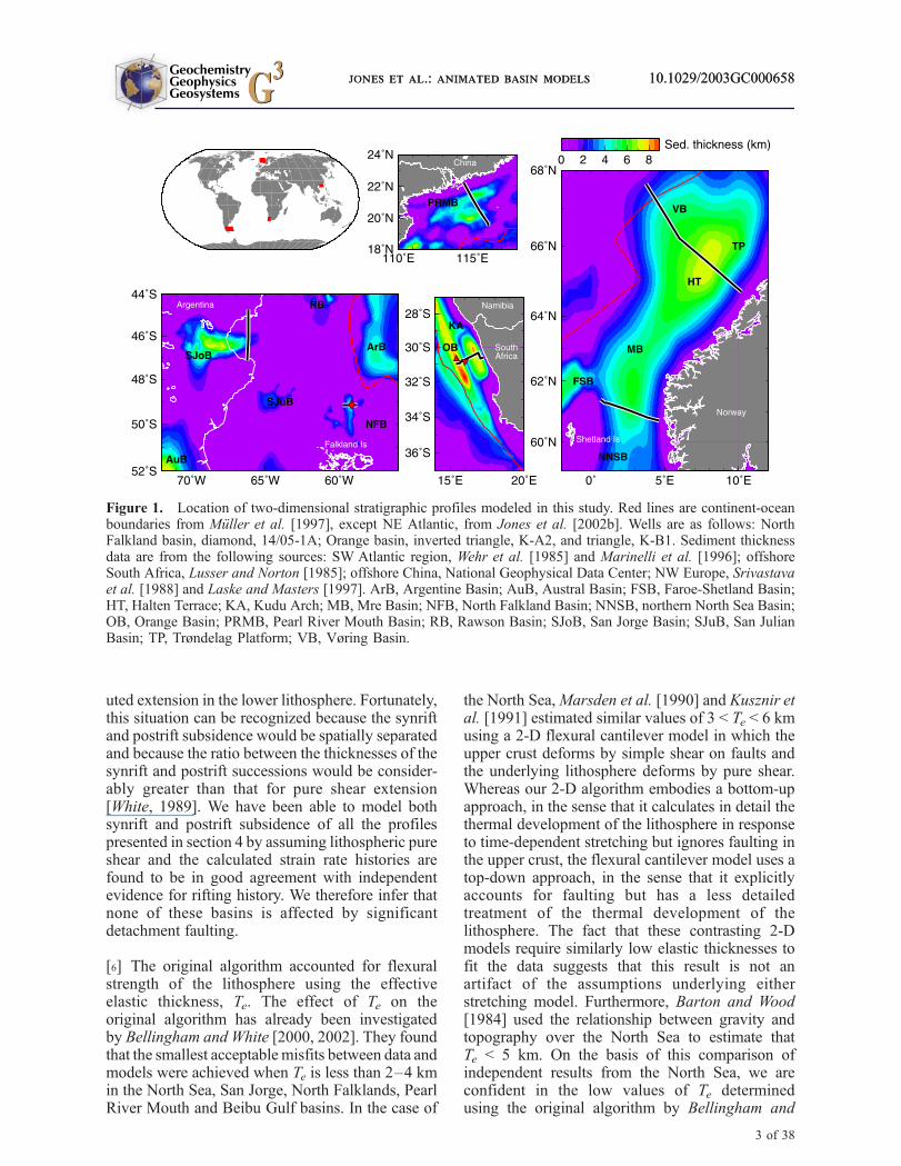
Figure 1. Location of two-dimensional stratigraphic profiles modeled in this study. Red lines are continent-oceanboundaries from Muller et al. [1997], except NE Atlantic, from Jones et al. [2002b]. Wells are as follows: NorthFalkland basin, diamond, 14/05-1A; Orange basin, inverted triangle, K-A2, and triangle, K-B1. Sediment thicknessdata are from the following sources: SW Atlantic region, Wehr et al. [1985] and Marinelli et al. [1996]; offshoreSouth Africa, Lusser and Norton [1985]; offshore China, National Geophysical Data Center; NW Europe, Srivastavaet al. [1988] and Laske and Masters [1997]. ArB, Argentine Basin; AuB, Austral Basin; FSB, Faroe-Shetland Basin;HT, Halten Terrace; KA, Kudu Arch; MB, Mre Basin; NFB, North Falkland Basin; NNSB, northern North Sea Basin;OB, Orange Basin; PRMB, Pearl River Mouth Basin; RB, Rawson Basin; SJoB, San Jorge Basin; SJuB, San JulianBasin; TP, Trøndelag Platform; VB, Vøring Basin.

GeochemistryGeophysicsGeosystems G3G3

jones et al.: animated basin models 10.1029/2003GC000658jones et al.: animated basin models 10.1029/2003GC000658

3 of 38

White [2000, 2002] and Faulkner [2000] for theSan Jorge, North Falkland and Pearl River Mouthbasins and the Orange margin.

[7] Bellingham and White [2000, 2002] did not testthe assumption inherent in the original algorithmthat Te remains constant through time. Temporalvariation in Te might be anticipated since thestrength of rocks has a strong inverse dependenceon temperature and the thermal structure of thelithosphere changes during and after stretching.This problem can be explored using measurementsof Te for terrains of different thermal age innorthwestern Europe. Both the British Isles andthe continental margin to the northwest have Te <5 km, comparable with Te measured in the NorthSea [Barton, 1992; Watts and Fairhead, 1997;Fowler and McKenzie, 1989; Tiley et al., 2003].The North Sea experienced stretching up to a factorof 2 in Triassic and Jurassic times (245–145 Ma),the British Isles is a relatively undeformed block atthe western margin of the North Sea, and thenorthwest European continental margin experi-enced rifting leading to continental breakup inlatest Paleocene time (55 Ma). The fact that avariety of techniques indicate no significant differ-ence between the elastic thickness of these differ-ent terrains suggests that there is no clear case fortime-dependent Te. Watts and Stewart [1998] per-formed a backstripping study of the Gabon passivemargin; they too found no evidence that Te hasvaried through time. In summary, we feel justifiedin restricting modeling of selected extensionalbasins to the Airy case (Te = 0 km) in order tosimplify calculations, based both on the low valuesof Te estimated in earlier studies of these regionsand the general lack of clear evidence for time-dependent in Te.

3. Modifications to theOriginal Algorithm

3.1. Water-Loaded VersusSediment-Loaded Modeling

[8] The original algorithm deals with water-loadedtectonic subsidence. The main advantage of thisscheme is that tectonic subsidence, driven bystretching of the lithosphere, is the fundamentalprocess that creates accommodation space in whichsediment accumulates. The load imparted by theaccumulating sediment then modifies the basin’sshape. Thus the actual subsidence history of ahorizon is influenced by tectonic subsidence, sed-iment supply rate and the physical characteristics

of the sediment, but it is tectonic subsidence thatoriginally creates the basin. Since the originalalgorithm models a water-filled basin, the inputstratigraphy must first be backstripped to removethe effect of the heterogeneous sediment loadbefore modeling [Steckler and Watts, 1978].

[9] Despite the fundamental importance of tectonicsubsidence, several important advantages can begained by modeling a sediment-loaded basin. First,the accumulation, compaction and temperature his-tory of a sediment pile are of great interest to thehydrocarbon industry. A second benefit is that it isrelatively easy to compare model stratigraphy withactual stratigraphy. In contrast, backstripped stratig-raphy is a more abstract concept that is less easilyunderstood by those unfamiliar with basinmodeling.There is a further, more philosophical advantage of asediment-loaded model. In order to use a water-loaded model, the input stratigraphic data must firstbe backstripped. Thus assumptions about parame-terization of the lithospheric template are requiredduring both processing and modeling of the data.Arguably, it would be better to directly modeldigitized stratigraphic profiles. In such a scheme,no modification of the input data set would berequired and all simplifying assumptions would becontained within the model. The ideal basin model-ing algorithm would therefore use the original strati-graphic profile directly as input to the inverseprocedure. This inversion algorithm would be basedon a forward model that simulates accumulation ofsediment as the basin grows. We develop sucha forward model below. However, note that thesediment-loaded basin movies presented in section4 are generated by loading the best fitting syntheticwater-loaded basin with sediment, rather than bydirect inversion of the sediment-loaded profile. Thisdeparture from our ideal procedure simply reflectsthe greater running time of the developmentalsediment-loaded inversion algorithm.

3.2. Sedimentation and Compaction

[10] The sediment-loaded forward model has twoparts. First, the geometry of a water-loaded basin iscalculated using the original algorithm. Then thewater-loaded basin is filled to a specified level withsediment of a given composition. For the lattercalculation, borehole information is used to char-acterize each model layer in terms of four param-eters: solid grain density, rS; depositional porosity,f0; compaction length scale, l; and conductivity ofsolid grains, kS (Table 1). The water-loaded accom-modation space W available for filling with sedi-

GeochemistryGeophysicsGeosystems G3G3

jones et al.: animated basin models 10.1029/2003GC000658

4 of 38

ment is determined from the depositional waterdepth and the total depth of the basin. AssumingAiry isostasy, sediment thickness can be deter-mined from water-loaded accommodation spaceusing

S ¼ WrA � rWrA � �r

� �ð1Þ

where �r is the average density of the sediment pile,rA = 3.18 Mg m�3 is the density of the astheno-sphere and rW = 1.03 Mg m�3 is the density ofseawater. Thus the thickness of a model sedimentlayer DSn deposited at time step n can be calculatedfrom the total water-loaded accommodation spaceWn using

DSn ¼ Wn rA � rWð Þ �Xn�1

i¼1

DSi rA � �rið Þ" #

= rA � �rnð Þ ð2Þ

where the summation accounts for compaction ofthe underlying sediment layers. Sediment layerdensities are calculated using

�r ¼ rS 1� �f� �

þ rW �f ð3Þ

where the average layer porosity �f is determined byintegrating the standard empirical compactionrelationship f = f0 exp (�z/l). At each modeltime step, equation (2) is solved by iteration to findthe thicknesses and average porosities of allsediment layers. Once deposited, the solid thicknessof each layer DSi (1 � �f) is altered only to accountfor later stretching of the basin, in order to conservemass, and no erosion is allowed. The assumption ofno erosion simplifies the calculations and is almostalways justified in the basins considered herein,which have suffered minor structural inversion atmost.

3.3. Depositional Water Depths

[11] The depth of the sediment-filled basin is givenby

BS x; tð Þ ¼ Dþ S Wð Þ ð4Þ

where D(x, t) is the depositional water depth andS(W, x, t) is the thickness of the sedimentarysection, calculated from the history of water-loadedaccommodation space using equation (2). Water-loaded accommodation space is given by

W x; tð Þ ¼ BW � D ð5Þ

where BW(x, t) is the depth of the water-filled basin,determined using the original algorithm. For thefinal model time step (i.e., the present-day), D(x, t)

can be parameterized as the observed depth of theseabed. At other times, D is never knownaccurately although lithologies and bedding geo-metries in the input stratigraphic profile provide arough guide. It is therefore sensible to adopt asimple parameterization of D. In addition, param-eterization of D affects the strain rate history outputfrom the inverse scheme and this dependence ismore easily gauged using a simple parameteriza-tion. One possible method is to assign an averagevalue of D to each input horizon, together with anerror range that is used when assessing the modelfit to the data; Bellingham and White [2002] usedthis method in their backstripping procedure. Itshould be adequate when variations in depositionalwater depth across a basin are small at any giventime. The most common geological situation thatsatisfies this condition is when sediment supply islarge enough to maintain the sediment surfacewithin a few hundred meters of sea level. However,the average depositional water depth method maybe less appropriate when water depth variessubstantially across the basin. This situation canarise when the basin is starved of sediment so thatwater deepens rapidly away from sediment inputpoints, a common situation at passive margins.Large lateral variation in depositional water depthcan be dealt with by increasing the error rangeabout the average value. However, in practice, ahorizon with a large error range exerts a negligibleconstraint during the strain rate inversion processand so data is effectively lost.

[12] We investigated an alternative simple param-eterization that allows water depth to vary acrossa basin. We define R as the ratio between water-loaded accommodation space and total basindepth, i.e., R = W/BW. Substituting equation (5)then gives

D tð Þ ¼ BW 1� Rð Þ ð6Þ

Table 1. Material Properties Used in Backstrippinga

Lithology f0 l, km rS, Mg m�3 kS, W m�1 �C�1

Basalt (BT) 0.1 2.5 3.00 2.3Dolostone (DS) 0.2 3.0 2.86 5.0Limestone (LS) 0.4 1.0 2.70 3.2Mudstone (MS) 0.6 2.0 2.70 2.5Sandstone (SS) 0.5 2.5 2.65 2.3

aVariables are as follows: f0, depositional porosity; l, compaction

scale length; rS, solid grain density; kS, solid grain thermal conductivity.These values used to find the average material properties of each layerthrough time, assuming the pore fluid is seawater of density rW =1.03 Mg m�3 and thermal conductivity kW = 0.61 W m�1 �C�1.

GeochemistryGeophysicsGeosystems G3G3

jones et al.: animated basin models 10.1029/2003GC000658

5 of 38

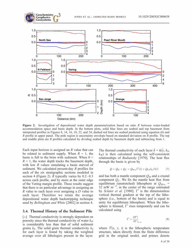
Each input horizon is assigned an R value that canbe related to sediment supply. When R = 1, thebasin is full to the brim with sediment. When 0 <R < 1, the water depth tracks the basement depth,with low R values simulating a basin starved ofsediment. We calculated present-day R profiles foreach of the six stratigraphic sections modeled insection 4 (Figure 2). R typically varies by 0.2–0.3across each profile, and by more at the outer edgeof the Vøring margin profile. These results suggestthat there is no particular advantage in assigning anR value to each layer over assigning a D value toeach layer. Therefore we retain the averagedepositional water depth backstripping techniqueused by Bellingham and White [2002] in section 4.

3.4. Thermal History of the Sediment Pile

[13] Thermal conductivity is strongly dependent onporosity since the thermal conductivity of water kWis considerably less than that of solid sedimentgrains kS. The solid grain thermal conductivity kSfor each layer is found by taking the weightedaverage over all lithologies present in the layer.

The thermal conductivity of each layer �k = k(�f, kS,kW) is then calculated using the self-consistentrelationships of Budiansky [1970]. The heat fluxthrough the basin is given by

Q ¼ QM þ QC ¼ QM1G0 tð Þ þ QC0b0=b tð Þ ð7Þ

and has both a mantle component QM and a crustalcomponent QC. We fix the mantle heat flux fromequilibrium (unstretched) lithosphere at QM1 =32 mW m�2, in the center of the range estimatedby Sclater et al. [1980]. G0 is the dimensionlessvertical thermal gradient at the top of the litho-sphere (i.e., bottom of the basin) and is equal tounity for equilibrium lithosphere. When the litho-sphere is thinned, G0 rises temporarily and can becalculated using

G0 ¼ @T 0

@z0

����z¼a

ð8Þ

where T0(x, z, t) is the lithospheric temperaturestructure, taken directly from the finite differencegrid in the original model, and primes denote

Figure 2. Investigation of depositional water depth parameterization based on ratio R between water-loadedaccommodation space and basin depth. In the bottom plots, solid blue lines are seabed and top basement frominterpreted profiles in Figures 8, 14, 16, 18, 22, and 24; dashed red lines are seabed predicted using equation (6) andR profile in upper panel. The pink region is uncertainty envelope based on standard deviation on R profile. The topand middle plots are R profiles calculated by dividing seabed depth by basement depth and subtracting from 1.

GeochemistryGeophysicsGeosystems G3G3

jones et al.: animated basin models 10.1029/2003GC000658

6 of 38

dimensionless variables. The crustal componentof heat flux QC is generated by radioactive decay[Sclater et al., 1980]. We assume that theradioactive isotopes are distributed uniformlythroughout the crust so that the decrease in heatflux as the crust is thinned by rifting can becalculated easily given the present-day crustalheat flux QC0 and stretching factor b0. QC0 canbe estimated using equation (7) when down-holetemperature measurements are available to con-strain the present-day total heat flux Q, since G0

and b can be calculated from the strain ratehistory. Finally, given the total heat flux and thetemperature at the sediment surface, the tempera-ture structure of the sediment pile is calculatedfrom the topmost layer downward using

T2 ¼ T1 þ QDS=�k ð9Þ

where T1 and T2 are the temperatures at the topand bottom of the layer respectively.

[14] A number of assumptions are inherent in themethod of temperature calculation outlined above.First, the sedimentary section is assumed to be inthermal equilibrium. This assumption is only likelyto fail when kilometers of sediment are deposited

in a few million years. Secondly, lateral conductionof heat is ignored. This assumption is only likely tobe a problem close to the basin margins in theupper part of the sedimentary section, because inthese regions there may be a significant differencebetween the thermal conductivities of sedimentsand basement. In deep basins, the lower part of thesedimentary section below about 5 km approacheszero porosity, and consequently these sedimentshave a similar thermal conductivity to basement.Thirdly, since the sediment-loading algorithm isdecoupled from the 2-D finite difference algorithm,the effect of sediment blanketing on the thermalstructure of the lithosphere, and hence on subsi-dence, is not taken into account. This assumptionmay be a significant source error in the subsidencecalculation for deep, highly stretched passive mar-gins but it is less of a problem for relativelyshallow, intracontinental basins. Fourthly, we ne-glect hydrothermal activity, which advects heatindependently of sediment accumulation. This ef-fect could be significant but it would be extremelydifficult to model even if detailed knowledge of thesedimentary pile and fault system within the basinwere available. Finally, we assume that no heat isgenerated by radioactive decay within the sedimentpile. This effect is probably less important than the

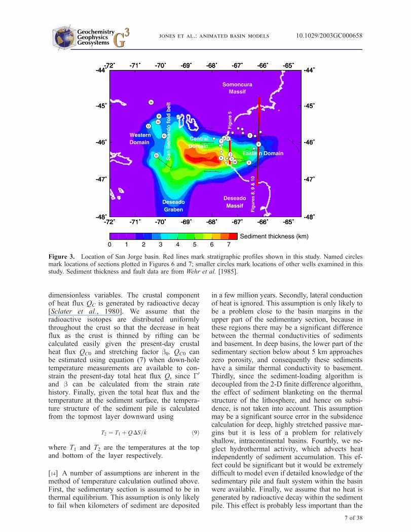
Figure 3. Location of San Jorge basin. Red lines mark stratigraphic profiles shown in this study. Named circlesmark locations of sections plotted in Figures 6 and 7; smaller circles mark locations of other wells examined in thisstudy. Sediment thickness and fault data are from Wehr et al. [1985].

GeochemistryGeophysicsGeosystems G3G3

jones et al.: animated basin models 10.1029/2003GC000658

7 of 38

Figure 4

GeochemistryGeophysicsGeosystems G3G3

jones et al.: animated basin models 10.1029/2003GC000658

8 of 38

combined effects of sediment blanketing and hy-drothermal circulation. Given these potential prob-lems in determining the temperature structurewithin a sedimentary pile, it seems sensible tobegin using the simple method of temperaturecalculation discussed above.

3.5. Animations

[15] The new forward model tracks the basin widthand the thickness and porosity of all horizonsthrough time. At any desired time step this infor-mation can be used to calculate the thermal struc-ture of the sediment pile and then to plot a snapshotof the developing basin. Groups of such snapshotsare then compiled into a movie using one of theMPEG video encoders freely available on theWeb. Results of 2-D inverse subsidence modelingare presented as a trio of figures for each basin.The first figure of each trio describes the fitbetween observed and model stratigraphy and alsoillustrates the best fitting strain rate history. Strainrate histories for all six profiles are plotted usingthe same color scale to facilitate comparison ofstrain rates that occur in different tectonicregimes. The second of each trio of figures isan MPEG movie showing development of thebest fitting model basin, calculated from the strainrate history. All movies share common spatialscales, a common color temperature scale andall are encoded at a default playback speed of20 Myr per second. The color temperature scalerelates to thermal maturation of the sediment pile.Blue shades represent temperatures less than100�C that are not thermally mature, white andyellow shades represent temperatures appropriatefor oil and gas generation respectively andorange-red shades represent temperatures that areovermature for hydrocarbon generation. The finalfigure in each trio is a montage of three or fourframes from the animation.

4. Application

4.1. San Jorge Basin

[16] The San Jorge basin straddles the southeasterncoast of Argentina, from the Andean Front in thewest onto the submarine continental shelf in theeast (Figure 3). This Mesozoic continental interiorbasin is an important hydrocarbon-producing re-gion in Argentina, with ultimate oil recovery esti-

mated at 4 billion barrels [Fitzgerald et al., 1990].The stratigraphic profile modeled here using the2-D algorithm here crosses the eastern domainoffshore. We have also examined a set of 34 wellsdrilled in the western and eastern structuraldomains of the basin and a grid of seismic linesthat mostly cover the offshore eastern domain. Ouraims are threefold: to introduce the modified 2-Dalgorithm; to compare the history of rifting inferredfrom sedimentological and structural observationswith strain rate histories retrieved using the 1-Dand 2-D schemes; and to better understand thekinematic history of the basin in the context ofregional tectonics.

[17] The San Jorge basin can be divided into threestructural domains in the west, center and east. Theeastern and central domains are characterized byWNW–ESE and W–E oriented normal faults.Broadly speaking, in the eastern domain the mainfaults are in the north and dip to the south and theopposite is the case in the western domain [Figariet al., 1999]. The western domain is dominated byNW–SE oriented normal faults. It is separatedfrom the central domain by the San Bernardo foldbelt, a N–S trending array of Cenozoic-aged foldsand detached thrust faults which are controlled byinversion along Mesozoic-aged normal faults.Most of the oil fields lie in the central domain.The basin fill is dominated by sedimentary rocksdeposited in a midplate setting characterized bylow-lying continental and nearshore marine envi-ronments. These deposits have proved difficult todate since they contain few biostratigraphicmarkers. Nevertheless, it is possible to synthesizea coherent stratigraphic column from well logs,biostratigraphic reports and the literature (Figure 4).The limited range in depositional environments isideal for subsidence modeling since uncertaintiesin depositional water depth are small.

4.1.1. Sedimentological and StructuralEvidence for Rifting

[18] Geological and geophysical work since 1950has lead to the view that the present-day San Jorgebasin formed by up to three discrete phasesof rifting during Jurassic and Cretaceous times[Fitzgerald et al., 1990, and references therein;Baldi and Nevistic, 1996; Courtade et al., 1999].The triple-rift hypothesis is based on field map-ping, borehole data and seismic reflection data but

Figure 4. Stratigraphy of San Jorge basin, compiled from well log information and after Zambrano and Urien[1970], Urien and Zambrano [1973], and Fitzgerald et al. [1990]. FA, foraminiferal assemblage; P, pollen.

GeochemistryGeophysicsGeosystems G3G3

jones et al.: animated basin models 10.1029/2003GC000658

9 of 38

little work has been done on subsidence modeling.The top of the basement mosaic of Precambrian-Devonian sedimentary, igneous and metamorphicrocks is well defined as an erosional surface onseismic reflection data. Fitzgerald et al. [1990] andBaldi and Nevistic [1996] have proposed that theSan Jorge basin began to form during a LateTriassic-Early Jurassic rifting event, but althoughTriassic rocks outcrop in the surrounding massifs,their existence within the basin itself is less wellconstrained. The earliest rift basin fill demonstrablein our data set is the Lias unit, which is laterallyrestricted within grabens and half grabens devel-oped on the Deseado massif and beneath the

present-day San Jorge basin. The overlying LoncoTrapail unit also shows marked thickness changesacross faults but is laterally more widespread thanthe Lias unit (Figure 5). Figari et al. [1999]consider the Lias a prerift deposit and suggest thatrifting began during Lonco Trapail time; this viewmay be a consequence of the localized spatialextent of the Lias. The Lonco Trapail unit containslarge volumes of basaltic and felsic volcanic rocksand volcaniclastic sediments, which have beeninterpreted as the products of synrift magmatism[Fitzgerald et al., 1990]. The Aguada Bandera andCerro Guadal units are thin and laterally patchy;they were deposited relatively slowly throughout

Figure 5. Seismic profile across the San Jorge basin shown both uninterpreted and interpreted. Location is markedon Figure 3.

GeochemistryGeophysicsGeosystems G3G3

jones et al.: animated basin models 10.1029/2003GC000658

10 of 38

Figure 6

GeochemistryGeophysicsGeosystems G3G3

jones et al.: animated basin models 10.1029/2003GC000658

11 of 38

Late Jurassic and earliest Cretaceous times. Lowsediment accumulation rates coupled with the ob-servation that the sediment surface remained closeto sealevel throughout this time period points tolow subsidence rates. Thus stratigraphical andstructural evidence suggests that the present-daySan Jorge basin began to form by rifting duringEarly-Middle Jurassic times (206–162 Ma), withthe Lias and Lonco Trapail units comprising thesynrift succession and the Aguada Bandera andCerro Guadal units deposited more slowly duringthe succeeding phase of thermal subsidence.

[19] Deposition of the D-129 unit marked a changein structural style within the basin: rocks beneath arelaterally restricted, often within grabens and halfgrabens; the layers above are more laterally exten-sive and aremuch less influenced by individual tiltedfault blocks (the ‘‘sag’’ phase of Fitzgerald et al.[1990]) (Figure 5). Although this change in layergeometry has the appearance of a synrift to postrifttransition, the post-D-129 rocks are cut by faults upto and including the Yaci de Trebol unit, showingthat at least one more rifting event occurred whichended in latest Cretaceous time at around 70 Ma.Most workers subdivide the Cretaceous rifting intotwo discrete events but the evidence for this division

can be subtle. For example, there is no consistentevidence that the Lower and Upper Cretaceouspackages show growth across faults while the Mid-dle Cretaceous unit maintains constant thickness(Figure 5 and seismic profiles of Fitzgerald et al.[1990] and Baldi and Nevistic [1996]). According toFitzgerald et al. [1990], most normal faulting ceasedtoward the end of D-129 times and the units aboveare marked by basin-wide stability shown by de-creased facies response to local conditions, puttingthe endof the secondbasin-wide rift event at 121Ma.A third rift event then faulted the younger rocksduring Late Cretaceous time. On some of seismicprofiles, a small subset of normal faults are rooted inthe D-129 unit rather than in basement, which couldbe interpreted as evidence of a discrete Late Creta-ceous rifting event. Perhaps the best evidence fortwo discrete phases of Cretaceous rifting is the rateof sediment accumulation, which can be determinedfrom Figure 4; the Middle Cretaceous Minadel Carmen unit was deposited considerably moreslowly than both the Lower Cretaceous D-129 unitand the Upper Cretaceous Comodoro Rivadavia-Yaci de Trebol succession. In summary, a secondbasin-wide phase of rifting commenced at around132 Ma and the D-129 unit represents the mainsynrift deposit. The Comodoro Rivadavia and Yaci

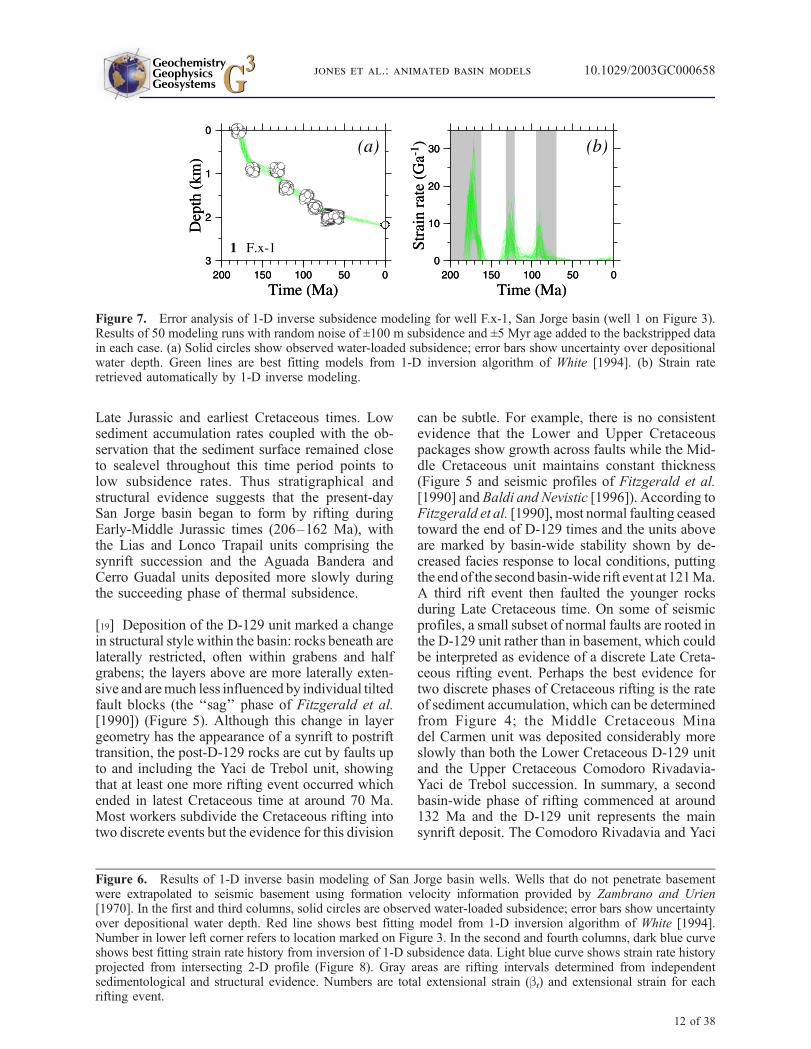
Figure 6. Results of 1-D inverse basin modeling of San Jorge basin wells. Wells that do not penetrate basementwere extrapolated to seismic basement using formation velocity information provided by Zambrano and Urien[1970]. In the first and third columns, solid circles are observed water-loaded subsidence; error bars show uncertaintyover depositional water depth. Red line shows best fitting model from 1-D inversion algorithm of White [1994].Number in lower left corner refers to location marked on Figure 3. In the second and fourth columns, dark blue curveshows best fitting strain rate history from inversion of 1-D subsidence data. Light blue curve shows strain rate historyprojected from intersecting 2-D profile (Figure 8). Gray areas are rifting intervals determined from independentsedimentological and structural evidence. Numbers are total extensional strain (bt) and extensional strain for eachrifting event.

Figure 7. Error analysis of 1-D inverse subsidence modeling for well F.x-1, San Jorge basin (well 1 on Figure 3).Results of 50 modeling runs with random noise of ±100 m subsidence and ±5 Myr age added to the backstripped datain each case. (a) Solid circles show observed water-loaded subsidence; error bars show uncertainty over depositionalwater depth. Green lines are best fitting models from 1-D inversion algorithm of White [1994]. (b) Strain rateretrieved automatically by 1-D inverse modeling.

GeochemistryGeophysicsGeosystems G3G3

jones et al.: animated basin models 10.1029/2003GC000658

12 of 38

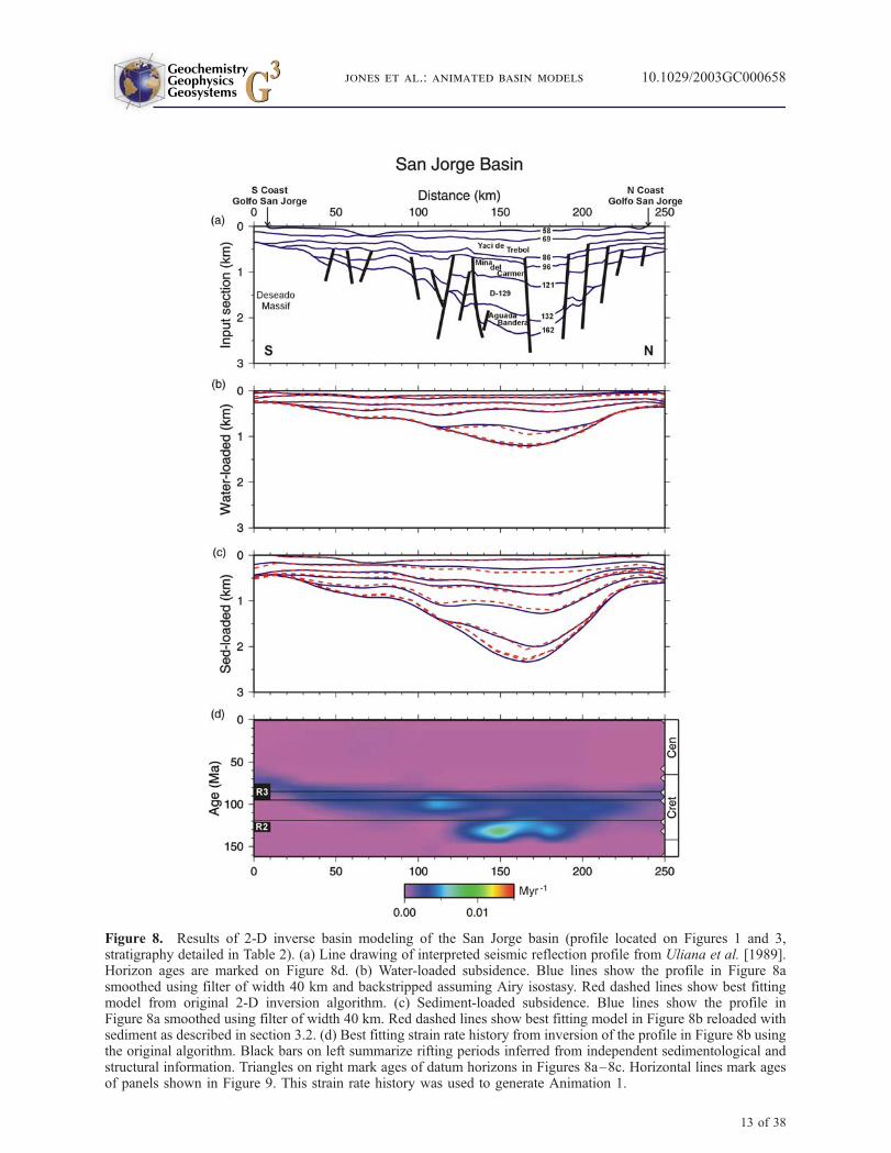
Figure 8. Results of 2-D inverse basin modeling of the San Jorge basin (profile located on Figures 1 and 3,stratigraphy detailed in Table 2). (a) Line drawing of interpreted seismic reflection profile from Uliana et al. [1989].Horizon ages are marked on Figure 8d. (b) Water-loaded subsidence. Blue lines show the profile in Figure 8asmoothed using filter of width 40 km and backstripped assuming Airy isostasy. Red dashed lines show best fittingmodel from original 2-D inversion algorithm. (c) Sediment-loaded subsidence. Blue lines show the profile inFigure 8a smoothed using filter of width 40 km. Red dashed lines show best fitting model in Figure 8b reloaded withsediment as described in section 3.2. (d) Best fitting strain rate history from inversion of the profile in Figure 8b usingthe original algorithm. Black bars on left summarize rifting periods inferred from independent sedimentological andstructural information. Triangles on right mark ages of datum horizons in Figures 8a–8c. Horizontal lines mark agesof panels shown in Figure 9. This strain rate history was used to generate Animation 1.

GeochemistryGeophysicsGeosystems G3G3

jones et al.: animated basin models 10.1029/2003GC000658

13 of 38

Figure 9. Selected frames from the animated model of the San Jorge Basin (Animation 1).

GeochemistryGeophysicsGeosystems G3G3

jones et al.: animated basin models 10.1029/2003GC000658

14 of 38

de Trebol units may have been deposited during athird phase of rifting which began at around 95 Maand ended not later than 70 Ma.

[20] The latest Cretaceous and Cenozoic rocks aremostly unfaulted and are therefore generallyviewed as postrift deposits (Figure 5) [Fitzgeraldet al., 1990]. Basin-wide unconformities duringEarly-Middle Eocene and Middle Oligocene timeswere associated with regional uplift events thatlead to erosion of the basin margins and imparted agentle eastward tilt to the basin. Structural short-ening also occurred during the Cenozoic, particu-larly in the San Bernardo fold belt between thewestern and central structural domains. Localizedgraben and half graben of Oligocene-Miocene agehave been interpreted as evidence for regionalextension [Bellosi, 1995], although the timingsuggests they are more likely small-scale featuresgenetically linked with the San Bernado foldbelt. Extrusive and intrusive volcanism occurredthrough Oligocene-Miocene times and again

through Plio-Pleistocene times [Baker et al.,1981]. These authors suggested that the volcanismmay reflect incipient crustal rifting in a back arcenvironment. On the basis of modeling of organicgeochemical data, Rodriguez and Littke [2001]estimate that the Cenozoic section reached a max-imum thickness of 1–1.5 km during Early Oligo-cene time, so that regional uplift removed roughlyhalf of the original Cenozoic section.

4.1.2. Results of 1-D and2-D Subsidence Modeling

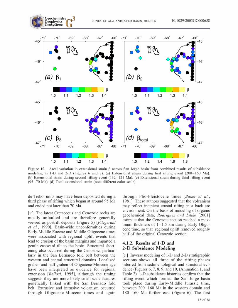
[21] Inverse modeling of 1-D and 2-D stratigraphicsections shows all three of the rifting phasesinferred from sedimentological and structural evi-dence (Figures 6, 7, 8, 9, and 10, (Animation 1, andTable 2). 1-D subsidence histories confirm that therifting event which formed the San Jorge basintook place during Early-Middle Jurassic time,between 200–160 Ma in the western domain and180–160 Ma further east (Figure 6). The first

Figure 10. Areal variation in extensional strain b across San Jorge basin from combined results of subsidencemodeling in 1-D and 2-D (Figures 6 and 8). (a) Extensional strain during first rifting event (200–160 Ma).(b) Extensional strain during second rifting event (132–121 Ma). (c) Extensional strain during third rifting event(95–70 Ma). (d) Total extensional strain (note different color scale).

GeochemistryGeophysicsGeosystems G3G3

jones et al.: animated basin models 10.1029/2003GC000658

15 of 38

regional rifting event is not seen in the 2-Dmodel nor in the 1-D results from the east ofthe basin because the Lias and Lonco Trapailunits are not present in the east (Figures 8 and10). Although seismic and well data indicate anerosional unconformity between the Lias andLonco Trapial units that compose the first riftingevent, the few wells from the western domainthat contain both these units reveal no evidencethat this rifting event was subdivided into twodiscrete phases. The second and third regionalrifting events are constrained by both 2-D and1-D modeling results (Figures 6, 7 and 8 andAnimation 1). Despite the absence of conclusiveseismic and lithological evidence for one or tworifting events during Cretaceous times, inversemodeling automatically retrieves two discreterifting events (Figures 6 and 8). Sensitivity testson one of the 1-D sections confirm that twoCretaceous rifting events are required by the data(Figure 7). The second regional rifting event ismore intense than the third and lasts from 140–120 Ma. It occurs throughout the basin, althoughthe greatest degrees of stretching occur in thecentral domain of the basin. The third riftingevent lasts from 100 to 80 Ma, is more spatiallydiffuse with lower strain rates and does not occurin the west of the basin. The timings of boththese rifting events are in good agreement withthe independent sedimentological and structuralevidence. The greatest amount of total stretchingoccurred in the center of the basin close to thepresent-day coastline. The transition from synriftto postrift subsidence is particularly clear on the2-D animated subsidence history (Animation 1).The basin extends by 25 km until Late Creta-ceous times and coeval relatively rapid subsi-dence occurs. After �80 Ma, strain rates reduceautomatically to negligible values and extensionof the right hand edge of the model ceases butsubsidence continues throughout Cenozoic time,

decreasing exponentially in rate. Lacustrine,organic-rich shales of the D-129 sequence arethe principal source of hydrocarbons in the SanJorge Basin. Our thermal calculations suggestthat this horizon is barely in the oil window atpresent in the eastern domain of the basin(Figure 9 and Animation 1). It is therefore likelythe D-129 is presently mature in the region ofthe present coastline, where 1-D results showthat greater stretching has occurred (Figure 10).This scenario is consistent with the fact that mostof the oilfields are situated in the central struc-tural domain of the basin.

4.1.3. Discussion

[22] The first regional rifting event (200–160Ma) inthe San Jorge basin was coeval with rifting in theCuyo and Neuquen basins to the northwest. It tookplace before breakup of western Gondwana and wasmore likely related to subduction along the westernedge of South America. One-dimensional and two-dimensional subsidence histories record rifting ear-lier in the western domain and later in the easterndomain. If the prerift basement surface lay at auniform height across the incipient San Jorge basin,then the observed subsidence pattern implies thatextension began in thewest and propagated eastwardthrough Early and Middle Jurassic times. Alterna-tively, the basement surface in the eastern domainmay have formed a topographic high relative thissurface in the western domain. In this case, riftingcould have begun simultaneously across the entireSan Jorge basin but the western domain began toaccumulate sediments relatively early in the riftingphase since it lay structurally lower. The latterscenario is perhaps more consistent with sedimen-tological evidence thatmarine incursions entered theSan Jorge basin from the Pacific Ocean via theNeuquen basin in the northwest during Early Juras-sic times [Fitzgerald et al., 1990].

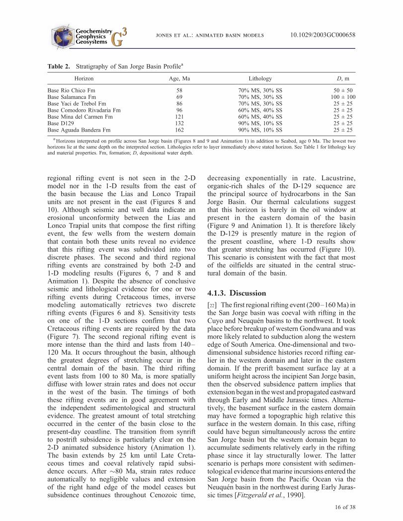
Table 2. Stratigraphy of San Jorge Basin Profilea

Horizon Age, Ma Lithology D, m

Base Rio Chico Fm 58 70% MS, 30% SS 50 ± 50Base Salamanca Fm 69 70% MS, 30% SS 100 ± 100Base Yaci de Trebol Fm 86 70% MS, 30% SS 25 ± 25Base Comodoro Rivadaria Fm 96 60% MS, 40% SS 25 ± 25Base Mina del Carmen Fm 121 60% MS, 40% SS 25 ± 25Base D129 132 90% MS, 10% SS 25 ± 25Base Aguada Bandera Fm 162 90% MS, 10% SS 25 ± 25

aHorizons interpreted on profile across San Jorge basin (Figures 8 and 9 and Animation 1) in addition to Seabed, age 0 Ma. The lowest two

horizons lie at the same depth on the interpreted section. Lithologies refer to layer immediately above stated horizon. See Table 1 for lithology keyand material properties. Fm, formation; D, depositional water depth.

GeochemistryGeophysicsGeosystems G3G3

jones et al.: animated basin models 10.1029/2003GC000658

16 of 38

[23] The second regional rifting event was prob-ably related to the breakup of western Gondwanaand the onset of seafloor spreading in the SouthAtlantic. Onset of the rifting that would lead toseafloor spreading is thought correlated with aphase of dyke injection along the Namibian andSouth African coasts, dated as 134 ± 3 Ma usingthe Ar-Ar method and 132 ± 6 Ma using the K-Armethod [Reid and Rex, 1994]. These dates agreewell with the onset of rifting and D-129 deposi-tion in the San Jorge basin. Onset of seafloorspreading is constrained by Barremian (127–121 Ma) sedimentary rocks immediately overlyingoceanic basement in DSDP hole 361 [Bolli et al.,1978] and the magnetic age of oldest oceaniccrust of about 127 Ma [Nurnberg and Muller,1991]. Rifting in the San Jorge basin ended onlyslightly later at about 120 Ma. The coincidence intiming between the second phase of rifting in theSan Jorge basin and rifting leading to SouthAtlantic seafloor spreading is perhaps unexpectedsince the South Atlantic is oriented perpendicularto the San Jorge basin. The tectonic explanationfor the third regional rifting event is less clear.Our regional studies suggest that coeval riftingoccurred in the Colorado and Salado basins,which lie to the north along the coast of Argen-tina, and that coeval uplift and erosion occurredon the African side of the Atlantic [Faulkner,2000]. Fitzgerald et al. [1990] suggest that thethird rifting event is related to a change in platemotions and Uliana et al. [1989] suggest it couldbe associated with development of the Andes.Indeed, the start of the third rifting event inCenomanian times coincides with major uplift ofthe Andean Cordillera [Barker et al., 1991]. Theresulting regional eastward tilt may have driventhe relatively small amounts of extension in theSan Jorge basin implied by the modeled strainrate histories.

[24] The various Cenozoic regional unconform-ities have not prevented us from accuratelyfitting the 1-D and 2-D subsidence data. Neitherthe 1-D nor the 2-D algorithm specificallyaccounts for erosion. Thinning of sedimentarysequences either by nondeposition or erosionwould therefore be accounted for by spuriousnegative strain rate values. Lack of negativestrain rates in the model results therefore impliesthat the total amount of rock removed was lessthan a few hundred meters, equivalent to theuncertainty associated with depositional waterdepths. Thus the maximum thickness of sedimentdeposited during Cenozoic times may have been

generally less than the 1–1.5 km estimated byRodriguez and Littke [2001] and significant ero-sion probably occurred only at the basin margins.

4.2. North Falkland Basin

[25] The North Falkland basin lies offshore northof the Falkland Islands within the northern part ofthe Falkland Plateau, an eastward projection of theSouth American continental shelf (Figure 1). Untilrecently, the geological history of the North Falk-land basin was based on seismic reflection, gravityand magnetic data and the age of the basin wasinferred by indirect correlation with other SouthAmerican and southern African sedimentary basinswhich had been drilled [Lawrence and Johnson,1995; Ross et al., 1996; Richards et al., 1996;Richards and Fannin, 1997]. Here we use datafrom wells drilled in the basin during 1998 toquantify the rifting history via 1-D and 2-D subsi-dence modeling. Aside from presenting a second2-D animated basin history, an important aim inthis section is to further investigate the effect ofspatial filtering of the input stratigraphic profile on2-D inverse modeling.

4.2.1. Stratigraphy and Structural Evidencefor Rifting

[26] Our 2-D profile crosses the North FalklandGraben region toward the northern part of theNorth Falkland basin (Figure 1). The North Falk-land Graben is a N-S trending extensional systemaround 250 km long and 40 km wide. It isdominated by steep, planar, normal faults withlittle or no evidence of inversion or strike-slipmovement. The main graben can be divided intoeastern and western subbasins separated by acentral ridge (Figure 11). The eastern subbasinhas a half-graben geometry with the master faulton its eastern side while the western subbasin hasfaults which dip both eastward and westward.Seismic profiles clearly show a lower, faultedsection and an upper, unfaulted section, indicatingthat, broadly speaking, an early phase of riftingwas followed by postrift subsidence. To date thishistory of basin evolution we use a scheme basedon biostratigraphic, core and wire line log resultsfrom two wells drilled during the 1998 explorationcampaign (Figure 12). The basement in the regionis Devonian in age, similar in character to sedi-mentary rocks which outcrop on the FalklandIslands. Basement rocks are overlain by a succes-sion of clastic sedimentary rocks with interbeddedtuffs, thought to represent alluvial fan environ-

GeochemistryGeophysicsGeosystems G3G3

jones et al.: animated basin models 10.1029/2003GC000658

17 of 38

Figure 11. Seismic profile across the North Falkland basin used for for 2-D inverse modeling in Figure 14.Location marked on Figure 1. Well 14/05-1A was extrapolated to seismic basement using VSP check shot (timeversus depth) data.

GeochemistryGeophysicsGeosystems G3G3

jones et al.: animated basin models 10.1029/2003GC000658

18 of 38

ments followed by lacustrine environments. Poorbiostratigraphical control and lack of regional wellpenetration prevent exact dating of this unit.Richards and Hillier [2000a] observe from bio-

stratigraphic evidence that the unit can be no olderthan Middle Jurassic but could be as young asValanginian. Lawrence et al. [1999] and Bransdenet al. [1999] suggest a correlation between volca-

Figure 12. Stratigraphic scheme for the North Falkland basin based on well logs and biostratigraphic information inunpublished oil company reports. Lithology key is on Figure 4. D, dinocyst; FA, freshwater algae; MS, miospore;P, pollen.

GeochemistryGeophysicsGeosystems G3G3

jones et al.: animated basin models 10.1029/2003GC000658

19 of 38

niclastic rocks in the North Falkland basin and thosein the Middle-Upper Jurassic Tobifera and ChonAike successions in the San Jorge basin (e.g.,Figure 4). Well 14/05-1A was drilled toward thecenter of the eastern depocenter of the North Falk-land Graben and proved that the synrift sequenceconsists of Upper Jurassic-Lower Cretaceous clasticsedimentary rocks deposited in a lacustrine orfluvial environments with abundant volcaniclasticmaterial. The youngest sediments that are clearlyfaulted are probably of Middle Cretaceous age(�125 Ma in our stratigraphic scheme). The limitedrange of depositional water depths throughout thesynrift period is ideal for subsidence modeling.Although the ages of the faulted sediments broadlysuggest that the North Falkland basin formed byrifting during Late Jurassic-Early Cretaceous times,there is much disagreement over whether this riftingoccurred as several discrete phases. Lawrence et al.[1999] propose that three rift sequences are distin-guishable, separated by two midrift unconformities.Bransden et al. [1999] note that the earliest of theserift sequences is represented only by a set of EarlyJurassic dykes which outcrop on Falkland Islands.Instead, they suggest that two rift phases of riftingoccurred, the first of which produced a NW–SEoriented system which was later crosscut and/orlocally reactivated by N–S extensional faults. Sev-eral other authors divide the synrift succession intotwo on the basis of seismic interpretation [Ross etal., 1996; Richards and Fannin, 1997; Thompsonand Underhill, 1999]. Ross et al. [1996] suggestthat the younger rift event was more aerially exten-sive than the earlier event, although Lawrence andJohnson [1995] and Richards et al. [1996] concludethat both phases were controlled by the same faultset.

[27] The postrift succession within the easternsubbasin records a general transition from fluvial/lacustrine to marginal marine and then open ma-rine conditions from Middle Cretaceous timesonwards, although more restricted depositionalenvironments persisted over structural highs[Richards and Hillier, 2000a]. However, postriftthermal subsidence may have been punctuated byone or more periods of uplift and shortening.Richards and Fannin [1997] and Lawrence et al.[1999] suggest that flower-type fault structures inthe south of the North Falkland basin and elsewhererelate to a period of Maastrichtian-Paleocene re-gional uplift. Thompson and Underhill [1999] con-clude that the flower structures are in fact syntheticand antithetic to larger extensional faults and thatdomal features near the half graben axes are related

to lateral facies changes and differential compactionrather that structural inversion. Richards and Hillier[2000a] compile biostratigraphic data from the 6wells and state that the two most significant regionalunconformities span late-Cenomanian-Santoniantimes and much of Maastrichtian times. Vitrinitereflectance data suggest that around 800 m ofsedimentary rock was eroded from structural highsduring these times, although the eastern subbasinmay have experienced more or less continuousdeposition [Richards and Hillier, 2000b].

4.2.2. Results and Discussion of 1-D and2-D Subsidence Modeling

[28] Both 2-D and 1-D inverse modeling provide agood fit to the observed stratigraphy (Figures 13,14, and 15, Animation 2, and Table 3). Thecalculated strain rate histories show a single peakclose to the Jurassic-Cretaceous boundary (144 Ma;Figures 13 and 14). Strain rates decrease automat-ically through the Early Cretaceous to negligiblevalues by Middle Cretaceous times (120–100 Ma)in good agreement with the pattern of faultingobserved on seismic profiles. One-dimensionaland two-dimensional results are clearly compatible,although the rifting event retrieved by 1-D model-ing has a higher peak strain rate and a shorterduration than that retrieved by 2-D modeling, fortwo reasons (Figure 13). First, the 1-D and 2-Dstrain rate histories are discretized in 5 and 10 Myrtime steps respectively both because of the greaternumber of unconstrained dimensions in the 2-Dproblem and because the 1-D problem is con-strained by more age-depth data points. Second,the 1-D section is measured close to the deepestpart of a graben, whereas the spatial filtering of the2-D stratigraphy generates an average profile thatbalances the expanded synrift succession in thegrabens with the condensed synrift succession onthe horsts. Thus the 2-D animation yields the betterestimate of the total extension across the region,which amounts to about 10 km (Figure 15 andAnimation 2). We conclude that no significantstrain rate information is lost during lateral filteringof the stratigraphy.

[29] Both 2-D and 1-D results show that develop-ment of the North Falkland basin is compatiblewith a single phase of rifting, in contrast with manyof the studies mentioned above. The distinctchange in subsidence rate clearly seen as a corneron the 1-D subsidence plot effectively determinesthe age of the end of rifting retrieved by the inverseschemes. This corner is a robust feature even whenuncertainties of up to ±10 Myr in estimates of the

GeochemistryGeophysicsGeosystems G3G3

jones et al.: animated basin models 10.1029/2003GC000658

20 of 38

age of the synrift and early postrift sequences areconsidered, and is associated with the youngestfaulted rocks independent of the absolute ageassigned to it. A twin-peaked strain rate historywould only be feasible if the poorly dated lower-most synrift succession accumulated rapidly inMiddle Jurassic times and a marked unconformitythen developed prior to deposition of the remainderof the synrift succession. Our adopted stratigraphyplaces the synrift period toward the younger end ofthe range given by Richards and Hillier [2000a]. Inhindsight, this choice seems sensible because theend of the observed and calculated rifting eventcoincides with the onset of seafloor spreading in the

SouthAtlantic, which occurred around 127–121Ma(section 4.5). In this scenario, rifting terminated inbasins bordering the incipient ocean when regionalextension began to be accommodated at the new,hot, weak spreading center.

[30] The strain rate history determined by 2-Dinverse modeling displays a minor Paleocene-Eocene event of roughly constant magnitude acrossthe entire basin. This second event is probably anartifact of the observed minor regional unconform-ities of Late Cretaceous age recognized in the welldata. Transient uplift that generated the unconform-ities probably lead to condensation or erosion ofthe Upper Cretaceous postrift section and recoveryof this uplift then lead to a corresponding thicken-ing of the Paleogene section. The 2-D inversionalgorithm has detected the post-Paleocene increasein sedimentation rate and interpreted it as a minorrift event. The strain rate history determined from1-D inverse modeling does not show a comparableminor increase in strain rate. Its absence is asexpected since the well is located within the deep-est part of a graben where localized rapid subsi-dence preserved a continuous succession duringregional uplift, as indicated by vitrinite reflectancedata [Richards and Hillier, 2000a]. In contrast,spatial filtering of the 2-D section averages thecomplete stratigraphic sections in the graben andthe less complete sections on the horst blocks.

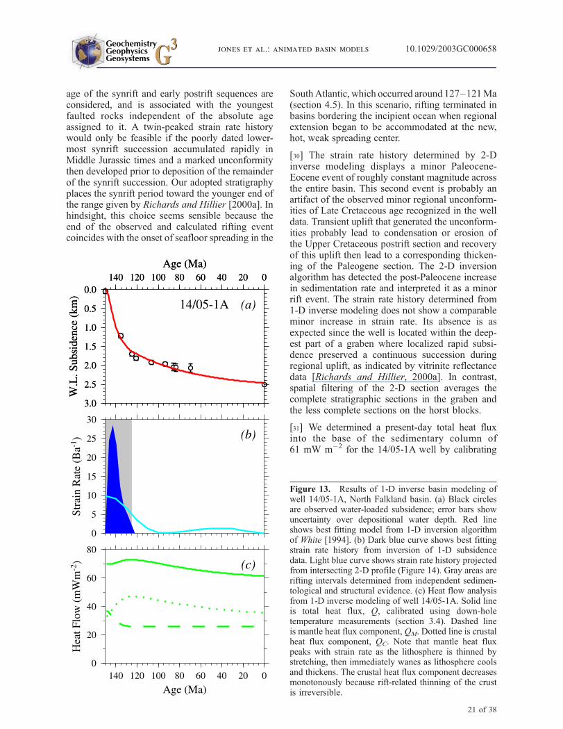
[31] We determined a present-day total heat fluxinto the base of the sedimentary column of61 mW m�2 for the 14/05-1A well by calibrating

Figure 13. Results of 1-D inverse basin modeling ofwell 14/05-1A, North Falkland basin. (a) Black circlesare observed water-loaded subsidence; error bars showuncertainty over depositional water depth. Red lineshows best fitting model from 1-D inversion algorithmof White [1994]. (b) Dark blue curve shows best fittingstrain rate history from inversion of 1-D subsidencedata. Light blue curve shows strain rate history projectedfrom intersecting 2-D profile (Figure 14). Gray areas arerifting intervals determined from independent sedimen-tological and structural evidence. (c) Heat flow analysisfrom 1-D inverse modeling of well 14/05-1A. Solid lineis total heat flux, Q, calibrated using down-holetemperature measurements (section 3.4). Dashed lineis mantle heat flux component, QM. Dotted line is crustalheat flux component, QC. Note that mantle heat fluxpeaks with strain rate as the lithosphere is thinned bystretching, then immediately wanes as lithosphere coolsand thickens. The crustal heat flux component decreasesmonotonously because rift-related thinning of the crustis irreversible.

GeochemistryGeophysicsGeosystems G3G3

jones et al.: animated basin models 10.1029/2003GC000658

21 of 38

Figure 14. Results of 2-D inverse basin modeling of the North Falkland Basin. Stratigraphy is detailed in Table 3.(a) Line drawing of interpreted seismic reflection profile (Figure 11). Horizons ages are marked on Figure 14d.(b) Water-loaded subsidence. Blue lines show the profile in Figure 14a smoothed using filter of width 40 km andbackstripped assuming Airy isostasy. Red dashed lines show best fitting model from original 2-D inversion algorithm.(c) Sediment-loaded subsidence. Blue lines show the profile in Figure 14a smoothed using filter of width 40 km. Reddashed lines show best fitting model in Figure 14b reloaded with sediment as described in section 3.2. (d) Best fittingstrain rate history from inversion of the profile in Figure 14b using the original algorithm. Black bars on leftsummarize rifting periods inferred from independent sedimentological and structural information. Triangles on rightmark ages of datum horizons in Figures 14a–14c. Horizontal lines mark ages of panels shown in Figure 15. Thisstrain rate history was used to generate Animation 2.

GeochemistryGeophysicsGeosystems G3G3

jones et al.: animated basin models 10.1029/2003GC000658

22 of 38

the calculated temperature in the sediment pile todown-hole temperature measurements (Figure 13).The calculated heat flux value lies within theobserved range for Mesozoic continental rift basins[Sclater et al., 1980]. We estimate that the wellexperienced an estimated maximum heat flux of73 mW m�2 at �125 Ma, close to the end of therifting phase. The present-day heat flux estimate

has been used to determine the thermal history inthe 2-D sediment-loaded model (Animation 2). Thesource rock interval in the North Falkland Basincorresponds to the synrift and early postrift suc-cession [Richards and Hillier, 2000b]. Our thermalmodeling suggests that the base of this interval ispresently in the oil generation window. Bearing inmind that the hanging walls are up to 1 km more

Figure 15. Selected frames from the animated model of the North Falkland Basin (Animation 2).

Table 3. Stratigraphy of North Falkland Basin Profilea

Horizon Age, Ma Lithology D, m

Intra Maastrictian 69 60% MS, 40% SS 100 ± 100Base Santonian 86 50% MS, 50% SS 100 ± 100Base Turonian 94 50% MS, 45% SS, 5% DS 50 ± 50Intra Albian 106 50% SS, 45% MS, 5% DS 25 ± 25Intra Barremian 125 60% SS, 40% MS 25 ± 25Intra Valanginian 136 80% SS, 20% MS 25 ± 25Intra Kimmeridgian 150 80% SS, 20% MS 25 ± 25

aHorizons interpreted on profile across North Falkland basin (Figures 14 and 15 and Animation 2) in addition to Seabed, age 0 Ma. Lithologies

refer to layer immediately above stated horizon. See Table 1 for lithology key and material properties.

GeochemistryGeophysicsGeosystems G3G3

jones et al.: animated basin models 10.1029/2003GC000658

23 of 38

deeply buried than the spatially filtered stratigra-phy, it is likely that deepest parts of the basin arethermally postmature. These results are in broadagreement with geochemical analysis of samplesrecovered from the basin [Richards and Hillier,2000b].

4.3. North Sea Basin

[32] Bellingham and White [2002] carried out adetailed analysis of a 2-D profile crossing the NorthSea during development of the original 2-D inver-sion algorithm. Here we extend Bellingham andWhite’s work by presenting a 2-D animated modelof the same 2-D profile (Figures 16 and 17,Animation 3), and Table 4). The stratigraphicprofile crosses the East Shetland basin and VikingGraben at 61�N (Figure 1) and clearly shows theclassic tilted fault block geometries typical of theregion (Figure 16). The structural development andsubsidence history of the North Sea basin havebeen investigated exhaustively using a variety of1-D and 2-D forward modeling techniques [e.g.,Barton and Wood, 1984; Marsden et al., 1990].The latest phase of rifting occurred in Late Jurassictimes and is well understood [e.g., Glennie, 1998;Parker, 1993]. In contrast, lack of well penetrationinto the pre-Jurassic section means that the preced-ing Triassic extensional episode is poorly under-stood, so we concentrate on modeling the LateJurassic extensional event for simplicity. Results of2-D inverse modeling show a good fit to the synriftstratigraphy but the fit to the postrift stratigraphy isless good. The calculated strain rate distributionpicks out the principal rifting event in Late Jurassictimes (155–145 Ma). Strain rates are much lowerduring Cretaceous and Cenozoic times, but they donot vanish as might be expected given the lack ofseismic evidence for post-Jurassic rifting. AlthoughCretaceous rifting occurred in the Møre basinadjoining to the north, there is little seismic evi-dence for coeval rifting in the North Sea [Parker,1993], and Hall and White [1994] have shown thatCenozoic extension is negligible. Thus the variousminor strain rate events that vary in spatial distribu-tion and occur between Late Cretaceous and Mio-cene times are probably similar to the Paleocenesubsidence anomaly observed in the North FalklandBasin (section 4.2); the inversion algorithm is pick-ing up small increases in subsidence rate that cannotbe accounted for by thermal subsidence followingLate Jurassic rifting. Mid-Cretaceous subsidenceanomalies have previously been recognized in theNorth Sea basin [Gabrielsen et al., 2001]. It ispossible that they reflect a regional epeirogenic

event since coeval subsidence anomalies are ob-served in many other basins surrounding Britainand Ireland [McMahon and Turner, 1998]. Subsi-dence anomalies of Cenozoic age can be linked todevelopment of the Icelandic mantle convectivesystem. Transient uplift of up to 500 m wasprobably related to the asthenospheric thermalanomaly that generated the North Atlantic IgneousProvince; this thermal anomaly was emplacedbeneath the plate during Late Paleocene timesand decayed through Eocene times [Nadin et al.,1997; Jones and White, 2003]. Apatite fissiontrack studies indicate that uplift of SW Scandina-via generated several kilometers of denudationduring Oligocene-Miocene times and these eventsmay have also been linked to Iceland Plumeactivity [Rohrman and van der Beek, 1996;Cederbom et al., 2000; Jones et al., 2002a]. TheKimmeridge Clay is a world-class oil-pronesource rock in the North Sea that lies midwaybetween the two oldest modeled horizons. Ourthermal model indicates that this source rock ispresently within the oil generation window withinthe East Shetland Platform and is producing gas inthe Viking Graben. This prediction is corroboratedby extensive geochemical studies of source rockmaturation [e.g., Glennie, 1988].

4.4. Pearl River Mouth Basin

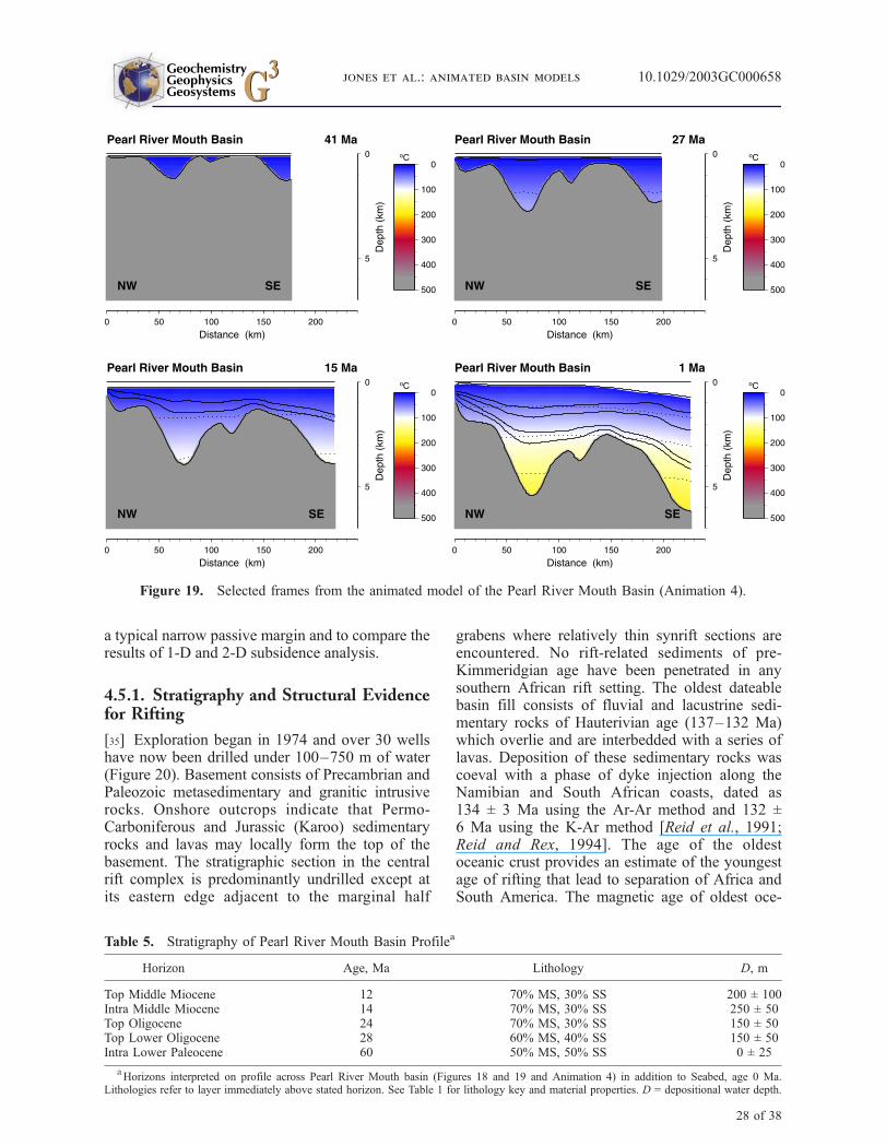
[33] The Pearl River Mouth basin is located onthe northern margin of the South China Sea(Figure 1). We present a 2-D animated modelof a stratigraphic profile across the basin whichends just inboard of a highly extended passivemargin (Figures 18 and 19, Animation 4, andTable 5). This profile was modeled using theoriginal algorithm by Wheeler and White [2002].These authors also compared the results of 1-Dand 2-D strain rate modeling, showed that thecalculated 1-D and 2-D strain rate histories agreewith the timing of faulting observed on seismicreflection profiles and showed that the calculatedtotal stretching agrees with crustal thinning im-aged on a coincident seismic refraction profile.Here we are interested in the Pearl River Mouthbasin as an example of a relatively youngextensional basin in a back arc setting. It isinstructive to compare and contrast the animatedhistory in Animation 4 with the animations ofintracontinental basins (Animations 1, 2, and 3)and of passive margins (Animations 5 and 6). Inparticular, comparison between the Pearl RiverMouth and North Sea basins reveals importantdifferences between the kinematics of intraconti-

GeochemistryGeophysicsGeosystems G3G3

jones et al.: animated basin models 10.1029/2003GC000658

24 of 38

Figure 16. Results of two-dimensional inverse basin modeling of the North Sea Basin. Stratigraphy is detailed inTable 4. (a) Line drawing of interpreted seismic reflection profile from Bellingham and White [2002]. Horizons agesare marked on Figure 16d. (b) Water-loaded subsidence. Blue lines show the profile in Figure 16a smoothed usingfilter of width 40 km and backstripped assuming Airy isostasy. Red dashed lines show best fitting model fromoriginal 2-D inversion algorithm. (c) Sediment-loaded subsidence. Blue lines show the profile in Figure 16asmoothed using filter of width 40 km. Red dashed lines show best fitting model in Figure 16b reloaded with sedimentas described in section 3.2. (d) Best fitting strain rate history from inversion of the profile in Figure 16b using theoriginal algorithm. Black bars on left summarize rifting periods inferred from independent sedimentological andstructural information. Triangles on right mark ages of datum horizons in Figures 16a–16c. Horizontal lines markages of panels shown in Figure 17. This strain rate history was used to generate Animation 3.

GeochemistryGeophysicsGeosystems G3G3

jones et al.: animated basin models 10.1029/2003GC000658

25 of 38

nental and back arc extensional terrains (Animations3 and 4). The North Sea basin extended by 25 kmrelatively slowly while the Pearl River Mouth basinextended by 50 km much more rapidly. Relativelyhigh peak strain rates and extensional strains arecharacteristic of extensional basins in a back arcenvironment [Newman and White, 1999]. Despitethe clear differences in peak strain rate, duration ofrifting and age of rifting, the two basins havecomparable depths at present. However, the NorthSea is relatively old and therefore close to itsequilibrium depth whereas the Pearl River Mouthbasin is younger and will subside to depths more

comparable with the Orange or Vøring margins overthe next hundredmillion years if it remains a passivemargin.

4.5. Orange Margin

[34] The Orange basin lies offshore west of SouthAfrica and forms part of a typical passive margin(Figure 1). It comprises two structural provinces, thefirst a series of marginal rift basins lying 20–80 kmoutboard of the present coastline and the second adeeper graben located 100–200 km from the coast.Our aims here are to present a 2-D animatedmodel of

Figure 17. Selected frames from the animated model of the North Sea Basin (Animation 3).

Table 4. Stratigraphy of Northern North Sea Basin Profilea

Horizon Age, Ma Lithology D, m

Top Eocene 34 55% MS, 45% SS 150 ± 150Top Paleocene 55 75% MS, 25% SS 250 ± 250Top Cretaceous 65 80% MS, 16% SS, 4% LS 265 ± 235Top Campanian 71 80% MS, 10% SS, 10% LS 265 ± 235Top Albian 99 80% MS, 10% SS, 10% LS 265 ± 235Top Jurassic 142 75% MS, 20% SS, 5% LS 150 ± 150Top Callovian 159 75% MS, 20% SS, 5% LS 0 ± 50

aHorizons interpreted on profile across northern North Sea basin (Figures 16 and 17 and Animation 3) in addition to Seabed, age 0 Ma.

Lithologies refer to layer immediately above stated horizon. See Table 1 for lithology key and material properties. D = depositional water depth.

GeochemistryGeophysicsGeosystems G3G3

jones et al.: animated basin models 10.1029/2003GC000658

26 of 38

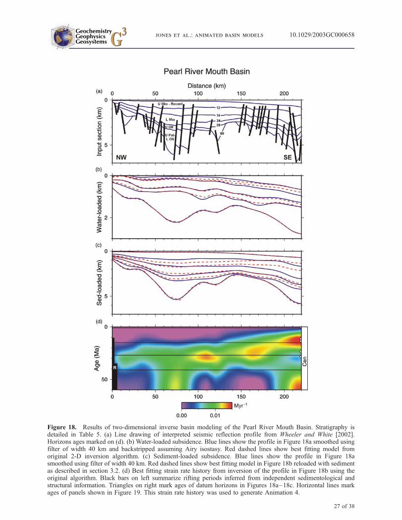
Figure 18. Results of two-dimensional inverse basin modeling of the Pearl River Mouth Basin. Stratigraphy isdetailed in Table 5. (a) Line drawing of interpreted seismic reflection profile from Wheeler and White [2002].Horizons ages marked on (d). (b) Water-loaded subsidence. Blue lines show the profile in Figure 18a smoothed usingfilter of width 40 km and backstripped assuming Airy isostasy. Red dashed lines show best fitting model fromoriginal 2-D inversion algorithm. (c) Sediment-loaded subsidence. Blue lines show the profile in Figure 18asmoothed using filter of width 40 km. Red dashed lines show best fitting model in Figure 18b reloaded with sedimentas described in section 3.2. (d) Best fitting strain rate history from inversion of the profile in Figure 18b using theoriginal algorithm. Black bars on left summarize rifting periods inferred from independent sedimentological andstructural information. Triangles on right mark ages of datum horizons in Figures 18a–18c. Horizontal lines markages of panels shown in Figure 19. This strain rate history was used to generate Animation 4.

GeochemistryGeophysicsGeosystems G3G3

jones et al.: animated basin models 10.1029/2003GC000658

27 of 38

a typical narrow passive margin and to compare theresults of 1-D and 2-D subsidence analysis.

4.5.1. Stratigraphy and Structural Evidencefor Rifting

[35] Exploration began in 1974 and over 30 wellshave now been drilled under 100–750 m of water(Figure 20). Basement consists of Precambrian andPaleozoic metasedimentary and granitic intrusiverocks. Onshore outcrops indicate that Permo-Carboniferous and Jurassic (Karoo) sedimentaryrocks and lavas may locally form the top of thebasement. The stratigraphic section in the centralrift complex is predominantly undrilled except atits eastern edge adjacent to the marginal half

grabens where relatively thin synrift sections areencountered. No rift-related sediments of pre-Kimmeridgian age have been penetrated in anysouthern African rift setting. The oldest dateablebasin fill consists of fluvial and lacustrine sedi-mentary rocks of Hauterivian age (137–132 Ma)which overlie and are interbedded with a series oflavas. Deposition of these sedimentary rocks wascoeval with a phase of dyke injection along theNamibian and South African coasts, dated as134 ± 3 Ma using the Ar-Ar method and 132 ±6 Ma using the K-Ar method [Reid et al., 1991;Reid and Rex, 1994]. The age of the oldestoceanic crust provides an estimate of the youngestage of rifting that lead to separation of Africa andSouth America. The magnetic age of oldest oce-

Figure 19. Selected frames from the animated model of the Pearl River Mouth Basin (Animation 4).

Table 5. Stratigraphy of Pearl River Mouth Basin Profilea

Horizon Age, Ma Lithology D, m

Top Middle Miocene 12 70% MS, 30% SS 200 ± 100Intra Middle Miocene 14 70% MS, 30% SS 250 ± 50Top Oligocene 24 70% MS, 30% SS 150 ± 50Top Lower Oligocene 28 60% MS, 40% SS 150 ± 50Intra Lower Paleocene 60 50% MS, 50% SS 0 ± 25

aHorizons interpreted on profile across Pearl River Mouth basin (Figures 18 and 19 and Animation 4) in addition to Seabed, age 0 Ma.

Lithologies refer to layer immediately above stated horizon. See Table 1 for lithology key and material properties. D = depositional water depth.

GeochemistryGeophysicsGeosystems G3G3

jones et al.: animated basin models 10.1029/2003GC000658

28 of 38

anic crust is about 127 Ma [Nurnberg and Muller,1991]. DSDP hole 361, sited over oceanic crustWSW of Cape Town, was abandoned 50–100 mabove basement in Early Aptian sediments(�120 Ma). Extrapolation of sediment accumula-tion rates gives a Barremian (127–121 Ma) age

for the basement [Bolli et al., 1978]. Seismicinterpretation suggests that the rift-drift transitionis represented by the 6At1 unconformity (125 Ma)[Pegler and McMillan, 1998]. In summary, riftingleading to continental breakup and formation ofthe Orange margin probably took place during

Figure 20. Stratigraphic scheme for the Orange basin based on biostratigraphic information, well log data, the workof Dingle et al. [1983], and the work of Brown et al. [1995]. Lithology key is on Figure 4.

GeochemistryGeophysicsGeosystems G3G3

jones et al.: animated basin models 10.1029/2003GC000658

29 of 38

Valanginian-Barremian times (137–125 Ma).Continental and shallow marine sediments accu-mulated during the early postrift phase beforeonset of fully marine conditions in Mid-Aptiantimes (around 118 Ma) [Pegler and McMillan,1998]. The Upper Cretaceous-Cenozoic successionconsists of progradational deltaic sediments, whosegeometry attests to progressive enlargement of thepaleo-Orange River drainage catchment. Gravity-induced slumping and listric faulting associatedwith the deltaic shelf-slope break are widespread[Muntingh, 1993] but no further tectonic riftingevents have affected the margin. The postrift suc-cession contains many unconformities, somethought associated with denudation of up to 1 km[Pegler and McMillan, 1998].

4.5.2. Results of 1-D and 2-D Modeling

[36] Two-dimensional and one-dimensional inversemodeling provides a good match to the observedstratigraphy (Figures 21, 22, 23, Animation 5, andTable 6). The 2-D algorithm retrieves a singlerifting event with a single peak that finishes be-tween 125–115 Ma in good agreement with theindependent observations (Animation 5). This rel-atively short period of rifting and the abrupt tran-sition to postrift, thermal subsidence can be seenclearly on the 2-D animated model (Figure 22).The 1-D strain rate histories show a single riftingevent with a double peak (Figure 21), althoughsensitivity tests similar to the one in Figure 7suggest that the double peak is not significantfeature [Faulkner, 2000]. It is encouraging thatthe anticipated breakup-related rifting event is soclear given that postrift denudation and slumpingpotentially affect subsidence analysis on this pas-sive margin. Unconformities within the postriftsuccession have not been mapped into spuriousstrain rate events in the 2-D strain rate history(Animation 5). In the 1-D modeling, calculatedsubsidence is less than observed subsidence dur-ing Late Cretaceous-Early Cenozoic times andgreater than the observed present-day subsidence.The total strain (b) estimated from the 1-D strainrate history is greater than that estimated from the2-D strain rate history because the present-daysubsidence is overestimated in the 1-D modeling.It is not possible to achieve a better fit to the 1-Dpostrift subsidence data without without invokingnegative strain rates, which suggests that some ofthe postrift succession has been removed byerosion, although it seems unlikely that denuda-tion of up to the 1 km suggested by Pegler andMcMillan [1998] has occurred. Heat flow models

of the two well sections have been calibrated todown-hole temperature measurements (Figure 21).Calculated heat flow peaked at 70–75 mW m�2 at115 Ma and decayed to about 55 mW m�2 at thepresent-day. In comparison with the North Falk-land basin well, the greater degree of stretching inthe Orange basin means that present-day mantleheat flux component is relatively high and thecrustal heat flux component is correspondinglylower (Figures 13 and 21). The decay of the totalheat flux from its peak at 115 Ma to its present-dayvalue can be seen by watching the temperaturecontours on the 2-D animated model during thepostrift phase (Figure 22).

4.6. Vøring Margin

[37] The Vøring margin profile runs from the Nor-wegian coast to the North Atlantic continent-oceanboundary 400 km to the northwest (Figures 1, 24,and 25, Animation 6, and Table 7). It crosses fourdifferent terrains, each with a distinctive riftinghistory [Brekke, 2000]. Immediately offshore Nor-way lies the Trøndelag platform, which accumu-lated a relatively thick continental and shallowmarine Permo-Triassic-Jurassic succession fol-lowed by a relatively condensed Cretaceous-Cenozoic succession likely deposited under afew hundred meters of water. The Vøring basinproper lies further outboard and contains morethan 10 km of Cretaceous-Cenozoic sedimentaryrock deposited in �1 km of water. The HaltenTerrace lies between the Trøndelag Platform andthe Vøring basin. The Vøring volcanic passivemargin forms the outboard edge of the Vøringbasin and was generated by latest Paleocene con-tinental breakup between Greenland and Europeabove unusually hot asthenosphere [Barton andWhite, 1997]. The Trøndelag Platform and HaltenTerrace have been drilled extensively but greaterwater depth and sediment thickness in the Vøringbasin mean that few wells have been drilled, noneof which penetrates below the Cenomanian level.An unresolved question is whether the Permo-Triassic-Jurassic sequence encountered on theTrøndelag Platform also exists within the Vøringbasin. The prevailing view, based on a regionalstudy of NW European basins, is that Permo-Triassic rifting was low in intensity and spatiallywidespread, while Cretaceous rifting was of higherintensity and more spatially localized [Dore et al.,1999]. However, uncertainty over the stratigraphymeans that the rifting history retrieved from inver-sion the Vøring margin profile is poorly con-strained in comparison with the other profiles

GeochemistryGeophysicsGeosystems G3G3

jones et al.: animated basin models 10.1029/2003GC000658

30 of 38

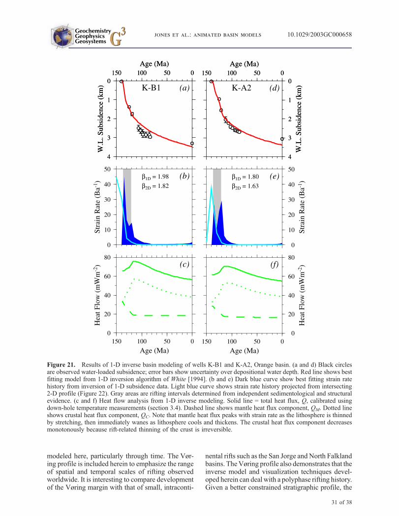
modeled here, particularly through time. The Vør-ing profile is included herein to emphasize the rangeof spatial and temporal scales of rifting observedworldwide. It is interesting to compare developmentof the Vøring margin with that of small, intraconti-

nental rifts such as the San Jorge and North Falklandbasins. TheVøring profile also demonstrates that theinverse model and visualization techniques devel-oped herein can deal with a polyphase rifting history.Given a better constrained stratigraphic profile, the

Figure 21. Results of 1-D inverse basin modeling of wells K-B1 and K-A2, Orange basin. (a and d) Black circlesare observed water-loaded subsidence; error bars show uncertainty over depositional water depth. Red line shows bestfitting model from 1-D inversion algorithm of White [1994]. (b and e) Dark blue curve show best fitting strain ratehistory from inversion of 1-D subsidence data. Light blue curve shows strain rate history projected from intersecting2-D profile (Figure 22). Gray areas are rifting intervals determined from independent sedimentological and structuralevidence. (c and f) Heat flow analysis from 1-D inverse modeling. Solid line = total heat flux, Q, calibrated usingdown-hole temperature measurements (section 3.4). Dashed line shows mantle heat flux component, QM. Dotted lineshows crustal heat flux component, QC. Note that mantle heat flux peaks with strain rate as the lithosphere is thinnedby stretching, then immediately wanes as lithosphere cools and thickens. The crustal heat flux component decreasesmonotonously because rift-related thinning of the crust is irreversible.

GeochemistryGeophysicsGeosystems G3G3

jones et al.: animated basin models 10.1029/2003GC000658

31 of 38

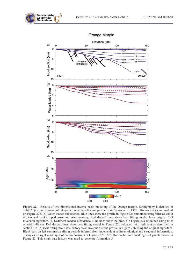
Figure 22. Results of two-dimensional inverse basin modeling of the Orange margin. Stratigraphy is detailed inTable 6. (a) Line drawing of interpreted seismic reflection profile from Brown et al. [1995]. Horizons ages are markedon Figure 22d. (b) Water-loaded subsidence. Blue lines show the profile in Figure 22a smoothed using filter of width40 km and backstripped assuming Airy isostasy. Red dashed lines show best fitting model from original 2-Dinversion algorithm. (c) Sediment-loaded subsidence. Blue lines show the profile in Figure 22a smoothed using filterof width 40 km. Red dashed lines show best fitting model in Figure 22b reloaded with sediment as described insection 3.2. (d) Best fitting strain rate history from inversion of the profile in Figure 22b using the original algorithm.Black bars on left summarize rifting periods inferred from independent sedimentological and structural information.Triangles on right mark ages of datum horizons in Figures 22a–22c. Horizontal lines mark ages of panels shown inFigure 23. This strain rate history was used to generate Animation 5.

GeochemistryGeophysicsGeosystems G3G3

jones et al.: animated basin models 10.1029/2003GC000658

32 of 38

resulting animated model would allow easy under-standing of the progressive growth of the margin.

5. Conclusions

[38] We have further developed the two-dimen-sional inverse model of White and Bellingham[2002] and Bellingham and White [2002] forextracting spatial and temporal variations in strainrate from extensional sedimentary basins and pas-sive margins. The original forward model calcu-lates the velocity field for lithospheric deformation,the thermal and density structures of the litho-sphere and hence the water-loaded subsidencehistory, given a strain rate history. The originalinverse model calculates a strain rate history from abackstripped stratigraphic profile using a directsearch method. We modified the forward modelto calculate the evolution of sedimentary layers as

they accumulate and compact. This modification isa step toward a scheme that directly inverts sedi-ment-loaded stratigraphic profiles without the needfor backstripping. Our modified model also esti-mates the temperature of the sediment pile, whichdepends on the porosity structure and on the heatflow in to the base of the basin, calculated from therifting history. We combined snapshots of thesediment-loaded model basin at many time stepsto produce animations.

[39] We have applied the original inverse model tobackstripped stratigraphic profiles across the SanJorge, North Falkland and North Sea extensionalsedimentary basins and the Pearl River Mouth,Orange and Vøring passive margins. In each case,the main features of the calculated strain ratehistory are in agreement with independent esti-mates of the number and duration of rift events.

Figure 23. Selected frames from the animated model of the Orange margin (Animation 5).

Table 6. Stratigraphy of Orange Margin Profilea

Horizon Age, Ma Lithology D, m

22At1, L 65 80% MS, 20% SS 50 ± 5017At1, Z 84 65% SS, 30% MS, 5% LS 50 ± 5015At1, N, W 94 60% MS, 40% SS 50 ± 5015At1, N, W 112 65% MS, 35% SS 0 ± 5013At1, P 119 50% MS, 45% SS, 5% LS 150 ± 1006At1, R 125 50% MS, 50% SS 200 ± 150T 140 50% SS, 50% BT 0 ± 53

aHorizons interpreted on profile across Orange margin (Figures 22 and 23 and Animation 5) in addition to Seabed, age 0 Ma. Some horizons

have alternative names. Stratigraphy based on SOEKOR internal reports [Faulkner, 2000]. Lithologies refer to layer immediately above statedhorizon. See Table 1 for lithology key and material properties.

GeochemistryGeophysicsGeosystems G3G3

jones et al.: animated basin models 10.1029/2003GC000658

33 of 38

Figure 24. Results of two-dimensional inverse basin modeling of the Vøring margin. (a) Line drawing ofinterpreted seismic reflection profile from Brekke [2000]. Stratigraphy is detailed in Table 7. Horizons ages aremarked on Figure 24d. (b) Water-loaded subsidence. Blue lines show the profile in Figure 24a smoothed using filterof width 40 km and backstripped assuming Airy isostasy. Red dashed lines show best fitting model from original 2-Dinversion algorithm. (c) Sediment-loaded subsidence. Blue lines show the profile in Figure 24a smoothed using filterof width 40 km. Red dashed lines show best fitting model in Figure 24b reloaded with sediment as described insection 3.2. (d) Best fitting strain rate history from inversion of the profile in Figure 24b using the original algorithm.Triangles on right mark ages of datum horizons in Figures 24a–24c. Horizontal lines mark ages of panels shown inFigure 25. This strain rate history was used to generate the Animation 6.

GeochemistryGeophysicsGeosystems G3G3

jones et al.: animated basin models 10.1029/2003GC000658

34 of 38

In some basins, minor strain rate events occur inthe calculated strain rate history at times whenthere is no independent evidence for extension.These events probably reflect noise introduced byregional uplift and denudation unrelated to rifting.

We use each strain rate history to generate ananimated model that tracks sediment accumulation,compaction and thermal history. The animationsaid visualization of the development of individualbasins as they extend, subside and fill with sedi-

Figure 25. Selected frames from the animated model of the Vøring margin (Animation 6).

Table 7. Stratigraphy of Vøring Margin Profilea

Horizon Age, Ma Lithology D, m

Top Cretaceous 65 100% MS 50 ± 50Top Cenomanian 94 100% MS 50 ± 50Base Cretaceous 142 100% MS 50 ± 50Base Jurassic 208 100% MS 50 ± 50Base Permo-Triassic 245 100% MS 50 ± 50

aHorizons interpreted on profile across Vøring margin (Figures 24 and 25 and Animation 6) in addition to Seabed, age 0 Ma. Lithologies refer to

layer immediately above stated horizon. See Table 1 for lithology key and material properties. Horizon ages picks and layer lithologies are generallypoorly constrained (section 4.6).

GeochemistryGeophysicsGeosystems G3G3

jones et al.: animated basin models 10.1029/2003GC000658

35 of 38

ment, and allow easy comparison of basins andmargins worldwide. They show that the basicphysical processes governing lithospheric exten-sion can lead to a wide variety of basin and marginstyles.

Acknowledgments

[40] SMJ was funded by CASP and by a Natural Environ-

ment Research Council postdoctoral grant. PAF was funded by

a Natural Environment Research Council postgraduate stu-

dentship. We are very grateful to YPF-Repsol (formerly YPF),

Petroleum Agency SA (formerly SOEKOR), Shell and Amer-

ada Hess for providing data. C Lightfoot and S Pearse gave

helpful advice on the animations and D Hanne, R Hardy,

D Lyness and R Scott also helped in various ways. We thank

M Gurnis, L Moresi and an anonymous reviewer for construc-

tive comments on the original manuscript. Department of

Earth Sciences contribution ES.7847.

References

Baker, P. E., W. J. Rea, J. Skarmeta, R. Caminos, and D. C.Rex (1981), Igneous history of the Andean Cordillera andPatagonia Plateau around latitude 46�S, Philos. Trans. R.Soc. London, Ser. A, 303, 105–149.

Baldi, J. E., and V. A. Nevistic (1996), Cuenca costa afuera delGolfo San Jorge, in Geologia y recursos naturales de laplataforma continental Argentina. XIII Congreso GeologicoArgentino y III Congreso de Exploracion de Hidrocarburos,Relatorio 10, edited by V. A. Ramos and M. A. Turic,pp. 171–192, Asoc. Geol. Argentina, Inst. Argentino delPetrol., Buenos Aires.

Barker, P. F., I. W. D. Dalziel, and B. C. Storey (1991), Tec-tonic development of the Scotia Arc region, in The Geologyof Antarctica, vol. 6, edited by R. J. Tingley, pp. 215–248,Clarendon, U. K.

Barton, A. J., and R. S. White (1997), Crustal structure ofEdoras Bank continental margin and mantle thermal anoma-lies beneath the North Atlantic, J. Geophys. Res., 102,3109–3129.

Barton, P. J. (1992), LISPB revisited: A new look under theCaledonides of northern Britain, Geophys. J. Int., 110, 371–391.

Barton, P. J., and R. J. Wood (1984), Tectonic evolution of theNorth Sea basin: Crustal stretching and subsidence, Geo-phys. J. R. Astron. Soc., 79, 987–1022.

Bellingham, P., and N. White (2000), A general inverse methodfor modelling extensional sedimentary basins, Basin Res., 12,2190–225.

Bellingham, P., and N. White (2002), A two-dimensionalinverse model for extensional sedimentary basins: 2. Appli-cation, J. Geophys. Res., 107(B10), 2260, doi:10.1029/2001JB000174.

Bellosi, E. S. (1995), Paleogeografıa y cambios ambientales dela Patagonia Central durante el Terciario Medio, Bol. Inf.Petroleras Tercera epoca, 44, 50–83.

Bolli, H. M., W. B. F. Ryan, and DSDP Leg 40 Scientific Party(1978), Cape basin continental rise—Sites 360 and 361,Initial Rep. Deep Sea Drill. Proj., 40, 29–182.

Bransden, P. J. E., P. Burges, M. J. Durham, and J. G. Hall(1999), Evidence for multi-phase rifting in the North Falk-lands Basin, The Oil and Gas Habitats of the South Atlantic,

edited by N. R. Cameron, R. H. Bate, and V. S. Clure, Geol.Soc. Spec. Publ., 153, 425–442.

Brekke, H. (2000), The tectonic evolution of the NorwegianSea continental margin with emphasis on the Vøring andMøre basins, in Dynamics of the Norwegian Margin, editedby A. Nøttvedt et al., Geol. Soc. Spec. Publ., 167, 327–387.

Brown, L. F., Jr., J. M. Benson, G. J. Brink, S. Doherty,A. Jollands, E. H. A. Jungslager, J. H. G. Keenan,A. Muntingh, and N. J. S. Van Wyk (1995), Sequence strati-graphy in offshore South African divergent basins: An atlason exploration for Cretaceous lowstand traps by Soekor (Pty)Ltd, AAPG Stud. Geol., 41, 184 pp.

Budiansky, B. (1970), Thermal and thermoelastic properties ofisotropic composites, J. Composite Mater., 4, 286–295.

Cederbom, C., S. A Larson, E.-L. Tullborg, and J.-P. Stiberg(2000), Fission track thermochronology applied to Phanero-zoic thermotectonic events in central and southern Sweden,Tectonophysics, 316, 153–167.

Courtade, S., J. C. Rodriguez, E.Merlo,M. Russo,M. Ledesma,and J. C. Bett (1999), Stratigraphy and sedimentology of theUpper Cretaceous and Lower Tertiary at the northern flank ofSan Jorge Basin, Argentina, Actas Congr. Explor. DesarrolloHidrocarburos, 4(2), 887–889.

Dingle, R. V., W. G. Siesser, and A. R. Newton (1983),Mesozoic and Tertiary Geology of Southern Africa, 375 pp.,A. A. Balkema, Brookfield, Vt.

Dore, A. G., E. R. Lundin, L. N. Jensen, Ø. Birkeland, P. E.Eliassen, and C. Fichler (1999), Principal tectonic events inthe evolution of the northwest European Atlantic margin, inPetroleum Geology of Northwest Europe: Proceedings of the5th Conference, edited by A. J. Fleet and S. A. R. Boldy,pp. 41–61, Geol. Soc., London.

Faulkner, P. A. (2000), Tectonic and thermal evolution ofSouth Atlantic marginal basins, Ph.D. dissertation, Univ. ofCambridge, Cambridge, U. K.

Figari, E., E. Strelkov, G. Laffitte,M. Cid de la Paz, S. Courtade,J. Celaya, A. Vottero, P. Laufourcade, R. Martinez, andH. Villar (1999), Los sistemas petroleros de la Cuence delGolfo San Jorge: Sıntesis Estructural, Estratigraphica y Geo-quımica, Actas Congr. Explor. Desarrollo Hidrocarburos,4(2), 197–237.

Fitzgerald, M. G., R. M. Mitchum Jr., M. A. Uliana, and K. T.Biddle (1990), Evolution of the San Jorge Basin, Argentina,AAPG Bull., 74, 879–920.

Fowler, S. R., and D. P. McKenzie (1989), Gravity studies ofthe Rockall and Exmouth Plateaux using SEASAT altimetry,Basin Res., 2, 27–34.

Gabrielsen, R. H., R. Kyrkjebø, J. I. Faleide, W. Fjeldskaar,and T. Kjennerud (2001), The Cretaceous post-rift basin con-figuration of the northern North Sea, Pet. Geosci., 7, 137–154.

Glennie, K. W. (Ed.) (1998), Petroleum Geology of the NorthSea: Basic Concepts and Recent Advances, 4th ed., 635 pp.,Blackwell Sci., Malden, Mass.

Hall, B. D., and N. White (1994), Origin of anomalous Tertiarysubsidence adjacent to North Atlantic Continental Margins,Marine Petrol. Geol., 11, 702–714.

Jones, S. M., and N. White (2003), Shape and size of thestarting Iceland Plume swell, Earth Planet. Sci. Lett., 216,271–282.

Jones, S. M., N. White, B. J. Clarke, E. Rowley, andK. Gallagher (2002a), Present and past influence of the Ice-land Plume on sedimentation, in Exhumation of the NorthAtlantic Margin: Timing Mechanisms and Implications forPetroleum Exploration, edited by A. G. Dore et al., Geol.Soc. Spec. Publ., 196, 1–25.

GeochemistryGeophysicsGeosystems G3G3

jones et al.: animated basin models 10.1029/2003GC000658

36 of 38

Jones, S. M., N. White, and J. Maclennan (2002b), V-shapedridge around Iceland: Implications for spatial and temporalpatterns of mantle convection, Geochem. Geophys. Geosyst.,3(10), 1059, doi:10.1029/2002GC000361.

Kusznir, N. J., G. Marsden, and S. S. Egan (1991), A flexuralcantilever simple-shear/pure-shear model of continentallithospheric extension: Applications to the Jeanne d’Arc ba-sin, Grand Banks and Viking Graben, North Sea, inThe Geometry of Normal Faults, edited by A. M. Roberts,G. Yielding, and B. Freeman, Geol. Soc. Spec. Publ., 56,41–60.

Laske, G., and G. Masters (1997), Global digital map of sedi-ment thickness, Eos Trans. AGU, 78(46), Fall Meet. Suppl.,F483.

Lawrence, S. R., and M. Johnson (1995), Shelf north of Falk-lands may be new S Atlantic petroleum province, Oil Gas J.,93(10), 52–55.

Lawrence, S. R., M. Johnson, S. R. Tubb, and S. J. Marshallsea(1999), Tectono-stratigraphic evolution of the North Falk-lands region, in The Oil and Gas Habitats of the South Atlan-tic, edited by N. R. Cameron, R. H. Bate, and V. S. Clure,Geol. Soc. Spec. Publ., 153, 409–424.

Lusser, C. U., and I. O. Norton (1985), Tectonic Map of theWorld, Panel 16, Exxon Mobil Corp., Houston, Tex.

Marinelli, R. V., G. A. Rebay, and H. J. Franzin (1996), Cuen-cas del talud continental, in Geologia y recursos naturales dela platforma continental Argentina. XIII Congresso Geolo-gico Argentino y III Congresso de Exploracion de Hidrocar-buros, Relatorio 18, edited by V. A. Ramos and M. A. Turic,pp. 343–357, Asoc. Geol. Argentina, Inst. Argentino delPetrol., Buenos Aires.

Marsden, G., G. Yielding, A. M. Roberts, and N. J. Kusznir(1990), Application of a flexural cantilever simple-shear/pure-shear model of continental lithospheric extension tothe formation of the North Sea basin, in Tectonic Evolutionof North Sea Rifts, edited by D. J. Blundell and A. D. Gibbs,Clarendon, pp. 240–261, Oxford, U. K.

McKenzie, D. (1978), Some remarks on the development ofsedimentary basins, Earth Planet. Sci. Lett., 40, 25–32.

McMahon, N. A., and J. Turner (1998), The documentationof a latest Jurassic-earliest Cretaceous uplift throughoutsouthern England and adjacent offshore areas, in Develop-ment, Evolution and Petroleum Geology of the WessexBasin, edited by J. R. Underhill, Geol. Soc. Spec. Publ.,133, 215–240.

Muller, R. D., W. R. Roest, J.-Y. Royer, L. M. Gahagan, andJ. G. Sclater (1997), Digital isochrons of the world’s oceanfloor, J. Geophys. Res., 102(B2), 3211–3214.

Muntingh, A. (1993), Geology, prospects in Orange basin off-shore western South Africa, Oil Gas J., 91, 106–109.

Nadin, P., N. Kusznir, and M. Cheadle (1997), Early Tertiaryplume uplift of the North Sea and Faroe-Shetland Basins,Earth Planet. Sci. Lett., 148, 109–127.

Newman, R., and N. White (1999), The dynamics of exten-sional sedimentary basins: Constraints from subsidence in-version, Philos. Trans. R. Soc. London, Ser. A, 357, 805–834.

Nurnberg, D., and R. D. Muller (1991), The tectonic evolutionof the South Atlantic from Late Jurassic to present, Tectono-physics, 191, 27–53.

Parker, J. R., (Ed.) (1993), Petroleum Geology of NorthwestEurope: Proceedings of the 4th Conference, 1542 pp., Geol.Soc., London.

Pegler, E. A., and I. K. McMillan (1998), Tectonostratigraphi-cal evolution of the Orange Basin, southwestern Africa,J. Afr. Earth Sci., 27, 147.

Reid, D. L., and D. C. Rex (1994), Cretaceous dykes asso-ciated with the opening of the South Atlantic: The Mehl-berg dyke, northern Richtersveld, J. Afr. Earth Sci., 97,135–145.

Reid, D. L., A. J. Erlank, and D. C. Rex (1991), Age andcorrelation of the False Bay dolerite dyke swarm, south-western Cape, Cape Province, S. Afr. J. Geol., 94, 155–158.

Richards, P. C., and N. G. T. Fannin (1997), Geology of theNorth Falkland basin, J. Pet. Geol., 20(2), 165–183.

Richards, P. C., and B. V. Hillier (2000a), Post-drilling analysisof the North Falkland Basin—part 1: Tectono-stratigraphicframework, J. Petrol. Geol., 23, 253–272.

Richards, P. C., and B. V. Hillier (2000b), Post-drilling analy-sis of the North Falkland Basin—part 2: Petroleum systemand future prospects, J. Petrol. Geol., 23, 273–292.

Richards, P. C., R. W. Gatliff, M. F. Quinn, J. P. Williamson,and N. G. T. Fannin (1996), The geological evolution of theFalkland Islands continental shelf, in Weddell Sea Tectonicsand Gondwana Break-up, edited by B. C. Storey, E. C. King,and R. A. Livermore, Geol. Soc. Spec. Publ., 108, 105–128.

Rodriguez, J. F. R., and R. Littke (2001), Petroleum gen-eration and accumulation in the Golfo San Jorge Basin,Argentina: A basin modeling study, Mar. Pet. Geol., 18,995–1028.

Rohrman, M., and P. van der Beek (1996), Cenozoic postriftdomal uplift of North Atlantic margins: An asthenosphericdiapir model, Geology, 24, 901–904.

Ross, J. G., J. Pinchin, D. G. Griffin, M. G. Dinkelman,M. A. Turic, and V. A. Nevistic (1996), Cuenca de Mal-vinas Norte, in Geologia y recursos naturales de la pla-taforma continental Argentina. XIII Congreso GeologicoArgentino y III Congreso de Exploracion de Hidrocar-buros, Relatorio 14, edited by V. A. Ramos and M. A.Turic, pp. 253–271 Asoc. Geol. Argentina, Inst. Argentinodel Petrol., Buenos Aires.

Sclater, J. G., C. Jaupart, and D. Galson (1980), The heat flowthrough oceanic and continental crust and the heat loss of theearth, Rev. Geophys., 18, 269–311.

Srivastava, S. P., D. Voppel, and B. Tucholke (1988), Geophys-ical atlas of the North Atlantic between 50� to 70�N and 0� to65�W, Dtsch. Hydrogr. Inst., Hamburg, Germany.

Steckler, M. S., and A. B. Watts (1978), Subsidence of theAtlantic-type continental margin off New York, Earth Planet.Sci. Lett., 41, 1–13.

Su, D., N. White, and D. McKenzie (1989), Extension andsubsidence of the Pearl River Mouth Basin, northern SouthChina Sea, Basin Res., 2, 205–222.

Thompson, K., and J. R. Underhill (1999), Frontier explorationin the South Atlantic: Structural prospectivity in the NorthFalkland Basin, AAPG Bull., 83, 778–797.

Tiley, R., D. P. McKenzie, and N. J. White (2003), The elasticthickness of the British Isles, J. Geol. Soc. London, 160,499–502.

Uliana, M. A., K. T. Biddle, and J. Cerdan (1989), Mesozoicextension and the formation of Argentine sedimentary ba-sins, in Extensional Tectonics and Stratigraphy of the NorthAtlantic Matgins, edited by A. J. Tankard and H. R. Balkwill,AAPG Mem., 46, 599–614.

Urien, C. M., and J. J. Zambrano (1973), The geology of thebasins of the Argentine continental margin and Malvinasplateau, in The Ocean Basins and Margins, vol. 1, TheSouth Atlantic, edited by A. E. M. Nairn and F. G. Stehli,pp. 135–169, Plenum, New York.

Watts, A. B., and J. D. Fairhead (1997), Gravity anomalies andmagmatism at the British Isles continental margin, J. Geol.Soc. London, 154, 523–529.

GeochemistryGeophysicsGeosystems G3G3

jones et al.: animated basin models 10.1029/2003GC000658

37 of 38

Watts, A. B., and J. Stewart (1998), Gravity anomalies andsegmentation of the continental margin offshore West Africa,Earth Planet. Sci. Lett., 156, 239–252.

Wehr, F. L., G. M. Skerlec, and I. O. Norton (1985), TectonicMap of the World, Panel 14, Exxon Mobil Corp., Houston,Tex.

Wheeler, P., and N. White (2002), Measuring dynamic topog-raphy: An analysis of Southeast Asia, Tectonics, 21(5), 1040,doi:10.1029/2001TC900023.

White, N. (1989), The nature of lithospheric extension in theNorth Sea, Geology, 17, 111–114.

White, N. (1994), An inverse method for determining litho-spheric strain rate variation on geological timescales, EarthPlanet. Sci. Lett., 122, 351–371.

White, N., and P. Bellingham (2002), A two-dimensional in-verse model for extensional sedimentary basins: 1. Theory,J. Geophys. Res., 107(B10), 2259, doi:10.1029/2001JB000173.

Zambrano, J. J., and C. M. Urien (1970), Geological out-line of the basins in southern Argentina and their con-tinuation off the Atlantic shore, J. Geophys. Res., 75,1363–1396.

GeochemistryGeophysicsGeosystems G3G3

jones et al.: animated basin models 10.1029/2003GC000658

38 of 38