Conference Proceedings

Bulletin of Monetary Ecoomics and Baking

Andi M. Alfian Parewangi Solikin M. Juhro

10th International Conference – Jakarta, August 2016

EDITORS

Jakarta, February 2017

2

First published, 2017

© 2017 Bank Indonesia

Bank Indonesia,

J. MH. Thamrin No. 1-2, Jakarta Pusat, 10010, INDONESIA

All rights reserved. No part of this b ook may be reproduced in any form by any electronic or mechanical means (including photocopying, recording, or information storage and retrieval) without written permission from the publisher. This book is published by Center for Central Banking Research and Education, Bank Indonesia.

Except in the Republic of Indonesia, this book is sold subject to the condition that it shall not, by way of trade or otherwise, be lent, resold, hired out, or otherwise circulated without the punblisher‘s prior consent in any form of binding or cover other than that in which it is published and without a similar condition including this condition being imposed on the subsequent purchaser.

Library of Indonesian Catalogue-in-Publication Data

Financial Stability and the Global Landscape / edited by; Solikin M. Juhro and Andi M. Alfian Parewangi.

p. cm.

Includes index

400. 25.7

I. Title)

ISBN _________________ (printed)

ISBN _________________ (online)

Editors:

Solikin M. Juhro Andi M. Alfian Parewangi

4

PATRON

The Governor of Bank Indonesia

EDITOR

Solikin M. Juhro, Andi Alfian Parewangi

PROJECT TEAM

Perry Warjiyo, Darsono, Solikin M. Juhro, Andi M. Alfian Parewangi., Rita Krisdiana,

Wahyu Yuwana, Tri Subandoro, Aliyah Farwah, Didy Laksmono R., Wijoyo Santoso,

Wahyu Dewati, Siti Astiyah, Ronald L. Toruan, Arifin M.S., Triatmo, Doriyanto,

Nurhemi, Irwan, Wahyu Yuwana H., Doni Septadijaya, Trinil Arimurti, Guruh Suryani

R., R. Aga Nugraha, Tri Subandoro, Rizma Magribhi, Susana, Satyani O., Miftakul

Khoiri, Pebri Haryanto, Erwin Deky, Annisa Fauziah, M. Rizky Hutomo, Sandy, Junita

Naditya, Sendy.

COVER, LAYOUT, AND DESIGN

Mandiri Digital Media and Publishing

PUBLISHER

Bank Indonesia Institute, Bank Indonesia

COPYRIGHTS: © Bank Indonesia

Assalaamu ‘alaikum Wr. Wb,

We are pleased to launch this book. This volume contains the

proceeding of the International Conference on Promoting Financial

Stability in The Changing Global Financial Landscape, held at Jakarta–

Indonesia, August 8 - 9, 2016. This is the 10th International

Conference coordinated by the Bulletin of Monetary Economics

and Banking, an international joural published by Bank Indonesia.

This book present the empirical findings, projection, in

dept analysis, and thoughtful discussion from many researchers,

academician, practitioneers, and policy makers. The angle of

analysis is very interesting and rich, that we ar sure the readers can

understand the measure of financial stability, the causes, the

dynamics, and its impact; not only globally or nationally, but also

until the most disaggregated level of household.

One measure is the aggregate financial stability index

(AFSI). You will find on this book how the AFSI is constructed

from nineteen individual indicators and group them into four

composite sub-indices. One chapter apply the intuitionistic fuzzy

sets to put weights for the sub-indices and the quality level of

financial stability in Azerbaijan, and provide strong evidence the

2

Fro

m E

dito

rs

index is more capable to capture a major periods of financial

stability.

Another interesting measure provided on this book is the

early warning system (EWS); widely used as surveillance

mechanism for preserving financial system stability. The major

question on assessing the accuracy of the EWS is what indicator to

use and how good they are on signaling adverse shocks towards

the financial resilience.

Talking about the source of instability, one may easier to

look at the externally source of shock, and one of famously

recognized is the international imbalances. The imbalance in the

current account has been debated for a long time. Deficits in the

long term into often raises concern because of the economic crisis

is often preceded by a prolonged of current account deficits. This

book should keep the readers in mind if the current account

deficit is not always caused by the inability of the economy to

compete in the global market which makes the value of imports

greater than exports. The current account deficit on the other side

is a reflection of the saving - domestic investment position in the

economy. If the deficit is caused by the position of investment

larger than savings, then this is a good indication for an economy.

One chapter of this book investigate the external relation

of Indonesia, and found the dynamics of Indonesian current

account can be divided into two episodes; first is saving -

investment period before crisis in 1997, and second, the export -

import period after the crisis. The author used SVAR and

conclude the exchange rate is the greatest influence on the current

account dynamics. Furhtermore, this chapter also provide the

speed of adjustment for the current account to return to

equilibrium pattern.

On the next chapter of this book, you will find the further

discussion on international imbalances related to how strong one

country to optimize the stability of his exchange rate,

independency of his monetary policy, and how good they manage

the fast moving in or out of fund in the era of free capital

3

Fro

m E

dit

ors

mobility. This is simply the topic of trilemma where the interest is

the best policy to impose to achieve higher economic growth amid

financial crisis.

One section of this book provide the experiences of

Southeast Asia countries. To measure trilemma, this paper uses

balanced panel data approach from Indonesia, Thailand,

Philippines and Malaysia during the period of 1980 to 2013. This

paper includes trilemma index as independent variable alongside

with inflation, openness and foreign currency reserve in explaining

the variance of economic growth. Based on estimation result, it is

found that during global financial crisis, exchange rate stability and

financial openness policies induce higher economic growth

compared to monetary independence as indicated by negative

coefficient of monetary independence index. Nonetheless, those

three policies are not statistically significant improving economic

growth during East Asian financial crisis in 1997.

The second source of instability is the contagion and the

spillover effect across regions. This book provide an empirical

paper that investigates the macro-characteristics that reduce the

spillover effect of unconventional monetary policy from

developed countries to the emerging market countries.

Empirically, this research used 24 UMP announcements and a

panel fixed effects model to examine the characteristics of the

emerging markets, the spillover channel considered in this study is

countries‘ exchange rate. Very interesting and empirically rich, the

result shows that deeper financial markets contribute to better

resilience. Trade linkages with China provide less vulnerable

currency position of the emerging markets while trade linkages

with developed countries provide mixed evidence. The macro-

prudential policy and the capital flow measures that the emerging

markets countries implemented before to the announcements are

moderately effective in reducing the spillover.

On national level, financial stability is highly related to the

monetary authority, particularly their credibility and the power of

their monetary policy. In principle, the measurement of the

4

Fro

m E

dito

rs

efficiency of monetary policy was based on inflation and output

variations. Monetary policy is considered to be efficient if the

policy generates low fluctuation of output and inflation. Low and

stable inflation will encourage the output growth in the long term,

while high fluctuation of inflation will cause a social loss. Some

economists have tried to formulate the monetary policy efficiency

measures such as Cecchetti (2006) and Romer (2006). However,

these formulations still in a general form and cannot be used

operationally. In this paper, the authors formulate a method for

measuring the efficiency of monetary policy and applied to the

data of inflation and output in Indonesia. The efficiency of

monetary policy is measured by the deviation of actual monetary

policy from ideal monetary policy. Ideal monetary policy is policy

that creates a minimum variation of output and inflation.

Further investigation analyze how monetary policy may

affect the comparative advantage of capital intensive industry

(technology-intensive industry and human capital-intensive

industry) in international trade. This is also important when we are

dealing with international imbalances. Basically, the lower interest

rates lead capital more affordable and the standard Heckscher-

Ohlin model dictated countries with comparative advantages

should export goods that require factors of production that they

have in abundance.

From the opposite view, one may ask about how the

financial stability influence the economic condition. Economic

crisis that had happened at 1997-1998 in Indonesia triggered by

financial condition that was not stable. It stimulates the

researchers to study more. Since financial condition is a

foundation in a country. So if economic crisis happened then

many sectors will get huge impact of it. Financial stability means

variables as export-import, GNI, GDP and inflation in a good

range. Due to the financial condition consist of dynamic variables

then to measure its stability the dynamic system is needed. The

financial stability will be tested using time series analysis and

dynamic system which is optimized by genetic algorithm. In this

research gave result around 80% - 90% for accuracy data GNI,

5

Fro

m E

dit

ors

GDP and inflation. Meanwhile, the accuracy of data export -

import around 40% - 75%. These results proved that the dynamic

system able to fit data in finding historical pattern with tolerance

error.

To the end, the global stability will arrive on the household

security. By standard definition, economic security of a household

reflect their ability to achieve income necessary for covering their

needs and to create financial reserves to use when a case of

unfavorable accidence. We will interestingly follow how the

educational and professional experiences, controlling for economy

conditions, may affect the economic resourcefulness of

household‘s members and, as a consequence, their economic

security. The case is presented by one of our author, Maria, for the

case of Polish.

Grom global to regional economy, the ASEAN Economic

Community (AEC) implemented in 2015 is a recent good sample.

The agreement demanded the liberalization of the flow of goods

and services, which enable the entry of foreign retail business

across country members. To many extent, this is another source of

domestic instability when the traditional market and Micro, Small

and Medium Enterprises (UMKM) pose large proportion of

corresponding economy. Usually, the major concern over the

competition and the free market is the poverty. It is indeed the

central problem to sustainable human development.

This book provide several insight on the poverty

alleviation including the role of financial sector and the banking

sector in particular. One paper discuss very neatly about the

empirical evidence on Grameen Bank and Islamic Bank

microcredit performance in Bangladesh. In general, most of the

findings from the literature have shown that Islami Bank

microcredit borrowers are doing well to reduce their vulnerability

and poverty as well as improved socioeconomic status after access

credit. Interestingly, many experiences suggests that social welfare

projects sponsored by most of the NGOs in Bangladesh and

elsewhere in Muslim countries tend to create a built-in

6

Fro

m E

dito

rs

dependency. Once the support of the NGOs are withdrawn or the

flow of aid stops for one reasons or another, this project cease to

exist or make its beneficiary worse off in the sense that

discontinuation of support push them back beyond their original

level of living.

Another paper on this book discuss the trend of

commercial banks increasingly adopting stricter credit evaluation

standards in giving loans to micro-entrepreneurs, This study

propose the use of ‗cash waqf‘ as an alternative and an additional

source of capital for microfinance to promote the growth of

Islamic microfinance in Muslim countries in general.

Islamic banking ability to survive of the economic crisis in

1998 is sufficient to provide evidence that it can play a role in

maintaining the stability of the financial system in Indonesia. This

was absolutely influenced by the various types of financing

contracts that Islamic banks offer to their customers. Therefore,

this study aims to determine the best portfolios simulation of

Islamic financing that can maintain the stability withstand to

economic shocks.

Related to the fundamental side of the financial stability, a

very basic question we try to bring to all readers is who use the

financial product? Worldwide, an estimated 2 billion working-age

adults globally—more than half of the total adult population—has

no access to the types of formal financial services delivered by

regulated financial institutions that wealthier people rely on,

(World Bank, 2014). Instead they depend on informal mechanisms

for saving and protecting themselves against risk. They buy

livestock as a form of savings, they pawn jewelry, and they turn to

the money lender for credit. These mechanisms are risky and

often expensive.

Currently, the highest score for Financial Inclusion Index

goes to Peru (90), Columbia (86), Philippines (81), India (71), and

Pakistan (64); while the five lowest ranks are Haiti (24), Dem.

Republic of Congo (26), Madagascar (27), Lebanon (29), and

Egypt (29). For another country in Asia, Indonesia scored 56,

7

Fro

m E

dit

ors

Cambodia (55), Thailand (49), and Vietnam (34), while China

record 42. All these figures are much lower than the Philippines,

(Global Microscope, 2015). Regionally, the following table

provides initial insight of the financial inclusion determinants for

East and South Asia.

The issue of financial inclusion is highly related to the

structure of banking industry. With a highly diverse size and

margin, the implementation of Asean Economic Community and

regional arrangements (ASEAN 10), the ASEAN + 3 (China,

Japan, Korea), the RCEP or ASEAN+6 (China, Japan, Korea,

India, Australia, NZ), and the CEPA (Thailand & RoK) leave big

challenges for the government, financial authority, and local banks

in each country member to reconcile and to adopt.

Again, we always need to look the issue from diferent

perspective. As you will find on this book, the financial inclusion

is one of strategy on one hand but may cause instability in the

financial system when financial inclusion causes reducting in credit

standard, inceasing risk of bank reputation, and uncoresponding

regulation in microfinance. One way to test it is by testing their

causality, and this book provide the empirical test including 19

countries based on income group from 2004-2011.

The next section of this book present the keynote from

the Governor of Bank Indonesia, followed with very interesting

plenary sessions. We strongly suggest all the readers to follow the

thoughfull, open, yet humble presentation from Perry Warjiyo,

Halim Alamsjah, and Suahasil Nazara.

To conclude our introduction before you continue your

reading, we emphaisize that all papers on this book are subject to a

review to ensure the comparative framework and analysis that

holds the papers together on explaining the theme of the

conference. For this succesfull task, we greatly appreciate the

contributions of all Scientific Chairs of the conference.

This Proceeding book is available on printed on digital.

Both cover regional and international distribution. We inivite all

8

Fro

m E

dito

rs

the readers to read and disseminate this book, which we believe

will enhance greater discussion within the growth and

macroeconomic stability issues. We gratefully acknowledge the

contribution of Triatmo Doriyanto, Rita Kristiana, Shinta S.,

Nurhemy, Tri Subandoro, Aliyah Farwaha, Sendy, Junita, and all

the team during the publishing this book. To reach broader reader

and to intensify further discussion, any individuals or institution

can print the book with written notification to the editors.

Furthermore, printing on demand may also available.

We expect this book provides systematically presented

literatures on the Growth and Macroeconomic Stability for all

readers, and encourage them to participate on the upcoming

Conference 2017 and beyond.

Wa’alaikumsalam Wr. Wb.

Solikin M. Juhro

Head of BI Institute, Bank Indonesia Editorial Board, Bulletin of Monetary Economics and Banking

Andi M. Alfian Parewangi

Managing Editor, Bulletin of Monetary Economics and Banking

9

FROM EDITORS ....................................................................1

CONTENTS............................................................................................. 9

OPENING & PLENARY

1. Governor of Bank Indonesia ................................................... 13

Agus D W Martowardojo

2. Financial Stability in Volatile Environment ........................... 23

Halim Alamsyah

3. The Central Bank ...................................................................... 31

Perry Warjiyo

4. Fiscal Stance ................................................................................ 39

Suahasil Nazara

SEMINARY PAPERS

5. Measuring Financial Stability In Azerbaijan........................... 47

G.C. Imanov, H.S.Alieva, R.A.Yusifzadeh

6. Financial Inclusion ..................................................................... 65

Azka Azifah Dienillah , Lukytawati Anggraeni, Sahara

10

7. An Early Warning....................................................................... 81

Jarita Duasa, Dimas Bagus Wiranatakusuma, Sumandi

8. What Protects Emerging Markets ......................................... 106

Eko Sumando

9. Monetary Policy Efficiency..................................................... 138

Eka Purwanda, Siti Herni Rochana

10. Monetary Policy ........................................................................ 163

Chandra Utama, Ruth Meilianna

11. Trilemma Policy ........................................................................ 179

Ahmad Mikail, Kenny Devita Indraswari

12. Current Account and Financial Stability .............................. 201

Ni Putu Wiwin Setyari

13. Dynamic System ....................................................................... 233

Saadah S

14. Household Security .................................................................. 247

Maria Piotrowska

15. Regional Revitalization ............................................................ 268

Achmad Noer Maulidi, Fathor Rozi, Syofia Dwi Jayanti

16. Cash Waqf Financing............................................................... 292

Rubaiyat Ahsan Bhuiyan

17. Islamic Financing ..................................................................... 321

Amrin Barata

POSTER PRESENTATION

18. Allocation Fund for Energy EfficiencyError! Bookmark not defined.

Joko Tri Haryanto

19. Fiscal and Monetary Policy InteractionError! Bookmark not defined.

Eko Sumando

20. Capital Market Industry on Industry CreativeError! Bookmark not defined.

Achmad Noer Maulidi

11

21. Economic Transformation ..Error! Bookmark not defined.

Imam Sumardjoko

22. Stock Returns .........................Error! Bookmark not defined.

Perwito, Rita Zulbetti

23. Entrepreneurship ...................Error! Bookmark not defined.

Ayu Dwidyah Rini

24. Monetary Transmission ........Error! Bookmark not defined.

Chaerani Nisa, Syahril Djaddang

25. Agriculture ..............................Error! Bookmark not defined.

Liska Simamora

26. Stability of Inflation ..............Error! Bookmark not defined.

Zulkifly Walbot

27. Financial Secrecy....................Error! Bookmark not defined.

Lury Sofyan

28. Growth Revisited...................Error! Bookmark not defined.

Dian Purnamasari, Alfa Farah

29. ASEAN+3 Common CurrencyError! Bookmark not defined.

Chandra Utama, Yohanes Maynard Kevin Sihotang

30. CSR and Tax Agressive ........Error! Bookmark not defined.

Muhammad Rifky Santoso

Agus Martowardoyo Governor of Bank Indonesia

Halim Alamsyah

Chairman of Indonesia Deposit Insurance Corporation Board of Commisioner

Perry Warjiyo

Deputy Governor of Bank Indonesia

Suahasil Nazara

Head of Fiscal Policy Agency Ministry of Finance of the Republic of Indonesia

Moderator: Edhie Purnawan

Vice Dean of Gadjah Mada University

Governor of Bank Indonesia

Macroprudential Policy to Promote Financial Stability in the Changing Global Financial Landscape

Agus D W Martowardojo

Governor of Bank Indonesia

Assalamu’alaikum Wr. Wb,

It is a great pleasure for me today, to address this distinguished

gathering and welcome you to the 10th International Conference,

Bulletin of Monetary Economics and Banking 2016. I am indeed

delighted to see distinguished speakers and guests from my fellow

from government institutions, researchers, embassies, and

academia attending this conference.

This year, we are pleased to conduct a conference entitled

―Macroprudential Policy to Promote Financial Stability in the Changing

Global Financial Landscape‖. The topic of today‘s conference is very

timely, as many new developments continue to loom in the area of

financial stability that entails us to keep on adjusting our policies

to the newly emerged development so as to maintain our

14

Op

enin

g & P

lenary

credibility as central bank in providing conducive climate to

promote sustainable economic growth.

As the current global recovery moved only at a sluggish

pace, while the current government is at the height of boosting the

economy, we are of the view that credible effort is needed so as to

maintain financial stability while at the same time supporting

government program to improve the living standard of our

people.

World Economy

Entering the second half of 2016, the global economy continues

its feeble and fragile recovery in the face of considerable

uncertainty that has gripped us since the global financial crises of

2008. In addition, the world financial markets are surprised to see

the outcome of the U.K referendum called ―Brexit‖, which could

aggravate the global outlook for 2016-17, notwithstanding better

than expected performance in early 2016. With declining global

growth and renewed uncertainty following Brexit is still unfolding,

the baseline global growth forecast has therefore been revised

down modestly relative to the April 2016 as reported by WEO.

The result of the U.K. referendum that caught financial

markets by surprised has led to financial turbulence worldwide.

The pound depreciated sharply, while other major currencies saw

limited pressures. In emerging markets, asset price and exchange

rate have been generally more stable. Overall, the outcomes of

Brexit vote imply substantial repercussion covering economic,

political and institutional fronts. It is presumed to give a negative

macroeconomic impact, especially in advanced Euro area

economies. However, as the process is still unfolding, we have yet

to assess the damage to the world economy. As for Indonesia,

however, we envisage that the impact of Brexit to Indonesian

economy is limited and the economy continues to steam ahead.

The outlook for emerging market economies remains

diverse. In China, near-term outlook improved following the

recent policy support by the fiscal and monetary authorities.

15

Sem

inar

Pap

ers

Op

enin

g &

Ple

nar

y

Infrastructure spending has picked up and credit growth

improved. In Brazil, the economy seemed to have been bottoming

out, as contraction receded. In India, the country continued to see

the thriving economy, despite lower than expected pace.

Meanwhile the Middle East oil exporting countries saw modest

benefit due to recovery in oil prices, but fiscal consolidation

remains necessary.

Domestic Economy

Despite tangible results from efforts to enhance resilience to

external shocks, the vulnerability of emerging economies remains,

due to their rather weak economic structures. Indonesia‘s

economy in particular, has managed to pick up its growth in 2016

supported by increased government consumption on goods and

investment in infrastructure projects. In addition with the passage

of Tax Amnesty Law last June, we expect this would boost market

sentiment, leading to stronger capital inflows and firming rupiah

exchange rate. We envisage that tax-amnesty-induced capital flow

would peak towards the end of this year. We are confident that

these developments should benefit investment and other

economic activities in general.

Broadly speaking, macroeconomic stability is well

preserved. Domestic economic activities in the second quarter of

2016 are seen to record an improvement. Improved private

consumption as well as large increase in the realization of

government capital and goods programs becomes the major

impetus of domestic economic growth amidst weakened exports.

The overall growth in 2016 is expected to stay within the target

range of 5.0-5.4% (yoy).

At the external front, Indonesia‘s balance of payments

recorded narrower current account deficit in June 2016, primarily

originating from increased trade surplus stemmed from higher

non-oil manufacturing exports. At the end of June 30, 2016

foreign exchange reserves stood at $109.8 billion, enough to cover

8.4 months of imports or 8.1 month of imports and servicing

public debt, well above the international standards.

16

Op

enin

g & P

lenary

The strengthening confidence on Indonesia‘s economy

contributed to a more stable Rupiah with an appreciating trend

and lower exchange rate volatility. This comes on the back of

favorable macroeconomic fundamental, as represented by

narrowing current account deficit, lower expected inflation, and

renewed positive sentiment towards economic prospects. The

Rupiah recovered its value against the dollar, following its

depreciation in the earlier months as risk mounted in the global

financial market due to the anticipated Fed Fund Rate hike. But it

makes a turnaround following the recent announcement of new

cabinet by the President.

The consistent monetary policy to maintain

macroeconomic stability, accompanied with policy coordination

between Bank Indonesia and the Government, succeeded in

bringing about low inflation. We are on track towards achieving

low and stable Rupiah. In the past two years, Indonesia has

managed to contain inflation at the level below 5% supported by

lower energy prices and better food production and distribution.

We believe that this process will continue.

Inflation is well under control in July 2016 at a low 0.69%,

leading to 3.21% yoy inflation. The whole year inflation is

envisaged to move well within the target corridor of 4 + 1% for

2016. Policy interest rate—BI rate— is left unchanged at 6.5%,

along with deposit facility and lending facility at 4.5% and 7.00%,

respectively. Bank Indonesia also announced the BI-7-Day Repo

Rate is maintained at 5.25%. This will serve as policy rate to

replace BI rate, with effect from mid-August this year.

Financial System Stability

Financial system remains stable, on the back of resilient banking

system, supported by stronger capital ratio and liquidity, as

indicated by persistently improved index at 0.87% in May 2016.

Nevertheless, we should be mindful on moderating banking

intermediation as well as increasing credit risk.

Bank deposit grew at about 6.53% (yoy) in May 2016,

while credit moved higher as compare to previous month at

17

Sem

inar

Pap

ers

Op

enin

g &

Ple

nar

y

8.34% (yoy). Credit to SMEs also grew at 8.0% (yoy) along with

increased risk. Meanwhile, Micro Credit Program (MCP) has

reached almost 50% of its target in 2016, mostly from state-owned

banks. With domestic demand expanding at modest space, non-

performing loan is slightly increased and recorded 3.11% in May

2016, brought about by increase of non-performing loans in

industry and trade sectors.

Banking industry is well capitalized; its ratio continued to

increase and reach a high 22.15% in June. Bank liquidity also

remains ample, supported by government expansion. Albeit

operating expense-operating income ratio increased and return on

assets ratio decreased, banking industry remains intact. Overall, we

remain optimistic that our banking and financial stability is well

preserved. Notwithstanding, we should carefully monitor the

emerging global fragilities.

Outlook, Risks and Policies

Against the background of maintained stability while anticipating

the possible renewed vulnerabilities, we remain optimistic that

domestic economic growth is envisaged to pick up modestly in

2016, supported by measured monetary easing and more

accommodative macro-prudential policies, fiscal stimuli in the

form of the Tax Amnesty Law, and stronger government

spending.

Yet, we are aware the prevailing of some overshadowing

risks on the horizon, both external and domestic origins, including

the widely expected another Fed Fund Rate hike in the second

half of 2016. Equally important is the risk of the slowdown in the

Chinese economy, the aftermath of U.K‘s Brexit, and the rising of

volatile food inflation domestically.

Distinguished Guests, Ladies and Gentlemen

In this opportunity along with the 63th anniversary of Bank

Indonesia, we proudly launch a newly published book entitled

―Perjuangan Mendirikan Bank Sentral Republik Indonesia‖ (The Fight

for Establishing the Central Bank of the Republic of Indonesia).

18

Op

enin

g & P

lenary

This book is written with the aim to highlight issues related to

establishing our central bank from Bank Indonesia‘s perspective.

The process of establishing a central bank in Indonesia

begins with the announcement of Government Regulation in Lieu

of Law Number 2 of 1946. The Government established Bank

Negara Indonesia 1946 (BNI 46), responsible for implementing

central bank mandates. In the event, however, this newly created

central bank was confronted with difficulties, namely incompetent

and inexperienced staff, limited branch offices networks, and

political instability. It failed considerably to function as circulating

bank.

As the political process continued and as a consequence of

the Dutch-Indonesian Round Table Conference held in the Haque

1949, to end Dutch occupation in Indonesia, it is agreed that De

Javasche Bank was to take over responsibility as circulating bank

from BNI 46. De Javasche Bank should undertake a number of

issues.

The first is that central bank as the issuer of currency

would like to encourage its people to use their own banknotes in

their transaction within the Indonesian territory. This measure is

to show to the world the sovereignty of the government of the

Republic of Indonesia during its early years of independence. The

second is to reaffirm that Bank Indonesia is absolutely not the

legacy of the previous Dutch administration. The overtaking of

De Javasche Bank by the Indonesian government is done through

purchasing its stock, adhering to international best practices. It is

not a nationalization. The third is to help the newly born

government in financing its budget needs, at the time. Of course

as time evolves, the central bank is now mandated to promote

macroeconomic and financial stability.

Distinguished Guests, Ladies and Gentlemen,

The next book we also proudly launch entitled ―Mengupas Kebijakan

Macroprudential‖ [Unveiling Macroprudential Policy]. This book

aims to enhance public understanding on macroprudential issues,

so that it helps promote greater effectiveness in managing

19

Sem

inar

Pap

ers

Op

enin

g &

Ple

nar

y

systemic risk as well as financial imbalances to safeguard financial

system stability.

The global financial crisis prompted a rethinking of

macroeconomic policy framework. There is a global consensus

that monetary and financial stability are interrelated, hence it

should be taken into account in designing policy formulation.

Bank Indonesia, and some other emerging economies, has

adopted macroprudential policy as an integral part of its macro-

monetary policies after the Asian financial crisis of 1997/98.

It is worth noting that microprudential policy has been

transferred to Financial Services Authority under the Act No. 21

of 2011 concerning Financial Services Authority. Both

macroprudential and microprudential should complement each

other. Macroprudential policy seeks to oversee, assess, and deliver

appropriate response to the evolving financial system as a whole,

rather than focusing on individual institutions or certain economic

measures and isolation. Central bank is naturally position to play a

prominent role in macroprudential policies.

Macroprudential issues in international level are a fairly

new field in macro management area, not discussed widely until

just recently. Not too many people have solid understanding of

the substance of macroprudential policy. Thus this book would

bring a better perspective on macroprudential issues and policies,

and it should contribute to the success of its implementation.

Lastly, this book shed light on the evolving roles of Bank

Indonesia as the guardian of monetary stability to improve the

living standards of our people. It also talks about the

macroprudential policy strategies in Bank Indonesia, particularly

how Bank Indonesia conducts crisis prevention and resolution.

Research and Publication

As we may all know that the Bulletin of Monetary Economics and

Banking, a peer-reviewed journal, has four missions, namely: (i) to

encourage research activities from academia and public in general;

(ii) to provide medium of knowledge sharing for researchers; (iii)

20

Op

enin

g & P

lenary

to facilitate dissemination of research findings; and (iv) to bridge

the gap between theory and practice in the area of monetary

economics and banking, and related topics in finance and

economics, and macro-prudential, the theme of this year event. It

is expected that BEMP will be internationally accredited in the

very near term. The Journal is published four times a year, and

available in the digital and printed version.

Quality research and data are an integral part of policy

formulation in Cental Bank. Understandably the policy will impact

all walks of society. To this end, Bank Indonesia continues to

enhance research platform, including seminars, call for papers, and

the publication of internationally accredited journal. In this regard,

we challenge policymakers, researchers and academia to share

their valuable knowledges and thoughts.

Furthermore, Bank Indonesia does not conduct research

in isolation. It involves wider stakeholders. This is the reason why

Bank Indonesia invites researchers from all parts of Indonesia and

around the world to participate in BEMP‘s call for paper. It is

expected that the participants could enhance their research

networkings with other researchers, authorities, and practitioners

through this Conference.

In this occasion, we are pleased to announce that we also

hold a research fair for the first time in Bank Indonesia. The

research fair in which you could find various papers and books

published by Bank Indonesia, is intended to disseminate the

outcomes of research projects and a range of books written by our

internal staff or in collaboration with outside researchers.

Looking to the future we see challenges on the horizon.

We have to promote a strong synergy between maintaining

stability and supporting far reaching government economic

programme. Macroeconomic stability is indeed worth promoting

for as it is the prerequisite for sustainable growth. Thus, through

this conference I wish you all to have an intense but fruitful

discussion. I am confident that by the end of this conference we

21

Sem

inar

Pap

ers

Op

enin

g &

Ple

nar

y

could deepen and enhance our understanding of the issues being

discussed as a take away and food for thoughts to bring home.

I thank you for your kind attention.

Wassalamu’alaikum Wr. Wb

Thank you,

Jakarta, August 9, 2016.

Agus D.W. Martowardojo

Governor of Bank Indonesia

Financial Stability in Volatile Environment

The Experience of Indonesia

Halim Alamsyah

Chairman of Indonesia Deposit Insurance Corporation

Board of Commisioner

After the Asian financial crisis broke out 16 years ago, most

central bank, in Asia especially put serious effort in strengthening

their surveillance on the built up of financial risk or systemic risk

coming out of financial imbalances of balance sheet from financial

firms, banks, nonbank financial institutions as well as nonfinancial

firms including commercial enterprises and households. Asian‘s

central banks were more incline to use macroprudential regulation

with the view to maintaining financial stability. So, this is actually

what we call now as macroprudential policy.

After the great financial crisis in 2007–2008, the

incarnation has just compounded because it is not only emerging

economies but also advanced economies are now trying to use

macroprudential policy. There is already a lot of research has

shown empirically as well as theoretically that monetary policy

alone will not be sufficient maintaining macroeconomic stability

(price stability does not guarantee macroeconomic stability). In

24

Op

enin

g & P

lenary

fact, this research has found those low inflation especially in

advanced economies with low yield on financial assets tend to

promote excessive risk taking and dangerous financial imbalances.

In globalize financial landscape right now, the search for yield

motives has induce more capital flows in and out emerging

economies with less developed financial market and does creating

excessive volatilities and which in turn can create financial

instability in many of these small and less developed financial

markets.

Recent experience has shown that cooperating in financial

stability mandate is necessary to maintain macroeconomic stability.

But cooperating in financial system stability is not that easy, it is a

wide objective and it is much broaden mandate if it compares with

monetary stability. It has many wide aspect and intellect ages. It is

almost impossible if those matters are being born by one

institution. Increasingly, financial stability is seen as a shared

responsibility. Despite some debates, whether financial stability

mandate should be given only to the central bank, it is important

to be aware about the strength and the limit of each policy:

macroeconomic policy, monetary policy, as well as microeconomic

policy.

Monetary policy instruments are well known for each

broader impact to the economy but less capable to deal with

sectoral risks and financial imbalances while macroprudential

instruments are more direct and can be targeted to specific risks or

financial imbalances. But unfortunately, there are still many

unknown on the efficacy of these macroprudential regulations.

Not rescinding our knowledge on transmission mechanism, trade-

offs, and optimal combination of these instruments in effecting

output prices and financial stability.

So when we are talking about trade-offs, actually we are

talking about something that we are not familiar with.

Unfortunately, central bankers do not have enough time to do

some research before actually apply it. When the problems emerge

usually central bankers have to act based on intuition and

professional judgment. And fortunately, some of the central

bankers in the world are still retaining the financial supervision

25

Sem

inar

Pap

ers

Op

enin

g &

Ple

nar

y

authority inside the central bank. Thus they have in a way, maybe

the right hand or the left hand to help the monetary policy

objective. If a country does not have that kind of authority, then

those authorities related have to coordinate, including Indonesia.

However, trade-offs is not the same as coordination. Trade-offs is

related toward the nature and the efficacy of the regulations if we

are talking about coordination between micro and macro

regulations. But coordination is about how to achieve a single

objective or a common objective and try to make a good planning

and sequence and such that we can have an optimal impact on the

targeted objective.

As we all know, when the unconventional monetary policy

has rattled the global financial landscape, it has created many

spillovers especially on capital flows to many emerging economies

including in Asia. And as we all know also, many emerging

economies in Asia in particular has to resort to some capital flows

measures or capital flows management. One of the key reasons to

do this because the authority would like to maintain the

competitiveness while adopting a monetary policy‘s stand

conducive to manage their economic growth momentum.

Instruments such as regulations to manage foreign exchange

maturity and denomination mismatches, capes on external debt,

taxes on foreign asset holdings, or even lengthening its holding

period are commonly used. These instruments are commonly also

accompanied by stricter prudential regulations on bank‘s liquidity

position, capes on property and consumer loans, in effort to

manage a safer and resilient banking system and a more

productive composition of output in the economies. These

policies respond are coming out of research and closer

surveillance on the sources on financial vulnerabilities.

Discussions on these topics are widespread right now in many

regionals as well as in many forums.

In the Indonesia context, as a small and open economy,

sources of financial instability may come from external factors as

well as internal one. The external factors are notorious as the

financial sector is getting more integrated into a more globalize

financial system. As we know the word contagion, herding

26

Op

enin

g & P

lenary

behavior, risks on, risks off are very notorious buzzwords. On the

internal side, we are talking about home global vulnerabilities and

usually in macroeconomic perspective these home global

vulnerabilities will come out of balance sheets of financial firms

and nonfinancial firms including households. And the central bank

or any institution that are tasked by macroprudential and

macroeconomic stability objective need to take those phenomena

seriously. Furthermore, financially risky behavior such as excessive

risk taking both from the demand side: households and deficit

units firms and from the supply side: lower lending standard for

example or maybe lower capital adequacy ratio as a presentation of

lower loss absorption capacity are also important to be monitored.

Last but not least, shocks related to policies taken in the financial

area should also be closely watched when those policies are deem

not in line with ―market‘s consensus or market‘s expectation‖ and

thus it may have unattended consequences.

A framework analysis: linking financial system stability

with macroeconomic policies is very useful especially in

identifying the sources of financial imbalances and possible risk

register that need to be analyzed and monitored closely. Financial

stability mandate covers a wide coverage of a need in extensive

information and data mining covering not only banks, but also

nonfinancial institutions as well as corporations and households.

And that is the reason when we are talking about financial

stability; it is a wide coverage and very wide mandate. A good

grasp of understanding on what is going on in financial monetary,

fiscal, and real size of economy is a must. Not resending a good

coordination and collaboration with other financial authorities, in

Indonesia that means a good collaboration and coordination with

OJK, Ministry of Finance, and also Indonesian Deposit Insurance

Corporation.

Now we will talk about how Indonesia has already taken

some macroprudential regulations to maintain financial stability.

During the last financial cycle upturn in Indonesia, it is quite easy

to spot at least three phenomena took place about the same time.

The first is excessive lending growth, the second is price bubbles

27

Sem

inar

Pap

ers

Op

enin

g &

Ple

nar

y

in property sector, and the third is acceleration in external debts

especially private external debts.

In the last financial upturn, a famous phenomenon named

procyclicality of loans growth was happened. When the GDP

growth is accelerating, it will also induce the same acceleration in

loan growth, including in this case mortgage or KPR (Kredit

Perumahan Rakyat). When the GDP growth is accelerating, it also

shows the same development in KPR. Based on data from

September 2001–March 2015, the total mortgage is much more

responsive comparing to the total loans. This is the first

phenomenon.

And secondly, we can also look what happened with the

property sector. There was very high growth of property loan

since middle 2010 has been accompanied by bubble in property

prices. Whenever the GDP growth is increasing above the trend

line, the credit growth would also grow above the trend. And after

so many years being dormant, the property price suddenly shot up

especially during 2010 and over currently is bit declining. And

during that period, it is also quite clear that the speculation is

rampant. Many debtors have more than 2 mortgage loans at the

same time. In fact, at the time it was quite common to see 1

debtor has more than 2 or even more than 3 loans. And this is one

of the reasons why the property price shot up leading toward price

bubble eventhough the distribution of this price increases would

not spreading throughout Indonesia. But at least, this is the first

phenomenon that we should take care very carefully.

And what is more interesting, eventhough the loan growth

has already grew by over 40% during the same period, we still saw

an acceleration in private external debt. This is what we call as

―business cycle‖. Business cycle is characterized by the GDP

growth, ups and downs. But if we are talking about financial cycle,

we are talking a much longer and much deeper and also higher

amplitude of the cycle. So it is possible actually at financial cycle,

the GDP growth is slowing down but the financial cycle is still on

the rise. This is what happens in Indonesia.

The total external debts have increased for about 24% in

2012 to 36.5% in Q1 2016. The ratio of private sectors over total

28

Op

enin

g & P

lenary

external debt is soaring from 36% (2014) to 52% (Q1 2016). Only

recently the private sector external debts is slowing sharply since

2012. But it might indicate at the same time of the slowing growth

of business expansion. Now we are having a slow down in

business cycle, but at the same time we may have a slow down in

financial cycle. So when these two cycles are coincided, usually we

will have some difficulties in reviving the economy and also in

reviving the financial sector.

Then the situation from our corporations, the domestic

corporations show a weakening performance and especially on

commodity sectors. And we hope the revival of commodities‘

market during the last several months will have some relieves of

some companies and we do hope that it will be the trend. But if

not, the world of cushion is really inappropriate.

Next, it is about the policy responses have been given by

Bank Indonesia especially. When we are talking about trade-off,

what we need is actually the knowledge, whether we know exactly

what are the objectives of monetary policy as well as what are the

objectives of macroprudential policy. As long as we know which

policy affects which sectors then we may have the chance to have

a good policy design. Monetary policy affects the magnitude and

the pace of output and prices because macroprudential policy will

not be able to reduce inflation for example, it is only part of price

pressures. While macroprudential policy will handle the

composition of output. If we do not want the loan growth too

high for some sectors for example, then we may be able to tweak

growth in those sectors. And sometimes we can also contain some

imbalances especially when it is coming out of some imprudent

behaviors. This is what the policy responses have been taken by

Bank Indonesia. If we look at what happened during 2012–2015,

BI has taken tight-biased monetary policy and it adopted more

flexible exchange rate regime. At the same time, BI also

administered macroprudential regulation in the area of liquidity of

the banking sector, foreign exchange transaction, directly try to

contain property and consumer loans, and try to look and reduce

financial imbalances in the corporations‘ balance sheet. Then since

the last quarter of 2015, because the economy is slowing down, BI

29

Sem

inar

Pap

ers

Op

enin

g &

Ple

nar

y

has switched to a laxer monetary policy and it has already reverse

some of the macroprudential regulations such as higher LTV ratio

or lower reserve requirements. Whether it is effective or not to

revive the economy, we still need more research before we can do

a more objective evaluation.

This is one illustration how effective is LTV ratio

regulation. Seems that during the first and the second LTV ratio

regulation, when the economy is already slowing down, this is the

peak when the mortgage loan growth was very high. And it is slow

down gradually before peak up a bit before BI took second LTV.

But after that, the loan growth was declining. But now, the key

question is whether the last relaxation of LTV will have the same

symmetry response from the market, from the property side

whether it can also jump start a revival in loan growth of property

sector.

What we have learned so far, some researches in the area

of financial stability has been accelerating and new findings and

understandings has also been quite encouraging. But, there are still

much yet we still do not know. Mandate on achieving financial

stability is currently given only to one institution. In coordination

arrangement toward a distributed model like Indonesia for

example, complicated and fragmented decision-making process

should be avoided as it only create confusion, lack of credibility,

and maybe also late responses. So, strong coordination and

collaboration is needed to harness the potential synergies among

policy makers.

The shape of real coordination will depend on the

effectiveness of governance‘s process and structure, the

instrument choices, as well as coordination culture. Nevertheless

one thing is clear, that each policy maker must have a common

understanding about the efficacy and the limits of its policies, as

such that monetary policy is to focus on price stability while

macroprudential is to limit the builds up of system wide financial

risks and microprudential regulation focus on the safety and the

soundness of individual financial firms. So the trade-off may in

fact be minimize if those policies can be designed as a

complementary to each others.

30

Op

enin

g & P

lenary

Success in financial stability during normal period may not

be taken for granted, that it will also work during stress or crisis

situations. Thus a clear guidance on crisis management protocol

and a lead institution will be critical in ensuring effective and fast

policy responses. When dealing with financial stability matters, our

experience shows that prompt corrective actions are desirable as

prevention is much better.

Lastly, achieving financial stability is not a clear-cut

mandate as like monetary target. We can speak inflation target or

interest rate or money supply very easily, but when we are talking

about financial stability it will be not that such clear. So legal and

political shield is a must in ensuring decisive an objective policy

responses.

Thank you,

Jakarta, August 9, 2016.

Halim Alamsjah

Chairman of Indonesia Deposit Insurance Corporation

Board of Commisioner

The Central Bank 1 The Role of Central Bank to Support Financial System

Stability

Perry Warjiyo

Deputy Governor Bank Indonesia Chief Editor, Bulletin of Monetary Economics and Banking

There are three aspects that will be explained in this paper. First is

we define what the financial system stability is. This important to

let us stand on the same ground of understanding. Second, this

paper will identify and emphasize the role of Central Bank on

financial system stability. This section is based on theoretical

concept, existeing literatures, as well as our empirical experiences.

Third section will discuss and answer the question of how we

marry the monetary and macro-prudential policy conceptually in

Bank Indonesia.

Financial System Stability

The global financial crisis reminds us the important of financial

system stability. In every crisis, we are searching the new factors

and finding the new impetus for policy. This financial system

stability is what we invent since the global financial crisis. A

1 We invite the reader to read Solikin J. (2010). Central Bank Policy and Practice, Bank Indonesia, Ch. 14 and 15.

32

Op

enin

g & P

lenary

number of definitions has been put in the literatures. We can refer

to Sinasi (2004), he said that the financial stability was defined as a

financial system which arranges of stability that capable of

facilitating rather than impeding the performance of the economy.

The ECB define as well as Central Bank in Indonesia, that

the financial system stability crisis prevention is financial stability

as condition in which the financial system, intermediaries, market,

and market infrastructure can withstand shock without major

disruption in financial intermediation and in the general supply of

financial services. This is the definition that we can infer from a

number of literatures which are concluding into the following 5

key aspects that we learned from crisis to crisis.

The 5 key aspects of financial system stability. The first is

that the financial system stability is not only about the individual

soundness of the financial system. Soundness of the bank is very

important, soundness of financial institution is important, in

necessary but not enough.

The second aspect of financial system stability is the causes.

If we learnt from the crisis, there are four causes which are

inherent with financial system stability; (1) excessive lending, (2)

excessive external borrowing, (3) asset price and property bubble,

and (4) capital reversal. These are the four aspects of inherent risk

of financial system stability. Mexican crisis, Latin crisis is caused

by public external debt crisis. Asian crisis is caused by private

external debt and the banking crisis as well as the balance of

payment crisis. The reason of financial system stability‘s pressure

is coming from the capital reversal. So, second key of financial

system stability is we have to understand the causes of the crisis,

they are excessive lending, excessive external borrowing, asset

price and property bubble, and capital reversal.

Third aspect on financial system stability is the important

of interconnectedness in the financial system. The crisis can be

caused by individual banking, capital reversal and price bubble, but

the systemic risk, the propagation of the crisis in the financial

system has interconnection. These may be cause the domino

effect from bank to bank and central counterparty risk in the

payment system.

33

Sem

inar

Pap

ers

Op

enin

g &

Ple

nar

y

The fourth aspect of financial stability is about the

contagious aspect, the herding behavior, which is very difficult to

predict and very difficult to model. The crisis can be happen

because the individual banking, external crisis, propagation of the

interconnectedness. While, in the term of herding behavior, the

information contagion is the thing that makes the crisis become so

difficult to predict and resolved. See what happen in US, the crisis

is not because of the individual bank, it is because of excessive

lending and housing price bubble. Facilitated by structured

product, interconnectedness in the financial market, the

propagation and the difficultness of resolving those crisis is cause

of information contagion.

Lastly, the fifth aspect of financial stability is the share

responsibility. Halim Alamsjah emphasize that financial system

stability everywhere from the beginning, now and to the future is a

share responsibility. There is no way a single issue can assume and

can be accountable of financial system stability. Central bank

cannot do financial system stability alone, financial service

authority cannot do financial system stability alone, and Indonesia

Deposit Insurance Corporation cannot do financial system

stability alone, and also the minister of finance. A share

responsibility is a must because the crisis can be happened from

the bank, the global, external debt, as well as other aspects of

financial infrastructure.

This is a strong reason why in Indonesia, financial system

stability particulary prevention and resolution policy are mandated

among the four agency; Ministry of Finance, Central Bank,

Financial Service Authority, and Indonesia Deposit Insurance

Corporation. So if you heard that one people/institution want to

assume the financial system stability alone, there is no way that

he/institution can do.

The Role of Central Bank

The practice of central bank may varies from country to country.

Among others, it depends on whether the mandate of individual

banking supervision and regulation still lay within the central bank

34

Op

enin

g & P

lenary

or not. It also depends on whether the rule of lender of last resort

as well as the deposit insurance mechanism.

In some countries, the central bank still assume the

mandate of individual banking supervision and also as the greater

on financial system stability, but in other countries where the

individual banking supervision is within FSA, there is a share

responsibility in financial system stability. But in many countries

and most countries, the central bank has a role as macro-

prudential policy. Regardless, individual banking supervision

within central bank or not. Pak Halim talking about what is

macro-prudential policy, basically macro-prudential policy is

regulation and supervision to financial institution from the

macroeconomic perspective and focus on systemic risk. These are

the two keys to understand: focus on macro perspective and

systemic risk.

What is the meaning of macro perspective and systemic

risk? Macro perspective meaning that we look into the function of

financial system stability in intermediation in the economy. Both

in the perspective of cross section and time dimension. On the

time dimension, we can resort to the thinking on Ben Bernanke

and Kyotaki and more about the financial acceleration hypothesis,

the thinking goes beyond the initial thinking or original thinking of

Hayman Minsky of financial system instability.

Basically, this is the nature of financial system stability.

When the economic is booming, the financial cycle, which is Pak

Halim talking about, is accelerating the economic cycle. When the

economic growth, nominal GDP growth say about 13%, during

the economic boom, the lending growth can accelerate to 20%

why? Because there is thinking of external premium theory of Ben

Bernanke. Or the valuation of the asset as underlying of the

guarantee also increasing.

During the economic boom, the property price increase

more than the inflation. So, as a collateral, those properties can be

used to accelerate the lending. So, the lending growth, the

valuation of the property are always accelerate as others. This is

where financial accelerator hypothesis hold. This is what we are

talking about time dimension of macro-prudential policy which

35

Sem

inar

Pap

ers

Op

enin

g &

Ple

nar

y

macro-prudential policy is the policy that can minimize the

mitigating of procyclicality nature of the lending. How can we

control the lending growth which too excessive in the boom

aspect? How can we stimulate the ending growth during the

recession? This is the instrument that we use loan to value ratio

counter-cyclical buffer and other tools of macro-prudential to

dampen the volatility of the procyclicality nature of financial cycle

beyond the economic cycle. This is the first dimension of macro-

prudential. This is by dissemination, regulation, supervision of

financial system from the macro perspective.

How about focusing on risk of the system. This is where

the area of interconnectedness of the financial system is very

important. In the interbank market, counter-party in the financial

system need to be regulated, controlled, structured in such a way

to minimize the risk of the systemic in the financial system

stability. This is the role of the central bank in those two aspects in

managing the excessive lending, excessive external borrowing,

mitigating the capital, flows management as well as in the

interconnectedness of the financial system. Why the central bank

as the institution that very important can take the role of macro

prudential policy.

There are three reasons why central bank everywhere

assume the responsibility of macro prudential policy. Since 1684,

Bank of England being setup because the central banks

everywhere since the beginning are providing as the lender of the

last resort. This is the first reason for the central bank to hold the

responsibility on macro prudential policy.

Secodly, macro prudential is talking about macro financial

linkage, the role of financial system in intermediating the

economy. This is where the expertise of central bank is kicked in.

Everywhere, central bank in formulating monetary policy always

looking into macro-economy aspect; forecasting analysis, growth,

GDP growth, inflation, lending, current account deficit,

macroeconomic aspect. You just need to add the financial sector

in it. Then you have macro prudential aspect of the financial

system stability. After all, macro prudential is about macro

36

Op

enin

g & P

lenary

financial linkage. The linkage between financial system and macro

economy.

Third, the causes of financial system stability can arise

from macroeconomic shocks; external borrowing, capital reversal,

which is not under control of the FSA or other agency. Those

factors causing financial system that are: external borrowing,

capital reversal, some of the macroeconomic shocks are under

control of the central bank. By adding macro prudential policy, it

will more easy to assume the macro prudential stability to the

central bank.

This is the second issue that I‘m talking about the central

bank everywhere regardless whether individual banking

supervision are under the center bank or not. Everywhere, macro

prudential policy are within center bank. Macro prudential is about

rule and regulation of financial system from macro perspective

and systemic risk because central bank assume as the lender of last

resort and it has expertise in analyzing and forecasting the policy

perspective of macro financial linkage. It is also because the

central bank also use policy for controlling external borrowing,

capital flows, and other aspect that causing financial system

stability.

Marrying Monetary Policy and Macro Prudential Policy

This is the issue that Pak Halim talking about whether there is

tradeoff between financial stability and price stability. The tradeoff

maybe exist depending on where actually the economic states are

lying, whether the forecasts of risk on the price stability are low or

high. Whether the risk of financial stability are low or high, there

is tradeoff inherent on the aspect, but this is doesn‘t mean we

can‘t marry monetary policy and macro prudential policy. One of

example: during the 2010-2013 there is a case in Indonesia that

price stability is very low but accumulation of risk of financial

stability are rising.

During the episode, inflation was very low, because of low

inflation in domestically and appreciation of rupiah. On the other

hand, risk of financial stability are rising because credit excessive

37

Sem

inar

Pap

ers

Op

enin

g &

Ple

nar

y

and the external borrowing are rising. So, there is inherent risk of

financial system stability.

Besides the inflation targeting framework, there is other

aspect of monetary policy: reserve requirement and capital flows

restriction. In Indonesia we practice during the period to mitigate

financial system stability. So, there is room to marry between

monetary and macro prudential policy. Not through interest rate

policy but with other aspect; reserve requirement and capital flows

management. In this episode also there is room for macro

prudential policy. This is the case where Indonesia issuing loan to

value ratio. Those experience is refer to Pak Halim‘s presentation

about how to marry monetary and macro prudential policy. There

is some tradeoffs but we can marry both instrument monetary and

macro prudential policy.

I will close for two notes. The conceptual and

experimental of the policy I think we are already progressing. But

in practice, there are at least two challenges that we have to think

about, both in theoretical as well as in policy making.

In theoretical, modeling of the policy of monetary and

macro prudential is limited. How we design monetary and macro

prudential to be optimal policy mixed. I think this is one area that

academician can provide better perspective or some input on how

we move forward in the financial stability and the role of the

central bank in financial stability.

From practical perspective, the challenge is coming from

on how we need to do a lot of simulation and mixing those

policies and how we communicate better to the public in

delivering the policy to support the financial system stability. This

is the new breath of central bank‘s role, which is not only

achieving price stability but also promoting financial system

stability in Indonesia and everywhere.

Thank you,

Jakarta, August 9, 2016.

Perry Warjiyo

Deputy Governor Bank Indonesia

Chief Editor, Bulletin of Monetary Economics and Banking

Fiscal Stance Fiscal Policy and Its Support on Financial System

Stability

Suahasil Nazara

Head of Fiscal Policy Agency

Ministry of Finance of the Republic Of Indonesia

Very good morning about the noon ladies and gentlement. Pak

Syahril, Pak Burhanudin, Ibu Miranda, Pak Perry Warjiyo, Pak

Halim Alamsjah, our moderator Pak Edhie, and all participants of

this great conferences, thank you for this opportunity. I will use

my seession to outline the budgeting process of the Indonesia

government, specifically about the allocated budget and the link

between the fiscal policy and financial stability.

Pak Halim already elaborated very nicely about the

financial system stability framework, Pak Perry already elaborated

about two important things, first, that financial stability cannot be

done only by one institution only; and secondly, the roles of the

Bank Central. Now let me start with the newly enacted law on the

financial sector stability system.

The law has just been enacted last April. In that law, there

is a committee, what we called the Financial System Stability

40

Op

enin

g & P

lenary

Committee, or the ―Komite Stabilitas Sistem Keuangan‖—KSSK.

And the KSSK is chaired or coordinated by the Minister of

Finance, and members are the Central Bank‘s Governor and also

the Head Commissioner of OJK as well as the LPS.

Four institutions, Ministry of Finance, Central Bank,

Deposit Insurance, and also the Financial Service Supervision

Authority, are really the four important pillars of the financial

system stability in Indonesia. Different operational regulations are

on their way, and we are preparing all of the necessary regulations

at the Secretariat of the KSSK. I think it‘s very important to note

that our financial system stability law put a very big focus on the

banking sector. Furthermore, the law emphasize heavily the bail-in

principles, rather than the bail-out. And that is by choice or by

design.

The decision has gone through long days and nights

discussions by looking from our past experiences, as well as

looking at some benchmarking to other countries. At the end of

the day, that is the political approval. That is a political decision

that is subject to further analysis. As an analyst everybody are very

welcome to analyze the law.

To note, this law is a breakthrough of about seven years of

deadlock. The government and the parliament last year, mid 2015,

decided to start from scratch, drafting the law, and initiate the

discussion with the parliament starting mid of 2015, culminated in

the enactment in that law last April. I would like to invite

researchers and also analyst to look at it, and to review it, and to

tell us what we should watch furthermore, especially on the

operational regulations of that law.

Series of socializations are underway and then I‘m very

proud to tell you as well that the law is actually a product of four

institutions together with parliament. It is not only product of

government and the parliament, because I‘m very happy to see

that my colleagues from Bank Indonesia as well as colleagues from

the OJK as well as LPS, a very much involve in the formulation of

that law. So it is a law that we produce together and it is the law

that we going to use in times when it is indeed.

41

Sem

inar

Pap

ers

Op

enin

g &

Ple

nar

y

Hopefully, in many future volumes of the Bulletin of

Monetary Economics and Banking, we will see some review about

this. Hopefully ya Pak Erwin and also Pak Perry, we can look at

this very carefully in the future. So there is number one.

Fiscal Policy and Financial System Stability

Previously Pak Halim explain the framework of financial stability,

which include the fiscal policy. I would like to expain the 2016

Budget and to illustrate about the post in the budget that can link

to the financial stability.

In revised budget 2016, the ―APBN Revision 2016‖, based

on realization of the first semester, last June and the prognosis of

semester II, the remaining of the year, we know the

implementation of the budget is approaching 100 percent. On the

revenue side, the realization is 1,786; semester I, 634, slightly

below the realization of semester I last year, 667; but look at the

prognosis of semester II, we must collect as much as 1,151. This is

almost double the first semester, and one thing we know, the

likelihood is very small.

So, right from the first number we know that how tough is

the budget for the second semester. Of course, parts of the

revenue, the biggest chance of the revenue is from the tax. First

semester 552 trillion, and the second semester we have to collect

1,017 trillion. That is if we want 100 percent realization of the

budget. And I can tell you that, never in the history of Indonesian

fiscal policy that in one semester we collect 1,000 trillion. Last

year, we collected 1,000 trillion rupiah. This year, first semester

552 and 1,017 trillion in the second semester is highly unlikely.

This is really reflection of what our Minister, Ibu Sri Mulyani,

mention earlier that the tax revenue target is somewhat ambitious.

So this is really the number.

The Risk

Now, what are the risks? As we all may already have known or

suspected, the tax officials will try their maximum effort to collect

the tax. And then of course, given the economic cycle, our growth

42

Op

enin

g & P

lenary

start last year was 4.8. We do have quarter by quarter increase,

starting the 3rd quarter last year, but we believe, the tax revenue of

what we collected this year is somewhat a function of the activity

last year.

Profit last year will impact what we are collecting today.

The value added tax is a function of transaction. Yes, if the

economic growth is the case, then the transaction will be bigger.

Probably the value added tax is bigger. However, the recovery will

be somewhere in the next three or four quarters, but most likely

not now.

That is the very-short story on the revenue side. The

second story is from the expenditure side. Expenditure, first

semester realization is 865 trillion, which is 100 trillion more of

what we achieve last year. The Central Government loan 481

trillion, compared to last year 417 trillion, or sixty-five trillion

higher; somewhat a good story.

From January to June this year, the absorptions is higher

compared to January to June last year. It is good to know that the

personal expenditure is fine, though we hae a little spike up due to

the ―gaji ke-13‖, the thirteenth month salary, the ―THR‖.

On the other hand, the capital expenditure is very robust.

From month after month the capital expenditure is increasing.

Goods and services expenditure share similar pattern. Social

assistant expenditure is also like that. The story so far is that good

expenditure but weak revenue.

This situation will have impact to the surplus and deficits

of govenrment. Our deficit in June, is already 1.83 percent

compared to last year 0.73 percent. And more importantly, is in

this number, the realization of domestic financing, is already 100

percent. So, we start to see the link to the financial system because

most of the financing is coming from the market. Although we do

have financing from loans but the proportion is very small. This

potentially can lead us cornered by the market.

This is the situation of the current budget. Probably what

Bu Sri Mulyani mention to the media the other day, ―tax revenue

is ambitious‖ is one sentence. The picture of the real numbers are

all public by now. You can analyze this numbers yourself. And we

43

Sem

inar

Pap

ers

Op

enin

g &

Ple

nar

y

are know this is the link to the financial system from our budget

financing, which also comes from the financial market.

The Way Out

What should we do in this situation? Last week the Government

decided that we had to have proper outlook of the budget without

having to set a new posture. That is not saying we have to come

up with the new APBN Revisions. Based on the law, when the

government does not have enough cash, than the government can

use the excess liquidity from last year, the SAL, ―Sisa Anggaran

Lebih‖. The government can also expand the SBN issuance,

which will go to the market. Lastly, the government can cut down

his expenditures.

The last option allow us to cut down expenditures without

having to request for the APBN Revisions. Since the numbers of

the expenditures that we have in our budget is the maximum

allocation, the government can decideto lower the absorption or

lower the expenditures. This is what the the government did in

previous years.

Government decided that the tax would be shortfall about

218 trillion rupiah based on the government outlook by the end of

the year. We are not creating a new posture. We are just calculate

the half outlook of shortfall 218 trillion. By having that, we have

to manage the expenditures.

The expenditure on the Central Government Line

Ministry‘s will be absorbed by 96 percent of the allocation. With

Line Ministry‘s of about 267, the four percent will leaving us a

spare of around 30 trillion. The other source is cutting down the

expenditures by 65 trillion, which has already been announced.

Which mechanism is now being develop, you know, to translate it

down to the different Line Ministry‘s budget? Sixty five trillion all

together, and the Transfers to the Region is cut down by about 68

trillion. To cut down the transfers to the Region by 68 trillion to,

one can recalculate the revenue sharing. As usual, the revenue

sharing that we put in the budget is prognosis. But in the fourth

quarter, we will recalculated according to the actual numbers;

actual oil lifting, actual tax, etc.

44

Op

enin

g & P

lenary

Number two, there are also ideas that Special Allocation

Grant, the ―Dana Alokasi Khusus‖, can also be cut down because

usually the absorption is lower than 100 percent. This includes the

rural fund (dana desa), which we consider not absorbed about 3

trillion. This is absorption outlook.

All together there is also a discussion to discuss about

General Allocation Fund, especially to region who has enough

cash. Now, the total cash in hands by all local governments is no

less than 200 trillion rupiah. Two hundred trillion rupiah cash in

hands held by all local government in Indonesia.

We know several local governments are really cash rich.

And we think that if we can manage a system together then their

expenditures will not be, you know, suffered. But the Central

Government may have enough leeway. In addition to that, our

outlook of the deficits, is widen from 2.35 percent of the GDP to

become 2.5 percent of the GDP. So, increasing about 0.15

percentage points of the GDP equivalent to about 17 trillion

rupiah more financing, most likely from the market. The concern

is how the points may link to the financial stability?

Money supply may have some effect to the financial

stability. Last year, in December 2015, the amount of money in

the hand of Local Governments in Indonesia is around 250

trillion. It happens to be that last December was series of

―Pilkada‖ and many people becoming ―Sinterklas‖.

In December they spend money, reaching about 150

trillion. This number has a lot to do with the financial stability

because in the first two weeks of January, banking sector were

crying out loud. Their liquidity is drying. Why? Because this 150

trillion are taken out by the Local Governments, and they spend.

One hundred fifty trillion over the total of about 4,000 trillion, just

in one month is something.

We know that we must manage this problems to the

future. Local Governments consist of about 500 local

governments Individually they may not be large, but all together

thery are big entity. Now, by telling the Local Government that we

will cut down the transfer, right from the mid of the year, we hope

45

Sem

inar

Pap

ers

Op

enin

g &

Ple

nar

y

this can adjust the behavior as well as the sudden impact or

surprises to the banking sector.

And number three relates to the government deficits. We

believe that increasing the government deficits to 2.5 percent of

the GDP, or taking 17 trillion more from the market, is not going

to make the market too jittery about Indonesia. We believe that by

having this well spoken out will be better to manage the

expectations rather than in November we just increase the deficits

a little bit.

The last point that I would like to make is that in the

financial stability mindset, it is very important to have a good

communication. And this is actually what we are doing right now.

The Government may have an option not to spell this out openly

to the media, to the public, to the economy. But, we can just do it.

We can cut down the expenditures. And I think, Ministry of

Finance is very well known to have that very special ability to put

marks or stars.

We can just cut down expenditures, and that is where a

Ministry of Finance is famous about. Right now, we choose to

communicate this and the Minister started that. We can go on

with the numbers but we choose to open and to communicate this

to the public because in our view, at the end of the day, financial

stability is a matter of how we perceive the economy. The signal is

very important. Yes, the data, the numbers, statistics will have to

come through but then the way we communicate this to the public

is one very good starting point to have a stability in our financial

system.

Thank you very much, everyone.

Suahasil Nazara

Head of Fiscal Policy Agency

Ministry of Finance of the Republic Of Indonesia

G.C. Imanov, H.S.Alieva, R.A.Yusifzadeh Azka

Azifah Dienillah , Lukytawati Anggraeni, Sahara Jarita Duasa

Dimas Bagus Wiranatakusuma Sumandi Eko

Sumando Eka Purwanda

Siti Herni Rochana

Chandra Utama Ruth Meilianna Ahmad Mikail

Kenny Devita Indraswari

Ni Putu Wiwin Setyari

Saadah S

Maria Piotrowska

Achmad Noer Maulidi Fathor Rozi

Syofia Dwi Jayanti

Rubaiyat Ahsan Bhuiyan

Amrin Barata

47

Sem

inar

Pap

ers

Sem

inar

y P

aper

s

Measuring Financial Stability In Azerbaijan

G.C. Imanov, H.S.Alieva, R.A.Yusifzadeh

Institute of Control Systems

National Academy Sciences of Azerbaijan Republic,

Corresponding: korkmazi2000@gmail.com.

heyranaliyeva@gmail.com, rashad.yusifzada@gmail.com

This paper develops an aggregate financial stability index (AFSI)

for Azerbaijan financial system, over the period 2005-2015. The

main objective of the paper is to provide a new approach in

calculation of the weights in aggregate index, which considered

equally and determined by authors' judgment in a number of

studies. For the purpose of construction aggregate index nineteen

individual indicators were grouped into four composite indices

(sub-indices). Then using intuitionistic fuzzy sets the weights of

sub-indices and quality level of financial stability in Azerbaijan

were defined for the period of 2005-2015. Main contribution of

this research is determining the weights appropriately according to

different years.

The outcome of the study shows that as compared to

standard approach, fuzzy assessment of the index is more capable

to capture a major periods of financial stability during the analyzed

48

Sem

inar P

apers

period. Source of the data are World Bank (WB), International

Monetary Fund (IMF) and Central Bank of the Republic of

Azerbaijan (CBAR).

Keywords: financial stability, intuitionistic fuzzy sets, financial development

index, financial vulnerability index, financial soundness index

JEL Classification: C43, C51, C53, E58

1. INTRODUCTION

Financial stability is a broad concept, included different aspects of

financial system, such as institutions, infrastructure, and markets.

This is an important phenomena in terms of the real economic

growth. The financial system is stable only when it is able to

promote the productivity of the economy and to prevent financial

imbalances that arise endogenously or as a result of adverse and

unforeseen events, Shinasi (2004).

Consequences of the financial and economic crises of the

late XX and early XXI extended the necessity for researches on

financial stability in central banks, financial institutions and

independent experts at the national and international levels. The

purpose of these researches was to develop appropriate

approaches and evaluation methods for timely identification of

sources of financial instability and to design a correct appropriate

response to them. The major objective of analysis of financial

stability is to examine the different relationships, detecting

negative trends, as well as economic, regulatory and institutional

determinants for assessing state of the financial system and its

vulnerabilities.

Considering the financial stability of the system as a

phenomenon within a particular state or region is commonly used

a set of indicators that reflect the state of not only the financial

sector institutions, infrastructure and the market in general, but

also real, public, external sectors of the economy. So that it takes

into account changes in the macroeconomic environment, which

have a significant impact on the financial system.

From the international comparability of indicators have

been developed guidelines for the compilation of financial

49

Sem

inar

Pap

ers

Sem

inar

y P

aper

s

soundness indicators , by IMF and the monetary authorities of

countries. Furthermore, the European Central Bank has developed

a list of indicators for macro prudential monitoring financial

stability of the European Union banking system.

In order to assess and monitor the financial stability for

individual country an independent experts and the monetary

authorities of the European Union have developed indicators

taking into consideration the features of national economies

(Gersl (2004)- National Bank of Czech Republic, Van den End

(2005)- Central Bank of Netherlands, Rouabah (2007) - Central

Bank of Luxembourg and etc.).

The aim of this research is to add new input to the

financial stability literature by examining the case of emerging

country like Azerbaijan. Specifically, the main objective of the

paper is to provide a new approach in weighting procedure to

estimate an aggregate financial stability index.

To the best of our knowledge the paucity of studies on

financial stability index is very striking in the case of Azerbaijan.

Moreover, this is the first attempt to fuzzy estimation of this

index.

In this paper first on the base of yearly data for the period

2005-2015 were used standard method to estimate an aggregate

index (AFSI) and corresponding composite indices, where the

weights of sub-indices were taken equal to 0.25. Then to compute

the weights we applied intuitionistic fuzzy sets, which allow to

avoid subjectivity. However it is worth to note that fuzzy approach

allow to acquire some advantages

The first advantage is that in a standard calculation of

financial stability index, the value "0" indicates unstability and "1"

recorded as a stability of the financial system. But fuzzy approach

is convinient to avoid this kind of disjunction by determining a

distributed terms such as "very low stability", "low stability" and

etc. Second, diversified terms are obtained not only for aggregated

index, but also for composite indices. This gives an opportunity to

establish a stability level for sub-indices individually.

Moreover, in a large empirical literature the weights for

individual indicators and for AFSI have assigned equally, but some

50

Sem

inar P

apers

of them have been defined differently depending on the author's

judgments. As mentioned in Albulescu (2004) latter requires

complete data and it is difficult to justify and demonstrate the

choice of the statistical weight. In our case we assumed an impact

of individual indicators on financial stability equally, but

composite indexes are weighted by intuisionistic fuzzy sets, which

provide obtaining the different weights according to years. For the

deepening of the research we are dealing with extention of the list

of individual indicators and then to apply fuzzy approach to all

indicators in order to obtain different weight for the individual

indicators. This is the third advantage of using fuzzy approach.

The remainder of the paper is structured as follows. A

brief literature reviewed in section two. Next we present

methodology of the construction of the stability indices in the

third section. Section four contains the calculation of an aggregate

stability index for Azerbaijan financial system. The last section

points out of the findings of this study.

2. LITERATURE REVIEW

Recent global financial crisis and changes in world economy have

re-kindled the interest of central bankers and policy makers on the

financial system stability assessment.

From the empirical prospects a large body of literature has

applied various indexes in measurement of financial stability. Illing

and Liu (2003) developed the Financial Stress Index (FSI) for

Canada. In the study using daily data from the survey have been

chosen variables reflecting banking sector, foreign exchange

market and debt market. A standard method and credit weighting

techniques were used for calculation.

Experts from Netherlands Central Bank Van den End

(2006) created a Financial Condition Index (FCI) for Netherlands

and six OECD countries. FCI index was built based on interest

rates, effective exchange rate, real estate prices, stock prices,

solvency of financial institutions and volatility of financial

institutions stock index. Then the FCI index has been extended to

Financial Stability Condition index (FSCI). Weighting of the

51

Sem

inar

Pap

ers

Sem

inar

y P

aper

s

indicators have been employed by combining backward-looking IS

curve and VAR (Vector Autoregressive Model).

In the paper for the Romanian financial system stability

Albulescu (2009) developed a synthetic index in which aggregates

different indicators for financial stability. For the purpose of

constructing aggregate index based on quarterly data a twenty

individual indicators were incorporated into four composite

indices: (i) financial development index, (ii) financial vulnerability

index, (iii) financial soundness index, (iv) world economic climate

index. Aggregating of indicators employed by standard approach

with equal weighting for individual indicators.

In the research developed by Morris (2010) for Jamaica

applied normalization and aggregation procedures to create

financial stability index. In their study weight of the sub-indices

are determined by judgmental approach.

The next paper from a large literature on FSI assessment is

Gersl and Hermanek (2006) aggregate index for the Czech

Republic banking sector, which was called Banking Stability

Aggregate Index (BSAI). The indicators were selected based on

current international practice and weights established based on

authors experience and judgments.

Nelson and Perli (2005) have constructed a Financial

Fragility Index (FFI) for United States financial system in two-step

process. First step involves three group indicators which take into

consideration the level, volatility and correlation of twelve

individual variables. Second step present logit model estimation to

obtain the probability that the behavior of financial markets

corresponds to previous financial crisis.

For the Azerbaijan there are a few papers developed for

the financial stability assessment. One of them are employed by

Yusifzade and Mammadova (2015). However in the paper is

developed panel estimation for developing and developed

countries, which aggregated data are obtained by using principle of

components. The study captures four aspects of financial system

as depth, access, efficiency and stability. Then aggregated index is

used to estimate relationship between financial development and

economic growth. According to panel estimation results show that

52

Sem

inar P

apers

as financial stability reaches some intermediate level it starts to

ensure economic development. However, economic development

reverses if financial system is excessively stable and financial

intermediaries keep more capital and liquidity than what is needed.

In the following section, we will describe construction

method of financial stability index for Azerbaijan financial system,

using standard procedure with fuzzy approach in weighting of

sub-indices.

3. METHODOLOGY

The Construction Of The Stability Index For The Azerbaijan

Financial System

Selection of indicators. In order to measure aggregated financial

stability index where used following sub-groups‘ indicators.

Indicators of sub-indices of financial stability consist of the

following:

The indicators of Financial Market Index - FMI

1. Total credit to GDP ratio (DC) - provides information about

the ability of credit institutions in performing their

intermediation functions. High value of this indicator

increases the value of sub-index.

2. Interest Spread (IS) - defined as the difference between credit

rates and deposits rates. The high spreads interpreted as

incompetence of intermediation and allocation of resources,

and low spreads are an indicator of the effectiveness of the

banking system. High interest spreads have a negative impact

on financial stability.

3. Herfindahl–Hirschman Index (HHI) in assets - demonstrates

the concentration level of financial market. US Department

of Justice considers markets with HHI value equal to less

than 1,000-unconcentrated, 1000-800 - moderately, above

1000 - highly concentrated markets.

Market capitalization data was unavailable for analyzed period,

thus we were satisfied with data represented above

53

Sem

inar

Pap

ers

Sem

inar

y P

aper

s

The indicators of Financial Vulnerability Index - FVI

1. Fiscal deficit to GDP ratio (FD) - is taken as an indicator of

financial system stress. High value of the indicator has a

negative impact on economic development.

2. Current account (CA). The indicators of balance of payments

allow to track up the coming external shocks. A significant

deficit in current account may indicate to increasing

possibility of a currency crisis and reducing the liquidity of

the national financial system.

3. Inflation rate (IN) - rising inflation distorts price proportions

and profitability indicators of economic processes, which

leads to inefficient use of financial resources; deters the

inflow of foreign investment; devalues national currency

savings.

4. Real Effective Exchange Rate (REER) - this indicator reflects

the exports competitiveness. The increase in this indicator

expresses the competitiveness of the sector. High volatility

negatively affects the financial system.

5. Public Debt to GDP ratio (PD) - a high level of this indicator

negatively affects financial stability.

6. International Reserves to Import ratio (IR) - a sufficient level

of international reserves allows the monetary authorities to

conduct an independent and flexible monetary and currency

policy by adjusting the level and volatility of the exchange

rate of national currency and provide liquidity to the

economic agents of financial markets in a stressful and crisis

periods. High value of this indicator positively affects the

financial system.

7. Non-government Credit to Total Credit ratio (NGC) -

Reduction in the value of this indicator has a negative impact.

8. Ratio of M2 to International Reserves (MIR) - the increase

adversely affects the adequacy of reserves.

9. M2 multiplier (MM) - High level of value has a negative

influence to financial stability.

54

Sem

inar P

apers

Indicators of Financial Soundness Index - FSI

1. Return on Assets (ROA) - High value refers to effectiveness

of banking system.

2. Bank Capital to Assets Ratio (BCA) - increase in this

indicator has a positive effect on performance of the banking

system.

3. Liquid Assets to Total Assets ratio (LAA) - The growth

indicates increasing liquidity, while reduction shows decline in

the liquidity of banking sector.

4. Bank regulatory capital to risk weighted assets (RCRA) - the

growth in the value of this indicator negatively affects

banking system.

Indicators of World Economic Climate Index (WEI)

1. World Economic Growth (WEG) - Azerbaijan has new

formulated financial system and growth in the global

economy positively impact on financial system of country

2. Oil Price in the world market (OPR)[9] - due to Azerbaijan is

resource rich country and economy more supported by oil

revenues, rise in oil prices has a positive effect in the

economy as a whole.

All financial systems are interconnected and deterioration of these

indicators such as, world economic growth, world inflation and oil

prices has negative impact at national level for economic and

financial stability, Albulescu (2010).

Standard Approach of Measuring Aggregated Financial

Stability Index

To identify the in direct effects of growth on poverty reduction

through labor market and local redistribution mediation models

are applied. A variable is regarded a mediator when it transmits the

impact of independent variable (X) on dependent variable (Y). It

is assumed the mediation effect occurs when: 1) the variable X

influences mediator significantly; 2) the variable X influences the

Y in the absence of the mediator; 3) the mediator influences Y

55

Sem

inar

Pap

ers

Sem

inar

y P

aper

s

significantly; and 4) the influence of the X on the Y shrinks upon

the addition of the mediator to the model.

The research uses Sobel, Aroian and Goodman tests. The

tests are applied to evaluate mediation effects of labor-market

variables. It means the following hypotheses are verified:The

indirect impact of real GDP on poverty (Watts index) - via, for

example: employment in sections/wages in these sections - is

significantly different from zero. The values of parameters used in

the mediation tests are estimated in the panel data models.

Fuzzy Approach to Measuring Financial Stability Index

Measurement performs two quite distinct roles. One is to help

ensure the accountability of the authorities responsible for

performing the task. The other is to support the implementation

of the chosen strategy to achieve the goal in the real time. The

former calls for ex post measurement of financial instability, i.e.

for assessments of whether financial instability prevailed or not at

some point in the past. The latter relies on ex ante measurement,

i.e. on assessment of whether the financial system is fragile or not

today. While both ex ante and ex post measurement are ―fuzzy‖,

the challenges in supporting strategy implementation are tougher

(Borio and Drehmann (2009).

The literature mentions several methods for determining

the weights of the variables in the FSI. These are econometric

estimations with a macroeconomic model, a reduced form

aggregate demand function (backward-looking IS curve), or a

Vector Autoregression Model (VAR). The weights can also be

determined by the way of economic arguments, such as a

variable‘s importance for the financial system. Alternatively, each

variable in the index can be given in equal weights. In some

studies, the above methods are combined (Van den End, 2006).

In determining the weights of sub-indices are mainly used

expert assessments. However, it should be noted that the values of

these weights depend not only on time but also on situation

existing in the various financial markets and global economy. In

56

Sem

inar P

apers

order to define the weights of individual sub-indices of aggregated

index, we have used intuitionistic fuzzy set technique.

The intuitionistic fuzzy set, proposed by K.Atanassov

(1986), is a generalization of L. Zadeh's fuzzy set. The

intuitionistic fuzzy set is defined as:

* ( ) ( ) | +,

where,

, - , -

if ( ) ( )

( ) ( ) , -

Numbers indicate the degree of membership and non-

membership of x to a respectively. For each intuitionistic fuzzy set

X, there is intuitionistic index x in A; ( ) ( ) ( ).

In this study in order to define weights of financial

stability sub-indices, we used generalized entropy measure of

intuitionistic fuzzy set F, composed of n elements, proposed by

E.Szmidt and J.Kacprzyk (2001):

( )

∑ (

( )

( )

) ,

where,

⟨ (

) (

)⟩,

⟨ (

) (

)⟩.

The weights of each individual index are defined on the basis of

the following formula:

( )

∑ ( )

4. RESULTS AND ANALYSIS

Standard procedure of measuring AFSI

According standard method of calculation an aggregate financial

stability index in the first step individual indicators have been

normalized. Table 1 shows the normalized value of indicators for

2005-2015 years.

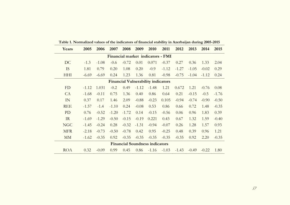
57

Table 1. Normalized values of the indicators of financial stability in Azerbaijan during 2005-2015

Years 2005 2006 2007 2008 2009 2010 2011 2012 2013 2014 2015

Financial market indicators - FMI

DC -1.3 -1.08 -0.6 -0.72 0.01 0.071 -0.37 0.27 0.36 1.33 2.04

IS 1.81 0.79 0.20 1.08 0.20 -0.9 -1.12 -1.27 -1.05 -0.02 0.29

HHI -6.69 -6.69 0.24 1.23 1.36 0.81 -0.98 -0.75 -1.04 -1.12 0.24

Financial Vulnerability indicators

FD -1.12 1.031 -0.2 0.49 -1.12 -1.48 1.21 0.672 1.21 -0.76 0.08

CA -1.68 -0.11 0.75 1.36 0.40 0.86 0.64 0.21 -0.15 -0.5 -1.76

IN 0.37 0.17 1.46 2.09 -0.88 -0.23 0.105 -0.94 -0.74 -0.90 -0.50

REE -1.57 -1.4 -1.10 0.24 -0.08 0.53 0.86 0.66 0.72 1.48 -0.35

PD 0.76 -0.52 -1.20 -1.72 0.14 -0.15 -0.56 0.06 0.96 1.83 0.39

IR -1.69 -1.29 -0.50 -0.15 -0.19 0.221 0.43 0.67 1.32 1.59 -0.40

NGC -1.45 -0.24 0.28 -0.32 -1.31 -0.94 -0.07 0.26 1.28 1.57 0.93

MFR -2.18 -0.73 -0.50 -0.78 0.42 0.95 -0.25 0.48 0.39 0.96 1.21

MM -1.62 -0.35 0.92 -0.35 -0.35 -0.35 -0.35 -0.35 0.92 2.20 -0.35

Financial Soundness indicators

ROA 0.32 -0.09 0.99 0.45 0.86 -1.16 -1.03 -1.43 -0.49 -0.22 1.80

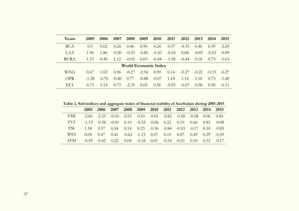
58

Sem

inary P

apers

Years 2005 2006 2007 2008 2009 2010 2011 2012 2013 2014 2015

BCA 0.9 0.02 0.24 0.46 0.90 0.24 -0.57 -0.35 0.46 0.39 -2.69

LAA 1.96 1.86 -0.20 -0.33 -0.85 -0.10 -0.18 0.08 -0.85 -0.53 -0.89

RCRA 1.53 0.49 1.12 -0.02 0.03 -0.44 -1.58 -0.44 0.18 0.75 -1.63

World Economic Index

WEG 0.67 1.02 0.96 -0.27 -2.54 0.90 0.14 -0.27 -0.21 -0.15 -0.27

OPR -1.28 -0.76 -0.40 0.77 -0.88 -0.07 1.10 1.14 1.10 0.73 -1.40

ECI 0.73 1.14 0.73 -2.35 0.02 0.58 -0.95 -0.67 0.58 0.30 -0.11

Table 2. Sub-indices and aggregate index of financial stability of Azerbaijan during 2005-2015

2005 2006 2007 2008 2009 2010 2011 2012 2013 2014 2015

FMI -2.06 -2.33 -0.05 0.53 0.53 -0.01 -0.82 -0.58 -0.58 0.06 0.85

FVI -1.13 -0.38 -0.01 0.10 -0.33 -0.06 0.22 0.19 0.66 0.83 -0.08

FSI 1.18 0.57 0.54 0.14 0.23 -0.36 -0.84 -0.53 -0.17 0.10 -0.85

WEI 0.04 0.47 0.41 -0.62 -1.13 0.47 0.10 0.07 0.49 0.29 -0.59

AFSI -0.49 -0.42 0.22 0.04 -0.18 0.01 -0.34 -0.21 0.10 0.32 -0.17

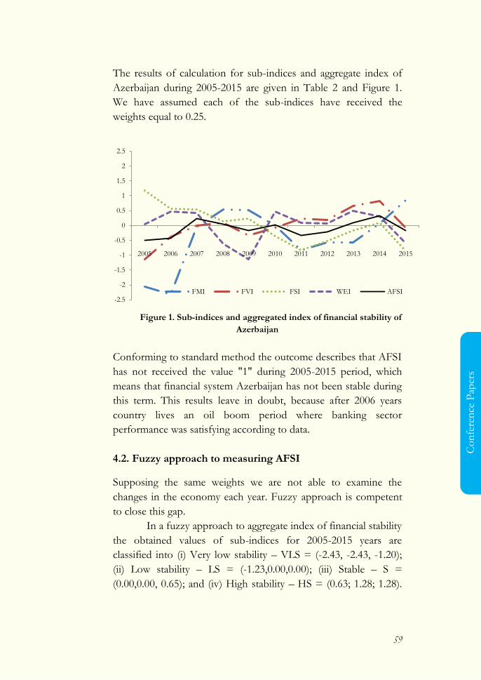
59

Co

nfe

ren

ce P

aper

s

The results of calculation for sub-indices and aggregate index of

Azerbaijan during 2005-2015 are given in Table 2 and Figure 1.

We have assumed each of the sub-indices have received the

weights equal to 0.25.

Figure 1. Sub-indices and aggregated index of financial stability of

Azerbaijan

Conforming to standard method the outcome describes that AFSI

has not received the value "1" during 2005-2015 period, which

means that financial system Azerbaijan has not been stable during

this term. This results leave in doubt, because after 2006 years

country lives an oil boom period where banking sector

performance was satisfying according to data.

4.2. Fuzzy approach to measuring AFSI

Supposing the same weights we are not able to examine the

changes in the economy each year. Fuzzy approach is competent

to close this gap.

In a fuzzy approach to aggregate index of financial stability

the obtained values of sub-indices for 2005-2015 years are

classified into (i) Very low stability – VLS = (-2.43, -2.43, -1.20);

(ii) Low stability – LS = (-1.23,0.00,0.00); (iii) Stable – S =

(0.00,0.00, 0.65); and (iv) High stability – HS = (0.63; 1.28; 1.28).

-2.5

-2

-1.5

-1

-0.5

0

0.5

1

1.5

2

2.5

2005 2006 2007 2008 2009 2010 2011 2012 2013 2014 2015

FMI FVI FSI WEI AFSI

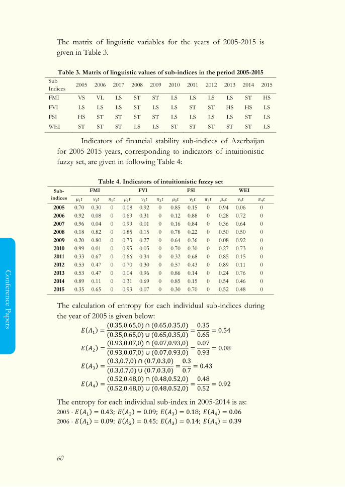
60

Co

nferen

ce Pap

ers

The matrix of linguistic variables for the years of 2005-2015 is

given in Table 3.

Table 3. Matrix of linguistic values of sub-indices in the period 2005-2015

Sub

Indices 2005 2006 2007 2008 2009 2010 2011 2012 2013 2014 2015

FMI VS VL LS ST ST LS LS LS LS ST HS

FVI LS LS LS ST LS LS ST ST HS HS LS

FSI HS ST ST ST ST LS LS LS LS ST LS

WEI ST ST ST LS LS ST ST ST ST ST LS

Indicators of financial stability sub-indices of Azerbaijan

for 2005-2015 years, corresponding to indicators of intuitionistic

fuzzy set, are given in following Table 4:

Table 4. Indicators of intuitionistic fuzzy set

Sub-

indices

FMI FVI FSI WEI

2005 0.70 0.30 0 0.08 0.92 0 0.85 0.15 0 0.94 0.06 0

2006 0.92 0.08 0 0.69 0.31 0 0.12 0.88 0 0.28 0.72 0

2007 0.96 0.04 0 0.99 0.01 0 0.16 0.84 0 0.36 0.64 0

2008 0.18 0.82 0 0.85 0.15 0 0.78 0.22 0 0.50 0.50 0

2009 0.20 0.80 0 0.73 0.27 0 0.64 0.36 0 0.08 0.92 0

2010 0.99 0.01 0 0.95 0.05 0 0.70 0.30 0 0.27 0.73 0

2011 0.33 0.67 0 0.66 0.34 0 0.32 0.68 0 0.85 0.15 0

2012 0.53 0.47 0 0.70 0.30 0 0.57 0.43 0 0.89 0.11 0

2013 0.53 0.47 0 0.04 0.96 0 0.86 0.14 0 0.24 0.76 0

2014 0.89 0.11 0 0.31 0.69 0 0.85 0.15 0 0.54 0.46 0

2015 0.35 0.65 0 0.93 0.07 0 0.30 0.70 0 0.52 0.48 0

The calculation of entropy for each individual sub-indices during

the year of 2005 is given below:

( ) ( ) ( )

( ) ( )

( ) ( ) ( )

( ) ( )

( ) ( ) ( )

( ) ( )

( ) ( ) ( )

( ) ( )

The entropy for each individual sub-index in 2005-2014 is as:

2005 - ( ) ( ) ( ) ( )

2006 - ( ) ( ) ( ) ( )

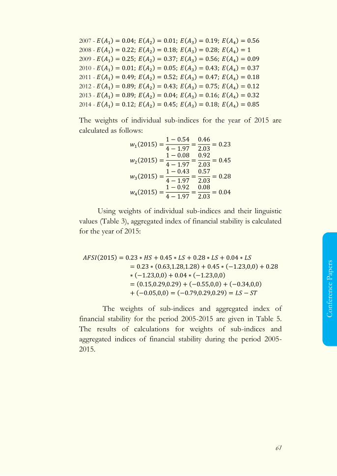
61

Co

nfe

ren

ce P

aper

s

2007 - ( ) ( ) ( ) ( )

2008 - ( ) ( ) ( ) ( )

2009 - ( ) ( ) ( ) ( )

2010 - ( ) ( ) ( ) ( )

2011 - ( ) ( ) ( ) ( )

2012 - ( ) ( ) ( ) ( )

2013 - ( ) ( ) ( ) ( )

2014 - ( ) ( ) ( ) ( )

The weights of individual sub-indices for the year of 2015 are

calculated as follows:

( )

( )

( )

( )

Using weights of individual sub-indices and their linguistic

values (Table 3), aggregated index of financial stability is calculated

for the year of 2015:

( )

( ) ( )

( ) ( )

( ) ( ) ( )

( ) ( )

The weights of sub-indices and aggregated index of

financial stability for the period 2005-2015 are given in Table 5.

The results of calculations for weights of sub-indices and

aggregated indices of financial stability during the period 2005-

2015.

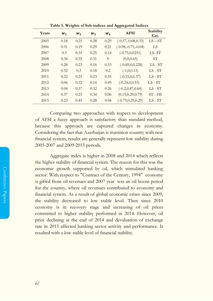
62

Co

nferen

ce Pap

ers

Table 5. Weights of Sub-indices and Aggregated Indices

Years AFSI Stability

Cat.

2005 0.18 0.25 0.28 0.29 (-0.57,-0.08,0.33) LS – ST

2006 0.31 0.19 0.29 0.21 (-0.98,-0.75,-0.04) LS

2007 0.3 0.31 0.25 0.14 (-0.75,0,0251) LS- ST

2008 0.34 0.35 0.31 0 (0,0,0.65) ST

2009 0.28 0.23 0.16 0.33 (-0.69,0,0.228) LS - ST

2010 0.32 0.3 0.18 0.2 (-1,0,0.13) LS - ST

2011 0.22 0.21 0.23 0.35 (-0.55,0,0.37) LS - ST

2012 0.06 0.32 0.14 0.49 (-0.24,0,0.53) LS - ST

2013 0.04 0.37 0.32 0.26 (-0.2,0.47,0.64) LS - ST

2014 0.37 0.23 0.34 0.06 (0.15,0.29,0.79) ST - HS

2015 0.23 0.45 0.28 0.04 (-0.79,0.29,0.29) LS - ST

Comparing two approaches with respect to development

of AFSI a fuzzy approach is satisfactory than standard method,

because this approach are captured changes in economy.

Considering the fact that Azerbaijan is transition country with new

financial system, results are generally represent low stability during

2005-2007 and 2009-2013 periods.

Aggregate index is higher in 2008 and 2014 which reflects

the higher stability of financial system. The reason for this was the

economic growth supported by oil, which stimulated banking

sector. With respect to "Contract of the Century, 1994" economy

is gifted from oil revenues and 2007 year was an oil boom period

for the country, where oil revenues contributed to economy and

financial system. As a result of global economic crises since 2009,

the stability decreased to low stable level. Then since 2010

economy is in recovery stage and increasing of oil prices

committed to higher stability performed in 2014. However, oil

price declining at the end of 2014 and devaluation of exchange

rate in 2015 affected banking sector activity and performance. It

resulted with a low stable level of financial stability.

63

Co

nfe

ren

ce P

aper

s

4. CONCLUSION

This paper developed method for calculation of the weights of

composite indices and quality level of financial stability in

Azerbaijan for the period of 2005-2015.

Main contribution was determining the weights

appropriately for the years. It is worth to note that implementation

equal weights to the aggregate index is not capable to cover the

economic changes in 2005-2015. Fuzzy approach allows to obtain

weights represented for the years separately. Moreover this

approach made possible to avoid disjunction of the phenomen

such as "stability" and "unstability" by determining "very low

stability", "low stability" and etc. terms.

However, results of fuzzy approach are more acceptable

than standard methods because these are able to capture key

periods of financial stability during the sample period. For the

future to enhance of the outcomes and for deepening of the

reseach our main goal is to extend the list of individual indicators

and then apply fuzzy approach to obtain different weights for all

individual indicators.

REFERENCES

Albulescu, C.T. 2008. Assessing Romanian Financial Sector

Stability by Means of an Aggregate Index. Oeconomica,

17(2): 67-87.

Albulescu, C.T. 2010. Forecasting the Romanian Financial System

Stability Using a Stochastic Simulation Model. Romanian

Journal of Economic Forecasting, (1): 81-98.

Morris, V.C. 2011. Measuring and Forecasting Financial Stability:

The Composition of an Aggregate Financial Stability Index

for Jamaica, Journal of Business, Finance and Economics

in Emerging Economies, 6(2): 34-51

Nasreen, S. and Anwar, S. and Shahzadi, H. 2015. Financial

Stability and Macroeconomic Environment: Evidence

64

Co

nferen

ce Pap

ers

from Panel Data Analysis of South Asian Countries.

Pakistan Journal of Social Sciences, 35(1):145-160

Atanassov, K. 1986. Intuitionistic fuzzy sets. Fuzzy Sets and Systems,

20(1): 87-96

Szmidt, E. and Kacprzyk, K. 2001. Entropy for intuitionistic fuzzy

sets. Fuzzy Sets and Systems,(118): 467-477

G.J.Shinasi, G.J. 2004. Defining Financial Stability, International

Monetary Fund WP/187

Illing, M. and Y, Liu. 2003. An Index of Financial Stress for

Canada. National Bank of Canada Working Paper /14: 63p.

Van den End, J.W. 2006. Indicator and Boundaries of Financial

Stability. De Nederlandsche Bank Working Paper /97: 24 p.

Borio, C. and Drehmann, M. 2009. Towards an operational

framework for financial stability: ―fuzzy‖ measurement

and its consequences, BIS Working Papers /284: 50 p.

Jordan, A and Smith, L. 2014. Measuring the Level of Financial

Stability in the Bahamas. 46th Annual Monetary Studies

Conference: Macro-Prudential Supervision, Financial Stability And

Monetary Policy, Central Bank of Trinidad and Tobago

Karanovic, G. and Karanovic, B. 2015. Developing an Aggregate

Index for Measuring Financial Stability in the Balkans. 7th

International Conference, The Economies of Balkan and Eastern

Europe Countries in the changed world, EBEEC: 3-17

BP Statistical Review of World Energy, 64th edition, June 2015, 45

p.

CESifo Group Munich, www.ifo.de/w/4LsApn939

65

Co

nfe

ren

ce P

aper

s

Financial Inclusion Impact on Financial Stability across Group Countries

Azka Azifah Dienillah , Lukytawati Anggraeni, Sahara

Departement of Economics, Faculty of Economics and Management, Bogor Agricultural University

Corresponding author: azifahazka@yahoo.co.id

Preliminary draft, plase do not quote. Complete version will be published on forthcoming issue on

Bulleitn of Monetary Economics and Banking

Abstract

Financial inclusion is one of strategy to increase inclusive growth

in many countries. However it may cause either stability or

instability in the financial system and the impact can be different

among income group countries. Potential instability in the

financial system occurs when financial inclusion causes reducting

in credit standard, inceasing risk of bank reputation, and

uncoresponding regulation in microfinance.

This research aimed to measure financial inclusion and

financial stability indexes between countries and analyze the

impact of financial inclusion on financial stability in 19 countries

based on income group from 2004-2011. Data were collected

from World Bank, the International Monetary Fund (IMF)

66

Co

nferen

ce Pap

ers

database, and other sources. The methods used Sarma index to

calculate financial inclusion, Albulescu and Goyeau index to

calculate financial stability, and tobit model to analyze the impact

of financial inclusion on financial stability.

The results show higher income countries have higher

financial inclusion and financial stability index than lower income

countries. Financial inclusion only has positive significant effect to

financial stability in high income countries. Lower and upper

middle income countries have to increase availability of financial

services to enhance financial inclusion. Moreover, lower and

upper middle income countries have to increase financial

development to enhance financial stability.

Keywords: financial inclusion index, financial stability index, tobit

model

JEL Classification: C5, E6, C1

1. INTRODUCTION

Financial inclusion becomes an important program at

national and international level because there are 2.6 billion people

or more than 50% of world population not having access to

credit, insurance, and savings (CGAP 2013). Financial inclusion

program is expected to increase inclusive growth in many

countries. Increasing in financial inclusion enhances based deposit

as source of credit. The credit can improve real sector

peformance. These will reduce poverty, improve income

distribution, and improve the stability of the financial system in

order to achieve growth that is felt by the entire community (Khan

2011).

Seriousness of the international communities in

implementing the program of financial inclusion can be seen from

increasing of formal financial services products. In Figure 1 below

shows an average increase of outstanding loans from 2004 to

2011. Upper middle income countries group has the highest

average growth of outstanding loans. the percentage of

outstanding loans growth in Upper middle income countries

67

Co

nfe

ren

ce P

aper

s

group is 13.3%. Lower middle income countries group has

negative growth of loans per 1000 adult population. The growth

rate of lower middle income countries group is -8.3%. Average

world has positive credit accounts per 1000 adult population

growth rate amount of 8.1%.

There are few studies about the impact of financial

inclusion on financial stability with different result. Some studies

about the impact of financial inclusion on financial stability which

show the positive impact was conducted by Dienillah (2015),

Morgan and Pontines (2014), Cull et al. (2012), and Huang and

Rakovski (2011). Furthermore, some studies which show potential

negative impact of financial inclusion on financial stability

undertaken by Dupas et al. (2012) and Khan (2011). Since there

are different result of the impact of financial inclusion on financial

stability, we need more research about this topic.

In the theory, high level of financial inclusion will be

followed by strong financial system. In addition, people with lower

income level should have a better impact of financial inclusion on

financial stability than people with higher income (CGAP 2013).

This is because people with higher income have a faster response

when the crisis happen than people with lower income. The

response can be seen from the massive withdrawal of higher-

income customers when a crisis occurs. However, from some

studies and fact haven‘t confirmed these theory so further

research is needed.

Han and Melecky (2013) state that financial inclusion has a

positive impact on financial stability in high income countries and

upper middle income countries. This is because increasing in

financial inclusion can improve deposits in commercial bank so it

will make resilience of the funding base of deposits in banking

sector when crisis occurs. In contrast to high-income countries

group and upper middle income group, the lower middle income

countries group has the potential instability in financial system due

to financial inclusion (Khan 2011).

68

Co

nferen

ce Pap

ers

In previous studies about the impact of financial inclusion

on financial stability still use a proxy to represent the level of

financial inclusion and a level of financial stability. Morgan and

pontines (2014) suggest to include other variables in describing

financial inclusion and financial stability since financial inclusion is

not only seen by financial products indicator such as SMEs

outstanding loans but also seen by penetration and product access

to formal financial institutions indicators (Sarma 2008). The

stability of the financial system is not only seen by Bank Z score

because the financial system is not only influenced by the banking

sector, but also influenced by the state of real economy,

households, corporations, external factors, and so on. So it is

necessary to build a more representative index describes the

financial inclusion and stability of financial system. Therefore, this

research raise the question on how is the financial inclusion

among countries based on income group countrries in 2004-2011.

2. METHODOLOGY

Types and Sources of Data

The data used is secondary data which is an annual data with an

unbalanced panel data structurre. The panel data consist of a cross

section data including lower middle-income countries group

(Egypt, El savador, India, Indonesia, and Nigeria), upper middle-

income countries group (Argentina, Bosnia, Chile, Colombia,

Macedonia, Malaysia, Mexico, Namibia, and Thailand), and high-

income countries group (Belgium, Czech, Hungary, Korea, and

Switzerland). Time series data from 2004 to 2011. The data were

collected from various sources such as: World Bank, World

Development Indicators (WDI), International Monetary Fund

(IMF) database, and other sources. This research was conducted

with software such as STATA and Microsoft Excel.

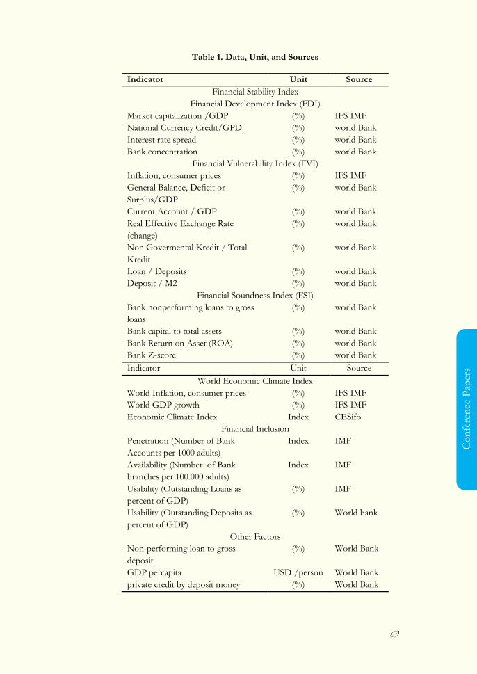
69

Co

nfe

ren

ce P

aper

s

Table 1. Data, Unit, and Sources

Indicator Unit Source

Financial Stability Index

Financial Development Index (FDI)

Market capitalization /GDP (%) IFS IMF

National Currency Credit/GPD (%) world Bank

Interest rate spread (%) world Bank

Bank concentration (%) world Bank

Financial Vulnerability Index (FVI)

Inflation, consumer prices (%) IFS IMF

General Balance, Deficit or

Surplus/GDP

(%) world Bank

Current Account / GDP (%) world Bank

Real Effective Exchange Rate

(change)

(%) world Bank

Non Govermental Kredit / Total

Kredit

(%) world Bank

Loan / Deposits (%) world Bank

Deposit / M2 (%) world Bank

Financial Soundness Index (FSI)

Bank nonperforming loans to gross

loans

(%) world Bank

Bank capital to total assets (%) world Bank

Bank Return on Asset (ROA) (%) world Bank

Bank Z-score (%) world Bank

Indicator Unit Source

World Economic Climate Index

World Inflation, consumer prices (%) IFS IMF

World GDP growth (%) IFS IMF

Economic Climate Index Index CESifo

Financial Inclusion

Penetration (Number of Bank

Accounts per 1000 adults)

Index IMF

Availability (Number of Bank

branches per 100.000 adults)

Index IMF

Usability (Outstanding Loans as

percent of GDP)

(%) IMF

Usability (Outstanding Deposits as

percent of GDP)

(%) World bank

Other Factors

Non-performing loan to gross

deposit

(%) World Bank

GDP percapita USD /person World Bank

private credit by deposit money (%) World Bank

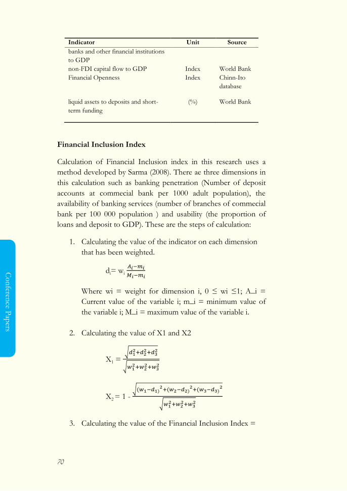
70

Co

nferen

ce Pap

ers

Indicator Unit Source

banks and other financial institutions

to GDP

non-FDI capital flow to GDP Index World Bank

Financial Openness Index Chinn-Ito

database

liquid assets to deposits and short-

term funding

(%) World Bank

Financial Inclusion Index

Calculation of Financial Inclusion index in this research uses a

method developed by Sarma (2008). There ae three dimensions in

this calculation such as banking penetration (Number of deposit

accounts at commecial bank per 1000 adult population), the

availability of banking services (number of branches of commecial

bank per 100 000 population ) and usability (the proportion of

loans and deposit to GDP). These are the steps of calculation:

1. Calculating the value of the indicator on each dimension

that has been weighted.

di= wi

Where wi = weight for dimension i, 0 ≤ wi ≤1; A_i =

Current value of the variable i; m_i = minimum value of

the variable i; M_i = maximum value of the variable i.

2. Calculating the value of X1 and X2

X1 = √

√

X2 = 1 - √( )

( ) ( )

√

3. Calculating the value of the Financial Inclusion Index =

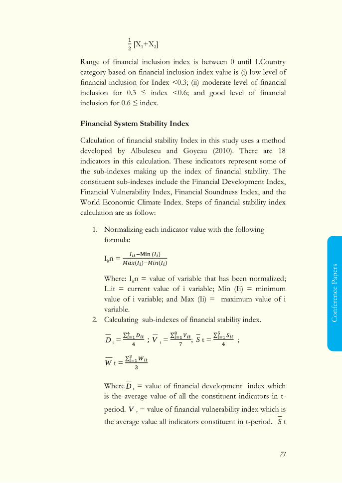
71

Co

nfe

ren

ce P

aper

s

[X1+X2]

Range of financial inclusion index is between 0 until 1.Country

category based on financial inclusion index value is (i) low level of

financial inclusion for Index <0.3; (ii) moderate level of financial

inclusion for 0.3 ≤ index <0.6; and good level of financial

inclusion for 0.6 ≤ index.

Financial System Stability Index

Calculation of financial stability Index in this study uses a method

developed by Albulescu and Goyeau (2010). There are 18

indicators in this calculation. These indicators represent some of

the sub-indexes making up the index of financial stability. The

constituent sub-indexes include the Financial Development Index,

Financial Vulnerability Index, Financial Soundness Index, and the

World Economic Climate Index. Steps of financial stability index

calculation are as follow:

1. Normalizing each indicator value with the following

formula:

Iitn = ( )

( ) ( )

Where: Iitn = value of variable that has been normalized;

I_it = current value of i variable; Min (Ii) = minimum

value of i variable; and Max (Ii) = maximum value of i

variable.

2. Calculating sub-indexes of financial stability index.

D t = ∑

V t =

∑

; S t =

∑

;

W t = ∑

Where D t = value of financial development index which

is the average value of all the constituent indicators in t-

period. V t = value of financial vulnerability index which is

the average value all indicators constituent in t-period. S t

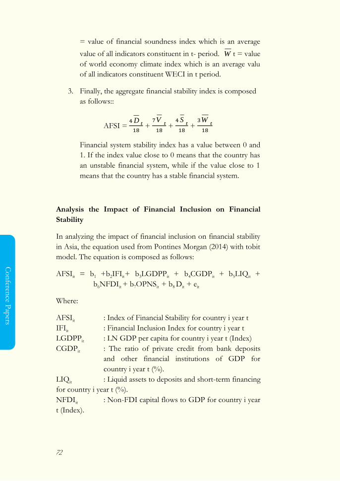
72

Co

nferen

ce Pap

ers

= value of financial soundness index which is an average

value of all indicators constituent in t- period. W t = value

of world economy climate index which is an average valu

of all indicators constituent WECI in t period.

3. Finally, the aggregate financial stability index is composed

as follows::

AFSI = D

+

V

+

S

+

W

Financial system stability index has a value between 0 and

1. If the index value close to 0 means that the country has

an unstable financial system, while if the value close to 1

means that the country has a stable financial system.

Analysis the Impact of Financial Inclusion on Financial

Stability

In analyzing the impact of financial inclusion on financial stability

in Asia, the equation used from Pontines Morgan (2014) with tobit

model. The equation is composed as follows:

AFSIit = b1 +b2IFIit+ b3LGDPPit + b4CGDPit + b5LIQit +

b6NFDIit + b7OPNSit + b8 Dit + eit

Where:

AFSIit : Index of Financial Stability for country i year t

IFIit : Financial Inclusion Index for country i year t

LGDPPit : LN GDP per capita for country i year t (Index)

CGDPit : The ratio of private credit from bank deposits

and other financial institutions of GDP for

country i year t (%).

LIQit : Liquid assets to deposits and short-term financing

for country i year t (%).

NFDIit : Non-FDI capital flows to GDP for country i year

t (Index).

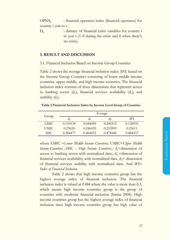
73

Co

nfe

ren

ce P

aper

s

OPNSit : financial openness index (financial openness) for

country i year to t.

Dit : dummy of financial crisis variables for country i

in year t (1 if during the crisis and 0 when there‘s

no crisis).

3. RESULT AND DISCUSSION

3.1. Financial Inclusion Based on Income Group Countries

Table 2 shows the average financial inclusion index (IFI) based on

the Income Group Countries consisting of lower middle income

countries, upper middle, and high income countries. The financial

inclusion index consists of three dimensions that represent access

to banking sector (d1), financial services availability (d2), and

usability (d3).

Table 2 Financial Inclusion Index by Income Level Group of Countries

Group Average

d1 d2 d3 IFI

LMIC 0.110138 0.044099 0.200312 0.126935

UMIC 0.23624 0.186435 0.253909 0.23611

HIC 0.584477 0.404452 0.478446 0.484437

where LMIC =Lower Middle Income Countries; UMIC=Upper Middle

Income Countries. ; HIC : High Income Countries.; d1=dimension of

access to banking sector with normalized data.; d2 =dimension of

financial services availability with normalized data. d3= dimension

of financial services usability with normalized data. And IFI=

Index of Financial Inclusion.

Table 2 shows that high income countries group has the

highest average index of financial inclusion. The financial

inclusion index is valued at 0.484 where the value is more than 0.3,

which means high income countries group is the group of

countries with moderate financial inclusion (Sarma 2008). High

income countries group has the highest average index of financial

inclusion since high income countries group has high value of

74

Co

nferen

ce Pap

ers

banking penetration dimension represented by the number of

deposit accounts at commercial bank per 1000 adult population,

availability of financial services dimensions represented by a

number of commercial bank branches per 100 000 population

adults, and product usability of formal financial institutions

dimensions represented by the proportion of outstanding loans

and deposit to GDP.

Upper-middle income countries has an average value of

financial inclusion index at 0.236. The index value is less than 0.3

so classified in the group of countries with poor financial inclusion

(Sarma 2008). Dimension that contribute the greatest value on the

financial inclusion index in upper middle income countries group

is dimension of financial services usability. It is represented by the

relatively high proportion of outstanding loans and deposit to

GDP compared to other dimensions. The obstacles in the

implementation of financial inclusive in Upper-middle income

countries group is lack of financial services illustrated by low

number of branches provided by commercial banks.

Lower middle income countries group has the lowest

average value of financial inclusion index at 0.127. The index value

is less than 0.3 so classified in the group of countries with poor

financial inclusion (Sarma 2008). All dimension of financial

inclusion in the group of middle income countries is the lowest

compared to other groups. Moreover, the lowest dimension in

lower middle income group of countries is availability of financial

services illustrated by the low number of branches provided by

commercial banks.

Financial Stability Based on Income Group Countries

Table 3 shows the results of calculation for the average financial

stability index based on Income Group Countries. Financial

system stability index is composed of four sub-indexes

representing the development of financial sector, the vulnerability

of financial sector, the soundness of financial sector, and world

economic climate. From the calculation results obtained as

follows:

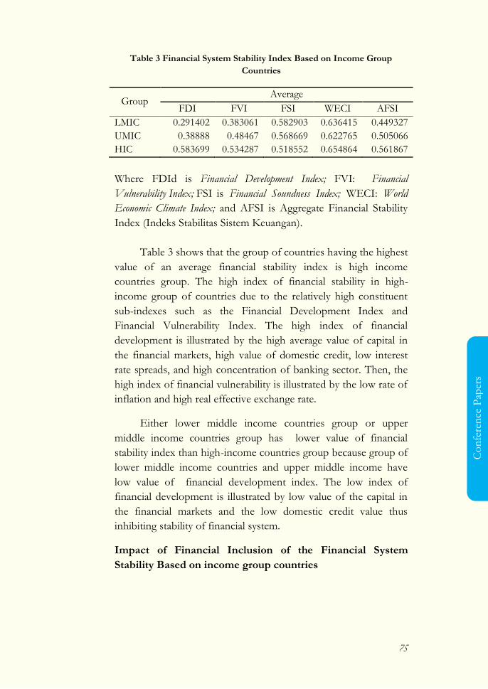
75

Co

nfe

ren

ce P

aper

s

Table 3 Financial System Stability Index Based on Income Group

Countries

Group Average

FDI FVI FSI WECI AFSI

LMIC 0.291402 0.383061 0.582903 0.636415 0.449327

UMIC 0.38888 0.48467 0.568669 0.622765 0.505066

HIC 0.583699 0.534287 0.518552 0.654864 0.561867

Where FDId is Financial Development Index; FVI: Financial

Vulnerability Index; FSI is Financial Soundness Index; WECI: World

Economic Climate Index; and AFSI is Aggregate Financial Stability

Index (Indeks Stabilitas Sistem Keuangan).

Table 3 shows that the group of countries having the highest

value of an average financial stability index is high income

countries group. The high index of financial stability in high-

income group of countries due to the relatively high constituent

sub-indexes such as the Financial Development Index and

Financial Vulnerability Index. The high index of financial

development is illustrated by the high average value of capital in

the financial markets, high value of domestic credit, low interest

rate spreads, and high concentration of banking sector. Then, the

high index of financial vulnerability is illustrated by the low rate of

inflation and high real effective exchange rate.

Either lower middle income countries group or upper

middle income countries group has lower value of financial

stability index than high-income countries group because group of

lower middle income countries and upper middle income have

low value of financial development index. The low index of

financial development is illustrated by low value of the capital in

the financial markets and the low domestic credit value thus

inhibiting stability of financial system.

Impact of Financial Inclusion of the Financial System

Stability Based on income group countries

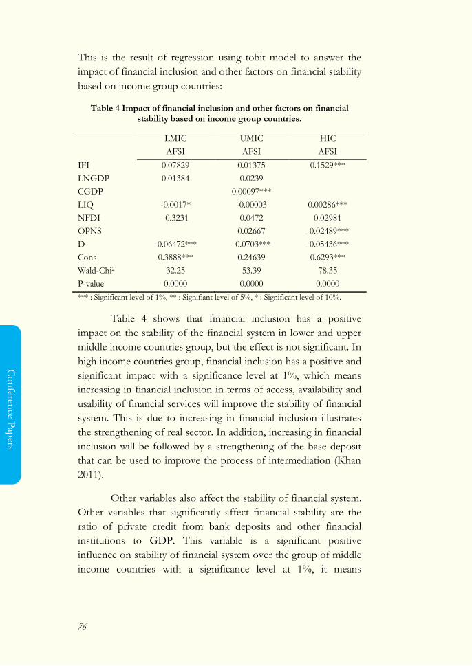
76

Co

nferen

ce Pap

ers

This is the result of regression using tobit model to answer the

impact of financial inclusion and other factors on financial stability

based on income group countries:

Table 4 Impact of financial inclusion and other factors on financial stability based on income group countries.

LMIC UMIC HIC

AFSI AFSI AFSI

IFI 0.07829 0.01375 0.1529***

LNGDP 0.01384 0.0239

CGDP 0.00097***

LIQ -0.0017* -0.00003 0.00286***

NFDI -0.3231 0.0472 0.02981

OPNS 0.02667 -0.02489***

D -0.06472*** -0.0703*** -0.05436***

Cons 0.3888*** 0.24639 0.6293***

Wald-Chi2 32.25 53.39 78.35

P-value 0.0000 0.0000 0.0000

*** : Significant level of 1%, ** : Signifiant level of 5%, * : Significant level of 10%.

Table 4 shows that financial inclusion has a positive

impact on the stability of the financial system in lower and upper

middle income countries group, but the effect is not significant. In

high income countries group, financial inclusion has a positive and

significant impact with a significance level at 1%, which means

increasing in financial inclusion in terms of access, availability and

usability of financial services will improve the stability of financial

system. This is due to increasing in financial inclusion illustrates

the strengthening of real sector. In addition, increasing in financial

inclusion will be followed by a strengthening of the base deposit

that can be used to improve the process of intermediation (Khan

2011).

Other variables also affect the stability of financial system.

Other variables that significantly affect financial stability are the

ratio of private credit from bank deposits and other financial

institutions to GDP. This variable is a significant positive

influence on stability of financial system over the group of middle

income countries with a significance level at 1%, it means

77

Co

nfe

ren

ce P

aper

s

increasing in the ratio of private credit from bank deposits and

other financial institutions to GDP will improve the stability of

financial system. This is because increasing in private credit will

lead to growth in the real sector and growth in financial sector

that will strengthen the stability of financial system (Sahay et al.

2015).

Liquid assets to deposits and short-term financing in lower

middle income countries has significantly negative affect on

financial stability with a significance level at 5%. The negative

impact due to increasing in the availability of liquid assets liabilities

will reduce the proportion of credit so it will resist function of

formal financial institutions (Calderon and Serven 2011). In the

group of high-income countries, liquid assets to deposits and

short-term financing has a positive and significant impact on

financial stability with a significance level at 1%, which means

increasing in liquid assets to deposits and short-term financing will

improve stability of financial system. The positive impact due to

increasing in liquid assets will enhance customer‘s trust to the

bank when shock happened (Morgan and Pontines 2014).

Financial openness has a significant negative impact on

stability of financial system in high-income countries at the level

of 1%. It means increasing in financial openness will reduce the

stability of financial system due to high level of financial openness

will increase the vulnerability to capital outflows from short-term

capital when shocks occur. Capital outflow will be followed by

volatile capital (depreciation of capital in the stock market) and the

depreciation of the currency will eventually enhance instability in

financial system (Estrada, Park, and Ramayandi 2015).

Last variables that affect the stability of financial system is

crisis dummy variable. The financial crisis significantly affects the

stability of financial system with a significance level at 1% in all

income level group. The impact of crisis causes instability in the

financial system. This is because the financial crisis lead to

reducing customer‘s trust. it will lead to bank runs that may cause

78

Co

nferen

ce Pap

ers

ineffectiveness of the financial system, which means creating a

financial system instability (Han and Melecky 2013).

4. FINDING AND CONCLUSION

Group of countries with higher income level has a better level of

average access, availability and usability of financial services so

that it has higher value of financial inclusion index than lower

income group. Group of countries with higher income level also

has higher value of financial stability index than lower income

group. The high average index of financial stability in group of

countries with higher income due to many factors such as having

high value of capital in the financial markets, having high

concentrations of banking sector, and having low level of

inflation, and so on.

Financial inclusion has a positive impact but not

significant to the stability of financial system in the group of

lower and upper middle income countries, but has a significant

positive impact on the stability of financial system in high-income

countries group. This is because increasing in financial inclusion

illustrates the strengthening of the real sector. In addition, the

increase in financial inclusion will be followed by a strengthening

of the base deposit that can be used to improve the process of

banking intermediation (Khan 2011).

This paper provide three recommendation: first, for the

financial services authority and banking sector, especially in lower

middle income group and upper middle income group should

encourage the availability of financial services such as an

increasing in the number of bank branches in order to encourage

financial inclusion. Second, for the government and the financial

sector in lower middle income and upper middle income countries

should encourage sub-index of financial development by

encouraging capital flow in financial markets and enhancing

domestic credit. For the financial services authority and banking

sector in high income countries, to encourage financial inclusion

can also push the financial soundness index by increasing bank

capital to assets and reducing volatility of banking return on assets.

79

Co

nfe

ren

ce P

aper

s

It may be strategies to enhance stability of financial system. Third,

for further research, it‘s better to add low-income countries group

if it hasn‘t problem of data availability.

References

Albulescu CT, Goyeau D. 2010. Assessing and Forecasting

Romanian Financial System‘s Stability Using an Aggregate

Index. [jurnal]. Romanian Journal of Economic Literature,

vol. 1/2010

[CGAP] Consultative Group to Assist the Poor. 2013. Financial

Access 2012 Getting to a More Comprehensive Picture.

Washington DC (US) : CGAP.

Calderon,C Serven, L. 2011. Macro-Prudential over the Cycle in

Latin America. Mimeo [internet]. [Juni 2015] Tersedia pada

ww.webmeets.com/files/papers/LACEA-

LAMES/2012/456/CC-

LS%20LAC%20Macroprudential%202012.pdf.

Cull,R Kunt,D. 2007. Financial Performance and Outreach: A

Global Analysis Leading Microfinance Institutions. [jurnal].

The Economic Journal, vol. 117 (517); 107-133

Dienillah,A.A. 2015. Dampak Inklusi Keuangan terhadap

Stabilitas Sistem Keuangan di Asia. [Skripsi]. Bogor (ID) :

Institut Pertanian Bogor.

Dupas,P Green,S Keats,A Robinson,J. 2012. Challenges in

Banking the Rural Poor: Evidence from Kenya's Western

Province. [working paper]. Cambridge (GB) : National Bureau

of Economic Research.

Estrada,Gemma Park,Donghyun Ramayandi,Arief. 2015. Financial

Development, financial openness, and Economic Growth.

[working paper]. Tokyo (JP) : ADB economics Woking Paper

Series, vol. 442.

Han,R Melecky,M. 2013. Financial Inclusion for Financial

Stability. Access to Bank Deposits and the Growth of

80

Co

nferen

ce Pap

ers

Deposits in the Global Financial Crisis [Working Paper].

Washington DC(US) : World Bank.

Huang, R Ratnovski,L. 2011. The Dark Side of Bank Wholesale

Funding. [Jurnal]. Journal of Financial Intermediation, vol.

20(2): 24-63.

Khan,H.R. 2011. Financial inclusion and financial stability: are

they two sides of the same coin?. Chennai (IN): The Indian

Bankers Association and Indian Overseas Bank.

Morgan,P Pontines,V. 2014. Financial Stability and Financial

Inclusion [Working Paper 2014]. Tokyo (JP) : Asian

Development Bank Institute.

Sahay et al. 2015. Rethinking Financial Deepening:Stability and

Growth in Emerging Markets. imf staff discussion note.

Sarma,M Pais,J. 2008. Financial Inclusion and Development: A

Cross Country Analysis. [Working Paper]. Berlin (GE): Berlin

Working Papers on Money, Finance, Trade and

development.

[World Bank]. 2013. Jumlah rekening kredit per 1 000 populasi

dewasa [internet]. [diunduh pada 2016 Febuari] tersedia

pada; http://www.worldbank.org/

81

Co

nfe

ren

ce P

aper

s

An Early Warning Towards The Resilience of Islamic Banking In Indonesia

Jarita Duasa Professor of Economics, Department of Economics, Kulliyyah of Economics and

Management Sciences, International Islamic University Malaysia. Corresponding author: jarita@iium.edu.my

Dimas Bagus Wiranatakusuma

Lecturer at Department of Economics, Universitas Muhammadiyah Yogyakarta, and PhD Candidate in Economics, International Islamic University Malaysia.

dimas_kusuma@umy.ac.id

Sumandi

Bachelor Student in Economics,

Universitas Muhammadiyah Yogyakarta. andi.excellent@yahoo.co.id

Abstract

An early warning system (EWS) is widely used as surveillance

mechanism for preserving financial system stability. It is

conducted by identifying some potential variables that can issue

alarm preceeding crisis. Islamic banking which is part of financial

system, is also prone to crisis due to adverse external shocks and

given interconnectedness nature in the financial system. This

paper addresses one primary question, namely which

macroconomic variables that are capable of signaling adverse

shocks towards the resilience of Islamic banking in Indonesia. We

82

Co

nferen

ce Pap

ers

use an extraction signal approach as EWS mechanism. The

reasons are (a) this approach is the simplest approach for EWS,

(b) the approach can be updated regularly, usually in monthly

basis, (c) this approach has the lowest cost, and (d) the approach

can develop a composite index that can be used as a signaling

device. This paper employs various time horizons and thresholds

in order to measure the predictive power of leading variables. The

results suggest that there are several variables that (1) IBRI, which

is composed from standardized deposit and financing since 2004

until 2016 in monthly basis, is able to figure out the resilience of

Islamic banking. The resilience of Islamic banking was worst in

2004, but gradually decreased and stable. Interestingly, the

resilience of Islamic banking was considered stable since the index

was moving below the normal line during the global financial

crises, and (2) Some selected macrofinancial variables, M2/reserve

(M2res), credit growth (CG), real effective exchange rate (REER),

and inflation rate (INF) empirically show low noise to signal ratio.

It means that these four variables are capable of signaling

vulnerabilities from adverse external shocks. This paper is

considered a very preliminary work in the area of early warning

system for the resilience of Islamic banking. However, there is no

clear cut leading indicators to comprehensively monitor its

resilience. More macroeconomic and financial variables are needed

to be included as leading indicators for capturing the resilience of

Islamic banking. In addition, given that macroeconomic and

financial variables play the important thing in providing the

resilience, the macroprudential policy needs to be more specifically

addressing procyclicality in the financial sector. Meanwhile, the

resilience of Islamic banking needs to be supported by the

resilience in the real sector. It is because the core operations of

Islamic banking are dealing with productive sector. Therefore, the

synergic policies are needed to establish strong resilience of

Islamic banking, namely stable macroeconomic envirounment and

strong real sector development.

Keywords: early warning system, resilience of Islamic banking, extraction

signal approach

JEL Classification: E44, F15, G01

83

Co

nfe

ren

ce P

aper

s

1. INTRODUCTION

Islamic banking operation in Indonesia was started in 1992 when

the first full-fledged Islamic bank was established, Bank Muamalat

Indonesia. This Islamic bank provely survived from the 1998

Asian financial crisis without any government asistance. The

growth of Islamic banking proliferated rapidly after the new

banking act was officially stipulated in 1998. Afterwards, the

Islamic banks operations become widely expanded and well-

accepted by all level of society in Indonesia. The growth of Islamic

banking industry can be traced back from growth on its asset,

deposit, and financing side. In terms of asset, it grew drastically

from only Rp 21 trillion or 0.17% share out of total assets in the

banking industry in 2005 to Rp 242 trillion or 4.89% out of total

asset in banking industry in 2013. In terms of deposit, it increased

from only Rp 16 trillion in 2005 to Rp 184 trillion in 2013.

Likewise, in terms of financing side, there was a significant

increase from only Rp 15 trilllions in 2005 to Rp 184 trillion in

2013. Overall, asset, deposit, and financing grew steadily on

average at 30% over the year 2005 to 2013.

There are two main risk assessments conducted by Bank

Indonesia (BI) on Islamic banking, financing risk and liquidity risk.

In terms of financing risk, in semester I 2015, the growth of gross

Non-performing Financing (NPF) had dropped significantly from

65.15% in semester II 2014 to 20.79%. This condition is driven by

a successful domestic banking consolidation, namely the

adjustment of financing-to-Value (FTV) which enable banking

industry aggresively to extend the financing towards value-added

economic sectors for generating economic growth. However, the

nominal NPF increased slightly in semester I around 4.72%, from

4.33% in semester II 2014. In general, according to financing risk

assessment, the resilience of Islamic banking is on alert condition

NPF ratio almost reaches the stipulated tolerance limit of BI

around maximum at 5% (BI Regulation No 15, year 2013).

In terms of liquidity risk, Islamic banks faced a decrease

liquidity ratio in semester I 2015. It was shown by dropping the

ratio of liquid tools, namely liquid asset (LA) over negotiable

cerfificate of deposit or banking deposit guarantee (NCD), and

84

Co

nferen

ce Pap

ers

liquid asset (LA) over deposited funds (DPK), from 98.16% and

16.31%, in semester II 2014 to 71.30% and 12.60%, respectively

in semester I 2015. A higher of ratios indicate that Islamic banking

is having a sufficient liquid assets over the liabilities, or in other

words Islamic banks are capable of avoiding and minimizing

liquidity mismatch arising from banking operations. In this case,

Islamic banking may expose to liquidity risk due to a decreased in

the amount of liquid assets.

The resilience of Islamic banking can be defined as the

ability of Islamic banking to resist adverse shocks originated from

macroeconomic factors, so this ability can preserve the soundness

of its balance sheet. The adverse shocks are exogeneous shocks

which then damage the resilience of Islamic banking due to

incomplete markets in financial system. Incomplete markets

denote a condition where markets become incapable to hedge all

possible risks exposed into them. This incomplete market may

create financial fragility, contagion, and bubbles in financial system

due to the shocks are not smoothly absorbed. Likewise, Islamic

banking can fall into default as its inability to withstand amplified

shocks, shown by deterioration in its balance sheet. Given that the

financial system is interconnected, the failure in Islamic banking

can create panic behavior in the markets and ultimately encourage

bank-run. The balance sheet then becomes worst as shocks

become endogeneously deteriorating. A situation which makes

Islamic banking fail and may trigger a larger crisis, expressed in a

general worsening of Islamic banking‘s balance sheets, is due to a

deterioration of the macroeconomic envirounment. On this

regards, major crises in financial system cannot simply be avoided

from macroeconomy stability due to there is a dynamic interaction

between financial system - which Islamic banking is part of it –

and macro conditions. Therefore, unanticipated response from

financial system in absorbing shocks from macroeconomic

envirounment can make Islamic banking fail and may cause chain

reactions in a tightening surrounding, including worsening of

bank‘s balance sheet.

The current study aims to identify which macroeconomic

variables are capable of signaling adverse shocks towards the

85

Co

nfe

ren

ce P

aper

s

resilience of Islamic banking in Indonesia. This study uses the

simple approaches in EWS mechanism as surveillance tools for

the resilience of Islamic Banking in Indonesia.

2. LITERATURE REVIEW

The development of the leading indicators of banking distress and

early-warning systems has long been a main interest of central

banks and academics. Studies on this were written by Caprio and

Klingebiel (1996), Lindgren et al. (1996), Sachs et al. (1996),

Honohan (1997), Eichengreen and Rose (1998), Demirgüç-Kunt

and Detragiache (1998, 2000), Hardy and Pazarbasioglu (1999),

Glick and Hutchison (2001), González-Hermosillo (1999),

Kaminsky and Reinhart (1999), Duttagupta R. and P. Cashin

(2011), Davis and Karim (2008). In practice, there are approaches

commonly used to deal with early warning system (EWS),

including non-parametric and parametric approaches.

Among those, Eichengreen and Rose (1998) use

multivariate Probit regression for understanding the role of

international shocks in determining banking crises in developing

and emerging economies. They find that interest rate shocks

stemming from OECD countries as well as their GDP growth rate

have a significant and strong effect on bank fragility in developing

countries. Hutchison (2002) estimates multivariate Probit models

linking the probability of banking risks to domestic

macroeconomic variables and institutional characteristics. He finds

that the following variables are strongly and significantly

associated to banking crisis: inflation, GDP growth, exchange rate

turbulence 1 as well as variables describing the characteristics of

the financial and the regulatory environments. Demirgüç-Kunt

and Detragiache (1998) find that low GDP growth, high real

interest rates, and high inflation are significantly correlated with

the occurrence of a banking crisis. Demirgüç-Kunt and

Detragiache (2000) compare the results with the signal approach

of Kaminsky and Reinhart (1999), and show that their model

performs better in terms of in-sample prediction.

86

Co

nferen

ce Pap

ers

Yucel (2011) did some observations regarding a non-

exhaustive collection of the early warning literature from 1971 to

2011. In terms of the methodologies, binary dependent variable

(the logit analysis) has been the most popular used, meanwhile

signal extraction analysis shares the second place.

In the literature, large number of empirical investigations

has been carried out using multivariate logit or probit models for

developing banking distress leading indicators. Wong et.al (2007),

for example, developed a probit econometric model to identify a

set of leading indicators of banking distress and estimate banking

distress probability for Hong Kong and other EMEAP

(Executives' Meeting of East Asia and Pacific Central Banks )

namely Australia, China, Indonesia, Japan, Korea, Malaysia, New

Zealand, the Philippines, Singapore, and Thailand economies.

Macroeconomic fundamentals, currency crisis vulnerability, credit

risk of banks and companies, asset price bubbles, credit growth,

and the occurrence of distress of other economies in the region

are found to be important leading indicators of banking distress in

the home economy. A case study of Hong Kong based on the

latest estimate of banking distress probability and stress testing

results shows that currently the banking sector in Hong Kong is

healthy and should be able to withstand well certain possible

adverse shocks. The study also finds that banking distress is

contagious, suggesting that to be effective in monitoring banking

distress, close cooperation between central banks should be in

place.

Further, Wong et.al (2010) developed a panel probit

econometric model to identify the leading indicators of banking

distress and to estimate the banking distress probability for

EMEAP economies. Macroeconomic fundamentals, currency

crisis vulnerability, credit risks of banks and non-financial

companies, asset price gaps, credit growth, and the occurrence of

distress in other economies are found to be important leading

indicators.

87

Co

nfe

ren

ce P

aper

s

Matthieu Bussiere and Marcel Fratzscher (2006) developed

an early warning system (EWS) model, based on a multinomial

logit model, for predicting financial crises. It is shown that

commonly used EWS approaches, which use binomial discrete-

dependent-variable models, are subject to what we call a post-

crisis bias. We show that applying a multinomial logit model,

which allows distinguishing between more than two states, is a

valid way of solving this problem and constitutes a substantial

improvement in the ability to forecast financial crises. The

empirical results reveal that, for a set of 20 open emerging markets

for the period 1993-2001, the model would have correctly

predicted a large majority of crises in emerging markets.

Another commonly adopted approach is the signal

extraction approach. Extraction signal approach produced variable

importance rankings that can be used in the stepwise

specifications of logistic regression. This nonparametric approach

makes fewer assumptions about the underlying populations, less

sensitive to outlying observations, and easier for practitioners to

understand. This approach was elaborated by Kaminsky and

Reinhart (1996) by evaluating the usefulness of several leading

indicators in signaling an impeding crisis. Related to this approach,

Gurnain et.al (2013) focused on a quantitative method to identify

vulnerabilities, specifically an imbalance indicator model and its

application to Canada. The model proves useful for isolating

historical imbalances that could be indicators of financial system

vulnerabilities. It complements other sources of information,

including market intelligence and regular monitoring of economic

and financial data.

Manasse et.al (2013) employed a recent statistical

algorithm (CRAGGING) in order to build an early warning model

for banking crises in emerging markets. They perturb the data set

many times and create ―artificial‖ samples from which we

estimated our model, so that, by construction, it is flexible enough

to be applied to new data for out-of-sample prediction. The study

finds that, out of a large number (540) of candidate explanatory

variables, from macroeconomic to balance sheet indicators of the

88

Co

nferen

ce Pap

ers

countries‘ financial sector, they can accurately predict banking

crises by just a handful of variables. Using data over the period

from 1980 to 2010, the model identifies two basic types of

banking crises in emerging markets: a ―Latin American type‖,

resulting from the combination of a (past) credit boom, a flight

from domestic assets, and high levels of interest rates on deposits;

and an ―Asian type‖, which is characterized by an investment

boom financed by banks‘ foreign debt. The model is compared to

other models obtained using more traditional techniques, a

Stepwise Logit, a Classification Tree, and an ―Average‖ model,

and they find that their model strongly dominates the others in

terms of out-of-sample predictive power.

3. RESEARCH METHODOLOGY

3.1. Research Approach

This paper empirically identifies some selected macroeconomic

variables that can affect the resilience of Islamic banking. An

extraction signal approach was initially elaborated by Kaminsky

and Reinhart (1996). An early warning system (EWS) mechanism

evaluates the usefulness of several variables in signaling a crisis.

This approach is considered as non parametric approach since it

involves monitoring the evolution of a number of economic

variables. The EWS monitors behavior of variables which usually

departs from ―normal/tranquil‖ in the period preceeding a crisis.

Deviations of these variables from their ―normal‖ level beyond a

certain threshold values are considered as warning‖signal‖ of a

crisis within a specified period.

Kibritcioglu (2003) argued that there are three advantages

of non-parametric approaches:

(1) The developed index is an important component to

extract a crisis and then useful as surveillance tool.

(2) Non-parametric approach is easily employed within a

single-country framework.

(3) It can be used to differentiate between ―normal‖ and

―crisis‖ condition by setting a certain threshold.

89

Co

nfe

ren

ce P

aper

s

Similarly, Adiningsih, et. al (2002), following the approach

developed by Herrera and Garcia (1999), where they used the

extraction signal approach for some reasons:

(1) This approach is the simplest approach for EWS

(2) The approach can be updated regularly, usually in monthly

basis

(3) It has the lowest feasible cost

(4) It can be used to aggregate the individual leading

indicators into a composite index, and this index is used as

a signaling device.

3.2. Stages for Building EWS through Signal Approach

1. Defining The Resilience of Islamic Banking

Financially, a bank is exposed to the risk as the value of its asset

and liability dynamically change in the financial market.

Subsequently, the risk can lead to trigger instability in the financial

system. Some of selected risks which are potentially exposed due

to external shocks on Islamic banking are: (1) liquidity risk due to

the presence of massive bank run; (2) credit risk due to rising non-

performing loans. A bank‘s worth and failure in Islamic banking

can be associated with the excessive risk taking behavior. Some

studies incorporated massive bank run and withdrawals (Diamond

and Dybvig, 1983), lending booms (Hanohan, 1997), and are

considered among the most important causes that affecting the

resilience of banking system, including Islamic banking.

In respect to repeated financial crisis in the modern

financial system, this paper develops Islamic Banking Resilience

Index (IBRI) to support monitoring tasks by incorporating some

components. The components are intended to display the relative

importance of the various risks in the composition of the IBRI.

There are two important risks covered in the IBRI, namely

liquidity and credit risk. Credit risk relates with the banking

operation in the midst high non performing loans. Banks are

financial intermediaries whose liabilities are mainly short-term

deposits and whose assets are considered short and long term.

When the value of banks‘ assets fall short of the value of their

liabilities, banks can be trapped into insolvent situation. This fall is

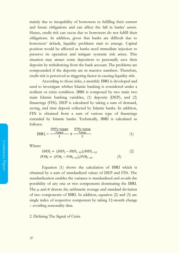
90

Co

nferen

ce Pap

ers

mainly due to incapability of borrowers to fulfillng their current

and future obligations and can affect the fall in banks‘ assets.

Hence, credit risk can occur due to borrowers do not fulfill their

obligations. In addition, given that banks are difficult due to

borrowers‘ default, liquidity problems start to emerge. Capital

position would be affected as banks need immediate injection to

preserve its operation and mitigate systemic risk arises. This

situation may attract some depositors to personally save their

deposits by withdrawing from the bank account. The problems are

compounded if the deposits are in massive numbers. Therefore,

credit risk is perceived as triggering factor in causing liquidity risk.

According to those risks, a monthly IBRI is developed and

used to investigate whther Islamic banking is considered under a

resilient or crisis condition. IBRI is composed by two main two

main Islamic banking variables, (1) deposits (DEP), and (2)

financings (FIN). DEP is calculated by taking a sum of demand,

saving, and time deposit collected by Islamic banks. In addition,

FIN is obtained from a sum of various type of financings

extended by Islamic banks. Technically, IBRI is calculated as

follows:

IBRIt =

(1)

Where:

( ) (2)

( ) (3)

Equation (1) shows the calculation of IBRI which is

obtained by a sum of standardized values of DEP and FIN. The

standardization enables the variance is standardized and avoids the

possibility of any one or two components dominating the IBRI.

The µ and denote the arithmetic average and standard deviation

of two components of IBRI. In addition, equation (2) and (3) are

single index of respective component by taking 12-month change

– avoiding seasonality data.

2. Defining The Signal of Crisis

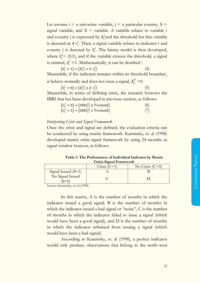
91

Co

nfe

ren

ce P

aper

s

Let assume i = a univariate variable, j = a particular country, S =

signal variable, and X = variable. A variable relates to variable i

and country j is expressed by and the threshold for this variable

is denoted as . Then, a signal variable relates to indicator i and

country j is denoted by . The binary model is then developed,

where = (0,1), and if the variable crosses the threshold, a signal

is emitted, =1. Mathematically, it can be desribed :

{

} { |

} (4)

Meanwhile, if the indicator remains within its threshold boundary,

it behave normally and does not issue a signal, =0.

{

} { |

} (5)

Meanwhile, in terms of defining crisis, the research borrows the

IBRI that has been developed in previous section, as follows:

{

} { | } (6)

{

} { | } (7)

Interpreting Crisis and Signal Framework

Once the crisis and signal are defined, the evaluation criteria can

be conducted by using matrix framework. Kaminsky, et. al (1998)

developed matrix crisis-signal framework by using 24 months as

signal window horizon, as follows:

Table 1. The Performance of Individual Indicator by Matrix Crisis-Signal Framework

Crisis (C=1) No Crisis (C=0)

Signal Issued (S=1) A B No Signal Issued

(S=0) C D

Source: Kaminsky, et. al (1998)

In this matrix, A is the number of months in which the

indicator issued a good signal, B is the number of months in

which the indicator issued a bad signal or ―noise‖, C is the number

of months in which the indicator failed to issue a signal (which

would have been a good signal), and D is the number of months

in which the indicator refrained from issuing a signal (which

would have been a bad signal).

According to Kaminsky, et. al (1998), a perfect indicator

would only produce observations that belong to the north-west

92

Co

nferen

ce Pap

ers

and south-east cells of this matrix. It would issue a signal in every

month that is to be followed by a crisis (within the next n months,

example 24 months), so that A > 0 and C = 0, and it would

refrain from issuing a signal in every month that is not to be

followed by a crisis (within the next n months, example 24

months), so that B = 0 and D > 0. For sure, none of the

indicators fit the profile of a perfect indicator, but the matrix will

be a useful reference to assess how close or how far is each

indicator from that profile.

2. Determining Evaluation Criteria

This paper employs six evaluation criteria in order to assess the

performance of leading variables which was identified through

crisis-signal framework, as follows:

(1) The proportion of observations correctly called =

( ) ( ), defined as the proportion that all

observations correctly bring information about crisis

and not crisis. This implies that the higher proportion

occurred will lead to best evaluation criteria.

(2) The noise-to-Signal-Ratio = ( )

( ), it measures the

false signals as a ratio of the good signals issued. The

selection rule is to pick the variable or model that

minimizes the noise to signal ratio (NTS).

(3) The proportion of crises correctly called =

,

defined as the proportion of crisis happened once the

signal was issued. Thus, the higher of its proportion

would be fitting of a perfect indicator in signaling the

crisis.

(4) The proportion of false alarm of total alarms issued =

, given that an individual indicator exposes a

frequent false signal. Thus, the lower of its proportion

would be good to minimize the panic behavior in the

markets.

93

Co

nfe

ren

ce P

aper

s

(5) The proportion of crisis given an alarm issued =

,

given that an individual indicator generates different

signals. This criterion is to select indicators that can

maximize the probability of a crisis, given a signal was

issued as alarm.

(6) The proportion of probability of crisis given no alarm

issued =

, given the signal is important, an

occurence of crisis without signals was extremely

reduced or minimized.

3. Determining Signaling Horizon

This paper involves various signaling horizons. This signaling

horizons are range of period that has ability for anticipating a

crisis. Kaminsky (1997) uses 24 month signaling horizon. He

argued that the longer signaling horizon would enable policy

makers to anticipate a crisis. Meanwhile, Bussiere and Fratzscher

(2002) set 12 and 18 month as signal horizon. They argues that

various time horizons would provide the best achievable trade-off

between missing crises and wrong signal. In addition, this paper

adds another 3 and 6 month as signaling horizons considering that

a crisis is difficult to be predicted. Providing short horizon enables

policy makers to react immediately as crisis starts to buildup.

4. Determining Thresholds

The economy evolves through phases of booms and recession.

This change in phase of a particular series is captured empirically

by finding a ―threshold‖. It turns a fluctuation of a given variable

into a signal of an upcoming recession or crisis. The threshold is

the one that minimizes the noise-to-signal ratio of a particular

indicator.

5. Determining Leading Indicators

Vulnerabilities in a financial system can build overtime and the

system‘s operation depends on macroeconomic developments that

ultimately can affect individual institutions. Developing a set of

94

Co

nferen

ce Pap

ers

indicators is important to help detecting in advance

macroeconomic and financial vulnerabilities that can affect the

banking system. There is no clear-cut macroeconomic model to

analyze the macro-fundamental that are relevant as leading

indicators for the resilience of Islamic banking. This paper adopts

some variables suggested by Susatyo (2002) in detecting currency

crises. He used data since 1990-2000 in monthly basis by using 14

variables in order to identify leading indicators. He found that out

of 14 variables, only M2/Reserve, inflatio rate, credit growth, and

real effective exchange rate that are relevant as leading indicator

for currency crises in Indonesia. Similarly, Garcia and Herrera

(1999) studied on early warning for currency crisis and suggested

M2/reserve, credit growth, real effective exchange rate, and

inflation rate. Although these leading leading indicators are used

for currency crises, Jacobs and Kuper (2004) argued that banking

crises may be associated with currency crises trough a number of

channels of causation or the other way round. Therefore, these

leading indicators will be used in the case for banking crises in

Indonesia, as follows:

1. M2/Reserve (M2Res) is used to capture the vulnerability

as the sudden capital outflows. The higher ratio M2/total

reserve denotes the increase of likelihood of banking crisis

or reducing the resilience of Islamic banking

2. Credit growth (CG) is defined as the percentage change of

the total credit approved in several banks, namely national

banks, regional development banks, national private banks,

and foreign banks. This variable indicates the fast

expansion of loans which later give additional default risk

in the banking system. In addition, Credit growth which is

considered excessive may lead to systemic risk, given

inconnectedness in the financial system. Rapid credit

growth episode can increase likelihood of systemic risk

and deterioration of banks‘ balance sheets.

3. Real effective exchange rate (REER) is defined as the

variable which is obtained by deflating Nominal exchange

rate with the ratio between standardized (based on a

certain base year period). Consumer price index (CPI)

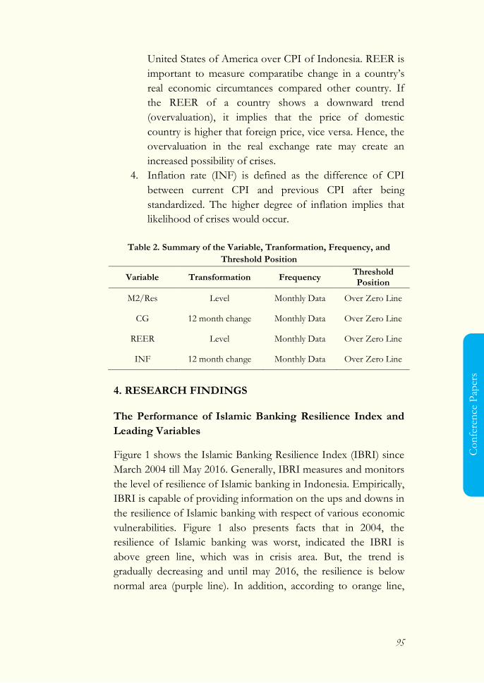
95

Co

nfe

ren

ce P

aper

s

United States of America over CPI of Indonesia. REER is

important to measure comparatibe change in a country‘s

real economic circumtances compared other country. If

the REER of a country shows a downward trend

(overvaluation), it implies that the price of domestic

country is higher that foreign price, vice versa. Hence, the

overvaluation in the real exchange rate may create an

increased possibility of crises.

4. Inflation rate (INF) is defined as the difference of CPI

between current CPI and previous CPI after being

standardized. The higher degree of inflation implies that

likelihood of crises would occur.

Table 2. Summary of the Variable, Tranformation, Frequency, and

Threshold Position

Variable Transformation Frequency Threshold Position

M2/Res Level Monthly Data Over Zero Line

CG 12 month change Monthly Data Over Zero Line

REER Level Monthly Data Over Zero Line

INF 12 month change Monthly Data Over Zero Line

4. RESEARCH FINDINGS

The Performance of Islamic Banking Resilience Index and

Leading Variables

Figure 1 shows the Islamic Banking Resilience Index (IBRI) since

March 2004 till May 2016. Generally, IBRI measures and monitors

the level of resilience of Islamic banking in Indonesia. Empirically,

IBRI is capable of providing information on the ups and downs in

the resilience of Islamic banking with respect of various economic

vulnerabilities. Figure 1 also presents facts that in 2004, the

resilience of Islamic banking was worst, indicated the IBRI is

above green line, which was in crisis area. But, the trend is

gradually decreasing and until may 2016, the resilience is below

normal area (purple line). In addition, according to orange line,

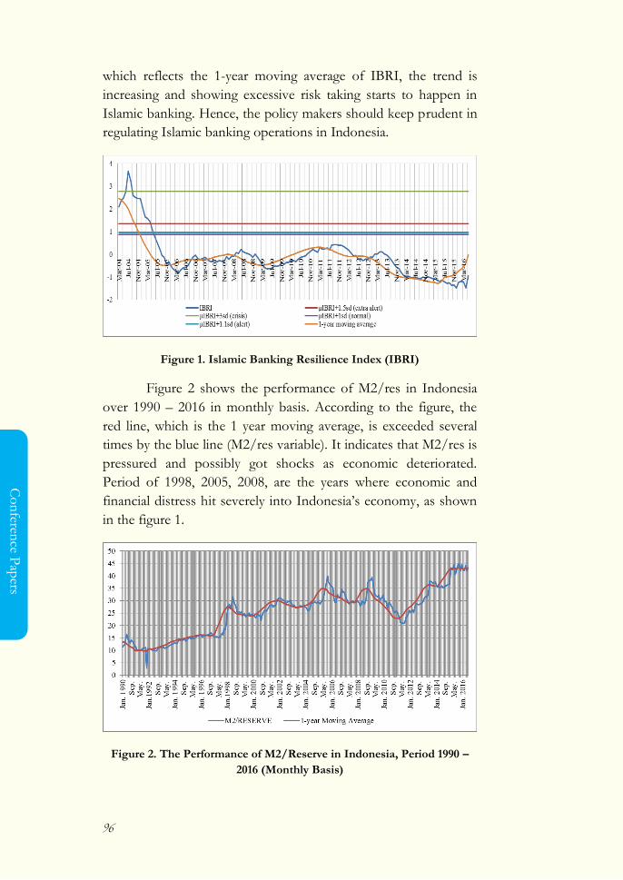
96

Co

nferen

ce Pap

ers

which reflects the 1-year moving average of IBRI, the trend is

increasing and showing excessive risk taking starts to happen in

Islamic banking. Hence, the policy makers should keep prudent in

regulating Islamic banking operations in Indonesia.

Figure 1. Islamic Banking Resilience Index (IBRI)

Figure 2 shows the performance of M2/res in Indonesia

over 1990 – 2016 in monthly basis. According to the figure, the

red line, which is the 1 year moving average, is exceeded several

times by the blue line (M2/res variable). It indicates that M2/res is

pressured and possibly got shocks as economic deteriorated.

Period of 1998, 2005, 2008, are the years where economic and

financial distress hit severely into Indonesia‘s economy, as shown

in the figure 1.

Figure 2. The Performance of M2/Reserve in Indonesia, Period 1990 –

2016 (Monthly Basis)

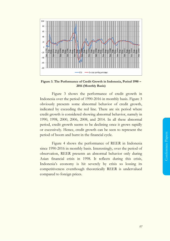
97

Co

nfe

ren

ce P

aper

s

Figure 3. The Performance of Credit Growth in Indonesia, Period 1990 –

2016 (Monthly Basis)

Figure 3 shows the performance of credit growth in

Indonesia over the period of 1990-2016 in monthly basis. Figure 3

obviously presents some abnormal behavior of credit growth,

indicated by exceeding the red line. There are six period where

credit growth is considered showing abnormal behavior, namely in

1990, 1998, 2000, 2006, 2008, and 2014. In all these abnormal

period, credit growth seems to be declining once it grows rapidly

or excessively. Hence, credit growth can be seen to represent the

period of boom and burst in the financial cycle.

Figure 4 shows the performance of REER in Indonesia

since 1990-2016 in monthly basis. Interestingly, over the period of

observation, REER presents an abnormal behavior only during

Asian financial crisis in 1998. It reflects during this crisis,

Indonesia‘s economy is hit severely by crisis so lossing its

competitiveness eventhough theoretically REER is undervalued

compared to foreign prices.

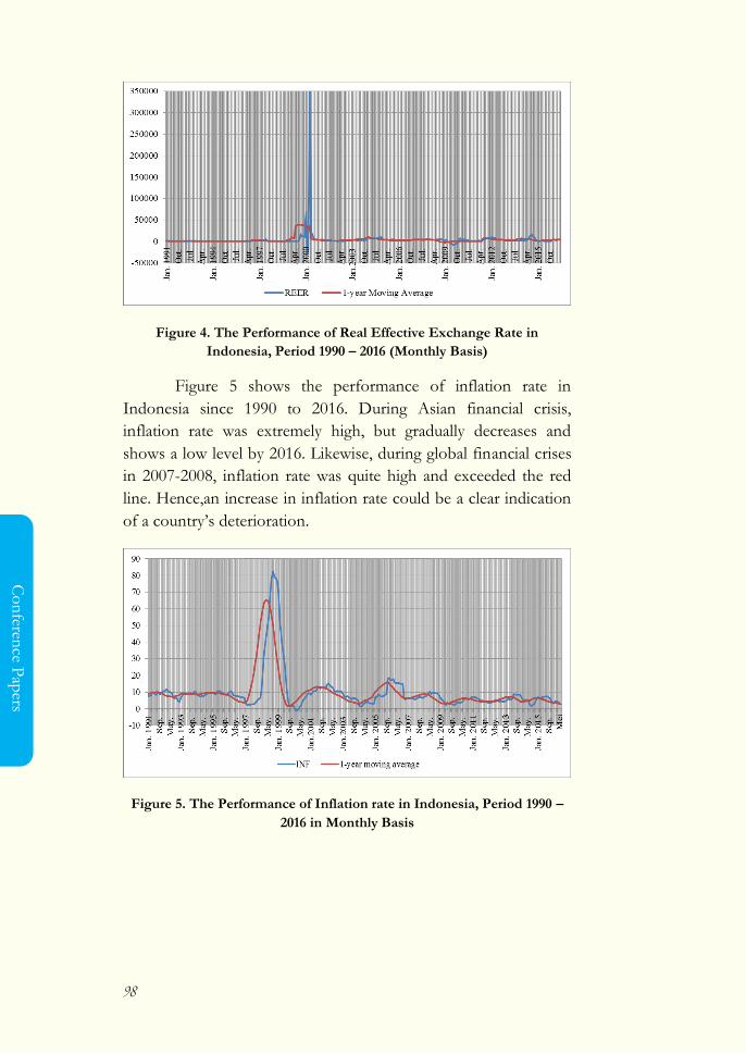
98

Co

nferen

ce Pap

ers

Figure 4. The Performance of Real Effective Exchange Rate in

Indonesia, Period 1990 – 2016 (Monthly Basis)

Figure 5 shows the performance of inflation rate in

Indonesia since 1990 to 2016. During Asian financial crisis,

inflation rate was extremely high, but gradually decreases and

shows a low level by 2016. Likewise, during global financial crises

in 2007-2008, inflation rate was quite high and exceeded the red

line. Hence,an increase in inflation rate could be a clear indication

of a country‘s deterioration.

Figure 5. The Performance of Inflation rate in Indonesia, Period 1990 –

2016 in Monthly Basis

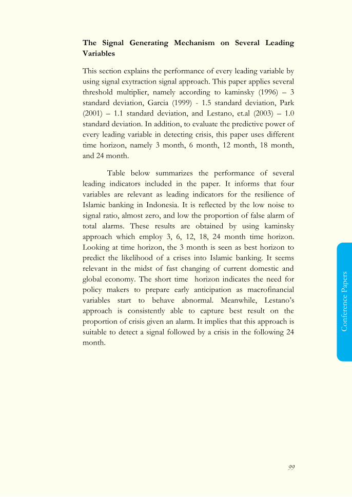
99

Co

nfe

ren

ce P

aper

s

The Signal Generating Mechanism on Several Leading

Variables

This section explains the performance of every leading variable by

using signal exytraction signal approach. This paper applies several

threshold multiplier, namely according to kaminsky (1996) – 3

standard deviation, Garcia (1999) - 1.5 standard deviation, Park

(2001) – 1.1 standard deviation, and Lestano, et.al (2003) – 1.0

standard deviation. In addition, to evaluate the predictive power of

every leading variable in detecting crisis, this paper uses different

time horizon, namely 3 month, 6 month, 12 month, 18 month,

and 24 month.

Table below summarizes the performance of several

leading indicators included in the paper. It informs that four

variables are relevant as leading indicators for the resilience of

Islamic banking in Indonesia. It is reflected by the low noise to

signal ratio, almost zero, and low the proportion of false alarm of

total alarms. These results are obtained by using kaminsky

approach which employ 3, 6, 12, 18, 24 month time horizon.

Looking at time horizon, the 3 month is seen as best horizon to

predict the likelihood of a crises into Islamic banking. It seems

relevant in the midst of fast changing of current domestic and

global economy. The short time horizon indicates the need for

policy makers to prepare early anticipation as macrofinancial

variables start to behave abnormal. Meanwhile, Lestano‘s

approach is consistently able to capture best result on the

proportion of crisis given an alarm. It implies that this approach is

suitable to detect a signal followed by a crisis in the following 24

month.

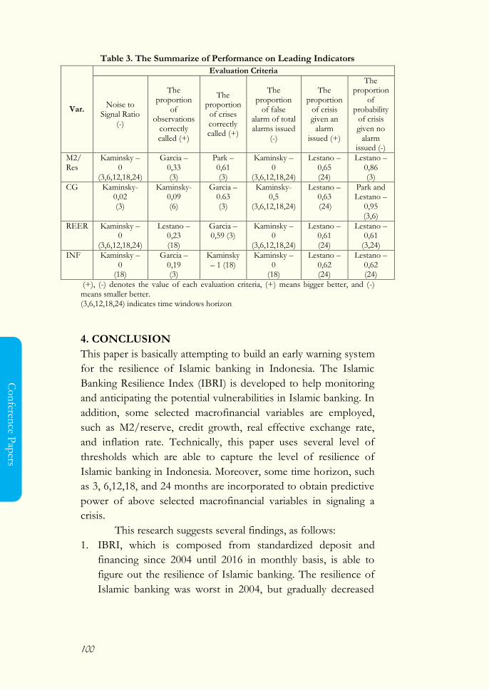
100

Co

nferen

ce Pap

ers

Table 3. The Summarize of Performance on Leading Indicators

Var.

Evaluation Criteria

Noise to Signal Ratio

(-)

The proportion

of observations

correctly called (+)

The proportion

of crises correctly called (+)

The proportion

of false alarm of total alarms issued

(-)

The proportion

of crisis given an

alarm issued (+)

The proportion

of probability

of crisis given no

alarm issued (-)

M2/ Res

Kaminsky – 0

(3,6,12,18,24)

Garcia – 0,33 (3)

Park – 0,61 (3)

Kaminsky – 0

(3,6,12,18,24)

Lestano – 0,65 (24)

Lestano – 0,86 (3)

CG Kaminsky- 0,02 (3)

Kaminsky- 0,09 (6)

Garcia – 0.63 (3)

Kaminsky- 0,5

(3,6,12,18,24)

Lestano – 0,63 (24)

Park and Lestano –

0,95 (3,6)

REER Kaminsky – 0

(3,6,12,18,24)

Lestano – 0,23 (18)

Garcia – 0,59 (3)

Kaminsky – 0

(3,6,12,18,24)

Lestano – 0,61 (24)

Lestano – 0,61

(3,24)

INF Kaminsky – 0

(18)

Garcia – 0,19 (3)

Kaminsky – 1 (18)

Kaminsky – 0

(18)

Lestano – 0,62 (24)

Lestano – 0,62 (24)

(+), (-) denotes the value of each evaluation criteria, (+) means bigger better, and (-) means smaller better. (3,6,12,18,24) indicates time windows horizon

4. CONCLUSION

This paper is basically attempting to build an early warning system

for the resilience of Islamic banking in Indonesia. The Islamic

Banking Resilience Index (IBRI) is developed to help monitoring

and anticipating the potential vulnerabilities in Islamic banking. In

addition, some selected macrofinancial variables are employed,

such as M2/reserve, credit growth, real effective exchange rate,

and inflation rate. Technically, this paper uses several level of

thresholds which are able to capture the level of resilience of

Islamic banking in Indonesia. Moreover, some time horizon, such

as 3, 6,12,18, and 24 months are incorporated to obtain predictive

power of above selected macrofinancial variables in signaling a

crisis.

This research suggests several findings, as follows:

1. IBRI, which is composed from standardized deposit and

financing since 2004 until 2016 in monthly basis, is able to

figure out the resilience of Islamic banking. The resilience of

Islamic banking was worst in 2004, but gradually decreased

101

Co

nfe

ren

ce P

aper

s

and stable. Interestingly, the resilience of Islamic banking was

considered stable since the index was moving below the

normal line during the global financial crises.

2. Some selected macrofinancial variables, M2/reserve (M2res),

credit growth (CG), real effective exchange rate (REER), and

inflation rate (INF) empirically show low noise to signal ratio.

It means that these four variables are capable of signaling

vulnerabilities from adverse external shocks.

This paper is considered a very preliminary work in the

area of early warning system for the resilience of Islamic banking.

However, there is no clear cut leading indicators to

comprehensively monitor its resilience. More macroeconomic and

financial variables are needed to be included as leading indicators

for capturing the resilience of Islamic banking. In addition, given

that macroeconomic and financial variables play the important

thing in providing the resilience, the macroprudential policy needs

to be more specifically addressing procyclicality in the financial

sector. Meanwhile, the resilience of Islamic banking needs to be

supported by the resilience in the real sector. It is because the core

operations of Islamic banking are dealing with productive sector.

Therefore, the synergic policies are needed to establish strong

resilience of Islamic banking, namely stable macroeconomic

envirounment and strong real sector development.

REFERENCES

Adiningsih, S., Setiawati, D. N., & Sholihah. (2002). Macroeconomic

Vulnerability in Indonesia. EADN Regional Project. Bangkok.

Retrieved from

http://tdri.or.th/archives/download/reports/published/ead

n/indo1.pdf

Bank Indonesia. Kewajiban Penyediaan Modal Minimum Bank

Umum, Pub. L. No. 15/12/PBI/2013 (2013). Indonesia:

Bank Indonesia. Retrieved from

http://www.bi.go.id/id/peraturan/perbankan/Documents/

pbi_151213rev.pdf

102

Co

nferen

ce Pap

ers

Bussiere, M, and M. Fratzscher (2002). ―Towards a New Early

Warning System of Financial Crises‖, European Central Bank

Working Paper, No. 145

Caprio, G. Jr. and Klingebiel, D. (1996), ―Bank Insolvency: Bad

luck, Bad Policy or Bad Banking?‖, Paper presented at the

1996 Annual Bank Conference on Development

Economics, World Bank Economic Review, January 1997

Davis, E. and D., Karim (2008). ―Comparing Early Warning

Systems for Banking Crisis‖, Journal of Financial Stability, 4,

89-120

Demirgüç-Kunt, A. and E. Detragiache (1998). ‗The Determinants

of Banking Crises: Evidence from Developing and

Developed Countries‖, IMF Staff Papers, 45, 81-109.

Demirgüç-Kunt, A. and E. Detragiache. (2000). ―Monitoring

Banking Sector Fragility: A Multivariate Logit‖, World Bank

Economic Review, 14(2), 287-307.

Duttagupta R. and P. Cashin (2011). ―Anatomy of Banking Crises

in Developing and Emerging Market Countries‖, Journal of

International Money and Finance, 30, 354-376.

Eichengreen, B. and A. Rose (1998). ―Staying Afloat When the

Wind Shifts: External Factors and Emerging-Market

Banking Crises‖, NBER Working paper no. 6370, January

Glick, R. and M. Hutchison (2001). ―Banking and Currency Crises:

How Common Are Twins?‖ in R. Glick, R. Moreno and M.

Spiegel (eds.), Financial Crises in Emerging Markets,

Cambridge University Press, Cambridge, UK.

González-Hermosillo, B. (1999). ―Determinants of Ex-Ante

Banking System Distress: A Macro-Micro Empirical

Exploration of Some Recent Episodes‖, IMF Working

Paper 99/33, March.

103

Co

nfe

ren

ce P

aper

s

Gurnain Pasricha, Tom Roberts, Ian Christensen & Brad Howell

(2013) Assessing Financial SystemVulnerabilities: An Early

Warning Approach, Bank of Canada Review, Autumn 2013,

pp. 10-19

Hardy, D. and C. Pazarbasioglu (1999), ―Determinants and

Leading Indicators of Banking Crises: Further Evidence‖,

IMF Staff Papers, 46, 3, 247-58.

Herrera, S., & Garcia, C. (1999). User’s Guide to an Early Warning

System for Macroeconomic Vulnerability in Latin American

Countries (No. 2233). Policy Research Working Paper.

Washington DC. Retrieved from

http://siteresources.worldbank.org/BRAZILINPOREXT

N/Resources/3817166-1185895645304/4044168-

1186403960425/77pub_br167.pdf

Honohan, P. (1997), ―Banking System Failures in Developing and

Transition Countries: Diagnosis and Predictions‖, Working

Paper 39, Bank for International Settlements.

Hutchinson, M. (2002). ―European Banking Distress and EMU:

Institutional and Macroeconomic Risks‖, Scandinavian

Journal of Economics, 104(3), 365-389

Kaminsky, G., Kizondo, S., and Reinhart, C. M. (1998). Leading

Indicators of Currency Crises. IMF Staff Papers Staff Papers,

45(1), 48. http://doi.org/10.1016/S1566-0141(02)00002-X

Kaminsky, G.,L., and Reinhart, C. (1996). ―Banking and Balance

of Payment Crises: Models and Evidence‖. Washington

DC: Board of Governor of the Federal Reserve System.

Kaminsky, G. and Reinhart, C.M. (1999), ‗The Twin Crises: the

Causes of Banking and Balance of Payments Problems‘,

American Economic Review, 89, 473-500

104

Co

nferen

ce Pap

ers

Kibritcioglu, Aykut, (2003) ―Monitoring Banking Sector Fragility,

The Arab Bank Review, Vol 5, No.2 October.

Lindgren, C. J., Garcia, C., and Saal, M. (1996), Bank Soundness and

Macroeconomic Policy, International Monetary Fund,

Washington DC.

Lestano, Jan Jacobs, and Gerard H. Kuper. (2003) ―Indicators Of

Financial Crises do Work!: An Early Warning System for

Six Asian Countrie‖, CCSO Working Paper 13, Department

of Economics, University Of Groningen, Netherland.

Matthieu Bussiere & Marcel Fratzscher (2006), Towards a new

early warning system of financial crises, Journal of

International Money and Finance 25, pp. 953-973.

Manasse, Paolo , Roberto Savona & Marika Vezzoli (2013) Rules

of Thumb for Banking Crises in Emerging Markets,

Quaderni - Working Paper DSE No. 872, University of

Bologna, Italy.

Park, Won-Am. (2001) ―An Indicators on the Sustainable

Development of Korea‖, Paper prepared for EADN

meeting, Singapore, June 25-27, 2001.

Sachs, J. D., Tornell, A., and Velasco, A. (1996), ―Financial Crises

in Emerging Markets: the Lessons from 1995‖, Working

Paper 5576, National Bureau of Economic Research.

Wong, Jim and Wong, T. C. and Leung, Phyllis (2007) A Leading

Indicator Model of Banking Distress - Developing an Early

Warning System for Hong Hong and Other EMEAP

Economies (December 18, 2007). Hong Kong Monetary

Authority Working Paper No. 22/2007. Available at

SSRN: http://ssrn.com/abstract=1078765 orhttp://dx.doi.

org/10.2139/ssrn.1078765

105

Co

nfe

ren

ce P

aper

s

Wong J, TC Wong & P Leung (2010) Predicting banking distress

in the EMEAP economies, Journal of Financial Stability,

vol. 6, issue 3, pp.169-179

Yucel, E. (2011). A Review and Bibliography of Early Warning

Models. Munich Personal RePEc Archive, (32893), 19.

Retrieved from https://mpra.ub.uni-

muenchen.de/32893/1/ewm11_004.pdf

106

Co

nferen

ce Pap

ers

What Protects Emerging Markets

from Developed Countries Unconventional Monetary Policy Spillover?

Eko Sumando

Preliminary draft; please do not cite. The revised version will be prepared for forthcoming on Bulletin of Monetary and Banking

Abstract

This paper investigates the macro-characteristics that reduce the

developed countries unconventional monetary policy (UMP)

spillover effect on the emerging market countries. An event study

method is used to examine 24 UMP announcements and a panel

fixed effects model to examine the characteristics of the emerging

markets, the spillover channel considered in this study is countries‘

exchange rate. The results show an unclear significance of

macroeconomic fundamentals to the emerging markets‘ currency

resilience. Deeper financial markets contribute to better resilience.

Trade linkages with China provide less vulnerable currency

position of the emerging markets while trade linkages with

developed countries provide mixed evidence. The macro-

prudential policy and the capital flow measures that the emerging

107

Co

nfe

ren

ce P

aper

s

markets countries implemented before to the announcements are

moderately effective in reducing the spillover.

Keywords: unconventional monetary policy, emerging markets,

international spillover

JEL Classification: E52, E58

1. INTRODUCTION

The global financial crisis in 2008 had a significant impact to the

design and implementation of developed countries monetary

policy. In response to the crisis, the Federal Reserve Bank (FED),

the European Central Bank (ECB), the Bank of England (BOE),

and the Bank of Japan (BOJ) adjusted their short term interest

rates to zero and applied Quantitative Easing (QE) as an

alternative monetary policy strategy (Fawley & Neely 2013). The

QE action included large scale purchases of government bonds

and private securities, and several lending programmes (Bean

2012). Recently there has been wide interest in the impact of

developed countries unconventional monetary policy not only on

the country themselves but also on their international spillovers.

The International Monetary Fund (IMF) (2013) suggests

that developed countries unconventional monetary policy generate

greater global financial spillovers when the policy objectives were

meant to restore financial market stability. Global trade, liquidity

and portfolio rebalancing may transmit the impact of

unconventional monetary policy measures adopted in the

developed countries to other countries (Chen et al., 2012). Despite

this new challenge in the monetary system, few studies in literature

focus on the effect of developed countries unconventional

monetary policy on emerging market. Having a better

understanding of the international implications of developed

countries unconventional monetary policy is important for

emerging market policy makers to cope better with the challenges

implied by such policies.

108

Co

nferen

ce Pap

ers

Few studies have discussed this issue and the evidence

about the effect of developed countries unconventional monetary

policy on emerging market is mixed (Chen et al. 2012; Fic 2013;

Fratzscher et al. 2013; Mishra et al. 2014; Moore et al. 2013). A

question remains whether the emerging market macroeconomic

fundamentals, financial system characteristics and macro-

prudential policy are significant in reducing the spillover impacts

of unconventional monetary policy. However, the focus has been

on the effects of the FED‘s QE. This study contributes to the

existing literature in two ways: First, it fills a gap by analyzing all

developed countries unconventional monetary policy, including

not only the FED, but also the policy from the ECB, the BOE

and BOJ between 2008 and 2012. Secondly, this study sheds new

understanding on the importance of macroeconomic

fundamentals, financial depth, trade linkages and macro-prudential

policy in reducing the spillover of developed countries

unconventional monetary policy, particularly through exchange

rate as the spillover channel.

This paper examines 24 developed countries

unconventional monetary policy announcement events and 15

emerging markets reactions using a two-step method. First, an

event study method is used to analyze the significance of the

announcement to the exchange rate change with a two-day

window event. Then, the panel data fixed effects model is used to

reveal the individual characteristics of the countries prior to the

event that may enforce the spillover.

The results show unclear significance of the

macroeconomic fundamentals. From three main indicators, only

inflation was found to significantly contribute positively to

exchange rate depreciation. Deeper financial markets contribute to

better country resilience to exchange rate depreciation. Countries

with high stock market capitalization and larger liquid assets (M3)

are more stable than countries that are not. Trade linkage with

China provides less vulnerable currency position to the emerging

markets. On the other hand, trade linkages with developed

countries provide mixed evidence. Higher imports from the US

and the UK contribute to higher currency volatility. Furthermore,

109

Co

nfe

ren

ce P

aper

s

macro-prudential policy and capital flow management measures

implemented by the emerging markets prior to the unconventional

monetary policy announcement were found to be moderately

effective in reducing the country exchange rate depreciation from

the spillover.

The rest of the paper is organized as follows: Section 2

provides a literature review on unconventional monetary policy

and its international spillovers, particularly to the emerging

market. Section 3 describes the data used in this study. Section 4

describes the method. Section 5 describes the result and provides

discussion. Section 6 concludes.

2. LITERATURE REVIEW

2.1 Developed Countries Unconventional Monetary Policy

Generally, central banks implement monetary policy through

managing the short term policy rate. However, facing near-zero

short term interest rates, developed countries central banks have

turned to unconventional monetary policies involving large scale

asset purchases. The FED, the BOE, the ECB and the BOJ began

to apply QE and asset purchases on a very large scale since 2008

until 2013 (Figure 1). The consequence of these policies was a

large increase in central bank balance sheets. Figure 1 shows the

evolution of short term interest rates in the US, the UK, the Euro

Area and Japan, and the size of individual banks‘ balance sheets

(normalized to 100 at the beginning of August 2007) which

reflects the scale of unconventional monetary policy actions (Fic

2013).

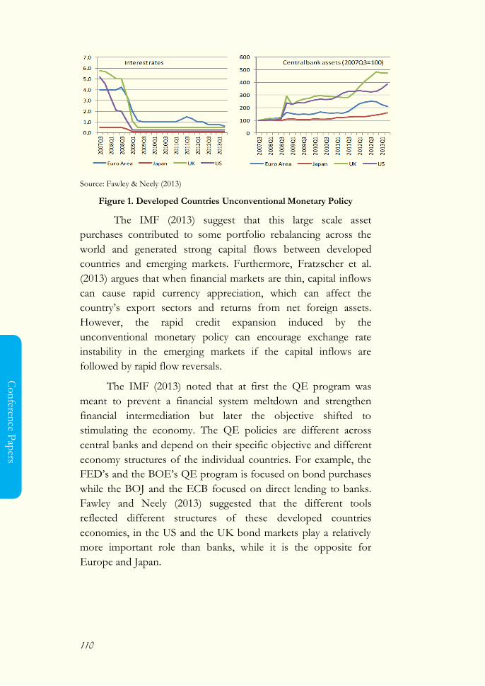
110

Co

nferen

ce Pap

ers

Source: Fawley & Neely (2013)

Figure 1. Developed Countries Unconventional Monetary Policy

The IMF (2013) suggest that this large scale asset

purchases contributed to some portfolio rebalancing across the

world and generated strong capital flows between developed

countries and emerging markets. Furthermore, Fratzscher et al.

(2013) argues that when financial markets are thin, capital inflows

can cause rapid currency appreciation, which can affect the

country‘s export sectors and returns from net foreign assets.

However, the rapid credit expansion induced by the

unconventional monetary policy can encourage exchange rate

instability in the emerging markets if the capital inflows are

followed by rapid flow reversals.

The IMF (2013) noted that at first the QE program was

meant to prevent a financial system meltdown and strengthen

financial intermediation but later the objective shifted to

stimulating the economy. The QE policies are different across

central banks and depend on their specific objective and different

economy structures of the individual countries. For example, the

FED‘s and the BOE‘s QE program is focused on bond purchases

while the BOJ and the ECB focused on direct lending to banks.

Fawley and Neely (2013) suggested that the different tools

reflected different structures of these developed countries

economies, in the US and the UK bond markets play a relatively

more important role than banks, while it is the opposite for

Europe and Japan.

111

Co

nfe

ren

ce P

aper

s

2.2 Unconventional Monetary Policy and International

Spillovers

The developed countries unconventional monetary policy

measures had a definite impact to the emerging market countries.

Emerging markets countries leaders, particularly Brazil, describes

the quantitative easing is comparable to a monetary tsunami that

can trigger sudden capital reversal away from emerging market

countries (Fic 2013; Fratzscher et al. 2013). Some studies provide

evidence about the international spillovers of developed countries

unconventional monetary policy to the emerging markets.

However, the studies available mainly focused on the FED policy

spillovers.

Chen et al. (2012) studied the cross-border spillovers of

developed countries QE to 16 emerging market countries. Using

an event study method, they examine the cross-border financial

market impact of the FED QE announcements of asset purchase

during 2008 to 2012. They find that the FED QE announcement

influenced a broad range of emerging market assets prices, raising

equity prices, and lowering government and corporate bond yields.

This evidence supports the view that developed countries QE

program influenced international market expectations about the

strength of international capital flows to the emerging market. In

other words, the QE measures increased the global liquidity

through the immediate re-pricing of assets in international

financial markets. Furthermore, they used a global vector error-

correcting model (VECM) to measure the estimated size of the

spillover and found that the size effects differed across regions. In

some economies such as Hong Kong and Brazil, the expansionary

impact of US quantitative easing was significant and associated

with rapid credit growth and strong capital inflow, currency

appreciation and inflationary pressures.

In addition, Moore et al. (2013) studied the FED large-

scale asset purchases (LSAPs) announcement impact on capital

flows from the US to 10 emerging market countries from 2008 to

2010. Using panel ordinary least square, they find that a 10-basis-

point reduction in long-term U.S. Treasury yields contributes to

112

Co

nferen

ce Pap

ers

almost 0.4-percentage-point increase in the foreign ownership

share of emerging market debt which in turn estimated will reduce

the emerging market government bond yields by almost 1.7 basis

points. Their study suggests the significance of the US capital

outflows to the emerging markets and its impact on the long-term

emerging market government bond yields. Furthermore, the

author assess the robustness of these estimates by employing

event study and vector autoregression method and find similar

results in aggregates. They also find different marginal effects

across emerging market countries but do not explore the country

specific characteristics.

To complement the evidence about the international

spillover of developed countries unconventional monetary policy,

Fic (2013) investigates the effect of all unconventional monetary

policy implemented four major developed countries central bank

on four major developing countries: Brazil, Russia, India and

China from 2008 to 2012. This means the analysis not only

focused on the FED policy, but also the ECB, the BOE and the

BOJ. Using the event study method, she finds that developed

countries unconventional monetary policy affected exchange rates,

equity prices, and long term yields. The unconventional monetary

policy has had a significant spillover through channels such as

global trade, global liquidity and global portfolio rebalancing. Her

event study analysis shows that the quantitative easing policy

contributed to long term yields decreasing by almost 175 basis

points in Brazil, and 25 basis points in Russia, India and China.

The quantitative easing policy has also contributed to increases in

equity prices in the Brazil, China and India.

The impact of developed countries unconventional

monetary policy on the developing economies may vary. Chen et

al. (2013), Fic (2013) and Moore et al. (2013) argues that it

depends on the scale of their exposure to the developed countries

in terms of trade and financial linkages or other spillover channel,

and the type and scale of response of the monetary authorities in

that country to capital flows. However, three studies above do

not mention the characteristics of macroeconomic fundamentals,

financial system and capital flow regulation of each country.

113

Co

nfe

ren

ce P

aper

s

2.3 Unconventional Monetary Policy Spillover and

Emerging Markets Characteristics

Fratzscher, et al. (2013) address this emerging markets

characteristics issue by analyzing the global impact of the FED

unconventional monetary policy from 2007 to 2010 on 65 foreign

financial markets, including emerging markets, through net capital

inflows and price of bonds and equity as the spillover channel.

They found that the FED unconventional monetary policy has

influenced the reallocation of portfolio in worldwide financial

markets. The first phase of quantitative easing triggered a rapid

capital outflow from the emerging markets to the US but the next

phase triggered it to the opposite direction. Furthermore, they

found no evidence that exchange rate or capital account policies

may aided the emerging market countries in protecting themselves

from the US monetary policy spillovers. This study illustrates how

US unconventional monetary policy has contributed to portfolio

reallocation as well as a re-pricing of risk in global financial

markets.

In addition, Eichengreen and Gupta (2014) use cross

sectional regression of emerging market foreign reserves, equity

prices, and exchange rates and relate the reaction of these

variables to macroeconomic fundamentals and country‘s financial

markets characteristics. They examine the spillover effect of the

FED tapering announcement from April to August 2013 and

found that the tapering talk brings immediate sharp negative

impact on emerging markets. Furthermore, they show that the

impacts vary across countries. Countries with higher financial

depth experienced higher exchange rate depreciations. However,

countries with better macroeconomics fundamentals

characteristics such as lower budget deficit, lower public debt,

high level of reserves, or high rate of economic growth did not

experienced a significant different impact compared to those who

are not. It shows that the size of the country‘s financial market is a

more important determinant than their macroeconomic

fundamentals. This may interpreted as the global investors‘

114

Co

nferen

ce Pap

ers

capacity to rebalance their portfolios when the target country has a

relatively large and liquid financial market (IMF 2013a).

In the opposite of both studies, Mishra, et al. (2014) argue

that macroeconomic fundamentals and macro-prudential policy

are important in minimizing the spillover effect of US monetary

policy. They conducted an event study analysis of the FED QE

announcement using government bond yields, stock prices and

exchange rates daily data, between January 2013 and January 2014,

for 21 emerging markets. The results suggest that markets

differentiated across countries during the episodes unconventional

monetary policy announcement based on countries characteristics,

including macroeconomic fundamentals and economic and

financial structures. Countries with deeper financial markets,

better macroeconomic fundamentals, and better macro-prudential

policy experienced less exchange rate depreciations and less

increase in government bond yields. They also found that having

strong trade exposure with China can help reduce markets

negative reaction.

The different period of announcements, length of data

sets of countries and methodology in each paper may explain the

ambiguous findings. The mixed evidence of previous studies also

shows two gaps which this research will address. These are the

need to cover all developed countries unconventional monetary

policy spillover effects on emerging markets, and also to examine

whether macro fundamentals, financial structure and macro-

prudential policy is significant in minimizing spillover.

3. METHODOLOGY

Data

This study examined 24 unconventional monetary policy

announcement events by the FED, the BOE, the ECB and the

BOJ as described in Table 8 (Appendix). The key spillover channel

are daily exchange rates (local currency/US$) from January 2008

to December 2012.

The study used data from 15 Emerging Markets including

Brazil, Colombia, Chile, Indonesia, India, Korea, Mexico,

115

Co

nfe

ren

ce P

aper

s

Malaysia, Philippines, Peru, Russia, South Africa, Singapore,

Turkey and Thailand. The selected country macro-characteristics

are decomposed into several categories: (a) macroeconomics

fundamentals: growth rate, inflation, and the ratio of current

account balance to GDP; (b) financial depth: the ratio of stock

market capitalization to GDP, the ratio of M2 to GDP and the

ratio of M3 to GDP ratio; (c) trade linkage with Developed

Countries: the United States, the United Kingdom, Europe area

and Japan; (d) trade linkage with China, and (e) macro-prudential

policy and or capital flow measures implemented by the countries

fiscal and monetary authorities. Table 9 (Appendix) listed the

variables description and data source are. All the variables

occurred a quarter before the event.

The data for the macro-prudential policy and the capital

flow management measure conducted by emerging market

countries during 2008 to 2012 are taken from Zhang and Zoli

(2014), and the IMF (2012) policy paper about the interaction of

monetary and macro-prudential policies and the Annual Report on

Exchange Arrangements and Exchange Restrictions (IMF 2013c).

Method

The method in this study replicate Mishra et al. (2014) which

proceeds in two steps. First, an event study analysis is used to

examine the significance of each event to the change of the

exchange rate in two-day window (a day before and a day after the

event). Secondly, panel fixed effect model is used to examine the

relation of the change in the exchange rate with the countries

macroeconomic characteristics a quarter before the event.

3.1 Examining The Announcement Event

An event study analysis was used to examine the developed

countries unconventional monetary policy announcements,

because this method is able to capture the impact of an event in a

short time window, since the spillover effects of developed

countries unconventional monetary policy is expected to rapidly

transmit around the date of the event. This method is also used in

previous studies (Chen et al. 2012; Fic 2013; Mishra et al. 2014).

116

Co

nferen

ce Pap

ers

The ―events‖ or the dates of the FED, the ECB, the BOE and the

BOJ announcements (Appendix) and market reactions around

these events will be pooled around each year period. These events

will be analyzed using model (1).

(1)

where is the exchange rate change (two-day window) of

country c at the event i; is a dummy for the announcement

event i. This model will provide a matrix of the change in

exchange rate of emerging market countries when an

unconventional monetary policy announcement happened.

A pooled time-series analysis will be used to measure the

significance and the size of the coefficient β. Positive β coefficient

indicates exchange rate depreciation while negative β coefficient

indicates exchange rate appreciation. In this study, the event that

contribute to exchange rate depreciation will be classified as a

negative event ( ).

Measuring The Change in The Exchange Rate

In order to standardized the change of the exchange rate (local

currencies/US$) of emerging markets countries ( ), this study

used two measurement of change which are the logarithm change

after and before the event described in (i) and the mean deviation

of the log change in the year when the event i occurs described in

(ii).

( )

where is the change in exchange rate of country c, at the

announcement event i which come from the log of exchange rate

at the day after the event ( ) minus the log of exchange

rate at the day before the event ( ).

where is the change in exchange rate of country c, at the

announcement event i which come from the log of exchange rate

of country c, at the time of the event i ( ) minus the mean of

117

Co

nfe

ren

ce P

aper

s

log of exchange rate of country c in the year when the event i

occurs ( ) divided by the standard deviation of log of

exchange rate of country c in the same year ( ).

3.2 Significance of Macroeconomic Country Characteristics

Secondly, panel regressions will be estimated by pooling the

events across the emerging markets. The panel fixed effects

regressions in model (2) will examine the relationship of the

exchange rate changes of the negative events with each country

characteristics and the event and characteristics interactions. The

panel fixed effects model also used in previous studies

(Eichengreen & Gupta 2014; Moore et al. 2013)

The model specification is as follows:

(2)

where is a dummy for negative event i (when the country

experienced exchange rate depreciation), is the country c

macroeconomics and financial system characteristic a quarter

before the event, is the country-fixed effect. controls

country characteristics that are not varying over time. Country

fixed effects also control for other country variables which are not

likely to change over the one year period. can be time

varying and non-time varying. For regressions where is

time-invariant, the variable will be collinear with the country fixed

effect and will drop out. is the coefficient of interaction variable

that capture the effect of the event and country characteristics at

the same time.

4. RESULTS AND DISCUSSIONS

4.1 Unconventional Monetary Policy Announcements

Effect

An event study method used to examine the immediate markets

reactions around the unconventional monetary policy event

announcement listed in Table 8 (Appendix). The method employs

118

Co

nferen

ce Pap

ers

Equation (1) which relates the two-day logarithm change (i) and

the mean deviation to the exchange rate logarithm change (ii) to a

constant and a dummy of the events.

The regression result in Table 1 shows that emerging

markets reacted negatively or experienced exchange rate

depreciation to announcements (2), (15), and (16) referred to in

Table 8. The opposite reaction happened in the (13) and (17)

announcement. Interestingly, the result shows that the FED, the

ECB, the BOE and the BOJ have an effect on the emerging

market significantly in some announcements.

The first significant and strongest markets‘ reaction is on

October 15 2008, when the ECB announced and expanded long

term refinancing operations. This event is happen at the same time

with the beginning of the GFC episode in 2008. The significant

currency depreciation among emerging market on this day is

consistent with Fic (2014) and Chen et al. (2012), where they

noted that the ECB measures to stabilize the macroeconomic

condition in Europe and the GFC contributed significantly to net

capital outflows from emerging markets. These findings may

indicate that ECB unconventional monetary policy measures may

have intensified the magnitude of the capital outflow at the time

of crisis.

The next significant reaction is on September 21 2011,

when the FED announced the purchasing of US$ 400 billion US

Treasury securities. This action by the FED that focused on

purchases of US Treasury securities has a primary aim on

stimulating the US economy by lowering yields, and pushing up

asset prices in riskier market segments (Fratzscher et al. 2013).

This action builds pressure to the emerging markets currency.

Furthermore, Figure 3 (Appendix) shows that 13 out of 15

countries experienced exchange rate depreciation at this date.

Only Turkey and Indonesia do not experience the currency

depreciation impact.

The last significant depreciation event is on August 30

2010, when the BOJ added 10 trillion JPY in 6 month loans to the

fixed rate operations. The BOJ central bank balance sheet policies

119

Co

nfe

ren

ce P

aper

s

have a small but significant financial spillover. This policy might

have had negative spillover on some trade competitors via the

exchange rate channel (IMF 2013b).

Beside the depreciation episode, two announcements

significantly contribute to exchange rate appreciation. First is

when the ECB conducted an intervention in the Euro Area

private and public debt securities markets in May 2010. This

finding bring into line what the IMF policy paper (IMF 2013a)

mention about the importance of the ECB announcements in

sending the market stability signal in the Euro area. The

announcement of the debt intervention in some core euro area

countries and in much of the rest has significantly lowered bond

yields in the euro area. This reduction in the yield in the euro area

led to a generalized rally in of capital flows into the emerging

markets (IMF 2013a).

The next event is interesting because it involves two

central bank policies. In October 2011, the BOE announced the

purchase of nearly £275 billion in assets. At the same time, the

ECB announced the purchasing of €40 billion in Euro-

denominated covered bonds. This policy resulted in significant

capital inflows to emerging markets and exchange rate

appreciation described in Figure 4. Hosono and Isobe (2014)

study confirm that these two policies contribute to the lower bond

yield in this two big economies. This may generate capital inflows

from developed countries to emerging markets.

Overall, these findings are consistent with the results from

Chen et al. (2012) and Fic (2013) that suggest developed countries

unconventional monetary policies contributes to some capital flow

episodes between developed countries and the emerging markets.

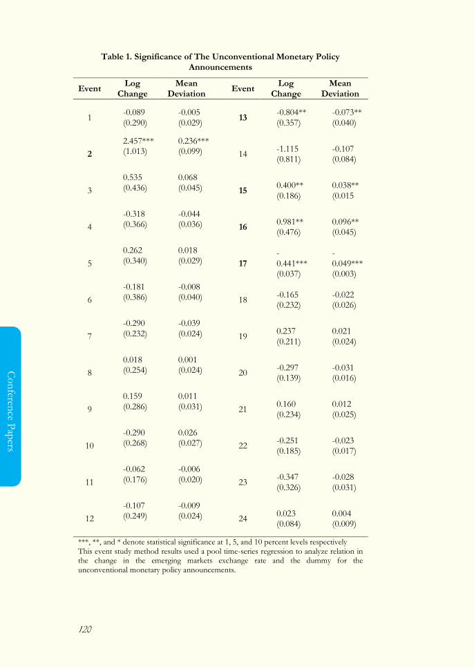
120

Co

nferen

ce Pap

ers

Table 1. Significance of The Unconventional Monetary Policy Announcements

Event Log

Change Mean

Deviation Event

Log Change

Mean Deviation

1 -0.089 (0.290)

-0.005 (0.029)

13 -0.804** (0.357)

-0.073** (0.040)

2

2.457*** (1.013)

0.236*** (0.099)

14 -1.115 (0.811)

-0.107 (0.084)

3

0.535 (0.436)

0.068 (0.045)

15 0.400** (0.186)

0.038** (0.015

4

-0.318 (0.366)

-0.044 (0.036)

16 0.981** (0.476)

0.096** (0.045)

5

0.262 (0.340)

0.018 (0.029)

17 -0.441*** (0.037)

-0.049*** (0.003)

6

-0.181 (0.386)

-0.008 (0.040)

18 -0.165 (0.232)

-0.022 (0.026)

7

-0.290 (0.232)

-0.039 (0.024)

19 0.237 (0.211)

0.021 (0.024)

8

0.018 (0.254)

0.001 (0.024)

20 -0.297 (0.139)

-0.031 (0.016)

9

0.159 (0.286)

0.011 (0.031)

21 0.160 (0.234)

0.012 (0.025)

10

-0.290 (0.268)

0.026 (0.027)

22 -0.251 (0.185)

-0.023 (0.017)

11

-0.062 (0.176)

-0.006 (0.020)

23 -0.347 (0.326)

-0.028 (0.031)

12

-0.107 (0.249)

-0.009 (0.024)

24 0.023 (0.084)

0.004 (0.009)

***, **, and * denote statistical significance at 1, 5, and 10 percent levels respectively This event study method results used a pool time-series regression to analyze relation in the change in the emerging markets exchange rate and the dummy for the unconventional monetary policy announcements.

121

Co

nfe

ren

ce P

aper

s

4.2. Market Reaction and Country Characteristics

Macro Fundamentals

The results in Table 2 show that the exchange rates for emerging

markets are differentiated only on the basis of inflation. Countries

with higher inflation have higher depreciation of their exchange

rate. This is rather unexpected because unlike the current account

balance and economic growth which is a macroeconomic indicator

for countries‘ trade and output, inflation only indicates price

changes. The coefficient is significant and suggests that a country

with a 1 per cent higher inflation rate will have higher currency

depreciation by 0.11 percentage points compared to other

countries. The interaction term shows that inflation will reinforce

exchange rate depreciation only if it occurs at the same time with

the announcements.

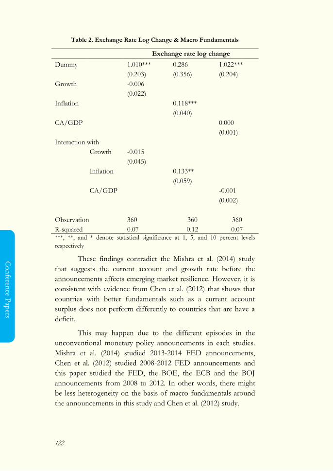
122

Co

nferen

ce Pap

ers

Table 2. Exchange Rate Log Change & Macro Fundamentals

Exchange rate log change

Dummy

1.010*** 0.286 1.022***

(0.203) (0.356) (0.204)

Growth

-0.006

(0.022)

Inflation

0.118***

(0.040)

CA/GDP

0.000

(0.001)

Interaction with

Growth -0.015

(0.045)

Inflation

0.133**

(0.059)

CA/GDP

-0.001

(0.002)

Observation 360 360 360

R-squared 0.07 0.12 0.07 ***, **, and * denote statistical significance at 1, 5, and 10 percent levels

respectively

These findings contradict the Mishra et al. (2014) study

that suggests the current account and growth rate before the

announcements affects emerging market resilience. However, it is

consistent with evidence from Chen et al. (2012) that shows that

countries with better fundamentals such as a current account

surplus does not perform differently to countries that are have a

deficit.

This may happen due to the different episodes in the

unconventional monetary policy announcements in each studies.

Mishra et al. (2014) studied 2013-2014 FED announcements,

Chen et al. (2012) studied 2008-2012 FED announcements and

this paper studied the FED, the BOE, the ECB and the BOJ

announcements from 2008 to 2012. In other words, there might

be less heterogeneity on the basis of macro-fundamentals around

the announcements in this study and Chen et al. (2012) study.

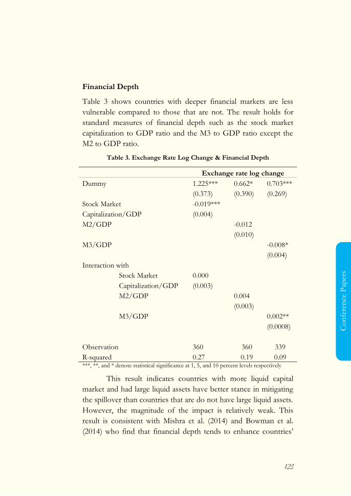
123

Co

nfe

ren

ce P

aper

s

Financial Depth

Table 3 shows countries with deeper financial markets are less

vulnerable compared to those that are not. The result holds for

standard measures of financial depth such as the stock market

capitalization to GDP ratio and the M3 to GDP ratio except the

M2 to GDP ratio.

Table 3. Exchange Rate Log Change & Financial Depth

Exchange rate log change

Dummy

1.225*** 0.662* 0.703***

(0.373) (0.390) (0.269)

Stock Market -0.019*** Capitalization/GDP (0.004) M2/GDP

-0.012

(0.010)

M3/GDP

-0.008*

(0.004)

Interaction with

Stock Market 0.000

Capitalization/GDP (0.003)

M2/GDP

0.004

(0.003)

M3/GDP

0.002**

(0.0008)

Observation 360 360 339

R-squared 0.27 0.19 0.09 ***, **, and * denote statistical significance at 1, 5, and 10 percent levels respectively

This result indicates countries with more liquid capital

market and had large liquid assets have better stance in mitigating

the spillover than countries that are do not have large liquid assets.

However, the magnitude of the impact is relatively weak. This

result is consistent with Mishra et al. (2014) and Bowman et al.

(2014) who find that financial depth tends to enhance countries‘

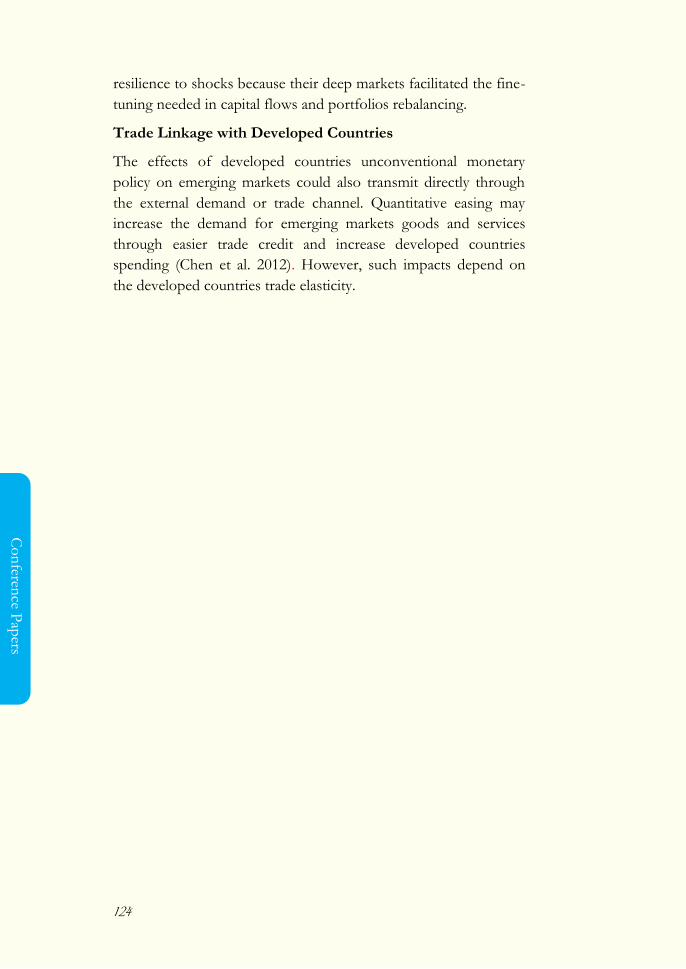
124

Co

nferen

ce Pap

ers

resilience to shocks because their deep markets facilitated the fine-

tuning needed in capital flows and portfolios rebalancing.

Trade Linkage with Developed Countries

The effects of developed countries unconventional monetary

policy on emerging markets could also transmit directly through

the external demand or trade channel. Quantitative easing may

increase the demand for emerging markets goods and services

through easier trade credit and increase developed countries

spending (Chen et al. 2012). However, such impacts depend on

the developed countries trade elasticity.

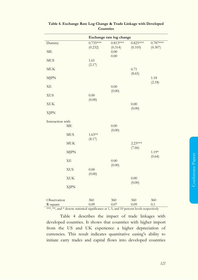
125

Co

nfe

ren

ce P

aper

s

Table 4. Exchange Rate Log Change & Trade Linkage with Developed

Countries

Exchange rate log change

Dummy

0.735*** 0.813*** 0.825*** 0.787***

(0.232) (0.314) (0.310) (0.307)

ME

0.00

0.00

MUS

1.61

(2.17)

MUK

6.71

(8.65)

MJPN

1.18

(2.18)

XE

0.00

(0.00)

XUS

0.00

(0.00)

XUK

0.00

(0.00)

XJPN

Interaction with

ME

0.00

(0.00)

MUS 1.63**

(8.17)

MUK

2.23***

(7.66)

MJPN

1.19*

(0.64)

XE

0.00

(0.00)

XUS 0.00

(0.00)

XUK

0.00

(0.00)

XJPN

Observation 360 360 360 360 R-square 0.09 0.07 0.09 0.1 ***, **, and * denote statistical significance at 1, 5, and 10 percent levels respectively

Table 4 describes the impact of trade linkages with

developed countries. It shows that countries with higher import

from the US and UK experience a higher depreciation of

currencies. This result indicates quantitative easing‘s ability to

initiate carry trades and capital flows into developed countries

126

Co

nferen

ce Pap

ers

when it is able to push consumer demand and increase asset

prices.

Trade Linkage with China

Results in Table 5 show that countries with higher trade exposure

to China have a much lower currency depreciation at the

announcement event. Exposure to China is measured by the sum

of a country‘s exports to and imports from China as a ratio of its

GDP. This result supports Mishra (2014) that suggest that greater

trade linkage to other big economies offers better opportunity for

diversifying risks, which helps reduce emerging market countries

reactions to the developed countries unconventional monetary

policy.

Table 5. Exchange Rate Log Change & Trade With China

Exchange rate log change

Dummy

0.863***

(0.204)

Export to China -1.93

(5.48)

Interaction with

Export to China 6.40**

(2.72)

Observation 360

R-squared 0.09

***, **, and * denote statistical significance at 1, 5, and 10 percent levels respectively

The coefficient on the interaction between the negative

event dummy and exposure to China is negative and statistically

significant. Countries with stronger trade links to China were less

hit during the volatility episodes. These results can be interpreted

as linkages with China acting as a buffer, whereby investors tend

to display more confidence in countries which have greater

exposure to China.

Macro Prudential Policy & Capital Flow Measures

Table 6 describes 13 countries out of 15 that are recorded to have

implemented Macro-prudential policy and or capital flow

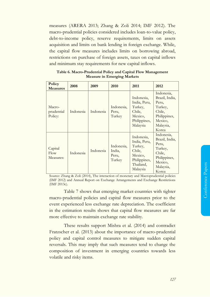
127

Co

nfe

ren

ce P

aper

s

measures (ARERA 2013; Zhang & Zoli 2014; IMF 2012). The

macro-prudential policies considered includes loan-to-value policy,

debt-to-income policy, reserve requirements, limits on assets

acquisition and limits on bank lending in foreign exchange. While,

the capital flow measures includes limits on borrowing abroad,

restrictions on purchase of foreign assets, taxes on capital inflows

and minimum stay requirements for new capital inflows.

Table 6. Macro-Prudential Policy and Capital Flow Management Measure in Emerging Markets

Policy Measures

2008 2009 2010 2011 2012

Macro-prudential Policy:

Indonesia Indonesia Indonesia, Peru, Turkey

Indonesia, India, Peru, Turkey, Chile, Mexico, Philippines, Malaysia

Indonesia, Brazil, India, Peru, Turkey, Chile, Philippines, Mexico, Malaysia, Korea

Capital Flow Measures:

Indonesia Indonesia

Indonesia, India, Peru, Turkey

Indonesia, India, Peru, Turkey, Chile, Mexico, Philippines, Thailand, Malaysia

Indonesia, Brazil, India, Peru, Turkey, Chile, Philippines, Mexico, Malaysia, Korea

Source: Zhang & Zoli (2014), The interaction of monetary and Macroprudential policies (IMF 2012) and Annual Report on Exchange Arrangements and Exchange Restrictions (IMF 2013c).

Table 7 shows that emerging market countries with tighter

macro-prudential policies and capital flow measures prior to the

event experienced less exchange rate depreciation. The coefficient

in the estimation results shows that capital flow measures are far

more effective to maintain exchange rate stability.

These results support Mishra et al. (2014) and contradict

Fratzscher et al. (2013) about the importance of macro-prudential

policy and capital control measures to mitigate sudden capital

reversals. This may imply that such measures tend to change the

composition of investment in emerging countries towards less

volatile and risky items.

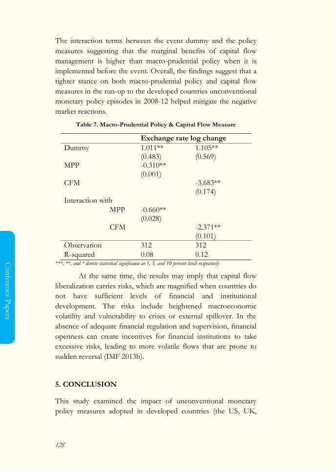
128

Co

nferen

ce Pap

ers

The interaction terms between the event dummy and the policy

measures suggesting that the marginal benefits of capital flow

management is higher than macro-prudential policy when it is

implemented before the event. Overall, the findings suggest that a

tighter stance on both macro-prudential policy and capital flow

measures in the run-up to the developed countries unconventional

monetary policy episodes in 2008-12 helped mitigate the negative

market reactions.

Table 7. Macro-Prudential Policy & Capital Flow Measure

Exchange rate log change

Dummy 1.011** (0.483)

1.105** (0.569)

MPP -0.310** (0.001)

CFM -3.683** (0.174)

Interaction with

MPP -0.660** (0.028)

CFM -2.371** (0.101)

Observation 312 312

R-squared 0.08 0.12 ***, **, and * denote statistical significance at 1, 5, and 10 percent levels respectively

At the same time, the results may imply that capital flow

liberalization carries risks, which are magnified when countries do

not have sufficient levels of financial and institutional

development. The risks include heightened macroeconomic

volatility and vulnerability to crises or external spillover. In the

absence of adequate financial regulation and supervision, financial

openness can create incentives for financial institutions to take

excessive risks, leading to more volatile flows that are prone to

sudden reversal (IMF 2013b).

5. CONCLUSION

This study examined the impact of unconventional monetary

policy measures adopted in developed countries (the US, UK,

129

Co

nfe

ren

ce P

aper

s

Euro Area and Japan) on 15 emerging market countries from 2008

to 2012. The method was decomposed into two steps. First, event

study techniques were used to study the impact of 24 QE

announcements on the exchange rate change of emerging market

countries. Then, panel fixed effect model was used to analyze the

characteristics of the country that suffer the spillover effect before

the announcements.

The event study results shows five announcements events

that contributes significantly to exchanges rate changes in 15

emerging markets. Three announcements contribute to exchange

rate depreciation while two announcements contribute to

exchange rate appreciation. The significant exchange rate changes

indicate sudden capital flows between developed countries and the

emerging market countries.

The panel fixed effect regressions reveals the country

characteristics prior to the events. The importance of Macro

fundamentals is not clear. The interaction term showed only

inflation reinforced the spillover effects when it occurs at the same

time with the announcements. A deeper financial market enhances

country resilience to the exchange rate depreciation.

This result consistent with other studies and indicate that

the more liquid the countries financial market the better the

country in adjusting to global monetary change (Eichengreen &

Gupta 2014; Mishra et al. 2014). The trade linkage with China is

beneficiary for emerging markets, the higher the net export

volume to china, the less vulnerable they are to currency

depreciation. On the other hand, higher imports from the US and

the UK contribute to higher exchange rate depreciation.

Macro-prudential policy and capital flow measure

contributes significantly to the country resilience to the spillovers.

This study is consistent with Mishra et al. (2014) and contradicts

Fratzscher et al. (2013) about the importance of macro-prudential

policy and capital flow management measures. This paper also

highlights the IMF (2013) notes about the efficacy of macro-

prudential policy and capital flow management regulation to

mitigate global risk on the emerging markets.

130

Co

nferen

ce Pap

ers

One policy implication for emerging market country policy

makers is the need to employ macro-prudential policy and capital

flow management measure to face possible sudden capital reversal

when developed countries central banks conduct large scale asset

purchases. Furthermore, policymakers in emerging markets need

to emphasize to developed countries policymakers the importance

of conducting unconventional monetary policy in an orderly

manner to avoid turbulence in the global markets (IMF 2013b).

One limitation of this study, especially in the event study

method, was the investor was assumed to be forward looking and

the time-window for this assumption was very short (only two

days) suggesting immediate reaction of the investors. Future

research could incorporate a longer time window, for example: a

week or more to consider a longer time reaction of investors.

REFERENCES

Aizenman, J, Binici, M, & Hutchinson, M 2014. Transmission of

Federal Reserve Tapering to Emerging Financial

Markets, NBER Working Paper, no. 19980, National Bureau

of Economic Research, Cambridge.

Bean, C 2012. Panel remarks: global aspects of unconventional

monetary policies, Conference on quantitative easing and other

unconventional monetary policies, Bank of England. Viewed on

20 October 2014

<http://www.bankofengland.co.uk/publications/Docu

ments/speeches/2013/speech674.pdf>

Bowdler, C, & Radia, A 2012. Unconventional Monetary Policy:

The Assessment, Oxford Review of Economic Policy, vol. 28,

no. 4, Oxford, pp.603-621.

Bowman, D, Londono, JM, & Sapriza, H 2014. US

Unconventional Monetary Policy and Transmission to

Emerging Market Economies, International Finance

Discussion Papers, no 1109, Board of Governors of the

Federal Reserve System.

131

Co

nfe

ren

ce P

aper

s

Chen, Q, Filardo, A, He, D, & Zhu, F 2012. International

Spillovers of Central Bank Balance Sheet Policies, BIS

Working Paper, no. 66, Bank International Settlements.

Directorate General for Internal Policies, European Parliament

2012, Unconventional Monetary Policy Measures: A Comparison

of The ECB, FED and BOE, Directorate General for

Internal Policies, European Parliament.

Fic, T 2013. The Spillover Effects of Unconventional Monetary

Policies in Major Developed Countries on Developing

Countries, DESA Working Paper No. 131, Department of

Economic and Social Affairs, United Nations.

Fawley, BW & Neely, CJ 2013. Four stories of Quantitative

Easing, Federal Reserve Bank of St. Louis Review, vol. 95, pp.

51-88.

Fratzscher, M, Lo Duca, M, & Straub, R 2013, On the

International Spillovers of US Quantitative Easing, ECB

Working Paper, no. 1557, European Central Bank.

Hosono, K and Isobe, S 2014. The Financial Market Impact of

Unconventional Monetary Policies in the U.S., the U.K.,

the Eurozone, and Japan, PRI Discussion Paper Series,

no.14A-05, Policy Research Institute, MOF, Japan.

International Monetary Fund (IMF) 2012, The interaction of

monetary and macro-prudential policies, IMF Policy

Paper, Washington DC.

International Monetary Fund 2013a, ‗Global impact and

challenges of unconventional monetary policy‘, IMF

Policy Paper, Washington DC.

International Monetary Fund 2013b. Unconventional monetary

policies-recent experience and prospects, International

Monetary Fund, Washington DC.

International Monetary Fund 2013c. The Annual Report on

Exchange Arrangements and Exchange Restrictions

2013, International Monetary Fund, Washington DC.

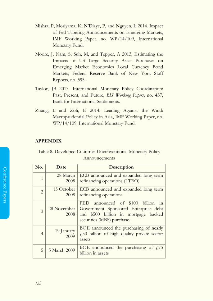
132

Co

nferen

ce Pap

ers

Mishra, P, Moriyama, K, N‘Diaye, P, and Nguyen, L 2014. Impact

of Fed Tapering Announcements on Emerging Markets,

IMF Working Paper, no. WP/14/109, International

Monetary Fund.

Moore, J, Nam, S, Suh, M, and Tepper, A 2013, Estimating the

Impacts of US Large Security Asset Purchases on

Emerging Market Economies Local Currency Bond

Markets, Federal Reserve Bank of New York Staff

Reports, no. 595.

Taylor, JB 2013. International Monetary Policy Coordination:

Past, Present, and Future, BIS Working Papers, no. 437,

Bank for International Settlements.

Zhang, L and Zoli, E 2014. Leaning Against the Wind:

Macroprudential Policy in Asia, IMF Working Paper, no.

WP/14/109, International Monetary Fund.

APPENDIX

Table 8. Developed Countries Unconventional Monetary Policy

Announcements

No. Date Description

1 28 March

2008 ECB announced and expanded long term refinancing operations (LTRO)

2 15 October

2008 ECB announced and expanded long term refinancing operations

3 28 November

2008

FED announced of $100 billion in Government Sponsored Enterprise debt and $500 billion in mortgage backed securities (MBS) purchase.

4 19 January

2009

BOE announced the purchasing of nearly £50 billion of high quality private sector assets

5 5 March 2009 BOE announced the purchasing of £75 billion in assets

133

Co

nfe

ren

ce P

aper

s

No. Date Description

6 18 March

2009

FED announced the purchasing of $300 billion in long term Treasuries and $750 billion in MBS, and $100 billion in MBS.

7 7 May 2009

BOE announced the purchasing of nearly £125 billion in assets; ECB announced the purchasing of €60 billion in Euro-denominated covered bonds; 12 month LTRO announced

8 6 August

2009 BoE announced the purchasing of nearly £175 billion in assets

9 5 November

2009 BoE announced the purchasing of £200 billion in assets

10 1 December

2009 BOJ offered 10 trillion JPY in 3 month loans

11 11 March

2010 FED announced the purchasing of $600 billion in Treasuries

12 17 March

2010 BOJ expanded the size of the fixed rate operations to 20 trillion JPY

13 10 May 2010 ECB conducted interventions in the Euro Area private and public debt securities markets.

14 21 May 2010 BOJ offered 3 trillion JPY in 1-year loans to private institutions

15 30 August

2010 BOJ added 10 trillion JPY in 6 month loans to the fixed rate operations

16 21 September

2011 FED announced the purchasing of $400 billion in Treasuries

17 6 October

2011

BOE announced the purchasing of nearly £275 billion in assets;

ECB announced the purchasing of €40 billion in Euro-denominated covered bonds

18 8 December

2011 ECB LTRO expanded, 36 month LTRO announced

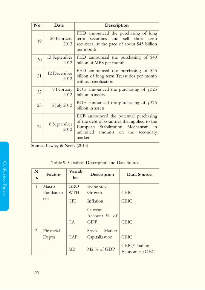
134

Co

nferen

ce Pap

ers

No. Date Description

19 20 February

2012

FED announced the purchasing of long term securities and sell short term securities; at the pace of about $45 billion per month

20 13 September

2012 FED announced the purchasing of $40 billion of MBS per month

21 12 December

2012

FED announced the purchasing of $45 billion of long term Treasuries per month without sterilization

22 9 February

2012 BOE announced the purchasing of £325 billion in assets

23 5 July 2012 BOE announced the purchasing of £375 billion in assets

24 6 September

2012

ECB announced the potential purchasing of the debt of countries that applied to the European Stabilization Mechanism in unlimited amounts on the secondary market.

Source: Fawley & Neely (2013)

Table 9. Variables Description and Data Source

N

o. Factors

Variab

les Description Data Source

1

Macro

Fundamen

tals

GRO

WTH

Economic

Growth CEIC

CPI Inflation CEIC

CA

Current

Account % of

GDP CEIC

2

Financial

Depth

CAP

Stock Market

Capitalization CEIC

M2 M2 % of GDP CEIC/Trading

Economics/OEC

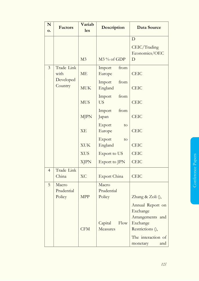
135

Co

nfe

ren

ce P

aper

s

N

o. Factors

Variab

les Description Data Source

D

M3 M3 % of GDP

CEIC/Trading

Economics/OEC

D

3

Trade Link

with

Developed

Country

ME

Import from

Europe CEIC

MUK

Import from

England CEIC

MUS

Import from

US CEIC

MJPN

Import from

Japan CEIC

XE

Export to

Europe CEIC

XUK

Export to

England CEIC

XUS Export to US CEIC

XJPN Export to JPN CEIC

4 Trade Link

China XC Export China CEIC

5 Macro

Prudential

Policy MPP

Macro

Prudential

Policy Zhang & Zoli (),

CFM

Capital Flow

Measures

Annual Report on

Exchange

Arrangements and

Exchange

Restrictions (),

The interaction of

monetary and

136

Co

nferen

ce Pap

ers

N

o. Factors

Variab

les Description Data Source

Macroprudential

policies—IMF ().

References

Adams, Robert M. dan Dean F. Amel (2011), Market structure

and the pass-through of the federal funds rate. Journal of

Banking & Finance, 35: 1087–1096.

Amidu, Mohammed dan Simon Wolfe (2013), The effect of

banking market structure on the lending channel:

Evidence from emerging markets. Review of Financial

Economics, 22: 146–157

Angelini, Paolo dan Nicola Cetorelli (2003), The Effects of

Regulatory Reform on Competition in the Banking

Industry, Journal of Money, Credit and Banking, Vol. 35, No.

5: 663-684

Arellano, M., and S. Bond. (1991). Some tests of specification for

panel data: Monte Carlo evidence and an application to

employment equations. Review of Economic Studies, 58: 277–

97.

Ariefianto, M.D. (2009). Perilaku Persaingan Industri Perbankan

Di Indonesia Pasca Krisis, Analisa Dengan Pendekatan

Teori Oligopoli Dan Ekonometrika Panel Data 2002-2008,

PhD Dissertation, University of Indonesia.

Borio, C. and Fritz, W. (1995) The response of short-term bank

lending rates to policy rates: a cross-country perspective,

BIS Working Paper No. 27. 5

Claessens, Stijn dan Luc Laeven (2004), What Drives Bank

Competition? Some International Evidence, Journal of

Money, Credit and Banking, 36 (3): 563-583.

137

Co

nfe

ren

ce P

aper

s

Cottarelli, C. and Kourelis, A. (1994) Financial structure, bank

lending rates and the transmission of monetary policy,

IMF Staff Paper, 42: 670–700.

Freixas X. and J.-C. Rochet (2008), The microeconomics of banking,

Boston: The MIT Press, 2nd edition.

Gunji , Hiroshi, Kazuki Miura dan Yuan Yuan (2009), Bank

competition and monetary policy, Japan and the World

Economy, 21: 105–115

Klein, Michael A. (1971), A Theory of the Banking Firm. Journal of

Money, Credit and Banking, 3(2): 205-218.

Olivero, María Pía, Yuan Li, dan Bang Nam Jeon (2011),

Competition in banking and the lending channel: Evidence

from bank-level data in Asia and Latin America, Journal of

Banking & Finance 35, 560–571

Roodman, D. (2009), How to do xtabond2: An introduction to

difference and system GMM in Stata. The Stata Journal, 9

(1): 86–136.

Toolsema-Veldman, L. & Schoonbeek, L. 1999, Bank behavior

and the interbank rate in an oligopolistic market. Working

paper, University of Groningen, SOM research school.

Van Leuvensteijn, Michiel (2013), Impact of bank competition on

the interest rate pass-through in the Euro area, Applied

Economics, 45: 1359–1380

138

Co

nferen

ce Pap

ers

Monetary Policy Efficiency

Measurement of Its Efficiency in Indonesia

Eka Purwanda

STIE STEMBI Bandung

Siti Herni Rochana

Program Studi Perencanaan Wilayah dan Kota ITB. (siti_hr@sappk.itb.ac.id)

Abstract

Since 2000, monetary policy in Indonesia has experienced

significant changes over the implementation of Law 23 year 1999.

Under the legislation, monetary policy in Indonesia started to use

strategies ITF (Inflation Targeting Framework). The purpose of

this policy is to stabilize the value of the rupiah through the BI

rate determination to achieve inflation targeted. To evaluate the

performance of the monetary policy base on the ITF strategy, it is

required indicators for the success of the policy namely the

efficiency rate.

ITF monetary policy strategy is a rule-based monetary

policy. In the rule-based policy, the determination of the interest

rate is determined using a specific formula. The formula of the

interest rate determination is usually based on the equation of the

139

Co

nfe

ren

ce P

aper

s

modified Taylor Rule. Theoretically, rule-based monetary policy

supposed to be more efficient than discretion monetary policy.

This is because in the rule-based monetary policy, interest rates

was calculated based on the inflation targeted. Thus inflation is

expected to be more stable so the policies more efficient.

In principle, the measurement of the efficiency of

monetary policy was based on inflation and output variations.

Monetary policy is considered to be efficient if the policy

generates low fluctuation of output and inflation. Low and stable

inflation will encourage the output growth in the long term, while

high fluctuation of inflation will cause a social loss. Some

economists have tried to formulate the monetary policy efficiency

measures such as Cecchetti (2006) and Romer (2006). However,

these formulations still in a general form and can not be used

operationally. In this paper, the authors formulate a method for

measuring the efficiency of monetary policy and applied to the

data of inflation and output in Indonesia. The efficiency of

monetary policy is measured by the deviation of actual monetary

policy from ideal monetary policy. Ideal monetary policy is policy

that creates a minimum variation of output and inflation.

The measurement results since the implementation of

monetary policy based ITF, the efficiency of monetary policy has

not changed significantly. However, there was a tendency to

increase the efficiency of monetary policy after the full

implementation of the ITF framework after 2005 than in the

transition period 2000-2005. The full-fledged implementation of

ITF will strengthen public expectation toward the decrease of

inflation and encourage low and stable inflation.

Keywords: monetary policy, inflation targeting framework, loss function,

efficiency.

JEL Classification: E10, E31, E52

1. INTRODUCTION

140

Co

nferen

ce Pap

ers

In the past few decades, policy makers around the world have

become increasingly aware of the social and economic costs due

to inflation. Economists and politicians have began to discuss the

costs caused by the high inflation since 1960 in which the world

has been experiencing the rising inflation. Inflation may lead to

uncertainty concerning relative prices and price rates in the future,

which brings into companies and individuals to find if difficult to

make a decision, and in turn, this lowers the economic efficiency

consensus. Economists claim that inflation may harm economic

growth, especially when the inflation is high level (Mishkin, 2007).

The awareness of high costs due to inflation lands to the

viewpoint that low and stable inflation will encourage the

productivity of economic resources and support economic

growth, price stability becomes an important factor for the long

term healthy economic growth. Therefore, price stability defined

as low and stable inflation is regarded as the main goal of the

monetary policy.

Relation to the matters, the central element which is necessary

for the monetary policy is the use of a nominal anchor to be uses

as a policy strategy. Nominal anchor is a nominal variable such as

inflation, and money supply that could limit the movement of

prices in order to achieve price stability. There are three monetary

policy strategies that is nominal anchor determination (implicit

nominal anchor), (Mishkin, 2007).

The monetary policy with an inflation target strategy has been

widely adopted by many countries. New Zealand was the first

country which implemented the strategy of the inflation targeting

in 1990, followed by Canada in 1991, England in 1992, Sweden

and Finland in 1993, Australia and Spain in 1994, followed by

other countries such as Israel, Chile, and Brazil.

In Indonesia, the monetary policy with the nominal anchor

began to be implemented along with the implementation of Act

23 year 1999 concerning Bank of Indonesia. In the legislation, it is

stated that the task of Bank Indonesia is focused on keeping the

rupiah value stable. In the implementation, Bank Indonesia is

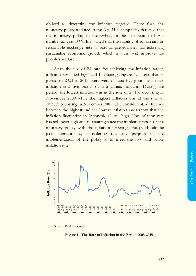
141

Co

nfe

ren

ce P

aper

s

obliged to determine the inflation targeted. There fore, the

monetary policy outlined in the Act 23 has implicitly detected that

the monetary policy of meanwhile, in the explanation of Act

number 23 year 1999. It is stated that the stability of rupiah and its

reasonable exchange rate is part of prerequisites for achieving

sustainable economic growth which in turn will improve the

people‘s welfare.

Since the use of BI rate for achieving the inflation target,

inflation remained high and fluctuating. Figure 1. shows that in

period of 2003 to 2015 there were of least five points of climax

inflation and five points of anti climax inflation. During the

period, the lowest inflation was at the rate of 2.41% occurring in

November 2009 while the highest inflation was at the rate of

18.38% occurring in November 2005. The considerable difference

between the highest and the lowest inflation rates show that the

inflation fluctuation in Indonesia 13 still high. The inflation rate

has still been high and fluctuating since the implementation of the

monetary policy with the inflation targeting strategy should be

paid attention to, considering that the purpose of the

implementation of the policy is to meet the low and stable

inflation rate.

Source: Bank Indonesia

Figure 1. The Rate of Inflation in the Period 2003-2015

0

2

4

6

8

10

12

14

16

18

20

Jan

-03

Jul-

03

Jan

-04

Jul-

04

Jan

-05

Jul-

05

Jan

-06

Jul-

06

Jan

-07

Jul-

07

Jan

-08

Jul-

08

Jan

-09

Jul-

09

Jan

-10

Jul-

10

Jan

-11

Jul-

11

Jan

-12

Jul-

12

Jan

-13

Jul-

13

Jan

-14

Jul-

14

Jan

-15

Jul-

15

Infl

ati

on

Rate

(%

)

142

Co

nferen

ce Pap

ers

A fairly large inflation fluctuation in Indonesia requires a

method of evaluation to measure the accuracy of the method in

achieving the targeted inflation. The indicators of the success of

the monetary policy within the framework of the ITF are usually

measured by counting efficiency. The efficiency monetary policy

views the accuracy of the policy in achieving the inflation target.

The accuracy is seen through how big the inflation deviation

occurring from the inflation targeted. On the other hand, inflation

has a tradeoff relationship with the output, where the output is

alsothe goal of economic development. Therefore, in measuring

the efficiency of the monetary policy, in addition to inflation

variation, the output variation is also calculated. Therefore, the

efficiency of the monetary policy is usually calculated from the

output variation and the inflation variation.

There are several methods for calculating the efficiency of the

monetary policy offered by economics Romer (2006) and

Cecchetti et. al. (2006) are economists who have built a method

for measuring the efficiency of monetary policy. In this study, the

authors developed a method for measuring the efficiency policy

based on a formula that had been previously established. Then the

authors use the technique for measuring the efficiency of the

monetary policy in Indonesia.

2. LITERATURE REVIEW

The purpose of the monetary policy in the ITF Framework is to

achieve the inflation rate targeted. The success of the monetary

policy is indicated by its capability in maintaining stable inflation,

called efficiency. On the other hand, inflation has trade off

relationship with the output. Several models of efficiency

measurement have been made by economists such as Cecchetti et

al. (2006), and Romer (2006). Basically the models of efficiency

measurement was made by calculating gap between optimum loss

function. That is minimum output and inflation variation with the

actual condition of the inflation variation and output variation.

The efficiency measurement of the monetary policy is done

in two phases. First, identifying the minimum loss function. The

minimum loss functions is formed from the determination of

143

Co

nfe

ren

ce P

aper

s

optimum interest rate. Further, identifying output and inflation

variation. The gap between minimum loss function and actual

condition indicates the degree of the efficiency of monetary policy.

The smaller gap between the optimal and the actual monetary

policy, the more efficient the monetary policy.

2.1 Optimal Interest Rate

The efficiency monetary policy is calculated by considering the

inflation variation and the optimal output variation. Optimal

output and inflation variation occurring in the interest rate results

in the minimum los function. Rodenbush and Svensson (Walsh,

2003:508-512 stated that the optimal monetary policy was given by

the equation of output and inflation as follows.

ttttttt uEiayayay )( 1132211 (1)

tttt y 1 (2)

From the equation (2) inflation expectation may be made into

equation: 11 tttt yEE and inserted into the output

equation, it is abstained:

1131211 )( tttttttt uyEiayayay

1

3

3121

1

)(

t

ttttu

a

iayaya

(3)

If :

3

3121

1

)(

a

iayaya tttt

t

so output and inflation of period t+1 is:

11 tt uy (4)

11 ttttt v

(5)

Where: 111 ttt uv

The value function from the loss function is:

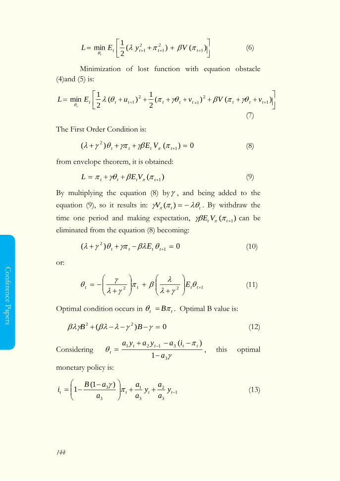
144

Co

nferen

ce Pap

ers

)()(

2

1min 1

2

1

2

1 tttt VyELt

(6)

Minimization of lost function with equation obstacle

(4)and (5) is:

)()(

2

1)(

2

1min 1

2

1

2

1 ttttttttt vVvuELt

(7)

The First Order Condition is:

0)()( 1

2 tttt VE (8)

from envelope theorem, it is obtained:

)( 1 tttt VEL (9)

By multiplying the equation (8) by , and being added to the

equation (9), so it results in: ttV )( . By withdraw the

time one period and making expectation, )( 1tt VE can be

eliminated from the equation (8) becoming:

0)( 1

2 tttt E (10)

or:

122

tttt E

(11)

Optimal condition occurs in tt B . Optimal B value is:

0)(22

BB (12)

Considering

3

3121

1

)(

a

iayaya tttt

t

, this optimal

monetary policy is:

1

3

2

3

1

3

3 )1(1

tttt y

a

ay

a

a

a

aBi

(13)

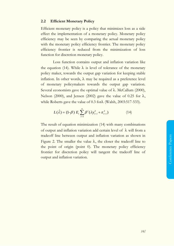
145

Co

nfe

ren

ce P

aper

s

2.2 Efficient Monetary Policy

Efficient monetary policy is a policy that minimizes loss as a side

effect the implementation of a monetary policy. Monetary policy

efficiency may be seen by comparing the actual monetary policy

with the monetary policy efficiency frontier. The monetary policy

efficiency frontier is reduced from the minimization of loss

function for discretion monetary policy.

Loss function contains output and inflation variation like

the equation (14). While is level of tolerance of the monetary

policy maker, towards the output gap variation for keeping stable

inflation. In other words, may be required as a preference level

of monetary policymakers towards the output gap variation.

Several economists gave the optimal value of . McCallum (2000),

Nelson (2000), and Jensen (2002) gave the value of 0.25 for ,

while Roberts gave the value of 0.3 for (Walsh, 2003:517-533).

1

22)()1()ˆ(

i

itit

i

t yEL (14)

The result of equation minimization (14) with many combinations

of output and inflation variation add certain level of will from a

tradeoff line between output and inflation variation as shown in

Figure 2. The smaller the value , the closer the tradeoff line to

the point of origin (point 0). The monetary policy efficiency

frontier for discretion policy will tangent the tradeoff line of

output and inflation variation.

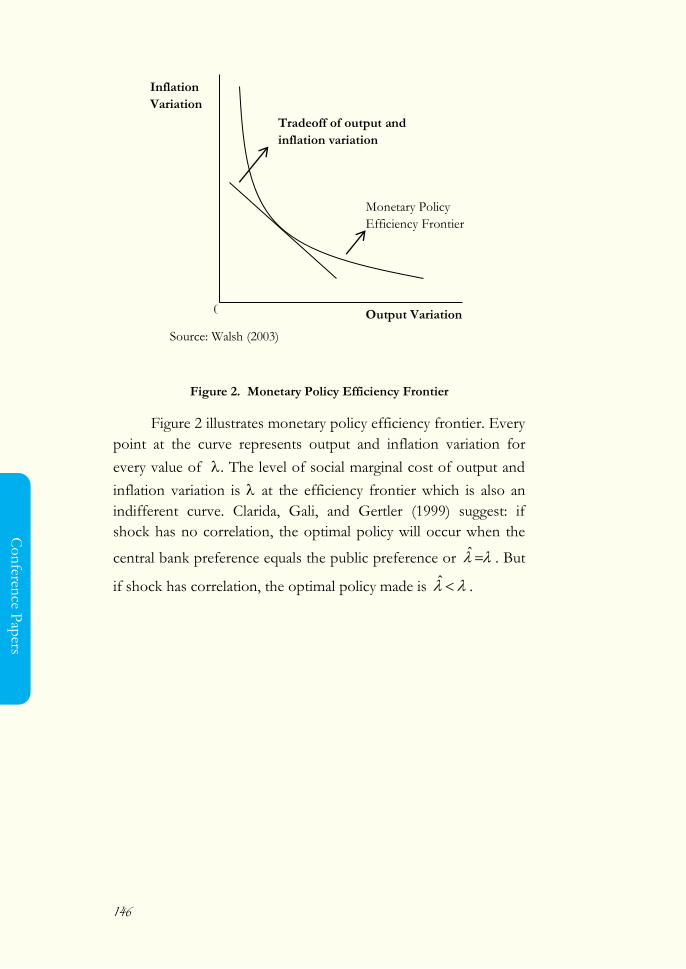
146

Co

nferen

ce Pap

ers

Figure 2. Monetary Policy Efficiency Frontier

Figure 2 illustrates monetary policy efficiency frontier. Every

point at the curve represents output and inflation variation for

every value of . The level of social marginal cost of output and

inflation variation is at the efficiency frontier which is also an

indifferent curve. Clarida, Gali, and Gertler (1999) suggest: if

shock has no correlation, the optimal policy will occur when the

central bank preference equals the public preference or ˆ . But

if shock has correlation, the optimal policy made is ˆ .

Inflation

Variation

Output Variation

Source: Walsh (2003)

Tradeoff of output and

inflation variation

Monetary Policy

Efficiency Frontier

0

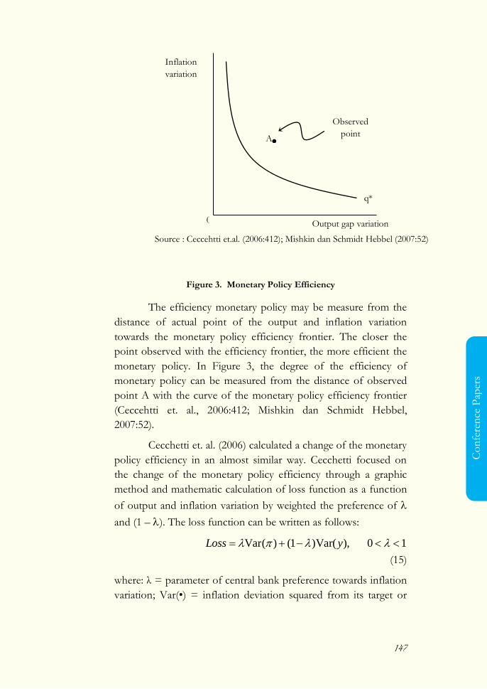
147

Co

nfe

ren

ce P

aper

s

Figure 3. Monetary Policy Efficiency

The efficiency monetary policy may be measure from the

distance of actual point of the output and inflation variation

towards the monetary policy efficiency frontier. The closer the

point observed with the efficiency frontier, the more efficient the

monetary policy. In Figure 3, the degree of the efficiency of

monetary policy can be measured from the distance of observed

point A with the curve of the monetary policy efficiency frontier

(Ceccehtti et. al., 2006:412; Mishkin dan Schmidt Hebbel,

2007:52).

Cecchetti et. al. (2006) calculated a change of the monetary

policy efficiency in an almost similar way. Cecchetti focused on

the change of the monetary policy efficiency through a graphic

method and mathematic calculation of loss function as a function

of output and inflation variation by weighted the preference of

and (1 – ). The loss function can be written as follows:

10 ),Var()1()(Var yLoss

(15)

where: λ = parameter of central bank preference towards inflation

variation; Var(•) = inflation deviation squared from its target or

Source : Ceccehtti et.al. (2006:412); Mishkin dan Schmidt Hebbel (2007:52)

Observed

point A

Inflation

variation

Output gap variation

q*

0

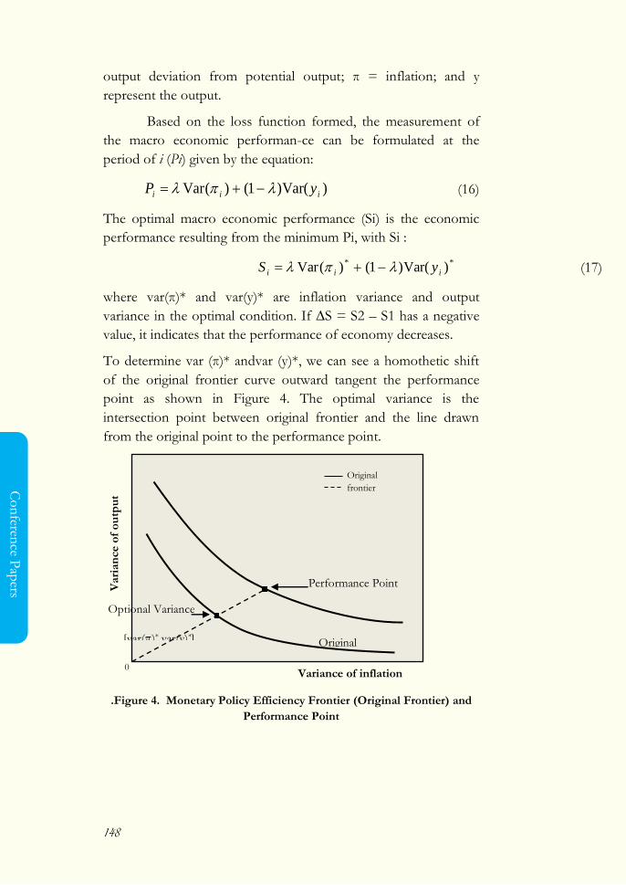
148

Co

nferen

ce Pap

ers

output deviation from potential output; π = inflation; and y

represent the output.

Based on the loss function formed, the measurement of

the macro economic performan-ce can be formulated at the

period of i (Pi) given by the equation:

)Var()1()(Var iii yP (16)

The optimal macro economic performance (Si) is the economic

performance resulting from the minimum Pi, with Si :

**)Var()1()(Var iii yS (17)

where var(π)* and var(y)* are inflation variance and output

variance in the optimal condition. If ∆S = S2 – S1 has a negative

value, it indicates that the performance of economy decreases.

To determine var (π)* andvar (y)*, we can see a homothetic shift

of the original frontier curve outward tangent the performance

point as shown in Figure 4. The optimal variance is the

intersection point between original frontier and the line drawn

from the original point to the performance point.

.Figure 4. Monetary Policy Efficiency Frontier (Original Frontier) and

Performance Point

Optional Variance

[var()*,var(y)*]

Performance Point

[var(),var(y)]

Original

frontier

Vari

an

ce o

f o

utp

ut

Variance of inflation

Original

0

149

Co

nfe

ren

ce P

aper

s

The efficiency of the monetary policy is calculated from

the distance of the actual performance toward the optimal

performance. The inefficency level for every period i is:

])Var()Var()[1(])(Var)(Var[

iiiii yyE (18)

Then, the variable of monetary policy efficiency ∆E is calculated,

based on the proportion toward ∆P that is:

|| P

EQ

(19)

Furthermore, the average inefficiency between two periods wil be

calculated by assumed that central bank chooses the interest rate

minimizing the loss function that is minimizing deviation squared

from the inflation and output of the average target. The average is

formulated as follows:

])()1()([)(22*

yyELE ii (20)

Where π* and y* are the inflation target and the output target for

every t taken from the average value, and t is the inflation level

for every t taken from the average value.

3. MEASUREMENT FOR EFFICIENCY OF

MONETARY POLICY

Monetary policy is considered to be efficient if the policy

generates low fluctuation of output and inflation. Low and stable

inflation will encourage the output growth in the long term. High

fluctuation of inflation will cause social loss, in which model is

called loss function. The equation of loss function is defined as

follows: LF = (inflation variance) + (1 - )(output variance). The

symbol , valued between 0 and 1, is level of tolerance of BI

toward the inflation fluctuation, while the level of tolerance of BI

toward the output fluctuation is 1-. Theoretically, output and

inflation variation at time t is calculated toward the target value

and its potential.

150

Co

nferen

ce Pap

ers

Efficency is measurement for optimal policy in limiting the

output growth in order that inflation is not to high for the

purpose of output growth stability. Optimal policy is macro

economic policy resulting in minimal loss function. The los

function used in this research is:

)Var()1()(Var yLoss , where 0 <λ< 1.

Var (•) show deviation squared toward its target that is var (π) = (π

– π*)2and var (y) = (y – y*)2, where π and y are inflation and

output. The inflation variability aversion uses is λ = 0,3 according

to the recomendation of Cecchetti et. al.(2006) for developing

countries. The approach of Mc Callum (2000), Nelson (2000),

and Jensen (2002) recommended preference quality for is 1 : 0,25

(Walsh, 2003) or = 4, is not used in this research because the

value is more suitable for developed countries. After is

determined, efficiency analysis can be continued.

In this research, this efficency that will be measured is the

efficiency variable between two periods. The first period is the

period before purre ITF is used or FFIT (Full Fledged Inflation

Targeting)in 2001 (I) up to 2005 (II). The second period was the

period sure ITF was implemented or FFIT in which only one

nominal anchor had beed used that is the inflation occured in

2005 (III) up to 2008 (IV).

Stages of analysis are as follows:

1. In each period, determine the least loss function value from

the actual data in Indonesia by using = 0,3 in all quarter in

the related period.

2. Forming original frontier. The curve was derived by changing

the value of with the minimal loss function value derived at

the stage 1. Some pair combinations of var (π) andvar(y) are

derived as a result of value . Plotting var(π) in vertical axis and

and var(y) in horizontal axis will from a curve of indifference or

curve of efficiency frontier, in which stage is called the curve of

original frontier (This curve has social MRS = /(1-)). To

improve the formation of the curve of efficiency frontier to be

151

Co

nfe

ren

ce P

aper

s

steeper, it may be done by a simple regression of var(y) toward

1/var(π) as follows:

)(

1)( 10

VaryVar

If β1 significant (β0 is not significant), the curva original

frontier can be formed from1)()( VaryVar .

3. In each period var(π)* and var(y)* are graphically searcher for.

The variation is obtained from the tangency point between the

lines drawn from the original point to the performance point

as shown in Figure 4.

4. Calculating Pi and Si

)(Var)1()(Var iyiiP

*)(Var)1(

*)(Var iyiiS

where Pi is economic performance and Si is inflation and output variation in the optimal condition. Pi and Si is calculated once each for every period of i by taking the average of πi and average yi in each period.

5. Calculating Ei and E

Ei is a difference of Pi and Siare Ei = Pi – Sior it can be

calculated by a formula as follows:

])Var()Var()[1(])(Var)(Var[

iiiii yyE

Then it is calculated:

21 EEE

The value of positive ΔE indicates an increase or gain of

monetary policy efficiency.

6. Calculating Q

P

EQ

The positive value of ΔP indicates an increase or gain in macro

economic performance (performance gain). Value of Q

152

Co

nferen

ce Pap

ers

indicates the efficiency variable of the monetary policy. The

value of positive Q indicates that the monetary policy is

getting more efficient. If var (π) indicates inflation variable or

var (y) indicates output variable, correlating between periods

and is statistically significant, the optimal policy is

implemented in condition ˆ (Walsh, 2003:533). This

research takes < 0,3.

4. THE EFFICIENCY OF MONETARY POLICY IN

INDONESIA

4.1 Measurement of the Efficiency of Monetary Policy

In this part, the efficiency of monetary policy will be calculated in

the first and the second period. The first period is the period

before ITF was fully used or FFIT (Full Fledged Inflation

Targeting) in 2001 (1) to 2005 (II). The second period was the

period after ITF was fully implemented or FFIT where only one

nominal anchor had been used, that is the inflation occurring in

2005 (III) to 2009 (III). The stages of analysis are explained below.

Determining the least loss function

The value of for calculating loss function is determined through

several methods ie: determined by central bank, choosing the

value of recommended, or calculated. According to the method

of Cecchetti et al (2006) that country with high inflation can be

uses the value of = 0,3;and = 0,8for developed countries (The

countries with low inflation). In Indonesia the quarterly inflation

during, the research period was 2 percent on the average, this rate

was considered high. Therefore, in this model of efficiency the

value of = 0,3 is applied. With being mentioned, the value of

loss function was chosen from the actual data in Indonesia in the

whole quarter for each of the first and the second period. In the

first period, the minimum loss function value was 0.4393

occurring in 2005 (II) and the loss function in the second period

was 1.009 occurring in 2007 (II).

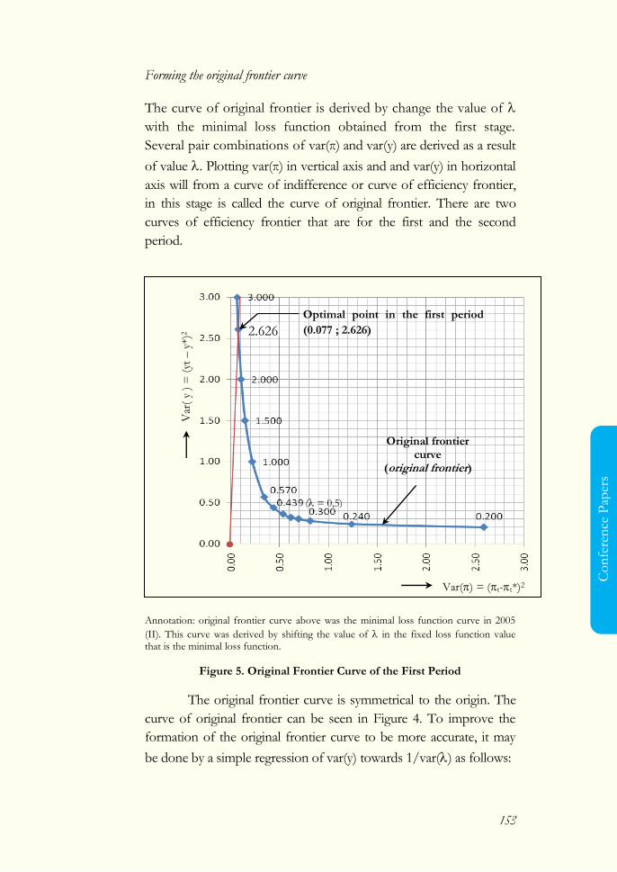
153

Co

nfe

ren

ce P

aper

s

Forming the original frontier curve

The curve of original frontier is derived by change the value of

with the minimal loss function obtained from the first stage.

Several pair combinations of var(π) and var(y) are derived as a result

of value . Plotting var(π) in vertical axis and and var(y) in horizontal

axis will from a curve of indifference or curve of efficiency frontier,

in this stage is called the curve of original frontier. There are two

curves of efficiency frontier that are for the first and the second

period.

Annotation: original frontier curve above was the minimal loss function curve in 2005

(II). This curve was derived by shifting the value of in the fixed loss function value that is the minimal loss function.

Figure 5. Original Frontier Curve of the First Period

The original frontier curve is symmetrical to the origin. The

curve of original frontier can be seen in Figure 4. To improve the

formation of the original frontier curve to be more accurate, it may

be done by a simple regression of var(y) towards 1/var() as follows:

Var() = (t-t*)2

Var

( y

) =

(yt

– y

*)2

Original frontier curve

(original frontier)

( = 0,5)

2.626

Optimal point in the first period

(0.077 ; 2.626)

154

Co

nferen

ce Pap

ers

)(

1)( 10

VaryVar =

)(

1 201,0043,0)(

VaryVar

This regression equation is required to seek var(π)* and

var(y)* in the third stage. Followed by the formation process of

original frontier for the second period. Below is a figure of pairs

of var(y) and var( ) in the minimal loss function of the second

period as input to make the original frontier in this period.

Like the first period, in =0,5 (the value of tolerance of

output and inflation in the equation of loss function) had the same

strength, the value of var(y) was the same as the value of var(π).

This shows that the original frontier curve is symmetrical to the

origin. The original frontier can be seen in Figure 5.

To improve the formation of the original frontier curve to

be more accurate, a simple regression of var(y) toward 1/var(π)

can be done as follows:

)(Var

1)y(Var 10

)(Var

1 903,0030,0)y(Var

This regression equation is required to seek var()* dan

var(y)* in the third stage.

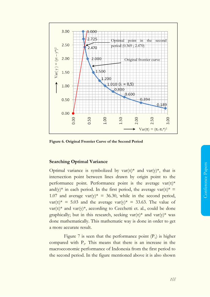
155

Co

nfe

ren

ce P

aper

s

Figure 6. Original Frontier Curve of the Second Period

Searching Optimal Variance

Optimal variance is symbolized by var(π)* and var(y)*, that is

intersection point between lines drawn by origin point to the

performance point. Performance point is the average var(π)*

and(y)* in each period. In the first period, the average var(π)* =

1.07 and average var(y)* = 36.30, while in the second period,

var(π)* = 5.03 and the average var(y)* = 33.63. The value of

var(π)* and var(y)*, according to Cecchetti et. al., could be done

graphically; but in this research, seeking var(π)* and var(y)* was

done mathematically. This mathematic way is done in order to get

a more accurate result.

Figure 7 is seen that the performance point (P1) is higher

compared with P2. This means that there is an increase in the

macroeconomic performance of Indonesia from the first period to

the second period. In the figure mentioned above it is also shown

Var() = (t-t*)2

Var

( y

) =

(yt

– y

*)2

( = 0,5)

Original frontier curve

Optimal point in the second

period (0.369 ; 2.470) 2.470

156

Co

nferen

ce Pap

ers

that E1 is bigger than E2 indicating that the efficiency of monetary

policy is increasing. From the first period to the second period.

Comparing P1 with P2 or E1 with E2 can only be done with the

condition of constant , if of the first period is difference from

the seconds period, P1 and E1 cannot be compared with P2 and E2.

In this research the value of mentioned above is 0.3 both in the

first and in the second period. The decrease in the value of P2

compared with P1 indicates that the macroeconomic performance

increases due to the ITF implementation, that is the inflation

determination as target of monetary policy.

Figure 7. Original Frontier and Loss Function Curve of the First and the

Second Period

Figure 7 shows that the line drawn from the origin to the

performance point rotates to the right. This indicates that the BI

preference toward inflation in full implementation of ITF is

relatively decreasing as compared with the implementation of

transitional ITF. In period of full implementation of ITF, the

average inflation fluctuation between quarters is bigger as

compared with the period in the implementation of transitional

ITF, but is output fluctuation is smaller as compared with the

transitional period. Overall, social loss function in the period of

full application of ITF is smaller compared with the previous

period. The increase in inflation fluctuation and the decrease in

output fluctuation in the full application of ITF (after July 2005)

Varians (yt)

Varians (t)

P1

S1

P2

S2

E2

E1

Average of loss function of

the First Period

Average of loss function of

the Second Period

Original Frontier of the

Second Period

Original Frontier of the

First Period

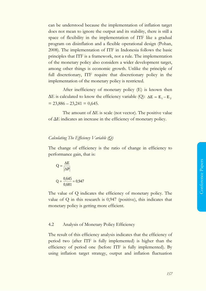
157

Co

nfe

ren

ce P

aper

s

can be understood because the implementation of inflation target

does not mean to ignore the output and its stability, there is still a

space of flexibility in the implementation of ITF like a gradual

program on disinflation and a flexible operational design (Pohan,

2008). The implementation of ITF in Indonesia follows the basic

principles that ITF is a framework, not a rule. The implementation

of the monetary policy also considers a wider development target,

among other things is economic growth. Unlike the principle of

full discretionary, ITF require that discretionary policy in the

implementation of the monetary policy is restricted.

After inefficiency of monetary policy (E) is known then

E is calculated to know the efficiency variable (Q): 21 EEE

= 23,886 – 23,241 = 0,645.

The amount of E is scale (not vector). The positive value

of ΔE indicates an increase in the efficiency of monetary policy.

Calculating The Efficiency Variable (Q)

The change of efficiency is the ratio of change in efficiency to

performance gain, that is:

P

EQ

947,0681,0

645,0Q

The value of Q indicates the efficiency of monetary policy. The

value of Q in this research is 0,947 (positive), this indicates that

monetary policy is getting more efficient.

4.2 Analysis of Monetary Policy Efficiency

The result of this efficiency analysis indicates that the efficiency of

period two (after ITF is fully implemented) is higher than the

efficiency of period one (before ITF is fully implemented). By

using inflation target strategy, output and inflation fluctuation

158

Co

nferen

ce Pap

ers

become small indicating that output and inflation are relatively low

and stable since ITF fully implemented.

With the inflation target being determined by BI, inflation

expectation will get close to or the same as the inflation target of

Bank of Indonesia by t+1, or it applies to Ett+1 = t+1. So bias

between public inflation expectation and inflation target is getting

small or zero, which in turn, will decrease the inflation fluctuation.

Furthermore, the decrease in inflation fluctuation, bends to

encourage the decrease in gap between actual output and potential

output (output in full employment). Therefore, monetary policy

becomes more efficient.

On the other hand, the decrease in inflation fluctuation

will make social less function smaller. This relationship is

illustrated in model of Money in the Utility Function (MUF),

where inflation relationship with loss function is positive (Walsh,

2003). The higher the inflation fluctuation the bigger the social

loss function. On the contrary, the lower the inflation, the smaller

the social loss. The result of the analysis of monetary policy

efficiency indicates that the efficiency is getting bigger which

means that the social loss is getting smaller.

In Indonesia, the monetary policy with ITF strategy has

been applied since 2000. This policy has only one, single target

that is inflation. This is different from the policy which was

applied before 2000 that is monetary targeting which had a

multiple target.

But in the beginning of the application of ITF policy,

banking condition in Indonesia was not yet completely stable so

the transmit slow of the monetary policy in the framework of

achieving: the inflation/targethad not worked out well.

Observation on transmission mechanism was not an easy job.

While in the ITF implementation, the running of this transmission

mechanism played an important role considering the mandate

given to achieve the stability of prices. In the condition like this,

the increase in the interest rate of monetary instrument (SBI) to

absorb cartel money to go back to the banking system was after

late due to the response of deposit interest rate so to encourage

159

Co

nfe

ren

ce P

aper

s

the incoming of cartel money to banking system required of the

increase in the interest rate which was higher than it should have

been.

Never the less, the obstacle mentioned was not a specific

obstacle for the application of inflation target framework, because

basically, monetary policy with any framework because basically,

monetary policy with and framework requires the presence of a

healthy financial system so that the target achievement becomes

credible. A mature preparation is required so timer in applying the

inflation target framework, BJ can increase inflation prediction

accuracy and understanding of the monetary policy transmission

in Indonesia. This preparation is required for the application of

full inflation target framework.

The ITF approach has advantages compared with the

monetary targeting approach. With ITF, the monetary policy may

focused better on domestic issues and respond immediately every

shock occurring in domestic economy. Stability of relations

between monetary aggregates and inflation is not a very important

issue as the success of policy does not depend on the relation

mentioned above. The ITF approach enables monetary authority

to use all the information available in determining the policy

direction that will be taken. In addition, with ITF the public may

understand easily the policy direction that has been taken due to

the presence of transparency of the policy taking process and the

increase in central bank accountability with regard to the explicit

inflation target announcement to the public. The ITF approach

may also avoid the possibility of central bank to be trapped under

politic pressure. Central bank may carry out the monetary policy

independently.

The ITF approach in the monetary policy implementation

in several developed countries generally noted a success stories. In

Indonesia, the full-fledged implementation of ITF by leaving

monetary targeting in practice had just begin since the middle

2005. The observation on empirical data in Indonesia indicated

that the inflation fluctuation and the output fluctuation were

relatively small since the full-fledged application of ITF. From the

160

Co

nferen

ce Pap

ers

result of this research the monetary policy efficiency in Indonesia

on the full-fledged application of ITF (Romer's Method) was

higher than the monetary policy efficiency before the full-fledged

application of ITF was used. Unfortunately the increase in the

efficiency was not significant. This means that a longer period is

required an order that is shifting from the monetary targeting to

ITF can run well. The time passed was too short to evaluate

significantly whether or not the policy implementation taken was

successful.

The performance of Bank Indonesia to minimize the

inflation and output fluctuation was relatively successful. The

credibility of Bank Indonesia in controlling the inflation has begun

to get better and the inflation tends to decline. The full-fledged

implementation of ITF will strengthen public expectation toward

the inflation decrease and speed the disinflation program being

carried out. This in turn, will increase the credibility of Bank

Indonesia in controlling the inflation. In addition, the inflation

target containing the element of good governance for a modern

central bank likes goal clarity, the transparency and accountability

are parallel in the effort of Bank Indonesia to increase the

credibility in the implementation of ITF.

Consistence and more focus are paying close attention to

the inflation are expected to encourage the output growth in a

long term. The session result of board of governors of Bank of

Indonesia in April, 2010 stated that Bank Indonesia had to

maintain reference interest rate (BI rate) at the level 6,5 percent

was expected to be successful. The BI rate at this level is expected

to be conducive to strength the economic recovery process,

maintain the financial stability and encourage banking

intermediation. The decision to maintain the BI rate at the level

6,5 percent was based on the evaluation result of the economic

performance during the trimaster 1 in the year 2010.

5. CONCLUSION

The efficiency of monetary policy can be measured by calculating

the distance of performance point to the original frontier curve.

Performance point is the average variance of inflation and the

161

Co

nfe

ren

ce P

aper

s

average variance of the output gap, while the original frontier

curve is a curve obtained by varying the λ at the minimum loss

function, where the value of λ is the degree of tolerance of Bank

Indonesia to the inflation fluctuations.

This efficiency measurement method was applied to the

data of Indonesia during the transitional ITF implementation

period 2000-2005 and full implementation period 2005-2009.

Since the monetary policy was fully implemented with the ITF on

July 2005, there has been a tendency that the monetary policy

efficiency increased as compared with the ITF application in the

transitional period in 2000 to 2005. The monetary policy with full-

fledged ITF application resulted in lower costs (inflation

fluctuation and output fluctuation). This is due to the fact that the

ITF policy is a set framework, starting from the instrument used,

target to the policy goal.

REFERENCES

Atkinson, A., V.V. Chari, and Patrick J. Kehoe. 2007. ―On The Optimal Choice of Monetary Policy Instrument‖. NBER Working Paper 13398, 2007.

Pohan Aulia (2008). Kerangka Kebijakan Moneter & Implementasinya di Indonesia. PT Raja Grafindo Persada, Jakarta.

Cecchetti, Stephen G., Alfonso Flores-Langunes, and Stefan

Krause. ―Has Monetary Policy Become More Efficient? A

Cross-Country Analysis‖. The Economic Journal 2006, 116:

408-433.

Collins, Sean and Pierre L. Siklos. ―Optimal Monetary Policy Rules and Inflation Targets: Are Australia, Canada and New Zealand Different from the U.S.?‖ Open Economies Review 2004, 15: 347-362.

Cover, James Peery, and Paul Pecorino. ―Price and Output Stability under Price-Level Targeting‖. Southern Economic Journal 2005, 72(1): 152-166.

Fritsche, Ulrich and Vladimir Kuzin. ―Declining Output Volatility in Germany: Impulses, Propagation, and the Role of

162

Co

nferen

ce Pap

ers

Monetary Policy‖. Applied Economics 2005, 37(21) : 2445-2458.

McCallum, Benett T. ―Monetary Policy in East Asia : the Case of

Singapore‖. IMES Discussion Paper 2007-E-10.

Romer, David. (2006). Advanced Macroeconomics. Third Edition. McGraw-Hill, New York.

Walsh, Carl E. (2003). Monetary Theory and Policy. Second Edition.

The MIT Press, Cambridge.

163

Co

nfe

ren

ce P

aper

s

Monetary Policy Its Role to Comparative Advantage of Capital Intensive

Industry In Indonesia

Chandra Utama

Faculty of Economic, Universitas Katolik Parahyangan (chandradst@yahoo.com;

chandradst@unpar.ac.id)

Ruth Meilianna

Center for Economics Studies (CES)-Department of Economics Universitas Katolik

Parahyangan (ruth_1111056@yahoo.com)

Abstract

The purpose of this paper is to examine the effect of monetary

policy to comparative advantage of capital intensive industry

(technology-intensive industry and human capital-intensive

industry) in international trade. Ever since Indonesia implemented

inflation targeting policy (ITF) in 2005, the average interest rate

gradually down than before.

The lower interest rates lead capital more affordable in

Indonesia. Heckscher-Ohlin (H-O) model states countries with

comparative advantages should export goods that require factors

of production that they have in abundance. This study used annual

data exports and imports three-digit the standard international

164

Co

nferen

ce Pap

ers

trade classification (SITC) revision 2 from UN-COMTRADE

period 2000 and 2014.

The study used analytical tool by combining two

fundamental Revealed symmetric comparative advantage (RSCA)

index by Laursen (1998) and Trade balance index by Lafay (1992)

that analyzed used products mapping by Widodo (2008). The

study also used double difference (DD) model to measure real

impact of ITF to capital intensive industry. We use unskilled-

labor intensive products as control group in DD model since it is

assume not significantly influence by interest rate.

Based on product mapping, the condition is better in 2000

than 2014, in era ITF. However, DD explain the worse is not

cause by ITF. The DD shows the ITF have positive impact to

comparative advantage and trade balance of capital-intensive

products.

Keywords: Monetary Policy, Interest rates, International trade, Comparative

advantage

JEL Classification: E52, E4, F4, N7

1. INTRODUCTION

Not only in Indonesia, monetary authority in various countries

have justified the adoption of short-term interest rate as their

operational target rather than monetary aggregate. Therefore,

policy models started to set aside the relationship between money

supply and inflation, and started to focus on the relationship

between interest rate and inflation. This phenomenon was

reviewed by MacCallum and Nelson (2010) who have shown that

most publications which contributed to monetary handbook are

minimizing the role of monetary aggregate in the theory and

analysis of monetary policy.

Bank Indonesia officially run inflation targeting framework

(ITF) on July 2005. However, the socialization ITF has been done

since 2001. Based on Taylor rule, the monetary authority can

influence inflation using short run interest rates. Furthermore, the

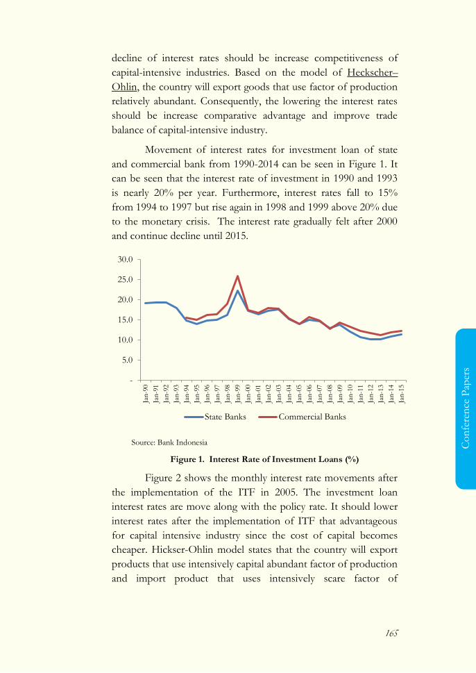
165

Co

nfe

ren

ce P

aper

s

decline of interest rates should be increase competitiveness of

capital-intensive industries. Based on the model of Heckscher–

Ohlin, the country will export goods that use factor of production

relatively abundant. Consequently, the lowering the interest rates

should be increase comparative advantage and improve trade

balance of capital-intensive industry.

Movement of interest rates for investment loan of state

and commercial bank from 1990-2014 can be seen in Figure 1. It

can be seen that the interest rate of investment in 1990 and 1993

is nearly 20% per year. Furthermore, interest rates fall to 15%

from 1994 to 1997 but rise again in 1998 and 1999 above 20% due

to the monetary crisis. The interest rate gradually felt after 2000

and continue decline until 2015.

Source: Bank Indonesia

Figure 1. Interest Rate of Investment Loans (%)

Figure 2 shows the monthly interest rate movements after

the implementation of the ITF in 2005. The investment loan

interest rates are move along with the policy rate. It should lower

interest rates after the implementation of ITF that advantageous

for capital intensive industry since the cost of capital becomes

cheaper. Hickser-Ohlin model states that the country will export

products that use intensively capital abundant factor of production

and import product that uses intensively scare factor of

-

5.0

10.0

15.0

20.0

25.0

30.0

Jan-9

0

Jan-9

1

Jan-9

2

Jan-9

3

Jan-9

4

Jan-9

5

Jan-9

6

Jan-9

7

Jan-9

8

Jan-9

9

Jan-0

0

Jan-0

1

Jan-0

2

Jan-0

3

Jan-0

4

Jan-0

5

Jan-0

6

Jan-0

7

Jan-0

8

Jan-0

9

Jan-1

0

Jan-1

1

Jan-1

2

Jan-1

3

Jan-1

4

Jan-1

5

State Banks Commercial Banks

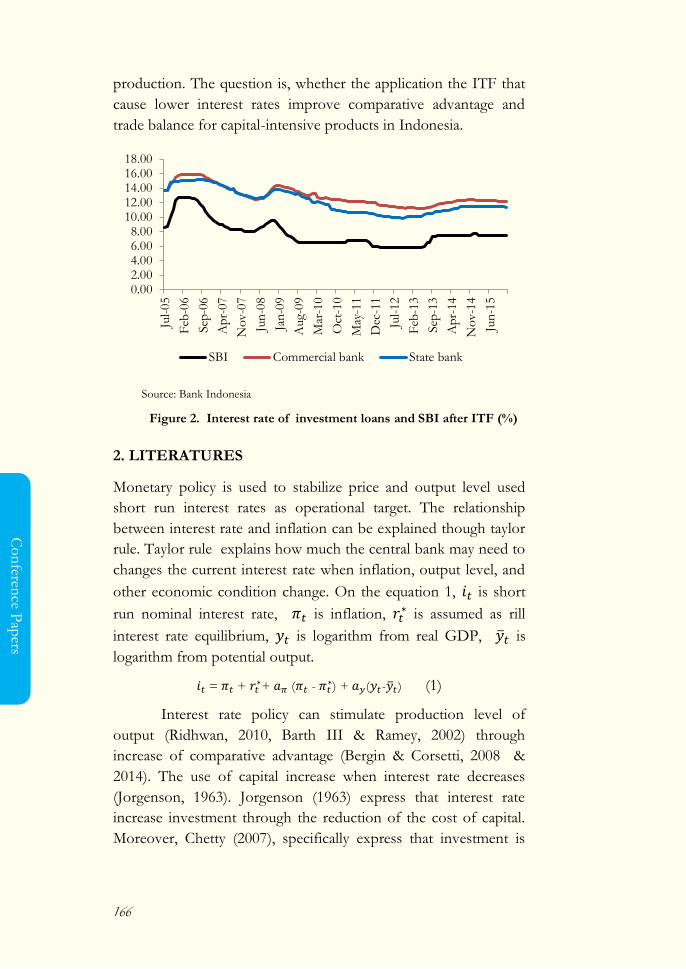
166

Co

nferen

ce Pap

ers

production. The question is, whether the application the ITF that

cause lower interest rates improve comparative advantage and

trade balance for capital-intensive products in Indonesia.

Source: Bank Indonesia

Figure 2. Interest rate of investment loans and SBI after ITF (%)

2. LITERATURES

Monetary policy is used to stabilize price and output level used

short run interest rates as operational target. The relationship

between interest rate and inflation can be explained though taylor

rule. Taylor rule explains how much the central bank may need to

changes the current interest rate when inflation, output level, and

other economic condition change. On the equation 1, is short

run nominal interest rate, is inflation, is assumed as rill

interest rate equilibrium, is logarithm from real GDP, ̅ is

logarithm from potential output.

= + + ( -

) + ( - ̅ ) (1)

Interest rate policy can stimulate production level of

output (Ridhwan, 2010, Barth III & Ramey, 2002) through

increase of comparative advantage (Bergin & Corsetti, 2008 &

2014). The use of capital increase when interest rate decreases

(Jorgenson, 1963). Jorgenson (1963) express that interest rate

increase investment through the reduction of the cost of capital.

Moreover, Chetty (2007), specifically express that investment is

0.002.004.006.008.00

10.0012.0014.0016.0018.00

Jul-

05

Feb

-06

Sep

-06

Apr-

07

Nov-0

7

Jun

-08

Jan

-09

Aug-0

9

Mar

-10

Oct

-10

May

-11

Dec

-11

Jul-

12

Feb

-13

Sep

-13

Apr-

14

Nov-1

4

Jun

-15

SBI Commercial bank State bank

167

Co

nfe

ren

ce P

aper

s

the backward-bending function from interest rate. Peng &

Thibodeau (2016) empirically analyze non-monotic of changes in

the interest rate on irreversible investment used dataset 1416

individual capital improvement of big firm like apartment,

industrial and retail properties, for period 1978-2009 found that

the effect non-monotonic is capture from interactions between

interest rate with capitalization level from property firm. In

contrast to studies which found that interest rate gives negative

effect on capital and investment, Capozza and Li (2001) ware used

data of 56 metropolitan housing for period 1980-1989 found that

investment level gives positive effect to interest rate.

Furthermore, companies need input or factors of

production, which in simply term is capital and labor. Heckscher–

Ohlin model explain that each countries have the difference in

proportion of factor of production cause the difference in the

good price. It makes country specialize produce goods that used

intensively abundant factor of production and competitive

advantage.

The increase of capital will rise output and net export of

capital-intensive products. Rybczynski theorm express that the

increase in the supply on one factor of production factor will

increase output but can decrease other output (Akay & Dogan,

2013, Hanson & Slaughter, 1999). However Bernstein &

Weinstein (2002) found other conclusion. Akay and Dogan

(2013) was used US data for 1979-2001, found that the increase on

labor supply rise output in all industry but the magnitude is

depend on elasticity on each industry. The same with Akay and

Dogan (2001), Hanson and Slaughter (1999) was used OLS

method, and 40 sectors in US period 1980-1990, found that there

are linear relationship between labor supply and the change of

output mix in US.

There are previous research which found the effect of

interest rate on competitive advantage. Bergin and Corsetti (2014)

used New Keynesian model prove that monetary policy can

increase comparative advantage firm. Bergin and Corsetti (2008)

express that the decrease on interest rate will increase expected

168

Co

nferen

ce Pap

ers

discounted profit by create new firm, so that encourages new firm

entry. Bergin and Corsetti (2014) were used US data as home

country and aggregate of 10 EURO country to foreign country

from 1972-2004, found that with stabilizing markup, monetary

policy can foster competitiveness of firm, encourages investment

and differentiation from the production of goods, increase output,

and export. In contrast Ridhwan et al. 2010 found monetary

policy influences output but insignificantly effect export.

3. METHODOLOGY

This paper use data of exports and imports published by the

United Nations Commodity Trade Statistics Database (UN-

COMTRADE). We use three-digit the standard international trade

classification (SITC) Revision 2 and focuses on group of product

classified by Empirical Trade Analysis (ETA). We use data of

export and import for 2004 and 2014. ETA distinguished the

following five products or industries: primary-industries (83

SITC), natural resource-intensive industries (21 SITC), unskilled

labor-intensive industries (26 SITC), technology-intensive

industries (62 SITC), and human capital-intensive industries (43

SITC). The classification table is available upon request.

The research use technology-intensive product and human

capital products as capital intensive products. However, unskilled

labor-intensive products used as control group that is compared to

classification 5 and 6. The procedure comparing the group discuss

later.

We use Revealed Symmetric Comparative Advantage

(RSCA) by Laursen (1998) and Trade Balace Index by Lafay

(1992) to measure comparative advantage and trade balance. RCA

index is formulated as follows:

( ) ( ) (2)

The values of index has value between minus one to one.

greater than zero implies that country i has comparative

advantage in group of products j. However, less than zero

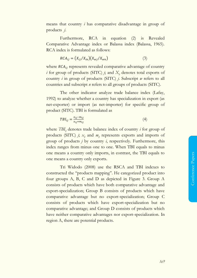
169

Co

nfe

ren

ce P

aper

s

means that country i has comparative disadvantage in group of

products j.

Furthermore, RCA in equation (2) is Revealed

Comparative Advantage index or Balassa index (Balassa, 1965).

RCA index is formulated as follows:

( ⁄ )( ⁄ ) (3)

where represents revealed comparative advantage of country

i for group of products (SITC) j; and Xij denotes total exports of

country i in group of products (SITC) j. Subscript w refers to all

countries and subscript n refers to all groups of products (SITC).

The other indicator analyze trade balance index (Lafay,

1992) to analyze whether a country has specialization in export (as

net-exporter) or import (as net-importer) for specific group of

product (SITC). TBI is formulated as

(4)

where TBIij denotes trade balance index of country i for group of

products (SITC) j; xij and mij represents exports and imports of

group of products j by country i, respectively. Furthermore, this

index ranges from minus one to one. When TBI equals to minus

one means a country only imports, in contrast, the TBI equals to

one means a country only exports.

Tri Widodo (2008) use the RSCA and TBI indexes to

constructed the ‗‗products mapping‘‘. He categorized product into

four groups A, B, C and D as depicted in Figure 3. Group A

consists of products which have both comparative advantage and

export-specialization; Group B consists of products which have

comparative advantage but no export-specialization; Group C

consists of products which have export-specialization but no

comparative advantage; and Group D consists of products which

have neither comparative advantages nor export-specialization. In

region A, there are potential products.

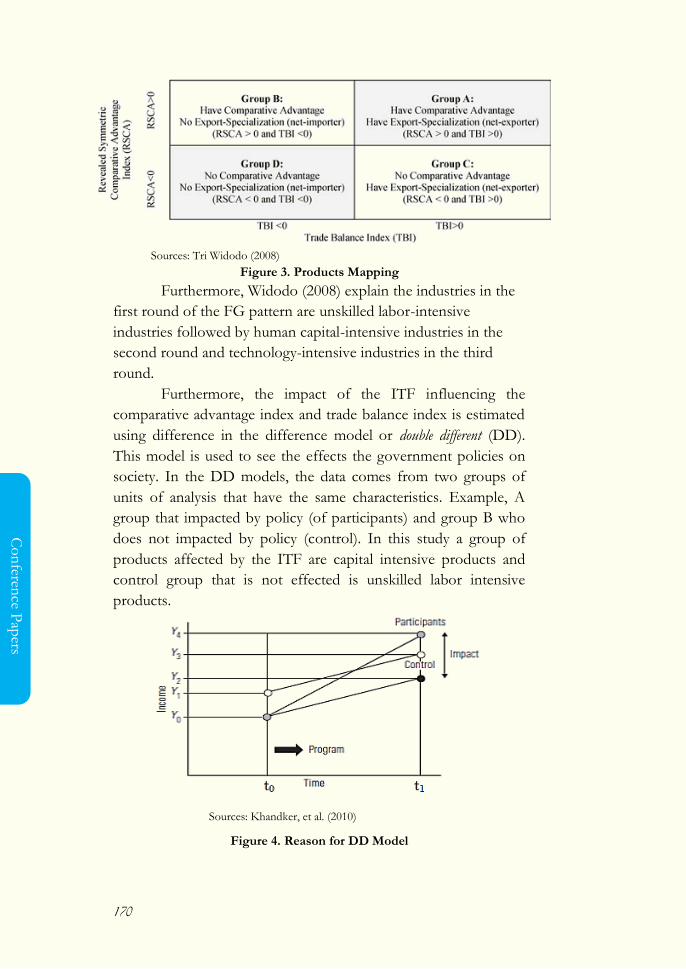
170

Co

nferen

ce Pap

ers

Sources: Tri Widodo (2008)

Figure 3. Products Mapping

Furthermore, Widodo (2008) explain the industries in the

first round of the FG pattern are unskilled labor-intensive

industries followed by human capital-intensive industries in the

second round and technology-intensive industries in the third

round.

Furthermore, the impact of the ITF influencing the

comparative advantage index and trade balance index is estimated

using difference in the difference model or double different (DD).

This model is used to see the effects the government policies on

society. In the DD models, the data comes from two groups of

units of analysis that have the same characteristics. Example, A

group that impacted by policy (of participants) and group B who

does not impacted by policy (control). In this study a group of

products affected by the ITF are capital intensive products and

control group that is not effected is unskilled labor intensive

products.

Sources: Khandker, et al. (2010)

Figure 4. Reason for DD Model

171

Co

nfe

ren

ce P

aper

s

Figure 3 shows the researchers assumed that the distance

between the groups of products, B and A at the time before the

ITF or t0 is (Y1-Y0), where Y is RSCA or TBI index. The distance

of RSCA and TBI will be the same at the next measurement t1

when there is no ITF. The model shows without ITF policy

which tends ITF the distance is (Y3-Y2). The distance between Y3

to Y4 is impact of the ITF policy. Khandker et. al. (2010) also state

the advantage of DD is relaxes the assumption of conditional

selection only on observed characteristics. It also provides a

tractable, intuitive way to account for selection on unobserved

characteristics.

Based DD, this study use Ordinary Least Square (OLS) to

investigate the causality relationship between ITF and capital

intensive products. In the model, 2000 used as time before the

policy and 2014 used as the time in policy. Furthermore, unskilled

labor-intensive product is used as control variable. White

heteroskedasticity-consistent standard errors & covariance apply

and model can be formulated as:

(5)

where d14 is dummy 2014 (period of policy) and dtech is dummy

technology-intensive products. The equation 5 use to estimate ITF

effect to technology-intensive products. Furthermore, the DD for

human capital-intensive products estimated using the following

equation:

(6)

Where is dummy human capital-intensive products. In DD,

coefficient is important because it measures the real effect of

ITF on RSCA and TBI. The coefficient exclude the other effect

that influence RSCA and TBI that assume effected treatment

group, technology-intensive or human capital-intensive products,

and control group, unskilled-labor intensive products.

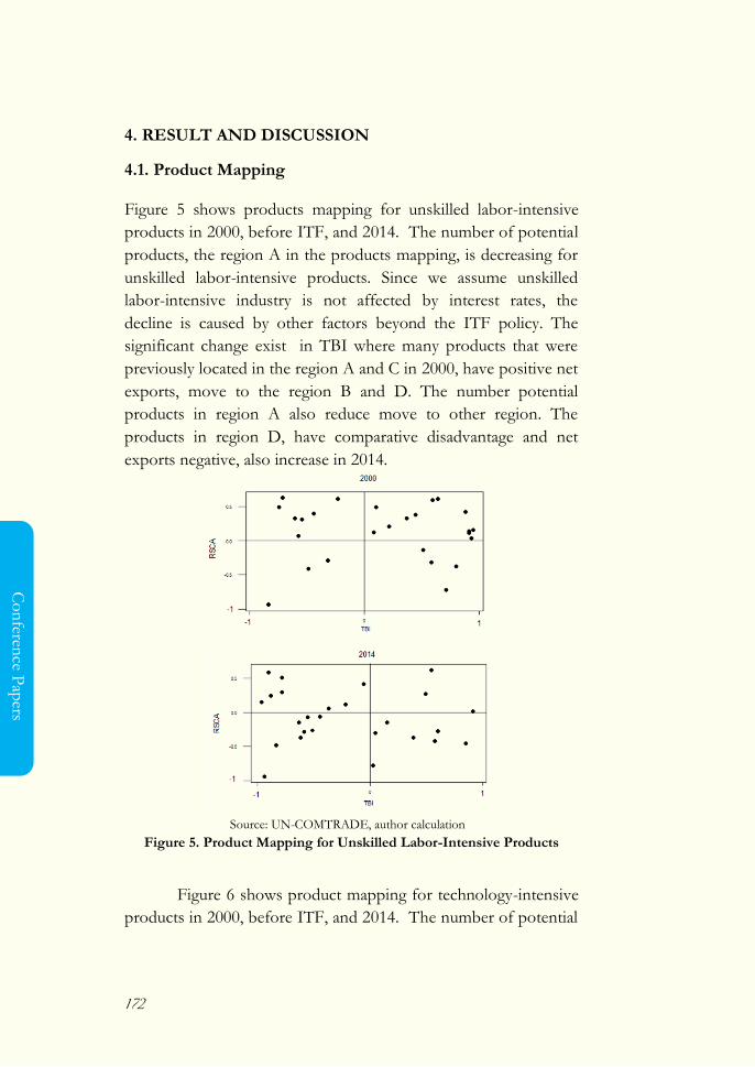
172

Co

nferen

ce Pap

ers

4. RESULT AND DISCUSSION

4.1. Product Mapping

Figure 5 shows products mapping for unskilled labor-intensive

products in 2000, before ITF, and 2014. The number of potential

products, the region A in the products mapping, is decreasing for

unskilled labor-intensive products. Since we assume unskilled

labor-intensive industry is not affected by interest rates, the

decline is caused by other factors beyond the ITF policy. The

significant change exist in TBI where many products that were

previously located in the region A and C in 2000, have positive net

exports, move to the region B and D. The number potential

products in region A also reduce move to other region. The

products in region D, have comparative disadvantage and net

exports negative, also increase in 2014.

Source: UN-COMTRADE, author calculation

Figure 5. Product Mapping for Unskilled Labor-Intensive Products

Figure 6 shows product mapping for technology-intensive

products in 2000, before ITF, and 2014. The number of potential

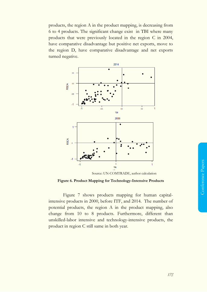
173

Co

nfe

ren

ce P

aper

s

products, the region A in the product mapping, is decreasing from

6 to 4 products. The significant change exist in TBI where many

products that were previously located in the region C in 2004,

have comparative disadvantage but positive net exports, move to

the region D, have comparative disadvantage and net exports

turned negative.

Source: UN-COMTRADE, author calculation

Figure 6. Product Mapping for Technology-Intensive Products

Figure 7 shows products mapping for human capital-

intensive products in 2000, before ITF, and 2014. The number of

potential products, the region A in the product mapping, also

change from 10 to 8 products. Furthermore, different than

unskilled-labor intensive and technology-intensive products, the

product in region C still same in both year.

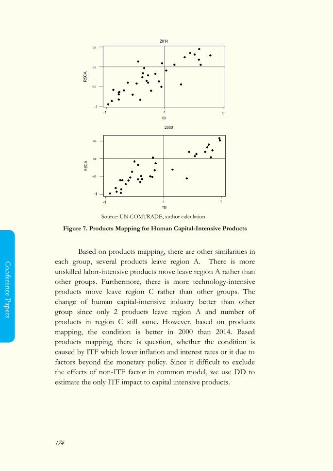
174

Co

nferen

ce Pap

ers

Source: UN-COMTRADE, author calculation

Figure 7. Products Mapping for Human Capital-Intensive Products

Based on products mapping, there are other similarities in

each group, several products leave region A. There is more

unskilled labor-intensive products move leave region A rather than

other groups. Furthermore, there is more technology-intensive

products move leave region C rather than other groups. The

change of human capital-intensive industry better than other

group since only 2 products leave region A and number of

products in region C still same. However, based on products

mapping, the condition is better in 2000 than 2014. Based

products mapping, there is question, whether the condition is

caused by ITF which lower inflation and interest rates or it due to

factors beyond the monetary policy. Since it difficult to exclude

the effects of non-ITF factor in common model, we use DD to

estimate the only ITF impact to capital intensive products.

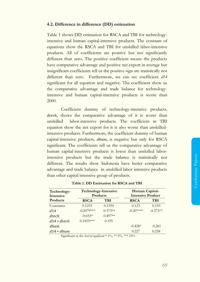
175

Co

nfe

ren

ce P

aper

s

4.2. Difference in difference (DD) estimation

Table 1 shows DD estimation for RSCA and TBI for technology-

intensive and human capital-intensive products. The constant of

equations show the RSCA and TBI for unskilled labor-intensive

products. All of coefficients are positive but not significantly

different than zero. The positive coefficient means the products

have comparative advantage and positive net export in average but

insignificant coefficients tell us the positive sign are statistically not

different than zero. Furthermore, we can see coefficient d14

significant for all equation and negative. The coefficient show us

the comparative advantage and trade balance for technology-

intensive and human capital-intensive products is worse than

2000.

Coefficient dummy of technology-intensive products,

, shows the comparative advantage of it is worse than

unskilled labor-intensive products. The coefficient in TBI

equation show the net export for it is also worse than unskilled-

intensive products. Furthermore, the coefficient dummy of human

capital-intensive products, , is negative but only for RSCA

significant. The coefficients tell us the comparative advantage of

human capital-intensive products is lower than unskilled labor-

intensive products but the trade balance is statistically not

different. The results show Indonesia have better comparative

advantage and trade balance in unskilled labor intensive products

than other capital intensive group of products.

Table 1. DD Estimation for RSCA and TBI

Technology-Intensive Products

Technology-Intensive Products

Human Capital-Intensive Product

RSCA TBI RSCA TBI

Constanta 0.1253 0.1594 0.123 0.159

-0.2079*** -0.373** -0.207*** -0.373**

-0.653* -0.497**

0.2455*** 0.195

-0.428* -0.261

0.227 0.258

Significant at the level of significant * 1%, ** 5%, *** 10%

176

Co

nferen

ce Pap

ers

The DD coefficient for technology-intensive products,

, explains the ITF have significantly positive impact

on comparative advantage and positive but not significant impact

on trade balance of capital-intensive products. Furthermore, the

ITF also have positive but not significant impact on comparative

advantage as well as trade balance for human capital-intensive

products. The result tell us the ITF that lower interest rate

increase comparative advantage for capital intensive industry,

especially technology-intensive industry, but does not significantly

increase export of product.

5. CONCLUSION

ITF policy aimed at reducing inflation using interest rates as

operational targets. ITF in Indonesia, that socialize since 2001 and

formally executed in 2005, gradually reduce inflation by lowering

the policy interest rate (SBI). The decline of SBI also accompanied

by a decrease in interest rates on loans for investment and should

favor capital intensive industry. In international trade perspective,

the lower interest rates should increase comparative advantage for

capital intensive industry that will impact better trade balance.

ETA group product based on the factor of productions

used intensively in production. We investigate the ITF impact to

comparative advantage and trade balance of technology-intensive

and human capital-intensive products use products mapping and

DD. We use unskilled-labor intensive products as control group in

DD model since it is assume not significantly influence by interest

rate. As control group it also assume effected by factor excluded

ITF same like capital intensive groups.

Based on product mapping, the condition is better in

2000 than 2014, in era ITF. However, DD explain the worse is

not cause by ITF. The DD coefficient that measure real effect of

ITF shows the ITF significantly increase comparative advantage

of technology-intensive products. The worse condition is

influenced by other factor. The ITF increase comparative

advantage significantly for technology-intensive product. The ITF

also increase but statistically insignificant trade balance of

technology-intensive products and comparative advantage as well

177

Co

nfe

ren

ce P

aper

s

as trade balance for human capital-intensive products. This study

concludes the ITF have positive impact on capital-intensive

products.

REFERENCES

Akay, G. H., & Dogan, C. (2013). The effect of labor supply

changes on output: empirical evidence from US industries.

J. Prod Annal, 39, 123-130.

Balassa, B. (1965). Trade liberalization and ‗‗revealed‘‘ comparative

advantage. The Manchester School of Economics and

Social Studies, Vol. 33, pp. 99-123

Barth III, M. J., & Ramey, V. A. (2001). The cost channel of

monetary transmission. NBER Macroeconomics Annual No

16.

Bergin, P. R., & Corsetti, G. (2015). Beyond competitive

devaluation: the monetary dimention of comparative

advantage. Cambrige-INET Working Paper No. 16.

Capozza, D. R., & Li, Y. (2002). Optimal land development

decision. Journal of Urban Economics, 51, 123-142.

Chetty, R. (2007). Interest rates, irreversibility, and backward-

bending investment. Review of Economic Studies, 74, 67-91.

Hanson, G. H., & Slaughter, M. J. (1999). The rybczynnski

theorem, factor-price equalization, and immigration:

evidence from U.S States. NNBER Working Paper No.

7074.

Jeffrey, B. R., & Weinstein, D. E. (2002). Do endowments predic

the location of production? evidence from nation and

international data. Jurnal of International Economics, 56, 55-76.

Jorgenson, D. W. (1963). Capital theory and investment

behaviour. American Economic Association, 53(2), 247-259.

Khandker, S. R., Koolwal, G. B., & Samad, H. A. (2010).

Handbook on Impact Evaluation Quantitative Methods

and Practices. The International Bank for Reconstruction

and Development / The World Bank.

178

Co

nferen

ce Pap

ers

Lafay, G. (1992). The measurement of revealed comparative

advantages. in Dagenais, M.G. and Muet, P.A. (Eds),

International TradeModeling, Chapman & Hill, London.

Laursen, K. (1998). Revealed comparative advantage and the

alternatives as measures of international specialization.

working paper 98-30, Danish Research Unit for Industrial

Dynamics (DRUID).

McCallum, B. T., & Nelson, E. (2010). Money and inflation: some

critical issues," Handbook of monetary economics, in:

Benjamin M. Friedman & Michael Woodford (ed.),

Handbook of Monetary Economics, edition 1, volume 3,

chapter 3, pages 97-153 Elsevier.

Peng, L., & Thibodeau, T. G. (2016). Interest rte and investment

under uncertainty: evidence from commerial real estate

capital improvements. University of Colorado at Boulder.

Ridhwan, M. M., De Groot, H. L., Nijkamp, P., & Rietveld, P.

(2010). The impact of monetary policy on economic

activity - evidence from a meta-analysis. Tinbergen Institute

Discussuin Paper No. 3.

Widodo, T. (2008). Dynamic changes in comparative advantage: Japan ‗‗flying geese‘‘model and its implications for China. Journal of Chinese Economic and Foreign Trade Studies Vol. 1 No. 3, pp. 200-213.

179

Co

nfe

ren

ce P

aper

s

Trilemma Policy and Economic Growth Stability in Southeast Asia

Ahmad Mikail

Kenny Devita Indraswari

Program of Islamic Economics, Department of Economics,

Universitas Indonesia, Gedung Dekanat FEB UI, Kampus Widjojo Nitisastro

Jl. Prof. Dr. Sumitro Djojohadikusumo, Depok 16424, Indonesia,

Corresponding author: ahmadmikailzaini@gmail.com

Abstract

Trilemma is the limitation of a country to simultaneously attaining

three condition at the same time namely fixed exchange rate,

independent monetary policy and free capital mobility.

Accordingly, this paper tries to investigate what is the best policy

to be imposed by central bank to achieve higher economic growth

amid financial crisis based on experiences of Southeast Asia

countries. To measure trilemma, this paper uses balanced panel

data approach from Indonesia, Thailand, Philippines and Malaysia

during the period of 1980 to 2013. This paper includes trilemma

index as independent variable alongside with inflation, openness

and foreign currency reserve in explaining the variance of

economic growth. Based on estimation result, it is found that

during global financial crisis, exchange rate stability and financial

openness policies induce higher economic growth compared to

180

Co

nferen

ce Pap

ers

monetary independence as indicated by negative coefficient of

monetary independence index. Nonetheless, those three policies

are not statistically significant improving economic growth during

East Asian financial crisis in 1997.

Keywords: trilemma; economic growth; Southeast Asia; financial crisis

JEL Classification: F31, F32, F36

1. INTRODUCTION

Trilemma, or impossible, trinity can be defined as the limitation of

a country to simultaneously target the exchange rate, acquire

independent monetary policy, and full financial integration at the

same time (Aizenman andSengupta, 2012). It occurs due to the

lack of policy maker to achieve interest parity when they want to

implement all of those three policies. Therefore, policy maker has

to face such trade-off in designing its macroeconomic goals.

Policy maker has only two maximum options: 1) to promote one

of the three goals or 2) to combine two policies at the same time.

The decision is being determined by domestic interest at the

country level. However, rapid growing of globalization, in terms

of trade and finance, has created several challenges for policy

maker to deal with those macroeconomic goals in dynamic way.

Moreover, financial turbulence as a result of financial openness

circumstance has lead policy maker to choose different

combination of policy at different environment.

One of good example to study the effect of those

macroeconomic management policies under impossible trinity is

by analyzing the experience of Southeast Asia emerging market

economies. Southeast Asia is a dynamic region in term of its

economic growth and economic integration toward global

economy. Emerging market economies namely Indonesia,

Malaysia, Thailand and Philippines are source of economic growth

in this region. This region has been hit by East Asia financial crisis

in 1997 and global financial crisis in 2008. However, they were

able to maintain relatively high economic growth under market-

based policy. The average of economic growth in the last three

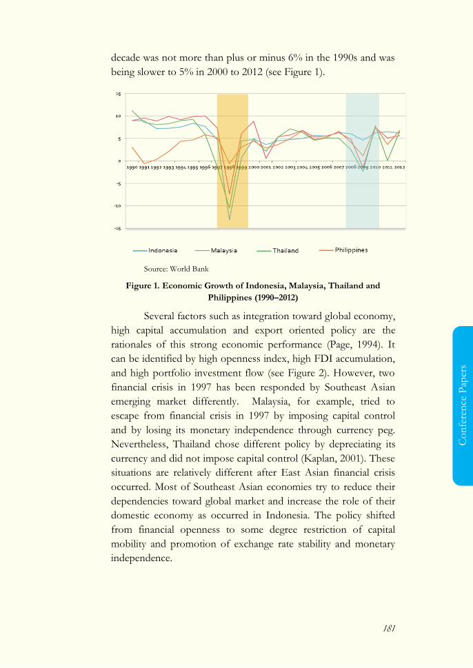
181

Co

nfe

ren

ce P

aper

s

decade was not more than plus or minus 6% in the 1990s and was

being slower to 5% in 2000 to 2012 (see Figure 1).

Source: World Bank

Figure 1. Economic Growth of Indonesia, Malaysia, Thailand and

Philippines (1990–2012)

Several factors such as integration toward global economy,

high capital accumulation and export oriented policy are the

rationales of this strong economic performance (Page, 1994). It

can be identified by high openness index, high FDI accumulation,

and high portfolio investment flow (see Figure 2). However, two

financial crisis in 1997 has been responded by Southeast Asian

emerging market differently. Malaysia, for example, tried to

escape from financial crisis in 1997 by imposing capital control

and by losing its monetary independence through currency peg.

Nevertheless, Thailand chose different policy by depreciating its

currency and did not impose capital control (Kaplan, 2001). These

situations are relatively different after East Asian financial crisis

occurred. Most of Southeast Asian economies try to reduce their

dependencies toward global market and increase the role of their

domestic economy as occurred in Indonesia. The policy shifted

from financial openness to some degree restriction of capital

mobility and promotion of exchange rate stability and monetary

independence.

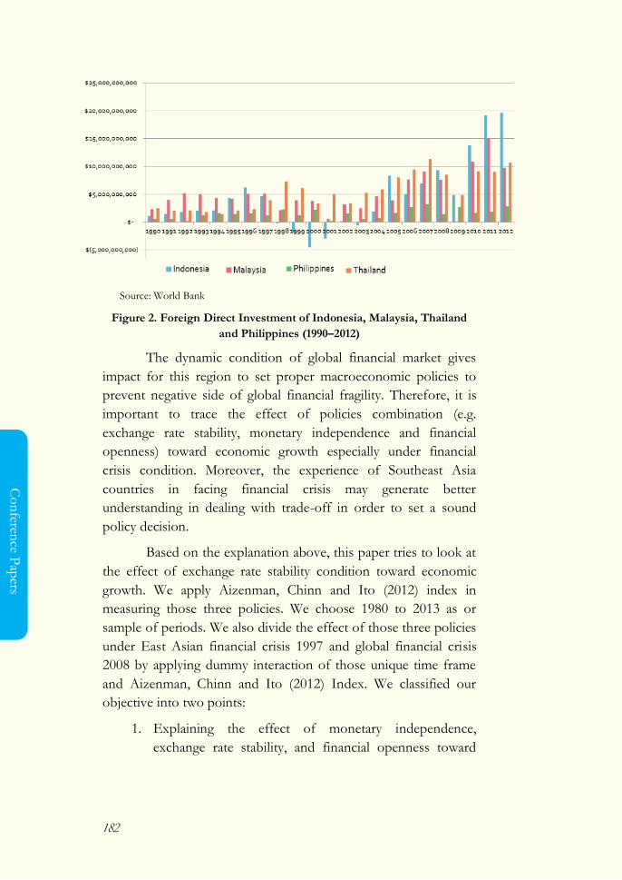
182

Co

nferen

ce Pap

ers

Source: World Bank

Figure 2. Foreign Direct Investment of Indonesia, Malaysia, Thailand

and Philippines (1990–2012)

The dynamic condition of global financial market gives

impact for this region to set proper macroeconomic policies to

prevent negative side of global financial fragility. Therefore, it is

important to trace the effect of policies combination (e.g.

exchange rate stability, monetary independence and financial

openness) toward economic growth especially under financial

crisis condition. Moreover, the experience of Southeast Asia

countries in facing financial crisis may generate better

understanding in dealing with trade-off in order to set a sound

policy decision.

Based on the explanation above, this paper tries to look at

the effect of exchange rate stability condition toward economic

growth. We apply Aizenman, Chinn and Ito (2012) index in

measuring those three policies. We choose 1980 to 2013 as or

sample of periods. We also divide the effect of those three policies

under East Asian financial crisis 1997 and global financial crisis

2008 by applying dummy interaction of those unique time frame

and Aizenman, Chinn and Ito (2012) Index. We classified our

objective into two points:

1. Explaining the effect of monetary independence,

exchange rate stability, and financial openness toward

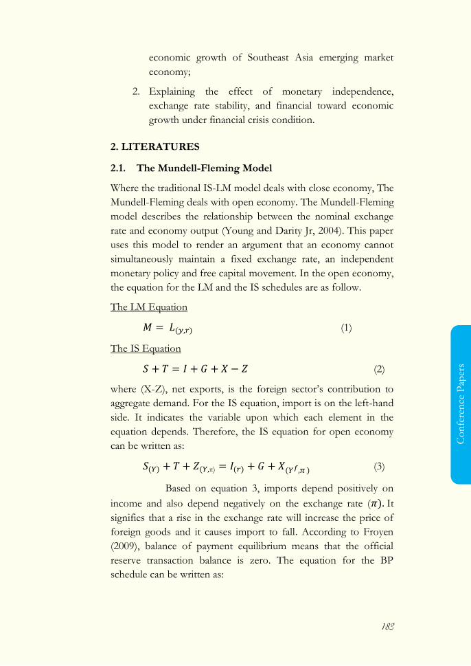
183

Co

nfe

ren

ce P

aper

s

economic growth of Southeast Asia emerging market

economy;

2. Explaining the effect of monetary independence,

exchange rate stability, and financial toward economic

growth under financial crisis condition.

2. LITERATURES

2.1. The Mundell-Fleming Model

Where the traditional IS-LM model deals with close economy, The

Mundell-Fleming deals with open economy. The Mundell-Fleming

model describes the relationship between the nominal exchange

rate and economy output (Young and Darity Jr, 2004). This paper

uses this model to render an argument that an economy cannot

simultaneously maintain a fixed exchange rate, an independent

monetary policy and free capital movement. In the open economy,

the equation for the LM and the IS schedules are as follow.

The LM Equation

( ) (1)

The IS Equation

(2)

where (X-Z), net exports, is the foreign sector‘s contribution to

aggregate demand. For the IS equation, import is on the left-hand

side. It indicates the variable upon which each element in the

equation depends. Therefore, the IS equation for open economy

can be written as:

( ) ( π) ( ) ( ) (3)

Based on equation 3, imports depend positively on

income and also depend negatively on the exchange rate ( ) It

signifies that a rise in the exchange rate will increase the price of

foreign goods and it causes import to fall. According to Froyen

(2009), balance of payment equilibrium means that the official

reserve transaction balance is zero. The equation for the BP

schedule can be written as:

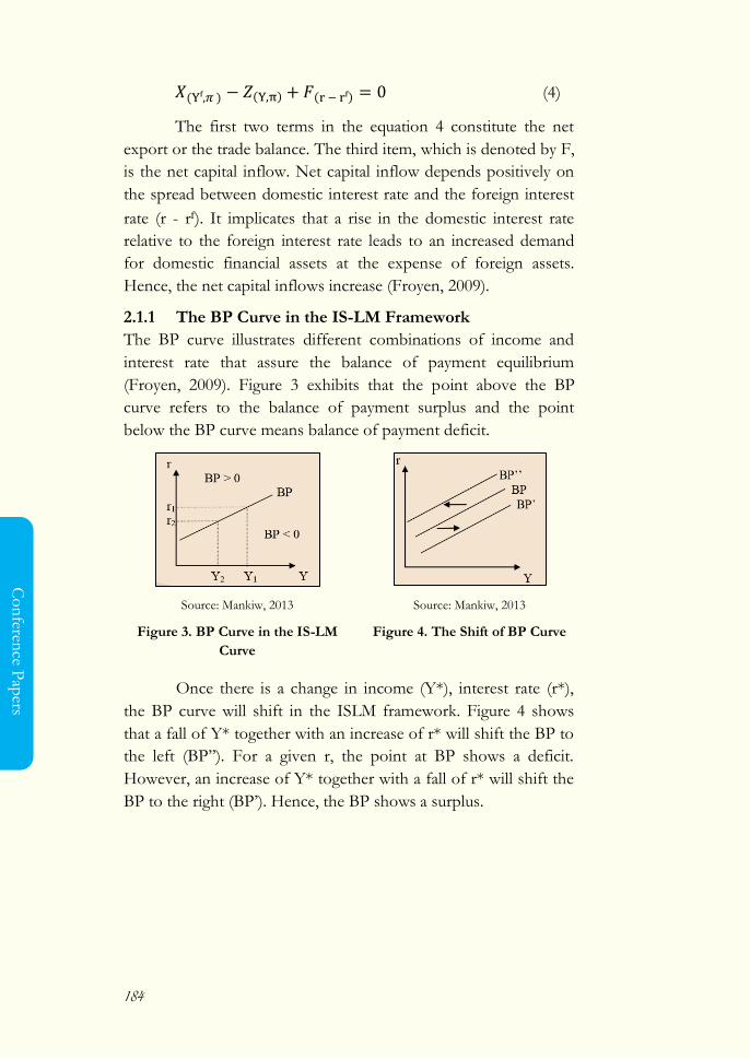
184

Co

nferen

ce Pap

ers

( ) ( ) ( ) (4)

The first two terms in the equation 4 constitute the net

export or the trade balance. The third item, which is denoted by F,

is the net capital inflow. Net capital inflow depends positively on

the spread between domestic interest rate and the foreign interest

rate (r - rᶠ). It implicates that a rise in the domestic interest rate

relative to the foreign interest rate leads to an increased demand

for domestic financial assets at the expense of foreign assets.

Hence, the net capital inflows increase (Froyen, 2009).

2.1.1 The BP Curve in the IS-LM Framework

The BP curve illustrates different combinations of income and

interest rate that assure the balance of payment equilibrium

(Froyen, 2009). Figure 3 exhibits that the point above the BP

curve refers to the balance of payment surplus and the point

below the BP curve means balance of payment deficit.

Source: Mankiw, 2013

Figure 3. BP Curve in the IS-LM

Curve

Source: Mankiw, 2013

Figure 4. The Shift of BP Curve

Once there is a change in income (Y*), interest rate (r*),

the BP curve will shift in the ISLM framework. Figure 4 shows

that a fall of Y* together with an increase of r* will shift the BP to

the left (BP‘‘). For a given r, the point at BP shows a deficit.

However, an increase of Y* together with a fall of r* will shift the

BP to the right (BP‘). Hence, the BP shows a surplus.

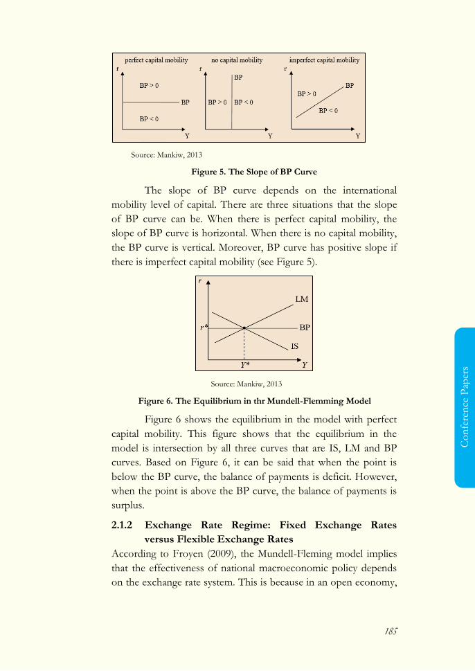
185

Co

nfe

ren

ce P

aper

s

Source: Mankiw, 2013

Figure 5. The Slope of BP Curve

The slope of BP curve depends on the international

mobility level of capital. There are three situations that the slope

of BP curve can be. When there is perfect capital mobility, the

slope of BP curve is horizontal. When there is no capital mobility,

the BP curve is vertical. Moreover, BP curve has positive slope if

there is imperfect capital mobility (see Figure 5).

Source: Mankiw, 2013

Figure 6. The Equilibrium in thr Mundell-Flemming Model

Figure 6 shows the equilibrium in the model with perfect

capital mobility. This figure shows that the equilibrium in the

model is intersection by all three curves that are IS, LM and BP

curves. Based on Figure 6, it can be said that when the point is

below the BP curve, the balance of payments is deficit. However,

when the point is above the BP curve, the balance of payments is

surplus.

2.1.2 Exchange Rate Regime: Fixed Exchange Rates

versus Flexible Exchange Rates

According to Froyen (2009), the Mundell-Fleming model implies

that the effectiveness of national macroeconomic policy depends

on the exchange rate system. This is because in an open economy,

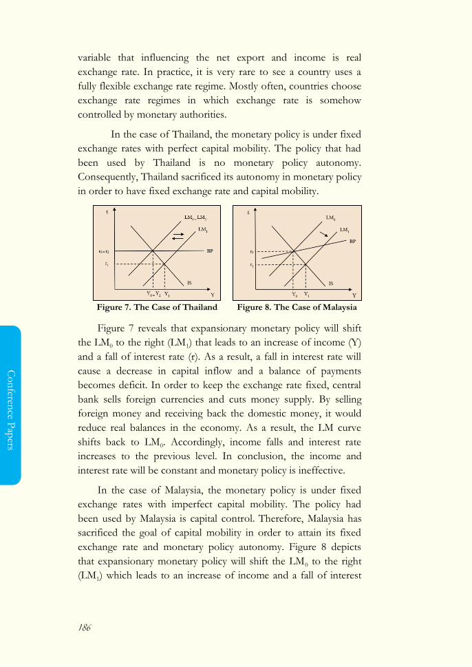
186

Co

nferen

ce Pap

ers

variable that influencing the net export and income is real

exchange rate. In practice, it is very rare to see a country uses a

fully flexible exchange rate regime. Mostly often, countries choose

exchange rate regimes in which exchange rate is somehow

controlled by monetary authorities.

In the case of Thailand, the monetary policy is under fixed

exchange rates with perfect capital mobility. The policy that had

been used by Thailand is no monetary policy autonomy.

Consequently, Thailand sacrificed its autonomy in monetary policy

in order to have fixed exchange rate and capital mobility.

Figure 7. The Case of Thailand Figure 8. The Case of Malaysia

Figure 7 reveals that expansionary monetary policy will shift

the LM0 to the right (LM1) that leads to an increase of income (Y)

and a fall of interest rate (r). As a result, a fall in interest rate will

cause a decrease in capital inflow and a balance of payments

becomes deficit. In order to keep the exchange rate fixed, central

bank sells foreign currencies and cuts money supply. By selling

foreign money and receiving back the domestic money, it would

reduce real balances in the economy. As a result, the LM curve

shifts back to LM0. Accordingly, income falls and interest rate

increases to the previous level. In conclusion, the income and

interest rate will be constant and monetary policy is ineffective.

In the case of Malaysia, the monetary policy is under fixed

exchange rates with imperfect capital mobility. The policy had

been used by Malaysia is capital control. Therefore, Malaysia has

sacrificed the goal of capital mobility in order to attain its fixed

exchange rate and monetary policy autonomy. Figure 8 depicts

that expansionary monetary policy will shift the LM0 to the right

(LM1) which leads to an increase of income and a fall of interest

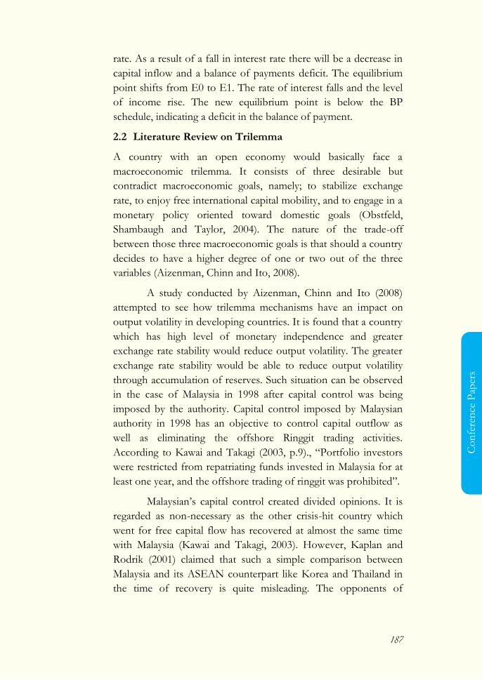
187

Co

nfe

ren

ce P

aper

s

rate. As a result of a fall in interest rate there will be a decrease in

capital inflow and a balance of payments deficit. The equilibrium

point shifts from E0 to E1. The rate of interest falls and the level

of income rise. The new equilibrium point is below the BP

schedule, indicating a deficit in the balance of payment.

2.2 Literature Review on Trilemma

A country with an open economy would basically face a

macroeconomic trilemma. It consists of three desirable but

contradict macroeconomic goals, namely; to stabilize exchange

rate, to enjoy free international capital mobility, and to engage in a

monetary policy oriented toward domestic goals (Obstfeld,

Shambaugh and Taylor, 2004). The nature of the trade-off

between those three macroeconomic goals is that should a country

decides to have a higher degree of one or two out of the three

variables (Aizenman, Chinn and Ito, 2008).

A study conducted by Aizenman, Chinn and Ito (2008)

attempted to see how trilemma mechanisms have an impact on

output volatility in developing countries. It is found that a country

which has high level of monetary independence and greater

exchange rate stability would reduce output volatility. The greater

exchange rate stability would be able to reduce output volatility

through accumulation of reserves. Such situation can be observed

in the case of Malaysia in 1998 after capital control was being

imposed by the authority. Capital control imposed by Malaysian

authority in 1998 has an objective to control capital outflow as

well as eliminating the offshore Ringgit trading activities.

According to Kawai and Takagi (2003, p.9)., ―Portfolio investors

were restricted from repatriating funds invested in Malaysia for at

least one year, and the offshore trading of ringgit was prohibited‖.

Malaysian‘s capital control created divided opinions. It is

regarded as non-necessary as the other crisis-hit country which

went for free capital flow has recovered at almost the same time

with Malaysia (Kawai and Takagi, 2003). However, Kaplan and

Rodrik (2001) claimed that such a simple comparison between

Malaysia and its ASEAN counterpart like Korea and Thailand in

the time of recovery is quite misleading. The opponents of

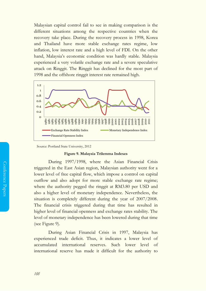
188

Co

nferen

ce Pap

ers

Malaysian capital control fail to see in making comparison is the

different situations among the respective countries when the

recovery take place. During the recovery process in 1998, Korea

and Thailand have more stable exchange rates regime, low

inflation, low interest rate and a high level of FDI. On the other

hand, Malaysia‘s economic condition was hardly stable. Malaysia

experienced a very volatile exchange rate and a severe speculative

attack on Ringgit. The Ringgit has declined for the most part of

1998 and the offshore ringgit interest rate remained high.

Source: Portland State University, 2012

Figure 9. Malaysia Trilemma Indexes

During 1997/1998, where the Asian Financial Crisis

triggered in the East Asian region, Malaysian authority went for a

lower level of free capital flow, which impose a control on capital

outflow and also adopt for more stable exchange rate regime;

where the authority pegged the ringgit at RM3.80 per USD and

also a higher level of monetary independence. Nevertheless, the

situation is completely different during the year of 2007/2008.

The financial crisis triggered during that time has resulted in

higher level of financial openness and exchange rates stability. The

level of monetary independence has been lowered during that time

(see Figure 9).

During Asian Financial Crisis in 1997, Malaysia has

experienced trade deficit. Thus, it indicates a lower level of

accumulated international reserves. Such lower level of

international reserve has made it difficult for the authority to

0

0.2

0.4

0.6

0.8

1

1.2

198

019

81

198

219

83

198

419

85

198

619

87

198

819

89

199

019

91

199

219

93

199

419

95

199

619

97

199

819

99

20

00

20

01

20

02

20

03

20

04

20

05

20

06

20

07

20

08

20

09

20

102

011

Exchange Rate Stability Index Monetary Independence Index

Financial Openness Index

189

Co

nfe

ren

ce P

aper

s

maintain stability in exchange rates regime. Therefore, in order to

ensure stability in exchange rates regime, they need to have higher

level of monetary independence and some degree of control has

been imposed on the capital outflow; to prevent huge speculative

attacks against the ringgits which would result in a highly volatile

exchange rates.

On the other hand, during the 2008 Global Financial

Crisis, Malaysia has experienced trade surplus, which is associated

with a high level of financial openness in the country, it would

enable them to accumulate adequate international reserves to

stabilize their exchange rates. Due to having both exchange rates

stability and financial openness, the authority will not go for

higher level of monetary independence. In conclusion, it can be

observed that the main objective that Malaysian authority wants to

achieve is by having a high level of exchange rates stability. It can

be done by either forgoing or lowering the level of either

monetary independence or financial openness.

3. METHODOLOGY

3.1 Model and Data Source

This paper also modified the model of Aizenman and Sengupta

(2012) and added financial crisis interaction to identify the

effectiveness of those three policy in dealing with financial shock.

The model used in this paper is as follows:

In the second model, this paper uses moderated dummy

financial crisis with first model to investigate the effect of

financial crisis on three different polices toward economic

growth of selected Southeast Asian countries.

The definition of each variable is depicted in table 1 below:

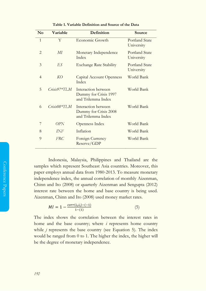
190

Co

nferen

ce Pap

ers

Table 1. Variable Definition and Source of the Data

No Variable Definition Source

1 Y Economic Growth Portland State University

2 MI Monetary Independence Index

Portland State University

3 ES Exchange Rate Stability Portland State University

4 KO Capital Account Openness Index

World Bank

5 Crisis97*TLM Interaction between Dummy for Crisis 1997 and Trilemma Index

World Bank

6 Crisis08*TLM Interaction between Dummy for Crisis 2008 and Trilemma Index

World Bank

7 OPN Openness Index World Bank

8 INF Inflation World Bank

9 FRC Foreign Currency Reserve/GDP

World Bank

Indonesia, Malaysia, Philippines and Thailand are the

samples which represent Southeast Asia countries. Moreover, this

paper employs annual data from 1980-2013. To measure monetary

independence index, the annual correlation of monthly Aizenman,

Chinn and Ito (2008) or quarterly Aizenman and Sengupta (2012)

interest rate between the home and base country is being used.

Aizenman, Chinn and Ito (2008) used money market rates.

( ) ( )

( ) (5)

The index shows the correlation between the interest rates in

home and the base country; where i represents home country

while j represents the base country (see Equation 5). The index

would be ranged from 0 to 1. The higher the index, the higher will

be the degree of monetary independence.

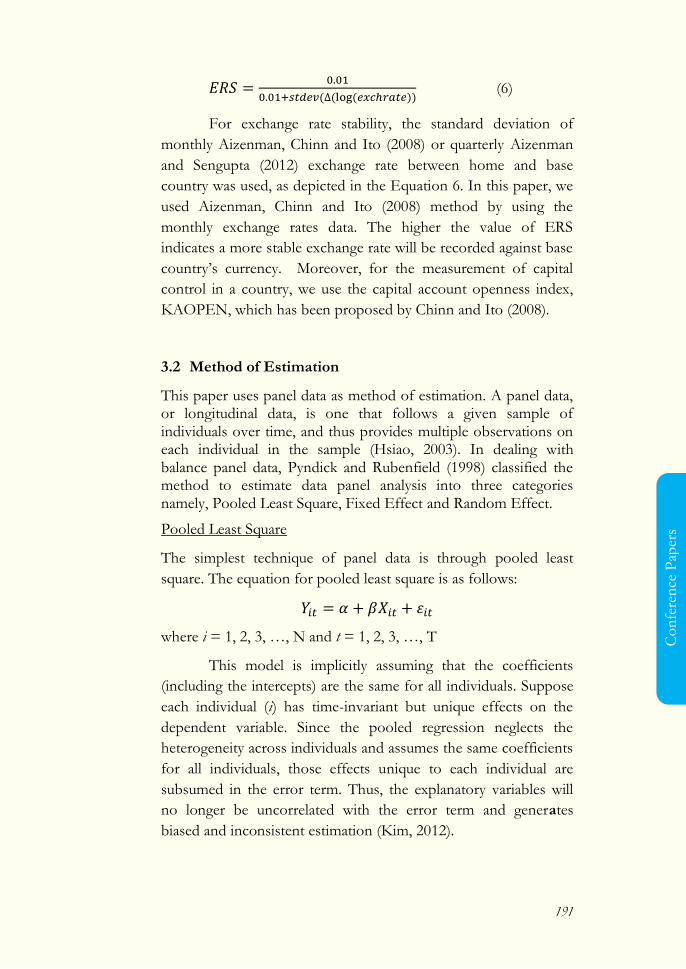
191

Co

nfe

ren

ce P

aper

s

( ( ( )) (6)

For exchange rate stability, the standard deviation of

monthly Aizenman, Chinn and Ito (2008) or quarterly Aizenman

and Sengupta (2012) exchange rate between home and base

country was used, as depicted in the Equation 6. In this paper, we

used Aizenman, Chinn and Ito (2008) method by using the

monthly exchange rates data. The higher the value of ERS

indicates a more stable exchange rate will be recorded against base

country‘s currency. Moreover, for the measurement of capital

control in a country, we use the capital account openness index,

KAOPEN, which has been proposed by Chinn and Ito (2008).

3.2 Method of Estimation

This paper uses panel data as method of estimation. A panel data, or longitudinal data, is one that follows a given sample of individuals over time, and thus provides multiple observations on each individual in the sample (Hsiao, 2003). In dealing with balance panel data, Pyndick and Rubenfield (1998) classified the method to estimate data panel analysis into three categories namely, Pooled Least Square, Fixed Effect and Random Effect.

Pooled Least Square

The simplest technique of panel data is through pooled least

square. The equation for pooled least square is as follows:

where i = 1, 2, 3, …, N and t = 1, 2, 3, …, T

This model is implicitly assuming that the coefficients

(including the intercepts) are the same for all individuals. Suppose

each individual (i) has time-invariant but unique effects on the

dependent variable. Since the pooled regression neglects the

heterogeneity across individuals and assumes the same coefficients

for all individuals, those effects unique to each individual are

subsumed in the error term. Thus, the explanatory variables will

no longer be uncorrelated with the error term and generates

biased and inconsistent estimation (Kim, 2012).

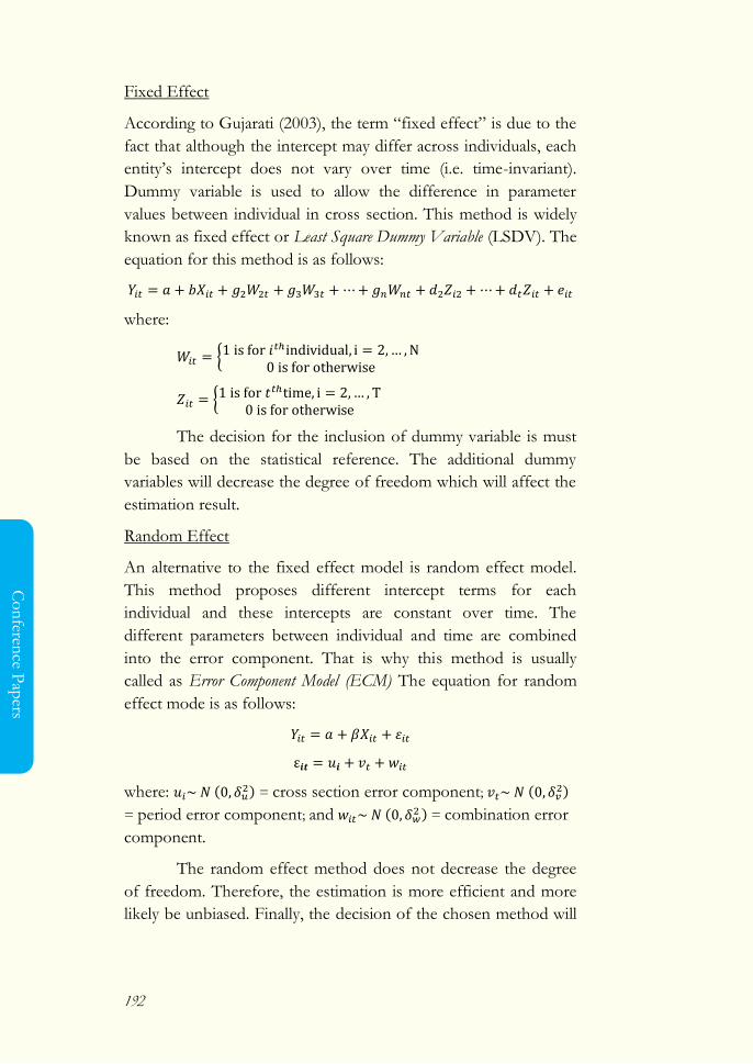
192

Co

nferen

ce Pap

ers

Fixed Effect

According to Gujarati (2003), the term ―fixed effect‖ is due to the

fact that although the intercept may differ across individuals, each

entity‘s intercept does not vary over time (i.e. time-invariant).

Dummy variable is used to allow the difference in parameter

values between individual in cross section. This method is widely

known as fixed effect or Least Square Dummy Variable (LSDV). The

equation for this method is as follows:

where:

{

{

The decision for the inclusion of dummy variable is must

be based on the statistical reference. The additional dummy

variables will decrease the degree of freedom which will affect the

estimation result.

Random Effect

An alternative to the fixed effect model is random effect model.

This method proposes different intercept terms for each

individual and these intercepts are constant over time. The

different parameters between individual and time are combined

into the error component. That is why this method is usually

called as Error Component Model (ECM) The equation for random

effect mode is as follows:

where: ( ) = cross section error component; (

)

= period error component; and ( ) = combination error

component.

The random effect method does not decrease the degree

of freedom. Therefore, the estimation is more efficient and more

likely be unbiased. Finally, the decision of the chosen method will

193

Co

nfe

ren

ce P

aper

s

be based on the Chow Test, Hausman Test and The Breusch-Pagan

LM Test.

Chow Test

Chow test is used to choose the method between pooled least

square and fixed effect which can give the best estimation result to

the model. The hypothesis for this test is Ho : Pooled Least

Squared; while H1 : Fixed Effect.

The value of the F-statistic as the basis to reject or do not

reject H0 is as follows:

( ) ( )⁄

( ) ( )⁄

Where RRSS is restricted residual sum squared, URSS in

unrestricted residual sum squared, N is the total of cross section

data, T is the total of time series data and k is total of the

explanatory variables. If the value of prob F < α, then H0 is

rejected and use fixed effect. If prob F > α, then H0 is not rejected

and use pooled least squared.

Hausman Test

Hausman test is used to choose the best method between fixed

effect and random effect. The hypothesis for this test H0: Random

Effect; while H1 : Fixed Effect. If the value of prob F < α, then

H0 is rejected and use random effect. If prob F > α, then H0 is not

rejected and use fixed effect.

The Breusch-Pagan LM Test

The Breusch-Pagan LM test is applied to choose between random

effect and pooled least square which gives the best estimation

result. The hypothesis for this test is H0 : Pooled Least Square;

otherwise H1 : Random Effect. If the value of prob F < α, then H0

is rejected and use random effect. If prob F > α, then H0 is not

rejected and use pooled least square.

194

Co

nferen

ce Pap

ers

4. RESULT AND DISCUSSION

Before we get the best model to apply regression analysis to our

data, we apply several steps to find the best panel analysis model.

Firstly, we begin with chow test to compare which one of the

model, OLS or fixed effect, giving us the best result. F-probability

statistic shows 0.00 percent means that we have to choose fixed

effect rather than OLS model.

Secondly, we apply LM test to determine the best model

between OLS and random effect. The probability Chi-squared

shows values 0.00. It means we have to reject null-Hypothesis and

conclude that random effect is better model. Thirdly, we choose

Hausman test to find the best model between random effect and

fixed effect. The Hausman probability chi-square shows 0.00

percent lower than 0.05 percent. It means we have to reject null-

hypothesis and choose fixed effect as our best model. Table 5.1

shows us the estimation result from random effect and fixed

effect. Based on Hausman test the fixed effect give us the best

result to be interpreted.

The estimation result indicates that the monetary

independence and financial openness are negatively significant in

determining economic growth in the entire sample periods. The

monetary independence is significant at alpha 10 percent with

coefficient -0.25 and financial openness is significant at alpha 1

percent with coefficient –0.70. These estimation results show us

that monetary independence and financial openness is not

desirable target for economic growth. One of possible explanation

why monetary independence negatively correlated with the

economic growth in these region was that it could trigger currency

fluctuation in small and open economy which need exchange rate

stability. Moreover, the negative sign of financial openness

exhibits that capital control for some degree positively afflict

economic growth.

This result is in line with Kaplan and Rodrik (2001) who

confirmed the positive effect of capital control in reducing

volatility in financial market that lead to sound economic

condition. Substantial capital inflow or outflow in emerging

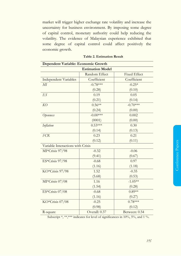
195

Co

nfe

ren

ce P

aper

s

market will trigger higher exchange rate volatility and increase the

uncertainty for business environment. By imposing some degree

of capital control, monetary authority could help reducing the

volatility. The evidence of Malaysian experience exhibited that

some degree of capital control could affect positively the

economic growth.

Table 2. Estimation Result

Dependent Variable: Economic Growth

Estimation Model

Random Effect Fixed Effect

Independent Variables Coefficient Coefficient

MI -0.78***

(0.28)

-0.25*

(0.10)

ES 0.19

(0.21)

0.05

(0.14)

KO 0.56**

(0.24)

-0.70***

(0.00)

Openness -0.00***

(0001)

0.002

(0.00)

Inflation 0.53***

(0.14)

0.30

(0.13)

FCR 0.23

(0.12)

0.21

(0.11)

Variable Interactions with Crisis

MI*Crisis 97/98 -0.32

(9.41)

-0.06

(0.67)

ES*Crisis 97/98 -0.68

(1.16)

0.97

(1.18)

KO*Crisis 97/98 1.52

(5.68)

-0.35

(0.53)

MI*Crisis 07/08 1.16

(1.54)

-1.05**

(0.28)

ES*Crisis 07/08 -0.68

(1.16)

0.89**

(0.27)

KO*Crisis 07/08 -0.25

(0.98)

0.78***

(0.12)

R-square Overall: 0.37 Between: 0.54

Subscript *, **,*** indicates for level of significances in 10%, 5%, and 1 %.

196

Co

nferen

ce Pap

ers

Moreover, the exchange rate stability is not significant.

The positive coefficient of this variable indicates that exchange

rate stability policy might be desirable for attaining higher

economic growth in Southeast Asia emerging market. The

problem of currency instability that lead East Asian financial crisis

was a good example of how currency stability is the necessary

condition for open economy. Moreover, control variables (e.g.

inflation and openness index) show insignificancies on economic

growth in this model.

With regard to the crisis, Southeast Asia emerging market

countries were afflicted by two financial crises. First is the Asian

financial crisis in 1997/1998 and second was the global financial

crisis in 2008/2009. The estimation result of variable interaction

with crisis shows that during 1997 Asian financial crisis, monetary

independence, exchange rate stability and financial openness are

not statistically significant. However, the negative coefficient for

monetary independence and financial openness variables exhibits

that during that crisis, both monetary independence and financial

openness policies worsen the economic growth. Hence, the

exchange rate stability policy was desirable during the 1997 Asian

financial crisis. The exchange rate stability was needed at that time

to reduce uncertainty on real business activity and inflation.

Furthermore, the global financial crisis in 2008 provided

different conclusion with the 1997 Asian financial crisis. During

the global financial crisis period, financial openness and exchange

rate stability were positively affected economic growth of those

countries, while the monetary independence index was negatively

affected economic growth. The exchange rate stability is

significant at alpha 5 percent with coefficient 0.89 and the

financial openness is significant at alpha 1 percent with coefficient

0.78. The monetary independence is significant at alpha 1 percent

with coefficient -1.05. These estimation results indicate that

exchange rate stability is desirable policy to reduce the negative

effect of global financial crisis for economic growth of those

countries. This result shows the advantage of promoting

macroeconomic combination policy between exchange rate

stability and financial openness by losing monetary independence.

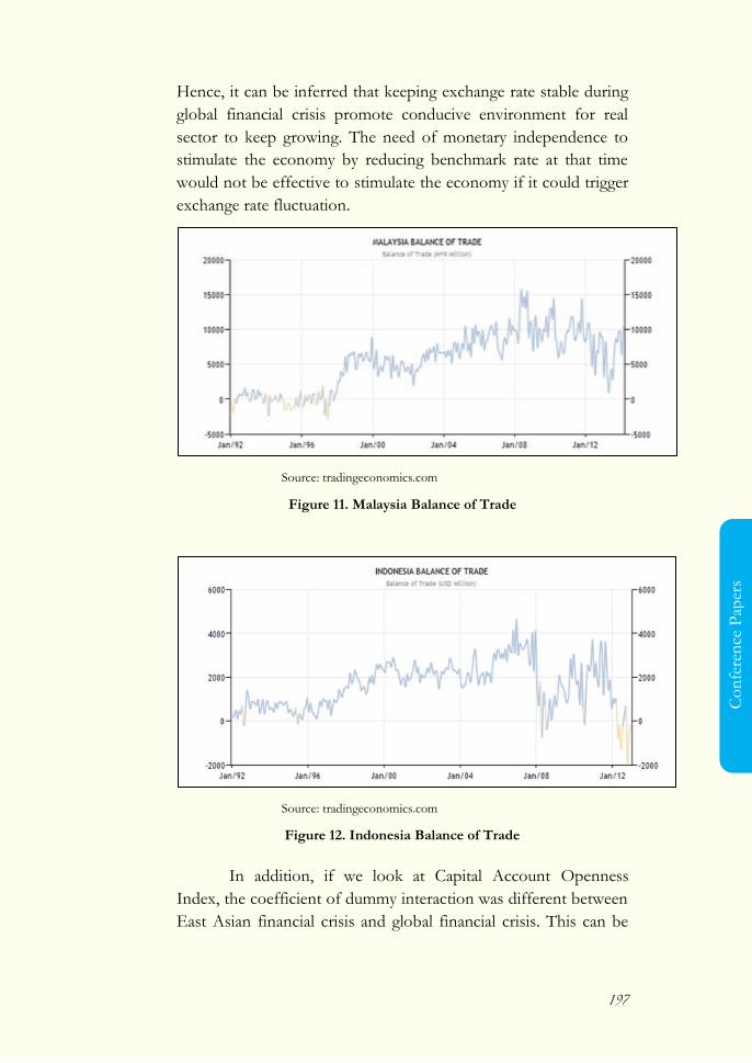
197

Co

nfe

ren

ce P

aper

s

Hence, it can be inferred that keeping exchange rate stable during

global financial crisis promote conducive environment for real

sector to keep growing. The need of monetary independence to

stimulate the economy by reducing benchmark rate at that time

would not be effective to stimulate the economy if it could trigger

exchange rate fluctuation.

Source: tradingeconomics.com

Figure 11. Malaysia Balance of Trade

Source: tradingeconomics.com

Figure 12. Indonesia Balance of Trade

In addition, if we look at Capital Account Openness

Index, the coefficient of dummy interaction was different between

East Asian financial crisis and global financial crisis. This can be

198

Co

nferen

ce Pap

ers

explained by analyzing the balance of payment of Southeast Asia

emerging market. Before East Asian financial crisis Indonesia,

Malaysia, Thailand, and Philippines suffer with trade deficit (see

Figure 11 and Figure 12). The financial openness during crisis only

leads toward instability in currency exchange. On the other hand,

those countries had been experiencing trade surplus after East

Asian financial crisis and financial openness was not affected the

capacity of those countries to maintain exchange rate stability.

5. CONCLUSION

Trilemma is a condition in which a country cannot attain all the

target of exchange rate stability, monetary independence and

financial openness. There are at least one or two targets which are

achievable. The experience of Southeast Asia emerging market

economy shows the capability of those countries to tackle the

effect of 1997 Asian financial crisis and global financial crisis in

2008. By using balanced panel data approach with data ranging

from 1980-2013, this study attempts to investigate the effect of

monetary independence, capital control and exchange rate stability

toward economic growth in Indonesia, Malaysia, Thailand and

Philippines as the Southeast Asia representative. According the

estimation result, there are some salient findings that need to be

highlighted:

1. The financial openness significantly affects the economic

growth of Southeast Asian emerging market with negative

coefficient. This negative coefficient indicates that capital

control, for some degree, positively affects the economic

growth of those countries. The role of capital control in this

sense is to reduce the volatility in the financial market and

lead to stabilization of economic condition.

2. During, the 1997 Asian financial crisis, there are none of the

variables which is significant toward economic growth.

However, the negative coefficient for monetary independence

and financial openness shows that both policies will worsen

the economic growth.

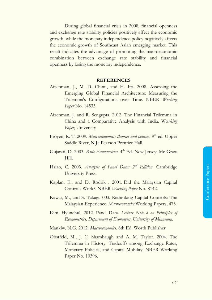
199

Co

nfe

ren

ce P

aper

s

During global financial crisis in 2008, financial openness

and exchange rate stability policies positively affect the economic

growth, while the monetary independence policy negatively affects

the economic growth of Southeast Asian emerging market. This

result indicates the advantage of promoting the macroeconomic

combination between exchange rate stability and financial

openness by losing the monetary independence.

REFERENCES

Aizenman, J., M. D. Chinn, and H. Ito. 2008. Assessing the

Emerging Global Financial Architecture: Measuring the

Trilemma's Configurations over Time. NBER Working

Paper No. 14533.

Aizenman, J. and R. Sengupta. 2012. The Financial Trilemma in

China and a Comparative Analysis with India. Working

Paper, University

Froyen, R. T. 2009. Macroeconomics: theories and policies. 9th ed. Upper

Saddle River, N.J.: Pearson Prentice Hall.

Gujarati, D. 2003. Basic Econometrics. 4th Ed. New Jersey: Mc Graw

Hill.

Hsiao, C. 2003. Analysis of Panel Data: 2nd Edition. Cambridge

University Press.

Kaplan, E., and D. Rodrik . 2001. Did the Malaysian Capital

Controls Work?. NBER Working Paper No. 8142.

Kawai, M., and S. Takagi. 003. Rethinking Capital Controls: The

Malaysian Experience. Macroeconomics Working Papers, 473.

Kim, Hyunchul. 2012. Panel Data. Lecture Note 8 on Principles of

Econometrics, Department of Economics, University of Minnesota.

Mankiw, N.G. 2012. Macroeconomics. 8th Ed. Worth Publisher

Obstfeld, M., J. C. Shambaugh and A. M. Taylor. 2004. The

Trilemma in History: Tradeoffs among Exchange Rates,

Monetary Policies, and Capital Mobility. NBER Working

Paper No. 10396.

200

Co

nferen

ce Pap

ers

Page, J. 1994. The East Asian Miracle: Four Lessons for

Development Policy. In Stanley F. and Julio. J. R. (Eds.),

NBER Book Series NEVER Macroeconomics Annual.

Cambridge: MIT Press.

Pyndick, R. S. and D. L. Rubenfield. 1998. Econometrics Models and

Economic Forecast. 4th Ed. Singapore: Mc Graw Hill.

Young, Warren and William Darity Jr. 2004. IS-LM-BP: An

Inquest. Journal of History of Political Economy, 36(5): 127-164.

201

Co

nfe

ren

ce P

aper

s

Current Account and Financial Stability

Driving Factors of Current Account Movement and Indonesian Financial Stability

Ni Putu Wiwin Setyari

Economics and Business Faculty, Universitas Udayana.

Address: Jalan P.B Sudirman, Denpasar, Bali, 80225. Email: wi2nset@yahoo.co.id

Abstract

The imbalance in the current account has been debated for a long

time. Deficits in the long term into often raises concern because

of the economic crisis is often preceded by a prolonged of current

account deficits. But keep in mind if the current account deficit is

not always caused by the inability of the economy to compete in

the global market which makes the value of imports greater than

exports. The current account deficit on the other side is a

reflection of the saving - domestic investment position in the

economy. If the deficit is caused by the position of investment

larger than savings, then this is a good indication for an economy.

The study in this paper shows if the Indonesian current account

movement can be divided into two episodes, which is a reflection

of saving - investment in the period before crisis in 1997, and a

reflection of export - import in the period after the crisis. Hence it

is important to see further how Indonesian current account ability

202

Co

nferen

ce Pap

ers

to overcome the existing shocks. Analysis used SVAR method

indicates that the exchange rate is a variable that gives the greatest

influence on the movement of Indonesian current account. The

ability of the current account Indonesia in overcoming the shocks

is quite weak, because of its ability to return to equilibrium pattern

are relatively takes long time.

Keywords: saving-investment approach, current account adjustment, open

economy, demographic effect

JEL Classification: E22, F32, F41, J11

1. INTRODUCTION

Financial stability is difficult to define and even more difficult to

measure. Strictly speaking, a financial system can be characterized

as stable in the absence of excessive volatility, stress or crises.

Policymakers and academic researchers have focused on a number

of quantitative measures in order to assess financial stability.

Basically, the measurement is focused on six sectors, one of which

can be accessed through the external sector reflected on the

exchange rate, foreign exchange reserves, current account and

capital flows (Gadanecz & Jayaram, 2008).

The imbalance in the current account balance has been

controversial in the analysis of international trade policy. Debates

which reflect back the David Hume theory with emphasis on the

current account balance as a potential tool in the international

transmission shocks or as financial vulnerability. Some evidence

indicates if a crisis is often preceded by the current account deficit

in large numbers, including in some developed countries (Obstfeld

M. , 2012).

Current account balance generally shows the difference

between exports and imports of goods (including services).

Intertemporal approach to the current account analysis widened in

the approach through private saving and investment decisions as

well as the government's decision as a result of forward based

calculation on expectations of future productivity growth, demand

for government spending, the real interest rate, and many more.

203

Co

nfe

ren

ce P

aper

s

Current account imbalances can be caused by a mismatch between

savings and investment. When the savings position lower than

expected investment, the foreign party will balance both. Period

magnitude of capital inflows are generally accompanied by

increased investment. The IMF itself has highlighted the need to

look at the movement of domestic savings and investment in

analyzing the current account phenomenon.

The question then arises whether the current account

deficit is a good or bad indication for an economy? If the deficit

reflects an excess of imports over exports, it may be indicative of

competitiveness problems, but because the current account deficit

also implies an excess of investment over savings, it could equally

be pointing to a highly productive, growing economy. If the deficit

reflects low savings rather than high investment, it could be

caused by reckless fiscal policy or a consumption binge. Or it

could reflect perfectly sensible intertemporal trade, perhaps

because of a temporary shock or shifting demographics. Without

knowing which of these is at play, it makes little sense to talk of a

deficit being ―good‖ or ―bad.‖ Deficits reflect underlying

economic trends, which may be desirable or undesirable for a

country at a particular point in time (Ghosh & Ramakrishnan,

2012).

Studies in five ASEAN countries, namely Malaysia,

Indonesia, Thailand, Philippines, and Singapore indicate if the

trade in manufactured goods trend in these countries, especially

Indonesia and Malaysia, provide surplus figures, but the current

account deficit remained during the period of the 1990s (Moreno,

2007). Export growth looks larger and more stable over the period

of the current account deficit compared to those experienced after

1996. of the Condition reversal of deficit to the surplus current

account is said does not reflects the strong export boost because

the opposite things happenned. Exports value in 1998 in almost

all samples becomes contracted. It suggested should be further

studies on the different dimensions of the current account to

explain it.

204

Co

nferen

ce Pap

ers

The position of Indonesia's current account itself

persistently deficit from early 1980s until then experienced a sharp

reversal in 1997. The current account surplus lasted until 2011,

before returning deficit. This study examines several variables

effects which are considered to encourage the Indonesian current

account movement. The equation systems in the model are

estimated by the Structural Vector Autoregressive (SVAR)

approach. This approach is interesting because it can still be based

on economic theories that exist on long-term relationships in a

model system, while the short-term dynamics can also be

estimated as within the VAR framework.

Structural Vector Autoregressive (SVAR) models are

frequently used to detect a relationship across macroeconomic

fundamentals because these models enable an analysis of how

current account responds to macroeconomic fundamentals

shocks. The use of the SVAR approach encounters some

restrictions imposed by economic theory in defining these shocks.

Tiwari et al (2015) attempt to test the relationship between budget

deficit and current account balance in Greece, from 1976 to 2009

using a structural autoregressive (SVAR) model. They find that in

case of Greece there is no long run relationship between budget

deficit and current account deficit either in the presence or in

absence of structural breaks in the data set. Further, impulse

response functions (IRFs) calculated shows that increase in budget

deficit increases the current account deficit, which is consistent

with the twin deficit hypothesis.

Lee and Chinn (1998) using SVAR to analysis the current

account and the real exchange rate for seven major industrialized

countries (the US, Canada, the UK, Japan, Germany, France, and

Italy). They find temporary shock which is associated with a

monetary innovation play a bigger role in explaining the variation

in the current account, except for the US. A permanent shock

which interprets as a technology innovation induces a permanent

appreciation of the real exchange rate. Except for UK, the

temporary shock depreciates the real exchange rate and improves

the current account balance.

205

Co

nfe

ren

ce P

aper

s

Both previous research showed the movement of the

current account is affected by shocks originating from fiscal and

monetary policy, but they do not show how the mechanism of the

shocks affecting the current account over savings or domestic

investment explicitly. Aquino and Espino (2013) examined the

Harberger-Laursen-Metzler (HLM) effect in Peru. The HLM

effect is the deterioration in the savings level of an economy due

to a decline in their terms of trade for a given level of investment.

This deterioration is caused by lower revenues which worsen the

current account. The results show that shocks to the terms of

trade and price of exports improve the current account through an

increase on the saving rate, but such effect vanishes as investment

increase faster than saving does. A similar shock to the price of

imports negatively affects the current account through the

deterioration of saving.

This study analyzes several factors that theoretically and

empirically said to affect the Indonesian current account

Indonesia. As mentioned earlier, surplus or deficit in the current

account can not mean good or bad without seeing what factors are

behind the movement. Therefore, the variables used here consider

their effects on international trade transactions and domestic

saving - investment movement. It is intended to provide a clearer

picture of the driving variable of the current account movement

and the strength of Indonesian current account handles various

shocks, especially external shocks.

The analysis shows if Indonesian current account is very

responsive to the various shocks that were tested in this study.

Exchange rate is a variable that had the highest impact and

persistently encourages the movement of Indonesian current

account. The result also shows if the Indonesian current account

tend to be more elastic as a result of an external shock that occurs

in real sector (output gap) than external shock that occurred in

monetary sector (real interest rate gap). But it must be underlined,

if the ability of Indonesian current account is relatively less

powerful in the face of existing shock because its pattern is need

relatively long time to the early equilibrium value. The paper is

organized as follows. The first part is an introduction. The second

206

Co

nferen

ce Pap

ers

part shows the literature review. The third part contains data and

methodology used. Section four contains the result and analysis,

and conclusions on the fifth.

2. LITERATURES

2.1 Key Financial Stability Definition: A Brief Review

In recent years, financial stability issues have been receiving

priority attention from policy makers around the world. One main

catalyst for this trend was the East Asian financial crisis of the late

1990s. Following that turmoil, the World Bank and the

International Monetary Fund (IMF) introduced the Financial

Sector Assessment Program (FSAP) in 1999, aimed at assessing

regularly the strengths and weaknesses of financial systems in their

member countries (Alawode & Al Sadek, 2008). Despite this

increased focus on financial stability issues, it is notable that a

widely accepted definition of ―financial stability‖ does not exist

and the concept has generated a fair amount of debate among

academics, market participants and policy makers. This difficulty is

often explained by the relative infancy of the field of financial

stability, compared to the analysis of price or monetary stability

which has a much longer history.

Two schools of thought are clearly discernible in the

literature: first, writers who prefer to define financial instability.

Davis (2003) define financial instability or disorder as entailing

heightened risk of a financial crisis as a major collapse of the

financial system, entailing inability to provide payments services or

to allocate credit to productive investment opportunities. Davis

stressed that the crisis will in turn have a major impact on the

overall economy. Mishkin (1999) states that financial instability

occurs when shocks to the financial system interfere with

information flow so that the financial system can no longer do its

job of channeling funds to those with productive investment

opportunities. Both stressed that financial instability occurs when

there is an inability to perform duties of the financial system in

allocating funds on productive investment opportunities.Second,

writers who attempt to define financial stability.

207

Co

nfe

ren

ce P

aper

s

Petrovska and Mihajlovska (2013) using the definition of

the National Bank of the Republic of Macedonia which defines

financial stability as the requirement for smooth operation of all

segments of the financial system, with each of them providing the

highest possible level of flexibility to absorb potential shocks.

Simpler definition used by Gadanecz and Jayaram (2008) yang

menyatakan a financial system can be characterized as stable in the

absence of excessive volatility, stress or crises. But they also

underline if this narrow definition is relatively simple to formulate,

but fails to capture the positive contribution of a well-functioning

financial system to overall economic performance. They also

mention broader definitions of financial stability encompass the

smooth functioning of a complex nexus of relationships among

financial markets, infrastructures and institutions operating within

the given legal, fiscal and accounting frameworks. Fundamental

similarities between the two indicate if the financial stability or

flexibility characterized by the ability of the financial system to

absorb various shocks, volatility, or crisis.

Stakeholders have focused on a number of quantitative

measures in order to assess financial stability. Gadanecz and

Jayaram (2008) summarizes the measures commonly used in the

literature, their frequency, what they measure, as well as their

signaling properties.

1) the real sector is described by GDP growth, the fiscal position

of the government and inflation. GDP growth reflects the

ability of the economy to create wealth and its risk of

overheating. The fiscal position of the government mirrors its

ability to find financing for its expenses above its revenue (and

the associated vulnerability of the country to the unavailability

of financing). Inflation may indicate structural problems in the

economy, and public dissatisfaction with it may in turn lead to

political instability.

2) the corporate sector’s riskiness can be assessed by its leverage and

expense ratios, its net foreign exchange exposure to equity and

the number of applications for protection against creditors.

3) the household sector‘s health can be gauged through its net assets

(assets minus liabilities) and net disposable income (earnings

208

Co

nferen

ce Pap

ers

minus consumption minus debt service and principal

payments). Net assets and net disposable earnings can measure

households‘ ability to weather (unexpected) downturns.

4) The conditions in the external sector are reflected by real

exchange rates, foreign exchange reserves, the current account,

capital flows and maturity/currency mismatches. These

variables can be reflective of sudden changes in the direction

of capital inflows, of loss of export competitiveness, and of

the sustainability of the foreign financing of domestic debt.

5) the financial sector is characterized by monetary aggregates, real

interest rates, risk measures for the banking sector, banks‘

capital and liquidity ratios, the quality of their loan book,

standalone credit ratings and the concentration/systemic focus

of their lending activities. All these proxies can be reflective of

problems in the banking or financial sector and, if a crisis

occurs, they can gauge the cost of such a crisis to the real

economy.

6) variables that are relevant to describe conditions on financial

markets are equity indices, corporate spreads, liquidity premia

and volatility. High levels of risk spreads can indicate a loss of

investors‘ risk appetite and possibly financing problems for

the rest of the economy. Liquidity disruptions may be a

materialization of the market‘s ability to efficiently allocate

surplus funds to investment opportunities within the

economy.

Typically financial stability analysis would use several

sectoral variables either individually or in combinations. The use

of such measures including the financial soundness indicators as

key indicators of financial stability depends on the benchmarks

and thresholds which would characterize their behavior in normal

times and during periods of stress. In the absence of benchmarks,

the analysis of these measures would depend on identifying

changes in trend, major disturbances and other outliers (Worrell,

2004)

209

Co

nfe

ren

ce P

aper

s

2.2 Current Account and International Capital Flows

Position

Theoretically, the current account not only exports minus imports

but also net capital gains on existing foreign assets (Obstfeld &

Rogoff, 1995). The current account also shows the position of

national saving minus domestic investment. If savings is lower

than expected investment, foreigners will balance both.

Balance of payments and data associated with international

investment position conceptually have very close relationship with

recording system of national account balance. National account

balance provides a framework that is more comprehensive and

systematic in collection and presentation of economic statistics

(International Monetary Fund, 1993). The relationship between

aggregate economic accounts and balance of payments flows can

be summarized in terms of saving-investment (International

Monetary Fund, 2009).

(1)

where: C is private consumption expenditure; G = government

consumption expenditure; I = gross domestic investment; S =

gross saving; X = exports of goods and services; and M = imports

of goods and services.

Gross national disposable income (GNDY) definition is

GDP added by net income from abroad:

(.2)

where: BPI is balance on primary income and BSI is balance on

secondary income (net current transfers).

Current account becomes:

(3)

Current account balance can be seen in proportion to the

difference between disposable income and expenditure.

(4)

or

(5)

210

Co

nferen

ce Pap

ers

Definition used in the System of National Accounts (SNA) on revenue

account:

(6)

Substitution of equation (5) in equation (6):

(7)

or:

(8)

It can be seen if the current account balance is the

difference between saving and investment, so that the current

account balance is a reflection of the behavior of saving and

investment in the economy.

Analysis of current account balance change in an economy

is important to pay attention to changes that reflect the savings

and investment movement. For example, an increase in

investment relative to savings would be the same effect on the

current account as well as a decrease in savings relative to

investment, at least in the short term. Long-term implications for

the external economy could be slightly different. Identity above

generally indicates if any change in the current account of an

economy (e.g., enlargement of the surplus or deficit shrinks) is

essentially proportional to the increase in savings relative to

investment. This relationship demonstrates the importance of the

implementation of policies that can be designed to change the

current account directly (for example, changes in tariffs, quotas,

and exchange rates) that affect the saving and investment

behavior.

The relationship between domestic transactions and

international identity shown in equation (2.4). The implications of

this relationship to the analysis of the balance of payments is an

increase in the current account of a country requires a reduction in

spending relative to income. Alternatively, it is possible to improve

the position of the current account balance by increasing the

national income which is not in accordance with the increase in

consumption or an increase in domestic investment.

211

Co

nfe

ren

ce P

aper

s

Implementation of structural measurements of increased

economic efficiency could be one way to achieve that goal.

The other important point is shown on the above identity

that are more indicative of the relationship between variables

definition compared than the of economic agents behavior

explanation. Identity above alone cannot provide a complete

analysis of the factors that determine the current account

development. For example, total expenditure on goods and

services by domestic residents (C + G + I) seem affected by the

part of their income (GNDY). Therefore the analysis of GNDY

changes effects to current account balance is not enough only use

equation (2.4) identity without considering the inclusion of

consumption and capital formation responses in these changes.

The illustration shows the importance of understanding the

population expenditure part in an economy when analyzing the

balance of payments.

International capital flows can be divided into two types

(Ju & Wei, 2006), namely: 1) the flow of financial capital are

decided by the investor, and 2) foreign direct investment which is

determined by the employer. The flow of financial capital occurs

when investors invest their resources into the international

financial markets or directly into an activity carried out by foreign

businessmen. Foreign direct investment on the other hand occurs

when employers engage in activities outside the country and

produce there. Investors will invest in countries with higher

interest rates, while entrepreneurs will put their activities in

countries with lower production costs.

Capital flows will be determined by: rrrr /ˆ * , where

r* is the yield of capital abroad and r is the yield on domestic

capital. If ̂ > 0, financial capital moves from domestic to

overseas. A country that is relatively rich in labor has an interest

rate (r) higher if it domestic financial sector is more developed or

have a smaller risk.

Lucas using one sector model expressed the paradox when

a lot of capital does not move from rich countries to poor

countries (Ju & Wei, 2006). Because of free trade, the prices of

212

Co

nferen

ce Pap

ers

goods will be balanced in all countries. The law of diminishing

returns resulting higher r in countries with smaller capital per

capita. The difference yields value to be a reason the flow of

capital from rich countries to poor countries. The conditions did

not happen so called Lucas paradox.

The standard model Heckscher-Ohlin-Samuelson known

as the model of 2x2x2 (two goods, two factors of production, and

two countries), indicates if any company would earn zero profit:

p1 = c1 (w; r) dan p2 = c2 (w; r) (9)

where c(. ) is a cost per unit function. On given particular product

prices, the value of w and r are determined by L and K factors

resources owned by the country. Improved K alter the

composition of the product. Capital-intensive goods produced

more and the opposite occurs for labor-intensive goods. Marginal

yield on physical capital in each sector have not changed. Free

trade will balance products prices and thus balancing factors

return in each country even though there are no international

factor movements. Capital flows is fully substituted by trading in

goods.

The capital flows into developing countries are caused by

several factors (Indawan et al., 2013). The high degree of financial

integration in line with the rapid development of technology,

especially information and communication technologies play a

major role in accelerating the increased of capital flows mobility.

Capital market infrastructure development, along with capital

market liberalization such as the elimination of barriers to the

repatriation, reduction of participation barriers, and foreign

ownership also contribute to the expansion of capital flows to

emerging markets.

Theoretically, the relationship between trade and capital

liberalization is not straightforward. Economic integration on the

one hand increases the demand and new investment opportunities

as well as the importance of reallocating capital makes domestic

financial development become more relevant. On the other hand,

the integration allows some of the tradable sector gain greater

213

Co

nfe

ren

ce P

aper

s

accesses to international capital markets which make the local

financial system become less relevant (Braun & Raddatz, 2007).

The current account deficit is the result of consumption

and savings decision in an open economy with the capital flow

possibility (Calvo et al., 1996). The model developed from Irving

Fisher model derivation indicates that changes in interest rates

pushed the income effect and the substitution effect. For a debtor

country, decrease in interest rates led to the expansion of

consumption and increasingly current account deficit. Declines in

interest rates mean lower net debt present value which gives a

positive income effect. Meanwhile the substitution effect occurs

because the debt becomes cheaper so that consumption increased.

In an open economy model, the increase in capital flows tend to

be accompanied by increased of consumption and investment,

which in turn increase the current account deficit.

Empirical studies conducted by Bosworth and Collins

(1999) found that a large portion of capital flows to developing

countries are used to finance current account deficit, which means

the transfer of capital flows directly intended for investment,

rather than consumption. The results of their study showed that

there are significant differences between various types of capital

flows on investment. Foreign direct investment has a large effect

on domestic investment, but instead in the form of portfolio

capital seems to have no impact. Capital flows in the form of

loans or debts fall somewhere in between.

3. METHODOLOGY

3.1 Estimation Technique

Structural vector autoregression (SVAR) models have become a

popular tool in recent years in the analysis of the monetary

transmission mechanism and sources of business cycle

fluctuations. The identification problem is the same as that in a

dynamic simultaneous equation model, but SVAR models take

another approach to achieve identification by focusing on the role

of shocks for the dynamics of the model. This approach avoids

214

Co

nferen

ce Pap

ers

some of the difficulties inherent in the traditional approach to

identification, but it also implies that SVAR models cannot

perform the same tasks as dynamic simultaneous equation models.

In the field of monetary economics, for example, SVAR models

are not well suited for policy simulation, which is a strength of the

dynamic simultaneous equation models, but have instead an

advantage in the analysis of the monetary transmission mechanism

(Gottschalk, 2001).

The structural VAR model continues to be the most

popular tool used by researchers in empirical investigation, for

three major reasons. First, it can be easily used to investigate the

average response of the model variables to a given one-time

structural shock. Second, it allows the construction of forecast

error variance decompositions that quantify the average

contribution of a given structural shock to the variability of the

data. Third, it can be used to provide historical decompositions

that measure the cumulative contribution of each structural shock

to the evolution of each variable over time. Historical

decompositions are essential, for example, in understanding the

dynamics of current account deficit spikes in the data

(Nikolaychuk & Shapovalenko, 2013).

Main requirement that must be met to use SVAR model is

data free from the of autocorrelation and heteroscedasticity

problems. LM autocorrelation testing method shows if there is

serial correlation at lag 1, but the serial correlation at lag 2 and so

on significantly accept the nul hypothesis (no serial correlation). The

White heteroscedasticity method result shows chi-square value

amounted to 520.0856 which can not reject the hypothesis of no

cross terms. Therefore it can be concluded if the estimates are free

of both issues.

3.2 Data Description and Unit Root

All data are taken from the World Bank World Development

Indicators. We use data of ( ) i.e. the gap between world

real output and domestic in the natural logarithm, ( )

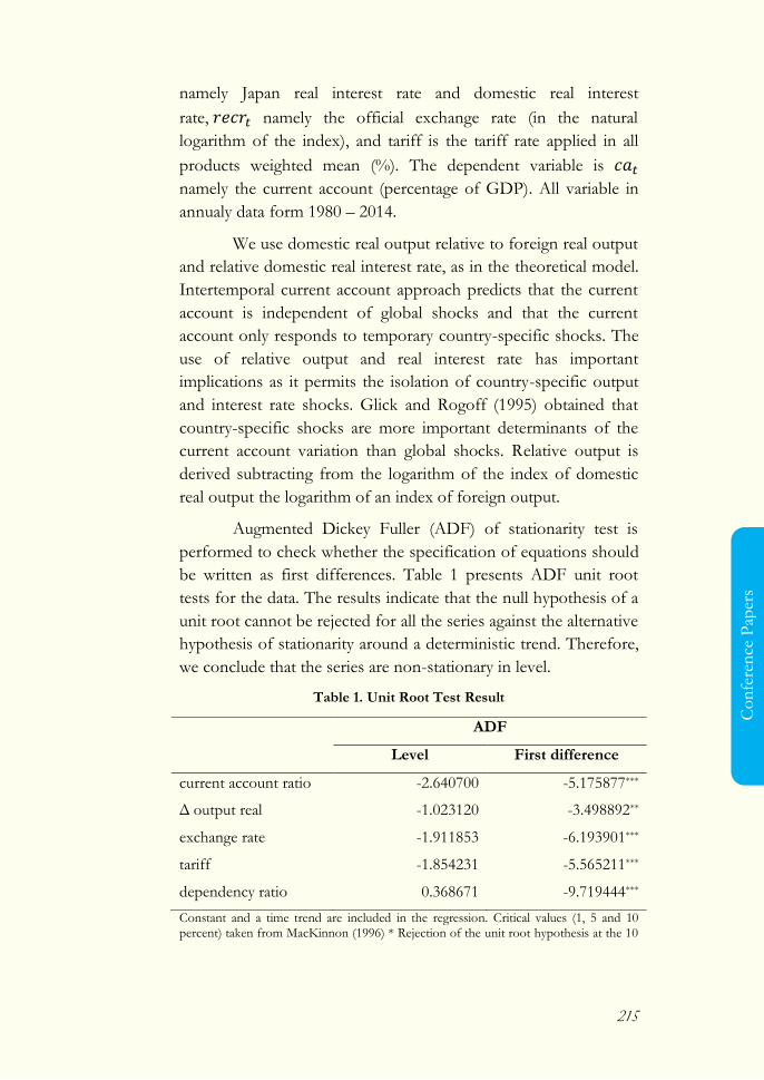
215

Co

nfe

ren

ce P

aper

s

namely Japan real interest rate and domestic real interest

rate, namely the official exchange rate (in the natural

logarithm of the index), and tariff is the tariff rate applied in all

products weighted mean (%). The dependent variable is

namely the current account (percentage of GDP). All variable in

annualy data form 1980 – 2014.

We use domestic real output relative to foreign real output

and relative domestic real interest rate, as in the theoretical model.

Intertemporal current account approach predicts that the current

account is independent of global shocks and that the current

account only responds to temporary country-specific shocks. The

use of relative output and real interest rate has important

implications as it permits the isolation of country-specific output

and interest rate shocks. Glick and Rogoff (1995) obtained that

country-specific shocks are more important determinants of the

current account variation than global shocks. Relative output is

derived subtracting from the logarithm of the index of domestic

real output the logarithm of an index of foreign output.

Augmented Dickey Fuller (ADF) of stationarity test is

performed to check whether the specification of equations should

be written as first differences. Table 1 presents ADF unit root

tests for the data. The results indicate that the null hypothesis of a

unit root cannot be rejected for all the series against the alternative

hypothesis of stationarity around a deterministic trend. Therefore,

we conclude that the series are non-stationary in level.

Table 1. Unit Root Test Result

ADF

Level First difference

current account ratio -2.640700 -5.175877***

Δ output real -1.023120 -3.498892**

exchange rate -1.911853 -6.193901***

tariff -1.854231 -5.565211***

dependency ratio 0.368671 -9.719444***

Constant and a time trend are included in the regression. Critical values (1, 5 and 10 percent) taken from MacKinnon (1996) * Rejection of the unit root hypothesis at the 10

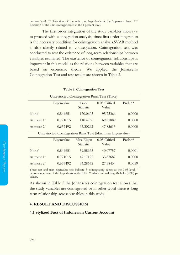
216

Co

nferen

ce Pap

ers

percent level. ** Rejection of the unit root hypothesis at the 5 percent level. *** Rejection of the unit root hypothesis at the 1 percent level.

The first order integration of the study variables allows us

to proceed with cointegration analysis, since first order integration

is the necessary condition for cointegration analysis.SVAR method

is also closely related to cointegration. Cointegration test was

conducted to test the existence of long-term relationships between

variables estimated. The existence of cointegration relationships is

important in this model as the relations between variables that are

based on economic theory. We applied the Johansen's

Cointegration Test and test results are shown in Table 2.

Table 2. Cointegration Test

Unrestricted Cointegration Rank Test (Trace)

Eigenvalue Trace Statistic

0.05 Critical Value

Prob.**

None* 0.844651 170.0603 95.75366 0.0000

At most 1* 0.771015 110.4736 69.81889 0.0000

At most 2* 0.657492 63.30242 47.85613 0.0000

Unrestricted Cointegration Rank Test (Maximum Eigenvalue)

Eigenvalue Max-Eigen Statistic

0.05 Critical Value

Prob.**

None* 0.844651 59.58665 40.07757 0.0001

At most 1* 0.771015 47.17122 33.87687 0.0008

At most 2* 0.657492 34.28672 27.58434 0.0059

Trace test and max-eigenvalue test indicate 3 cointegrating eqn(s) at the 0.05 level. *

denotes rejection of the hypothesis at the 0.05. ** MacKinnon-Haug-Michelis (1999) p-values.

As shown in Table 2 the Johansen's cointegration test shows that

the study variables are cointegrated or in other word there is long

term relationship across variables in this study.

4. RESULT AND DISCUSSION

4.1 Stylized Fact of Indonesian Current Account

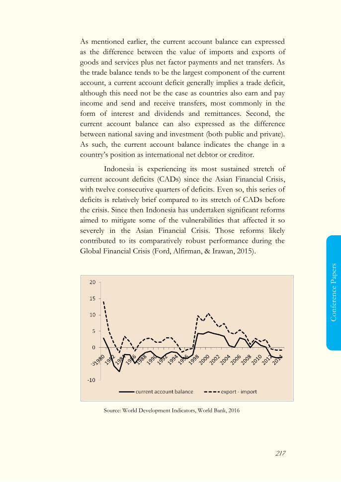
217

Co

nfe

ren

ce P

aper

s

As mentioned earlier, the current account balance can expressed

as the difference between the value of imports and exports of

goods and services plus net factor payments and net transfers. As

the trade balance tends to be the largest component of the current

account, a current account deficit generally implies a trade deficit,

although this need not be the case as countries also earn and pay

income and send and receive transfers, most commonly in the

form of interest and dividends and remittances. Second, the

current account balance can also expressed as the difference

between national saving and investment (both public and private).

As such, the current account balance indicates the change in a

country‘s position as international net debtor or creditor.

Indonesia is experiencing its most sustained stretch of

current account deficits (CADs) since the Asian Financial Crisis,

with twelve consecutive quarters of deficits. Even so, this series of

deficits is relatively brief compared to its stretch of CADs before

the crisis. Since then Indonesia has undertaken significant reforms

aimed to mitigate some of the vulnerabilities that affected it so

severely in the Asian Financial Crisis. Those reforms likely

contributed to its comparatively robust performance during the

Global Financial Crisis (Ford, Alfirman, & Irawan, 2015).

Source: World Development Indicators, World Bank, 2016

218

Co

nferen

ce Pap

ers

Figure 1. Indonesian Current Account Expressed as Export - Import Difference (% of GDP)

Figure 1 shows Indonesian current account which

expressed as exports and imports difference (net trade balance).

Prior to 1997, the Indonesian current account deficit prolonged

although Indonesia tend to experience a surplus in its trade

balance during this period. This phenomenon is similar to those

presented by Moreno (2007). At the time of the financial crisis in

mid-1997, the current account Indonesia crept up and is always a

surplus after it. In 1997/1998 countries in Asia have to face the

economic crisis that started with the collapse of the Thai Baht.

Indonesia among the countries worst affected. According to the

agreement with the International Monetary Fund (IMF),

significant reforms to trade policies are taken to reduce tariff and

non tariff barriers and encourage exports. The government

lowered various import tariffs, eliminate trade obstacles affecting

import licensing, trade monopoly, and marketing agreements.

Government is also committed to eliminate export taxes and

export obstacles gradually. Plus a very sharp depreciation of the

rupiah against the dollar makes exports become fueled ride.

Indonesia‘s current account fell into deficit in late 2011 for

the first time since the 1997/8 crisis. Current account decline in

this time is said to be due deterioration happening in the balance

in goods and services trade. The recent shift into deficit has been

based on two structural developments and a combination of

adverse exogenous and policy shocks (Varela, Nedeljkovic, &

Savini Zangrandi, 2015). First, since the early 2000s Indonesia‘s

economy has grown faster than its major trading partners. Second,

while investment growth has been generally strong, gross national

saving have stagnated around 32 percent of GDP since 2009,

dropping to 30 percent in 2013. Third, Indonesia was hit by a

major terms of trade shock as the end of a decade-long

commodity ―super-cycle‖ hit exports prices, leading to a sizable

drop in the value of Indonesia‘s commodity exports. The shock

was compounded, until mid-2014, by sustained high oil prices

relative to non-oil commodities and strong domestic demand for

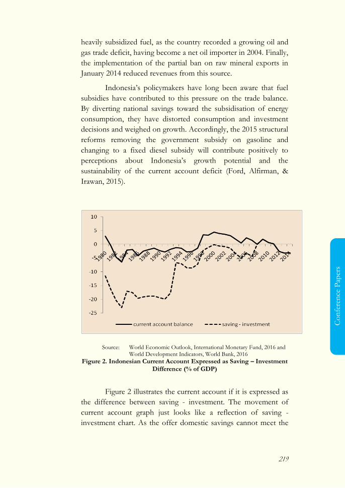
219

Co

nfe

ren

ce P

aper

s

heavily subsidized fuel, as the country recorded a growing oil and

gas trade deficit, having become a net oil importer in 2004. Finally,

the implementation of the partial ban on raw mineral exports in

January 2014 reduced revenues from this source.

Indonesia‘s policymakers have long been aware that fuel

subsidies have contributed to this pressure on the trade balance.

By diverting national savings toward the subsidisation of energy

consumption, they have distorted consumption and investment

decisions and weighed on growth. Accordingly, the 2015 structural

reforms removing the government subsidy on gasoline and

changing to a fixed diesel subsidy will contribute positively to

perceptions about Indonesia‘s growth potential and the

sustainability of the current account deficit (Ford, Alfirman, &

Irawan, 2015).

Source: World Economic Outlook, International Monetary Fund, 2016 and World Development Indicators, World Bank, 2016

Figure 2. Indonesian Current Account Expressed as Saving – Investment Difference (% of GDP)

Figure 2 illustrates the current account if it is expressed as

the difference between saving - investment. The movement of

current account graph just looks like a reflection of saving -

investment chart. As the offer domestic savings cannot meet the

220

Co

nferen

ce Pap

ers

needs of investment, capital inflows from abroad will balance

these two. These results are similar to the of Ford (2015) and

Varela (2015) opinions which emphasizes if at a high level, the

reduction in the current account balance is due to a combination

of very strong private investment and public sector dissaving. A

current account deficit itself is merely reflective of the economy-

wide set of investment and consumption possibilities and is not

inherently problematic. When viewed in this light, the issue of the

‗sustainability‘ of the current account deficit is moot, as long as it

is the result of productive consumption and investment decisions

then, in aggregate, the external position ought to be ‗sustainable.

A comparative look of the two figures, the movement of

Indonesian current account can be said experienced two waves. In

the early 1980s until the phase prior to the crisis, Indonesian

current account deficit is due to the large investment needs

compared to domestic savings that are not able to fulfill, so that

the flow of foreign capital needed to finance the development.

After the financial crisis in 1997an, the current account is more

driven by the trade balance and its contributing factors, including

the terms of trade and oil subsidies.

As the current account turned negative, financing has

come to rely increasingly on portfolio and ―other‖ investments (as

opposed to foreign direct investment), exposing Indonesia to

short-term financing constraints. Short-term external funding

pressures could therefore emerge not only from a reduction in the

availability of external financing relative to the current account

deficit, but also external debt amortizations (Ford, Alfirman, &

Irawan, 2015).

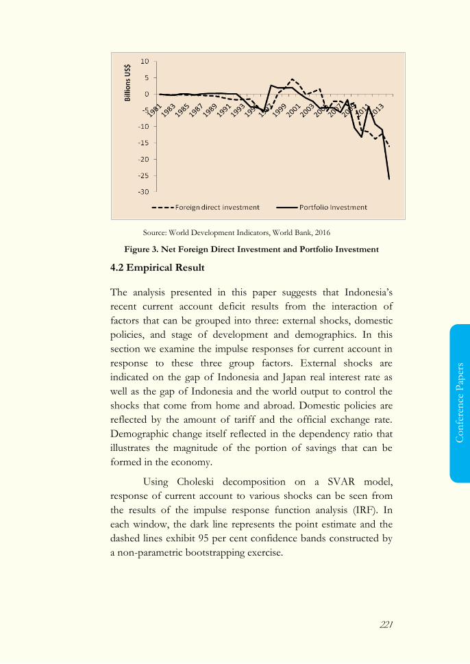
221

Co

nfe

ren

ce P

aper

s

Source: World Development Indicators, World Bank, 2016

Figure 3. Net Foreign Direct Investment and Portfolio Investment

4.2 Empirical Result

The analysis presented in this paper suggests that Indonesia‘s

recent current account deficit results from the interaction of

factors that can be grouped into three: external shocks, domestic

policies, and stage of development and demographics. In this

section we examine the impulse responses for current account in

response to these three group factors. External shocks are

indicated on the gap of Indonesia and Japan real interest rate as

well as the gap of Indonesia and the world output to control the

shocks that come from home and abroad. Domestic policies are

reflected by the amount of tariff and the official exchange rate.

Demographic change itself reflected in the dependency ratio that

illustrates the magnitude of the portion of savings that can be

formed in the economy.

Using Choleski decomposition on a SVAR model,

response of current account to various shocks can be seen from

the results of the impulse response function analysis (IRF). In

each window, the dark line represents the point estimate and the

dashed lines exhibit 95 per cent confidence bands constructed by

a non-parametric bootstrapping exercise.

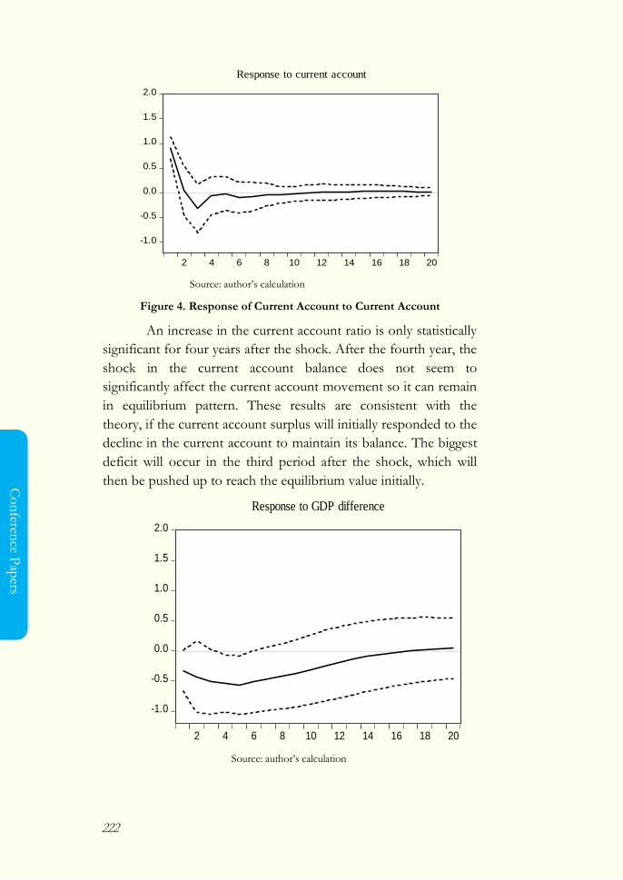
222

Co

nferen

ce Pap

ers

Source: author‘s calculation

Figure 4. Response of Current Account to Current Account

An increase in the current account ratio is only statistically

significant for four years after the shock. After the fourth year, the

shock in the current account balance does not seem to

significantly affect the current account movement so it can remain

in equilibrium pattern. These results are consistent with the

theory, if the current account surplus will initially responded to the

decline in the current account to maintain its balance. The biggest

deficit will occur in the third period after the shock, which will

then be pushed up to reach the equilibrium value initially.

Source: author‘s calculation

-1.0

-0.5

0.0

0.5

1.0

1.5

2.0

2 4 6 8 10 12 14 16 18 20

Response to current account

-1.0

-0.5

0.0

0.5

1.0

1.5

2.0

2 4 6 8 10 12 14 16 18 20

Response to GDP difference

223

Co

nfe

ren

ce P

aper

s

Figure 5. Response of Current Account to GDP Difference

GDP difference is gap between world output and domestic

output. As mentioned earlier, this variable intended to counter the

influence of global shocks by controlling country specific shock.

The increase in world output (relative to domestic output) initially

pushed the deficit in the current account and statistically

significant until the fifth year before returning pushed the current

account surplus. The response shown by the current account

balance as a result of shock on output gap tends to be slow and

smooth running.

Tariff effect looks more ambiguous than two previous

shock effects. In the short term, the increase in tariffs will lead to

a surplus in the current account, although only for two periods.

This could be due to the tariff, the domestic industry can be

protected and encourage more exports. However, the tariff policy

cannot always bring in surplus. The highest surplus will be

received in the second or eleventh periods, and the current

account return to deficit slowly. This result confirms if the tariff

policy does not provide a positive influence on the current

account movement, because it will reduce the performance of

international trade and comparative advantage of Indonesia's

export products in the world market. Moreover, with the

deepening of Indonesian market integration with the global

international trade.

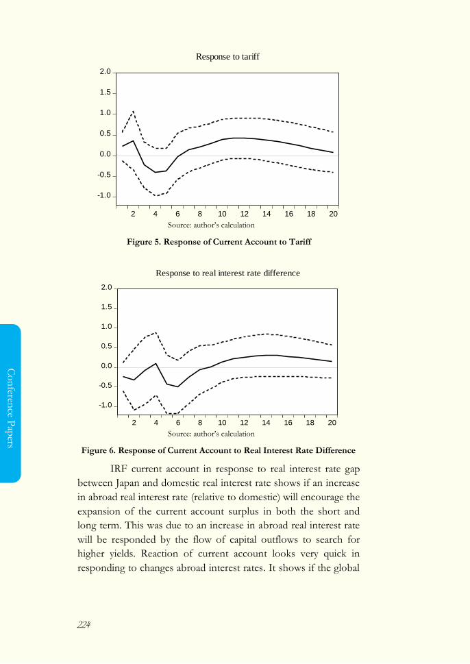
224

Co

nferen

ce Pap

ers

Source: author‘s calculation

Figure 5. Response of Current Account to Tariff

Source: author‘s calculation

Figure 6. Response of Current Account to Real Interest Rate Difference

IRF current account in response to real interest rate gap

between Japan and domestic real interest rate shows if an increase

in abroad real interest rate (relative to domestic) will encourage the

expansion of the current account surplus in both the short and

long term. This was due to an increase in abroad real interest rate

will be responded by the flow of capital outflows to search for

higher yields. Reaction of current account looks very quick in

responding to changes abroad interest rates. It shows if the global

-1.0

-0.5

0.0

0.5

1.0

1.5

2.0

2 4 6 8 10 12 14 16 18 20

Response to tariff

-1.0

-0.5

0.0

0.5

1.0

1.5

2.0

2 4 6 8 10 12 14 16 18 20

Response to real interest rate difference

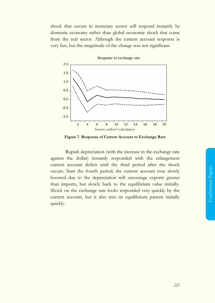
225

Co

nfe

ren

ce P

aper

s

shock that occurs in monetary sector will respond instantly by

domestic economy rather than global economic shock that come

from the real sector. Although the current account response is

very fast, but the magnitude of the change was not significant.

Source: author‘s calculation

Figure 7. Response of Current Account to Exchange Rate

Rupiah depreciation (with the increase in the exchange rate

against the dollar) instantly responded with the enlargement

current account deficit until the third period after the shock

occurs. Start the fourth period, the current account rose slowly

boosted due to the depreciation will encourage exports greater

than imports, but slowly back to the equilibrium value initially.

Shock on the exchange rate looks responded very quickly by the

current account, but it also into its equilibrium pattern initially

quickly.

-1.0

-0.5

0.0

0.5

1.0

1.5

2.0

2 4 6 8 10 12 14 16 18 20

Response to exchange rate

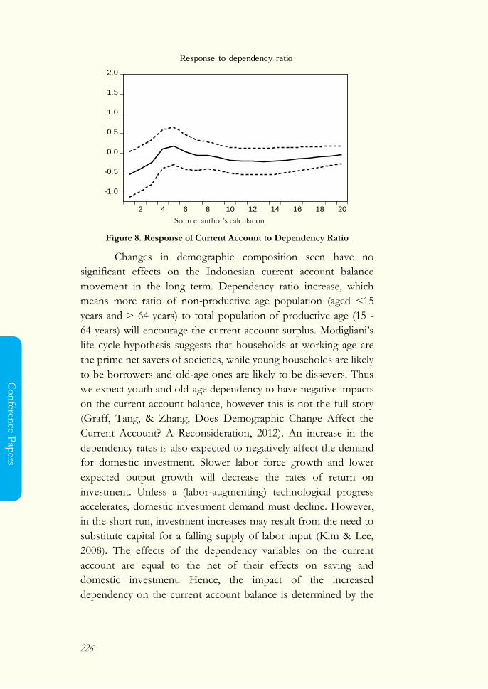
226

Co

nferen

ce Pap

ers

Source: author‘s calculation

Figure 8. Response of Current Account to Dependency Ratio

Changes in demographic composition seen have no

significant effects on the Indonesian current account balance

movement in the long term. Dependency ratio increase, which

means more ratio of non-productive age population (aged <15

years and > 64 years) to total population of productive age (15 -

64 years) will encourage the current account surplus. Modigliani‘s

life cycle hypothesis suggests that households at working age are

the prime net savers of societies, while young households are likely

to be borrowers and old-age ones are likely to be dissevers. Thus

we expect youth and old-age dependency to have negative impacts

on the current account balance, however this is not the full story

(Graff, Tang, & Zhang, Does Demographic Change Affect the

Current Account? A Reconsideration, 2012). An increase in the

dependency rates is also expected to negatively affect the demand

for domestic investment. Slower labor force growth and lower

expected output growth will decrease the rates of return on

investment. Unless a (labor-augmenting) technological progress

accelerates, domestic investment demand must decline. However,

in the short run, investment increases may result from the need to

substitute capital for a falling supply of labor input (Kim & Lee,

2008). The effects of the dependency variables on the current

account are equal to the net of their effects on saving and

domestic investment. Hence, the impact of the increased

dependency on the current account balance is determined by the

-1.0

-0.5

0.0

0.5

1.0

1.5

2.0

2 4 6 8 10 12 14 16 18 20

Response to dependency ratio

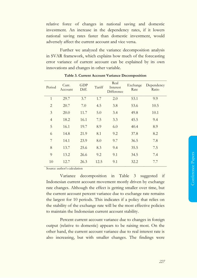
227

Co

nfe

ren

ce P

aper

s

relative force of changes in national saving and domestic

investment. An increase in the dependency rates, if it lowers

national saving rates faster than domestic investment, would

adversely affect the current account and vice versa.

Further we analyzed the variance decomposition analysis

in SVAR framework, which explains how much of the forecasting

error variance of current account can be explained by its own

innovations and changes in other variable.

Table 3. Current Account Variance Decomposition

Period Curr.

Account GDP Diff.

Tariff Real

Interest Difference

Exchange Rate

Dependency Ratio

1 29.7 3.7 1.7 2.0 53.1 9.9

2 20.7 7.0 4.5 3.8 53.6 10.5

3 20.0 11.7 5.0 3.4 49.8 10.1

4 18.2 16.1 7.5 3.3 45.5 9.4

5 16.1 19.7 8.9 6.0 40.4 8.9

6 14.8 21.9 8.1 9.2 37.8 8.2

7 14.1 23.9 8.0 9.7 36.5 7.8

8 13.7 25.6 8.3 9.4 35.5 7.5

9 13.2 26.6 9.2 9.1 34.5 7.4

10 12.7 26.3 12.5 9.1 32.2 7.7

Source: author‘s calculation

Variance decomposition in Table 3 suggested if

Indonesian current account movement mostly driven by exchange

rate changes. Although the effect is getting smaller over time, but

the current account percent variance due to exchange rate remains

the largest for 10 periods. This indicates if a policy that relies on

the stability of the exchange rate will be the most effective policies

to maintain the Indonesian current account stability.

Percent current account variance due to changes in foreign

output (relative to domestic) appears to be raising most. On the

other hand, the current account variance due to real interest rate is

also increasing, but with smaller changes. The findings were

228

Co

nferen

ce Pap

ers

similar to the results of Ferrero et al (2008) analysis which states

that international variables behavior (one of which is the current

account) are relatively insensitive to changes in monetary, unlike

what happened in real variables such as output and inflation. In

terms of the elasticity of the current account changes caused by

changes in monetary variables (real interest rate) is relatively

smaller than if there is a change in the real sector (output).

A change in tariff is the most minor shocks influence in

the current account balance, especially in the short term.

Notwithstanding the effects of tariff in the long run will be even

greater. This indicates if the process of trade and economic

integration will have a significant effect on the Indonesian

economy, though the effect is not instant. Dependency ratio has a

relatively large influence on the Indonesian current account

movement, but tends not effects significantly.

5. CONCLUSION

Financial stability is difficult to define but generally speaking if

financial system stability can be characterized as stable in the

absence of excessive volatility, stress or crises. Basically

measurement is focused on six sectors, one of which can be

accessed through the external sector is reflected through the

current account as analyzed in this paper. The method used is

SVAR meant to see how the Indonesian current account response

to the existing shocks.

Variables which indicated be shocks here is the official

rupiah exchange rate against the dollar, the gap between the

world's output to domestic output, real interest rate gap between

world (in this case Japan) with domestic, tariff, and the

dependency rate ratio. The whole variables are to accommodate

the possibility of the current account movement phenomenon

from two different viewpoints, namely the import - export and

saving - investment. Since the factors that are likely affect the

position of these two need to be analyzed further.

The study shows that if the current account Indonesia

tend to be unstable in the sense that is very responsive to a wide

229

Co

nfe

ren

ce P

aper

s

range of shock that occurs, both from within and from abroad. Its

ability to return to the early equilibrium value is also very slow.

Indonesia's current account deficit picture also more reflects

saving positions which lower than investment needs. This may

indicates a growing economy that requires capital inflows from

abroad as a source of financing. However, it should be underlined

if that goes then is the short-term financing in the form of a

portfolio, rather than foreign direct investment, the current

account deficit need to be aware of the possibility of capital

reversal that could causes financial instability.

The analysis showed the five shocks observed; the

exchange rate had the highest impact. Lee and Chinn (1998) found

that permanent shock in productivity have large long term effect

on the real exchange rate. These results explain if the effect of

exchange rates on current account Indonesia are causing changes

in the position of saving - investment, rather than because of the

competitive issues in international trade. Dependency ratios have

relatively smallest influence on the Indonesian current account

movement, and tend to be less significant. This result shows the

changing demographics have not become an important issue in

assessing the current account in Indonesia.

REFERENCES

Alawode, A. A., & Al Sadek, M. (2008). What is Financial Stability?

Central Bank of Bahrain Financial Stability Paper Series

No. 1.

Aquino, J. C., & Espino, F. (2013). Terms of Trade and Current

Account Fluctuations: a Vector Autoregression Approach. Central

Reserve Bank of Peru Working Paper No. 2013-008.

Bosworth, B. P., & Collins, S. M. (1999). Capital Flows to

Developing Economies: Implication for Saving and

Investment . Brooking Papers on Economic Activity, No. 1 .

Braun, M., & Raddatz, C. (2007). Trade Liberalization, Capital

Account Liberalization, and the Real Effects of Financial

Development. Journal of International Money and Finance, Vol.

26, No. 5 , 730-761.

230

Co

nferen

ce Pap

ers

Calvo, G. A., Leiderman, L., & Reinhart, C. M. (1996). Inflows of

Capital to Developing Countries in the 1990s. The Journal of

Economic Perspectives, Vol. 10, N0. 2 , 123-139.

Davis, E. P. (2003). Towards a Typology for Systemic Financial

Instability. Austrian National Bank Financial Stability

Review No 2 .

Ferrero, A., Gertler, M., & Svensson, L. E. (2008). Current Account

Dynamics and Monetary Policy. National Bureau of Economic

Research Working Paper No. 13906.

Ford, B., Alfirman, L., & Irawan, F. (2015, January). Shared

Learnings: Indonesia's and Australia's Current Account Balances .

Retrieved July 10, 2016, from http://www.treasury.gov.au:

http://www.treasury.gov.au/~/media/Treasury/Publicati

ons%20and%20Media/Publications/2015/Roundup%200

1/Downloads/PDF/Roundup_01-

2015_article2_Indonesia.ashx

Fund, I. M. (2009). Balance of Payents and International Investment

Position Manual. Sixth Edition (BPM6). Washington D.C:

International Monetary Fund.

International Monetary Fund. (1993). Balance of Payments Manual.

Washington D.C: International Monetary Fund.

Gadanecz, B. G., & Jayaram, K. (2008). Measures of Financial

Stability – A Rreview. Proceedings of the IFC Conference on

"Measuring Financial Innovation and Its Impact" (p. 365). Basel:

Bank for International Settlements.

Ghosh, A., & Ramakrishnan, U. (2012). Current Account Deficits:

Is There a Problem? Finance & Development .

Gottschalk, J. (2001). An Introduction into the SVAR Methodology:

Identification, Interpretation and Limitations of SVAR models.

Kiel: Kiel Institute of World Economics Working Paper

No. 1072.

Graff, M., Tang, K. K., & Zhang, J. (2012). Does Demographic

Change Affect the Current Account? A Reconsideration .

231

Co

nfe

ren

ce P

aper

s

Global Economy Journal : GEJ.- Berlin : De Gruyter, Vol. 12 , 1-

24.

Graff, M., Tang, K. K., & Zhang, J. (2012). Does Demographic

Change Affect the Current Account? A Reconsideration.

Global economy journal : GEJ.- Berlin : De Gruyter, Vol. 12. , 1-

24.

Higgins, M. (1998). Demography, National Savings, and

International Capital Flows. International Economic Review,

Vol. 39, No. 2 , 343-369.

Indawan, F., Fitriani, S., Permata, M. I., & Karlina, I. (2013).

Capital Flows di Indonesia: Perilaku, Peran, dan

Optimalitas Penggunannya bagi Perekonomian. Buletin

Ekonomi, Moneter, dan Perbankan, Vol. 15, No. 3 , 27-58.

Ju, J., & Wei, S.-J. (2006). A Solution to Two Paradoxes of International

Capital Flows. Washington D.C: International Monetary

Fund Working Paper No. WP/06/178.

Kim, S., & Lee, J.-W. (2008). Demographic Changes, Saving, and

Current Account: An Analysis based on a Panel VAR

Model. Japan and the World Economy, Volume 20, Issue 2 ,

236–256.

Kim, S., & Lee, J.-W. (2008). Demographic Changes, Saving, and

Current Account: An Analysis Based on a Panel VAR

Model. Japan and the World Economy, Vol. 20, Issue 2 , 236-

256.

Lee, J., & Chinn, M. D. (1998). The Current Account and the Real

Exchange Rate: A Structural VAR Analysis of Major Currencies.

Cambridge: National Bureau of Economic Research

Working Paper No. 6495.

Mishkin, F. (1999). Global Financial Instability: Framework,

Events, Issues . Journal of Economic Perspectives, Vol. 13, No.

4 , 3-20.

Moreno, R. (2007). Experiences with Current Account Deficits in

Southeast Asia. Chile: Central Bank of Chile.

232

Co

nferen

ce Pap

ers

Narciso, A. (2010). The Impact of Population Ageing on International

Capital. MPRA Paper No. 26457.

Nikolaychuk, S., & Shapovalenko, N. (2013). The Identification of the

Sources of Current Account Fluctuations in Ukraine. Sweden:

Economic Education and Research Consortium Working

Paper Series.

Obstfeld, M. (2012). Does the Current Account Still Matter? .

Cambridge: National Bureau of Economic Research.

Obstfeld, M., & Rogoff, K. (1995). The Intertemporal Approach

to the Current Account. In G. Grossman, & K. Rogoff,

Handbook of International Economics, Vol. 3. Amsterdam:

Elsevvier Science.

Petrovska, M., & Mihajlovska, E. M. (2013). Measures of Financial

Stability in Macedonia. Journal of Central Banking Theory and

Practice, Vol. 3 , 85-110.

Tiwari, A. K., G, S. K., & MutaȘcu, M. (2015). A Structural VAR

Analysis of Fiscal Shocks on Current Accounts in Greece.

Theoretical and Applied Economics, Volume XXII, No. 3(604) ,

5-20.

Varela, G. J., Nedeljkovic, M., & Savini Zangrandi, M. (2015, July).

Indonesia - Current Account Assessment. Retrieved July 10,

2016, from

http://documents.worldbank.org/curated/en/2015/07/2

4818068/indonesia-current-account-assessment

Worrell, D. (2004). Quantitative Assessment of the Financial Sector: An

Integrated Approach. International Monetary Fund Working

Paper No WP/04/153.

233

Co

nfe

ren

ce P

aper

s

Dynamic System to Measure Economic Crisis in Indonesia

Saadah S

Telkom University, Indonesia (tisataz@gmail.com)

Abstract

Financial stability influence economic condition. Economic crisis

that had happened at 1997-1998 in Indonesia triggered by

financial condition that was not stable. It stimulates the

researchers to study more. Since financial condition is a

foundation in a country. So if economic crisis happened then

many sectors will get huge impact of it. Financial stability means

variables as export-import, GNI, GDP and inflation in a good

range. Due to the financial condition consist of dynamic variables

then to measure its stability the dynamic system is needed. The

financial stability will be tested using time series analysis and

dynamic system which is optimized by genetic algorithm. In this

research gave result around 80% - 90% for accuracy data GNI,

GDP and inflation. Meanwhile, the accuracy of data export -

import around 40% - 75%. These results proved that the dynamic

system able to fit data in finding historical pattern with tolerance

error.

234

Co

nferen

ce Pap

ers

Keywords: financial stability, economic crisis, dynamic system, time series

analysis, genetic algorithm

JEL Classification: G18, G21, G28

1. INTRODUCTION

Financial stability is a significant problem that a country meet.

Due to, it holds people necessity to continue their economic life.

Because of that, economic is a study which involve many aspect

that will bring into dynamic condition. This condition based on

data economic indicator. So that, research to measure economic

crisis in dynamic system still emerge until now. Research about it

could be found from Arthur (2013), Vlad (2010), Guegan (2009),

Goojier (2006), Parlitz (2005). Unfortunately, the measure to

predict economic crisis need more concern not only from the

dynamic of mathematic equation but also the better result of

accuracy. Since, this issue have to solved while measure the real

economic condition then. In Indonesia, economic indicators lay in

data per year about inflation, GDP, GNI and export-import [18].

In other word, it can be said these indicators represent the

condition of economic in Indonesia indirectly [21]. So that, the

dynamic system would be presented by capture of the time series

data leading of economic indicators that would been optimized by

optimization algorithm.

2. LITERATURES

Dynamic System to Measure Economic Crisis

Dynamic system is dealing with the value of states in a system

over time. It purposes in getting value of characteristic to measure

economic crisis in Indonesia with any fluctuate condition [12]. On

the other hand, dynamic system are a computer simulation

modeling for studying and managing complex feedback systems,

such as economic systems [13]. Use of the data indicator in

dynamic system is to see the dependencies each other. In order

that, the system in this research will be built using the following

model dynamic:

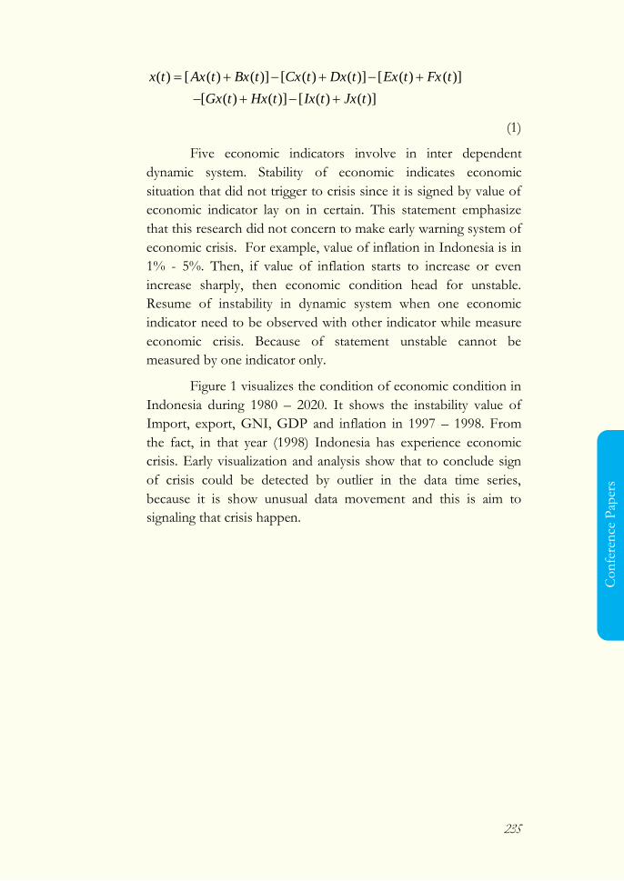
235

Co

nfe

ren

ce P

aper

s

)]()([)]()([

)]()([)]()([)]()([)(

tJxtIxtHxtGx

tFxtExtDxtCxtBxtAxtx

(1)

Five economic indicators involve in inter dependent

dynamic system. Stability of economic indicates economic

situation that did not trigger to crisis since it is signed by value of

economic indicator lay on in certain. This statement emphasize

that this research did not concern to make early warning system of

economic crisis. For example, value of inflation in Indonesia is in

1% - 5%. Then, if value of inflation starts to increase or even

increase sharply, then economic condition head for unstable.

Resume of instability in dynamic system when one economic

indicator need to be observed with other indicator while measure

economic crisis. Because of statement unstable cannot be

measured by one indicator only.

Figure 1 visualizes the condition of economic condition in

Indonesia during 1980 – 2020. It shows the instability value of

Import, export, GNI, GDP and inflation in 1997 – 1998. From

the fact, in that year (1998) Indonesia has experience economic

crisis. Early visualization and analysis show that to conclude sign

of crisis could be detected by outlier in the data time series,

because it is show unusual data movement and this is aim to

signaling that crisis happen.

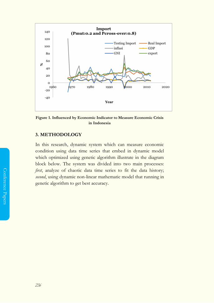
236

Co

nferen

ce Pap

ers

Figure 1. Influenced by Economic Indicator to Measure Economic Crisis

in Indonesia

3. METHODOLOGY

In this research, dynamic system which can measure economic

condition using data time series that embed in dynamic model

which optimized using genetic algorithm illustrate in the diagram

block below. The system was divided into two main processes:

first, analyze of chaotic data time series to fit the data history;

second, using dynamic non-linear mathematic model that running in

genetic algorithm to get best accuracy.

-40

-20

0

20

40

60

80

100

120

140

1960 1970 1980 1990 2000 2010 2020

%

Year

Import (Pmut:0.2 and Pcross-over:0.8)

Testing Import Real Import

inflasi GDP

GNI export

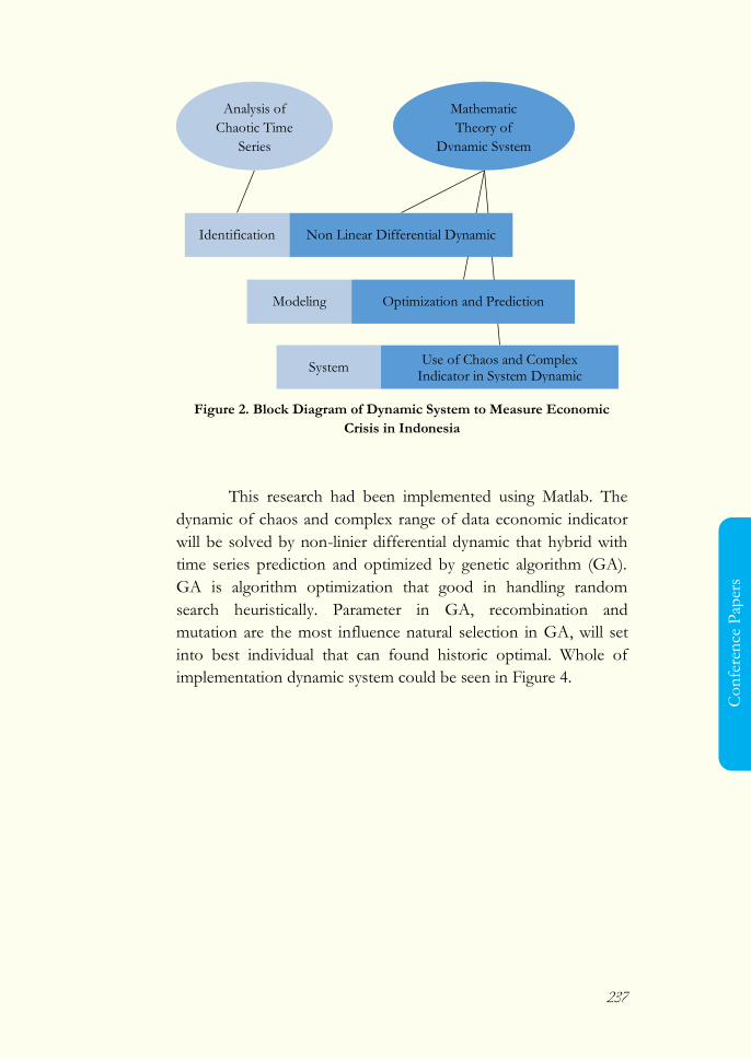
237

Co

nfe

ren

ce P

aper

s

Figure 2. Block Diagram of Dynamic System to Measure Economic

Crisis in Indonesia

This research had been implemented using Matlab. The

dynamic of chaos and complex range of data economic indicator

will be solved by non-linier differential dynamic that hybrid with

time series prediction and optimized by genetic algorithm (GA).

GA is algorithm optimization that good in handling random

search heuristically. Parameter in GA, recombination and

mutation are the most influence natural selection in GA, will set

into best individual that can found historic optimal. Whole of

implementation dynamic system could be seen in Figure 4.

Analysis of

Chaotic Time

Series

Non Linear Differential Dynamic Identification

System

Optimization and Prediction Modeling

Use of Chaos and Complex Indicator in System Dynamic

Mathematic

Theory of

Dynamic System

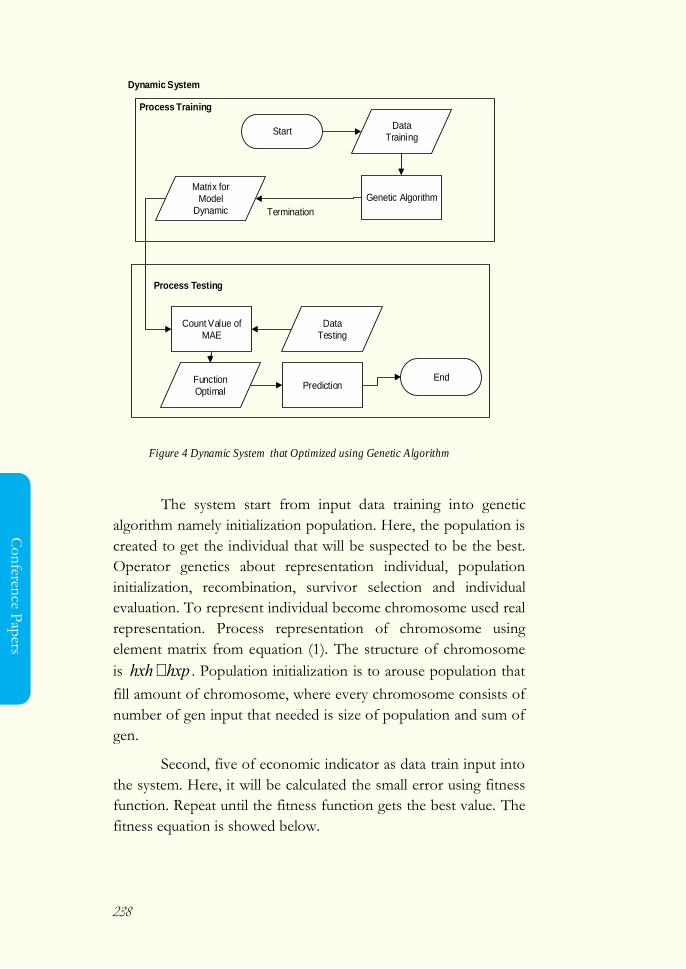
238

Co

nferen

ce Pap

ers

The system start from input data training into genetic

algorithm namely initialization population. Here, the population is

created to get the individual that will be suspected to be the best.

Operator genetics about representation individual, population

initialization, recombination, survivor selection and individual

evaluation. To represent individual become chromosome used real

representation. Process representation of chromosome using

element matrix from equation (1). The structure of chromosome

is hxh+hxp . Population initialization is to arouse population that

fill amount of chromosome, where every chromosome consists of

number of gen input that needed is size of population and sum of

gen.

Second, five of economic indicator as data train input into

the system. Here, it will be calculated the small error using fitness

function. Repeat until the fitness function gets the best value. The

fitness equation is showed below.

Process Testing

Start

Genetic Algorithm

Data Training

Matrix for Model

Dynamic Termination

Process Training

Count Value of MAE

Function Optimal

Dynamic System

PredictionEnd

Data Testing

Figure 4 Dynamic System that Optimized using Genetic Algorithm

239

Co

nfe

ren

ce P

aper

s

bEf

1 (2)

Where b is the smallest number (avoid divided by 0); and E is

absoult square error of prediction fault toward data actual. With

the equation of E is:

N

i nn yyE1

2')( (3)

Where: N = Total of prediction data; '

ny = data result of predict;

and ny = data actual.

Third, after get value of fitness, the individual will select

the next parent. Where selection parent included the important

thing to get the best individual at system. After the parent was

founded, then the system will do the recombination to get the

child to the next generation. Result of the child can be good by

doing mutation. Because, it is the other way to get the best

individual then by natural selection. From this population will be

see the best individual that survive from the selection of loop

evolution. If the generated in GA has finished yet. Then repeat all

the step above.

After the loop evolution done, the system had found out

the best coefficient to dynamic model and calculates the result of

error training use MAPE. The calculations of accuracy system

predict was used the equation below:

( ) (4)

MAPE (Mean Absolute Percentage Error) was used here to

calculate the error between data prediction and actual. The

equation of MAPE was showed below:

∑ |

|

(5)

Where N is total of prediction data; z is actual data; and *z is

predicted data.

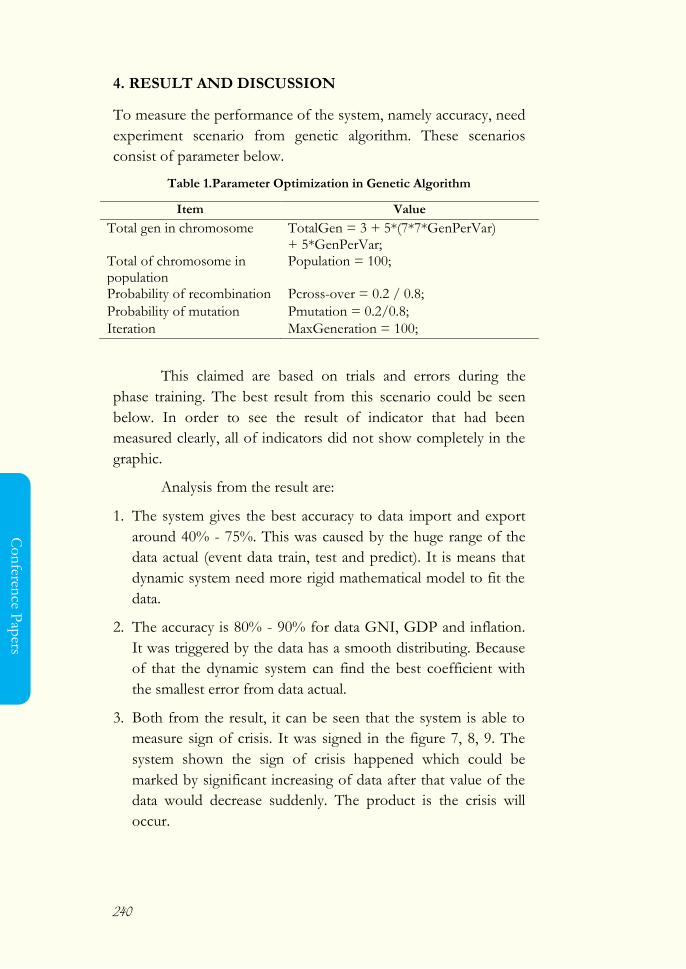
240

Co

nferen

ce Pap

ers

4. RESULT AND DISCUSSION

To measure the performance of the system, namely accuracy, need

experiment scenario from genetic algorithm. These scenarios

consist of parameter below.

Table 1.Parameter Optimization in Genetic Algorithm

Item Value

Total gen in chromosome TotalGen = 3 + 5*(7*7*GenPerVar) + 5*GenPerVar;

Total of chromosome in population

Population = 100;

Probability of recombination Pcross-over = 0.2 / 0.8;

Probability of mutation Pmutation = 0.2/0.8;

Iteration MaxGeneration = 100;

This claimed are based on trials and errors during the

phase training. The best result from this scenario could be seen

below. In order to see the result of indicator that had been

measured clearly, all of indicators did not show completely in the

graphic.

Analysis from the result are:

1. The system gives the best accuracy to data import and export

around 40% - 75%. This was caused by the huge range of the

data actual (event data train, test and predict). It is means that

dynamic system need more rigid mathematical model to fit the

data.

2. The accuracy is 80% - 90% for data GNI, GDP and inflation.

It was triggered by the data has a smooth distributing. Because

of that the dynamic system can find the best coefficient with

the smallest error from data actual.

3. Both from the result, it can be seen that the system is able to

measure sign of crisis. It was signed in the figure 7, 8, 9. The

system shown the sign of crisis happened which could be

marked by significant increasing of data after that value of the

data would decrease suddenly. The product is the crisis will

occur.

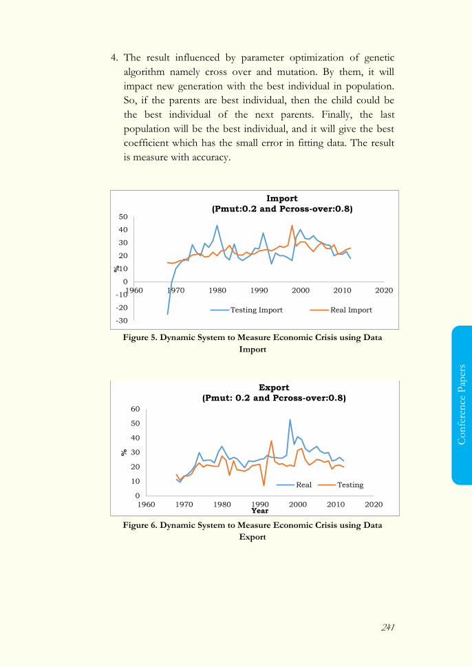
241

Co

nfe

ren

ce P

aper

s

4. The result influenced by parameter optimization of genetic

algorithm namely cross over and mutation. By them, it will

impact new generation with the best individual in population.

So, if the parents are best individual, then the child could be

the best individual of the next parents. Finally, the last

population will be the best individual, and it will give the best

coefficient which has the small error in fitting data. The result

is measure with accuracy.

Figure 5. Dynamic System to Measure Economic Crisis using Data

Import

Figure 6. Dynamic System to Measure Economic Crisis using Data

Export

-30

-20

-10

0

10

20

30

40

50

1960 1970 1980 1990 2000 2010 2020

%

Import

(Pmut:0.2 and Pcross-over:0.8)

Testing Import Real Import

0

10

20

30

40

50

60

1960 1970 1980 1990 2000 2010 2020

%

Year

Export

(Pmut: 0.2 and Pcross-over:0.8)

Real Testing

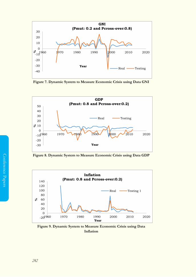
242

Co

nferen

ce Pap

ers

Figure 7. Dynamic System to Measure Economic Crisis using Data GNI

Figure 8. Dynamic System to Measure Economic Crisis using Data GDP

Figure 9. Dynamic System to Measure Economic Crisis using Data

Inflation

-40

-30

-20

-10

0

10

20

30

1960 1970 1980 1990 2000 2010 2020%

Year

GNI

(Pmut: 0.2 and Pcross-over:0.8)

Real Testing

-30

-20

-10

0

10

20

30

40

50

1960 1970 1980 1990 2000 2010 2020

%

Year

GDP

(Pmut: 0.8 and Pcross-over:0.2)

Real Testing

-20

0

20

40

60

80

100

120

140

1960 1970 1980 1990 2000 2010 2020

%

Year

Inflation

(Pmut: 0.8 and Pcross-over:0.2)

Real Testing 1

243

Co

nfe

ren

ce P

aper

s

5. CONCLUSION

Dynamic system should concern about the range of the data real

while measure economic crisis. It is really important since data of

economic have chaos and complex aspect. Because of that, the

results of accuracy differ between data export – import and GNI –

GDP – inflation. In fact, the fluctuated range of data cannot be

avoided. Besides, the dynamic system should prepare for more

flexible input. So that, genetic algorithm that optimized to fit the

data need other dynamic differential non-linear model. Due to, the

parameter optimization could present better accuracy.

REFERENCES

Goojier, J.G.De and Hyndmann, R.J. 2006. 25 Years of Time

Series Forecasting. Department of Quantitative

Economics. Amsterdam and Department of Econometrics

and Business Statisics, Australia.

Zbiec K. 2007. A Linear Approximation Method in Prediction o

Chaotic Time Series. University of Bialystok. Studies in

Logic, Grammar and Rhetoric 11 (24). ISBN 978-83-7431-

158-8.

Guegan D. 26 November 2009. Chaos in Economics and Finance.

HAL Id: halshs-00375713.

Vlad S, Pascu P and Morariu N. January 2010. Chaos Models in

Economics. Journal of Computing, Volume 2, Issue 1.

Liu Z. 2010. Chaotic Time Series Analysis. Mathematical Problems in

Engineering. Volume 2010, 31 pages.

Doi:10.1155/2010/720190.

Arthur B.W. 2013. Complexity Economics: A Different

Framework for Economic Thought. SFI Working Paper:

2013-040012.

244

Co

nferen

ce Pap

ers

Jeanne O. 2000. Currency Crises: A Perspective on Recent

Theoretical Developments. Special Papers in International

Economics, No.20. International Finance Section, Department of

Economics. Princeton University, New Jersey.

Kodba S, Perc M and Marhl M. 2005. Detecting Chaos from a

Time Series. Institute of Physic Publishing, European Journal of

Physics. Eur.J.Phys.26 (2005) 205-215. Doi:10.1088/0143-

0807/26/1/021.

Parlitz U and Hornstein A. 2005. Dynamical Prediction of Chaotic

Time Series. Chaos and Complexity Letters. Volume 1, Number

2, pp. 135-144.

Hommes C. 2004. Economic Dynamics. CeNDEF, University of

Amsterdam. Encyclopedia of Nonlinear Science, Routledge.

Barnett W.A and Chauvet M. 2011. How Better Monetary

Statistics Could Have Signaled the Financial Crisis. Journal

of Econometrics 161 (2011) 6-23.

Airaudo M and Zanna L-F. 2012. Interest Rate Rule, Endogenous

Cycles, and Chaotic Dynamics in Open Economies. IMF

Working Paper.

Banas D A. 2015. Modeling of Essential Characteristics of

Dynamics of the Economic Entity. Journal of International

Scientific Publications. Economy & Business. ISSN 1314-7242,

Volume 9.

Smirnov D.A and Bezruchko B.P. 2005. Nonlinear Dynamical

Models from Chaotic Time Series: Methods and

Applications.

Vacha L and Vosvrda M.S. 2005. Dynamical Agents‘ Strategies

and the Fractal Market Hypothesis. Prague Economic Papers,

2.

Lai Y-C and Ye N. 2003. Recent Developments in Chaotic Time

Series Analysis. International Journal of Bifurcation and Chaos,

Vol.13, No.6 (2003) 1383-1422.

Reiss J.D. 2001. The Analysis of Chaotic Time Series. Georgia

Institute of Technology.

245

Co

nfe

ren

ce P

aper

s

Saadah S, Houw Liong T, Adiwijaya. 2012. International

Conference of Science Engineering and Technology

(ICSET). Bandung Institute of Technology, Indonesia.

Prediction System of Economic Crisis in Indonesia using

Time Series Analysis and Dynamic System Optimized by

Genetic Algorithm. IEEE, ISBN 978-1-4673-2375-8.

Saadah S, Houw Liong T, Adiwijaya. 28th – 29th September,

2013. International Conference on Advance Computer

Science and Information Systems (ICACSIS). University of

Indonesia. Machine learning of forecasting Long-term

economic crisis in Indonesia. IEEE Explore, Indonesia

Section. 10.1109/ICACSIS.2013.6761586.

Saadah S and Wulandari G.S. Hotel Panghegar 28-30 April 2014.

International Conference of Information and

Communication Technology, ICOICT 2014. Telkom

University. Prediction Time Series of Economic Indicator

in Indonesia Optimized by Genetic Algorithm. IEEE

Indonesia Section.

Saadah S and Wulandari G.S. February 24-26, 2015. 6th

International Conference on Information Science and

Applications (ICISA 2015), Pattaya, Thailand.

Interconnection Learning between Economic Indicators in

Indonesia Optimized by Genetic Algorithm. Springer

Heidelberg New York Dordrecht London.

Saadah S. 2015. Chaos and Complex in Measuring Sustainability of

Economic Condition in Indonesia. The 2nd International

Conference on Information Science and Security (ICISS), Seoul

Korea. Indexed in IEEE and scopus.

http://icatse.org/iciss-2015-seoul-korea/

Shuhong, Z. 2007. The Self Adaptable Modelling Of Socio-

Economic Complex System Based On Genetic Algorithm.

Journal of International for General Systems Studies.

Hubei University of Economics, Wuhan. China.

Smyrlis Y.S. and Papageorgiou D.T. 1991. Predicting Chaos for

Infinite Dimensional Dynamical Systems: The Kuramoto-

246

Co

nferen

ce Pap

ers

Sivashinsky Equation, a Case Study. Proc. Natl. Acad. Sci.

USA. Applied Mathematics. Vol.88 pp. 11129-11132.

Tambunan T. 2010. Building an Economic Crisis Early Warning

System for Indonesia: Model and Empirical Test. Trisakti

University.

Tong H. 2010. Threshold Models in Time Series Anlysis-30 Years

On. The University of Hong Kong.

247

Co

nfe

ren

ce P

aper

s

Household Security Household Economic Security Across Cohorts

Maria Piotrowska

The paper is based on the findings from the research project financed by the National Centre

for Science (DEC-2011/01/B/HS4/03239)

Correspondence: maria.piotrowska@ue.wroc.pl

Abstract

The paper is aimed to explain differentiation in economic security

of households through cohort differences. Identifying cohorts is

based on common educational and professional experiences. The

research introduces the concept of economic resourcefulness

defined as the capability to make economic decisions that

contribute to economic security of a household. Economic

security of a household is defined as the ability to achieve income

necessary for covering household needs at its suitable level and to

create financial reserves to be at disposal in case of unfavorable

accidence. The research uses an exploratory analysis based on

structural equation modeling. The questionnaire survey carried out

in Poland in 2013 is a source of data for observed variables in an

empirical model of economic security. The findings confirm that

common educational and professional experiences, controlling for

economy conditions, influence economic resourcefulness of

household‘s members and, as a consequence, their economic

248

Co

nferen

ce Pap

ers

security. The conclusion, however, refers to the Polish society

and socio-economic development experienced by cohorts of Poles

since 1990.

Keywords: Security, Household, Cohort, Resourcefulness JEL

Classification: D14

1. INTRODUCTION

Economic security of households is one of financial stability

dimensions. The economic security at a microeconomic level

influences the welfare of individuals, individual identity and

behavior in the labor market and at a macroeconomic level is the

primary goal of the state and consumes a significant portion of

public expenditure. Carrying out monetary and fiscal policies as

well as using some macroprudential tools such as loan-to-value

(LTV) and debt-to-income (DTI) ratios require information on

economic decisions made by households which contribute to

security of a family.

The purpose of the paper is to find out differences in

economic security across cohorts. It is presumed that common

educational and professional experiences, controlling for economy

conditions, influence economic security of households. Poland is a

case used to illustrate an approaching to economic security

suggested by the paper.

The paper structure is as follows: the definitions of

economic security suggested in the literature are presented in the

second section; the third section covers a research hypothesis,

objectives, the definitions of the main concepts, a description of a

conceptual model as well as an empirical model; the research

results are discussed in the forth section; and finally conclusions

and research limitations are in the fifth section.

2. LITERATURES

Twenty-first century has brought a wider research related to

economic security. Initially, the researchers focused on economic

risk. Hacker, in his well-known book ‖The great risk shift. The

249

Co

nfe

ren

ce P

aper

s

New Economic insecurity and the decline of the American

Dream‖ (2006) stressed that for Americans income inequality has

become less of a problem, and on the first plan came the fear for

the future life of their families. The reason for this fear has

become a very significant increase in the volatility of family

income and the increase in risk associated with a decrease in the

value of assets. The works of Hacker (2006, 2007) initiated a wave

of empirical research on the trends of changes in income (Jacobs

2007). Consequently, researchers began to shift attention from the

risk in the direction of economic security.

In the literature economic security is usually determined by

the conditions required for sense of security. Beeferman (2002, p.

1) proposes a practical definition of what it means that people

have a sense of economic security. They need assurance that in the

short term they will be able to meet basic needs and in the long

run – that they gain a well-paid job, will be able to improve the

qualifications and will have sufficient financial resources to buy a

flat or a house, start a business, start a new career and that these

resources will allow them to survive the changes and crises in their

lives and ensure a high quality of life when retired.

The report, ―By a Thread: The New Experience of

America's Middle Class‖ (2007) prepared jointly by the Demos: A

Network for Ideas and Action, and The Institute on Assets and

Social Policy at Brandeis University, an index of security of the

middle class was based on responses to the question: what should

have the middle class to feel safe in an economic sense? The

answer is as follows: financial assets, education, income and health

care for all members of the family.

International Labour Organization (www.ilo.org) in the

ILO Socio-Economic Security Programme has adopted the

definition of ―economic security‖, which indicates a number of

conditions, fulfillment of which can be identified with a sense of

security. Economic security in this definition consists of two parts:

the basic social security and work-related safety.

250

Co

nferen

ce Pap

ers

Summing up, in the short term protection against adverse

situations are: a stable income from work or other sources (equity,

real estate), insurance (private and social), liquid resources,

including precautionary savings, human capital, social capital and

common equity. In the long term, economic security can result

also from ownership of less liquid assets (houses, flats, durable

goods), but the most important components of economic security

are the stability of geo-political situation and favorable

demographic trends.

3. METHODOLOGY

3.1. Purpose, Hypothesis and Objectives of Study

In the paper economic security of households is defined as the

ability to achieve income necessary for covering household needs

at its suitable level and to create financial reserves to be at disposal

in case of unfavorable accidence (sickness, job loss, family

breakdown).

The research introduces a concept of economic

resourcefulness to explain the perception of economic security.

Economic resourcefulness is defined as a set of family member

capabilities to make economic decisions - in the fields of labor,

saving, investing, borrowing and insuring – aimed at building

economic security of a family.

The purpose of the paper is to find out differences in

economic security across cohorts. It is presumed that common

educational and professional experiences, controlling for economy

conditions, influence economic resourcefulness of households and

as a consequence their economic security. Poland is a case used to

illustrate an approaching to economic security suggested by the

paper.

A hypothesis verified in the paper states: There are differences

in economic security of households which can be explained by socio-economic

development experienced by different cohorts. The detailed objectives are;

(i) to build a conceptual model of economic security; (ii) to

251

Co

nfe

ren

ce P

aper

s

measure economic security across cohorts; and (iii) to identify

cohort differences in: 1) the relationships between variables in

empirical models of economic security; 2) the resourcefulness

effects; and 3) changes in mean values of economic security, by

educational level.

3.2. A conceptual model of economic security

A conceptual model of economic security, suggested in the paper,

covers the antecedents of individual economic resourcefulness

and economic security as a consequence of economic

resourcefulness, as well as mediators.

Antecedents of Individual Economic Resourcefulness

Socio-economic status of parents and socio-economic

development in which an individual has experienced in his life

make him more or less resourceful economically. Parents‘

educational attainment and their well-being have impact on

economic decision made by their mature children.

Socio-economic development refers, in the paper, to

educational and professional experiences as well as to economic

conditions under which an individual enters a labor market, and a

career stage of an individual during an economic disturbances.

Economic Resourcefulness

A resourceful individual has a stable, well-paid job and he is able

to find additional work facing financial problems. He posses a real

estate or/and valuable belongings which are insured. He is able to

borrow money, if necessary, from bank or other sources. He

invests in his children. His behavior, regarding saving and running

up debts, contributes to economic security of his family.

Economic Security of a Household

Economically secure family meets its needs at an acceptable level.

It is able to maintain its living standards in the closer and further

future, to meet unexpected expenses, to survive from an

unexpected decrease in household income and.

252

Co

nferen

ce Pap

ers

Mediators

There are two mechanisms, or mediators, included in the model.

Educational and professional aspirations of an individual are a

mediator of effects of parental socio-economic status on

economic resourcefulness of a mature child. Health of a mature

child is a second mediator that links both parental socio-economic

status and socio-economic development with economic security

of a mature child‘s family.

3.3. Cohort-Sequential Design with Independent Samples

The accomplishment of the research aim requires proper design

of the study. There are two constrains to consider: 1) in a simple

comparison of persons who are at different ages at one point in

time (cross-sectional data), age effects may be confused with

cohort effects and 2) unfortunately in Poland there are no

available longitudinal data connected with the paper scope.

The lack of longitudinal data implies a lack of information

about personal developmental changes what it neglects the

possibility to reveal cohort effects and age effects. The cohort

effect is defined as the effect that having been born in a certain

time, region, period or having experienced the same life

experience (in the same time period) has on the development or

perceptions of a particular group. These perceptions,

characteristics or effects are unique to the group in question. In

other words, a birth cohort experiences the same historical, social,

and environmental events at the same age, potentially giving rise to

unique, cohort- specific values, attitudes, and preferences. Age

effects are variations resulting from the biological and social

processes of aging specific to individuals, such as physiological

changes and the buildup of social experience.

The solution which can reduce the single cross section

studies limitation is cohort-sequential design with independent

samples. Admittedly such a design does not give full information

on intra-individual change and inter-individual differences across

generations. However, cohort-sequential design with independent

253

Co

nfe

ren

ce P

aper

s

samples allows to differentiate cohort differences and age

differences controlling for history (Schaie, 1994, p.51).

It is assumed the basis of personality is created until the age

of 6 then the period of cohort feature creation follows and covers

the age of 6–20 . Between 15 and 20 the phase of cohort signal

identification occurs thus the common cohort value pattern is

formed.

The socio-economic context for differentiation of cohorts

is connected with economic and social changes in Poland during

transition from a central planned economy under the communistic

regime to a market economy. The first stage of transition took

place in the 90s, the second one covered the years 2000-2004 and

it was aimed at the ultimate preparation of Poland to the EU

accession in 2004. Since 2005 Poland has developed in a direction

of an advanced market economy, although it still belongs to a

group of emerging markets. The transition has resulted in three

great changes in the economy and the society: 1) dynamic growth

of private sector, (a contribution of the private sector to the GDP

is dominate, small and medium size enterprises create the majority

of jobs), 2) openness of the economy (FDI growth, high

technology, the western style of management not only in foreign

firms but also in domestic ones, two millions of Poles have found

jobs abroad), and 3) very dynamic growth in a fraction of high

educated people (a number of people in age of 25-64 with a

tertiary level of education increased from 10% in 1995 to 22% in

2011 as well a number of mothers with a tertiary educational level

increased from 6% at the beginning of the 90s to more than 47%

in 2013 while a number of mothers with primary education/or

even without any educational level attained declined in this period

from 18% to 4%).

The research covers three samples of respondents which

represent three cohorts named: cohort 1: ―Children of transition‖;

cohort 2: ―Youth of transition‖; cohort 3: ―Mobile-working-age-

adults of transition‖.

Cohort 1: ―Children of transition‖ – respondents are characterized

as follows: all levels of education attained in a market economy,

254

Co

nferen

ce Pap

ers

possibilities to study in the EU, difficult entry to the labor market

after the financial crisis, professional training in an advanced

market economy (―an advanced market economy‖ in comparison

to the first stage of transition, not in comparison to the old

members of the EU) ;

Cohort 2: ―Youth of transition‖ – respondents are characterized

as follows: secondary and tertiary levels of education in a market

economy, easy entry to the labor market just after Poland‘s

transition to the EU (dynamic growth during 2005-2007),

extended professional experiences and more or less stable

professional carrier during the financial crisis ;

Cohort 3: ―Mobile-working-age-adults of transition‖ –

respondents are characterized as follows: childhood in the

communism time, all educational levels in the communism times,

professional experiences achieved in the communism times,

training at the first stage of transition, stable professional position

during the financial crisis.

3.4. Data

The questionnaire survey is a source of data for observed

variables. The survey was carried out by the professional polling

agency in Poland in June 2013. The respondents were asked to

express their opinions directly in the course of face-to-face

interviews. The polling agency carrying out the survey has chosen

respondents at random. The selection of the respondents had

been representative due to the voivodship (Poland is divided into

16 administrative units called voivodships), age, gender and

educational level attained. The whole sample covers 800

respondents in age between 25 to 64. This sample is divided into

three cohorts. The cohort 1: ―Children of transition‖ covers 215

respondents; the cohort 2: ―Youth of transition‖ – 197

respondents; the cohort 3: ―Mobile-working-age-adults of

transition‖ – 388 respondents. General information on

respondents in each cohorts is presented in Table 1.

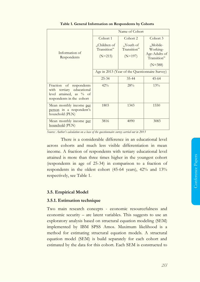
255

Co

nfe

ren

ce P

aper

s

Table 1. General Information on Respondents by Cohorts

Information of Respondents

Name of Cohort

Cohort 1

„Children of Transition‖

(N=215)

Cohort 2

„Youth of Transition‖

(N=197)

Cohort 3

„Mobile-Working-

Age-Adults of Transition‖

(N=388)

Age in 2013 (Year of the Questionnaire Survey)

25-34 35-44 45-64

Fraction of respondents with tertiary educational level attained, as % of respondents in the cohort

42% 28% 13%

Mean monthly income per person in a respondent‘s household (PLN)

1803 1343 1550

Mean monthly income per household (PLN)

3816 4090 3083

Source: Author’s calculation on a base of the questionnaire survey carried out in 2013

There is a considerable difference in an educational level

across cohorts and much less visible differentiation in mean

income. A fraction of respondents with tertiary educational level

attained is more than three times higher in the youngest cohort

(respondents in age of 25-34) in comparison to a fraction of

respondents in the oldest cohort (45-64 years), 42% and 13%

respectively, see Table 1.

3.5. Empirical Model

3.5.1. Estimation technique

Two main research concepts - economic resourcefulness and

economic security – are latent variables. This suggests to use an

exploratory analysis based on structural equation modeling (SEM)

implemented by IBM SPSS Amos. Maximum likelihood is a

method for estimating structural equation models. A structural

equation model (SEM) is build separately for each cohort and

estimated by the data for this cohort. Each SEM is constructed to

256

Co

nferen

ce Pap

ers

specify hypothetical relationships among variables: 1) how the

latent (or unobserved) variables can be related to each other (this

part of the model is called the structural model) and 2) how the

observed variables can depend on the latent variables (this part of

the model is called the measurement model).

The structural model (the relationships between the latents)

for each cohort covers the same six latent variables. The set

includes: (i) Socio-economic status of respondent‘s parents; (ii)

Aspirations of a respondent; (iii) Economic resourcefulness of a

respondent; (iv) Propensity to save; (v) Propensity to run-up-debts

; (vi) Economic security of a respondent‘s household.

3.5.2. Measures

The measurement model for each cohort consists of six distinct

measurement submodels which specify how each of the six latent

variables influences a group of observed variables. The details of

all variables used on SEM model are presented on Table 2, and is

available on the author.

Some of the observed variable are based on responses to

the question in the questionnaire survey. We employ several

measures to proxy certain variable, for instance on describing the

best the way of managing the household income, we use the

following 10 (ten) options, including the ‗no answer‘.

1. There is enough for everything and for saving for the future

2. There is enough for everything without renunciation but no

savings for the future,

3. We live economically and there is enough money for

everything,

4. We live economically to save for major spending,

5. There is enough money for cheep food, clothing, apartment

rent and installment of credit repayment,

6. There is enough money for cheep food, clothing, apartment

rent but not for installment of credit repayment,

7. There is enough money for cheep food and clothing, but not

for apartment rent,

257

Co

nfe

ren

ce P

aper

s

8. There is enough money for cheep food but not for clothing,

9. There is not enough money even for cheep food,

10. No answer

Measures of the observed variables are based on responses

to the questions in the questionnaire survey. The majority

questions refer to individual attainment/ opinion/behavior of a

respondent. Smaller part of questions concerns a financial

situation of a respondent‘s household, like income per person, a

level of savings/ total indebtedness, managing of household‘s

income. Regarding such questions it is assumed that responses

given by a respondent are representative for her/his household as

a whole (only one member of a household was asked).

The measures of observed variables are scaled:

1 – it means a high level of a variable

0 – it means a low level of a variable

For the questions with a choice of options:

EDU, Q31A, Q31B – 1 for a tertiary level of education while 0 for other levels

M22_2 – 1 for options 1-4 while 0 for options 5-8 (see the explanation for the variable M22_2 under Table 2)

Q12 – 1 for option 1 while 0 for options 2-3 (see the explanation for the variable in Table 2)

A few observed variables are measured in other way:

o Income per person in a household is measured in Polish

currency, PLN, (in ln)

o Q5 - What unexpected expenses can you meet during few days

without any loans and any financial support from the others? -

is measured in PLN, (in ln)

o Q42 – a value of a respondent‘s flat/house, PLN, (in ln)

o Q7 – a level of savings as a multiplicity of household‘s monthly

income

258

Co

nferen

ce Pap

ers

o Q10 – a level of total indebtedness as a multiplicity of

household‘s monthly income

o Q15 – measured in a number of months

The matrix of implied covariances for all variables in the

model can be used to carry out a regression of the unobserved

(latent) variable on the observed variables. The resulting

regression weight estimates can be obtained from Amos and they

are named the factor score weights. These factor score weights

give regression weights for predicting the unobserved variables

from the observed variables. A measure of a latent variable is a

weighted sum of the individual observed scores using the factor

score weights. In the paper the factor score weights are calculated

separately for each cohort. For example, the measure of

resourcefulness for an individual in the cohort ―Children of

transition‖ is the sum of observed scores computed as follows:

individual response to Q31A (1 or 0) x cohort-factor-

score-weight for Q31A + …..

3.5.3. Model evaluation

All regression coefficients in each SEM estimated for the cohort

are significant at the 0.05 level (a majority of them are significant

at the 0.01 level). All covariances between the errors included in

the model are significant at the 0.05 level.

Model evaluation is one of the most unsettled and difficult

issues connected with structural modeling. The literature suggests

several fit measures. In the paper the SEM estimated for each

cohort is evaluated on a base of the following ones:

P is a ―p value‖ for testing the hypothesis that the model

fits perfectly in the population.

CMIN/DF is the minimum discrepancy, divided by its

degrees of freedom. The ratio should be close to 1 for

correct models.

CFI is the comparative fit index. CFI values close to 1

indicate a very good fit.

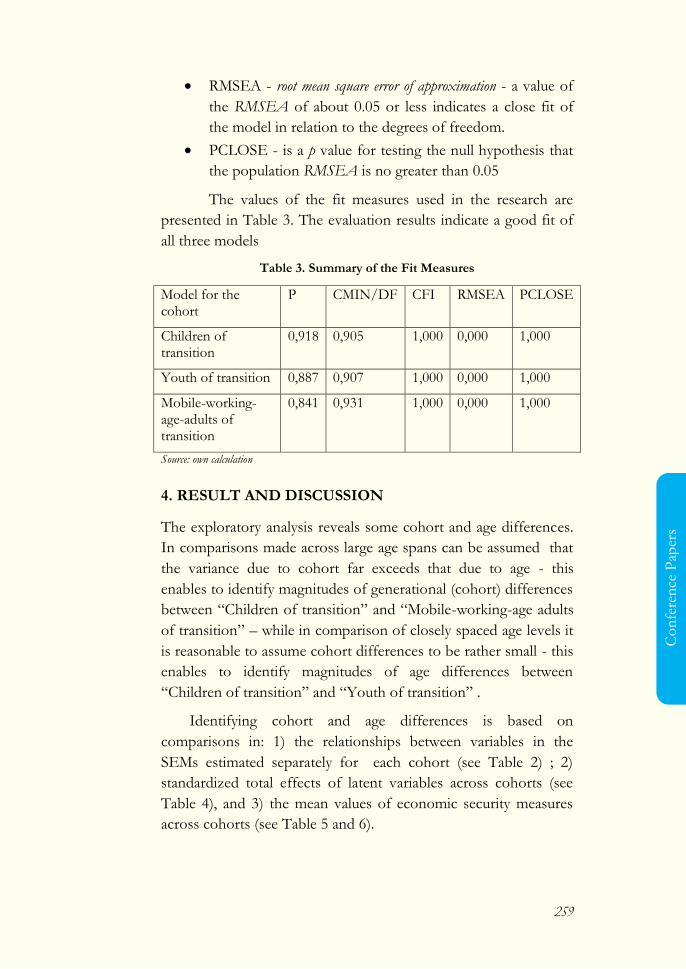
259

Co

nfe

ren

ce P

aper

s

RMSEA - root mean square error of approximation - a value of

the RMSEA of about 0.05 or less indicates a close fit of

the model in relation to the degrees of freedom.

PCLOSE - is a p value for testing the null hypothesis that

the population RMSEA is no greater than 0.05

The values of the fit measures used in the research are

presented in Table 3. The evaluation results indicate a good fit of

all three models

Table 3. Summary of the Fit Measures

Model for the cohort

P CMIN/DF CFI RMSEA PCLOSE

Children of transition

0,918 0,905 1,000 0,000 1,000

Youth of transition 0,887 0,907 1,000 0,000 1,000

Mobile-working-age-adults of transition

0,841 0,931 1,000 0,000 1,000

Source: own calculation

4. RESULT AND DISCUSSION

The exploratory analysis reveals some cohort and age differences.

In comparisons made across large age spans can be assumed that

the variance due to cohort far exceeds that due to age - this

enables to identify magnitudes of generational (cohort) differences

between ―Children of transition‖ and ―Mobile-working-age adults

of transition‖ – while in comparison of closely spaced age levels it

is reasonable to assume cohort differences to be rather small - this

enables to identify magnitudes of age differences between

―Children of transition‖ and ―Youth of transition‖ .

Identifying cohort and age differences is based on

comparisons in: 1) the relationships between variables in the

SEMs estimated separately for each cohort (see Table 2) ; 2)

standardized total effects of latent variables across cohorts (see

Table 4), and 3) the mean values of economic security measures

across cohorts (see Table 5 and 6).

260

Co

nferen

ce Pap

ers

4.1 Relationships between Variables in SEMs

In general, respondents in the cohort ―Children of transition‖

(respondents in age of 25-34) are much better educated and much

more familiar with products in a financial market (all levels of their

education attained in the market economy, professional training in

the advanced market economy) than respondents in the cohort

―Mobile-working-age adults of transition‖ (shortly, ―Adults of

transition, respondents in age of 45-64).

This can explain a difference in the impact of ―Propensity

to save‖ on ―Diversification in income sources of maintenance

during retirement‖. For the ―Children of transition‖ (as well as for

the cohort 2 – respondents in age of 35-44) diversifying long-term

investment is one of direct measures of their behavior in saving

process, while for the ―Adults of transition‖ the impact is

mediated by their opinion whether their well-being depends on

themselves (―Do you think it is up to you how much money you

will have in your life?), see Table 3.

Experiences of the ―Children of transition‖ in a financial

market make them more independent from the parental influence.

This can explain why in their SEM ―Propensity to run up debts‖

depends directly only on their ―Resourcefulness‖, while in the

SEM of ―Adults of transition‖ this latent is influenced additionally

by ―Financial problems of their parents‖, see Table 3.

In general, comparison in the SEMs suggests that

economic decisions made by the ―Children of transition‖ depend

directly on their own resourcefulness and the impact of parental

socio-economic status on their decisions is only indirect, mediated

by their ―Aspirations‖ (however this indirect impact is the

strongest in the cohort 1 because, parental status of respondents

in the cohort ―Children of transition‖ is much higher than in the

cohort ―Adults of transition‖ - mean value of the latent variable

―Socio-economic status of respondent‘s parents‖ is 0,454 in

comparison to 0,188). While in the SEM of the ―Adults of

transition‖ parental status influences directly two variables: the

261

Co

nfe

ren

ce P

aper

s

ability to find additional job and a value of real estate possessed by

a mature child. This statistical significance of parental support

results from informal relationships among older members of the

Polish society.

There is one more cohort difference linked with a

perception of investment in children. For the ―Children of

transition‖ money spent on child development is one of

resourcefulness measures, while for the ―Adults of transition‖

investment in a child‘s activities has been a matter of their

aspiration, see Table 3.

4.2 Standardized Total Effects

A standardized total effect is a measure of both direct

(unmediated) and indirect (mediated) effects of a variable A on

variable B after standardizing all variables. See Table 4 that

presents the total effect of each column variable on each row

variable, for example the standardized total (direct and indirect)

effect of ―Economic resourcefulness of a respondent‖ on

―Propensity to save‖ is 0.961. That is, due to both direct

(unmediated) and indirect (mediated) effects of ―Resourcefulness

of a respondent‖ on ―Propensity to save‖, when

―Resourcefulness of a respondent‖ goes up by 1 standard

deviation, ―Propensity to save‖ goes up by 0,961 standard

deviation.

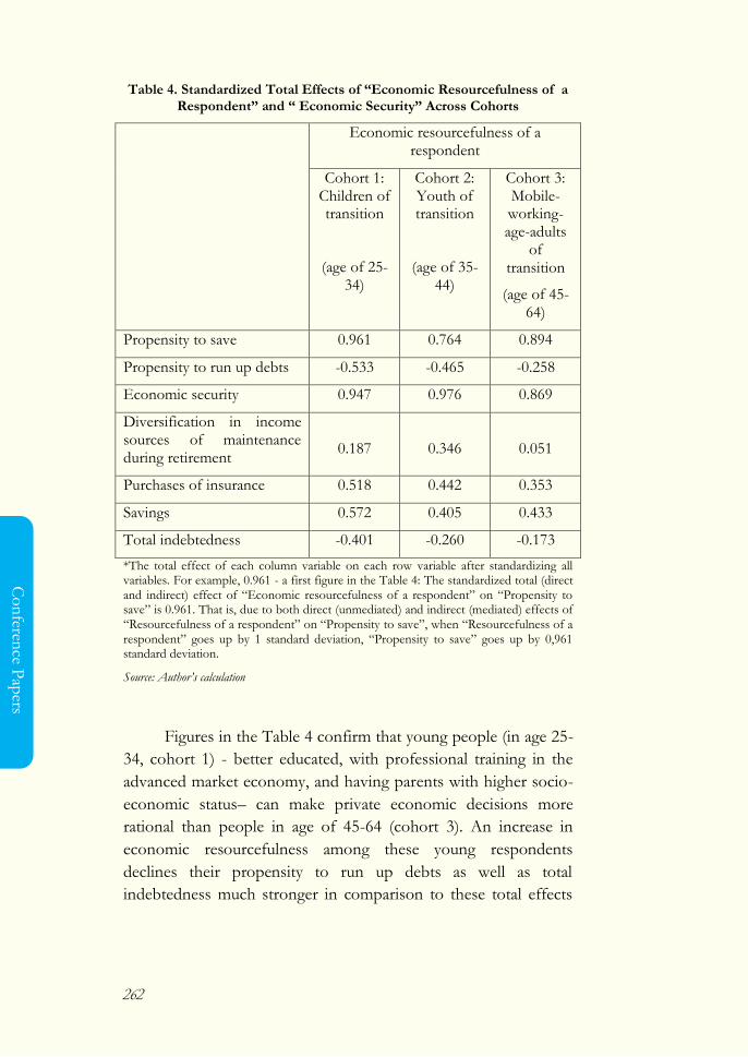
262

Co

nferen

ce Pap

ers

Table 4. Standardized Total Effects of “Economic Resourcefulness of a Respondent” and “ Economic Security” Across Cohorts

Economic resourcefulness of a respondent

Cohort 1: Children of transition

(age of 25-34)

Cohort 2: Youth of transition

(age of 35-44)

Cohort 3: Mobile-working-age-adults

of transition

(age of 45-64)

Propensity to save 0.961 0.764 0.894

Propensity to run up debts -0.533 -0.465 -0.258

Economic security 0.947 0.976 0.869

Diversification in income sources of maintenance during retirement

0.187

0.346

0.051

Purchases of insurance 0.518 0.442 0.353

Savings 0.572 0.405 0.433

Total indebtedness -0.401 -0.260 -0.173

*The total effect of each column variable on each row variable after standardizing all variables. For example, 0.961 - a first figure in the Table 4: The standardized total (direct and indirect) effect of ―Economic resourcefulness of a respondent‖ on ―Propensity to save‖ is 0.961. That is, due to both direct (unmediated) and indirect (mediated) effects of ―Resourcefulness of a respondent‖ on ―Propensity to save‖, when ―Resourcefulness of a respondent‖ goes up by 1 standard deviation, ―Propensity to save‖ goes up by 0,961 standard deviation.

Source: Author’s calculation

Figures in the Table 4 confirm that young people (in age 25-

34, cohort 1) - better educated, with professional training in the

advanced market economy, and having parents with higher socio-

economic status– can make private economic decisions more

rational than people in age of 45-64 (cohort 3). An increase in

economic resourcefulness among these young respondents

declines their propensity to run up debts as well as total

indebtedness much stronger in comparison to these total effects

263

Co

nfe

ren

ce P

aper

s

among the oldest cohort of respondents (age of 45-64) – compare

-0.533 to -0.258 and -0.401 to -0.173 in Table 4.

Two other visible differences refer to total effects of

resourcefulness on purchasing insurance and diversifying

retirement investments. The impact of resourcefulness in both

cases is stronger for the cohort 1 than cohort 3 – compare 0.518

to 0.353 and 0.187 to 0.051 in Table 4. Moreover, the effects of

resourcefulness on propensity to save as well as savings are the

strongest for the youngest cohort.

4.3 Comparison in Mean Values of Economic Security

Across Cohorts

The measure of economic security is calculated on a base of the

SEMs for each cohort and it is normalized from 0 to 1. Higher

value, higher economic security of a respondent‘s household, see

Table 5. Higher mean values of economic security for the oldest

cohort (cohort 3) than for the youngest one (cohort 1) suggests an

age difference rather than a cohort one. In general, people in age

of 45-64 should be economically secure more than people in 25-34

because they have had more time to gather more wealth and pay

out their loans. This conclusion is obvious.

Interesting figures are in Table 6 where the mean value of

economic security for the cohort 2 (―Youth of transition‖ –

respondents in age of 35-44) is a base for comparisons. The

changes in mean economic security are differentiated across

cohorts and by education level. The age difference is visible only

in reference to people with low and very low educational level.

They are more secure economically in age of 45-64 than people in

middle age (cohort 2, age of 35-44). While the cohort difference

can be recognized regarding people in age of 45-64 with tertiary

and secondary levels of education. These people have the same

economic security, in average, as people in a middle age (35-44

years).

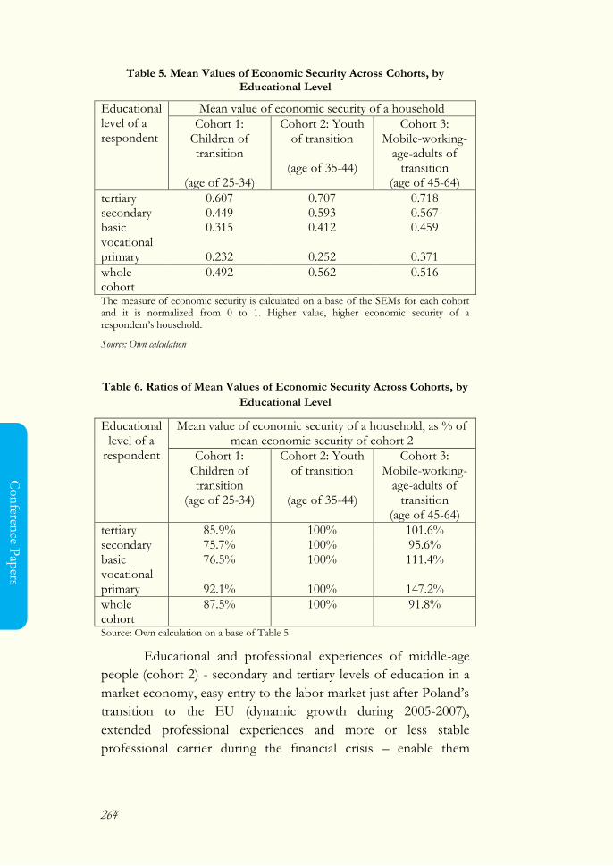
264

Co

nferen

ce Pap

ers

Table 5. Mean Values of Economic Security Across Cohorts, by Educational Level

Educational level of a respondent

Mean value of economic security of a household

Cohort 1: Children of transition

(age of 25-34)

Cohort 2: Youth of transition

(age of 35-44)

Cohort 3: Mobile-working-

age-adults of transition

(age of 45-64)

tertiary 0.607 0.707 0.718 secondary 0.449 0.593 0.567 basic vocational

0.315 0.412 0.459

primary 0.232 0.252 0.371

whole cohort

0.492 0.562 0.516

The measure of economic security is calculated on a base of the SEMs for each cohort and it is normalized from 0 to 1. Higher value, higher economic security of a respondent‘s household.

Source: Own calculation

Table 6. Ratios of Mean Values of Economic Security Across Cohorts, by

Educational Level

Educational level of a

respondent

Mean value of economic security of a household, as % of mean economic security of cohort 2

Cohort 1: Children of transition

(age of 25-34)

Cohort 2: Youth of transition

(age of 35-44)

Cohort 3: Mobile-working-

age-adults of transition

(age of 45-64)

tertiary 85.9% 100% 101.6% secondary 75.7% 100% 95.6% basic vocational

76.5% 100% 111.4%

primary 92.1% 100% 147.2%

whole cohort

87.5% 100% 91.8%

Source: Own calculation on a base of Table 5

Educational and professional experiences of middle-age

people (cohort 2) - secondary and tertiary levels of education in a

market economy, easy entry to the labor market just after Poland‘s

transition to the EU (dynamic growth during 2005-2007),

extended professional experiences and more or less stable

professional carrier during the financial crisis – enable them

265

Co

nfe

ren

ce P

aper

s

receive economic security at the same level like people 10-20 years

older. This suggests that qualification of the cohort 2 must be

higher than skills and knowledge of older people (cohort 3), even

with the same educational level. This can be recognize as evidence

of the cohort difference.

5. CONCLUSION

The paper is aimed to explain differentiation in economic security

of households through cohort differences. Identifying cohorts is

based on common educational and professional experiences. The

research introduces the concept of economic resourcefulness

defined as the capability to make economic decisions that

contribute to economic security of a household.

The findings reveal first that economic decisions made by

the members of the youngest cohort having educational and

professional skills attained in a market economy depend directly

on their own resourcefulness and the impact of parental socio-

economic status on their decisions is only indirect, mediated by

their ―Aspirations‖, While in the SEM of the oldest cohort

parental status influences directly two variables: the ability to find

additional job by a mature child and a value of real estate

possessed by a mature child

Second, an increase in economic resourcefulness among the

youngest respondents declines their propensity to run up debts as

well as total indebtedness much stronger in comparison to these

total effects among the oldest cohort of respondents.

Third, total effects of economic resourcefulness on

purchasing insurance and diversifying retirement investments are

stronger for the youngest cohort than the oldest one.

Fourth, the effects of resourcefulness on propensity to save

as well as savings are the strongest for the youngest cohort.

266

Co

nferen

ce Pap

ers

Fifth, educational and professional experiences of middle-

age people (it means secondary and tertiary levels of education

attained in a market economy, easy entry to the labor market just

after Poland‘s transition to the EU (dynamic growth during 2005-

2007), extended professional experiences and more or less stable

professional carrier during the financial crisis) enable them receive

economic security at the same level like people 10-20 years older.

The research results confirm that common educational

and professional experiences, controlling for economy conditions,

influence economic resourcefulness of household‘s members and,

as a consequence, their economic security.

The research limitations should be emphasized. The

conclusions refer to the Polish society and socio-economic

development experienced by cohorts of Poles since 1990. More

country studies are required to generalize the main conclusion that

cohort differences explain differentiation in economic security of

households.

REFERENCES

Beeferman, L. W. 2002. The asset index: Assessing the progress of

states in promoting economic security and opportunity, The

Heller School for Social Policy and Management, Brandeis

University,

https://iasp.brandeis.edu/pdfs/2002/The%20Asset%20Ind

ex.pdf

Hacker, J. S. 2006. The Great Risk Shift: The New Economic

Insecurity and the Decline of the American Dream. Oxford

University Press.

——— 2007. The New Economic Insecurity – And What Can Be

Done About It, Harvard Law & Policy Review, 1, 111-126.

ILO Socio-Economic Security Programme, International Labour

Organization in, www.ilo.org

267

Co

nfe

ren

ce P

aper

s

Jacobs, E. 2007. The politics of economic insecurity, The

Brookings Institution: Issues in Governance Studies, 12, 1-

13.

Report By a Thread: The New Experience of America‘s Middle

Class. 2007.Prepared together by Demos: A Network for

Ideas & Action and The Institute on Assets and Social

Policy at Brandeis University.

Schaie, K. W. (1994), ―Developmental designs revisited‖. In S. H.

Cohen and H. W. Reese (eds), Life-span developmental

psychology: Theoretical issues revisited, Hillsdale, 45-64,

N.J.: Erlbaum.

268

Co

nferen

ce Pap

ers

Regional Revitalization

Sharia Traditional Market Area: Revitalization Of Traditional Markets in Maintaining Regional Financial

Stability through Optimization Potential Waqaf

Achmad Noer Maulidi, Fathor Rozi, Syofia Dwi Jayanti

Syariah Banking Program, Stain Pamekasan

Corresponding: achnoermaulidi@gmail.com

Abstract

Facing the Asean Economic Community (AEC) in 2015 which

demanded the liberalization of the flow of goods and services,

especially alert to the entry of foreign retail business and the

modern, the traditional market revitalization in Indonesia has

significant importance in empowering Micro, Small and Medium

Enterprises (UMKM) in Indonesia. Traditional markets as a

reflection of the people's economy is the foundation for the life of

the little people, the middle income who are engaged in the

informal sector, micro, small and medium businesses that thrive

and depend on traditional markets

269

Co

nfe

ren

ce P

aper

s

The bad image of the traditional markets in the society was

also a factor increasingly waning existence of traditional markets in

Indonesia, causing the shift of consumers from traditional markets

to modern market. Poor market conditions, means incomplete,

not product quality standards as well as the atmosphere

uncomfortable and have still limited access to capital financing

with low interest for traders, also became an obstacle. Required a

concept and approach to redefine traditional market revitalization.

Islamic economics as an alternative solution to the problems of

this nation. On the other hand the problem to revitalize traditional

markets requires considerable cost. However, problems such

funds can be circumvented by exploiting the potential cash waqf

funds.

Sharia Traditional Market Area is a solution to community

empowerment effective and productive. Sharia Traditional Market

Area has been built, will be managed professionally and in

accordance with the values of shari'ah 'ah. Traditional Market Area

Sharia will not only contribute significantly to community

empowerment. But also can play a role childbirth featured

merchants based on the values of sharia applicative program

launched by the manager of Sharia Traditional Market Area.

Keywords: Traditional Market, Waqaf, Sharia Traditional Market Area,

JEL Classification: G18, G21, G28

1. INTRODUCTION

Background

"And God justifies the purchase and Proscribe Riba" (Al-Baqarah; 275)

Facing the Asean Economic Community (AEC) in 2015 which

demanded the liberalization of the flow of goods and services,

especially alert to the entry of foreign retail business and the

modern, the traditional market revitalization in Indonesia has

significant importance in empowering Micro, Small and Medium

Enterprises (UKM) in Indonesia. Traditional markets as a

reflection of the people's economy is the foundation for the life of

the little people, the middle income who are engaged in the

270

Co

nferen

ce Pap

ers

informal sector, micro, small and medium businesses that thrive

and depend on traditional markets.

Based on research conducted Rafinaldi (2006) and the fact

of Kementrian Koperasi and Micro, Small and Medium

Enterprises (UMKM) (2012) states that the optimism of UKM in

Indonesia, among others: (1) its position as a major player in

economic activity in various sectors: the number of UKM in

Indonesia in 2011 reached 53,823,732 units or 99.99% of total

business units with a donation of GDP at constant prices of

57.60% with a growth of 6.76% since the base year 2010, (2) the

largest provider of employment reached 97.24% of labor force, (3)

a significant player in the development of local economic activity

and community development, (4) the creators of new markets and

sources of innovation, and (5) contribution in maintaining the

balance of payments through the activities of non-oil exports

amounted to 187,441.82 billion or 16:44%.

But in fact, UKM in Indonesia are still struggling in

various polemical issues in the arena of national economy. Sharif

(2011) formulated had scales of priority problems faced by UKM

in Indonesia today. The study was based on a decline in the

average scale of business seen from the fixed price, the low index

of well-being of UKM, as well as increasingly smaller role in the

crop sector comestible, Porternakan, plantations and fisheries.

One reason is the existence of traditional markets is fading in this

era of global competition.

"A growing increasingly desperate parents". That's the

nature of traditional markets on which the UMKM in Indonesia

today. The rapid development of modern market with all the

benefits a negative impact on the existence of traditional markets.

Data from Ministry of Commerce noted that the number of

traditional markets is now an 10,000-lived, while the modern

market has already reached 14,000. Modern market totaled 14,000

is divided into 358 outlets in the form of convenience stores,

minimarkets 11 569, 1,146 supermarkets, 141 hypermarkets and

260 shaped grocery store or wholesaler. Results traditional market

271

Co

nfe

ren

ce P

aper

s

mapping conducted the Ministry of Commerce in 2010 to 4,000

markets in 12 provinces to 95 percent mention the age of the

traditional market is already 25 years which means in a very fragile

condition. Even the Deputy Minister of Trade, Krisnamurthi,

traditional markets predict just be a memory the next 12 years if

they are not made efforts to rebuild these markets (Windarto,

2012).

In addition, the negative image of traditional markets in

the society was also a factor increasingly waning existence of

traditional markets in Indonesia, causing the shift of consumers

from traditional markets to modern market. Poor market

conditions, means incomplete, not product quality standards as

well as the atmosphere uncomfortable and have still limited access

to capital financing with low interest for traders, also became an

obstacle. According to data from Indonesia Market Vendors

Association (LGAs) in 2008, the number of traditional markets

there are 13,450 fruit market and approximately 4,707 or 35% of

whom have been abandoned by the merchant. LGAs revealed, in

Jakarta every year there are 400 stalls were closed because of

competition from modern markets (Marsyahid, 2009).

Wiboonpongse and Sriboonchitta (2006), Poseoro (2007), the

research also revealed that internal factors may also lead to a

serious waning existence of traditional markets, among others:

poor management of the market, the inability to meet the needs of

consumers, there are no economies of scale and collaboration with

suppliers, infrastructure was minimal, traditional markets as "cash

cows" for retribution, the proliferation of street vendors (PKL),

and the lack of capitalization assistance.

In line with the foregoing, Nurmalasari (2007) revealed

that there are several factors that significantly affect society as a

consumer preference for shopping at traditional markets, among

others, the quality of traded goods, hygiene traditional markets

and convenience in shopping.

His research also revealed that people's income has no

influence on his preference choose traditional market means

272

Co

nferen

ce Pap

ers

people are expecting satisfaction are met with maximum service

condition rather than thinking about the price.

If it turns out to be explored deeper managerial side who

have often neglected the development proved to have

considerable influence on the waning competitiveness of

traditional market today. You could say, lack of awareness is also a

lack of knowledge of traditional market players become a factor if

the service has been done is not oriented to the satisfaction or

consumer preferences, but only to the extent the behavior of

market participants traditional subsistence.

Whereas traditional markets have an important role that

can absorb the labor force in large numbers, as a distribution

center for goods and for economic growth that can develop both

rural and urban regions. Research conducted by Alfian Tumbuan,

et al (2006) about the significance of the traditional market in the

city of Manado mention of the power market that is not owned by

a supermarket, namely:

[1] The strong fraternal relations with society, history, and culture,

[2] free access to the market,

[3] existence and presence in remote small town,

[4] have loyal customers,

[5] have diversified products and power to negotiate prices.

In addition, as disclosed by Jati (2012) states that the

essence of economic transactions contained in the traditional

market is a form of cooperation (cooperation), which is a pattern

best practices in Indonesia. Traditional markets arising from the

insistence of the local community needs rise to a social capital in

the form of "Cooperation" and "trust" are not only focused on the

advantages and economics gain from all parties but also to build

ties of kinship and brotherhood. It is also called Clifford Geertz as

the uniqueness of the economic pattern in Indonesia, Economic

Bazaar.

Based on the above exposure, we need a concept and

approach to redefine traditional market revitalization. Islamic

economics as an alternative solution to the problems of this

273

Co

nfe

ren

ce P

aper

s

nation. The problems mentioned above, can be overcome with

how the government can provide containers as a means of

empowering traditional market players who must not be separated

in the corridors of Islamic economics.

Efforts to revitalize traditional markets often cause a

problem before, during and after the execution took place. Instead

of helping the people's economy, the revitalization of traditional

markets often cause social conflicts causing long program

increasingly abandoned even fail, call it market Klewer Solo,

Pancur Pasar Batu, Deli Serdang. Even if revitalization is

successful the results were often disappointing, that still lonely

customers like Ayu Market, Market Nusukan, Sidodadi Market

and Flower Market in Solo. The reason is that the general is a lack

of transparency, the small role of traditional market players (both

merchant and consumer), and revitalization is oriented mainly to

the physical dimensions of the market such as buildings and

infrastructure in the traditional market.

Of course, this revitalization issue into a dilemma that is

very detrimental to both the traditional market players (in this case

the trader and the consumer), the government and investors.

Simalakama like fruit, as the revitalization of traditional markets

which had occurred did not have a positive impact. If nothing is

done, then the existence of traditional markets will continue to be

undermined by the modern market. If you do then the threat of

social conflict and the failure of revitalization was also

overshadowing, so it would be a waste, especially the government

budget.

On the other hand the problem to revitalize traditional

markets requires considerable cost. However, problems such

funds can be circumvented by exploiting the potential cash waqf

funds, because there is no obligation to refund and provide certain

profit level to wakif (which provides endowment funds) but

channeling the profits to benefit the people and keep these funds

in order not reduced. Until now, the management of cash waqf is

still very less attention even though its potential is very promising.

274

Co

nferen

ce Pap

ers

It is necessary for the management of a professional through an

approach that allows solving problems of revitalization of

traditional markets that can be exploited for the benefit of the

economy.

2. LITERATURES

Traditional markets

Traditional markets are traditionally selling place (hereditary), a

meeting place for sellers and buyers where goods are bought and

sold depending on consumer demand, the price set an agreed

price through a bidding process. In general, traditional markets are

point of sale materials basic needs. Sometimes traditional market

activities within the limits specified time as the morning market,

evening market, weekend market and so forth. Traditional markets

are managed by the government or private amenities such as

sheds, warehouses, stores, kiosks, public toilets at around

traditional markets.

The process of buying and selling in the traditional

markets take place humanely and communication with family

values are high (source http://id.wikipedia.org). Meanwhile,

according to the Presidential Decree of the Republic of Indonesia

of 2007 No. 112 concerning construction, arrangement and

development of traditional markets, decided that "traditional

market" is a market that is built and managed by the Government,

Local Government, Private, State Owned Enterprises and

Regional Owned Enterprises including cooperation with the

private sector with businesses such as shops, kiosks, stalls and

tents owned / managed by small traders, medium-sized, non-

governmental or cooperative with small-scale enterprises, small

capital and with the process of buying and selling merchandise

through bargaining. There is a striking difference in the

characteristics between the traditional with the modern market in

Indonesia as shown in table 1.

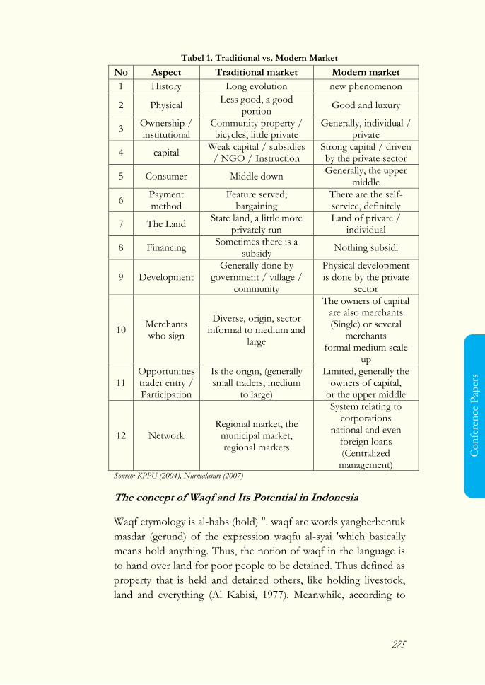
275

Co

nfe

ren

ce P

aper

s

Tabel 1. Traditional vs. Modern Market

No Aspect Traditional market Modern market

1 History Long evolution new phenomenon

2 Physical Less good, a good

portion Good and luxury

3 Ownership / institutional

Community property / bicycles, little private

Generally, individual / private

4 capital Weak capital / subsidies

/ NGO / Instruction Strong capital / driven by the private sector

5 Consumer Middle down Generally, the upper

middle

6 Payment method

Feature served, bargaining

There are the self-service, definitely

7 The Land State land, a little more

privately run Land of private /

individual

8 Financing Sometimes there is a

subsidy Nothing subsidi

9 Development Generally done by

government / village / community

Physical development is done by the private

sector

10 Merchants who sign

Diverse, origin, sector informal to medium and

large

The owners of capital are also merchants (Single) or several

merchants formal medium scale

up

11 Opportunities trader entry / Participation

Is the origin, (generally small traders, medium

to large)

Limited, generally the owners of capital,

or the upper middle

12 Network Regional market, the

municipal market, regional markets

System relating to corporations

national and even foreign loans (Centralized

management) Sourch: KPPU (2004), Nurmalasari (2007)

The concept of Waqf and Its Potential in Indonesia

Waqf etymology is al-habs (hold) ". waqf are words yangberbentuk

masdar (gerund) of the expression waqfu al-syai 'which basically

means hold anything. Thus, the notion of waqf in the language is

to hand over land for poor people to be detained. Thus defined as

property that is held and detained others, like holding livestock,

land and everything (Al Kabisi, 1977). Meanwhile, according to

276

Co

nferen

ce Pap

ers

Law No. 41 of 2004 on Waqf.

Waqf defined by legal act Wakif to separate and / or hand

over part of their wealth either permanently or for a specified

period in accordance with their interests for purposes of worship

and / or general well-being according to sharia.

While the decision fatwa Fatwa Committee Indonesian Ulema

Council (MUI) on cash waqf decided that the waqf money (cash

waqf) are waqf that a person, group of people, institutions or legal

entities in the form of cash, including marketable securities, and

the law jawaz (allowed). The use of cash waqf should only be

channeled and used for things that are permitted by sharia and

should guarantee its preservation, may not be sold, assigned, and /

or inherited.

In the Qur "an there are some verses that are based as the

foundation waqf command. "You never come to virtue (perfect), before

you spend sehahagian that which ye love. And whatever you spend, Allah

knows." (Qur'an, Ali Imran: 92).

Another verse says: "The parable (income incurred by) those who

spend their wealth in Allah is like a seed that grows seven ears, in every ear a

hundred grains. Allah magnifies (reward) for whom He will. and Allah is the

area (his gift), the Knower. " (QS. Al-Baqarah: 261).

There are three fundamental reasons why the Ottoman era

jurisprudents arrange cash waqf buildings: first, the notion that

mobile assets can be a waqf property. Second, assessment and

acceptance of money as an asset moves. Third, the agreement on

the provision of cash.

Meanwhile, there are four pillars waqf that must be met in

berwakaf. First, people who berwakaf (al-Waqif). Second, objects

diwakafkan (al-mauquf). Third, those who receive the benefit of

waqf (al-mauquf 'alaihi). Fourth, lafadz or pledge waqf (sighah). In

Act No. 41 of 2004, there are two additional things that have to be

met: waqf property allotment and term waqf. In order to achieve

the objectives and functions of waqf, according to Law No. 41 of

2004 on Wakaf, waqf property invested reserved only for five

277

Co

nfe

ren

ce P

aper

s

kinds of things, namely: (a) facilities and religious activities; (B) the

means and education and health; (C) assistance to the poor,

abandoned children, orphans, scholarships; (D) progress and

economic improvement of the people, and / or; (E) the progress

of other public welfare that are not contrary to the sharia and

legislation.

With the potential large population reached 237 million in

the 2010 census, and the potential for world Muslims, then the

potential endowment in Indonesia is something promising,

especially when supported by their waqf Act No. 41 of 2004.

Many Islamic banks nor the institution of waqf waqf issued

various products collected from the community. Baitul Mal

Muamalat, for example, launched the Cash Waqf Muamalat

(Waqtumu), Republika Dhuafa Wallet launched Tabung Wakaf

Indonesia (TWI), and Pos Keadilan Peduli Umat (PKPU)

launched a cash waqf.

With cash waqf is implemented, then the reception with

these instruments being higher than other instruments such as

zakat, infaq, sadaqah, or otherwise. Arena with cash waqf, the

waqf instrument is no longer the monopoly of the "rich". Lower

middle class can participate. If only there were 10 million only

Muslim society that donating funds as much as Rp 100 thousand,

it will obtain the endowment fund raising Rp 1 trillion per month

(Rp12 trillion per year). And if it is invested with an investment

rate of 10% per year it will obtain additional endowment fund of

Rp 8 billion per month (100 billion per year). A fund can not be

said to be small when compared with profit of 145 national banks

which amounted to Rp 9.26 trillion (Infobank, July 2006) the

acquisition or realization of income tax in 2005 amounted to Rp57

trillion (www.bwi.or.id).

If you look at the level of generosity of the people of

Indonesia as described above, then it becomes something that is

not impossible can happen. Moreover, based on the last survey

conducted by PIRAC (Public Interest Research and Advocacy

Center) in 2004, it turns out rate of giving the people of Indonesia

278

Co

nferen

ce Pap

ers

is still quite high. Based on these survey results rate of giving the

people of Indonesia is 96% done for individuals, 84% (Rp 304,000

per donor per year) for a religious institution and 77% for non-

religious institutions.

Calculations carried out by Mustafa Nasution (2001)

revealed that cash waqf Muslims in Indonesia at this time is

assumed to reach 3 trillion annually; and it could even be much

greater. This is because the scope of the giver target cash waqf

(wakif) can be very broad compared with regular waqf. Certificates

of cash waqf, which is based on rules BWI at least 1 million, can

be paid in installments or can be made in a variety of

denominations that are tailored to target Muslim segment which

approximately has a high awareness of the charity. For example,

Rp.10.000,00, Rp 25,000, Rp 50,000, Rp 100,000, Rp 500 000, Rp

1,000. 000, 00, Rp 2,000,000.

Economic Empowerment of People in the Perspective of

Islamic Economics

Empowerment is the language, from the Indonesian derived from

the word "power" which means strength, which is the term means:

Efforts to build a power possessed by d} uafa to encourage,

motivate, and raise awareness about their potential and try to

develop (Esack, 2000).

In al-Qur "an says power is referred to as" al-Quwwah ",

in different variants, called 33 times (Thematic Interpretation,

2000). In Arabic it is called "al-Quwwah", in English called

"empower" which, according to Cornell University Empowerment

Group in Saleebey cited by Malik (2012) Empowerment is: "A

process of deliberate and continues over time, which was centered

in the life local communities, include: mutual respect, an attitude

of critical reflection, the awareness and participation of the group,

through which people who feel they have less joint valuable

resources into obtaining greater access to get and control of these

resources".

Economic empowerment of Muslims is very important for

279

Co

nfe

ren

ce P

aper

s

several reasons: The first is due to the threat of God against the

liars religion. In the interpretation of the letter al-Ma 'un described

Allah says: "Do you (people) who reject religion. That's the guy

who rebuked orphans and does not recommend giving Eat poor

people. So woe to those who pray. (They are) those who are

neglectful of their prayers "(QS.al-Ma'un: 1-5).

Said feed by M. Quraish Shihab (2002) every person who

encourages or gives not feel that he has been feeding people in

need. From asbab an-Nuzul it shows that criticism can be directed

to anyone even if they provide assistance, meaning that if the aid is

not well targeted to people who really need help and assistance,

such as the reluctant help of orphans due orphans will not give up

hope anything.

The second is for the hope of God's promise to those who

assist or empower others. "Parable (income incurred by) those who spend

their wealth in the way of Allah is like a seed that grows seven ears, in every

ear a hundred grains. God magnifies (reward) for whom He will. and Allah

is the area (his gift) again Knowledgeable, ie those who spend their wealth in

Allah's way, then they do not accompany what dinafkahkannya with

menyebutnyebut grant and with not hurt (feelings of the recipient), their reward

is their Lord. no fear come upon them and not (also) they grieve. "(QS. Al-

Baqarah: 261-262).

Muslims yearn for the glory and prosperity as was the case

at the time of Caliph Umar ibn 'Abd al' Aziz. r.a. Caliphs were

justly famous, when he was caliph only thirty months, at that time

everyone who has a debt can get assistance from the typical state,

all the basic needs are met, after all the basic needs are met, he

provides assistance to small farmers to manage their land well , by

providing credit from typical State. This policy is already several

hundred years before the world knew of banks lending to

agriculture.

Before the time of Umar ibn Abd "Aziz during the time of

Umar bin Khattab at that time no one is willing to accept charity.

Thus welfare under the auspices of Islamic justice to the extent

that all have the right to obtain them (Qaradawi, 2002).

280

Co

nferen

ce Pap

ers

In conclusion, that the obligations and guidance of religion

established by God, do not have any other purpose than for the

benefit of mankind. God wants harmonious relations among all

His creatures, in order to achieve happiness in this world and

hereafter.

3. METHODOLOGY

This paper use descriptive qualitative approach. The type of data

used in this paper is secondary data, generally in the form of

evidence, records, or historical reports that have been compiled in

the archive (documentary data), both published and unpublished

(Moeloeng, 2004).

The technique used to collect the data in this paper are: (1)

Study of literature, a series of activities related to data collection

methods literature, reading and recording and processing of

materials research; (2) Documentary, documentation Studies done

by reading the previous writing reports and articles that are

accessible from the Internet, books and journals that fit the

problem. In this method the authors only transfer relevant data

from a source or document required; (3) The discussion, which is

the data collected by the talks and exchange ideas with people who

are competent with the object that is being studied in order to

solve a particular problem; (4) Intuitive-Subjective, is the

involvement of the authors' opinion on the issue at hand. (Ghofar,

1999).

4. RESULT AND DISCUSSION

Concept Sharia Traditional Market Area

Sharia Traditional Market Area is the concept of revitalization of

traditional market-based economic empowerment by the people

who built and developed through the use of endowment funds. In

the process, all forms of operations using the principles of Islamic

Shari'a and social economy is to achieve the welfare of the world

and the hereafter kaffah. Construction and development of the

tradiosonal market area is a strategic move to create endowment

funds to be more productive and make a significant contribution

281

Co

nfe

ren

ce P

aper

s

to the welfare of the people. Sharia Traditional Market Area is a

solution to community empowerment effective and productive.

Sharia Traditional Market Area has been built, will be managed

professionally and in accordance with the values of shari'ah 'ah.

Traditional Market Area Sharia will not only contribute

significantly to community empowerment. But also can play a role

childbirth featured merchants based on the values of sharia

applicative program launched by the manager of Sharia Traditional

Market Area.

Forms of Economic Empowerment of People in the

Revitalization of Traditional Markets Perspective Based on

Sharia

Under the conditions of the existence of traditional markets for

populist economics is needed synergy across sectors that help

significantly in revitalizing traditional markets. The economic

empowerment of the people would aim to accommodate the role

of government, academia and practitioners, and of course the

traditional market players (in this case the involvement of traders

and consumers) to assess further events to produce a

recommendation of action to be implemented by the traditional

traders in accordance perspective sharia. Research in this case is

the scientific tools needed to address the problems that often arise

which sometimes exacerbate the existence of traditional markets.

The concept of economic empowerment of the people in

the traditional market revitalization aims to support the

optimization of the value of participation among elements of

organizing economic activity in a sustainable approach.

Participation and cooperation is very important, because it can

overlap the weaknesses that exist for this.

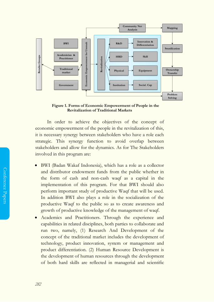
282

Co

nferen

ce Pap

ers

Figure 1. Forms of Economic Empowerment of People in the

Revitalization of Traditional Markets

In order to achieve the objectives of the concept of

economic empowerment of the people in the revitalization of this,

it is necessary synergy between stakeholders who have a role each

strategic. This synergy function to avoid overlap between

stakeholders and allow for the dynamics. As for The Stakeholders

involved in this program are:

BWI (Badan Wakaf Indonesia), which has a role as a collector

and distributor endowment funds from the public whether in

the form of cash and non-cash waqf as a capital in the

implementation of this program. For that BWI should also

perform important study of productive Waqf that will be used.

In addition BWI also plays a role in the socialization of the

productive Waqf to the public so as to create awareness and

growth of productive knowledge of the management of waqf.

Academics and Practitioners. Through the experience and

capabilities in related disciplines, both parties to collaborate and

run two, namely, (1) Research And Development of the

concept of the traditional market includes the development of

technology, product innovation, system or management and

product differentiation. (2) Human Resource Development is

the development of human resources through the development

of both hard skills are reflected in managerial and scientific

BWI

Academician &

Practitioner

Traditional

market

Government

Stratification

Ownership

Transfer

Problem

Solving

R&D

HRD

Physical

Institution

Innovation &

Differentiation

Skill

Equipment

Social. Cap

Reta

iler

Gro

up

s

Eco

no

mic

Em

po

werm

en

t fo

r U

mm

ah

Revi

tali

zati

on

MappingCommunity Net

Analysis

283

Co

nfe

ren

ce P

aper

s

concept of development as well as soft as reflected in the ability

of the management of emotions in organizational management

related institutions in the traditional markets.

The government, which includes the role of government (both

central and especially regional) in terms of stimulating the

program which includes (1) Regulation role, in the form of

policy-making and the protection and enforcement of laws

related to this program are the support and commitment of the

government, such as the control of competition business,

environmental control and others. (2) Allocation role, in the

form of distribution of scarce resources in this matter experts,

support infrastructure, capital support, technology transfer and

other inputs.

The community particularly market traders who are members

of various groups of merchants that act as the subject of

economic empowerment of the people, especially the

supporting performance of the application of this concept in

the revitalization of traditional markets through an active role

in participating. In addition it also takes the role of influential

public figures as mediation in the institutionalization of the

community to create social capital thus improving the

efficiency of the implementation of the coordinated program

regularly

The application of the concept of economic empowerment

of the people in the traditional market revitalization is divided into

several stages, namely:

Community Net Analysis, is to do a comprehensive analysis

that comes from the traditional market players is the first step

to determine the factors that affect traditional markets in the

upstream to the downstream sector. This issue will be

examined in accordance with the competence of each party, but

at the same goal orientation by involving the larger traditional

market traders.

Then stakeholders do Mapping (mapping) deep and also

formulate a solution and do Stratification of dividing the job

description based on the role and capabilities of the problems

284

Co

nferen

ce Pap

ers

that may be encountered by traditional market players either

already, is happening or will happen, so it will not cause a shock

in excessive the traditional market traders in case of a problem

identical.

Furthermore, through the development of a sense of belonging

(ownership transfer) between stakeholders as a tool for

understanding the social, cultural, and economic activity, to

realize the ease in understanding the reality of the problem and

the traditional market conditions and its ability to improve and

compete with modern markets. The move is also aimed at

realizing the institutionalization of the community to build

relationships based on social capital, so that the relationship can

be equal and mutually supportive. This is important, because

the traditional market players (traders and consumers) are the

main actors who will run the program. Normatively, all

stakeholders sit together and perform together in a symbiotic

mutualism to do research, learn to understand the problem and

solve the problem together (participatory).

Next will be a solution to problems through strategic

movement (strategic planning) to solve the problem in the

traditional markets. Then, arrangement of systematic steps,

determine the stakeholders and formulate likelihood of success

and failure of a planned program to address the issue of the

internal market.

Once the problem is completed or minimized, then the next

step is to revitalize based strategic planning that has been made.

The revitalization process not only focused on physical

dimensions such as the improvement of infrastructure already

fragile market or unfit but also social revitalization concerning

the empowerment of traders in traditional markets. The

concept of revitalization that carried the authors include four

kinds as shown in the table below, namely:

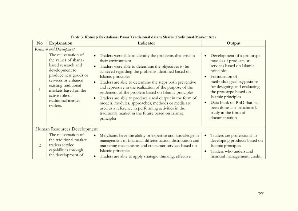
285

Table 3. Konsep Revitalisasi Pasar Tradisional dalam Sharia Traditional Market Area

No Explanation Indicator Output

Research and Development

1

The rejuvenation of the values of sharia-based research and development to produce new goods or services or enhance existing traditional markets based on the active role of traditional market traders.

Traders were able to identify the problems that arise in their environment

Traders were able to determine the objectives to be achieved regarding the problems identified based on Islamic principles

Traders are able to determine the steps both preventive and repressive in the realization of the purpose of the settlement of the problem based on Islamic principles

Traders are able to produce a real output in the form of models, modules, approaches, methods or media are used as a reference in performing activities in the traditional market in the future based on Islamic principles

Development of a prototype models of products or services based on Islamic principles

Formulation of methodological suggestions for designing and evaluating the prototype based on Islamic principles

Data Bank on RnD that has been done as a benchmark study in the form of documentation

Human Resources Development

2

The rejuvenation of the traditional market traders service capabilities through the development of

Merchants have the ability or expertise and knowledge in management of financial, differentiation, distribution and marketing mechanisms and consumer services based on Islamic principles

Traders are able to apply strategic thinking, effective

Traders are professional in developing products based on Islamic principles

Traders who understand financial management, credit,

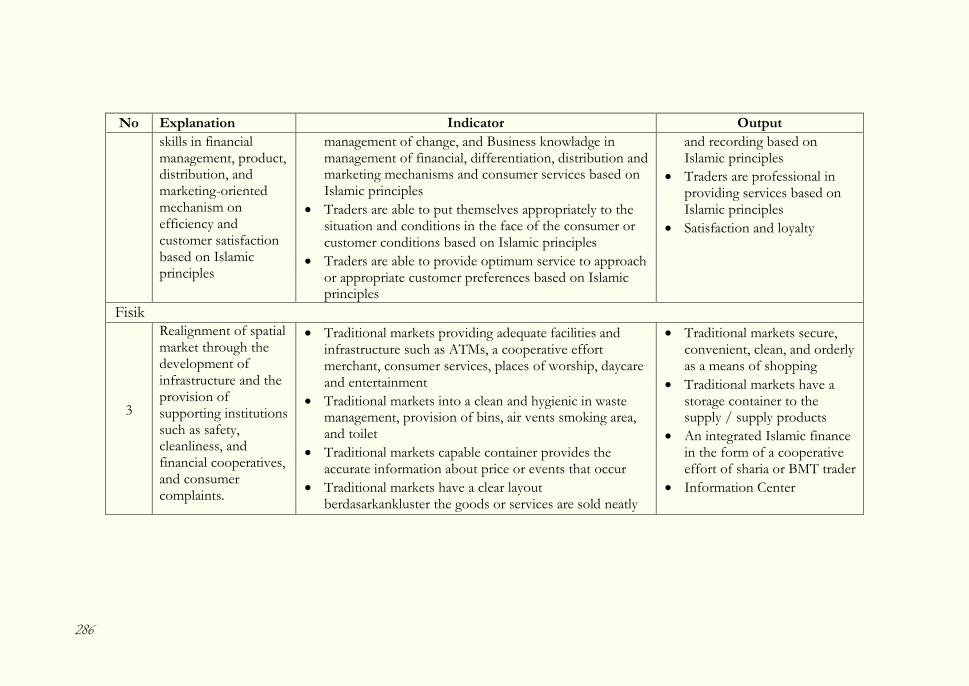
286

Sem

inary P

apers

No Explanation Indicator Output

skills in financial management, product, distribution, and marketing-oriented mechanism on efficiency and customer satisfaction based on Islamic principles

management of change, and Business knowladge in management of financial, differentiation, distribution and marketing mechanisms and consumer services based on Islamic principles

Traders are able to put themselves appropriately to the situation and conditions in the face of the consumer or customer conditions based on Islamic principles

Traders are able to provide optimum service to approach or appropriate customer preferences based on Islamic principles

and recording based on Islamic principles

Traders are professional in providing services based on Islamic principles

Satisfaction and loyalty

Fisik

3

Realignment of spatial market through the development of infrastructure and the provision of supporting institutions such as safety, cleanliness, and financial cooperatives, and consumer complaints.

Traditional markets providing adequate facilities and infrastructure such as ATMs, a cooperative effort merchant, consumer services, places of worship, daycare and entertainment

Traditional markets into a clean and hygienic in waste management, provision of bins, air vents smoking area, and toilet

Traditional markets capable container provides the accurate information about price or events that occur

Traditional markets have a clear layout berdasarkankluster the goods or services are sold neatly

Traditional markets secure, convenient, clean, and orderly as a means of shopping

Traditional markets have a storage container to the supply / supply products

An integrated Islamic finance in the form of a cooperative effort of sharia or BMT trader

Information Center

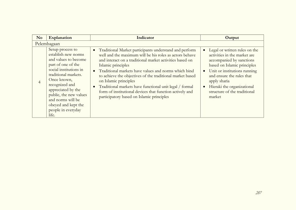
287

No Explanation Indicator Output

Pelembagaan

4

Setup process to establish new norms and values to become part of one of the social institutions in traditional markets. Once known, recognized and appreciated by the public, the new values and norms will be obeyed and kept the people in everyday life.

Traditional Market participants understand and perform well and the maximum will be his roles as actors behave and interact on a traditional market activities based on Islamic principles

Traditional markets have values and norms which bind to achieve the objectives of the traditional market based on Islamic principles

Traditional markets have functional unit legal / formal form of institutional devices that function actively and participatory based on Islamic principles

Legal or written rules on the activities in the market are accompanied by sanctions based on Islamic principles

Unit or institutions running and ensure the rules that apply sharia

Hieraki the organizational structure of the traditional market

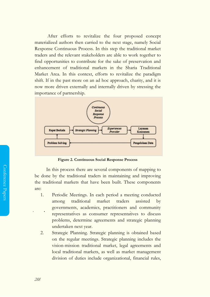
288

Co

nferen

ce Pap

ers

After efforts to revitalize the four proposed concept

materialized authors then carried to the next stage, namely Social

Response Continuous Process. In this step the traditional market

traders and the relevant stakeholders are able to work together to

find opportunities to contribute for the sake of preservation and

enhancement of traditional markets in the Sharia Traditional

Market Area. In this context, efforts to revitalize the paradigm

shift. If in the past more on an ad hoc approach, charity, and it is

now more driven externally and internally driven by stressing the

importance of partnership.

Figure 2. Continuous Social Response Process

In this process there are several components of mapping to

be done by the traditional traders in maintaining and improving

the traditional markets that have been built. These components

are:

1. Periodic Meetings. In each period a meeting conducted

among traditional market traders assisted by

governments, academics, practitioners and community

representatives as consumer representatives to discuss

problems, determine agreements and strategic planning

undertaken next year.

2. Strategic Planning. Strategic planning is obtained based

on the regular meetings. Strategic planning includes the

vision-mission traditional market, legal agreements and

local traditional markets, as well as market management

division of duties include organizational, financial rules,

289

Co

nfe

ren

ce P

aper

s

fees, taxes and rent, procurement of equipment and the

formulation of a traditional market partnership with

relevant stakeholders based on Islamic principles.

3. Experiences Provider, namely the means or tools to give

or provide the consumer experience appropriate strategic

planning that has been made. Based on the statement of

Schmitt in Andreani (2006) experiential providers

include: (1) Communication: advertising, public relations,

newsletters, brochures, annual reports and megalogs; (2)

Visual identity; Merck and logo market; (3) Product

presence: product design, packaging, fresh product, and

look distinctively services market; (4) Co-ing: event

marketing, alliances and partnerships, and licensing; (5)

Environment: interior design and characterize a unique

market including the design of the response in response

to the cultural, religious, or other major holidays; (6)

Website tardisional market and other electronic media;

(7) People: sales, sellers appearance, and the figure is

seeded.

4. The service consumer, which means to load the

aspirations and means of the active role of consumers on

provider experiences provided in the traditional markets.

5. Data Management. Every trader must file all the

aspirations of consumers who shop at traditional

markets. It is intended to make archiving for further

learning.

6. Problem Solving. The results of the data collected to

formulate managed seeds of a strategy to solve the

problems. This strategy delivered in accordance creativity

traditional merchants, but must not conflict with the

strategic planning that has been made.

5. CONCLUSION

Sharia Traditional Market Area is the concept of revitalization of

traditional market-based economic empowerment by the people

who built and developed through the utilization of funds very

large endowments reached Rp 3 trillion per year. The concept of

290

Co

nferen

ce Pap

ers

economic empowerment of the people in the traditional market

revitalization through Sharia Traditional market a solution that is

realized through the synergy role of BWI, academics and

practitioners, governments and communities, especially traditional

market traders. This is realized through the stages in the form of

community net analysis, mapping, stratification, transfer

ownership, problem selving and revitalization. Once that is done

by the social response continious process. The application of this

concept through the synergy of stakeholders will certainly produce

an increase in the independent existence of traditional markets and

sustained by prnsip sharia.

REFERENCES

Anonymous. Pasar Tradisional. Id.wikipedia.com/pasar_tradisional

Arif, Syarifudin. 2010. Wakaf Tunai sebagai Mekanisme Alternatif

Redistribusi Keuangan Islam. Jurnal La_Riba. Volume IV No

01, Juli 2010. Hal 85-115

Undang-undang Nomor 41 Tahun 2004 tentang Wakaf. Jakarta:

Direktorat Jenderal Bimbingan Masyarakat Islam.

Esack, Farid. 2000. Membebaskan Yang Tertindas, penj. Watung A.

Budiman. Bandung: Mizan

Jati, Wasisto R. 2012. Dilema Ekonomi: Pasar Tradisional versus

Liberalisasi

Bisnis Ritel di Indonesia. Jurnal Ekonomi Studi Pembangunan, Vol. 4,

No.2, 2012. 223-242

Kementrian Koperasi dan UMKM. Perkembangan Data Usaha

Mikro, Kecil, Menengah (UMKM) Dan Usaha Besar (UB) Tahun

2010-2011.

Keputusan Fatwa Komisi Fatwa MUI tentang Wakaf Uang. 11

Mei 2002

Malik, Hatta A.. 2012. Pemikiran Agama untuk Pemberdayaan.

Junal Dimas Semarang: LPM IAIN Walisongo

Muhammad Abid Abdullah al-Kabisi, Ahkam al-Waqf fi al-Syariah

al-Islamiyah. (Baghdad: Mathba‟ah al-Irsyad, 1977). Alih

bahasa Ahrul Sani

Faturrahman dkk, judul Indonesia: Hukum Wakaf, (Jakarta: DD

Republika dan IIMan, 2004)

291

Co

nfe

ren

ce P

aper

s

Moleong, Lexy J. 2004. Metode Penelitian Kualitatif. Bandung:

Remaja

Rosdakarya Nasution, Mustafa Edwin. 2001. ―Wakaf Tunai dan

Sektor Volunter: Strategiuntuk Mensejahterakan Masyarakat

dan Melepaskan Ketergantungan

Hutang Luar Negeri.‖ Makalah disampaikan dalam Seminar Wakaf

Tunai-Inovasi Finansial Islam: Peluang dan Tantangan dalam

Mewujudkan Kesejahteraan Sosial, Jakarta, 10 November 2001

Peraturan Presiden Republi k Indo nesia Tahun 2007 Nomor 1 12

Tentang Pembangunan, Penataan dan Pembinaan Pasar Tradisi

onal, Pusat Perbelanjaan Dan Toko Modern

Poesoro, Adi. 2007. Pasar Tradisional di Era Persaingan Global.

Jakarta: Lembaga Penelitian Semeru

Qaradhawi, Tusuf 2002. Teologi Kemiskinan, penj. A. Maimun

Syamsuddin dan A. Wahid Hasan. Yogyakarta: Mitra

Pustaka

Rafinaldi, Neddy. 2006. Remapping Potential and Characteristic of

Small Medium Enterprise (SME) in Indonesia: Guide for

Business Development. Infokop No. 29 Tahun XXII.

Syihab, M. Quraish. 2002. Tafsir al-Misbah. Jakarta: Lentera Hati

Syarif, Teuku. 2012. Pemetaan Kendala Pengembangan Sistem

Koordinasi Pemberdayaan Usaha Mikro Kecil dan

Menengah (UMKM)*). Jurnal Pengkajian Koperasi Dan

UKM.7: 138.

Tafsir Tematik Departemen Agama RI.. 2008. Al-Qur’an Dan

Pemberdayaan Kaum Duafa’ . Jakata: Departemen Agama RI

Tumbuan, Alfian., Lotje Kawet., and Yoshiharu Shiratake. 2006.

Significance of Traditional Market and Supermarket

Functions for Local Farmers and Consumers: A Case Study

on Marketing of Vegetables in Manado, North Sulawesi,

Indonesia. Journal Bull. Fac. Agr., Saga Univ. No.92:79~94.

292

Co

nferen

ce Pap

ers

Cash Waqf Financing A New Scheme To Support Economic Growth

Rubaiyat Ahsan Bhuiyan

Abstract

Poverty is the central problem to sustainable human development.

While this study reviews empirical evidence on the common

findings from the existing literature on Grameen Bank and Islami

Bank microcredit performance in Bangladesh. In general, most of

the findings from the literature have shown that Islami Bank

microcredit borrowers are doing well to reduce their vulnerability

and poverty as well as improved socioeconomic status after access

credit. Experience suggests that social welfare projects sponsored

by most of the NGOs in Bangladesh and elsewhere in Muslim

countries tend to create a built-in dependency. Once the support

of the NGOs are withdrawn or the flow of aid stops for one

reasons or another, this project cease to exist or make its

beneficiary worse off in the sense that discontinuation of support

push them back beyond their original level of living. This study

also identifies some problems Islamic MFIs face in obtaining

funds from external sources. Though some funds are available

from government agencies, they impose certain terms and

conditions. Some of these terms and conditions are contrary to

Islamic principles and limit the flexibility in the operations of

Islamic MFIs. Since commercial banks are increasingly adopting

293

Co

nfe

ren

ce P

aper

s

stricter credit evaluation standards in giving loans to micro-

entrepreneurs, This study propose the use of ‗cash waqf‘ as an

alternative and an additional source of capital for microfinance to

promote the growth of Islamic microfinance in Muslim countries

in general.

Keywords: Islamic finance, waqf, micro enterprise.

JEL Classification: G18, G21, G28

1. INTRODUCTION

Poor and poverty is the ancient history of human civilization. As

the world around us is becoming progressively globalized but still

record of poverty and its alleviation does not show remarkable

progress where half of total population are living under poverty

line in the world. Microfinance was come as the name of

revolutionary approaches with the accessibility of the poor to

credit without assets for collateral, enough financial records and

credit history to increase their productivity in the self-employed

economic activities for reducing vulnerability and poverty.

According to Yunus and Abed, microfinance is an effective tool to

alleviate poverty. The success of several microfinance programmes

around the world, such as Grameen Bank in Bangladesh, Bank

Rakyat Indonesia in Indonesia, Amanah Ikhtiar Malaysia in

Malaysia, CARD in the Philippines, FINCA and ACCION in

Latin America, and other microfinance institutions all over the

world.

According to CGAP (2008) 72% of people living in

Muslim majority countries do not use formal financial services.

Even when financial services are accessible some Muslims view

conventional banking products as incompatible with Islamic

principles and laws (Sharia law). Some microfinance institutions

(MFI) have stepped in to service poor Muslim clients who

demand financial products in accordance with Islamic financial

principles leading to the development of Islamic microfinance as a

new market niche. Recognizing that microfinance can be an

important channel in poverty alleviation, Islamic microfinance is

294

Co

nferen

ce Pap

ers

increasingly seen, especially in Muslim majority countries, as an

alternative to conventional microfinance to alleviate the poor out

of poverty. Islamic MFIs have been developed with the sole

purpose of providing the poor which have little or no access to

capital from the commercial banking sector with viable financial

services that are in accordance with Islamic principles. Zarqa

(1988) points out that there are various institutions and structures

that Islam has instilled to redistribute income and wealth for the

fulfilment of the basic needs for all in the society. The institutions

include, among others, zakah, waqf and qard hasan. Siddiqi (2004)

asserts that the ingenuity of the Islamic financial sector would be

to integrate the vision of a moral society and socially responsible

finance into functioning institutions. In line with this assertion,

this paper studies the prospects of a waqf-based poverty-focused

microfinance institution.

Suggestions of establishing waqf-based financing

institutions serving the poor have been made by various scholars.

Cizakca (2004) suggests a model in which the concept of cash waqf

can be used in contemporary times to serve the social objectives in

the society. One use of cash waqf would be to provide

microfinance to the poor. Similarly, Elgari (2004) proposes

establishing a nonprofit financial intermediary, the qard hassan

bank that gives interest free loan (qard hassan) to finance consumer

lending for the poor. The capital of the bank would come from

monetary (cash) waqf donated by wealthy Muslims. Kahf (2004)

and Ahmed (2003) propose establishing a microfinance

institutions based on zakah, awqaf, and sadaqat. They suggest that

the returns from awqaf and funds from sadaqat can be used to

finance productive microenterprises at subsidized rates. In

addition, zakah can be given out to the poor for consumption

purposes to avoid diversion of funds from productive heads. This

paper studies the economics of micro-financing and discusses the

sustainability and operational issues of a waqf-based MFI in details.

To do so, I first outline the features of the conventional MFIs and

critically examine their strengths and weaknesses. Drawing on the

strengths of conventional MFIs, an alternative of Islamic micro-

financing based of waqf is then outlined.

295

Co

nfe

ren

ce P

aper

s

2. LITERATURES

Microcredit System Of Grameen Bank In Bangladesh

Bangladesh is the home of microcredit and it has been started by

Dr. Mohammad Yunus in 1970s; through as an action project in

Jobra village in the district of Chittagong, Bangladesh (Jolis, 1996).

At present there are more than three thousands active

Microfinance Institutions (MFIs) are working for move out

poverty. Microcredit is a very effective instrument to empower the

poor (especially to women). It is cost-effective and sustainable,

creates self-employment for the most poor and opportunity to

move out of poverty, builds on trust and mutual co-operation,

dedicates to establish credit as a human right, and the poor do not

have to come to the bank but the bank goes to the poor.

Grassroots organizational development is an integral part of GB‘s

credit program which helps in building up viable grassroots units

in the form of groups and centers to promote strong group

solidarity.

Structure of Grameen Bank

The Board of Directors of GB consists of 13 members of whom 9

are elected from among the borrower shareholders and the rest 4

are appointed by the government of Bangladesh. This board

approves bank policies and serves as the link between the bank,

the Ministry of Finance, and other government organizations.

Various activities of the bank are organized and implemented by

four tiers of administrative set-up such as branch office, area

office, zonal office and head office.

The branch offices are the lowest operation units of GB

which are located in the villages. One branch serves a cluster of

120–150 centers and it has a manager, six or seven workers, two

to three trainee workers and an accountant. The branch offices

select and organize the target clienteles, supervise credit

operations, and recommend sanction of loans. An area office

296

Co

nferen

ce Pap

ers

supervises about 10 to 15 branch offices which are assisted by

program officers. The area manager works under the supervision

of the zonal office that is located in the district headquarter which

is at the top of the hierarchy at the field level.

A zonal manager supervises about 8 to 10 area offices. The

zonal manager is responsible for handling accounts, managing

funds, and monitoring, evaluating and supervising the social

development programmes. The head office of GB is situated in

the capital city Dhaka. It is responsible for monitoring and

evaluation, research and development, supervision of training, and

similar activities which are benefited from access to information

from different operational areas. The Chief Executive of GB is the

Managing Director. He is responsible for the overall

implementation of the policies of GB and has to maintain close

contact with various departmental heads in the head office and

zonal managers to assist in formulation and change of policies.

The features of Grameen Bank are as follows (Hulme

2008):

a. Lend to poor rural women, as they were less likely than

men to use loans badly and were more reliable for

repayment.

b. Organize women into cells of five which took collective

responsibility for each other‘s loans.

c. Establish centers where six cells consists of 30 women met

at a set time each week, to apply for loans and make

repayments.

d. Charge a higher rate of interest than government schemes

and NGO loans programmes.

e. Require clients to make compulsory micro savings each

week and to make promises about their social conduct,

Simple, standardized products that required regular, small

repayments, and recruiting and training bright, young graduates to

administer services to minimize corruption.

297

Co

nfe

ren

ce P

aper

s

Grameen Bank has started from one village in 1976 and at

present it is covering to 68 thousand villages (all the villages of

Bangladesh). It has provided services to 42 poorest borrowers in

1976. In 1983 GB had established as a bank with 36,000

borrowers and a portfolio of $3.1 million. In 1997 GB had a

portfolio of $260 million and 2.3 million members, most of them

were very poor, more than 90% of them were women, and all of

them from rural areas. In December 1999 the branches of GB

became about 1,149 which were operating in 39,706 villages with

67,691 centers. Also there were 2,357,083 members, of which

2,234,181 were female and 122,902 male (Grameen Bank 1999).

The first disbursement was Tk.856 ($27) and in 2006, it

covers 6.23 million borrowers through 2,121 branches of whom

96.52% are women and the cumulative disbursement is Tk.276.54

billion ($5.52 billion). The recovery rate of the bank is 98.55%.

The outstanding amount is Tk.31.13 billion ($444.39 million) and

the balance of deposits is Tk.35.49 billion ($506.66 million) (Barua

2006). By the end of February 2008 GB had 7.4 million clients and

outstanding loans of $545 million (Hulme 2008).

Working System of Grameen Bank

Five new members form a group and 5 to 8 groups form a centre,

and all members in the centre meet with a loan officer weekly and

members must sit in straight rows, salute, chant, and sometimes

perform exercises (Hashemi 1997). The chant related to praise

small families, prohibit dowry and child marriage, promote

gardens, admire education, and encourage members to drink clean

water and to use sanitary latrines. Each borrower has learned to

sign their names, and memorize a set of vows to self-improvement

and save $0.02 a week. A group can have only one person from

any particular household and relatives must not be in the same

group. Groups have either male or female members but not both.

Each group elects a chair, and each centre elects a chief. New

members must also buy a share of stock in GB for 100 taka ($1=

Tk.48.5 in December 1998).

298

Co

nferen

ce Pap

ers

The group members select a chairperson and a secretary,

and these positions rotate cyclically among the members on a

yearly basis so that all members can learn the responsibility of

these positions. The chairperson‘s work is to maintain discipline in

the group and for supervision of loan utilization by the members.

All members in the centre meet with a loan officer weekly.

The group chairpersons elect the chief and the deputy

chief of the centre for a one-year term. They are required to

ensure attendance at the general meetings, payment of instalments,

and overall discipline of the centre members. The members

promise to repay but some break their promises. If any member

fails to repay the loan then other members of the group must pay

the amount of the defaulter and the group is banish if they fail to

repay the full loan at the end of the year and will not find loan in

future which is called joint liability by the GB rule.

The safe borrowers who repay the loan regularly have to

subsidize risky borrowers of the group who are default. But the

GB never safe a sincere borrower from a risky one and end of the

week the GB officer takes repayment from the chairperson.

Sometimes the chairperson has to pay full repayment. If the

subsidize rates are sufficiently high, safe borrowers are unlikely to

apply for a loan, because they face heavy loss by taking loan from

GB.

Joint liability at GB is more subtle than the popular

perception and more complex than the theory. But Rai and

Sjöström (2001) show that joint liability is not enough to

efficiently induce borrowers to help each other (discusses later).

Such cross-reporting is used by the GB at village meetings where

loan repayments are collected (Rahman 1999).

Most formal lenders require assets such as land, houses, or

bank balances to avoid risks which also help to take loan in future.

As a result most borrowers repay because they want to preserve

their future access to loans (Schreiner 1999). To avoid risk GB

applies techniques such as 2 members get loans first, if they pay

the instalments regularly during the observation period of 6–8

weeks, 2 more members get loans one month later and after one

more month, the last member, the chairperson receives a loan.

299

Co

nfe

ren

ce P

aper

s

Loans have to repay within one year (Hashemi 1997).

Loan sizes are modest, ranging from Tk.3,000 ($75) to Tk.10,000

($250) and no collateral is required for a loan, and the borrowers

invest the loan in the area of their choice. The group chairperson

and bank workers monitor borrowers to see whether they are

utilizing the money properly (Sarker 2001). Borrowers who have

paid most of their debts have incentives to make sure that their

peers also repay on time.

If the GB fails to collect the entire loan with interest

within one year it may suspend all disbursement at a centre until

all debts are up-to-date. Then the officers may also scold the

women or detain them in the centre longer than normal which

shames women and may subject them to the wrath of their

husbands when they finally are released (Rahman 1999).

The new borrowers get very small loans and the amount

increases gradually depending on creditworthiness. After returning

previous loan GB offers bigger loans such as housing loans with

bigger disbursements, longer terms, and lower interest rates. But

housing loans provide women with legal rights to the land and the

house (Islam et al. 1989). Later GB made a quantum leap to loans

for education expenses and for cell phones (Zwingle 1998). GB

provides loans to the poor women for buying Grameen mobile

phone and women do business by offering mobile services in the

rural areas that have not been linked to the nationwide

telecommunication schemes, as so the poorest women are able to

raise income and savings (Mair and Schoen 2007).

GB has four types of forced savings, where saving is

compulsory and withdrawals are restricted but members can

borrow against in emergencies and GB calls it emergency fund

(Morduch 1999a, Khandker, Khalily and Khan 1995). The first

two types are not really savings at all but rather fees which

members will never get back. After taking their first loan each

member must pay $0.01 each week to support schools (where

members learn rules of loans and payments of GB) run by the

centre. They must also pay 0.5% of disbursements in excess of

300

Co

nferen

ce Pap

ers

$20 into a fund used to cover losses from default. The last two

types of forced savings are real savings. Members must deposit 4

cents each week into personal savings with interest 8.5%, and

withdrawals are unrestricted. In addition, 5% of each

disbursement goes to the group fund with same interest 8.5% and

makes loans from the group fund after floods and other natural

calamities. Members cannot withdraw their savings in the group

fund until they leave GB or until they have ten years of

membership. But a member can borrow from the group fund for

consumption at times of sickness or social ceremony. GB manages

the emergency fund for use as insurance against potential default

because of death, disability, or other misfortunes. This fund is also

used to provide life accident insurance to all groups‘ members,

repay bad debts, and undertake activities that improve the health,

skills, education, and investment opportunities of group members.

GB wanted to change the social and economic structure of

rural Bangladesh and it supplies loans and insurance, what it calls

discipline (Montgomery 1996). The most important non-financial

service of GB is social intermediation (Bennett 1998) where

membership in GB gives women a socially accepted excuse to

gather and to talk (Larance 1998). The impacts are both

psychological and economic and not only women feel less isolated

but also strengthen their support networks for when various

troubles strike.

As the clienteles GB are from the impoverished part of

society, it intends to provide training on health and nourishment

and creates consciousness among its borrowers regarding the tree

plantations and clean environments. It offers seeds of vegetables

and fruits to its borrowers and motivates the borrowers for

making and developing a kitchen garden in order to increase the

daily basis income of borrowers (Hossain et al. 2001).

GB realizes that besides income and production risk, lack

of financial and social discipline is an important source of poverty.

It encouraged planting trees, growing kitchen gardens, raising

small families, and building houses and sanitary latrines. It

301

Co

nfe

ren

ce P

aper

s

mobilizes the poor into groups for training and disseminating

information about contraceptives, children‘s education, health and

nutrition, and other socioeconomic indicators of development. Its

objective has become to empower women by enabling them to

undertake independent income-earning activities (Khandker 1996).

GB intervention has helped develop happy partnerships between

husband and wife in terms of decision making regarding family

affairs (Todd 1996). GB development programmes have given

many women a sense of empowerment in the society.

4. RESULT AND DISCUSSION

Islamic Bank Microcredit in Bangladesh

As Islam is the complete guideline for all mankind in their whole

parts of life. It has treated poverty is not only social evil but

ideological evil also. It is the obligation of Allah to the rich to help

the needy for its so much, so that the neglect of this obligation

resembles denial of Islam itself. In such situation, Islami Bank

Bangladesh Limited was founded with the major objective of

establishing Islamic economy for balanced economic growth by

ensuring reduction of rural-urban disparity and equitable

distribution of income on the basis of Islamic rules and

regulations. It is the largest private bank in the country (Ahmed,

2004; Alam, 2009;

Hossain, 2005; IBBL, 2006; Mizanur Rahmana, 2008;

Parveen, 2009). In according to the objectives of bank, it has been

operated group based microcredit scheme known as ‗Rural

Development Scheme (RDS)‘ was launched in 1995 as a pilot

program styled after the Grameen Bank model except that the

scheme used Islamic modes of investment. The main goals of

RDS to provide the financial access for creating opportunity of

income generation of the rural people with a view to alleviate

poverty (IBBL, 2006; Mizanur Rahmana, 2008).

The main objectives of RDS are:

To extend investment facilities to agricultural, other

farming and off-farming activities in the rural areas.

302

Co

nferen

ce Pap

ers

To finance self-employment and income generating

activities of the rural people, particularly the rural

unemployed youths and the rural poor.

To alleviate rural poverty through integrated rural

development approach.

To extend investment facilities for hand tube-wells and

rural housing, keeping in view the needs of safe drinking

water and housing facilities of the rural poor

To provide education and Medicare facilities to the down-

trodden people.

Initially it has been started as a pilot operation in the rural

areas of several districts under the direct supervision of the nearby

Branches of the Bank. At present, it is extended to all the 61

districts out of 64 districts of the country through 139 Branches of

the Bank. The metropolitan areas and three Chittagong Hill

Districts are kept outside of RDS (IBBL, 2006).

It has been practiced Murabaha and Bai-muajjal modes of

investment for financing the participants. Very recently, RDS has

started practicing Musharaka mode as well. In all cases the Branch

must ensure strict adherence to the banking and shariah in norms.

For this investment, RDS charge only 10 per cent profit on flat

rate with a rebate of 2.5 per cent for timely payment while, the

conventional microcredit institutions charges 15 to 22 per cent

interest for income generation which is much higher compared to

traditional banks. The investment recovery rate of RDS is 99.57

percent (IBBL, 2009).

The role of Islamic Microcredit on Socioeconomic

Development in Bangladesh

Habib et.el. have been done good study in 2003 to examine the

effectiveness of RDS credit provided by the Islami Bank

Bangladesh Limited through interviewing a few randomly selected

program beneficiaries located in Sadar and Fulbaria Upazila of

Mymensingh district. Most of the beneficiaries were observed to

have required loan money within reasonable time limit during the

303

Co

nfe

ren

ce P

aper

s

study period. Loan was found to have been productively used

irrespective of loan holder categories. Loan repayment

performance of the beneficiaries was observed to be satisfactory.

Self-consciousness and hope of receiving future loan were

observed to be the major contributing factors for good loan

repayment behaviour of the beneficiaries. Small borrowers were

good re-payers followed by the medium and large borrowers

(Habib, 2003). Moreover, another study was undertaken to

examine the effectiveness of RDS credit provided by the Islami

Bank Bangladesh Limited through interviewing a few randomly

selected program beneficiaries located in Sadar and Fulbaria

Upazila of Mymensingh district. Most of the beneficiaries were

observed to have required loan money within reasonable time

limit during the study period. Loan was found to have been

productively used irrespective of loan holder categories. Loan

repayment performance of the beneficiaries was observed to be

satisfactory. Self-consciousness and hope of receiving future loan

were observed to be the major contributing factors for good loan

repayment behaviour of the beneficiaries. Small borrowers were

good re-payer‘s followed by the medium and large borrowers

(Habib, 2004). In the same time, another study has been asserted

that Islamic banks are predisposed to provide microfinance in a

"win-win" situation. In other words, Islamic banks can finance the

poor at no extra cost.

Theoretical arguments presented show that Islamic banks

can provide microfinance more efficiently benefiting from its scale

of operations. To support some of the theoretical assertions,

empirical evidence is given from the experience of Rural

Development Scheme, a microfinance program of Islamic Bank

Bangladesh Limited (Ahmed, 2004). Furthermore, Ahmed has

found in his study‘s that the success of a micro finance

programme depends on its impact on raising the income of its

members and ultimately on improving the living standard of the

poor. However, Mannan in 2006 has been done an analytical

review of an innovation in Islamic Micro-finance in terms of

Family Empowerment Micro-Credit as operation by Social

Investment Bank, Dhaka, Bangladesh in contrast to 20,000 or so

304

Co

nferen

ce Pap

ers

non-Governmental organization (NGOs) operating mainly in the

country's 86,000 villages, providing micro-credit mainly to women.

A country case study and comparative approach are adopted. It is

demonstrated that Family Empowerment Micro-Credit program

that ensures joint liability of husband and wife linking credit to

culture works better than the approach adopted by NGOs in

Bangladesh. Family empowerment micro-finance represents a

paradigm shift in Islamic Finance. It is linked to culture based on

convention and custom of a society. It is argued that the

regulation and standardization of Islamic Microfinance operations

in non-formal and non-corporate sector have to be ―custom

tailored‖ in the context of diverse Socio economic settings

(Mannan, 2006). Another study has been assessed the potentials of

Islamic financing schemes for micro financing purposes. They

argued that Islamic finance has an important role for furthering

socio-economic development of the poor and small (micro)

entrepreneurs without charging interest (read: riba‘). Furthermore,

Islamic financing schemes have moral and ethical attributes that

can effectively motivate micro entrepreneurs to thrive. In the

other way M. Mizanur Rahmana found in 2008 that most of the

clients have utilized their borrowed.

Money and increased household income and expenditure

had increased significantly and clients had a positive opinion

towards the micro investment program as it improved their

standards of living but the reality is that not all the clients have

invested their borrowed money in income generating activities.

This study is an endeavour by the researcher to examine mainly

the institutional, financial and economical sustainability of the

above model by using various indicators. The empirical analysis of

the study reveals that RDS of IBBL has been treated as a

sustainable MFI in the rural development and poverty alleviation

of Bangladesh with a short span of time of its establishment.

While conventional microfinance products have been successful in

Muslim majority countries, these products do not fulfil the needs

of all Muslim clients.

The burning issues which hampers the growth of MFI :

305

Co

nfe

ren

ce P

aper

s

Grameen Bank in Bangladesh intends to empower the women, as

opposed to man (as over 95% of its client are women) and most

of the other NGOs intend to empower the poor, as opposed to

rich, they are heavily dependent on foreign loans, aids and grants

and work on high interest rate basis of implicit assumptions of

social class conflict. Experience suggests that social welfare

projects sponsored by most of the NGOs in Bangladesh and

elsewhere in Muslim countries tend to create a built-in

dependency. Once the support of the NGOs are withdrawn or the

flow of aid stops for one reasons or another, this project cease to

exist or make its beneficiary worse off in the sense that

discontinuation of support push them back beyond their original

level of living. Here adjustment process is painful and tends to

generate social stress, tension, alienation and protest. Eventually,

this venerable groups turns into a class of alienated people, most

likely to commit social crime in both rural and urban setting

(Mannan, 2006).

The current definitions of microfinance in Malaysia, instead,

include population segments that are not considered as poor to be

eligible customers for microfinance products. The ‗real‘ customers,

i.e., the real poor, could be deprived from benefiting from the

microfinance services if the current definition is applied, because a

loan given to someone who is better off means that a poor person,

in turn, would be deprived from having such a loan.(Norma)

Successful Islamic microfinance experiments in Muslim

societies are small in number. Further, these institutions are not

integrated into the formal financial systems, with the notable

exception of Indonesia. Cases of Islamic banks practicing

microfinance are even fewer. While these MFIs use various

Islamic modes of financing on the assets side, they face certain

problems on the liabilities side. A survey of Islamic MFIs in

Bangladesh identifies lack of funds as one of the major constraints

to growth and efficient operations (Ahmed 2002). The same

survey identifies some problems Islamic MFIs face in obtaining

funds from external sources. Though some funds are available

from government agencies, they impose certain terms and

306

Co

nferen

ce Pap

ers

conditions. Some of these terms and conditions are contrary to

Islamic principles and limit the flexibility in the operations of

Islamic MFIs. For example, the funds are given on interest and the

MFIs may be required to recover a certain fixed rate of return on

their investments. As a result, funds from these sources cannot be

employed in micro-financing with certain Islamic modes of

financing like mudarabah and musharakah. Other than limiting the

expansion of operations of MFIs, lack of funds has other

detrimental implications. The MFIs cannot hire sufficient workers

at competitive wages. Lack of funds also means employing fewer

field level workers, lowering the employee-beneficiary ratio,

adversely affecting supervision and monitoring. Paying lower

wages also implies that they can employ relatively low productivity

workers. Low pay sometimes induces employees with experience

to move on to other MFIs paying better pay and benefits. These

factors increase the probability of default and lowering the

expected income of MFIs. The cost of fund invested in current

Micro credit program is relatively high due to supervision cost

(Mannan, 2006).

Toward New Concepts and Applications of Microfinance

During a period of crisis – such as the current global financial

crisis – funds are diverted away from micro financing purposes in

order to give loans to big corporations. The preference of banks

and financial institutions to do business with big companies could

mean that there will be fewer funds channelled for microfinance

purposes. Since micro-entrepreneurs have to compete for credit

from the commercial banks against the stronger big corporations

and since commercial banks are increasingly adopting stricter

credit evaluation standards in giving loans to micro-entrepreneurs,

I propose the use of ‗cash waqf‘ as an alternative and an additional

source of capital for microfinance to promote the growth of

Islamic microfinance in Muslim countries in general.

According to Amadou Cisse, the Vice President of the

Islamic Development Bank, the amount of ‗cash waqf‘, as well as

that of zakāt funds throughout the Muslim world reaches

hundreds of billions dollars a year, and the capacity for mobilising

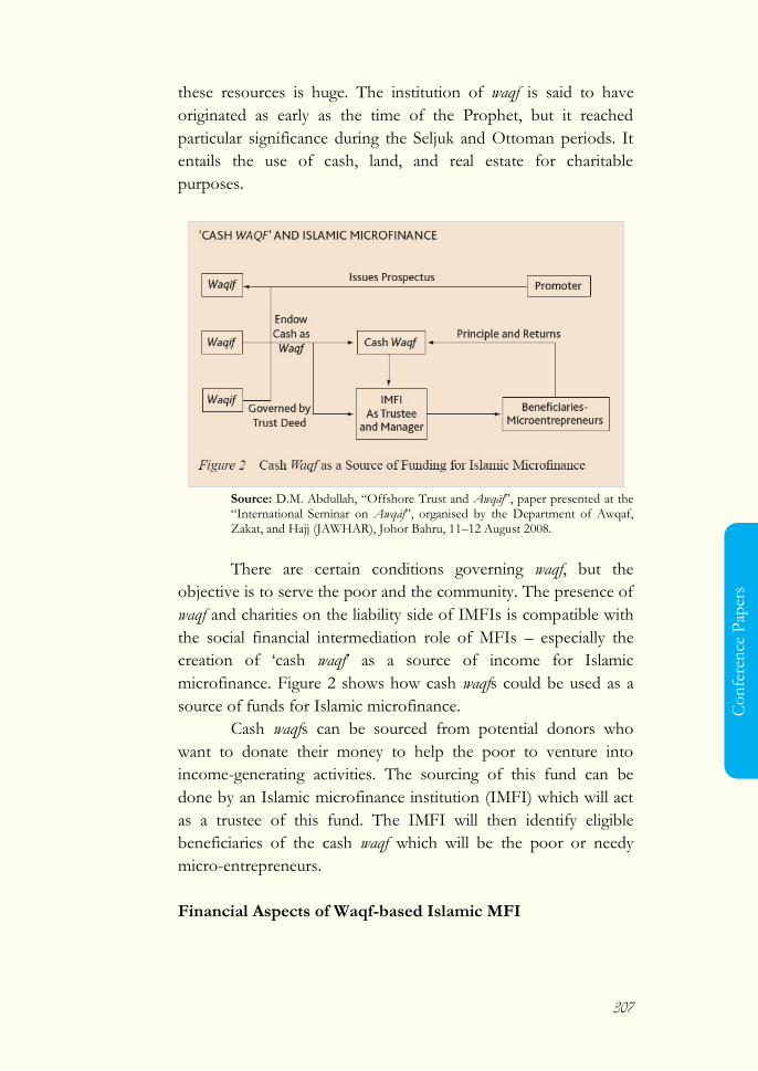
307

Co

nfe

ren

ce P

aper

s

these resources is huge. The institution of waqf is said to have

originated as early as the time of the Prophet, but it reached

particular significance during the Seljuk and Ottoman periods. It

entails the use of cash, land, and real estate for charitable

purposes.

Source: D.M. Abdullah, ―Offshore Trust and Awqāf‖, paper presented at the ―International Seminar on Awqāf‖, organised by the Department of Awqaf, Zakat, and Hajj (JAWHAR), Johor Bahru, 11–12 August 2008.

There are certain conditions governing waqf, but the

objective is to serve the poor and the community. The presence of

waqf and charities on the liability side of IMFIs is compatible with

the social financial intermediation role of MFIs – especially the

creation of ‗cash waqf‘ as a source of income for Islamic

microfinance. Figure 2 shows how cash waqfs could be used as a

source of funds for Islamic microfinance.

Cash waqfs can be sourced from potential donors who

want to donate their money to help the poor to venture into

income-generating activities. The sourcing of this fund can be

done by an Islamic microfinance institution (IMFI) which will act

as a trustee of this fund. The IMFI will then identify eligible

beneficiaries of the cash waqf which will be the poor or needy

micro-entrepreneurs.

Financial Aspects of Waqf-based Islamic MFI

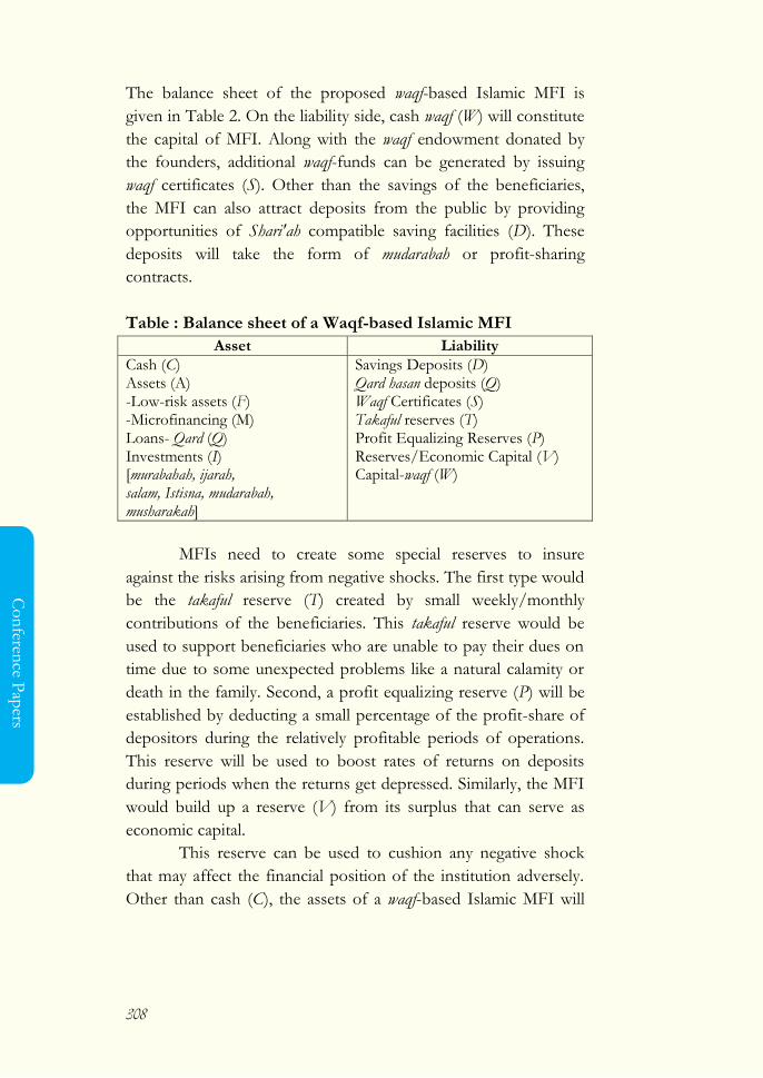
308

Co

nferen

ce Pap

ers

The balance sheet of the proposed waqf-based Islamic MFI is

given in Table 2. On the liability side, cash waqf (W) will constitute

the capital of MFI. Along with the waqf endowment donated by

the founders, additional waqf-funds can be generated by issuing

waqf certificates (S). Other than the savings of the beneficiaries,

the MFI can also attract deposits from the public by providing

opportunities of Shari'ah compatible saving facilities (D). These

deposits will take the form of mudarabah or profit-sharing

contracts.

Table : Balance sheet of a Waqf-based Islamic MFI

Asset Liability

Cash (C) Assets (A) -Low-risk assets (F) -Microfinancing (M) Loans- Qard (Q) Investments (I) [murabahah, ijarah, salam, Istisna, mudarabah, musharakah]

Savings Deposits (D) Qard hasan deposits (Q) Waqf Certificates (S) Takaful reserves (T) Profit Equalizing Reserves (P) Reserves/Economic Capital (V) Capital-waqf (W)

MFIs need to create some special reserves to insure

against the risks arising from negative shocks. The first type would

be the takaful reserve (T) created by small weekly/monthly

contributions of the beneficiaries. This takaful reserve would be

used to support beneficiaries who are unable to pay their dues on

time due to some unexpected problems like a natural calamity or

death in the family. Second, a profit equalizing reserve (P) will be

established by deducting a small percentage of the profit-share of

depositors during the relatively profitable periods of operations.

This reserve will be used to boost rates of returns on deposits

during periods when the returns get depressed. Similarly, the MFI

would build up a reserve (V) from its surplus that can serve as

economic capital.

This reserve can be used to cushion any negative shock

that may affect the financial position of the institution adversely.

Other than cash (C), the assets of a waqf-based Islamic MFI will

309

Co

nfe

ren

ce P

aper

s

comprise different types of non-interest bearing financial

instruments.

Due to reasons discussed below, a waqf-based Islamic MFI

will hold a combination of low-risk fixed-income assets (F) along

with micro-financing activities (M).2 Micro-financing will include

investments (I) and qard (Q).

For investments purposes, a variety of Islamic modes of

financing may be used. The type of financing instrument will

depend on the type of activity for which funds are granted. The

economic activities that microenterprises usually engage in

production, trading, and providing (transport) services.

Some of the appropriate Islamic modes of financing for

these activities are pointed out below. The principles of Islamic

financing can be broadly classified as partnerships (sharikat) and

exchange contracts (mu’awadat).3 Various kinds of financing

arrangements can be used to finance different kinds of activities.

Musharakah principle can be adopted in production (agricultural

and non-agricultural).

The Islamic MFI can provide part of the financial capital

to produce an output and in return receive a share of the profit. In

trading, the Islamic MFI and the client can jointly finance the

purchase and selling of a certain good and distribute the profit.

Production undertaken under mudarabah principle would imply

that the Islamic MFI finances and the client manages the project.

In agricultural production, output sharing can take the form of

muzara’a.

The Islamic MFI may fund the purchase of irrigation

equipment, fertilizers, etc., which the landowner uses on his land

to cultivate a certain crop. The harvested crop is then shared by

the landowner and the Islamic MFI at an agreed ratio. Other than

profit-sharing principle discussed above, murabahah and ijarah

forms of financing can also be used in production. For example, if

2 Low-risk and risk-free are used to identify these class of assets would

include either deposits in Islamic banks on placement in murabahah funds. 3 Detailed expositions of the different principles of Islamic financing are

found in Kahf and Khan (1992) and Ahmad (1993).

310

Co

nferen

ce Pap

ers

a client is in need of initial physical capital (equipment, gadgets,

etc.), the Islamic MFI can buy the items and sell these to the client

at a mark-up (murabahah). In agriculture, the item may be a cow or

poultry that the Islamic MFI sells at a mark-up. The client pays

back the price in agreed upon installments in the future. Similar

transaction can take place under a leasing (ijarah) contract. In

trading, profit sharing schemes and deferred trading contracts can

be used. Under profit sharing scheme, the Islamic MFI becomes a

partner in the trading business and gets a share of the profit.

The murabahah principle can also be applied where the

items to be traded are first bought by Islamic MFI and then sold

at a mark-up to the clients. The clients pay back the Islamic MFI

once they sell the goods. In transport services, both mark-up

principle and the leasing principle can be applied. For example, if a

client wants to buy a rickshaw, the Islamic MFI can purchase it

and sell it to the client at a mark-up. The client then pays the price

on an agreed instalment plan. Alternatively, hire-purchase

arrangement can be made in which the client pays rent plus a part

of the capital in his instalments. Once the instalments are fully

paid, the client becomes the owner of the machinery or vehicle.

Given the small scale nature of the operations of the

micro entrepreneurs, it may be difficult for the Islamic MFI to use

either sale-based or partnership modes of financing.4 It is too

costly (in terms of man-hours) and at times impossible to buy the

goods/assets that beneficiaries want. For example, it becomes very

difficult to accompany a beneficiary who may want a particular

kind of good sold in a far off market. One way to overcome this is

to use profit-sharing modes of financing. The sharing modes of

financing, however, have their own problems. The main problem

is the moral hazard problem arising from false underreporting of

profit as it is very difficult to assess the financial accounts. This

problem can be mitigated by supervising the operations and

4 See Ahmed (2002) for a discussion on the responses from a field survey on

problems of using Islamic modes of financing in micro-financing.

311

Co

nfe

ren

ce P

aper

s

monitoring accounts of the beneficiaries. Supervision and

monitoring, however, is costly.

In some special cases, the MFI can use loans (qard ) that

charge service costs only. These loans would be used for poorest

sections of the population and for activities where other modes of

financing cannot be used. The borrower of qarḍ al-ḥasan is only

required to repay the original amount of the loan. Scholars argue

that the administrative fee or service charge for loan transactions

is not against Islamic principles. The Islamic Development Bank

in Jeddah, for instance, recovers a service charge of 2 per cent to 3

per cent on interest free loans. Therefore, if qard al-ḥasan is given

by any financial institution, the imposition of a service charge or

administrative fee would be permissible. In other circumstances, if

microfinance is given for personal financing, Islamic MFI should

extend credit based on tawarruq. With the context of an ‗Islamic

transaction‘, al-tawarruq means buying goods or assets in

instalments and then selling them for cash at a lower price to a

third party who is not the original seller of the commodity or

asset.

Sustainability of Waqf-based Islamic MFI

We discuss the status of waqf-based Islamic MFIs with regard to

the three fundamental problems related to operations and

sustainability of financing microenterprises next.5

Mitigating Credit Risk

As mentioned above, the innovative operational format of MFIs

suits the poor, whose lack of physical collateral disqualify them to

borrow from traditional commercial banks. Waqf-based Islamic

MFIs will retain the innovative format of operation of

conventional MFIs and oriented the program towards Islamic

principles and values. Thus, like their conventional counterparts,

5 These conclusions are based on a survey on Islamic MFIs by Ahmed (2002).

312

Co

nferen

ce Pap

ers

Islamic MFIs have largely resolved the credit risks through social

collateral of groups and weekly repayments.

Resolving Moral Hazard Problem

Islamic MFIs have some inherent characteristics that can resolve

the moral hazard problem faced by conventional MFIs pointed

above. The main mode of financing used by the Islamic MFIs is

murabahah/bai-muajjal or ijarah (leasing). These instruments involve

real transaction and instead of cash being given out, asset/good is

exchanged. As a result, the opportunity of diverting funds for

non-productive uses other than that requested for is reduced, if

not eliminated. This increases the profitability of the MFI by

decreasing the default rate.

In cases where Islamic MFIs get funds from traditional

interest-based outlets, the financing costs appear to be high. For

example, the financing costs of two small Islamic MFIs, Noble

and Rescue in Bangladesh, were 35.8 percent and 12.5 percent of

the total expenditures respectively (Ahmed 2002). As the bulk of

the waqf-based Islamic MFIs funds will come from waqf

endowment, the financing costs of these institutions will be

significantly lower than their conventional counterparts. Given the

philanthropic nature of these funds, no returns are expected by

contributors. While Islamic MFIs will pay returns on funds

coming from external sources like deposits and beneficiary

savings, the waqf component of funds will significantly reduce the

financial costs and improve financial viability of the institution.

The above discussion shows that by adopting the group

based financing of the conventional MFIs, Islamic MFIs have

resolved the problem of credit risk. Furthermore, the use of

Islamic modes of financing linked to real transactions subsides the

moral hazard problem by preventing diversion of funds for other

purposes in Islamic MFIs. Furthermore, Islamic MFIs can tackle

the economic viability problem by reducing their financing costs

significantly.

Other Approaches To Funding MFI Operations

313

Co

nfe

ren

ce P

aper

s

While the paper proposes the use of a waqf-based MFI to finance

the poor, some other sources of funds can be used to further

enhance the scope of Islamic microfinancing. Some of these

sources are discussed below.

Along with waqf and qard Hassan

The institutions of zakah and sadaqat can be integrated into

microfinancing program to effectively alleviate absolute poverty.

These traditional instruments of social welfare can be used in

financing the poor entrepreneurs. Integrating zakah into

microfinancing can prevent fund diversions and benefit the

poorest beneficiaries (Ahmed 2002). Zakah given to the poor can

be used for consumption, asset building, and productive purposes

to complement funds of Islamic MFIs. As these complementary

funds will reduce the need for diverting money for consumption

and/or purchase of assets, it is expected the funds taken for

productive activities will be invested accordingly. As a result, the

overall return on invested funds is expected to be higher and the

probability of default lower. Thus, integrating Islamic institutions

of zakah and charities with microfinancing will increase the

probability of repayment of the funds to theIslamic MFI.

The scope of Islamic microfinancing can also be increased by getting Islamic

banks involved.

Ahmed (2003) shows that Islamic banks are predisposed to

provide microfinance in a "win-win" situation. It is argued that

Islamic banks can provide microfinance at lower operating and

financing costs. The operating costs of providing microfinance in

case of Islamic banks will be much smaller than MFIs, and these

institutions will provide microfinance from existing branches and

not incur any extra fixed costs (rent, utilities, etc.). Furthermore, it

will not require a whole range of professionals/employees,

particularly at the top management level at the head office and

regional offices. Similarly financing costs for Islamic banks is

expected to be lower. Most Islamic banks have excess liquidity

given the lack of Islamic compatible money-market instruments to

314

Co

nferen

ce Pap

ers

park funds for shorter periods of time. Given this excess liquidity,

the opportunity cost of using these funds is almost zero. These

funds can be used for micro financing as no extra cost. Thus,

Islamic banks can finance microenterprises more efficiently (at a

lower cost) than MFIs.

Additionally, Islamic banks can use income derived

From late-payment penalties and other proceeds which it cannot

include in its income (like interest earnings from treasury

operations). Islamic banks can create a waqf from these funds and

use these for microfinance operations. As suggested in point 2

above, Islamic banks will be able to provide microfinancing at a

lower cost than MFIs due to lower operating and financing costs.

5. CONCLUSION

Muslim countries tend to create a built-in dependency. Once the

support of the NGOs are withdrawn or the flow of aid stops for

one reasons or another, this make its beneficiary worse off in the

sense that discontinuation of support push them back beyond

their original level of living. Cases of Islamic banks practicing

microfinance are even fewer. This crucial problem for Islamic

MFIs faces in obtaining funds from external sources. Though

some funds are available from government agencies, they impose

certain terms and conditions. Some of these terms and conditions

are contrary to Islamic principles and limit the flexibility in the

operations of Islamic MFIs. These factors increase the probability

of default and lowering the expected income of MFIs. The cost of

fund invested in current Micro credit program is relatively high

due to supervision cost.

Given these shortcomings, the article suggests the

possibility of using cash-waqf as a new source of funding for

Islamic microfinance and proposes new concepts and applications

of Islamic microfinance, thereby putting it in line with the true

Islamic spirit of microfinance. Furthermore, the article also

proposes the use of other modes of financing such as muḍārabah,

315

Co

nfe

ren

ce P

aper

s

murābaḥah, ijara, and muzara‘a as well as qarḍ al-ḥasan and

tawarruq in extending credit to the poor. With this new concept

and application of Islamic microfinance, it will be able to further

enhance the growth of microfinance to reach millions of poor

Muslims, whether in Bangladesh, other Muslim countries, or

among Muslim minorities in non-Muslim countries.

The paper also suggests some other sources of funds that

Islamic MFIs can tap into to expand their operations. Other than

using zakah and sadaqat as additional resources, Islamic banks can

also provide micro-financing efficiently without cutting into their

profits. As Islamic modes of financing involve transfer of real

assets/goods, use of these instruments by these institutions can

lessen the problem of diversion of funds to non-productive.

Furthermore, using waqf to finance MFI operations can reduce the

financing costs and improve the viability of these institutions.

In addition, with this new concept and application of

Islamic microfinance, we are convinced that the use of

microfinance would genuinely cater for the needs of the poor and

the needy and as a means to combat poverty as well as generating

socio-economic growth in the Muslim world.

REFERENCES

Ahmed, M. (1985), Status, Perception, Awareness and Marital

Adjustment of Rural Women: The Role of Grameen Bank,

Grameen Bank, Dhaka.

Auwal, M.A. (1996), Promoting Microcapitalism in the Service of

the Poor: The Grameen Model and its Crosscultural

Adaptation, The Journal of Business Communication, 33(1): 27-

42.

Ahmed, Habib (2004), Role of Zakah and Awqaf in Poverty Alleviation,

Occasional Paper No. 8, Islamic Research and Training

Institute, Islamic Development Bank, Jeddah.

316

Co

nferen

ce Pap

ers

Ahmed, Habib (2006), "Withdrawal Risk in Islamic Banks, Market

Discipline and Bank Stability" in Tariqullah Khan and

Dadang Muljawan(Editors), Islamic Financial Architecture:

Risk Management and Financial Stability, Conference

Proceedings, Islamic Research and Training Institute,

Islamic Development Bank Group.

Ahmad, Ausaf (1993), Contemporary Practice of Islamic Financing

Techniques, Islamic Research and Training Institute,

Research Paper No. 20.

Ahmed, H., 2004. Frontiers of Islamic Banking: A Synthesis of

Social Role and Micro finance. Forthcoming The

European Journal of Management and Public Policy.

Amin, S., A.S. Rai and G. Topa, 2003. Does microcredit reach the

poor and vulnerable? Evidence from northern Bangladesh.

Journal of Development Economics, 70(1): 59-82.

Ahmed, Habib (2003), "The Role of Islamic Financial Institutions

in Financing Microenterprises: Theory and Practice",

paper presented at the Forum on Islamic Economics and

Finance held in Amman Jordan during September 27-29,

2003 organized by The Arab Academy for Banking and

Financial Sciences.

Banerjee, M.M. (1998), Micro-Enterprise Development: A

Response to Poverty, Journal of Community Practice, 5(1/2):

63-83.

Besley, T. and Coate, S. (1995), Group Lending, Repayment

Incentives, and Social Collateral, Journal of Development

Economics, 46: 1-18.

Bhatt, N. and Tang, S.Y. (1998), The Problem of Transaction

Costs in Group-Based Microlending: An Institutional

Perspective, World Development, 26(4): 623-637.

317

Co

nfe

ren

ce P

aper

s

Chapra, M. Umer (1985), Towards a Just Monetary System, The

Islamic Foundation, Leicester.

Chapra, M. Umer and Habib Ahmed (2002), Corporate Governance in

Islamic Financial Institutions, Occasional Paper No. 6, Islamic

Research and Training Institute, Islamic Development

Bank.

Dusuki, A.W., 2008. Banking for the poor: the role of Islamic

banking in microfinance initiatives. Humanomics, 24(1):

49-66.

Grameen Bank (2009), Grameen Bank Monthly Report, Source:

Grameen Bank, July, 2009, Website:

http://www.grameen-info.org

Hashemi, S.M. (1997), Building up Capacity for Banking with the

Poor: The Grameen Bank of Bangladesh, in Hartmut

Schneider (ed), Microfinance for the Poor? Organization for

Economic Co-operation and Development:109-128.

Hossain, M. (1988), Credit for Alleviation of Rural Poverty: The Grameen

Bank in Bangladesh, Bangladesh Institute of Development

Studies, Dhaka.

Hossain, M.M.; Maskooki, M. and Gunasekaran, A. (2001),

Implications of Grameen Banking System in Europe:

Prospects and Prosperity, European Business Review, 13(1):

26-42.

Habib, M.A., et al., 2004. Micro Credit: An Experience of Islami

Bank Bangladesh Limited. Department of Agricultural

Finance Bangladesh Agricultural University, Mymensingh-

2202, Bangladesh.

318

Co

nferen

ce Pap

ers

Habib (2002), ―Financing Microenterprises: An Analytical Study

of Islamic Microfinance Institutions,‖ Islamic Economic

Studies, 9 (2), 27-64.

IBBL, A.R., Performance of Rural Development Scheme 2009,

Islami Bank Bangladesh Limited Dhaka, Bangladesh.

IBBL, A.R., Performance of Rural Development Scheme 2007,

Islami Bank Bangladesh Limited Dhaka, Bangladesh.

Kahf, Monzer (2004), "Shari'a h and Historical Aspects of Zakah

and Awqaf", background paper prepared for Islamic

Research and Training Institute, Islamic Development

Bank.

Kahf, Monzer and Tariqullah Khan (1992), Principles of Islamic

Financing, A Survey, Islamic Research and Training

Institute, Research Paper No. 16. Khan, M. Fahim (1997),

"Social Dimensions of Islamic Banks in Theory and

Practice," Islamic Research and Training Institute, Islamic

Development Bank, manuscript.

Khandker, S.R. (1996), Grameen Bank: Impact, Costs, and

Program Sustainability, Asian Development Review, 14(1): 65-

85.

Khandker, S.R.; Khalily, B. and Khan, Z. (1995), Grameen Bank:

Performance and Sustainability, Discussion Paper No. 306,

Washington DC: World Bank.

Larance, L.Y. (1998), Building Social Capital From the Center: A

Village-Level Investigation of Bangladesh‘s Grameen

Bank, Center for Social Development, Washington

University in St. Louis, Working Paper No. 98-4.

Morduch, J. (1999b), The Microfinance Promise, Journal of

Economic Literature, 37(4): 1569-1614.

319

Co

nfe

ren

ce P

aper

s

Mair, M. and Schoen, O. (2007), Successful Social Entrepreneurial

Business Models in the Context of Developing

Economies, International Journal of Emerging Markets, 2(1):

54-68.

Mannan, M.A., 2006. Innovation and Operational Experience of

Risk Management of Islamic Micro-finance Local

Challenges and Global Opportunities: A Case Study

Approach in Seventh Harvard University Forum on

Islamic Finance. 2006, Cambridge, MA, USA: Harvard

University, USA.

Mizanur, M., Rahmana, M. Jafrullahb and A.T. Islamc, 2008. Rural

Development Scheme Bangladesh Limited (IBBL):

Assessment Challenges. IIUM Journal of Economics and

Management, 16(2): 139-163.

Rahman, A. (1999b), Micro-credit Initiatives for Equitable and

Sustainable Development: Who Pays? World Development,

27(1): 67-82.

Rahim, A. and A. Rahman, 2007. Islamic Microfinance: A Missing

Component in Islamic Banking. Kyoto, Bulletin of Islamic

Area Studies, 1-2: 38-53.

Sarker, A.E. (2001), The Secrets of Success: the Grameen Bank

Experience in Bangladesh, Labour and Management in

Development Journal, 2(1): 1-17.

Schreiner, M. (1999), A Cost-effectiveness Analysis of the

Grameen Bank of Bangladesh, Center for Social

Development, World Bank (2001), Poverty Analysis; Web:

http://web.worldbank.org.

Todd, H. (1996), Women at the Center: Grameen Bank Borrowers after

one Decade, Westview Press, Boulder, Colorado.

320

Co

nferen

ce Pap

ers

Yunus, M. (1994a), Credit is a Human Right, Grameen Bank, Dhaka.

Yunus, M. (1994b), We Can Create a Poverty-Free World in Our Life-

Time, Grameen Bank, Dhaka.

Yunus, M. (1998), Poverty Alleviation: Is Economics Any Help?

Lessons from the Grameen Bank Experience, Journal of

International Affairs, 52(1): 47-65.

Zarqa, Muhammad Anas (1988), "Islamic Distributive Schemes",

in Munawar Iqbal (Editor), Distributive Justice and Need

Fulfillment in an Islamic Economy,The Islamic Foundation,

Leicester, pp. 163-216.

321

Co

nfe

ren

ce P

aper

s

Islamic Financing Risk And Return Simulation of Islamic Financing

Withstand to Economic Shocks: A Case Study in Indonesia

Amrin Barata

Regional Account and Statistics Analysis subdivision in Statistics Indonesia (BPS),

Wakatobi Regency, Indonesia

Abstract

In pursuit of supporting the implementation of national

development, Shariah banking often faced with stability problems

of financing instruments being operated. In this case, it is

measured by the gap between the actual rate of return (RoR) and

the expected rate of return. The individual actual rate of return of

this instrument will generate an expected rate of return. This raises

the gap or difference between the actual rate of return and the

expected rate of return of individual instruments, which in this

case is called the abnormal rate of return.

The stability of abnormal rate of return of individual

instruments is certainly influenced by the stability of the expected

rate of return. Expected rate of return has a volatility or

fluctuation levels for each financing instrument, as well as a key

element or material basis for the establishment of an individual

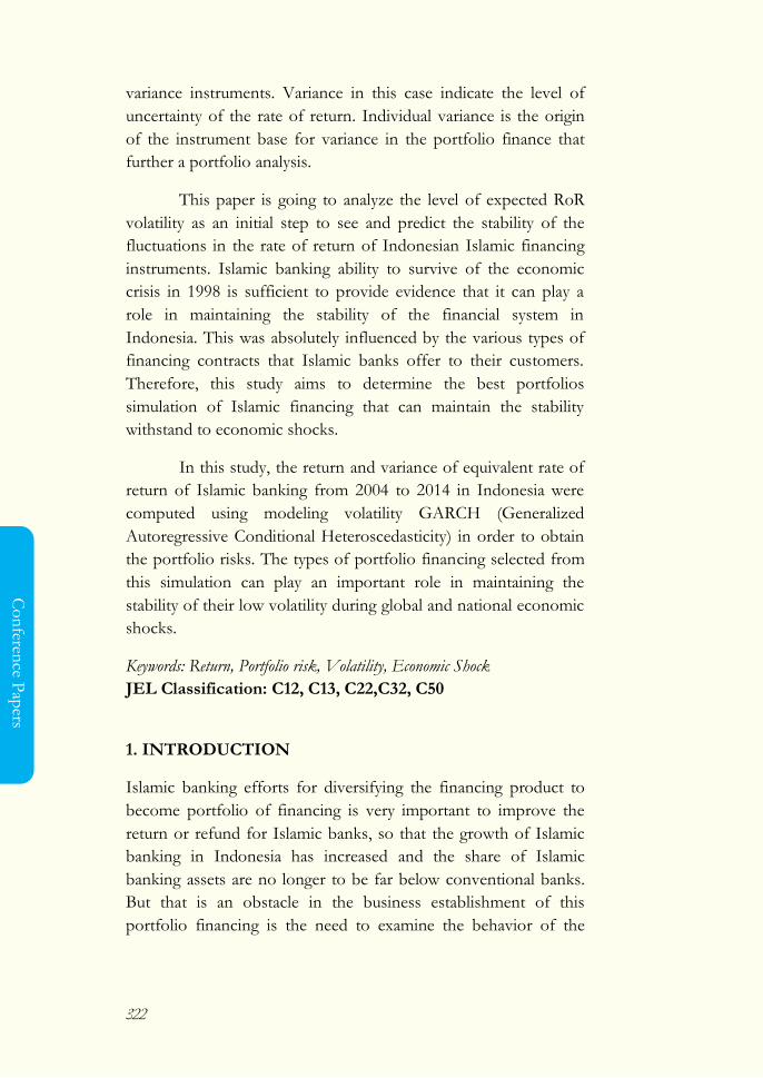
322

Co

nferen

ce Pap

ers

variance instruments. Variance in this case indicate the level of

uncertainty of the rate of return. Individual variance is the origin

of the instrument base for variance in the portfolio finance that

further a portfolio analysis.

This paper is going to analyze the level of expected RoR

volatility as an initial step to see and predict the stability of the

fluctuations in the rate of return of Indonesian Islamic financing

instruments. Islamic banking ability to survive of the economic

crisis in 1998 is sufficient to provide evidence that it can play a

role in maintaining the stability of the financial system in

Indonesia. This was absolutely influenced by the various types of

financing contracts that Islamic banks offer to their customers.

Therefore, this study aims to determine the best portfolios

simulation of Islamic financing that can maintain the stability

withstand to economic shocks.

In this study, the return and variance of equivalent rate of

return of Islamic banking from 2004 to 2014 in Indonesia were

computed using modeling volatility GARCH (Generalized

Autoregressive Conditional Heteroscedasticity) in order to obtain

the portfolio risks. The types of portfolio financing selected from

this simulation can play an important role in maintaining the

stability of their low volatility during global and national economic

shocks.

Keywords: Return, Portfolio risk, Volatility, Economic Shock

JEL Classification: C12, C13, C22,C32, C50

1. INTRODUCTION

Islamic banking efforts for diversifying the financing product to

become portfolio of financing is very important to improve the

return or refund for Islamic banks, so that the growth of Islamic

banking in Indonesia has increased and the share of Islamic

banking assets are no longer to be far below conventional banks.

But that is an obstacle in the business establishment of this

portfolio financing is the need to examine the behavior of the

323

Co

nfe

ren

ce P

aper

s

return of each islamic financing instruments, namely how the

expectations of return of each instrument before between one

instrument combined with other instruments. Whether expected

rate of return of each these forms of financing that shows the

behavior/characteristics that tend to be stable or fluctuating.

Financing return is not the only obstacle in this case, but

also the risk which is a measure of the uncertainty of the expected

rate of return to be earned in the future of the portfolio financing.

Islamic banking will certainly avoid the high risk of finance in

contracting the finance portfolio to investors. Not stop here only

because it is also important to consider the level of fluctuations

(volatility) of the gap between the actual rate of return and the

expected rate of return of Islamic financing instruments,

considering the monthly time series data in the financial sector or

financial (rate of return) very high level of volatility. This gap is

called the abnormal rate of return. The high volatility is

characterized by a phase in which the fluctuation is relatively high

and then followed a low fluctuation and high back, in other words,

the data is averaged and variants are not constant. Thus, the

volatility of the abnormal rate of return of Islamic financing

instruments is also a measure of uncertainty as additional

consideration to establish the financing portfolio in this study to

look at the volatility of the expected rate of return as the element.

The economic crisis in 1998 which was very powerful had

caused many banks in Indonesia got financial difficulties and some

of them even went bankrupt. But Islamic banks were proven to be

resilient to the economic shocks. Absolutely, the existence of

Islamic financing instruments would be one that plays major role

in saving Islamic banks from various risks due to economic

shocks.

The existence of Islamic financing instruments must not

be separated from the possibility of uncertainty of risk and return

that arise. Furthermore, to minimize risk and increase returns,

Islamic banks can diversify their earning assets into a portfolio of

financings. It is very important for Islamic banks to have a good

324

Co

nferen

ce Pap

ers

portfolio of financings in order to ensure they can deliver

competitive rates of return to their investors along with the lowest

possible risk. In order to form a good portfolio of financings, it is

important to examine the behavior of each Islamic financing

instrument that forms the portfolio especially the expected rate of

return of each instrument when it is combined with other

instruments.

However, it is important to remember that Islamic banks

should not only concern on the rate of return but also the risk of

the portfolio. The risk of a portfolio is the uncertainty of the

expected rate of return to be earned in the future of the financing

portfolio. Islamic banks will certainly avoid the high risk of

financings to be included in their portfolios. Therefore, it is very

important to look at the behavior of risk of each financing

instrument when it is combined with other Islamic financing

instruments in a portfolio to ensure the combination of those

instruments create optimum results. In other words, the

combination must minimize the risk not increase the risk. In

addition, it is also important to consider the level of fluctuations

(volatility) of the portfolio risk of Islamic financing instruments.

This is because in practice, the monthly time series data of Islamic

banks' rate of return is very volatile.

Given the importance of risk, risk volatility and rate of

return, this study tries to analyze the behavior of portfolios risk

and return of Islamic banking financings. Furthermore, this study

also calculates the volatility of the portfolio risk of Islamic banks

in Indonesia. In this study, various combinations of Islamic

financing instruments of Islamic banks in Indonesia are formed

for the simulation and the risk-return behaviour is analyzed in

order to the reaction of the ideal portfolio to the economic shocks

during 2004-2014.

By this, the problems raised in this research is how to

make the risk-return simulation of Islamic financing to withstand

the economic shocks that matter as long as 2004-2014 period.

325

Co

nfe

ren

ce P

aper

s

The results of this study are expected to help Islamic

banks in Indonesia in evaluating, assessing, and planning funding

and financing products strategies that have good prospect for the

future and improving financing instruments which have bad risk-

return behaviour and have high levels of portfolio risks volatility.

With that, hopefully it will stimulate the growth of Islamic banks

in Indonesia and make it survive over economic shocks. This

study is not only for Indonesia, but also it can be applied for

western and middle east country.

2. LITERATURES

Ismal (2010) attempted to determine the most efficient portfolio

frontier of financial instruments of Islamic banks in Indonesia by

analyzing the risk and return of each Islamic banks' possible

portfolios. Return on Assets (ROA) for each financing instrument

was used as a proxy to the equivalent rate of return/profit sharing

from financing instruments of Islamic banks in Indonesia. The

data in the form of financing instruments like mushakarah,

mudaraba, murabaha and, istisna from 2001-2007 was collected

and analyzed. Taking into account the findings of the individual

and overall performance of the portfolio, efficient portfolio

frontier curve explained that the Indonesian Islamic banking can

optimize financing portfolio by not only focusing on the

distribution of funds in murabaha but also in mudaraba.

Engle (2001) found that the kind of GARCH model can

be used as a technique to construct an equation that measures the

volatility (foresee or predict the variance) of the stock return and

portfolio. Savickas (2003) also found that the kind of GARCH

model is the best model that can capture the volatility effect of

stock return data, compared to other methods such as the method

of mean rank and standardized cross-sectional.

Alberto (2005) also found that the kind of GARCH

method is better estimated in return of a stock than the OLS

estimates. Alessandro (2007) also found that the kind of GARCH

model, both the mean and variance models used to predict the

return and risk over several periods ahead. Based on consideration

326

Co

nferen

ce Pap

ers

of forecasting the portfolio return and risk, it will be considered

which one for the best portfolio.

Based on the previous studies above, it is found that the

best method to conduct this study is the GARCH model. The

next section elaborates in more details this method.

3. METHODOLOGY

3.1 Data Collection and Research Method

This study uses secondary data measured time series. Islamic

Banks in Indonesia used as the sample in this study are

categorized into Islamic Commercial Bank (BUS), Islamic

Business Unit of a Conventional Bank (UUS) and Islamic Rural

Bank (BPRS). The data was collected from Bank Indonesia

particularly the monthly Islamic Banking Statistics (SPS) which is

available on the website of Bank Indonesia and the Financial

Services Authority (OJK). Time period of this study is from 2004

until 2014. The software used in this study is a Microsoft Office

Excel 2007 and Eviews 6.0.

There are five types of financing instruments of Islamic

banking used in this study, namely murabaha, mudaraba,

musharaka, istishna and qardh. These are types of financings

based on contracts offered by Islamic banks in Indonesia to their

cusromers (Bank Indonesia, 2004-2013). This study uses a

quantitative approach. As the previous studies, the econometric

analysis conducted to support the analysis of return and risk and

detect the volatility of portfolio rate of returns is ARCH/GARCH

(p, q) models.

Risk-return portfolio theory is used to analyze the rate of

return of each instrument, the expected rate of return, probability

of occurrence and market share. Moreover, the risk-return

portfolio theory also detects each risk financing instruments

through the variation of the actual level and the expected rate of

return.. The expected rate of return of one and more than one

financial instruments is defined as follows:

327

Co

nfe

ren

ce P

aper

s

N

i

iii rpRE1

)( (1)

)(......)()()()( 332211 nnp REwREwREwREwRE

(>1instrument) (2)

Where ip is probability of occurrence of rate of return, and ir is

rate of return (RoR) instrument. Because Islamic finance theory

states that future profits should not be ascertained, then this

calculation uses historical data as a predictor (good predictor-

proxy) for the probability of occurrence ( ip ) above. For more

than one instruments, then each instrument will be weighted ( nw )

derived from the market value as written in equation 2 above. This

method will provide proportionate treatment for all financial

instruments are analyzed.

Then the difference between the expected rate of return

and the actual value describes the variation (variance) instrument

)( with the general formula equation 3 below. High variance

showed no consistency (inconsistency) the movement of return on

a particular indicative target (expected RoR) which among other

things means that a relatively high risk of uncertainty (risk

financing) a financing instrument during the period of the

observations made. Variance of the instrument is shown by

equation 4.

n

i

n

j

jijip wwRVar1 1

,)( (3)

N

i

inn

ii

i j

jiji

RErp

RErp

wwRVar

1

2

2

1

1

1

1

1

1

)]([(

......)]([

,)(

(4)

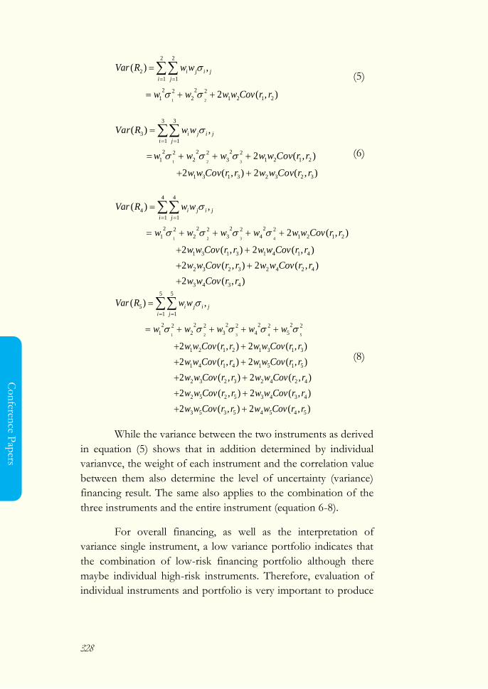
328

Co

nferen

ce Pap

ers

),(2

,)(

2121

22

2

22

1

2

1

2

1

2

21rrCovwwww

wwRVari j

jiji

(5)

),(2),(2

),(2

,)(

32323131

2121

22

3

22

2

22

1

3

1

3

1

3

321

rrCovwwrrCovww

rrCovwwwww

wwRVari j

jiji

(6)

),(2

),(2),(2

),(2),(2

),(2

,)(

4343

42423232

41413131

2121

22

4

22

3

22

2

22

1

4

1

4

1

4

4321

rrCovww

rrCovwwrrCovww

rrCovwwrrCovww

rrCovwwwwww

wwRVari j

jiji

),(2),(2

),(2),(2

),(2),(2

),(2),(2

),(2),(2

,)(

54545353

43435252

42423232

51514141

31312121

22

5

22

4

22

3

22

2

22

1

5

1

5

1

5

54321

rrCovwwrrCovww

rrCovwwrrCovww

rrCovwwrrCovww

rrCovwwrrCovww

rrCovwwrrCovww

wwwww

wwRVari j

jiji

(8)

While the variance between the two instruments as derived

in equation (5) shows that in addition determined by individual

varianvce, the weight of each instrument and the correlation value

between them also determine the level of uncertainty (variance)

financing result. The same also applies to the combination of the

three instruments and the entire instrument (equation 6-8).

For overall financing, as well as the interpretation of

variance single instrument, a low variance portfolio indicates that

the combination of low-risk financing portfolio although there

maybe individual high-risk instruments. Therefore, evaluation of

individual instruments and portfolio is very important to produce

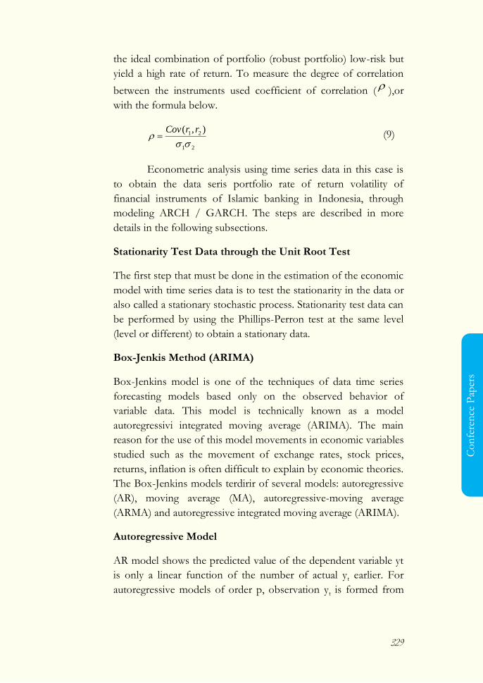
329

Co

nfe

ren

ce P

aper

s

the ideal combination of portfolio (robust portfolio) low-risk but

yield a high rate of return. To measure the degree of correlation

between the instruments used coefficient of correlation ( ),or

with the formula below.

21

21 ),(

rrCov (9)

Econometric analysis using time series data in this case is

to obtain the data seris portfolio rate of return volatility of

financial instruments of Islamic banking in Indonesia, through

modeling ARCH / GARCH. The steps are described in more

details in the following subsections.

Stationarity Test Data through the Unit Root Test

The first step that must be done in the estimation of the economic

model with time series data is to test the stationarity in the data or

also called a stationary stochastic process. Stationarity test data can

be performed by using the Phillips-Perron test at the same level

(level or different) to obtain a stationary data.

Box-Jenkis Method (ARIMA)

Box-Jenkins model is one of the techniques of data time series

forecasting models based only on the observed behavior of

variable data. This model is technically known as a model

autoregressivi integrated moving average (ARIMA). The main

reason for the use of this model movements in economic variables

studied such as the movement of exchange rates, stock prices,

returns, inflation is often difficult to explain by economic theories.

The Box-Jenkins models terdirir of several models: autoregressive

(AR), moving average (MA), autoregressive-moving average

(ARMA) and autoregressive integrated moving average (ARIMA).

Autoregressive Model

AR model shows the predicted value of the dependent variable yt

is only a linear function of the number of actual yt earlier. For

autoregressive models of order p, observation yt is formed from

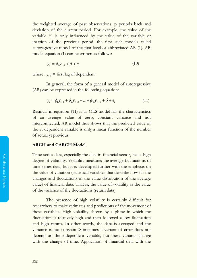
330

Co

nferen

ce Pap

ers

the weighted average of past observations, p periods back and

deviation of the current period. For example, the value of the

variable Yt is only influenced by the value of the variable or

inaction of the previous period, the first such models called

autoregressive model of the first level or abbreviated AR (1). AR

model equation (1) can be written as follows:

ttt eyy 11 (10)

where : yt-1 = first lag of dependent.

In general, the form of a general model of autoregressive

(AR) can be expressed in the following equation:

tptpttt eyyyy ...2211 (11)

Residual in equation (11) is as OLS model has the characteristics

of an average value of zero, constant variance and not

interconnected. AR model thus shows that the predicted value of

the yt dependent variable is only a linear function of the number

of actual yt previous.

ARCH and GARCH Model

Time series data, especially the data in financial sector, has a high

degree of volatility. Volatility measures the average fluctuations of

time series data, but it is developed further with the emphasis on

the value of variation (statistical variables that describe how far the

changes and fluctuations in the value distribution of the average

value) of financial data. That is, the value of volatility as the value

of the variance of the fluctuations (return data).

The presence of high volatility is certainly difficult for

researchers to make estimates and predictions of the movement of

these variables. High volatility shown by a phase in which the

fluctuation is relatively high and then followed a low fluctuation

and high return. In other words, the data is averaged and the

variance is not constant. Sometimes a variant of error does not

depend on the independent variable, but these variants change

with the change of time. Application of financial data with the

331

Co

nfe

ren

ce P

aper

s

characteristics usually on modeling the return of capital markets,

inflation and interest rates. Thus volatility patterns indicate

heteroscedasticity because there are variants error whose

magnitude depends on the volatility of the error in the past.

Autoregressive Moving Average (ARMA) Model is often

used in the modeling of time series data. This model has a

stationarity assumption on the data and constant residual variance

(homoscedasticity). This assumption is not easily fulfilled on time

series data data financially. The financial data has its own

characteristics compared to the time series data in general, which

shows high volatility following the period of time that shows

volatility, variance for a long period of time the data is constant

but there are some periods where the data variance is relatively

high. This is called conditionally heteroskedastic. If detected, the

conditionally heteroskedastic autoregressive moving average

models (ARMA) no longer appropriate to use. The data get

heteroscedasticity properties like this can be modeled by

Autoregresive Conditional Heteroscedasticity (ARCH) which was

introduced by Robert Engle.

ARCH method is a refinement of the ARMA method. At

ARMA, the variance is not the center of attention when one uses

the model is that we want to see a large deviation in the forecast,

which means also the contribution of predictor variables that we

input into the model works. For that ARCH is required to see the

pattern of residual variance, so that we can evaluate and improve

the return forecasts that we make, because this method further

support the existence of other predictor variables are unknown or

are not included in the model. ARCH designed specifically to

produce models and forecasting (forecast) due to the presence of

conditionals variance.

There are several reasons underlying the establishment of

ARCH models and forecast volatility; first, the need to analyze the

risks of the assets that we have or the value of an option; second,

forecasting confidence intervals are at different times, so to get the

interval can be obtained from the model variance of the error; and

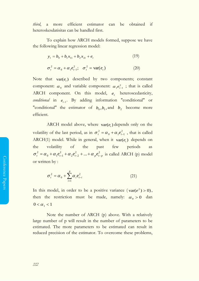
332

Co

nferen

ce Pap

ers

third, a more efficient estimator can be obtained if

heteroskesdatisitas can be handled first.

To explain how ARCH models formed, suppose we have

the following linear regression model:

ttt exbxbby 221110 (19)

)var(;22

110

2

tttt ee (20)

Note that )var( te described by two components; constant

component: 0

and variable component: 2

11 te ; that is called

ARCH component. On this model, te heteroscedasticity,

conditional in 1te . By adding information "conditional" or

"conditional" the estimator of ,, 10 bb and 2b become more

efficient.

ARCH model above, where )var( te depends only on the

volatility of the last period, as in 2

110

2

tt e , that is called

ARCH(1) model. While in general, when it )var( te depends on

the volatility of the past few periods as 22

22

2

110

2... ptpttt eee is called ARCH (p) model

or written by :

p

i

itit e1

2

0

2 (21)

In this model, in order to be a positive variance ( )0)var(2e ,

then the restriction must be made, namely: 00 dan

10 1

Note the number of ARCH (p) above. With a relatively

large number of p will result in the number of parameters to be

estimated. The more parameters to be estimated can result in

reduced precision of the estimator. To overcome these problems,

333

Co

nfe

ren

ce P

aper

s

so that the estimated parameters are not too much, the )var( te can

be used the following model:

2

11

2

110

2

ttt e (22)

This model is called the GARCH (1,1) because 2

t depend on 2

1te

and 2

1t each of which has a time lag. Similarly, ARCH models, in

order to be a positive variance ( )0)var(2e , then on this model

should also be made restrictions, namely: 10 ;0 and ;01

and 111 .

As ARCH model, the GARCH model can also be

estimated by Maximum Likelihood technique. In general, the

)var( te can be represented by the form:

22

11

22

110

2...... qtqtptptt ee or written by:

q

i

iti

p

i

itit e1

2

1

2

0

2 (23)

The Model above is called GARCH(p,q) model.

From the model above shows that the amount of )var( te

in addition to allegedly depends on 2e also dep ends on 2 the

past.

At the time series data of finance of the ARCH/GARCH

element or a form of authoregressive of residual quadratic phase

which is characterized by high fluctuations and then followed a

low fluctuation and high return.

The steps in determining the ARCH / GARCH model

includes first, identification of the mean models, testing the

conditional variance heterogeneity, estimation of the parameters

of ARCH / GARCH model, model diagnosis, and selecting for

the best model.

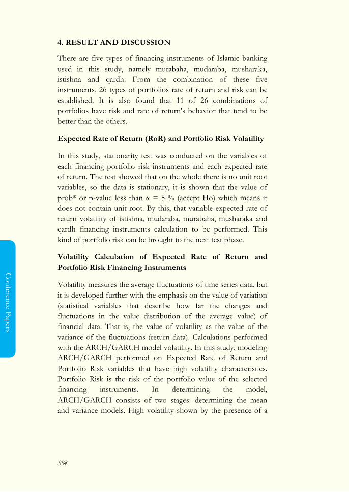
334

Co

nferen

ce Pap

ers

4. RESULT AND DISCUSSION

There are five types of financing instruments of Islamic banking

used in this study, namely murabaha, mudaraba, musharaka,

istishna and qardh. From the combination of these five

instruments, 26 types of portfolios rate of return and risk can be

established. It is also found that 11 of 26 combinations of

portfolios have risk and rate of return's behavior that tend to be

better than the others.

Expected Rate of Return (RoR) and Portfolio Risk Volatility

In this study, stationarity test was conducted on the variables of

each financing portfolio risk instruments and each expected rate

of return. The test showed that on the whole there is no unit root

variables, so the data is stationary, it is shown that the value of

prob* or p-value less than α = 5 % (accept Ho) which means it

does not contain unit root. By this, that variable expected rate of

return volatility of istishna, mudaraba, murabaha, musharaka and

qardh financing instruments calculation to be performed. This

kind of portfolio risk can be brought to the next test phase.

Volatility Calculation of Expected Rate of Return and

Portfolio Risk Financing Instruments

Volatility measures the average fluctuations of time series data, but

it is developed further with the emphasis on the value of variation

(statistical variables that describe how far the changes and

fluctuations in the value distribution of the average value) of

financial data. That is, the value of volatility as the value of the

variance of the fluctuations (return data). Calculations performed

with the ARCH/GARCH model volatility. In this study, modeling

ARCH/GARCH performed on Expected Rate of Return and

Portfolio Risk variables that have high volatility characteristics.

Portfolio Risk is the risk of the portfolio value of the selected

financing instruments. In determining the model,

ARCH/GARCH consists of two stages: determining the mean

and variance models. High volatility shown by the presence of a

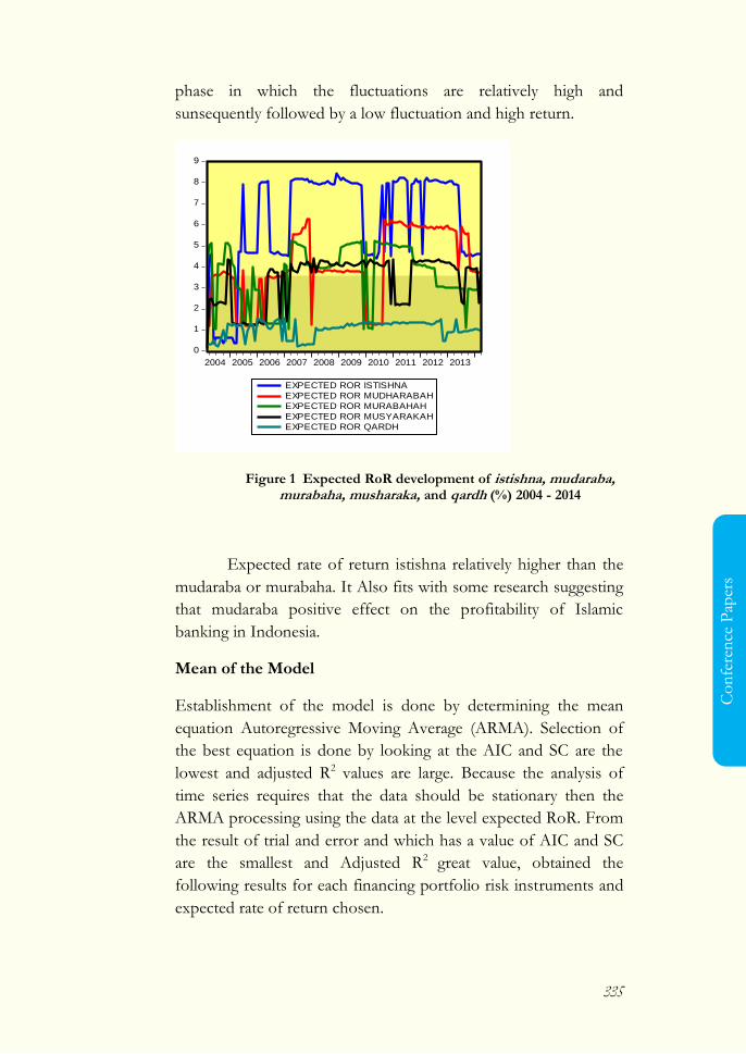
335

Co

nfe

ren

ce P

aper

s

phase in which the fluctuations are relatively high and

sunsequently followed by a low fluctuation and high return.

Figure 1 Expected RoR development of istishna, mudaraba, murabaha, musharaka, and qardh (%) 2004 - 2014

Expected rate of return istishna relatively higher than the

mudaraba or murabaha. It Also fits with some research suggesting

that mudaraba positive effect on the profitability of Islamic

banking in Indonesia.

Mean of the Model

Establishment of the model is done by determining the mean

equation Autoregressive Moving Average (ARMA). Selection of

the best equation is done by looking at the AIC and SC are the

lowest and adjusted R2 values are large. Because the analysis of

time series requires that the data should be stationary then the

ARMA processing using the data at the level expected RoR. From

the result of trial and error and which has a value of AIC and SC

are the smallest and Adjusted R2 great value, obtained the

following results for each financing portfolio risk instruments and

expected rate of return chosen.

0

1

2

3

4

5

6

7

8

9

2004 2005 2006 2007 2008 2009 2010 2011 2012 2013

EXPECTED ROR ISTISHNA

EXPECTED ROR MUDHARABAH

EXPECTED ROR MURABAHAH

EXPECTED ROR MUSYARAKAH

EXPECTED ROR QARDH

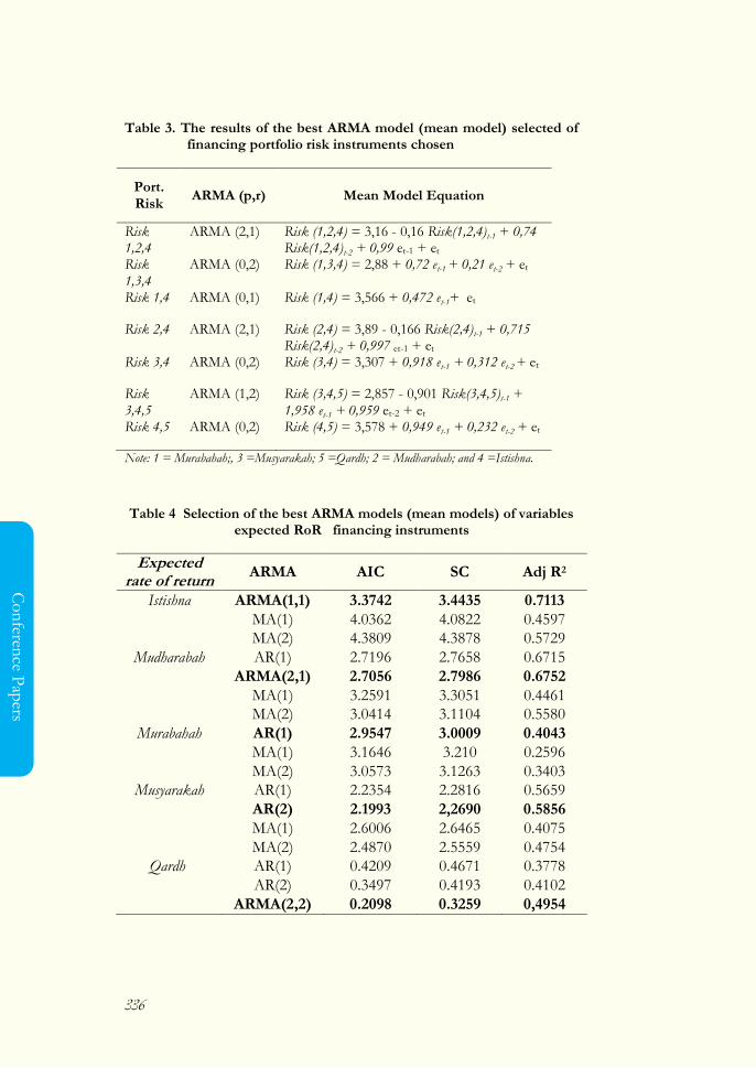
336

Co

nferen

ce Pap

ers

Table 3. The results of the best ARMA model (mean model) selected of financing portfolio risk instruments chosen

Port. Risk

ARMA (p,r) Mean Model Equation

Risk 1,2,4

ARMA (2,1) Risk (1,2,4) = 3,16 - 0,16 Risk(1,2,4)t-1 + 0,74 Risk(1,2,4)t-2 + 0,99 et-1 + et

Risk 1,3,4

ARMA (0,2) Risk (1,3,4) = 2,88 + 0,72 et-1 + 0,21 et-2 + et

Risk 1,4 ARMA (0,1) Risk (1,4) = 3,566 + 0,472 et-1+ et

Risk 2,4 ARMA (2,1) Risk (2,4) = 3,89 - 0,166 Risk(2,4)t-1 + 0,715 Risk(2,4)t-2 + 0,997 et-1 + et

Risk 3,4 ARMA (0,2) Risk (3,4) = 3,307 + 0,918 et-1 + 0,312 et-2 + et

Risk 3,4,5

ARMA (1,2) Risk (3,4,5) = 2,857 - 0,901 Risk(3,4,5)t-1 + 1,958 et-1 + 0,959 et-2 + et

Risk 4,5 ARMA (0,2) Risk (4,5) = 3,578 + 0,949 et-1 + 0,232 et-2 + et

Note: 1 = Murabahah;, 3 =Musyarakah; 5 =Qardh; 2 = Mudharabah; and 4 =Istishna.

Table 4 Selection of the best ARMA models (mean models) of variables expected RoR financing instruments

Expected rate of return

ARMA AIC SC Adj R2

Istishna ARMA(1,1) 3.3742 3.4435 0.7113

MA(1) 4.0362 4.0822 0.4597

MA(2) 4.3809 4.3878 0.5729

Mudharabah AR(1) 2.7196 2.7658 0.6715

ARMA(2,1) 2.7056 2.7986 0.6752

MA(1) 3.2591 3.3051 0.4461

MA(2) 3.0414 3.1104 0.5580

Murabahah AR(1) 2.9547 3.0009 0.4043

MA(1) 3.1646 3.210 0.2596

MA(2) 3.0573 3.1263 0.3403

Musyarakah AR(1) 2.2354 2.2816 0.5659

AR(2) 2.1993 2,2690 0.5856

MA(1) 2.6006 2.6465 0.4075

MA(2) 2.4870 2.5559 0.4754

Qardh AR(1) 0.4209 0.4671 0.3778

AR(2) 0.3497 0.4193 0.4102

ARMA(2,2) 0.2098 0.3259 0,4954

337

Co

nfe

ren

ce P

aper

s

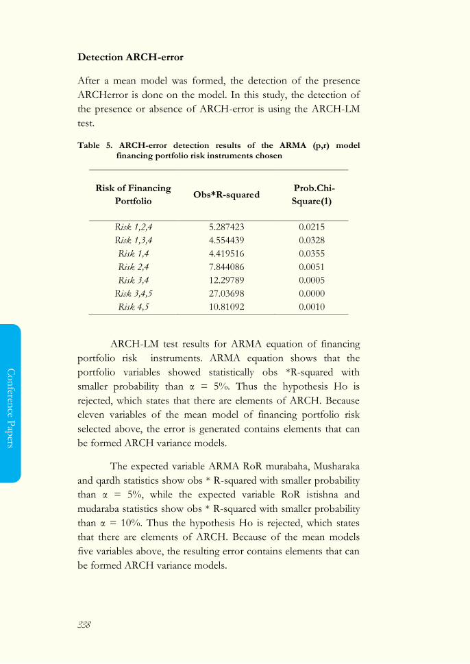
338

Co

nferen

ce Pap

ers

Detection ARCH-error

After a mean model was formed, the detection of the presence

ARCHerror is done on the model. In this study, the detection of

the presence or absence of ARCH-error is using the ARCH-LM

test.

Table 5. ARCH-error detection results of the ARMA (p,r) model financing portfolio risk instruments chosen

Risk of Financing

Portfolio Obs*R-squared

Prob.Chi-

Square(1)

Risk 1,2,4 5.287423 0.0215

Risk 1,3,4 4.554439 0.0328

Risk 1,4 4.419516 0.0355

Risk 2,4 7.844086 0.0051

Risk 3,4 12.29789 0.0005

Risk 3,4,5 27.03698 0.0000

Risk 4,5 10.81092 0.0010

ARCH-LM test results for ARMA equation of financing

portfolio risk instruments. ARMA equation shows that the

portfolio variables showed statistically obs *R-squared with

smaller probability than α = 5%. Thus the hypothesis Ho is

rejected, which states that there are elements of ARCH. Because

eleven variables of the mean model of financing portfolio risk

selected above, the error is generated contains elements that can

be formed ARCH variance models.

The expected variable ARMA RoR murabaha, Musharaka

and qardh statistics show obs * R-squared with smaller probability

than α = 5%, while the expected variable RoR istishna and

mudaraba statistics show obs * R-squared with smaller probability

than α = 10%. Thus the hypothesis Ho is rejected, which states

that there are elements of ARCH. Because of the mean models

five variables above, the resulting error contains elements that can

be formed ARCH variance models.

339

Co

nfe

ren

ce P

aper

s

Variance Model

As in the process of establishing the model mean, variance

formation step models are also through a process of trial and

error. However, it should be followed by testing the normality of

the residual model of ARCH / GARCH that will be selected. Test

results showed that all models of ARCH / GARCH have no

normal distribution of residuals. It is marked with a p-value or

probability of the Jarque-Bera that less than 5% significance level,

so that H0 is rejected, stating that the residuals do not follow a

normal distribution. To overcome this, the corrected standard

errors in the subsequent estimation using the Bollerslev-

Wooldridge correction (Bollerslev-Wooldridge robust standard

errors and covariance) of the estimated quasi-maximum likelihood

(QML) were performed. This is because although the residual

abnormal, resulting estimation of maximum quasi-likelihood

estimation (QML) remained consistent. So, the results of the

estimated parameters remain valid even if not asymptotically

normally distributed. Then proceed to test the significance of

parameters. The final step in the determination of the variance

model is to look at the value of the smallest AIC and SC, as well

as the largest log likelihood.

340

Co

nferen

ce Pap

ers

Table 6. Selection of ARCH/GARCH Best Models (Variance Model)

financing portfolio risk instruments of variables selected

Port. Risk

ARMA (p,r) Variance Model Equation

Risk 1,2,4

GARCH (1,1)

ht = 0,0016 + 1,775 e2t-1 + 0,104 σ2t-1

Risk 1,3,4

GARCH (1,2)

ht = 0,00048 + 0,578 e2t-1 + 0,819 σ2t-1 - 0,259 σ2t-2

Risk 1,4 GARCH (2,2)

ht = 0,00013 + 0,647 e2t-1 + 0,687 e2t-1 - 0,212 σ2t-1 + 0,266 σ2t-2

GARCH (1,0)

ht = 0,0021 + 6,623 e2t-1

GARCH (2,1)

ht = 0,00083 + 0,152 e2t-1 - 0,266 e2t-1 + 1,043 σ2t-1

Risk 2,4 GARCH (1,2)

ht = 0,00038 - 0,055 e2t-1 + 1,62 σ2t-1 - 0,61 σ2t-2

Risk 3,4 GARCH (1,2)

ht = 0,0042 + 0,447 e2t-1 - 0,161 σ2t-1 + 0,614 σ2t-2

Risk 3,4,5

GARCH (1,1)

ht = 0,0016 + 1,775 e2t-1 + 0,104 σ2t-1

Risk 4,5 GARCH (1,2)

ht = 0,00048 + 0,578 e2t-1 + 0,819 σ2t-1 - 0,259 σ2t-2

Note: ht = σ2t = variance of squared residuals at t-month; e2

t-p = squared residuals in

(t-p)-month; and σ2t-q = variance of squared residuals in (t-q)-month

Checking the Model

Testing can be done by using the autocorrelation correlogram, or a

unit root test. Test results showed that all the statistics Q (Q-Stat)

of expected RoR istishna and qardh financing instruments variable

is not statistically significant, with probability (prob) over α = 5%.

This means that the error does not contain the autocorrelation.

For expected RoR mudaraba, murabaha, and musharaka financing

instruments variable, there is still a significant Q statistics on some

initial lag. However, after testing the unit root test stationarity,

were error models are stationary at level I (0) (statistically

significant at α = 5%). Therefore concluded that the error of the

model does not contain the autocorrelation.

Terms good model is not contained in the residual element

ARCH variance models and there is no autocorrelation in the

error equation of ARCH / GARCH models. ARCH-LM test

results for equation of ARCH / GARCH for financing portfolio

341

Co

nfe

ren

ce P

aper

s

risk instruments variable for the equation shows that the GARCH

(p, q) of expected RoR istishna, mudaraba, murabaha, musharaka,

and qardh variables and then the GARCH (p, q) eleventh variable

portfolio risk statistics show obs * R-squared with probability

greater than α = 5%. Thus the hypothesis Ho failed rejected

stating there is no element of ARCH or not heteroscedasticity on

the model.

Overview The Volatility of Expected RoR and Portfolio Risk

Selected

Volatility of Expected RoR

Volatility of expected rate of return is a risk of instability or

uncertainty of the expected rate of return financing instruments.

ARCH/GARCH model volatility variable is used to form the

expected rate of return based on the best model. To obtain the

volatility of expected rate of return, first create the best ARIMA

modeling each financing instrument as noted previously.

Furthermore, the detection of whether the residual variance of the

data expected RoR is not constant and varies from one period to

another, or contain elements of heteroscedasticity. To detect this

using ARCH-LM test. However, the residual variance not only

depend on the residual period, but also depends on the residual

variance ago period. So perform the modeling generalized

autoregressive conditional heteroscedasticity (GARCH) as in the

previous stage. From this is derived volatility GARCH of expected

rate of return.

The movement of the volatility expected RoR can be seen

in Figure 2 below. From this figure it is concluded that the

expected RoR volatility of the financing instrument of mudharaba,

murabaha, istishna tend to be more volatile than the expected

RoR volatility of Musharaka and qardh financing instruments.

This means that the expected RoR volatility of the musharaka and

qardh financing instruments tend to be more stable than other

instruments.

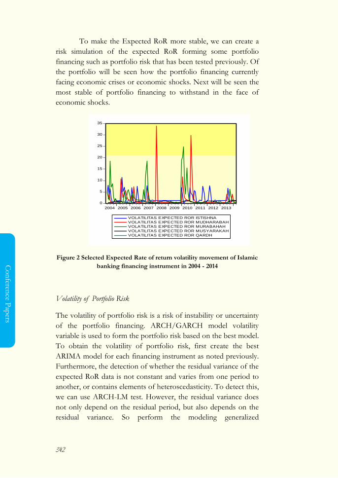
342

Co

nferen

ce Pap

ers

To make the Expected RoR more stable, we can create a

risk simulation of the expected RoR forming some portfolio

financing such as portfolio risk that has been tested previously. Of

the portfolio will be seen how the portfolio financing currently

facing economic crises or economic shocks. Next will be seen the

most stable of portfolio financing to withstand in the face of

economic shocks.

Figure 2 Selected Expected Rate of return volatility movement of Islamic

banking financing instrument in 2004 - 2014

Volatility of Portfolio Risk

The volatility of portfolio risk is a risk of instability or uncertainty

of the portfolio financing. ARCH/GARCH model volatility

variable is used to form the portfolio risk based on the best model.

To obtain the volatility of portfolio risk, first create the best

ARIMA model for each financing instrument as noted previously.

Furthermore, the detection of whether the residual variance of the

expected RoR data is not constant and varies from one period to

another, or contains elements of heteroscedasticity. To detect this,

we can use ARCH-LM test. However, the residual variance does

not only depend on the residual period, but also depends on the

residual variance. So perform the modeling generalized

0

5

10

15

20

25

30

35

2004 2005 2006 2007 2008 2009 2010 2011 2012 2013

VOLATILITAS EXPECTED ROR ISTISHNA

VOLATILITAS EXPECTED ROR MUDHARABAH

VOLATILITAS EXPECTED ROR MURABAHAH

VOLATILITAS EXPECTED ROR MUSYARAKAH

VOLATILITAS EXPECTED ROR QARDH

343

Co

nfe

ren

ce P

aper

s

autoregressive conditional heteroscedasticity (GARCH) as in the

previous stage. From this is derived GARCH portfolio risk

volatility.

The movement of the portfolio risk volatility can be seen

in Figure 3 below. From this figure is concluded that the volatility

of the financing portfolio risk instruments of Risk (1,2,4); Risk

(1,3,4); Risk (1,4); and Risk (2,4) tend to be more volatile than the

volatility of Risk (3,4); Risk (3,4,5); and Risk (4,5). This means that

the portfolio risk volatility of musharaka, istishna financing

instruments (Risk (3,4)); musharaka, istishna, qardh (Risk (3,4,5));

and istishna, qardh (Risk (4,5)) tend to be more stable than other

financing instruments. From the figure it is also seen that a

significant fluctuation occurred in 2004-2005. Then over time, the

three types of financing portfolios apparently show that the better

risk behavior until today when seen from a stable trend over the

period of time from 2006 to 2014.

Further interpretation can be seen from the shock at the

beginning of 2010 of financing portfolio risk volatility

performance in general, this happens because of the economic

turmoil in 2008-2009. In that year there was an increase in fuel

prices (fuel oil) in Indonesia, which also affect the prices of other

goods and services. As a result, banks and customers expect that

the rate of return also rose. In addition, the global crisis of 2008-

2009 and the turbulence effects (shock) in the year in general to all

types of financing portfolio risk, where the impact of the

economic pressures are also being felt in 2010 that is characterized

by the presence of turbulence (shock) . But it was not so

influential on the three types financing portfolio risk that have a

low level of volatility, the previous three portfolio risks that tends

to be most stable. The three types of portfolio risk are musharaka,

istishna (Risk (3,4)); musharaka, istishna, qardh (Risk (3,4,5)); and

istishna, qardh (Risk (4,5)) appeared to have potential defenses

that tend to be more powerful than any economic turmoils that

arise.

344

Co

nferen

ce Pap

ers

The three types of portfolio risk are musharaka, istishna

financing (Risk (3,4)); Musharaka, istishna, qardh (Risk (3,4,5));

and istishna, qardh (Risk (4,5)) only showed the significant

presence of turmoils (shock) in 2004 and 2005. This occurred

because of the devastating natural disasters in 2004 (tsunami

Aceh), which became the center of attention at the time, as well as

the increase in fuel prices (fuel oil) in 2005. But then the three type

of financing portfolio risk remained at the level of risk volatility

those have good stability.

The mudharaba financing instrument (risk 2) tend to

increase the variance (risk of uncertainty) of financing portfolio in

the event of a crisis. This is because of the financing is based on

the real sector investment, so it tends to be sensitive to the

economic sector. However it can be seen that the combination of

istishna and musharaka financing instrument (risk 3.4) shows a

very good risk behavior because the financing portfolio is likely to

stabilize at a relatively lower risk. In 2008-2009 (global financial

crisis) and entering in 2013 (starting of economic pressure), the

portfolio financing risk in which a financing instrument combined

with murabaha instrument (risk 1), causing the risk of financing

portfolio has increased. This is because when the economy is

depressed, interest rates will rise so that the cost of funds or

funding needs will increase. And the same thing happened in

Islamic banks, especially in financing instruments based selling.

When interest rates rise, of course in Islamic banking customers

expect that returns also increased so that banks charge to

employers in order to return ride. And it should be emphasized

here that the true in Islamic finance, the high risk offset by higher

returns.

Furthermore, in 2007 began to increase due to economic

pressures. The peak increase in financing portfolio risk uncertainty

occurs when the global crisis period (2008-2009). And back up

again ascending current economic pressures (in 2013). And the

financing portfolio containing mudaraba financing instrument are

very sensitive to any changes Indonesian economic conditions,

due to the strong relationship between this instrument with the

345

Co

nfe

ren

ce P

aper

s

real sector. This is because of the financing is based on the real

sector investment, so it tends to be sensitive to the economic

sector. However, the financing portfolio consists of a combination

of these mudaraba instrument not only has the level of high

uncertainty/risk (varince), but also offset by higher expected rate

of return which is a necessity in Islamic finance (Sharia-

compliant). This also shows that financing based mudaraba (profit

sharing) is indeed the spirit of Islamic banking.

The emergence of the global crisis in 2008 led to price

stability and output did not ensure the stability of the financial

system (anual BI Report 2010). However, from the results of the

analysis of selected portfolio risk previously shown that there are

types of financing portfolios that have the potential to survive in

the event of economic turmoils.

By this, it can be concluded that the portfolio of

musharaka, istishna (Risk (3,4)); musharaka, istishna, qardh (Risk

(3,4,5)); and istishna, qardh financing instruments (Risk (4,5)) has

strong potential in maintaining the stability of the financial system

as potential financing portfolio that is able to absorb the shock

that occur in order to prevent disruption to the real sector

activities.

Financing portfolio instruments like musharaka, istishna

(Risk (3,4)); musharaka, istishna, qardh (Risk (3,4,5)); and istishna,

qardh (Risk (4,5)) again has a strong potential in terms of

maintaining the stability of the financial system because of the

potential for strong financing portfolio and resistant to a variety of

economic disruption that is still able to spread the risk as well.

The strong potential of the portfolio financing instruments

like musharaka, istishna (Risk (3,4)); musharaka, istishna, qardh

(Risk (3,4,5)); and istishna, qardh (Risk (4.5)) in terms of risk

management function properly.

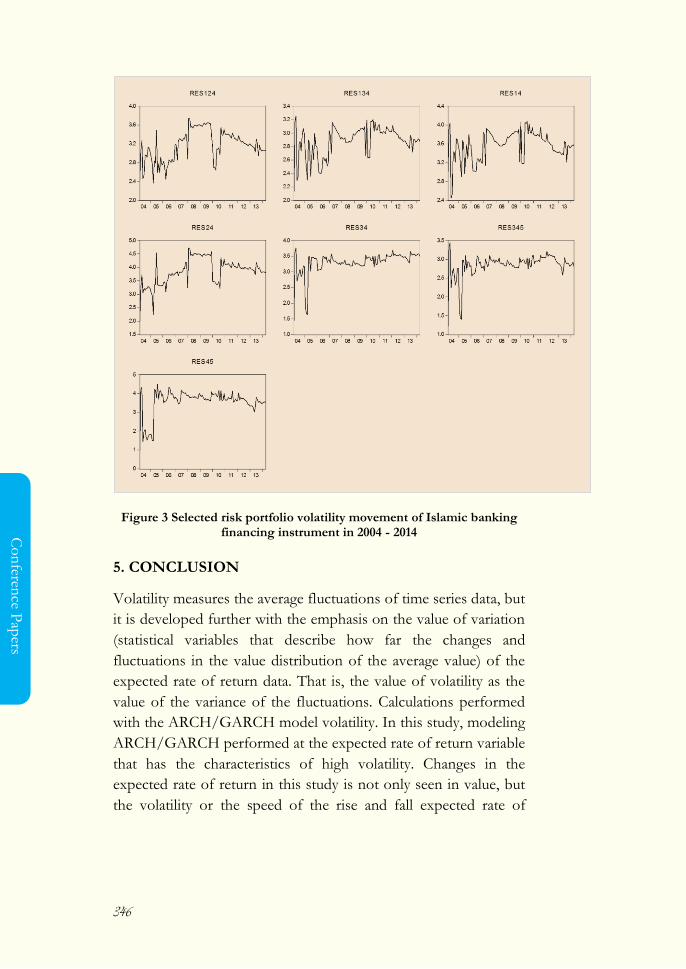
346

Co

nferen

ce Pap

ers

Figure 3 Selected risk portfolio volatility movement of Islamic banking financing instrument in 2004 - 2014

5. CONCLUSION

Volatility measures the average fluctuations of time series data, but

it is developed further with the emphasis on the value of variation

(statistical variables that describe how far the changes and

fluctuations in the value distribution of the average value) of the

expected rate of return data. That is, the value of volatility as the

value of the variance of the fluctuations. Calculations performed

with the ARCH/GARCH model volatility. In this study, modeling

ARCH/GARCH performed at the expected rate of return variable

that has the characteristics of high volatility. Changes in the

expected rate of return in this study is not only seen in value, but

the volatility or the speed of the rise and fall expected rate of

347

Co

nfe

ren

ce P

aper

s

return also observed. In determining the ARCH/GARCH model

consists of two stages: determine the mean and variance models.

Expected RoR (Rate of Return) volatility of movement in

this study it is concluded that the expected RoR volatility of

mudharaba, murabaha and istishna financing instruments tend to

be more volatile than expected RoR volatility of Musharaka and

Qardh financing instruments. This means that abnormal RoR

volatility of Musharakaand Qardh financing instruments tend to

be more stable than other Islamic financing instruments.

Regardless of the factors that influence the volatility of the

Islamic financing instruments, of course, this result gives an idea

of how stable the five Islamic financing instruments to be

developed as well as anticipated in developing Islamic banking in

Indonesia, whether it will be used for the basic preparation of

diversification product or financing portfolio serve as an

opportunity to invest.

We can create a risk simulation of the expected RoR

forming some portfolio financing such as portfolio risk that has

been tested. Of the portfolio will be seen how the portfolio

financing currently facing economic crises or economic shocks.

Based on this simulation study, the volatility of portfolio

financing risk instruments of Risk (1,2,4); Risk (1,3,4); Risk (1,4);

and Risk (2,4) tend to be more volatile than the volatility of Risk

(3,4); Risk (3,4,5); and Risk (4,5). This means that the volatility of

the portfolio risk of musharaka, istishna (Risk (3,4)); musharaka,

istishna, qardh (Risk (3,4,5)); and istishna, qardh financing

instruments (Risk (4,5)) tend to be more stable than other financial

instruments.

Islamic banks' portfolio financing generally reacts

significantly when the turmoil and economic pressures arise. But it

was not so influential on financing portfolio risk of the three types

of financing portfolios that have a low level of volatility. The three

portfolio risk previous that tends to be the most stable. The three

types of portfolio are musharaka, istishna (Risk (3,4)); musharaka,

348

Co

nferen

ce Pap

ers

istishna, qardh (Risk (3,4,5)); and istishna, qardh (Risk (4,5))

appeared to have potential defenses that tend to be more powerful

than any economic turmoils that arise. The three types of

financing portfolio remained at the level of good stability of risk

volatility.

Financing portfolio like musharaka, istishna (Risk (3,4));

musharaka, istishna, qardh (Risk (3,4,5)); and istishna, qardh (Risk

(4,5)) have strong potential in maintaining the the financial system

stability because the three portfolios are able to absorb the shocks

that occur in order to prevent disruption to the real sector

activities.

Regardless of the factors that influence the Islamic

financing instruments volatility, of course, this result give an idea

on how stable the Islamic financing instruments as well as the

possibility of investment portfolio and anticipated to be developed

in an effort to develop Islamic banking in Indonesia to be a

potential stake in maintaining the financial system stability of the

national, either would be used for a basic preparation of product

diversification / financing portfolio or used as an opportunity for

investment. This simulation study show that portfolio of Islamic

financing in Indonesia withstand to economic shocks. And it can

be applied for more countries like western and middle east.

REFERENCES

Otoritas Jasa Keuangan. (multiple years). Statistik Perbankan Syariah

Indonesia. Jakarta: OJK

Barata, Amrin. (2013). Penentuan Komposisi Optimal Kontrak

Instrumen Pembiayaan Perbankan Syariah di Indonesia

melalui Pembentukan Efficient Portfolio Frontier tahun 2004-

2012 (Pendekatan Risk-Return dan Pemodelan GARCH).

Jakarta : Sekolah Tinggi Ilmu Statistik.

349

Co

nfe

ren

ce P

aper

s

Barata, Amrin. (2014). Pendeteksian Volatilitas Expected Rate of

Return dari Instrumen Pembiayaan Perbankan Syariah

Indonesia melalui Pemodelan GARCH (Generalized

Autoregressive Conditional Heteroscedasticity). Bogor: STEI

TAZKIA.

Bilbiee, Florin. (2000). Applications of ARCH Modelling in Financial

Time Series: the Case of Germany. Research Techniques

Project : Department of Economics University of

Warwick.

Cardinali, Alessandro. (2007). An Out-of-sample Analysis of Mean-

Variance Portfolios with Orthogonal GARCH Factors.

International Econometric Review (IER) Volume 4, Issue

1.

Edi,dkk. (2009). Quasi-Maximum Likelihood untuk Regresi Panel

Spasial [Paper]. Surabaya: Institut Teknologi

Sepuluh November (ITS).

Engle, Robert. (2001). The Use of ARCH/GARCH Models in

Applied Econometrics. Jurnal of Economic

Perspectives.

Huda, Nurul, dan Nasution, Mustafa. (2009). Current Issues Lembaga

Keuangan Syariah. Jakarta: Kencana Prenada

Media Group.

Ismal, Rifki. (2010). The Indonesian Islamic Banking (Theory and

Practices). Bogor: Phd Gramata Publishing.

Joko, Kandung. (2007). Pengaruh Volatilitas Nilai Tukar Dan Nilai

Neto Ekspor Terhadap Volatilitas Cadangan Devisa Indonesia

Periode 1980-2006 [Skripsi]. Jakarta: Sekolah Tinggi Ilmu

Statistik (STIS).

Lewis, Mervyn dan Al-Qaoud, Latifa. (2001). Perbankan Syari’ah:

Prinsip, Praktik, Prospek. Jakarta : Serambi.

Lee, Sang dan Hansen, Bruce. (1994). Asymptotic Theory For The

Garch (1,1) Quasi-Maximum Likelihoode Stimator.

350

Co

nferen

ce Pap

ers

Econometric Theory, 10, 1994, 29-52. Printed in the

United States of America.

Markowitx H.M. (1991). Foundations of Portfolio Theory. Journal of

Finance.

Nachrowi, dan Usman, Hardius. (2006). Ekonometrika untuk

Analisis Ekonomi dan Keuangan. Jakarta: Lembaga Penerbit

Fakultas Ekonomi Universitas Indonesia.

Ribeiro, Otavio, dan Shigueru, Alberto. (2005). Brazilian Market

Reaction to Equity Issue Announcements. Journal.

Posedel, Petra. (2005). Properties and Estimation of GARCH(1,1)

Model. Metodoloˇski zvezki, Vol. 2, No. 2,

2005, 243-257.

Supranto, Johanes. (2004). Statistik Pasar Modal Keuangan dan

Perbankan. Jakarta: Rineka Cipta.

Syafi‘i, Muhammad. (2001). Bank Syari’ah dari Teori ke Praktik.

Jakarta: Gema Insani.

Yahya, Arya. (2011). Pengaruh Perilaku Kurs(Rp/US$) Terhadap

Ekspor Nonmigas Dan Produk Domestik Bruto Nonmigas

Indonesia Periode 1993-2010 [Skripsi]. Jakarta : Sekolah

Tinggi Ilmu Statistik.

351

Co

nfe

ren

ce P

aper

s

Bulletin of Monetary Economics and Banking

We invite you to write on this journal.

The submission is fully online with Online Joural System made possible

by Public Knowledge Project.

The printed book of the journal is distributed internationally. Free

subscription is available upon request. If you are academic institution,

library, or research center, please contact us for your inclusion in the

distribution list.

Flagship Program International Conference | BMEB Goes to Campuss | ―Meet the Author‖

| Editor Reviewer Author Partnerhsip Program

www.bmeb-bi.org

support: bmeb@bi.go.id/ paper.bemp@gmail.com