Analyzing of the San Andreas Fault slipping using strainmeter data

H., Samadi Alinia

PhD. student, Dept. Geophysics, Faculty of Earth Sciences, University of University of Western Ontario,

London, Ontario, Canada

Email: hsamadia@uwo.ca, phone: +1 (519) 697 6035

Abstract

The San Andreas Fault is one of the most well-known destructive fault which is a boundary of

two moving plates; the Pacific Plate (on the west) and North American Plate (on the east) that

meet in western California, in which the west side moves northwestward relative to the east side.

Huge earthquakes occurred during the long history of this fault at each year and follow that the

displacements made in the features on the surface near the fault, motivate scientists to attempt to

forecast the next huge earthquake along that. In 1985, the US Geological Survey predicted that

there would be a comparably-sized earthquake in this community by 1993, but no such event

came until September 28, 2004, when a magnitude-6.0 earthquake struck at 17:15:24

Coordinated Universal Time, UTC; epicenter location 35.8158 N, 120.3748W; depth 7.9 km).

There is a hope that by observing the collected data and studying the changes that precede an

earthquake of that size helps scientists to better understand the physics of the earthquakes and

faulting and also issue predictions for major earthquakes along this fault and around the world.

To achieve this, requires observing them using different geodetic instruments with high

resolution. Among variety existence instruments, borehole Gladwin Tensor Strainmeter (GTSM)

capable to record changes in strains and deformation around the rock at a resolution of better

than a nanostrain at periods of minutes to months (short term). It accomplishes this to measure

different signals range from several nanostrain to many hundreds of nanostrain for example the

strain resulted from lunar and solar tides. Strain data from GTSM are three measurements in

different directions at each time; Areal strain and two types of shear strains.

The main goal in this project is to determine slipping occurred into the near-surface region of the

hypocentre in during, or as a result of, the passage of the seismic waves that trigger tremor near

the San Andreas Fault, for time periods of 2 month before and about one month after that, using

continuous strain data recorded on two boreholes Gladwin Tensor Strainmeters (GTSM) located

in the opposite sides of the fault within the distribution of tremor the epicenter of this earthquake.

In this project the obtained GTSM data with concerning that only tidal and drift signals are

effective parameters on these data, will be modeled.

1. Introduction

The San Andreas Fault system extends from northern California to Cajon Pass near San

Bernardino and forms a visible narrow break in California coastal region. This fault system

defines about 1300 km (800 mi) portion of the boundary between the Pacific and North

American plates (Hill and Dibblee, 1953). As the west side moves north, it causes several

earthquakes. This fault is known as a complex continuous fault system made up of different

segments but rather is a fault zone in which in some spots extends to the depth of as much as 16

km (10 miles) within the Earth. Displacement of the fault is right-lateral strike-slip that

accommodates most of the relative motion between the plates. To the north, a complex of

transform faults and spreading centers accommodates the motion of the Gorda and Juan de Fuca

plates. To the south, a similar complex of spreading centers and transform faults accommodate

the displacement in the Gulf of California (Fig. 1).

Figure. 1. A "creeping" section (green) separates locked stretches north of San Juan Bautista and

south of Cholame. The Parkfield section (red) is a transition zone between the creeping and southern

locked section. Stippled area marks the surface rupture in the 1857 Fort Tejon earthquake (USGS,

2012a).

The Town of Parkfield is situated on a few hundred meters east of the main trace of this fault.

Large earthquakes including the Magnitude 8.3 Fort Tejon earthquake of 1857 occurred in the

South of Parkfield (USGS, 2012a). From both geodetic and seismic data, currently, the southern

section appears to be locked producing no movement or small to moderate sized earthquakes.

The northern fault section also has produced large earthquakes, including the Magnitude 8.3 San

Francisco earthquake in 1906 and the Magnitude 7.1 Loma Prieta earthquake in 1989. Most of

the northern section of the fault is also currently locked, with no detectable movement and few

earthquakes since 1906. Between these locked sections, the San Andreas Fault creeps (slips

aseismically). From San Juan Bautista to Parkfield, the creeping section produces numerous

small (mostly M5 and smaller) earthquakes but no large ones. The stretch of the fault between

Parkfield and Gold Hill defines a transition zone between the creeping and locked behavior of

the fault.

2. Background

The similarities in the distribution of the magnitude of earthquakes and local seismicity

sequences make Parkfield noteworthy. Occurrence of six similar earthquakes with M~6 on the

San Andreas Fault near this city, since 1857 with apparent one nearly every 22 years also

similarities of waveform recorded by regional seismographs for the 1922, 1934 and 1966

tremors, confirms the importance of this area for modeling of its seismicity and lead scientists to

anticipate earthquakes involved in the area with same properties.

Figure 2 shows seismograms from two of the Parkfield earthquakes, both recorded in Berkeley,

California in both E-W and N-S directions. The similarity of the first few cycles of the P and S

waves means that these events ruptured the same part of the fault.

Figure. 2. East-west and north-south components of ground motion for the 1922 and 1934 Parkfield

events recorded at Berkeley, California (USGS, 2012b)

Adding to the sense of repetition, similar-size foreshocks occurred 17 minutes before both the

1934 and 1966 Parkfield earthquakes and they produced approximately identical Wood-

Anderson seismograms near Berkeley California. During an earthquake, the rocks under strain

break and generating a fracture along a fault to release of stored energy. The slip produces

changes in the local strain out into the surrounding rock subsequently lead to aftershocks. On the

other hand, the aftershocks are created by further slips of the fault. After the earthquake, the

loading process and building up of strain in rocks starts again until it become larger than the

forces putting the rocks together and it causes the fault snaps again and produces another

earthquake. If the loading rate is constant, the timing of the earthquakes would be regular. These

concepts suggest that there may be some predictability in the occurrence of earthquakes, at least

at Parkfield. In addition, much is being learned about the physics of earthquakes from advances

at Parkfield, including the discovery of repeating micro-earthquakes (Ellsworth, 1995) and

earthquake "streaks" (Waldhauser et al., 1999; Rubin et al., 1999).

The occurrence of the 28 September 2004, M 6.0 Parkfield earthquake in the middle of a

borehole strainmeter array at Parkfield provides the best near-field strain data before, during, and

after an earthquake of this magnitude. Separation of the earthquake rupture co-seismic slip and

immediate post-seismic slip can be resolved using the changes in strain data recorded for this

earthquake. Preliminary seismic moment tensor inversion indicates a moment for the earthquake

of about 1018

Nm (M 6.0) that results predominantly from right-lateral faulting on the near-

vertical main San Andreas Fault with some minor slip contributions on the southwest trace

(Bakun et al., 2005). The slip distribution along the rupture was mostly in a N43W direction

from the hypocenter at a depth of 7.9 km under Gold Hill and was initially localized between

about 4 km and 8 km in depth where it reached a peak of just over 60 cm about 10 km north of

the epicenter. The initial rupture length was about 20 km, and post-seismic slip quickly broke

through to the surface in the hours following the earthquake. Significant post-seismic slip above

and around the earthquake slip has continued in the months following the earthquake (Langbein

et al., 2006).

3. Data

Our measurement system consists of two borehole tensor strainmeters (Gladwin, 1984) from

Gladwin Tensor Strain Monitor (GTSM) which measures horizontal strain in the earth due to

tectonic or engineering stress. It allows direct evaluation of variation of the amplitude and the

orientation of the principle components of strain. This system was the first high precision, high

stability multi-component (tensor) system developed for deep boreholes.

The most important of these sites which were installed in 1987 in California are FLT, DLT and

EDT corresponding to the Frolich, Donna Lee, and Eades. The GTSM data from the third

Parkfield site (Eades) were not included because the instrument failed in 2002 so that data are

not available for the considered event at 2004. Locations and depth of these two sites is listed in

Table 1.

Table 1. Locations and Depths of the considered tensor strainmeter

Site Latitude Longitude Elevation

(m)

Depth

(m)

Location

FLT

DLT

35.9107

35.9401

-120.4859

-120.4234

674

572

237.3

174.0

Parkfield, CA

Parkfield, CA

The two other sites, FLT and DLT, are located on the west and east side of the fault near the

region of peak slip from the earthquake 28 September 2004, are considered in this study (Fig. 3).

Figure 3. Locations of considered strainmeter stations in this study (Yellow Placemark), epicenter of the

28 September 2004 Parkfield earthquake (red star), the main trace of the San Andreas Fault (the long

southwest red line) and the town of Parkfield.

3.1. Measurement of Strain using a Borehole Tensor Strain instrument

The basic measurement is the horizontal extension, ui of three or four gages mounted inside the

borehole at different azimuths, approximately 120 apart. At the surface of the earth, the vertical

stress is zero, and so the equations for the plane stress case can be used to describe strains in the

horizontal plane. The horizontal strain tensor at each point (site) has three independent

components, , , . Elongation at an angle is a linear combination of these three

components. Alternatively, the deformation can be described by the areal strain, A= ,

the differential extension, = , and the shear, = .

These also completely describe the strain state, but isolate the areal or compressional strain (A)

from the shear strain in and . In Areal strain, deformation is identical at all direction in which a

circular borehole remains circular. is a pure engineering shear which is maximum across planes

oriented N-W or N-E (ie. At 45 degrees to the coordinate system) whereas is a pure engineering shear

with maximum shear across planes N-S and E-W.

For the Parkfield strainmeters, one can obtain either the gage measurements nominally corrected

to strain units, or areal and shear strains measurements. In this study, the resolved strain data, A,

, and are used. We do so because we want to compare signals from different sites and the

gages may have different orientations.

Figure 4 illustrates the areal and tensor strains data recorded in micro-strain at FRT and DLT

from 2 month before and about one month after the M 6.0 28 September 2004 Parkfield

earthquake. These data can be obtained from the GTSM company website

(http://www.gtsmtechnologies.com). In the convention used here, contraction is positive and

units are micro-strain (parts per million).

The sample rates are every 18 min for Donna Lee and 30 min for Frolich, respectively, with a

sample missed every three hours in the data recorded at the Donna Lee site. Also, irregular gaps

of a single sample to hours exist in the data from both sites. Instead of interpolating and

resampling the data, and identifying all the gaps manually, the data is used as recorded. However

the instrument resets from these data were removed.

M6

M5

Figure 4. Areal, differential extension and shear strain data recorded at the two tensor strainmeters (DLT

and FLT) from 24 July 2004 to 24 October 2004, before and after the M 6.0 28 September Parkfield

earthquake.

This figure confirms no obvious changes in strain before the earthquake. However it shows

significant post-seismic compressive strain appears to have occurred during the 12 hour

following the earthquake and this has continued in the month following the earthquake. The

erratic post-seismic response of the FRT instrument may indicate that this instrument is failing

after the earthquake.

The offsets generated by the Parkfield earthquake from 30-min tensor strain data for FLT and

36-min for DLT are listed in table 2. Because the strain data after 18 min from the earthquake for

DLT is spurious, is not considered here.

Table 2. Observed Co-seismic Tensor Strain Offsets for the 2004 Parkfield Earthquake

(Compression positive in micro-strain)

Site Areal

Strain (A)

Gamma1

Gamma2

FLT

DLT

+0.47

-0.86

-2.42

+0.57

-1.3

+0.73

As the offsets in figure 4 and table 2 indicate, as a consequence of the different sample times, the

co-seismic areal strain data from the two sites with tensor strain are slightly different.

To search for very small changes in strain immediately before the earthquake, earth tides with

ocean-loading components (Agnew, 1997; Tamura, 1991) and atmospheric pressure loading

(Rabbel and Zschau, 1985) must first be predicted and removed from the data using least-squares

methods.

4. Methodology

Following Tamura et al. [1991], it was assumed that the measured strain, u(t), as a function of

time, t, may be modeled as a sum of the response to (i) the tides , (t), (ii) atmospheric pressure

changes or other measured ‘‘auxiliary’’ loads, a(t), (iii) possibly some tectonic process such as a

transient slow slip event, e(t), (IV) ‘‘drift’’, d(t), and (V) the remaining unmodeled signal or

residual signal, r(t). Drift refers to signals of presumed nontectonic origin with periods longer

those of the tides. So the measured stain is in eq. 1:

(1)

The Parkfield GTSM strainmeters are approximately insensitive to atmospheric pressure changes

(E. Roeloffs et al., Draft review of borehole strainmeter data collected by the U.S. Geological

Survey, 1985– 2004, prepared for PBO, 2004) so that a(t) 0. The ideal null hypothesis is that

the fault is not slipping, which could be tested by fitting u(t) under the assumption that e(t) = 0

and employing parameterized models of (t) and d(t). The residual signal can be obtained

by difference between the modeled and observed signals (eq.2):

(2)

We model the tidal signal, (t), as a sum of N sine waves with periods, Tn, and solve for the

amplitude, Sn, and phase, , of each that maximizes the fit to the data. We choose the minimum

number of periods required to fit the tidal signals, expected to dominate at Parkfield (Table 3).

Table 3. Modeled Tidal Frequencies

Tidal Component

Site O1 M2 S1 S2 Q1 N2

Period (hours)

Frequency

(cycles/d)

25.8193

0.929537

12.4206

1.93227

24

1

12

2

26.8684

0.893243

12.6583

1.89599

Linearizing the tidal fitting process is done using the identity (eq. 3):

(3)

Where, = √

,

,

Since the data are sampled at M discrete time points, , so our tidal signal model is written as

(eq. 4) :

∑ (4)

For parameterizing the drift, d(t), we use the same approach as Tamura et al. (1991), as a time

series sampled at the same time points as the data and constrained to be ‘‘smooth’’.

To test the hypothesis that the data reflect only the response to the tides and drift, we solve the

linear eq. 5 as follow:

(5)

Then the forward modeling is written as in which the “data” vector contains the M

observed strain values and the unknowns ( ) are the 2N weights corresponding to the N tidal

frequencies and M values of the drift at each time point. There is a need to find a solution that

can adequately fit the data in the sense that ‖ ‖ is small enough. Because of this system

is ill-conditioned and under-determined inverse problem, regularization of the model is

necessary.

To satisfy the smoothness of drift, the second derivative of d(t) is used numerically. As the time

interval of Parkfield data have gaps and are not evenly sampled, the complete form of numerical

derivative at is used in this study, eq.6. In this equation is a sample

interval:

(6)

In this study, Generalized Cross-Validation (GCV) approach is used to obtain a solution that

minimizes second derivative of and reflect a preference for a smooth model. Indeed, we are

looking for a value (Tikhonov regularization parameter), which we call it alpha here, using GCV

which optimize both ‖ ‖ and ‖ ‖ . So we solve the regularized least squares problem

in the following manner (7):

min ‖ ‖ ‖ ‖

(7)

5. Application to the earthquake 28 September 2004 Parkfield

Our analysis strategy involved analyzing each strain component, the shear ( and ) and areal

(A) strains, independently fitting tidal and drift models, (t) and d(t), to each using the

formulation described in the previous section and finding a least squares solution.

As it was described, GCV function is used to find minimum value for alpha to minimize the

noises for each component and for two sites. For each time period, the raw and modeled time

series were compared at the Donna Lee and Frolich sites to assess the accuracy of the data,

appropriateness of our assumptions, and to identify signals indicative of slow slip events.

Figure 5 shows the example of GCV curves and its minimum which were obtained for Areal

strains for DLT and FLT sites.

Figure 5. GCV curves for modeling the Areal components. (a) GCV curve for Areal component

for site DLT with the minimum value alpha equal to 2.92*10^-5 (b) GCV curve for Areal

component for site FLT with the minimum value alpha equal to 1.54*10^-4

The observed and modeled Areal strains obtained by computed regularized parameters for two

tensor strainmeters for time windows of few days before the earthquake are demonstrated in

figure 6. It shows strain data after earth tides and drift have been removed.

M6

DLT

Earthquake origin time

𝛼= 2.92*10^-5 𝛼= 1.54*10^-4

(a) (b)

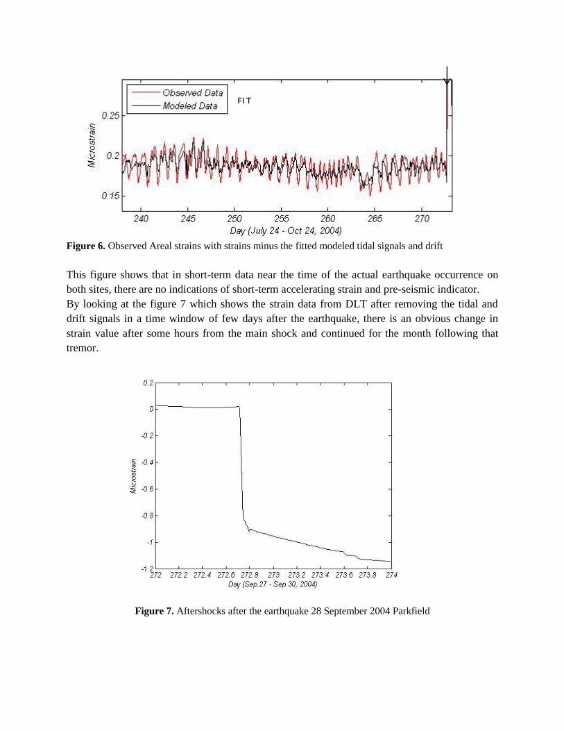
Figure 6. Observed Areal strains with strains minus the fitted modeled tidal signals and drift

This figure shows that in short-term data near the time of the actual earthquake occurrence on

both sites, there are no indications of short-term accelerating strain and pre-seismic indicator.

By looking at the figure 7 which shows the strain data from DLT after removing the tidal and

drift signals in a time window of few days after the earthquake, there is an obvious change in

strain value after some hours from the main shock and continued for the month following that

tremor.

Figure 7. Aftershocks after the earthquake 28 September 2004 Parkfield

FLT

Figure 8 shows Comparison of the observed and modeled (as a superposition of fit sine waves of

specified frequencies (eq. 4)) tidal signals for the same strain component at the two sites provide

a measure of the accuracy of the calibrations and stability of the responses (Fig. 8).

Figure 8. Modeled tidal and drift signals (Areal component)

It can be seen in Figure 8 that the tidal loads are different in both Donna lee and Frolich, it

confirms that the calibrations are uncertain by a factor of approximately 2, although we cannot

determine which strainmeter is incorrect. Actually it shows that the tidal phase responses are

different between these two sites. For example the modeled tidal signal obtained from Areal

strain for Donna lee site is in phase but it is not true for Frolich. The largest change in FLT

before the earthquake arises as this instrument reset itself or the timing system failed suddenly.

DLT

FLT

(a) Residuals for strains

(b) Residuals for strains

Figure 9. Comparison of residuals data (observed minus modeled strain data)

Also by looking at the figures 9a and 9b, it can be understood that the peak-to-peak tidal amplitude

of shear and differential extension components at the time of earthquake is larger at the Frolich

site.

Quantitative assessment also can be done at the two sites on the ratios of RMS tidal signals. Although the

tidal signals are time varying, ratios between signals from the two sites should be unity. The ratio

of RMS for components and calculated for estimated residuals signal from the Frolich site is

about twice those at Donna lee (Table 4). The ratios in table 4 clearly show that the level of noise (non-

tectonic signals) in strain from Frolich relative to the Donna lee site is greater and is about 2.

Table 4. RMS of residuals signal (Micro-strain units)

Sites A

Frolich 0.0215 0.0124 0.0094

Donna lee 0.0072 0.0101 0.0124

Ratio (FLT/DLT) 290% 122% 75%

Visual inspection in residual signals confirms that exceed the long-term variability in the

differences on multiple components and at the two nearby sites lead to consider rejecting the

hypothesis that no detectable slow slip is occurring.

6. Conclusions

The details of 2004 Mw 6.0 Parkfield earthquake are of particular interest as the Parkfield

earthquake sequence is extremely important for testing ideas of earthquake recurrence and

predictability. Historically, the Parkfield earthquake series provide the impetus for formulating

the characteristic earthquake hypothesis that still greatly impacts ideas used in seismic hazard

analysis. By comparing kinematic inversions of past earthquakes at Parkfield we can determine

to what extent these earthquakes are similar, and thus, to what extent ideas developed in this

region can be extrapolated to future seismicity on other faults.

In this project the records of two borehole tensor strainmeters (FLT and DLT) which were

located about 15 km from the epicenter of this earthquake were considered to model and study

the strain changes and slips of the San Andreas Fault which might occurred before, during or

after the tremor. The modeled strains provide a bound on the detectability of any slow slip signals. The slow slips signals

would be undetected if they happened over days and were smaller than the long-term residual strains.

From the results obtained for residual strains, the long term detection threshold at Donna lee site is about

10 nanostrain or 0.01 micro-strain. By visualizing the short-term and long-term residuals plots a detection

threshold of approximately 5 nanostrain or 0.05 micro-strain, half of the long-term value is estimated.

To have more accurate evidence whether pre-seismic strain changes occurred need the high sample rate

recorder about 10-20 sec.

References

Agnew, D. C. (1997) “NLOADF: a program for computing ocean-tide loading”, J.

Geophys. Res. 102, pp. 5109–5110.

Bakun, W. H., B. Aagaard, B. Dost, W. L. Ellsworth, J. L. Hardebeck, R. A. Harris, M. J.

S. Johnston, J. Langbein, J. J. Lienkaemper, A. J. Michael, J. R. Murray, R. M. Nadeau, P. A.

Reasenberg, E. A. Roeloffs, A. Shakal, R. W. Simpson, and F. Waldhauser (2005) “Implications

for prediction and hazard assessment from the 2004 Parkfield Earthquake”, Nature 437, pp. 969-

974.

Ellsworth, W. L. (1995) “Characteristic earthquakes and long-term earthquake forecasts:

implications of central California Seismicity, in: Urban Disaster Mitigation: the Role of Science

and Technology, Cheng, F. Y., and Sheu, M. S. eds., Elsevier Science Ltd., 1-14.

Gladwin, M. T. (1984). High precision multi-component borehole deformation

monitoring, Rev. Sci. Instrument. 55, pp. 2011–2016.

Hill, M.L. and Dibblee, T., (1953). San Andreas, Garlock, and Big faults,

California,Geological Society of America Bulletin, p. 443-458.

Langbein, J., J. R. Murray, and H. A. Snyder, (2006) “Coseismic and initial postseismic

deformation from the 2004 Parkfield, California earthquake, observed by Global Positioning

System, creepmeters, and borehole strainmeters”, Bull. Seis. Soc. Am. 96, doi:

10.1785/0120050823, S304-S320.

Rabbel, W., and J. Zschau (1985) “Static deformations and gravity changes at the earth’s

surface due to atmospheric loading”, J. Geophysics 56, pp. 1–99.

Rubin, A.M., D. Gillard, and J.L. Got (1999) “Streaks of micro-earthquakes along

creeping faults”, Nature.,400, pp. 635-641.

Tamura, Y., T. Sato, M. Ote, and M. Ishiguro (1991), A procedure for tidal analysis with

a Bayesian information criterion, Geophys. J. Int., 104, pp.507-516, doi:10.1111/j.1365-

246X.1991.tb05697.x.

Waldhauser, F., W.L. Ellsworth, and A. Cole (1999), Slip-parallel seismic lineations

along the northern Hayward fault, California, Geophys. Res. Lett., 26, pp. 3525-3528.