Analyticity and Gevrey-Class Regularity for the Second-Grade Fluid Equations

arX

iv:0

912.

1327

v1 [

mat

h.A

P] 7

Dec

200

9 Analyticity and Gevrey-class regularity for the second-grade fluid

equations

Marius Paicu and Vlad Vicol

Abstract. We address the global persistence of analyticity and Gevrey-class regularity of solutionsto the two and three-dimensional visco-elastic second-grade fluid equations. We obtain an explicitnovel lower bound on the radius of analyticity of the solutions to the second-grade fluid equationsthat does not vanish as t → ∞. Applications to the damped Euler equations are given.

Contents

1. Introduction 12. Preliminaries 33. The two-dimensional case 54. The three-dimensional case 105. Applications to the damped Euler equations 156. Appendix 17References 22

1. Introduction

In this paper we address the regularity of an asymptotically smooth system arising in non-Newtonian fluid mechanics, which is not smoothing in finite time, but admits a compact globalattractor (in the two-dimensional case). More precisely, we consider the system of visco-elasticsecond-grade fluids

∂t(u− α2∆u) − ν∆u+ curl(u− α2∆u) × u+ ∇p = 0, (1.1)

div u = 0, (1.2)

u(0, x) = u0(x), (1.3)

where α > 0 is a material parameter, ν ≥ 0 is the kinematic viscosity, the vector field u representsthe velocity of the fluid, and the scalar field p represents the pressure. Here (x, t) ∈ T

d × [0,∞),where T

d = [0, 2π]d is the d-dimensional torus, and d ∈ {2, 3}. Without loss of generality weconsider velocities that have zero-mean on T

d.

2000 Mathematics Subject Classification. 76B03,35L60.Key words and phrases. Second grade fluids, global well-posedness, Gevrey class, analyticity radius.

1

http://arxiv.org/abs/0912.1327v1

2 MARIUS PAICU AND VLAD VICOL

Fluids of second-grade are a particular class of non-Newtonian Rivlin-Ericksen fluids of differ-ential type and the above precise form has been justified by Dunn and Fosdick [18]. The localexistence in time, and the uniqueness of strong solutions of the equations (1.1)–(1.3) in a two orthree-dimensional bounded domain with no slip boundary conditions has been addressed by Cio-ranescu and Ouazar [14]. Moreover, in the two-dimensional case, they obtained the global in timeexistence of solutions (see also [13, 24, 25, 29]). Moise, Rosa, and Wang [40] have shown laterthat in two dimensions these equations admit a compact global attractor Aα (see also [26, 45]).The question of regularity and finite-dimensional behavior of Aα was studied by Paicu, Raugel,and Rekalo in [45], where it was shown that the compact global attractor in H3(T2) is containedin any Sobolev space Hm(T2) provided that the material coefficient α is small enough, and theforcing term is regular. Moreover, on the global attractor, the second-grade fluid system can bereduced to a finite-dimensional system of ordinary differential equations with an infinite delay. Asa consequence, the existence of a finite number of determining modes for the equation of fluids ofgrade two was established in [45].

Note that the equations (1.1)–(1.3) essentially differ from the α-Navier-Stokes system (cf. Foias,Holm, and Titi [20, 21], and references therein). Indeed, the α-Navier-Stokes model (cf. [21])contains the very regularizing term −ν∆(u − α2∆u), instead of −ν∆u, and thus is a semi-linearproblem. This is not the case for the second-grade fluid equations where the dissipative term is veryweak — it behaves like a damping term — and the system is not smoothing in finite time. The α-models are used, in particular, as an alternative to the usual Navier-Stokes for numerical modelingof turbulence phenomena in pipes and channels. Note that the physics underlying the second-grade fluid equations and the α-models are quite different. There are numerous papers devotedto the asymptotic behavior of the α-models, including Camassa-Holm equations, α-Navier-Stokesequations, α-Bardina equations (cf. [9, 20, 21, 34, 37]).

In this paper we characterize the domain of analyticity and Gevrey-class regularity of solutionsto the second-grade fluids equation, and of the Euler equation with damping term. We emphasizethat the radius of analyticity gives an estimate on the minimal scale in the flow [28, 31], and it alsogives the explicit rate of exponential decay of its Fourier coefficients [23]. We recall also that thesystem of second-grade fluids has a unique strong solution u ∈ L∞

loc([0,∞);H3) in two-dimensionalsetting (cf. [14]). Thus, opposite to the Navier-Stokes equations, the system of second-grade fluidscannot be smoothing in finite time.

We prove that if the initial data u0 is of Gevrey-class s, with s ≥ 1, then the unique smoothsolution u(t) remains of Gevrey-class s for all t < T∗, where T∗ ∈ (0,∞] is the maximal time ofexistence in the Sobolev norm of the solution. Moreover, for all ν ≥ 0 we obtain an explicit lower

bound for the real-analyticity radius of the solution, that depends algebraically∫ t0 ‖∇u(s)‖L∞ds.

A similar lower bound on the analyticity radius for solutions to the incompressible Euler equationswas obtained by Kukavica and Vicol [32, 33] (see also [1, 3, 4, 6, 36]). The proof is based on themethod of Gevrey-class regularity introduced by Foias and Temam [23] to study the analyticityof the Navier-Stokes equations (see also [11, 19, 32, 34, 35, 36, 43, 44]). We emphasize thatthe technique of analytic estimates may be used to obtain the existence of global solutions for theNavier-Stokes equation with some type of large initial data ([12, 46]).

Note that if ν > 0, and d = 2, or if d = 3 and u0 is small in a certain norm, then T∗ = ∞, bothfor the second-grade fluids (1.1)–(1.3), and for the damped Euler equations (5.1)–(5.3). The noveltyof our result is that in this case the lower bound on the radius of analyticity does not vanish ast→ ∞. Instead, it is bounded from below for all time by a positive quantity that depends solely onν, α, the analytic norm, and the radius of analyticity of the initial data. In contrast, we note that

ANALYTICITY FOR THE SECOND-GRADE FLUIDS 3

the shear flow example of Bardos and Titi [5] (cf. [17]) may be used to construct explicit solutionsto the incompressible two and three-dimensional Euler equations (in the absence of damping) whoseradius of analyticity is decaying for all time, and hence vanishes as t→ ∞.

The main results of our paper are given bellow (for the definitions see the following sections).

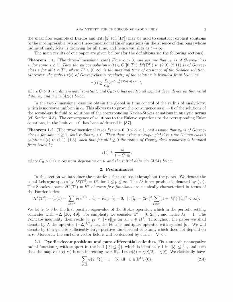
Theorem 1.1. (The three-dimensional case) Fix ν, α > 0, and assume that ω0 is of Gevrey-classs, for some s ≥ 1. Then the unique solution ω(t) ∈ C([0, T ∗);L2(T3)) to (2.9)–(2.11) is of Gevrey-class s for all t < T ∗, where T ∗ ∈ (0,∞] is the maximal time of existence of the Sobolev solution.Moreover, the radius τ(t) of Gevrey-class s regularity of the solution is bounded from below as

τ(t) ≥τ0C0e−C

R t0‖∇u(s)‖L∞ds,

where C > 0 is a dimensional constant, and C0 > 0 has additional explicit dependence on the initialdata, α, and ν via (4.25) below.

In the two dimensional case we obtain the global in time control of the radius of analyticity,which is moreover uniform in α. This allows us to prove the convergence as α→ 0 of the solutions ofthe second-grade fluid to solutions of the corresponding Navier-Stokes equations in analytic norms(cf. Section 3.3). The convergence of solutions to the Euler-α equations to the corresponding Eulerequations, in the limit α→ 0, has been addressed in [37].

Theorem 1.2. (The two-dimensional case) Fix ν > 0, 0 ≤ α < 1, and assume that u0 is of Gevrey-class s for some s ≥ 1, with radius τ0 > 0. Then there exists a unique global in time Gevrey-class ssolution u(t) to (1.1)–(1.3), such that for all t ≥ 0 the radius of Gevrey-class regularity is boundedfrom below by

τ(t) ≥τ0

1 + C0τ0,

where C0 > 0 is a constant depending on ν and the initial data via (3.24) below.

2. Preliminaries

In this section we introduce the notations that are used throughout the paper. We denote theusual Lebesgue spaces by Lp(Td) = Lp, for 1 ≤ p ≤ ∞. The L2-inner product is denoted by 〈·, ·〉.The Sobolev spaces Hr(Td) = Hr of mean-free functions are classically characterized in terms ofthe Fourier series

Hr(Td) = {v(x) =∑

k∈Zd

vkeik·x : vk = v−k, v0 = 0, ‖v‖2

Hr = (2π)3∑

k∈Zd

(1 + |k|2)r|vk|2 <∞}.

We let λ1 > 0 be the first positive eigenvalue of the Stokes operator, which in the periodic settingcoincides with −∆ [16, 49]. For simplicity we consider T

d = [0, 2π]d, and hence λ1 = 1. ThePoincare inequality then reads ‖v‖L2 ≤ ‖∇v‖L2 for all v ∈ H1. Throughout the paper we shall

denote by Λ the operator (−∆)1/2, i.e., the Fourier multiplier operator with symbol |k|. We willdenote by C a generic sufficiently large positive dimensional constant, which does not depend onα, ν. Moreover, the curl of a vector field v will be denoted by curl v = ∇× v.

2.1. Dyadic decompositions and para-differential calculus. Fix a smooth nonnegativeradial function χ with support in the ball {|ξ| ≤ 4

3}, which is identically 1 in {|ξ| ≤ 34}, and such

that the map r 7→ χ(|r|) is non-increasing over R+. Let ϕ(ξ) = χ(ξ/2) − χ(ξ). We classically have∑

q∈Z

ϕ(2−qξ) = 1 for all ξ ∈ Rd \ {0}. (2.4)


We define the spectral localization operators ∆q and Sq (q ∈ Z) by

∆q u := ϕ(2−qD)u =∑

k∈Zd

u(k)eikxϕ(2−q |k|)

and

Sq u := χ(2−qD)u =∑

k∈Zd

u(k)eikxχ(2−q|k|).

We have the following quasi-orthogonality property :

∆k∆qu ≡ 0 if |k − q| ≥ 2 and ∆k(Sq−1u∆qv) ≡ 0 if |k − q| ≥ 5. (2.5)

We recall the very useful Bernstein inequality.

Lemma 2.1. Let n ∈ N, 1 ≤ p1 ≤ p2 ≤ ∞ and ψ ∈ C∞c (Rd). There exists a constant C depending

only on n, d and Suppψ such that

‖Dnψ(2−qD)u‖Lp2 ≤ C2q(n+N

(1

p1− 1

p2

))‖ψ(2−qD)u‖Lp1 ,

and

C−12q(n+N

(1

p1− 1

p2

))‖ϕ(2−qD)u‖Lp1 ≤ sup

|α|=n‖∂αϕ(2−qD)u‖Lp2 ≤ C2

q(n+N

(1

p1− 1

p2

))‖ϕ(2−qD)u‖Lp1 .

In order to obtain optimal bounds on the nonlinear terms in a system, we use the paradifferentialcalculus, a tool which was introduced by J.-M. Bony in [7]. More precisely, the product of twofunctions f and g may be decomposed according to

fg = Tfg + Tgf +R(f, g) (2.6)

where the paraproduct operator T is defined by the formula

Tfg :=∑

q

Sq−1f ∆qg,

and the remainder operator, R, by

R(f, g) :=∑

q

∆qf∆qg with ∆q := ∆q−1 + ∆q + ∆q+1.

2.2. Analytic and Gevrey-class norms. Classically, a C∞(Td) function v is in the Gevrey-class s, for some s > 0 if there exist M, τ > 0 such that

|∂βv(x)| ≤Mβ!s

τ |β|,

for all x ∈ Td, and all multi-indices β ∈ N

30. We will refer to τ as the radius of Gevrey-class

regularity of the function v. When s = 1 we recover the class of real-analytic functions, and theradius of analyticity τ is (up to a dimensional constant) the radius of convergence of the Taylorseries at each point. When s > 1 the Gevrey-classes consist of C∞ functions which however are notanalytic. It is however more convenient in PDEs to use an equivalent characterization, introducedby Foias and Temam [23] to address the analyticity of solutions of the Navier-Stokes equations.Namely, for all s ≥ 1 the Gevrey-class s is given by

⋃

τ>0

D(ΛreτΛ1/s)


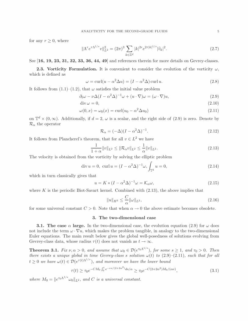
for any r ≥ 0, where

‖ΛreτΛ1/sv‖2

L2 = (2π)3∑

k∈Zd

|k|2re2τ |k|1/s|vk|

2. (2.7)

See [16, 19, 23, 31, 32, 33, 36, 44, 49] and references therein for more details on Gevrey-classes.

2.3. Vorticity Formulation. It is convenient to consider the evolution of the vorticity ω,which is defined as

ω = curl(u− α2∆u) = (I − α2∆) curlu. (2.8)

It follows from (1.1)–(1.2), that ω satisfies the initial value problem

∂tω − ν∆(I − α2∆)−1ω + (u · ∇)ω = (ω · ∇)u, (2.9)

divω = 0, (2.10)

ω(0, x) = ω0(x) = curl(u0 − α2∆u0) (2.11)

on Td × (0,∞). Additionally, if d = 2, ω is a scalar, and the right side of (2.9) is zero. Denote by

Rα the operator

Rα = (−∆)(I − α2∆)−1. (2.12)

It follows from Plancherel’s theorem, that for all v ∈ L2 we have

1

1 + α‖v‖L2 ≤ ‖Rαv‖L2 ≤

1

α‖v‖L2 . (2.13)

The velocity is obtained from the vorticity by solving the elliptic problem

div u = 0, curlu = (I − α2∆)−1ω,

∫

T3

u = 0, (2.14)

which in turn classically gives that

u = K ∗ (I − α2∆)−1ω = Kαω, (2.15)

where K is the periodic Biot-Savart kernel. Combined with (2.13), the above implies that

‖u‖H3 ≤C

α‖ω‖L2 , (2.16)

for some universal constant C > 0. Note that when α→ 0 the above estimate becomes obsolete.

3. The two-dimensional case

3.1. The case α large. In the two-dimensional case, the evolution equation (2.9) for ω doesnot include the term ω · ∇u, which makes the problem tangible, in analogy to the two-dimensionalEuler equations. The main result below gives the global well-posedness of solutions evolving fromGevrey-class data, whose radius τ(t) does not vanish as t→ ∞.

Theorem 3.1. Fix ν, α > 0, and assume that ω0 ∈ D(eτ0Λ1/s), for some s ≥ 1, and τ0 > 0. Then

there exists a unique global in time Gevrey-class s solution ω(t) to (2.9)–(2.11), such that for all

t ≥ 0 we have ω(t) ∈ D(eτ(t)Λ1/s), and moreover we have the lower bound

τ(t) ≥ τ0e−CM0

R t0 e−νs/(2+2α2)ds/α ≥ τ0e

−C(2+2α2)M0/(αν), (3.1)

where M0 = ‖eτ0Λ1/sω0‖L2 , and C is a universal constant.


Proof of Theorem 3.1. We take the L2-inner product of ∂tω + νRαω + (u · ∇)ω = 0 with

e2τΛ1/sand obtain

1

2

d

dt‖eτΛ1/s

ω‖2L2 − τ‖Λ1/2seτΛ1/s

ω‖2L2 + 〈eτΛ1/s

Rαω, eτΛ1/s

ω〉 = −〈eτΛ1/s(u · ∇ω), eτΛ1/s

ω〉. (3.2)

Note that the Fourier multiplier symbol of the operator Rα is an increasing function of |k| ≥ 1,and therefore by Plancherel’s theorem and Parseval’s identity we have

〈eτΛ1/sRαω,Λe

τΛ1/sω〉 = (2π)2

∑

k∈Z2\{0}

|k|2

1 + α2|k|2|ωk|

2e2τ |k|1/s

≥(2π)2

1 + α2

∑

k∈Z2\{0}

|ωk|2e2τ |k|1/s

=1

1 + α2‖eτΛ1/s

ω‖2L2 .

We therefore have the a priori estimate

1

2

d

dt‖eτΛ1/s

ω‖2L2 − τ‖Λ1/2seτΛ1/s

ω‖2L2 +

ν

1 + α2‖eτΛ1/s

ω‖2L2 ≤ |〈u · ∇ω, e2τΛ1/s

ω〉|. (3.3)

The following lemma gives a bound on the convection term on the right of (3.3) above.

Lemma 3.2. There exists a dimensional constant C > 0 such that for all ω ∈ D(Λ1/2seτΛ1/s), and

divergence free u = Kαω, we have∣∣∣〈u · ∇ω, e2τΛ1/s

ω〉∣∣∣ ≤

Cτ

α‖eτΛ1/s

ω‖L2‖Λ1/2seτΛ1/sω‖2

L2 . (3.4)

Therefore, by (3.3) and (3.4), if we chose τ that satisfies

τ +Cτ

α‖eτΛ1/s

ω‖L2 = 0, (3.5)

then we have1

2

d

dt‖ω‖2

Xs,τ+

ν

1 + α2‖ω‖2

Xs,τ≤ 0,

and hence

‖eτ(t)Λ1/sω(t)‖L2 ≤ ‖eτ0Λ1/s

ω0‖L2e−γt, (3.6)

where we have denoted γ = ν/(2 + 2α2). The above estimate and condition (3.5) show that

τ(t) ≥ τ0e−C

α‖eτ0Λ1/s

ω0‖L2

R t0 e−γsds ≥ τ0e

−C(2+2α2)‖eτ0Λ1/sω0‖L2/(να), (3.7)

which concludes the proof of the theorem. The above a priori estimates are made rigorous using aclassical Fourier-Galerkin approximating sequence. We omit further details. �

3.2. The case α small. The lower bound (3.1) on the radius of Gevrey-class regularity goesto 0 as α→ 0. In this section we give a new estimate on τ(t), in the case when α is small.

Theorem 3.3. Fix ν > 0, 0 ≤ α < 1, and assume that curlu0 ∈ D(∆eτ0Λ1/s), for some s ≥ 1, and

τ0 > 0. Then there exists a unique global in time Gevrey-class s solution u(t) to (1.1)–(1.3), such

that for all t ≥ 0 we have u(t) ∈ D(eτ(t)Λ1/s), and moreover we have the lower bound

τ(t) ≥τ0

1 + C0τ0, (3.8)

where C0 = C0(ν, ‖u0‖H3 , ‖Λeτ0Λ1/scurlu0‖L2 , ‖eτΛ1/s

curl∆u0‖L2) is given explicitly in (3.24).


Proof of Theorem 3.3. For simplicity of the presentation, we give the proof in the cases = 1. Taking the L2-inner product of (1.1) with −e2τΛ curl∆u, we obtain

1

2

d

dt

(‖ΛeτΛ curlu‖2

L2 + α2‖eτΛ curl∆u‖2L2

)+ ν‖eτΛ curl∆u‖2

L2

− τ(‖Λ3/2eτΛ curlu‖2

L2 + α2‖Λ1/2eτΛ curl∆u‖2L2

)≤ T1 + T2, (3.9)

where

T1 = α2∣∣〈eτΛ ((u · ∇)∆ curlu) , eτΛ∆ curlu〉

∣∣ , (3.10)

and

T2 =∣∣〈ΛeτΛ ((u · ∇) curl u) ,ΛeτΛ curlu〉

∣∣ . (3.11)

The upper bounds for T1 and T2 are given in the following lemma.

Lemma 3.4. Let ν, τ > 0, 0 ≤ α < 1, and u be such that curlu ∈ D(Λ5/2eτΛ). Then

T1 ≤ν

4‖eτΛ curl∆u‖2

L2 +Cα4τ2

ν‖Λ1/2eτΛ curl∆u‖2

L2‖eτΛ curl∆u‖2

L2 , (3.12)

and

T2 ≤ν

4‖eτΛ∆ curlu‖2

L2 +C

ν3‖ curl u‖4

L2‖ΛeτΛ curlu‖2

L2

+Cτ2

ν‖Λ3/2eτΛ curlu‖2


L2 , (3.13)

where C > 0 is a universal constant.

We give the proof of the above lemma in the Appendix (cf. Section 6.1). Assuming thatestimates (3.12) and (3.13) are proven, we obtain from (4.13) that

1

2

d

dt

(‖ΛeτΛ curlu‖2

L2 + α2‖eτΛ curl∆u‖2L2

)+ν


L2

≤C

ν3‖ curlu‖4


L2 +

(τ +

Cτ2

ν‖ΛeτΛ curlu‖2

L2

)‖Λ3/2eτΛ curlu‖2

L2

+ α2

(τ + α2Cτ

2

ν‖eτΛ curl∆u‖2

L2

)‖Λ1/2eτΛ curl∆u‖2

L2 . (3.14)

Define

Z(t) = ‖ΛeτΛ curlu‖2L2

and

W (t) = ‖eτΛ curl∆u‖2L2 .

We let τ be decreasing fast enough so that

τ (t) +Cτ(t)2

νW (t) = 0, (3.15)

which by the Poincare inequality implies

τ +Cτ2

ν‖ΛeτΛ curlu‖2

L2 ≤ 0,


and also

τ + α2Cτ2

ν‖eτΛ curl∆u‖2

L2 ≤ 0,

since by assumption α ≤ 1. It follows that for all 0 ≤ α ≤ 1 we have

1

2

d

dt(Z + α2W ) +

ν

2W ≤

C

ν3‖ curlu‖4

L2Z (3.16)

≤C

ν3‖ curlu‖4

L2(Z + α2W ). (3.17)

We recall that ω = curl(I − α2∆)u solves the equation

∂tω + νRαω + (u · ∇)ω = 0 (3.18)

which by the classical energy estimates implies

1

2

d

dt‖ω(t)‖2

L2 +ν

1 + α2‖ω(t)‖2

L2 ≤ 0 (3.19)

and therefore

‖ω(t)‖2L2 ≤ ‖ω0‖

2L2e

−2γt (3.20)

where γ = ν/(2 + 2α2). Using that 0 ≤ α < 1 and

‖ω‖2L2 = ‖ curl u‖2

L2 + 2α2‖∆u‖2L2 + α4‖ curl∆u‖2

L2 (3.21)

we obtain the exponential decay rate

‖ curlu(t)‖L2 ≤ C‖u0‖H3e−γt. (3.22)

Combining (3.17) and (3.22), and using α ≤ 1, we get

Z(t) ≤ (Z(0) + α2W (0))eCν3

R t0 ‖ curl u(s)‖4

L2 ds

≤ (Z(0) + α2W (0))eC

4γν‖u0‖4

H3 ≤ (Z(0) +W (0))eCν4 M4

0 , (3.23)

where we have denoted M0 = ‖u0‖H3 . Plugging the above bound in (3.16) and integrating in time,we obtain

Z(t) + α2W (t) +ν

2

∫ t

0W (s) ds ≤ (Z(0) +W (0))

(1 +

C

ν3eCM4

0 /ν4∫ t

0‖ curl u(s)‖4

L2 ds

)

≤ (Z(0) +W (0))

(1

ν2+CM4

0

ν6eCM4

0 /ν4

)ν2 = C0ν

2, (3.24)

where C0 = C0(ν, ‖u0‖H3 , Z(0),W (0)) > 0 is a constant depending on the data. Thus, by theconstruction of τ in (3.15) and the above estimate, by possibly enlarging C0, we have the lowerbound

τ(t) =

(1

τ0+C

ν

∫ t

0W (s) ds

)−1

≥τ0

1 + τ0C0, (3.25)

thereby proving (3.8). We note that this lower bound is independent of t ≥ 0, and 0 ≤ α ≤ 1.This concludes the a priori estimates needed to prove Theorem 3.3. The formal construction of thereal-analytic solution is standard and we omit details. The proof of the theorem in the case s > 1follows mutatis mutandis. �


3.3. Convergence to the Navier-Stokes equations as α→ 0. In this section we comparein an analytic norm the solutions of the second-grade fluids equations with those of the correspond-ing Navier-Stokes equations, in the limit as α goes to zero. The fact that the analyticity radiusfor the solutions of the second-grade fluids is bounded from bellow by a positive constant, for allpositive time, will play a fundamental role. We consider a > 0 and u0 such that eaΛu0 ∈ H3(T2).We recall that the Navier-Stokes equations

∂tu− ν∆u+ curlu× u+ ∇p = 0

div u = 0 (3.26)

u|t=0 = u0,

have a unique global regular solution when u0 ∈ L2(T2). Moreover, this solution is analytic forevery t > 0, and if eδΛu0 ∈ H3 one can prove that eδΛu(t) ∈ H3 for all t > 0 (for example, onecan use the same proof as in the one in Section 5). Let uα denote the solution of the second-gradefluids equations; then z = uα − u satisfies the following equation

∂t(z − α2∆z) − ν∆z + curl z × uα + curlu× z + ∇(pα − p) = α2∂t∆u+ α2 curl∆uα × uα

div z = 0 (3.27)

z(0) = 0.

The following product Sobolev estimate (see [11]) will prove to be very useful

‖eδΛ(ab)‖Hs1+s2−1(T2) ≤ ‖eδΛa‖Hs1 (T2)‖eδΛb‖Hs2 (T2), (3.28)

where s1 + s2 > 0, s1 < 1, s2 < 1. Applying eδΛ with 0 < δ < a fixed but small enough (given forexample by (3.25)) to the equation, denoting by zδ(t) = eδΛz(t), and considering the L2(T2) energyestimates, using (3.28), the Young inequality, and the classical Sobolev inequalities, we obtain thefollowing estimate

1

2

d

dt(‖zδ‖2

L2 + α2‖∇zδ‖2L2) + ν‖∇zδ‖2

L2

≤Cα4

ν‖∂t∇u

δ‖2L2 +

C

ν‖uδ

α‖2

H12‖zδ‖2

H12

+ν

50‖∇zδ‖2

L2

+ α2‖ curl ∆uδα‖L2‖uδ

α‖H12‖zδ‖

H12

+ ‖ curl uδ‖L2‖zδ‖2

H12

≤Cα4

ν‖∂t∇u

δ‖2L2 +

C

ν‖uδ

α‖L2‖∇uδα‖L2‖zδ‖L2‖∇zδ‖L2 +

ν

50‖∇zδ‖2

L2

+ α2‖ curl ∆uδα‖L2‖uδ

α‖12

L2‖∇uδα‖

12

L2‖zδ‖

12

L2‖∇zδ‖

12

L2 + ‖uδ‖H1‖zδ‖L2‖∇zδ‖L2

≤Cα4

ν‖∂t∇u

δ‖2L2 +

ν

4‖∇zδ‖2

L2 +C

ν2‖uδ

α‖2L2‖∇u

δα‖

2L2‖z

δ‖2L2

+Cα4

ν‖ curl∆uδ

α‖2L2‖u

δα‖L2‖∇uδ

α‖L2 +ν

4‖zδ‖2

L2 +C

ν‖uδ‖2

H1‖zδ‖2

L2 .

From the above estimate and the Poincare inequality, we deduce that for t ≥ 0

d

dt(‖zδ‖2

L2 + α2‖∇zδ‖2L2) + γ

(‖zδ‖2

L2 + α2‖∇zδ‖2L2

)≤

(C

ν‖uδ‖2

H1 +C

ν2‖uδ

α‖2L2‖∇u

δα‖

2L2

)‖zδ‖2

L2

+Cα4

ν

(‖∂t∇u

δ‖2L2 + ‖ curl ∆uδ

α‖2L2‖u

δα‖L2‖∇uδ

α‖L2

),


where 0 < γ = ν/(2+2α2). Integrating this inequality from 0 to t and using the Gronwall inequality,we obtain

‖zδ(t)‖2L2 + α2‖∇zδ(t)‖2

L2 ≤

∫ t

0

(C

ν‖uδ‖2

H1 +C

ν2‖uδ

α‖2L2‖∇u

δα‖

2L2

)‖zδ‖2

L2ds

+Cα4

ν

∫ t

0exp (γ(s− t))

(‖∂t∇u

δ(s)‖2L2 + ‖ curl∆uδ

α‖2L2‖u

δα‖L2‖∇uδ

α‖L2

)ds.

Using one more time the Gronwall lemma, we deduce from the above estimate that, for t ≥ 0

‖zδ(t)‖2L2 + α2‖∇zδ(t)‖2

L2 ≤ exp

(∫ t

0

(Cν‖uδ‖2

H1 +C

ν2‖uδ

α‖2L2‖∇u

δα‖

2L2

)ds

)

×Cα4

ν

∫ t

0exp(γ(s− t))

(‖∂t∇u

δ(s)‖2L2 + ‖ curl ∆uδ

α‖2L2‖u

δα‖L2‖∇uδ

α‖L2

)ds. (3.29)

We recall the estimate (3.24) on uδα, which gives

‖∆uδα‖

2L2 + α2‖ curl∆uδ

α‖2L2 + ν

∫ t

0‖ curl ∆uδ

α‖2L2 ≤M0. (3.30)

The equation on uα gives that ∂tuα = (I − α2∆)−1[ν∆uα − P(curl(uα − α2∆uα) × uα)], and usingthe estimate (3.28), the previous bound and the fact that the operator α∇(I−α2∆)−1 is uniformlybounded on L2(T2), we obtain that α‖∂t∇u

δα‖L2 ≤ CM0. When α ≤ 1, the inequality (3.29)

together with the above uniform bounds and the corresponding property for the Navier-Stokes

equation, namely∫ t0 ‖uδ‖2

H1 ≤M , implies that

‖zδ(t)‖2L2 + α‖∇zδ(t)‖2

L2 ≤ α2K0eK1 , (3.31)

where K0 and K1 are positive constants depending only on ‖eaΛu0‖H3 . Thus, we obtain theconvergence in the analytic norm as α→ 0 of the solution of the second-grade fluid to the solutionsof Navier-Stokes equations, with same analytic initial data u0, such that eaΛu0 ∈ H3.

4. The three-dimensional case

4.1. Global in time results for small initial data. In this section we state our main resultin the case ν > 0, with small initial data. There exists a global in time solution whose Gevrey-classradius is bounded from below by a positive constant for all time. A similar result for small data isobtained in [41].

Theorem 4.1. Fix ν, α > 0, and assume that ω0 ∈ D(Λ1/2seτ0Λ1/s), for some s ≥ 1, and τ0 > 0.

There exists a positive sufficiently large dimensional constant κ, such that if

κ‖ω0‖L2 ≤να

2(1 + α2), (4.1)

then there exists a unique global in time Gevrey-class s solution ω(t) to (2.9)–(2.11), such that for

all t ≥ 0 we have ω(t) ∈ D(eτ(t)Λ1/s), and moreover we have the lower bound

τ(t) ≥ τ0e−κ(4+4α2)M0/(να) (4.2)

for all t ≥ 0, where M0 = ‖eτ0Λ1/sω0‖L2 .


The smallness condition (4.1) ensures that ‖ω(t)‖L2 decays exponentially in time, and hence bythe Sobolev and Poincare inequalities the same decay holds for ‖∇u(t)‖L∞ . Therefore, as opposedto the case of large initial data treated in Section 4.2, in this case there is no loss in expressing theradius of Gevrey-class regularity in terms of the vorticity ω(t). It is thus more transparent to proveTheorem 4.1 by just using the operator Λ (cf. [36]), instead of using the operators Λm (cf. [32])which are used to prove Theorem 4.3 below.

Proof of Theorem 4.1. Similarly to (3.3), we have the a priori estimate

1

2

d

dt‖eτΛ1/s

ω‖2L2 +

ν

1 + α2‖eτΛ1/s

ω‖2L2 ≤ τ‖Λ1/2seτΛ1/s

ω‖2L2

+ |(u · ∇ω, e2τΛ1/sω)| + |(ω · ∇u, e2τΛ1/s

ω)|. (4.3)

The convection term and the vorticity stretching term are estimated in the following lemma.

Lemma 4.2. There exists a positive dimensional constant C such that for ω ∈ Ys,τ , and u = Kα

is divergence-free, we have

|(u · ∇ω, e2τΛ1/sω)| ≤

Cτ

α‖eτΛ1/s


L2 , (4.4)

and

|(ω · ∇u, e2τΛ1/sω)| ≤

C

α‖ω‖L2‖eτΛ1/s

ω‖2L2 +

Cτ

α‖eτΛ1/s


L2 . (4.5)

The proof of the above lemma is similar to [36, Lemma 8], but for the sake of completeness asketch is given in the Appendix (cf. Section 6.2).

The smallness condition (4.1) implies via the Sobolev and Poincare inequalities that ‖∇u0‖L∞ ≤ν/(2 + 2α2), if κ is chosen sufficiently large. Let γ = ν/(2 + 2α2). It follows from standard energy

inequalities that ‖ω(t)‖L2 ≤ ‖ω0‖L2e−γt/2 ≤ ‖ω0‖L2 . Combining this estimate with (4.3), (4.4),and (4.5), we obtain

1

2

d

dt‖eτΛ1/s

ω‖2L2 + γ‖eτΛ1/s

ω‖2L2 ≤

(τ +

Cτ

α‖eτΛ1/s

ω‖L2

)‖Λ1/2seτΛ1/s

ω‖2L2 , (4.6)

where we have used that κ was chosen sufficiently large, i.e., κ ≥ C. The above a-priori estimate

gives the global in time Gevrey-class s solution ω(t) ∈ D(eτ(t)Λ1/s), if the radius of Gevrey-class

regularity τ(t) is chosen such that

τ +Cτ

α‖eτΛ1/s

ω‖L2 ≤ 0. (4.7)

Since under this condition we have

‖eτ(t)Λ1/sω(t)‖L2 ≤ ‖eτ0Λ1/s

ω0‖L2e−γt/2

for all t ≥ 0, it is sufficient to let τ(t) be such that τ + CM0e−γt/2τ/α = 0, where we let M0 =

‖eτ0Λ1/sω0‖L2 . We obtain

τ(t) = τ0e−CM0

R t0 e−γs/2ds/α, (4.8)

and in particular the radius of analyticity does not vanish as t→ ∞, since it is bounded as

τ(t) ≥ τ0e−2CM0/(γα) = τ0e

−CM0(4+4α2)/(να), (4.9)

for all t ≥ 0, thereby concluding the proof of Theorem 4.1. �


4.2. Large initial data. The main theorem of this section deals with the case of large initialdata, where only the local in time existence of solutions is known (cf. [13, 14]). We prove thepersistence of Gevrey-class regularity: as long as the solution exists does not blow-up in the Sobolevnorm, it does not blow-up in the Gevrey-class norm. Similarly to the Euler equations, the finitetime blow-up remains an open problem.

Theorem 4.3. Fix ν, α > 0, and assume that ω0 is of Gevrey-class s, for some s ≥ 1. Then theunique solution ω(t) ∈ C([0, T ∗);L2(T3)) to (2.9)–(2.11) is of Gevrey-class s for all t < T ∗, whereT ∗ ∈ (0,∞] is the maximal time of existence of the Sobolev solution. Moreover, the radius τ(t) ofGevrey-class s regularity of the solution is bounded from below as

τ(t) ≥τ0C0e−C

R t0‖∇u(s)‖L∞ds, (4.10)

where C > 0 is a dimensional constant, and C0 > 0 has additional explicit dependence on the initialdata, α, and ν via (4.25) below.

We note that the radius of Gevrey-class regularity is expressed in terms of ‖∇u‖L∞ , as opposedto an exponential in terms of higher Sobolev norms of the velocity. Hence Theorem 4.3 may beviewed as a blow-up criterion: if the initial data is of Gevrey-class s (its Fourier coefficients decay

at the exponential rate e−τ0|k|1/s), and at time T∗ the Fourier coefficients of the solution u(T∗) do

not decay sufficiently fast, then the solution blows up at T∗.To prove Theorem 4.3, let us first introduce the functional setting. For fixed s ≥ 1, τ ≥ 0, and

m ∈ {1, 2, 3}, we define via the Fourier transform the space

D(ΛmeτΛ

1/sm ) =

{ω ∈ C∞(Td) : divω = 0,

∫

Td

ω = 0,

∥∥∥ΛmeτΛ

1/sm ω

∥∥∥2

L2= (2π)d

∑

k∈Zd

|km|2e2τ |km|1/s|ωk|

2 <∞

},

where ωk is the kth Fourier coefficient of ω, and Λm is the Fourier-multiplier operator with symbol|km|. For s, τ as before, also define the normed spaces Ys,τ ⊂ Xs,τ by

Xs,τ =3⋂

m=1

D(ΛmeτΛ

1/sm ), ‖ω‖2

Xs,τ=

3∑

m=1

∥∥∥ΛmeτΛ

1/sm ω

∥∥∥2

L2, (4.11)

and

Ys,τ =3⋂

m=1

D(Λ1+s/2m eτΛ

1/sm ), ‖ω‖2

Ys,τ=

3∑

m=1

∥∥∥Λ1+s/2m eτΛ

1/sm ω

∥∥∥2

L2, (4.12)

It follows from the triangle inequality that if ω ∈ Xs,τ then ω is a function of Gevrey-class s,with radius proportional to τ (up to a dimensional constant). If instead of the Xs,τ norm we use

‖ΛeτΛ1/sω‖L2 (cf. [16, 36]), then the lower bound for the radius of Gevrey-class regularity will

decay exponentially in ‖ω‖H1 (i.e., a higher Sobolev norm of the velocity). It was shown in [32]that using the spaces Xs,τ it is possible give lower bounds on τ that depend algebraically on thehigher Sobolev norms of u, and exponentially on ‖∇u(t)‖L∞ , which in turn gives a better estimateon the analyticity radius.


Proof of Theorem 4.3. Assume that the initial datum ω0 is of Gevrey-class s, for somes ≥ 1, with ω0 ∈ Ys,τ0, for some τ0 = τ(0) > 0. We take the L2-inner product of (2.9) with

Λ2me

2τ(t)Λ1/sm ω(t) and obtain

(∂tω,Λ2me

2τΛ1/sm ω) + ν(Rαω,Λ

2me

2τΛ1/sm ω) + (u · ∇ω,Λ2

me2τΛ

1/sm ω) − (ω · ∇u,Λ2

me2τΛ

1/sm ω).

For convenience we have omitted the time dependence of τ and ω. The above implies

(∂tΛmeτΛ

1/sm ω,Λme

τΛ1/sm ω) − τ(Λ1+s/2

m eτΛ1/sm ω,Λ1+s/2

m eτΛ1/sm ω) + ν(RαΛme

τΛ1/sm ω,Λme

τΛ1/sm ω)

= −(u · ∇ω,Λ2me

2τΛ1/sm ω) + (ω · ∇u,Λ2

me2τΛ

1/sm ω). (4.13)

Note that the Fourier multiplier symbol of the operator Rα is an increasing function of |k| ≥ 1,and therefore by Plancherel’s thorem and Parseval’s identity we have

(RαΛmeτΛ

1/sm ω,Λme

τΛ1/sm ω) = (2π)3

∑

k∈Z3\{0}

|k|2

1 + α2|k|2|km|2|ωk|

2e2τ |k|s

≥(2π)3

1 + α2

∑

k∈Z3\{0}

|km|2|ωk|2e2τ |k|s =

1

1 + α2‖Λme

τΛ1/sm ω‖2

L2 .

The above estimate combined with (4.13) gives for all m ∈ {1, 2, 3}, the a-priori estimate

1

2

d

dt‖Λme

τΛ1/sm ω‖2

L2 +ν

1 + α2‖Λme

τΛ1/sm ω‖2

L2 − τ‖Λ1+s/2m eτΛ

1/sm ω‖2

L2 ≤ T1 + T2, (4.14)

where we have denoted

T1 =∣∣∣(u · ∇ω,Λ2

me2τΛ

1/sm ω)

∣∣∣ , and T2 =∣∣∣(ω · ∇u,Λ2

me2τΛ

1/sm ω)

∣∣∣ . (4.15)

The convection term T1, and the vorticity stretching term T2 are estimated using the fact thatdiv u = 0, and that u = Kαω.

Lemma 4.4. For all m ∈ {1, 2, 3} and ω ∈ Ys,τ , we have

T1 + T2 ≤ C ‖∇u‖L∞ ‖ω‖2Xs,τ

+C

α(1 + τ) ‖ω‖2

H1 ‖ω‖Xs,τ

+

(Cτ ‖∇u‖L∞ +

Cτ2

α‖ω‖H1 +

Cτ2

α‖ω‖Xs,τ

)‖ω‖2

Ys,τ, (4.16)

where C > 0 is a dimensional constant.

This lemma in the context of the Euler equations was proven by Kukavica and Vicol [32, Lemma2.5], but for the sake of completeness we sketch the proof in the Appendix (cf. Section 6.3). Thenovelty of this lemma is that the term ‖∇u‖L∞ is paired with τ , while the term ‖ω‖H1 is pairedwith τ2. This gives the exponential dependence on the gradient norm and the algebraic dependenceof the Sobolev norm. By summing over m = 1, 2, 3 in (4.14), and using (4.16), we have proven thea-priori estimate

1

2

d

dt‖ω‖2

Xs,τ+

ν

1 + α2‖ω‖2

Xs,τ≤ C‖∇u‖L∞‖ω‖2

Xs,τ+C

α(1 + τ) ‖ω‖2

H1 ‖ω‖Xs,τ

+

(τ + Cτ ‖∇u‖L∞ +

Cτ2

α‖ω‖H1 +

Cτ2

α‖ω‖Xs,τ

)‖ω‖2

Ys,τ. (4.17)


Therefore, if the radius of Gevrey-class regularity is chosen to decay fast enough so that

τ + Cτ ‖∇u‖L∞ +Cτ2

α‖ω‖H1 +

Cτ2

α‖ω‖Xs,τ

≤ 0, (4.18)

then for all ν > 0 we have

d

dt‖ω‖Xs,τ + 2γ‖ω‖Xs,τ ≤ C‖∇u‖L∞‖ω‖Xs,τ +

C

α(1 + τ0) ‖ω‖

2H1 , (4.19)

where as before γ = ν/(2 + 2α2). Hence by Gronwall’s inequality

‖ω(t)‖Xs,τ(t)≤M(t)e−2γt

(‖ω0‖Xs,τ0

+C

α(1 + τ0)

∫ t

0‖ω(s)‖2

H1e2γsM(s)−1ds

). (4.20)

where for the sake of compactness we have denoted

M(t) = eCR t0‖∇u(s)‖L∞ds.

Thus it is sufficient to consider the Gevrey-class radius τ(t) that solves

τ(t) + Cτ(t) ‖∇u(t)‖L∞ +Cτ2(t)

α‖ω(t)‖H1

+Cτ2(t)

αM(t)e−2γt

(‖ω0‖Xs,τ0

+C

α(1 + τ0)

∫ t

0‖ω(s)‖2

H1e2γsM(s)−1ds

)= 0. (4.21)

The explicit dependence of τ is hence algebraically on ‖ω‖H1 and exponentially on ‖∇u‖L∞ via

τ(t) = M(t)−1

(1

τ0+C

α

∫ t

0‖ω(s)‖H1M(s)−1 + e−2γs‖ω0‖Xs,τ0

ds

+C(1 + τ0)

α2

∫ t

0e−2γs

∫ s

0‖ω(s′)‖2

H1M(s′)−1e2γs′ ds′ ds

)−1

. (4.22)

A more compact lower bound for τ(t) is obtained by noting that if ν ≥ 0 we have

‖ω(t)‖2H1 ≤M(t)e−2γt‖ω0‖

2H1 (4.23)

for all t ≥ 0. Assuming (4.23) holds, if ν > 0 (and hence γ > 0), then

τ(t) ≥M(t)−1

(1

τ0+ C

‖ω0‖H1 + ‖ω0‖Xs,τ0

αγ+ C

(1 + τ0)‖ω0‖2H1

4α2γ2

)−1

≥τ0C0M(t)−1, (4.24)

where the constant C0 = C0(ν, α, τ0, ω0) is given explicitly by

C0 = 1 +Cτ0(‖ω0‖H1 + ‖ω0‖Xs,τ0)1 + α2

να+ Cτ0(1 + τ0)‖ω0‖

2H1

(1 + α2)2

ν2α2. (4.25)

The proof of the theorem is hence complete, modulo the proof of estimate (4.23), which is given inthe Appendix (cf. Section 6.4). �


5. Applications to the damped Euler equations

The initial value problem for the damped Euler equations in terms of the vorticity ω = curlu is

∂tω + νω + (u · ∇)ω = (ω · ∇)u (5.1)

u = Kd ∗ ω (5.2)

ω(0) = ω0 = curlu0, (5.3)

where Kd is the Td-periodic Biot-Savart kernel, and ν ≥ 0 is a fixed positive parameter. Here u

and ω are Td-periodic functions with

∫Td u = 0, and d = 2, 3. When d = 2 the vorticity is a scalar

and the term on the right of (5.1) is absent. It is a classical result that if d = 2, and for any ν ≥ 0,the initial value problem (5.1)–(5.3) has a global in time smooth solution in the Sobolev space Hr,with r > 2. We refer the reader to [10, 38] for details. Moreover, in the case d = 3, and ν > 0, ifthe initial data satisfies ‖∇u0‖L∞ < ν/κ for some sufficiently large positive dimensional constantκ, if follows from standard energy estimates that (5.1)–(5.3) has a global in time smooth solutionin Hr, with r > 5/2.

For results concerning the analyticity and Gevrey-class regularity of (5.1)–(5.3), with ν = 0,i.e. the classical incompressible Euler equations, we refer the reader to [1, 3, 4, 6, 32, 36]. Notethat in this case one can construct explicit solutions (cf. [5, 17]) to (5.1)–(5.3) whose radius ofanalyticity is decaying for all time and hence vanishes as t→ ∞, both for d = 2 and d = 3. In thissection we show that if ν > 0, and either d = 2, or if d = 3 and the initial data is small comparedto ν, then this is not possible: there exists a positive constant such that the radius of analyticityof the solution never drops below it. The following is our main result.

Theorem 5.1. Assume that ν > 0, and that the divergence-free ω0 is of Gevrey-class s, for somes ≥ 1. If additionally, one of the following conditions is satisfied,

(i) d = 2(ii) d = 3 and ‖∇u0‖L∞ ≤ ν/κ, for some sufficiently large positive constant κ,

then there exists a unique global in time Gevrey-class s solution to (5.1)–(5.3), with ω(t) ∈ D(Λreτ(t)Λ1/s)

for all t ≥ 0, and moreover we have the lower bound

τ(t) ≥ τ(0)e−CR t0 e−νs/2ds ≥ τ(0)e−2C/ν , (5.4)

where C > 0 is a constant depending only on ω0.

Proof of Theorem 5.1. Let us first treat the case when d = 2, with ν > 0 fixed. Sincediv u = 0, it classically follows from (5.1) that for all 1 ≤ p ≤ ∞ we have

‖ω(t)‖Lp ≤ ‖ω0‖Lpe−νt, (5.5)

t ≥ 0, and for any r > 0 the Sobolev energy inequality holds

1

2

d

dt‖ω(t)‖2

Hr + ν‖ω(t)‖2Hr ≤ C‖∇u(t)‖L∞‖ω(t)‖2

Hr , (5.6)

where C is a positive dimensional constant depending on r. Moreover, if r > 1 the classical potentialestimate(cf. [8, 38])

‖∇u‖L∞ ≤ C‖ω‖L2 + C‖ω‖L∞ + C‖ω‖L∞ log

(1 +

‖ω‖Hr

‖ω‖L∞

)


combined with (5.5) shows that

‖∇u(t)‖L∞ ≤ Ce−νt

(‖ω0‖L2 + ‖ω0‖L∞ + ‖ω0‖L∞ log

(1 +

eνt‖ω(t)‖Hr

‖ω0‖L∞

))

≤ CC0e−νt(2 + log

(1 + eνt‖ω(t)‖Hr/C0

)), (5.7)

where C0 = max{‖ω0‖L2 , ‖ω0‖L∞} > 0. Multiplying (5.6) by eνt and combining with the aboveestimate (5.7), upon letting y(t) = eνt‖ω(t)‖Hr/C0, we obtain

y(t) ≤ Ce−νty(t) (2 + log(1 + y(t))) .

By Gronwall’s inequality, the above implies that there exists a positive constant C1 = C(C0, ν, ‖ω0‖Hr)such that y(t) ≤ C1/C0 for all t ≥ 0, and therefore by the definition of y(t) we have

‖ω(t)‖Hr ≤ C1e−νt, (5.8)

for all t ≥ 0. Similarly, by (5.7), there exists C2 = C(C0, C1) > 0 such that for all t ≥ 0 we have

‖∇u(t)‖L∞ ≤ C2e−νt. (5.9)

We now turn to the corresponding Gevrey-class estimates. For r > 5/2, and initial vorticity

satisfying ‖Λr+1/2seτ0Λ1/sω0‖L2 <∞, the following estimate can be deduced from [36]

1

2

d

dt‖ΛreτΛ1/s

ω‖2L2 + ν‖ΛreτΛ1/s

ω‖2L2 ≤ C‖ω‖3

Hr +(τ + Cτ‖ΛreτΛ1/s

ω‖L2

)‖Λr+1/2seτΛ1/s

ω‖2L2 .

(5.10)

Therefore, if τ(t) decays fast enough so that τ(t) +Cτ(t)‖Λreτ(t)Λ1/sω(t)‖L2 ≤ 0 for all t ≥ 0, then

using (5.8) we have

1

2

d

dt‖Λreτ(t)Λ1/s

ω(t)‖2L2 + ν‖Λreτ(t)Λ1/s

ω(t)‖2L2 ≤ CC3

1e−3νt, (5.11)

and hence there exists a positive constant C3 = C(C1, ν, ‖Λreτ0Λ1/s

ω0‖L2) such that for all t ≥ 0

‖Λreτ(t)Λ1/sω(t)‖L2 ≤ C3e

−νt/2. (5.12)

Then it is sufficient to impose

τ(t) +CC3τ(t)e−νt/2 = 0, (5.13)

and hence we obtain the lower bound for the radius of Gevrey-class regularity

τ(t) ≥ τ0e−CC3

R t0 e−νs/2ds. (5.14)

In particular it follows that for all t ≥ 0,

τ(t) ≥ τ0e−2CC3/ν , (5.15)

which proves the first part of the theorem. The case d = 3 is treated similarly: the estimate (5.10)holds also if d = 3, so the missing ingredient is the exponential decay of the Sobolev norms. Butas noted earlier, the smallness condition on ‖∇u‖L∞ , not only gives the global in time existence ofHr solutions, but also their exponential decay. We omit further details. �


6. Appendix

6.1. Proof of Lemma 3.4.

Proof of (3.12). Recall that we need to bound the quantity

T1 = α2∣∣〈eτΛ ((u · ∇)∆ curlu) , eτΛ∆ curlu〉

∣∣

= α2∣∣〈eτΛ ((u · ∇)∆ curlu) , eτΛ∆ curlu〉 − 〈(u · ∇)eτΛ∆ curlu, eτΛ∆ curlu〉

∣∣ , (6.1)

since div u = 0. By Plancherel’s theorem we have

T1 ≤ Cα2∑

j+k=l; j,k,l 6=0

(eτ |l| − eτ |k|

)|uj · j||k|

2|k × uk||l|2|l × ul|e

τ |l|. (6.2)

Since |eτ |l| − eτ |k|| ≤ Cτ |j|emax{|k|,|l|}, we obtain

T1 ≤ Cα2τ∑

j+k=l; j,k,l 6=0

|j|2|uj |eτ |j||k|2|k × uk|e

τ |k||l|2|l × ul|eτ |l|

≤ Cα2τ∑

j+k=l; j,k,l 6=0; |l|≥|k|

|j|3/2|uj|eτ |j||k|2|k × uk|e

τ |k||l|5/2|l × ul|eτ |l|

≤ Cα2τ‖Λ1/2eτΛ curl∆u‖L2‖eτΛ curl∆u‖L2

∑

j 6=0

|j|3/2|uj |eτ |j|

≤ Cα2τ‖Λ1/2eτΛ curl∆u‖L2‖eτΛ curl∆u‖2L2 . (6.3)

In the above we have used the triangle inequality |j|1/2 ≤ |k|1/2 + |l|1/2, the fact that in the two-dimensional case we have

∑j∈Z2\{0} |j|

−3 <∞, and the Cauchy-Schwartz inequality. The proof of

(3.12) is concluded by estimating the right side of (6.3) as

ν


L2 +Cα4τ2

ν‖Λ1/2eτΛ curl∆u‖2

L2‖eτΛ curl∆u‖2

L2 (6.4)

�

Proof of (3.13). Recall that we need to bound the quantity T2, which can be written as

T2 =∣∣〈ΛeτΛ ((u · ∇) curlu) ,ΛeτΛ curlu〉 − 〈(u · ∇)ΛeτΛ curlu,ΛeτΛ curlu〉

∣∣ , (6.5)

using the fact that div u = 0. By Plancherel’s theorem we have

T2 ≤ C∑

j+k=l; j,k,l 6=0

(|l|eτ |l| − |k|eτ |k|

)|uj · j||k × uk||l||l × ul|e

τ |l|. (6.6)

By the mean value theorem, we have∣∣∣|l|eτ |l| − |k|eτ |k|

∣∣∣ ≤ |j|(1 + τ max{|l|, |k|})eτ max{|l|,|k|},

and therefore by the triangle inequality we obtain

T2 ≤ C∑

j+k=l; j,k,l 6=0

|uj ||j|2eτ |j||k × uk|e

τ |k||l||l × ul|eτ |l|

+ Cτ∑

j+k=l; j,k,l 6=0

|uj ||j|2eτ |j|(|j| + |k|)|k × uk|e

τ |k||l||l × ul|eτ |l|. (6.7)


By symmetry, and the inequality ex ≤ 1 + xex for all x ≥ 0, we get

T2 ≤ C∑

j+k=l; j,k,l 6=0; |j|≤|l|

|uj ||j|eτ |j||k × uk||l|

2|l × ul|eτ |l|

+ Cτ∑

j+k=l; j,k,l 6=0; |j|≤|k|,|l|

|uj ||j|1/2eτ |j||k|3/2|k × uk|e

τ |k||l|2|l × ul|eτ |l|,

and by the Cauchy-Schwartz inequality,

T2 ≤ C‖ curlu‖L2‖eτΛ curl∆u‖L2

∑

j 6=0

|uj ||j|eτ |j|

+ Cτ‖Λ3/2eτΛ curlu‖L2‖eτΛ curl∆u‖L2

∑

j 6=0

|uj||j|1/2eτ |j|. (6.8)

Note that in the two-dimensional case, by the Cauchy-Schwartz inequality we have

∑

j 6=0

|uj ||j|eτ |j| =

∑

j 6=0

(|j||uj |

1/2eτ |j|/2)(

|j|3/2|uj |1/2eτ |j|/2

)|j|−3/2

≤ C‖ΛeτΛ curlu‖1/2L2 ‖eτΛ curl∆u‖

1/2L2 . (6.9)

Similarly,∑

j 6=0

|j|1/2|uj |eτ |j| ≤

∑

j 6=0

|j|2|uj |eτ |j||j|−3/2 ≤ C‖ΛeτΛ curlu‖L2 , (6.10)

and therefore

T2 ≤ C‖ curlu‖L2‖ΛeτΛ curlu‖1/2L2 ‖eτΛ curl∆u‖

3/2L2

+ Cτ‖Λ3/2eτΛ curlu‖L2‖ΛeτΛ curlu‖L2‖eτΛ curl∆u‖L2 . (6.11)

The above estimate and Young’s inequality concludes the proof of (3.13). �

6.2. Proof of Lemma 4.2. For convenience of notation we let ζ = 1/s, so that ζ ∈ (0, 1].

Since div u = 0, cf. [32, 36] we have (u · ∇eτΛζω, eτΛζ

ω) = 0, and therefore

T1 =∣∣∣(u · ∇ω, e2τΛζ

ω)∣∣∣ =

∣∣∣(u · ∇ω, e2τΛζω) − (u · ∇eτΛζ

ω, eτΛζω)∣∣∣ .

As in [23, 32, 36], using Plancherel’s theorem we write the above term as

T1 =

∣∣∣∣∣∣(2π)3i

∑

j+k=l

(uj · k)(ωk · ¯ωl)eτ |l|ζ

(eτ |l|

ζ− eτ |k|

ζ)∣∣∣∣∣∣, (6.12)

where the sum is taken over all j, k, l ∈ Z3 \ {0}. Using the inequality ex − 1 ≤ xex for x ≥ 0, the

mean-value theorem, and the triangle inequality |k + j|ζ ≤ |k|ζ + |j|ζ , we estimate

∣∣∣eτ |l|ζ− eτ |k|

ζ∣∣∣ ≤ τ

∣∣|l|ζ − |k|ζ∣∣eτ max{|l|ζ ,|k|ζ} ≤ Cτ

|j|

|k|1−ζ + |l|1−ζeτ |j|

ζeτ |k|

ζ,


for all ζ ∈ (0, 1], where C > 0 is a dimensional constant. By (6.12), the triangle inequality, and theCauchy-Schwartz inequality we obtain

T1 ≤ Cτ∑

j+k=l

|j||uj |eτ |j|ζ |ωk|e

τ |k|ζ |ωl|eτ |l|ζ |k|

|k|1−ζ + |l|1−ζ

≤ Cτ∑

j+k=l

|j||uj |eτ |j|ζ |ωk|e

τ |k|ζ |ωl|eτ |l|ζ |k|ζ/2

(|j|ζ/2 + |l|ζ/2

)

≤ Cτ‖eτΛζω‖L2‖Λζ/2eτΛζ

ω‖L2

∑

j 6=0

|j|1+ζ/2|uj |eτ |j|ζ + Cτ‖Λζ/2eτΛζ

ω‖2L2

∑

j 6=0

|j||uj |eτ |j|ζ

≤ Cτ‖eτΛζω‖L2‖Λζ/2eτΛζ

ω‖L2‖Λ3+ζ/2eτΛζu‖L2 + Cτ‖Λζ/2eτΛζ

ω‖2L2‖Λ

3eτΛζu‖L2 (6.13)

In the above we used the fact that∑

j 6=0, j∈Z3 |j|−4 <∞. We recall that by (2.15) we have u = Kαω,and therefore for α > 0 we have

‖Λ3u‖L2 ≤C

α‖ω‖L2 ,

and similarly

‖Λ3eτΛζu‖L2 ≤

C

α‖eτΛζ

ω‖L2 , and ‖Λ3+ζ/2eτΛζu‖L2 ≤

C

α‖Λζ/2eτΛζ

ω‖L2 . (6.14)

By combining (6.13) and (6.14) above, we obtain for all τ ≥ 0, and ζ ∈ (0, 1] that

T1 ≤Cτ

α‖eτΛζ

ω‖L2‖Λζ/2eτΛζω‖2

L2 , (6.15)

for some sufficiently large dimensional constant C, thereby proving (4.4), since ζ = 1/s.The estimate for the vorticity stretching term is similar. By the triangle inequality and the the

estimate ex ≤ 1 + xex for all x ≥ 0, we have

T2 =∣∣∣(ω · u, e2τΛζ

ω)∣∣∣ =

∣∣∣∣∣∣(2π)3i

∑

j+k=l

(ωj · k)(uk · ¯ωl)e2τ |l|ζ

∣∣∣∣∣∣

≤ C∑

j+k=l

|ωj|eτ |j|ζ |k||uk|e

τ |k|ζ |ωl|eτ |l|ζ

≤ C∑

j+k=l

|ωj|eτ |j|ζ |k||uk||ωl|e

τ |l|ζ + Cτ∑

j+k=l

|ωj |eτ |j|ζ |k|1+ζ |uk|e

τ |k|ζ |ωl|eτ |l|ζ

≤C

α‖ω‖L2‖eτΛζ

ω‖2L2 +

Cτ

α‖eτΛζ

ω‖L2‖Λζ/2eτΛζω‖2

L2 . (6.16)

In the last inequality above we also used ‖Λ3u‖L2 ≤ C‖ω‖L2/α. This proves (4.5) and henceconcludes the proof of the lemma.

6.3. Proof of Lemma 4.4. For ease of notation we let ζ = 1/s, so that ζ ∈ (0, 1]. Followingnotations in Section 4, for any m ∈ {1, 2, 3}, we need to estimate

T1 = (u · ∇ω,Λ2me

2τΛζmω), (6.17)

and

T2 = (ω · ∇u,Λ2me

2τΛζmω). (6.18)


First we bound the term T1. Note that since div u = 0, we have (u · ∇ΛmeτΛζ

mω,ΛmeτΛζ

mω) = 0,and therefore by Plancherel’s theorem we have (see also [32])

T1 = (u · ∇ω,Λ2me

2τΛζmω) − (u · ∇Λme

τΛζmω,Λme

τΛζmω)

= i(2π)3∑

j+k=l

(|lm|eτ |lm|ζ − |km|eτ |lm|ζ

)(uj · k)(ωk · ¯ωl)|lm|eτ |lm|ζ , (6.19)

where the summation is taken over all j, k, l ∈ Z3 \ {0}. We split the Fourier symbol arising from

the commutator, namely |lm|eτ |lm|ζ − |km|eτ |lm|ζ , in four parts (cf. [32]) by letting

T11 = i(2π)3∑

j+k=l

(|lm| − |km|) eτ |km|ζ(uj · k)(ωk · ¯ωl)|lm|eτ |lm|ζ ,

T12 = i(2π)3∑

j+k=l

|lm|eτ |km|ζ(eτ(|lm|ζ−|km|ζ) − 1 − τ(|lm|ζ − |km|ζ)

)(uj · k)(ωk · ¯ωl)|lm|eτ |lm|ζ ,

T13 = i(2π)3∑

j+k=l

τ |km|1−ζ/2eτ |km|ζ(|lm|ζ − |km|ζ

)(uj · k)(ωk · ¯ωl)|lm|1+ζ/2eτ |lm|ζ ,

T14 = i(2π)3∑

j+k=l

τ(|lm| − |km|)eτ |km|ζ(|lm|1−ζ/2 − |km|1−ζ/2

)(uj · k)(ωk · ¯ωl)|lm|1+ζ/2eτ |lm|ζ .

To isolate the term ‖∇u‖L∞ arising from T11 and T13, we need to use the inverse Fourier transformand hence may not directly bound these two terms in absolute value. The key idea is to use theone-dimensional identity (cf. [32])

|jm + km| − |km| = jm sgn(km) + 2(jm + km) sgn(jm)χ{sgn(km+jm) sgn(km)=−1}, (6.20)

an notice that on the region {sgn(km + jm) sgn(km) = −1}, we have 0 ≤ |km| ≤ |jm|. Define theoperator Hm as the fourier multiplier with symbol sgn(km), which is hence bounded on L2. From(6.19), the defintion of T11, and (6.20), it follows that

T11 = (∂mu · ∇HmeτΛζ

mω,ΛmeτΛζ

mω)

+ i(2π)3∑

j+k=l;{sgn(km+jm) sgn(km)=−1}

2(jm + km) sgn(jm)eτ |km|ζ(uj · k)(ωk · ¯ωl)|lm|eτ |lm|ζ .

(6.21)

The first term in the above is bounded by the Holder inequality by ‖∇u‖L∞‖ω‖2Xs,τ

. The second

term is bounded in absolute value, by making use of eτ |km|ζ ≤ e+τ2|km|2ζeτ |km|ζ , and of |km| ≤ |jm|,by the quantity

C‖ω‖H1‖ω‖Xs,τ

∑

j 6=0

|jm||uj |

+ Cτ2‖ω‖2Ys,τ

∑

j 6=0

|jm|1+ζ |uj |

. (6.22)

By the Cauchy-Schwartz inequality, and the fact that 2(ζ − 3) < −3 for all ζ ∈ (0, 1], we have∑

j 6=0

|jm|1+ζ |uj | =∑

j 6=0

|jm|1+ζ |j|3−ζ |uj ||j|−3+ζ ≤ C‖Λ1+ζ

m Λ3−ζu‖L2 ≤ C‖ω‖H1/α, (6.23)


and similarly∑

j 6=0 |jm||uj | ≤ C‖ω‖H1/α. Therefore

|T11| ≤ C‖∇u‖L∞‖ω‖2Xs,τ

+C

α‖ω‖2

H1‖ω‖Xs,τ +C

ατ2‖ω‖H1‖ω‖2

Ys,τ. (6.24)

To bound T13 one proceeds exactly the same if s = ζ = 1. If ζ ∈ (0, 1), (6.20) may not be applieddirectly to |lm|ζ − |km|ζ . In this case, by the mean value theorem, for any |lm|, |km| ≥ 0, thereexists θm,k,l ∈ (0, 1) such that

|lm|ζ − |km|ζ = ζ(|lm| − |km|)|km|ζ−1

+ ζ(|lm| − |km|)((θm,k,l|km| + (1 − θm,k,l)|lm|)ζ−1 − |km|ζ−1

). (6.25)

It is possible to apply (6.20) to the first term in the above identity, while the second term is boundedin absolute value by ζ(1− ζ)|jm|2|km|ζ−1/min{|km|, |lm|}. The rest of the T13 estimate is the sameas the one for T11 and one similarly obtains

|T13| ≤ C‖∇u‖L∞‖ω‖2Xs,τ

+C

α‖ω‖2

H1‖ω‖Xs,τ +C


Ys,τ. (6.26)

The term T12 is estimated in absolute value, by making use of the inequality |ex − 1 − x| ≤ x2e|x|,and of ||lm|ζ − |km|ζ | ≤ C|jm|/(|km|1−ζ + |lm|1−ζ). It follows from the Cauchy-Schwartz inequalityapplied in the Fourier variables that

|T12| ≤C

ατ2‖ω‖Xs,τ ‖ω‖

2Ys,τ

. (6.27)

Similarly, by using that ex − 1 ≤ xex for all x ≥ 0, it follows that

|T14| ≤C

ατ‖ω‖2

H1‖ω‖Xs,τ +C


Ys,τ. (6.28)

Combining the estimates (6.24), (6.27), (6.26), and (6.28), and using that τ(t) ≤ τ(0) ≤ C, weobtain the desired estimate on T1. To estimate T2, we proceed similarly. Here we do not have acommutator, and all terms are estimated in absolute value in Fourier space. We omit details andrefer the interested reader to [32, Proof of Lemma 2.5].

6.4. Proof of Estimate (4.23). If we take the inner product of (2.9) with ω, and then with∆ω, using the fact that

∫u∇ω∆ω = −

∫∂kui ∂iωj ∂kωj by integrating by parts, we obtain

d

2dt‖ω‖2

H1 +ν

1 + α2‖ω‖2

H1 ≤ C‖∇u‖L∞‖ω‖2H1 + |〈∂k(ω · ∇u), ∂kω〉|. (6.29)

The proof of (4.23) follows from the above estimate by using Holder’s inequality and Gronwall’sinequality and assuming that we have

‖ω · ∇u‖H1 ≤ C‖∇u‖L∞‖ω‖H1 . (6.30)

The latter can be proved by using the Bony’s para-differential calculus [10]. This inequality isequivalent to proving that

‖∆q(ω · ∇u)‖L2 ≤ C2−qaq‖∇u‖L∞‖ω‖H1 ,

for some 0 ≤ aq ∈ ℓ2(N) with∑a2

q ≤ 1. Let ∆q(ab) = ∆qTab+ ∆qTba+ ∆qR(a, b), where

∆qR(a, b) =∑

q′>q−3

∆q(∆q′a∆q′b),


and

∆qTab =∑

|q−q′|≤4

∆q(Sq′−1b∆q′a).

We have ∆q(ω∇u) = ∆qTω∇u+∆qT∇uω+∆qR(∇u, ω). Using a Bernstein type inequality we have

‖Sq′−1ω‖L∞ ≤ C22q′‖∇u‖L∞

and also

‖∆q′∇u‖L2 ≤ C2−2q′ sup|α|=2

‖∆q′∂α∇u‖L2 ≤ Cα−12−2q‖∆q′ω‖L2 .

So, we obtain

‖∆qTω∇u‖L2 ≤ C‖∇u‖L∞‖∆q′ω‖L2 ≤ C2−qaq‖∇u‖L∞‖ω‖H1 ,

where aq ∈ ℓ2(N). Similarly, we have

‖∆qT∇uω‖L2 ≤ C‖∇u‖L∞‖∆q′ω‖L2 ≤ C2−qaq‖∇u‖L∞‖ω‖H1 .

Concerning the rest term, we have

‖∆qR(ω,∇u)‖L2 ≤∑

q′>q−3

‖∆q′ω‖L∞‖∆q′∇u‖L2

≤∑

q′>q−3

‖∇u‖L∞‖∆q′ω‖L2

≤ C∑

q′>q−3

2−q′aq′‖∇u‖L∞‖ω‖H1 ≤ C2−qaq‖∇u‖L∞‖ω‖H1 (6.31)

where aq =∑

q′>q−3 2−(q′−q)aq′ ∈ ℓ2(N). This complete the proof.

References

[1] S. Alinhac and G. Metivier, Propagation de l’analyticite locale pour les solutions de l’equation d’Euler. Arch. Ra-tional Mech. Anal. 92 (1986), no. 4, 287–296.

[2] A.V. Babin and M.I. Vishik, Attractors of Evolutionary Equations. North–Holland (1989).[3] C. Bardos and S. Benachour, Domaine d’analycite des solutions de l’equation d’Euler dans un ouvert de R

n,Ann. Scuola Norm. Sup. Pisa Cl. Sci. (4) 4 (1977), 647–687.

[4] C. Bardos, S. Benachour, and M. Zerner, Analycite des solutions periodiques de l’equation d’Euler en deux

dimensions, C. R. Acad. Sci. Paris 282 (1976), 995–998.[5] C. Bardos, and E.S. Titi, Loss of smoothness and energy conserving rough weak solutions for the 3d Euler

equations. arXiv:0906.2029v1 [math.AP][6] S. Benachour, Analycite des solutions periodiques de l’equation d’Euler en trois dimension,

C. R. Acad. Sci. Paris 283 (1976), 107–110.[7] J.-M. Bony: Calcul symbolique et propagation des singularites pour les equations aux derivees partielles non

lineaires, Annales Scientifiques de l’Ecole Normale Superieure, 14, (1981), 209–246.[8] H. Brezis and T. Gallouet, Nonlinear Shrodinger evolution equation. Nonlinear Anal. 4 (1980), no. 4, 677–681.[9] Y. Cao, E. M. Lunasin and E.S. Titi, Global well-posedness of three-dimensional viscous and inviscid simplified

Bardina turbulence models. Commun. Math. Sci. 4 (2006), no. 4, 823–848.[10] J.-Y. Chemin , Fluides parfaits incompressibles. Asterisque No. 230 (1995).[11] J.-Y. Chemin, Le systeme de Navier-Stokes incompressible soixante dix ans apres Jean Leray, Seminaire et

Congres, 9, 2004, pages 99–123.[12] J.-Y. Chemin, I. Gallagher, M. Paicu, Global regularity for some classes of large solutions to the Navier-Stokes

equations, accepted Annals of Mathematics.[13] D. Cioranescu and V. Girault, Weak and classical solutions of a family of second-grade fluids. Internat. J. Non-

Linear Mech. 32 (1997), no. 2, 317–335.

http://arxiv.org/abs/0906.2029


[14] D. Cioranescu and E.H. Ouazar, Existence and uniqueness for fluids of second-grade. Nonlinear partial differentialequations and their applications. College de France seminar, Vol. VI (Paris, 1982/1983), 178–197, Res. Notes inMath., 109, Pitman, Boston, MA, 1984.

[15] B. Cockburn, D. Jones, and E.S. Titi, Estimating the number of asymptotic degrees of freedom for nonlinear

dissipative systems, Math. Comput. 66 (1997), 1073–1087.[16] P. Constantin and C. Foias, Navier–Stokes equations, Chicago Lectures in Mathematics, University of Chicago

Press, Chicago IL, 1988.[17] R. DiPerna and A. Majda, Oscillations and concentrations in weak solutions of the incompressible fluid equations.

Comm. Math. Phys. 108 (1987), no. 4, 667-689.[18] J.E. Dunn, R.L. Fosdick, Thermodynamics, stability and boundedness of fluids of complexity 2 and fluids of

second-grade. Arch. Rational Mech. Anal. 56 (1974), 191–252.[19] A.B. Ferrari and E.S. Titi, Gevrey regularity for nonlinear analytic parabolicequations. Comm. Partial Differential

Equations 23 (1998), no. 1–2, 1–16.[20] C. Foias, D. Holm, and E.S. Titi, The three dimensional viscous Camassa-Holm equations and their relation to

the Navier-Stokes equations and turbulence theory, J. Dynam. Differential Equations 14 (2002), no. 1, 1–35.[21] C. Foias, D. Holm, and E.S. Titi, The Navier-Stokes-alpha model of fluid turbulence. Advances in nonlinear

mathematics and science. Phys. D 152/153 (2001), 505–519.[22] C. Foias and G. Prodi, Sur le comportement global des solutions non stationnaires des equations de Navier-Stokes

en dimension deux. Rend. Sem. Mat. Univ. Padova 39 (1967), 1–34.[23] C. Foias and R. Temam, Gevrey class regularity for the solutions of the Navier–Stokes equations.

J. Funct. Anal. 87 (1989), 359–369.[24] G.P. Galdi and A. Sequeira, Further existence results for classical solutions of the equations of second-grade

fluids, Arch. Rational Mech. Anal. 128 (1994), 297–312.[25] G.P. Galdi, M. Grobbelaar-van Dalsen, and N. Sauer, Existence and uniqueness of classical-solutions of the

equations of motion for second-grade fluids, Arch. Rational Mech. Anal. 124 (1993), 221–237.[26] J.-M. Ghidaglia and R. Temam Regularity of the solutions of second order evolution equations and their attractors.

Ann. Scuola Norm. Sup. Pisa Cl. Sci. (4) 14 (1987), no. 3, 485–511.[27] J.K. Hale and G. Raugel, Regularity, determining modes and Galerkin method. J. Math. Pures Appl. (9) 82

(2003), no. 9, 1075–1136.[28] W.D. Henshaw, H.-O. Kreiss, and L.G. Reyna, Smallest scale estimates for the Navier-Stokes equations for

incompressible fluids. Arch. Rational Mech. Anal. 112 (1990), no. 1, 21–44.[29] D. Iftimie, Remarques sur la limite α → 0 pour les fluides de grade 2. C. R. Acad. Sci. Paris Ser. I Math. 334,

no. 1, (2002), 83–86.[30] D. Jones and E.S. Titi, Upper bounds on the number of determining modes, nodes, and volume elements for the

Navier-Stokes equations. Indiana Math. J. 42 (1993), 875–887.[31] I. Kukavica, On the dissipative scale for the Navier-Stokes equation. Indiana Univ. Math. J. 48 (1999), no. 3,

1057–1081.[32] I. Kukavica and V. Vicol, On the radius of analyticity of solutions to the three-dimensional Euler equations.

Proc. Amer. Math. Soc. 137 (2009), 669-677.[33] I. Kukavica and V. Vicol, The domain of analyticity of solutions to the three-dimensional Euler equations in a

half space. Discrete Contin. Dyn. Syst. Series A, accepted.[34] A. Larios and E.S. Titi, On the Higher-Order Global Regularity of the Inviscid Voigt-Regularization of Three-

Dimensional Hydrodynamic Models. arXiv:0910.3354v1[35] P.G. Lemarie–Rieusset, Une remarque sur l’analyticite des solutions milds des equations de Navier–Stokes dans

R3. C. R. Acad. Sci. Paris Ser. I Math. 330 (2000), no. 3, 183–186.

[36] C.D. Levermore and M. Oliver, Analyticity of solutions for a generalized Euler equation. J. Differential Equa-tions 133 (1997), no. 2, 321–339.

[37] J.S. Linshiz and E.S. Titi, On the convergence rate of the Euler-α, an inviscid second-grade complex fluid, model

to the Euler equations. arXiv:0911.1846v1[38] A.J. Majda and A.L. Bertozzi, Vorticity and incompressible flow. Cambridge Textsin Applied Mathematics,

vol. 27, Cambridge University Press, Cambridge, 2002.[39] I. Moise and R. Rosa, On the regularity of the global attractor of a weakly damped, forced Korteweg-de Vries

equation. Adv. Differential Equations 2 (1997), 257–296.




[40] I. Moise, R. Rosa, and X. Wang, Attractors for non-compact semigroups via energy equations. Nonlinearity 11(1998), 1369–1393.

[41] V.S. Ngo, These de l’Universite Paris-Sud, 2009.[42] R. Nussbaum, Periodic solutions of analytic functional differential equations are analytic. Mich. Math. J. 20

(1973), 249–255.[43] M. Oliver and E.S. Titi, Analyticity of the attractor and the number of determining nodes for a weakly damped

driven nonlinear Schrodinger equation. Indiana Univ. Math. J. 47 (1998), 49–73.[44] M. Oliver and E.S. Titi, On the domain of analyticity of solutions of second order analytic nonlinear differential

equations. J. Differential Equations 174 (2001), no. 1, 55–74.[45] M. Paicu, G. Raugel, and A. Rekalo, Regularity of the global attractor and finite-dimensional behaviour for the

second grade fluid equations. J. Differential Equations, accepted.[46] M. Paicu, Z. Zhang, Global Regularity for the Navier-Stokes equations with large, slowly varying initial data in

the vertical direction, preprint, 2009.[47] G. Raugel, Global attractors in partial differential equations. Handbook of dynamical systems, Vol. 2, 885–982,

North-Holland, Amsterdam, 2002.[48] R.S. Rivlin and J.L. Ericksen, Stress-deformation relations for isotropic materials. J. Rational Mech. Anal. 4

(1955), 323–425.[49] R. Temam, Navier-Stokes Equations, Theory and Numerical Analysis, Third Edition, North-Holland, 2001.

Universit Paris-Sud, Laboratoire de Mathmatiques, 91405 Orsay Cedex, France

E-mail address: [email protected]

Department of Mathematics, University of Southern California, Los Angeles, CA 90089, USA

E-mail address: [email protected]

Analyticity and Gevrey-Class Regularity for the Second-Grade Fluid Equations

Documents

Transcript of Analyticity and Gevrey-Class Regularity for the Second-Grade Fluid Equations