Analytical Solutions for Tunnels of Elliptical Cross-Section in Rheological Rock Accounting for...

ORIGINAL PAPER

Analytical Solutions for Tunnels of Elliptical Cross-Sectionin Rheological Rock Accounting for Sequential Excavation

H. N. Wang • S. Utili • M. J. Jiang •

P. He

Received: 30 March 2014 / Accepted: 9 November 2014

� Springer-Verlag Wien 2014

Abstract Time dependency in tunnel excavation is mainly

due to the rheological properties of rock and sequential

excavation. In this paper, analytical solutions for deeply

buried tunnels with elliptical cross-section excavated in

linear viscoelastic media are derived accounting for the

process of sequential excavation. For this purpose, an

extension of the principle of correspondence to solid media

with time varying boundaries is formulated for the first time.

An initial anisotropic stress field is assumed. To simulate

realistically the process of tunnel excavation, solutions are

developed for a time-dependent excavation process with the

major and minor axes of the elliptical tunnel changing from

zero until a final value according to time-dependent func-

tions specified by the designers. In the paper, analytical

expressions in integral form are obtained assuming the

incompressible generalized Kelvin viscoelastic model for

the rheology of the rock mass, with Maxwell and Kelvin

models solved as particular cases. An extensive parametric

analysis is then performed to investigate the effects of var-

ious excavation methods and excavation rates. Also the

distribution of displacements and stresses in space at dif-

ferent times is illustrated. Several dimensionless charts for

ease of use of practitioners are provided.

Keywords Rheological rock � Non-circular tunnel �Analytical solution � Sequential excavation

List of symbols

A, A0 and Ai

(i ¼ 1; 2; . . .; 1)

Coefficients in inverse conformal

mapping

AjBi and AkB

ijCoefficients correlated to

coordinates and material parameters

of generalized Kelvin model in

Appendix

AjMi and AkM

ijCoefficients correlated to

coordinates and material parameters

of Maxwell model in Appendix

a(t) Function of half major axis with

respect to time

a0 Initial value of half major axis (at

time t = 0)

a1 Final value of half major axis

Bi (i ¼ 1; 2; . . .; 9) Coefficients in displacement

solutions

Bji (i ¼ 1; 2;

j ¼ 1; 2)

Terms defined in Eqs. (66) and (68)

b(t) Function of half minor axis with

respect to time

b0 Initial value of half minor axis (at

time t = 0)

H. N. Wang (&) � M. J. Jiang

State Key Laboratory of Disaster Reduction in Civil

Engineering, Tongji University, Shanghai 200092, China

e-mail: [email protected]

H. N. Wang

School of Aerospace Engineering and Applied Mechanics,

Tongji University, Shanghai 200092, China

S. Utili

School of Engineering, University of Warwick,

Coventry CV4 7AL, UK

M. J. Jiang � P. He

Department of Geotechnical Engineering, College of Civil

Engineering, Tongji University, Shanghai 200092, China

M. J. Jiang

Key Laboratory of Geotechnical and Underground Engineering

of Ministry of Education, Tongji University, Shanghai 200092,

China

123

Rock Mech Rock Eng

DOI 10.1007/s00603-014-0685-7

b1 Final value of half minor axis

CBi (i ¼ 1; 2) Coefficients correlated to material

parameters of generalized Kelvin

model in Appendix

CM1

Coefficients correlated to material

parameters of Maxwell model in

Appendix

c(t) Parameter in conformal mapping

(defined in Eq. (26))

d Ratio of major over minor axis

Di (i ¼ 1; 2) Coefficients in stress solutions (in

Eq. 37)

Fji (i ¼ 1; 2;

j ¼ 1; 2)

Terms defined in Eqs. (55), (56),

(57) and (58)

f0 Inverse conformal mapping with

respect to variable z

f1 Inverse conformal mapping with

respect to variable z1

G(t) Time-dependent relaxation shear

modulus for viscoelastic model

Ge Shear modulus of elastic problem

GH Shear elastic modulus of the

Hookean element in the Generalized

Kelvin model

GK Shear elastic modulus of the Kelvin

element in the Generalized Kelvin

model

GS Permanent shear modulus of the

generalized viscoelastic model:

GS ¼ GHGK=ðGH þ GKÞH Function defined in Eq. (48)

I1 and I2 Function defined in Eq. (59)

K(t) Time-dependent relaxation bulk

modulus in the rock viscoelastic model

Ke Bulk modulus of elastic problem

l Number of items in inverse

conformal mapping

m(t) Parameter in conformal mapping

(defined in Eq. (26))

nj Vector indicating the direction

normal to the boundary

ðnv; nsÞ Local coordinates

nKr

Normalized excavation rate for the

generalized Kelvin model

nMr

Normalized excavation rate for the

Maxwell model

Pi (i ¼ 1; 2; 3) Prescribed time-dependent stresses

at stress boundary

Px (Py) Tractions (surface forces) along the

x (y) direction on the stress boundary

p0 Vertical compressive stress at infinity

px (py) Boundary tractions (surface forces)

applied on the tunnel wall to

calculate the excavation-induced

displacements and stresses

q Number of points adopted to

determine the coefficients of inverse

conformal mapping

R* Radius of the axisymmetric problem

used to normalize displacements

Sr (Su) Time-dependent stress

(displacement) boundaries

s Variable in the Laplace transform

seij, ee

ij Tensors of the stress and strain

deviators for the elastic case

svij, ev

ij Tensors of the stress and strain

deviators for the viscoelastic case

TK Retardation time of Kelvin

component of the generalized

Kelvin viscoelastic model

TM Relaxation time of the Maxwell

viscoelastic model

t Time variable (t = 0 is the

beginning of excavation)

t1 End time of excavation

t0 Time variable (t0 = 0 is the time the

initial pressure applied)

t00

Start time of excavation

ui Prescribed displacements on the

displacement boundary

uðAÞvx (u

ðAÞvy ) Displacement corresponding to

viscoelastic problem of case A (in

Cartesian coordinates)

uðCÞvx (u

ðCÞvy ) Excavation-induced displacement

for viscoelastic problem (in


uðCÞvv (u

ðCÞvs ) Excavation-induced displacement

for viscoelastic problem (in local

coordinates)

uex (ue

y) Displacement along x (y) direction

for the elastic problem

usx (us

y) Prescribed displacement along x and

y direction on displacement

boundary

uvx (uv

y) Displacement along x (y) direction

for the viscoelastic problem

uvi (rv

ij) Displacements (stresses) tensor for

the viscoelastic problem

ues Radial displacement at the tunnel

wall for the axisymmetric elastic

problem with radius R� and shear

modulus GS

H. N. Wang et al.

123

ues0 Radial displacement at the tunnel

wall for the axisymmetric elastic

problem with radius R� and shear

modulus GH in the Maxwell model

u�i (r�ij) Displacements (stresses) tensor

obtained by replacing Ge with

sL GðtÞ½ � and Ke with sL KðtÞ½ � in

the general solution for the

associated elastic problem

vr Cross-section excavation rate

X Position vector of a point on the

plane

X0 Position vector of a point on the

boundary

(x, y) Cartesian coordinates

z Complex variable: z = x ? iy

zA Arbitrary point on the boundary

z0 Generic point on the time-dependent

boundary at time t0

zr Point on time-dependent stress

boundary

z1 Complex variable defined in

Eq. (32)

z1j Boundary points in z1 plane

determined by Eq. (33)

corresponding to point fj

Greek symbols

a Angle between nv and x direction

d Dirac delta function

dij Unit tensor

c Function with respect to s obtained by

replacing Ge with sL GðtÞ½ � and Ke with

sL KðtÞ½ � in jDPx(DPy) Prescribed stresses along the boundaries

in calculation of excavation-induced

displacements and stresses

Dsvij (Dev

ij) Incremental stresses (strains) induced by

tunnel excavation

f Complex variable: f ¼ nþ gi

fj Points in f plane determined by Eq. (34)

corresponding to point z1

g Imaginary part of fgK Viscosity coefficient of the dashpot

element in the generalized Kelvin model

j Material coefficient defined by Eq. (14)

k Ratio of horizontal over vertical stress

n Real part of fðq; hÞ Polar coordinates

rvij (ev

ij) Stress (strain) tensor for viscoelastic case

rekk (ee

kk) Mean stress (strain) for elastic case

rvkk (ev

kk) Mean stress (strain) for viscoelastic case

rvx , rv

y Normal stress along x and y direction for

viscoelastic case

rex, re

y Normal stress along x and y direction for

elastic case

rvxy (re

xy) Shear stress for viscoelastic (elastic) case

rðAÞx , rðAÞy , rðAÞxyStresses corresponding to viscoelastic

problem of case A (in global Cartesian

coordinates)

rðCÞx , rðCÞy , rðCÞxyExcavation-induced stresses (in global


rðAÞv , rðAÞs , rðAÞvsStresses corresponding to viscoelastic

problem of case A (in local Cartesian

coordinates)

rðCÞv , rðCÞs , rðCÞvsExcavation-induced stresses (in local


u1 and w1 Two complex potentials

u2 and w2 Two complex potentials obtained by

replacing Ge with sL GðtÞ½ � and Ke with

sL KðtÞ½ � in u1 and w1

uðAÞ1 and wðAÞ1Two complex potentials for the elastic

problem A

uðBÞ1 and wðBÞ1Two complex potentials for the elastic

problem B

uðCÞ1 and wðCÞ1Two complex potentials for calculating

the excavation-induced displacements

and stresses for the elastic case

x Conformal mapping determined in

Eq. (25)

1 Introduction

Analytical solutions are invaluable to gather understanding

of the physical generation of deformations and stresses

taking place during the excavation of tunnels. Closed-form

solutions allow highlighting the fundamental relationships

existing between the variables and parameters of the

problem at hand, for instance between applied stresses and

ground displacements. Moreover, although numerical

methods such as finite element, finite difference and to a

lesser extent boundary element are increasingly used in

tunnel design, full 3D analyses for extended longitudinal

portions of a tunnel still require long runtimes, so that the

conceptual phase of the design process relies on 2D ana-

lytical models. In fact, analytical solutions allow per-

forming parametric sensitivity analyses for a wide range of

values of the design parameters so that preliminary esti-

mates of the parameters to be used in the successive phases

of the design process can be obtained. In addition, they

provide a benchmark against which the overall correctness

of sophisticated numerical analyses, performed in the final

design stage, can be assessed.

Analytical Solutions for Tunnels of Elliptical Cross-Section

123

Most types of rocks, whether hard or soft, exhibit time-

dependent behaviors (Malan 2002), which induce gradual

deformations over time even after completion of the tunnel

excavation process. Elastic and elastoplastic models ignore

the effect of time dependency which may contribute up to

70 % of the total deformation (Sulem et al. 1987a). In case

of sequential excavation, the observed time-dependent

convergence is also a function of the interaction between

the prescribed excavation steps and the natural rock rhe-

ology. Therefore, proper simulation of the whole sequence

of excavation is of great importance for the determination

of the optimal values of the tunneling parameters to

achieve optimal design (Tonon 2010; Sharifzadeh et al.

2012). Sequential excavation is a technique becoming

increasingly popular for the excavation of tunnels large

cross-section in several countries (Tonon 2010; Miura et al.

2003). For instance, 200 km of tunnels along the new

Tomei and Meishin expressways in Japan, were built via

the so-called center drift advanced method. This sequential

excavation technique has been adopted by the Japanese

authorities ‘‘as the standard excavation method of moun-

tain tunnel’’ (Miura 2003).

In this paper, the rock rheology is accounted for by

linear viscoelasticity. The so-called generalized Kelvin,

Maxwell and Kelvin rheological models according to the

classical terminology used in rock mechanics (Jaeger et al.

2007) will be considered. Unlike the case of linear elastic

materials with constitutive equations in the form of alge-

braic equations, linear viscoelastic materials have their

constitutive relations expressed by a set of operator equa-

tions. In general, it is very difficult to obtain analytical

solutions for most of the viscoelastic problems, especially

in case of time-dependent boundaries, although some

closed-form solutions have been developed (Brady and

Brown 1985; Gnirk and Johnson 1964; Ladanyi and Gill

1984). However, in all these works, only tunnels with

circular cross-section are considered, with the excavation

being assumed to take place instantaneously. In the liter-

ature, the process of sequential excavation is usually

ignored since it prevents the use of the principle of corre-

spondence which has been traditionally restricted to solid

bodies with time-invariant geometrical boundaries (Lee

1955; Christensen 1982; Gurtin and Sternberg 1962).

However, recently, analytical methods have been intro-

duced to obtain analytical solutions for circulars tunnels

excavated in viscoelastic rock accounting for sequential

excavation (Wang and Nie 2010, 2011; Wang et al. 2013,

2014). But for tunnels of complex cross-sectional geome-

tries, (e.g., elliptic, rectangular, semi-circular, inverted

U-shaped, circular with a notch, etc.), analytical solutions

are available only in case of elastic medium (Lei et al.

2001; Exadaktylos and Stavropoulou 2002; Exadaktylos

et al. 2003), hence disregarding the influence of the time-

dependent rheological behavior of the rock and sequential

excavation. In this paper instead, an analytical solution is

derived for sequentially excavated tunnels of non-circular

(elliptical) cross-section in linearly viscoelastic rock sub-

ject to a non-uniform initial stress state. The stress field

considered is anisotropic so that complex geological con-

ditions can be accounted for. The solution is achieved

employing complex variable theory and the Laplace

transform.

Elliptical and horse-shoe sections with the longer axis in

the vertical direction are rather common for railway tunnels

(Steiner 1996; Amberg 1983; Anagnostou and Ehrbar

2013) and caverns in rock, e.g., the East Side Access

Project in New York (Wone et al. 2003). Sequential

excavation is employed for these types of sections much

more often than for circular sections since tunnel boring

machine excavation is not available for non-circular sec-

tions. Also subway tunnels are often featured by elliptical

or horse-shoe cross-sections (Hochmuth et al. 1987).

Moreover, several road tunnels require an elliptical or

nearly elliptical cross-section with the longer axis in the

horizontal direction to minimize the excavation volume

whilst meeting the geometrical constraints required for the

construction of the road and related walk-ways (Miura

et al. 2003). In Japan, elliptical sections are specifically

prescribed for mountainous regions (Miura 2003).

A limitation of the analytical solutions here proposed is

due to the absence of lining in the cross-section considered.

The presence of lining makes the problem mathematically

intractable due to the consequent structure–ground inter-

action. Also in case of non-circular cross-sections, the

confinement convergence method cannot be applied due to

the anisotropy of the displacement field. Till now, even for

the fix-boundary viscoelastic problem, no solutions are

proposed for non-circular tunnel with liner in the refer-

ences. However, the analytical solutions here introduced

can be employed to predict tunnel convergence to assess

whether the presence of a lining would be necessary in the

preliminary design phase. Also, they allow obtaining a first

estimate of the magnitude of the excavation-induced dis-

placement field before installation of linings. Moreover,

they stand for some tunnels in hard rocks where lining may

be unnecessary or is just installed for additional safety with

no pressure applied on the lining.

In the paper, analytical solutions are provided for a

generic time-dependent excavation process with the major

and minor axes of the cross-section increasing monotoni-

cally over time according to a function to be specified by

the designers. The analytical solutions have been derived in

integral form for the case of a generalized Kelvin visco-

elastic rock. The case of Maxwell and Kelvin models

H. N. Wang et al.

123

can be obtained as particular cases of the solution obtained

for the generalized Kelvin model. To calculate the dis-

placement and stress fields, numerical integration of the

analytical expressions in integral form has been carried out.

Then, a parametric study investigating the influence of

various excavation methods, as well as excavation rates, on

the excavation-induced displacements and stresses is

illustrated. Several dimensionless charts of results are

plotted for the ease of use of practitioners.

2 Formulation of the Problem

The present study focuses on the excavation of an elliptical

tunnel in a rheological rock mass. In the analysis, the fol-

lowing assumptions were made:

1. The rock mass is considered to consist of homoge-

neous, isotropic, and linearly viscoelastic material

under isothermal conditions.

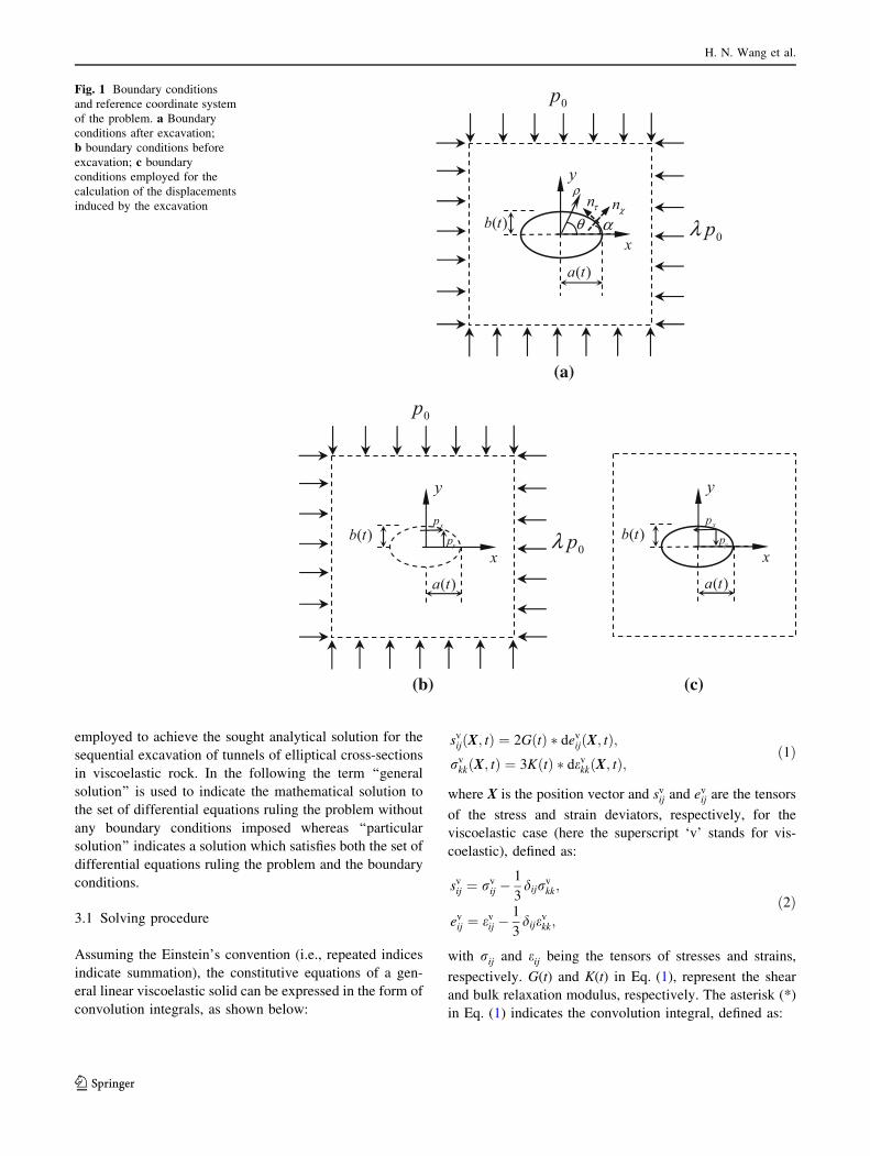
2. The initial stress field in the rock mass is idealized as

made of a vertical stress p0 and horizontal stress kp0,

where k is a prescribed ratio, as shown in Fig. 1a.

3. The tunnel is deeply buried, hence no linear variation

of the stresses with depth is considered.

4. The excavation speed is low enough that no dynamic

stresses are ever induced so that stress changes occur in

a quasi-static fashion at all times.

5. The cross-section of the tunnel is sequentially exca-

vated, that is, the half major and minor axes of the

elliptical tunnel section, a and b, respectively, are time

dependent. The tunneling process may be divided into

two stages: the first (i.e., excavation) stage, spans

from time t ¼ 0 to t ¼ t1, with t1 being the end time of

the cross-section excavation whilst the second stage

runs from t ¼ t1 onwards. In the first stage, the size of

the half major and minor axes varies according to the

time-dependent functions, a(t) and b(t), respectively,

that are likely to be discontinuous over time due to

technological requirements since sequential excava-

tions tend to occur step-like. So, an important feature

of the analytical solutions provided in this paper is

that they are applicable to any type of sequential

excavations either stepwise or continuous over time.

Note that in case the ratio of the ellipse axes remains

constant, the section grows homothetically; whereas if

the ratio changes over time, the shape of the section

evolves too (for instance from an initial circular pilot

tunnel to a final elliptical section). Since in most of

the cases the shape of the cross-section changes over

time, the general case of dðtÞ ¼ aðtÞ=bðtÞ will be

considered. The second stage spans from t ¼ t1

onwards, with the values of the half major and minor

elliptical axes being equal to a(t� t1) = a1 and

b(t� t1) = b1, respectively.

In the analysis, the effect of the advancement of the

tunnel along the longitudinal direction is not accounted for.

The effect of tunnel advancement can easily be considered

employing a fictitious pressure as shown in (Sulem et al.

1987b; Wang et al. 2014), but it is here omitted for sake of

simplicity in the derivation of the solution. So the cross-

section considered in the analysis is located at a sufficient

distance from the tunnel face that stresses and strains are

unaffected by three-dimensional effects. According to the

aforementioned assumptions, the problem can be formu-

lated as plane strain in the plane of the considered tunnel

cross-section. This plane will be assumed to be of infinite

size, with an internal elliptical hole growing over time,

subject to a uniform anisotropic stress field, and made of a

viscoelastic medium. Since the hole is not circular, polar

coordinates are no longer advantageous for the derivation

of the analytical solution. Hence, in this paper Cartesian

coordinates (x, y) are employed for the derivation of the

solution (see Fig. 1a) which are then transformed into polar

coordinates ðq; hÞ to show that the (already known) solu-

tion for a circular cross-section can be obtained as a par-

ticular case. A system of local coordinates ðnv; nsÞ is also

employed in the paper, with nv and ns being the normal and

tangential directions, respectively, along the elliptical

boundary (see Fig. 1a). In the following analysis, sign

convention is defined as positive for tension and negative

for compression.

3 Derivation of the Analytical Solution

To find analytical solutions for boundary value problems of

linear viscoelasticity, the most widely used methods are

based on the Laplace transform of the differential and

boundary condition equations governing the problem,

which, in this case, are time-dependent due to the fact that

sequential excavation is accounted for. Lee (1955) presents

the classical form of the correspondence principle between

linear elastic and linear viscoelastic solutions for boundary

value problems. The principle establishes a correspondence

between a viscoelastic solid and an associated fictitious

elastic solid of the same geometry. But until now, this

method has been applied only to solid bodies with time-

invariant boundaries because when boundaries are func-

tions of time, the boundary conditions cannot be Laplace

transformed. In this section, we describe an extension of

the principle to time varying stress boundaries that will be


123

employed to achieve the sought analytical solution for the

sequential excavation of tunnels of elliptical cross-sections

in viscoelastic rock. In the following the term ‘‘general

solution’’ is used to indicate the mathematical solution to

the set of differential equations ruling the problem without

any boundary conditions imposed whereas ‘‘particular

solution’’ indicates a solution which satisfies both the set of

differential equations ruling the problem and the boundary

conditions.

3.1 Solving procedure

Assuming the Einstein’s convention (i.e., repeated indices

indicate summation), the constitutive equations of a gen-

eral linear viscoelastic solid can be expressed in the form of

convolution integrals, as shown below:

svijðX; tÞ ¼ 2GðtÞ � dev

ijðX; tÞ;rv

kkðX; tÞ ¼ 3KðtÞ � devkkðX; tÞ;

ð1Þ

where X is the position vector and svij and ev

ij are the tensors

of the stress and strain deviators, respectively, for the

viscoelastic case (here the superscript ‘v’ stands for vis-

coelastic), defined as:

svij ¼ rv

ij �1

3dijr

vkk;

evij ¼ ev

ij �1

3dije

vkk;

ð2Þ

with rij and eij being the tensors of stresses and strains,

respectively. G(t) and K(t) in Eq. (1), represent the shear

and bulk relaxation modulus, respectively. The asterisk (*)

in Eq. (1) indicates the convolution integral, defined as:

(a)

(b) (c)

( )a t

( )b t

ρ

θnτ

αnχ

x

y

0p

0pλ

x

y

xp

yp

( )a t

( )b t

0p

0pλ

( )a t

( )b tx

y

xp

yp

Fig. 1 Boundary conditions

and reference coordinate system

of the problem. a Boundary

conditions after excavation;

b boundary conditions before

excavation; c boundary

conditions employed for the

calculation of the displacements

induced by the excavation

H. N. Wang et al.

123

f1ðtÞ � df2ðtÞ ¼ f1ðtÞ � f2ð0Þ þZ t

0

f1ðt � sÞ df2ðsÞds

ds: ð3Þ

The Laplace transform of Eq. (1) yields the following:

L svijðX; tÞ

h i¼ 2sL GðtÞ½ � �L ev

ijðX; tÞh i

;

L rvkkðX; tÞ

� �¼ 3sL KðtÞ½ � �L ev

kkðX; tÞ� �

;ð4Þ

where L f ðtÞ½ � is a function of the variable s defined in the

Laplace transform of the time function f ðtÞ, defined as:

L f ðtÞ½ � ¼Z 1

0

exp�st f ðtÞdt: ð5Þ

The Laplace transform of the linear elastic constitutive

equations is as follows (here the superscript ‘e’ stands for

elastic):

L seijðX; tÞ

h i¼ 2GeL ee

ijðX; tÞh i

;

L rekkðX; tÞ

� �¼ 3KeL ee

kkðX; tÞ� �

;ð6Þ

with Ge and Ke being the elastic shear and bulk modulus,

respectively. Note that Eq. (4) can be obtained from

Eq. (6) by replacing Ge with sL GðtÞ½ � and Ke with

sL KðtÞ½ �. Therefore, the general solution for a viscoelastic

isothermal problem, satisfying the set of differential

equations governing static equilibrium, kinematic com-

patibility and the constitutive relationship of the rock in the

time-dependent domain, can be obtained by replacing Ge

with sL GðtÞ½ � and Ke with sL KðtÞ½ � in the general solution

obtained for the associated elastic problem. Then, per-

forming a Laplace inverse transform, we obtain:

uvi ðX; tÞ ¼L�1 L u�i ðX; t; sÞ

� �� ð7aÞ

rvijðX; tÞ ¼L�1 L r�ijðX; t; sÞ

� �h i; ð7bÞ

where u�i ðX; t; sÞ and r�ijðX; t; sÞ are the displacements and

stresses, respectively, obtained by replacing Ge with

sL GðtÞ½ � and Ke with sL KðtÞ½ � in the general solution for

the associated elastic problem and L�1½gðsÞ � indicates the

inverse Laplace transform, defined as:

L�1½gðsÞ� ¼ 1

2pi

Z bþi1

b�i1gðsÞ expst ds: ð8Þ

The general viscoelastic solution in Eq. (7) contains yet

unknown functions of time, t, which have to be determined

by imposition of the boundary conditions. Displacement

boundary conditions may be expressed as follows:

uvi ðX0; tÞ ¼ uiðtÞ with X0 2 SuðtÞ; ð9aÞ

and stress boundary conditions as:

rvijðX0; tÞnj ¼ PiðtÞ; with X0 2 SrðtÞ; ð9bÞ

where X0 is the position of a point on the boundary, nj is

the unit vector normal to the boundary, SrðtÞ and SuðtÞ are

the boundary surfaces where stress and displacement con-

ditions, respectively, are applied, and Pi(t) and ui(t) are two

prescribed functions of time. Unlike problems with time-

invariant geometrical boundaries, X0 and nj in Eq. (9), are

functions of time, hence they are not constant with respect

to the Laplace transform, so they cannot be taken out of the

transform operator. Therefore, the relationship between the

particular solution of the viscoelastic problem and the

solution of the associated elastic one is unknown.

Replacing uvi and rv

ij with the expressions in Eq. (7), Eq. (9)

can be rewritten as:

uvi ðX; tÞ

��X¼X0¼L�1 L u�i ðX; t; sÞ

� �� X¼X0

¼ uiðtÞ;X0 2 SuðtÞ;

ð10aÞ

rvijðX; tÞnj

��X¼X0

¼L�1 L r�ijðX; t; sÞ� �h i

nj

��X¼X0

¼ PiðtÞ;X0 2 SrðtÞ:

ð10bÞ

The system of Eq. (10) together with Eq. (7) define the

set of equations to be satisfied by the particular solution

that we seek. To find the solution, complex potential theory

will be employed (see the next section).

3.2 Problem Formulation

Complex potential theory has been widely used to analyze

mathematical problems associated with underground con-

structions, especially in the analysis of non-circular open-

ings. For a two-dimensional (2D) elastic problem,

displacements and stresses can be expressed in terms of

two analytical functions of complex variable, i.e., u1 zð Þand w1 zð Þ with z ¼ xþ iy and i ¼

ffiffiffiffiffiffiffi�1p

, which are called

potential functions. So stresses and displacements can be

written as (Muskhelishvili 1963):

2Geðuex þ iue

yÞ ¼ ju1ðz; tÞ � zou1ðz; tÞ

oz� w1ðz; tÞ; ð11Þ

rex þ re

y ¼ 4Reou1ðz; tÞ

oz

�; ð12Þ

rey � re

x þ 2irexy ¼ 2 z

o2u1ðz; tÞoz2

þ ow1ðz; tÞoz

�; ð13Þ

with x, y being Cartesian coordinates in the tunnel cross-

section plane (see Fig. 1a),

j ¼1þ 6Ge

3Ke þ Ge

in case of plane strains

15Ke þ 8Ge

9Ke

in case of plane stresses

8>><>>:

ð14Þ


123

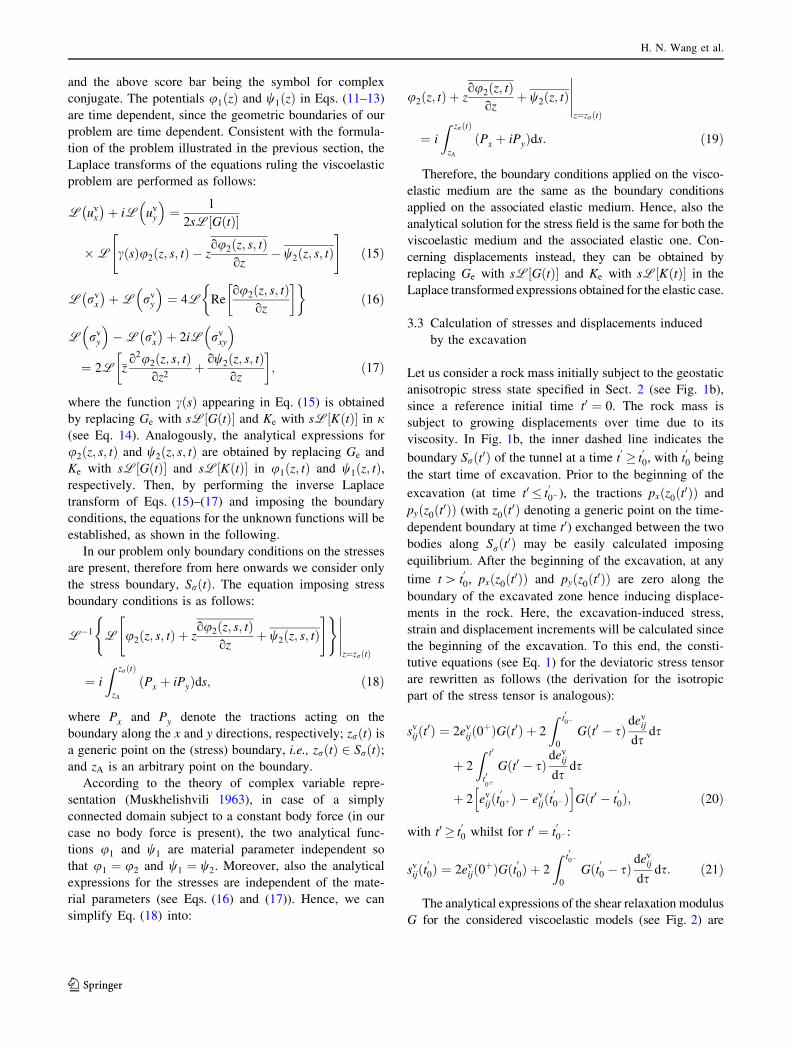
and the above score bar being the symbol for complex

conjugate. The potentials u1 zð Þ and w1 zð Þ in Eqs. (11–13)

are time dependent, since the geometric boundaries of our

problem are time dependent. Consistent with the formula-

tion of the problem illustrated in the previous section, the

Laplace transforms of the equations ruling the viscoelastic

problem are performed as follows:

L uvx

� �þ iL uv

y

� �¼ 1

2sL GðtÞ½ �

�L cðsÞu2ðz; s; tÞ � zou2ðz; s; tÞ

oz� w2ðz; s; tÞ

" #ð15Þ

L rvx

� �þL rv

y

� �¼ 4L Re

ou2ðz; s; tÞoz

�� ð16Þ

L rvy

� ��L rv

x

� �þ 2iL rv

xy

� �

¼ 2L zo2u2ðz; s; tÞ

oz2þ ow2ðz; s; tÞ

oz

�; ð17Þ

where the function cðsÞ appearing in Eq. (15) is obtained

by replacing Ge with sL GðtÞ½ � and Ke with sL KðtÞ½ � in j(see Eq. 14). Analogously, the analytical expressions for

u2ðz; s; tÞ and w2ðz; s; tÞ are obtained by replacing Ge and

Ke with sL GðtÞ½ � and sL KðtÞ½ � in u1ðz; tÞ and w1ðz; tÞ,respectively. Then, by performing the inverse Laplace

transform of Eqs. (15)–(17) and imposing the boundary

conditions, the equations for the unknown functions will be

established, as shown in the following.

In our problem only boundary conditions on the stresses

are present, therefore from here onwards we consider only

the stress boundary, SrðtÞ. The equation imposing stress

boundary conditions is as follows:

L�1 L u2ðz; s; tÞ þ zou2ðz; s; tÞ

ozþ w2ðz; s; tÞ

" #( )��z¼zrðtÞ

¼ i

Z zrðtÞ

zA

ðPx þ iPyÞds; ð18Þ

where Px and Py denote the tractions acting on the

boundary along the x and y directions, respectively; zrðtÞ is

a generic point on the (stress) boundary, i.e., zrðtÞ 2 SrðtÞ;and zA is an arbitrary point on the boundary.

According to the theory of complex variable repre-

sentation (Muskhelishvili 1963), in case of a simply

connected domain subject to a constant body force (in our

case no body force is present), the two analytical func-

tions u1 and w1 are material parameter independent so

that u1 ¼ u2 and w1 ¼ w2. Moreover, also the analytical

expressions for the stresses are independent of the mate-

rial parameters (see Eqs. (16) and (17)). Hence, we can

simplify Eq. (18) into:

u2ðz; tÞ þ zou2ðz; tÞ

ozþ w2ðz; tÞ

��z¼zrðtÞ

¼ i

Z zrðtÞ

zA

ðPx þ iPyÞds: ð19Þ

Therefore, the boundary conditions applied on the visco-

elastic medium are the same as the boundary conditions

applied on the associated elastic medium. Hence, also the

analytical solution for the stress field is the same for both the

viscoelastic medium and the associated elastic one. Con-

cerning displacements instead, they can be obtained by

replacing Ge with sL GðtÞ½ � and Ke with sL KðtÞ½ � in the

Laplace transformed expressions obtained for the elastic case.

3.3 Calculation of stresses and displacements induced

by the excavation

Let us consider a rock mass initially subject to the geostatic

anisotropic stress state specified in Sect. 2 (see Fig. 1b),

since a reference initial time t0 ¼ 0. The rock mass is

subject to growing displacements over time due to its

viscosity. In Fig. 1b, the inner dashed line indicates the

boundary Srðt0Þ of the tunnel at a time t0 � t

00, with t

00 being

the start time of excavation. Prior to the beginning of the

excavation (at time t0 � t0

0�), the tractions pxðz0ðt0ÞÞ and

pyðz0ðt0ÞÞ (with z0ðt0Þ denoting a generic point on the time-

dependent boundary at time t0) exchanged between the two

bodies along Srðt0Þ may be easily calculated imposing

equilibrium. After the beginning of the excavation, at any

time t [ t00, pxðz0ðt0ÞÞ and pyðz0ðt0ÞÞ are zero along the

boundary of the excavated zone hence inducing displace-

ments in the rock. Here, the excavation-induced stress,

strain and displacement increments will be calculated since

the beginning of the excavation. To this end, the consti-

tutive equations (see Eq. 1) for the deviatoric stress tensor

are rewritten as follows (the derivation for the isotropic

part of the stress tensor is analogous):

svijðt0Þ ¼ 2ev

ijð0þÞGðt0Þ þ 2

Z t00�

0

Gðt0 � sÞdev

ij

dsds

þ 2

Z t0

t00þ

Gðt0 � sÞdev

ij

dsds

þ 2 evijðt

0

0þÞ � evijðt

0

0�Þh i

Gðt0 � t0

0Þ; ð20Þ

with t0 � t0

0 whilst for t0 ¼ t0

0� :

svijðt

0

0Þ ¼ 2evijð0þÞGðt

0

0Þ þ 2

Z t00�

0

Gðt00 � sÞdev

ij

dsds: ð21Þ

The analytical expressions of the shear relaxation modulus

G for the considered viscoelastic models (see Fig. 2) are

H. N. Wang et al.

123

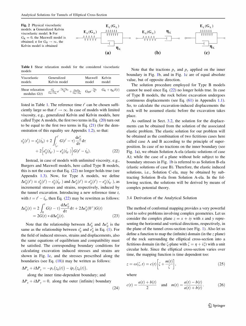
listed in Table 1. The reference time t0 can be chosen suffi-

ciently large so that t0 ! 1. In case of models with limited

viscosity, e.g., generalized Kelvin and Kelvin models, here

called Type A models, the first two terms in Eq. (20) turn out

to be equal to the first two terms in Eq. (21) (for the dem-

onstration of this equality see Appendix 1.2), so that:

svijðt0Þ ¼ sv

ijðt0

0Þ þ 2

Z t0

t00þ

Gðt0 � sÞdev

ij

dsds

þ 2 evijðt

0

0þÞ � evijðt

0

0�Þh i

Gðt0 � t0

0Þ: ð22Þ

Instead, in case of models with unlimited viscosity, e.g.,

Burgers and Maxwell models, here called Type B models,

this is not the case so that Eq. (22) no longer holds true (see

Appendix 1.3). Now, for Type A models, we define

Dsvijðt0Þ sv

ijðt0Þ � svijðt

00�Þ and Dev

ijðt0Þ evijðt0Þ � ev

ijðt00�Þ, as

incremental stresses and strains, respectively, induced by

the tunnel excavation. Introducing a new reference time t,

with t ¼ t0 � t00, then Eq. (22) may be rewritten as follows:

DsvijðtÞ ¼ 2

Z t

0

Gðt � sÞdDev

ij

dsdsþ 2Dev

ijð0þÞGðtÞ

¼ 2GðtÞ � dDevijðtÞ: ð23Þ

Note that the relationship between Dsvij and Dev

ij is the

same as the relationship between svij and ev

ij in Eq. (1). For

the field of induced stresses, strains and displacements, also

the same equations of equilibrium and compatibility must

be satisfied. The corresponding boundary conditions for

calculating excavation induced stresses and strains are

shown in Fig. 1c, and the stresses prescribed along the

boundaries (see Eq. (18)) may be written as follows:

DPx þ iDPy ¼ �px z0ðtÞ� �

� ipy z0ðtÞ� �

;

along the inner time-dependent boundary; and

DPx þ iDPy ¼ 0; along the outer infiniteð Þ boundary

ð24Þ

Note that the tractions px and py applied on the inner

boundary in Fig. 1b, and in Fig. 1c are of equal absolute

value, but of opposite direction.

The solution procedure employed for Type B models

cannot be used since Eq. (22) no longer holds true. In case

of Type B models, the rock before excavation undergoes

continuous displacements (see Eq. (61) in Appendix 1.1).

So, to calculate the excavation-induced displacements the

rock will be assumed elastic before the excavation takes

place.

As outlined in Sect. 3.2, the solution for the displace-

ments can be obtained from the solution of the associated

elastic problem. The elastic solution for our problem will

be obtained as the combination of two fictitious cases here

called case A and B according to the principle of super-

position. In case of no tractions on the inner boundary (see

Fig. 1a), we obtain Solution A-ela (elastic solutions of case

A); while the case of a plane without hole subject to the

boundary stresses in Fig. 1b is referred to as Solution B-ela

(elastic solutions of case B). Therefore, the elastic induced

solutions, i.e., Solution C-ela, may be obtained by sub-

tracting Solution B-ela from Solution A-ela. In the fol-

lowing section, the solutions will be derived by means of

complex potential theory.

3.4 Derivation of the Analytical Solution

The method of conformal mapping provides a very powerful

tool to solve problems involving complex geometries. Let us

consider the complex plane z = x ? iy with x and y repre-

senting the horizontal and vertical directions, respectively, in

the plane of the tunnel cross-section (see Fig. 1). Also let us

define a function to map the (infinite) domain (in the z plane)

of the rock surrounding the elliptical cross-section into a

fictitious domain (in the f-plane with f ¼ gþ in) with a unit

circular hole. Since the elliptical cross-section varies over

time, the mapping function is time dependent too:

z ¼ x f; tð Þ ¼ c tð Þ fþ mðtÞf

�; ð25Þ

where

cðtÞ ¼ aðtÞ þ bðtÞ2

and mðtÞ ¼ aðtÞ � bðtÞaðtÞ þ bðtÞ : ð26Þ

(a) (b) (c)

H H( )E G KηH H( )E G

Kη

K K( )E G

Kη

K K( )E GFig. 2 Physical viscoelastic

models. a Generalized Kelvin

viscoelastic model. b For

GK = 0, the Maxwell model is

obtained; c for GH !1, the

Kelvin model is obtained

Table 1 Shear relaxation moduli for the considered viscoelastic

models

Viscoelastic

models

Generalized

Kelvin model

Maxwell

model

Kelvin

model

Shear relaxation

modulus G(t)

G2H

GHþGKe�GHþGK

gKt þ GHGK

GHþGKGHe

�GHgK

t GK þ gKdðtÞ


123

IfaðtÞbðtÞ is constant during the excavation stage, the exca-

vation expands homothetically and m remains constant

over time. According to the boundary conditions shown in

Fig. 1a, two complex potentials for the elastic problem A

with time-dependent boundaries may be derived as follows

(Muskhelishvili 1963):

uðAÞ1 f; tð Þ ¼ �ð1þ kÞp0cðtÞ4

fþ mðtÞf

�

þ 1� kþ ð1þ kÞmðtÞ½ �p0cðtÞ2f

ð27Þ

wðAÞ1 f; tð Þ ¼ ðk� 1Þp0cðtÞ2

fþ mðtÞf

�

þ p0cðtÞ2f

ð1þ kÞð1þ m2ðtÞÞ þ 2ð1� kÞmðtÞ� �

þ 1� kþ ð1þ kÞmðtÞ½ � 1þ m2ðtÞ½ �p0cðtÞ2f f2 � mðtÞ� � :

ð28Þ

According to elasticity theory, the two potentials calcu-

lating the elastic displacements of an infinite plane subject to

the anisotropic initial stress state prior to excavation (Solu-

tion B-ela) are as follows (Einstein and Schwartz 1979):

uðBÞ1 f; tð Þ ¼ � ð1þ kÞp0cðtÞ4

fþ mðtÞf

�;

wðBÞ1 f; tð Þ ¼ � ð1� kÞp0cðtÞ2

fþ mðtÞf

�:

ð29Þ

According to the superposition principle of elasticity,

the potentials for calculating the excavation-induced dis-

placements are as follows (Solution C-ela):

uðCÞ1 f; tð Þ ¼ uðAÞ1 f; tð Þ � uðBÞ1 f; tð Þ

¼ 1� kþ ð1þ kÞmðtÞ½ �p0cðtÞ2f

ð30Þ

wðCÞ1 f; tð Þ ¼ wðAÞ1 f; tð Þ � wðBÞ1 f; tð Þ

¼ p0cðtÞ2f

ð1þ kÞ 1þ m2ðtÞ� �

þ 2ð1� kÞmðtÞ� �

þ 1� kþ ð1þ kÞmðtÞ½ � 1þ m2ðtÞ½ �p0cðtÞ2f f2 � mðtÞ� � :

ð31Þ

Substituting Eqs. (30) and (31) into Eqs. (11), (12) and

(13), the elastic displacements and stresses (Solution C-ela)

on the plane f may be calculated.

According to the analysis in Sect. 3.2, the solution for

the viscoelastic case can be obtained by applying the

principle of correspondence, and the Laplace inverse

transform of the variables (stresses, strains, etc.) calculated

for the elastic case with the variable z treated as a constant

in the Laplace transform. However, in Eqs. (30) and (31)

the variable f appears rather than z. To replace f with z and

t, the inverse function of the conformal mapping f ¼f0 z; tð Þ needs to be found. If f in Eqs. (30) and (31) is

replaced with f0 z; tð Þ, then all the time-dependent functions

in Eqs. (30) and (31) may be Laplace transformed, and the

viscoelastic solution may be derived from Eqs. (15), (16)

and (17). Then, defining:

z0 ¼ z

cðtÞ ð32Þ

and substituting in Eq. (25), the following is obtained:

z0 ¼ fþ mðtÞf: ð33Þ

If the excavation process is homothetic, i.e., m is a

constant, then there is no variable t in Eq. (33), and the

inverse conformal mapping may be expressed as (Zhang

et al. 2001):

f ¼ f1ðz0; tÞ ¼ Az0 þX1k¼0

Ak z0ð Þ�k; ð34Þ

with the yet undetermined coefficients A; Ak k ¼ 0; 1;ð. . .; 1Þ. For numerical reasons, the series will be truncated

to a finite number, l, of terms to calculate the function

approximately. Due to the fact that the inverse conformal

mapping is derived from the corresponding direct confor-

mal mapping, there is a one-to-one correspondence

between all the values of one function, with the values of

the other function. Let us choose a number of points fj

ðj ¼ 1; 2; . . .; qÞ, with q = 160, lying on the inner

boundary of the unit circle in the f plane to calculate the

corresponding points z0

j lying on the inner boundary in the

z0 plane using Eq. (33). Then, q linear equations for A and

Ak can be obtained by substituting fj and z0j into Eq. (34):

f1 ¼ Az01 þ

Pl

k¼0

Akz0�k1

f2 ¼ Az02 þ

Pl

k¼0

Akz0�k2

..

.

fj ¼ Az0

j þPl

k¼0

Akz0�kj

..

.

fq ¼ Az0q þ

Pl

k¼0

Akz0�kq :

8>>>>>>>>>>>>>>>>><>>>>>>>>>>>>>>>>>:

ð35Þ

Since the number of independent equations is larger than

the number of unknown coefficients (A, A0, A1, …, Al), the

system is indeterminate. To solve the system, i.e., to

determine the unknown coefficients, we employed the

method of minimum least squares. The non-zero coeffi-

cients obtained for the elliptical shapes here considered, are

listed in Table 2 for l = 15. In Fig. 3, the curves on plane

z0 and f determined by direct and inverse conformal map-

ping, respectively, are plotted for various shapes of the

H. N. Wang et al.

123

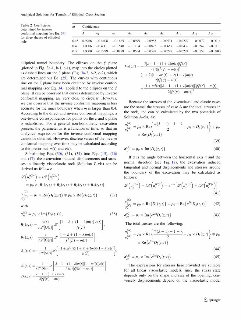
elliptical tunnel boundary. The ellipses on the z0 plane

(plotted in Fig. 3a-1, b-1, c-1), map into the circles plotted

as dashed lines on the f plane (Fig. 3a-2, b-2, c-2), which

are determined via Eq. (25). The curves with continuous

line on the f plane have been obtained by inverse confor-

mal mapping (see Eq. 34), applied to the ellipses on the z0

plane. It can be observed that curves determined by inverse

conformal mapping, are very close to circular. However,

we can observe that the inverse conformal mapping is less

accurate for the inner boundary when m is larger than 0.4.

According to the direct and inverse conformal mappings, a

one-to-one correspondence for points on the z and f plane

is established. For a general non-homothetic excavation

process, the parameter m is a function of time, so that an

analytical expression for the inverse conformal mapping

cannot be obtained. However, discrete values of the inverse

conformal mapping over time may be calculated according

to the prescribed m(t) and c(t).

Substituting Eqs. (30), (31), (34) into Eqs. (15), (16)

and (17), the excavation-induced displacements and stres-

ses in linearly viscoelastic rock (Solution C-vis) can be

derived as follows:

L uðCÞvx

� �þ iL uðCÞvy

� �

¼ p0 � B1ðz; sÞ þ B2ðz; sÞ þ B3ðz; sÞ þ B4ðz; sÞ½ �

rðCÞx

rðCÞy

¼ p0 � Re D1ðz; tÞf g p0 � Re D2ðz; tÞf g ð37Þ

with

rðCÞxy ¼ p0 � Im D2ðz; tÞf g; ð38Þ

B1ðz; sÞ ¼cðsÞ

sL GðtÞ½ �L1� kþ ð1þ kÞmðtÞ½ �cðtÞ

f1ðz0Þ

�;

B2ðz; sÞ ¼z

sL GðtÞ½ �L1� kþ ð1þ kÞmðtÞ

f 21 ðz0Þ � mðtÞ

�;

B3ðz; sÞ ¼ �1

sL GðtÞ½ �L1þ m2ðtÞð Þð1þ kÞ þ 2mðtÞð1� kÞ½ �c tð Þ

f1 z0� �

( );

B4ðz; sÞ ¼1

sL GðtÞ½ �Lk� 1� ð1þ kÞmðtÞ½ � 1þ m2ðtÞ½ �c tð Þ

f1ðz0Þ f 21 ðz0Þ � mðtÞ� �

" #;

D1ðz; tÞ ¼k� 1� ð1þ kÞmðtÞ

2½f 21 ðz0Þ � mðtÞ� ;

D2ðz; tÞ ¼ �z k� 1� ð1þ kÞmðtÞ½ �f 3

1 ðz0ÞcðtÞ½f 2

1 ðz0Þ � mðtÞ�3

� ð1þ kÞ 1þ m2ðtÞ½ � þ 2ð1� kÞmðtÞ2½f 2

1 ðz0Þ � mðtÞ�

þ 1þ m2ðtÞ½ � k� 1� ð1þ kÞmðtÞ½ �½3f 21 ðz0Þ � mðtÞ�

2 f 21 ðz0Þ � mðtÞ� �3 :

Because the stresses of the viscoelastic and elastic cases

are the same, the stresses of case A are the total stresses in

the rock, and can be calculated by the two potentials of

Solution A-ela, as:

rðAÞx

rðAÞy

¼ p0 � Reðk� 1Þ � 1� k

2þ p0 � D1ðz; tÞ

� p0

� Re D2ðz; tÞf gð39Þ

rðAÞxy ¼ p0 � Im D2ðz; tÞf g: ð40Þ

If a is the angle between the horizontal axis x and the

normal direction (see Fig. 1a), the excavation induced

tangential and normal displacements and stresses around

the boundary of the excavation may be calculated as

follows:

L uðCÞvv

� �þ iL uðCÞvs

� �¼ e�ia L uðCÞvx

� �þ iL uðCÞvy

� �h i

ð41Þ

rðCÞv

rðCÞs

¼ p0 � Re D1ðz; tÞf g p0 � Re e2iaD2ðz; tÞ� �

ð42Þ

rðCÞvs ¼ p0 � Im e2iaD2ðz; tÞ� �

ð43Þ

The total tresses are the following:

rðAÞv

rðAÞs

¼ p0 � Reðk� 1Þ � 1� k

2þ p0 � D1ðz; tÞ

� p0

� Re e2iaD2ðz; tÞ� �

ð44Þ

rðAÞvs ¼ p0 � Im e2iaD2ðz; tÞ� �

: ð45Þ

The expressions for stresses here provided are suitable

for all linear viscoelastic models, since the stress state

depends only on the shape and size of the opening; con-

versely displacements depend on the viscoelastic model

Table 2 Coefficients

determined by inverse

conformal mapping (see Eq. 34)

for three shapes of elliptical

hole

m Coefficients

A A1 A3 A5 A7 A9 A11 A13 A15

0.45 0.9966 -0.4408 -0.1665 -0.0979 -0.0983 -0.0531 -0.0229 0.0072 0.0014

0.40 1.0006 -0.4001 -0.1540 -0.1104 -0.0872 -0.0657 -0.0439 -0.0247 -0.0113

0.30 1.0000 -0.2999 -0.0898 -0.0534 -0.0388 -0.0298 -0.0224 -0.0153 -0.0900


123

The inner boundary

The inner boundary

-2.5 -2 -1.5 -1 -0.5 0 0.5 1 1.5 2 2.5-2.5

-2

-1.5

-1

-0.5

0

0.5

1

1.5

2

2.5

-2.5 -2 -1.5 -1 -0.5 0 0.5 1 1.5 2 2.5-2.5

-2

-1.5

-1

-0.5

0

0.5

1

1.5

2

2.5m=0.4 z'

y'

x'

ζη

ξ

-2.5 -2 -1.5 -1 -0.5 0 0.5 1 1.5 2 2.5-2.5

-2

-1.5

-1

-0.5

0

0.5

1

1.5

2

2.5

-2.5 -2 -1.5 -1 -0.5 0 0.5 1 1.5 2 2.5-2.5

-2

-1.5

-1

-0.5

0

0.5

1

1.5

2

2.5

m=0.3 z'y'

x'

ζη

ξ

The inner boundary

Inverse conformal mapping

Conformal mapping

m=0.45

-2.5 -2 -1.5 -1 -0.5 0 0.5 1 1.5 2 2.5-2.5

-2

-1.5

-1

-0.5

0

0.5

1

1.5

2

2.5

-2.5 -2 -1.5 -1 -0.5 0 0.5 1 1.5 2 2.5-2.5

-2

-1.5

-1

-0.5

0

0.5

1

1.5

2

2.5z' ζ

y'

x'

η

ξ

Unit circle (in dashed line)

Unit circle obtained by inverse conformal mapping (in continuous line)

1.0r =

1.2r =1.5r =

2.0r =

(a1) (a2)

(b1) (b2)

(c1) (c2)

Fig. 3 Curves determined by conformal mapping and inverse

conformal mapping: a-1, b-1, c-1 ellipses in plane z0 (z0 ¼ x0 þ y0i)determined by conformal mapping for m = 0.45, 0.4 and 0.3,

respectively; a-2, b-2, c-2 mapped circles (continuous line) in plane

f (f ¼ nþ gi ¼ reih1 ) determined by inverse conformal mapping

H. N. Wang et al.

123

considered. The analytical solution for the displacements is

provided in the next section.

3.5 Displacement solution for the generalized Kelvin

model

Rock masses which have strong mechanical properties or

are subject to low stresses exhibit limited viscosity. For this

type of behavior, the generalized Kelvin viscoelastic model

(see Fig. 2a) is commonly employed (Dai et al. 2004). On

the other hand, weak, soft or highly jointed rock masses

and/or rock masses subject to high stresses are prone to

excavation-induced continuous viscous flows. In this case,

the Maxwell model (see Fig. 2b) is suitable to simulate

their rheology, due to the fact that this model is able to

account for secondary creep. In this section, the analytical

solution for the generalized Kelvin model is developed.

The constitutive parameters of this model are as follows:

(1) the elastic shear moduli GH, due to the Hookean ele-

ment in the model; (2) GK, due to the spring element of the

Kelvin component; (3) the viscosity coefficient gK, due to

the dashpot element of the Kelvin component (see Fig. 2c).

The solution for the Maxwell model may be obtained as a

particular case of the generalized Kelvin model, for

GK = 0. The solution for the Kelvin model (see Fig. 2c)

Part : Excavated at t=0 day







Model far-boundaries located at

distances x=80 m and y=80 m.

The initial size: a0=1.5 m, b0=1.0 m.

The final size: a1=6.0 m, b1=4.0 m.

‘Radial’ mesh with rectangular far-boundaries; the mesh

has 384 elements in the radial direction and 40 elements

in the circumferential direction; the total number of the

elements is 15360.

x

y0b

1b

0a1a

Part Part

Part

PartPart

Part Part

Fig. 4 FEM mesh used to

model the elliptical sequential

excavation

Table 3 Values of the half

major and minor axes of the

elliptical opening prescribed in

the FEM analysis

Time t (day) 0; 1½ Þ 1; 2½ Þ 2; 3½ Þ 3; 4½ Þ 4; 5½ Þ 5; 6½ Þ 6;1½ Þ

Corresponding excavated rock in Fig. 4 Part I Part II Part III Part IV Part V Part VI Part VII

Half major axis, a (m) 1.50 2.25 3.00 3.75 4.50 5.25 6.00

Half minor axis, b (m) 1.00 1.50 2.00 2.50 3.00 3.50 4.00

0 2 4 6 8 10 12 14 16 180

2

4

6

8

10

12

14

16

18

Line 1

Line 2

Line 3

Tunnel boundary

x [m]

y[m

]

Point 1

Point 2

Point 3

Point 1: x=6, y=0Point 2: x=3.28, y=3.35Point 3: x=0, y=4

unit: m49.8o

Fig. 5 Selected points and lines for the comparison between

analytical solution and FEM results illustrated in Figs. 6, 7, and 8


123

may also be obtained as another particular case of the

generalized Kelvin model for GH !1.

Assuming that the rock is incompressible, i.e.,

K tð Þ ! 1, the two relaxation moduli appearing in the

constitutive equations (see Eq. 1) are as follows:

G tð Þ ¼ G2H

GH þ GK

e�GHþGK

gKt þ GHGK

GH þ GK

; K tð Þ ¼ 1 ð46Þ

The induced displacements, Solution C-vis, may be

derived by substituting Eq. (46) into Eq. (41):

uðCÞvv þ iuðCÞvs ¼ e�iap0

4B5ðz; tÞ þ B6ðz; tÞ þ B7ðz; tÞ þ B8ðz; tÞ½ �;

ð47Þ

with B5ðz;tÞ¼R t

0Hðt;sÞc sð Þ 1�kþð1þkÞmðsÞ½ �

f1½z0ðsÞ� ds, B6ðz;tÞ¼zR t

0Hðt;sÞ

1�kþð1þkÞmðsÞf 21½z0ðsÞ��mðsÞ

�ds, B7ðz;tÞ¼

R t

0

Hðt;sÞc sð Þ 1þm2ðsÞð Þð1þkÞþ2mðsÞð1�kÞ½ �f1½z0ðsÞ�

ds,

B8ðz;tÞ¼R t

0

Hðt;sÞc sð Þ k�1�ð1þkÞmðsÞ½ � 1þm2ðsÞ½ �f1½z0ðsÞ� f 2

1½z0ðsÞ��mðsÞf g ds, and

Hðt; sÞ ¼ 1

GH

d t � sð Þ þ 1

gK

e�GK

gKt�sð Þ

: ð48Þ

Note that when m = 0 and k = 1, the problem reduces

to a circular tunnel subject to a hydrostatic state of stress

hence the problem becomes axisymmetric. The solution in

Eq. (47) is degenerate and coincides with the solution

provided in (Wang and Nie 2010).

(a)

(c)

(b)

Fig. 6 Comparison between analytical solution and FEM results in terms of stresses and displacements versus time for Points 1, 2, 3 (location

shown in Fig. 5): a displacements at Points 1, 2 and 3; b stresses at Points 1 and 3; c stresses at Point 2

H. N. Wang et al.

123

4 Comparison with FEM Results

Two types of FEM analyses were run employing the FEM

code ANSYS (version 11.0, employing the module of

structural mechanics). The first FEM analysis wants to

replicate the viscoelastic problem of solution A-vis;

whereas the second one, the problem of solution C-vis. All

FEM analyses were carried out with a small displacement

formulation to be consistent with the derivation of the

analytical solution.

The analytical solution A-vis for generalized Kelvin

viscoelastic model can be derived by substituting

Eqs. (27), (28), (34) and (46) into Eqs. (15)–(17). The

expression for the displacements is as follows:

uðAÞvx þ iuðAÞvy

¼ p0

4B5ðz; tÞ þ B6ðz; tÞ þ B7ðz; tÞ þ B8ðz; tÞ þ B9ðz; tÞ½ �;

ð49Þ

where B9ðz; tÞ ¼ ð1� kÞzR t

0Hðt; sÞds. Displacements and

stresses of solution C-vis and stresses of solution A-vis can

be found in Eqs. (47), (37), (38), (39) and (40),

respectively.

First, we shall compare displacements and stresses of

solution A-vis obtained by the analytical solution with the

FEM analysis along three directions (horizontal, vertical,

49.8� over the horizontal). Second, the excavation-induced

stresses and displacements from the analytical solution

C-vis and FEM along the line (49.8� over the horizontal)

will be compared to validate the analytical solution

achieved. In the FEM analysis of case A-vis, initial stresses

are applied on a planar domain having an elliptical hole

with the major axis being 2a0 long and minor axis 2b0 long

(part I in Fig. 4). Then, the rock is sequentially excavated

at different times (see part II to VII in Fig. 4), as listed in

Table 3. In the second simulation instead, initial stresses

are first applied on a finite rectangular domain without

hole, then an excavation starting after 50 days is simulated.

Part I to VII are excavated at t0 = 50th day, 51th day, …,

56th day, respectively. Finally, the excavation-induced

stresses and displacements can be obtained by subtracting

the initial values before excavation from the ones calcu-

lated in the excavation stage. In the FEM analyses, ele-

ments are deleted at the time of excavation by setting the

stiffness of the deleted elements to zero (by multiplying the

stiffness matrix by 10-6).

A vertical stress, p0 ¼ 10 MPa, and a horizontal stress,

kp0 with k ¼ 0:5, were applied at the boundaries of

the domain. The rock was simulated as a generalized

Kelvin medium, with the following constitutive para-

meters adopted: GH ¼ 2; 000 MPa, GK ¼ 1; 000 MPa and

gK ¼ 10; 000 MPa day. The excavation sequence here

considered is specified by the values of the major and

minor axes of the elliptical section listed in Table 3 with an

initial value of 2a0 = 3.0 m for the major axis and

2b0 = 2.0 m for the minor axis. Note that the ratio

m(t) = const, i.e., the elliptical section evolves homothet-

ically. The FEM mesh nearby the hole is plotted in Fig. 4.

The points and lines selected for comparison between

the FEM analysis and the analytical solution are plotted in

Fig. 5: three points on the inner boundary (Points 1, 2, 3 in

Fig. 5) and three lines, one horizontal (Line 1), one vertical

0 2 4 6 8 10 12 14 16 18 20-30

-25

-20

-15

-10

-5

0

5

6

12

18

24

30

36

42

48

FEM results

Analytical solution uxv for Line 1

t =1st day

t =20th day

t =6th day

t =3rd day

Distance to centre of ellipse [m]

t =1st dayt =3rd day

t =20th day

t =6th day

Analytical solution uyv for Line 3

Dis

plac

emen

t uxv [m

m]

Dis

plac

emen

t uyv [m

m]

Lines 1 and 3

0 2 4 6 8 10 12 14 16 18 20 22-16

-8

-6

-4

-2

0

2

4

0

4

8

12

16

20

24

28

32

36

40

-14

-12

-10

Dis

plac

emen

t uxv [m

m]

Analytical solution uxv for Line 2

Analytical solution uyv for Line 2

Distance to centre of ellipse [m]

Dis

plac

emen

t uyv [m

m]

Line 2

FEM results(3)

(3)

(4)

(4)

(2)

(2)(1)

(1)

t =1st day(1)(2) t =3rd day

t =6th day(3)(4) t =20th day

(a) (b)

Fig. 7 Comparison between analytical solution and FEM results in

terms of displacements along Lines 1, 2 and 3 (locations shown in

Fig. 5) versus distance to the ellipse center at different times (t = 1st,

3rd, 6th and 20th days): a displacements along Lines 1 and 3;

b displacement along Line 2


123

(Line 3) and one inclined at 49.8� over the horizontal (Line

2), were chosen. In Fig. 6, displacements and stresses for

Points 1, 2 and 3 are plotted versus time. In Figs. 7 and 8

displacements and stresses, respectively, at four different

times (t = 1st, 3rd, 6th and 20th days) are plotted for Lines

1, 2 and 3 versus the distance to the center of the ellipse. It

emerges that the predictions from the analytical solution

are in excellent agreement with the results from the FEM

analysis. Obviously displacements and stresses undergo a

stepwise increase following instantaneous excavation

events (1st, 2nd, 3rd,… 6th days, see Fig. 6).

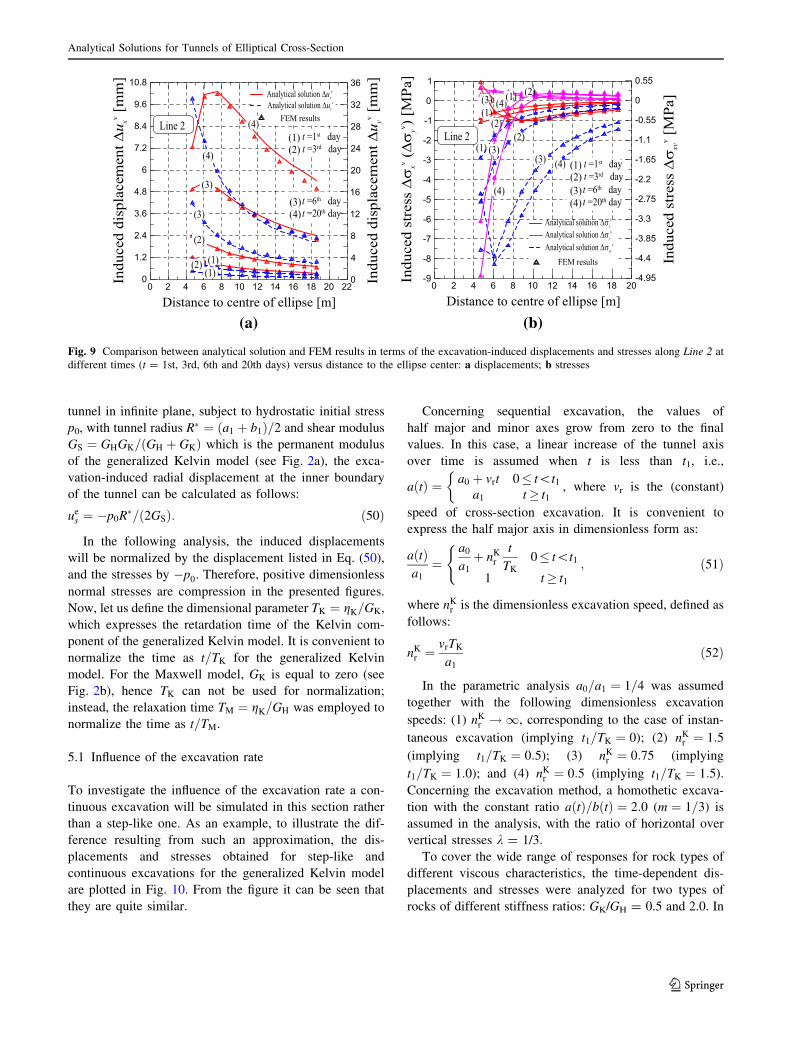
In Fig. 9, the excavation-induced displacements and

stresses along Line 2 obtained from the analytical solution

and FEM analysis are plotted. A good agreement in terms

of both stresses and displacements can be observed. Unlike

the case of solution A, almost all the induced displace-

ments are decreasing functions of the distance to the center

of the ellipse.

5 Parametric Investigation

To study the influence of excavation rate and methods, as

well as the time-dependent displacements and stresses, a

parametric investigation is carried out in this section.

Assuming an axisymmetric elastic problem, i.e., circular

(a)

(c)

(b)

Fig. 8 Comparison between analytical solution and FEM results in

terms of stresses along Lines 1, 2 and 3 (locations shown in Fig. 5)

versus distance to the ellipse center at different times (t = 1st, 3rd,

6th and 20th days): in a–c the stresses along Lines 1, 2 and 3,

respectively, are plotted

H. N. Wang et al.

123

tunnel in infinite plane, subject to hydrostatic initial stress

p0, with tunnel radius R� ¼ ða1 þ b1Þ=2 and shear modulus

GS ¼ GHGK=ðGH þ GKÞ which is the permanent modulus

of the generalized Kelvin model (see Fig. 2a), the exca-

vation-induced radial displacement at the inner boundary

of the tunnel can be calculated as follows:

ues ¼ �p0R�=ð2GSÞ: ð50Þ

In the following analysis, the induced displacements

will be normalized by the displacement listed in Eq. (50),

and the stresses by �p0. Therefore, positive dimensionless

normal stresses are compression in the presented figures.

Now, let us define the dimensional parameter TK ¼ gK=GK,

which expresses the retardation time of the Kelvin com-

ponent of the generalized Kelvin model. It is convenient to

normalize the time as t=TK for the generalized Kelvin

model. For the Maxwell model, GK is equal to zero (see

Fig. 2b), hence TK can not be used for normalization;

instead, the relaxation time TM ¼ gK=GH was employed to

normalize the time as t=TM.

5.1 Influence of the excavation rate

To investigate the influence of the excavation rate a con-

tinuous excavation will be simulated in this section rather

than a step-like one. As an example, to illustrate the dif-

ference resulting from such an approximation, the dis-

placements and stresses obtained for step-like and

continuous excavations for the generalized Kelvin model

are plotted in Fig. 10. From the figure it can be seen that

they are quite similar.

Concerning sequential excavation, the values of

half major and minor axes grow from zero to the final

values. In this case, a linear increase of the tunnel axis

over time is assumed when t is less than t1, i.e.,

aðtÞ ¼ a0 þ vrt 0� t\t1a1 t� t1

�, where vr is the (constant)

speed of cross-section excavation. It is convenient to

express the half major axis in dimensionless form as:

aðtÞa1

¼a0

a1

þ nKr

t

TK

0� t\t1

1 t� t1

(; ð51Þ

where nKr is the dimensionless excavation speed, defined as

follows:

nKr ¼

vrTK

a1

ð52Þ

In the parametric analysis a0=a1 ¼ 1=4 was assumed

together with the following dimensionless excavation

speeds: (1) nKr !1, corresponding to the case of instan-

taneous excavation (implying t1=TK ¼ 0); (2) nKr ¼ 1:5

(implying t1=TK ¼ 0:5); (3) nKr ¼ 0:75 (implying

t1=TK ¼ 1:0); and (4) nKr ¼ 0:5 (implying t1=TK ¼ 1:5).

Concerning the excavation method, a homothetic excava-

tion with the constant ratio aðtÞ=bðtÞ ¼ 2:0 (m ¼ 1=3) is

assumed in the analysis, with the ratio of horizontal over

vertical stresses k = 1/3.

To cover the wide range of responses for rock types of

different viscous characteristics, the time-dependent dis-

placements and stresses were analyzed for two types of

rocks of different stiffness ratios: GK/GH = 0.5 and 2.0. In

(a) (b)

Fig. 9 Comparison between analytical solution and FEM results in terms of the excavation-induced displacements and stresses along Line 2 at

different times (t = 1st, 3rd, 6th and 20th days) versus distance to the ellipse center: a displacements; b stresses


123

Figs. 11 and 12, the time-dependent radial and tangential

displacements for the rock along the final tunnel face (i.e.,

along the visible face of the tunnel obtained at the end of

sequential excavation) with angle h ¼ 0�, 45� and 90� are

plotted for the types of rock and excavation rates consid-

ered. The symbol ‘•’ represents the end time of excavation,

t1. The figures show that the normal displacement increases

with time and reaches a constant value after a certain

period of time; however, the tangential displacement first

decreases with time and increases rapidly towards the end

of the excavation, then subsequently it reaches a constant

value. Comparing Fig. 11 with Fig. 12, the final displace-

ments are reached later for rocks with small stiffness ratios

(Fig. 11). It can also be noted that the bigger the stiffness

ratio, the larger the displacements occurring after excava-

tion are. For both types of rock, the results show that a

lower excavation rate implies a longer excavation time,

which in turn leads to a larger value of normal displace-

ment at the tunnel wall with h ¼ 45� and 90� when t ¼ t1;

however, the tangential displacement at h ¼ 45� and the

(a)

(c)

(b)

Fig. 10 Displacements (a, b), and principal stresses (c) versus time at a point on the final tunnel face obtained from gradual and step-like

excavations for the generalized Kelvin model

H. N. Wang et al.

123

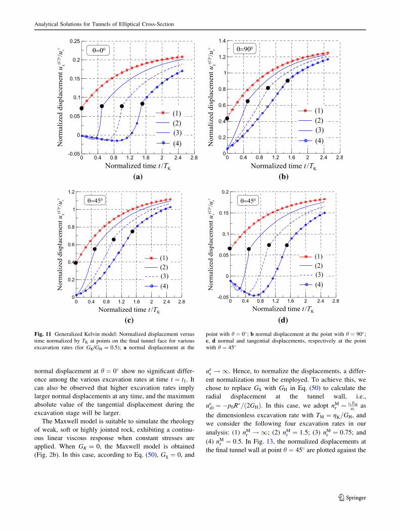
normal displacement at h ¼ 0� show no significant differ-

ence among the various excavation rates at time t ¼ t1. It

can also be observed that higher excavation rates imply

larger normal displacements at any time, and the maximum

absolute value of the tangential displacement during the

excavation stage will be larger.

The Maxwell model is suitable to simulate the rheology

of weak, soft or highly jointed rock, exhibiting a continu-

ous linear viscous response when constant stresses are

applied. When GK = 0, the Maxwell model is obtained

(Fig. 2b). In this case, according to Eq. (50), GS ¼ 0, and

ues !1. Hence, to normalize the displacements, a differ-

ent normalization must be employed. To achieve this, we

chose to replace GS with GH in Eq. (50) to calculate the

radial displacement at the tunnel wall, i.e.,

ues0 ¼ �p0R�=ð2GHÞ. In this case, we adopt nM

r ¼ vrTM

a1as

the dimensionless excavation rate with TM ¼ gK=GH, and

we consider the following four excavation rates in our

analysis: (1) nMr !1; (2) nM

r ¼ 1:5; (3) nMr ¼ 0:75; and

(4) nMr ¼ 0:5. In Fig. 13, the normalized displacements at

the final tunnel wall at point h ¼ 45� are plotted against the

(a) (b)

(d)(c)

Fig. 11 Generalized Kelvin model: Normalized displacement versus

time normalized by TK at points on the final tunnel face for various

excavation rates (for GK/GH = 0.5); a normal displacement at the

point with h ¼ 0�; b normal displacement at the point with h ¼ 90�;c, d normal and tangential displacements, respectively at the point

with h ¼ 45�


123

normalized time t/TM. In Fig. 13, the displacements after

excavation grow linearly over time since the stresses of the

rock are constant (see Eqs. (44) and (45)). Also, it emerges

that the influence of the excavation rate for Maxwell model

is similar to that for the generalized Kelvin model.

Observing Eqs. (44) and (45), it is shown that the

stresses depend only on the size and shape of the

opening, hence given a prescribed sequential excavation

the stress field is identical for all the viscoelastic models.

In Fig. 14, the principal stresses of the rock at the tunnel

wall at points h ¼ 0�, h ¼ 45� and h ¼ 90�, are plotted

for various excavation rates. As it can be expected, the

variation of stresses with time is more gradual for lower

excavation rates. In all the cases, the maximum differ-

ence between the two principal stresses occurs after

excavation.

(a) (b)

(c) (d)

Fig. 12 Generalized Kelvin model: Normalized displacement versus

time normalized by TK at points on the final tunnel face for various

excavation rates (for GK/GH = 2.0); a normal displacement at the

point with h ¼ 0�; b normal displacement at the point with h ¼ 90�;c, d normal and tangential displacements, respectively at the point

with h ¼ 45�

H. N. Wang et al.

123

5.2 Influence of the Excavation Methods

In this section, the final values of the major and minor axes

and the ratio of horizontal over vertical stresses k are the

same as in the previous section with the end time of

excavation being t1/TK = 1.0. The time-dependent tunnel

inner boundaries, which simulate the real across-section

excavation process as center drift advanced method (Miura

et al. 2003) (e.g., method C shown in Fig. 15), and drilling

and blasting method (Tonon 2010) (e.g., methods A, B1

and B2 shown in Fig. 15), are shown in Fig. 15a–c. The

functions a(t) and b(t) are plotted in Fig. 16 with their

analytical expressions provided in Table 4.

Sequential excavation methods A and C are stepwise

excavations, in which parts � to ˜ (or � to ˆ) are exca-

vated instantaneously in succession. In Fig. 15, it is shown

that the shape of the opening in method A first changes

from ellipse to circle, and then to ellipse, by sequential

excavation along the major axis direction. Obviously, the

excavation is non-homothetic. Figure 16 shows that in this

method the adopted excavation rate is faster at the begin-

ning and slower near the end of excavation. In method C,

the initial shape of the opening is circular, then gradually

changes to elliptical with the ratio a(t)/b(t) increasing over

time. The excavation rate is slower at the beginning and

becomes faster near the end of excavation, which is

opposite to what happens in method A. Excavation meth-

ods B1 and B2 instead, are continuous homothetic exca-

vations (a(t)/b(t) = 2.0). Method B1 consists of a linear

excavation at uniform speed, whereas method B2 consists

of an excavation function a(t) in quadratic form, with a

faster excavation rate at the end.

The time-dependent normal and tangential displace-

ments at the final tunnel face are plotted in Figs. 17 and 18

for the four excavation methods considered. It emerges that

the induced displacements are sensitive to the excavation

method adopted. In particular it can be observed that the

methods with faster speeds in the early stages lead to larger

normal displacements at any time considered (except for

the case of h ¼ 0�). For all the excavation methods, the

normal displacements at h ¼ 45� and 90� increase over

time and reach a constant positive value after a certain

period of time; whereas the normal displacements at h ¼ 0�

are approximately zero in the early stages of excavation,

and increase rapidly near the end of excavation for methods

B1, B2 and C. The tangential displacements at h ¼ 45� in

Fig. 17d are negative and first decrease in the early stages

and then increase to positive values.

To analyze the difference of displacements among the

excavation methods considered, the normalized displace-

ments of methods A and C and the ratio of their differences

at time t = t1 (the difference between methods A and C is

the largest one among all the methods according to Figs. 17

and 18) are listed in Table 5. The ratio of the difference of

the normal displacements for a rock with GK/GH = 0.5

ranges from 26 to 33 %. The ratio for the tangential dis-

(a) (b)

Fig. 13 Maxwell model (GK = 0): normalized displacement versus time normalized by TM at a point on the final tunnel face with h ¼ 45� for

various excavation rates; a normal displacement; b tangential displacement


123

placements is up to 60 %. For the case of GK/GH = 2.0, the

ratios range from 7 to 13 % for normal displacements and

up to 20 % for tangential displacements.

Figure 19 presents the normalized principal stresses

calculated at the final tunnel face. It may be observed that

the stresses show no difference for all of the excavation

methods when t� t1, because the final shape and size of the

tunnel are the same. However, during the excavation stage

the stress field is clearly affected by the excavation method

adopted. This stress analysis accounting for sequential

excavation is valuable to check for potential failure

mechanisms since it provides the stress state at any time for

any point in the rock.

5.3 Distribution of Displacements and Stresses

for Different Excavation Methods

In this section, the distributions of displacements and

stresses assuming GK/GH = 0.5 are analyzed, adopting

sequential excavation methods A and C for the same end

time of excavation. Four points in time are considered in

the following analysis: time t(1): t(1)/TK = 0.0, the

(a)

(c)

(b)

Fig. 14 Normalized principal stresses versus time normalized by TK for the generalized Kelvin model and by TM for the Maxwell model at

different locations on the final tunnel face for various excavation rates; a–c principal stresses at points h ¼ 0�, h ¼ 45� and h ¼ 90�, respectively

H. N. Wang et al.

123

beginning of excavation; time t(2): t(2)/TK = 0.5, during the

excavation stage; time t(3): t(3)/TK = 1.0, the end of exca-

vation; and time t(4): t(4)/TK = 2.5, the time after excava-

tion when no further displacements practically occur.

Figure 20 presents the contour plots of the normal dis-

placements at times t(3) and t(4) for methods A and C,

respectively; and Fig. 21 presents the contour plots of the

tangential displacements. Figure 20 shows that, the spatial

distribution of normal displacements at the same time after

excavation (e.g., the displacements in Fig. 20a and c and in

Fig. 20b and d), is very similar. However, the values of

displacement at the same position exhibit a significant

difference especially around the tunnel crown when

t = t(3). Conversely at t(4), the difference is very small.

Figure 21 shows that the maximum negative tangential

displacement occurs inside the ground, and the maximum

positive one occurs at the tunnel face with h approximately

equal to 10�–30�. Furthermore, also the distribution of

tangential displacements for different excavation methods

is very similar. In Fig. 22a, b, the contours of the major and

-1.2

-0.8

-0.4

0

0.4

0.8

1.2

-1.2

-0.8

-0.4

0

0.4

0.8

1.2

-1.2 -0.8 -0.4 0 0.4 0.8 1.2 -1.2 -0.8 -0.4 0 0.4 0.8 1.2-1.2 -0.8 -0.4 0 0.4 0.8 1.2-1.2

-0.8

-0.4

0

0.4

0.8

1.2

x/a1

y/a1

x/a1

y/a1

x/a1

y/a1

1

2

34 5 1

23 4

Method A Method CMethod B1 and B2

homothetic excavation

(a) (b) (c)

Fig. 15 Variation of the shape of the inner boundary due to sequential excavation for a excavation method A; b method B1 and B2; c method C

0 0.2 0.4 0.6 0.8 1 1.20.1

0.2

0.3

0.4

0.5

0.6

0.7

0.8

0.9

1

Method AMethod B1Method B2Method C

t / TK

a(t) /a1

0 0.2 0.4 0.6 0.8 1 1.20.1

0.2

0.3

0.4

0.5

0.6

0.7

0.8

0.9

1Method AMethod B1Method B2Method C

t /TK

b(t) / a1

Method A

Method B1Method B2

Method C

Method A

Method B1

Method B2

Method C

(a) (b)

Fig. 16 Size of the elliptical

tunnel versus time according to

four excavation methods; a half

major axis versus time; b half

minor axis versus time


123

minor principal stresses, respectively, are plotted at time

t(3).

Figure 23a, b present the distribution of normal and

tangential displacements at the final tunnel face as a

function of the angle h for excavation method A and C at

various times, which due to the symmetry of the problem,

is illustrated in the range h ¼ 0� to 90� only. It emerges

that the normal displacement is a monotonically increasing

function of the angle, and the curve shapes for various

excavation methods are similar. However, at times t(2) and

t(3), the values of normal displacement for the two exca-

vation methods are significantly different. Unlike the nor-

mal displacement, the tangential displacement increases

with h for 0\h\hmax, then decreases for hmax\h\p=2.

Furthermore, the angle corresponding to the maximum

displacement, hmax, decreases over time. At time t(2) (dur-

ing the excavation stage), the sign of the tangential dis-

placement is opposite in the two excavation methods,

exhibiting approximately the same hmax. Considering the

difference of induced tangential displacements between the

two excavation methods, at the end of excavation it is

smaller, whereas it becomes larger afterwards with a rapid

decrease of displacement in method C. In addition, the

angle corresponding to the maximal value, hmax, is larger in

method A than that in method C. The difference between

the displacements of the two methods is smallest when t/

TK = 2.5 (t(4)).

In Fig. 24a, b, the principal stresses at the final tunnel

face as a function of the angle h are plotted for methods

A and C, respectively. Because the stresses depend only

on the size and shape of the opening, the stresses at time

t(4), which are the same as the ones at time t(3), are not

included in the figure. It can be noted that at the end time

of excavation, t/TK = 1.0, the distribution of stresses is

the same whatever excavation method is adopted, with

the largest compressive major principal stress being at

h ¼ 0�. Conversely, the distribution of stresses during

excavation is significantly different for the two excava-

tion methods.

6 Conclusions

Analytical expressions of the stresses and displacements in

the rock for deeply buried elliptical tunnels excavated in

viscoelastic rocks were derived accounting for sequential

excavation processes. An initial anisotropic stress field was

assumed so that complex geological conditions can be

accounted for, with the rock mass modeled as linearly

viscoelastic. Solutions were derived for a sequential

excavation process, with the major and minor axes of the

tunnel growing monotonically, according to time-depen-

dent functions to be specified by the designers.

First, an extension of the principle of correspondence to

solve viscoelastic problems involving time-dependent

stress boundaries was laid out employing the Laplace

transform technique and complex potential theory. From

the problem formulation, it emerges that the stress field

depends only on the shape and size of the opening, whereas

displacements are a function of the rock rheological

properties. The methodology described in this paper may in

principle be applied to obtain analytical solutions for any

other arbitrary cross-sectional shapes of tunnels excavated

in viscoelastic rock.

The solution for sequentially excavated tunnels of

elliptical cross-section was derived by introducing an

inverse conformal mapping which allows eliminating the

variable t from the conformal mapping in the two complex

potentials. The analytical integral expressions of the solu-

tion obtained for the generalized Kelvin viscoelastic model

include the Maxwell and Kelvin models as particular cases.

Table 4 Values of a(t) and b(t) for the four excavation methods

Excavation method t=TK

0; 18

� �18; 1

4

� �14; 3

8

� �38; 1

� �1;1½ Þ

Method (A)

Excavated part in Fig. 14 � ` ´ ˆ ˜

a(t)/a114

12

34

78

1.0

b(t)/a118

12

12

12

12

Method B1

a(t)/a1 [b(t) = 0.5 a(t)] 14þ 3

4� t

TK1.0

Method B2

a(t)/a1 [b(t) = 0.5 a(t)] 14þ 3

4� t

TK

� �2 1.0

0; 14

� �14; 1

2

� �12; 1

� �1;1½ Þ –

Method C

Excavated part in Fig. 14 � ` ´ ˆ –

a(t)/a118

516

12

1.0 –

b(t)/a118

14

38

12

–

H. N. Wang et al.

123

To validate the methodology, FEM analyses were run. A

good agreement between analytical solution and FEM

analyses was shown.

Finally, a parametric analysis for various excavation

rates and excavation methods was performed from which

the following conclusions may be drawn:

• Slow excavation rates lead to larger normal displace-

ments at the end of the excavation time, whilst

tangential displacements show no significant difference

for various excavation rates. The maximum absolute

value of tangential displacement during the sequential

excavation stage is larger for slower excavation rates.

(a) (b)

(c) (d)

Fig. 17 Normalized excavation-induced displacements versus nor-

malized time at some points lying on the final tunnel face for various

excavation rates (for GK/GH = 0.5); a–c normal displacements at

points with h ¼ 0�, h ¼ 45� and h ¼ 90�, respectively; d tangential

displacement at point with h ¼ 45�


123

(a) (b)

(c) (d)

Fig. 18 Normalized excavation-induced displacements versus time at

points on final tunnel wall for various excavation rates (for the type of

rock with GK/GH = 2.0); a–c normal displacements at point with

h ¼ 0�, h ¼ 45� and h ¼ 90�, respectively; d tangential displacement

at a point with h ¼ 45�

Table 5 Normalized

displacements and difference

ratio (differences between

displacements of method A and

the ones of method C divided by

the ones of method A) at the end

time of excavation

GK/GH Normalized displacement and

difference ratios

0� 45� 90�

nv direction nv direction ns direction nv direction

0.5 Method A uv½A�ð Þ =ue

s0.0985 0.7544 0.0994 0.8788

Method C uv½C�ð Þ =ue

s0.0722 0.5022 0.0399 0.6373

Difference ratio ½uv½A�ð Þ � u

v½C�ð Þ �=u

v½A�ð Þ

26.7 % 33.4 % 59.9 % 27.5 %

2.0 Method A uv½A�ð Þ =ue

s0.1591 0.9680 0.1466 1.1017

Method C uv½C�ð Þ =ue

s0.1473 0.8423 0.1169 0.9812

Difference ratio ½uv½A�ð Þ � u

v½C�ð Þ �=u

v½A�ð Þ

7.4 % 13.0 % 20.3 % 10.9 %

H. N. Wang et al.

123

• For rocks of small stiffness ratios, GK/GH, the final steady

state is reached later with the displacements occurring

after the end of the excavation process being larger.

• Sequential excavation methods prescribing a faster

excavation rate in the early stages lead to larger normal

displacements and smaller absolute values of negative

(c)

(a) (b)

Fig. 19 Normalized principal stresses versus time for various excavation methods; a–c principal stresses at points on the final tunnel wall with

h ¼ 0�, h ¼ 45� and h ¼ 90�, respectively


123

(a) (b)

(c) (d)

Fig. 20 Contours of normal displacement induced by excavation of method A and C at different times. a, b Contours for method A at times

t ¼ TK and t ¼ 2:5TK, respectively; c, d contours for method C at times t ¼ TK and t ¼ 2:5TK, respectively

(a) (b)

(c) (d)

Fig. 21 Contours for tangential displacement induced by excavation method A and C at different times. a, b Contours for method A at times

t ¼ TK and t ¼ 2:5TK, respectively; c, d Contours for method C at times t ¼ TK and t ¼ 2:5TK, respectively

H. N. Wang et al.

123

tangential displacements but larger positive ones after

excavation.

• Normal displacements increase with the angle from the

horizontal of the direction considered, whereas tangen-

tial displacements show first an increase then a

decrease. The angle of the orientation corresponding

to the maximum tangential displacement becomes

smaller over time.

(a) (b)

Fig. 22 Contours of normalized principal stresses at time t ¼ TK . a Contour of major principal stress normalized by p0; b contour of minor

principal stress normalized by p0

(a) (b)

Fig. 23 Normalized displacements at the final tunnel face versus the angle h with method A and C at four different times; a normal displacement

versus h; b tangential displacement versus h


123

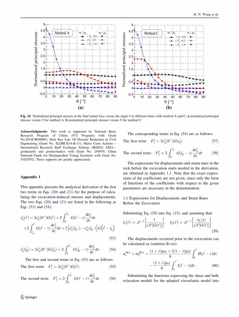
Acknowledgments This work is supported by National Basic

Research Program of China (973 Program) with Grant

No.2014CB046901; State Key Lab. Of Disaster Reduction in Civil

Engineering (Grant No. SLDRCE14-B-11); Marie Curie Actions—

International Research Staff Exchange Scheme (IRSES): GEO—

geohazards and geomechanics with Grant No. 294976; China

National Funds for Distinguished Young Scientists with Grant No.

51025932. These supports are greatly appreciated.

Appendix 1

This appendix presents the analytical derivation of the first

two terms in Eqs. (20) and (21) for the purpose of calcu-

lating the excavation-induced stresses and displacements.

The two Eqs. (20) and (21) are listed in the following as

Eqs. (53) and (54):

svijðt0Þ ¼ 2ev

ijð0þÞGðt0Þ þ 2

Z t00�

0

Gðt0 � sÞdev

ij

dsds

þ2

Z t0

t00þ

Gðt0 � sÞdev

ij

dsdsþ 2 ev

ijðt0

0þÞ � evijðt

0

0�Þh i

G t0 � t0

0

� �

ð53Þ

svijðt

0

0Þ ¼ 2evijð0þÞGðt

0

0Þ þ 2

Z t00�

0

Gðt00 � sÞdev

ij

dsds: ð54Þ

The first and second terms in Eq. (53) are as follows:

The first term: F11 ¼ 2ev

ijð0þÞGðt0Þ ð55Þ

The second term: F12 ¼ 2

Z t00�

0

Gðt0 � sÞdev

ij

dsds ð56Þ

The corresponding terms in Eq. (54) are as follows:

The first term: F21 ¼ 2ev

ijð0þÞGðt0

0Þ ð57Þ

The second term: F22 ¼ 2

Z t00�

0

Gðt00 � sÞdev

ij

dsds ð58Þ

The expressions for displacements and strain rates in the

rock before the excavation starts needed in the derivation,

are obtained in Appendix 1.1. Note that the exact expres-

sions of the coefficients are not given, since only the form

of functions of the coefficients with respect to the given

parameters are necessary in the demonstration.

1.1 Expressions for Displacements and Strain Rates

Before the Excavation

Substituting Eq. (29) into Eq. (15), and assuming that:

I1ðt0Þ ¼L�1 1

sL Gðt0Þ½ �

�; I2ðt0Þ ¼L�1 jLðsÞ

sL Gðt0Þ½ �

�:

ð59Þ

The displacements occurred prior to the excavation can

be calculated as (solution B-vis):

uðBÞvx þ iuðBÞvy ¼ ð1þ kÞp0zþ 2ð1� kÞp0z

8

Z t0

0

Hðt0 � sÞds

� ð1þ kÞp0z

8

Z t0

0

Iðt0 � sÞds: ð60Þ

Substituting the functions expressing the shear and bulk

relaxation moduli for the adopted viscoelastic model into

(a) (b)

Fig. 24 Normalized principal stresses at the final tunnel face versus the angle h at different times with method A and C; a normalized principal

stresses versus h for method A; b normalized principal stresses versus h for method C

H. N. Wang et al.

123

Eq. (60), the explicit expressions can be obtained. If only

shear viscoelasticity is considered, i.e., K(t) = Ke, dis-

placements can be derived as follows:

uðBÞvi ¼ A1M

i ðzÞ þ A2Mi ðzÞt0 þ A3M

i ðzÞ expð�kM1t0Þ;i ¼ 1; 2; kM1 [ 0; for the Maxwell model

ð61Þ

uðBÞvi ¼ A1B

i ðzÞ þ A2Bi ðzÞ expð�kB1t0Þ þ A3B

i ðzÞ expð�kB2t0Þ;i ¼ 1; 2; kB1 [ 0; kB2 [ 0 for the generalized Kelvin model

ð62Þ

where the terms with subscript i = 1 denote the compo-

nents along the x direction, and i = 2 denote the compo-

nents along the y direction. The coefficients AjMi , A

jBi

(i = 1, 2 and j = 1–3) are determined via Eq. (60).

According to Eqs. (61) and (62), and the strain–dis-

placement relationships, evij ¼ 1

2½uv

i;j þ uvj;i�, as well as the

definition of strain deviators given in Eq. (2), the derivative

of strain deviators for time t’ can be calculated as follows:

devij

dt0¼ A4M

ij ðzÞ þ A5Mij ðzÞ expð�kM1t0Þ;

i ¼ 1; 2; j ¼ 1; 2 for the Maxwell model

devij

dt0¼ A4B

ij ðzÞ expð�kB1t0Þ þ A5Bij ðzÞ expð�kB2t0Þ;

i ¼ 1; 2; j ¼ 1; 2 for the generalized Kelvin model

For models with unlimited viscosity (Type B models),

e.g., Burgers model, the expressions for displacement and

strain rate are analogous to Eqs. (61) and (63), where the

values of the coefficients A to be used depend on the rhe-

ological models; conversely for models of limited viscos-

ity, e.g., Kelvin model, the expressions are analogous to

Eqs. (62) and (64).

1.2 Derivation for the generalized Kelvin model

According to the expression of G(t) for the generalized

Kelvin model in Eq. (46), when time tends to infinity or is

large enough, G(t) will be a constant, which is a general

law for Type A viscoelastic models. Because the excava-

tion started at a time much later than the time when the

initial stresses were applied, the time t00 (beginning of

excavation,), and the generic time t0 � t00, can be assumed

to be infinite. Therefore, Gðt0Þ ¼ Gðt00Þ and the first terms

in Eqs. (53) and (54) are equal, that is F11 ¼ F2

1.

Substituting Eq. (46) into Eq. (56), yields

F12 ¼ 2

Z t00�

0

Gðt0 � sÞdev

ij

dsds ¼ 2

Z t00�

0

CB1 exp �kBðt0 � sÞ½ � þ CB

2

� � devij

dsds

¼ 2

Z t00�

0

CB1 exp �kBðt0 � sÞ½ �

devij

dsdsþ

Z t00�

0

CB2

devij

dsds

( )

¼ 2 B11 þ B1

2

� �;

ð65Þ

where CB1 and CB

2 are coefficients independent of time, and:

B11 ¼

Z t00�

0


devij

dsds

B12 ¼

Z t00�

0

CB2

devij

dsds:

ð66Þ

Substituting Eq. (46) into Eq. (58), yields:

F22 ¼ 2

Z t00�

0

Gðt00 � sÞdev

ij

dsds ¼ 2

Z t00�

0

CB1 exp �kBðt

0

0 � sÞh i

þ CB2

h i devij

dsds

¼ 2

Z t00�

0

CB1 exp �kBðt

0

0 � sÞh i dev

ij

dsdsþ

Z t00�

0

CB2

devij

dsds

( )

¼ 2 B21 þ B2

2

� �;

ð67Þ

where:

B21 ¼

Z t00�

0

CB1 exp �kBðt0

0 � sÞ½ �dev

ij

dsds

B22 ¼

Z t00�

0

CB2

devij

dsds:

ð68Þ

It can be noted from Eqs. (66) and (68) that B12 ¼ B2

2.

Substituting Eq. (64) into the expression of B11 (in Eq. 66),

yields:

B11 ¼

Z t00�

0


A4Bij expð�kB1sÞ þ A5B

ij expð�kB2sÞh i

ds:

ð69Þ

After integration, then rearranging:

B11 ¼ D1B

ij exp �k3ðt0 � t0

0Þ� �

exp �kB1t0ð Þ � exp �kBt0ð Þh i

þ D2Bij exp �k4ðt0 � t

0

0Þ� �

exp �kB2t0ð Þ � exp �kBt0ð Þh i

;

ð70Þ

where k3 ¼ kB � kB1 [ 0, k4 ¼ kB � kB2 [ 0. When t0 !1 and t

0

0 !1, Eq. (70) becomes:

B11

��t0!1t00!1¼ 0 ð71Þ


123

Substituting Eq. (64) into the expression of B21 yields:

B21 ¼ D1B

ij exp �kB1t0

0

� �� exp �kBt

0

0

� �h i

þ D2Bij exp �kB2t

0

0

� �� exp �kBt

0

0

� �h ið72Þ

when t00 !1, B2

1 ¼ 0. According to Eqs. (65) and (67), as

well as the fact that B12 ¼ B2

2, B11 ¼ B2

1 ¼ 0, the second term

of Eq. (53) is equal to that of Eq. (54), that is, F12 ¼ F2

2 .

Owing to the fact that the first and second term in Eq. (53)

are equal to the corresponding terms in Eq. (54), the

equality between the sums of the first and second terms in

Eqs. (53) and (54) is demonstrated. This equality is used in

Sect. 3.3. An analogous demonstration can be carried out

for rheological models with limited viscosity (Type A).

1.3 Derivation for the Maxwell model

The expression of G(t) for the Maxwell model is in the

form of an exponential function as shown in Table 1. It is

obvious that Gðt0Þ ¼ Gðt00Þ because t0(t0[ t0) and t00 can be

regarded as infinite. Substituting Gðt0Þ ¼ Gðt00Þ into Eqs.

(55) and (57) yields F11 ¼ F2

1 . Therefore, the first terms

from Eqs. (53) and (54) are equal. For any value of t0 and

t00, the second term of Eq. (53) can be written as:

F12 ¼ 2

Z t00�

0

CM1 exp �kM2ðt0 � sÞð Þ

� � devij

dsds

¼ exp �kM2ðt0 � t0

0Þ� �

� 2

Z t00�

0

Gðt00 � sÞdev

ij

dsds

¼ exp �kM2ðt0 � t

0

0Þ� �

F22 :

ð73Þ

The term exp �kM2ðt0 � t00Þ

� �is non zero. The second

term of Eq. (54) can be written as:

F22 ¼ 2

Z t00�

0

CM1 exp �kM2ðt

0

0 � sÞ� �h i

� A4Mij þ A5M

ij expð�kM1sÞh i

ds:

ð74Þ

After integration and rearranging, yields:

F22 ¼ D1M

ij 1� exp �kM2t0

0

� �h i

þ D2Mij exp �kM1t

0

0

� �� exp �kM2t

0

0

� �h i: ð75Þ

When t0 ! 1 and t0

0 !1, the above equation

becomes:

F22 ¼ D1M

ij 6¼ 0 ð76Þ

According to Eqs. (73) and (76), the second terms in

Eqs. (53) and (54) are not equal, but hold the relationship

shown in Eq. (73).

References

Amberg R (1983) Design and construction of the Furka base tunnel.

Rock Mech Rock Eng 16:215–231

Anagnostou G, Ehrbar H (2013) Tunnelling Switzerland. Vdf

Hochschulverlag AG an der ETH Zurich

Brady B, Brown E (1985) Rock mechanics for underground mining.

George Allen & Unwin, London

Christensen RM (1982) Theory of viscoelasticity: an introduction,

2nd edn. Academic Press, New York

Dai HL, Wang X, Xie GX, Wang XY (2004) Theoretical model and

solution for the rheological problem of anchor-grouting a soft

rock tunnel. Int J Pressure Vessels Piping 81:739–748

Einstein HH, Schwartz CW (1979) Simplified analysis for tunnel

supports. ASCE J Geotech Eng Div 104(4):499–518

Exadaktylos GE, Stavropoulou MC (2002) A closed-form elastic

solution for stresses and displacements around tunnels. Int J

Rock Mech Min Sci 39(7):905–916

Exadaktylos GE, Liolios PA, Stavropoulou MC (2003) A semi-

analytical elastic stress-displacement solution for notched circu-

lar openings in rocks. Int J Solids Struct 40(5):1165–1187

Gnirk PF, Johnson RE (1964) The deformational behavior of a

circular mine shaft situated in a viscoelastic medium under

hydrostatic stress. In: Proceeding of 6th symposium rock

mechanics. University of Missouri, Rolla, pp 231–259

Gurtin ME, Sternberg E (1962) On the linear theory of viscoelasticity.

Arch Ration Mech Anal 11:291–356

Hochmuth W, Kritschke A, Weber J (1987) Subway construction in

Munich, developments in tunneling with shotcrete support. Rock

Mech Rock Eng 20:1–38

Jaeger JC, Cook NGW, Zimmerman RW (2007) Fundamentals of

rock mechanics, 4th edn. Blackwell, USA

Ladanyi B, Gill D (1984) Tunnel lining design in creeping rocks.

Symposium on design and performance of underground exca-

vations. ISRM, Cambridge

Lee EH (1955) Stress analysis in viscoelastic bodies. Q Appl Math

13:183

Lei GH, Ng CWW, Rigby DB (2001) Stress and displacement around

an elastic artificial rectangular hole. J Eng Mech ASCE

127(9):880–890

Malan DF (2002) Simulating the time-dependent behavior of

excavations in hard rock. Rock Mech Rock Eng 35(4):225–254

Miura K (2003) Design and construction of mountain tunnels in

Japan. Tunn Undergr Space Technol 18:115–126

Miura K, Yagi H, Shiroma H, Takekuni K (2003) Study on design and

construction method for the New Tomei-Meishin expressway

tunnels. Tunn Undergr Space Technol 18:271–281

Muskhelishvili NI (1963) Some basic problems of the mathematical

theory of elasticity. Noordhoff, Groningen

Sharifzadeh M, Daraei R, Broojerdi M (2012) Design of sequential

excavation tunneling in weak rocks through findings obtained

from displacements based back analysis. Tunn Undergr Space

Technol 28:10–17

Steiner W (1996) Tunneling in squeezing rocks: case histories. Rock

Mech Rock Eng 29:211–246

Sulem J, Panet M, Guenot A (1987a) Closure analysis in deep tunnels.

Int J Rock Mech Min Sci Geomech Abstr 24(3):145–154

Sulem J, Panet M, Guenot A (1987b) An analytical solution for time-

dependent displacements in circular tunnel. Int J Rock Mech Min

Sci Geomech Abst 24(3):155–164

Tonon F (2010) Sequential excavation, NATM and ADECO: What

they have in common and how they differ. Tunn Undergr Space

Technol 25:245–265

Wang HN, Nie GH (2010) Analytical expressions for stress and

displacement fields in viscoelastic axisymmetric plane problem

H. N. Wang et al.

123

involving time-dependent boundary regions. Acta Mech

210:315–330

Wang HN, Nie GH (2011) Solutions for viscoelastic axisymmetric

plane problem involving time-dependent boundary regions under

mixed boundary condition. Acta Mech 216:59–73

Wang HN, Li Y, Ni Q, Utili S, Jiang MJ, Liu F (2013) Analytical

solutions for the construction of deeply buried circular tunnels

with two liners in rheological rock. Rock Mech Rock Eng

46(6):1481–1498

Wang HN, Utili S, Jiang MJ (2014) An analytical approach for the

sequential excavation of axisymmetric lined tunnels in visco-

elastic rock. Int J Rock Mech Min Sci 68:85–106

Wone M, Nasri V, Ryzhevskiy M (2003) Rock tunnelling challenges

in Manhattan. In: 29th ITA World Tunnelling Congress,

Amsterdam, vol 1, pp 145–151

Zhang LQ, Lu AZ, Yang ZF (2001) An analytic algorithm of stresses

for any double hole problem in plane elastostatics. J Appl Mech

ASME 68(2):350–353


123

Analytical Solutions for Tunnels of Elliptical Cross-Section in Rheological Rock Accounting for...

Documents

Transcript of Analytical Solutions for Tunnels of Elliptical Cross-Section in Rheological Rock Accounting for...