HSEHealth & Safety

Executive

Modelling of dense gasdispersion in tunnels

Prepared by WS Atkins Consultants Limited

for the Health and Safety Executive

CONTRACT RESEARCH REPORT

359/2001

HSEHealth & Safety

Executive

Modelling of dense gasdispersion in tunnels

Robin C HallWS Atkins Consultants Ltd

Woodcote GroveAshley Road

EpsomSurrey

KT18 5BWUnited Kingdom

This study concerns the transport of dangerous goods through tunnels and, in particular, considershow an incident involving a release of dense gas in a road tunnel would develop and how it could beconsidered in a risk assessment.

CFD modelling has been undertaken to provide a qualitative picture of some aspects of dense gasdispersion in tunnels. This modelling has considered a 3-D simulation of a tunnel with vehicles and aparametric study of release, ventilation and slope effects using a 2-D approach.

The main objective of the study has been to explore the problems involved in developing a simplemethodology for predicting the behaviour of dense gas releases in road tunnels, taking account of theeffects of source phenomena, tunnel gradients, ventilation airflows and the presence of vehicles. Amodel has been developed and the results compared with those obtained from experiments and CFDsimulations. The model requires further work on both physical and numerical modelling aspects andcannot be regarded yet as suitable as a practical tool for routine use.

This report and the work it describes were funded by the Health and Safety Executive (HSE). Itscontents, including any opinions and/or conclusions expressed, are those of the author alone and donot necessarily reflect HSE policy.

HSE BOOKS

ii

© Crown copyright 2001Applications for reproduction should be made in writing to:Copyright Unit, Her Majesty’s Stationery Office,St Clements House, 2-16 Colegate, Norwich NR3 1BQ

First published 2001

ISBN 0 7176 2078 6

All rights reserved. No part of this publication may bereproduced, stored in a retrieval system, or transmittedin any form or by any means (electronic, mechanical,photocopying, recording or otherwise) without the priorwritten permission of the copyright owner.

iii

CONTENTS

Page

1. INTRODUCTION ..............................................................................................................11.1 Background 11.2 Objectives 11.3 Scope of Work 11.4 Layout of the Report 2

2. APPLICATION OF CFD MODELLING ............................................................................32.1 Introduction 32.2 3-D Modelling Strategy 32.3 Results from 3-D Modelling 52.4 2-D Modelling Strategy 102.5 Results from 2-D Modelling 112.6 Analysis of 2-D Results 12

3. DEVELOPMENT OF A SIMPLE MODEL ......................................................................253.1 General Approach 253.2 Tunnel Parameters 253.3 Main Equations 263.4 Entrainment 273.5 Resistance Effects at Cloud Fronts 283.6 Ventilation Effects 283.7 Heat Transfer from Surfaces 293.8 Implementation and Numerical Modelling Aspects 30

4. MODEL EVALUATION ..................................................................................................334.1 Slumping over Flat Ground 334.2 Instantaneous Release of Wedge-shaped Cloud on a Slope 344.3 Instantaneous Release with Heat Transfer Effects 364.4 Instantaneous Release with Cloud Trapping 384.5 Comparison with CFD Test Cases 414.6 Vehicle and Ventilation Extract Cases 414.7 Lock Exchange 44

5. DEMONSTRATION APPLICATION ..............................................................................47

6. DISCUSSION OF RESULTS ...........................................................................................536.1 CFD Modelling 536.2 Simple Modelling 536.3 Implications for real scenarios 55

7. CONCLUSIONS & RECOMMENDATIONS...................................................................577.1 Conclusions 577.2 Recommendations for Further Work 58

8. REFERENCES .................................................................................................................59

APPENDIX A COMPARISON OF CFD AND MODEL PREDICTIONS ...........................61

Printed and published by the Health and Safety ExecutiveC30 1/98

iv

1

1. INTRODUCTION

1.1 BACKGROUND

Substantial research has been undertaken into dense gas dispersion modelling in open air.Currently, many of the available models are being evaluated as part of the EuropeanCommission funded SMEDIS project (in which WS Atkins is a participant). In contrast, therehave been few published studies for tunnels. One example is the work by Considine et al (1989).Calculations were carried out using a modified version of an atmospheric dispersion modelassuming longitudinal tunnel ventilation and the formation of a spreading dense gas layer. Theeffects of tunnel gradient were not treated and no detailed consideration was given to the near-source effects. It was assumed that, where the amount of air available for entrainment waslimited, then the additional heat required for vaporisation of the toxic substance would be drawnfrom adjacent walls and vehicles. Relevant experimental work has included small-scalemodelling of intruding gravity fronts in channels (for example, Gröbelbauer (1995)). However,these studies have not dealt with the many of the characteristics of real tunnels.

The limitations of such approaches are as follows:

• The precise nature of the source phenomena is highly uncertain, e.g. the size and shape ofthe cloud formed in a tunnel under restricted airflow conditions.

• Very few road tunnels in the UK are level. A significant number of tunnels, e.g. the Conwytunnel in North Wales, pass under rivers or estuaries and therefore slope downwards fromthe portals to a lowest point near the midpoint of the tunnel.

• Not all tunnels are longitudinally ventilated; for example, the Blackwall tunnel incorporatesa semi-transverse ventilation approach.

• Stationary vehicles would affect the spreading behaviour of a dense gas layer in a tunnel.

1.2 OBJECTIVES

The objective of this study has been to explore the problems involved in developing a simplemethodology for predicting the behaviour of dense gas releases in road tunnels taking accountof the effects of source phenomena, tunnel gradients, ventilation airflows and the presence ofvehicles.

Whilst there have been no major road transport incidents in the UK involving a release of densegas in a tunnel, the possibility of a serious incident remains. This work is intended to lead to abetter understanding of how real scenarios would develop and how they could be considered inrisk assessments.

1.3 SCOPE OF WORK

The work described in this report has included the following main aspects:

a) Initially the key parameter ranges of interest (gradient, ventilation, releases, etc) weredefined and a matrix of representative cases produced. A brief review of literature wasundertaken to identify any recent relevant research and to determine appropriate modellingstrategies that could be developed or adapted for practical applications.

2

b) CFD modelling was performed of a dense gas release in a tunnel with vehicles. Thecomplex momentum, thermodynamic and two-phase effects near the source were notrepresented, rather the modelling was intended as a basic demonstration of the effects ofvehicles on lateral and vertical spreading.

c) CFD modelling of dispersion along tunnels was undertaken to provide some insight intohow dense gas would spread in real systems and some confirmation of the behaviourassumed in the simple modelling. The effects of tunnel gradients and ventilation airflowshave been considered.

d) Simple modelling of dispersion along tunnels has been the main part of the work. Theintention was to put the key elements together and gain an overview of the problemsinvolved in developing a simple model to predict the basic effects of a dispersing dense gaslayer, taking account of tunnel ventilation conditions, vehicles blocking the roadway andheat exchange with tunnel walls and vehicles. The required output from the model includedthe height and velocity of the spreading dense gas layer along the tunnel and at the portals.

1.4 LAYOUT OF THE REPORT

The CFD modelling is described in Section 2, both for the 3-D modelling of dispersion in thepresence of vehicles and the 2-D modelling of dispersion along tunnels. Section 3 describes thedevelopment of the simple model. Section 4 presents a comparison of model results withpublished results and the CFD results obtained here. The limitations of the model are discussedin Section 5. The conclusions and recommendations are given in Section 6.

3

2. APPLICATION OF CFD MODELLING

2.1 INTRODUCTION

This section describes modelling of the dispersion of a dense gas in a tunnel usingComputational Fluid Dynamics (CFD) techniques. The computer program STAR-CD(Computational Dynamics Ltd (1998)) has been used. Both two-dimensional (2-D) and three-dimensional (3-D) modelling have been carried out.

The 3-D tunnel model was developed in order to illustrate dispersion behaviour in the vicinityof vehicles. The 3-D computational mesh is based on a section of the Blackwall Tunnel,measuring approximately 200m. The mesh was developed previously for transient simulationsof ventilation airflows and pollution build-up along the whole length of the tunnel. For thepresent demonstration purposes, it was acceptable to re-use this mesh. A single scenario hasbeen examined, involving two lanes of stationary cars and trucks. The release of dense gas fromthe rear of one of the trucks is considered.

Simulating the tunnel flow with a 2-D mesh is justified for the present purposes on the basis thatthe dense gas would mix rapidly across the width of the tunnel. Three separate 2-D models wereconstructed, representing a 500m long tunnel with different gradients: level, 5 degrees (i.e.ambient airflow up slope) and -5 degrees (ambient airflow down slope). A further 2-D modelwas constructed in order to explore the effects of point extraction of air from a tunnel via a duct.Three release rates have been considered. These are a continuous release of 1.3 kg/s, a release of46.1 kg/s for 380s and an instantaneous release of 17,500 kg/s. These rates were selected tocover a representative range of typical accidental releases from tankers, as described by theHealth & Safety Commission (1991).

The validity of a 2-D modelling approach has not been proven. Such an approach has been usedfor smoke modelling both for compartments and for tunnels. In some respects, it is arguable thata 2-D approach should be more valid for dense gas releases than for hot smoke. For hot smokelayers, the density differences and the resulting stratification depend entirely on the temperatureof the smoke. Heat transfer at the walls leads to cooling and downward flow of the smoke. Formost dense gas layer problems of interest, the gas density depends strongly on the molecularweight as well as on temperature, and density differences and stratification are likely to occureven after thermal equilibrium has been reached. On the other hand, vehicles will producesignificant 3-D mixing effects. The 3-D modelling is intended to provide some insights in thisrespect.

The complex momentum, thermodynamic and two-phase effects near the source have not beenconsidered in any of the simulations performed in this study. Sensitivity studies to check thesuitability of the mesh and boundary conditions have not been undertaken.

In view of the uncertainties, it is emphasised therefore that the results presented here canprovide at best only a qualitative picture of some aspects of dispersion in a tunnel.

2.2 3-D MODELLING STRATEGY

The 3-D model represents a portion of the Blackwall tunnel, with a length of approximately200m, a maximum height of 6.1m and a maximum width of 8.3m. The model has 47,000 cells.Figure 2.1 shows a cross section of the tunnel near the portal and Figure 2.2 shows a view of thevehicles within the tunnel. The gas source is shown as a block of cells at the rear of a truck. The

4

mesh is uniform in the lateral and longitudinal directions where cell dimensions are 0.42m and1.2m respectively. The thickness of the cell layer at the ground is 0.16m increasing to 0.77m atthe arched ceiling of the tunnel.

Figure 2.1Cross-sectional view of tunnel mesh

Figure 2.2View of mesh around vehicles and dense gas source

Generally when modelling tunnel flows, the mesh should be extended sufficiently far beyondthe portals such that the flows inside the tunnel and at the portals are not significantly affectedby the actual boundaries. For the present case, since the interest lies in dispersion behaviouralong a relatively short length of tunnel, inlet and outlet boundaries have been specified directlyat the ends of the tunnel section.

The steady state ventilation flow field was obtained prior to modelling the release of gas.Regarding the boundary conditions used, at the walls and floor of the tunnel, a ‘no-slip’condition was applied with, for simplicity, the same roughness length of about 0.01meverywhere. At the outlet boundary, a ‘zero gradient’ boundary condition was imposed, i.e. thevalues at the boundary are assumed to be the same as those at a point just inside the boundary.The velocity and turbulence conditions were specified at the inlet boundary. Turbulence wasmodelled using the k- ε model. The turbulent kinetic energy k and dissipation rate of turbulentkinetic energy ε were obtained using:

( )2

23 iuk = (2.1)

L

C 3/23/4kµε = (2.2)

where u is the velocity (m/s), i is the turbulence intensity (assumed to be 10% at the portals), CT

is a constant equal to 0.09 and L is the turbulent length scale taken as 10% of the height of thetunnel, i.e. 0.6m.

5

For the transient gas release simulation, the inlet and outlet boundary conditions at the portalswere changed to piezometric pressure boundaries. This type of boundary condition allows bothflows into or out of the tunnel, as appropriate. The pressures at the boundaries correspond to thepreviously computed steady state ventilation conditions. The gas concentration for incomingflow is fixed to zero.

For the present purposes the dense gas was taken to be chlorine. The mixture density iscalculated using the ideal gas law. At ambient pressure and temperature, the pure chlorine andair densities are 2.96 kg/m3 and 1.21 kg/m3 respectively. The dense gas is injected into a regionmeasuring 0.5m x 0.5m x 2m, located at ground level at the rear of the upstream truck. The gasis injected with zero vertical velocity, while the horizontal component has been matched to theaverage ambient airflow velocity at the box, before the release of gas, in order to minimise thedisturbance to the ambient flow. The mass fraction of the gas release is set to 1.0 (i.e. nodilution). The turbulence intensity at the source is assumed to be 50% corresponding to veryhigh turbulence which would be expected with jets and sprays impinging violently on adjacentsurfaces. The gas is injected at ambient temperature. The source is situated on the tunnel floor inorder to avoid areas of re-circulation that might arise below elevated source cells.

The PISO solution algorithm is selected both for the steady state simulation for the empty tunneland the transient releases of dense gas. The ‘self-filtered central differencing’ scheme (SFCD) isused for all variables with the exception of density which is solved using the ‘centraldifferencing’ (CD) scheme. A constant time-step of 0.05s was used for all runs.

2.3 RESULTS FROM 3-D MODELLING

A release of 46.1 kg/s was simulated with an ambient tunnel ventilation velocity of 1 m/s.Figure 2.3 shows the velocities in the vicinity of the trucks before releasing the dense gas. Thehighest velocities, of the order 1.5 m/s, occur along the central axis of the tunnel and betweenthe north wall and the truck adjacent to this wall. There are high velocities between the southwall and the trucks adjacent to the south wall. The velocities are lowest in the wake of the carsand there is a region of low velocity behind the source truck along the south wall.

The dispersion of the dense gas in a section of the tunnel of approximate length 34m centredabout the source is shown in Figures 2.4 to 2.7 at times 5, 10, 15, 30, 60 and 90s. Horizontalslices of the tunnel are shown at heights of 0.3, 0.8, 1.3 and 1.8m above the floor. Figure 2.4shows the distribution of concentration at 0.3m above ground level. The dispersion ischaracterised by the movement of the dense gas along the north wall. Very little upstreamdispersion occurs. The contours at 0.8m above the floor, shown in Figure 2.5, are similar tothose at a height of 0.3m. Downstream dispersion of high concentrations is less rapid. Theconcentration contours at heights of 1.3m and 1.8m are shown in Figures 2.6 and 2.7.

Figure 2.3Contours of the magnitude of velocity at a horizontal plane through the

tunnel at a height of 0.32m before the injection of the dense gas

6

Figure 2.4Contours of concentration at horizontal plane at height of 0.3m at times of 5, 10, 15, 30,

60 and 90s (top to bottom)

7

Figure 2.5Contours of concentration at horizontal plane at height of 0.8m at times of 5, 10, 15, 30,

60 and 90s (top to bottom)

8

Figure 2.6Contours of the concentration at a horizontal plane through the tunnel at a height of 1.3m

at times of 5, 10, 15, 30, 60 and 90s from top to bottom

9

Figure 2.7Contours of the concentration at a horizontal plane through the tunnel at a height of 1.8m

at times of 5, 10, 15, 30, 60 and 90s from top to bottom

10

2.4 2-D MODELLING STRATEGY

The 2-D model domain consists of a total of 5,250 cells and has a length of 500m and a heightof 6m. Figure 2.8 shows the computational mesh in the region of the source. The source isshown as a block of cells located on the tunnel floor and monitoring stations can be seen locatedat either side. Thirty-seven monitoring stations were set up at locations along the tunnel. Eachstation consists of a column of cells which are located at intervals of five metres both upstreamand downstream from the source for a distance of 50m, then at 25m intervals for a further 200mincluding stations situated at the portals. The concentration of the pollutant, the density of themixture and the velocity components are recorded and the height of the cloud is calculated ateach station. The mesh is refined near the source, where large concentration gradients areexpected. In this region the dimensions of the cells are approximately 0.2m x 0.2m. Theresolution of the cells near the walls is finer in order to satisfy the requirements of the wallboundary conditions; here the cells have height of 0.1m. The mesh ‘stretches’ away from thecentre of the tunnel with an expansion ratio of 1.15 giving a maximum cell length ofapproximately 10m at the portals.

Figure 2.82-D mesh showing source region and selected monitoring stations

The strategy adopted for the boundary and source conditions and solution techniques followsthe 3-D modelling strategy closely. The floor and ceiling were treated as ‘no-slip’ walls, whilethe sides of the model were treated as symmetry planes. The inlet and outlet boundaryconditions were handled in the same way as for the 3-D model. Regarding the source, the gaswas injected into a region measuring 2m high x 0.82m long located in the centre of the tunnel.

For one case, a duct was added to the top of the mesh, to examine the effects of a ventilationextract on dense gas dispersion along the tunnel. The duct is located midway between the sourceand the right-hand portal. The opening measures 5m along the tunnel and across the full widthof the tunnel. The mesh has been refined in the vicinity of the duct increasing the total numberof cells in the model to 6200. A pressure boundary condition was imposed at the duct outlet.The pressure was taken to be equal to the pressure obtained when air is extracted through theduct at a rate of 180 m3/s. This extraction rate corresponds to 60% of the flow along a tunnel 6mhigh by 10m wide with an airflow velocity of 5 m/s.

The 2-D test cases considered are summarised in Table 2.1.

11

Table 2.1Summary of releases in the 2-D model

CaseNumber

TunnelGradient (deg)

Exhaust AmbientVelocity (m/s)

Mass ReleaseRate (kg/s)

Duration(s)

1 0 - 1 1.3 134602 0 - 1 46.1 3803 0 - 5 1.3 134604 0 - 5 46.1 3805 +5 - 1 1.3 134606 +5 - 1 46.1 3807 -5 - 1 1.3 134608 -5 - 1 46.1 3809 0 60% of inlet flow 5 (at inlet) 46.1 380

2.5 RESULTS FROM 2-D MODELLING

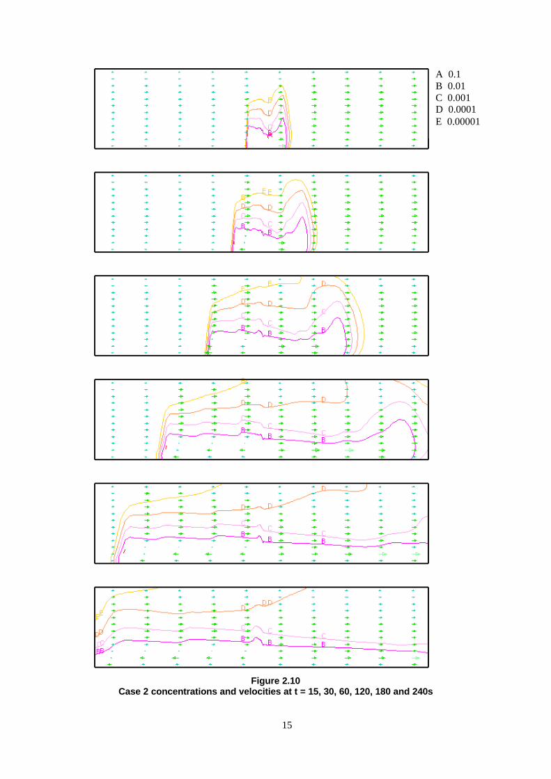
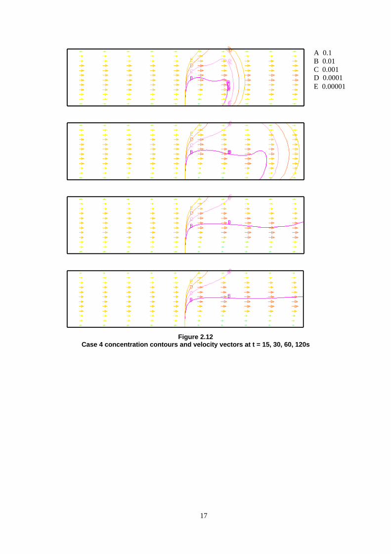
The results for Cases 1 to 9 are illustrated as plots of concentration and velocity vectors onvertical sections in Figures 2.9 to 2.17. The legend on Figures 2.9 to 2.17 relates to the massfraction concentration of the pollutant. It should be noted that the velocity vectors are plotted ona ‘presentation’ grid and not on the computational grid.

Figure 2.9 shows the concentration contours and velocity at time intervals from 15s to 600s forCase 1. The dispersion of the pollutant is mainly downwind, accompanied by a small amount ofupwind dispersion. The dense gas has an influence on the ambient tunnel airflow in the regionof the source. The dense gas appears to exit the right-hand portal between 120s and 180s and by240s the concentration has risen to nearly 0.001. Between 360s and 600s the dense gas ischaracterised by the 0.01 contour which has an approximately constant height above groundfrom the source to the right-hand portal.

Case 2 is characterised by both upwind and downwind dispersion as shown in Figure 2.10. Theambient tunnel airflow is significantly affected by the introduction of the dense gas, with areversal in the velocity field within the upwind body of the cloud. The dense gas exits the right-hand portal at between 60s and 120s, which is earlier than Case 1 due to the increased pollutantrelease rate.

For Cases 3 and 4 the dense gas reaches the east portal at between 30s and 60s and there is noupwind dispersion. The results are shown in Figures 2.11 and 2.12 respectively. In Case 3, thevelocity field appears to be unaffected by the introduction of the dense gas. In Case 4, thevelocities are reduced in the gas layer downstream of the release location.

In Cases 5 and 6 the tunnel has a slope of 5 degrees. The results are shown in Figures 2.13 and2.14 respectively. In Case 5 the dense gas moves under the influence of gravity towards the left-hand portal but is also transported downwind towards the right-hand portal. The layer heightincreases in the downwind direction. In Case 6, the addition of dense gas at a rate of 46.1 kg/scauses the entire ambient airflow to reverse direction. There is little downwind dispersion. By120s the gas has filled the upwind part of the tunnel with a concentration of order 0.01. Theambient velocity field is restored after approximately 30 minutes, the small amount of pollutantremaining is transported away through the right-hand portal.

Cases 7 and 8 are releases in a tunnel with a negative slope of 5 degrees. The results are shownin Figures 2.15 and 2.16 respectively. Both cases are characterised by rapid motion of gas

12

towards the right-hand portal. A sharp increase in the layer height in the frontal region isevident.

Case 9 is similar to Case 4 but includes extraction of air and gas at a section of the tunnel roof.The results are shown in Figure 2.17. Before the dense gas is injected into the tunnel the airenters at the left-hand portal and exits both through the right-hand portal and the exhaust duct.Due to the extraction of air, the air velocity is reduced from an average of 5 m/s to about 1 m/sin the region of the tunnel between the exhaust duct and the right-hand portal. It is apparent thatsome dense gas is drawn up into the exhaust duct. However, the concentration contoursdownstream of the extract duct indicate that a substantial proportion of the dense gas layerappears to remain in the tunnel, mixed over the height of the tunnel. These results tend tosuggest that ventilation extracts located along the tunnel roof may be relatively inefficient forremoving dense gas in a layer at road level. For this case, the validity of 2-D modelling is animportant issue. Whilst the geometry is two-dimensional, the 2-D assumption precludes anylocal flow phenomena varying across the width of the tunnel. For example, it is arguable thatthere might be longitudinal flows passing beneath the extract duct with dense gas being locallydrawn upwards alongside the walls into the extract duct. Such phenomena cannot be accountedfor with a 2-D approach. Confirmation is therefore needed on whether 2-D modelling is valid ornot under these circumstances.

2.6 ANALYSIS OF 2-D RESULTS

The CFD results have been analysed to determine values of the effective height, concentrationand velocity at different stations and times. These derived quantities can then be used forcomparison with the tunnel dispersion model described in the next section.

The centre of mass of the dense gas is calculated at each station. The height of the dense gaslayer h is defined to be twice the height of the centre of mass given by

∫

∫

∆

∆=

H

0

H

0

d

d

h~

z

zz

ρ

ρ(2.3)

For the computational mesh, this equation can be approximated by:

∑∑

∆∆

∆∆=

i

i

z

zzh~

ρ

ρ(2.4)

where cell number is represented by i, z is distance from ground to cell i, ∆ρ is the differencebetween the density of the cloud and ambient air in cell i and ∆z is the depth of cell i.

The height-weighted concentration ~c is defined as:

h

z∑ ∆= i

cc~ (2.5)

The height-weighted velocity is defined as:

h

z∑ ∆= i

uu~ (2.6)

13

Figure 2.9Case 1 concentrations and velocities at t = 15, 30, 60s

A 0.1B 0.01C 0.001D 0.0001E 0.00001

14

Figure 2.9 (cont.)Case 1 results at 120, 180, 240, 300, 360 and 600s

A 0.1B 0.01C 0.001D 0.0001E 0.00001

15

Figure 2.10Case 2 concentrations and velocities at t = 15, 30, 60, 120, 180 and 240s

A 0.1B 0.01C 0.001D 0.0001E 0.00001

16

Figure 2.11Case 3 concentrations and velocity vectors at t = 15, 30, 60 and 120s

A 0.1B 0.01C 0.001D 0.0001E 0.00001

17

Figure 2.12Case 4 concentration contours and velocity vectors at t = 15, 30, 60, 120s

A 0.1B 0.01C 0.001D 0.0001E 0.00001

18

Figure 2.13Case 5 concentrations and velocities at t = 15, 30, 60, 120, 180 and 240s

A 0.1B 0.01C 0.001D 0.0001E 0.00001

19

Figure 2.13 (cont)Case 5 concentration contours and velocity vectors at t = 300, 360, and 600s

A 0.1B 0.01C 0.001D 0.0001E 0.00001

20

Figure 2.14Case 6 concentration contours and velocity vectors at t = 15, 30, 60, 120, 180, 240s

A 0.1B 0.01C 0.001D 0.0001E 0.00001

21

Figure 2.14 (cont)Case 6 concentration contours and velocity vectors at t = 10, 15 and 30 minutes

22

Figure 2.15Case 7 concentration contours and velocity vectors at t = 15, 30, 60, 120, 180 and 240s

A 0.1B 0.01C 0.001D 0.0001E 0.00001

23

Figure 2.16Case 8 concentration contours and velocity vectors at t = 15, 30, 60, 120, 180 and 240s

A 0.1B 0.01C 0.001D 0.0001E 0.00001

24

Figure 2.17Case 9 concentration contours and velocity vectors at t = 15, 30, 60, 120 and 180s

A 0.1B 0.01C 0.001D 0.0001E 0.00001

25

3. DEVELOPMENT OF A SIMPLE MODEL

3.1 GENERAL APPROACH

Zone modelling techniques have been widely adopted for modelling dense gas releases in theatmosphere. The simplest approach is to represent the whole cloud by a box which is blowndownwind and changes its size as a result of slumping, entrainment, obstacles, etc. Analternative approach, for steady releases, is to calculate the spreading behaviour of the plumealong the trajectory of the plume downwind of the source. Examples of such types of model areHEGABOX and HEGADAS respectively (Post (1994)).

Some aspects of the tunnel problem are not straightforward to treat in a zone model. Forexample, the effects of gradient and ventilation can be transmitted to all parts of a cloud. It wasrecognised that some of the modelling challenges and the strategies to deal with them weresimilar to those addressed by shallow layer modelling. Shallow layer models have already beentried and tested for complex terrain by a number of researchers including Jones et al (1991),Würtz (1993), Hankin (1995), Gröbelbauer (1995), Ott and Nielsen (1996) and Nielsen (1998). These studieshave demonstrated how the approach can address ‘complex’ gradient situations, as encounteredin submerged tunnels.

For the present exploratory work, the emphasis was deliberately placed on integrating simplesub-models rather than on developing a rigorous theoretical framework, which wouldundoubtedly have required more resources than was available. The various techniques usedhave been drawn from relevant published research.

For the present model, shallow layer modelling techniques have been used, in combination withsimple techniques to take account of how the gas cloud can affect the ventilation flows throughthe tunnel, and heat transfer at tunnel and vehicle surfaces. The model represents only the densegas layer and not the ambient tunnel air. This is obviously a major simplification that limits thegenerality of the model. Nevertheless, the model should still be applicable to a wide range ofscenarios of interest. The CFD modelling described in the previous section shows layer heightsgenerally remaining below the mid-point except for peaks in some cases.

3.2 TUNNEL PARAMETERS

The representation of the tunnel follows the approach taken in the OECD tunnel consequencemodel (Cassini et al (1999)). Consideration was given to the range of tunnel parameters that needto be taken into account. In practice, tunnels vary enormously in terms of their lengths,gradients, ventilation and drainage systems, traffic control systems and many other features. Itwould be difficult to develop a simple methodology that was comprehensive enough to dealwith the large range of design features. Instead, a reduced set of parameters was chosen, asdescribed below.

The tunnel cross-section is assumed to be rectangular in shape. For tunnel cross-sections that arecircular in shape, the equivalent rectangular cross-sections can be considered. The width andheight are assumed to be uniform along the length of the tunnel.

For the purpose of considering the effects of tunnel gradient and different ventilation systems,tunnels are assumed to comprise a number of sections. The lengths of these sections can bechosen to give the most representative idealisation of the tunnel. The gradient is assumed to beuniform within each of the sections, but a different value may be used in each section.

26

Figure 3.1 shows the representation of a tunnel using segments and nodes.

portal Bportal A

sections

nodes

Figure 3.1Tunnel sections

3.3 MAIN EQUATIONS

The density ρ of the cloud mixture (dense gas and air) is given by:

−−

=

g

a

aa

M

Mc

T

T

11

ρρ (3.1)

where c is the concentration (-)ρa is the density of air at Ta (kg/m3)Ta is the absolute temperature of air (K)T is the absolute temperature of the cloud mixture (K)Ma is the molecular weight of air (kg/kmol)Mg is the molecular weight of the dense gas (kg/kmol)

Conservation equations are solved for the following parameters:• cloud mass• cloud momentum• cloud enthalpy• dense gas

The cloud mass conservation equation is:

ρρρρρ xaegs wwwhux

ht

−+=∂∂

+∂∂

)()( (3.2)

where h is the cloud height (m)t is the time (s)x is the tunnel axial co-ordinate (m)u is the downwind velocity (m/s)ws is the gas source velocity (m/s)ρg is the density of dense gas at Tg (kg/m3)Tg is the absolute temperature of the gas at source (K)we is the entrainment velocity (m/s) (see section 3.4)wx is the ventilation extract velocity (m/s)

27

The conservation equation for cloud momentum is:

( )

∆−∆

∂∂

−=∂

∂+

∂∂

θρρρρ

sin2)( 2

21

2

hhx

gx

hu

t

hu

frxaeadvvv fuwuwuuCAn −−++− ρρρ ||)C( 212

f

(3.3)

where g is the gravitational acceleration (m/s2)∆ρ is the density difference ρ-ρa (kg/m3)θ is the angle of the ground slope (rads)Cf is the ground friction factor (-)f fr is a cloud front factor used to control the propagation speed (see section 3.5)ua is the tunnel air velocity (m/s) (see section 3.6)

The product nvAvCdv combines the vehicle density, frontal area and drag coefficient. The frontalarea is assumed to be 2.5 m2 for a car and 10 m2 for a heavy goods vehicle (HGV). The dragcoefficient is assumed to be 0.3. The user inputs to the model include the number of lanes oftraffic and fraction of all vehicles which are HGVs. The model uses a length-weighted frontalarea based on an assumed car length of 5m and HGV length of 15m.

The conservation equation for dense gas is given by:

cwcwchux

cht xsgs ρρρρ −=

∂∂

+∂∂

)()( (3.4)

where cs is the source concentration (-).

The enthalpy conservation equation is given by:

vwxpaeapagsgpgpp HHTwCwTCwTCThuCx

ThCt

++−+=∂∂

+∂∂

ρρρρρ )()( (3.5)

where Hw and Hv account for heat fluxes from tunnel walls and vehicles (see section 3.8)Cpa is the heat capacity of air (J/kgK)Cpg is the heat capacity for dense gas (J/kgK)Cp is the heat capacity of the cloud (J/kgK), given by:

pgpap cCCcC +−= )1( (3.6)

3.4 ENTRAINMENT

A large number of different correlations have been studied for the entrainment velocity (such asthose listed by Nielsen (1998)). In general these have been determined from considerations of theatmospheric boundary layer. Reference is often made to a Richardson number based onturbulent velocity scales u* and/or w*. Given the focus of the present study and the absence ofsuitable experimental data specific to tunnels, a simpler approach was considered here. Initiallythe following relationship from Würtz was used:

22)( uuuCw aee +−= (3.7)

28

During trials with the above expression, it was found that inclusion of the velocity differenceterm (u - ua)

2 could lead to excessive cloud height at a cloud front, when the front moved in theopposite direction to the tunnel airflow. The even simpler relationship shown below wassubsequently adopted:

uCw ee = (3.8)

A constant value of 0.01 was used for Ce. This was selected on the basis of comparisons withthe 2-D CFD predictions described in Section 2 and the experimental results ofGröbelbauer (1995) described in Section 4.

3.5 RESISTANCE EFFECTS AT CLOUD FRONTS

Following Hankin (1995), a front resistance force ffr is included in the momentum equation (3.3) toaccount for the effects at a cloud leading edge front or hydraulic jump:

∂−∂

+∂−∂

−=x

uuhu

t

uuhkf a

aa

afrfr

)()(ρ (3.9)

This front condition can be viewed as the setting of an imposed Froude number u2/g´h at theleading edge. The term is small everywhere except close to a leading edge or jump. A value of0.5 was generally used for the constant kfr, selected on the basis of comparisons with the 2-DCFD predictions described in Section 2 and the results of Jones et al (1991) and Gröbelbauer (1995)

described in Section 4.

3.6 VENTILATION EFFECTS

The airflows in the tunnel are calculated using:

0=∆−∆−∆−∆+∆ outinfmv PPPPP (3.10)

Where ∆Pv is the pressure difference generated by the tunnel ventilation system∆Pm is the meteorological pressure difference between the portals∆Pf is the pressure loss along the tunnel due to friction∆Pin is the pressure loss at the entry portal∆Pout is the pressure loss at the exit portal

The user inputs to the model include the tunnel airflow velocity under normal operatingconditions before the gas release and meteorological pressure difference between the portals.The pressure loss coefficients at the inflow and outflow portals are assumed to be 0.5 and 1.0respectively. The pressure difference generated by the tunnel ventilation system in the absenceof the gas release, and assuming vehicle motion has ceased, is then deduced from:

moutPinPt

avPav PCCd

xfuCuP ∆−++==∆ )(2

212

21 ρρ

(3.11)

where f is the wall friction factor (constant value of 0.015 assumed)xt is the tunnel length (m)d is the hydraulic diameter (m)

29

Once gas has been released there is a further resistance term due to cloud drag. In the model,this is estimated from:

bhCuP dacd2

21 ρ=∆ (3.12)

The cloud drag coefficient Cd is assumed to be 0.5. A modified airflow velocity in the tunnel isthen estimated from:

)(21 bhCCC

d

xf

PPu

doutPinPt

mva

+++

∆+∆=

ρ

(3.13)

A major simplification is that this velocity is assumed to be uniform throughout the tunnel.

3.7 HEAT TRANSFER FROM SURFACES

The term Hw in the enthalpy conservation equation accounts for the heat flux from the tunnelfloor, walls and roof to the cloud. It is estimated here by means of:

)( TThH wcw −= (3.14)

where hc is the convective heat transfer coefficient (W/m2K). A variety of convective heattransfer correlations may be found in the literature. For turbulent flow over a flat plate(Reynolds number, Re > 3 x 105), the following correlation is given by (Drysdale (1985)):

333.08.0 PrRe037.0d

kh a

c =(3.15)

where ka is the thermal conductivity of the gas (W/mK) (air properties assumed)Re is the Reynolds number (= ρud/µ).Pr is the Prandtl number (=µCp/k).

A possible approach for determining the tunnel surface temperature would be to solve the one-dimensional equation for heat conduction through the tunnel walls with a boundary conditionfor convective heat transfer at the wall, thus linking it to the conservation equations for densegas dispersion. However, this would require a significant number of closely spaced nodes acrossthe thickness of the walls, thus adding significantly to the computational work required. Asimpler approach has therefore been adopted here. This involves adapting a standard solutionfor heat transfer in a semi-infinite slab with a boundary condition, from Carslaw and Jaeger(1959), as given below:

++−−+= )/2

())/(

exp()2

()(2

cwcww

cwowow hk

t

t

zerfc

hk

t

k

zh

t

zerfcTTTT

α

αα

α(3.16)

where Tw is the wall temperature (K)Two is the initial wall temperature (K)z is the distance into the solid from the surface (m)hc is the convective heat transfer coefficient (W/m2K)kw is the wall thermal conductivity (W/mK)

30

This solution is valid for fixed T and hc, but by assuming these parameters would vary relativelyslowly during the passage of the dense gas, a quasi-static solution approach can be adopted.With T and hc varying each time step, this allows an estimate to be made of wall heat transfer.The variation of surface temperature with time is obtained by setting z = 0 in the aboveequation, giving:

−−+= )/

())/(

exp(1)(2

cwcw

wowow hk

terfc

hk

tTTTT

αα(3.17)

The term Hv in equation 3.5 accounts for the heat flux from vehicles to the cloud. It is hereestimated by means of:

)( TThH vcv −= (3.18)

Vehicles are treated as lumped masses distributed along the tunnel. Heat transfer is estimated bytreating the masses as ‘thin’ slabs, assuming that the temperature gradients within the solid maybe ignored (Drysdale (1985)):

)2

exp(pvv

c

vo

v

C

th

TT

TT

τρ−=

−− (3.19)

where Tv is the vehicle temperature (K)Tvo is the initial vehicle temperature (K)ρv is the effective density (kg/m3)Cpv is the effective specific heat capacity (J/kgK)

The effective slab thickness τ is estimated assuming a characteristic vertical dimension of 1m, arepresentative car mass and spacing length of 400 kg and 5m, and a heavy goods vehicle (HGV)mass and spacing length of 4000 kg and 15m. The user inputs to the model include the fractionof all vehicles which are HGVs. The model uses a length-weighted mass. The vehicle massesare assumed to be initially at a raised temperature of 50K above the ambient temperature. Theheat transfer coefficient is assumed to be the same as calculated for the tunnel floor and walls.

The vehicle temperature solution is also valid for fixed T and hc, but by assuming theseparameters would vary relatively slowly during the passage of the dense gas, a quasi-staticsolution approach can be adopted, in the same way as for tunnel wall heat transfer.

3.8 IMPLEMENTATION AND NUMERICAL MODELLING ASPECTS

The model has been developed using Microsoft Excel 97 with Visual Basic macroprogramming. The software has been developed as a research prototyping tool rather than withthe intention of providing a finished tool that is reliable and robust enough for routine usage inrisk assessments.

The solution of shallow layer equations requires careful treatment of the moving dense gasfronts. In this model, the Flux Corrected Transport (FCT) scheme of Boris et al (1993) has beenadopted. Standard subroutines are available in this reference for implementation of the scheme.Using these available subroutines, the main effort in developing the overall solution algorithmhas focused on developing an appropriate software framework.

There are significant numerical modelling issues relating to instabilities which can arise whendealing with these types of flows and algorithms:

31

a) The choice of time step depends on the segment length ∆x and cloud velocity u. With thisFCT algorithm, the maximum time step is given by ∆t ≤ 0.5 ∆x / u. A smaller value, givenby ∆t ≤ 0.2 (∆x / u)min, is actually used in the model. If an inappropriate time step is used,the solution can sometimes fail.

b) The occurrence of ‘spikes’ in the predicted solutions is not uncommon. For example, thepredicted heights may exhibit a sharp spike at the position of the leading edge of the densegas cloud.

c) Whilst the conserved quantities (ρh, ρhu, ρhc, ρhe) exhibit smooth distributions in mostsituations, derived distributions of parameters such as specific heat capacity and temperatureare can be quite oscillatory even when reasonably fine meshes are used, e.g. 1m sub-segments.

Both b) and c) can be addressed by using finer mesh resolution. However the use of smaller sub-segments leads to longer computing times.

32

33

4. MODEL EVALUATION

4.1 SLUMPING OVER FLAT GROUND

Initial testing of the model was carried out using simple 2-D test cases as considered by Würtz(1993), covering gravity slumping, entrainment and heat transfer from the ground. The results forthe various test cases agreed closely with those of Würtz, thus providing some verification thatthe basic elements of the model have been implemented correctly.

As an illustration, results are presented below for a slumping dense gas column in still air. Theinitial gas temperature is assumed to be 200K, compared to an ambient temperature of 300K.The ratio of molecular weights Mg/Ma is set to 2.0, giving an initial gas density ρg = 3ρa. For thiscase, heat transfer from the ground is given by Hw = Chρ Cp (Tw – T) |u|, assuming Ch = 0.01, andthe entrainment velocity we = 0.149 |u|. The height, concentration, velocity and temperatureresults are shown in Figures 4.1 to 4.4 respectively.

0

1

2

3

4

5

6

7

8

9

10

0 50 100 150 200Distance (m)

Hei

ght (

m)

0

0.5

1.0

1.5

2.0

2.5

3.0

3.5

4.0

4.5

5.0

Figure 4.1Cloud height, non-isothermal slumping case

0

0.1

0.2

0.3

0.4

0.5

0.6

0.7

0.8

0.9

1

0 50 100 150 200

Distance (m)

Con

cent

ratio

n (-

)

0

0.5

1.0

1.5

2.0

2.5

3.0

3.5

4.0

4.5

5.0

Figure 4.2Concentration, non-isothermal slumping case

34

-10

-8

-6

-4

-2

0

2

4

6

8

10

0 50 100 150 200

Distance (m)

Vel

ocity

(m

/s)

0

0.5

1.0

1.5

2.0

2.5

3.0

3.5

4.0

4.5

5.0

Figure 4.3Cloud velocity, non-isothermal slumping case

200

210

220

230

240

250

260

270

280

290

300

0 50 100 150 200

Distance (m)

Tem

pera

ture

(K

)

0

0.5

1.0

1.5

2.0

2.5

3.0

3.5

4.0

4.5

5.0

Figure 4.4Temperature, non-isothermal slumping case

4.2 INSTANTANEOUS RELEASE OF WEDGE-SHAPED CLOUD ON A SLOPE

This test case concerns an instantaneous release of a wedge-shaped cloud on a uniform slope, asconsidered by Jones et al (1991). For this calculation, a 5m region of still dense gas is defined atthe top of the slope. The predicted results are shown in Figures 4.3 to 4.7. The cloud movesdown the slope into the undisturbed ambient fluid. A hydraulic jump develops in the flowduring the first 90 seconds. Between the hydraulic jump and the cloud front there is a region ofdense gas in which the upper surface of the cloud is almost level. After about 90 seconds, thehydraulic jump disappears and the cloud motion settles down to a steady state. The cloudappears to have the same shape as the initial shape but moves with a constant velocity. Thecalculations presented here were obtained with a fixed mesh with 400 cells each of length 0.5m.Jones et al used an expanding mesh comprising 200 cells with a resisting boundary conditionimposed at the dense gas front. In spite of the coarser mesh, the results shown here clearlyexhibit the same hydraulic jump behaviour and asymptotic self-similar profiles moving at thesame speed.

35

9.55

9.6

9.65

9.7

9.75

9.8

9.85

9.9

9.95

10

10.05

0 10 20 30 40 50

Distance (m)

Hei

ght (

m)

0

10

20

30

40

50

60

70

80

90

100

Figure 4.5Instantaneous release on slope

0

0.01

0.02

0.03

0.04

0.05

0 10 20 30 40 50Distance (m)

Hei

ght (

m)

0

10

20

30

40

50

60

70

80

90

100

Figure 4.6Height above ground (0 to 100 seconds)

0

0.2

0.4

0.6

0.8

1

1.2

0 10 20 30 40 50

Distance (m)

Vel

ocity

(m

/s)

0

10

20

30

40

50

60

70

80

90

100

Figure 4.7Cloud velocity (0 to 100 seconds)

36

0

0.01

0.02

0.03

0.04

0.05

40 50 60 70 80 90Distance (m)

Hei

ght (

m)

0

20

40

60

80

100

120

140

160

180

200

Figure 4.8Height above ground (100 to 200 seconds)

0

0.2

0.4

0.6

0.8

1

1.2

40 50 60 70 80 90

Distance (m)

Vel

ocity

(m

/s)

0

20

40

60

80

100

120

140

160

180

200

Figure 4.9Cloud velocity (100 to 200 seconds)

4.3 INSTANTANEOUS RELEASE WITH HEAT TRANSFER EFFECTS

Gröbelbauer (1995) carried out laboratory experiments involving a release of LN2 in a two-dimensional level channel measuring approximately 12m length, 1.2m width and 1.0m width.The LN2 was released into a 1.28m long closed section at one end of the channel, and allowed tosettle for about 35 seconds before releasing into the channel itself. The average temperature ofthe cloud was 240K and its height was 0.8m. Due to mixing in the box, the cloud initiallycomprised 87.5% N2 and 12.5% air. The floor of the channel was consisted of a styrofoam plate.

Figure 4.10 presents a comparison between predicted and experimental results for the behaviourof the cloud front. This shows the distance travelled by the cloud front and the frontal velocity.It is evident that the model under-predicts the velocity and therefore under-predicts the distancetravelled. At 15 seconds, the discrepancy in distance travelled is about 4.5%.

It is noted that these results agree closely with those obtained by Gröbelbauer using the shallowlayer model SHALADIS. The approach used in SHALADIS is broadly similar to that employed

37

here, but one significant difference concerns the treatment of heat transfer at the floor. InSHALADIS, the one-dimensional heat conduction equation is solved across the depth of thefloor.

Figure 4.11 shows the predicted surface heat flux at different stations along the channel. Incomparison with the experimental results, the model under-predicts the surface heat fluxes nearthe source box after about 5 seconds, although initially the heat fluxes are in agreement with theexperiments.

0

2

4

6

8

10

12

0 4 8 12 16

Time (secs)

Dis

tanc

e (m

)

0.4

0.5

0.6

0.7

0.8

0.9

1

Vel

ocity

(m

/s)

xf expt

xf model

uf expt

uf model

Figure 4.10Comparison of model and experimental cloud front propagation

0

50

100

150

200

250

300

350

400

0 5 10 15 20

Time (s)

Sur

face

hea

t flu

x (W

/m2)

0.3

1.7

3.1

4.5

5.9

7.2

8.8

10.1

Figure 4.11Comparison of model and experimental surface heat fluxes at

different stations along channel

38

4.4 INSTANTANEOUS RELEASE WITH CLOUD TRAPPING

In one set of experiments, Gröbelbauer introduced a change in slope after 5m. Experiments werecarried out with slopes of -10º and 6º beyond 5m. In other respects the same initial andboundary conditions apply as considered in Section 4.3.

Figure 4.12 shows that the model under-predicts the distance travelled by the cloud for allslopes, suggesting that the method used to evaluate entrainment or frontal resistance force couldbe usefully improved. Figure 4.13 shows that in a level tunnel the cloud front height decreasesas the cloud spreads along the tunnel. Comparison with Figures 4.14 and 4.15 illustrates theeffects of a change in slope angle. With a downward slope, the layer height dips fairly abruptlyat the edge of the slope but increases at the front itself as the cloud picks up speed going downthe slope (see Figure 4.16). With an upward slope, some fluid is forced up the slope but theheight decreases fairly quickly towards the ‘front’ as the cloud slows down. Figure 4.17 showsthat the front reaches the change in slope at between 6 and 8 seconds. There appears to be a stepchange in velocity at this point. After about 14 seconds, the dense gas starts to move back downthe slope. By 20 seconds, the ‘returning’ front has moved to within 2m of the source box.

3

4

5

6

7

8

9

10

11

12

4 8 12 16

Time (secs)

Dis

tanc

e (m

)

-10deg expt

-10deg model

6deg expt

6deg model

0deg expt

0deg model

Figure 4.12Comparison of cloud propagation rates for different changes in slope

0

0.05

0.1

0.15

0.2

0.25

0.3

0.35

0.4

0 1 2 3 4 5 6 7 8 9 10 11

Distance (m)

Hei

ght (

m)

0

2

4

6

8

10

12

14

16

18

20

Figure 4.13Cloud heights with 0º slope beyond 5m

39

0

0.05

0.1

0.15

0.2

0.25

0.3

0.35

0.4

0 1 2 3 4 5 6 7 8 9 10 11

Distance (m)

Hei

ght (

m)

0

2

4

6

8

10

12

14

16

18

20

Figure 4.14Cloud heights with -10º slope beyond 5m

0

0.05

0.1

0.15

0.2

0.25

0.3

0.35

0.4

0 1 2 3 4 5 6 7 8 9 10 11

Distance (m)

Hei

ght (

m)

0

2

4

6

8

10

12

14

16

18

20

Figure 4.15Cloud heights with 6º slope beyond 5m

40

0

0.1

0.2

0.3

0.4

0.5

0.6

0.7

0.8

0.9

1

0 1 2 3 4 5 6 7 8 9 10 11

Distance (m)

Vel

ocity

(m

/s)

0

2

4

6

8

10

12

14

16

18

20

Figure 4.16Cloud velocities with 0º slope after 5m

0

0.1

0.2

0.3

0.4

0.5

0.6

0.7

0.8

0.9

1

0 1 2 3 4 5 6 7 8 9 10 11

Distance (m)

Vel

ocity

(m

/s)

0

2

4

6

8

10

12

14

16

18

20

Figure 4.17Cloud velocities with -10º slope beyond 5m

-0.4

-0.2

0

0.2

0.4

0.6

0.8

1

0 1 2 3 4 5 6 7 8 9 10 11

Distance (m)

Vel

ocity

(m

/s)

0

2

4

6

8

10

12

14

16

18

20

Figure 4.18Cloud velocities with 6º slope beyond 5m

41

4.5 COMPARISON WITH CFD TEST CASES

The predictions of the model, described in Section 3, are shown for comparison with the CFDmodelling in Figures A1 to A8 (in Appendix A) for Cases 1 to 8 respectively.

For Case 1, the model and CFD results are in reasonable agreement in some respects. Bothmodel and CFD predictions show little upstream dispersion. The frontal velocities are about 1.0m/s for both CFD and model predictions, though the model slightly over-predicts the speed ofthe cloud front compared to the CFD predictions. The CFD concentration at the origin isapproximately 0.5 compared to a concentration of 1.0 in the model, but the rate of decay ofconcentration is similar away from the source.

For Case 2, the model predictions appear to show excessive growth in cloud height due to airentrainment, particularly near the upstream front. The model assumes that all of the dense gasremains in the layer. Possibly, better results might be obtained by considering detrainment as analternative interpretation of mixing at the front in such situations. The velocity field is similarfor both sets of results.

For Case 3, the model under-predicts the distance travelled by the cloud front compared to theCFD results. The model under-predicts the cloud velocity at all locations and times; amagnitude of about 4 m/s is predicted compared to about 5 m/s for the CFD results. The modelover-predicts the concentrations due to a concentration of 1.0 being assumed at the source.

Comparison of the model and CFD results for Case 4 shows similar trends to those observed forCase 3. The model under-predicts cloud front speed. It also appears to under-predict airentrainment at the front.

For Cases 5 and 6, there are notable differences between the model and CFD results. Inparticular, the model over-predicts upstream (down slope) travel and under-predicts downstream(up slope) travel. The comment made for case 2 regarding entrainment or detrainment mightwell be applicable to these cases as well.

For Cases 7 and 8, the main difference is again the over-prediction of cloud travel. Whilst thereis good agreement for the peak cloud velocities, the agreement near the cloud front is poorer.

Overall, the model appears to capture the gross effects of the cloud behaviour, as predicted bythe CFD modelling. However, there are significant discrepancies in the region of the cloudfronts. Where the cloud moves in the same direction as the ‘prevailing’ tunnel airflow, thenentrainment appears to be under-predicted. In contrast, where the cloud moves in the oppositedirection to the tunnel airflow, then the entrainment into the layer is over-predicted.

4.6 VEHICLE AND VENTILATION EXTRACT CASES

There is little data available for comparison with the model, concerning the effects of vehiclesand ventilation systems other than longitudinal systems. Although validation of these aspects isnot possible, consideration of the model sensitivity to these aspects is worthwhile.

The model incorporates the effects of vehicles in two ways: firstly, vehicles have a drag effecton cloud movement, and secondly, the model accounts for heat transfer from the warm vehiclecomponents to the cold gas cloud. Figures 4.19 to 4.21 provide a comparison for Case 2 of theCFD scenarios, involving a 46 kg/s release in a level tunnel with a 1 m/s tunnel airflow velocity.These figures correspond to: no vehicles; vehicle drag only; and drag and heat transfer together.The results show the upstream movement of the dense gas is impeded by the vehicles, which are

42

located on the left-hand side of the release at 250m. At 180s, the cloud has moved about 200mtowards the left-hand portal when there are no vehicles, compared to about 100-150m whenvehicles are present. Heat transfer has an influence on the upstream movement but apparentlythis is less significant than the drag effects.

0

0.5

1

1.5

2

2.5

3

0 100 200 300 400 500

Distance (m)

Hei

ght (

m)

0

30

60

90

120

150

180

210

240

270

300

Figure 4.19Cloud heights with no vehicles

0

0.5

1

1.5

2

2.5

3

0 100 200 300 400 500

Distance (m)

Hei

ght (

m)

0

30

60

90

120

150

180

210

240

270

300

Figure 4.20Cloud heights with vehicle drag

43

0

0.5

1

1.5

2

2.5

3

0 100 200 300 400 500

Distance (m)

Hei

ght (

m)

0

30

60

90

120

150

180

210

240

270

300

Figure 4.21Cloud heights with vehicle drag and heat transfer

Considering ventilation extracts, the 2-D CFD modelling considered a case (Case 9) with aventilation extract located at roof level. The simulation was carried out with the extract flow rateset at 75% of the tunnel airflow (assuming an airflow velocity of 5 m/s). The CFD results (seeFigure 2.17) showed that the roof extract was relatively inefficient for removal of dense gas atroad level. Figure 4.22 shows the cloud height results for the model when 0% and 100%extraction efficiencies are assumed. The CFD results obviously correspond to a situationsomewhere between 0% and 100%. The use of an extraction efficiency factor could beconsidered, perhaps based on the height of the dense gas layer relative to the tunnel height.However, since the suction effect of the roof extract is missing from the model, the model couldnot predict dense gas being drawn up towards the roof. Further work is needed to examine theseaspects of the modelling.

Figure 4.22Cloud concentrations for ventilation extraction efficiencies of 0% (left) and 100% (right)

0

0.1

0.2

0.3

0.4

0.5

0.6

0.7

0.8

0.9

1

0 100 200 300 400 500Distance (m)

Con

cent

ratio

n (-

)

0

15

30

45

60

75

90

105

120

135

150

0

0.1

0.2

0.3

0.4

0.5

0.6

0.7

0.8

0.9

1

0 100 200 300 400 500Distance (m)

Con

cent

ratio

n (-

)

44

4.7 LOCK EXCHANGE

The model described above does not simulate the ambient air in the tunnel. Instead a single‘average’ airflow velocity is used and this is allowed to vary according to the resistance of thegas cloud. The preceding test cases have involved ‘open’ scenarios for which the overall impactof the dense gas layer on the ambient airflows has been modest and not had a major effect onthe subsequent dense gas behaviour. The lock exchange scenario involves a ‘closed’ system andrepresents the most extreme case in which the dense gas and ambient air behaviour are veryclosely coupled and the local air velocity varies considerably with location.

Model predictions are presented below for one case with a density ratio of 2.99. A 6m longchannel of cross-section 0.3 x 0.3m is considered, divided by a gate halfway along the length ofthe channel. This case was studied experimentally by Gröbelbauer (1995). At the start of thesimulation, the right hand end of the channel is assumed to be full with the dense gas. Figure4.23 shows the predictions of the basic model. In the model, the front resistance term (describedin Section 3.5) uses the local air velocity, but as mentioned above, the local air velocity is notsimulated in this case. The model under-predicts the additional resistance to dense flow causedby the closed ends and over-predicts the speed of the dense gas front. To achieve betteragreement with the experimental results, the front resistance needs to be evaluated morerealistically. In the absence of local air velocity information, some insight can be gained bymodifying the front constant kfr. Figure 4.24 shows the results when kfr is increased from 0.5 to2.5. The movement of the dense gas front now agrees tolerably well with the experiment. Theheight of the dense gas layer is now fairly close to theoretically expected value of half thechannel height. However the characteristics of the intruding cavity are poorly predicted. Asdemonstrated by Gröbelbauer, for this combination of densities, the light gas front is expected totravel more slowly than the dense gas front.

0

0.05

0.1

0.15

0.2

0.25

0.3

-3 -2 -1 0 1 2 3Distance (m)

Hei

ght (

m)

0.0

0.2

0.4

0.6

0.8

1.0

1.2

1.4

1.6

1.8

2.0

Figure 4.23Lock exchange predictions for standard model

45

0

0.05

0.1

0.15

0.2

0.25

0.3

-3 -2 -1 0 1 2 3Distance (m)

Hei

ght (

m)

0.0

0.2

0.4

0.6

0.8

1.0

1.2

1.4

1.6

1.8

2.0

Figure 4.24Lock exchange predictions for model with modified front constant

46

47

5. DEMONSTRATION APPLICATION

An example is presented here to demonstrate the application of the model to a more realisticscenario than considered in the previous test cases. The example is loosely based on the ConwyTunnel.

The tunnel length is 1000m, the width is 10m and the height is 6m. The longitudinal profilethrough the tunnel is defined by 5 segments, with a ‘boundary’ segment added at each end toallow gas that has exited at the portals to re-enter if flow reversal takes place in the tunnel due toslope effects. For the present purposes, external wind effects on the dense gas layer have beenignored. A total of 200 sub-segments were used, with sub-segment lengths of 10m.

Segment - 1 2 3 4 5 -length (m) 500 125 300 25 300 250 500slope (%) 0 5 0 0 0 5 0

portal Bportal Asource

1 2 3 4 5segments

Figure 5.1Model definition of tunnel

Chlorine is released at a rate of 46 kg/s for 380 seconds, in segment 3. Both traffic lanes areassumed to be full on the upstream side of the release. Downstream of the release (i.e. on theright-hand side of the incident), the tunnel is assumed to be empty of vehicles.

Two cases are considered, involving tunnel airflow velocities of 1 and 5 m/s. The height,concentration, velocity, and cloud and wall temperature plots are shown in Figures 5.1 to.5.5respectively for a tunnel velocity of 1 m/s. Figures 5.6 to 5.10 present the results for a tunnelvelocity of 5 m/s.

Figure 5.1 shows that the height of the left and right hand fronts of the cloud increase as itspreads upstream and downstream. When the cloud reaches the sloping sections, the front heightdecreases sharply in the same manner as Figure 4.16. The velocity characteristics shown inFigure 5.3 are initially similar to Figure 4.17. As the cloud passes the change in slope angle,there is an abrupt reduction in velocity. This continues until a stage where the motion of thecloud reverses. At the left-hand end of the tunnel by 600s the cloud has not yet reached thechange in slope. The other figures show the concentration decreasing as the cloud spreads alongthe tunnel and the temperature increasing away from the source (Figure 5.4) due to absorptionof heat from the floor and entrainment of warm air into the cloud. The temperature of the floordrops significantly beneath the cold cloud.

With the 5 m/s airflow, the cloud spreads downstream with very little upstream dispersion dueto the strong ventilation. By the time the gas layer reaches the base of the slope, the dense gashas spread vertically over the full height of the tunnel. Figure 5.9 shows the cloud reaches astage where it appears to become practically stationary.

48

There is significant uncertainty about the model predictions in this situation, involving transienteffects and dense gas filling a section of tunnel. Further work is needed to determine howrealistic is the behaviour predicted here.

0

1

2

3

4

5

6

0 125 250 375 500 625 750 875 1000

Distance (m)

Hei

ght (

m)

0

60

120

180

240

300

360

420

480

540

600

Figure 5.2Cloud heights, 1 m/s airflow

0

0.1

0.2

0.3

0.4

0.5

0.6

0.7

0.8

0.9

1

0 125 250 375 500 625 750 875 1000

Distance (m)

Con

cent

ratio

n (-

)

0

60

120

180

240

300

360

420

480

540

600

Figure 5.3Cloud concentrations, 1 m/s airflow

49

-1

-0.5

0

0.5

1

1.5

2

2.5

0 125 250 375 500 625 750 875 1000

Distance (m)

Vel

ocity

(m

/s)

0

60

120

180

240

300

360

420

480

540

600

Figure 5.4Cloud velocities, 1 m/s airflow

240

250

260

270

280

290

300

0 125 250 375 500 625 750 875 1000

Distance (m)

Tem

pera

ture

(K

)

0

60

120

180

240

300

360

420

480

540

600

Figure 5.5Cloud temperatures, 1 m/s airflow

240

250

260

270

280

290

300

0 125 250 375 500 625 750 875 1000

Distance (m)

Wal

l tem

pera

ture

(K

)

0

60

120

180

240

300

360

420

480

540

600

Figure 5.6Wall temperatures, 1 m/s airflow

50

0

1

2

3

4

5

6

0 125 250 375 500 625 750 875 1000Distance (m)

Hei

ght (

m)

0

60

120

180

240

300

360

420

480

540

600

Figure 5.7Cloud heights, 5 m/s airflow

0

0.1

0.2

0.3

0.4

0.5

0.6

0.7

0.8

0.9

1

0 125 250 375 500 625 750 875 1000

Distance (m)

Con

cent

ratio

n (-

)

0

60

120

180

240

300

360

420

480

540

600

Figure 5.8Cloud concentrations, 5 m/s airflow

-1

0

1

2

3

4

5

0 125 250 375 500 625 750 875 1000

Distance (m)

Vel

ocity

(m

/s)

0

60

120

180

240

300

360

420

480

540

600

Figure 5.9Cloud velocities, 5 m/s airflow

51

240

250

260

270

280

290

300

0 125 250 375 500 625 750 875 1000

Distance (m)

Tem

pera

ture

(K

)

0

60

120

180

240

300

360

420

480

540

600

Figure 5.10Cloud temperatures, 5 m/s airflow

240

250

260

270

280

290

300

0 125 250 375 500 625 750 875 1000

Distance (m)

Wal

l tem

pera

ture

(K

)

0

60

120

180

240

300

360

420

480

540

600

Figure 5.11Wall temperatures, 5 m/s airflow

52

53

6. DISCUSSION OF RESULTS

6.1 CFD MODELLING

The CFD modelling has illustrated a range of cloud behaviour effects relating to vehicles, tunnelventilation and slopes.

The 3-D simulation showed, for a large 46 kg/s release in a congested tunnel with a 1 m/s tunnelairflow, dense gas spread rapidly across the width but more slowly over the height of the tunnel.After 1 minute, the dense gas front had advanced 40-50m and appeared to be quite well mixedacross the tunnel. At the same time, there was still a distinct vertical concentration gradient. Asexpected, this illustrates enhanced mixing around vehicles with less mixing in the clear regionabove the rows of cars.

The 2-D simulations have shown that large releases can affect the tunnel ventilation airflowsand the disrupted conditions can persist for quite a long time. In one case, the ambient tunnelairflows re-established only after 20-30 minutes, compared to the gas release duration ofapproximately 6½ minutes.

Ventilation extracts located along the tunnel roof appeared to be relatively inefficient forremoving dense gas release at road level in the one case considered with CFD modelling.

The above conclusions are of course subject to the important limitations of the modellingstrategies adopted. In particular, source momentum, heat transfer and two-phase effects have notbeen considered in any of the simulations, and the validity of the 2-D approach used for theparametric study of release, ventilation and slope effects has not been confirmed.

6.2 SIMPLE MODELLING

The main limitations of the simple model are discussed below.

The fundamental limitation of the present approach for tunnel dispersion is that fluid flowconservation equations are solved only for the dense gas layer and not for the ventilationairflows as well. The lock exchange test case illustrates the limitations clearly. Whilst the modelcan predict the movement of the dense gas front reasonably well, the intruding light gas is notmodelled directly and the characteristics of the intruding cavity are poorly captured. Theprediction of how a dense gas layer develops becomes more uncertain as the dense gas layerheight increases, especially when the layer fills half of the tunnel height. In practice the densegas and air layers might be expected to mix fairly rapidly after a certain point, whereas thismodel will predict a separate dense gas layer existing right up until the soffit of the tunnel isreached. Ultimately, this may not have a great impact on an assessment of risks to tunnel userssince toxic doses will be evaluated at say 1.5m above the tunnel floor, but further work wouldbe needed to quantify the actual impact of this modelling limitation.

A simple approach has been taken to include ventilation effects involving the estimation ofcloud drag and modification of the tunnel velocity. This velocity is then assumed to be constantalong the full length of the tunnel. The limitation of this approach is most evident for Case 9 ofthe CFD test cases, which features extraction. Extraction has a major impact on the variation ofventilation airflow velocity along the tunnel. Currently, it would be necessary to undertakeindependent ventilation calculations in order to determine the velocities in each sub-segment ofthe dispersion model. Quite apart from the potential complexity of the initial velocity

54

distribution, once gas is released, the cloud could have a major impact on the ventilation. Thishas been demonstrated by the CFD results. In this respect, a better approach would be toperform coupled airflow layer and cloud layer calculations in order to determine the local, time-varying airflow velocities. As a further benefit, this would allow the availability of fresh air tobe determined for calculation of source effects with flashing releases or evaporating pools.

Another key issue for tunnel dispersion is the treatment of entrainment. A correlation based on|u - ua| was tried initially. Whilst this is physically more sensible than a correlation based on |u|,the model gave more variable results. A simple correlation based on |u| was used to obtain theresults shown in Sections 4 and 5. Two main problems with this are apparent in the results.Firstly, the results show over-prediction of entrainment for opposing flows, that is, when thedense gas layer and the tunnel airflow are directed towards each other. The second problembecomes apparent particularly when the cloud front slows down, for example, due to a slope. Asthe layer velocity approaches zero, the entrainment also approaches zero irrespective of themagnitude of the tunnel airflow. The assumption that all of the dense gas remains in the layeralso deserves consideration. It might be appropriate to consider detrainment of dense gas fromthe layer.

A related issue is the treatment of the resistance effects at cloud fronts – the resistance termderived by Hankin (1995) has been included in the momentum equation. The choice of theconstant in this term was chosen by comparison with the Gröbelbauer and CFD results. Furtherexamination of entrainment would need to include this as well since entrainment near the frontand the front speed are obviously inter-dependent.

The treatment of heat transfer between the dense gas cloud and tunnel floor, walls and roof hasinvolved some important simplifications. The model treats the entire circumference of thetunnel lining as a single lumped mass. Clearly this approach is not accurate when the layerheight changes rapidly. In such cases there will be a temperature gradient in the circumferentialdirection as well as in the radial direction. Radial heat transfer in the floor/walls/roof assumesthat cloud and wall temperatures and heat transfer coefficient vary relatively slowly during thepassage of the dense gas. This effectively assumes that at each time step the temperature in thefloor/walls/roof is uniform. A better approach would be to differentiate between different partsof the tunnel ‘lining’ and solve a one-dimensional conduction equation for each. The increase incomputing effort would however be substantial.

It is important to emphasise that the model requires further work on both physical and numericalmodelling aspects and cannot be regarded yet as a practical tool for routine use. In addition tothe physical modelling limitations discussed above, there are sometimes solution problems. Forexample, an explicit time-stepping algorithm has been used and whilst this is straightforward fordevelopment purposes, the approach is prone to instabilities relating to time step choice thanimplicit algorithms. In addition, as with any computational model, the choice of mesh resolutionis a compromise between accuracy and computing effort.

Thus far, the limitations of the model have been discussed. More positively, the model doesprovide qualitative predictions for a broad range of tunnel scenarios of interest. With regard toquantitative accuracy, comparison with the experimental results of Gröbelbauer (1995) (slopes /heat transfer / no ventilation) has indicated agreement to an accuracy of about 5-10% for cloudfront propagation for relatively weak fronts. In terms of using the model, a typical calculationinvolving 200 sub-segments (i.e. 5m sub-segment length for a 1km tunnel) requires a computingtime of order 30 minutes on a Pentium II 300 MHz PC. Within Microsoft Excel it is alsostraightforward to perform a batch of scenario runs. The model therefore allows the user to carryout parametric studies for a range of ventilation conditions, vehicle distributions, etc withrelative ease.

55

6.3 IMPLICATIONS FOR REAL SCENARIOS

The practical implications of the modelling include the following:

Firstly, the optimum protocol used to control smoke in the event of a fire will not necessarily beappropriate for a dense gas release. The location of vehicles and the gradients along the tunnelwill generally be more important for dense gas releases than for tunnel fires. Most UK tunnelsare located under rivers or estuaries and thus slope downwards from the portals. Whilst smokewill tend to rise naturally to the portals, dense gas could become trapped and this was illustratedin the low airflow demonstration case. Regarding vehicles, these will interfere directly with agas layer at floor level.

The second practical issue is the blocking effect of a dense gas cloud on the ventilation airflow.The results suggest that in some situations the tunnel ventilation may take several minutes toclear dense gas from the tunnel. Considering life safety in the tunnel, the need for rapiddetection and emergency response is clear.

Finally considering the discharge of dense gas into the atmosphere at the portals, it is evidentthat a tunnel would modify the gas release in a similar manner to how a gas release within abuilding can be attenuated by the building. Both release rate and duration at the portal arechanged and this would need to be considered in a risk assessment concerned with dangerousgoods accidents in tunnels.

56

57

7. CONCLUSIONS & RECOMMENDATIONS

7.1 CONCLUSIONS

The conclusions from the study are as follows:

1) CFD modelling has proved to be a useful tool for gaining insights into the physicalmechanisms involved in dense gas dispersion in tunnels. The results have highlighted somesignificant issues:

a) Large releases of dense gas, such as a release of 46 kg/s of chlorine, can have a stronginfluence on the tunnel airflow conditions. In extreme cases involving significantrelease rates and sloping tunnels, the results suggest that the ambient airflow may notreturn to normal until 20-30 minutes after the release.

b) Ventilation extracts located along the roof of a tunnel appear to be inefficient forremoval of dense gas in layers at road level, however, the validity of the 2-D approachused for this scenario has not been confirmed.

2) The CFD modelling has involved some major simplifications. In particular, sourcemomentum and heat transfer effects were not considered, and a 2-D approach was used forthe parametric study of release, ventilation and slope effects. The validity of the 2-Dapproach has not been confirmed by comparison with experimental results.

3) A ‘simple’ model of tunnel dense gas dispersion has been developed using Microsoft Excelwith Visual Basic macro programming. The model requires further work on both physicaland numerical modelling aspects. The physical modelling strategy cannot be regarded yet assuitable for a practical tool for routine use. Nevertheless, the model provides a convenientframework for development of improved techniques for tunnel dispersion modelling.

4) Comparisons between the model predictions and available experimental and CFD resultsindicate:

a) The model provides qualitative predictions for a broad range of tunnel scenarios ofinterest.

b) For a range of validation cases with slopes and heat transfer, but without ventilationeffects, the model predictions of cloud front propagation agree with the experimentalresults to an accuracy of about 5-10%.

5) Application of the model to realistic, transient scenarios based on a 1 km submerged tunnelhas shown significant effects such as cloud trapping between upgrade sections. Thishighlights the need for rapid emergency response and appropriate ventilation to control themovement of the dense gas cloud.

6) The main limitations of the model are:

a) The fluid flow conservation equations are solved only for the dense gas layer and notfor the ambient tunnel air. As a result, the validity of the predictions becomes moreuncertain as the dense gas layer height increases, particularly above half of the tunnelheight.

b) Entrainment and frontal resistance effects are not well predicted for opposing flows andwhen a dense gas front changes direction.

58

c) Source effects such as flashing releases or evaporating pools are not included.

d) The effects of ventilation extracts at roof level are not included, although extractiondirectly from a dense gas layer can be examined.

e) The numerical solution techniques used in the model are sometimes less than robust.

7.2 RECOMMENDATIONS FOR FURTHER WORK

The recommendations from the study are as follows:

1) Experimental data is needed for realistic scenarios involving dense gas flows in road tunnelswith ventilation, slope and heat transfer effects.

2) The use of CFD modelling has provided useful insights into the dispersion characteristicsbut requires validation.

3) The tunnel dispersion model would benefit from several enhancements including:

a) A coupled approach for the dense gas dispersion and tunnel ventilation would providegreater generality and flexibility for modelling realistic release and tunnel ventilationscenarios.

b) The treatment of entrainment and frontal resistance effects requires further attention.

c) The treatment of flashing releases, evaporating pools and other source effects need to beimplemented.

d) A more robust time stepping algorithm.

59

8. REFERENCES

1. Boris J P, Landsberg A M, Oran E S and Gardner J H. ‘LCPFCT – Flux-CorrectedTransport Algorithm for Solving Generalized Continuity Equations’, ReportNRL/MR/6410-93-7192, US Naval Research Laboratory, Washington, April 1993.

2. Carslaw H S and Jaeger J C. Conduction of Heat in Solids. 2nd Edition, Oxford UniversityPress, 1959.

3. Cassini P, Hall R C and Pons P. Transport of Dangerous Goods through road tunnelsQuantitative Risk Assessment Model (Version 3.20) User Guide. OECD, 1999.

4. Computational Fluid Dynamics Ltd. STAR-CD Version 3.05 User Manuals, 1999.

5. Considine M, Parry S T and Blything K. ‘Risk assessments of the transportation ofhazardous substances through road tunnels in the United Kingdom’, (Safety and ReliabilityDirectorate UKAEA), Contractor Report 139, Transport and Road Research Laboratory,Department of Transport, 1989.

6. Gröbelbauer H P. ‘Experimental Study on the Dispersion of Instantaneously ReleasedDense Gas Clouds’, Diss ETH No. 10973, 1995.

7. Hankin R K S. ‘Heavy gas dispersion over complex terrain’, PhD thesis, University ofCambridge, June 1995.

8. Health & Safety Commission. ‘Major Hazard Aspects of the Transport of DangerousSubstances: Report and Appendices’, Advisory Committee on Dangerous Substances, 1991.

9. Jones S J, Martin D, Webber D M and Wren T. ‘The effects of natural and man-madeobstacles on heavy gas dispersion’, SRD/CEC/22938/02, AEA Technology, June 1991.

10. McQuaid J. ‘Some experiments on the structure of stably-stratified shear flows’, SMRETechnical paper P21, 1976.

11. Nielsen M. ‘Dense Gas Dispersion in the Atmosphere’, Riso-R-1030(EN), Riso NationalLaboratory, Denmark, September 1998.

12. Ott S and Nielsen M. ‘Shallow Layer Modelling of Dense Gas Clouds’, Riso-R-901(EN),Riso National Laboratory, Denmark, November 1996.

13. Post L (ed.). HGSYSTEM 3.0 Technical Reference Manual. Report TNER.94.059, ShellResearch Ltd, Thornton Research Centre, Chester, UK, 1994.

14. WS Atkins Consultants Ltd. ‘Blackwall Tunnel: a ventilation study of carbon monoxidebuild-up in the wakes of stationary vehicles’, WSA Report AM6763/002-RO1, September1996.

15. Würtz J. ‘A transient one-dimensional shallow layer model for dispersion of denser-than-airgases in obstructed terrain under non-isothermal conditions’, EUR 15343 EN. 1993, JointResearch Centre, Ispra, 1993.

60

APPENDIX ACOMPARISON OF CFD AND MODEL PREDICTIONS

This appendix contains the CFD and Model predictions of layer height (m), concentration (-)and velocity (m/s) for the 2-D test cases described in Section 3.

CFD Model

0

0.2

0.4

0.6

0.8

1

1.2

1.4

1.6

-250 -150 -50 50 150 250

Dis tance (m)

Hei

ght (

m)

3 0s60s120s180s360s600s

0

0.1

0.2

0.3

0.4

0.5

0.6

0.7

0.8

0.9

1

-250 -150 -50 50 150 250

Dis tance (m)

Con

cent

ratio

n (-

) 3 0s60s120s180s360s600s

-0.4

-0.2

0

0.2

0.4

0.6

0.8

1

1.2

1.4

1.6

-250 -150 -50 50 150 250

Dis tance (m)

Vel

ocity

(m

/s) 3 0s

60s120s180s360s600s

Figure A1Case 1 height of dense gas layer, average cloud concentration and average cloud velocity

-0.4

-0.2

0

0.2

0.4

0.6

0.8

1

1.2

1.4

1.6

0 100 200 300 400 500

Distance (m)

Vel

ocity

(m

/s)

0

30

60

90

120

150

180

210

240

270

300

0

0.2

0.4

0.6

0.8

1

1.2

1.4

1.6

1.8

2

0 100 200 300 400 500

Distance (m)

Hei

ght (

m)

0

30

60

90

120

150

180

210

240

270

300

0

0.1

0.2

0.3

0.4

0.5

0.6

0.7

0.8

0.9

1

0 100 200 300 400 500

Distance (m)

Con

cent

ratio

n (-

)

0

30

60

90

120

150

180

210

240

270

300

CFD Model

0

0.5

1

1.5

2

2.5

3

-250 -150 -50 50 150 250

Dis tance (m)

Hei

ght (

m) 3 0s

60s120s180s240s

0

0.1

0.2

0.3

0.4

0.5

0.6

0.7

0.8

0.9

1

-250 -150 -50 50 150 250

Dis tance (m)

Con

cent

ratio

n (-

)

3 0s60s120s180s240s

-3.0

-2.0

-1.0

0.0

1.0

2.0

3.0

4.0

-250 -150 -50 50 150 250

Dis tance (m)

Vel

ocity

(m

/s) 3 0s

60s120s180s240s

Figure A2Case 2 height of dense gas layer, average cloud concentration and average cloud velocity

-3

-2

-1

0

1

2

3

4

0 100 200 300 400 500

Distance (m)

Vel

ocity

(m

/s)

0

30

60

90

120

150

180

210

240

270

300

0

0.5

1

1.5

2

2.5

3

0 100 200 300 400 500

Distance (m)

Hei

ght (

m)

0

30

60

90

120

150

180

210

240

270

300

0

0.1

0.2

0.3

0.4

0.5

0.6

0.7

0.8

0.9

1

0 100 200 300 400 500

Distance (m)

Con

cent

ratio

n (-

)

0

30

60

90

120

150

180

210

240

270

300

CFD Model

0

0 . 5

1

1 . 5

2

2 . 5

3

3 . 5

4

4 . 5

5

- 2 5 0 - 1 5 0 - 5 0 5 0 1 5 0 2 5 0

D i s t a n c e ( m )

Hei

ght (

m)

3 0 s6 0 s1 2 0 s

0

0.005

0.01

0.015

0.02

0.025

0.03

0.035

0.04

0.045

0.05

-250 -150 -50 50 150 250

Distance (m)

Con

cent

ratio

n (-

)

30s60s120s

0

1

2

3

4

5

6

7

- 2 5 0 - 1 5 0 - 5 0 5 0 1 5 0 2 5 0

D i s t a n c e ( m )

Vel

ocity

(m

/s)

3 0 s6 0 s1 2 0 s

Figure A3Case 3 height of dense gas layer, average cloud concentration and average cloud velocity

0

1

2

3

4

5

6

7

0 100 200 300 400 500

Distance (m)

Vel

ocity

(m

/s)

0

15

30

45

60

75

90

105

120

135

150

0

0.5

1

1.5

2

2.5

3

3.5

4

4.5

5

0 100 200 300 400 500

Distance (m)

Hei

ght (

m)

0

15

30

45

60

75

90

105

120

135

150

0

0.005

0.01

0.015

0.02

0.025

0.03

0.035

0.04

0.045

0.05

0 100 200 300 400 500

Distance (m)

Con

cent

ratio

n (-

)

0

15

30

45

60

75

90

105

120

135

150

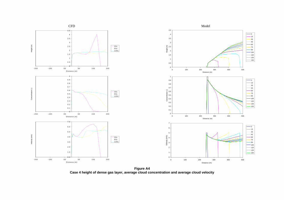
CFD Model

0

0.5

1

1.5

2

2.5

3

3.5

4

4.5

-250 -150 -50 50 150 250

Distance (m)

Hei

ght (

m)

3 0s60s120s

0

0.1

0.2

0.3

0.4

0.5

0.6

0.7

0.8

0.9

1

-250 -150 -50 50 150 250

Distance (m)

Con

cent

ratio

n (-

)

3 0s60s120s

0.0

1.0

2.0

3.0

4.0

5.0

6.0

7.0

-250 -150 -50 50 150 250

Distance (m)

Vel

ocity

(m

/s)

3 0s60s120s

Figure A4Case 4 height of dense gas layer, average cloud concentration and average cloud velocity

0

1

2

3

4

5

6

7

0 100 200 300 400 500

Distance (m)

Vel

ocity

(m

/s)

0

15

30

45

60

75

90

105

120

135

150

0

0.5

1

1.5

2

2.5

3

3.5

4

4.5

0 100 200 300 400 500

Distance (m)

Hei

ght (

m)

0

15

30

45

60

75

90

105

120

135

150

0

0.1

0.2

0.3

0.4

0.5

0.6

0.7

0.8

0.9

1

0 100 200 300 400 500

Distance (m)

Con

cent

ratio

n (-

)

0

15

30

45

60

75

90

105

120

135

150

CFD Model

0

0.5

1

1.5

2

2.5

3

3.5

4

4.5

5

-250 -150 -50 50 150 250

Distance (m)

Hei

ght (

m)

3 0s60s120s180s360s600s

0

0.05

0.1

0.15

0.2

0.25

0.3

0.35

0.4

0.45

0.5

-250 -150 -50 50 150 250

Distance (m)

Con

cent

ratio

n (-

) 3 0s60s120s180s360s600s

-2

-1.5

-1

-0.5

0

0.5

1

1.5

-250 -150 -50 50 150 250

Distance (m)

Vel

ocity

(m

/s) 3 0s

60s120s180s360s600s

Figure A5Case 5 height of dense gas layer, average cloud concentration and average cloud velocity

-2

-1.5

-1

-0.5

0

0.5

1

1.5

0 100 200 300 400 500

Distance (m)

Vel

ocity

(m

/s)

0

30

60

90

120

150

180

210

240

270

300

0

0.5

1

1.5

2

2.5

3

3.5

4

4.5

5

0 100 200 300 400 500

Distance (m)

Hei

ght (

m)

0

30

60

90

120

150

180

210

240

270

300

0

0.05

0.1

0.15

0.2

0.25

0.3

0.35

0.4

0.45

0.5

0 100 200 300 400 500

Distance (m)

Con

cent

ratio

n (-

)

0

30

60

90

120

150

180

210

240

270

300

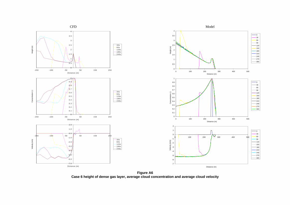
CFD Model

0

0.5

1

1.5

2

2.5

3

3.5

4

-250 -150 -50 50 150 250

Distance (m)

Hei

ght (

m) 3 0s

60s120s180s240s

0

0.1

0.2

0.3

0.4

0.5

0.6

0.7

0.8

0.9

1

-250 -150 -50 50 150 250

Distance (m)

Con

cent

ratio

n (-

)

3 0s60s120s180s240s

-7.0

-6.0

-5.0

-4.0

-3.0

-2.0

-1.0

0.0

1.0

2.0

-250 -150 -50 50 150 250

Distance (m)

Vel

ocity

(m

/s) 3 0s

60s120s180s240s

Figure A6Case 6 height of dense gas layer, average cloud concentration and average cloud velocity

-7

-6

-5

-4

-3

-2

-1

0

1

2

0 100 200 300 400 500

Distance (m)

Vel

ocity

(m

/s)

0

30

60

90

120

150

180

210

240

270

300

0

0.5

1

1.5

2

2.5

3

3.5

4

0 100 200 300 400 500

Distance (m)

Hei

ght (

m)

0

30

60

90

120

150

180

210

240

270

300

0

0.1

0.2

0.3

0.4

0.5

0.6

0.7

0.8

0.9

1

0 100 200 300 400 500

Distance (m)

Con

cent

ratio

n (-

)

0

30

60

90

120

150

180

210

240

270

300

CFD Model

0

0.5

1

1.5

2

2.5

3

3.5

4

4.5

-250 -150 -50 50 150 250

Distance (m)

Hei

ght (

m) 3 0s

60s120s180s240s

0

0.05

0.1

0.15

0.2

0.25

0.3

0.35

0.4

0.45

0.5

-250 -150 -50 50 150 250

Distance (m)

Con

cent

ratio

n (-

)

3 0s60s120s180s240s

0

0.5

1

1.5

2

2.5

3

-250 -150 -50 50 150 250

Distance (m)

Vel

ocity

(m

/s) 3 0s

60s120s180s240s

Figure A7Case 7 height of dense gas layer, average cloud concentration and average cloud velocity

0

0.5

1

1.5

2

2.5

3

0 100 200 300 400 500

Distance (m)

Vel

ocity

(m

/s)

0

30

60

90

120

150

180

210

240

270

300

0

0.5

1

1.5

2

2.5

3

3.5

4

4.5

0 100 200 300 400 500

Distance (m)

Hei

ght (

m)

0

30

60

90

120

150

180

210

240

270

300

0

0.05

0.1

0.15

0.2

0.25

0.3

0.35

0.4

0.45

0.5

0 100 200 300 400 500

Distance (m)

Con

cent

ratio

n (-

)

0

30

60

90

120

150

180

210

240

270

300

CFD Model

0

0.5

1

1.5

2

2.5

3

3.5

4

-250 -150 -50 50 150 250

Distance (m)

Hei

ght (

m) 3 0s

60s120s180s240s

0

0.1

0.2

0.3

0.4

0.5

0.6

0.7

0.8

0.9

1

-250 -150 -50 50 150 250

Distance (m)

Con

cent

ratio

n (-

)

3 0s60s120s180s240s

-1.0

0.0

1.0

2.0

3.0

4.0

5.0

6.0

7.0

-250 -150 -50 50 150 250

Distance (m)

Vel

ocity

(m

/s) 3 0s

60s120s180s240s

Figure A8Case 8 height of dense gas layer, average cloud concentration and average cloud velocity

-1

0

1

2

3

4

5

6

7

0 100 200 300 400 500

Distance (m)

Vel

ocity

(m

/s)

0

30

60

90

120

150

180

210

240

270

300

0

0.5

1

1.5

2

2.5

3

3.5

4

0 100 200 300 400 500

Distance (m)

Hei

ght (

m)

0

30

60

90

120

150

180

210

240

270

300

0

0.1

0.2

0.3

0.4

0.5

0.6

0.7

0.8

0.9

1

0 100 200 300 400 500

Distance (m)

Con

cent

ratio

n (-

)

0

30

60

90

120

150

180

210

240

270

300

Printed and published by the Health and Safety ExecutiveC30 1/98

Printed and published by the Health and Safety ExecutiveC1 08/01

CRR 359

£25.00 9 780717 620784

ISBN 0-7176-2078-6