Mathematical Biosciences 245 (2013) 249–257

Contents lists available at ScienceDirect

Mathematical Biosciences

journal homepage: www.elsevier .com/locate /mbs

Analytical methods for detecting pesticide switches with evolutionof pesticide resistance

0025-5564/$ - see front matter � 2013 Elsevier Inc. All rights reserved.http://dx.doi.org/10.1016/j.mbs.2013.07.008

⇑ Corresponding author. Tel.: +86 15934823867.E-mail addresses: sytang@snnu.edu.cn, sanyitang219@hotmail.com (S. Tang).

Juhua Liang a, Sanyi Tang a,⇑, Juan J. Nieto b, Robert A. Cheke c

a College of Mathematics and Information Science, Shaanxi Normal University, Xi’an 710062, People’s Republic of Chinab Departamento de Análisis Matemático, Universidad de Santiago de Compostela, Santiago de Compostela 15782, Spainc Natural Resources Institute, University of Greenwich at Medway, Central Avenue, Chatham Maritime, Chatham, Kent ME4 4TB, UK

a r t i c l e i n f o

Article history:Received 5 November 2012Received in revised form 14 July 2013Accepted 15 July 2013Available online 24 July 2013

Keywords:Pesticide switchesDynamic thresholdPesticide application frequencyEvolutionPulse spraying

a b s t r a c t

After a pest develops resistance to a pesticide, switching between different unrelated pesticides is a com-mon management option, but this raises the following questions: (1) What is the optimal frequency ofpesticide use? (2) How do the frequencies of pesticide applications affect the evolution of pesticide resis-tance? (3) How can the time when the pest population reaches the economic injury level (EIL) be esti-mated and (4) how can the most efficient frequency of pesticide applications be determined? Toaddress these questions, we have developed a novel pest population growth model incorporating the evo-lution of pesticide resistance and pulse spraying of pesticides. Moreover, three pesticide switching meth-ods, threshold condition-guided, density-guided and EIL-guided, are modelled, to determine the bestchoice under different conditions with the overall aim of eradicating the pest or maintaining its popula-tion density below the EIL. Furthermore, the pest control outcomes based on those three pesticideswitching methods are discussed. Our results suggest that either the density-guided or EIL-guidedmethod is the optimal pesticide switching strategy, depending on the frequency (or period) of pesticideapplications.

� 2013 Elsevier Inc. All rights reserved.

1. Introduction

Pesticide resistance is the adaptation of a pest populationtargeted by a pesticide, resulting in decreased susceptibility ofthe pest to the chemical. Pesticide resistance is increasing andfarmers’ and other pest managers’ dependencies on chemicalinsecticides have led to a high frequency of insecticide resistancein some crop systems [1]. In the 1940s, farmers in the USA lost7% of their crops to pests. Since the 1980s, the percentage losthas increased to 13%, even though more pesticides are being used,this is because more than 500 species of pests have developedresistance to pesticides since 1945 [2–4], and the situation is oftencaused by the same classes of pesticides being used repeatedly fora long time. Other problems ensue such as pest resurgence, acuteand chronic health problems, environmental pollution and uneco-nomic crop production.

Therefore, knowledge of the mechanisms for the evolution ofpesticide resistance is important for developing strategies to avoidthe creation of resistance in pest populations, with the underlyingprinciple being the preservation of susceptible genes in pest popu-lations. Therefore, in order to fight pesticide resistance and basedon a knowledge of the genetics of the development of pesticide

resistance, a number of principles have been proposed aimed atdelaying the emergence of resistance or avoiding it entirely. Theseprinciples include pesticide rotation or switching, avoiding unnec-essary pesticide applications, using non-chemical control tech-niques [5], and leaving untreated refuges where susceptible pestscan survive, within the concept of integrated pest management(IPM) [6–10].

When pesticides are the sole or predominant method of pestcontrol, resistance is commonly managed through pesticide rota-tions or pesticide switches. This means after a pest species devel-ops resistance to a particular pesticide, one method is to use adifferent pesticide, especially one in a different chemical class orfamily of pesticides that has a different mode of action againstthe pest. So far, switching among unrelated insecticides in re-sponse to detection of resistance has been the main method used.For instance, during the WHO Onchocerciasis Control Programme(OCP) in West Africa examples of different categories of pesticideswere used in rotation after the blackfly vectors of Onchocerciasisdeveloped resistance to the chemical of choice, the organophos-phate temephos [11]. Similarly, in agriculture, insecticide rotationhas been widely used to combat resistance in a major pest of bras-sica crops, the Diamondback Moth Plutella xylostella [12].

To achieve pest resistance management using pesticideswitches or rotations, the key problems that we are facing are:What is the optimal frequency of pesticide use? How do the

250 J. Liang et al. / Mathematical Biosciences 245 (2013) 249–257

frequencies of pesticide applications affect the evolution of pesti-cide resistance and when does the pest population reach the criti-cal threshold value?

In order to address those questions, mathematical models canbe useful for determining the optimal frequency of pesticide appli-cations, when is best to switch pesticides and for predicting howfast pesticide resistance develops. To do this, we have developeda novel pest population growth model concerning evolution of pestresistance and pulse spraying of pesticides. The model incorporatesthree different pesticide switching tactics for eradicating the pestor maintaining its population density below a given critical level.

The first justification for stopping the use of a given pesticideand switching a new type of pesticide (so called as pesticideswitching method throughout this paper) is based on the thresholdcondition (the threshold condition-guided method) which ensuresthe extinction of the pest population, i.e. the pesticide is switchedonce the threshold value increases due to evolution of pesticideresistance and exceeds one, which determines the stability of pesteradication solutions.

The second pesticide switching method depends on the densityof the pest population just before the pesticide is applied (the den-sity-guided method). This switching action occurs when the effi-cacy of the pesticide begins to wear off, i.e. there is resurgence.

An important concept in IPM is that of the economic threshold(ET), which is usually defined as the number of pests in the fieldwhen control actions must be taken to prevent the economic injurylevel (EIL) from being reached and exceeded. The EIL is defined asthe lowest pest population density that will cause economic dam-age [6,8–10]). For an IPM strategy, action must be taken once a crit-ical density of pests is observed in the field so that the EIL is notexceeded. Thus, the third switching action is instigated when thepest population reaches the EIL (the EIL-guided method).

We provide analytical formulae for the optimal times to switchbetween different unrelated pesticides for all of the above threemethods. Based on different situations, the optimal choices for eachof these three methods, with the intention of eradicating the pests ormaintaining their population density below a tolerable level, arediscussed. Our results suggest that either the density-guided orthe EIL-guided method is the optimal pesticide switching strategy,depending on the frequency (or period) of the pesticide applications.

2. Pest growth model with evolution of pesticide resistance

In this section, we will develop a simple pest population growthmodel concerning the evolution of pest resistance. In particular,the effects of the frequency of pesticide applications are modelledand investigated. One of our main purposes is to investigate how toimplement a chemical control strategy and manage pest resistancesuch that the pest population dies out eventually or its density ismaintained below the EIL. In order to address this topic, we focuson the threshold condition which guarantees the extinction ofthe pest population and discuss optimal strategies for pesticideswitches.

2.1. Simple pest growth model with pesticide resistance

Throughout this study, the pest population is assumed to growlogistically with an intrinsic growth rate r and a carrying capacityparameter g. Then the pest population follows

dPdt¼ rPð1� gPÞ:

In the following, the total pest population is divided into twoparts: susceptible pests (denoted by PS) and resistant pests(denoted by PR), and the proportion of susceptible pests in the

population is denoted by a fraction x, the remaining fraction1�x is resistant, so we have PS ¼ xP and PR ¼ ð1�xÞP. Suscep-tible pests are those that have not developed resistance to the pes-ticide. That is to say, x may be thought of as the stock ofeffectiveness of the pesticide, and it is the proportion of the pestpopulation to which the toxin is lethal. Naturally, the susceptiblepests are assumed to die with a higher mortality rate, d1, and theresistant pests are assumed to die with mortality rate, d2, whenchemical control is implemented. Then the growth of susceptibleand resistant pests can be modelled as follows:

dPSdt ¼ xrPð1� gPÞ � d1PS;

dPRdt ¼ ð1�xÞrPð1� gPÞ � d2PR:

(ð1Þ

However, for simplification we assume that the resistant pests dis-play near-complete resistance to the pesticide, which means thatd2 � 0 [13]. Consequently, the evolution of the total pest populationfollows

dPdt¼ dPS

dtþ dPR

dt¼ rPð1� gPÞ �xd1P: ð2Þ

Since x ¼ PS=P, then the evolution of the fraction of the susceptiblepests in the total pest population is

dxdt¼ d

dtPS

P

� �¼ dPS

dtP � PS

dPdt

� �=P2 ¼ d1xðx� 1Þ: ð3Þ

Note that this resistance evolution equation has been widely usedrecently in different fields [13–17].

Therefore, the model (1) can be written as

dPdt ¼ rPð1� gPÞ �xd1P;dxdt ¼ d1xðx� 1Þ:

(ð4Þ

In reality, the pesticides are applied instantaneously. Thus themodel (4) can be developed by introducing an impulsive sprayingof pesticide at a critical time and modelling the consequences ofpopulation densities changing very rapidly.

If the pesticides is applied at time point si�1 for i 2 N withs0 ¼ 0, where N ¼ f1;2;3; . . .g and 0 ¼ s0 < s1 < s2 < � � �, thenthe number of pests killed at time si�1 is d1xðsi�1ÞPðsi�1Þ. There-fore, we have the following impulsive differential equation

dPðtÞdt ¼ rPðtÞð1� gPðtÞÞ; t – si;

Pðsþi Þ ¼ ð1�xðsiÞd1ÞPðsiÞ; t ¼ si;dxðtÞ

dt ¼ d1xðtÞðxðtÞ � 1Þ;

8><>: ð5Þ

where Pðsþ0 Þ ¼ P0 and xðs0Þ ¼ x0. This indicates that the initialcondition of the pest population in model (5) is chosen as the pop-ulation density after the first application of pesticide at time s0.

It is clear from model (5) that the efficacy of the pesticide on thetarget pest population depends on the evolution of pest resistance,as the killing efficacy will decrease as pest resistance develops. Adetailed analysis of model (5) will be given in the coming sections.

2.2. The effects of frequency of pesticide applications on evolution ofresistance

The formula (3) indicates how the pest resistance develops withrespect to time. However, it does not involve the effects of the fre-quency of pesticide applications, the pesticide application periodor the dosage of the applications on the evolution of resistance,and those factors do influence resistance patterns. Although it isdifficult to involve these factors in the model (3), we note thatthe speed with which resistance develops depends on severalfactors including the rate, timing and number of applicationsmade. Based on this fact, we assume that at each time point

J. Liang et al. / Mathematical Biosciences 245 (2013) 249–257 251

si�1; i 2 N , one pulse of pesticide is applied, which yields the fol-lowing equation for the fraction of susceptible pests

dxðtÞdt

¼ d1x xqi � 1ð Þ; si�1 6 t 6 si; i 2 N ð6Þ

with initial value xðsi�1Þ at each time interval si�1 6 t 6 si andxðs0Þ ¼ xð0Þ ¼ x0 is given, where qi should be a function of thenumber of pesticide applications, dosage Di of the ith pesticideapplication and time interval Dsi ¼ si � si�1 between the ith andði� 1Þth pesticide applications. For simplification, we assume thateach time the same dosage of pesticide is applied, i.e. Di is a con-stant and without loss of generality we let Di ¼ 1 for all i 2 N . Thusthe simplest formula for qi could be defined as qi ¼ i=Dsi. For exam-ple, if i ¼ 1, then the differential equation

dxðtÞdt

¼ d1x xq1 � 1ð Þ; s0 6 t 6 s1; xð0Þ ¼ x0

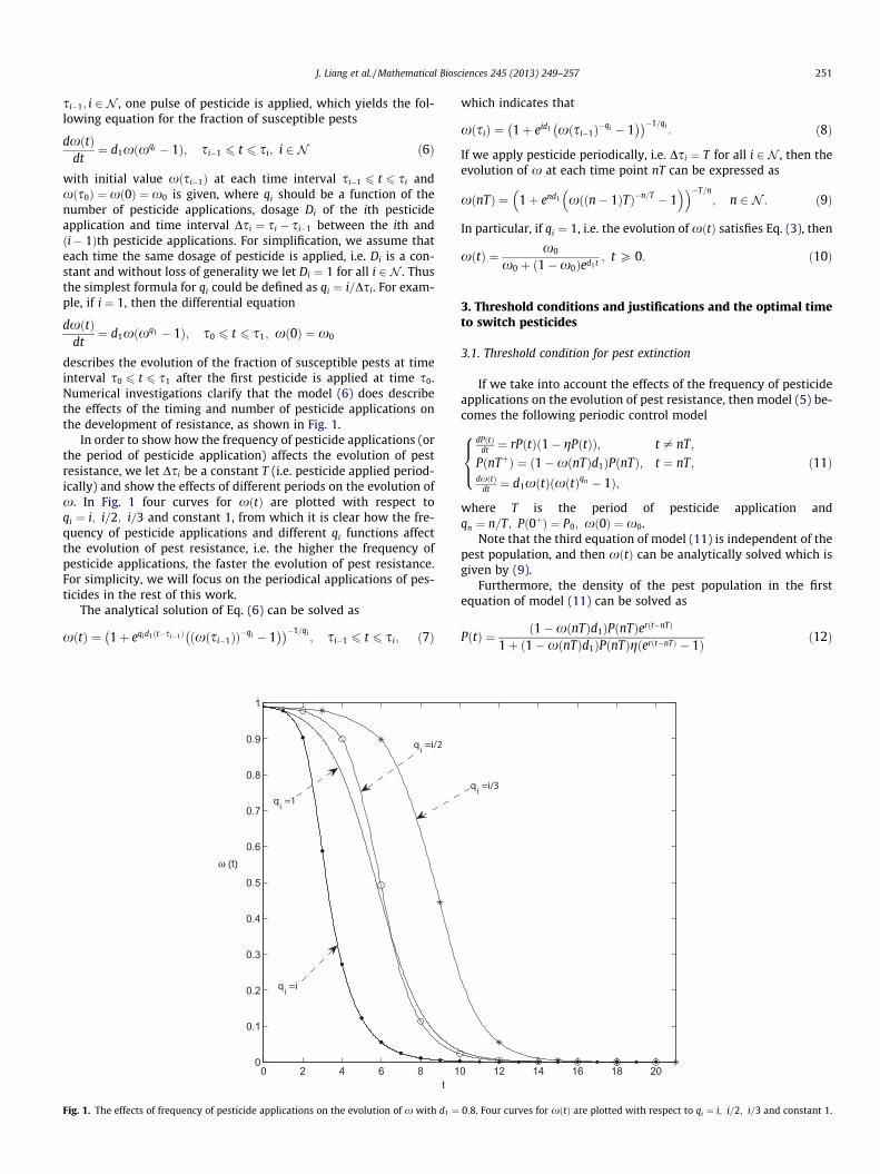
describes the evolution of the fraction of susceptible pests at timeinterval s0 6 t 6 s1 after the first pesticide is applied at time s0.Numerical investigations clarify that the model (6) does describethe effects of the timing and number of pesticide applications onthe development of resistance, as shown in Fig. 1.

In order to show how the frequency of pesticide applications (orthe period of pesticide application) affects the evolution of pestresistance, we let Dsi be a constant T (i.e. pesticide applied period-ically) and show the effects of different periods on the evolution ofx. In Fig. 1 four curves for xðtÞ are plotted with respect toqi ¼ i; i=2; i=3 and constant 1, from which it is clear how the fre-quency of pesticide applications and different qi functions affectthe evolution of pest resistance, i.e. the higher the frequency ofpesticide applications, the faster the evolution of pest resistance.For simplicity, we will focus on the periodical applications of pes-ticides in the rest of this work.

The analytical solution of Eq. (6) can be solved as

xðtÞ ¼ 1þ eqid1ðt�si�1Þ ðxðsi�1ÞÞ�qi � 1� �� ��1=qi

; si�1 6 t 6 si; ð7Þ

0 2 4 6 8 10

0.1

0.2

0.3

0.4

0.5

0.6

0.7

0.8

0.9

1

t

ω (t)

Fig. 1. The effects of frequency of pesticide applications on the evolution of x with d1 ¼

which indicates that

xðsiÞ ¼ 1þ eid1 xðsi�1Þ�qi � 1� �� ��1=qi

: ð8Þ

If we apply pesticide periodically, i.e. Dsi ¼ T for all i 2 N , then theevolution of x at each time point nT can be expressed as

xðnTÞ ¼ 1þ end1 xððn� 1ÞTÞ�n=T � 1� �� ��T=n

; n 2 N : ð9Þ

In particular, if qi ¼ 1, i.e. the evolution of xðtÞ satisfies Eq. (3), then

xðtÞ ¼ x0

x0 þ ð1�x0Þed1t; t P 0: ð10Þ

3. Threshold conditions and justifications and the optimal timeto switch pesticides

3.1. Threshold condition for pest extinction

If we take into account the effects of the frequency of pesticideapplications on the evolution of pest resistance, then model (5) be-comes the following periodic control model

dPðtÞdt ¼ rPðtÞð1� gPðtÞÞ; t – nT;

PðnTþÞ ¼ ð1�xðnTÞd1ÞPðnTÞ; t ¼ nT;dxðtÞ

dt ¼ d1xðtÞðxðtÞqn � 1Þ;

8><>: ð11Þ

where T is the period of pesticide application andqn ¼ n=T; Pð0þÞ ¼ P0; xð0Þ ¼ x0.

Note that the third equation of model (11) is independent of thepest population, and then xðtÞ can be analytically solved which isgiven by (9).

Furthermore, the density of the pest population in the firstequation of model (11) can be solved as

PðtÞ ¼ ð1�xðnTÞd1ÞPðnTÞerðt�nTÞ

1þ ð1�xðnTÞd1ÞPðnTÞgðerðt�nTÞ � 1Þ ð12Þ

0 12 14 16 18 20

0:8. Four curves for xðtÞ are plotted with respect to qi ¼ i; i=2; i=3 and constant 1.

0 2 4 6 8 10 12 14 160

20

40

60

80

t

P (t)

(a)

0 2 4 6 8 10 12 14 160

1

2

3

4

5

6

t

R0(n,T)

(b)

TH=60 T=1.8

T=3.4T=0.4

Fig. 2. The effects of period of pesticide applications on the density of the pest population of model (11) and threshold condition R0ðn; TÞ forT ¼ 0:4ð��Þ; T ¼ 1:8ð��Þ; T ¼ 3:4ð��Þ, respectively. Here we integrate Eq. (11) until the density of the pest population exceeds a given threshold value TH, and thebaseline parameter values are fixed as follows: d1 ¼ 0:8; r ¼ 0:5; x0 ¼ 0:99; g ¼ 0:01; P0 ¼ 20 and initial value Pð0þÞ ¼ 20. (a) density of pest populations; (b) the thresholdcondition R0ðn; TÞ corresponding to three solutions shown in (a). Note that we choose same initial values for the three solutions with different periods of spraying pesticides,so the first times of spraying pesticide for three different periods lie on the same curve in (a).

252 J. Liang et al. / Mathematical Biosciences 245 (2013) 249–257

for any pulse interval nT < t 6 ðnþ 1ÞT; n ¼ 0;1;2; . . . . Therefore,

Pððnþ 1ÞTÞ ¼ ð1�xðnTÞd1ÞerT PðnTÞ1þ ð1�xðnTÞd1ÞgðerT � 1ÞPðnTÞ : ð13Þ

Denote Yn ¼ PðnTÞ, then we have the following non-autonomousdifference equation

Ynþ1 ¼ð1�xðnTÞd1ÞerT Yn

1þ ð1�xðnTÞd1ÞgðerT � 1ÞYn; ð14Þ

this is similar to the well-known Beverton–Holt model [18–20].Note that the difference Eq. (14) is very dynamic since xðnTÞ de-pends on the third equation of model (11), which indicates thatthe difference equation discussed in present work is much more dif-ficult than those in references [21–23]. In fact, the non-autonomousor impulsive Beverton–Holt difference equations have been studiedextensively. For example, the asymptotic properties of Beverton–Holt difference equation have been discussed by Berezansky andBraverman [21] and Kocic [22,23]. In this work, based on our prac-tical problem we are interested in the stability of zero solution ofEq. (14). It is seen that the inequality

Ynþ1 < ð1�xðnTÞd1ÞerT Yn

holds true for all n 2 N . So we can define the dynamic threshold va-lue R0ðn; TÞ as follows

R0ðn; TÞ¼: 1� d1xðnTÞð ÞerT : ð15Þ

with xðnTÞÞ is given by (9). Therefore, if R0ðn; TÞ < 1 for all n 2 N ,then the zero solution of Eq. (14), i.e. non-autonomous differenceEq. (14), is globally asymptotically stable.

This indicates that the pest population will die out if the thresh-old value R0ðn; TÞ < 1 for all n 2 N . The threshold value is very dy-namic and depends on the number of pesticide applications, andwe will show this in more detail later.

In particular, if qn ¼ 1 for n 2 N (i.e. xðtÞ satisfies Eq. (3)), then

R0ðn; TÞ ¼ 1� d1x0

x0 þ ð1�x0Þed1nT

� �erT¼: R1

0ðn; TÞ: ð16Þ

Note that, in reality, R0ðn; TÞ < 1 may hold true for the first fewpesticide applications and then it will increase and exceed 1 due tothe evolution of pest resistance. Fig. 2 provides an example to showhow the density of the pest population and the threshold valueR0ðn; TÞ change as the number of pesticide applications increases.If we fixed all parameter values as those in Fig. 2 and let period Tvary, Fig. 2(a) gives three numerical solutions with different periodT. Here we stop to integrate Eq. (11) until the density of the pestpopulation exceeds a given threshold value TH (such as EIL). It isseen that the density of the pest population at time points nT de-creases firstly due to the high efficacy of the pesticides, and thenincreases because of the evolution of pest resistance. For more de-tails, see Fig. 3. The threshold value R0ðn; TÞ corresponding to threesolutions in Fig. 2(a) at each time point nT is given in Fig. 2(b).

It is interesting to note that resurgence by the pest populationcan occur very quickly once the pest resistance develops.Fig. 2(a) also shows that the less frequent (larger period T) arethe pesticide applications, the higher the level that pest outbreakscan reach. However, as mentioned before, the higher the frequencyof pesticide applications, the faster the evolution of pest resistance.Therefore, the question is how to manage the pest resistance, i.e.what is the optimal time to switch to a new type of pesticide?We address this question in the following subsection.

3.2. Justifications and the optimal time to switch pesticides

As mentioned in the introduction, the density of resistant pestswill grow quickly if one kind of pesticide is sprayed frequently (asshown in Fig. 2(a)), and it will lead to a pest outbreak or

0 2 4 6 8 10 12 14 160

20

40

60

80

100

t

P(t)

(a)

0 0.5 1 1.5 2 2.5 3 3.510111213141516

T

τ

(b)

0 0.5 1 1.5 2 2.5 3 3.50

10

20

30

40

T

n1(3)

(c)

TH=60

Fig. 3. The effects of period of pesticide applications on the density of the pest population of model (11), time s and number of pesticide applications. (a) The effects of controlperiod on the pest population of model (11), the color from light blue to mauve with T from small to large. The baseline parameter values are as follows:d1 ¼ 0;8; r ¼ 0:5; x0 ¼ 0:99; g ¼ 0:01; P0 ¼ 20; TH ¼ 60; (b) The relationship between control period T and switching time s under the EIL-guided method; (c) Therelationship between control period T and spraying times nð3Þ1 before the pest population size reaches TH. (For interpretation of the references to color in this figure legend, thereader is referred to the web version of this article.)

J. Liang et al. / Mathematical Biosciences 245 (2013) 249–257 253

resurgence. Therefore, people usually switch pesticides at some gi-ven time and how to choose the optimal time for a switch is animportant practical question. In the following, we will providethree different methods based on our model (11) to choose theoptimal time for switching pesticides according to different justifi-cations. We should emphasize that for each new type of pesticide,we assume that the evolution of pesticide resistance, i.e. x, followsthe same equation and has the same initial condition x0.

Method 1 Optimal time for switching pesticides with R0ðn; TÞ asa guide.

It follows from Fig. 2(b) that R0ðn; TÞ is increasing with respectto n. Therefore, in order to eradicate the pest population we shouldmaintain R0ðn; TÞ < 1 to hold true for all n 2 N . This clarifies thatwe need to switch the pesticide once the threshold value R0ðn; TÞgoes to one. Without loss of generality, we assume that the thresh-old value R0ðn; TÞ will exceed one unit after nð1Þ1 pesticide applica-tions, i.e.

nð1Þ1 ¼maxfn : R0ðn; TÞ 6 1g: ð17Þ

In order to find nð1Þ1 , we let R0ðn; TÞ ¼ 1, then

xðnTÞ ¼ 1� e�rT

d1;

where xðnTÞ is given by (9). Therefore,

nð1Þ1 ¼ n : xðnTÞ ¼ 1� erT

d1

� �;

and [a] denotes the greatest integer no larger than a.In particular, if qn ¼ 1 then R0ðn; TÞ ¼ R1

0ðn; TÞ. Let R10ðn; TÞ ¼ 1,

we can solve the above equation with respect to n and yield theoptimal switching time nð1Þ1 T , where

nð1Þ1 ¼1

d1Tln

x0 � ð1� d1Þx0erT

ð1�x0ÞðerT � 1Þ

�:

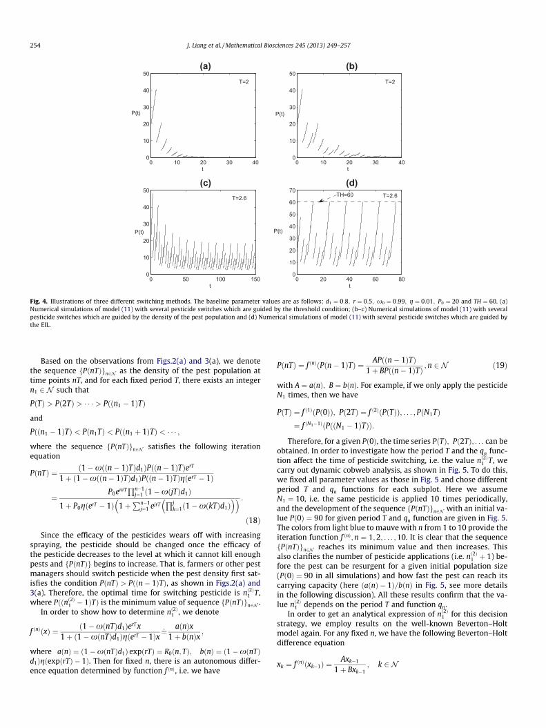
If we switch pesticides according to this decision strategy, i.e. athreshold condition-guided method, then the pest population canbe completely eradicated after several pesticide switches. To showthis, Fig. 4(a) depicts numerical simulation under this strategy. Itfollows from Fig. 4(a) that the pest population will die out eventu-ally, where nð1Þ1 ¼ 2. That is after three pesticide applications of onekind of pesticide (note that the first pesticide application is at timet ¼ 0), the farmers must switch to another kind of pesticide toeradicate the pest quickly.

Method 2 Optimal time for switching pesticides with PðnTÞ as aguide.

Note that xðnTÞd1 represents the instant killing rate of the pes-ticide at time nT, and DPðnTÞ ¼ PðnTÞ � PðnTþÞ ¼ xðnTÞd1PðnTÞ de-notes the number of pests killed after spraying pesticide at time nT.It follows from Fig. 2(a) and the evolution of x that if the sprayingperiod is fixed, fDPðnTÞg is a monotonically decreasing sequence,and DPðnTÞ ! 0 as n!1 due to xðnTÞ ! 0. However, PðnTÞ isnot monotonic, which indicates that the effects of the pesticidewear off naturally with increasing spraying times because of theincreasing pest resistance.

0 10 20 30 400

10

20

30

40

50

t

P(t)

(b)T=2

0 10 20 30 400

10

20

30

40

50

t

P(t)

(a)T=2

0 50 100 1500

10

20

30

40

50

t

P(t)

(c)T=2.6

0 20 40 60 800

10

20

30

40

50

60

70

t

P(t)

(d)T=2.6TH=60

Fig. 4. Illustrations of three different switching methods. The baseline parameter values are as follows: d1 ¼ 0:8; r ¼ 0:5; x0 ¼ 0:99; g ¼ 0:01; P0 ¼ 20 and TH ¼ 60. (a)Numerical simulations of model (11) with several pesticide switches which are guided by the threshold condition; (b–c) Numerical simulations of model (11) with severalpesticide switches which are guided by the density of the pest population and (d) Numerical simulations of model (11) with several pesticide switches which are guided bythe EIL.

254 J. Liang et al. / Mathematical Biosciences 245 (2013) 249–257

Based on the observations from Figs.2(a) and 3(a), we denotethe sequence fPðnTÞgn2N as the density of the pest population attime points nT, and for each fixed period T, there exists an integern1 2 N such that

PðTÞ > Pð2TÞ > � � � > Pððn1 � 1ÞTÞ

and

Pððn1 � 1ÞTÞ < Pðn1TÞ < Pððn1 þ 1ÞTÞ < � � � ;

where the sequence fPðnTÞgn2N satisfies the following iterationequation

PðnTÞ ¼ 1�xððn� 1ÞTÞd1ð ÞPððn� 1ÞTÞerT

1þ ð1�xððn� 1ÞTÞd1ÞPððn� 1ÞTÞgðerT � 1Þ

¼P0enrT

Qn�1j¼1 1�xðjTÞd1ð Þ

1þ P0gðerT � 1Þ 1þPn�1

j¼1 ejrTQj

k¼1ð1�xðkTÞd1Þ� �� � :

ð18Þ

Since the efficacy of the pesticides wears off with increasingspraying, the pesticide should be changed once the efficacy ofthe pesticide decreases to the level at which it cannot kill enoughpests and fPðnTÞg begins to increase. That is, farmers or other pestmanagers should switch pesticide when the pest density first sat-isfies the condition PðnTÞ > Pððn� 1ÞTÞ, as shown in Figs.2(a) and3(a). Therefore, the optimal time for switching pesticide is nð2Þ1 T ,where Pððnð2Þ1 � 1ÞTÞ is the minimum value of sequence fPðnTÞgn2N .

In order to show how to determine nð2Þ1 , we denote

f ðnÞðxÞ ¼ 1�xðnTÞd1ð ÞerT x1þ ð1�xðnTÞd1ÞgðerT � 1Þx¼

: aðnÞx1þ bðnÞx ;

where aðnÞ ¼ 1�xðnTÞd1ð Þ expðrTÞ ¼ R0ðn; TÞ; bðnÞ ¼ ð1�xðnTÞd1ÞgðexpðrTÞ � 1Þ. Then for fixed n, there is an autonomous differ-ence equation determined by function f ðnÞ, i.e. we have

PðnTÞ ¼ f ðnÞðPðn� 1ÞTÞ ¼ APððn� 1ÞTÞ1þ BPððn� 1ÞTÞ ;n 2 N ð19Þ

with A ¼ aðnÞ; B ¼ bðnÞ. For example, if we only apply the pesticideN1 times, then we have

PðTÞ ¼ f ð1ÞðPð0ÞÞ; Pð2TÞ ¼ f ð2ÞðPðTÞÞ; . . . ; PðN1TÞ¼ f ðN1�1ÞðPððN1 � 1ÞTÞÞ:

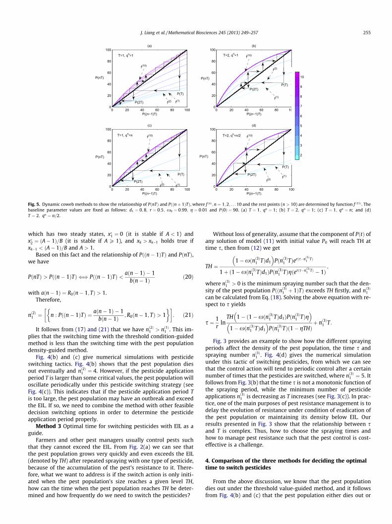
Therefore, for a given Pð0Þ, the time series PðTÞ; Pð2TÞ; . . . can beobtained. In order to investigate how the period T and the qn func-tion affect the time of pesticide switching, i.e. the value nð2Þ1 T, wecarry out dynamic cobweb analysis, as shown in Fig. 5. To do this,we fixed all parameter values as those in Fig. 5 and chose differentperiod T and qn functions for each subplot. Here we assumeN1 ¼ 10, i.e. the same pesticide is applied 10 times periodically,and the development of the sequence fPðnTÞgn2N with an initial va-lue Pð0Þ ¼ 90 for given period T and qn function are given in Fig. 5.The colors from light blue to mauve with n from 1 to 10 provide theiteration function f ðnÞ; n ¼ 1;2; . . . ;10. It is clear that the sequencefPðnTÞgn2N reaches its minimum value and then increases. Thisalso clarifies the number of pesticide applications (i.e. nð2Þ1 þ 1) be-fore the pest can be resurgent for a given initial population size(Pð0Þ ¼ 90 in all simulations) and how fast the pest can reach itscarrying capacity (here ðaðnÞ � 1Þ=bðnÞ in Fig. 5, see more detailsin the following discussion). All these results confirm that the va-lue nð2Þ1 depends on the period T and function qn.

In order to get an analytical expression of nð2Þ1 for this decisionstrategy, we employ results on the well-known Beverton–Holtmodel again. For any fixed n, we have the following Beverton–Holtdifference equation

xk ¼ f ðnÞðxk�1Þ ¼Axk�1

1þ Bxk�1; k 2 N

0 20 40 60 80 1000

20

40

60

80

100

P((n−1)T)

P(nT)

(b)

T=2, qn=1

P(T)P(2T)

0 20 40 60 80 1000

20

40

60

80

100

P((n−1)T)

P(nT)

(a)

T=1, qn=1

P(T)

P(2T)

0 20 40 60 80 1000

20

40

60

80

100

P((n−1)T)

P(nT)

(c)

T=1, qn=n

P(T)

P(2T)

0 20 40 60 80 1000

20

40

60

80

100

P((n−1)T)

P(nT)

(d)

T=2, qn=n/2

P(T)

P(2T)

2

3

4

5

6

7

8

9

10

f(1)

f(2)

f(1)f(2)

f(1)f(2)

f(1)

f(2)

f(10)

f(10)

f(10) f(10)

Fig. 5. Dynamic coweb methods to show the relationship of PðnTÞ and Pððnþ 1ÞTÞ, where f ðnÞ;n ¼ 1;2; . . . 10 and the rest points (n > 10) are determined by function f ð11Þ. Thebaseline parameter values are fixed as follows: d1 ¼ 0;8; r ¼ 0:5; x0 ¼ 0:99; g ¼ 0:01 and Pð0Þ ¼ 90. (a) T ¼ 1; qn ¼ 1; (b) T ¼ 2; qn ¼ 1; (c) T ¼ 1; qn ¼ n; and (d)T ¼ 2; qn ¼ n=2.

J. Liang et al. / Mathematical Biosciences 245 (2013) 249–257 255

which has two steady states, x�1 ¼ 0 (it is stable if A < 1) andx�2 ¼ ðA� 1Þ=B (it is stable if A P 1), and xk > xk�1 holds true ifxk�1 < ðA� 1Þ=B and A > 1.

Based on this fact and the relationship of Pððn� 1ÞTÞ and PðnTÞ,we have

PðnTÞ > Pððn� 1ÞTÞ () Pððn� 1ÞTÞ < aðn� 1Þ � 1bðn� 1Þ ð20Þ

with aðn� 1Þ ¼ R0ðn� 1; TÞ > 1.Therefore,

nð2Þ1 ¼ n : Pððn� 1ÞTÞ ¼ aðn� 1Þ � 1bðn� 1Þ ;R0ðn� 1; TÞ > 1

� �: ð21Þ

It follows from (17) and (21) that we have nð2Þ1 > nð1Þ1 . This im-plies that the switching time with the threshold condition-guidedmethod is less than the switching time with the pest populationdensity-guided method.

Fig. 4(b) and (c) give numerical simulations with pesticideswitching tactics. Fig. 4(b) shows that the pest population diesout eventually and nð2Þ1 ¼ 4. However, if the pesticide applicationperiod T is larger than some critical values, the pest population willoscillate periodically under this pesticide switching strategy (seeFig. 4(c)). This indicates that if the pesticide application period Tis too large, the pest population may have an outbreak and exceedthe EIL. If so, we need to combine the method with other feasibledecision switching options in order to determine the pesticideapplication period properly.

Method 3 Optimal time for switching pesticides with EIL as aguide.

Farmers and other pest managers usually control pests suchthat they cannot exceed the EIL. From Fig. 2(a) we can see thatthe pest population grows very quickly and even exceeds the EIL(denoted by TH) after repeated spraying with one type of pesticide,because of the accumulation of the pest’s resistance to it. There-fore, what we want to address is if the switch action is only initi-ated when the pest population’s size reaches a given level TH,how can the time when the pest population reaches TH be deter-mined and how frequently do we need to switch the pesticides?

Without loss of generality, assume that the component of PðtÞ ofany solution of model (11) with initial value P0 will reach TH attime s, then from (12) we get

TH ¼1�xðnð3Þ1 TÞd1

� �Pðnð3Þ1 TÞerðs�nð3Þ1 TÞ

1þ ð1�xðnð3Þ1 TÞd1ÞPðnð3Þ1 TÞgðerðs�nð3Þ1 TÞ � 1Þ;

where nð3Þ1 > 0 is the minimum spraying number such that the den-sity of the pest population Pððnð3Þ1 þ 1ÞTÞ exceeds TH firstly, and nð3Þ1

can be calculated from Eq. (18). Solving the above equation with re-spect to s yields

s ¼ 1r

lnTH 1� ð1�xðnð3Þ1 TÞd1ÞPðnð3Þ1 TÞg� �

1�xðnð3Þ1 TÞd1

� �Pðnð3Þ1 TÞð1� gTHÞ

þ nð3Þ1 T:

Fig. 3 provides an example to show how the different sprayingperiods affect the density of the pest population, the time s andspraying number nð3Þ1 . Fig. 4(d) gives the numerical simulationunder this tactic of switching pesticides, from which we can seethat the control action will tend to periodic control after a certainnumber of times that the pesticides are switched, where nð3Þ1 ¼ 5. Itfollows from Fig. 3(b) that the time s is not a monotonic function ofthe spraying period, while the minimum number of pesticideapplications nð3Þ1 is decreasing as T increases (see Fig. 3(c)). In prac-tice, one of the main purposes of pest resistance management is todelay the evolution of resistance under condition of eradication ofthe pest population or maintaining its density below EIL. Ourresults presented in Fig. 3 show that the relationship between sand T is complex. Thus, how to choose the spraying times andhow to manage pest resistance such that the pest control is cost-effective is a challenge.

4. Comparison of the three methods for deciding the optimaltime to switch pesticides

From the above discussion, we know that the pest populationdies out under the threshold value-guided method, and it followsfrom Fig. 4(b) and (c) that the pest population either dies out or

256 J. Liang et al. / Mathematical Biosciences 245 (2013) 249–257

tends to a periodic solution under the PðnTÞ guided method,depending on the period of pesticide applications, while the pestpopulation oscillates with a maximum value TH under the EILguided method. The question is which method is an optimal choicein practice? We discuss this question below.

We first would like to derive the conditions to determine if thepest population dies out or oscillates periodically under the densityof pest population PðnTÞ guided method.

Let ni be the number of effective pesticide applications of the ithpesticide switches and PðiÞðkTÞ is the pest population at time kTafter the ith pesticide switch, that is PðiÞðkTÞ ¼ Pðð

Pij¼1nj þ kÞTÞ

and PðiÞð0Þ ¼ Pði�1Þðni�1TþÞ ¼ ð1�xðni�1TÞd1ÞPði�1Þðni�1TÞ. Accord-ing to Eq. (18) we have

PðiÞðniTÞ¼ð1�xðni�1TÞd1ÞPði�1Þðni�1TÞeni rT

Qni�1j¼1 1�xðjTÞd1ð Þ

1þð1�xðni�1TÞd1ÞPði�1Þðni�1TÞgðerT �1Þ 1þPni�1

j¼1 ejrTQj

k¼1ð1�xðkTÞd1Þ� �� � :

ð22Þ

Denote Y ðiÞ ¼ PðiÞðniTÞ, then we have the following differenceequation

Y ðiÞ ¼ð1�xðni�1TÞd1ÞY ði�1ÞenirTQni�1

j¼1 1�xðjTÞd1ð Þ

1þð1�xðni�1TÞd1ÞY ði�1ÞgðerT �1Þ 1þPni�1

j¼1 ejrTQj

k¼1ð1�xðkTÞd1Þ� �� � :

ð23Þ

Again this is the well-known Beverton–Holt model, which has azero equilibrium Y�1 ¼ 0. It is stable provided that

gðTÞ¼: ð1�xðni�1TÞd1ÞenirTYni�1

j¼1

1�xðjTÞd1ð Þ < 1: ð24Þ

If gðTÞ > 1, then (23) has a stable positive equilibrium

Y�2¼ð1�xðni�1TÞd1ÞenirTQni�1

j¼1 1�xðjTÞd1ð Þ�1

ð1�xðni�1TÞd1ÞgðerT �1Þ 1þPni�1

j¼1 ejrTQj

k¼1ð1�xðkTÞd1Þ� �� � :

Let T1 be the solution of equation gðTÞ ¼ 1, then if T < T1, thepest population will die out after several pesticide switchings,and if T > T1, the pest population will fluctuate periodically.

Therefore, if we aim to eradicate the pest population and theperiod of pesticide applications must satisfy T < T1, our resultssupport the density guided method (i.e. method 2) because ofnð2Þ1 > nð1Þ1 , as shown in Fig. 4(b).

If the period of pesticide applications T is larger than T1, thenthe periodic switching of pesticides will result in oscillating ofthe pest population periodically under the density guided method,as shown in Fig. 4(c). However, for this case the amplitude of thepest population could be very large and its maximum value can ex-ceed EIL (i.e. Y� > TH), which will result in great economic loss.These results confirm that if T P T1, the tactic of switching pesti-cides with the EIL-guided method is better than the tactic ofswitching pesticides with the density guided method, becausethe EIL-guided method is in good agreement with the aims of anIPM strategy, that is control action must be taken once a criticaldensity of the pests is observed in the field so that the EIL is not ex-ceeded [6,8–10].

5. Discussion

Chemical methods in IPM are the most direct and effective[6,8–10]. However, frequent use of one kind of pesticide in thelong-term may create selection pressure for evolution of pest resis-tance to the pesticide. If too large a proportion of a pest populationdevelops resistance to the pesticide toxin, the susceptibility of theentire pest population to the pesticide toxin will be lost eventually,leading to pest resurgences and outbreaks.

Natural enemies may keep a pest population relatively stable inthe absence of any pesticide application. Indeed, a key componentof an IPM strategy is often biological control [24,25], which is de-fined as the reduction of pest populations by natural enemies. Ittypically involves impulsive perturbations, such as the release ofnatural enemies at a critical time of the season when insufficientreproduction of the natural enemies already present is likely to oc-cur and pest control will be achieved exclusively by the releasedindividuals themselves (augmentation) [26,27].

Pulse-like pest management actions such as spraying pesticidesand killing a pest instantly and the release of natural enemies atcritical times can be modelled with impulsive differential equa-tions. Recently, many mathematical models with impulsive chem-ical control tactics and releases of natural enemies have beenproposed to model an IPM strategy such as spraying of pesticides[25,28–33] or releases of natural enemies at critical times[27,34–41]. Those studies mainly focused on the effects of chemi-cal control and biological control on the permanence or extinctionof pest populations, and did not consider the effects of pesticideresistance. In particular, they paid no attention to questions suchas (1) how to determine the period of pesticide switches? (2) Whatis the optimal justification for switching from one kind pesticide toanother, unrelated, new kind pesticide? And (3) how to determinethe time when the density of the pest population reaches or ex-ceeds EIL? All these questions are key issues for the managementof pesticide resistance and applying cost-effective pest controlstrategies in practice.

To answer such questions, we developed a pest populationgrowth model including pesticide resistance. In particular, weinvestigated how the number of pesticide applications or the fre-quency of pesticide applications affects the evolution of pesticideresistance, and consequently affects the success or failure of pestcontrol.

In particular, we have provided three possible methods whichcan help us to judge when we should switch pesticides: thethreshold condition-guided method; the density of pest popula-tion-guided method and the EIL-guided method. If we want tocompletely eradicate the pest population, then the threshold con-dition-guided method or density-guided method can be employedto determine the frequency of pesticide switches. However, our re-sults confirm that if we properly choose the period of pesticideapplication, the density-guided method is better than the thresh-old condition-guided method in terms of the timing for pesticideswitching. Moreover, the method for determining the period ofpesticide applications is also provided. We also would like to pointout that this guided method may be easily implemented in prac-tice, because we only need to record the density of the pest popu-lation at the time of each pulse spraying of pesticides and monitorthe density at the most recent time of pulse spraying. But weshould emphasize here that the period of pesticide applicationsmust be carefully designed based on our method.

If we want to maintain the density of pests below some prede-fined threshold value such as EIL rather than eradicating the pestpopulation, then the density-guided method or EIL-guided methodcan be employed to determine the frequency of pesticide switches.Our results confirm that the EIL-guided method should also beused to determine the timing of pesticide applications, due to theuncertainties involved in the density-guided method, i.e. theamplitude of the pest population may be very large (vast pestoutbreaks may occur, e.g. in locust populations) if the period ofpesticide applications is not chosen properly. Moreover, the EIL-guided method can maintain the density of pest populations belowthe EIL forever, which is one of the main purposes of IPM strategies[6,8–10,42]. Note that the time when the pest population growsand reaches the EIL is not monotonic with respect to the frequencyof the pesticide applications. This indicates that although the

J. Liang et al. / Mathematical Biosciences 245 (2013) 249–257 257

effects of the pesticide naturally wear off with the increasing ofspraying times, the effects of the period of pesticide applicationson their timing s shown in Fig. 3 is complex.

To avoid multiple resistance, we need to adopt the IPM ap-proach [7]. Therefore, we will extend our single pest populationgrowth model to include natural enemies in the future. Due tothe pesticide wearing off, repeated releases of the same numberof natural enemies is either insufficient as they no longer suppressthe pest population once the pest resistance develops, or the num-ber released is too large which is not cost effective and may causesecondary outbreaks or pest resurgence. If so, how should onedetermine the new number of natural enemies to be released ateach control action? This question will be addressed in futureresearch. Meanwhile, the growth rate of a pest population can bestrongly impacted by environmental conditions, thus the pestcontrol strategies should be adaptable to changing conditions.Therefore, both stochasticity in growth rate and the ability to adaptcontrol methods in response to changing conditions will be alsoaddressed to make the model more realistic and practical.

Acknowledgments

This work was partially supported by the National NaturalScience Foundation of China (11171199), and by the FundamentalResearch Funds for the Central Universities (GK201104009,GK201302004).

References

[1] M.B. Thomas, Ecological approaches and the development of truly integratedpest management, Proc. Nat. Acad. Sci. 96 (1999) 5944.

[2] G.P. Georghiou, Overview of Insecticide Resistance, in: M.B. Green, H.M.LeBaron, W.K. Moberg (Eds.), Managing Resistance to Agrochemicals: FromFundamental Research to Practical Strategies, American Chemical Society,Washington DC, 1990, p. 18.

[3] M.J. Kotchen, Incorporating Resistance in Pesticide Management: A DynamicRegional Approach, Springer Verlag, New York, 1999 (p. 126).

[4] Pesticides 101 - A Primer, http://<www.panna.org/issues/pesticides-101-primer>.

[5] Y. Dumont, J.M. Tchuenche, Mathematical studies on the sterile insecttechnique for the Chikungunya disease and Aedes albopictus, J. Math. Biol.(2011), http://dx.doi.org/10.1007/s00285-011-0477-6 (in print).

[6] M.L. Flint, Integrated Pest Management for Walnuts, University of CaliforniaStatewide Integrated Pest Management Project, Division of Agriculture andNatural Resources, second ed., Oakland, CA, Publication, University ofCalifornia, 1987 (p. 3270).

[7] D.W. Onstad, Insect Resistance Management, Elsevier, Amsterdam, 2008.[8] J.C. Van Lenteren, J. Woets, Biological and integrated pest control in

greenhouses, Annu. Rev. Entomol. 33 (1988) 239.[9] J.C. Van Lenteren, Integrated Pest Management in Protected Crops, in: D. Dent

(Ed.), Integrated Pest Management, Chapman & Hall, London, 1995, p. 311.[10] J.C. Van Lenteren, Measures of Success in Biological Control of Arthropods By

Augmentation of Natural Enemies, in: S. Wratten, G. Gurr (Eds.), Measures ofSuccess in Biological Control, Kluwer Academic Publishers, Dordrecht, 2000, p.77.

[11] D. Kurtak, R. Meyer, M. Ocran, M. Ouedraogo, P. Renaud, R.O. Sawadogo, B.Tele, Management of insecticide resistance in control of the Simuliumdamnosum complex by the Onchocerciasis Control programme, West Africa:potential use of negative correlation between organophosphate resistance andpyrethroid susceptibility, Med. Veterinary Entomol. 1 (1987) 137.

[12] P.J. Cameron, G.P. Walker, Diamondback Moth Resistance Management andPrevention Strategy, in: N.A. Martin, R.M. Beresford, K.C. Harrington (Eds.),Pesticide Resistance: Prevention and Management Strategies 2005, The NewZealand Plant Protection Society, Hastings, New Zealand, 2005, p. 49.

[13] R.J. Hall, S. Gubbins, C.A. Gilligan, Invasion of drug and pesticide resistance isdetermined by a trade-off between treatment efficacy and relative fitness, Bull.Math. Biol. 66 (2004) 825.

[14] S. Bonhoeffer, M.A. Nowak, Pre-existence and emergence of drug resistance inHIV-1 infection, Proc. R. Soc. London B 264 (1997) 631.

[15] S. Gubbins, C.A. Gilligan, Invasion thresholds for fungicide resistance:deterministic and stochastic analyses, Proc. R. Soc. London B 266 (1999) 2539.

[16] R. Laxminarayan, R.D. Simpson, Biological limits on agriculturalintensification: an example from resistance management, Resour. Future(2000) 47.

[17] M.G. Milgroom, S.A. Levin, W.E. Fry, Population Genetics Theory and FungicideResistance, in: K.J. Leonard, W.E. Fry (Eds.), Plant Disease Epidemiology 2:Genetics, Resistance and Management, McGraw-Hill, New York, 1989, p. 340.

[18] R.J.H. Beverton, S.J. Holt, On the Dynamics of Exploited Fish Populations,Fishery Investigations, Series 2, Vol. 19, H.M. Stationery Office, London, 1957.

[19] A� Brännström, D.J.T. Sumpter, The role of competition and clustering inpopulation dynamics, Proc. R. Soc. B 272 (2005) 2065.

[20] S.A.H. Geritz, Éva Kisdi, On the mechanistic underpinning of discrete-timepopulation models with complex dynamics, J. Theor. Biol. 228 (2004) 261.

[21] L. Berezansky, E. Braverman, On impulsive Beverton–Holt difference equationand their applications, J. Differ. Equ. Appl. 10 (2004) 851.

[22] V.L. Kocic, D. Stutson, G. Arora, Global behavior of solutions of anonautonomous delay logistic difference equation, J. Differ. Equ. Appl. 10(2004) 1267.

[23] V.L. Kocic, A note on the nonautonomous Beverton–Holt model, J. Differ. Equ.Appl. 11 (2005) 415.

[24] D.J. Greathead, Natural Enemies of Tropical Locusts and Grasshoppers: TheirImpact and Potential as Biological Control Agents, in: C.J. Lomer, C. Prior (Eds.),Biological Control of Locusts and Grasshoppers, C.A.B. International,Wallingford, UK, 1992, p. 105.

[25] F.D. Parker, Management of Pest Populations by Manipulating Densities ofBoth Host and Parasites Through Periodic Releases, in: C.B. Huffaker (Ed.),Biological Control, Plenum Press, New York, 1971.

[26] M.P. Hoffmann, A.C. Frodsham, Natural Enemies of Vegetable Insect Pests,Cooperative Extension, Cornell University, Ithaca, NY, 1993 (p. 63).

[27] P. Neuenschwander, H.R. Herren, Biological control of the Cassava Mealybug,Phenacoccus manihoti, by the exotic parasitoid Epidinocarsis lopezi in Africa,Phil. Trans. R. Soc. London B 318 (1988) 319.

[28] C.T. Li, S.Y. Tang, The dynamical behavior of non-smooth system withimpulsive control strategies, Int. J. Biomath. 5 (1) (2012), http://dx.doi.org/10.1142/S1793524511001532.

[29] J.H. Liang, S.Y. Tang, Optimal dosage and economic threshold of multiplepesticide applications for pest control, Math. Comput. Model. 51 (2010) 487.

[30] Y.S. Tan, J.H. Liang, S.Y. Tang, The effects of timing of pulse spraying andreleasing periods on dynamics of generalized predator–prey model, Int. J.Biomath. 5 (3) (2012), http://dx.doi.org/10.1142/S1793524512600182.

[31] L.M. Wang, L.S. Chen, J.J. Nieto, The dynamics of an epidemic model for pestcontrol with impulsive effect, Nonlinear Anal.: Real World Appl. 11 (2010)1374.

[32] Y. Xue, S.Y. Tang, J.H. Liang, Optimal timing of interventions in fishery resourceand pest management, Nonlinear Anal.: Real World Appl. 13 (2012) 1630.

[33] H. Zhang, L.S. Chen, J.J. Nieto, A delayed epidemic model with stage-structureand pulses for pest management strategy, Nonlinear Anal.: Real World Appl. 9(2008) 1714.

[34] J.J. Jiao, S.H. Cai, L.S. Chen, Analysis of a stage-structured predator-prey systemwith birth pulse and impulsive harvesting at different moments, NonlinearAnal: Real World Appl. 12 (2011) 2232.

[35] J.H. Liang, S.Y. Tang, An integrated pest management model with delayedresponses to pesticide applications and its threshold dynamics, NonlinearAnal.: Real World Appl. 13 (2012) 2352.

[36] S.Y. Tang, Y.N. Xiao, L.S. Chen, R.A. Cheke, Integrated pest management modelsand their dynamical behaviour, Bull. Math. Biol. 67 (2005) 115.

[37] S.Y. Tang, Y.N. Xiao, R.A. Cheke, Multiple attractors of host-parasitoid modelswith integrated pest management strategies: eradication, persistence andoutbreak, Theor. Popul. Biol. 73 (2008) 181.

[38] S.Y. Tang, R.A. Cheke, Models for integrated pest control and their biologicalimplications, Math. Biosci. 215 (2008) 115.

[39] S.Y. Tang, Y.N. Xiao, R.A. Cheke, Effects of predator and prey dispersal onsuccess or failure of biological control, Bull. Math. Biol. 71 (2009) 2025.

[40] S.Y. Tang, G.Y. Tang, R.A. Cheke, Optimum timing for integrated pestmanagement: modelling rates of pesticide application and natural enemyreleases, J. Theor. Biol. 264 (2010) 623.

[41] S.Y. Tang, J.H. Liang, Y.S. Tan, R.A. Cheke, Threshold conditions for integratedpest management models with pesticides that have residual effects, J. Math.Biol. 66 (2013) 1.

[42] W. Zhang, S.M. Swinton, Optimal control of soybean aphid in the presence ofnatural enemies and the implied value of their ecosystem services, J. Environ.Manage. 96 (2012) 7.