Analytical findings for power law cross-sections: Uniform flow depth
25
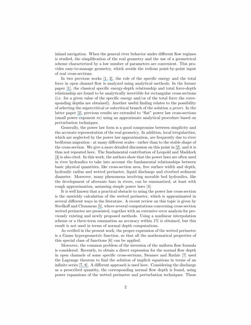
Analytical findings for power-law cross-sections: uniform flow depth A. Valiani *,a , V. Caleffi a a Universit` a degli Studi di Ferrara, Dipartimento di Ingegneria, Via Saragat, 1 - 44122 Ferrara, Italy Abstract Analytical results concerning open channel flows are presented, assuming that the cross-section is defined by a power law relationship between the channel width and the channel depth. Explicit equations to compute the normal flow depth are derived by considering the liquid discharge, the channel roughness height and the cross-section geometry (based on knowledge of the power law exponent, the reference width, and the reference depth) as known quantities. Such equations are deduced by writing the physical quantities as a power expansion in the power law exponent and expressing the wetted perimeter using a Gauss hypergeometric function. With the designed procedure, an accurate estimations of the integrals required to invert the uniform flow formula are obtained, at least for cross-sections characterized by aspect ratios of technical interest. Two relationships are proposed between the normal depth and the flow dis- charge. The first relationship is shown to work well for any discharge, provided that the width to depth ratio is sufficiently large. If this is not the case, the sec- ond procedure must be used for non-dimensional discharge larger than a given threshold, while the former procedure remains valid under the threshold. Key words: Open channel flows, Analytical results, Power law cross-sections, Normal flow depth 1. Introduction The present work regards the common problem of the inversion of the uni- form flow formula, and together with our previous work [1, 2], constitutes a basic set of analytical tools to manage rectangular and power law, cross-section channel flows. The need for these analytical methods arises from several calculations on real rivers, regarding preliminary design of river regulation works devoted to * Corresponding author. Email addresses: [email protected] (A. Valiani), [email protected] (V. Caleffi) Preprint submitted to Advances in Water Resources March 6, 2013
Transcript of Analytical findings for power law cross-sections: Uniform flow depth
Analytical findings for power-law cross-sections:uniform flow depth
A. Valiani∗,a, V. Caleffia
aUniversita degli Studi di Ferrara, Dipartimento di Ingegneria, Via Saragat, 1 - 44122Ferrara, Italy
Abstract
Analytical results concerning open channel flows are presented, assuming thatthe cross-section is defined by a power law relationship between the channelwidth and the channel depth. Explicit equations to compute the normal flowdepth are derived by considering the liquid discharge, the channel roughnessheight and the cross-section geometry (based on knowledge of the power lawexponent, the reference width, and the reference depth) as known quantities.
Such equations are deduced by writing the physical quantities as a powerexpansion in the power law exponent and expressing the wetted perimeter usinga Gauss hypergeometric function. With the designed procedure, an accurateestimations of the integrals required to invert the uniform flow formula areobtained, at least for cross-sections characterized by aspect ratios of technicalinterest.
Two relationships are proposed between the normal depth and the flow dis-charge. The first relationship is shown to work well for any discharge, providedthat the width to depth ratio is sufficiently large. If this is not the case, the sec-ond procedure must be used for non-dimensional discharge larger than a giventhreshold, while the former procedure remains valid under the threshold.
Key words: Open channel flows, Analytical results, Power law cross-sections,Normal flow depth
1. Introduction
The present work regards the common problem of the inversion of the uni-form flow formula, and together with our previous work [1, 2], constitutes abasic set of analytical tools to manage rectangular and power law, cross-sectionchannel flows.
The need for these analytical methods arises from several calculations onreal rivers, regarding preliminary design of river regulation works devoted to
∗Corresponding author.Email addresses: [email protected] (A. Valiani),
[email protected] (V. Caleffi)
Preprint submitted to Advances in Water Resources March 6, 2013
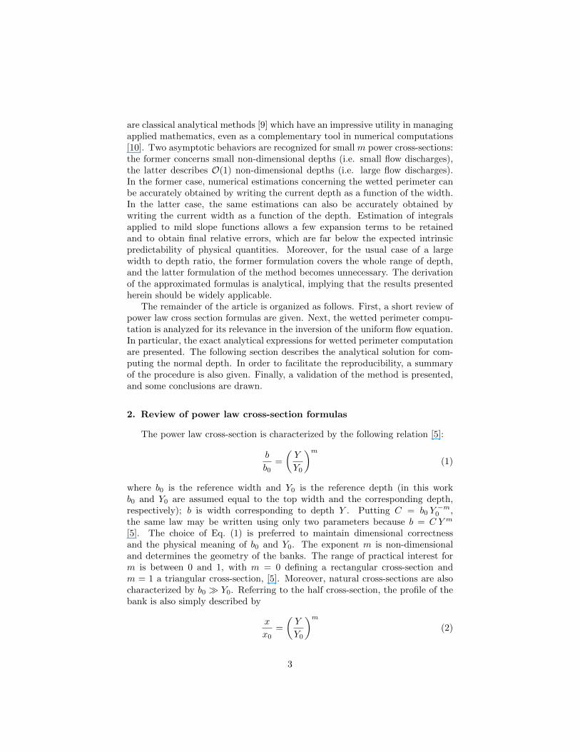
inland navigation. When the general river behavior under different flow regimesis studied, the simplification of the real geometry and the use of a geometricalscheme characterized by a low number of parameters are convenient. This pro-vides easy-to-manage geometry, which avoids the tedious point-by-point inputof real cross-sections.
In two previous works [1, 2], the role of the specific energy and the totalforce in open channel flow is analyzed using analytical methods. In the formerpaper [1], the classical specific energy-depth relationship and total force-depthrelationship are found to be analytically invertible for rectangular cross-sections(i.e. for a given value of the specific energy and/or of the total force the corre-sponding depths are obtained). Another useful finding relates to the possibilityof selecting the supercritical or subcritical branch of the solution a priori. In thelatter paper [2], previous results are extended to “flat” power law cross-sections(small power exponent m) using an approximate analytical procedure based onperturbation techniques.
Generally, the power law form is a good compromise between simplicity andthe accurate representation of the real geometry. In addition, local irregularities,which are neglected by the power law approximation, are frequently due to riverbedforms migration - at many different scales - rather than to the stable shape ofthe cross-section. We give a more detailed discussion on this point in [2], and it isthus not repeated here. The fundamental contribution of Leopold and Maddock[3] is also cited. In this work, the authors show that the power laws are often usedin river hydraulics to take into account the fundamental relationships betweenbasic physical quantities, like cross-section area, free surface width and depth,hydraulic radius and wetted perimeter, liquid discharge and riverbed sedimentdiameter. Moreover, many phenomena involving movable bed hydraulics, likethe development of alternate bars in rivers, can be summarized, at least withrough approximation, assuming simple power laws [4].
It is well known that a practical obstacle to using the power law cross-sectionis the unwieldy calculation of the wetted perimeter, which is approximated inseveral different ways in the literature. A recent review on this topic is given byStrelkoff and Clemmens [5], where several computations concerning cross-sectionwetted perimeter are presented, together with an extensive error analysis for pre-viously existing and newly proposed methods. Using a nonlinear interpolationscheme or a three-term summation an accuracy within 1% is obtained, but thisresult is not used in terms of normal depth computations.
As verified in the present work, the proper expression of the wetted perimeteris a Gauss hypergeometric function, so that all the mathematical properties ofthis special class of functions [6] can be applied.
Moreover, the common problem of the inversion of the uniform flow formulais considered. Recently, to obtain a direct expression for the normal flow depthin open channels of some specific cross-sections, Swamee and Rathie [7] usedthe Lagrange theorem to find the solution of implicit equations in terms of aninfinite series [7, 8]. A different approach is used here. Considering the dischargeas a prescribed quantity, the corresponding normal flow depth is found, usingpower expansions of the wetted perimeter and perturbation techniques. These
2
are classical analytical methods [9] which have an impressive utility in managingapplied mathematics, even as a complementary tool in numerical computations[10]. Two asymptotic behaviors are recognized for small m power cross-sections:the former concerns small non-dimensional depths (i.e. small flow discharges),the latter describes O(1) non-dimensional depths (i.e. large flow discharges).In the former case, numerical estimations concerning the wetted perimeter canbe accurately obtained by writing the current depth as a function of the width.In the latter case, the same estimations can also be accurately obtained bywriting the current width as a function of the depth. Estimation of integralsapplied to mild slope functions allows a few expansion terms to be retainedand to obtain final relative errors, which are far below the expected intrinsicpredictability of physical quantities. Moreover, for the usual case of a largewidth to depth ratio, the former formulation covers the whole range of depth,and the latter formulation of the method becomes unnecessary. The derivationof the approximated formulas is analytical, implying that the results presentedherein should be widely applicable.
The remainder of the article is organized as follows. First, a short review ofpower law cross section formulas are given. Next, the wetted perimeter compu-tation is analyzed for its relevance in the inversion of the uniform flow equation.In particular, the exact analytical expressions for wetted perimeter computationare presented. The following section describes the analytical solution for com-puting the normal depth. In order to facilitate the reproducibility, a summaryof the procedure is also given. Finally, a validation of the method is presented,and some conclusions are drawn.
2. Review of power law cross-section formulas
The power law cross-section is characterized by the following relation [5]:
b
b0=
(Y
Y0
)m(1)
where b0 is the reference width and Y0 is the reference depth (in this workb0 and Y0 are assumed equal to the top width and the corresponding depth,respectively); b is width corresponding to depth Y . Putting C = b0 Y
−m0 ,
the same law may be written using only two parameters because b = C Y m
[5]. The choice of Eq. (1) is preferred to maintain dimensional correctnessand the physical meaning of b0 and Y0. The exponent m is non-dimensionaland determines the geometry of the banks. The range of practical interest form is between 0 and 1, with m = 0 defining a rectangular cross-section andm = 1 a triangular cross-section, [5]. Moreover, natural cross-sections are alsocharacterized by b0 Y0. Referring to the half cross-section, the profile of thebank is also simply described by
x
x0=
(Y
Y0
)m(2)
3
where x0 is the reference half-width, and x is the horizontal distance of thebank from the cross-section axis.
By integrating Eq. (1), the expression of the wetted area, Ω, becomes
Ω =b0 Y0
(1 +m)
(Y
Y0
)1+m
. (3)
In non-dimensional form, both Eq. (1) and Eq. (2) may be written as
ξ = ηm, (4)
where ξ = x/x0 = b/b0 and η = Y/Y0, while Eq. (3) becomes
ω =1
(1 +m)η1+m, (5)
where ω = Ω/(b0 Y0) is the non-dimensional wetted area.Other non-dimensional expressions of fundamental quantities can be found
in [2] where the static moment of the wetted cross-section, the specific energyand the total force of the flow are analyzed.
The well-known uniform flow relationship for open channels is
Q = C Ω√g RS0, (6)
where Q is the liquid discharge; g is the acceleration due to gravity; and S0 isthe longitudinal bed slope. C = U/v∗ is the non-dimensional Chezy coefficient,corresponding to the average velocity to friction velocity ratio. Finally, R =Ω/P is the hydraulic radius, defined by the ratio between the wetted area, Ω,and the wetted perimeter, P .
A power law formula for the flow resistance is used [11, 12]:
C = C0
(R
ε
)1/6
, (7)
where C0 is a non-dimensional constant (7.66 for large cross-section, [11, 13]),and ε is the roughness height.
This method for computing the flow resistance is completely equivalent tothe use of Manning relation, provided that
C√g =
1
nR1/6, (8)
where n is the Manning coefficient (obviously n ∝ ε1/6). Eq. (7) is preferred toEq. (8) to maintain dimensional correctness.
If the discharge Q, the roughness height ε, and the longitudinal bed slopeS0, are known, the uniform flow formula is rearranged as
Qε1/6
C0
√g S0
=Ω5/3
P 2/3. (9)
4
The LHS of Eq. (9) does not depend on the current depth, while the RHSdepends on the depth through the cross-section geometry. In the simple case ofwide rectangular cross-sections, the RHS of Eq. (9) is proportional to Y 5/3.
Now, the non-dimensional wetted perimeter ψ = P/b0 and the referencedepth to half-width ratio,
ry =Y0x0, (10)
are introduced. For real channels, the parameter ry assumes finite but usuallysmall values. Moreover, the non-dimensional discharge is defined as follows:
Φ =Qε1/6
C0 Y1/60 (b0 Y0)
√g Y0 S0
=Qε1/6
C0 b0 Y5/30
√g S0
. (11)
Consequently, the non-dimensional form of Eq. (9) becomes
Φ = Φ(η) =ω5/3
ψ2/3. (12)
Thus, finding the non-dimensional normal depth corresponds to solvingEq. (12), remembering that, for a given geometry, ω and ψ are only functionsof the non-dimensional depth, η.
3. Wetted Perimeter
In power law cross-sections, the computation of the wetted perimeter isnot straightforward, as extensively discussed by Strelkoff and Clemmens [5],who reviewed existing methods for obtaining approximate estimations. In thiswork, an approach to the wetted perimeter calculation, based on an analyticalexact solution, is suggested. Two different forms, which are equivalent from theanalytical point of view, are presented. Each of them is used in the followingsection to obtain approximated power series expansions, suitable for the normaldepth computation.
Making reference to an infinitesimal portion of wetted perimeter [5], dP =2√dx2 + dY 2, we can write
dP = 2 dx
√1 +
(dY
dx
)2
, (13)
and also
dP = 2 dY
√1 +
(dx
dY
)2
. (14)
Integrating Eq. (13) and writing the result in non-dimensional form, thenon-dimensional wetted perimeter is obtained as a function of the current non-dimensional width ξ:
ψ =
∫ ξ
0
√1 +
r2ym2
t2−2m
m dt. (15)
5
being t a dummy variable defined on the interval [0, ξ].In a similar manner, using Eq. (14), the non-dimensional wetted perimeter
is obtained as a function of the current non-dimensional depth η:
ψ = ry
∫ η
0
√1 +
m2
r2y
1
ζ2−2mdζ. (16)
being ζ a dummy variable in the interval [0, η].The two forms of the integral reported in Eqs. (15) and (16) are different in
practice from several points of view.A first, remarkable, difference is that the integral in Eq. (15) is proper, at
least for m 6= 0 (the existence of this singularity does not represent a limit of themethod because m = 0 corresponds to the straightforward case of rectangularcross-section), while the integral in Eq. (16) is improper, because taking thelimit as ζ → 0 the integrand approaches ∞. For this reason, the manipulationof Eq. (15) is easier than of Eq. (16); therefore, the use of the former is suggestedas the basis for the general analytical expression of wetted perimeter.
Notwithstanding this, Eq. (16) is useful for evaluating the portion of thecross section perimeter, ψu, between the two limits, η and 1, when η is O(1) (asexplained later):
ψu = ry
∫ 1
η
√1 +
m2
r2y
1
ζ2−2mdζ. (17)
A second important difference regards the well-posedness of the two formswhen the integral is approximated with a series expansion. For given m and ry,Eq. (15) leads to a well-posed series for a sufficiently small upper limit ξ, whileEq. (17) leads to a well-posed series for a sufficiently large lower limit η. In fact,it is easy to note that in order to have an accurate integral approximation, theuse of the expression (15) for small depth is a better choice because near thethalweg, the side slope Y ′ = dY/dx is small, while the integral form of Eq. (17)is a better choice for large depths because the slope x′ = dx/dY is small farfrom the thalweg.
As a consequence, we can state that Eq. (15) is sufficient to analyticallycompute the wetted perimeter (Section 3.1), while both Eq. (15) and Eq. (17)have to be used to obtain an approximate solution.
Finally, the proposed idea is as follows:
- to compute the approximated wetted perimeter using Eq. (15) if the upperlimit ξ is lower than a suitable non-dimensional width, ξs = ηms , relatedto a specific depth threshold, ηs (to be defined later);
- to compute analytically the wetted perimeter of the full cross-section, Ψ,starting from Eq. (15) and subtracting the part of the perimeter betweenη and 1, which is computed using Eq. (17).
6
In the latter case, we have the following initial analytical expression:
ψ = Ψ− ry∫ 1
η
√1 +
m2
r2y
1
ζ2−2mdζ, (18)
where
Ψ =
∫ 1
0
√1 +
r2ym2
t2−2m
m dt. (19)
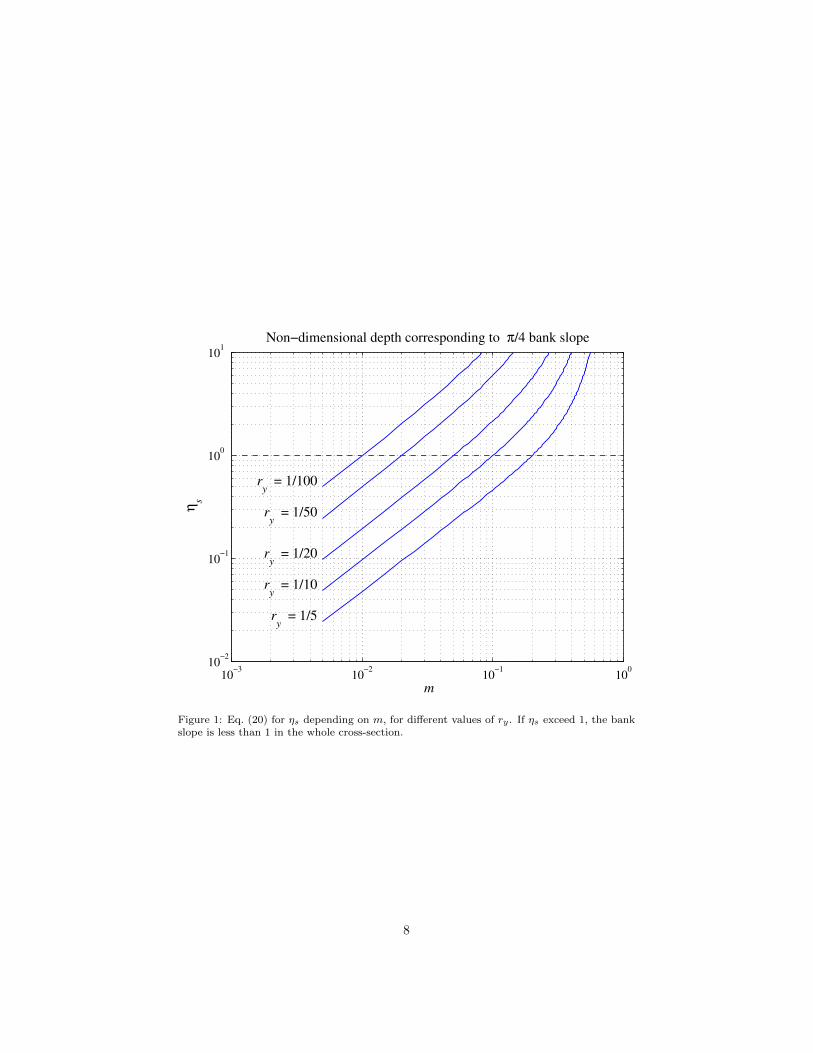
The suggested criteria for the selection of the threshold, ηs, are strictlyrelated to the well-posedness of the integrals in Eqs. (15) and (17). We suggestthe former expression of the integral be used when the slope Y ′ is less than theslope x′, and the latter form elsewhere. Such reasoning implies that ηs is definedas the depth corresponding to the point where Y ′ = x′ = 1, which coincideswith the location where the bank slope is equal to π/4. So, the depth threshold,ηs, is defined as
dY
dx= 1 =⇒ ηs =
(m
ry
) 1(1−m)
. (20)
The function ηs = f(m, ry) is plotted in Fig. 1. The range of interest forthe m parameter is 0 < m < 0.4, even if a larger range, in the field of concavecross-sections, 0 < m < 1, is reported for completeness. Also, ry is selected inthe field of practical interest values. It is interesting to observe that when mincreases, the bank slope is less than 1:1 in the whole cross-section for a largerrange of ry values.
In the following, Eq. (15) is used in the range 0 < η < ηs while Eq. (18)is used in the range ηs < η < 1, to obtain well-conditioned computations andmeaningful power series having as few terms as possible, while still preservinggood accuracy (the error of the computed results is much less 1%).
3.1. Exact solutions for the wetted perimeter
The exact solution of (15) is
ψ =
∫ ξ
0
√1 +
r2ym2
t2−2m
m dt = ξ G (ξ) , (21)
where
G (ξ) = 2F1
(−1
2,
m
2− 2m;
2−m2− 2m
; −r2ym2
ξ2−2m
m
), (22)
where 2F1 is the Gauss hypergeometric function, some properties of which arerecalled in Appendix A.
The exact solution of Eq. (18) is
ψ = Ψ− ry∫ 1
η
√1 +
m2
r2y
1
ζ2−2mdζ = Ψ− ry [F (1)− ηF (η)] , (23)
7
10−3
10−2
10−1
100
10−2
10−1
100
101
ry = 1/5
ry = 1/10
ry = 1/20
ry = 1/50
ry = 1/100
m
ηs
Non−dimensional depth corresponding to π/4 bank slope
Figure 1: Eq. (20) for ηs depending on m, for different values of ry . If ηs exceed 1, the bankslope is less than 1 in the whole cross-section.
8
where
F (1) = 2F1
(−1
2, − 1
2− 2m;
1− 2m
2− 2m; −m
2
r2y
); (24)
and
F (η) = 2F1
(−1
2, − 1
2− 2m;
1− 2m
2− 2m; −m
2
r2y
1
η2−2m
). (25)
4. Analytical solution for the normal flow depth
In this section, for a given non-dimensional flow discharge Φ, the non-dimensional uniform flow relationship, Eq. (12), is analytically inverted to com-pute the corresponding non-dimensional normal depth, η. The inversion is car-ried out as follows: given a certain value of the non-dimensional discharge Φ,we have to find the only value of η that satisfies Eq. (12), while ψ = ψ(η) andω = ω(η). This is not trivial, mainly because of the complex dependence of thenon-dimensional wetted perimeter, ψ, and the depth, η. To achieve a reason-able simple framework, Eq. (12) must be manipulated starting from a properlyapproximated expression for the wetted perimeter.
First, the specific non-dimensional discharge, Φs, is introduced as
Φs =ω5/3s
ψ2/3s
, (26)
where the specific non-dimensional wetted area, ωs, corresponding to a non-dimensional depth, ηs, is
ωs =1
(1 +m)η1+ms , (27)
and the specific non-dimensional wetted perimeter, ψs is
ψs =
∫ ξs
0
√1 +
r2ym2
t2−2m
m dt = ξs G (ξs) , (28)
assuming ξs = ηms .The inversion procedure is performed in different manners for the low stage,
Φ < Φs, and high stage, Φ > Φs, of non-dimensional discharge which correspondto η < ηs and η > ηs, respectively.
4.1. Low stage discharge Φ < Φs and η < ηs
We start from Eqs. (21) and (22), the analytical exact solution of the Eq. (15).Assuming as a small parameter the quantity
(r2y/m
2 t2−2m/m), and considering
the expansion reported in Eq. (56), the wetted perimeter approximation up tothe second order becomes
ψ = ξ +(rym
)2 m
2 (2−m)ξ
2−mm −
(rym
)4 m
8 (4− 3m)ξ
4−3mm , (29)
9
0 0.1 0.2 0.3 0.4 0.5 0.6 0.7 0.8 0.9 10
0.2
0.4
0.6
0.8
1
η
ψ
Non−dimensional wetted perimeter vs non−dimensional depth, ry = 1/5
a)
Exact m = 0.05
Exact m = 0.10
Exact m = 0.20
Exact m = 0.40
2nd
order expansion
Limit value
0 0.1 0.2 0.3 0.4 0.5 0.6 0.7 0.8 0.9 1
10−10
10−8
10−6
10−4
10−2
100
η
|∆ ψ
|
Error on approximate non−dimensional wetted perimeter, ry = 1/5
b)
m = 0.05
m = 0.10
m = 0.20
m = 0.40
Limit value
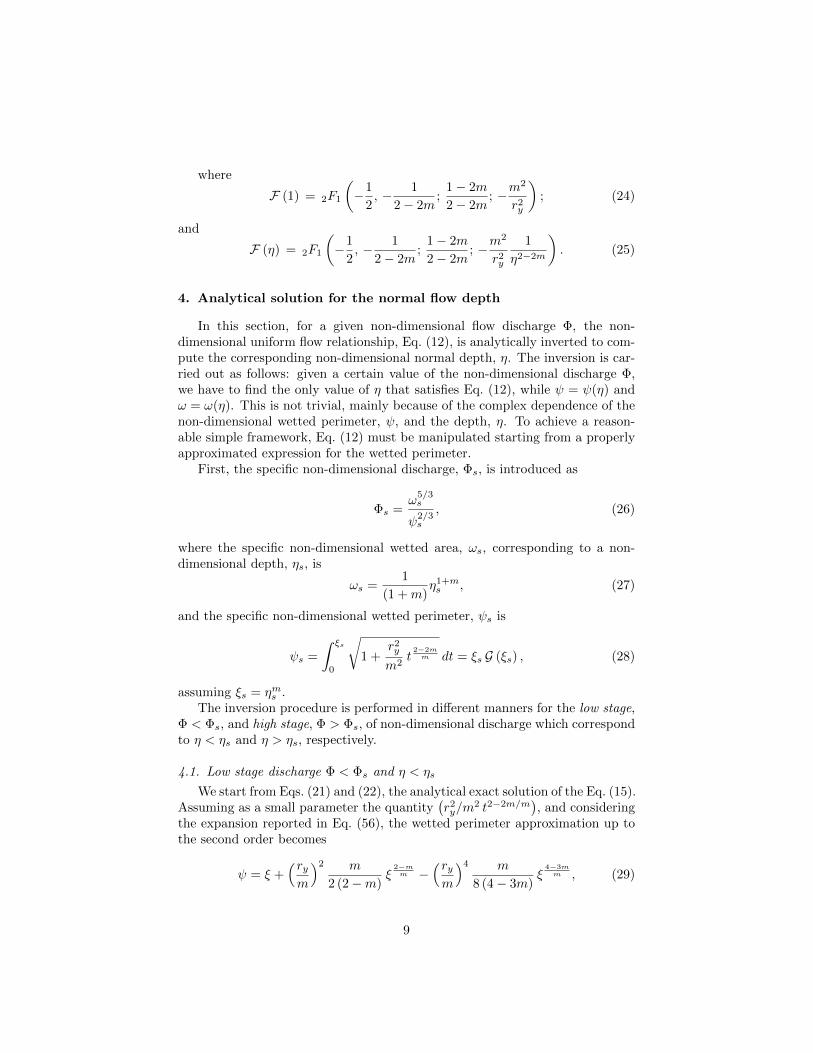
Figure 2: a) Approximation of n.d wetted perimeter using Eq. (30) for ry = 1/5. b) Error onapproximation of non-dimensional wetted perimeter using Eq. (30), for ry = 1/5. The limitvalue, ηs, is computed by Eq. (20).
that is, using Eq. (4):
ψ = ηm[1 +
(rym
)2 m
2 (2−m)η2−2m −
(rym
)4 m
8 (4− 3m)η4−4m
]. (30)
To show the accuracy obtainable with this expansion, a comparison betweenthe values of the wetted perimeter computed using Eq. (30) and the exact valuecomputed using Eq. (22) is performed, for different values of m, in the range0 < η < 1. The very good agreement between the two computations in therange 0 < η < ηs is evident from the analysis of Fig. 2, where the results arepresented for a depth to half-width ratio of 1/5. The choice of a large ry is madein order to show the worst case of practical interest. Fig. 2a) shows how theapproximate expression of the wetted perimeter is indistinguishable from theexact solution for non-dimensional depth η less than the threshold ηs. To allowan easy error estimation, Fig. 2b) represents the absolute value of the differencebetween the approximate, Eq. (30), and the exact solution, Eq. (22).
When increasing the width to depth ratio (i.e. reducing ry), the proposedapproximation of Eq. (30) works well over the whole range of depths, as can be
10
0 0.1 0.2 0.3 0.4 0.5 0.6 0.7 0.8 0.9 10
0.2
0.4
0.6
0.8
1
η
ψ
Non−dimensional wetted perimeter vs non−dimensional depth, ry = 1/25
a)
Exact m = 0.05
Exact m = 0.10
Exact m = 0.20
Exact m = 0.40
2nd
order expansion
0 0.1 0.2 0.3 0.4 0.5 0.6 0.7 0.8 0.9 1
10−14
10−12
10−10
10−8
10−6
10−4
η
|∆ ψ
|
Error on approximate non−dimensional wetted perimeter, ry = 1/25
b)
m = 0.05
m = 0.10
m = 0.20
m = 0.40
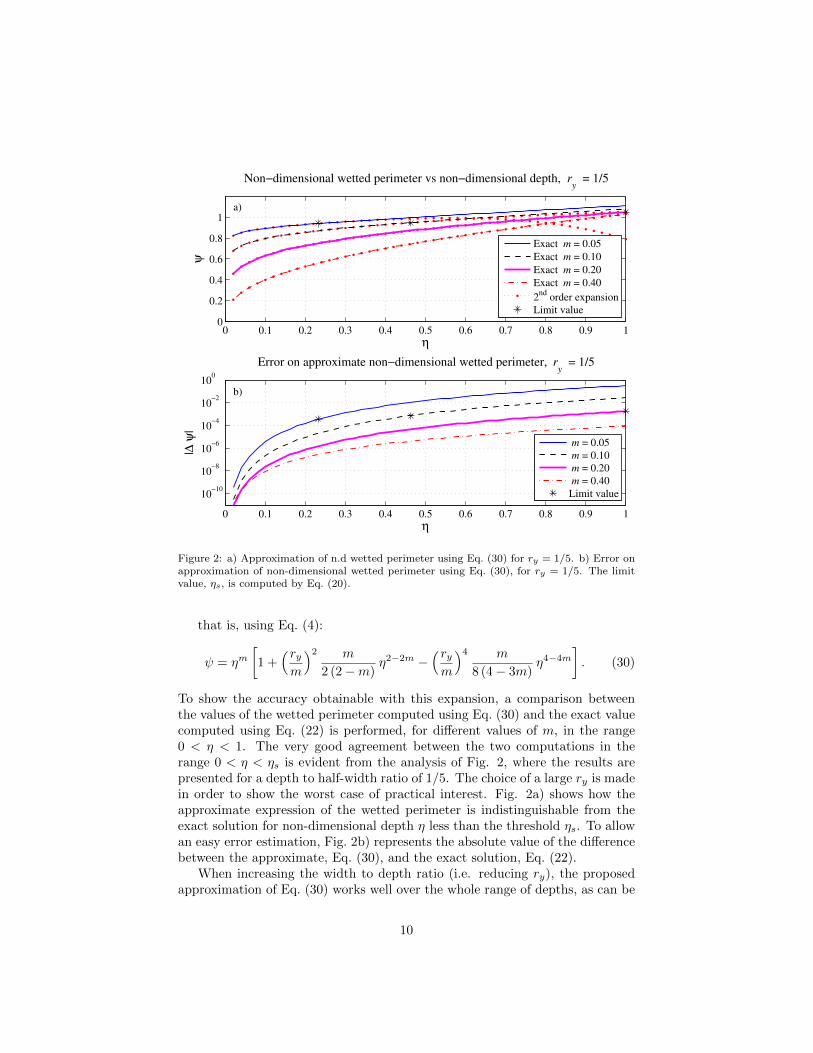
Figure 3: a) Approximation of n.d wetted perimeter using Eq. (30) for ry = 1/25. b) Erroron approximation of non-dimensional wetted perimeter using Eq. (30), for ry = 1/25.
observed in the Fig. 3. In particular, Fig. 3b) shows that maximum computingerror is under 10−4.
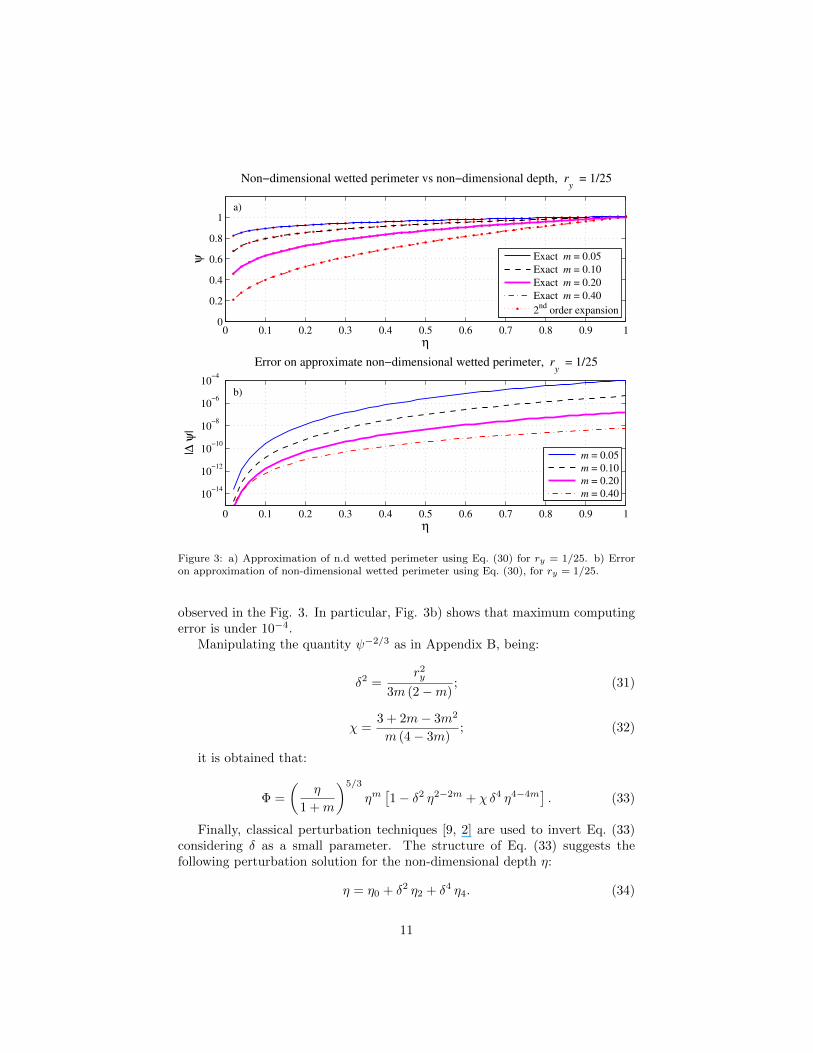
Manipulating the quantity ψ−2/3 as in Appendix B, being:
δ2 =r2y
3m (2−m); (31)
χ =3 + 2m− 3m2
m (4− 3m); (32)
it is obtained that:
Φ =
(η
1 +m
)5/3
ηm[1− δ2 η2−2m + χ δ4 η4−4m
]. (33)
Finally, classical perturbation techniques [9, 2] are used to invert Eq. (33)considering δ as a small parameter. The structure of Eq. (33) suggests thefollowing perturbation solution for the non-dimensional depth η:
η = η0 + δ2 η2 + δ4 η4. (34)
11
As usual, solving Eq. (33) by further approximations, taking into account ofEq. (34), the following coefficients are obtained:
η0 =[(1 +m)
5/3Φ] 3
5+3m
; (35)
η2 =3
5 + 3mη3−2m0 ; (36)
η4 =3 (20− 9m− 10χ− 6mχ)
2 (5 + 3m)2 η5−4m0 . (37)
The smaller the ratio ry/m, the more accurate is the solution.
4.2. High stage discharge Φ > Φs and η > ηs
We now describe the procedure to invert Eq. (12) for high stage discharge.In such a case, expressing the non-dimensional wetted perimeter as a function
of the wetted area ω is convenient. The area becomes the unknown in Eq. (12)(LHS depends on ω, RHS does not). Such an equation is rewritten as follows:
ψ (ω)
ω5/2=
1
Φ3/2, (38)
where η is replaced by the corresponding value of ω (see Eq. 3):
η = [(1 +m) ω]1
(1+m) . (39)
Now, to have a well-conditioned problem, we make an estimate of the wettedperimeter starting from Eq. (23):
ψ (η) = Ψ− ry∫ 1
η
√1 +
m2
r2y
1
ζ2−2mdζ = Ψ− ψu, (40)
where ψu is defined in Eq. (17).Taking into account that
ψu = ry [F (1)− ηF (η)] , (41)
the difference [F (1)− ηF (η)] is evaluated as a fourth order series, accordingto Eq. (56), and the following expansion is found:
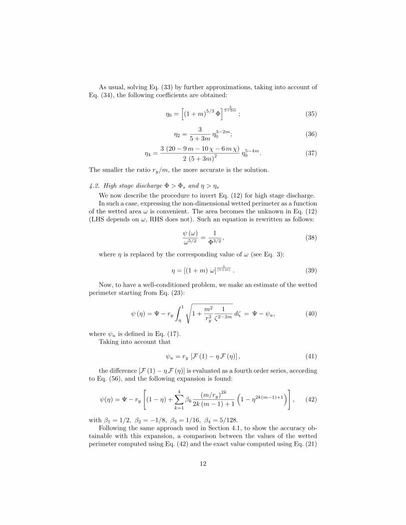
ψ(η) = Ψ− ry
[(1− η) +
4∑k=1
βk(m/ry)
2k
2k (m− 1) + 1
(1− η2k(m−1)+1
)], (42)
with β1 = 1/2, β2 = −1/8, β3 = 1/16, β4 = 5/128.Following the same approach used in Section 4.1, to show the accuracy ob-
tainable with this expansion, a comparison between the values of the wettedperimeter computed using Eq. (42) and the exact value computed using Eq. (21)
12
0 0.1 0.2 0.3 0.4 0.5 0.6 0.7 0.8 0.9 10
0.2
0.4
0.6
0.8
1
η
ψ
Non−dimensional wetted perimeter vs non−dimensional depth, ry = 1/5
a)
Exact m = 0.01
Exact m = 0.05
Exact m = 0.10
Exact m = 0.20
4th
order expansion
Limit value
0 0.1 0.2 0.3 0.4 0.5 0.6 0.7 0.8 0.9 1
10−12
10−10
10−8
10−6
10−4
10−2
100
η
|∆ ψ
|
Error on approximate non−dimensional wetted perimeter, ry = 1/5
b)
m = 0.01
m = 0.05
m = 0.10
m = 0.20
Limit value
Figure 4: a) Approximation of non-dimensional wetted perimeter using Eq. (42) for ry = 1/5.b) Error of approximation of non-dimensional wetted perimeter using Eq. (42), for ry = 1/5.The limit value, ηs, is computed by Eq. (20).
13
is performed for different values of m in the range 0 < η < 1. From the analysisof Fig. 4, it is clear that there is good agreement between the two computationsin the range ηs < η < 1. Fig. 4a) shows that the approximate expression of thewetted perimeter is a good compromise between simplicity and accuracy. Theabsolute value of the difference between the exact solution and the approximatednon-dimensional perimeter, |∆ψ|, is small at least for η > ηs. To allow an easyerror estimation, Fig. 4b) represents the difference between the approximateand the exact solution.
Taking into account Eq. (39), the non-dimensional depth η is replaced withthe non-dimensional area ω in Eq. (42), and the resulting expression is substi-tuted in Eq. (38). Then, considering m as a small parameter, classical pertur-bation techniques are used [9, 2]. Therefore, the wetted area, ω, is expanded atthe third order in the powers of m:
ω = ω0 +mω1 +m2 ω2 +m3 ω3. (43)
Successively, Eq. (43) is replaced in Eq. (38).By imposing the obtained equation at different orders of approximation, we
obtain that:
1. ω0 is the real solution of the fifth degree polynomial (in $):
$5 − ry2 Φ3$2 − 2 ry ( Ψ − ry) Φ3$ − ( Ψ − ry)2
Φ3 = 0. (44)
Eq. (44) is analyzed in Section 4.2.1.
2. ω1 becomes
ω1 =2ω0
2 ry [1− log(ω0)]
5 Ψ− 5 ry + 3 ry ω0, (45)
3. ω2 becomes
ω2 =ω2a + ω2b + ω2c
4 ry ω0 (5 Ψ− 5 ry + 3 ry ω0), (46)
where
ω2a = −4ω0 + 4ω02 − 8 ry
2 ω03 (47)
ω2b = −20 ry2 ω0
2 ω1 + 35 Ψ ry ω12 − 35 ry
2 ω12 + 15 ry
2 ω0 ω12
ω2c = 12 ry2 ω0
2 ω1 log(ω0) + 4 ry2 ω0
3 log(ω0)2
4. ω3 becomes
ω3 =ω3a + ω3b + ω3c + ω3d + ω3e
24 ry ω02 (5 Ψ− 5 ry + 3 ry ω0)
, (48)
where
ω3a = −24ω02 + 48ω0
3 + 24 ry2 ω0
4 (49)
ω3b = 84ω0 ω1 − 60ω02 ω1 + 72 ry
2 ω03 ω1
14
+ 186 ry2 ω0
2 ω12 − 315 Ψ ry ω1
3 + 315 ry2 ω1
3
ω3c = −105 ry2 ω0 ω1
3 − 120 ry2 ω0
3 ω2
+ 420 Ψ ry ω0 ω1 ω2 − 420 ry2 ω0 ω1 ω2 + 180 ry
2 ω02 ω1 ω2
ω3d = −72ω02 log(ω0) + 48 ry
2 ω04 log(ω0) + 48 ry
2 ω03 ω1 log(ω0)
− 90 ry2 ω0
2 ω12 log(ω0) + 72 ry
2 ω03 ω2 log(ω0)
ω3e = −24 ry2 ω0
4 log(ω0)2 − 36 ry2 ω0
3 ω1 log(ω0)2
− 8 ry2 ω0
4 log(ω0)3
Finally, when the value of ω corresponding to the uniform flow is found, thenormal flow depth is computed by Eq. (39).
4.2.1. Finding ω0
The zero order coefficient, ω0, must satisfy Eq. (44). In the physical rangeof parameters (0 < ψs < 1, 0 < Φ < 1, 0 < ry < 1), Eq. (44) has only one realsolution, while the other four are complex conjugate pairs. Standard packagesof scientific computing easily find the target root numerically, but in order tomanage each element of the proposed procedure analytically, a perturbationsolution is performed [9, 2]. Therefore, ω0 is expanded in a power series of ry,up to the fourth order of approximation:
ω0 = ω00 + ry ω01 + ry2 ω02 + ry
3 ω03 + ry4 ω04. (50)
Imposing that Eq. (44) is satisfied at each order of approximation, we obtain
ω00 = Ψ2/5 Φ3/5; (51)
ω01 =2
5
(Ψ2/5 Φ3/5 − 1
) Φ3/5
Ψ3/5; (52)
ω02 =1
25
(Ψ4/5 Φ6/5 + 2 Ψ2/5 Φ3/5 − 3
) Φ3/5
Ψ8/5; (53)
ω03 = − 2
125
(Ψ6/5 Φ9/5 − 2 Ψ4/5 Φ6/5 − 3 Ψ2/5 Φ3/5 + 4
) Φ3/5
Ψ13/5; (54)
ω04 = − 2
625
(7 Ψ6/5 Φ9/5 − 9 Ψ4/5 Φ6/5 − 11 Ψ2/5 Φ3/5 + 13
) Φ3/5
Ψ18/5. (55)
Eq. (50) is intentionally developed at a very high order of approximation to bepractically “exact” with respect to all other computations. The reason for thisis that the expansion is carried out in ry, rather than in m, and we want tomake the only restrictive hypothesis on m and a very general hypothesis on ry.In any case, ry is usually very small for real world rivers.
The approximate solution given by Eq. (50) is very close to the unique realsolution satisfying Eq. (44), numerically evaluated with an admissible toleranceof 10−14, as shown in Fig. 5. In particular, in Fig. 5a) the approximate and theexact solutions are nearly indistinguishable. In Fig. 5b) it is possible to see thatthe fourth order expansion in ry gives an error lower than 10−5, for ry = 1/5.
15

10−3
10−2
10−1
100
10−4
10−3
10−2
10−1
100
η
ω0
Computation of ω0, r
y = 1/5
a)
Exact m = 0.05
Exact m = 0.10
Exact m = 0.20
Exact m = 0.40
4th
order expansion
10−3
10−2
10−1
100
10−10
10−9
10−8
10−7
10−6
10−5
η
|∆ ω
0|
Error on ω0, r
y = 1/5
b)
m = 0.05
m = 0.10
m = 0.20
m = 0.40
Figure 5: a) Approximation of ω0 using Eq. (50), for a prescribed reference depth to half-width ratio. b) Absolute difference between numerically computed and exact wetted area.For higher ratio value, the approximation works even better.
The greater the ratio ry is (1/25, 1/100, . . . ), the better are the results. Toconclude, Eq. (50) can be considered as exact for practical purposes to estimateω0 for any ry less than 1/5.
5. Summary of the procedure
A brief description of the algorithm for the analytical inversion of Eq. (12)is reported. The ry ratio, the exponent m and the non-dimensional dischargeΦ are assumed to be known quantities, while the value of the non-dimensionalnormal depth is the unknown quantity. The steps of the proposed procedureare the following:
1. The non-dimensional threshold, ηs, is computed using Eq. (20).
2. The corresponding wetted area, ωs, and wetted perimeter, ψs, are deter-mined using Eqs. (27) and (28), while the corresponding non-dimensionaldischarge, Φs, is computed by Eq. (26).
16

3a. If Φ ≤ Φs, the approach for low discharge may be used. Therefore, δ2 andχ are computed by Eq. (31) and Eq. (32), respectively.
4a. Finally, the non-dimensional normal depth, η, is obtained using Eq. (34).
3b. If Φ > Φs, the approach for high discharge is used. Therefore, the valueof ω0 must be evaluated using Eq. (50).
4b. The non-dimensional wetted area ω is computed using Eq. (43).
5b. Finally, the non-dimensional normal depth, η, is computed using Eq. (39).
6. Validation of the analytical method
To validate the proposed method, the following analysis is performed. Fora given set of non-dimensional depth values, in the range 0 < η < 1, the cor-responding exact non-dimensional discharge is computed using Eq. (12), whereω and ψ are obtained from Eq. (5) and Eq. (21), respectively. Therefore, theexact non-dimensional rating curve, Φ(η), is determined.
The approximated solution summarized in Section 5 is applied to each valueof the discharge. The result is a set of approximate normal depths. Moreover,to allow the validation of each part of the method, a second set of normaldepths is evaluated using the equations holding on for low stage discharges(Φ < Φs). A similar approach is followed using the equations suitable forthe high stage discharges (Φ > Φs). In this manner, three non-dimensionalapproximated rating curves are obtained: a rating curve evaluated using thelow stage equations; one evaluated using the high stage equations; and oneevaluated with the complete set of equations.
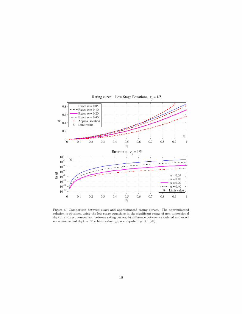
Fig. 6a) shows the direct comparison between the exact and the approx-imated rating curves based only on the equations for low stage discharges,Φ < Φs. A quite large value of the reference depth to half width ratio, ry = 1/5,is considered to show the behavior of the method in the worst reasonable case.For smaller values of such a ratio, the method performs much better. A signifi-cant range of m values is also taken into account. Fig. 6b) shows the absolutevalue of the difference between the approximate and the exact non-dimensionaldepth, |∆η|, allowing a quantitative analysis of the computational errors. Suchan approximated solution and the exact rating curve are technically indistin-guishable for low discharge (low depth), as can be seen from these figures. Onlyfor large m parameter values and large values of the non-dimensional dischargedo the errors become meaningful.
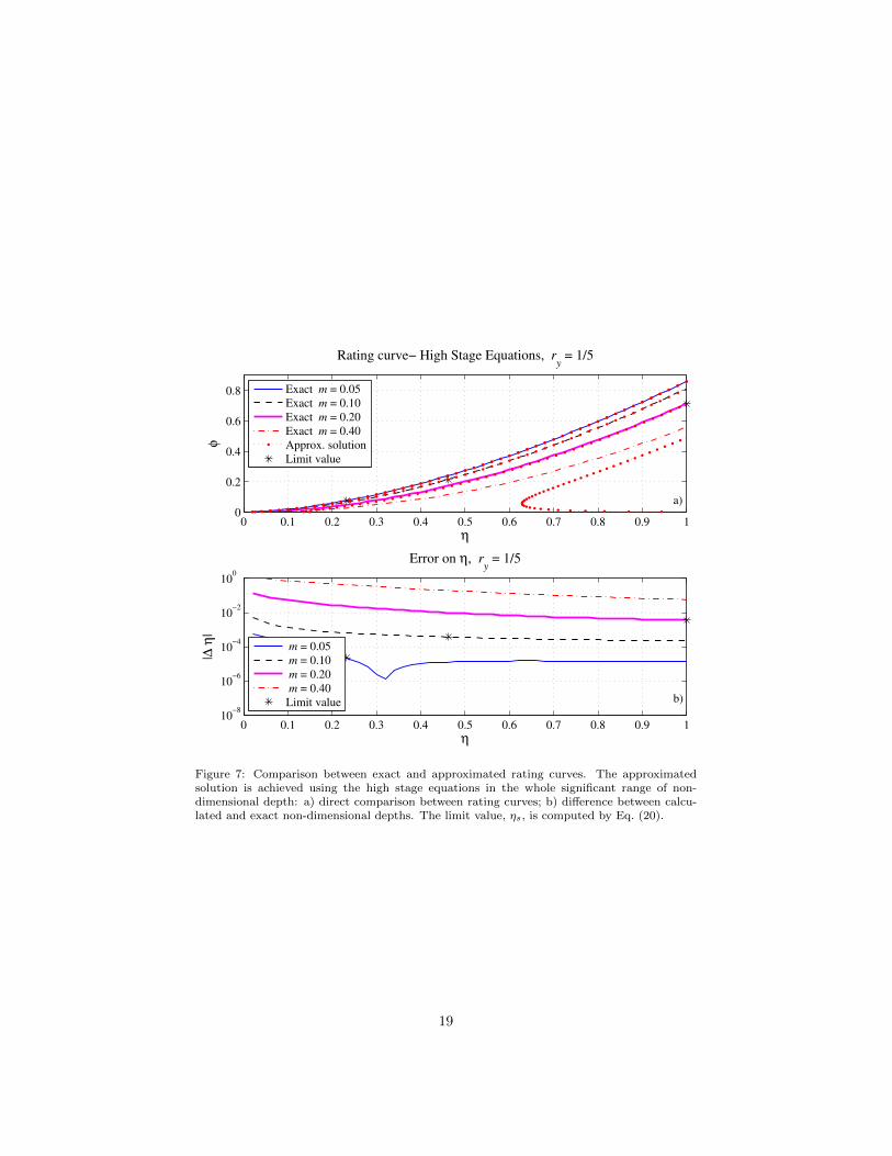
Fig. 7 shows the comparison between approximated and exact solutions. Inthis case, the approximated solution is achieved using the high stage equationsfor each value of non-dimensional discharge. The exact rating curve are prac-tically indistinguishable for high discharge (high depth). Only for small valuesof the m parameter and small values of the non-dimensional discharge do theerrors become significant.
17
0 0.1 0.2 0.3 0.4 0.5 0.6 0.7 0.8 0.9 10
0.2
0.4
0.6
0.8
η
φ
Rating curve − Low Stage Equations, ry = 1/5
a)
Exact m = 0.05
Exact m = 0.10
Exact m = 0.20
Exact m = 0.40
Approx. solution
Limit value
0 0.1 0.2 0.3 0.4 0.5 0.6 0.7 0.8 0.9 1
10−14
10−12
10−10
10−8
10−6
10−4
10−2
100
η
|∆ η
|
Error on η, ry = 1/5
b)
m = 0.05
m = 0.10
m = 0.20
m = 0.40
Limit value
Figure 6: Comparison between exact and approximated rating curves. The approximatedsolution is obtained using the low stage equations in the significant range of non-dimensionaldepth: a) direct comparison between rating curves; b) difference between calculated and exactnon-dimensional depths. The limit value, ηs, is computed by Eq. (20).
18
0 0.1 0.2 0.3 0.4 0.5 0.6 0.7 0.8 0.9 10
0.2
0.4
0.6
0.8
η
φ
Rating curve− High Stage Equations, ry = 1/5
a)
Exact m = 0.05
Exact m = 0.10
Exact m = 0.20
Exact m = 0.40
Approx. solution
Limit value
0 0.1 0.2 0.3 0.4 0.5 0.6 0.7 0.8 0.9 110
−8
10−6
10−4
10−2
100
η
|∆ η
|
Error on η, ry = 1/5
b)
m = 0.05
m = 0.10
m = 0.20
m = 0.40
Limit value
Figure 7: Comparison between exact and approximated rating curves. The approximatedsolution is achieved using the high stage equations in the whole significant range of non-dimensional depth: a) direct comparison between rating curves; b) difference between calcu-lated and exact non-dimensional depths. The limit value, ηs, is computed by Eq. (20).
19

0 0.1 0.2 0.3 0.4 0.5 0.6 0.7 0.8 0.9 10
0.2
0.4
0.6
0.8
η
φ
Rating curve − Complete Equations, ry = 1/5
a)
Exact m = 0.05
Exact m = 0.10
Exact m = 0.20
Exact m = 0.40
Approx. solution
Limit value
0 0.1 0.2 0.3 0.4 0.5 0.6 0.7 0.8 0.9 1
10−14
10−12
10−10
10−8
10−6
10−4
η
|∆ η
|
Error on η, ry = 1/5
b)
m = 0.05
m = 0.10
m = 0.20
m = 0.40
Limit value
Figure 8: Comparison between exact and approximated rating curves. The approximatedsolution is achieved using the complete method: a) direct comparison between rating curves;b) difference between calculated and exact non-dimensional depths. The limit value, ηs, iscomputed by Eq. (20).
20
−20 −15 −10 −5 0 5 10 15 20
0
2
4
6
x [m]
y [m
]
Reno River cross−section − chainage 80886 [m]
Actual section
Power−law section
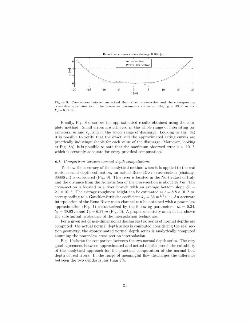
Figure 9: Comparison between an actual Reno river cross-section and the correspondingpower-law approximation. The power-law parameters are m = 0.34, b0 = 39.03 m andY0 = 6.37 m.
Finally, Fig. 8 describes the approximated results obtained using the com-plete method. Small errors are achieved in the whole range of interesting pa-rameters, m and ry, and in the whole range of discharge. Looking to Fig. 8a)it is possible to verify that the exact and the approximated rating curves arepractically indistinguishable for each value of the discharge. Moreover, lookingat Fig. 8b), it is possible to note that the maximum observed error is 4 · 10−4,which is certainly adequate for every practical computation.
6.1. Comparison between normal depth computations
To show the accuracy of the analytical method when it is applied to the realworld normal depth estimation, an actual Reno River cross-section (chainage80886 m) is considered (Fig. 9). This river is located in the North-East of Italyand the distance from the Adriatic Sea of the cross-section is about 38 km. Thecross-section is located in a river branch with an average bottom slope S0 =2.1×10⁻⁴. The average roughness height can be estimated as ε = 8.8×10⁻² m,corresponding to a Gauckler-Strickler coefficient ks = 36 m1/3s−1. An accurateinterpolation of the Reno River main-channel can be obtained with a power-lawapproximation (Eq. 1) characterized by the following parameters: m = 0.34,b0 = 39.03 m and Y0 = 6.37 m (Fig. 9). A proper sensitivity analysis has shownthe substantial irrelevance of the interpolation techniques.
For a given set of non-dimensional discharges two series of normal depths arecomputed: the actual normal depth series is computed considering the real sec-tion geometry; the approximated normal depth series is analytically computedassuming the power-law cross section interpolation.
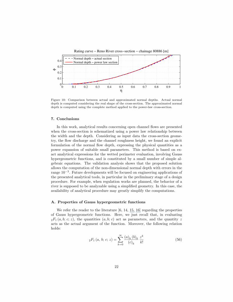
Fig. 10 shows the comparison between the two normal depth series. The verygood agreement between approximated and actual depths proofs the suitabilityof the analytical approach for the practical computation of the normal flowdepth of real rivers. In the range of meaningful flow discharges the differencebetween the two depths is less than 3%.
21
0 0.1 0.2 0.3 0.4 0.5 0.6 0.7 0.8 0.9 10
0.1
0.2
0.3
0.4
η
φRating curve − Reno River cross−section − chainage 80886 [m]
Normal depth − actual section
Normal depth − power law section
Figure 10: Comparison between actual and approximated normal depths. Actual normaldepth is computed considering the real shape of the cross-section. The approximated normaldepth is computed using the complete method applied to the power-law cross-section.
7. Conclusions
In this work, analytical results concerning open channel flows are presentedwhen the cross-section is schematized using a power law relationship betweenthe width and the depth. Considering as input data the cross-section geome-try, the flow discharge and the channel roughness height, we found an explicitformulation of the normal flow depth, expressing the physical quantities as apower expansion of suitable small parameters. This method is based on ex-act analytical expressions for the wetted perimeter evaluation, involving Gausshypergeometric functions, and is constituted by a small number of simple al-gebraic equations. The validation analysis shows that the proposed solutionallows the computation of the non-dimensional normal depth with errors in therange 10−3. Future developments will be focused on engineering applications ofthe presented analytical tools, in particular in the preliminary stage of a designprocedure. For example, when regulation works are planned, the behavior of ariver is supposed to be analyzable using a simplified geometry. In this case, theavailability of analytical procedure may greatly simplify the computations.
A. Properties of Gauss hypergeometric functions
We refer the reader to the literature [6, 14, 15, 16] regarding the propertiesof Gauss hypergeometric functions. Here, we just recall that, in evaluating
2F1 (a, b; c; z), the quantities (a, b; c) act as parameters, and the quantity zacts as the actual argument of the function. Moreover, the following relationholds:
2F1 (a, b; c; z) =
∞∑k=0
(a)k (b)k(c)k
zk
k!(56)
22
where for each real number p, (p)k is the rising factorial, or Pochhammer symbol[6]:
(p)k = 1 for k = 0 (57)
(p)k = p for k = 1
(p)k = p (p+ 1) (p+ 2) . . . (p+ k − 1) for k > 1
The Gauss hypergeometric function is usually implemented as an internalfunction in scientific computing packages (e.g. Matlab [17]).
B. Mathematical manipulations
To obtain a simplified expression for the quantity appearing in Eq. (12),ψ−2/3, consider the following substitutions:
α =(rym
)2 m
2 (2−m); (58)
β =(rym
)4 m
8 (4− 3m); (59)
z = η1−m. (60)
The quantity in the square brackets of Eq. (30), using Eqs. (58)-(60), may bewritten as
[1 + α z2 + β z4
], and the following Taylor series, up to the fourth
order, holds:
[1 + α z2 + β z4
]−2/3= 1− 2
3α z2 +
(5
9α2 − 2
3β
)z4 + o
(z4). (61)
Now, considering Eqs. (30)-(61), it is easy to write the following:
ψ−2/3 =1
η2m/3
[1− m
3 (2−m)
(rym
)2η2−2m+ (62)
+m(3 + 2m− 3m2
)9 (2−m)
2(4− 3m)
(rym
)4η4−4m
].
Considering Eq. (5), the following equation may be written:
ω5/3
ψ2/3=
(η
1 +m
)5/3
ηm[1− δ2 η2−2m + χ δ4 η4−4m
], (63)
Defining δ2 =r2y
3m(2−m) and χ = 3+2m−3m2
m(4−3m) , the equation to be solved be-
comes Eq. (33) in the Subsection 4.1.
23
References
[1] A. Valiani, V. Caleffi, Depth–energy and depth–force relationships in openchannel flows: analytical findings, Advances in Water Resources 31 (3)(2008) 447–454. doi:10.1016/j.advwatres.2007.09.007.
[2] A. Valiani, V. Caleffi, Depth–energy and depth-force relationshipsin open channel flows. ii: Analytical findings for power–law cross–sections, Advances in Water Resources 32 (2) (2009) 213–224.doi:10.1016/j.advwatres.2008.10.015.
[3] L. B. Leopold, T. Maddock, The Hydraulic Geometry of Stream Chan-nels and Some Physiographic Implications, US Geological Survey, NationalCenter, Washington, 1953.
[4] M. S. Yalin, River Mechanics, Pergamon, Tarrytown, NY, 1992.
[5] T. Strelkoff, A. Clemmens, Approximating wetted perimeter in power-lawcross section, Journal of Irrigation and Drainage Engineering 126 (2) (2000)98–109.
[6] E. W. Weisstein, Hypergeometric function,From MathWorld – A Wolfram Web Resource-Http://mathworld.wolfram.com/HypergeometricFunction.html.
[7] P. K. Swamee, P. N. Rathie, Exact solutions for normal depth problem,Journal of Hydraulic Research Vol. 42, No. 5 (2004) 541–547.
[8] E. Whittaker, G. Watson, A Course of Modern Analysis, Cambridge Uni-versity Press, Cambridge, UK., 1965.
[9] A. H. Nayfeh, Perturbation methods, John Wiley & Sons New York, 1973.
[10] Y. Wu, K. Cheung, Explicit solution to the exact Riemann problem andapplication in nonlinear shallow-water equations, International Journal forNumerical Methods in Fluids 57 (11).
[11] A. Valiani, F. Gabellini, Modello numerico dell’arno dalla diga di levanealla foce, Idrotecnica 6 (1993) 329–344.
[12] F. M. Henderson, Open Channel Flow, Prentice Hall, New York, 1966.
[13] V. T. Chow, Open-channel hydraulics, McGraw-Hill Inc., New York, 1959.
[14] C. F. Gauss, Disquisitiones generales circa seriem infinitam ... pars prior,Commentationes Societiones Regiae Scientiarum Gottingensis RecentioresReprinted in Gesammelte Werke II 3 (1812 1866) 123–163 and 207–229.
[15] E. W. Barnes, A new development in the theory of the hypergeometricfunctions, Proc. London Math. Soc. 6 (1908) 141–177.
24
[16] M. Abramowitz, I. A. Stegun, ”Hypergeometric Functions” Ch. 15 in Hand-book of Mathematical Functions with Formulas, Graphs, and MathematicalTables, Dover, New York, 9th printing, 1972.
[17] The MathWorks, Inc., Reference Manual Matlab, Release: R2008b, (Oc-tober 2008).
25