Analytical expression for compartment mathematical model of liver

59 | P a g e

Journal of Advanced & Applied Sciences (JAAS) Volume 03, Issue 02, Pages 46-50, 2015

ISSN: 2289-6260

Analytical expression for compartment mathematical model of liver

V.Ananthaswamy1,*, S.Uma Maheswari2

1Department of Mathematics, The Madura College, Madurai, Tamil Nadu, India. 2M.Phil., Mathematics, The Madura College, Madurai, Tamil Nadu, India.

* Corresponding author. Tel.:8903550705;

E-mail address: [email protected]

A b s t r a c t

Keywords:

Pharmacokinetics;

Compartment model; liver;

System of ordinary

differential equations;

Homotopy perturbation

method. .

In this research article, we discuss the mathematical model of pharmacokinetics is a growing

area in drug development. Pharmacokinetics concerns with the distribution of drugs,

chemicals tracers as a fluid among the different compartment of human body. The system of

ordinary differential equations is solved by using the Homotopy perturbation method (HPM).

Our analytical results are compared with the previous work and a satisfactory agreement is

noted. This method can be easily extended to solve the other non-liner initial and boundary

value problems in physical, chemical in engineering and sciences.

Accepted:18 April2015 © Academic Research Online Publisher. All rights reserved.

1. Introduction

A mathematical model is a description of a system

using mathematical concepts and language. The

process of developing a mathematical model is

termed mathematical modeling .A model may help

to explain a system and to study the effects of

different components and to make predictions

about behavior. Mathematical models can take

many forms, including but not limited to dynamical

system, statistical models, differential equations, or

game theoretic models.

The liver is a vital organ of vertibrates and

some other animals. In the human it is located in

the upper right quadrant of the abdomen, below the

diaphragam. The liver is a gland and plays a major

role in metabolism.

Pharmacokinetics concerns with the

distribution of drugs, chemicals tracers by a fluid

among the different compartment of human body

[2]. The present research of this three compartment

model related to the liver in the human body [3-5].

The liver carries a substance thyroxin, when it is

injected into the blood stream. Thyroxin is

transformed to iodine by the liver, iodine is

immersed into the bile [6]. Though, the

transformation or the immersion would occur

simultaneously. Thyroxin would be re circulated

when they are entered into the blood stream. The

three compartment mathematical models are given

below:

Compartment 1 represents the blood vessels,

Compartment 2 represents the liver, Compartment

3 represents the bile are shown in the following

figure;

http://www.aropub.org/journals/journal-of-advanced-applied-sciences-jaas/

V. Ananthaswamy et al. / Journal of Advanced & Applied Sciences (JAAS) 3 (2): 46-50, 2015

60 | P a g e

K12

K23 K21 K23

Fig.1: Mathematical model for liver

Where tX 1 is the quantity of thyroxin in blood

vessel at the instant time ‘ t ’, tX 2 is the quantity

of iodine in the liver, tX 3 is the quantity of

iodine absorbed in to the bile, 12K is the rate of

conversion of thyroxin into iodine, 21K is the rate

of quantity of unabsorbed thyroxin sent out for

recycling from compartment 2 , 23K is the rate of

absorption of iodine from compartment 2 into bile

compartment3. 2010 , XX and 30X are initial

values of 21 , XX and 3X respectively and the

rate of constants 2112, KK and 23K are positive

values.

It is assumed that the rate tx1 which

thyroxin is converted to iodine as it is transferred

from compartment 1 to compartment 2 is

proportional to concentration tX 1 of thyroxin in

the compartment 1.

2. Model block diagrams and model equations:

= = +

From above diagram we get the equation,

1012211121 0, XXXKXK

dt

dX (1)

= - -

-

From above diagram we get the equation,

Compartment 3

(X3)

Bile

Compartment 2

(X2)

Liver

Compartment 1

(X1)

Blood vessels

The rate of change of

thyroxin in compartment1

x1 (t)

The rate of conversion of

thyroxin into Iodine from

compartment 1 to

compartment2

(K12 X1)

(K12X1

The rate of reentry of

uncovered thyroxin from

compartment2 to

compartment 1

(K21 X2)

The rate of

absorption of

Iodine

compartment2

X2(t)

The rate of entry of

thyroxin into

compartment2 from

compartment1

(K12 X1)

The rate of reentry

from compartment2 to

compartment 1 for

recycling

(K21 X2)

The rate of transfer

of iodine from

compartment2 to

compartment3

(K23 X2)


61 | P a g e

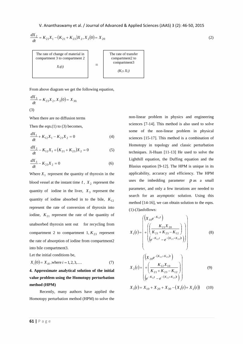
202223211212 0, XXXKKXK

dt

dX (2)

=

From above diagram we get the following equation,

.3032233 0, XXXK

dt

dX

(3)

When there are no diffusion terms

Then the eqn.(1) to (3) becomes,

02211121 XKXK

dt

dX (4)

0223211122 XKKXK

dt

dX (5)

02233 XK

dt

dX (6)

Where 1X represent the quantity of thyroxin in the

blood vessel at the instant time t , 2X represent the

quantity of iodine in the liver, 3X represent the

quantity of iodine absorbed in to the bile, 12K

represent the rate of conversion of thyroxin into

iodine, 21K represent the rate of the quantity of

unabsorbed thyroxin sent out for recycling from

compartment 2 to compartment 1, 23K represent

the rate of absorption of iodine from compartment2

into bile compartment3.

Let the initial conditions be,

00 ii XX ,where ,....3,2,1i (7)

4. Approximate analytical solution of the initial

value problem using the Homotopy perturbation

method (HPM)

Recently, many authors have applied the

Homotopy perturbation method (HPM) to solve the

non-linear problem in physics and engineering

sciences [7-14]. This method is also used to solve

some of the non-linear problem in physical

sciences [15-17]. This method is a combination of

Homotopy in topology and classic perturbation

techniques. Ji-Huan [11-13] He used to solve the

Lighthill equation, the Duffing equation and the

Blasius equation [9-12]. The HPM is unique in its

applicability, accuracy and efficiency. The HPM

uses the imbedding parameter p as a small

parameter, and only a few iterations are needed to

search for an asymptotic solution. Using this

method [14-16], we can obtain solution to the eqns.

(1)-(3)asfollows:

tKKtK

tK

ee

KKK

XK

eX

tX

232112

12

122321

2021

10

1 (8)

tKKtK

tKK

ee

KKK

XK

eX

tX

232112

2321

122321

1012

20

2 (9)

tXtXXXXtX 213020103

(10)

The rate of change of material in

compartment 3 to compartment 2

X3(t)

The rate of transfer

compartment2 to

compartment3

(K23 X2)


62 | P a g e

4. Results and discussion

Fig .2: The variation of thyroxin 1X , iodine 2X , bile 3X verses the dimensionless time t . The variations 321 ,, XXX

are computed by using eqns. (8-10) in some fixed coefficient values 232112 ,, KKK , when .1000t






63 | P a g e


are computed by using eqns. (8-10) in some fixed coefficient values 232112 ,, KKK , when .500 t






64 | P a g e



Fig .9: The variation of thyroxin 1X verses the dimensionless time t . The variation of 1X are computed by using eqns. (8-

10) in some fixed coefficient values of 2112, KK and different values of 23K , when .1000t

Fig. 10: The variation of iodine 2X verses the dimensionless time t . The variation of 2X are computed by using eqns.

(8-10) in some fixed coefficient values of 2112, KK and different values of 23K , when .1000t


65 | P a g e

Fig. 11: The variation of bile 3X verses the dimensionless time t . The variations 3X are computed by using eqns. (8-10)

in some fixed coefficient values 2112, KK and different values of 23K , when .1000t

Figs.(2)-(8) represents the variation of thyroxin

1X , iodine 2X , bile 3X verses the

dimensionless time t . The variations of 321 ,, XXX

are computed by using the eqns. (8-10) in some

fixed values of the dimensionless parameters

232112 and, KKK . From the Figs.(2)-(4), it is

clear that when t increases the variables 1X and

2X decreases and the variables 3X increases in

some fixed values of the dimensionless parameters

in the range of .1000t Fig.(5)-(8) represents

thyroxin 1X , iodine 2X , bile 3X verses the

dimensionless time t respectively. From Figs.(5)-

(8), it is observed that, when the time increases the

variables 1X and 2X decreases and the variables

3X increases in some fixed values of the

dimensionless parameters in the range of

.500t Fig.(9) represents thyroxin 1X versus

the dimensionless time t . From Fig.(9) it is noted

that when time increases the variable 1X decreases

in some fixed values of the dimensionless

parameters. Fig.(10) denotes the iodine 2X

versus the dimensionless time .t From Fig.(10) it is

clear that when the time increases the variable 2X

decreases in some fixed values of the

dimensionless parameters. Fig.(11) indicates the

bile 3X versus the dimensionless time t . From

Fig.(11), we observe that when the time increases,

the variable 3X increases in some fixed values of

the dimensionless parameters.

5. Conclusion

The system of linear ordinary differential

equations for a three compartment mathematical

model of liver has been solved analytically. The

variation of thyroxin tX1 , iodine tX 2 , bile

tX 3 where obtained by using the Homotopy

perturbation method (HPM). Our analytical results

are compared with previous work and found to be

in good agreement. The primary result of this work

is simple and approximate expressions for all

values of the dimensionless parameters.

Acknowledgement

The authors are thankful to Shri. S.

Natanagopal, Secretary, The Madura College

Board, Dr. R. Murali, The Principal and Mr. S.

Muthukumar, Head of the Department of

Mathematics, The Madura College (Autonomous),

Madurai, Tamil Nadu, India for their constant

encouragement.


66 | P a g e

Appendix A

Basic concept of the Homotopy perturbation

method (HPM) [10-12]

To explain this method, let us consider the

following function:

r ,0)()( rfuDo (A.1)

with the boundary conditions of

r ,0) ,(

n

uuBo (A.2)

where oD is a general differential operator, oB is

a boundary operator, )(rf is a known analytical

function and is the boundary of the domain .

In general, the operator oD can be divided into a

linear part L and a non-linear part N . The eqn.

(A.1) can therefore be written as

0)()()( rfuNuL (A.3)

By the Homotopy technique, we construct a

Homotopy ]1,0[:),( prv that satisfies

.0)]()([

)]()()[1(),(

0

rfvDp

uLvLppvH

o

(A.4)

.0)]()([)(

)()(),(

0

0

rfvNpupL

uLvLpvH (A.5)

where p[0, 1] is an embedding parameter, and

0u is an initial approximation of eqn. (A.1) that

satisfies the boundary conditions. From eqns. (A.4)

and (A.5), we have

0)()()0,( 0 uLvLvH (A.6)

0)()()1,( rfvDvH o (A.7)

When p=0, the eqns. (A.4) and (A.5) become linear

equations. When p =1, they become non-linear

equations. The process of changing p from zero to

unity is that of 0)()( 0 uLvL to

0)()( rfvDo . We first use the embedding

parameter p as a “small parameter” and assume

that the solutions of eqns. (A.4) and (A.5) can be

written as a power series in p :

...22

10 vppvvv (A.8)

Setting 1p results in the approximate solution

of the eqn. (A.1):

...lim 2101

vvvvup

(A.9)

This is the basic idea of the HPM.

Appendix B

Solution of the boundary value problem eqns.

(1)-(3) using the Homotopy perturbation method

[7-17]

In this appendix we indicate the equations (4) – (7)

are derived in this paper. To find the solution of the

equations (1) – (3), we construct a Homotopy as

follows:

0

1

2211121

1121

XKXKdt

dXp

XKdt

dXp

(B.1)

0

1

223211122

223212

XKKXKdt

dXp

XKKdt

dXp

(B.2)

01 22333

XK

dt

dXp

dt

dXp (B.3)

The analytical solutions of (B.1),(B.2) and (B.3) is,

........210 1

2111 XppXXX (B.4)

........210

22

222 XppXXX (B.5)

........210

32

333 XppXXX (B.6)

Substituting the eqns. (B.4), (B.5) and (B.6) in

(B.1), (B.2) and (B.3) respectively we get,


67 | P a g e

0

.....

.....

.....

.....

.....

1

2

10

2

10

210

2

10

210

22

22

21

12

11

12

12

11

12

11

12

12

11

Xp

pXXK

Xp

pXXK

dt

XppXXd

p

Xp

pXXK

dt

XppXXd

p

(B.7)

0

.....

.....

)(

.....

.....

)

.....

1

2

10

2

10

2

10

2

10

210

12

11

12

22

22

2321

22

22

22

22

2321

22

22

Xp

pXXK

Xp

pXX

KK

dt

Xp

pXXd

p

Xp

pXX

KK

dt

XppXXd

p

(B.8)

0

.....

.....

.....1

2

102

210

210

22

2

23

32

33

32

33

Xp

pXX

K

dt

XppXXd

p

dt

XppXXdp

(B.9)

Comparing the coefficients like powers of p in

(B.7), (B.8) and (B.9) we get,

.0:0

0

112

10 XKdt

dXp (B.10)

.0:0

0

22321

20 XKKdt

dXp (B.11)

.0: 030 dt

dXp (B.12)

01

1

221112

11 : XKXKdt

dXp (B.13)

.:01

1

11222321

21 XKXKKdt

dXp (B.14)

.:0

1

223

31 XKdt

dXp (B.15)

The initial approximations are as follows:

303202101 )0(;)0(;0 XXXXXX (B.16)

......,3,2,1;00 iX i (B.17)

Solving the eqns. (B.10) to (B.15) and using the

initial conditions (B.16) and (B.17), we obtain the

following results:

tX01 tK

eX 1210

(B.18)

tX11

.

232112

122321

2021

tKKtKee

KKK

XK

(B.19)

tX02

tKKeX 2321

20

(B.20)

tX12

tKKtKee

KKK

XK

232112

122321

1012

(B.21)

tXtXXXXtX 213020103 (B.22)

According to the HPM, we can conclude that

)(lim 111

11 10

XXtXXp

(B.23)

)(lim10 222

12 XXtXX

p

(B.24)

)(lim 333

13 10

XXtXXp

(B.25)

After putting the eqns. (B.18) and (B.19) into an

eqn. (B.23) and (B.20) and (B.21) into an eqn. eqn.

(B.24) and (B.22) into an eqn. (B.25) we obtain the

solutions in the text eqns. (8)-(10).


68 | P a g e

Appendix: C

Nomenclature

Symbol Meaning

tX1 The quantity of thyroxin in the blood vessels at the instant time t

tX 2 The quantity of iodine in the liver.

tX 3 The quantity of iodine absorbed in to the bile.

12K The rate of conversion of thyroxin into iodine.

21K The rate of the quantity of un absorbed thyroxin sent out for recycling from

compartment 2 to compartment 1.

23K Rate of absorption of iodine from compartment 2 into bile compartment 3.

tx1 The rate of change of thyroxin into iodine from compartment 1 to compartment 2is proportional to

concentration of thyroxin in the compartment 1.

References

[1] Anand V, Pattabhi Ramacharyalu N Ch .

A three compartment mathematical model of liver,

ARPN Journal of engineering and applied sciences,

2014; 9(11).

[2] Kapur J N. Mathematical models in Biology

and Medicine, Affiliated east-west press pvt .Ltd,

1985;316-317.

[3] Evert C F, Randal M F. Formulation and

computation of compartment models, J. pharm. Sci,

1970; 9(3):102-114.

[4] Jacquez John A. compartment analysis in

biology and medicine, New York: Elsevier

scientific publishing company.

[5] Watt J M, Andrew Young. An attempt to

simulate the liver on a computer, computer

Journal, 1962;5:221-227.

[6] Geoffery G. System simulation, Prenticehal

India, 1999;34-36.

[7] Ozis T, Yildirim A. A Comparative study of

He’s Homotopy perturbation method for

determining frequency-amplitude relation of a

nonlinear oscillator with discontinuities, Int. J.

Nonlinear Sci. Numer. Simulat 2007;8:243-248.

[8] Li S J , Liu Y X , An Improved approach to

nonlinear dynamical system identification using

PID neural networks, Int. J. Nonlinear Sci. Numer.

Simulat, 2006;7:177-182.

[9] Mousa M M, Ragab.S F, Nturforsch Z.

Application of homotopy perturbation method to

linear and nonlinear Schrödinger equations,.

Zeitschrift für Naturforschung,2008;63:140-144

[10] He J H. Homotopy perturbation technique,

Comp Meth. Appl. Mech. Eng, 1999;178:257-262.

[11] He J H. Homotopy perturbation method: a new

nonlinear analytical technique, Appl. Math.

Comput, 2003;135:73-79.

[12] He J H. A simple perturbation approach to

Blasius equation, Appl. Math. Comput

2003;140:217-222.

[13] Ariel P D. Alternative approaches to

construction of Homotopy perturbation

Algorithms, Nonlinear. Sci. Letts. 2010;A.1:43-52.

[14] Ananthaswamy V , Rajendran L. Approximate

analytical solution of non-linear kinetic equation in

a porous pellet, Global Journal of pure and applied

mathematics, 2012;8(2):101-111.

[15] Ananthaswamy V , Rajendran.L. Analytical

solution of two-point non-linear boundary value

problems in a porous catalyst particles,

International Journal of Mathematical Archive,

2012;3(3):810-821.


69 | P a g e

[16] Ananthaswamy V ,Rajendran L. Analytical

solution of non-isothermal diffusion-reaction

processeses and effectiveness factors, ISRN-

Physical chemistry, 2013;1-14.

[17] Ananthaswamy V , Ganesan S, Rajendran L,

Approximate analytical solution ofnon-linear

boundary value problem in steady state flow of a

liquid film: Homotopy perturbation method,

International Journal of applied sciences and

engineering research, 2013;2(5):569-578.

Analytical expression for compartment mathematical model of liver

Documents

Transcript of Analytical expression for compartment mathematical model of liver