1

Analytical Estimation of Path Duration in Mobile

Ad Hoc NetworksKamesh R. Namuduri

Department of Electrical Engineering

University of North Texas

Email: kamesh.namuduri@unt.edu

Manivannan Srinivasan

Email: manivannan.srinivasan@gmail.com

SreeKalyan Devaraj and Ravi Pendse

Department of Electrical and Computer Engineering

Wichita State University

Email: sxdevaraj@wichita.edu, ravi.pendse@wichita.edu

Abstract

Path duration is an important design parameter that determines the performance of a mobile ad hoc network

(MANET). For example, it can be used to estimate the route expiry time parameter for routes in “on demand” routing

protocols. This paper proposes an analytical model to estimate the path duration in a MANET using random way point

(RWP) mobility model as a reference. The salient feature of the proposed model is that it establishes a relationship

between path duration and MANET design parameters including node density, transmission range, number of hops,

and velocity of nodes. Although this relationship has been previously demonstrated through simulations, a detailed

analytical model is not available in the literature to date. In particular, the relationship between path duration and

node density has not been derived in previous models. The accuracy of the proposed model is validated by comparing

the results obtained from the analytical model with the experimental results available in literature.

I. INTRODUCTION

Ad hoc networks have numerous real world applications including emergency search and rescue, defense, and

surveillance to mention few. Although fixed or static ad hoc networks (for example, metro Wi-Fi mesh network)

have gained momentum in the business community, there are numerous challenges that need to be addressed by

the research community, before the deployment of MANETs becomes practical. One such challenge is the design

and development of routing techniques that can adapt to the highly unpredictable topological changes that occur

due to mobility of nodes in a MANET.

2

Whenever a route becomes invalid, a mobile node has to find a new route to the destination. This affects the

ongoing communication and increases the overhead (for example, control traffic) created by the routing protocol.

Accurate prediction of path duration (for which a typical route will be valid) will help increase the performance of

a routing protocol. Path duration is the minimum link residual life along the path to the destination consisting of

individual links. Having the knowledge of link residual life and path duration in the network helps in the assignment

of an optimum value to the route expiry time parameter, the duration for which a route should be active in the

routing table, in a routing protocol.

The prediction of path duration for a selected path is not easy, as it depends on several parameters such as the

position and number of relay nodes, their velocity, direction of movement etc. Such a prediction would be easy for

GPS (Global Positioning System) installed networks, but very few MANETs use GPS. The most popular routing

protocols (designed for ad hoc networks) such as the Dynamic Source Routing (DSR) and the Adhoc On-demand

Distance Vector (AODV) routing protocol, do not select a path based on its expected duration. DSR selects a

path which has the minimum hop count to reach the destination and AODV selects the first available route. The

knowledge of the expected path duration, if incorporated, will significantly enhance the performance of the routing

protocols as well as the throughput of the MANET.

This paper proposes an analytical model for estimating the path duration in a MANET. Previous work done on

this subject relied mainly on simulations. There is no analytical model in the literature that includes node density

that can be used for estimating the path duration in a MANET to our knowledge. Due to the highly unpredictable

nature of mobile nodes, it is a challenge to model path duration. This paper demonstrates its feasibility under a

few reasonable assumptions. In this process, we make use of the fact that most routing protocols developed for

MANET are based on the principle of Least Remaining Distance (LRD). The LRD forwarding technique is similar

to the shortest path forwarding, where a route to a destination is selected based on the principle of least number

of hops.

The remainder of this paper is organized as follows. Section 2 presents the literature survey on path duration

and mobility models, particularly on Random Way Point (RWP) model. Section 3 presents the proposed model

for path duration in detail. Section 4 presents the results and a comparison between the theoretical results and the

experimental results available in the literature. Conclusions are presented in section 5.

II. LITERATURE REVIEW

Mobility models play an important role in analytical modeling of mobile ad hoc networks. Random waypont

(RWP) mobility, reference point group (RPG) mobility, free way (FW), and Manhattan are some of the models that

have bene proposed in the literature. Among these models, RWP model, due to its wide use, has been a subject of

active research. For example, an analysis of a generalized RWP model is presented in [3] and it has been suggested

that RWP fails to provide a steady state in terms of average speed in [4]. An analytical study of the spatial node

distribution in RWP has been developed and an exact expression of this distribution is presented in [5].

3

Initial attempts to link path duration to performance of mobile ad hoc networks appeared in [6]–[8]. The

correlation between average path duration, throughput and overhead of the reactive routing protocols is investigated

in [6]. It presents the probability density functions (PDFs) of the path duration and link residual life for various

mobility models including RWP, RPG, FW, and Manhattan. The main parameters considered in this model include

relative velocity of nodes, transmission range and number of hops which influence path duration. The path duration

model is based on a combination of logical reasoning and simulations. Even though the authors identified node

density as an important parameter that influences path duration, they didn’t attempt to develop this relationship.

This is the motivation for our work, in which we develop a clear and simple model for predicting the average path

duration based on the known network parameters. In particular, we establish the influence of network density (along

with other parameters such as the transmission range, maximum velocity and number of hops) on path duration.

The PDF of average path duration is assumed to be exponential (as in [6], [7], [9]).

A model that demonstrates the exponential nature of path duration (viewed as a random variable) is presented in

[9]. Palm’s theorem has been used to prove the emergence of exponential distribution under a set of mild conditions.

The correlation between the excess life times of two neighboring links has been studied and it has been concluded

that this correlation is often very weak for RWP mobility model. The two models developed in [6] and [9] assume

that the behavior of most existing “on demand” routing protocols are based on the principle of shortest path. The

assumption of shortest path for MANET routing protocols has also been used in [10].

Link distances and their relationship with hop count has been examined in [2]. In developing this relationship, it

is assumed that the selection of a relay node is a function of the least remaining distance (LRD) to destination. The

authors also point out that the process of node localization, and estimation of end-to-end delay, jitter and transmit

power also benefit from the knowledge of hop count. An analytical model for LRD and bounds on hop distance

for a given Euclidean distance between nodes has been developed [2]. This paper also assumes that the shortest

path forwarding process is identical or can be approximated to LRD forwarding. A relatively simple method that

helps in the analysis of path duration is used for LRD forwarding.

Optimal transmission radius for radio terminals has been investigated in [11]. The authors analyzed the relationship

between average distance progress per hop and link distances. A relationship between network throughput and the

average degree of a node has also been developed. It has been shown that for a constant average degree, throughput

is proportional to the square root of the number of nodes in the network. It has been shown that the optimal number

of neighbors that a node can have is six, when a tradeoff between channel usage and number of hops in achieving

maximum throughput is considered.

Stability and hop count based ad hoc routing has been proposed in [12]. It is an enhancement to the existing hop

count based routing protocols such as DSR and AODV. The stability metric used in this analysis is the residual

life time of a link. Residual life time of a link is defined as the difference between the average link duration and

the current age of the link. It has been suggested that the notion of “older links are more stable”, used by other

stability based routing protocols such as the Associativity Based Routing (ABR) will not hold good for a wide

4

spectrum of speeds and mobility models and the reverse hypothesis could be true (new links are more stable).

A scheme to explore long lifetime routing in MANETs is proposed in [13]. This paper suggests that the shortest

path is not the best path when the path duration is taken into account. It has been also suggested that simply

extending the route length will not fetch paths of longer duration. Furthermore, this paper points out that the

lifetime estimation of links is essential for finding routes that can sustain for longer time. An algorithm for long

lifetime route selection is proposed and it is shown that the algorithm works best, if the nodes are able to acquire

global knowledge.

There have been very limited number of studies that focussed on the theoretical aspects of link lifetime in

MANETs. The behavior of communication links in random mobility environment has been investigated in [1]. The

authors developed the probability distributions of link lifetime, new link arrival time, and link change interarrival

time. Mobility metrics including link availability, link persistence, link residual tome, and link duration in MANETs

are investigated in [14]. The authors derived the probability distribution of link lifetime under random-walk mobility

model. Both these studies provide insights into the analysis of link lifetime. However, neither of these models

considered node density explicitly in the derivations. and discuss the relationships among these metrics. they also

present a theoretical framework for calculating these metrics.

Link stability and route lifetime have been analyzed in [15]. This paper also discusses a phenomenon called

“edge effect” that occurs at high node density. It is pointed out that when the node density is high, the chances of

finding relay nodes at the edges of transmission radius are very high. In such a situation, even a small movement

of nodes will lead to link breakage and ultimately to the path breakage. Due to the edge effect, the average lifetime

of a route decreases. This result indicates that increasing the node density of network may not result in higher

performance of a mobile network, unless this increase is accompanied by suitable routing protocols. It is under

these circumstances, our proposed model becomes more useful.

III. NETWORK MODEL

A mobile ad hoc network can be viewed as a static network at a particular instant of time, in which, the topology

changes can be predicted from that instant to the next instant based on the assumed mobility model. Consistent

with the literature, let us use the LRD forwarding process as an approximation to shortest path based forwarding.

Since there could be many paths between the source and the destination, analyzing the duration of all these paths

is not feasible. Given that the behavior of “on demand” routing protocols is closely associated with the shortest

path, the analysis of average path duration based on shortest path principle is appropriate and meaningful.

A. Least remaining distance (LRD) and shortest path

In LRD forwarding, among all the available forwarding (or relay) nodes, the node which has the minimum

distance to the destination is selected as relay node [2]. This behavior is similar to shortest path because shortest

path attempts to reach the destination with the least number of hops, which is possible only when the node with

5

minimum remaining distance to destination is selected as a relay node. This observation is true when suboptimal

methods (such as greedy methods) for shortest path selection are used. It may not be true in certain cases for

example, when the node density is low and shortest path based on global optimization is used.

B. Link residual life

Link residual life is defined as the time during which a link will be active once it becomes a part of a path. A

link between two mobile nodes will be active as long as they are in the transmission range of each other. Link

residual life (t) can be expressed as the ratio

t =d

vr, (1)

where d is the distance that the neighbor (relay) node needs to travel to get out of the transmission range of its

neighbor and vr is the relative velocity between the two neighbors.

In the following subsections, the PDF for the path duration Tpath and its expected value are derived using

fundamental principles. In order to find the distribution of link residual life, the distributions of D and Vr need to

be known. In this analysis, the neighbors that do not fall in the path towards the destination are ignored and only

those nodes which are on the path to destination are considered.

C. Link distance

Let us start with the link distance, which is dependent on the underlying routing protocol used in the MANET.

Since most “on demand” routing protocols such as DSR and AODV are based on the principle of shortest path,

link distances can be analyzed based on the same principle. Shortest path is achieved in LRD forwarding method

by the selection of a relay node with least distance to the destination.

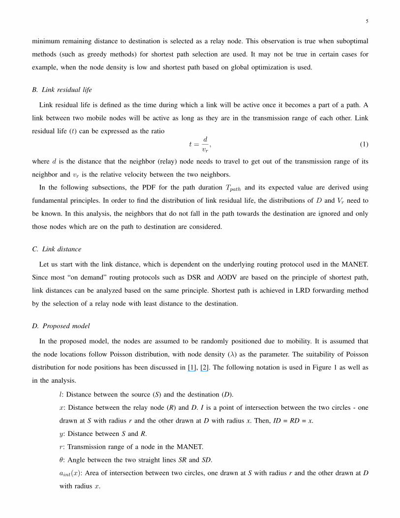
D. Proposed model

In the proposed model, the nodes are assumed to be randomly positioned due to mobility. It is assumed that

the node locations follow Poisson distribution, with node density (λ) as the parameter. The suitability of Poisson

distribution for node positions has been discussed in [1], [2]. The following notation is used in Figure 1 as well as

in the analysis.

l: Distance between the source (S) and the destination (D).

x: Distance between the relay node (R) and D. I is a point of intersection between the two circles - one

drawn at S with radius r and the other drawn at D with radius x. Then, ID = RD = x.

y: Distance between S and R.

r: Transmission range of a node in the MANET.

θ: Angle between the two straight lines SR and SD.

aint(x): Area of intersection between two circles, one drawn at S with radius r and the other drawn at D

with radius x.

6

θ2l

x

Dθ1

θy

r

A2

A1s

z

R

Δx

x: distance between I and D, same as the distance between R and Dy: distance between S and Rl: distance between S and Dr: transmission range of Sθ : angle between SR and SDz: straight line distance between S and RA1+A2: area of intersection between circles drawn at S and D θ1: angle between SI and SDθ2: angle between ID and SD

I

S: sourceD: destinationR: relayI: point on the circle which is atthe same distance as R from D

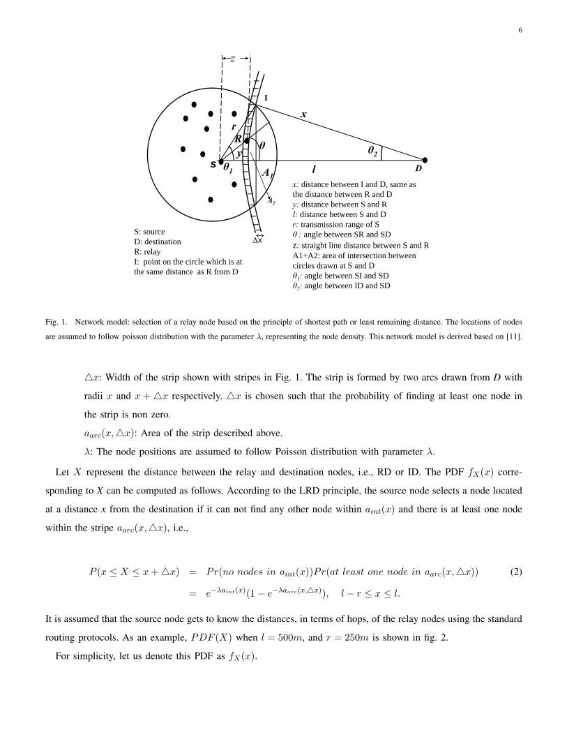
Fig. 1. Network model: selection of a relay node based on the principle of shortest path or least remaining distance. The locations of nodes

are assumed to follow poisson distribution with the parameter λ, representing the node density. This network model is derived based on [11].

4x: Width of the strip shown with stripes in Fig. 1. The strip is formed by two arcs drawn from D with

radii x and x +4x respectively. 4x is chosen such that the probability of finding at least one node in

the strip is non zero.

aarc(x,4x): Area of the strip described above.

λ: The node positions are assumed to follow Poisson distribution with parameter λ.

Let X represent the distance between the relay and destination nodes, i.e., RD or ID. The PDF fX(x) corre-

sponding to X can be computed as follows. According to the LRD principle, the source node selects a node located

at a distance x from the destination if it can not find any other node within aint(x) and there is at least one node

within the stripe aarc(x,4x), i.e.,

P (x ≤ X ≤ x+4x) = Pr(no nodes in aint(x))Pr(at least one node in aarc(x,4x)) (2)

= e−λaint(x)(1− e−λaarc(x,4x)), l − r ≤ x ≤ l.

It is assumed that the source node gets to know the distances, in terms of hops, of the relay nodes using the standard

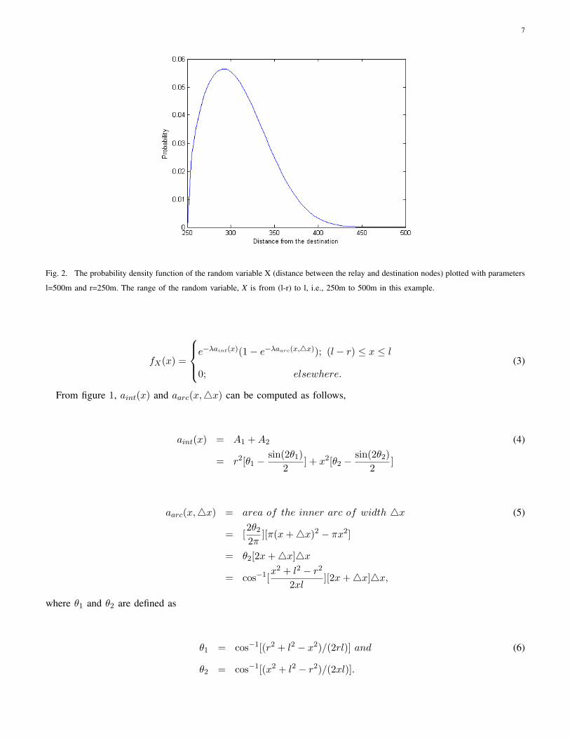
routing protocols. As an example, PDF (X) when l = 500m, and r = 250m is shown in fig. 2.

For simplicity, let us denote this PDF as fX(x).

7

Fig. 2. The probability density function of the random variable X (distance between the relay and destination nodes) plotted with parameters

l=500m and r=250m. The range of the random variable, X is from (l-r) to l, i.e., 250m to 500m in this example.

fX(x) =

e−λaint(x)(1− e−λaarc(x,4x)); (l − r) ≤ x ≤ l

0; elsewhere.

(3)

From figure 1, aint(x) and aarc(x,4x) can be computed as follows,

aint(x) = A1 +A2 (4)

= r2[θ1 −sin(2θ1)

2] + x2[θ2 −

sin(2θ2)2

]

aarc(x,4x) = area of the inner arc of width 4x (5)

= [2θ22π

][π(x+4x)2 − πx2]

= θ2[2x+4x]4x

= cos−1[x2 + l2 − r2

2xl][2x+4x]4x,

where θ1 and θ2 are defined as

θ1 = cos−1[(r2 + l2 − x2)/(2rl)] and (6)

θ2 = cos−1[(x2 + l2 − r2)/(2xl)].

8

Details of these derivations are given in appendix A. From fX(x), the expected distance from the relay node to

the destination node can be computed as,

E[X] =1A

∫ l

(l−r)xfX(x)dx

=1A

∫ l

(l−r)xe−λaint(x)(1− e−λaarc(x,4x))dx. (7)

Let us define z, the distance progress per hop towards the destination, made by the choice of the relay node.

From fig.1,

z = l − xcosθ2. (8)

Substituting the value of cosθ2 from (7)

z = l − x(x2 + l2 − r2)2xl

(9)

which leads to

x2 = l2 + r2 − 2lz. (10)

Therefore,

x =√l2 + r2 − 2lz = g−1(z), and (11)

z =

√l2 + r2 − x2

2l= g(x).

In order to compute fZ(z) from fX(x), we use

fZ(z) = fX [g−1(z)]dg−1(z)dz

. (12)

The differentiation of g−1(z) is,

dg−1(z)dz

=−l√

l2 + r2 − 2lz. (13)

Since r and l are constants with respect to z, we get,

dx =−l√

l2 + r2 − 2lzdz. (14)

From the expression for x in equation (12) we get,

∆x =−l√

l2 + r2 − 2lz∆z. (15)

From (7), θ1 and θ2 can be expressed in terms of z as follows:

θ1(z) = cos−1(zr

)and (16)

θ2(z) = cos−1

(l − z√

l2 + r2 − 2lz

).

9

Therefore, aarc(x,4x) can be expressed in terms of z as follows,

aarc(z,4z) = cos−1

(l − z√

l2 + r2 − 2lz

)[2− l4z

l2 + r2 − 2lz

](−l4z). (17)

Similarly, aint(z) is given by,

aint(z) = r2[θ1(z)− sin 2θ1(z)

2

]+ (l2 + r2 − 2lz)

[θ2(z)− sin 2θ2(z)

2

](18)

= r2

[cos−1(

z

r)− z

√r2 − z2

r

]+ (l2 + r2 − 2lz)

[cos−1(

l − zl2 + r2 − 2lz

)−√

r2 − z2

l2 + r2 − 2lz

].

Also,

fX(g−1(z)) = e−λaint(z)[1− e−λaarc(z,4z)]. (19)

By substituting the expressions for dg−1(z)dz in and fX(g−1(z)) into equation (12), we obtain,

fZ(z) =−l√

l2 + r2 − 2lze−λaint(z)[1− e−λaarc(z,4z)]. (20)

Once fZ(z) is known, the expected value of this length is calculated by,

E[Z] =∫ r

0zfZ(z)dz. (21)

E. Relative velocity

In order to find the PDF corresponding to the relative velocity, the source node S is assumed to be fixed and

the relative movement of the relay node with respect to S is considered. Relative velocity between the source and

relay nodes is given by,

vr =√v21 + v2

2 − 2v1v2 cosα (22)

where, α is the angle between the velocity vectors v1 , v2. Assuming that all nodes move with an average (constant)

velocity, we can write v1 = v2 = v. Hence, vr can be expressed as follows,

vr = v√

2− 2 cosα = 2v sinα

2(23)

where, α is a random variable whose range is (0, 2π). The relay node may move either towards the source node or

away from the source node with equal probability (0.5). The link between the source and relay node breaks when

the relay node moves in the direction away from the source node. It is sufficient if node movement away from

the source is considered since this causes the link between the source and the relay node to break. Since α varies

within (0, 2π) with uniform probability, α2 can be assumed to vary with uniform probability between (0, π), the

pdf of fα2(α2 ) is given by

fα2(α

2) =

1π. (24)

10

From (23), the pdf of Vr, fVr(vr) is expressed as,

fVr(vr) =1√

4v2 − v2r

1π. (25)

F. Link residual life

Link residual life t is given by,

t =d

vr.

where d = r−z, which is the straight line distance that the relay node needs to travel to get out of the transmission

range of S. Hence, fT (t) is given by,

fT (t) =∫ vmax

0vrfDVr(vrt, vr)dvr

=∫ vmax

0[fD(d)]d=vrt[

vr√4v2 − v2

r

1π

]dvr (26)

where vmax is the maximum relative velocity and v is the velocity of a node as described in (23). The above

equation corresponds to the one hop residual life of a link.

G. Path duration

Path duration (tpath) is derived from the PDF of the link residual life. If the number of hops needed to reach

the destination is h, then tpath can be written as

tpath = min(t1, t2, t3....th) (27)

where ti is the link resiudal time corresponding to ith link. Using Baye’s theorem [2] and Chapter 6 in [16], the

PDF of Tpath can be expressed as

f(Tpath) = hfTpath(tpath)Ch−1Tpath

(28)

where CTpath = 1− FTpath is the complementary CDF of Tpath. Expanding fTpath(tpath), we get,

fTpath(tpath) = h

[∫ vmax

0[fD(d)]d=vrt

[vr√

4v2 − v2r

1π

]dvr

][

1−∫ tpath

0

[∫ vmax

0[fD(d)]d=vrt[

vr√4v2 − v2

r

1π

]dvr

]dtpath

]h−1

.

(29)

Average path duration is given by,

11

E[Tpath] =∫ α

0tpathfTpath(tpath)dtpath. (30)

The average number of hops to reach the destination, E[H], is expressed as,

E[H] =E[L]E[Z]

(31)

where E[L] is the average distance between the source and destination (average path length) and E[Z] is the average

distance progress per hop. From [9],

E[L] =12845π

r. (32)

IV. RESULTS AND DISCUSSION

In this section, the proposed model is validated by comparing the theoretical results obtained from this model

using MATLAB with the experimental results obtained based on RWP mobility model presented in [6]. In the

following subsections, average path duration is computed by varying the each parameter that path duration depends

on. The set of independent parameters that determine path duration include transmission range, maximum velocity,

number of hops and node density. Validation of the proposed model is achieved by using the same values for input

parameters as used in [6].

A. Average path duration versus transmission range

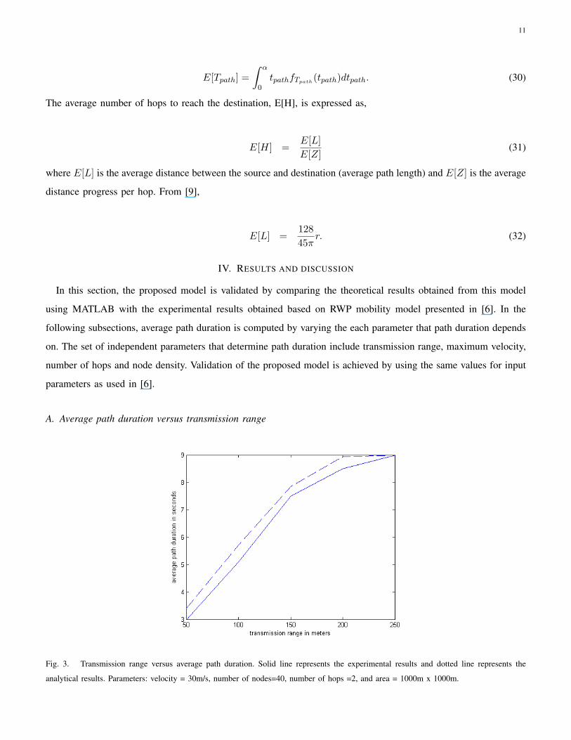
Fig. 3. Transmission range versus average path duration. Solid line represents the experimental results and dotted line represents the

analytical results. Parameters: velocity = 30m/s, number of nodes=40, number of hops =2, and area = 1000m x 1000m.

12

Figure 3 shows the plot between transmission range and average path duration. This plot suggests that the average

path duration increases linearly with increase in transmission range. If the transmission range is high, the probability

of a relay node’s location being well within the circle of transmission range, is higher. Hence, the distance that the

relay node needs to travel for the link to break is higher. This gives greater room for mobility of the relay node,

thereby resulting in higher path duration.

B. Average path duration versus average node velocity

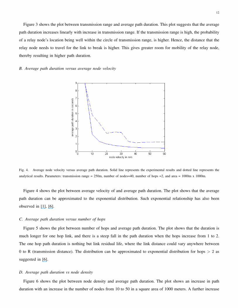
Fig. 4. Average node velocity versus average path duration. Solid line represents the experimental results and dotted line represents the

analytical results. Parameters: transmission range = 250m, number of nodes=40, number of hops =2, and area = 1000m x 1000m.

Figure 4 shows the plot between average velocity of and average path duration. The plot shows that the average

path duration can be approximated to the exponential distribution. Such exponential relationship has also been

observed in [1], [6].

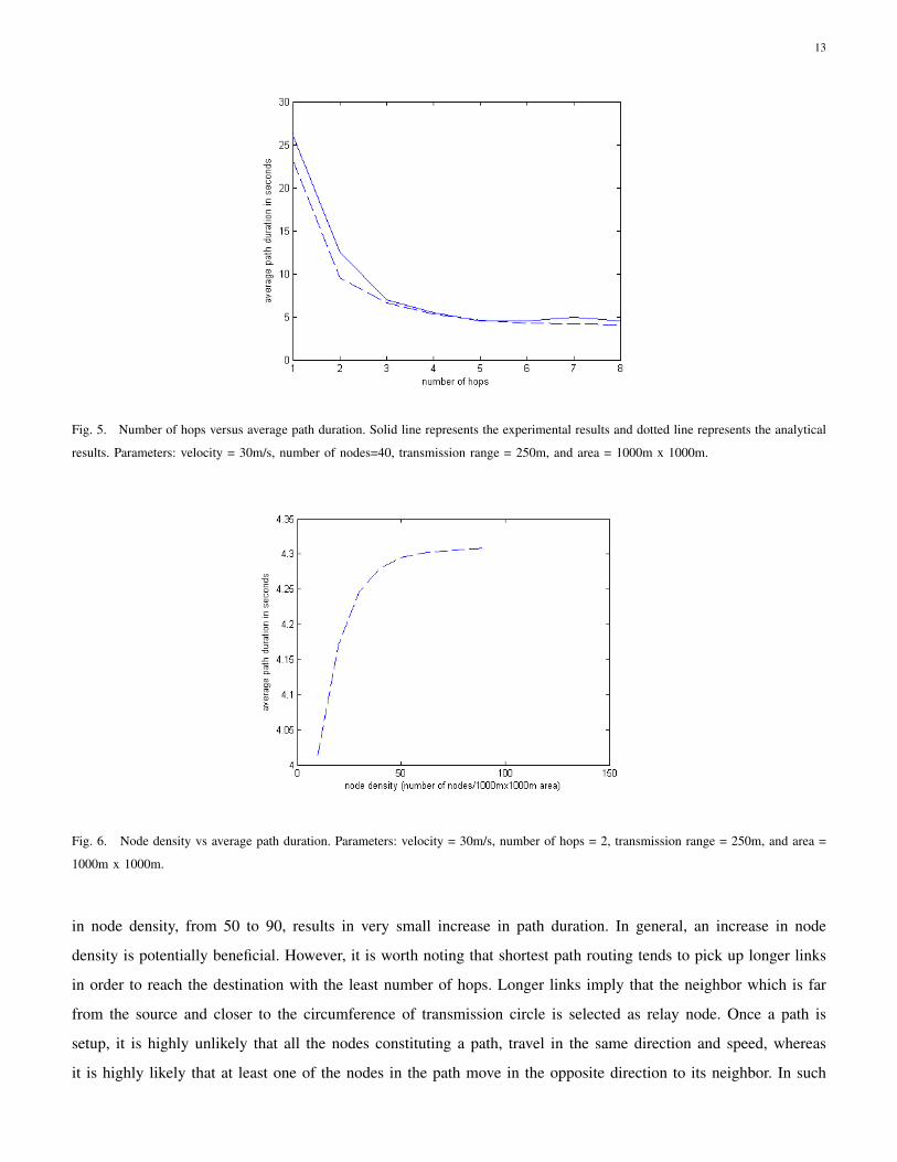
C. Average path duration versus number of hops

Figure 5 shows the plot between number of hops and average path duration. The plot shows that the duration is

much longer for one hop link, and there is a steep fall in the path duration when the hops increase from 1 to 2.

The one hop path duration is nothing but link residual life, where the link distance could vary anywhere between

0 to R (transmission distance). The distribution can be approximated to exponential distribution for hops > 2 as

suggested in [6].

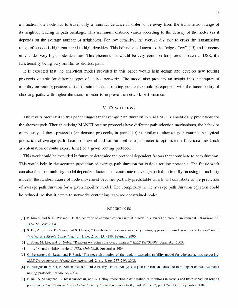
D. Average path duration vs node density

Figure 6 shows the plot between node density and average path duration. The plot shows an increase in path

duration with an increase in the number of nodes from 10 to 50 in a square area of 1000 meters. A further increase

13

Fig. 5. Number of hops versus average path duration. Solid line represents the experimental results and dotted line represents the analytical

results. Parameters: velocity = 30m/s, number of nodes=40, transmission range = 250m, and area = 1000m x 1000m.

Fig. 6. Node density vs average path duration. Parameters: velocity = 30m/s, number of hops = 2, transmission range = 250m, and area =

1000m x 1000m.

in node density, from 50 to 90, results in very small increase in path duration. In general, an increase in node

density is potentially beneficial. However, it is worth noting that shortest path routing tends to pick up longer links

in order to reach the destination with the least number of hops. Longer links imply that the neighbor which is far

from the source and closer to the circumference of transmission circle is selected as relay node. Once a path is

setup, it is highly unlikely that all the nodes constituting a path, travel in the same direction and speed, whereas

it is highly likely that at least one of the nodes in the path move in the opposite direction to its neighbor. In such

14

a situation, the node has to travel only a minimal distance in order to be away from the transmission range of

its neighbor leading to path breakage. This minimum distance varies according to the density of the nodes (as it

depends on the average number of neighbors). For low densities, the average distance to cross the transmission

range of a node is high compared to high densities. This behavior is known as the “edge effect” [15] and it occurs

only under very high node densities. This phenomenon would be very common for protocols such as DSR, the

functionality being very similar to shortest path.

It is expected that the analytical model provided in this paper would help design and develop new routing

protocols suitable for different types of ad hoc networks. The model also provides an insight into the impact of

mobility on routing protocols. It also points out that routing protocols should be equipped with the functionality of

choosing paths with higher duration, in order to improve the network performance.

V. CONCLUSIONS

The results presented in this paper suggest that average path duration in a MANET is analytically predictable for

the shortest path. Though existing MANET routing protocols have different path selection mechanisms, the behavior

of majority of these protocols (on-demand protocols, in particular) is similar to shortest path routing. Analytical

prediction of average path duration is useful and can be used as a parameter to optimize the functionalities (such

as calculation of route expiry time) of a given routing protocol.

This work could be extended in future to determine the protocol dependent factors that contribute to path duration.

This would help in the accurate prediction of average path duration for various routing protocols. The future work

can also focus on mobility model dependent factors that contribute to average path duration. By focusing on mobility

models, the random nature of node movement becomes partially predictable which will contribute to the prediction

of average path duration for a given mobility model. The complexity in the average path duration equation could

be reduced, so that it caters to networks containing resource constrained nodes.

REFERENCES

[1] P. Kumar and S. B. Wicker, “On the behavior of communication links of a node in a multi-hop mobile environment,” MobiHoc, pp.

145–156, May 2004.

[2] S. De, A. Caruso, T. Chaira, and S. Chessa, “Bounds on hop distance in greedy routing approach in wireless ad hoc networks,” Int. J.

Wireless and Mobile Computing, vol. 1, no. 2, pp. 131–140, February 2006.

[3] J. Yoon, M. Liu, and B. Noble, “Random waypoint considered harmful,” IEEE INFOCOM, September 2003.

[4] ——, “Sound mobility models,” IEEE MobiCOM, September 2003.

[5] C. Bettstetter, G. Resta, and P. Santi, “The node distribution of the random waypoint mobility model for wireless ad hoc networks,”

IEEE Transactions on Mobile Computing, vol. 2, no. 3, pp. 257–269, 2003.

[6] N. Sadagopan, F. Bai, B. Krishnamachari, and A.Helmy, “Paths: Analysis of path duration statistics and their impact on reactive manet

routing protocols,” MobiHoc, 2003.

[7] F. Bai, N. Sadagopan, B. Krishnamachari, and A. Helmy, “Modeling path duration distributions in manets and their impact on routing

performance,” IEEE Journal on Selected Areas of Communications (JSAC), vol. 22, no. 7, pp. 1357–1373, September 2004.

15

[8] A. Mcdonald and T. Znati, “A path availability model for wireless ad-hoc networks,” Proceedings of the IEEE Wireless Communications

and Networking Conference, 1999.

[9] Y. Han, R. J. La, and A. M. Makowski, “Distribution of path durations in mobile ad-hoc networks - palm’s theorem at work,” ITC

Specialist Seminar on Performance Evaluation of Wireless and Mobile Systems (ITCSS), 2004.

[10] R. J. La and Y. Han, “Distribution of path durations in mobile ad-hoc networks and path selection,” IEEE/ACM Transactions on

Networking, vol. 15, no. 5, 2007.

[11] L. Kleinrock and J. Silvester, “Optimum transmission radii for packet radio networks or why six is a magic number,” Proc. IEEE Nat.

Telecomm. Conf, December 1978.

[12] K. N. Sridhar and M. C. Chan, “Stability and hop-count based approach for route computation in manet,” ICCCN, October 2005.

[13] Z. Cheng and W. B. Heinzelman, “Exploring long lifetime routing (llr) in ad hoc networks,” Proceedings of the 7th ACM international

symposium on Modeling, analysis and simulation of wireless and mobile systems, 2004.

[14] S. Xu, K. L. Blackmore, and H. M. Jones, “An analysis framework for mobility metrics in mobile ad hoc networks,” EURASIP Journal

on Wireless Communications and Networking, pp. 1–16, 2007.

[15] G. Lim, K. Shin, S. Lee, Y. H, and J. S. Ma, “Link stability and route lifetime in ad-hoc wireless networks,” Proceedings of International

Conference on Parallel Processing, 2002.

[16] A. Papoulis, “Probability, random variables, and stochastic processes.” McGraw-Hill, Inc., 3rd Ed., 1991.

APPENDIX

r

zl-z

x

k

I

SD

θ1

θ2

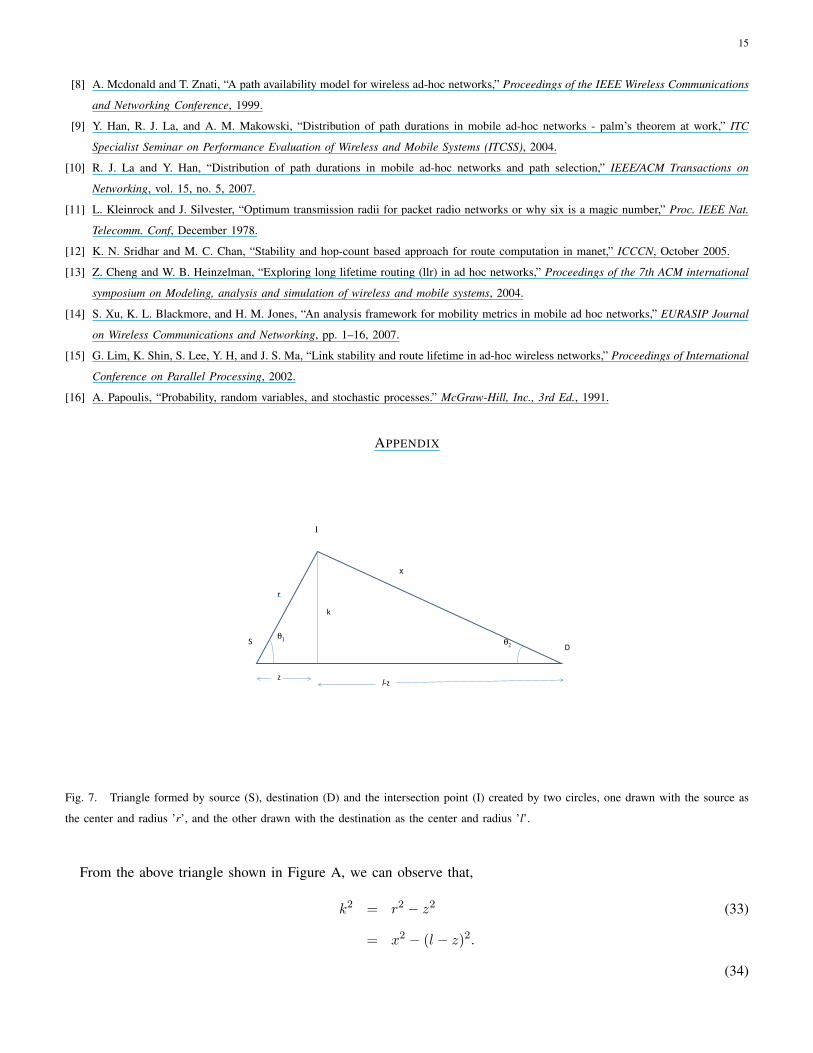
Fig. 7. Triangle formed by source (S), destination (D) and the intersection point (I) created by two circles, one drawn with the source as

the center and radius ’r’, and the other drawn with the destination as the center and radius ’l’.

From the above triangle shown in Figure A, we can observe that,

k2 = r2 − z2 (33)

= x2 − (l − z)2.

(34)

16

From the above, we can deduce that

r2 − z2 = x2 − (l − z)2 (35)

= x2 − (l2 + z2 − 2lz).

Solving for z, we get,

z =l2 + r2 − x2

2l. (36)

Now, cos(θ1) is given by

cos(θ1) =z

r(37)

=l2 + r2 − x2

2lr.

In the same manner, cos(θ2) can also be computed.