Analytical approximations for low frequency band gaps in periodic arrays of elastic shells

Analytical approximations for low frequency band gapsin periodic arrays of elastic shells

Anton Krynkina)

School of Engineering, Design and Technology, University of Bradford, Bradford, United Kingdom

Olga UmnovaAcoustics Research Centre, The University of Salford, Salford, Greater Manchester, United Kingdom

Shahram Taherzadeh and Keith AttenboroughDepartment of Design Development Environment and Materials, The Open University, Milton Keynes,United Kingdom

(Received 28 June 2012; revised 16 November 2012; accepted 28 November 2012)

This paper presents and compares three analytical methods for calculating low frequency band

gap boundaries in doubly periodic arrays of resonating thin elastic shells. It is shown that both

Foldy-type equations (derived with lattice sum expansions in the vicinity of its poles) and a

self-consistent scheme could be used to predict boundaries of low-frequency (below the first Bragg

band gap) band gaps due to axisymmetric (n ¼ 0) and dipolar (n ¼ 1) shell resonances. The accuracy

of the former method is limited to low filling fraction arrays, however, as the filling fraction increases

the application of the matched asymptotic expansions could significantly improve approximations of

the upper boundary of band gap related to axisymmetric resonance. The self-consistent scheme is

shown to be very robust and gives reliable results even for dense arrays with filling fractions around

70%. The estimates of band gap boundaries can be used in analyzing the performance of periodic

arrays (in terms of the band gap width) without using full semi-analytical and numerical models. The

results are used to predict the dependence of the position and width of the low frequency band gap on

the properties of shells and their periodic arrays.VC 2013 Acoustical Society of America. [http://dx.doi.org/10.1121/1.4773257]

PACS number(s): 43.40.Fz, 43.20.Bi, 43.20.Ks, 43.50.Gf [KML] Pages: 781–791

I. INTRODUCTION

Periodic and random arrangements of scatterers with

low frequency resonances in air have attracted a significant

amount of attention recently due to their applications as

locally resonant acoustic metamaterials.1–3 Different types

of scatterers have been shown to possess these types of

resonances, among them the most notable are split rings, i.e.,

2D analogs of Helmholtz resonators.4

It has been demonstrated recently that periodic arrays of

thin elastic shells in air can possess multiple resonant band

gaps in the frequency range below the first Bragg band

gap.5,6 Data from experiments with finite arrays of elastic

shells5 have shown that the insertion loss (IL) peak corre-

sponding to the axisymmetric (n ¼ 0) resonance is compara-

ble to that for the first Bragg band gap but at a lower

frequency. The IL peak corresponding to the n ¼ 1 reso-

nance also appears at a lower frequency but is less strong.

The position and width of the complete band gaps can be

obtained using standard numerical and semi-analytical techni-

ques.7,8 However it would be attractive to have analytical or

semi-analytical expressions allowing approximate estimates of

band gap boundaries. This would help to better understand their

dependence on scatterer and array parameters and hence facili-

tate the design of resonant metamaterials with desired properties.

In this paper several methods allowing simple estimations

of resonant band gaps boundaries in periodic arrays of elastic

shells are presented. In Sec. II the dispersion relation and

expressions for lower and upper band gap bounds are derived

using expansion of the lattice sum within the vicinity of its

pole.9 The derived dispersion relation is similar to that

obtained with Foldy approximations.10 This method allows

analytical approximations of two resonant band gaps (n ¼ 0

and n ¼ 1). In Sec. III matched asymptotic expansions are

used to improve approximations for the upper boundary of a

band gap associated with the axisymmetric (n ¼ 0) resonance.

A self-consistent method, also known as coherent potential

approximation,11,12 is used to derive simple expressions for

effective density and bulk modulus of the array and hence to

obtain a dispersion relation in Sec. IV. The band gaps due to

n ¼ 0 and n ¼ 1 resonances are determined by finding the fre-

quency ranges where the effective density or the bulk modu-

lus (respectively) are negative. The results of all techniques

are compared with each other and with numerical model pre-

dictions. In Sec. V the derived approximations are applied

to estimate the width of the band gaps with respect to the vari-

ation in elastic shell radius, its thickness, lattice cell size (i.e.,

lattice constant) and Young’s modulus of the elastic shell.

II. FOLDY TYPE FORMULA

First consider an eigenvalue problem stated for acoustic

wave propagation through a doubly periodic array of circular

scatterers Cj, j ¼ 0; 1; 2; ::: . The scatterers are arranged in an

a)Author to whom correspondence should be addressed. Electronic mail:

[email protected]

J. Acoust. Soc. Am. 133 (2), February 2013 VC 2013 Acoustical Society of America 7810001-4966/2013/133(2)/781/11/$30.00

Downloaded 15 Feb 2013 to 146.87.0.77. Redistribution subject to ASA license or copyright; see http://asadl.org/terms

mailto:[email protected]

infinite lattice K with lattice constant L. The acoustic envi-

ronment is characterized by its density qo and sound speed

co. In this section the origins of Cartesian coordinates

r ¼ ðx; yÞ and polar coordinates coincide with the center of

scatterer C0 in the primary cell. Center Oj of each scatterer

Cj in the jth cell of lattice K is defined by the position vector

Rj ¼ n1a1 þ n2a2; n1; n2 2 Z; (1)

where a1 and a2 are the fundamental translation vectors. The

solution in acoustic medium pðrÞ satisfies the Helmholtz

equation

Dpþ k2op ¼ 0; (2)

where D¼ð1=rÞð@=@rÞ½rð@=@rÞ�þð1=r2Þð@2=@h2Þ, ko¼x=co

is the wavenumber defined as a ratio between angular fre-

quency x and sound speed co. Throughout this paper the

time-harmonic dependence is taken as e�ixt.

Solution pðrÞ is subject to the boundary conditions speci-

fied later in this paper and the Floquet–Bloch conditions, also

referred to as quasi-periodicity conditions, that are

pðrþ RjÞ ¼ eib�Rj pðrÞ; (3)

where r is the position vector of a field point, Rj is the posi-

tion vector of each scatterer center, b ¼ ðq1; q2Þ is a given

wave vector, and the center dot stands for the scalar product

of two vectors. The components of the wave vector b can also

be defined in polar coordinates as q1 ¼ bcoss and q2 ¼ bsins.

The general solution of the Helmholtz equation (2) is

given by

pðr; hÞ ¼Xþ1n¼�1

½BJnJnðkorÞ þ BY

n YnðkorÞ�einh: (4)

Applying the quasi-periodicity conditions (3) together with

the boundary conditions imposed on the surface of each scat-

terer to Eq. (4) results in the dispersion relation referred to as

the Rayleigh identity7

BJn �Xþ1p¼�1

ð�1Þp�nrYp�nðko; bÞZpBJ

p ¼ 0; n 2 Z; (5)

where factor Zn is defined by boundary conditions on the

scatterer’s surface. For example, zero normal velocity at the

surface of the rigid scatterers of radius a gives

Zn ¼ �J0n ðkoaÞY0n ðkoaÞ (6)

with the prime denoting derivative with respect to polar

coordinate r. The lattice sum rYn ðko; bÞ in Eq. (5) can be

derived in the lattice K as

rYn ðko; bÞ ¼

XRj2Knf0g

eib�Rj YnðkRjÞeinaj ; (7)

where the representation Rj ¼ Rjðcosaj; sinajÞ has been

used.

The lattice sum can also be derived in a reciprocal lat-

tice K? defined by lattice vectors

R?m ¼ 2pðm1b1 þ m2b2Þ; m ¼ ðm1;m2Þ 2 Z2: (8)

The fundamental translational vectors b1 and b2 in K? are

related to those in K through

ai � bj ¼ dij; i; j ¼ 1; 2: (9)

It is shown7,13 that

rYn ðko; bÞ ¼

4in

A

XR?

m2K?

JnðbmnÞJnðkonÞ

einsm

k2o � b2

m

� d0nY0ðkonÞJ0ðkonÞ

;

(10)

where A is the area of a lattice cell, bm ¼ bþ R?m ¼ bm

ðcossm; sinsmÞ and n 2 ½0; f� with

f6 minRj2K;Rj 6¼0

Rj: (11)

The lattice sum given by Eq. (10) has simple poles k ¼ bm

that correspond to plane wave solutions satisfying Floquet–

Bloch conditions (3) in the absence of the scatterers.9 The

magnitude bm is defined by M pairs of integer numbers

ðm1;m2Þ 2 Z2M that gives M different wave vectors bm. In the

vicinity of this pole the related M terms of the lattice sum (10)

take the leading order that is

rYn ðko; bÞ ¼

4in

A

Xm2Z2

M

einsm

k2o � b2

m

þ rY;2n ðko; bÞ; (12)

where rY;2n ðk; bÞ is the next order in expansion over14

ðk2 � b2mÞL2 � 1; m 2 Z2

M: (13)

In this section it is assumed that only one pair

ðm1;m2Þ ¼ ð0; 0Þ contributes to the leading order of expan-

sion (12). This results in bm ¼ b. It is noted that this is true

for the case when koL� 1 and bmL� 1.

It is also assumed that bL is taken within the first irre-

ducible Brillouin zone8 that can be described by the contour

ð0; 0Þ � ðp; 0Þ � ðp; pÞ.The smallness of bL and approximation of lattice sum

(12) by the summand related to the pair of ðm1;m2Þ ¼ ð0; 0Þmake valid further approximations along ð0; 0Þ � ðp; 0Þ and

ðp; pÞ � ð0; 0Þ lines. This also leads to a symmetry around

point ð0; 0Þ so that vector b is only considered within the

interval ð0; 0Þ � ðp; 0Þ (i.e., b ¼ q1 and s ¼ 0 with q1 2 ½0; q�and qL� p). As a result the leading order of the lattice sum

(12) is simplified to

rYn ðk; bÞ � rY;1

n ðk; bÞ ¼in

A

4

k2o � b2

: (14)

Substituting equations (14) into dispersion relation (5)

one can obtain the following system of homogeneous

algebraic equations with respect to unknown coefficients

BJn; n 2 Z

782 J. Acoust. Soc. Am., Vol. 133, No. 2, February 2013 Krynkin et al.: Boundaries of low frequency band gaps


BJn�

4

Aðk2o � b2Þ

Xþ1p¼�1

ð�iÞp�nBJpZp ¼ 0; n 2Z: (15)

By multiplying both sides of Eq. (15) by ð�iÞn it is possible

to redefine the unknown coefficients as BJ

n ¼ ð�iÞnBJn; n 2 Z

so that the system of equations (15) becomes similar to that

derived in Ref. 15 [Eq. (71)]. This equation can now be

employed to derive a Foldy type dispersion relation. Follow-

ing the derivations in Ref. 15 [Eqs. (76) and (77)] it is con-

cluded that coefficients BJ

n; n 2 Z are identical for all indices

n 2 Z, yielding

b2 ¼ k2o �

4

AF; (16)

where F ¼Pþ1

p¼�1Zp is determined by boundary condi-

tions on the scatterer’s surface. It also coincides with the

imaginary part of the far-field pattern of a single scatterer.

The consistency of Eqs. (13) and (16) requires that

4

AFL2 � 1: (17)

It must be noted that for the resonant scatterers F have singu-

lar points that give resonance frequencies. Therefore, in the

vicinity of resonances the asymptotic orders of factors

Zn; n 2 Z can invalidate the derivation of dispersion relation

(16). This, however, can also signify the existence of a band

gap due to resonance.

Now consider a square periodic array of thin-walled

elastic shells with area of lattice cell A ¼ L2. The application

of long-wave low-frequency approximations results in the

following expressions for factor Zn; n 2 Z described by5

[Eq. (22)]

Zn ¼ �½J0n ðkoaÞ�2½1� ðk3aÞ2 þ n2�

J0n ðkoaÞY0n ðkoaÞ½1� ðk3aÞ2 þ n2� þ ½n2 � ðk3aÞ2�qoðqpahÞ�1; Z�n ¼ Zn; (18)

where q is the density of an elastic material, k3 ¼ x=c3, a is

shell mid-surface radius (referred to as radius of the elastic

shell), and h is its half-thickness. Here the dilatational wave

speed c3 for a thin elastic plate is recalled

c3 ¼ffiffiffiffiffiffiffiffiffiffiffiffiffiffiffiffiffiffiffiffi

E

qð1� �2Þ

s; (19)

within which E and � are Young’s modulus and Poisson ratio

of elastic shell, respectively.

For the low frequency range that contains n ¼ 0 (i.e.

axisymmetric resonance) and n ¼ 61 resonances the far-

field pattern of elastic shell can be approximated by its first

two terms that gives

F ¼ Z0 þ 2Z1: (20)

The assumption that wavelength of a propagating acoustic

wave is much bigger than the lattice cell size (i.e., lattice

constant L) immediately results in

� ¼ koa� 1: (21)

The latter can be used to simplify Eq. (18) by expanding

Bessel functions. It is also assumed that the elastic shell is

“soft” [i.e., qo=q ¼ Oð�2Þ and c3=c ¼ Oð�Þ] so that acoustic

waves are able to penetrate it. Thus

Z0 � �2 p4

K20 � k2

o

K2

0 � k2o

; (22)

Z1 � �2 p4�1þ qoa

qh

K20 � k2

o

2K20 � k2

o

�

þ �2 1

2log

�

2þ 1

8ð5þ 4cÞ

� ��; (23)

where wavenumbers

K0 ¼1

a

ffiffiffiffiffiffiKc

p; (24)

K0 ¼1

a

ffiffiffiffiffiffiffiffiffiffiffiffiffiffiffiffiffiKq þKc

p(25)

with

Kq ¼qo

qa

h(26)

and

Kc ¼c3

co

� �2

(27)

correspond to axisymmetric resonances of shell in vacuum

with vacuum and acoustic medium inside, respectively. In

Eq. (23) approximated Z1 has a singularity at k2o ¼ 2K2

0

related to the leading order of resonance frequency with

index n ¼ 1. From this approximation it can be concluded

that frequency of n ¼ 1 resonance of a thin elastic shell

defined from

K1 ¼ffiffiffi2p

K0 (28)

has no dependence on the physical parameters of the sur-

rounding acoustic environment in the leading order.

As bL! 0, Eq. (16) gives two non-zero solutions for ko

in addition to ko ¼ 0. These solutions can be used to find the

size of the corresponding band gaps.

In the vicinity of axisymmetric resonance K0 as bL! 0

the dispersion relation (16) can be transformed to

J. Acoust. Soc. Am., Vol. 133, No. 2, February 2013 Krynkin et al.: Boundaries of low frequency band gaps 783


FKqðKc �KqÞ þ ½ðkoaÞ2 � ðKc þKqÞ�� ½ð1þ FÞðKq �KcÞ � FKqð1þ 2KqÞ� ¼ 0:

(29)

This results in the following solution for ko > 0

ko;2 ¼1

a

ffiffiffiffiffiffiffiffiffiffiffiffiffiffiffiffiffiffiffiffiffiffiffiffiffiffiffiffiffiffiffiffiffiffiffiffiffiffiffiffiffiffiffiffiffiffiffiffiffiffiffiffiffiffiffiffiffiffiffiffiffiffiffiffiffiffiffiffiffiffiffiffiffiKq þKc þ

FKqðKq �KcÞKq �Kc � FðKc þ 2K2

qÞ

s

� 1

a

ffiffiffiffiffiffiffiffiffiffiffiffiffiffiffiffiffiffiffiffiffiffiffiffiffiffia2K

2

0 þ FKq

q; (30)

where F ¼ pa2=A is the scatterer filling fraction. Expression

(30) immediately estimates the upper limit of the band gap.

Note that the lower limit of the mentioned band gap is given

by ko;1 ¼ K0L. Therefore, based on the derived approxima-

tions, it is possible to conclude that in the doubly periodic

array of thin elastic shells (with filling fraction F � 1)

waves do not propagate in the frequency interval

½f ln¼0; f u

n¼0� ¼c3

2pa

ffiffiffiffiffiffiffiffiffiffiffiffiffiffi1þKq

Kc

s;

c3

2pa

ffiffiffiffiffiffiffiffiffiffiffiffiffiffiffiffiffiffiffiffiffiffiffiffiffiffiffiffiffiffiffi1þKq

Kcð1þ FÞ

s" #:

(31)

In the vicinity of n ¼ 1 resonance K1 is approximated

by Eq. (28) and as bL! 0 the dispersion relation (16) can

be transformed to

2FKqKcðKq �KcÞ þ ½ðkoaÞ2 � 2KcÞ�� ½ð1þ 2F � 2FKqÞðKc �KqÞ �FKcð1þ 2KqÞ� ¼ 0:

(32)

For ko > 0 the solution of this equation takes the following

form:

ko;2 ¼1

a

ffiffiffiffiffiffiffiffiffiffiffiffiffiffiffiffiffiffiffiffiffiffiffiffiffiffiffiffiffiffiffiffiffiffiffiffiffiffiffiffiffiffiffiffiffiffiffiffiffiffiffiffiffiffiffiffiffiffiffiffiffiffiffiffiffiffiffiffiffiffiffiffiffiffiffiffiffiffiffiffiffiffiffiffiffiffiffiffiffiffiffiffiffiffiffiffiffiffiffiffiffiffiffiffiffiffiffiffiffiffiffiffiffiffiffiffi2Kc þ

2FKqKcðKc �KqÞKc �Kq þ F½2ðKc �KqÞð1�KqÞ � Kcð1þ 2KqÞ�

s� 1

a

ffiffiffiffiffiffiffiffiffiffiffiffiffiffiffiffiffiffiffiffiffiffiffiffiffiffiffiffiffiffiffiffiffia2K2

1 þ 2FKqKc

q: (33)

The lower limit of the band gap related to n ¼ 1 resonance is

given by Eq. (28). Therefore the frequency interval where

waves do not propagate is estimated as

½f ln¼1; f

un¼1� ¼

ffiffiffi2p

c3

2pa;

ffiffiffi2p

c3

2pa

ffiffiffiffiffiffiffiffiffiffiffiffiffiffiffiffiffiffi1þ FKq

p� �: (34)

In Fig. 1 the solutions of dispersion relation (16)

obtained for F that contains only two terms n ¼ 0; 1 are

shown. Throughout this paper unless otherwise specified the

material parameters of thin elastic shell are identical to those

in Ref. 5 and its thickness 2h ¼ 0:00025 m. The radius of

the elastic shell is varied whereas the lattice constant L is

fixed (L ¼ 0:08 m) so that two values of the filling fraction

F are considered: � 0:4 and � 0:7. Two band gaps related

to the resonances K0, n ¼ 0 andffiffiffi2p

K0, n ¼ 1 are observed

below the first band gap associated with the array periodic-

ity. According to Fig. 1(a) the estimates of the lower and

upper limits of the band gap are within 5% of the exact val-

ues as long as the filling fraction is relatively low (F � 0:4).

However, as the filling fraction is increased up to 0:7 the ac-

curacy is expected to decrease according to the condition

(17). This is illustrated in Fig. 1(b) where the error between

the estimated and exact values of the upper boundary of the

band gap associated with n ¼ 0 is 30%. It must also be noted

that this upper boundary obtained with Foldy’s equation

depends on the form of the factor Zn. Its approximated form

might give more accurate results than the original form of Zn

given by Eq. (18). This inconsistency implies that to obtain

more accurate and consistent results, Eq. (16) has to be

modified to include the periodicity effects.

III. MATCHED ASYMPTOTIC EXPANSION

The results obtained in the previous section can be

improved by using the technique based on matched asymptotic

expansions (MAEs).9,16 This technique allows approximating

FIG. 1. (Color online) Foldy’s approximation 16 (dashed line) compared

with the semi-analytical solution of Rayleigh identity (5) (solid line). (a)

a ¼ 0:0275 m and (c) a ¼ 0:0375 m.



eigenvalues of Eqs. (2),(3) when koL ¼ Oð1Þ in the vicinity of

band gaps associated with the periodicity (Bragg band gaps).

However in this paper MAEs are used to estimate the solution

that forms the upper boundary of the band gap due to the axi-

symmetric resonance (n ¼ 0) of a thin elastic shell.

First outer and inner regions are introduced. In the inner

region surrounding each scatterer the solution is solved in

conjunction with the boundary conditions imposed on the

surface of the scatterer. The characteristic length of this

region is the radius a of scatterer. Thus a dimensionless inner

coordinate is given by

x ¼ r

a: (35)

In the outer region the scatterers are replaced by point sour-

ces and the solution is subject to quasi-periodicity condi-

tions. The characteristic length in this region is equal to the

wavelength of sound. Thus a dimensionless outer coordinate

is given by

y ¼ kor: (36)

The wavelength is assumed to be much bigger than the scat-

terer radius. This requirement results in small parameter �introduced in Section II that connects two regions through

y ¼ �x: (37)

A. Inner solution

The inner solution is found from the boundary value

problem for a single thin elastic shell. The solution around

the cylinder is represented as

wðx; hÞ ¼Xþ1n¼�1

BJn½Jnð�xÞ þ ZnYnð�xÞ�einh (38)

with unknown constants BJn and coefficients Zn defined by

Eq. (18). According to Eq. (22), factor Z0 takes order Oð�2Þif its singular points (i.e., resonances) are isolated. In the vi-

cinity of axisymmetric resonance the order of factor Z0 can

be transformed to OðgÞ that is

Z0 ¼ dZg; with dZ ¼ Oð1Þ; (39)

where small parameter g is bigger than � and is assumed to be

g ¼ 1

K � log�; (40)

within which K is the unknown constant.

By assuming Z0 of order g the proximity of k0 to the axi-

symmetric resonance K0 is restricted by

ko � K0 ¼ O�2

g

� �: (41)

Expanding solution (38) up to the order g first with

respect to the inner coordinate x and then with respect to the

outer coordinate y results in

wðg;gÞðx; hÞ ¼ BJ0 1� 2

pdZ þ g

2

pdZ log x

� �: (42)

It is noted that the terms in Oð1Þ and OðgÞ orders have no az-

imuthal dependence.

B. Outer solution

The outer solution of the Helmholtz Eq. (2) satisfies the

quasi-periodicity conditions (3) and is singular at the points

Oj. This results in

Wðr; hÞ ¼Xþ1n¼�1

An

XRj2Knf0g

eib�Rj Hð1Þn ðkorjÞeinhj ; (43)

where local coordinates ðrj; hjÞ with origin at Oj are used.

It is assumed that the leading order of coefficients

An; n 2 Z is bounded by the small parameter g. This approach

is similar to that derived in Refs. 14 and 16 (Sec. 6.8). Thus

An ¼ gAn: (44)

The use of addition theorem for the Bessel functions17

and lattice sum representation in the reciprocal lattice K?

transform the outer solution (43) to

WðgÞðy; hÞ ¼ gXþ1n¼�1

An

�Hð1Þn ðyÞeinh

þXþ1p¼�1

ð�1Þn�prn�pðko; bÞJpðyÞeiph

�

(45)

and

rnðko; bÞ ¼ �d0;n þ irYn ðko; bÞ; (46)

where rYn ðko; bÞ is given by Eq. (10).

The form of the inner solution (42) assumes that the

leading order should include axisymmetric terms only. In

contrast to Sec. II it is assumed here that for n ¼ 0 the entire

lattice sum (10) [not only pair ðm1;m2Þ ¼ ð0; 0Þ] contributes

to the outer solution as

rY0 ðko; bÞ ¼

dg; with d ¼ Oð1Þ: (47)

Then expanding outer solution in terms of the inner coordi-

nate x up to order g leads to

Wðg;gÞðx; hÞ ¼ iA0 d� 2

pþ g

2

pðK þ c� log2þ logxÞ

� �:

(48)

C. Matching

The inner expansion of the outer solution (48) can now

be matched with the outer expansion of the inner solution

(42). First factors of logn in order g give



A0 ¼ �idZBJ0: (49)

Matching constants in order g results in

K ¼ log2� c: (50)

Finally the consistency of the leading orders in Eqs. (42) and

(48) requires that

Z0rY0 ðko; bÞ � 1 ¼ 0; (51)

where Eqs. (39), (47), and (49) have been used.

As bL! 0 the lattice sum in Eq. (51) can be approxi-

mated by

rY0 ðko; bL! 0Þ � 1

J0ðkonÞ4L2

A

1

ðkoLÞ2� Y0ðkonÞ

"

þ 4L2

A

XR?m2K?R?

m 6¼ð0;0Þ

J0ðR?mnÞðkoLÞ2 � ðR?mLÞ2

35:

(52)

It is noted that the last term given as a series over the re-

ciprocal lattice represents the correction factor to the

upper limit of the band gap related to the axisymmetric

resonance. This correction factor includes the periodicity

effects.

For the square lattice with lattice constant L and n ¼ L=2

the lattice sum (52) is transformed into

rY0 ðko; bL ¼ 0Þ ¼ 1

J0ðkoL=2Þ

� 4

ðkoLÞ2� Y0ðkoL=2Þ þ 4SðkoLÞ

" #;

(53)

with

SðkoLÞ ¼X

m2Z2m 6¼ð0;0Þ

J0ðpffiffiffiffiffiffiffiffiffiffiffiffiffiffiffiffiffim2

1 þ m22

pÞ

ðkoLÞ2 � 4p2ðm21 þ m2

2Þ: (54)

It is noted that n is chosen from the interval set in Eq. (11) to

improve the convergence of S.

The lattice sum (53) and the dispersion relation (51) can

be used to improve the upper limit of the band gap found in

Eq. (30). Thus the improved estimate is given by the solution

of the following equation:

Z0f4� ðkoLÞ2½Y0ðkoLÞ þ 4SðkoLÞ�g� ðkoLÞ2J0ðkoLÞ ¼ 0;

(55)

within which koL 6¼ 0 and J0ðkoLÞ 6¼ 0. To find the solution

of Eq. (55) the infinite sum (54) has to be truncated. The

results are accurate to three decimal places for both jm1j 8

and jm2j 8.

Figure 2 demonstrates the improvement in approximation

of the upper boundary of the band gap due to axisymmetric

resonance given by Eq. (55) compared to Foldy’s approxima-

tion Eq. (30). For a low filling fraction (i.e., F � 0:4) the

results are accurate within 1% from those obtained with

Foldy’s equation, see Fig. 2(a). As the filling fraction

increases the approximation of the dispersion curve represent-

ing the upper bound deteriorates. However, the limiting point

at bL ¼ 0 and its vicinity are not affected, see Fig. 2(b) so

that the estimate remains valid even for large filling fraction

(0:7 � F < Fmax) with the accuracy within 1% from the

exact solution where the maximum filling fraction Fmax of

the circular scatterer is found to be given by Fmax ¼ p=4. It is

also noted that results in this paper should be modified in

close proximity to Fmax to include the effect of viscous and

thermal boundary layers.18

IV. SELF-CONSISTENT EFFECTIVE MEDIUMFORMULATION

The effective medium approach provides an alternative

method for estimating the boundaries of band gaps due to

resonances with indices n ¼ 0 and n ¼ 1.

Consider an effective medium that represents a periodic

array of scatterers in a fluid matrix (see Fig. 3). The homoge-

nization11,19 becomes possible only when the wavelength in

FIG. 2. (Color online) MAE approximation of the upper limit (55) (dotted

line) compared with Foldy’s approximation (16) (dashed line) and the semi-

analytical solution of Rayleigh identity (5) (solid line). (a) a ¼ 0:0275 and

(b) a ¼ 0:0375.



both fluid and effective medium is much bigger than the ra-

dius of scatterers a and separation distance between them

(lattice constant L) that is koL� 1 and keffL� 1.

The solution of the Helmholtz equation

Dpa þ k2apa ¼ 0 (56)

is given in terms of the displacement potential paðrÞ; where

ka ¼ x=ca is the wavenumber, ca ¼ffiffiffiffiffiffiffiffiffiffiffiffiBa=qa

pis speed of

sound, index a relates solution p to one of the regions [i.e.,

“eff” is the effective medium (I), o is the matching fluid

layer between scatterer and effective medium]. The problem

is solved in polar coordinates r ¼ ðr; hÞ. It is also noted that

the physical parameters of the matching fluid layer coincide

with the acoustic medium introduced in Sec. II.

To find the effective medium parameters (effective den-

sity qeff and bulk modulus Beff ) and hence its wavenumber

keff ¼ xffiffiffiffiffiffiffiffiffiffiffiffiffiffiffiffiffiqeff=Beff

pthe problem is split into three regions.20

(1) Region (I)—circular scatterer.

(2) Region (II)—fluid layer with properties identical to those

of the fluid matrix.

(3) Region (III)—effective medium with yet unknown

properties.

Regions (I) and (II) are introduced to derive parameters of

the effective medium through matching acoustic potentials

at the interface of the region (II) and (III) r ¼ Ro. That is,

po ¼qeff

qo

peff ;

@po

@r¼ @peff

@r;

(57)

where outer radius Ro is derived in terms of the scatterer ra-

dius and the filling fraction of the original periodic array

with lattice constant L so that the filling fraction in a com-

posite inclusion remains equal to that of the original periodic

array. This gives21

Ro ¼affiffiffiffiFp : (58)

The total wave field in region (III) is given by

peff ¼ pinc þ pscat; (59)

pinc ¼ eikeff rcosðh�bÞ; (60)

where pinc is plane wave incident at an angle b and pscat

represents scattered wave field. Having assumed that the

effective medium behaves as a homogeneous fluid the scat-

tered wave field vanishes that leads to

peff ¼ pinc; (61)

with the plane wave expanded over the regular Bessel func-

tions JnðkeffrÞ as (see Ref. 17, Eqs. 9.1.44 and 9.1.45)

pinc ¼Xþ1n¼�1

inJnðkeffrÞeinðh�bÞ: (62)

The solution inside the annular layer (II) takes the form

po ¼Xþ1n¼�1

Bn½JnðkorÞ þ ZnYnðkorÞ�einh; (63)

where factors Zn are defined by Eq. (18).

Substitution of Eqs. (62) and (63) into the boundary con-

ditions (57) leads to

Bn½JnðkoRoÞ þ ZnYnðkoRoÞ� ¼qeff

qo

JnðkeffRoÞeinðp=2�bÞ;

Bn½J0n ðkoRoÞ þ ZnY0n ðkoRoÞ� ¼ J0n ðkeffRoÞeinðp=2�bÞ;

(64)

where n 2 Z. To solve system (64) it first has to be truncated

at some integer number N that gives

Ax ¼ b; (65)

where matrix A has 4N rows and 2N columns, vector x has

2N elements, vector b has 4N elements, and

FIG. 3. Geometry of the effective

medium.



A ¼

½J�NðkoRoÞ þ Z�NY�NðkoRoÞ� 0 � � � 0

½J0�NðkoRoÞ þ Z�NY0�NðkoRoÞ� 0 � � � 0

� � �

0 0 � � � ½JNðkoRoÞ þ ZNYNðkoRoÞ�0 0 � � � ½J0NðkoRoÞ þ ZNY0NðkoRoÞ�

0BBBBBBB@

1CCCCCCCA; (66)

x ¼

B�N

B�Nþ1

�

BN

0BBB@

1CCCA; (67)

b ¼

qeff

qo

J�NðkeffRoÞe�iNðp=2�bÞ

J0�NðkeffRoÞe�iNðp=2�bÞ

�qeff

qo

JNðkeffRoÞeiNðp=2�bÞ

J0NðkeffRoÞeiNðp=2�bÞ

0BBBBBBBBBB@

1CCCCCCCCCCA: (68)

According to the Kronecker–Capelli theorem,22 the

overdetermined system (65) is compatible if the rank of its

coefficient matrix is equal to that of the augmented matrix.

On the other hand, the unique solution of system (65) exists

if the rank of matrix A is equal to number of variables (i.e.,

number of columns 2N). Hence combination of these two

statements and application of Gaussian elimination algo-

rithm to the augmented matrix ðAjbÞ yield the criteria for the

existence of the solution that is

J0nðkoRoÞ þ ZnY0nðkoRoÞJnðkoRoÞ þ ZnYnðkoRoÞ

¼ qo

qeff

J0nðkeffRoÞJnðkeffRoÞ

;

n ¼ �N � � �N:(69)

These equations can now be simplified by recalling the

assumptions

g ¼ koRo � 1 and keffRo � 1: (70)

Also Eq. (69) needs to be rewritten as

_JnðgÞ þ Zn_YnðgÞ

JnðgÞ þ ZnYnðgÞ¼ nq

_JnðgncÞJnðgncÞ

; n ¼ �N � � �N; (71)

where the overdot stands for the derivative of Bessel func-

tions with respect to dimensionless parameter g. Parameters

nq and nc depend on the effective medium properties as

nq ¼qo

qeff

; (72)

nc ¼co

ceff

: (73)

Bessel functions and their derivatives in Eq. (71) can be

replaced by their approximations in the leading orders as

g! 0,17 yielding

JnðgÞ �g2

n 1

n!; n 0; (74)

YnðgÞ � �g2

�n ðn� 1Þ!p

; n > 0; (75)

_JnðgÞ �g2

n n

n!g�1 � 1

2ðnþ 1Þ! g� �

; n 0; (76)

_YnðgÞ �g2

�n�1 n!ð1þ d0;nÞ2p

; n 0: (77)

It is convenient to consider subsequently that Bessel func-

tions have only zero and positive integer orders with

Y0ðgÞ ¼ 2=plogðgÞ. For the negative orders of Bessel func-

tions fnðgÞ ¼ fJnðgÞ; YnðgÞg, Eq. (71) is identical to that with

n > 0 due to the relation f�nðgÞ ¼ ð�1ÞnfnðgÞ.Substitution of Eqs. (74)–(77) into Eqs. (71) gives for

n ¼ 0

ðg=2Þ2 � Z0=p1þ 2Z0logðgÞ=p ¼ nqn

2c

g2

2

(78)

and for n > 0

ðg=2Þ2n½ðn� 1Þ!��1f1=2� ðg=2Þ2½nðnþ 1Þ��1g þ Znn!ð2pÞ�1

ðg=2Þ2nðn!Þ�1 � Znðn� 1Þ!p�1¼

nq

2n� gnc

2

� �22

nþ 1

" #: (79)

Following the orders of smallness involved in equations (78)

and (79) the factor Zn has to appear as

Zn ¼ðg=2Þ2pZ0;0; for n ¼ 0;

ðg=2Þ2n pðn� 1Þ!n!

Zn;0 for n > 0:

8<: (80)



This assumption can be easily justified for the circular scat-

terers by expanding Zn with respect to the small parameter,

see Eqs. (22) and (23).

By collecting the same orders of smallness in Eqs. (78) and

(79) the leading orders can be derived in the following form:

nqn2c ¼ 1� Z0;0; n ¼ 0; (81)

nq ¼1þ Zn;0

1� Zn;0; n > 0: (82)

From these two equations the parameters of the effective

medium are derived in the following order:

Beff ¼ Bo1

1� Z0;0; n ¼ 0; (83)

qeff ¼ qo

1� Zn;0

1þ Zn;0; n > 0; (84)

where Bo ¼ c2oqo is bulk modulus of matching fluid layer

(i.e., air).

The effective density (84) depends on index n since coeffi-

cient Zn;0 F n. This limits the use of the proposed model and

can only include the contribution of two harmonics that are

n ¼ 0 and any non-zero index n. The usual choice of n ¼ 0

and n ¼ 1 which are the harmonics that contribute most is fol-

lowed now. Using Eqs. (22) and (23) the following expressions

are derived for effective density and bulk modulus:

Beff

Bo¼ Kc þKq � ðkoaÞ2

Kcð1� FÞ þ Kq � ðkoaÞ2ð1� FÞ; (85)

qeff

qo

¼ Kc½2þ Fð2�KqÞ� � ðkoaÞ2½1þ Fð1�KqÞ�Kc½2� Fð2�KqÞ� � ðkoaÞ2½1� Fð1�KqÞ�

;

(86)

where Kq and Kc are defined by Eqs. (26) and (27).

The dispersion relation of the effective medium is

k2eff ¼

qeff

qo

Bo

Beff

k2o; (87)

which has two poles corresponding to resonances with n ¼ 0

and n ¼ 1. Moreover there are two intervals where keff is

imaginary, i.e., band gaps. In the first interval the bulk mod-

ulus Beff in Eq. (85) is negative,

ko >1

a

ffiffiffiffiffiffiffiffiffiffiffiffiffiffiffiffiffiKq þKc

p¼ K0; (88)

ko <1

a

ffiffiffiffiffiffiffiffiffiffiffiffiffiffiffiffiffiffiffiffiffiffiffiffiffiffiffiffiffiffiffiffiffiffiffiffiKq þKc þ

FKq

1� F

r�F� 1

1

a

ffiffiffiffiffiffiffiffiffiffiffiffiffiffiffiffiffiffiffiffiffiffiffiffiffiffia2K

2

0 þ FKq

q;

(89)

whereas the second interval gives negative effective density qeff ,

ko >1

a

ffiffiffiffiffiffiffiffiffiffiffiffiffiffiffiffiffiffiffiffiffiffiffiffiffiffiffiffiffiffiffiffiffiffiffiffiffiffiffiffiffiffiffi2Kc �

FKqKc

1�Fð1�KqÞ

s�F�1

1

a

ffiffiffiffiffiffiffiffiffiffiffiffiffiffiffiffiffiffiffiffiffiffiffiffiffiffiffiffiffiffiffia2K

2

1�FKqKc

q;

(90)

ko <1

a

ffiffiffiffiffiffiffiffiffiffiffiffiffiffiffiffiffiffiffiffiffiffiffiffiffiffiffiffiffiffiffiffiffiffiffiffiffiffiffiffiffiffiffi2Kc þ

FKqKc

1þFð1�KqÞ

s�F�1

1

a

ffiffiffiffiffiffiffiffiffiffiffiffiffiffiffiffiffiffiffiffiffiffiffiffiffiffiffiffiffiffiffia2K

2

1þFKqKc

q:

(91)

Therefore the band gap due to the axisymmetric resonance

corresponds to the frequency range where effective bulk

modulus is negative:

½f l

n¼0; fu

n¼0� ¼c3

2pa

ffiffiffiffiffiffiffiffiffiffiffiffiffiffi1þKq

Kc

s;

c3

2pa

ffiffiffiffiffiffiffiffiffiffiffiffiffiffiffiffiffiffiffiffiffiffiffiffiffiffiffiffiffiffiffiffiffiffiffiffiffiffiffiffiffi1þKq

Kc1þ F

1�F

� �s" #

(92)

while band gap due to n¼ 1 resonance corresponds to the

frequency range where effective density is negative:

hf

l

n¼1; fu

n¼1

i¼

ffiffiffi2p

c3

2pa

ffiffiffiffiffiffiffiffiffiffiffiffiffiffiffiffiffiffiffiffiffiffiffiffiffiffiffiffiffiffiffiffiffiffiffiffiffiffiffiffiffiffiffiffi1� FKq

2½1� Fð1�KqÞ�

s;

"ffiffiffi2p

c3

2pa

ffiffiffiffiffiffiffiffiffiffiffiffiffiffiffiffiffiffiffiffiffiffiffiffiffiffiffiffiffiffiffiffiffiffiffiffiffiffiffiffiffiffiffiffi1þ FKq

2½1þ Fð1�KqÞ�

s #(93)

Comparing n ¼ 0 band gap limits approximated by Eq. (92)

with those derived using lattice sum expansion (31) it can be

seen that they coincide as F ! 0. On the other hand the

limits (93) for the n ¼ 1 band gap are shifted towards lower

frequency compared to the interval (34). It is noted that as

F ! 0 the approximation of the lower limit fl

n¼1 coincides

with the resonance n ¼ 1 of the elastic shell embedded into

FIG. 4. (Color online) Dispersion relation predicted by self-consistent

method (87) (dash-dotted line) compared with the semi-analytical solution

of Rayleigh identity (5) (solid line), Foldy’s approximations (16) (dashed

line), and MAE solution (55) (dotted line). (a) a ¼ 0:0275 and (b)

a ¼ 0:0375.



the hollow cylinder with rigid walls and radius equal to that

of the composite inclusion.

In Fig. 4 the dispersion relation (87) is compared with the

approximations derived in Secs. II and III in the interval

keffL 2 ½0; p�. This interval coincides with that chosen in Sec.

II for the wave vector b (i.e., bL belongs to ½0; p�). It is

observed that for relatively low filling fractions [see Fig. 4(a)

for F � 0:4] as well as for high filling fractions [see Fig. 4(b)

for F � 0:7] the results are accurate to within 5% of the

semi-analytical solution. It is also noted that as the filling frac-

tion increases the approximation of the upper limit of n ¼ 0

band gap is less accurate than that obtained with Eq. (55).

V. RESULTS BAND GAP WIDTH

In Fig. 5 the results illustrate the application of the

approximations derived in the previous sections to estimate

the width of the band gaps.

The dependence of the band gaps related to the shell

resonances with indices n ¼ 0 and n ¼ 1 on the filling frac-

tion is shown in Figs. 5(a) and 5(b). The Bragg frequency

f ¼ co=ð2LÞ is constant with respect to F in Fig. 5(a) where

the characteristic size of the square lattice cell (i.e., lattice

constant L) is fixed and the shell radius is varied. It is noted

that the approximations based on Foldy’s equation underesti-

mate the upper limit of n ¼ 0 band gap as F ! p=4. This is

improved with the help of the matched asymptotic results

and the self-consistent method. It is also observed that for

low filling fractions (i.e., F < 0:1) the axisymmetric reso-

nance and the corresponding band gap are expected to be

observed above the first Bragg frequency where the obtained

approximations are not valid. For the band gap attributed to

the shell resonance with index n ¼ 1, the approximations

based on Foldy’s equation predicts smaller gap width then

that obtained with the self-consistent method. This is due to

the fact that the lower limit is fixed on the shell resonance

whereas in the self-consistent method it depends on the fill-

ing fraction. In Fig. 5(b) the shell radius is fixed and the lat-

tice constant is varied. This results in the variation of the

Brag frequencies. The obtained results are similar to those in

Fig. 5(a). Again the derived approximations should accu-

rately predict the n ¼ 0 band gap width.

FIG. 5. (Color online) Limits of the band gap n ¼ 0 and n ¼ 1 obtained with Foldy’s approximations (16) (dashed line), MAE solution (55) (dotted line), and

self-consistent method (87) (dash-dotted line). The first Bragg frequency is plotted with a solid line. (a) Variation of the shell mid-surface radius a. (b) Variation

of the lattice constant L. (c) Variation of the thickness 2h with filling fraction F � 0:4. (d) Variation of the Young’s modulus E with filling fraction F � 0:4.



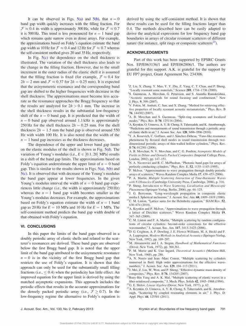
It can be observed in Figs. 5(a) and 5(b), that n ¼ 0

band gap width quickly increases with the filling fraction. For

F � 0:4 its width is approximately 300 Hz, while for F � 0:7it is 500 Hz. This trend is less pronounced for n ¼ 1 band gap

which remains quite narrow even in dense arrays. For example,

the approximations based on Foldy’s equation estimate the band

gap width as 10 Hz forF � 0:4 and 12 Hz forF � 0:7 whereas

the self-consistent method gives 20 and 35 Hz, respectively.

In Fig. 5(c) the dependence on the shell thickness is

illustrated. The variation of the shell thickness also leads to

the change in the filling fraction. However, due to the small

increment in the outer radius of the elastic shell it is assumed

that the filling fraction is fixed (for example, F � 0:4 for

2h ¼ 2 mm and F � 0:37 for 2h ¼ 0:25 mm). It is expected

that the axisymmetric resonance and the corresponding band

gap are shifted to the higher frequencies with decrease in the

shell thickness. The approximations must become less accu-

rate as the resonance approaches the Bragg frequency so that

the results are analyzed for 2h > 0:1 mm. The increase in

the shell thickness results in the substantial low-frequency

shift of the n ¼ 0 band gap. It is predicted that the width of

n ¼ 0 band gap observed around 1.1 kHz is approximately

250 Hz for the shell thickness 2h ¼ 0:25 mm. For the shell

thickness 2h ¼ 1:5 mm the band gap is observed around 550

Hz with width 100 Hz. It is also noted that the width of the

n ¼ 1 band gap increases as the thickness decreases.

The dependence of the upper and lower band gap limits

on the elastic modulus of the shell is shown in Fig. 5(d). The

variation of Young’s modulus (i.e., E 2 ½0:1; 20� MPa) results

in a shift of the band gap limits. The approximations based on

Foldy’s equation underestimate the upper limit of n ¼ 0 band

gap. This is similar to the results shown in Figs. 5(a), 5(b) and

5(c). It is observed that with decrease of the Young’s modulus

the band gaps appear at lower frequencies. In the given

Young’s modulus interval the width of n ¼ 0 band gap expe-

riences little change (i.e., the width is approximately 250 Hz)

whereas the n ¼ 1 band gap width becomes smaller as the

Young’s modulus decreases. For example, the approximations

based on Foldy’s equation estimate the width of n ¼ 1 band

gap as 20 Hz for E ¼ 10 MPa and 10 Hz for E ¼ 1 MPa. The

self-consistent method predicts the band gap width double of

that obtained with Foldy’s equation.

VI. CONCLUSIONS

In this paper the limits of the band gaps observed in a

doubly periodic array of elastic shells and related to the scat-

terer’s resonances are derived. These band gaps are observed

below the first Bragg band gap. It is noted that the upper

limit of the band gap attributed to the axisymmetric resonance

n ¼ 0 is in the vicinity of the first Bragg band gap that

restricts the use of Foldy’s equation. It is shown that this

approach can only be used for the substantially small filling

fractions (i.e., � 0:4) when the periodicity has little effect. An

improved equation for the upper limit is derived by using the

matched asymptotic expansions. This approach includes the

periodic effects that results in the accurate approximations for

the densely packed periodic array (i.e., F 0:7). In the

low-frequency regime the alternative to Foldy’s equation is

derived by using the self-consistent method. It is shown that

these results can be used for the filling fractions larger than

0:4. The methods described here can be easily adapted to

derive the analytical expressions for low frequency band gap

boundaries in arrays of circular resonant scatterers of different

nature (for instance, split rings or composite scatterers23).

ACKNOWLEDGMENTS

Part of this work has been supported by EPSRC Grants

Nos. EP/E063136/1 and EP/E062806/1. The authors are

grateful for this support. A.K. is grateful for the support by

EU FP7 project, Grant Agreement No. 234306.

1Z. Liu, X. Zhang. Y. Mao, Y. Y. Zhu, Z. Yang, C. T. Chan, and P. Sheng,

“Locally resonant sonic materials,” Science 289, 1734–1736 (2000).2S. Guenneau, A. Movchan, G. Petursson, and S. Anantha Ramakrishna,

“Acoustic metamaterials for sound focusing and confinement,” New

J. Phys. 9, 399 (2007).3V. Fokin, M. Ambati, C. Sun, and X. Zhang, “Method for retrieving effec-

tive properties of locally resonant acoustic metamaterials,” Phys. Rev. B

76, 144302 (2007).4A. B. Movchan and S. Guenneau, “Split-ring resonators and localized

modes,” Phys. Rev. B 70, 125116 (2004).5A. Krynkin, O. Umnova, A. Y. B. Chong, S. Taherzadeh, and K. Attenborough,

“Predictions and measurements of sound transmission through a periodic array

of elastic shells in air,” J. Acoust. Soc. Am. 128, 3496–3506 (2010).6Y. A. Kosevich, C. Goffaux, and J. S�anchez-Dehesa, “Fano-like resonance

phenomena by flexural shell modes in sound transmission through two-

dimensional periodic arrays of thin-walled hollow cylinders,” Phys. Rev.

B 74, 012301 (2006).7A. B. Movchan, N. V. Movchan, and C. G. Poulton, Asymptotic Models ofFields in Dilute and Densely Packed Composites (Imperial College Press,

London, 2002), pp. 147–151.8N. A. Nicorovici and R. C. McPhedran, “Photonic band gaps for arrays of

perfectly conducting cylinders,” Phys. Rev. E, 52, 1135–1145 (1995).9P. McIver, “Approximations to wave propagation through doubly-periodic

arrays of scatterers,” Waves Random Complex Media 17, 439–453 (2006).10P. A. Martin, Multiple Scattering Interaction of Time-Harmonic Waves

with N Obstacles (Cambridge University Press, Cambridge, 2006), p. 316.11P. Sheng, Introduction to Wave Scattering, Localization and Mesoscopic

Phenomena (Springer-Verlag, Berlin, 2006), pp. 44–125.12J. G. Berryman, “Long-wavelength propagation in composite elastic

media I. Spherical inclusions,” J. Acoust. Soc. Am. 68, 1809–1819 (1980).13C. M. Linton, “Lattice sums for the Helmholtz equation,” SIAM Rev. 52,

630–674 (2010).14A. Krynkin and P. McIver, “Approximations to wave propagation through

a lattice of Dirichlet scatterers,” Waves Random Complex Media 19,

347–365 (2009).15C. M. Linton and P. A. Martin, “Multiple scattering by random configura-

tions of circular cylinders: Second-order corrections for the effective

wavenumber,” J. Acoust. Soc. Am. 117, 3413–3423 (2006).16D. G. Crighton, A. P. Dowling, J. E. Ffowcs Williams, M. A. Heckl and F.

A. Leppington, Modern Methods in Analytical Acoustics (Springer-Verlag,

New York, 1992), pp. 169–207.17M. Abramowitz and I. A. Stegun, Handbook of Mathematical Functions

(Dover, New York, 1972), pp. 360,361.18P. M. Morse and K. Uno Ingard, Theoretical Acoustics (McGraw-Hill,

New York, 1968), pp. 286.19A. N. Norris and Jean -Marc Conoir, “Multiple scattering by cylinders

immersed in fluid: High order approximations for the effective wave-

numbers,” J. Acoust. Soc. Am. 129, 104–113 (2011).20J. Mei, Z. Liu, W. Wen, and P. Sheng, “Effective dynamic mass density of

composites,” Phys. Rev. B 76, 134205 (2007).21Ruey-Bin Yang and A. K. Mal, “Multiple scattering of elastic waves in a

fiber-reinforced composite,” J. Mech. Phys. Solids 42, 1945–1968 (1994).22G. E. Shilov, Linear Algebra (Dover, New York, 1977), p. 62.23A. Krynkin, O. Umnova, A. Y. B. Chong, S. Taherzadeh, and K. Attenbor-

ough, “Scattering by coupled resonating elements in air,” J. Phys. D:

Appl. Phys. 44, 125501 (2011).



Analytical approximations for low frequency band gaps in periodic arrays of elastic shells

Documents

Transcript of Analytical approximations for low frequency band gaps in periodic arrays of elastic shells