Analytical and numerical study of a model of dynamically triangulated random surfaces

Nuclear Physics B275 [FS17] (1986) 641-686 North-Holland, Amsterdam

ANALYTICAL AND NUMERICAL STUDY OF A MODEL OF DYNAMICALLY TRIANGULATED RANDOM SURFACES

D.V. BOULATOV 1, V.A. KAZAKOV 1, I.K. KOSTOV 2 and A.A. MIGDAL 1

Received 14 April 1986

We report the results of our analytical and numerical investigation of a model of randomly triangulated random surfaces which is a discrete analog of the quantized string model suggested by Polyakov. A physical quantity of major interest was the mean square extent ~X 2 ) of the surface embedded in a D-dimensional space as a function of its area A. In the exactly solvable case, D = - 2 , the law ( X 2 ) - In(A) is found. Some exact properties of the phase diagram of the model in the limiting cases D ~ _+ oo are discussed. The numerical results for D > 0 suggest the existence of a power law ( X 2 ) - A 2~ with u * 0 in a rather large area of the phase plane. The distribution of the internal curvature is calculated analytically for D = 0 and measured for some other dimensions. Snapshots of typical triangulations are presented.

I. Introduction

Traditional quantum field theory operates with point-like excitations (particles). From a certain point of view it can be considered as a statistical mechanics study of interacting random walks. However, there are theories (the most appealing at present) for which this scheme is too restrictive. Instead of propagation of particles we have to deal with the random motion of extended objects. Strings propagating along random surfaces (world sheets) arise as elementary excitations in confining gauge theories and appear in a variety of problems in condensed matter physics ranging from interfacial effects to bond percolation. Finally, there is an ambitious project to construct a unified theory of all interactions where the elementary particles are described as bound states of a string at ultrasmall distances.

The construction of a quantized theory of strings represents a hard and challeng- ing problem. Earlier attempts inspired by the dual-resonance models [1] were plagued by severe problems such as the existence of a tachyon and a critical dimension D = 26 below which the naive Lorentz-invariant quantization is ob- structed by anomalies. Several years ago, Polyakov [2] proposed a quantization

1 Laboratory for Nonlinear Problems in Computational Physics, Cybernetics Council, Academy of Sciences, Moscow 117333, ul. Vavilova 40, USSR.

2 Institute for Nuclear Research and Nuclear Energy, 72 Boul. Lenin, 1784 Sofia, Bulgaria.

0619-6823/86/$03.50©Elsevier Science Publishers B.V. (North-Holland Physics Publishing Division)

642 D. V, Boulatov et al. / Random surfaces

procedure where the position of the surface in the embedding space and its internal geometry were treated as independent fields. The fluctuations of the internal geometry develop an additional longitudinal degree of freedom through the confor- mal anomaly (the Liouville mode) which restores the Lorentz invariance below the critical dimension. However, this approach faces the difficult problem of computing the correlation functions in the Liouville field theory. There arose additional problems mainly related to the conformally invariant regularization procedure. Hopes for the exact integrability of the quantum Liouville theory have yet to be realized.

The aim of this paper is to investigate a nonperturbative regularization of the Polyakov string based on triangulated surfaces. Attempts to find an unambiguous definition of bosonic random surfaces based on a discretization of the configuration space were initiated by Weingarten [3], who considered a model of planar surfaces embedded in a hypercubical lattice. The numerical [4] and analytical [5] investigation showed that in the continuum limit this lattice string develops a single massless excitation due to the dominance of tree-like surfaces (branched polymers). Thus the lattice regularization failed to supply a sensible definition of the random surface.

An alternative discretization (the one we use below) includes piecewise linear surfaces made up of flat triangles which can be deformed by moving the vertices in the embedding space. That is, the space of parameters ~ = (~1, ~2) of a parametrized surface defined by the function X,(~), ~t = 1 . . . . . D, is replaced by a two-dimensional lattice. The case of a regular lattice with the topology of a torus was studied in ref. [6]. At the critical point this random surface was shown to be identical to a two-dimensional free massless field, independently of the dimension D of the embedding euclidean space. The reason for this trivial critical behaviour is that the regular lattice describes properly only small fluctuations around a flat internal metric. To saturate the space of all internal metrics one has in addition to sum over all possible triangulations, i.e. the triangulation should be chosen dynamically. This has been proposed independently by Kazakov [7] and David [8] (see also [9]).

In a letter [10] we reported some preliminary results of our study of a model of dynamically triangulated surfaces embedded in a D-dimensional space. In the present paper we present the details and some new results as well (they were briefly announced in two letters [11]). We consider a generalized version of the model described by two coupling constants: the "cosmological constant"/3 and a parameter a coupled to the square of the intrinsic curvature of the surface. We recon- structed qualitatively the phase diagram in the c~-/3 plane; the Weingarten- and Liouville-type critical regimes correspond (at least qualitatively) to different phases of our model. In addition, there exists a third phase of strongly collapsed (effectively point-like) surfaces and possibly a phase with nontrivial critical exponents. The existence of this latter phase follows from the results of our Monte Carlo experiments. Our results in general confirm those of David [12] based on a numerical study of the strong-coupling expansion up to e -18~ terms, but there are some

D. V. Boulatov et al. / Random surfaces 643

discrepancies as well. In the meantime there appeared several interesting papers

[13-15] devoted to the same model, which will be discussed in the text. This paper is organized as follows. In sect. 2 we define the model and discuss its

relation to the Polyakov string theory. In sect. 3 we present our analytical results concerning the critical indices and the fluctuations of the internal geometry. This includes the calculation of the critical index "y characterizing the entropy of surfaces, the mean square extent of an average surface at D = - 2 and the distribution of the internal curvature at D = 0. We also developed a mean field theory about D = 0 and investigated the limits a, D ~ _+ ~ . Sect. 4 contains the results of our Monte Carlo simulations, namely the mean square extent of the surface as a function of its internal area (number of triangles) and the distribution of the internal curvature. We will show that our numerical data are consistent with the analytical results and provide new information about the critical behaviour of the random surface. The results are systematized in the concluding sect. 5. The appendices are devoted to some technical details.

2. Triangulated Polyakov surface: definition of the model

2.1. DISCRETIZATION OF THE STRING ACTION

Planar random surfaces provide a good example of a system with a gauge symmetry (the reparametrization invariance). A surface embedded in a D-dimensional space is an equivalence class of parametrized surfaces

= ( ~ , ~2) --+ X,(~I, ~2), /~ = 1 . . . . . D. (2.1)

To define properly the partition function of a planar random surface (equivalent to a free-quantized bosonic string) we need a gauge invariant measure in the functional space of the parametrized surfaces (2.1) as well as a gauge invariant action. The simplest model of this type is defined by the Nambu-Goto action which is the area of the embedded surface; the area is defined with respect to that induced by the embedding metric hab = aX~, /a~a aX~, /O~ b. Such a model does not, unfortunately, provide any tractable integration measure.

A more attractive variant arises if we rewrite the Nambu-Goto action in the form suggested by Brink, di Vecchia and Howe [16]

(2.2)

and consider the position field X~(~) and the internal metric gab(~) a s independent quantum variables, as was proposed by Polyakov [2]. A parametrized surface in this approach is defined as a couple of fields (X, g). The corresponding functional

644 D. V. Boulatov et al. / Random surfaces

measure follows from the norms

= d f defd~(~X~) , 113Xtl 2 f 2 2 (2.3)

il3glL z= f d2f dgrd~6g, bSgcd( C,g~bg cd + c2g"~ghd). (2.4)

It still remains to be seen whether this model may exhibit interesting critical behaviour. Perhaps some extra terms have to be added, like

8,~'= a ,f d2f d e ~ ½R2(g),

where R(g) is the intrinsic curvature, or

(2.5)

82a/= ~2f d2f dv/ff~ g (a X) 2 , (2.6)

where

a ( g ) = (det g)-1/2 0a(det g)l/2gabOb (2.7)

is the spin-zero Laplace-Beltrami operator for the metric gab(f)" A string model of Nambu-Goto type modified by the term (2.6) was recently discussed by Polyakov [17]. In the following sections we will demonstrate that the incorporation of the term (2.5) in the action may change the critical behaviour of the random surface.

Our present aim is to replace the parameter f-manifold by a discrete set of points { f, } and define a discrete action reproducing (2.2) in the naive continuum limit.

We can assume that the f-manifold is triangulated by a two-dimensional simplicial lattice. Below we will consider only triangulations with the topology of a sphere. Our experience with gauge theories tells us that it is absolutely necessary to preserve what is left of the reparametrization invariance after the discretization. This means that the discretized action should be invariant under deformations of the triangulation of the f-space: fi---' f~ + 3fi. Thus, what we need is an abstract two-dimensional simplicial lattice with the topology of a sphere. We will continue to call it a triangulation.

Each triangulation is characterized by its points i, links (0") and triangles (/jk). However, to define the triangulation uniquely, it is sufficient to define which are the nearest-neighbour pairs (ij). In other words, we have to know the adjacency matrix

1, i, j are nearest neighbours (2.8) G,j = 0, otherwise

Two triangulations are equivalent if their adjacency matrices are identical up to a transposition of the points. By Euler's theorem

# (points) - # (links) + # (triangles) = 2 (2.9)

D. 11". Boulatov et al. / Random surfaces

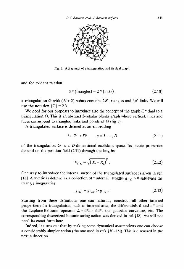
Fig. 1. A fragment of a triangulation and its dual graph.

645

and the evident relation

3 # (triangles) = 2 # (links), (2.10)

a triangulation G with (N + 2) points contains 2N triangles and 3N links. We will

use the notation IGI = 2N. We need for our purposes to introduce also the concept of the graph G* dual to a

triangulation G. This is an abstract 3-regular planar graph whose vertices, lines and faces correspond to triangles, links and points of G (fig 1).

A triangulated surface is defined as an embedding

i ~ G ~ X~, /~ = 1 . . . . . D (2.11)

of the triangulation G in a D-dimensional euclidean space. Its metric properties depend on the position field (2.11) through the lengths

h ( i j ) = ~ / ( X i - X j ) 2 • (2.12)

One way to introduce the internal metric of the triangulated surface is given in ref. [18]. A metric is defined as a collection of "internal" lengths g(ij> > 0 satisfying the triangle inequalities

g(ij> + g(jk) > g(ik)" (2.13)

Starting from these definitions one can naturally construct all other internal properties of a triangulation, such as internal area, the differentials d and d* and the Laplace-Beltrami operator A = d*d + dd*, the gaussian curvature, etc. The corresponding discretized bosonic string action was derived in ref. [18]; we will not need its exact form here.

Indeed, it turns out that by making some dynamical assumptions one can choose a considerably simpler action (the one used in refs. [10-15]). This is discussed in the next subsection.

646 D.V. Boulatov et al. / Random surfaces

2.2. D E F I N I T I O N OF THE MODEL

Each continuum surface can be approximated by triangulated surfaces with any accuracy, if we choose appropriate triangulations. The choice of the most relevant triangulation depends on the geometry of the surface and there is no universal one which fits for all surface configurations. For example, the regular triangular lattice describes properly only those surfaces which are small deformations of a plane. Thus all possible triangulations have to be considered on an equal footing.

There are two alternatives. We can take the average with respect to the surfaces with fixed triangulation and then average the result over all triangulations (quenched average). Such an average was used in MC simulations in ref. [9].

On the other hand, we can treat the triangulation dynamically, i.e. take the average simultaneously over the positions and the triangulations of the random surface (annealed average). This concept was used in [10-15].

We choose the second alternative for the following reason. Considering the triangulation as a dynamical field we can describe the fluctuations of the internal geometry without taking the average over the internal lengths g<ii> as was pre- scribed in [18]. Thus we simply postulate that all internal lengths are equal, i.e. all triangles are equilateral in the sense of the internal geometry. We expect that this assumption will not change the critical behaviour of the model. As we know from the theory of phase transitions, the restrictions on the field variables in the bare action effectively disappear in the vicinity of the critical point. The long-range effective action depends on the block-spin variables which are not restricted. For example, in the Ising model the block spins vary from - oo to + oo, in spite of the hmitation s i = +_ 1 on the initial spins.

One may also say that each choice of the internal geometry defined by g<ij> may be considered as induced by an embedding of the lattice G in a virtual euclidean space of sufficiently high dimensionality.

It is convenient to choose g<o> = 21/23t/4; then all triangles will have unit area. Also, the volume og of the dual image of the point i ~ G (which is the discrete analog of the invariant volume vrg d2~) is proportional to the number of nearest neighbours (the coordination number) q, of this point:

1 o,= 3qi, ~ ~ = IGI. (2.14) i ~ G

Since all triangles are now equilateral, the curvature R i at the point i of G can be expressed through the coordination number q, as well:

R~ = ~r(6 - q~)/q~, E o~R~ = 4~r. (2.15) i ~ G

Finally, the action functional (2.2) takes the following simple form

~discrete = 1 E ( X i - X j ) 2 " ~ f l E ° i " (2.16) <0">

D. V. Boulatov et al. / Random surfaces 6 4 7

The integration measure over the position field now has the form

D X = I-Io, D/2 dDx , , (2.17) i

implied by the discretization ]l~gll 2= ~,o i3g , 2 of eq. (2.3). To kill the translational zero mode we suppress one of the integrations.

We also would like to add to the action a counterterm of the type (2.5)

1 2 ~ l ~ d i s c r e t e - E o i ~ R i , ( 2 . 1 8 )

i

with the curvature R i defined by (2.15). For technical reasons we prefer to use another version of this term, namely

~ { " ~ d i s c r e t e - - - - Eln( o,)= E o , 1 + In 1 + - . i i 77

(2.19)

Being expanded in Ri, this term coincides with (2.18) up to R~ terms due to Euler's theorem (2.9). Thus the counterterm (2.18) can be incorporated simply by changing

1 the power ~D in (2.17) to an arbitrary real number a. Now we are in a position to write down the partition function of the planar

triangulated surface. The sum over surfaces includes integration over the embed- dings of a given triangulation and a sum over triangulations.

The contribution of the surfaces with a fixed triangulation G is defined by

(2~r)o/zexp - ~ E ( X / - X j ) 2 • (2.20)

The primed product sign means that one of the integrations has to be omitted. The full partition function reads

1

= ~_, e 2t~JVzu(a, D) . (2.21) N = I

The factor 1 / k counts for the possible symmetry of the graph G. Two triangulations which can be transformed one into another by a permutation of the points are considered identical. The coefficient Z u can be interpreted as the microcanonical partition function for surfaces with fixed internal area I GI = 2N.

Up to now we have not discussed the class of triangulations to be considered. One of the possibilities is to sum over the set ~0 of all possible triangulations including the singular ones containing parallel links or links with coinciding ends. The

648 D.V. Boulatoo et aL / Random surfaces

corresponding dual graphs form the set f¢0* of all possible q~3 planar vacuum graphs. This version of the model is most convenient for the analytical study. On the other hand, in numerical simulations it is convenient to drop the most singular triangulations in order to speed up the calculation. We considered the class ~2 of triangulations satisfying the conditions that

(i) there are no links with coinciding ends, (ii) two points may be connected by no more than one link (i.e. parallel links are

forbidden). The set of the corresponding dual graphs if2* contains those planar graphs which have no tadpoles and self-energy parts. An intermediate version of the model where the sum is performed within the class ffl of the triangulations satisfying only the condition (i) is also considered. The quantities calculated in the version 0, 1 or 2 of the model will be supplied with an index 0, 1 or 2 if necessary. All three versions are expected to exhibit the same critical behaviour.

One can impose stronger restrictions on the triangulations to be used, in case they are local ones; we will not discuss this point here (see, for example, ref. [19]).

The model of random surfaces defined by eq. (2.21) was proposed independentiy by David [12] and three of the authors [10]. It has the advantage of being extremely simple and easy to be computer simulated. We expect that, unlike the discrete surface model based on a rigid triangulation [6], the model defined by eq. (2.21) will supply a reliable regularization of the Polyakov string. Its most essential feature is that the triangulation G of the random surface is treated as a dynamical field (the discrete counterpart of the internal metric g,b(~))"

The continuum of reparametrization symmetry transformations in the discrete model degenerates to the set of renumerations of the points and edges of a triangulation. One may object that this symmetry is too trivial and noninformative. But each reparametrization is indeed in some sense a renumeration of the points of the manifold. The discretization only makes this more transparent.

2.3. CORRELATION FUNCTIONS AND CRITICAL EXPONENTS

The n-point correlation function of the ensemble of closed planar surfaces is defined as the sum over all surfaces pinned at n points Y1 . . . . . Y,, divided by the partition function. We will be interested only in the two-point correlator G(Y1 - Y2). In the momentum space

1 G( P2) = Z 1 ~. ~ icGI-[ o/~e-~°' Z Z(*s)(P2IG),

G k,s (2.22)

d°Xi [ ] z' ')(P21a) = f (21r)°/----------2exp[ -½ (O) ~ ( X i - X j ) 2 - i P ( X I ' - X ' ) " (2.23)

The coefficients in the expansion of the partition function (2.21) will be shown to


behave for large N as

Z u - A N N -b . (2.24)

Then the series (2.21) will be convergent up to some critical value of the expansion parameter x = e -2a, namely x c = 1/.4, and analytic in the circle Irl < Ixcl in the complex r-plane.

The critical exponent ~, for the susceptibility

is defined by

O0 2

X = -7-aw,~Z(a, fl, D ) - G(p2) le2=o (2.25) Ol, S-

- -y X (,8) 8_.,~c (,8 &) + const. (2.26)

It is related to the asymptotics (2.24) by

y = - b + 3. (2.27)

One can show by methods developed in ref. [5] that in any model of noninter- acting planar surfaces with positive weights, ~{ ~< ½. On the other hand, the perturbative treatment of the continuum Polyakov surface yields [20]

~, = I ( D - 7). (2.28)

This means that above some critical dimension the Liouville theory fails to describe the fluctuating surface.

Another important characteristic of the random surface is its fractal (or Haus- dorff) dimension

ln({X2)u) di~ = ½ lim (2.29)

N--,~ I n ( N ) '

where the mean square extent {X2)N of the surfaces with 2N triangles may be defined as

f d D X X 2 G u ( X ) O 2 (X2)N= f d D X G N ( X ) = - D - o ~ l n [ G N ( P )] ,,'=o" (2.30)

Here GN(X ) denotes the two-point correlator for the microcanonical ensemble of surfaces with area IG[ = 2N. It is defined by the same formula (2.22), with the sum restricted to triangulations G with [G t = 2N and the factor Z -1 replaced by ZN 1. For a more refined definition of d n see, for example, ref. [9].


The mass gap of the model is defined by the asymptotics of the correlator (2.22) in the X-space

G ( X ) - e x p [ - m ( f l ) l X I ] . (2.31) IxI--, oo

The mass gap may or may not vanish at the critical point fl = tic- David [12] speculated that if m(flc)> 0 then (X2)N grows logarithmically with the internal area 2N. However, we cannot agree with his argument which is based on the assumption that the critical exponent ,/' of the two-point function may depend on p2. Actually, G(P) is not obliged to behave as a single power in (fl - tic) near the critical point. It can rather be a sum of two terms with different y's. As an illustration (and a trivial counterexample) we consider the sum over closed loops in appendix A. Thus, it is quite possible to have a nonvanishing mass gap and finite Hausdorff dimension.

When m (t ic)= 0, we have the standard scaling relations

= v ( 2 - ~), v = 1 /d H, (2.32)

where the critical indices v and ~/ are defined by

m ( / 3 ) = C ( / 3 - / 3 c ) ~, /3~,B~, (2.33)

a ( s ) - ISlZ-°-~e m(~)m, 1 << IXl << m - l ( f l ) . (2.34)

2.4. DUALITY RELATIONS

The partition function for fluctuating surfaces with the topology of a sphere and defined by the action (2.2) is invariant under a duality transformation interchanging the coordinate and momentum spaces. The self-duality property actually holds for any fixed configuration of the internal metric gab(~)"

The integral over the position field can be replaced by an integral over the velocities Va ~ = OaX" by imposing the constraint

1 c - t,b O,Vb ~ = 0 (2.35) Vg

through a Lagrange multiplier Y~(~). The gaussian integral over V~ ~ in the resulting expression

f DV~ ~ Dr"exp{ - of d2~ ¢-gg.bV~Vp,


can be performed and we reconstruct the original action with o and X~(~) replaced by 1 / o and Y~(~). Unfortunately, this self-duality is of no use since the partition function does not depend on o. However, in the discrete model it leads to interesting analogies.

Consider the contribution of a given triangulation G and replace the integral over the positions Xi of its points by an integral over the independent differences

V~j) = X/~ - X~ (2.37)

defined on the links (0) of G. The discrete analog of the constraint (2.35) is

+ v k> + v?k,> = 0 (2.38)

for each triangle (ijk). Consider the dual graph G* and denote by u* = 1, 2 . . . . . 2N its vertices. To each line (u'v*) of G* we associate a variable V~,v, = V~k > where (ik) is the link of G dual to the line (u'v*). Further, the condition (2.38) can be imposed through a set of Lagrange multipliers Yo*

1 exp(iY~,~V~,~,). (2.39)

Since only 2 N - 1 conditions of the type (2.38) are independent, one of the integrations (2.47) has to be omitted. The contribution of the dual lattice G* after the integration over the differences V~,o, takes the form

(2~r)(N-1)/2 f o*~G*dDy°*exp[--2flN-- (u'v*) ~-~ l(Yu*- Yv*)2] " (2.40)

This expression can be interpreted as follows. The dual graph G* can be thought of as a vacuum diagram of a planar q~3 theory with gaussian propagator exp( - ½(Y- y , )2) and a coupling constant g = (2~r)O/ae-a.

In the special case a = 0 this analogy can be pursued further. The lattice G and its dual graph G* have the same symmetry so that the partition function (2.21) of the model in its 0-version (see subsect. 2.2) reproduces the vacuum energy E(fl) of the 03 model. This last quantity is defined by

E ( f l ) = N-,o~lim [Ne(volume)]-llog(fDq~(Y)e-S[~]), (2.41)

S[ep]=Ntr(½ f doydOY'e(V-v')2/2ep(Y)ep(Y')-lgf dOyck3(Y)), (2.42)

where ,~(Y) represents an N × N hermitian matrix field.


To obtain the partition function of the version 1 of the model we have to subtract all diagrams with tadpoles. This can be achieved by adding a term linear in q~ in the action (2.50). Finally, the partition function of the version 2 of the model is obtained by subtracting both the diagrams with tadpoles and with self-energy insertions. This can be done by adding two terms to the ac t i on - linear and quadratic in ~.

The discussed relation between the random surface model and the gaussian q~3 planar model has been observed independently by David [12] and three of the authors [10]. Some earlier suggestions on the relevance of the gaussian ~3 model for random surfaces have been made by Frfhlich [21]. Note, however, that the equivalence between the triangulated surfaces and the q,3 planar model holds only for the partition functions. The two-point function of the model of triangulated surfaces has nothing to do with that of the q~3 model. The relation between the two models is similar to the one between planar random surfaces on a hypercubical lattice and the reduced version of the Weingarten gauge model.

3. Analytical study

3.1. COMBINATORIAL RULES FOR THE GAUSSIAN INTEGRATION

In this subsection we collect some well known formulas (see, for example, [22]) allowing us to perform the gaussian integration in eqs. (2.20) and (2.23).

Let F be a connected graph with points labeled by i = 1 . . . . . N 0. As before, the line connecting the points i and j will be denoted by (O'). A subgraph T c F is called a tree on F (or a tree spanning F) if it (i) contains all points of F, (ii) has no cycles, and (iii) is connected. A subgraph T 2 c F satisfying the conditions (i) and (ii) and having exactly two connected components is called a 2-tree on F. A subgraph T c c F is a tree with a cycle if it satisfies the conditions (i) and (iii) and has exactly one cycle.

The quantities Z( I " ) and Z k s ( P 2, I ' ) defined by eqs. (2.20) and (2.23) depend on the structure of the graph F through the following remarkable relations

Z ( / ' ) = [T(G)]-D/z, (3.1)

Z('J)( P2IY) = [T(G)I 2 T(u)(F) } r ( r ) '

(3.2)

where T ( F ) is the number of trees on the graph F and T2(iJ)(F) is the number of 2-trees on F containing the points i and j in different connected components.

In the case when the graph /" defines a two-dimensional complex with the topology of a sphere, its dual graph F* has the same property. For each subgraph F 1 c F there is a unique subgraph F 1 c / ' * which is defined as the complement of


the dual image of/ '1 . It is easily seen that trees on F correspond to trees on F*, and 2-trees on F correspond to trees with a cycle on F*. Thus the r.h.s, of eqs. (3.1) and (3.2) can be expressed in terms of the dual graph F*.

A tree with a cycle on F* divides the set of the dual images of the points of F into two connected components. Denote by TcUJ}(F *) the number of all trees with a cycle on r * such that the dual images of the points i and j belong to different connected components. Then

z ( r ) = z ( r * ) = [ T ( r * ) ] - , / 2 , (3.3)

Z{,J)(pZlr)=[T(F.)]-ZVZexp{_½p2 ) r ( r * ) •

(3.4)

These relations allow us to reduce the calculation of the partition function (2.21) and the two-point correlator (2.22) to pure combinatorics.

For the mean square extent of the surfaces with internal area 2N we have

( x2)N = BN/AN, 0.5)

1 B u = ½ E k(G) I-I o ; E T2(iJ)(G)[T(G)]-D/2-1

IGI=2N k ~ G i , j ~ G (3.6)

1 E

IGI=2N --(N+2)2VIo~[T(G)] D/Z=(N+2)ZZN, (3.7)

i ~ G

where the sum goes over triangulations with I GI = 2N triangles. As an illustration of this tree calculus we considered in appendix A the ensemble of free random loops.

To conclude this section we recall the representation of the gaussian integral (2.20) in terms of random paths

where I2/~ is the sum of all closed nonoriented paths on the graph F taken with a weight 1/q i for each site and nonincidental with a given point i 0 ~ F. Of course, the result does not depend on the choice of i 0.

It follows immediately from eq. (3.8) that the number of trees on a triangulation G grows at most exponentially with the number of triangles I GI = 2N:

T(G) < I-[ qi < 6N+2- (3.9) i ~ G

654 D.V. Boulatov et a L / Random surfaces

This inequality justifies the assumption (2.24) for the behaviour of the coefficients Z u in the expansion (2.21) of the partition function. For the critical coupling we have the bound

fie < - ¼DN ln6. (3.10)

In the next two subsections we present some exact results in two special cases (a = 0; D - - - 0 , - 2 ) corresponding to the gaussian 43 planar model in D = 0 and D = - 2 dimensions.

3.2. D = 0 , a = 0

This case has already been considered in [7, 8]. The corresponding zero-dimensional planar theory was solved exactly (in all three versions) in ref. [23]. For example, the explicit form of the microcanonical partition function in the variant (0) of the model is

8Nir(3N) - N- 7/2 (12f3-) N (3.11) Z(u°) = (N + 2)!F(½N + 1) N - ~

which implies that the canonical partition function (2.21) becomes singular at exp(2flc) = 12v~-. In all three versions of the model the critical exponent 7 has the same value T = - ½, as expected.

In appendix B we present the calculation of an interesting quantity characterising locally the internal geometry of an average surface. This is the probability distribution of the coordination numbers qi of the points of the surface. Let us consider the ensemble of surfaces with 2N triangles and one point (say, io) fixed. The corresponding microcanonical partition function is equal to the original one times the number of points N + 2. On the other hand it is equal to the sum

(N+ 2)ZN= E IO(N) q q ~ q ' (3.12)

w h e r e Q(qN) stands for the contribution of the surfaces with q triangles joined at the fixed point i 0. The probability distribution PN(q) of the coordination number q is given by the mean number of vertices with qi = q divided by the total number of vertices N + 2:

Q(qU) (3.13) PN(q)-- q (N+ 2)Z N "

But the quantity Q~N) is exactly the number of 4 3 planar graphs with 2 N - q vertices and q external lines (unrestricted for the versions (0) and (1) and connected


in the version (2) of the model). Thus the distribution of the coordination numbers can be extracted from the Green functions of the q~3 planar theory; this has been calculated in ref. [23].

It is most interesting to find explicitly the probability distribution PN(q) in the version (2) of the model which will be used in our numerical calculations. The calculation (appendix B) yields

3 ) q ( q -- 2)(2q - 2)! p~2)(q) = 16 ~-~ q!(--~---1)-! " (3.14)

At large q this distribution decays as exp ( -oq ) with o = In 4 = 0.288. We conclude that at D = 0, a = 0 the average surface is far from being regular.

Though the average coordination number is equal to six, as it should be,

to

E qPoo(q) = 6, (3.15) q=3

the distribution is rather smooth and most of the vertices have 3 or 4 links. Note that the parameter o characterising the exponential decay of P~(q) is not

universal. Similar calculations for the version (0) of the model yield

o (°) = ln(3 - v~-) = 0.237. (3.16)

3.3. D = - 2 , a = 0

In this special case we were able to calculate both the partition function [10] and the mean square extent [11] of the model in its version (0).

It was subsequently noticed by David [24] that the corresponding planar q53 model can be obtained by Parisi-Sourlas dimensional reduction from a zero-dimensional planar theory. In particular, it was shown in [24] that the critical exponent 7 is the same for all three versions of the model. Here we will present the combinatorial method since it allows us to calculate also the mean square extent of the surface. Our results read

y = - 1 , d H = o c ( ( X 2 ) u - l n (N) ) . (3.17)

(A) The partition function. At D = - 2 the contribution of each triangulation is linear in the number of trees and the microcanonical partition function can be written as a double sum

1 ZN= E k (G*) Z 1, (3.18)

IG*I=2N T o G *


where [G*[ is the number of vertices of the dual graph G*. To get rid of the combinatorial factor 1 / k ( G * ) it is convenient to replace the sum over vacuum graphs G* with a sum over vacuum graphs G~ with a marked vertex

1 1

k ( G * ) . . . . Z 3IG~---- ~ " '" (3.19) G* G~'

The factor ~ counts for the cyclic symmetry of the marked vertex. Each tree T c G~ defines a tree 7 ~ which is obtained by cutting all lines of G~'

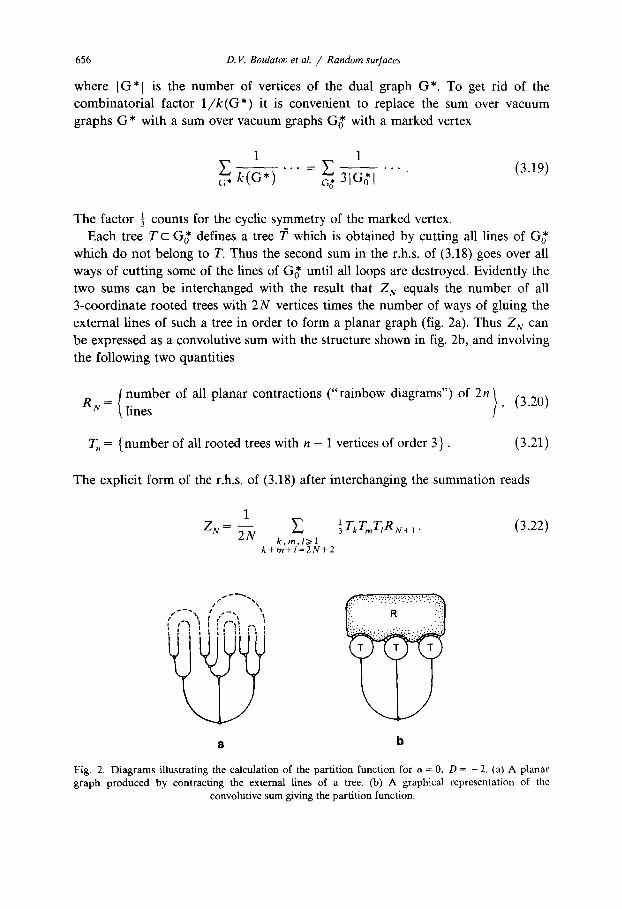
which do not belong to T. Thus the second sum in the r.h.s, of (3.18) goes over all ways of cutting some of the lines of G~ until all loops are destroyed. Evidently the two sums can be interchanged with the result that Z N equals the number of all 3-coordinate rooted trees with 2N vertices times the number of ways of gluing the external lines of such a tree in order to form a planar graph (fig. 2a). Thus Z n can be expressed as a convolutive sum with the structure shown in fig. 2b, and involving the following two quantities

number of all planar contractions ("rainbow diagrams") of 2n} (3.20) R N = lines

T. = (number of all rooted trees with n - 1 vertices of order 3 }. (3.21)

The explicit form of the r.h.s, of (3.18) after interchanging the summation reads

1 = 3 T k T , , T t R N + , (3.22) Z~ 2N Y" t

k,m,l>~l k + m + l ~ 2 N + 2

/ / " ' " "x

Fig. 2. Diagrams illustrating the calculation of the partition function for a = 0, D = -2. (a) A planar graph produced by contracting the external lines of a tree. (b) A graphical representation of the

convolutive sum giving the partition function.

The quantities R n and recurrence relations

D. V. Boulatov et aL / Random surfaces 657

7". can be calculated instantly. They satisfy identical

n - 1 n - 1

TN= Y'~ T,T._~, R .= ~_~ RkR._I_ k, (3.23) k = l k=O

which are solved by the Catalan numbers

( 2 . - 2 ) ! Rn-1 = Tn = / ' / ! ( n - 1 ) ! " ( 3 . 2 4 )

The corresponding ½(1 - (i- - 4z ) satisfies the equation

generating function T(z) -~ TIZ + T2 Z2 -{- T3 Z3 + . . .

r ( ~ ) = ~ + r : ( z ) .

T,.IT,.fl.3= TM- TM 1

As a consequence of eq. (3.25)

E ml,m2,m3>~l

(3.25)

(3.26)

rnl + m2 + m3 = M

and we finally obtain for the rnicrocanonical partition function

1 Z ~ ° ) l D = _ 2 = - 6 - - ~ T N + 2 ( T 2 N + 2 - T2N+I )

1 (4N)! - 2 ( N + l ) TN+zT2N+I= (2N) I (N+I ) ! (N+2) ! " (3.27)

It follows from the asymptotics

that the critical exponent for the susceptibility is y = - 4 + 3 = - 1 and the critical coupling for the version (0) of the model is given by

e -~°' = ~ = 0.125. (3.29)


The critical couplings for the other two versions have been calculated in ref. [24]

e x n ( - (1)]= = .-- , ~-, 131 , (11~87r)2 0.13554

128 , exp(-/3~ (2)) = 1--0-~- (2 - 212/(15"tr ) 2 ) 1 / 2 = 0 . 1 5 3 0 2 . . . . (3.30)

(B) The mean square extent ~ 2 X )N" We have to calculate the coefficients A N and B N in the r.h.s, of (3.5). The denominator is already known

( N + 2) 2 43N

AN 2 ( U + 1) TN+2T2N+I -- ~¢'2N 2" (3.31)

To calculate B N it is again convenient to eliminate the symmetry factor 1 /k(G) by applying eq. (3.19):

1 BN= 6- ~ ~ ~Tc~i'J)(G~)=B'N+ B~. (3.32)

IG~I=2N i , j

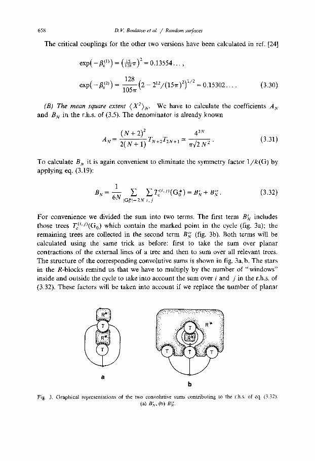
For convenience we divided the sum into two terms. The first term B~v includes those trees Tc(i'J)(G0) which contain the marked point in the cycle (fig. 3a); the remaining trees are collected in the second term B)~ (fig. 3b). Both terms will be calculated using the same trick as before: first to take the sum over planar contractions of the external lines of a tree and then to sum over all relevant trees. The structure of the corresponding convolutive sums is shown in fig. 3a, b. The stars in the R-blocks remind us that we have to multiply by the number of "windows" inside and outside the cycle to take into account the sum over i and j in the r.h.s, of (3.32). These factors will be taken into account if we replace the number of planar

I r

i! b

Fig. 3. Graphical representations of the two convolutive sums contributing to the r.h.s, of eq. (3.32). (a) B~v, (b) B~.

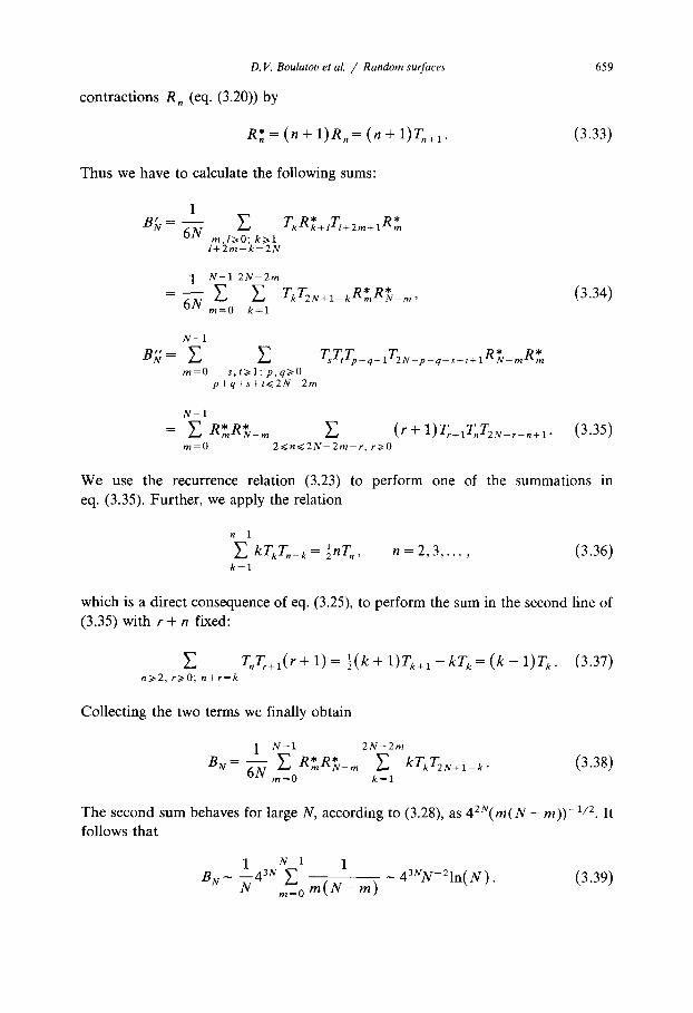
D.V. Boulatov et al. / Random surfaces 659

contractions R , (eq. (3.20)) by

R* = (n + 1)R. = (n + 1)T~+ 1. (3.33)

Thus we have to calculate the following sums:

1 , = TkRk+tTl+zm+xR,, BN 6N Y'~ * *

m,l>~O; k>~l 1+2m+k=2N

1 N - I 2 N - 2 m

6N y'~ Y'~ m=O k = l T k T2 N + * * 1-kRmRN-m, (3.34)

N - 1

r! ~ E BN m = O

E Z s T t T p + q + l Z 2 N - p - q s - t + l R ~ - m R * m s,t>~l; p,q>~O

p+q+s+t<~2N-2m

N - 1

m = O ~, ( r + 1)Tr+ITnT2N_ r n + l " (3.35)

2<~n<~2N 2 m - r , r>~O

We use the recurrence relation (3.23) to perform one of the summations in eq. (3.35). Further, we apply the relation

n 1

E kr, ro_, 1 = 7 n T , , n = 2, 3 . . . . . ( 3 .36 ) k = l

which is a direct consequence of eq. (3.25), to perform the sum in the second line of (3.35) with r + n fixed:

~_~ T n T r + l ( r + l ) = ½ ( k + l ) T k + l - k T k = ( k - 1 ) T k . (3 .37 ) n~>2, r~>O; n+r=k

Collecting the two terms we finally obtain

1 N - 1 2 N - 2 m

BN= - ~ ~., R*R*N_ m ~ kTkT2N+I_ k. (3.38) m = O k = l

The second sum behaves for large N, according to (3.28), as 42U(rn(N - m)) -1/2. It follows that

1 N 1 1 BN -- - - 43N E 43NN- 21n(N ). (3.39)

N m ( U - m ) rn~O


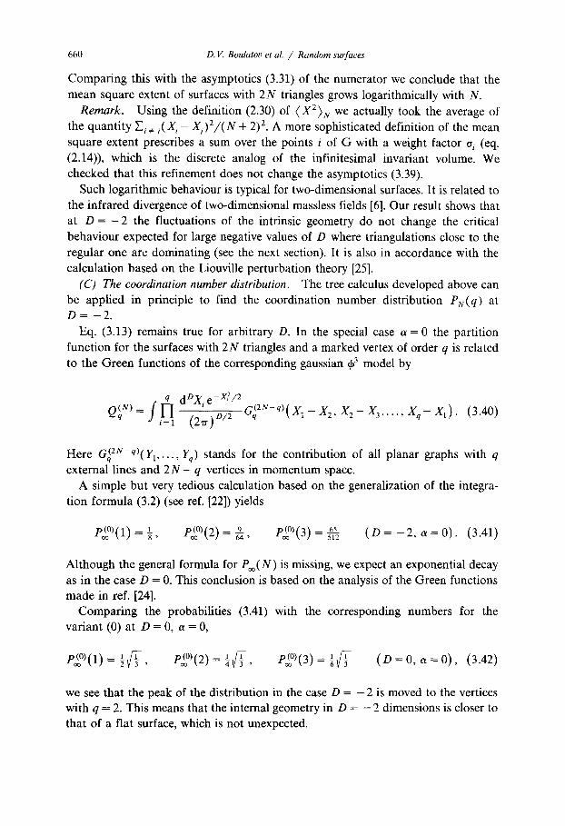
Comparing this with the asymptotics (3.31) of the numerator we conclude that the mean square extent of surfaces with 2N triangles grows logarithmically with N.

Remark. Using the definition (2.30) of (X2)N we actually took the average of the quantity Ei ~ j (X,- Xj)2/(N + 2)2. A more sophisticated definition of the mean square extent prescribes a sum over the points i of G with a weight factor oi (eq. (2.14)), which is the discrete analog of the infinitesimal invariant volume. We checked that this refinement does not change the asymptotics (3.39).

Such logarithmic behaviour is typical for two-dimensional surfaces. It is related to the infrared divergence of two-dimensional massless fields [6]. Our result shows that at D = - 2 the fluctuations of the intrinsic geometry do not change the critical behaviour expected for large negative values of D where triangulations close to the regular one are dominating (see the next section). It is also in accordance with the calculation based on the Liouville perturbation theory [25].

(C) The coordination number distribution. The tree calculus developed above can be applied in principle to find the coordination number distribution PN(q) at D = - 2 .

Eq. (3.13) remains true for arbitrary D. In the special case a = 0 the partition function for the surfaces with 2N triangles and a marked vertex of order q is related to the Green functions of the corresponding gaussian 4~ 3 model by

q dDXie-X,2: Q~N)= f i~=1 ( 2 ~ ) D / 2 G ~ 2 N - q ) ( x 1 - X 2 . . . . X 2 - X 3 , . . X q - X l ) (3.40)

(Tr(2N-q)(Y1,... , stands for contribution all planar q Here _q , Yq) the of graphs with external lines and 2 N - q vertices in momentum space.

A simple but very tedious calculation based on the generalization of the integration formula (3.2) (see ref. [22]) yields

P~°}(1) = ~, P~°)(2) ~--- ~4' P~°)(3) = 51262 (D = - 2 , a = 0) . (3.41)

Although the general formula for Poo(N) is missing, we expect an exponential decay as in the case D = 0. This conclusion is based on the analysis of the Green functions made in ref. [24].

Comparing the probabilities (3.41) with the corresponding numbers for the variant (0) at D = 0, a = 0,

1 1 1 1 1 P~°)(X) = 5Vf~ -, P~°)(2) = ~ - 3 , P~°)(3) = ~/~-~ (D=O, a=O), (3.42)

we see that the peak of the distribution in the case D = - 2 is moved to the vertices with q = 2. This means that the internal geometry in D = - 2 dimensions is closer to that of a flat surface, which is not unexpected.


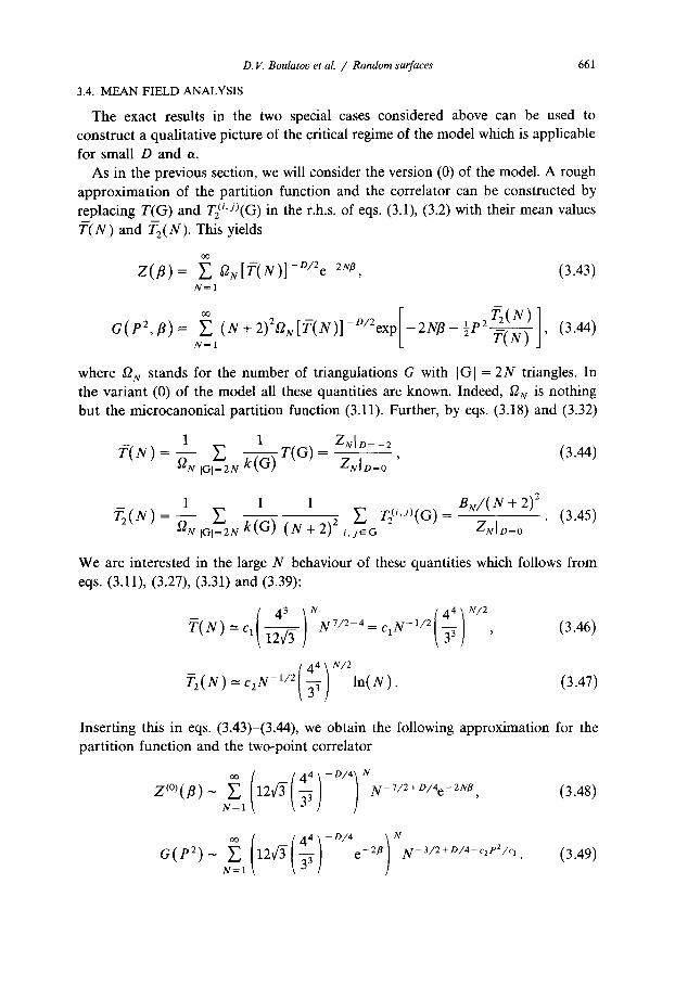
3.4. MEAN FIELD ANALYSIS

The exact results in the two special cases considered above can be used to construct a qualitative picture of the critical regime of the model which is applicable for small D and a.

As in the previous section, we will consider the version (0) of the model. A rough approximation of the partition function and the correlator can be constructed by replacing T(G) and Tz~i'J)(G) in the r.h.s, of eqs. (3.1), (3.2) with their mean values T(N) and Tz(N ). This yields

Z ( f l ) = ~ ON[f(N)l-D/2e-aN¢, (3.43) N=I

G(p2'fl)= N=I ~ (N+2)2~N[T(N)]-D/2exp[ -2N~-I 5P2T2(N)]T=(N) ' (3.44)

where O N stands for the number of triangulations G with [G[ = 2N triangles. In the variant (0) of the model all these quantities are known. Indeed, O N is nothing but the microcanonical partition function (3.11). Further, by eqs. (3.18) and (3.32)

1 1 ZNID= -2 T ( N ) = ~N E k(G) T (G)= , (3.44)

IGI=2N ZNI D=O

1 1 1

= - - E k(G) (N+2) 2 E ~ ( N ) gu IGI=2N i , j~G

B N / ( N + 2) 2 T2¢" J)(G) - (3.45)

ZNI~=0

We are interested in the large N behaviour of these quantities which follows from eqs. (3.11), (3.27), (3.31) and (3.39):

(43) (44) J2 T(N) = C 1 1 ~ N7/2-4 = CLN-1/2 ' ~

T 2 ( N ) = ¢2 N-1/2 "~ I n ( N ) .

(3.46)

(3.47)

Inserting this in eqs. (3.43)-(3.44), we obtain the following approximation for the partition function and the two-point correlator

z ( ° ) ( B ) - N=I

12 N- 7/2 + D/4 e - 2 US, (3.48)

N

/3 3 ] ] (3.49)


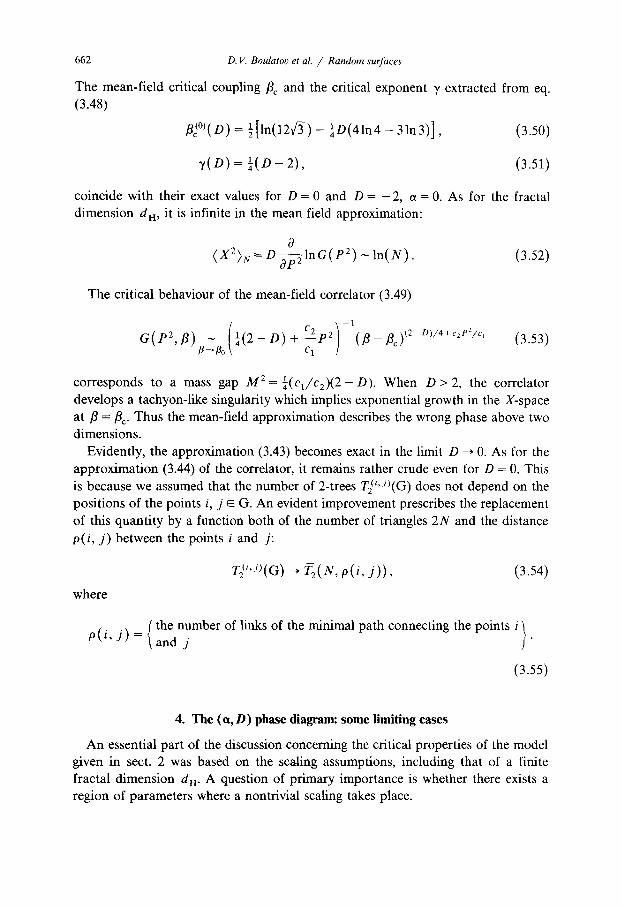
The mean-field critical coupling tic and the critical exponent -f extracted from eq. (3.48)

fl~°)(D) = 1[ln(12q~-) - ¼D(41n4- 31n3)], (3.50)

"f(D) = ¼(D - 2), (3.51)

coincide with their exact values for D = 0 and D = - 2 , a = 0. As for the fractal dimension dH, it is infinite in the mean field approximation:

0 ( X2)N = D~--ilnG( P 2) ~ l n ( N ) . (3.52)

The critical behaviour of the mean-field correlator (3.49)

1

G(P2 , fl)~St~ ° J ( 2 - D ) + c z P 2] ( f l - R ] ~2 m/n+c2P2/, , Cl ] r-c/

(3.53)

corresponds to a mass gap M 2= ¼(el/c2)(2-D). When D > 2, the correlator develops a tachyon-like singularity which implies exponential growth in the X-space at fl = tic. Thus the mean-field approximation describes the wrong phase above two dimensions.

Evidently, the approximation (3.43) becomes exact in the limit D ~ 0. As for the approximation (3.44) of the correlator, it remains rather crude even for D = 0. This is because we assumed that the number of 2-trees T2(i,J)(G) does not depend on the positions of the points i, j ~ G. An evident improvement prescribes the replacement of this quantity by a function both of the number of triangles 2N and the distance p(i, j) between the points i and j:

Tff ' /)(G) ~ ~(N, p(i, j ) ) , (3.54)

where

the number of links of the minimal path connecting the points i ) p ( i , j ) - - and j

(3.55)

4. The (ct, D) phase diagram: some limiting cases

An essential part of the discussion concerning the critical properties of the model given in sect. 2 was based on the scaling assumptions, including that of a finite fractal dimension d H. A question of primary importance is whether there exists a region of parameters where a nontrivial scaling takes place.


Before trying to answer this difficult question, we will reconstruct the phase diagram in those parts of the (a, D)-plane where an exact treatment is possible.

We will identify three different types of critical behaviour depending on the

values of D and a. In the limit D ~ - o 0 there are two possible phases. For a larger than some

critical value ac - D we are in the phase of real two-dimensional surfaces which is

consistent with the Liouville string theory. When a becomes smaller than a t (D) , the average surface collapses into an essentially pointlike object. We call this phenome-

non "crumpling". In the limit D ~ ~ there are again two phases depending on the value of a.

These are the phase of crumpled surfaces (for a < ac(D)) and the phase of branched polymers (for a > ac(D)). In the latter case the dominant triangulations have the structure of trees made up of thin tubes.

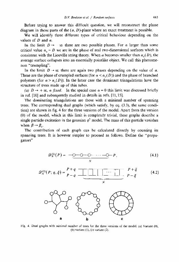
(a) D ~ + oo, a f i xed . In the special case a = 0 this limit was discussed briefly in ref. [10] and subsequently studied in details in refs. [11,15].

The dominating triangulations are those with a minimal number of spanning trees. The corresponding dual graphs (which satisfy, by eq. (3.3), the same condition) are shown in fig. 4 for the three versions of the model. Apart from the version (0) of the model, which in this limit is completely trivial, these graphs describe a single particle excitation in the gaussian q,3 model. The mass of this particle vanishes

when fl ~ tic" The contribution of each graph can be calculated directly by counting its

spanning trees. It is however simpler to proceed as follows. Define the "propa- gators"

N ~ ) ( P ) = ~ - . . - - O - - P , (4.1) N

P + q (4.2) 1-? I_L ~ 2 ) ( p ; q, ~ ) = P _ q

N

a b c

Fig. 4. Dual graphs with minimal number of trees for the three versions of the model. (a) Variant (0), (b) variant (1), (c) variant (2).


By the corresponding recurrent equations one finds

~ ) ( P ) - 2-nN/2exp(--3 Np2 ) , (4.3)

.@(N2)(Pq~I) - (2 + ~/~)-DN/2exp[-Np 2 - ½(1 + ~/~)(q2 + #2)], (4.4)

when N is large. Then the partition function of the versions (1) and (2) of the model are given by

oo ZO)(fl, a) - • (2-n/2(2)"e-2/~)N'N2~-D/2-X, (4.5)

N ~ I

oo z ( Z ) ( • , ° t ) - E [ ( 2 + V t 3 ) - o / 2 ( ~ ) a e - 2 B ] N ' N 2 a - O / 2 - x " (4.6)

N=I

In both cases we have the same critical exponent

x 2(a + 1) (4.7) 7 = ~D +

As for the mean square extent, it follows from eqs. (3.5)-(3.7) that

( X2)N N~o~ const. (4.8)

The fact that the mean size of the surfaces remains finite when N ~ o¢ will become rather obvious if we return to the original triangulations. These are characterized by extremely singular internal geometry. Most of the vertices are with positive curvature (q < 6), which is compensated by two huge stars with negative curvature of order N (fig. 5). The average internal distance between two points (eq. (3.55)) remains of order one in the limit N---, oo and so does the mean square extent ( X Z ) N . This is why we call this phase "the phase of crumpled surfaces".

a b

Fig. 5. Triangulations characterizing the (most) crumpled surfaces (a) for the variant (1), (b) for the variant (2).

D. V. Boulatov et al. / Random surfaces

a b

665

Fig. 6. Dual graphs with minimal number of trees under the condition that each "window" involves exactly 6 lines for the variants (0) and (1) of the model.

Evidently, large negative a works in the same direction as large positive D; the surfaces with maximal local curvature are tolerated. Thus the phase of crumpled surfaces extends to all a < ac (D ). The critical line a c ( D ) will be found below in the limits D ---, + oo.

(b) D ~ oo, a ---, oo (a >> D). In this case the partition function is saturated by the triangulations with minimal number of spanning trees under the condition of locally flat internal geometry. For each N there are two triangulations with this property; the corresponding dual graphs are shown in fig. 6 for the versions (0) and (1), and in fig. 7 for the version (2) of the model. These triangulations possess the internal geometry of long thin tubes.

The contribution of the first diagram in fig. 6a has been already calculated; it is given by the function (4.2) with ~ = 0. One can check immediately that the other diagram yields the same quantity. Thus the partition function for these tubes reads

Z(° ' l ) ( /~ ,a ) - ~'~ ((2 + ~)-O/22"e-2B)N (4.9) N=I

a b

Fig. 7. Dual graphs with minimal number of trees and locally flat structure for the variant (2) of the model.

666 D. V. Boulatoo et al. / Random surfaces

Actually for any finite value of a the critical behaviour of the model is that of branched polymers made up of tubes. Indeed, in this case there are no short-distance singularities as in the phase of crumpled surfaces and the Ornstein-Zernike equations, previously used in the analysis of the hypercubical model [5] can be applied. As a result we encounter a scaling behaviour of branched polymers characterized by

3' = ½, ( X 2 ) N l v ~ o ~ v / N . (4.10)

Note that although the type of singularity changes if we allow the tube to materialize, the critical coupling remains the same in the limit D --* oo. Comparing the critical couplings following from eqs. (4.5) and (4.9) we find that the transition between crumpled surfaces and branched polymers takes place along the line

ln(2 + v ~ - ) - ln(2) 5c(D) = ½D ln(3) = 0.36D, (4.11)

when D tends to infinity. (c) D ~ - oo, a f i x e d . The partition function in this limit is saturated by

triangulations with maximal number of spanning trees or, which is the same, with largest determinant of the lattice laplacian

Ais(G) = Gij - qi6i j . (4.12)

It was argued in ref. [10] that the determinant of the matrix (4.12) takes its maximal value for the regular triangular lattice Greg. This is the triangulation with flat internal geometry (R i = 0 for all points i).

We therefore expect that the dominating triangulations in the limit D ~ - oo will be approximately regular, with a small number of defects (points with q 4= 6) needed to form a closed surface.

For such triangulations the random walk representation (3.8) of the determinant is more informative than the formula with trees (3.1). As a first approximation we can ignore the exponent which is less sensitive to local deformations. The remaining factor takes its largest value when all qi are equal, i.e. for the regular lattice.

The determinant T(Greg ) of the laplacian (4.12) for the regular triangulation is given up to a power of N = ]Greg I by

N 2~ Z(Greg)=exp ~ - ~ f0 f d0ld021n( 6 -

= (5.02954) U.

2 cos 01 - 2cos 02 - 2 cos(01 - 02))I

(4.13)


We claim that eq. (4.13) gives the exact upper bound on the exponential growth of

the number of trees spanning a triangulation with N vertices. Note that the exact result (4.13) is well approximated by the first factor 6 N o n the r.h.s, of (3.8).

As for the pre-exponential factor, it should be the same as that obtained for a smooth surface [20]. Thus in the limit D ~ - oo the partition function is reduced to the sum

Z(fl, a)- ~ [(5.03) D/22%-2#]NND/6. (4.14) N=I

Here we neglected the entropy of the approximately flat triangulations; it may cause at most a constant shift of the critical exponent ¥:

y(D) =1 gD + const. (4.15)

The mean square size of an approximately regular surface grows logarithmically with its internal area,

( X 2 ) N = 2 ( A - 1 ) i j -- In N . (4.16) i , j

We call the surfaces with such logarithmic growth of ( X 2 ) N smooth or Liouville surfaces since this is the behaviour predicted by the Liouville perturbation theory [20]. Our exact results for D = - 2 imply that the Liouville phase extends at least up to D = - 2. Note however that the exact values 7(0) = - ½ and 7( - 2) = - 1 are larger than the perturbative result y ( D ) = ~ ( D - 7) characterizing the quasiclassical limit D -~ - m of the Liouville string theory.

(d) D ~ - ~ , a ~ - co ( a - D) . It is seen from eq. (3.8) that the a-factor in the weight of each triangulation competes with its determinant. When a becomes sufficiently large and negative, we enter the phase of crumpled surfaces.

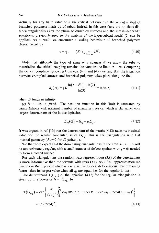
The transition between smooth and crumpled surfaces arises when the regular triangulation becomes unstable under small deformations. A minimal deformation consists of one link flipped (fig. 8).

In appendix C we give the calculation of the ratio of the determinants of the regular lattice with a flip Greng p and the unperturbed lattice Greg. The result is

T(Gr~ p) /T(Greg ) = 0.9573. (4.17)

Taking into account the change of the coordination numbers (a flip creates two defects with q = 5 and two with q = 7) we obtain for the change of the effective action caused by a flip

AS(flip) = l n [ (0 .957 ) - ° /2 (~ ) '~] = (2.86a - 2.18D) × 10 -2. (4.18)


Fig. 8. A flip in the regular triangulation.

Thus we expect a phase transition along the line 6c(D)=O.387D where the "energy" of a flip becomes negative. If we decrease u keeping D fixed, the regular triangulation will be stable down to a = ~c(D). At this point a rapid condensation of flips will cause a collapse into the crumpled surfaces. Indeed, one can check from eqs. (4.6) and (4.14) that the surfaces shown in fig. 5b become more favorable than the regular one when a < 0.368D, i.e. before the line ~c(D) is reached.

We identified three different phases surviving in the limits D ~ + oo. If these are the only possible ones, then the critical dimension of the model will be determined by the line dividing the phases of smooth and tree-like surfaces. Presumably the smooth surfaces collapse into branched polymers when a tachion excitation appears. Our mean-field prediction for the critical dimension is D c = 2. However, our Monte Carlo experiments strongly suggest that between smooth surfaces and trees there exists a fourth phase in which the mean square size (X2)N grows as N ~, with

0 < u ( D , a ) < ½. Such a pattern of possible critical regimes seems very natural from the point of

view of the continuum theory. The functional measure over the configurations of the position field is reproduced correctly in the continuum limit for some a = ac(D ) in the definition (2.21). When a > a t (D) , we have an additional (curvature) 2 term of the type (2.18) in the discretized action. By dimensional reasons such term will be irrelevant in the continuum limit and the critical behaviour is expected to depend only on the dimension D. As we mentioned above, the transition Liouville surfaces- branched polymers can be explained with the appearance of a tachion. When a < a t (D) , the coefficient in front of the R 2 term becomes negative and the continuum limit simply does not exist due to unremovable short distance singularities. This region of parameters corresponds to the phase of crumpled surfaces.

5. Monte Carlo simulation

We performed Monte Carlo simulations of the version (2) of the model for various values of D, a and the number of points fixed. We also tried to simulate the grand canonical ensemble; the results of these experiments will be published in a separate paper [26].

D. V. Boulatov et at / Random surfaces 669

Let us describe our algorithm in some detail (the basic idea was announced in a letter [10]). We averaged simultaneously over coordinates X¢ and graph G. The gaussian variables X~ were updated by the heat bath method; a given coordinate X¢ was led to thermal equilibrium with its neighbours by means of random gaussian shifts

1 qi 1 - , ( 5 , 1 )

q i k = l vq,

where ~u is a D-dimensional vector of random gaussian numbers generated by the standard method. The site of the triangulation to be updated was chosen at random.

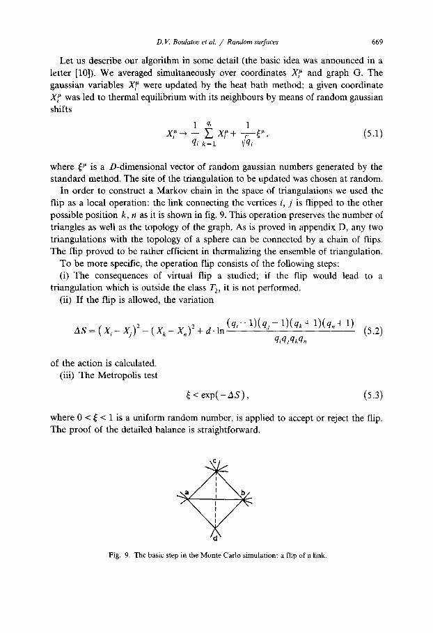
In order to construct a Markov chain in the space of triangulations we used the flip as a local operation: the link connecting the vertices i, j is flipped to the other possible position k, n as it is shown in fig. 9. This operation preserves the number of triangles as well as the topology of the graph. As is proved in appendix D, any two triangulations with the topology of a sphere can be connected by a chain of flips. The flip proved to be rather efficient in thermalizing the ensemble of triangulation.

To be more specific, the operation flip consists of the following steps: (i) The consequences of virtual flip a studied; if the flip would lead to a

triangulation which is outside the class T2, it is not performed. (ii) If the flip is allowed, the variation

(q, 1)(qj 1)(qk + 1 ) ( G + 1) A S ~- ( X i - Xj) 2 - ( X k - X n ) 2 -b d " In

q~qjqkq, , (5.2)

of the action is calculated. (iii) The Metropolis test

< e x p ( - a S ) , (5.3)

where 0 < ~ < 1 is a uniform random number, is applied to accept or reject the flip. The proof of the detailed balance is straightforward.

Fig. 9. The basic step in the Monte Carlo simulation: a flip of a link.


We also checked the detailed balance in vivo, by comparing the data for coordination number distribution at D = 0, a = 0 with the exact numbers (see appendix B) for the corresponding number of triangles. The agreement was perfect, and it did not take much longer runs to gain high statistics.

The gaussian shifts and flips were performed independently at random, so that in average the shifts were twice as frequent. The acceptance rate was reasonable unless a or D were > 10. We also varied the frequency ratio and checked that the results do not change.

The graphs were drawn up from a tetrahedron by adding points inside triangles and by subsequent sweep for thermalization. By definition the number of flips per sweep was equal to the number of links. When desired N was reached the first 1024 sweeps along the graph were skipped, and after that each second sweep was used for measurements. Each run took 16 392 sweeps. The obvious problem of correlations between such close measurements was avoided as follows. The observable Q was averaged twice - the moving average

1 t

Q'= T E Qk (5.4) k = l

was averaged once more with the weight v~:

(5.5)

A similar procedure was applied to the statistical error:

(~5, 2 ) / ( ~-~, 1/v~-) (5.6) 8Q2(") = ( Q t - (Q)t) v/7 'r . t = l t = l

One can show by means of standard statistical methods that the correlations between subsequent measurements do not influence these definitions of the mean value and statistical error.

The basic quantity we measured was the mean square extent*:

1 N

X 2 - 2 N ( N - 1) E ( X i - Xj)2°i°j - (5.7) i , j = l

The N-dependence of (X2)N for various D and a was fitted byA + B log N as well as by AN2~; the power fit was always better more than 10 times. In fig. 10 we

* In the case D = 0 the expression of this quantity in terms of matrix elements of the inverse laplacian was used for numerical simulations. It is worth to note that we used O(N 2) matrix invertion algorithm for sparse matrices.

D. V. Boulatov et aL / Random surfaces 671

,3

@ (]) ~) _ _ @ , _ (]) @'D=60

~ / ~. D=18

2 , ~ ~ --------~ ~ ~ ~ ~ /kD:8

z , , k / x /k ~ _m D=6 -'<- / / k / A / - ~ /

l z ,¢, n / .....-. ~ / ' - - " - .-----• D =4

..,.,..~ r:'l ~ • B / / O

0 .......__._....-- • " " " • / • - / + D=2

~ X

.-1

--2

/ x / x

.-3 LN[N]

3 41 51 61 71 81 91 101 11

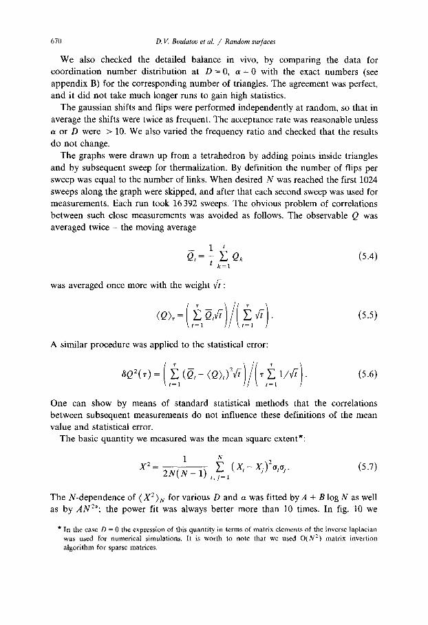
Fig. 10. A log-log plot of the mean square size (X2)N of the triangulated surface versus the number of points N + 2 for a = 0 and various D.

present the log-log plot of (x2)N versus N for a = 0 and several values of D

ranging f rom 0 to 60. The range of the number of points N was limited in our simulations by 512 points because relaxation time grew as N 2 made greater values

of N unachievable for us. The results for D = 0 were obtained by inverting the

laplacian (4.12) for each triangulation. For 4 ~ N ~ 9 we checked that the data agree within the error bars with the corresponding exact values obtained by a method similar to that used by David [12].

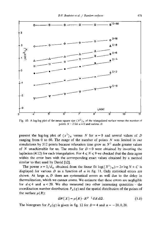
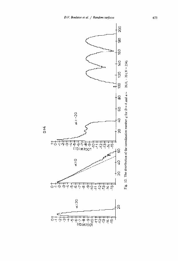
The power u = 1/d H obtained from the linear fit log( (X 2) s ) = 2u log N + C is displayed for various D as a function of a in fig. 11. Only statistical errors are shown. At large a, D there are systematical errors as well due to the delay in thermalization, which we cannot assess. We estimate that these errors are negligible for d ~< 4 and a < 20. We also measured two other interesting quan t i t i e s - the coordination number distribution PN(q) and the spatial distribution of the points of the surface O (R):

d W ( X ) = p ( R ) . R D ldRd~2 . (5.8)

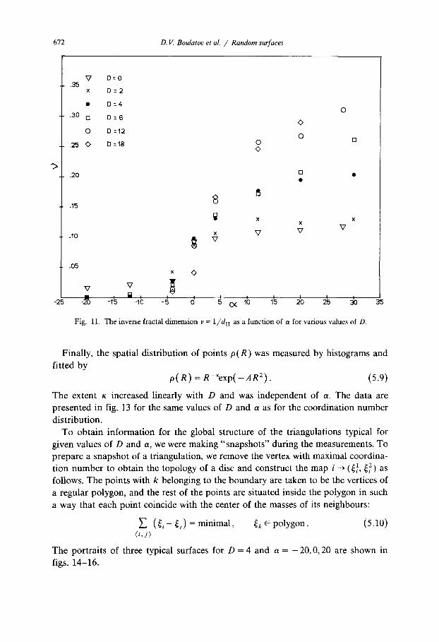
The histogram for PN(q) is given in fig. 12 for D = 4 and a = -20 ,0 ,20 .


,.>

V D=O 35

x D = 2

• D=4

.30 [] D = 6

0 D :12

.25 0 D = 18 o <>

0

0

.20

.15

.10

8 ;J x

x V

D •

x v v

.05

-25 35

x <>

,7 v

-~0 -1~5 c a ! ~ : I 1~3 15 2~D 215 30 -IO -5 o 5 0(.

Fig. 11. The inverse fractal d imens ion ~, = i / d H as a funct ion of a for var ious values of D.

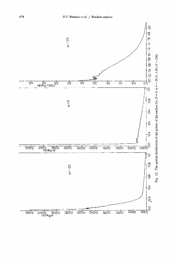
Finally, the spatial distribution of points p ( R ) was measured by histograms and fitted by

p( R ) = R ~exp( -AR2) . (5.9)

The extent K increased linearly with D and was independent of a. The data are presented in fig. 13 for the same values of D and a as for the coordination number distribution.

To obtain information for the global structure of the triangulations typical for given values of D and a, we were making "snapshots" during the measurements. To prepare a snapshot of a triangulation, we remove the vertex with maximal coordina-

__~ 1 tion number to obtain the topology of a disc and construct the map i ((i , ~2) as follows. The points with k belonging to the boundary are taken to be the vertices of a regular polygon, and the rest of the points are situated inside the polygon in such a way that each point coincide with the center of the masses of its neighbours:

( ~ i - ~j) = minimal, ~k ~ polygon. (5.10) (i , j)

The portraits of three typical surfaces for D = 4 and a = -2 0 ,0 , 20 are shown in figs. 14-16.

LOG[W(Q)] ,.~.~,.,.,., , ,

(~f I ,I 01 ~-OJ r,J --~0 1 : ', 1 I : I I l I ~ ; 1 "

• .,.____-------~

Ix.) 0

e~

Q-

0

p~ 0

0

II

e~

II I

+

II

N.I 0

0

.p. O'

0

0~. 0

o

bJ 0 (:D

~- ~o~ ~0~.e ~'.o ' 1 : ~ : ~ I I I I I I 1 I I I t

Z

~. ~- ~- k '- LOG[W(Qj]

• , i i i , i i i I i i , ......... ,~ I I

II

,b 0

1:3 11

EL9 saavfans luopuv~t / 7 v la aotvlno ~ "A "(7

6 7 4

J i £ E £"7 I&l),'~ ~-(~ 01,) " O'E

D.V. Boulatov et al. / Random surfaces

0 o,I ~L

• ffl, 0'l, cj'o

0 04 .CO

.c',l

II

o ~

+

o ~

I

II

0 i i

I I s'~cl'o o,~d'o ~J0 o~d'o ~ ' o o~o"o sLJ'o oLoo ~oo'o ooo" ( ~ I M £'--~d

.0

II

Z

o

E m

0

J c~90io , i l I ' c~O(~'O 000 090'0 c~EO'O 0[0'0 &EO'O 0~(3'0 c~OLO 0~0"0

3 ' - "

-.,r. o

f'NI

0 C5

D. 1I. Boulatov et a L / Random surfaces 675

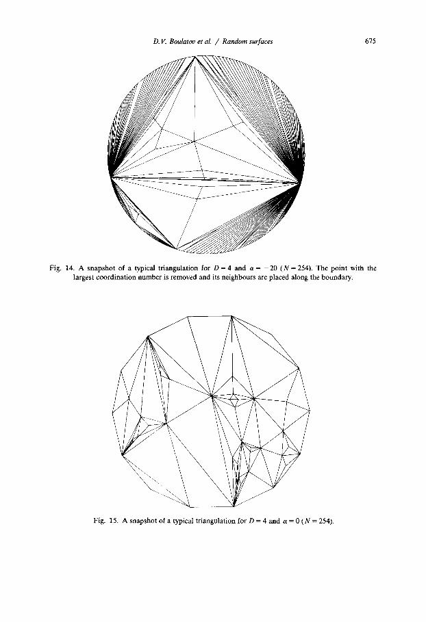
Fig. 14. A snapshot of a typical triangulation for D = 4 and a = - 2 0 ( N = 254). The point with the largest coordination number is removed and its neighbours are placed along the boundary.

Fig. 15. A snapshot of a typical triangulation for D = 4 and a = 0 (N = 254).


/ / / I

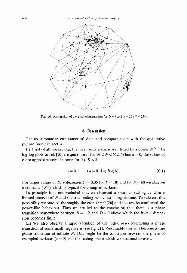
Fig. 16. A snapshot of a typical triangulation for D = 4 and a = 20 ( N = 254).

6. Discussion

Let us summarize our numerical data and compare them with the qualitative

picture found in sect. 4.

(i) First of all, we see that the mean square size is well fitted by a power N 2~. The

log-log plots in ref. [10] are quite linear for 16 ~< N ~< 512. When a = 0, the values of

u are approximately the same for 0 ~ D ~ 8

v - - 0 . 1 (~ = 0, 1 ~ D ~ 8). (6.1)

Fo r larger values of D, ~ decreases (u = 0.05 for D = 18) and for D = 60 we observe a constant ( X 2) which is typical for crumpled surfaces.

In principle it is not excluded that we observed a spurious scaling valid in a limited interval of N and the true scaling behaviour is logarithmic. To rule out this

possibili ty we studied thoroughly the case D = 0 [26] and the results confirmed the power-l ike behaviour. Thus we are led to the conclusion that there is a phase transit ion somewhere between D = - 2 and D = 0 above which the fractal dimen-

sion becomes finite. (ii) We also observe a rapid variation of the index u ( a ) resembling a phase

transit ion at some small negative a (see fig. 11). Presumably this will become a true phase transit ion at infinite N. This might be the transition between the phase of c rumpled surfaces (u = 0) and the scaling phase which we assumed to exist.


When we are in the scaling phase, the index v increases with both D and a. It is

expected to approach the upper bound v = ¼ when the regime of branched polymers is reached. However when a is large the measured values of v clearly violate this upper bound for D >/6 (the same phenomenon was observed by the authors of [14]). The power v being larger than ¼ is evidently an artifact of the limited interval of N used in the calculations. Indeed, we examined several samples of surfaces with 256 points and observed a structure of a single tube or a tree with three branches. Each branch therefore requires a large amount of triangles and for N _< 500 the surface cannot grow into a big tree. For such unsuccessful trees a value of v somewhere between ¼ and ½ is not at all surprising.

Thus we can definitely say that the phase of branched polymers extends down to D = 6 when a is large. It is not clear from fig. 1 whether this phase can be reached along the line D = 4; in any case when a becomes large the typical surfaces have the structure of trees (see below).

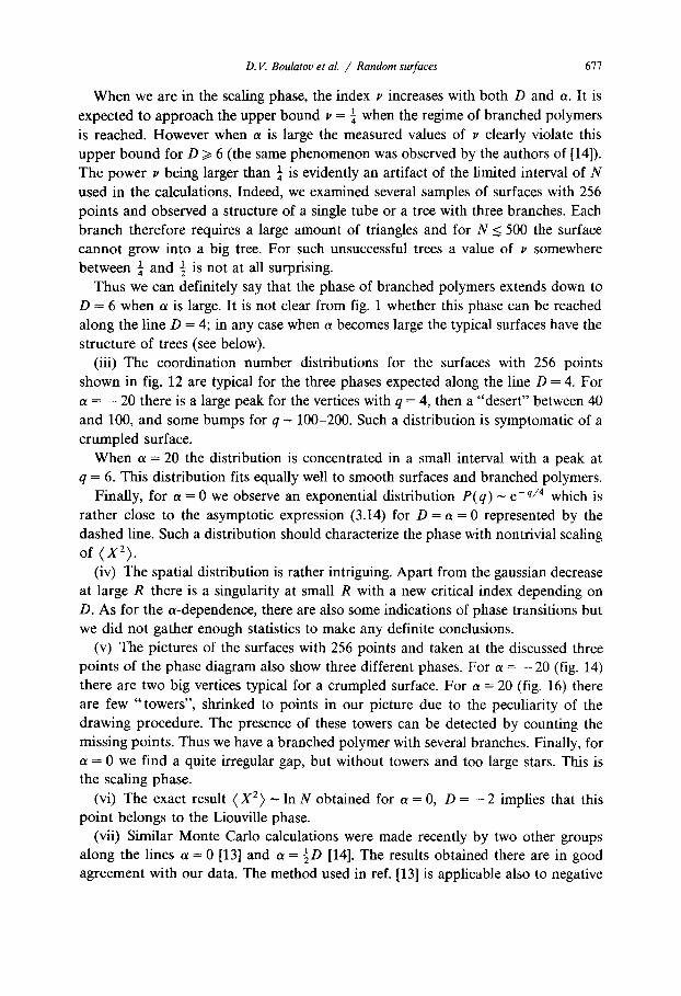
(iii) The coordination number distributions for the surfaces with 256 points shown in fig. 12 are typical for the three phases expected along the line D = 4. For a = - 20 there is a large peak for the vertices with q = 4, then a "desert" between 40 and 100, and some bumps for q - 100-200. Such a distribution is symptomatic of a crumpled surface.

When a = 20 the distribution is concentrated in a small interval with a peak at q = 6. This distribution fits equally well to smooth surfaces and branched polymers.

Finally, for a = 0 we observe an exponential distribution P(q) - e - q / 4 which is rather close to the asymptotic expression (3.14) for D = a = 0 represented by the dashed line. Such a distribution should characterize the phase with nontrivial scaling of (X2) .

(iv) The spatial distribution is rather intriguing. Apart from the gaussian decrease at large R there is a singularity at small R with a new critical index depending on D. As for the a-dependence, there are also some indications of phase transitions but we did not gather enough statistics to make any definite conclusions.

(v) The pictures of the surfaces with 256 points and taken at the discussed three points of the phase diagram also show three different phases. For a = - 2 0 (fig. 14) there are two big vertices typical for a crumpled surface. For a = 20 (fig. 16) there are few "towers", shrinked to points in our picture due to the peculiarity of the drawing procedure. The presence of these towers can be detected by counting the missing points. Thus we have a branched polymer with several branches. Finally, for a = 0 we find a quite irregular gap, but without towers and too large stars. This is the scaling phase.

(vi) The exact result (X 2) - I n N obtained for a = 0, D = - 2 implies that this point belongs to the Liouville phase.

(vii) Similar Monte Carlo calculations were made recently by two other groups [14]. The results obtained there are in good along the lines a = 0 [13] and a = ~D

agreement with our data. The method used in ref. [13] is applicable also to negative


(9 <x 2> -const

<x2> N1/2

<x2> ~lnN

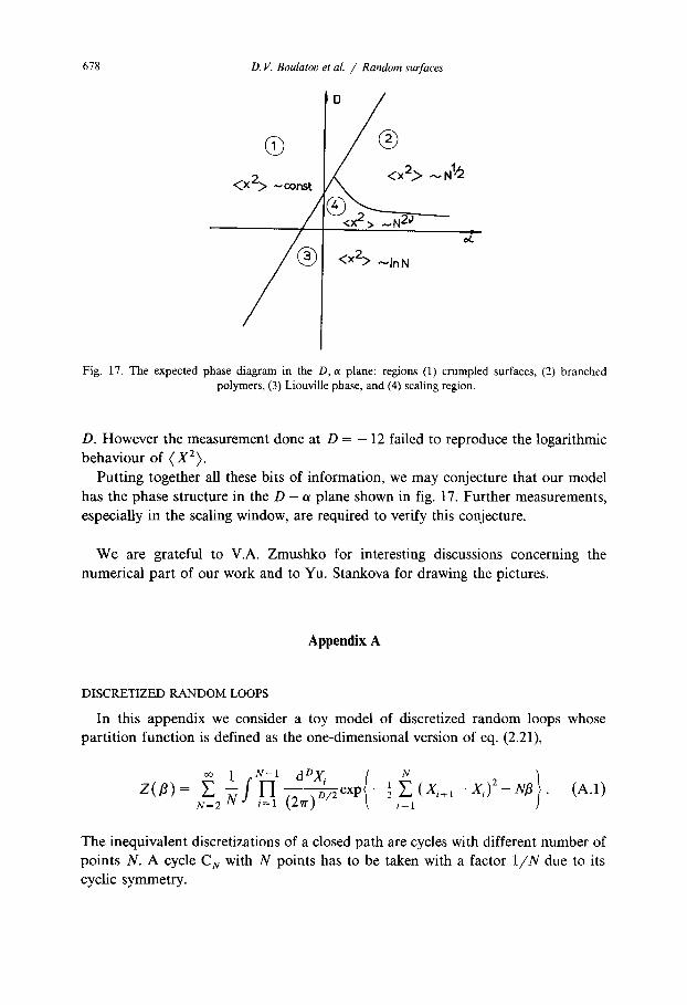
Fig. 17. The expected phase diagram in the D, a plane: regions (1) crumpled surfaces, (2) branched polymers, (3) Liouville phase, and (4) scaling region.

D. However the measurement done at D = - 12 failed to reproduce the logarithmic behaviour of (X2) .

Putting together all these bits of information, we may conjecture that our model has the phase structure in the D - a plane shown in fig. 17. Further measurements, especially in the scaling window, are required to verify this conjecture.

We are grateful to V.A. Zmushko for interesting discussions concerning the numerical part of our work and to Yu. Stankova for drawing the pictures.

Appendix A

DISCRETIZED RANDOM LOOPS

In this appendix we consider a toy model of discretized random loops whose partition function is defined as the one-dimensional version of eq. (2.21),

Z ( ~ ) = Ea f= ~_ (2rr) --b~exp - ½ i=tE ( X i + l - X i ) 2-N1~ " (A.1)

The inequivalent discretizations of a closed path are cycles with different number of points N. A cycle C s with N points has to be taken with a factor 1 / N due to its cyclic symmetry.

D. I/. Boulatov et al. / Random surfaces 679

The two-point function is, correspondingly,

N - 1 dDXi

G ( e : , / 3 ) = (2~r)D/2

N ( N / X E exp - N i l - ½ E (Xi+I -- X i ) - i P ( X k - Xs) • (A.2)

k , s= l i=1

The number of trees on the cycle C N is

T(C N) = N. (A.3)

The number of 2-trees containing the points k, s in different connected components is

T2~k's)(CN) = I k - sl " ( N - I k - sl). (A.4)

G(P2,/3) = N-D/2 N= 2 1 exp -- Nfl . (A.6)

It follows from eq. (A.5) that the critical exponent for the susceptibility X = Z"(/3) is

1 (1 .7 ) " / = 2 - ~D.

The mass gap m(/3) = 2 V / ~ is determined by the position of the singularity in p2. After substitution t = k / N we obtain from (A.6) the singular part of the Green function

G ( p 2 + i 0 , / 3 ) - f 2 ° ° d N N 1 - D / 2 f o l d t e x p [ - N ( / 3 q - 1 / ( 1 - t ) e 2 ) ]

- foldt [/3 + ½t(1 - t ) p 2 ] D/2-2 (A.8)

Note that G(P 2, fl) behaves as a power of/3 only when p 2 = 0. The mean square extent of a loop with N points is, according to (2.30),

N-1 (X2)N = ½ DND/2-' E k(1 - k / N ) N -D/2 = ~DN, (A.9)

k=l

By eqs. (3.1) and (3.2)

Z(fl) = ~ N-a-D/2e -~N, (1.5) N=2


which implies the familiar result

d n = 2. (A.10)

Eq. (A.10) is consistent with the index v = 1 following from (A.8) and the second scaling relation (2.32). The index 7/ follows from the asymptotics

G( X) - (IXl2-%-v@lxl) 2= IxlZ-O-ne miX] (A.11)

and satisfies the first of the scaling relations (2.32).

Appendix B

C O O R D I N A T I O N N U M B E R D I S T R I B U T I O N A T D = 0, a = 0

Our starting point will be eq. (3.13) which in a slightly different form reads

6N G (c) n , 2 N - 1 P(u2)(n) = n(N + 2) G~C,)N-----~I ; (B.1)

here G~,~% is the number of all connected ~3 planar graphs without tadpoles and self-energies and having n external lines and M vertices. The generating function tk(j, g) for these numbers

~k(j, g) = 1 + ~ G~C)(g)j" (B.2) n = l

has been found in a classical paper [23]. In our notation g corresponds to 3g in the notation of ref. [23]. We also inserted the missing factor j in one of the terms in eq. (65) of ref. [23]. As a result we arrive at the following equation for q:(j, g)

_g~2 + + [ g + j ( m + 1)] =j(m + 1) - gj2 + j 3 ,

where m and g are related as follows

(B.3)

One can readily check that

=0, Gz~C)(g) = 1, m

o C)(g) = - . (B .5) g

m = a ( l - 2a ) , gZ= a(1 - a) 3. (B.4)


The expansion of m(g) can be found from (B.4). The result for G~c,)vN_I in our notation reads

2 ( 4 N - 3)! G (c) = (B.6) 3,2N-1 ( 3 N - 1)!N! "

In order to generate ~(c) we introduce the new variables x = j / g , y = g2: V n , 2 N - n

e(x, y) = (gx, g) = g2N E (B.7) "~ V n , 2 N - n " N=0 n=0

This function satisfies the equation

with

- F 2 + F(1 + x ( m + 1)) = x ( m + 1) - y x 2 + yx 3,

2(4l + 1)! m ( y ) = i ( 3 l + 2 ) ! ( l + 1 1 ! Y ' . 1=0

(B.8)

(B.9)

We wrote a Fortran program to find recursively the expansion coefficients of the function F(x , y) from these equations. We used them to test our MC program for D - - 0 .

The limiting distribution Poo(n) can be found in an explicit form. The asymptotics of the series is determined by the discontinuity of the generating function along the corresponding cut and near the endpoint.

Let us find an equation for the discontinuityAyF along the cut going from Yo-- 25627 to infinity. The point Yo corresponds to a ~ ¼ in the parametric equation (B.4). In the vicinity of this point

m ~ ~ + 3 ( y / y 0 - 1) - ~4 V~-(1 - y / y o ) 3/2 + . . . . (B.IO)

Thus we find for y ~Y0 + 0

--~-(Y 1) 3/2 . (B.11) m 0 = ~, Aym ~ 24 Yo

The discontinuity AyF linearized equation (B.8)

( - 2 F o + 1 + x ( m o + 1 ) ) A y F + x F o A y m = x A y m ,

i.e.

aeF= Aymx(1 -- Fo)/(1 + x ( m o + 1) - 2Fo).

is determined in the leading order i n Aym from the

(B.12)

(B.13)


Comparing this with the singularity of

we conclude that the ratio

is generated by

o0 G~C)g = ~ "2Nt '~ ' (c)

6 ~ 3 , 2 N - 1 = r e ( y ) N = I

where

R . = lim N ~

G(C) ) G(C)

3 , 2 N - 1

= ( a , F 1 = R ( x ) = Y'.R,,x"n l Aym ] Y=Yo

x ( 1 - Fo(x))

1 - 2Fo(x ) + 9 x '

Fo(x) = ~ + ~x + ½(1-3 ),/2 XX

After some simple algebra we find

3 "~ - 3 /2 R(x) = l ~ x - ½ x ( 1 - 9 x ) ( 1 - a x ) ,

which, after being expanded in x, gives eq. (3.14).

Appendix C

T H E E N E R G Y O F A F L I P IN T H E R E G U L A R L A T T I C E

A link flipped (fig. 8) will change the quadratic form

E x , ai, x, = E < j ( x i - ~ ) 2 ij i , j

by a quantity

E x ia~p% = (Xo - xb) 2 - (xc - xd) 2. i , j

Our aim is to calculate the ratio of the two determinants

(B.14)

(B.15)

(B.16)

(B.17)

(B.18)

(c.1)

(C.2)

The determinant in the r.h.s, is actually the determinant of a 4 x 4 matrix involving

det(A + A (nip)) /2 = = det(g + z~-lA(nJP)). (C.3)

det(a)


the following quantities

2~r d20

ff A = ( A - 1 ) a a = 0 ~ - ~ ( 3 - c O s o l - c O S 0 2 - c O S ( o l - o 2 ) ) - I (C.4)

2~r d20 B = (A - 11 ac = ff (3 - cos 01 - cos 02 - cos(01 - 02)) - lcos 01 = A - 61

(c.5) 2~r d20

C : ( A - 1 ) a b : f f (3 . . . . COS01 COS 02 COS(01 02))-1cOS(01 "[- 02). ~6

Inserting (C.4)-(C.6) into eq. (C.3) we obtain

I2 = (1 + 2 ( B - A ) ) ( 1 + 2(A - C)) = 3(1 + 2(A - C))

1 -- COS(01 -1- 02) d20

2__f 3-- COSO 1 -- COS02- COS(O I - 02) (2'/7") 2 1 +

= z + - - =0.9573. 3 ,7/.

(C.6)

(C.7)

Appendix D

REDUCTION OF PLANAR GRAPHS TO A STANDARD FORM BY MEANS OF FLIPS

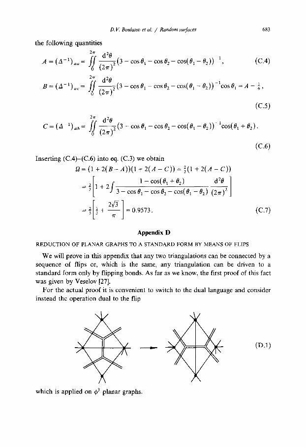
We will prove in this appendix that any two triangulations can be connected by a sequence of flips or, which is the same, any triangulation can be driven to a standard form only by flipping bonds. As far as we know, the first proof of this fact was given by Veselov [27].

For the actual proof it is convenient to switch to the dual language and consider instead the operation dual to the flip

which is applied on q~3 planar graphs.

(D.1)

684 D. V. Boulatov et al, / Random surfaces

Here we will consider the set of planar graphs if2* (i.e. those without tadpoles and self-energy insertions) which was used in our Monte Carlo calculations.

Let us introduce the following graphical notations. A one-particle irreducible (1PI) planar vertex will be denoted by a circle

(D.2 t

and a chain of vertices will be represented by a rectangle as follows

/D3t

These two types of amplitudes satisfy the following Dyson-Schwinger equations [28]

(D.4)

l l l l , II11

n n m n-~rn

(D.5)

Let us show that by means of flips the graphs contributing to both amplitudes can be reduced to the following standard form

1111 ( ---I . . . . . . [ . . . . . . - / ~ (D.6)

This is a tree graph up to ladders dressing its vertices.


Evidently, eq. (D.5) is compatible with such reduction: if the r.h.s, is in a standard form, so does the 1.h.s. Below we will demonstrate that if the r.h.s, of eq. (D4) is in a standard form, the 1.h.s. can be driven to a standard form by a sequence of flips. Thus, applying many times (D.4) and (D.5) each planar graph can be reduced to the

standard form (D.6). A flip can be viewed as the result of sliding a vertex along a line of the graph

(D.7)

The upper leg is moved to the left, passing through the vertex without any harm. This means that any leg in a planar graph can be moved along the corresponding line.

Let us apply this transformation to eq. (C.4) with the rectangle in a standard form:

(0.8)

We cannot move the arrow further to the left, since it would lead to a self-energy graph. But we are allowed to move the ladder's stairs of the left vertex

Now we reached the standard form

(D.9) , o ,

~ ... (D.9')

This completes the proof.

686 D.V. Boulato~ et aL / Random surfaces

References

[1] S. Mandelstam, Phys. Reports 13C (1974) 259 [2] A.M. Polyakov, Phys. Lett. 103B (1981) 207 [3] D. Weingarten, Phys. Lett. 90B (1980) 285;

T. Eguchi and H. Kawai, Phys. Lett. ll0B (1982) 143 [4] H. Kawai and Y. Okamoto, Phys. Lett. 130B (1983) 415 [5] B. Durhuus, J. Fr~hlich and T. Jonsson, Nucl. Phys. B240 [FS12] (1984) 453 [6] D. Gross, Phys. Lett. 138B (1984) 185;

A. Billoire, D. Gross and E. Marinary, Phys. Lett. 139B (1984) 75 [7] V. Kazakov, Phys. Lett. 150B (1985) 282 [8] F. David, Nucl. Phys. B257 (1985) 45 [9] J. Ambjorn, B. Durhuus and J. Fr~Shlich, Nucl. Phys. B257 (1985) 433

[10] V. Kazakov, I. Kostov and A. Migdal, Phys. Lett. 157B (1985) 295 [11] D. Boulatov, V. Kazakov, I. Kostov and A. Migdal, Phys. Lett. B174 (1986) 87 [12] F. David, Nucl. Phys. 257 [FS14] (1985) 543 [13] A. Billoire and F. David, Saclay preprint PhT 85-187 (November 1985) [14] J. Jurkiewicz, A. Krzywicki, B. Peterson, Orsay preprint LPTHE 85/36 (October 1985) [15] J. Ambjorn, B. Durhuus, J. Fr~Shlich and P. Orland, Nucl. Phys. B270 [FS16] (1986) 457 [16] L. Brink, P. di Vecchia and O. Hove, Phys. Lett. 65B (1976) 471 [17] A.M. Polyakov, Nucl. Phys. B268 (1986) 406 [18] M. Bander and C. Itzykson, Lecture Notes in Physics, vol. 226 (Springer, Berlin, 1985) [19] E. Efizalde, Phys. Lett. 166B (1986) 314 [20] A.B. Zamolodchikov, Phys. Lett. 117B (1982) 87 [21] J. Fr~Shlich, Lecture notes in Physics, vol. 216, ed. L. Garido (Springer, Berlin, 1985) [22] N.N. Bogolyubov and D.V. Shirkov, Introduction to the theory of quantized fields (lnterscience,

New York, 1959) [23] E. Brfzin, C. Itzykson, G. Parisi and J.-B. Zuber, Comm. Math. Phys. 59 (1978) 35 [24] F. David, Phys. Lett. 159B (1985) 543 [25] J. Jurkievich and A. Krzywicki, Phys. Lett. 148B (1984) 148 [26] D.V. Boulatov, V.A. Kazakov, A. Migdal and V. Zmushko, to be published [27] A.V. Veselov, private communication [28] A. Neveu, J. Koplik and S. Nussinov, Nucl. Phys. B123 (1977) 109

Analytical and numerical study of a model of dynamically triangulated random surfaces

Documents

Transcript of Analytical and numerical study of a model of dynamically triangulated random surfaces