University of South FloridaScholar Commons

Graduate Theses and Dissertations Graduate School

11-3-2008

Analysis of Water Seepage Through EarthenStructures Using the Particulate ApproachKalyani JeyisankerUniversity of South Florida

Follow this and additional works at: https://scholarcommons.usf.edu/etd

Part of the American Studies Commons

This Dissertation is brought to you for free and open access by the Graduate School at Scholar Commons. It has been accepted for inclusion inGraduate Theses and Dissertations by an authorized administrator of Scholar Commons. For more information, please contactscholarcommons@usf.edu.

Scholar Commons CitationJeyisanker, Kalyani, "Analysis of Water Seepage Through Earthen Structures Using the Particulate Approach" (2008). Graduate Thesesand Dissertations.https://scholarcommons.usf.edu/etd/317

Analysis of Water Seepage Through Earthen Structures Using the Particulate Approach

by

Kalyani Jeyisanker

A dissertation submitted in partial fulfillment of the requirements for the degree of

Doctor of Philosophy Department of Civil and Environmental Engineering

College of Engineering University of South Florida

Major Professor: Manjriker Gunaratne, Ph.D. Alaa Ashmawy, Ph.D.

Mark Luther, Ph.D. Gray Mullins, Ph.D.

Muhammad Mustafizur Rahman, Ph.D.

Date of Approval: November 03, 2008

Keywords: Navier Stokes Equations, Monte-Carlo Simulation, Volumetric Compatibility, Staggered Grid, Critical Localized Condition, Unsaturated, Soil Water Characteristic Curve

© Copyright 2008, Kalyani Jeyisanker

DEDICATION

This work is dedicated to my husband, Jeyisanker and my daughter, Harinie.

Jeyisanker has been a tremendous support. He was always there in the hard days

throughout the research. Without his support and encouragement, I would never achieve

this.

ACKNOWLEDGMENTS

I would like to thank my advisor, Dr. Manjriker Gunaratne, for his guidance and support

throughout the research. Dr. Gunaratne was always there to suggest ideas and to improve

my writing skills, and to expand my academic knowledge in Geotechnical Engineering.

Additionally, I would like to extend my thanks to the members of my examining

committee Dr. Alaa Ashmawy, Dr. Gray Mullins, Dr. Mark Luther and Dr. Muhammad

Mustafizur Rahman for all their support and courage given to me to complete my

research. I would like to thank Dr. Nimal Seneviratne for his advice to complete my

studies successfully.

My thanks go to my colleagues, Ms. S.Amarasiri, Mr. L.Fuentes, Mr. M.Rajapakse, Mr.

J.Kosgolle and Ms. K.Kranthi for their help especially when I am out of office.

i

TABLE OF CONTENTS

LIST OF TABLES ...............................................................................................................v

LIST OF FIGURES ........................................................................................................... vi

ABSTRACT .........................................................................................................................x

CHAPTER ONE: INTRODUCTION ..................................................................................1

1.1 Background ........................................................................................................1

1.2 Literature Review...............................................................................................2

1.3 Objectives .........................................................................................................4

1.3.1 Pavement Filter Design .......................................................................4

1.3.2 Retention Pond Design .......................................................................6

1.4 Numerical Modeling ..........................................................................................8

1.4.1 Solid Continuum Methods ..................................................................8

1.4.2 Discrete Element Methods ..................................................................8

1.5 Assembling of Particles in the Particle Flow Code ...........................................9

1.5.1 Theoretical Background of PFC .......................................................10

1.5.1.1 Particle Interactions ...........................................................10

1.6 Organization of Dissertation ............................................................................11

CHAPTER TWO: ANALYSIS OF STEADY STATE WATER SEEPAGE IN A PAVEMENT SYSTEM USING THE PARTICULATE APPROACH .......12

2.1 Preliminary Studies Using Existing Software .................................................12

2.2 Methodology Followed to Develop a Novel Algorithm ................................ 14

2.2.1 Modeling of Soil Structure (3D Random Packing of Soil Particles) ..........................................................................................17

2.2.1.1 Simulation of Maximum and Minimum Void Ratios Using PSD ..............................................................17

ii

2.2.1.2 Implementation of the Packing Procedure .........................18

2.2.1.3 Determination of the Natural Void Ratio Distribution ......20

2.3 Modeling of Steady State Flow .......................................................................23

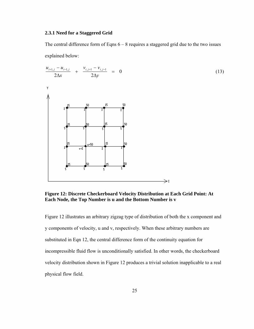
2.3.1 Need for a Staggered Grid ................................................................25

2.3.2 Numerical Solution Technique .........................................................28

2.3.3 Semi-Implicit Method for Pressure-Linked Equations (SIMPLE) Algorithm ........................................................................31

2.3.3.1 Derivation of the Pressure Correction Formula .................32

2.3.3.2 Boundary Conditions for Pavement System ......................36

2.4 Validation of the Numerical Model .................................................................37

2.5 Numerical Illustration ......................................................................................39

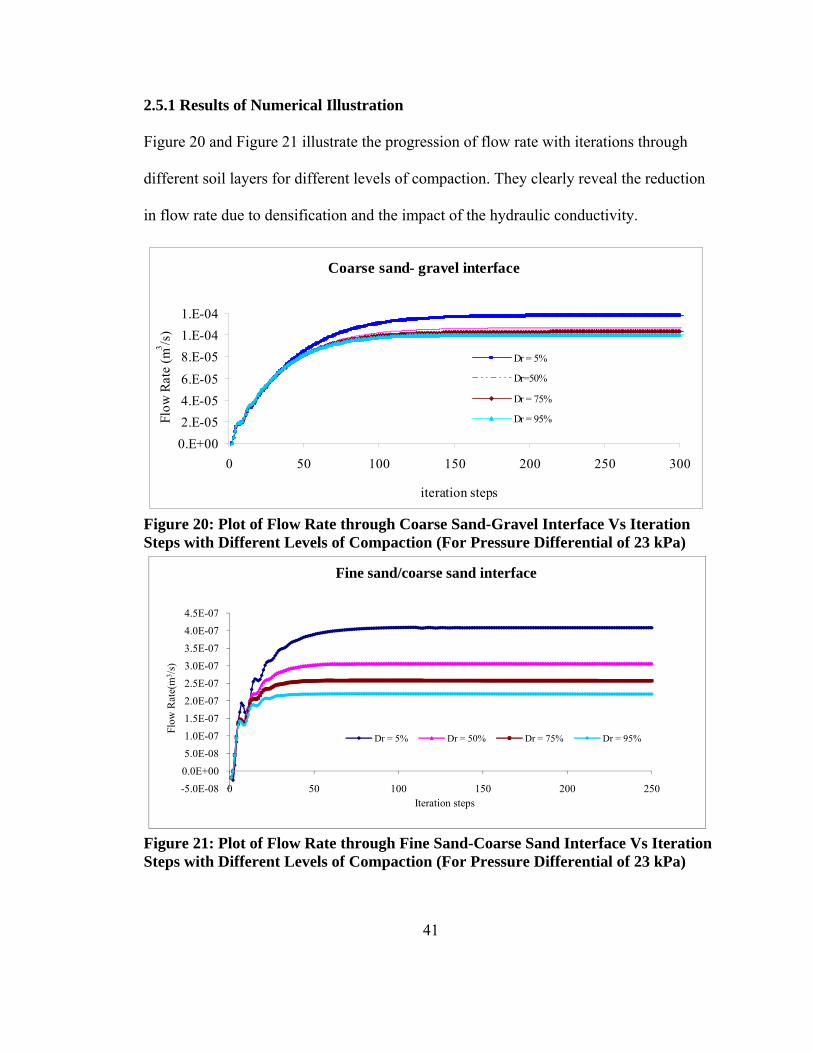
2.5.1 Results of Numerical Illustration ......................................................41

2.6 Conclusions ......................................................................................................43

CHAPTER THREE: ANALYSIS OF TRANSIENT WATER SEEPAGE IN A PAVEMENT SYSTEM USING THE PARTICULATE APPROACH ................44

3.1 Modeling of Transient Flow ............................................................................44

3.1.1 Transient Navier Stokes Equations ...................................................46

3.1.2 Volumetric Compatibility of Solid and Fluid Phases .......................47

3.1.3 Numerical Solution Technique .........................................................48

3.1.4 Boundary Conditions ........................................................................52

3.2 Interface Effect in FDM ...................................................................................53

3.3 Validation of the Numerical Models ...............................................................54

3.4 Numerical Illustration ......................................................................................56

3.5 Selection of Time Step .....................................................................................56

3.6 Results of Numerical Illustration .....................................................................57

3.7 Limitations of the Model .................................................................................65

3.8 Conclusions ......................................................................................................66

CHAPTER FOUR: TRANSIENT SEEPAGE MODEL FOR PARTLY SATURATED AND SATURATED SOILS USING THE PARTICULATE APPROACH ..............................................................................68

4.1 Introduction ......................................................................................................68

iii

4.2 Existing Particulate Models .............................................................................69

4.3 Flow in Partly Saturated Soils .........................................................................70

4.4 Overview of the New Model…………………………………………………73

4.5 Modeling of Soil Structure (3D Random Packing of Soil Particles) ...............76

4.5.1 Simulation of Maximum and Minimum Void Ratios Using PSD .........................................................................................76

4.5.2 Implementation of the Packing Procedure ........................................77

4.5.3 Determination of the Natural Void Ratio Distribution .....................79

4.6 Modeling of Fluid Flow in Partially Saturated Soils ...................................... 82

4.6.1 Soil Water Characteristic Curve/Water Moisture Retention Curve ................................................................................83

4.6.2 Determination of the Unsaturated Permeability Function .............. 85

4.7 Development of the Analytical Model .............................................................86

4.7.1 Navier Stokes Equations ...................................................................86

4.7.2 Modification of Drag Force for Water Flow through Unsaturated Soils ..............................................................................88

4.8 Numerical Solution Technique ........................................................................89

4.9 Numerical Applications of the Model..............................................................97

4.9.1 Modeling Confined Flow through a Partly Saturated Fine Sand Layer (Case I) ..........................................................................97

4.9.2 Boundary Conditions ..........................................................................98

4.9.3 Results ................................................................................................99

4.10 Conclusions ..................................................................................................102

CHAPTER FIVE: MODELING UNCONFINED FLOW AROUND A RETENTION POND ...........................................................................................103

5.1 Introduction ....................................................................................................103

5.2 Existing Design of Retention Pond ................................................................104

5.3 Modeling of Soil Structure (3D Random Packing of Soil Particles) .............106

5.4 Numerical Procedure for Determination of the Free-Surface ........................107

5.4.1 Navier Stokes Equations .................................................................109

5.4.2 Boundary Conditions ......................................................................110

iv

5.5 Determination of Free-Surface from Dupuit’s Theory ..................................112

5.6 Results on Free-Surface .................................................................................112

5.7 Prediction of Recovery Time .........................................................................114

5.8 Conclusions ....................................................................................................118

REFERENCES ................................................................................................................119

ABOUT THE AUTHOR ................................................................................... END PAGE

v

LIST OF TABLES

Table 1: Size Characteristics of Pavement Layers .............................................................19

Table 2: Comparison of 3-D Coefficients of Hydraulic Conductivity Derived from SIMPLE Algorithm .....................................................................................38

Table 3: Model Parameters ................................................................................................40

Table 4: Comparison of 3-D Coefficients of Hydraulic Conductivity Derived from the Numerical Methodology .....................................................................54

Table 5: Soil Characteristics ..............................................................................................78

Table 6: Parameters Used to Define the SWCC for Sand [23] ..........................................84

vi

LIST OF FIGURES

Figure 1: Typical Pavement Structure ...............................................................................5

Figure 2: Pavement Layer Interfaces .................................................................................5

Figure 3: Computational Cycle in PFC ............................................................................10

Figure 4: Illustration of Inter-Particle Forces ..................................................................10

Figure 5: Analysis of Flow Problem Using Existing Software ........................................13

Figure 6a: Highway Pavement Layers ...............................................................................13

Figure 6b: Comparison of Hydraulic Gradients Obtained Using Continuum and Discrete Methods (Steady State) ...............................................................14

Figure 7: Flow Chart Illustrating the Analytical Model for Steady State Flow ...............16

Figure 8: Particle Size Distributions for Gravel, Coarse Sand and Fine Sand ...............18

Figure 9: Random Packing of Soil Particles ....................................................................20

Figure 10: Probability Density Function (PDF) of Maximum and Minimum Void Ratios ..................................................................................................... 22

Figure 11: Cumulative Frequencies of Maximum and Minimum Void Ratios .................23

Figure 12: Discrete Checkerboard Velocity Distribution at Each Grid Point: At Each Node, the Top Number is u and the Bottom Number is v .................25

Figure 13: Discrete Checkerboard Pressure Distribution ..................................................26

Figure 14: A Typical Staggered Grid Arrangement (Solid Circles Represent Pressure Nodes and Open Circles Represent Velocity Nodes) ........................28

Figure 15: Computational Module for the X-Momentum Equation ..................................29

Figure 16: Flow Chart for SIMPLE Algorithm for Steady State Condition ......................32

Figure 17: Designation of Nodal Points on a Grid Used in SIMPLE Algorithm ..............34

Figure 18: Boundary Conditions Incorporated in the Flow through the Pavement System .............................................................................................37

vii

Figure 19: Relationship between Hydraulic Conductivity Vs Diameter for Uniformly Distributed Soils ...........................................................................38

Figure 20: Plot of Flow Rate through Coarse Sand-Gravel Interface Vs

Iteration Steps with Different Levels of Compaction (For Pressure Differential of 23 kPa) .............................................................41

Figure 21: Plot of Flow Rate through Fine Sand-Coarse Sand Interface Vs

Iteration Steps with Different Levels of Compaction (For Pressure Differential of 23 kPa) ....................................................................................41

Figure 22: Comparison of Hydraulic Gradients Obtained Using Continuum

and Particulate Approaches (Using SIMPLE Algorithm Steady State) ...........42 Figure 23: Plot of Flow Rate Vs Iteration Step for High Hydraulic Gradient

(i = 1.7 icr) ......................................................................................................42

Figure 24: Flow Chart Illustrating the Analytical Model for Transient and Steady State Flow ...........................................................................................45

Figure 25: Computational Grid for the X-Momentum Equation ......................................49

Figure 26: Designation of Nodal Points on a Grid Used in the Iterative Procedure .........50

Figure 27: Boundary Conditions Incorporated in the Flow through the Pavement System (Saturated Soil)....................................................................................53

Figure 28: Development of Water Pressure within the Coarse Sand-Gravel Layers with Time (For Pressure Differential of 23 kPa) .................................57

Figure 29: Development of Water Velocity within the Coarse Sand-Gravel Layers with Time (For Pressure Differential of 23 kPa) .................................58

Figure 30a: Plot of Flow Rate through Coarse Sand-Gravel Layers Vs Time Steps with Different Levels of Compaction (For Pressure Differential of 23 kPa) .....................................................................................58

Figure 30b: Plot of Flow Rate through Fine Sand-Coarse Sand Layers Vs Time Steps with Different Levels of Compaction (For Pressure Differential of 23 kPa) .....................................................................................59

Figure 31a: Plot of Maximum Hydraulic Gradient within the Coarse Sand- Gravel Layers Vs Time Steps for Different Levels of Compaction (For Pressure Differential of 23 kPa) ...............................................................60

Figure 31b: Plot of Difference in Maximum Hydraulic Gradients Within the Coarse Sand-Gravel Layers Vs Time Steps for Different Levels of Compaction (For Pressure Differential of 23 kPa) ....................................61

viii

Figure 32: Comparison of Hydraulic Gradients Obtained Using Continuum and Particulate Approaches (Steady State) ....................................................62

Figure 33: Porosity Distribution for Coarse Sand-Gravel Interface with Non-Uniform Compaction (Circled Area is Packed with Dr of 5% and the Remaining Area is Packed with Dr of 95%) ...........................63

Figure 34: Velocity Vector Plots: (a) Uniformly Compacted Soil Media (Dr = 95%) (b) Deficiency of Compaction in Local Area .............................64

Figure 35: Plot of Fluid Pressure Distribution across the Coarse Sand-Gravel Interface: (a) Uniformly Compacted Coarse Sand-Gravel Interface (Dr = 95%) (b) Deficiency of Compaction in Local Area .............................64

Figure 36: Plot of Localized Hydraulic Gradients for Coarse Sand- Gravel Interface with Weak Region ...............................................................65

Figure 37: Schematic Diagram to Show the Movement Cycle of Water from Atmosphere to the Groundwater Table [20] ..........................................71

Figure 38: Flow Chart Illustrating the Analytical Model for Flow through Unsaturated Soils ..............................................................................75

Figure 39: Particle Size Distribution for Fine Sand .........................................................76

Figure 40: Packing Procedure ..........................................................................................79

Figure 41: Cumulative Distribution for Natural Void Ratios for the Fine Sand with Dr = 50% ........................................................................................81

Figure 42: Initialization of Water Pressure in the Saturated and Unsaturated Zones ..............................................................................................................82

Figure 43a: Typical Soil Water Characteristic Curve and wm2 for a Saturated- Unsaturated Soil [10] ......................................................................................83

Figure 43b: Soil Water Characteristic Curve for Specific Soil Types [23] .......................83

Figure 44: Unsaturated Permeability Function for Selected Soil Types [23] ..................86

Figure 45: Computational Grid for the X-Momentum Equation .....................................90

Figure 46: Soil Water Characteristic Curve for Fine Sand ..............................................93

Figure 47: Neighborhood Points Used in the Iterative Procedure ..................................94

Figure 48: Illustration of the Flow through the Unsaturated Fine Sand Layer ................97

Figure 49: Boundary Conditions Incorporated in the Flow through Saturated - Unsaturated Soil Layer ...................................................................................98

Figure 50: The Variation of Water Porosity with Water Pressure at a Point within the Unsaturated Zone (At Point A in Figure 49) .................................99

ix

Figure 51: The Variation of Degree of Saturation with Water Pressure (At Point A in Figure 49) .............................................................................................100

Figure 52: Velocity Vector Plots for Flow through Saturated and Partly- Saturated Soil Layer ....................................................................................101

Figure 53: Variation of Discharge Flow Rate with Time Step ......................................102

Figure 54: Typical Retention Pond ...............................................................................103

Figure 55: Particle Size Distributions for Coarse Sand .................................................107

Figure 56: Determination of Dry and Wet Zones around the Retention Pond ..............109

Figure 57: Boundary and Initial Conditions Incorporated in the Flow around the Retention Pond .......................................................................................111

Figure 58: Analytical Method to Determine the Free-Surface ......................................112

Figure 59: Comparison of Free-Surface around the Retention Pond .............................113

Figure 60: Location of Free-Surface around the Retention Pond with Time ................114

Figure 61: Saturated Infiltration Analysis Using MODFLOW .....................................115

Figure 62: Prediction of Recovery Time from Numerical Method ...............................116

Figure 63: Sample Plot to Determine Recovery Time from MODFLOW ....................117

x

ANALYSIS OF WATER SEEPAGE THROUGH EARTHEN STRUCTURES USING THE PARTICULATE APPROACH

KALYANI JEYISANKER

ABSTRACT

A particulate model is developed to analyze the effects of steady state and transient

seepage of water through a randomly-packed coarse-grained soil as an improvement to

conventional seepage analysis based on continuum models. In the new model the soil

skeleton and pore water are volumetrically coupled. In the first phase of the study, the

concept of relative density has been used to define different compaction levels of the soil

layers of a completely saturated pavement filter system and observe the seepage response

to compaction. First, Monte-Carlo simulation is used to randomly pack discrete spherical

particles from a specified Particle Size Distribution (PSD) to achieve a desired relative

density based on the theoretical minimum and maximum void ratios. Then, a water

pressure gradient is applied across one two-layer filter unit to trigger water seepage. The

pore water motion is idealized using Navier Stokes (NS) equations which also

incorporate drag forces acting between the water and soil particles. The NS equations are

discretized using finite differences and applied to discrete elements in a staggered,

structured grid. The model predicted hydraulic conductivities are validated using widely

used equations. The critical water velocities, hydraulic gradients and flow within the

xi

saturated soil layers are identified under both steady state and transient conditions.

Significantly critical transient conditions seem to develop.

In the second phase of the study the model is extended to analyze the confined flow

through a partly saturated pavement layer and unconfined flow from a retention pond into

the surrounding saturated granular soil medium. In partly saturated soil, the water

porosity changes resulting from water flow is updated using the Soil Water

Characteristics Curve (SWCC) of the soil. The results show how complete saturation

develops due to water flow following the water porosity Vs pressure trend defined by the

SWCC. Finally, the model is used to predict the gradual reduction in the water level of a

retention pond and the location of the free-surface. The free-surface is determined by

differentiating the wet and dry zones based on the Heaviside step function modified NS

equations.

1

CHAPTER ONE

INTRODUCTION

1.1 Background

Durability of earthen structures such as dams, levees, embankments and pavements is

determined by one dominant factor; the nature of interaction of soil particles with water

flow. Hence accurate analysis of water seepage through soils is essential to achieve more

durable designs of such structures. The majority of currently available design criteria are

formulated based on either the analysis of steady state laminar flow through saturated soil

continua or empiricism. However, very often, field observations are also used to refine or

calibrate the design criteria. In the conventional models, the dynamic flow of water

through soil pores is commonly idealized using the Darcy’s law. Experimental studies

show that Darcy’s law could be inaccurate for modeling transient conditions and high

fluid velocities that develop under excessive hydraulic gradients [1]. It is also known that,

under wind and tidal impacts as well as rainfall and rapid reservoir drawdown, it is the

transient and non-laminar flow that plays a more crucial role in determining the stability

of earthen and hydraulic infrastructure. In order to evaluate localized critical zones, one

has to replace the conventional method of analysis based on a continuum to an alternative

approach with a discrete soil skeleton which allows passage of water through its

2

interstices. Moreover, forensic investigations of failures often remind the civil

engineering community of

1) The vital role of the discontinuous or particulate nature of soil

2) The importance of analyzing the flow through unsaturated soils, and

3) The importance of incorporating critical transient effects that generally precede

the eventual steady state flow.

1.2 Literature Review

Modeling of seepage through particulate media considering soil-water interaction is

relatively new to computational geomechanics. Due to its complexity, Fredlund [2] used

Richard’s equation (Eqn 1) and the continuum approach to obtain approximate solutions

for slope stability problems.

thm

yh

yk

xh

xk

yhk

xhk w

yxyx ∂

∂=

∂∂

∂

∂+

∂∂

∂∂

+∂∂

+∂∂ 2

2

2

2

2

(1)

Where, h is the total hydraulic head, kx and ky are the x and y directional hydraulic

conductivities and mw2 is the water storage coefficient equal to the slope of Soil-Water

Characteristic Curve.

As for non-steady state or transient flow problems, Fredlund [2] used Richard’s equation

(Eqn 1) and the continuum approach to obtain approximate solutions.

Where, h is the total hydraulic head, kx and ky are the x and y directional hydraulic

conductivities and mw2 is the water storage coefficient equal to the slope of Soil-Water

Characteristic Curve [2]. Ng and Shi [3] also used Eqn1 to numerically investigate the

3

stability of unsaturated soil slopes subjected to transient seepage. In Ng and Shi’s [3]

work, a finite element model was used to investigate the influence of various rainfall

events and initial ground water conditions on transient seepage. However, slope stability

was analyzed without considering the localized effects of high pressure build-up and high

hydraulic gradients within the slope.

Modeling of seepage through particulate media considering soil-water interaction is

relatively new to computational geomechanics. The discrete element method (DEM)

provides an effective tool to model granular soils in particular based on micro mechanical

idealizations. El Shamy et al. [4] presented a computational micro-mechanical model for

coupled analysis of pore water flow and deformation of granular assemblies. El Shamy et

al. [4] have used their model and investigated the validity of Darcy’s law in terms of

particle sizes and porosities. In addition, El Shamy and Zeghal [5] conducted simulations

to investigate the three dimensional response of sandy deposits when subjected to critical

and over-critical upward pore fluid flow using a coupled hydromechanical model. These

simulations provide valuable information on a number of salient microscale mechanisms

of granular media liquefaction under quicksand conditions. In addition, Shimizu’s [6]

particle-fluid coupling scheme with a mixed Lagrangian-Eulerian approach which

enables simulation of coupling problems with large Reynolds numbers is implemented in

PFC 2D and PFC 3D released by Itasca Consulting Group, Inc. [7]. The models used by

El Shamy and Zeghal [5] and Shimizu [6] are both based on the work by Anderson and

Jackson [8] and Tsuji et al. [9]. Anderson and Jackson [8] modeled pore fluid motion

using averaged Navier Stokes equations. Tsuji et al. [9] simulated the process of particle

4

mixing of a two-dimensional gas-fluidized bed using averaged Navier Stokes equations

for comparison with experiments. For all the above cited studies, granular assemblies are

modeled using the discrete element model developed by Cundall and Strack [10] and the

averaged Navier Stokes equations are discretized using a finite volume technique on a

staggered grid [11].

The discrete nature of soil makes the required constitutive relationships to be exceedingly

complex needing a large number of parameters to be evaluated in order to model the soil

behavior accurately. However, the state-of-the-art high performance computer facilities

would help the designer save time on the computations. Furthermore, nanoscale

experimentation can be performed to establish model parameters such as the coefficients

of normal and shear stiffness between the grains.

1.3 Objectives

1.3.1 Pavement Filter Design

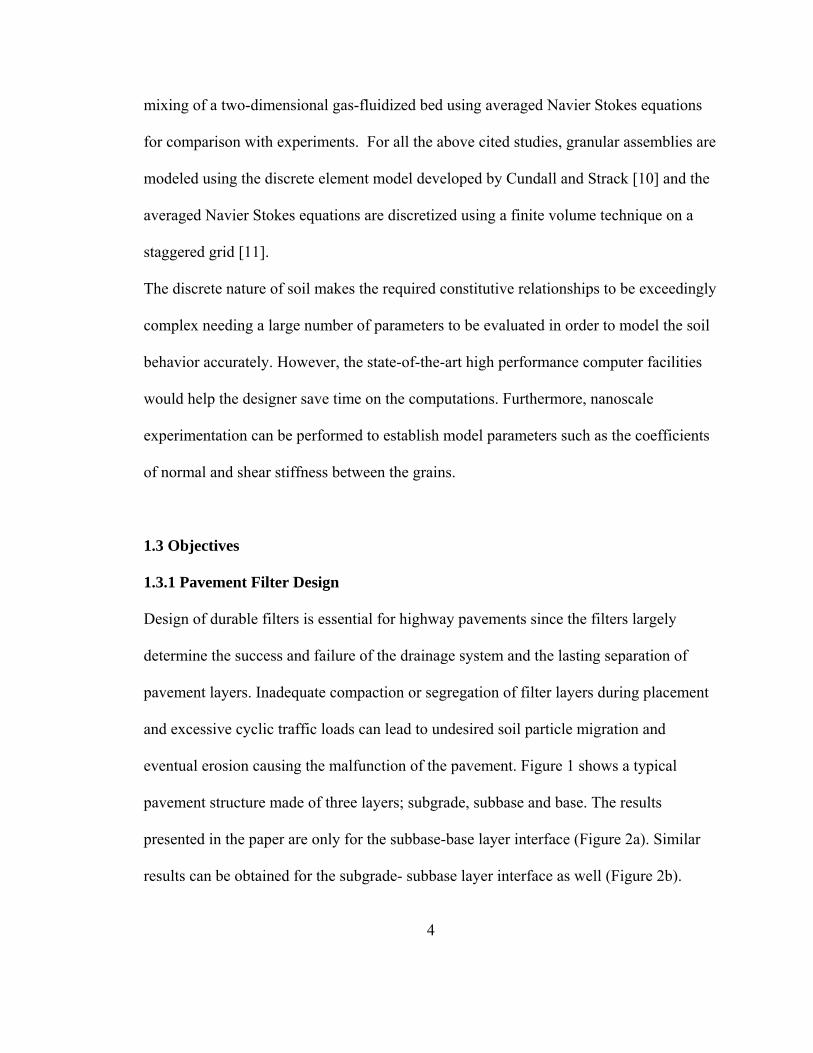
Design of durable filters is essential for highway pavements since the filters largely

determine the success and failure of the drainage system and the lasting separation of

pavement layers. Inadequate compaction or segregation of filter layers during placement

and excessive cyclic traffic loads can lead to undesired soil particle migration and

eventual erosion causing the malfunction of the pavement. Figure 1 shows a typical

pavement structure made of three layers; subgrade, subbase and base. The results

presented in the paper are only for the subbase-base layer interface (Figure 2a). Similar

results can be obtained for the subgrade- subbase layer interface as well (Figure 2b).

5

Currently, the conventional criteria (Eqn 2) proposed by U.S. Army Corps of Engineers

[12] are used for filter design. In these criteria, the filter refers to coarser layer and the

finer layer is defined as the soil.

Figure 1: Typical Pavement Structure

(a) (b)

Figure 2: Pavement Layer Interfaces

Clogging criterion:

585

15 ≤soil

filter

DD (2a)

Permeability criterion:

515

15 ≥soil

filter

DD (2b)

Additional criterion:

2550

50 <soil

filter

DD (2c)

Base (Example: Gravel) Subbase (Example: Coarse sand)

Subgrade (Example: Fine sand)

Gravel (Base)

Coarse sand (Subbase)

500 mm (20 in.)

750 mm (30 in.)

Coarse sand (Subbase)

Fine sand (Subgrade)

6

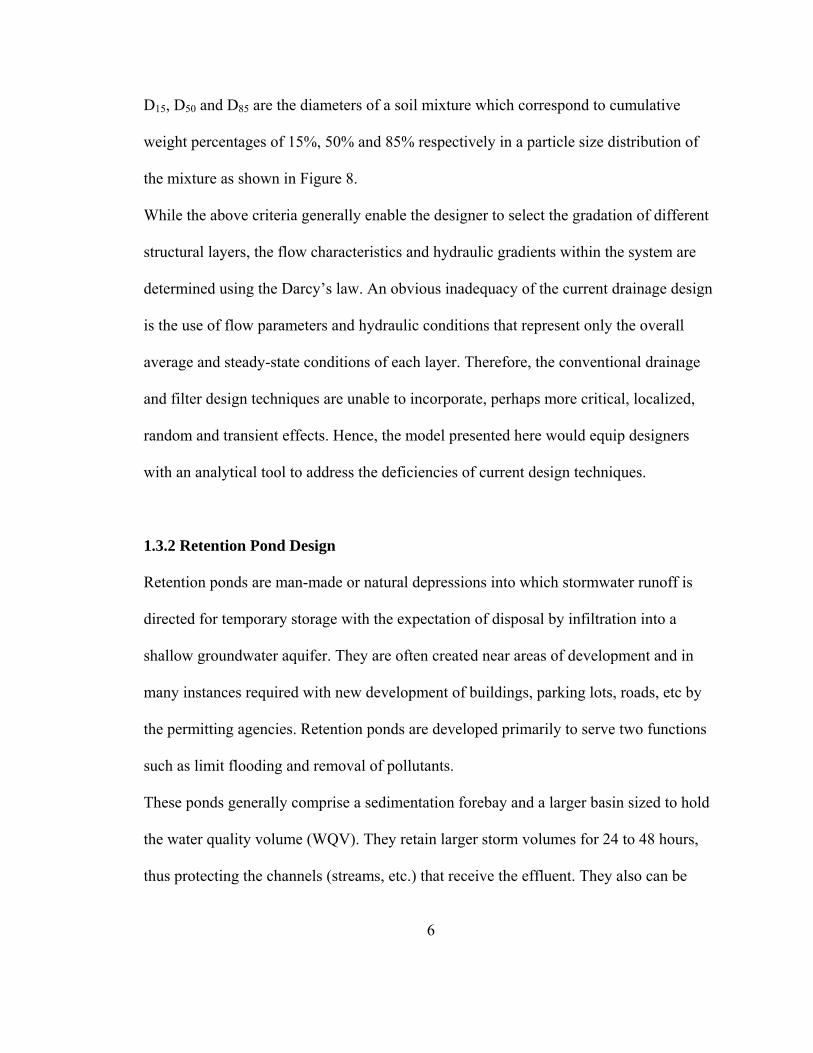
D15, D50 and D85 are the diameters of a soil mixture which correspond to cumulative

weight percentages of 15%, 50% and 85% respectively in a particle size distribution of

the mixture as shown in Figure 8.

While the above criteria generally enable the designer to select the gradation of different

structural layers, the flow characteristics and hydraulic gradients within the system are

determined using the Darcy’s law. An obvious inadequacy of the current drainage design

is the use of flow parameters and hydraulic conditions that represent only the overall

average and steady-state conditions of each layer. Therefore, the conventional drainage

and filter design techniques are unable to incorporate, perhaps more critical, localized,

random and transient effects. Hence, the model presented here would equip designers

with an analytical tool to address the deficiencies of current design techniques.

1.3.2 Retention Pond Design

Retention ponds are man-made or natural depressions into which stormwater runoff is

directed for temporary storage with the expectation of disposal by infiltration into a

shallow groundwater aquifer. They are often created near areas of development and in

many instances required with new development of buildings, parking lots, roads, etc by

the permitting agencies. Retention ponds are developed primarily to serve two functions

such as limit flooding and removal of pollutants.

These ponds generally comprise a sedimentation forebay and a larger basin sized to hold

the water quality volume (WQV). They retain larger storm volumes for 24 to 48 hours,

thus protecting the channels (streams, etc.) that receive the effluent. They also can be

7

designed to retain larger volumes generated by 10- to 100-year rain events. Water

treatment is achieved naturally when particles settle along the flow path between inlet

and outlet of the pond, and between storms when additional settling occurs. Nutrient

removal occurs between storms via plant uptake. Rain events provide a fresh influx of

stormwater runoff, which forces standing water out of the system. Maintenance

requirements of retention ponds include the periodic removal of sediment and vegetation

to restore storage capacity. Sediment removal is performed primarily in the forebay,

which can be designed for easy equipment access.

The model presented in this dissertation first uses a self-developed packing algorithm to

randomly pack a three dimensional discrete soil skeleton. Then the model is used to

determine the water flow behavior of the particulate soil medium consisting of

volumetrically coupled water continuum and the discrete soil skeleton. The flow of water

through the particulate medium is modeled using the Navier Stokes (NS) equations which

are discretized using the finite difference method (FDM) [13]. The new model is capable

of predicting both transient and steady state flow effects. The model is applied to a

pavement structure designed based on the U.S. Army Corps of Engineers’ filter designed

criteria [12] to analyze the localized transient and steady state seepage effects in terms of

water velocities and hydraulic gradients at different degrees of compaction. Appropriate

boundary conditions have been employed to simulate the conditions resulting from of a

sudden surge of ground water just beneath the pavement subbase. It is assumed in the

new model that reasonably accurate estimates of the above parameters can be obtained by

volumetric coupling of water and the soil skeleton.

8

1.4 Numerical Modeling

Numerical modeling can be performed to solve geomechanics problems using two

different approaches:

1) Solid continuum methods

2) Discrete element methods

1.4.1 Solid Continuum Methods

In the solid continuum approach, the entire soil body is first divided into a number of

small elements and the governing equations are mathematically solved for each element.

In this regard, the following three methods are widely used:

1) Finite Difference method

2) Finite Element method

3) Finite Volume method

1.4.2 Discrete Element Methods

Discrete element methods (DEM) comprise a suite of numerical techniques developed to

model granular materials, rock, and other discontinua at the scale of grains. In most cases,

the granular particles modeled as 3D spheres or 2D discs are individually packed in the

structure. Then, appropriate inter-particle characteristics such as coefficients of normal

and shear stiffness, friction between adjacent particles and friction between particles and

other structures are introduced in the analysis. As in the case of continuum methods, the

governing equations are solved numerically. Due to the nature of this analysis, DEM are

also known as particle modeling methods. Particle Flow Code (PFC) [7] is one of the

discrete element methods.

9

1.5 Assembling of Particles in the Particle Flow Code

Using the PFC program, individual soil particles can be packed to model a given

geotechnical structure such as an earthen dam or a pavement layer by closely simulating

the transient dynamics of that particulate medium involved with the construction of that

structure. The following laws govern the packing (construction) mechanism to achieve

the final force equilibrium.

1) Law of motion (Newton’s second law)

2) Appropriate force displacement (constitutive) laws for normal and shear

deformation

The computational cycle in PFC-2D is a time stepping algorithm that consists of the

repeated application of the law of motion to each particle, a force-displacement law to

each contact, and constant updating of boundaries. The force-displacement law based on

the contact constitutive model is repeatedly applied to each contact to update the contact

forces based on the relative motion between the two entities at the contact. Until the

particles reach equilibrium, the above laws will be applied in a loop as shown in Figure

3.

10

Figure 3: Computational Cycle in PFC

1.5.1 Theoretical Background of PFC

1.5.1.1 Particle Interactions

Figure 4: Illustration of Inter-Particle Forces

The above-mentioned rigid circular particles (or spherical in 3-D) interact by way of

normal and shear contacts modeled by a simplified mass-spring system as shown in

Figure 3. For each pair of particles, the interactive force can be written as

(3a) sskNNkF sni .. Δ+Δ=

S (Shear)

N (Normal)

11

Where, kN - Coefficient of normal stiffness, ks - Coefficient of shear stiffness, ΔN –

Normal deformation and Δs – Shear deformation. Then, the total force acting on a

particle given by,

∑= itotal FF (3b)

1.6 Organization of Dissertation

Chapter 2 describes the methodology used to randomly pack the soil particles and the

mathematical formulation for steady state flow through a particulate pavement system.

Chapter 3 presents the modification made on the governing equations for analyzing the

transient behavior of water through particulate pavement system using the volumetric

compatibility of the two phase media, such as water and solid particles. Chapter 4

describes the mathematical formulation of flow through partly-saturated and saturated

soils using Navier Stokes equations. Chapter 5 illustrates the application of the developed

models for analyzing flow around retention ponds in order to determine the free-surface

(Phreatic surface) using Navier Stokes equations. The different approaches are proposed

to determine the free-surface for flow from retention pond. Results are included in each

Chapter.

12

CHAPTER TWO

ANALYSIS OF STEADY STATE WATER SEEPAGE IN A PAVEMENT SYSTEM USING THE PARTICULATE APPROACH

2.1 Preliminary Studies Using Existing Software

The existing finite-element software (Seep/W) and discrete element software (PFC2D)

were used at the time of preliminary studies in order to visualize the effects of continuum

and discrete approaches on flow problems. A simple model shown in Figure 5 was used

to identify the localized effects within a two-layer pavement system. Under same

pressure gradient, the flow rates are compared using continuum and discrete methods.

Flow rate obtained using discrete method (0.0025 m3/s/m width) is less than that of

continuum method (q = 0.0027 m3/s/m width) due to additional drag forces in the

particulate matrix.

13

Figure 5: Analysis of Flow Problem Using Existing Software

Figure 6a: Highway Pavement Layers

DEM (PFC 2D) FEM (Seep/W)

(Contours for pressure head are shown)

Subb

ase

Subg

rade

14

Figure 6b: Comparison of Hydraulic Gradients Obtained Using Continuum and Discrete Methods (Steady State)

The seepage through two-layer pavement shown in Figure 6a was modeled using the

PFC2D. As illustrated in Figure 6b, there is a significant difference in hydraulic gradients

using the continuum and discrete approaches. At the interface, ilocal exceeds the iConventional

analysis. However, since the three-dimensional porosities are realistic, the authors

developed a three-dimensional packing algorithm. The results obtained from the

preliminary studies motivated the authors for analyzing the seepage phenomena through

particulate soil media.

2.2 Methodology Followed to Develop a Novel Algorithm

The comprehensive analytical procedure and the computer code developed for its

implementation are illustrated in Figure 7. The analytical procedure consists of two

primary tasks such as random assembly of the particulate medium (granular soil) and

solution of the fluid flow governing equations using partial coupling between the two

Plot of hydraulic gradient across a two-layer soil

0

20

40

60

80

0 10 20 30 40

Hydraulic gradient

Dep

th (m

m)

Localized i - DEMi across subgrade- Darcyi across subbase-Darcy

Subgrade-subbase interface

15

media. The flow chart also includes the sections, equation numbers and figure numbers

corresponding to each stage.

16

Figure 7: Flow Chart Illustrating the Analytical Model for Steady State Flow

Packing to determine maximum and minimum void ratios for each particle size distribution (Section 2.2.1)

Application of Monte-Carlo simulation to obtain randomly distributed in-situ void ratios at specified relative densities (Section 2.2.1.3)

Assignment of random in-situ void ratios for grid elements used in the fluid flow analysis

Application of Navier-Stokes equations to each grid element (Section 2.3)

Numerical discretization based on a staggered grid (Section 2.3.2 & Figure 15)

Solid phase

Fluid phase

Execution of SIMPLE algorithm (Fig. 16)

Analysis of results – critical velocities and hydraulic gradients at the steady-state (Section 2.5)

Mass imbalance term < tol.

Yes

Validating the model by determining the coefficients of hydraulic conductivities (Section 2.4)

Iterative solution for steady-state

No

17

2.2.1 Modeling of Soil Structure (3D Random Packing of Soil Particles)

The particle size distribution curves (PSDs) shown in Figure 8 were selected to satisfy the

US. Army Corps of Engineers΄ filter criteria (Eqn 2) for a typical pavement system made

of a gravel base, a coarse sand subbase and a fine sand subgrade [12].

2.2.1.1 Simulation of Maximum and Minimum Void Ratios Using PSD

In this model the soil particles are assumed to be of spherical shape. To determine the

maximum and minimum void ratios (emax and emin) corresponding to each soil type in

Figure 8, a customized random packing algorithm was developed. In the case of gravel,

28 mm × 28 mm × 28 mm cubes were packed using the corresponding PSD in Figure 8.

It can be noted that the PSDs in Figure 8 are cumulative probability distributions of

particle size for each soil type. Therefore, by using an adequately large array of random

numbers from a uniform distribution between 0 and 100 (the y axis range in Figure 8),

one can select the corresponding array of particle diameters that conforms to a selected

PSD, from the x axis. This technique, known as the Monte-Carlo simulation [14] is used

to select the array of packing diameters for each cube. It is noted that the resulting

maximum and minimum void ratio distributions change in each packing trial since the

order of diameters used for packing is changed randomly. Similarly, 16 mm ×16 mm ×

16 mm cubes and 3 mm ×3 mm × 3 mm cubes were used to obtain emax and emin in coarse

sand packing and fine sand packing respectively (Figure 8). Smaller cubes are used to

pack smaller particle sizes to reduce the computer running time assuming that an

18

adequate number of particles are within the cube to determine representative emax and emin

for each type of soil.

0

10

20

30

40

50

60

70

80

90

100

0.01 0.1 1 10 100Grain size/(mm)

% C

umul

ativ

e fr

eque

ncy

Coarse sand Gravel Fine sand

Figure 8: Particle Size Distributions for Gravel, Coarse Sand and Fine Sand

2.2.1.2 Implementation of the Packing Procedure

In order to obtain the loosest state of each type of soil (emax) within the corresponding

cubes described above, different sizes of soil particles inscribed in boxes are packed as

indicated Figure 9a using a MATLAB code developed by the authors. The side length of

each box is the same as the diameter of the inscribed soil particle. Based on the minimum

particle diameter of the selected PSD, the side lengths of each cube is divided into a finite

number of sub-divisions (Figure 9a). Then, the packing algorithm tracks the total number

of sub-divisions occupied by each incoming box, i.e. each packed soil particle, as packing

proceeds based on the Monte-Carlo simulation corresponding to a given PSD. Finally, the

19

automated algorithm fills the maximum possible number of sub-divisions until it finds

that no space is available within the considered cube for further packing of soil particles

from the given PSD.

On the other hand, in order to obtain the minimum void ratio (densest packing), the

maximum number of spheres smaller than the inscribing sphere in each box is also

packed into the unoccupied space at the corners of each box (Figure 9c and 9d) before

that box is placed in the cube (Figure 9b). For each type of soil, 400 such cubes (trials)

were packed randomly using the Monte-Carlo simulation. Since the maximum and

minimum void ratios obtained in each trial would be different as explained above, they

are considered as random variables. Thus, the probability distributions of emax and emin

obtained from those 400 trials are shown in Figure 10. The ranges derived for emax and

emin as shown in Table 1 agree with the typical values in [15].

Table 1: Size Characteristics of Pavement Layers

Soil type D15 (mm) D50 (mm) D85 (mm) emin emax

Gravel 9.85 13 19 0.59 – 0.8 0.98 – 1.18

Coarse sand 1.85 2.5 3.5 0.73 – 0.93 0.91 – 1.10

Fine sand 0.16 0.29 0.49 0.54 – 0.79 0.91-1.26

20

Figure 9: Random Packing of Soil Particles

2.2.1.3 Determination of the Natural Void Ratio Distribution

The concept of relative density is helpful in quantifying the level of compaction of

coarse-grained soils. The relative density of a coarse-grained soil at a given compaction

level expresses the ratio of the reduction in the voids at the given compaction level, to the

maximum possible decrease in the voids (Eqn 3). The in-situ void ratio distribution (e)

corresponding to a relative density (Dr) is obtained using the previously obtained emax and

emin (Eqns 3 or 4).

%100minmax

max ×−−

=ee

eeDr (4)

21

or

minmax 1001001 eDeDe rr +⎟

⎠⎞

⎜⎝⎛ −=

(5)

Where, emax is the randomly distributed void ratio of gravel/sand in its loosest state. emin is

the randomly distributed void ratio of gravel/sand in its densest state. e is the randomly

distributed void ratio of gravel/sand in its natural state in the field.

Thus,

( ) ( ) ( )[ ]reeen DefefFef ,, minmax= (6)

Where ( )efen , ( )efe max and ( )efe min are Probability Density Functions (pdf) of in-situ

natural void ratio, maximum void ratio and minimum void ratio respectively.

If e is a function of two random variables (emax = e1, emin = e2) and µ1 and µ2 are the mean

values of these random variables, the expected mean value of “e” can be expressed using

the second-order Taylor series approximation as

( ) ( ) [ ]21

2

1

2

1 21

2

21 ,21, eeCov

eeeeeE

i i∑∑= =

⎟⎟⎠

⎞⎜⎜⎝

⎛

∂∂∂

+= μμ (7)

Furthermore, the variance of “e” can be expressed as

[ ] [ ]212

2

1

2

1 1,

21

eeCovee

eeeV

i i μμ⎟⎟⎠

⎞⎜⎜⎝

⎛∂∂

⎟⎟⎠

⎞⎜⎜⎝

⎛∂∂

= ∑∑= =

(8)

22

0

0.1

0.2

0.3

0.4

0.5

0.6

0.7

0.8

0.9

1

0.55 0.65 0.75 0.85 0.95 1.05 1.15

void ratio

Prob

abili

ty d

ensi

ty o

r fre

quen

cy

maximum void ratio for gravel

minimum void ratio for gravel

Figure 10: Probability Density Function (PDF) of Maximum and Minimum Void Ratios

Two alternative approaches can be followed to determine the probability distribution of

the natural void ratio (e) from the probability distributions of the maximum and minimum

void ratios (Eqn 5):

1) Assume an appropriate Probability Density Function (Example: Log-normal) with

mean and variance calculated using Eqn 6 and Eqn 7 from the means (µ1, µ2) and

variances (V (e1), V (e2)) of emax and emin.

2) Generating the probability distribution of natural void ratios (e) using Eqn 4 and

the Monte-Carlo simulation technique.

In this model, the method (2) listed above is used. When the probability distributions of

emax and emin are known for each soil type (Figure 10) the corresponding cumulative

distributions of emax and emin can be derived (Figure 11). Then, once more the Monte-

µ1 µ2

V (e1) V (e2)

23

Carlo simulation (Section 3.1) can be used to pick two arrays of emax and emin values for

that soil type. Finally, with the emax and emin arrays, a corresponding array of natural void

ratio (e) of any of the above soil types, for a given relative density (Dr) can be obtained

from Eqn 4. The spatial distributions of natural void ratios (porosities) so obtained

assumed to be representative of each soil layer will be used in the analysis of flow

(Section 4).

Figure 11: Cumulative Frequencies of Maximum and Minimum Void Ratios

2.3 Modeling of Steady State Flow

In modeling the pavement layers, the three dimensional porosities obtained from particle

packing are coupled with two dimensional water flow. This is because flow is constrained

in the third direction due to the two dimensional nature of the pavement. Due to the

incompatibility of the sizes of the particles of the three layers and since the same grid

element size is used for entire pavement structure, only two pavement layers are modeled

at a time. Navier Stokes equations [13] are given by:

Random selection

24

Mass Conservation (Continuity Equation):

( ) ( ) 0=∂

∂+

∂∂

yvn

xun (9)

Momentum Conservation (Momentum Equations):

X direction:

( ) ( ) ( )⎟⎟⎠

⎞⎜⎜⎝

⎛

∂∂

+∂∂

++∂∂

−=∂

∂+

∂∂

+∂

∂2

2

2

22

yun

xunD

xpn

yvun

xun

tun x

ρμ

ρρ (10)

Y direction:

( ) ( ) ( )y

y gny

vnx

vnDypn

yvn

xvun

tvn

+⎟⎟⎠

⎞⎜⎜⎝

⎛

∂∂

+∂∂

++∂∂

−=∂

∂+

∂∂

+∂

∂2

2

2

22

ρμ

ρρ (11)

Where, n – porosity at the location (x, y) at time t, u, v – fluid velocities in the x and y

directions respectively, ρ – fluid density, p – fluid pressure, µ - fluid viscosity, gy -

gravitational force per unit mass in the y direction.

Averaged fluid-particle interactions (drag forces) are quantified using semi-empirical

relationships provided in Eqn 9 [6].

( ) ( )⎟⎟⎟

⎠

⎞

⎜⎜⎜

⎝

⎛ −+

−−= 2

222

2 175.11150 udnnu

dnnD

pp

x ρμ (12)

Where, pd - averaged particle diameter; Dx – x directional average fluid-particle

iteration force per unit volume. A similar expression for Dy is used for y directional

averaged fluid-particle interactions.

25

2.3.1 Need for a Staggered Grid

The central difference form of Eqns 6 – 8 requires a staggered grid due to the two issues

explained below:

022

1,1,,1,1 =Δ

−+

Δ

− −+−+

yvv

xuu jijijiji (13)

Figure 12: Discrete Checkerboard Velocity Distribution at Each Grid Point: At Each Node, the Top Number is u and the Bottom Number is v

Figure 12 illustrates an arbitrary zigzag type of distribution of both the x component and

y components of velocity, u and v, respectively. When these arbitrary numbers are

substituted in Eqn 12, the central difference form of the continuity equation for

incompressible fluid flow is unconditionally satisfied. In other words, the checkerboard

velocity distribution shown in Figure 12 produces a trivial solution inapplicable to a real

physical flow field.

26

Considering a two-dimensional discrete, checkerboard pressure pattern as illustrated in

Figure 13, the second order central difference formulation for the pressure gradients

which appear in the momentum equations can be written as follows:

xPP

xP jiji

Δ

−=

∂∂ −+

2,1.1

(14)

yPP

yP jiji

Δ

−=

∂∂ −+

21,1, (15)

Figure 13: Discrete Checkerboard Pressure Distribution

The checkerboard pressure distribution (Figure 13) gives zero pressure gradients in the

momentum equations in the x and y directions written in terms of the central difference

scheme (Eqns 13 and 14 respectively). In other words, the pressure field would not be

27

incorporated in the discretized Navier Stokes equations and hence the numerical solution

would effectively see only uniform pressure distributions in the x and y directions.

In order to address the above issue, an innovative remedy for the checkerboard

distribution is to use a “staggered mesh” where discrete pressures and velocities are

expressed only wherever required. A typical two-dimensional staggered mesh

arrangement is shown in Figure 14. In the staggered grid, the velocity components are

computed for the points that lie on the faces of the flow elements. Thus, the x-directional

velocity, u, is computed on the planes or surfaces that are normal to the x-direction and

similarly, the y-directional velocity, v, is computed on the planes or surfaces that are

normal to the y-direction. On the other hand, the pressures are computed at the center of

the flow elements.

By introducing a staggered grid, the mass flow rates across the flow element faces can be

evaluated without any interpolation of the relevant velocity components. Moreover, for a

typical flow element, it will be easy to see that the discretized continuity equation would

contain the differences of adjacent velocity components thus preventing a wavy velocity

field resulting from the continuity equation. When the staggered grid is used, only

“realistic” velocity fields would have the possibility of being acceptable to the continuity

equation. Consequently, pressure fields in the momentum equations would no longer be

felt as uniform pressure fields.

28

Figure 14: A Typical Staggered Grid Arrangement (Solid Circles Represent Pressure Nodes and Open Circles Represent Velocity Nodes)

2.3.2 Numerical Solution Technique

Based on the staggered grid arrangement introduced in Section 4.2, a finite-difference

approach is used to discretize the Eqns 9, 10 and 11. The scheme is based on forward

difference in time and central difference in space. The numerical form of the x directional

momentum equation is written in Eqn 10, referring to the notation in Figure 15 for the

sequential iteration steps of N and N+1.

Y

X

29

Figure 15: Computational Module for the X-Momentum Equation

( ) ( )⎟⎟⎟⎟

⎠

⎞

⎜⎜⎜⎜

⎝

⎛−

+ρ

−μ−⎟⎟

⎠

⎞⎜⎜⎝

⎛

Δ

−

ρ−

=Δ

−

+Δ

−+

Δ

−

−−+

−+−+−+++++

−−+++++

2j,2

1ij,ip

2j,i

j,ij,2

1i2j,ip

2j,i

2j,ij,ij,1ij,i

21j,2

1i1j,21i1j,i

21j,2

1i1j,21i1j,i

2j,2

1ij,1i2

j,23ij,1i

Nj,2

1ij,i1N

j,21ij,i

udn

n175.1u

dn

n1150

xppn

y2

vunvun

x2

unun

t

unun

( )

( ) ⎥⎥⎥⎥⎥⎥

⎦

⎤

⎢⎢⎢⎢⎢⎢

⎣

⎡

Δ

−+

+Δ

−+

ρμ

++−+−+++

+−−++

2

j,21ij,i1j,2

1i1j,i1j,21i1j,i

2

j,21ij,ij,2

1ij,1ij,23ij,1i

y

un2ununx

un2unun

(16a)

Where, ⎟⎠⎞

⎜⎝⎛ += +++++

21j,1i2

1j,i21j,2

1i vv21v,aintpoAt (16b)

30

⎟⎠⎞

⎜⎝⎛ += −+−−+

21j,1i2

1j,i21j,2

1i vv21v,bintpoAt (16c)

Within the staggered grid some velocities need to be interpolated as shown in Eqns 16b

and 16c. In a concise form, Eqn 16a can be written as

( ) ( )tAx

pp)t(AtAunun j,ij,1iN

j,21ij,i

1Nj,2

1ij,i Δ+⎟⎟⎠

⎞⎜⎜⎝

⎛

Δ

−Δ+Δ+= +

+++

(16d)

Where,

+Δ

−=

−−++

x2

ununA

2j,2

1ij,1i2

j,23ij,1i

y2

vunvun2

1j,21i1j,2

1i1j,i2

1j,21i1j,2

1i1j,i

Δ

− −+−+−+++++ (16e)

ρ−= j,in

A (16f)

and

( ) ( )+

⎟⎟⎟⎟

⎠

⎞

⎜⎜⎜⎜

⎝

⎛−

+ρ

−μ−=

−−2

j,21i

j,ip2

j,i

j,ij,2

1i2j,ip

2j,i

2j,i u

dn

n175.1u

dn

n1150A

( )

( ) ⎥⎥⎥⎥⎥⎥

⎦

⎤

⎢⎢⎢⎢⎢⎢

⎣

⎡

Δ

−+

+Δ

−+

ρμ

+−+−+++

+−−++

2

j,21ij,i1j,2

1i1j,i1j,21i1j,i

2

j,21ij,ij,2

1ij,1ij,23ij,1i

y

un2ununx

un2unun

(16g)

The numerical form of the y directional momentum equation can be written similarly

based on Eqn 11.

31

2.3.3 Semi-Implicit Method for Pressure-Linked Equations (SIMPLE) Algorithm

An iterative process called the pressure correction technique has found widespread

application in the numerical solution of the incompressible, viscous Navier Stokes

equations. This technique is a vehicle by which the velocity and pressure fields are

directed towards a solution that satisfies both the discrete continuity and momentum

equations. This technique is embodied in an algorithm called Semi-Implicit Method for

Pressure-Linked Equations (SIMPLE) [11]. The primary idea behind SIMPLE is to create

a discrete equation for pressure, in terms of the pressure correction, from the discrete

continuity equation. Figure 16 shows the step-by-step procedure for the SIMPLE

algorithm.

32

Figure 16: Flow Chart for SIMPLE Algorithm for Steady State Condition

2.3.3.1 Derivation of the Pressure Correction Formula

At the beginning of each new iteration, jip , is set to *, jip , where *

, jip is the pressure from

the previous iteration. Then, Eqn 16d will be transformed to Eqn 17.

( ) ( )tAx

pp)t(AtAunun

*j,i*

j,1i***N

j,21i

*j,i

1N

j,21i

*j,i Δ+

⎟⎟

⎠

⎞

⎜⎜

⎝

⎛

Δ−

Δ+Δ+= ++

+

+ (17)

Similarly re-arranged y directional equation would be Eqn 18.

( ) ( ) ( ) yj,i*j,i

*1j,i

***N

21j,i

*j,i

1N

21j,i

*j,i gntB

ypp

tBtBvnvn ρ+Δ+⎟⎟

⎠

⎞

⎜⎜

⎝

⎛

Δ−

Δ+Δ+= ++

+

+ (18)

Iteration for steady-state

Assume trial values of (p*) n, (u*) n, (v*) n for nth iteration

Solve momentum equations for (n+1)th iteration [(u*) n+1 and (v*) n+1]

Solve a pressure-correction equation for p' using a relaxation technique

Calculate pn+1 = (p*) n + p' Correct the velocities u n+1 = (u*) n + u' v n+1 = (v*) n + v'

Visualize steady-state results

Determine the mass imbalance term (mit)

mit < tol.

Yes

No

33

Next, Eqns 17 and 18 are subtracted from Eqn 16d and its y directional counterpart to

obtain Eqns 19 and 20 respectively.

⎟⎟

⎠

⎞

⎜⎜

⎝

⎛

Δ

−Δ+= +

+++ x

p'p)t('A'un'un

j,i'

j,1iNj,2

1ij,i1N

j,21ij,i (19)

( ) ⎟⎟

⎠

⎞

⎜⎜

⎝

⎛

Δ

−Δ+=

+

+++ y

'ppt'B'vn'vn j,i1j,i

'N

21j,ij,i

1N

21j,ij,i (20)

Where, the pressure correction *,,

', jijiji ppp −= , *' AAA −= , *' AAA −=

ρjin

AAAand .*' −=== .

BB ′,' and B′ can be defined similarly from the y directional coefficients.

Eqn 9 can be re-written in the discretized form as in Eqn 21 using the central difference

scheme with the staggered grids,

(21)

The semi-implicit terminology refers to arbitrary setting of A ,A '' and the corresponding

y directional coefficients equal to zero, thus allowing the ultimate pressure correction

formula, (Eqn 21), to have p΄ appearing only at four neighborhood grid points illustrated

in Figure 17. Omission of Nji

u,2

1'+

, Nji

v2

1,'

+, A ,A '' and the corresponding y directional

coefficients in the pressure correction derivation does not affect the final solution because

0y

vnvn

x

unun2

1j,ij,i2

1j,i1j,ij,21ij,ij,2

1ij,1i=

Δ

−+

Δ

− −++−++

34

the pressure correction and velocity corrections would in fact be zero for a converged

solution. Arbitrarily setting Nji

u,2

1'+

and Nji

v2

1,'

+ equal to zero in Eqns 19 and 20 produce,

⎟⎟

⎠

⎞

⎜⎜

⎝

⎛

Δ

−Δ=−= ++

+++

++ x

p'p)t('Aunun'un

j,i'

j,1i1N

j,21i

*j,i

1Nj,2

1ij,i1N

j,21ij,i (22)

( ) ⎟⎟

⎠

⎞

⎜⎜

⎝

⎛

Δ

−Δ=−=

++

+++

++ y

'ppt'Bvnvn'vn j,i1j,i

'1N

21j,i

*j,i

1N

21j,ij,i

1N

21j,ij,i (23)

Using Eqns 22 and 23, the discretized continuity equation (Eqn 21) can be expressed as a

pressure correction formula in terms of ', jip values of only the neighboring four grid

points as illustrated in Figure 17 (Eqn 21).

Figure 17: Designation of Nodal Points on a Grid Used in SIMPLE Algorithm

0fpepdpcpbpa j,i'

1j,ij,i'

1j,ij,i'

j,1ij,i'

j,1ij,i'

j,ij,i =+++++ −+−+ (24a)

Where,

( ) ( ) ⎟⎟⎠

⎞⎜⎜⎝

⎛

Δρ

Δ+

Δρ

Δ= 22j,ij,i

yt

xtn2a (24b)

( )2j,ij,ixtnb

Δρ

Δ−= (24c)

35

( )2j,ij,ixtnc

Δρ

Δ−= (24d)

( )2j,ij,iytnd

Δρ

Δ−= (24e)

( )2j,ij,iytne

Δρ

Δ−= (24f)

and

( ) ( )y

vnvn

x

ununf

1Nj,1ij.i

1Nj,1ij.i

1N1j,ij.i

1N1j,ij.i

j,i Δ

×−×+

Δ

×−×=

+−

++

+−

++ (24g)

After determining the pressure correction, ', jip from Eqn 24, the pressure and velocity

components at every node are updated as follows:

'j,i

*j,ij,i ppp += (25)

'j,i

*j,ij,i uuu += (26)

'j,i

*j,ij,i vvv += (27)

Where, ⎟⎟

⎠

⎞

⎜⎜

⎝

⎛

Δ

−Δ= +

+ xp'p

n)t('A'u

j,i'

j,1i

j,ij,21i

(28)

and

( )⎟⎟

⎠

⎞

⎜⎜

⎝

⎛

Δ

−Δ=

+

+ y

'pp

nt'B'v j,i1j,i

'

j,i21j,i

(29)

The pressure correction Equation (Eqn 24), which is of Poisson format in terms of p΄, can

be solved by employing a numerical relaxation technique. The term jif , (Eqn 24g) is

called the “mass imbalance term” which must vanish theoretically in the last iteration

36

where the velocity field converges to a field that satisfies the continuity equation (Eqn 9).

In the numerical algorithm developed in this work, the mass imbalance term is used as a

stopping criterion to assure that the solution converges to the correct velocity field. The

function of the pressure correction formula is to set the iterative process in such a

direction that, when the velocity distribution is determined from the momentum

equations, it will eventually converge to the correct distribution which satisfies the

continuity equation. Because the pressure correction method is designed to solve for the

steady flow condition via an iterative process, the superscripts N and N+1 used in the

equations are the sequential iteration steps, with no significance to any real transient

variation. Under the steady state conditions, the term of Δt can be treated as a parameter

which has some effect on the speed at which the convergence is achieved.

2.3.3.2 Boundary Conditions for Pavement System

The boundary conditions appropriate for the actual water flow through the pavement

system are specified in the computer code as indicated in Figure 18.

1) At the inflow boundary, the pressure and velocities are specified. Hence, the

pressure correction, p΄, is zero at the inflow boundary.

2) At the outflow boundary, the pressure is specified and velocity components are

allowed to float. Hence, p΄ is zero at the outflow boundary as well.

3) At the vertical walls, the slip conditions are maintained. Thus, the velocity

component, u, normal to the walls is set to zero.

37

Figure 18: Boundary Conditions Incorporated in the Flow through the Pavement System 2.4 Validation of the Numerical Model

In order to validate the flow model described in Section 4, the coefficients of hydraulic

conductivity of several uniformly graded soil types which are not used in the current

illustration are determined from the numerical model and compared with widely used

empirical relationships proposed by Hazen (Eqn 30) and Chapius (Eqn 31) [16]. The

results of this comparison are summarized in Table 2.

210Dc)s/cm(k = (30)

( )

7825.0

e1eD4622.2)s/cm(k

3210

⎥⎥⎦

⎤

⎢⎢⎣

⎡

+= (31)

Where, c - a constant that varies from 1.0 to 1.5 and D10 - the effective size in mm.

38

Table 2: Comparison of 3-D Coefficients of Hydraulic Conductivity Derived from SIMPLE Algorithm

Figure 19: Relationship between Hydraulic Conductivity Vs Diameter for Uniformly Distributed Soils

It can be concluded from Table 2 that the coefficients of hydraulic conductivities

determined from the model agree fairly well with those computed from common

empirical relationships. Furthermore, it was determined that the coefficients of hydraulic

conductivity for gravel, coarse sand and fine sand used in the Numerical Illustration

Soil

type

(1)

Effective size

(D10) mm

(2)

K model

(cm/s)

(3)

KHazen

(cm/s)

(4)

KChapius (cm/s)

(5)

a 0.5 0.979871 0.375 0.497428

b 1 3.108229 1.5 1.47206

c 2 6.811264 6 4.532172

d 3 9.374428 9 8.247057

e 4 12.34681 16 12.94549

39

(Section 7) are 0.097 m/s ,0.043 m/s and 0.00024 m/s respectively. These values are

within the ranges of typical hydraulic conductivities presented in the literature [16] for

the corresponding PSDs shown in Figure 8. According to the developed model, the

relationship between hydraulic conductivity Vs square of the tenth percentile diameter for

uniformly distributed soils is shown in Figure 19. Therefore, the empirical equation (Eqn

45) does not seem to be accurate.

2.5 Numerical Illustration

The numerical model was applied to the pavement layer interfaces shown in Figure 2.

The material properties and other model parameters shown in Table 1 and 3 were used

for this purpose.

40

Table 3: Model Parameters

Particles

Number of gravel particles considered for determining the

porosity distribution

137668

Number of coarse sand particles considered for determining

the porosity distribution

205332

Number of fine sand particles considered for determining

the porosity distribution

855450

Gravel particle size 2 mm- 24 mm

Coarse sand particle size 1 mm- 5mm

Fine sand particle size 0.04 mm – 0.62 mm

Average density of saturated soil 1900 kg/m3

Average compression index for granular soils 0.37 [18]

Specific gravity of soil 2.65

Average void ratio of gravel packing (Dr = 50%) 0.86

Average void ratio of coarse sand packing (Dr = 50%) 0.90

Average critical hydraulic gradient 0.88

Water

Density 1000 Kg/m3

Dynamic viscosity 10-3 Pa.s

Flow calculations

Gravitational acceleration 9.81 m/s2

Number of grid elements 50 by 50

41

2.5.1 Results of Numerical Illustration

Figure 20 and Figure 21 illustrate the progression of flow rate with iterations through

different soil layers for different levels of compaction. They clearly reveal the reduction

in flow rate due to densification and the impact of the hydraulic conductivity.

Coarse sand- gravel interface

0.E+002.E-054.E-056.E-05

8.E-051.E-041.E-04

0 50 100 150 200 250 300

iteration steps

Flow

Rat

e (m

3 /s)

Dr = 5%

Dr=50%

Dr = 75%

Dr = 95%

Figure 20: Plot of Flow Rate through Coarse Sand-Gravel Interface Vs Iteration Steps with Different Levels of Compaction (For Pressure Differential of 23 kPa)

-5.0E-08

0.0E+00

5.0E-08

1.0E-071.5E-07

2.0E-07

2.5E-07

3.0E-07

3.5E-07

4.0E-07

4.5E-07

0 50 100 150 200 250

Flow

Rat

e(m

3 /s)

Iteration steps

Fine sand/coarse sand interface

Dr = 5% Dr = 50% Dr = 75% Dr = 95%

Figure 21: Plot of Flow Rate through Fine Sand-Coarse Sand Interface Vs Iteration Steps with Different Levels of Compaction (For Pressure Differential of 23 kPa)

42

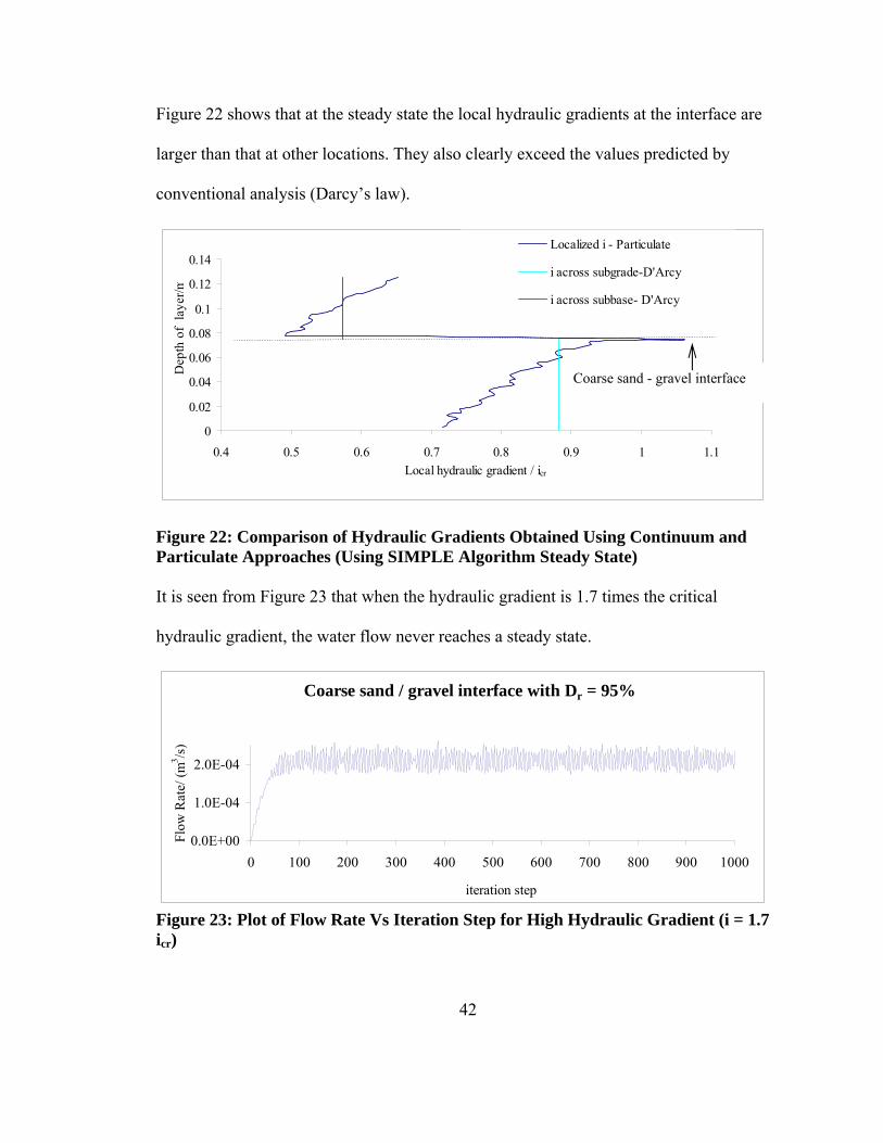
Figure 22 shows that at the steady state the local hydraulic gradients at the interface are

larger than that at other locations. They also clearly exceed the values predicted by

conventional analysis (Darcy’s law).

0

0.02

0.04

0.06

0.08

0.1

0.12

0.14

0.4 0.5 0.6 0.7 0.8 0.9 1 1.1Local hydraulic gradient / icr

Dep

th o

f la

yer/m

Localized i - Particulate

i across subgrade-D'Arcy

i across subbase- D'Arcy

Figure 22: Comparison of Hydraulic Gradients Obtained Using Continuum and Particulate Approaches (Using SIMPLE Algorithm Steady State) It is seen from Figure 23 that when the hydraulic gradient is 1.7 times the critical

hydraulic gradient, the water flow never reaches a steady state.

Coarse sand / gravel interface with Dr = 95%

0.0E+00

1.0E-04

2.0E-04

0 100 200 300 400 500 600 700 800 900 1000

iteration step

Flow

Rat

e/ (m

3 /s)

Figure 23: Plot of Flow Rate Vs Iteration Step for High Hydraulic Gradient (i = 1.7 icr)

Coarse sand - gravel interface

43

2.6 Conclusions

The current practice of designing pavement filter systems does not consider

1) The interaction between pore water and the individual soil particles.

2) The localized effects.

In order to determine the realistic limiting hydraulic gradients that can be applied within

pavement layers, a design methodology based on a particulate approach that incorporates

particle-soil interaction needs to be used. In this Chapter, the steady state water seepage

in two saturated filter interfaces with varying levels of compaction was analyzed using a

soil particulate model. The particulate effects of soil with different levels of compaction

were incorporated conveniently in the model using a random packing technique, while

the flow of water within the particulate assembly was modeled by the Navier Stokes flow

equations. Two separate filter interfaces, i.e. coarse sand-gravel and fine sand-coarse

sand were assembled using particle size distributions that satisfied the conventional filter

design criteria. Then, a pressure differential that corresponded to the critical hydraulic

gradient was applied across the layer interface. In order to verify the model, the

coefficients of hydraulic conductivity predicted from the model are compared with those

computed from the empirical relationships widely used in drainage design. The steady

state flow algorithm is modified in the next Chapter to analyze the transient behavior of

seepage through two-layer particulate pavement system which predicts the critical

conditions for erosion, piping and clogging.

44

CHAPTER THREE

ANALYSIS OF TRANSIENT WATER SEEPAGE IN A PAVEMENT SYSTEM USING THE PARTICULATE APPROACH

3.1 Modeling of Transient Flow

The comprehensive analytical procedure and the computer code developed for its

implementation are illustrated in Figure 24. The analytical procedure consists of two

primary tasks such as the random assembly of the particulate medium (granular soil) and

the solution of the fluid flow governing equations using partial coupling between the two

media. The flow chart also includes the sections, equation numbers and figure numbers

corresponding to each stage.

45

Figure 24: Flow Chart Illustrating the Analytical Model for Transient and Steady State Flow

No

Yes

No Yes

No

Packing to determine maximum and minimum void ratios for each particle size distribution (Section 2.2.1)

Application of Monte-Carlo simulation to obtain randomly distributed in-situ void ratios at specified relative densities (Section 2.2.1.3)

Assignment of random in-situ void ratios for grid elements used in the fluid flow analysis

Application of Navier-Stokes equations to each grid element (Section 3.1.1)

Numerical discretization based on a staggered grid (Section 3.1.3 & Figure 25)

Analysis of results – critical velocities and hydraulic gradients during transient and steady- state conditions (Section 3.4)

Solid phase Fluid phase

Iterative solution for water pressure (p) distribution in the grid (Eqn. 44 & Figure 26)

Time marching

Δp < Tol

Time-based change in water

velocity (Δv) < Tol

Validating the model by determining the coefficients of hydraulic conductivities (Section 3.3)

Yes

mit < tol.

Determination of porosity change satisfying the volumetric compatibility (Eqn. 43).

Determine the mass imbalance term (mit)

46

3.1.1 Transient Navier Stokes Equations

In modeling the pavement layers, the three dimensional porosities obtained from particle

packing are coupled with two dimensional water flow. This is because flow is constrained

in the third direction due to the two dimensional nature of the pavement. Navier Stokes

equations [13] are given by:

Mass Conservation (Continuity Equation):

( ) ( ) 0=∂∂

+∂

∂+

∂∂

yvn

xun

tn (32)

Momentum Conservation (Momentum Equations):

X direction:

( ) ( ) ( )⎟⎟⎠

⎞⎜⎜⎝

⎛

∂∂

+∂∂

++∂∂

−=∂

∂+

∂∂

+∂

∂2

2

2

22

yun

xunD

xpn

yvun

xun

tun x

ρμ

ρρ (33)

Y direction:

( ) ( ) ( )y

y gny

vnx

vnDypn

yvn

xvun

tvn

+⎟⎟⎠

⎞⎜⎜⎝

⎛

∂∂

+∂∂

++∂∂

−=∂

∂+

∂∂

+∂

∂2

2

2

22

ρμ

ρρ (34)

Where, n – porosity at the location (x, y) at time t, u, v – fluid velocities in the x and y

directions respectively, ρ – fluid density, p – fluid pressure, µ - fluid viscosity, gy -

gravitational force per unit mass in the y direction.

Averaged fluid-particle interactions (drag forces) are quantified using semi-empirical

relationships provided in Eqn 35 [6].

( ) ( )⎟⎟

⎠

⎞

⎜⎜

⎝

⎛ −+

−−= 2

222

2 175.11150 u

dnn

udn

nDpp

x ρμ (35)

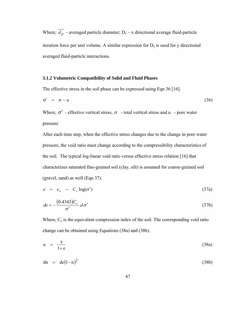
47

Where, pd - averaged particle diameter; Dx – x directional average fluid-particle

iteration force per unit volume. A similar expression for Dy is used for y directional

averaged fluid-particle interactions.

3.1.2 Volumetric Compatibility of Solid and Fluid Phases

The effective stress in the soil phase can be expressed using Eqn 36 [16].

u−σ=σ′ (36)

Where, σ ′ - effective vertical stress, σ - total vertical stress and u - pore water

pressure

After each time step, when the effective stress changes due to the change in pore water

pressure, the void ratio must change according to the compressibility characteristics of

the soil. The typical log-linear void ratio versus effective stress relation [16] that

characterizes saturated fine-grained soil (clay, silt) is assumed for coarse-grained soil

(gravel, sand) as well (Eqn 37).

)log(σ ′−= co Cee (37a)

( )σ

σ′

′−= d

Cde c4343.0

(37b)

Where, Cc is the equivalent compression index of the soil. The corresponding void ratio

change can be obtained using Equations (38a) and (38b).

e1en+

= (38a)

( )2n1dedn −= (38b)

48

3.1.3 Numerical Solution Technique

A finite-difference approach [12] is used to discretize the Eqns 32, 33 and 34. The

scheme is based on forward difference in time and porosity, and central difference in

space. A typical two-dimensional staggered mesh arrangement [11, 13] was used to

discretize the Eqns 32, 33 and 34. On the other hand, Patankar’s original formulation [11]

is based on the “pressure correction method” involving a finite-volume approach.

The pavement layers were divided into a 50 × 50 grid for the finite difference analysis.

One fluid cell, known herein as a grid element, was selected to be 25 mm × 25 mm × 1m

(2-D flow) to be compatible with the cube sizes (28 mm × 28 mm × 28 mm or 16 mm ×

16 mm × 16 mm) used for packing (Section 3.1). 1 m has been selected in the third

direction assuming two dimensional water flow. Since the Navier Stokes equations are

written in terms of porosities, the spatial probability distribution of natural void ratios are

first converted to porosities (Eqn 41a). First, natural porosities (void ratios) were assigned

to each grid element based on the spatial probability distribution of natural void ratios

determined from packing (Section 3.3). Within each grid element, the fluid-particle

interaction is quantified considering the averaged particle diameter which is defined as

the arithmetic mean of the diameters of all the particles in each grid. The authors΄

modified numerical scheme is described as follows:

Eqn 39a expresses the x directional momentum equation in the numerical form for the

sequential time steps of N and N+1 referring to the notation in Figure 25.

49

Figure 25: Computational Grid for the X-Momentum Equation

( ) ( )⎟⎟⎟⎟

⎠

⎞

⎜⎜⎜⎜

⎝

⎛−

+ρ

−μ−⎟⎟

⎠

⎞⎜⎜⎝

⎛

Δ

−

ρ−

=Δ

−

+Δ

−+

Δ

−

−−+

−+−+−+++++

−−+++++++

2j,2

1ij,ip

2j,i

j,ij,2

1i2j,ip

2j,i

2j,ij,ij,1ij,i

21j,2

1i1j,21i1j,i

21j,2

1i1j,21i1j,i

2j,2

1ij,21i

2j,2

3ij,23i

Nj,2

1ij,21i

1Nj,2

1ij,21i

udn

n175.1u

dn

n1150

xppn

y2

vunvun

x2

unun

t

unun

( )

( ) ⎥⎥⎥⎥⎥⎥

⎦

⎤

⎢⎢⎢⎢⎢⎢

⎣

⎡

Δ

−+

+Δ

−+

ρμ

++−+−+++

+−−++

2

j,21ij,i1j,2

1i1j,i1j,21i1j,i

2

j,21ij,ij,2

1ij,1ij,23ij,1i

y

un2ununx

un2unun

(39a)

Where,

At point a, ⎟⎠⎞

⎜⎝⎛ += +++++ 2

1j,1i21j,i2

1j,21i vv2

1v (39b)

50

At point b, ⎟⎠⎞

⎜⎝⎛ += −+−−+ 2

1j,1i21j,i2

1j,21i vv2

1v (39c)

Similarly, the y directional momentum equation can be written numerically.

Equations (37b) and (38b) can be used to express the change in porosity within the time

interval Δt using the volumetric compatibility between solid and fluid phases. Then, Eqn

32 can also be discretized as follows:

tn

y

vnvn

x

unun 1N

21j,i2

1j,i1N

21j,i2

1j,i1N

j,21ij,2

1i1N

j,21ij,2

1i

ΔΔ

−=⎥⎥⎥

⎦

⎤

⎢⎢⎢

⎣

⎡

Δ

−+

Δ

− +−−

+++

+−−

+++

( ) [ ]

t1

p

ppn1C4343.0N

j,iN

j,i

1Nj,i

Nj,i

2j,ic

Δ⎥⎥

⎦

⎤

⎢⎢

⎣

⎡

−σ

−−=

−

(40)

To compute the change in porosity in the transient continuity equation in an explicit

manner, the water pressure difference between the time steps (N-1) and N has been used

in Eqn 40. By substituting velocities of the new time step by those of the previous time

step, Eqn 40 is reduced to Eqn 41, which is a Poisson equation in terms of water pressure

(p).

Figure 26: Designation of Nodal Points on a Grid Used in the Iterative Procedure

0,1,,1,,,1,,1,,, =+++++ −+−+ jijijijijijijijijijiji Spepdpcpbpa (41a)

Where,

51

( )N

jiji

jic

jijijijiji p

nCt

y

nn

x

nna

.,

2,

2

22

1,21,

2

,21,2

1

,

14343.0

−

−−

Δ⎥⎥

⎦

⎤

⎢⎢

⎣

⎡

⎟⎟

⎠

⎞

⎜⎜

⎝

⎛

Δ

++⎟

⎟

⎠

⎞

⎜⎜

⎝

⎛

Δ

+=

−+−+

σρ (41b)

ρ

2

2

,21

,t

x

nb

jiji

Δ⎟⎟

⎠

⎞

⎜⎜

⎝

⎛

Δ−=

+ (41c)

ρ

2

2

,21

,t

x

nc

jiji

Δ⎟⎟

⎠

⎞

⎜⎜

⎝

⎛

Δ−=

− (41d)

ρ

2

22

1,,

ty

nd

jiji

Δ⎟⎟

⎠

⎞

⎜⎜

⎝

⎛

Δ−=

+ (41e)

ρ

2

22

1,,

ty

ne

jiji

Δ⎟⎟

⎠

⎞

⎜⎜

⎝

⎛

Δ−=

− (41f)

and

( ) 1,

,,

2,2

1,21.2

1,21.

,21.2

1,21.2

12

21,2

1,

2

21,2

1,

2

,21,2

1

2

,21,2

1,

14343.0−

−−++

−−++−+

−+−+−+

−

−+Δ

Δ

⎟⎠⎞⎜

⎝⎛ ×−×

+ΔΔ

⎟⎠⎞⎜

⎝⎛ ×−×

+ΔΔ

⎟⎠⎞

⎜⎝⎛ −+

ΔΔ

⎟⎠⎞⎜

⎝⎛ −+

ΔΔ

⎟⎠⎞

⎜⎝⎛ −+

ΔΔ

⎟⎠⎞⎜

⎝⎛ −=

NjiN

jiji

jic

Njiji

Njiji

Njiji

NjijiN

ji

N

ji

Nji

Nji

N

ji

N

jiN

jiN

jiji

pp

nCt

y

vnvn

tx

unun

ytBB

ytBB

xtAA

xtAAS

σ

ytgnn yjiji Δ

Δ⎟⎠⎞⎜

⎝⎛ −+

−+

2

21,2

1, (41g)

Where, A , A , B and B is a collection of velocity derivatives from the discretized

momentum equations in both x and y directions.

52

Similar to the pressure correction method introduced by Patankar [11], the authors΄

modified algorithm solves the Poisson equation (Eqn 41) iteratively in terms of water

pressures (p) at the neighboring nodes shown in Figure 26. Within each time step, when

the water pressure difference at any node computed in each iteration becomes negligible,

the algorithm checks the volumetric compatibility of solid and fluid phases throughout

the entire pavement system (Eqn 40). Until the velocities become constant at each node,

the time marching is continued while solving for water pressures iteratively at each time

step (Figure 24).

3.1.4 Boundary Conditions

The boundary conditions appropriate for the actual water flow through the pavement

system are specified in the computer code as indicated in Figure 27.

1) At the inflow boundary, the pressure and velocities are specified.

2) At the outflow boundary, the pressure is specified and velocity components are

allowed to float.

3) At the vertical walls, the slip conditions are maintained. Thus, the velocity

component, u, normal to the walls is set to zero.

53

Figure 27: Boundary Conditions Incorporated in the Flow through the Pavement System (Saturated Soil)

3.2 Interface Effect in FDM

Since the hydraulic properties are different in different layers, Eqn 44 must be solved

separately within each layer excluding the interface grid points. On the other hand, at the

interface, Eqn 44h is used to satisfy the continuity of flow from one layer to the other.

2

21,2

1,21,2

1,2

21,2

1,

21,2

1,1,2

1,1,2

1,int,

21,2

1,

++++−−

−−++−−+−

′−−′

+++=⎟⎠⎞⎜

⎝⎛ +

jijijijijiji

jijijijijijierface

jijiji

vkvkvk

vkpnpnpnn (41h)

Where, ydn

nk

jipji

ji

ji Δ⎟⎠⎞⎜

⎝⎛ −−

=

−−

−

− 22

21,

2

21,

21,

21,

1150

ρ

μ and y

dn

nk

jiji p

ji

ji Δ⎟⎠⎞⎜

⎝⎛ −−

=−−

−

−

21,2

1,2

2

21,'

21,

175.1

Saturated soil

54

3.3 Validation of the Numerical Models

In order to validate the flow model described in Section 3.2, the coefficients of hydraulic

conductivity of several uniformly graded soil types which are not used in the current

illustration are determined from the numerical model and compared with widely used

empirical relationships proposed by Hazen (Eqn 42) and Chapius (Eqn 43) [16]. The

results of this comparison are summarized in Table 4.

210Dc)s/cm(k = (42)

( )

7825.0

e1eD4622.2)s/cm(k

3210

⎥⎥⎦

⎤

⎢⎢⎣

⎡

+= (43)

Where, c – a constant that varies from 1.0 to 1.5 and D10 - the effective size in mm.

Table 4: Comparison of 3-D Coefficients of Hydraulic Conductivity Derived from the Numerical Methodology Soil

type

Effective size

(D10) mm

K from steady flow

model using SIMPLE

algorithm (Chapter 2)

(cm/s)

Kfrom current

model

(cm/s)

KHazen

(cm/s)

KChapius (cm/s)

a 0.5 0.979871 1.01984 0.375 0.497428

b 1 3.108229 3.230112 1.5 1.47206

c 2 6.811264 6.766702 6 4.532172

d 3 9.374428 9.603897 9 8.247057

e 4 12.34681 11.62177 16 12.94549

55

In order to solve the transient continuity equation and Navier Stokes equations, the

authors have developed the model presented in this study considering the volumetric

compatibility between solid and fluid phases. As opposed to Patankar’s work [11], there

is no pressure correction method involved in the authors’ modification. Instead, an

elliptic equation in terms of the water pressure is iteratively solved until the volumetric

imbalance in any grid element becomes negligible. The coefficients of hydraulic

conductivity determined using the current model are labeled as “K from current model”

in Table 4.

As an alternative, the authors have also analyzed flow through the same pavement system

solving time-independent (steady state) continuity equation and Navier Stokes equations

using a finite-difference approach similar to the pressure correction method in the

SIMPLE (Semi Implicit Method for Pressure-Linked Equations) algorithm [11]. For the

purpose of comparing the solutions obtained from the current model for the special case

of steady state flow, the “K” value was also computed from steady state flow analysis in

Chapter 2. In Table 4, these values are labeled as “K from steady flow model using

SIMPLE algorithm”.

It can be concluded from Table 4 that the coefficients of hydraulic conductivities

determined from the current model agree fairly well with those computed from common

empirical relationships. It also agrees with the “K” values predicted from a separate

numerical model which the authors have developed based on the SIMPLE algorithm in

Chapter 2 to solve just the steady fluid flow problems. Furthermore, it was determined

that the coefficients of hydraulic conductivity for gravel and coarse sand used in the

56

Numerical Illustration (Section 3.4) are 0.097 m/s and 0.043 m/s respectively. These

values are within the ranges of typical hydraulic conductivities presented in the literature

[16] for the corresponding PSDs shown in Figure 8.

3.4 Numerical Illustration

The numerical model was applied to the pavement layer interface shown in Figure (2a).

The material properties and other model parameters shown in Table 1 and 3 were used

for this purpose.

3.5 Selection of Time Step

Eqn 41a can be re-written in the matrix form as

[ ]{ } { }SpA = (44)

Where [ ]A will be a banded matrix with elements that are formed from ai,j , bi,j , ci,j , di,j

and ei,j evaluated at nodes where (pi,j ) are unknown nodal pressures. { }p is the vector of

unknown pressures. Meanwhile, the { }S vector contains Si,j terms evaluated at all the

nodes and the known (fixed) nodal pressures (pi,j) at boundaries. Extremely small time

steps can make the coefficient matrix [A] become ill-conditioned which could result in

numerical instability in the solution procedure. On the other hand, if the time step is too

large the numerical methods would not provide precise solutions due to truncation errors

associated with the difference expression for the time derivative [13]. Hence, an optimum

time step of 1e-4 seconds is used in this paper.

57

3.6 Results of Numerical Illustration

Figures 28 and 29 respectively illustrate how the pore water pressures and water

velocities are developed within the layers in real time upon a sudden pressure build-up at

the bottom of the coarse sand-gravel layer system. The transient effects are clearly seen

from the isochrones shown in Figures 28 and 29. It is also seen that it takes 2.5e-2

seconds for the steady state flow to establish.

Coarse sand-gravel layersDr = 95%

iapplied = icr = 0.88

0

0.25

0.5

0.75

1

1.25

1.5

-5000 0 5000 10000 15000 20000 25000Water pressure / Pa

Dep

th o

f pav

emen

t/m

t=1e-4 sect = 4e-4 sect = 2.5e-3 secSteady condition t = 2.5e-2 sec

Figure 28: Development of Water Pressure within the Coarse Sand-Gravel Layers with Time (For Pressure Differential of 23 kPa)

58

0

0.25

0.5

0.75

1

1.25

-0.01 0 0.01 0.02 0.03 0.04

Dep

th o

f pav

emen

t/m

Water velocity (m/s)

Coarse sand-gravel layers Dr = 95%

iapplied = icr = 0.88

t=1e-4 sec

t = 2e-4 sec

t = 4e-4 sec

Figure 29: Development of Water Velocity within the Coarse Sand-Gravel Layers with Time (For Pressure Differential of 23 kPa)

Figure 30 illustrates the progression of flow rate with time for different levels of

compaction. They clearly reveal the reduction in flow rate due to densification and the

impact of compaction on the hydraulic conductivity.

Coarse sand-gravel layers iapplied = icr = 0.88

-2.0E-05

2.0E-05

6.0E-05

1.0E-04

1.4E-04

0 200 400 600 800 1000Time steps (Δ t = 1e-4 sec)

Flow

Rat

e/ A

rea

(m/s

)

Dr = 95% Dr = 75%

Dr = 50% Dr = 5%

Figure 30a: Plot of Flow Rate through Coarse Sand-Gravel Layers Vs Time Steps with Different Levels of Compaction (For Pressure Differential of 23 kPa)

59

Figure 30b: Plot of Flow Rate through Fine Sand-Coarse Sand Layers Vs Time Steps with Different Levels of Compaction (For Pressure Differential of 23 kPa)

Determination of the localized maximum hydraulic gradients and their locations would

be helpful in the design of pavements. Figure 31a was produced to depict the highest

value of imax/icr anywhere within the coarse sand-gravel layer system. During initial time

steps, the high imax/icr appears close to the bottom boundary where a high water pressure

of 23 kPa is applied suddenly to initiate flow. This is natural, because in reality, sudden

application of high pressure creates instability at the point of application. With time, the

magnitude of imax/icr reduces and the high imax/icr gradually moves closer to the interface

(Figure 31). As illustrated in Figure 31a, when the steady state is reached the spatial

maximum hydraulic gradient is nearly equal to the average hydraulic gradient applied

across the pavement layers i.e. the critical hydraulic gradient. Moreover, the overall

(temporal) maximum hydraulic gradient that occurs after the initial condition effects on

60

bottom boundary is seen close to the interface during transient condition, varying slightly

with the compaction level. From Figure 31b, it can be seen that the impact of compaction

on the maximum hydraulic gradient is only marginal even under transient conditions.

1

6

11

16

21

26

31

0 20 40 60 80 100

i max

/ icr

Time steps

Coarse sand-gravel layersiapplied = icr = 0.88

Dr = 95%

Dr = 75%

Dr = 50%

Dr = 5%

Figure 31a: Plot of Maximum Hydraulic Gradient within the Coarse Sand-Gravel Layers Vs Time Steps for Different Levels of Compaction (For Pressure Differential of 23 kPa)

Max imax ≈ 3

Initial condition effects on bottom boundary

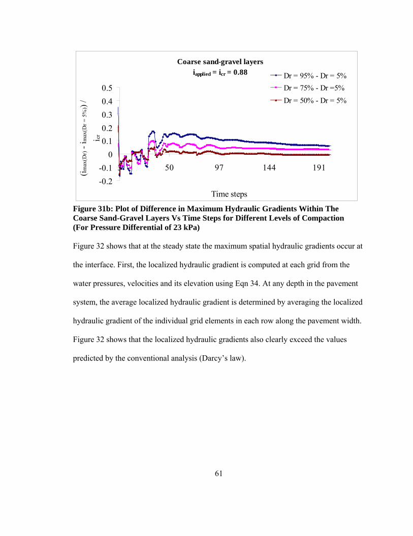
61

Coarse sand-gravel layersiapplied = icr = 0.88

-0.2-0.1

00.10.20.30.40.5

3 50 97 144 191

Time steps

(i max

(Dr) -

i max

(Dr =

5%

)) /

i cr

Dr = 95% - Dr = 5%Dr = 75% - Dr =5%Dr = 50% - Dr = 5%

Figure 31b: Plot of Difference in Maximum Hydraulic Gradients Within The Coarse Sand-Gravel Layers Vs Time Steps for Different Levels of Compaction (For Pressure Differential of 23 kPa) Figure 32 shows that at the steady state the maximum spatial hydraulic gradients occur at

the interface. First, the localized hydraulic gradient is computed at each grid from the

water pressures, velocities and its elevation using Eqn 34. At any depth in the pavement

system, the average localized hydraulic gradient is determined by averaging the localized

hydraulic gradient of the individual grid elements in each row along the pavement width.

Figure 32 shows that the localized hydraulic gradients also clearly exceed the values

predicted by the conventional analysis (Darcy’s law).

62

Gravel-coarse sand layersDr = 95%

iappl ie d = icr = 0.88

0

0.25

0.5

0.75

1

1.25

0.2 0.4 0.6 0.8 1 1.2 1.4

Averaged localized hydraulic gradient

Dep

th o

f pav

emen

t/m

Localized i-Transient model(at steadystate)Localized i-Steady state SIMPLEalgorithm i across coarse sand (deterministic -Darcy)i across gravel (deterministic-Darcy)

Figure 32: Comparison of Hydraulic Gradients Obtained Using Continuum and Particulate Approaches (Steady State)

As illustrated in Figure 33, when the soil is not uniformly compacted, some localized

porosities would be high. In this study, in order to clearly visualize the local effects, the

coarse sand/gravel interface is assembled with a local region poorly compacted (Dr = 5%)

compared to other regions (Dr = 95%).

Coarse sand - gravel interface

63

Figure 33: Porosity Distribution for Coarse Sand-Gravel Interface with Non-Uniform Compaction (Circled Area is Packed with Dr of 5% and the Remaining Area is Packed with Dr of 95%)

Figure 34 shows the impact of the localized weak zone on the flow pattern. As illustrated

in Figure 35, fluid pressure varies linearly within each layer and shows a sudden change

at the interface due to differences in grain size and porosity. On the other hand, a

deficiency of compaction makes the fluid pressure distribution non-linear which affects

the localized flow quantities. That is, an abrupt pressure change between two adjacent

grid elements leads to undesirable higher localized hydraulic gradients as seen in Figure

36. An advantage of this model is that by making the size of the grid elements as small

as possible, the desired localized effects can be observed more effectively.

Deficiency of compaction, Dr = 5%

64

(a) (b)

Figure 34: Velocity Vector Plots: (a) Uniformly Compacted Soil Media (Dr = 95%) (b) Deficiency of Compaction in Local Area

(a) (b)

Figure 35: Plot of Fluid Pressure Distribution across the Coarse Sand-Gravel Interface: (a) Uniformly Compacted Coarse Sand-Gravel Interface ((Dr = 95%) (b) Deficiency of Compaction in Local Area

Localized effects

Localized effects

65

Figure 36: Plot of Localized Hydraulic Gradients for Coarse Sand-Gravel Interface with Weak Region

3.7 Limitations of the Model

In this simplified particulate model, the fluid phase is partially coupled with the solid

phase only in terms of the volumetric compatibility. Therefore, the intricate dynamics of

individual soil particle interactions with water, which would not impact the flow

characteristics significantly, are not taken into account. Also, the soil particles are

assumed to be perfect spheres neglecting the angularity and roughness. One realizes that

the angularity of soil particles could widen the ranges of both the maximum and

minimum void ratio and hence that of the natural void ratio. Because of the probability of

having relatively larger changes in void ratio of adjacent grid elements due to angularity,

excessive localized hydraulic gradients of larger magnitude could result. This issue could

be addressed partly, by incorporating the compression indices (Eqn 43) modified for

subrounded, subangular and angular particles as detailed in [18]. Furthermore, in this

Localized effects

66

model, the three dimensional porosities obtained from particle packing are coupled with

the flow constrained in the third direction due to the assumed two dimensional nature of

the pavement system. The above 2D assumption seems to be reasonable because the

predicted hydraulic conductivities do not deviate much from those determined using

widely used empirical equations. To compute the change in porosity in the transient

continuity equation, the water pressure difference during the previous time step [(N-1)

N] was used in Eqn 16 to make the numerical scheme explicit. When the time step

is adequately small, this limitation would not affect the solution since the variation in

water pressure within small time duration can be considered linear and hence equal for all

equal time steps.

3.8 Conclusions

In this study, water seepage in a couple of two-layer filter interface with different levels

of compaction was analyzed using a soil particulate model with Navier Stokes flow

principles. The particulate effects of soil with different levels of compaction were

conveniently incorporated in the model using a random packing technique, while the flow

of water within the particulate assembly was modeled by the Navier Stokes equations.

Compaction effects were incorporated in the model using the concept of relative density.

Two separate two-layer interfaces, i.e. coarse sand/gravel and fine sand/coarse sand were

assembled using particle size distributions that satisfied the conventional filter design

criteria. Then, a pressure differential that corresponded to the critical hydraulic gradient

was applied across the layer interface. The relative density certainly impacts the flow rate

67

but has an insignificant effect on the localized hydraulic gradients. Furthermore, the

localized hydraulic gradients determined using the particulate approach differed widely

from their average values across the entire layer highlighting the importance of

considering localized effects in formulating more applicable design criteria. The

preliminary results obtained from this model illustrate the advantage of the particulate

approach in predicting the critical conditions for erosion, piping and clogging, especially

in transient flow conditions, well before the filter fails to function. Extended and more

extensive research in this direction is expected to provide deeper insight into more

accurate filter design criteria.

68

CHAPTER FOUR

TRANSIENT SEEPAGE MODEL FOR PARTLY SATURATED AND SATURATED SOILS USING THE PARTICULATE APPROACH

4.1 Introduction

Functionality of earthen structures such as dams, levees, retention ponds and pavements

is determined by one dominant factor; the nature of interaction of soil particles with water

flow. Hence accurate analysis of water seepage through soils is essential to achieve more

economic designs of such structures. The majority of currently available design criteria

are formulated based on either empiricism or the analysis of steady state laminar flow

through saturated soil continua. However, very often, field observations are also used to

refine or calibrate the design criteria. In the conventional models, the dynamic flow of

water through soil pores is commonly idealized using the Darcy’s law. Experimental

studies show that Darcy’s law would not be applicable to model transient conditions and

high fluid velocities that develop under excessive hydraulic gradients and unsaturated

soils [1]. It is also known that it is the transient flow caused by abrupt fluctuations in

groundwater conditions plays a more crucial role in determining the durability of

pavement structures. Furthermore, hydraulic infrastructures like retention ponds almost

always operate under transient flow conditions. Hence, one has to replace the

conventional method of analysis based on a steady state continuum to an alternative

69

approach with a discrete soil skeleton with the ability to incorporate transient effects

which includes pre-saturation flow that generally precede the eventual steady state flow.

In this study, the author develops a finite-difference model that uses the Soil-Water

Characteristic Curves concepts [19] and the Navier Stoke equations for analyzing

transient fluid flow through partly saturated and saturated soils. Then, the model is

applied to two specific problems:

1) Confined flow occurring in a partly saturated pavement layer during sudden rise

of the groundwater table and

2) Transient seepage from retention pond into surrounding granular soil medium.

In the first case, the results show how saturation achieves following the water porosity Vs

water pressure trend defined by SWCC. In the second case, the model is able to predict

the gradual reduction in the water level of the retention pond including the location of the

free-surface.

4.2 Existing Particulate Models

In the conventional seepage models, the flow of water through saturated soil pores is

idealized using the Darcy’s law based on a continuum approach. In the above approach, a

single representative value of hydraulic conductivity determined from field tests or

laboratory tests is used to model the entire soil domain. Alternatively, if seepage through

soils is analyzed using the particulate approach then one can certainly account for the

spatial variation of hydraulic conductivity more accurately by incorporating drag forces

acting between soil particles and water in the Navier Stokes equations. Moreover, when

70

using the particulate approach, the effects of intricate particle dynamics on the water flow

can also be considered whenever needed. However, modeling of seepage through

particulate media by considering soil-water interaction is relatively new to computational

geomechanics. The discrete element method (DEM) does provide an effective tool to

model granular soils in particular based on micro mechanical idealizations. El Shamy et

al. [4] presented a computational micro-mechanical model for coupled analysis of pore

water flow and deformation of saturated granular assemblies. Shimizu’s [6] particle-fluid

coupling scheme with a mixed Lagrangian-Eulerian approach which enables simulation

of coupling problems with large Reynolds numbers is implemented in PFC 2D and PFC

3D released by Itasca Consulting Group, Inc. [7]. The models used by El Shamy et al.

and Shimizu are both based on the work by Anderson and Jackson [8] and Tsuji et al. [9].

Anderson and Jackson [8] modeled pore fluid motion through saturated soil mass using

averaged Navier Stokes equations. Tsuji et al. [9] simulated the process of particle

mixing of a two-dimensional gas-fluidized bed using averaged Navier Stokes equations

for comparison with experiments. For all the above cited studies, granular assemblies are

modeled using the discrete element model developed by Cundall and Strack [10] and the

averaged Navier Stokes equations are discretized using a finite volume technique on a

staggered grid [11].

4.3 Flow in Partly Saturated Soils

Although partly saturated subsurface soils are common in most building sites, the

concepts of partly saturated soil mechanics are rarely introduced in geotechnical designs.

71

Furthermore, most geotechnical engineering problems are dealt with assuming positive

pore water pressures when suction can occur even in saturated soils. The solutions of

many practical problems involving partly saturated soils require an understanding of the

hydraulics, mechanics and interfacial physics of partially saturated soils [20]. Slope

stability analysis that also incorporates unsaturated soil mechanics would provide more

accurate results in most cases. However, water flow in partly saturated soils is, in general,

complicated and difficult to describe quantitatively, since it often entails changes in the

state and content of soil water.

Figure 37: Schematic Diagram to Show the Movement Cycle of Water from Atmosphere to the Groundwater Table [20]

Figure 37 is the schematic representation of the water movement cycle between the

atmosphere to the groundwater table. Below the water table, soil is generally saturated

with positive pore-water pressures. Immediately above the water table is the capillary

72

fringe where the degree of saturation approaches 100 percent with negative pore water

pressures (suction). In partly saturated soils, the two phases of air and water coexist in the

inter-connected pore channels. In order to analyze seepage through saturated-unsaturated

soils under transient conditions, Fredlund and Morgenstern [21] proposed Eqn 45a using

the constitutive equations relating the volumetric strain in a soil due to total stress and

pore water pressure changes.

( ) ( )t

uum

tu

myhk

yxhk

xaww

2aw

1yx ∂−∂

+∂−σ∂

−=⎟⎟⎠

⎞⎜⎜⎝

⎛∂∂

∂∂

+⎟⎟⎠

⎞⎜⎜⎝

⎛∂∂

∂∂ (45a)

( )zyx31

σ+σ+σ=σ . (45b)

Where, h - total hydraulic head ,σ – mean normal stress ,ua – pore-air pressure, uw – pore-

water pressure, (ua – uw) – matric suction, kx and ky - x and y directional hydraulic

conductivities, wm1 and wm2 are the corresponding partial compressibilities due to (σ – ua)

and (uw – ua) respectively.

Darcy’s law is also applicable to flow through partly saturated soils with the use of

variable hydraulic conductivities with respect to suction as shown later in Section 3.2. In

saturated soils, any minor changes in the hydraulic conductivity due to changes in

porosity are neglected whereas in unsaturated soils, hydraulic conductivity is

significantly affected by combined changes in the void ratio and the degree of saturation

(or water content) of the soil.

From a geotechnical engineering point of view, it is the flow in the water phase of the

unsaturated zone that is of practical interest. Therefore, the flow through unsaturated soils

can be simplified assuming that the air phase is continuous throughout the soil matrix

73

with a pressure equal to that of the atmosphere. Using the “single- phase” flow approach

which is accurate enough for many practical purposes, an unsaturated flow model was

developed by Lam et al. [22]. If no external loads are applied on the soil mass during

water flow ( 0t=

∂σ∂ ) and if the air phase is continuous and open to the atmosphere (ua =

0), Eqn 45a can be simplified to Eqn 45c.

tum

yhk

yxhk

xww

yx ∂∂

=⎟⎟⎠

⎞⎜⎜⎝

⎛∂∂

∂∂

+⎟⎟⎠

⎞⎜⎜⎝

⎛∂∂

∂∂

2 (45c)

Ng and Shi [3] also used Eqn 48c to numerically investigate the stability of unsaturated

soil slopes subjected to transient seepage. In Ng and Shi’s [3] work, a finite element

model was used to investigate the influence of various rainfall events and initial ground

water conditions during transient seepage. However, slope stability was analyzed without

considering the localized zones of high pressure build-up and high hydraulic gradients

within the slope.

4.4 Overview of the New Model

The model presented in this paper first uses a newly-developed packing algorithm to

randomly pack a three dimensional discrete soil skeleton resembling a natural soil deposit

that exists at a given relative density or particle size distribution. Then the model is used

to determine the water flow behavior in a particulate saturated – partly saturated soil

medium. The seepage of water through the particulate medium is modeled using the

Navier Stokes (NS) equations which are discretized using the finite difference method

(FDM) [13]. The new model is capable of predicting both transient and steady state flow

74

effects under both saturated and partly saturated conditions. First, the model is applied to

simulate flow in a single layer of granular soil resulting from of a sudden surge of

groundwater. Second, the model is applied to simulate flow around a retention pond built

in granular soil. The comprehensive analytical procedure and the computer code

developed for its implementation are illustrated in Figure 38. The analytical procedure

consists of two primary tasks such as the random assembly of the particulate medium

(granular soil) and the solution of the fluid flow governing equations. The flow chart also

includes the section, equation and figure numbers corresponding to each stage.

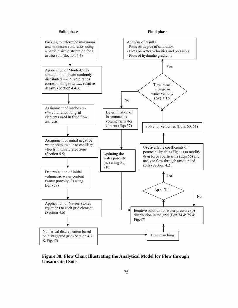
75

Figure 38: Flow Chart Illustrating the Analytical Model for Flow through Unsaturated Soils

No

Yes

Yes

No

Packing to determine maximum and minimum void ratios using a particle size distribution for a in-situ soil (Section 4.4)

Application of Monte-Carlo simulation to obtain randomly distributed in-situ void ratios corresponding to in-situ relative density (Section 4.4.3)

Assignment of random in-situ void ratios for grid elements used in fluid flow analysis

Application of Navier-Stokes equations to each grid element (Section 4.6)

Numerical discretization based on a staggered grid (Section 4.7 & Fig.45)

Analysis of results - Plots on degree of saturation - Plots on water velocities and pressures - Plots of hydraulic gradients

Solid phase Fluid phase

Iterative solution for water pressure (p) distribution in the grid (Eqn 74 & 75 & Fig.47)

Time marching

Δp < Tol

Time-based change in

water velocity (Δv) < Tol

Assignment of initial negative water pressure due to capillary effects in unsaturated zone (Section 4.5)

Determination of initial volumetric water content (water porosity, θ) using Eqn (57)

Updating the water porosity (nw) using Eqn 71b.

Use available coefficients of permeability data (Fig.44) to modify drag force coefficients (Eqn 66) and analyze flow through unsaturated soils (Section 4.2).

Determination of instantaneous volumetric water content (Eqn 57) Solve for velocities (Eqns 60, 61)

76

4.5 Modeling of Soil Structure (3D Random Packing of Soil Particles)

Fine sand represented by the Particle Size Distribution (PSD) curve in Figure 39 is used

in this study.

Figure 39: Particle Size Distribution for Fine Sand

4.5.1 Simulation of Maximum and Minimum Void Ratios Using PSD

In this model the soil particles are assumed to be of spherical shape. To determine the

maximum and minimum void ratios (emax and emin) corresponding to fine sand in Figure

39, a customized random packing algorithm was developed. Using this algorithm, 3 mm

× 3 mm × 3 mm cubes (Figure 40a) were packed using soil particles picked from the PSD

in Figure 39. It must be noted that the PSD in Figure 43 is in fact the cumulative

probability distribution of the fine sand particles. Therefore, by using an adequately large

array of random numbers from a uniform distribution ranging from 0 and 100 (the y axis

range in Figure 39), one can select the corresponding array of particle diameters that

77

conforms to the selected PSD, from the x axis. This technique, known as the Monte-Carlo

simulation [14] is used to select the array of packing diameters for each cube (Figure

40a). It is noted that the resulting maximum and minimum void ratio distributions change

in each packing trial since the order of diameters used for packing is changed randomly.

An adequate number of particles must be within the cube to determine the representative

emax and emin for the fine sand.

4.5.2 Implementation of the Packing Procedure

In order to obtain the loosest state of fine sand (emax) within the cubes described above,

different sizes of soil particles inscribed in boxes are packed as indicated in Figure 40a

using a MATLAB code developed by the authors. The side length of each box is the

same as the diameter of the inscribed soil particle. Based on the minimum particle

diameter of fine sand (0.04 mm), the side length of each cube is divided into a finite

number of sub-divisions (Figure 40a). Then, the packing algorithm tracks the total

number of sub-divisions occupied by each incoming box, i.e. each packed soil particle, as

packing proceeds based on the Monte-Carlo simulation corresponding to a given PSD

(Figure 39). Finally, the automated algorithm fills all sub-divisions until it finds that not a

single sub-division is available within the considered cube for further packing of soil

particles from the given PSD. As packing of each cube approaches completion, the void

ratio reaches a constant value of 0.9098 which can be identified as the maximum void

ratio for simple cubical packing [15].

78

On the other hand, in order to obtain the minimum void ratio (densest packing), the

maximum number of spheres smaller than the inscribing sphere in each box is also

packed into the unoccupied space at the corners of each box (Figure 40c and 40d) before

that box is placed in the cube (Figure 40b). 50 such cubes (trials) were packed randomly

using the Monte-Carlo simulation. Since the minimum void ratio obtained in each trial

would be different depending on how the unoccupied space in each box filled, it can be

considered as random variable. The range derived for emin as shown in Table 5 agrees

with the typical values in [15].

Table 5: Soil Characteristics

Soil type Fine sand

Sizes of particle (mm) (Figure 39) 0.04 – 0.62

D15 (mm) (Figure 39) 0.16

D50 (mm) (Figure 39) 0.29

D85 (mm) (Figure 39) 0.49

emax (Packing) 0.9098

emin (Packing) 0.54 – 0.79

Mean of emin 0.48

Standard deviation of emin 0.0037

79

Figure 40: Packing Procedure

4.5.3 Determination of the Natural Void Ratio Distribution

The property of relative density is helpful in quantifying the level of compaction of

coarse-grained soils. The relative density of a coarse-grained soil expresses the ratio of

the reduction in the voids in the current state, to the maximum possible reduction in the

voids (Eqn 2). The in-situ void ratio distribution (e) corresponding to a given relative

density (Dr) is obtained using the previously obtained emax and emin (Eqns 46 or 47).

minmax

max

eeee

Dr −−

= (46)

or

80

( )rr DeeDe −+= 1maxmin (47)

Where, emax is the void ratio of fine sand in its loosest state (= 0.9098). emin is the

randomly distributed void ratio of fine sand in its densest state. e is the randomly

distributed void ratio of sand in its natural state in the field.

For a relative density of 50%, Eqn 51 reduces to

45.0e5.0e min += (48)

The mean ( e ) and the standard deviation (Se) of natural void ratios are determined from

Eqns 49 and 50

)1(9098.0min rr DeDe −+= (49)

minere SDS = (50)

Where, mine (Eqn 51a) and Se min (Eqn 51b) are the mean and standard deviation of the

minimum void ratio (Table 5) obtained from the packing procedure described in Section

4.4.

( )∑=50

minmin 501

iiee (51a)

( )( )∑ −=50 2

minminmin 501

iie eeS (51b)

Knowing the mean and standard deviation of the natural void ratio (Eqns 49 and 50) and

assuming a normally distributed probability density function for the natural void ratio (e),

its cumulative distribution (Figure 41) is obtained using Eqn 52.

*e ZSee += (52a)

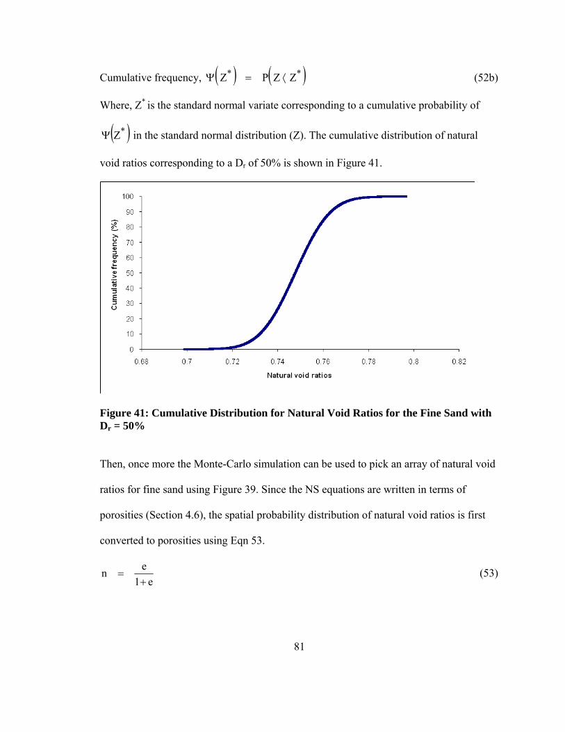
81

Cumulative frequency, ( ) ( )** ZZPZ ⟨=Ψ (52b)

Where, Z* is the standard normal variate corresponding to a cumulative probability of

( )*ZΨ in the standard normal distribution (Z). The cumulative distribution of natural

void ratios corresponding to a Dr of 50% is shown in Figure 41.

Figure 41: Cumulative Distribution for Natural Void Ratios for the Fine Sand with Dr = 50%

Then, once more the Monte-Carlo simulation can be used to pick an array of natural void

ratios for fine sand using Figure 39. Since the NS equations are written in terms of

porosities (Section 4.6), the spatial probability distribution of natural void ratios is first

converted to porosities using Eqn 53.

e1en+

= (53)

82

The spatial distributions of natural void ratios (porosities) so obtained assumed to be

representative of the fine sand will be used in the seepage analysis model presented in

Section 4.6.

4.6 Modeling of Fluid Flow in Partially Saturated Soils

When the developed model is applied to a partially saturated granular soil layer, the

initial water pressures within the saturated and unsaturated zones are assumed to be due

to hydrostatic pressure and the capillary suction effects respectively, as shown in Figure

42.

Figure 42: Initialization of Water Pressure in the Saturated and Unsaturated Zones

Saturated soil

Unsaturated soil

Capillary fringe soil

Suction due to capillary

Hydrostatic pressures

Groundwater table

83

4.6.1 Soil Water Characteristic Curve/Water Moisture Retention Curve

The Soil Water Characteristic Curve (SWCC) [17] depicts the relationship between soil

water content (θ) and soil water pressure potential (suction, Ψ). The soil parameters

defining a typical Soil Water Characteristic Curve are shown in Figure 43a while the Soil

Water Characteristic Curves for different particle size distributions are presented in

Figure 43b. From Figure 43b, it is seen that sands and gravels lose water quite readily

upon suction induced drainage while loams and clays lose much less water upon

drainage. There are a number of empirical equations proposed to best-fit the Soil Water

Characteristic Curves [19] using the soil parameters shown in Figure 43a. In this model,

Eqn 54a –Eqn 54c are used to determine the volumetric water content (θ) for a particular

suction (Ψ).

Volumetric water content, VV w=θ (54a)

Where, V is the total volume of a soil sample and Vw is the volume of water in that

sample.

Figure 43a: Typical Soil Water Characteristic Curve and wm2 for a Saturated -Unsaturated Soil [10]

Figure 43b: Soil Water Characteristic Curve for Specific Soil Types [23]

84

( ) ( ) mn

s

ae

Cmna

⎪⎭

⎪⎬⎫

⎪⎩

⎪⎨⎧

⎥⎥⎦

⎤

⎢⎢⎣

⎡⎟⎠⎞

⎜⎝⎛+

=ψ

θψψθ

ln

,,, (54b)

Where, C(Ψ) is a correction function defined as:

( ) 1101ln

1ln

6+

⎥⎦⎤

⎢⎣⎡

⎟⎠⎞⎜

⎝⎛+

⎟⎠⎞⎜

⎝⎛ +−

=

r

rC

ψ

ψψ

ψ (54c)

Where, e = 2.71828; Ψr is the suction corresponding to the residual water content, θr. θs is

the (saturated) volumetric water content at zero pressure and a, m, and n are fitting

parameters. In this model, θs in each grid element is set to the porosity of that element

obtained from initial packing (Section 4.4). In the particulate approach, although the θs

varies with the spatial distribution of porosity, the average θs corresponding to 50% of

degree of compaction is used in this study for simplicity. The parameters for Eqn 54b –

Eqn 54c relevant to the fine sand modeled in the current study are shown in Table 6.

Table 6: Parameters Used to Define the SWCC for Sand [23]

Ψr 50 kPa Average θs 0.45 a 1.948 kPa m 2.708 n 1.084

85

In Section 4.6, θ will also used as the water porosity in formulating the continuity

equation and Navier Stokes equations for partly saturated soils. Furthermore, using

fundamental soil mechanics, the degree of saturation can be shown that

nS θ

= (55)

Where, S- degree of saturation, n – total porosity of the soil.

4.6.2 Determination of the Unsaturated Permeability Function

The hydraulic conductivity is commonly referred to as the coefficient of permeability in

geotechnical engineering. In unsaturated soils, the coefficient of permeability is primarily

determined by the pore-size distribution and the degree of saturation. The permeability

functions for unsaturated soils are used to represent the relationship between the

coefficient of permeability and soil suction. Figure 44 illustrates the variation of the

coefficient of permeability with suction for different types of soils. There are several

empirical equations and statistical models used to determine the permeability functions

[19]. One such approach uses the Soil Water Characteristic Curve (Figure 43a) to predict

the permeability function [19].

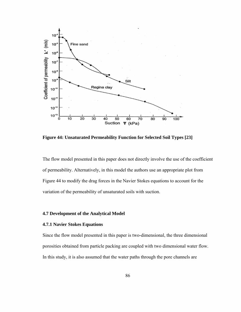
86

Figure 44: Unsaturated Permeability Function for Selected Soil Types [23]

The flow model presented in this paper does not directly involve the use of the coefficient

of permeability. Alternatively, in this model the authors use an appropriate plot from

Figure 44 to modify the drag forces in the Navier Stokes equations to account for the

variation of the permeability of unsaturated soils with suction.

4.7 Development of the Analytical Model

4.7.1 Navier Stokes Equations

Since the flow model presented in this paper is two-dimensional, the three dimensional

porosities obtained from particle packing are coupled with two dimensional water flow.

In this study, it is also assumed that the water paths through the pore channels are

87

continuous for partly saturated soils near saturation. Hence, Navier Stokes equations can

be written as follows in a generalized form in terms of the water porosity, θ (= Sn)

expressed by Eqn 56:

Water mass Conservation (Continuity Equation):

( ) ( ) ( ) 0=∂

∂+

∂∂

+∂

∂y

vnSx

unStnS (56)

Momentum Conservation (Momentum Equations):

X direction:

( ) ( ) ( ) ( )⎟⎟⎠

⎞⎜⎜⎝

⎛∂

∂+

∂∂

++∂∂

−=∂

∂+

∂∂

+∂

∂2

2

2

22

yunS

xunSD

xpnS

yvunS

xunS

tunS x

ρμ

ρρ (57)

Y direction:

( ) ( ) ( ) ( ) ( )⎟⎟⎠

⎞⎜⎜⎝

⎛∂

∂+

∂∂

++∂∂

−=∂

∂+

∂∂

+∂

∂2

2

2

22

yvnS

xvnSD

ypnS

yvnS

xvunS

tvnS y

ρμ

ρρ

ygnS+ (58)

Where, n and S – porosity and degree of saturation at the location (x, y) at time t

respectively, u, v – fluid velocities in the x and y directions respectively, ρ – fluid

density (1000 Kg/m3), p – fluid pressure, μ - fluid viscosity (10-3 Pa.s), gy - gravitational

force per unit mass in the y direction (9.81m/s2). The following conditions are assumed in

the analysis:

1) Under saturated conditions: S = 1 and n varies due to the compressibility of the

soil skeleton as described in Section 4.4.

2) Under unsaturated conditions: n is constant and S increases as suction decreases.

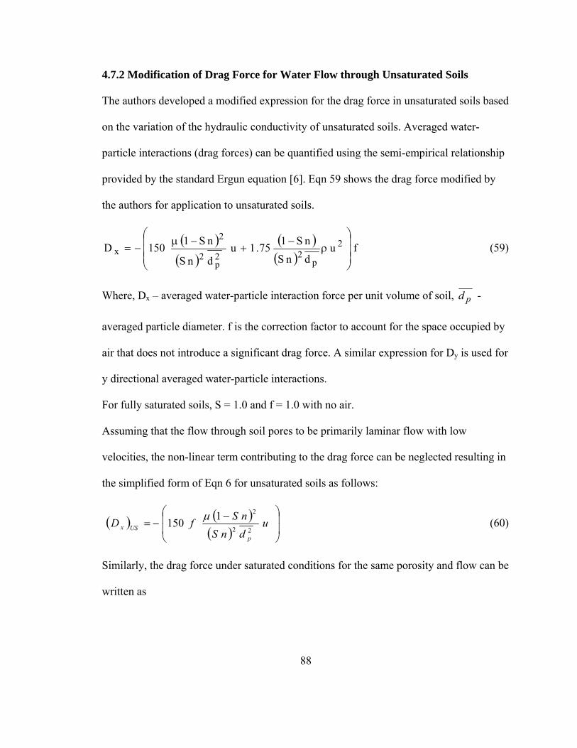
88

4.7.2 Modification of Drag Force for Water Flow through Unsaturated Soils

The authors developed a modified expression for the drag force in unsaturated soils based

on the variation of the hydraulic conductivity of unsaturated soils. Averaged water-

particle interactions (drag forces) can be quantified using the semi-empirical relationship

provided by the standard Ergun equation [6]. Eqn 59 shows the drag force modified by

the authors for application to unsaturated soils.

( )( )

( )( )

fudnSnS175.1u

dnS

nS1150D 2

p22

p2

2x

⎟⎟⎟

⎠

⎞

⎜⎜⎜

⎝

⎛ρ

−+

−μ−= (59)

Where, Dx – averaged water-particle interaction force per unit volume of soil, pd -

averaged particle diameter. f is the correction factor to account for the space occupied by

air that does not introduce a significant drag force. A similar expression for Dy is used for

y directional averaged water-particle interactions.

For fully saturated soils, S = 1.0 and f = 1.0 with no air.

Assuming that the flow through soil pores to be primarily laminar flow with low

velocities, the non-linear term contributing to the drag force can be neglected resulting in

the simplified form of Eqn 6 for unsaturated soils as follows:

( ) ( )( ) ⎟

⎟

⎠

⎞

⎜⎜

⎝

⎛ −−= u

dnSnSfD

pUSx 22

21150 μ (60)

Similarly, the drag force under saturated conditions for the same porosity and flow can be

written as

89

( ) ( )⎟⎟

⎠

⎞

⎜⎜

⎝

⎛ −−= u

dnnDp

Sx 22

21150 μ (61)

Drag forces cause resistance to water flow and hence they can be considered as being

inversely proportional to the coefficient of hydraulic conductivity (K) as,

( )( ) f

KK

DD

US

S

Sx

USx == (62)

From Eqns 60 and 61, ( )

( )2

22

11

nSnS

KK

fUS

S

−−

= (63)

Where, KS and KUS are the hydraulic conductivities of saturated and unsaturated soils

respectively.

4.8 Numerical Solution Technique

A finite-difference scheme is used to discretize the Eqns 56, 57 and 58. This scheme is

based on forward difference in time and porosity, and central difference in space with a

two-dimensional staggered mesh arrangement [11, 13]. Eqn 64a expresses the x

directional momentum equation in the numerical form for the sequential time steps of N

and N+1 referring to the notation in Figure 45.

90

Figure 45: Computational Grid for the X-Momentum Equation

( ) ( ) ( ) ( )

( ) ( )

( ) ( )( )( ) ⎟⎟

⎟

⎠

⎞

⎜⎜⎜

⎝

⎛ −−⎟⎟

⎠

⎞⎜⎜⎝

⎛Δ

−−

=Δ

−

+Δ

−+

Δ

−

−

+

−+−+−+++++

−−+++++

++

jipji

jijijiji

jijijijijiji

jijijijiN

jijiN

jiji

udSn

Snf

xppSn

y

vuSnvuSn

x

uSnuSn

t

uSnuSn

ji

,2122

,

2,,,1,

21,2

11,211,

21,2

11,211,

2,2

1,21

2,2

3,23,2

1,21

1,2

1,21

,

1150

2

2

ρ

μρ

( ) ( ) ( )

( )( ) ( ) ( )

( ) ⎥⎥⎥⎥⎥⎥

⎦

⎤

⎢⎢⎢⎢⎢⎢

⎣

⎡

Δ

−+

+Δ

−+

ρμ

++−+−+++

+−−++

2j,2

1ij,i1j,21i1j,i1j,2

1i1j,i

2j,2

1ij,ij,21ij,1ij,2

3ij,1i

y

uSn2uSnuSnx

uSn2uSnuSn

(64a)

Where,

⎟⎠⎞⎜

⎝⎛ +=

+++++ 21,12

1,21,2

1 21

jijijivvv (64b)

91

⎟⎠⎞⎜

⎝⎛ +=

−+−−+ 21,12

1,21,2

1 21

jijiji vvv (64c)

Within the staggered grid, some velocities need to be interpolated as shown in Eqns 64b

and 67c.

In a concise form, Eqn 64a can be re-written as

( ) ( ) ( ) ( )tAx

pptAtAuSnuSn

N

i

Nji

NjiN

jiN

jiN

jijiN

jiji Δ+⎟⎟⎠

⎞⎜⎜⎝

⎛

Δ

−Δ+Δ+= +

+

+++++

++ 21

,,1,2

1,21,2

1,21

1,2

1,21 )( (64d)

Where,

( ) ( )

( ) ( )

y2

vuSnvuSn

x2

uSnuSnA

21j,2

1i1j,21i1j,i

21j,2

1i1j,21i1j,i

2j,2

1ij,21i

2j,2

3ij,23i

j,21i

Δ

−

+Δ

−−=

−+−+−+++++

−−++

+ (64e)

( )ρ

−=+

+j,2

1ij,2

1iSn

A (64f)

and

( )( )( )

+⎟⎟⎟

⎠

⎞

⎜⎜⎜

⎝

⎛ −−=

++ jipji

jiji u

dSn

SnfA

ji

,2122

,

2,

,21

,

1150

ρ

μ

( ) ( ) ( )( )

( ) ( ) ( )( ) ⎥

⎥⎥⎥⎥

⎦

⎤

⎢⎢⎢⎢⎢

⎣

⎡

Δ

−+

+Δ

−+

+−+−+++

+−−++

2

,21,1,2

11,1,211,

2

,21,,2

1,1,23,1

2

2

y

uSnuSnuSnx

uSnuSnuSn

jijijijijiji

jijijijijiji

ρμ (64g)

The numerical form of the y directional momentum equation can be written similarly

based on Eqn 58 as Eqn 65.

92

( ) ( ) ( ) ( )

( ) ( ) ( )tgSntB

y

pptBtBvSnvSn

y21j,i

N

21j,i

Nj,i

N1j,iN

21j,i

N

21j,i

N

21j,i2

1j,i1N

21j,i2

1j,i

Δ+Δ+

⎟⎟⎟

⎠

⎞

⎜⎜⎜

⎝

⎛

Δ

−Δ+Δ+=

++

+++++

+++

(65)

The discretized continuity equation of water is given by Eqn 66. In computing the change

in porosity in the transient continuity equation, the numerical scheme is made explicit by

using porosity during the previous time step (N-1) in Eqn 66.

( ) ( ) ( ) ( )=

⎥⎥⎥

⎦

⎤

⎢⎢⎢

⎣

⎡

Δ

−+

Δ

− +−−

+++

+−−

+++

y

vSnvSn

x

uSnuSn 1N

21j,i2

1j,i1N

21j,i2

1j,i1N

j,21ij,2

1i1N

j,21ij,2

1i

( ) ( ) ( )t

SnSnt

SnN

jiN

ji

Δ

−−=

ΔΔ

−1,, (66)

Finally, using either Eqn 67a or Eqn 67b, the change in water porosity ( SnΔ ) during a

time step, ∆t, can be determined and used in the discretized continuity equation (Eqn 66).

In the saturated zone (p > 0 and S = 1), the change in porosity is determined using Eqn

67a.

( ) ( ) [ ]tp

ppnCtn

Nji

Nji

Nji

Njijic

Δ⎥⎥⎦

⎤

⎢⎢⎣

⎡

−

−−−=

ΔΔ − 114343.0

,,

1,,

2,

σ (67a)

Where, Cc - equivalent compression index of the soil, σ- total vertical stress in soil.

Meanwhile, in the partly saturated zone (p < 0 and S < 1), the Soil-Water Characteristic

Curve is used to determine the change in water porosity using Eqn 67b.

93

( ) ( ) [ ]tpp

mt

Sn Nji

Nji

jiw

Δ

−−=

ΔΔ −1

,,,2 (67b)

The slope of the Soil Water Characteristic Curve for fine sand, wm2 ,at a particular suction

is obtained by curve-fitting the corresponding SWCC assumed for fine sand (Figure 46)

in this study.

Figure 46: Soil Water Characteristic Curve for Fine Sand

Now, Eqn 64 and Eqn 65 can be written for two adjacent control volumes as shown in

Eqn 68 and Eqn 69.

( ) ( ) ( ) ( )tAx

pp)t(AtAuSnuSn

N

21i

Nj,1i

Nj,iN

j,21i

Nj,2

1iN

j,21ij,2

1i1N

j,21ij,2

1i Δ+⎟⎟⎟

⎠

⎞

⎜⎜⎜

⎝

⎛

Δ

−Δ+Δ+=

−−

−−+−+−− (68)

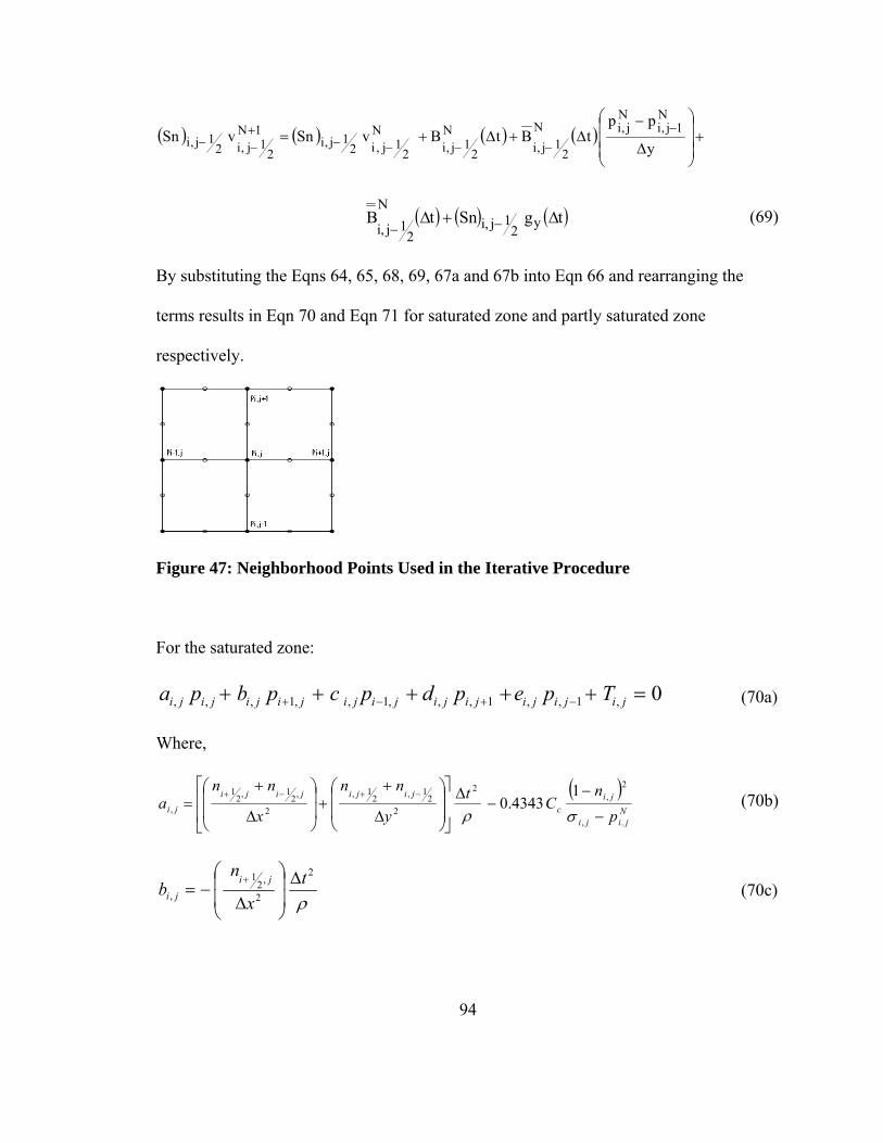
94

( ) ( ) ( ) ( ) +⎟⎟⎟

⎠

⎞

⎜⎜⎜

⎝

⎛

Δ

−Δ+Δ+= −

−−−−+−− y

pptBtBvSnvSn

N1j,i

Nj,iN

21j,i

N

21j,i

N

21j,i2

1j,i1N

21j,i2

1j,i

( ) ( ) ( )tgSntB y21j,i

N

21j,i

Δ+Δ −− (69)

By substituting the Eqns 64, 65, 68, 69, 67a and 67b into Eqn 66 and rearranging the

terms results in Eqn 70 and Eqn 71 for saturated zone and partly saturated zone

respectively.

Figure 47: Neighborhood Points Used in the Iterative Procedure

For the saturated zone:

0,1,,1,,,1,,1,,, =+++++ −+−+ jijijijijijijijijijiji Tpepdpcpbpa (70a)

Where,

( )N

jiji

jic

jijijiji

ji pn

Cty

nn

x

nna

.,

2,

2

22

1,21,

2

,21,2

1

,

14343.0

−

−−

Δ⎥⎥

⎦

⎤

⎢⎢

⎣

⎡

⎟⎟

⎠

⎞

⎜⎜

⎝

⎛

Δ

++⎟

⎟

⎠

⎞

⎜⎜

⎝

⎛

Δ

+=

−+−+

σρ (70b)

ρ

2

2

,21

,t

x

nb

jiji

Δ⎟⎟

⎠

⎞

⎜⎜

⎝

⎛

Δ−=

+ (70c)

95

ρ

2

2

,21

,t

x

nc

jiji

Δ⎟⎟

⎠

⎞

⎜⎜

⎝

⎛

Δ−=

− (70d)

ρ

2

22

1,,

ty

nd

jiji

Δ⎟⎟

⎠

⎞

⎜⎜

⎝

⎛

Δ−=

+ (70e)

ρ

2

22

1,,

ty

ne

jiji

Δ⎟⎟

⎠

⎞

⎜⎜

⎝

⎛

Δ−=

− (70f)

and

( ) 1,

,,

2,2

1,21.2

1,21.

,21.2

1,21.2

12

21,2

1,

2

21,2

1,

2

,21,2

1

2

,21,2

1,

14343.0 −−−++

−−++−+

−+−+−+

−

−+Δ

Δ

⎟⎠⎞⎜

⎝⎛ ×−×

+ΔΔ

⎟⎠⎞⎜

⎝⎛ ×−×

+ΔΔ

⎟⎠⎞

⎜⎝⎛ −+

ΔΔ

⎟⎠⎞⎜

⎝⎛ −+

ΔΔ

⎟⎠⎞

⎜⎝⎛ −+

ΔΔ

⎟⎠⎞⎜

⎝⎛ −=

NjiN

jiji

jic

Njiji

Njiji

Njiji

NjijiN

jiN

ji

Nji

Nji

Nji

Nji

Nji

Njiji

pp

nCt

y

vnvn

tx

unun

ytBB

ytBB

xtAA

xtAAT

σ

ytgnn yjiji Δ

Δ⎟⎠⎞⎜

⎝⎛ −+

−+

2

21,2

1, (70g)

For the partly saturated zone:

0Tpepdpcpbpa 'j,i1j,i

'j,i1j,i

'j,ij,1i

'j,ij,1i

'j,ij,i

'j,i =+++++ −+−+ (71a)

Where,

( ) ( ) ( ) ( ) ( ) j,iw2

2

22

1j,i21j,i

2

j,21ij,2

1i'j,i mt

y

SnSn

x

SnSna −

ρΔ

⎥⎥

⎦

⎤

⎢⎢

⎣

⎡

⎟⎟

⎠

⎞

⎜⎜

⎝

⎛

Δ

++⎟

⎟

⎠

⎞

⎜⎜

⎝

⎛

Δ

+=

−+−+ (71b)

96

( )ρΔ

⎟⎟

⎠

⎞

⎜⎜

⎝

⎛

Δ−=

+ 2

2

j,21i'

j,it

x

Snb (71c)

( )ρ

Δ⎟⎟

⎠

⎞

⎜⎜

⎝

⎛

Δ−=

− 2

2

j,21i'

j,it

x

Snc (71d)

( )ρΔ

⎟⎟

⎠

⎞

⎜⎜

⎝

⎛

Δ−=

+ 2

22

1j,i'j,i

ty

Snd (71e)

( )ρ

Δ⎟⎟

⎠

⎞

⎜⎜

⎝

⎛

Δ−=

− 2

22

1j,i'j,i

ty

Sne (71f)

and

( ) ( )

( ) ( )( )( ) ( ) ( )( )

ytgSnSnpmt

y

vnSvSn

tx

uSnuSn

ytBB

ytBB

xtAA

xtAAT

yjijiN

jijiw

Njiji

Njiji

Njiji

NjijiN

ji

N

ji

Nji

Nji

N

ji

N

jiN

jiN

jiji

ΔΔ

−++ΔΔ

⎟⎠⎞⎜

⎝⎛ ×−×

+ΔΔ

⎟⎠⎞⎜

⎝⎛ ×−×

+ΔΔ

⎟⎠⎞

⎜⎝⎛ −

+ΔΔ

⎟⎠⎞⎜

⎝⎛ −+

ΔΔ

⎟⎠⎞

⎜⎝⎛ −+

ΔΔ

⎟⎠⎞⎜

⎝⎛ −=

−+−−−++

−−++

−+

−+−+−+

2

21,2

1,1

,,22

1,21.

21,2

1.

,21.2

1,21.2

12

21,2

1,

2

21,2

1,

2

,21,2

1

2

,21,2

1',

(71g)

97

4.9 Numerical Application of the Model

4.9.1 Modeling Confined Flow through a Partly Saturated Fine Sand Layer (Case I)

Figure 48: Illustration of the Flow through the Unsaturated Fine Sand Layer

The fine sand layer (Figure 48) was divided into a 50 × 50 grid for the finite difference

analysis. One fluid cell, known herein as a grid element, was selected to be 2.5 mm × 2.5

mm × 1m. A unit width has been selected in the third direction assuming two

dimensional water flow. First, natural porosities (void ratios) were assigned to each grid

element based on the spatial probability distribution of natural void ratios determined

from packing (Section 4.4). Within each grid element, the fluid-particle interaction is

quantified considering the averaged particle diameter which is defined as the arithmetic

mean of the diameters of all the particles in that grid.

0.12

5 m

98

4.9.2 Boundary Conditions

The boundary conditions appropriate for the water flow through the single soil layer are

specified in the computer code as indicated in Figure 49.

1) At the inflow boundary, the pressure and velocities are specified.

2) At the outflow boundary, the pressure is specified and velocity components are

allowed to float.

3) At the vertical walls, the slip conditions are maintained. Thus, the velocity

component, u, normal to the walls is set to zero.

Figure 49: Boundary Conditions Incorporated in the Flow through Saturated - Unsaturated Soil Layer

. A

99

4.9.3 Results

Upon the application of the elevated water pressure that causes a sudden hydraulic

gradient across the pavement layer in Figure 50, the variation of water porosity

(volumetric water content) with water pressure is illustrated in Figure 50. Figure 50 also

shows that suction within the soil mass is gradually converted to a positive pressure under

the application of elevated pressure at the bottom of the soil layer. The corresponding

variations of degree of saturation are shown in Figure 51.

0.4

0.41

0.42

0.43

0.44

0.45

0.46

-1500 -1000 -500 0 500 1000 1500 2000 2500 3000

Water pressure (Pa)

Wat

er p

oros

ity

Figure 50: The Variation of Water Porosity with Water Pressure at a Point within the Unsaturated Zone (At Point A in Figure 49)

100

90

91

92

93

94

95

96

97

98

99

100

-1500 -1000 -500 0 500 1000 1500 2000 2500 3000

Water pressure (Pa)

Deg

ree

of sa

tura

tion

Figure 51: The Variation of the Degree of Saturation with Water Pressure (At Point A in Figure 49)

Figures 52a -52c show how the partly saturated zone gradually becomes fully saturated

due to the upward water seepage. From Figure 53, it is seen that it takes approximately 50

time steps (5×10-3 seconds) for complete saturation of the layer and 80 time steps (8×10-3

seconds) to reach the steady state flow through the fully saturated zone.

101

Figure 52: Velocity Vector Plots for Flow through Saturated and Partly-Saturated Soil Layer

(d) t = 100

(a) t = 1

(c) t = 50

(b) t = 25

102

Figure 53: Variation of Discharge Flow Rate with Time Step

4.10 Conclusions

The results show that

1) The partly saturated zone having capillary pressures (suction) gradually becomes

fully saturated due to seepage caused by an elevated water pressure at the bottom

of the fine sand layer.

2) It takes the fine sand layer almost 80 time steps (8×10-3 seconds) to become fully

saturated.

3) The water porosity Vs suction plot and the degree of saturation Vs suction plot

show good agreement with the corresponding characteristics plots for fine sand.

Based on the above it can be concluded that model is applicable to partly saturated soils

as well.

Time of saturation Time of steady flow

103

CHAPTER FIVE

MODELING UNCONFINED FLOW AROUND A RETENTION POND

5.1 Introduction

Retention ponds are man-made or natural depressions into which stormwater runoff is

directed for temporary storage [Figure 54] with the expectation of disposal by infiltration

into a shallow groundwater aquifer. They are often created near areas of development and

in many instances required with new development of buildings, parking lots, roads, etc by

the permitting agencies. Retention ponds are developed primarily to serve two functions

such as limit flooding and the removal of pollutants.

Figure 54: Typical Retention Pond

104

5.2 Existing Design of Retention Pond

The required size of a retention pond depends on the rate of inflow to the pond and the

total quantity of flow as well as the rate of infiltration during a storm event, given the

antecedent conditions of the receiving aquifer. In order to avoid the overflow or flooding,

the retention volume recovery time should be adequate to completely dissipate the

retained stormwater from the pond after the design storm event. The retention volume

recovery time is defined as the time it takes to infiltrate the retention volume. This

depends on subsurface soil conditions and the input due to surface runoff.

In the conventional models that are used to design retention ponds, the soil skeleton is

treated as a continuum and the dynamic flow of water through soil pores is commonly

idealized using the Darcy’s law. MODFLOW [24] is a U.S. Geological Survey’s modular

finite-difference saturated flow model, which is currently the most widely used numerical

model in the U.S. Geological Survey (USGS) for analyzing groundwater flow problems.

The above program is used by hydrogeologists to simulate the flow of groundwater

through aquifers. In MODFLOW, a groundwater flow equation derived from Darcy’s

law is solved using the finite-difference approximation. The partial differential equation

of groundwater flow used in MODFLOW is

thSW

zhK

zyhK

yxhK

x szyx ∂∂

=+⎟⎟⎠

⎞⎜⎜⎝

⎛∂∂

∂∂

+⎟⎟⎠

⎞⎜⎜⎝

⎛∂∂

∂∂

+⎟⎟⎠

⎞⎜⎜⎝

⎛∂∂

∂∂ (72)

Where, Kx, Ky and Kz are values of hydraulic conductivity along x, y and z coordinate

axes respectively; h is the hydraulic head; W is a volumetric flux per unit volume

representing sources and/or sinks of water (W < zero for flow out of the groundwater

105

system and W > zero for flow in) and Ss is the specific storage of the soil. Eqn 72, when

combined with boundary and initial conditions, describes transient three-dimensional

groundwater flow in a heterogeneous and anisotropic medium.

MODRET (Computer MODEL to Design RETENTION Ponds) is an interactive

computer program that can be used to calculate the unsaturated and saturated infiltration

losses from stormwater retention ponds into unconfined aquifers using a modified version

of MODFLOW. MODRET was originally developed in 1990 as a complement to a

research and development project for South West Florida Water Management District

(SWFWMD). The Infiltration Module of the MODRET program uses a modified Green

and Ampt infiltration equation [25] to calculate the unsaturated infiltration and a

modified USGS’s model [24] to calculate the saturated infiltration. The Green and Ampt

infiltration equation [25] was originally presented as an empirical description for

unsaturated infiltration analysis; later, its empirical constants were theoretically

investigated [26]. For all above analysis, the coefficients of hydraulic conductivities

determined from the field tests or laboratory experiments are used in determining the

infiltration losses through retention ponds. But, instead of using the a single value of

coefficient of hydraulic conductivity for entire flow domain on a continuum basis, the

current particulate model uses spatially localized coefficients of hydraulic conductivities

in terms of drag forces between solid particles and pore fluid which are instantaneously

determined from the average particle diameters and the localized porosities.

106

5.3 Modeling of Soil Structure (3D Random Packing of Soil Particles)

The particle size distribution curve shown in Figure 55 was selected to model the

retention pond. The soil particles are assumed to be of spherical shape and to determine

the natural void ratio for coarse sand shown in Figure 55, a customized random packing

algorithm was developed. In the case of coarse sand, 16 mm × 16 mm × 16 mm cubes

were packed. It must be noted that the PSD in Figure 55 is cumulative probability

distribution of particle size for coarse sand. Therefore, by using an adequately large array

of random numbers from a uniform distribution between 0 and 100 (the y axis range in

Figure 55), one can select the corresponding array of particle diameters that conforms to

a selected PSD, from the x axis. This technique, known as the Monte-Carlo simulation

[14] is used to select the array of packing diameters for each cube. It is noted that the

resulting natural void ratio distribution change in each packing trial since the order of

diameters used for packing is changed randomly. The detailed packing procedure can be

found in [27]. A thousand of such cubes were randomly packed in order to model the half

of the retention pond defined by mesh of 100 by 150. The asymmetry of the retention

pond caused by the nature of random packing is neglected in this study.

107

0

10

20

30

40

50

60

70

80

90

100

1 10Grain size/(mm)

% C

umul

ativ

e fr

eque

nc

Figure 55: Particle Size Distributions for Coarse Sand

5.4 Numerical Procedure for Determination of the Free-Surface

Determination of the free-surface is required in the analysis of unconfined seepage

problems such as flow through earthen dams and retention ponds. One commonly used

approach to determine the free-surface is the graphical approach based on Dupuit’s

theory [1]. In addition, there are numerical techniques proposed by various researchers in

the literature [28 – 32]. In this study, a modified technique resembling the extended

pressure (EP) method first proposed by Brezis et al. [33] is employed with Navier Stokes

equations in order to determine the free-surface for flow around a retention pond.

The dry zone and wet zone around the retention pond are defined using the fundamentals

of streamlines, i.e., the locus of the path of flow of an individual particle of water and

continuity of flow quantity through a cross section. Along any flow line, the path of

108

water passing through point P(x1, y1) can be expressed (Figure 56) in mathematical form

as

1

1uv

dxdy

= (73)

Hence knowing one point, P(x1, y1) on the free-surface, the next point, Q (x2, y2) along

the free-surface can be obtained using Eqn 74.

( ) ( )12P1

112 yy

vu

xx −⎟⎟⎠

⎞⎜⎜⎝

⎛=− (74a)

yvu

xxP1

112 Δ⎟⎟

⎠

⎞⎜⎜⎝

⎛+= (74b)

In generalized form,

yvuxx

j1

1j1j Δ⎟⎟

⎠

⎞⎜⎜⎝

⎛+=+ (74c)

Once, the extreme boundary point, Q, is determined along the free-surface, the dry zone

is identified using a Heaviside step function in Section 5.5.

109

Figure 56: Determination of Dry and Wet Zones around the Retention Pond

5.4.1 Navier Stokes Equations

In the current formulation, water seepage is analyzed using Navier Stokes equations

written in terms of water pressures and velocities. Hence, the authors use a Heaviside step

function with water pressures and velocities in order to identify the dry and wet zones in

conjunction with Navier Stokes equations. For this work, the Heaviside-step function

(Eqn 75) is expressed in terms of the coordinates of the extreme boundary point on the

free-surface at any horizontal level (xj) as follows:

0 , if x > xj

H (x) = (75)

1 , if x < xj

To achieve this objective, Navier Stokes equations are written incorporating the

Heaviside step function as follows:

Free-surface

Dry zone

Wet zone

x

y v1

u1

Q(x2, y2)

P(x1, y1)

Groundwater level

Cen

ter l

ine

(xj,yj) (xj+1,yj+1)

110

Mass Conservation (Continuity Equation):

( ) ( )tn

yHvn

xHun

∂∂

−=∂

∂+

∂∂ (76)

Momentum Conservation (Momentum Equations):

X direction:

( ) ( ) ( )xpHnHD

yHun

xunH

yvunH

xHun

tunH x

∂∂

−=−⎟⎟⎠

⎞⎜⎜⎝

⎛∂

∂+

∂∂

−∂

∂+

∂∂

+∂

∂ρρρ

μ2

2

2

22

(77)

Y direction:

( ) ( ) ( )y

y ngypHnHD

yHvn

xHvn

yHvn

xvHun

tHvn

+∂∂

−=−⎟⎟⎠

⎞⎜⎜⎝

⎛∂

∂+

∂∂

−∂

∂+

∂∂

+∂

∂ρρρ

μ2

2

2

22

(78)

It is seen that Eqns 76 – 78 are inactivated in the dry zone (i ≥ i*). This can be assured by

using the Heaviside-step function in Eqns 75. Now, Eqns 76-78 can be applied both in

the wet and dry zones.

5.4.2 Boundary Conditions

The boundary conditions appropriate for the actual water flow around the retention pond

are specified in the computer code as indicated in Figure 57.

1) Hydrostatic pressure distribution (hγw) is specified along the retention pond walls

based on the water level in the pond (h).

2) Along the walls of the retention pond, non-slip velocity boundary conditions are

specified as shown in Figure 57.

111

3) At the exterior vertical wall boundaries within the two-phase media, the slip

conditions are maintained. Thus, the velocity component, u, normal to the walls is

set to zero.

4) At the groundwater table, water pressure is set to zero; water velocities allow

floating.

5) As an initial condition, the completely filled retention pond is considered.

Figure 57: Boundary and Initial Conditions Incorporated in the Flow around the Retention Pond

Groundwater table

112

5.5 Determination of Free-Surface from Dupuit’s Theory

Figure 58: Analytical Method to Determine the Free-Surface

Using the configuration of the retention pond irrespective of soil properties, the free-

surface is analytically determined using Eqn 79.

(79a)

(79b)

5.6 Results on Free-Surface

The free-surfaces around the retention pond obtained using the numerical procedure and

Dupuit’s theory are compared as shown in Figure 58. There are discrepancies which can

be due to the fact that the Dupuit’s theory does not take into account the hydraulic

conductivities around the retention pond whereas the numerical procedure incorporates

22LeLBx L

y+⎟

⎠⎞

⎜⎝⎛ −

=±−π

HBL 2+=

113

the localized variations of hydraulic conductivities. Therefore, the free-surface

determined from the numerical method is more accurate than that of Dupuit’s theory.

Moreover, it is seen from Figure 59, that the influence zone covered by the free-surface is

getting wider as time increases.

Figure 59: Comparison of Free-Surface around the Retention Pond

114

Figure 60: Location of Free-Surface around the Retention Pond with Time

5.7 Prediction of Recovery Time

Recovery time is defined as a length of time required for the design treatment volume in a

pond to subside to the normal level or bottom of the pond. Three-dimensional Finite

Difference Groundwater Flow Model (MODFLOW) developed by U.S. Geological

Survey [24] for saturated groundwater flow modeling is used to compare the recovery

time predicted using the model developed in this study. A schematic of an unconfined

aquifer is shown in Figure 60 with the notations used in the equations. The aquifer is

assumed to be homogeneous and isotropic, and it is underlain by an impervious

horizontal layer.

115

Figure 61: Saturated Infiltration Analysis using MODFLOW

Dimensionless parameters, Fx and Fy are defined in terms of

1) Hydraulic parameters of the aquifer

2) Recharge rate and duration,

3) The physical configuration of the pond and the desired time period.

(80a)

(80b)

(80c)

Where, hc - Height of water level in the retention pond above the initial groundwater

table, hb - Height of the pond bottom above the groundwater table, hv - Maximum height

21

2

4 ⎟⎟⎠

⎞⎜⎜⎝

⎛=

tDKWF

Hx

T

cy H

hF =

vbT hhH +=

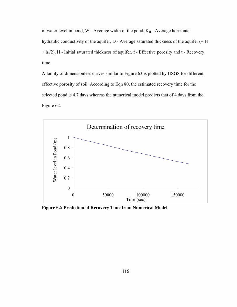
116

of water level in pond, W - Average width of the pond, KH - Average horizontal

hydraulic conductivity of the aquifer, D - Average saturated thickness of the aquifer (= H

+ hc/2), H - Initial saturated thickness of aquifer, f - Effective porosity and t - Recovery

time.

A family of dimensionless curves similar to Figure 63 is plotted by USGS for different

effective porosity of soil. According to Eqn 80, the estimated recovery time for the

selected pond is 4.7 days whereas the numerical model predicts that of 4 days from the

Figure 62.

Determination of recovery time

0

0.2

0.4

0.6

0.8

1

0 50000 100000 150000Time (sec)

Wat

er le

vel i

n Po

nd (m

)

Figure 62: Prediction of Recovery Time from Numerical Model

117

Figure 63: Sample Plot to Determine Recovery Time from MODFLOW

118

5.8 Conclusions

The application of the model developed in the first phase of the study has been extended

to predict the recovery time for the retention pond including the location of the free-

surface. The recovery time obtained from the developed model agrees with that of the

MODFLOW analysis. Furthermore, the free-surface around the retention determined

from the numerical model shows good agreement with that predicted by the Dupuit’s

theory.

119

REFERENCES

1. Harr ME. Groundwater and seepage. Dover publications: New York, 1991. 2. Fredlund DG. Second symposium and short course on unsaturated soils and environmental Geotechnics. University of Saskatchewan, Canada, 2003. 3. Ng CWW. and Shi Q. A Numerical Investigation of the Stability of unsaturated soil slopes subjected to transient seepage. Computers and Geotechnics 1998; 22(1):1-18. 4. El Shamy U, Zeghal M, Shephard M, Dobry R, Fish J, and Abdoun T. Discrete element simulations of water flow through granular soils. 15th ASCE Engineering Mechanics Conference, 2002. 5. El Shamy U., and Zeghal M. Coupled Continuum-Discrete model for saturated granular soils, Journal of Engineering Mechanics, April 2005. 6. Shimizu Y. Fluid coupling in PFC2D and PFC 3D, Manual, Itasca Consulting Group, Numerical Modeling in Micromechanics via Particle Methods, 2004. 7. Itasca. Particle Flow Code, PFC3D, release 3.0. Itasca Consulting Group, Inc., Minneapolis, Minnesota, 2003. 8. Anderson TB and Jackson R. A Fluid Mechanical Description of Fluidized Beds, Industrial Engineering Chemical Fundamentals, 1967; 6(4): 527-539. 9. Tsuji Y., Kawaguchi T., and Tanaka T., Discrete particles simulation of 2-dimensional fluidized bed. Powder Technology, 1993; 77: 79-87. 10. Cundall PA and Strack ODL. A Discrete Numerical Model for Granular Assemblies, Geotechnique 1979; 1: 47-65. 11. Patankar S. Numerical Heat Transfer and Fluid Flow: Taylor and Francis, London. 1980.

120

12. Engineer Manual No. 1110-2-1901, Department of the Army, U.S. Army Corps of Engineers, Washington, DC, April, 1993. 13. Anderson J. Computational Fluid Dynamics- the Basics with applications, McGraw Hill, Inc. 1995. 14. Harr ME. Mechanics of Particulate Media. A Probabilistic Approach: New York, McGraw Hill, 1977. 15. Bowles JE. Physical and Geotechnical Properties of Soils, McGraw Hill, Inc.1984. 16. Das BM. Principles of Geotechnical Engineering: Brooks/Cole Thomson learning, sixth edition, 2006. 17. Jeyisanker, K. and Gunaratne, M, Analysis of Steady State Water Seepage in a Particulate Pavement System, under review by Transportation Research Board, 2008. 18. Pestana JM, Whittle AJ. and Salvati LA. Evaluation of a constitutive model for clays and sands: Part 1 – Sand behavior, International Journal for Numerical and Analytical Methods in Geomechanics 2002; 26:1097-1121. 19. Fredlund DG, and Xing A., Equations for the Soil-Water Characteristic Curve. Canadian Geotechnical Journal, 31; 3:521-532. 20. Lu.N, Likos WJ, Unsaturated Soil Mechanics, Wiley Publishers, May, 2004. 21. Fredlund DG., and Morgenstern NR., Stress State Variables for Unsaturated Soils, Journal of the Geotechnical Engineering Division, American Society of Civil Engineers, 103;GT5: 447-466. 22. Lam.L, Fredlund, DG., and Barbour.SL., Transient Seepage Model for Saturated-Unsaturated Soil Systems: A Geotechnical Engineering Approach, Canadian Geotechnical Journal, 1987; 24: 565-580. 23. Clifton AW, Barbour SL, and Wilson GW. The Emergence of Unsaturated Soil Mechanics, Fredlund Volume, NRC Research Press, Ottawa, 1999. 24. Harbaugh, A.W., and M.G. McDonald. 1996. User's documentation update to the U.S. Geological Survey modular finite-difference U.S. Geological Survey Open-File Report 96-485, 56p. 25. Green, W. H., and Ampt, G. A. “Studies on soil physics. 1. The flow of air and water through soils.” J. Agric. Sci., 1911, 4(1), 1–24.

121

26. Bouwer, H., Infiltration of Water into Non-uniform soil, Journal of the Irrigation and Drainage Division, ASCE, 1969, No. IR4, 451-462. 27. Jeyisanker, K. and Gunaratne, M. Analysis of Water Seepage in a Pavement System Using the Particulate Approach, accepted for the publication, Computers and Geotechnics, 2008. 28. Taylor RL, Brown CB, Darcy flow solutions with a free surface, Journal of Hydraulic Division, ASCE, 1967; 93: 25-33. 29. Bardet J.-P, Tobita T, A Practical Method for Solving Free-Surface Seepage Problems. Computers and Geotechnics, 2002; 29; 451-475. 30. Desai CS, Li GC A residual flow procedure and application for free surface flow in porous media. Advanced Water Resources 1983; 6; 27-35. 31. Alt HW, Numerical Solution of Steady State Porous Flow Free Boundary Problems. Numerical Mathematics 1980; 31: 73-98. 32. Kikuchi N. An Analysis of the variational Inequalities of Seepage Flow by Finite-Element Methods. Quartitative Applied Mathematics 1977; 35: 149-163. 33. Brezis H, Kinderlehrer D, Stampacchia G, Sur une nouvelle formulation du probleme de l’ecoulement a travers une digue, Serie A. paris: C.R.Academie des Sciences; 1978.

ABOUT THE AUTHOR

Kalyani Jeyisanker received her B.Sc. (Eng), with honors, in Civil Engineering from

University of Peradeniya, Sri Lanka in 2001. She earned her Master’s degree in

Mechanical Engineering from Texas Tech University in 2004 and enrolled in PhD

program in 2005 at University of South Florida. While pursuing the PhD, Ms. Jeyisanker

actively participated in numerous research projects. She also coauthored two journal

papers and two conference papers.