Maximally flat differentiators through WLS Taylor decomposition
Upload
khangminh22Category
view
2download
0
University of Central Florida University of Central Florida
STARS STARS
Electronic Theses and Dissertations, 2004-2019
2011
Finite Depth Seepage Below Flat Apron With End Cutoffs And A Finite Depth Seepage Below Flat Apron With End Cutoffs And A
Downstream Step Downstream Step
Arun K. Jain University of Central Florida
Part of the Engineering Commons
Find similar works at: https://stars.library.ucf.edu/etd
University of Central Florida Libraries http://library.ucf.edu
This Doctoral Dissertation (Open Access) is brought to you for free and open access by STARS. It has been accepted
for inclusion in Electronic Theses and Dissertations, 2004-2019 by an authorized administrator of STARS. For more
information, please contact [email protected].
STARS Citation STARS Citation Jain, Arun K., "Finite Depth Seepage Below Flat Apron With End Cutoffs And A Downstream Step" (2011). Electronic Theses and Dissertations, 2004-2019. 1853. https://stars.library.ucf.edu/etd/1853

FINITE DEPTH SEEPAGE BELOW FLAT APRON WITH END CUTOFFS
AND A DOWNSTREAM STEP
by
ARUN K. JAIN
B.E. University of Jodhpur, 1990
M.E. J.N.V. University, 1995
A dissertation submitted in partial fulfillment of the requirements
for the degree of Doctor of Philosophy
in the Department of Civil, Environmental, and Construction Engineering
in the College of Engineering and Computer Science
at the University of Central Florida
Orlando, Florida
Summer Term
2011
Major Professor: Lakshmi N. Reddi

ii
Arun K. Jain

iii
ABSTRACT
Hydraulic structures with water level differences between upstream and downstream are
subjected to seepage in foundation soils. Two sources of weakness are to be guarded against: (1)
percolation or seepage may cause under-mining, resulting in the collapse of the whole structure,
and (2) the floor of the apron may be forced upwards, owing to the upward pressure of water
seeping through pervious soil under the structure. Many earlier failures of hydraulic structures
have been reported due to these two reasons.
The curves and charts prepared by Khosla, Bose, and Taylor still form the basis for the
determination of uplift pressure and exit gradient for weir apron founded on pervious soil of
infinite depth. However, in actual practice, the pervious medium may be of finite depth owing to
the occurrence of a clay seam or hard strata at shallow depths in the river basin. Also, a general
case of weir profile may consist of cutoffs, at the two ends of the weir apron. In addition to the
cutoffs, pervious aprons are also provided at the downstream end in the form of (i) inverted filter,
and (ii) launching apron. These pervious aprons may have a thickness of 2 to 5. In order to
accommodate this thickness, the bed adjacent to the downstream side of downstream cutoff has
to be excavated. This gives rise to the formation of step at the downstream end.
Closed form theoretical solutions for the case of finite depth seepage below weir aprons
with end cutoffs, with a step at the downstream side are obtained in this research. The parameters
studied are : (i) finite depth of pervious medium, (ii) two cut offs at the ends, and (iii) a step at
the downstream end.

iv
The resulting implicit equations, containing elliptic integrals of first and third kind, have
been used to obtain various seepage characteristics. The results have been compared with
existing solutions for some known boundary conditions. Design curves for uplift pressure at key
points, exit gradient factor and seepage discharge factor have been presented in terms of non-
dimensional floor profile ratios.
Publications resulting from the dissertation are:
1. Jain, Arun K. and Reddi, L. N. “Finite depth seepage below flat aprons with equal end
cutoffs.” (Submitted to Journal of Hydraulic Engineering, ASCE, and reviewed).
2. Jain, Arun K. and Reddi, L. N. “Seepage below flat apron with end cutoffs founded on
pervious medium of finite depth.” (Submitted to Journal of Irrigation & Drainage
Engineering, ASCE).
3. Jain, Arun K. and Reddi, L. N. “Closed form theoretical solution for finite depth seepage
below flat apron with equal end cutoffs and a downstream step.” (Submitted to Journal of
Hydrologic Engineering, ASCE).
4. Jain, Arun K. and Reddi, L. N. “Closed form theoretical solution for finite depth seepage
below flat apron with end cutoffs and a downstream step.” (Submitted to Journal of
Engineering Mechanics, ASCE).

v
I dedicate this dissertation to
God Almighty
Who has provided me with the strength and motivation to carry on this work
My father, Prof. Bal Chandra Punmia
Who has been my role model and inspiration to achieve my goals
My mother, Kewal Punmia
Who has dedicated her life bringing the best in me
My wife, Smita Jain
Who has encouraged me throughout this work and otherwise
and
My brother, Ashok K. Jain
Who has been taking care of me in all ups and downs of life.

vi
ACKNOWLEDGMENTS
I would like to express my deepest appreciation to the Committee Chair Professor
Lakshmi Reddi for this guidance, support, and insight throughout the research work. I
also thank him for his philosophical guidance and personal attention to re-build my
strengths, through the difficult period I went through.
Thanks go out to the other committee members, Dr. Manoj Chopra, Dr. Scott Hagen, and
Dr. Eduardo Divo for their suggestions and comments.
I convey my thanks and appreciation to my family and friends for their understanding,
encouragements, and patience. I would like to mention some who have helped me
immensely – Rupesh Bhomia, Michel Machado, Mrs. Padma Reddi, Mrs. Kiran Jalota,
Justin Vogel, Laxmikant Sharma, Shantanu Shekhar, Mool Singh Gahlot, Juan Cruz and
Chandra Prakash Shukla. I would also like to thank Dr. Rose M. Emery, who has been
one of the biggest supports during the most difficult times of this study. I thank my son,
Aseem Jain for his co-operation and patience. I extend my thanks to Indian Student
Association – UCF, and Jain Society of Central Florida, Altamonte Springs and Nurses
and doctors at Florida Cancer Institute, Orlando for their everlasting care.
Last but not least, I am thankful to all colleagues, staff and faculty in the Civil,
Environmental, & Construction Engineering department who made my academic
experience at the University of Central Florida a memorable, valuable, and enjoyable
one.

vii
TABLE OF CONTENTS LIST OF FIGURES ....................................................................................................................x
LIST OF TABLES ...................................................................................................................xvi
CHAPTER 1 INTRODUCTION .................................................................................................1
1.1 General ..............................................................................................................................1
1.2 Early Theories ...................................................................................................................2
1.2.1 The Hydraulic Gradient Theory .................................................................................2
1.2.2 Bligh’s Creep Theory ................................................................................................2
1.2.3 Lane’s Weighted Creep Theory .................................................................................3
1.2.4 Work of Weaver, Harza and Haigh ............................................................................4
1.3 Methods of Analysis ..........................................................................................................5
1.3.1 Finite Difference Method (FDM) ..............................................................................6
1.3.2 Finite Element Method (FEM) ..................................................................................7
1.3.3 Boundary Element Method (BEM) ............................................................................9
1.3.4 Software Packages .................................................................................................. 11
1.3.5 Method of Fragments .............................................................................................. 12
1.3.6 Closed Form Analytical Solutions ........................................................................... 12
1.3.6.1 Khosla’s Analysis .......................................................................................... 14
1.3.6.2 Work by Pavlovsky and other Russian Workers............................................. 14
1.3.6.3 Confined Seepage Research by others ........................................................... 15
1.4 Scope of Present Investigations ...................................................................................... 16
CHAPTER 2 FLAT APRON WITH EQUAL END CUTOFFS ................................................. 18
2.1 Introduction ..................................................................................................................... 18

viii
2.2 Theoretical Analysis ........................................................................................................ 18
2.2.1 First Transformation ................................................................................................ 21
2.2.2 Second Transformation ........................................................................................... 29
2.3 Computations .................................................................................................................. 35
2.4 Design Charts .................................................................................................................. 45
2.5 Comparison with Infinite Depth Case .............................................................................. 50
2.6 Development of Interference Formulae ............................................................................ 50
2.7 Development of Simplified Equations for PE, PD and GEc/H............................................ 57
2.8 Conclusions ..................................................................................................................... 59
CHAPTER 3 FLAT APRON WITH UNEQUAL END CUTOFFS AND A STEP AT
DOWNSTREAM END ............................................................................................................. 60
3.1. Introduction .................................................................................................................... 60
3.2. Theoretical Analysis ....................................................................................................... 60
3.2.1 First Transformation ................................................................................................ 63
3.3 Computations and Results ............................................................................................... 92
3.4 Design Charts ................................................................................................................ 105
3.5 Conclusions ................................................................................................................... 105
CHAPTER 4 FLAT APRON WITH UNEQUAL END CUTOFFS ......................................... 133
4.1 Introduction ................................................................................................................... 133
4.2 Theoretical Analysis ...................................................................................................... 133
4.2.1 First Transformation .............................................................................................. 135
4.2.2 Second Transformation ......................................................................................... 146
4.3 Computations and Results ............................................................................................. 151

ix
4.4 Design Charts ................................................................................................................ 155
4.5 Conclusions ................................................................................................................... 168
CHAPTER 5 FLAT APRON WITH EQUAL END CUTOFFS AND A STEP AT
DOWNSTREAM END ........................................................................................................... 169
5.1 Introduction ................................................................................................................... 169
5.2 Theoretical Analysis ...................................................................................................... 169
5.2.1 First Transformation .............................................................................................. 170
5.2.2 Second Transformation ......................................................................................... 181
5.3 Computations and Results ............................................................................................. 186
5.4 Design Charts ................................................................................................................ 189
5.5 Conclusions ................................................................................................................... 199
CHAPTER 6 SUMMARY, CONCLUSIONS AND RECOMMENDATIONS ........................ 200
6.1 Summary and Conclusions ............................................................................................ 200
6.1.1 Flat Apron with Equal End Cutoffs ....................................................................... 200
6.1.2 Flat Apron with Unequal End Cutoffs and a Step at Downstream End ................... 202
6.1.3 Flat Apron with Unequal End Cutoffs ................................................................... 204
6.1.4 Flat Apron with Equal End Cutoffs and a Step at the Downstream End ................. 206
6.2 Recommendations for Future Work ............................................................................... 208
APPENDIX A SCHWARZ – CHRISTOFFEL TRANSFORMATION ................................... 211
APPENDIX B ELLIPTIC INTEGRALS ................................................................................. 215
REFFRENCES........................................................................................................................ 220

x
LIST OF FIGURES
Fig. 1.1 Generalized model development by finite difference and finite element method .............8
Fig. 2.1 Illustrations of the problem – Schwarz Christoffel transformations ............................... 20
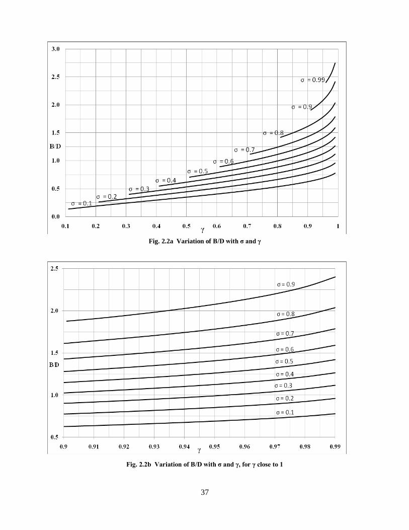
Fig. 2.2a Variation of B/D with σ and γ .................................................................................... 37
Fig. 2.2b Variation of B/D with σ and γ, for γ close to 1 ........................................................... 37
Fig. 2.3a Variation of B/c with σ and γ ..................................................................................... 38
Fig. 2.3b Variation of B/c with σ and γ, for γ close to 1 ............................................................ 38
Fig. 2.4 Determination of σ and γ ............................................................................................ 40
Fig 2.5 Design curves for PE ...................................................................................................... 46
Fig 2.6 Design curves for PD ..................................................................................................... 47
Fig 2.7 Design curves for q/kH .................................................................................................. 48
Fig 2.8 Design curves for GEc/H ............................................................................................... 49
Fig. 2.9 Interference Correction for PE....................................................................................... 53
Fig. 2.10 Interference Correction for PD .................................................................................... 54
Fig. 2.11 Interference Correction for E
G c H/ .......................................................................... 55
Fig. 3.1 Illustrations of the problem – Schwarz Christoffel transformations .............................. 62
Fig. 3.2a Variation of PE with a/c2 (B/c2 = 10 & c1/c2 = 0.4) .................................................... 106
Fig. 3.2b Variation of PD with a/c2 (B/c2 = 10 & c1/c2 = 0.4) .................................................... 106
Fig. 3.3a Variation of PE1 with a/c2 (B/c2 = 10 & c1/c2 = 0.4) ................................................... 107
Fig. 3.3b Variation of PD1 with a/c2 (B/c2 = 10 & c1/c2 = 0.4) .................................................. 107
Fig. 3.4a Variation of q
kH with a/c2 (B/c2 = 10 & c1/c2 = 0.4)................................................. 108
Fig. 3.4b Variation of 2
E
cG
H with a/c2 (B/c2 = 10 & c1/c2 = 0.4) ............................................. 108

xi
Fig. 3.5a Design curve for PE (c1/c2 = 0.2 & a/c2 = 0.1) ........................................................... 109
Fig. 3.5b Design curve for PE for (c1/c2 = 0.4 & a/c2 = 0.1) ...................................................... 109
Fig. 3.5c Design curve for PE (c1/c2 = 0.6 & a/c2 = 0.1) ........................................................... 110
Fig. 3.5d Design curve for PE for (c1/c2 = 0.8 & a/c2 = 0.1) ...................................................... 110
Fig. 3.6a Design curve for PE (c1/c2 = 0.2 & a/c2 = 0.2) ........................................................... 111
Fig. 3.6b Design curve for PE for (c1/c2 = 0.4 & a/c2 = 0.2) ...................................................... 111
Fig. 3.6c Design curve for PE (c1/c2 = 0.6 & a/c2 = 0.2) ........................................................... 112
Fig. 3.6d Design curve for PE for (c1/c2 = 0.8 & a/c2 = 0.2) ...................................................... 112
Fig. 3.7a Design curve for PD (c1/c2 = 0.2 & a/c2 = 0.1) ........................................................... 113
Fig. 3.7b Design curve for PD for (c1/c2 = 0.4 & a/c2 = 0.1) ..................................................... 113
Fig. 3.7c Design curve for PD (c1/c2 = 0.6 & a/c2 = 0.1) ........................................................... 114
Fig. 3.7d Design curve for PD for (c1/c2 = 0.8 & a/c2 = 0.1) ..................................................... 114
Fig. 3.8a Design curve for PD (c1/c2 = 0.2 & a/c2 = 0.2) ........................................................... 115
Fig. 3.8b Design curve for PD for (c1/c2 = 0.4 & a/c2 = 0.2) ..................................................... 115
Fig. 3.8c Design curve for PD (c1/c2 = 0.6 & a/c2 = 0.2) ........................................................... 116
Fig. 3.8d Design curve for PD for (c1/c2 = 0.8 & a/c2 = 0.2) ..................................................... 116
Fig. 3.9a Design curve for PE1 (c1/c2 = 0.2 & a/c2 = 0.1) .......................................................... 117
Fig. 3.9b Design curve for PE1 for (c1/c2 = 0.4 & a/c2 = 0.1) .................................................... 117
Fig. 3.9c Design curve for PE1 (c1/c2 = 0.6 & a/c2 = 0.1) .......................................................... 118
Fig. 3.9d Design curve for PE1 for (c1/c2 = 0.8 & a/c2 = 0.1) ................. 118
Fig. 3.10a Design curve for PE1 (c1/c2 = 0.2 & a/c2 = 0.2) ........................................................ 119
Fig. 3.10b Design curve for PE1 for (c1/c2 = 0.4 & a/c2 = 0.2)................................................... 119
Fig. 3.10c Design curve for PE1 (c1/c2 = 0.6 & a/c2 = 0.2) ........................................................ 120

xii
Fig. 3.10d Design curve for PE1 for (c1/c2 = 0.8 & a/c2 = 0.2)................................................... 120
Fig. 3.11a Design curve for PD1 (c1/c2 = 0.2 & a/c2 = 0.1) ........................................................ 121
Fig. 3.11b Design curve for PD1 for (c1/c2 = 0.4 & a/c2 = 0.1) .................................................. 121
Fig. 3.11c Design curve for PD1 (c1/c2 = 0.6 & a/c2 = 0.1) ........................................................ 122
Fig. 3.11d Design curve for PD1 for (c1/c2 = 0.8 & a/c2 = 0.1) .................................................. 122
Fig. 3.12a Design curve for PD1 (c1/c2 = 0.2 & a/c2 = 0.2) ........................................................ 123
Fig. 3.12b Design curve for PD1 for (c1/c2 = 0.4 & a/c2 = 0.2) .................................................. 123
Fig. 3.12c Design curve for PD1 (c1/c2 = 0.6 & a/c2 = 0.2) ........................................................ 124
Fig. 3.12d Design curve for PD1 for (c1/c2 = 0.8 & a/c2 = 0.2) .............................................. 124
Fig. 3.13a Design curve for q
kH(c1/c2 = 0.2 & a/c2 = 0.1) ........................................................ 125
Fig. 3.13b Design curve for q
kHfor (c1/c2 = 0.4 & a/c2 = 0.1) ................................................... 125
Fig. 3.13c Design curve for q
kH(c1/c2 = 0.6 & a/c2 = 0.1) ........................................................ 126
Fig. 3.13d Design curve for q
kH (c1/c2 = 0.8 & a/c2 = 0.1) ....................................................... 126
Fig. 3.14a Design curve for q
kH(c1/c2 = 0.2 & a/c2 = 0.2) ........................................................ 127
Fig. 3.14b Design curve for q
kH (c1/c2 = 0.4 & a/c2 = 0.2) ....................................................... 127
Fig. 3.14c Design curve for q
kH(c1/c2 = 0.6 & a/c2 = 0.2) ........................................................ 128
Fig. 3.14d Design curve for q
kH (c1/c2 = 0.8 & a/c2 = 0.2) ....................................................... 128
Fig. 3.15a Design curve for 2E
cG
H(c1/c2 = 0.2 & a/c2 = 0.1) ...................................................... 129
xiii
Fig.3.15b Design curve for 2E
cG
H (c1/c2 = 0.4 & a/c2 = 0.1)...................................................... 129
Fig. 3.15c Design curve for 2E
cG
H(c1/c2 = 0.6 & a/c2 = 0.1) ...................................................... 130
Fig.3.15d Design curve for 2E
cG
H (c1/c2 = 0.8 & a/c2 = 0.1)...................................................... 130
Fig. 3.16a Design curve for 2E
cG
H(c1/c2 = 0.2 & a/c2 = 0.2) ...................................................... 131
Fig.3.16b Design curve for 2E
cG
H (c1/c2 = 0.4 & a/c2 = 0.2)...................................................... 131
Fig. 3.16c Design curve for 2E
cG
H(c1/c2 = 0.6 & a/c2 = 0.2) ...................................................... 132
Fig.3.16d Design curve for 2E
cG
H (c1/c2 = 0.8 & a/c2 = 0.2)...................................................... 132
Fig. 4.1 Illustrations of the problem – Schwarz-Christoffel transformations............................. 134
Fig. 4.2a Design curves for PE for c1/c2 = 0.2 ........................................................................... 156
Fig. 4.2b Design curves for PE for c1/c2 = 0.4 .......................................................................... 156
Fig. 4.2c Design curves for PE for c1/c2 = 0.6 ........................................................................... 157
Fig. 4.2d Design curves for PE for c1/c2 = 0.8 .......................................................................... 157
Fig. 4.3a Design curves for PD for c1/c2 = 0.2 .......................................................................... 158
Fig. 4.3b Design curves for PD for c1/c2 = 0.4 .......................................................................... 158
Fig. 4.3c Design curves for PE for c1/c2 = 0.6 ........................................................................... 159
Fig. 4.3d Design curves for PE for c1/c2 = 0.8 .......................................................................... 159
Fig. 4.4a Design curves for PE1 for c1/c2 = 0.2 ......................................................................... 160
Fig. 4.4b Design curves for PE1 for c1/c2 = 0.4 ......................................................................... 160
Fig. 4.4c Design curves for PE1 for c1/c2 = 0.6 ......................................................................... 161
Fig. 4.4d Design curves for PE1 for c1/c2 = 0.8 ......................................................................... 161

xiv
Fig. 4.5a Design curves for PD1 for c1/c2 = 0.2 ......................................................................... 162
Fig. 4.5b Design curves for PD1 for c1/c2 = 0.4 ......................................................................... 162
Fig. 4.5c Design curves for PD1 for c1/c2 = 0.6 ......................................................................... 163
Fig. 4.5d Design curves for PD1 for c1/c2 = 0.8 ......................................................................... 163
Fig. 4.6a Design curves for GEc2/H for c1/c2 = 0.2 ................................................................... 164
Fig. 4.6b Design curves for GEc2/H for c1/c2 = 0.4 ................................................................... 164
Fig. 4.6c Design curves for GEc2/H for c1/c2 = 0.6 ................................................................... 165
Fig. 4.6d Design curves for GEc2/H for c1/c2 = 0.8 ................................................................... 165
Fig. 4.7a Design curves for q/kH for c1/c2 = 0.2 ....................................................................... 166
Fig. 4.7b Design curves for q/kH for c1/c2 = 0.4 ...................................................................... 166
Fig. 4.7c Design curves for q/kH for c1/c2 = 0.6 ....................................................................... 167
Fig. 4.7d Design curves for q/kH for c1/c2 = 0.8 ...................................................................... 167
Fig. 5.1 Illustrations of the problem: Schwarz – Christoffel transformations ............................ 171
Fig. 5.2a Variational curve for PE for B/c = 10 ........................................................................ 190
Fig. 5.2b Variational curve for PD for B/c = 10 ........................................................................ 190
Fig. 5.3a Variational curve for PE1 for B/c = 10 ....................................................................... 191
Fig. 5.3b Variational curve for PD1 for B/c = 10....................................................................... 191
Fig. 5.4a Variational curve for discharge factor for B/c = 10 ................................................... 192
Fig. 5.4b Variational curve for exit gradient factor for B/c = 10 ............................................... 192
Fig. 5.5a Design curve for PE for a/c = 0.1 ............................................................................... 193
Fig. 5.5b Design curve for PE for a/c = 0.2 .............................................................................. 193
Fig. 5.7a Design curve for PE1 for a/c = 0.1 ............................................................................. 195
Fig. 5.7b Design curve for PE1 for a/c = 0.2 ............................................................................. 195

xv
Fig. 5.8a Design curve for PD1 for a/c = 0.1 ............................................................................. 196
Fig. 5.8b Design curve for PD1 for a/c = 0.2 ........................................................................... 196
Fig. 5.9a Design curve for discharge factor for a/c = 0.1 .......................................................... 197
Fig. 5.9b Design curve for discharge factor for a/c = 0.2 ......................................................... 197
Fig. 5.10a Design curve for exit gradient factor for a/c = 0.1 ................................................... 198
Fig. 5.10b Design curve for exit gradient factor for a/c = 0.2 ................................................... 198
Fig. 6.1 Finite depth problems for future work ........................................................................ 210
Fig. A-1 Schwarz-Christoffel transformation ........................................................................... 213

xvi
LIST OF TABLES
Table 2.1 Computed Values for 0.5 .................................................................................... 39
Table 2.2 Data Generated from Matching the Given Values of B/D and B/c Ratios ................... 41
Table 2.3 Comparison with Infinite Depth Case ........................................................................ 50
Table 2.4 Interference Values (I) ............................................................................................... 52
Table 2.5 Values of Factors a and n........................................................................................... 56
Table 2.6 Comparison of Values of PE from the Formula .......................................................... 58
Table 3.2. Comparison with Malhotra's case of Infinite Depth. .................................................. 93
Table 3.1 Computed values for B/D = 0.2, a/c2 = 0.1 ................................................................. 94
Table 4.1 Computed Values .................................................................................................... 152
Table 4.2 Comparison with Malhotra's Case of Infinite Depth ................................................. 155
Table 5.1 Computed Values .................................................................................................... 187
Table 5.2 Comparison with Malhotra's Case of Infinite Depth ................................................. 189

1
CHAPTER 1. INTRODUCTION
1.1 General
If a structure is built on a pervious soil and water level upstream of the structure is higher
than it is downstream, enforced percolation or seepage will occur in the underlying permeable
soil. The design of apron is intimately connected with the possibility of this percolation.
Two sources of weakness are to be guarded against: (1) percolation may cause
undermining of the pervious granular foundation, which starts from the tail end of the work and
may result in collapse of the whole structure, and (2) the floor or the apron may be forced
upwards, owing to the upward pressure of water seeping through the pervious soil under the
structure. The failure of the old Manufla regulator in Egypt was due to undermining, whereas the
failure of Narora weir in India was due to excessive water pressure causing the floor of the weir
to be blown upwards.
The two essentials to be considered in the design of impervious apron of a hydraulic
structure are:
(i) Residual or uplift pressure at any point at the bottom of the floor, and
(ii) Exit gradient.

2
1.2 Early Theories
1.2.1 The Hydraulic Gradient Theory
The law of flow of water through permeable soil was enunciated for the first time in 1856
by H. Darcy who, as a result of experiments, found that for laminar flow conditions, the velocity
of flow varied directly as the head and inversely as the length of path of flow. Later work on the
flow was done in the United States by Allen Hazen (1892) and C.S. Slichter (1899), and in India
by Col. J. Clibborn and J.S. Beresford. Clibborn and Beresford carried out experiments (1895-
97) with a tube 120 ft long and 2 ft internal diameter filled with Khanki sand, in connection, with
the proposals for repairs to the damage to the Khanki weir on Chenab River. The hydraulic
gradient theory for weir design, apparently originated between Sir John Ottely and Thoman
Higham, and was developed as a result of experiments by Col. Clibborn. With the publication of
Clibborn's experiments in 1902, the Hydraulic Gradient Theory was generally accepted in India.
According to the hydraulic gradient theory, the safety of a weir founded on a permeable
soil medium depends upon its path of percolation that is the distance through which water would
have to travel below the weir floor before it could rise up on the downstream, and cause scour.
Whether the masonry was laid horizontally or vertically was immaterial, so long as the current
below the structure was exposed to friction for the same length of the soil.
1.2.2 Bligh’s Creep Theory
In 1907, Bligh, in his book `Practical Design of Irrigation Works' evolved a concept
according to which the stability of a weir apron depended on its weight. But in 1910 edition of
the book, he admitted the fallacy of this original concept and became converted to the `Hydraulic
Gradient Theory' of Ottley, Higham and Clibborn, and gave his `creep theory'. In Bligh's creep

3
theory; he stated that the length of the path of flow had the same effectiveness, length for length,
in reducing the uplift pressures, whether it was along the horizontal or the vertical. He assumed
the percolating water to creep along the contact of the base profile of the weir with the subsoil
losing head enroute, proportional to the length of its travel. He called this loss of head per unit
length as the percolation coefficient (C) and assigned a safe value to C for different types of
soils.
Bligh's conclusions were based on the study of failure of only two dams, both on fine
sand foundations and only experimental data available at the time were of Clibbron. From these
meager data, Bligh evolved a simple formula which fitted neither Clibborn results with sheet
piles nor those at Narora Weir. However, because of its simplicity, this theory found
general acceptance. Some works designed on this theory failed while others stood, depending on
the extent to which they ignored or took note of the importance of vertical cutoffs at the
upstream and downstream ends.
1.2.3 Lane’s Weighted Creep Theory
Colman (1916) for the first time carried out tests with weir models resting on sand to
determine the distribution of pressure under the weir base, and the relative effect of sheet piles at
the upstream and down stream ends. These experiments established that vertical contacts are
more effective than horizontal contacts, contradicting Bligh's assumptions.
Lane (1935), after analyzing over 200 dams on pervious foundations all over the World,
advanced a theory known as `Weighted Creep Theory and accounted for the vertical and
horizontal cutoffs in a modified way. Lane was of the view that water can occasionally travel
along the line of creep because it is not easy to have close contact between the two surfaces, i.e.

4
the flat surface of the solid foundation of the weir and the pervious soil upon which it is founded.
In practice, an intimate contact between the vertical and steeply sloping surface is more possible
than in horizontal or slightly sloping. Thus contact between earth and sheet pile is more intimate
than for concrete foundation cast over flat bedding. This led to different weights to the vertical
and horizontal creeps. According to Lane, the weighted creep distance is the sum of vertical
creep distance (steeper than 45°), plus one third the horizontal creep distances (less than 45°).
Though a statistical examination of a large number of dams confirm the basic idea of
relative creep effectiveness on the lines of Lane, but to try to suggest such simple ratios of their
effectiveness was considered to be too arbitrary.
1.2.4 Work of Weaver, Harza and Haigh
The problem of uplift pressure on the base of a dam founded on pervious medium of
infinite depth was mathematically analyzed by Weaver (1932). He showed that with no sheet
piling, the path of flow are the lower halves of a family of confocal ellipses with foci at heel and
toe, respectively and the equipotential lines are the conjugate family of confocal hyperbolas. This
shows that the pressure gradient is no more a straight line as assumed by Bligh, but is sinusoidal.
Weaver, however, did not consider the exit gradient.
Harza (1934) and Haigh (1935) independently published two papers on similar lines. All
these attempts were responsible for a shift from empirical approach towards the rational
approach, for the design of base of weir aprons. They gave due weightage to exit gradient as
controlling factor in stability and discussed the distribution of pressures which could be
considered as safe.
5
1.3 Methods of Analysis
The process of seepage through porous media can be classified according to the
dimensional character of the flow, the boundaries of flow region or domain, and the properties of
the medium and of the fluid (Rushton and Redshaw, 1979). Any scenario in the seepage studies
consists of a governing along with boundary conditions and initial conditions which control
seepage in a particular problem domain. If the domain has a complex configuration, analytic
solution seems to be difficult to contrive at and hence one may resort to approximating
techniques for solution of the governing equation. The goal of these approximate methods is thus
to find a function (or some discrete approximation to this function) that satisfies a given
relationship between various derivatives on some given region of space and/or time, along with
some boundary conditions along the edges of this domain.
Thus, these approximate methods provide a rationale for operating on differential
equations that make up a model and for transforming them into a set of algebraic equations.
Using computer, one can solve large number of algebraic equations by iterative techniques or by
direct matrix methods. The solution obtained can be compared with that determined from
analytical solution, if one is available or with values observed in the field or from laboratory
experiments. It should be noted that the numerical procedures (approximate methods) yield
solutions for only a predetermined number of points, as compared to analytical solutions that can
be used to determine values at any point in a problem domain. The next five sub-sections are
devoted to different approximate methods which are chiefly used in seepage studies.

6
1.3.1 Finite Difference Method (FDM)
A finite difference method proceeds by replacing the derivatives in the governing
differential equation with finite-difference approximations. This gives a large, but finite
algebraic system of equations to be solved in place of differential equation, which can be done
using computer. Thus, the method actually performs discretization of the flow domain by
dividing into a mesh that is usually rectangular, where the potential or head is computed at the
grid points by solving the differential equation in finite difference form throughout the mesh or
the grid system. There are two common types of grids: mesh-centered and block-centered.
Associated with the grids are node points that represent the position at which the solution of the
unknown values (head, for example) is obtained. The choice of grid to use depends largely on the
boundary conditions.
Hence, this method, also known as relaxation method is a process of steadily improved
approximation for the solution of simultaneous equations, and any problem that can be
formulated in terms of simultaneous equations can, theoretically, be solved by this method. One
of the earliest uses of this method was by Richardson (1911) who applied it for a masonry dam
problem. Several other researchers (Shaw and Southwell, 1941; Van Deemter, 1951; Jeppson,
1968a, 1968b; Herbert, 1968; Cooley, 1971; Freeze, 1971; Bruch Jr. et al., 1972; Huntoon, 1974;
Ronzhin, 1975; Bruch Jr. et al., 1978; Gureghian, 1978; Caffrey and Bruch, 1979; Dennis and
Smith, 1980; Karadi et al., 1980; Walsum and Koopmans, 1984; Pollock, 1988; Das et al. 1994;
Naouss and Najjar, 1995; Korkmaz and Önder, 2006; Jeyisanker and Gunaratne, 2009; Igboekwe
and Achi, 2011) have used FDM as method of analysis for different seepage and groundwater
problems.

7
The summary of important components and steps of model development for FDM and
finite element method (discussed in next sub-section) are shown in figure 1.1.
1.3.2 Finite Element Method (FEM)
There are two basic problems in calculus: one relating to integration and the other to
differentiation. Whereas FDM approximates differential equations by a differential approach,
FEM approximates differential equations by an integral approach. Based on inverse property of
differentiation and integration to one another, one would expect the two methods to be related
and to converge to same solution, but perhaps from different directions (Faust and Mercer,
1980).
FEM is essentially a numerical method in which a region is subdivided into sub regions
called elements, whose shapes are determined by a set of points called nodes. The flexibility of
elements allows consideration of regions with complex geometry. The first step in applying the
FEM, as shown in figure 1.1, is to develop an integral representation of the partial differential
equation. The next step is to approximate the dependent variables (head, for example) in terms of
interpolation functions, which are called the basis functions, and are selected to satisfy certain
mathematical requirements and for ease of computation. As the element is generally small, the
interpolation function can be adequately approximated by a low-order polynomial, for example,
linear, quadratic, or cubic. As an example, consider a linear basis function for a triangular
element. This basis function describes a plane surface including the values of dependent variable
(head) at the node points in the element. Having basis functions specified and the grid designed,
the integral relationships are expressed for each element as a function of the coordinates of all
node points of the element. Next the values of the integrals are calculated for each element.

8
Fig. 1.1 Generalized model development by finite difference and finite element method
(Adapted from Faust and Mercer, 1980)

9
The values for all elements are combined, including boundary conditions, to yield a system of
first-order linear differential equations in time (Faust and Mercer, 1980).
A number of researchers (Neuman and Witherspoon, 1970; Doctors, 1970; France et al., 1971;
McLean and Krizek, 1971; Desai, 1973, 1976; Ponter, 1972; France, 1974; Semenov and
Shevarina, 1976; Kikuchi, 1977; Choi, 1978; Christian, 1980; Florea and Popa, 1980; Nath,
1981; Aalto, 1984; Rulon et al., 1985; Lacy and Prevost, 1987; Tracy and Radhakrishnan,1989;
Rogers and Selim, 1989; Morland, and Gioda, 1990; Griffiths and Fenton, 1993, 1997, 1998;
Hnang, 1996; Karthikeyan et al., 2001; Simpson and Clement, 2003; Benmebarek et al, 2005;
Soleimanbeigi and Jafarzadeh, 2005; Im et al., 2006; Hlepas, 2008; Ahmed, 2009; Ahmed and
Bazaraa, 2009; Ahmed and Elleboudy, 2010) have successfully used FEM in a wide variety of
groundwater flow and seepage problems.
FEM differs from FDM in two respects. In the first place the domain is discretized into a
mesh of finite elements of any shape, such as triangles. In the second place, the differential
equation is not solved directly but replaced by a variational formulation (Strack, 1989).
1.3.3 Boundary Element Method (BEM)
Boundary element method constitutes a recent development in computational
mathematics for the solution of boundary value problems in various branches of science and
technology. For flow through porous media, Liggett (1977) was the first to use BEM for finding
location of free surface in porous media where the solution is desired at a limited number of
points (for example, on a failure surface in determining slope stability) or in a limited area of the
flow.

10
BEM is based on integral equation formulation of boundary value problems and requires
discretization of only the boundary (surface or curve) and not the interior of the region under
consideration. Unlike, the ‘domain type’ methods e.g. FDM and FEM, the order of
dimensionality reduces by unity in boundary element formulation, thus simplifying the analysis
and the computer code to a large extent by solving a small system of algebraic equations (Kythe,
1995). This method is suitable for problems with complicated boundaries and unbounded
regions, offering greatly reduced nodes for the same degree of accuracy as in FEM.
Various researchers (Brebbia and Wrobel, 1979; Herrera, 1980; Hromadka, 1984;
Liggett, 1985; Gipson et al. 1986; Elsworth, 1987; Karageorghis, 1987; Chugh, 1988; Savant et
al., 1988; Chang, 1988; Aral, 1989; Abdrabbo and Mahmoud, 1991; Chen et al., 1994;
Demetracopoulos and Hadjitheodorou, 1996; Tsay et al., 1997; Leontiev and Huacasi, 2001;
Abdel-Gawad and Shamaa, 2004; Shen and Zhang, 2008; Filho and Leontiev, 2009) have used
BEM for different groundwater and seepage problems.
Summarizing, the main features of the above mentioned three numerical methods are
(Bear et al., 1996):
1. The solution is sought for the numerical values of state variables which are at specified points
in the space and time domains defined for the problem (rather than their continuous variations in
these domains).
2. The partial differential equations that represent balances of the considered extensive quantities
are replaced by a set of algebraic equations (written in terms of the sought, discrete values of the
state variables at the discrete points in space and time).

11
3. The solution is obtained for a set of specified set of numerical values of the various model
coefficients (rather than as a general relationship in terms of these coefficients).
4. Since a large number of equations must be solved simultaneously, a computer program is
prepared.
1.3.4 Software Packages
In recent years, computer programming codes have been developed for almost all the
classes of problems encountered in the management of ground water. Some codes are very
comprehensive and can handle a variety of specific problems as special cases, while others are
tailor-made for particular problems (Bear et al., 1996). To name a few, some commercial and
other softwares are (along with the name of the authors of the software): MODFLOW
(McDonald and Harbaugh, 1988), WALTON (Walton, 1970), FEMWATER (Yeh and Ward,
1979), FLONET: FLOWTRANS (Guiger et al., 1994), FLOWPATH (Franz and Guiger, 1994),
TRACR3D (Travis, 1984) and SEEP2D (Fred Tracy of the U.S. Army Engineer Waterways
Experiment Station; Jones, 1999).
Many of these provide modeling for groundwater flow, while others deal with
solute transport as well. Some deal with saturated cases only while a few deal with complexities
of unsaturated flow cases, etc. A few models can be used for 3D flows, while others for 2D flow
or both. It should be kept in mind that all these models rely on numerical (approximate) methods
mentioned in previous three sub-sections, while some use a combination of these methods, thus
inheriting the limitations of these methods.
12
1.3.5 Method of Fragments
In many practical cases of seepage analysis, the solution by exact methods either leads to
extremely complicated relationships or is not possible at all. It was proposed by Pavlovsky
(1936, 1937) that it is possible to single out an extensive group of problems of this kind which
are characterized by means of surfaces which are close to the isopiestic surfaces or to the
surfaces generated by the streamlines. In this division, the seepage region is split into sections or
fragments for each of it is possible to obtain, by some method, a theoretical solution. The
solutions derived for individual fragments, in the seepage region are linked by given
relationships, by means of which a solution is subsequently obtained for the seepage flow as a
whole (Aravin and Numerov, 1965).
Hence, the accuracy of the solution obtained from this method will depend how closely
the preassigned (hypothetical) isopiestic or stream-surfaces approximate the true ones.
Polubarinova-Kochina (1962), Harr (1962) and Reddi (2003) present an exclusive treatise on this
method. Several researchers (Devison, 1937; Christoulas, 1971; Griffiths, 1984; Mishra and
Singh, 2005; Shehata, 2006; Sivakugan et al., 2006) have applied this method for obtaining
solutions to complex configurations.
1.3.6 Closed Form Analytical Solutions
It generally refers to a solution that captures the entire physics and mathematics of a
problem as opposed to one that is approximate. It is generally in terms of functions and
mathematical operations from a given generally accepted set. The mathematical result will show
the functional importance of the various parameters, in a way a numerical solution cannot, and is
therefore more useful in guiding design decisions.

13
Ascertaining the importance of these solutions, Ilyinsky et al. (1998) state “….Numerical
techniques have become of ever greater significance in solving practical problems of seepage
theory since the introduction of powerful computers in the sixties. However, even so analytical
methods have proved to be necessary not only to develop and test the numerical algorithms but
also to gain a deeper understanding of the underlying physics, as well as for the parametric
analysis of complex flow patterns and the optimization and estimation of the properties of
seepage fields, including in situations characterized by a high degree of uncertainty with respect
to the porous medium parameters, the mechanisms of interaction between the fluid and the
matrix, the boundary conditions and even the flow domain boundary itself.” Another author,
Reddi (2003) mentions in his book – “…The early phases of development of the study of
seepage in soils attracted the attention of several eminent mathematicians. As a result, we have a
wealth of closed-form analytical solutions available to solve problems even with complicated
flow domains. It is painfully obvious at times that these solutions are not being exploited in
industry. Often, numerical models that require extensive computing times are used to solve
problems for which simple analytic solutions exist in the literature. Numerical solutions obtained
using a discretization of flow domain, although required in a number of complicated cases, are
no match for analytical closed-form solutions (where available) in providing an insight into the
nature of the problem.”
In the next few sub-sections analytical solutions for different seepage scenarios in
confined seepage domain are discussed.

14
1.3.6.1 Khosla’s Analysis
Inspired by Weaver's theoretical analysis, Khosla, Bose and Taylor (1936) made
outstanding contributions towards the design of weirs on permeable foundations. Khosla and his
associates gave a generalized solution to the problem of a weir floor with an intermediate sheet
pile and a step, founded on pervious medium of infinite depth. They also verified the results
obtained from theoretical analysis, by conducting tests on electrical analogy models.
For more complicated weir profiles, Kholsa gave the `method of independent variables'.
In this method, a complex weir profile is splitted up into its elementary standard forms for which
theoretical solutions were available. Each elementary form is then treated as independent of
others and the pressures at key points are found. The key points are the junction points of the
floor and the pile line of that particular elementary form, the bottom points of that pile line and
the bottom corners in the case of depressed floor. The results at the junction points are then
corrected for (i) mutual interference of piles, (ii) the floor thickness, and (iii) the slope of the
floor. In all these cases, the depth of the pervious medium was assumed to be infinite.
Malhotra (1936) solved mathematically the problem of seepage below a flat apron, with
two equal cutoffs, at either end and founded on pervious medium of infinite depth. His results
compared favorably with those obtained from electrical analogy experiments and from Khosla's
method of independent variables.
1.3.6.2 Work by Pavlovsky and other Russian Workers
A general theory, and large number of individual solutions of the conformal
transformation problems, as applied to weir foundation design, were published by Prof. N.N.
Pavlovsky (1922, 33, 56) but as the text was in Russian, this work remained almost unknown to

15
the profession. Pavlovsky work was described in English by Leliavsky (1955), Harr (1962) and
Polubarinova Kochina (1962).
The fundamental principle adopted by Pavlovsky is Riemann's original theorem. He
transformed both the profiles, i.e. true weir profile and the rectangular filed, on to the same semi-
infinite plane. The plane thus serves as a link joining the two planes of the analysis into one
consistent unit. Both the cases of apron founded on finite as well as infinite depth of pervious
medium were analyzed by him. Polubarinova-Kochina (1962) outlined several cases of weir
profiles analyzed by various Russian workers. Fil'chakov (1959, 1960) studied analytically finite
depth seepage that includes several schemes of weirs with cutoffs.
1.3.6.3 Confined Seepage Research by others
The last few decades have seen tremendous growth in the approximate methods for
seepage studies; however, studies with closed form solutions are very few. King (1967)
numerically solved the analytical solution to the problem of seepage below depressed floor on
pervious medium of finite depth, originally formulated by Pavlovsky. Chawla (1975) made
analytical studies on stability of structures with intermediate filters. Seepage characteristics of
foundations with a downstream crack were analyzed by Sakthivadivel and Thiruvengadachari
(1975). Kumar et al. (1982) analyzed the case of seepage flow under a weir, resting on isotropic
porous medium of infinite depth, with a vertical sheet pile at the toe and a segmental circular
scour. Chawla and Kumar (1983) found an exact solution for hydraulic structures with two end
cutoffs, resting on infinite media. Elganainy (1986) solved analytically for the flow underneath a
pair of structures with intermediate filters on a drained stratum. Muleshkov and Banerjee (1987)
developed an analytical solution for seepage towards vertical cuts. Kacimov and Nicolaev (1992)

16
analytically solved the problem of steady seepage near an impermeable obstacle in terms of a
model for 2-D seepage flow with a capillary fringe. Ijam (1994) obtained an exact solution for
seepage flow below a hydraulic structure founded on permeable soil of infinite depth for a flat
floor with an inclined cut-off at the downstream end. Banerjee and Muleshkov (1993) gave
analytical solution for finite depth seepage into double walled cofferdams. Farouk and Smith
(2000) analytically solved the case of hydraulic structures with two intermediate filters. Salem
and Ghazaw (2001) investigated the characteristics of seepage flow beneath two structures with
an intermediate filter. Goel and Pillai (2010) studied the effect of downstream stone protection
on exit gradient due to infinite depth seepage below a flat apron with an end cutoff. Bereslavskii
(2009) conducted analytical studies on the design of the iso-velocity contour for the flow past the
base of a dam with a confining bed. Bereslavskii and Aleksandrova (2009) analytically modeled
the base of a hydraulic structure with constant flow velocity sections and a curvilinear confining
layer. Abdulrahman and Mardini (2010) used Pavlovsky's method of two stage transformation to
analyze Khosla’s case of infinite depth seepage below flat apron with intermediate cutoff.
1.4 Scope of Present Investigations
Flat aprons of hydraulic structures are invariably provided with cutoffs at both upstream
and downstream ends. The cutoff at downstream end of apron safeguards the structure both
against exit gradient as well as downstream scour, though it increases the uplift pressure all along
the upstream side. The cutoff at upstream end protects the apron against upstream scour and at
the same time reduces uplift pressure all along the downstream side. In addition to the cutoffs at
both the ends, pervious aprons are also provided at the downstream side of the end cutoff in the
form of inverted filter and launching apron. These pervious aprons may have a thickness of 2 to
17
5. In order to accommodate this thickness, the bed to the downstream side of downstream cutoff
has to be excavated. This gives rise to the formation of a step at the downstream end.
The investigations reported herein envisage a theoretical study of seepage characteristics
below the weir aprons of various boundary conditions, including a step at downstream side. The
depth of pervious medium has been taken to be finite. Closed form theoretical solutions have
been found by following the procedure originally suggested by Pavlovsky.
A general case of weir profile results when two cutoffs of depths c1 and c2 are provided at
the upstream and downstream ends, and when the depth of medium is finite. For a similar floor
profile founded on pervious medium of infinite depth, Khosla did not provide any theoretical
solution, but instead suggested the use of an empirical method of independent variables a
method still followed in design offices. However, in the present analysis, a complete theoretical
solution has been founded, considering three additional parameters: (i) two cutoffs, one at each
end (ii) the finite depth of pervious medium, and (iii) a step at the downstream side end cutoff.
The resulting analytical solution in terms of implicit equations, containing elliptic
integrals of first and third kind, have been used in obtaining various seepage characteristics such
as uplift pressures at key points, seepage discharge factor and exit gradient factor. Design curves
have been produced, in easy to use form, for these seepage characteristics, in terms of non-
dimensional floor profile ratios.
18
CHAPTER 2. FLAT APRON WITH EQUAL END CUTOFFS
2.1 Introduction
Flat aprons are invariably used for majority of hydraulic structures. However, in order to
control the exit gradient, cutoff at the downstream end is absolutely essential. Downstream cutoff
is also essential for protection of the apron against scour at the tail end. Similarly, cutoff is
provided at the upstream end to serve two purposes: (i) to protect the apron against scour at the
upstream end, and (ii) to reduce the uplift pressure all along. Incidentally, cutoffs provided at
both the ends also reduce the seepage discharge. Malhotra analyzed the case of flat apron with
equal end cutoffs, founded on pervious medium of infinite depth. However the present case deals
with the flat apron with equal end cutoffs founded on pervious medium of finite depth.
2.2 Theoretical Analysis
Fig. 2.1(a) shows the floor profile in z-plane. Fig. 2.1(c) shows the well known w-plane,
relating and . The points in the z and w-planes are denoted by complex co-ordinates
z x iy and w i respectively, where 1i . The problem is solved by determining the
functional relationship ( ).w f z This is achieved by transforming both the z-plane and w-plane
onto an infinite half plane, t-plane, shown in Fig. 2.1 (b) thus obtaining the relationships
1z f ( t ) and 2w f ( t ) .
19
Floor Parameters
The floor of the hydraulic structure, shown in Fig. 2.1(a) has the following floor
parameters:
(i) Length of the apron : B
(ii) Finite depth of pervious medium : D
(iii) Depth of upstream and downstream cutoffs : c
The resulting independent non-dimensional floor profile ratios are:
(i) B
D (Finiteness ratio)
and (ii) B
c (Length - cutoff ratio)
The dependent non-dimensional floor profile ratio is
(iii) c
D (Cutoff depth ratio)
where c c B
D B D

20
Fig. 2.1 Illustrations of the problem – Schwarz Christoffel transformations

21
2.2.1 First Transformation
The Schwarz-Christoffel transformation of the floor from z-plane to t-plane is
z81 2
1 101 2 8( ) ( ) .........( )
t dtM N
t t t t t t
Here 1 2 2/ / 1 1 2/
2 2 2 1
3 2 2/ / 3 1 2
4 2 2/ / 4 1 2
5 2 5 1
6 2 2/ / 6 1 2
7 0 7 1
8 0 8 1
Choosing 1t 2 3 4 5 6 7 1, t , t , t , t , t , t and 8 1t
we get
z 1 11 1 1 101 1 1 12 2 2 2 1 1
t dtM N
( t ) ( t ) ( t ) ( t ) ( t ) ( t ) ( t ) ( t )
or z2 2
1 10 2 2 2 2 21
t ( t )dtM N
( t ) ( t )( t )
(2.1)
or z2 2
1 10 2 2 2 2 2
[( 1) ( 1)]
( 1) ( ) ( )
t t dtM N
t t t
22
or z2
1 10 02 2 2 2 2 2 2 2 2
( 1)
( ) ( ) ( 1) ( ) ( )
t tdt dtM N
t t t t t
Putting T t / so that dt dT , we get
or z2
1 12 2 2 2 2 2 2 2 2 2 2 2 2 2
(1 )
( ) ( ) (1 ) ( ) ( )
dt dTM N
T T T T T
or z2
1 12 2
2 2 2 2 2 2
(1 )
(1 ) 1 (1 ) (1 ) 1
dT dTM N
T T T T T
or z2 21
1[ ( , ) (1 ) ( , , )]M
F m m N
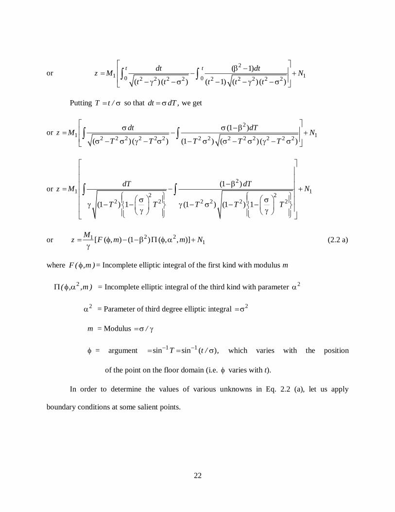
(2.2 a)
where F ( ,m ) = Incomplete elliptic integral of the first kind with modulus m
2( , ,m ) = Incomplete elliptic integral of the third kind with parameter 2
2 = Parameter of third degree elliptic integral 2
m = Modulus /
= argument 1 1sin sin ( )T t / , which varies with the position
of the point on the floor domain (i.e. varies with t).
In order to determine the values of various unknowns in Eq. 2.2 (a), let us apply
boundary conditions at some salient points.

23
BOUNDARY CONDITIONS
(i) Point 0: At point 0, t = 0 and z = 0
1 1sin sin / 0T t
(0, ) 0F m and 20 0, ,m
Hence from (2), we get
0 11[0 0]
MN
From which 1 0N
Hence Eq. (2 a) becomes
z2 21 [ ( , ) (1 ) ( , , )]
MF m m
(2.2)
(ii) Point 4: (Point E): At point 4, 2
Bz and z=
11 1 1sin sin ( / ) sin ( / ) sin 1 / 2T t
( , )F m ,2
F m K
complete elliptic integral of the first kind.
and 2( , , )m 2
0, ,2
m
= complete elliptic integral of the third kind.
Hence from Eq. 2.2, we have
2
B 210[ (1 ) ]
MK
or B21
0
2[ (1 ) ]
MK
(2.3)
or B 12[ ]
ME
(2.3 a)

24
where E 2
0[ (1 ) ]K (2.3 b)
(iii) Point 9: At point 9, z=iD and t
t
sin . Hence argument becomes i so that sin i sinh
Making use of standard identity 161.02 (Bird and Friedman, 1971)
( , )F i m ( , )iF m
where, 1 1tan (sinh ) tan2
( , )F i m ,2
iF m i K
and 2( , , )i m 2 2
2
[ ( , ) ( , , )]
1
i F m m
2
02[ ]
1
iK
where 0 2, ,
2m
complete elliptic integrate of third kind with modulus m' and
parameter 2 .
2 21 and 2m 21 m
Substituting these values in Eq. (2), we get
iD2
2102
(1 ){ }
1
M iiK K
where
or D2
2102
(1 ){ }
1
MK K
(2.4)
or D 1 [ ]M
L
(2.4 a)

25
where L2
2
02
(1 ){ }
1K K
(2.4 b)
(iv) Point 5: At point 5, 2
Bz ic and t =
1 1 1sin sin ( / ) sin ( / )T t .
Hence from Eq. 2.2
2
Bic 1 2 1 21 sin , (1 ) sin , , )
MF m m
Substituting the value of 2
B from Eq. 2.3, we get
210[ (1 ) ]
MK ic
1 2 1 21 sin , (1 ) sin , , )M
F m m
or ic1 2 1 21
0sin , (1 ) sin , , )M
F m K m
(2.5)
In the above equation, the argument of the elliptic integral is given by
1sin / sin ( / )or .
But . Hence sin 1. The argument is therefore complex.
Since 1
sin ,m
we have the following reduction formula:
( , )F m ( , )K iF A m
and 2( , , )m 2
2
0 12( , ) ( , , )
1i F A m A m
where A= new amplitude
2
1 sin 1sin
sinm
2 2 2
1 1( / ) 1sin sin
( / )m m

26
2
12 2
2 21 1
m m
Substituting in Eq. 2.5 we get
ic 2
2 210 1 02
( , ) (1 ) ( , ) ( , , )1
MK iF A m K i F A m A m
or c2
2 2 2112
1( , ) ( , , )
1
MF A m A m
(2.6)
or c 1 [ ]M
G
(2.6 a)
where G2
2 2 2
12
1( , ) ( , , )
1F A m A m
(2.6 b)
(v) Point 6: At point 6, 2
Bz and t
1 1sin / sin ( / ) sin (1/ )t m .
Substituting in Eq. 2.2, we get
2
B 1 2 1 21 1 1sin , (1 ) sin , , )
MF m m
m m
(2.7)
From identity 111.09, Bird and Friedman,
1 1sin ,F m
m
K iK
and 1 21sin , ,m
m
2
0 02 2
mi
m
where 0 2, ,2
m

27
0 2, ,
2m
22 2
2 2
m
m
2
B
221
0 02 2(1 )
M mK iK i
m
Substituting the value of 2
B from Eq. 2.3, we get
210(1 )
MK
2
210 02 2
(1 )M m
K iK im
or 2
2
0 0 02 2{ } (1 ) 0
mK iK K i
m
or 2
2
02 2(1 ) 0
mK
m
Substituting the value of /m and , we get
2(1 )2 2 2 2
2
2 2
00 0
( / ). (1 )
( / )
K m K K
m
1/ 2
2
0
1 (1 )K
(2.8)
Thus, we find that is not an independent variable. Instead, it depends on and . Hence, there
are only two unknowns (i.e., and ) in the t-plane.

28
General Relationship: 1z = f (t)
From Eq. 2.3,
1M2
0
.
2[ (1 ) ] 2
B B
K E
(2.9 a)
Hence from Eq. 2.2
z2 2
2
0
[ ( , ) (1 ) ( , , )]
2[ (1 ) ]
B F m m
K
(2.9)
which is the required relationship 1( )z f t
Floor Profile Ratios
From Eqs. 2.3. and 2.4, we have
B
D
210
221
02
2[ (1 ) ]
1
1
MK
MK K
or B
D
2
0
22
02
2[ (1 ) ] 2
1
1
K E
LK K
(2.10 a)
From Eqs. 2.3. and 2.5., we get
B
c
210
2 22 21
0 12
2[ (1 ) ]
2
(1 )( , ) ( , , )
1
MK
E
GMF A m A m
(2.10 b)
Hence
c
D
2 2B B E E G
D c L G L (2.10 c)

29
2.2.2 Second Transformation
Refer Fig. 2.1 (c).
The Schwarz Christoffel equation for transformation from w-plane to t-plane is
w6 7 812 2
01 6 7 8( ) ( ) ( ) ( )
t dtM N
t t t t t t t t
Here 1 6 7 8
1
2
1 ;t 6 8; 1t t and 7 1t
Hence w1/ 2 1/ 2 1/ 22 21/ 20 ( ) ( ) ( 1) ( 1)
t dtM N
t t t t
or w 2 22 2 20 ( ) ( 1)
t dtM N
t t
Putting /T t so that ,dt dT we get
2
2
w N
M
2 2 2 2 2 20 0( 1) ( 1) (1 ) (1 )
T TdT dT
T T T T
This is the elliptic integral of the first kind (F0) with modulus m0 =
2
2
w N
M
0 ( , )F
where 1 1sin sin ( / )T t
Boundary conditions
(i) Point 0: At point 0, / 2w kH and t = 0
T = t/ = 0
and 1 1sin sin 0 0T and F0 ( ) = F0 (0, ) = 0

30
Hence from Eq. (2.11)
2
2
w N
M
0
From which 2 / 2N w kH (2.12)
Thus, the value of the additive constant N2 is known.
(ii) Point 6: At point 6, w = 0 and t =
T = t / = / =1
1 1sin sin 12
T and 0 0,
2F K
Hence from Eq. 2.11
20
2
0 NK
M
or 2
2
0 02
N kHM
K K (2.13)
Thus, the value of the multiplier constant M2 is also known.
(iii) Point 7: At point 7, w iq and 1t
/ 1/T t and 1 1 1
sin sinT
1
0 0
1sin ,F K iK
Substituting in Eq. 2.11, we get
w 1
2 0 2
1sin ,M F N
or iq 00 0
0 0
[ ]2 2 2
kH KkH kHK i K i
K K

31
Hence q 0
02
kH K
K
(2.14 a)
Seepage discharge factor, 0
02
Kq
kH K
(2.14)
General Relationship 2 ( )w f t
Substituting the values of M2 and N2 in Eq. 2.11, we get
w2 0 2 0
0
( , ) ( , )2 2
kH kHM F N F
K
or w0 0
0
[ ( , ) ]2
kHF K
K (2.15)
which is the required relationship 2 ( )w f t
Uplift pressure distribution
For the base of the apron, 0
xw kh
(i) Point E (point 4)
Ew kh and t
/ /T t
E1sin sinT
Hence from Eq. 2.15, Ekh 1
0 0
0
sin ,2
kHF K
K

32
or Eh
1
0
0
sin ,
12
FH
K
or EP 100 50Eh
H
1
0
0
sin ,
1
F
K
(2.16)
(ii) Point C (point 3)
At point 3, Cw kh and t
T = t / = – /
1 1 1sin ( ) sin sinT
1 1
0 0sin , sin ,F F
Hence from Eq. 2.15, Ckh 1
0 0
0
sin ,2
kHF K
K
or CP 100 50Ch
H
1
0
0
sin ,
1
F
K
(2.17)
From Eqs. 2.16 and 2.17, we note that PE + PC = 100% which is in conformity with the principle
of reversibility of flow.
(iii) Point D (point 5)
Dw kh and t

33
/ /T t and D
1sin sinT
Dkh 1
0 0
0
sin ,2
kHF K
K
From which DP 100 50Dh
H
1
0
0
sin ,
1
F
K
(2.18)
(iv) Point D' (point 2)
Following the same procedure,
DP 50
1
0
0
sin ,
1
F
K
(2.19)
so that 100%D DP P
Exit Gradient
The Schwarz-Christoffel equation for transformation from z-plane to t-plane is
z2 2
1 12 2 2 2 20
( )
( 1) ( ) ( )
t t dtM N
t t t
(2.20)
or dz
dt
2 2
1
2 2 2 2 2
( )
( 1) ( ) ( )
M t
t t t
where 1M2
02[ (1 ) ]
B
K

34
dz
dt 2
0
.2[ (1 ) ]
B
K
2 2
2 2 2 2 2
( )
( 1) ( ) ( )
t
t t t
(2.20 a)
where K is the complete elliptic integral of the first kind with modulus / .
0 2, ,2
complete elliptic integral of third kind with modulus / and
parameter 2 2 .
Similarly, the transformation equation between w and t plane is
w 2 22 2 2( ) ( 1)
dtM N
t t
or dw
dt
2
2 2 2( ) ( 1)
M
t t
where
2
02
kHM
K
dw
dt0
.2
kH
K
2 2 2
1
( ) ( 1)t t (2.20 b)
where K0 is the complete elliptic integral of first kind with modulus
If u and v are the velocity components in x and y directions, we have
Complex velocity .dw dw dt
u ivdz dt dz
For the exit surface, 0u and Ev v
Eiv .dw dt
dt dz
Now from Darcy law, E Ev k G
EG1
. .Ev dw dt
k ik dt dz

35
Substituting the values of dw
dt and
dt
dz, we get
EG
2 2 2 2 22
0
2 22 2 20
( 1) ( ) ( )2[ (1 ) ]1 1. .
2 ( )( )( 1)
t t tKkh
ik K tt t
or EG B
H
22 2 2
0
2 2 2
0
(1 )1.
1
Kt t
t K t
At the exit end, t
EG B
H
22 2 2
0
2 2 2
0
(1 )1.
1
K
K
(2.21)
Now .E
cG
H
EG B c
H B
or E
cG
H
2 22 2
0 1222 2 2
0
2 2 2 2
0 0
(1 )( , ) ( , , )
1(1 )1.
1 2[ (1 ) ]
F A m A mK
K K
(2.22 a)
or E
cG
H
2 2 22 2 2
2 2 2 2 2
0 0
1(1 )( )
2 1 2 ( )
G G
K K
(2.22)
2.3 Computations
Computations were carried out for the determination of the following:
(i) B/D
(ii) B/c
(iii) Uplift pressures at the key points E, D, C and D'.
(iv) Seepage discharge factor, q/kH and

36
(v) Exit gradient factor, GE c/H.
Since Eqs. 2.10 (a) and 2.10 (b) for B/D and B/c ratios, respectively, are not explicit in
transformation parameters, direct solution of these equations for the parameters and ,
corresponding to given values of floor profile ratios (B/D, B/c) is not suitable and practical.
However, these equations can be solved for physical floor profile ratios B/D and B/c, for
assumed values of and . Hence B/D and B/c were computed for values 0 1 . In
the computer programme, was varied from 0.01 to 0.99 in the steps of 0.01. For each
value of , parameter was varied from an initial value of to 0.99 in the steps of 0.01.
Parameter was computed from Eq. 2.8, for each set of values of and . Table 2.1 gives
the specimen results for 0.5
In order to determine the values of and for a given pair of values of B/D and B/c
ratios, both B/D and B/c were separately plotted with and . Fig. 2.2. (a), (b), show the
variation of B/D with and , plotting on x-axis and on various nomographs. The
starting point of each nomograph is not the same, as the minimum value of is .
Similarly, Figs. 2.3(a), (b) show variation of B/c with and . From both these Figs., values
of and were determined for selected values B/D = 0.2, 0.4, 0.6, 0.8, 1, 1.25, 1.5, 1.75, 2,
2.25, 2.5 and 3 and selected values of B/c = 4, 6, 8, 10, 15, 20, 25 and 30.
37
Fig. 2.2a Variation of B/D with σ and γ
Fig. 2.2b Variation of B/D with σ and γ, for γ close to 1

38
Fig. 2.3a Variation of B/c with σ and γ
Fig. 2.3b Variation of B/c with σ and γ, for γ close to 1

39
Table 2.1 Computed Values for 0.5
B/D B/c c/D EP
DP q/kH /EG c H
0.5 0.51 0.505017 0.708 165.67 0.004 6.80 4.80 0.632 0.034
0.5 0.6 0.551977 0.787 17.19 0.046 20.33 14.18 0.570 0.099
0.5 0.7 0.60955 0.884 8.74 0.101 27.33 18.79 0.505 0.129
0.5 0.8 0.676933 0.997 5.74 0.174 32.23 21.78 0.439 0.147
0.5 0.9 0.76523 1.148 4.01 0.286 36.44 24.02 0.363 0.157
0.5 0.91 0.776333 1.167 3.86 0.302 36.88 24.22 0.354 0.158
0.5 0.92 0.788134 1.188 3.71 0.320 37.32 24.41 0.344 0.159
0.5 0.93 0.800776 1.210 3.56 0.339 37.78 24.61 0.334 0.159
0.5 0.94 0.814458 1.234 3.41 0.361 38.26 24.80 0.323 0.159
0.5 0.95 0.829468 1.260 3.26 0.387 38.77 24.99 0.311 0.159
0.5 0.96 0.846252 1.289 3.10 0.416 39.33 25.18 0.298 0.159
0.5 0.97 0.865561 1.323 2.92 0.453 39.95 25.36 0.282 0.158
0.5 0.98 0.888874 1.365 2.72 0.501 40.70 25.55 0.263 0.156
0.5 0.99 0.920035 1.420 2.47 0.575 41.73 25.73 0.235 0.153
The resulting values of and so obtained were plotted against each value of B/D and
B/c (Fig. 2.4) giving rise to double set of nomographs corresponding to the above mentioned
values of B/D and B/c. Fig. 2.4 is helpful in determining the values of and corresponding to
a given set of values of B/D and B/c. In order to obtain more precise values of and , further
iterative programming was done, using the values of and so obtained from Fig. 2.4 as initial
input parameters.
Table 2.2 shows the values of and for the above mentioned sets of B/D and B/c
ratio. Computer programme was re-run using these values of and as input values to confirm
the values of B/D and B/c ratios and also to compute the seepage characteristics, PE, PD, q/kH
and GE c/H. The computed values of these characteristic are also shown in Table 2.2.

40
Fig. 2.4 Determination of σ and γ

41
Table 2.2 Data Generated from Matching the Given Values of B/D and B/c Ratios
B/D B/c c/D EP
DP q/kH /EG c H
0.2
2 0.100 0.048 0.324 0.185 45.38 31.13 0.791 0.212
4 0.050 0.090 0.239 0.165 37.84 25.97 0.893 0.179
6 0.033 0.109 0.210 0.160 32.73 22.61 0.934 0.156
8 0.025 0.120 0.196 0.158 29.18 20.25 0.957 0.141
10 0.020 0.127 0.188 0.157 26.55 18.49 0.971 0.129
15 0.013 0.136 0.177 0.156 22.18 15.52 0.990 0.109
20 0.010 0.141 0.171 0.156 19.43 13.63 1.00 0.096
25 0.008 0.144 0.168 0.156 17.49 12.29 1.006 0.086
30 0.007 0.146 0.166 0.156 16.04 11.28 1.010 0.079
B/D B/c c/D
EP DP q/kH /EG c H
0.4
2 0.200 0.098 0.597 0.365 45.25 30.73 0.572 0.206
4 0.100 0.180 0.454 0.323 37.68 25.74 0.675 0.176
6 0.067 0.217 0.403 0.313 32.58 22.44 0.716 0.155
8 0.050 0.237 0.378 0.309 29.03 20.11 0.739 0.139
10 0.040 0.250 0.363 0.307 26.41 18.36 0.753 0.128
15 0.027 0.267 0.343 0.306 22.06 15.41 0.772 0.108
20 0.020 0.276 0.333 0.305 19.32 13.54 0.782 0.095
25 0.016 0.282 0.327 0.305 17.40 12.21 0.788 0.086
30 0.013 0.285 0.323 0.305 15.95 11.21 0.792 0.079
B/D B/c c/D EP DP q/kH /EG c H
0.6
2 0.300 0.153 0.790 0.534 45.05 30.09 0.446 0.197
4 0.150 0.269 0.630 0.467 37.43 25.39 0.550 0.172
6 0.100 0.320 0.568 0.452 32.33 22.17 0.592 0.152
8 0.075 0.348 0.536 0.447 28.80 19.88 0.614 0.137
10 0.060 0.366 0.516 0.444 26.19 18.16 0.628 0.126
15 0.040 0.389 0.490 0.441 21.87 15.26 0.647 0.106
20 0.030 0.402 0.478 0.440 19.15 13.40 0.656 0.094
25 0.024 0.409 0.470 0.440 17.24 12.09 0.662 0.085
30 0.020 0.414 0.465 0.440 15.81 11.10 0.666 0.078

42
B/D B/c c/D EP
DP q/kH /EG c H
0.8
2 0.400 0.214 0.905 0.685 44.78 29.24 0.358 0.186
4 0.200 0.356 0.762 0.594 37.12 24.94 0.465 0.167
6 0.133 0.418 0.698 0.574 32.02 29.83 0.506 0.149
8 0.100 0.451 0.664 0.567 28.50 19.59 0.528 0.135
10 0.080 0.471 0.643 0.563 25.92 17.91 0.542 0.124
15 0.053 0.500 0.615 0.560 21.62 15.05 0.560 0.105
20 0.040 0.514 0.600 0.558 18.93 13.22 0.570 0.092
25 0.032 0.522 0.592 0.558 17.04 11.93 0.575 0.084
30 0.027 0.528 0.586 0.558 15.62 10.95 0.579 0.077
B/D B/c c/D EP
DP q/kH /EG c H
1
2 0.500 0.283 0.964 0.808 44.48 28.28 0.292 0.173
4 0.250 0.440 0.853 0.700 36.75 24.43 0.401 0.162
6 0.167 0.508 0.795 0.676 31.66 21.44 0.442 0.145
8 0.125 0.544 0.763 0.668 28.16 19.26 0.464 0.132
10 0.100 0.566 0.743 0.663 25.59 17.61 0.477 0.121
15 0.067 0.596 0.714 0.659 21.33 14.81 0.495 0.103
20 0.050 0.611 0.700 0.658 18.67 13.02 0.505 0.091
25 0.040 0.620 0.691 0.657 16.80 11.75 0.510 0.082
30 0.033 0.626 0.685 0.657 15.40 10.79 0.514 0.076
B/D B/c c/D EP DP q/kH /EG c H
1.25
2 0.625 0.383 0.992 0.915 44.11 27.03 0.228 0.157
4 0.313 0.539 0.924 0.804 36.27 23.75 0.340 0.155
6 0.208 0.608 0.879 0.777 31.18 20.91 0.381 0.140
8 0.156 0.645 0.851 0.767 27.70 18.81 0.402 0.128
10 0.125 0.667 0.833 0.762 27.15 17.21 0.415 0.118
15 0.083 0.696 0.808 0.758 20.94 14.48 0.433 0.100
20 0.063 0.711 0.795 0.756 18.31 12.73 0.442 0.089
25 0.050 0.719 0.787 0.755 16.47 11.49 0.448 0.080
30 0.042 0.725 0.782 0.755 15.09 10.55 0.451 0.074

43
B/D B/c c/D EP DP q/kH /EG c H
1.5
2 0.750 0.492 0.999 0.972 43.92 25.90 0.177 0.138
4 0.375 0.630 0.963 0.877 35.80 23.08 0.293 0.147
6 0.250 0.694 0.930 0.851 30.69 20.38 0.334 0.135
8 0.188 0.728 0.909 0.840 27.22 18.35 0.355 0.123
10 0.150 0.748 0.895 0.836 24.69 16.80 0.368 0.114
15 0.100 0.775 0.874 0.831 20.53 14.14 0.385 0.097
20 0.075 0.788 0.863 0.829 17.94 12.44 0.394 0.086
25 0.060 0.796 0.856 0.828 16.13 11.22 0.399 0.078
30 0.050 0.801 0.851 0.828 14.77 10.31 0.402 0.072
B/D B/c c/D EP DP q/kH /EG c H
1.75
4 0.438 0.710 0.983 0.926 35.38 22.45 0.256 0.140
6 0.292 0.766 0.961 0.902 30.22 19.86 0.296 0.130
8 0.219 0.795 0.945 0.893 26.75 17.90 0.317 0.119
10 0.175 0.813 0.934 0.888 24.24 16.39 0.329 0.111
15 0.117 0.836 0.918 0.883 20.12 13.80 0.346 0.095
20 0.088 0.847 0.909 0.882 17.56 12.14 0.355 0.084
25 0.070 0.854 0.903 0.881 15.79 10.96 0.360 0.076
30 0.058 0.858 0.900 0.881 14.45 10.06 0.363 0.070
B/D B/c c/D EP DP q/kH /EG c H
2
4 0.500 0.777 0.993 0.958 35.03 21.89 0.225 0.134
6 0.333 0.823 0.979 0.937 29.79 19.38 0.266 0.125
8 0.250 0.848 0.968 0.929 26.32 17.47 0.286 0.116
10 0.200 0.862 0.960 0.925 23.80 16.00 0.298 0.107
15 0.133 0.881 0.947 0.921 19.72 13.47 0.315 0.092
20 0.100 0.891 0.940 0.919 17.19 11.85 0.323 0.082
25 0.080 0.896 0.936 0.918 15.44 10.69 0.328 0.074
30 0.067 0.900 0.933 0.918 14.13 9.82 0.331 0.068

44
B/D B/c c/D EP
DP q/kH /EG c H
2.25
4 0.562 0.832 0.997 0.977 34.79 21.40 0.199 0.127
6 0.375 0.868 0.989 0.960 29.41 18.94 0.240 0.121
8 0.281 0.888 0.981 0.953 25.91 17.07 0.260 0.112
10 0.225 0.900 0.975 0.950 23.40 15.63 0.272 0.104
15 0.150 0.915 0.966 0.946 19.34 13.16 0.288 0.089
20 0.133 0.922 0.961 0.945 16.84 11.57 0.296 0.079
25 0.090 0.927 0.958 0.944 15.11 10.44 0.301 0.072
30 0.075 0.930 0.956 0.944 13.82 9.59 0.304 0.066
B/D B/c c/D EP
DP q/kH /EG c H
2.5
4 0.625 0.876 0.999 0.988 34.66 20.98 0.177 0.121
6 0.417 0.903 0.994 0.976 29.09 18.54 0.218 0.117
8 0.312 0.918 0.989 0.970 25.54 16.69 0.238 0.109
10 0.250 0.927 0.985 0.967 23.02 15.28 0.250 0.101
15 0.167 0.939 0.979 0.964 18.98 12.86 0.266 0.087
20 0.125 0.945 0.975 0.963 16.51 11.30 0.273 0.077
25 0.100 0.959 0.972 0.962 14.80 10.20 0.278 0.070
30 0.083 0.951 0.971 0.962 13.53 9.36 0.281 0.065
B/D B/c c/D EP DP q/kH /EG c H
3
8 0.375 0.957 0.996 0.988 24.94 16.06 0.204 0.102
10 0.300 0.963 0.995 0.986 22.35 14.65 0.215 0.096
15 0.200 0.970 0.991 0.984 18.34 12.32 0.230 0.083
20 0.150 0.973 0.989 0.983 15.90 10.82 0.237 0.074
25 0.120 0.975 0.988 0.983 14.23 9.76 0.241 0.067
30 0.100 0.976 0.987 0.983 12.99 8.95 0.244 0.062

45
2.4 Design Charts
Table 2.2 also gives the values of uplift pressures PE and PD at key points, as well as the
values of seepage discharge factor (q/kH) and exit gradient factor GE c/H. These results are used
to create design charts. Figs. 2.5, 2.6, 2.7 and 2.8 show design charts for PE, PD, GE c/H and q/kH
respectively. From these charts, it is observed that when / 0.2B D , the values of PE, PD and GE
c/H approach those for the infinite depth case. The corresponding values of infinite depth case,
analyzed by Malhotra (1936), are shown by dotted curve on these charts.

46
Fig 2.5 Design curves for PE

47
Fig 2.6 Design curves for PD
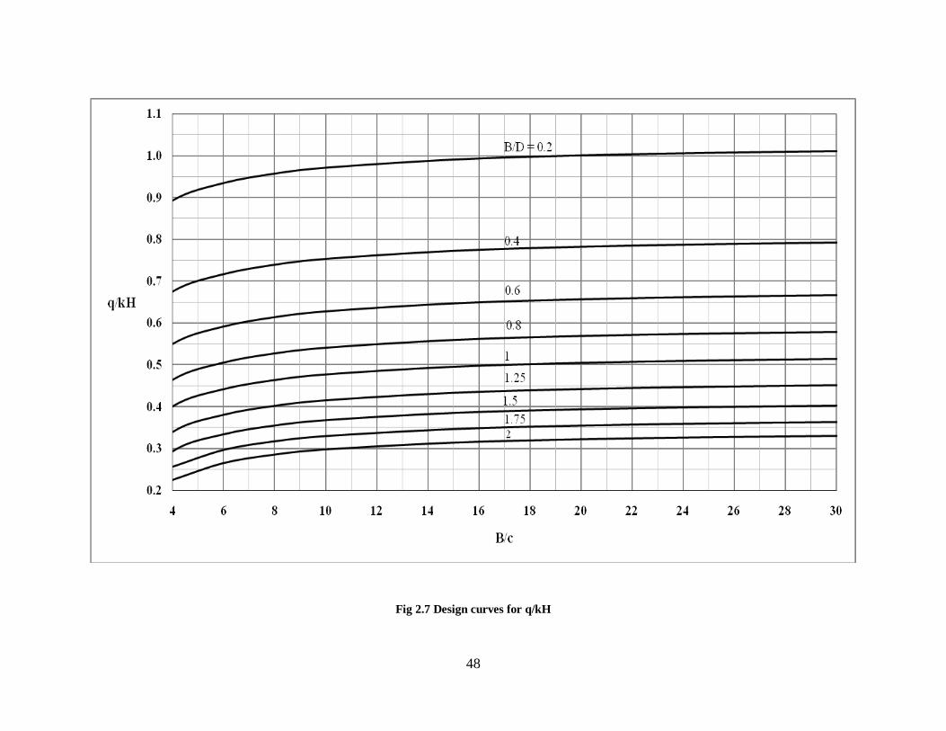
48
Fig 2.7 Design curves for q/kH

49
Fig 2.8 Design curves for GEc/H

50
2.5 Comparison with Infinite Depth Case
Malhotra (1936) obtained theoretical solution for uplift pressure below flat apron with
equal end cutoffs, founded on pervious medium of infinite depth. The results of the present
theoretical solution for B/D=0.4 and B/D = 0.2 were compared with those of Malhotra's solution.
Table 2.3 gives the values of uplift pressure PE at point E and PD at point D for some selected
values of B/c ratios. It is seen from Table 2.3 as well as from Fig. 2.5, 2.6 and 2.7 that when
/ 0.2,B D the results from both the analyses are practically the same.
Table 2.3 Comparison with Infinite Depth Case
B/c
%Pressure PE at point E % Pressure PD at point D
Infinite
Depth case by
Malhotra
Present
Analysis
for
B/D=0.2
Present
Analysis
for
B/D=0.4
Infinite
Depth
case by
Malhotra
Present
Analysis
for
B/D=0.2
Present
Analysis
for
B/D=0.4
3 41.4 41.3 41.1 28.4 28.2 28.0
4 37.9 37.8 37.7 26.1 26.0 25.7
6 32.9 32.7 32.6 22.7 22.6 22.4
8 29.2 29.2 29.0 20.3 20.3 20.1
12 24.6 24.5 24.4 17.2 17.1 17.0
24 17.8 17.8 17.7 12.6 12.5 12.4
2.6 Development of Interference Formulae
Since 1936, the prevalent practice has been to use the design curve or equation given by
Khosla et al. for the case of apron with end cutoff and apply interference formula suggested by
him to take into account the effect of presence of another cutoff at the upstream side when the
depth of pervious medium is infinite. A similar effort has been made here to develop interference
equations for the seepage characteristics to take into account the effect of presence of cutoff at

51
the upstream end. The equations for PE, PD and GE c/H for the case of apron with downstream
cutoff, developed by Pavlovsky are quite explicit and are amenable to direct computations while
the equations developed in the present analysis for the case of cutoff at both the ends are not
explicit. However, the above seepage characteristics can first be computed by Pavlovsky's
equations and the interference formulae given below can be applied to take into account the
effect of upstream cutoff.
For any seepage characteristic (such as PE, PD, GE c/H), we have
( )EPI [( ) ( ) ]E SP E DPP P
( )DPI [( ) ( ) ]D SP D DPP P
and /( )
EG c HI [( / ) ( / ) ]E SP E DPG c H G c H (2.23)
where I stands for interference correction, SP stands for single pile case and DP stands for
double pile case. Since computed values of these characteristics are available both for double
pile case, as well as single pile case (Pavlovsky), the values of interference corrections (I) were
found for B/D = 0.8, 1, 1.5 and 2 and for B/c = 4, 6, 8, 10, 12, 15, 20 and 30. Table 2.4 gives the
computed interference values. Figs. 2.9, 2.10 and 2.11 shows curves between interference values
(I), on y-axis, B/c values on x-axis and B/D values on nomographs, for ,E DP P and / .EG c H
From these curves, equations for interference correction were developed in the following form:
( )SCI
nB
aC
(2.24)
where ( )SCI Interference correction for any seepage characteristic
a = Multiplying factor
n = Power factor

52
Table 2.4 Interference Values (I)
B/D B/c ( )EPI ( )
DPI (I)Q/KH /( )
EG c HI
0.8
4 5.547 3.465 0.057 0.022
6 3.136 2.047 0.042 0.014
8 2.070 1.381 0.033 0.009
10 1.495 1.009 0.027 0.007
15 0.822 0.564 0.019 0.004
20 0.537 0.371 0.014 0.003
25 0.385 0.267 0.012 0.002
30 0.293 0.204 0.010 0.001
1
4 5.794 3.644 0.056 0.023
6 3.259 2.135 0.041 0.014
8 2.146 1.434 0.032 0.010
10 1.547 1.046 0.026 0.007
15 0.849 0.583 0.018 0.004
20 0.554 0.383 0.014 0.003
25 0.397 0.276 0.011 0.002
30 0.303 0.211 0.009 0.001
1.5
4 6.556 4.127 0.052 0.026
6 3.610 2.364 0.038 0.016
8 2.352 1.571 0.030 0.010
10 1.685 1.138 0.024 0.008
15 0.917 0.629 0.017 0.004
20 0.595 0.412 0.013 0.003
25 0.426 0.296 0.010 0.002
30 0.324 0.226 0.009 0.002
2
4 7.938 5.202 0.046 0.027
6 4.044 2.647 0.035 0.017
8 2.541 1.674 0.028 0.011
10 1.784 1.182 0.023 0.008
15 0.942 0.629 0.016 0.005
20 0.598 0.400 0.012 0.003
25 0.419 0.280 0.010 0.002
30 0.313 0.209 0.008 0.002

53
Fig. 2.9 Interference Correction for PE

54
Fig. 2.10 Interference Correction for PD

55
Fig. 2.11 Interference Correction for E
G c H/

56
Thus, for a given seepage characteristic (such as PE), four such equations (one for each
value of B/D ratio) were developed. Table 2.5 gives the factors a and n for various seepage
characteristics, for each chosen value of B/D ratio.
Table 2.5 Values of Factors a and n
B/D Factors for PE Factors for PD Factors for GE c/H
a n a n a n
0.8 42.955 1.463 25.516 1.413 0.157 1.374
1 45.135 1.469 27.056 1.422 0.167 1.383
1.5 52.406 1.494 31.424 1.447 0.191 1.406
2.0 71.284 1.597 45.860 1.585 0.202 1.405
To apply the interference correction, let us take a case of B/D= 1 and B/c= 10. For these
values, c/D = 0.1. Hence from the direct solution of Pavlovsky's equations, we get the following
values for the case of apron with cutoff at downstream end.
EP 27.14%, 18.66%DP and . / 0.128EG c H
From Table 2.5 the factors a and n for PE for B/D=1 are 45.135 and 1.469 respectively.
Hence
( )PEI 1.169( / ) 45.135(10)na B c 1.53%
Since the provision of pile at the upstream end reduces the pressure at E, the above
interference correction is negative.
Hence ( )E DPP ( ) ( ) 27.14 1.53 25.61%E SP SPP I
Value of PE obtained by the present analysis of apron with cutoffs at both the ends is
25.59%. For this excellent agreement, the interference formula can be applied with sufficient

57
degree of accuracy. Similar computations can be done for pressure at point D (i.e. PD) and exit
gradient factor GE. c/H without the need for solving the exact equations of implicit nature.
2.7 Development of Simplified Equations for PE, PD and GEc/H
In the design curves given in Figs. 5, 6 and 8, linear interpolation is required for
intermediate values of B/D ratios. In order to avoid this, the following algebraic equations have
been developed, based on computer generated values for various values of B/D and B/c.
EP0.035( / )0.037 0.422
68.74B De
B B
D c
(2.25)
DP0.0240.411/( / )
0.114( / )
49.865
( )
B DB D B
ec
(2.26)
and E
cG
H
0.42260.0378( / )
0.214( / )
0.354
( )
B D
B D
B
ce
(2.27)
In order to illustrate the use of the above equations, taking
B/D = 2 and B/c = 20, we get
EP0.035(2)0.037 0.422
68.7417.27%
(2) (20) e
which agrees well with the value of 17.19% computed from rigorous analysis of this case.
DP0.0240.114 2 0.411/(2)
49.86511.83%
(2) (20)
which agrees well with the value of 11.85% computed from rigorous analysis of this case.
E
cG
H
0.42260.0378(2)
0.214(2)
0.354.(20) 0.0816
( )e

58
which agrees well with the value of 0.082 computed from rigorous analysis of this case.
Thus, the values computed by the use of above simplified equations match closely with
the values computed from the rigorous analyses of this chapter. Table 2.6 gives the values of
values of PE computed from the simplified formula as well as from rigorous analysis, along with
the difference in two values for various pairs of values of B/D and B/c. From this table, we find
that the difference between the computed and actual values is well within two percent.
Table 2.6 Comparison of Values of PE from the Formula
Calculated values of PE from the formula
B/D → 0.6 0.8 1 1.25 1.5 1.75 2
B/c
6 32.37 31.85 31.42 30.94 30.52 30.14 29.77
8 28.59 28.11 27.7 27.26 26.86 26.49 26.14
10 25.97 25.52 25.13 24.7 24.32 23.96 23.63
15 21.81 21.4 21.05 20.66 20.31 19.98 19.67
20 19.26 18.89 18.56 18.2 17.87 17.56 17.27
Actual values of PE from rigorous analysis
B/D → 0.6 0.8 1 1.25 1.5 1.75 2
B/c
6 32.33 32.02 31.66 31.18 30.69 30.22 29.79
8 28.8 28.5 28.16 27.7 27.21 26.75 26.32
10 26.19 25.92 25.59 25.15 24.69 24.24 23.8
15 21.87 21.62 21.33 20.94 20.53 20.12 19.72
20 19.15 18.93 18.67 18.31 17.94 17.56 17.19
% Difference = 100(Actual – Calculated)/Actual
B/D → 0.6 0.8 1 1.25 1.5 1.75 2
B/c
6 -0.12 0.53 0.76 0.77 0.55 0.26 0.07
8 0.73 1.37 1.63 1.59 1.29 0.97 0.68
10 0.84 1.54 1.80 1.79 1.50 1.16 0.71
15 0.27 1.02 1.31 1.34 1.07 0.70 0.25
20 -0.57 0.21 0.59 0.60 0.39 0.00 -0.47

59
2.8 Conclusions
The general solution to the finite depth seepage under an impervious flat apron with equal
end cutoffs is obtained using the method of conformal transformation. The results obtained from
the solution of implicit equations have been used to present design charts for seepage
characteristics, such as uplift pressures at key points, discharge factor and exit gradient factor, in
terms of non-dimensional floor profile ratios. When the depth of permeable soil is large, the
numerical solutions tend toward the values given by the established solution for infinite depth.
Since the equations derived for various seepage characteristics involve elliptic integrals,
simplified algebraic equations have also been suggested, results from which are in excellent
agreement with those obtained through rigorous solutions.
60
CHAPTER 3. FLAT APRON WITH UNEQUAL END CUTOFFS AND A STEP AT
DOWNSTREAM END
3.1. Introduction
Flat aprons of hydraulic structures are invariably provided with cutoffs at both upstream
and downstream ends. The cutoff at the downstream end of apron safeguards the structure both
against exit gradient as well as scour though it increases uplift pressure all along the upstream
side. The cutoff at the upstream end protects the apron against scour and at the same time
reduces the uplift pressure all along the downstream side. In addition to these, pervious aprons
are provided at the downstream side of end cutoff in the form of inverted filter and launching
apron. In order to accommodate the thickness of these pervious aprons, the downstream bed is
excavated resulting in the formation of a step at the downstream end.
3.2. Theoretical Analysis
Fig 3.1(a) shows the floor profile in z-plane, with relative values of stream function and
potential function on the boundaries. Fig 3.1(c) shows the well known w-plane, relating and
. The points in z and w-planes are denoted by complex coordinates z = x + iy and w = + i
respectively in which 1i .The problem is solved by transforming both the z-plane and w-
plane onto an infinite half plane, t-plane, shown in Fig. 3.1(b), thus obtaining z = f1 (t) and
w = f2 (t).

61
Floor Parameters
The floor of the hydraulic structure, shown in Fig. 3.1(a), has the following floor
parameters:
(i) Length of the apron : B
(ii) Finite depth of pervious medium : D
(iii) Depth of upstream cutoff : c1
(iv) Depth of downstream cutoff : c2
(v) Depth of downstream step : a
The resulting independent non-dimensional floor profile ratios are:
1. B/D 2. B/c2 3. c1/c2, and 4. a/c2

62
Fig. 3.1
Illustrations of the problem – Schwarz Christoffel transformations

63
3.2.1 First Transformation
The Schwarz-Christoffel equation for transformation of the floor from z-plane to t-plane
is given by
z7 81 2
1 1
1 2 7 8( ) ( ) ........( ) ( )
dtM N
t t t t t t t t
(3.1 a)
where 1 2 2/ / ; 1 1 2/
2 2 ; 2 1
3 2 2/ / ; 3 1 2
4 2 2/ / ; 4 1 2
5 2 ; 5 1
6 2 2/ / ; 6 1 2
7 0 ; 7 1
8 0 ; 8 1
Substituting the values of 's , we get
z 1 11/ 2 1 1/ 2 1/ 2 1 1/ 2 1 11 2 3 4 5 6 7 8( ) ( ) ( ) ( ) ( ) ( ) ( ) ( )
dtM N
t t t t t t t t t t t t t t t t
or z 2 51 1
7 8 1 3 4 6
( ) ( )
( ) ( ) ( ) ( )( ) ( )
t t t t dtM N
t t t t t t t t t t t t
(3.1)
This is an elliptic integral.
Referring to Identity 254, Byrd and Friedman (1971),
Let 2sn u 4 1 3
4 3 1
( ) ( )
( ) ( )
t t t t
t t t t
(i a)
Such that 2m 4 3 6 1
4 1 6 3
( ) ( )
( ) ( )
t t t t
t t t t
(i b)
Differentiating Eq. (i a)
2 sn u cn u dn u du 1 34 12
4 3 1
( ) ( )( )
( ) ( )
t t t tt tdt
t t t t
Substituting the values of sn u, cn u, dn u and noting that

64
cnu21 sn u and 2 2dn 1 sn ,u m u we get
dt 4 1 3 4 1 3
4 3 1 4 3 1
( ) ( ) ( ) ( )2 . 1
( ) ( ) ( ) ( )
t t t t t t t tdu
t t t t t t t t
2
4 3 6 1 4 1 3 4 3 1
4 1 6 3 4 3 1 4 1 3 1
( ) ( ) ( ) ( ) ( ) ( )1 .
( ) ( ) ( ) ( ) ( ) ( )
t t t t t t t t t t t t
t t t t t t t t t t t t
Simplifying and rearranging, we get
1 3 4 6 4 1 6 3
2
( ) ( ) ( ) ( ) ( ) ( )
dt du
t t t t t t t t t t t t
(ii)
Again from Eq. (i a)
3
1
t t
t t
24 3
4 1
snt t
ut t
or 3t t 2 24 3 4 31
4 1 4 1
sn snt t t t
t u t ut t t t
From which
t
24 33 1
4 1
24 3
4 1
sn
1 sn
t tt t u
t t
t tu
t t
For any point having co-ordinate ,mt we have
mt t
24 33 1
4 1
24 3
4 1
( ) ( ) sn
1 sn
m m
t tt t t t u
t t
t tu
t t

65
Hence 2( )t t
24 33 2 1 2
4 1
24 3
4 1
( ) ( ) sn
1 sn
t tt t t t u
t t
t tu
t t
(a)
5( )t t
24 33 5 1 5
4 1
24 3
4 1
( ) ( ) sn
1 sn
t tt t t t u
t t
t tu
t t
(b)
7( )t t
24 33 7 1 7
4 1
24 3
4 1
( ) ( ) sn
1 sn
t tt t t t u
t t
t tu
t t
(c)
and 8( )t t
24 33 8 1 8
4 1
24 3
4 1
( ) ( ) sn
1 sn
t tt t t t u
t t
t tu
t t
(d)
Hence 2 5
7 8
( ) ( )
( ) ( )
t t t t
t t t t
2 24 3 4 33 2 1 2 3 5 1 5
4 1 4 1
2 24 3 4 33 7 1 7 3 8 1 8
4 1 4 1
( ) ( ) sn ( ) ( ) sn
( ) ( ) sn ( ) ( ) sn
t t t tt t t t u t t t t u
t t t t
t t t tt t t t u t t t t u
t t t t
(iii)
Let 3 2 1t t a 2 1 1( )t t b
3 5 2t t a 5 1 2( )t t b
3 7 3t t a 7 1 3( )t t b
3 8 4t t a 8 1 4( )t t b

66
and 24 3
4 1
snt t
u pt t
Hence R.H.S. of Eq. (iii) 1 1 2 2
3 3 4 4
( ) ( )
( ) ( )
a b p a b p
a b p a b p
2
1 2 1 2 1 2 1 22
3 4 3 4 4 3 3 4
( )
( )
b b p p a b b a a a
b b p p a b a b a a
Numerator 21 23 4 3 4 4 3 3 4
3 4
( )b b
b b p p a b a b a ab b
3 4 1 2 3 41 2 1 2
1 2 1 2
( )b b a a b b
p a b b ab b b b
3 4 4 3 3 4( )p a b a b a a
R.H.S.
1 3 4 2 3 4 1 2 3 43 4 4 3 3 4
1 2 1 21 22
3 4 3 4 3 4 4 3 3 4
1( )
a b b a b b a a b bp a b a b a a
b b b bb b
b b b b p p a b a b a a
1 2 3 1 2 3 41 2 41 2 1 2 1 2
3 4 3 41 2
3 4 3 3 4 4( ) ( )
b b a b b a ab b ap a b b a a a
b b b bb b
b b a b p a b p
1 2 1 2
3 4 3 3 4 4( ) ( )
b b p
b b a b p a b p
(iv)
where 1 = coefficient of 1 2 3 1 2 41 2 1 2
3 4
b b a b b ap a b b a
b b
2 = constant term 1 2 3 41 2
3 4
b b a aa a
b b

67
Now let 1 2
3 3 4 4( ) ( )
p
a b p a b p
3 3 4 4
A B
a b p a b p
(iv a)
4 3 4 3
3 3 4 4
( ) ( )
( ) ( )
p Ab Bb Aa Ba
a b p a b p
Hence we get 1 4 3Ab Bb
and 2 4 3Aa ba
From the above the equations, we have
A 3 31 2
3 4 3 4 3 4 3 4
a b
a b b a a b b a
and B 4 41 2
3 4 3 4 3 4 3 4
a b
b a a b b a a b
Substituting the values of 1 and 2, we get
A 3 1 2 3 3 1 2 3 41 2 41 2 1 2 1 2
3 4 3 4 3 4 3 4 3 4 3 4
a b b a b b b a ab b aa b b a a a
a b b a b b a b b a b b
2 21 2 4 3 3 3 1 2 3 43 3 1 2 3 3 1 2 1 2 3 3 1 2
3 3 4 3 4 4 4
1
( )
b b a a b b b b a aa b a b a b b a b b a b a a
b a b b a b b
2 23 3 1 2 3 3 1 2 1 2 3 1 2 3
3 3 4 3 4
1
( )a b a b a b b a b b a a a b
b a b b a
2 3 2 3 3 1 3 1
3 3 4 3 4
( ) ( )
( )
a b b a a b b a
b a b b a
Similarly,
B 1 2 3 1 2 3 44 1 2 4 41 2 1 2 1 2
3 4 3 4 3 4 3 4 3 4 3 4
b b a b b a aa b b a ba b b a a a
b a a b b b b a a b b b
2 24 4 1 2 3 1 2 3 4 4
4 4 1 2 4 4 1 2 1 2 4 4 1 24 3 4 3 4 3 3
1
( )
a b b b a b b a a ba b a b a b b a b b a b a a
b b a a b b b

68
2 24 4 1 2 4 4 1 2 1 2 4 1 2 4
4 3 4 3 4
1
( )a b a b a b b a b b a a a b
b b a a b
2 4 2 4 4 1 4 1
4 3 4 3 4
( ) ( )
( )
a b b a a b b a
b b a a b
Substituting the values of A and B in Eqs. (iv) and (iv a), we get
R.H.S. of Eq. (4) 2 3 2 3 3 1 3 11 2 2 4 2 4 4 1 4 1
3 4 3 3 4 3 4 3 3 4 3 4 3 4 4 4
( )( ) ( )( )
( )( ) ( )( )
a b b a a b b ab b a b b a a b b a
b b b a b b a a b p b b a a b a b p
(v)
= p + q + r
Substituting the values of a1, a2........etc., we get
p 2 1 5 11 2
3 4 7 1 8 1
( )( )
( ) ( )
t t t tb b
b b t t t t
(v a)
q 2 3 2 3 3 1 3 1
3 3 4 3 4 3 3
( )( )
( )( )
a b b a a b b a
b a b b a a b p
3 5 7 1 5 1 3 7 3 7 2 1 7 1 3 2
7 1 3 7 3 7 8 1 7 1 3 8 27 1 4 3
7 3 4 1
( )( ) ( )( ) [( ) ( ) ( )( )]
( ) ( )[( )( ) ( ) ( )]1 sn
t t t t t t t t t t t t t t t t
t t t t t t t t t t t t t t t tu
t t t t
3 7 5 7 3 1 5 1 5 3 1 3 5 7 1 7 3 2 7 2 3 1 7 1 7 3 1 3 7 2 1 2
27 1 4 37 1 3 7 3 8 7 8 3 1 7 1 7 3 1 3 7 8 1 8
7 3 4 1
[ ][ ]
( ) ( )[ ] 1 . sn
t t t t t t t t t t t t t t t t t t t t t t t t t t t t t t t t
t t t tt t t t t t t t t t t t t t t t t t t t u
t t t t
3 1 7 5 2 7 3 1
27 1 4 37 1 3 7 3 1 8 7
7 3 4 1
( )( ) ( )( )
( ) ( )( ) ( ) 1 sn
t t t t t t t t
t t t tt t t t t t t t u
t t t t
7 5 3 1 2 7
27 1 4 37 1 8 7 3 7
7 3 4 1
( )( ) ( )
( ) ( )( ) 1 sn
t t t t t t
t t t tt t t t t t u
t t t t
7 5 7 2 3 12 2
7 1 8 7 7 3 2
( )( ) ( )
( ) ( )( )[1 sn ]
t t t t t t
t t t t t t u
(v b)

69
where 22
7 1 4 3
7 3 4 1
.t t t t
t t t t
r 2 4 2 4 4 1 4 1
4 3 4 3 4 4 4
( )( )
( )( )
a b b a a b b a
b b a a b a b p
3 5 8 1 5 1 3 8 3 8 2 1 8 1 3 2
8 1 3 8 7 1 3 8 3 7 8 1 28 1 4 3
8 3 4 1
[( )( ) ( )( )] [( ) ( ) ( )( )]
( ) ( )[( ) ( ) ( )( )]1 sn
t t t t t t t t t t t t t t t t
t t t t t t t t t t t t t t t tu
t t t t
3 8 5 8 3 1 5 1 5 3 1 3 5 8 1 8
8 1 3 8 7 3 1 3 7 8 1 8 3 8 7 8 3 1 7 1
[ ]
( ) ( )[ ]
t t t t t t t t t t t t t t t t
t t t t t t t t t t t t t t t t t t t t
3 2 8 2 3 1 8 1 8 3 1 3 8 2 1 2
28 1 4 3
8 3 4 1
1 . sn
t t t t t t t t t t t t t t t t
t t t tu
t t t t
8 5 3 1 8 2 1 3
8 1 3 8 7 8 3 1 28 1 4 3
8 3 4 1
( )( ) ( )( ) 1
( ) ( )( ) ( )1 sn
t t t t t t t t
t t t t t t t t t t t tu
t t t t
8 5 8 2 3 12 2
8 1 8 3 7 8 1
( )( ) ( )
( ) ( )( )[1 sn ]
t t t t t t
t t t t t t u
(v c)
where 21
8 1 4 3
8 3 4 1
t t t t
t t t t
Again, from Eqs. 3.1 and 3.3, we have
z 2 51 1
7 8 4 1 6 3
( ) ( ) 2
( ) ( ) ( ) ( )
t t t t duM N
t t t t t t t t
or z 2 511
7 84 1 6 3
( ) ( )2
( ) ( )( ) ( )
t t t tMdu N
t t t tt t t t
or z 11
4 1 6 3
2(R.H.S. of Eq. )
( ) ( )
Miii du N
t t t t

70
or z 22 1 5 1 7 5 7 2 3 112
7 1 8 1 7 1 8 7 7 34 1 6 3
( ) ( ) ( ) ( ) ( )2( , , )
( ) ( ) ( ) ( ) ( )( ) ( )
t t t t t t t t t tMu u m
t t t t t t t t t tt t t t
28 5 8 2 3 11 1
7 8 8 3 8 1
( ) ( ) ( )( , , )
( ) ( ) ( )
t t t t t tu m N
t t t t t t
or z 22 1 5 1 3 1 8 5 8 211
7 1 8 1 7 8 8 3 8 14 1 6 3
( ) ( ) ( ) ( )2( , , )
( ) ( ) ( ) ( )( ) ( )
t t t t t t t t t tMu u m
t t t t t t t t t tt t t t
27 5 7 22 1
7 1 7 3
( ) ( )( , , )
( ) ( )
t t t tu m N
t t t t
Again, 2sn u 4 1 3
4 3 1
( ) ( )
( ) ( )
t t t t
t t t t
u 1 4 1 3
4 3 1
( ) ( )sn ( , )
( ) ( )
t t t tF m
t t t t
where 1 4 1 3
4 3 1
( ) ( )sin
( ) ( )
t t t t
t t t t
and 2( , , )u m 2( , , )m
z 22 1 5 1 3 1 8 5 8 211
7 1 8 1 7 8 8 3 8 14 1 6 3
( ) ( ) ( ) ( ) ( )2( , ) ( , , )
( ) ( ) ( ) ( ) ( )( ) ( )
t t t t t t t t t tMF m m
t t t t t t t t t tt t t t
27 5 7 22 1
7 1 7 3
( ) ( )( , , )
( ) ( )
t t t tm N
t t t t
(vi)
Here, we observe from t-plane that
1 1t 5 2t
2 1t 6 2t
3t 7 1t
4t 8 1t

71
Substituting in Eq. (7), we get
21 1 1 2 1 1 2 11
1 1 11 2
2 ( )( ) ( ) ( 1 )( 1 )( , ) ( , , )
(1 )( 1 ) 2 ( 1 )( 1 )( )( )
Mz F m m
22 12 1
1
(1 )(1 )( , , )
(1 )(1 )m N
(3.2 a)
or z2 2
1 1 1 1 1 2 1[ F( , ) ( , , ) ( , , )]M A m B m C m N (3.2)
where 1A 1 1 1 2
1 1 1 2
2( ) ( ) 1
(1 )(1 ) ( ) ( )
(3.3a)
1B 1 1 2
1 1 2
( ) (1 )(1 ) 1
(1 )(1 ) ( ) ( )
(3.3b)
1C 1 1 2
1 1 2
( ) (1 )(1 ) 1
(1 )(1 ) ( ) ( )
(3.3c)
2sn u 1 1
1 1
( ) ( ) ( ) ( )
( )( ) 2 ( )
t t
t t
(3.4a)
1 11 1
1 1
( ) ( ) ( ) ( )sin sin
( )( ) 2 ( )
t t
t t
(3.4b)
and 2m 2 1 1 2
1 2 1 2
( ) ( ) 2 ( )
( )( ) ( ) ( )
(3.4c)
21( , , )m =Third degree elliptic integral with amplitude , parameter
21 and
modulus m
22( , , )m =Third degree elliptic integral with amplitude , parameter
22 and
modulus m
21
8 1 4 3 1 1
8 3 4 1 1 1
( ) ( ) 1 12 2.
( ) ( ) 1 1
t t t t
t t t t
(3.5 a)

72
22
7 1 4 3 1
7 3 4 1 1
( ) ( ) 1 2
( ) ( ) 1
t t t t
t t t t
(3.5 b)
In Eq. 3.2 there are seven unknown parameters : 1 2 1 2, , , , , 1M and 1N and hence
seven equations are required to determine these, which can be obtained from boundary
conditions at points 3, 4, 2, 5, 1, 6 and 9. The simultaneous solutions of these equations would
yield the values of the unknown parameters in the t-plane in terms of floor parameters of z-plane.
Boundary conditions
(i) Point 3 (Point E1):
At point 3, z = – B/2 and t = –
1 11
1
( ) ( )sin sin (0) 0
2 ( )
( , )F m (0, ) 0F m and 2( , , )m 2(0, , ) 0m
Hence from Eq. 3.2, / 2B 1 1[0]M N
From which 12
BN (3.6)
(2) Point 4 (Point E):
At point 4, / 2z B and t
1 11
1
( ) ( )sin sin 1
2 ( ) 2
( , )F m ,2
F m K
and 2( , , )m 2 2
0, , ( , )2
m m

73
where 0 = complete elliptic integral of third kind.
Hence from Eq. 3.2
/ 2B 2 21 1 1 0 1 1 0 2[ ( , ) ( , )] / 2M A K B m C m B
or 2 21 1 1 0 1 1 0 2 1[ ( , ) ( , )]B M A K B m C m M R (3.7)
where 1M2 2
1 1 0 1 1 0 2( , ) ( , )
B B
RA K B m C m
(3.8 a)
and R2 2
1 1 0 1 1 0 2( , ) ( , )A K B m C m (3.8 b)
(3) Point 7:
At point 7, z = and t = + 1. Hence the point that is mapped into t = + 1 is a simple pole
of integrand (3.1).
iD 11( 1). ( ).
ti M Lt t f t dt
Here ( )f t 2 57
7 8 1 3 4 6
( ) ( ), where 1
( ) ( ) ( )( ) ( )( )
t t t tt
t t t t t t t t t t t t
( 1) ( )t f t 2 5
8 1 3 4 6
( ) ( )
( ) ( )( ) ( ) ( )
t t t t
t t t t t t t t t t
1 2
1 2
( ) ( )
( 1) ( )( ) ( ) ( )
t t
t t t t t
iD 1i M 1 2
1 2
(1 ) (1 )
(1 1) (1 )(1 ) (1 ) (1 )
D 1
2
M 1 2
1
1 2
(1 ) (1 )
(1 )(1 ) (1 ) (1 )M J
(3.9)
where J1 2
D
M
1 2
1 2
(1 ) (1 )
(1 )(1 ) (1 ) (1 )
(3.9 a)

74
(4) Point 6:
At point 6, z = B/2 + i a and t = 2
1 11 2
1 2
( ) ( ) 1sin sin
2 ( ) m
1 1sin ,F m K iK
m
and 2
1 2 2 20 02 2
1sin , , ( , ) ( , )
imm m m
m m
where 22 2
2 2
m
m
Hence from Eq. 3.2, we get
2
Bia
22 2
1 1 1 0 1 0 12 21
( ) ( , ) ( , )im
M A K iK B m mm
2
2 21 0 2 0 22 2
2
( , ) ( , )2
im BC m m
m
where 21
2 212 2
1
m
m
and 2
22 222 2
2
m
m
B ia 2 21 1 1 0 1 1 0 2[ ( , ) ( , )]M A K B m C m
2 2
2 21 1 1 0 1 1 0 22 2 2 2
1 2
( , ) ( , )m m
i M A K B m C mm m
Separating real and imaginary parts, we get
B2 2
1 1 1 0 1 1 0 2 1[ ( , ) ( , )] .M A K B m C m M R
(which is the same as Eq. 3.7)
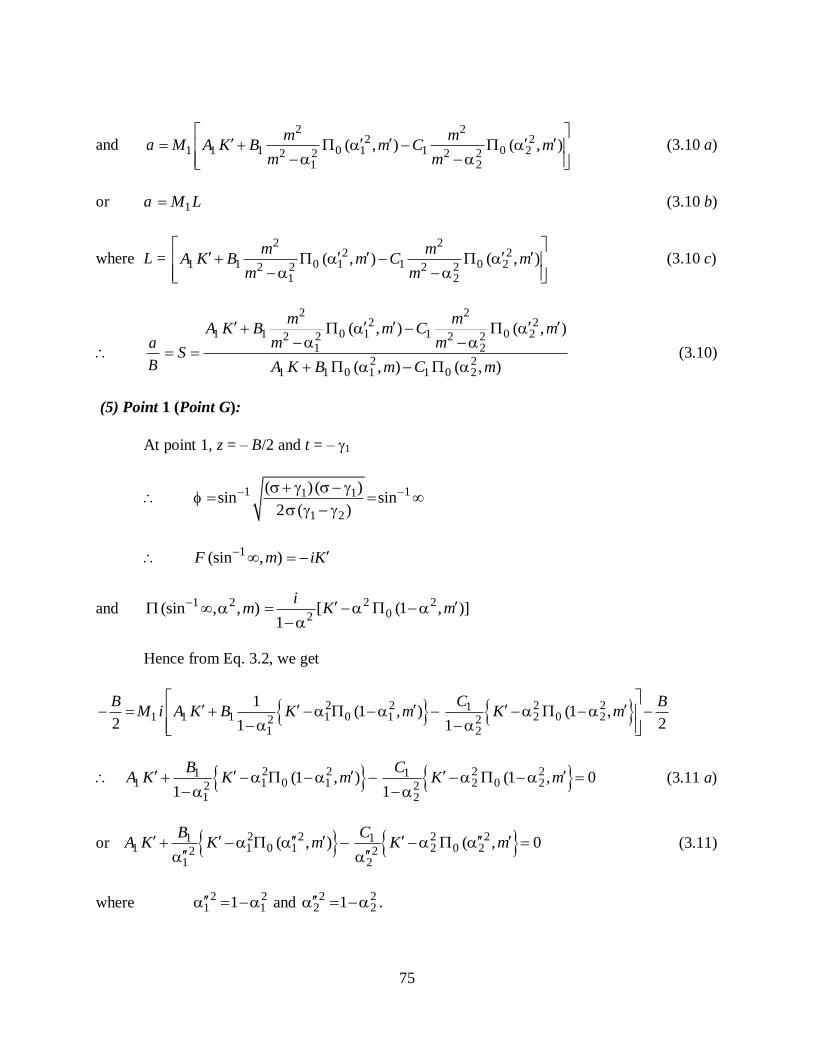
75
and a2 2
2 21 1 1 0 1 1 0 22 2 2 2
1 2
( , ) ( , )m m
M A K B m C mm m
(3.10 a)
or a 1M L (3.10 b)
where L = 2 2
2 21 1 0 1 1 0 22 2 2 2
1 2
( , ) ( , )m m
A K B m C mm m
(3.10 c)
a
B
2 22 2
1 1 0 1 1 0 22 2 2 21 2
2 21 1 0 1 1 0 2
( , ) ( , )
( , ) ( , )
m mA K B m C m
m mS
A K B m C m
(3.10)
(5) Point 1 (Point G):
At point 1, z = – B/2 and t = – 1
1 11 1
1 2
( ) ( )sin sin
2 ( )
1(sin , )F m iK
and 1 2(sin , , )m 2 2
02[ (1 , )]
1
iK m
Hence from Eq. 3.2, we get
2 2 2 211 1 1 1 0 1 2 0 22 2
1 2
1(1 , ) (1 ,
2 21 1
CB BM i A K B K m K m
2 2 2 21 11 1 0 1 2 0 22 2
1 2
(1 , ) (1 , 01 1
B CA K K m K m
(3.11 a)
or 2 2 2 21 11 1 0 1 2 0 22 2
1 2
( , ) ( , 0B C
A K K m K m
(3.11)
where 2
1211 and
2 22 21 .

76
(5) Point 5 (Point D):
At point 5, z = B/2+ i c2 and t = + 2
1 11 2
1 2
( ) ( )sin sin
2 ( )y
where 1
1ym
Hence from Identity 115.02, Byrd and Friedman (1971)
( , )F m ( , )K i F m
and 2( , , )m 2 2
20 2 2
( , ) ( , ) , ,1 1
mm i F m m
where 2 2
1 1
2 2
1 1sin sin
y y
m y m y
1 2
1 1 2
1 2 1 2
1 2 1 2
( ) ( )1
2 ( )sin
2 ( ) ( )( )1
( )( ) 2 ( )
1 1 2 1 2
1 2 1 21 2
1 2
( ) ( ) 2 ( )sin
( )( ) 2 ( )( )( )
( )( )
2
1 1 2 1 2 22
21 2 1 2
sin
1 11 2 2 1 2 2
1 2 2 1 2 2
( )( ) ( ) ( )( ) ( )sin sin
( )( ) ( ) ( )( ) ( )
or 1 2 2
2 2
( ) ( )sin
( ) ( )

77
Hence from Eq. 3.2.
22
Bic
2 22 1
1 1 1 0 1 2 21 1
( , ) ( , ) ( , ) , ,1 1
mM A K iF m B m i F m m
2 22 2
1 0 2 2 22 2
( , ) ( , ) , ,21 1
m BC m i F m m
Separating real and imaginary parts, we get
2 21 1 1 0 1 1 0 2 1[ ( , ) ( , )]B M A K B m C m M R
(as found earlier in Eq. 3.7)
and 2c2 2
1 11 1 1 1 2 2
1 1
[ ( , ){ } , ,1 1
B mM F m A B C m
2 22
1 2 22 2
, ,1 1
mC m
(3.12)
or 2c 1M T (3.12 a)
where T2
21 11 1 1 32
1
( , ){ } ( , , )1
F m A B C m
222
1 422
( , )1
C m
(3.12 b)
23
2
211
m
and 2
42
221
m
(7) Point 2 (Point D1):
At point 2, z = – B/2 + i c1 and t = – 1
11 1 1 1
1 1 1 1
( ) ( ) ( ) ( )sin sin
2 ( ) 2 ( )i
1sin y , where 1
1 1
( ) ( )
2 ( )y ix i

78
Since y = i x, the upper limit of is imaginary.
Hence becomes i
sin i i x or sinhi i x
x sinh
( , )F i m ( , )i F m
and 2( , , )i m 2 2
2[ ( , ) ( ,1 , )]
1
iF m m
where 1 1tan (sinh ) tan x
or 1 1
1 1
( ) ( )tan
2 ( )
Hence from Eq. 3.2.
12
Bic 2 21
1 1 1 121
( , ) ( , ) ( ,1 , )1
B iM A iF m F m m
2 212 22
2
( , ) ( ,1 ,21
C i BF m m
1c2 2
2 21 1 1 1 1 21 1 1 22 2 2 2
1 2 1 2
( , ) ( ,1 , ) ( ,1 , )1 1 1 1
B C B CM F m A m m
(3.13)
or 1c = M1 . P (3.13 a)
2 22 21 1 1 1 1 2
1 1 22 2 2 21 2 1 2
where ( , ) ( ,1 , ) ( ,1 , )1 1 1 1
B C B CP F m A m m
(3.13 b)

79
General Relationship: 1( )z f t
From Eq. 3.8 (a)
1M2 2
1 1 0 1 1 0 2( , ) ( , )
B
A K B m C m
Hence from Eq. 3.2
z2 2
1 1 1 1 22 2
1 1 0 1 1 0 2
[ F( , ) ( , , ) ( , , )]
2( , ) ( , )
B A m B m C m B
A K B m C m
which is the required relationship 1( )z f t
Determination of Floor Profile Ratios
There are five parameters in z-plane:
(i) Length of the apron, B
(ii) Finite depth of pervious medium, D
(iii) Depth of upstream cutoff, 1c
(iv) Depth of downstream cutoff, 2c , and
(v) Depth of downstream scour a
Consequently, we have the following non-dimensional floor profile ratios:
(1) B/D (2) 2/B c (3) 1 2/c c , and (4) 2/a c
From Eqs. 3.9 and 3.10a,
1 1 1( )D D a M J M L M J L
Hence from above equation and Eq. 3.7, we get
1
1( )
M RB R
D M J L J L
(3.14)

80
From Eqs. 3.7 and 3.12a,
1
2 1
M RB R
c M T T (3.15)
From Eqs. 3.13a and 3.12a,
1 1
2 1
c M P P
c M T T (3.16)
Also, 2 2
a a B RS
c B c T (3.17)
where R, J, L and T are given by Eqs. 3.8b, 3.9a, 3.10c and 3.12b respectively.
Determination of 1 and 2
From Eq. 3.10, we have
2 22 2
1 1 0 1 1 0 22 2 2 21 2
2 21 1 0 1 1 0 2
( , ) ( , )
( , ) ( , )
m mA K B m C m
m m aS
BA K B m C m
or 2 2
2 21 1 0 1 1 0 22 2 2 2
1 2
( , ) ( , )m m
A K B m C mm m
2 21 1 0 1 1 0 2[ ( , ) ( , )]S A K B m C m
or 2
2 21 1 0 1 0 12 2
1
{ } ( , ) ( , )m
A K SK B m S mm
22 2
1 0 2 0 22 22
( , ) ( , ) 0m
C m S mm
Substituting the values of 1 1,A B and 1C and cancelling common terms,

81
22 21 1 1 2 1 1 2
0 1 0 12 21 1 1 1
2( )( ) ( )(1 )(1 ){ } ( , ) ( , )
(1 ) (1 ) (1 ) (1 )
mK SK m S m
m
22 21 1 2
0 2 0 22 21 2
( )(1 )(1 )( , ) ( , ) 0
(1 ) (1 )
mm S m
m
2 1 1 1 2 2 1 2 2 1 2( )( ) (1 )(1 ) (1 )(1 ) 0A B C (I)
where 2A1 1
2( )
(1 )(1 )
K SK
(3.18 a)
22 21
2 0 1 0 12 21 1
( )( , ) ( , )
(1 ) (1 )
mB m S m
m
(3.18 b)
22 21
2 0 2 0 22 21 2
( )( , ) ( , )
(1 ) (1 )
mC m S m
m
(3.18 c)
Again, From Eq. 3.11, we have
2 2 2 21 11 1 0 1 2 0 22 2
1 2
( , ) ( , 0B C
A K K m K m
(where 21
211 and 2 2
1 21 )
Substituting the values of 1 1,A B and C1 and cancelling common terms,
2 21 1 1 2 1 1 21 0 12
1 1 1 1
2( )( ) ( )(1 )(1 ) 1. ( , )
(1 ) (1 ) (1 ) (1 )K K m
2 21 1 22 0 22
1 2
( )(1 )(1 ) 1. ( , ) 0
(1 ) (1 )K m
or 3 1 1 1 2 3 1 2 3 1 2( )( ) (1 )(1 ) (1 )(1 ) 0A B C (II)
where 3A1 1
2
(1 )(1 )
K
(3.19 a)

82
2 213 1 0 12
1 1
( )( , )
(1 ) (1 )B K m
(3.19 b)
and 2 213 2 0 22
1 2
( )( , )
(1 ) (1 )C K m
(3.19 c)
Thus, we get the following two simultaneous equations from which 1 and 2 can be
computed for each pair of values of 1 2( , , and S):
2 1 1 1 2 2 1 2 2 1 2( )( ) (1 )(1 ) (1 )(1 ) 0A B C (I)
and 3 1 1 1 2 3 1 2 3 1 2( )( ) (1 )(1 ) (1 )(1 ) 0A B C (II)
From (I), 22 1 2 1 1 2 1 2 2 1 2 2 2 1 2 2 2 1 2( ) ( )A A A A B B B B
2 2 1 2 2 2 1 2( ) 0C C C C
or 21 2 1 2 2 2 2 1 2 2 1 2 2 2 2 2 1 2 2( ) ( ) ( ) ( ) 0A B C A B C A B C A B C
or 2
2 2 2 2 1 2 21 2 1 2
2 1 2 2 2 1 2 2
0A B C A B C
A B C A B C
or 1 2 1 1 2 2 0P P (III)
where 1P 2 2 2
2 1 2 2
A B C
A B C
(3.20 a)
2P2
2 1 2 2
2 1 2 2
A B C
A B C
(3.20 b)
Also, from (II), 2
3 1 3 1 1 3 1 2 3 1 2 3 3 1 3 2 3 1 2( ) ( )A A A A B B B B
3 3 1 3 2 3 1 2( ) 0C C C C
or 2
1 3 1 3 3 2 3 1 3 3 1 2 3 3 3 3 1 3 3( ) ( ) ( ) ( ) 0A B C A B C A B C A B C

83
or 2
3 3 3 3 1 3 31 2 1 2 2
3 1 3 3 3 1 3 3
0A B C A B C
A B C A B C
or 1 2 1 1 2 2 0Q Q (IV)
where 1Q 3 3 3
3 1 3 3
A B C
A B C
(3.21 a)
2Q2
3 1 3 3
3 1 3 3
A B C
A B C
(3.21 b)
Hence we have following two simultaneous equations:
1 2 1 1 2 2 0P P (III)
and 1 2 1 1 2 2 0Q Q (IV)
where values of 1 2,,P P Q and 2Q are now known.
Adding (III) and (IV), we get
1 2 1 1 2 2( )P Q P Q
or 2 2
1 21 1
P Q
P Q
From which 22 2
1 1 1
1.
P Q
P Q
(V)
Substituting the values of 2 and 12 in (IV), we get
12 2 2 2
1 21 1 1 1 1
10
P Q P QQ Q
P Q P Q
or 2 2 2 2 21 1 2 1
1 1 1 1
0P Q P Q
Q QP Q P Q
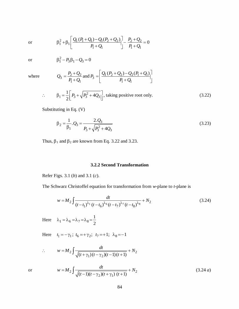
84
or 2 1 1 1 1 2 2 2 21 1
1 1 1 1
( ) ( )0
Q P Q Q P Q P Q
P Q P Q
or 21 3 1 3 0P Q
where 2 2 1 2 2 2 1 13 3
1 1 1 1
( ) ( )and
P Q Q P Q Q P QQ P
P Q P Q
12
3 3 3
14
2P P Q
, taking positive root only. (3.22)
Substituting in Eq. (V)
23
32
1 3 3 3
2.1.
4
P P Q
(3.23)
Thus, 1 and 2 are known from Eq. 3.22 and 3.23.
3.2.2 Second Transformation
Refer Figs. 3.1 (b) and 3.1 (c).
The Schwarz Christoffel equation for transformation from w-plane to t-plane is
w6 7 81
2 2
1 6 7 8( ) ( ) ( ) ( )
dtM N
t t t t t t t t
(3.24)
Here 1 6 7 8
1
2
Here 1t 1 6 2 7 8; ; 1; 1t t
w 2 2
1 2( ) ( )( 1) ( 1)
dtM N
t t t t
or w 2 2
2 1( 1)( )( ) ( 1)
dtM N
t t t t
(3.24 a)

85
Using Identity 254, Byrd and Friedman (1971) and noting that
2 11, ,a b c and d = – 1 for the present purpose,
we have
2sn u 2 1
2 1
( 1)( )( ) ( )
( ) ( ) ( ) ( 1)
tb d t c
b c t d t
20m 1 2
1 2
2( )( ) ( )
( ) ( ) (1 ) (1 )
b c a d
a c b d
and 1 1 2 1
2 1
( 1)( )( ) ( )sin sin
( ) ( ) ( ) ( 1)
tb d t c
b c t d t
Differentiating,
2 sn u cn u dn u du 2 12
1 2
1 1
(1 )dt
t
Substituting the values of sn u, cn u, dn u in the above and noting that cn
u 21 sn u and 2 20dn 1 snu m u , we get
dt2
1 2 2 1 2 1
2 1 1 2 1 2
( ) (1 ) ( 1) ( ) ( 1)( )2 1
( 1) (1 ) ( ) ( 1) ( ) ( 1)
t t tdu
t t
1 2 2 1
1 2 1 2
2( ) (1 ) ( )1
(1 ) (1 ) ( ) ( 1)
t
t
or dt2
1 2 2 1 1 2 1 2 2 1 2 1
2 1 1 2 1 2
( )(1 ) (1 )( )2
(1 )(1 ) ( )( 1) ( ) ( 1)
t t t t t tdu
t t
1 1 1
1
1 2 2
(1 ) ( 1)
t t t
t

86
or dt2
1 2 2 1 1 2 1
2 1 1 2 1 2 1
( )( 1) (1 )( ) (1 )( ) (1 )(1 )2
(1 )(1 ) ( )( 1) ( ) ( 1) (1 )( 1)
t t t tdu
t t t
or dt 1 2
2 1
(1 )( ) ( ) (1 )2
(1 ) (1 )
t t t tdu
or 1 2(1 ) ( ) ( ) (1 )
dt
t t t t 1 2
2
(1 ) (1 )
du
or 2 1 1 2
2
( 1) ( )( )( 1) (1 ) (1 )
dt du
t t t t
Substituting in Eq. 3.24 (a) we get
w12
201 2
2
(1 ) (1 )
uMdu N
or 2
2
w N
M
1
1 2
2
(1 ) (1 )u
or 2
2
w N
M
10
1 2
2sn (sin , )
(1 ) (1 )m
or 2
2
w N
M
0 0
1 2
2( , )
(1 ) (1 )F m
(3.25)
where 1 2 1
1 2
(1 ) ( )sin
( ) ( 1)
t
t
(3.25 a)
Boundary Conditions
(i) Point 1: At point 1, w kH and 1t
1sin (0) 0
0 ( , )F m (0, ) 0F m
Hence from (ii) 2 0w N

87
or 2N w kH (3.26)
(ii) Point 6: At point 6, 0w and 2t
1 12 2 1
1 2 2
(1 ) ( )sin sin (1)
( ) ( 1) 2
0 ( , )F m 0 0 0,2
F m K
where modulus 1 20
1 2
2( )
(1 ) (1 )m
Hence from Eq. 3.25
2
0 kH
M
0
1 2
2
(1 ) (1 )K
2M 1 20
(1 )(1 )2
kH
K (3.27)
Hence the transformation equation becomes
w 0 0 00
[ ( , ) ]kH
F m KK
(3.28)
Seepage Discharge
At point 7, w iq and 1t
71 12 1
1 2 0
(1 ) (1 ) 1sin sin
( ) (1 1) m
0 7 0( , )F m 10 0 0
0
1sin ,F m K iK
m
Hence from Eq. 3.28

88
iq 0 0 00
[ ]kH
K iK KK
q 0
0
KkH
K
or q
kH
0
0
K
K
(3.29)
Pressure Distribution
For the base of the apron, xw kh
w 0 0 00
[ ( , ) ]x
kHkh F m K
K
Let xP 100 %xh
H pressure at any point below the apron.
xP 0 0 00
100[ ( , ) ]F m K
K
or xP 0 0
0
( , )100 1
F m
K
(3.30)
(i) At point 6 (Point R): 2t
R1 12 1 2
1 2 2
(1 ) ( )sin sin 1
( ) ( 1) 2
0 0( , )RF m 0 0 0,2
F m K
Hence RP 0
0
100 1 0,K
K
as expected.

89
(ii) At point 4 (point E): t
E1 2 1
1 2
( 1) ( )sin
( ) (1 )
(3.31 a)
Hence EP 0 0
0
( , )100 1 EF m
K
(3.31)
(iii) At point 3 (point E1): t
1E1 2 1
1 2
(1 ) ( )sin
( ) (1 )
(3.32 a)
and 1EP 0 1 0
0
( , )100 1 EF m
K
(3.32)
(iv) Point 1 (point G): 1t
G 0 00; ( , ) 0GF m
GP 100% , as expected
(v) Point 5 (point D): 2t
D1 2 2 1
1 2 2
(1 ) ( )sin
( ) ( 1)
(3.33 a)
DP 0 0
0
( , )100 1 DF m
K
(3.33)
(vi) Point 2 (point D1): 1t
1D1 2 1 1
1 2 1
(1 ) ( )sin
( ) (1 )
(3.34 a)

90
1DP 0 1 0
0
( , )100 1 DF m
K
(3.34)
Exit Gradient
The Schwarz-Christoffel equation for transformation from z-plane to t-plane is
dz
dt
2 51
7 8 1 3 4 6
( ) ( )
( ) ( ) ( ) ( ) ( ) ( )
t t t tM
t t t t t t t t t t t t
where 1t 1 2 1 3 4, , ;t t t
5t 2 6 2 7 8; ; 1; 1t t t
dz
dt
1 21
1 2
( ) ( )
( 1) ( 1) ( ) ( ) ( ) ( )
t tM
t t t t t t
or dz
dt
1 21
2 2 21 2
( ) ( )
( 1) ( ) ( )( )
t tM
t t t t
where 1M2 2
1 1 0 1 1 0 2( , ) ( , )
B B
RA K B m C m
and R2 2
1 1 0 1 1 0 2( , ) ( , )A K B m C m
Hence dz
dt
1 2
2 2 21 2
( ) ( ).( 1) ( ) ( )( )
t tB
R t t t t
Similarly, the transformation equation between w and t plane is
dw
dt
2
21 2( 1) ( )( )
M
t t t
where 2M 1 20
(1 )(1 )2
kH
K
dw
dt1 2
20 1 2
1(1 ) (1 )
2 ( 1) ( )( )
kH
K t t t

91
If u and v are the velocity components in x and y directions, we have
Complex velocity dw
dz.
dw dtu iv
dt dz
At the exit end, u = 0 and v = vE
.E
dw dti v
dt dz
Now, from Darcy law, vE = k GE
EG1
. .Ev dw dt
k ik dt dz (3.35)
Substituting the values of dw
dt and
dt
dz, we get
EG
2 2 21 21 2
20 1 21 2
( 1) ( )( )( )(1 ) (1 )1
2 ( ) ( )( 1)( )( )
t t t tkH R
ik K B t tt t t
or EG B
H
2 2 21 2
20 1 2
(1 ) (1 )(1 ) ( )
2 ( ) ( ) 1
tR t
K t t t
Now 2EG c
H
2 2. whereE
c cB TG
H B B R
2EG c
H
2 2 21 2
20 1 2
(1 ) (1 )(1 ) ( )
2 ( ) ( ) 1
tR T t
K R t t t
or 2E
cG
H
2 2 21 2
20 1 2
(1 ) (1 )(1 ) ( ).
2 ( ) ( ) 1
tT t
K t t t
At the exit end, 2t
2E
cG
H
2 2 22 1 2 2
20 2 1 2 2 2
(1 ) (1 )(1 ) ( ).
2 ( ) ( ) 1
T
k
(3.36 a)

92
or 2E
cG
H
2 2 21 2 2 2
0 2 1 2 2
(1 )(1 )(1 )( ).
2 ( ) ( )
T
K
(3.36)
3.3 Computations and Results
Eqs. 3.14, 3.15 and 3.16 for floor profile ratios B/D, B/c2 and c1/c2 are not explicit in
transformation parameters , 1 and 2. Hence direct solution of these equations for the
parameters , 1 and 2 corresponding to given set of values of floor profile ratios (B/D, B/c2 and
c1/c2) are extremely difficult. However, these equations can be solved for physical floor profile
ratios B/D, B/c2 and c1/c2 for some assumed values of , 1 and 2 and for some selected values of
step ratio 2( / )a c . Hence B/D, B/c2 and c1/c2 were first computed for values of 1 20 1
corresponding to pre-selected values of step ratios a/c2=0.1, 0.2, 0.3 and 0.4. The parameters 1
and 2 were computed from Eqs. 3.22 and 3.23, for each set of values of , 1 and 2 and step
ratio a/c2. From these values of floor profile ratios, iterative procedures were developed to
compute the values of , 1 and 2 (and then of 1 and 2) for chosen pair of values of B/D, B/c2
and c1/c2 ratios, corresponding to each pre-selected values of step ratio (a/c2). The corresponding
values of various seepage characteristics, such as PE, PD, PE1, PD1, q/kH and GE c2/H were
computed from Eqs. 3.31, 3.33, 3.32, 3.34, 3.29 and 3.36 respectively. Table 3.1 gives the
resulting values.
Comparison with Infinite Depth case (when c1 = c2 = c and a/c2 = 0)
Malhotra (1936) obtained the theoretical solution for uplift pressure below flat apron with
equal end cutoffs (c1 = c2 = c) for the case of infinite depth of pervious foundation. The results of
the present theoretical solution for B/D = 0.4 and B/D =0.2 were compared with those of
Malhotra's solution. Table 3.2 gives the values of uplift pressure PE at point E (Fig. 3.1 a) and PD

93
at point D, for selected values of B/c ratios. It is seen from Table 3.2 that when / 0.2B D , the
results of both the analyses are practically the same.
Table 3.2. Comparison with Malhotra's case of Infinite Depth.
B/c ratio
% Pressure PE at E % Pressure PD at point D
Infinite
Depth case
by Malhotra
Present
analysis for
B
0.2D
Present
analysis for
B
0.4D
Infinite
Depth case
by Malhotra
Present
analysis for
B
0.2D
Present
analysis for
B
0.4D
3 41.4 41.3 41.1 28.4 28.2 28.0
4 37.9 37.8 37.7 26.1 26.0 25.7
6 32.9 32.7 32.6 22.7 22.6 22.4
8 29.2 29.2 29.0 20.3 20.3 20.1
12 24.6 24.5 24.4 17.2 17.1 17.0
24 17.8 17.8 17.7 12.6 12.5 12.4
Effect of step on downstream side
Fig. 3.2 (a) shows the effect of increase in step ratio (a/c2) on PE, the uplift pressure at
point E when B/c2 = 10 and c1/c2=0.4. Fig. 3.2 (b) shows the effect of increase in step ratio on
PD. Similarly, Figs. 3.3 (a), 3.3 (b), 3.4 (a) and Fig. 3.4 (b) show the variation of PE1, PD1, q/kH
and GE c2/H, respectively, with increase in step ratio (a/c2) at the downstream side, for B/c2=10
and c1/c2=0.4, for different values of B/D ratios.

94
Table 3.1 Computed values for B/D = 0.2, a/c2 = 0.1
B/D B/c2 c1/c2 a/c2 σ β1 β2 γ1 γ2 PE PD PE1 PD1 q/kH GEc2/H
0.2 5 0.2 0.1 0.1215 0.1335 0.1818 0.1456 0.2370 37.41 25.16 83.85 88.64 0.9641 0.1919
0.2 10 0.2 0.1 0.1376 0.1437 0.1677 0.1498 0.1956 27.11 18.53 87.92 91.48 0.9977 0.1431
0.2 15 0.2 0.1 0.1433 0.1474 0.1634 0.1515 0.1821 22.30 15.33 89.96 92.91 1.0090 0.1190
0.2 20 0.2 0.1 0.1463 0.1494 0.1614 0.1524 0.1754 19.39 13.36 91.23 93.81 1.0147 0.1039
0.2 5 0.4 0.1 0.1158 0.1400 0.1761 0.1640 0.2314 36.67 24.70 77.28 84.10 0.9537 0.1886
0.2 10 0.4 0.1 0.1346 0.1468 0.1647 0.1590 0.1927 26.83 18.35 82.96 88.03 0.9920 0.1418
0.2 15 0.4 0.1 0.1413 0.1495 0.1614 0.1577 0.1801 22.15 15.23 85.83 90.02 1.0051 0.1182
0.2 20 0.4 0.1 0.1448 0.1509 0.1599 0.1571 0.1739 19.29 13.30 87.61 91.27 1.0116 0.1034
0.2 5 0.6 0.1 0.1105 0.1467 0.1706 0.1827 0.2258 35.92 24.24 72.33 80.74 0.9434 0.1853
0.2 10 0.6 0.1 0.1317 0.1500 0.1618 0.1683 0.1898 26.56 18.17 79.20 85.42 0.9862 0.1404
0.2 15 0.6 0.1 0.1394 0.1516 0.1595 0.1638 0.1781 22.00 15.13 82.68 87.83 1.0011 0.1174
0.2 20 0.6 0.1 0.1433 0.1525 0.1584 0.1617 0.1724 19.19 13.23 84.85 89.34 1.0086 0.1029
0.2 5 0.8 0.1 0.1054 0.1536 0.1652 0.2014 0.2203 35.17 23.77 68.23 78.01 0.9331 0.1819
0.2 10 0.8 0.1 0.1289 0.1533 0.1590 0.1776 0.1869 26.28 17.99 76.05 83.27 0.9804 0.1391
0.2 15 0.8 0.1 0.1374 0.1538 0.1575 0.1700 0.1762 21.85 15.03 80.04 86.01 0.9971 0.1167
0.2 20 0.8 0.1 0.1418 0.1541 0.1569 0.1663 0.1709 19.09 13.16 82.54 87.73 1.0056 0.1024

95
Table 3.1 (contd.) Computed values for B/D = 0.5; a/c2 = 0.1
B/D B/c2 c1/c2 a/c2 σ β1 β2 γ1 γ2 PE PD PE1 PD1 q/kH GEc2/H
0.5 5 0.2 0.1 0.2976 0.3254 0.4319 0.3528 0.5424 37.24 24.92 84.07 88.81 0.6757 0.1890
0.5 10 0.2 0.1 0.3335 0.3473 0.4004 0.3610 0.4593 26.91 18.35 88.06 91.59 0.7096 0.1413
0.5 15 0.2 0.1 0.3463 0.3555 0.3908 0.3646 0.4308 22.12 15.18 90.07 93.00 0.7208 0.1176
0.5 20 0.2 0.1 0.3529 0.3597 0.3862 0.3665 0.4164 19.22 13.23 91.32 93.88 0.7265 0.1028
0.5 5 0.4 0.1 0.2846 0.3402 0.4200 0.3937 0.5319 36.49 24.45 77.55 84.34 0.6656 0.1855
0.5 10 0.4 0.1 0.3268 0.3544 0.3940 0.3815 0.4533 26.63 18.16 83.15 88.17 0.7039 0.1399
0.5 15 0.4 0.1 0.3418 0.3601 0.3865 0.3782 0.4266 21.96 15.07 85.98 90.14 0.7170 0.1168
0.5 20 0.4 0.1 0.3495 0.3632 0.3829 0.3768 0.4133 19.11 13.16 87.75 91.37 0.7235 0.1022
0.5 5 0.6 0.1 0.2722 0.3555 0.4083 0.4340 0.5215 35.72 23.96 72.62 81.02 0.6554 0.1821
0.5 10 0.6 0.1 0.3202 0.3617 0.3877 0.4017 0.4473 26.35 17.98 79.41 85.60 0.6982 0.1385
0.5 15 0.6 0.1 0.3374 0.3649 0.3822 0.3917 0.4225 21.81 14.97 82.85 87.97 0.7131 0.1160
0.5 20 0.6 0.1 0.3462 0.3667 0.3797 0.3869 0.4101 19.01 13.09 85.01 89.46 0.7205 0.1017
0.5 5 0.8 0.1 0.2604 0.3714 0.3970 0.4733 0.5113 34.93 23.48 68.51 78.31 0.6452 0.1785
0.5 10 0.8 0.1 0.3138 0.3690 0.3816 0.4218 0.4415 26.06 17.79 76.28 83.47 0.6926 0.1371
0.5 15 0.8 0.1 0.3330 0.3697 0.3779 0.4052 0.4184 21.65 14.86 80.23 86.16 0.7091 0.1152
0.5 20 0.8 0.1 0.3429 0.3703 0.3765 0.3970 0.4070 18.91 13.02 82.71 87.87 0.7175 0.1012

96
Table 3.1 (contd.) Computed values for B/D = 1; a/c2 = 0.1
B/D B/c2 c1/c2 a/c2 σ β1 β2 γ1 γ2 PE PD PE1 PD1 q/kH GEc2/H
1.0 5 0.2 0.1 0.5522 0.5940 0.7341 0.6329 0.8435 36.76 24.20 84.75 89.33 0.4674 0.1803
1.0 10 0.2 0.1 0.6020 0.6216 0.6920 0.6405 0.7604 26.30 17.79 88.49 91.91 0.5011 0.1359
1.0 15 0.2 0.1 0.6192 0.6319 0.6789 0.6443 0.7276 21.55 14.71 90.41 93.25 0.5122 0.1133
1.0 20 0.2 0.1 0.6279 0.6373 0.6725 0.6465 0.7102 18.70 12.82 91.62 94.09 0.5177 0.0992
1.0 5 0.4 0.1 0.5325 0.6159 0.7207 0.6876 0.8351 35.94 23.68 78.40 85.04 0.4579 0.1765
1.0 10 0.4 0.1 0.5925 0.6316 0.6841 0.6679 0.7540 26.00 17.59 83.72 88.62 0.4958 0.1344
1.0 15 0.4 0.1 0.6132 0.6386 0.6736 0.6627 0.7229 21.38 14.59 86.45 90.49 0.5084 0.1124
1.0 20 0.4 0.1 0.6235 0.6424 0.6685 0.6604 0.7066 18.58 12.74 88.15 91.67 0.5148 0.0986
1.0 5 0.6 0.1 0.5137 0.6383 0.7077 0.7368 0.8267 35.10 23.15 73.52 81.85 0.4483 0.1726
1.0 10 0.6 0.1 0.5831 0.6418 0.6764 0.6939 0.7477 25.70 17.38 80.06 86.13 0.4904 0.1328
1.0 15 0.6 0.1 0.6070 0.6451 0.6681 0.6803 0.7182 21.22 14.48 83.40 88.39 0.5048 0.1116
1.0 20 0.6 0.1 0.6190 0.6472 0.6644 0.6738 0.7029 18.47 12.66 85.49 89.82 0.5119 0.0980
1.0 5 0.8 0.1 0.4958 0.6611 0.6949 0.7807 0.8185 34.24 22.60 69.40 79.24 0.4385 0.1686
1.0 10 0.8 0.1 0.5739 0.6521 0.6687 0.7185 0.7415 25.39 17.18 76.98 84.07 0.4850 0.1313
1.0 15 0.8 0.1 0.6008 0.6517 0.6627 0.6973 0.7134 21.05 14.37 80.83 86.65 0.5011 0.1107
1.0 20 0.8 0.1 0.6144 0.6520 0.6603 0.6867 0.6991 18.36 12.59 83.24 88.28 0.5091 0.0974

97
Table 3.1 (contd.) Computed values for B/D = 1.5; a/c2 = 0.1
B/D B/c2 c1/c2 a/c2 σ β1 β2 γ1 γ2 PE PD PE1 PD1 q/kH GEc2/H
1.5 5 0.2 0.1 0.7381 0.7780 0.8921 0.8125 0.9552 36.24 23.35 85.63 90.00 0.3564 0.1699
1.5 10 0.2 0.1 0.7811 0.7988 0.8573 0.8152 0.9057 25.55 17.09 89.05 92.32 0.3897 0.1291
1.5 15 0.2 0.1 0.7963 0.8075 0.8466 0.8182 0.8830 20.82 14.10 90.86 93.57 0.4001 0.1079
1.5 20 0.2 0.1 0.8050 0.8131 0.8423 0.8210 0.8711 17.98 12.26 92.02 94.38 0.4046 0.0943
1.5 5 0.4 0.1 0.7191 0.7985 0.8834 0.8574 0.9514 35.34 22.77 79.50 85.94 0.3479 0.1658
1.5 10 0.4 0.1 0.7727 0.8080 0.8516 0.8383 0.9018 25.22 16.87 84.46 89.18 0.3848 0.1275
1.5 15 0.4 0.1 0.7905 0.8129 0.8421 0.8332 0.8795 20.65 13.99 87.04 90.93 0.3970 0.1070
1.5 20 0.4 0.1 0.7995 0.8159 0.8378 0.8311 0.8674 17.90 12.20 88.67 92.05 0.4029 0.0939
1.5 5 0.6 0.1 0.7009 0.8191 0.8750 0.8937 0.9477 34.39 22.17 74.67 82.89 0.3390 0.1615
1.5 10 0.6 0.1 0.7642 0.8170 0.8457 0.8590 0.8978 24.88 16.65 80.90 86.80 0.3798 0.1258
1.5 15 0.6 0.1 0.7852 0.8188 0.8379 0.8476 0.8763 20.46 13.86 84.10 88.93 0.3935 0.1060
1.5 20 0.6 0.1 0.7955 0.8200 0.8344 0.8419 0.8646 17.78 12.13 86.10 90.28 0.4003 0.0933
1.5 5 0.8 0.1 0.6836 0.8397 0.8668 0.9225 0.9442 33.41 21.54 70.50 80.36 0.3297 0.1570
1.5 10 0.8 0.1 0.7558 0.8261 0.8400 0.8776 0.8938 24.54 16.42 77.87 84.83 0.3748 0.1241
1.5 15 0.8 0.1 0.7798 0.8245 0.8338 0.8609 0.8730 20.28 13.74 81.60 87.26 0.3900 0.1051
1.5 20 0.8 0.1 0.7916 0.8243 0.8312 0.8523 0.8619 17.66 12.04 83.92 88.81 0.3977 0.0927

98
Table 3.1 (contd.) Computed values for B/D = 2.0; a/c2 = 0.1
B/D B/c2 c1/c2 a/c2 σ β1 β2 γ1 γ2 PE PD PE1 PD1 q/kH GEc2/H
2.0 5 0.2 0.1 0.8566 0.8867 0.9604 0.9108 0.9886 36.16 22.90 86.60 90.72 0.2846 0.1593
2.0 10 0.2 0.1 0.8870 0.8997 0.9383 0.9110 0.9654 24.73 16.33 89.63 92.74 0.3181 0.1222
2.0 15 0.2 0.1 0.8986 0.9063 0.9319 0.9135 0.9534 19.95 13.39 91.35 93.93 0.3272 0.1020
2.0 20 0.2 0.1 0.9039 0.9095 0.9287 0.9148 0.9462 17.19 11.64 92.43 94.68 0.3318 0.0893
2.0 5 0.4 0.1 0.8422 0.9019 0.9562 0.9398 0.9874 35.33 22.45 80.75 86.93 0.2764 0.1547
2.0 10 0.4 0.1 0.8800 0.9054 0.9344 0.9257 0.9631 24.43 16.13 85.20 89.75 0.3141 0.1206
2.0 15 0.4 0.1 0.8933 0.9090 0.9283 0.9225 0.9509 19.83 13.31 87.67 91.40 0.3252 0.1013
2.0 20 0.4 0.1 0.9005 0.9118 0.9261 0.9218 0.9443 17.09 11.57 89.24 92.47 0.3299 0.0888
2.0 5 0.6 0.1 0.8284 0.9168 0.9521 0.9607 0.9862 34.43 21.98 76.04 84.06 0.2676 0.1498
2.0 10 0.6 0.1 0.8737 0.9118 0.9308 0.9388 0.9611 24.09 15.92 81.73 87.48 0.3095 0.1189
2.0 15 0.6 0.1 0.8888 0.9125 0.9253 0.9313 0.9488 19.66 13.20 84.80 89.48 0.3224 0.1005
2.0 20 0.6 0.1 0.8968 0.9138 0.9233 0.9281 0.9421 17.00 11.51 86.75 90.77 0.3283 0.0884
2.0 5 0.8 0.1 0.8156 0.9313 0.9482 0.9754 0.9850 33.41 21.42 71.86 81.64 0.2584 0.1446
2.0 10 0.8 0.1 0.8677 0.9182 0.9274 0.9500 0.9592 23.75 15.70 78.76 85.58 0.3047 0.1170
2.0 15 0.8 0.1 0.8847 0.9163 0.9225 0.9395 0.9468 19.47 13.07 82.36 87.87 0.3194 0.0995
2.0 20 0.8 0.1 0.8934 0.9162 0.9208 0.9342 0.9402 16.90 11.44 84.62 89.35 0.3263 0.0878

99
Table 3.1 (contd.) Computed values for B/D = 0.2; a/c2 = 0.2
B/D B/c2 c1/c2 a/c2 σ β1 β2 γ1 γ2 PE PD PE1 PD1 q/kH GEc2/H
0.2 5 0.2 0.2 0.1207 0.1327 0.1799 0.1447 0.2303 36.71 24.22 83.70 88.54 0.9706 0.2077
0.2 10 0.2 0.2 0.1369 0.1430 0.1664 0.1491 0.1919 26.51 17.77 87.85 91.43 1.0019 0.1542
0.2 15 0.2 0.2 0.1428 0.1469 0.1625 0.1509 0.1794 21.78 14.68 89.91 92.88 1.0122 0.1279
0.2 20 0.2 0.2 0.1458 0.1489 0.1606 0.1520 0.1733 18.92 12.79 91.20 93.79 1.0172 0.1117
0.2 5 0.4 0.2 0.1151 0.1391 0.1742 0.1631 0.2247 35.98 23.77 77.08 83.96 0.9601 0.2040
0.2 10 0.4 0.2 0.1339 0.1461 0.1635 0.1583 0.1889 26.24 17.60 82.86 87.96 0.9961 0.1527
0.2 15 0.4 0.2 0.1408 0.1489 0.1605 0.1571 0.1775 21.63 14.58 85.77 89.98 1.0082 0.1271
0.2 20 0.4 0.2 0.1443 0.1505 0.1591 0.1566 0.1718 18.82 12.72 87.57 91.24 1.0141 0.1111
0.2 5 0.6 0.2 0.1097 0.1458 0.1687 0.1817 0.2191 35.23 23.32 72.08 80.58 0.9496 0.2004
0.2 10 0.6 0.2 0.1310 0.1493 0.1606 0.1676 0.1860 25.97 17.42 79.08 85.34 0.9903 0.1513
0.2 15 0.6 0.2 0.1388 0.1511 0.1585 0.1632 0.1755 21.48 14.49 82.60 87.78 1.0042 0.1263
0.2 20 0.6 0.2 0.1428 0.1520 0.1576 0.1612 0.1704 18.72 12.66 84.80 89.31 1.0111 0.1106
0.2 5 0.8 0.2 0.1047 0.1527 0.1634 0.2004 0.2137 34.48 22.86 67.95 77.82 0.9391 0.1967
0.2 10 0.8 0.2 0.1282 0.1526 0.1578 0.1769 0.1832 25.70 17.25 75.91 83.18 0.9844 0.1498
0.2 15 0.8 0.2 0.1369 0.1532 0.1566 0.1694 0.1736 21.34 14.39 79.95 85.95 1.0001 0.1254
0.2 20 0.8 0.2 0.1414 0.1536 0.1561 0.1658 0.1689 18.63 12.59 82.48 87.69 1.0080 0.1100

100
Table 3.1 (contd.) Computed values for B/D = 0.5; a/c2 = 0.2
B/D B/c2 c1/c2 a/c2 σ β1 β2 γ1 γ2 PE PD PE1 PD1 q/kH GEc2/H
0.5 5 0.2 0.2 0.2963 0.3241 0.4288 0.3515 0.5307 36.55 23.99 83.92 88.70 0.6814 0.2047
0.5 10 0.2 0.2 0.3323 0.3461 0.3981 0.3598 0.4520 26.32 17.60 87.99 91.54 0.7133 0.1523
0.5 15 0.2 0.2 0.3453 0.3545 0.3890 0.3636 0.4256 21.60 14.54 90.03 92.96 0.7237 0.1265
0.5 20 0.2 0.2 0.3520 0.3588 0.3847 0.3656 0.4123 18.75 12.66 91.29 93.85 0.7288 0.1104
0.5 5 0.4 0.2 0.2833 0.3389 0.4168 0.3924 0.5200 35.80 23.53 77.35 84.19 0.6711 0.2009
0.5 10 0.4 0.2 0.3256 0.3532 0.3917 0.3803 0.4460 26.05 17.42 83.05 88.10 0.7076 0.1508
0.5 15 0.4 0.2 0.3408 0.3591 0.3847 0.3772 0.4214 21.45 14.44 85.92 90.09 0.7197 0.1256
0.5 20 0.4 0.2 0.3486 0.3623 0.3814 0.3759 0.4091 18.65 12.59 87.70 91.34 0.7257 0.1099
0.5 5 0.6 0.2 0.2709 0.3542 0.4052 0.4326 0.5095 35.04 23.06 72.37 80.85 0.6607 0.1971
0.5 10 0.6 0.2 0.3191 0.3605 0.3854 0.4006 0.4400 25.77 17.24 79.29 85.52 0.7018 0.1493
0.5 15 0.6 0.2 0.3364 0.3638 0.3804 0.3907 0.4172 21.30 14.34 82.78 87.92 0.7158 0.1248
0.5 20 0.6 0.2 0.3453 0.3658 0.3782 0.3860 0.4060 18.55 12.53 84.96 89.42 0.7227 0.1093
0.5 5 0.8 0.2 0.2592 0.3700 0.3939 0.4719 0.4991 34.26 22.58 68.24 78.12 0.6503 0.1932
0.5 10 0.8 0.2 0.3127 0.3679 0.3793 0.4206 0.4341 25.49 17.06 76.14 83.38 0.6961 0.1478
0.5 15 0.8 0.2 0.3320 0.3686 0.3761 0.4042 0.4131 21.15 14.23 80.15 86.10 0.7118 0.1239
0.5 20 0.8 0.2 0.3420 0.3694 0.3749 0.3961 0.4028 18.45 12.46 82.65 87.83 0.7198 0.1087

101
Table 3.1 (contd.) Computed values for B/D = 1.0; a/c2 = 0.2
B/D B/c2 c1/c2 a/c2 σ β1 β2 γ1 γ2 PE PD PE1 PD1 q/kH GEc2/H
1.0 5 0.2 0.2 0.5513 0.5931 0.7317 0.6320 0.8348 36.09 23.31 84.60 89.23 0.4718 0.1957
1.0 10 0.2 0.2 0.6009 0.6206 0.6898 0.6395 0.7532 25.73 17.07 88.42 91.86 0.5041 0.1466
1.0 15 0.2 0.2 0.6182 0.6310 0.6770 0.6434 0.7219 21.05 14.09 90.37 93.22 0.5145 0.1220
1.0 20 0.2 0.2 0.6270 0.6364 0.6709 0.6456 0.7055 18.25 12.27 91.59 94.07 0.5196 0.1066
1.0 5 0.4 0.2 0.5315 0.6150 0.7182 0.6868 0.8259 35.28 22.81 78.20 84.90 0.4622 0.1915
1.0 10 0.4 0.2 0.5913 0.6306 0.6819 0.6669 0.7467 25.44 16.87 83.62 88.55 0.4987 0.1450
1.0 15 0.4 0.2 0.6121 0.6376 0.6717 0.6618 0.7172 20.89 13.98 86.38 90.44 0.5107 0.1210
1.0 20 0.4 0.2 0.6226 0.6415 0.6669 0.6596 0.7019 18.14 12.19 88.10 91.64 0.5167 0.1060
1.0 5 0.6 0.2 0.5127 0.6374 0.7051 0.7361 0.8171 34.44 22.29 73.28 81.68 0.4523 0.1873
1.0 10 0.6 0.2 0.5819 0.6408 0.6741 0.6930 0.7402 25.14 16.68 79.94 86.05 0.4933 0.1433
1.0 15 0.6 0.2 0.6059 0.6442 0.6662 0.6794 0.7124 20.72 13.87 83.32 88.34 0.5070 0.1201
1.0 20 0.6 0.2 0.6181 0.6463 0.6628 0.6729 0.6982 18.03 12.12 85.43 89.79 0.5138 0.1054
1.0 5 0.8 0.2 0.4947 0.6603 0.6922 0.7801 0.8085 33.59 21.76 69.13 79.05 0.4423 0.1829
1.0 10 0.8 0.2 0.5727 0.6511 0.6664 0.7177 0.7338 24.83 16.48 76.84 83.98 0.4879 0.1416
1.0 15 0.8 0.2 0.5998 0.6507 0.6608 0.6964 0.7076 20.56 13.76 80.75 86.59 0.5033 0.1192
1.0 20 0.8 0.2 0.6135 0.6512 0.6586 0.6859 0.6943 17.92 12.05 83.18 88.24 0.5110 0.1047

102
Table 3.1 (contd.) Computed values for B/D = 1.5; a/c2 = 0.2
B/D B/c2 c1/c2 a/c2 σ β1 β2 γ1 γ2 PE PD PE1 PD1 q/kH GEc2/H
1.5 5 0.2 0.2 0.7376 0.7776 0.8910 0.8121 0.9514 35.59 22.50 85.49 89.90 0.3598 0.1849
1.5 10 0.2 0.2 0.7805 0.7982 0.8560 0.8147 0.9014 25.00 16.40 88.98 92.27 0.3922 0.1395
1.5 15 0.2 0.2 0.7957 0.8069 0.8454 0.8176 0.8793 20.34 13.51 90.82 93.54 0.4021 0.1162
1.5 20 0.2 0.2 0.8044 0.8125 0.8412 0.8204 0.8679 17.55 11.73 91.98 94.35 0.4062 0.1015
1.5 5 0.4 0.2 0.7186 0.7981 0.8823 0.8571 0.9474 34.70 21.94 79.31 85.81 0.3512 0.1804
1.5 10 0.4 0.2 0.7720 0.8074 0.8502 0.8378 0.8973 24.67 16.19 84.36 89.11 0.3872 0.1377
1.5 15 0.4 0.2 0.7899 0.8123 0.8408 0.8327 0.8757 20.17 13.40 86.98 90.89 0.3988 0.1153
1.5 20 0.4 0.2 0.7989 0.8153 0.8367 0.8305 0.8641 17.47 11.68 88.62 92.02 0.4045 0.1011
1.5 5 0.6 0.2 0.7003 0.8188 0.8737 0.8935 0.9434 33.76 21.36 74.44 82.73 0.3421 0.1757
1.5 10 0.6 0.2 0.7635 0.8165 0.8443 0.8586 0.8931 24.34 15.98 80.78 86.72 0.3822 0.1359
1.5 15 0.6 0.2 0.7845 0.8182 0.8367 0.8471 0.8723 19.99 13.28 84.02 88.88 0.3953 0.1143
1.5 20 0.6 0.2 0.7949 0.8195 0.8333 0.8414 0.8612 17.36 11.61 86.04 90.25 0.4019 0.1004
1.5 5 0.8 0.2 0.6831 0.8394 0.8655 0.9223 0.9395 32.78 20.74 70.24 80.19 0.3326 0.1707
1.5 10 0.8 0.2 0.7551 0.8256 0.8385 0.8772 0.8890 24.01 15.76 77.73 84.74 0.3770 0.1341
1.5 15 0.8 0.2 0.7791 0.8240 0.8325 0.8604 0.8690 19.81 13.16 81.51 87.20 0.3918 0.1132
1.5 20 0.8 0.2 0.7909 0.8237 0.8300 0.8518 0.8585 17.24 11.53 83.86 88.77 0.3992 0.0997

103
Table 3.1 (contd.) Computed values for B/D = 2.0; a/c2 = 0.2
B/D B/c2 c1/c2 a/c2 σ β1 β2 γ1 γ2 PE PD PE1 PD1 q/kH GEc2/H
2.0 5 0.2 0.2 0.8564 0.8865 0.9600 0.9106 0.9874 35.49 22.04 86.46 90.62 0.2875 0.1740
2.0 15 0.2 0.2 0.8982 0.9060 0.9313 0.9132 0.9514 19.49 12.84 91.31 93.90 0.3288 0.1100
2.0 20 0.2 0.2 0.9036 0.9092 0.9281 0.9145 0.9444 16.78 11.14 92.40 94.65 0.3331 0.0962
2.0 10 0.2 0.2 0.8867 0.8994 0.9377 0.9108 0.9633 24.19 15.67 89.56 92.70 0.3202 0.1322
2.0 10 0.4 0.2 0.8796 0.9052 0.9337 0.9255 0.9609 23.90 15.48 85.10 89.68 0.3161 0.1305
2.0 5 0.4 0.2 0.8420 0.9018 0.9557 0.9397 0.9860 34.66 21.61 80.55 86.80 0.2791 0.1689
2.0 15 0.4 0.2 0.8929 0.9087 0.9277 0.9223 0.9488 19.37 12.75 87.61 91.36 0.3267 0.1093
2.0 20 0.4 0.2 0.9002 0.9114 0.9255 0.9215 0.9424 16.68 11.08 89.20 92.44 0.3312 0.0956
2.0 5 0.6 0.2 0.8282 0.9167 0.9516 0.9606 0.9847 33.78 21.16 75.81 83.90 0.2701 0.1634
2.0 10 0.6 0.2 0.8734 0.9115 0.9301 0.9386 0.9588 23.56 15.27 81.62 87.40 0.3115 0.1286
2.0 15 0.6 0.2 0.8884 0.9122 0.9246 0.9311 0.9466 19.20 12.64 84.73 89.43 0.3240 0.1083
2.0 20 0.6 0.2 0.8964 0.9135 0.9227 0.9278 0.9402 16.60 11.02 86.69 90.74 0.3296 0.0952
2.0 5 0.8 0.2 0.8154 0.9312 0.9477 0.9754 0.9834 32.80 20.65 71.61 81.47 0.2607 0.1577
2.0 10 0.8 0.2 0.8673 0.9180 0.9267 0.9498 0.9567 23.22 15.06 78.62 85.49 0.3066 0.1266
2.0 15 0.8 0.2 0.8844 0.9160 0.9218 0.9393 0.9446 19.02 12.52 82.28 87.81 0.3209 0.1073
2.0 20 0.8 0.2 0.8931 0.9159 0.9201 0.9340 0.9382 16.49 10.95 84.56 89.31 0.3275 0.0946

104
Table 3.1 (contd.) Computed values for B/c2 = 10; a/c2 = 0.3 and 0.4 and c1/c2 = 0.4
B/D B/c2 c1/c2 a/c2 σ Β1 β2 γ1 γ2 PE PD PE1 PD1 q/kH GEc2/H
0.2 10 0.4 0.3 0.1332 0.1454 0.1622 0.1576 0.1851 25.61 16.78 82.76 87.89 1.0004 0.1662
0.5 10 0.4 0.3 0.3244 0.3520 0.3893 0.3790 0.4384 25.42 16.61 82.94 88.03 0.7114 0.1642
1.0 10 0.4 0.3 0.5901 0.6295 0.6795 0.6658 0.7389 24.83 16.10 83.52 88.47 0.5019 0.1580
1.5 10 0.4 0.3 0.7712 0.8068 0.8487 0.8373 0.8924 24.08 15.45 84.26 89.04 0.3897 0.1503
2.0 10 0.4 0.3 0.8792 0.9049 0.9329 0.9252 0.9585 23.32 14.77 85.00 89.61 0.3183 0.1426
0.2 10 0.4 0.4 0.1325 0.1447 0.1608 0.1568 0.1810 24.91 15.88 82.65 87.81 1.0050 0.1831
0.5 10 0.4 0.4 0.3231 0.3507 0.3866 0.3777 0.4304 24.73 15.73 82.83 87.95 0.7155 0.1810
1.0 10 0.4 0.4 0.5889 0.6283 0.6768 0.6647 0.7304 24.17 15.25 83.40 88.39 0.5052 0.1744
1.5 10 0.4 0.4 0.7704 0.8060 0.8470 0.8366 0.8869 23.44 14.64 84.14 88.96 0.3925 0.1661
2.0 10 0.4 0.4 0.8788 0.9045 0.9320 0.9250 0.9557 22.70 13.99 84.90 89.54 0.3206 0.1578

105
3.4 Design Charts
The values of seepage characteristics PE, PD, PE1, PD1, q/kH and GE c2/H, obtained
corresponding to some selected pairs of floor profile ratios (B/D, B/c2 and c1/c2) and selected
values of step ratios a/c2 (= 0.1, 0.2, 0.3, 0.4) were used to prepare design charts for practical use
in design office. Fig. 3.5 (a), (b), (c), (d) show design charts for PE for step ratio a/c2 = 0.1 and
c1/c2 = 0.2, 0.4, 0.6 and 0.8 respectively, while Figs. 3.6 (a), (b), (c), (d) gives design charts for
PE for step ratio a/c2 = 0.2. Similarly, Figs. 3.7 and 3.8 shows design charts for PD, Figs. 3.9 and
3.10 show design charts for PE1, Fig 3.11 and 3.12 gives design charts for PD1, Fig. 3.13 and 3.14
gives the design charts for seepage discharge factor (q/kH), and Fig. 3.15, 3.16 show the design
charts for exit gradient factor (GE c2/H).
3.5 Conclusions
The closed-form theoretical solution to the problem of finite depth seepage under an
impervious apron with unequal end cutoffs followed with a step at downstream end is obtained using
Schwarz-Christoffel transformation in two stages. The results obtained from the solution of implicit
equations involving elliptic integrals have been used to present design charts for various seepage
characteristics such as uplift pressure at key points, seepage discharge factor and exit gradient factor in
terms of non-dimensional floor profile ratios. It is seen that uplift pressures at all the four key points
decrease with increase in step ratio. However, the seepage discharge factor increases by very little
margin, while the exit gradient factor increases sharply with increase in the downstream step ratio.
Also, for a given cutoff ratio and step ratio, the uplift pressure at key points E and D as well as exit
gradient increase with decrease in B/D ratio, and are maximum for infinite depth of pervious medium.
When the depth of permeable soil is large, the numerical solutions tend towards the values for infinite
depth.

106
Fig. 3.2a Variation of PE with a/c2 (B/c2 = 10 & c1/c2 = 0.4)
Fig. 3.2b Variation of PD with a/c2 (B/c2 = 10 & c1/c2 = 0.4)

107
Fig. 3.3a Variation of PE1 with a/c2 (B/c2 = 10 & c1/c2 = 0.4)
Fig. 3.3b Variation of PD1 with a/c2 (B/c2 = 10 & c1/c2 = 0.4)

108
Fig. 3.4a Variation of q
kH with a/c2 (B/c2 = 10 & c1/c2 = 0.4)
Fig. 3.4b Variation of 2
E
cG
H with a/c2 (B/c2 = 10 & c1/c2 = 0.4)

109
Fig. 3.5a Design curve for PE (c1/c2 = 0.2 & a/c2 = 0.1)
Fig. 3.5b Design curve for PE for (c1/c2 = 0.4 & a/c2 = 0.1)

110
Fig. 3.5c Design curve for PE (c1/c2 = 0.6 & a/c2 = 0.1)
Fig. 3.5d Design curve for PE for (c1/c2 = 0.8 & a/c2 = 0.1)

111
Fig. 3.6a Design curve for PE (c1/c2 = 0.2 & a/c2 = 0.2)
Fig. 3.6b Design curve for PE for (c1/c2 = 0.4 & a/c2 = 0.2)
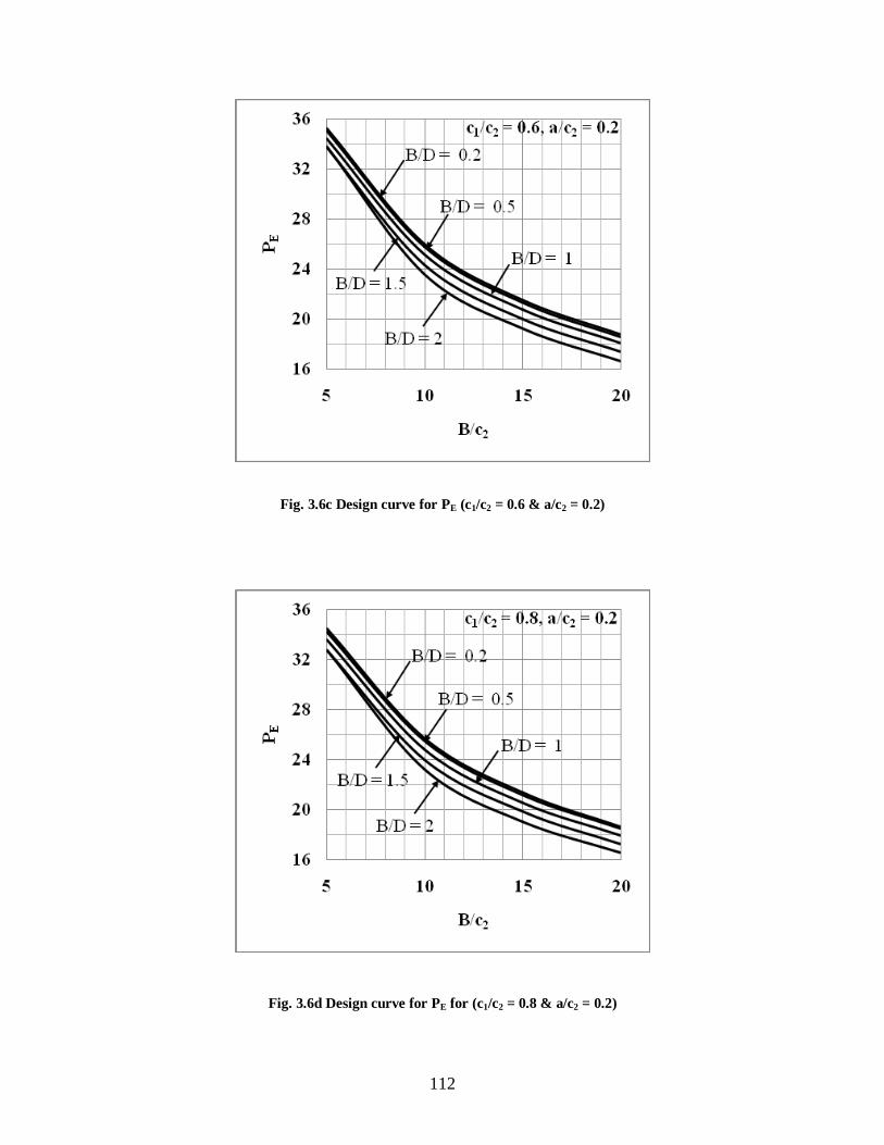
112
Fig. 3.6c Design curve for PE (c1/c2 = 0.6 & a/c2 = 0.2)
Fig. 3.6d Design curve for PE for (c1/c2 = 0.8 & a/c2 = 0.2)

113
Fig. 3.7a Design curve for PD (c1/c2 = 0.2 & a/c2 = 0.1)
Fig. 3.7b Design curve for PD for (c1/c2 = 0.4 & a/c2 = 0.1)

114
Fig. 3.7c Design curve for PD (c1/c2 = 0.6 & a/c2 = 0.1)
Fig. 3.7d Design curve for PD for (c1/c2 = 0.8 & a/c2 = 0.1)

115
Fig. 3.8a Design curve for PD (c1/c2 = 0.2 & a/c2 = 0.2)
Fig. 3.8b Design curve for PD for (c1/c2 = 0.4 & a/c2 = 0.2)

116
Fig. 3.8c Design curve for PD (c1/c2 = 0.6 & a/c2 = 0.2)
Fig. 3.8d Design curve for PD for (c1/c2 = 0.8 & a/c2 = 0.2)
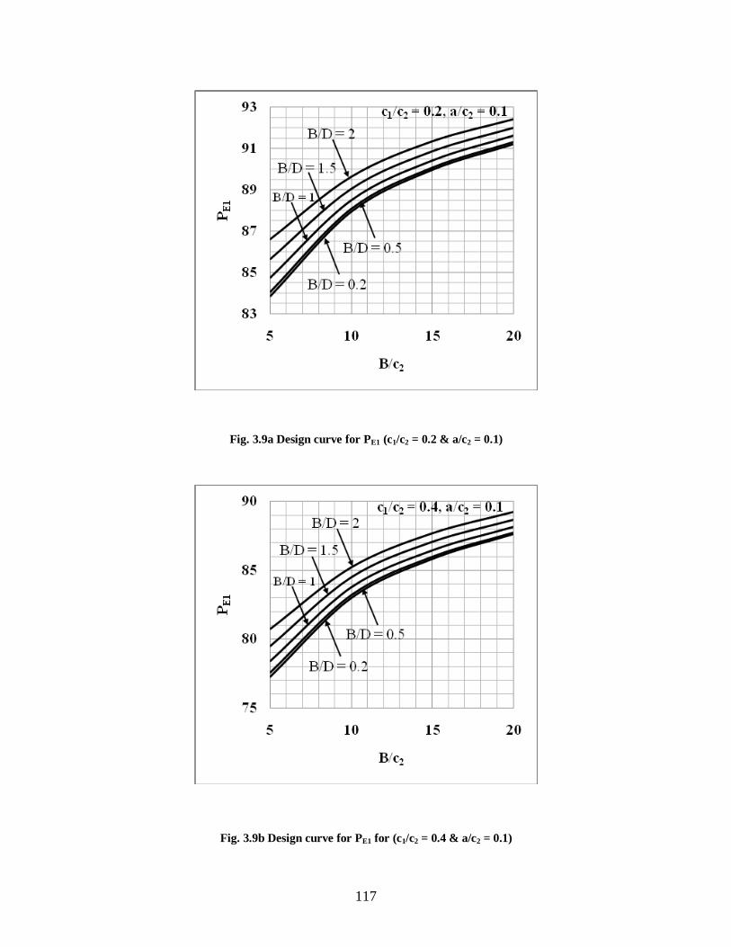
117
Fig. 3.9a Design curve for PE1 (c1/c2 = 0.2 & a/c2 = 0.1)
Fig. 3.9b Design curve for PE1 for (c1/c2 = 0.4 & a/c2 = 0.1)

118
Fig. 3.9c Design curve for PE1 (c1/c2 = 0.6 & a/c2 = 0.1)
Fig. 3.9d Design curve for PE1 for (c1/c2 = 0.8 & a/c2 = 0.1)

119
Fig. 3.10a Design curve for PE1 (c1/c2 = 0.2 & a/c2 = 0.2)
Fig. 3.10b Design curve for PE1 for (c1/c2 = 0.4 & a/c2 = 0.2)
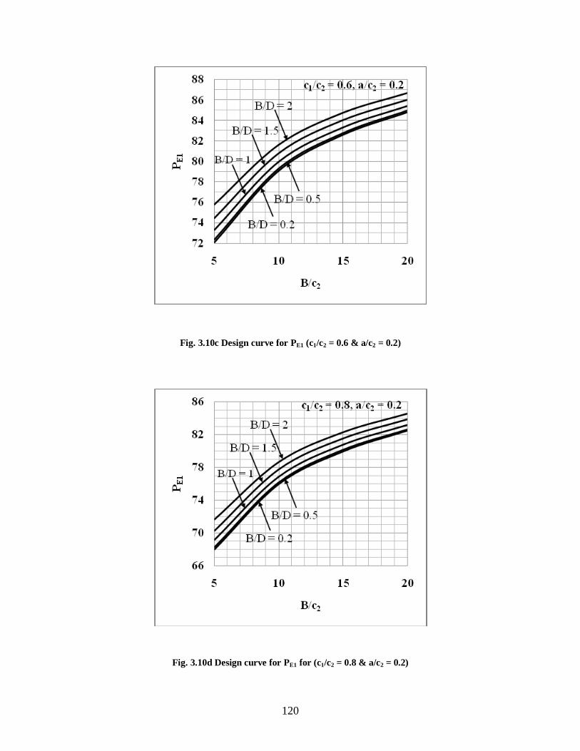
120
Fig. 3.10c Design curve for PE1 (c1/c2 = 0.6 & a/c2 = 0.2)
Fig. 3.10d Design curve for PE1 for (c1/c2 = 0.8 & a/c2 = 0.2)

121
Fig. 3.11a Design curve for PD1 (c1/c2 = 0.2 & a/c2 = 0.1)
Fig. 3.11b Design curve for PD1 for (c1/c2 = 0.4 & a/c2 = 0.1)

122
Fig. 3.11c Design curve for PD1 (c1/c2 = 0.6 & a/c2 = 0.1)
Fig. 3.11d Design curve for PD1 for (c1/c2 = 0.8 & a/c2 = 0.1)
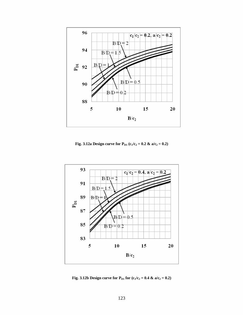
123
Fig. 3.12a Design curve for PD1 (c1/c2 = 0.2 & a/c2 = 0.2)
Fig. 3.12b Design curve for PD1 for (c1/c2 = 0.4 & a/c2 = 0.2)

124
Fig. 3.12c Design curve for PD1 (c1/c2 = 0.6 & a/c2 = 0.2)
Fig. 3.12d Design curve for PD1 for (c1/c2 = 0.8 & a/c2 = 0.2)

125
Fig. 3.13a Design curve for q
kH(c1/c2 = 0.2 & a/c2 = 0.1)
Fig. 3.13b Design curve for q
kHfor (c1/c2 = 0.4 & a/c2 = 0.1)

126
Fig. 3.13c Design curve for q
kH(c1/c2 = 0.6 & a/c2 = 0.1)
Fig. 3.13d Design curve for q
kH (c1/c2 = 0.8 & a/c2 = 0.1)

127
Fig. 3.14a Design curve for q
kH(c1/c2 = 0.2 & a/c2 = 0.2)
Fig. 3.14b Design curve for q
kH (c1/c2 = 0.4 & a/c2 = 0.2)

128
Fig. 3.14c Design curve for q
kH(c1/c2 = 0.6 & a/c2 = 0.2)
Fig. 3.14d Design curve for q
kH (c1/c2 = 0.8 & a/c2 = 0.2)

129
Fig. 3.15a Design curve for 2E
cG
H(c1/c2 = 0.2 & a/c2 = 0.1)
Fig.3.15b Design curve for 2E
cG
H (c1/c2 = 0.4 & a/c2 = 0.1)

130
Fig. 3.15c Design curve for 2E
cG
H(c1/c2 = 0.6 & a/c2 = 0.1)
Fig.3.15d Design curve for 2E
cG
H (c1/c2 = 0.8 & a/c2 = 0.1)

131
Fig. 3.16a Design curve for 2E
cG
H(c1/c2 = 0.2 & a/c2 = 0.2)
Fig.3.16b Design curve for 2E
cG
H (c1/c2 = 0.4 & a/c2 = 0.2)

132
Fig. 3.16c Design curve for 2E
cG
H(c1/c2 = 0.6 & a/c2 = 0.2)
Fig.3.16d Design curve for 2E
cG
H (c1/c2 = 0.8 & a/c2 = 0.2)

133
CHAPTER 4. FLAT APRON WITH UNEQUAL END CUTOFFS
4.1 Introduction
This chapter deals with the common case of flat apron with unequal cutoffs at the ends.
Downstream cutoff is provided for two purposes: (i) Protection of the apron against undermining
due to excessive exit gradient, and (ii) Protection of the apron due to down stream scour.
Similarly, the upstream cutoff is provided for two purposes: (i) Reduction of uplift pressure all
along downstream side, and (ii) Protection of the apron against upstream scour. In both these
locations, the bottom of cutoff is provided below the corresponding deepest scour level.
However, since the depth of downstream deepest scour is always more than the depth of
upstream deepest scour, the depth of the upstream cutoff is normally kept lesser than the depth of
the downstream cutoff.
4.2 Theoretical Analysis
Fig. 4.1 (a) shows floor profile in z-plane, with relative values of stream function and
potential function on the boundaries. Fig. 4.1 (c) shows the well known w-plane relating and
. The points in z and w-planes are denoted by complex coordinates z x iy and w i
respectively, where 1.i The problem is solved by transforming both z-planes and w-planes
on the infinite half-plane, t-plane, shown in Fig. 4.1 (b), thus obtaining 1( )z f t and 2( ).w f t

134
Fig. 4.1 Illustrations of the problem – Schwarz-Christoffel transformations

135
Floor Parameters
The floor of the hydraulic structure, shown in Fig. 4.1(a) has the following floor
parameters:
(i) Length of the apron : B
(ii) Finite depth of pervious medium : D
(iii) Depth of upstream cut off : c1
(iv) Depth of down stream cutoff : c2
The resulting independent non-dimensional floor-profile ratios are:
1. B/D, 2. B/c2, and 3. c1/c2.
4.2.1 First Transformation
The Schwarz - Christoffel equation of transformation of the floor from z-plane to t-plane
is given by:
z7 81 2
1 1
1 2 7 8( ) ( ) ........( ) ( )
dtM N
t t t t t t t t
(4.1 a)
where 1 2 2/ / ; 1 1 2/
2 2 ; 2 1
3 2 2/ / ; 3 1 2
4 2 2/ / ; 4 1 2
5 2 ; 5 1
6 2 2/ / ; 6 1 2
7 0 ; 7 1
8 0 ; 8 1
Substituting the values of 's , we get
z 1 11/ 2 1 1/ 2 1/ 2 1 1/ 2 1 11 2 3 4 5 6 7 8( ) ( ) ( ) ( ) ( ) ( ) ( ) ( )
dtM N
t t t t t t t t t t t t t t t t

136
or z 2 51 1
7 8 1 3 4 6
( ) ( )
( ) ( ) ( ) ( )( ) ( )
t t t t dtM N
t t t t t t t t t t t t
(4.1)
where t1, t2 ........ t8 are the co-ordinates of the mapped points on t-plane, and M1,
N1 are constants to be determined.
Eq. 4.1 is an elliptic integral. Referring to Identity 254, Bird and Friedman (1971),
Let 2sn u 4 1 3
4 3 1
( ) ( )
( ) ( )
t t t t
t t t t
(4.2 a)
So that u 1 4 1 3
4 3 1
( ) ( )sn ( , )
( ) ( )
t t t tF m
t t t t
(4.2 b)
where sn u = Jacobi's elliptic function, sinus amplitudinus
( , )F m = Elliptic integral of first kind (Legendre's notation)
m = modulus 4 3 6 1
4 1 6 3
( ) ( )
( ) ( )
t t t t
t t t t
(4.2 c)
= amplitude 1 4 1 3
4 3 1
( ) ( )sin
( ) ( )
t t t t
t t t t
(4.2 d)
Differentiating Eq. 2 (a) and simplifying we get
1 3 4 6 4 1 6 3
2
( )( )( )( ) ( )( )
dt du
t t t t t t t t t t t t
(4.3)
From Eqs. 4.1 and 4.3, we obtain, after simplification.
z 2 51 1
7 8 4 1 6 3
( ) ( ) 2
( ) ( ) ( )( )
t t t t duM N
t t t t t t t t
Carrying out the above integration, (as in chapter 3), we get
z 22 1 5 1 3 1 8 5 8 211
7 1 8 1 7 8 8 3 8 14 1 6 3
( ) ( ) ( ) ( )2( , ) ( , , )
( ) ( ) ( ) ( )( ) ( )
t t t t t t t t t tMF m m
t t t t t t t t t tt t t t

137
27 5 7 22 1
7 1 7 3
( ) ( )( , , )
( ) ( )
t t t tm N
t t t t
(4.4)
From Fig. 4.1(b), choosing 1 1 2 1 3 4 5, , , ,t t t t t , 2 ,
6t 2 7 1t and 8 1t , we get from Eq. 4.4
z 1 1 1 2 1
1 11 2
2 ( ) ( )( , )
(1 ) ( 1 )( ) ( )
MF m
2 21 1 2 1 2 11 2 1
1 1
( ) ( 1 ) ( 1 ) (1 ) (1 )( , , ) ( , , )
2 ( 1 ) ( 1 ) (1 ) (1 )m m N
or z 2 2
1 1 1 1 1 2 1[ ( , ) ( , , ) ( , , )]M A F m B m C m N (4.5)
where 2
1( , , )m and 2
2( , , )m are elliptic integrals of third kind with
parameters, 2
1 and 2
2 respectively, given by
2
18 1 4 3 1
8 3 4 1 1
1 2.
1
t t t t
t t t t
and 2
27 1 4 3 1
7 3 4 1 1
1 2.
1
t t t t
t t t t
(4.6 a)
1A 1 1 1 2
1 1 1 2
2( ) ( ) 1
(1 ) (1 ) ( ) ( )
(4.7 a)
1B 1 1 2
1 1 2
( ) (1 ) (1 ) 1
(1 ) (1 ) ( ) ( )
(4.7 b)
1C 1 1 2
1 1 2
( ) (1 ) (1 ) 1
(1 ) (1 ) ( ) ( )
(4.7 c)
= amplitude 1 1
1
( ) ( )sin
2 ( )
t
t
(4.8 a)
m = modulus 1 2
1 2
2 ( )
( ) ( )
(4.8 b)

138
In Eq. 4.5, there are seven unknowns: 1 2 1 2 1, , , , , ,M and 1N , the values of
which are determined by applying boundary conditions at various points.
Boundary conditions
1. Point 3 (Point E1): At point 3, z = – B/2 and t = –
1 11
1
( ) ( )sin sin (0) 0
2 ( )
Hence ( , ) 0F m and 2( , , )m = 0
Hence from Eq. 4.5, we get 1 / 2N B (4.9)
2. Point 4 (Point E): At point 4, z = B/2 and t =
1 11
1
( ) ( )sin sin (1)
2 ( ) 2
Hence ( , ) ,2
F m F m K
and 2 2 2
0( , , ) , , ( , )2
m m m
where K = complete elliptic integral of first kind.
and 2
0 ( , )m = complete elliptic integral of third kind.
Hence from Eq. 4.5, we obtain.
B 2 2
1 1 1 0 1 1 0 2 1[ ( , ) ( , )] .M A K B m C m M R (4.10)
or 1M /B R (4.10 a)
where R 2 2
1 1 0 1 1 0 2( , ) ( , )]A K B m C m (4.10 b)
3. Point 7: At point 7, z and t = 1
Hence the point that is mapped into t = + 1 is a simple pole of integrand (1).

139
iD 1 1. ( 1) ( ) .
ti M Lt t f t dt
Here ( )f t 2 57
7 8 1 3 4 6
( ) ( ), where 1
( ) ( ) ( )( ) ( )( )
t t t tt
t t t t t t t t t t t t
( 1) ( )t f t 2 5
8 1 3 4 6
( ) ( )
( ) ( )( ) ( ) ( )
t t t t
t t t t t t t t t t
1 2
1 2
( ) ( )
( 1) ( )( ) ( ) ( )
t t
t t t t t
iD 1 21
1 2
(1 ) (1 )
(1 1) (1 ) (1 ) (1 )(1 )i M
From which D 1 21 1
1 2
(1 ) (1 ).
2 (1 ) (1 )(1 ) (1 )M M J
(4.11)
Where J 1 2
1 1 2
(1 ) (1 ).
2 (1 ) (1 )(1 ) (1 )
D
M
(4.11 a)
4. Point 6: At point 6, / 2z B and 2t
1 11 2
1 2
( ) ( ) 1sin sin
2 ( ) m
1 1sin ,F m
m
K i K
and 1 21sin , ,m
m
2
2 2
0 02 2, ,
imm m
m
Hence from Eq. 4.5, we get:
2
B 22 2
1 1 1 0 1 0 12 21
( ) ( , ) ( , )im
M A K iK B m mm
2
2 21 0 2 0 22 2
2
( , ) ( , )2
im BC m m
m

140
B2 2
1 1 1 0 1 1 0 2[ ( , ) ( , )]M A K B m C m
2 2
2 21 1 1 0 1 1 0 22 2 2 2
1 2
( , ) ( , )m m
i M A K B m C mm m
Separating real and imaginary parts, we get
B2 2
1 1 1 0 1 1 0 2 1[ ( , ) ( , )] .M A K B m C m M R
(which is the same as obtained in Eq. 4.10)
and 2 2
2 2
1 1 0 1 1 0 22 2 2 2
1 2
( , ) ( , ) 0m m
A K B m C mm m
(4.12)
where 2
0 1( , )m and 2
0 2( , )m are complete elliptic integrals of third kind
with modulus 2
1 and 2
2 respectively, given by
2
1
2 2
1
221
,m
m
and 2
2
2 2
2
222
,m
m
(4.13)
5. Point 1: At point 1, z = – B/2 and t = –
1 11 1
1 1
( ) ( )sin sin ( )
2 ( )
1(sin , )F m iK
and 1 2(sin , , )m 2 2
02[ (1 , )]
1
iK m
Hence from Eq. 4.5, we get, after simplification,
2 2 2 21 11 1 0 1 2 0 22 2
1 2
(1 , ) (1 , ) 01 1
B CA K K m K m
(4.14)

141
where 2
0 1(1 , )m and 2
0 2(1 , )m are the complete elliptic integrals of
third kind with parameters 2
1(1 ) and 2
2(1 ) respectively.
6. Point 5: At point 5, z = B/2 +i c2 and t = +
1 11 2
1 2
( ) ( )sin sin
2 ( )y
where 1
1ym
Hence from Identity 115.02, Bird and Friedman (1971),
( , )F m ( , )K i F m
and 2( , , )m
2
2 22
0 2( , ) ( , ) , ,
1 1
mm i F m m
where
2 21 1
2 2
1 1sin sin
y y
m y m y
1 2
1 1 2
1 2 1 2
1 2 1 2
( ) ( )1
2 ( )sin
2 ( ) ( )( )1
( )( ) 2 ( )
1 1 2 1 2
1 2 1 21 2
1 2
( ) ( ) 2 ( )sin
( )( ) 2 ( )( )( )
( )( )
2
1 1 2 1 2 22
21 2 1 2
sin
1 11 2 2 1 2 2
1 1 2 1 2 2
( )( ) ( ) ( )( ) ( )sin sin
( )( ) ( ) ( )( ) ( )

142
or 1 2 2
2 2
( ) ( )sin
( ) ( )
Hence from Eq. 4.5
22
Bic
2 2
2 11 1 1 0 1 2 2
1 1
( , ) ( , ) ( , ) , ,1 1
mM A K iF m B m i F m m
2 22 2
1 0 2 2 22 2
( , ) ( , ) , ,21 1
m BC m i F m m
Separating real and imaginary parts, we get
2 2
1 1 1 0 1 1 0 2 1[ ( , ) ( , )]B M A K B m C m M R
(as found earlier in Eq. 4.10)
and 2c2 2
1 11 1 1 1 2 2
1 1
[ ( , ){ } , ,1 1
B mM F m A B C m
2 22
1 2 22 2
, ,1 1
mC m
(4.15)
or 2c 1M T (4.15 a)
where T2
21 11 1 1 32
1
( , ){ } ( , , )1
F m A B C m
222
1 422
( , )1
C m
(4.15 b)
where 23
2
211
m
and
24
2
221
m
(4.15 c)
7. Point 2 (Point D1): At point 2, z = – B/2 +i c1 and t = –
1 1 11 1 1 1
1 1 1 1
( ) ( ) ( ) ( )sin sin sin
2 ( ) 2 ( )i i x

143
Thus, the upper limit of is imaginary, due to which becomes i.
Hence ( , )F i m ( , )i F m
and 2( , , )i m 2 2
2( , ) ,1 ,
1
iF m m
where = new amplitude 1 1 1
1 1
( ) ( )tan
2 ( )
(4.16 a)
Hence from Eq (5), we obtain, after simplification
1c2
21 1 1 11 1 12 2 2
1 2 1
( , ) ( ,1 , )1 1 1
B C BM F m A m
2
221 22
2
( ,1 ,1
C m
(4.16)
or 1c = M1 . P (4.16 b)
2 22 21 1 1 1 1 2
1 1 22 2 2 21 2 1 2
where ( , ) ( ,1 , ) ( ,1 , )1 1 1 1
B C B CP F m A m m
(4.16 c)
Determination of 1 and 2
Parameters 1 and 2 are not independent parameters; instead, they depend on the
values of , 1 and2. The values of 1 and 2 can be determined as under.
From Eq. 4.12
2 2
2 2
1 1 0 1 1 0 22 2 2 2
1 2
( , ) ( , ) 0m m
A K B m C mm m
Substituting the values of A1, B1 and C1 and simplifying, we get
2 1 1 1 2 2 1 2 2 1 2( )( ) (1 )(1 ) (1 )(1 ) 0A B C (4.17)

144
where 2A1 1
2
(1 )(1 )
K
(4.17 a)
2B2
210 12 2
1 1
( ). ( , )
(1 )(1 )
mm
m
(4.17 b)
and 2C2
210 22 2
1 2
( ). ( , )
(1 )(1 )
mm
m
(4.17 c)
Similarly, from Eq. 4.14, we get
3 1 1 1 2 3 1 2 3 1 2( )( ) (1 )(1 ) (1 )(1 ) 0A B C (4.18)
where 3A1 1
2
(1 )(1 )
K
(4.18 a)
3B 2 211 0 12
1 1
( ) 1. (1 , )
(1 )(1 ) 1K m
(4.18 b)
and 3C 2 212 0 22
1 2
( ) 1. (1 , )
(1 )(1 ) 1K m
(4.18 c)
Solving Eqs 4.17 and 4.18, we get
12
3 3 3
14
2P P Q
(4.19 a)
23 3
213 3 3
2
4
Q Q
P P Q
(4.19 b)
where 3Q 2 2
1 1
P Q
P Q
(4.19 c)
and 3P 1 2 2 2 1 1
1 1
( ) ( )Q P Q Q P Q
P Q
(4.19 d)
1P 2 2 2
2 1 2 2
;A B C
A B C
(4.19 e)

145
2P2
2 1 2 2
2 1 2 2
A B C
A B C
(4.19 f)
1Q 3 3 3
3 1 3 3
;A B C
A B C
(4.19 g)
2Q2
3 1 2 3
3 1 3 3
A B C
A B C
(4.19 h)
General Relationship: z = f1 (t)
From Eq. 4.10, we have
1M2 2
1 1 0 1 1 0 2( , ) ( , )
B
A K B m C m
Hence from Eq. 4.5 we get
z
2 2
1 1 1 1 2
2 2
1 1 0 1 1 0 2
[ ( , ) ( , , ) ( , , )]
( , ) ( , ) 2
A F m B m C m B
A K B m C m
(4.20)
which is the required relationship z = f1 (t)
Determination of floor profile ratios
There are four floor parameters in z-plane
(i) Length of apron, B
(ii) Finite depth of pervious medium, D
(iii) Depth of upstream cutoff, c1, and
(iv) Depth of down stream cutoff, c2
Consequently, we have the following non-dimensional floor profile ratios:
(1) B/D, (2) B/c2, and (3) c1/c2.
From Eqs. 4.10 and 4.11, we get

146
B
D
2 2
1 1 0 1 1 0 2
1 2
1 2
[ ( , ) ( , )]
(1 ) (1 )
2 (1 ) (1 )(1 )(1 )
A K B m C m
(4.21)
or B
D=
R
J (4.21 a)
From Eqs. 4.10 and 4.15, we have
2
B
c
2 2
1 1 0 1 1 0 2
2 22 2
1 1 1 21 1 1 2 2 2 2
1 1 2 2
[ ( , ) ( , )]
( , )( ) , , , ,1 1 1 1
A K B m C m
B Cm mF m A B C m m
(4.22)
or 2
B
c=
R
T (4.22 a)
Finally, from Eqs. 4.16 and 4.15
1
2
c
c
2 22 21 1 1 1 1 2
1 1 1 22 2 2 2
1 2 1 2
2 22 2
1 1 1 21 1 1 2 2 2 2
1 1 2 2
( ) ( ,1 , ) ( ,1 , )1 1 1 1
( , )( ) , , , ,1 1 1 1
B C B CF m A m m
B Cm mF m A B C m m
(4.23)
or 1
2
c
c=
P
T (4.23 a)
4.2.2 Second Transformation
The transformation of w-plane to t-plane yields
w1
2 26 7 81 6 7 8( ) ( ) ( ) ( )
dtM N
t t t t t t t t
Here 1 6 7 8
1
2
1t 1 6 2 7 8; ; 1; 1t t

147
w 2 2
2 1( 1)( )( ) ( 1)
dtM N
t t t t
(4.24)
This is an elliptic integral.
Using Identity 254, Byrd and Friedman (1971), and carrying out the above
integration (as in chapter 3), we get.
w 20 0 2
1 2
2( , )
(1 )(1 )
MF m N
(4.25)
where 0 0( , )F m = Elliptic integral of first kind with modulus m0
0m 1 2
1 2
2( )
(1 )(1 )
(4.25 a)
= Amplitude 1 2 1
2 1
(1 )( )sin
( )( 1)
t
t
(4.25 b)
In order to find the values of constants M2 and N2, we apply boundary conditions
at point 1 and 6.
Boundary Conditions
(i) Point 1: At point 1, w = – kH and t = –
1sin (0) 0 and 0 0 0( , ) (0, ) 0F m F m
Hence from Eq. 4.25, 2N kH (4.26)
(ii) Point 6: At point 6, w = 0 and t =
1 12 2 1
1 2 2
(1 ) ( )sin sin (1)
( )( 1) 2
0 0( , )F m 0 0 0,2
F m K
where K0 = Complete elliptic integral of first kind with modulus m0.
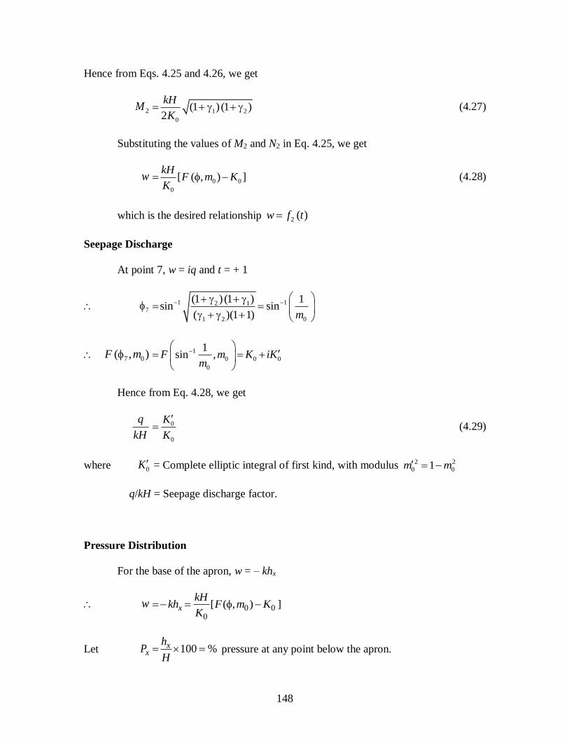
148
Hence from Eqs. 4.25 and 4.26, we get
2M1 2
0
(1 ) (1 )2
kH
K (4.27)
Substituting the values of M2 and N2 in Eq. 4.25, we get
w0 0
0
[ ( , ) ]kH
F m KK
(4.28)
which is the desired relationship 2 ( )w f t
Seepage Discharge
At point 7, w = iq and t = + 1
71 12 1
1 2 0
(1 ) (1 ) 1sin sin
( )(1 1) m
7 0( , )F m 1
0 0 0
0
1sin ,F m K iK
m
Hence from Eq. 4.28, we get
q
kH0
0
K
K
(4.29)
where 0K = Complete elliptic integral of first kind, with modulus 2 2
0 01m m
q/kH = Seepage discharge factor.
Pressure Distribution
For the base of the apron, w = – khx
w 0 00
[ ( , ) ]x
kHkh F m K
K
Let xP 100 %xh
H pressure at any point below the apron.

149
xP 0 00
100[ ( , ) ]F m K
K
or xP 0
0
( , )100 1
F m
K
(4.30)
(i) At point 6 (Point R): 2t
R1 12 1 2
1 2 2
(1 ) ( )sin sin 1
( )( 1) 2
0 0( , )RF m 0 0 0,2
F m K
Hence RP 0
0
100 1 0K
K
as expected
(ii) At point 4 (Point E): t =
E1 2 1
1 2
( 1) ( )sin
( )(1 )
(4.31 a)
Hence EP 0 0
0
( , )100 1 EF m
K
(4.31)
(iii) At point 3 (Point E1): t = –
1E1 2 1
1 2
(1 ) ( )sin
( )(1 )
(4.32 a)
and 1EP 0 1 0
0
( , )100 1 EF m
K
(4.32)

150
(iv) At Point 1 (Point G): t = –
G 0 00 ; ( , ) 0GF m
GP 100% as expected
(v) At point 5 (Point D): t =
D1 2 2 1
1 2 2
(1 ) ( )sin
( )( 1)
(4.33 a)
DP 0 0
0
( , )100 1 DF m
K
(4.33)
(vi) At point 2 (Point D1): t = –
1D1 2 1 1
1 2 1
(1 ) ( )sin
( )(1 )
(4.34 a)
1DP 0 1 0
0
( , )100 1 DF m
K
(4.34)
Exit Gradient
From the first transformation, we have
dz
dt
1 2
2 2 21 2
( ) ( ).( 1) ( )( ) ( )
t tB
R t t t t
(i)
Similarly, from the second transformation, we have
dw
dt
1 2
20 1 2
(1 ) (1 )
2 ( 1) ( ) ( )
kH
K t t t
(ii)
As shown chapter 3, the exit gradient GE is given by
EG1
.dw dt
ik dt dz

151
Substituting the values of dw
dt and
dz
dt simplifying, (as in chapter 3) we get
2E
cG
H
2 2 2
1 2 2 2
0 2 1 2 2
(1 )(1 )(1 )( )
2 ( ) ( )
T
K
where 2E
cG
H = Exit gradient factor
4.3 Computations and Results
Eqs. 4.21, 4.22, 4.23 for floor profile ratios B/D, B/c2 and c1/c2 are not explicit in
transformation parameters, , 1 and 2. Hence direct solution of these equations for the
parameters, , 1 and 2 corresponding to given sets of values of floor profile ratios (B/D,
B/c2 and c1/c2) are not practical. However these equations can be solved for physical floor
profile ratios B/D, B/c2 and c1/c2 for assumed values of , 1 and 2. Hence B/D, B/c2 and
c1/c2 were first computed for values of 1 20 1. The parameters 1 and 2 were
computed from Eqs. 4.19 (a) and 4.19 (b). From these values of floor profile ratios,
iterative procedures were developed to compute the values of , 1 and 2 (and then of
1and 2) for chosen pairs of values of B/D, B/c2 and c1/c2 ratio. Table 4.1 gives the
resulting values of , 1 and 2 for some chosen pairs of values of floor profile ratios
along with seepage characteristics.

152
Table 4.1 Computed Values
B/D B/c2 c1/c2 1 2 PE PD PE1 PD1 q/kh GE c2/H
0.2 5 0.2 0.1222 0.1464 0.2435 38.06 26.03 83.99 88.74 0.9578 0.1787
0.2 5 0.4 0.1166 0.1649 0.2378 37.32 25.56 77.47 84.24 0.9476 0.1757
0.2 5 0.6 0.1112 0.1836 0.2323 36.46 25.09 72.56 80.90 0.9375 0.1727
0.2 5 0.8 0.1061 0.2024 0.2268 35.80 24.61 68.49 78.18 0.9273 0.1696
0.2 5 1 0.1013 0.2214 0.2214 35.03 24.13 64.97 75.87 0.9172 0.1665
0.2 10 0.2 0.1382 0.1504 0.1992 27.66 19.23 87.98 91.53 0.9937 0.1339
0.2 10 0.4 0.1352 0.1597 0.1963 27.39 19.05 83.05 88.09 0.9880 0.1326
0.2 10 0.6 0.1323 0.1690 0.1934 27.11 18.86 79.31 85.50 0.9823 0.1314
0.2 10 0.8 0.1295 0.1783 0.1905 26.83 18.67 76.18 83.36 0.9766 0.1301
0.2 10 1 0.1267 0.1877 0.1877 26.55 18.49 73.45 81.51 0.9709 0.1288
0.2 15 0.2 0.1439 0.1521 0.1846 22.79 15.93 90.00 92.94 1.0060 0.1115
0.2 15 0.4 0.1419 0.1582 0.1827 22.64 15.83 85.89 90.06 1.0021 0.1107
0.2 15 0.6 0.1399 0.1644 0.1807 22.49 15.73 82.75 87.88 0.9981 0.1100
0.2 15 0.8 0.1380 0.1706 0.1787 22.33 15.62 80.12 86.06 0.9942 0.1093
0.2 15 1 0.1360 0.1768 0.1768 22.18 15.52 77.82 84.48 0.9903 0.1086
0.2 20 0.2 0.1468 0.1529 0.1774 19.83 13.90 91.26 93.83 1.0123 0.0975
0.2 20 0.4 0.1453 0.1576 0.1759 19.73 13.83 87.66 91.13 1.0092 0.0970
0.2 20 0.6 0.1438 0.1622 0.1744 19.63 13.76 84.90 89.38 1.0062 0.0965
0.2 20 0.8 0.1423 0.1668 0.1729 19.53 13.69 82.60 87.77 1.0032 0.0961
0.2 20 1 0.1409 0.1715 0.1715 19.43 13.62 80.57 86.38 1.0002 0.0956
0.5 5 0.2 0.2988 0.3540 0.5535 37.89 25.78 84.21 88.91 0.6703 0.1759
0.5 5 0.4 0.2857 0.3950 0.5431 37.12 25.29 77.75 84.47 0.6604 0.1727
0.5 5 0.6 0.2733 0.4352 0.5329 36.35 24.80 72.85 81.17 0.6504 0.1695
0.5 5 0.8 0.2616 0.4745 0.5228 35.56 24.30 68.78 78.49 0.6404 0.1663
0.5 5 1 0.2504 0.5128 0.5128 34.76 23.80 65.24 76.20 0.6303 0.1630
0.5 10 0.2 0.3346 0.3621 0.4662 27.46 19.04 88.12 91.63 0.7060 0.1321
0.5 10 0.4 0.3279 0.3826 0.4603 27.18 18.85 83.24 88.24 0.7004 0.1308
0.5 10 0.6 0.3214 0.4029 0.4544 26.89 18.66 79.52 85.68 0.6948 0.1295
0.5 10 0.8 0.3149 0.4229 0.4485 26.60 18.46 76.41 83.56 0.6892 0.1282
0.5 10 1 0.3087 0.4428 0.4428 26.31 18.27 73.69 81.73 0.6836 0.1269
0.5 15 0.2 0.3473 0.3656 0.4359 22.60 15.77 90.11 93.03 0.7182 0.1101
0.5 15 0.4 0.3428 0.3792 0.4317 22.45 15.67 86.04 90.08 0.7143 0.1094
0.5 15 0.6 0.3384 0.3927 0.4276 22.29 15.56 82.93 80.02 0.7104 0.1086
0.5 15 0.8 0.3340 0.4061 0.4235 22.13 15.45 80.32 86.22 0.7065 0.1079
0.5 15 1 0.3297 0.4195 0.4195 21.97 15.34 78.03 84.66 0.7027 0.1072
0.5 20 0.2 0.3537 0.3674 0.4205 19.65 13.76 91.35 93.90 0.7243 0.0964
0.5 20 0.4 0.3504 0.3776 0.4173 19.55 13.69 87.79 91.40 0.7213 0.0959
0.5 20 0.6 0.3471 0.3878 0.4142 19.45 13.62 85.06 89.50 0.7184 0.0954

153
B/D B/c2 c1/c2 1 2 PE PD PE1 PD1 q/kh GE c2/H
0.5 20 0.8 0.3438 0.3979 0.4110 19.34 13.55 82.77 87.91 0.7154 0.0949
0.5 20 1 0.3405 0.4079 0.4079 19.24 13.47 80.76 86.53 0.7125 0.0944
1 5 0.2 0.5531 0.6336 0.8515 37.38 25.02 84.89 89.42 0.4633 0.1674
1 5 0.4 0.5334 0.6883 0.8434 36.56 24.49 78.59 85.17 0.4540 0.1639
1 5 0.6 0.5146 0.7375 0.8354 35.71 23.94 73.75 82.00 0.4445 0.1604
1 5 0.8 0.4967 0.7813 0.8276 34.84 23.38 69.66 79.41 0.4348 0.1567
1 5 1 0.4798 0.8198 0.8198 33.95 22.81 66.05 77.19 0.4250 0.1530
1 10 0.2 0.6030 0.6414 0.7671 26.84 18.45 88.56 91.96 0.4982 0.1269
1 10 0.4 0.5935 0.6688 0.7609 26.53 18.25 83.82 88.68 0.4930 0.1255
1 10 0.6 0.5841 0.6947 0.7547 26.22 18.04 80.18 86.21 0.4877 0.1241
1 10 0.8 0.5749 0.7193 0.7486 25.91 17.82 77.11 84.16 0.4824 0.1226
1 10 1 0.5659 0.7426 0.7426 25.59 17.61 74.41 82.39 0.4770 0.1212
1 15 0.2 0.6202 0.6453 0.7330 22.02 15.28 90.46 93.28 0.5100 0.1061
1 15 0.4 0.6141 0.6636 0.7284 21.85 15.16 86.51 90.53 0.5063 0.1052
1 15 0.6 0.6079 0.6812 0.7237 21.68 15.05 83.47 88.44 0.5026 0.1044
1 15 0.8 0.6018 0.6981 0.7191 21.51 14.93 80.92 86.70 0.4990 0.1036
1 15 1 0.5958 0.7144 0.7144 21.33 14.81 78.67 85.19 0.4953 0.1028
1 20 0.2 0.6287 0.6474 0.7146 19.12 13.33 91.65 94.11 0.5159 0.0929
1 20 0.4 0.6244 0.6613 0.7111 19.00 13.25 88.19 91.70 0.5130 0.0924
1 20 0.6 0.6199 0.6746 0.7074 18.89 13.17 85.54 89.86 0.5102 0.0918
1 20 0.8 0.6153 0.6875 0.7037 18.78 13.09 83.30 88.32 0.5074 0.0913
1 20 1 0.6108 0.7000 0.7000 18.67 13.02 81.33 86.98 0.5046 0.0908
1.5 5 0.2 0.7385 0.8128 0.9584 36.84 24.12 85.76 90.09 0.3532 0.1574
1.5 5 0.4 0.7195 0.8577 0.9550 35.93 23.53 79.68 86.06 0.3449 0.1536
1.5 5 0.6 0.7013 0.8939 0.9516 34.98 22.91 74.89 83.03 0.3361 0.1497
1.5 5 0.8 0.6841 0.9226 0.9482 33.98 22.27 70.75 80.53 0.3269 0.1456
1.5 5 1 0.6679 0.9450 0.9450 32.96 21.61 67.02 78.36 0.3173 0.1412
1.5 10 0.2 0.7817 0.8158 0.9096 26.06 17.22 89.11 92.36 0.3874 0.1204
1.5 10 0.4 0.7733 0.8388 0.9059 25.72 17.49 84.55 89.24 0.3825 0.1189
1.5 10 0.6 0.7648 0.8594 0.9021 25.39 17.27 81.01 86.88 0.3776 0.1173
1.5 10 0.8 0.7565 0.8780 0.8983 25.04 17.03 77.99 84.91 0.3726 0.1158
1.5 10 1 0.7483 0.8945 0.8945 24.69 16.79 75.31 83.20 0.3675 0.1142
1.5 15 0.2 0.7969 0.8187 0.8866 21.27 14.65 90.90 93.60 0.3983 0.1009
1.5 15 0.4 0.7911 0.8337 0.8831 21.09 14.53 87.10 90.97 0.3952 0.1001
1.5 15 0.6 0.7858 0.8480 0.8800 20.91 14.40 84.17 88.98 0.3917 0.0992
1.5 15 0.8 0.7805 0.8613 0.8768 20.72 14.27 81.68 87.31 0.3883 0.0983
1.5 15 1 0.7751 0.8737 0.8737 20.53 14.14 79.47 85.86 0.3848 0.0974
1.5 20 0.2 0.8056 0.8215 0.8742 18.38 12.74 92.05 94.40 0.4031 0.0883
1.5 20 0.4 0.8001 0.8316 0.8705 18.30 12.69 88.71 92.08 0.4014 0.0880
1.5 20 0.6 0.7961 0.8424 0.8678 18.18 12.61 86.15 90.32 0.3985 0.0874

154
B/D B/c2 c1/c2 1 2 PE PD PE1 PD1 q/kh GE c2/H
1.5 20 0.8 0.7922 0.8527 0.8651 18.06 12.52 83.98 88.85 0.3962 0.0868
1.5 20 1 0.7883 0.8625 0.8625 17.94 12.44 82.06 87.56 0.3936 0.0862
2 5 0.2 0.8567 0.9109 0.9896 36.78 23.68 86.73 90.81 0.2819 0.1471
2 5 0.4 0.8423 0.9398 0.9885 35.94 23.23 80.92 87.05 0.2738 0.1429
2 5 0.6 0.8286 0.9607 0.9874 35.02 22.73 76.25 84.20 0.2652 0.1384
2 5 0.8 0.8158 0.9754 0.9864 33.96 22.10 72.09 81.79 0.2563 0.1337
2 5 1 0.8039 0.9854 0.9854 32.60 21.21 68.11 79.59 0.2476 0.1292
2 10 0.2 0.8873 0.9113 0.9673 25.22 16.94 89.69 92.79 0.3162 0.1138
2 10 0.4 0.8803 0.9259 0.9651 24.92 16.74 85.29 89.81 0.3123 0.1124
2 10 0.6 0.8740 0.9389 0.9632 24.59 16.52 81.84 87.55 0.3077 0.1107
2 10 0.8 0.8680 0.9501 0.9614 24.24 16.30 78.88 85.67 0.3029 0.1090
2 10 1 0.8621 0.9596 0.9596 23.90 16.09 76.22 84.02 0.2979 0.1072
2 15 0.2 0.8989 0.9138 0.9552 20.38 13.91 91.39 93.95 0.3257 0.0953
2 15 0.4 0.8936 0.9228 0.9528 20.25 13.82 87.73 91.44 0.3237 0.0947
2 15 0.6 0.8891 0.9315 0.9508 20.09 13.71 84.87 89.52 0.3210 0.0939
2 15 0.8 0.8851 0.9397 0.9489 19.90 13.58 82.44 87.92 0.3179 0.0930
2 15 1 0.8812 0.9471 0.9471 19.71 13.45 80.27 86.52 0.3147 0.0920
2 20 0.2 0.9042 0.9151 0.9479 17.57 12.10 92.46 94.70 0.3305 0.0836
2 20 0.4 0.9008 0.9220 0.9460 17.48 12.03 89.28 92.50 0.3287 0.0831
2 20 0.6 0.8971 0.9283 0.9439 17.39 11.97 86.80 90.81 0.3271 0.0827
2 20 0.8 0.8938 0.9344 0.9420 17.28 11.89 84.68 89.39 0.3251 0.0822
2 20 1 0.8907 0.9403 0.9403 17.16 11.81 82.80 88.15 0.3228 0.0816
Comparison with Infinite Depth Case when c1 = c2 = c
Malhotra (1936) obtained theoretical solution for uplift pressure below flat apron
with equal end cutoffs (i.e. when c1=c2=c) for the case of infinite depth of the pervious
foundation. The results of the present theoretical solution for B/D = 0.4 and B/D = 0.2
were compared with those of Malhotra's solution. Table 4.2 gives the values of uplift
pressure PE at point E and PD at point D, for some selected values of B/c ratios. It is seen
from Table 4.2 that when / 0.2B D , the results of both the analyses are practically the
same.

155
Table 4.2 Comparison with Malhotra's Case of Infinite Depth
B/c
PE PD
Infinite
Depth case
of Malhotra
Present
analysis for
B/D = 0.2
Present
analysis for
B/D = 0.4
Infinite
Depth case
of Malhotra
Present
analysis for
B/D = 0.2
Present
analysis for
B/D = 0.4
3 41.4 41.3 41.1 28.4 28.2 28.0
4 37.9 37.8 37.7 26.1 26.0 25.7
6 32.9 32.7 32.6 22.7 22.6 22.4
8 29.2 29.2 29.0 20.3 20.3 20.1
12 24.6 24.5 24.4 17.2 17.1 17.0
24 17.8 17.8 17.7 12.6 12.5 12.4
4.4 Design Charts
The values of seepage characteristics PE, PD, PE1, PD1, q/kH and GE c2/H, obtained
corresponding to some selected pairs of values of floor profile ratios were used to prepare
design charts for practical use in the design office. Figs 4.2(a), (b), (c) (d) shows the
design charts for uplift pressure PE at key point E, for cut off ratios c1/c2 = 0.2, 0.4, 0.6
and 0.8 respectively. Similarly, Figs. 4.3, 4.4, 4.5, 4.6 and 4.7 show the design charts for
pressure PD at point D, PE1 at E1, PD1 at D1, exit gradient factor GE c2/H and seepage
discharge factor q/kH respectively.

156
Fig. 4.2a Design curves for PE for c1/c2 = 0.2
Fig. 4.2b Design curves for PE for c1/c2 = 0.4

157
Fig. 4.2c Design curves for PE for c1/c2 = 0.6
Fig. 4.2d Design curves for PE for c1/c2 = 0.8

158
Fig. 4.3a Design curves for PD for c1/c2 = 0.2
Fig. 4.3b Design curves for PD for c1/c2 = 0.4

159
Fig. 4.3c Design curves for PE for c1/c2 = 0.6
Fig. 4.3d Design curves for PE for c1/c2 = 0.8

160
Fig. 4.4a Design curves for PE1 for c1/c2 = 0.2
Fig. 4.4b Design curves for PE1 for c1/c2 = 0.4

161
Fig. 4.4c Design curves for PE1 for c1/c2 = 0.6
Fig. 4.4d Design curves for PE1 for c1/c2 = 0.8

162
Fig. 4.5a Design curves for PD1 for c1/c2 = 0.2
Fig. 4.5b Design curves for PD1 for c1/c2 = 0.4

163
Fig. 4.5c Design curves for PD1 for c1/c2 = 0.6
Fig. 4.5d Design curves for PD1 for c1/c2 = 0.8

164
Fig. 4.6a Design curves for GEc2/H for c1/c2 = 0.2
Fig. 4.6b Design curves for GEc2/H for c1/c2 = 0.4

165
Fig. 4.6c Design curves for GEc2/H for c1/c2 = 0.6
Fig. 4.6d Design curves for GEc2/H for c1/c2 = 0.8

166
Fig. 4.7a Design curves for q/kH for c1/c2 = 0.2
Fig. 4.7b Design curves for q/kH for c1/c2 = 0.4

167
Fig. 4.7c Design curves for q/kH for c1/c2 = 0.6
Fig. 4.7d Design curves for q/kH for c1/c2 = 0.8

168
4.5 Conclusions
The general solution to the finite depth seepage under an impervious flat apron
with unequal end cutoffs is obtained using the conformal transformations. The results
obtained from the solution of implicit equations have been used to present design charts
for various seepage characteristics such as uplift pressures at key points, seepage
discharge factor and exit gradient in terms of non-dimensional floor profile ratios. It is
seen that uplift pressures at points E and D increase with the increase in the depth of
downstream cutoff, while the reverse is true for pressures at points E1 and D1. However
the exit gradient and seepage discharge decrease with increase in the downstream cutoff.
Also the uplift pressure at key points, as well as exit gradient, increases with decrease in
B/D ratio. When the depth of permeable soils is large, the numerical solutions tend
towards the established solution for infinite depth.
169
CHAPTER 5. FLAT APRON WITH EQUAL END CUTOFFS
AND A STEP AT DOWNSTREAM END
5.1 Introduction
Flat aprons with end cutoffs are invariably provided for various hydraulic structures
such as weirs, barrages, head regulators, aqueducts, siphons etc. The purpose of
downstream cutoff is to protect the apron against excessive exit gradient and downstream
scour, though it increases the uplift pressure all along the upstream side. The purpose of
upstream cutoff is to protect the apron against upstream scour, and to reduce the uplift
pressure all along the down stream side. In many cases, the depths of both these cutoffs
are kept equal. In addition to these cutoffs, pervious aprons are provided at the
downstream side of end cutoff in the form of inverted filter and launching apron. The
thickness of these pervious aprons may vary from 2 ft to 5 ft. In order to accommodate
the thickness of these pervious aprons, the downstream bed is excavated resulting in the
formation of a ‘step’ at the downstream end.
5.2 Theoretical Analysis
Fig. 5.1 (a) shows the floor profile in z-plane, with relative values of stream
function and potential function on the boundaries. Fig. 5.1 (c) shows the well known
w-plane, relating and The points in z and w-planes are denoted by complex co-
ordinates z x iy and w i respectively where 1i . The problem is solved
by transforming both the z-plane and w-plane on to an infinite half plane, t-plane,
shown in Fig. 5.1 (b), thus obtaining z = f1(z) and w = f2(t) and finally the desired relation
z = F(w).

170
Floor Parameters
The floor of the hydraulic structure shown in Fig. 5.1 (a) has the following floor
parameters:
(i) Length of the apron : B
(ii) Depth of pervious medium : D
(iii) Depth of cutoffs : c
(iv) Depth of downstream step : a
The resulting independent non-dimensional floor profile ratios are:
1. Floor - depth ratio, B/D
2. Floor-cutoff ratio, B/c, and
3. Step ratio, a/c
5.2.1 First Transformation
The Schwarz-Christoffel transformation equation for the transformation of floor
profile from z-plane (Fig. 1 a) to t-plane (Fig. 1 b) is
z7 81 2
1 1
1 2 7 8( ) ( ) ........( ) ( )
dtM N
t t t t t t t t
(5.1 a)
where 1 2 2/ / ; 1 1 2/
2 2 ; 2 1
3 2 2/ / ; 3 1 2
4 2 2/ / ; 4 1 2
5 2 ; 5 1
6 2 2/ / ; 6 1 2
7 0 ; 7 1
8 0 ; 8 1

171
Fig. 5.1 Illustrations of the problem: Schwarz – Christoffel transformations

172
Substituting the values of 's, we get
z 2 51 1
7 8 1 3 4 6
( ) ( )
( ) ( ) ( )( )( )( )
t t t t dtM N
t t t t t t t t t t t t
(5.1)
where t1, t2 ........ t8 are the co-ordinates of the mapped points on t-plane, and M1, N1 are the
constants to be determined.
Eq. (5.1) is an elliptic integral. Referring to Identity 254, Byrd and Friedman (1971),
Let 2sn u 4 1 3
4 3 1
( ) ( )
( ) ( )
t t t t
t t t t
(5.2 a)
so that u 1 4 1 3
4 3 1
( ) ( )sn ( , )
( ) ( )
t t t tF m
t t t t
(5.2 b)
where sn u = Jacobi's elliptic function, sinus amplitudinus
( , )F m = Elliptic integral of first kind (Legendre's notation)
m = modulus 4 3 6 1
4 1 6 3
( ) ( )
( ) ( )
t t t t
t t t t
(5.2 c)
=amplitude 1 4 1 3
4 3 1
( ) ( )sin
( ) ( )
t t t t
t t t t
(5.2 d)
Differentiating Eq. 5.2 (a) and simplifying we get
1 3 4 6 4 1 6 3
2
( )( )( )( ) ( )( )
dt du
t t t t t t t t t t t t
(5.3)
From Eqs (5.1) and (5.3), we obtain, after simplification
z 2 51 1
7 8 4 1 6 3
( ) ( ) 2
( ) ( ) ( )( )
t t t t duM N
t t t t t t t t
Carrying out the above integration, (as in Chapter 3) we get

173
z 22 1 5 1 3 1 8 5 8 211
7 1 8 1 7 8 8 3 8 14 1 6 3
( ) ( ) ( ) ( )2( , ) ( , , )
( ) ( ) ( ) ( )( ) ( )
t t t t t t t t t tMF m m
t t t t t t t t t tt t t t
27 5 7 22 1
7 1 7 3
( ) ( )( , , )
( ) ( )
t t t tm N
t t t t
(5.4)
From Fig. 5.1(b), choosing 1 1 2 1 3 4 5 6 2, , , , ,t t t t t t , 7 1t and
8 1t , we get from Eq. (5.4),
z 1 1 1
1 11 2
2 ( ) ( )( , )
(1 ) ( 1 )( ) ( )
MF m
2 211 2 1
1 1
( ) ( 1 ) ( 1 ) (1 ) (1 )( , , ) ( , , )
2 ( 1 ) ( 1 ) (1 ) (1 )m m N
or z2 2
1 1 1 1 1 2 1[ ( , ) ( , , ) ( , , )]M A F m B m C m N (5.5)
where 21( , , )m and 2
2( , , )m are elliptic integrals of third kind with parameters,
2
1 and 2
2 respectively, given by
21
8 1 4 3 1
8 3 4 1 1
1 2.
1
t t t t
t t t t
and 2
2 7 1 4 3 1
7 3 4 1 1
1 2.
1
t t t t
t t t t
...(5.6)
= amplitude 1 1
1
( ) ( )sin
2 ( )
t
t
(5.7 a)
m = modulus 1 2
1 2
2 ( )
( ) ( )
(5.7 b)
1A2 21
21 21
2( ) 1
( ) ( )(1 )
(5.8 a)
1B2
1
1 1 2
( ) (1 ) 1
(1 ) (1 ) ( ) ( )
(5.8 b)

174
1C2
1
1 1 2
( ) (1 ) 1
(1 ) (1 ) ( ) ( )
(5.8 c)
In Eq. (5.5), there are six unknowns: 1 2 1, , , , M and 1N , the values of which are
determined by applying boundary conditions at various points.
Boundary Conditions
1. Point 3 (Point E1): At point 3, z = – B/2 and t = –
1 11
1
( ) ( )sin sin (0) 0
2 ( )
( , )F m (0, ) 0F m
and 2( , , )m 2(0, , ) 0m
Hence from Eq. (5.5), we get 12
BN (5.9)
2. Point 4 (Point E): At point 4, z = +B/2 and t = +
1 11
1
( ) ( )sin sin (1)
2 ( ) 2
( , ) ,2
F m F m K
2 2 20( , , ) , , ( , )
2m m m
where K = complete elliptic integral of first kind.
and 2
0 ( , )m = complete elliptic integral of third kind.
Hence from Eq. (5.5),
B2 2
1 1 1 0 1 1 2 1[ ( , ) ( , )] .M A K B m C m M R (5.10)

175
where R2 2
1 1 0 1 1 0 2( , ) ( , )]A K B m C m (5.10 a)
or 1M /B R (5.10 b)
3. Point 7: At point 7, z and t = 1.
Hence the point that is mapped into t = + 1 is a simple pole of integrand (5.1).
iD 1 1. ( 1) ( ) .
ti M Lt t f t dt
Here ( )f t 2 5
7 8 1 3 4 6
( )( ),
( ) ( ) ( )( )( )( )
t t t t
t t t t t t t t t t t t
where 7 1t
( 1) ( )t f t 2 5
8 1 3 4 6
( )( ),
( ) ( )( )( )( )
t t t t
t t t t t t t t t t
1 2
( )( )
( 1) ( )( )( )( )
t t
t t t t t
or iD 1
1 2
(1 ) (1 )
(1 1) (1 ) (1 ) (1 )(1 )i M
From which D2
11
2
1 2
(1 ).
2 (1 )(1 ) (1 )
MM J
(5.11)
where J2
2
1 2
1.
2 (1 )(1 ) (1 )
(5.11 a)
4. Point 6: At point 6, 2
Bz ia and 2t
1 11 2
1 2
( ) ( ) 1sin sin
2 ( ) m
1 1sin ,F m
m
K i K

176
and 1 21sin , ,m
m
2
2 2
0 02 2, ,
imm m
m
Hence from Eq.( 5.5), we get, after simplification (as in Chapter 3):
2 2
2 2
1 1 1 0 1 1 0 2 12 2 2 2
1 2
[ ( , ) ( , )] . .m m
a M A K B m C m M Lm m
(5.12)
where L2 2
2 2
1 1 0 1 1 0 22 2 2 2
1 2
( , ) ( , )m m
A K B m C mm m
(5.12 a)
Adding Eqs. (5.11) and (5.12), we get
( )D a 1 1 1 ( )D M J M L M J L (5.13)
Also, from Eq. 5.12, noting that 1 /M B R
a
B
2 22 2
1 1 0 1 1 0 22 2 2 2
1 2
2 2
1 1 0 1 1 0 2
( , ) ( , )
( , ) ( , )
m mA K B m C m
m m LS
A K B m C m R
(5.14)
where 21
2 212 2
1
,m
m
and 2
2
2 2
2
222
,m
m
(5.14 a)
5. Point 1 (Point G): At point 1, z = – B/2 and t = –
1 11 1
1 1
( ) ( )sin sin ( )
2 ( )
1(sin , )F m iK
and 1 2(sin , , )m 2 2
02[ (1 , )]
1
iK m
Hence from Eq. (5.5), we get, after simplification,
1 2 2 2 211 1 0 1 2 0 22 2
1 2
( , ) ( , ) 01 1
B CA K K m K m
(5.15)
177
where 2 2
1 11 and 2 2
1 21
and 2
0 1( , )m and 2
0 2( , )m are the complete elliptic integrals of third kind with
parameters 2
1 and 2
2 respectively.
6. Point 5 (Point D): At point 5, 2
Bz ic and t = +
1 11
1
( ) ( )sin sin
2 ( )y
where 1
1ym
Hence from Identity 115.02, Byrd and Friedman (1971),
( , )F m ( , )K i F m
and 2
0 ( , , )m 2 2
2
0 22
( , ) ( , ) , ,11
mm i F m m
where = new amplitude 1 2
2
( ) ( )sin
( ) ( )
Hence from Eq. (5.5), we get, after simplification (as in Chapter 3).
c
2 21 1
1 1 1 1 2 21 1
( , ){ } , ,1 1
B mM F m A B C m
2 21 2
2 2
2 2
, ,1 1
C mm
(5.16)
or c 1M T
where T
221 22 21 1
1 1 1 3 42 21 2
( , ){ } ( , , ) ( , , )1 1
CBF m A B C m m
; (5.16 a)

178
23
2
211
m
and 2
42
221
m
(5.16 b)
7. Point 2 (Point D1): At point 2, z 2
B +i c and t = –
1 1 11 1
1 1
( ) ( ) ( ) ( )sin sin sin
2 ( ) 2 ( )i i x
Thus, the upper limit of is imaginary, due to which becomes i.
Hence ( , )F i m ( , )i F m
and 2( , , )i m 2 2
2( , ) ,1 ,
1
iF m m
where = new amplitude 1 1
1
( ) ( )tan
2 ( )
( 5.17)
Hence from Eq (5.5), we obtain, after simplification (as in Chapter 3)
c
21 1 1 21
1 1 12 2 21 2 1
( , ) ( ,1 , )1 1 1
B BCM F m A m
21 2 2
222
( ,1 ,1
Cm
(5.18)
or c = M1 . P (5.18 a)
where
2 21 1 1 1 22 21
1 1 22 2 2 21 2 1 2
( , ) ( ,1 , ) ( ,1 , )1 1 1 1
B B CCP F m A m m
(5.18 b)

179
Determination of
Parameter is not an independent parameter; instead, it depends on the values of , 1
and 2. However, to start with, let the t-coordinates of points 2 and 5 be 1 and 2 respectively,
though 1 = 2 =
From Eq. 5.14, we have
2
2 21 1 0 1 0 12 2
1
( ) ( , ) ( , )m
A K SK B m S mm
2
2 21 0 2 0 22 2
2
( , ) ( , ) 0m
C m S mm
Substituting the values of 1 1,A B and 2C and simplifying (as in Chapter 3), we get
2 1 1 1 2 2 1 2 2 1 2( )( ) (1 )(1 ) (1 )(1 ) 0A B C
or 1 2 1 1 2 2 0P P (I)
Similarly, substituting the values of A1, B1 and C1 in Eq. 5.15 and simplifying (as in
Chapter 3), we get
or 3 1 1 1 2 3 1 2 3 1 2( )( ) (1 )(1 ) (1 )(1 ) 0A B C
1 2 1 1 2 2 0Q Q (II)
Adding Eqs. (I) and (II), we get
2 2
1 21 1
P Q
P Q
Making 1 = 2 = (as is really the case), we have
2 2
1 1
P Q
P Q
(5.19)

180
where 1P 2 2 2
2 1 2 2
A B C
A B C
; 2P
22 1 2 2
2 1 2 2
A B C
A B C
1Q 3 3 3
3 1 3 3
A B C
A B C
; 2Q2
3 1 3 3
3 1 3 3
A B C
A B C
where 2A1 1
2( )
(1 )(1 )
K SK
2B2
2 210 1 0 12 2
1 1
( )( , ) ( , )
(1 ) (1 )
mm S m
m
2C2
2 210 2 0 22 2
1 2
( )( , ) ( , )
(1 ) (1 )
mm S m
m
3A1 1
2
(1 )(1 )
K
3B 2 211 0 12
1 1
( )( , )
(1 ) (1 )K m
3C 2 212 0 22
1 2
( )( , )
(1 ) (1 )K m
General Relationship: z = f1 (t)
From Eq. 5.10 (a), we have
1M2 2
1 1 0 1 1 0 2( , ) ( , )
B
A K B m C m
Hence from Eqs. (5.5) and (5.9), we get
z
2 21 1 1 1 2
2 21 1 0 1 1 0 2
[ ( , ) ( , , ) ( , , )]
2( , ) ( , )
B A F m B m C m B
A K B m C m
(5.20)
which is the required relationship z = f1 (t)

181
Determination of floor profile ratios
From Eqs. (5.10) and (5.13), we get
B
D=
R
J L (5.21)
From Eq. (5.10) and (5.16)
or B
c=
R
T (5.22)
Also, from Eqs. (5.12) and (5.16)
a
c=
L SR
T T (5.23)
where R, J, L and T are given by Eqs. 5.10 (a), 5.11 (a), 5.12 (a) and 5.16 (a) respectively.
5.2.2 Second Transformation
The transformation of w-plane (Fig. 5.1 c) to t-plane (Fig. 5.1 b) yields
w6 7 81
2 2
1 6 7 8( ) ( ) ( ) ( )
dtM N
t t t t t t t t
Here 1 6 7 8 1/ 2
and 1t 1 6 2 7 8; ; 1; 1t t t
w 2 2
2 1( 1) ( )( ) ( 1)
dtM N
t t t t
(5.24)
This is an elliptic integral
Using Identity 254, Byrd and Friedman (1971) and carrying out the above integration, we
get.
w 20 0 2
1 2
2( , )
(1 )(1 )
MF m N
(5.25)

182
where 0 0( , )F m = Elliptic integral of first kind with modulus m0
0m 1 2
1 2
2( )
(1 )(1 )
(5.25 a)
= amplitude 1 2 1
2 1
(1 )( )sin
( )( 1)
t
t
(5.25 b)
In order to find the values of constants M2 and N2, we apply boundary conditions at
points 1 and 6.
(i) Point 1: At point 1, w = – kH and t = –
1sin (0) 0 and 0 0 0( , ) (0, ) 0F m F m
Hence from Eq. 5.25, 2N kH (5.26)
(ii) Point 6: At point 6, w = 0 and t =
1 12 2 1
1 2 2
(1 ) ( )sin sin (1)
( )( 1) 2
0 0( , )F m 0 0 0,2
F m K
where K0 = Complete elliptic integral of first kind with modulus m0.
Hence from Eqs. 5.25 and 5.26, we get
2M 1 20
(1 ) (1 )2
kH
K (5.27)
Substituting the values of M2 and N2 in Eq. 5.25, the transformation equation becomes:
w 0 0 00
[ ( , ) ]kH
F m KK
(5.28)
which is the desired relationship 2 ( )w f t

183
Seepage Discharge
At point 7, w = iq and t = + 1
71 12 1
1 2 0
(1 ) (1 ) 1sin sin
( )(1 1) m
0 7 0( , )F m 10 0 0 0
0
1sin ,F m K iK
m
Hence from Eq. 5.28, we get
q
kH
0
0
K
K
(5.29)
where 0K = Complete elliptic integral of first kind, with modulus m0 and 20 01m m
q/kH = Seepage discharge factor.
Pressure Distribution
For the base of the apron, w = – khx
w 0 0 00
[ ( , ) ]x
kHkh F m K
K
Let xP 100%xh
H pressure at any point below the apron.
xP 0 0 00
100[ ( , ) ]F m K
K
or xP 0 0
0
( , )100 1
F m
K
(5.30)

184
(i) At point 6 (Point R): At point 6, 2t
R1 12 1 2
1 2 2
(1 ) ( )sin sin 1
( )( 1) 2
0 0( , )RF m 0 0 0,2
F m K
Hence RP 0
0
100 1 0K
K
, as expected
(ii) At point 4 (Point E): At point 4, t =
E1 2 1
1 2
( 1) ( )sin
( )(1 )
(5.31 a)
Hence EP 0 0
0
( , )100 1 EF m
K
(5.31)
(iii) At point 3 (Point E1): At point 3, t = –
1E1 2 1
1 2
(1 ) ( )sin
( )(1 )
(5.32 a)
and 1EP 0 1 0
0
( , )100 1 EF m
K
(5.32)
(iv) At Point 1 (Point G): At point 1, t = –
G1 12 1 1
1 2 1
(1 ) ( )sin sin (0) 0
( )( 1)
0 0( , ) 0GF m
Hence GP 100[1 0] 100% as expected
(v) At point 5 (Point D): At point 5, t =

185
D1 2 1
1 2
(1 ) ( )sin
( )( 1)
(5.33 a)
DP 0 0
0
( , )100 1 DF m
K
(5.33)
(vi) At point 2 (Point D1): At point 2, t = –
1D1 2 1
1 2
(1 ) ( )sin
( )(1 )
(5.34 a)
1DP 0 1 0
0
( , )100 1 DF m
K
(34)
Exit Gradient
From the first transformation, we have
dz
dt 2 2 21 2
( ) ( ).
( 1) ( )( ) ( )
B t t
Rt t t t
Similarly, from the second transformation, we have
dw
dt
1 2
20 1 2
(1 ) (1 )
2 ( 1) ( ) ( )
kH
K t t t
The exit gradient GE is given by
EG1
.dw dt
ik dt dz
Substituting the values of dw
dt and
dt
dz and simplifying (as in Chapter 3), we get
E
BG
H
2 2 21 2
20
(1 ) (1 )(1 )
2 ( ) ( ) 1
tR t
K t t t

186
Now, E
cG
HE
B cG
H B (where
c T
B R )
E
cG
H
2 2 21 2
20
(1 ) (1 )(1 )
2 ( ) ( ) 1
tT t
K t t t
Substituting 2t at the exit end, and simplifying, we get
E
cG
H
2 2 21 2 2 2
2 20 2
(1 )(1 )(1 )( )
2 ( )
T
K
(5.35)
where /EG c H = Exit gradient factor
5.3 Computations and Results
Eqs. 5.21 and 5.22 for floor profile ratios B/D and B/c are not explicit in transformation
parameters , 1 and 2. Hence direct solutions of these equations for the parameters , 1 and 2
corresponding to given set of values of floor profile ratios (B/D and B/c) and given step ratio are
extremely difficult. However, these equations can be solved for physical floor profile ratios B/D
and B/c for assumed values of , 1 and 2 and desired value of step ratio (a/c). Hence B/D and
B/c ratios were first computed for values of 1 20 1, for some pre-selected values of
step ratio (a/c). From these values of floor profile ratios, iterative procedures were developed to
compute the values of , 1 and 2 for chosen pairs of values of B/D and B/c ratios,
corresponding to each selected value of step ratio (a/c). Finally, computer program was executed
using these values of , 1 and 2 as input values to confirm the values of these chosen floor
profile ratios (B/D, B/c) and also to compute and the desired seepage characteristics PE, PD, PE1,
PD1 , q/kH and GE c/H. Table 5.1 gives the resulting values.

187
Table 5.1 Computed Values
B/D B/c a/c σ γ1 γ2 PE PD PE1 PD1 q/kH GEc/H
0.2 5 0.1 0.1006 0.2204 0.2150 34.40 23.30 64.68 75.68 0.9228 0.1785
0.2 10 0.1 0.1261 0.1870 0.1841 26.01 17.80 73.31 81.42 0.9747 0.1377
0.2 15 0.1 0.1355 0.1762 0.1743 21.70 14.92 77.73 84.42 0.9931 0.1159
0.2 20 0.1 0.1404 0.1710 0.1695 18.99 13.10 80.51 86.33 1.0026 0.1019
0.2 5 0.2 0.0999 0.2193 0.2083 33.72 22.40 64.38 75.48 0.9286 0.1929
0.2 10 0.2 0.1255 0.1862 0.1804 25.42 17.07 73.16 81.31 0.9786 0.1483
0.2 15 0.2 0.1350 0.1756 0.1716 21.19 14.29 77.64 84.36 0.9961 0.1246
0.2 20 0.2 0.1399 0.1705 0.1674 18.53 12.53 80.44 86.28 1.0050 0.1095
0.5 5 0.1 0.2493 0.5115 0.5012 34.14 22.98 64.95 76.01 0.6350 0.1750
0.5 10 0.1 0.3076 0.4417 0.4357 25.78 17.60 73.54 81.63 0.6869 0.1357
0.5 15 0.1 0.3287 0.4185 0.4143 21.50 14.76 77.94 84.60 0.7052 0.1144
0.5 20 0.1 0.3396 0.4071 0.4039 18.81 12.95 80.69 86.48 0.7146 0.1007
0.5 5 0.2 0.2480 0.5102 0.4889 33.47 22.10 64.65 75.81 0.6399 0.1893
0.5 10 0.2 0.3064 0.4405 0.4283 25.20 16.87 73.39 81.53 0.6903 0.1462
0.5 15 0.2 0.3277 0.4175 0.4090 20.99 14.13 77.84 84.53 0.7079 0.1230
0.5 20 0.2 0.3387 0.4062 0.3997 18.35 12.39 80.63 86.43 0.7168 0.1081
1.0 5 0.1 0.4788 0.8193 0.8103 33.35 22.04 65.77 77.00 0.4284 0.1646
1.0 10 0.1 0.5648 0.7418 0.7353 25.07 16.97 74.27 82.29 0.4796 0.1297
1.0 15 0.1 0.5948 0.7137 0.7088 20.88 14.25 78.57 85.13 0.4973 0.1098
1.0 20 0.1 0.6099 0.6993 0.6954 18.25 12.51 81.27 86.94 0.5063 0.0968
1.0 5 0.2 0.4777 0.8188 0.8000 32.71 21.21 65.47 76.80 0.4321 0.1784
1.0 10 0.2 0.5637 0.7410 0.7275 24.52 16.28 74.11 82.19 0.4824 0.1399
1.0 15 0.2 0.5937 0.7128 0.7028 20.39 13.65 78.48 85.06 0.4995 0.1182
1.0 20 0.2 0.6089 0.6985 0.6905 17.81 11.98 81.20 86.89 0.5081 0.1041
1.5 5 0.1 0.6674 0.9449 0.9407 32.38 20.89 66.75 78.18 0.3199 0.1523
1.5 10 0.1 0.7476 0.8942 0.8899 24.19 16.19 75.17 83.11 0.3696 0.1224
1.5 15 0.1 0.7745 0.8733 0.8698 20.09 13.61 79.38 85.80 0.3865 0.1041
1.5 20 0.1 0.7877 0.8621 0.8592 17.54 11.96 82.00 87.52 0.3950 0.0920
1.5 5 0.2 0.6668 0.9448 0.9358 31.77 20.11 66.46 77.99 0.3227 0.1656

188
Table 5.1 (contd.) Computed Values
B/D B/c a/c σ γ1 γ2 PE PD PE1 PD1 q/kH GEc/H
1.5 10 0.2 0.7468 0.8939 0.8850 23.66 15.53 75.02 83.01 0.3718 0.1322
1.5 15 0.2 0.7738 0.8728 0.8656 19.62 13.04 79.29 85.73 0.3883 0.1122
1.5 20 0.2 0.7870 0.8616 0.8557 17.12 11.45 81.93 87.47 0.3965 0.0990
2.0 5 0.1 0.8037 0.9854 0.9839 32.12 20.61 67.89 79.45 0.2493 0.1395
2.0 10 0.1 0.8618 0.9594 0.9572 23.41 15.50 76.08 83.93 0.2996 0.1150
2.0 15 0.1 0.8809 0.9470 0.9450 19.28 12.94 80.18 86.46 0.3161 0.0985
2.0 20 0.1 0.8904 0.9401 0.9384 16.78 11.36 82.74 88.11 0.3240 0.0872
2.0 5 0.2 0.8035 0.9854 0.9822 31.58 19.93 67.64 79.29 0.2512 0.1520
2.0 10 0.2 0.8614 0.9593 0.9547 22.88 14.86 75.93 83.83 0.3015 0.1244
2.0 15 0.2 0.8805 0.9468 0.9427 18.83 12.40 80.09 86.40 0.3176 0.1062
2.0 20 0.2 0.8900 0.9399 0.9364 16.38 10.87 82.67 88.06 0.3252 0.0939
0.2 10 0.3 0.1248 0.1854 0.1765 24.80 16.27 73.00 81.21 0.9827 0.1613
0.5 10 0.3 0.3052 0.4393 0.4206 24.59 16.09 73.23 81.42 0.6940 0.1591
1.0 10 0.3 0.5624 0.7402 0.7192 23.93 15.53 73.95 82.08 0.4853 0.1524
1.5 10 0.3 0.7460 0.8935 0.8795 23.10 14.82 74.86 82.90 0.3742 0.1442
2.0 10 0.3 0.8610 0.9592 0.9518 22.32 14.16 75.77 83.72 0.3035 0.1360
0.2 10 0.4 0.1241 0.1846 0.1725 24.12 15.40 72.83 81.09 0.9871 0.1777
0.5 10 0.4 0.3039 0.4380 0.4125 23.92 15.23 73.06 81.30 0.6978 0.1753
1.0 10 0.4 0.5611 0.7392 0.7102 23.28 14.70 73.78 81.96 0.4884 0.1682
1.5 10 0.4 0.7451 0.8931 0.8735 22.48 14.04 74.69 82.78 0.3767 0.1593
2.0 10 0.4 0.8605 0.9590 0.9486 21.70 13.40 75.60 83.61 0.3056 0.1505
Comparison with Infinite Depth Case when a/c = 0
Malhotra (1936) obtained theoretical solution for uplift pressure below flat apron with
equal end cutoffs, for the case of infinite depth of the pervious foundation. The results of the
present theoretical solution for B/D = 0.4 and B/D = 0.2 were compared with those of Malhotra's
solution. Table 5.2 gives the values of uplift pressure PE at point E and PD at point D, for some

189
selected values of B/c ratios. It is seen from Table 5.2 that when / 0.2B D , the results of both
the analyses are practically the same.
Table 5.2 Comparison with Malhotra's Case of Infinite Depth
B/c
% Pressure PE at E % Pressure PD at point D
Infinite
Depth case
by Malhotra
Present
Analysis for
B/D = 0.2
Present
analysis for
B/D = 0.4
Infinite
Depth case
by Malhotra
Present
Analysis for
B/D = 0.2
Present
analysis for
B/D = 0.4
3 41.4 41.3 41.1 28.4 28.2 28.0
4 37.9 37.8 37.7 26.1 26.0 25.7
6 32.9 32.7 32.6 22.7 22.6 22.4
8 29.2 29.2 29.0 20.3 20.3 20.1
12 24.6 24.5 24.4 17.2 17.1 17.0
24 17.8 17.8 17.7 12.6 12.5 12.4
Effect of Step at Downstream end
Fig. 5.2 (a) shows the effect of increase in step ratio (a/c) on PE, the uplift pressure at
point E, when the B/c = 10. Fig. 5.2 (b) shows the effect of increase in step ratio (a/c) on PD, the
pressure at point D. Similarly, Fig. 5.3 (a), 5.3 (b), 5.4 (a) and 5.4 (b) show the variation of PE1,
PD1, q/kH and GE c/H respectively, with increase in step ratio a/c from 0.0 to 0.4, when B/c = 10,
for different values of B/D ratios.
5.4 Design Charts
The values of seepage characteristics PE, PD, PE1, PD1, q/kH and GE c/H obtained
corresponding to some selected pairs of floor profile ratios (B/D and B/c) and selected values of
step ratio a/c (= 0.1, 0.2, 0.3, 0.4) were used to prepare design charts for use in design office.
Figs. 5.5 (a) and 5.5 (b) show the design charts for uplift pressure PE, for step ratio a/c = 0.1 and
0.2 respectively. Similarly, Figs. 5.6, 5.7, 5.8, 5.9, and 5.10 show design charts for PD, PE1, PD1,
seepage discharge factor (q/kH) and exit gradient factor (GE c/H) respectively.

190
Fig. 5.2a Variational curve for PE for B/c = 10
Fig. 5.2b Variational curve for PD for B/c = 10

191
Fig. 5.3a Variational curve for PE1 for B/c = 10
Fig. 5.3b Variational curve for PD1 for B/c = 10

192
Fig. 5.4a Variational curve for discharge factor for B/c = 10
Fig. 5.4b Variational curve for exit gradient factor for B/c = 10

193
Fig. 5.5a Design curve for PE for a/c = 0.1
Fig. 5.5b Design curve for PE for a/c = 0.2

194
Fig. 5.6a Design curve for PD for a/c = 0.1
Fig. 5.6b Design curve for PD for a/c = 0.2
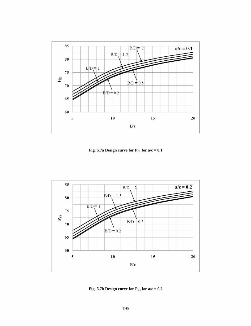
195
Fig. 5.7a Design curve for PE1 for a/c = 0.1
Fig. 5.7b Design curve for PE1 for a/c = 0.2

196
Fig. 5.8a Design curve for PD1 for a/c = 0.1
Fig. 5.8b Design curve for PD1 for a/c = 0.2

197
Fig. 5.9a Design curve for discharge factor for a/c = 0.1
Fig. 5.9b Design curve for discharge factor for a/c = 0.2

198
Fig. 5.10a Design curve for exit gradient factor for a/c = 0.1
Fig. 5.10b Design curve for exit gradient factor for a/c = 0.2
199
5.5 Conclusions
The closed-form solution to the problem of finite depth seepage under an impervious flat
apron with equal end cutoffs, with a downstream step, is obtained using the conformal
transformations. The results obtained from the solution of implicit equations have been used to
present design charts for various seepage characteristics such as uplift pressures at key points,
seepage discharge factor and exit gradient factor in terms of non-dimensional floor profile ratios.
It is seen that uplift pressures at points E, D, E1 and D1 decrease with the increase in step ratio.
However, the seepage discharge factor increases by very small margin, while the exit gradient
factor increases sharply with increase in the downstream step. Also, for a given step ratio (a/c),
the uplift pressures at points E and D, as well as exit gradient increase with decrease in B/D ratio,
and are maximum for infinite depth of pervious medium. When the depth of permeable soil is
large, the numerical solution tends towards the values for infinite depth.

200
CHAPTER 6
SUMMARY, CONCLUSIONS AND RECOMMENDATIONS
6.1 Summary and Conclusions
The present work envisages a theoretical study of seepage characteristics below the weir
aprons of various boundary conditions, including a step at downstream side. The depth of
pervious medium has been taken to be finite. Closed form theoretical solutions have been found
by following the procedure originally suggested by Pavlovsky. The work has been sub-divided
into four cases. Analysis and conclusions for each case are summarized below.
6.1.1 Flat Apron with Equal End Cutoffs
(a) Effect of increase in B/c ratio
1. For a given B/D ratio, the uplift pressures at point E and D decrease with increase in B/c
ratio, while the reverse is true for uplift pressures at points C and D'.
The decrease in B/c ratio corresponds to the increase in the depth of piles and increase in
pile penetration ratio. Hence greater depth of cut off results in an increase in uplift
pressure at key point E and D. However, greater depth of cutoff results in decrease in
pressure at key points C and D'.
2. For a given B/D ratio, the seepage discharge factor increases marginally with the increase
in B/c ratio. However, this increase is more for smaller values of B/D ratio and less for
higher value of B/D ratio.
3. For a given B/D ratio, the exit gradient factor decreases with increase in the B/c ratio.
However, the actual exit gradient increases. The increase in B/c ratio corresponds to the
decrease in depth of pile, which results in the increase in the exit gradient.

201
(b) Effect of depth of pervious medium
1. For given B/c ratio, uplift pressure at key points E and D increase with decrease in B/D
ratio. The reverse is true for uplift pressure at key point C and D'. For the downstream
half of the apron, the uplift pressures increases with decrease in B/D ratio while the
reverse is true for the upstream half of the apron.
2. For a given B/c ratio, the seepage discharge factor increases with the decrease in the B/D
ratio. As expected, the seepage discharge factor decreases with decrease in the depth of
pervious media.
3. For a given B/c ratio, the exit gradient factor and hence actual exit gradient, increases
with decrease in the B/D ratio. The infinite depth case gives the maximum exit gradient.
4. When / 0.2,B D the values of uplift pressure ,( )E DP P and the exit gradient factor
( / )EG c H are quit close to the corresponding values for the infinite depth case. Hence
when the depth of pervious medium is equal to or more than five times the length of the
impervious apron, the depth of pervious medium may be assumed to be infinite.
5. The assumption of infinite depth of pervious medium results in greater values of uplift
pressure ( , )E DP P and exit gradient. Hence the current design practice of the use of design
curves for infinite depth case in safe though conservative.

202
(c) Use of Design Curves
The design curves for uplift pressures at key points E and D and for exit gradient factor
( / )EG c H will be useful for determining these without running the computer programme. The
uplift pressures at key points C and D' can be found from the following relations based on
principle of reversibility of flow:
CP 100 EP and DP 100 DP
6.1.2 Flat Apron with Unequal End Cutoffs and a Step at Downstream End
(a) Effect of increase in step ratio (a/c2)
1. Uplift pressure PE and PD at point E and D, respectively, decrease almost linearly with
increase in step ratio a/c2. The variation curves for various B/D ratios are almost parallel.
2. Uplift pressure PE1 and PD1 at point E1 and D1, respectively, also marginally decrease
linearly with increase in step ratio. Here also, the variation curves for various B/D ratios
are almost parallel.
3. There is very small increase in seepage discharge factor (q/kH) with the increase in step
ratio (a/c2). Here again, the curves corresponding to various values of B/D ratio are
almost linear and parallel.
4. There is very sharp increase in exit gradient factor GE c2/H (and hence the exit gradient
itself) with increase in step ratio (a/c2). The curves corresponding to various values of
B/D are almost parallel, though curvilinear.

203
b) Effect of increase in B/c2 ratio
1. For a given B/D ratio, the uplift pressure at point E and D decrease with increase in B/c2
ratio, while the reverse is true for uplift pressure at point E1 and D1. The decrease in B/c2
ratio corresponds to increase in the depth of downstream pile. Hence greater depth of
downstream cutoff results is an increase of uplift pressure at key points E and D.
However, greater depth of downstream cutoff results in decrease in pressure at point E1
and D1.
2. For a given B/D ratio, the seepage discharge factor increase only marginally with the
increase in B/c2 ratio.
3. For a given B/D ratio, the exit gradient factor decrease with increase in B/c2 ratio.
However, the actual exit gradient increases. The increase in B/c2 ratio corresponds to
decrease in depth of downstream pile, which results in the increase in the exit gradient.
(c) Effect of c1/c2 ratio
1. From Table 3.1, we find that for a given values of B/c2 ratio, uplift pressure PE, PD, PE1
and PD1 at all the four key point decrease with increase in c1/c2 ratio (i.e. with increase in
the depth of upstream pile).
2. The seepage discharge factor also decreases with the increase in c1/c2 ratio.
3. Similarly, for a given values of B/D ratio and B/c2 ratio, the exit gradient factor, and
hence the exit gradient decreases with increase in the c1/c2 ratio. Hence contrary to the
common belief, the depth of upstream cutoff also helps in controlling the exit gradient,
though at much flatter rate.

204
(d) Effect of depth of pervious medium
1. For a given B/c2 ratio, the uplift pressure at key point E and D increase with decrease in
B/D ratio. The reverse is true for uplift pressure at key point E1 and D1. For the
downstream half of the apron, the uplift pressures increase in decrease in B/D ratio while
the reverse is true for the upstream half of the apron.
2. For a given B/c2 ratio, the seepage discharge factor increases with decrease in B/D ratio.
As expected, the seepage discharge factor decreases with decrease in the depth of
pervious medium.
3. For a given B/c2 ratio, the exit gradient factor, and hence the exit gradient increases with
the decrease in B/D ratio. The infinite depth case gives maximum exit gradient.
4. When / 0.2B D , the values of uplift pressures (PE, PD) and the exit gradient factor (GE
c2/H) are quite close to the corresponding values for the infinite depth case. Hence when
the depth of pervious medium is equal or more than five times the length of impervious
apron, the depth of pervious medium may be assumed to be infinite.
5. The assumption of infinite depth of pervious medium results in higher values of uplift
pressure (PE, PD) and exit gradient. Hence the current design practice of use of design
curves for infinite depth case is safe though conservative.
6.1.3 Flat Apron with Unequal End Cutoffs
(a) Effect of increase in B/c2 ratio
1. For a given B/D ratio, the uplift pressures at points E and D decrease with increase in B/c2
ratio, while the reverse is true for uplift pressures at point E1 and D1. The decrease in B/c2
ratio corresponds to increase in the depth of downstream pile. Hence greater depth of

205
downstream cutoff results in an increase of uplift pressure at key points E and D. However,
greater depth of downstream cutoff results in decrease in pressures at point E1 and D1.
2. For a given B/D ratio, the seepage discharge factor increases marginally with the increase in
B/c2 ratio.
3. For a given B/D, ratio the exit gradient factor decrease with increase in B/c2 ratio. However,
the actual exit gradient increases. The increase in B/c2 ratio corresponds to decrease in depth
of downstream pile, which results in the increase in the exit gradient.
(b) Effect of c1/c2 ratio
1. From Table 4.1, we find that for a given value of B/c2 ratio, uplift pressure PE, PD, PE1 and
PD1 at all the four key points decrease with increase in c1/c2 ratio (i.e. with increase in the
depth of upstream pile).
2. The seepage discharge factor also decreases with the increase in c1/c2 ratio.
3. Similarly for a given values of B/D ratio and B/c2 ratio, the exit gradient factor, and hence the
exit gradient decreases with increase in the c1/c2 ratio. Hence contrary to the common belief,
the depth of upstream cutoff also helps in controlling the exit gradient, though at a much
flatter rate.
(c) Effect of depth of pervious medium
1. For a given B/c2 ratio, the uplift pressure at key point E and D increase with decrease in B/D
ratio. The reverse is true for uplift pressure at key point E1 and D1. For the downstream half
of the apron, the uplift pressures increase with decrease in B/D ratio while the reverse is true
for the upstream half of the apron.

206
2. For a given B/c2 ratio, the seepage discharge factor increases with decrease in B/D ratio. As
expected, the seepage discharge factor decreases, with decrease in the depth of pervious
medium.
3. For given B/c2 ratio, the exit gradient factor, and hence the exit gradient increases with the
decrease in B/D ratio. The infinite depth case gives maximum exit gradient.
4. When / 0.2B D , the values of uplift pressure (PE, PD) and the exit gradient factor (GE c2/H)
are quite close to the corresponding values for the infinite depth case. Hence when the depth
of pervious medium is equal or more than five times the length of impervious apron, the
depth of pervious medium may be assumed to be infinite.
5. The assumption of infinite depth of pervious medium results in higher values of uplift
pressures (PE, PD) and exit gradient. Hence the current design practice of use of design
curves for infinite depth case is safe though conservative.
6.1.4 Flat Apron with Equal End Cutoffs and a Step at the Downstream End
(a) Effect of increase in step ratio (a/c)
1. Uplift pressure PE and PD at point E and D, respectively, decrease almost linearly with
increase in step ratio a/c. The variation curves for various values of
B/D = 0.2, 0.5, 1, 1.5 and 2 are almost parallel.
2. Uplift pressures PE1 and PD1 at point E1 and D1, respectively, also marginally decrease
linearly with increase in step ratio. Here also, the variational curves for various B/D ratios
are almost parallel.

207
3. There is very minute increase in seepage discharge factor (q/kH) with the increase in step
ratio (a/c). Here again, the curves corresponding to various values of B/D ratio are almost
linear and parallel.
4. There is very sharp increase in exit gradient factor GE c/H (and hence the exit gradient
itself) with increase in step ratio (a/c). The curves corresponding to various values of B/D
ratio are almost parallel, though curvilinear.
(b) Effect of increase in B/c ratio
1. For a given B/D ratio, the uplift pressures at points E and D decrease with increase in B/c
ratio, while the reverse is true for uplift pressures at points E1 and D1. The decrease in B/c
ratio corresponds to increase in the depth of downstream pile. Hence greater depth of
downstream cutoff results is an increase of uplift pressure at key points E and D.
However, greater depth of downstream cutoff results in decrease in pressures at point E1
and D1.
2. For a given B/D ratio, the seepage discharge factor increases only marginally with the
increase in B/c ratio.
3. For a given B/D ratio, the exit gradient factor decreases with increase in B/c ratio.
However, the actual exit gradient increases. The increase in B/c ratio corresponds to
decrease in depth of downstream pile, which results in the increase in the exit gradient.
(c) Effect of depth of pervious medium
1. For a given B/c ratio, the uplift pressure at key points E and D increase with decrease in
B/D ratio. The reverse is true for uplift pressures at key points E1 and D1. For the

208
downstream half of the apron, the uplift pressures increase with decrease in B/D ratio
while the reverse is true for the upstream half of the apron.
2. For a given B/c ratio, the seepage discharge factor increases with decrease in B/D ratio.
As expected, the seepage discharge factor decreases with decrease in the depth of
pervious medium.
3. For a given B/c ratio, the exit gradient factor, and hence the exit gradient increases with
the decrease in B/D ratio. The infinite depth case gives maximum value of exit gradient.
4. When / 0.2B D , the values of uplift pressures (PE , PD) and the exit gradient factor (GE
c/H) are quite close to the corresponding values for the infinite depth case. Hence when
the depth of pervious medium is equal to or more than five times the length of impervious
apron, the depth of pervious medium may be assumed to be infinite.
5. The assumption of infinite depth of pervious medium results in higher values of uplift
pressures (PE, PD) and exit gradient. Hence the current design practice of use of design
curves for infinite depth case is safe though conservative.
6.2 Recommendations for Future Work
The present work formulates an exact solution for the problems considered in this
dissertation. The solutions contain unknown parameters in implicit form in the equations
derived. When the unknown parameters are three or more, the iteration for the computations
becomes extremely difficult. Hence, an inverse method of solution of equations has to be
employed for hydraulic structures having an intricate subsurface profile. The closed form
solution method used here is more useful and practical when the pressure distribution along
the boundaries is to be determined.

209
This method is applicable to all those situations where Laplace equation is applicable.
Hence, the method of solution is not applicable to heterogeneous soils, where the soil
properties change from point to point. However, it is applicable for homogeneous anisotropic
soils.
There are many seepage scenarios under hydraulic structures where analytical solution
has not been attempted. The author proposes four different weir profiles with flat aprons on
finite depth, where analytic solution could be found. These are shown in Fig. 6.1. The first
weir profile shown in Fig. 6.1a is a flat apron with two unequal intermediate cutoffs. Another
case (Fig. 6.1b) is an inclined apron with single end cutoff or with double end cutoffs. The
inclined floors are provided for energy dissipation through formation of hydraulic jumps. The
effect of width of concrete cutoff may have an appreciable effect on various seepage
characteristics. This case, as shown in Fig. 6.1c is equally interesting. Finally, the effect of
crack in a downstream end cutoff, leading to leakage offers a challenging problem for
analytical-solution seekers (Fig. 6.1d).
The research for obtaining seepage characteristics under hydraulic structures was initiated
for infinite depth cases. An impervious boundary may occur at a finite depth, which alters
seepage characteristics in the seepage domain considerably. Only a few cases have been
solved for finite depth of pervious medium; hence it is recommended to lay more emphasis
on finite depth scenarios.

210
Fig. 6.1 Finite depth problems for future work

211
APPENDIX A. SCHWARZ – CHRISTOFFEL TRANSFORMATION

212
A seepage scenario is governed by Laplace equation. To determine the seepage characteristics,
the solution of Laplace equation is required. Consider any region under seepage. This region has
infinite sets of curvilinear orthogonal lines, namely the equipotential lines and the stream-lines.
If for any such curvilinear square, velocity potential (Φ) and stream function (Ψ) are known, then
the Laplace equation is said to be solved at that point. Since, the Laplace equation is continuous
in this region, values of Φ and Ψ for all curvilinear squares or for the whole flow-net must be
known.
Let us assume that we have a known square that represents the seepage region. The
values of Φ and Ψ on this square would then indicate a solution of Laplace equation for the
region. A mathematical process can be found, which can relate this known rectangular field (Φ –
Ψ plane, also known as w – plane) to the real flow domain. That process could give us the
change in the expressions of equipotential lines and stream-lines in the real domain. This leads us
to the theorem by Schwarz and Christoffel. The theorem gives us a differential equation which
embodies the nature of change in a function of real plane, say z-plane, bounded by any straight-
sided figure in order that the boundary may be opened out into one straight line; the opening-out
involving, of course, the distortion of the function.
Thus, if F1 is a function representing the flow region in z-plane, and if it can be
transformed into a straight line in t-plane, this relationship can be written as
z = F1(t)
Similarly, if the known rectangular field in w-plane is represented by a function F2, and if it can
be transformed into the same straight line (mentioned above) in the t-plane, following
relationship is known:
w = F2(t)
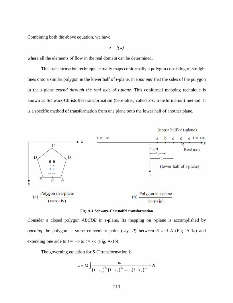
213
Combining both the above equation, we have
z = f(w)
where all the elements of flow in the real domain can be determined.
This transformation technique actually maps conformally a polygon consisting of straight
lines onto a similar polygon in the lower half of t-plane, in a manner that the sides of the polygon
in the z-plane extend through the real axis of t-plane. This conformal mapping technique is
known as Schwarz-Christoffel transformation (here-after, called S-C transformation) method. It
is a specific method of transformation from one plane onto the lower half of another plane.
Fig. A-1 Schwarz-Christoffel transformation
Consider a closed polygon ABCDE in z-plane. Its mapping on t-plane is accomplished by
opening the polygon at some convenient point (say, P) between E and A (Fig. A-1a) and
extending one side to t = +∞ to t = -∞ (Fig. A-1b).
The governing equation for S-C transformation is
.......a b n
a b n
dtz M N
t t t t t t

214
Where
1i
interior angle at point i in z-plane
,
and , ,....a b nt t t co-ordinates of the mapped points on t-plane.
Notes:
1) The interior angle at point P of the opening in the z-plane is π.
Since 1 1 0P
interior angle at P
, point P has no part in the transformation.
However, the point of opening, P in the z-plane is represented in the lower-half of the t-
plane by a semi-circle of infinite radius.
2) The S-C transformation, in effect maps conformally the interior region of the polygon
ABCDE of the z-plane into the interior of the polygon bounded by ab, bc, cd,…. and a
semi-circle with a radius of infinity in the lower half of the t-plane.
3) The S-C transformation theorem is applicable only for mapping the sides of closed
polygon of z-plane into a straight line profile of t-plane, where the angles between the
sides of π.
4) The origin of the t-plane can be located at any convenient point.
5) Any three values of , , ,.....a b c nt t t t can be chosen arbitrarily, while the remaining n - 3
values of t-coordiantes are found from boundary conditions.

215
APPENDIX B. ELLIPTIC INTEGRALS

216
1. Types of Elliptic Integrals
Integrals of the form [ , ( )] ,R t P t dt where P(t) is a polynomial of the third or fourth
degree and R is a rational function, are known as elliptic integrals because a special example of
this type arose in the rectification of the arc of an ellipse.
Thus the integral
I 04 3 2
1 2 3 4[ , ]R t a t a t a t a t a dt
is called the elliptic integral if the equation
04 3 2
1 2 3 4 0a t a t a t a t a (a0 and a1 not both zero)
has no multiple roots and if R is a rational function of t and of the square root of the above
equation.
Although some early work on these was done by Fragnano, Euler, Legendre and Landen,
they were first treated systematically by Legendre, who showed that any elliptic integral may be
made to depend on three fundamental integrals which he denoted by ( , ), ( , )F m E m and
2( , , ).m These three integrals are called Legendres canonical elliptic integrals of the first,
second and third kind respectively.
(i) Elliptic Integral of First Kind
The elliptic integral of first kind in canonical form is
2 2 2
0 (1 ) (1 )
ydt
t m t (1)
where m is the modulus of the integral. Substituting t sin in the above equation, we have

217
( , )F m2 2
0 1 sin
d
m
(1a)
where 1sin y amplitude of the integral. ( , )F m is in Legendre notation and is the usual
tabular notation. In many tables, the modulus is given as
sinm
where is the modular angle.
When ,2
we get complete elliptic integral of first kind:
K
/ 2
2 20
,2 1 sin
dF m
m
(1b)
(ii) Elliptic Integral of Second Kind
The elliptic integral of the second kind in the canonical form of Legendre is defined as
2 2
20
1
1
ym t
dtt
(2)
Substituting t sin , we have
( , )E m 2 2
0
1 sinm d
(2a)
where is the amplitude and E (, m) is Legendre's notation for the elliptic integral of
second kind. When ,2
we get complete elliptic integral of second kind:
E
/ 22 2
0
, 1 sin2
E m m d
(2b)

218
(iii) Elliptic Integral of Third Kind
The elliptic integral of the third kind in the canonical form of Legendre is:
2( , , )y m 2 2 2 2 2
0 (1 ) (1 ) (1 )
ydt
t t m t
(3)
where m is the modulus and 2 is the parameter.
Substituting t sin ,
2( , , )m 2 2 2 2
0 (1 sin ) (1 sin )
d
m
(3a)
where is the amplitude. When = /2, we get the complete elliptic integral of third
kind.
2
0 , ,2
m
/ 2
2 2 2 20 (1 sin ) (1 sin )
d
m
(3b)
2. JACOBIAN ELLIPTIC FUNCTIONS
Let us consider the equivalence of the integrals
u2 2 2
0 (1 ) (1 )
ydt
t m t
2 2
0 1 sin
d
m
(4)
which are related by the substitution t = sin .
The Jacobian elliptic functions are defined by the relations:
sn u = sin , cn u = cos and dn u 2 21 sinm
or by the equivalent set
sn u = y cn u = 21 y and dn u
2 21 m y

219
The amplitude of the integral is written as
= am u
From Eqs. 4 we have
u = F ( , m) = sn–1
(y, m) (5)
where sn–1
(y, m) is the inverse of the Jacobian elliptic function `Sinus Amplitudinis’
(sn u).
There are in all twelve Jacobian Elliptic Functions. However, the above three functions
are more commonly used and are related by the following equations:
2 2sn cnu u 1
2 2 2sn cnm u u 1
2 2 2dn cnu m u 2m (6)
and 2 2 2sn cnm u u 2dn u
The Jacobian elliptic functions are related to Legendre's Elliptic Integrals by the
following equations:
( , )F m 1sn ( , )du u y m (7 a)
( , )E m 2 .dn u du (7 b)
2( , , )m 2 21 sn
du
u
(7 c)
220
REFFRENCES
Aalto, J. (1984). “Finite element seepage flow nets.” Int. J. Numer. Anal. Meth. Geomech. Vol. 8(3),
pp. 297-303.
Abdel-Gawad, Hossam A. and Shamaa, Mohamed T. (2004). “Seepage through earth dams with
horizontal filters and founded on impervious foundation (numerical analysis with boundary
element method).” Alexandria Engineering Journal, Vol. 43, No. 6, pp. 891-903.
Abdrabbo, F. M. and Mahmoud, M. A. (1991). “Interruption of a seepage flow from a water source.”
Applied Mathematical Modelling, Vol. 15, Issue 8, pp. 406-415.
Abdulrahman, A. and Mardini, Jack (2010). “Seepage analysis under dams with vertical sheet pile using
Schwarz-Christoffel Transformation.” International Journal of Geotechnical Engineering, Vol. 4,
No.4, pp. 537-547.
Ahmed, A. A. and Bazaraa, A. S. (2009). “Three-Dimensional Analysis of Seepage below and around
Hydraulic Structures.” J. Hydrol. Eng., Vol. 14, no. 3, pp. 243-247.
Ahmed, Ashraf A. (2009). “Stochastic analysis of free surface flow through earth dams.” Computers and
Geotechnics, Vol. 36, Issue 7, pp. 1186-1190.
Ahmed, Ashraf A. and Elleboudy, Azza M. (2010). “Effect of Sheetpile Configuration on Seepage
beneath Hydraulic Structures.” ASCE Conf. Proc. on Scour and Erosion (ICSE-5), pp. 511-518.
Aral, M. M. (1989). “Semianalytic boundary element solution of groundwater seepage problems.” Water
Resources Research, Vol. 25, No. 7, pp. 1495-1503.
Aravin, Vladimir Ivanovich and Numerov, S. N. (1965). Theory of fluid flow in undeformable porous
media. Israel Program for Scientific Translations.
Banerjee, S. and Muleshkov, A. (1992). "Analytical solution of steady seepage into Double-Walled coffer
Dams." ASCE, Journal of Engineering Mechanics, Vol. 118, No. 3.
Bear, J, Beljin, Milovan S. and Ross, Randall R. (1996). 'Fundamentals of Ground-Water Modeling'
Chapter 9: EPA environmental assessment sourcebook, Edited by Boulding, Russell J., CRC
Press.
Benmebarek, N., Benmebarek, S., and Kastner, R. (2005). “Numerical studies of seepage failure of sand
within a cofferdam.” Computers and Geotechnics, Vol. 32, Issue 4, pp. 264-273.
Bereslavskii E. N. and Aleksandrova L. A. (2009). “Modeling of the base of a hydraulic structure with
constant flow velocity sections and a curvilinear confining layer.” Russian Mathematics (Iz.
VUZ), Vol. 53, No. 3, pp. 61–66.
221
Bereslavskii, E.N. (2009). “The design of the iso-velocity contour for the flow past the base of a dam with
a confining bed.” Journal of Applied Mathematics and Mechanics, Vol. 73, Issue 4, pp. 426-433.
Bligh, W.G. (1910). Practical Design of Irrigation Works, Second Edition. Van Nostrand.
Brebbia, C. A. and Wrobel, L. C. (1979). “Boundary element method for fluid flow.” Advances in Water
Resources, Vol. 2, pp. 83-89.
Bruch Jr., John C., Frederick C. Sayle, Sloss, James M. (1978). “Seepage from a trapezoidal and a
rectangular channel using variational inequalities.” Journal of Hydrology, Vol. 36, Issues 3-4,
pp. 247-260.
Bruch, John C., Jr., Fernandez Sainz and Leandro B. (1972). “Analytical Flow Nets in Channel Seepage
Flows.” Water Resources Research, Vol. 8, Issue 2, pp. 519-524.
Byrd, P. F. and Friedman, M.D. (1971). Hand Book of Elliptic Integrals for Engineers and Scientists,
Second Edition, Springer Verlag.
Desai, C. S. (1975). “Free surface seepage through foundation and berm of cofferdams.” Indian
Geotechnical Journal, Vol. 5, No. 1, pp 1 – 10.
Desai, C.S. (1976) “Finite element residual schemes for unconfined flow.” International Journal for
Numerical Methods in Engineering, Vol. 10, pp. 1415-1418.
Desai, C. S. and Beseghi, B. (1988). “Theory of residual flow procedure for 3-D free surface seepage.”
Advances in Water Resources, Vol. 11, No. 4, pp. 192 – 203.
Caffrey, J. and Bruch Jr., J. C. (1979). “Three-dimensional seepage through a homogeneous dam.”
Advances in Water Resources, Vol. 2, pp. 167-176.
Chang, Ching S. (1988). “Boundary-Element analysis for unconfined seepage problems.” Journal of
Geotechnical Engineering, Vol. 114, No. 5, pp. 556-572.
Chawla, A. S. (1975). “Stability of structures with intermediate filters.” Journal of Hydraulic
Engineering. Vol. 101, No. 2, pp. 223-241.
Chawla, A. S. and Kumar, A. (1983). "Stability of structure with two-end cutoffs." Journal of Institution
of Engineers (India), Vol. 63, No. 5, pp. 272-279
Chen, J.T., Hong, H.-K. and Chyuan, S.W. (1994). “Boundary element analysis and design in seepage
problems using dual integral formulation.” Finite Elements in Analysis and Design, Vol. 17, Issue
1, pp. 1-20.
Choi, E. C. C. (1978). “A finite element study of steady state flow in an unconfined aquifer resting on a
sloping bed.” Water Resources Research, Vol. 14, No. 3, pp. 391-394.
Christian, J. T. (1980). “Flow nets from finite element data.” Int. J. Numer. Anal. Meth. Geomech., 4(2),
pp. 191-196.

222
Christoulas, Demetrius G. (1971). “Approximate Solution to Flow Problem under Dams.” Journal of the
Soil Mechanics and Foundations Division, Vol. 97, No. 11, pp. 1573-1592.
Chugh, A. K. (1988). “Flow nets for zoned anisotropic media by the boundary element method.”
Computers & Structures, Vol. 29, Issue 2, pp. 207-220.
Clibborn, C. and Beresfod, J.S. (1902). "Experiment on the Passage of water through sand". Govt. of
India, Central Printing office.
Colman, J. B. T. (1916). "The action of water under dam", ASCE paper No. 1356.
Cooley, R. L. (1971). “A finite difference method for unsteady flow in variably saturated porous media:
application to a single pumping well.” Water Resource Research 7(6), pp. 1607–1625.
Das, B., Steinberg, S., Weber, S., and Schaffer, S. (1994). “Finite difference methods for modeling porous
media flows.” Transport in Porous Media. Vol. 17, No. 2, pp. 171-200.
Demetracopoulos, A. C. and Hadjitheodorou, C. (1996). “Seepage from surface canals by boundary
element method.” Journal of Irrigation and Drainage Engineering, Vol. 122, no. 1, pp. 40-48.
Dennis, S. C. R. and Smith, F. T. (1980). “Steady flow through a channel with a symmetrical constriction
in the form of a step.” Proceedings, Series A - Mathematical and Physical Sciences, Royal
Society (London), Vol. 372, No. 1750, pp. 393-414.
Desai, Chandrakant S. (1973). “Approximate solution for unconfined seepage.” Journal of the Irrigation
and Drainage Division, Vol. 99, No. 1, pp. 71-87.
Desai, Chandrakant S. (1976). “Finite element residual schemes for unconfined flow.” Int. J. Numer.
Meth. Engng., 10(6), pp. 1415-1418.
Devison, B. B. (1937). “A simplified scheme for the computation of confined ground water flow.” (In
Russian). Trudy Gosudarstvennogo gidrologicheskogo institute, No. 5.
Doctors, L. J. (1970). “An application of the finite element technique to boundary value problems of
potential flow.” Int. J. Numer. Meth. Engng., 2(2), pp. 243-252.
Elganainy, M. A. (1986). “Flow underneath a pair of structures with intermediate filters on a drained
stratum.” Applied Mathematical Modelling, Vol. 10, Issue 6, pp. 394-400.
Elsworth, D. (1987). “Boundary Element - Finite Element procedure for porous and fractured media
flow.” Water Resources Research WRERAQ Vol. 23, No. 4, pp. 551-560.
Farouk, M. I. and Smith, I. M. (2000). “Design of hydraulic structures with two intermediate filters.”
Applied Math Modelling. Vol. 24, No. 11, pp. 779-794.
Faust, C. R. and Mercer, J. W. (1980). “Ground-water modelling: numerical models.” Ground Water,
Vol. 18, No. 4, pp. 395-409.

223
Filchakov, P. F. (1959, 60). "The Theory of Filtration beneath Hydro-technical Structures” (In Russian):
Vols.1 and 2, Izd. AN UkrSSR, Kiev.
Filho, O. Piermatei and Leontiev, A. (2009). “An optimization approach for unconfined seepage problem
with semipermeable conditions.” Structural and multidisciplinary optimization, Vol. 39, Issue 6,
pp. 581 -588.
Florea, J., Seteanu, I. and Popa, R. (1980). “Finite Element Method in Solving Some Unusual Problems
of Infiltration in Porous Media. Finite Elements in Water Resources. Volume 1.” Preprints of the
Third International Conference (2 Vol.), Mississippi University, Oxford, May 19-23, 1980.
pp. 2.239-2.248.
France, P. W. (1974). “Finite element analysis of three-dimensional groundwater flow problems.” Journal
of Hydrology, Vol. 21, Issue 4, pp. 381-398.
France, P. W., Parekh, C., Peters, J. C., and Taylor, C. (1971). “Numerical analysis of free surface
seepage problems.” Journal of the Irrigation and Drainage Division, Vol. 97, No. 1, pp. 165-179.
Freeze, R. A. (1971). “Influence of the unsaturated flow domain on seepage through earth dams.” Water
Resources Research, Vol. 7, No. 4, pp. 929-941.
Gipson, G. S., Ortiz, J. C., Brewer, J. A. III, Walters, H. G., and Cook, R. M. (1986). “A graphics driven
boundary element system.” Betech 86; Proceedings of the Second Boundary Element Technology
Conference, Cambridge, MA, UK.
Goel, A. and Pillai, N. N. (2010). "Variation of exit gradient downside of weirs on permeable
foundations." The Pacific Journal of Science and Technology, Vol. 11, No.1, pp. 28-36.
Griffiths, D. V. (1984). “Rationalized charts for the method of fragments applied to confined seepage.”
Géotechnique, Vol. 35, Issue 3, pp. 375 –377.
Griffiths, D. V. and Fenton, Gordon A. (1993). “Seepage beneath water retaining structures founded on
spatially random soil.” Geotechnique. Vol. 43, no. 4, pp. 577-87.
Griffiths, D. V. and Fenton, Gordon A. (1997). “Three-Dimensional Seepage Through Spatially Random
Soil.” Journal of Geotechnical and Geoenvironmental Engineering, Vol. 123, No. 2, pp. 153-160.
Griffiths, D. V. and Fenton, Gordon A. (1998). “Probabilistic Analysis of Exit Gradients Due to Steady
Seepage.” Journal of Geotechnical and Geoenvironmental Engineering, Vol. 124, No. 9, pp. 789-797.
Gureghian, A. B. (1978). “Solutions of Boussinesq's Equation for Seepage Flow.” Water Resources
Research, Vol. 14, Issue 2, pp. 231-236.
Haigh, F. F. (1935). "Design of weirs on sand foundations." Punjab Engineering Congress Paper No. 182.
Harr, M.E. (1962). Ground Water and Seepage, McGraw Hill Book Co. Inc., New York.
Harza, L.F. (1934). "Uplift and seepage under dams on sand." Proceedings, ASCE, Paper No. 1920.

224
Herbert, R. (1968). “Seepage under Sheet Piles.” Civ. Eng. Vol. 63, No. 746, pp. 977-980.
Herrera, I. (1980). "Boundary Methods in flow problems." Proceedings Third International Conference
on Finite Elements in Flow Problems, Banff, Canada, 10-13 June, Vol. 1, pp. 30-42.
Hlepas, Georgette (2008). “Stabilized finite element methods for porous media flows.” Dissertation
Abstracts International. Vol. 69, No. 6.
Hnang, Tien-kuen (1996). “Stability analysis of an earth dam under steady state seepage.” Computers &
Structures, Volume 58, Issue 6, pp. 1075-1082.
Hromadka II, T. V. (1984). “A simple model of a phreatic surface through an earth dam”. Advances in
Water Resources, Vol. 7, Issue 3, pp. 141-143.
Huntoon, R. W., (1974). Finite difference methods as applied to the solution of groundwater flow
problems, Wyo. Water Resour. Res. Inst., University of Wyoming, Laramie, WY, 98 pp.
Igboekwe, Magnus. U. and Achi, N. J. (2011). “Finite Difference Method of Modelling Groundwater
Flow.” Journal of Water Resource and Protection. 3(3), pp. 192-198.
Ijam, Abbas Z. (1994). “Conformal analysis of seepage below a hydraulic structure with an inclined
cutoff.” Int. J. Numer. Anal. Meth. Geomech. 18(5), pp. 345-353.
Ilyinsky N. B., Kacimov, A. R. and Yakimov, N. D. (1998). “Analytical solutions of seepage theory
problems. Inverse method, variational theorems, optimization and estimates (a review).” Fluid
Dynamics, Vol. 33, No. 2, pp. 157-168.
Im, D-K., Yeo, H-K., Kim, K-H. and Kang, J-G. (2006). “Suitability Analysis of Numerical Models
Related to Seepage through a Levee.” Journal of Korea Water Resources Association. Vol. 39,
Issue 3, pp. 241-252.
Jeppson, R. W. (1968a). “Seepage from ditches—Solution by finite differences.” J. Hydr. Div., 94HY1,
pp. 259–283.
Jeppson, R. W. (1968b). “Seepage through dams in the complex potential plane.” ASCE Proc., J. Irrig.
and Drainage Div. Vol. 94, IR1, PAP 5835, pp. 23-39.
Jeyisanker, Kalyani and Gunaratne, Manjriker (2009). “Analysis of water seepage in a pavement system
using the particulate approach.” Computers and Geotechnics, Vol. 36, Issue 4, pp. 641-654.
Jones, N. L. (1999). SEEP2D Primer Manual. Utah: Environmental Modeling Research Laboratory,
Brigham Young University.
Kacimov, A. R. and Nicolaev, A. N. (1992). “Steady seepage near an impermeable obstacle.” Journal of
Hydrology, Vol. 138, Issues 1-2, pp. 17-40.
Karadi, Gabor M., De Miguel, Enrique and Krizek, Raymond J. (1980). “Analysis of leaky sheetpile by
Summary Representation.” Int. J. Numer. Anal. Meth. Geomech. 4(3), pp. 199-213.

225
Karageorghis, A. (1987). “Numerical solution of a shallow dam problem by a boundary element method.”
Computer Methods in Applied Mechanics and Engineering, Vol. 61, Issue 3, pp. 265-276.
Karthikeyan M., Tan T-S. and Phoon K-K. (2001). “Numerical oscillation in seepage analysis of
unsaturated soils.” Canadian Geotechnical Journal, 38(3), pp. 639-651.
Khosla, A. N., Bose, N. K. and Taylor, E. M. (1936). "Design of weirs on permeable foundations"
Publication No. 12, Central Board of Irrigation, India.
Kikuchi, Noboru. (1977). “Seepage flow problems by variational inequalities: Theory and
approximation.” Int. J. Numer. Anal. Meth. Geomech. 1(3), pp. 283-297.
King, G. J. W. (1967). "Seepage under a rectangular dam." Journal of soil Mechanics and Foundation
Division, ASCE, Vol. 93, No. SM2, pp. 45-64.
Korkmaz, Serdar and Önder, Halil (2006). “Seepage from a Rectangular Ditch to the Groundwater
Table.” Journal of Irrigation and Drainage Engineering. Vol. 132, No. 3, pp. 263-271.
Kumar, D., Chandra, S. and Mishra, G. C. (1982). “Flow under weir on scoured bed.” Journal of
Hydraulic Engineering. Vol. 108, No. 4, pp. 529-543.
Kythe, Prem K. (1995). An introduction to boundary element methods, CRC Press.
Lacy, Sara J. and Prevost, Jean H. (1987). “Flow through porous media: A procedure for locating the free
surface.” Int. J. Numer. Anal. Meth. Geomech. 11(6), pp. 585-601.
Lane, E. W. (1935). "Security from under seepage: Masonry dam on earth foundations." Trans. ASCE 60
(4), pp. 929-966.
Leliavsky, S. (1955). Irrigation and Hydraulic Design Vol. 1, Chapman and Hall, London, England.
Leontiev, A. and Huacasi, W. (2001). “Mathematical programming approach for unconfined seepage flow
problem.” Engineering Analysis with Boundary Elements, Vol. 25, Issue 1, pp. 49-56.
Liggett, J. A. (1977). “Location of free surface in porous media.” J. Hydraul. Div., Am. Soc. Civil Eng.,
103, HY4, pp. 353-65.
Liggett, J. A. (1985). “Multiple boundary conditions, free surface flow and the boundary element
method.” Commun. Appl. Numer. Methods, 1(3), pp. 105-112.
Malhotra, J. K. (1936). "Notes on Khosla’s Principle of Independent Variables I-Mutual interference of
equal piles at ends of a floor." Memoir of the Punjab Irrigation Research Institute, Vol. II No. 22,
Article reproduced in reference: Khosla et al. (1936).
McDonald, M.G., and Harbaugh, A.W. (1988). A modular three-dimensional finite-difference ground-
water flow model: U.S. Geological Survey Techniques of Water-Resources Investigations,
Book 6, Chap. A1, 586 p.

226
McLean, F. G. and Krizek, R. J. (1971). “Seepage characteristics of imperfect cutoffs.” Journal of the
Soil Mechanics and Foundations Division, Vol. 97, No. 1, pp. 305-312.
Mishra, G. C. and Singh, A. K. (2005). “Seepage through a levee.” International Journal of
Geomechanics. Vol. 5, No. 1, pp. 74-79.
Morland, L. W. and Gioda, G. (1990). “A mapping technique for steady-state unconfined seepage
analysis.” Int. J. Numer. Anal. Meth. Geomech. 14(5), pp. 303-323.
Muleshkov, A. and Banerjee, S. (1987). “Seepage towards vertical cuts.” Journal of Geotechnical
Engineering. Vol. 113, No. 12, pp. 1419-1431.
Najjar, Y. and Naouss, W. (1999). "Finite Element based seepage design charts for sheet pile penetrating
heterogeneous media." Transportation Research Record: Journal of the Transportation Research
Board, Vol. 1963, pp. 64-70.
Najjar, Y. and Naouss, W. (2004). "Seepage design charts for embedded dams resting on heterogeneous
media." ASCE conf. Proc. 143(4), pp. 49-61.
Naoss, W. and Najjar, Y. (1995). "Seepage design charts for flat bottom dams resting on heterogeneous
media." Int. J. Numer. Anal. Meth. Geomech., Vol. 19, No. 9, pp. 637-51.
Nath, B. (1981). “A novel finite element method for seepage analysis.” Int. J. Numer. Anal. Meth.
Geomech. 5(2), pp. 139-163.
Neuman, Shlomo P. and Witherspoon, Paul A. (1970). “Finite element method of analyzing steady
seepage with a free surface.” Water Resources Research, Vol. 6, No. 3, pp. 889-897.
Pavlovsky, N. N. (1922). The Theory of Ground Water Flow Beneath Hydrotechnical Structures,
Petrograd, U.S.S.R. (In Russian).
Pavlovsky, N. N. (1936). “Principles of Hydromechanical Computations for Senkov-Type Barrages.”
(In Russian). Gidrotekhnicheskoe stroitel’stvo, No. 8-9.
Pavlovsky, N. N. (1937). “Hydromechanical Computations for Senkov-Type Barrages.” (In Russian).
ONTI.
Pavlovsky, N. N. (1956). Collected works, Akad, Nauk, U.S.S.R. Leningrad.
Pollock, D. W. (1988). “Semianalytical computation of path lines for finite-difference models.” Ground
Water, 26(6), pp. 743-750.
Polubarinova-Kochina, P.Ya. (1962). Theory of Groundwater Movement, translated by J.M. Roger de
Wiest, Princeton Univ. Press, Princeton, N. J.
Ponter, A. R. S. (1972). “The application of dual minimum theorems to the finite element solution of
potential problems with special reference to seepage.” Int. J. Numer. Meth. Engng. 4(1),
pp. 85-93.

227
Reddi, L. N. (2003). Seepage in soils: Principles and Applications, John Wiley and Sons.
Richardson, L. F., (1911). “The Approximate Arithmetical Solution by Finite Differences of Physical
Problems Involving Differential Equations, with an Application to the Stresses in a Masonry
Dam.” Phil. Trans. Roy. Soc. Lond. A, 210, pp. 307-357.
Rogers, J. S. and Selim, H. M. (1989). “Water flow through layered anisotropic bedded soil with
subsurface drains.” Soil Science Society of America Journal. Vol. 53, no. 1, pp. 18-24.
Ronzhin, I. (1975). “Analog analysis of seepage under dams.” Power Technology and Engineering.
Vol. 9, Issue 7, pp. 618-620.
Rulon, Jennifer J., Rodway, Ray and Freeze, R. Allan (1985). “The Development of Multiple Seepage
Faces on Layered Slopes.” Water Resources Research, Vol. 21, No. 11, pp. 1625-1636.
Rushton, K. R. and Redshaw, S. C. (1979). Seepage and groundwater flow: numerical analysis by analog
and digital methods, Wiley.
Sakthivadivel, R. and Thiruvengadachari, S. (1975). “Seepage characteristics of foundations with a
downstream crack.” Journal of Hydraulic Research, Vol. 13, No. 1, pp. 57-77.
Salem, A. A. S. and Ghazaw, Y. (2001). “Stability of two consecutive floors with intermediate filters.”
Journal of Hydraulic Research, Vol. 39, No. 5, pp. 549-556.
Savant, S. A., Reible, D. D., Ortiz, J. C. and Gipson, G. Steven. (1988). “A direct method for
equipotential and streamline tracing in the boundary element method.” Engineering Analysis,
Vol. 5, Issue 3, pp. 155-160.
Semenov, V. V. and Shevarina, N. N. (1976). “Application of the finite-element method in calculating
seepage in the foundations of hydraulic structures.” Power Technology and Engineering. Vol. 10,
Issue 4, pp. 326 -331.
Shaw, F. S. and Southwell, R. V. (1941). “Relaxation Methods Applied to Engineering Problems. VII.
Problems Relating to the Percolation of Fluids through Porous Materials.” Proceedings of the
Royal Society of London. Series A, Mathematical and Physical Sciences, Vol. 178, No. 972,
pp. 1-17.
Shehata, A. K. (2006). "Design of downstream blanket for overflow spillway founded on complex
formation." Journal of Applied Sciences Research, 2 (12), pp. 1217-1227.
Shen, Jun and Zhang, Jian. (2008). “Analysis and solution to boundary element of seepage in
engineering.” Meitian Dizhi yu Kantan (Coal Geology & Exploration). Vol. 36, No. 3, pp. 59-62.
Simpson, M. J. and Clement, T. P. (2003). “Comparison of finite difference and finite element solutions
to the variably saturated flow equation.” Journal of Hydrology, Vol. 270, Issues 1-2, pp. 49-64.

228
Sivakugan, N., Rankine, K. J. and Rankine, K. S. (2006). “Study of drainage through hydraulic fill stopes
using method of fragments.” Geotechnical and Geological Engineering. Vol. 24, No. 1, pp. 79-89.
Soleimanbeigi, Ali and Jafarzadeh, Fardin (2005). “3D Steady State Seepage Analysis of Embankment
Dams.” Electronic Journal of Geotechnical Engineering, Vol. 10, No. F.
Strack, Otto D. L. (1989). Groundwater Mechanics. Prentice Hall, New Jersey.
Tracy, Fred T. and Radhakrishnan, N. (1989). “Automatic Generation of Seepage Flow Nets by Finite
Element Method.” Journal of Computing in Civil Engineering, Vol. 3, No. 3, pp. 268-284.
Travis, B. J. (1984). “TRACR3D: A model of flow and transport in porous/fractured media.” Report LA-
9667-MS, Los Alamos Natl. Lab., Los Alamos, NM.
Tsay, R., Chiou, Y-J., and Cheng, T-C. (1997). “Boundary element analysis for free surface of seepage in
earth dams.” Journal of the Chinese Institute of Engineers, Vol. 20, No. 1, pp. 95-101.
Van Deemter, J. (1951). “Results of mathematical approach to some flow problems connected with
drainage and irrigation.” Applied Scientific Research, Springer Netherlands. 2(1), pp. 33-53.
Walsum, P. E. V Van and Koopmans, R. W. R. (1984). “Steady two-dimensional groundwater seepage:
numerical analysis in the ϕ-ψ-plane.” Journal of Hydrology, Vol. 72, Issues 3-4, pp. 331-354.
Walton, W. C., (1970). Groundwater Resource Evaluation. New York: McGraw Hill, p. 664.
Yeh, G. T. and Ward, D. S. (1979). “FEMWATER: A finite-element model of water flow through
saturated-unsaturated porous media.” Report ORNL-5567. Oak Ridge Natl. Lab. Oak Ridge, TN.
Copyright © 2022 FDOKUMEN