
Intraocular lens alignment from an en face optical coherence tomography image Purkinje-like method
Upload
khangminh22Category
view
0download
0
Analysis of Ultrasound and Optical CoherenceTomography for Markerless Volumetric Image
Guidance in Robotic Radiosurgery
Vom Promotionsausschuss derTechnischen Universität Hamburg
zur Erlangung des akademischen Grades
Doktor-Ingenieur (Dr.-Ing.)
genehmigte Dissertation
vonMatthias Schlüter
ausKiel
2021

1. Gutachter: Prof. Dr.-Ing. Alexander Schlaefer2. Gutachter: Prof. Dr.-Ing. Rolf-Rainer GrigatTag der mündlichen Prüfung: 29.06.2021
Summary
This thesis analyzes different aspects of image guidance in robotic radiosurgeryconsidering the modalities ultrasound imaging and optical coherence tomography(OCT). Robotic radiosurgery is a specific type of radiation therapy. It employsan X-ray source, which is mounted to a robot, to generate high-energy beamsfor cancer treatment. Due to the radiation’s harmful effect on healthy tissue, ahighly accurate delivery of the dose is necessary to fully cover the target whilesparing healthy structures. For this purpose, beams are delivered from manydifferent directions such that the dose accumulates only within the target areaand falls off quickly outside of the target. The robot-mounted source allows toactively compensate for patient motion occurring during an irradiation sessionby adjusting the beam directions in real time. However, this requires imagingthroughout a treatment to reliably detect any motion of the patient or any internalorgan motion.Common imaging modalities for guiding radiation therapy are X-ray-based tech-
niques, optical tracking systems, electromagnetic tracking, and magnetic reso-nance imaging. However, each of these methods comes with some drawbacks.For example, some of them are harmful and do not allow for continuous imaging,require indirect marker tracking, only provide projective imaging, or their inte-gration in existing treatment systems is challenging. For this reason, this thesisconsiders harmless modalities providing direct volumetric tracking of targets with-out requiring markers. On the one hand, we study aspects of ultrasound-basedimage guidance for abdominal treatment sites. This modality allows for markerlessvolumetric tracking of internal soft-tissue targets. However, manual operation ofan ultrasound transducer is not feasible in a treatment room, requiring some kindof robotic system to hold the transducer steadily onto the patient’s abdominalwall. Previous studies have shown that such approaches and systems are feasi-ble. However, there are remaining issues in practical application, because a robotis typically radiopaque and thereby interferes with the beam delivery by block-ing directions for treatment beams. Therefore, we propose and evaluate methodsto optimize and analyze such a robot setup in order to mitigate deterioration oftreatment quality. We demonstrate the effects of our methods on cases of prostatecancer. On the other hand, this thesis considers OCT for markerless volumetrictracking of, for example, a patient’s head during cranial radiosurgery. The sub-surface information accessible for OCT might allow for direct tracking of poorlystructured surfaces for which conventional superficially scanning optical systemsfail. We develop and experimentally characterize a prototypical OCT-based track-ing system.


Abstract
Für eine präzise Strahlenchirurgie müssen Bewegungen während der Behandlungzuverlässig detektiert und kompensiert werden. Diese Arbeit untersucht Ansätzezur markerlosen volumetrischen Bildführung. Der Einfluss robotischer transabdo-minaler Ultraschallbildgebung wird analysiert und optimiert. Für kraniale Zielewird ein neuartiger Ansatz mittels optischer Kohärenztomographie beschrieben.
An accurate dose delivery in radiosurgery requires to reliably detect and com-pensate any motion of the target during the treatment. In this thesis, we studyapproaches for markerless volumetric image guidance. For abdominal targets, weanalyze and optimize the impact of robotic transabdominal ultrasound imaging.For cranial targets, we describe a novel setup using optical coherence tomography.


Acknowledgements
Diese Arbeit entstand während meiner Zeit als wissenschaftlicher Mitarbeiter amInstitut für Medizintechnische und Intelligente Systeme der TUHH. Für diese Mög-lichkeit und die Betreuung möchte ich mich herzlich bei Herrn Prof. Schlaeferbedanken. Außerdem danke ich Herrn Prof. Grigat für die Begutachtung dieserArbeit und sein ausführliches Feedback.Ich möchte mich bei allen ehemaligen Kollegen für die gemeinsame Zeit bedan-
ken, auch über die Arbeit hinaus. Insbesondere danke ich Christoph und Thore,von denen ich sehr viel lernen konnte. Michael, Marco und Katrin danke ich fürihre organisatorische und administrative Unterstützung. Außerdem Omer, Sven,Sarah, Nils, Johanna, Martin, Max und Stefan für die gemeinsamen Projekte sowieLukas für seine Unterstützung als HiWi. Darüber hinaus möchte ich mich für dieZusammenarbeit bei den Kollegen des Instituts für Biomedizinische Bildgebungam UKE und der Max Planck Gruppe für Dynamik in Atomarer Auflösung be-danken. Ganz besonders danke ich Herrn Christoph Fürweger und seinen Kollegenam Cyberknife Zentrum in München.Für das Gegenlesen dieser Arbeit möchte ich Lukas, Johanna und Sven danken.
Außerdem danke ich meiner Familie, Freunden sowie ganz besonders Johannafür die ständige Unterstützung. Meinen neuen Kollegen bei Ibeo möchte ich fürdie sehr angenehme Arbeitsatmosphäre danken, die auch zur Fertigstellung dieserArbeit beitrug.


Contents
Summary iii
Abstract v
Acknowledgements vii
List of Acronyms xiii
1 Introduction 11.1 Motivation . . . . . . . . . . . . . . . . . . . . . . . . . . . . . . . 11.2 Research Questions . . . . . . . . . . . . . . . . . . . . . . . . . . . 41.3 Organization . . . . . . . . . . . . . . . . . . . . . . . . . . . . . . 4
2 Radiation Therapy and Robotic Radiosurgery 72.1 Medical and Physical Background . . . . . . . . . . . . . . . . . . 7
2.1.1 Types of Radiation Therapy . . . . . . . . . . . . . . . . . . 72.1.2 Radiation Therapy with Photon Beams . . . . . . . . . . . 10
2.2 The CyberKnife System . . . . . . . . . . . . . . . . . . . . . . . . 122.3 Inverse Planning . . . . . . . . . . . . . . . . . . . . . . . . . . . . 14
2.3.1 Data for Treatment Planning . . . . . . . . . . . . . . . . . 142.3.2 Clinical Goals . . . . . . . . . . . . . . . . . . . . . . . . . . 172.3.3 Dose Model . . . . . . . . . . . . . . . . . . . . . . . . . . . 182.3.4 Sampling of Cylindrical Beams . . . . . . . . . . . . . . . . 202.3.5 Linear-Programming Approach . . . . . . . . . . . . . . . . 21
3 Image Guidance in Radiation Therapy 253.1 Immobilization of the Patient . . . . . . . . . . . . . . . . . . . . . 263.2 X-ray Imaging . . . . . . . . . . . . . . . . . . . . . . . . . . . . . 27
3.2.1 Basic Principles . . . . . . . . . . . . . . . . . . . . . . . . . 273.2.2 Stereoscopic X-ray Imaging . . . . . . . . . . . . . . . . . . 283.2.3 Cone Beam CT . . . . . . . . . . . . . . . . . . . . . . . . . 293.2.4 Portal Imaging . . . . . . . . . . . . . . . . . . . . . . . . . 30
3.3 Optical Tracking . . . . . . . . . . . . . . . . . . . . . . . . . . . . 303.3.1 Basic Concepts . . . . . . . . . . . . . . . . . . . . . . . . . 313.3.2 Surface Imaging for Patient Setup . . . . . . . . . . . . . . 313.3.3 Surrogate Tracking for Internal Respiratory Motion . . . . 323.3.4 Head Tracking . . . . . . . . . . . . . . . . . . . . . . . . . 33
3.4 Electromagnetic Tracking . . . . . . . . . . . . . . . . . . . . . . . 34
ix
Contents
3.5 Magnetic Resonance Imaging . . . . . . . . . . . . . . . . . . . . . 353.5.1 Basic Principles . . . . . . . . . . . . . . . . . . . . . . . . . 353.5.2 Integration in the Treatment Room . . . . . . . . . . . . . . 35
3.6 Ultrasound Imaging . . . . . . . . . . . . . . . . . . . . . . . . . . 363.6.1 Basic Principles . . . . . . . . . . . . . . . . . . . . . . . . . 373.6.2 Inter-Fractional Positioning of the Patient . . . . . . . . . . 383.6.3 Intra-Fractional Systems and Setups . . . . . . . . . . . . . 40
4 Basic Treatment-Planning Setup for Ultrasound-Guided Radiosurgery 454.1 Patient Data and Planning Parameters . . . . . . . . . . . . . . . . 454.2 Robot-Arm Model for Image Guidance . . . . . . . . . . . . . . . . 464.3 Finding Blocked Beams . . . . . . . . . . . . . . . . . . . . . . . . 484.4 Experimental Setup and Evaluation Metrics . . . . . . . . . . . . . 504.5 Results . . . . . . . . . . . . . . . . . . . . . . . . . . . . . . . . . . 514.6 Discussion . . . . . . . . . . . . . . . . . . . . . . . . . . . . . . . . 55
5 Optimizing a Robotic Setup for Ultrasound-Guided Radiosurgery 575.1 Optimization of the Robot Positioning . . . . . . . . . . . . . . . . 58
5.1.1 Search Space . . . . . . . . . . . . . . . . . . . . . . . . . . 585.1.2 Objective Functions . . . . . . . . . . . . . . . . . . . . . . 595.1.3 Optimization Strategies . . . . . . . . . . . . . . . . . . . . 605.1.4 Experimental Setup . . . . . . . . . . . . . . . . . . . . . . 64
5.2 Selection of an Efficient Set of Robot Configurations . . . . . . . . 655.2.1 Discretization . . . . . . . . . . . . . . . . . . . . . . . . . . 655.2.2 Post-Processing as a Set Cover Problem . . . . . . . . . . . 665.2.3 Direct Integration into the Planning LP . . . . . . . . . . . 675.2.4 Experimental Setup . . . . . . . . . . . . . . . . . . . . . . 69
5.3 Results . . . . . . . . . . . . . . . . . . . . . . . . . . . . . . . . . . 705.3.1 Optimized Positioning . . . . . . . . . . . . . . . . . . . . . 705.3.2 Efficient Configurations . . . . . . . . . . . . . . . . . . . . 75
5.4 Discussion . . . . . . . . . . . . . . . . . . . . . . . . . . . . . . . . 77
6 Synchronizing Robot Motion and Beam Delivery in Ultrasound-GuidedRadiosurgery 816.1 Model for Efficient Beam Delivery . . . . . . . . . . . . . . . . . . 82
6.1.1 The Traveling Salesman Problem . . . . . . . . . . . . . . . 826.1.2 Modeling the Beam Delivery . . . . . . . . . . . . . . . . . 846.1.3 Solving TSPs . . . . . . . . . . . . . . . . . . . . . . . . . . 84
6.2 Model for Synchronized Robot Motion . . . . . . . . . . . . . . . . 856.2.1 The Generalized Traveling Salesman Problem . . . . . . . . 866.2.2 Modeling the Robot Synchronization . . . . . . . . . . . . . 876.2.3 Solving GTSPs . . . . . . . . . . . . . . . . . . . . . . . . . 88
6.3 Experimental Setup . . . . . . . . . . . . . . . . . . . . . . . . . . 896.3.1 Robot Models and Parameters . . . . . . . . . . . . . . . . 89
x

Contents
6.3.2 Methods for Synchronization . . . . . . . . . . . . . . . . . 916.4 Results . . . . . . . . . . . . . . . . . . . . . . . . . . . . . . . . . . 936.5 Discussion . . . . . . . . . . . . . . . . . . . . . . . . . . . . . . . . 94
7 Towards Optical Coherence Tomography for Image Guidance in Cra-nial Radiosurgery 1017.1 Basic Principles . . . . . . . . . . . . . . . . . . . . . . . . . . . . . 102
7.1.1 Low-Coherence Interferometry . . . . . . . . . . . . . . . . 1037.1.2 Fourier-Domain OCT . . . . . . . . . . . . . . . . . . . . . 1047.1.3 Lateral Scanning . . . . . . . . . . . . . . . . . . . . . . . . 1057.1.4 Practical SS-OCT Image Reconstruction . . . . . . . . . . . 106
7.2 OCT-Based Navigation and Tracking . . . . . . . . . . . . . . . . . 1077.3 Design of an OCT-Based Tracking System . . . . . . . . . . . . . . 108
7.3.1 Hardware Setup . . . . . . . . . . . . . . . . . . . . . . . . 1107.3.2 Data Processing Pipeline . . . . . . . . . . . . . . . . . . . 1137.3.3 Calibration to Cartesian Coordinate System . . . . . . . . . 1157.3.4 Multi-Template Tracking . . . . . . . . . . . . . . . . . . . 116
7.4 Tracking Algorithms . . . . . . . . . . . . . . . . . . . . . . . . . . 1177.4.1 Phase Correlation . . . . . . . . . . . . . . . . . . . . . . . 1187.4.2 MOSSE Filter . . . . . . . . . . . . . . . . . . . . . . . . . 1197.4.3 Deep Learning Methods . . . . . . . . . . . . . . . . . . . . 121
7.5 Experimental Setup for System Characterization . . . . . . . . . . 1217.5.1 Phantoms . . . . . . . . . . . . . . . . . . . . . . . . . . . . 1217.5.2 Simulating Motion . . . . . . . . . . . . . . . . . . . . . . . 1237.5.3 Experiments . . . . . . . . . . . . . . . . . . . . . . . . . . 1247.5.4 Evaluation Methods . . . . . . . . . . . . . . . . . . . . . . 125
7.6 Results . . . . . . . . . . . . . . . . . . . . . . . . . . . . . . . . . . 1277.6.1 Phase Correlation . . . . . . . . . . . . . . . . . . . . . . . 1277.6.2 Cartesian Calibration . . . . . . . . . . . . . . . . . . . . . 1277.6.3 Single-Template Tracking . . . . . . . . . . . . . . . . . . . 1287.6.4 Multi-Template Tracking . . . . . . . . . . . . . . . . . . . 132
7.7 Discussion . . . . . . . . . . . . . . . . . . . . . . . . . . . . . . . . 136
8 Conclusion and Outlook 141
Bibliography 145
xi


List of Acronyms
AP anterior-posteriorATSP asymmetric traveling salesman problemCBCT cone beam computed tomographyCT computed tomographyCTSP clustered traveling salesman problemCTV clinical target volumeDOF degree of freedomDRR digitally reconstructed radiographDVH dose-volume histogramEBRT external beam radiation therapyEM electromagneticFDML Fourier-domain mode lockingFD-OCT Fourier-domain optical coherence tomographyFFT fast Fourier transformFOV field of viewGPU graphics processing unitGTSP generalized traveling salesman problemGTV gross tumor volumeHPP shortest Hamiltonian path problemiff if and only ifIGRT image-guided radiation therapyILP integer linear programIMRT intensity-modulated radiation therapyLINAC linear acceleratorLP linear programMIP mixed-integer linear programMLC multi-leaf collimatorMRI magnetic resonance imagingMU monitor unitNMR nuclear magnetic resonanceOAR organ at riskOCO optimization of the coverageOCO-OV OCO objective valueOCT optical coherence tomographyPRV planning organ-at-risk volumePTV planning target volumeRF radio frequency
xiii

List of Acronyms
RL right-leftRMSE root-mean-square errorSAD source-axis distanceSBRT stereotactic body radiation therapySCP set cover problemSD-OCT spectral-domain optical coherence tomographySI superior-inferiorSimAn simulated annealingSIRC segmental inverse robot constructionSRS stereotactic radiosurgerySS-OCT swept-source optical coherence tomographySTSP symmetric traveling salesman problemSVD singular value decompositionTAUS transabdominal ultrasoundTD-OCT time-domain optical coherence tomographyTPUS transperineal ultrasoundTRUS transrectal ultrasoundTSP traveling salesman problemVMAT volumetric arc therapyVOI volume of interest
xiv
1 Introduction
1.1 MotivationCancer is a frequent cause of death world-wide. The WHO’s International Agencyfor Research on Cancer reported for 2018 a total of 9 555 027 deaths over all agesand sexes [107]. Lung cancer has caused 18.4 % of these deaths and is the mostfrequent type with twice as many deaths as the following colorectal cancer. Liverand prostate cancer caused 8.2 % and 3.8 %, respectively. The most-frequentlydiagnosed types are lung and breast cancer, which have each been diagnosed in11.6 % of 2018’s 18 078 957 new cases. Prostate cancer has been diagnosed in7.1 % of them. For Germany, the Robert Koch Institut reported in 2013 a total of223 093 deaths and 482 470 new cases, which is close to the average rate within theEuropean Union [213]. From the 252 550 new cases for men, 59 620 were due toprostate cancer. Siegel et al. [251] estimate for the USA that one in three personswill develop some type of invasive cancer in their life.Different treatment approaches exist for cancer and applying combinations of
them is common. They include a surgical resection, chemotherapy, and radiationtherapy. Chemotherapy and radiation therapy use drugs and ionizing radiation,respectively, to kill cancer cells. All approaches carry risks, can cause secondarydiseases, and cannot guarantee a cure. The decision for the most suitable approachdepends, for example, on site, size, and spread of the tumor, on the impact onquality of life, and on the age of the patient. Miller et al. [179] report extensivestatistics on the cancer treatments of tumors at different stages in the USA.In the field of radiation therapy, a variety of approaches and systems exist (see
Section 2.1). One of them is the external delivery of photon beams with energies ofsome megaelectronvolts. Delivering a sequence of beams from multiple directions,as illustrated in Figure 1.1, allows to deposit a high amount of energy in the tumorarea for cell killing while other healthy structures can be spared to minimize theirdamage and the probability of secondary diseases. One specific treatment systemis the CyberKnife (Accuray, USA), which uses a robot arm to deliver a high num-ber of beams from directions all around the patient (see Section 2.2). It has beendesigned in particular for hypofractionated radiosurgery, which means that onlya few irradiation sessions, called fractions, are necessary but a high dose is deliv-ered in each of these. In contrast, the conventional radiation-therapy approachconsiders more fractions with lower doses each. Employing higher doses requiresa higher spatial accuracy to ensure that the actual target is irradiated and thedose to healthy structures is minimized. This requires a sophisticated planning ofthe treatment based on volumetric image data (see Section 2.3). However, differ-
1

1 Introduction
Figure 1.1: Beam delivery from multiple directions with different beam shapes and acti-vation times allows to realize a high dose (red) in the target and low doses tosurrounding healthy structures due to superposition.
ent kinds of motion will occur during the treatment which change the patient’sanatomic geometry relative to the treatment machine. Thereby, the pre-treatmentimage data used for planning is no longer reflecting the actual treatment geom-etry leading to irradiation of wrong areas if the plan is not corrected. Commonintra-fractional motion events include involuntary patient movements, respiration-induced motion, and spontaneous organ motion. Furthermore, it is necessary toverify before each fraction that there is no inter-fractional motion, i.e., the patientis positioned exactly as assumed by the treatment plan and no relevant anatomicalchanges, for example due to different bladder or rectum filling, appeared. There-fore, a fast, accurate, and reliable image guidance is needed to detect and, ideally,compensate any motion w.r.t. the treatment plan. Several imaging modalities arecommonly used for image-guided radiation therapy (IGRT). Their application de-pends on treatment site and system, but they often involve X-ray-based imagingsupported by optical systems, electromagnetic (EM) tracking, ultrasound imaging,or magnetic resonance imaging (MRI) (see Chapter 3).In the course of this thesis, we consider the following properties as interesting
for effective intra-fractional image guidance in radiosurgery.
Continuous Imaging Only continuous acquisition and real-time processing ofimages can ensure to detect all relevant motion events. The first aspect mainlyrequires that the duration of imaging is not safety critical for the patient. Thelatter requires sufficiently fast imaging procedures and algorithms.
Markerless Imaging The direct imaging and tracking of the actual target insteadof tracking surrogates or markers allows, in general, for lower uncertainty and lesscomplex setup. In contrast, we would need an accurate and reliable model tocorrectly derive the motion of the target from the observed motion of a surrogate.This requires a sophisticated design and placement of fiducial markers, whichadditionally have to be compatible to the treatment environment.
2

1.1 Motivation
Volumetric Imaging Reconstructing 3D information from projective images isfeasible but introduces additional errors. Furthermore, these errors can be non-isotropically distributed resulting in a varying accuracy depending on the directionof motion. In contrast, volumetric imaging allows to directly access 3D shapes andtheir motion or deformation.
Additionally, an image guidance system should have as few requirements on theenvironment, i.e., treatment room and patient setup, as possible. This aspectallows for an easy integration and flexible use in existing setups.
If we consider these properties and radiosurgery targets in the abdomen, likeprostate or liver, ultrasound imaging is an interesting candidate modality. It isnot harmful and provides direct real-time volumetric imaging of organs which arenot shadowed by bones or air (see Section 3.6.1). In the context of radiation ther-apy, ultrasound imaging has been mainly used for inter-fractional imaging andpatient positioning in the past (see Section 3.6.2), but it recently received increas-ing interest for intra-fractional imaging and guidance. The most flexible approachfor abdominal targets is to place an ultrasound transducer onto the abdominalwall close to the target. However, the ionizing radiation in the treatment roomforbids a manual operation of the transducer as in conventional diagnostic ultra-sound imaging. For this reason, different robotic systems have been proposed (seeSection 3.6.3). However, both transducers and robots contain radiopaque mate-rials which interfere with treatment beams. The beam directions shadowed bythe transducer or robot are not available for treatment which can result in unac-ceptable deterioration of the plan quality [79]. Therefore, transabdominal roboticultrasound requires a sophisticated setup w.r.t. the beam delivery for practicalapplication.
For cranial targets, like for example brain lesions, ultrasound imaging is notapplicable due to the skull. We have for these sites, however, in general a morerigid relation between external motion of the head and the internal motion ofthe target than for abdominal sites. Hence, tracking external motion can besufficient. Considering our defined properties of interest, we find that opticalcoherence tomography (OCT) might be an interesting approach. Employing in-frared light and interferometric measurement, it provides volumetric imaging attens-of-micrometers spatial resolution and allows to visualize also structures a fewmillimeters below a surface (see Section 7.1). The basic principle is comparableto ultrasound imaging, because OCT measures path length differences of receivedreflections to reconstruct depth profiles. The additional information about sub-surface structures acquired by OCT compared to conventional optical imagingtechniques could allow for tracking targets without requiring markers even if theirsurface is poorly structured. Thereby, OCT might outperform the common su-perficially scanning modalities.
3

1 Introduction
1.2 Research Questions
The purpose of this thesis is to investigate aspects of markerless volumetric imageguidance in the context of robotic radiosurgery. As motivated in the previoussection, we consider ultrasound imaging for abdominal targets and OCT-basedtracking for cranial targets.
Robotic ultrasound guidance for abdominal treatments has already been stud-ied. Especially, there is previous work on employing a kinematically redundantrobot arm to efficiently avoid blocking of beam directions by the ultrasound trans-ducer or the robot arm [78, 79]. The kinematic redundancy further allows to movethe robot arm while maintaining a steady pose of the transducer as required forcontinuous imaging. This, in turn, allows to actively elude beams during treatmentto some degree and achieve even less impact on the treatment plans. However,these studies only showed that there are positionings and configurations of therobot arm leading to acceptable treatment plans. They did not show how todetermine them and how to implement an actual synchronization between themotion of the ultrasound robot and the beam delivery.In this thesis, our first research question is how to automatically find suitable
positionings and configurations of a kinematically redundant robot arm for ultra-sound guidance (Chapter 5). This question implies an analysis and optimizationof the setup and its relation to the quality of treatment plans.The second research question is how to achieve an efficient synchronization
between movements of the robot arm and the beam delivery (Chapter 6). Boththe motion of the ultrasound robot and the motion of the robot for beam deliverytake time prolonging the treatment and should be minimized.Regarding OCT-based tracking, there are no direct previous studies on which we
could build because it has not been used for such kind of application yet. There-fore, the third research question of this thesis is whether it is possible to develop amarkerless volumetric tracking system based on OCT (Chapter 7). This involvesboth the design of a prototypical system and an experimental characterization onphantoms.
1.3 Organization
The remaining chapters of this thesis are organized as follows. The second chapterintroduces the physical and mathematical background of radiation therapy andtreatment planning. Subsequently, we review the state-of-the-art imaging modal-ities for IGRT in Chapter 3 and especially discuss the application of ultrasoundimaging. In Chapter 4, we introduce our basic experimental setup and param-eters for treatment plan optimization during robotic-ultrasound guidance, whichwe consider in the two following chapters as well. The first of these two chaptersproposes and evaluates methods to optimize the robotic setup, addressing the firstresearch question. The second one describes and evaluates methods for the syn-
4

1.3 Organization
chronization between the robot for ultrasound guidance and the robot for beamdelivery as outlined in the second research question. In Chapter 7, we move fromabdominal to cranial targets. Following the third research question, we intro-duce OCT and describe and evaluate a prototypical tracking system based on thismodality. Finally, we summarize the results of this thesis and provide an outlookfor future research.In the following, we outline the contents of each chapter in more detail. Parts of
this thesis have been published in journals [230, 232, 233] and have been presentedat conferences [228, 231, 234, 235].
Chapter 2: Radiation Therapy and Robotic Radiosurgery After starting witha short general overview of the different kinds of radiation therapy, basic physi-cal properties, and available clinical systems, this chapter focuses on introducingtreatment planning for robotic radiosurgery as implemented by the CyberKnifesystem. It describes the required input data, dose calculations, and the mathe-matical foundations of the inverse planning problem.
Chapter 3: Image Guidance in Radiation Therapy In this chapter, we reviewthe state-of-the-art modalities for image guidance and motion tracking in radiationtherapy. While the main part of this thesis only considers the task of intra-fractional tracking, i.e., tracking motion occurring during an irradiation session,we also discuss systems for patient positioning and compensation of inter-fractionalchanges in this chapter. The chapter covers X-ray-based imaging, optical systems,EM tracking, and MRI. Furthermore, we put a major emphasis on ultrasoundimaging. In particular, we will discuss an intra-fractional setup for markerlessvolumetric image guidance employing a kinematically redundant robot arm, whichwe analyze and optimize in the following three chapters.
Chapter 4: Basic Treatment-Planning Setup for Ultrasound-Guided Radio-surgery This chapter introduces the basic treatment planning setup, which weconsider for image guidance by robotic transabdominal ultrasound imaging duringradiosurgery. A description of the robot model under consideration is given andthe patient data of real cases of prostate cancer, which we use for evaluation, arepresented. Furthermore, we provide and discuss basic planning aspects and resultswhen employing a kinematically redundant robot arm for ultrasound guidance.
Chapter 5: Optimizing a Robotic Setup for Ultrasound-Guided RadiosurgeryIn this chapter, we propose and evaluate methods for optimal positioning of theultrasound-guiding robot arm in terms of plan quality. We especially analyzethe selection of suitable configurations provided by the arm’s redundant kinemat-ics. Parts of this chapter have been published in a journal [232] and have beenpresented at conferences [228, 231].
5

1 Introduction
Chapter 6: Synchronizing Robot Motion and Beam Delivery in Ultrasound-Guided Radiosurgery When exploiting the kinematic redundancy of our robotarm under consideration for ultrasound guidance, a synchronization to the beamdelivery is necessary. This chapter describes and evaluates methods to model andoptimize this synchronization problem. Parts of this chapter have been publishedin a journal [230].
Chapter 7: Towards Optical Coherence Tomography for Image Guidance inCranial Radiosurgery Ultrasound imaging is not suitable for cranial targets.Therefore, we propose a prototypical tracking system based on OCT for mark-erless volumetric image guidance during cranial treatments in this chapter. Wedescribe the hardware setup and data processing and provide an experimentalcharacterization of the prototypical system on phantoms. Parts of this chapterhave been published in a journal [233] and have been presented at conferences[234, 235].
Chapter 8: Conclusion and Outlook This final chapter summarizes the findingsof this thesis and provides an outlook on aspects for future research.
6

2 Radiation Therapy and RoboticRadiosurgery
In this chapter, we discuss the basic aspects of radiation therapy and especiallythe sub-fields of stereotactic body radiation therapy (SBRT) and robotic radio-surgery. After a general introduction to the medical and physical backgroundof radiation therapy, we add more details on treatment with a CyberKnife sys-tem. Besides the technical aspects, we describe algorithms for dose calculationand inverse treatment planning.
2.1 Medical and Physical Background
Today, various methods for treating patients with cancer exist. Besides for ex-ample surgical resection or chemotherapy, there are different approaches whichemploy ionizing radiation to kill the cancerous cells and they are commonly sum-marized as radiation therapy or radiotherapy. Also combinations of the mentionedtechniques are common [179]. For example, radiation therapy can follow a surgicalresection of the macroscopic parts of a tumor.A basic measure in radiation therapy is the delivered dose. It describes the
absorbed energy per unit mass and has the SI-unit gray (symbol Gy), which isjoule per kilogram in base units. The more energy is absorbed, the more ioniza-tion occurs in the material, i.e., the more pairs of electrons and positive ions areproduced. In the human body, ionization causes damaging or death of cells. Animportant property of tissue and tumors for radiation therapy is their radiosen-sitivity. The higher the radiosensitivity of a tissue, the less dose is required todamage or kill the cells. In particular, a high radiosensitivity of tumor cells com-pared to surrounding healthy tissue can facilitate safe and efficient treatment byirradiation. Furthermore, the applicability of radiation therapy typically requiresthat the tumor is rather local. If the tumor is spreading throughout the wholebody, a reasonable irradiation is often not possible.
2.1.1 Types of Radiation Therapy
Radiation therapy is divided into different sub-classes which differ in the type ofradiation and the way of delivery. For the latter, we can differentiate betweenexternal beam radiation therapy (EBRT), which we will consider throughout thisthesis, and brachytherapy.
7

2 Radiation Therapy and Robotic Radiosurgery
In brachytherapy, the source of radiation is placed very close to the target area.For example, sealed or unsealed seeds are placed directly into or next to the tumortissue. These seeds contain a radiation source with only a very short range suchthat a precise treatment of the cancer is possible while the surrounding healthytissue is spared. Depending on the application, either a superficial placement isfeasible or a brachytherapy needle is used for insertion of the seeds. However,this technique is only suitable for localized and rather small tumors in sufficientlyaccessible areas. Brachytherapy involves many further details which have resultedin many sub-types of it. For example, we have to distinguish how long the sourceremains within the patient, the dose rate of the delivery, and the type of theemployed radionuclide.The name EBRT already implies that in this technique the beams of ionizing
radiation are created outside of the patient. Therefore, a beam has to, at leastpartially, pass through the patient’s body in order to reach an internal target, likefor example the prostate, the liver, or the lungs. In contrast to brachytherapy, itis thus unavoidable to also irradiate and potentially damage healthy structures,which also leads to longer treatment durations.In EBRT, we can use different types of radiation. The most important difference
between them is the process of energy absorption when penetrating through tissue.In the following we will briefly compare the behavior of electron, proton, andphoton beams. The latter is the type of radiation employed by the CyberKnife.For a more detailed physical description, see for example Pawlicki et al. [199].
Electron beams A beam of electrons continuously interacts with other electronswhile passing through a material. At each interaction, an electron of the beamis scattered, i.e., changes its direction of travel, and transmits a minor part of itskinetic energy to an electron of the material. Eventually, all energy of an electronhas been transmitted by these interactions and the electron stops. This is aninteresting aspect, because no energy will be deposited beyond a certain depth atwhich all electrons of the beams have stopped with a high probability (Figure 2.1a).Thereby, no deeper healthy structures will be damaged in a treatment. The falloffof the dose, however, happens rather shortly below the skin. This approach istherefore mainly used for superficial targets or intra-operatively.
If an electron of the material is ejected from its atom by an interaction withthe electron beam, then this atom is ionized. The ejected electron, in turn, caninteract with electrons of other atoms and ionize these as well. If further electronsare ejected this way, they are referred to as secondary electrons.
Proton beams Proton-beam and electron-beam radiation therapy can be sum-marized as charged-particle therapy as they have similar properties. However,protons are much heavier making them less subject to scattering. Furthermore,they penetrate much farther into tissue and deliver a very high dose shortly beforethey stop. This so-called Bragg peak is shown in Figure 2.1a. It allows to con-
8

2.1 Medical and Physical Background
0.4
0.6
0.8
1
Electron
Proton
Photon
Depth
Nor
mal
ized
dose
(a) Qualitative dose curves
0
0.5
1
Depth
Nor
mal
ized
dose
(b) Effective proton-beam dose curve
Figure 2.1: Qualitative sketch of the dose curves for electron (a, dashed), proton (a, dot-ted), and photon beams (a, solid). The effective dose curve (b, solid) for protonbeams can be flattened by using beams with different energies (b, dotted).
centrate the dose delivery in an internal target, if its depth matches the depth ofthe Bragg peak. Note that this does not relate to the geometrical depth, but theeffective depth considering the varying tissue densities along the path. Typically,this is expressed as the equivalent depth in water or another reference material.While a sharp peak is typically too extreme for a homogeneous treatment of atarget, the dose curve can be flattened by using beams of different energy becausethe energy relates directly to the depth of the Bragg peak (Figure 2.1b).
Photon beams The radiation in photon-beam-based radiation therapy are X-rays or γ-rays, though their distinction is not fully consistent in the literature. Inearlier days, their distinction was often based on the energy, or equivalently thewavelength, of the photons. Photons with energies below arbitrary limits in theorder of 100 keV were considered as X-rays and photons with higher energies as γ-rays. Today, γ-rays are rather defined as the product of nuclear decay and X-raysas the product of electron interactions outside of the nucleus. For the radiationtherapy itself, the distinction does not matter as both X-rays and γ-rays showequivalent behavior within tissue for the same energy.The main type of interaction between tissue and photon beams with energies
of some megaelectronvolt, as employed in the CyberKnife, is Compton scattering[199]. An incident photon collides with an outer electron of an atom. If thephoton’s energy is above the electron’s binding energy, it ejects the electron. Thephoton and the electron then move at different angles and the sum of their newkinetic energies equals the previous energy of the incident photon reduced by therather small binding energy. The higher the electron density of a material, i.e.,the number of electrons per unit mass, the more Compton scattering will occur.However, the mass per volume has to be considered as well when comparing theattenuation of photons in different materials. For example, the high density ofbones compensates their rather low electron density compared to fat tissue leading
9
2 Radiation Therapy and Robotic Radiosurgery
in consequence to a much higher attenuation. Furthermore, the ejected electronscan ionize further atoms as a secondary effect, similar to electron beams.
In contrast to proton beams, the dose curve of photon beams has its peakclose to the skin (Figure 2.1). For the CyberKnife system, it is about 15 mmbelow the skin. Nevertheless, the exposure to the skin is considered as lower thanfor proton beams [252]. The subsequent falloff of the dose curve is rather flatallowing to deliver dose to deep targets. However, dose delivery does not end at aspecific depth but continues throughout the whole body. Besides these dosimetricdifferences, photon-therapy devices are considerably cheaper than proton-therapydevices.
2.1.2 Radiation Therapy with Photon Beams
Photon beams are typically generated by a linear accelerator (LINAC) today. Aprominent exception is the Gamma Knife (Elekta, Sweden), which is in clinicaluse since 1968 [157]. It uses Cobalt-60 sources to produce γ-rays by radioactivedecay. The Gamma Knife is designed for treatment of brain tumors and for thisreason it consists of about 200 sources arranged as a helmet-like device aroundthe patient’s head.In contrast, a LINAC accelerates electrons with a voltage of some megavolts and
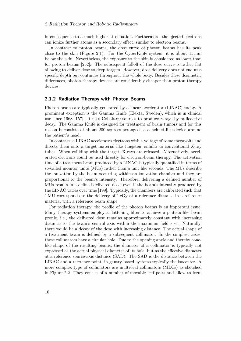
directs them onto a target material like tungsten, similar to conventional X-raytubes. When colliding with the target, X-rays are released. Alternatively, accel-erated electrons could be used directly for electron-beam therapy. The activationtime of a treatment beam produced by a LINAC is typically quantified in terms ofso-called monitor units (MUs) rather than a unit like seconds. The MUs describethe ionization by the beam occurring within an ionization chamber and they areproportional to the beam’s intensity. Therefore, delivering a defined number ofMUs results in a defined delivered dose, even if the beam’s intensity produced bythe LINAC varies over time [199]. Typically, the chambers are calibrated such that1 MU corresponds to the delivery of 1 cGy at a reference distance in a referencematerial with a reference beam shape.For radiation therapy, the profile of the photon beams is an important issue.
Many therapy systems employ a flattening filter to achieve a plateau-like beamprofile, i.e., the delivered dose remains approximately constant with increasingdistance to the beam’s central axis within the maximum field size. Naturally,there would be a decay of the dose with increasing distance. The actual shape ofa treatment beam is defined by a subsequent collimator. In the simplest cases,these collimators have a circular hole. Due to the opening angle and thereby cone-like shape of the resulting beams, the diameter of a collimator is typically notexpressed as the actual physical diameter of its hole, but as the effective diameterat a reference source-axis distance (SAD). The SAD is the distance between theLINAC and a reference point, in gantry-based systems typically the isocenter. Amore complex type of collimators are multi-leaf collimators (MLCs) as sketchedin Figure 2.2. They consist of a number of movable leaf pairs and allow to form
10
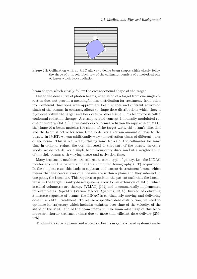
2.1 Medical and Physical Background
Figure 2.2: Collimation with an MLC allows to define beam shapes which closely followthe shape of a target. Each row of the collimator consists of a motorized pairof leaves which block radiation.
beam shapes which closely follow the cross-sectional shape of the target.Due to the dose curve of photon beams, irradiation of a target from one single di-
rection does not provide a meaningful dose distribution for treatment. Irradiationfrom different directions with appropriate beam shapes and different activationtimes of the beams, in contrast, allows to shape dose distributions which show ahigh dose within the target and low doses to other tissue. This technique is calledconformal radiation therapy. A closely related concept is intensity-modulated ra-diation therapy (IMRT). If we consider conformal radiation therapy with an MLC,the shape of a beam matches the shape of the target w.r.t. this beam’s directionand the beam is active for some time to deliver a certain amount of dose to thetarget. In IMRT, we can additionally vary the activation times of different partsof the beam. This is realized by closing some leaves of the collimator for sometime in order to reduce the dose delivered to that part of the target. In otherwords, we do not deliver a single beam from every direction but a weighted sumof multiple beams with varying shape and activation time.Many treatment machines are realized as some type of gantry, i.e., the LINAC
rotates around the patient similar to a computed tomography (CT) acquisition.In the simplest case, this leads to coplanar and isocentric treatment beams whichmeans that the central axes of all beams are within a plane and they intersect inone point, the isocenter. This requires to position the patient such that the isocen-ter is in the target. Gantry-based systems allow for an extension of IMRT whichis called volumetric arc therapy (VMAT) [194] and is commercially implementedfor example as RapidArc (Varian Medical Systems, USA). Instead of deliveringa discrete sequence of beams, the LINAC is continuously moving and deliveringdose in a VMAT treatment. To realize a specified dose distribution, we need tooptimize its trajectory which includes variation over time of the velocity, of theshape of the MLC, and of the beam intensity. The main advantage of this tech-nique are shorter treatment times due to more time-efficient dose delivery [256,276].The limitation to coplanar and isocentric beams in gantry-based systems can be
11

2 Radiation Therapy and Robotic Radiosurgery
removed by employing a robotic treatment couch. Moving the couch allows to shiftthe isocenter w.r.t. the target and, by rotations, to irradiate from non-coplanardirections. Non-coplanar and non-isocentric beams typically allow for a steeperdose falloff around the target and better sparing of healthy structures [103, 249]. Inhelical tomotherapy, especially implemented in the TomoTherapy (Accuray, USA)system, the patient couch is axially moved through the rotating gantry to realizea continuous helical beam delivery [170]. The combination of couch rotation andVMAT has been proposed, sometimes under the name 4π therapy, and allowsfor continuous spherical trajectories around the patient providing time-efficientirradiation from more directions [48, 253, 282].A treatment is separated into multiple sessions, which is called fractionation
[260]. In each fraction, only some fraction of the total dose is delivered. The timebetween the fractions allows healthy cells to recover from collateral damage, whiletumor cells are often not able to repair themselves sufficiently fast. Thereby, sideeffects can be reduced. Fractionation can result in daily treatment over severalweeks. Therefore, the accurate and reproducible positioning and aligning of thepatient w.r.t. the treatment system is an essential issue. Any variation occurringbetween two fractions is referred to as inter-fractional while a variation in thecourse of the delivery of a fraction is referred to as intra-fractional.Another approach is hypofractionation, which only uses a few fractions with
high doses each, or even only one single fraction [89, 127]. These approaches arecommonly called stereotactic, which refers to a fixation of the patient to allowfor a very accurate delivery of the dose to the target. This accuracy is espe-cially needed when delivering high doses. Stereotactic treatments are further sep-arated into stereotactic radiosurgery (SRS) in case of cranial targets and SBRT orstereotactic ablative body radiotherapy (SABR) in case of other sites, includinglungs or prostate. Due to the high dose per fraction, the dose has to be deliv-ered from many different directions to efficiently spare surrounding healthy tissue.While proper fixation is feasible for cranial targets, accurate dose delivery to othersites always requires high-quality image guidance, i.e., IGRT, to ensure that thetarget has not moved and is still correctly irradiated [16]. The Gamma Knife hasbeen pioneering in SRS. Today, the CyberKnife is an important system for SRSand SBRT.
2.2 The CyberKnife System
The CyberKnife has been originally proposed for SRS of intra-cranial targets. Theaim was to develop a system which does not require a fixating stereotactic frame[2, 3]. Instead, it uses image guidance and a robot-mounted LINAC (Figure 2.3)to allow for delivery of non-coplanar and non-isocentric beams and to adapt theirradiation to motion [240]. It is now used for treatment of targets throughoutthe body [125], including SBRT of lungs, liver, and prostate. Its current versionis the CyberKnife M6, which is technically summarized in Kilby et al. [126].
12
2.2 The CyberKnife System
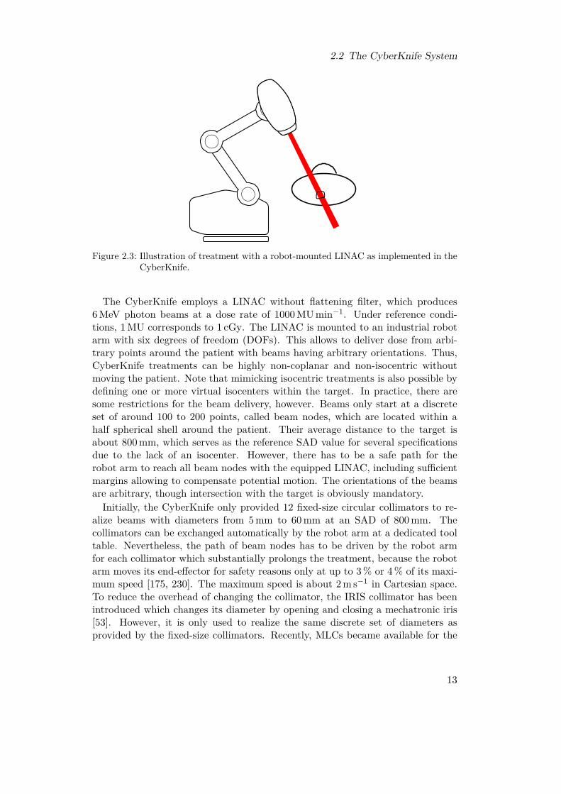
Figure 2.3: Illustration of treatment with a robot-mounted LINAC as implemented in theCyberKnife.
The CyberKnife employs a LINAC without flattening filter, which produces6 MeV photon beams at a dose rate of 1000 MU min−1. Under reference condi-tions, 1 MU corresponds to 1 cGy. The LINAC is mounted to an industrial robotarm with six degrees of freedom (DOFs). This allows to deliver dose from arbi-trary points around the patient with beams having arbitrary orientations. Thus,CyberKnife treatments can be highly non-coplanar and non-isocentric withoutmoving the patient. Note that mimicking isocentric treatments is also possible bydefining one or more virtual isocenters within the target. In practice, there aresome restrictions for the beam delivery, however. Beams only start at a discreteset of around 100 to 200 points, called beam nodes, which are located within ahalf spherical shell around the patient. Their average distance to the target isabout 800 mm, which serves as the reference SAD value for several specificationsdue to the lack of an isocenter. However, there has to be a safe path for therobot arm to reach all beam nodes with the equipped LINAC, including sufficientmargins allowing to compensate potential motion. The orientations of the beamsare arbitrary, though intersection with the target is obviously mandatory.
Initially, the CyberKnife only provided 12 fixed-size circular collimators to re-alize beams with diameters from 5 mm to 60 mm at an SAD of 800 mm. Thecollimators can be exchanged automatically by the robot arm at a dedicated tooltable. Nevertheless, the path of beam nodes has to be driven by the robot armfor each collimator which substantially prolongs the treatment, because the robotarm moves its end-effector for safety reasons only at up to 3 % or 4 % of its maxi-mum speed [175, 230]. The maximum speed is about 2 m s−1 in Cartesian space.To reduce the overhead of changing the collimator, the IRIS collimator has beenintroduced which changes its diameter by opening and closing a mechatronic iris[53]. However, it is only used to realize the same discrete set of diameters asprovided by the fixed-size collimators. Recently, MLCs became available for the
13

2 Radiation Therapy and Robotic Radiosurgery
Cyberknife [8, 75]. The InCise 2 MLC provides 26 pairs of tungsten leaves whichhave a width of 3.85 mm and provide a total treatment field of size 115× 100 mm2
at an SAD of 800 mm. As for MLCs in general, the idea is to provide more efficienttreatments of similar quality as with circular collimators [175]. Nevertheless, thefixed-size collimators still provide the beam shapes with lowest uncertainty [126].The CyberKnife only provides step-and-shoot treatments where a sequence of in-dividual beams is delivered. However, there have been experimental approachesdescribed recently for continuous irradiation with the MLC along arcs, similar tonon-coplanar VMAT [13, 123, 124].For intra-fractional image guidance, the CyberKnife is equipped with stereo-
scopic X-ray imaging and an optical tracking system. This basic setup has alreadybeen introduced in 2000 [241]. Detected target motion can be compensated byadjusting the pose of the LINAC by moving the robot arm. If the motion exceedssome centimeters or some degrees depending on the axis, an emergency stop istriggered in order to re-position the patient. Furthermore, the CyberKnife pro-vides a robotic treatment couch. However, this couch is only intended to supportpositioning of the patient and does not provide active motion compensation dur-ing an irradiation, because there is no rigid relation between the couch and thepatient [126]. Positioning is further supported by, for example, a laser pointingfrom the LINAC along the beams’ central axes.
2.3 Inverse PlanningIn forward planning for radiation therapy, the planner manually selects a set ofbeam directions and shapes. The computer then computes the activation times ofthese beams to match a given dose and visualizes the resulting dose distribution.Based on this feedback, the planner modifies the input parameters until they resultin an acceptable distribution. This approach is only suitable for rather easy casesand few beams. Not only for complex scenarios like CyberKnife treatments witha few hundred non-coplanar and non-isocentric beams, forward planning has beenmostly replaced by inverse planning. In inverse planning, the physician definesvolumes of interest (VOIs) in image data and assigns goals and constraints forthe dose distribution. Based on this input, the planning software automaticallysets up and solves an optimization problem. It outputs a set of beam directions,shapes, and activation times which fulfills all constraints and optimizes one ormore selected goals.
2.3.1 Data for Treatment PlanningIn order to compute the dose delivered by a treatment beam to a region withinthe patient, a high-resolution planning CT is required. From this volumetric scan,the electron densities can be derived. The first planning step, however, is thedelineation and contouring of relevant VOIs by a physician [30]. Due to the ratherpoor soft-tissue contrast of CT, delineation can be supported by other imaging
14

2.3 Inverse Planning
Right
Left
Superior Inferior
Anterior
Posteriorx
z y
Figure 2.4: Relation between anatomical coordinate axes and the axes of our world coor-dinate system.
modalities like MRI or a positron-emission tomography (PET) scan with a suitabletracer [117]. Via multi-modal image registration, the defined contours can betransferred to the planning CT for all subsequent planning steps. Delineation istypically done slice-wise in volumetric images, either manually or supported by animage-segmentation algorithm.Different anatomical coordinate systems are used in medical contexts. The fol-
lowing axes can be defined with respect to the patient (Figure 2.4). The superior-inferior (SI) axis points from the head (superior) towards the feet (inferior), theanterior-posterior (AP) axis points from the front (anterior) to the back (pos-terior), and the right-left (RL) axis points from the right shoulder to the leftshoulder. The planning CT typically consists of cross-sectional slices acquiredalong the SI-axis. If a beam intersects with the patient outside of the planningCT scan, that beam has to be rejected because the dose delivered to the patientcould not be completely evaluated. Therefore, the planning CT should not onlybe centered around the target and all relevant VOIs but also cover sufficient addi-tional tissue to allow for a wide range of beam directions. Exemplary slices froma contoured planning CT are shown in Figure 2.5. Furthermore, one point withinthe planning CT is defined as the reference point for all alignments relative to thetreatment room, including the beam-node positions and the field of view (FOV)of the stereoscopic X-ray imaging. In this thesis, we use a so-called LPS coordi-nate system for treatment planning, i.e., the x-axis is the RL-direction, the y-axisis the AP-direction, and the z-axis is the negative SI-direction. In terms of thetreatment room, in which the patient is lying on a couch, the y-axis points towardsthe floor.The most essential VOI to be delineated is the tumor area, which is the target
for the irradiation. The resulting VOI is called gross tumor volume (GTV) anddescribes the macroscopically identifiable part of the tumor. An extension of theGTV by microscopic parts of the tumor leads to the clinical target volume (CTV).This accounts for the typical spreading of cancerous cells and ensures that thewhole actual tumor will be treated. If radiation therapy follows a resection, there
15
2 Radiation Therapy and Robotic Radiosurgery
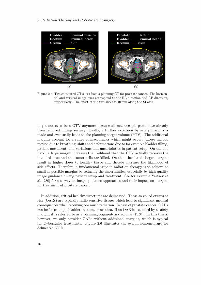
Bladder Seminal vesiclesRectum Femural headsUretha Skin
(a)
Prostate UrethaBladder Femural headsRectum Skin
(b)
Figure 2.5: Two contoured CT slices from a planning CT for prostate cancer. The horizon-tal and vertical image axes correspond to the RL-direction and AP-direction,respectively. The offset of the two slices is 10 mm along the SI-axis.
might not even be a GTV anymore because all macroscopic parts have alreadybeen removed during surgery. Lastly, a further extension by safety margins ismade and eventually leads to the planning target volume (PTV). The additionalmargins account for a range of inaccuracies which might occur. These includemotion due to breathing, shifts and deformations due to for example bladder filling,patient movement, and variations and uncertainties in patient setup. On the onehand, a large margin increases the likelihood that the CTV actually receives theintended dose and the tumor cells are killed. On the other hand, larger marginsresult in higher doses to healthy tissue and thereby increase the likelihood ofside effects. Therefore, a fundamental issue in radiation therapy is to achieve assmall as possible margins by reducing the uncertainties, especially by high-qualityimage guidance during patient setup and treatment. See for example Yartsev etal. [280] for a survey on image-guidance approaches and their impact on marginsfor treatment of prostate cancer.
In addition, critical healthy structures are delineated. These so-called organs atrisk (OARs) are typically radio-sensitive tissues which lead to significant medicalconsequences when receiving too much radiation. In case of prostate cancer, OARscan be for example bladder, rectum, or urethra. If an OAR is extended by a safetymargin, it is referred to as a planning organ-at-risk volume (PRV). In this thesis,however, we only consider OARs without additional margins, which is typicalfor CyberKnife treatments. Figure 2.6 illustrates the overall nomenclature fordelineated VOIs.
16

2.3 Inverse Planning
GTV
CTV
PTV
OAR
PRV
Figure 2.6: Illustration of GTV (macroscopic tumor), CTV (microscopic spread), andPTV (safety margins). In this sketch, we have an overlap with an OAR,which can also be extended by safety margins to a PRV.
2.3.2 Clinical GoalsTo describe and compare the quality of treatment plans quantitatively, severalfigures of merit are in use. These are sometimes called clinical goals, becausethey are typically not directly equivalent to the objective functions of the actualmathematical optimization problems which are solved to create the plans. Theyare rather related to the shape of the dose distribution w.r.t. to the VOIs. In thefollowing, we will introduce some of the most prominent clinical goals.
Dose Volume The dose volume V VOId describes which percentage of a certain
VOI receives at least the dose d. A common goal described by dose volumes is torestrict higher doses to a small fraction of an OAR. Furthermore, restrictions onunder-dosage within the PTV can be expressed by dose volumes.
Volume Dose Complementary to the dose volume, the volume dose dVOIp is the
highest dose which is received by at least p percent of a VOI.
Coverage If there is a prescribed dose dps for the PTV, then the coverage COVis the percentage of the PTV which receives at least dps. Therefore, it is simplythe special dose volume
COV = V PTVdps . (2.1)
and should be as high as possible, ideally 100 %.
Homogeneity Index There are different definitions for the homogeneity index HIin the literature [119]. They all relate in some way the maximum and minimumdose in the PTV to describe how homogeneous the dose is delivered. Sometimesthe extreme values are replaced, for example, by the 5 % and 95 % quantiles of thedose distribution, respectively. This leads to
HI = dPTV5dPTV95
. (2.2)
For a homogeneous irradiation, HI should be close to 1.
17
2 Radiation Therapy and Robotic Radiosurgery
Conformity Index The conformity index CI measures how much tissue has beenirradiated with at least dps relative to the size of the PTV V PTV, i.e.,
CI =V patientdps
V PTV . (2.3)
The basic idea is that ideally only the PTV receives a high dose, there is a steepdose gradient around it, and there are no high-dose areas farther away from thePTV. There exist alternative formulations for (2.3) [59]. One of them is calledthe new conformity index
nCI =V patientdps
V PTVdps
· VPTV
V PTVdps
(2.4)
and is the inverse of the Paddick conformity index [195]. Ideally, conformity in-dices reach a value of 1.
Note that none of these goals is individually meaningful, because each of themonly describes one specific aspect of the dose distribution. Beside these quanti-tative values, the qualitative goal is to achieve a high dose throughout the targetand spare the OARs as much as possible. Also the dose to other healthy tissueshould be minimized, which requires a sharp falloff of the dose outside the PTV.Furthermore, there are more general goals as, for example, short treatment timewhich improves aspects like patient comfort, additional dose due to X-ray-basedimage guidance, and patient throughput. All these goals, however, are conflictingin general. Higher dose in the target requires higher dose in surrounding tissuedue to the nature of dose delivery by photon beams. A high and homogeneouscoverage conflicts with a sharp dose falloff. Employing more beam directions canimprove OAR sparing but increases the treatment time. Therefore, treatmentplanning for radiation therapy is a multi-criteria optimization problem with con-flicting objectives and both hard and soft constraints.
A standard method to visualize and evaluate treatment plans with respect to thedose distribution in a VOI are dose-volume histograms (DVHs) [50]. This type ofdiagram has the received dose on the horizontal axis and the percentage of a VOI,which receives at least that dose, on the vertical axis. However, both DVHs andthe values of the clinical goals do not provide any spatial information. For spatialvisualization, isodose curves can be plotted within slices of the planning CT orthe deviation from a prescribed dose can be encoded by overlaid colors. Strategieshave been proposed to provide the planner a more visual and interactive feedbackduring in the planning process [222, 268].
2.3.3 Dose ModelTo evaluate and optimize the beams for a treatment, we need to have a physicalmodel of the dose delivery and energy deposition of each beam within the body
18
2.3 Inverse Planning
depending on its activation time. For photon-beam therapy, the dose delivered bya beam depends on the local electron densities in the tissue. These densities can bederived from the intensities in the planning CT. For very precise calculation of thedelivered dose, Monte-Carlo simulations are employed. However, these typicallyhave a high computational effort and require detailed information about the treat-ment machine and setup. As an alternative, we can use simpler models yieldingalgorithms which are fast but still sufficiently accurate for basic planning tasks.In practice, however, final validation of the plan with a Monte-Carlo algorithmmight be necessary [192, 274]. The CyberKnife provides a ray-tracing algorithm asan alternative to a Monte-Carlo-based algorithm [125]. Note that this algorithmis only suitable for treatments with the fixed-size or iris collimators. In case ofMLC-based treatments, the CyberKnife provides a finite-size pencil beam (FSPB)algorithm [112, 113] as a fast alternative to Monte Carlo, which accounts for thearbitrary beam shapes realizable by an MLC.In this thesis, we only consider the circular collimators and dose calculations
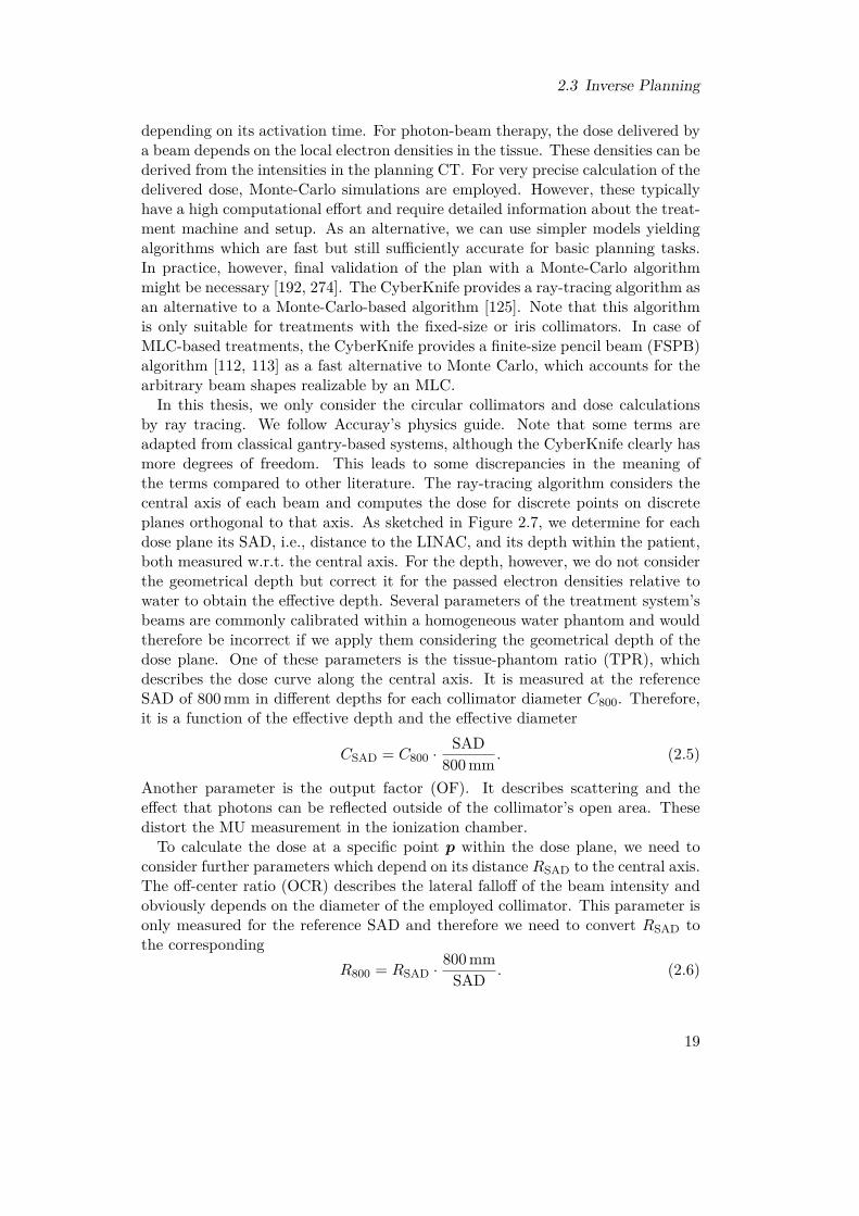
by ray tracing. We follow Accuray’s physics guide. Note that some terms areadapted from classical gantry-based systems, although the CyberKnife clearly hasmore degrees of freedom. This leads to some discrepancies in the meaning ofthe terms compared to other literature. The ray-tracing algorithm considers thecentral axis of each beam and computes the dose for discrete points on discreteplanes orthogonal to that axis. As sketched in Figure 2.7, we determine for eachdose plane its SAD, i.e., distance to the LINAC, and its depth within the patient,both measured w.r.t. the central axis. For the depth, however, we do not considerthe geometrical depth but correct it for the passed electron densities relative towater to obtain the effective depth. Several parameters of the treatment system’sbeams are commonly calibrated within a homogeneous water phantom and wouldtherefore be incorrect if we apply them considering the geometrical depth of thedose plane. One of these parameters is the tissue-phantom ratio (TPR), whichdescribes the dose curve along the central axis. It is measured at the referenceSAD of 800 mm in different depths for each collimator diameter C800. Therefore,it is a function of the effective depth and the effective diameter
CSAD = C800 ·SAD
800 mm . (2.5)
Another parameter is the output factor (OF). It describes scattering and theeffect that photons can be reflected outside of the collimator’s open area. Thesedistort the MU measurement in the ionization chamber.To calculate the dose at a specific point p within the dose plane, we need to
consider further parameters which depend on its distance RSAD to the central axis.The off-center ratio (OCR) describes the lateral falloff of the beam intensity andobviously depends on the diameter of the employed collimator. This parameter isonly measured for the reference SAD and therefore we need to convert RSAD tothe corresponding
R800 = RSAD ·800 mmSAD . (2.6)
19

2 Radiation Therapy and Robotic Radiosurgery
Planning CT grid
Beam node
Central axis
Dose planep
Depth
SAD
RSAD
Figure 2.7: Two-dimensional sketch of a dose calculation point p. The SAD and radiusRSAD are geometrically measured, while we have to distinguish between ge-ometrical depth and effective depth w.r.t. electron densities along the path.Note that both SAD and depth are measured w.r.t. central axis and doseplane, independent of the actual position of p within the plane.
With these parameters, which all provide only relative values, we can calculatethe dose per MU delivered to point p as
D (C800,SAD,deptheff, RSAD) = 1 cGy MU−1 · OCR (C800, R800, deptheff)
· TPR (CSAD, deptheff) · OF (C800,SAD) ·(800 mm
SAD
)2, (2.7)
which additionally includes the inverse-square law. The system is calibrated toprovide a dose rate of 1 cGy MU−1 in (2.7) for the 60 mm collimator at the referenceSAD of 800 mm in an effective depth of 15 mm on the beam’s central axis.
2.3.4 Sampling of Cylindrical Beams
The theoretical freedom of the CyberKnife’s beam delivery is already practicallylimited by its concept of beam nodes. Furthermore, some beams have to be re-jected due to the limited extend of the planning CT. In practice, there mightbe further undesired beams, like beams which intersect with an OAR before in-tersecting the PTV. Nevertheless, it is still intractable to consider all possiblecombinations of beam node, collimator diameter, and orientation for planning.
20
2.3 Inverse Planning
The common strategy for CyberKnife treatment planning is to randomly samplea set of N beams. Thereby, only the activation times of these so-called candidatebeams are variables for planning. We refer to the subset of the candidate beamswhich is actually active after planning as the set of treatment beams. With in-creasing number of candidate beams, we can expect the difference to the solutionof the complete problem to vanish. Thus, we have to decide for a proper trade-offbetween the computational complexity and the quality of the solution, which isthe typical trade-off decision in heuristic optimization. Different approaches havebeen proposed which aim to find more efficient candidate beams than randomsampling. They consider, for example, anatomical projections from beam nodesto derive promising orientations from previous plans by techniques like matchingwith a database [223] or deep learning [77, 80]. Alternatively, the planning prob-lem can be solved multiple times and all inactive beams of the previous run arereplaced by newly sampled beams [242].Given a set of candidate beams, we can setup a matrix D, the dose-coefficient
matrix, which maps the activation times x of the candidate beams to the dosed = Dx delivered to the voxels of the planning CT. Therefore, each row of Dcorresponds to one voxel and each column to one candidate beam. We obtainthe entries by calculating point doses for every beam by (2.7) and resampling theresults to the grid of the planning CT. If we are only interested in the dose to acertain VOI, we simply consider the related subset of rows of D.
2.3.5 Linear-Programming Approach
The CyberKnife provides a stepwise multi-criteria optimization approach based onsolving a sequence of linear programs (LPs) [159, 221]. An LP can be solved withguaranteed global optimality by, for example, the simplex algorithm or interiorpoint methods. In the stepwise approach, we do not combine multiple objectivesby weighting factors to a single objective function. Instead, we only optimize oneobjective in each iteration. The result of the current iteration is then transformedinto a new constraint. Therefore, it cannot be accidentally deteriorated in anyfollowing iteration. Nevertheless, the constraints can be manually relaxed if theydo not allow for an acceptable result in any later iteration. Furthermore, thereare post-processing routines which allow to maintain a similar plan quality butwith fewer beams and nodes in order to reduce the treatment time. Recently,the VOLO algorithm has been added to the CyberKnife’s planning software, es-pecially because the stepwise implementation is not designed for optimization ofMLC apertures [126, 237]. VOLO optimizes a weighted sum of multiple quadraticobjective functions and additionally provides methods to include optimization ofMLC apertures.Several objective functions are available for the stepwise optimization. They
include maximizing the minimum dose in a target VOI, minimizing the maximumdose in an OAR, minimizing the mean dose in an OAR, or minimizing the totalnumber of MU. In this thesis, we focus on optimization of the coverage (OCO)
21

2 Radiation Therapy and Robotic Radiosurgery
and employ hard constraints on the other objectives. Thereby, we can more easilycompare results for different scenarios, because only one objective varies and thehard constraints prevent unacceptable results for the other aspects.
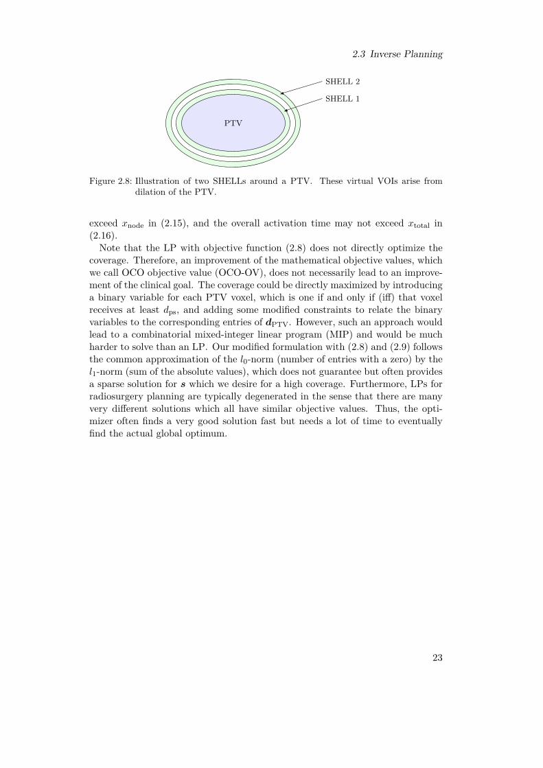
In order to not only control the dose in the VOIs but also the dose gradientaround the PTV, additional virtual VOIs are commonly introduced and calledSHELLs [236]. Note that the term shell is sometimes also used in the radiation-therapy context for masks which immobilize the patient during a treatment. Weconsider two SHELLs around the PTV. As illustrated in Figure 2.8, the SHELLsarise from isotropic dilation of the PTV. By setting upper dose bounds for theSHELLs, we can enforce a certain dose falloff around the PTV. Therefore, thedose bound should become lower from inner SHELLs to outer SHELLs. The basicLP structure which we consider for OCO can be described as
minx,s
1ᵀs (2.8)
s.t. dPTV + s ≥ dps (2.9)dPTV ≥ dmin (2.10)dPTV ≤ dmax (2.11)dOARi ≤ dOARi (2.12)dSHELLj ≤ dSHELLj (2.13)x ≤ xbeam (2.14)Nx ≤ xnode (2.15)1ᵀx ≤ xtotal (2.16)x ≥ 0 (2.17)s ≥ 0 (2.18)
with the vector of non-negative activation times x. Note that we imply element-wise comparison if we have a vector on the left-hand side but a scalar value onthe right-hand side of a constraint. A dose vector d containing the dose of eachvoxel can be calculated using the dose-coefficient matrix D as d = Dx. If only thevoxels of a certain VOI, e.g., dPTV for the PTV, are needed, this can be achievedby only using the corresponding rows of D. The coverage is modeled by (2.9)in combination with the objective function (2.8). If the dose in a PTV voxel isbelow dps, then the corresponding entry of the non-negative auxiliary vector shas to have a sufficiently high positive value to not violate the constraint (2.9).By minimizing the sum of the entries in s, we enforce that the doses are pushedtowards dps and in the ideal case we would achieve a dose of at least dps in allPTV voxels. Further, all voxels of the PTV get a lower dose limit dmin and anupper dose limit dmax in (2.10) and (2.11), respectively. For the voxels of the i-thOAR, there is an upper limit of dOARi set in (2.12). Analogously, upper limits forthe SHELLs are set in (2.13). Also the activation times themselves are restricted.An individual beam may not exceed the activation time xbeam in (2.14), all beamsof a node, which are summed by a matrix N having one row per node, may not
22
2.3 Inverse Planning
PTV
SHELL 1
SHELL 2
Figure 2.8: Illustration of two SHELLs around a PTV. These virtual VOIs arise fromdilation of the PTV.
exceed xnode in (2.15), and the overall activation time may not exceed xtotal in(2.16).Note that the LP with objective function (2.8) does not directly optimize the
coverage. Therefore, an improvement of the mathematical objective values, whichwe call OCO objective value (OCO-OV), does not necessarily lead to an improve-ment of the clinical goal. The coverage could be directly maximized by introducinga binary variable for each PTV voxel, which is one if and only if (iff) that voxelreceives at least dps, and adding some modified constraints to relate the binaryvariables to the corresponding entries of dPTV. However, such an approach wouldlead to a combinatorial mixed-integer linear program (MIP) and would be muchharder to solve than an LP. Our modified formulation with (2.8) and (2.9) followsthe common approximation of the l0-norm (number of entries with a zero) by thel1-norm (sum of the absolute values), which does not guarantee but often providesa sparse solution for s which we desire for a high coverage. Furthermore, LPs forradiosurgery planning are typically degenerated in the sense that there are manyvery different solutions which all have similar objective values. Thus, the opti-mizer often finds a very good solution fast but needs a lot of time to eventuallyfind the actual global optimum.
23


3 Image Guidance in Radiation Therapy
The dose delivery in radiation therapy is planned on a CT scan of the patient,which has been acquired beforehand. This allows to design highly conformal dosedistributions, which accurately cover the target but spare the OARs. However,the patient has to be positioned carefully before the delivery of each fraction. Theplanning process assumes a certain spatial relation between the coordinate frameof the treatment machine, the planning CT, and the patient’s actual anatomy.Therefore, the patient has to be positioned accurately and remaining deviationsfrom the setup assumed during planning have to be detected and accounted forin the treatment plan. Deviations can also arise from different conditions of thepatient, for example a different filling of the bladder which moves and deformsalso neighboring structures [36]. We refer to daily anatomical changes w.r.t. theplanning CT as inter-fractional motion. The anatomical changes observed in dailypre-treatment imaging can be used to generate a new plan [142, 201]. Remainingpositioning errors can partly be compensated by margins which are added tothe CTV (compare Section 2.3.1). The margins result in a larger area whichreceives a high treatment dose. Thereby, the tumor is adequately irradiated aslong as the positioning errors actually remain smaller than the margins. The severedrawback of larger margins is, however, that also more surrounding healthy tissueis irradiated. For this reason, it is a very important issue in radiation therapyand radiosurgery to minimize remaining uncertainty and thereby minimize therequired margins.Furthermore, there will be some inevitable motion by the patient during the
actual treatment, i.e., intra-fractional motion, which changes the anatomical ge-ometry compared to the planning CT. This motion includes not only predictablemovements caused by, for example, respiration [46] but also irregular spontaneousmovements. For example, prostate motion shows properties of a random walk [10]and the likelihood of larger motion increases with increasing treatment duration[197, 263]. During longer treatments, patients might even fall asleep resulting ininvoluntary and uncontrolled motion [34]. All kinds of movements, or more gener-ally unexpected events, during the treatment need to be detected reliably in realtime using appropriate imaging modalities [19]. Ensuring a precise dose deliveryis especially important during hypofractionated treatments. The CyberKnife sys-tem is able to compensate for small motion of the target by adjusting the poseof the LINAC. Larger motion of the target, however, results in an emergencystop and a repositioning of the patient. Note that also relative motion betweenthe target and an OAR might occur and could be additionally considered duringplanning [220]. As for inter-fractional motion management, the remaining uncer-
25

3 Image Guidance in Radiation Therapy
tainty can be accounted for by introducing further margins. Systems without arobot-mounted LINAC or a gimballed LINAC, as implemented in the Vero system(Brainlab, Germany, and Mitsubishi Heavy Industries, Japan) [44, 254], can usea motorized treatment couch to correct for motion [41, 143]. Another approachis an online adaption of MLC leaves to compensate for shifts or shape variationsof the target [122, 131]. Nevertheless, remaining uncertainties still require addingfurther margins to the VOIs to ensure sufficient dose delivery to the target.
Another approach to reduce margins is to directly include expected motion intoplanning. For example, instead of a single plan, we can create a library of plansconsidering different realistic states of critical organs. Before each fraction, weselect the plan which fits best to the current anatomical state of the patient [4, 14,38]. In robust optimization, we consider probability distributions for the entries ofthe dose-coefficient matrix [37], which effectively models uncertainty in the dosebeing actually delivered by a beam to each voxel of the planning CT. Thereby, theobjective function of the treatment plan becomes a function of random variablesand optimization is employed, for example, in terms of the average objective valueor the worst-case objective value [266]. Such approaches can also be extended toexplicitly reflect the multi-criteria nature of planning [35]. A recent study considersonline re-planning within a fraction to deliver the remaining dose correctly aftera detected motion event without interruption [130].In this chapter, we first discuss approaches which reduce motion of the patient
by fixation. Subsequently, we review the most common imaging modalities forIGRT, which are X-ray-based imaging, optical systems, EM tracking, and MRI.Finally, we provide an extended review and discussion of ultrasound imaging forinter-fractional and intra-fractional guidance.
3.1 Immobilization of the Patient
As motion needs to be reliably detected and compensated in radiation therapy,an intuitive step is to firstly minimize the likelihood and amplitude of potentialmotion by immobilization of the patient. In case of cranial radiosurgery, theclassical approach is to attach a stereotactic frame to the patient’s head [158,167, 169]. The frame is also fixed to parts of the treatment room or device, forexample the couch, and does not only limit the motion of the patient but alsodefines a rigidly attached reference coordinate frame. Already the planning CTis acquired with the frame attached. Therefore, the spatial relation between theinternal target and the frame can be measured in the CT scan. Later on, the poseof the target can be determined from this mapping in combination with externallocalization of the frame. Stereotactic frames are invasively attached to the skulland may be supported by other fixations like a bite block, ear plugs, or a headrest. Such fixations also allow to develop relocatable and less invasive frames [84].An obvious disadvantage of frames is the resulting patient discomfort and thetreatment might require at least local anesthesia. The main advantage is that
26
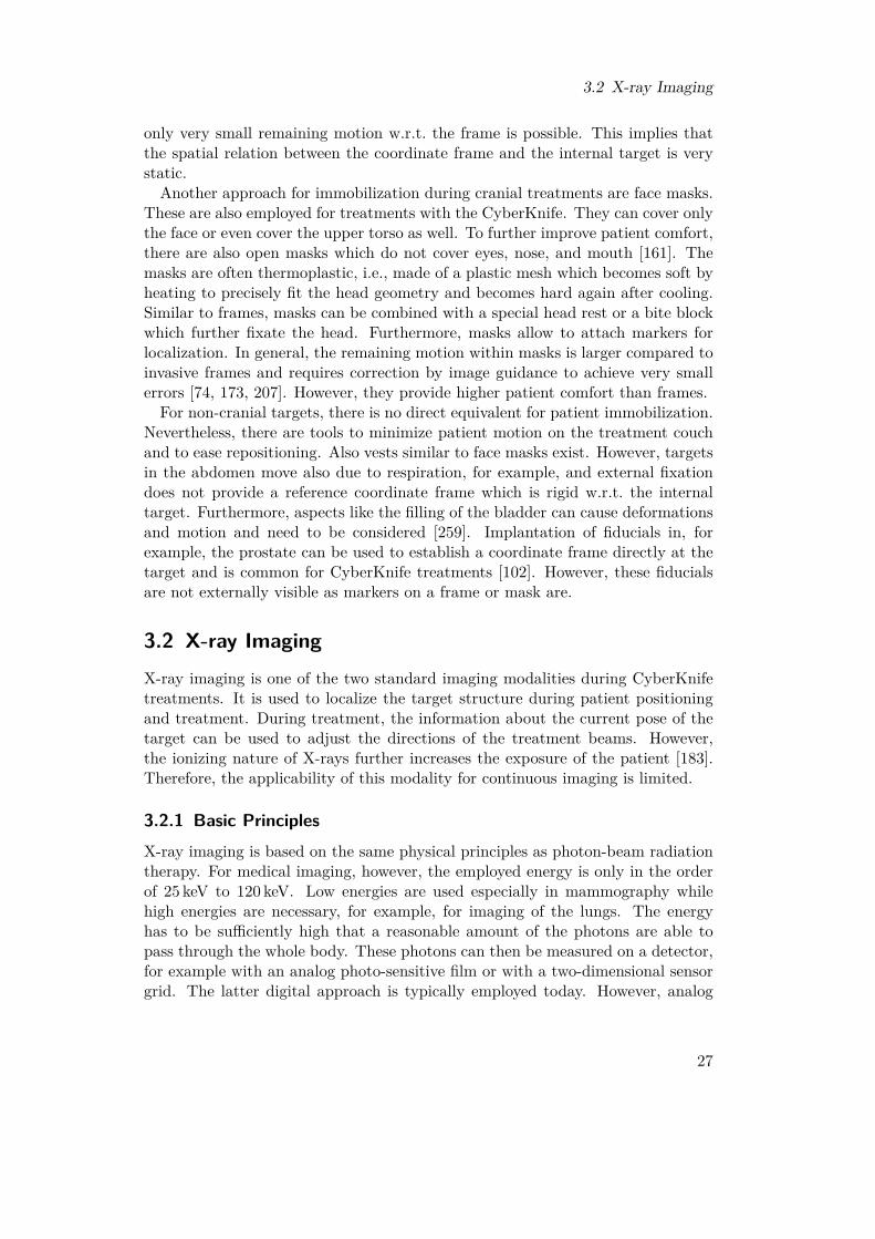
3.2 X-ray Imaging
only very small remaining motion w.r.t. the frame is possible. This implies thatthe spatial relation between the coordinate frame and the internal target is verystatic.Another approach for immobilization during cranial treatments are face masks.
These are also employed for treatments with the CyberKnife. They can cover onlythe face or even cover the upper torso as well. To further improve patient comfort,there are also open masks which do not cover eyes, nose, and mouth [161]. Themasks are often thermoplastic, i.e., made of a plastic mesh which becomes soft byheating to precisely fit the head geometry and becomes hard again after cooling.Similar to frames, masks can be combined with a special head rest or a bite blockwhich further fixate the head. Furthermore, masks allow to attach markers forlocalization. In general, the remaining motion within masks is larger compared toinvasive frames and requires correction by image guidance to achieve very smallerrors [74, 173, 207]. However, they provide higher patient comfort than frames.For non-cranial targets, there is no direct equivalent for patient immobilization.
Nevertheless, there are tools to minimize patient motion on the treatment couchand to ease repositioning. Also vests similar to face masks exist. However, targetsin the abdomen move also due to respiration, for example, and external fixationdoes not provide a reference coordinate frame which is rigid w.r.t. the internaltarget. Furthermore, aspects like the filling of the bladder can cause deformationsand motion and need to be considered [259]. Implantation of fiducials in, forexample, the prostate can be used to establish a coordinate frame directly at thetarget and is common for CyberKnife treatments [102]. However, these fiducialsare not externally visible as markers on a frame or mask are.
3.2 X-ray ImagingX-ray imaging is one of the two standard imaging modalities during CyberKnifetreatments. It is used to localize the target structure during patient positioningand treatment. During treatment, the information about the current pose of thetarget can be used to adjust the directions of the treatment beams. However,the ionizing nature of X-rays further increases the exposure of the patient [183].Therefore, the applicability of this modality for continuous imaging is limited.
3.2.1 Basic PrinciplesX-ray imaging is based on the same physical principles as photon-beam radiationtherapy. For medical imaging, however, the employed energy is only in the orderof 25 keV to 120 keV. Low energies are used especially in mammography whilehigh energies are necessary, for example, for imaging of the lungs. The energyhas to be sufficiently high that a reasonable amount of the photons are able topass through the whole body. These photons can then be measured on a detector,for example with an analog photo-sensitive film or with a two-dimensional sensorgrid. The latter digital approach is typically employed today. However, analog
27
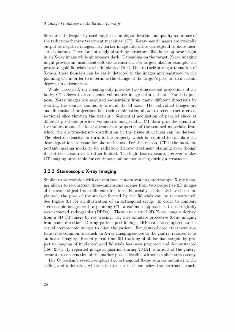
3 Image Guidance in Radiation Therapy
films are still frequently used for, for example, calibration and quality assurance ofthe radiation-therapy treatment machines [177]. X-ray-based images are typicallyoutput as negative images, i.e., darker image intensities correspond to more mea-sured photons. Therefore, strongly absorbing structures like bones appear brightin an X-ray image while air appears dark. Depending on the target, X-ray imagingmight provide an insufficient soft-tissue contrast. For targets like, for example, theprostate, gold fiducials can be implanted [102]. Due to their strong attenuation ofX-rays, these fiducials can be easily detected in the images and registered to theplanning CT in order to determine the change of the target’s pose or, to a certaindegree, its deformation.
While classical X-ray imaging only provides two-dimensional projections of thebody, CT allows to reconstruct volumetric images of a patient. For this pur-pose, X-ray images are acquired sequentially from many different directions byrotating the source, commonly around the SI-axis. The individual images areone-dimensional projections but their combination allows to reconstruct a cross-sectional slice through the patient. Sequential acquisition of parallel slices atdifferent positions provides volumetric image data. CT data provides quantita-tive values about the local attenuation properties of the scanned materials, fromwhich the electron-density distribution in the tissue structures can be derived.The electron density, in turn, is the property which is required to calculate thedose deposition in tissue for photon beams. For this reason, CT is the most im-portant imaging modality for radiation therapy treatment planning even thoughits soft-tissue contrast is rather limited. The high dose exposure, however, makesCT imaging unsuitable for continuous online monitoring during a treatment.
3.2.2 Stereoscopic X-ray Imaging
Similar to stereovision with conventional camera systems, stereoscopic X-ray imag-ing allows to reconstruct three-dimensional scenes from two projective 2D imagesof the same object from different directions. Especially if fiducials have been im-planted, the pose of the marker formed by the fiducials can be reconstructed.See Figure 3.1 for an illustration of an orthogonal setup. In order to comparestereoscopic images with a planning CT, a common approach is to use digitallyreconstructed radiographs (DRRs). These are virtual 2D X-ray images derivedfrom a 3D CT image by ray tracing, i.e., they simulate projective X-ray imagingfrom some direction. During patient positioning, DRRs can be compared to theactual stereoscopic images to align the patient. For gantry-based treatment sys-tems, it is common to attach an X-ray imaging source to the gantry, referred to ason-board imaging. Recently, real-time 6D tracking of abdominal targets by pro-jective imaging of implanted gold fiducials has been proposed and demonstrated[186, 258]. By repeated image acquisition during VMAT rotations of the gantry,accurate reconstruction of the marker pose is feasible without explicit stereoscopy.The CyberKnife system employs two orthogonal X-ray sources mounted to the
ceiling and a detector, which is located on the floor below the treatment couch.
28

3.2 X-ray Imaging
X-ray source 2
Detector 2
X-ray sou
rce1
Detecto
r 1
PTV
Figure 3.1: Cross-sectional sketch of orthogonal 2D X-ray imaging with the isocenter insidethe PTV.
The setup is aligned to the reference point defined in the planning CT by theplanner. The X-ray imaging can be used both for positioning and image guidanceduring treatment. Due to the additional exposure of the patient to ionizing ra-diation, the CyberKnife acquires images during treatment only every 30 s to 60 s[126]. This interval-based approach might therefore detect movements only with acertain delay. Furthermore, it might completely miss motion events which exceedthe tolerable limits only in the time frame between two sequent acquisitions. Inaddition, a temporal synchronization between X-ray imaging and motion of therobot-mounted LINAC is necessary, because otherwise the robot arm can blockthe line-of-sight and thereby the imaging intervals become too large.Conventionally, fiducials are implanted for tracking. However, the CyberKnife
offers the fiducial-free systems Xsight lung [70, 278] and Xsight spine [100, 182].The Xsight tracking system for lungs uses directly the soft-tissue contrast andregisters the stereoscopic images to DRRs to derive 6D motion information. Thisis only feasible if the tumor has a certain extent. For spine tracking, static bonystructures are localized in the images and compared to data from the planningCT. Both systems are also used for patient positioning. For SRS, the CyberKnifeprovides 6D tracking of the skull based on skeletal features [71, 118].
3.2.3 Cone Beam CT
Classical CT is based in its simplest implementation on the sequential acquisitionof one-dimensional measurements with line detectors and is also called fan beamcomputed tomography (FBCT). In the advanced multi slice computed tomogra-phy (MSCT), multiple adjacent lines are acquired simultaneously. Another alter-native is cone beam computed tomography (CBCT), in which the X-ray beamshave a three-dimensional conical shape to directly cover a whole volume instead
29
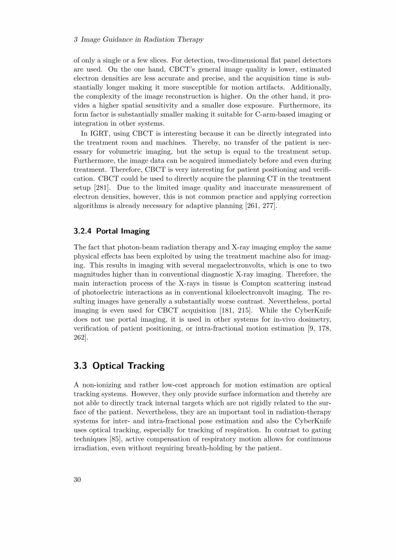
3 Image Guidance in Radiation Therapy
of only a single or a few slices. For detection, two-dimensional flat panel detectorsare used. On the one hand, CBCT’s general image quality is lower, estimatedelectron densities are less accurate and precise, and the acquisition time is sub-stantially longer making it more susceptible for motion artifacts. Additionally,the complexity of the image reconstruction is higher. On the other hand, it pro-vides a higher spatial sensitivity and a smaller dose exposure. Furthermore, itsform factor is substantially smaller making it suitable for C-arm-based imaging orintegration in other systems.
In IGRT, using CBCT is interesting because it can be directly integrated intothe treatment room and machines. Thereby, no transfer of the patient is nec-essary for volumetric imaging, but the setup is equal to the treatment setup.Furthermore, the image data can be acquired immediately before and even duringtreatment. Therefore, CBCT is very interesting for patient positioning and verifi-cation. CBCT could be used to directly acquire the planning CT in the treatmentsetup [281]. Due to the limited image quality and inaccurate measurement ofelectron densities, however, this is not common practice and applying correctionalgorithms is already necessary for adaptive planning [261, 277].
3.2.4 Portal Imaging
The fact that photon-beam radiation therapy and X-ray imaging employ the samephysical effects has been exploited by using the treatment machine also for imag-ing. This results in imaging with several megaelectronvolts, which is one to twomagnitudes higher than in conventional diagnostic X-ray imaging. Therefore, themain interaction process of the X-rays in tissue is Compton scattering insteadof photoelectric interactions as in conventional kiloelectronvolt imaging. The re-sulting images have generally a substantially worse contrast. Nevertheless, portalimaging is even used for CBCT acquisition [181, 215]. While the CyberKnifedoes not use portal imaging, it is used in other systems for in-vivo dosimetry,verification of patient positioning, or intra-fractional motion estimation [9, 178,262].
3.3 Optical Tracking
A non-ionizing and rather low-cost approach for motion estimation are opticaltracking systems. However, they only provide surface information and thereby arenot able to directly track internal targets which are not rigidly related to the sur-face of the patient. Nevertheless, they are an important tool in radiation-therapysystems for inter- and intra-fractional pose estimation and also the CyberKnifeuses optical tracking, especially for tracking of respiration. In contrast to gatingtechniques [85], active compensation of respiratory motion allows for continuousirradiation, even without requiring breath-holding by the patient.
30

3.3 Optical Tracking
3.3.1 Basic Concepts
Optical tracking typically refers to systems which employ visible or infrared light.Many commercial tracking systems use dedicated infrared markers which are lo-calized in stereoscopic images to estimate the position and orientation of a target.For this purpose, markers have to be rigidly attached closely to the actual struc-ture of interest. Marker geometry and placement can have a substantial influenceon the tracking errors [272]. A further distinction is made between active andpassive marker-based systems. Passive systems measure the reflection of light. Incontrast, active systems employ light emitting markers, for example a set of LEDs.An advantage of active markers is that they can be turned on sequentially to di-rectly provide a unique identification in image sequences. Furthermore, they cancreate a strong and easy-to-detect signal. Disadvantages are the required powersupply and electronics for control, often including cable connections.Common devices for markerless pose estimation are depth-sensing cameras. The
two major variants are time-of-flight (ToF) cameras and cameras employing struc-tured light. The former emits light, typically infrared, and measures the time untilthe reflection is received. From this time difference, the spatial distance to thereflecting object can be derived. The whole three-dimensional scene is illuminatedsimultaneously and a two-dimensional sensor matrix allows to reconstruct a pointcloud representing the surfaces in the scene. Therefore, tracking algorithms candirectly exploit height variations on a target surface to match the measured pointcloud with previous scans or a model and to estimate the pose. In structuredlight, light is emitted which forms a known geometric pattern, for example a grid.If the pattern is reflected on an object with a non-flat surface, we receive on thedetector a deformed version of the pattern. From the deformation, we can recoverthe shape of the reflecting surface. Structured light can employ infrared light inorder to minimize interference with other visible-light optical devices like RGBcameras.A common issue of optical tracking systems is that they require a steady line-of-
sight. Redundant markers and multiple cameras viewing from different directionscan reduce this effect. However, this is still difficult in scenarios like surgical track-ing with limited space, moving obstacles, and frequently changing environments.The advantages of optical tracking compared to other imaging modalities are therather cheap and light-weight systems, no harmful radiation, no electromagneticfields interfering with other devices or materials, fast acquisition and processing,and the common integration into small medical instruments.
3.3.2 Surface Imaging for Patient Setup
A common application for optical systems in radiation therapy is patient setup.The most basic approach are visible-light laser beams or patterns in the treatmentroom, which guide drawing marks on the patient’s skin or on an immobilization de-vice. Due to the markings and the fixed laser setup, it is possible to reproduce the
31
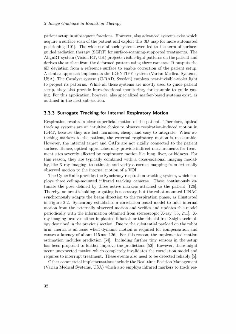
3 Image Guidance in Radiation Therapy
patient setup in subsequent fractions. However, also advanced systems exist whichacquire a surface scan of the patient and exploit this 3D map for more automatedpositioning [101]. The wide use of such systems even led to the term of surface-guided radiation therapy (SGRT) for surface-scanning-supported treatments. TheAlignRT system (Vision RT, UK) projects visible-light patterns on the patient andderives the surface from the deformed pattern using three cameras. It outputs the6D deviation from a reference surface to enable correction of the patient setup.A similar approach implements the IDENTIFY system (Varian Medical Systems,USA). The Catalyst system (C-RAD, Sweden) employs near-invisible-violet lightto project its patterns. While all these systems are mostly used to guide patientsetup, they also provide intra-fractional monitoring, for example to guide gat-ing. For this application, however, also specialized marker-based systems exist, asoutlined in the next sub-section.
3.3.3 Surrogate Tracking for Internal Respiratory Motion
Respiration results in clear superficial motion of the patient. Therefore, opticaltracking systems are an intuitive choice to observe respiration-induced motion inIGRT, because they are fast, harmless, cheap, and easy to integrate. When at-taching markers to the patient, the external respiratory motion is measurable.However, the internal target and OARs are not rigidly connected to the patientsurface. Hence, optical approaches only provide indirect measurements for treat-ment sites severely affected by respiratory motion like lung, liver, or kidneys. Forthis reason, they are typically combined with a cross-sectional imaging modal-ity, like X-ray imaging, to estimate and verify a correct mapping from externallyobserved motion to the internal motion of a VOI.
The CyberKnife provides the Synchrony respiration tracking system, which em-ploys three ceiling-mounted infrared tracking cameras. These continuously es-timate the pose defined by three active markers attached to the patient [126].Thereby, no breath-holding or gating is necessary, but the robot-mounted LINACsynchronously adapts the beam direction to the respiration phase, as illustratedin Figure 3.2. Synchrony establishes a correlation-based model to infer internalmotion from the externally observed motion and verifies and updates this modelperiodically with the information obtained from stereoscopic X-ray [55, 241]. X-ray imaging involves either implanted fiducials or the fiducial-free Xsight technol-ogy described in the previous section. Due to the substantial payload on the robotarm, inertia is an issue when dynamic motion is required for compensation andcauses a latency of about 115 ms [126]. For this reason, the implemented motionestimation includes prediction [54]. Including further tiny sensors in the setuphas been proposed to further improve the predictions [52]. However, there mightoccur unexpected motion which completely invalidates the correlation model andrequires to interrupt treatment. These events also need to be detected reliably [5].Other commercial implementations include the Real-time Position Management
(Varian Medical Systems, USA) which also employs infrared markers to track res-
32

3.3 Optical Tracking
PTV
Correlationmodel
Markertracking
Geometriccalibration
Figure 3.2: A correlation model relates the tracked motion of external markers to theinternal motion of the target. The geometrical calibration between trackingsystem and robotic LINAC allows to adjust the beam delivery accordingly.
piratory motion, in this case for gating. A markerless alternative is ExacTrac(Brainlab, Germany) which combines optical surface imaging since lately withthermal imaging to enhance accuracy [28]. Similar to Synchrony, ExacTrac com-plements the optical tracking with stereoscopic X-ray imaging to verify and updateits patient model. It is designed for use in both patient setup and intra-fractionaltracking.
3.3.4 Head Tracking
The task of tracking a patient’s head motion during an intervention does notonly appear in cranial radiation therapy, but also in other fields like transcranialmagnetic stimulation (TMS) [88, 212] or artifact-free brain imaging [69, 140]. Inradiation therapy with stereotactic frames, markers can be attached to the framefor tracking by an optical tracking system. Attachment of markers to masks orbite blocks [185] are alternative approaches in case of frame-less treatments, whichimprove patient comfort as discussed in Section 3.1. In any case, marker-basedapproaches have the drawback of the critical placement procedure and limitedrigidity w.r.t. the actual target. An alternative is markerless surface imaging [34,39, 160]. However, extracting motion in surface imaging requires to perform im-age registration and the accuracy of rigid registration suffers from any occurringnon-rigidity [90]. Non-rigid registration, in turn, has higher requirements on ex-ploitable features in the data. For this reason, different techniques have beenproposed to enhance surface data with additional information, like thermal imag-ing [28] or local tissue thickness estimation with infrared light [275].
33

3 Image Guidance in Radiation Therapy
3.4 Electromagnetic Tracking
EM tracking is a technique which effectively localizes small markers by sensingvariations of electromagnetic fields. It is widely employed in medical interventions[68]. In contrast to optical tracking, it does not require a line-of-sight and allows totrack internal targets. For the latter, however, it is necessary to place the markersinvasively in the target.
There are mainly three different approaches for EM tracking systems [20]. Thefirst approach utilizes alternating magnetic fields which are externally generatedand measured by small coils attached to the target. The received signals are readand evaluated for localization of the coils w.r.t. to the field. This typically requiresa wired connection between the coils and the computer system which processes thesignals. The second approach employs fluxgate sensors which are able to measurestatic magnetic fields. The remaining setup is essentially equal to that of systemsusing alternating fields.The third approach uses passive transponders which are attached to the target.
If these transponders are excited by a magnetic field, they emit a radio signal.This signal is received by antennas and the position of the transponder is derivedfrom signal properties like the delay or the intensity. If each employed transponderrequires excitation with a different frequency and they form a known geometry,they can be localized sequentially and the pose of their geometry can be estimatedw.r.t. the magnetic field.A drawback of EM tracking is its sensitivity to distortions of the fields caused
by other devices or materials [279], which compromise the localization procedure.Furthermore, there has to be sufficient space for appropriate integration of therequired hardware, which might include cable connections. Lastly, the accuracyof EM tracking systems is lower than the accuracy of optical tracking systems.However, EM tracking systems allow for integration into small instruments, likecatheters or endoscopes, and tracking of those instruments inside the patient with-out requiring a line-of-sight.The transponder-based approach allows to implant wireless transponders in or-
gans and to track their motion. This procedure is similar to the implantationof fiducials to enable X-ray-based localization but suitable for continuous moni-toring. In radiation therapy, this is implemented by the Calypso system (VarianMedical Systems, USA) for prostate [139] and lung [110, 248] tracking. The sys-tem employs three cylindrical transponders with diameters of 1.4 mm or 2.1 mmwhich are suitable for permanent implantation. The EM tracking system itself islocalized within the treatment room by an optical tracking system. For prostatetracking, accuracies similar to those achieved by orthogonal X-ray imaging havebeen reported [267]. It has also been used to guide MLC tracking [25, 122]. An-other clinical system for prostate tracking is RayPilot (Micropos Medical, Sweden)which uses wired transponders which are retracted after the treatment. The Cy-berKnife does not natively provide EM tracking.
34

3.5 Magnetic Resonance Imaging
3.5 Magnetic Resonance Imaging3.5.1 Basic PrinciplesIn MRI, we use a physical effect called nuclear magnetic resonance (NMR) togenerate high-resolution volumetric images of a patient. The images especiallyprovide a very good contrast between different soft tissues. For this reason, MRIis often used during treatment planning for delineation of the target and the OARsand registered to the planning CT. It only uses magnetic fields which are consid-ered to be safe for humans as long as they are operated reasonably. Nevertheless,there are remaining risks [43]. The basic component of an MRI scanner is a strongstatic magnetic field having a flux density in the order of 0.5 T to 7 T. Therefore,MRI cannot be used for patients with artificial cardiac pacemakers or metallicpieces or implants. Furthermore, it requires a shielded room which only containsNMR-compatible materials and devices. The strong magnetic field is typically re-alized with a magnet cooled by liquid helium to establish superconductivity. Thiscooling procedure is expensive and time-consuming. For this reason, MRI systemsare kept active even during standby phases.The imaging physics and practical instrumentation in MRI are complex and
beyond the scope of this section. Details can be found in Brown et al. [29], forexample. However, the basic idea is that the strong static magnetic field alignshydrogen nuclei inside the human body. This results in a small but measur-able magnetization. The orientation of this magnetization can be manipulatedby applying radio frequency (RF) pulses with a suitable frequency, the Larmorfrequency, which depends on the magnetic flux density of the static field. Afterthe RF pulse is turned off, relaxation processes start, which align the magnetiza-tion with the static field again and can be measured with external coils. The timerequired for relaxation is tissue-dependent and provides the contrast in the imageswhen spatially resolved. Many different sequences of RF pulses and measurementprotocols exist, which result in different contrasts in the images and allow to sup-press signals from specific structures. Furthermore, various contrast agents andboluses exist.The static magnetic field is typically aligned with the patient’s SI-axis and,
comparable to CT, we either acquire a sequence of axial slices or a whole volumeat once. Spatial encoding of the signals received in the coils can be realized bythree small gradient fields which slightly modify the frequency and the phase inthe received signal depending on the 3D location of the source. This encodingallows to reconstruct three-dimensional images from the signals recorded by thereceive coils.
3.5.2 Integration in the Treatment RoomMRI provides harmless volumetric imaging with a large FOV and very good soft-tissue contrast. However, image acquisition is rather slow for conventional diag-nostic scanning. Therefore, interventional MRI employs advanced strategies like
35
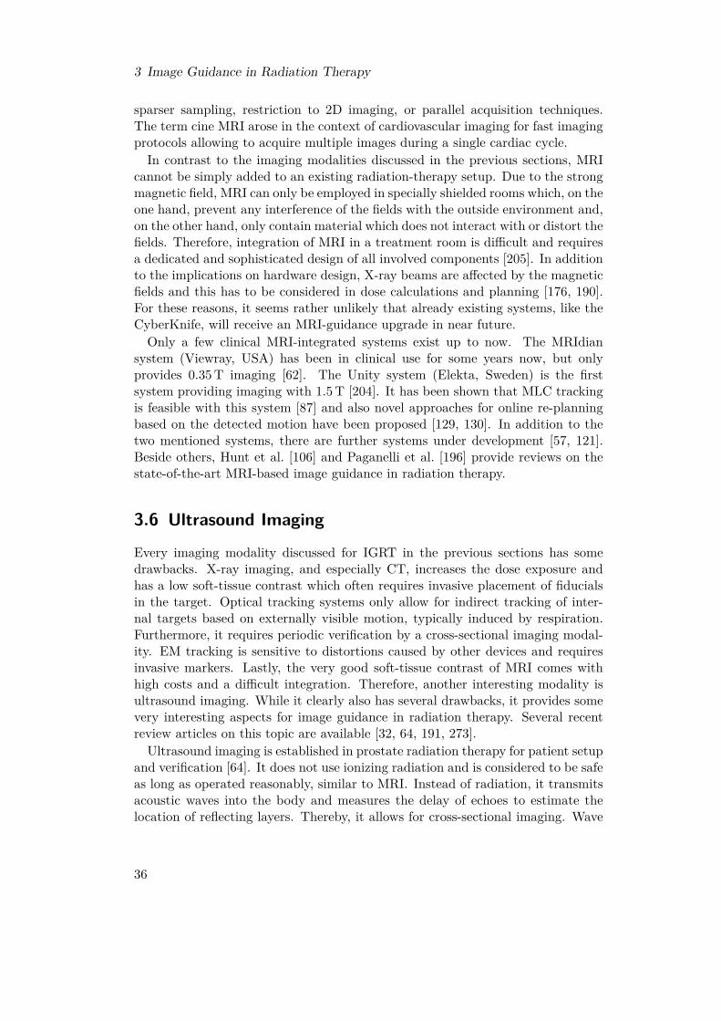
3 Image Guidance in Radiation Therapy
sparser sampling, restriction to 2D imaging, or parallel acquisition techniques.The term cine MRI arose in the context of cardiovascular imaging for fast imagingprotocols allowing to acquire multiple images during a single cardiac cycle.
In contrast to the imaging modalities discussed in the previous sections, MRIcannot be simply added to an existing radiation-therapy setup. Due to the strongmagnetic field, MRI can only be employed in specially shielded rooms which, on theone hand, prevent any interference of the fields with the outside environment and,on the other hand, only contain material which does not interact with or distort thefields. Therefore, integration of MRI in a treatment room is difficult and requiresa dedicated and sophisticated design of all involved components [205]. In additionto the implications on hardware design, X-ray beams are affected by the magneticfields and this has to be considered in dose calculations and planning [176, 190].For these reasons, it seems rather unlikely that already existing systems, like theCyberKnife, will receive an MRI-guidance upgrade in near future.Only a few clinical MRI-integrated systems exist up to now. The MRIdian
system (Viewray, USA) has been in clinical use for some years now, but onlyprovides 0.35 T imaging [62]. The Unity system (Elekta, Sweden) is the firstsystem providing imaging with 1.5 T [204]. It has been shown that MLC trackingis feasible with this system [87] and also novel approaches for online re-planningbased on the detected motion have been proposed [129, 130]. In addition to thetwo mentioned systems, there are further systems under development [57, 121].Beside others, Hunt et al. [106] and Paganelli et al. [196] provide reviews on thestate-of-the-art MRI-based image guidance in radiation therapy.
3.6 Ultrasound Imaging
Every imaging modality discussed for IGRT in the previous sections has somedrawbacks. X-ray imaging, and especially CT, increases the dose exposure andhas a low soft-tissue contrast which often requires invasive placement of fiducialsin the target. Optical tracking systems only allow for indirect tracking of inter-nal targets based on externally visible motion, typically induced by respiration.Furthermore, it requires periodic verification by a cross-sectional imaging modal-ity. EM tracking is sensitive to distortions caused by other devices and requiresinvasive markers. Lastly, the very good soft-tissue contrast of MRI comes withhigh costs and a difficult integration. Therefore, another interesting modality isultrasound imaging. While it clearly also has several drawbacks, it provides somevery interesting aspects for image guidance in radiation therapy. Several recentreview articles on this topic are available [32, 64, 191, 273].Ultrasound imaging is established in prostate radiation therapy for patient setup
and verification [64]. It does not use ionizing radiation and is considered to be safeas long as operated reasonably, similar to MRI. Instead of radiation, it transmitsacoustic waves into the body and measures the delay of echoes to estimate thelocation of reflecting layers. Thereby, it allows for cross-sectional imaging. Wave
36
3.6 Ultrasound Imaging
transmission requires direct contact of a so-called transducer or probe, which isconventionally hand-held, with the patient surface. The penetration and imagingdepth is severely limited in contrast to X-ray imaging or MRI. Furthermore,structures like bones or air enclosures further limit the effective imaging depthand can produce artifacts. Nevertheless, ultrasound imaging allows to visualizeinternal structures in real-time as one-, two-, or three-dimensional images, referredto as A-scans, B-scans, and C-scans, respectively. The systems are rather cheapcompared to CT or MRI and do not require a specific environment or shielding.Recently, there has been an increasing interest in employing ultrasound for intra-fractional guidance [191, 273]. This has been encouraged by recent advances in thereal-time capability of volumetric imaging with reasonable resolution and FOV size[108]. However, intra-fractional application requires to find practical solutions forseveral issues. The conventional manual operation of the ultrasound transduceris not feasible in the treatment room during a treatment due to the radiation.Further issues include the blocking of beam directions by the transducer and itsmounting and the limited reproducibility of a transducer’s position and its pressureonto the abdomen.In this section, we first describe the basic principles of ultrasound imaging.
Subsequently, we review the state-of-the-art application of ultrasound imaging forpatient setup and inter-fractional guidance. Lastly, we discuss recent approachesto intra-fractional guidance and the remaining difficulties and open questions. Inparticular, we review a recent approach employing a general-purpose robot armwith redundant kinematics for holding the transducer. For this specific setup, wewill analyze and optimize different aspects in the following chapters.
3.6.1 Basic Principles
In ultrasound imaging, we send acoustic waves into the patient’s body and measurethe time until we receive echoes due to reflections. The relevant tissue property isthe tissue-dependent acoustic impedance and reflections mainly occur where theimpedance abruptly changes. The frequency of the waves is typically in the orderof 1 MHz to 20 MHz, but depends on the specific application. The higher the fre-quency, the higher the spatial resolution. However, waves with higher frequenciesexperience a stronger attenuation in tissue and therefore ultrasound imaging withlower frequencies provides signals from deeper structures. The imaging depth canreach from a few centimeters to beyond 20 cm and the spatial resolution is typi-cally in the order of 0.1 mm to 3 mm depending on the parameters of the system’scomponents [257]. The axial resolution, i.e., in depth direction, is often betterthan the lateral resolution.Generation of the ultrasound waves is based on the piezo-electric effect. An
ultrasound transducer, also called probe, contains piezo crystals which mechan-ically oscillate in resonance when supplied with a proper alternating voltage. Ifwe have a direct contact between the transducer and the surface of a patient, theoscillation creates an acoustic wave which propagates through the tissue. The
37
3 Image Guidance in Radiation Therapy
oscillation is only excited for a small time interval and thereby we obtain a shortpulsed wave. After excitation, the same piezo crystals can be used to sense echoesby employing the reciprocal effect until we excite them again to generate the nextpulse. This repetition time determines from how deep we can receive echoes,because the echo delay is directly related to the traveled distance. In the sim-plest case, the temporal sequence of echoes from each pulse corresponds to oneone-dimensional depth scan. This so-called A-scan contains the amplitudes of thereceived echoes depending on the time which has passed since excitation. In prac-tice, the echo time is converted to a distance by assuming a homogeneous mediumwith a speed of sound of about 1540 m s−1 in case of soft-tissue imaging. This sim-plifying assumption is clearly never true in reality and this fact is important wheninterpreting the images because they do not provide correct geometric distances[21, 216]. Therefore, correction algorithms considering the actual local speed ofsound should be applied for quantitative measurements [65, 66]. Furthermore, theattenuation of a wave increases with increasing depth which requires to apply anecho-time-dependent intensity compensation in the images to obtain reasonableand comparable contrast over the whole depth range. Contrast agents can helpto image structures not having a good natural contrast in ultrasound images.Several transducer designs exist which allow for two- and three-dimensional
imaging. The most intuitive approach are flat one- and two-dimensional arraysof piezo crystals. The crystals are sequentially excited and thereby record depthscans at different locations. Other transducers use so-called beam forming. Byexciting multiple crystals simultaneously but with small delays, we can definean arbitrary orientation for the resulting superimposed wave. Given only a 2Dimaging transducer, mechanical sweeping or wobbling can alter the direction ofthe 2D plane to assemble 3D images. Alternatively, manual sweeping can bedone to create 3D images with a 2D transducer. More detailed information abouttransducer designs and the principles of ultrasound imaging in general can befound, for example, in Szabo [257].Other diagnostic modes of ultrasound include Doppler imaging to estimate flows
and elastography to derive mechanical tissue properties. In photoacoustic imaging,we record ultrasonic emissions in tissue caused by excitation with a laser pulse.Furthermore, integration of ultrasound imaging into catheters for intra-vascularimaging is an established technique. Similar to MRI, ultrasound imaging is consid-ered as safe when operated reasonable. Risks arise in longer procedures especiallyfrom thermal effects caused by the attenuated sound waves. Ultrasound is alsoemployed as a therapeutic tool in different variants. They include high-intensityfocused ultrasound (HIFU), which allows for insertion-free thermal ablation, andlow-intensity stimulation, which can accelerate healing of fractures.
3.6.2 Inter-Fractional Positioning of the Patient
Ultrasound imaging is used in the context of radiation therapy mostly for inter-fractional imaging of the prostate. Treatment sites like the brain or lungs are
38
3.6 Ultrasound Imaging
hardly accessible with ultrasound due to their bony and air-filled environment,respectively. Nevertheless, lung surface tracking has been demonstrated [214].Although studies have investigated ultrasound for various other sites, like liver,pancreas, kidneys, gallbladder, bladder, and most notably breast cancer [64, 191],the application is not clinically established and the few commercial systems focuson prostate treatments. For prostate imaging, there are three different approachesto place a transducer such that the prostate will be visible in the images [32].In transrectal ultrasound (TRUS), a specially designed ultrasound probe is in-
serted in the rectum for imaging close to the prostate with good image quality.However, this approach is uncomfortable for the patient and not used for posi-tioning or tracking in radiation therapy [32]. Nevertheless, TRUS is suitable fordiagnostic imaging and can also be used to guide placement of fiducials in theprostate [114, 145]. In brachytherapy, TRUS can guide needle insertions [11].The second approach is transperineal ultrasound (TPUS), in which we position
the transducer non-invasively onto the perineum, i.e., the area between scrotumand rectum. This requires a specific positioning of the patient in a rather uncom-fortable pose. The approach is commercially implemented in the Clarity Autoscansystem (Elekta, Sweden) [1, 93, 141]. Its mechanically-swept 2D transducer allowsfor automatic 3D imaging. The system allows for both inter- and intra-fractionalapplication, where we discuss the latter in the next sub-section.Transabdominal ultrasound (TAUS) is the third and most flexible approach in
the sense that other abdominal treatment sites, like the liver, could be imagedthe same way. A transducer is simply placed onto the abdominal wall close tothe prostate. Typically, the bladder provides a suitable imaging window if filledappropriately. However, the farther distance to the prostate compared to TRUSor TPUS requires to image at lower frequencies to achieve the necessary imagingdepth resulting in lower image quality. The TAUS approach has been commerciallyimplemented for inter-fractional motion detection. Two systems are SonArray(Varian Medical Systems, USA) [200, 219] and BAT, later called BATCAM, (BestNomos, USA) [144, 148, 217]. Another system is Clarity (Elekta, Sweden) which isan earlier and simpler version of Clarity Autoscan and requires manual sweeping ofthe 2D transducer to acquire and reconstruct 3D images [162]. Hence, the systemrequires some experience of the operator to achieve good quality and reproducibleimaging [60]. Severe operator and training dependence, however, is a general issuein ultrasound guidance [180].Localizing the transducer within in the treatment room is essential for registra-
tion and patient alignment. For this purpose, optical tracking can be employed.An alternative are passive probe holders, which are fixed in the treatment roomand sense the pose of the transducer. This has been used in the BAT system[144]. Also EM tracking of the transducer is an option. Furthermore, a spatialcalibration between the estimated transducer pose and the actual ultrasound im-age is necessary to directly relate points in the image to room coordinates [202,226]. Acquiring a reference ultrasound image for daily alignment along with theplanning CT is commonly considered as more accurate and reliable than employ-
39

3 Image Guidance in Radiation Therapy
ing inter-modality alignment with contours extracted from the planning CT [40,180]. The former approach avoids, for example, registration issues related to thegeometric distortion in ultrasound images or related to displacements due to thetransducer’s pressure onto the patient, which are not present in the planning CT.
3.6.3 Intra-Fractional Systems and Setups
It has been demonstrated that real-time volumetric ultrasound imaging is suitablefor intra-fractional motion monitoring [239] and even tasks like guiding dynamicMLC tracking [58, 109]. However, it requires to solve some practical problems de-pending on the specific system setup. The most important issue in intra-fractionalultrasound imaging arises from the fact that we need to ensure continuous con-tact between the transducer and the patient. Normally, a physician holds thetransducer and as a matter of routine adapts its pose to compensate, for example,breathing-induced motion of the patient. During a radiation-therapy treatment,however, manual operation is not feasible due to the ionizing radiation in thetreatment room. Therefore, some kind of automatic system is required which en-sures a steady contact to the patient’s surface. Only an initial setup immediatelybefore the treatment could be done manually. However, even this can be difficultdue to the generally strong operator dependence. Robotic ultrasound systems arealso relevant in other medical applications, especially in needle guidance and somekinds of surgeries [203].
While the Clarity system requiring manual sweeping clearly disqualifies fromintra-fractional application, its TPUS-based motorized version Clarity Autoscanhas been evaluated for intra-fractional imaging in various studies [92, 141, 210,211]. The transperineal transducer placement rarely interferes with treatmentbeams and only leads to minor pressure-induced artifacts. This system is the onlyestablished commercial solution for intra-fractional ultrasound guidance.TAUS has the advantage over TPUS that it is more generic as several treatment
sites could be imaged with the same system. In contrast, the TPUS approach islimited to prostate imaging. Furthermore, TAUS does not require a special pose ofthe patient for prostate imaging. However, especially when considering the beamdirections used in CyberKnife treatments which are mainly from anterior, blockingof treatment beams by the transducer is a bigger issue than for TPUS. Thefeasibility of radiolucent transducers for 3D imaging has been demonstrated [225],but all commercial transducers contain metal and other materials which interferewith X-ray beams. Bazalova-Carter et al. [12] have proposed Monte-Carlo-baseddose models which can account for such interfering transducers during treatmentplanning. However, the authors recommend to rather avoid intersections of thetreatment beams with the transducer, if possible, because these beams becomevery inefficient, the model requires precise reproduction of the transducer setupduring planning and all fractions, and the long-term effect of the radiation onthe transducers is not yet clear. It has been demonstrated for liver [224, 285]and prostate treatments [79, 227] with different treatment devices and systems for
40
3.6 Ultrasound Imaging
ultrasound guidance that the sparing beam directions which would interfere withthe transducer can generally still lead to acceptable plans.Şen et al. [245] developed a collaborative robotic system for intra-fractional ul-
trasound imaging. The in-house-constructed system integrates force sensing andprovides five active DOFs and additionally six passive DOFs. Note that a con-ventional robot arm which can realize any end-effector pose within its workspacerequires six DOFs. Adding more DOFs allows to realize the same pose in differentconfigurations which is interesting when, for example, reaching around obstaclesis necessary. The research group has put a major emphasis on the workflow forreproducible transducer placement [246]. After acquiring a reference ultrasoundimage, they replace the transducer for acquisition of the planning CT with a modelwhich, in contrast to the actual transducer, does not produce artifacts in the CTimage. The model is automatically positioned based on the previous pose andreaction forces of the actual transducer [15]. For transducer placement before thedaily alignment, a similar protocol is used in which first the operator performs arough manual alignment and afterwards the robot guides the precise alignmentwith force feedback [244, 247]. To account for anatomical changes, however, theoperator decides the eventual placement. In Şen et al. [246], the authors concludeto replace their specialized robot design with a commercial general-purpose robotarm to ease handling.Another research group started with tele-robotic 2D imaging [227] and devel-
oped an autonomous robotic system for 3D image guidance during treatmentsof the liver [224]. For the latter, they have put emphasis on investigating notonly the blocking of beams by the transducer but also by the robot arm. Thein-house-constructed robot arm provides nine DOFs allowing to flexibly handle awide range of patient geometries.The approach which we will consider in the subsequent chapters of this the-
sis has been developed at University of Lübeck [133, 134, 135]. Similar to thepreviously described approaches, it considers employing a robotic arm and forcesensing to realize a continuous contact between the ultrasound transducer andthe patient. However, instead of an in-house-built specialized robotic system, itconsiders a commercially-available general-purpose robot arm with seven DOFsand integrated force sensing. Thereby, the mechatronic part is already matureand does not require major additional engineering. Furthermore, this system isflexible and does not make any assumption on the environment or treatment site.Currently, two commercial light-weight robot arms with seven DOFs are available,namely the LBR iiwa (KUKA Roboter, Germany) and the Panda (Franka Emika,Germany) which we show in Figure 3.3a and Figure 3.3b, respectively. Note thatFigure 3.3a shows an LBR iiwa version allowing for up to 14 kg payload. There isa slimmer version limited to 7 kg which is more similar to the shown Panda havinga maximum payload of 3 kg. The two robot arms have very similar kinematicsand both provide integrated force sensing. Seitz et al. [243] have demonstratedhow the LBR iiwa’s force sensing allows to compensate for breathing and othermotion and thereby enables continuous contact and ultrasound imaging. While
41

3 Image Guidance in Radiation Therapy
(a) LBR iiwa (b) Panda
Figure 3.3: A high-payload version of the LBR iiwa (a) and a Panda (b) robot arm withseven DOFs and integrated force sensing.
the Panda is rather intended for application in research, the LBR iiwa is specifi-cally designed for safe human-robot collaboration and also available in specializedversions for operation in clean rooms and for medical applications. Note, thatthere are further commercial 7-DOF robot arms like, for example, the PA 10-7C(Mitsubishi Heavy Industries, Japan) and the Single-arm YuMi (ABB, Switzer-land). However, they are either rather heavy systems, intended for industry andlogistics, lack force sensing, or are not designed for collaboration with humans.Similar to the other robotic-ultrasound systems, the 7th DOF leading to a
redundant kinematic increases the dexterity of the robot arm [136] and therebyprovides additional flexibility for the ultrasound setup. This is interesting foravoiding the blocking of important beam directions. However, because all DOFsare actively actuated, it is even possible to vary the robot arm’s configurationduring a treatment without manual intervention. The kinematic design of boththe LBR iiwa and the Panda allows to continuously rotate the arm’s elbow whilemaintaining the same end-effector pose, as illustrated in Figure 3.4 for two angles.This allows to further reduce blocking of beam directions, because the robot armcould literally elude treatment beams. Kuhlemann et al. [137] derived for the LBRiiwa an analytic inverse kinematic, i.e., an explicit and deterministic algorithm tocompute all joint angles given the desired end-effector pose, which allows to controlthe angle of the elbow, which we call LIFT, directly with a single additionalparameter. This severely simplifies the control of elbow rotations with steadyend-effector pose.Using a kinematically redundant robot arm, however, cannot fully circumvent
beam blocking. Both the pose of the ultrasound transducer and the robot’s baseare fixed and mainly the intermediate links not directly connected to the end-
42
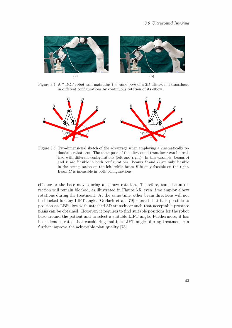
3.6 Ultrasound Imaging
(a) (b)
Figure 3.4: A 7-DOF robot arm maintains the same pose of a 2D ultrasound transducerin different configurations by continuous rotation of its elbow.
PTV
A
B
C D
E
F
PTV
A
B
C D
E
F
Figure 3.5: Two-dimensional sketch of the advantage when employing a kinematically re-dundant robot arm. The same pose of the ultrasound transducer can be real-ized with different configurations (left and right). In this example, beams Aand F are feasible in both configurations. Beams D and E are only feasiblein the configuration on the left, while beam B is only feasible on the right.Beam C is infeasible in both configurations.
effector or the base move during an elbow rotation. Therefore, some beam di-rection will remain blocked, as illustrated in Figure 3.5, even if we employ elbowrotations during the treatment. At the same time, other beam directions will notbe blocked for any LIFT angle. Gerlach et al. [79] showed that it is possible toposition an LBR iiwa with attached 3D transducer such that acceptable prostateplans can be obtained. However, it requires to find suitable positions for the robotbase around the patient and to select a suitable LIFT angle. Furthermore, it hasbeen demonstrated that considering multiple LIFT angles during treatment canfurther improve the achievable plan quality [78].
43

4 Basic Treatment-Planning Setup forUltrasound-Guided Radiosurgery
If we consider a kinematically redundant robot arm for image guidance by trans-abdominal ultrasound imaging, as introduced in Section 3.6.3, this has an impacton treatment planning for radiosurgery. Ultrasound imaging requires a steadycontact between the ultrasound transducer and the patient. Therefore, the robotarm which holds the transducer has to be positioned close to the patient and ithas to place and maintain the transducer directly onto the abdominal wall at asuitable viewport w.r.t. the imaging target. However, conventional robot arms areradiopaque, i.e., we cannot deliver dose through them. Therefore, we can onlyconsider candidate beams for planning, which do not intersect with any part ofthe robot arm or the ultrasound transducer, which conventionally is radiopaque aswell. This can deteriorate the achievable treatment plan quality if the blocked di-rections cannot be adequately compensated by beams from the remaining feasibledirections. The redundant kinematics of our 7-DOF robot arm under considera-tion provides additional flexibility in comparison to a setup with a conventional6-DOF robot arm, because an end-effector pose can be realized by infinitely manyconfigurations.In this chapter, we review and discuss the basic treatment planning aspects
which are required for an ultrasound-guidance setup with a kinematically redun-dant robot arm. We study planning on real cases of prostate cancer. For thispurpose, we first introduce the patient data and planning parameters, which weemploy in the following chapters as well. Afterwards, we introduce the robot modelwhich we consider for image guidance. We then review an algorithm to determinewhether a beam is feasible or blocked given a positioning and configuration of theguiding robot arm [79]. Finally, we present some basic results for our patient dataand three manually selected robot-arm setups, which will serve as a reference forour methods and experiments in the following chapters.
4.1 Patient Data and Planning ParametersIn this thesis, we will consider ten cases of prostate cancer, which have been treatedwith the CyberKnife at Europäisches Cyberknife Zentrum München-Großhadern.The data has been provided by Christoph Fürweger. Besides the planning CTs andcontours of the VOIs, the data also contains the parameters for the ray-tracing-based dose model. Our planning data and parameters essentially follow previousfeasibility studies [78, 79]. We consider treatment with cylindrical collimators with
45

4 Basic Treatment-Planning Setup for Ultrasound-Guided Radiosurgery
Table 4.1: Common treatment planning parameters for all patients. They contain theprescribed dose, lower and upper dose bound for the PTV, upper dose boundsfor the OARs, i.e., bladder and rectum, and the upper MU limits for eachindividual beam, all beams of a node, and all beams (compare Section 2.3.5 forthe notation).
dps dmin dmax dbladder drectum3625 cGy 0 cGy 4050 cGy 3600 cGy 3600 cGy
xbeam xnode xtotal300 MU 10 000 MU 40 000 MU
diameters of 10 mm, 15 mm, 20 mm, 30 mm, and 40 mm at an SAD of 800 mm.For all patients, we consider 99 beam nodes, which are the union of the actuallyemployed nodes of all patients. However, some of the beam nodes cannot producefeasible beams for some patients due to the specific geometries of the setups.We focus on the OCO approach introduced in Section 2.3.5, which maximizes
the coverage of, in our case, the PTV. Basic parameters for the LP which we willsolve for planning are listed in Table 4.1. They have been adapted from a five-fraction protocol and the prescribed dose for the PTV is set to 3625 cGy. We donot consider an explicit lower bound for the dose in the PTV but an upper boundof 4050 cGy. We consider two OARs, the bladder and the rectum. The dose toboth structures is limited to 3600 cGy. Furthermore, we have upper bounds onthe MUs. Any individual beam has at most 300 MU and the sum of all beams ofa node is limited to 10 000 MU. This bound, however, has rather low impact dueto the bound for the individual beams in combination with a total MU bound of40 000 MU.To obtain similar planning results for the different patients, we consider different
upper dose limits for two SHELLs around the PTV. Table 4.2 shows the bounds,which range from 3500 cGy to 3660 cGy and from 2700 cGy to 2975 cGy for theinner and outer SHELL, respectively. They have been manually tuned to achievea mean coverage of about 95 % for each patient. The table also lists the VOI sizesfor planning of each patient.
4.2 Robot-Arm Model for Image Guidance
We consider an LBR iiwa robot arm for ultrasound guidance to follow the setupdescribed in Section 3.6.3. In more detail, this light-weight model is specifically de-signed for human-robot collaboration tasks, especially in medical environments. Ithas seven rotational joints, which provide seven DOFs. While six DOFs are suffi-cient to realize arbitrary poses, i.e., positions and orientations of the end-effector,within a robot’s workspace, the additional DOF provides further flexibility byallowing to realize the same end-effector pose in, in this case, infinitely manyconfigurations which are continuously connected. Continuously connected means
46
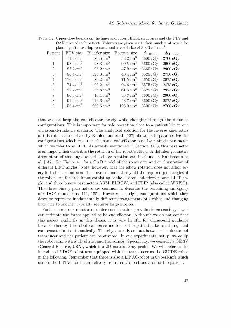
4.2 Robot-Arm Model for Image Guidance
Table 4.2: Upper dose bounds on the inner and outer SHELL structures and the PTV andOAR sizes of each patient. Volumes are given w.r.t. their number of voxels forplanning after overlap removal and a voxel size of 3× 3× 3 mm3.
Patient PTV size Bladder size Rectum size dSHELL1 dSHELL2
0 71.0 cm3 80.6 cm3 53.2 cm3 3600 cGy 2700 cGy1 98.9 cm3 98.3 cm3 90.5 cm3 3660 cGy 2900 cGy2 87.2 cm3 98.2 cm3 47.9 cm3 3660 cGy 2900 cGy3 86.4 cm3 125.8 cm3 40.4 cm3 3525 cGy 2750 cGy4 116.3 cm3 80.2 cm3 71.5 cm3 3650 cGy 2975 cGy5 74.4 cm3 196.2 cm3 94.6 cm3 3575 cGy 2875 cGy6 122.7 cm3 58.8 cm3 61.3 cm3 3625 cGy 2925 cGy7 90.5 cm3 40.4 cm3 56.3 cm3 3600 cGy 2900 cGy8 92.9 cm3 116.6 cm3 43.7 cm3 3600 cGy 2875 cGy9 56.4 cm3 269.6 cm3 125.0 cm3 3500 cGy 2700 cGy
that we can keep the end-effector steady while changing through the differentconfigurations. This is important for safe operation close to a patient like in ourultrasound-guidance scenario. The analytical solution for the inverse kinematicsof this robot arm derived by Kuhlemann et al. [137] allows us to parametrize theconfigurations which result in the same end-effector pose by a single parameterwhich we refer to as LIFT. As already mentioned in Section 3.6.3, this parameteris an angle which describes the rotation of the robot’s elbow. A detailed geometricdescription of this angle and the elbow rotation can be found in Kuhlemann etal. [137]. See Figure 4.1 for a CAD model of the robot arm and an illustration ofdifferent LIFT angles. Note, however, that the elbow rotation does not affect ev-ery link of the robot arm. The inverse kinematics yield the required joint angles ofthe robot arm for each input consisting of the desired end-effector pose, LIFT an-gle, and three binary parameters ARM, ELBOW, and FLIP (also called WRIST).The three binary parameters are common to describe the remaining ambiguityof 6-DOF robot arms [111, 155]. However, the eight configurations which theydescribe represent fundamentally different arrangements of a robot and changingfrom one to another typically requires large motion.Furthermore, our robot arm under consideration provides force sensing, i.e., it
can estimate the forces applied to its end-effector. Although we do not considerthis aspect explicitly in this thesis, it is very helpful for ultrasound guidancebecause thereby the robot can sense motion of the patient, like breathing, andcompensate for it automatically. Thereby, a steady contact between the ultrasoundtransducer and the patient can be ensured. In our experimental setup, we equipthe robot arm with a 3D ultrasound transducer. Specifically, we consider a GE 3V(General Electric, USA), which is a 2D matrix array probe. We will refer to theintroduced 7-DOF robot arm equipped with the transducer as the GUIDE-robotin the following. Remember that there is also a LINAC-robot in CyberKnife whichcarries the LINAC for beam delivery from many directions around the patient.
47
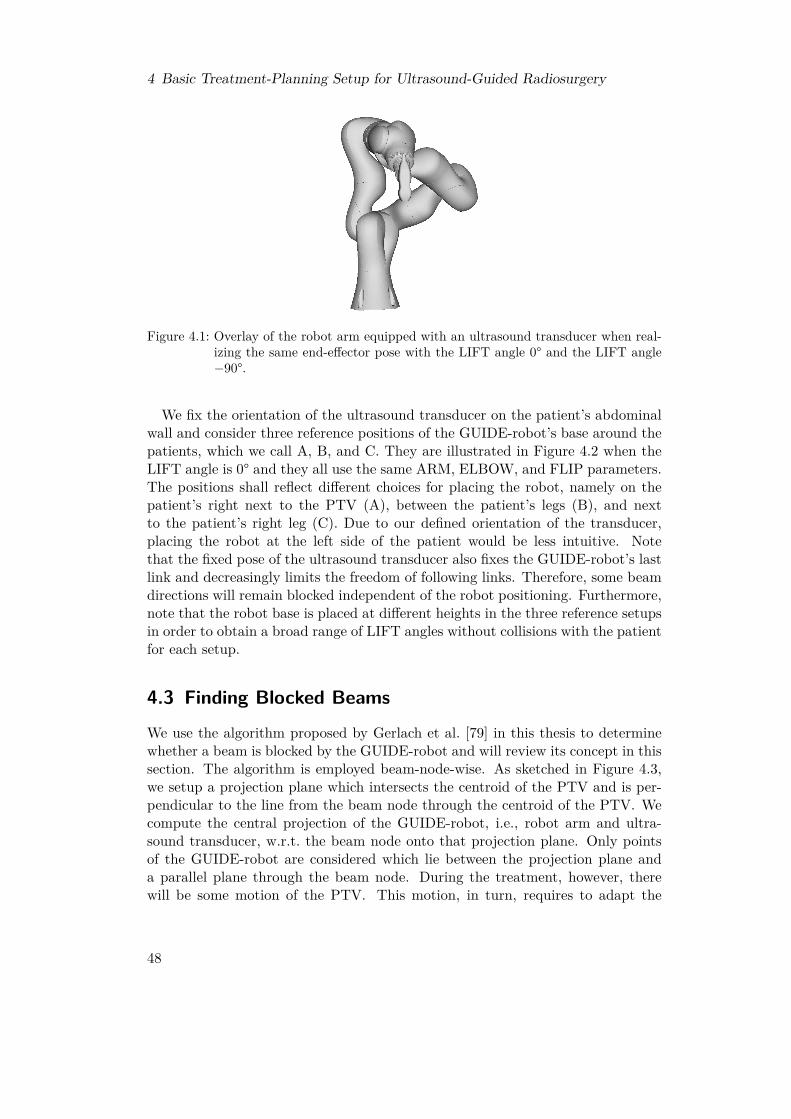
4 Basic Treatment-Planning Setup for Ultrasound-Guided Radiosurgery
Figure 4.1: Overlay of the robot arm equipped with an ultrasound transducer when real-izing the same end-effector pose with the LIFT angle 0° and the LIFT angle−90°.
We fix the orientation of the ultrasound transducer on the patient’s abdominalwall and consider three reference positions of the GUIDE-robot’s base around thepatients, which we call A, B, and C. They are illustrated in Figure 4.2 when theLIFT angle is 0° and they all use the same ARM, ELBOW, and FLIP parameters.The positions shall reflect different choices for placing the robot, namely on thepatient’s right next to the PTV (A), between the patient’s legs (B), and nextto the patient’s right leg (C). Due to our defined orientation of the transducer,placing the robot at the left side of the patient would be less intuitive. Notethat the fixed pose of the ultrasound transducer also fixes the GUIDE-robot’s lastlink and decreasingly limits the freedom of following links. Therefore, some beamdirections will remain blocked independent of the robot positioning. Furthermore,note that the robot base is placed at different heights in the three reference setupsin order to obtain a broad range of LIFT angles without collisions with the patientfor each setup.
4.3 Finding Blocked Beams
We use the algorithm proposed by Gerlach et al. [79] in this thesis to determinewhether a beam is blocked by the GUIDE-robot and will review its concept in thissection. The algorithm is employed beam-node-wise. As sketched in Figure 4.3,we setup a projection plane which intersects the centroid of the PTV and is per-pendicular to the line from the beam node through the centroid of the PTV. Wecompute the central projection of the GUIDE-robot, i.e., robot arm and ultra-sound transducer, w.r.t. the beam node onto that projection plane. Only pointsof the GUIDE-robot are considered which lie between the projection plane anda parallel plane through the beam node. During the treatment, however, therewill be some motion of the PTV. This motion, in turn, requires to adapt the
48

4.3 Finding Blocked Beams
R LI
S
(a) Robot A (b) Robot B (c) Robot C
Figure 4.2: Anterior views on the three reference positions, which we call A, B, and C, ofthe GUIDE-robot holding the ultrasound transducer when the LIFT angle is0°. The planning CT scan of patient 0 is shown.
Projection plane
PTV
Beam node
Figure 4.3: Central projection of the GUIDE robot from a beam node onto a plane or-thogonal to the line from beam node to PTV centroid (blue). The projectionis extended in the projection plane by a safety margin to account for potentialmotion during treatment (red).
positioning of the ultrasound transducer and of the delivered beam. For this rea-son, we extend the GUIDE-robot’s projection by a safety margin of 20 mm. Thismargin size has been shown to be a reasonable choice [79]. The information of theprojection is stored as a discrete grid with pixel size of 3× 3 mm2.Having the projection of the GUIDE-robot extended by the safety margin, we
check for every candidate beam starting at that beam node whether it intersectswith the projection. For this purpose, we need the extension of the intersection ofthe beam with the projection plane. We estimate that as the distance-transformeddiameter of its collimator w.r.t. the distance from beam node to PTV centroid,extended by a diameter-dependent margin factor. This value describes a diameter
49
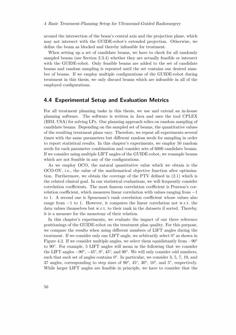
4 Basic Treatment-Planning Setup for Ultrasound-Guided Radiosurgery
around the intersection of the beam’s central axis and the projection plane, whichmay not intersect with the GUIDE-robot’s extended projection. Otherwise, wedefine the beam as blocked and thereby infeasible for treatment.
When setting up a set of candidate beams, we have to check for all randomlysampled beams (see Section 2.3.4) whether they are actually feasible or intersectwith the GUIDE-robot. Only feasible beams are added to the set of candidatebeams and random sampling is repeated until the set contains our desired num-ber of beams. If we employ multiple configurations of the GUIDE-robot duringtreatment in this thesis, we only discard beams which are infeasible in all of theemployed configurations.
4.4 Experimental Setup and Evaluation Metrics
For all treatment planning tasks in this thesis, we use and extend an in-houseplanning software. The software is written in Java and uses the tool CPLEX(IBM, USA) for solving LPs. Our planning approach relies on random sampling ofcandidate beams. Depending on the sampled set of beams, the quantitative valuesof the resulting treatment plans vary. Therefore, we repeat all experiments severaltimes with the same parameters but different random seeds for sampling in orderto report statistical results. In this chapter’s experiments, we employ 50 randomseeds for each parameter combination and consider sets of 6000 candidate beams.If we consider using multiple LIFT angles of the GUIDE-robot, we resample beamswhich are not feasible in any of the configurations.As we employ OCO, the natural quantitative value which we obtain is the
OCO-OV, i.e., the value of the mathematical objective function after optimiza-tion. Furthermore, we obtain the coverage of the PTV defined in (2.1) which isthe related clinical goal. In our statistical evaluations, we will frequently considercorrelation coefficients. The most famous correlation coefficient is Pearson’s cor-relation coefficient, which measures linear correlation with values ranging from −1to 1. A second one is Spearman’s rank correlation coefficient whose values alsorange from −1 to 1. However, it computes the linear correlation not w.r.t. thedata values themselves but w.r.t. to their rank in the datasets if sorted. Thereby,it is a measure for the monotony of their relation.In this chapter’s experiments, we evaluate the impact of our three reference
positionings of the GUIDE-robot on the treatment plan quality. For this purpose,we compare the results when using different numbers of LIFT angles during thetreatment. If we consider only one LIFT angle, we arbitrarily select 0° as shown inFigure 4.2. If we consider multiple angles, we select them equidistantly from −90°to 90°. For example, 5 LIFT angles will mean in the following that we considerthe LIFT angles −90°, −45°, 0°, 45°, and 90°. We will only consider odd numbers,such that each set of angles contains 0°. In particular, we consider 3, 5, 7, 19, and37 angles, corresponding to step sizes of 90°, 45°, 30°, 10°, and 5°, respectively.While larger LIFT angles are feasible in principle, we have to consider that the
50
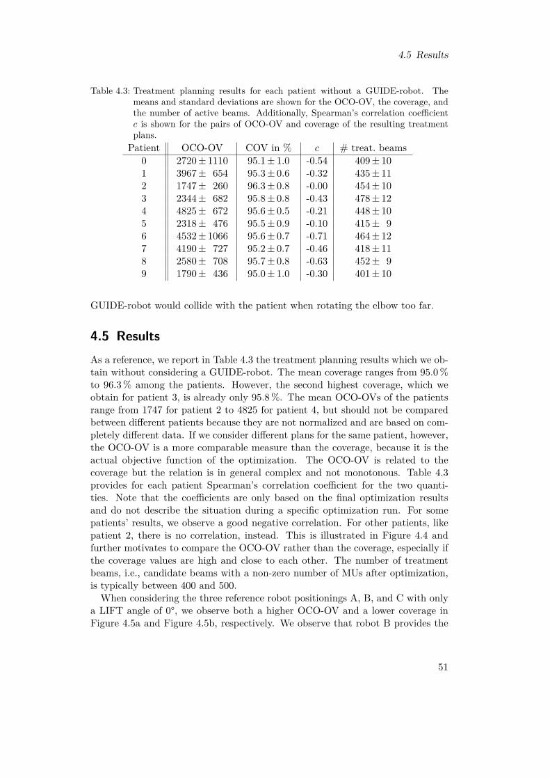
4.5 Results
Table 4.3: Treatment planning results for each patient without a GUIDE-robot. Themeans and standard deviations are shown for the OCO-OV, the coverage, andthe number of active beams. Additionally, Spearman’s correlation coefficientc is shown for the pairs of OCO-OV and coverage of the resulting treatmentplans.
Patient OCO-OV COV in % c # treat. beams0 2720± 1110 95.1± 1.0 -0.54 409± 101 3967± 654 95.3± 0.6 -0.32 435± 112 1747± 260 96.3± 0.8 -0.00 454± 103 2344± 682 95.8± 0.8 -0.43 478± 124 4825± 672 95.6± 0.5 -0.21 448± 105 2318± 476 95.5± 0.9 -0.10 415± 96 4532± 1066 95.6± 0.7 -0.71 464± 127 4190± 727 95.2± 0.7 -0.46 418± 118 2580± 708 95.7± 0.8 -0.63 452± 99 1790± 436 95.0± 1.0 -0.30 401± 10
GUIDE-robot would collide with the patient when rotating the elbow too far.
4.5 ResultsAs a reference, we report in Table 4.3 the treatment planning results which we ob-tain without considering a GUIDE-robot. The mean coverage ranges from 95.0 %to 96.3 % among the patients. However, the second highest coverage, which weobtain for patient 3, is already only 95.8 %. The mean OCO-OVs of the patientsrange from 1747 for patient 2 to 4825 for patient 4, but should not be comparedbetween different patients because they are not normalized and are based on com-pletely different data. If we consider different plans for the same patient, however,the OCO-OV is a more comparable measure than the coverage, because it is theactual objective function of the optimization. The OCO-OV is related to thecoverage but the relation is in general complex and not monotonous. Table 4.3provides for each patient Spearman’s correlation coefficient for the two quanti-ties. Note that the coefficients are only based on the final optimization resultsand do not describe the situation during a specific optimization run. For somepatients’ results, we observe a good negative correlation. For other patients, likepatient 2, there is no correlation, instead. This is illustrated in Figure 4.4 andfurther motivates to compare the OCO-OV rather than the coverage, especially ifthe coverage values are high and close to each other. The number of treatmentbeams, i.e., candidate beams with a non-zero number of MUs after optimization,is typically between 400 and 500.
When considering the three reference robot positionings A, B, and C with onlya LIFT angle of 0°, we observe both a higher OCO-OV and a lower coverage inFigure 4.5a and Figure 4.5b, respectively. We observe that robot B provides the
51

4 Basic Treatment-Planning Setup for Ultrasound-Guided Radiosurgery
2,000 4,000 6,000
94
95
96
97
98
OCO-OV
Cov
erag
ein
%
Patient 2Patient 6
Figure 4.4: Scatter plot of the OCO-OV and coverage of the final treatment plans fromall random seeds for patients 2 and 6.
worst results, except for patient 4. If we employ three LIFT angles, i.e., −90°,0°, and 90°, then we observe better results. For some patients, results are alreadyclose to the results without a GUIDE-robot. For patient 1, the planning resultswith robots A and B even have higher median coverages than without the GUIDE-robot. However, this is not the case for the OCO-OV, i.e., the actual objectivevalue from planning. We further observe that the influence of the robot positionis much smaller when employing three LIFT angles compared to the results forone LIFT angle. This observation highlights the impact and importance of thekinematic redundancy of the GUIDE-robot.In more detail, Table 4.4 provides the mean OCO-OVs for robot A and dif-
ferent numbers of employed LIFT angles. It shows that employing three insteadof only one LIFT angle provides a large improvement compared to the furtherimprovements by employing at least five LIFT angles. Especially the results forpatient 4 show no clear monotonicity. This is also the only patient for which fiveLIFT angles provide the lowest mean OCO-OV. For all others, we obtain the low-est result for 37 LIFT angles. However, the differences for the higher numbers ofLIFT angles are about one order of magnitude smaller than the observed standarddeviations.Table 4.5 underlines that the impact of the robot position reduces when employ-
ing many LIFT angles during the treatment. For employing a single LIFT angle,the OCO-OVs are typically notably higher for robot B than for robot A and C.An exception is again patient 4, for which we observe the largest value for robotA. In summary, robot A provides the best mean values for six of the patients androbot C for the other four of them. This situation is different when considering 37LIFT angles. The results of all three robots are rather close and robot B providesthe lowest mean for five patients. Robot A is now only the best choice for three
52

4.5 Results
0 1 2 3 4 5 6 7 8 91
2
3
4
5
Patient
Rel
ativ
em
edia
nO
CO
-OV Without robot
Robot A, 1 LIFTRobot A, 3 LIFTsRobot B, 1 LIFTRobot B, 3 LIFTsRobot C, 1 LIFTRobot C, 3 LIFTs
(a) Relative OCO-OVs. Note that the result of robot A with 3 LIFT angles is hidden by robotB’s result with 3 LIFT angles for patient 2 and robot B’s result with 3 LIFT angles forpatient 9 is hidden by robot C with 3 LIFT angles.
0 1 2 3 4 5 6 7 8 9
92
94
96
Patient
Med
ian
cove
rage
in%
Without robotRobot A, 1 LIFTRobot A, 3 LIFTsRobot B, 1 LIFTRobot B, 3 LIFTsRobot C, 1 LIFTRobot C, 3 LIFTs
(b) Coverage
Figure 4.5: Comparison of the median OCO-OV relative to the setup without a GUIDE-robot (a) and the median coverage with and without GUIDE-robot (b). Forthe single LIFT angle cases, we select 0°. We additionally select −90° and 90°in the case of three LIFT angles.
Table 4.4: Means and standard deviations of the OCO-OVs when employing robot A withdifferent numbers of LIFT angles. Angles are selected equidistantly from −90°to 90°. The first column is the patient index and the lowest mean achieved isprinted bold for each patient.
1 LIFT 3 LIFTs 5 LIFTs 7 LIFTs 19 LIFTs 37 LIFTs0 3630± 1222 3085± 1098 3061± 1067 3073± 1073 3067± 1044 2960± 10411 6023± 1049 4616± 779 4545± 771 4586± 763 4497± 748 4321± 7292 2784± 479 2450± 412 2398± 396 2404± 405 2402± 393 2334± 3743 3950± 762 2918± 625 2938± 635 2933± 632 2935± 631 2809± 5824 12352± 1439 8550± 1045 8399± 1081 8584± 1113 8455± 1109 8445± 11115 3725± 615 2988± 574 2800± 545 2818± 550 2793± 560 2730± 5436 18114± 3118 14575± 2531 14182± 2450 14261± 2425 14150± 2492 14030± 24917 10250± 1279 8889± 1154 8632± 1153 8719± 1175 8621± 1162 8586± 11398 5363± 1095 4620± 875 4537± 841 4538± 840 4535± 831 4527± 8299 2789± 581 2521± 554 2510± 531 2528± 540 2521± 534 2509± 548
53
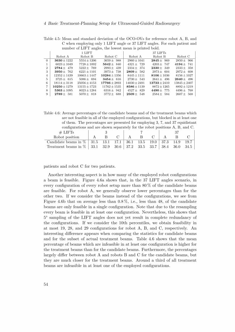
4 Basic Treatment-Planning Setup for Ultrasound-Guided Radiosurgery
Table 4.5: Mean and standard deviation of the OCO-OVs for reference robot A, B, andC when employing only 1 LIFT angle or 37 LIFT angles. For each patient andnumber of LIFT angles, the lowest mean is printed bold.
1 LIFT 37 LIFTsRobot A Robot B Robot C Robot A Robot B Robot C
0 3630± 1222 5554± 1206 3659± 988 2960± 1041 2845± 969 2850± 9661 6023± 1049 7728± 1092 5642± 840 4321± 729 4203± 747 4194± 7412 2784± 479 5222± 769 2993± 439 2334± 374 2330± 349 2333± 3583 3950± 762 6221± 1101 3973± 738 2809± 582 2973± 604 2972± 6084 12352± 1439 10663± 1447 10284± 1356 8445± 1111 8106± 1036 8156± 10275 3725± 615 5086± 694 3454± 616 2730± 543 2641± 496 2640± 4966 18114± 3118 25056± 4153 17766± 2893 14030± 2491 13733± 2410 13845± 24077 10250± 1279 13155± 1723 11762± 1535 8586± 1139 8872± 1265 8892± 12198 5363± 1095 8023± 1284 6316± 942 4527± 829 4490± 775 4496± 7689 2789± 581 5070± 818 3772± 688 2509± 548 2584± 584 2607± 568
Table 4.6: Average percentages of the candidate beams and of the treatment beams whichare not feasible in all of the employed configurations, but blocked in at least oneof them. The percentages are presented for employing 3, 7, and 37 equidistantconfigurations and are shown separately for the robot positions A, B, and C.
# LIFTs 3 7 37Robot position A B C A B C A B C
Candidate beams in % 31.5 13.1 17.1 36.1 13.5 19.0 37.3 14.9 19.7Treatment beams in % 33.1 32.9 30.6 37.2 33.5 33.7 38.4 36.0 34.5
patients and robot C for two patients.
Another interesting aspect is in how many of the employed robot configurationsa beam is feasible. Figure 4.6a shows that, in the 37 LIFT angles scenario, inevery configuration of every robot setup more than 80 % of the candidate beamsare feasible. For robot A, we generally observe lower percentages than for theother two. If we consider the beams instead of the configurations, we see fromFigure 4.6b that on average less than 0.8 %, i.e., less than 48, of the candidatebeams are only feasible in a single configuration. Note that due to the resamplingevery beam is feasible in at least one configuration. Nevertheless, this shows that5° sampling of the LIFT angles does not yet result in complete redundancy ofthe configurations. If we consider the 10th percentiles, we obtain feasibility inat most 19, 28, and 29 configurations for robot A, B, and C, respectively. Aninteresting difference appears when comparing the statistics for candidate beamsand for the subset of actual treatment beams. Table 4.6 shows that the meanpercentage of beams which are infeasible in at least one configuration is higher forthe treatment beams than for the candidate beams. Furthermore, the percentageslargely differ between robot A and robots B and C for the candidate beams, butthey are much closer for the treatment beams. Around a third of all treatmentbeams are infeasible in at least one of the employed configurations.
54
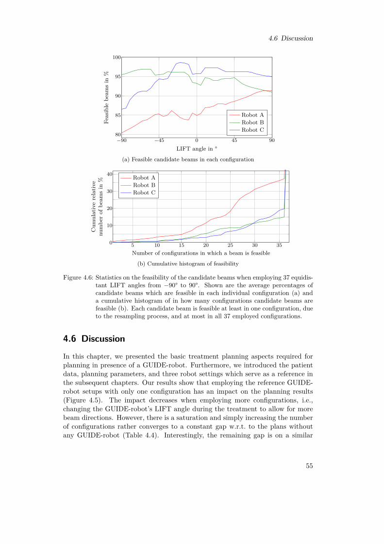
4.6 Discussion
−90 −45 0 45 9080
85
90
95
100
LIFT angle in °
Feas
ible
beam
sin
%Robot ARobot BRobot C
(a) Feasible candidate beams in each configuration
5 10 15 20 25 30 350
10
20
30
40
Number of configurations in which a beam is feasible
Cum
ulativerelativ
enu
mbe
rof
beam
sin
% Robot ARobot BRobot C
(b) Cumulative histogram of feasibility
Figure 4.6: Statistics on the feasibility of the candidate beams when employing 37 equidis-tant LIFT angles from −90° to 90°. Shown are the average percentages ofcandidate beams which are feasible in each individual configuration (a) anda cumulative histogram of in how many configurations candidate beams arefeasible (b). Each candidate beam is feasible at least in one configuration, dueto the resampling process, and at most in all 37 employed configurations.
4.6 Discussion
In this chapter, we presented the basic treatment planning aspects required forplanning in presence of a GUIDE-robot. Furthermore, we introduced the patientdata, planning parameters, and three robot settings which serve as a reference inthe subsequent chapters. Our results show that employing the reference GUIDE-robot setups with only one configuration has an impact on the planning results(Figure 4.5). The impact decreases when employing more configurations, i.e.,changing the GUIDE-robot’s LIFT angle during the treatment to allow for morebeam directions. However, there is a saturation and simply increasing the numberof configurations rather converges to a constant gap w.r.t. to the plans withoutany GUIDE-robot (Table 4.4). Interestingly, the remaining gap is on a similar
55
4 Basic Treatment-Planning Setup for Ultrasound-Guided Radiosurgery
level for all three reference robots while their results in case of employing onlyone LIFT angle differ notably (Table 4.5). This indicates that the remaining gapshould be mainly caused by the ultrasound transducer and the robot parts closeto the end-effector, which are positioned similarly for the three robots due to thedefined pose of the ultrasound transducer. Lastly, we showed that beams whichare not feasible in all employed configurations are over-proportionately selectedfor treatment (Table 4.6). This emphasizes again the impact and importance ofemploying multiple configurations.
Although our results indicate that employing multiple configurations duringtreatment seems to be a good choice for planning, it has some practical difficulties.First, changing the configuration takes time and, second, it has to be synchronizedwith the beam delivery to ensure that we can always actually deliver the currentbeam. Third, the robot motion is quite close to the patient. With respect toboth safety and patient comfort, we should aim to minimize that motion. Wewill further discuss these issues in Chapter 6, where we will present methods tosynchronize the motion of the GUIDE-robot and the beam delivery. Prior to this,however, we will study in Chapter 5 how we can optimize the GUIDE-robot setupin order to obtain better planning results with low numbers of configurationsin order to keep the synchronization effort already as low as possible. We willboth investigate positioning of the robot, which we have shown to be especiallyimportant when employing only a few configurations, and the selection process ofsuitable LIFT angles for treatment.
56
5 Optimizing a Robotic Setup forUltrasound-Guided Radiosurgery
In the previous chapter, we confirmed and extended results from previous studies[78, 79] which have shown that ultrasound guidance using a kinematically redun-dant robot arm is feasible for prostate treatments from a treatment plan quality’spoint of view. However, these studies also indicated that the achievable plan qual-ity can severely vary depending on the positioning of the robot around the patient.The studies came to this conclusion by evaluating a variety of manually definedpositionings. For this reason, the first aspect of this chapter, is how the robotpositioning problem can be formalized for systematic evaluation and automaticoptimization, which we will analyze in Section 5.1.The mentioned studies further showed that exploiting the kinematic redundancy
of the robot arm during the treatment can further mitigate the negative impactof beam blocking on treatment plan quality. This was tested by evaluating threeconfigurations of the robot’s elbow which correspond to a rotation of the centralconfiguration by −90° and 90°. We confirmed this observation in the previouschapter but additionally observed that adding a very high number of configu-rations arbitrarily is not meaningful. This leads us to the second aspect of thischapter. We will analyze in Section 5.2 the problem to decide which configurationsshould actually be used and provide two optimization approaches. While usingmore configuration would obviously never decrease the expectable plan quality,it still has some other disadvantages. On the one hand, it requires robot motionclose to the patient which might in general be undesired due to safety aspects andalso patient comfort. On the other hand, it requires a synchronization with thebeam delivery, because not every treatment beam can be delivered in every config-uration of the GUIDE-robot. This potentially increases the overall treatment timedue to additional idle times of the LINAC during robot movement if no efficientsynchronization between the GUIDE-robot and the LINAC-robot exists.In summary, this chapter addresses the first of the research questions formu-
lated in Section 1.2. We separately consider the analysis and optimization of theGUIDE-robot’s positioning and the selection of suitable configurations given a po-sitioning. Furthermore, we evaluate the methods and their impact on plan qualityin comparison to our reference setups introduced in the previous chapter. Partsof this chapter have been published in a journal [232] and have been presented atconferences [228, 231].
57
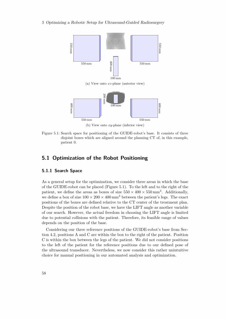
5 Optimizing a Robotic Setup for Ultrasound-Guided Radiosurgery
550mm
550 mm550m
m550 mm
400mm
100 mm
(a) View onto xz-plane (anterior view)
400mm
550 mm
400mm
550 mm
100 mm
200mm
(b) View onto xy-plane (inferior view)
Figure 5.1: Search space for positioning of the GUIDE-robot’s base. It consists of threedisjoint boxes which are aligned around the planning CT of, in this example,patient 0.
5.1 Optimization of the Robot Positioning
5.1.1 Search Space
As a general setup for the optimization, we consider three areas in which the baseof the GUIDE-robot can be placed (Figure 5.1). To the left and to the right of thepatient, we define the areas as boxes of size 550× 400× 550 mm3. Additionally,we define a box of size 100× 200× 400 mm3 between the patient’s legs. The exactpositions of the boxes are defined relative to the CT center of the treatment plan.Despite the position of the robot base, we have the LIFT angle as another variableof our search. However, the actual freedom in choosing the LIFT angle is limiteddue to potential collisions with the patient. Therefore, its feasible range of valuesdepends on the position of the base.Considering our three reference positions of the GUIDE-robot’s base from Sec-
tion 4.2, positions A and C are within the box to the right of the patient. PositionC is within the box between the legs of the patient. We did not consider positionsto the left of the patient for the reference positions due to our defined pose ofthe ultrasound transducer. Nevertheless, we now consider this rather unintuitivechoice for manual positioning in our automated analysis and optimization.
58

5.1 Optimization of the Robot Positioning
PTV
Figure 5.2: Sketch of a setup with three blocked beams (red lines), one blocked node(red circle), and two free nodes (green circles). Following our definition, thefourth node (yellow circle) is neither blocked nor free because both blockedand non-blocked beams (green lines) start at this node.
5.1.2 Objective Functions
In order to formulate an optimization problem for the positioning of the GUIDE-robot, we need to define meaningful objective functions. All objective functionswhich we propose in the following assume that we already have a fixed set ofcandidate beams, which we can use to evaluate them.
Number of Blocked Beams (BB) For this objective, we count how many of thecandidate beams are blocked by the current robot positioning. The less beamsare blocked, the less impact the GUIDE-robot has on the treatment planning.Figure 5.2 illustrates a small example, in which the BB objective value is 3.
Overlap of Projected Robot and PTV (OP) The beam-blocking algorithmprojects the GUIDE-robot onto a plane which is orthogonal to the line from abeam node to the centroid of the PTV (see Section 4.3). For this objective func-tion, we additionally project the PTV onto the same plane and count how manypixels of the projected GUIDE-robot, including the safety margin, and the pro-jected PTV overlap. For the objective value, we simply sum up the overlappingpixels w.r.t. all beam nodes. The more overlap we observe, the more shadowedis the PTV by the GUIDE-robot. In comparison to the BB objective, this ob-jective is less dependent on the candidate beam set. However, we only considerprojections from beam nodes at which at least one candidate beam starts. If thecandidate beam set is sufficiently large, we can assume that the other nodes arenot usable for treatment at all.
59

5 Optimizing a Robotic Setup for Ultrasound-Guided Radiosurgery
Number of Blocked Nodes (BN) We count the number of beam nodes for whichall candidate beams are blocked and define them as blocked nodes. These nodeseffectively have to be removed from treatment planning. Figure 5.2 illustrates anexample, in which the BN objective value is 1.
Number of Free Nodes (FN) In contrast to the previous objective, we countthe number of beam nodes for which no candidate beam is blocked and definethem as free nodes. Therefore, these nodes are fully available for planning andnot influenced by the image-guidance setup, at least w.r.t. the candidate beamsat hand. Figure 5.2 illustrates an example, in which the FN objective value is 2.
All proposed objective functions require to apply the beam-blocking algorithmfrom Section 4.3 for evaluation. Therefore, it is not possible to give analyticexpressions for them. Furthermore, they are highly discontinuous due to countingand the discrete nature of the beams, for which we assume a finite diameter tocalculate blocking. For this reason, we will have to employ heuristic optimizationalgorithms which do not give any guarantees for the quality of their solutions.
5.1.3 Optimization Strategies
We propose two optimization strategies for optimizing the positioning of theGUIDE-robot. The first approach, which we call segmental inverse robot con-struction (SIRC), is a problem-specific heuristic search strategy. The second oneis an implementation of the generic strategy simulated annealing (SimAn).
Segmental Inverse Robot Construction (SIRC)
A robot arm is a sequence of links and sequential links are connected by a joint.The typical task in robotics is to determine suitable joint angles given a fixed poseof the robot base and a desired end-effector pose. In our case, however, we do nothave a fixed pose of the base but aim to optimize it w.r.t. the objective functionsproposed in the previous section. Nevertheless, we consider a fixed pose of theultrasound transducer fixing the GUIDE-robot’s end-effector pose, i.e., the anglesof the last joints. In the SIRC approach which we propose, we iteratively fix theremaining joints.For this purpose, we describe the GUIDE-robot by five points P1, ..., P5 where
P1 is at the base and P5 at the end-effector. This concept is sketched in Figure 5.3.The points are chosen in such a way that they need to maintain a defined physicaldistance in every configuration of the robot due to the geometry of the links. Thisis the case for the centers of joints not forming a line with their two neighboringjoints in every configuration. P5 and P4 are already fixed due to the fixed positionand orientation of the ultrasound transducer. The remaining three points aresubject to our optimization. Due to their physically required distances, eachremaining point Pi, where i ∈ {1, 2, 3}, has to be located on a sphere around Pi+1.
60
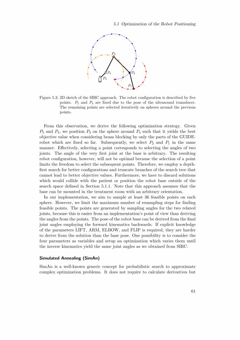
5.1 Optimization of the Robot Positioning
P5
P4
P3
P2
P1
Figure 5.3: 2D sketch of the SIRC approach. The robot configuration is described by fivepoints. P5 and P4 are fixed due to the pose of the ultrasound transducer.The remaining points are selected iteratively on spheres around the previouspoints.
From this observation, we derive the following optimization strategy. GivenP5 and P4, we position P3 on the sphere around P4 such that it yields the bestobjective value when considering beam blocking by only the parts of the GUIDE-robot which are fixed so far. Subsequently, we select P2 and P1 in the samemanner. Effectively, selecting a point corresponds to selecting the angles of twojoints. The angle of the very first joint at the base is arbitrary. The resultingrobot configuration, however, will not be optimal because the selection of a pointlimits the freedom to select the subsequent points. Therefore, we employ a depth-first search for better configurations and truncate branches of the search tree thatcannot lead to better objective values. Furthermore, we have to discard solutionswhich would collide with the patient or position the robot base outside of thesearch space defined in Section 5.1.1. Note that this approach assumes that thebase can be mounted in the treatment room with an arbitrary orientation.In our implementation, we aim to sample at least 36 feasible points on each
sphere. However, we limit the maximum number of resampling steps for findingfeasible points. The points are generated by sampling angles for the two relatedjoints, because this is easier from an implementation’s point of view than derivingthe angles from the points. The pose of the robot base can be derived from the finaljoint angles employing the forward kinematics backwards. If explicit knowledgeof the parameters LIFT, ARM, ELBOW, and FLIP is required, they are harderto derive from the solution than the base pose. One possibility is to consider thefour parameters as variables and setup an optimization which varies them untilthe inverse kinematics yield the same joint angles as we obtained from SIRC.
Simulated Annealing (SimAn)
SimAn is a well-known generic concept for probabilistic search to approximatecomplex optimization problems. It does not require to calculate derivatives but
61
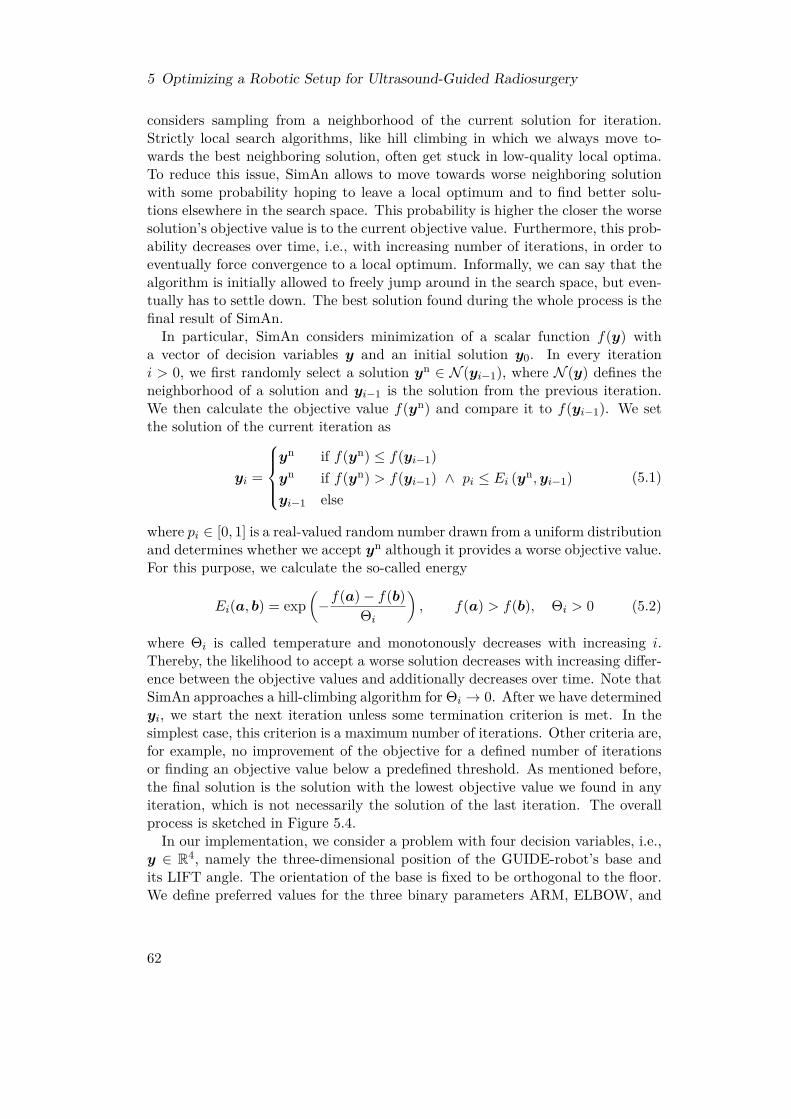
5 Optimizing a Robotic Setup for Ultrasound-Guided Radiosurgery
considers sampling from a neighborhood of the current solution for iteration.Strictly local search algorithms, like hill climbing in which we always move to-wards the best neighboring solution, often get stuck in low-quality local optima.To reduce this issue, SimAn allows to move towards worse neighboring solutionwith some probability hoping to leave a local optimum and to find better solu-tions elsewhere in the search space. This probability is higher the closer the worsesolution’s objective value is to the current objective value. Furthermore, this prob-ability decreases over time, i.e., with increasing number of iterations, in order toeventually force convergence to a local optimum. Informally, we can say that thealgorithm is initially allowed to freely jump around in the search space, but even-tually has to settle down. The best solution found during the whole process is thefinal result of SimAn.
In particular, SimAn considers minimization of a scalar function f(y) witha vector of decision variables y and an initial solution y0. In every iterationi > 0, we first randomly select a solution yn ∈ N (yi−1), where N (y) defines theneighborhood of a solution and yi−1 is the solution from the previous iteration.We then calculate the objective value f(yn) and compare it to f(yi−1). We setthe solution of the current iteration as
yi =
yn if f(yn) ≤ f(yi−1)yn if f(yn) > f(yi−1) ∧ pi ≤ Ei (yn,yi−1)yi−1 else
(5.1)
where pi ∈ [0, 1] is a real-valued random number drawn from a uniform distributionand determines whether we accept yn although it provides a worse objective value.For this purpose, we calculate the so-called energy
Ei(a, b) = exp(−f(a)− f(b)
Θi
), f(a) > f(b), Θi > 0 (5.2)
where Θi is called temperature and monotonously decreases with increasing i.Thereby, the likelihood to accept a worse solution decreases with increasing differ-ence between the objective values and additionally decreases over time. Note thatSimAn approaches a hill-climbing algorithm for Θi → 0. After we have determinedyi, we start the next iteration unless some termination criterion is met. In thesimplest case, this criterion is a maximum number of iterations. Other criteria are,for example, no improvement of the objective for a defined number of iterationsor finding an objective value below a predefined threshold. As mentioned before,the final solution is the solution with the lowest objective value we found in anyiteration, which is not necessarily the solution of the last iteration. The overallprocess is sketched in Figure 5.4.In our implementation, we consider a problem with four decision variables, i.e.,
y ∈ R4, namely the three-dimensional position of the GUIDE-robot’s base andits LIFT angle. The orientation of the base is fixed to be orthogonal to the floor.We define preferred values for the three binary parameters ARM, ELBOW, and
62

5.1 Optimization of the Robot Positioning
input y0
drawyn ∈ N (yi−1) f(yn) ≤ f(yi−1)
?
pi ≤ Ei(yn, yi−1)?
yi := yn
yi := yi−1
terminate?
output bestsolution
i := 1yes
noyes
noyes
no
i := i + 1
Figure 5.4: Basic steps of SimAn.
FLIP (see Section 4.2) but try all combinations if the preferred combination is notfeasible for a given base position and LIFT angle. Feasibility of a solution alsoincludes that the GUIDE-robot does not collide with the patient. If no feasibleconfiguration exists for a solution, then this solution is discarded. Mostly, SimAn isapplied to discrete variables. However, we employ a continuous approach allowingarbitrary real values for y. For this purpose, we define drawing a neighboringsolution yn for yi−1 as
yn = yi−1 + Θi
50 ri � l, (5.3)
where ri ∈ R4 is a vector of random numbers drawn from a standard normaldistribution, which is element-wisely multiplied with a vector l ∈ R4 containingthe range between lower and upper bound for each of the four decision variables.Therefore, the neighboring solution is obtained from the last iteration’s solutionby making a step of random size in each dimension. The step size decreases overtime because we include the temperature Θi. Another uncommon aspect of ourproblem-at-hand is that the search space consists of three unconnected boxes.Therefore, we implement the possibility to move from one box to another whenthe neighboring solution reaches a border in direction to the other box.We define a maximum number of 500 iterations as the termination criterion.
The temperature is initially Θ0 = 10 and is halved after every 100 iterations.SimAn requires to provide an initial solution y0 which, in general, influences theresult. We consider five initial solutions for each parameter combination. Theyall have a LIFT angle of 0° and are located far left, close left, inferior, close right,and far right as shown in Figure 5.5.On the one hand, the SimAn approach is less problem-specific than SIRC. Fur-
thermore, our implementation only considers a fixed orientation of the base to havea small number of decision variables. On the other hand, it provides direct accessto the variables-of-interest. In particular, it allows to explicitly control the LIFT
63
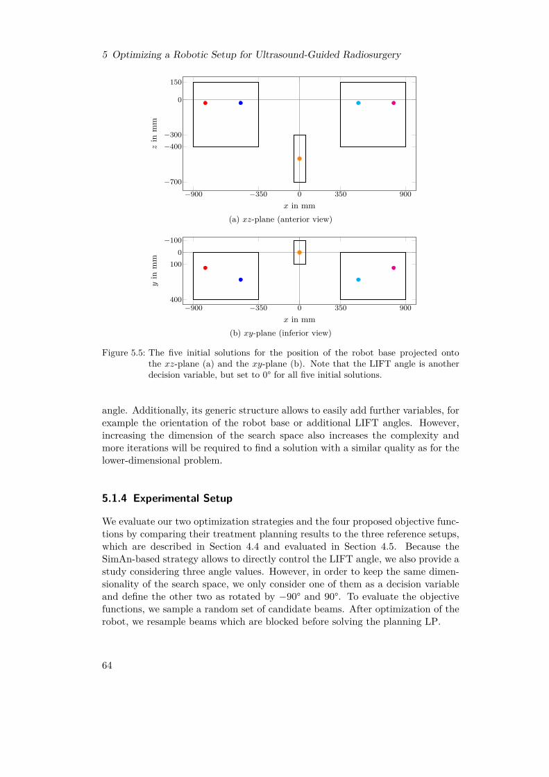
5 Optimizing a Robotic Setup for Ultrasound-Guided Radiosurgery
−900 −350 0 350 900−700
−400−300
0
150
x in mm
zin
mm
(a) xz-plane (anterior view)
−900 −350 0 350 900
−1000
100
400
x in mm
yin
mm
(b) xy-plane (inferior view)
Figure 5.5: The five initial solutions for the position of the robot base projected ontothe xz-plane (a) and the xy-plane (b). Note that the LIFT angle is anotherdecision variable, but set to 0° for all five initial solutions.
angle. Additionally, its generic structure allows to easily add further variables, forexample the orientation of the robot base or additional LIFT angles. However,increasing the dimension of the search space also increases the complexity andmore iterations will be required to find a solution with a similar quality as for thelower-dimensional problem.
5.1.4 Experimental Setup
We evaluate our two optimization strategies and the four proposed objective func-tions by comparing their treatment planning results to the three reference setups,which are described in Section 4.4 and evaluated in Section 4.5. Because theSimAn-based strategy allows to directly control the LIFT angle, we also provide astudy considering three angle values. However, in order to keep the same dimen-sionality of the search space, we only consider one of them as a decision variableand define the other two as rotated by −90° and 90°. To evaluate the objectivefunctions, we sample a random set of candidate beams. After optimization of therobot, we resample beams which are blocked before solving the planning LP.
64

5.2 Selection of an Efficient Set of Robot Configurations
5.2 Selection of an Efficient Set of Robot Configurations
The SimAn approach which we introduced in the previous section is very genericand can easily be extended to optimize further variables. However, if we addvariables, i.e., increase the dimensionality of the search space, it becomes harder toobtain high-quality solutions. We can expect to need more iterations to adequatelyexplore the larger search space. If we specifically consider the selection of multipleconfigurations for the GUIDE-robot, then we will also find some problem-specificissues. First, we have to define beforehand how many configuration we want toconsider. Second, we have to re-compute the beam blocking in each iteration forthe current positioning of the robot and all current LIFT angles, which might bemany. Third, if the optimization finishes, then it is still not clear whether ournumber of configurations is actually a good choice or whether it is lower or higherthan necessary. This issue could be fixed by extending the objective function tooptimize further criteria related to the configurations, but this would increase thecomplexity and obscure the underlying model even more.For these reasons, we introduce in this section two different approaches towards
the configuration selection, which split the problem from the positioning problem.For a fixed robot positioning, we first describe a post-processing approach whichreduces the number of configurations given a set of treatment beams resultingfrom inverse planning. Second, we show that the selection problem can be directlyintegrated into the treatment planning LP, which allows for more control over theoptimization process and direct inclusion of the treatment planning objectives. Incontrast, the generic SimAn approach has to use a surrogate objective function,because solving the planning LP in each iteration is computationally not tractable.With the direct integration in the planning problem, we can hope to obtain betterinsights into the problem and the influence of the number and distribution ofconfigurations on treatment plan quality.
5.2.1 Discretization
If we allow for arbitrary configurations, i.e., have continuous variables describ-ing the angle of a configuration, we will always end up with a highly non-linearproblem, because it implies computing the blocking or non-blocking by the cur-rent configurations for each beam throughout the optimization steps. Therefore,it seems more promising to discretize the infinite set of configurations to a finiteset. This is especially meaningful as we only consider a finite set of beams aswell. From a certain level of granularity on, a finer discretization cannot createnew beam blocking patterns, but they will be equal to those of their neighbor-ing configurations. Configurations blocking the exactly same beams are for ourapplication equivalent, as long as we do not assign further objectives or figuresof merit. In theory, there are 2N different blocking patterns if we consider Nbeams. In practice, however, we expect only a much smaller subset to be actuallyrealizable due to the underlying geometry of the GUIDE-robot and the spatial ar-
65
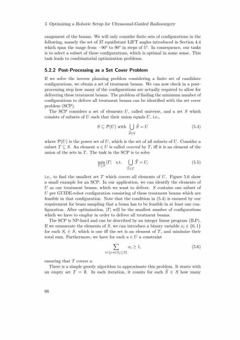
5 Optimizing a Robotic Setup for Ultrasound-Guided Radiosurgery
rangement of the beams. We will only consider finite sets of configurations in thefollowing, namely the set of 37 equidistant LIFT angles introduced in Section 4.4which span the range from −90° to 90° in steps of 5°. In consequence, our tasksis to select a subset of these configurations, which is optimal in some sense. Thistask leads to combinatorial optimization problems.
5.2.2 Post-Processing as a Set Cover ProblemIf we solve the inverse planning problem considering a finite set of candidateconfigurations, we obtain a set of treatment beams. We can now check in a post-processing step how many of the configurations are actually required to allow fordelivering these treatment beams. The problem of finding the minimum number ofconfigurations to deliver all treatment beams can be identified with the set coverproblem (SCP).The SCP considers a set of elements U , called universe, and a set S which
consists of subsets of U such that their union equals U , i.e.,
S ⊆ P(U) with⋃S∈S
S = U (5.4)
where P(U) is the power set of U , which is the set of all subsets of U . Consider asubset T ⊆ S. An element u ∈ U is called covered by T , iff it is an element of theunion of the sets in T . The task in the SCP is to solve
minT⊆S|T | s.t.
⋃T∈T
T = U, (5.5)
i.e., to find the smallest set T which covers all elements of U . Figure 5.6 showa small example for an SCP. In our application, we can identify the elements ofU as our treatment beams, which we want to deliver. S contains one subset ofU per GUIDE-robot configuration consisting of these treatment beams which arefeasible in that configuration. Note that the condition in (5.4) is ensured by ourrequirement for beam sampling that a beam has to be feasible in at least one con-figuration. After optimization, |T | will be the smallest number of configurationswhich we have to employ in order to deliver all treatment beams.The SCP is NP-hard and can be described by an integer linear program (ILP).
If we enumerate the elements of S, we can introduce a binary variable xi ∈ {0, 1}for each Si ∈ S, which is one iff the set is an element of T , and minimize theirtotal sum. Furthermore, we have for each u ∈ U a constraint∑
i∈{j:u∈Sj⊆S}xi ≥ 1, (5.6)
ensuring that T covers u.There is a simple greedy algorithm to approximate this problem. It starts with
an empty set T = ∅. In each iteration, it counts for each S ∈ S how many
66
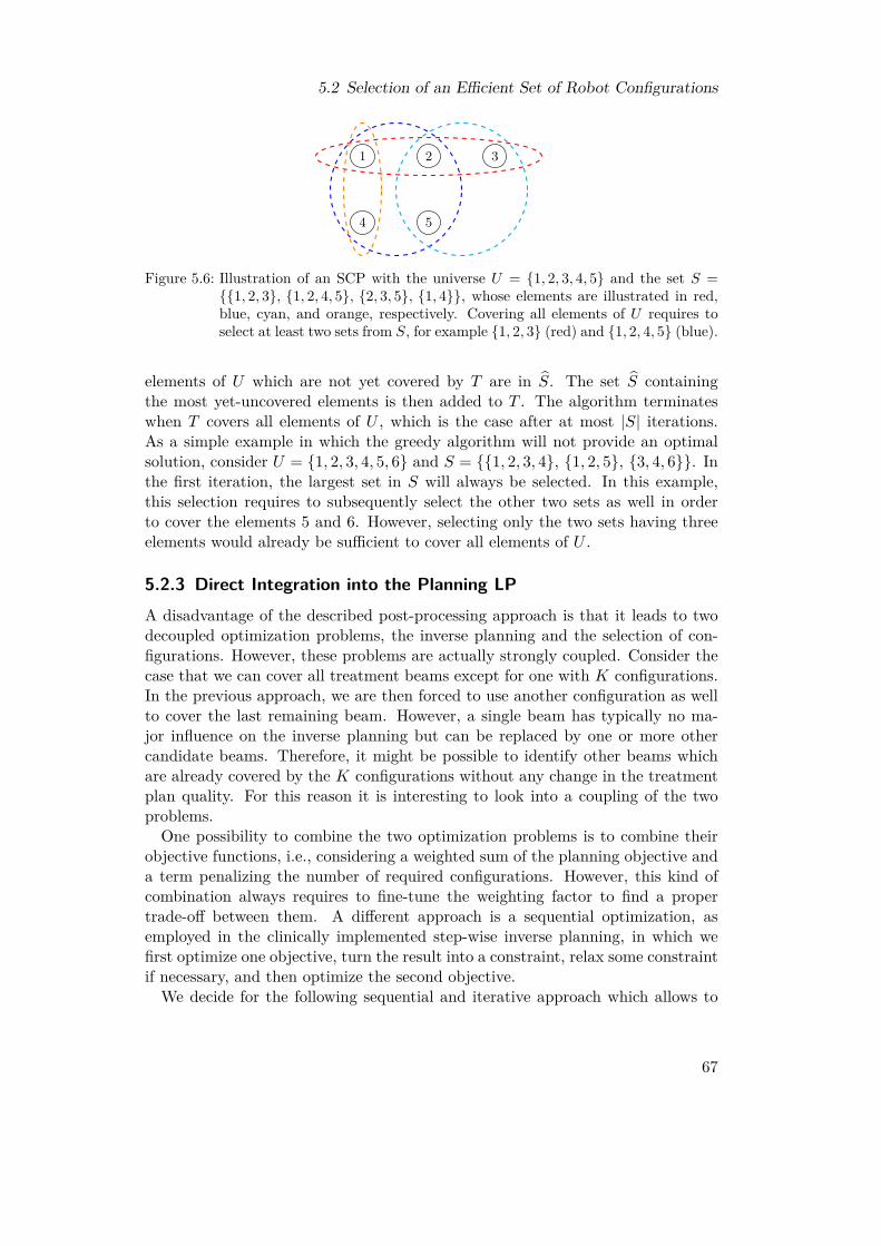
5.2 Selection of an Efficient Set of Robot Configurations
1 2 3
4 5
Figure 5.6: Illustration of an SCP with the universe U = {1, 2, 3, 4, 5} and the set S ={{1, 2, 3}, {1, 2, 4, 5}, {2, 3, 5}, {1, 4}}, whose elements are illustrated in red,blue, cyan, and orange, respectively. Covering all elements of U requires toselect at least two sets from S, for example {1, 2, 3} (red) and {1, 2, 4, 5} (blue).
elements of U which are not yet covered by T are in S. The set S containingthe most yet-uncovered elements is then added to T . The algorithm terminateswhen T covers all elements of U , which is the case after at most |S| iterations.As a simple example in which the greedy algorithm will not provide an optimalsolution, consider U = {1, 2, 3, 4, 5, 6} and S = {{1, 2, 3, 4}, {1, 2, 5}, {3, 4, 6}}. Inthe first iteration, the largest set in S will always be selected. In this example,this selection requires to subsequently select the other two sets as well in orderto cover the elements 5 and 6. However, selecting only the two sets having threeelements would already be sufficient to cover all elements of U .
5.2.3 Direct Integration into the Planning LPA disadvantage of the described post-processing approach is that it leads to twodecoupled optimization problems, the inverse planning and the selection of con-figurations. However, these problems are actually strongly coupled. Consider thecase that we can cover all treatment beams except for one with K configurations.In the previous approach, we are then forced to use another configuration as wellto cover the last remaining beam. However, a single beam has typically no ma-jor influence on the inverse planning but can be replaced by one or more othercandidate beams. Therefore, it might be possible to identify other beams whichare already covered by the K configurations without any change in the treatmentplan quality. For this reason it is interesting to look into a coupling of the twoproblems.One possibility to combine the two optimization problems is to combine their
objective functions, i.e., considering a weighted sum of the planning objective anda term penalizing the number of required configurations. However, this kind ofcombination always requires to fine-tune the weighting factor to find a propertrade-off between them. A different approach is a sequential optimization, asemployed in the clinically implemented step-wise inverse planning, in which wefirst optimize one objective, turn the result into a constraint, relax some constraintif necessary, and then optimize the second objective.We decide for the following sequential and iterative approach which allows to
67
5 Optimizing a Robotic Setup for Ultrasound-Guided Radiosurgery
analyze the actually required number of configurations. First, we sample a finiteset of candidate configurations and sample random candidate beams which arefeasible in at least one of the configurations. Using these candidate beams, wesolve the inverse planning LP for OCO. This results in an objective value s∗describing the remaining gap to full coverage. In the second step, we minimizethe number of configurations but convert (2.8) to a constraint
1ᵀs ≤ r · s∗ (5.7)
with a relaxation factor r > 1 close to one. In other words, we seek for the smallestsubset of configurations which provides the same or a better OCO-OV. Note thatthe activation times of all candidate beams are still decision variables and the setof treatment beams might therefore change during this second optimization step.However, we have to provide a mathematical model to describe the mentionedobjective and the fact that a beam might become infeasible if we deselect someconfigurations.The probably most intuitive approach introducesM binary variables ci ∈ {0, 1},
i = 1, ...,M , one for each of the M candidate configurations. The variable ci iszero iff configuration i is not used. The objective to be optimized then simply is
minM∑i=1
ci. (5.8)
We can further introduce binary constants fij ∈ {0, 1} which are one iff beam j isfeasible in configuration i. The constraint that a beam j cannot be active, i.e., werequire xj = 0, if it is not feasible in any of the configurations in use then becomes
xj ≤ H ·M∑i=1
fijci (5.9)
where H is a sufficiently large constant, like for example the upper MU boundxbeam for each beam from (2.14). If there is at least one i with fijci = 1, then theconstraint does not actively limit the activation time xj . Otherwise, this beam isno longer feasible and xj is forced by the constraint to be zero.This approach turns the inverse planning problem into a MIP, which is much
harder to solve. In the worst case, for each of the 2M theoretical combinations ofconfigurations a modified planning LP has to be solved to find the optimal MIPsolution. Therefore, we relax the problem above by defining ci as non-negative real-valued variables, instead, to obtain an LP. Nevertheless, our previous definitionthat ci is zero iff the configuration is not used still holds. We can also still use (5.8)and (5.9), but their numerical values are now more difficult to interpret. Insteadof directly looking at the value of (5.8), we have to count the variables ci whichhave a non-zero value to get the actual number of configurations in use. In (5.9),a beam still has to be inactive if none of the configurations in which it is feasibleis used. However, we could now even use any constant H > 0, and especially
68

5.2 Selection of an Efficient Set of Robot Configurations
sample beams inverseplanning
minimizeconfigurations
areconfigurations
zero?
inverseplanning
removeconfigurationsresample beams
no
yes
Figure 5.7: Workflow for the integrated minimization of the number of configurations.
H = 1, because it only scales the range of the values of the variables ci which wewill observe. The constraint (5.7) is not affected by the definition of ci. Of course,we have to include all other constraints of the original inverse planning problemas well.We propose to realize the integration of the relaxed minimization of configura-
tions into the planning process as illustrated in Figure 5.7. In the first step, werandomly sample beams with respect to all candidate configurations. Afterwards,we solve the inverse planning problem. In the third step, we solve the relaxed prob-lem which minimizes the number of configurations. If any ci is zero afterwards, wefix these variables and resample all beams which have become infeasible. This isrepeated until no further configuration can be removed. Finally, the inverse plan-ning is solved again to establish optimality with respect to the OCO-OV. Notethat due to the resampling, this last step can lead to a better OCO-OV than theinitial treatment plan which considers all candidate configurations.
5.2.4 Experimental Setup
Similar to Section 4.4, we consider the three reference robot positions A, B, and Cand initially employ 37 LIFT angles as the candidate configurations. We considerthe greedy algorithm for the SCP model to approximate in a post-processing stepthe minimum number of configurations, which is actually required to deliver alltreatment beams.Furthermore, we study minimizing the number of configurations directly by
extending planning with another LP as illustrated in Figure 5.7. We set therelaxation factor r for the original OCO-OV to 1.001. Note that due to theresampling of blocked beams due to removed configurations, the final OCO-OVis typically even smaller than the original one. To potentially avoid the effort ofpatient-specific optimization, we also study whether the most-frequently selectedconfigurations for a set of training patients can be applied to other patients withoutfurther optimization.
69
5 Optimizing a Robotic Setup for Ultrasound-Guided Radiosurgery
5.3 Results
5.3.1 Optimized Positioning
In Section 5.1.2, we proposed four objectives to optimize the positioning of theGUIDE-robot, namely minimizing the number of blocked beams (BB), minimizingthe overlap between GUIDE-robot projection and PTV projection (OP), minimiz-ing the number of blocked beam nodes (BN), and maximizing the number of freebeam nodes (FN). To solve the resulting optimization problems, we proposedthe two strategies simulated annealing (SimAn) and segmental inverse robot con-struction (SIRC) in Section 5.1.3. We compare the results of these approachesin Table 5.1. For the SimAn strategy, we observe that the BB objective outper-forms the other objectives. Only for patient 7, OP provides a higher improvement.While all approaches achieve better median OCO-OVs than reference robot B, im-proving robot A turns out to be challenging. No optimization approach is able toimprove robot A’s result for patient 9. BB is at least able to improve the resultsfor all other patients. OP leads to slightly worse results for two further patients,while BN and FN lead to worse results for five and six patients, respectively. Forpatient 6, employing FN even leads to a 30.4 % higher median OCO-OV.When considering the SIRC strategy in Table 5.1, the differences between the
four proposed objectives are less clear. In fact, BB leads to the best result for onlya single patient. OP provides the best results for four patients, BN for one, andFN for four. Nevertheless, FN leads to bad results for patients 7, 8, and 9 and BNfails for patient 6 compared to the other objectives. Therefore, only BB and OPseem to be rather consistent. Major differences between these two only appear forpatients 2 and 9. For patient 9, we are again not able to achieve an improvementof robot A’s result, though the gap when employing OP or BN is clearly smallerthan for SimAn.If we compare the results of SimAn and SIRC obtained with BB, for patients
6 and 9 we observe rather clear outperformance by SimAn and for patients 2, 7,and 8 by SIRC. Note, however, that both are outperformed for patient 9 by SIRCwith OP or BN. If we consider for each patient the best results obtained with anyobjective, SimAn is only advantageous for patient 6.The observation that there is a substantial dependency on the patient under
consideration is confirmed by Figure 5.8. It shows the OCO-OVs which we obtainby grid-based sampling of the search space and compares them to the OCO-OVswhen only considering the grid points whose BB, OP, BN, or FN objective valuebelongs to the best 3-percentile. In Figure 5.8a, we mainly observe that the veryhigh OCO-OVs do not appear when considering only the points with good objec-tive value. However, neither the median nor the box limits are substantially betterfor this patient. In contrast, considering any objective improves the OCO-OV dis-tribution in Figure 5.8b. Nevertheless, relying on BB would clearly be the bestchoice in this case. Figure 5.8c is an example for the case that one objective failswhile the other three objectives perform well. Lastly, Figure 5.8d shows how the
70
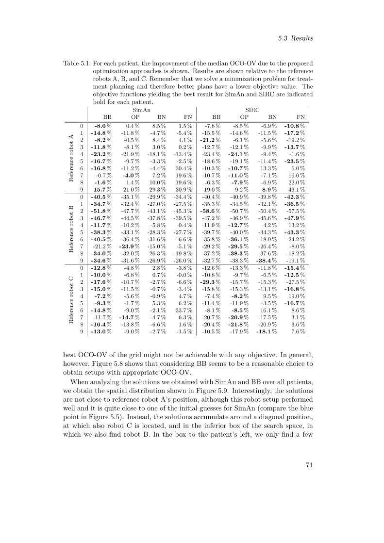
5.3 Results
Table 5.1: For each patient, the improvement of the median OCO-OV due to the proposedoptimization approaches is shown. Results are shown relative to the referencerobots A, B, and C. Remember that we solve a minimization problem for treat-ment planning and therefore better plans have a lower objective value. Theobjective functions yielding the best result for SimAn and SIRC are indicatedbold for each patient.
SimAn SIRCBB OP BN FN BB OP BN FN
Referen
cerobo
tA
0 -8.0% 0.4% 8.5% 1.5% -7.8% -8.5% -6.9% -10.8%1 -14.8% -11.8% -4.7% -5.4% -15.5% -14.6% -11.5% -17.2%2 -8.2% -0.5% 8.4% 4.1% -21.2% -6.1% -5.6% -19.2%3 -11.8% -8.1% 3.0% 0.2% -12.7% -12.1% -9.9% -13.7%4 -23.2% -21.9% -18.1% -13.4% -23.4% -24.1% -9.4% -1.6%5 -16.7% -9.7% -3.3% -2.5% -18.6% -19.1% -11.4% -23.5%6 -16.8% -11.2% -4.4% 30.4% -10.3% -10.7% 13.3% 6.0%7 -0.7% -4.0% 7.2% 19.6% -10.7% -11.0% -7.1% 16.0%8 -1.6% 1.4% 10.0% 19.6% -6.3% -7.9% -6.9% 22.0%9 15.7% 21.0% 29.3% 30.9% 19.0% 9.2% 8.9% 43.1%
Referen
cerobo
tB
0 -40.5% -35.1% -29.9% -34.4% -40.4% -40.9% -39.8% -42.3%1 -34.7% -32.4% -27.0% -27.5% -35.3% -34.5% -32.1% -36.5%2 -51.8% -47.7% -43.1% -45.3% -58.6% -50.7% -50.4% -57.5%3 -46.7% -44.5% -37.8% -39.5% -47.2% -46.9% -45.6% -47.9%4 -11.7% -10.2% -5.8% -0.4% -11.9% -12.7% 4.2% 13.2%5 -38.3% -33.1% -28.3% -27.7% -39.7% -40.0% -34.3% -43.3%6 -40.5% -36.4% -31.6% -6.6% -35.8% -36.1% -18.9% -24.2%7 -21.2% -23.9% -15.0% -5.1% -29.2% -29.5% -26.4% -8.0%8 -34.0% -32.0% -26.3% -19.8% -37.2% -38.3% -37.6% -18.2%9 -34.6% -31.6% -26.9% -26.0% -32.7% -38.3% -38.4% -19.1%
Referen
cerobo
tC
0 -12.8% -4.8% 2.8% -3.8% -12.6% -13.3% -11.8% -15.4%1 -10.0% -6.8% 0.7% -0.0% -10.8% -9.7% -6.5% -12.5%2 -17.6% -10.7% -2.7% -6.6% -29.3% -15.7% -15.3% -27.5%3 -15.0% -11.5% -0.7% -3.4% -15.8% -15.3% -13.1% -16.8%4 -7.2% -5.6% -0.9% 4.7% -7.4% -8.2% 9.5% 19.0%5 -9.3% -1.7% 5.3% 6.2% -11.4% -11.9% -3.5% -16.7%6 -14.8% -9.0% -2.1% 33.7% -8.1% -8.5% 16.1% 8.6%7 -11.7% -14.7% -4.7% 6.3% -20.7% -20.9% -17.5% 3.1%8 -16.4% -13.8% -6.6% 1.6% -20.4% -21.8% -20.9% 3.6%9 -13.0% -9.0% -2.7% -1.5% -10.5% -17.9% -18.1% 7.6%
best OCO-OV of the grid might not be achievable with any objective. In general,however, Figure 5.8 shows that considering BB seems to be a reasonable choice toobtain setups with appropriate OCO-OV.When analyzing the solutions we obtained with SimAn and BB over all patients,
we obtain the spatial distribution shown in Figure 5.9. Interestingly, the solutionsare not close to reference robot A’s position, although this robot setup performedwell and it is quite close to one of the initial guesses for SimAn (compare the bluepoint in Figure 5.5). Instead, the solutions accumulate around a diagonal position,at which also robot C is located, and in the inferior box of the search space, inwhich we also find robot B. In the box to the patient’s left, we only find a few
71
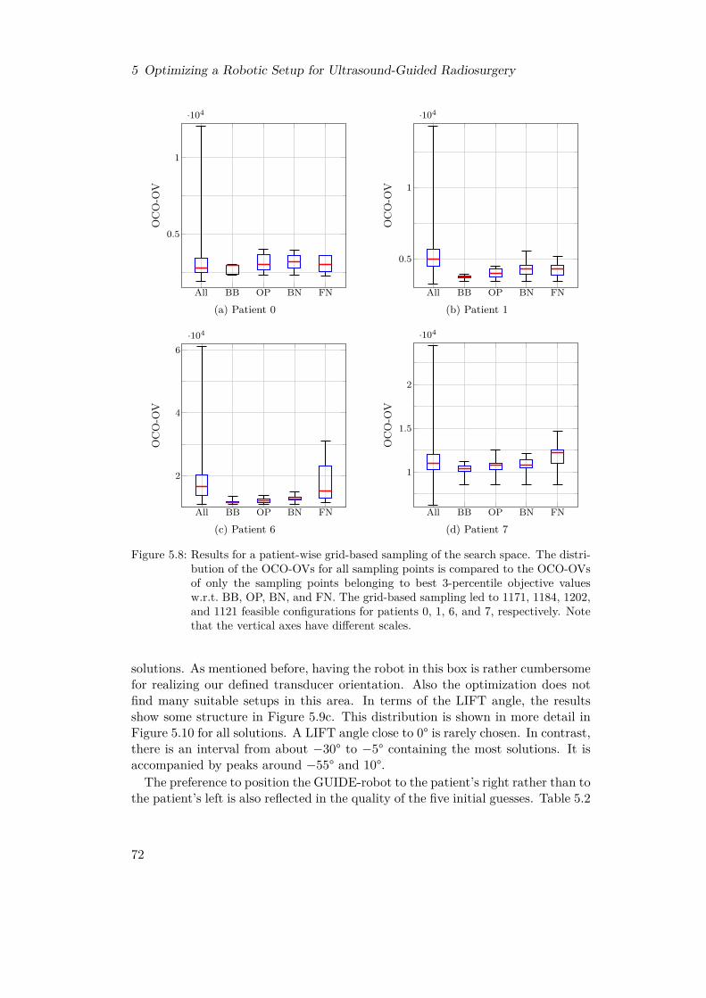
5 Optimizing a Robotic Setup for Ultrasound-Guided Radiosurgery
All BB OP BN FN
0.5
1
·104
OC
O-O
V
(a) Patient 0All BB OP BN FN
0.5
1
·104
OC
O-O
V
(b) Patient 1
All BB OP BN FN
2
4
6·104
OC
O-O
V
(c) Patient 6All BB OP BN FN
1
1.5
2
·104
OC
O-O
V
(d) Patient 7
Figure 5.8: Results for a patient-wise grid-based sampling of the search space. The distri-bution of the OCO-OVs for all sampling points is compared to the OCO-OVsof only the sampling points belonging to best 3-percentile objective valuesw.r.t. BB, OP, BN, and FN. The grid-based sampling led to 1171, 1184, 1202,and 1121 feasible configurations for patients 0, 1, 6, and 7, respectively. Notethat the vertical axes have different scales.
solutions. As mentioned before, having the robot in this box is rather cumbersomefor realizing our defined transducer orientation. Also the optimization does notfind many suitable setups in this area. In terms of the LIFT angle, the resultsshow some structure in Figure 5.9c. This distribution is shown in more detail inFigure 5.10 for all solutions. A LIFT angle close to 0° is rarely chosen. In contrast,there is an interval from about −30° to −5° containing the most solutions. It isaccompanied by peaks around −55° and 10°.The preference to position the GUIDE-robot to the patient’s right rather than to
the patient’s left is also reflected in the quality of the five initial guesses. Table 5.2
72
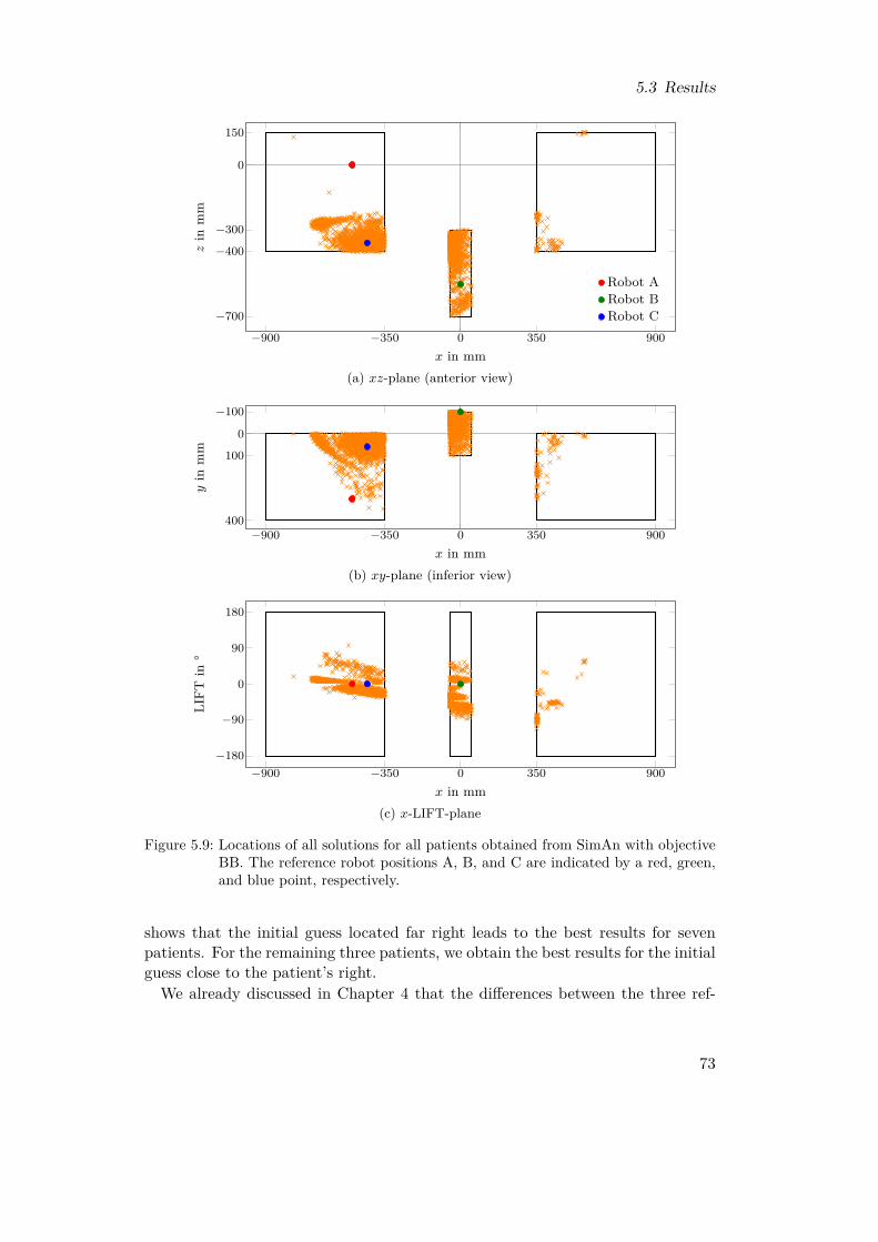
5.3 Results
−900 −350 0 350 900
−700
−400
−300
0
150
x in mm
zin
mm
Robot ARobot BRobot C
(a) xz-plane (anterior view)
−900 −350 0 350 900
−100
0
100
400
x in mm
yin
mm
(b) xy-plane (inferior view)
−900 −350 0 350 900−180
−90
0
90
180
x in mm
LIFT
in°
(c) x-LIFT-plane
Figure 5.9: Locations of all solutions for all patients obtained from SimAn with objectiveBB. The reference robot positions A, B, and C are indicated by a red, green,and blue point, respectively.
shows that the initial guess located far right leads to the best results for sevenpatients. For the remaining three patients, we obtain the best results for the initialguess close to the patient’s right.We already discussed in Chapter 4 that the differences between the three ref-
73
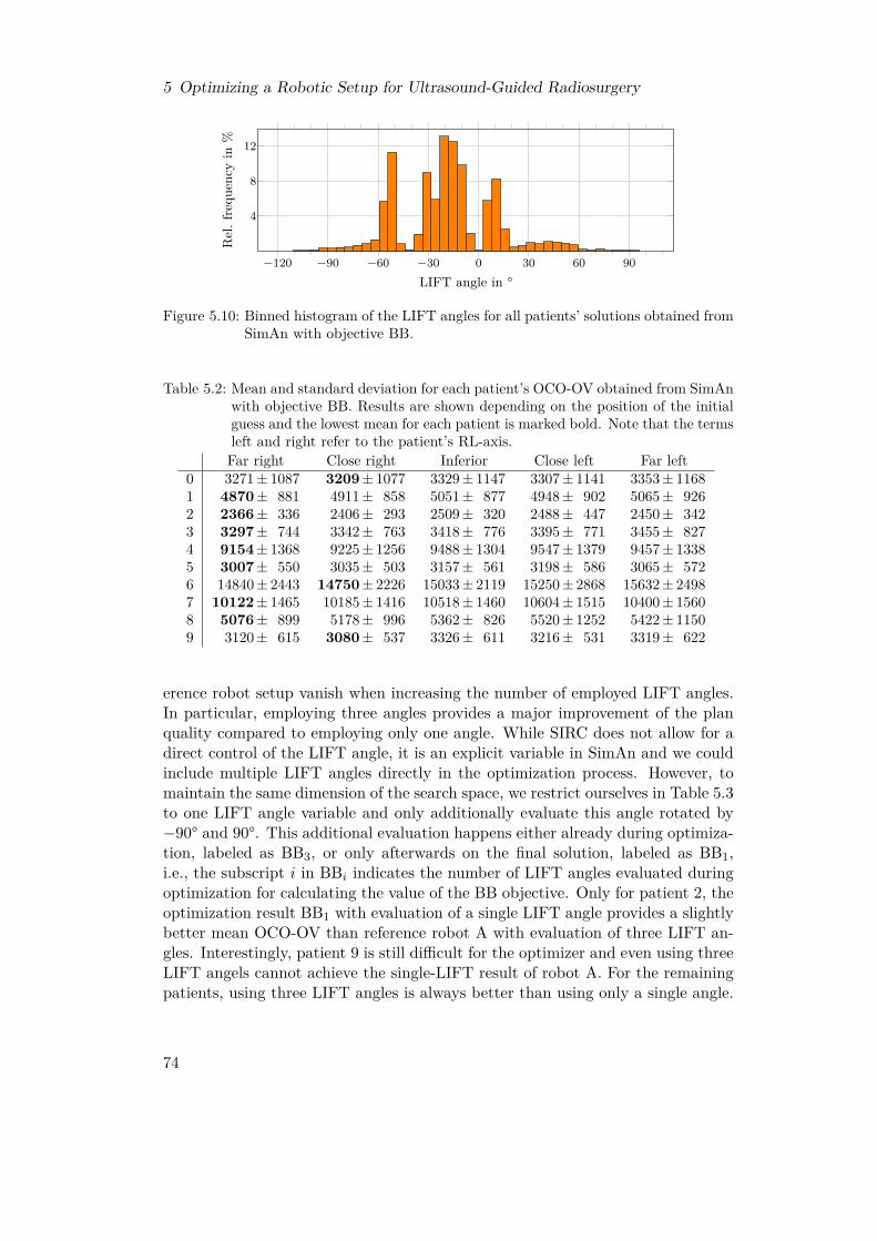
5 Optimizing a Robotic Setup for Ultrasound-Guided Radiosurgery
−120 −90 −60 −30 0 30 60 90
4
8
12
LIFT angle in °
Rel
.fre
quen
cyin
%
Figure 5.10: Binned histogram of the LIFT angles for all patients’ solutions obtained fromSimAn with objective BB.
Table 5.2: Mean and standard deviation for each patient’s OCO-OV obtained from SimAnwith objective BB. Results are shown depending on the position of the initialguess and the lowest mean for each patient is marked bold. Note that the termsleft and right refer to the patient’s RL-axis.Far right Close right Inferior Close left Far left
0 3271± 1087 3209± 1077 3329± 1147 3307± 1141 3353± 11681 4870± 881 4911± 858 5051± 877 4948± 902 5065± 9262 2366± 336 2406± 293 2509± 320 2488± 447 2450± 3423 3297± 744 3342± 763 3418± 776 3395± 771 3455± 8274 9154± 1368 9225± 1256 9488± 1304 9547± 1379 9457± 13385 3007± 550 3035± 503 3157± 561 3198± 586 3065± 5726 14840± 2443 14750± 2226 15033± 2119 15250± 2868 15632± 24987 10122± 1465 10185± 1416 10518± 1460 10604± 1515 10400± 15608 5076± 899 5178± 996 5362± 826 5520± 1252 5422± 11509 3120± 615 3080± 537 3326± 611 3216± 531 3319± 622
erence robot setup vanish when increasing the number of employed LIFT angles.In particular, employing three angles provides a major improvement of the planquality compared to employing only one angle. While SIRC does not allow for adirect control of the LIFT angle, it is an explicit variable in SimAn and we couldinclude multiple LIFT angles directly in the optimization process. However, tomaintain the same dimension of the search space, we restrict ourselves in Table 5.3to one LIFT angle variable and only additionally evaluate this angle rotated by−90° and 90°. This additional evaluation happens either already during optimiza-tion, labeled as BB3, or only afterwards on the final solution, labeled as BB1,i.e., the subscript i in BBi indicates the number of LIFT angles evaluated duringoptimization for calculating the value of the BB objective. Only for patient 2, theoptimization result BB1 with evaluation of a single LIFT angle provides a slightlybetter mean OCO-OV than reference robot A with evaluation of three LIFT an-gles. Interestingly, patient 9 is still difficult for the optimizer and even using threeLIFT angels cannot achieve the single-LIFT result of robot A. For the remainingpatients, using three LIFT angles is always better than using only a single angle.
74

5.3 Results
Table 5.3: Comparison of the OCO-OVs when using 1 or 3 LIFT angles for each patient.For 1 LIFT angle, we consider reference robot A and optimization of BB withSimAn. For 3 LIFT angles, we consider reference robot A and two optimiza-tion schemes with SimAn. BB1 evaluates the optimal solution obtained for 1LIFT angle with two additional angles rotated by ±90°, while BB3 considersthe additional angles already during optimization. The lowest mean for eachpatient is marked bold.
1 LIFT 3 LIFTsRobot A BB1 Robot A BB1 BB3
0 3630± 1222 3294± 1117 3085± 1098 3005± 1061 2981± 10581 6023± 1049 4969± 885 4616± 779 4573± 866 4520± 8612 2784± 479 2444± 353 2450± 412 2249± 290 2222± 2863 3950± 762 3381± 772 2918± 625 3068± 692 3018± 6304 12352± 1439 9374± 1328 8550± 1045 8907± 1210 8587± 11675 3725± 615 3093± 556 2988± 574 2808± 474 2784± 4666 18114± 3118 15101± 2446 14575± 2531 14862± 2294 14404± 22707 10250± 1279 10366± 1484 8889± 1154 9345± 1226 8853± 9848 5363± 1095 5312± 1041 4620± 875 4807± 926 4635± 8499 2789± 581 3212± 589 2521± 554 2881± 513 2800± 479
Table 5.4: Means and standard deviations for the number of configurations, which areactually required to deliver all candidate or treatment beams, obtained fromthe greedy algorithm for the SCP.
Robot A Robot B Robot CCandidate beams 11.1± 2.1 9.0± 2.4 7.8± 2.4Treatment beams 5.2± 1.2 4.0± 1.1 3.3± 1.3
Further, for four patients neither BB1 nor BB3 with three LIFT angles can achievethe results of robot A with three LIFT angles. Considering three angles alreadyduring optimization via BB3 is always better than considering only the centralangle during optimization via BB1.
5.3.2 Efficient Configurations
To analyze the efficient selection of GUIDE-robot configurations, we consider 37equidistant LIFT angles from −90° to 90° defining the candidate configurations foreach of the three reference robot setups A, B, and C. Considering the candidateconfigurations and candidate beams as an SCP and solving it with the greedyalgorithm described in Section 5.2.2, however, we see from Table 5.4 that onaverage already 11.1, 9.0, and 7.8 configurations are sufficient to realize all thecandidate beams for robots A, B, and C, respectively. For the much smaller setof actual treatment beams, even selecting 5.2, 4.0, and 3.3 of the 37 candidateconfigurations is sufficient on average.When integrating the iterative minimization of the number configuration in
75
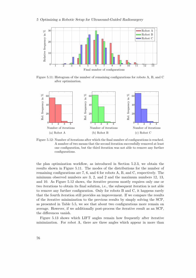
5 Optimizing a Robotic Setup for Ultrasound-Guided Radiosurgery
1 2 3 4 5 6 7 8 9 10 11 12 130
10
20
30
Final number of configurations
Relativefreque
ncyin
% Robot ARobot BRobot C
Figure 5.11: Histogram of the number of remaining configurations for robots A, B, and Cafter optimization.
1 2 3 40
20
40
60
Number of iterations
Rel
.fre
quen
cyin
%
(a) Robot A
1 2 3 40
20
40
60
Number of iterations
Rel
.fre
quen
cyin
%
(b) Robot B
1 2 3 40
20
40
60
Number of iterationsR
el.f
requ
ency
in%
(c) Robot C
Figure 5.12: Number of iterations after which the final number of configurations is reached.A number of two means that the second iteration successfully removed at leastone configuration, but the third iteration was not able to remove any furtherconfigurations.
the plan optimization workflow, as introduced in Section 5.2.3, we obtain theresults shown in Figure 5.11. The modes of the distributions for the number ofremaining configurations are 7, 6, and 6 for robots A, B, and C, respectively. Theminimum observed numbers are 3, 2, and 2 and the maximum numbers 12, 13,and 10. As Figure 5.12 shows, the iterative process mostly requires only one ortwo iterations to obtain its final solution, i.e., the subsequent iteration is not ableto remove any further configuration. Only for robots B and C, it happens rarelythat the fourth iteration still provides an improvement. If we compare the resultsof the iterative minimization to the previous results by simply solving the SCP,as presented in Table 5.5, we see that about two configurations more remain onaverage. However, if we additionally post-process the iterative result as an SCP,the differences vanish.Figure 5.13 shows which LIFT angles remain how frequently after iterative
minimization. For robot A, there are three angles which appear in more than
76
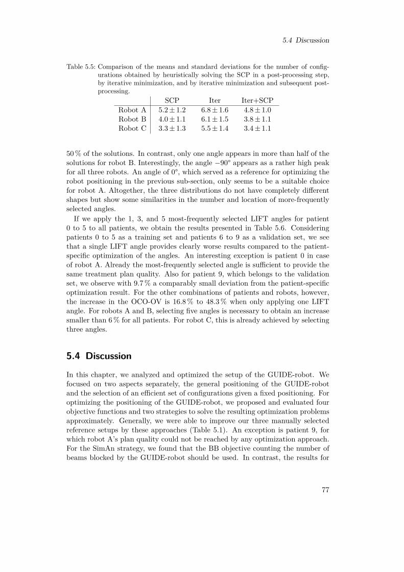
5.4 Discussion
Table 5.5: Comparison of the means and standard deviations for the number of config-urations obtained by heuristically solving the SCP in a post-processing step,by iterative minimization, and by iterative minimization and subsequent post-processing.
SCP Iter Iter+SCPRobot A 5.2± 1.2 6.8± 1.6 4.8± 1.0Robot B 4.0± 1.1 6.1± 1.5 3.8± 1.1Robot C 3.3± 1.3 5.5± 1.4 3.4± 1.1
50 % of the solutions. In contrast, only one angle appears in more than half of thesolutions for robot B. Interestingly, the angle −90° appears as a rather high peakfor all three robots. An angle of 0°, which served as a reference for optimizing therobot positioning in the previous sub-section, only seems to be a suitable choicefor robot A. Altogether, the three distributions do not have completely differentshapes but show some similarities in the number and location of more-frequentlyselected angles.If we apply the 1, 3, and 5 most-frequently selected LIFT angles for patient
0 to 5 to all patients, we obtain the results presented in Table 5.6. Consideringpatients 0 to 5 as a training set and patients 6 to 9 as a validation set, we seethat a single LIFT angle provides clearly worse results compared to the patient-specific optimization of the angles. An interesting exception is patient 0 in caseof robot A. Already the most-frequently selected angle is sufficient to provide thesame treatment plan quality. Also for patient 9, which belongs to the validationset, we observe with 9.7 % a comparably small deviation from the patient-specificoptimization result. For the other combinations of patients and robots, however,the increase in the OCO-OV is 16.8 % to 48.3 % when only applying one LIFTangle. For robots A and B, selecting five angles is necessary to obtain an increasesmaller than 6 % for all patients. For robot C, this is already achieved by selectingthree angles.
5.4 Discussion
In this chapter, we analyzed and optimized the setup of the GUIDE-robot. Wefocused on two aspects separately, the general positioning of the GUIDE-robotand the selection of an efficient set of configurations given a fixed positioning. Foroptimizing the positioning of the GUIDE-robot, we proposed and evaluated fourobjective functions and two strategies to solve the resulting optimization problemsapproximately. Generally, we were able to improve our three manually selectedreference setups by these approaches (Table 5.1). An exception is patient 9, forwhich robot A’s plan quality could not be reached by any optimization approach.For the SimAn strategy, we found that the BB objective counting the number ofbeams blocked by the GUIDE-robot should be used. In contrast, the results for
77
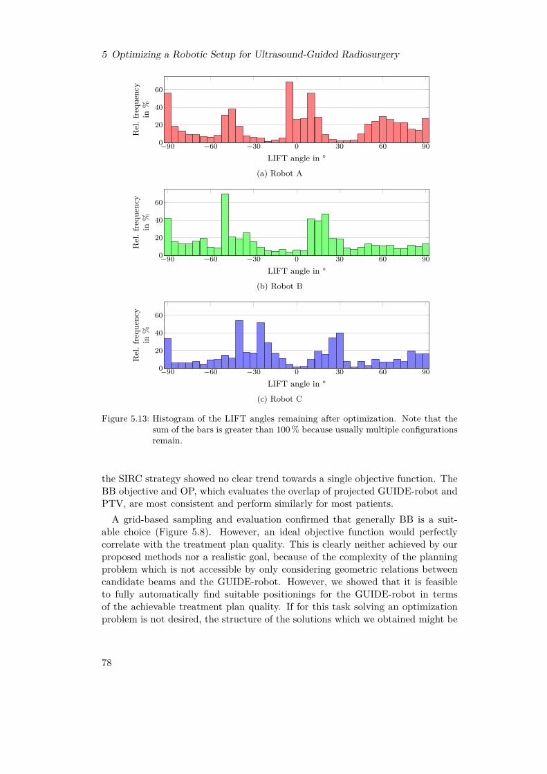
5 Optimizing a Robotic Setup for Ultrasound-Guided Radiosurgery
−90 −60 −30 0 30 60 900
20
40
60
LIFT angle in °
Rel
.fre
quen
cyin
%
(a) Robot A
−90 −60 −30 0 30 60 900
20
40
60
LIFT angle in °
Rel
.fre
quen
cyin
%
(b) Robot B
−90 −60 −30 0 30 60 900
20
40
60
LIFT angle in °
Rel
.fre
quen
cyin
%
(c) Robot C
Figure 5.13: Histogram of the LIFT angles remaining after optimization. Note that thesum of the bars is greater than 100 % because usually multiple configurationsremain.
the SIRC strategy showed no clear trend towards a single objective function. TheBB objective and OP, which evaluates the overlap of projected GUIDE-robot andPTV, are most consistent and perform similarly for most patients.
A grid-based sampling and evaluation confirmed that generally BB is a suit-able choice (Figure 5.8). However, an ideal objective function would perfectlycorrelate with the treatment plan quality. This is clearly neither achieved by ourproposed methods nor a realistic goal, because of the complexity of the planningproblem which is not accessible by only considering geometric relations betweencandidate beams and the GUIDE-robot. However, we showed that it is feasibleto fully automatically find suitable positionings for the GUIDE-robot in termsof the achievable treatment plan quality. If for this task solving an optimizationproblem is not desired, the structure of the solutions which we obtained might be
78

5.4 Discussion
Table 5.6: Mean change of the median OCO-OV when applying the 1, 3, or 5 most-frequently selected LIFT angles for patients 0 to 5 directly to all patients with-out patient-specific optimization. The most-frequent angles are specific to therobots A, B, and C. Note that smaller OCO-OVs are better.
Robot A Robot B Robot C1 3 5 1 3 5 1 3 5
Training
0 −0.8 % −1.2 % 0.1 % 32.6 % 1.5 % 0.7 % 27.0 % 0.1 % 0.0 %1 34.2 % 4.2 % 2.3 % 33.0 % 3.5 % −0.8 % 19.5 % 0.8 % 0.4 %2 16.8 % 3.6 % 2.1 % 32.5 % 8.6 % 3.5 % 37.7 % 5.7 % 4.9 %3 28.3 % 2.6 % 1.6 % 34.3 % 3.1 % 0.1 % 25.8 % 0.1 % 0.0 %4 48.3 % 8.0 % 2.0 % 24.9 % 9.2 % 0.5 % 17.4 % 0.4 % −0.5 %5 37.8 % 6.9 % 0.4 % 33.3 % 4.2 % 1.1 % 27.2 % 0.9 % 0.9 %
Valid
ation 6 35.7 % 13.8 % 2.7 % 34.1 % 8.9 % 3.8 % 27.4 % 1.9 % 1.6 %
7 30.6 % 6.7 % 4.7 % 30.4 % 11.2 % 1.5 % 31.2 % 1.3 % 1.1 %8 47.9 % 12.6 % 5.3 % 41.5 % 8.8 % 1.1 % 34.6 % 0.7 % 1.4 %9 9.7 % 5.6 % 0.4 % 39.3 % 9.2 % 1.7 % 34.0 % 0.9 % 0.9 %
a helpful guide for manual positioning, because they accumulated in some areasaround the patients (Figure 5.9). Note, however, that these results are partlybiased by our defined orientation of the ultrasound transducer. If the transduceris rotated around the AP-axis, the preferable locations for the robot base shouldbe expected to rotate around the patient as well. This should also be consideredfor the initial guess when employing the SimAn approach (Table 5.2). Our resultsconfirmed furthermore that the choice of the LIFT angle is important. Interest-ingly, the optimizer frequently selected them from a rather small range of angles(Figure 5.10).Eventually, we confirmed the previous observation that considering more LIFT
angles during the treatment is in general advantageous (Table 5.3). In this point,there is an essential difference between the SimAn and the SIRC strategy. SIRCappeared to explore the search space better because it provided satisfying resultswith multiple objectives functions. By design, however, it does not allow to controlthe GUIDE-robot explicitly, while evaluation and optimization of arbitrarily manyLIFT angles can easily be realized in SimAn. However, this increases both thecomputational effort for evaluation of an objective function and the dimensionalityof the search space. For this reason, we also discussed in this chapter separatelyhow to select efficient configurations of the GUIDE-robot given a fixed positioningfor the robot base.We proposed two approaches to determine an efficient subset of a set of candi-
date configurations for the GUIDE-robot. The SCP formulation of this problem,which we proposed, is very inexpensive when solved by a greedy algorithm. Weapplied it after treatment plan optimization to obtain a small subset of configura-tions which is actually required to deliver all treatment beams. From 37 candidateconfigurations, only about three to five were actually required on average, depend-ing on the reference robot setup under consideration (Table 5.4). This shows thatconsidering many configurations for planning is also practically meaningful, be-
79

5 Optimizing a Robotic Setup for Ultrasound-Guided Radiosurgery
cause eventually only a small number of them is actually required. Therefore, thesynchronization problem between the GUIDE-robot and the beam delivery, whichwe will discuss in the next chapter in detail, remains tractable and realistic whilewe can fully exploit the kinematic redundancy for minimizing beam blocking andplan deterioration.
Additionally, we proposed an extension of the treatment planning LP which iter-atively tries to minimize the number of configurations. We relaxed the exact MIPmodel to an easier to handle LP and obtained numbers of configurations whichwere slightly higher than for the SCP approach (Figure 5.11). This shows that oursimple relaxation leads to a relevant gap to the optimal MIP solution. In particu-lar, because we can further reduce the number of configurations when applying theSCP approach subsequently (Table 5.5). Nevertheless, the iterative LP approachyields some further insights in the nature of the problem. In contrast to the SCPapproach which is a post-processing step, the iterative LP approach directly inter-acts with the planning problem. Hence, its solutions indicate which LIFT anglesare generally preferable for a GUIDE-robot setup (Figure 5.13). These angleswere even applicable to new patients to achieve reasonable plan qualities withoutrepeating the whole optimization for these patients (Table 5.6).In summary, we saw in this chapter that it is feasible to automatically determine
suitable GUIDE-robot setups. Finding multiple suitable configurations can eitherbe directly included in this procedure or realized separately. We saw that evenwhen we initially considered many candidate configurations in order to block asfew beam directions as possible for plan optimization, we can eventually reducethem easily to a reasonable number without any deterioration of the plan quality.
80
6 Synchronizing Robot Motion andBeam Delivery in Ultrasound-GuidedRadiosurgery
In the two preceding chapters, we showed that considering multiple configura-tions of the GUIDE-robot during a treatment can severely decrease the impactof blocked beam directions on the treatment plan quality. However, employingmultiple configurations requires a synchronization between the GUIDE-robot andthe beam delivery, as outlined in Section 1.2 as the second research question ofthis thesis. A beam can only be delivered if the GUIDE-robot is in one of its non-blocking configurations. A simple approach would be to start in one configurationof the GUIDE-robot, deliver all feasible beams, move to the next configuration,deliver all feasible and not yet delivered beams, and so on. However, this ap-proach will lead to rather inefficient trajectories for the LINAC-robot, which inturn increase the total treatment time. Furthermore, this approach results in someremaining questions. Two of them are, in which order we should use the configu-rations and whether we really should deliver a feasible beam directly or whetherit would be more time-efficient to wait for another configuration.In this chapter, we develop models to describe and optimize the synchronization
problem between the GUIDE-robot’s configuration changes and the beam deliv-ery of the LINAC-robot. For this purpose, we start in Section 6.1 by describinga model to determine the most efficient trajectory for a beam delivery withoutthe GUIDE-robot. This problem is of course not new but relevant for any Cy-berKnife treatment. We describe how the problem can be modeled as a travelingsalesman problem (TSP), which conceptually is also employed in the current gen-eration of the CyberKnife system [126]. However, in Section 6.2, we show howour TSP-based approach can be directly extended to a generalized traveling sales-man problem (GTSP) in order to model the synchronization problem betweenthe configuration changes by the GUIDE-robot and the beam delivery under theassumption that the GUIDE-robot does not move during active beam delivery.This assumption reduces the effort for ensuring safety, because beam blocking hasonly to be verified for a small finite set of static robot configurations. We discussand evaluate different approaches to solve the GTSP model, which is known to bepractically hard to solve. Parts of this chapter have been published in a journal[230].Throughout this chapter, we assume that the elements of a set A have an arbi-
trary enumeration, i.e., we write A = {a1, ..., a|A|} without implying an ordering
81

6 Synchronizing Robot Motion and Beam Delivery in Ultrasound-Guided Radiosurgery
relation. Depending on the context and convenience, we refer to an element ofthe set either as a ∈ A or as ai ∈ A and implicitly assume i ∈ {1, ..., |A|} for thelatter. In contrast, we refer to ordered tuples either as (a, b, ...) where a, b, ... ∈ Aor as (ai, aj , ...) where ai, aj , ... ∈ A.
6.1 Model for Efficient Beam DeliveryIn order to deliver a treatment beam, the LINAC-robot has to position its end-effector, and thereby the attached LINAC, accordingly. This has to be done foreach treatment beam in some sequence. While the order of the beams does notaffect the outcome of the treatment, it affects the idle times of the LINAC due tothe required robot motion in between.In this section, we describe a mathematical model, the TSP, and describe how
we apply it to model the beam sequencing problem of the LINAC-robot. Wealso discuss different approaches for solving TSPs. While the first versions of theCyberKnife only used predefined paths through the beam nodes [45], the currentsystem also solves a TSP-like problem to obtain efficient paths [126]. In contrastto our simplified model, the actual implementation considers further obstaclesand the requirement that the LINAC-robot must not block the stereoscopic X-rayimaging for too long time intervals.
6.1.1 The Traveling Salesman ProblemInformally, the TSP can be illustrated by a salesman who is going to visit cus-tomers in different cities. He would like to know the shortest route which startsat his home town, takes him to each of the other cities exactly once, and finallytakes him back home. Finding an answer to this question requires to define theterm shortest in more detail. We could select, for example, the distance to travel,the time traveling takes, or the resulting financial costs. This decision, in turn,leads to new details which have to be considered. For example, the bee-line dis-tance from city A to city B is the same as from B to A. However, this symmetrymight not hold if we consider the time for traveling instead, for example if thespeed limits on a highway are different for each direction due to construction work.This property is distinguished in the literature by the terms symmetric travelingsalesman problem (STSP) and asymmetric traveling salesman problem (ATSP).Furthermore, the bee-line distance fulfills the triangle inequality as going from Ato B via C is never shorter than going from A to B directly. This, again, doesnot have to be true in general, for example if we consider the time or costs of dif-ferent train connections. Fulfillment of the triangle inequality results in anotherdistinction of different subtypes of the TSP and there are several more subtypesand variations in the literature [96]. They have been applied for modeling andoptimization in various fields.
Mathematically, the TSP is defined on a graph (V,E). V is a set of vertices,corresponding to the cities to visit in our illustrative example. The vertices are
82

6.1 Model for Efficient Beam Delivery
v1
v2
v3 v4
d(v
1,v 2
)
d(v1,v3) d(v1 , v4 )
d(v 2,
v 3)
d(v2 , v
4 )
d(v3, v4)
Figure 6.1: Illustration of an STSP with four vertices.
connected by a set of edges E. If we consider a fully-connected graph, E containsan edge for every pair of vertices vi, vj ∈ V , i.e.,
E = {(vi, vj) : vi, vj ∈ V } . (6.1)
More generally, however, there can also be pairs of vertices without direct connec-tions. Furthermore, edges can be directed or undirected, i.e., (vi, vj) and (vj , vi)are equivalent for the latter case. For a TSP, each edge is associated with a costd(vi, vj), as illustrated in Figure 6.1, which is also called weight or distance. Often,only non-negative and integer-valued costs are used, although this is not a formalrequirement.On such a graph, we have typically multiple possibilities to get from one vertex
to another vertex. These so-called walks between two vertices can be uniquelydescribed by providing the sequence of vertices, which are visited. In the simplestcase, a walk only consists of the two vertices themselves. Note that a walk, incontrast to a directed walk, does not have a defined direction in which the sequenceis interpreted. If a walk contains only distinct vertices, then we call it a path. Awalk for which only the first and last vertex are equal is a cycle. In the TSP,however, we ask for the shortest tour. A tour is a cycle containing each vertex ofthe graph. The costs of a tour are the summed costs of all edges, which connectthe sequentially visited vertices of the tour. When solving a TSP, the task is tofind a tour with minimum costs.If a fully-connected graph has N vertices, there are actually not N ! different
tours in terms of solving the related TSP, but only (N −1)! in case of asymmetriccosts because a tour does not have a defined start. In case of symmetric costs,the number of non-equivalent tours further reduces to (N − 1)!/2 because the di-rection is not relevant. Therefore, for an exemplary fully-connected graph withV = {v1, v2, v3} and symmetric costs, the tours (v1, v2, v3, v1), (v2, v3, v1, v2), and(v1, v3, v2, v1) are all equivalent in terms of solving the related TSP. In our illus-trative example, this means that for the optimal tour it is neither relevant which of
83
6 Synchronizing Robot Motion and Beam Delivery in Ultrasound-Guided Radiosurgery
the cities is the salesman’s home town nor in which direction the salesman travelsthe tour.
6.1.2 Modeling the Beam Delivery
In the beam sequencing problem for the LINAC-robot, we identify the set oftreatment beams B as the set of vertices of our graph for the TSP model, i.e.,V := B. In this thesis, we assume that each vertex is connected to each othervertex. In practice, however, there might be collisions with the patient or otherobstacles in the treatment room for some pairs of beams. We could account forthese by assigning a very high cost to the related edges in the graph in order toenforce that they cannot be part of an optimal tour. We define the costs d(bi, bj),bi, bj ∈ B, of an edge as the time required for moving the LINAC-robot and assumethat this motion results in symmetric costs, i.e., an STSP.A major discrepancy between the described TSP model and the real scenario is
the fact that a tour, by definition, is a cycle. This implies that the LINAC-roboteventually moves back to the pose for delivery of the first beam again. This isunnecessary because this beam has already been delivered. A more appropriatemodel would be a so-called shortest Hamiltonian path problem (HPP). In thisproblem, we search for a Hamiltonian path, which is a path containing each vertexof the graph, i.e., a walk containing each vertex exactly once. Note that thisproblem’s solution provides a defined first and last vertex, i.e., treatment beam.An HPP can easily be transformed into a TSP and after solving this TSP its
solution can easily be transformed into the solution of the original HPP [96]. Thetransformation into a TSP requires to add another vertex to the graph, which isconnected to every other vertex by zero-cost edges, in case of only non-negativecosts. It can be interpreted as a kind of joker which allows to skip the costs formoving between one pair of vertices. In the resulting tour, the neighboring verticesof the additional vertex are the first and last vertex of the corresponding optimalHamiltonian path. As an example, consider a fully connected graph G = (V,E)with symmetric non-negative costs and vertices V := {v1, v2, v3}. To solve theHPP on this graph, we solve the TSP on the fully connected graph G = (V , E)with V = V ∪ {z} and the costs d(v, z) = 0 for edges between the additionalvertex z and any v ∈ V . If the optimal tour is (v3, v1, z, v2, v3), then we obtain thesolution for the HPP through opening the cycle by removing z, i.e., the solutionis (v2, v3, v1).
6.1.3 Solving TSPs
Due to the described transformation of an HPP into a TSP, we can employ anyTSP solver for HPPs as well. Therefore, we only discuss the more common taskof solving TSPs in the following. However, we will only briefly cover two selectedapproaches in the following.
84

6.2 Model for Synchronized Robot Motion
Integer Linear Programming
The TSP is an NP-hard combinatorial optimization problem. One approach forsolving is to formulate it as an ILP. One prominent formulation for the STSPis the double index or subtour elimination formulation [96]. It introduces binaryvariables xe, e ∈ E, which are one iff the related edge is part of the solution.Therefore, the objective function to be minimized sums the costs of an edge emultiplied with xe over all e ∈ E. Only two main types of constraints are requiredto enforce that solutions are valid tours. First, for each vertex, there have to beexactly two edges in the solution which are connected to that vertex. Second, asolution has to actually be a single cycle and not a set of multiple disjoint cyclescovering all vertices. The latter aspect led to the name subtour elimination of thisformulation.In practice, the binary constraints on the variables xe have to be relaxed in order
to apply an LP solver with efficient branch-and-bound or cutting-plane methods.Therefore, the properties of the relaxation determine how suitable a formulationis for practical solving. More details including different preprocessing, branch-and-bound, and cutting-plane techniques can be found, for example, in Gutin etal. [96].
Lin-Kernighan Heuristic
One specific heuristic approach for solving TSPs is based on so-called k-opt im-provements [163]. Given a valid tour for the problem, we select k edges and replacethem by k shorter edges. In 2-opt, the selection of two edges uniquely defines thetwo replacing edges, because we have to maintain a valid tour. We repeatedlycheck for all pairs of edges whether replacement would provide a better tour. If noimprovement is possible anymore, we found a 2-optimal solution. The general ap-proach k-opt uses the same concept, but the number of possibilities to select the kedges to be replaced follows a binomial coefficient and the number of combinationsfor selecting k replacing edges increases exponentially. Therefore, k is typicallyonly chosen as 2 to 4 to maintain a reasonable computational effort. A strategybuilding upon the basic k-opt strategy is the Lin-Kernighan heuristic [164], whichadaptively chooses k and introduces additional rules for the selection of edges tofind efficient improvements in short time.
Several modifications and extensions have been proposed for the Lin-Kernighanheuristic [6, 270]. One particular variant of its steps and rules is the Lin-Kernighan-Helsgaun heuristic [97, 98].
6.2 Model for Synchronized Robot Motion
We now have to extend the model for the beam delivery to also account for therequired configuration changes by the GUIDE-robot. For this purpose, we firstintroduce the GTSP, which is a generalization of the TSP. Afterwards, we show
85

6 Synchronizing Robot Motion and Beam Delivery in Ultrasound-Guided Radiosurgery
v1
v2
v3
v4 v5
d(v1, v2)
d(v1, v3)
d(v1 , v4 )
d(v1 , v5 )
d(v
2,v 5
)
d(v 2
, v4)
d(v3,
v4)
d(v 3
, v5)
G1
G2
G3
Figure 6.2: Illustration of a GTSP with five vertices v1, ..., v5 and three groups G1, G2, G3.Vertices belonging to the same group are never connected.
how this model can be used to describe and optimize the synchronization problembetween the two robots for beam delivery and ultrasound guidance.
6.2.1 The Generalized Traveling Salesman Problem
In the GTSP, we do no longer want to visit every vertex of our graph. Instead,we define K groups {G1, ..., GK}, K ≥ 3, assign each vertex v ∈ V to exactly onegroup, and search for the shortest cycle which contains exactly one vertex of eachgroup. Because a valid solution only visits exactly one vertex of each group, thereare no edges in the graph between vertices of the same group. Figure 6.2 showsan example for this problem. In fact, a TSP is a special instance of a GTSP inwhich each group only contains one vertex. Thereby, groups and vertices becomeequivalent.Another view on the GTSP is that it consists of two coupled problems. Firstly,
we have to select a tour w.r.t. to the groups. For K groups, there are (K − 1)!/2tours as for STSPs. Secondly, we have to select one vertex from each group.The number of combinations is the product of the sizes of the groups, i.e., thereare ∏K
i=1 |Gi| combinations. If the N vertices are equally distributed among thegroups, i.e., each group contains N/K vertices, there are (K − 1)!/2 · (N/K)Kfeasible solutions for the GTSP.Note that there exist different names for this problem in the literature. They
include international TSP, group TSP, and set TSP. Further, our definition of theGTSP is sometimes referred to as the equality GTSP. In this case, GTSP refersto the related problem that at least one vertex of each group has to be visited,
86
6.2 Model for Synchronized Robot Motion
instead.
6.2.2 Modeling the Robot SynchronizationGiven a set of GUIDE-robot configurations C which we employ for the treatment,we have to consider the sequencing of combinations (b, c) of beams b ∈ B andconfigurations c ∈ C. However, not all beams are feasible in all configurations.Therefore, we define the set of configurations in which a beam b ∈ B is feasible as
F (b) = {c : b feasible in c ∈ C} . (6.2)
The set of vertices in our model can then be defined as
V := {(b, c) : b ∈ B, c ∈ F (b)} . (6.3)
We only have to deliver each beam once. Therefore, all vertices representing thesame beam bi form the group Gi of the GTSP, i.e.,
Gi := {(bi, c) : bi ∈ B, c ∈ F (bi)} , i = 1, ..., |B|. (6.4)
By definition, vertices of the same group are not connected by an edge. This im-plies, on application level, that we cannot change the GUIDE-robot’s configurationwithout also moving the LINAC-robot for delivery of the next beam. However,this is not limiting due to our initially formulated assumption that the GUIDE-robot never moves during beam delivery. Therefore, it would not be meaningfulto move the GUIDE-robot without also moving the LINAC-robot.Both robots can move simultaneously, because we assume that there is no active
beam delivery. Thus only the robot which needs longer for its motion contributesto the costs of an edge. This leads us to the costs
d ((bi, ck), (bj , cl)) = max {d(bi, bj), d(ck, cl)} ,for bi, bj ∈ B, bi 6= bj , ck ∈ F (bi), cl ∈ F (bj)
(6.5)
for edges between vertices of different groups. As in the TSP model for the beamdelivery, d(bi, bj) is the symmetric time needed for moving the LINAC-robot be-tween delivery of two different beams bi and bj . In addition, we consider thesymmetric time d(ck, cl) to change between the GUIDE-robot’s configurations ckand cl. In case of ck = cl, we have d(ck, ck) = 0 and the LINAC-robot’s motiondefines the costs of the edge.In the model for beam delivery, we discussed that the HPP is closer to our actual
problem than the TSP. We have the same issue when considering the actual taskof the GTSP as we are rather interested in having a defined first and last group,i.e., treatment beam to deliver, and not a closed cycle. We fix this, as before, byadding another group with a single vertex, which is connected to all other verticeswith zero costs, solving the resulting GTSP, and deriving our actual solution fromthis GTSP’s solution.
87

6 Synchronizing Robot Motion and Beam Delivery in Ultrasound-Guided Radiosurgery
6.2.3 Solving GTSPs
In the following, we briefly discuss some selected approaches to practically solveGTSPs.
Integer Linear Programming
Formulating a GTSP as an ILP is similar to the formulation of the TSP in terms ofintroducing binary variables xe representing the edges e ∈ E and formulating theobjective function. However, we need to introduce one additional binary variableyv for each vertex v ∈ V , which is one iff v is the vertex of its group which isactually visited. The sum over all yv of the vertices of a group has to be one,i.e., exactly one of the group’s vertices is visited. As for the TSP, we need alsoconstraints which ensure that the solution is a single cycle. There are branch-and-bound and cutting-plane strategies exploiting the ILP formulation of the GTSP[63], but due to the computational effort they are still limited to rather smallinstances of the problem.
Transformation into a TSP
In principle, any GTSP can be converted to an STSP in a straight-forward mannerand then be solved by any standard solver for TSPs. Noon et al. [189] describea method to first convert the GTSP to a clustered traveling salesman problem(CTSP), then to an ATSP, and eventually to an STSP. The CTSP has somesimilarities to the GTSP extension of the TSP. Each vertex is assigned to exactlyone so-called cluster. However, we search for an optimal tour visiting actuallyeach vertex of each cluster exactly once. The special constraint is that whenvisiting a vertex of a cluster, we have to visit all other vertices of that clusteras well before we are allowed to visit a vertex of any other cluster. In termsof our initial illustrative example, we can consider the clusters as cities and thevertices as the customers, which are located within a city. When entering a city,the salesman has to visit all the customers before moving on to the next city. Heis not allowed to partition them into multiple visits. Although it seems intuitivefor many applications, it is formally not required that the costs of edges within acluster are small compared to the costs of edges connecting different clusters.Transforming GTSPs to TSPs and applying standard solvers seems to be a
satisfying strategy. However, the transformation has been shown to produce TSPswith structures which are very unsuitable for the usually very efficient heuristics ofexact TSP solvers [116, 146]. The transformation involves adding many edges withvery high costs to enforce that the TSP solution actually fulfills the constraints ofthe GTSP after back transformation. This requires to compute exact solutions forthe TSP because near-optimal solutions from heuristic TSP solvers can correspondto infeasible GTSP solutions. Therefore, several strategies and heuristics havebeen developed specifically for GTSPs [24, 95, 116, 250]. However, Helsgaun [99]showed recently that the Lin-Kernighan-Helsgaun heuristic for TSPs can perform
88
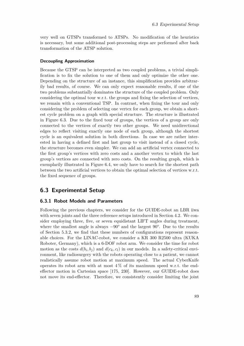
6.3 Experimental Setup
very well on GTSPs transformed to ATSPs. No modification of the heuristicsis necessary, but some additional post-processing steps are performed after backtransformation of the ATSP solution.
Decoupling Approximation
Because the GTSP can be interpreted as two coupled problems, a trivial simpli-fication is to fix the solution to one of them and only optimize the other one.Depending on the structure of an instance, this simplification provides arbitrar-ily bad results, of course. We can only expect reasonable results, if one of thetwo problems substantially dominates the structure of the coupled problem. Onlyconsidering the optimal tour w.r.t. the groups and fixing the selection of vertices,we remain with a conventional TSP. In contrast, when fixing the tour and onlyconsidering the problem of selecting one vertex for each group, we obtain a short-est cycle problem on a graph with special structure. The structure is illustratedin Figure 6.3. Due to the fixed tour of groups, the vertices of a group are onlyconnected to the vertices of exactly two other groups. We need unidirectionaledges to reflect visiting exactly one node of each group, although the shortestcycle is an equivalent solution in both directions. In case we are rather inter-ested in having a defined first and last group to visit instead of a closed cycle,the structure becomes even simpler. We can add an artificial vertex connected tothe first group’s vertices with zero costs and a another vertex to which the lastgroup’s vertices are connected with zero costs. On the resulting graph, which isexemplarily illustrated in Figure 6.4, we only have to search for the shortest pathbetween the two artificial vertices to obtain the optimal selection of vertices w.r.t.the fixed sequence of groups.
6.3 Experimental Setup
6.3.1 Robot Models and Parameters
Following the previous chapters, we consider for the GUIDE-robot an LBR iiwawith seven joints and the three reference setups introduced in Section 4.2. We con-sider employing three, five, or seven equidistant LIFT angles during treatment,where the smallest angle is always −90° and the largest 90°. Due to the resultsof Section 5.3.2, we find that these numbers of configurations represent reason-able choices. For the LINAC-robot, we consider a KR 300 R2500 ultra (KUKARoboter, Germany), which is a 6-DOF robot arm. We consider the time for robotmotion as the costs d(bi, bj) and d(ck, cl) in our models. In a safety-critical envi-ronment, like radiosurgery with the robots operating close to a patient, we cannotrealistically assume robot motion at maximum speed. The actual CyberKnifeoperates its robot arm with at most 4 % of its maximum speed w.r.t. the end-effector motion in Cartesian space [175, 230]. However, our GUIDE-robot doesnot move its end-effector. Therefore, we consistently consider limiting the joint
89

6 Synchronizing Robot Motion and Beam Delivery in Ultrasound-Guided Radiosurgery
v1
v2
v3
v4
v5
v6
v7
v8
v9v10
G1
G2
G3
G4
G5
Figure 6.3: Illustration of the graph structure for the shortest cycle problem, which re-mains when fixing the tour for visiting the groups of a GTSP. The costs ofthe edges are omitted in this plot.
source sink
v1
v2
v3
v4
v5
v6
v7
v8
v9
v10
G1G2
G3G4 G5
Figure 6.4: Illustration of the shortest path problem, which remains if we consider a fixedHamiltonian path for visiting the groups of a GTSP. The artificially addedvertices are labeled as source and sink. The costs of the edges are omitted inthis plot.
speeds for both robot arms. Table 6.1 presents for each joint θg of each robotarm the maximum rotational speeds sLINACg and sGUIDE
g , respectively, convertedfrom radians to degree. We limit the speed of each joint of the LINAC-robot andthe GUIDE-robot to a fraction λLINAC and λGUIDE, respectively, of its maximumspeed. Therefore, we estimate the time required for robot motion as
d(bi, bj) = maxg∈{1,...,6}
∣∣∣θig − θjg∣∣∣λLINAC · sLINACg
(6.6)
90
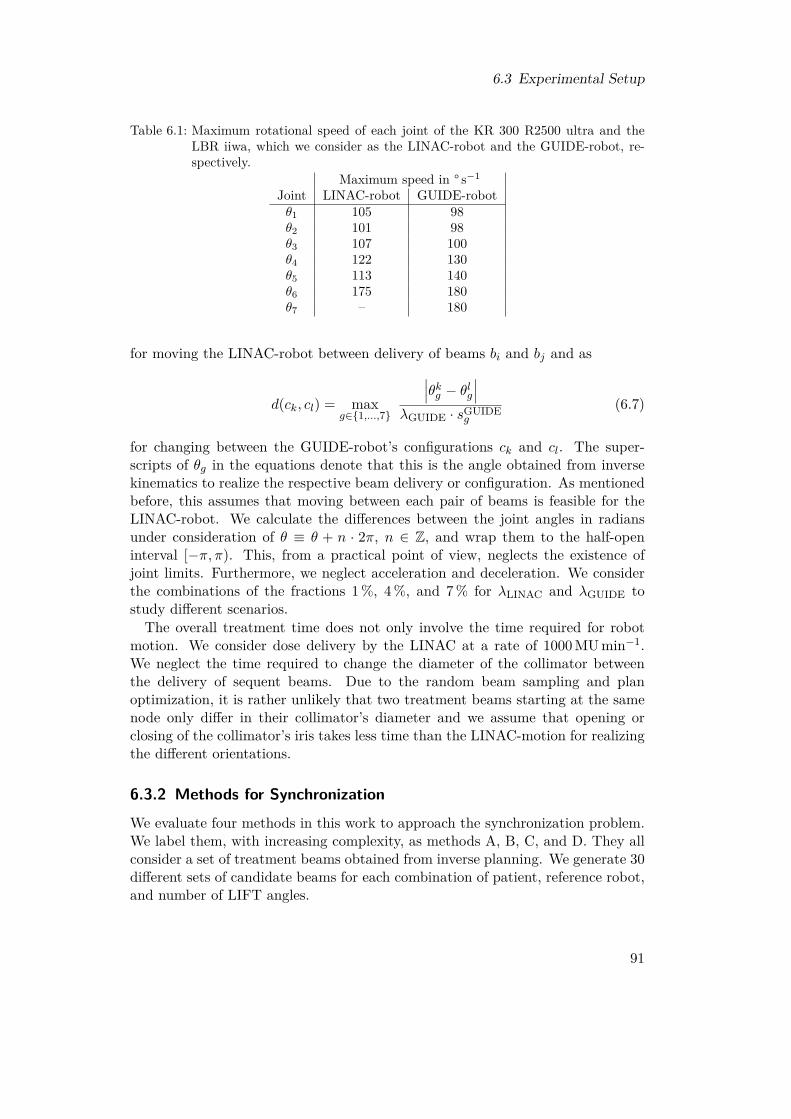
6.3 Experimental Setup
Table 6.1: Maximum rotational speed of each joint of the KR 300 R2500 ultra and theLBR iiwa, which we consider as the LINAC-robot and the GUIDE-robot, re-spectively.
Maximum speed in ° s−1
Joint LINAC-robot GUIDE-robotθ1 105 98θ2 101 98θ3 107 100θ4 122 130θ5 113 140θ6 175 180θ7 – 180
for moving the LINAC-robot between delivery of beams bi and bj and as
d(ck, cl) = maxg∈{1,...,7}
∣∣∣θkg − θlg∣∣∣λGUIDE · sGUIDE
g
(6.7)
for changing between the GUIDE-robot’s configurations ck and cl. The super-scripts of θg in the equations denote that this is the angle obtained from inversekinematics to realize the respective beam delivery or configuration. As mentionedbefore, this assumes that moving between each pair of beams is feasible for theLINAC-robot. We calculate the differences between the joint angles in radiansunder consideration of θ ≡ θ + n · 2π, n ∈ Z, and wrap them to the half-openinterval [−π, π). This, from a practical point of view, neglects the existence ofjoint limits. Furthermore, we neglect acceleration and deceleration. We considerthe combinations of the fractions 1 %, 4 %, and 7 % for λLINAC and λGUIDE tostudy different scenarios.The overall treatment time does not only involve the time required for robot
motion. We consider dose delivery by the LINAC at a rate of 1000 MU min−1.We neglect the time required to change the diameter of the collimator betweenthe delivery of sequent beams. Due to the random beam sampling and planoptimization, it is rather unlikely that two treatment beams starting at the samenode only differ in their collimator’s diameter and we assume that opening orclosing of the collimator’s iris takes less time than the LINAC-motion for realizingthe different orientations.
6.3.2 Methods for Synchronization
We evaluate four methods in this work to approach the synchronization problem.We label them, with increasing complexity, as methods A, B, C, and D. They allconsider a set of treatment beams obtained from inverse planning. We generate 30different sets of candidate beams for each combination of patient, reference robot,and number of LIFT angles.
91
6 Synchronizing Robot Motion and Beam Delivery in Ultrasound-Guided Radiosurgery
Method A: No GUIDE-robot In this method, we only consider optimizing thebeam sequence for the LINAC-robot as an HPP and ignore the GUIDE-robot.Note that the treatment beams are based on the setup including the GUIDE-robot,nevertheless, and hence we should rather interpret this method as considering aninfinitely fast GUIDE-robot. We use the software tool Concorde (version 03.12.19,written by David Applegate, Robert Bixby, Vasek Chvátal, and William Cook)which, besides providing heuristic algorithms, allows to solve TSPs exactly andvery efficiently. The solution of method A will serve as the baseline for evaluatingthe following methods, which actually consider the GUIDE-robot and thereforehave to lead to solutions with at least the same costs.
Method B: Non-optimized GUIDE-robot In this method, we fix the beam se-quence obtained from method A and naively switch the GUIDE-robot’s configu-rations as necessary. For this purpose, we start in an arbitrary configuration inwhich the first beam is feasible. If the subsequent beam is not feasible in thecurrent configuration, we switch to the closest configuration in which the beamis actually feasible. Therefore, there is no real optimization of the sequence ofconfigurations involved.
Method C: Decoupled robot optimization We employ the decoupling describedin Section 6.2.3. As in method B, we fix the beam sequence obtained from methodA. However, we use the Dijkstra algorithm [47] to solve the remaining shortest pathproblem. Thereby, we obtain the optimal sequence of GUIDE-robot configurationsgiven the fixed beam sequence. The solution of method B is part of method C’ssearch space. As method C is exact, we cannot obtain a worse solution. However,we can only expect reasonable results from this decoupling if the costs for movingthe LINAC-robot dominate the quality of solutions. In contrast, results will beof low quality if we need to severely adapt the sequence of treatment beams forefficient synchronous motion.
Method D: GTSP-based coupled optimization We use the software tool GLKH(version 1.0, written by Keld Helsgaun) to approximately solve the full GTSPmodel. It implements the approach mentioned in Section 6.2.3 which convertsthe GTSP to an ATSP and employs the Lin-Kernighan-Helsgaun heuristic withGTSP-specific post-processing routines. We extract a path visiting all groups fromthe solution. Both the solutions from method B and method C are part of thesearch space of method D. However, method D is not exact and therefore we haveno guarantee to find a solution of equal or better quality. This could be fixed byproviding method B’s or method C’s solution as an initial guess. However, weonly evaluate random initial guesses in this thesis to obtain information about thecomplexity of solving the full GTSP model without bias.
92
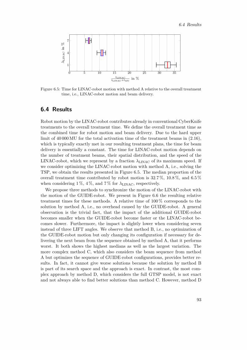
6.4 Results
0 5 10 15 20 25 30 35
1
4
7
tLINACtLINAC+tMU
in %
λL
INA
Cin
%
Figure 6.5: Time for LINAC-robot motion with method A relative to the overall treatmenttime, i.e., LINAC-robot motion and beam delivery.
6.4 Results
Robot motion by the LINAC-robot contributes already in conventional CyberKnifetreatments to the overall treatment time. We define the overall treatment time asthe combined time for robot motion and beam delivery. Due to the hard upperlimit of 40 000 MU for the total activation time of the treatment beams in (2.16),which is typically exactly met in our resulting treatment plans, the time for beamdelivery is essentially a constant. The time for LINAC-robot motion depends onthe number of treatment beams, their spatial distribution, and the speed of theLINAC-robot, which we represent by a fraction λLINAC of its maximum speed. Ifwe consider optimizing the LINAC-robot motion with method A, i.e., solving theTSP, we obtain the results presented in Figure 6.5. The median proportion of theoverall treatment time contributed by robot motion is 32.7 %, 10.8 %, and 6.5 %when considering 1 %, 4 %, and 7 % for λLINAC, respectively.
We propose three methods to synchronize the motion of the LINAC-robot withthe motion of the GUIDE-robot. We present in Figure 6.6 the resulting relativetreatment times for these methods. A relative time of 100 % corresponds to thesolution by method A, i.e., no overhead caused by the GUIDE-robot. A generalobservation is the trivial fact, that the impact of the additional GUIDE-robotbecomes smaller when the GUIDE-robot become faster or the LINAC-robot be-comes slower. Furthermore, the impact is slightly lower when considering seveninstead of three LIFT angles. We observe that method B, i.e., no optimization ofthe GUIDE-robot motion but only changing its configuration if necessary for de-livering the next beam from the sequence obtained by method A, that it performsworst. It both shows the highest medians as well as the largest variation. Themore complex method C, which also considers the beam sequence from methodA but optimizes the sequence of GUIDE-robot configurations, provides better re-sults. In fact, it cannot give worse solutions because the solution by method Bis part of its search space and the approach is exact. In contrast, the most com-plex approach by method D, which considers the full GTSP model, is not exactand not always able to find better solutions than method C. However, method D
93
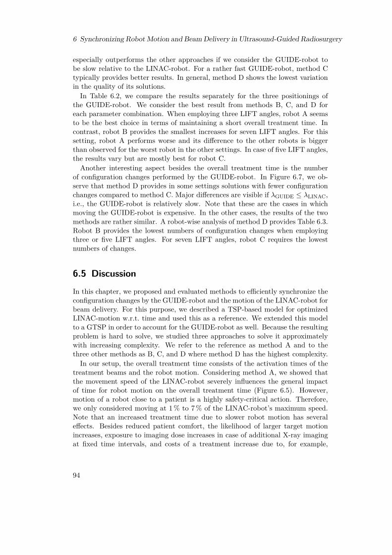
6 Synchronizing Robot Motion and Beam Delivery in Ultrasound-Guided Radiosurgery
especially outperforms the other approaches if we consider the GUIDE-robot tobe slow relative to the LINAC-robot. For a rather fast GUIDE-robot, method Ctypically provides better results. In general, method D shows the lowest variationin the quality of its solutions.
In Table 6.2, we compare the results separately for the three positionings ofthe GUIDE-robot. We consider the best result from methods B, C, and D foreach parameter combination. When employing three LIFT angles, robot A seemsto be the best choice in terms of maintaining a short overall treatment time. Incontrast, robot B provides the smallest increases for seven LIFT angles. For thissetting, robot A performs worse and its difference to the other robots is biggerthan observed for the worst robot in the other settings. In case of five LIFT angles,the results vary but are mostly best for robot C.Another interesting aspect besides the overall treatment time is the number
of configuration changes performed by the GUIDE-robot. In Figure 6.7, we ob-serve that method D provides in some settings solutions with fewer configurationchanges compared to method C. Major differences are visible if λGUIDE ≤ λLINAC,i.e., the GUIDE-robot is relatively slow. Note that these are the cases in whichmoving the GUIDE-robot is expensive. In the other cases, the results of the twomethods are rather similar. A robot-wise analysis of method D provides Table 6.3.Robot B provides the lowest numbers of configuration changes when employingthree or five LIFT angles. For seven LIFT angles, robot C requires the lowestnumbers of changes.
6.5 Discussion
In this chapter, we proposed and evaluated methods to efficiently synchronize theconfiguration changes by the GUIDE-robot and the motion of the LINAC-robot forbeam delivery. For this purpose, we described a TSP-based model for optimizedLINAC-motion w.r.t. time and used this as a reference. We extended this modelto a GTSP in order to account for the GUIDE-robot as well. Because the resultingproblem is hard to solve, we studied three approaches to solve it approximatelywith increasing complexity. We refer to the reference as method A and to thethree other methods as B, C, and D where method D has the highest complexity.In our setup, the overall treatment time consists of the activation times of the
treatment beams and the robot motion. Considering method A, we showed thatthe movement speed of the LINAC-robot severely influences the general impactof time for robot motion on the overall treatment time (Figure 6.5). However,motion of a robot close to a patient is a highly safety-critical action. Therefore,we only considered moving at 1 % to 7 % of the LINAC-robot’s maximum speed.Note that an increased treatment time due to slower robot motion has severaleffects. Besides reduced patient comfort, the likelihood of larger target motionincreases, exposure to imaging dose increases in case of additional X-ray imagingat fixed time intervals, and costs of a treatment increase due to, for example,
94
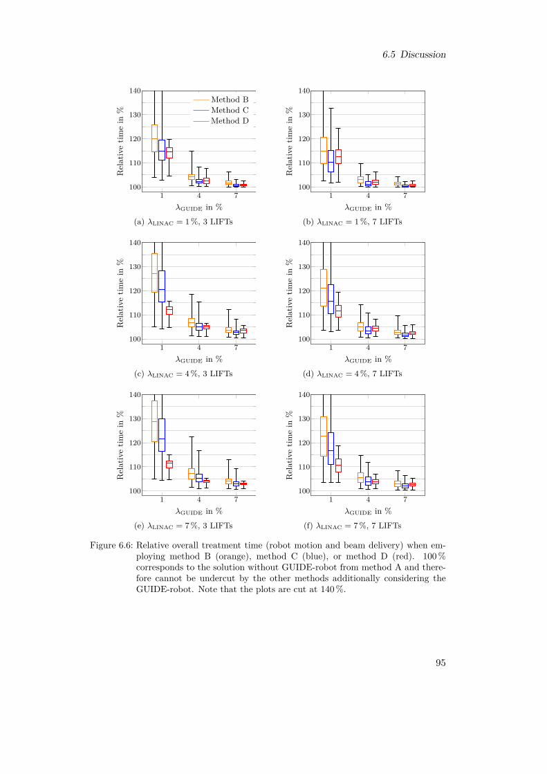
6.5 Discussion
1 4 7100
110
120
130
140
λGUIDE in %
Rel
ativ
etim
ein
%
Method BMethod CMethod D
(a) λLINAC = 1 %, 3 LIFTs
1 4 7100
110
120
130
140
λGUIDE in %
Rel
ativ
etim
ein
%
(b) λLINAC = 1 %, 7 LIFTs
1 4 7100
110
120
130
140
λGUIDE in %
Rel
ativ
etim
ein
%
(c) λLINAC = 4 %, 3 LIFTs
1 4 7100
110
120
130
140
λGUIDE in %
Rel
ativ
etim
ein
%
(d) λLINAC = 4 %, 7 LIFTs
1 4 7100
110
120
130
140
λGUIDE in %
Rel
ativ
etim
ein
%
(e) λLINAC = 7 %, 3 LIFTs
1 4 7100
110
120
130
140
λGUIDE in %
Rel
ativ
etim
ein
%
(f) λLINAC = 7 %, 7 LIFTs
Figure 6.6: Relative overall treatment time (robot motion and beam delivery) when em-ploying method B (orange), method C (blue), or method D (red). 100 %corresponds to the solution without GUIDE-robot from method A and there-fore cannot be undercut by the other methods additionally considering theGUIDE-robot. Note that the plots are cut at 140 %.
95

6 Synchronizing Robot Motion and Beam Delivery in Ultrasound-Guided Radiosurgery
Table 6.2: Mean and standard deviation of the relative increase of the overall treatmenttime (robot motion and treatment time) in percent for the three GUIDE-robotsetups. The increase is relative to method A which does not consider theGUIDE-robot. For each experiment, the best of the three results obtainedfrom method B, method C, and method D is considered. For each parametercombination, the best result is marked bold.# LIFTs λLINAC λGUIDE robot A robot B robot C
3
1 %1 % 11.4± 3.3 12.6± 4.1 11.7± 3.74 % 1.6± 0.8 2.6± 1.2 2.0± 1.17 % 0.6± 0.3 0.7± 0.5 0.6± 0.4
4 %1 % 9.8± 2.4 12.1± 3.4 11.4± 2.04 % 3.9± 1.2 4.3± 1.4 4.0± 1.27 % 2.2± 0.8 2.7± 1.0 2.4± 0.9
7 %1 % 9.1± 2.3 11.8± 3.2 11.1± 1.64 % 3.3± 0.9 3.8± 1.1 3.6± 0.97 % 2.4± 0.7 2.5± 0.8 2.4± 0.7
5
1 %1 % 13.6± 3.5 12.3± 4.5 11.5± 4.14 % 1.9± 0.9 1.7± 1.0 1.6± 0.87 % 0.8± 0.3 0.4± 0.4 0.4± 0.3
4 %1 % 12.3± 2.4 13.3± 3.7 13.2± 3.24 % 4.6± 1.1 4.1± 1.5 3.8± 1.47 % 2.6± 0.8 2.2± 0.9 2.0± 0.9
7 %1 % 11.6± 2.1 13.0± 3.4 12.3± 2.74 % 4.1± 1.0 4.2± 1.3 3.9± 1.27 % 2.8± 0.7 2.5± 0.9 2.3± 0.9
7
1 %1 % 12.8± 3.4 7.8± 3.8 8.2± 4.14 % 1.8± 0.8 0.8± 0.7 0.8± 0.67 % 0.7± 0.3 0.2± 0.3 0.2± 0.2
4 %1 % 12.5± 2.6 9.3± 3.9 10.2± 3.94 % 4.3± 1.1 2.6± 1.3 2.8± 1.47 % 2.3± 0.7 1.2± 0.7 1.3± 0.7
7 %1 % 11.8± 2.3 8.6± 3.5 9.8± 3.84 % 4.0± 1.0 2.7± 1.2 3.0± 1.37 % 2.6± 0.7 1.5± 0.8 1.7± 0.8
higher personal expenses for each treatment and lower patient throughput on themachine.
To minimize the increase in treatment time due to additional time required formoving the GUIDE-robot, we employed the three methods B, C, and D (Fig-ure 6.6). Clearly, the speed of the GUIDE-robot relative to the LINAC-robotdictates the general increase in treatment time. We observed that the simplicityof method B, which does not optimize the sequence of configuration changes atall, leads to worse solutions than the other two methods. Interestingly, method Cwhich fixes the beam sequence from method A and only optimizes the sequence ofconfiguration changes outperformed in some scenarios method D which simultane-ously optimizes both sequences. This especially happened if the GUIDE-robot was
96

6.5 Discussion
1 4 70
20
40
60
λGUIDE in %
Num
ber
ofch
ange
s
(a) λLINAC = 1 %, method C
1 4 70
10
20
λGUIDE in %
Num
ber
ofch
ange
s
(b) λLINAC = 4 %, method C
1 4 70
10
20
λGUIDE in %
Num
ber
ofch
ange
s
(c) λLINAC = 7 %, method C
1 4 70
20
40
60
λGUIDE in %
Num
ber
ofch
ange
s
(d) λLINAC = 1 %, method D
1 4 70
10
20
λGUIDE in %
Num
ber
ofch
ange
s
(e) λLINAC = 4 %, method D
1 4 70
10
20
λGUIDE in %
Num
ber
ofch
ange
s
(f) λLINAC = 7 %, method D
Figure 6.7: Resulting number of configuration changes by the GUIDE-robot when em-ploying method C (a-c) or method D (d-f). Note that the y-axis scaling in (a)and (d) is different to that in the other sub-figures. Further, note that someboxes in (d), (e), and (f) collapse due to the small and discrete variation.
moving faster than the LINAC-robot. In this case, the influence of the GUIDE-robot is rather small and the most-efficient beam sequence from method A is stilla good choice. The results showed that solving the full problem is practically diffi-cult. However, a simple improvement would be to consider the result from methodC as the initial guess for the underlying heuristic solver of method D. Thereby,the result of method D cannot be worse than the result of method C. Because wecan employ method C without relevant computational effort, this option shoulddefinitely be considered in practical application of this synchronization procedure,although it might also add an unfavorable bias in some cases.Furthermore, we showed that the increase of the overall treatment time also dif-
fers for the three reference positionings of the GUIDE-robot (Table 6.2). Depend-ing on the number of employed LIFT angles, a different setup was advantageous.We already observed in previous chapters that the influence of the positioningvanishes w.r.t. the plan quality with increasing number of LIFT angles underconsideration. Hence, this chapter’s analysis might provide a suitable metric fordeciding between different setups in case of employing multiple angles as it con-siders a completely different figure of merit.An aspect which our proposed methods do not explicitly take into account is the
97
6 Synchronizing Robot Motion and Beam Delivery in Ultrasound-Guided Radiosurgery
Table 6.3: Mean and standard deviation for the number of configuration changes by theGUIDE-robot in the solutions obtained with Method D. The best result foreach parameter combination is marked bold.# LIFTs λLINAC λGUIDE Robot A Robot B Robot C
3
1 %1 % 1.8± 0.4 1.7± 0.5 1.9± 0.34 % 3.3± 1.6 2.9± 0.9 3.4± 1.37 % 7.5± 2.6 4.6± 1.5 6.5± 1.9
4 %1 % 1.8± 0.4 1.7± 0.5 1.9± 0.34 % 1.8± 0.4 1.7± 0.4 1.9± 0.27 % 1.9± 0.6 1.7± 0.4 2.0± 0.3
7 %1 % 1.8± 0.4 1.7± 0.5 1.9± 0.34 % 1.8± 0.4 1.7± 0.5 1.9± 0.37 % 1.8± 0.4 1.7± 0.5 2.0± 0.2
5
1 %1 % 4.5± 1.5 3.5± 1.3 3.9± 1.34 % 25.8± 6.2 16.8± 5.3 21.2± 6.07 % 36.9± 5.8 33.7± 6.5 35.8± 6.4
4 %1 % 3.1± 0.7 2.8± 0.8 3.0± 0.84 % 4.8± 1.5 3.5± 1.3 3.9± 1.27 % 7.8± 2.3 5.3± 1.9 5.9± 2.0
7 %1 % 3.2± 0.7 2.7± 0.8 2.9± 0.84 % 3.6± 0.9 3.1± 1.1 3.3± 1.07 % 4.7± 1.4 3.6± 1.3 4.1± 1.3
7
1 %1 % 9.2± 2.3 6.6± 2.3 5.7± 2.64 % 40.0± 8.0 42.4± 6.5 37.7± 7.47 % 49.8± 8.0 50.6± 7.5 48.1± 6.9
4 %1 % 4.4± 1.1 3.8± 1.3 3.6± 1.34 % 9.5± 2.4 6.2± 2.3 6.0± 2.37 % 16.7± 3.6 11.9± 3.5 10.8± 3.8
7 %1 % 4.3± 1.0 3.7± 1.1 3.5± 1.44 % 5.8± 1.7 4.7± 1.7 4.2± 1.87 % 9.2± 2.3 6.5± 2.3 5.9± 2.5
number of configuration changes, which we need to realize the sequence of config-urations (Figure 6.7 and Table 6.3). This number severely depends on the numberof LIFT angles we consider and the speeds of the two robots. Although fewer con-figuration changes obviously correspond to less GUIDE-robot motion, the actualrelationship between the number of configuration changes and the increase of theoverall treatment time is more complicated. The faster the GUIDE-robot is com-pared to the LINAC-robot, the more motion it can perform without affecting theoverall time. For this reason, we observed even beyond 50 configuration changes insome of our solutions although we only considered seven different configurations.It might be interesting to limit this number in order to decrease the frequency ofGUIDE-robot motion. One motivation for this action is again the patient comfort.The GUIDE-robot is very close to the patient and frequent motion might causediscomfort.In the actual CyberKnife system, the LINAC-robot moves at about 4 % of its
98

6.5 Discussion
maximum speed. Considering the same limitation for the GUIDE-robot, we ob-tained in our evaluations moderate increases in the overall treatment time in theorder of 3 % to 5 %, depending on the exact setup (Table 6.2). Note that weconsidered an optimal trajectory of the LINAC-robot as the reference for thesevalues. In practice, there are additional factors already leading to less efficienttrajectories. First, there might be obstacles or other limitations for safe robotmotion forbidding to travel directly between some pairs of beam nodes. This as-pect would directly affect our ultrasound-guidance setup as well. Second, the realsystem requires X-ray imaging in defined intervals for reliable tracking of targetmotion. The LINAC-robot can block these imaging X-ray beams similar to ourGUIDE-robot blocking treatment beams. Thus, more time-consuming trajectoriesmight be necessary to comply with the required imaging intervals throughout thewhole course of the treatment. This aspect has an interesting effect when consid-ering the impact on treatment time of our ultrasound-guidance setup, because afundamental motivation of the ultrasound guidance is to reduce the necessity forX-ray imaging. Thus, future studies should compare the impact of more efficientLINAC-robot trajectories due to less X-ray imaging to the impact of less efficienttrajectories due to motion of the GUIDE-robot.
99

7 Towards Optical CoherenceTomography for Image Guidance inCranial Radiosurgery
In the previous chapters, we discussed different treatment-planning aspects ap-pearing in robotic ultrasound guidance. Ultrasound imaging is a promising modal-ity for abdominal targets because it is non-ionizing, allows for real-time volumetricimaging, and provides direct and markerless imaging of internal targets. The in-tegration of intra-fractional ultrasound imaging in the treatment room is not asexpensive as MRI, but requires to replace the conventional manual operator with arobotic system and to consider the blocking of treatment beams by the ultrasoundtransducer and the robot.However, ultrasound is not applicable for guiding cranial treatments due to the
skull. We discussed in Section 3.3.4 that optical tracking systems can be em-ployed to track head motion during cranial radiation therapy. These are also non-ionizing, low-cost, allow for real-time imaging, and integration in the treatmentroom mainly requires to establish a steady line-of-sight. A drawback compared toother imaging modalities like ultrasound, CT, MRI, or EM tracking is the super-ficial scanning of conventional optical tracking systems. While external trackingof head motion itself is rather uncritical for cranial treatment sites because theinternal targets do not move much relative to the skull, it requires either to attachmarkers which increase the effort for integration or, in case of surface scanning,to have clear and rigid features for precise image registration.A relatively new and less common optical imaging modality is OCT. Similar
to the measurement of acoustic reflections from different layers within tissue inultrasound imaging, OCT measures reflections of light to reconstruct depth pro-files. Employing near-infrared light allows, in addition to surface reflections, toreceive reflections from structures which are a few millimeters within the tissue.In consequence, one of OCT’s main characteristics is its small FOV. However,state-of-art systems provide volumetric imaging with a spatial resolution in theorder of 10 µm. Nevertheless, the temporal resolution has been a limiting factorfor a long time. This has changed recently due to major improvements in lasertechnology and high-resolution volumetric OCT imaging is feasible today at videorate and with few motion artifacts. For this reason, we propose to employ OCTimaging to realize motion tracking. Due to its high spatial resolution, it can ac-quire tiny superficial structures which cannot be exploited in larger-scale opticalsystems. Furthermore, OCT can exploit structures below the surface that are
101
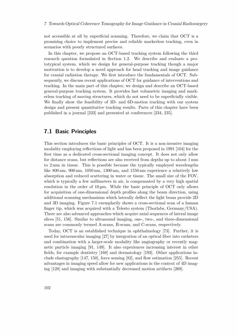
7 Towards Optical Coherence Tomography for Image Guidance in Cranial Radiosurgery
not accessible at all by superficial scanning. Therefore, we claim that OCT is apromising choice to implement precise and reliable markerless tracking, even inscenarios with poorly structured surfaces.
In this chapter, we propose an OCT-based tracking system following the thirdresearch question formulated in Section 1.2. We describe and evaluate a pro-totypical system, which we design for general-purpose tracking though a majormotivation is to develop a novel approach for head tracking and image guidancefor cranial radiation therapy. We first introduce the fundamentals of OCT. Sub-sequently, we discuss recent applications of OCT for guidance of interventions andtracking. In the main part of this chapter, we design and describe an OCT-basedgeneral-purpose tracking system. It provides fast volumetric imaging and mark-erless tracking of moving structures, which do not need to be superficially visible.We finally show the feasibility of 3D- and 6D-motion tracking with our systemdesign and present quantitative tracking results. Parts of this chapter have beenpublished in a journal [233] and presented at conferences [234, 235].
7.1 Basic Principles
This section introduces the basic principles of OCT. It is a non-invasive imagingmodality employing reflections of light and has been proposed in 1991 [104] for thefirst time as a dedicated cross-sectional imaging concept. It does not only allowfor distance scans, but reflections are also received from depths up to about 1 mmto 2 mm in tissue. This is possible because the typically employed wavelengthslike 800 nm, 900 nm, 1050 nm, 1300 nm, and 1550 nm experience a relatively lowabsorption and reduced scattering in water or tissue. The small size of the FOV,which is typically a few millimeters in air, is compensated by a very high spatialresolution in the order of 10 µm. While the basic principle of OCT only allowsfor acquisition of one-dimensional depth profiles along the beam direction, usingadditional scanning mechanisms which laterally deflect the light beam provide 2Dand 3D imaging. Figure 7.1 exemplarily shows a cross-sectional scan of a humanfinger tip, which was acquired with a Telesto system (Thorlabs, Germany/USA).There are also advanced approaches which acquire axial sequences of lateral imageslices [51, 156]. Similar to ultrasound imaging, one-, two-, and three-dimensionalscans are commonly termed A-scans, B-scans, and C-scans, respectively.Today, OCT is an established technique in ophthalmology [73]. Further, it is
used for intravascular imaging [27] by integration of an optical fiber into cathetersand combination with a larger-scale modality like angiography or recently mag-netic particle imaging [91, 149]. It also experiences increasing interest in otherfields, for example dentistry [168] and dermatology [193]. Other applications in-clude elastography [147, 150], force sensing [82], and flow estimation [255]. Recentadvantages in imaging speed allow for new applications in the context of 4D imag-ing [128] and imaging with substantially decreased motion artifacts [269].
102
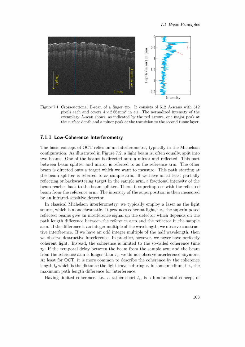
7.1 Basic Principles
Depth
1 mm
1mm
inair
0
0.5
1
1.5
2
2.5
Intensity
Dep
th(in
air)
inm
m
Figure 7.1: Cross-sectional B-scan of a finger tip. It consists of 512 A-scans with 512pixels each and covers 4× 2.66 mm2 in air. The normalized intensity of theexemplary A-scan shows, as indicated by the red arrows, one major peak atthe surface depth and a minor peak at the transition to the second tissue layer.
7.1.1 Low-Coherence Interferometry
The basic concept of OCT relies on an interferometer, typically in the Michelsonconfiguration. As illustrated in Figure 7.2, a light beam is, often equally, split intotwo beams. One of the beams is directed onto a mirror and reflected. This partbetween beam splitter and mirror is referred to as the reference arm. The otherbeam is directed onto a target which we want to measure. This path starting atthe beam splitter is referred to as sample arm. If we have an at least partiallyreflecting or backscattering target in the sample arm, a fractional intensity of thebeam reaches back to the beam splitter. There, it superimposes with the reflectedbeam from the reference arm. The intensity of the superposition is then measuredby an infrared-sensitive detector.In classical Michelson interferometry, we typically employ a laser as the light
source, which is monochromatic. It produces coherent light, i.e., the superimposedreflected beams give an interference signal on the detector which depends on thepath length difference between the reference arm and the reflector in the samplearm. If the difference is an integer multiple of the wavelength, we observe construc-tive interference. If we have an odd integer multiple of the half wavelength, thenwe observe destructive interference. In practice, however, we never have perfectlycoherent light. Instead, the coherence is limited to the so-called coherence timeτc. If the temporal delay between the beam from the sample arm and the beamfrom the reference arm is longer than τc, we do not observe interference anymore.At least for OCT, it is more common to describe the coherence by the coherencelength lc which is the distance the light travels during τc in some medium, i.e., themaximum path length difference for interference.Having limited coherence, i.e., a rather short lc, is a fundamental concept of
103

7 Towards Optical Coherence Tomography for Image Guidance in Cranial Radiosurgery
Lightsource
s(z)
1√2 s(z)
1√2 s(z)
Detector
√Rr√4 s(z) +
√Rs√4 s(z − 2∆z)
Rr
Rs
Reference arm
Sample
arm
∆zzr
zr
Figure 7.2: Sketch of a Michelson interferometer. A light beam is splitted into two beamswith half intensity. The beam in the reference arm is reflected at a mirrorwith power reflectivity Rr at distance zr. The beam in the second arm isreflected at a sample with power reflectivity Rs at distance zr+∆z. Eventually,the intensity of their superposition is recorded at a detector and contains aninterference signal depending on ∆z and the wavelength.
OCT. We only obtain an interference signal from reflecting structures whose pathdifference to the reference mirror is covered by the coherence length. This providesa spatial encoding. If we have multiple reflecting layers in the sample arm, we caniteratively increase the length of the reference arm and only observe constructiveinterference at the detector, if the current length matches the distance to one ofthe layers. Thereby, we can record a depth profile and this concept results intime-domain optical coherence tomography (TD-OCT). It also illustrates thatthe axial resolution in OCT is directly related to the coherence length of the lightsource. The lateral resolution is mainly determined by the employed optics.
7.1.2 Fourier-Domain OCT
TD-OCT allows to record arbitrarily long depth profiles. However, an iterativemechanical movement of the reference mirror is very slow for reasonable num-bers of measurements and therefore does not allow for satisfying A-scan rates.The approach has been almost completely replaced by Fourier-domain optical co-herence tomography (FD-OCT). As the name suggests, it records the spectralinformation of the interference signal. There are two main versions of FD-OCT,spectral-domain optical coherence tomography (SD-OCT) and swept-source opti-cal coherence tomography (SS-OCT). Both have in common that the referencemirror, i.e., the reference arm length, is fixed during A-scan acquisition. Theirdifference is the way we record the spectral information.In SD-OCT, we use a broad-band light source and a spectrometer. Each element
104
7.1 Basic Principles
of a spectrometer’s line sensor measures the incident intensity of a small range offrequencies. If we consider N discrete layers in the sample arm with reflectivitiesRsi , i = 1, ..., N , and path differences ∆zi compared to the reference mirror, thenthe signal ID(k) at the detector is
ID(k) ∝ S(k)4
(Rr +
N∑i=1
Rsi
)
+ S(k)2
N∑i=1
√RrRsi cos(2k∆zi)
+ S(k)2
N∑i=1
N∑j=i+1
√RsiRsj cos(2k(∆zi −∆zj))
(7.1)
with the power spectrum S(k) of the light source. More details can be found,for example, in Drexler et al. [49]. The first term in (7.1) describes the constantreceived intensities. The second term is the interference signal we are actuallyinterested in. The third term describes pairwise interference between the layers inthe sample arm. If we only consider the second term, we observe a set of cosines atthe detector and their frequencies correspond to twice the path differences ∆zi. Ifwe apply a Fourier transform, we obtain peaks at exactly these frequencies and thisis the A-scan signal. Typically, one re-scales the depth axis to have peaks at ∆zirather than at 2∆zi. The power spectrum is related to the coherence function viaFourier transform and smears the peaks in the A-scan depending on the coherencelength. The fact that we cannot retrieve the sign of the path difference from (7.1)results in ambiguities. The signals of layers with difference ∆z and with difference−∆z appear at the same position in the A-scan. This effect can be described asa mirroring artifact.The idea of SS-OCT is to avoid using speed-limiting line cameras. Instead,
a narrow-band light source varies its frequency over time and we can therebyrecord the interference spectrum with a single detector element as a function oftime. Typically, the frequency variation, called sweep, is assumed to have a linearrelationship between frequency and time and each sweep yields the spectrum ofone A-scan. Especially Fourier-domain mode locking (FDML) lasers [105] canrealize sweeps with high repetition rates.
7.1.3 Lateral ScanningIn order to acquire two- or three-dimensional OCT images, the light beam hasto be deflected such that we acquire a sequence of A-scans at different positions.The classical approach for volumetric scanning is a scan head which containstwo galvanometer mirrors (galvos) as illustrated in Figure 7.3. Each mirror isresponsible for imaging along one axis and changes the angle of the outgoingbeam by rotation. These two mirrors alone would position the A-scans radially.Ideally, a fully telecentric f-theta lens as shown in Figure 7.4 is used for scanning.
105

7 Towards Optical Coherence Tomography for Image Guidance in Cranial Radiosurgery
Scan head
Optical fiber
3D FOV
Scan lens
Figure 7.3: A scan head uses two galvos to deflect the light beam laterally over time.Thereby, they realize a 2D grid of A-scans resulting in a 3D FOV and volu-metric images.
f
f · θθ
Figure 7.4: Illustration of galvo-based scanning with an ideal telecentric f-theta lens.
Its f-theta design allows to scan within a plane and with a linear relation betweeningoing beam angle and outgoing lateral shift. Furthermore, telecentricity resultsin parallel A-scans, although there is always a remaining angle in real lenses.
7.1.4 Practical SS-OCT Image Reconstruction
The following steps are typical for reconstructing an A-scan for an SS-OCT devicebased on an FDML laser. We adopt the terminology used by the company Optores(Germany) for their systems. Before we can reconstruct a digital raw A-scan signalr = (r1, ..., rN ) consisting of N samples recorded by the detector, basic calibrationsignals have to be acquired and processed. This is necessary, because real systemsdo not produce a perfectly linear frequency sweep. Due to any non-linearity, linearsampling in time results in non-linear sampling in frequency space, resulting inchirp-like effects in the spectrum. If a Fourier transform were directly appliedto these samples, the A-scans would suffer from severe artifacts and distortions.Therefore, the following steps are made initially.
• Acquire a background signal b of length N by closing the sampling arm witha shutter. Thereby, the signal does not contain any actual information butonly the constant signal from the reference arm (compare (7.1)) and possibly
106
7.2 OCT-Based Navigation and Tracking
noise due to internal reflections and interferences.
• Acquire a recalibration signal c of length N by closing the sampling arm andopening a so-called recalibration arm. This arm is split from the referencearm and contains a mirror which is aligned to the mirror in the referencearm.
• Estimate the non-linearity of the sweep from the background-corrected re-calibration signal c− s and determine points for linear re-sampling.
The last step requires to solve an inverse problem. It is based on the assumptionthat the mirror in the recalibration arm leads to a single interference signal, i.e.,c− b is a single cosine with a certain frequency. As one approach, one can identifythe zero crossings of this signal which would be equidistantly separated in case ofa linear sweep. From the actual distances one can estimate the non-linearity anddetermine sampling points which represent measuring a linear sweep.
After the initial calibration, we can start to reconstruct A-scans. This involvesthe following steps which are executed on each A-scan separately.
• Acquire a raw A-scan r.
• Subtract the background signal b from r and resample it, for example bylinear interpolation, to compensate for the non-linear sweep.
• Multiply the corrected signal with a windowing function, e.g., a Hann win-dow, and apply a discrete Fourier transform (DFT), commonly implementedas a computationally more efficient fast Fourier transform (FFT).
• Take the absolute values of the result’s complex values which correspond topositive frequencies and apply logarithmic compression.
All these steps have rather low computational effort. Due to the fact that all A-scans of a C-scan can be reconstructed independently of each other, reconstructioncan easily be parallelized. If we acquire B-scans in both scanning directions of theresonant galvo, we eventually have to reverse the order of the A-scans in everyother B-scan.
7.2 OCT-Based Navigation and TrackingOCT imaging is established in ophthalmology and therefore compensating retinalmotion is an important issue for artifact-free imaging and reliable diagnosis [31,151, 218]. In this thesis, however, we do not consider imaging of the eye but areinterested in rather generic tracking targets. Therefore, we focus in this sectionon discussing previous application of OCT to navigation of non-ophthalmologicinterventions by tissue tracking.
Many studies investigated OCT for guidance of different types of medical lasers[26, 72, 120, 264]. One particular setting is guidance during cochleastomy. The
107

7 Towards Optical Coherence Tomography for Image Guidance in Cranial Radiosurgery
ability to identify borders below the surface has also been exploited to guideablation [283]. Also rotary OCT probes have been studied for imaging and pre-operative planning [94]. Furthermore, Zhang et al. [284] proposed to ablate tinydots superficially and use them as artificial markers for 6-DOF tracking. A similarapproach has been used for calibration between a robotic ablation system and anOCT scan head to enable targeted soft-tissue ablation and spatial mapping ofmass-spectrometric characterizations [229]. Gessert et al. [83] showed that deeplearning approaches can estimate the pose of a known marker in volumetric OCTdata even in occluded settings. This task is related to OCT-based tracking ofinstruments like needles [271], which can rely on information about the artificialtools in contrast to direct tissue tracking. A markerless concept to realize visualservoing for precise repetitive positioning of an OCT probe has been described byDahroug et al. [42].
The limited size of the FOV motivated studies considering image stitching. Onestrategy is to use a robotic system which moves the OCT scanner. Stitching is thenemployed purely relying on a calibration [206] or with additional post-processingwith some registration method [61]. Other studies focused on the algorithmicstitching part instead of the hardware setups to realize acquisition [76, 153, 166].Several studies suggested the prominent feature descriptor SIFT [165] to registerOCT volumes [76, 166, 187]. Other approaches rather considered maximum in-tensity projections or depth maps [152, 154]. Also an explicit separation betweenestimation of the lateral and axial motion has been proposed [76, 188].
7.3 Design of an OCT-Based Tracking System
The basis of our tracking system is a commercial OCT device including a scanhead for C-scan acquisition. The design of the actual tracking system is based onthe following specifications and considerations.
Volumetric imaging In contrast to depth cameras which rather provide 2.5Dinformation, we want to exploit the full 3D imaging capability of OCT. Thispotentially allows to track targets with structure-less surfaces as long as there isstructure below the surface.
Markerless tracking We do not want to require prior knowledge about a tar-get for tracking. Instead, the C-scans should be evaluated for generic informa-tion about motion. Typically, this results in feature-based or intensity-based ap-proaches which determine motion with respect to a defined template C-scan. Thisrequires to maintain a certain amount of overlap between subsequent C-scans.
High imaging and tracking rate The slower the acquisition process of the imag-ing system, the more motion artifacts we observe in the images. For OCT, the
108
7.3 Design of an OCT-Based Tracking System
acquisition rate of commercial systems is mainly advertised in terms of the A-scan rate. The more A-scans we acquire per C-scan, the lower is our C-scan rateand the more motion effects are present within a C-scan. Therefore, using vol-umes consisting of as few A-scans as reasonably possible automatically reducesthe sensitivity to motion artifacts. Additionally, these small C-scans reduce thecomputational effort for image processing and thereby allow for higher trackingrates.
Motion beyond the FOV size OCT only provides a small FOV in the order ofsome millimeters and an arbitrarily moving target will quickly leave it. Therefore,we desire to have a tracking system which is able to adapt the position of theFOV in order to follow larger-scale motion as well. This also allows to maintain aproper overlap of the C-scans as required for tracking algorithms.
6D motion In general, natural motion of rigid objects consists of translationsand rotations. Therefore, we aim to track these types of motion and to quantita-tively estimate the trajectory.
We design the tracking system mainly with respect to these five considerations andthe details will be described in the following subsections. In terms of image pro-cessing, we need a computationally efficient volumetric approach which does notrequire predefined structures in the image data. For this purpose, we will considercorrelation filters which work intensity-based and can be efficiently calculated inFourier domain. In terms of hardware, we need a setup which allows to move theFOV in space to follow a moving target. As a side effect, this allows to keep thesame part of the target in the FOV which reduces the risk for drifting effects intemplate-based tracking algorithms compared to using different locations as tem-plates over time [154, 174]. One approach would be mounting an OCT scan headto a robot [206]. While such an approach allows to realize 6D repositioning of theFOV, it has limited dynamics due to the mechanical movements and additionallyvibrations might distort the scanning. Instead, we directly exploit the fact thataxial shifting can be realized by adjusting the length of the reference arm. Fur-ther, we adapt the galvo-based scanning process which realizes the transition fromA-scans to C-scans. By setting up a second scanning stage, we can laterally shifta whole C-scan to different scanning positions. A disadvantage of this approach isthat the range of motion is much more limited than for a robot-mounted scan headand that we cannot follow rotational movements of the target directly. However,we will show how we can overcome this limitation, at least for rotations within acertain range, by tracking multiple points on a target periodically.
109

7 Towards Optical Coherence Tomography for Image Guidance in Cranial Radiosurgery
7.3.1 Hardware SetupOCT System
We employ a commercially available SS-OCT system (OMES, Optores, Germany)with a center wavelength of 1315 nm and an A-scan rate of about 1.59 MHz. Wecrop the A-scans to 480 pixels corresponding to an imaging range of about 3.5 mmin air. For C-scan imaging, we have two scan heads available. They employa resonant galvo with a frequency of about 15 kHz and 5.67 kHz, respectively,for the fast scanning direction to allow for high acquisition rates. To furtherincrease the rate, one B-scan is acquired during forward movement of the galvoand another one during backward movement, i.e., the A-scans of every second B-scan are spatially acquired in reverse order, resulting in scan rates of about 30 kHzand 11.3 kHz, respectively. Not all A-scans during a half-period of the galvo aremeaningful, however. Close to its turning points, the galvo has to accelerate anddecelerate which leads to non-linear sampling effects. For an equidistantly sampledvolume, as typically used in imaging, only about 85 % of the A-scans can be usedand the remaining are discarded. The general setup is illustrated in Figure 7.5.Furthermore, a synchronization is necessary in order to have the forward and thebackward acquired B-scans properly aligned. For a resonant galvo with frequencyfRG and a system with A-scan rate fA-scan, we can acquire at most
Nmax = fA-scanfB-scan
· 0.85 (7.2)
linearly sampled A-scans, where fB-scan = 2fRG if we employ both forward andbackward acquisition of B-scans. Interestingly, the C-scan rate of an OCT systemwith a resonant galvo does not directly depend on the system’s A-scan rate. In-stead, we have to consider the fixed B-scan rate fB-scan and the number of B-scansper C-scan N , which is essentially unlimited for non-resonant galvos but assumedto be equal to the number of A-scans per B-scan throughout this thesis. Therefore,we have N ≤ Nmax and the C-scan rate is
fC-scan = fB-scanN + 4 . (7.3)
The additive constant of four is due to the fact that we have to move back thenon-resonant galvo to its origin after acquisition of each C-scan which takes sometime, in our case equal to the acquisition time of four B-scans. This time is ratherchosen empirically and conservatively and in principle would not be necessary ifC-scans were, similar to the B-scans, acquired during both forward and backwardmotion of the galvo.The resonant galvos have two major drawbacks. Firstly, their amplitude is
regulated with an analog rotary knob. This limits the reproducibility of a specificFOV size compared to the digitally controlled slow scanning direction. Secondly,the frequency of the galvo is in reality not fixed but slightly varies and drifts,for example due to varying temperature. This complicates the synchronization
110

7.3 Design of an OCT-Based Tracking System
0 1 2 3 4 5 6 7-0.5
-0.25
0
0.25
0.5
B-scan C-scan
Normalized time
Nor
mal
ized
ampl
itude
Figure 7.5: Illustration of the amplitudes of a resonant (red) and a stepper galvo (blue)during C-scan acquisition with an FOV of size 1× 1 in normalized units. Inthis example, a C-scan consists of only four B-scans. A-scans acquired aroundthe resonant galvo’s turning points have to be discarded due to the geometricdistortions. Therefore, the amplitude of the resonant galvo has to be chosenlarger than the desired FOV of the B-scans. Furthermore, B-scans have to bediscarded while the stepper galvo moves back after a C-scan.
between the forward and the backward acquired B-scans, which might have to beadapted if drifting effects occur over time.
Computing Device
A computer with a digitizer board (ATS9373, Alazartech, Canada) records 2432raw samples for each A-scan. The computer is equipped with two graphics pro-cessing units (GPUs), one Geforce GTX Titan X and one Geforce GTX 980 Ti(Nvidia, USA). The first GPU is intended for image reconstruction while the sec-ond GPU is intended for running the tracking algorithms.
Axial and Lateral Repositioning
If we change the length of an OCT system’s reference arm, then the length of thesample arm, i.e., the axial position of the FOV, changes equally. Therefore, itis intuitive to equip the reference arm with a motorized mirror to automaticallyadapt the axial FOV position. While our OCT system already provides sucha motorized reference arm internally, we use a self-built external reference armshown in Figure 7.6a, instead, which allows for faster motion. Note that, equal tothe internal reference arm, not the actual mirror is mounted to a stepper motorbut a retro-reflector. Therefore, the light travels from the collimator to the retro-reflector and then the same distance again to the mirror. Therefore, moving themotor along a distance ∆z shifts the FOV by 2∆z. The dynamics of steppermotors, however, are not designed for applications like ours. They are especiallyslow if they change their direction of travel, which can be expected to happenrather frequently during tracking and is further increased by noise in the resultsof the tracking algorithm or oscillations caused by the closed control loop.
111

7 Towards Optical Coherence Tomography for Image Guidance in Cranial Radiosurgery
2
3
1
Variable distance
(a) Moving the retro-reflector (1) with the stepper motor changes the distance tothe collimator (2) and the mirror (3).
4
(b) Second pair of galvos (4)for lateral positioning ofthe FOV.
6
4
5
(c) The galvo pair (4) shifts the C-scan created bythe scan head (5) and the beams are then fo-cussed by an achromatic lens (6).
Figure 7.6: Motorized reference arm (a), second pair of galvos (b), and the setup withscan head, second pair of galvos, and lens (c).
For lateral repositioning of the FOV, we use the same concept as employed inscan heads. A pair of stepper galvos (Figure 7.6b) shifts the whole C-scan in space.The concept is illustrated in Figure 7.7. To focus the beam, we use an achromaticlens with a diameter of 50.8 mm (2 inch) and a focal distance of 300 mm. Thefirst version of the second scanning stage was setup by Schünemann [238]. Incomparison to more sophisticated scan lenses, our employed lens provides a ratherlarge diameter, focal distance, and depth of view while having much lower costs.The diameter is a critical parameter because it limits how far we can shift the FOVlaterally. The focal length of 300 mm provides us a reasonable distance betweenthe target and the tracking system. Finally, a large depth of view, i.e., range inwhich the spot size of the beam is reasonably small, is important for axial tracking.Both galvos and the stepper motor of the reference arm are controlled by an
STM32F407 microcontroller (STMicroelectronic, Switzerland) which communi-cates with the measurement computer via a USB connection. This connectionintroduces some delay. On average, a ping, i.e., sending a command to the mi-crocontroller and receiving an answer, takes 6 ms and a minimum of 4 ms. In theworst case, the delay can be arbitrarily large because the computer is not running
112

7.3 Design of an OCT-Based Tracking System
Scan head
Optical fiber
Second galvo pair
Lens
Figure 7.7: Illustration of the second galvo pair in front of the scan head to shift the wholeC-scans laterally.
Computer
GPU 1
GPU 2
Digitizer board
OCT systemScan head
Microcontroller Galvo 2
Galvo 1
Stepper Motor
Data processing FOV positioning
Image acquisition
Communicate
Read
Sample
Control
Control
Control
Control
Compute
Compute
Access
Figure 7.8: Interaction of the tracking system’s main components.
a real-time operating system.
7.3.2 Data Processing Pipeline
The data processing pipeline consists of several parallel units shown in Figure 7.9which asynchronously provide their results to other units. This allows for over-lapping computations and furthermore allows for dynamic processing rates of theindividual units. The first unit is responsible to organize the transfer of the rawOCT signals from the digitizer board into the computer’s main memory.The raw OCT signals then have to be reconstructed and assembled to C-scans.
113
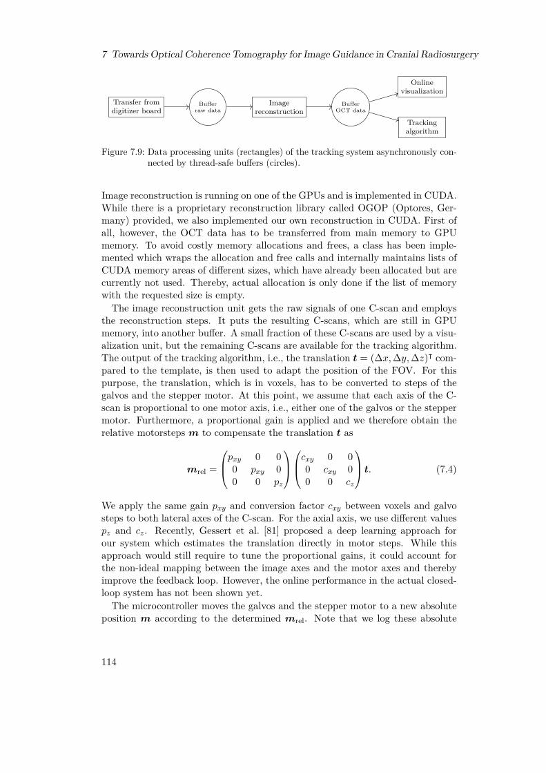
7 Towards Optical Coherence Tomography for Image Guidance in Cranial Radiosurgery
Transfer fromdigitizer board
Imagereconstruction
Onlinevisualization
Trackingalgorithm
Bufferraw data
BufferOCT data
Figure 7.9: Data processing units (rectangles) of the tracking system asynchronously con-nected by thread-safe buffers (circles).
Image reconstruction is running on one of the GPUs and is implemented in CUDA.While there is a proprietary reconstruction library called OGOP (Optores, Ger-many) provided, we also implemented our own reconstruction in CUDA. First ofall, however, the OCT data has to be transferred from main memory to GPUmemory. To avoid costly memory allocations and frees, a class has been imple-mented which wraps the allocation and free calls and internally maintains lists ofCUDA memory areas of different sizes, which have already been allocated but arecurrently not used. Thereby, actual allocation is only done if the list of memorywith the requested size is empty.The image reconstruction unit gets the raw signals of one C-scan and employs
the reconstruction steps. It puts the resulting C-scans, which are still in GPUmemory, into another buffer. A small fraction of these C-scans are used by a visu-alization unit, but the remaining C-scans are available for the tracking algorithm.The output of the tracking algorithm, i.e., the translation t = (∆x,∆y,∆z)ᵀ com-pared to the template, is then used to adapt the position of the FOV. For thispurpose, the translation, which is in voxels, has to be converted to steps of thegalvos and the stepper motor. At this point, we assume that each axis of the C-scan is proportional to one motor axis, i.e., either one of the galvos or the steppermotor. Furthermore, a proportional gain is applied and we therefore obtain therelative motorsteps m to compensate the translation t as
mrel =
pxy 0 00 pxy 00 0 pz
cxy 0 0
0 cxy 00 0 cz
t. (7.4)
We apply the same gain pxy and conversion factor cxy between voxels and galvosteps to both lateral axes of the C-scan. For the axial axis, we use different valuespz and cz. Recently, Gessert et al. [81] proposed a deep learning approach forour system which estimates the translation directly in motor steps. While thisapproach would still require to tune the proportional gains, it could account forthe non-ideal mapping between the image axes and the motor axes and therebyimprove the feedback loop. However, the online performance in the actual closed-loop system has not been shown yet.The microcontroller moves the galvos and the stepper motor to a new absolute
position m according to the determined mrel. Note that we log these absolute
114

7.3 Design of an OCT-Based Tracking System
positions to determine the current position of our target. We do not use the cal-culated translations directly for this purpose. This allows that the microcontrollercould discard remaining motion of the stepper motor as soon as it received newmotorsteps and this information is not contained in the translations.
7.3.3 Calibration to Cartesian Coordinate SystemThe quantitative values recorded by our tracking system are the positions of thetwo galvos and of the stepper motor over time. Firstly, this results in values withno meaningful units. Secondly, the galvos and the stepper motor do not form anorthogonal coordinate system, but we can even expect some spherical effects dueto the rotating galvos. Therefore, we introduce a calibration procedure requiringa 3D motion stage to transform the motor positions to a Cartesian coordinateframe with physical units.The general idea is to use single-template tracking of a phantom which is moved
by a motion stage in order to acquire calibration data, i.e., pairs of motor positionsand corresponding positions of the motion stage. In principle, this data could beacquired continuously. However, we use a more discrete approach by moving themotion stage to a position, wait there for some time, record the current motorposition several times, and then move on to the next position. The waiting allowsthe tracking system to reach a steady position eliminating any delay occurringduring dynamic tracking. By recording the motor position for the same motion-stage position several times, we account for potential residual noise, i.e., the motorposition slightly alters although the target is steady. After obtaining M pairs ofcorresponding positions pi of the motion stage and motor positions mi, we canestablish a spatial transformation between the two coordinate frames. Note thatwe actually do not need the absolute positions pi, but it is sufficient to considerthem relative to the initial position to obtain a Cartesian coordinate frame for ourtracking system. Thereby, we can freely define which motor steps correspond tothe origin.Typically, spatial calibrations involve estimating a rigid transformation, which
consists of a translation and rotation. In our case, we need more degrees offreedom. Firstly, each axis can have an individual scaling from motor steps tomillimeter. Secondly, the motor axes are not necessarily orthogonal. Thirdly, themotor steps might not even define a proper right-handed coordinate frame and wemight need to allow for reflections as well. These aspects can be represented byan affine transformation, represented as a matrix A ∈ R3×4. In contrast to rigidtransformations, it has full twelve degrees of freedom. The only formal constraintis that the 3× 3 sub-matrix formed by the first three columns of A is regular. Toobtain the coefficients of A, we can solve
minA
M−1∑i=0
∥∥∥∥∥pi −A[mi
1
]∥∥∥∥∥2
. (7.5)
However, as mentioned before, we have to expect spherical distortions due to
115
7 Towards Optical Coherence Tomography for Image Guidance in Cranial Radiosurgery
the nature of the galvos and the employed lens. These cannot be corrected by anaffine transform. Therefore, we propose to additionally fit a function fB : R3 → R3
having a set of parameters B in a second step. In a least-squares sense, this leadsto solving
minB
M−1∑i=0
∥∥∥∥∥pi − fB
(A
[mi
1
])∥∥∥∥∥2
. (7.6)
We especially propose to fit a quadratic function, which in total has 30 parameters,or a cubic function, which has 57 parameters. Afterwards, we can transform anymotor position m into the corresponding Cartesian motor position
m = fB
(A
[m1
]). (7.7)
7.3.4 Multi-Template Tracking
If we consider a rigid body, we can track its orientation by observing the motionof at least three non-collinear points of it. Therefore, we propose to employ amulti-template tracking approach to estimate orientations. It essentially consistsof applying single-template tracking to at least three spatially separated partsof the same target simultaneously. For this purpose, we define N initial motorpositions m0
n, n = 1, ..., N , on a circle around c = (x0, y0, z0)ᵀ with radius r as
m0n = c +
r · cos
(2π n−1
N
)r · sin
(2π n−1
N
)0
(7.8)
when tracking N ≥ 3 templates simultaneously. This simple approach is illus-trated in Figure 7.10, but it is only applicable if the target is sufficiently flatwithin r, i.e., the target is within the FOV at every motor position. Otherwisewe should replace z0 with adequate individual values z0
n. Note that non-circulararrangements are also possible.At each initial motor position m0
n, we acquire a template volume which wedenote with V 0
n . Afterwards, we continuously iterate through the positions. If weare in iteration i ≥ 1 and consider template n, then we first move to mi−1
n andacquire V i
n. Second, we calculate the translation tin between V 0n and V i
n and useit to determine mi
n. However, we do not yet move to this new motor positionand start iteration i + 1. Instead, we repeat the procedure for template n + 1 orstart iteration i + 1 with template 0 in case of n = N . Thereby, we implementa multi-template tracking. In fact, we can increase efficiency by pipelining somesteps. After we acquired V i
n, we can immediately move from mi−1n to mi−1
n+1 anddo the calculation of mi
n in parallel.To actually estimate the current orientation in iteration i, we need all N Carte-
sian motor positions min. However, these do not represent the same point in time
116
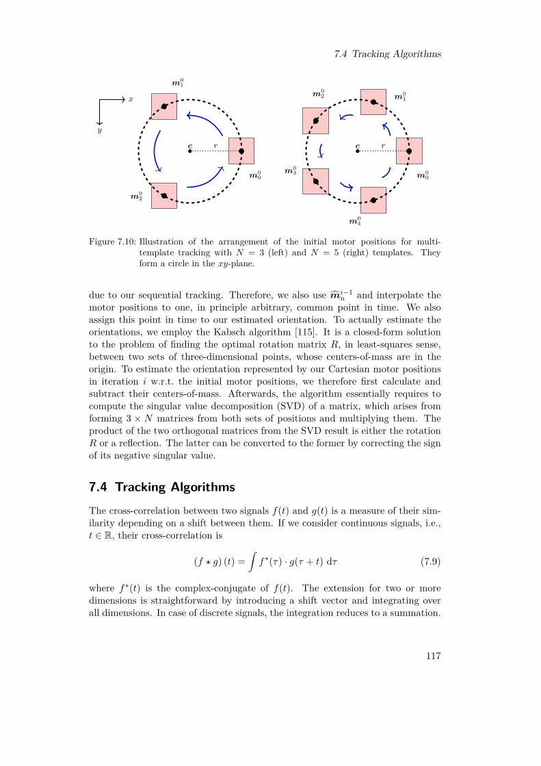
7.4 Tracking Algorithms
m00
m01
m02
rc
x
y
m00
m01
m02
m03
m04
rc
Figure 7.10: Illustration of the arrangement of the initial motor positions for multi-template tracking with N = 3 (left) and N = 5 (right) templates. Theyform a circle in the xy-plane.
due to our sequential tracking. Therefore, we also use mi−1n and interpolate the
motor positions to one, in principle arbitrary, common point in time. We alsoassign this point in time to our estimated orientation. To actually estimate theorientations, we employ the Kabsch algorithm [115]. It is a closed-form solutionto the problem of finding the optimal rotation matrix R, in least-squares sense,between two sets of three-dimensional points, whose centers-of-mass are in theorigin. To estimate the orientation represented by our Cartesian motor positionsin iteration i w.r.t. the initial motor positions, we therefore first calculate andsubtract their centers-of-mass. Afterwards, the algorithm essentially requires tocompute the singular value decomposition (SVD) of a matrix, which arises fromforming 3 × N matrices from both sets of positions and multiplying them. Theproduct of the two orthogonal matrices from the SVD result is either the rotationR or a reflection. The latter can be converted to the former by correcting the signof its negative singular value.
7.4 Tracking AlgorithmsThe cross-correlation between two signals f(t) and g(t) is a measure of their sim-ilarity depending on a shift between them. If we consider continuous signals, i.e.,t ∈ R, their cross-correlation is
(f ? g) (t) =∫f∗(τ) · g(τ + t) dτ (7.9)
where f∗(t) is the complex-conjugate of f(t). The extension for two or moredimensions is straightforward by introducing a shift vector and integrating overall dimensions. In case of discrete signals, the integration reduces to a summation.
117
7 Towards Optical Coherence Tomography for Image Guidance in Cranial Radiosurgery
If g(t) is a shifted version of f(t), i.e., g(t) = f(t − ∆t), we can determine theshift ∆t by finding the shift which maximizes their cross-correlation. However,this requires to evaluate the cross-correlation for every possible shift leading toextensive computational effort. This effort can be reduced by employing Fourier-domain methods. Because cross-correlating f(t) and g(t) is equal to convolvingf∗(−t) and g(t), we can employ a fast convolution, i.e., a multiplication in Fourierdomain, instead of direct evaluation of (7.9) in spatial domain. Therefore, methodsexploiting this relationship are very interesting for applications which require highprocessing rates.One approach to estimate translations between images is the phase correlation
method which is based on evaluating cross-correlation in Fourier domain [132]. Inits basic form, it assumes purely translational motion and can be implementedvery efficiently. We can define one image as the template and then determinethe translations of all following images with respect to that template. Phasecorrelation, however, can be expected to fail as soon as the appearance of the targetseverely changes in the image data because it will no longer be sufficiently similarto the template. Such large changes have to be expected if the target’s motioncannot be approximated by translations but it substantially rotates, which cannotbe compensated by shifting the position of the FOV. For this reason, Glandorf [86]proposed to employ the MOSSE filter [22] in this tracking setup instead. Thisalgorithm is a special kind of correlation filter with a concept very similar tophase correlation, but it allows for a more general definition of the template andfurthermore allows to update the template during tracking. Thereby, this filter canadapt to appearance changes over time. However, template updates always havethe risk to cause drifting effects, i.e., after some time the current template doesnot correspond to the original target anymore but represents a different structure[174].
7.4.1 Phase Correlation
Consider a signal f(x), x ∈ RD, and its shifted version g(x) = f(x −∆x). LetF (k) be the D-dimensional Fourier transform of f(x). From the Fourier shifttheorem, we obtain
G(k) = F (k) · e−i2πkᵀ∆x (7.10)
as the Fourier transform of g(x), where i is the imaginary unit. The so-callednormalized cross-power spectrum
Rf,g(k) = F (k) ·G∗(k)|F (k) ·G∗(k)| (7.11)
118
7.4 Tracking Algorithms
is the normalized Fourier transform of the signals’ cross correlation. Due to (7.10),in our case we can write
Rf,g(k) = F (k) · F ∗(k) · ei2πkᵀ∆x∣∣F (k) · F ∗(k) · ei2πkᵀ∆x∣∣
= F (k) · F ∗(k) · ei2πkᵀ∆x
|F (k) · F ∗(k)|= ei2πkᵀ∆x
(7.12)
and see that the result is a pure phase term which depends on the shift ∆x. Byapplying the inverse Fourier transform, we obtain
rf,g(x) = δ(x + ∆x), (7.13)
i.e., a Dirac peak at the position which corresponds to the shift of the signals.This algorithm is known as the phase-correlation method [132]. In practical
image processing, it has several issues. We typically apply it to discrete imagedata and therefore the derivation would require that all shifts are cyclic. This isnot the case in reality, however, and introduces distortions. Additionally, a shiftis typically not aligned with the image grid and extensions of the algorithm arenecessary to have sub-pixel accuracy [67]. Furthermore, we typically do not haveimages which are related by a pure translation and therefore we obtain furtherdistortions in the result due to the additional transformations missing in the model.The basic form of phase correlation is computationally very efficient. If we
assume using a fixed template image, we need only two (multi-dimensional) FFTs,simple element-wise operations, and a search for the location of the maximumintensity to determine the shift between the template and another image. Forthe FFT, efficient implementations exist and element-wise operation can easily beparallelized on, for example, a GPU. The search for the location of the maximumintensity can be parallelized by employing the parallel-reduction design pattern.In our implementation, we additionally apply a Hann-shaped low pass to Rf,g(k)to increase robustness.Phase correlation has not only been extended for sub-pixel accuracy. In case of
two-dimensional images, we can also use it to estimate rotations [33] and scaling[208]. Reddy et al. [208] showed that both transformations can be obtained viaphase correlation with deterministic computational effort after applying suitablecoordinate transformations. There is also an extension which allows to determinerotations of 3D images [184]. However, this involves an iterative estimation ofthe parameters and furthermore assumes 3D objects which can be represented bypolygon meshes.
7.4.2 MOSSE FilterThe general setup for correlation filters is a large image which contains a smalltarget to be tracked. Classical correlation filters construct an optimal filter which
119

7 Towards Optical Coherence Tomography for Image Guidance in Cranial Radiosurgery
we then apply to smaller parts, i.e., sub-images, of the large image. The filtershould only output a high value for the sub-image which corresponds to the target.Thus, the natural output of the filter is a single correlation-like value for each sub-image. The optimal filter is constructed from a training set consisting of matchingand non-matching small input images and corresponding training output values.There are many different variants of correlation filters, which mainly differ in theway the filter is constructed and the constraints it has to fulfill [138, 171, 172,209].
This general approach has been substantially extended by the so-called ASEFfilters which allow to specify training output not only as a single correlation valuebut as a full cross-correlation-like map [23]. This allows to use large images directlyas the training input and to define a peak in the output map at the position ofthe target within this image. The actual application of the constructed filter h(x)is done in frequency domain. If we apply the filter to an image f(x), we obtainthe frequency-domain output as
O(k) = F (k) ·H∗(k) (7.14)
and in spatial domain it should show a peak at the position of the target. Thisoperation is very similar to the operation (7.11) and the result (7.13) in the phase-correlation method. However, correlation filters allow for much more flexibility dueto the training process which can consider arbitrarily many training images fj(x).These can, for example, be images of the same object but with different noiseor even under different conditions like illumination. Each training output oj(x)would still be a peak at the same location in this case. However, we can also trainthe filter with images in which the target is located at different positions. This isreflected by the training outputs in which the peak is shifted accordingly. Aftertraining, applying the filter to a new image has the same low computational effortas phase correlation.One particular variant specifically designed for tracking tasks is the MOSSE
(minimum output sum of squared error) filter [22]. We will employ this variant inthis thesis. The training outputs are typically not defined as ideal peaks, but asGaussians
oj(x) = 1(√2πσ
)D · exp(−(sj − x)ᵀ(sj − x)
2σ2
)(7.15)
with standard deviation σ and shift sj . The MOSSE filter computes the optimalfilter, in the discrete case, by minimizing the sum over all training images ofthe summed squared differences between the actual and the target output. Theclosed-form solution to this optimization problem presented by Bolme et al. [22]is
H∗(k) =∑j Oj(k) · F ∗j (k)∑j Fj(k) · F ∗j (k) , (7.16)
but typically a regularization constant λ is added to the denominator.
120
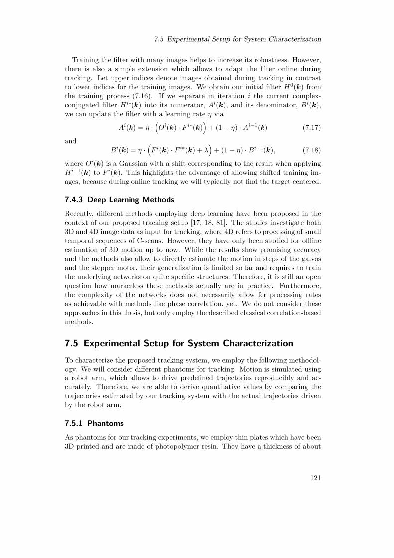
7.5 Experimental Setup for System Characterization
Training the filter with many images helps to increase its robustness. However,there is also a simple extension which allows to adapt the filter online duringtracking. Let upper indices denote images obtained during tracking in contrastto lower indices for the training images. We obtain our initial filter H0(k) fromthe training process (7.16). If we separate in iteration i the current complex-conjugated filter H i∗(k) into its numerator, Ai(k), and its denominator, Bi(k),we can update the filter with a learning rate η via
Ai(k) = η ·(Oi(k) · F i∗(k)
)+ (1− η) ·Ai−1(k) (7.17)
andBi(k) = η ·
(F i(k) · F i∗(k) + λ
)+ (1− η) ·Bi−1(k), (7.18)
where Oi(k) is a Gaussian with a shift corresponding to the result when applyingH i−1(k) to F i(k). This highlights the advantage of allowing shifted training im-ages, because during online tracking we will typically not find the target centered.
7.4.3 Deep Learning MethodsRecently, different methods employing deep learning have been proposed in thecontext of our proposed tracking setup [17, 18, 81]. The studies investigate both3D and 4D image data as input for tracking, where 4D refers to processing of smalltemporal sequences of C-scans. However, they have only been studied for offlineestimation of 3D motion up to now. While the results show promising accuracyand the methods also allow to directly estimate the motion in steps of the galvosand the stepper motor, their generalization is limited so far and requires to trainthe underlying networks on quite specific structures. Therefore, it is still an openquestion how markerless these methods actually are in practice. Furthermore,the complexity of the networks does not necessarily allow for processing ratesas achievable with methods like phase correlation, yet. We do not consider theseapproaches in this thesis, but only employ the described classical correlation-basedmethods.
7.5 Experimental Setup for System CharacterizationTo characterize the proposed tracking system, we employ the following methodol-ogy. We will consider different phantoms for tracking. Motion is simulated usinga robot arm, which allows to drive predefined trajectories reproducibly and ac-curately. Therefore, we are able to derive quantitative values by comparing thetrajectories estimated by our tracking system with the actual trajectories drivenby the robot arm.
7.5.1 PhantomsAs phantoms for our tracking experiments, we employ thin plates which have been3D printed and are made of photopolymer resin. They have a thickness of about
121

7 Towards Optical Coherence Tomography for Image Guidance in Cranial Radiosurgery
40 mm
40m
m
(a)
40 mm
40m
m
(b)
depth
air
plate
mounting
(c) (d)
Figure 7.11: Photographies (top row) and B-scans (bottom row) of the structured-surface phantom (left column) and the flat-surface phantom (right col-umn). Red squares illustrate the size of the OCT’s lateral FOV which is2.5× 2.5× 3.5 mm3.
1 mm and a lateral size of 40× 40 mm2. As Figure 7.11 shows, both the front- andthe backside of a plate are visible in the OCT images. We consider two differentplates. One of them has a fine random structure, i.e., height variations of fewhundreds of micrometers, on both sides. The other one only has one structured sidewhile the other side is flat. We use the flat side as the front side and the structuredside as the backside during tracking, i.e., there is visually no information on thesurface from the tracking system’s point of view.
Furthermore, we use samples of chicken breast to simulate tracking of tissue. InFigure 7.12, an exemplary chicken-breast sample is attached to a sample holder.We arbitrarily select spots on the chicken breast for tracking and only adjust theaxial position in order to have the surface properly within the OCT’s FOV.
122
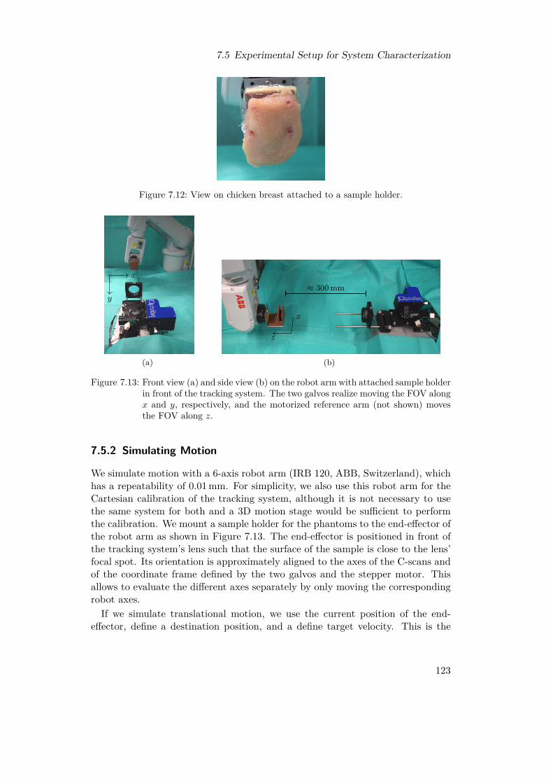
7.5 Experimental Setup for System Characterization
Figure 7.12: View on chicken breast attached to a sample holder.
x
y
(a)
≈ 300 mm
z
x
(b)
Figure 7.13: Front view (a) and side view (b) on the robot arm with attached sample holderin front of the tracking system. The two galvos realize moving the FOV alongx and y, respectively, and the motorized reference arm (not shown) movesthe FOV along z.
7.5.2 Simulating Motion
We simulate motion with a 6-axis robot arm (IRB 120, ABB, Switzerland), whichhas a repeatability of 0.01 mm. For simplicity, we also use this robot arm for theCartesian calibration of the tracking system, although it is not necessary to usethe same system for both and a 3D motion stage would be sufficient to performthe calibration. We mount a sample holder for the phantoms to the end-effector ofthe robot arm as shown in Figure 7.13. The end-effector is positioned in front ofthe tracking system’s lens such that the surface of the sample is close to the lens’focal spot. Its orientation is approximately aligned to the axes of the C-scans andof the coordinate frame defined by the two galvos and the stepper motor. Thisallows to evaluate the different axes separately by only moving the correspondingrobot axes.If we simulate translational motion, we use the current position of the end-
effector, define a destination position, and a define target velocity. This is the
123
7 Towards Optical Coherence Tomography for Image Guidance in Cranial Radiosurgery
maximum velocity in Cartesian space, i.e., the constant velocity we obtain afterthe necessary acceleration phase and before deceleration. Afterwards, we directlymove to the next position until we reach the experiment’s defined total duration.We will on the one hand consider motion back and forth along a line. This line iseither along one robot axis, the diagonal of a square spanned by two axes, or thediagonal of the cube spanned by all three axes. In particular, we will distinguishlateral motion, i.e., motion at constant depth from the OCT’s point of view, andaxial motion, i.e., motion along the OCT’s depth axis. On the other hand, wewill consider random motion in the sense that we define a random sequence ofpositions and drive from one to the next with the pre-defined maximum velocity.
For rotational motion, we define the maximum angular velocity. Analogouslyto the translations along a line, we consider rotations around two fixed axes toevaluate different components. The first axis of rotation is the axial OCT axis.Rotating around this axis can be described as in-plane rotations with respectto the OCT’s lateral plane. The second axis equals one of the lateral axes andtherefore results in out-of-plane rotations. The first should only require movingthe galvos, while the second should involve one galvo and the stepper motor.Furthermore, we consider random rotations. For this purpose, we define a se-
quence of random axes of rotation and random angles. They are always relative tothe initial orientation of the end-effector. Thereby, we can define a maximum angleαmax and draw the actual angles uniformly from the interval [0, αmax]. To createa random axis, we can define a vector a = (x, y, z)ᵀ, draw each of its elementsfrom a Gaussian distribution, and use a/‖a‖ as the axis of rotation. Because wecan rotate around any axis in space, drawing non-negative angles is sufficient.If we consider 6D motion, we define the translational and rotational part in-
dependently. Therefore, we obtain a sequence of positions and a sequence oforientations and realize them in parallel.
7.5.3 Experiments
For our tracking experiments, we employ the fast scan head. It provides imagingwith 32× 32 A-scans per C-scans at a volume rate of 831 Hz. The FOV is about2.5× 2.5× 3.5 mm3 when considering 480 pixels along the depth direction. Weemploy the slower scan head only for evaluating the performance of the phasecorrelation implementation.Before the actual tracking experiments, we have to perform a calibration to
Cartesian coordinates to allow for a quantitative evaluation of the tracking per-formance. For this purpose, we move the robot arm at a speed of 2 mm s−1 to thecalibration positions while employing single-template tracking with phase correla-tion.Each experiment consists of 45 s with active tracking. During this time, the
robot arm moves continuously and we log its poses and the related timestamps.For each repetition of an experiment with the same parameters, we reposition thetarget in front of the tracking system. Thereby, we track different parts of the
124
7.5 Experimental Setup for System Characterization
target in each repetition.For single-template tracking, we log the motor positions at about 80 Hz asyn-
chronously to tracking and employ phase correlation. The template C-scan isacquired before the robot arm starts to move, i.e., while the target is static.For multi-template tracking, we log the motor positions for each of theN tracked
templates directly. At each template-defining motor position m0n, n = 1, ..., N , we
initially train one MOSSE filter on ten C-scans of the static target. Therefore, thetraining outputs are centered smoothed peaks following (7.15) and the trainingmainly accounts for the noise during static OCT acquisition. Subsequently, wewill update the filters each time we apply them. When we acquire the new C-scanin iteration i ≥ 1 at motor position mi
n, we apply the corresponding filter. Thisyields us the translation which we use to determine mi+1
n and which we also use forupdating the filter by converting it to the required shifted filter output in (7.17).
7.5.4 Evaluation MethodsTo quantitatively evaluate tracking, the trajectories of the tracking system andof the reference system, in our case the robot arm, have to be transformed intothe same coordinate frame. For purely translational motion, we can simply usethe result of the calibration to Cartesian coordinates and evaluate the relativemotion performed by the robot arm and the relative motion estimated by thetracking system. If we want to evaluate full 6D motion, we also have to describethe rotations in a common coordinate frame. The problem of finding the requiredtransformations is commonly referred to as a hand-eye calibration. The term handrefers to the dynamic system, typically some kind of robot, realizing motion andproviding ground-truth information. The term eye refers to some kind of staticcamera system. The transformations are assumed to be rigid, i.e., we can describethem with homogeneous matrices
T =[R t0ᵀ 1
](7.19)
with a rotation matrix R ∈ R3×3, a translation vector t ∈ R3, and a vector 0 ∈ R3
only containing zeros. If we realize several poses BT(i)E of the end-effector w.r.t to
the base coordinate frame of the robot and measure the corresponding poses CT(i)M
of some suitable marker w.r.t. the camera coordinate frame, we obtain equations
BT(i)E
ETM = BTCCT
(i)M . (7.20)
when considering the chain of transformations illustrated in Figure 7.14. The con-stant spatial relations between the marker and the end-effector ETM and betweenthe camera and the robot base BTC are the unknown parameters we need to solvefor. Common algorithms for this problem exploit the structure of the transforma-tions and separate estimation of the translational and the rotational parts [198,265]. There are other approaches which, for example, ignore the structure of the
125
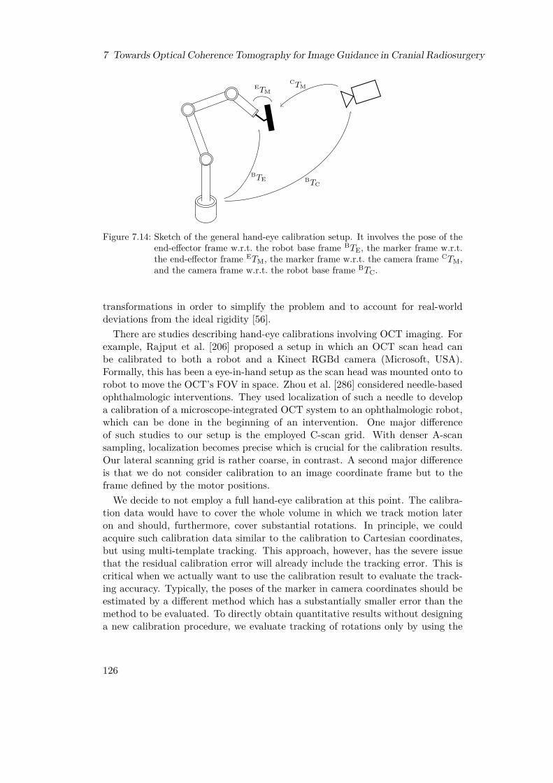
7 Towards Optical Coherence Tomography for Image Guidance in Cranial Radiosurgery
BTE
ETM
BTC
CTM
Figure 7.14: Sketch of the general hand-eye calibration setup. It involves the pose of theend-effector frame w.r.t. the robot base frame BTE, the marker frame w.r.t.the end-effector frame ETM, the marker frame w.r.t. the camera frame CTM,and the camera frame w.r.t. the robot base frame BTC.
transformations in order to simplify the problem and to account for real-worlddeviations from the ideal rigidity [56].There are studies describing hand-eye calibrations involving OCT imaging. For
example, Rajput et al. [206] proposed a setup in which an OCT scan head canbe calibrated to both a robot and a Kinect RGBd camera (Microsoft, USA).Formally, this has been a eye-in-hand setup as the scan head was mounted onto torobot to move the OCT’s FOV in space. Zhou et al. [286] considered needle-basedophthalmologic interventions. They used localization of such a needle to developa calibration of a microscope-integrated OCT system to an ophthalmologic robot,which can be done in the beginning of an intervention. One major differenceof such studies to our setup is the employed C-scan grid. With denser A-scansampling, localization becomes precise which is crucial for the calibration results.Our lateral scanning grid is rather coarse, in contrast. A second major differenceis that we do not consider calibration to an image coordinate frame but to theframe defined by the motor positions.We decide to not employ a full hand-eye calibration at this point. The calibra-
tion data would have to cover the whole volume in which we track motion lateron and should, furthermore, cover substantial rotations. In principle, we couldacquire such calibration data similar to the calibration to Cartesian coordinates,but using multi-template tracking. This approach, however, has the severe issuethat the residual calibration error will already include the tracking error. This iscritical when we actually want to use the calibration result to evaluate the track-ing accuracy. Typically, the poses of the marker in camera coordinates should beestimated by a different method which has a substantially smaller error than themethod to be evaluated. To directly obtain quantitative results without designinga new calibration procedure, we evaluate tracking of rotations only by using the
126
7.6 Results
axis-angle representation of orientations instead, i.e., we describe an orientationrelative to another orientation by one angle around one axis of rotation. In thisrepresentation, the absolute value of the angle is independent of the coordinatesystems.As a quantitative measure, we will mostly consider the root-mean-square error
(RMSE), which is
RMSE(e) =
√√√√ 1N
N∑i=1
e2i (7.21)
for a vector e = (e1, ..., eN )ᵀ containing N error values. Its unit is equal to the unitof the underlying errors. We apply the RMSE to either the norm of the differencebetween the relative positions recorded by the robot arm and the tracking systemor to the difference of their axis-angle angles relative to the initial orientation. Weuse timestamps to resample the poses smoothly logged by the robot arm to theposes logged by the tracking system.
7.6 Results
Before presenting the results of the actual tracking experiments, we firstly eval-uate the performance of our implementation of the phase-correlation algorithm.We then show results for the Cartesian calibration of the system. Subsequently,we evaluate single-template tracking for purely translational motion and multi-template tracking for 6D motion.
7.6.1 Phase Correlation
We see from Table 7.1 that our implementation of the phase correlation is suf-ficiently fast to handle all relevant volume sizes of our two scan heads underconsideration. The average computational times are 712 µs, 1863 µs, and 6568 µsfor 32× 32, 64× 64, and 116× 116 A-scans per C-scan, respectively, but weremeasured on an idle system. If we consider actual tracking with the fast scanhead, i.e., having overhead especially due to copying the raw data to the GPUand reconstructing the A-scans, we only achieve a full tracking rate of 821 Hz andvisualization rate of 10 Hz when employing our own implementation of the imagereconstruction. Otherwise, we achieve a tracking rate slightly above 600 Hz.
7.6.2 Cartesian Calibration
Our calibration to a Cartesian coordinate system has two major parameters, thetype of the fitted function and the number of positions which we record. Fig-ure 7.15 compares the residual calibration errors and the errors on a test set fordifferent settings. The calibration positions are within a cylinder with diameterand depth of 40 mm. The test set’s positions are only within a diameter and depth
127
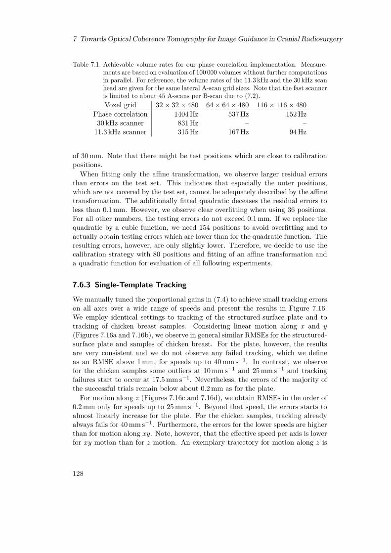
7 Towards Optical Coherence Tomography for Image Guidance in Cranial Radiosurgery
Table 7.1: Achievable volume rates for our phase correlation implementation. Measure-ments are based on evaluation of 100 000 volumes without further computationsin parallel. For reference, the volume rates of the 11.3 kHz and the 30 kHz scanhead are given for the same lateral A-scan grid sizes. Note that the fast scanneris limited to about 45 A-scans per B-scan due to (7.2).Voxel grid 32× 32× 480 64× 64× 480 116× 116× 480
Phase correlation 1404 Hz 537 Hz 152 Hz30 kHz scanner 831 Hz – –
11.3 kHz scanner 315 Hz 167 Hz 94 Hz
of 30 mm. Note that there might be test positions which are close to calibrationpositions.When fitting only the affine transformation, we observe larger residual errors
than errors on the test set. This indicates that especially the outer positions,which are not covered by the test set, cannot be adequately described by the affinetransformation. The additionally fitted quadratic deceases the residual errors toless than 0.1 mm. However, we observe clear overfitting when using 36 positions.For all other numbers, the testing errors do not exceed 0.1 mm. If we replace thequadratic by a cubic function, we need 154 positions to avoid overfitting and toactually obtain testing errors which are lower than for the quadratic function. Theresulting errors, however, are only slightly lower. Therefore, we decide to use thecalibration strategy with 80 positions and fitting of an affine transformation anda quadratic function for evaluation of all following experiments.
7.6.3 Single-Template Tracking
We manually tuned the proportional gains in (7.4) to achieve small tracking errorson all axes over a wide range of speeds and present the results in Figure 7.16.We employ identical settings to tracking of the structured-surface plate and totracking of chicken breast samples. Considering linear motion along x and y(Figures 7.16a and 7.16b), we observe in general similar RMSEs for the structured-surface plate and samples of chicken breast. For the plate, however, the resultsare very consistent and we do not observe any failed tracking, which we defineas an RMSE above 1 mm, for speeds up to 40 mm s−1. In contrast, we observefor the chicken samples some outliers at 10 mm s−1 and 25 mm s−1 and trackingfailures start to occur at 17.5 mm s−1. Nevertheless, the errors of the majority ofthe successful trials remain below about 0.2 mm as for the plate.For motion along z (Figures 7.16c and 7.16d), we obtain RMSEs in the order of
0.2 mm only for speeds up to 25 mm s−1. Beyond that speed, the errors starts toalmost linearly increase for the plate. For the chicken samples, tracking alreadyalways fails for 40 mm s−1. Furthermore, the errors for the lower speeds are higherthan for motion along xy. Note, however, that the effective speed per axis is lowerfor xy motion than for z motion. An exemplary trajectory for motion along z is
128

7.6 Results
8036 114 154
0.1
0.2
0.3
Number of calibration positionsR
MSE
inm
m
Residual errorTest error
(a) Affine
8036 114 154
0.1
0.2
0.31.60.70.7
Number of calibration positions
RM
SEin
mm
(b) Affine + Quadratic
8036 114 154
0.1
0.2
0.33.52.92.4
0.40.40.4
Number of calibration positions
RM
SEin
mm
(c) Affine + Cubic
Figure 7.15: Residual RMSEs (blue crosses) of the Cartesian calibration and RMSEs ona test set consisting of 252 positions (red circles). The positions are withina cylinder with equal diameter and depth, which are 40 mm and 30 mm forcalibration and testing, respectively. Three calibrations for each number ofpositions were performed and calibration involved fitting an affine transform(a) and fitting additionally a quadratic (b) or cubic (c) function. RMSEvalues above 0.35 mm are printed as text.
shown in Figure 7.17.When considering linear motion along all three axes (Figures 7.16e and 7.16f),
we mainly observe RMSEs up to about 0.2 mm for up to 40 mm s−1. For thechicken samples, however, the results are again less consistent and we have somehigher errors and few tracking failures. Beyond 40 mm s−1, the errors are clearlyincreasing. For random motion along all axes as illustrated in Figure 7.18, the erroris worse than for the linear motion (Figures 7.16g and 7.16h). We observe trackingfailures for lower speeds and the errors start to increase earlier. Nevertheless, theplate can still be tracked without failures for up to 40 mm s−1 and successful trialsat 40 mm s−1 have errors about 0.3 mm.
129
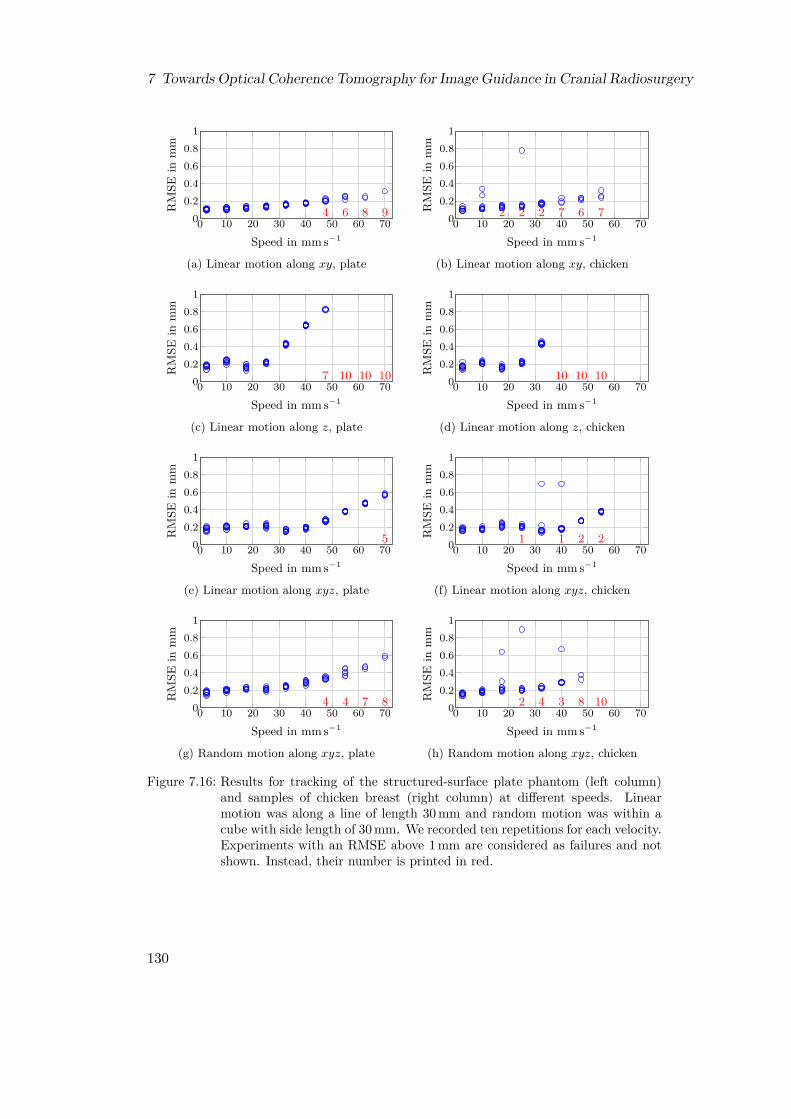
7 Towards Optical Coherence Tomography for Image Guidance in Cranial Radiosurgery
0 10 20 30 40 50 60 7000.20.40.60.8
1
4 6 8 9
Speed in mm s−1
RM
SEin
mm
(a) Linear motion along xy, plate
0 10 20 30 40 50 60 7000.20.40.60.8
1
2 2 2 7 6 7
Speed in mm s−1
RM
SEin
mm
(b) Linear motion along xy, chicken
0 10 20 30 40 50 60 7000.20.40.60.8
1
7 10 10 10
Speed in mm s−1
RM
SEin
mm
(c) Linear motion along z, plate
0 10 20 30 40 50 60 7000.20.40.60.8
1
10 10 10
Speed in mm s−1
RM
SEin
mm
(d) Linear motion along z, chicken
0 10 20 30 40 50 60 7000.20.40.60.8
1
5
Speed in mm s−1
RM
SEin
mm
(e) Linear motion along xyz, plate
0 10 20 30 40 50 60 7000.20.40.60.8
1
1 1 2 2
Speed in mm s−1
RM
SEin
mm
(f) Linear motion along xyz, chicken
0 10 20 30 40 50 60 7000.20.40.60.8
1
4 4 7 8
Speed in mm s−1
RM
SEin
mm
(g) Random motion along xyz, plate
0 10 20 30 40 50 60 7000.20.40.60.8
1
2 4 3 8 10
Speed in mm s−1
RM
SEin
mm
(h) Random motion along xyz, chicken
Figure 7.16: Results for tracking of the structured-surface plate phantom (left column)and samples of chicken breast (right column) at different speeds. Linearmotion was along a line of length 30 mm and random motion was within acube with side length of 30 mm. We recorded ten repetitions for each velocity.Experiments with an RMSE above 1 mm are considered as failures and notshown. Instead, their number is printed in red.
130

7.6 Results
0 10 20 30 40
−10
0
10
Time in sPo
sitio
nin
mm Tracking x
Tracking y
Tracking z
Robot x
Robot y
Robot z
(a) Linear motion along z
30 30.2 30.4 30.6 30.8 31
−14
−12
−10
Time in s
Posit
ion
inm
m Tracking x
Tracking y
Tracking z
Robot x
Robot y
Robot z
(b) Zoom into (a)
Figure 7.17: Linear motion trajectory of a chicken-breast sample at 10 mm s−1 along theaxial z-axis. Therefore, the x and y components are almost zero. We showthe full trajectory (a) and a zoom into a turning point (b).
0 10 20 30 40
−10
0
10
Time in s
Posit
ion
inm
m Tracking x
Tracking y
Tracking z
Robot x
Robot y
Robot z
(a) Random motion along xyz
32.6 32.8 33
5
10
Time in s
Posit
ion
inm
m Tracking x
Tracking y
Tracking z
Robot x
Robot y
Robot z
(b) Zoom into (c)
Figure 7.18: Random motion trajectory of a chicken-breast sample at 10 mm s−1 involvingall axes. We show the full trajectory (a) and a zoom (b).
131

7 Towards Optical Coherence Tomography for Image Guidance in Cranial Radiosurgery
0.01 0.015 0.02 0.025 0.030
0.1
0.2
Learning rate ηR
MSE
inm
m
Figure 7.19: RMSEs depending on the learning rate η for translational motion with12 mm s−1. The trajectory is a line covering all three axes.
7.6.4 Multi-Template Tracking
While the single-template tracking with phase correlation is limited to 3D motion,our proposed multi-template tracking with the adaptive MOSSE filter allows totrack 6D motion. Before the experiments, we again manually tune the proportionalgains in (7.4) and keep these parameters for all experiments. We mainly considertracking the structured-surface phantom (Figure 7.11a) and employ as the baselineparameters for multi-template tracking (compare Figure 7.10) N = 3 templatesarranged at a radius of r = 200 in motor steps, which corresponds to about5.4 mm. Figure 7.19 shows that the results obtained with multi-template trackingand the adaptive MOSSE filter for purely translational motion are comparable tothe results we obtained in the previous sub-section for single-template tracking.The evaluated learning rates η do not seem to impact the results. Note thatη = 0, i.e., a conventional non-adaptive MOSSE filter, is not able to track anyrotations with substantial angle and therefore not considered in this section. Inthe following, we first analyze tracking of purely rotational motion. We separatethis analysis into in-plane and out-of-plane rotations. During in-plane rotations,the phantom rotates approximately around the OCT’s z-axis, i.e., within the xy-plane. During out-of-plane rotations, the rotation is around one of the OCT’slateral axes. Second, we analyze true 6D motion.
In-Plane Rotations
In-plane rotations keep the phantom orientated almost parallel to the lateral planeof the C-scans. Therefore, no major motion of the motorized reference arm isnecessary for compensation. For the baseline parameters and different learningrates η, we obtain the results shown in Figure 7.20. When rotating at 4 ° s−1,we obtain for η = 0.01 RMSEs in the order of 0.2° for both maximum rotationangles of 8° and 13°. Higher learning rates slightly increase the errors to about
132
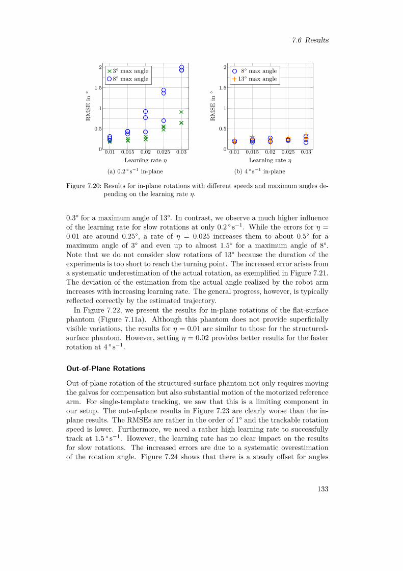
7.6 Results
0.01 0.015 0.02 0.025 0.030
0.5
1
1.5
2
Learning rate η
RM
SEin
°
3° max angle8° max angle
(a) 0.2 ° s−1 in-plane
0.01 0.015 0.02 0.025 0.030
0.5
1
1.5
2
Learning rate η
RM
SEin
°
8° max angle13° max angle
(b) 4 ° s−1 in-plane
Figure 7.20: Results for in-plane rotations with different speeds and maximum angles de-pending on the learning rate η.
0.3° for a maximum angle of 13°. In contrast, we observe a much higher influenceof the learning rate for slow rotations at only 0.2 ° s−1. While the errors for η =0.01 are around 0.25°, a rate of η = 0.025 increases them to about 0.5° for amaximum angle of 3° and even up to almost 1.5° for a maximum angle of 8°.Note that we do not consider slow rotations of 13° because the duration of theexperiments is too short to reach the turning point. The increased error arises froma systematic underestimation of the actual rotation, as exemplified in Figure 7.21.The deviation of the estimation from the actual angle realized by the robot armincreases with increasing learning rate. The general progress, however, is typicallyreflected correctly by the estimated trajectory.In Figure 7.22, we present the results for in-plane rotations of the flat-surface
phantom (Figure 7.11a). Although this phantom does not provide superficiallyvisible variations, the results for η = 0.01 are similar to those for the structured-surface phantom. However, setting η = 0.02 provides better results for the fasterrotation at 4 ° s−1.
Out-of-Plane Rotations
Out-of-plane rotation of the structured-surface phantom not only requires movingthe galvos for compensation but also substantial motion of the motorized referencearm. For single-template tracking, we saw that this is a limiting component inour setup. The out-of-plane results in Figure 7.23 are clearly worse than the in-plane results. The RMSEs are rather in the order of 1° and the trackable rotationspeed is lower. Furthermore, we need a rather high learning rate to successfullytrack at 1.5 ° s−1. However, the learning rate has no clear impact on the resultsfor slow rotations. The increased errors are due to a systematic overestimationof the rotation angle. Figure 7.24 shows that there is a steady offset for angles
133
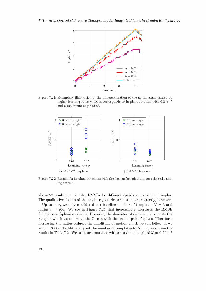
7 Towards Optical Coherence Tomography for Image Guidance in Cranial Radiosurgery
0 10 20 30 400
2
4
6
8
Time in s
Ang
lein
°η = 0.01η = 0.02η = 0.03
Robot arm
Figure 7.21: Exemplary illustration of the underestimation of the actual angle caused byhigher learning rates η. Data corresponds to in-plane rotation with 0.2 ° s−1
and a maximum angle of 8°.
0.01 0.020
0.5
1
Learning rate η
RM
SEin
°
3° max angle8° max angle
(a) 0.2 ° s−1 in-plane
0.01 0.020
0.5
1
Learning rate η
RM
SEin
°
3° max angle8° max angle
(b) 4 ° s−1 in-plane
Figure 7.22: Results for in-plane rotations with the flat-surface phantom for selected learn-ing rates η.
above 2° resulting in similar RMSEs for different speeds and maximum angles.The qualitative shapes of the angle trajectories are estimated correctly, however.Up to now, we only considered our baseline number of templates N = 3 and
radius r = 200. We see in Figure 7.25 that increasing r decreases the RMSEfor the out-of-plane rotations. However, the diameter of our scan lens limits therange in which we can move the C-scan with the second pair of galvos. Therefore,increasing the radius reduces the amplitude of motion which we can follow. If weset r = 300 and additionally set the number of templates to N = 7, we obtain theresults in Table 7.2. We can track rotations with a maximum angle of 3° at 0.2 ° s−1
134
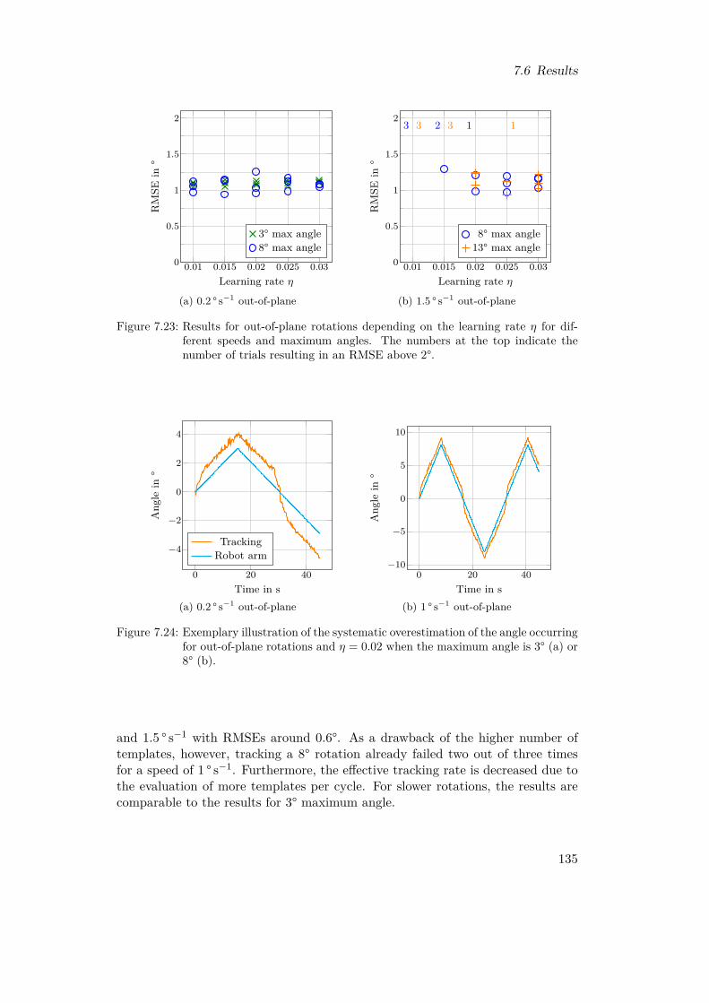
7.6 Results
0.01 0.015 0.02 0.025 0.030
0.5
1
1.5
2
Learning rate η
RM
SEin
°
3° max angle8° max angle
(a) 0.2 ° s−1 out-of-plane
0.01 0.015 0.02 0.025 0.030
0.5
1
1.5
2 3 2 13 3 1
Learning rate η
RM
SEin
°
8° max angle13° max angle
(b) 1.5 ° s−1 out-of-plane
Figure 7.23: Results for out-of-plane rotations depending on the learning rate η for dif-ferent speeds and maximum angles. The numbers at the top indicate thenumber of trials resulting in an RMSE above 2°.
0 20 40
−4
−2
0
2
4
Time in s
Ang
lein
°
TrackingRobot arm
(a) 0.2 ° s−1 out-of-plane
0 20 40−10
−5
0
5
10
Time in s
Ang
lein
°
(b) 1 ° s−1 out-of-plane
Figure 7.24: Exemplary illustration of the systematic overestimation of the angle occurringfor out-of-plane rotations and η = 0.02 when the maximum angle is 3° (a) or8° (b).
and 1.5 ° s−1 with RMSEs around 0.6°. As a drawback of the higher number oftemplates, however, tracking a 8° rotation already failed two out of three timesfor a speed of 1 ° s−1. Furthermore, the effective tracking rate is decreased due tothe evaluation of more templates per cycle. For slower rotations, the results arecomparable to the results for 3° maximum angle.
135
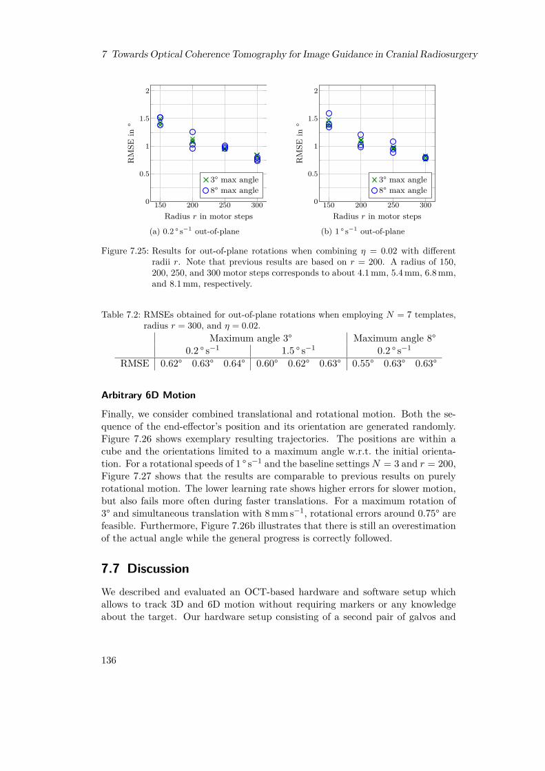
7 Towards Optical Coherence Tomography for Image Guidance in Cranial Radiosurgery
150 200 250 3000
0.5
1
1.5
2
Radius r in motor steps
RM
SEin
°
3° max angle8° max angle
(a) 0.2 ° s−1 out-of-plane
150 200 250 3000
0.5
1
1.5
2
Radius r in motor steps
RM
SEin
°
3° max angle8° max angle
(b) 1 ° s−1 out-of-plane
Figure 7.25: Results for out-of-plane rotations when combining η = 0.02 with differentradii r. Note that previous results are based on r = 200. A radius of 150,200, 250, and 300 motor steps corresponds to about 4.1 mm, 5.4 mm, 6.8 mm,and 8.1 mm, respectively.
Table 7.2: RMSEs obtained for out-of-plane rotations when employing N = 7 templates,radius r = 300, and η = 0.02.
Maximum angle 3° Maximum angle 8°0.2 ° s−1 1.5 ° s−1 0.2 ° s−1
RMSE 0.62° 0.63° 0.64° 0.60° 0.62° 0.63° 0.55° 0.63° 0.63°
Arbitrary 6D Motion
Finally, we consider combined translational and rotational motion. Both the se-quence of the end-effector’s position and its orientation are generated randomly.Figure 7.26 shows exemplary resulting trajectories. The positions are within acube and the orientations limited to a maximum angle w.r.t. the initial orienta-tion. For a rotational speeds of 1 ° s−1 and the baseline settingsN = 3 and r = 200,Figure 7.27 shows that the results are comparable to previous results on purelyrotational motion. The lower learning rate shows higher errors for slower motion,but also fails more often during faster translations. For a maximum rotation of3° and simultaneous translation with 8 mm s−1, rotational errors around 0.75° arefeasible. Furthermore, Figure 7.26b illustrates that there is still an overestimationof the actual angle while the general progress is correctly followed.
7.7 DiscussionWe described and evaluated an OCT-based hardware and software setup whichallows to track 3D and 6D motion without requiring markers or any knowledgeabout the target. Our hardware setup consisting of a second pair of galvos and
136
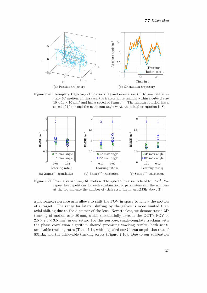
7.7 Discussion
−50
5 −5
0
5
−5
0
5
x
y
z
(a) Position trajectory
0 20 40
0
2.5
5
7.5
Time in s
Abs
olut
ean
gle
in°
TrackingRobot arm
(b) Orientation trajectory
Figure 7.26: Exemplary trajectory of positions (a) and orientation (b) to simulate arbi-trary 6D motion. In this case, the translation is random within a cube of size10× 10× 10 mm3 and has a speed of 8 mm s−1. The random rotation has aspeed of 1 ° s−1 and the maximum angle w.r.t. the initial orientation is 8°.
0.01 0.020
0.5
1
1.5
22
Learning rate η
RM
SEin
°
3° max angle8° max angle
(a) 2 mm s−1 translation
0.01 0.020
0.5
1
1.5
22 1
Learning rate η
RM
SEin
°
3° max angle8° max angle
(b) 5 mm s−1 translation
0.01 0.020
0.5
1
1.5
24 1
Learning rate η
RM
SEin
°
3° max angle8° max angle
(c) 8 mm s−1 translation
Figure 7.27: Results for arbitrary 6D motion. The speed of rotation is fixed to 1 ° s−1. Wereport five repetitions for each combination of parameters and the numbersat the top indicate the number of trials resulting in an RMSE above 2°.
a motorized reference arm allows to shift the FOV in space to follow the motionof a target. The range for lateral shifting by the galvos is more limited thanaxial shifting due to the diameter of the lens. Nevertheless, we demonstrated 3Dtracking of motion over 30 mm, which substantially exceeds the OCT’s FOV of2.5× 2.5× 3.5 mm3 in our setup. For this purpose, single-template tracking withthe phase correlation algorithm showed promising tracking results, both w.r.t.achievable tracking rates (Table 7.1), which equaled our C-scan acquisition rate of831 Hz, and the achievable tracking errors (Figure 7.16). Due to our calibration
137
7 Towards Optical Coherence Tomography for Image Guidance in Cranial Radiosurgery
procedure between the tracking system and the reference robot arm with residualerrors below 0.1 mm on a test set (Figure 7.15), we are able to quantify the trackingaccuracy. We obtain RMSEs in the order of 0.2 mm for arbitrary 3D motion withspeeds up to about 25 mm s−1 for both our phantom and chicken breast samples.Tracking of up to 40 mm s−1 is feasible with errors around 0.3 mm. For chickenbreast samples, however, there are outliers indicating that reliability might beimprovable by adding a method to estimate the quality of the template and, ifnecessary, slightly move the FOV to another location.Furthermore, our results show that the motorized reference arm is a limiting
factor. While we have been able to track lateral motion at 70 mm s−1, the fastestaxial motion has been 47.5 mm s−1. However, successful trials with errors below0.4 mm are even limited to 25 mm s−1. Note that the proportional gains allow forsome tuning of the tracking performance for specific scenarios, like an emphasis onspeed or on tracking errors. In the future, we should consider a different technicalrealization for adjusting the reference arm length, if tracking of faster motion isrequired. Stepper motors are especially limited if the direction of travel changesfrequently and if acceleration and deceleration dominate compared to traveling atfull speed.In order to track 6D motion, i.e., not only translations but also rotations, we
evaluated a multi-template tracking approach. While we are still not able to rotatethe FOV in space, tracking at least three spatially separated templates allows us toderive the full pose of a target. This requires us to apply methods which are robustto appearance changes. Therefore, we proposed to use an adaptive MOSSE filter.Tracking pure translations is still feasible with RMSEs in the order of 0.2 mm anddid not show sensitivity to the MOSSE filter’s learning rate (Figure 7.19).When tracking pure rotations, however, we observed multiple important depen-
dencies and properties. For in-plane rotations around the OCT’s z-axis, we areable to track rotations by 13° with 4 ° s−1 with low RMSEs around 0.25° (Fig-ure 7.20b). However, if the learning rate is set too high, severely increased errorsoccur for slow rotations (Figure 7.20a). Because there is no major influence ofthe learning rate on the results for faster rotations, drifting effects seem to oc-cur in which the template update suppresses the detection of motion resulting inunderestimation of the angle (Figure 7.21). Nevertheless, tracking in-plane ro-tations by a flat-surface phantom, i.e., no superficially visible changes, has alsobeen demonstrated (Figure 7.22) with similar errors when selecting an appropriatelearning rate. This emphasizes the potential benefit of exploiting the sub-surfaceinformation provided by OCT in contrast to other optical imaging modalities.While in-plane rotations do not require shifting the FOV by moving the motor-
ized reference arm, this is necessary to follow out-of-plane rotations. Due to thefact that we need to move the FOV to the next template’s current position beforewe can acquire the next C-scan for evaluation, the motion of the motorized refer-ence arm can severely decrease the tracking rate, especially during large rotationangles. Our results for pure out-of-plane rotations show, firstly, RMSEs in the or-der of 1° which is a factor of four higher than for in-plane rotations (Figure 7.23)
138
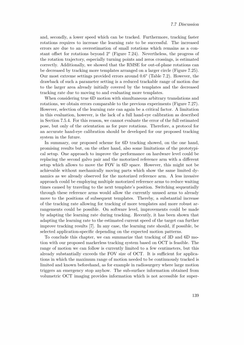
7.7 Discussion
and, secondly, a lower speed which can be tracked. Furthermore, tracking fasterrotations requires to increase the learning rate to be successful. The increasederrors are due to an overestimation of small rotations which remains as a con-stant offset for rotations beyond 2° (Figure 7.24). Nevertheless, the progress ofthe rotation trajectory, especially turning points and zeros crossings, is estimatedcorrectly. Additionally, we showed that the RMSE for out-of-plane rotations canbe decreased by tracking more templates arranged on a larger circle (Figure 7.25).Our most extreme settings provided errors around 0.6° (Table 7.2). However, thedrawback of such a parameter setting is a reduced trackable range of motion dueto the larger area already initially covered by the templates and the decreasedtracking rate due to moving to and evaluating more templates.When considering true 6D motion with simultaneous arbitrary translations and
rotations, we obtain errors comparable to the previous experiments (Figure 7.27).However, selection of the learning rate can again be a critical factor. A limitationin this evaluation, however, is the lack of a full hand-eye calibration as describedin Section 7.5.4. For this reason, we cannot evaluate the error of the full estimatedpose, but only of the orientation as for pure rotations. Therefore, a protocol foran accurate hand-eye calibration should be developed for our proposed trackingsystem in the future.In summary, our proposed scheme for 6D tracking showed, on the one hand,
promising results but, on the other hand, also some limitations of the prototypi-cal setup. One approach to improve the performance on hardware level could bereplacing the second galvo pair and the motorized reference arm with a differentsetup which allows to move the FOV in 6D space. However, this might not beachievable without mechanically moving parts which show the same limited dy-namics as we already observed for the motorized reference arm. A less invasiveapproach could be employing multiple motorized reference arms to reduce waitingtimes caused by traveling to the next template’s position. Switching sequentiallythrough these reference arms would allow the currently unused arms to alreadymove to the positions of subsequent templates. Thereby, a substantial increaseof the tracking rate allowing for tracking of more templates and more robust ar-rangements could be possible. On software level, improvements could be madeby adapting the learning rate during tracking. Recently, it has been shown thatadapting the learning rate to the estimated current speed of the target can furtherimprove tracking results [7]. In any case, the learning rate should, if possible, beselected application-specific depending on the expected motion patterns.To conclude this chapter, we can summarize that tracking of 3D and 6D mo-
tion with our proposed markerless tracking system based on OCT is feasible. Therange of motion we can follow is currently limited to a few centimeters, but thisalready substantially exceeds the FOV size of OCT. It is sufficient for applica-tions in which the maximum range of motion needed to be continuously tracked islimited and known beforehand, as for example in radiosurgery where large motiontriggers an emergency stop anyhow. The sub-surface information obtained fromvolumetric OCT imaging provides information which is not accessible for super-
139

7 Towards Optical Coherence Tomography for Image Guidance in Cranial Radiosurgery
ficially scanning optical systems. While we found efficient algorithms to extractmotion without specific knowledge about the target, the prototypical hardwaresetup, especially the motorized reference arm for axially shifting the FOV, showssome limitations which should be tackled. Nevertheless, the presented results showthat OCT is promising for general-purpose motion tracking with high accuracyin scenarios like, for example, head tracking and image guidance during cranialradiosurgery.
140
8 Conclusion and Outlook
In this thesis, we analyzed different aspects of ultrasound imaging and OCT formarkerless and volumetric intra-fractional image guidance during robotic radio-surgery. Our analysis has been guided by the three research questions which weformulated in Section 1.2. The first and the second question are related to trans-abdominal ultrasound guidance with the kinematically redundant robot-arm setupreviewed in Section 3.6.3 and further evaluated in Chapter 4. The third questionrelates to the feasibility of OCT-based tracking as a novel alternative for cranialimage guidance. In this chapter, we summarize the findings of this thesis w.r.t.these three research questions and provide outlooks for aspects requiring furtherresearch or providing starting points for further improvement.In the first research question, we asked how to automatically determine a suit-
able robot setup for ultrasound guidance in order to minimize the negative impacton treatment plan quality due to beam blocking by the robot arm and the ul-trasound transducer. This question has been addressed in Chapter 5, where weproposed automatic strategies and demonstrated their effectiveness. We proposeddifferent optimization schemes for the GUIDE-robot holding the ultrasound trans-ducer. First, we proposed and compared strategies to optimize the position of theGUIDE-robot’s base and simultaneously select a suitable LIFT angle. We evalu-ated the methods based on prostate cases and compared the results to manuallydetermined reference setups. The results showed that the optimization strategiesactually allow to determine good setups in most cases. However, the quality de-pended on the patient and in one case we were not able to outperform one of thereference setups with our approach. Second, we provided methods to select effi-cient sets of LIFT angles for treatment given a base position for the GUIDE-robot.The main result was that even if we initially consider a large number of config-urations for the GUIDE-robot in order to have many beam directions availablefor planning, we can eventually reduce this number to a reasonably small numberwhile maintaining the same plan quality.The second research question considered the synchronization problem arising if
we consider multiple configurations for the GUIDE-robot. We showed in Chapter 6how this problem can be modeled and demonstrated that the resulting robottrajectories require only a reasonable amount of temporal overhead. Starting froma model to optimize the LINAC-robot’s trajectory for beam delivery, we extendedthe model to account for the GUIDE-robot changing its configuration. We showedfor robot speeds which were in the same order as the actual speed of the LINAC-robot during real CyberKnife treatments that it is feasible to generate efficienttrajectories for both robot arms. These trajectories result in only small overhead
141

8 Conclusion and Outlook
compared to the ideal trajectory of the LINAC-robot. However, our model didnot provide a direct control of the number of configuration changes occurring inthe solution. This might be an interesting future aspect if it is desired to limitthat number.
Note that we evaluated our proposed methods addressing the first and secondresearch question in case studies on prostate cancer. However, both the GUIDE-robot setup and our methods are flexible and can be applied to other abdominaltargets like the liver as well. By defining a new target pose of the ultrasoundtransducer, we can immediately evaluate beam blocking for guiding treatment ofanother site. Our optimization of the robot setup only requires to additionallydefine the new search space for positioning the robot’s base. Our selection ofefficient LIFT angles and our synchronization between GUIDE-robot and LINAC-robot do not require any changes. However, the importance of some aspects andthe room for improvements might vary with the treatment site due to a differentgeneral treatment geometry. Therefore, the methods should be evaluated for othertreatment sites in the future to analyze the differences and prove the practicalapplicability of such generic ultrasound guidance.In general, the robot setup could be further extended to provide even more
flexibility. Instead of a fixed mounting of the robot’s base, we could considermoving the base, for example on a rail, during treatment. This could allow formore motion of the links during treatment effectively leading to less blocked beamdirections. Some flexibility in mounting the robot base might be required inpractical installations anyway in order to allow for a flexible adaption to differentpatients, couch poses, treatment sites, or potential obstacles in the room. Notethat we always considered the robot as being positioned relative to the patientrather than at absolute coordinates in the treatment room.Regarding the third research question, we provided in Chapter 7 a design and
feasibility study for markerless volumetric tracking based on OCT. The motivationfor this study was to develop an alternative approach for image guidance duringcranial radiosurgery. However, we did not yet consider specific tracking scenariosbut demonstrated that OCT can be a valuable basis for general tracking tasks incases where conventional superficially-scanning systems fail. Nevertheless, futurework should consider more specifically the illustrated application and prove thatthe proposed system design is appropriate for this specific task. Furthermore,our prototypical system can be improved in several aspects. In particular, theaxial repositioning of the FOV to follow a moving target currently suffers fromthe limited dynamics of the motorized reference arm. Further improvements couldconsider a predictive tracking approach and an automatic local search for optimaltemplate locations.A practical implementation of OCT guidance in a treatment room would lead
to similar issues as our transabdominal ultrasound guidance. The OCT-basedtracking system should be mounted to some kind of holder which allows to alignit with the patient’s head. Even a passive probe holder could, in addition tothe tracking system’s components, interfere with the delivery of treatment beams.
142
Therefore, mounting the tracking system to a kinematically redundant robot armcould again be an interesting option. In this case, we could directly apply ourmethods developed for transabdominal ultrasound to optimize the setup. However,our OCT tracking, in contrast to the ultrasound guidance, does not require directcontact to the patient. The distance to the surface should have a positive effect onthe beam blocking issue. Furthermore, we have more freedom in choosing the poseof the tracking system. For ultrasound guidance, we need to have a good viewon the rather small target which is limited by bones, air, or other surroundingstructures. For head tracking, however, we can consider different regions of thehead. Due to the small FOV of the OCT, it might even be possible to adapt animmobilizing face mask with minor effort in order to allow for tracking of certainspots identified as very suitable. Furthermore, we could switch between differentspots during treatment to allow for even more beam directions. Having the systemmounted to a robot arm, this switching could happen automatically and fast.To conclude this thesis, we can summarize that we provided and evaluated
methods which solve some important issues arising in practical application ofultrasound-based image guidance with a kinematically redundant robot arm inabdominal radiosurgery. Furthermore, we provided a prototypical design andexperimental characterization for a novel OCT-based tracking system. This ap-proach can potentially overcome some limitations of conventional tracking systemscurrently used for guiding cranial radiosurgery.
143


Bibliography[1] M. C. Abramowitz, E. Bossart, R. Flook, X. Wu, R. Brooks, M. Lachaine, F. Lath-
uiliere, and A. Pollack. “Noninvasive real-time prostate tracking using a transper-ineal ultrasound approach”. In: International Journal of Radiation Oncology*Bi-ology*Physics 84.3 (2012), S133. doi: 10.1016/j.ijrobp.2012.07.145.
[2] J. R. Adler, M. J. Murphy, S. D. Chang, and S. L. Hancock. “Image-guidedRobotic Radiosurgery”. In: Neurosurgery 44.6 (1999), pp. 1299–1306. doi: 10.1097/00006123-199906000-00079.
[3] J. R. Adler Jr, S. D. Chang, M. J. Murphy, J. Doty, P. Geis, and S. L. Han-cock. “The Cyberknife: A Frameless Robotic System for Radiosurgery”. In: Stereo-tactic and Functional Neurosurgery 69.1-4 (1997), pp. 124–128. doi: 10.1159/000099863.
[4] M. Antico, P. Prinsen, F. Cellini, A. Fracassi, A. A. Isola, D. Cobben, and D.Fontanarosa. “Real-time adaptive planning method for radiotherapy treatmentdelivery for prostate cancer patients, based on a library of plans accounting forpossible anatomy configuration changes”. In: PLOS ONE 14.2 (2019), e0213002.doi: 10.1371/journal.pone.0213002.
[5] S.-T. Antoni, J. Rinast, X. Ma, S. Schupp, and A. Schlaefer. “Online model check-ing for monitoring surrogate-based respiratory motion tracking in radiation ther-apy”. In: International Journal of Computer Assisted Radiology and Surgery 11.11(2016), pp. 2085–2096. doi: 10.1007/s11548-016-1423-2.
[6] D. Applegate, W. Cook, and A. Rohe. “Chained Lin-Kernighan for Large TravelingSalesman Problems”. In: INFORMS Journal on Computing 15.1 (2003), pp. 82–92. doi: 10.1287/ijoc.15.1.82.15157.
[7] C. S. Asha and A. V. Narasimhadhan. “Adaptive Learning Rate for Visual Track-ing Using Correlation Filters”. In: Procedia Computer Science 89 (2016), pp. 614–622. doi: 10.1016/j.procs.2016.06.023.
[8] G. Asmerom, D. Bourne, J. Chappelow, L. M. Goggin, R. Heitz, P. Jordan, W.Kilby, T. Laing, C. R. Maurer Jr, J. M. Noll, S. Sayeh, and A. Weber. “The designand physical characterization of a multileaf collimator for robotic radiosurgery”.In: Biomedical Physics & Engineering Express 2.1 (2016), p. 017003. doi: 10.1088/2057-1976/2/1/017003.
[9] J. D. Azcona, R. Li, E. Mok, S. Hancock, and L. Xing. “Automatic ProstateTracking and Motion Assessment in Volumetric Modulated Arc Therapy With anElectronic Portal Imaging Device”. In: International Journal of Radiation Oncol-ogy*Biology*Physics 86.4 (2013), pp. 762–768. doi: 10.1016/j.ijrobp.2013.03.007.
[10] H. Ballhausen, M. Li, N.-S. Hegemann, U. Ganswindt, and C. Belka. “Intra-fraction motion of the prostate is a random walk”. In: Physics in Medicine &Biology 60.2 (2014), pp. 549–563. doi: 10.1088/0031-9155/60/2/549.
145

Bibliography
[11] D. Batchelar, M. Gaztañaga, M. Schmid, C. Araujo, F. Bachand, and J. Crook.“Validation study of ultrasound-based high-dose-rate prostate brachytherapy plan-ning compared with CT-based planning”. In: Brachytherapy 13.1 (2014), pp. 75–79. doi: 10.1016/j.brachy.2013.08.004.
[12] M. Bazalova-Carter, J. Schlosser, J. Chen, and D. Hristov. “Monte Carlo modelingof ultrasound probes for image guided radiotherapy”. In: Medical Physics 42.10(2015), pp. 5745–5756. doi: 10.1118/1.4929978.
[13] J. L. Bedford, H. S. Tsang, S. Nill, and U. Oelfke. “Treatment planning optimiza-tion with beam motion modelling for dynamic arc delivery of SBRT using Cy-berknife with multileaf collimation”. In: Medical Physics 46.12 (2019), pp. 5421–5433. doi: 10.1002/mp.13848.
[14] C. Beekman, B. van Triest, S. van Beek, J.-J. Sonke, and P. Remeijer. “Marginand PTV volume reduction using a population based library of plans strategy forrectal cancer radiotherapy”. In: Medical Physics 45.10 (2018), pp. 4345–4354. doi:10.1002/mp.13137.
[15] M. A. L. Bell, H. T. Sen, I. I. Iordachita, P. Kazanzides, and J. Wong. “In vivoreproducibility of robotic probe placement for a novel ultrasound-guided radiationtherapy system”. In: Journal of Medical Imaging 1.2 (2014), p. 025001. doi: 10.1117/1.JMI.1.2.025001.
[16] S. H. Benedict, K. M. Yenice, D. Followill, J. M. Galvin, W. Hinson, B. Kavanagh,P. Keall, M. Lovelock, S. Meeks, L. Papiez, T. Purdie, R. Sadagopan, M. C. Schell,B. Salter, D. J. Schlesinger, A. S. Shiu, T. Solberg, D. Y. Song, V. Stieber, R.Timmerman, W. A. Tomé, D. Verellen, L. Wang, and F.-F. Yin. “Stereotactic bodyradiation therapy: The report of AAPM Task Group 101”. In:Medical Physics 37.8(2010), pp. 4078–4101. doi: 10.1118/1.3438081.
[17] M. Bengs, N. Gessert, and A. Schlaefer. “A Deep Learning Approach for Mo-tion Forecasting Using 4D OCT Data”. In: International Conference on MedicalImaging with Deep Learning. 2020.
[18] M. Bengs, N. Gessert, M. Schlüter, and A. Schlaefer. “Spatio-temporal deep learn-ing methods for motion estimation using 4D OCT image data”. In: InternationalJournal of Computer Assisted Radiology and Surgery 15.6 (2020), pp. 943–952.doi: 10.1007/s11548-020-02178-z.
[19] J. Bertholet, A. Knopf, B. Eiben, J. McClelland, A. Grimwood, E. Harris, M.Menten, P. Poulsen, D. T. Nguyen, P. Keall, and U. Oelfke. “Real-time intrafrac-tion motion monitoring in external beam radiotherapy”. In: Physics in Medicine& Biology 64.15 (2019), 15TR01. doi: 10.1088/1361-6560/ab2ba8.
[20] W. Birkfellner, J. Hummel, E. Wilson, and K. Cleary. “Tracking Devices”. In:Image-Guided Interventions. Technology and Applications. Ed. by T. Peters andK. Cleary. Springer US, 2008, pp. 23–44. doi: 10.1007/978-0-387-73858-1_2.
[21] T. Bland, J. Tong, B. Ward, and N. G. Parker. “Geometric distortion of area inmedical ultrasound images”. In: Journal of Physics: Conference Series 797 (2017),p. 012002. doi: 10.1088/1742-6596/797/1/012002.
[22] D. S. Bolme, J. R. Beveridge, B. A. Draper, and Y. M. Lui. “Visual object trackingusing adaptive correlation filters”. In: IEEE Conference on Computer Vision andPattern Recognition. 2010, pp. 2544–2550. doi: 10.1109/cvpr.2010.5539960.
146
[23] D. S. Bolme, B. A. Draper, and J. R. Beveridge. “Average of Synthetic ExactFilters”. In: IEEE Conference on Computer Vision and Pattern Recognition. 2009,pp. 2105–2112. doi: 10.1109/cvpr.2009.5206701.
[24] B. Bontoux, C. Artigues, and D. Feillet. “A Memetic Algorithm with a largeneighborhood crossover operator for the Generalized Traveling Salesman Prob-lem”. In: Computers & Operations Research 37.11 (2010), pp. 1844–1852. doi:10.1016/j.cor.2009.05.004.
[25] J. T. Booth, V. Caillet, N. Hardcastle, R. O’Brien, K. Szymura, C. Crasta, B.Harris, C. Haddad, T. Eade, and P. J. Keall. “The first patient treatment ofelectromagnetic-guided real time adaptive radiotherapy using MLC tracking forlung SABR”. In: Radiotherapy and Oncology 121.1 (2016), pp. 19–25. doi: 10.1016/j.radonc.2016.08.025.
[26] S. A. Boppart, J. Herrmann, C. Pitris, D. L. Stamper, M. E. Brezinski, and J. G.Fujimoto. “High-Resolution Optical Coherence Tomography-Guided Laser Abla-tion of Surgical Tissue”. In: Journal of Surgical Research 82.2 (1999), pp. 275–284.doi: 10.1006/jsre.1998.5555.
[27] B. E. Bouma, M. Villiger, K. Otsuka, and W.-Y. Oh. “Intravascular optical co-herence tomography [Invited]”. In: Biomedical Optics Express 8.5 (2017), p. 2660.doi: 10.1364/boe.8.002660.
[28] Brainlab AG. Potential and Challenges of Surface Guidance in Radiation Ther-apy. White Paper. Version Rev1. 2019. url: https://www.brainlab.com/de/potential-and-challenges-of-sgrt_brainlab/ (visited on 05/26/2020).
[29] R. W. Brown, Y.-C. N. Cheng, E. M. Haacke, M. R. Thompson, and R. Venkate-san.Magnetic Resonance Imaging. Physical Principles and Sequence Design. 2nd ed.John Wiley & Sons, 2014. doi: 10.1002/9781118633953.
[30] N. G. Burnet. “Defining the tumour and target volumes for radiotherapy”. In:Cancer Imaging 4.2 (2004), pp. 153–161. doi: 10.1102/1470-7330.2004.0054.
[31] A. Camino, M. Zhang, S. S. Gao, T. S. Hwang, U. Sharma, D. J. Wilson, D.Huang, and Y. Jia. “Evaluation of artifact reduction in optical coherence tomog-raphy angiography with real-time tracking and motion correction technology”. In:Biomedical Optics Express 7.10 (2016), p. 3905. doi: 10.1364/boe.7.003905.
[32] S. M. Camps, D. Fontanarosa, P. H. N. de With, F. Verhaegen, and B. G. L.Vanneste. “The use of ultrasound imaging in the external beam radiotherapyworkflow of prostate cancer patients”. In: BioMed Research International 2018(2018), p. 7569590. doi: 10.1155/2018/7569590.
[33] E. de Castro and C. Morandi. “Registration of Translated and Rotated ImagesUsing Finite Fourier Transforms”. In: IEEE Transactions on Pattern Analysisand Machine Intelligence PAMI-9.5 (1987), pp. 700–703. doi: 10.1109/tpami.1987.4767966.
[34] L. I. Cerviño, N. Detorie, M. Taylor, J. D. Lawson, T. Harry, K. T. Murphy, A. J.Mundt, S. B. Jiang, and T. A. Pawlicki. “Initial clinical experience with a frame-less and maskless stereotactic radiosurgery treatment”. In: Practical RadiationOncology 2.1 (2012), pp. 54–62. doi: 10.1016/j.prro.2011.04.005.
147

Bibliography
[35] W. Chen, J. Unkelbach, A. Trofimov, T. Madden, H. Kooy, T. Bortfeld, and D.Craft. “Including robustness in multi-criteria optimization for intensity-modulatedproton therapy”. In: Physics in Medicine & Biology 57.3 (2012), pp. 591–608. doi:10.1088/0031-9155/57/3/591.
[36] Z. Chen, Z. Yang, J. Wang, and W. Hu. “Dosimetric impact of different bladderand rectum filling during prostate cancer radiotherapy”. In: Radiation Oncology11.1 (2016), p. 103. doi: 10.1186/s13014-016-0681-z.
[37] M. Chu, Y. Zinchenko, S. G. Henderson, and M. B. Sharpe. “Robust optimizationfor intensity modulated radiation therapy treatment planning under uncertainty”.In: Physics in Medicine & Biology 50.23 (2005), pp. 5463–5477. doi: 10.1088/0031-9155/50/23/003.
[38] S. D. Collins and M. M. Leech. “A review of plan library approaches in adaptiveradiotherapy of bladder cancer”. In: Acta Oncologica 57.5 (2018), pp. 566–573.doi: 10.1080/0284186x.2017.1420908.
[39] E. L. Covington, J. B. Fiveash, X. Wu, I. Brezovich, C. D. Willey, K. Riley, andR. A. Popple. “Optical surface guidance for submillimeter monitoring of patientposition during frameless stereotactic radiotherapy”. In: Journal of Applied Clin-ical Medical Physics 20.6 (2019), pp. 91–98. doi: 10.1002/acm2.12611.
[40] F. L. B. Cury, G. Shenouda, L. Souhami, M. Duclos, S. L. Faria, M. David, F.Verhaegen, R. Corns, and T. Falco. “Ultrasound-based image guided radiotherapyfor prostate cancer – comparison of cross-modality and intramodality methods fordaily localization during external beam radiotherapy”. In: International Journal ofRadiation Oncology*Biology*Physics 66.5 (2006), pp. 1562–1567. doi: 10.1016/j.ijrobp.2006.07.1375.
[41] W. D. D’Souza, S. A. Naqvi, and C. X. Yu. “Real-time intra-fraction-motion track-ing using the treatment couch: a feasibility study”. In: Physics in Medicine &Biology 50.17 (2005), pp. 4021–4033. doi: 10.1088/0031-9155/50/17/007.
[42] B. Dahroug, B. Tamadazte, and N. Andreff. “PCA-Based Visual Servoing UsingOptical Coherence Tomography”. In: IEEE Robotics and Automation Letters 5.2(2020), pp. 3430–3437. doi: 10.1109/lra.2020.2977259.
[43] J. G. Delfino, D. M. Krainak, S. A. Flesher, and D. L. Miller. “MRI-related FDAadverse event reports: A 10-yr review”. In:Medical Physics 46.12 (2019), pp. 5562–5571. doi: 10.1002/mp.13768.
[44] T. Depuydt, K. Poels, D. Verellen, B. Engels, C. Collen, C. Haverbeke, T. Gevaert,N. Buls, G. van Gompel, T. Reynders, M. Duchateau, K. Tournel, M. Boussaer,F. Steenbeke, F. Vandenbroucke, and M. de Ridder. “Initial assessment of tumortracking with a gimbaled linac system in clinical circumstances: A patient sim-ulation study”. In: Radiotherapy and Oncology 106.2 (2013), pp. 236–240. doi:10.1016/j.radonc.2012.12.015.
[45] S. Dieterich and I. C. Gibbs. “The CyberKnife in clinical use: current roles, futureexpectations”. In: IMRT, IGRT, SBRT – Advances in the Treatment Planningand Delivery of Radiotherapy. Vol. 43. Karger, 2011, pp. 181–194. doi: 10.1159/000322423.
[46] S. Dieterich, O. Green, and J. Booth. “SBRT targets that move with respiration”.In: Physica Medica 56 (2018), pp. 19–24. doi: 10.1016/j.ejmp.2018.10.021.
148
[47] E. W. Dijkstra. “A note on two problems in connexion with graphs”. In: Nu-merische Mathematik 1.1 (1959), pp. 269–271. doi: 10.1007/bf01386390.
[48] P. Dong, P. Lee, D. Ruan, T. Long, E. Romeijn, Y. Yang, D. Low, P. Kupelian, andK. Sheng. “4π Non-Coplanar Liver SBRT: A Novel Delivery Technique”. In: In-ternational Journal of Radiation Oncology*Biology*Physics 85.5 (2013), pp. 1360–1366. doi: 10.1016/j.ijrobp.2012.09.028.
[49] W. Drexler and J. G. Fujimoto, eds. Optical Coherence Tomography. Technologyand Applications. Springer Berlin Heidelberg, 2008. doi: 10.1007/978-3-540-77550-8.
[50] R. E. Drzymala, R. Mohan, L. Brewster, J. Chu, M. Goitein, W. Harms, and M.Urie. “Dose-volume histograms”. In: International Journal of Radiation Oncol-ogy*Biology*Physics 21.1 (1991), pp. 71–78. doi: 10.1016/0360-3016(91)90168-4.
[51] A. Dubois, K. Grieve, G. Moneron, R. Lecaque, L. Vabre, and C. Boccara. “Ultra-high-resolution full-field optical coherence tomography”. In: Applied Optics 43.14(2004), p. 2874. doi: 10.1364/ao.43.002874.
[52] R. Dürichen, T. Wissel, F. Ernst, A. Schlaefer, and A. Schweikard. “Multivariaterespiratory motion prediction”. In: Physics in Medicine & Biology 59.20 (2014),pp. 6043–6060. doi: 10.1088/0031-9155/59/20/6043.
[53] G. G. Echner, W. Kilby, M. Lee, E. Earnst, S. Sayeh, A. Schlaefer, B. Rhein,J. R. Dooley, C. Lang, O. Blanck, E. Lessard, C. R. Maurer Jr, and W. Schlegel.“The design, physical properties and clinical utility of an iris collimator for roboticradiosurgery”. In: Physics in Medicine & Biology 54.18 (2009), p. 5359. doi: 10.1088/0031-9155/54/18/001.
[54] F. Ernst, R. Dürichen, A. Schlaefer, and A. Schweikard. “Evaluating and com-paring algorithms for respiratory motion prediction”. In: Physics in Medicine &Biology 58.11 (2013), pp. 3911–3929. doi: 10.1088/0031-9155/58/11/3911.
[55] F. Ernst, R. Bruder, A. Schlaefer, and A. Schweikard. “Correlation between exter-nal and internal respiratory motion: a validation study”. In: International Jour-nal of Computer Assisted Radiology and Surgery 7.3 (2012), pp. 483–492. doi:10.1007/s11548-011-0653-6.
[56] F. Ernst, L. Richter, L. Matthäus, V. Martens, R. Bruder, A. Schlaefer, and A.Schweikard. “Non-orthogonal tool/flange and robot/world calibration”. In: TheInternational Journal of Medical Robotics and Computer Assisted Surgery 8.4(2012), pp. 407–420. doi: 10.1002/rcs.1427.
[57] B. G. Fallone. “The Rotating Biplanar Linac-Magnetic Resonance Imaging Sys-tem”. In: Seminars in Radiation Oncology 24.3 (2014), pp. 200–202. doi: 10.1016/j.semradonc.2014.02.011.
[58] M. F. Fast, T. P. O’Shea, S. Nill, U. Oelfke, and E. J. Harris. “First evaluation ofthe feasibility of MLC tracking using ultrasound motion estimation”. In: MedicalPhysics 43.8Part1 (2016), pp. 4628–4633. doi: 10.1118/1.4955440.
[59] L. Feuvret, G. Noël, J.-J. Mazeron, and P. Bey. “Conformity index: A review”. In:International Journal of Radiation Oncology*Biology*Physics 64.2 (2006), pp. 333–342. doi: 10.1016/j.ijrobp.2005.09.028.
149
Bibliography
[60] C. Fiandra, A. Guarneri, F. Muñoz, F. Moretto, A. R. Filippi, M. Levis, R. Ragona,and U. Ricardi. “Impact of the observers’ experience on daily prostate localizationaccuracy in ultrasound-based IGRT with the Clarity platform”. In: Journal ofApplied Clinical Medical Physics 15.4 (2014), pp. 168–173. doi: 10.1120/jacmp.v15i4.4795.
[61] M. Finke, S. Kantelhardt, A. Schlaefer, R. Bruder, E. Lankenau, A. Giese, andA. Schweikard. “Automatic scanning of large tissue areas in neurosurgery usingoptical coherence tomography”. In: The International Journal of Medical Roboticsand Computer Assisted Surgery 8.3 (2012), pp. 327–336. doi: 10.1002/rcs.1425.
[62] B. W. Fischer-Valuck, L. Henke, O. Green, R. Kashani, S. Acharya, J. D. Bradley,C. G. Robinson, M. Thomas, I. Zoberi, W. Thorstad, H. Gay, J. Huang, M. Roach,V. Rodriguez, L. Santanam, H. Li, H. Li, J. Contreras, T. Mazur, D. Hallahan,J. R. Olsen, P. Parikh, S. Mutic, and J. Michalski. “Two-and-a-half-year clinicalexperience with the world’s first magnetic resonance image guided radiation ther-apy system”. In: Advances in Radiation Oncology 2.3 (2017), pp. 485–493. doi:10.1016/j.adro.2017.05.006.
[63] M. Fischetti, J. J. Salazar González, and P. Toth. “A branch-and-cut algorithm forthe symmetric generalized traveling salesman problem”. In: Operations Research45.3 (1997), pp. 378–394. doi: 10.1287/opre.45.3.378.
[64] D. Fontanarosa, S. van der Meer, J. Bamber, E. Harris, T. O’Shea, and F. Ver-haegen. “Review of ultrasound image guidance in external beam radiotherapy:I. Treatment planning and inter-fraction motion management”. In: Physics inMedicine & Biology 60.3 (2015), R77–R114. doi: 10.1088/0031-9155/60/3/r77.
[65] D. Fontanarosa, S. van der Meer, E. Harris, and F. Verhaegen. “A CT basedcorrection method for speed of sound aberration for ultrasound based image guidedradiotherapy”. In: Medical Physics 38.5 (2011), pp. 2665–2673. doi: 10.1118/1.3583475.
[66] D. Fontanarosa, S. Pesente, F. Pascoli, D. Ermacora, I. A. Rumeileh, and F. Ver-haegen. “A speed of sound aberration correction algorithm for curvilinear ultra-sound transducers in ultrasound-based image-guided radiotherapy”. In: Physics inMedicine & Biology 58.5 (2013), pp. 1341–1360. doi: 10.1088/0031-9155/58/5/1341.
[67] H. Foroosh, J. B. Zerubia, and M. Berthod. “Extension of phase correlation tosubpixel registration”. In: IEEE Transactions on Image Processing 11.3 (2002),pp. 188–200. doi: 10.1109/83.988953.
[68] A. M. Franz, T. Haidegger, W. Birkfellner, K. Cleary, T. M. Peters, and L. Maier-Hein. “Electromagnetic Tracking in Medicine—A Review of Technology, Valida-tion, and Applications”. In: IEEE Transactions on Medical Imaging 33.8 (2014),pp. 1702–1725. doi: 10.1109/tmi.2014.2321777.
[69] R. Frost, P. Wighton, F. I. Karahanoğlu, R. L. Robertson, P. E. Grant, B. Fischl,M. D. Tisdall, and A. van der Kouwe. “Markerless high-frequency prospectivemotion correction for neuroanatomical MRI”. In: Magnetic Resonance in Medicine82.1 (2019), pp. 126–144. doi: 10.1002/mrm.27705.
150

[70] D. Fu, R. Kahn, B. Wang, H. Wang, Z. Mu, J. Park, G. Kuduvalli, and C. R. Mau-rer Jr. “Xsight Lung Tracking System: A Fiducial-Less Method for RespiratoryMotion Tracking”. In: Treating Tumors that Move with Respiration. Ed. by H. C.Urschel, J. J. Kresl, J. D. Luketich, L. Papiez, and R. D. Timmerman. SpringerBerlin Heidelberg, 2007, pp. 265–282. doi: 10.1007/978-3-540-69886-9_26.
[71] D. Fu, G. Kuduvalli, V. Mitrovic, W. Main, and L. Thomson. “Automated skulltracking for the CyberKnife image-guided radiosurgery system”. In: SPIE MedicalImaging. 2005, pp. 366–377. doi: 10.1117/12.594984.
[72] A. Fuchs, S. Pengel, J. Bergmeier, L. A. Kahrs, and T. Ortmaier. “Fast and auto-matic depth control of iterative bone ablation based on optical coherence tomog-raphy data”. In: SPIE European Conferences on Biomedical Optics. 2015, 95420P.doi: 10.1117/12.2183695.
[73] J. Fujimoto and E. Swanson. “The Development, Commercialization, and Impactof Optical Coherence Tomography”. In: Investigative Opthalmology & Visual Sci-ence 57.9 (2016), OCT1. doi: 10.1167/iovs.16-19963.
[74] J. Furtak and M. Harat. “Large In-mask Motion during Frameless Radiosurgery ofa Brain Metastasis”. In: Journal of Neurological Surgery Part A: Central EuropeanNeurosurgery 79.04 (2018), pp. 341–343. doi: 10.1055/s-0037-1604285.
[75] C. Fürweger, P. Prins, H. Coskan, and B. J. M. Heijmen. “Characteristics and per-formance of the first commercial multileaf collimator for a robotic radiosurgery sys-tem”. In: Medical Physics 43.5 (2016), pp. 2063–2071. doi: 10.1118/1.4944740.
[76] Y. Gan, W. Yao, K. M. Myers, and C. P. Hendon. “An automated 3D registrationmethod for optical coherence tomography volumes”. In: Annual International Con-ference of the IEEE Engineering in Medicine and Biology Society. 2014, pp. 3873–3876. doi: 10.1109/embc.2014.6944469.
[77] S. Gerlach, C. Fürweger, T. Hofmann, and A. Schlaefer. “Feasibility and analysisof CNN based candidate beam generation for robotic radiosurgery”. In: MedicalPhysics 47.9 (2020), pp. 3806–3815. doi: 10.1002/mp.14331.
[78] S. Gerlach, I. Kuhlemann, F. Ernst, C. Fürweger, and A. Schlaefer. “Impact ofrobotic ultrasound image guidance on plan quality in SBRT of the prostate”. In:The British Journal of Radiology 90.1078 (2017), p. 20160926. doi: 10.1259/bjr.20160926.
[79] S. Gerlach, I. Kuhlemann, P. Jauer, R. Bruder, F. Ernst, C. Fürweger, and A.Schlaefer. “Robotic ultrasound-guided SBRT of the prostate: feasibility with re-spect to plan quality”. In: International Journal of Computer Assisted Radiologyand Surgery 12.1 (2017), pp. 149–159. doi: 10.1007/s11548-016-1455-7.
[80] S. Gerlach, M. Schlüter, C. Fürweger, and A. Schlaefer. “Machbarkeit CNN-basierter Erzeugung von Kandidatenstrahlen für Radiochirurgie der Prostata”. In:Jahrestagung der Deutschen Gesellschaft für Computer- und Roboter AssistierteChirurgie. 2019, pp. 128–129.
[81] N. Gessert, M. Gromniak, M. Schlüter, and A. Schlaefer. “Two-path 3D CNNs forcalibration of system parameters for OCT-based motion compensation”. In: SPIEMedical Imaging. 2019, p. 1095108. doi: 10.1117/12.2512823.
151

Bibliography
[82] N. Gessert, T. Priegnitz, T. Saathoff, S.-T. Antoni, D. Meyer, M. F. Hamann, K.-P.Jünemann, C. Otte, and A. Schlaefer. “Needle Tip Force Estimation Using an OCTFiber and a Fused convGRU-CNN Architecture”. In: International Conference onMedical Image Computing and Computer Assisted Intervention. 2018, pp. 222–229. doi: 10.1007/978-3-030-00937-3_26.
[83] N. Gessert, M. Schlüter, and A. Schlaefer. “A deep learning approach for poseestimation from volumetric OCT data”. In: Medical Image Analysis 46 (2018),pp. 162–179. doi: 10.1016/j.media.2018.03.002.
[84] S. S. Gill, D. G. T. Thomas, A. P. Warrington, and M. Brada. “Relocatable framefor stereotactic external beam radiotherapy”. In: International Journal of Radi-ation Oncology*Biology*Physics 20.3 (1991), pp. 599–603. doi: 10.1016/0360-3016(91)90076-g.
[85] P. Giraud and A. Houle. “Respiratory Gating for Radiotherapy: Main TechnicalAspects and Clinical Benefits”. In: ISRN Pulmonology 2013 (2013), pp. 1–13. doi:10.1155/2013/519602.
[86] L. Glandorf. “Multi-Volume OCT-Tracking for Robust 6-DOF Motion Estima-tion”. Master’s thesis. Hamburg University of Technology, Dec. 17, 2019.
[87] M. Glitzner, P. L. Woodhead, P. T. S. Borman, J. J. W. Lagendijk, and B. W.Raaymakers. “Technical note: MLC-tracking performance on the Elekta UnityMRI-linac”. In: Physics in Medicine & Biology 64.15 (2019), 15NT02. doi: 10.1088/1361-6560/ab2667.
[88] S. M. Goetz, I. C. Kozyrkov, B. Luber, S. H. Lisanby, D. L. K. Murphy, W. M.Grill, and A. V. Peterchev. “Accuracy of robotic coil positioning during tran-scranial magnetic stimulation”. In: Journal of Neural Engineering 16.5 (2019),p. 054003. doi: 10.1088/1741-2552/ab2953.
[89] K. A. Goodman, E. A. Wiegner, K. E. Maturen, Z. Zhang, Q. Mo, G. Yang, I. C.Gibbs, G. A. Fisher, and A. C. Koong. “Dose-Escalation Study of Single-FractionStereotactic Body Radiotherapy for Liver Malignancies”. In: International Journalof Radiation Oncology*Biology*Physics 78.2 (2010), pp. 486–493. doi: 10.1016/j.ijrobp.2009.08.020.
[90] O. Gopan and Q. Wu. “Evaluation of the Accuracy of a 3D Surface Imaging Sys-tem for Patient Setup in Head and Neck Cancer Radiotherapy”. In: InternationalJournal of Radiation Oncology*Biology*Physics 84.2 (2012), pp. 547–552. doi:10.1016/j.ijrobp.2011.12.004.
[91] F. Griese, S. Latus, M. Schlüter, M. Graeser, M. Lutz, A. Schlaefer, and T. Knopp.“In-Vitro MPI-guided IVOCT catheter tracking in real time for motion artifactcompensation”. In: PLOS ONE 15.3 (2020), e0230821. doi: 10.1371/journal.pone.0230821.
[92] A. Grimwood, H. A. McNair, T. P. O’Shea, S. Gilroy, K. Thomas, J. C. Bamber,A. C. Tree, and E. J. Harris. “In Vivo Validation of Elekta’s Clarity Autoscan forUltrasound-based Intrafraction Motion Estimation of the Prostate During Radia-tion Therapy”. In: International Journal of Radiation Oncology*Biology*Physics102.4 (2018), pp. 912–921. doi: 10.1016/j.ijrobp.2018.04.008.
152
[93] A. Grimwood, H. Rivaz, H. Zhou, H. A. McNair, K. Yakubowski, J. C. Bamber,A. C. Tree, and E. J. Harris. “Improving 3D ultrasound prostate localisation inradiotherapy through increased automation of interfraction matching”. In: Radio-therapy and Oncology 149 (2020), pp. 134–141. doi: 10.1016/j.radonc.2020.04.044.
[94] S. S. Gurbani, P. Wilkening, M. Zhao, B. Gonenc, G. W. Cheon, I. I. Iordachita,W. Chien, R. H. Taylor, J. K. Niparko, and J. U. Kang. “Robot-assisted three-dimensional registration for cochlear implant surgery using a common-path swept-source optical coherence tomography probe”. In: Journal of Biomedical Optics 19.5(2014), p. 057004. doi: 10.1117/1.jbo.19.5.057004.
[95] G. Gutin and D. Karapetyan. “A memetic algorithm for the generalized travelingsalesman problem”. In: Natural Computing 9.1 (2010), pp. 47–60. doi: 10.1007/s11047-009-9111-6.
[96] G. Gutin and A. P. Punnen, eds. The Traveling Salesman Problem and Its Vari-ations. Springer US, 2007. doi: 10.1007/b101971.
[97] K. Helsgaun. “An effective implementation of the Lin–Kernighan traveling sales-man heuristic”. In: European Journal of Operational Research 126.1 (2000), pp. 106–130. doi: 10.1016/s0377-2217(99)00284-2.
[98] K. Helsgaun. “General k-opt submoves for the Lin–Kernighan TSP heuristic”. In:Mathematical Programming Computation 1.2 (2009), pp. 119–163. doi: 10.1007/s12532-009-0004-6.
[99] K. Helsgaun. “Solving the equality generalized traveling salesman problem usingthe Lin–Kernighan–Helsgaun Algorithm”. In: Mathematical Programming Com-putation 7.3 (2015), pp. 269–287. doi: 10.1007/s12532-015-0080-8.
[100] A. K. Ho, D. Fu, C. Cotrutz, S. L. Hancock, S. D. Chang, I. C. Gibbs, C. R. MaurerJr, and J. R. Adler. “A Study of the Accuracy of CyberKnife Spinal RadiosurgeryUsing Skeletal Structure Tracking”. In: Operative Neurosurgery 60.suppl_2 (2007),ONS–147–ONS–156. doi: 10.1227/01.neu.0000249248.55923.ec.
[101] J. D. P. Hoisak and T. Pawlicki. “The Role of Optical Surface Imaging Systemsin Radiation Therapy”. In: Seminars in Radiation Oncology 28.3 (2018), pp. 185–193. doi: 10.1016/j.semradonc.2018.02.003.
[102] O. E. Holmes, J. Gratton, J. Szanto, E. Vandervoort, J. Doody, E. Henderson,S. C. Morgan, J. O’Sullivan, and S. Malone. “Reducing errors in prostate trackingwith an improved fiducial implantation protocol for CyberKnife based stereotacticbody radiotherapy (SBRT)”. In: Journal of Radiosurgery and SBRT 5.3 (2018),pp. 217–227.
[103] S. Hossain, P. Xia, K. Huang, M. Descovich, C. Chuang, A. R. Gottschalk, M.Roach, and L. Ma. “Dose Gradient Near Target-Normal Structure Interface forNonisocentric CyberKnife and Isocentric Intensity-Modulated Body Radiother-apy for Prostate Cancer”. In: International Journal of Radiation Oncology*Biol-ogy*Physics 78.1 (2010), pp. 58–63. doi: 10.1016/j.ijrobp.2009.07.1752.
[104] D. Huang, E. A. Swanson, C. P. Lin, J. S. Schuman, W. G. Stinson, W. Chang,M. R. Hee, T. Flotte, K. Gregory, C. A. Puliafito, and J. G. Fujimoto. “Opticalcoherence tomography”. In: Science 254.5035 (1991), pp. 1178–1181. doi: 10 .1126/science.1957169.
153

Bibliography
[105] R. Huber, M. Wojtkowski, and J. G. Fujimoto. “Fourier Domain Mode Locking(FDML): A new laser operating regime and applications for optical coherencetomography”. In: Optics Express 14.8 (2006), p. 3225. doi: 10.1364/oe.14.003225.
[106] A. Hunt, V. N. Hansen, U. Oelfke, S. Nill, and S. Hafeez. “Adaptive RadiotherapyEnabled by MRI Guidance”. In: Clinical Oncology 30.11 (2018), pp. 711–719. doi:10.1016/j.clon.2018.08.001.
[107] International Agency for Research on Cancer. Cancer Fact Sheets. All cancers2018. 2019. url: https://gco.iarc.fr/today/fact-sheets-cancers.
[108] S. Ipsen, R. Bruder, V. García-Vázquez, A. Schweikard, and F. Ernst. “Assessmentof 4D Ultrasound Systems for Image-guided Radiation Therapy – Image Quality,Framerates and CT Artifacts”. In: Current Directions in Biomedical Engineering5.1 (2019), pp. 245–248. doi: 10.1515/cdbme-2019-0062.
[109] S. Ipsen, R. Bruder, R. O’Brien, P. J. Keall, A. Schweikard, and P. R. Poulsen.“Online 4D ultrasound guidance for real-time motion compensation by MLC track-ing”. In: Medical Physics 43.10 (2016), pp. 5695–5704. doi: 10.1118/1.4962932.
[110] M. Jaccard, A. Champion, A. Dubouloz, C. Picardi, J. Plojoux, P. Soccal, R.Miralbell, G. Dipasquale, and F. Caparrotti. “Clinical experience with lung-specificelectromagnetic transponders for real-time tumor tracking in lung stereotacticbody radiotherapy”. In: Physics and Imaging in Radiation Oncology 12 (2019),pp. 30–37. doi: 10.1016/j.phro.2019.11.002.
[111] R. N. Jazar. Theory of Applied Robotics. 2nd ed. Springer US, 2010. doi: 10.1007/978-1-4419-1750-8.
[112] U. Jeleń and M. Alber. “A finite size pencil beam algorithm for IMRT dose op-timization: density corrections.” In: Physics in Medicine & Biology 52.3 (2007),pp. 617–633. doi: 10.1088/0031-9155/52/3/006.
[113] U. Jeleń, M. Söhn, and M. Alber. “A finite size pencil beam for IMRT dose op-timization.” In: Physics in Medicine & Biology 50.8 (2005), pp. 1747–1766. doi:10.1088/0031-9155/50/8/009.
[114] I. Kably, M. Bordegaray, K. Shah, J. Salsamendi, and G. Narayanan. “Single-Center Experience in Prostate Fiducial Marker Placement: Technique and MidtermFollow-up”. In: Journal of Vascular and Interventional Radiology 25.7 (2014),1125–1132.e1. doi: 10.1016/j.jvir.2014.03.017.
[115] W. Kabsch. “A solution for the best rotation to relate two sets of vectors”.In: Acta Crystallographica Section A 32.5 (1976), pp. 922–923. doi: 10.1107/s0567739476001873.
[116] D. Karapetyan and G. Gutin. “Lin-Kernighan heuristic adaptations for the gener-alized traveling salesman problem”. In: European Journal of Operational Research208.3 (2011), pp. 221–232. doi: 10.1016/j.ejor.2010.08.011.
[117] K. Karki, S. Saraiya, G. D. Hugo, N. Mukhopadhyay, N. Jan, J. Schuster, M.Schutzer, L. Fahrner, R. Groves, K. M. Olsen, J. C. Ford, and E. Weiss. “Vari-abilities of Magnetic Resonance Imaging–, Computed Tomography–, and PositronEmission Tomography–Computed Tomography–Based Tumor and Lymph NodeDelineations for Lung Cancer Radiation Therapy Planning”. In: InternationalJournal of Radiation Oncology*Biology*Physics 99.1 (2017), pp. 80–89. doi: 10.1016/j.ijrobp.2017.05.002.
154
[118] T. Kataria, K. Narang, D. Gupta, S. S. Bisht, A. Abhishek, S. Goyal, T. Basu, andK. P. Karrthick. “Analysis of intrafraction motion in CyberKnife-based stereotaxyusing mask based immobilization and 6D-skull tracking”. In: Journal of Radio-surgery and SBRT 4.3 (2016), pp. 203–212.
[119] T. Kataria, K. Sharma, V. Subramani, K. P. Karrthick, and S. S. Bisht. “Ho-mogeneity Index: An objective tool for assessment of conformal radiation treat-ments”. In: Journal of Medical Physics 37.4 (2012), p. 207. doi: 10.4103/0971-6203.103606.
[120] N. Katta, A. B. McElroy, A. D. Estrada, and T. E. Milner. “Optical coherencetomography image-guided smart laser knife for surgery”. In: Lasers in Surgery andMedicine 50.3 (2017), pp. 202–212. doi: 10.1002/lsm.22705.
[121] P. J. Keall, M. Barton, and S. Crozier. “The Australian Magnetic ResonanceImaging-Linac Program”. In: Seminars in Radiation Oncology 24.3 (2014), pp. 203–206. doi: 10.1016/j.semradonc.2014.02.015.
[122] P. J. Keall, E. Colvill, R. O’Brien, V. Caillet, T. Eade, A. Kneebone, G. Hruby,P. R. Poulsen, B. Zwan, P. B. Greer, and J. Booth. “Electromagnetic-Guided MLCTracking Radiation Therapy for Prostate Cancer Patients: Prospective ClinicalTrial Results”. In: International Journal of Radiation Oncology*Biology*Physics101.2 (2018), pp. 387–395. doi: 10.1016/j.ijrobp.2018.01.098.
[123] V. Kearney, J. P. Cheung, C. McGuinness, and T. D. Solberg. “CyberArc: a non-coplanar-arc optimization algorithm for CyberKnife”. In: Physics in Medicine &Biology 62.14 (2017), p. 5777. doi: 10.1088/1361-6560/aa6f92.
[124] V. Kearney, M. Descovich, A. Sudhyadhom, J. P. Cheung, C. McGuinness, andT. D. Solberg. “A continuous arc delivery optimization algorithm for CyberKnifeM6”. In: Medical Physics 45.8 (2018), pp. 3861–3870. doi: 10.1002/mp.13022.
[125] W. Kilby, J. R. Dooley, G. Kuduvalli, S. Sayeh, and C. R. Maurer Jr. “The Cy-berKnife® Robotic Radiosurgery System in 2010”. In: Technology in Cancer Re-search & Treatment 9.5 (2010), pp. 433–452. doi: 10.1177/153303461000900502.
[126] W. Kilby, M. Naylor, J. R. Dooley, C. R. Maurer Jr, and S. Sayeh. “A TechnicalOverview of the CyberKnife System”. In: Handbook of Robotic and Image-GuidedSurgery. Ed. by M. H. Abedin-Nasab. Elsevier, 2020, pp. 15–38. doi: 10.1016/b978-0-12-814245-5.00002-5.
[127] J. P. Kirkpatrick, S. G. Soltys, S. S. Lo, K. Beal, D. C. Shrieve, and P. D. Brown.“The radiosurgery fractionation quandary: single fraction or hypofractionation?”In: Neuro-Oncology 19 (2017), pp. ii38–ii49. doi: 10.1093/neuonc/now301.
[128] J. P. Kolb, W. Draxinger, J. Klee, T. Pfeiffer, M. Eibl, T. Klein, W. Wieser, andR. Huber. “Live video rate volumetric OCT imaging of the retina with multi-MHzA-scan rates”. In: PLOS ONE 14.3 (2019), e0213144. doi: 10.1371/journal.pone.0213144.
[129] C. Kontaxis, G. H. Bol, J. J. W. Lagendijk, and B. W. Raaymakers. “A newmethodology for inter- and intrafraction plan adaptation for the MR-linac”. In:Physics in Medicine & Biology 60.19 (2015), pp. 7485–7497. doi: 10.1088/0031-9155/60/19/7485.
155

Bibliography
[130] C. Kontaxis, G. H. Bol, B. Stemkens, M. Glitzner, F. M. Prins, L. G. W. Kerkmei-jer, J. J. W. Lagendijk, and B. W. Raaymakers. “Towards fast online intrafrac-tion replanning for free-breathing stereotactic body radiation therapy with theMR-linac”. In: Physics in Medicine & Biology 62.18 (2017), pp. 7233–7248. doi:10.1088/1361-6560/aa82ae.
[131] A. Krauss, M. F. Fast, S. Nill, and U. Oelfke. “Multileaf collimator tracking in-tegrated with a novel X-ray imaging system and external surrogate monitoring”.In: Physics in Medicine & Biology 57.8 (2012), p. 2425. doi: 10.1088/0031-9155/57/8/2425.
[132] C. D. Kuglin and D. C. Hines. “The phase correlation image alignment method”.In: IEEE Conference on Cybernetics and Society. 1975, pp. 163–165.
[133] I. Kuhlemann, R. Bruder, F. Ernst, and A. Schweikard. “WE-G-BRF-09: Force-and Image-Adaptive Strategies for Robotised Placement of 4D Ultrasound Probes”.In: Medical Physics 41.6Part30 (2014), p. 523. doi: 10.1118/1.4889502.
[134] I. Kuhlemann, P. Jauer, A. Schweikard, and F. Ernst. “SU-G-JeP3-08: RoboticSystem for Ultrasound Tracking in Radiation Therapy”. In: Medical Physics 43.6(2016), p. 3672. doi: 10.1118/1.4957073.
[135] I. Kuhlemann. “Methods for Quasi-Static Tasks with Redundant Manipulators.Advances in Kinematics, Dexterity and Sensitivity”. PhD thesis. University ofLübeck, 2019.
[136] I. Kuhlemann, P. Jauer, F. Ernst, and A. Schweikard. “Robots with seven degreesof freedom: Is the additional DoF worth it?” In: IEEE International Conferenceon Control, Automation and Robotics. 2016, pp. 80–84. doi: 10.1109/iccar.2016.7486703.
[137] I. Kuhlemann, A. Schweikard, P. Jauer, and F. Ernst. “Robust inverse kinematicsby configuration control for redundant manipulators with seven DoF”. In: IEEEInternational Conference on Control, Automation and Robotics. 2016, pp. 49–55.doi: 10.1109/iccar.2016.7486697.
[138] B. V. K. V. Kumar. “Minimum-variance synthetic discriminant functions”. In:Journal of the Optical Society of America A 3.10 (1986), pp. 1579–1584. doi:10.1364/josaa.3.001579.
[139] P. Kupelian, T. Willoughby, A. Mahadevan, T. Djemil, G. Weinstein, S. Jani, C.Enke, T. Solberg, N. Flores, D. Liu, D. Beyer, and L. Levine. “Multi-institutionalclinical experience with the Calypso System in localization and continuous, real-time monitoring of the prostate gland during external radiotherapy”. In: Interna-tional Journal of Radiation Oncology*Biology*Physics 67.4 (2007), pp. 1088–1098.doi: 10.1016/j.ijrobp.2006.10.026.
[140] A. Z. Kyme, S. Se, S. R. Meikle, and R. R. Fulton. “Markerless motion estimationfor motion-compensated clinical brain imaging”. In: Physics in Medicine & Biology63.10 (2018), p. 105018. doi: 10.1088/1361-6560/aabd48.
[141] M. Lachaine and T. Falco. “Intrafractional prostate motion management with theClarity Autoscan system”. In: Medical Physics International Journal 1.1 (2013),pp. 72–80.
156

[142] J. Lamb, M. Cao, A. Kishan, N. Agazaryan, D. H. Thomas, N. Shaverdian, Y.Yang, S. Ray, D. A. Low, A. Raldow, M. L. Steinberg, and P. Lee. “Online Adap-tive Radiation Therapy: Implementation of a New Process of Care”. In: Cureus9.8 (2017), e1618. doi: 10.7759/cureus.1618.
[143] S. Lang, J. Zeimetz, G. Ochsner, M. S. Daners, O. Riesterer, and S. Klöck. “Devel-opment and evaluation of a prototype tracking system using the treatment couch”.In: Medical Physics 41.2 (2014), p. 021720. doi: 10.1118/1.4862077.
[144] K. M. Langen, J. Pouliot, C. Anezinos, M. Aubin, A. R. Gottschalk, I.-C. Hsu,D. Lowther, Y.-M. Liu, K. Shinohara, L. J. Verhey, V. Weinberg, and M. Roach.“Evaluation of ultrasound-based prostate localization for image-guided radiother-apy”. In: International Journal of Radiation Oncology*Biology*Physics 57.3 (2003),pp. 635–644. doi: 10.1016/s0360-3016(03)00633-3.
[145] J. F. Langenhuijsen, E. N. J. T. van Lin, L. A. Kiemeney, L. P. van der Vight,G. M. McColl, A. G. Visser, and J. A. Witjes. “Ultrasound-Guided TransrectalImplantation of Gold Markers for Prostate Localization During External BeamRadiotherapy: Complication Rate and Risk Factors”. In: International Journal ofRadiation Oncology*Biology*Physics 69.3 (2007), pp. 671–676. doi: 10.1016/j.ijrobp.2007.04.009.
[146] G. Laporte and F. Semet. “Computational Evaluation Of A Transformation Proce-dure For The Symmetric Generalized Traveling Salesman Problem”. In: INFOR:Information Systems and Operational Research 37.2 (1999), pp. 114–120. doi:10.1080/03155986.1999.11732374.
[147] K. V. Larin and D. D. Sampson. “Optical coherence elastography – OCT at work intissue biomechanics [Invited]”. In: Biomedical Optics Express 8.2 (2017), p. 1172.doi: 10.1364/boe.8.001172.
[148] J. Lattanzi, S. McNeeley, W. Pinover, E. Horwitz, I. Das, T. E. Schultheiss,and G. E. Hanks. “A comparison of daily CT localization to a daily ultrasound-based system in prostate cancer”. In: International Journal of Radiation Oncol-ogy*Biology*Physics 43.4 (1999), pp. 719–725. doi: 10.1016/s0360-3016(98)00496-9.
[149] S. Latus, F. Griese, M. Schlüter, C. Otte, M. Möddel, M. Graeser, T. Saathoff, T.Knopp, and A. Schlaefer. “Bimodal intravascular volumetric imaging combiningOCT and MPI”. In: Medical Physics 46.3 (2019), pp. 1371–1383. doi: 10.1002/mp.13388.
[150] S. Latus, C. Otte, M. Schlüter, J. Rehra, K. Bizon, H. Schulz-Hildebrandt, T.Saathoff, G. Hüttmann, and A. Schlaefer. “An Approach for Needle Based OpticalCoherence Elastography Measurements”. In: International Conference on MedicalImage Computing and Computer Assisted Intervention. 2017, pp. 655–663. doi:10.1007/978-3-319-66185-8_74.
[151] J. L. Lauermann, M. Treder, P. Heiduschka, C. R. Clemens, N. Eter, and F. Alten.“Impact of eye-tracking technology on OCT-angiography imaging quality in age-related macular degeneration”. In: Graefe’s Archive for Clinical and ExperimentalOphthalmology 255.8 (2017), pp. 1535–1542. doi: 10.1007/s00417-017-3684-z.
[152] M.-H. Laves, S. Ihler, L. A. Kahrs, and T. Ortmaier. “Deep-learning-based 2.5Dflow field estimation for maximum intensity projections of 4D optical coherence to-mography”. In: SPIE Medical Imaging. 2019, 109510R. doi: 10.1117/12.2512952.
157

Bibliography
[153] M.-H. Laves, L. A. Kahrs, and T. Ortmaier. “Volumetric 3D stitching of opticalcoherence tomography volumes”. In: Current Directions in Biomedical Engineering4.1 (2018), pp. 327–330. doi: 10.1515/cdbme-2018-0079.
[154] M.-H. Laves, A. Schoob, L. A. Kahrs, T. Pfeiffer, R. Huber, and T. Ortmaier. “Fea-ture tracking for automated volume of interest stabilization on 4D-OCT images”.In: SPIE Medical Imaging. 2017, 101350W. doi: 10.1117/12.2255090.
[155] C. S. G. Lee and M. Ziegler. “Geometric Approach in Solving Inverse Kinematicsof PUMA Robots”. In: IEEE Transactions on Aerospace and Electronic SystemsAES-20.6 (1984), pp. 695–706. doi: 10.1109/TAES.1984.310452.
[156] R. A. Leitgeb. “En face optical coherence tomography: a technology review [In-vited]”. In: Biomedical Optics Express 10.5 (2019), p. 2177. doi: 10.1364/boe.10.002177.
[157] L. Leksell. “Cerebral Radiosurgery. I. Gammathalamotomy in Two Cases of In-tractable Pain.” In: Acta Chirurgica Scandinavica 134 (1968), pp. 585–589.
[158] L. Leksell. “Stereotactic radiosurgery.” In: Journal of Neurology, Neurosurgery &Psychiatry 46.9 (1983), pp. 797–803. doi: 10.1136/jnnp.46.9.797.
[159] E. Lessard, W. Kilby, J. Dooley, C. Sims, A. Schlaefer, O. Blanck, and C. R.Maurer Jr. “Sequential Optimization Scripts to Facilitate Treatment Planning forRobotic Radiosurgery Clinical Studies for Prostate and Lung Cancers”. In: IFMBEProceedings. 2009, pp. 1031–1034. doi: 10.1007/978-3-642-03474-9_290.
[160] G. Li, Å. Ballangrud, L. C. Kuo, H. Kang, A. Kirov, M. Lovelock, Y. Yamada,J. Mechalakos, and H. Amols. “Motion monitoring for cranial frameless stereotac-tic radiosurgery using video-based three-dimensional optical surface imaging”. In:Medical Physics 38.7 (2011), pp. 3981–3994. doi: 10.1118/1.3596526.
[161] G. Li, D. M. Lovelock, J. Mechalakos, S. Rao, C. Della-Biancia, H. Amols, andN. Lee. “Migration from full-head mask to "open-face" mask for immobilizationof patients with head and neck cancer”. In: Journal of Applied Clinical MedicalPhysics 14.5 (2013), pp. 243–254. doi: 10.1120/jacmp.v14i5.4400.
[162] M. Li, H. Ballhausen, N.-S. Hegemann, U. Ganswindt, F. Manapov, S. Tritschler,A. Roosen, C. Gratzke, M. Reiner, and C. Belka. “A comparative assessment ofprostate positioning guided by three-dimensional ultrasound and cone beam CT”.In: Radiation Oncology 10.1 (2015), p. 82. doi: 10.1186/s13014-015-0380-1.
[163] S. Lin. “Computer Solutions of the Traveling Salesman Problem”. In: Bell SystemTechnical Journal 44.10 (1965), pp. 2245–2269. doi: 10.1002/j.1538- 7305.1965.tb04146.x.
[164] S. Lin and B. W. Kernighan. “An effective heuristic algorithm for the traveling-salesman problem”. In: Operations Research 21.2 (1973), pp. 498–516. doi: 10.1287/opre.21.2.498.
[165] D. G. Lowe. “Distinctive Image Features from Scale-Invariant Keypoints”. In:International Journal of Computer Vision 60.2 (2004), pp. 91–110. doi: 10.1023/b:visi.0000029664.99615.94.
[166] K. L. Lurie and A. K. Ellerbee. “Volumetric mosaicing for optical coherence to-mography for large area bladder wall visualization”. In: SPIE BiOS. 2014, 89261P.doi: 10.1117/12.2036325.
158
[167] W. Lutz, K. R. Winston, and N. Maleki. “A system for stereotactic radiosurgerywith a linear accelerator”. In: International Journal of Radiation Oncology*Biol-ogy*Physics 14.2 (1988), pp. 373–381. doi: 10.1016/0360-3016(88)90446-4.
[168] M. Machoy, J. Seeliger, L. Szyszka-Sommerfeld, R. Koprowski, T. Gedrange, andK. Woźniak. “The Use of Optical Coherence Tomography in Dental Diagnostics:A State-of-the-Art Review”. In: Journal of Healthcare Engineering 2017 (2017),p. 7560645. doi: 10.1155/2017/7560645.
[169] R. J. Maciunas, R. L. Galloway Jr, J. Latimer, C. Cobb, E. Zaccharias, A. Moore,and V. R. Mandava. “An Independent Application Accuracy Evaluation of Stereo-tactic Frame Systems”. In: Stereotactic and Functional Neurosurgery 58.1-4 (1992),pp. 103–107. doi: 10.1159/000098981.
[170] T. R. Mackie, J. Balog, K. Ruchala, D. Shepard, S. Aldridge, E. Fitchard, P.Reckwerdt, G. Olivera, T. McNutt, and M. Mehta. “Tomotherapy”. In: Seminarsin Radiation Oncology 9.1 (1999), pp. 108–117. doi: 10.1016/s1053-4296(99)80058-7.
[171] A. Mahalanobis, B. V. K. V. Kumar, and D. Casasent. “Minimum average cor-relation energy filters”. In: Applied Optics 26.17 (1987), pp. 3633–3640. doi: 10.1364/ao.26.003633.
[172] A. Mahalanobis, B. V. K. V. Kumar, S. Song, S. R. F. Sims, and J. F. Epperson.“Unconstrained correlation filters”. In: Applied Optics 33.17 (1994), pp. 3751–3759.doi: 10.1364/ao.33.003751.
[173] L. Masi, F. Casamassima, C. Polli, C. Menichelli, I. Bonucci, and C. Cavedon.“Cone Beam CT Image Guidance for Intracranial Stereotactic Treatments: Com-parison With a Frame Guided Set-Up”. In: International Journal of RadiationOncology*Biology*Physics 71.3 (2008), pp. 926–933. doi: 10.1016/j.ijrobp.2008.03.006.
[174] L. Matthews, T. Ishikawa, and S. Baker. “The template update problem”. In:IEEE Transactions on Pattern Analysis and Machine Intelligence 26.6 (2004),pp. 810–815. doi: 10.1109/tpami.2004.16.
[175] C. M. McGuinness, A. R. Gottschalk, E. Lessard, J. L. Nakamura, D. Pinnaduwage,J. Pouliot, C. Sims, and M. Descovich. “Investigating the clinical advantages of arobotic linac equipped with a multileaf collimator in the treatment of brain andprostate cancer patients”. In: Journal of Applied Clinical Medical Physics 16.5(2015), pp. 284–295. doi: 10.1120/jacmp.v16i5.5502.
[176] M. J. Menten, M. F. Fast, S. Nill, C. P. Kamerling, F. McDonald, and U. Oelfke.“Lung stereotactic body radiotherapy with an MR-linac – Quantifying the impactof the magnetic field and real-time tumor tracking”. In: Radiotherapy and Oncology119.3 (2016), pp. 461–466. doi: 10.1016/j.radonc.2016.04.019.
[177] M. Miften, A. Olch, D. Mihailidis, J. Moran, T. Pawlicki, A. Molineu, H. Li, K.Wijesooriya, J. Shi, P. Xia, N. Papanikolaou, and D. A. Low. “Tolerance limits andmethodologies for IMRT measurement-based verification QA: Recommendationsof AAPM Task Group No. 218”. In: Medical Physics 45.4 (2018), e53–e83. doi:10.1002/mp.12810.
159

Bibliography
[178] B. J. Mijnheer, P. González, I. Olaciregui-Ruiz, R. A. Rozendaal, M. van Herk,and A. Mans. “Overview of 3-year experience with large-scale electronic portalimaging device–based 3-dimensional transit dosimetry”. In: Practical RadiationOncology 5.6 (2015), e679–e687. doi: 10.1016/j.prro.2015.07.001.
[179] K. D. Miller, L. Nogueira, A. B. Mariotto, J. H. Rowland, K. R. Yabroff, C. M.Alfano, A. Jemal, J. L. Kramer, and R. L. Siegel. “Cancer treatment and sur-vivorship statistics, 2019”. In: CA: A Cancer Journal for Clinicians 69.5 (2019),pp. 363–385. doi: 10.3322/caac.21565.
[180] J. A. Molloy, G. Chan, A. Markovic, S. McNeeley, D. Pfeiffer, B. Salter, andW. A. Tome. “Quality assurance of U.S.-guided external beam radiotherapy forprostate cancer: Report of AAPM Task Group 154”. In: Medical Physics 38.2(2011), pp. 857–871. doi: 10.1118/1.3531674.
[181] O. Morin, A. Gillis, J. Chen, M. Aubin, M. K. Bucci, M. Roach, and J. Pouliot.“Megavoltage cone-beam CT: System description and clinical applications”. In:Medical Dosimetry 31.1 (2006), pp. 51–61. doi: 10.1016/j.meddos.2005.12.009.
[182] A. Muacevic, M. Staehler, C. Drexler, B. Wowra, M. Reiser, and J.-C. Tonn. “Tech-nical description, phantom accuracy, and clinical feasibility for fiducial-free frame-less real-time image-guided spinal radiosurgery”. In: Journal of Neurosurgery:Spine 5.4 (2006), pp. 303–312. doi: 10.3171/spi.2006.5.4.303.
[183] M. J. Murphy, J. Balter, S. Balter, J. A. BenComo Jr, I. J. Das, S. B. Jiang, C.-M.Ma, G. H. Olivera, R. F. Rodebaugh, K. J. Ruchala, H. Shirato, and F.-F. Yin.“The management of imaging dose during image-guided radiotherapy: Report ofthe AAPM Task Group 75”. In: Medical Physics 34.10 (2007), pp. 4041–4063. doi:10.1118/1.2775667.
[184] T. Nakamori, H. Okabayashi, and A. Kawanaka. “3-D Object matching usingphase correlation method”. In: IEEE International Conference on Signal Process-ing. 2010, pp. 1275–1278. doi: 10.1109/icosp.2010.5656976.
[185] S. K. Nath, J. D. Lawson, J.-Z. Wang, D. R. Simpson, C. B. Newman, J. F. Alksne,A. J. Mundt, and K. T. Murphy. “Optically-guided frameless linac-based radio-surgery for brain metastases: clinical experience”. In: Journal of Neuro-Oncology97.1 (2009), pp. 67–72. doi: 10.1007/s11060-009-9989-y.
[186] D. T. Nguyen, R. O’Brien, J.-H. Kim, C.-Y. Huang, L. Wilton, P. Greer, K. Legge,J. T. Booth, P. R. Poulsen, J. Martin, and P. J. Keall. “The first clinical implemen-tation of a real-time six degree of freedom target tracking system during radiationtherapy based on Kilovoltage Intrafraction Monitoring (KIM)”. In: Radiotherapyand Oncology 123.1 (2017), pp. 37–42. doi: 10.1016/j.radonc.2017.02.013.
[187] M. Niemeijer, M. K. Garvin, K. Lee, B. van Ginneken, M. D. Abràmoff, and M.Sonka. “Registration of 3D spectral OCT volumes using 3D SIFT feature pointmatching”. In: SPIE Medical Imaging. 2009, p. 72591I. doi: 10.1117/12.811906.
[188] M. Niemeijer, K. Lee, M. K. Garvin, M. D. Abràmoff, and M. Sonka. “Registrationof 3D spectral OCT volumes combining ICP with a graph-based approach”. In:SPIE Medical Imaging. 2012, 83141A. doi: 10.1117/12.911104.
[189] C. Noon and J. Bean. “An Efficient Transformation Of The Generalized TravelingSalesman Problem”. In: INFOR: Information Systems and Operational Research31.1 (1993), pp. 39–44. doi: 10.1080/03155986.1993.11732212.
160
[190] D. J. O’Brien, J. Dolan, S. Pencea, N. Schupp, and G. O. Sawakuchi. “Relativedosimetry with an MR-linac: Response of ion chambers, diamond, and diode de-tectors for off-axis, depth dose, and output factor measurements”. In: MedicalPhysics 45.2 (2017), pp. 884–897. doi: 10.1002/mp.12699.
[191] T. O’Shea, J. Bamber, D. Fontanarosa, S. van der Meer, F. Verhaegen, and E.Harris. “Review of ultrasound image guidance in external beam radiotherapypart II: intra-fraction motion management and novel applications”. In: Physics inMedicine & Biology 61.8 (2016), R90–R137. doi: 10.1088/0031-9155/61/8/r90.
[192] C. C. Okoye, R. B. Patel, S. Hasan, T. Podder, A. Khouri, J. Fabien, Y. Zhang,D. Dobbins, J. W. Sohn, J. Yuan, M. Yao, M. Machtay, A. E. Sloan, J. Miller, andS. S. Lo. “Comparison of Ray Tracing and Monte Carlo Calculation Algorithmsfor Thoracic Spine Lesions Treated With CyberKnife-Based Stereotactic BodyRadiation Therapy”. In: Technology in Cancer Research & Treatment 15.1 (2015),pp. 196–202. doi: 10.1177/1533034614568026.
[193] J. Olsen, J. Holmes, and G. B. E. Jemec. “Advances in optical coherence tomog-raphy in dermatology—a review”. In: Journal of Biomedical Optics 23.04 (2018),p. 040901. doi: 10.1117/1.jbo.23.4.040901.
[194] K. Otto. “Volumetric modulated arc therapy: IMRT in a single gantry arc”. In:Medical Physics 35.1 (2007), pp. 310–317. doi: 10.1118/1.2818738.
[195] I. Paddick. “A simple scoring ratio to index the conformity of radiosurgical treat-ment plans”. In: Journal of Neurosurgery 93.supplement_3 (2000), pp. 219–222.doi: 10.3171/jns.2000.93.supplement_3.0219.
[196] C. Paganelli, B. Whelan, M. Peroni, P. Summers, M. Fast, T. van de Lindt, J.McClelland, B. Eiben, P. Keall, T. Lomax, M. Riboldi, and G. Baroni. “MRI-guidance for motion management in external beam radiotherapy: current statusand future challenges”. In: Physics in Medicine & Biology 63.22 (2018), 22TR03.doi: 10.1088/1361-6560/aaebcf.
[197] E. P. P. Pang, K. Knight, S. Y. Park, W. Lian, Z. Master, M. Baird, J. W. X. Chan,M. L. C. Wang, T. W. K. Tan, M. L. K. Chua, E. T. Chua, W. S. Looi, W. L.Nei, and J. K. L. Tuan. “Duration-dependent margins for prostate radiotherapy–apractical motion mitigation strategy”. In: Strahlentherapie und Onkologie 196.7(2020), pp. 657–663. doi: 10.1007/s00066-019-01558-y.
[198] F. C. Park and B. J. Martin. “Robot sensor calibration: solving AX=XB on theEuclidean group”. In: IEEE Transactions on Robotics and Automation 10.5 (1994),pp. 717–721. doi: 10.1109/70.326576.
[199] T. Pawlicki, D. J. Scanderbeg, and G. Starkschall. Hendee’s Radiation TherapyPhysics. 4th ed. John Wiley & Sons Inc, 2016. doi: 10.1002/9781118575338.
[200] K. Peignaux, G. Truc, I. Barillot, A. Ammor, S. Naudy, G. Créhange, and P.Maingon. “Clinical assessment of the use of the Sonarray system for daily prostatelocalization”. In: Radiotherapy and Oncology 81.2 (2006), pp. 176–178. doi: 10.1016/j.radonc.2006.08.027.
[201] C. Peng, G. Chen, E. Ahunbay, D. Wang, C. Lawton, and X. A. Li. “Validationof an online replanning technique for prostate adaptive radiotherapy”. In: Physicsin Medicine & Biology 56.12 (2011), pp. 3659–3668. doi: 10.1088/0031-9155/56/12/013.
161

Bibliography
[202] T. C. Poon and R. N. Rohling. “Comparison of calibration methods for spatialtracking of a 3-D ultrasound probe”. In: Ultrasound in Medicine & Biology 31.8(2005), pp. 1095–1108. doi: 10.1016/j.ultrasmedbio.2005.04.003.
[203] A. M. Priester, S. Natarajan, and M. O. Culjat. “Robotic ultrasound systems inmedicine”. In: IEEE Transactions on Ultrasonics, Ferroelectrics, and FrequencyControl 60.3 (2013), pp. 507–523. doi: 10.1109/tuffc.2013.2593.
[204] B. W. Raaymakers, I. M. Jürgenliemk-Schulz, G. H. Bol, M. Glitzner, A. N. T. J.Kotte, B. van Asselen, J. C. J. de Boer, J. J. Bluemink, S. L. Hackett, M. A.Moerland, S. J. Woodings, J. W. H. Wolthaus, H. M. van Zijp, M. E. P. Philippens,R. Tijssen, J. G. M. Kok, E. N. de Groot-van Breugel, I. Kiekebosch, L. T. C.Meijers, C. N. Nomden, G. G. Sikkes, P. A. H. Doornaert, W. S. C. Eppinga,N. Kasperts, L. G. W. Kerkmeijer, J. H. A. Tersteeg, K. J. Brown, B. Pais, P.Woodhead, and J. J. W. Lagendijk. “First patients treated with a 1.5 TMRI-Linac:clinical proof of concept of a high-precision, high-field MRI guided radiotherapytreatment”. In: Physics in Medicine & Biology 62.23 (2017), pp. L41–L50. doi:10.1088/1361-6560/aa9517.
[205] B. W. Raaymakers, J. J. W. Lagendijk, J. Overweg, J. G. M. Kok, A. J. E.Raaijmakers, E. M. Kerkhof, R. W. van der Put, I. Meijsing, S. P. M. Crijns,F. Benedosso, M. van Vulpen, C. H. W. de Graaff, J. Allen, and K. J. Brown.“Integrating a 1.5 T MRI scanner with a 6 MV accelerator: proof of concept”. In:Physics in Medicine & Biology 54.12 (2009), N229–N237. doi: 10.1088/0031-9155/54/12/n01.
[206] O. Rajput, S.-T. Antoni, C. Otte, T. Saathoff, L. Matthäus, and A. Schlaefer.“High accuracy 3D data acquisition using co-registered OCT and kinect”. In: IEEEInternational Conference on Multisensor Fusion and Integration for IntelligentSystems. 2016, pp. 32–37. doi: 10.1109/mfi.2016.7849463.
[207] N. Ramakrishna, F. Rosca, S. Friesen, E. Tezcanli, P. Zygmanszki, and F. Hacker.“A clinical comparison of patient setup and intra-fraction motion using frame-based radiosurgery versus a frameless image-guided radiosurgery system for in-tracranial lesions”. In: Radiotherapy and Oncology 95.1 (2010), pp. 109–115. doi:10.1016/j.radonc.2009.12.030.
[208] B. S. Reddy and B. N. Chatterji. “An FFT-based technique for translation, ro-tation, and scale-invariant image registration”. In: IEEE Transactions on ImageProcessing 5.8 (1996), pp. 1266–1271. doi: 10.1109/83.506761.
[209] P. Refregier. “Optimal trade-off filters for noise robustness, sharpness of the corre-lation peak, and Horner efficiency”. In: Optics Letters 16.11 (1991), pp. 829–831.doi: 10.1364/ol.16.000829.
[210] A. K. Richardson and P. Jacobs. “Intrafraction monitoring of prostate motion dur-ing radiotherapy using the Clarity® Autoscan Transperineal Ultrasound (TPUS)system”. In: Radiography 23.4 (2017), pp. 310–313. doi: 10.1016/j.radi.2017.07.003.
[211] A. Richter, F. Exner, S. Weick, I. Lawrenz, B. Polat, M. Flentje, and F. Mantel.“Evaluation of intrafraction prostate motion tracking using the Clarity Autoscansystem for safety margin validation”. In: Zeitschrift für Medizinische Physik 30.2(2020), pp. 135–141. doi: 10.1016/j.zemedi.2019.12.004.
162
[212] L. Richter, P. Trillenberg, A. Schweikard, and A. Schlaefer. “Stimulus Intensity forHand Held and Robotic Transcranial Magnetic Stimulation”. In: Brain Stimulation6.3 (2013), pp. 315–321. doi: 10.1016/j.brs.2012.06.002.
[213] Robert Koch Institut. Bericht zum Krebsgeschehen in Deutschland 2016. 2016.url: https://www.krebsdaten.de/Krebs/DE/Content/Publikationen/Krebs_in_Deutschland/krebs_in_deutschland_node.html (visited on 06/28/2020).
[214] J. M. Rubin, M. Feng, S. W. Hadley, J. B. Fowlkes, and J. D. Hamilton. “Poten-tial Use of Ultrasound Speckle Tracking for Motion Management During Radio-therapy”. In: Journal of Ultrasound in Medicine 31.3 (2012), pp. 469–481. doi:10.7863/jum.2012.31.3.469.
[215] K. J. Ruchala, G. H. Olivera, E. A. Schloesser, and T. R. Mackie. “MegavoltageCT on a tomotherapy system”. In: Physics in Medicine & Biology 44.10 (1999),pp. 2597–2621. doi: 10.1088/0031-9155/44/10/316.
[216] B. J. Salter, B. Wang, M. W. Szegedi, P. Rassiah-Szegedi, D. C. Shrieve, R. Cheng,and M. Fuss. “Evaluation of alignment error due to a speed artifact in stereotac-tic ultrasound image guidance”. In: Physics in Medicine & Biology 53.23 (2008),N437–N445. doi: 10.1088/0031-9155/53/23/n03.
[217] B. J. Salter, M. Szegedi, C. Boehm, V. Sarkar, P. Rassiah-Szegedi, B. Wang,H. Zhao, J. Huang, L. Huang, K. Kokeny, and J. D. Tward. “Comparison of 2transabdominal ultrasound image guidance techniques for prostate and prostaticfossa radiation therapy”. In: Practical Radiation Oncology 7.2 (2017), e99–e107.doi: 10.1016/j.prro.2016.07.001.
[218] E. A. T. Say, S. Ferenczy, G. N. Magrath, W. A. Samara, C. T. L. Khoo, andC. L. Shields. “Image Quality and Artifacts on Optical Coherence Tomogra-phy Angiography”. In: Retina 37.9 (2017), pp. 1660–1673. doi: 10.1097/iae.0000000000001414.
[219] T. J. Scarbrough, N. M. Golden, J. Y. Ting, C. D. Fuller, A. Wong, P. A. Ku-pelian, and C. R. Thomas. “Comparison of ultrasound and implanted seed markerprostate localization methods: Implications for image-guided radiotherapy”. In: In-ternational Journal of Radiation Oncology*Biology*Physics 65.2 (2006), pp. 378–387. doi: 10.1016/j.ijrobp.2006.01.008.
[220] A. Schlaefer, J. Fisseler, S. Dieterich, H. Shiomi, K. Cleary, and A. Schweikard.“Feasibility of four-dimensional conformal planning for robotic radiosurgery”. In:Medical Physics 32.12 (2005), pp. 3786–3792. doi: 10.1118/1.2122607.
[221] A. Schlaefer and A. Schweikard. “Stepwise multi-criteria optimization for roboticradiosurgery”. In: Medical Physics 35.5 (2008), pp. 2094–2103. doi: 10.1118/1.2900716.
[222] A. Schlaefer, T. Viulet, A. Muacevic, and C. Fürweger. “Multicriteria optimizationof the spatial dose distribution”. In: Medical Physics 40.12 (2013), p. 121720. doi:10.1118/1.4828840.
[223] A. Schlaefer and S. Dieterich. “Feasibility of case-based beam generation for roboticradiosurgery”. In: Artificial Intelligence in Medicine 52.2 (2011), pp. 67–75. doi:10.1016/j.artmed.2011.04.008.
163

Bibliography
[224] J. Schlosser, R. H. Gong, R. Bruder, A. Schweikard, S. Jang, J. Henrie, A. Kamaya,A. C. Koong, D. T. Chang, and D. Hristov. “Robotic intrafractional US guidancefor liver SABR: System design, beam avoidance, and clinical imaging”. In: MedicalPhysics 43.11 (2016), pp. 5951–5963. doi: 10.1118/1.4964454.
[225] J. Schlosser and D. Hristov. “Radiolucent 4D Ultrasound Imaging: System Designand Application to Radiotherapy Guidance”. In: IEEE Transactions on MedicalImaging 35.10 (2016), pp. 2292–2300. doi: 10.1109/tmi.2016.2559499.
[226] J. Schlosser, C. Kirmizibayrak, V. Shamdasani, S. Metz, and D. Hristov. “Au-tomatic 3D ultrasound calibration for image guided therapy using intramodalityimage registration”. In: Physics in Medicine & Biology 58.21 (2013), pp. 7481–7496. doi: 10.1088/0031-9155/58/21/7481.
[227] J. Schlosser, K. Salisbury, and D. Hristov. “Telerobotic system concept for real-time soft-tissue imaging during radiotherapy beam delivery”. In: Medical Physics37.12 (2010), pp. 6357–6367. doi: 10.1118/1.3515457.
[228] M. Schlüter, C. Fürweger, and A. Schlaefer. “Optimizing Configurations for 7-DoFRobotic Ultrasound Guidance in Radiotherapy of the Prostate”. In: Annual In-ternational Conference of the IEEE Engineering in Medicine and Biology Society.2019, pp. 6983–6986. doi: 10.1109/EMBC.2019.8857245.
[229] M. Schlüter, M. M. Fuh, S. Maier, C. Otte, P. Kiani, N.-O. Hansen, R. J. D.Miller, H. Schlüter, and A. Schlaefer. “Towards OCT-Navigated Tissue Ablationwith a Picosecond Infrared Laser (PIRL) and Mass-Spectrometric Analysis”. In:Annual International Conference of the IEEE Engineering in Medicine and BiologySociety. 2019, pp. 158–161. doi: 10.1109/embc.2019.8856808.
[230] M. Schlüter, C. Fürweger, and A. Schlaefer. “Optimizing robot motion for roboticultrasound-guided radiation therapy”. In: Physics in Medicine & Biology (2019),p. 195012. doi: 10.1088/1361-6560/ab3bfb.
[231] M. Schlüter, S. Gerlach, C. Fürweger, and A. Schlaefer. “Analysis and optimizationof the robot setup for robotic-ultrasound-guided radiation therapy”. Presentedat International Congress and Exhibition on Computer Assisted Radiology andSurgery. 2019.
[232] M. Schlüter, S. Gerlach, C. Fürweger, and A. Schlaefer. “Analysis and optimizationof the robot setup for robotic-ultrasound-guided radiation therapy”. In: Interna-tional Journal of Computer Assisted Radiology and Surgery 14.8 (2019), pp. 1379–1387. doi: 10.1007/s11548-019-02009-w.
[233] M. Schlüter, L. Glandorf, M. Gromniak, T. Saathoff, and A. Schlaefer. “Conceptfor Markerless 6D Tracking Employing Volumetric Optical Coherence Tomogra-phy”. In: Sensors 20.9 (2020), p. 2678. doi: 10.3390/s20092678.
[234] M. Schlüter, L. Glandorf, J. Sprenger, M. Gromniak, M. Neidhardt, T. Saathoff,and A. Schlaefer. “High-Speed Markerless Tissue Motion Tracking Using Volumet-ric Optical Coherence Tomography Images”. In: IEEE International Symposiumon Biomedical Imaging. 2020, pp. 1979–1982. doi: 10.1109/ISBI45749.2020.9098448.
[235] M. Schlüter, C. Otte, T. Saathoff, N. Gessert, and A. Schlaefer. “Feasibility ofa markerless tracking system based on optical coherence tomography”. In: SPIEMedical Imaging. 2019, p. 1095107. doi: 10.1117/12.2512178.
164

[236] M. Schlüter, D. Schmitt, C. Fürweger, A. Schweikard, and A. Schlaefer. “Treat-ment Planning”. In: CyberKnife NeuroRadiosurgery. A practical Guide. Ed. by A.Conti, P. Romanelli, E. Pantelis, S. G. Soltys, Y. H. Cho, and M. Lim. Springer,2020, pp. 59–73. doi: 10.1007/978-3-030-50668-1_5.
[237] E. Schüler, A. Lo, C. F. Chuang, S. G. Soltys, E. L. Pollom, and L. Wang. “Clinicalimpact of the VOLO optimizer on treatment plan quality and clinical treatmentefficiency for CyberKnife”. In: Journal of Applied Clinical Medical Physics 21.5(2020), pp. 38–47. doi: 10.1002/acm2.12851.
[238] P. Schünemann. “Design and Implementation of a 3D-OCT Tracking System”.Master’s thesis. Hamburg University of Technology, Apr. 19, 2016.
[239] J. Schwaab, M. Prall, C. Sarti, R. Kaderka, C. Bert, C. Kurz, K. Parodi, M.Guenther, and J. E. Jenne. “Ultrasound tracking for intra-fractional motion com-pensation in radiation therapy”. In: Physica Medica 30.5 (2014), pp. 578–582. doi:10.1016/j.ejmp.2014.03.003.
[240] A. Schweikard, M. Bodduluri, and J. R. Adler. “Planning for camera-guidedrobotic radiosurgery”. In: IEEE Transactions on Robotics and Automation 14.6(1998), pp. 951–962. doi: 10.1109/70.736778.
[241] A. Schweikard, G. Glosser, M. Bodduluri, M. J. Murphy, and J. R. Adler. “RoboticMotion Compensation for Respiratory Movement during Radiosurgery”. In: Com-puter Aided Surgery 5.4 (2000), pp. 263–277. doi: 10.3109/10929080009148894.
[242] A. Schweikard, A. Schlaefer, and J. R. Adler. “Resampling: an optimization methodfor inverse planning in robotic radiosurgery”. In: Medical Physics 33.11 (2006),pp. 4005–4011. doi: 10.1118/1.2357020.
[243] P. K. Seitz, B. Baumann, W. Johnen, C. Lissek, J. Seidel, and R. Bendl. “De-velopment of a robot-assisted ultrasound-guided radiation therapy (USgRT)”. In:International Journal of Computer Assisted Radiology and Surgery 15.3 (2019),pp. 491–501. doi: 10.1007/s11548-019-02104-y.
[244] H. T. Şen, M. A. L. Bell, I. Iordachita, J. Wong, and P. Kazanzides. “A coop-eratively controlled robot for ultrasound monitoring of radiation therapy”. In:IEEE/RSJ International Conference on Intelligent Robots and Systems. 2013,pp. 3071–3076. doi: 10.1109/iros.2013.6696791.
[245] H. T. Şen, M. A. L. Bell, Y. Zhang, K. Ding, J. Wong, I. Iordachita, and P.Kazanzides. “System integration and preliminary in-vivo experiments of a robotfor ultrasound guidance and monitoring during radiotherapy”. In: InternationalConference on Advanced Robotics. 2015, pp. 53–59. doi: 10.1109/icar.2015.7251433.
[246] H. T. Şen, M. A. L. Bell, Y. Zhang, K. Ding, E. Boctor, J. Wong, I. Iordachita,and P. Kazanzides. “System Integration and In Vivo Testing of a Robot for Ultra-sound Guidance and Monitoring During Radiotherapy”. In: IEEE Transactions onBiomedical Engineering 64.7 (2017), pp. 1608–1618. doi: 10.1109/tbme.2016.2612229.
[247] H. T. Şen, A. Cheng, K. Ding, E. Boctor, J. Wong, I. Iordachita, and P. Kazanzides.“Cooperative Control with Ultrasound Guidance for Radiation Therapy”. In: Fron-tiers in Robotics and AI 3 (2016), p. 49. doi: 10.3389/frobt.2016.00049.
165

Bibliography
[248] A. P. Shah, P. A. Kupelian, B. J. Waghorn, T. R. Willoughby, J. M. Rineer, R. R.Mañon, M. A. Vollenweider, and S. L. Meeks. “Real-Time Tumor Tracking in theLung Using an Electromagnetic Tracking System”. In: International Journal ofRadiation Oncology*Biology*Physics 86.3 (2013), pp. 477–483. doi: 10.1016/j.ijrobp.2012.12.030.
[249] A. W. M. Sharfo, M. L. P. Dirkx, S. Breedveld, A. M. Romero, and B. J. M. Heij-men. “VMAT plus a few computer-optimized non-coplanar IMRT beams (VMAT+)tested for liver SBRT”. In: Radiotherapy and Oncology 123.1 (2017), pp. 49–56.doi: 10.1016/j.radonc.2017.02.018.
[250] X. H. Shi, Y. C. Liang, H. P. Lee, C. Lu, and Q. X. Wang. “Particle swarmoptimization-based algorithms for TSP and generalized TSP”. In: InformationProcessing Letters 103.5 (2007), pp. 169–176. doi: 10.1016/j.ipl.2007.03.010.
[251] R. L. Siegel, K. D. Miller, and A. Jemal. “Cancer statistics, 2019”. In: CA: ACancer Journal for Clinicians 69.1 (2019), pp. 7–34. doi: 10.3322/caac.21551.
[252] A. R. Smith. “Vision 20/20: Proton therapy”. In: Medical Physics 36.2 (2009),pp. 556–568. doi: 10.1118/1.3058485.
[253] G. Smyth, J. C. Bamber, P. M. Evans, and J. L. Bedford. “Trajectory optimizationfor dynamic couch rotation during volumetric modulated arc radiotherapy”. In:Physics in Medicine & Biology 58.22 (2013), pp. 8163–8177. doi: 10.1088/0031-9155/58/22/8163.
[254] T. Sothmann, O. Blanck, K. Poels, R. Werner, and T. Gauer. “Real time trackingin liver SBRT: comparison of CyberKnife and Vero by planning structure-basedγ-evaluation and dose-area-histograms”. In: Physics in Medicine & Biology 61.4(2016), pp. 1677–1691. doi: 10.1088/0031-9155/61/4/1677.
[255] V. J. Srinivasan, S. Sakadžić, I. Gorczynska, S. Ruvinskaya, W. Wu, J. G. Fuji-moto, and D. A. Boas. “Quantitative cerebral blood flow with Optical CoherenceTomography”. In: Optics Express 18.3 (2010), pp. 2477–2494. doi: 10.1364/oe.18.002477.
[256] M. T. Studenski, V. Bar-Ad, J. Siglin, D. Cognetti, J. Curry, M. Tuluc, and A. S.Harrison. “Clinical experience transitioning from IMRT to VMAT for head andneck cancer”. In: Medical Dosimetry 38.2 (2013), pp. 171–175. doi: 10.1016/j.meddos.2012.10.009.
[257] T. L. Szabo. Diagnostic Ultrasound Imaging: Inside Out. 2nd ed. Elsevier, 2014.doi: 10.1016/c2011-0-07261-7.
[258] J. N. Tehrani, R. T. O’Brien, P. R. Poulsen, and P. Keall. “Real-time estimationof prostate tumor rotation and translation with a kV imaging system based on aniterative closest point algorithm”. In: Physics in Medicine & Biology 58.23 (2013),pp. 8517–8533. doi: 10.1088/0031-9155/58/23/8517.
[259] R. K. ten Haken, J. D. Forman, D. K. Heimburger, A. Gerhardsson, D. L. McShan,C. Perez-Tamayo, S. L. Schoeppel, and A. S. Lichter. “Treatment planning issuesrelated to prostate movement in response to differential filling of the rectum andbladder”. In: International Journal of Radiation Oncology*Biology*Physics 20.6(1991), pp. 1317–1324. doi: 10.1016/0360-3016(91)90244-x.
[260] The Royal College of Radiologists. Radiotherapy dose fractionation. BFCO(19)3.2019. url: https : / / www . rcr . ac . uk / publication / radiotherapy - dose -fractionation-third-edition (visited on 06/30/2020).
166
[261] R. S. Thing, U. Bernchou, E. Mainegra-Hing, O. Hansen, and C. Brink. “Hounsfieldunit recovery in clinical cone beam CT images of the thorax acquired for im-age guided radiation therapy”. In: Physics in Medicine & Biology 61.15 (2016),pp. 5781–5802. doi: 10.1088/0031-9155/61/15/5781.
[262] M. S. Thomsen, U. Harrov, W. Fledelius, and P. R. Poulsen. “Inter- and intra-fraction geometric errors in daily image-guided radiotherapy of free-breathingbreast cancer patients measured with continuous portal imaging”. In: Acta Onco-logica 53.6 (2014), pp. 802–808. doi: 10.3109/0284186x.2014.905700.
[263] X. Tong, X. Chen, J. Li, Q. Xu, M.-h. Lin, L. Chen, R. A. Price, and C.-M. Ma.“Intrafractional prostate motion during external beam radiotherapy monitored bya real-time target localization system”. In: Journal of Applied Clinical MedicalPhysics 16.2 (2015), pp. 51–61. doi: 10.1120/jacmp.v16i2.5013.
[264] B. A. Torkian, S. Guo, A. W. Jahng, L.-H. L. Liaw, Z. Chen, and B. J. F. Wong.“Noninvasive Measurement of Ablation Crater Size and Thermal Injury after CO2Laser in the Vocal Cord with Optical Coherence Tomography”. In:Otolaryngology–Head and Neck Surgery 134.1 (2006), pp. 86–91. doi: 10.1016/j.otohns.2005.09.016.
[265] R. Y. Tsai and R. K. Lenz. “A new technique for fully autonomous and efficient3D robotics hand/eye calibration”. In: IEEE Transactions on Robotics and Au-tomation 5.3 (1989), pp. 345–358. doi: 10.1109/70.34770.
[266] J. Unkelbach, M. Alber, M. Bangert, R. Bokrantz, T. C. Y. Chan, J. O. Deasy,A. Fredriksson, B. L. Gorissen, M. van Herk, W. Liu, H. Mahmoudzadeh, O.Nohadani, J. V. Siebers, M. Witte, and H. Xu. “Robust radiotherapy planning”.In: Physics in Medicine & Biology 63.22 (2018), 22TR02. doi: 10.1088/1361-6560/aae659.
[267] A. Vanhanen, H. Syrén, and M. Kapanen. “Localization accuracy of two electro-magnetic tracking systems in prostate cancer radiotherapy: A comparison withfiducial marker based kilovoltage imaging”. In: Physica Medica 56 (2018), pp. 10–18. doi: 10.1016/j.ejmp.2018.11.007.
[268] T. Viulet. “An interactive approach to localised dose planning for radiotherapy”.PhD thesis. University of Lübeck, 2016.
[269] T. Wang, T. Pfeiffer, E. Regar, W. Wieser, H. van Beusekom, C. T. Lancee,G. Springeling, I. Krabbendam-Peters, A. F. van der Steen, R. Huber, and G.van Soest. “Heartbeat OCT and Motion-Free 3D In Vivo Coronary Artery Mi-croscopy”. In: JACC: Cardiovascular Imaging 9.5 (2016), pp. 622–623. doi: 10.1016/j.jcmg.2015.08.010.
[270] Y. Wang, J. Li, K. Gao, and Q. Pan. “Memetic Algorithm based on ImprovedInver–over operator and Lin–Kernighan local search for the Euclidean travelingsalesman problem”. In: Computers & Mathematics with Applications 62.7 (2011),pp. 2743–2754. doi: 10.1016/j.camwa.2011.06.063.
[271] J. Weiss, N. Rieke, M. A. Nasseri, M. Maier, A. Eslami, and N. Navab. “Fast5DOF needle tracking in iOCT”. In: International Journal of Computer AssistedRadiology and Surgery 13.6 (2018), pp. 787–796. doi: 10.1007/s11548- 018-1751-5.
167
Bibliography
[272] J. B. West, J. M. Fitzpatrick, S. A. Toms, C. R. Maurer Jr, and R. J. Maciunas.“Fiducial Point Placement and the Accuracy of Point-based, Rigid Body Regis-tration”. In: Neurosurgery 48.4 (2001), pp. 810–817. doi: 10.1097/00006123-200104000-00023.
[273] C. Western, D. Hristov, and J. Schlosser. “Ultrasound imaging in radiation ther-apy: From interfractional to intrafractional guidance”. In: Cureus 7.6 (2015), e280.doi: 10.7759/cureus.280.
[274] E. E. Wilcox, G. M. Daskalov, H. Lincoln, R. C. Shumway, B. M. Kaplan, and J. M.Colasanto. “Comparison of Planned Dose Distributions Calculated by Monte Carloand Ray-Trace Algorithms for the Treatment of Lung Tumors With CyberKnife:A Preliminary Study in 33 Patients”. In: International Journal of Radiation On-cology*Biology*Physics 77.1 (2010), pp. 277–284. doi: 10.1016/j.ijrobp.2009.08.001.
[275] T. Wissel, P. Stüber, B. Wagner, R. Bruder, C. Erdmann, C.-S. Deutz, B. Sack, J.Manit, A. Schweikard, and F. Ernst. “Enhanced Optical Head Tracking for CranialRadiation Therapy: Supporting Surface Registration by Cutaneous Structures”.In: International Journal of Radiation Oncology*Biology*Physics 95.2 (2016), pp.810–817. doi: 10.1016/j.ijrobp.2016.01.041.
[276] D. Wolff, F. Stieler, G. Welzel, F. Lorenz, Y. Abo-Madyan, S. Mai, C. Herskind,M. Polednik, V. Steil, F. Wenz, and F. Lohr. “Volumetric modulated arc therapy(VMAT) vs. serial tomotherapy, step-and-shoot IMRT and 3D-conformal RT fortreatment of prostate cancer”. In: Radiotherapy and Oncology 93.2 (2009), pp. 226–233. doi: 10.1016/j.radonc.2009.08.011.
[277] Y. Xu, T. Bai, H. Yan, L. Ouyang, A. Pompos, J. Wang, L. Zhou, S. B. Jiang,and X. Jia. “A practical cone-beam CT scatter correction method with opti-mized Monte Carlo simulations for image-guided radiation therapy”. In: Physicsin Medicine & Biology 60.9 (2015), pp. 3567–3587. doi: 10.1088/0031-9155/60/9/3567.
[278] Z.-Y. Yang, Y. Chang, H.-Y. Liu, G. Liu, and Q. Li. “Target margin design for real-time lung tumor tracking stereotactic body radiation therapy using CyberKnifeXsight Lung Tracking System”. In: Scientific Reports 7.1 (2017), p. 10826. doi:10.1038/s41598-017-11128-w.
[279] Z. Yaniv, E. Wilson, D. Lindisch, and K. Cleary. “Electromagnetic tracking inthe clinical environment”. In: Medical Physics 36.3 (2009), pp. 876–892. doi: 10.1118/1.3075829.
[280] S. Yartsev and G. Bauman. “Target margins in radiotherapy of prostate cancer”.In: The British Journal of Radiology 89.1067 (2016), p. 20160312. doi: 10.1259/bjr.20160312.
[281] S. Yoo and F.-F. Yin. “Dosimetric feasibility of cone-beam CT-based treatmentplanning compared to CT-based treatment planning”. In: International Journal ofRadiation Oncology*Biology*Physics 66.5 (2006), pp. 1553–1561. doi: 10.1016/j.ijrobp.2006.08.031.
168
[282] V. Y. Yu, A. Landers, K. Woods, D. Nguyen, M. Cao, D. Du, R. K. Chin, K.Sheng, and T. B. Kaprealian. “A Prospective 4π Radiation Therapy Clinical Studyin Recurrent High-Grade Glioma Patients”. In: International Journal of RadiationOncology*Biology*Physics 101.1 (2018), pp. 144–151. doi: 10.1016/j.ijrobp.2018.01.048.
[283] Y. Zhang, T. Pfeiffer, M. Weller, W. Wieser, R. Huber, J. Raczkowsky, J. Schip-per, H. Wörn, and T. Klenzner. “Optical Coherence Tomography Guided LaserCochleostomy: Towards the Accuracy on Tens of Micrometer Scale”. In: BioMedResearch International 2014 (2014), p. 251814. doi: 10.1155/2014/251814.
[284] Y. Zhang and H. Wörn. “Optical coherence tomography as highly accurate op-tical tracking system”. In: IEEE/ASME International Conference on AdvancedIntelligent Mechatronics. 2014, pp. 1145–1150. doi: 10.1109/aim.2014.6878235.
[285] Y. Zhong, K. Stephans, P. Qi, N. Yu, J. Wong, and P. Xia. “Assessing feasibility ofreal-time ultrasound monitoring in stereotactic body radiotherapy of liver tumors”.In: Technology in Cancer Research & Treatment 12.3 (2013), pp. 243–250. doi:10.7785/tcrt.2012.500323.
[286] M. Zhou, M. Hamad, J. Weiss, A. Eslami, K. Huang, M. Maier, C. P. Lohmann, N.Navab, A. Knoll, and M. A. Nasseri. “Towards Robotic Eye Surgery: Marker-Free,Online Hand-Eye Calibration Using Optical Coherence Tomography Images”. In:IEEE Robotics and Automation Letters 3.4 (2018), pp. 3944–3951. doi: 10.1109/lra.2018.2858744.
169
Copyright © 2022 FDOKUMEN