Analysis of Statistical Models for Fast Time Series ECG ...

Analysis of Statistical Models for Fast Time SeriesECG Classifications

Ramkumar Rathi, Niraj Yagnik, Soham Tiwari, Chethan Sharma*

Abstract—This paper studies and compares several differentways of classifying time series data using machine learninginstead of popular deep learning models that need largeamounts of data and high computational requirements to train.The models are compared over the MIT-BIH Arrhythmiadatabase, which contains electrocardiogram (ECG) signal dataused to monitor a patient’s heartbeat, and classifies the datainto different types of diseases. The various methods exploredto classify this data are Time Series Forests (TSF), RandomInterval Spectral Ensemble (RISE), Word extraction for timeseries classification (WEASEL), and K-Nearest Neighbourswith Dynamic Time Warping (DTW). The models are thencompared on the basis of the amount of data needed to train,accuracy, precision, recall, time to train, and time to predictper sample. This research aims to compare the performanceof these unconventional dictionaries, frequency, and interval-based time series classification models and identify the fastestand most robust algorithm. Time Series Forests emerge to bethe fastest ML-based time series classifier, making it suitable formany potential smart devices which desire to perform on-devicetime series classification.

Index Terms—Classification, DTW, ECG, KNNs, RISE, Timeseries analysis, Time Series Forests, WEASEL.

I. INTRODUCTION

T IME series analysis (TSA) is the detailed analysisof chronological data to extract meaningful insights

from historical trends and to be able to make suitableprognostications about the future. Numerous methods havebeen developed, ranging from mathematical and statisticalmethods to advanced machine learning and deep learning al-gorithms. These methods excel at finding causal relationshipsand patterns in longitudinal data. TSA can help recognisethe different trends present and the seasonality in the dataset and then utilise the learned trends and seasonality tomake appropriate predictions. Hence time series analysisis extensively used in numerous applications which havechronological data such as:

• financial analysis and the prediction of stock prices;

Manuscript received August 13, 2021; revised March 7, 2022.Ramkumar Rathi is a final year student of the Department of Infor-

mation and Communication Technology, Manipal Institute of Technol-ogy, Manipal Academy of Higher Education, Manipal, Karnataka, India.(email:[email protected])

Niraj Yagnik is a final year student of the Department of Informationand Communication Technology, Manipal Institute of Technology, ManipalAcademy of Higher Education, Manipal, Karnataka, India. (email: [email protected])

Soham Tiwari is a final year student of the Department of Com-puter Science and Engineering, Manipal Institute of Technology, Ma-nipal Academy of Higher Education, Manipal, Karnataka, India.(email:[email protected])

Chethan Sharma is a Senior Assistant Professor in Department of Infor-mation and Communication Technology, Manipal Institute of Technology,Manipal Academy of Higher Education, Manipal, Karnataka, India. (Corre-sponding Author, e-mail: [email protected])..

• analysis of the trends in the weather of a region andpredict future weather conditions; however, the mostuseful of them all,

• health analysis, i.e. monitoring and analysing the pa-tients’ vitals.

TSA has many potential applications on portable devices.For example, one such application would include deployinga smart weather balloon, which can monitor the atmosphericvariables and even perform computations on devices or inthe field of healthcare, such as in smartwatches that haveECG sensors and can monitor the heart rate. The usefulnessof these devices can improve if they can perform TSA on thetime series data they collect. It would be useful to predictweather conditions using the collected weather data or clas-sify the health and condition of the heart by analysing theElectrocardiogram (ECG) signals. However, one significantlimitation is that portable smart devices usually have verylow compute power. Hence, expecting these devices to runstate of the heart TSA algorithms would be very difficult.Any deep learning algorithm would require a lot of computepower to make real-time predictions. On the other hand,ML algorithms are relatively more efficient and run on lowcompute devices.

Hence, this paper compares the performance of differentdictionary, frequency, and interval-based time series classifi-cation algorithms. We have chosen to compare the algorithmson the ECG dataset (1). The motivation behind using theECG dataset is that it belongs to the domain of healthcarewhich we are pretty motivated about. We try to identify thefastest and most robust algorithm by comparing them onseveral metrics such as accuracy, precision, recall, datasetsize and time to train and predict and various other modelparameters. In doing so, we find the most efficient algorithmof the ones we test. This algorithm can also be a candidateto be deployed on low compute devices to make rudimentaryand preliminary assessments of the wearer’s heart conditionswith high accuracy and speed. This might also be extendedto other such applications with appropriate research.

Electrocardiogram (ECG) signals are used to monitor thepatient’s heartbeats. ECG’s record the electrical activity ofthe heart muscles, as electrical pulses stimulate the heartmuscles to contract and pump blood throughout a body. Asa result, ECG’s can also record and detect any anomalyin a person’s heartbeat, technically known as arrhythmia.Hence, ECG recordings are instrumental in monitoring theheart’s condition and help determine diseases that might ailone’s heart as an anomaly or irregularity can be immedi-ately recorded in the ECG readings. Hence ECG analysisimmensely benefits from various TSA algorithms. Given anECG reading of a heart, these algorithms can yield insightsabout the heart’s condition and quickly detect abnormalitiesthat afflict the heart. Every cardiac cycle is typically defined

Engineering Letters, 30:2, EL_30_2_36

Volume 30, Issue 2: June 2022

______________________________________________________________________________________

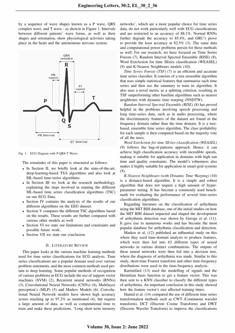
by a sequence of wave shapes known as a P wave, QRScomplex wave, and T wave - as showin in Figure 1. Intervalsbetween different patients’ wave forms, as well as theirshapes and orientation, show physiological activities takingplace in the heart and the autonomous nervous system.

Fig. 1. ECG Diagram with P-QRS-T Waves

The remainder of this paper is structured as follows:• In Section II, we briefly look at the state-of-the-art,

deep-learning-based TSA algorithms and also look atML-based time-series algorithms.

• In Section III we look at the research methodology,explaining the steps involved in running the differentML-based time series classification algorithms (TSC)on our ECG Data.

• Section IV contains the analysis of the results of ourdifferent algorithms on the EEG dataset.

• Section V compares the different TSC algorithms basedon the results. These results are further compared withvarious other models as well.

• Section VI we state our limitations and constraints andpossible future work.

• Section VII we state our conclusion.

II. LITERATURE REVIEW

This paper looks at the various machine learning methodsused for time series classifications for ECG analysis. Timeseries classifications are a popular domain used over variousproblem statements, and the most common methods used per-tain to deep learning. Some popular methods of recognitionof various problems in ECG include the use of support vectormachines (SVM) (2), Recurrent neural networks (RNNs)(3), Convolutional Neural Networks (CNNs) (4), Multilayerperceptron’s (MLP) (5) and Markov Models (6). Convolu-tional Neural Network models have shown high accuracyscores reaching up to 97.2% as mentioned (4), but requirea large amount of data, as well as computational time totrain and make these predictions. ’Long short term memory

networks’, which are a more popular choice for time seriesdata, do not work particularly well with ECG classificationsand are restricted to an accuracy of 88.1%. Normal RNNsfurther degrade the accuracy to 85.4%, and GRU’s proveto provide the least accuracy at 82.5% (3). The same dataand computational power problems persist for these methodsas well. For our research, we have focused on Time SeriesForests (7), Random Interval Spectral Ensemble (RISE) (8),Word ExtrAction for time SEries classification (WEASEL)(9) and K-Nearest Neighbours models (10).

Time Series Forests (TSF) (7) is an efficient and accuratetime series classifier. It consists of a tree ensemble algorithmthat uses simple statistical features that summarise each timeseries and then use the summary to train its algorithm. Italso uses a novel metric as a splitting criterion, resulting inTSF outperforming other baseline algorithms such as nearestneighbours with dynamic time warping (NNDTW).

Random Interval Spectral Ensemble (RISE) (8) has provedhelpful in the problems involving speech processing andlong time-series data, such as in audio processing, wherethe discriminatory features of the dataset are found in thefrequency domain rather than the time domain. It is a tree-based, ensemble time series algorithm, The class probabilityfor each sample is then computed based on the majority voteof all the trees.

Word ExtrAction for time SEries cLassification (WEASEL)(9) follows the bag-of-patterns approach. Hence, it canachieve high classification accuracy with incredible speeds,making it suitable for application in domains with high runtime and quality constraints. The model’s robustness alsomakes it highly suitable for application in smart-grid systems(9).

K-Nearest Neighbours (with Dynamic Time Warping) (10)is a distance-based algorithm. It is a simple and robustalgorithm that does not require a high amount of hyper-parameter tuning. It has become a commonly used bench-mark for evaluating the performance of several time-seriesclassification algorithms.

Regarding literature on the classification of arrhythmiausing the MIT BIH database, one of the initial studies on howthe MIT BIH dataset impacted and shaped the developmentof arrhythmia detection was shown by Geroge et al. (11).It gave rise to numerous works and has become the mostpopular database for arrhythmia classification and detection.

Markos et al. (12) published an influential study on thiswhere they used time-domain analysis to produce features,which were then fed into 63 different types of neuralnetworks in various distinct combinations. The outputs ofthese neural networks were then fed into a decision tree,where the diagnosis of arrhythmia was made. Similar to thisstudy, short-time Fourier transform and other time-frequencydistributions were used in the time-frequency analysis.

Karimifard (13) used the modelling of signals and theHermitian basis function to get a feature vector. This wasthen sent to a KNN classifier to classify the different typesof arrhythmia. An important conclusion in this study showedhow the feature vector’s size affected training times.

Hamid et al. (14) compared the use of different time seriestransformation methods such as CWT (Continuous wavelettransform), DCT (Discrete Cosine Transform) and DWT(Discrete Wavelet Transform) to improve the classifications



______________________________________________________________________________________

of ECG datasets when using Multi-Layer Perceptron’s (MLP)and Support Vector Machines (SVM). They used the featureextraction methods separately on the ECG signal and formed4 structures using MLP and 4 others using SVMs. Then, theycompared the efficiency of these feature extraction methodson time taken for the model to train.

Oscar (15) segmented the ECG signals from the MITBIH dataset and used three methods – fuzzy KNN’s, Multi-Layer Perceptron with Gradient Descent and momentumBackpropagation, and Multi-Layer Perceptron with ScaledConjugate Gradient Backpropagation to classify them into 5classes. They finally achieved the highest accuracy of 98%by combining the outputs of all three methods in a Mamdanitype fuzzy inference system.

Roland et al. (16) used Fast Fourier Transform as themethod of pre-processing for the signals and then passed thisto a neural network. They achieved an accuracy of 98.6% andconcluded that the diagnosis of heart abnormalities and earlydetection of debilitating medical conditions would improvewhen the medical community would adopt neural networksto analyze test data samples further.

Shirin et al. (17) used a block-based neural network whichconsisted of a 2D array of blocks connected. The structureof each block was dependent on the number of incomingand outgoing signals. The inputs in this method consisted oftemporal features and the Hermit function coefficient. Thenetwork structure and weights were then optimized usingParticle Swarm Optimization (PSO). This provided a uniquemethod to overcome the possible change of ECG from personto person as the BBNN would have a unique structure forevery person. They achieved an accuracy of 97%.

Saroj et al. (18) proposed the use of yet another deeplearning-based method called the Restricted Boltzmann Ma-chine (RBM) model. After the initial normalization and seg-mentation of signals, the RBM is used to extract the essentialfeatures, which are then passed to a SoftMax activationfunction. They classified the heartbeats into 4 distinct typesachieving an accuracy of 98.61%. We mention the drawbackof using specialized hardware and large datasets for thismethod to be useful, which our paper tries to solve.

Nirmala et al. (19) used Dual-Tree Complex WaveletTransform (DT-CWT) to extract features and then furtherpassed them to a neural attention mechanism to improveon the capturing of temporal patterns from the extractedfeatures. The attention-based model was trained using 8different arrhythmia classes and achieved an accuracy of98.5%.

Convolutional neural networks are well-researched meth-ods for arrhythmia classification. Bambang Et al. (20)showed how a 1 dimensional CNN could be used to detectatrial fibrillation detection with an accuracy of 96.36%. Thisstudy consisted of 3 normal, AF and non-AF and was trainedon 8232 records based on 8 different datasets. Mohammad etal. (21) similarly used a CNN to classify the MIT BIH datasetinto 5 different classes instead, obtaining an overall accuracyof 95.2%. Ozal et al. (22) further extended the number ofclasses to 17 and obtained an accuracy of 91.33% using a1D convolutional neural network. The study’s objective alsoextended to the time taken per classification, which averagedat 0.015s per sample. They thus proposed using this modelfor mobile devices and cloud computing. Mengze et al. (23)

use a 12 layer deep one dimensional CNN to classify thesignals into 5 distinct classes. They achieve an accuracy of97.2%, which is higher than other CNN, random forest andSVM based methods.

III. RESEARCH METHODOLOGY

A. Data Analysis & Pre-processing

The dataset being used in this study is the popular MIT-BIH Arrhythmia database (11) created by teams at BethIsrael Deaconess medical centre and MIT between the years1975 and 1979. This database contains two-channel ambula-tory ECG recordings samples of 47 patients resulting in 48hours’ worth of data. There are a total of 5 output classesrepresenting different types of human heartbeat patterns,which are:

• Non-Ectopic Beats (N) - These represent normal healthyhuman heartbeats.

• Supraventricular Ectopic Beats (S)• Ventricular Ectopic Beats (V)• Fusion Beats (F)• Unknown Beats (Q)

A graphical representation of each pattern is demonstratedin Figure 3.The distribution of the different classes in thedataset has been provided in Figure 4.

For the analysis and the application of various machinelearning methods on this dataset, the data was cropped intosmaller subsets resulting in a new dataset. This dataset hasa total of 109,446 samples. Each ECG sample has beenclipped and down-sampled to a 188 point dimension, i.e.,each sample has a length of 188. In the scenario wherethere are fewer points available, the samples are paddedwith zeroes to maintain uniform sample lengths. The datasetsamples are representative of the electrocardiogram signalsof the heartbeat, ranging from normal heartbeats to thoseafflicted by different arrhythmia’s and myocardial infarction,commonly known as a heart attack.

It is evident from the distribution chart (Figure 2) that thedataset is largely imbalanced and should ideally not be usedin this state for any analysis to be conducted on it. Hence,the data is re-sampled to provide an equal distribution of dataacross both test and training datasets. Each sample after thisstep accounts for 20% of the distribution. Next, Gaussiannoise is added to each sample to increase the generality ofthe algorithms during the training phase.

B. Training

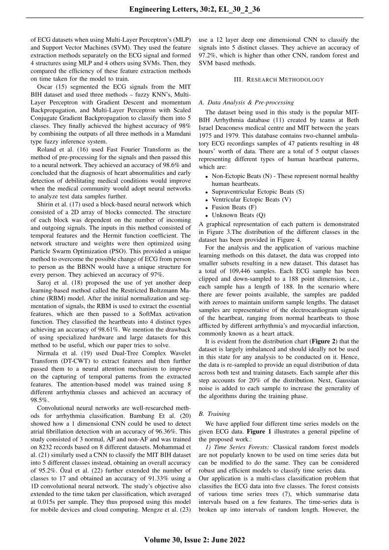
We have applied four different time series models on thegiven ECG data. Figure 1 illustrates a general pipeline ofthe proposed work.:

1) Time Series Forests: Classical random forest modelsare not popularly known to be used on time series data butcan be modified to do the same. They can be consideredrobust and efficient models to classify time series data.Our application is a multi-class classification problem thatclassifies the ECG data into five classes. The forest consistsof various time series trees (7), which summarise dataintervals based on a few features. The time-series data isbroken up into intervals of random length. However, the



______________________________________________________________________________________

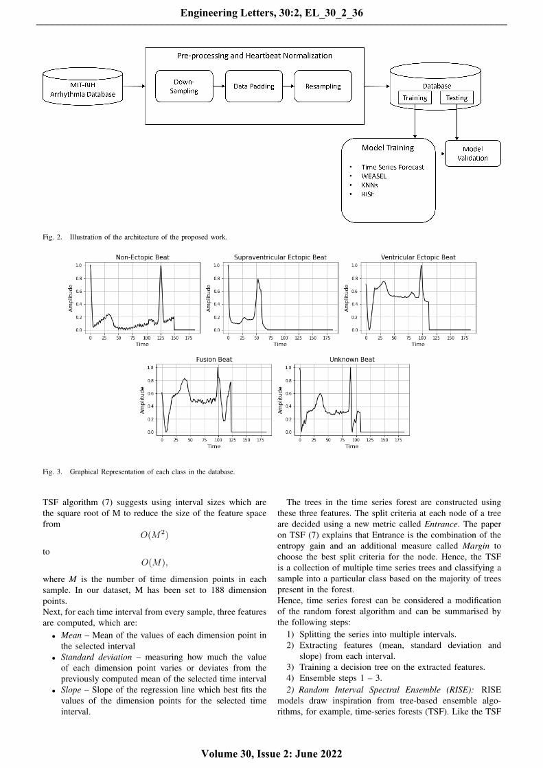
Fig. 2. Illustration of the architecture of the proposed work.

Fig. 3. Graphical Representation of each class in the database.

TSF algorithm (7) suggests using interval sizes which arethe square root of M to reduce the size of the feature spacefrom

O(M2)

toO(M),

where M is the number of time dimension points in eachsample. In our dataset, M has been set to 188 dimensionpoints.Next, for each time interval from every sample, three featuresare computed, which are:

• Mean – Mean of the values of each dimension point inthe selected interval

• Standard deviation – measuring how much the valueof each dimension point varies or deviates from thepreviously computed mean of the selected time interval

• Slope – Slope of the regression line which best fits thevalues of the dimension points for the selected timeinterval.

The trees in the time series forest are constructed usingthese three features. The split criteria at each node of a treeare decided using a new metric called Entrance. The paperon TSF (7) explains that Entrance is the combination of theentropy gain and an additional measure called Margin tochoose the best split criteria for the node. Hence, the TSFis a collection of multiple time series trees and classifying asample into a particular class based on the majority of treespresent in the forest.Hence, time series forest can be considered a modificationof the random forest algorithm and can be summarised bythe following steps:

1) Splitting the series into multiple intervals.2) Extracting features (mean, standard deviation and

slope) from each interval.3) Training a decision tree on the extracted features.4) Ensemble steps 1 – 3.2) Random Interval Spectral Ensemble (RISE): RISE

models draw inspiration from tree-based ensemble algo-rithms, for example, time-series forests (TSF). Like the TSF



______________________________________________________________________________________

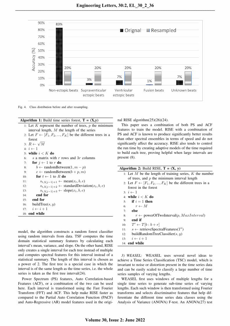
Fig. 4. Class distribution before and after resampling.

Algorithm 1: Build time series forest, T = (X,y)1: Let K represent the number of trees, p the minimum

interval length, M the length of the series2: Let F ← [F1, F2, ..., FK ] be the different trees in a

forest3: R←

√M

4: i← 15: while i < K do6: s a matrix with r rows and 3r columns7: for j ← 1 to r do8: b← randomBetween(1,m− p)9: e← randomBetween(b+ p,m)

10: for t← 1 to R do11: st,3(j−1)+1 ← mean(xt, b, e)12: st,3(j−1)+2 ← standardDeviation(xt, b, e)13: st,3(j−1)+3 ← slope(xt, b, e)14: end for15: end for16: buildTree(s, y)17: i← i+ 118: end while

model, the algorithm constructs a random forest classifierusing random intervals from data. TSF computes the timedomain statistical summary features by calculating eachinterval’s mean, variance, and slope. On the other hand, RISEonly creates a single interval for each tree instead of multipleand computes spectral features for this interval instead of astatistical summary. The length of this interval is chosen asa power of 2. The first tree is a special case in which theinterval is of the same length as the time series, i.e. the wholeseries is taken as the first tree interval(24).

Power Spectrum (PS) features, Auto Correlation-basedFeatures (ACF), or a combination of the two can be usedhere. Each interval is transformed using the Fast FourierTransform (FFT) and ACF. This help make RISE faster ascompared to the Partial Auto Correlation Function (PACF)and Auto-Regressive (AR) model features used in the origi-

nal RISE algorithm(25)(26)(24).This paper uses a combination of both PS and ACF

features to train the model. RISE with a combination ofPS and ACF is known to produce significantly better resultsthan other spectral ensembles in terms of speed and do notsignificantly affect the accuracy. RISE also tends to controlthe run time by creating adaptive models of the time requiredto build each tree, proving helpful when large intervals arepresent (8).

Algorithm 2: Build RISE, T = (X, y)1: Let M be the length of training series, K the number

of trees, and p the minimum interval length2: Let F ← [F1, F2, ..., FK ] be the different trees in a

forest in the forest3: i← 14: while i < K do5: if i = 1 then6: r ←M7: else8: r ← powerOfTwoInterval(p,MaxInterval)9: end if

10: T ′ ← T [b : b+ r]11: s← retrieveSpectralFeatures(T ′)12: buildRandomTreeClassifier(s, y)13: i← i+ 114: end while

3) WEASEL: WEASEL uses several novel ideas toachieve a Time Series Classification (TSC) model, which isinvariant to noise or distortion present in the time series dataand can be easily scaled to classify a large number of timeseries samples of varying lengths.

WEASEL first uses windows of multiple lengths for asingle time series to generate sub-time series of varyinglengths. Each such window is then transformed using Fouriertransforms and selects discriminative features that help dif-ferentiate the different time series data classes using theAnalysis of Variance (ANOVA) F-test. An ANOVA(27) test



______________________________________________________________________________________

in simple words helps to understand the difference betweenthe independent variables, or in this case, the features, andhow does it affect the dependent response variable. Also, toretain the temporal order in a time series, WEASEL includesa bi-gram model, which helps encode the order relationshipof the time series data in the model. Finally, to reducethe large number of features generated, WEASEL uses aChi-squared statistical test to determine relevant features,eliminating insignificant features whose absence does notaffect the model’s classification accuracy. As a result, thefeature-set obtained is highly effective in differentiatingbetween the different time series classes, then used in a fastlogistic regression model to make predictions. The logisticregression model proves to be much quicker than othercomplex classification algorithms due to its simplicity andprovides good classification accuracy, a merit of the featureset obtained.

Algorithm 3: Build WEASEL, T = (sample, I)1: Let I represent the number of Fourier values to keep2: b← empty BagOfPattern3: for all w in AllWindowLengths do4: AllWindows← slidingWindow(sample, w)5: normalize(AllWindows)6: for all (prevWindow,window) in AllWindows do

7: word← quantTransform(window, I)8: bag[w + word].increaseCount()9: prevWord← quantTransform(prevWindow, I)

10: bag[w + prevWord+ word].increaseCount()11: end for12: end for13: return ChiFeatureSelect(bag)

4) KNNs: KNN is a simple classification algorithm that isoften used as a baseline for various classification problems,as it classifies samples simply by comparing them with theirneighbours. The sample is labelled as the class with themost frequency in the first k closest neighbours, which areconsidered the most similar to the sample.

The standard KNN algorithm, however, makes use ofthe Euclidean Distance measure to determine the similarityof the input sample with all the other samples present inthe dataset. While this metric is suitable for cross-sectionaldata, it is not ideal for time series data classification. Twotime-series samples can have a similar structure but havedifferent phases, i.e., the two waves are displaced along time.Therefore, the Euclidean distance metric will compute thedifference between values corresponding to the same instanceand hence might not determine whether the two phase-shiftedtime series are similar.

The use of dynamic time warping (DTW) makes thek-nearest neighbours’ algorithm suitable for application totime series data. The distance between any two samples ismeasured using DTW, which measures the similarity betweensequences that may be displaced relative to each other alongtime or may have different speeds or lengths.

KNNs with DTW is used to establish a baseline accuracyquickly and easily for the time series classification problem.However, this algorithm is computationally very expensive

as it requires a lot of time to compare each time sequencewith all other time sequences and requires a lot of memoryin doing so. Moreover, this algorithm fails to explain whythe sequence was labelled a particular class.

The algorithm is also susceptible to noise in the dataset,which can severely distort the shape of a time sequenceresulting in it suffering a deviation from its valid class label.

Algorithm 4: K Nearest Neighbors, T = (X, y)1: Let N be a list of neighbors2: DistMatrix← calculateDistancesUsingDWT(X, y)3: N ← identifyKNN(DistMatrix)4: Label← findMode(N )5: return Label

Algorithm 5: Dynamic Time Warping, Input: (X, y)1: Let S be a two dimensional matrix with N ×M

dimensions2: S[0][0]← 03: for i← 1 to M do4: S[0, i]← inf5: end for6: for j ← 1 to N do7: S[j, 0]← inf8: end for9: for i← 1 to N do

10: for j ← 1 to M do11: cost← dist(X[i[, y[j])12: S[i, j]← cost+

min(S[i, j − 1], S[i− 1, j], S[i− 1, j − 1]))13: end for14: end for15: return S[N,M ]

IV. ANALYSIS AND RESULTS

Each of the mentioned four models has been tested usingdifferent values for the respective hyper-parameters. Plots forthe model’s accuracy vs the different hyper-parameter valueshave also been shown. The results for each run have beengathered and tabulated. The various columns in the tabulatedresults are:

• The Estimators column will only be found in the resultsof the tree-based algorithms. Estimators refer to thenumber of trees used in forest algorithms.

• The Number of samples column indicates the numberof samples over which the model was trained on.

• The Micro precision is micro averaged precision. Microaveraged precision helps capture the performance ofdifferent models when faced with datasets with classimbalance. They can account for the imbalance in thedataset of a multi-class classification problem, henceproviding more insights about the model’s precision andclassifying classes with low samples.

Micro− precision =

∑51 TPi∑5

1 TPi + FPi



______________________________________________________________________________________

• The Macro Precision column is macro-averaged preci-sion. Macro averaged precision reports the generalisedprecision values over the entire dataset. The metric failsto account for any dataset imbalance in a multi-classclassification problem. It will report a good precisionscore even when the poorly performing classes witnesspoor precision scores. This is because the metric is thesimple arithmetic mean of the precision scores of eachclass. As a result, the low scores will be compensatedby the high-performing classes’ high scores. Hence themacro-precision might provide misleading inferencesabout imbalanced datasets.

Macro− precision =

∑51 Precisioni

5

• The Micro Recall column is the score computed bymicro-averaging the recall values for all the classes. Thisis a better metric to analyse the recall of the model,classifying an imbalanced dataset into multiple classes.

Micro− recall =

∑51 TPi∑5

1 TPi + FNi

• The Macro Recall is computed by computing a macro-average of all the recall scores, i.e. finding the arithmeticmean of the individual recall scores for the variousclasses. Like all other macro-averaged metrics, it failsto account for any class imbalance and is prone toreporting misleading scores.

Macro− recall =

∑51 Recalli

5

• The Accuracy column reports accuracy scores of dif-ferent models for different configurations of the varioushyper-parameters involved. It tells us how many havebeen correctly classified out of all the classified samples.Another point to note is that the same values are re-ported for the metrics of micro-precision, micro-recall,and accuracy due to the nature of micro averages.

• The Time to train column signifies the amount of time(in seconds) for the model to fit the entire dataset.

• The Time per sample column, on the other hand, pro-vides the average time taken for the model to predict aclass for an input sample to the model.

Keeping in mind the definitions of the various columns,below are the results provided for the various models runover the dataset.

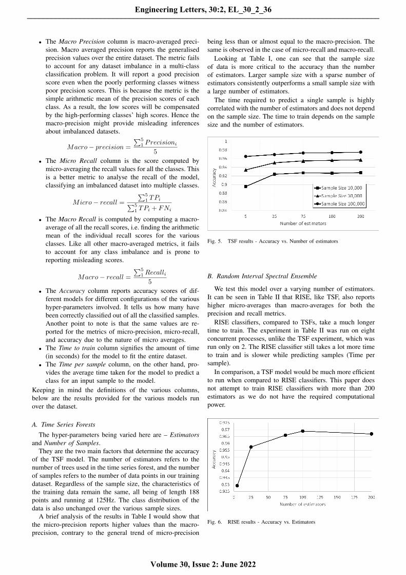
A. Time Series Forests

The hyper-parameters being varied here are – Estimatorsand Number of Samples.

They are the two main factors that determine the accuracyof the TSF model. The number of estimators refers to thenumber of trees used in the time series forest, and the numberof samples refers to the number of data points in our trainingdataset. Regardless of the sample size, the characteristics ofthe training data remain the same, all being of length 188points and running at 125Hz. The class distribution of thedata is also unchanged over the various sample sizes.

A brief analysis of the results in Table I would show thatthe micro-precision reports higher values than the macro-precision, contrary to the general trend of micro-precision

being less than or almost equal to the macro-precision. Thesame is observed in the case of micro-recall and macro-recall.

Looking at Table I, one can see that the sample sizeof data is more critical to the accuracy than the numberof estimators. Larger sample size with a sparse number ofestimators consistently outperforms a small sample size witha large number of estimators.

The time required to predict a single sample is highlycorrelated with the number of estimators and does not dependon the sample size. The time to train depends on the samplesize and the number of estimators.

Fig. 5. TSF results - Accuracy vs. Number of estimators

B. Random Interval Spectral Ensemble

We test this model over a varying number of estimators.It can be seen in Table II that RISE, like TSF, also reportshigher micro-averages than macro-averages for both theprecision and recall metrics.

RISE classifiers, compared to TSFs, take a much longertime to train. The experiment in Table II was run on eightconcurrent processes, unlike the TSF experiment, which wasrun only on 2. The RISE classifier still takes a lot more timeto train and is slower while predicting samples (Time persample).

In comparison, a TSF model would be much more efficientto run when compared to RISE classifiers. This paper doesnot attempt to train RISE classifiers with more than 200estimators as we do not have the required computationalpower.

Fig. 6. RISE results - Accuracy vs. Estimators



______________________________________________________________________________________

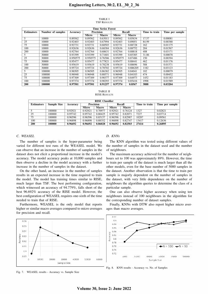
TABLE ITSF RESULTS

Time Series ForestEstimators Number of samples Accuracy Precision Recall Time to train Time per sample

Micro Macro Micro Macro5 10000 0.89562 0.89562 0.63011 0.89562 0.85634 17.57 0.0008125 10000 0.92403 0.92403 0.67994 0.92403 0.89051 84.99 0.0038875 10000 0.92731 0.92731 0.68503 0.92731 0.88728 162 0.01175100 10000 0.92636 0.92636 0.68384 0.92636 0.88752 204 0.01567200 10000 0.92764 0.92764 0.68631 0.92764 0.88818 408 0.031715 30000 0.93399 0.93399 0.71601 0.93399 0.85385 31.86 0.0007825 30000 0.950575 0.950575 0.76586 0.950575 0.87486 150 0.0039475 30000 0.95477 0.95477 0.77821 0.95477 0.88441 462 0.01176100 30000 0.95619 0.95619 0.78238 0.95619 0.88696 588 0.01571200 30000 0.95724 0.95724 0.78702 0.95724 0.886205 1182 0.031235 100000 0.96505 0.96505 0.86382 0.96505 0.84041 102 0.0007925 100000 0.96948 0.96948 0.88571 0.96948 0.84103 474 0.0045275 100000 0.97309 0.97309 0.90377 0.97309 0.84973 1452 0.01183100 100000 0.97374 0.97374 0.90293 0.97374 0.85416 1998 0.01589200 100000 0.97501 0.97501 0.91257 0.97374 0.8567 3888 0.03204

TABLE IIRISE RESULTS

RISE ClassifierEstimators Sample Size Accuracy Precision Recall Time to train Time per sample

Micro Macro Micro Macro5 100000 0.92921 0.92921 0.70977 0.92921 0.76124 1327 0.0282125 100000 0.95742 0.95742 0.80425 0.95742 0.82071 7227 0.0371475 100000 0.96596 0.96596 0.85157 0.96596 0.82987 10287 0.09561100 100000 0.96898 0.96898 0.88352 0.96898 0.82747 13417 0.12636200 100000 0.96692 0.96692 0.86028 0.96692 0.82503 27414 0.26895

C. WEASEL

The number of samples is the hyper-parameter beingvaried for different test runs of the WEASEL model. Wecan observe that an increase in the number of samples in thedataset does not elicit a proportional increase in the model’saccuracy. The model accuracy peaks at 10,000 samples andthen observe a decline in the model accuracy with a furtherincrease in the number of samples in the dataset.

On the other hand, an increase in the number of samplesresults in an expected increase in the time required to trainthe model. The model has training times similar to RISE,much larger than TSF. The best performing configuration,which witnessed an accuracy of 94.779%, falls short of thebest 96.692% accuracy of the RISE model. However, thebest configuration of WEASEL requires one-sixth of the timeneeded to train that of RISE.

Furthermore, WEASEL is the only model that reportshigher or similar macro averages compared to micro averagesfor precision and recall.

Fig. 7. WEASEL results - Accuracy vs. Sample Size

D. KNNs

The KNN algorithm was tested using different values ofthe number of samples in the dataset used and the numberof neighbours.

The maximum accuracy achieved for the number of neigh-bours set to 100 was approximately 89%. However, the timeto train per sample of the dataset is much larger than all theother models, even for the base number of 5000 samples inthe dataset. Another observation is that the time to train persample is majorly dependent on the number of samples inthe dataset, with very little dependence on the number ofneighbours the algorithm queries to determine the class of aparticular sample.

One can also observe higher accuracy when using tenneighbours instead of 100 neighbours in the algorithm forthe corresponding number of dataset samples.

Finally, KNNs with DTW also report higher micro aver-ages than macro averages.

Fig. 8. KNN results - Accuracy vs. No. of Samples



______________________________________________________________________________________

TABLE IIIWEASEL RESULTS

WEASELSample Size Accuracy Precision Recall Time per sample Time to Train (s)

Micro Macro Micro Macro2500 0.89558 0.89558 0.89907 0.89558 0.89706 0.03696 83910000 0.94779 0.94779 0.95199 0.94779 0.94859 0.03771 452525000 0.93172 0.93172 0.94004 0.93172 0.93282 0.03997 1293537500 0.91646 0.91646 0.92618 0.91646 0.91322 0.04235 2119550000 0.90763 0.90763 0.92379 0.90763 0.90763 0.04612 30393

TABLE IVKNN RESULTS

K-Nearest NeighborsSample Size Accuracy Precision Recall Time per sample Neighbors

Micro Macro Micro Macro5000 0.86153 0.86153 0.7516 0.86153 0.85964 0.13077 1025000 0.89231 0.89231 0.77485 0.89231 0.88188 0.65698 1030000 0.879518072 0.879518072 0.885011933 0.879518072 0.881456095 0.796532 1050000 0.883534137 0.883534137 0.893715061 0.883534137 0.885612958 1.336411468 1075000 0.879518072 0.879518072 0.892954956 0.879518072 0.881265132 1.999505015 10100000 0.895582329 0.895582329 0.909117694 0.895582329 0.897456095 2.726337341 105000 0.78461 0.78461 0.66766 0.78461 0.840388 0.13389 10025000 0.84615 0.84615 0.72854 0.84615 0.8513 0.65904 10030000 0.86153 0.86153 0.75205 0.86153 0.86601 0.77946 10050000 0.884165 0.884165 0.76455 0.884165 0.8781 1.33083 10075000 0.89231 0.89231 0.77495 0.89231 0.88227 2.00243 100100000 0.90131 0.90131 0.798857 0.90131 0.88644 2.63226 100

V. MODEL COMPARISON

In Figure 9, the highest possible accuracy’s of differentmodels have been plotted against the corresponding time taketaken for each sample by the model. One can infer fromFigure 9 that KNNs not only take the most time per samplebut also report the least accuracy. RISE reports a reasonablyhigh accuracy with respectable times per sample. However, itis not as good as the other two models. Although WEASELtakes a comparable amount of time per sample as TSF, TSFperforms better, as it is able to report higher classificationaccuracy.

Consequently, TSF is the best candidate TSC algorithmfor deploying on low-compute portable devices. It reports thehighest classification accuracy of the four ML TSC modelsand takes the least time to predict a class for each inputsample. As a result, one may expect the TSF algorithmto run smoothly on low-compute devices. However, furtherperformance testing with actual hardware is needed to becarried out to confirm the same.

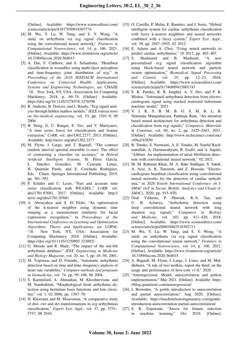
Table V showcases the performances of various state-of-the-art deep learning-based models and compares them tothe proposed work. They compare the accuracy of predictionover all classes, the type of model use and the number ofclasses that the data is classified into. The four machinelearning algorithms presented by the proposed research workprovides comparable accuracy results when compared to theaccuracy scores of the corresponding models.

TSF outperforms most deep learning models, thus verify-ing its efficacy despite utilising considerably lower hardwareresources and compute for training. RISE and WEASEL alsoprovide comparable results with several research works, fur-ther validating the consistency and reliability of the proposedwork.

VI. LIMITATIONS & SCOPE FOR FUTURE WORK

The proposed work has been limited to comparing fourdifferent machine learning (ML) algorithms. Our goal is toexperiment with lightweight algorithms that can potentiallybe deployed on portable devices. They should be capable ofproviding accurate results in the least amount of time witha smaller dataset. That is why we aimed to use machinelearning instead of deep learning models such as recurrentneural high computational requirements and large datasets,leading them to be less than ideal for healthcare purposes onportable systems.

However, deep learning models such as recurrent neuralnetworks (RNN) and convolutional neural networks (CNN)have been found to give a higher degree of accuracy for ourrequirement in some cases. Furthermore, genetic algorithmshave also been used in the past to classify time series data,which can also be experimented with for ECG classification.Scope for future work here would include increasing theaccuracy of these machine learning models while honouringthe same time and data constraints specified. Apart from that,there is a further need to look into different neural networkmodels which are faster in their approach and may not needa large amount of data, considering medical data is not aslargely available as other forms.

VII. CONCLUSION

Time series classification is a famous area of research,with a wide array of algorithms already available and new,faster, and better algorithms appearing every year. For ourapplication of ECG classification, we wanted an algorithmthat is robust and light enough to be potentially deployed onportable devices. We explored four algorithms – TSF, RISE,WEASEL and KNNs with DTW. TSF outshone the rest ofthe three algorithms tested in this paper. To summarise thiscomparison:



______________________________________________________________________________________

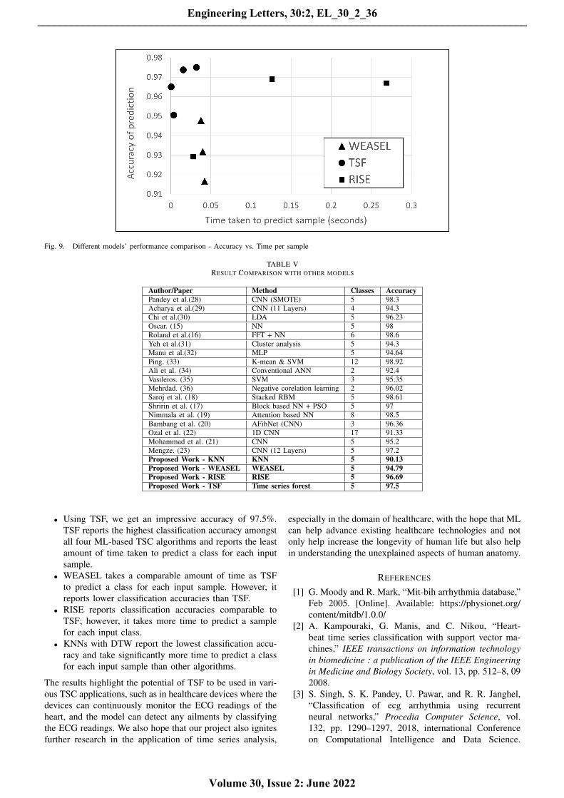
Fig. 9. Different models’ performance comparison - Accuracy vs. Time per sample

TABLE VRESULT COMPARISON WITH OTHER MODELS

Author/Paper Method Classes AccuracyPandey et al.(28) CNN (SMOTE) 5 98.3Acharya et al.(29) CNN (11 Layers) 4 94.3Chi et al.(30) LDA 5 96.23Oscar. (15) NN 5 98Roland et al.(16) FFT + NN 6 98.6Yeh et al.(31) Cluster analysis 5 94.3Manu et al.(32) MLP 5 94.64Ping. (33) K-mean & SVM 12 98.92Ali et al. (34) Conventional ANN 2 92.4Vasileios. (35) SVM 3 95.35Mehrdad. (36) Negative corelation learning 2 96.02Saroj et al. (18) Stacked RBM 5 98.61Shririn et al. (17) Block based NN + PSO 5 97Nimmala et al. (19) Attention based NN 8 98.5Bambang et al. (20) AFibNet (CNN) 3 96.36Ozal et al. (22) 1D CNN 17 91.33Mohammad et al. (21) CNN 5 95.2Mengze. (23) CNN (12 Layers) 5 97.2Proposed Work - KNN KNN 5 90.13Proposed Work - WEASEL WEASEL 5 94.79Proposed Work - RISE RISE 5 96.69Proposed Work - TSF Time series forest 5 97.5

• Using TSF, we get an impressive accuracy of 97.5%.TSF reports the highest classification accuracy amongstall four ML-based TSC algorithms and reports the leastamount of time taken to predict a class for each inputsample.

• WEASEL takes a comparable amount of time as TSFto predict a class for each input sample. However, itreports lower classification accuracies than TSF.

• RISE reports classification accuracies comparable toTSF; however, it takes more time to predict a samplefor each input class.

• KNNs with DTW report the lowest classification accu-racy and take significantly more time to predict a classfor each input sample than other algorithms.

The results highlight the potential of TSF to be used in vari-ous TSC applications, such as in healthcare devices where thedevices can continuously monitor the ECG readings of theheart, and the model can detect any ailments by classifyingthe ECG readings. We also hope that our project also ignitesfurther research in the application of time series analysis,

especially in the domain of healthcare, with the hope that MLcan help advance existing healthcare technologies and notonly help increase the longevity of human life but also helpin understanding the unexplained aspects of human anatomy.

REFERENCES

[1] G. Moody and R. Mark, “Mit-bih arrhythmia database,”Feb 2005. [Online]. Available: https://physionet.org/content/mitdb/1.0.0/

[2] A. Kampouraki, G. Manis, and C. Nikou, “Heart-beat time series classification with support vector ma-chines,” IEEE transactions on information technologyin biomedicine : a publication of the IEEE Engineeringin Medicine and Biology Society, vol. 13, pp. 512–8, 092008.

[3] S. Singh, S. K. Pandey, U. Pawar, and R. R. Janghel,“Classification of ecg arrhythmia using recurrentneural networks,” Procedia Computer Science, vol.132, pp. 1290–1297, 2018, international Conferenceon Computational Intelligence and Data Science.



______________________________________________________________________________________

[Online]. Available: https://www.sciencedirect.com/science/article/pii/S1877050918307774

[4] M. Wu, Y. Lu, W. Yang, and S. Y. Wong, “Astudy on arrhythmia via ecg signal classificationusing the convolutional neural network,” Frontiers inComputational Neuroscience, vol. 14, p. 106, 2021.[Online]. Available: https://www.frontiersin.org/article/10.3389/fncom.2020.564015

[5] A. Das, F. Catthoor, and S. Schaafsma, “Heartbeatclassification in wearables using multi-layer perceptronand time-frequency joint distribution of ecg,” inProceedings of the 2018 IEEE/ACM InternationalConference on Connected Health: Applications,Systems and Engineering Technologies, ser. CHASE’18. New York, NY, USA: Association for ComputingMachinery, 2018, p. 69–74. [Online]. Available:https://doi.org/10.1145/3278576.3278598

[6] R. Andreao, B. Dorizzi, and J. Boudy, “Ecg signal anal-ysis through hidden markov models,” IEEE transactionson bio-medical engineering, vol. 53, pp. 1541–9, 092006.

[7] H. Deng, G. C. Runger, E. Tuv, and V. Martyanov,“A time series forest for classification and featureextraction,” CoRR, vol. abs/1302.2277, 2013. [Online].Available: http://arxiv.org/abs/1302.2277

[8] M. Flynn, J. Large, and T. Bagnall, “The contractrandom interval spectral ensemble (c-rise): The effectof contracting a classifier on accuracy,” in HybridArtificial Intelligent Systems, H. Perez Garcıa,L. Sanchez Gonzalez, M. Castejon Limas,H. Quintian Pardo, and E. Corchado Rodrıguez,Eds. Cham: Springer International Publishing, 2019,pp. 381–392.

[9] P. Schafer and U. Leser, “Fast and accurate timeseries classification with WEASEL,” CoRR, vol.abs/1701.07681, 2017. [Online]. Available: http://arxiv.org/abs/1701.07681

[10] A. Abouyahya and S. El Fkihi, “An optimizationof the k-nearest neighbor using dynamic timewarping as a measurement similarity for facialexpressions recognition,” in Proceedings of theInternational Conference on Learning and OptimizationAlgorithms: Theory and Applications, ser. LOPAL’18. New York, NY, USA: Association forComputing Machinery, 2018. [Online]. Available:https://doi.org/10.1145/3230905.3230921

[11] G. Moody and R. Mark, “The impact of the mit-biharrhythmia database,” IEEE Engineering in Medicineand Biology Magazine, vol. 20, no. 3, pp. 45–50, 2001.

[12] M. Tsipouras and D. Fotiadis, “Automatic arrhythmiadetection based on time and time–frequency analysis ofheart rate variability,” Computer methods and programsin biomedicine, vol. 74, pp. 95–108, 06 2004.

[13] S. Karimifard, A. Ahmadian, M. Khoshnevisan, andM. Nambakhsh, “Morphological heart arrhythmia de-tection using hermitian basis functions and knn classi-fier,” vol. 1, 02 2006, pp. 1367–70.

[14] H. Khorrami and M. Moavenian, “A comparative studyof dwt, cwt and dct transformations in ecg arrhythmiasclassification,” Expert Syst. Appl., vol. 37, pp. 5751–5757, 08 2010.

[15] O. Castillo, P. Melin, E. Ramırez, and J. Soria, “Hybridintelligent system for cardiac arrhythmia classificationwith fuzzy k-nearest neighbors and neural networkscombined with a fuzzy system,” Expert Syst. Appl.,vol. 39, pp. 2947–2955, 02 2012.

[16] E. Adams and A. Choi, “Using neural networks topredict cardiac arrhythmias,” 10 2012, pp. 402–407.

[17] S. Shadmand and B. Mashoufi, “A newpersonalized ecg signal classification algorithmusing block-based neural network and particleswarm optimization,” Biomedical Signal Processingand Control, vol. 25, pp. 12–23, 2016.[Online]. Available: https://www.sciencedirect.com/science/article/pii/S1746809415001743

[18] S. K. Pandey, R. R. Janghel, A. V. Dev, and P. K.Mishra, “Automated arrhythmia detection from electro-cardiogram signal using stacked restricted boltzmannmachine model,” 2021.

[19] V. J. K. S. B. M. B. G. S. M. B. L. B.Nimmala Mangathayaru, Padmaja Rani, “An attentionbased neural architecture for arrhythmia detection andclassification from ecg signals,” Computers, Materials& Continua, vol. 69, no. 2, pp. 2425–2443, 2021.[Online]. Available: http://www.techscience.com/cmc/v69n2/43850

[20] B. Tutuko, S. Nurmaini, A. E. Tondas, M. Naufal Rach-matullah, A. Darmawahyuni, R. Esafri, and A. Sapitri,“Afibnet: An implementation of atrial fibrillation detec-tion with convolutional neural network,” 02 2021.

[21] M. M. Rahman Khan, M. A. Bakr Siddique, S. Sakib,A. Aziz, A. K. Tanzeem, and Z. Hossain, “Electro-cardiogram heartbeat classification using convolutionalneural networks for the detection of cardiac arrhyth-mia,” in 2020 Fourth International Conference on I-SMAC (IoT in Social, Mobile, Analytics and Cloud) (I-SMAC), 2020, pp. 915–920.

[22] Ozal Yıldırım, P. Pławiak, R.-S. Tan, andU. R. Acharya, “Arrhythmia detection usingdeep convolutional neural network with longduration ecg signals,” Computers in Biologyand Medicine, vol. 102, pp. 411–420, 2018.[Online]. Available: https://www.sciencedirect.com/science/article/pii/S0010482518302713

[23] M. Wu, Y. Lu, W. Yang, and S. Y. Wong, “Astudy on arrhythmia via ecg signal classificationusing the convolutional neural network,” Frontiers inComputational Neuroscience, vol. 14, p. 106, 2021.[Online]. Available: https://www.frontiersin.org/article/10.3389/fncom.2020.564015

[24] A. Bagnall, M. Flynn, J. Large, J. Lines, and M. Mid-dlehurst, “A tale of two toolkits, report the third: on theusage and performance of hive-cote v1.0,” 2020.

[25] “Autoregression: Model, autocorrelation and pythonimplementation,” Mar 2021. [Online]. Available: https://blog.quantinsti.com/autoregression/

[26] J. Brownlee, “A gentle introduction to autocorrelationand partial autocorrelation,” Aug 2020. [Online].Available: https://machinelearningmastery.com/gentle-introduction-autocorrelation-partial-autocorrelation/

[27] S. K. Gajawada, “Anova for feature selectionin machine learning,” Oct 2019. [Online].



______________________________________________________________________________________

Available: https://towardsdatascience.com/anova-for-feature-selection-in-machine-learning-d9305e228476

[28] S. K. Pandey and R. R. Janghel, “Automatic detectionof arrhythmia from imbalanced ecg database using cnnmodel with smote,” Australasian Physical & Engineer-ing Sciences in Medicine, vol. 42, pp. 1129 – 1139,2019.

[29] U. R. Acharya, H. Fujita, O. S. Lih, Y. Hagiwara,J. H. Tan, and M. Adam, “Automated detection ofarrhythmias using different intervals of tachycardiaecg segments with convolutional neural network,”Information Sciences, vol. 405, pp. 81–90, 2017.[Online]. Available: https://www.sciencedirect.com/science/article/pii/S0020025517306539

[30] Y.-C. Yeh, W.-J. Wang, and C. W. Chiou,“Cardiac arrhythmia diagnosis method usinglinear discriminant analysis on ecg signals,”Measurement, vol. 42, no. 5, pp. 778–789, 2009.[Online]. Available: https://www.sciencedirect.com/science/article/pii/S0263224109000050

[31] Y.-C. Yeh, C. W. Chiou, and H.-J. Lin,“Analyzing ecg for cardiac arrhythmia using clusteranalysis,” Expert Systems with Applications, vol. 39,no. 1, pp. 1000–1010, 2012. [Online]. Avail-able: https://www.sciencedirect.com/science/article/pii/S0957417411010633

[32] M. Thomas, M. K. Das, and S. Ari,“Automatic ecg arrhythmia classification usingdual tree complex wavelet based features,”AEU - International Journal of Electronics andCommunications, vol. 69, no. 4, pp. 715–721, 2015.[Online]. Available: https://www.sciencedirect.com/science/article/pii/S1434841114003641

[33] C.-P. Shen, W.-C. Kao, Y.-Y. Yang, M.-C. Hsu, Y.-T.Wu, and F. Lai, “Detection of cardiac arrhythmia inelectrocardiograms using adaptive feature extractionand modified support vector machines,” Expert Systemswith Applications, vol. 39, no. 9, pp. 7845–7852, 2012.[Online]. Available: https://www.sciencedirect.com/science/article/pii/S0957417412001066

[34] A. Isin and S. Ozdalili, “Cardiac arrhythmia detectionusing deep learning,” Procedia Computer Science, vol.120, pp. 268–275, 2017, 9th International Conferenceon Theory and Application of Soft Computing,Computing with Words and Perception, ICSCCW2017, 22-23 August 2017, Budapest, Hungary.[Online]. Available: https://www.sciencedirect.com/science/article/pii/S187705091732450X

[35] V. Tsoutsouras, D. Azariadi, S. Xydis, and D. Soudris,“Effective learning and filtering of faulty heart-beatsfor advanced ecg arrhythmia detection using mit-bihdatabase,” EAI Endorsed Transactions on PervasiveHealth and Technology, vol. 2, no. 8, 12 2015.

[36] M. Javadi, S. A. A. A. Arani, A. Sajedin,and R. Ebrahimpour, “Classification of ecgarrhythmia by a modular neural network basedon mixture of experts and negatively correlatedlearning,” Biomedical Signal Processing andControl, vol. 8, no. 3, pp. 289–296, 2013.[Online]. Available: https://www.sciencedirect.com/science/article/pii/S1746809412001127



______________________________________________________________________________________

Analysis of Statistical Models for Fast Time Series ECG ...

Documents

Transcript of Analysis of Statistical Models for Fast Time Series ECG ...