ANALYSIS OF STALL NACA 23021 PHENOMENON ... - CORE
180
i FINAL PROJECT – ME141502 ANALYSIS OF STALL NACA 23021 PHENOMENON ON APPLICATION HYDROFOIL Fitri Puspita Dewi NRP. 4213 101 005 Supervisor Irfan Syarif Arief, S.T., M.T. Edi Jadmiko, S.T., M.T. DOUBLE DEGREE PROGRAM OF MARINE ENGINEERING DEPARTMENT FACULTY OF MARINE ENGINEERING INSTITUT TEKNOLOGI SEPULUH NOPEMBER SURABAYA 2017
-
Upload
khangminh22 -
Category
Documents
-
view
3 -
download
0
Transcript of ANALYSIS OF STALL NACA 23021 PHENOMENON ... - CORE

i
FINAL PROJECT – ME141502
ANALYSIS OF STALL NACA 23021 PHENOMENON ON
APPLICATION HYDROFOIL
Fitri Puspita Dewi
NRP. 4213 101 005
Supervisor
Irfan Syarif Arief, S.T., M.T.
Edi Jadmiko, S.T., M.T.
DOUBLE DEGREE PROGRAM OF MARINE ENGINEERING DEPARTMENT
FACULTY OF MARINE ENGINEERING
INSTITUT TEKNOLOGI SEPULUH NOPEMBER
SURABAYA
2017

ii
“This page is intentionally left blank”

iii
TUGAS AKHIR – ME141502
ANALISA FENOMENA STALL NACA 23021 APLIKASI PADA
HIDROFOIL
Fitri Puspita Dewi
NRP. 4213 101 005
Dosen Pembimbing :
Irfan Syarif Arief, S.T., M.T.
Edi Jadmiko, S.T., M.T.
DOUBLE DEGREE PROGRAM OF MARINE ENGINEERING DEPARTMENT
FAKULTAS TEKNOLOGI KELAUTAN
INSTITUT TEKNOLOGI SEPULUH NOPEMBER
SURABAYA
2017

iv
“This page is intentionally left blank”

v
APPROVAL SHEET
ANALYSIS OF STALL NACA 23021 PHENOMENON ON APPLICATION
HYDROFOIL
FINAL PROJECT
Submitted to Comply One of The Requirements to Obtain a
Bachelor Engineering Degree on
Laboratory of Marine Manufacture and Design (MMD) Bachelor Degree
Program of Marine Engineering Department Faculty of Marine
Technology Institut Teknologi Sepuluh Nopember
Prepared by :
FITRI PUSPITA DEWI
NRP. 4213101005
Approved by
Supervisor of Final Project :
Irfan Syarif Arief, S.T., M.T.
NIP. 1969 1225 1997 02 1001 ( )
Edi Jadmiko, S.T., M.T.
NIP. 1978 0706 2008 01 1012 ( )
SURABAYA
Juli 2017

vi
“This page is intentionally left blank”

vii
APPROVAL SHEET
ANALYSIS OF STALL NACA 23021 PHENOMENON ON APPLICATION
HYDROFOIL
FINAL PROJECT
Submitted to Comply One of The Requirements to Obtain a Bachelor
Engineering Degree
on
Laboratory of Marine Manufacture and Design (MMD)
Bachelor Degree Program of Marine Engineering Department
Faculty of Marine Technology
Institut Teknologi Sepuluh Nopember
Prepared by :
FITRI PUSPITA DEWI
NRP. 4213101005
Approved by
Head of Marine Engineering Department
Dr. Eng. M. Badrus Zaman, S.T., M.T.
NIP. 1977 0802 2008 01 1007
SURABAYA
Juli 2017

viii
“This page is intentionally left blank”

ix
APPROVAL SHEET
ANALYSIS OF STALL NACA 23021 PHENOMENON ON APPLICATION
HYDROFOIL
FINAL PROJECT
Submitted to Comply One of The Requirements to Obtain a Bachelor
Engineering Degree
on
Laboratory of Marine Manufacture and Design (MMD)
Bachelor Degree Program of Marine Engineering Department
Faculty of Marine Technology
Institut Teknologi Sepuluh Nopember
Prepared by :
FITRI PUSPITA DEWI
NRP. 4213101005
Approved by
Representative Hochschule Wismar in Indonesia
Dr.-Ing Wolfgang Busse
SURABAYA
Juli 2017

x
“This page is intentionally left blank”

xi
DECLARATION OF HONOR
I, who signed below hereby confirm that:
This bachelor thesis report has written without any plagiarism act, and
confirm consciously that all the data, concepts, design, references, and
material in this report own by Marine Manufacturing and Design (MMD) in
Department of Marine Engineering ITS which are the product of research
study and reserve the right to use for further research study and its
development.
Name : Fitri Puspita Dewi
NRP : 4213 101 005
Bachelor Thesis Title : Analysis of Stall NACA 23021
Phenomenon On Aplication Hydrofoil
Department : Double Degree Program in Marine
Engineering
If there is plagiarism act in the future, I will fully responsible and receive the
penalty given by ITS according to the regulation applied.
Surabaya, July 2017
Fitri Puspita Dewi

xii
ANALYSIS OF STALL NACA 23021 PHENOMENON ON APPLICATION
HYDROFOIL
Student Name : Fitri Puspita Dewi
NRP : 4213101005
Department : Marine Engineering
Supervisor : 1. Irfan Syarif Arief, S.T., M.T.
2. Edi Jadmiko, S.T., M.T.
ABSTRACT
Hydrofoil is a ship with hull that has foil which is mounted on a strut under
the hull. One of the hydrofoil characteristics is the position of hydrofoil angle
which named angle of attack. Angle of attack is an angle that formed by chord
hydrofoil and flow velocity vector of frestream fluid. The aim from angle of attack
is to optimized lift force and drag ratio. Then, the stall condition in hydrofoil ship
is the result of strem separation at high angle of attack with lift force reduction
and drag force get bigger because of drag pressure. In this research will find the
optimal lift force on NACA 23021 by using CFD simulation. In this simulation will
get the pressure distribution and drag coefficient. There are several variables in
this research that angle of attack used 5 °, 10 °, 15 °, 20 ° and 25 °; Aspect ratio
used 0.05, 0.25, 0.45, 0.65, and 0.85; And Froude number used 0.1, 0.2, 0.3, 0.4,
and 0.5. The result of this simulation is the comparison between CL chart, CD
chart, and CL / CD chart with angle of attack. With the result are Aspect ratio 0.05
maximum value CL / CD at an angle of attack 20 ° with Fn 0.1, Aspect ratio 0.25
maximum value CL / CD at an angle of attack 15 ° with Fn 0.3, Aspect ratio 0.45
maximum value CL / CD at an angle of attack 15 ° with Fn 0.1, Aspect ratio 0.65
maximum value CL / CD at an angle of attack 15 ° with Fn 0.1, Aspect ratio 0.85
maximum value CL / CD at an angle of attack 15 ° with Fn 0.1.
Keywords : Hydrofoil, NACA 23021, Angle of Attack, Stall, lift

xiii
“This page is intentionally left blank”

xiv
ANALISA FENOMENA STALL NACA 23021 APLIKASI PADA
HYDROFOIL
Nama : Fitri Puspita Dewi
NRP : 4213101005
Departemen : Marine Engineering
Dosen Pembimbing : 1. Irfan Syarif Arief, S.T., M.T.
2. Edi Jadmiko, S.T., M.T.
ABSTRAK
Hidrofoil merupakan kapal dengan lambung yang memiliki sayap (foil) yang
dipasang pada penyangga (strut) di bawah lambung kapal. Salah satu
karakteristik hydrofoil adalah posisi sudut hydrofoil yang bisa disebut juga
dengan sudut serang. Sudut serang merupakan sudut yang dibentuk antara
chord hydrofoil dengan vector kecepatan aliran fluida freestream. Tujuan dari
sudut serang untuk mengoptimalkan gaya angkat pada rasio drag. Kondisi stall
pada hydrofoil ship merupakan akibat dari perpisahan aliran pada sudut serang
tinggi dengan pengurangan gaya angkat dan bertambah besarnya gaya hambat
akibat drag pressure. Pada penelitian ini akan menemukan gaya angkat yang
optimal pada NACA 23021 dengan menggunakan simulasi CFD. Dalam simulasi
ini akan mendapatkan ditribusi tekanan dengan koefisien drag. Ada beberapa
variable dalam penelitian ini yaitu sudut serang yang digunakan 5°, 10°, 15°, 20°
dan 25°; Aspect ratio yang digunakan 0.05 , 0.25 , 0.45 , 0.65 , dan 0.85; dan
Froude number yang digunakan 0.1 , 0.2, 0.3, 0.4, dan 0.5 . Hasil dari simulasi ini
berupa perbandingan antara grafik CL, grafik CD, dan grafik CL/CD dengan sudut
serang. Dengan hasil yaitu ketika Aspek rasio 0.05 nilai maksimal CL/CD pada
sudut serang 20° dengan Fn 0.1, AR pada 0.25 nilai maksimal CL/CD pada sudut
serang 15° dengan Fn 0.3, AR pada 0.45 nilai maksimal CL/CD pada sudut serang
15° dengan Fn 0.1, AR pada 0.65 nilai maksimal CL/CD pada sudut serang 15°
dengan Fn 0.1, AR pada 0.85 nilai maksimal CL/CD pada sudut serang 15° dengan
Fn 0.1.
Kata kunci : Hidrofoil, NACA 23021, Sudut serang, Stall, gaya angkat

xv
“This page is intentionally left blank”

xvi
PREFACE
The author is grateful to The Almighty God, Allah SWT who has given His
grace and blessing so the thesis entitled “Analysis of Stall NACA 23021
Phenomenon on Application Hydrofoil” can be well finished. This final project
can be done well by author because the support from my family and colleague.
Therefore, the author would like to thank to:
1. My father, Achmad Budiyono (alm) and my mother, Satinah and my
brother, Ahmad Maulana Saputra and for all of my family who have
given love, support, and prayers.
2. Dr. Eng M. Badruz Zaman, S.T, as the Head of Marine Engineering
Department
3. Prof. Semin, ST., MT., Ph.D as the Secretary of Marine Engineering
Department
4. My Lecture Advisor, Dr. I. Made Ariana, S.T., M.T., for his motivation,
guidance, support and kindness thorugh the learning process.
5. Mr. Irfan Syarif Arief, S.T., M.T. and Mr. Edi Jadmiko, S.T., M.T. as
academic advisor who have been guiding and giving a lot of
suggestion during my writing the final project.
6. Mr. Ir. Dwi Priyanta, MSE as Double Degree of Marine Engineering
Secretary who has advised provided beneficial advisory and
motivation.
7. Dr.-Ing Wolfgang Busse as coordinator of Hochschule Wismar in
Indonesia and marine engineering lecturer who has been guiding,
helping, and teaching the double degree student and giving
motivation to all student of the first batch of marine engineering
student in double degree program.
8. All of my friends BARAKUDA'13 who have given many stories over the
author completed education in Department of Marine Engineering FTK
- ITS.
9. All of my BARACUTE’13 who had help, cooperate, and support the
author.
10. All of my The Five friends ( Winnie, Nahed, Ahda, dan Amira) who gave
me huge support & motivation to done my bachelor and made many
discussions about grateful life.
11. All of my friends particulary member of MMD who gave me huge
support & motivation to done my bachelor. 12. All parties were unable author mentioned.

xvii
The author realizes that in the writing of this final project is still far from
perfect. Therefore, any suggestions are very welcomed by the author for the
improvement and advancement of this thesis. Hopefully, this final project
report can be useful for the readers and reference to write next final project.
Surabaya, Juli 2017
Penulis

xviii
“This page is intentionally left blank”

xix
TABLE OF CONTENTS
APPROVAL SHEET ............................................................................................................. vii
APPROVAL SHEET .............................................................................................................. ix
DECLARATION OF HONOR ............................................................................................ xi
ABSTRACT ............................................................................................................................ xii
ABSTRAK ............................................................................................................................. xiv
PREFACE .............................................................................................................................. xvi
TABLE OF CONTENTS ..................................................................................................... xix
TABLE OF FIGURES .......................................................................................................... xxi
TABLE OF TABLES .......................................................................................................... xxiii
CHAPTER I INTRODUCTION ........................................................................................... 1
1.1. Background ............................................................................................................... 1
1.2. Problems Statement .............................................................................................. 1
1.3. Research Scope ....................................................................................................... 2
1.4. Research Objectives ............................................................................................... 2
1.5. Research Benefits .................................................................................................... 2
CHAPTER II LITERATURE STUDY .................................................................................... 3
2.1. Hydrofoil Theory ..................................................................................................... 3
2.2. The Aerodynamic Force ........................................................................................ 4
2.3. Characteristics of Airfoil ....................................................................................... 4
2.4. NACA ........................................................................................................................... 6
2.5. Computational Fluid Dynamics Method ........................................................ 7
CHAPTER III METHODOLOGY ........................................................................................ 9
3.1. Research Methodology ........................................................................................ 9
3.1.1. Step I Preparation ..................................................................................... 9
3.1.2. Step II Analysis ......................................................................................... 10
3.1.3. Step III Conclusion ................................................................................. 10
3.2. Flowchart of Research Methodology ............................................................ 11
CHAPTER IV DATA ANALYSIS AND DISCUSSION................................................. 13

xx
4.1. General ...................................................................................................................... 13
4.2. Choice of Foil .......................................................................................................... 13
4.2.1. Meshing ................................................................................................. 16
4.2.2. The setting and Simulation Model .............................................. 19
4.3. Result of Model Simulation .............................................................................. 21
4.3.1. Discussion ............................................................................................ 22
4.3.2. Grafik CL pada AR 0.05 ................................................................... 24
4.3.3. Grafik CD pada AR 0.05 .................................................................. 25
4.3.4. Grafik CL/CD pada AR 0.05 ........................................................... 26
4.3.5. Grafik CL pada AR 0.25 ................................................................... 27
4.3.6. Grafik CD pada AR 0.25 .................................................................. 28
4.3.7. Grafik CL/CD pada AR 0.25 ........................................................... 29
4.3.8. Grafik CL pada AR 0.45 ................................................................... 30
4.3.9. Grafik CD pada AR 0.45 .................................................................. 31
4.3.10. Grafik CL/CD pada AR 0.45 ........................................................... 32
4.3.11. Grafik CL pada AR 0.65 ................................................................... 33
4.3.12. Grafik CD pada AR 0.65 .................................................................. 34
4.3.13. Grafik CL/CD pada AR 0.65 ........................................................... 35
4.3.14. Grafik CL pada AR 0.85 ................................................................... 36
4.3.15. Grafik CD pada AR 0.85 .................................................................. 37
4.3.16. Grafik CL/CD pada AR 0.85 ........................................................... 38
CHAPTER V CONCLUSION ............................................................................................ 40
5.1. Conclusion ............................................................................................................... 40
5.2. Recomendation ..................................................................................................... 40
BIBLIOGRAPHY................................................................................................................... 42
ATTACHMENT .................................................................................................................... 44

xxi
TABLE OF FIGURES
Figure 2. 1 Notation of Hydrofoil [7] ............................................................................................ 3
Figure 2. 2 Formation Process of Lift [4] ..................................................................................... 5
Figure 3. 1 Hydrofoil NACA 23021 .............................................................................................. 10
Figure 3. 2 Flowchart of Research ............................................................................................... 11
Figure 4. 1. 5 Degrees Angle ......................................................................................................... 13
Figure 4. 2 10 Degrees Angle ........................................................................................................ 13
Figure 4. 3 Foil Coordinate Configuration ................................................................................ 15
Figure 4. 4 Model Foil with AR 0.05 ............................................................................................ 15
Figure 4. 5 Model Foil with AR 0.25 ............................................................................................ 15
Figure 4. 6 Model Foil with AR 0.45 ............................................................................................ 16
Figure 4. 7 Model Foil with AR 0.65 ............................................................................................ 16
Figure 4. 8 Model Foil with AR 0.85 ............................................................................................ 16
Figure 4. 9 Standard Size of Domain Boundary ..................................................................... 17
Figure 4. 10 Start of Meshing ........................................................................................................ 17
Figure 4. 11 Adaptation of Geometry ........................................................................................ 17
Figure 4. 12 Result of Meshing ..................................................................................................... 18
Figure 4. 13 Parameter of Meshing Optimization ................................................................. 18
Figure 4. 14 Parameter of Fluid Type ......................................................................................... 19
Figure 4. 15 Parameter of Flow Type ......................................................................................... 20
Figure 4. 16 Parameter of Boundary Condition ..................................................................... 21

xxii
“This page is intentionally left blank”

xxiii
TABLE OF TABLES
Table 2. 1 Characteristics Comparison of Airfoil NACA Series ........................................... 6
Table 4. 1 The Coordinate of Foil NACA 23021 ..................................................................... 14
Table 4. 2 Picture of Simulation results for each variation ................................................ 21

xxiv
“This page is intentionally left blank”

1
CHAPTER I
INTRODUCTION
1.1. Background
In Maritime world industry, both management and operations of the
development of marine based industry need supporting facilities, such as ships with
a variety of specific types which are capable of serving the interest. The technology
used in ship-building have a high comfort level and able to fulfill the needs of time
travel efficiency. In this case, hydrofoil ship could be one of the options. The travel
time in hydrofoil ship is influenced by the foil. Foil or wing is a tool that used as
aerodynamic force generator to controls object during in the medium fluid, either
gases (especially) or liquids. Foil is divided into two form, that are airfoil and
hydrofoil. Airfoil is wing (airplane) that connected at each fuselage and it is a surface
that lifts airplane in the air [10] Hydrofoil is a ship with hull that has foil which is
mounted on a strut under the hull. The foil will lift the ship when its vessel increases
the velocity so that the hull was lifted in and out of the water. This leads to a
reduction of resistance and increases the velocity of hydrofoil ship. One of hydrofoil
series is NACA hydrofoil which is developed by the National Advisory Committee for
Aeronautics.
One of the hydrofoil characteristics is the position of hydrofoil angle which
named angle of attack. Angle of attack is an angle that formed by chord hydrofoil
and flow velocity vector of frestream fluid. The aim from angle of attack is to
optimized lift force and drag ratio. Then, the stall condition in hydrofoil ship is the
result of strem separation at high angle of attack with lift force reduction and drag
force get bigger because of drag pressure. Dynamic stall occurs when the lifting
surface is subjected to a quick motion of fluid or change in its direction. Any dynamic
change in flow or a blade that leads to variations in angle of attack (AOA) or free
stream velocity causes dynamic stall[8].
The reason of application wing (foil) in hydrofoil ship is because it will produce
lift force during the ship increasing speed so that the hull is lifted and out from the
water. Therefore, in this research we more focus to stall phenomenon at NACA
230201 with the application of hydrofoil ship by using CFD simulation.
1.2. Problems Statement
The problems that would be concerned on this research are:
a. How is the time estimation of stall NACA 23021 condition that needed by
hydrofoil at each Froude number.

2
b. How is the flow phenomenal on hydrofoil analyzed at each Froude number.
1.3. Research Scope
Scope of problems on this research are:
a. Analysis would be focused only on foil, not including ship.
b. The Froude number of hydrofoil determined by 0.1, 0.2, 0.3, 0.4, and 0.5.
c. The aspect ratio of hydrofoil determined by 0.05, 0.25, 0.45, 0.65 and 0.85
d. The angle of attack of hydrofoil determined by 5°, 10°, 15°, 20° and 25°
e. Analysis would be done on technical analysis but not economical
1.4. Research Objectives
This final report has these following objectives:
a. To determine time estimation of stall NACA 23021 condition that needed by
hydrofoil at each Froude number.
b. To know flow phenomenal on hydrofoil at each Froude number.
1.5. Research Benefits
The benefits from this final project as follows:
a. Knowing time estimation of stall NACA 23021 condition on ship’s application at
each Froude number
b. Determining flow phenomenal on hydrofoil at each Froude number.
c. The result of this final project is expected as reference on next research.

3
CHAPTER II
LITERATURE STUDY
2.1. Hydrofoil Theory
Hydrofoil is a form that can produce a large lifting force with obstacles as small
as possible. Lift and stall of the foil are very dependent on the geometrical shape
cross-section of the hydrofoil. Hydrofoil sectional geometric shapes in general can
be seen in the following figure [3]:
Figure 2. 1 Notation of Hydrofoil [7]
Parts of hydrofoil are as follows [7] :
Span : the length of wing
Chord : the width of wing
Spect ratio : span/chord
Dihedral angle : angle of wing from plane to wing to tip (purpose is stability)
Camber : curve of wing
Angle of attack : angle of wing to the oncoming air
Angle of incidence : angle of elevators to oncoming air
Leading edge : the front side hydrofoil
Trailing edge : the back side hydrofoil
Chord : distance between the leading edge and the trailing edge
Mean chamber line : the line that divides equally between the upper and lower
surfaces

4
Maximum chamber : the maximum distance between the line and the chord line
chamber
Maximum thickness : the maximum distance between the upper and lowe
surfaces.
2.2. The Aerodynamic Force
Lift (L) is a component of the fluid force on the hydrofoil is perpendicular to the
direction of movement. Based on the analysis of the equation lift dimensional shapes
are as follows [3]:
L = 1/2 ρV2 ApCL
Where,
L : lift force
CL : lift coefficient
ρ : fluid density
V : velocity
Ap : plan area (S), area maximum : chord × span
And to calculate the resistance generated by hydrofoil is as follows:
D = 1/2 ρV2 ApCD
Where,
D : drag force
CL : drag coeffecient
ρ : fluid density
V : velocity
Ap : plan area (S), area maximum : chord × span
2.3. Characteristics of Airfoil
The wing characteristics may be predicted from the known aerodynamic
characteristics of the wing section if the span is large with respect to the chord, if
the match number are subcritical, and if the chordwise component of velocity is
large compared with the spanwise component. Thus the wing-section characteristics
considered in this volume have large field of applicability. The lift is defined as the
component of force acting in the plane of symmetry in a direction perpendicular to
the line of flight. In addition to the lift, a force directly opposing the motion of the
wing through the air is always present and is called “drag” [9].
A convenient way of describing the aerodynamic characteristics of a wing is to
plot the values of the coefficients against the angle of attack, which is the angle

5
between the plane of the wing and direction of motion. The lift coefficient increases
almost linearly with angle of attack until maximum value is reached, whereupon the
wing is said to “stall”. The drag coefficient has a minimum value at low lift coefficient,
and the shape of the curve is approximately parabolic at angles of attack below the
stall. In as much as the high-speed lift coefficient is usually substantially less than
that corresponding to the best lift-drag ratio, one of the best ways of reducing the
wing drag is to reduce the wing area. This reducing of area is usually limited by
considerations of stalling speed or maneuverability. These considerations are
directly influenced by the maximum lift coefficient obtainable. The wing should
therefore have a maximum lift coefficient combined with low drag coefficient for
high speed and cruising flight[9].
Figure 2. 2 Formation Process of Lift [4]
Here is the formation process of lift:
• The flow of air is flowing through the airflow was divided into two flows,
above and below the surface of the airfoil.
• In trailing edge those flows unite again. But, because of the difference angle
of direction, the two flows will make a starting vortex with the direction of
rotation is counterclockwise.
• Due to the rotary momentum of initial flow is zero, then according to the law
of conservation of momentum, must arise a vortex against the direction of
this starting vortex. This vortex spins in a clockwise direction around the
airfoil and called bound vortex.
• Starting vortex will be shifted to the rear for forward movement.
• Due to this bound vortex, the flow above the surface will get extra speed,
and the flow under the surface will get a reduction in speed.
• Due to the difference of speed, according to the Bernoulli law, arise a force
which the direction goes up and it's called lift.

6
2.4. NACA
NACA (National Advisory Committee for Aeronautics) airfoil is one form of a
simple hydrodynamic which is useful to provide a certain lift against another form
and with mathematical completion it is possible to predict how many the amount of
lift generated by an airfoil shape. Airfoil geometry has a major influence on the
characteristics of hydrodynamic with important parameters such as CL (Coefficient
Lift) and then be associated with lift (lift generated).
Digit Series of NACA
a. Four Digit Series
For types of NACA’s four digit series, the meaning of its numbers is:
1. The first digit states the maximum percent of chamber to the chord
2. The second digit states tenths of the maximum position of the chamber on
the chord from the leading edge.
3. The last two digits expresses percent of airfoil thickness to chord.
Example of this numbering is airfoil NACA 2412, this means the airfoil has 0.02
of maximum chamber located at 0.4c from the leading edge and has 12% of
maximum thickness of chord or 0.12c.
b. Five Digit Series
Mean of chamber line of this series is different than the four digits series. This
change was made in order to shift the maximum of the next chamber, thereby
increasing the CL max. For this type of NACA's five digit series, the meaning of
its numbers is:
1. The first digit multiplied by 3/2 and then divided by ten gives design value
of lift coefficient.
2. The next two digits are the maximum percent of chamber to the chord
position.
3. The last two digits represent a percent thickness/thickness of the chord.
In addition to a series of four-digit and five-digit NACA still has the classification
of the other series, the NACA Series-1 (Series 16), NACA Series 6, NACA Series
7 and NACA Series 8.
Table 2. 1 Characteristics Comparison of Airfoil NACA Series
Series Advantages Disadvantages
4-Digits Have a good characteristic of stall Mostly have a low lift
coefficient

7
The center of the pressure
movement is small Have a relatively high drag
Not too influenced with roughness
Have a high maximum coefficient Big pitching moment
5-Digits
High maximum lift coefficient Bad stall behavior
Small pitching moment Have a relatively small drag
Not influenced with roughness
6-Digits
Drag is very low if airfoil works
inside operation area
Drag is very high if airfoil
works outside the operation
area
Have a high maximum coefficient Big pitching moment
Suitable for high wind velocity Susceptible with roughness
7-Digits
Drag is very low if airfoil works
inside operation are
Reduction of maximum lift
coefficient
Small pitching moment Bad stall behavior
16-
Digits
Avoiding low pressure peaks Have relatively small lift force
Low drag force at high velocity
2.5. Computational Fluid Dynamics Method
Computational Fluid Dynamics (CFD) is an image modeling to solve problems
related to fluid flow. CFD is used to simulate the interaction of fluids with surfaces
(boundary condition), to predict fluid flow, heat transfer, phase change, chemical
reactions and the voltage on the solid surface [3].
In the simulation process, there are three steps that must be done, namely: pre-
processing, solving and post-processing.
• Pre-processing is the process of entering data. This process includes:
a. Defining the boundaries conditions (boundary) of geometry
b. Determination of domains
c. Selection of the type of fluid to be analyzed
• Solving is a counting process of the input data that has been given to the
method of numerical solver. This stage is divided into several methods:
a. Finite difference method
b. Finite elements method
c. Finite volume method
d. Boundary element method

8
Post processing is a simulation stage to interpret conditions that have been
created.

9
CHAPTER III
METHODOLOGY
3.1. Research Methodology
To solve these problems would be used CFD method. Experimental design could
be seen on this flow chart below. On this experimental design divided by 3 primary
steps i.e. preparation (identification the problems, literature review, data collection,
determine variable data), analysis (make hydrofoil model, examination and
modification model, data analysis), and result.
3.1.1. Step I Preparation
a. Identify the problems
Identify the problem including the estimated time of the NACA 23021 stall
conditions required for hydrofoil vessel on each Froude number and state of the
sea that will be used to determine the flow phenomena in each Froude number.
b. Literature review
The study of literature of my thesis is by collecting reference material to be
studied as a supporting material such research activities is to find some
reference books, journals, papers or on the internet relating to the stall condition
of the hydrofoil and Froude number.
c. Data Collecting
Collecting data on the ocean wave conditions related with sailling that will be
performed by hydrofoil ship.
Design hydrofoil
NACA Type : NACA 23021
Angle of attack : 5°, 10°, 15°, 20° and 25°
d. Determining Veriable Test
Determination of parameters test in Computational Fluid Dynamics include:
• Control variable : The Froude Number, angle of attack, and aspect ratio
• Free variable : Flow type
• Fixed variable : Hydrofoil design and specification

10
3.1.2. Step II Analysis
a. Making Model of Foil in Software
Making model of foil standard is NACA 23021 with the existing data by using
software. NACA 23021 has the best quality on the previous studies have
calculated a series of NACA and determined that the NACA 23021 has a ratio X
/ C is better than others NACA series when used for hydrofoil.
Figure 3. 1 Hydrofoil NACA 23021
b. Testing and Model Modification
Testing and model modification is performed by simulating the model using
Computational Fluid Dynamics software. In this study, the model simulated
variations hydrofoil Froude number, attack angle and aspect ratio to determine
the time estimation of stall condition.
c. Data Analysis
Data analysis is obtained from model testing in each variable and showing that
data in the grafik and the visual. Results obtained in the form:
• Distribution of pressure on the foil
• 2The total force each direction on the foil
• Visualization flow hydrofoil
3.1.3. Step III Conclusion
After data analysis and the conclusions obtained then determined foil
configurations that give the results of time when the stall condition is occur.

11
3.2. Flowchart of Research Methodology
To solve the problems above, the flowchart as follows:
Figure 3. 2 Flowchart of Research

12
“This page is intentionally left blank”
13
CHAPTER IV
DATA ANALYSIS AND DISCUSSION
4.1. General
This chapter will explain about steps of completing the final project with the title
An Analysis of Stall NACA 23021 on Application Hydrofoil. The explanation starts
from the phase of modeling NACA 23021 software Computational Fluid Dynamics.
In this final project, the angle of attack of foil which is varied are 5°, 10°,15°, 20° dan
25°. Aspect ratio of foil which is varied are 0.05, 0.25, 0.45, 0.65, dan 0.85. Additionally
varied, the Froude number of ship also varied 0.1, 0.2,0.3,0.4, and 0.5 to determine
the distribution of pressure model foil at each change velocity.
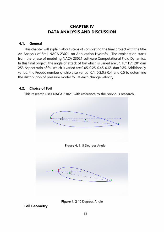
4.2. Choice of Foil
This research uses NACA 23021 with reference to the previous research.
Figure 4. 1. 5 Degrees Angle
Figure 4. 2 10 Degrees Angle
Foil Geometry

14
The foil geometry data is shown in Table.
Table 4. 1 The Coordinate of Foil NACA 23021
#GROUP POINT X-CORD Y-CORD Z-CORD
1 1 1,0000 0,0022 0
1 2 0,9500 0,0153 0
1 3 0,9000 0,0276 0
1 4 0,8000 0,0505 0
1 5 0,7000 0,0709 0
1 6 0,6000 0,0890 0
1 7 0,5000 0,1040 0
1 8 0,4000 0,1149 0
1 9 0,3000 0,1206 0
1 10 0,2500 0,1205 0
1 11 0,2000 0,1180 0
1 12 0,1500 0,1119 0
1 13 0,1000 0,1003 0
1 14 0,0750 0,0913 0
1 15 0,0500 0,0793 0
1 16 0,0250 0,0641 0
1 17 0,0125 0,0487 0
1 18 0,0000 0,0000 0
1 19 0,0125 -0,0208 0
1 20 0,0250 -0,0314 0
1 21 0,0500 -0,0452 0
1 22 0,0750 -0,0555 0
1 23 0,1000 -0,0632 0
1 24 0,1500 -0,0751 0
1 25 0,2000 -0,0830 0
1 26 0,2500 -0,0876 0
1 27 0,3000 -0,0895 0
1 28 0,4000 -0,0883 0
1 29 0,5000 -0,0814 0
1 30 0,6000 -0,0707 0
1 31 0,7000 -0,0572 0
1 32 0,8000 -0,0413 0
1 33 0,9000 -0,0230 0
1 34 0,9500 -0,0130 0
1 35 1,0000 -0,0022 0

15
In this step, every coordinate of foil NACA is illustrated according to types of
NACA which have been decided. The first step is to make points of coordinates in
accordance with NACA hydrofoil dimension is used, in this case used NACA 23021.
Figure 4. 3 Foil Coordinate Configuration
After that point coordinates connected with a curve, the curve is divided into
top and bottom so that the next analysis step becomes easier. Furthermore, the
finished shape of the curve is made into a solid by the parameter of AR are 0.05,
0.25, 0.45, 0.65, and 0.85.
Figure 4. 4 Model Foil with AR 0.05
Figure 4. 5 Model Foil with AR 0.25

16
Figure 4. 6 Model Foil with AR 0.45
Figure 4. 7 Model Foil with AR 0.65
Figure 4. 8 Model Foil with AR 0.85
4.2.1. Meshing
After finishing the model geometry foil, the next step is meshing. This stage is a
detailed division of geometry to be more subtle and specific by mesh sizing
optimization.

17
Before doing meshing, first performed the domain creation process. Domain
size has a standard size of a boundary so that the analysis results can correspond to
the actual state of the environment.
Figure 4. 9 Standard Size of Domain Boundary
The first meshing parameter is the initial mesh, where in the first parameter is
defined geometry size distribution of the entire domain. Domain is divided into
squares to match the domain that has been created.
Figure 4. 10 Start of Meshing
The second parameter defines the parts that should get more improvement than
others, usually found at the end of the domain.
Figure 4. 11 Adaptation of Geometry

18
The third parameter is about repair of first and second parameter where the
meshing will be more subtle and touching every part of the domain geometry. The
fourth parameter is the optimization parameters that follow form part meshing
domain.
Figure 4. 12 Result of Meshing
The fifth parameter is about meshing conditions at the surface of the object. In
this fifth meshing parameters, it requires the size and speed of the ship so that the
result of Reynolds number and Froude numbers are influenced the size and speed
of the ship.
Figure 4. 13 Parameter of Meshing Optimization

19
4.2.2. The setting and Simulation Model
The next process after meshing and geometry definition is a process flow
simulation parameter settings. Here are some parameters that should be defined at
this stage:
a. Flow Conditions
Flow conditions are divided into 2 types where the steady flow fixed flow rate
and unsteady flow in which the genre has a speed changing. The explanation
of the flow that is used in this study was unsteady flow.
b. Type of Fluid
Fluid used is water fluid.
Figure 4. 14 Parameter of Fluid Type
c. Flow Types
The most common of flow turbulence model used in this fluida flow analysis
is model of k-epsilon (Launder-Sharma). Parameter size and speed of the
vessel is required to obtain a value Reynolds Number and Froude Number.

20
Figure 4. 15 Parameter of Flow Type
d. Geometry Boundary Condition
Domain boundaries need to be defined to distinguish the types of
boundaries. The boundary conditions can be a function of the wall that has
a definition of friction value or limit without slip / friction.

21
Figure 4. 16 Parameter of Boundary Condition
e. Other Parameters
Variable Control and Analysis Report defines the number of time step and
period foil movement used. After all the parameters are defined, then we can
do the next process, running simulation process. The process of running the
simulation is computationally data calculation process by the computer (this
software has a relatively heavy load so that the computer used must also
have adequate specification in order the solver process can be executed).
4.3. Result of Model Simulation
Simulated models will produce data such as pressure distribution value at the
lift of foil and Coeffision friction value at the drag of foil. There are five models of
Aspect ratio of NACA 23021, five variations of angle of attack and five velocity
variations are analyzed. Here are the results to the model AR 0.05 with angle of
attack 5° and will be attachement for each model variations.
Table 4. 2 Picture of Simulation results for each variation

22
Aspect
Ratio
Angle of
Attack
Froude
Number Picture of Analysis Result
0.05 5° 0.1 Pressure Distribution
0.2 Pressure Distribution
0.3 Pressure Distribution
0.4 Pressure Distribution
0.5 Pressure Distribution
4.3.1. Discussion
The result of simulation is conducted by the 5 variation of angle of attack, the 5
variation of aspect ratio, and the 5 variation of velocity produces data value analysis

23
foil geometry. Existing data produced include pressure distribution, lift, drag. And
then, The data is plotted become a graph for the review to know the characteristics
from each model which are attachment.
Figure 4.17 The graphic of cartesian pressure
After the graph of cartesian pressure is obtained from all models, then the lift
force on the front of hydrofoil and behind of hydrofoil are calculated. The formula
that used is Bernoulli equiblirium.
P1-P2 = (F1-F2) A
Where :
P1 : Pressure under the Foil (Pa)
P2 : Pressure on the Foil (Pa)
F1 : Lift force under the Foil (Newton)
F2 : Lift force on the Foil (Newton)
A : Surface area of Foil (m2)
The lift force is get from the graph, then the CL value is determined for each
model and to get the CD value is from the simultion result graph. The formula that
used to determine the CL value is:
L = 1/2 ρV2 ApCL
Where,

24
L : lift force
CL : lift coefficient
ρ : fluid density
V : velocity
Ap : plan area (S), area maximum : chord × span
4.3.2. Grafik CL pada AR 0.05
In the graph 4.3.2. Can be seen on the angle of attack 20 ° with Fn 0,1 has the
largest CL ratio with other variation angle, that is equal to 2,233. And it just goes
down by a huge variation. Can be concluded with the largest optimal ratio of CL
is at an attack angle of 15 ° with Fn 0.1.
-1
-0.5
0
0.5
1
1.5
2
2.5
0 5 10 15 20 25 30
CL
Angle of Attack
Graphic of CL from AR 0.05
Fn 0.1 Fn 0.2 Fn 0.3 Fn 0.4 Fn 0.5

25
4.3.3. Grafik CD pada AR 0.05
In graph 4.3.3 2 can be seen that at the angle of attack 10 ° with Fn 0.1 there is an
increase of CD ratio with other Fn variation, that is equal to 0.0283. And the value
immediately decreases at an angle of 15 ° and then rises again at the next corner. It
can be concluded that at fn 0.1 has a high drag coefficient of other fn variations
0
0.005
0.01
0.015
0.02
0.025
0.03
0.035
0.04
0 5 10 15 20 25 30
CD
Angle of Attack
Graphic of CD from AR 0.05
Fn 0.1 Fn 0.2 Fn 0.3 Fn 0.4 Fn 0.5

26
4.3.4. Grafik CL/CD pada AR 0.05
In the graph 4.3.4 it can be seen that at an angle of attack 20 ° with Fn 0.1 there
is an increase in CL / CD ratio with another Fn variation, that is equal to 331. and
the value is directly decreased at an angle of 25 °. At an attack angle of 15 ° with
Fn 0.4 there is a decrease in CL / CD ratio with another Fn variation, that is -112
and the value rises directly as the angular variation increases.
-150
-100
-50
0
50
100
150
200
250
300
350
400
0 5 10 15 20 25 30
CL/
CD
Angle of Attack
Graphic of CL/CD from AR 0.05
Fn 0.1 Fn 0.2 Fn 0.3 Fn 0.4 Fn 0.5

27
4.3.5. Grafik CL pada AR 0.25
In graph 4.3.5 it can be seen that at the angle of attack 15 ° with Fn 0.3 has the
largest CL ratio with other variation angle, that is equal to 2,719. And the value
decreases as the angular variation increases. So it can be concluded that the largest
CL is at an attack angle of 15 ° with Fn 0.3.
-0.5
0
0.5
1
1.5
2
2.5
3
0 5 10 15 20 25 30
CL
Angle of Attack
Graphic of CL from AR 0.25
Fn 0.1 Fn 0.2 Fn 0.3 Fn 0.4 Fn 0.5

28
4.3.6. Grafik CD pada AR 0.25
In graph 4.3.6 it can be seen that at the angle of attack 25 ° with Fn 0.4 has the
largest CD ratio with other Fn variation, that is equal to 0.1805. So it can be
concluded that the largest CD is at an attack angle of 25 ° with Fn 0.4.
0
0.02
0.04
0.06
0.08
0.1
0.12
0.14
0.16
0.18
0.2
0 5 10 15 20 25 30
CD
Angle of Attack
Graphic of CD from AR 0.25
Fn 0.1 Fn 0.2 Fn 0.3 Fn 0.4 Fn 0.5

29
4.3.7. Grafik CL/CD pada AR 0.25
In graph 4.3.7 can be seen that at the angle of attack 15 ° with Fn 0.3
incremented ratio CL / CD with other Fn variation, that is equal to 403. and and
the value decrease with variation of angle with big cave. It can be concluded
that the largest CL / CD is at an attack angle of 15 ° with Fn 0.3.
-50
0
50
100
150
200
250
300
350
400
450
0 5 10 15 20 25 30
CL/
CD
Angle of Attack
Graphic of CL/CD from AR 0.25
Fn 0.1 Fn 0.2 Fn 0.3 Fn 0.4 Fn 0.5

30
4.3.8. Grafik CL pada AR 0.45
In graph 4.3.8 can be seen that at the angle of attack 5 ° with Fn 0.1 has the
largest CL ratio with other angle variation, that is equal to 1.89. And the value
decreases as the angular variation increases. It can be concluded that the largest
CL is at an angle of 5 ° with Fn 0.1.
-0.5
0
0.5
1
1.5
2
2.5
0 5 10 15 20 25 30
CL
Angle of Attack
Graphic of CL from AR 0.45
Fn 0.1 Fn 0.2 Fn 0.3 Fn 0.4 Fn 0.5

31
4.3.9. Grafik CD pada AR 0.45
In graph 4.3.9 can be seen that at the angle of attack 25 ° with Fn 0.4 has the
biggest CD ratio with other variation of angle, that is equal to 0.23. So it can be
concluded that the largest CD is at an attack angle of 25 ° with Fn 0.4.
0
0.05
0.1
0.15
0.2
0.25
0 5 10 15 20 25 30
CD
Angle of Attack
Graphic of CD from AR 0.45
Fn 0.1 Fn 0.2 Fn 0.3 Fn 0.4 Fn 0.5

32
4.3.10. Grafik CL/CD pada AR 0.45
In graph 4.3.10 it can be seen that at the angle of attack 5 ° with Fn 0.1 has the
biggest CL / CD ratio with other angle variation, which is 205. and the value
decreases with increasing angle variation. At Fn 0.1 it also has the largest CL /
CD value of any other Fn value. It can be concluded that the largest CL / CD is
at an angle of 5 ° with Fn 0.1.
-50
0
50
100
150
200
250
0 5 10 15 20 25 30
CL
Angle of Attack
Graphic of CL/CD from AR 0.45
Fn 0.1 Fn 0.2 Fn 0.3 Fn 0.4 Fn 0.5

33
4.3.11. Grafik CL pada AR 0.65
In graph 4.3.11 can be seen that the Fn 0.1 has the largest CL ratio with other
Fn variations and the largest value occurs at an angle of 15 ° that is equal to
2.06. And the value increases as the angular variation increases. It can be
concluded that the largest CL is at an attack angle of 15 ° with Fn 0.1.
-0.5
0
0.5
1
1.5
2
2.5
0 5 10 15 20 25 30
CL
Angle of Attack
Graphic of CL from AR 0.65
Fn 0.1 Fn 0.2 Fn 0.3 Fn 0.4 Fn 0.5

34
4.3.12. Grafik CD pada AR 0.65
In graph 4.3.12 it can be seen that at the angle of attack 25 ° with Fn 0.4 has the
largest CD ratio with other variation of angle, that is equal to 0.247. So it can be
concluded that the largest CD is at an attack angle of 25 ° with Fn 0.4.
0
0.05
0.1
0.15
0.2
0.25
0.3
0 5 10 15 20 25 30
CD
Angle of Attack
Graphic of CD from AR 0.65
Fn 0.1 Fn 0.2 Fn 0.3 Fn 0.4 Fn 0.5

35
4.3.13. Grafik CL/CD pada AR 0.65
In graph 4.3.13 it can be seen that at an angle of attack 15 ° with Fn 0.1 has the
largest CL ratio with other angle variations, which is 253. and the value decreases as
the angle variation increases. It can be concluded that the largest CL / CD is at an
attack angle of 15 ° with Fn 0.1.
-50
0
50
100
150
200
250
300
0 5 10 15 20 25 30
CL
Angle of Attack
Graphic of CL/CD from AR 0.65
Fn 0.1 Fn 0.2 Fn 0.3 Fn 0.4 Fn 0.5

36
4.3.14. Grafik CL pada AR 0.85
In graph 4.3.14 it can be seen that at an angle of attack 15 ° with Fn 0.1 has the
largest CL ratio with other angle variation, which is equal to 1.864. And the value
decreases as the angular variation increases. So it can be concluded that the largest
CL is at an attack angle of 15 ° with Fn 0.1.
-0.5
0
0.5
1
1.5
2
0 5 10 15 20 25 30
CL
Angle of Attack
Graphic of CL from AR 0.85
Fn 0.1 Fn 0.2 Fn 0.3 Fn 0.4 Fn 0.5

37
4.3.15. Grafik CD pada AR 0.85
In graph 4.3.1.15 dapat dilihat bahwa pada sudut serang 20° dengan Fn 0.1
memiliki rasio CD yang paling besar dengan variasi sudut lainnya, yaitu sebesar
2.018. dan nilai tersebut semakin menurun seiring variasi sudut yang bertambah
besar. Sehingga dapat disimpulkan bahwa CD terbesar berada pada sudut
serang 20° dengna Fn 0.1.
0
0.5
1
1.5
2
2.5
3
3.5
4
4.5
0 5 10 15 20 25 30
CD
Angle of Attack
Graphic of CD from AR 0.85
Fn 0.1 Fn 0.2 Fn 0.3 Fn 0.4 Fn 0.5
38
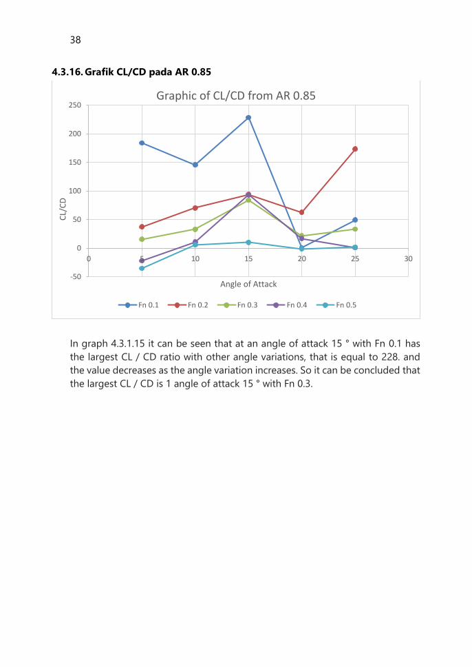
4.3.16. Grafik CL/CD pada AR 0.85
In graph 4.3.1.15 it can be seen that at an angle of attack 15 ° with Fn 0.1 has
the largest CL / CD ratio with other angle variations, that is equal to 228. and
the value decreases as the angle variation increases. So it can be concluded that
the largest CL / CD is 1 angle of attack 15 ° with Fn 0.3.
-50
0
50
100
150
200
250
0 5 10 15 20 25 30
CL/
CD
Angle of Attack
Graphic of CL/CD from AR 0.85
Fn 0.1 Fn 0.2 Fn 0.3 Fn 0.4 Fn 0.5

39
“This page is intentionally left blank”

40
CHAPTER V
CONCLUSION
5.1. Conclusion
According data analysis, the discussion, and simulation result, so it can be
concluded that.
1. At AR 0.05 has a maximum value of CL/CD at angle of attack 20 with fn 0.1
2. At AR 0.25 has a maximum value of CL/CD at angle of attack 15 with fn 0.3
3. At AR 0.45 has a maximum value of CL/CD at angle of attack 15 with fn 0.1
4. At AR 0.65 has a maximum value of CL/CD at angle of attack 15 with fn 0.1
5. At AR 0.85 has a maximum value of CL/CD at angle of attack 15 with fn 0.1
5.2. Recomendation
Recommendation that can be given by the author for further research are :
1. It is needed to get the comparision data by using different software.
2. The addition of analysis by using hydrofoil ship.
3. The different NACA foil analysis to be made as the comparison.
4. Analyze until the stall is reached for comparison by adding variations to the
angle of attack.
5. Meshing should be done more specifically according to guidance from
Numeca to produce more accurate results.

41

42
BIBLIOGRAPHY
[1] Wonggiawan, F., Budiarto, U. & Rindo, G., 2015. Studi Perancangan Hydrofoil
Kapal Penumpang Untuk Perairan Kepulauan Seribu. digilib ITS.
[2] Hidayat, Syahroni. Sawarno, & Hantoro, Ridho. 2009. Studi Eksperimental
Pengaruh Gaya Gelombang Laut Terhadap Pembangkitan Gaya Thrust
Hydrofoil Seri Naca 0012 Dan Naca 0018. Digilib ITS
[3] A.S. Slamet, Suastika Ketut. 2012. Kajian Eksperimental Pengaruh Posisi
Perletakan Hydrofoil Pendukung Terhadap Hambatan Kapal. Surabaya. Jurnal
Teknik Perkapalan
[4] Suryadi, Aji. 2016. Analisa Pengaruh Sudut Serang Hidrofoil Terhadap Gaya
Angkat Kapal Trimaran Hidrofoil. Jurusan Teknik Sistem Perkapalan. Institut
Teknologi Sepuluh Nopember. Surabaya
[5] Chang Cai, Zhigang Zuo, Shuhong Liu and Yulin Wu. 2015. Numerical
investigations of hydrodynamic performance of hydrofoils with leading-edge
protuberances. International Journal Mechanical Engineering.
[6] https://en.wikipedia.org/wiki/Froude_number. Acces at 06 Februari 2017
[7] http://www.kitegeneration.com/kite-surf-fly/wing-geometry-
definitions/#main. Acces at 06 Februari 2017
[8] Hamid Reza Kabarsian, Kyung Chun Kim. 2016. Numerical investigations on flow
structure and behaviour of vortices in the dynamic stall of an oscillating pitching
hydrofoil. International Journal Mechanical Engineering
[9] Ira H. Abbott, Albert E. Von Doenhoff. 1959. Theory of Wing Sections. New York.
USA

43
“This page is intentionally left blank”

44
ATTACHMENT
Distribution of pressure to lift force with AR 0.05
No Angle of
Attack
Froude
Number
Static Pressure (Pa) Plan area
Foil (m2)
Lift
(Newton) Down Upper
1
5
0.1 101128.1626 101080 0.003934 0.189471655
2 0.2 101144.85 101080 0.003934 0.2551199
3 0.3 101280.7 101080 0.003934 0.7895538
4 0.4 101205.2 101080 0.003934 0.4925368
5 0.5 101251.9 101080 0.003934 0.6762546
6
10
0.1 101265 101210 0.003934 0.21637
7 0.2 101263.95 101210 0.003934 0.2122393
8 0.3 101256.35 101210 0.003934 0.1823409
9 0.4 101181.7 101210 0.003934 -0.1113322
10 0.5 101207.15 101210 0.003934 -0.0112119
11
15
0.1 101284.45 101250 0.003934 0.1355263
12 0.2 102157 102050 0.003934 0.420938
13 0.3 101907.35 101650 0.003934 1.0124149
14 0.4 101471.1 101750 0.003934 -1.0971926
15 0.5 101382.95 101250 0.003934 0.5230253
16
20
0.1 101267.3 101200 0.003934 0.2647582
17 0.2 101276.25 101200 0.003934 0.2999675
18 0.3 101265.6 101200 0.003934 0.2580704
19 0.4 101245.55 101200 0.003934 0.1791937
20 0.5 101209.6 101200 0.003934 0.0377664
21
25
0.1 102136.05 102100 0.003934 0.1418207
22 0.2 101952.45 101800 0.003934 0.5997383
23 0.3 97335.8 97300 0.003934 0.1408372
24 0.4 90543.6 90500 0.003934 0.1715224
25 0.5 102408.8 101080 0.003934 5.2274992

45
Distribution of pressure to lift force with AR 0.25
No
Angle
of
Attack
Froude
Number
Static Pressure (Pa) Plan
area Foil
(m2)
Lift
(Newton) Down Upper
1
5
0.1 101275.2 101010 0.814455 44.957916
2 0.2 101271.55 101949.8 0.814455 41.98515525
3 0.3 101240 92333.2 0.814455 16.2891
4 0.4 101179.25 96533.2 0.814455 -33.18904125
5 0.5 101144.9 76666.4 0.814455 -61.1655705
6
10
0.1 101258.25 101060 0.814455 31.15290375
7 0.2 101282.4 101400 0.814455 50.821992
8 0.3 101262.5 102240 0.814455 34.6143375
9 0.4 101218.75 96260 0.814455 -1.01806875
10 0.5 101198.25 100720 0.814455 -17.71439625
11
15
0.1 101273.4 100240 0.814455 43.491897
12 0.2 102081.2 98060 0.814455 66.133746
13 0.3 101957.65 94720 0.814455 600.7827307
14 0.4 101571.35 91740 0.814455 286.1587643
15 0.5 101372.25 82720 0.814455 124.0007738
16
20
0.1 101266.1 99420 0.814455 37.5463755
17 0.2 101275.85 95140 0.814455 45.48731175
18 0.3 101260.3 87740 0.814455 32.8225365
19 0.4 105754.85 78560 0.814455 28.38375675
20 0.5 101211.5 60260 0.814455 -6.9228675
21
25
0.1 102138.95 98520 0.814455 31.72302225
22 0.2 101952.2 89360 0.814455 107.670951
23 0.3 102204 72000 0.814455 68.41422
24 0.4 86617.5 39660 0.814455 95.6984625
25 0.5 102448.6 36680 0.814455 1000.639413
46
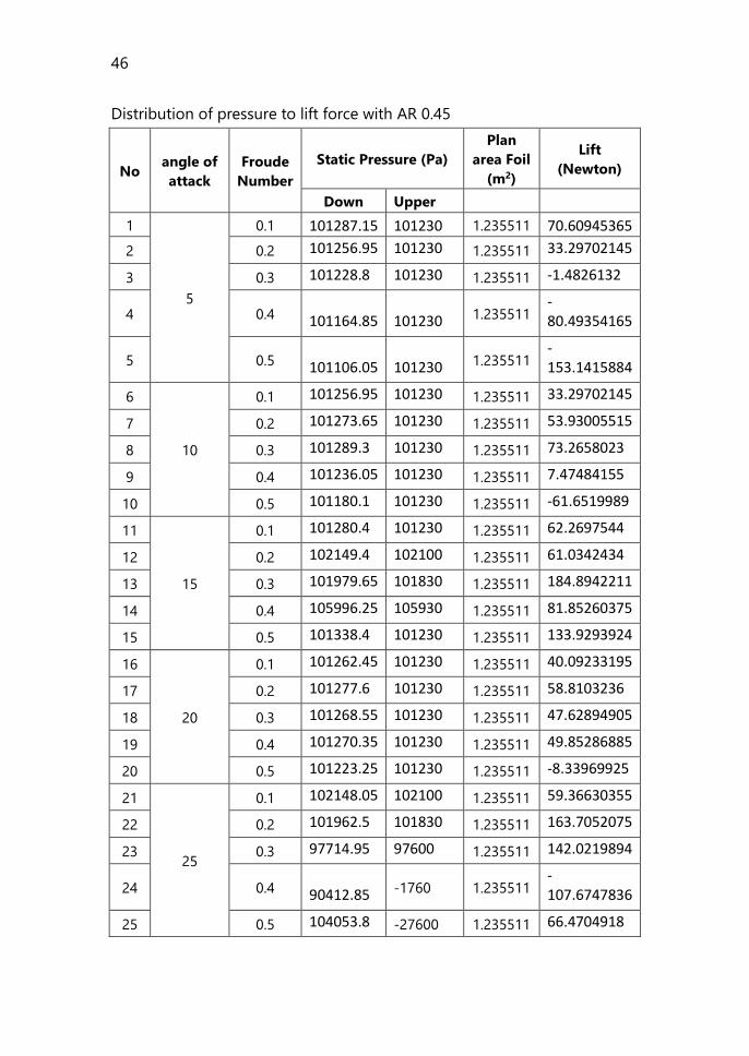
Distribution of pressure to lift force with AR 0.45
No angle of
attack
Froude
Number
Static Pressure (Pa)
Plan
area Foil
(m2)
Lift
(Newton)
Down Upper
1
5
0.1 101287.15 101230 1.235511 70.60945365
2 0.2 101256.95 101230 1.235511 33.29702145
3 0.3 101228.8 101230 1.235511 -1.4826132
4 0.4 101164.85 101230 1.235511 -80.49354165
5 0.5 101106.05 101230 1.235511 -153.1415884
6
10
0.1 101256.95 101230 1.235511 33.29702145
7 0.2 101273.65 101230 1.235511 53.93005515
8 0.3 101289.3 101230 1.235511 73.2658023
9 0.4 101236.05 101230 1.235511 7.47484155
10 0.5 101180.1 101230 1.235511 -61.6519989
11
15
0.1 101280.4 101230 1.235511 62.2697544
12 0.2 102149.4 102100 1.235511 61.0342434
13 0.3 101979.65 101830 1.235511 184.8942211
14 0.4 105996.25 105930 1.235511 81.85260375
15 0.5 101338.4 101230 1.235511 133.9293924
16
20
0.1 101262.45 101230 1.235511 40.09233195
17 0.2 101277.6 101230 1.235511 58.8103236
18 0.3 101268.55 101230 1.235511 47.62894905
19 0.4 101270.35 101230 1.235511 49.85286885
20 0.5 101223.25 101230 1.235511 -8.33969925
21
25
0.1 102148.05 102100 1.235511 59.36630355
22 0.2 101962.5 101830 1.235511 163.7052075
23 0.3 97714.95 97600 1.235511 142.0219894
24 0.4 90412.85 -1760 1.235511 -107.6747836
25 0.5 104053.8 -27600 1.235511 66.4704918

47
Distribution of pressure to lift force with AR 0.65
No Angle of
attack
Froude
Number
Static pressure (Pa) Plan
area Foil
(m2)
Lift (Newton) Down Up
1
5
0.1 101278.35 101220 1.656567 96.66068445
2 0.2 101256.55 101220 1.656567 60.54752385
3 0.3 101209 101220 1.656567 -18.222237
4 0.4 101167.3 101220 1.656567 -87.3010809
5 0.5 101103.35 101220 1.656567 -193.2385405
6
10
0.1 101256.4 101220 1.656567 60.2990388
7 0.2 101273.5 101220 1.656567 88.6263345
8 0.3 101263.75 101220 1.656567 72.47480625
9 0.4 101215.85 101220 1.656567 -6.87475305
10 0.5 101198.35 101220 1.656567 -35.86467555
11
15
0.1 101282.3 101220 1.656567 103.2041241
12 0.2 102151.3 102040 1.656567 184.3759071
13 0.3 102019.15 101780 1.656567 396.167998
14 0.4 101545.8 101220 1.656567 539.7095286
15 0.5 101381.15 101220 1.656567 266.955772
16
20
0.1 101264.7 101220 1.656567 74.0485449
17 0.2 101275.65 101220 1.656567 92.18795355
18 0.3 101264.4 101220 1.656567 73.5515748
19 0.4 101261.15 101220 1.656567 68.16773205
20 0.5 101215.5 101220 1.656567 -7.4545515
21
25
0.1 102152.8 102110 1.656567 70.9010676
22 0.2 101938.35 101780 1.656567 262.3173845
23 0.3 97463.75 97400 1.656567 105.6061463
24 0.4 90423.35 33060 1.656567 146672.4422
25 0.5 103837.05 11528 1.656567 208515.4014

48
Distribution of pressure to lift force with AR 0.85
No Angle of attack
Froude Number
Static pressure (Pa) Plan area
Foil (m2)
Lift (Newton)
Down Upper
1
5
0.1 101271.1 101220 2.077622 106.1664842
2 0.2 101255.15 101220 2.077622 73.0284133
3 0.3 101247.95 101220 2.077622 58.0695349
4 0.4 101155.6 101220 2.077622 -133.7988568
5 0.5 101056.35 101220 2.077622 -340.0028403
6
10
0.1 101255.85 101220 2.077622 74.4827487
7 0.2 101281.2 101220 2.077622 127.1504664
8 0.3 101279.7 101220 2.077622 124.0340334
9 0.4 101250.75 101220 2.077622 63.8868765
10 0.5 101245.4 101220 2.077622 52.7715988
11
15
0.1 101286.2 101230 2.077622 116.7623564
12 0.2 102181.85 102100 2.077622 170.0533607
13 0.3 102032.85 101880 2.077622 317.5645227
14 0.4 101494.95 101230 2.077622 550.4659489
15 0.5 101274.7 101230 2.077622 92.8697034
16
20
0.1 101267.35 101220 2.077622 98.3754017
17 0.2 101274.7 101220 2.077622 113.6459234
18 0.3 101259.4 101220 2.077622 81.8583068
19 0.4 101267.1 101220 2.077622 97.8559962
20 0.5 101214.2 101220 2.077622 -12.0502076
21
25
0.1 102182.3 102130 2.077622 108.6596306
22 0.2 101971.4 101820 2.077622 314.5519708
23 0.3 99948.95 99900 2.077622 101.6995969
24 0.4 90495.5 90400 2.077622 198.412901
25 0.5 103294.45 103220 2.077622 154.6789579

49
CL CD CL/CD foil With AR 0.05
No Angle of Attack
Froude Number
CL CD CL/CD
1
5
0.1 1.831757093 0.00922 198.6721359
2 0.2 0.427658868 0.0078 54.82806005
3 0.3 0.073742234 0.006665 11.06410113
4 0.4 -
0.084515514 0.006665 -12.68049715
5 0.5 -
0.099684752 0.006165 -16.16946504
6
10
0.1 1.269288203 0.008167 155.4167017
7 0.2 0.517670483 0.00724 71.5014479
8 0.3 0.156702247 0.0067325 23.27549161
9 0.4 -0.0025925 0.00591125 -0.438570592
10 0.5 -
0.028870085 0.0058575 -4.928738305
11
15
0.1 1.772025884 0.008167 216.9739052
12 0.2 0.673635308 0.00724 93.0435508
13 0.3 2.719797946 0.0067325 403.9803856
14 0.4 0.728700017 0.00591125 123.2734221
15 0.5 0.202090592 0.0058575 34.50116813
16
20
0.1 1.529782645 0.008167 187.3126784
17 0.2 0.463331674 0.00724 63.99608759
18 0.3 0.148590602 0.0067325 22.07064264
19 0.4 0.072278912 0.00591125 12.22734812
20 0.5 -
0.011282562 0.0058575 -1.92617359
21
25
0.1 1.292517007 0.03584 36.06353256
22 0.2 1.096731375 0.018515 59.23474888
23 0.3 0.309717383 0.0056615 54.70588764
24 0.4 0.243695039 0.1805 1.350111019
25 0.5 1.630794757 0.0617345 26.41626249

50
CL CD CL/CD foil with AR 0.25
No Angle of Attack
Froude Number
CL CD CL/CD
1
5
0.1 1.831757093 0.00922 198.6721359
2 0.2 0.427658868 0.0078 54.82806005
3 0.3 0.073742234 0.006665 11.06410113
4 0.4 -0.084515514 0.006665 -12.68049715
5 0.5 -0.099684752 0.006165 -16.16946504
6
10
0.1 1.269288203 0.008167 155.4167017
7 0.2 0.517670483 0.00724 71.5014479
8 0.3 0.156702247 0.0067325 23.27549161
9 0.4 -0.0025925 0.00591125 -0.438570592
10 0.5 -0.028870085 0.0058575 -4.928738305
11
15
0.1 1.772025884 0.008167 216.9739052
12 0.2 0.673635308 0.00724 93.0435508
13 0.3 2.719797946 0.0067325 403.9803856
14 0.4 0.728700017 0.00591125 123.2734221
15 0.5 0.202090592 0.0058575 34.50116813
16
20
0.1 1.529782645 0.008167 187.3126784
17 0.2 0.463331674 0.00724 63.99608759
18 0.3 0.148590602 0.0067325 22.07064264
19 0.4 0.072278912 0.00591125 12.22734812
20 0.5 -0.011282562 0.0058575 -1.92617359
21
25
0.1 1.292517007 0.03584 36.06353256
22 0.2 1.096731375 0.018515 59.23474888
23 0.3 0.309717383 0.0056615 54.70588764
24 0.4 0.243695039 0.1805 1.350111019
25 0.5 1.630794757 0.0617345 26.41626249

51
CL CD CL/CD foil with AR 0.45
No Angle of Attack
Froude Number
CL CD CL/CD
1
5
0.1 1.896465903 0.00922 205.6904451
2 0.2 0.223577236 0.0078 28.66374818
3 0.3 -0.004424534 0.006665 -0.663846068
4 0.4 -0.135121122 0.006075 -22.24215994
5 0.5 -0.164526298 0.006165 -26.68715301
6
10
0.1 0.894308943 0.008167 109.502748
7 0.2 0.362120458 0.00724 50.01663784
8 0.3 0.218645724 0.0067325 32.47615654
9 0.4 0.012547702 0.00591125 2.122681668
10 0.5 -0.066235275 0.0058575 -11.30777202
11
15
0.1 1.672473868 0.008167 204.7843599
12 0.2 0.409822466 0.00724 56.60531292
13 0.3 0.551776266 0.0067325 81.95711341
14 0.4 0.137402522 0.00591125 23.2442414
15 0.5 0.143885847 0.0058575 24.56437849
16
20
0.1 1.076820972 0.008167 131.8502476
17 0.2 0.394889663 0.00724 54.54277116
18 0.3 0.142138156 0.0067325 21.11224004
19 0.4 0.083685913 0.00591125 14.15705873
20 0.5 -0.008959681 0.0058575 -1.529608439
21
25
0.1 1.594491455 0.0347485 45.88662691
22 0.2 1.099220176 0.0174875 62.85747968
23 0.3 0.42383349 0.0051045 83.03134294
24 0.4 -0.180749129 0.236595 -0.763960054
25 0.5 0.071411979 0.096798 0.737742303

52
CL CD CL/CD foil dengan AR 0.65
No Angle of Attack
Froude Number
CL CD CL/CD
1
5
0.1 1.93628671 0.00922 210.0094045
2 0.2 0.303218849 0.0078 38.87421135
3 0.3 -0.040558229 0.006665 -6.085255621
4 0.4 -0.109299817 0.006075 -17.9917395
5 0.5 -0.154836569 0.006165 -25.11542073
6
10
0.1 1.207897793 0.008167 147.8998155
7 0.2 0.443836071 0.00724 61.30332473
8 0.3 0.161311137 0.0067325 23.9600649
9 0.4 -0.008607101 0.00591125 -1.456054367
10 0.5 -0.028737349 0.0058575 -4.906077439
11
15
0.1 2.067363531 0.008167 253.1362227
12 0.2 0.923344948 0.00724 127.5338326
13 0.3 0.881772763 0.0067325 130.9725605
14 0.4 0.675709308 0.00591125 114.3090392
15 0.5 0.213904098 0.0058575 36.51798519
16
20
0.1 1.483325037 0.008167 181.624224
17 0.2 0.461672474 0.00724 63.76691628
18 0.3 0.16370776 0.0067325 24.316043
19 0.4 0.085345114 0.00591125 14.4377439
20 0.5 -0.005973121 0.0058575 -1.01973896
21
25
0.1 1.420275427 0.034665 40.97145326
22 0.2 1.31367181 0.017815 73.73964694
23 0.3 0.235053371 0.00567 41.45562098
24 0.4 0.048427908 0.24758 0.195605088
25 0.5 0.062452298 0.080842 0.772522921

53
CL CD CL/CD foil with AR 0.85
No Angle of Attack
Froude Number
CL CD CL/CD
1
5
0.1 1.695702671 0.00922 183.915691
2 0.2 0.291604447 0.0078 37.38518547
3 0.3 0.103054772 0.006665 15.46208133
4 0.4 -0.133565621 0.006075 -21.98611051
5 0.5 -0.217222499 0.006165 -35.23479299
6
10
0.1 1.18964659 0.008167 145.6650655
7 0.2 0.507715281 0.00724 70.12642006
8 0.3 0.220120569 0.0067325 32.69521999
9 0.4 0.06377551 0.00591125 10.78883658
10 0.5 0.033714949 0.0058575 5.755859905
11
15
0.1 1.864941098 0.008167 228.3508141
12 0.2 0.679027709 0.00724 93.78835755
13 0.3 0.563575024 0.0067325 83.70962102
14 0.4 0.549506388 0.00591125 92.95942278
15 0.5 0.059333001 0.0058575 10.129407
16
20
0.1 1.571262651 4.018885 0.390969797
17 0.2 0.453791273 0.00724 62.67835257
18 0.3 0.145272201 0.0067325 21.57774987
19 0.4 0.097685416 0.00591125 16.52533992
20 0.5 -0.007698689 0.0058575 -1.314330215
21
25
0.1 1.735523478 0.035085 49.46625275
22 0.2 1.256014601 0.00724 173.4826797
23 0.3 0.180484118 0.0054337 33.21569424
24 0.4 0.198067032 0.25368 0.780775117
25 0.5 0.098821968 0.0623665 1.584536054

54
Attachment 1. AR 0.05 with angle of attack 5º
Figure 1. Distribution Static Pressure Fn 0.1
Figure 2. Coefficien Friction Fn 0.1

55
Figure 3. Distribution Static Pressure Fn 0.2
Figure 4. Coefficien Friction Fn 0.2
Figure 5. Distribution Static Pressure Fn 0.3

56
Figure 6. Coefficien Friction Fn 0.3
Figure 7. Distribution Static Pressure Fn 0.4
Figure 8. Coefficient Friction Fn 0.4

57
Figure 9. Distribution Static Pressure Fn 0.5
Figure 10. Coefficien Friction Fn 0.5

58
Attachment 2. AR 0.25 with angle of attack 5°
Figure 11. Distribution Static Pressure Fn 0.1
Figure 12. Coefficien Friction Fn 0.1
Figure 13. Distribution Static Pressure Fn 0.2

59
Figure 14. Coefficien Friction Fn 0.2
Figure 15. Distribution Static Pressure Fn 0.3
Figure 16. Coefficien Friction Fn 0,3

60
Figure 17. Distribution Static Pressure Fn 0.4
Figure 18. Coefficien Friction Fn 0.4
Figure 19. Distribution Static Pressure Fn 0.5
61
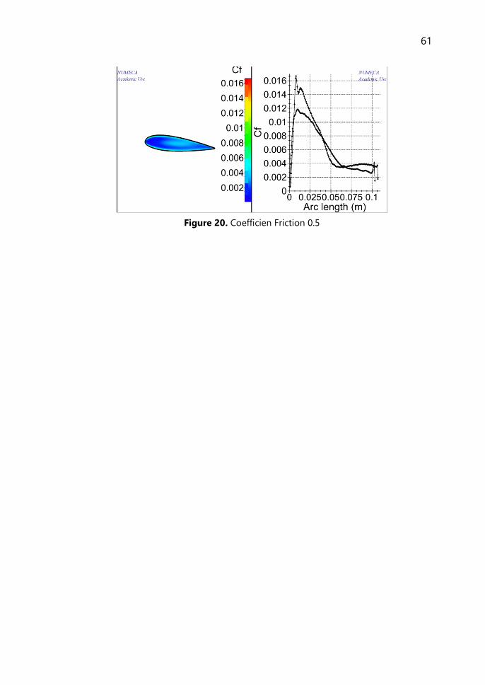
Figure 20. Coefficien Friction 0.5

62
Attachment 3. AR 0.45 with angle of attack 5°
Figure 21. Distribution Static Pressure Fn 0.1
Figure 22. Coefficien Friction Fn 0.1
Figure 23. Distribution Static Pressure Fn 0.2
63
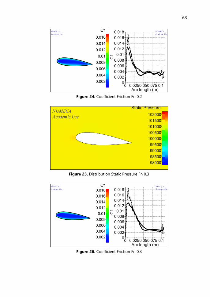
Figure 24. Coefficient Friction Fn 0.2
Figure 25. Distribution Static Pressure Fn 0.3
Figure 26. Coefficient Friction Fn 0,3

64
Figure 27. Distribution Static Pressure Fn 0.4
Figure 28. Coefficien Friction Fn 0.4
Figure 29. Distribution Static Pressure Fn 0.5

65
Figure 30. Coefficien Friction Fn 0.5
66
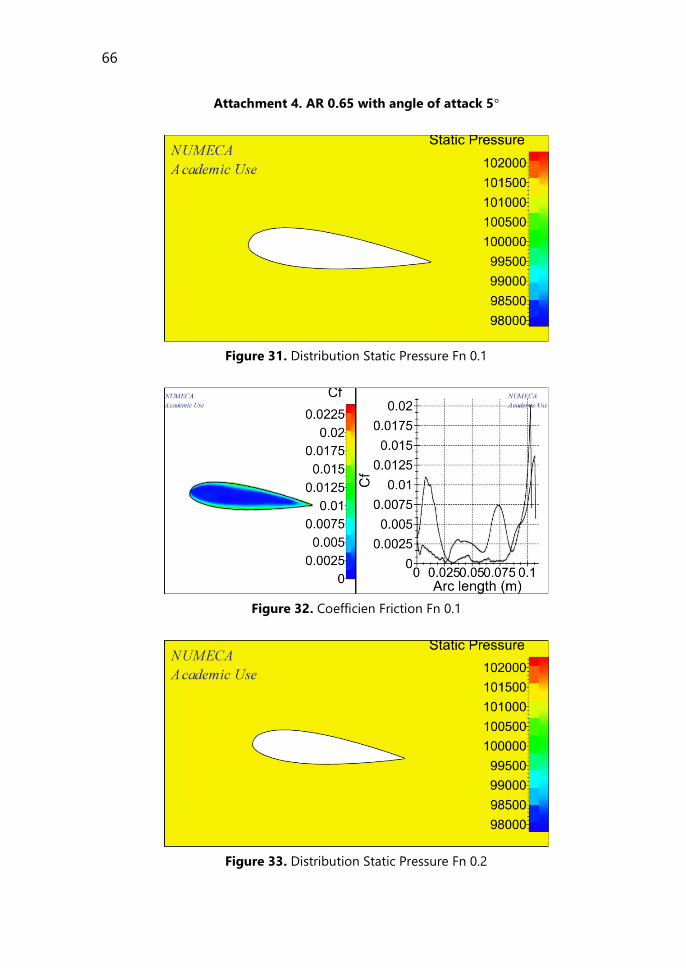
Attachment 4. AR 0.65 with angle of attack 5°
Figure 31. Distribution Static Pressure Fn 0.1
Figure 32. Coefficien Friction Fn 0.1
Figure 33. Distribution Static Pressure Fn 0.2

67
Figure 34. Coefficien Friction Fn 0.2
Figure 35. Distribution Static Pressure Fn 0.3
Figure 36. Coefficien Friction Fn 0.3

68
Figure 37. Distribution Static Pressure Fn 0.4
Figure 38. Coefficien Friction Fn 0.4
Figure 39. Distribution Static Pressure Fn 0.5

69
Figure 40. Coefficien Friction Fn 0.5

70
Attachment 5. AR 0.85 with angle of attack 5°
Figure 41. Distribution Static Pressure Fn 0.1
Figure 42. Coefficien Friction Fn 0.1
Figure 43. Distribution Static Pressure Fn 0.2

71
Figure 44. Coefficien Friction Fn 0.2
Figure 45. Distribution Static Pressure Fn 0.3
Figure 46. Coefficien Friction Fn 0.3

72
Figure 47. Distribution Static Pressure Fn 0.4
Figure 48. Coefficien Friction Fn 0.4
Figure 49. Distribution Static Pressure Fn 0.5

73
Figure 50. Coefficien Friction Fn 0.5
74
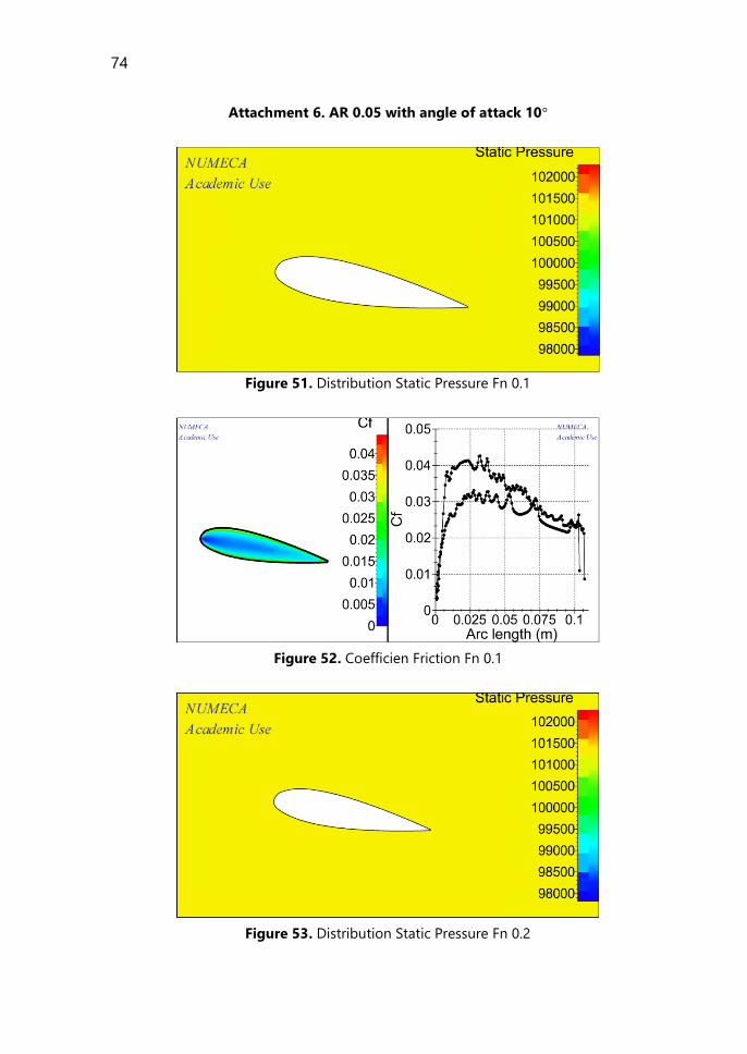
Attachment 6. AR 0.05 with angle of attack 10°
Figure 51. Distribution Static Pressure Fn 0.1
Figure 52. Coefficien Friction Fn 0.1
Figure 53. Distribution Static Pressure Fn 0.2

75
Figure 54. Coefficien Friction Fn 0.2
Figure 55. Distribution Static Pressure Fn 0.3
Figure 56. Coefficien Friction Fn 0.3

76
Figure 57. Distribution Static Pressure Fn 0.4
Figure 58. Coefficien Friction Fn 0.4
Figure 59. Distribution Static Pressure Fn 0.5

77
Figure 60. Coefficien Friction Fn 0.5

78
Attachment 7. AR 0.25 with angle of attack 10°
Figure 61. Distribution Static Pressure Fn 0.1
Figure 62. Coefficien Friction Fn 0.1
Figure 63. Distribution Static Pressure Fn 0.2

79
Figure 64. Coefficien Friction Fn 0.2
Figure 65. Distribution Static Pressure Fn 0.3
Figure 66. Coefficien Friction Fn 0.3

80
Figure 67. Distribution Static Pressure Fn 0.4
Figure 68. Coefficien Friction Fn 0.4
Figure 69. Distribution Static Pressure Fn 0.5

81
Figure 70. Coefficien Friction Fn 0.5
82
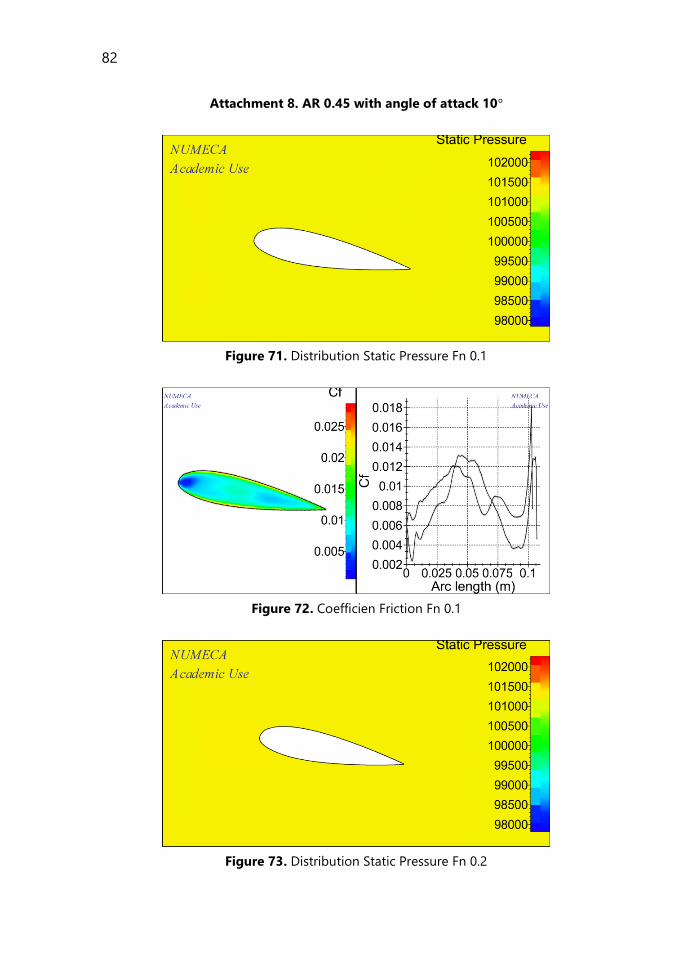
Attachment 8. AR 0.45 with angle of attack 10°
Figure 71. Distribution Static Pressure Fn 0.1
Figure 72. Coefficien Friction Fn 0.1
Figure 73. Distribution Static Pressure Fn 0.2

83
Figure 74. Coefficient Friction Fn 0,2
Figure 75. Distribution Static Pressure Fn 0.3
Figure 76. Coefficient Friction Fn 0.3

84
Figure 77. Distribution Static Pressure Fn 0.4
Figure 78. Coefficient Friction Fn 0.4
Figure 79. Distribution Static Pressure Fn 0.5

85
Figure 80. Coefficient Friction Fn 0.5

86
Attachment 9. AR 0.65 with angle of attack 10°
Figure 81. Distribution Static Pressure Fn 0.1
Figure 82. Coefficient Friction Fn 0.1
Figure 83. Distribution Static Pressure Fn 0.2

87
Figure 84. Coefficient Friction Fn 0.2
Figure 85. Distribution Static Pressure Fn 0.3
Figure 86. Coefficient Friction Fn 0.3

88
Figure 87. Distribution Static Pressure Fn 0.4
Figure 88. Coefficient Friction Fn 0.4
Figure 89. Distribution Static Pressure Fn 0.5

89
Figure 90. Coefficient Friction Fn 0.5

90
Lampiran 1. AR 0.85 with angle of attack 10°
Figure 91. Distribution Static Pressure Fn 0.1
Figure 92. Coefficient Friction Fn 0.1
Figure 93. Distribution Static Pressure Fn 0.2

91
Figure 94. Coefficient Friction Fn 0.2
Figure 95. Distribution Static Pressure Fn 0.3
Figure 96. Coefficient Friction Fn 0.3

92
Figure 97. Distribution Static Pressure Fn 0.4
Figure 98. Coefficient Friction Fn 0.4
Figure 99. Distribution Static Pressure Fn 0.5

93
Figure 100. Coefficient Friction Fn 0.5

94
Lampiran 2. AR 0.05 with angle of attack 15°
Figure 101. Distribution Static Pressure Fn 0.1
Figure 102. Coefficient Friction Fn 0.1
Figure 103. Distribution Static Pressure Fn 0.2

95
Figure 104. Coefficient Friction Fn 0.2
Figure 105. Distribution Static Pressure Fn 0.3
Figure 106. Coefficient Friction Fn 0.3

96
Figure 107. Distribution Static Pressure Fn 0.4
Figure 108, Coefficient Friction Fn 0.4
Figure 109. Distribution Static Pressure Fn 0.5

97
Figure 110. Coefficient Friction Fn 0.5

98
Lampiran 3. AR 0.25 with angle of attack 15°
Figure 111. Distribution Static Pressure Fn 0.1
Figure 112. Coefficient Friction Fn 0.1
Figure 113. Distribution Static Pressure Fn 0.2

99
Figure 114. Coefficient Friction Fn 0.2
Figure 115. Distribution Static Pressure Fn 0.3
Figure 116. Coefficient Friction Fn 0.3

100
Figure 117. Distribution Static Pressure Fn 0.4
Figure 118. Coefficient Friction Fn 0.4
Figure 119. Distribution Static Pressure Fn 0.5

101
Figure 120. Coefficient Friction Fn 0.5
102
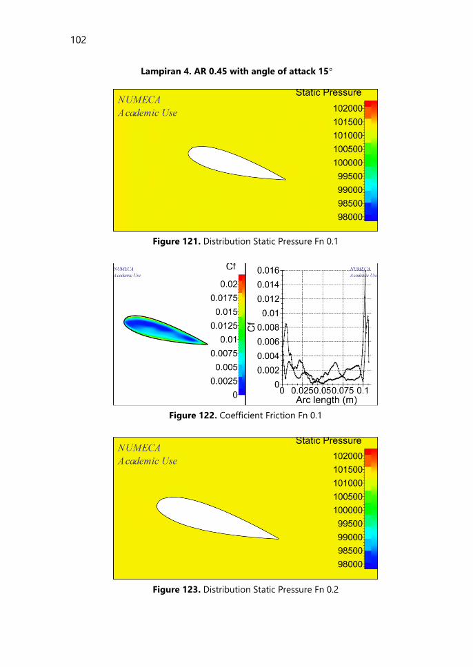
Lampiran 4. AR 0.45 with angle of attack 15°
Figure 121. Distribution Static Pressure Fn 0.1
Figure 122. Coefficient Friction Fn 0.1
Figure 123. Distribution Static Pressure Fn 0.2

103
Figure 124. Coefficient Friction Fn 0.2
Figure 125. Distribution Static Pressure Fn 0.3
Figure 126. Coefficient Friction Fn 0.3

104
Figure 127. Distribution Static Pressure Fn 0.4
Figure 128. Coefficient Friction Fn 0.4
Figure 129. Distribution Static Pressure Fn 0.5

105
Figure 130. Coefficient Friction Fn 0.5

106
Lampiran 5. AR 0.65 with angle of attack 15°
Figure 131. Distribution Static Pressure Fn 0.1
Figure 132. Coefficient Friction Fn 0.1
Figure 133. Distribution Static Pressure Fn 0.2

107
Figure 134. Coefficient Friction Fn 0.2
Figure 135. Distribution Static Pressure Fn 0.3
Figure 136. Coefficient Friction Fn 0.3

108
Figure 137. Distribution Static Pressure Fn 0.4
Figure 138. Coefficient Friction Fn 0.4
Figure 139. Distribution Static Pressure Fn 0.5

109
Figure 140. Coefficient Friction Fn 0.5

110
Lampiran 6. AR 0.85 with angle of attack 15°
Figure 141. Distribution Static Pressure Fn 0.1
Figure 142. Coefficient Friction Fn 0.1
Figure 143. Distribution Static Pressure Fn 0.2

111
Figure 144. Coefficient Friction Fn 0.2
Figure 145. Distribution Static Pressure Fn 0.3
Figure 146. Coefficient Friction Fn 0.3

112
Figure 147. Distribution Static Pressure Fn 0.4
Figure 148. Coefficient Friction Fn 0.4
Figure 149. Distribution Static Pressure Fn 0.5

113
Figure 150. Coefficient Friction Fn 0.5

114
Lampiran 7. AR 0.05 with angle of attack 20°
Figure 151. Distribution Static Pressure Fn 0.1
Figure 152. Coefficient Friction Fn 0.1
Figure 153. Distribution Static Pressure Fn 0.2

115
Figure 154. Coefficient Friction Fn 0.2
Figure 155. Distribution Static Pressure Fn 0.3
Figure 156. Coefficient Friction Fn 0.3

116
Figure 157. Distribution Static Pressure Fn 0.4
Figure 158. Coefficient Friction Fn 0.4
Figure 159. Distribution Static Pressure Fn 0.5

117
Figure 160. Coefficient Friction Fn 0.5

118
Lampiran 8. AR 0.25 with angle of attack 20°
Figure 161. Distribution Static Pressure Fn 0.1
Figure 162. Coefficient Friction Fn 0.1
Figure 163. Distribution Static Pressure Fn 0.2

119
Figure 164. Coefficient Friction Fn 0.2
Figure 165. Distribution Static Pressure Fn 0.3
Figure 166. Coefficient Friction Fn 0.3

120
Figure 167. Distribution Static Pressure Fn 0.4
Figure 168. Coefficient Friction Fn 0.4
Figure 169. Distribution Static Pressure Fn 0.5

121
Figure 170. Coefficient Friction Fn 0.5

122
Lampiran 9. AR 0.45 with angle of attack 20°
Figure 171. Distribution Static Pressure Fn 0.1
Figure 172. Coefficient Friction Fn 0.1
Figure 173. Distribution Static Pressure Fn 0.2

123
Figure 174. Coefficient Friction Fn 0.2
Figure 175. Distribution Static Pressure Fn 0.3
Figure 176. Coefficient Friction Fn 0.3

124
Figure 177. Distribution Static Pressure Fn 0.4
Figure 178. Coefficient Friction Fn 0.4
Figure 179. Distribution Static Pressure Fn 0.5

125
Figure 180. Coefficient Friction Fn 0.5

126
Lampiran 10. AR 0.65 with angle of attack 20°
Figure 181. Distribution Static Pressure Fn 0.1
Figure 182. Coefficient Friction Fn 0.1
Figure 183. Distribution Static Pressure Fn 0.2

127
Figure 184. Coefficient Friction Fn 0.2
Figure 185. Distribution Static Pressure Fn 0.3
Figure 186. Coefficient Friction Fn 0.3

128
Figure 187. Distribution Static Pressure Fn 0.4
Figure 188. Coefficient Friction Fn 0.4
Figure 189. Distribution Static Pressure Fn 0.5

129
Figure 190. Coefficient Friction Fn 0.5

130
Lampiran 11. AR 0.85 with angle of attack 20°
Figure 191. Distribution Static Pressure Fn 0.1
Figure 192. Coefficient Friction Fn 0.1
Figure 193. Distribution Static Pressure Fn 0.2

131
Figure 194. Coefficient Friction Fn 0.2
Figure 195. Distribution Static Pressure Fn 0.3
Figure 196. Coefficient Friction Fn 0.3

132
Figure 197. Distribution Static Pressure Fn 0.4
Figure 198. Coefficient Friction Fn 0.4
Figure 199. Distribution Static Pressure Fn 0.5

133
Figure 200. Coefficient Friction Fn 0.5

134
Attachment 210. AR 0.05 with angle of attack 25°
Figure 201. Distribution Static Pressure Fn 0.1
Figure 202. Coefficient Friction Fn 0.1
Figure 203. Distribution Static Pressure Fn 0.2

135
Figure 204. Coefficient Friction Fn 0.2
Figure 205. Distribution Static Pressure Fn 0.3
Figure 206. Coefficient Friction Fn 0.3

136
Figure 207. Distribution Static Pressure Fn 0.4
Figure 208. Coefficient Friction Fn 0.4
Figure 209. Distribution Static Pressure Fn 0.5

137
Figure 210. Coefficient Friction Fn 0.5

138
Attachment 211. AR 0.25 with angle of attack 25°
Figure 211. Distribution Static Pressure Fn 0.1
Figure 212. Coefficient Friction Fn 0.1
Figure 213. Distribution Static Pressure Fn 0.2

139
Figure 214. Coefficient Friction Fn 0.2
Figure 215. Distribution Static Pressure Fn 0.3
Figure 216. Coefficient Friction Fn 0.3

140
Figure 217. Distribution Static Pressure Fn 0.4
Figure 218. Coefficient Friction Fn 0.4
Figure 219. Distribution Static Pressure Fn 0.5

141
Figure 220. Coefficient Friction Fn 0.5

142
Attachment 212. AR 0.45 with angle of attack 25°
Figure 221. Distribution Static Pressure Fn 0.1
Figure 222. Coefficient Friction Fn 0.1
Figure 223. Distribution Static Pressure Fn 0.2

143
Figure 224. Coefficient Friction Fn 0.2
Figure 225. Distribution Static Pressure Fn 0.3
Figure 226. Coefficient Friction Fn 0.3

144
Figure 227. Distribution Static Pressure Fn 0.4
Figure 228. Coefficient Friction Fn 0.4
Figure 229. Distribution Static Pressure Fn 0.5

145
Figure 230. Coefficient Friction Fn 0.5

146
Attachment 213. AR 0.65 with angle of attack 25°
Figure 231. Distribution Static Pressure Fn 0.1
Figure 232. Coefficient Friction Fn 0.1
Figure 233. Distribution Static Pressure Fn 0.2

147
Figure 234. Coefficient Friction Fn 0.2
Figure 235. Distribution Static Pressure Fn 0.3
Figure 236. Coefficient Friction Fn 0.3

148
Figure 237. Distribution Static Pressure Fn 0.4
Figure 238. Coefficient Friction Fn 0.4
Figure 239. Distribution Static Pressure Fn 0.5

149
Figure 240. Coefficient Friction Fn 0.5


1
Attachment 214. AR 0.85 with angle of attack 25°
Figure 241. Distribution Static Pressure Fn 0.1
Figure 242. Coefficient Friction Fn 0.1
Figure 243. Distribution Static Pressure Fn 0.2

2
Figure 244. Coefficient Friction Fn 0.2
Figure 245. Distribution Static Pressure Fn 0.3
Figure 246. Coefficient Friction Fn 0.3

3
Figure 247. Distribution Static Pressure Fn 0.4
Figure 248. Coefficient Friction Fn 0.4
Figure 249. Distribution Static Pressure Fn 0.5

4
Figure 250. Coefficient Friction Fn 0.5

5

6
BIOGRAPHY
The author was born in Banjarmasin, 12 February 1995,
the author is the first child of two in her family and taken
formal education at MIN Teluk Dalam Banjarmasin
Elementary School, SMPN 2 Banjarmasin Junior High
School, and SMAN 1 Banjarmasin Senior High School.
The author was graduated from SMAN 1 Banjarmasin in
2013, then continuing to bachelor degree and
accepted at Institut Teknologi
Sepuluh Nopember (ITS), Faculty of Marine Technology,
Department of Marine Engineering in Double Degree Program with Hochschule
Wismar Germany in 2013 and registered with student number 4213101005.
The author has keen of learning, not only in classes but also by doing job
training, proved by job training at shipyard company, PT. IMS Indonesia
(Persero) in 2015 and reliability engineering company, PT. Antakusuma Inti
Raharja in 2016. The author take the Marine Manufacturing and Design (MMD)
Laboratory for her concern to do research for this final project. During studying
in Department of Marine Engineering, the author expect to be patient person,
having good personality, friendly to everyone, and to helpful for the family,
country, and community.
The author contact :
Phone : +628978703631
Email : [email protected]