Analysis of Site Response and BuildingDamage Distribution Induced by the31 October 2002 Earthquake at SanGiuliano di Puglia (Italy)

Rodolfo Puglia,a) Marco Vona,b) Peter Klin,c) Chiara Ladina,d)

Angelo Masi,b) Enrico Priolo,c) and Francesco Silvestrie)

This paper concerns the analysis of the site amplification that significantlyinfluenced the non-uniform damage distribution observed at San Giuliano diPuglia (Italy) after the 2002 Molise earthquake (MW ¼ 5.7). In fact, the historicalcore of the town, settled on outcropping rock, received less damage than the morerecent buildings, founded on a clayey subsoil. Comprehensive geotechnical andgeophysical investigations allowed a detailed definition of the subsoil model. Theseismic response of the subsoil was analyzed through 2-D finite-element and 3-Dspectral-element methods. The accuracy of such models was verified by compar-ing the numerical predictions to the aftershocks recorded by a temporary seismicnetwork. After calibration, the seismic response to a synthetic input motion repro-ducing the main shock was simulated. The influence of site amplification on thedamage distribution observed was finally interpreted by combining the predictedvariation of ground motion parameters with the structural vulnerability of thebuildings. [DOI: 10.1193/1.4000134]

THE MOLISE EARTHQUAKES OF 2002

On 31 October 2002, aMW 5.7 (Morasca et al. 2008) earthquake shook the Molise regionin southern Italy (Figure 1a). The main shock was followed by a comparable event (MW 5.7)on the day after, about 8 kmW (Figure 1b), and by a series of events with lower energy in thesubsequent month (Figure 1c). The main earthquakes of 31 October and 1 November 2002were caused by two different faults, with pure right-lateral strike-slip source mechanisms(Figure 1b), originating at a depth of between 10 km and 24 km. Both seismic sources appearconnected to the Mattinata fault, an active fault that cuts across the Gargano promontory andextends west beneath the main backbone of the Apennines chain (Valensise et al. 2004).

The macroseismic surveys after the two main earthquakes (Galli andMolin 2004) showedthat the overall intensity in the epicentral area equaled VII in the Mercalli-Cancani-Sieberg

Earthquake Spectra, Volume 29, No. 2, pages 497–526, May 2013; © 2013, Earthquake Engineering Research Institute

a) Istituto Nazionale di Geofisica e Vulcanologia, Sezione di Milano-Pavia, Milan, Italyb) Dipartimento di Strutture, Geotecnica e Geologia Applicata, Università degli Studi della Basilicata, Potenza,Italy

c) Centro Ricerche Sismologiche, Istituto Nazionale di Oceanografia e di Geofisica Sperimentale, Trieste, Italyd) Istituto Nazionale di Geofisica e Vulcanologia, CNT Roma, Italye) Dipartimento di Ingegneria Idraulica, Geotecnica ed Ambientale, Università degli Studi di Napoli “Federico II,”Napoli, Italy

497

(MCS) scale (Figure 1b). However, in the town of San Giuliano di Puglia, 5 km E of theepicenter of the first event, the macroseismic intensity, IMCS, was characterized by an anom-alous average value of VIII–IX, up to two degrees higher than that of the other villages(Bonefro, Santa Croce di Magliano, Colletorto) located near the epicenter of the firstmain shock (Figure 1c). The damage at San Giuliano di Puglia was caused mainly by thefirst event, since there were no differences between the macroseismic observations collectedby the quick earthquake survey team (QUEST) after the 31 October and 1 November mainshocks (Galli and Molin 2004). Also, it was evident that the damage distribution was stronglynon-uniform: the old part of town, founded on outcropping rock, was less damaged(IMCS ¼ VI� VII) while the most severe damage (IMCS ¼ IX� X) was concentrated inthe new part of the town, which lies on fine-grained soils. There, the partial collapse of aprimary school brought 28 casualties, and the neighboring buildings suffered severe, althoughless destructive, damage. Such evidence suggests that differential site amplification signifi-cantly affected seismic response in the town.

After the earthquake, comprehensive research studies were carried out on the town area,mostly supported by the Dipartimento di Protezione Civile (DPC) of the Italian government.

Figure 1. The 2002 Molise seismic sequence; (a) location in Italy; (b) macroseismic data andseismic networks; (c) close-up of the most damaged area, showing the epicenters and magnitudesof the aftershocks. Data after Galli and Molin (2004), Chiarabba et al. (2005), Basili and Vannoli(2005), Morasca et al. (2008).

498 PUGLIA ET AL.

A seismic microzonation study was soon planned for the reconstruction (Baranello et al.2003); afterwards, the town was selected as a representative case study for the DPC-INGVS3 Project 2004–2006 (Pacor and Mucciarelli 2006, Mucciarelli and Pacor 2009), promotedby Istituto Nazionale di Geofisica e Vulcanologia (INGV). This latter project gave the oppor-tunity to combine seismological, geological, geophysical, geotechnical, and structural exper-tise and data in order to analyze in detail the seismic site response at San Giuliano di Pugliaand to give a key for interpreting the observed damage distribution. The paper summarizes themain results achieved by the authors in this interdisciplinary research.

THE SUBSOIL PROPERTIES AT SAN GIULIANO DI PUGLIA

The first studies carried out on the subsoil conditions were committed to different com-panies and university laboratories in order to develop the seismic microzonation map of thearea (Baranello et al. 2003). The knowledge on subsoil properties was later integrated byfurther geological studies and geophysical surveys carried out in the framework of theDPC-INGV S3 Project 2004–2006 (http://esse3.mi.ingv.it/). Also, extended geotechnicaldata were made available from the investigations carried out for the reconstruction of thetown. Comprehensive data on the subsoil characterization were extensively reported bySilvestri et al. (2007), Mucciarelli et al. (2009), and d’Onofrio et al. (2009). The most sig-nificant results of the above-mentioned investigations will be briefly summarized here.

GEOLOGICAL SETTING

The town of San Giuliano di Puglia is located on the top of a ridge, extending about 1 kmalong the NNW–SSE direction (Figure 2). On the basis of surface surveys and after the ana-lysis of borehole logs, most geological studies (e.g., Baranello et al. 2003, Giaccio et al. 2004,Piscitelli et al. 2006, Mucciarelli et al. 2009) agree to recognize that the main formationsconstituting the subsoil of the urbanized area are:

• the deep deposit of Toppo Capuana clays, weathered down to a few meters andcovered by a shallow layer of made ground, remolded soil, and landslide debris;

• the Faeto flysch, a sedimentary succession of calcareous soft rocks and stiff soils.

The flyschoid formation is thought to rest on a complex formation of tectonic origin,resulting from a mélange of clayey and carbonatic materials, locally outcropping at somekilometers N–NE of the town; the mélange formation in turn overlays a Pliocenic deep car-bonatic bedrock (Mucciarelli et al. 2009).

The old part of the village, originally settled in pre-Roman times, developed during theMiddle Age in the southern part of the ridge, on the Faeto flysch outcrop, which appears to beintact; the newer part of the town expanded in more recent times toward the NNW, beingfounded on the Toppo Capuana clays formation (Figure 2).

The geological map shown in Figure 2 is based on the hypothesis that the area is con-stituted by a “flower structure” (Strollo et al. 2007), a complex geometry of the deposit ori-ginated by the uplift of the flysch formation above the clayey unit, which brought the clay to astrong overconsolidation state (Mucciarelli et al. 2009).

ANALYSIS OF SITE RESPONSE AND BUILDING DAMAGE DISTRIBUTION 499

GEOPHYSICAL SURVEYS

The geophysical investigation consisted of geoelectric and seismic tomographiescarried out across the urbanized area and a large-scale gravimetric survey over thewhole epicentral area. The procedures and results are described in detail by Mucciarelliet al. (2009).

Figure 2. Geological map (Mucciarelli et al. 2009) with locations of the mobile seismic stations(installed by Cara et al. 2005, and by the DPC) and field investigations (Silvestri et al. 2007,d’Onofrio et al. 2009) and the polar diagrams of the average SSR recorded during the aftershocks.

500 PUGLIA ET AL.

The three-dimensional inversion of Bouguer anomalies indicated a depth of the clayeyformation ranging between 200 m and 300 m under the town. This result was further con-firmed by a deep electric resistivity tomography (ERT) performed approximately along themain axis of the ridge crest, as well as from a high resolution P-wave reflection tomography,carried out along a 1,150 m alignment extending NNE from the urbanized area. The align-ments of both deep geophysical surveys are drawn in Figure 2, along with that of a shallowerERT, roughly transversal to the town. This latter detected a subvertical contact between theclayey and the flysch formations at the SW side of the hill (Mucciarelli et al. 2009).

It is worth noting that the thickness of the clay layer resulting from these geophysicalsurveys was consistent to the best estimated value reported by Puglia et al. (2007) after a backanalysis of the frequency content of the aftershocks recorded on the same formation.

GEOTECHNICAL CHARACTERIZATION

The field investigations carried out in different stages at San Giuliano di Puglia included alarge number of boreholes (more than 100), sampling pits, in-situ piezometric measurements,CPT, SCPT, cross-hole (CH), down-hole (DH), and seismic dilatometer (SDMT) tests(Figure 2). The laboratory experimental program involved oedometer, triaxial, and cyclic/dynamic torsional shear tests on undisturbed clay samples.

The results from laboratory and in-situ tests on the Toppo Capuana clays are described indetail by Vitone (2005), Silvestri et al. (2007), and d’Onofrio et al. (2009). According tolithology and mesostructure, the clayey formation can be further divided into three principalunits:

• A “debris cover,” less than 5 m thick, including made ground, organic matter, andshallow colluvial sediments

• A 4–12-m-thick layer of weathered “tawny clay,” characterized by medium tointense fissuring, resulting from the weathering and disturbance of the clay deposit

• A deep layer of “gray clay,” characterized by less intensely fissured mesostructure

Due to a nonpolarized source type used to execute CH tests, only the down-hole datawere considered reliable for the subsoil modeling (Silvestri et al. 2007, d’Onofrio et al. 2009).The ranges of shear wave velocity, VS, obtained from the DH tests indicated in Figure 2 areshown in Figure 3 with shaded areas corresponding to average � one standard deviationvalues. The hatched lines in Figure 3 represent the measurements of VS by resonant column(RC) tests, fitted by power functions of the in-situ effective overburden stress and plotted as afunction of depth. It can be noted that, as the fissuring spacing increases from tawny to grayclay, the scale effect for this latter seems to more sensibly affect the discrepancy betweenlaboratory and field measurements (d’Onofrio et al. 2009).

The shear wave velocity profile for the site response analysis (black solid line in Figure 3)was then modeled by scaling the laboratory VSðzÞ relationship for the tawny and gray clay tothe average field values measured in the DH tests. The profile of compression wave velocity,VP, was assumed as proportional to that of VS, according to the average experimental valuesof the ratio VP∕VS (or, equivalently, of the Poisson’s ratio, ν) measured in the same DH testsat different range of depths (Puglia 2008). For each of the three clay units, the initial dampingratio,D0, was assumed as the mean experimental value resulting from the cyclic and dynamic

ANALYSIS OF SITE RESPONSE AND BUILDING DAMAGE DISTRIBUTION 501

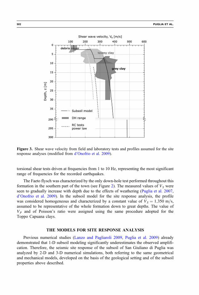
torsional shear tests driven at frequencies from 1 to 10 Hz, representing the most significantrange of frequencies for the recorded earthquakes.

The Faeto flysch was characterized by the only down-hole test performed throughout thisformation in the southern part of the town (see Figure 2). The measured values of VS wereseen to gradually increase with depth due to the effects of weathering (Puglia et al. 2007,d’Onofrio et al. 2009). In the subsoil model for the site response analysis, the profilewas considered homogeneous and characterized by a constant value of VS ¼ 1;350 m=s,assumed to be representative of the whole formation down to great depths. The value ofVP and of Poisson’s ratio were assigned using the same procedure adopted for theToppo Capuana clays.

THE MODELS FOR SITE RESPONSE ANALYSIS

Previous numerical studies (Lanzo and Pagliaroli 2009, Puglia et al. 2009) alreadydemonstrated that 1-D subsoil modeling significantly underestimates the observed amplifi-cation. Therefore, the seismic site response of the subsoil of San Giuliano di Puglia wasanalyzed by 2-D and 3-D numerical simulations, both referring to the same geometricaland mechanical models, developed on the basis of the geological setting and of the subsoilproperties above described.

Figure 3. Shear wave velocity from field and laboratory tests and profiles assumed for the siteresponse analyses (modified from d’Onofrio et al. 2009).

502 PUGLIA ET AL.

3-D MODEL

The integration of all the information resulting from geological, geostructural, and geo-physical investigations informed the construction of a digital 3-D model (Mucciarelli et al.2009) covering a volume extending to a depth of about 1,500 m and an area of 2 � 2 km2,centered around the town of San Giuliano di Puglia (Figure 4). At this scale, four main litho-logical units were considered: the Toppo Capuana clays, the Faeto flysch, the so-calledmélange formation, and the Pliocenic deep carbonate bedrock. Within the subsoil volume,the interfaces between the four units and the main tectonic discontinuities were locatedaccording to both surface and depth investigations.

In order to perform the 3-D numerical simulations of the seismic wave propagation, asubvolume was extracted from the 3-D model, covering a squared area with 960 m long sidesaligned with the geographic directions and extending 500 m in depth. Due to the heavynumerical constraints required by the analysis, the stratigraphy of the clay formation wassimplified by neglecting the thin shallow layer of debris cover. Moreover, the subvolumecould not include some geometrical features that can significantly affect the seismic response,such as the stratigraphic contact at the northern side between the Toppo Capuana clay and theFaeto flysch formation. As a result, two lithological units were considered for the character-ization of the subvolume: (1) Faeto flysch, which was treated as a homogeneous unit, and(2) Toppo Capuana clays, which were subdivided into six subunits, the uppermost consti-tuted by the tawny clay and the underlying gray clay discretized into five layers. The proper-ties of these units are summarized in Table 1.

The 3-D numerical simulations were aimed at obtaining the site transfer function in thefrequency range up to fmax ¼ 10 Hz, in the form of a 3� 3 matrixHðf Þ (e.g., Paolucci 1999).Each element Hijðf Þ of this matrix contains the frequency response at topographic surface inthe ith direction to an input motion in the jth direction. A set of three simulations was there-fore performed by exciting the seismic wave field in the 3-D model with a vertically incident

Figure 4. The 3-D subsoil model of the area around San Giuliano di Puglia (modified fromPuglia et al. 2009). The dashed line delimits the area corresponding to the subvolume consideredin the 3-D numerical simulation.

ANALYSIS OF SITE RESPONSE AND BUILDING DAMAGE DISTRIBUTION 503

impulsive plane wave consisting in an S-wave polarized along the EW direction, an S-wavepolarized along the NS direction, and a P-wave, respectively.

The 3-D numerical simulations were performed by means of an original implementationof the Fourier pseudo-spectral method (FPSM) on staggered grids, which solves the viscoe-lastic wave propagation in time domain in a layered subsoil model with irregular topographicsurface (Klin et al. 2010). This method combines the simplicity of the structured grid with theoptimal accuracy of the Fourier spatial differential operators. The material mechanical prop-erties are the velocities of the compression and shear elastic waves (VP and VS, respectively),the mass density ρ, which can be deduced from the unit weight γ, and the elastic qualityfactors for the compression and shear deformation modes (QK and Qμ, respectively). Inthe present work it was assumed QK ¼ ∞ (i.e., negligible dissipation for the dilatationmechanism), while Qμ was evaluated from the damping ratio D0 as Qμ ¼ 1∕ð2 D0Þ. Theseismic waves attenuation is described by the generalized Zener body (GZB) mechanicalmodel (Carcione et al. 1988).

When applying FPSM, the sampling step of the discretized model could be theoreticallyas short as λmin∕2, where λmin is the minimum considered wave length of the S-phases. Never-theless, in the presence of impedance contrasts and complex geometries, the methods basedon structured grids require finer sampling for an accurate computation of synthetic seismo-grams (Pelties et al. 2010). Considering fmax ¼ 10Hz and the lowest S-wave velocity in the3-D model VS min ¼ 250m=s gives the minimum wavelength λmin ¼ 25m. In order toaccount for the surface topography with sufficient accuracy, the domain was discretizedwith a regular grid along the horizontal directions, with a sampling step Δx ¼Δy ¼ 5m ¼ λmin∕5. The vertical sampling step was set to Δz ¼ 2m ¼ λmin∕12.5 in theupper part of the model; in order to avoid unnecessary oversampling in the deepest partof the model, where λmin ¼ 135m, a stretching was applied to the grid—that is, the samplingstep in the vertical direction was gradually increased with depth up to Δz ¼ 20m. As a result,the actual spatial domain consisted of a 3-D regular grid with 192 � 192 � 272 points. Inorder to avoid spurious reflections from the boundaries, the domain was surrounded by a

Table 1. Physical and mechanical properties of the different formations used for the 3-Danalysis

Formation

LayerthicknessH [m]

Unitweight

γ [kN/m3]

Shearwave

velocityVS [m/s]

Dampingratio

D0 [%]

Poisson’sratioν

Compressionwave

velocityVP [m/s]

ToppoCapuanaclays

Tawny clay 12 21.15 250 2.3 0.489 1700Gray clay (C) 8

21.20

339

2.5

0.485 1970Gray clay (D) 15 364 0.483 2000Gray clay (E) 30 391 0.481 2050Gray clay (F) 60 421 0.479 2100Gray clay (G) – 454 0.477 2160

Faeto flysch – 22.0 1350 0.5 0.392 3200

504 PUGLIA ET AL.

152-point-wide absorbing strip. The convolutional perfectly matched layer (CPML, seeKomatitsch and Martin 2007) technique was adopted to damp the wave field in thisstrip. The overall 3-D grid size involved in the computations was therefore 496 �496 � 424 points. In order to fulfill the stability condition with the given spatial sampling,a time step length Δt ¼ 10�4 s was chosen for the time-advancing scheme. Each simulationrequired a computational effort of about 200 hours using 16 cores of a SunFire server basedon AMD Opteron CPUs.

The results of the 3-D simulations consisted of 4-s-long nine-component time historiesHijðtÞ, where each ij component represents the response in the ith direction to the plane waveexcitation in the jth direction These basic solutions allow the computation of the response toany seismic input introduced as plane wave with vertical incidence, by applying the follow-ing expression:

EQ-TARGET;temp:intralink-;e1;62;488yiðtÞ ¼X1;3j

ujðtÞ � HijðtÞ; (1)

where uj are the components of the input motion at the bottom of the volume and yi are thecomponents of the motion at surface (Paolucci 1999).

2-D MODEL

Two-dimensional time domain analyses were carried out by the finite-element codeQUAD4M, which is based on an equivalent linear viscoelastic approach and on a Rayleighdamping formulation using two constraint frequencies (Hudson et al. 1994). The referencesection was chosen across the crest of the hill, along the main alignments of the borehole andsurface geophysical tests and of the mobile stations (see Figures 2–4). The 2-D model wasobtained as the vertical section of the 3-D model previously described along the referencedirection N344 (164°–344°N). Along this section, shown in Figure 5, the clay depositassumes the shape of an anvil, highlighting the “flower structure: of the subsoil. The overallsize of the 2-D domain is approximately 2.4 � 0.6 km.

Figure 5. Longitudinal section for the 2-D model; the zoom evidences the stratigraphic details(modified from Puglia et al. 2009).

ANALYSIS OF SITE RESPONSE AND BUILDING DAMAGE DISTRIBUTION 505

The drawbacks of the QUAD4M code, which may derive from wave reflections on theboundaries, were prevented by increasing the horizontal and vertical extension of the section.The transmitting base option was used for the lower boundary, by assigning to the underlyinghalf-space the same properties as the flysch. Both vertical and horizontal components of theinput motion were applied to the base nodes; those along the lateral boundaries were set asfree in the horizontal direction and, along the vertical, forced to move according to the cor-responding input motion component. Lateral boundaries were located at a distance of 800 mfrom the clayey deposit, that is, roughly equal to its longitudinal extension, whereas the baseof the model was placed at a depth of about twice the deposit thickness (Figure 5). Suchdomain extension should be enough to yield negligible reflected waves from the boundaries,as shown by the previous study on the same site by Lanzo and Pagliaroli (2009) and bysensitivity analyses reported in literature (e.g., Augello et al. 1998, Rathje and Bray2001, Pagliaroli 2006).

The interpretation of such a great number of boreholes permitted the use of geostatisticalprocedures to estimate the local variability of the thickness of both debris cover and tawnyclay throughout the urbanized area (Puglia 2008). Due to their lower seismic impedance withrespect to the underlying gray clay formation, a not-negligible influence of such stratigraphicdetail was expected on high-frequency amplification. Therefore, the spatial distribution ofthickness for the uppermost layers on the whole area was estimated through a classical inversedistance weighted (IDW) approach (Shepard 1968), that is, a weighting inversely proportionalto the distance of the measured thickness (Puglia 2008). The detail of the 2-D model sectionshown in Figure 5 reveals the resulting progressive thinning of the debris cover layer (A) from4 m in the northern part to 2 m in the southern part; by contrast, the weathered tawny clay(B) thickens as it approaches the historical center, reaching a maximum of 12 m.

The specific values of the geotechnical parameters adopted for the 2-D model are listed inTable 2. The debris cover and the tawny clay were considered with a variable thickness, H,along the section, according to the above-mentioned IDW approach.

Table 2. Physical and mechanical properties of the different formations used for the 2-Danalysis

Formation

LayerthicknessH [m]

Unitweight

γ [kN/m3]

Shearwave

velocityVS [m/s]

Dampingratio

D0 [%]

Poisson’sratioν

Compressionwave

velocityVP [m/s]

Elementthicknesshmax [m]

ToppoCapuanaclays

Debris cover 2 4 4 19.60 122 3.0 0.493 1010 1.2Tawny clay 4 4 12 21.15 250 2.3 0.489 1700 2.5Gray clay (C) 7.7

21.20

339

2.5

0.485 1970 3.4Gray clay (D) 15 364 0.483 2000 3.6Gray clay (E) 30 391 0.481 2050 3.9Gray clay (F) 60 421 0.479 2100 4.2Gray clay (G) − 454 0.477 2160 4.5

Faeto flysch − 22.0 1350 0.5 0.392 3200 13.5

506 PUGLIA ET AL.

The maximum thickness of mesh elements, hmax, for each subsoil unit was fixed accord-ing to the well-known condition by Kuhlemeyer and Lysmer (1973):

EQ-TARGET;temp:intralink-;e2;62;615hmax ¼VS

100<

VS

8 � fmax

; (2)

being fmax equal to 12 Hz, that is, the upper frequency of the low-pass filter that was appliedto the seismic input signals (see the next sections). The aspect ratio of the elements (i.e., thewidth divided by the thickness) was set not greater than 3. In this way, the mesh consisted ofabout 50,000 triangular elements, implying a computational effort for each analysis of about12 hours by a common personal computer.

GROUND MOTION AMPLIFICATION IN THE AFTERSHOCKS

A network of seismic stations, installed by INGV right after the main shocks, was oper-ating from 5 November to 25 November 2002 (Cara et al. 2005). The mobile network wascomposed of four 3-D CMG-40T velocimeters equipped with one Lennartz Marslite (20-bit)and three Reftek 72A (24-bit) digital recorders. The VIT1, SCL1, CHI1 (24-bit), and C147(20-bit) stations were located on the hill crest, longitudinally to the town (Figure 2), in thedirection of the 2-D section of Figure 5. At the same time, the DPC installed two additionalaccelerometric stations at the SCL1 and CHI1 sites (cf. Figure 2 and Figure 5). These stationswere equipped with Episensor FBA-3 sensors and Kinemetrics-Everest digitizers and wereoperating from 8 October to the end of December 2002.

The basic processing technique applied to both velocimetric and accelerometric data setsconsisted of: a linear baseline correction, to eliminate the offset; a 5% to 10% cosine tapering,to mitigate the effect of spectral leakage; and a band-pass Butterworth fourth-order filter, inthe range 0.2–25 Hz. Both empirical and analytical Fourier spectra were smoothed by adopt-ing the Konno and Ohmachi (1998) operator (b ¼ 40).

Figure 6 shows the ground motion recorded at VIT1, SCL1, and CHI1 stations during themost significant aftershock (ML ¼ 5.2, estimated by Bindi et al. 2006), which occurred on 12November 2002 (cf. map in Figure 1c), when the C147 station was temporarily not operating.The plots compare the recorded data, in terms of smoothed Fourier (Figure 6a) and response(Figure 6b) spectra, to those resulting from both 3-D FPSM and 2-D FEM linear simulationsalong the same N344 direction, that is, the same as the 2-D section in Figures 2 and 5.

The seismic input applied to the 2-D and 3-D models was the accelerometric record at theCHI1 site, assumed to be the reference station. Prior to the application at the base of the 3-DFPSM model, the three component records were halved, assuming a perfect reflection ofseismic waves at the free surface. Since QUAD4M code implicitly performs an internaldeconvolution to the bedrock (cf. Hudson et al. 1994), the seismic input for 2-D FEM ana-lysis coincided with the vertical and horizontal recorded components, the latter projectedalong the N344 direction. The input signals for the seismic response analysis have beenresampled to 0.02 s, then a Butterworth fourth-order band-pass filter between 0.15–10 Hz or 0.15–12.5 Hz was applied to the 3-D and 2-D input motions, respectively.

In Figure 6 it can be noted that the spectra recorded at the CHI1 site (bottom plots) arewell reproduced by both numerical analyses in the whole frequency range. In the other two

ANALYSIS OF SITE RESPONSE AND BUILDING DAMAGE DISTRIBUTION 507

recording sites, the simulations yield comparable results in terms of Fourier spectra at fre-quency lower than 1.5 Hz (i.e., at periods higher than 0.7 s in terms of response spectra). Athigher frequency (i.e., lower periods), the 2-D model reproduces a stronger ground motionthan that predicted by the 3-D model. Both analyses are in good agreement with the spectrarecorded at the SCL1 site (middle plots), where accelerometric and velocimetric records arequite similar in terms of both spectral representations. At VIT1 station (upper plots), althoughapparently very near to the SCL1 site and still lying on the clay formation, the record is quitedifferent, with pronounced peaks at frequencies around 4–6 Hz (i.e., 0.15–0.25 s); this high-frequency amplification is quite well reproduced by 2-D simulations but appears underes-timated by the 3-D model. This discrepancy is likely due to the oversimplification of themodel used in 3-D simulations, which does not reproduce both the gradual thinning ofthe tawny clay formation at the northern boundary and the presence of the debris cover.At frequencies higher than 8 Hz (or, equivalently, periods less than 0.13 s) neither 3-Dnor 2-D models are able to replicate the recorded amplification, again because of their over-simplification of shallow layers—which are considered homogeneous—with respect to thereality.

Figure 6. Comparison between: (a) recorded and simulated Fourier and (b) response spectra(5% structural damping) at VIT1, SCL1, and CHI1 sites during the aftershock on 12 November2002 (ML ¼ 5.2).

508 PUGLIA ET AL.

The standard spectral ratio (SSR) technique was applied to empirically evaluate siteamplification on the basis of the aftershocks recorded. The SSRs were computed takingCHI1 as the reference station, since it was placed in the southern part of the village onthe Faeto flysch formation. The empirical transfer functions were calculated at the veloci-metric stations VIT1, C147, and SCL1, located on the clay formation, from a data set of 130events with duration magnitude (MD) between 1.9 and 3.3 (cf. Cara et al. 2005). In particular,the spectral ratios at velocimetric stations VIT1, SCL1, and C147 were constructed using 27,23, and 19 events, respectively—that is, the common recordings between the station at handand the reference velocimetric station CHI1. The SSRs were also estimated for the DPCaccelerometric stations (SCL1 with respect to CHI1), considering the 12 strongest after-shocks of the Molise sequence, which are characterized by local magnitude, ML, rangingbetween 3.6 and 5.2 (Bindi et al. 2006).

To show the possible anisotropy of the local seismic response, the horizontal componentsof the time series were projected along variable directions between 0° and 175°, with a step of5°. The polar diagrams in Figure 2 represent the mean amplification obtained considering alog-normal distribution for the amplitudes of each SSR (i.e., relevant to each aftershock takeninto account). The plots are displayed in a concentric scale, with the lowest frequency at thecenter and the maximum frequency (10 Hz) at the border of the diagram; a darker colorindicates higher amplification. The polar diagrams show that, at least for VIT1 andSCL1, the main amplification appears along the direction 150°–330°, very close to thatof the alignment of the ridge and of the reference 2-D section (N344).

In Figure 7 the SSRs computed along the N345 direction are plotted in terms of mean �one standard deviation, respectively shown by gray and white bands for the velocimetric andaccelerometric data. The SSRs recorded at all the stations and those simulated through thedynamic models result in fair agreement throughout the low-frequency range (i.e., for f <1Hz or T > 1 s). Both 2-D and 3-D models show a well-defined low-frequency peak around0.8–0.9 Hz, which could be the fundamental frequency of the deposit. In fact, as expected, itis higher than the 1-D fundamental frequency (cf. Bard and Riepl-Thomas 1999), which wasestimated of the order of 0.5 Hz at the maximum depth of the clayey deposit (Puglia 2008).Despite the limited energy content of the aftershocks at low frequency, the empirical SSRsalso show a moderate amplification peak around 0.7 Hz at VIT1 and SCL1; for this latter sitethis peak is more apparent in the accelerometric SSRs. The high scatter of the empiricalspectral ratios at low frequencies can be attributed to the variability of the hypocentral posi-tion with respect to the study area (cf. Figure 1), causing different directions of incidentseismic waves for each event considered.

In the medium-frequency range (1–3 Hz), the empirical spectral ratios show a significantpeak with an amplitude between 3–4 (velocimetric SSRs) to 5–6 (accelerometric SSRs) atabout 2.5 Hz (0.4 s on the response spectra). The 2-D numerical simulation yields a similarpeak, at a slightly lower frequency (i.e., at around 2 Hz) but with a higher amplification; the3-D model seems to better reproduce the observed peak, in terms of both frequency andamplification. Therefore, the 3-D geometry seems to better capture the subsoil amplificationin this range, although it introduces a spurious peak at 1.5 Hz, not observed from records. Athigher frequencies (3 4 10 Hz), the empirical SSRs are characterized by two outstandingpeaks at about 4–5 and 6 Hz, with mean amplitudes around 4 for VIT1 and C147, and

ANALYSIS OF SITE RESPONSE AND BUILDING DAMAGE DISTRIBUTION 509

between 5 and 6 for SCL1. This amplification can be associated with the lower impedance ofthe weathered shallow layer (debris cover and tawny clay), the natural frequency of whichvaries between 4 and 6 Hz, depending on the layering. In this range, 2-D simulations yieldamplification functions similar to those recorded, while at least for SCL1 and VIT1 stations,the 3-D model underestimates the amplification, even with an attenuation observed around5 Hz at VIT1. This is likely due to the oversimplification of the clay layering in the3-D model.

The horizontal profiles in Figure 8a reproduce the amplification factor, A, in terms ofpeak ground acceleration, predicted with 3-D and 2-D models along the N344 section,assuming the CHI1 station as the reference site; for each station, the empirical amplificationfactors from velocimetric records are also reported, in terms of mean value � one standard

Figure 7. Empirical and analytical SSRs along N344 direction at the stations VIT1, SCL1, andC147.

510 PUGLIA ET AL.

deviation, considering a log-normal distribution of amplitudes. The amplifications factorsrecorded at the stations are higher than those estimated by the 3-D model, which underpre-dicts the subsoil response at high frequency, as discussed above. The horizontal profile com-puted by the 2-D model results in a fair agreement with the records, in particular for the

Figure 8. Amplification factor predicted by 3-D and 2-D models compared to the empirical after-shock records in terms of: (a) peak ground acceleration; (b) Housner intensity at 0.2–2.0 s; and(c) 0.1–0.5 s.

ANALYSIS OF SITE RESPONSE AND BUILDING DAMAGE DISTRIBUTION 511

northern stations, SCL1 and VIT1. The trend predicted along the clay deposit is quite irre-gular, due to the superposition of body and surface waves, these latter generated at the edge ofthe formation. The anomalous attenuation observed right across the flysch–clay contactmight then be attributed to a destructive interference phenomenon.

It must be remarked that the amplification in terms of peak ground acceleration (PGA)pertains to frequencies higher than those typical of the existing structures; thus, PGA can-not be considered as the most effective estimator of the potential damage induced by astrong ground motion. In fact, nonlinear dynamic analysis reported by Masi et al.(2011) demonstrated that the correlation of PGA with structural damage of buildings isvery poor when compared with integral ground motion parameters more strictly relatedto the dynamic response of structures. The same authors suggested that the integral para-meter most effectively correlated with building structural damage is the Housner intensity,SI (Housner 1952), that is, the integral of the pseudo-velocity response spectrum,PSVðξ;TÞ:

EQ-TARGET;temp:intralink-;e3;41;462SIT14T2ðξÞ ¼

ðT2

T1

PSVðξ; TÞdT ; (3)

corresponding to a structural damping ξ. In Equation 3, T1 and T2 represent the integrationrange of periods. Therefore, the ground motion amplification was also represented in termsof spectral intensity ratio (SIR), again computed by assuming the CHI1 station as the refer-ence site.

A first integration range considered for Equation 3 was 0.2–2.0 s, narrower than the con-ventional limits of 0.1–2.5 s defined by Housner (1952). The horizontal profile of the ampli-fication factor computed in terms of SI0:242:0 is depicted in Figure 8b. Compared to theamplification profile in terms of peak ground acceleration (Figure 8a), SIR0:242:0 showsa more regular trend, because of the lower frequency content taken into account in the spec-tral intensity. Due to the particular shape of the bedrock geometry, the 2-D profile presentsthree focusing points, two of which fall close to the C147 and SCL1 stations. On the otherhand, no focusing points are reproduced by the 3-D model, which yields an increasingresponse approaching the northern edge of the 3-D domain. The accuracy of 2-D predictionsseems to improve even at the C147 station; the 3-D modeling still underestimates the experi-mental values at the SCL1 and C147 stations, while at VIT1 the response is very close to therecorded amplifications.

Another representation of amplification in terms of spectral intensity ratio was referredto the narrower range of periods 0.1 to 0.5s (Figure 8c), because the fundamental frequen-cies of both historical and recent buildings of San Giuliano di Puglia—usually two to fourstories high—fall in this range (Baranello et al. 2003). The values of SIR0:140:5 predictedby the 2-D model slightly overestimate the recorded amplification at all the stations, andthe general trend presents local oscillations similar to those observed for the peak groundacceleration (cf. Figure 8a), since both amplification ratios pertain to relatively high fre-quencies. The amplification predicted in the same frequency range by the 3-D modelshows oscillations with a very similar trend but still underestimates the experimentalvalues.

512 PUGLIA ET AL.

ANALYSIS OF SITE RESPONSE AND DAMAGE DISTRIBUTIONINDUCED BY THE MAIN SHOCK

The strongly non-uniform damage distribution observed by QUEST just after the seismiccrisis (Galli and Molin 2004) was confirmed by more detailed surveys on the buildings(Baranello et al. 2003, Dolce et al. 2004). Figure 9 shows the damage grade assigned toeach building according to the classification given in the EMS98 scale (ESC WorkingGroup 1998), sketched in the same figure. The superposition of the damage grade distributionon the geological map indicates, even at first glance, the strong correlation between the sub-soil conditions and the building damage, regardless of building vulnerability.

The small (up to two to three stories) buildings in the historical center typically had arubble masonry structure, with poor construction quality, and were frequently connected inheterogeneous structural aggregates (Mucciarelli et al. 2003). After the two main shocks,many of these buildings showed light damage or none at all (Grade 0–2), several showedheavy damage (Grade 3) with some partial collapses (Grade 4), mainly due to local structuralweaknesses, whereas total collapses were not recorded (Figure 9). On the other hand, heavierand widespread damage was observed in the newer zones; such a finding can only partly beascribed to the seismic vulnerability of the buildings, as will be shown. Structural types hadalmost heterogeneous characteristics: rubble and brick masonry were present, often variouslycombined in the same structure, whereas recent maintenance or overraising interventionswere carried out; some framed reinforced concrete buildings built after the 1960s couldalso be found, generally of small size and regular shape (Mucciarelli et al. 2003). In several

Figure 9. Damage distribution at San Giuliano di Puglia produced by the 31 October 2002 earth-quake in terms of EMS98 scale (modified from Dolce et al. 2004).

ANALYSIS OF SITE RESPONSE AND BUILDING DAMAGE DISTRIBUTION 513

masonry buildings, partial or total collapse (Grade 4–5) occurred (Figure 9), particularlywhen the masonry was made of hollow brick blocks, arranged in two layers badly or notconnected, having poor load-bearing capacities also under vertical loads. Heavy nonstruc-tural and structural damage (Grade 2–3) occurred also in some reinforced concrete buildingsin the central part of the town, while the recent reinforced concrete buildings in the northernpart generally showed slight damage or none at all (Grade 0–1).

REFERENCE INPUT MOTION

No permanent stations of the Italian accelerometric network (Rete AccelerometricaNazionale, RAN) were operating in the epicentral area (cf. Figure 1) when the mainshock occurred. Gorini et al. (2003, 2004) and Franceschina et al. (2006) performed numer-ical modeling to estimate synthetic accelerograms of the main shocks, making up for the lackof recordings in the epicentral area. These simulations were calibrated by the recordings ofthe RAN stations away from the epicenter (cf. Figure 1), including possible directivity effectof the seismic source. In both above-mentioned studies, simulations and recordings of themain shocks showed a good agreement at RAN stations not affected by site amplification.

The reference input motion adopted to model the site response at San Giuliano di Pugliaduring the 31 October main shock was the accelerogram simulated in the frequency range0–11 Hz by Franceschina et al. (2006) through the hybrid integral-composite source model(HIC), considering the fault mechanism formulated by Basili and Vannoli (2005). Figures 10ato 10b show the acceleration time histories predicted on rock outcrop of the horizontal com-ponents after projection along the 2-D section (a) and orthogonally to it (b); the verticalcomponent (Figure 10c) is apparently characterized by a lead motion. The peak valuesresulted in fair agreement with those predicted by regional attenuation laws (Luzi et al.

Figure 10. (a, b) Horizontal and (c) vertical components and (d) relevant acceleration responsespectra of the reference input motion at San Giuliano di Puglia, computed by Franceschina et al.(2006) for the 31 October 2002 main shock.

514 PUGLIA ET AL.

2006). HIC acceleration response spectra (Figure 10d) show a dominant period around 0.15 s(i.e., 7 Hz), with the horizontal components having a secondary peak around 0.4–0.5 s(2.0–2.5 Hz). Comparing the spectral shapes in Figure 10d with those reported in Figure 6bfor the CHI1 station, it can be verified that the synthetic reference input motion is character-ized by a frequency content very similar to that of the most significant recorded aftershock;also, such frequency content shows a significant overlap to the range of the expected funda-mental periods of the undamaged building stock (see hatched area in Figure 10b).

SEISMIC RESPONSE ANALYSES AND DAMAGE MODELING

The site-response analyses of the 31 October main shock were carried out applying thereference input motion in Figure 10 to both 2-D QUAD4M and 3-D FPSM models describedin the previous sections.

The 2-D QUAD4M analysis was first performed adopting a linear equivalent approach(Puglia 2008), by considering for the three clay units the variations of normalized shear mod-ulus, G∕G0, and equivalent damping ratio, D, versus shear strain, γ, as measured in resonantcolumn tests at medium strain levels (Silvestri et al. 2007, d’Onofrio et al. 2009). However, itwas observed that the input motion was not strong enough to bring the three clay units to asignificant nonlinear behavior. In fact, the mean shear strain in each formation resulted as lowas 0.020% for the debris cover, 0.013% for the tawny clay, and 0.009% for the gray clays,that is, well below the linear threshold. Thus, for sake of consistency with the 3-D simula-tions, a linear approach was preferred in the 2-D final modeling.

To compare the damage distribution observed and simulated at the town of San Giulianodi Puglia after the 31 October earthquake, the urban center was subdivided into 50 � 150 mwide microzones across the 2-D section (Figure 9). These microzones are also reported inFigure 11a. Figures 11b–d report the comparison between 2-D and 3-D simulations of the 31October main shock, expressed as average values in each microzone of peak ground accel-eration (amax) and velocity (vmax) and Housner intensity (SI0:242:0) along the N344 direction.Both models provide similar results at the town’s historic core (microzones 1,200 4 1,450);in the remainder of the urban center, founded on the clayey formation, peak values from the2-D model are about twice those obtained from the 3-D analysis.

Figure 11e shows the results of 2-D simulation in terms of acceleration response spectraat the surface. Note the significant amplification of the clayey deposit for periods from 0.1 to0.7 seconds. In particular, a high-frequency peak around 0.15 s (about 7 Hz) is evidentthroughout the whole area where the clay outcrops, and a medium-frequency peak(0.5 s, i.e. 2Hz) appears around C147 and SCL1 sites. While the former is essentially asso-ciated with the dominant frequency of the input motion (see Figure 10d), the latter resultsfrom the amplification of the secondary peak of the incoming signal, due to a resonance of thesubsoil close to this frequency, as already shown by the spectral ratios of Figure 7 for thesame sites.

Figure 12 reports the contours of Housner intensity (SI0:242:0) simulated at ground sur-face by the 3-D model. Along the N344 section, SI0:242:0 varies between 0.07 and 0.13 m incorrespondence of sites CHI1 and SCL1, respectively. The spectral intensity reaches a max-imum of about 0.22 m, slightly lower than the peak value predicted by the 2-D model(0.27 m). Such value is attained along the ridge, about 100 m E of sites VIT1 and

ANALYSIS OF SITE RESPONSE AND BUILDING DAMAGE DISTRIBUTION 515

SCL1, and also 150 m away from C147 site. Such significant variability of surface groundmotion predicted by the 3-D model around the seismic stations depends on the irregularityof both the surface topography and the buried interface between the clay deposit and theFaeto flysch formation.

For each microzone, the ground motion parameters resulting from the simulationswere converted into macroseismic intensity values (Figures 13b–d) through empirical

Figure 11. (a) Map of building damage; (b, c, d) profiles of ground motion parameters (accel-eration, velocity, and Housner intensity) computed by 3-D and 2-D models; (e) accelerationresponse spectra computed by 2-D numerical simulation.

516 PUGLIA ET AL.

correlations. To convert the peak ground acceleration amax into macroseismic intensity(i.e., Figure 11b into Figure 13b), the correlation by Margottini et al. (1992) was appliedin the form:

EQ-TARGET;temp:intralink-;e4;62;248IEMS ¼∼ IMSK ¼ ð1∕0.258Þ � log10ðamax∕2.279Þ; (4)

where amax is expressed in cm/s2. An equivalence was considered between MSK and EMSscales, as suggested by ESC Working Group (1998). Recently, Faenza and Michelini(2010) proposed a relationship between peak ground velocity (in cm/s) and IMCS:

EQ-TARGET;temp:intralink-;e5;62;179IMCS ¼ 5.11þ 2.35 � log10ðvmaxÞ; (5)

which has been converted into IMSK, hence IEMS, by the expression:

EQ-TARGET;temp:intralink-;e6;62;136IEMS ≅ IMSK ¼ ðIMCS þ 0.76Þ∕1.17; (6)

deduced from Margottini et al. (1992). Equations 5 and 6 were therefore used to transformthe profiles in Figure 11c into those in Figure 13c. Also, the spectral intensity (Figure 11d)

Figure 12. Distribution of the maximum value between the two horizontal components of Hous-ner intensity computed in the 0.24 2.0 s period interval, along the surface of the 3-D model.White lines denote superficial discontinuities of the structural model. The black bold line indi-cates the trace of the vertical section used for 2-D simulations. The Gauss-Boaga coordinatesystem is used.

ANALYSIS OF SITE RESPONSE AND BUILDING DAMAGE DISTRIBUTION 517

could be converted into macroseismic intensity (Figure 13d) adopting the relationship sug-gested by Chiauzzi et al. (2012):

EQ-TARGET;temp:intralink-;e7;41;212IEMS ¼ maxf0.27 � lnðSI0:242:0Þ þ 6.02; 1.41 � lnðSI0:242:0Þ þ 7.98g; (7)

where SI0:242:0 (ξ ¼ 5%) is expressed in meters.

The cross symbols in Figures 13b–d indicate the distribution of macroseismic intensity interms of EMS scale, as observed by Dolce et al. (2004). The mean intensity varies fromIEMS ¼ VI in the historical center (microzones from 1,200 to 1,450 m in Figure 11) to IEMS ¼VII� VIII in the newer part of the town (between 750 and 1,200 m).

Whatever the correlation adopted, both 2-D and 3-D models provide pretty coherentestimates of the macroseismic intensity at the historical part of the village, the simulated

Figure 13. (a) Map of building damage; (b) profile of macroseismic intensity (EMS scale)observed versus those predicted by 3-D and 2-D models in terms of acceleration; (c) velocity;and (d) Housner intensity.

518 PUGLIA ET AL.

values of IEMS never differing more than half a degree from those observed (Figures 13b–d).The comparison between 2-D simulation of IEMS on the basis of amax (Equation 4) yields areliable estimation of the observations even at the newer part, with the exception of themicrozones between 1,050 and 1,200 m (Figure 13b). The 3-D model, on the otherhand, underestimates by even more than one degree the intensities observed in thenewer part (microzones from 750 to 1,200 m in Figure 13b), where it predicted peak groundaccelerations lower than those estimated by the 2-D model (cf. Figure 11b). Simulation ofIEMS on the basis of vmax (Equations 5 and 6) computed by both 2-D and 3-D models yieldsmuch flatter trends, with an average underestimate of the intensity observed in the newerpart of the town ranging around one degree (Figure 13c). The comparison is even morestriking in the case of SI0:242:0, a ground motion parameter that is generally the most repre-sentative of the damage potential: the discrepancy between the observed macroseismicintensity and that simulated by both models ranges around two degrees (Figure 13d).

In Figure 14b the damage distribution for each microzone is shown by histograms plot-ting the number of buildings associated with each damage level according to the EMS scale.Figure 14c reports the distribution of buildings into the vulnerability classes A, B, and C ofthe EMS scale, as assigned by Dolce et al. (2003, 2004). The bar graph clearly shows thatmost buildings in the historic center were assigned the highest vulnerability class A, while theaverage building vulnerability decreases moving toward the newer part of the town,.

The cross symbols in Figures 14d–f show the observed mean damage index (DIMED), thatis directly derived from the damage distribution of Figure 14b through the relationship sug-gested by Dolce et al. (2003):

EQ-TARGET;temp:intralink-;e8;62;360DIMED ¼Xn1

di � f in

; (8)

where di is a generic damage level (EMS scale) and f i is the relevant building frequency inthe microzone. The summation is calculated for the 5 nonzero damage levels, hence n ¼ 5.DIMED varies between 0 and 1, where DIMED ¼ 0 means total absence of damage andDIMED ¼ 1 corresponds to total destruction. The profile of the observed DIMED shows a rela-tively low mean damage at both the historic and the northern part of the town, whereDIMED isless than 0.3; indeed, the damage appears heavier in the central part of San Giuliano di Puglia,where frequently DIMED is higher than 0.4 and in some microzones rises to about 0.7.

While the observed damage distribution could be straightforwardly expressed by numer-ical values of DIMED, the typological analysis of the building stock shown in Figure 14c wasnecessary to convert the results of numerical simulations into estimated damage. Therefore,the damage distribution for each vulnerability class was estimated from the relevant macro-seismic intensity simulated for each microzone (Figures 13b–d), by referring to the damageprobability matrices (DPMs) suggested by Dolce et al. (2003, 2006). These were expressed interms of expected frequency of buildings of classes A, B, and C damaged with a given grade,for EMS intensity varying between V and VIII. By linear interpolation of the damagedistributions, Equation 8 permitted to calculate the mean damage index DIMED plotted inFigures 14d–f. In other words, such representations reflect the simulation of IEMS as reportedin Figures 13d–f filtered through the mean vulnerability of the building stock of eachmicrozone.

ANALYSIS OF SITE RESPONSE AND BUILDING DAMAGE DISTRIBUTION 519

Figure 14d shows that both 2-D and 3-D damage scenarios estimated on the basis ofnumerically predicted amax are in good agreement with observed DIMED in the historicalcore of the town; however, the numerical procedures tend to underestimate the observeddamage in the newer part, with the exception of the good performance of the 2-D model

Figure 14. (a) Map of building damage; (b) damage and (c) vulnerability distributions for eachmicrozone; profile of mean damage index observed versus those predicted by 2-D and 3-D mod-els in terms of (d) acceleration, (e) velocity, and (f) Housner intensity.

520 PUGLIA ET AL.

in the northern area (microzones between 750 and 950 m). Where the clay deposit outcrops,the damage scenarios predicted from vmax and SI0:242:0 computed by 2-D and 3-D analyses(Figures 14e and 14f), are less consistent with the observations than DIMED obtained fromamax (Figure 14d); however, they yield similar results on the flysch formation. Such consid-erations consistently reflect those already expressed for the predictions of seismic intensity.

CONCLUSIONS

The case history of San Giuliano di Puglia is currently the most accurately investigatedphenomenon of seismic site amplification in Italy; in particular, during the DPC-INGV S3Project (2004–2006) a huge amount of experimental data and numerical studies were gath-ered and compared. A comprehensive investigation on the subsoil properties was carried outthrough state-of-the-art field and laboratory geophysical and geotechnical tests; significantaftershock recordings taken on the thick clay formation and on the flysch rock outcrop wereavailable; furthermore, a detailed survey on building vulnerability and damage was carriedout. The cross-comparison of experimental and analytically simulated transfer functions gavethe opportunity to validate 2-D and 3-D models for the numerical simulation of the free-fieldseismic response of the subsoil.

The comparison and validation of two different numerical methods was necessary inorder to evaluate the uncertainties that are intrinsic in each simulation approach. As a matterof fact, not only do the subsoil model and the reference input motion withhold a level ofuncertainty, but also the computational algorithms represent and solve the idealized problemin an approximate way. For a more detailed discussion on the reliability of earthquake groundmotion evaluation by means of numerical methods refer to Chaljub et al. (2010). In compar-ing the model predictions against the aftershock records, none of the numerical methodsadopted appeared to be inherently conservative. Overall, the 3-D analyses predictedlower ground motion on the clayey deposit in the medium- to high-frequency range. The2-D simulations yielded a satisfying, although more variable, approximation of the recordedground motion, in terms of both absolute parameters (see Figure 6) and relative surface ampli-fication (see Figures 7 and 8). These different performances of 2-D and 3-D models could berationally attributed to their specific limitations in terms of geometry, extension, and resolu-tion in describing the subsoil. Such differences were consistently reflected in the comparisonsbetween the simulated and observed scenarios during the main shock; this time, both 2-D and3-D models almost systematically underpredicted the macroseismic intensity and damage.

The flowchart in Figure 15 gives an overview of the method adopted to compare in termsof mean damage index the observed damage distribution with the simulated earthquake sce-nario; the latter was obtained after postprocessing the free-field site response analysis throughthe vulnerability distribution of the building stock. In particular, in the left side of the chart,the simulated parameter (peak ground acceleration or peak ground velocity or Housner inten-sity) is averaged for each microzone (Figures 11b–d); then, with the aid of empirical correla-tions (Equations 4–7), the mean macroseismic intensity for each microzone is calculated(Figures 13b–d). At the same time (see the central part of the chart), the vulnerability classesdistribution (Figure 14c) is derived from the building map (Dolce et al. 2004). These dataconcur to obtain the simulated mean damage index (Figures 14d–f) through the damage prob-ability matrices (Dolce et al. 2003, 2006). On the right side of the diagram, the damage

ANALYSIS OF SITE RESPONSE AND BUILDING DAMAGE DISTRIBUTION 521

distribution (Figure 14b) is obtained from the damage map (Figure 14a) and directly trans-formed into observed mean damage index (Figures 14d–f) for comparison.

The proposed procedure might be a very promising methodological approach to the pre-diction of earthquake damage scenarios in urban areas. The reliability of such predictionsdepends on three main factors:

• The choice of the most representative input motion• The accuracy of the free-field seismic response analysis• The effectiveness of empirical correlations between ground motion parameters and

building damage

A critical point in the above procedure is the selection of the most appropriate groundmotion parameter (either amax, SI, or others) as the best damage predictor for the urban centerunder consideration. This choice should be optimized after an accurate evaluation of thespecific characteristics of regional seismicity, subsoil properties, and building stock inthe investigated area.

For instance, a crucial point in this study was the high-frequency content of the near-fieldreference input motion, which primarily affected the accuracy of prediction of peak groundacceleration obtained from free-field seismic response analysis. On the other hand, the surfacespectral amplitudes at medium to high periods (hence, the Housner intensity) were found to bemostly dependent on large-scale site amplification, due to the peculiar shape and high depth ofthe clay deposit. Also, the correlations used to convert the different ground motion parametersinto macroseismic intensity were found to typically underpredict the observed intensity (seeFigure 13), even when the numerical models were observed to be reliably validated by theweak-motion records (e.g., Figure 8). It must be noted that such correlations were calibrated

Figure 15. Flowchart of the procedure adopted for the comparison of the damage scenarios.

522 PUGLIA ET AL.

on the basis of previous experiences mostly referring to far-field earthquakes and buildingswith average vulnerability. Therefore, the underconservativeness of the predicted damage sce-nario can be attributed to the high-frequency content of the near-field inputmotion, aswell as tothe higher vulnerability of the structures at SanGiuliano di Pugliawith respect to the average ofthe data sets considered for the above empirical correlations. This latter uncertainty factor onthe vulnerabilitymodel appears to have also affected the damage estimation through theDPMs.

At present, more comprehensive procedures need to be developed and validated to extendthe reliability of seismic response models to reproduce site amplification in near-fault areasand to transform ground motion predictions into damage scenarios. To this purpose, the cur-rent vulnerability and damage models might be more effectively based on direct relationshipsbetween recorded ground motion and observed damage index.

Further developments are finally required to better calibrate the choice of the most sui-table range of periods for the computation of spectral intensity on the basis of the dynamicproperties of the building heritage at hand. In this way, the relationship between SI and IEMS

(Chiauzzi et al. 2012) could be redefined considering a wider range of periods (e.g., comput-ing SI between 0.1 s and 2 s) to more effectively estimate the damage distribution.

In order to profit from the lessons learned at San Giuliano di Puglia, the above consid-erations may address future research advances, aiming at more effective efforts for the reduc-tion of seismic risk in Italy.

ACKNOWLEDGMENTS

This work was developed in the framework of the DPC-INGV S3 Research Project, pro-moted by Istituto Nazionale di Geofisica e Vulcanologia (INGV) and funded by the Dipart-mento di Protezione Civile (DPC) of the Italian government. The authors wish to thank theDPC and the project team coordinators, Dr. Francesca Pacor and Prof. Marco Mucciarelli, fortheir valuable scientific and administrative support. An essential contribution was providedby Dr. Antonio Rovelli, who kindly made available the velocimetric recordings taken byINGV at San Giuliano di Puglia. All the researchers who contributed to the subsoil char-acterization (Prof. R. Caputo, Prof. F. Cotecchia, Prof. A. d’Onofrio, Prof. A. Guerricchio,late Prof. G. Melidoro, Prof. F. Santucci De Magistris, Dr. C. Vitone) and the previous seis-mic response analyses (Prof. G. Lanzo, Dr. A. Pagliaroli, Dr. S. Sica) are also warmlyacknowledged. The authors finally wish to thank the editor and the anonymous reviewers,whose suggestions were very helpful in improving the readability of the paper.

REFERENCES

Augello, A. J., Bray, J. D., Abrahamson, N. A., and Seed, R. B., 1998. Dynamic properties ofsolid waste based on back-analysis of the OII Landfill, J Geotech Eng 124, 211–222.

Baranello, S., Bernabini, M., Dolce, M., Pappone, G., Rosskopf, C., Sanò, T., Cara, P. L., DeNardis, R., Di Pasquale, G., Goretti, A., Gorini, A., Lembo, P., Marcucci, S., Marsan, P.,Martini, M. G., and Naso, G., 2003. Rapporto finale sulla Microzonazione Sismica del centroabitato di San Giuliano di Puglia, Dipartmento di Protezione Civile (DPC), Roma, Italy.

Bard, P. Y., and Riepl-Thomas, J., 1999. Wave propagation in complex geological structures andtheir effects on strong ground motion, inWave motion in Earthquake Engineering (Kausel andManolis, eds.), WIT Press, 37–95.

ANALYSIS OF SITE RESPONSE AND BUILDING DAMAGE DISTRIBUTION 523

Basili, R., and Vannoli, P., 2005. Source ITGG052 “San Giuliano di Puglia,” available at http://diss.rm.ingv.it/diss/. Cited in Basili, R., Valensise, G., Vannoli, P., Burrato, P., Fracassi, U.,Mariano, S., Tiberti, M. M., and Boschi, E., 2008. The Database of Individual SeismogenicSources (DISS), version 3: Summarizing 20 years of research on Italy’s earthquake geology,Tectonophysics 453, 20–43, doi: 10.1016/j.tecto.2007.04.014.

Bindi, D., Luzi, L., Morasca, P., Spallarossa, D., and Zolezzi, F., 2006. Deliverable D6: Data etaccelerometrico e velocimetrico della sequenza sismica del Molise (2002–2003), ResearchReport of INGV-S3 Project (in Italian), http://esse3.mi.ingv.it/.

Cara, F., Rovelli, A., Di Giulio, G., Marra, F., Braun, T., Cultrera, G., Azzara, R., and Boschi, E.,2005. The role of site effects on the intensity anomaly of San Giuliano di Puglia inferred fromaftershocks of the Molise, central southern Italy, sequence, November 2002, Bulletin of theSeismological Society of America 95, 1457–1468.

Carcione, J. M., Kosloff, D., and Kosloff, R., 1988. Wave propagation in a linear viscoelasticmedium. Geophys J Int 95, 597–611.

Chaljub, E., Moczo, P., Tsuno, S., Bard, P.-Y., Kristek, J., Käser, M., Stupazzini, M., andKristekova., M., 2010. Quantitative comparison of four numerical predictions of 3d groundmotion in the Grenoble Valley, France, Bulletin of the Seismological Society of America 100,1427–1455.

Chiarabba, C., De Gori, P., Chiaraluce, L., Bordoni, P., Cattaneo, M., De Martin, M., Frepoli, A.,Michelini, A., Monachesi, A., Moretti, M., Augliera, G. P., D’Alema, E., Frapiccini, M.,Gassi, A., Marzorati, S., Di Bartolomeo, P., Gentile, S., Govoni, A., Lovisa, L., Romanelli, M.,Ferretti, G., Pasta, M., Spallarossa, D., and Zunino, E., 2005. Mainshocks and aftershocksof the 2002 Molise seismic sequence, southern Italy, Journal of Seismology 9, 487–494.

Chiauzzi, L., Masi, A., Mucciarelli, M., Vona, M., Pacor, F., Cultrera, G., Gallovič, F., andEmolo, A., 2012. Building damage scenarios based on exploitation of Housner intensityderived from finite faults ground motion simulations, Bulletin of Earthquake Engineering10, 517–545, doi: 10.1007/s10518-011-9309-8.

Dolce, M., Masi, A., Marino, M., and Vona, M., 2003. Earthquake damage scenarios of the build-ing stock of Potenza (Southern Italy) including site effects, Bulletin of Earthquake Engineer-ing 1, 115–140.

Dolce, M., Masi, A., Samela, C., Santarsiero, G., Vona, M., Zuccaro, G., Cacace, F., and Papa, F.,2004. Esame delle caratteristiche tipologiche e del danneggiamento del patrimonio edilizio diSan Giuliano di Puglia, XI National Conference “L’ingegneria Sismica in Italia,” Genova,ANIDIS, Roma, Italy.

Dolce, M., Kappos, A., Masi, A., Penelis, G., and Vona, M., 2006. Vulnerability assessmentand earthquake scenarios of the building stock of Potenza (Southern Italy) using Italianand Greek methodologies, Engineering Structures 28, 357–371, doi: 10.1016/j.engstruct.2005.08.009.

d’Onofrio, A., Vitone, C., Cotecchia, F., Puglia, R., Santucci de Magistris, F., and Silvestri, F.,2009. Caratterizzazione geotecnica del sottosuolo di San Giuliano di Puglia, Rivista Italiana diGeotecnica (Italian Geotechnical Journal) 3, 43–61.

DPC-INGV S3 Project, 2004–2006. http://esse3.mi.ingv.it/.ESC Working Group (1998). European Macroseismic Scale 1998. GeoForschungsZentrum,

Potsdam, Germany.

Faenza, L., and Michelini, A., 2010. Regression analysis of MCS intensity and ground motionparameters in Italy and its application in ShakeMap, Geophys J Int 180, 1138–1152.

524 PUGLIA ET AL.

Franceschina, G., Pacor, F., Cultrera, G., Emolo, A., and Gallovič, F., 2006. Modelling directivityeffects of the October 31, 2002 (MW ¼ 5.8), Molise, Southern Italy, earthquake, FirstEuropean Conference on Earthquake Engineering and Seismology (1st ECEES), Geneva,Switzerland, paper no. 1424.

Galli, P., and Molin, D., 2004. Macroseismic survey of the 2002 Molise, Italy, earthquake andhistorical seismicity of San Giuliano di Puglia, Earthquake Spectra 20, S39–S52.

Giaccio, B., Ciancia, S., Messina, P., Pizzi, A., Saroli, M., Sposato, A., Cittadini, A., Di Donato,V., Esposito, P., and Galadini, F., 2004. Caratteristiche geologico-geomorfologiche ed effettidi sito a San Giuliano di Puglia (CB) e in altri abitati colpiti dalla sequenza sismica dell’ottobre-novembre 2002, Il Quaternario (Italian Journal of Quaternary Sciences) 17, 83–99.

Gorini, A., Marcucci, S., Marsan, P., and Milana, G., 2003. Acquisizione ed elaborazione di datisismologici nel comune di San Giuliano di Puglia, Ufficio Servizio Sismico Nazionale(USSN), Roma, Italy.

Gorini, A., Marcucci, S., Marsan, P., and Milana, G., 2004. Strong motion records of the 2002Molise, Italy, earthquake sequence and stochastic simulation of the main shock, EarthquakeSpectra 20, S65–S79.

Housner, G. W., 1952. Spectrum intensities of strong-motion earthquakes, Proc. Symp. on Earth-quake and Blast Effects Structures, Los Angeles, CA.

Hudson, M., Idriss, I. M., and Beikae, M., 1994. QUAD4M: A Computer Program to Evaluate theSeismic Response of Soil Structures Using Finite Element Procedures and Incorporating aCompliant Base, University of California, Davis.

Klin, P., Priolo, E., and Seriani, G., 2010. Numerical simulation of seismic wave propagation inrealistic 3-D geo-models with a Fourier pseudo-spectral method, Geophy J Int 183, 905–922.

Konno, K., and Ohmachi, T., 1998. Ground-motion characteristic estimated from spectral ratiobetween horizontal and vertical components of microtremor, Bulletin of the SeismologicalSociety of America 88, 228–241.

Komatitsch, D., and Martin, R., 2007. An unsplit convolutional perfectly matched layer improvedat grazing incidence for the seismic wave equation, Geophysics 72, SM155–SM167.

Kuhlemeyer, R. L., and Lysmer, J., 1973. Finite element method accuracy for wave propagationproblems, Journal of Soil Mechanics and Foundations Division 99, 421–427.

Lanzo, G., and Pagliaroli, A., 2009. Numerical modelling of site effects at San Giuliano di Puglia(Southern Italy) during the 2002 Molise seismic sequence, Journal of Geotechnical andGeoenvironmental Engineering 135, 1295–1313.

Luzi, L., Morasca, P., Zolezzi, F., Bindi, D., Pacor, F., Spallarossa, D., and Franceschina, G.,2006. Ground motion models for Molise region (Southern Italy), First European Conferenceon Earthquake Engineering and Seismology (1st ECEES), Geneva, Switzerland, paper no. 938.

Margottini, C., Molin, D., and Serva, L., 1992. Intensity versus ground motion: A new approachusing Italian Data, Eng Geol 33, 45–58.

Masi, A., Vona, M., and Mucciarelli, M., 2011. Selection of natural and synthetic accelerogramsfor seismic vulnerability studies on reinforced concrete frames, Journal of Structural Engi-neering, 137, 367–378. doi: 10.1061/(ASCE)ST.1943-541X.0000209.

Morasca, P., Zolezzi, F., Spallarossa, D., and Luzi, L., 2008. Ground motion models for theMolise region (Southern Italy), Soil Dynamics and Earthquake Engineering 28, 198–211.

Mucciarelli,M., Böhm,G., Caputo, R., Giocoli, A., Gueguen, E., Klin, P.,Marello, L., Palmieri, F.,Piscitelli, S., Priolo, E., Romano,G., andRizzo, E., 2009.Caratteri geologici e geofisici dell’areadiSanGiulianodiPuglia,Rivista ItalianadiGeotecnica(ItalianGeotechnical Journal)3, 32–42.

ANALYSIS OF SITE RESPONSE AND BUILDING DAMAGE DISTRIBUTION 525

Mucciarelli, M., Masi, A., Vona, M., Gallipoli, M. R., Harabaglia, P., Caputo, R., Piscitelli, S.,Rizzo, E., Picozzi, M., Albarello, D., and Lizza, C., 2003. Quick survey of the possiblecauses of damage enhancement observed in San Giuliano after the 2002 Molise, Italyseismic sequence, Journal of Earthquake Engineering 7, 599–614, doi: 10.1080/13632460309350466.

Mucciarelli, M., and Pacor, F., 2009. Introduzione alla modellazione degli effetti di sito a SanGiuliano di Puglia, Rivista Italiana di Geotecnica (Italian Geotechnical Journal) 3, 9–14.

Pacor, F., and Mucciarelli, M., 2006. Scenari di scuotimento e di danno atteso in aree di interesseprioritario e/o strategico, Research Report of INGV-S3 Project, http://esse3.mi.ingv.it/.

Pagliaroli, A., 2006. Studio numerico e sperimentale dei fenomeni di amplificazione sismicalocale di rilievi isolati, Ph.D. Thesis, (in Italian), University of Rome “La Sapienza,” Italy.

Paolucci, R., 1999. Numerical evaluation of the effect of cross-coupling of different componentsof ground motion in site response analyses, Bull Seism Soc Am 89, 877–887.

Pelties, C, Käser, M, Hermann, V., and Castro, C. E., 2010. Regular versus irregular meshingfor complicatedmodels and their effect on synthetic seismograms,GeophyJ Int183, 1031–1051.

Piscitelli, S., Rizzo, E., Silvestri, F., d’Onofrio, A., Guerricchio, A., Lanzo, G., Pagliaroli, A.,Puglia, R., Santucci de Magistris, F., Sica, S., Eva, C., Ferretti, G., and Di Capua, G., 2006.Modelli geotecnici 1D e/o 2D per i comuni di San Giuliano di Puglia, Bonefro, Ripabottoni,Colletorto e Santa Croce di Magliano, Research report of INGV-S3 Project, http://esse3.mi.ingv.it/.

Puglia, R., 2008. Analisi della risposta sismica locale di San Giuliano di Puglia, Ph.D. Thesis(in Italian), University of Reggio Calabria “Mediterranea,” Italy.

Puglia, R., Klin, P., Pagliaroli, A., Ladina, C., Priolo, E., Lanzo, G., and Silvestri, F., 2009.Analisi della risposta sismica locale a San Giuliano di Puglia con modelli 1D, 2D e 3D, RivistaItaliana di Geotecnica (Italian Geotechnical Journal) 3, 62–71.

Puglia, R., Lanzo, G., Pagliaroli, A., Sica, S., and Silvestri, F., 2007. Ground motion amplifica-tion in San Giuliano di Puglia (Southern Italy) during the 2002 Molise earthquake, IV Inter-national Conference on Earthquake Geotechnical Engineering, Thessaloniki, Greece, paperno. 1611.

Rathje, E. M., and Bray, J. D., 2001. One- and 2D seismic analysis of solid-waste landfills, CanGeotech J 38, 850–862.

Shepard, D., 1968. A two-dimensional interpolation function for irregularly-spaced data,Proceedings of the 1968 ACM National Conference, 517–524.

Silvestri, F., Vitone, C., d’Onofrio, A., Cotecchia, F., Puglia, R., and Santucci de Magistris, F.,2007. The influence of meso-structure on the mechanical behaviour of a marly clay from lowto high strains, Solid Mechanics and Its Applications 146, 330–350, doi: 10.1007/978-1-4020-6146-2_17.

Strollo, A., Richwalski, S. M., Parolai, S., Gallipoli, M. R., Mucciarelli, M., and Caputo, R.,2007. Site effects of the 2002 Molise earthquake, Italy: Analysis of strong motion, ambientnoise, and synthetic data from 2D modelling in San Giuliano di Puglia, Bulletin of EarthquakeEngineering 5, 347–362.

Valensise, G., Pantosti, D., and Basili, R., 2004. Seismology and tectonic setting of the 2002Molise, Italy, earthquake, Earthquake Spectra 20, S23–S37.

Vitone, C., 2005. Comportamento meccanico di argille da intensamente a mediamente fessurate,Ph.D. Thesis (in Italian), Technical University of Bari, Italy.

(Received 6 October 2011; accepted 21 March 2012)

526 PUGLIA ET AL.