Analysis of historical distribution of SAV in the Eastern Shore Coastal Basins and Mid-Bay Island...

ANALYSIS OF HISTORICAL DISTRIBUTION OF SAV IN THE EASTERN SHORE COASTAL BASINS AND MID-BAY ISLAND COMPLEXES AS EVIDENCE OF HISTORICAL WATER QUALITY

CONDITIONS AND A RESTORED BAY ECOSYSTEM

Kenneth Moore, David Wilcox, Britt Anderson and Robert Orth

The Virginia Institute of Marine Science School of Marine Science, College of William and Mary

Gloucester Point, Virginia 23062

Special Report No. 383 in Applied Marine Science and Ocean Engineering

Funded by:

Environmental Protection Agency Chesapeake Bay Program

Annapolis, MD 21401

Assistance ID No. CB983501-01-2

April 2003

i

Table of Contents

List of Figure and Tables................................................................................................................. ii

Executive Summary ....................................................................................................................... iii

Introduction ..................................................................................................................................... 1

Methods........................................................................................................................................... 3

Results and Discussion.................................................................................................................... 5

Literature Cited................................................................................................................................ 9

Appendix 1: CBP Bay Segments Showing Distribution and Abundance of Historical SAV....... 11

Appendix 2: 7.5 minute USGS Quadrangles Showing Distribution and Abundance of............... 16 Historical SAV

ii

List of Tables

Table 1 Historical SAV Distribution for Each CBP Bay Segment ...................................... 8

in Study Area (Total and by Depth Zone Below MLW) Table 2 Historical (Pre-1971), Tier 1, Tier 2, Tier 3, 1971-2001......................................... 8

Composite and Current (2001) Distribution of SAV by CBP Segment in Study Area

iii

Executive Summary

Historical black and white format photographs at scales of approximately 1:20,000, dating from 1952 to 1956 were used to delineate the maximum coverage of SAV in the study region. Coverage of photography from decades before and after this period were found to generally to be of poorer quality and show less SAV presence. Photo-interpretation of the aerial photographs was accomplished using a head-up, on-screen digitizing system at fixed image scale of 1:12,000 and followed as closely as possible the methods currently used to delineate SAV beds throughout the Chesapeake Bay as well as the delineation of historical SAV coverage for other region.

A total of 13,046 hectares of sub-tidal bottom in the Eastern Shore bay region between the tip of Fisherman’s Island to the Virginia-Maryland border, including the mid-bay island complex, were found to display SAV signatures. Of this historical total, approximately 10,451 ha, or 80%, were determined to be growing at depths shallower than 1 m MLW (Mean Low Water), 2,511 ha or 19% between 1 m and 2 m MLW, and 84 ha or <1% at depths below 2 m MLW. Approximately 6,116 ha of historical SAV were found growing in Bay Segment CB7PH along the eastern shoreline of the bay and extending into the lower one third of the various shoreline tidal creeks found there. Approximately 5,284 ha of historical SAV were growing in the Virginia portion of the mid-bay island complex (TANMH) and 1,646 ha in the Virginia portion of the Pocomoke River region (POCMH). An average of 49.1% of the historical SAV was mapped in 2001. Losses of SAV (between the 1950s and 2001) have occurred in all areas with the coastal basins and tidal tributaries along the eastern shoreline of Accomac and Northampton Counties (CB7PH) showing the least declines (39.3%) compared to 57.7% and 64.0% in segments TANMH and POCMH respectively. Within CB7PH losses have been least in the historical SAV areas located in the lower portions of the individual creek systems and along the bay shoreline and greatest within the creeks themselves.

1

Introduction

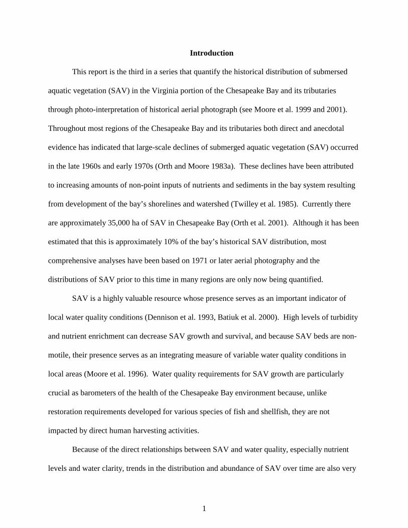
This report is the third in a series that quantify the historical distribution of submersed

aquatic vegetation (SAV) in the Virginia portion of the Chesapeake Bay and its tributaries

through photo-interpretation of historical aerial photograph (see Moore et al. 1999 and 2001).

Throughout most regions of the Chesapeake Bay and its tributaries both direct and anecdotal

evidence has indicated that large-scale declines of submerged aquatic vegetation (SAV) occurred

in the late 1960s and early 1970s (Orth and Moore 1983a). These declines have been attributed

to increasing amounts of non-point inputs of nutrients and sediments in the bay system resulting

from development of the bay’s shorelines and watershed (Twilley et al. 1985). Currently there

are approximately 35,000 ha of SAV in Chesapeake Bay (Orth et al. 2001). Although it has been

estimated that this is approximately 10% of the bay’s historical SAV distribution, most

comprehensive analyses have been based on 1971 or later aerial photography and the

distributions of SAV prior to this time in many regions are only now being quantified.

SAV is a highly valuable resource whose presence serves as an important indicator of

local water quality conditions (Dennison et al. 1993, Batiuk et al. 2000). High levels of turbidity

and nutrient enrichment can decrease SAV growth and survival, and because SAV beds are non-

motile, their presence serves as an integrating measure of variable water quality conditions in

local areas (Moore et al. 1996). Water quality requirements for SAV growth are particularly

crucial as barometers of the health of the Chesapeake Bay environment because, unlike

restoration requirements developed for various species of fish and shellfish, they are not

impacted by direct human harvesting activities.

Because of the direct relationships between SAV and water quality, especially nutrient

levels and water clarity, trends in the distribution and abundance of SAV over time are also very

2

useful in understanding trends in water quality. Review of photographic evidence from a number

of sites dating back to 1937 suggests that SAV, once abundant throughout the Chesapeake Bay

system, have declined from historic levels (Moore et al. 1999, 2001) and therefore water quality

conditions may have similarly deteriorated (Orth and Moore 1983a).

Goals for water clarity criteria for shallow water zones in Virginia that are currently being

developed by the Chesapeake Bay Program are based in large part on the historical depth limits

of SAV that are quantified by this work and previous work (Moore et al. 1999, 2001). Since

SAV growth and survival has been directly related to seasonal levels of water clarity (Batiuk et

al. 2000) historical growth to various depths such as 0.5 m, 1.0 m and 2.0 m suggest greater

levels of water clarity the greater the depth of growth. By superimposing isobaths with historical

SAV distributions the proportion of historical SAV growing at or below specific depths can be

determined, and subsequently used to set water clarity targets.

Areas with high currents and wave activity or sites where sediments are very high in

organic content may not be suitable for SAV growth. Therefore targets for the geographical

limits of SAV restoration have been based on documented evidence of previous SAV growth in

the region since 1971 (Batiuk et al. 1992, 2000).

SAV communities are particularly suitable for identification through analysis of aerial

photography from a variety of sources (Orth and Moore 1984). Although estuarine waters can be

quite turbid, SAV are generally found growing in littoral areas where depths are less than two

meters and their photographic signatures can be identified by experienced photo-interpreters.

Although the absence of SAV on historical aerial photographs does not necessarily preclude

SAV occurrence, SAV signatures are strong supporting evidence for the previous occurrence of

SAV (Orth and Moore 1983b).

3

The objectives of this study were: 1) To search photo archives for imagery of the

littoral zones in the tidal portions of the Eastern Shore coastal basins and mid-bay island

complexes (Appendix 1) for evidence of SAV. These beds represent an historical, pre-decline

benchmark of a healthy SAV community in these regions of the Chesapeake Bay and its

tributaries. 2) To create a digital composite database of these photo-interpreted bed outlines and

to quantify these historic SAV distributions using a computer-based GIS (Arc/Info) and to

provide this information to the Chesapeake Information Management System (CIMS).

Methods

Key photographic databases, including Virginia Department of Transportation (VDOT),

National Oceanic and Atmospheric Administration (NOAA), United States Department of

Agriculture (USDA), United States Geological Survey (USGS), and the Virginia Institute of

Marine Science (VIMS) archives as well as other published reports, were searched for

photography and other information relative to SAV occurrence in the Eastern Shore coastal

basins and mid-bay island complexes prior to the decline in the early 1970s. Photographic

databases ranging from the 1930s to the 1960s were searched by direct visits to view paper prints

and color transparencies. Photographs that contained images of SAV were scanned, photo-

interpreted and digitized as described below. Web-based USGS and NOAA databases were also

searched online using a web browser. Photo-interpretation of the selected aerial photographs

followed as closely as possible the methods currently used to delineate SAV beds throughout the

Chesapeake Bay in the annual aerial SAV surveys (eg. Orth et al. 2001) and earlier historical

SAV reports (Moore et al. 1999, 2001). Generally, high salinity SAV beds, which may have

occurred in regions of the Eastern Shore where salinities are typically above 10 psu, can be

identified in the shallow, near shore regions by their characteristic bottom patterns and

4

reflectance signatures. These patterns are similar to beds currently found in other regions of the

lower bay.

Initial screening of photographic prints was accomplished by viewing under a 10X

magnification viewer. Each print was searched for SAV signatures, and the quality of the

imagery for SAV delineation was estimated as “Good,” “Fair,” or “Poor.” Those prints that

showed some evidence of SAV signatures were scanned at a resolution of 600 dpi and viewed

using ERDAS Imagine™ image processing software.

The aerial photography that was determined to have SAV signatures was processed using

a heads-up, on-screen digitizing system. The system improves accuracy by combining the series

of images into a single geographically registered image permitting the final SAV interpretation to

be completed seamlessly in a single step. In addition, the images are available digitally and can

be printed along with the interpreted lines to show the precise character of the SAV beds.

The standard 9 in X 9 in, 1:24,000 scale black and white aerial photographs, which were

scanned at a resolution of 600 dpi, formed pixels approximately one meter in width. This is the

minimum resolution required to accurately delineate SAV beds and resulted in files that were

approximately 30 megabytes in size. The scanned images were then transferred to a Windows

2000 workstation for registration using ERDAS Orthobase™ (ERDAS, Atlanta, Ga.).

Horizontal control was taken from USGS digital orthophoto quarter quads (DOQQ) and USGS

1:24,000 scale topographic quadrangles. USGS DEMs for the region were merged and used for

vertical control. The Orthobase™ software combined both sources of control with a set of

common “tag” points that were identified on pairs of photos to generate a photogrammetric

solution and orthorectify the images, producing a single geographically corrected product that

5

was used for interpretation. The total RMS error for the solution varied among images from

2.6 meters to 4.1 meters with a mean of 3.5 meters.

SAV bed outlines were traced directly from the combined image displayed on the

computer screen using ERDAS Imagine™ into an ArcInfo™ (ESRI, Redlands, Ca.) GIS polygon

file. The image scale was held fixed at 1:12,000 and line segments for polygons characterizing

the beds were set to be no shorter than 20 meters to maintain consistency with previous historical

SAV surveys. The interpreted boundaries were drawn to include all visible SAV areas regardless

of patchiness or density.

Results and Discussion

Acquisition of Historical Photography

A variety of pre-1971 historical aerial photographic images of the Eastern Shore study

region were located and reviewed, however the quality of the imagery for determination of SAV

abundance ranged from good to poor. In general, a number of criteria must be met for

acquisition of aerial photographs that are optimum for delineation of estuarine SAV (eg. Orth and

Moore 1983a; Orth et al, 2001). These address tidal stage, plant growth stage, sun elevation,

water and atmospheric transparency, wind, sensor operation, flight line plotting and film type.

Most imagery used for historical SAV analyses was obtained for other purposes, usually land use

or farming analyses, and therefore, while criteria for atmospheric conditions are usually met (eg.

sun elevation, atmospheric transparency, etc.), those important for SAV delineation (eg. tidal

stage, water transparency, plant growth stage) may not be met. In addition, while standard black

and white, and color photographs are useful for SAV delineation (Orth and Moore 1984) other

film types such as infrared or color infrared photography, which effectively delineations upland

6

vegetation, are less useful in delineating submerged vegetation because of the rapid absorption of

the infrared wavelengths of sunlight in water.

In general, the most useful historical photography found in this study for delineation of

SAV in the Eastern Shore came from USDA. This photography acquired for land use and

agricultural purposes was primarily black and white format at scales of approximately 1:20,000.

The earliest photography is from USDA over-flights conducted during 1936 and 1937. However

much of this 1930s photography was found to show less SAV coverage than similar photography

from the 1950s. This pattern of coverage is similar to that found for many other regions of the

Virginia portion of the bay (Moore et al. 1999,2001). Qualitatively, in many areas the difference

appeared to be related to overall poorer atmospheric and water clarity conditions making SAV

less apparent. In many other areas it appeared that the SAV were generally less abundance during

the periods of the over-flights during the 1930s compared to the 1950s. Slight seasonal

differences may have also been a factor, however, both sets of photography were taken during the

approximate middle of the principal SAV growing season (April-October). Given these

differences, the 1950s series of USGS photographs ranging from 1952 to 1956 were chosen to

delineate maximum coverage of SAV in the study region.

Historical SAV Distribution

This study investigated the historical distribution of SAV in three bay segments: CB7PH,

POCMH and TANMH. Of these three only CB7PH is located entirely in Virginia. POCMH and

TANMH have portions in Maryland. In this report only the Virginia portions of these two

segments are discussed and summarized. These results are being combined with the results of a

companion Maryland historical SAV study to provide a bay-wide complete analysis of these and

other bay segments that cross state boundaries.

7

A total of 13,046 hectares of sub-tidal bottom in the Eastern Shore of Virginia bay study

area between the southern tip of Fisherman’s Island and the Virginia-Maryland border, including

the mid-bay island complex, were found to display historical SAV signatures. Of this total

approximately 10,451 ha, or 80%, were determined to be growing at depths shallower than 1 m

MLW (Mean Low Water), 2,511 ha or 19% between 1 m and 2 m MLW, and 84 ha or <1% at

depths below 2 m MLW (Table 1). Approximately 6,116 ha of the historical SAV in Bay

segment CB7PH (Table 2) were located along the eastern shoreline of the bay and extending into

the lower one-third of the various shoreline tidal creeks. Approximately 5,584 ha of historical

SAV were growing in the Virginia portion of the mid-bay island complex (TANMH) and 1,646

ha in the Virginia portion of the Pocomoke River region (POCMH).

The mid-bay island complex segment (TANMH) was found to have a greater proportion

of historical SAV growing deeper than 1 m (30.6 %) compared to the Pocomoke River segment

(17.8%; POCMH) or the Eastern Shore Coastal Bay segment (11.2%; CB7PH). This difference

may have been related to water clarity since both POCMH and CB7PH segments include areas

within tidal creeks and embayments that may have been subject to higher levels of runoff.

Additionally, many areas with depths between 1 and 2 meters in POCMH and CB7PH that might

have supported SAV from a water quality standpoint are located in areas that are subject to high

levels of physical stress that historically have been unprotected by bars or islands from the long

fetch to the west. SAV would have been excluded from these regions by physical factors.

An average of 50.1% of the historical SAV in this Eastern Shore study area was also

observed in 2001 (Table 2). Losses of SAV have occurred in all areas with the coastal basins and

tidal tributaries along the eastern shoreline of Accomac and Northampton Counties (CB7PH)

showing the least declines (39.3%) compared to 57.7% and 64.0% in segments TANMH and

8

Table 1. Historical SAV Distribution for Each CBP Bay Segment in Study Area (Total and by Depth Zone Below MLW)

DEPTH ZONES** 0 TO 1 METERS 1 TO 2 METERS > 2 METERS

BAY

SEGMENTS HECTARES % TOTAL

HECTARES % TOTAL

HECTARES % TOTAL

TOTAL

HISTORICAL (HECTARES)**

CB7PH 5,435 88.8 633 10.3 54 0.9 6,116 POCMH 1,353 82.2 284 17.3 9 0.5 1,646 TANMH 3,666 69.4 1,597 30.2 22 0.4 5,284 Total 10,451 80.1 2,511 19.2 84 0.6 13,047 ** = Include only Virginia areas. Table 2. Historical (Pre-1971), Tier 1, Tier 2, Tier 3, 1971-2001 Composite and Current (2001) Distribution of SAV by CBP Segment in Study Area

BAY SEGMENT

HISTORICAL SAV

(PRE 1971)**

TIER 1 GOAL*

TIER 2 TARGET*

TIER 3 TARGET*

1971-2001 COMPOSITETARGET**

2001 MAPPED

SAV**

2001 %

HISTORICAL** CB7PH 6,116 4889 11,538 13,183 6,265 3,712 60.7 POCMH 1,646 841 5,672 7,272 1,016 595 36.0 TANMH 5,566 8,053 15,732 23,482 4,012 2,234 40.1 Total 13,329 13,783 20,936 43,937 11,293 6,541 49.1 * = Include both Maryland and Virginia areas ** = Include only Virginia areas.

9

POCMH respectively. Within CB7PH losses have been least in the historical SAV areas located

in the lower portions of the individual creek systems and along the bay shoreline and greatest

within the creeks themselves. The Tier 1 goal and Tier 2 and 3 targets (Batiuk et al. 2000) have

not been established for the Virginia-only portions of these segments. The goal and targets for

the entire segments are presented in Table 2 for comparative purposes.

Literature Cited

Batiuk RA, Orth RJ, Moore KA, et al. 1992. Submerged Aquatic Vegetation Habitat Requirements and Restoration Targets: a Technical Synthesis. Annapolis, Maryland: USEPA, Chesapeake Bay Program. Batiuk, R., P. Bergstrom, M. Kemp, E. Koch, L. Murray, C. Stevenson, R. Bartleson, V. Carter, N. Rybicki, J. Landwehr, C. Gallegos, L. Karrh, M. Naylor, D. Wilcox, K. Moore, S. Ailstock, M. Teichberg. 2000. Chesapeake Bay submerged aquatic vegetation water quality and habitat-based requirements and restoration targets: A second technical synthesis. CBP/TRS 245/00. EPA 903-R-00-014, U.S. EPA, Chesapeake Bay Program, Annapolis, MD. Dennison WC, Orth RJ, Moore KA, et al. 1993. Assessing water quality with submersed aquatic

vegetation: habitat requirements as barometers of Chesapeake Bay health. BioScience, 43 (2): 86-94.

Moore K.A., Neckles H.A., Orth R.J. 1996. Zostera marina (eelgrass) growth and survival along

a gradient of nutrients and turbidity in the lower Chesapeake Bay. Marine Ecology Progress Series, 142: 247-259.

Moore, K.A., Wilcox, D., Orth, R., Bailey, E.. 1999. Analysis of historical distribution of submerged aquatic vegetation (SAV) in the James River. Special Report no. 355 in

Applied Marine Science and Ocean Engineering. The Virginia Institute of Marine Science, Gloucester Point, Va. 43 pp.

Moore, K.A. D.Wilcox, B.Anderson and R.J. Orth. 2001. Analysis of historical distribution of

submerged aquatic vegetation (SAV) in the York and Rappahannock rivers as evidence of historical water quality. Special Report No. 375 in Applied Marine Science and Ocean Engineering. VIMS. Gloucester Point, Va. 51p.

10

Orth, R.J., D.J. Wilcox, L.S. Nagey, A.L. Tillman and J.R. Whiting.. 2001. Distribution of Submerged Aquatic Vegetation in the Chesapeake Bay and Coastal Bays - 2000. VIMS

Special Scientific Report Number 143. Final Report to U.S. EPA, Chesapeake Bay Program, Annapolis, MD. Grant No.CB993777-04-0

Orth R.J. and K.A. Moore. 1983a. Chesapeake Bay: An unprecedented decline in submerged

aquatic vegetation. Science, 222: 51-53. Orth R.J. and K.A. Moore. 1983b. Submersed vascular plants: techniques for analyzing their

distribution and abundance. Marine Technology Progress Series, 17 (2): 38-52. Orth R.J. and K.A. Moore. 1984. Distribution and abundance of submerged aquatic vegetation in Chesapeake Bay: an historical perspective. Estuaries, 7 (4B): 531-540. Twilley R.R., W.M. Kemp, K.W. Staver, et al. 1985. Nutrient enrichment of estuarine submersed

vascular plant communities. 1. Algal growth and effects on production of plants and associated communities. Marine Ecology Progress Series, 23: 179-191.

11

Appendix 1

CBP Bay Segments Showing Distribution and Abundance of Historical SAV

Chesapeake B

ay

Delm

arva

Pen

insu

la

AtlanticOcean

187

CB7PH

TANMHPOCMH

76°15'W

76°15'W

76°0'W

76°0'W

75°45'W

75°45'W

75°30'W

75°30'W

37°0'N 37°0'N

37°15'N 37°15'N

37°30'N 37°30'N

37°45'N 37°45'N

38°0'N38°0'N

Study Area

12

HongaRiver

NanticokeRiver

MonieBay

Little Annemessex R.

FishingBay

Wicomico

River

Fog PointCove

CoveBack

Terrapin SandCove

CoveTwitch

TylerC

re ek

Cedar

Straits

Manokin

River

Big AnnemessexRiver

CoveOkahanikan

NortheastCove

JohnsonCove

Pry Cove

SheepsheadHarbor

Tangier

Sound

PocomokeSound

Po

co

moke

Rive

r

BeasleyBay

Chesapeake B

ay

Island

TangierIsland

FoxGreat

Islands

Island

SouthMarsh

Watts

Little

IslandDeal

IslandSmith

CheesemanIsland

ThorofareIsland

Rum

GooseIsland

Point

CedarIsland

Bloodsworth Island

37 52’30"

38 00’00"

38 07’30"

38 15’00"

76 00’00" 75 52’30" 75 45’00" 75 37’30"

2 0 2 4 6 8 10 KilometersHistorical SAV

TANMH (Hectares)

0

1000

2000

3000

4000

5000

6000Historical SAV

7879

*pd80

pd

81

pd

82

nd

83

nd

848586

0

8788

nd

899091929394959697989900

13

BayHoodRobin

Is.Halfmoon

Marm

usco Creek

East Creek

Johnso

nC

r .

MarshBig

Doe C

r.

Upper Bernard Island

Lower Bernard Island

MuddyC

r.

Guilford Cr.

GuilfordFlats

Is.Cedar

Pt.Flood

Pt.Sandy

ScottIs. Web

Is. Little Back CreekIs.Jacks

EastwardPt.

OystershellPt.

The Thorofare

HoleCreek

Ape

Beasley Bay

Po

com

oke River

Pocomoke Sound

37 45’00"

37 52’30"

38 00’00"

75 52’30" 75 45’00" 75 37’30" 75 30’00"


POCMH (Hectares)

0250500750

1000125015001750 Historical SAV

7879

nd

80

pd

81

pd

82

nd

83

nd

848586

0

8788

nd

899091929394959697989900

14

Onancock Cr.

Nassawadox

Cherrystone

BigMarsh

Chesconnessex Cr.

Pungoteague Cr.

Nandua Cr.

CreekOccohannock

CraddockCr.

Creek

Hungars Cr.Mattawoman Cr.

OldPlantation

Creek

Inlet

Chesapeake BayMouth of the

Che

sape

ake

Bay

Atlantic

Ocean

CapeCharles

TangierIsland Watt’s

Island

IslandFisherman

37 15’00"

37 30’00"

37 45’00"

76 00’00" 75 45’00" 75 30’00"


CB7PH (Hectares)

01000200030004000500060007000

Historical SAV

7879

nd

808182

nd

83

nd

848586

0

8788

nd

899091929394959697989900

15

16

Appendix 2

7.5 minute USGS Quadrangles Showing Distribution and Abundance

Of Historical SAV

Chesapeake B

ay

Delm

arva

Pen

insu

la

AtlanticOcean

187

186

142 143 212

177 133 134 184 213

178 124 214 215

119 216

113 114 217 218

183 179 107 108 109 219

099 100 101 102 198182

220

174098

106

112

118

123

132

141

147

151 15215076°15'W

76°15'W

76°0'W

76°0'W

75°45'W

75°45'W

75°30'W

75°30'W

37°0'N 37°0'N

37°15'N 37°15'N

37°30'N 37°30'N

37°45'N 37°45'N

38°0'N38°0'N

Study Area

17

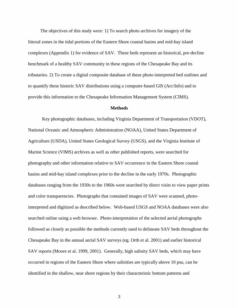
Historical Submerged Aquatic VegetationEwell, Md.- Va. (099)

Hectares of SAV: 1,787.98

Sources: VIMS,USGS

1000 0 1000 2000 metersHistorical SAV Coverage

18

Historical Submerged Aquatic VegetationGreat Fox Island, Va.- Md. (100)


Sources: VIMS,USGS


19

Historical Submerged Aquatic VegetationTangier Island, Va. (107)


Sources: VIMS,USGS


20

Historical Submerged Aquatic VegetationChesconessex, Va. (108)


Sources: VIMS,USGS


21

Historical Submerged Aquatic VegetationParksley, Va. (109)


Sources: VIMS,USGS


22

Historical Submerged Aquatic VegetationNandua Creek, Va. (113)

Hectares of SAV: 526.80

Sources: VIMS,USGS


23

Historical Submerged Aquatic VegetationPungoteague, Va. (114)


Sources: VIMS,USGS


24

Historical Submerged Aquatic VegetationJamesville, Va. (119)


Sources: VIMS,USGS


25

Historical Submerged Aquatic VegetationFranktown, Va. (124)


Sources: VIMS,USGS


26

Historical Submerged Aquatic VegetationCape Charles, Va. (133)


Sources: VIMS,USGS


27

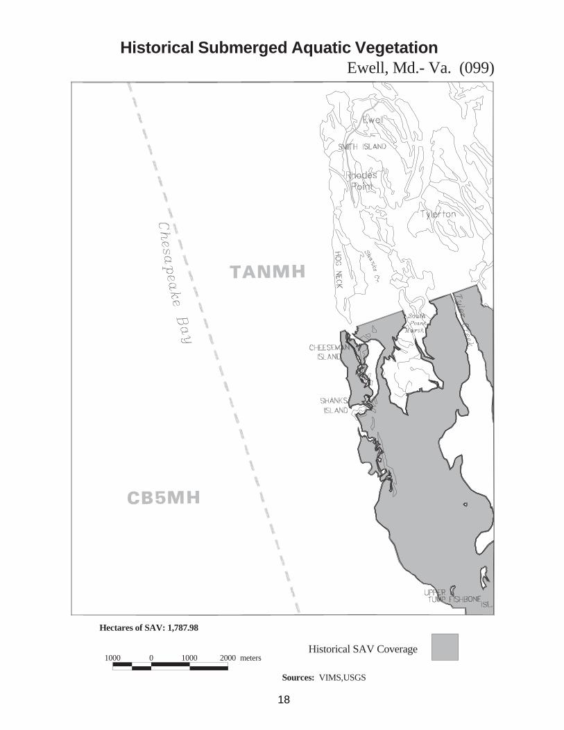
Historical Submerged Aquatic VegetationCheriton, Va. (134)


Sources: VIMS,USGS


28

Historical Submerged Aquatic VegetationElliotts Creek, Va. (142)


Sources: VIMS,USGS


29

Historical Submerged Aquatic VegetationTownsend, Va. (143)


Sources: VIMS,USGS


30

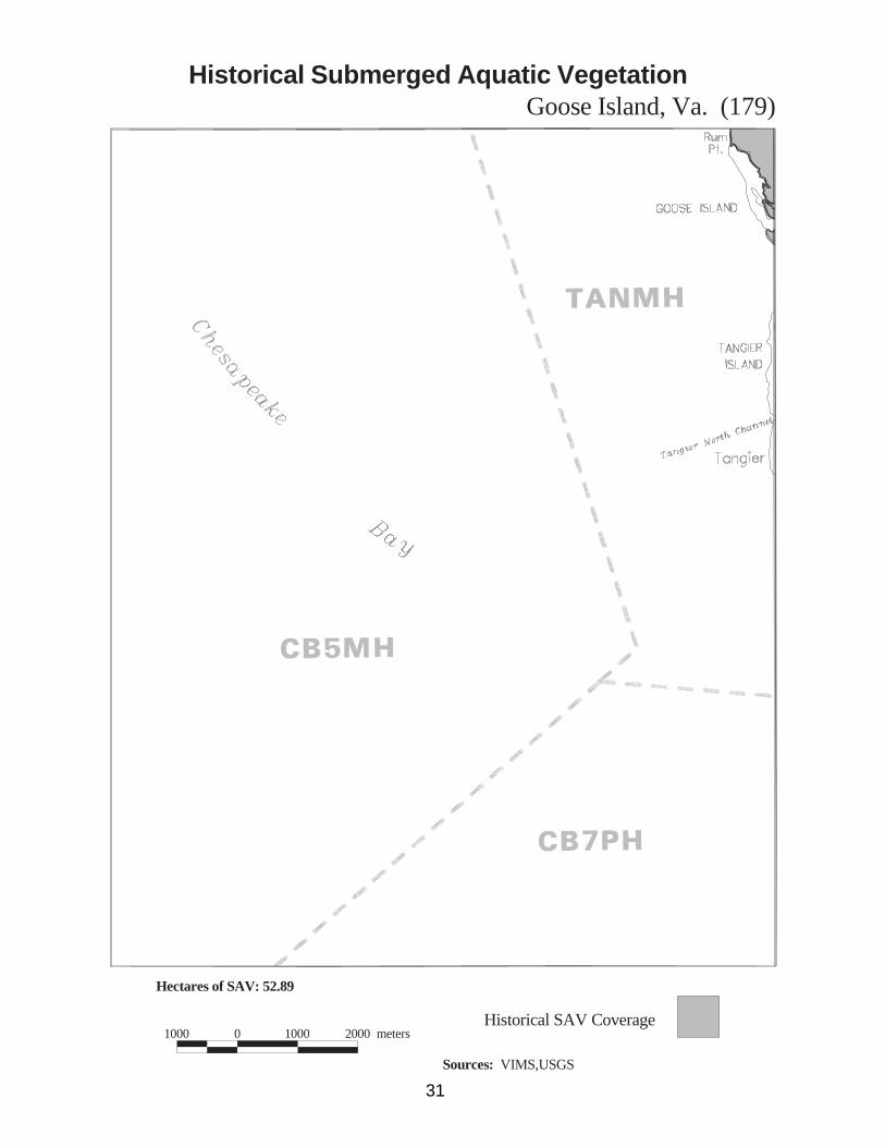
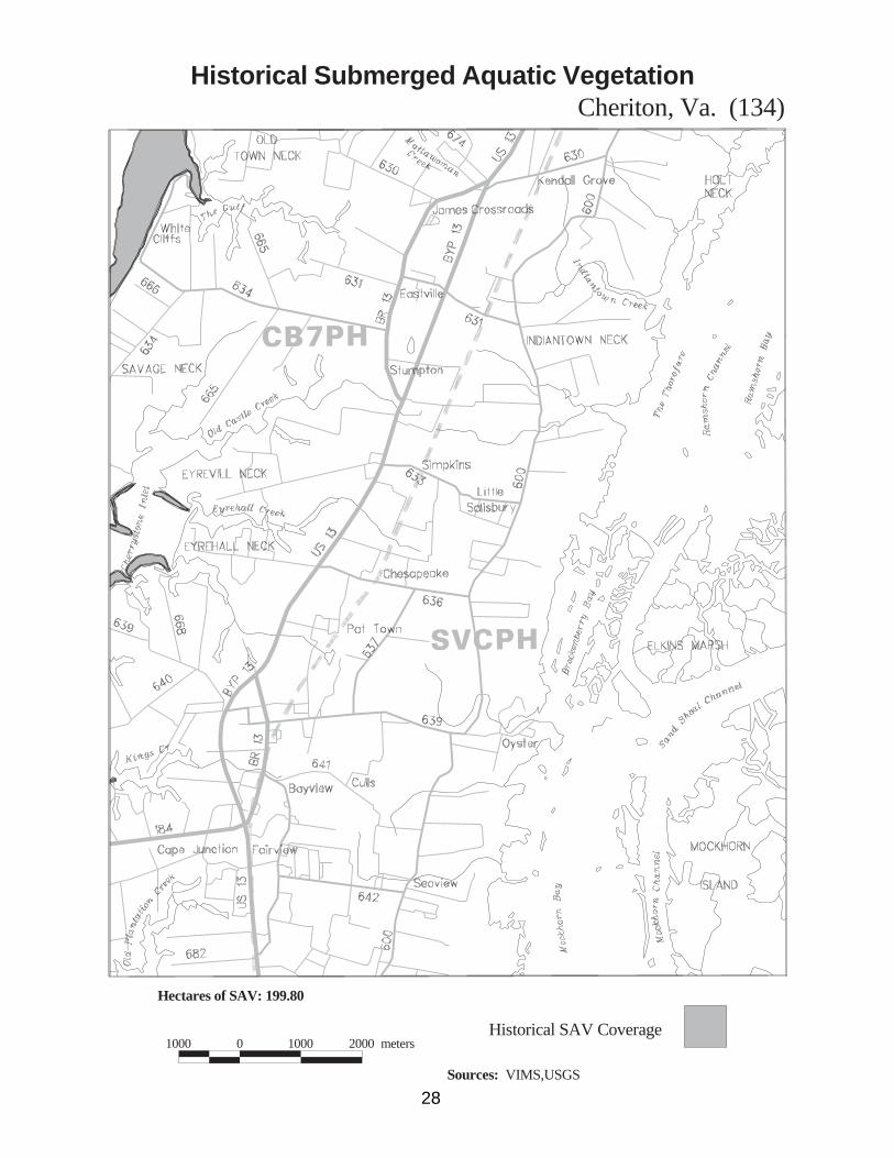
Historical Submerged Aquatic VegetationGoose Island, Va. (179)


Sources: VIMS,USGS


31

Historical Submerged Aquatic VegetationExmore, Va. (187)


Sources: VIMS,USGS


32

Analysis of historical distribution of SAV in the Eastern Shore Coastal Basins and Mid-Bay Island...

Documents

Transcript of Analysis of historical distribution of SAV in the Eastern Shore Coastal Basins and Mid-Bay Island...