Analysis of Geometric Primitives in Quantitative Structure ...

Remote Sens. 2015, 7, 4581-4603; doi:10.3390/rs70404581OPEN ACCESS

remote sensingISSN 2072-4292

www.mdpi.com/journal/remotesensing

Article

Analysis of Geometric Primitives in Quantitative StructureModels of Tree StemsMarkku Åkerblom 1,*, Pasi Raumonen 1, Mikko Kaasalainen 1 and Eric Casella 2

1 Department of Mathematics, Tampere University of Technology, P.O. Box 553, Tampere 33101,Finland; E-Mails: [email protected] (P.R.); [email protected] (M.K.)

2 Centre for Sustainable Forestry and Climate Change, Forest Research, Farnham GU10 4LH,UK; E-Mail: [email protected]

* Author to whom correspondence should be addressed; E-Mail: [email protected]

Academic Editors: Nicolas Baghdadi and Prasad S. Thenkabail

Received: 3 February 2015 / Accepted: 3 April 2015 / Published: 16 April 2015

Abstract: One way to model a tree is to use a collection of geometric primitives to representthe surface and topology of the stem and branches of a tree. The circular cylinder is oftenused as the geometric primitive, but it is not the only possible choice. We investigate variousgeometric primitives and modelling schemes, discuss their properties and give practicalestimates for expected modelling errors associated with the primitives. We find that thecircular cylinder is the most robust primitive in the sense of a well-bounded volumetricmodelling error, even with noise and gaps in the data. Its use does not cause errorssignificantly larger than those with more complex primitives, while the latter are much moresensitive to data quality. However, in some cases, a hybrid approach with more complexprimitives for the stem is useful.

Keywords: tree modelling; terrestrial laser scanning; shape fitting; biomass estimation;error analysis

1. Introduction

The reconstruction of precise structure models of trees is important in understanding tree growthand decay, competition for resources, soil processes, photosynthesis, etc. The models can be used to

Remote Sens. 2015, 7 4582

compute, e.g., volumes, biomass estimates and size distributions. Terrestrial laser scanning (TLS) offersfast and accurate point clouds from which plant geometry can be reconstructed.

Many possible reconstruction methods from TLS data have been presented [1]. These methods canbe divided roughly into three classes according to the way the tree structure is modelled. One classcomprises the voxel methods, where volumetric models are constructed by partitioning the point cloudinto voxels [2–4]. However, the ability of the voxel methods to model the tree structure is limited.The second class includes the parametric surface methods, where a single continuous surface is used topresent a single branch [5,6]. In some of these methods, the cross-section of a stem or branch can bemodelled as splines or other parameterizable curves [7]. The third class, and the one that we focus on,consists of shape-fitting methods, which use a geometric primitive to represent a part of a branch. Abranch is modelled as a collection of these primitives [8,9]. Thies et al. [10] have presented a methodthat uses overlapping cylinder primitives to assess stem properties, and we have previously presented areconstruction process based on geometric primitives [11].

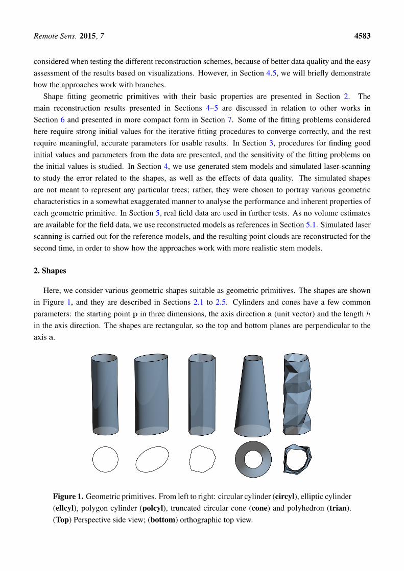
Most of the published shape-fitting methods use the (rectangular) circular cylinder as their elementarybuilding block. This choice is a compromise between simplicity and realistic reconstruction, as it iswell known that the cross-section boundary of stems is never exactly a circle. For example, when thelargest possible circle is fitted inside the cross-sections of eucalyptus trees, as much as 7% of the areais left outside the circle [12]. On average, the ratio between the minor and major diameters of variousconiferous tree species is 0.96, indicating some elliptic features [13]. For branches, the ratio is expectedto be even smaller due to gravity. Thus, it is a fair question if the use of circular cylinders is acceptablein such cases and if other shapes, that a priori appear more suitable, could be used instead with betterresults. Here, we study how the choice of the geometric primitive affects the model error and robustnessof the reconstruction process and what are the pros and cons of using different shapes. In addition tothe circular cylinder (circyl), we study the elliptical cylinder (ellcyl), the circular cone (cone) and thepolygonal cylinder (polcyl) as the possible elementary blocks or geometric primitives (see Figure 1). Inaddition, we use polyhedral cylinder surfaces (trian), which are triangulated meshes, to reconstruct treestems. Similar triangulated surfaces have been previously used for reconstruction with data collectedwith a digitizer from tree stems [14] and root systems [15] and for TLS data and root systems [16].

There is also another intuitive objection against the use of cylinders in particular, but also othergeometric primitives: blocks or primitives cannot be attached to each other, such that the resultingsurface is continuous and without gaps. However, we will show that, for most purposes, this is onlyan aesthetic problem, as all of the structural and geometric properties, such as the branching structure,branching angles, tapering, volumes, lengths, curvatures, etc., can be modelled accurately. Indeed, if allwe need are the structural and geometric properties, it is actually better to leave out continuity (and therelated details) altogether in the modelling process, as these would only make it more difficult, slowerand less reliable.

In the building-block approach, the first step is some segmentation of the point cloud into parts towhich the geometric primitives are fitted. The segmentation process described in [11] was used in thisstudy. This method divides the TLS point cloud efficiently into small surface patches that conform tothe tree surface. These sets are used to segment the point cloud into branches and each segment furtherinto sub-segments that are then reconstructed using shape fitting. In this study, mainly the tree stems are


considered when testing the different reconstruction schemes, because of better data quality and the easyassessment of the results based on visualizations. However, in Section 4.5, we will briefly demonstratehow the approaches work with branches.

Shape fitting geometric primitives with their basic properties are presented in Section 2. Themain reconstruction results presented in Sections 4–5 are discussed in relation to other works inSection 6 and presented in more compact form in Section 7. Some of the fitting problems consideredhere require strong initial values for the iterative fitting procedures to converge correctly, and the restrequire meaningful, accurate parameters for usable results. In Section 3, procedures for finding goodinitial values and parameters from the data are presented, and the sensitivity of the fitting problems onthe initial values is studied. In Section 4, we use generated stem models and simulated laser-scanningto study the error related to the shapes, as well as the effects of data quality. The simulated shapesare not meant to represent any particular trees; rather, they were chosen to portray various geometriccharacteristics in a somewhat exaggerated manner to analyse the performance and inherent properties ofeach geometric primitive. In Section 5, real field data are used in further tests. As no volume estimatesare available for the field data, we use reconstructed models as references in Section 5.1. Simulated laserscanning is carried out for the reference models, and the resulting point clouds are reconstructed for thesecond time, in order to show how the approaches work with more realistic stem models.

2. Shapes

Here, we consider various geometric shapes suitable as geometric primitives. The shapes are shownin Figure 1, and they are described in Sections 2.1 to 2.5. Cylinders and cones have a few commonparameters: the starting point p in three dimensions, the axis direction a (unit vector) and the length hin the axis direction. The shapes are rectangular, so the top and bottom planes are perpendicular to theaxis a.

Figure 1. Geometric primitives. From left to right: circular cylinder (circyl), elliptic cylinder(ellcyl), polygon cylinder (polcyl), truncated circular cone (cone) and polyhedron (trian).(Top) Perspective side view; (bottom) orthographic top view.


2.1. Circular Cylinder

The simplest reconstruction shape is the circular cylinder (circyl), which requires only one additionalparameter: the radius r. When using a circyl, the cross-section of a fraction of a branch is approximatedas a disk with the radius r. For the circyl, the envelope area E = 2πrh and volume V = πr2h. Theparameters of each circyl are iteratively fitted to the dataset, as described in [11]. Each cylinder fittingis done iteratively starting from initial values. For cylinder and cone fitting details and parametrization,see [17].

2.2. Elliptic Cylinder

The elliptic cylinder (ellcyl) approximates the cross-section as an ellipse. Three additional parametersare used to model the ellipse: a pair of semiaxes radii (r1, r2) and the direction α of the major semiaxis(measured as the angle from a reference direction). We use the following approximation for theenvelope area:

E ≈ 2πh

√r21 + r22

2. (1)

The volume V can be computed accurately V = πr1r2h.As a fitting problem when compared to the circyl, the additional parameters make the ellcyl more

complex and time consuming. Therefore, we implement ellcyl fitting in two steps:

1. Estimate axis direction by fitting a circyl.2. Project the points onto a plane perpendicular to the axis direction. Fit an ellipse to the

two-dimensional data.

Since the steps are done in sequence, the procedure is not fully iterative.

2.3. Polygon Cylinder

The cross-section of a cylinder can be defined by any closed curve. However, it is sensible to keep theshape complexity to a minimum to achieve reasonable robustness and computational cost. Therefore, weuse a polygon, which is a closed circuit of vertices v1,v2, . . . ,vk,v1 ∈ R3 connected by straight lines,that in this case is assumed not to intersect itself. In a polygon cylinder (polcyl), the sequence (vi )

ki=1

defines the base of the cylinder and the sequence (vi + ah )ki=1 the top of the cylinder.The perimeter p of a polygon is the sum of distances between consecutive vertices and the envelope

area E = ph. The area of the polygon can be found by projecting the vertices onto a plane orthogonallyand by using Gauss’ area formula for these 2D points (vi):

A =

∣∣∣∣∣k−1∑i=1

vi,1vi+1,2 − vi,2vi+1,1

2

∣∣∣∣∣ , (2)

where vi,1 and vi,2 are the first and second component of the the vertex i, respectively. The polcyl volumeV = Ah.

To fit a polygon cylinder to a point cloud P = {pi ∈ R3 }, we propose the following algorithm.


1. Estimate the axis direction a either by the approaches described in Section 3 or by fitting a circyl.2. Project the points onto a plane perpendicular to the axis a. The projected set is denoted by P⊥a.3. Compute a centre point c for the set P⊥a either by computing the mean or by least-squares circle

fitting [18].4. Divide the elements of the set P⊥a into k sectors around the centre point c.5. For each sector i, compute the mean point vi. If a sector has no elements, interpolate using the

next and previous non-empty sectors.6. Transform the points ( vi ) back to the original coordinate system. The transformed sequence (vi )

is the base of the reconstructed polcyl.

2.4. Cones

A circular cone (cone) is a shape that is limited by a base circle and circular cross-sections thatsmoothly taper to a single point, the apex. A part of a branch is usually not the shape of a completecone with an apex, but a truncated cone where the top is cut off. The fitting problem, however, remainsessentially the same as in the cylindrical case. Fitting a cone to 3D data is an extension of this, sincea cone has a minimum of six parameters [17]. There are two common ways to parametrize a circulartruncated cone, either by using the taper angle or a pair of radii. Here, the latter is chosen: r1 is the radiusof the base, and r2 is the radius of the top. In that case, the surface area E = π(r1+r2)

√h2 + (r2 − r1)2

and the enclosed volume V = 13πh(r21 + r1r2 + r22). Cone fitting is done iteratively starting from

initial values.

2.5. Polyhedron/Triangulation

A polyhedron is a considerably more general and flexible shape than cylinders or cones. In principle,the whole surface model of a tree could be given as a continuous polyhedron. However, due toinsufficiencies in TLS data, it can be impossible to reliably reconstruct a tree as a single polyhedronsurface, so sub-polyhedra as geometric primitives are an efficient means of interpolating between thegaps and for smoothing (regularizing) the effect of noise and outliers. Modelling a part of a tree as apolyhedron captures features in both the axial and radial directions. Polyhedron models are detailed and,compared to the other shapes, require more space for storing the data and are slower to compute.

Given an axis direction a and a reference point p, a point cloud P ⊂ R3 can be partitioned into cellsthe following way:

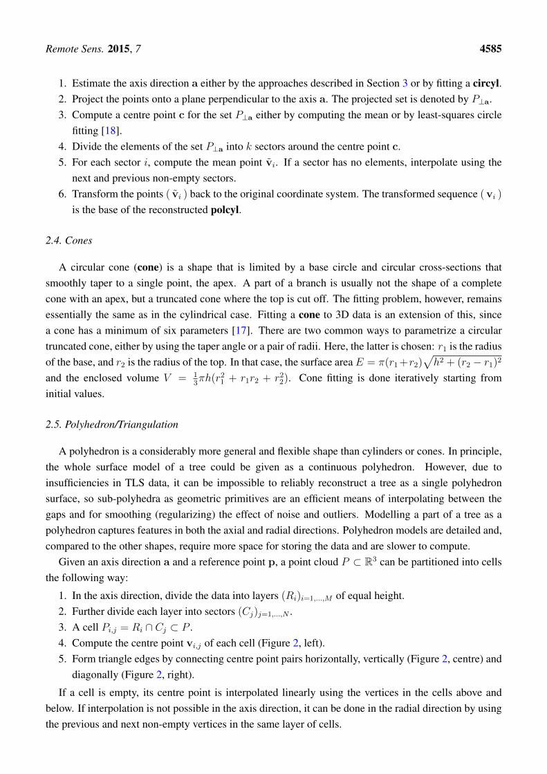
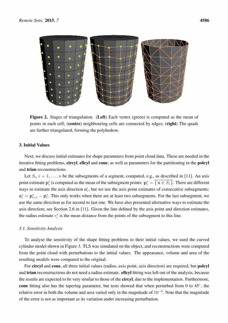
1. In the axis direction, divide the data into layers (Ri)i=1,...,M of equal height.2. Further divide each layer into sectors (Cj)j=1,...,N .3. A cell Pi,j = Ri ∩ Cj ⊂ P .4. Compute the centre point vi,j of each cell (Figure 2, left).5. Form triangle edges by connecting centre point pairs horizontally, vertically (Figure 2, centre) and

diagonally (Figure 2, right).

If a cell is empty, its centre point is interpolated linearly using the vertices in the cells above andbelow. If interpolation is not possible in the axis direction, it can be done in the radial direction by usingthe previous and next non-empty vertices in the same layer of cells.


Figure 2. Stages of triangulation. (Left) Each vertex (green) is computed as the mean ofpoints in each cell; (centre) neighbouring cells are connected by edges; (right) The quadsare further triangulated, forming the polyhedron.

3. Initial Values

Next, we discuss initial estimates for shape parameters from point cloud data. These are needed in theiterative fitting problems, circyl, ellcyl and cone, as well as parameters for the partitioning in the polcyland trian reconstructions.

Let Si, i = 1, . . . , n be the subsegments of a segment, computed, e.g., as described in [11]. An axispoint estimate p∗i is computed as the mean of the subsegment points: p∗i = {x ∈ Si }. There are differentways to estimate the axis direction a∗i , but we use the axis point estimates of consecutive subsegments:a∗i = p∗i+1 − p∗i . This only works when there are at least two subsegments. For the last subsegment, weuse the same direction as for second to last one. We have also presented alternative ways to estimate theaxis direction; see Section 2.6 in [11]. Given the line defined by the axis point and direction estimates,the radius estimate r∗i is the mean distance from the points of the subsegment to this line.

3.1. Sensitivity Analysis

To analyse the sensitivity of the shape fitting problems to their initial values, we used the curvedcylinder model shown in Figure 3. TLS was simulated on the object, and reconstructions were computedfrom the point cloud with perturbations to the initial values. The appearance, volume and area of theresulting models were compared to the original.

For circyl and cone, all three initial values (radius, axis point, axis direction) are required, but polcyland trian reconstructions do not need a radius estimate. ellcyl fitting was left out of the analysis, becausethe results are expected to be very similar to those of the circyl, due to the implementation. Furthermore,cone fitting also has the tapering parameter, but tests showed that when perturbed from 0 to 45◦, therelative error in both the volume and area varied only in the magnitude of 10−3. Note that the magnitudeof the error is not as important as its variation under increasing perturbation.


Figure 3. Curved pipe model used in the sensitivity analysis.

For the radius, perturbation was introduced by scaling the original estimate by factors from 0.1 to2.5. The test showed that circyl and cone are both very indifferent to the radius estimate. With factorsbetween 1.3 and 2.0, the perturbation had a minor effect on cone models, but the relative error stayedbelow 5% for both volume and area.

0 0.2 0.4 0.6 0.8 1 1.2 1.4 1.6 1.8 2 2.2 2.4

−50%

0%

50%

Axis point perturbation

volumeerror

circyl polcylcone trian

Figure 4. Relative volume error as a function of axis point estimate perturbation. Themagnitude of the transition was received by multiplying the radius estimate by the scalingfactor shown on the horizontal axis.

The axis point estimate was perturbed by moving it to a random direction perpendicular to theestimated axis direction. The magnitude of the move was the estimated radius scaled by a factor variedagain from 0.1 to 2.5. The effect of the perturbation on the model volume is presented in Figure 4. Forall of the shapes, the error remains small with scaling factor values lower than one. With larger values,as the axis point estimate moves outside the estimated cylinder hull, the error for polcyl starts to riseclose to linearly for both quantities. At 2.5, the errors are 500% and 150%, for the volume and area,respectively. trian overestimates the area by ∼10% and underestimates the volume by up to 50% withfactor values above 1.5.

The axis direction estimate was perturbed by rotating it in a random direction by an angle varyingfrom 0◦ to 90◦. The results for the volume are shown in Figure 5. The iterative fitting methods, circyland cone, remain unaffected with perturbations smaller or equal to 45◦. Even at 81◦, the errors in thevolume are only 5% and 7%, respectively. polcyl is very sensitive to the axis direction, even at smallangle perturbations. With large perturbations, the trian model error can be up to 50% underestimation.


0◦ 45◦ 90◦−50%

−25%

0%

25%

Axis direction perturbation

volumeerror

circyl polcylcone trian

Figure 5. Relative volume error as a function of axis direction estimate perturbation.

Above, each of the initial values was studied individually. In real cases, the perturbation is neverspecific to a single property, but rather all of them.

4. Reconstruction from Generated Data

The reconstruction accuracy for the different shapes was studied using generated stem objects in orderto better show the differences of the approaches. For this purpose, eight stem models were created usingthe 3D modelling software Blender. Some of the models are non-realistic, because the differences in themodelling approaches would not otherwise be visible. For a more realistic case, models derived fromreal oak trees were used in Section 5.1. The models were imported into MATLAB, where simulated TLSmeasurements were made. The resulting point clouds were reconstructed using all of the shapes.

4.1. Generation Process

The models (see Figure 6) are 15-m tall and consist of 302 consecutive 32-vertex rings. The diameterof the stems remains constant for the first 2 m at 0.40 m and then tapers smoothly to 0.12 m at thetop. Stems 2–4 are unrealistically elliptic on purpose, and Stems 4, 6 and 8 have random perturbationson the surface.

1 2 3 4 5 6 7 8

Figure 6. Flattened portraits of generated stem models (vertical dimension scaled downto 20%).


The simulated scans consisted of three positions around the model with an angular samplingresolution of 0.036◦ and a distance between the scanner and the models of ∼5 m. The scanner positionsare visualized in Section 4.4. The scans were co-registered perfectly and were made with two noiselevels: no noise and uniformly distributed noise between −3 mm and 3 mm.

4.2. Reconstruction Results

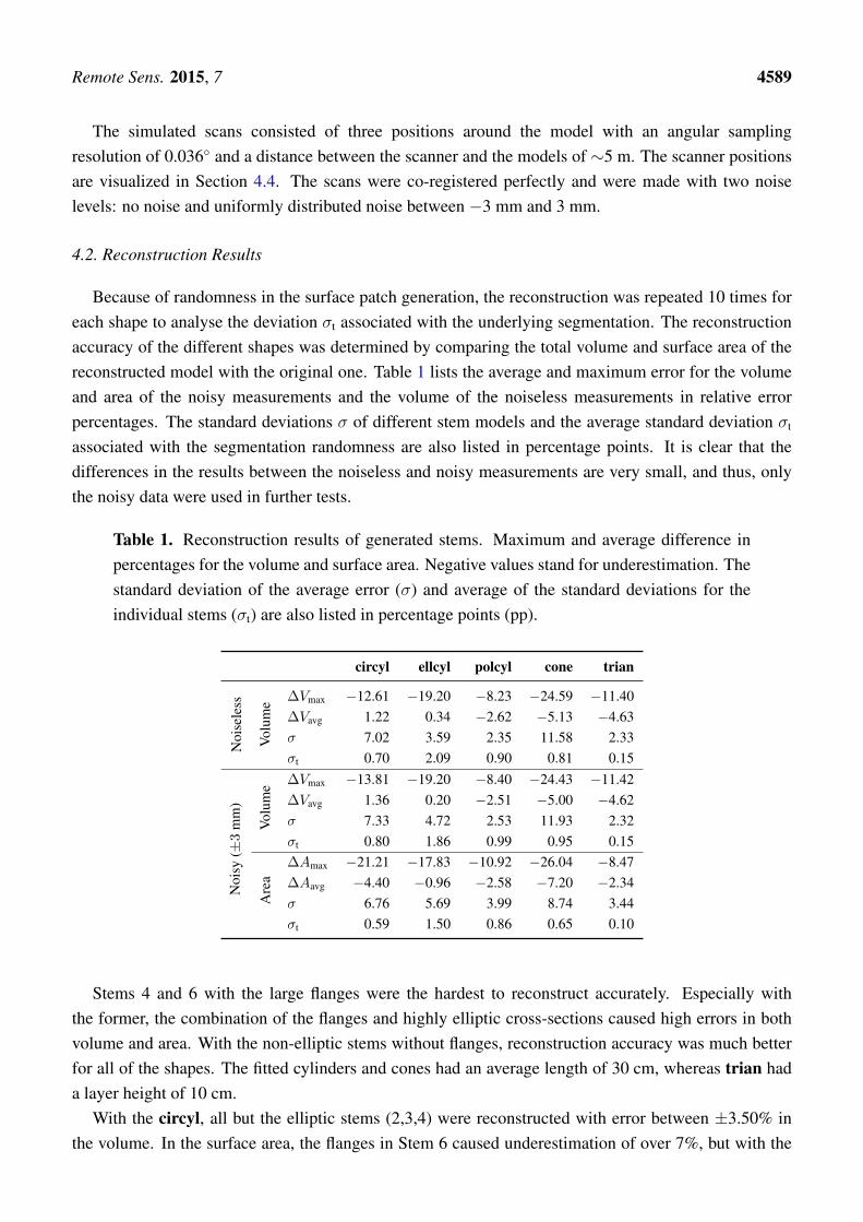
Because of randomness in the surface patch generation, the reconstruction was repeated 10 times foreach shape to analyse the deviation σt associated with the underlying segmentation. The reconstructionaccuracy of the different shapes was determined by comparing the total volume and surface area of thereconstructed model with the original one. Table 1 lists the average and maximum error for the volumeand area of the noisy measurements and the volume of the noiseless measurements in relative errorpercentages. The standard deviations σ of different stem models and the average standard deviation σt

associated with the segmentation randomness are also listed in percentage points. It is clear that thedifferences in the results between the noiseless and noisy measurements are very small, and thus, onlythe noisy data were used in further tests.

Table 1. Reconstruction results of generated stems. Maximum and average difference inpercentages for the volume and surface area. Negative values stand for underestimation. Thestandard deviation of the average error (σ) and average of the standard deviations for theindividual stems (σt) are also listed in percentage points (pp).

circyl ellcyl polcyl cone trian

Noi

sele

ss

Volu

me ∆Vmax −12.61 −19.20 −8.23 −24.59 −11.40

∆Vavg 1.22 0.34 −2.62 −5.13 −4.63σ 7.02 3.59 2.35 11.58 2.33σt 0.70 2.09 0.90 0.81 0.15

Noi

sy(±

3m

m)

Volu

me ∆Vmax −13.81 −19.20 −8.40 −24.43 −11.42

∆Vavg 1.36 0.20 −2.51 −5.00 −4.62σ 7.33 4.72 2.53 11.93 2.32σt 0.80 1.86 0.99 0.95 0.15

Are

a

∆Amax −21.21 −17.83 −10.92 −26.04 −8.47∆Aavg −4.40 −0.96 −2.58 −7.20 −2.34σ 6.76 5.69 3.99 8.74 3.44σt 0.59 1.50 0.86 0.65 0.10

Stems 4 and 6 with the large flanges were the hardest to reconstruct accurately. Especially withthe former, the combination of the flanges and highly elliptic cross-sections caused high errors in bothvolume and area. With the non-elliptic stems without flanges, reconstruction accuracy was much betterfor all of the shapes. The fitted cylinders and cones had an average length of 30 cm, whereas trian hada layer height of 10 cm.

With the circyl, all but the elliptic stems (2,3,4) were reconstructed with error between ±3.50% inthe volume. In the surface area, the flanges in Stem 6 caused underestimation of over 7%, but with the


other non-elliptic stems, the error was again between ±3%. The standard deviation σ seems relativelyhigh, but it is heavily affected by the elliptic stems.

Using the ellcyl usually resulted in 2%–3% error in volume and area, either from over- orunder-estimation. It did have the lowest average error, but also the highest average standard deviation σt.Overall, ellcyl seemed more unstable than the other approaches.

The polcyl approach seems to underestimate both the volume and the area by∼2.5% on average. Thelargest error appears again in Stems 4 and 6, which have large flanges. The standard deviation of theaverage error is lower than with the iterative approaches, but slightly higher than with trian.

The large flanges were particularly hard for cone to model: too much tapering in the first cone causederrors of over 20%. On stems without flanges or elliptic cross-sections, the volume was underestimatedonly by ∼5% and the area by 4%. The standard deviation of the average error was the highestof all of the shapes.

The trian approach underestimates the volume of most stems by 3% to 5%, although Stem 6 causeshigher error up to 10%. The surface area is reconstructed more accurately, with the average andmaximum errors of −2.34% and 8.47%. The average standard deviation σt is considerably lower thanwith any other approach, and if Stem 6 is discarded, the maximum deviation is only 0.05 percentagepoints (pp). The standard deviation of the average errors σ was also the lowest of all. For taper curvecomparison, see the Supplementary Material.

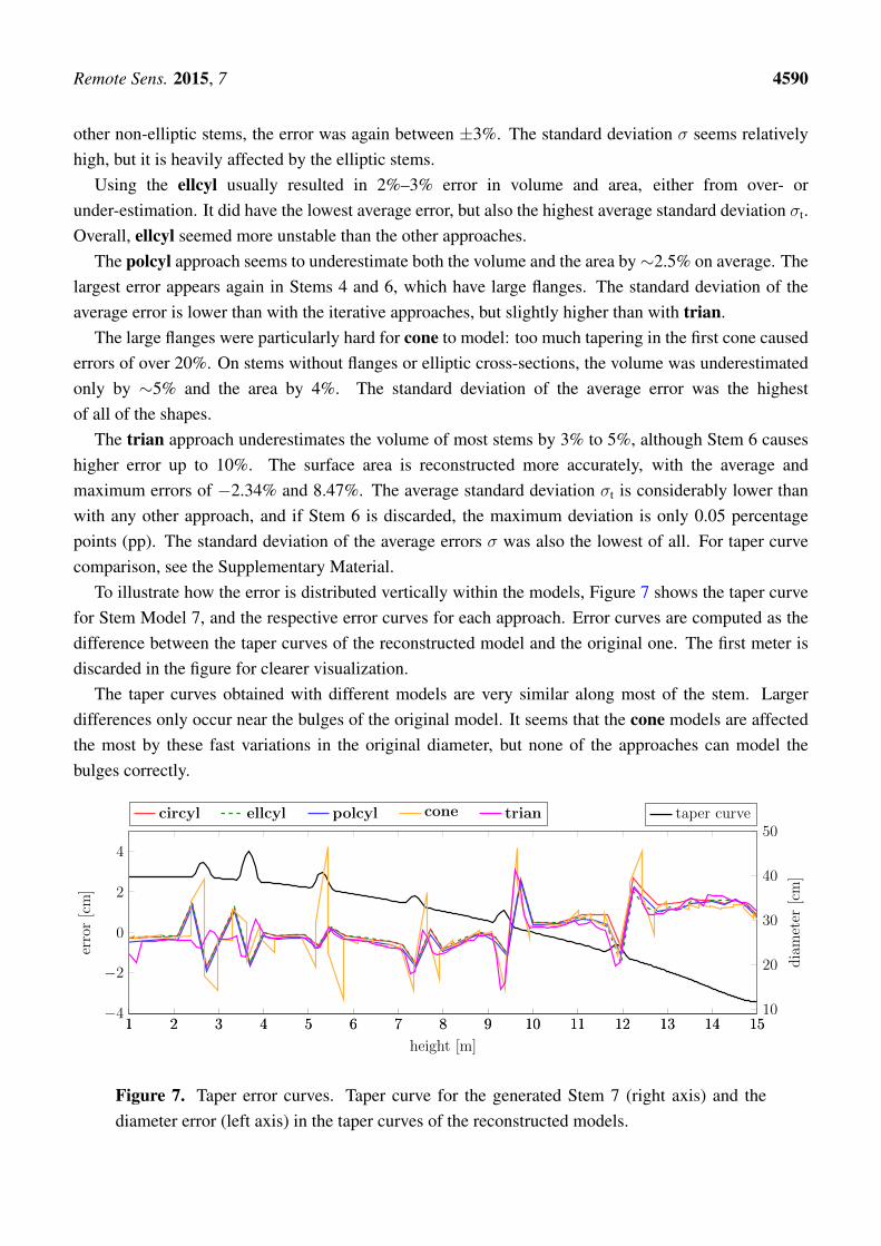
To illustrate how the error is distributed vertically within the models, Figure 7 shows the taper curvefor Stem Model 7, and the respective error curves for each approach. Error curves are computed as thedifference between the taper curves of the reconstructed model and the original one. The first meter isdiscarded in the figure for clearer visualization.

The taper curves obtained with different models are very similar along most of the stem. Largerdifferences only occur near the bulges of the original model. It seems that the cone models are affectedthe most by these fast variations in the original diameter, but none of the approaches can model thebulges correctly.

1 2 3 4 5 6 7 8 9 10 11 12 13 14 1510

20

30

40

50

diameter

[cm]

taper curve

1 2 3 4 5 6 7 8 9 10 11 12 13 14 15−4

−2

0

2

4

height [m]

error[cm]


Figure 7. Taper error curves. Taper curve for the generated Stem 7 (right axis) and thediameter error (left axis) in the taper curves of the reconstructed models.


At the bottom half of the stem, where there are no bulges, the error level stays low and relativelystable. On the top half, i.e., starting from 8 m, the trend of the error starts to rise almost linearly andturns from under- to over-estimation. This is due to the fact that as the diameter gets smaller, the noisebecomes more relevant and also the sample density drops. At 15 m, the trend of the diameter error getsclose to 2 cm.

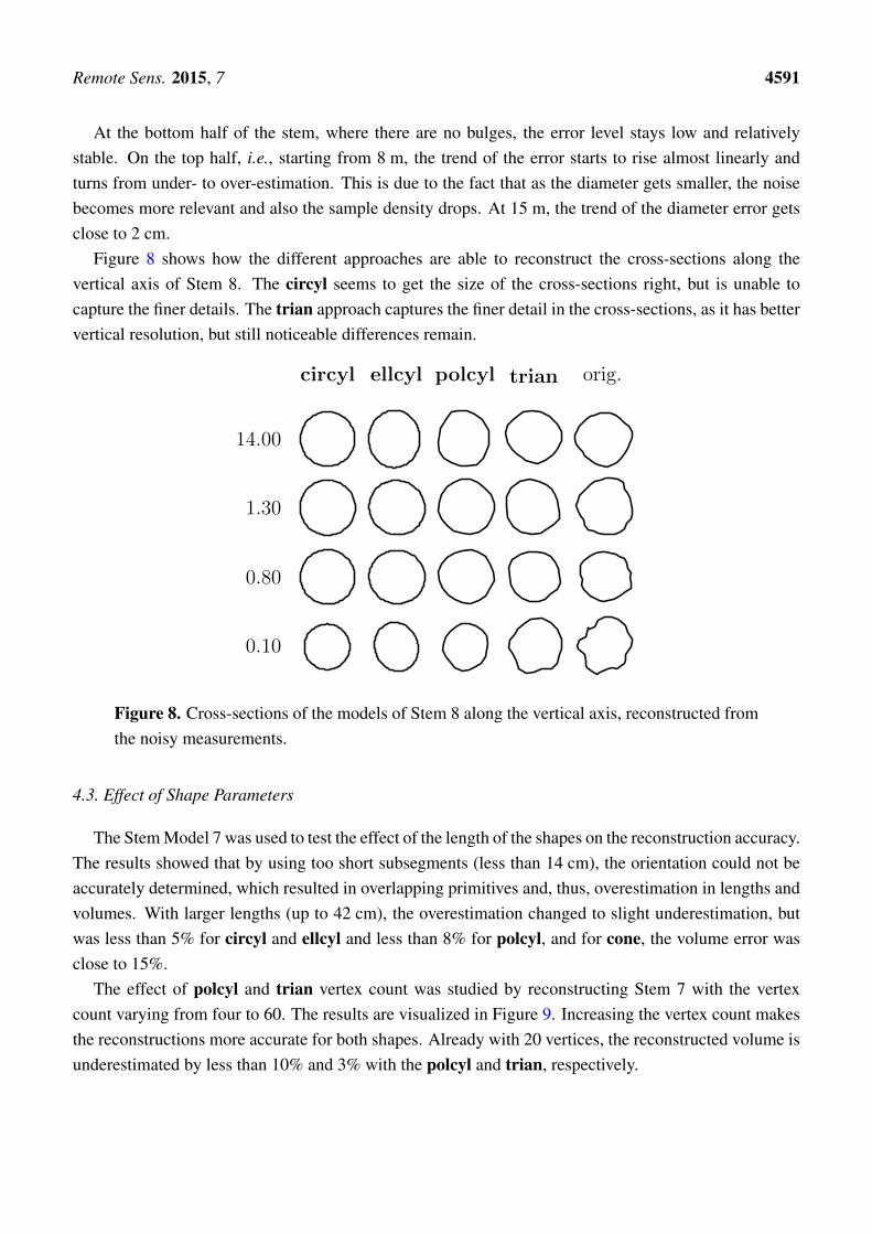
Figure 8 shows how the different approaches are able to reconstruct the cross-sections along thevertical axis of Stem 8. The circyl seems to get the size of the cross-sections right, but is unable tocapture the finer details. The trian approach captures the finer detail in the cross-sections, as it has bettervertical resolution, but still noticeable differences remain.

0.10

0.80

1.30

14.00

circyl ellcyl polcyl trian orig.

Figure 8. Cross-sections of the models of Stem 8 along the vertical axis, reconstructed fromthe noisy measurements.

4.3. Effect of Shape Parameters

The Stem Model 7 was used to test the effect of the length of the shapes on the reconstruction accuracy.The results showed that by using too short subsegments (less than 14 cm), the orientation could not beaccurately determined, which resulted in overlapping primitives and, thus, overestimation in lengths andvolumes. With larger lengths (up to 42 cm), the overestimation changed to slight underestimation, butwas less than 5% for circyl and ellcyl and less than 8% for polcyl, and for cone, the volume error wasclose to 15%.

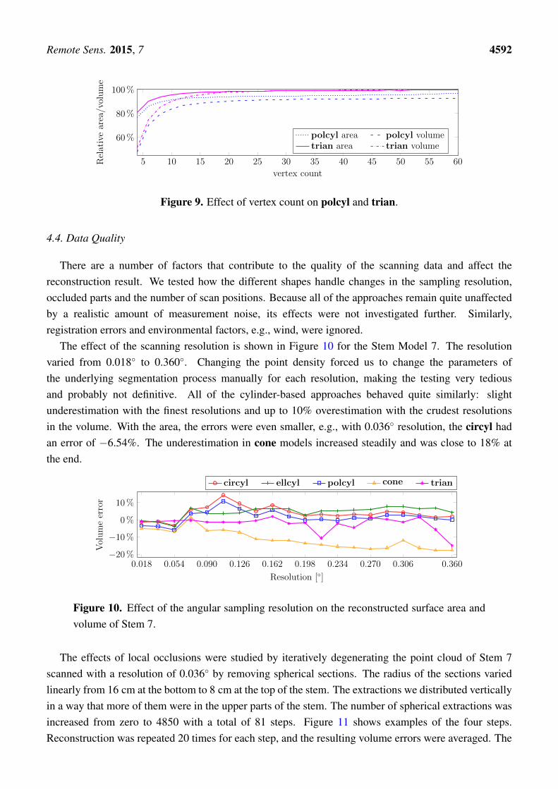
The effect of polcyl and trian vertex count was studied by reconstructing Stem 7 with the vertexcount varying from four to 60. The results are visualized in Figure 9. Increasing the vertex count makesthe reconstructions more accurate for both shapes. Already with 20 vertices, the reconstructed volume isunderestimated by less than 10% and 3% with the polcyl and trian, respectively.


5 10 15 20 25 30 35 40 45 50 55 60

60%

80%

100%

vertex count

Relativearea/volume

polcyl area polcyl volumetrian area trian volume

Figure 9. Effect of vertex count on polcyl and trian.

4.4. Data Quality

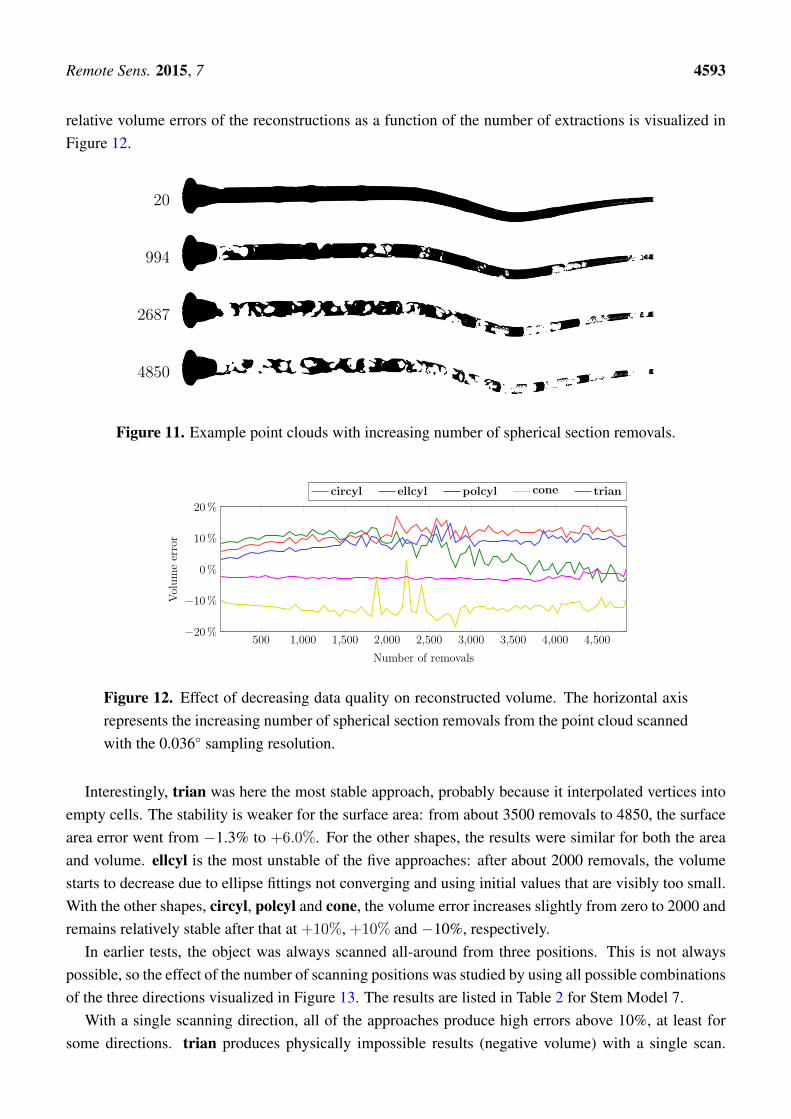
There are a number of factors that contribute to the quality of the scanning data and affect thereconstruction result. We tested how the different shapes handle changes in the sampling resolution,occluded parts and the number of scan positions. Because all of the approaches remain quite unaffectedby a realistic amount of measurement noise, its effects were not investigated further. Similarly,registration errors and environmental factors, e.g., wind, were ignored.

The effect of the scanning resolution is shown in Figure 10 for the Stem Model 7. The resolutionvaried from 0.018◦ to 0.360◦. Changing the point density forced us to change the parameters ofthe underlying segmentation process manually for each resolution, making the testing very tediousand probably not definitive. All of the cylinder-based approaches behaved quite similarly: slightunderestimation with the finest resolutions and up to 10% overestimation with the crudest resolutionsin the volume. With the area, the errors were even smaller, e.g., with 0.036◦ resolution, the circyl hadan error of −6.54%. The underestimation in cone models increased steadily and was close to 18% atthe end.

0.018 0.054 0.090 0.126 0.162 0.198 0.234 0.270 0.306 0.360−20%

−10%

0%

10%

Resolution [◦]

Volumeerror


Figure 10. Effect of the angular sampling resolution on the reconstructed surface area andvolume of Stem 7.

The effects of local occlusions were studied by iteratively degenerating the point cloud of Stem 7scanned with a resolution of 0.036◦ by removing spherical sections. The radius of the sections variedlinearly from 16 cm at the bottom to 8 cm at the top of the stem. The extractions we distributed verticallyin a way that more of them were in the upper parts of the stem. The number of spherical extractions wasincreased from zero to 4850 with a total of 81 steps. Figure 11 shows examples of the four steps.Reconstruction was repeated 20 times for each step, and the resulting volume errors were averaged. The


relative volume errors of the reconstructions as a function of the number of extractions is visualized inFigure 12.

20

994

2687

4850

Figure 11. Example point clouds with increasing number of spherical section removals.

500 1,000 1,500 2,000 2,500 3,000 3,500 4,000 4,500−20%

−10%

0%

10%

20%

Number of removals

Volumeerror


Figure 12. Effect of decreasing data quality on reconstructed volume. The horizontal axisrepresents the increasing number of spherical section removals from the point cloud scannedwith the 0.036◦ sampling resolution.

Interestingly, trian was here the most stable approach, probably because it interpolated vertices intoempty cells. The stability is weaker for the surface area: from about 3500 removals to 4850, the surfacearea error went from −1.3% to +6.0%. For the other shapes, the results were similar for both the areaand volume. ellcyl is the most unstable of the five approaches: after about 2000 removals, the volumestarts to decrease due to ellipse fittings not converging and using initial values that are visibly too small.With the other shapes, circyl, polcyl and cone, the volume error increases slightly from zero to 2000 andremains relatively stable after that at +10%, +10% and −10%, respectively.

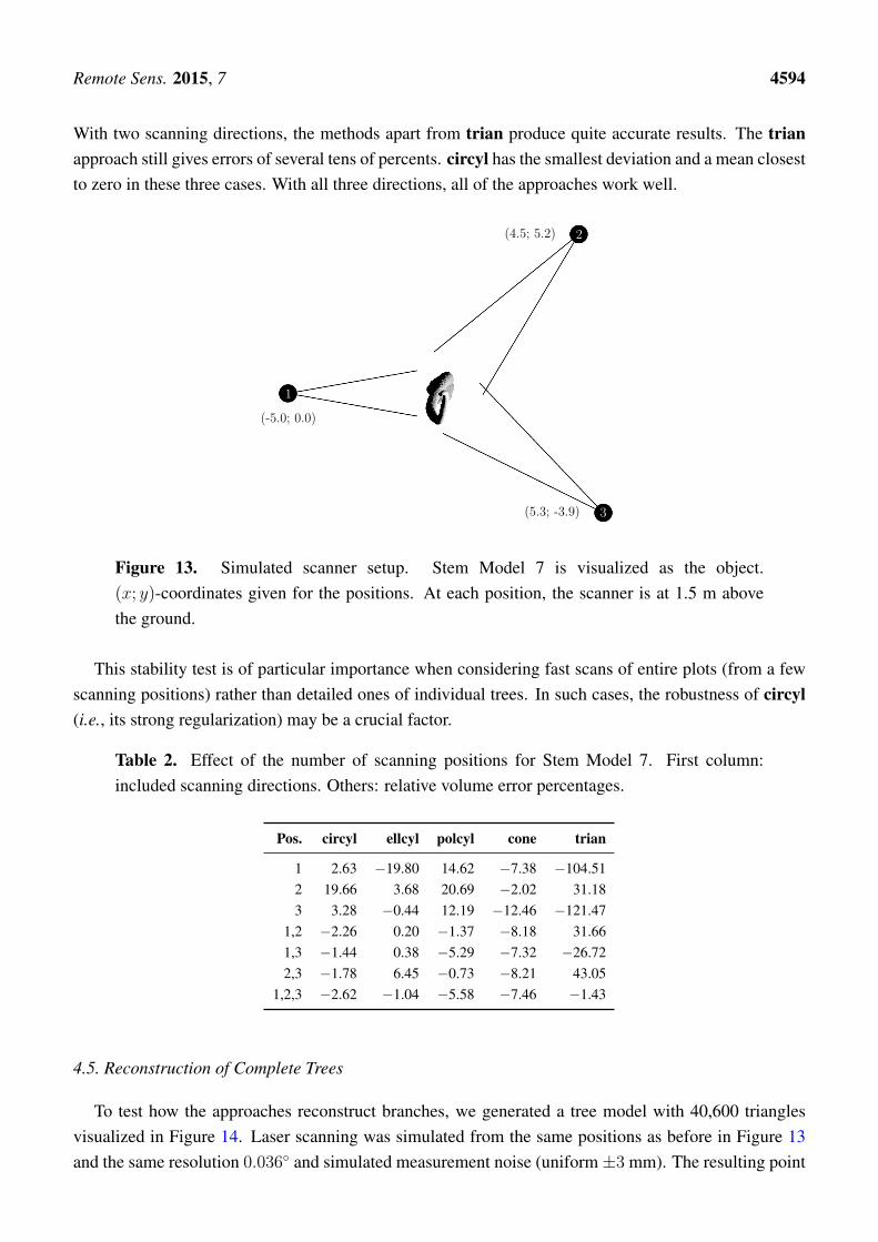
In earlier tests, the object was always scanned all-around from three positions. This is not alwayspossible, so the effect of the number of scanning positions was studied by using all possible combinationsof the three directions visualized in Figure 13. The results are listed in Table 2 for Stem Model 7.

With a single scanning direction, all of the approaches produce high errors above 10%, at least forsome directions. trian produces physically impossible results (negative volume) with a single scan.


With two scanning directions, the methods apart from trian produce quite accurate results. The trianapproach still gives errors of several tens of percents. circyl has the smallest deviation and a mean closestto zero in these three cases. With all three directions, all of the approaches work well.

1

2

3

(-5.0; 0.0)

(4.5; 5.2)

(5.3; -3.9)

Figure 13. Simulated scanner setup. Stem Model 7 is visualized as the object.(x; y)-coordinates given for the positions. At each position, the scanner is at 1.5 m abovethe ground.

This stability test is of particular importance when considering fast scans of entire plots (from a fewscanning positions) rather than detailed ones of individual trees. In such cases, the robustness of circyl(i.e., its strong regularization) may be a crucial factor.

Table 2. Effect of the number of scanning positions for Stem Model 7. First column:included scanning directions. Others: relative volume error percentages.

Pos. circyl ellcyl polcyl cone trian

1 2.63 −19.80 14.62 −7.38 −104.512 19.66 3.68 20.69 −2.02 31.183 3.28 −0.44 12.19 −12.46 −121.47

1,2 −2.26 0.20 −1.37 −8.18 31.661,3 −1.44 0.38 −5.29 −7.32 −26.722,3 −1.78 6.45 −0.73 −8.21 43.05

1,2,3 −2.62 −1.04 −5.58 −7.46 −1.43

4.5. Reconstruction of Complete Trees

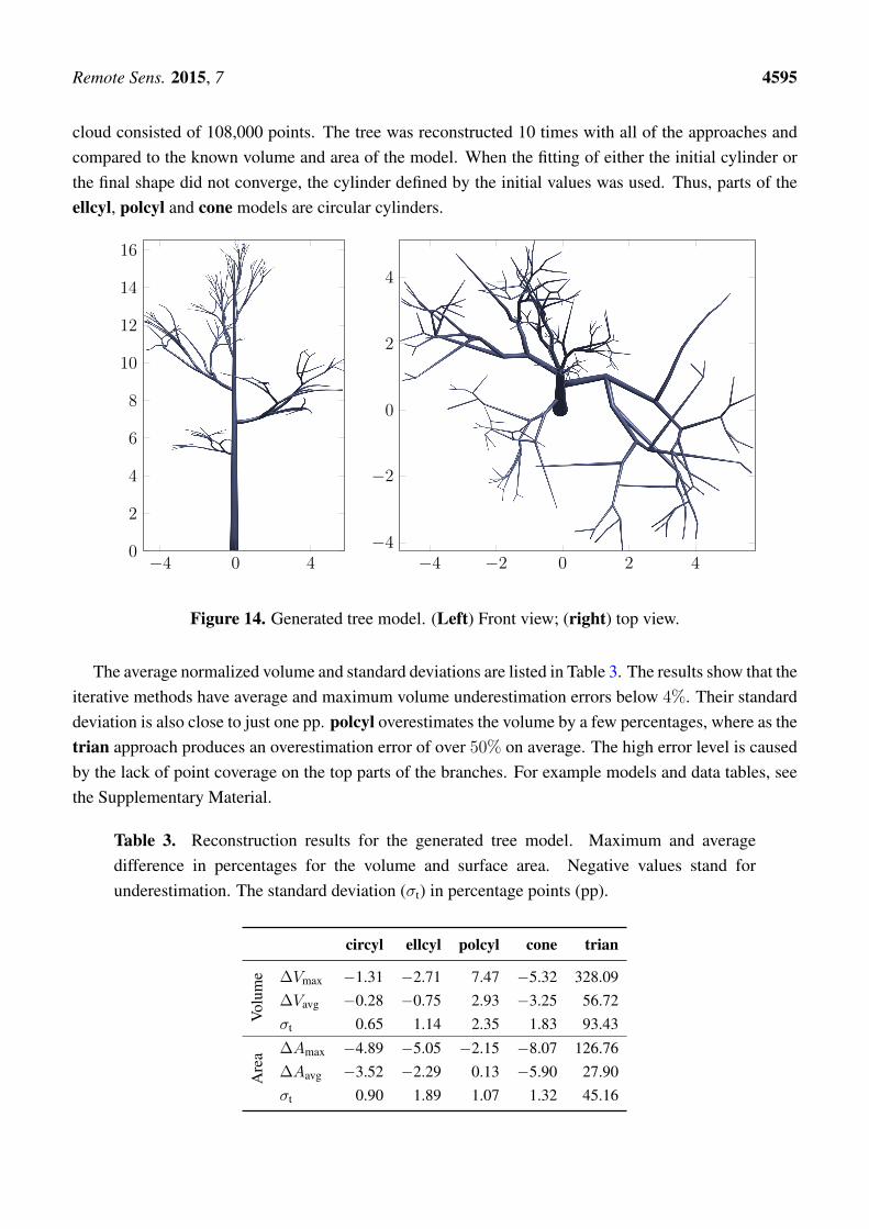
To test how the approaches reconstruct branches, we generated a tree model with 40,600 trianglesvisualized in Figure 14. Laser scanning was simulated from the same positions as before in Figure 13and the same resolution 0.036◦ and simulated measurement noise (uniform±3 mm). The resulting point


cloud consisted of 108,000 points. The tree was reconstructed 10 times with all of the approaches andcompared to the known volume and area of the model. When the fitting of either the initial cylinder orthe final shape did not converge, the cylinder defined by the initial values was used. Thus, parts of theellcyl, polcyl and cone models are circular cylinders.

−4 0 40

2

4

6

8

10

12

14

16

−4 −2 0 2 4−4

−2

0

2

4

Figure 14. Generated tree model. (Left) Front view; (right) top view.

The average normalized volume and standard deviations are listed in Table 3. The results show that theiterative methods have average and maximum volume underestimation errors below 4%. Their standarddeviation is also close to just one pp. polcyl overestimates the volume by a few percentages, where as thetrian approach produces an overestimation error of over 50% on average. The high error level is causedby the lack of point coverage on the top parts of the branches. For example models and data tables, seethe Supplementary Material.

Table 3. Reconstruction results for the generated tree model. Maximum and averagedifference in percentages for the volume and surface area. Negative values stand forunderestimation. The standard deviation (σt) in percentage points (pp).


Volu

me ∆Vmax −1.31 −2.71 7.47 −5.32 328.09

∆Vavg −0.28 −0.75 2.93 −3.25 56.72σt 0.65 1.14 2.35 1.83 93.43

Are

a ∆Amax −4.89 −5.05 −2.15 −8.07 126.76∆Aavg −3.52 −2.29 0.13 −5.90 27.90σt 0.90 1.89 1.07 1.32 45.16


5. Reconstruction from Measured Data

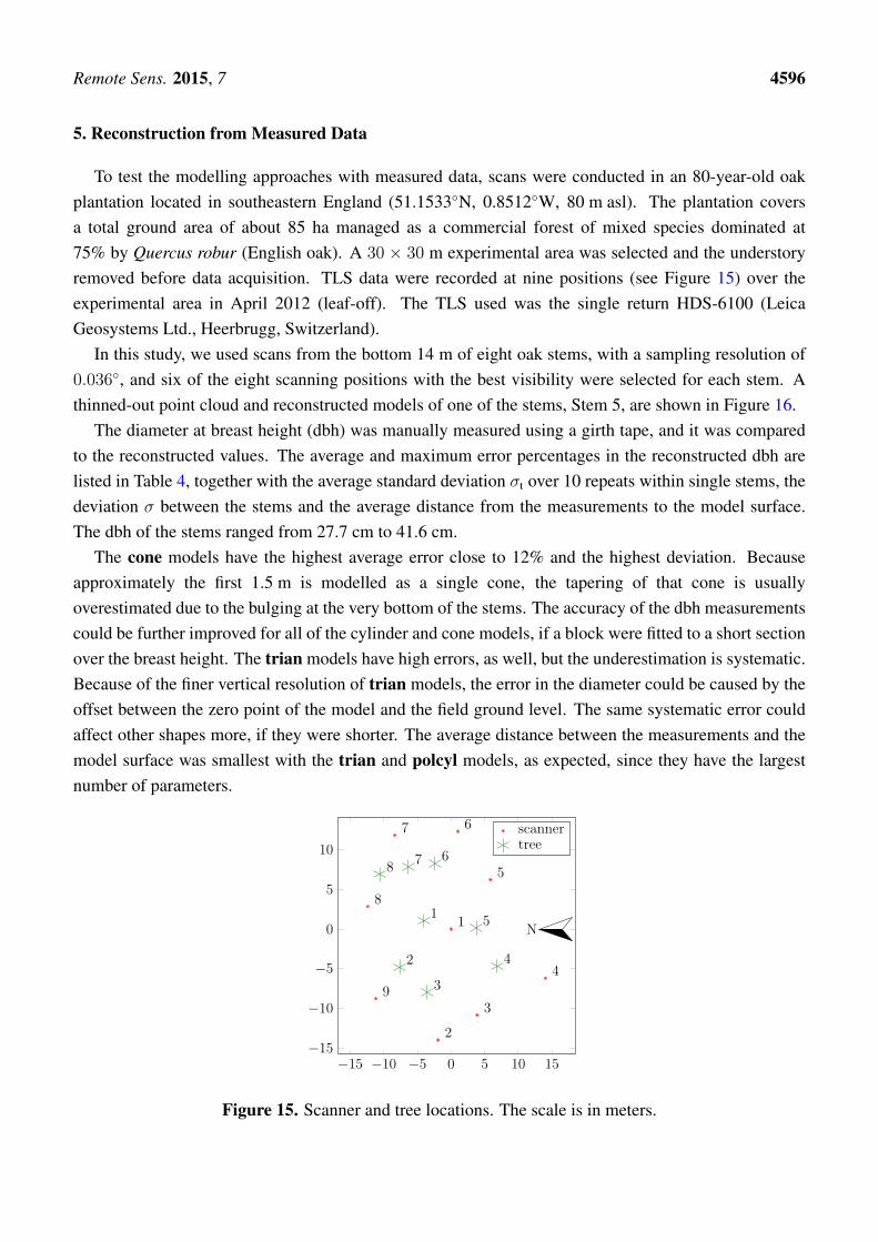
To test the modelling approaches with measured data, scans were conducted in an 80-year-old oakplantation located in southeastern England (51.1533◦N, 0.8512◦W, 80 m asl). The plantation coversa total ground area of about 85 ha managed as a commercial forest of mixed species dominated at75% by Quercus robur (English oak). A 30 × 30 m experimental area was selected and the understoryremoved before data acquisition. TLS data were recorded at nine positions (see Figure 15) over theexperimental area in April 2012 (leaf-off). The TLS used was the single return HDS-6100 (LeicaGeosystems Ltd., Heerbrugg, Switzerland).

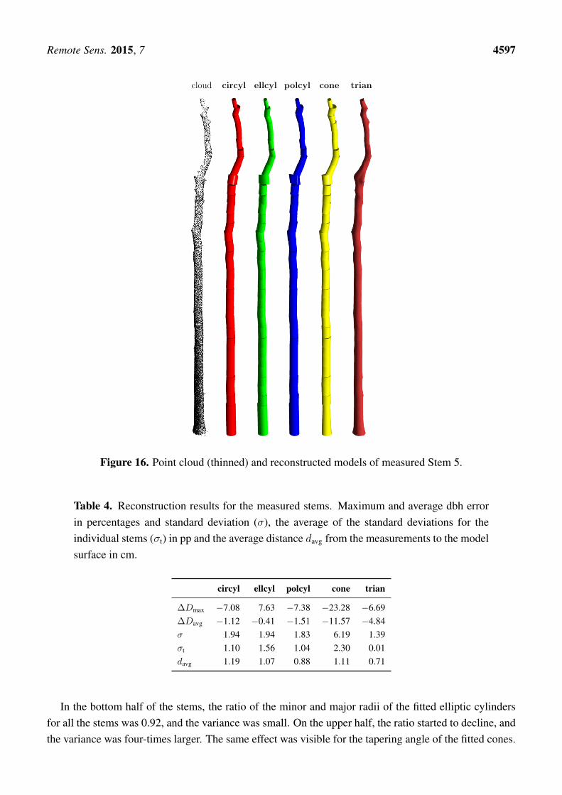
In this study, we used scans from the bottom 14 m of eight oak stems, with a sampling resolution of0.036◦, and six of the eight scanning positions with the best visibility were selected for each stem. Athinned-out point cloud and reconstructed models of one of the stems, Stem 5, are shown in Figure 16.

The diameter at breast height (dbh) was manually measured using a girth tape, and it was comparedto the reconstructed values. The average and maximum error percentages in the reconstructed dbh arelisted in Table 4, together with the average standard deviation σt over 10 repeats within single stems, thedeviation σ between the stems and the average distance from the measurements to the model surface.The dbh of the stems ranged from 27.7 cm to 41.6 cm.

The cone models have the highest average error close to 12% and the highest deviation. Becauseapproximately the first 1.5 m is modelled as a single cone, the tapering of that cone is usuallyoverestimated due to the bulging at the very bottom of the stems. The accuracy of the dbh measurementscould be further improved for all of the cylinder and cone models, if a block were fitted to a short sectionover the breast height. The trian models have high errors, as well, but the underestimation is systematic.Because of the finer vertical resolution of trian models, the error in the diameter could be caused by theoffset between the zero point of the model and the field ground level. The same systematic error couldaffect other shapes more, if they were shorter. The average distance between the measurements and themodel surface was smallest with the trian and polcyl models, as expected, since they have the largestnumber of parameters.

−15 −10 −5 0 5 10 15−15

−10

−5

0

5

10

1

2

3

4

5

67

8

9

1

2

3

4

5

678

N

scannertree

Figure 15. Scanner and tree locations. The scale is in meters.


cloud circyl ellcyl polcyl cone trian

Figure 16. Point cloud (thinned) and reconstructed models of measured Stem 5.

Table 4. Reconstruction results for the measured stems. Maximum and average dbh errorin percentages and standard deviation (σ), the average of the standard deviations for theindividual stems (σt) in pp and the average distance davg from the measurements to the modelsurface in cm.


∆Dmax −7.08 7.63 −7.38 −23.28 −6.69∆Davg −1.12 −0.41 −1.51 −11.57 −4.84σ 1.94 1.94 1.83 6.19 1.39σt 1.10 1.56 1.04 2.30 0.01davg 1.19 1.07 0.88 1.11 0.71

In the bottom half of the stems, the ratio of the minor and major radii of the fitted elliptic cylindersfor all the stems was 0.92, and the variance was small. On the upper half, the ratio started to decline, andthe variance was four-times larger. The same effect was visible for the tapering angle of the fitted cones.


The visualizations of the models showed that unrealistically tapering cones and elliptic cylinders werefitted to the upper parts of the stems. On average, the ellipse radii ratio was 0.87 and the cone taperingangle 0.33◦. Thus, additional constrains should be introduced when using these shapes for stem partswith high noise or a low number of returns.

5.1. Second Order Reconstructions

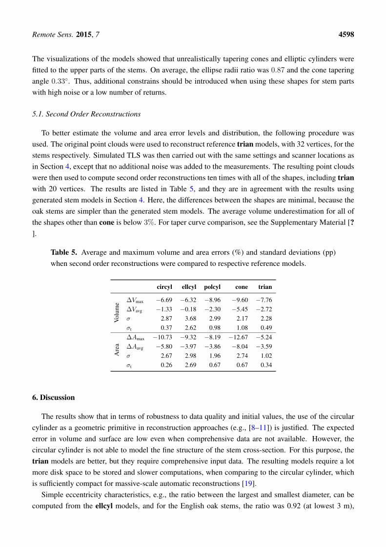
To better estimate the volume and area error levels and distribution, the following procedure wasused. The original point clouds were used to reconstruct reference trian models, with 32 vertices, for thestems respectively. Simulated TLS was then carried out with the same settings and scanner locations asin Section 4, except that no additional noise was added to the measurements. The resulting point cloudswere then used to compute second order reconstructions ten times with all of the shapes, including trianwith 20 vertices. The results are listed in Table 5, and they are in agreement with the results usinggenerated stem models in Section 4. Here, the differences between the shapes are minimal, because theoak stems are simpler than the generated stem models. The average volume underestimation for all ofthe shapes other than cone is below 3%. For taper curve comparison, see the Supplementary Material [?].

Table 5. Average and maximum volume and area errors (%) and standard deviations (pp)when second order reconstructions were compared to respective reference models.


Volu

me ∆Vmax −6.69 −6.32 −8.96 −9.60 −7.76

∆Vavg −1.33 −0.18 −2.30 −5.45 −2.72σ 2.87 3.68 2.99 2.17 2.28σt 0.37 2.62 0.98 1.08 0.49

Are

a

∆Amax −10.73 −9.32 −8.19 −12.67 −5.24∆Aavg −5.80 −3.97 −3.86 −8.04 −3.59σ 2.67 2.98 1.96 2.74 1.02σt 0.26 2.69 0.67 0.67 0.34

6. Discussion

The results show that in terms of robustness to data quality and initial values, the use of the circularcylinder as a geometric primitive in reconstruction approaches (e.g., [8–11]) is justified. The expectederror in volume and surface are low even when comprehensive data are not available. However, thecircular cylinder is not able to model the fine structure of the stem cross-section. For this purpose, thetrian models are better, but they require comprehensive input data. The resulting models require a lotmore disk space to be stored and slower computations, when comparing to the circular cylinder, whichis sufficiently compact for massive-scale automatic reconstructions [19].

Simple eccentricity characteristics, e.g., the ratio between the largest and smallest diameter, can becomputed from the ellcyl models, and for the English oak stems, the ratio was 0.92 (at lowest 3 m),


which seems realistic when comparing to the value of 0.96 measured for various coniferous species [13].Similar estimates could be computed from the polcyl and trian models. None of the presented structuremodels include information about the inner structure, e.g., pith eccentricity [20], and for that purpose,destructive measurements are still needed.

The problem with using more complex shapes is the increased requirement for measurement coveragearound the object. Lack of coverage combined with shape fitting instability can lead to very higherrors. Thus, it would be beneficial to analyse, e.g., the radial coverage locally around a given axisto determine the maximum complexity of the shape that should be fitted to those measurements. Byimplementing such local coverage analysis, the resulting models would consist of several types ofgeometric primitives. Especially, the lower part of stems has, in most cases, sufficient coverage forpolcyl or trian reconstruction. Thus, the resulting model would consist of the stem polyhedron and acollection of cylinders for the top part of the stem and the branches. Another possibility is to makeseveral reconstructions with different shapes for a single part and store all of them in the same model.Which representation to use could be determined later depending on the application (cf. [21]).

The data in Section 4 were generated using a combination of 3D modelling and simulatedlaser-scanning. By further developing and optimizing the scanning part, it would be possible to modelentire forest plots with understory and to simulate scans containing multiple trees or even to simulatecontinuous scans with moving scanners. Furthermore, on the tree level, this type of simulation offers aninexpensive way to study how to model tree abnormalities, such as cankers, seams or buttress roots. Thisway, it is possible to start with ideal data without any noise or occlusion present and to degenerate themin various ways to get data similar to real measurements.

7. Conclusions

In this study, reconstruction approaches based on four different geometric primitives and atriangulation approach were tested with both measured and simulated data. For all of the shapefitting approaches, the sub-segmentation procedure presented [11] was used, but most of the results areapplicable to any reconstruction procedures using the same geometric primitives [9,10]. Using simulateddata provided correct reference values of quantities, such as the volume, surface area and taper curves.These also served as a way to determine how much of the error was caused by the modelling and howmuch by the quality of the data. The most noticeable differences in the modelling approaches occurredin their ability to adapt to different shapes of stems and in their robustness to the quality of data. Addinga realistic amount of measurement noise did not noticeably change the reconstruction results in terms ofvolume or surface area. None of the tested approaches could accurately model complex cross-sections,such as flanges. On the other hand, the polyhedron method has been shown to give a good representationof complicated stump shapes that are not well represented by the other primitives [16,22].

Circular cylinderThe circyl primitive is the most commonly used [9–11]. It is robust, as it is veryindifferent to perturbations in all of the initial values of the fitting. Even coarse data-based estimatesconverge towards the correct solution; e.g, the axis direction estimate can be up to 45◦ off withoutcausing any error, and after that, the error was below 10%. For the generated stems, the averagevolume overestimation was 1.36% with an average standard deviation of 7.33 pps. The surface area


was underestimated with an average of 4.40% ± 6.76 pp. With field data, dbh was underestimated by1.12%, on average, with a standard deviation of 1.94 pp.

Elliptic cylinder The ellcyl fitting was implemented as a combination of circyl fitting andtwo-dimensional ellipse fitting to fine-tune the cross-section. Thus, in the initial values, it performedas circyl. With the generated data, it had the lowest average error at 0.20% for the volume and −0.96%for the area. The deviation between repeats was the highest at 1.86 pp for the volume and 1.50 pp for thearea. The high deviation means that ellcyl fitting can be unpredictable, but implementing the fitting as asingle iterative process might help stabilize it. If the data are comprehensive and have good quality, theellcyl fitting can produce good results. Furthermore, ellcyls fitted to the measured stems were ellipticalrather than circular, as the ratio of the major and minor radii was 0.87 on average.

Polygon-based cylinder The polcyl reconstruction is not an iterative process, so accurate initialvalues are crucial. Even small perturbations to the axis direction estimate caused volume and area errorsover 10%. However, in the tests with the generated and measured stems, the initial values received fromthe data were sufficient to produce error levels similar to the circyl, and when visualized, the modelsappeared accurate. On the generated stems, the average error in the volume was −2.51% ± 2.53 pp andon the area−2.58% ± 3.99 pp. As expected, the polcyl was more robust on the stem cross-section shapeand reconstructed the elliptic stems more accurately than circyl and cone. With 26 vertices on the basepolygon, the cylinder was able to reconstruct the dbh of the measured stems with an average diametererror of 7.38%.

Circular cone The cone handles initial value perturbations almost identically to the circyl. Usingcone resulted in an average 5.00% ± 11.93 pp underestimation of the volume and 7.2% ± 8.74 pp of thearea with the generated stems. It almost always resulted in the smallest volume of all of the models.Especially problematic was the bulging at the bottom of the stems, resulting in overestimation on thecone tapering. This caused high errors in the dbh values of the models. Most of the cone fitted to themeasured stems tapered only a little, 0.33◦ on average. Thus, the difference in volume in comparison tocircyl is not probably worth the increased instability, especially as the difference is expected to decreasewith the primitive length. If one were to use longer cones, the stability and accuracy should be increased.

Polyhedron The trian approach is fairly sensitive to the values of the axis point and axis direction,of which the former had the larger effect on accuracy. It requires full coverage around the object: wherethe other primitives performed well with just two scans, it required all three positions or the volumeerror was close to 30%. On the other hand, it was not sensitive to local occlusions in the data. With thegenerated stem models, it produced a volume error of −4.62% ± 2.32 pp, and the error in the surfacearea was even lower. The average diameter error in dbh was −4.84%, but seemed systematic and couldbe caused by either the selection of breast height in the model or too small a number of vertices used.

Overall The results show that any of the models, even with cruder than normal resolution, can achieveaccurate volume and area estimation. The average volume error for all models was below 5%, and using,e.g., the circular cylinder model on extremely elliptic stems, resulted in a maximum volume error below14%. These ties well with the field-calibrated studies of [16,23], as the volume and length errors aresimilar in all studies. In [16], it is shown that a hybrid version of polyhedral and cylindrical modelling isaccurate, even for the highly complex shapes of stump-root systems. Furthermore, [24] shows that usingallometric equations to predict the volume of eucalyptus trees results in a 36.6% average error with the


species-specific equation and a 29.9% error with the generic eucalyptus equation, while circular cylinderstructure models produce an error of 9.7%.

Extrapolating the stem-based results to branches predicts that increased occlusions and relative noiselevels and lower point density will increase the demand of robustness and the stability of the fittingscheme used. Thus, the general recipe is to use circyl for branches and, when necessary, more complexprimitives for parts of the stem. However, the advantage gained by the latter is not significant, at leastin terms of volume. For a fast and compact processing of a large number of trees, the circyl approachis rather sufficient. Taking into account the typical systematic errors and glitches that occur in fieldcampaigns, a rule-of-thumb volumetric error from any surface modelling approach can be expected to be±10%. The effect of the wind and co-registration error are expected to increase the error level, especiallyfor the branches, but they were not considered in this study.

Acknowledgements

This study was funded by the Academy of Finland research projects Inverse Problems of Regular andStochastic Surfaces and Centre of Excellence in Inverse Problems.

Author Contributions

Markku Åkerblom created the stem models for the generated data section, reconstructed the modelsfor both data types, computed the results, created the figures and wrote the main text. Pasi Raumonencreated the reconstruction procedure, guided the ideas of this manuscript, wrote parts of the text andgave feedback on it. Mikko Kaasalainen supervised the whole process from the idea-stage to the finalmanuscript, wrote parts of the text and gave vital feedback on rest of the text. Eric Casella carried-out thein situ measurements and provided the data used in Section 5, wrote the description of the measurementsand gave feedback on the manuscript.

Conflicts of Interest

The authors declare no conflict of interest.

References

1. Dassot, M.; Constant, T.; Fournier, M. The use of terrestrial LiDAR technology in forest science:Application fields, benefits and challenges. Ann. For. Sci. 2011, 68, 959–974.

2. Gorte, B.; Pfeifer, N. Structuring laser-scanned trees using 3D mathematical morphology.Int. Arch. Photogramm. Remote Sens. Spat. Inf. Sci. 2004, 35, 929–933.

3. Lefsky, M.; McHale, M.R. Volume estimates of trees with complex architecture from terrestriallaser scanning. J. Appl. Remote Sens. 2008, 2, 023521–023521.

4. Vonderach, C.; Voegtle, T.; Adler, P. Voxel-base approach for estimating urban tree volume fromterrestrial laser scanning data. Int. Arch. Photogramm. Remote Sens. Spat. Inf. Sci. 2012, 39, B8.

5. Xu, H.; Gossett, N.; Chen, B. Knowledge and heuristic-based modelling of laser-scanned trees.ACM Trans. Graph. 2007, 26, 19:1–19:13.


6. Yan, D.M.; Wintz, J.; Mourrain, B.; Wang, W.; Boudon, F.; Godin, C. Efficient and robust treemodel reconstruction from laser scanned data points. In Proceedings of the 11th IEEE Internationalconference on Computer-Aided Design and Computer Graphics, Huangshan, China, 19–21 August2009; pp. 572–576.

7. Pfeifer, N.; Winterhalder, D. Modelling of tree cross sections from terrestrial laser scanning datawith free-form curves. Int. Arch. Photogramm. Remote Sens. Spat. Inf. Sci. 2004, 36, W2.

8. Pfeifer, N.; Gorte, B.; Winterhalder, D. Automatic reconstruction of single trees from terrestriallaser scanner data. In Proceedings of the 20th ISPRS Congress, Istanbul, Turkey, 12–23 July 2004;pp. 114–119.

9. Cheng, Z.L.; Zhang, X.P.; Chen, B.Q. Simple reconstruction of tree branches from a single rangeimage. J. Comput. Sci. Technol. 2007, 22, 846–858.

10. Thies, M.; Pfeifer, N.; Winterhalder, D.; Gorte, B. Three-dimensional reconstruction of stems forassessment of taper, sweep and lean based on laser scanning of standing trees. Scand. J. For. Res.2004, 19, 571–581.

11. Raumonen, P.; Kaasalainen, M.; Åkerblom, M.; Kaasalainen, S.; Kaartinen, H.; Vastaranta, M.;Holopainen, M.; Disney, M.; Lewis, P. Fast automatic precision tree models from terrestrial laserscanner data. Remote Sens. 2013, 5, 491–520.

12. Medhurst, J.; Ottenschlaeger, M.; Wood, M.; Harwood, C.; Beadle, C.; Valencia, J.C. Stemeccentricity, crown dry mass distribution, and longitudinal growth strain of plantation-grownEucalyptus nitens after thinning. Can. J. For. Res. 2011, 41, 2209–2218.

13. Tong, Q.; Zhang, S. Stem form variations in the natural stands of major commercial softwoods ineastern Canada. For. Ecol. Manag. 2008, 256, 1303 – 1310.

14. Yoshimoto, A.; Surový, P.; Konoshima, M.; Kurth, W. Constructing tree stem form from digitizedsurface measurements by a programming approach within discrete mathematics. Trees 2014,28, 1577–1588.

15. Danjon, F.; Reubens, B. Assessing and analyzing 3D architecture of woody root systems, a reviewof methods and applications in tree and soil stability, resource acquisition and allocation. Plant Soil2008, 303, 1–34.

16. Smith, A.L.; Astrup, R.; Raumonen, P.; Liski, J.; Krooks, A.; Kaasalainen, S.; Åkerblom, M.;Kaasalainen, M. Tree root system characterization and volume estimation by terrestrial laserscanning and quantitative structure modelling. Forests 2014, 5, 3274–3294.

17. Lukács, G.; Martin, R.; Marshall, D. Faithful least-squares fitting of spheres, cylinders, cones andtori for reliable segmentation. In Computer Vision-ECCV’98; Springer Berlin Heidelberg: Berlin,Germany, 1998; pp. 671–686.

18. Wolberg, J. Data Analysis Using the Method of Least Squares: Extracting the Most Informationfrom Experiments; Springer-Verlag Berlin Heidelberg: Berlin, Germany, 2006.

19. Raumonen, P.; Casella, E.; Calders, K.; Murphy, S.; Åkerblom, M.; Kaasalainen, M. Massive-scaletree modelling from TLS data. ISPRS Ann. Photogramm. Remote Sens. Spat. Inf. Sci. 2015,II-3/W4, 189–196.

20. Robertson, A. Centroid of wood density, bole eccentricity, and tree-ring width in relation to vectorwinds in wave forests. Can. J. For. Res. 1991, 21, 73–82.


21. Godin, C.; Caraglio, Y. A multiscale model of plant topological structures. J. Theor. Boil. 1998,191, 1–46.

22. Liski, J.; Raumonen, P.; Kaasalainen, S.; Repo, A.; Krooks, A.; Akujärvi, A.; Kaasalainen, M.Indirect emissions of forest bioenergy: detailed modeling of stump-root systems. Glob. ChangeBiol. Bioenergy 2014, 6, 777–784.

23. Kaasalainen, S.; Krooks, A.; Liski, J.; Raumonen, P.; Kaartinen, H.; Kaasalainen, M.; Puttonen, E.;Anttila, K.; Mäkipää, R. Change detection of tree biomass with terrestrial laser scanning andquantitative structure modelling. Remote Sens. 2014, 6, 3906–3922.

24. Calders, K.; Newnham, G.; Burt, A.; Murphy, S.; Raumonen, P.; Herold, M.; Culvenor, D.;Avitabile, V.; Disney, M.; Armston, J.; et al. Non-destructive estimates of above-ground biomassusing terrestrial laser scanning. Methods Ecol. Evol. 2014, 6, 198–208.

c© 2015 by the authors; licensee MDPI, Basel, Switzerland. This article is an open access articledistributed under the terms and conditions of the Creative Commons Attribution license(http://creativecommons.org/licenses/by/4.0/).

Analysis of Geometric Primitives in Quantitative Structure ...

Documents

Transcript of Analysis of Geometric Primitives in Quantitative Structure ...