Design of advanced primitives for secure multiparty computation

Design of advanced primitives for secure multipartycomputation : special shuffles and integer comparisonCitation for published version (APA):Villegas Bautista, J. A. (2010). Design of advanced primitives for secure multiparty computation : special shufflesand integer comparison. [Phd Thesis 1 (Research TU/e / Graduation TU/e), Mathematics and ComputerScience]. Technische Universiteit Eindhoven. https://doi.org/10.6100/IR673070

DOI:10.6100/IR673070

Document status and date:Published: 01/01/2010

Document Version:Publisher’s PDF, also known as Version of Record (includes final page, issue and volume numbers)

Please check the document version of this publication:

• A submitted manuscript is the version of the article upon submission and before peer-review. There can beimportant differences between the submitted version and the official published version of record. Peopleinterested in the research are advised to contact the author for the final version of the publication, or visit theDOI to the publisher's website.• The final author version and the galley proof are versions of the publication after peer review.• The final published version features the final layout of the paper including the volume, issue and pagenumbers.Link to publication

General rightsCopyright and moral rights for the publications made accessible in the public portal are retained by the authors and/or other copyright ownersand it is a condition of accessing publications that users recognise and abide by the legal requirements associated with these rights.

• Users may download and print one copy of any publication from the public portal for the purpose of private study or research. • You may not further distribute the material or use it for any profit-making activity or commercial gain • You may freely distribute the URL identifying the publication in the public portal.

If the publication is distributed under the terms of Article 25fa of the Dutch Copyright Act, indicated by the “Taverne” license above, pleasefollow below link for the End User Agreement:www.tue.nl/taverne

Take down policyIf you believe that this document breaches copyright please contact us at:[email protected] details and we will investigate your claim.

Download date: 01. Oct. 2022

https://doi.org/10.6100/IR673070

https://doi.org/10.6100/IR673070

https://research.tue.nl/en/publications/b04e22f7-e850-4b62-81d2-0a272f05d266

Design of Advanced Primitives for Secure Multiparty Computation:Special Shuffles and Integer Comparison

CIP-DATA LIBRARY TECHNISCHE UNIVERSITEIT EINDHOVEN

c©Villegas Bautista, Jose Antonio

Design of advanced primitives for secure multiparty computation:special shuffles and integer comparison / door Jose Antonio Villegas Bautista. –Eindhoven : Technische Universiteit Eindhoven, 2010. –Proefschrift. – ISBN 978-90-386-2224-8NUR 919Subject headings : cryptology, secure computation, cryptographic protocols,Fourier transforms, fast Fourier transforms, algorithms

Printed by Printservice TU/e.Cover: Love game. Design by Paul Verspaget.

This researchwas financially supported by the Dutch Technology Foundation STWunderproject number 6680.

Design of Advanced Primitives for Secure Multiparty Computation:Special Shuffles and Integer Comparison

PROEFSCHRIFT

ter verkrijging van de graad van doctor aan deTechnische Universiteit Eindhoven, op gezag van derector magnificus, prof.dr.ir. C.J. van Duijn, voor een

commissie aangewezen door het College voorPromoties in het openbaar te verdedigenop donderdag 29 april 2010 om 16.00 uur

door

Jose Antonio Villegas Bautista

geboren te Salta, Argentinie

Dit proefscrift is goedgekeurd door de promotor:

prof.dr.ir. H.C.A. van Tilborg

Copromotor:dr.ir. L.A.M. Schoenmakers

Amis queridos padres...

To my dear parents...

Contents

1 Introduction 9

1.1 Special Shuffles of Homomorphic Encryptions . . . . . . . . . . . . . . . . 10

1.2 Integer comparison . . . . . . . . . . . . . . . . . . . . . . . . . . . . . . . . 11

1.3 Roadmap of this Thesis . . . . . . . . . . . . . . . . . . . . . . . . . . . . . . 12

2 Preliminaries 15

2.1 Basic Primitives . . . . . . . . . . . . . . . . . . . . . . . . . . . . . . . . . . 15

2.1.1 Pedersen Commitment . . . . . . . . . . . . . . . . . . . . . . . . . . 16

2.1.2 Threshold Homomorphic ElGamal Encryption . . . . . . . . . . . . 162.2 Honest-Verifier Zero-Knowledge Proofs of Knowledge . . . . . . . . . . . 18

2.2.1 Σ-Protocols . . . . . . . . . . . . . . . . . . . . . . . . . . . . . . . . 18

2.2.2 Witness-Extended Emulation . . . . . . . . . . . . . . . . . . . . . . 20

2.2.3 Some Useful Relations . . . . . . . . . . . . . . . . . . . . . . . . . . 25

2.3 Verifiable Shuffles of Homomorphic Encryptions . . . . . . . . . . . . . . . 27

2.3.1 Applications . . . . . . . . . . . . . . . . . . . . . . . . . . . . . . . . 28

2.3.2 Public Shuffle . . . . . . . . . . . . . . . . . . . . . . . . . . . . . . . 28

2.4 Secure Computation from Threshold Homomorphic Cryptosystems . . . . 292.4.1 Efficiency of Arithmetic Circuits . . . . . . . . . . . . . . . . . . . . 29

2.4.2 Concrete Instantiations . . . . . . . . . . . . . . . . . . . . . . . . . . 30

2.4.3 Secure Gates . . . . . . . . . . . . . . . . . . . . . . . . . . . . . . . . 30

3 Verifiable Rotations using the Discrete Fourier Transform 33

3.1 Verifiable Rotation . . . . . . . . . . . . . . . . . . . . . . . . . . . . . . . . 33

3.1.1 Cascade of Rotators . . . . . . . . . . . . . . . . . . . . . . . . . . . 34

3.1.2 Applications . . . . . . . . . . . . . . . . . . . . . . . . . . . . . . . . 34

3.2 DFT-based Solution . . . . . . . . . . . . . . . . . . . . . . . . . . . . . . . . 35

3.2.1 Introduction . . . . . . . . . . . . . . . . . . . . . . . . . . . . . . . . 353.2.2 Discrete Fourier Transform . . . . . . . . . . . . . . . . . . . . . . . 35

3.2.3 Properties of the DFT . . . . . . . . . . . . . . . . . . . . . . . . . . . 36

3.2.4 Rotation of Homomorphic Encryptions using DFT . . . . . . . . . . 38

3.2.5 Proof of Rotation using DFT . . . . . . . . . . . . . . . . . . . . . . . 39

3.2.6 Proof of Rotation of ElGamal Encryptions . . . . . . . . . . . . . . . 40

3.2.7 Cascade of Rotators . . . . . . . . . . . . . . . . . . . . . . . . . . . 40

3.2.8 Performance Analysis . . . . . . . . . . . . . . . . . . . . . . . . . . 43

3.3 Fast Fourier Transform . . . . . . . . . . . . . . . . . . . . . . . . . . . . . . 433.3.1 Cooley-Tukey FFT Algorithm . . . . . . . . . . . . . . . . . . . . . . 44

3.3.2 Bluestein’s FFT Algorithm . . . . . . . . . . . . . . . . . . . . . . . . 45

7

4 General Verifiable Rotations 514.1 Background . . . . . . . . . . . . . . . . . . . . . . . . . . . . . . . . . . . . 514.2 Proof of Multiple Encryptions of 0 . . . . . . . . . . . . . . . . . . . . . . . 524.3 General Proof of Rotation . . . . . . . . . . . . . . . . . . . . . . . . . . . . 61

4.3.1 Performance Analysis . . . . . . . . . . . . . . . . . . . . . . . . . . 624.3.2 Security Analysis . . . . . . . . . . . . . . . . . . . . . . . . . . . . . 634.3.3 Rotation of ElGamal Encryptions . . . . . . . . . . . . . . . . . . . . 65

4.4 Related Work and Efficiency Comparison . . . . . . . . . . . . . . . . . . . 66

5 Verifiable Multiply Fragile Shuffles 695.1 Fragile Permutations . . . . . . . . . . . . . . . . . . . . . . . . . . . . . . . 69

5.1.1 Transitive Sets of Permutations . . . . . . . . . . . . . . . . . . . . . 715.1.2 Basic Sharply Transitive Permutation Sets . . . . . . . . . . . . . . . 725.1.3 Affine Transformation . . . . . . . . . . . . . . . . . . . . . . . . . . 735.1.4 Mobius Transformation . . . . . . . . . . . . . . . . . . . . . . . . . 745.1.5 Multiply Sharply Transitive Sets . . . . . . . . . . . . . . . . . . . . 75

5.2 Shuffling according to an Affine Transformation . . . . . . . . . . . . . . . 775.2.1 Scaling Homomorphic Encryptions . . . . . . . . . . . . . . . . . . 775.2.2 Shuffles using an Affine Transformation . . . . . . . . . . . . . . . . 795.2.3 Performance Analysis . . . . . . . . . . . . . . . . . . . . . . . . . . 80

5.3 Shuffling according to a Mobius Transformation . . . . . . . . . . . . . . . 815.3.1 Proof of Shuffle using a Mobius Transformation . . . . . . . . . . . 815.3.2 Selecting a RandomMobius Transformation . . . . . . . . . . . . . 83

5.4 Multiply Fragile Cascades . . . . . . . . . . . . . . . . . . . . . . . . . . . . 835.4.1 Efficient Affine Cascade using DFT . . . . . . . . . . . . . . . . . . . 845.4.2 Efficient Mobius Cascade using DFT . . . . . . . . . . . . . . . . . . 85

6 Integer Comparison 876.1 Integer Comparison Circuits . . . . . . . . . . . . . . . . . . . . . . . . . . . 87

6.1.1 Our Solution . . . . . . . . . . . . . . . . . . . . . . . . . . . . . . . . 886.1.2 Performance Analysis . . . . . . . . . . . . . . . . . . . . . . . . . . 89

6.2 Constant Round 2-Party Protocol . . . . . . . . . . . . . . . . . . . . . . . . 916.2.1 Our Protocol . . . . . . . . . . . . . . . . . . . . . . . . . . . . . . . . 916.2.2 Security Analysis . . . . . . . . . . . . . . . . . . . . . . . . . . . . . 946.2.3 Variations . . . . . . . . . . . . . . . . . . . . . . . . . . . . . . . . . 986.2.4 Optimized Protocols . . . . . . . . . . . . . . . . . . . . . . . . . . . 996.2.5 Performance Evaluation . . . . . . . . . . . . . . . . . . . . . . . . . 1016.2.6 Yao’s Garbled Circuit Approach . . . . . . . . . . . . . . . . . . . . 103

6.3 Problems Related to Integer Comparison . . . . . . . . . . . . . . . . . . . 1066.3.1 Signum . . . . . . . . . . . . . . . . . . . . . . . . . . . . . . . . . . . 1066.3.2 Addition Circuits . . . . . . . . . . . . . . . . . . . . . . . . . . . . . 1076.3.3 Comparisons with Public Output . . . . . . . . . . . . . . . . . . . . 1086.3.4 Bit-decomposition Problems . . . . . . . . . . . . . . . . . . . . . . 110

6.4 A Cost Model for Arithmetic Circuits . . . . . . . . . . . . . . . . . . . . . . 111

7 Conclusions 113

8

Chapter 1

Introduction

Secure multiparty computation is a well-known problem in modern cryptography. A setof mutually distrusting parties need to perform a joint computation, where each partycontributes some private information as input, and these inputs should remain hidden asmuch as possible throughout the computation. This should be valid even in the presenceof an adversary who may corrupt some of the parties, meaning that the adversary sees alltheir internal data and may make them behave arbitrarily. A large body of research initi-ated in the early 1980s has shown that secure multiparty computation is feasible for anycomputable function [Yao82, Yao86, GMW87, BGW88, CCD88]. Lots of improvementshave been achieved since.

The design of secure multiparty protocols is very complex, since many aspects mustbe taken into account. One can have protocols withstanding adversaries with differentcapabilities. A passive adversary follows the protocol specification but records all infor-mation it has collected during the run of a protocol. In contrast, an active adversarybehaves arbitrarily, possibly aborting the protocol prematurely. An adversary is static ifthe set of corrupted parties is decided at the onset and fixed throughout the protocol ex-ecution, or the adversary is adaptive if parties are corrupted on the fly as the computationproceeds.

Another distinction between multiparty protocols is the model for communication.In the cryptographic model, the adversary may see all the information exchanged by theparties. Security in this case can be only guaranteed under a computational assumption.The information-theoretic model assumes a private channel between every pair of parties.Security is possible in an unconditional manner, without assuming any bound on thecomputational power of the adversary. Another important aspect is the environment inwhich a protocol is executed. A protocol may be analyzed in a stand-alone setting, or ina more general setting, allowing for concurrent and possibly interleaved executions; see,e.g., [Can01, PS04, Can05, Kus06, CDPW07].

Efficiency is an important aspect of the design of secure multiparty protocols. Thereare three widely accepted performance measures for protocols, usually analyzed as afunction of the size of the inputs. The computational complexity is the number of ele-mentary computing steps needed to execute the protocol. The communication complexitygives the number of bits transmitted between the parties. The round complexity mea-sures the number of messages exchanged by the parties running the protocol. Often,there are trade-offs between these complexity measures, which can be used to achieve agood balance in practical situations.

This thesis focuses on designing efficient protocols for two particular cryptographic

9

Chapter 1. Introduction

primitives. The first primitive concerns generalizations of verifiable shuffles, allowing forways to restrict the permutations applied to a special subset of permutations. The sec-ond primitive is integer comparison. Both of these primitives are of general importance inthe design of protocols for secure multiparty computation. For our purposes it sufficesto consider the basic setting of a static, active, computationally-bounded adversary in astand-alone setting. The basic setting allows for a relatively simple and concise presenta-tion, capturing the essence of the novel techniques and approaches used in our solutions.Using by-now standard techniques and set-up assumptions our solutions should carryover to stronger security models.

In the following, we give a brief description of the two primitives studied in the thesis.We include some of the main applications, describe relations to other problems and givefurther motivation for studying these primitives.

1.1 Special Shuffles of Homomorphic Encryptions

A shuffle is a rearrangement of a list of encrypted messages which produces a fresh listof encrypted messages such that the multiset of plaintexts of both lists is identical. Put inother words, there exists a permutation linking the plaintexts of both lists of encryptions.The crucial requirement to apply shuffles in cryptographic protocols is that the appliedpermutation is kept secret.

Shuffles of homomorphic encryptions is a simple but very powerful primitive. Thisis accomplished by permuting and “re-blinding” the list of encryptions. Verifiability ofa shuffle is achieved via a zero-knowledge proof of knowledge. One of the main ap-plication areas of shuffles is the construction of mix-networks. A mix-network [Cha81]consists of a cascade of shufflers which one after the other randomly shuffle the list ofencryptions received from the previous shuffler. The result is that the input-output listsof plaintexts are permuted and if at least one of the shufflers is honest, the end-to-endpermutation is random and unknown.

In this thesis we study a related primitive. Namely, we describe zero-knowledgeproofs of shuffles where a cyclic rotation is applied instead of an arbitrary permuta-tion. This kind of shuffles were first introduced by Reiter and Wang [RW04] togetherwith applications in the context of mix-networks. They argued that a shuffler is deterredfrom revealing information if there is only a limited number of allowed permutationsfor a shuffle. In the case of rotations, revealing any input-output correspondence of thepermutation applied completely reveals the permutation used in the shuffle.

We point out many other applications of rotations in cryptographic protocols. In fact,we note that rotations are a fundamental primitive for the design of secure protocols. Forinstance, rotations are used to conceal sensitive information in voting protocols, integercomparison solutions, and in some general approaches to secure function evaluation.Concretely, in scrambled circuit approaches, like that of Yao [Yao86] or Jakobsson andJuels [JJ00], the active row of the truth table selected during the evaluation of a scrambledgate must be hidden. This may be achieved by applying a rotation of the rows of thescrambled gate.

We use two interesting approaches to rotation. On the one hand, using properties ofthe Discrete Fourier Transform (DFT) we give a Σ-protocol for showing correctness ofa rotation. The use of the DFT imposes some mild restrictions on the system parame-ters. We believe that this is the first time that the DFT is used as the core tool of a zero-

10

1.2. Integer comparison

knowledge protocol. On the other hand, we use a completely different approach to provea rotation. We present a zero-knowledge proof for which we show the witness-extendedemulation property. This protocol works with virtually any homomorphic cryptosystemand does not put any constraints in the parameters. Our zero-knowledge protocols haveroughly the same complexity as the most efficient ones for general shuffles (e.g., [Gro03])while the only previously existing solution by Reiter and Wang [RW04] uses four invoca-tions of a general shuffle.

Reiter and Wang [RW04] also introduced the more general notion of a k-fragile setof permutations where revealing any k input-output correspondences of a permutationidentifies the permutation completely within the k-fragile set. That way, a shuffler whoapplied a k-fragile permutation may reveal up to k − 1 input-output mappings of thepermutation before the permutation itself gets completely exposed. A rotation is clearly1-fragile.

In this thesis, we present the first zero-knowledge proofs of knowledge for particu-lar cases of k-fragile permutations, with k > 1. We show how to prove that a shufflerapplied an affine transformation (2-fragile) and a Mobius transformation (3-fragile). Wecomplement this study by pointing out the equivalence with the well-known conceptof k-transitive sets of permutations. In fact, this enables us to give an overview of the(non-)existence results for multiply fragile permutations.

1.2 Integer comparison

The basic instance of integer comparison was introduced by Yao [Yao82] as the million-aires’ problem: two millionaires want to compare their net worths and know who is richerwithout revealing anything else. Secure integer comparison refers to any problem inwhich two integers must be compared. The essential requirement is that no informationis leaked about the two integers and possibly the result of the comparison.

These problems represent a fundamental primitive in secure computation protocolsand thereby they have received much attention in the literature. Applications that arebased on this primitive include electronic auctions [NPS99], secure data mining [LP00]and secure linear optimization [Tof09c] among many other problems.

In this thesis, we present integer comparison protocols within the framework for se-cure multiparty computation based on threshold homomorphic cryptosystems byCrameret al. [CDN01]. Our solutions assume that the inputs x and y are given as encrypted bitsof their binary representation and the output is an encryption of the bit deciding whetherx > y. The generality of our solutions enable the use of our protocols in numerous appli-cations.

The first type of solutions involves the evaluation of an arithmetic circuit composed ofelementary gates as in [CDN01]. Since the intermediate multiplications of the circuit areperformed on encrypted bits, one can apply conditional gates from [ST04] and thus it canbe based on threshold homomorphic ElGamal encryptions. Furthermore, we note thatthe circuit can be used to get unconditional security if encryptions are replaced by shar-ings as in [DFK+06]. The main achievements of this circuit are both low computationalcomplexity and low round complexity.

The second type of solutions uses a more intricate approach. We present protocolsthat only require a constant number of rounds assuming a fixed number of parties. Thecomputational complexity compares favorably with other existing solutions. In fact, our

11


solutions outperform any other protocol in a two-party setting in all the complexity mea-sures. The proof of security of these protocols is also interesting in its own right. Namely,we follow ideas from [ST06] in which a successful attacker of the protocol is convertedinto an attacker of the semantic security of the underlying cryptosystem. In this way,we show the integration of our solution in the general frameworks of [CDN01, ST04]mentioned above. We give a complete description for the two-party setting.

We discuss different variations of integer comparison which may be useful in certainapplications. For instance, we analyze how to get public output (instead of encryptedoutput) and how this affects the performance. We also describe the connection of integercomparison with other related problems. For example, one can show an equivalence be-tween greater-than comparison and computing the least-significant bit of an integer. Webelieve that shedding light on these connections may be of help in finding more efficientsolutions.

1.3 Roadmap of this Thesis

Below we give an overview of the structure and results of the thesis.

Chapter 2: Preliminaries

This chapter describes basic cryptographic primitives and building blocks. At the sametime, we present the notation that will be used throughout the rest of the thesis.

Chapter 3: Verifiable Rotations using the Discrete Fourier Transform

In this chapter, we present a protocol for rotation using the Discrete Fourier Transform(DFT). The obtained zero-knowledge protocol is a Σ-protocol and is as efficient as themost efficient protocol for general shuffles. The application of the DFT and its inverse us-ing encrypted values represents a bottleneck in the computation. We note, however, thatthe computation can be reduced with the use of the Fast Fourier Transform (FFT). In par-ticular, we have adapted Cooley-Tukey FFT and Bluestein’s FFT to work with encryptedvalues.

Parts of this chapter are based on joint work with Sebastiaan de Hoogh, Berry Schoen-makers and Boris Skoric [dHSSV09].

Chapter 4: General Verifiable Rotations

We present a completely new approach to get a zero-knowledge proof of rotation. Thissolution is general, applies to any homomorphic cryptosystem, and avoids any con-straints that the DFT-based approach puts on parameters. We show that the protocolsatisfies witness-extended emulation, using a detailed analysis that may be of indepen-dent interest.

The solution presented in this chapter improves upon the joint work with Sebasti-aan de Hoogh, Berry Schoenmakers and Boris Skoric [dHSSV09], following a differentapproach.

12

1.3. Roadmap of this Thesis

Chapter 5: Verifiable Multiply Fragile Shuffles

We consider zero-knowledge proofs for k-fragile permutations as defined by Reiter andWang [RW04]. In fact, we present the first zero-knowledge proofs of knowledge to showthat a shuffler used a k-fragile permutation, with k = 2, 3. Namely, we show how toshuffle according to an affine transformation (2-fragile) and a Mobius transformation (3-fragile). The chapter is complemented with an overview of (non-)existence results formultiply fragile sets of permutations. We do this by noting the link between fragility andthe well-studied concept of set transitivity.

Parts of this chapter are included in the joint work with Sebastiaan de Hoogh andBerry Schoenmakers [dHSV10].

Chapter 6: Integer Comparison

Two types of protocols for integer comparison are presented. Our first solution is anarithmetic circuit yielding a protocol of O(logm) rounds where m is the bit-size of theinputs. The computational complexity is low, as the work is only about 50% more thanthe most efficient known solution of [ST04], which requires O(m) rounds. Our secondsolution is based on a different approach that achieves constant rounds assuming a fixednumber of parties, while minimizing the computational work. The resulting protocol im-proves substantially over the constant rounds protocol of [GSV07]. The chapter endswithan overview of different variants of integer comparison protocols and related problems.

Parts of this chapter are based on joint work with Juan A. Garay and Berry Schoen-makers [GSV07].

13


14

Chapter 2

Preliminaries

In this chapter we review several basic cryptographic concepts and primitives whichplay an important role throughout the thesis. The presentation is informal and mainlyserves to introduce the notation and terminology that we need in later chapters. Forconcreteness and simplicity, we use a generic discrete log setting, involving a cyclic groupof prime order, as the main setting for our cryptographic constructions. Many of theresults are however more generally applicable, e.g., using an RSA-based setting, andwhere appropriate we will discuss such generalizations.

We will pay special attention to honest verifier zero-knowledge protocols, which playa central role in the thesis. The restriction to honest verifier zero-knowledge allows forrelatively simple and efficient protocols, capturing the essence of our constructions. Us-ing the Fiat-Shamir heuristic, these protocols can be converted –without loss of efficiency–into publicly-verifiable non-interactive proofs, for which the security can be proved in therandom oracle model. We will use the notion of witness-extended emulation as the mainsecurity property, which captures both soundness and zero-knowledgeness. Σ-protocolssatisfy the witness-extended emulation property. We include a direct proof of this knownfact to illustrate the typical structure of the witness-extended emulators for our protocolsin later chapters.

We review shuffles of homomorphic encryptions and applications, introducing somebasic notation. Finally, we briefly present the frameworks put forth by Cramer et al.[CDN01], and Schoenmakers and Tuyls [ST04] which enable general secure multipartycomputation from the evaluation of arithmetic circuits. The notion of security within theframework is discussed as well.

2.1 Basic Primitives

In this section we introduce some well-known cryptographic primitives for a standard,generic discrete log setting.

Discrete Log Setting

Let Gq = 〈g〉 be a (multiplicative) cyclic group of order q. Typical examples are primeorder subgroups of the multiplicative group of a finite field, or prime order subgroups ofthe points of an ordinary elliptic curve over a finite field.

For our applications we assume that the decision Diffie-Hellman (DDH) problem to beinfeasible. Namely, given random gx, gy and gz in Gq it is infeasible to decide whether

15

Chapter 2. Preliminaries

z = xy mod q.The DDH assumption implies that the computational Diffie-Hellman (CDH) problem is

infeasible as well. Namely, it is infeasible to compute gxy given gx and gy. In turn, thediscrete log (DL) problem, which is to compute x from gx, is infeasible too.

2.1.1 Pedersen Commitment

Consider a discrete log setting over the group Gq = 〈g〉. Let h ∈ Gq\1 be chosenat random, such that logg h is not known. In a Pedersen commitment, two parties, a

committer C and a receiver R run a protocol in the following two phases. During thecommit phase, the committer C commits to a private value m ∈ Zq by computing c =C(m, r) = grhm for random r ∈ Zq and sending c to R. In the reveal phase, the committerC opens the commitment c by revealing the values m and r to R who then checks thatc = C(m, r) = grhm.

Pedersen commitment has two properties, hiding and binding. Hiding property saysthat from c alone, R cannot get any information aboutm. Binding guarantees that C is notable to open c to a different value other thanm after c has been fixed. More concretely, thescheme is statistically hiding since the distribution of grhm is statistically independent ofthe value of m. The scheme is computationally binding under the discrete log assumption

on Gq since if two openings for a commitment c would exist, that is c = grhm = gr′hm′

with m 6= m′, then h = g(r−r′)/(m′−m).The notation c = C(m, r) is used throughout this thesis to indicate the commitment

function of a general commitment scheme where c is a commitment to m ∈ M usingrandomness r ∈ R. We assume that C satisfies the properties of hiding and binding.

2.1.2 Threshold Homomorphic ElGamal Encryption

Consider a discrete log setting over the group Gq = 〈g〉. The secret key x is selectedat random from Zq and the public key is h = gx. We present a variation of ElGamalcryptosystem [ElG85] that is additively homomorphic.

Upon message m ∈ Zq, a random r ∈ Zq is chosen to produce the ciphertext (a, b) =E(m, r) = (gr, gmhr). Decryption of the ciphertext (a, b) is done by retrieving m fromgm = b/ax .

A drawback, though, is that the set of possible plaintexts M ⊂ Zq to be decryptedshould be small otherwise the discrete log problem must be solved. Often |M| = 2. Theencryption scheme is semantically secure under the DDH assumption on Gq.

Most results presented in this thesis are general and work for any homomorphic cryp-tosystem. Hence, E denotes the encryption algorithm of a semantically secure homomor-phic public key cryptosystem with message spaceM and randomness space R. In thecase of homomorphic ElGamal,M = R = Zq. Other cryptosystems may be instanti-ated as well. For instance, Goldwasser-Micali cryptosystem [GM84] whereM = 0, 1,R = Z∗N, and Paillier cryptosystem [Pai99] whereM = ZN and R = Z∗N for an RSAmodulus N.

We use different notations for encryptions, with different meanings. Given m ∈ Mand r ∈ R, the full notation e = E(m, r) is used for the encryption of the message m usingrandomness r. The bracketed notation [[m]] is a shorthand notation of E(m, r) where therandomization is left implicit. In algorithms, [[m]] is used to denote an encrypted variablem whose actual value may not be known. The notation e = E(m) means a deterministic

16

2.1. Basic Primitives

encryption of the message m. That is, the randomness used is a predefined and publicvalue.

ElGamal cryptosystem is homomorphic. Given (a1, b1) = E(m1, r1) and (a2, b2) =E(m2, r2) two ElGamal encryptions as defined above. Then, (a1a2, b1b2) = E(m1 +m2, r1 +r2) = (gr1+r2, gm1+m2hr1+r2) is an encryption of m1 + m2. Furthermore, given constant

m′ ∈ Zq, it holds that (am′

1 , bm′

1 ) = E(m1m′, r1m

′) = (gr1m′, gm1m

′hr1m

′) is an encryption of

m1m′.

These homomorphic properties are described in a general cryptosystem assumingthat the message space (M,+, ·) is a ring. Then, given encryptions [[m1]] and [[m2]], amultiplicative operation for the ciphertexts corresponds to an additive transformation of

the plaintexts. That is, [[m1]][[m2]] = [[m1 +m2]]. Also, for a constant m′, e = [[m]]m′denotes

the deterministic transformation such that e = [[m ·m′]].

A particularly useful property of homomorphic cryptosystems is the re-randomization.Given a ciphertext [[m]] it can be ‘randomized’ by multiplying it with a random encryp-tion of 0. Clearly, if [[y]] = [[x]]E(0, s) for random s ∈ R then it holds that x = y.

Threshold Decryption

For n > 1 and 1 ≤ t ≤ n, in a (t, n)-threshold cryptosystem public key encryption schemethe secret key is shared among a set of n parties P1, . . . , Pn. Each party holds a share of thesecret key in such a way that if at least t of the parties collaborate, they are able to decryptmessages. Less than t parties, however, get no clue about the plaintext of a ciphertext.

Homomorphic ElGamal cryptosystem admits a threshold version. Firstly, parties in-volve in a distributed key generation protocol that allows the generation of a shared secretkey along with the corresponding public key. An efficient distributed key generationprotocol is presented in [Ped91, GJKR99]. The underlying idea is to share a the secret keyx using a secret sharing scheme.

For instance, using Shamir’s secret sharing [Sha79], the secret key may be shared asfollows. Let f be a polynomial of degree t− 1 over Zq such that xi = f (i) for i = 1, . . . , nwhere xi is the share of the secret key of Pi. Party Pi outputs hi = gxi . The secret keyis defined as x = f (0). The public key is obtained by Lagrange interpolation in the

exponents: given hi for 1 ≤ i ≤ t (or any other subset of t hi’s) one can obtain h = g f (0) =gx.

For threshold decryption of ciphertext e = (a, b), party Pi produces si = axi for i =1, . . . , n. If at least t of these shares are correct the value of ax = R(si1 , . . . , sit) can bereconstructed via Lagrange interpolation in the exponents and thus the message can berecovered by solving gm = b/ax .

The notation m← DECR([[m]]) is used to denote a run of the threshold decryptionprotocol. The parties involved in this protocol aswell as the keys involved are left implicitin the notation. However, all set up parameters should be understood from the context.

Other cryptosystems also admit a threshold variant, such as the case of Paillier and itsgeneralization in [DJ01]. It should be noted that the distributed key generation of Paillier(or any other cryptosystem where the secret key is the factorization of an RSA modulus)is a computational intensive task [ACS02]. In contrast, threshold ElGamal requires asimple protocol [Ped91, GJKR99, ST04].

17


2.2 Honest-Verifier Zero-Knowledge Proofs of Knowledge

Zero-knowledge proofs are a general class of protocols between two parties, a proverP and a verifier V, modeled as interactive probabilistic machines. By means of a zero-knowledge proof, the prover convinces the verifier of the validity of a given statementwithout revealing any information beyond the truth of the statement.

Let the pair (P,V) denote the interaction between those parties, which we call aninteractive system. We write tr← 〈P(x),V(y)〉 to denote the messages exchanged by Pand V on inputs x and y respectively. At the end of the interaction V either accepts orrejects, denoted by 〈P(x),V(y)〉 = b or 〈tr, y〉 = b with b = 1 or b = 0, respectively.

Definition 2.1 (NP-Relation) AnNP-relation is a binary relation R = (x;w) ⊂ 0, 1∗×0, 1∗ that can be evaluated efficiently and for which there exists a polynomial p such that |w| ≤p(|x|). The language induced by R is defined as LR = x : ∃w s.t. (x;w) ∈ R.

The pair (x;w) can be thought of as an instance of a computational problem where w isthe solution to that instance.

Consider a discrete log setting over a cyclic group Gq = 〈g〉 of prime order q. Thenthe discrete log relation is defined as

RDL = (g, h;w) : h = gw,

where w ∈ Zq. The language induced is LRDL= (g, h) : g, h ∈ Gq.

2.2.1 Σ-Protocols

Wenow consider a class of 3-move interactive systems between P andV where P acts firstand V provides randomly chosen challenges. Let (a, c, t) denote the messages exchangedbetween P and V. Based on the transcript (a, c, t) the verifier V either accepts or rejects.The structure of a Σ-protocol is given in Fig. 2.1.

Definition 2.2 (Σ-protocol) A 3-move protocol between interactive machines P and V where Pacts first is a Σ-protocol for relation R if the following holds.

• Completeness. For all (x;w) ∈ R, 〈P(x,w),V(x)〉 = 1.

• Special Soundness. There exists an efficient extractor E such that on any pair of con-versations (a, c, t) and (a, c′, t′) on common input x ∈ LR such that 〈(a, c, t), x〉 = 1,〈(a, c′ , t′), x〉 = 1, and c 6= c′, E computes w← E(x, a, c, t, c′, t′) such that (x;w) ∈ R.

• Special Honest-Verifier Zero-Knowledge. There exists an efficient algorithm S thaton input (x, c) with x ∈ LR, S outputs a transcript (a, c, t) with the same probabilitydistribution as the transcripts between honest P and V with common input x and challengec where P uses any witness w such that (x;w) ∈ R.

In a Σ-protocol the honest verifier is limited to provide random coin tosses indepen-dently of the inputs it has received. This kind of protocols is more generally referred toas public coin.

Special soundness indicates that if P is able to reply to two different challenges on afixed first message then it P actually knows the witness. It can be proved that a cheating

18

2.2. Honest-Verifier Zero-Knowledge Proofs of Knowledge

Prover P Verifier V

a← A(x,w, u)

−−−a−−−→

c ∈R 0, 1k

←−−−c−−−

t← T(x,w, c, u)

−−−t−−−→

〈(a, c, t), x〉?= 1

Figure 2.1: Structure of a Σ-protocol.

prover P∗ that does not know a witness has probability 1/2k of letting an honest verifierV accept. In other words, special soundness implies the standard notion of knowledgesoundness [BG92] of proof systems. A proof of this fact can be found in [Dam08].

Σ-protocols are proof systems with zero-knowledge property withstanding honestverifiers only. This means that an honest verifier gets no information whatsoever aboutthe witness that the prover is using. Despite withstanding only honest verifiers, Σ-protocols are very useful and powerful building blocks. For technical reasons, Σ-protocolare required to be special honest verifier zero-knowledge which means that the simulatorS produces conversations for a specified challenge.

A classic example of a Σ-protocol is Schnorr’s protocol [Sch91] to show the knowledgeof a witness for relation RDL. Other examples include Okamoto’s protocol [Oka93] toprove the knowledge of the opening of a Pedersen commitment.

Verifiable Non-Interactive Proofs

Σ-protocols can be made non-interactive using a cryptographic hash function. The Fiat-Shamir heuristic [FS87] makes this conversion by replacing the random coin tosses fromthe verifier with calls to a cryptographic hash function. The conversion does not affectthe efficiency of the protocols. The security of the resulting protocols can be shown inthe random oracle model [BR93]. This is a property that holds for any public coin proofsystems in general.

In the random oracle model, this technique not only makes public-coin zero-knowl-edge protocol non-interactive, but it forces honest behavior. Another distinctive featureof the application of the Fiat-Shamir heuristic, is that any entity may play the role ofthe verifier and check whether a proof is valid or not. This property is known as publicverifiability.

Composition Properties

Σ-protocols have some easily verified properties which we review in the following. Formore insightful details we refer the reader to [CDS94, Cra97].

The class of Σ-protocols is closed under parallel composition. Namely, if two instancesof a Σ-protocol with challenge length k are run in parallel, then the overall resultingprotocol is a Σ-protocol with challenge length 2k. This result can be used to prove that if

19


a Σ-protocol exists for relation R then there is a Σ-protocol for relation R for any challengelength k.

AND-Composition. Suppose that we have two Σ-protocols with challenge length k,one for relation R0 and the other for relation R1. Suppose that a prover P knowswitnessesw0 and w1 such that (x0;w0) ∈ R0 and (x1;w1) ∈ R1. If both Σ-protocols are run inparallel using a common challenge for both instances, then the result is a Σ-protocol forrelation R0 ∧ R1, where R0 ∧ R1 is defined as

R0 ∧ R1 = (x0, x1;w0,w1) : (x0;w0) ∈ R0 ∧ (x1;w1) ∈ R1.

This construction, referred to as the AND-composition, can be naturally generalizedto prove the knowledge of various witnesses simultaneously.

OR-Composition. Now, let two relations R0 and R1 be given and a common input(x0, x1) such that x0 ∈ LR0

and x1 ∈ LR1. The prover P wants to prove the knowl-

edge of a witness w such that (x0;w) ∈ R0 or (x1,w) ∈ R1 without indicating anythingelse. In particular, P does not want to disclose which case holds, if either (x0;w) ∈ R0 or(x1,w) ∈ R1 holds, or both. Namely, the prover P wants to prove it knows a witness forrelation R0 ∨ R1, where

R0 ∨ R1 = (x0, x1;w) : (x0;w) ∈ R0 ∨ (x1;w) ∈ R1.

If P knows the witness for xb for a unique b ∈ 0, 1 then P is able to give an acceptingproof for that instance. However, P may not be able to do the same for x1−b since it maysimply not know a witness for it. Note that P may run the simulator for R1−b on inputx1−b.

A Σ-protocol for R0 ∨ R1 is constructed by giving some freedom to the prover inchoosing the challenges in order to compute the final answer. Fig. 2.2 gives a descrip-tion of the resulting protocol. It is easy to verify that it is a Σ-protocol for R0 ∨ R1 andthat no information is leaked about the witness that is used.

This construction is usually referred to as the OR-composition, or proof of partialknowledge, as first introduced in [CDS94]. Analogously to the AND-composition, onecan proof the knowledge of at least one witness for various relations, and of course,combine AND and OR compositions in order to prove more elaborated statements.

2.2.2 Witness-Extended Emulation

Some of the honest verifier zero-knowledge protocols presented in this thesis are notΣ-protocols. Moreover, it is not easy and simple to prove that they satisfy knowledgesoundness as defined in [BG92]. We are able to prove that they satisfy a weaker property.Namely, they have a witness-extended emulator, a concept introduced by Lindell [Lin03],slightly redefined by Groth [Gro04].

Roughly speaking, an honest verifier zero-knowledge proof (P,V) has witness-ex-tended emulation w.r.t. an NP-relation R if given an adversarial prover P∗ that producesaccepting conversations with probability p, there exists an extractor that produces ac-cepting transcripts and at the same time gives a witness for R with roughly probabilityp.

Before going into the formal definition of witness-extended emulation, we definesome basic concepts.

20


Prover P Verifier V(knows xb)

ab← Ab(xb,w, u)(a1−b, c1−b, t1−b)←S1−b(x1−b)

−−a0, a1−−−−−→

c ∈R 0, 1k

←−−−−c−−−−

cb = c⊕ c1−btb← Tb(xb,w, cb, u)

−c0, c1, t0, t1−−−−−−−−→ c

?= c0 ⊕ c1

〈(a0, c0, t0), x〉?= 1

〈(a1, c1, t1), x〉?= 1

Figure 2.2: OR-composition of Σ-protocols for relations R0 and R1.

Definition 2.3 (Negligible Function) A non-negative function δ : N → R is said to be neg-ligible if for all c > 0, there exists k0 > 0 such that for any k > k0 it holds that δ(k) < k−c.

Definition 2.4 Two functions f , g : N → R are essentially the same if | f (k) − g(k)| is anegligible function.

We write f ∼= g if f and g are essentially the same.

Definition 2.5 (Witness-extended Emulation) An interactive system (P,V) has witness-extended emulation for relation R if for every deterministic polynomial-time machine P∗ thereexists an expected polynomial-time emulatorW such that for all computationally bounded adver-saries A we have,

P[(x, s)←A(1k); tr←〈P∗(x, s),V(x)〉 : A(tr) = 1] ∼=

P[(x, s)←A(1k); (tr,w)←WP∗(x,s)(x) : A(tr) = 1∧ (〈tr, x〉 = 1⇒ (x;w) ∈ R)],

where k is a security parameter.

Any adversarial strategy is divided into two machines, P∗ and A. Intuitively, A pro-grams P∗ to perform an attack by handing over (x, s) where s can be thought as the ran-domness used in the attack. The emulator W has rewindable oracle access to P∗ and itproduces a pair (tr,w) in which the value trmust be indistinguishable from a transcriptin which P∗ interacts with V. Moreover, if tr happens to be an accepting conversationthen w must be a witness of R. These two events must happen with essentially the sameprobability as P∗ interacting with V would succeed in producing an accepting transcript.

The technical advantages of this definition are two-fold. In the first place, we havethe original motivation of this definition given by Lindell [Lin03]. He observed that inthe proof of security of a protocol, where proofs of knowledge are used as subroutines,the simulator needs both a transcript and a witness for those proofs. This may be ob-tained by first running the zero-knowledge simulator of each proof and later, in a sep-arate stage, use rewinding techniques to extract a correct witness. A witness-extended

21


emulator obtains both in one go, simplifying the analysis considerably. Lindell [Lin03]formally proved the so-called witness-extended emulation lemma stating that any proof ofknowledge as defined by Bellare and Goldreich [BG92] has a witness-extended emulator,and therefore it can be used in the proof of security of higher-level protocols.

In the second place, Groth [Gro04] showed that witness-extended emulation impliesthe concept of knowledge soundness of a computationally convincing proof of knowledgeas defined by Damgard and Fujisaki [DF02]. Even though it is a weaker definition com-pared to conventional knowledge soundness [BG92], it is a widely accepted definitionfor protocols where a public key has been set up showing that, for example, trapdoorinformation of the keys gives no extra advantage to cheating provers.

Useful Results

The following lemma gives sufficient conditions to prove that a proof system haswitness-extended emulation.

Lemma 2.6 Let (P,V) be an interactive system, R an NP-relation and P∗ a deterministic pol-ynomial-time machine. An algorithm W with black-box access to P∗ is a witness-extendedemulator for R if for all computationally bounded adversaries A such that (x, s)←A(1k) the

following holds: for (tr,w)←WP∗(x,s),

(i) EmulatorW runs in expected polynomial-time;

(ii) The set of all transcripts tr produced byW have the same probability distribution as thoseproduced by the real interaction 〈P∗(x, s),V(x)〉;

(iii) If (x;w) ∈ R then 〈tr, x〉 = 1;

(iv) P[(x;w) ∈ R] ∼= P[〈tr, x〉 = 1].

The lemma suggests that given a machine that uses black-box access to P∗, runs in ex-pected polynomial-time, outputs transcripts that are indistinguishable from the real tran-scripts in the protocol, if whenever it gives a valid witness in R it gives an accepting con-versation, and it provides a valid witness in R with essentially the same probability asaccepting transcripts are produced, then we have a witness-extended emulator.

Before proving Lemma 2.6, we first sketch two useful properties.

Claim 2.7 Let A and B be two events, then the following holds.

(1) If B⇒ A and P[A] ∼= P[B] then P[A⇒ B] ∼= 1.

(2) If P[B] ∼= 1 then P[A ∧ B] ∼= P[A].

Proof. To prove implication (1) we use basic properties of probabilities.

P[A⇒ B] = P[A ∨ B]

= 1−P[A ∧ B]

= 1−P[A]−P[B] + P[A ∨ B]

= P[B]−P[A] + P[A ∨ B]∼= P[A ∨ B]

= P[B⇒ A]

= 1.

22


For (2) suppose P[B] = 1− δ for negligible δ. Then,

P[A ∧ B] = P[A] + P[B]−P[A ∨ B]

= P[A] + 1− δ−P[A ∨ B]

= P[A]− δ + P[A ∧ B]

≥ P[A]− δ.

Since P[A ∧ B] ≤ P[A], we have that P[A] − δ ≤ P[A ∧ B] ≤ P[A], showing thatP[A] ∼= P[A ∧ B].

Proof of Lemma 2.6. Let (tr,w)←W(x). First, we show that

P[〈tr, x〉 = 1⇒ (x;w) ∈ R] ∼= 1. (2.1)

We define the event A as 〈tr, x〉 = 1 and the event B as (x;w) ∈ R. Then we havethat hypothesis (iii) says B ⇒ A and hypothesis (iv) states that P[A] ∼= P[B]. Thus, byClaim 2.7 (1) we have that Eq. (2.1) holds.

Now, we define the events A and B as follows. Let A be the eventA(tr) = 1 and B be〈tr, x〉 = 1 ⇒ (x;w) ∈ R. By Claim 2.7 (2) and since P[B] ∼= 1 due to Eq. (2.1) it followsthat

P[A(tr) = 1∧ 〈tr, x〉 = 1⇒ (x;w) ∈ R] ∼= P[A(tr) = 1]. (2.2)

We now show that the definition of witness-extended emulator holds.

P[(x, s)←A(1k); (tr,w)←WP∗(x,s)(x) : A(tr) = 1∧ (〈tr, x〉 = 1⇒ (x;w) ∈ R)]∼= P[(x, s)←A(1k); (tr,w)←WP∗(x,s)(x) : A(tr) = 1] (by Eq. (2.2))

= P[(x, s)←A(1k); tr← 〈P∗(x, s),V(x)〉 : A(tr) = 1] (hypothesis (ii)).

Finally, using (i) we conclude thatW runs in expected polynomial-time which meansthatW is a witness-extended emulator for relation R.

Σ-protocols have the witness-extended emulatability property. This can be provedusing known results. Namely, Damgard [Dam08] proves that special soundness im-plies knowledge soundness which, in turn, implies witness-extended emulation usingthe witness-extended emulation lemma of Lindell [Lin03]. In the following, however,we present a direct proof which may be of independent interest. It follows the typicalstructure of a proof of witness-extended emulation in general.

Theorem 2.8 Let (P,V) be a Σ-protocol for relation R. Then (P,V) has witness-extended emu-lation.

Proof. W.l.o.g. assume that the challenge set is 0, 1k for security parameter k. Let P∗

be a deterministic polynomial-time machine and (x, s)←A(1k). Algorithm 2.1 describesthe emulatorW .

Note that once (x, s) is fixed, the fact that P∗ produces an accepting transcript or notwhen it is challenged can be represented by a 0, 1-vector v of length 2k. The vectorv is such that vc = 1 if and only if P∗ produces an accepting transcript when chal-lenge c ∈ 0, 1k is given. We define ǫ as the proportion of 1’s in v. Clearly, ǫ =P[〈P∗(x, s),V(x)〉 = 1] for an honest verifier V.

23


Algorithm 2.1 (W) Witness-extended emulator for a Σ-protocol for relation R.

pick c ∈R 0, 1k

run (a, c, t)←〈P∗(x, s), V(c)〉 V(c) is an interactive machine that gives c to P∗.if 〈(a, c, t), x〉 = 1 thenrepeatpick c′ ∈R 0, 1

k

run (a, c′, t′)← 〈P∗(x, s), V(c′)〉until 〈(a, c′ , t′), x〉 = 1if c 6= c′ thenrun w← E(x, a, c, t, c′, t′)return ((a, c, t),w)

elsereturn ((a, c, t),⊥)

end ifelsereturn ((a, c, t),⊥)

end if

We show that all conditions of Lemma 2.6 are met. To show (ii), one can easily see thatthe distribution of the transcripts tr thatW outputs is identically distributed as that ofthe real execution of the Σ-protocol. As for (iii), observe that whenever a valid witness isproduced, it comes with an accepting transcript tr. Conditions (i) and (iv) will be shownrespectively in the two following claims.

Claim 2.9 EmulatorW runs in expected polynomial-time.

Proof. The running time ofW is governed by the number of invocations of P∗. Let T bethe random variable counting the number of invocations of P∗. We calculate E[T]. Therunning time ofW is clearly determined by the condition that 〈(a, c, t), x〉 = 1. Thereforewe have that

E[T] = P[〈(a, c, t), x〉 = 1]E[T | 〈(a, c, t), x〉 = 1] +

P[〈(a, c, t), x〉 = 0]E[T | 〈(a, c, t), x〉 = 0]

= ǫ(1 + 1/ǫ) + (1− ǫ)

= 2.

Thus,W needs 2 expected runs of P∗ which itself runs in strict polynomial time. Thismeans thatW runs in expected polynomial-time.

Claim 2.10 Given (tr,w)←WP∗(x,s)(x), then P[(x;w) ∈ R] ∼= P[〈tr, x〉 = 1].

Proof. We know that ǫ = P[〈P∗(x, s),V(x)〉 = 1]. Note that since the transcript tr givenbyW is generated in the same way as when an instance of the protocol (P,V) is run withan honest verifier, we have that ǫ = P[〈tr, x〉 = 1].

Consider the event that w is a valid witness, that is, (x;w) ∈ R. This only happenswhen the first transcript (a, c, t) is accepting (with probability ǫ) and the second transcript(a, c′, t′) hits a c′ 6= c. We analyze the probability that c′ 6= c in terms of vector v.

24


Vector v has 2kǫ 1’s. The first accepting transcript (a, c, t) hits one of the 1’s. We areinterested to know if the second accepting transcript used c′ 6= c, i.e., it hits a different 1.This yields the probability (2kǫ− 1)/(2kǫ) = 1− 1/2kǫ that W gets to run extractor E.We therefore get P[(x;w) ∈ R] = ǫ(1− 1/2kǫ) = ǫ− 1/2k ∼= ǫ.

We meet all conditions of Lemma 2.6. Thus, W is a witness-extended emulator for a Σ-protocol.

2.2.3 Some Useful Relations

We now describe some useful NP-relations that will be used throughout this thesis. Weassume that an homomorphic cryptosystem is set up in advance. If we consider a discretelog setting, the protocols for these relations are based on standard protocols like Schnorr’sproof of knowledge of discrete logs [Sch91], and Okamoto’s proof of knowledge of twoexponents [Oka93] and suitable compositions thereof.

As a notational remark that will be used later the thesis, we use SDL to denote the sim-ulator, andWDL denotes the witness-extended emulator of the corresponding Σ-protocolfor relation RDL.

Known Plaintext. A prover wants to show that a given ciphertext c encrypts a publicplaintext x. That is, if c = E(x, s) for some random s, the prover wants to prove theknowledge of s without giving it away.

Since the cryptosystem is homomorphic, the problem can be rephrased to prove thatcE(−x) = E(0, s) where E(−x) is a deterministic encryption of −x. With d defined byd = cE(−x) the prover shows the knowledge of a witness for the following relation:

RZERO = (d; s) : d = E(0, s).

With RKNOWN defined by

RKNOWN = (c, x; s) : c = E(x, s),

we conclude that (d; s) ∈ RZERO if and only if (dE(x), x; s) ∈ RKNOWN.

Secret Plaintext. A prover wants to prove knowledge of both the plaintext and random-ness of a given encryption. That is, given c = E(x, s) no information on both x and s isdisclosed. This is captured by the following relation:

RSECRET = (c; x, s) : c = E(x, s).

1-out-of-2 Plaintexts. A prover wants to show that c = E(x, s) with x ∈ a, b withoutrevealing neither x nor the value s. That is, a proof is given for the following relation:

R(21)KNW

= (c, a, b; x, s) : c = E(x, s) ∧ x ∈ a, b.

This can be done via anOR-composition of two instances of RKNOWN. That is, (c, a, b; x, s) ∈R

(21)KNWif and only if (c, a; s) ∈ RKNOWN ∨ (c, b; s) ∈ RKNOWN.

25


The relation can be used to prove for instance that the plaintext of an encryption isa bit, or the plaintext is in the set −1, 1. We can generalize the relation to a provethat the plaintext is one of out of a finite number of possible plaintexts in a reasonablystraightforward way [CDS94].

Non-zero Secret Plaintext. We have ciphertext c = E(x, s) and want to prove that thewe know a plaintext and it is different from 0. We have the following relation:

RNO-ZERO = (c; x, s) : c = E(x, s) ∧ x 6= 0.

Correct Re-randomization. In an homomorphic cryptosystem it is possible to re-ran-domize a given encryption into another one such that both decrypt to the same plaintext.This is done by multiplying an encryption by a random encryption of 0. That is, givenc, it follows that if d = cE(0, s) then x = y where c = [[x]] and d = [[y]]. However, as aconsequence of the semantic security of the cryptosystem, given c and d it is impossiblefor an outsider to verify whether they have the same plaintext.

We want a protocol for the following relation:

RBLIND = (c, d; s) : d = cE(0, s).

This relation can be put in terms of RZERO. Observe that d = cE(0, s) if and only ifdc−1 = E(0, s) which means that (dc−1; s) ∈ RZERO.

Multiplicative Relations. The prover shows knowledge of secret plaintexts in encryp-tions c1 = E(x1, s1), c2 = E(x2, s2) and d = E(y, t) satisfying y = x1x2. Put in other terms,a prover wants to show that the plaintexts in the encryptions satisfy a multiplicative re-lation [CD98]. The relation is defined as follows:

RMULT = (c1, c2, d; x1, x2, s1, s2, t) : c1 = E(x1, s1) ∧ c2 = E(x2, s2) ∧ d = E(x1x2, t).

Private Multiplier. Using homomorphic properties of the cryptosystem one can multi-ply the plaintext of an encryption c = [[x]] with a publicly known constant y, by simplyperforming cy. Sometimes, however, the constant y has to be kept secret. This is easilyachieved by blinding cy with a random encryption of 0. That is, define d = cyE(0, s) for arandom s.

For showing that encryption d is well-formed, we consider the following relation:

RPRV-MLT = (c, d, e; y, s, t) : d = cyE(0, s) ∧ e = E(y, t).

Here, the auxiliary encryption e = [[y]] is published. If (c, d, e; y, s, t) ∈ RPRV-MLT andc = [[x]] then it holds that d = [[xy]].

Note that if the plaintext of c is known then the relation RMULT defined above can beused instead. In case of ElGamal encryptions, encryption emay be replaced by a Pedersencommitment to y. This results in a slightly optimized protocol for private multiplier,see [ST04].

26

2.3. Verifiable Shuffles of Homomorphic Encryptions

RelationComputation

CommunicationProve Verify

RKNOWN

2 3 2RZERO

RBLIND

RSECRET 1 3 2R

(21)KNW4 5 4

RNO-ZERO 3 5 3RMULT 5 4 4RPRV-MLT 5 6 4

Table 2.1: Complexity figures for Σ-protocols for basic relations based on homomorphicElGamal. Computation is given by the number of modular exponentiations while com-munication expresses the number of group elements exchanged.

Performance Considerations

For the case in which homomorphic ElGamal is used as underlying cryptosystem, thecomplexity figures of the Σ-protocols for the above relations are given in Table 2.1. Anestimation of the communication is given by the number of group elements that need tobe exchanged. For the number of computations, we estimate the modular exponentia-tions needed. For the count of modular exponentiations, we assume that the product oftwo (resp. three) exponentiations cost 1.25 and (resp. 1.5) single exponentiations. Thiscan be done using “Shamir’s trick” described in [ElG85] which is a special case of Straus’algorithm [Str64]. For the total number of exponentiations we round to the closest inte-ger.

Later in this thesis, we count the product of n exponentiations simply as n single ex-ponentiations, even though there are many ways to speed up such multiexponentiations.We highlight that defining the “right” criteria to benchmark protocols depends in manyfactors, such as the platform where the protocols are executed, storage considerations,etc. It is difficult therefore to decide what is the most efficient protocol just based in theconvention for the estimation of the computational complexity that we use in this thesis.

2.3 Verifiable Shuffles of Homomorphic Encryptions

A shuffle of a list of n ciphertexts is another list of n ciphertexts such that the multisetof plaintexts of both lists of ciphertexts is the same. Put in other words, there exists apermutation linking the plaintexts of the first list of encryptions with the plaintexts ofthe second list of encryptions. If the permutation does not need to be hidden, a shuffleis obtained easily: a permutation of the ciphertexts is performed in the clear. For crypto-graphic applications, though, it is required that such permutation is kept secret.

Shuffles of homomorphic encryptions have become popular since they are a powerfulbuilding block, applicable in many contexts. They are conceptually simple and easy to

obtain. Given a list of n homomorphic encryptions [[xk]]n−1k=0 , we select a permutation

π of the set 0, . . . , n− 1 and compute the list of encryptions [[yk]]n−1k=0 by performing

[[yπ(k)]] = [[xk]]E(0, sk) for random sk ∈ R, for all 0 ≤ k < n. Clearly, secrecy of π

27


follows from the indistinguishability of the encryptions (i.e., the semantic security of thecryptosystem).

Due to the semantic security as well, an outsider cannot verify that the shuffle wasperformed correctly. If, say, [[y0]] is a random encryption of an arbitrary message then no

one can decide on its own that [[xk]]n−1k=0 and [[yk ]]

n−1k=0 are a shuffle of each other. There-

fore, there must be a mechanism to verify a shuffle of the two sequences of homomorphicencryptions yet keeping the permutation secret.

We define the relation RSHUFFLE, that captures a shuffle of homomorphic encryptions.

RSHUFFLE = ([[xk ]]n−1k=0 , [[yk]]

n−1k=0 ;π, sk

n−1k=0 ) : [[yπ(k)]] = [[xk]]E(0, sk).

Giving a zero-knowledge proof of knowledge for this relation guarantees both goals ofkeeping the permutation secret and assuring that both lists of encryptions are indeed ashuffle of each other. If the proof is public coin one obtains a verifiable non-interactiveproof of shuffle, referred to as verifiable shuffle.

In the literature there have been many attempts to get the complexity of these proofsof knowledge to practical levels. In fact, it is possible to get O(n) computation and com-munication, where n is the number of encryptions being shuffled, see e.g. [Nef01, FS01,Gro03, Fur05, GL07].

2.3.1 Applications

The idea of shuffles of encryptions was first introduced by Chaum [Cha81] alongwith ap-plications in anonymous email and voting. The most common use of verifiable shufflesis in the construction of verifiable mix-networks [SK95]. In a mix-network or a cascade ofshuffles there are, say, m authorities each performing a verifiable shuffle. These authori-ties take a list of n homomorphic encryptions which they verifiably shuffle one after theother. Overall, if all shufflers performed the shuffle correctly, the output list of the cas-cade is a shuffle of the input list. Moreover, if at least one of the shufflers does not revealthe permutation it used during its turn, the permutation in the entire cascade is secret.

Mix-networks are a fundamental primitive for electronic voting protocols as a way ofanonymizing encrypted votes [SK95, Abe99, FS01, Nef01, FMM+03]. They have been ap-plied to solutions for secure integer comparison as a way to destroy leaking information[BK04, ABFL06, DGK07, GSV07].

2.3.2 Public Shuffle

We present basic solutions to a related problem of shuffles of homomorphic encryptions.Namely, we describe some relations to prove that a shuffler applies a public permutation.This particular problem is used in Chapter 5.

We should not get confused with a general shuffle where, as explained before, thepermutation used does not have to be released. Here, we instead consider problem inwhich the permutation is public but the blinding randomizers used must be kept secret.Namely, we consider the relation RPERM defined as follows:

RPERM = ([[xk ]]n−1k=0 , [[yk]]

n−1k=0 ,π; sk

n−1k=0 ) : [[yπ(k)]] = [[xk]]E(0, sk).

A zero-knowledge proof of knowledge for this relation is given using a composition of

basic proofs. The fact that ([[xk ]]n−1k=0 , [[yk]]

n−1k=0 ,π; sk

n−1k=0 ) ∈ RPERM is equivalent to

28

2.4. Secure Computation from Threshold Homomorphic Cryptosystems

saying that ([[xπ(k)]], [[yk]]; sk) ∈ RBLIND for all 0 ≤ k < n. This can be accomplished by an

n-way AND-composition thus giving an O(n) complexity protocol.Define now the relation ROR-PERM in which 1-out-of-2 known permutations is applied.

Here, the permutation used is not revealed.

ROR-PERM = ([[xk ]]n−1k=0 , [[yk]]

n−1k=0 ,π1,π2;π, sk

n−1k=0 ) :

[[yπ(k)]] = [[xk]]E(0, sk), π ∈ π1,π2.

A solution is obtained by an OR-composition of RPERM.This suggests a way to get to a solution for RSHUFFLE via an n!-way OR-composition

of RPERM. Certainly, this yields an O(n!) complexity protocol which is no practical at all.Note that in some applications, n may be around one million.

2.4 Secure Computation from Threshold Homomorphic

Cryptosystems

Cramer, Damgard and Nielsen [CDN01] put forth an approach to achieve multipartycomputation based on threshold homomorphic cryptosystems. Namely, a set of n partiesset up a (t, n)-threshold homomorphic cryptosystem with plaintext space being the ringM. A function f is represented as an arithmetic circuit over the ringM. Each gate ofthe circuit is evaluated in such a way that no information about input/output wires isrevealed.

More concretely, the approach is as follows. An m-input function f is represented asa circuit over the ringM. Given the encryptions [[x1]], . . . , [[xm]], parties get involved ina protocol to produce an encryption [[ f (x1, . . . , xm)]] as a result. Every gate of the circuitis evaluated in a similar fashion: an encryption of the gate’s output wire is producedstarting from the encryptions of its input wires. This gate-by-gate evaluation is donesuch that no information about the actual values of manipulated wires is ever leaked.

Addition and multiplication by a public constants are gates that can be publicly eval-uated in a deterministic way using homomorphic properties, without any interactionamong the parties. Multiplication gates, however, require the execution of a protocol. Amultiplication protocol takes two encryptions [[x]] and [[y]] as input and produces a randomencryption [[z]] such that z = xywithout leaking any information about x, y or xy. We de-note a run of the multiplication protocol with [[z]]←MULT([[x]], [[y]]). Note that the actualplaintexts x and y need not be known to any party.

2.4.1 Efficiency of Arithmetic Circuits

Since multiplication gates represent the most expensive part of the execution of an arith-metic circuit, they usually give an indication of the round, broadcast and computationalcomplexities of a protocol that evaluates the circuit. The usual measures for an arithmeticcircuit are its size, defined as the total number of multiplication gates, and the depth givenby the length of the critical path of multiplication gates. The size of a circuit is associatedwith the computational and broadcast complexities of the secure evaluation of a circuit.The depth gives an indication of the round complexity.

Addition and multiplication by public constants are assumed to be costless. No inter-action is needed, parties evaluate them locally and, although some computation may bestill required, multiplication protocols require higher order computations overall.

29


2.4.2 Concrete Instantiations

Multiplication gates are obtained differently depending on the underlying cryptosystem.In [CDN01] it is shown how to build multiplication gates for cryptosystems such as Pail-lier [Pai99] or its generalization [DJ01].

Schoenmakers and Tuyls [ST04] proved the impossibility of general multiplicationgates under threshold homomorphic ElGamal. They showed, though, that a limitedmultiplication gate is realizable, the so-called conditional gate. This multiplication pro-tocol only works when one of the multiplicands is in a two-valued domain, e.g. whenone of the multiplicands is a bit.

2.4.3 Secure Gates

As mentioned earlier, any function represented as an arithmetic circuit composed of ad-ditions and multiplications can be evaluated securely within the framework by Crameret al. [CDN01]. For certain functions, however, one may be able to provide protocols thatevaluate them securely. Namely, there is a protocol that computes [[ f (x1, . . . , xm)]] from[[x1]], . . . , [[xm]], and it is not the direct evaluation of a circuit. If this protocol is proved tobe secure, then it can be used as new gate within the framework of [CDN01].

Informally speaking, a protocol is secure if the view of corrupted parties can be simu-lated efficiently. More concretely, there is a simulator that on any sets of input and outputof the protocol is able to reproduce the view created by the honest parties only havingaccess to the information that corrupted parties are entitled to know.

As an example of the simulation of a protocol, we present a simplified version ofthe multiplication protocol given by Schoenmakers and Tuyls [ST04], the so-called con-ditional gate. We assume that 2 parties have set up a (2,2)-threshold homomorphic El-Gamal. Protocol 2.1 gives the description of the two-party conditional gate. Correct-ness of the protocol follows from observing that the output is an encryption of x2y2 =s1s2xs1s2y = xy since s21 = s22 = 1.

The security of this protocol in the semi-honest case follows intuitively from the obser-vation that apart from randomized encryptions, parties only see the decrypted value x2which gives no info on the inputs or the output. In fact, x2 hides statistically the originalvalue of x which is multiplied by a random and unknown value in −1, 1.

In order to withstand malicious behavior each step of the protocol is accompaniedwith zero-knowledge proofs of knowledge. In fact, parties use a private multiplier re-lation RPRV-MLT and a proof that the private multiplier is either −1 or 1, using relationR

(21)KNW. Threshold decryption, denoted as DECR, is a protocol run by the two parties

(see Section 2.1.2).Algorithm 2.2 describes a simulation of Protocol 2.1 assuming that party P1 is cor-

rupted. The simulator runs witness-extended emulators and simulators for the proofs ofzero-knowledge for the needed relations. Also, as a technical remark, it is assumed thatfor x← DECR([[x]]) there is a simulator SDECR. This simulator gets [[x]] (the ciphertext todecrypt) and x (the plaintext of the ciphertext) and gives a statistically indistinguishableview of that obtained during a run of x← DECR([[x]]).

An explanation of Algorithm 2.2 follows. First, the simulator waits for the encryp-tions that Party P1 is supposed to give. Then, witness-extended emulators for the corre-sponding proofs are run in order to both get a transcript and extract the witnesses. Thetranscripts are printed by the simulator. Extracted witnesses are used to check that P1 is

30

2.4. Secure Computation from Threshold Homomorphic Cryptosystems

Protocol 2.1 Multiplication gate

Input: [[x]], [[y]], x ∈ −1, 1Output: [[xy]]

Party P1 Party P2

pick s1 ∈R −1, 1pick t1, t2, t3 ∈R R[[x1]] = [[x]]s1E(0, t1)[[y1]] = [[y]]s1E(0, t2)[[s1]] = E(s1, t3)zk-proof [([[x]], [[x1]], [[s1]]; s1, t1, t3) ∈ RPRV-MLT

([[x]], [[y1]], [[s1]]; s1, t2, t3) ∈ RPRV-MLT

([[s1]],−1, 1; s1, t3) ∈ R(21)KNW

]

−−−[[x1]], [[y1]], [[s1]]−−−−−−−−−−−−−→

pick s2 ∈R −1, 1pick u1, u2, u3 ∈R R[[x2]] = [[x1]]

s2E(0, u1)[[y2]] = [[y1]]

s2E(0, u2)[[s2]] = E(s2, u3)zk-proof [([[x1]], [[x2]], [[s2]]; s2, u1, u3) ∈ RPRV-MLT

([[y1]], [[y2]], [[s2]]; s2, u2, u3) ∈ RPRV-MLT

([[s2]],−1, 1; s2, u3) ∈ R(21)KNW

]

←−−−[[x2]], [[y2]], [[s2]]−−−−−−−−−−−−−

run x2← DECR([[x2]])return [[y2]]

x2

executing the protocol correctly. If this is not the case, the simulator aborts. In the secondpart, the simulator emulates the view of Party P2. The first detail to notice is that the pro-tocol for threshold decryption on [[x2]] has to be simulated. Hence, the simulator mustprovide [[x2]] and the plaintext x2 to SDECR. Since this cannot be done by the simulator onthe “actual” [[x2]], it will generate a random x′2 ∈ −1, 1 instead. The rest of simulationis completed thanks to the simulators for private multiplier.

In the following, we note that all is done in a consistent way meaning that the val-ues of the manipulated plaintexts follow the same probability distribution as in the realprotocol. For instance, the simulator SPRV-MLT is run with input ([[x1]], [[x2]], [[s2]]) whichmeans that the plaintexts should satisfy that x2 = s2x1. This is indeed the case, becauses2 is defined as x′2(s1x) = x′2x1 where, by definition, x′2 = x2 and x1 = s1x ∈ −1, 1. Fi-nally, we have that s2 = x2x1 which is equivalent to x2 = s2x1, exactly as in the definitionof s2 in the simulation.

The same check can be done to the other simulation for SPRV-MLT with inputs [[y1]],[[y2]], and [[s2]]. We have see that y2 = y1s2 = s1xx2x1 = s1xx2s1y = x2xy as defined in theprotocol with the encrypted values.

In the last step, the simulator of the threshold decryption is invoked which we as-

31


Algorithm 2.2 Simulator for Protocol 2.1

Input: [[x]], [[y]], [[xy]]Party P1 gives [[x1]], [[y1]], [[s1]]run (tr1, (s1, t1, t3))←WPRV-MLT([[x]], [[x1]], [[s1]])run (tr2, (s1, t2, t3))←WPRV-MLT([[y]], [[y1]], [[s1]])run (tr3, (s1, t3))←W(21)KNW

([[s1]],−1, 1)

print tr1, tr2, tr3if s1 6∈ −1, 1 or any of transcript is non-accepting thenabort

end if

pick x′2 ∈R −1, 1

[[s2]] = [[x]]x′2s1

[[x2]] = [[x′2]]

[[y2]] = [[xy]]x′2

print [[x2]], [[y2]], [[s2]]print SPRV-MLT([[x1]], [[x2]], [[s2]])print SPRV-MLT([[y1]], [[y2]], [[s2]])print S

(21)KNW([[s2]],−1, 1)

print SDECR([[x2]], x2)

sumed it gives a indistinguishable view given [[x2]] and x2. All the encryptions producedby the simulation have plaintexts that are consistent with the distribution of the protocol.The simulators produce statistically indistinguishable views, and so does the simulatorfor Protocol 2.1.

32

Chapter 3

Verifiable Rotations using theDiscrete Fourier Transform

In this chapter, we present the first protocols for special verifiable shuffles. Namely, wegive a zero-knowledge proof of knowledge to show that a shuffle is performed on a cyclicrotation instead of a general permutation. We present the problem of verifiable rotationincluding an overview of some applications. Later on, we focus our attention on theDiscrete Fourier Transform (DFT) and show how it can be used to express convenientlya rotation of homomorphic encryptions. In the end, we give an overview on the FastFourier Transform and show how it can be used to optimize the application of the rotationprotocol based on the DFT.

3.1 Verifiable Rotation

A rotation of a list of n encryptions is a new list of n encryptions in which the multisetsof plaintexts of both lists of encryptions are a cyclic rotation of each other. This can beseen as a special shuffle of encryptions where instead of a general permutation π ∈ Sn

linking the plaintexts of the two lists of encryptions, the permutation π is of the formπ(k) = k + r mod n for some 0 ≤ r < n. Similar to shuffles, we require that the rotationoffset is kept secret.

When we consider a homomorphic cryptosystem, a rotation of a list of n encryptions

[[xk]]n−1k=0 can be achieved by rotating the encryptions and re-randomizing them like in

most shuffling schemes based on homomorphic encryptions. The list [[yk]]n−1k=0 defined

then as [[yk+r]] = [[xk]]E(0, sk), for random sk ∈ R for all 0 ≤ k < n where r, with0 ≤ r < n, is the rotation offset applied.

Secrecy of the rotation offset r between the two lists of encryptions comes from the se-mantic security of the cryptosystem. Verifying that the rotation was correctly performedwithout disclosing the rotation offset is guaranteed via a zero-knowledge proof for rela-tion RROT defined as follows:

RROT = ([[xk ]]n−1k=0 , [[yk]]

n−1k=0 ; r, sk

n−1k=0 ) : [[yk+r]] = [[xk]]E(0, sk).

The prover giving a proof for this relation is referred to as a rotator.

33

Chapter 3. Verifiable Rotations using the Discrete Fourier Transform

3.1.1 Cascade of Rotators

Similarly to a cascade of shuffles (a.k.a. mix-network), a cascade of verifiable rotationsyields a verifiable rotation of the input/output of the cascade which, unless all rotatorscollude, the overall rotation offset is not known to any of the parties. In a cascade ofverifiable rotations, a group of rotators sequentially take turns, one after the other, inrotating and re-randomizing the list of homomorphic encryptions obtained from the pre-vious rotator. Each rotator proves in zero-knowledge that it knows witnesses for relationRROT.

It is easy to verify that if all these proofs are accepting then the initial and final listsof encryptions in the cascade are a rotation of each other. Moreover, if at least one ofthe rotators in the cascade chooses a random rotation offset and keeps it secret then theoverall rotation offset is random and remains unknown.

3.1.2 Applications

Verifiable rotation has actually been introduced by Reiter and Wang [RW04] in the con-text of mix-networks. Under the name of “loop permutation”, they define the more gen-eral concept of ‘fragile mixing’ as a form of shuffling that deters leakage of information.Namely, when a single input-output correspondence of the permutation used in the frag-ile mix is revealed, then the permutation is completely revealed. A fragile mix may there-fore be restricted to the use of rotations. The protocol for rotations by Reiter and Wanguses four invocations of a verifiable shuffle protocol (and some further work) to performa verifiable rotation. In contrast, the solutions in this thesis reduce this to the work ofabout one verifiable shuffle, by following completely different, more direct approachesto the problem.

Apart from fragile mixing, however, there are many more applications of rotations ofhomomorphic encryptions. An important application arises in the context of secure inte-ger comparisons, as first noted in [RT09]. A common step in many integer comparisonprotocols [BK04, ABFL06, GSV07, DGK07, RT09], requires parties to find out whethera special value occurs in a given list of encryptions. For example, whether there is a 0among otherwise random values. The position of the special value should remain hid-den. To this end, the list will be randomly permuted before decrypting the encryptions.However, rather than using a fully random permutation, as commonly proposed, a ran-dom rotation suffices to hide the position of the special value.

Similarly, it is easily seen that for protocols such as Mix & Match [JJ00], which in-volve mixing of truth tables of Boolean gates, it suffices to apply a random rotation tothe rows of a truth table, rather than a fully random permutation. The reason is that inthe matching stage exactly one row will match, and a random rotation fully hides thecorresponding row of the original truth table. The same observation applies to otherforms of ‘garbled circuit evaluation’, which can be seen as variations of Yao’s originalmethod [Yao86]. Likewise, in protocols for secure linear programming [LA06] the po-sition of the pivot in each iteration of the simplex algorithm must be hidden to avoidleakage of information. Again, we note that the use of a rotation instead of a generalpermutation suffices.

Finally, we note that further applications exist in the context of electronic voting,where randomly rotated lists of encryptions are used in the construction of encryptedballot forms (see, e.g., Pret-a-Voter voting systems by Ryan and Schneider [RS06, Rya06]

34

3.2. DFT-based Solution

and references therein): voters get a receipt in which one out of n positions is marked;due to a random rotation, the marked position does not reveal the identity of the candi-date chosen. Wen and Buckland [WB09] present a secure protocol for determining thewinner of an election in a preferential electoral system which uses rotations as a methodto conceal sensitive information when scrutinizing an election.

3.2 DFT-based Solution

The key mathematical tool the solution presented in this chapter is the Discrete FourierTransform (DFT). Using the DFT one can express conveniently that two lists of encryp-tions are rotated versions of each other. This allows for an efficient Σ-protocol to make arotation verifiable.

3.2.1 Introduction

Roughly speaking, the Fourier Transform converts a function into another. Both func-tions are usually defined over different domains. Some manipulation of data in thetransformed domain may represent a certain kind of manipulation of data in the orig-inal domain, and vice versa. The Fourier transform is invertible and consequently aftersome processing has been applied in one domain, the transform (or its inverse) is appliedto execute some dual processing in the other domain.

In signal processing, functions defined on the complex plane are usually considered.The domain in which the original data live is usually referred to as the time domain, whilethe data after the transform is applied is said to be in the frequency domain. For instance,a chord of music which is a combination of notes per unit of time, can be described as anumber of oscillatory functions per frequency. The DFT realizes this conversion betweendomains in a very simple way.

The DFT can be adapted to any finite field. Although it lacks any physical interpre-tation, it is still attractive due to its interesting properties. In this thesis, we focus on theDiscrete Fourier Transform over a finite field and exploit its properties to convenientlyderive some rules for manipulating lists of finite field elements. Concretely, one can ex-press, in an easy manner, a rotation over a list of finite field elements, on which the DFTis well-defined.

3.2.2 Discrete Fourier Transform

Consider the field of integers reducedmodulo a prime q. Let n be a divisor of q− 1. Thereexists an element α ∈ Zq of order n, meaning that αn = 1 mod q and αj 6= 1 mod q for all1 ≤ j < n. We say that α is a primitive n-th root of unity and assume it to be fixed in thesequel.

Definition 3.1 (Discrete Fourier Transform) Given a list xkn−1k=0 of n elements of Zq its

Discrete Fourier Transform with respect to α is the list x′kn−1k=0 defined by

x′k =n−1

∑j=0

xjαkj mod q. (3.1)

35


We write x′kn−1k=0 = DFT(xk

n−1k=0 ) to denote the application of the DFT.

This is an invertible transformation. The inverse DFT is presented in the next propo-sition together with a proof that it indeed is the inverse.

Proposition 3.2 Let x′kn−1k=0 = DFT(xk

n−1k=0 ), we define the list xk

n−1k=0 as follows:

xk = n−1n−1

∑i=0

x′iα−ik mod q. (3.2)

Then it holds that xk = xk for all 0 ≤ k < n.

Proof.

xk = n−1n−1

∑i=0

x′iα−ik mod q

= n−1n−1

∑i=0

(n−1

∑j=0

xjαij)α−ik mod q

=n−1

∑j=0

xj(n−1

n−1

∑i=0

αi(j−k))mod q

=n−1

∑j=0

xjδk,j mod q

= xk.

Note that δk,j = n−1 ∑n−1j=0 αi(j−k) mod q is the Kronecker delta, defined by δk,j = 0 if k 6= j

and δk,j = 1 if k = j.

We denote the application of the inverse DFT by xkn−1k=0 = DFT−1(x′k

n−1k=0 ).

Viewing this from a different perspective, the DFT is a linear transformation whoseassociated matrix is Aij = αij mod q. Since α is a primitive n-root of unity it turns outthat A is a Vandermonde matrix and therefore we can find the respective inverse matrix,showing that the DFT is an invertible transformation.

From this point on, we work with elements in the finite field Zq in which an α is aprimitive root of n-th root of unity, so n | q− 1.

3.2.3 Properties of the DFT

There are various useful properties of the DFT. As mentioned earlier some processing onthe transformed domain produces some effect in the original domain. In the followingwe state and prove some of these properties. The DFT is attractive because most of theseproperties have as common feature that performing an operation in the transformed do-main realizes a desired processing in the original domain in a more convenient way thanperforming the processing directly over the original data domain.

In the following, we review some of the basic properties of the DFT.

Proposition 3.3 (Periodicity) For every integer ℓ it holds that x′k+ℓn = x′k, for all 0 ≤ k < n.

36


This property suggest that we can evaluate the transform for all the integers k instead ofonly for 0 ≤ k < n. Its validity follows from the definition of the DFT and the periodicityproperty of the root of unity α.

x′k+ℓn =n−1

∑j=0

xjα(k+ℓn)j =

n−1

∑j=0

xjαkj αℓnj︸︷︷︸=1

= x′k.

In other words, the DFT w.r.t. an n-th root of unity has period n. An interpretation of thisproperty is that the indices can be reduced modulo n.

Proposition 3.4 Let xkn−1k=0 and yk

n−1k=0 be two lists of n elements in Zq. Let r be an integer

0 ≤ r < n. Then yk+r = xk if and only if y′k = αrkx′k mod q.

Proof. We verify this property using the definitions.

y′k =n−1

∑j=0

yjαkj

=n−1

∑j=0

xj−rαkj

=n−1

∑j=0

xjαk(j+r)

= αrkx′k = βkx′k,

where β = αr.

This says that two lists of values are a rotation of the other in the time domain ifand only if there is an element-wise rescaling in the frequency domain. The element-wise rescaling factors are well defined and uniquely determined by the rotation offset rapplied.

Hence, first apply DFT to a list xkn−1k=0 yielding x′k

n−1k=0 , then compute y′k

n−1k=0 by

setting

y′k = βkx′k = αrkx′k, (3.3)

for 0 ≤ k < n, and finally apply inverse DFT to obtain the list ykn−1k=0 . Then, it follows

that yk+r = xk and thus, the two lists are a rotation of each other.We use this observation to efficiently achieve rotations of lists of homomorphic en-

cryptions. It allows us to perform both a rotation and prove in zero-knowledge that thisis the case, as we see later in this chapter.

We continue describing some properties of the DFT. The following one applies to finiteconvolutions, used later on in this chapter.

Definition 3.5 (Circular Convolution) The convolution of two lists xkm−1k=0 and yk

m−1k=0

of m elements in Zq is a new list zkm−1k=0 such that

zk =m−1

∑j=0

xjyk−j,

where the indices wrap-around cyclically.

37


We denote the circular convolution with zkm−1k=0 = CONV(xk

m−1k=0 , yk

m−1k=0 ).

The DFT allows the computation of convolutions by going to the transformed domainand multiplying the the lists element-wise as stated in the following proposition.

Proposition 3.6 Given two lists xkn−1k=0 and yk

n−1k=0 . Let x′k

n−1k=0 = DFT(xk

n−1k=0 ) and

y′kn−1k=0 = DFT(y′k

n−1k=0 ). Then,

CONV(xkn−1k=0 , yk

n−1k=0 ) = DFT

−1(x′ky′k

n−1k=0 ).

Proof. The proof follows from the definitions. Let zkn−1k=0 = DFT−1(x′ky

′k

n−1k=0 ). Then,

zk = n−1n−1

∑i=0

x′iy′iα−ik

= n−1n−1

∑i=0

(n−1

∑j1=0

xj1αij1)(

n−1

∑j2=0

yj2αij2)α−ik

=n−1

∑j1=0

xj1

n−1

∑j2=0

yj2(n−1

n−1

∑i=0

αi(j1+j2−k))

=n−1

∑j1=0

xj1

n−1

∑j2=0

yj2δj2,k−j1

=n−1

∑j1=0

xj1yk−j1 .

The value δi,j denotes the Kronecker delta.

3.2.4 Rotation of Homomorphic Encryptions using DFT

We show in the following how to perform DFT of encrypted values and how to use theproperties of DFT to rotate homomorphic encryptions. Since we will use the DFT ofencrypted values, we demand a homomorphic cryptosystem that has Zq, with q primeas the message space. Moreover, we consider lists of n elements with n | q− 1 such thata primitive n-th root of unity exists.

Algorithm 3.1 describes how to rotate a list of encryptions n by an offset r using aDFT w.r.t. an n-th root of unity α. The DFT and inverse DFT can be performed by justusing homomorphic properties, since both transformations are a linear combination ofthe encrypted values on known coefficients. This is done in Steps 1 and 3 which can beperformed by anyone publicly.

Note that the actual plaintexts need not be known, but it follows from Proposition 3.4that there is a rotation of the plaintexts of the input and output encrypted lists. This isdone in Step 2, by using the property that rescaling in the transformed domain translatesinto a rotation in the original domain. The rescaling can also be done using homomorphicproperties only. However, since our goal is to hide the rotation offset used, a randomencryption of 0 is used as a blinding factor.

Therefore, the lists of plaintexts of the input and output ciphertexts are a rotation ofeach other by an offset of r positions. In Algorithm 3.1, moreover, this offset is kept secret.

38


Algorithm 3.1 Rotating Homomorphic Encryptions using DFT

Input: [[xk]]n−1k=0 , rotation offset r

Output: [[yk]]n−1k=0 such that yk+r = xk.

Step 1 (Apply DFT). Using homomorphic properties compute:

for k = 0 to n− 1 do[[x′k]] = ∏

n−1j=0 [[xj]]

αkj

end for

Step 2 (Rotation).

for k = 0 to n− 1 dopick sk ∈R R

[[y′k]] = [[x′k]]αrkE(0, sk)

end for

Step 3 (Apply inverse DFT). Using homomorphic properties compute

for k = 0 to n− 1 do

[[yk]] =(

∏n−1i=0 [[y′i ]]

α−ik)n−1

end forreturn [[yk]]

n−1k=0

3.2.5 Proof of Rotation using DFT

The method to rotate lists of encryptions given in Algorithm 3.1 is fine if we consider anhonest rotator who wants to hide the rotation offset used. To be covered against a possi-bly malicious rotator we must provide a zero-knowledge proof of knowledge that Phase2 of the algorithm is performed properly. In other words, we want a zero-knowledgeproof of knowledge for the following relation:

RDFT = ([[x′k ]]n−1k=0 , [[y

′k]]

n−1k=0 ; r, sk

n−1k=0 ) : [[y

′k]] = [[x′k]]

αrkE(0, sk), for 0 ≤ k < n.

Defining β = αr we get that [[y′k]] = [[x′k]]βk

E(0, sk) and thus, we redefine RDFT as follows.

RDFT = ([[x′k ]]n−1k=0 , [[y

′k]]

n−1k=0 ; β, sk

n−1k=0 ) : [[y

′k]] = [[x′k]]

βkE(0, sk), for 0 ≤ k < n, βn = 1.

Observe that βn = 1 if and only if there exists r, 0 ≤ r < n such that αr = β because α isan element of order n.

We sketch in the following how to get a Σ-protocol to prove in zero-knowledge therelation RDFT. We decompose the relation into simpler relations for which we know that

there is an efficient Σ-protocol. Note that proving that [[y′k]] = [[x′k]]βk

E(0, sk) means that

the scalar βk is multiplied into the plaintext of [[x′k]] like in the private multiplier relation

RPRV-MLT (see Section 2.2.3). Auxiliary encryptions of βk may be required.In fact, we decompose the zero-knowledge proof of relation RDFT into two parts. First,

the rotator generates auxiliary encryptions to all powers of some β. With these, the rotatorproves that they are all powers of some β and also proves that βn = 1. Secondly, those

39


auxiliary encryptions are employed to prove that [[y′k]] = [[x′k]]βk

E(0, sk) using the privatemultiplier relation RPRV-MLT.

For the first part, the rotator gives the encryption c1 = E(β, t1) and defines ck+1 =

cβkE(0, tk+1) for all 1 ≤ k < n. By construction it follows that ck = [[βk ]]. This way ofgenerating random encryptions of the powers of β can be proved to be correct using aprivate multiplier relation since for all 1 ≤ k < n it holds that (ck, ck+1, c1; β, tk+1, t1) ∈RPRV-MLT. Moreover, using a relation of known plaintext, RKNOWN, it can be shown thatcn = E(1, t∗n) where t∗n = ∑

nj=0 βn−jtj. This shows that βn = 1.

In the second part, a proof that [[y′k]] = [[x′k]]βk

E(0, sk) is given using a private multi-

plier. With the encryptions ck = E(βk, t∗k), the rotator gives a proof that the powers of β

are used correctly, since ([[x′k]], [[y′k]], ck; βk, sk, t

∗k) ∈ RPRV-MLT. It can be easily checked that

t∗k = ∑kj=0 βk−jtj.

Overall, using the appropriate compositions of Σ-protocols, we can construct a Σ-protocol for the relation RDFT.

3.2.6 Proof of Rotation of ElGamal Encryptions

In this section we present a Σ-protocol for the relation RDFT using homomorphic ElGamal,including some optimizations. More concretely, given [[x′k]] = (ak , bk) and [[y′k]] = (dk, ek),for 0 ≤ k < n, the rotator has to prove that it knows β ∈ Zq, such that βn = 1, andrandomizers sk ∈ Zq, such that

dk = aβk

k gsk , ek = bβk

k hsk ,

for all 0 ≤ k < n.We basically follow the decomposition given in the previous section of two private

multipliers. One particular optimization is applied in the private multipliers of homo-morphic ElGamal. Namely, we use Pedersen commitments for the private multiplierinstead of an encryption, see Section 2.2.3.

Accordingly, the prover produces auxiliary Pedersen commitments to all n powers

of β by defining c1 = C(β) = gβht1 , and then ck+1 = cβk h

tk+1 = C(βk+1) for all 1 ≤k < n. Clearly, two successive commitments satisfy a multiplicative relation, since(c1, ck, ck+1; β, βk, t1, t

∗k , t∗k+1) ∈ RMULT. To prove that βn = 1 holds, observe that cn =

C(1, t∗n) as well, then (cn, 1; t∗n) ∈ RKNOWN. As before, t∗k = ∑kj=0 βk−jtj. Finally, a relation

of private multiplier is satisfied between [[x′k]], [[y′k]] and ck, since ([[x′k ]], [[y

′k]], ck; βk, sk, t

∗k ) ∈

RPRV-MLT.1

Protocol 3.1 is the Σ-protocol resulting from the composition of all relations describedabove.

3.2.7 Cascade of Rotators

As depicted in Algorithm 3.1, a verifiable rotation using DFT takes input list [[xk]]n−1k=0

and converts it to the transformed domain (Step 1). The rotation is executed in the trans-

1We note an abuse of notation with respect to the definitions of relations RMULT, RKNOWN and RPRV-MLT

given in Section 2.2.3. Those relations were introduced over encryptions and not over commitments asdone in this section. However, we note that realizing such proofs over commitments in a discrete logsetting is quite straightforward.

40


Protocol 3.1 Honest verifier zero-knowledge proof of knowledge for relation RDFT forhomomorphic ElGamal cryptosystem

Common Input : (ak , bk)n−1k=0 , (dk, ek)

n−1k=0

Prover’s Private Input : β, skn−1k=0

Prover Verifierm, b ∈R Zq

C = hm

mk, tk, uk, vk, mk ∈R Zq

ck+1 = cβk h

tk

Ck+1 = cbk hmk

Ck = guk hmk

Dk = aukk gvk

Ek = bukk hvk

−C, ck+1,Ck+1,Dk, Ek, Ck

n−1k=0

−−−−−−−−−−−−−−−−−−−−−→

t∗−1 = 0 ←−−−−−−−−−−λ−−−−−−−−−−− λ ∈R 0, 1

k

t∗k = ∑kj=0 βk−jtj

σ = b + λβ,η = m + λt∗n−1ψk = mk + λtkµk = uk + λβk

νk = vk + λskρk = mk + λt∗k−1

−−−σ, η, ψk, µk, νk, ρk

n−1k=0

−−−−−−−−−−−−−−−−−−→ hη ?= C(cn/g)λ

cσk h

ψk?= Ck+1c

λk+1

gµk hρk?= Ckc

λk

aµk

k gνk?= Dkd

λk

bµk

k hνk?= Eke

λk

formed domain (Step 2). Finally the encryptions are brought back to the original domainusing inverse DFT (Step 3). Note that Step 1 must also be executed for the verifiers of theproof given by a rotator. Step 3, on the other hand, has to be performed by the intendedreceivers of the rotated list. Even though Steps 1 and 3 consist of public homomorphicproperties, they represent a computational bottleneck O(n2) computation is needed tocomplete those steps. Verifiability of the whole rotation process relies on the proof ofknowledge for relation RDFT after Step 2 is performed.

In the context of a cascade of rotators, it naively means that every time a rotationneeds to be performed, these steps must be executed in sequence. That is, Steps 1, 2 and3 for one rotation, and again Steps 1, 2 and 3 for the next rotation, and so on. However,note that once the input list of encryptions to the cascade is converted to the transformeddomain (Step 1), all rotations can be performed in sequence without need of switchingdomains. After all rotators do their job (in the transformed domain), the transformed is

41


Protocol 3.2 Cascade of Rotators using DFT

Input: [[xk]]n−1k=0

Output: [[yk]]n−1k=0 such that yk+r = xk.

Step 1 (Apply DFT). Convert input encrypted list using the DFT.

for k = 0 to n− 1 do[[x′k

(0)]] = ∏n−1j=0 [[xj]]

αkj

end for

Step 2 (Cascade of Rotations). Rotators take turns to rotate.

rename [[x(0)k ]]n−1k=0 = [[xk]]

n−1k=0

for i = 1 to m doi-th rotator does the following:pick ri ∈R 0, . . . , n− 1for k = 0 to m− 1 do

pick s(i)k ∈R R

[[x′k(i)]] = [[x′k

(i−1)]]αrik

E(0, s(i)k )

end forend for

Step 3 (Apply inverse DFT). Convert final list of encryptions using the inverse DFT.


[[yk]] =(

∏n−1i=0 [[x′i

(m)]]α−ik)n−1


n−1k=0

inverted only once at the end of the cascade (Step 3) to get the encryptions back to theoriginal domain.

A rotation of a list of encryptions through a cascade of rotators is described in Proto-col 3.2. It is assumed that a set of m rotators take turns to rotate a list of homomorphicencryptions. Steps 1 and 3 are identical to Steps 1 and 3 of Algorithm 3.1 for a single ro-tation. In Step 2 of Protocol 3.2, rotations are performed one after another in the cascadekeeping the data in the transformed domain.

It is easy to see that the cascade works. Consider a list of encryptions [[x′k]]n−1k=0 =

DFT([[xk]]n−1k=0 ) applying Step 1 of Algorithm 3.1. A rotator gives list [[y′k]]

n−1k=0 by per-

forming [[y′k]] = [[x′k]]αr1kE(0, sk) for randomizers sk and rotation offset r1. Next rotator in

the cascade takes as input the list [[y′k]]n−1k=0 and produces the list [[z′k ]]

n−1k=0 defined as

[[z′k]] = [[y′k]]αr2k

E(0, tk) for randomizers tk and rotation offset r2.

Let [[zk ]]n−1k=0 = DFT−1([[z′k ]]

n−1k=0 ). Then zk+r1+r2 = xk for all 0 ≤ k < n. By construc-

42

3.3. Fast Fourier Transform

tion, for all 0 ≤ k < n,

[[z′k ]] = [[y′k]]αr2k

E(0, tk)

= ([[x′k]]αr1k

E(0, sk))αr2k

E(0, tk)

= [[x′k]]α(r1+r2)k

E(0, αr2ksk + tk),

which by Algorithm 3.1 means that zk+r1+r2 = xk.

3.2.8 Performance Analysis

It can be checked that Protocol 3.1 requires O(n) exponentiations, with small constants.However, in view of Algorithm 3.1, this proof of knowledge requires precomputationsand postcomputations (i.e., Steps 1 and 3). Even though these steps can be done publicly,we note that they require O(n2) exponentiations in the case of homomorphic ElGamal.This is because computing the DFT and the inverse DFT of encrypted values requires thecomputation of n times n-way exponentiations which involve O(n2) exponentiations.

In Section 3.3 we show that under certain conditions one can take advantage of partic-ular algorithms to compute the DFT efficiently, known as Fast Fourier Transforms (FFTfor short). These algorithms allow a reduction of the computation of the DFT and theinverse DFT of encrypted values to O(n log n) exponentiations. This means an overallO(n log n) computation to carry out a rotation using Algorithm 3.1.

We observe that in a cascade of rotators we can amortize the computation per rotator.Assuming that an efficient FFT algorithm is possible, one can average the computationalwork of the whole cascade. As the FFT needs to be applied in the beginning and possiblyat the end of the cascade, then when the length of the cascade is Ω(log n) the overallaverage work per rotator is reduced to O(n).

3.3 Fast Fourier Transform

An issue in the efficiency of the approach for rotation based on DFT is the computationof the DFT and the inverse DFT of encrypted values. Although they can be applied justusing homomorphic operations on the ciphertexts, these steps may be a computationalbottleneck as they involve the computation of n times n-way exponentiations for the caseof ElGamal encryptions. This costs O(n2) computations.

This is an issue inherent to the DFT in general. There are several approaches to re-duce the computational cost depending on the parameters of the DFT. These techniques,referred to as the Fast Fourier Transform (FFT), are algorithms that take advantage of thesymmetry and periodicity of roots of unity. Although all these algorithms were devel-oped for Fourier transforms with data on the complex field, they all only rely on basicproperties of the root of unity.

FFT algorithms seem to be transferable to transforms over finite fields but this is notalways the case. Basically, FFT algorithms over the field of the complex numbers rely onthe fact that n-th roots of unity for every integer n exist. In the field Zq, however, n-throots of unity only exist for the case in that n | q− 1. In particular, if α is a n-th root ofunity, αd is an n/d-th root of unity modulo q, for every integer d such that d | n.

Most FFT algorithms decompose the computation of the DFT by making use of thefactorization of n. They use the roots of unity for different divisors of n. Asymptotically

43


speaking, they reduce the computation of the DFT from O(n2) operations to O(n log n)operations.

3.3.1 Cooley-Tukey FFT Algorithm

The most popular and easy to understand FFT algorithm is the radix-2 Cooley-Tukey al-gorithm [CT65] applicable for the case that n is even. Below, we show how this algorithmreduces the computation of the DFT of encrypted values from n2 to 2(n/2)2 exponenti-ations, saving a factor 2 in the number of operations. If n is an integral power of 2, thealgorithm can be applied recursively reducing the overall computation to proportionalto n log n.

Case n is Even

Algorithm 3.2 illustrates the application of the radix-2 Cooley-Tukey FFT algorithm. Inthe following we explain how it works. Suppose that α is an n-th root of unity modulo qwith n even. Then the DFT of encrypted values can be splitted in the following way:

[[x′k]] =n−1

∏j=0

[[xj]]αkj

=n/2−1

∏j=0

[[x2j]]αk2j

[[x2j+1]]αk(2j+1)

=n/2−1

∏j=0

[[x2j]](α2)kj

(n/2−1

∏j=0

[[x2j+1]](α2)kj

)αk

.

We define [[e′k]] = ∏n/2−1j=0 [[ej]]

α2kj and [[o′k]] = ∏n/2−1j=0 [[oj]]

α2kj , where [[ek]] = [[x2k]] and

[[ok]] = [[x2k+1]] for 0 ≤ k < n/2. The lists [[e′k]]n/2k=0 and [[o

′k]]

n/2k=0 are both valid DFTs of

encrypted values w.r.t. α2 of the lists [[ek]]n/2k=0 and [[ok]]

n/2k=0, respectively. Note that α2

is an n/2-th root of unity.

Since lists [[e′k]]n/2k=0 and [[o′k]]

n/2k=0 are DFTs w.r.t. an n/2-th root of unity, they have

period n/2 and thus,

[[x′k]] = [[e′k]][[o′k ]]

αkfor 0 ≤ k < n/2,

[[x′k+n/2]] = [[e′k]][[o′k ]]−αk

for 0 ≤ k < n/2.

This way, we have reduced the problem of the computation of a DFT on a list of length nto solving two DFTs of lists of half the length plus one extra exponentiation.2 Wenote thatthe two half-length DFTs can be computed in parallel because they are independent ofeach other. Therefore, the total number of exponentiations has been reduced from aboutn2 to about 2(n/2)2 + n/2 which asymptotically means an improvement by a factor of 2.

When n is an integral power of 2, we can apply this method in a recursive manner,splitting the list in even and odd elements. We get that the number of exponentiationsis log n for half of the elements in the transformed list, yielding a total of (n/2) log nexponentiations overall.

2More precisely, once [[ok]]αk has been computed, [[ok]]

−αk may be obtained by computing some modularinversions.

44


Algorithm 3.2 DFT of encrypted values using Cooley-Tukey FFT for n even

Input: [[xk]]n−1k=0 , n = 2ℓ

Output: [[x′k]]n−1k=0 such that [[x′k]]

n−1k=0 = [[xk]]

n−1k=0

for k = 0 to n/2− 1 do[[ek]] = [[x2k]][[ok]] = [[x2k+1]]

end forcompute

[[e′k]]n/2−1k=0 = DFT([[ek]]

n/2−1k=0 )

[[o′k]]n/2−1k=0 = DFT([[ok ]]

n/2−1k=0 )

for k = 0 to n/2− 1 do[[x′k]] = [[e′k]][[o

′k ]]

αk

[[x′k+n/2]] = [[e′k]][[o′k ]]−αk

end forreturn [[x′k]]

n−1k=0

General Composite n

The general Cooley-Tukey decomposition of the computation, for n = n1n2 with n1, n2 >

1, uses k = n2k1 + k2 and j = n1 j2 + j1 for indices 0 ≤ k1, j1 < n1 and 0 ≤ k2, j2 < n2

[[x′n2k1+k2]] =

n1−1

∏j1=0

n2−1

∏j2=0

[[xn1 j2+j1]]α(n2k1+k2)(n1 j2+j1)

=n1−1

∏j1=0

(

n2−1

∏j2=0

[[xn1 j2+j1]]αn1 j2k2

)αj1k2

αn2 j1k1

.

As α is an n-th root of unity modulo q, and n = n1n2, it follows that αn1 is an n2-th rootof unity. Therefore, all interior products (indexed by j2) are DFTs of lists of n2 elements.There are n1 in total. These intermediate transforms are later raised to some constantsknown as twiddle factors. The new list is combined with the outer product which rep-resents n2 DFTs of length n1. Hence, we have reduced the problem of a DFT of lengthn = n1n2 into a problem of n1 DFTs of length n2 and n2 DFTs of length n1 plus n expo-nentiations. All this roughly amounts to n1n2

2 + n12n2 + n exponentiations, meaning a

reduction from n21n22 to n1n2

2 + n12n2 exponentiations. Algorithm 3.3 summarizes this

method.

3.3.2 Bluestein’s FFT Algorithm

Unfortunately, Cooley-Tukey’s technique does not consider the case when n is prime. Forthe complex field there exist other FFT algorithms that reduce the computation of a DFTof prime length n to the computation of other DFTs of composite length, allowing theapplication of, for example, the above mentioned FFT algorithms. In the following, wesketch Bluestein’s FFT algorithm [Blu70] that works in the case that n is odd.

45


Algorithm 3.3 DFT of encrypted values using General Cooley-Tukey FFT

Input: [[xk]]n−1k=0 , n = n1n2


n−1k=0 = [[xk]]

n−1k=0

for j1 = 0 to n1 − 1 dofor j2 = 0 to n2 − 1 do

[[yj1,j2]] = [[xn1 j2+j1]]end forcompute [[y′j1,j2 ]]

n2−1j2=0 = DFT([[yj1 ,j2]]

n2−1j2=0 )

end forfor k2 = 0 to n2 − 1 dofor j1 = 0 to n2 − 1 do

[[yj1,k2 ]] = [[yj1,k2 ]]αj1k2

These are the twiddle factors.end forcompute [[xj1,k2 ]]

n1−1j1=0 = DFT([[yj1 ,k2 ]]

n1−1j1=0 )

end forfor k1 = 0 to n1 − 1 dofor k2 = 0 to n2 − 1 do

[[x′n2k1+k2]] = [[xk1,k2 ]]

end forend forreturn [[x′k]]

n−1k=0

Convolutions of Homomorphic Encryptions

For later use in the exposition of Bluestein’s algorithm for FFT adapted to the case ofhomomorphic encryptions, we explain how to compute convolutions of encrypted valuesusing properties of the DFT.

Suppose we have a list of homomorphic encryptions [[xk]]n−1k=0 and a list of known

values akn−1k=0 all in Zq. Encryptions of the convolution of the lists xk

n−1k=0 and ak

n−1k=0

can be computed using homomorphic properties as follows:

[[zk]] =n−1

∏j=0

[[xj]]ak−j , (3.4)

where k ranges from 0 to n − 1. The straightforward way of computing a convolutionclearly requires O(n2) exponentiations.

Algorithm 3.4 gives a more efficient way of computing convolutions of encryptedvalues. Its correctness is based on Prop. 3.6. The overall number of exponentiationsreduces to the work required for the two DFTs under encryptions and n exponentiationsfor the intermediate point-wise multiplication. If n is (highly) composite we can takeadvantage of the Cooley-Tukey FFT of the two DFTs needed. In particular, if n is anintegral power of two, get that the number of exponentiations is proportional to n log n.

Parameter Requirements

At a high-level, Bluestein’s FFT algorithm reduces the computation of the DFT of a listof odd length n to the computation of two DFTs of length m ≥ 2n − 1. Obviously, the

46


Algorithm 3.4 Computing convolutions of encrypted values

Input: [[xk]]n−1k=0 , ak

n−1k=0

Output: [[zk]]n−1k=0 such that [[zk ]]

n−1k=0 = CONV([[xk ]]

n−1k=0 , ak

n−1k=0 )

compute[[x′k]]

n−1k=0 = DFT([[xk ]]

n−1k=0 )

a′kn−1k=0 = DFT(ak

n−1k=0 )

for k = 0 to n− 1 do[[z′k]] = [[x′k]]

a′k

end forcompute [[zk ]]

n−1k=0 = DFT−1([[z′k ]]

n−1k=0 )

return [[zk]]n−1k=0

computation of the DFT on lists of length m requires that an m-th root of unity exists,yielding the condition that m | q− 1. Furthermore, m is required to be highly compositeso that Cooley-Tukey’s method gives us some computational savings. In particular, it ishighly desired that m is an integral power of 2.

Hence, q, n and m should be such that n is odd, n | q− 1, m ≥ 2n− 1 and m | q− 1.Thus, it should hold that q = lcm(m, n)ℓ + 1 for some integer ℓ. Since we compute twoDFTs of length m, we may want to ensure that m = 2k in which case we request thatq = 2knℓ + 1, for an integer k such that 2k ≥ 2n− 1. For a discussion on the feasibility ofthese parameters, see [BA01] and references therein.

The Algorithm

Let [[xk]]n−1k=0 be the list of encryptions for which we have to compute the DFT on. Con-

sider the case that n is odd (in particular that n is prime). Then we have the following.

[[x′k]] =n−1

∏j=0

[[xj]]αkj

=n−1

∏j=0

[[xj]]α−(k−j)2/2+k2/2+j2/2

(3.5)

=

(n−1

∏j=0

([[xj]]α−j

2/2)α(k−j)2/2

)α−k2/2

. (3.6)

We start by expanding the expression of the DFT of encrypted values. Then, in Eq. (3.5)the product kj can be written as kj = −(k− j)2/2+ k2/2 + j2/2 which Eq. (3.6) yields byassociating the exponents accordingly.

Defining [[yj]] = [[xj]]α−j

2/2and aj = αj2/2 we take [[zk]]

n−1k=0 = CONV([[yk ]]

n−1k=0 ,

akn−1k=0 ) as in Eq. (3.4). This merely says that Eq. (3.6) can be rewritten as follows

[[x′k]] = [[zk ]]α−k

2/2. (3.7)

Therefore, we have to compute the convolution of encrypted values between [[yk]]n−1k=0

and akn−1k=0 . It is worth noticing that α1/2 exists only if α has odd order.

47


Algorithm 3.5 DFT of encrypted values using Bluestein’s FFT

Input: [[xk]]n−1k=0 , n is odd, m ≥ 2n− 1 with m | q− 1.


n−1k=0 = DFT([[xk ]]

n−1k=0 )

for k = 0 to n− 1 do[[yk]] = [[xk]]

−α2/2

ak = αj2/2

end forfor k = n to m− n− 1 do

[[yk]] = E(0)ak = 0

end forfor k = m− n to m− 1 do

[[yk]] = E(0)

ak = α(m−k)2/2

end forcompute [[zk ]]

m−1k=0 = CONV([[yk]]

m−1k=0 , ak

m−1k=0 )


[[x′k]] = [[zk]]α−k

2/2

end forreturn [[x′k]]

n−1k=0

If we apply Algorithm 3.4 at this stage, we would have traded the problem of com-puting the DFT of length n (our ultimate goal) to that of computing two DFTs of thesame length which makes no sense. Instead, we trade the problem for that of computinga convolution on lists of length m for which a much more efficient FFT algorithm may

be achieved. In order to do this, the lists [[yk]]n−1k=0 and ak

n−1k=0 are zero-padded in a

special way such that we can compute the original convolution of length n via the newconvolution of length m, where we additionally require that m ≥ 2n− 1.

The list [[yk]]n−1k=0 is zero-padded into [[yk]]

m−1k=0 in the usual way. Namely,

[[yk]] =

[[yk]], if 0 ≤ k < n,E(0), if n ≤ k < m.

Recall that E(0) is a deterministic encryption of 0.

On the other hand, the list akn−1k=0 is padded into ak

m−1k=0 differently.

ak =

ak, if 0 ≤ k < n,am−k, if m− n ≤ k < m,0, if n ≤ k < m− n.

The list akm−1k=0 consists of a copy of the list ak

m−1k=0 at the beginning and in reversed

order from the end. Clearly, the list a is well-defined if m ≥ 2n− 1.

Algorithm 3.4 can be used to efficiently compute [[zk ]]m−1k=0 = CONV([[yk]]

m−1k=0 ,

akm−1k=0 ). The correctness of Bluestein’s algorithm is based on the following fact.

48


It is easy to see that [[zk]]n−1k=0 = [[zk ]]

n−1k=0 . For all 0 ≤ k < n, we have:

[[zk]] =m−1

∏j=0

[[yj]]ak−j

=n−1

∏j=0

[[yj]]ak−j (3.8)

=k

∏j=0

[[yj]]ak−j

n−1

∏j=k+1

[[yj]]am−(j−k) (3.9)

=k

∏j=0

[[yj]]ak−j

n−1

∏j=k+1

[[yj]]aj−k (3.10)

=n−1

∏j=0

[[yj]]ak−j (3.11)

= [[zk ]].

In Eq. (3.8) we “throw away” the tail of the product since [[yj]] = E(0) for k + 1 ≤ j < m.For Eq. (3.9) note that k + 1 ≤ j < m implies that k− j ≤ 0 and since j− k ≤ m it holdsthat ak−j = am−(j−k). In Eq. (3.10) we use the definition of a observing that m − n ≤

m− (j− k) < m. Finally, Eq. (3.11) follows from the fact that by definition ak = a−k.Following this reasoning, we have that we can compute Eq. (3.7) efficiently if m is

highly composite. All these steps are summarized in Algorithm 3.5. This way, one isable to compute efficiently a DFT efficiently for odd list lengths n, in particular when n isprime.

49


50

Chapter 4

General Verifiable Rotations

The DFT-based protocol presented in the previous chapter puts some constraints on theparameters involved. This is a consequence of the requirement of the existence of a rootof unity. As a result, this limits the applicability of the approach. For example, if anadequate cryptosystem is already set up with message space Zq for prime q, the lengthof the list of homomorphic encryptions to be rotated is restricted to all n for which an n-th root of unity modulo q exists. Of course, depending on the application some paddingtechniques or other tricks may be applied to the list that is going to be rotated. In somesettings, if n is fixed, we have to set up a cryptosystem such that the plaintext is Zq with qprime such that n is a divisor of q− 1. Besides these two limitations, another drawback isthat the application of the DFT using homomorphic properties requires some additionalcomputations before and after the rotation takes place.

In this chapter we present a solution that does not put restrictions on the length nof the list to be rotated, once the cryptosystem is set up. In fact, this result applies toany homomorphic cryptosystem. We use a completely different approach which yieldsoverall O(n) computational complexity. Though the solution presented is not a standardΣ-protocol, we are able to show that the protocols are honest verifier zero-knowledgewith witness-extended emulation.

4.1 Background

We start presenting the Schwartz-Zippel lemma as the core tool for the soundness of ourprotocols. This lemma is commonly used to test equality of polynomials probabilistically.

Lemma 4.1 (Schwartz-Zippel) Let p ∈ F[x1, . . . , xm] be a non-zero multivariate polynomialof degree d over a field F and let S be a finite, non-empty subset of F of at least d elements. ThenP[p(z1, . . . , zm) = 0] ≤ d/|S|, where all zi, for 1 ≤ i ≤ m, are randomly chosen from S.

In other words, if a polynomial p evaluated at a random point from a finite set giveszero, it means that p is the zero polynomial except with some error probability. Clearly,checking equality of two polynomials s and t over a field F is equivalent to decide if thedifference polynomial p = s− t is the zero-polynomial.

The zero-polynomial test is formalized in the following proposition.

Proposition 4.2 Let p ∈ F[x1, . . . , xm] be a polynomial over F of degree at most d. Given S afinite non-empty subset of F with at least d elements, and β1, . . . , βm randomly selected from S.

51

Chapter 4. General Verifiable Rotations

1. If p = 0 then P[p(β1, . . . , βm) = 0] = 1;

2. If p 6= 0 then P[p(β1 . . . , βm) = 0] ≤ d/|S|.

Proof. (1) holds trivially. For (2) the Schwartz-Zippel lemma is applied to p since it hasdegree k ≤ d. Hence P[p(β1 , . . . , βm) = 0] ≤ k/|S| ≤ d/|S|.

The test gives a false positive (i.e., p(β) = 0 but p 6= 0) with probability at most d/|S|.To make the test accurate enough we either take S ⊂ F to be large enough or, when thisis not possible, we repeat the test independently as many times as necessary to make theprobability of failure very small.

Applications

As an application of this probabilistic test consider the problem of checking if a list of

field elements consists of all zero elements. More specifically, given a list zkn−1k=0 of n

elements in the field F, we want to check that zk = 0 for all 0 ≤ k < n. For the Schwartz-Zippel test, let S be a finite subset of F.

We define the polynomial p(x0, x1, . . . , xn−1) = ∑n−1j=0 zjxj. Clearly, p = 0 if and only

if zk = 0 for all 0 ≤ k < n. Using the probabilistic test given by Prop. 4.2 we get that thefailure probability of the test is upper-bounded by 1/|S| since p has degree 1.

Note that the polynomial may be defined differently. For example, consider the uni-

variate polynomial p(x) = ∑n−1j=0 zjx

j. Once more, zk = 0 for all 0 ≤ k < n if and only

if p is the zero-polynomial. Since p has degree at most n − 1, the failure probability isbounded above by (n− 1)/|S|.

The all-zero list test can be used to check whether two lists xkn−1k=1 and yk

n−1k=1 of n

field elements are identical. It suffices to define zk = xk − yk for all 0 ≤ k < n− 1.For the rest of this chapter, we use the all-zero test on the finite field Zq with q prime.

The set S will be chosen to be the whole space Zq.

4.2 Proof of Multiple Encryptions of 0

In this section we study a very related problem to the all-zero list test given above.Namely, we describe a protocol to prove in zero-knowledge that a list of homomor-phic ciphertexts all are encryptions of 0. The soundness of this protocol is based on theSchwartz-Zippel lemma, and formally proved by showing a witness-extender emulator.This protocol and the ideas used in the witness-extended emulation are a stepping stonefor the proof of rotation presented later in this chapter.

More concretely, this section treats an efficient proof of knowledge for the followingrelation:

RB-ZERO = ([[zk ]]n−1k=0 ; sk

n−1k=0 ) : [[zk]] = E(0, sk) for all 0 ≤ k < n.

A proof of knowledge for such a relation can be obtained by a Σ-protocol resulting ofan AND-composition of Σ-protocols for RZERO. Namely, showing that ([[zk ]]; sk) ∈ RZERO

for all 0 ≤ k < n, suffices to show that ([[zk ]]n−1k=0 ; sk

n−1k=0 ) ∈ RB-ZERO.

Such an approach requires 3 rounds of interaction and the computational work is ntimes that of a Σ-protocol for RZERO. That is, O(n) computations.

52

4.2. Proof of Multiple Encryptions of 0

Protocol 4.1 Honest verifier zero-knowledge proof of knowledge for relation RB-ZERO

Common Input : [[zk ]]n−1k=0

Prover’s Private Input : skn−1k=0

Prover Verifierβ ∈R Zq

←−−−−−−−β−−−−−−−

t = ∑n−1j=0 βjsj Everyone computes:

[[z]] = ∏n−1j=0 [[zj]]

βj

Run Σ-protocol for

RZERO([[z]]; t)

Protocol 4.1 gives a solution approaching the problem differently. It requires 4 roundsbut the computational work of a single invocation of a Σ-protocol for RZERO. Soundnessof this protocol relies on Prop. 4.2: it is like doing an all-zero list test under encryptedvalues.

Theorem 4.3 Protocol 4.1 is a complete, honest verifier zero-knowledge proof of knowledge withwitness-extended emulation for relation RB-ZERO.

Proof. We have to show that the protocol is complete, honest verifier zero-knowledgeand it has witness-extended emulation. Completeness follows immediately by simpleinspection. The remaining two properties are proved in the following.

Honest Verifier Zero-Knowledge. Algorithm 4.1 describes a simulator SB-ZERO for Proto-col 4.1 that produces conversation transcripts that are indistinguishable from the ones inan execution of the protocol assuming an honest verifier.

The simulator SZERO of the Σ-protocol for relation RZERO is used as a subroutine. Re-call that as it is honest verifier zero-knowledge, the simulator SZERO produces a tupletrZERO = (a, λ, u) statistically indistinguishable from a tuple representing a real worldtranscript. Using this fact, it is easy to conclude that (β, trZERO) is indistinguishable froma conversation transcript of Protocol 4.1.

Witness-Extended Emulation. Algorithm 4.2, denoted asWB-ZERO, is a witness-extendedemulator for Protocol 4.1. It follows the structure of a generic witness-extended emula-tion. The prover is first run on random challenges and then the emulator attempts toextract a witness only if the first conversation is accepting.

For the extraction process, the emulation makes use of extractor EB-ZERO describedin Algorithm 4.3. This extractor needs n witnesses of RZERO which are obtained by thespecial soundness extractor EZERO of its Σ-protocol. We note that extractor EB-ZERO onlyworks under the condition that all βi’s are different.

We show that WB-ZERO satisfies the sufficient conditions given in Lemma 2.6 for awitness-extended emulator. In fact, Lemma 2.6(ii) is satisfied straightforwardly sincethe algorithm always copies the result of the interaction with P∗. We now prove thatWB-ZERO outputs either ⊥ or a valid witness. This enables us to validate Lemma 2.6(iii).

53


Algorithm 4.1 (SB-ZERO) Simulator for Protocol 4.1

Input: [[zk ]]n−1k=0

pick β ∈ Zq

[[z]] = ∏n−1j=0 [[zj]]

βj

run trZERO←SZERO([[z]])return (β, trZERO)

Lemma 2.6(i) and (iv) are proved in Lemmas 4.5 and 4.6 respectively.

Before going into further details we define some notation and establish some con-ventions. Since P∗ is a deterministic algorithm, we define ǫ to be the probability thatP∗(x, s) gives an accepting conversation when it runs the protocol on randomly chosenchallenges (β, λ). This way, we can define a q× 2k 0, 1-matrix S such that Sβ,λ = 1 ifand only if P∗ gives an accepting conversation when executed on challenges β and λ. Wedenote with ǫβ the probability that P∗ gives an accepting proof on random λ, given thatit has received β as initial challenge. By definition, ǫ is the proportion of 1’s in S whereasǫβ is the proportion of 1’s in Sβ, the β-th row of S.

The specification of WB-ZERO can be expressed in terms of matrix S. In the first steps(line 1 through 4), matrix S is probed at a random position (β0, λ0). If a 0 is hit, thealgorithm halts copying the transcript of the protocol and there is no witness. If a 1 is hitthen it will do the following. Row Sβ0

is probed until a 1 is hit (lines 5 through 8). Afterthis, the following is repeated n − 1 times. The matrix is probed on random positionsuntil a 1 is hit. This is done in the first repeat loop (lines 10 through 14). Then, row Sβi

isprobed until a 1 is hit (lines 15 through 18).

Extractor WB-ZERO knows positions (βi, λi) and (βi, λ′i) for which Sβi ,λi

= Sβi ,λ′i= 1,

for 0 ≤ i < n. Note that some 1’smight have hit the same row, and some rowsmight havebeen overlapped. Note that the order in which these random queries are executed doesnot matter as every time independently random challenges are drawn. The emulator isable to extract a witness when λi 6= λ′i for all 0 ≤ i < n (i.e. there is no collusion in thesame row), and if βi 6= β j for i 6= j (i.e. there is no row overlapping).

For later use in Lemma 4.6, we now argue that Algorithm 4.3 always gives a validwitness whenever it outputs a witness.

Lemma 4.4 Let skn−1k=0 be the output of Algorithm 4.3 on inputs βi

n−1i=0 , ti

n−1i=0 such that

βi 6= β j for all i 6= j and ∏n−1j=0 [[zj]]

βji = E(0, ti) for all 0 ≤ i < n. Then, [[zk]] = E(0, sk), for all

0 ≤ k < n.

Proof. The core of Algorithm 4.3 is explained in the following. Consider the matrix B

defined by Bij = βji, for 0 ≤ i, j < n. By construction, B is a Vandermonde matrix since

βi 6= β j for all i 6= j. As B is an invertible matrix, so is its transpose BT. Hence, there exist

vectors dk such that BTdk is the (k + 1)-th unit vector, for 0 ≤ k < n − 1. This actually

means that ∑n−1i=0 BT

jidk,i = ∑n−1i=0 Bijdk,i = 1 only when j = k and it is 0 otherwise. Vectors

dk can be computed using basic linear algebra.

54


Algorithm 4.2 (WB-ZERO) Witness-extended emulator for Protocol 4.1

Input: x = [[zk]]n−1k=0

pick β0 ∈R Zq

pick λ0 ∈R 0, 1k

run (β0, a0, λ0, u0)← 〈P∗(x, s), V(β0, λ0)〉

if 〈(β0, a0, λ0, u0), x〉 = 1 then5: repeat

pick λ′0 ∈R 0, 1k

run (β0, a0, λ′0, u′0)← 〈P

∗(x, s), V(β0, λ′0)〉

until 〈(β0, a0, λ′0, u′0), x〉 = 1

for i = 1 to n− 1 do10: repeat

pick βi ∈R Zq

pick λi ∈R 0, 1k

run (βi , ai, λi, ui)←〈P∗(x, s), V(βi, λi)〉

until 〈(βi , ai, λi, ui), x〉 = 115: repeat

pick λ′i ∈R 0, 1k

run (βi , ai, λ′i, u′i)← 〈P

∗(x, s), V(βi , λ′i)〉

until 〈(βi , ai, λ′i, u′i), x〉 = 1

end for20: if λi 6= λ′i for all i and βi 6= β j for i 6= j then

for i = 0 to n− 1 do

[[z(i)]] = ∏n−1j=0 [[zj]]

βji

run ti← EZERO([[z(i) ]], ai, λi, ui, λ′i, u′i)

end for25: run sk

n−1k=0 ← EB-ZERO(βi

n−1i=0 , ti

n−1i=0 )

return ((β0, a0, λ0, u0), skn−1k=0 )

elsereturn ((β0, a0, λ0, u0),⊥)

end if30: else

return ((β0, a0, λ0, u0),⊥)end if

Algorithm 4.3 (EB-ZERO) Extractor for Protocol 4.1

Input: βin−1i=0 , ti

n−1i=0 where βi 6= β j for i 6= j.

Output: skn−1k=0 .

find dk ∈ Znq such that ∑

n−1i=0 β

jidk,i = 1 if j = k and ∑

n−1i=0 β

jidk,i = 0 otherwise

sk = ∑n−1j=0 tjdk,j for 0 ≤ k < n

return skn−1k=0

55


Now,

[[zk]] =n−1

∏i=0

(n−1

∏j=0

[[zj]]Bij

)dk,i

=n−1

∏i=0

(n−1

∏j=0

[[zj]]βji

)dk,i

=n−1

∏i=0

(E(0, ti))dk,i

= E(0,n−1

∑i=0

tidk,i) (using homomorphic properties).

From this equality, we can see that [[zk ]] = E(0,∑n−1j=0 tjdk,j) for 0 ≤ k < n. The output of

Algorithm 4.3 is sk = ∑n−1j=0 tjdk,j.

The proof that Algorithm 4.3 gives a valid witness follows by analyzing the context in

which the algorithm is executed. Observe that for all 0 ≤ i < n, ([[z(i)]]; ti) ∈ RZERO, andthus,

[[z(i)]] = E(0, ti), for 0 ≤ i < n, (4.1)

because they are extracted using the special soundness extractor EZERO of a Σ-protocol forrelation RZERO.

Moreover, we have that

[[z(i)]] =n−1

∏j=0

[[zj]]βji for 0 ≤ i < n. (4.2)

Combining Eq. (4.1) and Eq. (4.2) yields

n−1

∏j=0

[[zj]]βji = E(0, ti).

Thus, Lemma 4.4 tells us that the output of extractor EB-ZERO defined in Algorithm 4.3produces a valid witness for relation RB-ZERO.

Lemma 4.5 EmulatorWB-ZERO runs in expected polynomial-time.

Proof. Before going into the computation of the overall running time, we focus our at-tention to the for loop of lines 9 through 19 of Algorithm 4.2. Algorithm 4.4 represents asingle iteration of that loop. Let T′ denote the random variable that counts the numberof queries to P∗ in Algorithm 4.4. We calculate E[T′].

In Algorithm 4.4, there are two repeat loops. The expected number of queries to P∗

in the first loop is 1/ǫ since it is like sampling the matrix S until a 1 is hit. In the secondloop the expected time is 1/ǫβ given that the 1 found in the first loop hits row β of matrixS.

In this way,

56


E[T′] =q−1

∑v=0

P[β = v]E[T′ | β = v]

=q−1

∑v=0

ǫvqǫ

(1

ǫ+

1

ǫv)

=1

ǫ+

q−1

∑v=0

1

qǫ

=2

ǫ.

Note that in this context P[β = v] is the probability that after probing random posi-tions in S until hitting a 1, that 1 belongs to row v. This probability can be calculatedusing matrix S. That is, in row v there are 2kǫv 1’s out of a total of 2kqǫ in the wholematrix. Thus, P[βi = v] = ǫv/qǫ.

The expected number of invocations to P∗ the for loop of lines 9 through 19 ofWB-ZERO

is 2(n− 1)/ǫ. This is because Algorithm 4.4 is executed n− 1 independent times.We now calculate E[T] where T is the random variable counting the number of calls

to P∗ made by WB-ZERO. In order to shorten the notation, tri will denote the transcript(vi, ai, λi, ti)← 〈P

∗(x, s), V(vi, λi)〉.

E[T] =q−1

∑v0=0

P[β0 = v0]E[T | β0 = v0]

=1

q

q−1

∑v0=0

(P[〈tr0, x〉 = 1 | β0 = v0]E[T | β0 = v0 ∧ 〈tr0, x〉 = 1]

+P[〈tr0, x〉 = 0 | β0 = v0]E[T | β0 = v0 ∧ 〈tr0, x〉 = 0])

=1

q

q−1

∑v0=0

(ǫv0(1 +1

ǫv0+ (n− 1)

2

ǫ) + (1− ǫv0))

= 2+ 2(n− 1)q−1

∑v0=0

ǫv0qǫ

= 2n.

Here P[β0 = v0] = 1/q as β0 is picked at random from Zq. Overall, an average of 2ninvocations of P∗ are required. Since P∗ runs in strict polynomial-time, the running timeofWB-ZERO is thus expected polynomial.

Lemma 4.6 Let P∗(x, s) be given and let (tr,w)←WB-ZERO(P∗(x, s), x). ThenP[(x;w) ∈ RB-ZERO] ∼= ǫ.

Proof. This lemma shows that WB-ZERO gives a valid witness with essentially the sameprobability as P∗ would when running the protocol. Basically, we have to compute theprobability of success of the emulator where ‘success’ means that WB-ZERO manages to

57


Algorithm 4.4 Auxiliary Subroutine ofWB-ZERO

repeatpick β ∈R Zq

pick λ ∈R 0, 1k

run (β, a, λ, u)←〈P∗(x, s), V(β, λ)〉until 〈(β, a, λ, u), x〉 = 1repeatpick λ′ ∈R 0, 1

k

run (β, a, λ′ , u′)←〈P∗(x, s), V(β, λ′)〉until 〈(β, a, λ′ , u′), x〉 = 1

extract a witness for x. This happens when the conditions of line 16 are true. That is,λi 6= λ′i and βi 6= β j for all i 6= j, 1 ≤ i, j ≤ n. We denote this event with succ. Byconstruction, it immediately follows that P[succ] ≤ ǫ.

If ǫ happens to be negligible then the lemma trivially holds. In the following, weargue that the lemma also holds when ǫ is not negligible.

We observe that the event succ can be explained in terms of matrix S. We probe matrixS until we hit 2n 1’s. Then the probability of succ is the probability that there is nocollision within rows βi’s (i.e., γi 6= γ′i), and that all βi’s are different. We separate ouranalysis of the event succ in these two events.

First, let Cv be the event that there is no collision in row v. More specifically, lookingat Algorithm 4.4 we want to know what is the probability that given that β = v in thefirst repeat loop, it holds that λ 6= λ′. Since 1 out of 2kǫv 1’s gives a collision in row Sv,we conclude that P[Cv] = 1− 1/2kǫv.

Secondly, for the probability of different βi’s we consider the Algorithm 4.5 which isa subroutine ofWB-ZERO. It comprises all statements where different βi’s are probed untila total of n 1’s are hit in matrix S.

Let D denote the event that the βi’s selected in Algorithm 4.5 are all different. Then,

P[D] = ∑v0

P[β0 = v0]P[D | β0 = v0]

= ∑v0

ǫv0qǫ

(∑

v1 6∈v0

P[β1 = v1]P[D | β0 = v0 ∧ β1 = v1 ∧ v1 6= v0])

...

= ∑v0

ǫv0qǫ

(∑

v1 6∈v0

ǫv1qǫ

(∑

v2 6∈v0,v1

ǫv2qǫ

(· · · ( ∑vn−1 6∈vi

n−2i=0

ǫvn−1qǫ

) · · · )))

.

This probability is computed by conditioning on the different rows vi of S that are beinghit pondered with the probability that row vi is selected. This long expression for thisprobability is left as is. Below, we use it to compute the probability of the event succ.

Below, we analyze the probability of the event succ, combining the two parts dis-

58


Algorithm 4.5 Auxiliary Subroutine ofWB-ZERO

for i = 0 to n− 1 dorepeatpick βi ∈R Zq

pick λi ∈R 0, 1k

run (βi , ai, λi, ui)←〈P∗(x, s), V(βi, λi)〉

until 〈(βi , ai, λi, ui), x〉 = 1end forreturn βi

n−1i=0

cussed above.

P[succ] = P[〈tr0, x〉 = 1]P[succ | 〈tr0, x〉 = 1] + P[〈tr0, x〉 = 0]P[succ | 〈tr0, x〉 = 0])

= ǫ ∑v0

P[β0 = v0 | 〈tr0, x〉 = 1]P[succ | 〈tr0, x〉 = 1∧ β0 = v0]

= ǫ ∑v0

P[β0 = v0]P[succ | 〈tr0, x〉 = 1∧ β0 = v0]

= ǫ ∑v0

ǫv0qǫ

P[succ | 〈tr0, x〉 = 1 ∧ β0 = v0]

= ǫ ∑v0

ǫv0qǫ

P[Cv0 | 〈tr0, x〉 = 1∧ β0 = v0]P[succ | 〈tr0, x〉 = 1∧ β0 = v0 ∧ Cv0 ]

= ǫ ∑v0

ǫv0qǫ

P[Cv0 ]( ∑v1 6∈v0

P[β1 = v1] ·

P[succ | 〈tr0, x〉 = 1∧ β0 = v0 ∧ Cv0 ∧ β1 = v1])

= ǫ ∑v0

ǫv0qǫ

(1−1

2kǫv0)( ∑

v1 6∈v0

ǫv1qǫ·

P[Cv1 ]P[succ | 〈tr0, x〉 = 1∧ β0 = v0 ∧ Cv0 ∧ β1 = v1 ∧ Cv1 ])

= ǫ ∑v0

ǫv0qǫ

(1−1

2kǫv0)

(

∑v1 6∈v0

ǫv1qǫ

(1−1

2kǫv1)(· · ·

(∑

vn−2 6∈vin−3i=0

ǫvn−2qǫ

(1−1

2kǫvn−2)( ∑

vn−1 6∈vin−2i=0

ǫvn−1qǫ

(1−1

2kǫvn−1)))· · ·))

To evaluate this formula we define the following sequence:

fm = ∑vn−m 6∈vi

n−m−1i=0

ǫvn−mqǫ

(1−1

2kǫvn−m) fm−1.

where f0 = 1, and fm is a function of v0, . . . , vn−m−1. By construction, P[succ] = ǫ fn.

Claim 4.7 If ǫ is not negligible, then fm ≥ Bm for 0 ≤ m ≤ n, where

Bm = 1−mn−m−1

∑i=0

ǫviqǫ−

m(m− 1)

2qǫ−

m

2kǫ.

with Bm > 0.

59


Note that Bm is also a function of v0, . . . , vn−m−1.Proof. Let us first argue that Bm > 0. Assume the opposite, then

1−mn−m−1

∑i=0

ǫviqǫ−

m(m− 1)

2qǫ−

m

2kǫ≤ 0

1 ≤ mn−m−1

∑i=0

ǫviqǫ

+m(m− 1)

2qǫ+

m

2kǫ

ǫ ≤ mn−m−1

∑i=0

ǫviq

+m(m− 1)

2q+

m

2k.

This says that ǫ is bounded above by a negligible number which contradicts the assump-tion that ǫ is not negligible. Hence Bm must be positive.

We prove that fm ≥ Bm by induction on m. The bound clearly holds for m = 0.For any m, 0 ≤ m < n we have:

fm+1 = ∑vn−m−1 6∈vi

n−m−2i=0

ǫvn−m−1qǫ

(1−1

2kǫvn−m−1) fm

≥ ∑vn−m−1 6∈vi

n−m−2i=0

ǫvn−m−1qǫ

(1−1

2kǫvn−m−1)(1−m

n−m−1

∑i=0

ǫviqǫ−

m(m− 1)

2qǫ−

m

2kǫ)(4.3)

≥ ∑vn−m−1 6∈vi

n−m−2i=0

ǫvn−m−1qǫ

(1−mn−m−1

∑i=0

ǫviqǫ−

m(m− 1)

2qǫ−

m

2kǫ−

1

2kǫvn−m−1) (4.4)

=(

∑vn−m−1 6∈vi

n−m−2i=0

ǫvn−m−1qǫ

)(1−m

n−m−2

∑i=0

ǫviqǫ−

m(m− 1)

2qǫ−

m

2kǫ)−

−m ∑vn−m−1 6∈vi

n−m−2i=0

(ǫvn−m−1

qǫ

)2

− ∑vn−m−1 6∈vi

n−m−2i=0

1

2kqǫ

≥ (1−n−m−2

∑i=0

ǫviqǫ

)(1−mn−m−2

∑i=0

ǫviqǫ−

m(m− 1)

2qǫ−

m

2kǫ−

m

qǫ)−

1

2kǫ(4.5)

≥ 1− (m + 1)n−(m+1)−1

∑i=0

ǫviqǫ−

(m + 1)m

2qǫ−

m + 1

2kǫ. (4.6)

Eq. (4.3) follows from the induction hypothesis and because Bm is positive. To get Eq. (4.4)and (4.5) we discard all positive terms after distributing the multiplication. Moreover, inEq. (4.5) we note that ǫ2v ≤ ǫv because ǫv ≤ 1, and therefore ∑v ǫ2v ≤ ∑v ǫv. Discarding allpositive terms once more yields Eq. (4.6).

This finishes the proof of Claim 4.7.

Under the condition that ǫ is not negligible we see that fn ≥ Bn where Bn = 1−n(n− 1)/2qǫ− n/2kǫ with Bn > 0. This added to the fact that P[succ] = ǫ fn allows us toconclude that

P[succ] ≥ ǫ(1−n(n− 1)

2qǫ−

n

2kǫ) = ǫ−

n(n− 1)

2q−

n

2k.

60

4.3. General Proof of Rotation

Protocol 4.2 Honest verifier zero-knowledge proof of knowledge for relation RROT

Common Input : [[xk]]n−1k=0 , [[yk]]

n−1k=0 .

Prover’s Private Input : skn−1k=0 , rotation offset r with 0 ≤ r < n.


←−−−−−−−−−−−−β−−−−−−−−−−−−

Everyone computes:

t = ∑n−1j=0 βjsj, [[zk ]] = ∏

n−1j=0 ([[yj+k]]/[[xj ]])

βjn−1k=0

Run Σ-protocol for

ROR-ZERO([[zk ]]n−1k=0 ; r, t)

On the other hand, we know that P[succ] ≤ ǫ and thus ǫ − n(n − 1)/2q − n/2k ≤P[succ] ≤ ǫ meaning that P[succ] ∼= ǫ for non-negligible ǫ.

Once the event succ happens, it follows from Lemma 4.4 that the extractor EB-ZERO ofAlgorithm 4.3 gives a valid witness. Thus, P[(x;w) ∈ RB-ZERO] ∼= ǫ which finishes theproof of Lemma 4.6.

4.3 General Proof of Rotation

Protocol 4.2 gives a solution for the relation of rotation of homomorphic encryptionsRROT. The structure is similar to that of Protocol 4.1: the first message is a challenge andthe validity of the proof is tested via a Σ-protocol.

The intuition of the approach is as follows. First note that if the two lists of ho-

momorphic encryptions [[xk]]n−1k=0 and [[yk ]]

n−1k=0 are a rotation by r positions and re-

randomization of each other then for all 0 ≤ k < n it holds that [[yk+r]] = [[xk]]E(0, sk)for randomizers sk. This means that [[yk+r]]/[[xk ]] = E(0, sk) for all 0 ≤ k < n. Thiscan be proved using the proof of multiple encryptions of 0 given by Protocol 4.1 since

([[yk+r ]]/[[xk ]]n−1k=0 ; sk

n−1k=0 ) ∈ RB-ZERO. Doing this requires to compute publicly the

encryption [[zr ]] = ∏n−1j=0 ([[yj+r]]/[[xj]])

βjwhere the respective secret for the prover is

t = ∑n−1j=0 βjsj (see Protocol 4.1).

Unfortunately, the rotation offset r is exposed since [[zr ]] must be publicly computed.Protocol 4.2 avoids that by computing all [[zk ]] for 0 ≤ k < n for each possible rotationoffset. By means of an OR-composition of Σ-protocols it can be proved that one of the npossible rotation offsets is used while keeping the actual rotation offset in secret. Hence,we have the proof for rotation.

61


Algorithm 4.6 (ZLIST) Computing list [[zk ]]n−1k=0 of Protocol 4.2 efficiently

Input: β, [[xk]]n−1k=0 , [[yk ]]

n−1k=0 .

Output: [[zk]]n−1k=0 such that [[zk]] = ∏

n−1j=0 ([[yj+r]]/[[xj]])

βj.

[[G]] = ∏n−1j=0 [[xj]]

βj

[[H0]] = ∏n−1j=0 [[yj]]

βj

[[z0]] = [[H0]]/[[G]]for i = 1 to n− 1 do

[[Hi]] = ([[Hi−1]][[yi−1]]βn−1)β−1

[[zi ]] = [[Hi]]/[[G]]end forreturn [[zk]]

n−1k=0


Protocol 4.2 requires 4 rounds of interaction. As for the computational complexity, takinginto account only the Σ-protocol, the solution requiresO(n) computation as it is an n-wayOR-composition of Σ-protocols that require O(1) computation each.

Before the Σ-protocol for ROR-ZERO is performed both the prover and potential veri-

fiers must compute the list of encryptions [[zk ]]n−1k=0 . Note that it naively requires the

computation of n times n-way exponentiations, yielding a total of O(n2) computation.Fortunately, due to the special form of the exponents we can reduce the number of expo-nentiations to proportional to n using the observation below. The overall computationalcomplexity of Protocol 4.2 now becomes O(n).

Proposition 4.8 Let [[yk]]n−1k=0 be a list of n homomorphic encryptions and let β ∈ Zq. Then

the lists of encryptions [[Hk]]n−1k=0 and [[Hk]]

n−1k=0 are identical, where

[[Hi]] =n−1

∏j=0

[[yj+i]]βj, for 0 ≤ i < n, (4.7)

[[H0]] = [[H0]]; [[Hi]] = ([[Hi−1]][[yi−1]]βn−1)β−1 , for 1 ≤ i < n. (4.8)

Proof. By induction on i. [[H0]] = [[H0]], so we only need to prove the induction step.

62


Assume that [[Hi]] = [[Hi]] for 0 ≤ i < n. Then,

[[Hi+1]] =n−1

∏j=0

[[yj+i+1]]βj

= [[yi]]βn−1

n−2

∏j=0

[[yj+i+1]]βj

= (n−2

∏j=0

[[yj+i+1]]βj+1

)β−1 [[yi]]βn−1

= (n−1

∏j=1

[[yj+i]]βj

)β−1 [[yi ]]βn−1

= ([[Hi]]/[[yi ]])β−1 [[yi]]

βn−1

= ([[Hi]]/[[yi ]])β−1 [[yi]]

βn−1

= ([[Hi]][[yi ]]βn−1)β−1

= [[Hi+1]].

Computing list [[Hk]]n−1k=0 via [[Hk]]

n−1k=0 as in Eq. (4.8) requires only O(n) exponentia-

tions. This fact can be used in Protocol 4.2 to compute the list [[zk ]]n−1k=0 using a linear

number of exponentiations. Algorithm 4.6 shows an efficient way to do this.

Proposition 4.9 Algorithm 4.6 needs O(n) exponentiations to compute the list [[zk ]]n−1k=0 of

Protocol 4.2.

The result follows by observing that [[Hk]] = ∏n−1j=0 [[yj+k]]

βj, for 0 ≤ k < n using Prop. 4.8.

4.3.2 Security Analysis

Theorem 4.10 Protocol 4.2 is a complete, honest verifier zero-knowledge proof of knowledge withwitness-extended emulation for relation RROT.

Proof. Weproceed in a similar fashion as in Theorem 4.3. Indeed, completeness and zero-knowledgeness follow in the same way. We now address witness-extended emulation.

Algorithm 4.7 gives a full description ofWROT, a witness-extended emulator for Pro-tocol 4.2. Roughly speaking, it follows the same strategy of Algorithm 4.2 with a fewparticular features that we describe below.

We first argue that WROT extracts a witness for RROT on encryptions [[xk]]n−1k=0 and

[[yk]]n−1k=0 as inputs. It needs n witnesses for ROR-ZERO obtained on different challenges

βi’s. These witnesses are obtained using the special soundness property of the Σ-protocolfor relation ROR-ZERO by means of its extractor EOR-ZERO. Since we are dealing with anOR-composition of Σ-protocols, its extractor delivers a witness for (one of) the valid in-stance(s) of the composition.

In order to conclude a successful extraction of the witness for the relation RROT, weneed nwitnesses of ROR-ZERO where the same rotation offset r is obtained. We note that P∗

63


may give valid proofs for ROR-ZERO using different offsets each time. Think of the list of

encryptions [[xk]]n−1k=0 having all equal plaintexts for which the new list of encryptions

[[yk]]n−1k=0 is computed. Any rotation offset can be used to prove a rotation between the

two lists of encryptions.

Algorithm 4.7 (WROT) Witness-extended emulator for Protocol 4.2

Input: x = ([[xk]]n−1k=0 , [[yk]]

n−1k=0 )

pick β0 ∈R Zq

pick λ0 ∈R 0, 1k

run (β0, a0, λ0, u0)← 〈P∗(x, s), V(β0, λ0)〉

if 〈(β0, a0, λ0, u0), x〉 = 1 thenfor i = 1 to n(n− 1) dorepeatpick βi ∈R Zq

pick λi ∈R 0, 1k

run (βi, ai, λi, ui)← 〈P∗(x, s), V(βi , λi)〉

until 〈(βi , ai, λi, ui), x〉 = 1end forfor i = 0 to n(n− 1) dorepeatpick λ′i ∈R 0, 1

k

run (βi, ai, λ′i, u′i)← 〈P

∗(x, s), V(βi , λ′i)〉

until 〈(βi , ai, λ′i, u′i), x〉 = 1

end forif λi 6= λ′i for all i and βi 6= β j for i 6= j then

A = ∅

for i = 0 to n(n− 1) do

[[z(i)k ]]n−1k=0 = ZLIST(βi, [[xk]]

n−1k=0 , [[yk]]

n−1k=0 )

run (ri, ti)← EOR-ZERO([[z(i)k ]]n−1k=0 , ai, λi, ui, λ

′i, u′i)

A← A ∪ (ri , ti)end forLet ik be such that (rik , tik)

n−1k=0 ⊂ A with r = rik for 0 ≤ k < n.

run skn−1k=0 ← EB-ZERO(βik

n−1k=0 , tik

n−1k=0 )

return ((β0, a0, λ0, u0), (r, skn−1k=0 ))

elsereturn ((β0, a0, λ0, u0),⊥)

end ifelsereturn ((β0, a0, λ0, u0),⊥)

end if

To cover the possibility of having different rotation offsets extracted, emulatorWROT

collects a total of n(n − 1) + 1 valid witnesses for ROR-ZERO. After this many steps it isguaranteed that there exists an offset r such that there are n witnesses for that particularoffset r.

Let the nwitnesses of ROR-ZERO be (r, tij)n−1j=0 with their respective challenges βij

n−1j=0 .

64


Then

[[z(ij)r ]] = E(0, tij), (4.9)

where by definition

[[z(ij)r ]] =

n−1

∏l=0

([[yl+r]]

[[xl ]]

)βlij. (4.10)

Algorithm 4.3 is applied to inputs βijn−1j=0 and tij

n−1j=0 which satisfy Eqs. (4.9) and

(4.10). Therefore, the output skn−1k=0 satisfies

[[yk+r]]

[[xk]]= E(0, sk),

meaning that the list [[yk]]n−1k=0 is a rotation and re-randomization of the list [[xk]]

n−1k=0

by r positions with skn−1k=0 as the used randomizers.

We show that the hypotheses of Lemma 2.6 are satisfied by WROT following similararguments as in Theorem 4.3. Indistinguishability of transcripts (Lemma 2.6(ii)) and thatWROT outputs accepting transcripts when it gives valid witnesses (Lemma 2.6(iii)) arestraightforward to check. In the following two claims we analyze Lemma 2.6(i) and (iv)respectively.

Claim 4.11 EmulatorWROT runs in expected polynomial-time.

In fact, as in Lemma 4.5 it can be shown that the number of invocations of P∗ is 2(n(n −1) + 1), thus yielding overall expected polynomial-time.

Claim 4.12 If (tr,w)←WROT(x), then P[(x;w) ∈ RROT] ∼= ǫ.

Here ǫ is defined as before, being the probability that P∗ gives an accepting proof onrandomly selected challenges. In line with the reasoning used in Lemma 4.6 it is noweasy to show that if ǫ is not negligible then

ǫ−n4/2− n3 + n2 − n/2

q−

n(n− 1) + 1

2k≤ P[(x;w) ∈ RROT] ≤ ǫ,

whereas for negligible ǫ it is true that 0 ≤ P[(x;w) ∈ RROT] ≤ ǫ. In both cases we canconclude that P[(x;w) ∈ RROT] ∼= ǫ.

Thus,WROT has witness-extended emulation.

There are various ways in which the performance ofWROT can be optimized withoutspoiling its properties. For instance, emulatorWROT could keep track of all extracted ro-tation offsets in the witnesses for ROR-ZERO, and as soon as it gets nwith the same rotationoffset proceed to extract the witness for RROT. In the worst case, emulatorWROT will runloops of n(n− 1) + 1 iterations.

4.3.3 Rotation of ElGamal Encryptions

Protocol 4.3 presents the complete proof for the case of ElGamal encryptions. ProtocolOR-ZERO is the Σ-protocol of the OR-composition of relation RZERO.

The full description of the protocol shows that the Σ-protocol OR-ZERO requires ahandful of exponentiations. Also, the use of Algorithm 4.6 helps to keep the computation

of the list [[zk ]]n−1k=0 low as well.

65


Protocol 4.3Honest verifier zero-knowledge proof of knowledge for RROT for homomor-phic ElGamal cryptosystem

Common Input : (ak , bk) = [[xk]]n−1k=0 , (dk, ek) = [[yk]]

n−1k=0 .

Prover’s Private Input : skn−1k=0 , offset r with 0 ≤ r < n.


←−−−−−−−−−−−−−−β−−−−−−−−−−−−−−

Everyone computes:

t = ∑n−1j=0 βjsj,

(∏

n−1j=0 (dj+r/aj)

βj

,∏n−1j=0 (ej+r/bj)

βj

) =

for 0 ≤ k < n (zk1, zk2) = [[zk]]n−1k=0

OR-ZERO([[zk ]]n−1k=0 ; t)

u, ρj, λjj 6=r ∈R Zq

Aj = gρjzλj

j1j 6=r

Bj = hρjzλj

j2j 6=r

Ar = gu, Br = hu −−−−Ak, Bk

n−1k=0

−−−−−−−−−−−−→

←−−−−−−−−λ−−−−−−−−− λ ∈R Zq

λr = λ−∑j 6=r λj

ρr = u− λrt −−−−λk, ρk

n−1k=0

−−−−−−−−−−−−→ λ?= ∑

n−1j=0 λj

Ak?= gρkz

λkk1

Bk?= hρkz

λkk2

4.4 Related Work and Efficiency Comparison

There exist techniques in the literature to show that a rotation has been applied. Reiterand Wang [RW04] present the first protocol for shuffles restricted to a rotation. Theirapproach is rather inefficient as they need four sequential invocations to a protocol forgeneral shuffling. De Hoog et al. [dHSSV09] present a general protocol following a “two-stage paradigm”, analogous to that for general shuffling in [Nef01, Gro03, GI08]. Thehigh-level idea of all these shuffling protocols is to first give a protocol to show that a listof known values is committed in a shuffled (or, rotated) manner and use it as a stepping-stone to present the general solution.

Recently, Terelius and Wikstrom [TW10] have proposed a completely different andinteresting approach to prove that a shuffle uses a permutation in a restricted set. Therestricted set is the automorphism group of a partially oriented hypergraph. The ap-proach works by first letting the shuffler commit to its permutation and then prove boththat the permutation belongs to the automorphism group of a hypergraph and that theshuffle was done according the committed permutation. The idea of committing to a

66

4.4. Related Work and Efficiency Comparison

Protocol Prove Verify Rounds

Loop permutations [RW04] 30n 28n 28DFT-based (Protocol 3.1) 5n 4n 3General (Protocol 4.3) 9n 9n 4

General [dHSSV09] 9n 9n 6Graph automorphism [TW10] 11n 9n 5

Table 4.1: Computational and round complexities for different protocols for rotation.

permutation, first introduced in [Wik09], allows us to move the commitment stage to apre-computation phase, while checking that the shuffle is done according to the commit-ted matrix requires few computations in the on-line phase. In the particular case thatthe (hyper)graph has as automorphism group the set of all rotations, provides a proto-col that is overall slightly less efficient than our solutions. The technique is attractive,though, since it allows to prove a shuffle using a permutation from many interestingfamilies of permutations.

The solutions presented in this thesis are very efficient and the performance figuresare comparable to those for proving a general shuffle. In fact, the DFT-based solution(Protocol 3.1) is slightly more efficient than Groth’s shuffling protocol [Gro03]. The pro-tocol for rotation presented in this chapter is as efficient as the general protocol for ro-tations in [dHSSV09]. Our protocol, however, proves a rotation in one go, without anyauxiliary protocols, which results in a protocol with 4 rounds instead of 6 rounds.

Table 4.1 presents a comparison of the computational complexities for various proto-cols for rotation. In all cases, we assume that the protocols are based on homomorphicElGamal and Pedersen commitments. Additionally, for the protocol in [RW04] we as-sume that they use the proof of shuffle by Groth [Gro03] which is the computationallymost efficient to the best of our knowledge.

67


68

Chapter 5

Verifiable Multiply Fragile Shuffles

We consider a generalization of the problem of rotation in a shuffle of encryptions. Name-ly, we look at zero-knowledge protocols to show that the shuffle applied belongs to amultiply fragile set of permutations. A set of permutations is k-fragile, as defined by Re-iter andWang [RW04], if any k input-output correspondences of a permutation uniquelyidentifies a permutation within the set. Shuffles showing that a permutation is k-fragilemay be applied to construct fragile mixes.

In this chapter we present the first protocols for proving in zero-knowledge that a 2-fragile and 3-fragile permutation is applied in a shuffle. Concretely, we give protocols forthe affine transformation and the Mobius transformation on a projective field. Interest-ingly, the two main proofs presented in this chapter can be expressed in terms of proofsof rotations.

Note that since the set of affine transformations and the set of Mobius transforma-tions are both subgroups of the symmetric group, one can think of a cascade of thesesets of permutations. In this chapter we analyze how such cascades can be constructed.In particular, we see how the DFT-based solution can be based such that the averagecomputation per shuffler is amortized over the cascade length.

Besides of the protocol development, we point out the link between the definitions offragile and transitive set of permutations. In fact, we show that under some conditionsboth definitions are equivalent. The idea of a transitive set of permutations is a verywell studied problem in combinatorics. In fact, we review some (non-)existence resultsregarding multiply transitive set of permutations.

5.1 Fragile Permutations

Consider the following threat in the context of cascades of shufflers (a.k.a. mix-networks).After a cascade has been executed and successfully verified, no one can prevent any of theshufflers from disclosing partial information about the permutation they have used. Forinstance, all shufflers may disclose input-output correspondences throughout the cascadein order to track where a certain input element ends after the cascade of shuffles. Thispassive attack seriously compromises the secrecy that a cascade is supposed to provide,and is clearly undetectable by the users of the cascade.

With this attack inmind, Reiter andWang [RW04] defined the concept of fragile mixingas a way to discourage shufflers from revealing any information about the permutationused in a shuffle. In a fragile mix, some of the shufflers are required to shuffle using a

69

Chapter 5. Verifiable Multiply Fragile Shuffles

α β δ γ

π1

π2

π3

π4

β α γ δ

δ β α γ

α γ δ β

γ δ β α

Figure 5.1: A Latin square on alphabet A = α, β, δ,γ.

permutation belonging to a restricted set. The distinguishing feature of a k-fragile per-mutation set is that revealing k correspondences between input and output messagessuffices to reveal the permutation that has been used. A shuffler using such a fragilepermutation is able to disclose limited information about the permutation before the per-mutation is fully revealed. In fact, once the permutation is revealed its reputation asshuffler may be affected and therefore, the shuffler will be deterred from revealing “toomuch” information about the permutation used in a fragile-mix.

Before going into the formal definitions, we give some common notation used through-out this chapter. The set Sn denotes the symmetric group on a set X of n elements. WithSX we denote the symmetric group of permutations on the set X where the set X is ex-plicitly indicated.

Definition 5.1 The subset F of Sn is k-fragile if for any set D ⊂ X of k elements, and π, π′ ∈ Fit holds that π(x) = π′(x) for all x ∈ D only when π = π′.

The definition says that any element of the k-fragile set F is uniquely identified by acollection of k input-to-output mappings.

A trivial example of a 1-fragile set of permutations is a singleton set. We present inthe following some other more elaborated examples of 1-fragile sets of permutations.

• Rotation. The set of the n cyclic shifts of SZn , FROT = πr ∈ SZn : πr(x) = x +r mod n, r ∈ Zn.

• Latin square. A Latin square is a n × n array which contains elements from an al-phabet of n symbols in such a way that each symbol occurs exactly once in eachrow and exactly once in each column. If each column is associated with a uniquesymbol of the alphabet then the set of rows of that table are seen as the images ofthe permutations on the alphabet (see Fig. 5.1). That set of permutations is fragile.Also, multiplication tables of a group operation can be seen as a Latin squares.

• Scaling. This set comprises all permutations on Z∗n that rescale the positions by anelement in Z∗n. More specifically, FSCL = πa ∈ SZ∗n

: πa(x) = ax mod n, a ∈ Z∗n.

• One-time pad. Consider X = 0, 1ℓ. A permutation is obtained by bit-wise XOR-ing every element in X w.r.t. an ℓ-bit key. FOTP = πK ∈ SX : πK(x) = x⊕ K,K ∈X.

Proposition 5.2 Let F ⊂ Sn be a k-fragile set of permutations. Then |F| ≤ n!/(n − k)!.

70

5.1. Fragile Permutations

Proof. From the definition of fragility we can uniquely identify every permutation of Fwith a subset of k elements in X. We can associate π ∈ F with (π(x1), . . . ,π(xk)) fora fixed tuple (x1, . . . , xk) of elements in X. Since F is k-fragile, any other permutationπ′ ∈ F cannot be such that π′(xj) = π(xj). This upper-bounds the size of F by the num-ber of ordered subsets of k elements from X, so by n!/(n − k)!.

Observe moreover that if F is k-fragile, then so is F′ with F′ ⊂ F. A way to checkwhether a given set of permutations F ⊂ Sn is k-fragile is as follows. Clearly, if |F| >

n!/(n − k)! then F is not k-fragile. Otherwise, we take any subset D ⊂ X of k elementsand map it using each permutation in F. The k-fragility means that all images must bedifferent.

Proposition 5.3 A subset F ∈ Sn is k-fragile if and only if for every k distinct elements x0, . . . ,xk−1 ∈ X and y0, . . . , yk−1 ∈ X there exist at most one permutation π ∈ F such that π(xj) = yjfor all 0 ≤ j < k.

Proof. Let x0, . . . , xk−1 ∈ X and y0, . . . , yk−1 ∈ X be two lists of non-repeating elementssuch that there are at least two permutations π and π′ in F such that π(xj) = π′(xj) = yj.Then, F is not k-fragile.

If F is not k-fragile, then there exists a set D ⊂ F of k elements for which there aretwo permutations π and π′ with π(x) = π′(x) for all x ∈ D, yet π 6= π′. Definex0, . . . , xk−1 = D. Taking yj = π(xj) for all 0 ≤ j < k, we have that π and π′ aretwo different permutations satisfying π(xj) = yj, which yields a contradiction.

5.1.1 Transitive Sets of Permutations

The problem of identifying permutations in a set given k input-output correspondenceshas been extensively studied in combinatorics. A set of permutations is k-transitive if atleast one permutation is identified when any k input-output correspondences is fixed.

Definition 5.4 A subset H of Sn is called k-transitive if for every k distinct elements x0, . . . , xk−1and non-repeating y0, . . . , yk−1 of X there exists a permutation π ∈ H such that π(xj) = yj forall 0 ≤ j < k. If H is k-transitive and is a subgroup of Sn then H is called a k-transitive group.

We note that the definition can be applied to any group action. Instead of Sn wecould consider a group G acting on the set X. Then a set H ⊂ G is k-transitive if for anynon-repeating elements x0, . . . , xk−1 and y0, . . . , yk−1 of X there exists h ∈ H such thath · xj = yj for all 0 ≤ j < k, where · denotes the group action of G on X. In our definitionwe use group G = Sn acting on X which defines the set of all permutations on the set X.

From Prop. 5.3 we see the connection of the definitions of k-transitive set and k-fragileset. Given k input-output correspondences we have that a k-transitive set has at leastone permutation that passes through all k correspondences whereas a k-fragile set has atmost one permutation matching these k correspondences. In fact, we see in the followingthat all properties of k-transitivity are symmetric to those of k-fragility. We also point outunder which conditions transitivity and fragility are equivalent definitions.

Proposition 5.5 Let H ⊂ Sn is a k-transitive set of permutations. Then |H| ≥ n!/(n − k)!.

71


Proof. Let k non-repeating and fixed elements x0, . . . , xk−1 ∈ X be given. Since H is k-transitive, for every k-tuple (y0, . . . , yk−1) of non-repeating elements of X there must existat least one permutation π ∈ H such that π(xj) = yj, for all 0 ≤ j < k. Clearly, each ofsuch permutations is different, and hence |H| ≥ n!/(n − k)!.

Definition 5.6 A subset H of SX is called sharply k-transitive if H is k-transitive and for everysubset D ⊂ X of k-elements, if there exist permutations π,π′ ∈ H such that π(x) = π′(x), forall x ∈ D, then π = π′.

It follows in a straightforward way that a sharply k-transitive set is k-fragile. More pre-cisely, a sharply k-transitive set is a k-transitive set and a k-fragile set at the same time.

The concepts of k-fragility and k-transitivity are not equivalent. In fact, there existk-fragile sets of permutation that are not k-transitive. It suffices to consider a singletonset F = π for some π ∈ Sn. The set F is k-fragile, although it is not k-transitive. Onthe other hand, there exist k-transitive sets that are not k-fragile. As a counterexample,consider the a k-sharply transitive set F ⊂ Sn of size n!/(n − k)!. By definition, F is k-transitive and k-fragile. Define the set F′ by F′ = F ∪ π where π ∈ Sn\F. This set F′ isk-transitive, however, since the size of F′ is larger that the maximal possible for k-fragilityit clearly cannot be k-fragile.

In the following proposition, we discuss the equivalence between k-fragility and k-transitivity.

Proposition 5.7 Let H be a subset of Sn that has n!/(n− k)! elements. H is k-fragile if and onlyif H is k-transitive.

Proof. Let x0, . . . , xk−1 and y0, . . . , yk−1 be two sets of k different elements of X. Onone hand, observe that y0, . . . , yk−1 is one of the n!/(n − k)! ordered combinations ofk distinct elements chosen from the set X. On the other hand, since there are n!/(n −k)! permutations in F there are n!/(n − k)! possible different mappings of x0, . . . , xk−1,otherwise k-fragility and themaximal size of F cannot happen simultaneously. Therefore,there exists a permutation π ∈ F such that π(xj) = yj for all 0 ≤ j < n.

Suppose that D is a subset of X with k elements on which the k-fragility conditionfails. That is, there are two different permutations π and π′ that coincide in D. Since His k-transitive a counting argument implies that |H| > n!/(n − k)! which yields a contra-diction.

Corollary 5.8 H is a sharply k-transitive set if and only if H has n!/(n − k)! elements and isk-fragile.

5.1.2 Basic Sharply Transitive Permutation Sets

We consider trivial examples of sharply transitive sets.

Proposition 5.9 The set Sn of all permutations on X is sharply n-transitive and sharply (n− 1)-transitive.

72


Proof. A permutation in Sn becomes uniquely defined when n− 1 or n input-output cor-respondences are given, which proves that it is n and (n− 1)-fragile. The set Sn is sharply(n− 1)-transitive and sharply n-transitive since it is of maximal size n!.

Proposition 5.10 The alternating group An ⊂ Sn is a sharply (n− 2)-transitive set.

Proof. First, note that An is (n− 2)-fragile. Given n− 2 input-to-output correspondences,the two remaining ones are already determined in order to get even parity. Moreover,|An| = n!/2 which is the maximal size for an (n− 2)-fragile set of permutations. Thus,An is sharply (n− 2)-transitive.

A simple example of a sharply 1-transitive set is the set of all rotations of n elements, theset FROT defined above. The set FSCL of scaling is another example of sharply 1-transitiveset. They are both 1-fragile and of maximal size.

Proposition 5.11 All sharply 1-transitive sets are Latin squares, and vice versa.

On the one hand, the set permutations induced by a Latin square is fragile and of maxi-mal size. On the other hand, any sharply 1-transitive set of permutations can be seen asa Latin square.

5.1.3 Affine Transformation

The affine transformation over Zn is a function f : Zn → Zn parametrized by a ∈ Z∗nand b ∈ Zn defined as

f (x) = ax + b mod n.

Clearly, affine transformations are invertible, the inverse function is given by f−1(x) =(x− b)a−1 mod n. Notice that since f is invertible, it follows that f ∈ Sn.

Consider the set of affine transformations on Zn denoted as FAFF(n) = πa,b ∈ Sn :πa,b(x) = ax + b mod n, a ∈ Z∗n, b ∈ Zn.

Proposition 5.12 If n is prime, the set FAFF(n) ⊂ Sn is sharply 2-transitive.

Proof. We show that set FAFF(n) is 2-fragile using Proposition 5.3. Let x0, x1 and y0, y1be two pairs of different elements in Zn. We have to see that there exists at most onepermutation in FAFF linking them. This is, find a ∈ Z∗n and b ∈ Zn such that

ax0 + b = y0ax1 + b = y1

The unique solution for this system of equations is a = (y0 − y1)(x0 − x1)−1 mod n and

b = y0 − (y0 − y1)(x0 − x1)−1x0 mod n which always exist if n is prime.

Also, note that |FAFF(n)| = n(n− 1) which is the maximal size of a 2-fragile set. There-fore, FAFF(n) for prime n is sharply 2-transitive.

73


5.1.4 Mobius Transformation

Consider the projective line of a finite field Fq denoted with Fq. The set Fq is the set Fq

augmented with the point at infinity. For simplicity of exposition, we work in the fieldZn, n prime.

The Mobius transformation over Zn, with n prime, is a function f : Zn → Zn param-etrized by a, b, c, d ∈ Zn such that

f (x) =ax + b

cx + d,

where ad− bc 6= 0. The fraction is understood as operations over the projective line Zn.Namely, when c 6= 0 the function is defined such that f (∞) = a/c and f (−d/c) = ∞. Onthe other hand, if c = 0 then f (∞) = ∞.

We normalize the representation of a Mobius transformation. Given f (x) = (ax +b)/(cx + d), if c 6= 0 we divide c out, getting

f (x) =ac x + b

c

x + cd

.

In case c = 0, we divide by d, to get f (x) = (a/d)x + b/d which is an affine map overZn. Therefore, from now on we only consider Mobius transformations parametrized bya, b, c, d ∈ Zn such that ad− bc 6= 0, c ∈ 0, 1, and if c = 0 then d = 1.

The Mobius map f with normalized parameters a, b, c, d ∈ Zn with c = 1 can bedecomposed in simpler, elementary functions. Namely, consider the functions f1, f2, f3, f4defined as follows.

• f1(x) = x + d (cyclic rotation by d positions),

• f2(x) = 1/x (inversion),

• f3(x) = −(ad− b)x (scaling by non-zero factor −(ad− b)),

• f4(x) = x + a (cyclic rotation by a positions).

It can be easily checked that f = f4 f3 f2 f1. Since we have an affine mapping whenc = 0, it follows that Mobius transformations are invertible, and thus they are a subset ofSn+1.

Furthermore, note that if f is a Mobius transformation with parameters a, b, c, d ∈ Zn,then f−1 is a Mobius transformation as well. In fact, if c = 0 then f−1(x) = a−1x− a−1band if c = 1, then f−1(x) = (−dx + b)/(x − a).

Consider the set FMOB(n), for n prime, defined as follows:

FMOB(n) = π ∈ SZn

: π(x) = ax+bcx+d , a, b, c, d ∈ Zn, ad− bc 6= 0,

c ∈ 0, 1, if c = 1 then d = 0.

Proposition 5.13 If n is prime, the set FMOB(n) ⊂ Sn+1 is sharply 3-transitive.

To prove this property, we need the following lemma.

Lemma 5.14 Given non-repeating elements x0, x1, x2 ∈ Zn, there exists a Mobius transforma-tion f such that f (x0) = 0, f (x1) = 1, and f (x2) = ∞.

74


a b c dxi ∈ Zn x1 − x2 x0(x2 − x1) x1 − x0 x2(x0 − x1)

x0 = ∞, x1, x2 ∈ Zn 0 x2 − x1 −1 x2x1 = ∞, x0, x2 ∈ Zn 1 −x0 1 −x2x2 = ∞, x0, x1 ∈ Zn −1 x0 0 x2 − x1

Table 5.1: Values of parameters a, b, c, d for the Mobius transformation f (x) = (ax +d)/(cx + d) that passes through the points (x0, 0), (x1, 1), and (x2,∞).

Proof. We consider the following 4 cases: x0, x1, x2 are all in Zn, or one of them is∞. Parameters a, b, c, d up to normalization of the Mobius transformation f satisfyingf (x0) = 0, f (x1) = 1, and f (x2) = ∞ are depicted in Table 5.1.

It can be checked that a, b, c, d stated in the table are such that ad− bc 6= 0. The way todeduce those values is by noting that f (x) = (x− x0)(x1 − x2)/(x − x2)(x1 − x0) is thefunction fulfilling the requirement that f (x0) = 0, f (x1) = 1, and f (x2) = ∞ which is aMobius transformation in all cases.

Proof of Prop. 5.13. We show that FMOB(n) is a 3-fragile set of maximal size.We first establish the size of the set FMOB(n). Namely, we have to count the number

of normalized Mobius transformations in Zn. If c = 0 then d = 1, so we have to see allpossible combinations of a, b ∈ Zn with a 6= 0. This gives n(n− 1) possible permutations.When c = 1, we have to count how many a, b, d ∈ Zn satisfy ad− b 6= 0. There are, say, npossible values for each b and d. There is only one value of a that makes ad− b = 0, thusthere are n2(n − 1) possible permutations in this case. Summing up both cases of c, wehave n(n− 1) + n2(n− 1) = (n + 1)n(n − 1) different permutations in FMOB(n) which isthe maximal allowed size for a 3-fragile set.

Secondly, we prove that FMOB(n) is 3-fragile by means of Prop. 5.3. Let x0, x1, x2and y0, y1, y2 be two triples of non-repeating elements from Zn. Then, according toLemma 5.14 there exist Mobius transformations fx and fy such that fx(x0, x1, x2) =0, 1,∞ and fy(y0, y1, y2) = 0, 1,∞. Now note that, the Mobius transformation

g = f−1y fx satisfies g(xi) = yi for i = 0, 1, 2.

5.1.5 Multiply Sharply Transitive Sets

In the previous sections, we have given examples of sharply 1, 2 and 3-transitive sets ofpermutations. The natural question that arises is if we can find sharply transitive setsof higher degree, beyond the trivial examples of An and Sn. Some existence results areknown in the literature. They are included for completeness of the discussion on fragility.

The first distinction that is commonly made has to do with whether the sets of permu-tations are subgroups of the symmetric group or not. In fact, the set of all rotations, allscalings, all affine transformations, and all Mobius transformations are sharply transitivegroups. Latin squares are not necessarily groups.

Sharply multiply transitive groups are fully classified. Sharply 1-transitive groupsare the groups in which the only permutation fixing points is the identity [Rob95]. Acomprehensive classification of all sharply 2-transitive and sharply 3-transitive groupshas been made by Zassenhaus. Roughly speaking, all sharply 2-transitive groups are

75


Group Order Transitivity

M11 7920 = 24 · 32 · 5 · 11 sharply 4-transitiveM12 95040 = 26 · 33 · 5 · 11 sharply 5-transitiveM22 443520 = 27 · 32 · 5 · 7 · 11 3-transitiveM23 10200960 = 27 · 32 · 5 · 7 · 11 · 23 4-transitiveM24 244823040 = 210 · 33 · 5 · 7 · 11 · 23 5-transitive

Table 5.2: Mathieu Groups with order and transitivity.

related to the group of affine transformations, and sharply 3-transitivity relates to theMobius transformations. For more details, we refer to the reader to [Ker74, Rob95, DM96]and references therein.

Interestingly, Jordan [Jor72] proved that there are no sharply k-transitive groups, fork ≥ 4, other than the alternating and symmetric groups, with the exception of two spo-radic groups, the Mathieu groups M11 and M12.

Theorem 5.15 ([Jor72]) Suppose that k ≥ 4 and let G be a sharply k-transitive group of Sn

which is neither Sn nor An. Then either k = 4, n = 11, and G is the Mathieu group M11, ork = 5, n = 12, and G is the Mathieu group M12.

The groups M11 ⊂ S11 and M12 ⊂ S12 were discovered by Mathieu in 1861. ThisFrench mathematician was interested in finding multiply transitive groups. For illustra-tion purposes, Table 5.2 gives some information about some transitive groups of permu-tations found by Mathieu.

A classification of all sharply k-transitive groups is summarized in the following the-orem included in [Pas92].

Theorem 5.16 ([Pas92]) The following list classifies all sharply k-transitive groups, k ≥ 2:

• The symmetric group Sn is sharply n and (n− 1)-transitive.

• The alternating group An ⊂ Sn is sharply (n− 2)-transitive.

• Affine groups of fields or near fields are sharply 2-transitive.

• PGL(2, n) ⊂ Sn+1 is sharply 3-transitive.

• The subgroup G = 〈PSL(2, n2), σ〉 of PΓL(2, n2) ⊂ Sn2+1 with n odd and σ defined on

PG(2, n2) as σ(x, y) = (xn, yn) is sharply 3-transitive.

• The Mathieu group M11 ⊂ S11 is sharply 4-transitive.

• The Mathieu group M12 ⊂ S12 is sharply 5-transitive.

For a detailed definition of these groups, including notation, we refer the readerto [DM96].

For sharply multiply transitive sets the picture is not as complete as for groups, butthere are some results as well. For instance, Bonisoli and Quattrocchi [BQ00] present thefollowing results. Here, an invertible set of permutations contains the inverses of all itselements.

76

5.2. Shuffling according to an Affine Transformation

Theorem 5.17 ([BQ00]) The following statements hold.

• If G is a sharply 4-transitive set with the identity, then G = M11.

• If G is a sharply 5-transitive set with the identity, then G = M12.

• If G is a sharply k-transitive with k ≥ 4 and G is an invertible set, then G is a group.

• There is no sharply 6-transitive set in S13.

In particular, for k ≥ 4, all sharply k-transitive invertible sets of permutations are Sn, An

or the sporadic Mathieu groups M11 for k = 4 and M12 for k = 5.Quistorff [Qui04] shows the following non-existence result for sharply k-transitivity

for large k.

Theorem 5.18 ([Qui04]) If 4 ≤ n− k ≤ k then there is no sharply k-transitive set of permuta-tion in Sn.

This states that for k ≥ 4 and n/2 ≤ k ≤ n− 4 there is no sharply k-transitive set. A nicecompilation and detail treatment of the classification of fragile sets, we refer the readerto [Rob95, DM96].

5.2 Shuffling according to an Affine Transformation

In the previous section we showed the connection between the definition of fragile sets ofpermutations and sharply transitive sets of permutations. In this section, we design pro-tocols to show that an affine transformation is applied as a permutation in the applicationof a shuffle. This way, we achieve a 2-fragile shuffle.

As a stepping stone, we first describe how to prove that a scaling is performed in ashuffle, using our solutions for rotations. It uses a generic conversion which requires noextra cost at all. With this proof as a building block, we later show how to prove an affinetransformation in a shuffle.

5.2.1 Scaling Homomorphic Encryptions

We show how to construct a proof for the relation of scaling. That is, a zero-knowledgeprotocol for the relation RSCL defined as follows:

RSCL = ([[xk ]]k∈Z∗n, [[yk]]k∈Z∗n

; a, skk∈Z∗n) : [[yak]] = [[xk]]E(0, sk), for k ∈ Z

∗n, a ∈ Z

∗n.

The zero-knowledge proof of knowledge for this relation may be expressed in terms ofa proof of rotation for some values of n, using the following well-known result fromnumber theory.

Theorem 5.19 The multiplicative group Z∗n is cyclic if and only if n = 2, 4, pℓ, or 2pℓ for an oddprime p and non-negative integer ℓ.

In particular, this enables us to say that themultiplicative cyclic group Z∗n and the additivegroup Zφ(n) are isomorphic where the isomorphism is given by the map f : Zφ(n) → Z∗n

defined by f (k) = gk mod n where g is a generator of Z∗n. Here, φ denotes the Euler-φfunction.

77


Algorithm 5.1 Scaling of Homomorphic Encryptions using Rotations

Input: [[xk]]k∈Z∗n, a ∈ Z∗n, generator g of Z∗n.

Output: [[yk]]k∈Z∗nsuch that yk = xak.

Phase 1. The following re-ordering is applied to the inputs.

for k = 0 to φ(n)− 1 do[[zk]] = [[xgk ]]

end for

Phase 2 (Rotation). The rotation offset logg a is applied to the list [[zk ]]φ(n)−1k=0 .

for k = 0 to φ(n)− 1 dopick sk ∈R R[[wk+logg a

]] = [[zk]]E(0, sk)

end for

Phase 3. Revert re-ordering of Step 1.

for k = 0 to φ(n)− 1 do[[ygk ]] = [[wk]]

end forreturn [[yk]]k∈Z∗n

For the rest of this section we work with n such that Z∗n is cyclic. Given a list of φ(n)homomorphic encryptions, the scaling is done as in Algorithm 5.1. In particular, when nis a prime number, we perform a scaling on a list of homomorphic encryptions of n− 1elements.

Proposition 5.20 Algorithm 5.1 performs a scaling of ciphertexts.

Proof. This can be verified in a straightforward way as follows. Consider k ∈ Z∗n wehave,

xk = zlogg k = wlogg k+logg a= y

glogg k+logg a = yak.

We explain below how Algorithm 5.1 can be used to prove in zero-knowledge that alist of homomorphic encryptions [[xk]]k∈Z∗n

is rescaled into a list [[yk]]k∈Z∗n. A shuffler

executes Algorithm 5.1 on [[xk]]k∈Z∗n, and outputs [[yk]]k∈Z∗n

. Since Phases 1 and 3only re-order of lists of encryptions according to an agreed upon generator g of Z∗n, these

steps can be done publicly. In fact, the lists [[zk ]]φ(n)−1k=0 and [[wk]]

φ(n)−1k=0 are obtained

by respectively renaming [[zk]] = [[xgk ]] and [[ygk ]] = [[wk]] for all 0 ≤ k < φ(n). Therefore,

verifiability of the scaling is obtained by giving a zero-knowledge proof of knowledgethat

([[zk ]]φ(n)−1k=0 , [[wk]]

φ(n)−1k=0 ; logg a, sk

φ(n)−1k=0 ) ∈ RROT.

This way, it follows that ([[xk]]k∈Z∗n, [[yk]]k∈Z∗n

; a, tkk∈Z∗n) ∈ RSCL , where tgk = sk for

0 ≤ k < φ(n). In other words, we have traded the proof of scaling in Z∗n with a proof ofrotation of a list in Zφ(n).

78

5.2. Shuffling according to an Affine Transformation

Algorithm 5.2 Shuffling Encryptions using an affine transformation

Input: [[xk]]n−1k=0 , a ∈ Z∗n, b ∈ Zn, n prime.

Output: [[yk]]n−1k=0 such that yk = xak+b.

pick s(i)k

n−1k=0

2i=1 at random from R

Phase 1 (Scaling). Applying scaling on input list.


[[zak ]] = [[xk]]E(0, s(1)k )

end for[[z0]] = [[x0]]

Phase 2 (Rotation). A rotation is applied to resulting list.


[[yk+b]] = [[zk ]]E(0, s(2)k )


n−1k=0

Remark 5.21 Scaling can be performed directly by adopting an approach along the lines of thegeneral protocol for rotation (Protocol 4.2).

Thus, scaling can be performed on lists of any length φ(n) indexed by Z∗n, not only forthose where n = 2, 4, pℓ, 2pℓ. However, later in this chapter we will only need to applyscaling on lists of encryptions indexed by Z∗n with n prime.

Remark 5.22 Phase 2 of Algorithm 5.1 can be proved correct in zero-knowledge using the ap-proach based on DFT (Algorithm 3.1) if some mild conditions on the system parameters are satis-fied.

In fact, let Zq with q prime be the plaintext of the underlying homomorphic cryptosys-tem. Then it must hold that φ(n) | q − 1 so that a rotation of φ(n) elements can beperformed using DFT. In the particular case that n is prime, an (n − 1)-st root of unitymodulo q must exist.

5.2.2 Shuffles using an Affine Transformation

We focus our attention on how to prove that a list of n encryptions has been shuffledusing an affine transformation. More specifically, we provide a protocol for the followingrelation.

RAFF = ([[xk ]]n−1k=0 , [[yk]]

n−1k=0 ; a, b, sk

n−1k=0 ) :

[[yak+b]] = [[xk]]E(0, sk), for all 0 ≤ k < n, a ∈ Z∗n.

We assume that n is prime since affine transformations over Zn form a sharply 2-transitivegroup. Algorithm 5.2 presents an approach to shuffle a list of encryptions of length n,with n prime, according to an affine map. The approach is based on the decompositionof an affine transformation into a rotation and scaling. It is straightforward to see that

79


Figure 5.2: Applying an affine transformation using the DFT-based approach.

the algorithm shuffles the list of encryptions according to an affine transformation sincexk = zak = yak+b, for 0 ≤ k < n.

If a shuffler executes Algorithm 5.2 on a input list of encryptions [[xk]]n−1k=0 and

produces [[yk ]]n−1k=0 , then a shuffle according to an affine transformation has been per-

formed. Due to the blinding process in both the scaling and the rotation phases, theapplied affine transformation is hidden. The shuffler proves that an affine transforma-

tion is linking input and output ciphertexts by releasing the lists of ciphertexts [[zk ]]n−1k=0

and [[yk]]n−1k=1 , and giving zero-knowledge proofs for RSCL and RROT such that:

([[xk ]]n−1k=1 , [[zk]]

n−1k=1 ; a, s

(1)k

n−1k=1 ) ∈ RSCL and([[zk ]]

n−1k=0 , [[yk]]

n−1k=0 ; b, s

(2)k

n−1k=0 ) ∈ RROT.

Therefore, ([[xk ]]n−1k=0 , [[yk]]

n−1k=0 ; a, b, uk

n−1k=0 ) ∈ RAFF, where u0 = s

(2)0 and uk = s

(1)k +

s(2)ak for 1 ≤ k < n.


The zero-knowledge proof for RSCL is reduced to prove two rotations, one rotation of alist of n− 1 encryptions and the other of a list of n elements. Thus the overall complexityis that of these two rotations.

If the approach for rotation based on DFT (Algorithm 3.1) is used for both rotations,some constraints are imposed on the parameters. Namely, if Zq for prime q is the messagespace of the cryptosystem, we require prime numbers n, q be such that n | q− 1 and n− 1 |q− 1 so that the corresponding roots of unity exist. Performing a parallel composition ofboth Σ-protocols, the resulting protocol for affine transformation is a Σ-protocol as well.Fig. 5.2 sketches the order in which DFT and inverse DFT must be performed where α isan (n− 1)-st root of unity and β is an n-th root of unity.

Since one of the rotations is over n elements, FFT for n prime may be applicable. Toscale n− 1 elements, a rotation of n− 1 is required. If n− 1 is highly composite then anefficient FFT algorithm is possible as well.

Protocol 4.2 (or Protocol 4.3, for ElGamal encryptions) can be freely used, putting noconstraints in the system parameters. Furthermore, we have that the resulting proto-col for affine transformation is very efficient since O(n) computation is required as twoproofs of rotation on n encryptions are needed.

80

5.3. Shuffling according to a Mobius Transformation

5.3 Shuffling according to a Mobius Transformation

In this section we focus our attention on a proof of a shuffle in which a Mobius transfor-mation is applied. Suppose n is prime and that we work on the projective line Zn.

RMOB = ([[xk ]]k∈Zn, [[yk]]k∈Zn

; a, b, c, d, skn−1k=0 ) :

[[y ak+bck+d

]] = [[xk]]E(0, sk), for all k ∈ Zn, ad− bc 6= 0, c ∈ 0, 1, c = 0⇒ d = 1.

Algorithm 5.3 transforms a list of n + 1 homomorphic encryptions [[xk]]k∈Zninto

a list [[yk]]k∈Znusing a Mobius transform. It is based on the property that Mobius

transformations can be splitted into elementary, simpler functions (see Section 5.1.4). Thealgorithm takes as input two rotation offsets r1 and r2, a scaling factor s and a bit e.

Proposition 5.23 Algorithm 5.3 shuffles the input list of encryptions [[xk]]k∈Znaccording to

a Mobius transformation.

Proof. We show that the resulting re-ordering is indeed a Mobius transformation. Letr1, r2 ∈ Zn, s ∈ Z∗n and e ∈ 0, 1. If e = 0 then the shuffling map applied to the listof encryptions is an affine transformation over Zn defined by f (x) = sx + sr1 + r2. Inparticular, x∞ = t∞ = v∞ = u∞ = y∞.

If e = 1, the Mobius transformation that is applied is given by f (x) = (r2x + r1r2 +s)/(x + r1). This mapping represents a valid Mobius transformation since r2r1 − r1r2 −s 6= 0 as the scaling factor s is not allowed to be 0.

We observe that any Mobius transformation can be ‘reached’ in the shuffle producedby Algorithm 5.3. In fact, if an affine transformation is applied such that f (x) = ax + b,then r1 = 0, e = 0, s = a and r2 = b. If, on the other hand, a Mobius transformationf (x) = (ax + b)/(x + d) with normalized parameters a, b, d is applied, then r1 = d, e =1, s = −(ad − b) and r2 = a. This is obtained from the decomposition of Mobius trans-formations discussed in Section 5.1.4.

5.3.1 Proof of Shuffle using a Mobius Transformation

In order to construct a proof for relation RMOB on lists of homomorphic encryptions[[xk]]k∈Zn

and [[yk]]k∈Zn, it suffices to verify each of the phases of Algorithm 5.3.

Namely, for the auxiliary lists of encryptions [[tk ]]n−1k=0 , [[vk]]k∈Zn

and [[uk ]]n−1k=1 , the

following relations are proved.

• (xkn−1k=0 , [[tk]]

n−1k=0 ; r1, s

(1)k

n−1k=0 ) ∈ RROT,

• ([[tk ]]k∈Zn, [[vk]]k∈Zn

, id, inv;π, s(2)k k∈Zn

) ∈ ROR-PERM (see Section 2.3.2),

• ([[vk ]]n−1k=1 , [[uk]]

n−1k=1 ; s, s

(3)k

n−1k=1 ) ∈ RSCL

• (ukn−1k=0 , [[yk]]

n−1k=0 ; r2, s

(4)k

n−1k=0 ) ∈ RROT,

81


where id denotes the identity permutation and inv denotes the inverse permutation.

Therefore, we have that ([[xk]]k∈Zn, [[yk]]k∈Zn

; a, b, c, d, skk∈Zn) ∈ RMOB where the

following holds. If ([[tk ]]k∈Zn, [[vk]]k∈Zn

, inv; s(2)k k∈Zn

) ∈ RPERM, then a = r2, b =

r1r2 + s, c = 1, and d = r1. Moreover, s∞ = s(2)∞ + s

(4)0 , s−r1 = s

(2)0 + s

(1)−r1

, and sk =

s(1)k + s

(2)k+r1

+ s(3)

1k+r1

+ s(4)

sk+r1

.

If ([[tk ]]k∈Zn, [[vk]]k∈Zn

, id; s(2)k k∈Zn

) ∈ RPERM, then we have that a = s, b = sr1 +

r2, c = 0 and d = 1, with s∞ = s(2)∞ , s−r1 = s

(1)−r1

+ s(2)0 + s

(4)0 and for all other cases

sk = s(1)k + s

(2)k+r1

+ s(3)k+r1

+ s(4)sk+sr1

.

Algorithm 5.3 Shuffling Permutations according to the Mobius Transformation

Input: [[xk]]k∈Zn, r1, r2 ∈ Zn, s ∈ Z∗n, e ∈ 0, 1

Output: [[yk]]k∈Znsuch that y f (k) = xk for Mobius transformation f .

pick s(i)k

n−1k=0i=1,2,4, s

(2)∞ , s

(3)k

n−1k=1 at random from R

Phase 1 (Rotation)


[[tk+r1 ]] = [[xk]]E(0, s(1)k )

end for[[t∞]] = [[x∞]]

Phase 2 (Conditional Inversion)

Case e = 0: Case e = 1:


[[vk]] = [[tk ]]E(0, s(2)k )

end for[[v∞]] = [[t∞]]E(0, s

(2)∞ )


[[v1/k]] = [[tk]]E(0, s(2)k )

end for[[v0]] = [[t∞]]E(0, s

(2)∞ )

[[v∞]] = [[t0]]E(0, s(2)0 )

Phase 3 (Scaling)


[[usk ]] = [[vk]]E(0, s(3)k )

end for[[u0]] = [[v0]][[u∞]] = [[v∞]]

Phase 4 (Rotation)


[[yk+r2 ]] = [[uk ]]E(0, s(4)k )

end for[[y∞]] = [[u∞]]return [[yk]]k∈Zn

82

5.4. Multiply Fragile Cascades

5.3.2 Selecting a Random Mobius Transformation

So far we have seen that Algorithm 5.3 gives a procedure to shuffle a list of homomor-phic encryptions according to a Mobius transformation. Proving that this is the case isnot an issue, we basically use previously presented proofs to verify that all steps in Al-gorithm 5.3 are followed correctly.

We describe now how a shuffler can select a random Mobius transformation usingAlgorithm 5.3. Naturally, the shuffler can simply enumerate all (n + 1)n(n − 1) possibleMobius maps and pick a random number between 1 and (n + 1)n(n− 1) to select one ofthe transformations. Then the parameters a, b, c, d ∈ Zn of the picked transformation aretranslated into r1, r2 ∈ Zn, s ∈ Z∗n and e ∈ 0, 1 for Algorithm 5.3.

Note that the alternative of selecting r1, r2 ∈ Zn, s ∈ Z∗n and e ∈ 0, 1 independentlyand uniformly at random does not necessarily yield a Mobius transformation selecteduniformly at random among all possible transformations. Indeed, if e is uniformly se-lected at random, then it is assigning affine and non-affine transformations with 50%probability. However, there are n(n − 1) affine transformations versus n2(n − 1) non-affine ones.

The following selection of r1, r2, s, and e does yield a random Mobius map. Draw theoffsets r1, r2 independently at random from Zn, select scaling factor s independently atrandom from Z

∗n, and let bit e be 0 with probability 1/(n + 1) and 1 with probability

n/(n + 1).The intuition of the correctness of the argument is as follows. If e = 0 then the Mobius

map applied with Algorithm 5.3 is the affine transformation f0(x) = sx + (sr1 + r2)whose parameters are random since a = s is a random non-zero scaling factor andb = sr1 + r2 is a random offset. In the case e = 1, the Mobius transformation ap-plied is f1(x) = (r2x + r1r2 + s)/(x + r1) which is a non-affine map, all its parametersa = r2, b = r1r2 + s, and d = r1 are randomly chosen. Therefore, the biased election of bite balances the choices among all possible Mobius transformations.

As a little optimization of the method to select a uniformly random Mobius transfor-mation described above, note that in case e = 0 then the choice of r1 does not influencethe distribution of the affine map. Thus, r2 and s are selected independently and uni-formly at random, e is selected independently to be 0 with probability 1/(n + 1) and 1with probability n/(n + 1). If e = 1 then r1 is drawn uniformly, else r1 may equal anyconstant (no further randomness is needed).

5.4 Multiply Fragile Cascades

Since affine andMobius transformations are closed under composition, they can be com-posed in a cascade to produce a 2-fragile cascade and a 3-fragile cascade, respectively.The result is that the input and output ciphertexts of the cascade are shuffled accordingto an affine or Mobius transformation respectively. If all shufflers in the cascade provethat they use a fragile permutation and at least one of them keeps its permutation hid-den, the permutation linking input and output ciphertexts is kept secret, and it retainsthe fragility.

We have seen that in the approaches for affine transformation (Algorithm 5.2) andMobius transformation (Algorithm 5.3) all intermediate operations can be carried out bymeans of rotations. More concretely, proving an affine shuffle requires 2 rotations, while

83


DFT

...

IDFT

DFT

...

IDFT

Shuffler 1 Shuffler 2 Shuffler 3 Shuffler m

Re-order Re-order

Scaling

Rotation

...R DFT R DFT R DFT R DFT

R DFTR DFTR DFTR DFT

Figure 5.3: A cascade applying an affine transformation.

a Mobius transformation needs 3 rotations. In a cascade, this is repeated by each of theshufflers in the cascade.

In both cases, if the approach for general rotation as described in Chapter 4 is ap-plied the computation per shuffler is O(n). In the case of the approach based on DFT ofChapter 3 the average computation per shuffler isO(n log n) due to the fact that DFT andinverse DFT must be applied before and after each rotation. Here we assume that FFT ispossible for both n-th and (n− 1)-th root of unity.

In the following, we show how the computation in a cascade can be organized dif-ferently. In the case that the DFT approach is used, the computation per shuffler may beamortized over the length of the cascade so that the average work per rotator becomeslinear.

5.4.1 Efficient Affine Cascade using DFT

Suppose that in a cascade withm shufflers an affine transformation is applied at any nodein the cascade. Since any affine transformation can be splitted in a scaling phase and arotation phase, the same can be done in the cascade. Namely, in the first stage, there is asub-cascade of scalings, and in the second phase, there is a sub-cascade of rotators.

This gives some advantages in the DFT-based approach. Applying one affine transfor-mation after the other means that each shuffler must perform two rotations on differentroots of unity. Thus, a total of 4 DFTs under the encryptions must be performed pershuffler, meaning a total of 4m DFTs for the whole cascade.

By performing a sub-cascade of scalings followed by a sub-cascade of rotators, DFTand inverse DFT only need to be applied at the beginning and at the end of the sub-cascades respectively. Scaling and rotations within every sub-cascade are performed inthe transformed domain. This is depicted in Fig. 5.3.

The computational complexity of each shuffler may be amortized over the length ofthe cascade assuming that FFT of both length n and n − 1 is possible. There is only4 FFTs required in total. The cost of proving relation RDFT within the cascade requiresO(n) computation. We get an average computational work per shuffler proportional to(2nm + 4n log n)/m. In particular, if the number of shufflers is Ω(log n) we have that theaverage computational work per shuffler is O(n).

An evident drawback of this approach is that every shuffler must act at two differ-ent points in time. The secrecy of the end-to-end affine permutation of the full cascade

84

5.4. Multiply Fragile Cascades

DFT

...

IDFT

DFT

...

IDFT

Shuffler 1 Shuffler 2 Shuffler 3 Shuffler m

Re-order Re-order

Scaling

Rotation

...

R DFT R DFT R DFT R DFT

...


DFT

...

IDFT

Rotation


...

R OR-PERM R OR-PERM R OR-PERMR OR-PERM

...

Inversion orIdentity

Figure 5.4: A cascade applying a Mobius transformation.

remains 2-fragile assuming that at least one shuffler keeps both its scaling factor and itsrotation offset secret during the execution of the cascade.

Furthermore, this construction preserves a nice property of cascades. Namely, if atleast one of the shufflers picks both its scaling factor and rotation offset at random, thenthe overall end-to-end affine transformation that links input and output ciphertexts ofthe cascade is random.

5.4.2 Efficient Mobius Cascade using DFT

The same idea as with affine cascades can be applied to a cascade of Mobius transforma-tions. Following the idea of Algorithm 5.3, a cascade of shuffles using a Mobius transfor-mation can be divided in 4 sub-cascades that proceed as in each phase of Algorithm 5.3.

As in the case of affine cascade, we observe that the overall Mobius transform can bedecomposed in sub-cascades of rotations, conditional inversion, scalings and rotations.In the case that the DFT approach is applied, the sub-cascades using rotations and scal-ings need to perform DFT and inverse DFT at the beginning and at the end of the sub-cascades, respectively. Thus, only 6 DFTs under the encryptions for the entire Mobiuscascade which may amortize the computation per shuffler over the number of shufflers.

As before, the drawback is that every shuffler must be active at four different pointsin time. Yet, the end-to-end Mobius transformation remains hidden as long as at leastone shuffler does not disclose any information about its applied transformations.

85


RandomMobius transformation

Another drawback of this 4-way cascade is that it may be difficult to get a uniformly ran-dom Mobius transformation after the cascade. This is a consequence of the discussionin Section 5.3.2: even though the two rotation offsets and the scaling factor can be uni-form assuming at least a honest shuffler throughout the sub-cascades, the distributionof the overall inversion/no-inversion bit is not biased towards the correct distribution ingeneral.

If we assume that all the shufflers are honest, they can all agree to pick each particularbit e following a specific distribution that aggregated yields the desired 1/(n+ 1), n/(n+1) distribution (see Section 5.3.2). If no such an assumption is made, the cascade as is doesnot withstand malicious shufflers who may choose the bit e from any distribution andthus affecting the distribution of the end-to-end Mobius transformation of the cascade.

This can be amended with the use of secure multiparty computation. An encryptedbit [[e]] can be jointly computed in such a way that that e is randomly chosen from the1/(n + 1), n/(n + 1) distribution [SS07, Sid07]. Then, the selection between the identityand inverse permutation is done using a multiplication gate per element of the list ofencryptions (see Section 6.3.3 for a similar technique). This protocol requires interactionbetween the parties. However, it just produces an overhead of O(n) computations.

Still, using a cascade of shufflers applying a full and random Mobius transformationat a time will give rise to an unknown and uniformly at random end-to-endMobius trans-formation. In fact, the uniformity of the end-to-end transformation follows by assumingthat one of the shufflers is honest. When we use DFT for the rotations at each step, theaverage computational cost is O(n log n) per shuffler.

86

Chapter 6

Integer Comparison

Yao’s millionaires’ problem [Yao82] is nowadays a classic problem in secure computation:Two millionaires want to compare their wealth and decide who is richer without givingaway any other information, in particular, they do not want to disclose to each otherhowmuch their assets are worth. Solutions to this problem, usually referred to as integercomparison, are provided by the secure evaluation of the function GT(x, y) = [x > y].The bracket notation [B], for a condition B, is defined by [B] = 1 if B holds and [B] = 0otherwise (this is called Iverson’s convention; see [Knu97]).

In this chapter we discuss integer comparison protocols within the framework for se-cure multiparty computation based on threshold homomorphic cryptosystems put forthby Cramer et al. [CDN01]. We focus on the setting in which the inputs x and y are givenas encrypted bits of their binary representation, [[xm−1]], . . . , [[x0]] and [[ym−1]], . . . , [[y0]],

with x = ∑m−1i=0 xi2

i, y = ∑m−1i=0 yi2

i. The output is [[[x > y]]]. Both inputs and output areavailable in encrypted form only, the actual values of x and y need not be known to anyparty. Furthermore, the setting is not limited to two parties.

Our solutions can be classified in two types. First, we present solutions that involvethe evaluation of an arithmetic circuit composed of elementary gates as in [CDN01]. Theintermediate multiplications of the circuit are performed on encrypted bits which allowsus to apply conditional gates from [ST04]. We note that these circuits can be used to getunconditional security if encryptions are replaced by sharings as in [DFK+06].

Secondly, wemake use of a more intricate approach. The protocols given here achieveconstant rounds assuming that a fixed number of parties execute it. We give a completedescription for the two-party setting, although the solutions generalize easily to a settingwith more parties. The proofs of security use ideas from [ST06] in which a successful at-tacker to the protocol is reduced to an attacker of the semantic security of the underlyingcryptosystem.

Furthermore, we present further investigations regarding integer comparison and therelation to other problems. Even though these interrelations are part of the folklore ofinteger comparison, we describe and point out some of them since they may help toachieve more efficient solutions.

6.1 Integer Comparison Circuits

We first recall the linear-depth circuit of [ST04] for computing [x > y], using arithmeticgates only (addition, subtraction, multiplication). The circuit (or, oblivious program) is

87

Chapter 6. Integer Comparison

fully described by the following recurrence:

t0 = 0, ti+1 = (1− (xi − yi)2)ti + xi(1− yi),

where tm is the output bit (hence tm = [x > y]). Rather than starting from the mostsignificant bit as one may intuitively do, this circuit computes [x > y] starting from theleast significant bit. The advantage of this approach is that the circuit comprises 2m− 1multiplication gates only (compared to about 3mmultiplication gates when starting fromthe most significant bit, see [ST04]).

A disadvantage is that the depth of the circuit ism, hence inducing a critical path of msequential secure multiplications. Clearly, the terms x0y0, . . . , xm−1ym−1 can be computedin parallel, but the computation of t1, . . . , tm must be done sequentially.

6.1.1 Our Solution

We show how to reduce the depth of the circuit to roughly logm at the cost of a slightincrease of the circuit size. The idea relies on the following simple but crucial propertyof integer comparison. Write x = X1X0 and y = Y1Y0 as bit strings, where 0 ≤ |X1| =|Y1| ≤ m and 0 ≤ |X0| = |Y0| ≤ m. Then,

[x > y] =

[X1 > Y1], X1 6= Y1[X0 > Y0], X1 = Y1,

which may be “arithmetized” as

[x > y] = [X1 > Y1] + [X1 = Y1][X0 > Y0]. (6.1)

This property suggests a circuit that would first split the bit strings x and y in aboutequally long parts, compare these parts recursively and combine them to produce thefinal output. Note that in order to achieve this, we need to decide whether the most-significant parts of x and y are equal or not. Following the same recursive divide andconquer reasoning, the equality of bit-strings can be evaluated by first obtaining the resultof the equality for the sub-strings. That is,

[x = y] = [X1 = Y1][X0 = Y0]. (6.2)

Greater-than and equality comparisons on single bit strings are computed as follows.Given |x| = |y| = 1 we have that

[x > y] = x(1− y) = x− xy,

[x = y] = 1− (x− y)2 = 1− x + 2xy− y.

Both comparisons are computed using a single multiplication, xy, combined with linearoperations.

Given a bit-string s = sm−1 . . . s0, we let si,j denote the substring of s of length j com-posed of the bits si+j−1 . . . si+1si. Let ti,j and zi,j stand for the value of [xi,j > yi,j] and[xi,j = yi,j], respectively. Expressed explicitly in terms of the bits of x and y, a full solu-tion for [x > y] is obtained by evaluating t0,m from the following recurrence relation.

ti,j =

xi − xiyi, j = 1,ti+ℓ,j−ℓ + zi+ℓ,j−ℓti,ℓ, j > 1,

zi,j =

1− xi + 2xiyi − yi, j = 1,zi+ℓ,j−ℓzi,ℓ, j > 1,

(6.3)

88

6.1. Integer Comparison Circuits

t0,m

tm−1,1zm−1,1

t0,m−1

tm−2,1zm−2,1

t0,m−2

tm−2,1zm−2,1

. . .

t2,1z2,1

t0,2

t1,1z1,1

t0,1

Figure 6.1: This is the diagram of recursion when ℓ = j− 1. The resulting circuit has size2m− 1 and depth m.

where 1 ≤ ℓ ≤ j− 1.

Correctness of the computation is immediate from the recursion. The security followsassuming secure arithmetic gates as in the setting of Cramer et al. [CDN01]. Since multi-plication gates work on bits, conditional gates of [ST04] can be used assuming thresholdhomomorphic ElGamal.


The performance parameters of an arithmetic circuit are the size, measured as the num-ber of multiplication gates, and the depth which is associated with the critical path ofmultiplication gates (see Section 2.4.1).

We first focus on the depth of these circuits. From Eq. (6.3) it can be seen that takingℓ ≈ j/2 at each recursive invocation, the depth of the resulting circuits is reduced to⌈logm⌉+ 1. In contrast, taking either ℓ = j− 1 or ℓ = 1, the depth of the circuits stretchesto m. We note that these are respectively the msb-to-lsb and lsb-to-msb circuits of [ST04].

We turn our attention on the number of multiplication gates. Note that independentlyof how the recurrence relation is structured (i.e., which ℓ is chosen at each splitting step)the number of recursive steps is always the same. In fact, there are j− 1 recurrent calls toevaluate ti,j (resp. zi,j). Also, the recurrence relation of ti,j (resp. zi,j) will always evaluatethe elements ti′,1 (resp. zi′,1), for all i ≤ i′ < i + j.

For computing equality ofm-bit inputs, the value z0,m usesm− 1 recursive steps, eachrequiring one multiplication gate. Additionally, one multiplication is required for zi,1, forall 0 ≤ i < m. Together this adds up to 2m− 1 multiplication gates.

For greater-than comparison, the evaluation of ti,j requires two multiplications perrecursive call. Each leaf ti,1 requires one multiplication which can be “recycled” from thecomputation of zk,1. Thus, the number of multiplication gates for t0,m is 3m− 2.

89


Trade-offs between Size and Depth

The computation of the greater-than function using Eq. (6.1) tells us that equality of theleast-significant part of the inputs is not necessary. This is easy to see in the recurrencerelation of Eq. (6.3): the computation of t0,j, for any 0 ≤ j < m, does not require thevalues z0,j′ with j′ < j. Hence, some multiplications can be avoided. The extreme case istaking ℓ = j− 1 at each recursion step, getting a total of 2m− 1 multiplication gates forthe evaluation of t0,m. The recurrence relation of this case is depicted in Fig. 6.1.

Therefore, the more recursive calls to t0,j for j > 1 the less invocations to z0,j′ areneeded which means less multiplication gates. However, we note that the more multipli-cation gates are avoided this way, the bigger the depth of the circuit is. In the case thatℓ = j− 1 at each recursion step (Fig. 6.1) we have that the depth of the circuit is m. Thisclearly leads to a trade-off.

In the following we find an explicit formula for the size of the circuit based on thenumber of appearances of t0,j in the recurrence of Eq. (6.3). Also, we give a lower boundfor the depth of the same circuit.

Proposition 6.1 Consider a particular recurrence relation of the greater-than circuit of Eq.(6.1).Let d denote the depth and let r be the number of values of the form t0,∗ of the resulting circuit.Then r ≤ d and the size of the circuit is exactly 3m− 2− r.

Proof sketch. The bound r ≤ d follows from the fact that all t0,∗ must be evaluatedsequentially. The size of the circuit is analyzed by observing that m multiplication areneeded for t∗,1 (which can be used to compute z∗,1 eventually), and then 2(m − 1) forall the recursive splitting. Since all values of z0,∗ are not needed, we have a total of2(m− 1) + m− r = 3m− 2− r multiplication gates.

This means that increasing the number r reduces the size of the circuit while it may in-crease the depth of the circuit. In particular, when d = r depth and size are optimized.If d = r, saving one multiplication (i.e., increasing r) would inevitably increase the depthof the circuit.

This observation is useful in the following scenario. Suppose that the depth of the cir-cuit does not need to be optimized. That is, the depth of the circuit is allowed to be largerthan ⌈logm⌉+ 1. This situation may occur when parties have to run certain tasks in par-allel to the comparison protocol that require more rounds of interaction than the onesneeded for the evaluation of the comparison circuit. Thus, the circuit for integer compar-ison can be ‘stretched’ so that the size of the circuit is reduced (i.e., less computation), byincreasing the value of r as much as needed, so that the overall round complexity is notincreased.

Comparison to Related Work

We compare our arithmetic circuit for bit-wise greater-than with themost efficient greater-than circuits in the literature. This is summarized in Table 6.1.

It can be seen clearly that going from linear to logarithmic depth, means an approx-imated increase of 50% in the multiplication gates. However, going from logarithmic toconstant depth means a penalty of about 6 times more multiplication gates. On the otherhand, note that the break-even point of the depth of the circuit happens when logm = 8,

90

6.2. Constant Round 2-Party Protocol

Size Depth

Logarithmic depth (Eq. (6.3)) 3m− logm logmLinear depth [ST04] 2m− 1 mConstant depth [DFK+06, NO07] 19m 8

Table 6.1: Performance of the circuits of bit-wise greater-than arithmetic circuits.

meaning that the bit-length of integers must be at least m = 256, which means compar-ing integers larger than 2256. In practical situations one may need to compare integersof m = 64 bits for which our logarithmic circuit outperforms the constant depth circuit,especially if we consider the computation.

6.2 Constant Round 2-Party Protocol

In this section we seek to reduce the round complexity to a constant, adopting an ap-proach quite different from the logarithmic depth circuit. We consider the problem ofcomputing [[[x > y]]] in the two-party case given encryptions of the bit representation ofx and y which may be unknown to both parties.

Themain idea is to calculate the first position kwhere the bits of x and y differ, starting

from the most-significant bit. The position k indicates whether x > y or not, since xk −

yk = 1 if and only if x > y. Position k will be determined as the unique index in a list of

integers γkm−1k=0 satisfying γk = 0 and γk is random for k 6= k. Of course, position k leaks

information and must be hidden. This is achieved by letting the parties randomly rotatethe relevant lists. The output is obtained in encrypted form by using a kind of blindingof the shuffled lists at the end of the protocol.

6.2.1 Our Protocol

Protocol 6.1 presents our solution. We use boxes to depict the actual steps in the protocolof parties A and B, on the left hand side and right hand side respectively. The arrowsindicate the messages that are sent over and give an indication of the sequence in whichthe steps must be performed. Steps that are not in boxes are either operations that can bedone based on known values or subroutine calls to other protocols.

In the following we explain the role of each phase in the protocol. Phase 1 determines

the position, k, where the bits of x and y first differ starting from the most-significant bit.

List γkm−1k=0 is such that γk = 0 and γk 6= 0 for all k 6= k.

In Phase 2, unknown random numbers are assigned to uk for k 6= k, uk is set equalto xk − yk. Clearly, uk = 1 if x > y, and uk = −1 otherwise. Thus, the result of the

comparison is actually stored in uk. Note that giving away k leaks information on theinputs.

Phase 3 hides position k. This is achieved by randomly rotating the list ukm−1k=0 . Note

that since all other positions encrypt random numbers, this suffices to conceal position

k. The list vkm−1k=0 has a position k∗ such that vk∗ ∈ −1, 1 contains the answer to the

comparison, and vk is random for all k 6= k∗.

91


Protocol 6.1 Two-Party Greater-Than Comparison

Input: [[xk]]m−1k=0 , [[yk]]

m−1k=0 , xk, yk ∈ 0, 1.

Output: [[[x > y]]] where x = ∑m−1i=0 2ixi and y = ∑

m−1i=0 2iyi.

Party A Party B

pick sAj,km−1k=0

4j=2: s

Aj,k ∈R R

pick tA2,km−1k=0 , t

A4 : tA2,k, t

A4 ∈R R

pick rAk m−1k=0 , r

Ak ∈RM

pick 0 ≤ rA < m at randompick sA ∈R −1, 1

pick sBj,km−1k=0

4j=2: s

Bj,k ∈R R

pick tB2,km−1k=0 , t

B4 : tB2,k, t

B4 ∈R R

pick rBk m−1k=0 , r

Bk ∈RM

pick 0 ≤ rB < m at randompick sB ∈R −1, 1

Phase 1 (Identify interesting position) Parties A and B do the following.

for k = m− 1 down-to 0 dorun [[xkyk]]←MULT([[xk]], [[yk ]])[[ fk ]] = [[[xk 6= yk]]] = [[(xk − yk)

2]] = [[xk + yk − 2xkyk]][[γk]] = [[1 + (∑

m−1i=k+1 fi)− fk]]

end for

Phase 2 (Blind all but interesting position)

for k = 0 to m− 1 do[[rAk ]] = E(rAk , t

A2,k)

[[uAk ]] = [[γk]]

rAk E(0, sA2,k)zk-proof [([[γk]], [[u

Ak ]], [[rAk ]]; rAk , s

A2,k, t

A2,k) ∈ RMULT]

end for

[[rAk ]]m−1k=0 ,

−[[uA

k ]]m−1k=0−−−−−−−−→

[[rBk ]]m−1k=0 ,

←−[[uBk ]]m−1k=0−−−−−−−−

for k = 0 to m− 1 do[[rBk ]] = E(rBk , t

B2,k)

[[uBk ]] = [[γk]]rBk E(0, sB2,k)

zk-proof [([[γk]], [[u

Bk ]], [[rBk ]]; rBk , s

B2,k, t

B2,k) ∈ RMULT]

end for

Party A and B do the following:

for k = 0 to m− 1 do[[uk ]] = [[uA

k ]][[uBk ]][[xk − yk]] = [[uAk + uBk + (xk − yk)]]

end for

Phase 3 (Rotation) Parties A and B in sequence rotate the list [[uk]]m−1k=0 into

[[vk ]]m−1k=0 .

for k = 0 to m− 1 do[[u′k+rA

]] = [[uk]]E(0, sA3,k)

end forzk-proof [([[uk]]

m−1k=0 , [[u

′k]]

m−1k=0 ; rA , s

A3,k

m−1k=0 ) ∈ RROT]

−[[u′k ]]

m−1k=0

−−−−−−−−→

←−[[vk ]]

m−1k=0

−−−−−−−−

for k = 0 to m− 1 do[[vk+rB ]] = [[u′k]]E(0, sB3,k)

end forzk-proof [([[u′k]]

m−1k=0 , [[vk]]

m−1k=0 ; rB, s

B3,k

m−1k=0 ) ∈ RROT]

92


Protocol 6.1 (continued)

Phase 4 (Hiding Comparison Output)

[[sA]] = E(sA, tA4 )

for k = 0 to m− 1 do[[v′k]] = [[vk]]

sAE(0, sA4,k)zk-proof [([[vk]], [[v

′k]], [[sA]]; sA, s

A4,k, t

A4 ) ∈ RPRV-MLT]

end forzk-proof [([[sA]],−1, 1; sA, t

A4 ) ∈ R

(21)KNW]

[[sA]],

−[[v′k]]

m−1k=0

−−−−−−−−→

[[sB]],

←−[[wk]]

m−1k=0

−−−−−−−−

[[sB]] = E(sB, tB4 )

for k = 0 to m− 1 do[[wk]] = [[v′k]]

sBE(0, sB4,k)zk-proof [([[v′k]], [[wk]], [[sB]]; sB, s

B4,k, t

B4 ) ∈ RPRV-MLT]

end forzk-proof [([[sB]],−1, 1; sB, tB4 ) ∈ R

(21)KNW]

Phase 5 (Decryption) Party A and B do the following:

for k = 0 to m− 1 dorun wk← DECR([[wk ]])

end forfind k∗ such that wk∗ ∈ −1, 1return [[(vk∗ + 1)/2]]

In order to achieve encrypted output, in Phase 4 every member of list vkm−1k=0 is

multiplied by an unknown random element s ∈ −1, 1 yielding list wkm−1k=0 . This

is achieved by letting each party multiply, one after the other, list vkm−1k=0 by random

elements sA, sB ∈ −1, 1. That way wk∗ conceals vk∗ .

Finally, index k∗ is determined in Phase 5 by revealing the values wkm−1k=0 . The output

of the protocol is essentially vk∗ which is blinded in wk∗ . The value vk∗ is either −1 or 1,hence (vk∗ + 1)/2 is either 0 or 1, and gives the bit of information about x > y. This lineartransformation can be done for free using homomorphic properties.

Note that the position k such that γk = 0 is guaranteed to exist only if x and y aredifferent. We add some ‘sentinels’ to deal with the case that x = y. In fact, we definef−1 = 1 and [[u−1]] = [[uA

−1 + uB−1 − 1]]. The rest of the protocol is adapted accordingly.

Related Work

The approach of used in Protocol 6.1 resembles the protocol for conditional oblivioustransfer of Blake and Kolesnikov [BK04]. Ever since, some protocols for integer com-parison have been presented following more or less the same idea (e.g., [DGK07, RT09,GSV07]).

The differences of our solution with [BK04] include the fact that we allow for en-crypted inputs, rather than private inputs. Accordingly, we use a (2,2)-threshold homo-morphic cryptosystem instead of just a homomorphic cryptosystem, and multiplications

93


gates are used. Furthermore, the specific kind of blinding at the end of the protocol al-lows the extraction of the outcome of the integer comparison in encrypted form. As afurther important difference, we can actually use homomorphic cryptosystems such asElGamal since the multiplication gates work on bits (that is, conditional gates of [ST04]can be used) and decryption checks if encrypted values are in a two-value domain or not.In contrast, [BK04] makes essential use of Paillier.

Damgard et al. [DGK07] present protocol following a similar approach as ours but themain difference is the setting: one of the inputs is known to one of the parties, and the

output of the comparison is delivered in the clear. The definition of the list γkm−1k=0 of

Phase 1 is due to Damgard et al. [DGK07]. In fact, the list γkm−1k=0 grows linearly in m

unlike exponential growth in [BK04, GSV07]. The advantage is that the protocol can bebased on a cryptosystem with relatively small plaintext space.

Phase 3 is a common step in secure protocols for comparison following this approach(e.g., [BK04, ABFL06, DGK07, GSV07, RT09]) inwhich an unknown permutation of the el-

ements of the list ukm−1k=0 is applied. This is achieved in [BK04, ABFL06, DGK07, GSV07]

by letting the parties sequentially apply verifiable shuffles. Note, however, that apply-ing an unknown rotation produces the same effect as a general permutation. In the list

ukm−1k=0 all but one position are random numbers, the rotation suffices to achieve the goal

of hiding position k. This was first noted by Reistad and Toft [RT09], although their so-lution works in a complete different context than ours. Note that in general any 1-fragile

permutation may be applied in order to get the effect of hiding position k.

The protocol in the semi-honest case only needs multiplication gates in Phase 1. Therest of the protocol involves arithmetic operations over encryptions and randomized en-cryptions. At the decryption step in Phase 5, only random numbers are disclosed withthe additional notice that the position where −1 or 1 leaks no information (due to rota-tion of Phase 3, and hiding in Phase 4). In order to withstand active adversaries, (non-interactive) proofs of knowledge are attached to each action performed by the parties.

6.2.2 Security Analysis

For the proof of security, we want to be able to simulate this protocol assuming that one

of the participants is corrupted. The idea is to give the simulator the inputs [[xk]]m−1k=0

and [[yk]]m−1k=0 in such a way that a consistent view of the protocol can be constructed

without making use of the private information of the honest party.

Simulation of Building Blocks

We review the simulation requirements for the building blocks, as discussed in Sec-tion 2.4.3. The simulator SMULT needs encryptions [[x]] and [[y]] and [[xy]] in order tosimulate a multiplication gate. The same holds for the simulator of the threshold de-cryption protocol. Given encryption [[x]] and plaintext x, simulator SDECR([[x]], x) gives astatistically indistinguishable transcript.

We use zero-knowledge proofs of knowledge for relations RPRV-MLT, RROT, and R(21)KNW

.

We use their simulators to generate an indistinguishable view. The witness-extendedemulator for each of these proofs gives both an identical transcript and the witnesses forsuch relations.

94


Simulation of Protocol 6.1

We now turn our attention to the overall simulation strategy. We note that a problemarises when trying to simulate the multiplication gates in the first phase of the protocol.In order to simulate the multiplication gates, the simulator has to produce [[xkyk]] onlygiven [[xk]] and [[yk]], which is impossible. We circumvent such problems by adopting theapproach introduced in [ST06], in which a simulation for input/output of a special form(see Theorem 6.2 below) suffices to ensure integration with the framework of [CDN01].This is a consequence of the fact that the security proof in this framework centers aroundthe construction of a so-called YADb distribution, which is defined as a function of anencrypted bit [[b]].

The structure of the security proof in [CDN01] follows an ideal-model/real-modelapproach. The YAD0 distribution is identical to the distribution of the ideal case, whereasthe YAD1 distribution is statistically indistinguishable from the distribution in the realcase. Therefore, if an adversary can distinguish between the ideal/real cases, it impliesthat the adversary can distinguish the YAD0 distribution from the YAD1 distribution. Butthe choice between these two distributions is determined by the value of an encryptedbit b. It follows that the distinguisher for the ideal/real cases is a distinguisher for theunderlying encryption scheme. This is done in a tight way, i.e., without loss in the successprobability for the distinguisher. See [CDN01, Full version] for more details.

It is sufficient to show a simulation for inputs of a special form, namely, [[x]] = [[(1−

b)x(0) + bx(1)]], where x(0) and x(1) are given in the clear to the simulator, but b is only

given in encrypted form [[b]]. The values x(0) and x(1) correspond to the values arising inthe YAD0 and YAD1 cases, respectively.

Theorem 6.2 Given input values x(0)k

m−1k=0 , y

(0)k

m−1k=0 , x

(1)k

m−1k=0 and y

(1)k

m−1k=0 and an en-

cryption [[b]] with b ∈ 0, 1 Protocol 6.1 can be simulated statistically for inputs [[xk]]m−1k=0

and [[yk ]]m−1k=0 where [[xk]] = [[(1− b)x

(0)k + bx

(1)k ]] and [[yk]] = [[(1− b)y

(0)k + by

(1)k ]].

Proof. Let x(0)k

m−1k=0 , y

(0)k

m−1k=0 , x

(1)k

m−1k=0 and y

(1)k

m−1k=0 be binary representations of

x(0), y(0), x(1), y(1) respectively, and let the encryption [[b]] with b ∈ 0, 1 be given. Thesimulation is given in Algorithm 6.1 where party A∗ is assumed to be corrupted.

The description of Algorithm 6.1 does not include some checks that are done duringthe execution, just as an honest party will always do in Protocol 6.1. That is, the simulatormust check that the zero-knowledge proofs of knowledge are accepting. Otherwise, itmeans that the other party is corrupted and it is deviating from the protocol description.In fact, Algorithm 6.1 aborts if after running the witness-extended emulator of certainproof it got an invalid witness. For simplicity of presentation, these checks are left out.

We now briefly explain each step of the simulation.

1. The simulation for Phase 1 relies on the simulator for multiplication gates. Lists fand γ are prepared for the two sets of inputs, and the multiplication gate is sim-ulated depending on the value of the bit b. This simulation gives a statisticallyindistinguishable transcript of the protocol.

2. In phase 2, party A∗ gives list uA for which the blinding factors are extracted usingthe witness-extended emulator of the proof for relation RPRV-MLT. A transcript of thisconversation is also provided by the emulator. Note that, because of the properties

95



Input: x(0)k

m−1k=0 , y

(0)k

m−1k=0 , [[b]]

for k = 0 to m− 1 do

[[xk]] = [[(1− b)x(0)k + bx

(1)k ]]

[[yk]] = [[(1− b)y(0)k + by

(1)k ]]

end for

5: Phase 1.

for k = m− 1 down-to 0 doprint SMULT([[xk ]], [[yk]], [[(1− b)x(0)y(0) + bx(1)y(1)]])

end forfor j = 0, 1 do

10: for k = m− 1 down-to 0 do

f(j)k = [x

(j)k 6= y

(j)k ]

γ(j)k = 1+ (∑

m−1i=k+1 f

(j)i )− f

(j)k

end forlet kj s.t. γ

(j)kj

= 0

15: end forθ = k1 − k0for k = 0 to m− 1 do

[[γk]] = [[(1− b)γ(0)k + bγ

(1)k ]]

end for

20: Phase 2.

Party A∗ gives [[rAk ]]m−1k=0 , [[uAk ]]m−1k=0

for k = 0 to m− 1 dorun (tr, (rAk , s

A2,k, t

A2,k))←WPRV-MLT([[γk]], [[u

Ak ]], [[rAk ]])

print tr25: end for

pick s(0)B ∈R −1, 1

s(1)B = (−1)[[x(0)>y(0)] 6=[x(1)>y(1)]]s

(0)B


pick rB(0)k ∈RM

30: find rB(1)k s.t. s

(0)B

((rAk + r

B(0)k )γ

(0)k + (x

(0)k − y

(0)k ))=s

(1)B

((rAk+θ+r

B(1)k+θ )γ

(1)k+θ + (x

(1)k+θ −

y(1)k+θ)

)

for j = 0, 1 do

uB(j)k = r

B(j)k γ

(j)k

end for[[rBk ]] = [[(1− b)r

B(0)k + br

B(1)k ]]

35: [[uBk ]] = [[(1− b)uB(0)k + bu

B(1)k ]]

print [[rBk ]], [[uBk ]],SPRV-MLT([[γk]], [[uBk ]], [[rBk ]])

[[uk]] = [[uAk + uBk + (xk − yk)]]

end for

96


Algorithm 6.1 (continued)

Phase 3.Party A∗ gives [[u′k ]]

m−1k=0

run (tr, (rA, sA3,k

m−1k=0 ))←WROT([[uk ]]

m−1k=0 , [[u

′k ]]

m−1k=0 )

print tr45: pick k∗ ∈R 0, . . . ,m− 1

find r(0)B , r

(1)B s.t. k∗ = k0 + rA + r

(0)B = k1 + rA + r

(1)B

for j = 0, 1 dofor k = 0 to m− 1 do

v(j)

k+rA+r(j)B

= u(j)k

50: end forend forfor k = 0 to m− 1 dopick sB3,k ∈R R

[[vk]] = [[(1− b)v(0)k + bv

(1)k ]]E(0, sB3,k)

55: end forprint [[vk]]

m−1k=0 ,SROT([[u′k ]]

m−1k=0 , [[vk]]

m−1k=0 )

Phase 4.

Party A∗ gives [[sA]], [[v′k]]m−1k=0

run (tr, (sA, tA4 ))←W

(21)KNW([[sA]],−1, 1)

60: print trfor k = 0 to m− 1 dorun (tr, (sA, s

A4,k, t

A4,k))←WPRV-MLT([[vk]], [[v

′k]], [[sA]])

print trend for

65: [[sB]] = [[(1− b)s(0)B + bs

(1)B ]]

print [[sB]], S(21)KNW

([[sB]],−1, 1)


wk = sAs(0)B v

(0)k

pick sB4,k ∈R R

70: [[wk]] = E(wk, sB4,k)

print [[wk]], SPRV-MLT([[v′k ]], [[wk]], [[sB]])end for

Phase 5.

for k = 0 to m− 1 do75: print SDECR([[wk]], wk)

end for

97


of the witness-extended emulator, the witness is given with the same probabilityas A∗ would succeed in a real execution of the protocol. That is, if no witness isextracted, the simulation simply aborts (as honest party B would do in a real exe-cution of the protocol). Although is not stated in the description of the simulation,this check is done at every witness-extended emulation call.

Also, Algorithm 6.1 is accommodating the values within the simulation. Since thelast step require some decryptions, the simulator needs to know the plaintexts of

the corresponding ciphertexts. Notice that after Phase 2 is finished, the lists u(0)

and u(1) contain the same values up to a rotation with offset θ. The values in thelist u depend on the encrypted bit b, but independently of it, the distribution ofthe values is exactly the same as the distribution of the values of the list u in theprotocol. The simulator for RPRV-MLT is invoked to simulate the computation of listuB.

3. Next, party A∗ gives a list of encryptions that is rotated if the witness-extended em-ulator gives a valid witness. Also, the rotation step of honest party B is simulated.Here, the rotation offsets are chosen especially to let the list v have the same valuesno matter what the value of the encrypted bit b is.

4. As for phase 4, the blinding factor sA is extracted with the witness-extended emu-lator. The simulator also checks that sA is either −1 or 1. At the end, the blindingstep is simulated accordingly. Additionally, a simulation for R

(21)KNWis given for the

fact that sB is either −1 or 1.

5. In phase 5 threshold decryption is simulated. This is possible due to the fact thatthe simulator knows the value wk of the corresponding ciphertext [[wk]].

The values generated in this way by the simulator follow the same distribution as thevalues in the real protocol execution. Hence, an adversary cannot statistically distin-guish them from the ones resulting in a real execution. This completes the proof of thetheorem.

6.2.3 Variations

In this section we analyze different modifications of Protocol 6.1. In particular, we seehow to adapt it to provide equality test and public output.

Equality Test

Protocol 6.1 assumes that x 6= y, so that the position k such that xk 6= yk starting fromthe most significant bit is well-defined. We have discussed earlier how to modify theprotocol to handle a possible equality of the inputs by using some sentinels. The sameidea is applied to compute the bit saying whether x = y.

Wemodify Protocol 6.1 as follows. In Phase 1, we define f−1 = 1, while in Phase 2, we

redefine ukm−1k=−1 such that uk = uA

k + uBk − 1 for 0 ≤ k < m, and u−1 = uA−1 + uB−1 + 1.

The rest of the protocol is adapted in accordance with these modifications.We argue that the resulting protocol outputs [[[x = y]]]. If x = y then γk = 1 for

0 ≤ k < m and γ−1 = 0. This means that uk is random for all 0 ≤ k < n and u−1 = 1. In

98


case x 6= y, there exists k with 0 ≤ k < m such that γk = 0 and γk 6= 0 for k 6= k. Hence,

uk = −1 while uk is random for all k 6= k. Whether the list ukm−1k=−1 has a 1 or −1 among

otherwise random values tells if x = y or not, respectively. Phases 3 and 4 of Protocol 6.1hide any other information about this fact.

One Input is Public

Suppose now that, say, x is an integer that is known and wants to be compared with

y which is given in bit-wise encrypted form, i.e., we are given encryptions [[yk]]m−1k=0 .

Some multiplication gates can be avoided with this configuration. Namely, the m multi-plications for xkyk of Phase 1 do not need to be computed with a multiplication protocol.Private multiplication can be used instead.

Note that the same observation applies to the circuit of Eq. (6.3) where all multiplica-tions xkyk can be replaced by private multiplications where the party knowing its localinputs computes these multiplications.

Public Output

In some applications, parties comparing two encrypted numbers want to know the resultof the comparison right away after the computation. In that situation, Protocol 6.1 can beadapted to deliver the result of the comparison in the clear.

This is done by omitting Phase 4, and the parties directly decrypt the list of encryption

[[vk]]m−1k=0 in order to find the unique position k such that vk ∈ −1, 1. vk = −1 means

that x ≤ y, while and vk = 1 means that x > y.

6.2.4 Optimized Protocols

We now look at different optimizations of Protocol 6.1. Note that we can optimize theround complexity by simply changing the order in which the different steps are executed.For instance, Phase 3 and 4 can be overlapped in one phase in which each party appliesrotation (Phase 3) and the blinding factors (Phase 4). Table 6.2 uses this observation tocompute the round complexity.

Public Output

We analyze other alternatives but the core idea of the protocols is the same. We firstpresent Protocol 6.2 that performs a comparison with public output. Differences withProtocol 6.1 include the order in which the different phases are executed and the waythat the list f is computed. Interestingly, no multiplication gates are needed, yielding a3-round protocol.

Protocol 6.2 identifies position k in the first round in which γk = 0 if and only if x > y.Party A applies a non-zero blinding factor and rotates the list of encrypted γ’s. Party Breblinds and rotates the same list of γ’s. If in the decryption step a unique zero is found,it means that x > y, otherwise x ≤ y.

The protocol requires a cryptosystem with exponentially large plaintext to avoid a

possible wrap-around of the list γkm−1k=0 . Since the reblinding factors rAk and rBk are

used in a multiplicative way, they must be non-zero. In addition, no full decryption isneeded, but just zero/non-zero plaintext checking. Hence, homomorphic ElGamal is an

99


Protocol 6.2 Two-Party Greater-Than Comparison with Public Output

Input: [[xk]]m−1k=0 , [[yk]]

m−1k=0 , xk, yk ∈ 0, 1.

Output: [x > y].

Party A Party B

pick sAj,km−1k=0

2j=1 : s

Aj,k ∈R R

pick tAk m−1k=0 : tAk ∈R R

pick rAk m−1k=0 : rAk ∈RM\0

pick rA ∈R 0, . . . ,m− 1

pick sBj,km−1k=0

2j=1 : s

Bj,k ∈R R

pick tBk m−1k=0 : tBk ∈R R

pick rBk m−1k=0 , r

Bk ∈RM\0

pick rB ∈R 0, . . . ,m− 1

δm = 0for k = m− 1 down-to 0 do

[[δk]] = [[3δk+1 + (xk − yk)]][[γk]] = [[δk − 1]]

end for

for k = m− 1 down-to 0 do[[rAk ]] = E(rAk , t

Ak )

[[uk ]] = [[γk]]rAk E(0, sA1,k)

zk-proof [([[rAk ]]; rAk , t

Ak ) ∈ RNO-ZERO

([[γk]], [[uk]], [[rAk ]]; rAk , s

A1,k, t

Ak ) ∈ RPRV-MLT]

[[vAk+rA]] = [[uk ]]E(0, sA2,k)


m−1k=0 , [[v

Ak ]]m−1k=0 ; rA , s

A2,k

m−1k=0 ) ∈ RROT]

[[rAk ]]m−1k=0

−[[vAk ]]m−1k=0−−−−−−−−→

[[rBk ]]m−1k=0

←−[[wk]]

m−1k=0

−−−−−−−−


Bk )

[[vBk ]] = [[vAk ]]rBk E(0, sB1,k)

zk-proof [([[rBk ]]; rBk , t

Bk ) ∈ RNO-ZERO

([[vAk ]], [[vBk ]], [[rBk ]]; rAk , sB1,k, t

Bk ) ∈ RPRV-MLT]

[[wk+rB ]] = [[vBk ]]E(0, sB2,k)end forzk-proof [([[vBk ]]

m−1k=0 , [[wk]]

m−1k=0 ; rB, s

B2,k

m−1k=0 ) ∈ RROT]


end forreturn [∃k∗ : wk∗ = 0]

100


applicable cryptosystem. Protocol 6.2 can be readily extended to the multiparty case,but since rotations must be applied sequentially, the number of rounds grows with thenumber of parties.

Encrypted Output

We observe that using the special blinding technique used in Phase 4 of Protocol 6.1, wecan adapt Protocol 6.2 to deliver encrypted output. Protocol 6.3 depicts these changes.It adds a round at the beginning with a kind of blinding that produces a swap of theinputs. In fact, s is a randomly generated value from the two-value set −1, 1. If s = 1then the order of the inputs is not changed, while s = −1 means that the input’s order isswapped. Since parties generate s at random and they do not know what its actual valueis, the result of the comparison that is stored in the bit b does not say anything aboutthe result of the original comparison. The actual comparison result is corrected using band [[s]]. This trick, due to Toft [Tof09b], works in general in any greater-than comparisonprotocol (see Section 6.3.3). The resulting protocol has 4 rounds. In addition, no explicitmultiplication gates are required.

Protocol 6.3 can also be extended to handle comparison in a multiparty setting. How-ever, due to the sequential nature of both the blinding in the first round, and the rotations,the round complexity will grow linearly with the number of parties.

We give now a simulation of Protocol 6.3. Similarly as with Protocol 6.1 we give asimulation whose inputs depend on an encrypted bit [[b]]. The simulation follows thesame ideas and principles.

Theorem 6.3 Given input values x(0)k

m−1k=0 , y

(0)k

m−1k=0 , x

(1)k

m−1k=0 and y

(1)k

m−1k=0 and an en-

cryption [[b]] with b ∈ 0, 1 Protocol 6.3 can be simulated statistically for inputs [[xk]]m−1k=0

and [[yk ]]m−1k=0 where [[xk]] = [[(1− b)x

(0)k + bx

(1)k ]] and [[yk]] = [[(1− b)y

(0)k + by

(1)k ]].

Proof sketch. Algorithm 6.2 presents a simulator for Protocol 6.3 assuming that Party A∗

is corrupted. It follows the same structure of Algorithm 6.1 and the same results follow.

In fact, it works running the protocol for both sets of inputs x(0)k

m−1k=0 , y

(0)k

m−1k=0 . The ac-

tual selection between one problem or the another is done by the selection with b given inencrypted form. One of the main goals is to be able to run the simulation of the thresholddecryption which, as we know, requires ciphertexts and the plaintext encrypted in them.Thus, the simulator accommodates all internal values in such a way that eventually thetwo problems are equal at the decryption step, independently of bit b.

6.2.5 Performance Evaluation

We now present the performance figures of the protocol in this section. Furthermore, weput next to each other the arithmetic circuit with log-depth and Protocols 6.1 and 6.3. Weadd the linear depth circuit of [ST04] to complete the picture. In order to compare them,we assume that the 2-party setting where (2,2)-threshold homomorphic ElGamal is setup. We consider the number of rounds, the computational cost measured in exponenti-ations and the communication complexity calculated as the number of group elementsexchanged among the parties. The resulting complexities figures are presented in Ta-ble 6.2.

101


Protocol 6.3 Improved Two-Party Greater-Than Comparison

Input: [[xk]]m−1k=0 , [[yk]]

m−1k=0 , xk, yk ∈ 0, 1.

Output: [[[x > y]]].Party A Party B

pick sAj,km−1k=0

3j=1 : s

Aj,k ∈R R

pick tAk m−1k=0 : tAk ∈R R

pick uA1 , u

A2 ∈R R

pick rAk m−1k=0 , r

Ak ∈RM\0

pick rA ∈R 0, . . . ,m− 1pick sA ∈R −1, 1

pick sBj,km−1k=0

3j=1 : s

Bj,k ∈R R

pick tBk m−1k=0 : tBk ∈R R

pick uB1 ∈R R

pick rBk m−1k=0 : rBk ∈RM\0

pick rB ∈R 0, . . . ,m− 1pick sB ∈R −1, 1

←−[[sB]], [[gBk ]]m−1k=0−−−−−−−−−−−−

[[sB]] = E(sB, uB1 )

zk-proof [([[sB]],−1, 1; uB1 ) ∈ R

(21)KNW]

for k = 0 to m− 1 do[[gBk ]] = [[xk − yk]]

sBE(0, sB3,k)zk-proof [([[xk − yk ]], [[g

Bk ]], [[sB]]; sB, s

B3,k, u

B1 ) ∈ RPRV-MLT]

end for[[sA]] = E(sA, u

A1 )

[[s]] = [[sB]]sAE(0, uA2 )

zk-proof [([[sA]],−1, 1; uA

1 ) ∈ R(21)KNW

([[sB]], [[s]], [[sA]]; sA, uA2 , u

A1 ) ∈ RPRV-MLT]

for k = 0 to m− 1 do[[gk]] = [[gBk ]]sAE(0, sA3,k)zk-proof [([[gBk ]], [[gk ]], [[sA]]; sA , s

A3,k, u

A1 ) ∈ RPRV-MLT]

end forδm = 0for k = m− 1 down-to 0 do

[[δk]] = [[3δk+1 + gk]][[γk]] = [[δk − 1]][[rAk ]] = E(rAk , t

Ak )

[[uk]] = [[γk]]rAk E(0, sA1,k)

zk-proof [([[rAk ]]; rAk , t

Ak ) ∈ RNO-ZERO

([[γk]], [[uk]], [[rAk ]]; rAk , s

A1,k, t

Ak ) ∈ RPRV-MLT]

[[vAk+rA]] = [[uk ]]E(0, sA2,k)


m−1k=0 , [[v

Ak ]]m−1k=0 ; rA , s

A2,k

m−1k=0 ) ∈ RROT]

[[sA]], [[gk ]]m−1k=0 ,

[[rAk ]]m−1k=0 ,

[[uk ]]m−1k=0 ,

−[[s]], [[vAk ]]m−1k=0−−−−−−−−−−−→

102


Protocol 6.3 (continued)

[[rBk ]]m−1k=0 ,

[[vBk ]]m−1k=0 ,

←−[[wk]]

m−1k=0

−−−−−−−−


Bk )

[[vBk ]] = [[vAk ]]rBk E(0, sB1,k)

zk-proof [([[rBk ]]; rBk , t

Bk ) ∈ RNO-ZERO

([[vAk ]], [[vBk ]], [[rBk ]]; rAk , sB1,k, t

Bk ) ∈ RPRV-MLT]

[[wk+rB ]] = [[vBk ]]E(0, sB2,k)end forzk-proof [([[vBk ]]

m−1k=0 , [[wk]]

m−1k=0 ; rB, s

B2,k

m−1k=0 ) ∈ RROT]


end forb = [∃k∗ : wk∗ = 0]return [[1−s2 b + 1+s

2 (1− b)]]

Clearly, Protocol 6.3 outperforms all the others in this particular setting. However, assaid before, the number of rounds starts growing when considering a setting in whichmore parties are involved in the execution of the protocol.

Table 6.3 shows the performance of protocol from a more general point of view. Weassume an n-party setting in which integers of bit-length m are compared. A genericmultiplication gate costs c computations (e.g., modular exponentiations), b units of com-munication (e.g., groups elements) and r rounds of interaction. We see now that one ofthe protocols may be the best in a performance parameter under certain circumstances.For example, if the setting considers a large number of parties and a somewhat shortinput length, we see that Protocol 6.3 may involve many more rounds than Protocol 6.1and the arithmetic circuits. If multiplication gates are very efficient (that is, c and b arerather low), then the arithmetic circuits will become more efficient than the other twosolutions. Protocol 6.3 will not take any advantage of the fact that multiplications arecheap. This scenario of cheap multiplication gates happens when, for instance, the mul-tiplication gates can be replaced by private multiplier. This is the case when one of theinputs is public.

6.2.6 Yao’s Garbled Circuit Approach

There are other approaches to solve secure comparison, and more generally any securemultiparty computation, that are outside the scope of this thesis. These approaches maybe advantageous under different circumstances and thus can be applied in practice. Thegarbled circuit approach was introduced by Yao [Yao82] where it is shown how any func-tion can be evaluated securely by two parties in the semi-honest model. Later, the ap-proach has been extended to the malicious case [Lin03, Pin03, MNPS04, MF06, KS06b,LP07] and multiparty case [BMR90]. Yao’s protocol requires oblivious transfer and se-cure pseudorandom generators as building blocks.

Roughly speaking, Yao’s protocol works as follows. Assume two parties, A and Bwilling to securely evaluate f (x, y) which is represented as a binary circuit. Party A has

103



Input: x(0)k

m−1k=0 , y

(0)k

m−1k=0 , [[b]]


[[xk]] = [[(1− b)x(0)k + bx

(1)k ]]

[[yk]] = [[(1− b)y(0)k + by

(1)k ]]

end for

5: pick s(0)B ∈R −1, 1

s(1)B = (−1)[[x(0)>y(0)] 6=[x(1)>y(1)]]s

(0)B

[[sB]] = [[(1− b)s(0)B + bs

(1)B ]]

print [[sB]],S(21)KNW

([[sB]],−1, 1)


10: [[gBk ]] = [[(1− b)(x(0)k − y

(0)k )s

(0)B + b(x

(1)k − y

(1)k )s

(1)B ]]

print [[gBk ]],SPRV-MLT([[xk − yk]], [[gBk ]], [[sB]])

end for

Party A∗ gives [[sA]], [[gk ]]m−1k=0 , [[r

Ak ]]m−1k=0 , [[uk ]]

m−1k=0 , [[s]], [[v

Ak ]]m−1k=0

run (tr1, (sA, uA1 ))←W

(21)KNW([[sA]],−1, 1)

15: run (tr2, (sA, uA2 , u

A1 ))←WPRV-MLT([[sB]], [[s]], [[sA]])

for k = 0 to m− 1 dorun (tr3,k, (sA, s

A3,k, u

A1 ))←WPRV-MLT([[gBk ]], [[gk]], [[sA]])

end forfor j = 0, 1 do

20: δm = 0for k = m− 1 down-to 0 do

δk = 3δk+1 + sAs(j)B (x

(j)k − y

(j)k )

γ(j)k = δk − 1

end for25: if s

(0)B = 1 xor x(0) > y(0) thenpick kj ∈R 0, . . . ,m− 1

elselet kj s.t. γ

(j)kj

= 0

end if30: end for

θ = k1 − k0for k = m− 1 down-to 0 do

[[γk]] = [[(1− b)γ(0)k + bγ

(1)k ]]

run (tr4,k, (rAk , t

Ak ))←WNO-ZERO([[rAk ]])

35: run (tr5,k, (rAk , s

A1,k, t

Ak ))←WPRV-MLT([[γk]], [[uk ]], [[r

Ak ]])

end forrun (tr6, (rA, s

A2,k

m−1k=0 ))←WROT([[uk ]]

m−1k=0 , [[v

Ak ]]m−1k=0 )

print tr1, tr2, trj,km−1k=0

5j=3, tr6

104


Algorithm 6.2 (continued)


pick rB(0)k ∈RM\0

find rB(1)k s.t. r

B(0)k γ

(0)k rAk = r

B(1)k+θ γ

(1)k+θ r

Ak+θ

40: for j = 0, 1 dofor k = 0 to m− 1 do

vB(j)k = r

B(j)k γ

(j)k rAk

end forend for

45: [[rBk ]] = [[(1− b)rB(0)k + br

B(1)k ]]

[[vBk ]] = [[(1− b)vB(0)k + bv

B(1)k ]]

print [[rBk ]], [[vBk ]],SNO-ZERO([[rBk ]]),SPRV-MLT([[vAk ]], [[vBk ]], [[rBk ]])

pick r(0)B ∈R 0, . . . ,m− 1

r(1)B = r

(0)B − θ

50: wk+r

(0)B

= vB(0)k

end forprint [[wk]]

m−1k=0 ,SROT([[v

Bk ]]m−1k=0 , [[wk]]

m−1k=0 )

for k = 0 to m− 1 doprint SDECR([[wk]], wk)

55: end for

input x and party B has input y. The circuit for f is “encrypted” by one of the parties,say B, in which the input y is hard-coded. The encrypted circuit is sent to party A whowill “decrypt” it after getting the keys corresponding to the input x. These keys are ob-tained via a secure 1-out-of-2 oblivious transfer. This way, party A is only able to getthe value f (x, y) and nothing else since the evaluation of the internal encrypted gatesdoes not reveal any information. This enables constant round secure function evaluationindependent of the circuit size. This contrast with the approach using threshold homo-morphic cryptosystems where the parties must interact in a gate-by-gate fashion.

The performance of Yao’s protocol is determined by the number of oblivious trans-fer and the encryption and decryption of the circuit. If the circuit to be evaluated hassmall fan-in and the number of gates is relatively small, Yao’s protocol becomes efficient.However, if the circuit fan-in is large (which means many oblivious transfers) or the cir-cuit is significantly large (which means large computations encrypting and decryptingthe circuit), Yao’s may not be as attractive as using an arithmetic circuit, or any otherapproach.

In order to withstand malicious parties, additional commitments, proof of knowl-edge and a stronger oblivious transfer protocol are needed. Oblivious transfer protocolsshould work on committed values to prevent malicious parties from cheating. An obliv-ious transfer working on committed values is thus needed. Examples are protocols forcommitted oblivious transfer [Cre90, CvdGT95, CD97, GMY04, KSV07] or variations of itsuch as verifiable oblivious transfer [CC00, JS07] and committing OT [KS06a, KS08]. Theprotocols for these variants of oblivious transfer using commitments of [KSV07] need asimilar set up as the protocols presented in this thesis. That is, parties set up a threshold

105


Computation Communication Rounds

Linear depth circuit [ST04] 168m 84m 2mLog-depth circuit 252m− 84 logm 126m− 42 logm 2 logmProtocol 6.1 192m 84m 6Protocol 6.3 124m 48m 4

Table 6.2: Performance of protocols for greater-than comparison assuming that two par-ties use threshold homomorphic ElGamal. Computations are measured as the numberof exponentiations and communication is estimated with the number of group elementsexchanged.

homomorphic cryptosystem and run Yao’s protocol based on it.Integer comparison of m-bit integers is thus solved by applying Yao’s protocol on a

boolean circuit for comparison. The depth of those circuits does not affect the compu-tation of the protocol. Thus, the (boolean version of the) linear depth circuit of [ST04]is enough. The computational complexity is dominated by that of the computation ofm committed oblivious transfer, since the circuit is relatively small in size. In fact, espe-cially in the semi-honest case, Yao’s protocol is efficient. For example, Yao’s protocol isused to perform secure integer comparison in a protocol for face recognition by Sadeghiet al. [SSW09]. Note that Yao’s protocol requires that each party knows the integer to becompared, and hence it is less general than the approach considered in the thesis.

6.3 Problems Related to Integer Comparison

In this section, we overview various related problems to integer comparison. We alsodiscuss different variations of integer comparison.

6.3.1 Signum

The signum function is the three-valued function sgn : Z → −1, 0, 1 defined bysgn(z) = −1 if z < 0, sgn(z) = 0 if z = 0, and sgn(z) = 1 if z > 0. Given two non-negative integers x and y, the following relation holds.

sgn(x− y) = 2[x > y]− 1+ [x = y].

This suggests that having greater-than and equality comparisons of x and y, one obtainsthe signum of x− y for free.

Using the log-depth arithmetic circuit one can compute greater-than and equality atonce and hence the computation of the signum of x− y comes at virtually no extra cost.A more direct approach can be obtained by observing the following recursive formula.Splitting the inputs x and y in two chunks such that x = X1X0 and y = Y1Y0 of respec-tively the same size, we get that

sgn(x− y) = sgn(X1 −Y1) + [X1 = Y1] sgn(X0 − Y0).

The computation of the signum is then possible through a recurrence formula for bothsignum and equality. Splitting the strings x and y in about equally long chunks oneobtains a logarithmic depth circuit.

106

6.3. Problems Related to Integer Comparison

Computation Communication Rounds

Linear depth circuit [ST04] 2mc 2mb rmLog-depth circuit 3mc 3mb r logmProtocol 6.1 54mn + mc 21mn + mb 2+ r + nProtocol 6.3 62mn 24mn 2n

Table 6.3: Performance of protocols for greater-than comparison assuming n parties usinga threshold cryptosystem. Every multiplication induces a cost of c computations, b unitsof communication, and r rounds of interaction.

Analogously to the circuit for greater-than comparison, similar trade-offs betweensize and depth appear here. If the recurrence structure is set up in such a way that thelength the most significant part is always a bit, then the equality term requires a totalof m − 1 multiplication gates only. Additionally, m − 1 multiplications are needed forcomputing the recurrence, yielding a circuit of size 2m− 2 with depth m. On the otherhand, if the least significant bits in the recurrence have always length 1, we need 2m− 2multiplications for the equality computation and m− 1 multiplications for the recursivemerging, yielding 3m− 3multiplication in depthm. Note that in any case, the multiplica-tion x0y0 is not needed at all. These particular cases are the solutions presented in [ST04].In the case of equally long chunks at each recursive step, the depth of the circuit is logmwhile the size of the circuit is 3m− logm− 2.

6.3.2 Addition Circuits

Given two m-bit non-negative integers x and y, the bits zk of the sum z = x + y aredetermined by the carries ck and the bits xk and yk. More concretely, bit zk is computed aszk = xk + yk + ck−1 − 2ck, where ck is the k-th carry bit. A carry ck is set to 1 if either it isgenerated by the bits xk and yk, or the previous carry ck−1 is propagated. This is writtenas follows:

ck = gk + ck−1pk,

where gk indicates if a carry is generated while pk tells if a carry is propagated. A carrygeneration is given by gk = xkyk, while a propagation is pk = xk + yk − 2xkyk. Note thatonce xkyk is computed, gk, pk, and zk are obtained using linear operations.

Similarly as with the circuit for comparison, the following is noted. If x = X1X0 andy = Y1Y0 where |X0| = |Y0| and |X1| = |Y1| the sum x + y produces a carry c if eitherX1 + Y1 gives a carry C1, or X0 + Y0 gives a carry C0 and it propagates through X1 + Y1.Note that x + y propagates a carry only if both X0 + Y0 and X1 + Y1 propagate a carry.This induces the following recurrence formula

c = C1 + P1C0 (6.4)

p = P1P0,

which yields an arithmetic circuit with similar features as that of greater-than compari-son.

Note that a carry is propagated through x+ y exactly when x = y, where y denotes thebit-complement of y, i.e., y = 2m − 1− y. Otherwise, a propagated carry is “absorbed”by x + y.

107


Protocol 6.4 Greater-than comparison

Input: [[x]], [[y]]Output: [[[x = y]]]

Generate [[b]] such that b ∈R 0, 1Compute:[[x]] = [[(1− b)x + by]][[y]] = [[(1− b)y + bx]]

run c← GT([[x]], [[y]])return [[(1− b)c + b(1− c)]]

Interestingly, we can show an equivalence between computing the carry of x + y andgreater-than comparison. In fact, we can check that x + y gives a carry exactly whenx > y.

Proposition 6.4 Let x and y be m-bit integers. x > y if and only if x + y ≥ 2m.

Proof. x > y⇔ x + 2m − 1− y ≥ 2m ⇔ x− 1 ≥ y⇔ x > y

The proposition states that the computation of a greater-than comparison of twom-bit in-tegers immediately gives the carry of the sum of twom-bit integers. In fact, the recurrencegiven in Eq. (6.4) represents the same formula of Eq. (6.3) by replacing Ci = [Xi > Yi] andPi = [Xi = Yi].

The consequence is that it suffices to solve one of the problems to have a solution tothe other problem. This equivalence may be useful to use intrinsic properties of one ofthe problems to solve the other, say, more efficiently.

6.3.3 Comparisons with Public Output

Consider a protocol for any of the integer comparison on encrypted inputs that givesthe result in encrypted form. The comparison with public output is easily achieved byadding a threshold decryption step. The other way around, computing the result of thecomparison in encrypted form given a protocol for computing comparison in the clear ismuch trickier. In this section, we consider some issues appearing when comparison withpublic output is used to provide a solution with encrypted output.

Greater-Than Comparison

In the case of the greater-than comparison going from public output to encrypted outputrequires little overhead by the following observation made by Toft [Tof09b].

The construction described in Protocol 6.4 allows the computation of greater-thanwith encrypted output using any protocol for greater-than comparison with public out-puts. The intuition is that inputs can be swapped according to an unknown and randombit b, given in encrypted form. This swap is performed by using a multiplication gate[[(x − y)b]]← MULT([[x − y]], [[b]]). Then, using linear operations on the encryptions weget [[x]] = [[x− (x− y)b]] and [[y]] = [[y + (x− y)b]].

Clearly, if b = 0, then x = x and y = y or, vice versa, if b = 1 we have x = y and y = x.Since the bit b is unknown and random, the result of the comparison on x and y gives noclue about the comparison between x and y. The inputs are flipped with 50% probability.

108

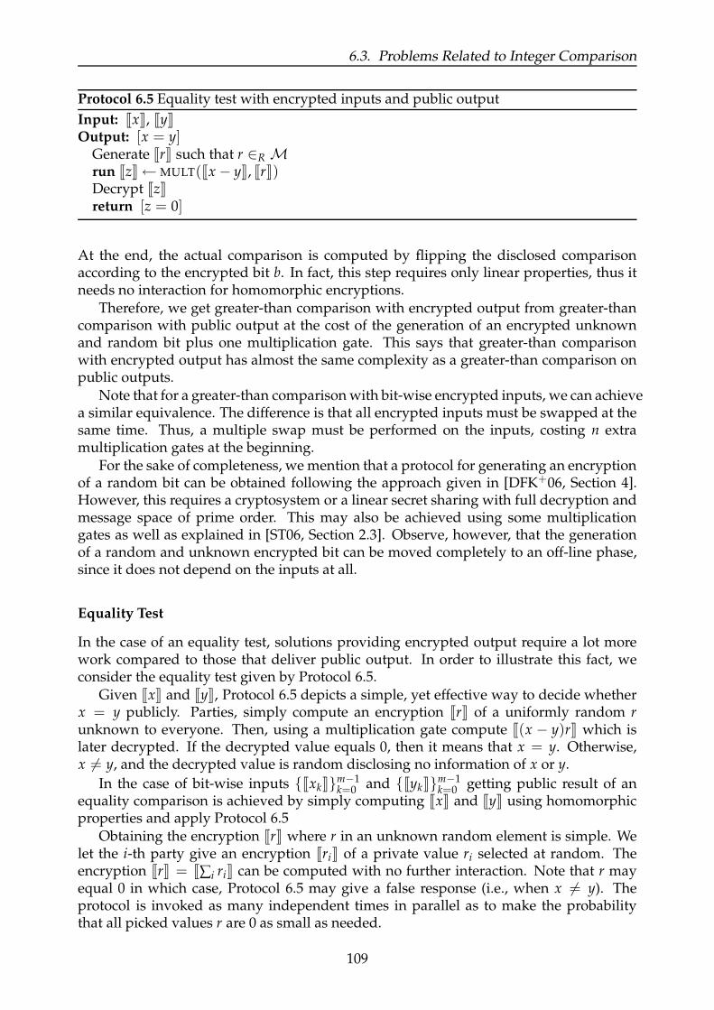
6.3. Problems Related to Integer Comparison

Protocol 6.5 Equality test with encrypted inputs and public output

Input: [[x]], [[y]]Output: [x = y]

Generate [[r]] such that r ∈RMrun [[z]]← MULT([[x − y]], [[r]])Decrypt [[z]]return [z = 0]

At the end, the actual comparison is computed by flipping the disclosed comparisonaccording to the encrypted bit b. In fact, this step requires only linear properties, thus itneeds no interaction for homomorphic encryptions.

Therefore, we get greater-than comparison with encrypted output from greater-thancomparison with public output at the cost of the generation of an encrypted unknownand random bit plus one multiplication gate. This says that greater-than comparisonwith encrypted output has almost the same complexity as a greater-than comparison onpublic outputs.

Note that for a greater-than comparisonwith bit-wise encrypted inputs, we can achievea similar equivalence. The difference is that all encrypted inputs must be swapped at thesame time. Thus, a multiple swap must be performed on the inputs, costing n extramultiplication gates at the beginning.

For the sake of completeness, we mention that a protocol for generating an encryptionof a random bit can be obtained following the approach given in [DFK+06, Section 4].However, this requires a cryptosystem or a linear secret sharing with full decryption andmessage space of prime order. This may also be achieved using some multiplicationgates as well as explained in [ST06, Section 2.3]. Observe, however, that the generationof a random and unknown encrypted bit can be moved completely to an off-line phase,since it does not depend on the inputs at all.

Equality Test

In the case of an equality test, solutions providing encrypted output require a lot morework compared to those that deliver public output. In order to illustrate this fact, weconsider the equality test given by Protocol 6.5.

Given [[x]] and [[y]], Protocol 6.5 depicts a simple, yet effective way to decide whetherx = y publicly. Parties, simply compute an encryption [[r]] of a uniformly random runknown to everyone. Then, using a multiplication gate compute [[(x − y)r]] which islater decrypted. If the decrypted value equals 0, then it means that x = y. Otherwise,x 6= y, and the decrypted value is random disclosing no information of x or y.

In the case of bit-wise inputs [[xk]]m−1k=0 and [[yk]]

m−1k=0 getting public result of an

equality comparison is achieved by simply computing [[x]] and [[y]] using homomorphicproperties and apply Protocol 6.5

Obtaining the encryption [[r]] where r in an unknown random element is simple. Welet the i-th party give an encryption [[ri]] of a private value ri selected at random. Theencryption [[r]] = [[∑i ri]] can be computed with no further interaction. Note that r mayequal 0 in which case, Protocol 6.5 may give a false response (i.e., when x 6= y). Theprotocol is invoked as many independent times in parallel as to make the probabilitythat all picked values r are 0 as small as needed.

109


Protocol 6.6 Bit-decomposition

Input: [[x]], 0 ≤ x < 2m.Output: [[xk]]

m−1k=0 such that x = ∑

m−1i=0 2ixi.

for k = m− 1 down-to 0 do[[xk]] = [[[x > 2k − 1]]] Note that [x > 2k − 1] = [x ≥ 2k][[x]]← [[x− 2kxk]]

end forreturn [[xk]]

m−1k=0

If the bit of information telling if x = y is required to be in an encryption, we needto apply a more elaborated protocol, as for instance shown in [DFK+06] and later im-proved in [NO07]. This protocol is the result of the evaluation of an arithmetic circuitthat requires the execution of many multiplication gates.

The same holds for bit-wise inputs. In fact, the circuits in Section 6.1 require at least2mmultiplications. Damgard et al. [DFK+06] present an arithmetic constant depth circuitvia the computation of an unbounded fan-in AND. The equality comparison is obtained

by computing bits fk = xkyk for all 0 ≤ k < n. Then [x = y] = ∏m−1k=0 fk.

6.3.4 Bit-decomposition Problems

Bit-decomposition protocols take as input an encrypted value [[x]] with x < 2m and pro-

duce encryptions [[xk]]m−1k=0 where xk

m−1k=0 is the bit representation of a non-negative

integer x. See [ACS02, DFK+06, ST06, NO07, Tof09a] for examples of protocols solvingthis kind of problems. Bit-decomposition is an important primitive in secure arithmeticsince it bridges the gap between problems that are inherently bit-oriented but the inputsare available in integer form.

A typical example is greater-than comparison. Suppose [[x]] and [[y]] be given as inputswith x and y being non-negative integers. A natural approach for circuits and protocolsis to compute [x > y] (or eventually [[[x > y]]]) relying on a bit-decomposition protocol.

Namely, inputs [[x]] and [[y]] are converted into [[xk]]m−1k=0 and [[yk ]]

m−1k=0 . Then, a bit-

wise greater-than comparison is performed, like the ones presented in this thesis. This isthe overall approach that is used in [DFK+06] where they get constant depth circuit forgreater-than comparison with encrypted integer input. This is acquired by using specialtricks to get both bit-decomposition and bit-wise greater-than in constant depth. How-ever, the size of the resulting circuit is very large and hence unsatisfactory for practicalapplications.

The bits of an m-bit integer x can be computed using greater-than comparisons asfollows. First, note that xk, the k-th bit of x, can be extracted by xk = [x ≥ 2k]. Protocol 6.6iteratively extract all bits.

A related primitive to bit-decomposition is the computation of the least significantbit of an encrypted integer. That is, given an encryption [[x]] compute [[x0]], where x0is the least significant bit of x, denoted with LSB(x). Protocols for this task have beeninvestigated by Schoenmakers and Tuyls [ST06] and Nishide and Otha [NO07].

The following proposition relates greater-than comparison and the least significantbit.

Proposition 6.5 Let q be an odd integer. x > (q− 1)/2 if and only if LSB(2x mod q) = 1.

110

6.4. A Cost Model for Arithmetic Circuits

In fact, if x > (q− 1)/2 then 2x ≥ q, and thus 2x mod q = 2x− q wraps around. Then,2x mod q is odd.

This equivalence is used by Nishide and Otha [NO07] to construct a general greater-than comparison circuit based only on comparisons with the public value (q − 1)/2,solving it via a protocol for the least significant bit. Interestingly, computing the leastsignificant bit reduces to computing bit-wise greater-than comparisons. Nishide andOtha [NO07] thus avoid the use of a bit-decomposition protocol to compute greater-thancomparison on encrypted integer inputs.

6.4 A Cost Model for Arithmetic Circuits

Circuit complexity is a branch of theoretical computer science in which a circuit is de-fined as a directed acyclic graph where nodes are gates, there are sources (input gates)and sinks (output gates). The complexity parameters are usually the size (number ofgates) and the depth (longest path in the graph). The analysis of the size and the depthof circuits is necessary in some practical scenarios, such as designing circuits for micro-processors, where minimizing the size and/or depth of circuits is important. More fun-damentally, circuit complexity provides a model in which one can prove lower boundson the depth or size of those circuits. In fact, a number of lower bounds for circuits areknown nowadays, and there is a still-growing range of techniques to prove these lowerbounds. We refer the reader to [Vol99, Chapter 3] and references therein for an overviewof these techniques.

Wewould like to answer similar questions about the arithmetic circuits we consider inthis chapter. In particular, since we are interested in computational efficiency, one couldbe interested to know a lower bound on the size of arithmetic circuits solving integercomparison. Remember that the size in our context just takes into account multiplicationgates only. Therefore one should define an appropriate cost model to bound the com-plexity. In most of cases, however, the lower bound is computed in a model where everygate is equally expensive, so one must count all gates.

In the following, we sketch a model that considers arithmetic circuits with an appro-priate cost model. LetM be a ring, and let x1, . . . , xn be a set of input variables. Anarithmetic circuit with inputs x1, . . . , xn is a directed acyclic graph where input gates arethe nodes with in-degree zero and output gates are the nodes with out-degree zero. In-put gates are labelled with the input variables, and we assume a number of gates labelledwith constants inM. Non-input gates have in-degree two and are labelled with either‘+’, ‘·’ or ‘×’ (in the first case the node is an addition gate, in the second case a multi-plication by a constant, and in the third case a multiplication gate). Addition gates maybe reached by any gate, while multiplication by a constant is restricted to be reached byexactly one constant input gate, and multiplication gates are not allowed to be reachedby constant input gates. Non-output gates may have out-degree larger than one.

Every node computes a polynomial in the ringM[x1, . . . , xn] in the following way.An input node just computes the input variable, or the constant it is labelled with. Anaddition gate computes the sum of the polynomials of all gates that reach it, while amultiplication by a contant and a multiplication gate compute the product of the twopolynomial of the gates that reach it. The polynomial g ∈ M[x1, . . . , xn] is said to becomputed by the arithmetic circuit if one of the output gates of the circuit computes g.

We define the size of the circuit as the number of multiplication gates while the depth

111


is the largest number of multiplication gates in any directed path going from any inputgate to any output gate. This definition of size and depth is motivated by the fact thatthe secure evaluation of an arithmetic circuit only multiplications require interaction.Additions and multiplication by a constant, however, are considered costless since theyare computed directly using homomorphic properties, and thus they do not affect thecomputation of the protocol. This model provides a framework where we can answerquestions like what is the minimal size of an arithmetic circuit for certain functionality.

Several lower bounds of circuits with different bases, cost models and restrictions canbe found across the literature. It is possible to prove the minimal size of a circuit for agiven (fixed) depth, or assuming a specific set of gates that circuits are allowed to use.As in our case, some gates may have assigned some cost which makes the problem ofcalculating lower bounds more challenging. In some cases, the most natural solutionis proved to be the best. An example is the boolean circuit for the addition of two m-bit integers. Red’kin [Red81] has shown that for this problem in particular, the folklorecircuit is the smallest one. More concretely, he has shown that 5m− 3 boolean gates is alower bound for a circuit computing that problem.

We turn the attention to integer comparison circuits. We have analyzed the complex-ity of various circuits in Table 6.1. We have seen that the most efficient circuit is thatin [ST04] which requires 2m− 1 multiplication gates for m-bit inputs. One may wonderif it is possible to get any better, and thus obtaining a more efficient solution. We believethat cost model for directed acyclic graphs representing arithmetic circuits as the one de-scribed above will help to find concrete answers to this kind of questions. In fact, westate the following conjecture.

Conjecture 1 Any arithmetic circuit (using the model described above) for integer comparisonon m-bit inputs has size at least 2m− 1.

In other words, we believe that the solution of [ST04] uses the minimal number ofmultiplication gates. We do note, however, that we do not claim that this is the mostefficient solution. As seen in Table 6.2 one can get more efficient solutions using differentapproaches. This conjecture suggests that no other protocol that limits itself to the evalu-ation of an arithmetic circuit for integer comparison (using additions and multiplicationsonly) can be better in a computational sense.

112

Chapter 7

Conclusions

In this thesis, we have presented solutions to two important primitives of secure multi-party computation: special verifiable shuffles and integer comparison. We have consid-ered three types of special shuffles, namely rotations, affine transformations, andMobiustransformations. The protocols presented in this thesis for these verifiable special shuf-fles are the most efficient to date. We have also studied efficient protocols for integercomparison in the setting where multiple parties do secure computations using a thresh-old homomorphic cryptosystem. Our solutions are competitive compared to the existingsolutions in the literature, especially regarding computational performance.

We have seen that verifiable rotation can be used in a variety of problems, like fragile-mixes [RW04], specific electronic voting protocols [RS06], and integer comparison pro-tocols [BK04, ABFL06, GSV07, DGK07, RT09]. Moreover, rotations are fundamental insome settings, for example in protocols for secure function evaluation based on mix-and-match [JJ00] or tallying protocols for preferential elections [WB09]. We believe that thereare many other cryptographic scenarios where we can apply rotations and multiple frag-ile permutations.

We have presented zero-knowledge proofs of knowledge for rotations for which wecan prove witness-extended emulation. This property implies computationally convinc-ing proof of knowledge [DF02], a widely accepted notion that shows that a possiblycheating prover who knows some trapdoor information of the public key of the sur-rounding cryptosystem does not gain any advantage to cheat in the protocol. Eventhough this property is less general than general knowledge soundness, witness-extendedemulation has the advantage of providing a simple and compact analysis. As an ex-tra advantage, witness extended-emulation simplifies the construction of a simulator forzero-knowledge proofs used in higher-level protocols.

For integer comparison we have studied two types of solutions. On the one hand,we have presented a protocol that is the result of the secure evaluation of an arithmeticcircuit. On the other hand, we have used a more direct approach that combines basiccryptographic building blocks to construct the solutions. These two types of solutionshave pros and cons which we briefly summarize in the following.

The circuit approach abstracts away all details of the implementation of the gates. Itsuffices to construct an arithmetic circuit for the desired functionality. The arithmetic cir-cuit is compiled into a secure protocol following the guidelines of the underlying frame-work (e.g., [CDN01, ST04]). The performance of the resulting protocol is determined bythe size and the depth of the arithmetic circuit. A circuit for the desired functionality maybe chosen trading off performance needs: a circuit with few multiplication gates yields

113

Chapter 7. Conclusions

an efficient protocol, whereas with a shallow circuit one gets low round complexity.The direct approach, in contrast, lacks the simplicity of the circuit approach. Instead,

one has to craft the protocols almost from scratch and prove their security formally. How-ever, since one has more freedom to look at the intrinsic properties of the problem, wemay be able to optimize the performance of the resulting protocols. In fact, this is thelesson learned for integer comparison protocols: the use of a direct approach has givenrise to protocols with improved performance.

We have worked with a security model that assumes the execution of our protocols inisolation (i.e., in a stand-alone model). More general security frameworks are consideredtoday, in which several instances of a protocol may be running simultaneously (e.g., theuniversal composability (UC) model of Canetti [Can01, Can05]). We believe that ourprotocols can be adapted to stronger models using standard techniques.

Due to the recent work by Terelius and Wikstrom [TW10] one can prove in zero-knowledge that a shuffle uses a permutation from a restricted set, more specifically, theautomorphism group of a hypergraph. The hypergraph can be set up to have as automor-phism group the set of all rotations, fragile permutations, or other sets of permutationssuch as all permutations that keep a rooted tree intact. This opens the door to the study ofshuffles using other families of permutations together with potential applications wherethe properties of these special families of permutations can be exploited.

One may wonder if it is possible to further improve the performance of the existingcircuit-based solutions for integer comparison. As stated above, the performance of aprotocol based on an arithmetic circuit is improved by optimizing the size and/or thedepth. A natural question is: what is the best size and/or depth that one can achievefor any integer comparison circuit? This kind of question may be addressed using sometechniques from circuit complexity.

Arithmetic circuits are directed acyclic graphs where nodes are gates and edges arewires. There are input gates (sources) and output gates (sinks) and the other gates canbe either addition gates or multiplication gates (see Section 6.4). This provides a modelto ask questions like what is the minimal number of multiplication gates required forany integer comparison protocol. The smallest known arithmetic circuit for integer com-parison is the msb-to-lsb solution of [ST04], requiring 2m − 1 multiplication gates. Weconjecture that this is the best one can get, and leave as an open problem proving thatthis is indeed the case.

114

Index

addition circuit, 107automorphism of a hypergraph, 67

bit decomposition protocol, 110

carrygeneration, 107propagation, 107

cascade of shufflers, 282-fragile, 843-fragile, 85general shuffle, 10rotations, 34, 40, 94

ciphertext indistinguishability, see semanticsecurity

circular convolution, 37, 46composition of Σ-protocol, 19, 25, 40, 52, 61,

63, 65, 80computational convincing proof of knowl-

edge, 22conditional gate, 30, 89

Diffie-Hellman problemcomputational, 16decision, 16

directed acyclic graph, 111Discrete Fourier Transform, 35, 67, 79, 80,

83discrete logarithm problem, 16

Fast Fourier Transform, 43, 80, 84Fiat-Shamir heuristic, 19fragile mixing, 69fragile permutation, 70

input swapping, 101, 108

Latin square, 70, 73, 75least significant bit, 110loop permutation, 34, 67

Mathieu groups, 76, 77

mix-and-match approach, see scrambled cir-cuit approach

mix-network, see cascade of shufflers

oblivious transfercommitted oblivious transfer, 106conditional oblivious transfer, 93

proof of rotation, 33, 39, 40, 61, 77, 80, 82,94, 99, 101

public shuffle, 28, 81

random oracle model, 19

Schwartz-Zippel lemma, 51scrambled circuit approach, 10, 34, 103semantic security, 16, 28, 33, 87sign function, see signumsignum, 106

threshold decryption, 17, 30, 94, 101, 108Toft’s trick, see input swapping

verifiability, 19, 28, 41, 78

witness-extended emulation, 21, 23, 53, 94

Yao’s protocol, 34, 103

115

Bibliography

[Abe99] M. Abe. Mix-networks on permutation networks. In ASIACRYPT 1999,volume 1716 of Lecture Notes in Computer Science, pages 258–273. Springer-Verlag, 1999.

[ABFL06] M. J. Atallah, M. Blanton, K. B. Frikken, and J. Li. Efficient correlated actionselection. In Financial Cryptography – FC 2006, volume 4107 of Lecture Notesin Computer Science, pages 296–310. Springer-Verlag, 2006.

[ACS02] J. Alesheimer, J. Camenisch, and V. Shoup. Efficient computation modulo ashared secret with application to the generation of shared safe-prime prod-ucts. In CRYPTO 2002, volume 2442 of Lecture Notes in Computer Science,pages 417–432. Springer-Verlag, 2002.

[BA01] M. Bhattacharya and J. Astola. Recursive structure for linear filtering usingnumber theoretic transform. 8th IEEE International Conference on Electronics,Circuits and Systems, 2001. ICECS 2001, 1:525–528, 2001.

[BG92] M. Bellare and O. Goldreich. On defining proofs of knowledge. InCRYPTO 1992, volume 740 of Lecture Notes in Computer Science, pages 390–420. Springer, 1992.

[BGW88] M. Ben-Or, S. Goldwasser, and A. Wigderson. Completeness theoremsfor non-cryptographic fault-tolerant distributed computation (extended ab-stract). In ACM Symposium on Theory of Computing – STOC 1988, pages 1–10.ACM Press, 1988.

[BK04] I. Blake and V. Kolesnikov. Strong conditional oblivious transfer and com-puting on intervals. In ASIACRYPT 2004, volume 3329 of Lecture Notes inComputer Science, pages 515–529. Springer-Verlag, 2004.

[Blu70] L. Bluestein. A linear filtering approach to the computation of the discreteFourier transform. IEEE Trans. Audio. Electroacust., AU-18:451–455, 1970.

[BMR90] D. Beaver, S. Micali, and P. Rogaway. The round complexity of secure proto-cols. InACM Symposium on Theory of Computing – STOC 1990, pages 503–513.ACM Press, 1990.

[BQ00] A. Bonisoli and P. Quattrocchi. Each invertible sharply d-transitive finitepermutation set with d ≥ 4 is a group. Journal of Algebraic Combinatorics,12(3):241–250, 2000.

117

[BR93] M. Bellare and P. Rogaway. Random oracles are practical. In ACM conferenceon Computer and Communications Security – CCS 1993, pages 62–73. ACM,1993.

[Can01] R. Canetti. Universally composable security: A new paradigm for crypto-graphic protocols. In IEEE Symposium on Foundations of Computer Science,pages 136–145, 2001.

[Can05] R. Canetti. Universally composable security: A new paradigm for cryp-tographic protocols. Cryptology ePrint Archive, Report 2000/067, 2005.http://eprint.iacr.org/2000/067.

[CC00] C. Cachin and J. Camenisch. Optimistic fair secure computation. InCRYPTO 2000, volume 1880 of Lecture Notes in Computer Science, pages 93–111. Springer-Verlag, 2000.

[CCD88] D. Chaum, C. Crepeau, and I. Damgard. Multiparty unconditionally secureprotocols (extended abstract). In ACM Symposium on Theory of Computing –STOC 1988, pages 11–19. ACM Press, 1988.

[CD97] R. Cramer and I. Damgard. Linear zero-knowledge – a note on efficient zero-knowledge proofs and arguments. In ACM Symposium on Theory of Comput-ing – STOC 1997, pages 436–445. ACM Press, 1997.

[CD98] R. Cramer and I. Damgard. Zero-knowledge for finite field arithmetic. Or:Can zero-knowledge be for free? In CRYPTO 1998, volume 1462 of LectureNotes in Computer Science, pages 424–441. Springer-Verlag, 1998.

[CDN01] R. Cramer, I. Damgard, and J. Nielsen. Multiparty computation from thresh-old homomorphic encryption. In EUROCRYPT 2001, volume 2045 of LectureNotes in Computer Science, pages 280–300. Springer-Verlag, 2001.

[CDPW07] R. Canetti, Y. Dodis, R. Pass, and S.Walfish. Universally composable securitywith global setup. In Theory of Cryptography Conference – TCC 2007, volume4392 of Lecture Notes in Computer Science, pages 61–85. Springer-Verlag, 2007.

[CDS94] R. Cramer, I. Damgard, and B. Schoenmakers. Proofs of partial knowledgeand simplified design of witness hiding protocols. In CRYPTO 1994, vol-ume 839 of Lecture Notes in Computer Science, pages 174–187. Springer-Verlag,1994.

[Cha81] D. Chaum. Untraceable electronic mail, return addresses, and digitalpseudonyms. Communications of the ACM, 24(2):84–88, 1981.

[Cra97] R. Cramer. Modular Design of Secure yet Practical Cryptographic Protocols. PhDthesis, Universiteit van Amsterdam, Netherlands, 1997.

[Cre90] C. Crepeau. Verifiable disclosure of secrets and applications. In EURO-CRYPT 1990, volume 434 of Lecture Notes in Computer Science, pages 181–191.Springer-Verlag, 1990.

[CT65] J. Cooley and J. Tukey. An algorithm for the machine calculation of complexFourier series. Mathematics of Computation, 19(90):297–301, 1965.

118

[CvdGT95] C. Crepeau, J. van de Graaf, and A. Tapp. Committed oblivious transfer andprivate multi-party computation. In CRYPTO 1995, volume 963 of LectureNotes in Computer Science, pages 110–123. Springer-Verlag, 1995.

[Dam08] I. Damgard. On Σ-protocols. Lecture Notes for the courseCryptographic Protocol Theory, A rhus University, 2008.http://www.daimi.au.dk/~ivan/CPT.html.

[DF02] I. Damgard and E. Fujisaki. Efficient concurrent zero-knowledge in the aux-iliary string model. In ASIACRYPT 2002, volume 2501 of Lecture Notes inComputer Science, pages 125–142. Springer-Verlag, 2002.

[DFK+06] I. Damgard, M. Fitzi, E. Kiltz, J. Nielsen, and T. Toft. Unconditionally secureconstant-rounds multi-party computation for equality, comparison, bits andexponentiation. In Theory of Cryptography Conference – TCC 2006, volume 3876of Lecture Notes in Computer Science, pages 285–304. Springer-Verlag, 2006.

[DGK07] I. Damgard, M. Geisler, and M. Krøigaard. Efficient and secure comparisonfor on-line auctions. In Australasian Conference Information Security and Pri-vacy – ACISP 2007, volume 4586 of Lecture Notes in Computer Science, pages416–430. Springer-Verlag, 2007.

[dHSSV09] S. de Hoogh, B. Schoenmakers, B. Skoric, and J. Villegas. Verifiable rotatorsof homomorphic encryptions. In Public Key Cryptography–PKC 2009, volume5443 of Lecture Notes in Computer Science, pages 393–410. Springer-Verlag,2009.

[dHSV10] S. de Hoogh, B. Schoenmakers, and J. Villegas. Verifiable multiply fragileshuffles, 2010. Unpublished Manuscript.

[DJ01] I. Damgard and M. Jurik. A generalization, a simplification and someapplications of Paillier’s probabilistic public-key system. In Public KeyCryptography–PKC 2001, volume 1992 of Lecture Notes in Computer Science,pages 119–136. Springer-Verlag, 2001.

[DM96] J. Dixon and B. Mortimer. Permutation Groups, volume 163 of Graduate Textsin Mathematics. Springer, 1996.

[ElG85] T. ElGamal. A public key cryptosystem and a signature scheme based ondiscrete logarithms. In IEEE Transactions on Information Theory IT-31, pages469–472, 1985.

[FMM+03] J. Furukawa, H. Miyauchi, K. Mori, S. Obana, and K. Sako. An implementa-tion of a universally verifiable electronic voting scheme based on shuffling.In Financial Cryptography – FC 2002, volume 2357 of Lecture Notes in ComputerScience, pages 16–30. Springer-Verlag, 2003.

[FS87] A. Fiat and A. Shamir. How to prove yourself: Practical solution to identifi-cation and signature problems. In CRYPTO 1986, volume 223 of Lecture Notesin Computer Science, pages 186–194. Springer-Verlag, 1987.

119

[FS01] J. Furukawa and K. Sako. An efficient scheme for proving a shuffle. InCRYPTO 2001, volume 2139 of Lecture Notes in Computer Science, pages 368–387. Springer-Verlag, 2001.

[Fur05] J. Furukawa. Efficient and verifiable shuffling and shuffle-decryption. IEICETrans Fundamentals, E88-A:172–188, 2005.

[GI08] J. Groth and Y. Ishai. Sub-linear zero-knowledge argument for correctnessof a shuffle. In EUROCRYPT 2008, volume 4965 of Lecture Notes in ComputerScience, pages 379–396. Springer-Verlag, 2008.

[GJKR99] R. Gennaro, S. Jarecki, H. Krawczyk, and T. Rabin. Secure distributed keygeneration for discrete-log based cryptosystems. In EUROCRYPT 1999,volume 1592 of Lecture Notes in Computer Science, pages 295–310. Springer-Verlag, 1999.

[GL07] J. Groth and S. Lu. Verifiable shuffle of large size ciphertexts. In Public KeyCryptography–PKC 2007, volume 4450 of Lecture Notes in Computer Science,pages 377–392. Springer-Verlag, 2007.

[GM84] S. Goldwasser and S. Micali. Probabilistic encryption. Special issue of Journalof Computer and Systems Sciences, 28(2):270–299, 1984.

[GMW87] O. Goldreich, S. Micali, and A. Wigderson. How to play any mental game ora completeness theorem for protocols with honest majority. In ACM Sympo-sium on Theory of Computing – STOC 1987, pages 218–229. ACM Press, 1987.

[GMY04] J. Garay, P. MacKenzie, and K. Yang. Efficient and universally composablecommitted oblivious transfer and applications. In Theory of CryptographyConference – TCC 2004, volume 2951 of Lecture Notes in Computer Science,pages 297–316. Springer-Verlag, 2004.

[Gro03] J. Groth. A verifiable secret shuffle of homomorphic encryptions. In Pub-lic Key Cryptography–PKC 2003, volume 2567 of Lecture Notes in ComputerScience, pages 145–160. Springer-Verlag, 2003. Full version available athttp://eprint.iacr.org/2005/246.

[Gro04] J. Groth. Honest Verifier Zero-Knowledge Arguments Applied. PhD thesis, Uni-versity of Arhus, 2004.

[GSV07] J. Garay, B. Schoenmakers, and J. Villegas. Practical and secure solutions forinteger comparison. In Public Key Cryptography–PKC 2007, volume 4450 ofLecture Notes in Computer Science, pages 330–342. Springer-Verlag, 2007.

[JJ00] M. Jakobsson and A. Juels. Mix and match: Secure function evaluation viaciphertexts. In ASIACRYPT 2000, volume 1976 of Lecture Notes in ComputerScience, pages 162–177. Springer-Verlag, 2000.

[Jor72] C. Jordan. Recherches sur les substitutions. Journal Math. Pures Appl.,17(2):351–363, 1872.

120

[JS07] S. Jarecki and V. Shmatikov. Efficient two-party secure computation on com-mitted inputs. In EUROCRYPT 2007, volume 4515 of Lecture Notes in Com-puter Science, pages 97–114. Springer-Verlag, 2007.

[Ker74] W. Kerby. On infinite sharply multiply transitive groups. Vandenhoeck &Ruprecht, Gottingen, 1974.

[Knu97] D. E. Knuth. The Art of Computer Programming, volume 1. Addison-Wesley,Reading, MA, USA, 3rd. edition, 1997.

[KS06a] M. Kiraz and B. Schoenmakers. A protocol issue for the malicious case ofYao’s garbled circuit construction. In 27th Symposium on Information Theoryin the Benelux, pages 283–290, 2006.

[KS06b] M. Kiraz and B. Schoenmakers. Securing Yao’s garbled circuit constructionagainst active adversaries. In Online Proceedings of 1st Benelux Workshop onInformation and System Security–WISSec 2006, 2006.

[KS08] M. Kiraz and B. Schoenmakers. An efficient protocol for fair secure two-party computation. In Topics in Cryptology – CT-RSA 2008, volume 4964 ofLecture Notes in Computer Science, pages 88–105. Springer-Verlag, 2008.

[KSV07] M. Kiraz, B. Schoenmakers, and J. Villegas. Efficient committed oblivioustransfer of bit strings. In Information Security Conference – ISC 2007, volume4779 of Lecture Notes in Computer Science, pages 130–144. Springer-Verlag,2007.

[Kus06] R. Kusters. Simulation-based security with inexhaustible interactive Turingmachines. In 19th IEEE Computer Security Foundations Workshop–CSFW 2006,pages 309–320. IEEE Computer Society, 2006.

[LA06] J. Li and M. Atallah. Secure and private collaborative linear programming.Collaborative Computing: Networking, Applications and Worksharing, 2006. Col-laborateCom 2006, pages 1–8, 2006.

[Lin03] Y. Lindell. Parallel coin-tossing and constant-round secure two-party com-putation. Journal of Cryptology, 16(3):143–184, 2003.

[LP00] Y. Lindell and B. Pinkas. Privacy preserving data mining. Journal of Cryptol-ogy, 15(3):177–206, 2000.

[LP07] Y. Lindell and B. Pinkas. An efficient protocol for secure two-party computa-tion in the presence of malicious adversaries. In EUROCRYPT 2007, volume4515 of Lecture Notes in Computer Science, pages 52–78, 2007.

[MF06] P. Mohassel and M. Franklin. Efficiency tradeoffs for malicious two-partycomputation. In Public Key Cryptography–PKC 2006, volume 3958 of LectureNotes in Computer Science, pages 458–473, 2006.

[MNPS04] D. Malkhi, N. Nisan, B. Pinkas, and Y. Sella. Fairplay – a secure two-partycomputation system. In USENIX Security, pages 287–302, 2004.

121

[Nef01] C. Neff. A verifiable secret shuffle and its application to e-voting. In 8thACM conference on Computer and Communications Security – CCS 2001, pages116–125. ACM, 2001.

[NO07] T. Nishide and K. Ohta. Multiparty computation for interval, equality, andcomparison without bit-decomposition protocol. In Public Key Cryptography–PKC 2007, volume 4450 of Lecture Notes in Computer Science, pages 343–360.Springer-Verlag, 2007.

[NPS99] M. Naor, B. Pinkas, and R. Sumner. Privacy preserving auctions and mech-anism design. In 1st ACM conference on Electronic Commerce–EC 1999, pages129–139. ACM Press, 1999.

[Oka93] T. Okamoto. Provably secure and practical identification schemes and corre-sponding signature schemes. In CRYPTO 1992, volume 740 of Lecture Notesin Computer Science, pages 31–53. Springer, 1993.

[Pai99] P. Paillier. Public-key cryptosystems based on composite degree residuos-ity classes. In EUROCRYPT 1999, volume 1592 of Lecture Notes in ComputerScience, pages 223–238. Springer-Verlag, 1999.

[Pas92] A. Pasini. Diagram geometries for sharply n-transitive sets of permutationsor of mappings. Design, Codes and Cryptography, (1):275–297, 1992.

[Ped91] T. Pedersen. A threshold cryptosystem without trusted party. In EURO-CRYPT 1991, volume 547 of Lecture Notes in Computer Science, pages 522–526.Springer-Verlag, 1991.

[Pin03] B. Pinkas. Fair secure twoparty computation. In EUROCRYPT 2003, vol-ume 2656 of Lecture Notes in Computer Science, pages 87–105. Springer-Verlag,2003.

[PS04] M. Prabhakaran and A. Sahai. New notions of security: Achieving univer-sal composability without trusted setup. In ACM Symposium on Theory ofComputing – STOC 2004, pages 242–251. ACM Press, 2004.

[Qui04] J. Quistorff. A new nonexistence result for sharply multiply transitive per-mutation sets. Discrete Mathematics, 288:185–186, 2004.

[Red81] N. P. Red’kin. On the minimal realization of a binary adder. Problemy Kiber-net, 38:181–216, 1981.

[Rob95] D. Robinson. A Course in the Theory of Groups. Springer-Verlag, New York,1995.

[RS06] P. Ryan and F. Schneider. Pret-a-Voter with re-encryption mixes. In ComputerSecurity – ESORICS 2006, volume 4189 of Lecture Notes in Computer Science,pages 313–326, Berlin, 2006. Springer-Verlag.

[RT09] T. Reistad and T. Toft. Secret sharing comparison by transformation androtation. In Proceedings of the International Conference on Information TheoreticSecurity–ICITS 2007, volume 4883, pages 169–180. Springer-Verlag, 2009.

122

[RW04] M. Reiter and X. Wang. Fragile mixing. In ACM conference on Computer andCommunications Security – CCS 2004, pages 227–235. ACM, 2004.

[Rya06] P. Ryan. Pret-a-Voter with Paillier encryption, 2006. Technical Re-port CS-TR No 965, School of Computing Science, Newcastle University.http://www.cs.ncl.ac.uk/publications/trs/papers/965.pdf.

[Sch91] C. Schnorr. Efficient signature generation by smart cards. Journal of Cryptol-ogy, 4(3):161–174, 1991.

[Sha79] A. Shamir. How to share a secret. In Communications of the ACM, 22, pages612–613, 1979.

[Sid07] A. Sidorenko. Design and Analysis of Provably Secure Pseudorandom Generators.PhD thesis, Eindhoven University of Technology, 2007.

[SK95] K. Sako and J. Killian. Receipt-free mix-type voting scheme. In EURO-CRYPT 1995, volume 921 of Lecture Notes in Computer Science, pages 393–403.Springer-Verlag, 1995.

[SS07] B. Schoenmakers and A. Sidorenko. Distributed generation of uniformlyrandom bounded integers, 2007. Unpublished Manuscript.

[SSW09] A. Sadeghi, T. Schneider, and I. Wehrenberg. Efficient privacy-preservingface recognition. In International Conference on Information and CommunicationsSecurity–ICICS 2009, Lecture Notes in Computer Science. Springer-Verlag,2009. To appear.

[ST04] B. Schoenmakers and P. Tuyls. Practical two-party computation based onthe conditional gate. In ASIACRYPT 2004, volume 3329 of Lecture Notes inComputer Science, pages 119–136. Springer-Verlag, 2004.

[ST06] B. Schoenmakers and P. Tuyls. Efficient binary conversion for Paillier en-crypted values. In EUROCRYPT 2006, volume 4004 of Lecture Notes in Com-puter Science, pages 522–537. Springer-Verlag, 2006.

[Str64] E. Straus. Addition chains of vectors (problem 5125). American MathematicalMonthly, 71:806–808, 1964.

[Tof09a] T. Toft. Constant-rounds, almost-linear bit-decomposition of secret sharedvalues. In Topics in Cryptology – CT-RSA 2009, volume 5473 of Lecture Notesin Computer Science, pages 357–371. Springer-Verlag, 2009.

[Tof09b] T. Toft. Personal communication with the author, 2009.

[Tof09c] T. Toft. Solving linear programs using multiparty computation. In FinancialCryptography – FC 2009, volume 5628 of Lecture Notes in Computer Science,pages 90–107. Springer-Verlag, 2009.

[TW10] B. Terelius and D. Wikstrom. Proofs of restricted shuffles. In AFRICACRYPT2010, Lecture Notes in Computer Science. Springer-Verlag, 2010. To appear.

123

[Vol99] H. Vollmer. Introduction to circuit complexity: a uniform approach. Springer,1999.

[WB09] R. Wen and R. Buckland. Minimum disclosure counting for the alternativevote. In E-Voting and Identity – VOTE-ID 2009, volume 5767 of Lecture Notesin Computer Science, pages 122–140. Springer-Verlag, 2009.

[Wik09] D. Wikstrom. A commitment-consistent proof of a shuffle. In AustralasianConference Information Security and Privacy – ACISP 2009, volume 5594 of Lec-ture Notes in Computer Science, pages 407–421. Springer-Verlag, 2009.

[Yao82] A. Yao. Protocols for secure computation. In 23rd IEEE Symposium on Foun-dations of Computer Science, pages 160–164, 1982.

[Yao86] A. Yao. How to generate and exchange secrets. In 27th IEEE Symposium onFoundations of Computer Science, pages 162–168, 1986.

124

Summary

In modern cryptography, the problem of secure multiparty computation is about the co-operation between mutually distrusting parties computing a given function. Each partyholds some private information that should remain secret as much as possible through-out the computation. A large body of research initiated in the early 1980’s has shown thatany computable function can be evaluated using secure multiparty computation. Thoughthese feasibility results are general, their applicability in practical situations is rather un-satisfactory. This thesis concerns the study of two particular cryptographic primitiveswith focus on efficiency.

The first primitive studied is a generalization of verifiable shuffles of homomorphicencryptions, where the shuffler is only allowed to apply a permutation from a restrictedset of permutations. In this thesis, we consider shuffles using permutations from a k-fragile set, meaning that any k input-output correspondences uniquely identify a permu-tation within the set. We provide verifiable shuffles restricted to the set of all rotations (1-fragile), affine transformations (2-fragile), andMobius transformations (3-fragile). Appli-cations of these special shuffles include fragile mixing, electronic elections, secure func-tion evaluation using scrambled circuits, and secure integer comparison.

Two approaches for verifiable rotations are presented. On the one hand, we use prop-erties of the Discrete Fourier Transform (DFT) to express in a compact way that a rotationis applied in a shuffle. The solution is efficient, but imposes some mild restrictions on theparameters to allow DFT to work. On the other hand, we present a general solution thatdoes not impose any parameter constraint and works on any homomorphic cryptosys-tem. These protocols for rotations are used to build efficient shuffling protocols for affineand Mobius transformations.

The second primitive is secure integer comparison. In a general scenario, parties aregiven homomorphic encryptions of the bits of two integers and, after running a protocol,an encryption of a bit is produced, telling the result of the greater-than comparison of thetwo integers. This is a useful building block for higher-level protocols such as electronicvoting, biometrics authentication or electronic auctions. A study of the relationship ofother problems to integer comparison is given as well.

We present two types of solutions for integer comparison. Firstly, we consider anarithmetic circuit yielding secure protocols within the framework for multiparty com-putation based on threshold homomorphic cryptosystems. Our circuit achieves a goodbalance between round and computational complexities, when compared to the similarsolutions in the literature. The second type of solutions uses a intricate approach wheredifferent building blocks are used. A full analysis ismade for the two-party casewhere ef-ficiency of the resulting protocols compares favorably to other solutions and approaches.

125

Samenvatting

Binnen de moderne cryptografie bestaat het onderzoeksgebied secure multiparty com-putation. In dit gebied onderzoekt men de samenwerking van elkaar wantrouwendepersonen om via een protocol een gegeven functie uit te rekenen. Elke persoon heefteen persoonlijke invoer voor de functie en wil deze gedurende de berekening zoveel mo-gelijk geheim houden. Een grote hoeveelheid onderzoek uit begin jaren ’80 toont aan datelke berekenbare functie op een dergelijke veilige manier berekend kan worden. Hoeweldeze resultaten veelbelovend zijn, blijken de gebruikte technieken niet erg efficient tezijn. Dit proefschrift behandelt twee specifieke primitieven en concentreert daarbij op deefficientie.

De eerste primitieve is een generalisatie van het verifieerbaar herverdelen van homo-morfe encrypties, waarbij de verdeler slechts gebruik mag maken van een beperkt aantalpermutaties. Dit proefschrift gaat in op herverdelingen die gebruikmaken van k-fragielepermutaties, wat inhoudt dat de permutatie vastgelegd wordt door elk k-tupel van in-en uitvoer. We geven constructies voor het gebruik met rotaties (1-fragiel), affiene trans-formaties (2-fragiel) en Mobius-transformaties (3-fragiel). Deze specifieke constructieshebben toepassingen in fragiele mixnetwerken, elektronische verkiezingen en secure in-teger comparison.

We presenteren twee aanpakken voor verifieerbare rotaties. De eerste aanpak maaktgebruik van de eigenschappen van de discrete Fouriertransformatie (DFT) om de rotatieop een compacte manier vast te leggen. Dit levert een efficient protocol op, maar legtook enkele beperkingen op aan het gebruikte scenario. De tweede aanpak geeft een al-gemene oplossing die geen beperkingen oplegt en met ieder homomorf cryptosysteem tegebruiken is. De op deze wijze verkregen constructies worden vervolgens gebruikt omefficiente protocollen voor affiene en Mobius-transformaties te verkrijgen.

De tweede primitieve in dit proefschrift is het zogenaamde secure integer compari-son. In dit protocol hebben de verschillende deelnemers toegang tot een encryptie vande bits van twee gehele. Ze willen graag de encryptie van een enkel bit berekenen dataangeeft welk van de twee gehele getallen groter is. Dit is een handige bouwsteen vooruitgebreidere protocollen voor bijvoorbeeld elektronisch stemmen, elektronische veilin-gen en authenticatie met biometrieen. We bestuderen onder andere de relatie tusseninteger comparison en andere problemen.

We geven twee soorten oplossingen. In de eerste plaats bekijken we aritmetische cir-cuits. Dit levert protocollen op die passen binnen de multiparty compution gebaseerdop threshold homomorfic encryption. De gevonden circuits geven – in vergelijking metbestaande oplossingen – een goede balans tussen de rondecomplexiteit en de computa-tionele complexiteit. De tweede oplossing is een complexe aanpak, waarbij een samen-stelling van diverse cryptografische primitieven als bouwblok worden gebruikt. Wemaken een uitgebreide analyse in het geval van twee deelnemers; hier blijkt de efficientievan de resulterende protocollen beter blijkt te zijn dan bij bestaande oplossingen.

127

Acknowledgements

This thesis would not have been made without the help and support of many people.First and foremost, I would like to express my most sincere appreciation to my supervi-sor, Berry Schoenmakers, for his advice, support and patience during these years. I amvery grateful to him for inviting me to do my Ph.D. in Eindhoven. I also thank Henk vanTilborg who, apart from being my promotor, has always supported me during these fouryears, and has given me a lot of nice feedback in this thesis. This work would not havebeen the same without their invaluable feedback.

The members of the reading committee of my Ph.D. thesis are Juan A. Garay, RonaldCramer and Andries Brouwer. I appreciate their work reading my thesis and comment-ing on it. External members of the Ph.D. committee, Jorge Guajardo and Ahmad-RezaSadeghi are also thanked for taking part in the defense of this dissertation. I especiallythank Juan who gave me a lot of feedback that helped to improve this work significantly.He also guided, mentored and adviced me at earlier stages of Ph.D. studies. I didn’tpanic and hanged in there :-)

My Ph.D. studies were part of the PASC project (“Practical Approaches to SecureComputation”) that has been funded by the Dutch Technology Foundation (STW). Apartfrom the financial support, we held regular meetings with the “user committee”, com-posed people coming from the different partners supporting the project. These meetingsprovided quite good feedback in the direction that my research should aim at.

Some results included in this thesis have been discussed at the MPC club, a weeklygathering with the protocol guys of the coding and crypto group where we brainstormand discuss interesting stuff. Special thanks go to Boris Skoric, Sebastiaan de Hoogh,Peter van Liesdonk and Tomas Toft for the many club sessions spent on my researchproblems. They helped to improve this work a lot! On top of this, Sebastiaan proof-readsome chapters, and Peter helped me with a translation of the summary. I thank DanRoozemond, Cicek Guven and Maxim Hendiks for a last minute advice on bibliographicreferences concerning multiply sharply transitive groups.

I am grateful to all my colleagues of the crypto and security groups in special to allmembers of the “big Ph.D. office”, HG. 8.79, including Reza, Peter B., Christianne, Petervan L., Sebastiaan, Jing, Peter S., Michael, and all the newcomers. They all have managedto make coming to the office very enjoyable, even when the office was very crowded.Together with the guys of the other big office, Bruno, Daniel, Antonino, Mayla, Relindeand Gaetan they all created a nice atmosphere at lunch time and during the afternoontea-brakes.

I could never forget the support of Ellen, Reza, Andrey and Mehmet at early stagesof my doctorate, thanks! Anita, Benne, Wil, Tanja, Dan and all the other members of thegroups coding and crypto, security, and discrete algebra and geometry complemented anice and unforgettable working atmosphere.

I am indebted to my family who, from the distance, have given me the strength and

129

support to face everyday. I want to thank my parents to have shaped me as I am now,encouraging me everyday to give a step forward and being there in good and especiallyin bad circumstances. With their strong and endless support, I would not have been ableto be where I am now. There will never be a way to return all this.

Estoy totalmente agradecido a mi familia quienes, desde la distancia, me han dadola fuerza y el apoyo para poder hacer frente a cada dıa. Quiero agradecer a mis padrespor haberme curtido de la manera que soy, dandome el valor para dar un paso adelante yestar ahı en las buenas y especialmente en las malas. Con su inacabable e infinito soporte,no hubiera sido capaz de estar en donde me encuentro ahora. Nunca encontrare la formade devolverles todo esto.

I do not want to forget all nice people and friends I have met since I landed in Eind-hoven. If you are reading this and feel identified in this group of people, I thank you forthe hospitality, the many enjoyable moments, and understanding my busy schedule inthe last year. A special thank go to Cipri Cornea and his co-author for some translationdone in this thesis (see below).

And last but not least, I thank my wife Iulia. You have not only given me love andunconditional support, but a lovely family in Romania and a welcoming group of Roma-nian friends. I appreciate very much the passion you put on everything you do in life.You fill me and give me the confidence and strength I need everyday. Without your infi-nite support and encouragement, I would not have been able to manage in the stressfulmoments of writing this thesis. I will work hard to return everything you give me duringthe whole life together ahead of us...

Iar ın final, ıi multumesc sotiei mele Iulia. Mi-ai oferit nu doar dragoste si sprijinneconditionat, ci o familie minunata ın Romania si un grup primitor de prieteni romani.Iti apreciez foarte mult pasiunea cu care te ocupi de orice lucru pe care ıl faci. Ma faci sama simt ıntreg alaturi de tine, ımi oferi ıncrederea si puterea de care am nevoie ın fiecarezi. Fara necontenitul tau sprijin si ıncurajare nu as fi reusit sa trec cu bine momenteleıncordate din timpul scrierii tezei. Ma voi stradui pe tot parcursul vietii ce ne asteaptaımpreuna sa iti ofer si eu tie aceeasi grija, aceeasi pasiune, aceeasi dragoste pe care tu mile oferi constant...

Jose VillegasEindhoven, March 2010

130

Curriculum Vitae

Jose Villegas was born on July 17, 1981 in Salta, Argentina. He finished his pre-universityeducation at the Technical High School “Gral. Guemes” in Salta, and started his studiesat the Salta National University in March 2000.

Starting with his second year in software engineering, he followed extra-curricularcourses in discrete mathematics. Jose’s interest in cryptography has led him to carry outthe implementation of a software package providing cryptographic functionalities as hisfinal project. He received his Bachelor’s degree with honors in May 2003. In November2005, after writing his master’s thesis titled “Analysis and Implementation of ObliviousTransfer Protocols”, Jose finished his Master’s degree in computer science with honors.

He did different activities next to his university studies. He worked as an ICT assis-tant for the migration to Linux OS in the university (2002), as a teaching assistant (2002– 2004), and was a member of the university council (2004). He worked as a databasemaintainer in Damesco Supermarkets (summer of 2005). In the winter of 2005 he joined aresearch project to analyze the warehouse management of Termoandes, a electric genera-tion plant. During 2005, he followed different courses of the master’s in applied discretemathematics as a complement to his background.

In January 2006, Jose joined the Coding and Crypto group at the Eindhoven Univer-sity of Technology. Until mid 2010 he was a PhD student under the supervision of dr.ir.Berry Schoenmakers.

131

Design of advanced primitives for secure multiparty computation

Documents

Transcript of Design of advanced primitives for secure multiparty computation