Nanyang Technological University

School of Chemical and BioMedical

EngineeringDivision of Bioengineering

BG2802 Bioengineering Year 2 Lab

Lab Report

Analysis of Cyclic Fatigue Failure Datausing Least-square Regression

Author:Yang WANGa

a Matriculation Number: U1220560J

19 Febuary, 2013

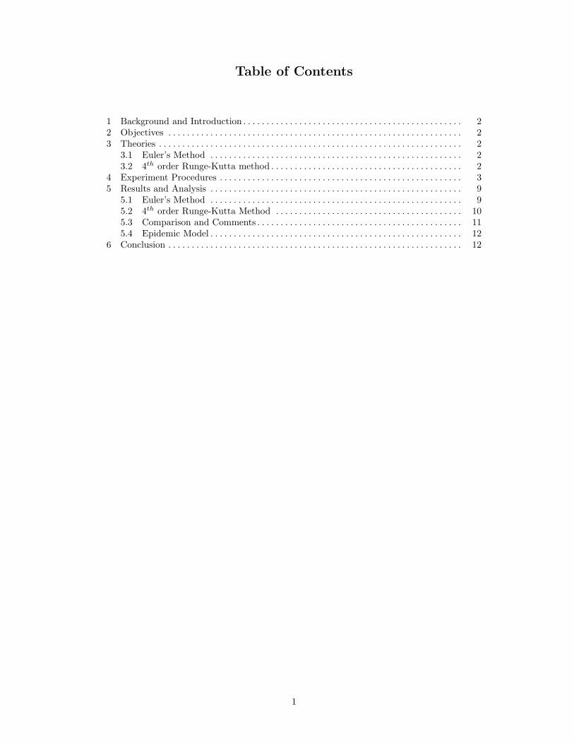
Table of Contents

1 Background and Introduction . . . . . . . . . . . . . . . . . . . . . . . . . . . . . . . . . . . . . . . . . . . . . . . 22 Objectives . . . . . . . . . . . . . . . . . . . . . . . . . . . . . . . . . . . . . . . . . . . . . . . . . . . . . . . . . . . . . . . 23 Theories . . . . . . . . . . . . . . . . . . . . . . . . . . . . . . . . . . . . . . . . . . . . . . . . . . . . . . . . . . . . . . . . . 2

3.1 Euler’s Method . . . . . . . . . . . . . . . . . . . . . . . . . . . . . . . . . . . . . . . . . . . . . . . . . . . . . . 23.2 4th order Runge-Kutta method . . . . . . . . . . . . . . . . . . . . . . . . . . . . . . . . . . . . . . . . . 2

4 Experiment Procedures . . . . . . . . . . . . . . . . . . . . . . . . . . . . . . . . . . . . . . . . . . . . . . . . . . . . 35 Results and Analysis . . . . . . . . . . . . . . . . . . . . . . . . . . . . . . . . . . . . . . . . . . . . . . . . . . . . . . 9

5.1 Euler’s Method . . . . . . . . . . . . . . . . . . . . . . . . . . . . . . . . . . . . . . . . . . . . . . . . . . . . . . 95.2 4th order Runge-Kutta Method . . . . . . . . . . . . . . . . . . . . . . . . . . . . . . . . . . . . . . . . 105.3 Comparison and Comments . . . . . . . . . . . . . . . . . . . . . . . . . . . . . . . . . . . . . . . . . . . . 115.4 Epidemic Model . . . . . . . . . . . . . . . . . . . . . . . . . . . . . . . . . . . . . . . . . . . . . . . . . . . . . . 12

6 Conclusion . . . . . . . . . . . . . . . . . . . . . . . . . . . . . . . . . . . . . . . . . . . . . . . . . . . . . . . . . . . . . . . 12

1

2

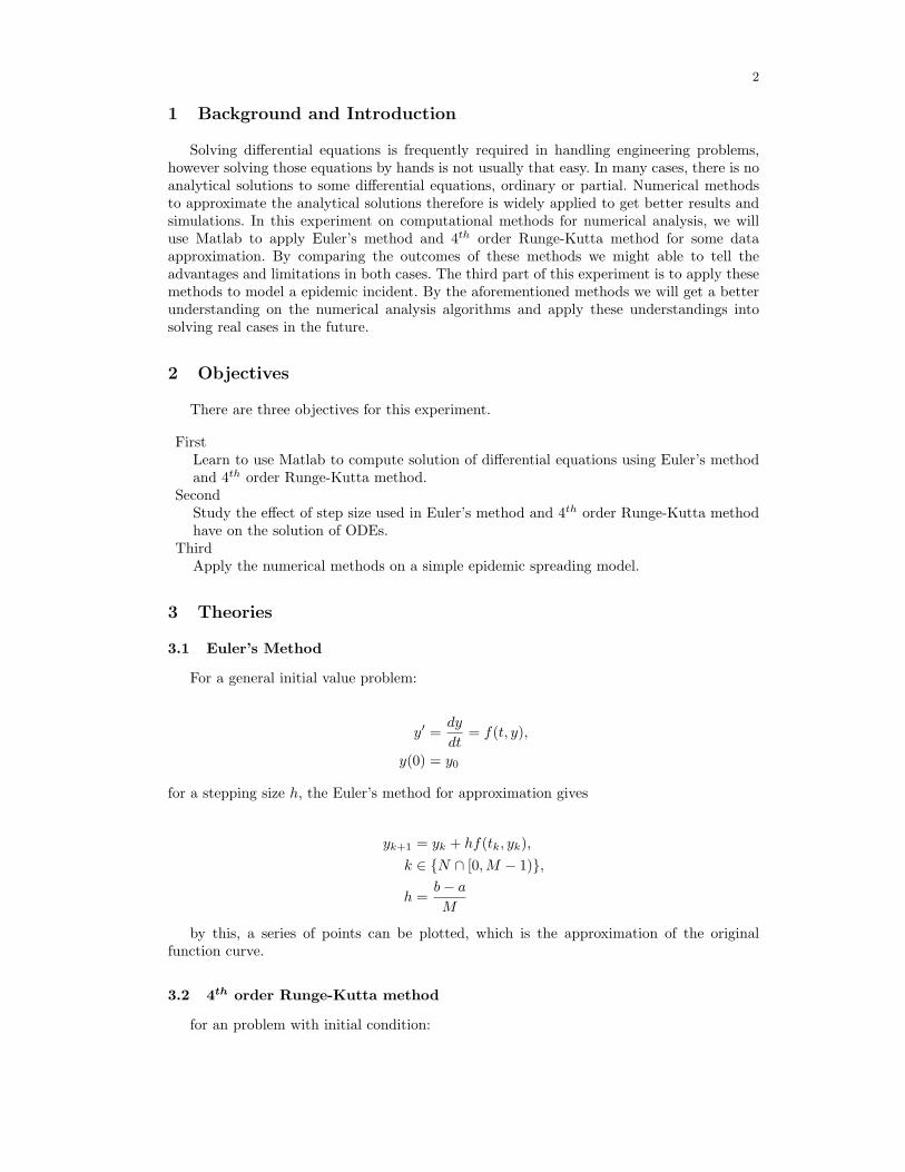
1 Background and Introduction

Solving differential equations is frequently required in handling engineering problems,however solving those equations by hands is not usually that easy. In many cases, there is noanalytical solutions to some differential equations, ordinary or partial. Numerical methodsto approximate the analytical solutions therefore is widely applied to get better results andsimulations. In this experiment on computational methods for numerical analysis, we willuse Matlab to apply Euler’s method and 4th order Runge-Kutta method for some dataapproximation. By comparing the outcomes of these methods we might able to tell theadvantages and limitations in both cases. The third part of this experiment is to apply thesemethods to model a epidemic incident. By the aforementioned methods we will get a betterunderstanding on the numerical analysis algorithms and apply these understandings intosolving real cases in the future.

2 Objectives

There are three objectives for this experiment.

FirstLearn to use Matlab to compute solution of differential equations using Euler’s methodand 4th order Runge-Kutta method.

SecondStudy the effect of step size used in Euler’s method and 4th order Runge-Kutta methodhave on the solution of ODEs.

ThirdApply the numerical methods on a simple epidemic spreading model.

3 Theories

3.1 Euler’s Method

For a general initial value problem:

y′ =dy

dt= f(t, y),

y(0) = y0

for a stepping size h, the Euler’s method for approximation gives

yk+1 = yk + hf(tk, yk),

k ∈ {N ∩ [0,M − 1)},

h =b− a

M

by this, a series of points can be plotted, which is the approximation of the originalfunction curve.

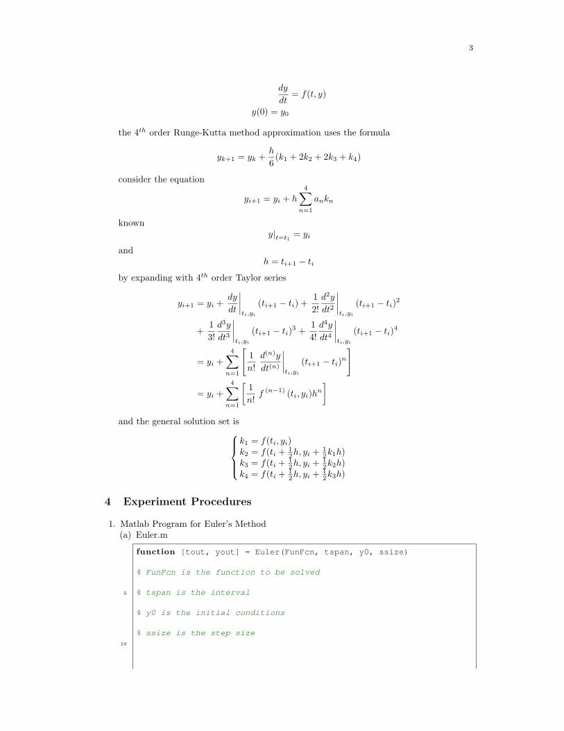
3.2 4th order Runge-Kutta method

for an problem with initial condition:

3

dy

dt= f(t, y)

y(0) = y0

the 4th order Runge-Kutta method approximation uses the formula

yk+1 = yk +h

6(k1 + 2k2 + 2k3 + k4)

consider the equation

yi+1 = yi + h4∑

n=1

ankn

knowny|t=t1

= yi

andh = ti+1 − ti

by expanding with 4th order Taylor series

yi+1 = yi +dy

dt

∣∣∣∣ti,yi

(ti+1 − ti) +1

2!

d2y

dt2

∣∣∣∣ti,yi

(ti+1 − ti)2

+1

3!

d3y

dt3

∣∣∣∣ti,yi

(ti+1 − ti)3 +

1

4!

d4y

dt4

∣∣∣∣ti,yi

(ti+1 − ti)4

= yi +4∑

n=1

[1

n!

d(n)y

dt(n)

∣∣∣∣ti,yi

(ti+1 − ti)n

]

= yi +4∑

n=1

[1

n!f (n−1) (ti, yi)h

n

]and the general solution set is

k1 = f(ti, yi)k2 = f(ti +

12h, yi +

12k1h)

k3 = f(ti +12h, yi +

12k2h)

k4 = f(ti +12h, yi +

12k3h)

4 Experiment Procedures

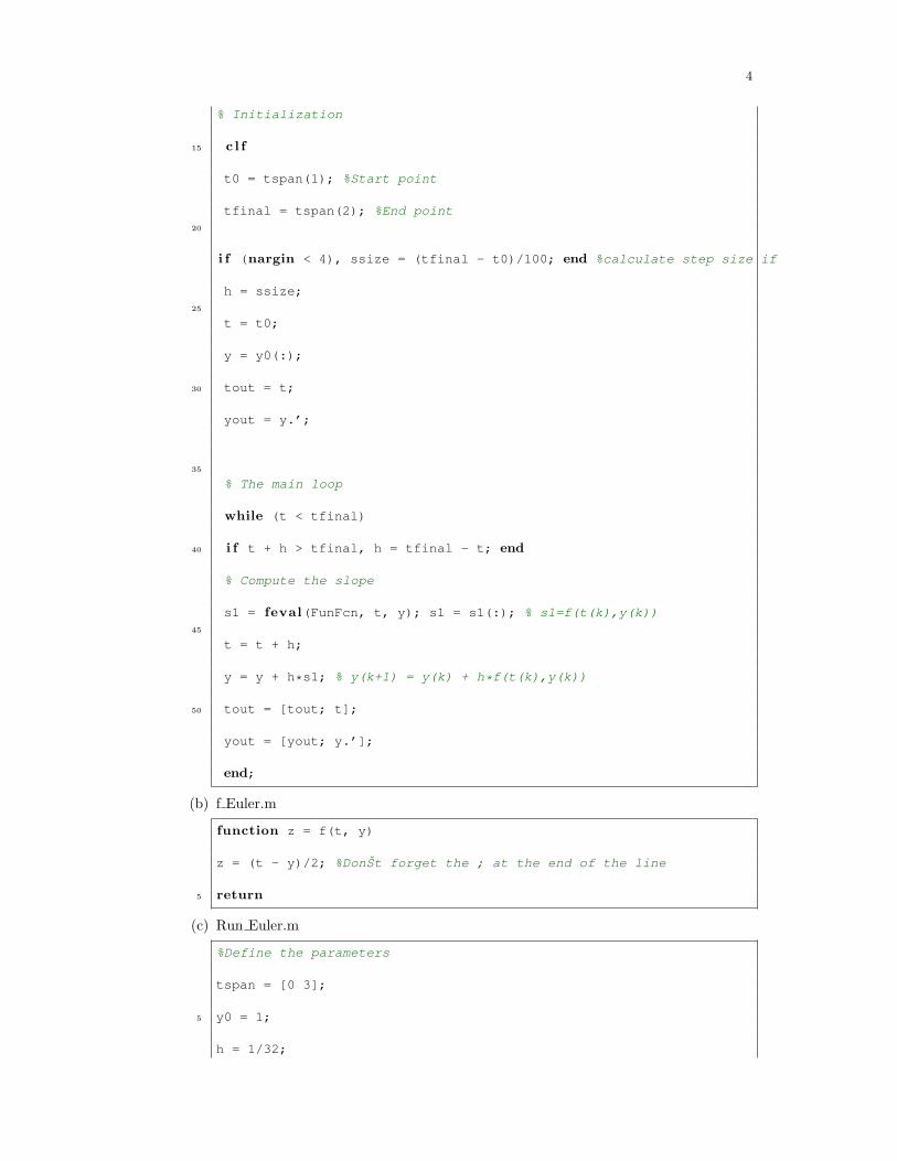
1. Matlab Program for Euler’s Method(a) Euler.m

function [tout, yout] = Euler(FunFcn, tspan, y0, ssize)

% FunFcn is the function to be solved

5 % tspan is the interval

% y0 is the initial conditions

% ssize is the step size10

4

% Initialization

15 c l f

t0 = tspan(1); %Start point

tfinal = tspan(2); %End point20

i f (nargin < 4), ssize = (tfinal - t0)/100; end %calculate step size if

h = ssize;25

t = t0;

y = y0(:);

30 tout = t;

yout = y.’;

35

% The main loop

while (t < tfinal)

40 i f t + h > tfinal, h = tfinal - t; end

% Compute the slope

s1 = feval(FunFcn, t, y); s1 = s1(:); % s1=f(t(k),y(k))45

t = t + h;

y = y + h*s1; % y(k+1) = y(k) + h*f(t(k),y(k))

50 tout = [tout; t];

yout = [yout; y.’];

end;

(b) f Euler.m

function z = f(t, y)

z = (t - y)/2; %DonŠt forget the ; at the end of the line

5 return

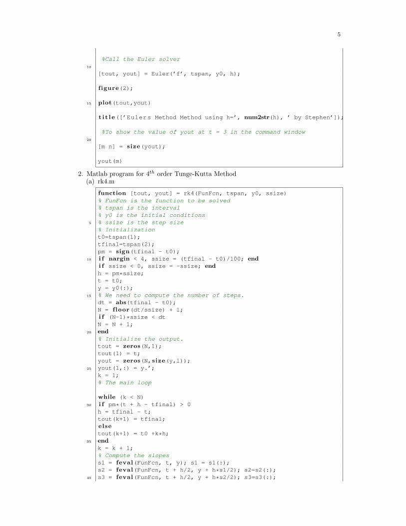
(c) Run Euler.m

%Define the parameters

tspan = [0 3];

5 y0 = 1;

h = 1/32;

5

%Call the Euler solver10

[tout, yout] = Euler(’f’, tspan, y0, h);

figure(2);

15 plot(tout,yout)

t i t l e([’Eulers Method Method using h=’, num2str(h), ’ by Stephen’]);

%To show the value of yout at t = 3 in the command window20

[m n] = size(yout);

yout(m)

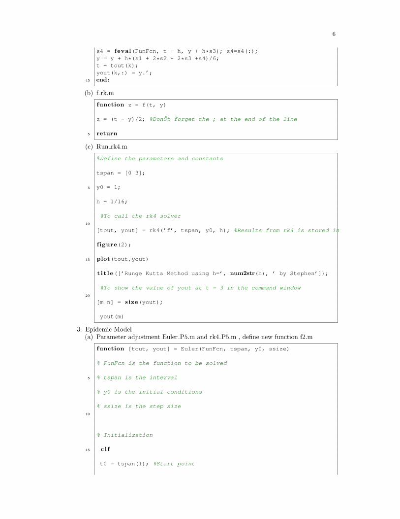
2. Matlab program for 4th order Tunge-Kutta Method(a) rk4.m

function [tout, yout] = rk4(FunFcn, tspan, y0, ssize)% FunFcn is the function to be solved% tspan is the interval% y0 is the initial conditions

5 % ssize is the step size% Initializationt0=tspan(1);tfinal=tspan(2);pm = sign(tfinal - t0);

10 i f nargin < 4, ssize = (tfinal - t0)/100; endi f ssize < 0, ssize = -ssize; endh = pm*ssize;t = t0;y = y0(:);

15 % We need to compute the number of steps.dt = abs(tfinal - t0);N = f loor(dt/ssize) + 1;i f (N-1)*ssize < dtN = N + 1;

20 end% Initialize the output.tout = zeros(N,1);tout(1) = t;yout = zeros(N,size(y,1));

25 yout(1,:) = y.’;k = 1;% The main loop

while (k < N)30 i f pm*(t + h - tfinal) > 0

h = tfinal - t;tout(k+1) = tfinal;elsetout(k+1) = t0 +k*h;

35 endk = k + 1;% Compute the slopess1 = feval(FunFcn, t, y); s1 = s1(:);s2 = feval(FunFcn, t + h/2, y + h*s1/2); s2=s2(:);

40 s3 = feval(FunFcn, t + h/2, y + h*s2/2); s3=s3(:);

6

s4 = feval(FunFcn, t + h, y + h*s3); s4=s4(:);y = y + h*(s1 + 2*s2 + 2*s3 +s4)/6;t = tout(k);yout(k,:) = y.’;

45 end;

(b) f rk.m

function z = f(t, y)

z = (t - y)/2; %DonŠt forget the ; at the end of the line

5 return

(c) Run rk4.m

%Define the parameters and constants

tspan = [0 3];

5 y0 = 1;

h = 1/16;

%To call the rk4 solver10

[tout, yout] = rk4(’f’, tspan, y0, h); %Results from rk4 is stored in

figure(2);

15 plot(tout,yout)

t i t l e([’Runge Kutta Method using h=’, num2str(h), ’ by Stephen’]);

%To show the value of yout at t = 3 in the command window20

[m n] = size(yout);

yout(m)

3. Epidemic Model(a) Parameter adjustment Euler P5.m and rk4 P5.m , define new function f2.m

function [tout, yout] = Euler(FunFcn, tspan, y0, ssize)

% FunFcn is the function to be solved

5 % tspan is the interval

% y0 is the initial conditions

% ssize is the step size10

% Initialization

15 c l f

t0 = tspan(1); %Start point

7

tfinal = tspan(2); %End point20

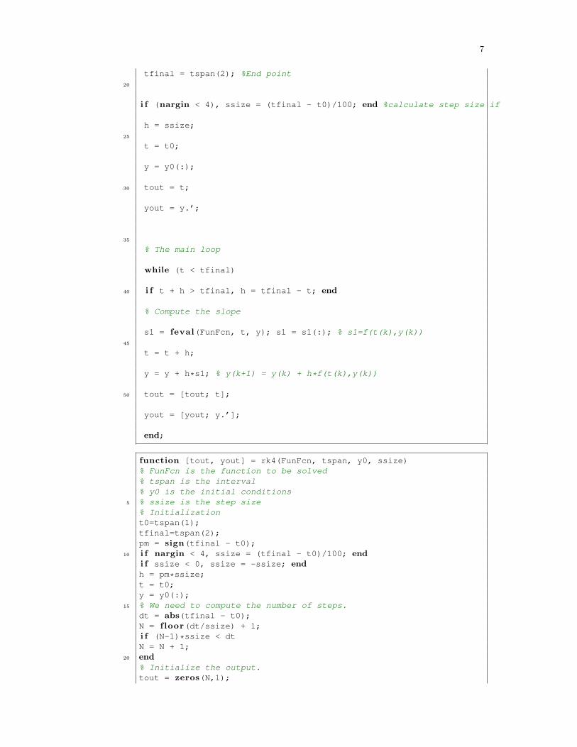
i f (nargin < 4), ssize = (tfinal - t0)/100; end %calculate step size if

h = ssize;25

t = t0;

y = y0(:);

30 tout = t;

yout = y.’;

35

% The main loop

while (t < tfinal)

40 i f t + h > tfinal, h = tfinal - t; end

% Compute the slope

s1 = feval(FunFcn, t, y); s1 = s1(:); % s1=f(t(k),y(k))45

t = t + h;

y = y + h*s1; % y(k+1) = y(k) + h*f(t(k),y(k))

50 tout = [tout; t];

yout = [yout; y.’];

end;

function [tout, yout] = rk4(FunFcn, tspan, y0, ssize)% FunFcn is the function to be solved% tspan is the interval% y0 is the initial conditions

5 % ssize is the step size% Initializationt0=tspan(1);tfinal=tspan(2);pm = sign(tfinal - t0);

10 i f nargin < 4, ssize = (tfinal - t0)/100; endi f ssize < 0, ssize = -ssize; endh = pm*ssize;t = t0;y = y0(:);

15 % We need to compute the number of steps.dt = abs(tfinal - t0);N = f loor(dt/ssize) + 1;i f (N-1)*ssize < dtN = N + 1;

20 end% Initialize the output.tout = zeros(N,1);

8

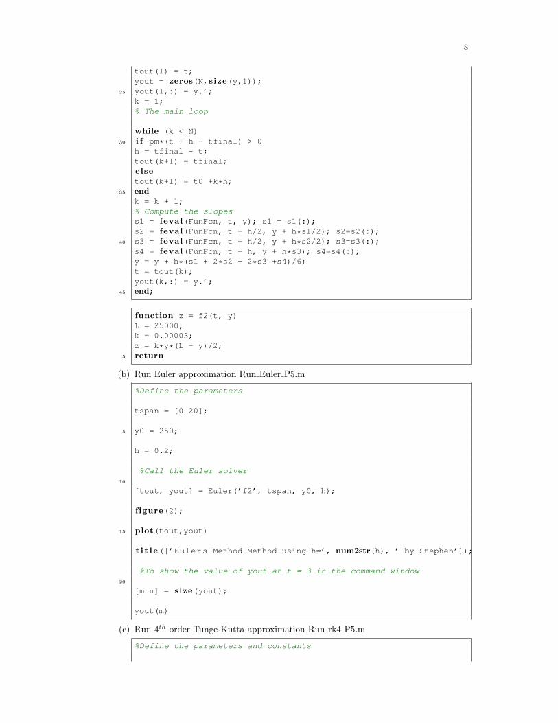
tout(1) = t;yout = zeros(N,size(y,1));

25 yout(1,:) = y.’;k = 1;% The main loop

while (k < N)30 i f pm*(t + h - tfinal) > 0

h = tfinal - t;tout(k+1) = tfinal;elsetout(k+1) = t0 +k*h;

35 endk = k + 1;% Compute the slopess1 = feval(FunFcn, t, y); s1 = s1(:);s2 = feval(FunFcn, t + h/2, y + h*s1/2); s2=s2(:);

40 s3 = feval(FunFcn, t + h/2, y + h*s2/2); s3=s3(:);s4 = feval(FunFcn, t + h, y + h*s3); s4=s4(:);y = y + h*(s1 + 2*s2 + 2*s3 +s4)/6;t = tout(k);yout(k,:) = y.’;

45 end;

function z = f2(t, y)L = 25000;k = 0.00003;z = k*y*(L - y)/2;

5 return

(b) Run Euler approximation Run Euler P5.m

%Define the parameters

tspan = [0 20];

5 y0 = 250;

h = 0.2;

%Call the Euler solver10

[tout, yout] = Euler(’f2’, tspan, y0, h);

figure(2);

15 plot(tout,yout)

t i t l e([’Eulers Method Method using h=’, num2str(h), ’ by Stephen’]);

%To show the value of yout at t = 3 in the command window20

[m n] = size(yout);

yout(m)

(c) Run 4th order Tunge-Kutta approximation Run rk4 P5.m

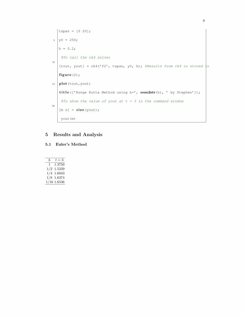
%Define the parameters and constants

9

tspan = [0 20];

5 y0 = 250;

h = 0.2;

%To call the rk4 solver10

[tout, yout] = rk4(’f2’, tspan, y0, h); %Results from rk4 is stored in

figure(2);

15 plot(tout,yout)

t i t l e([’Runge Kutta Method using h=’, num2str(h), ’ by Stephen’]);

%To show the value of yout at t = 3 in the command window20

[m n] = size(yout);

yout(m)

5 Results and Analysis

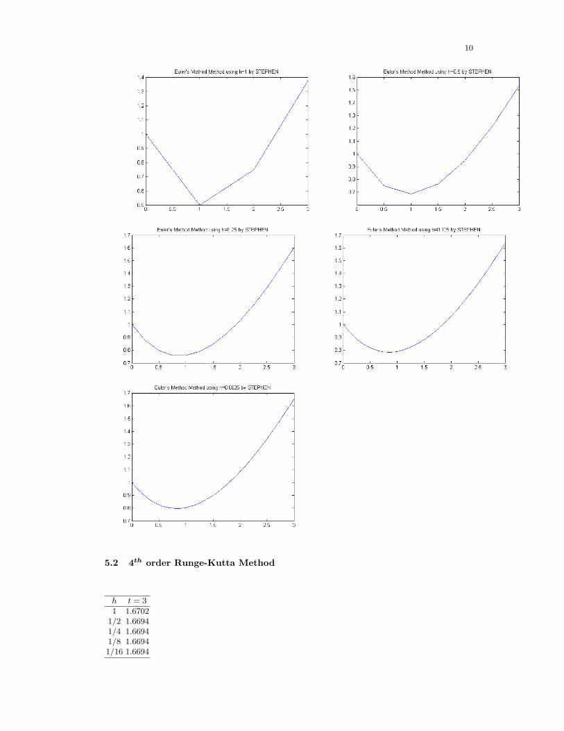
5.1 Euler’s Method

h t = 3

1 1.37501/2 1.53391/4 1.60431/8 1.63741/16 1.6536

10

5.2 4th order Runge-Kutta Method

h t = 3

1 1.67021/2 1.66941/4 1.66941/8 1.66941/16 1.6694

11

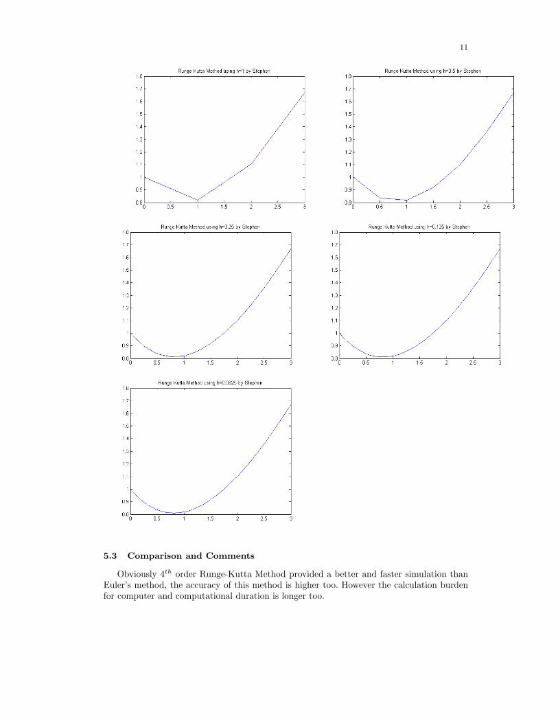
5.3 Comparison and Comments

Obviously 4th order Runge-Kutta Method provided a better and faster simulation thanEuler’s method, the accuracy of this method is higher too. However the calculation burdenfor computer and computational duration is longer too.

12

Euler’s Method 4th order Runge-Kutta Method

t = 20 2.3625× 104 2.3702× 104

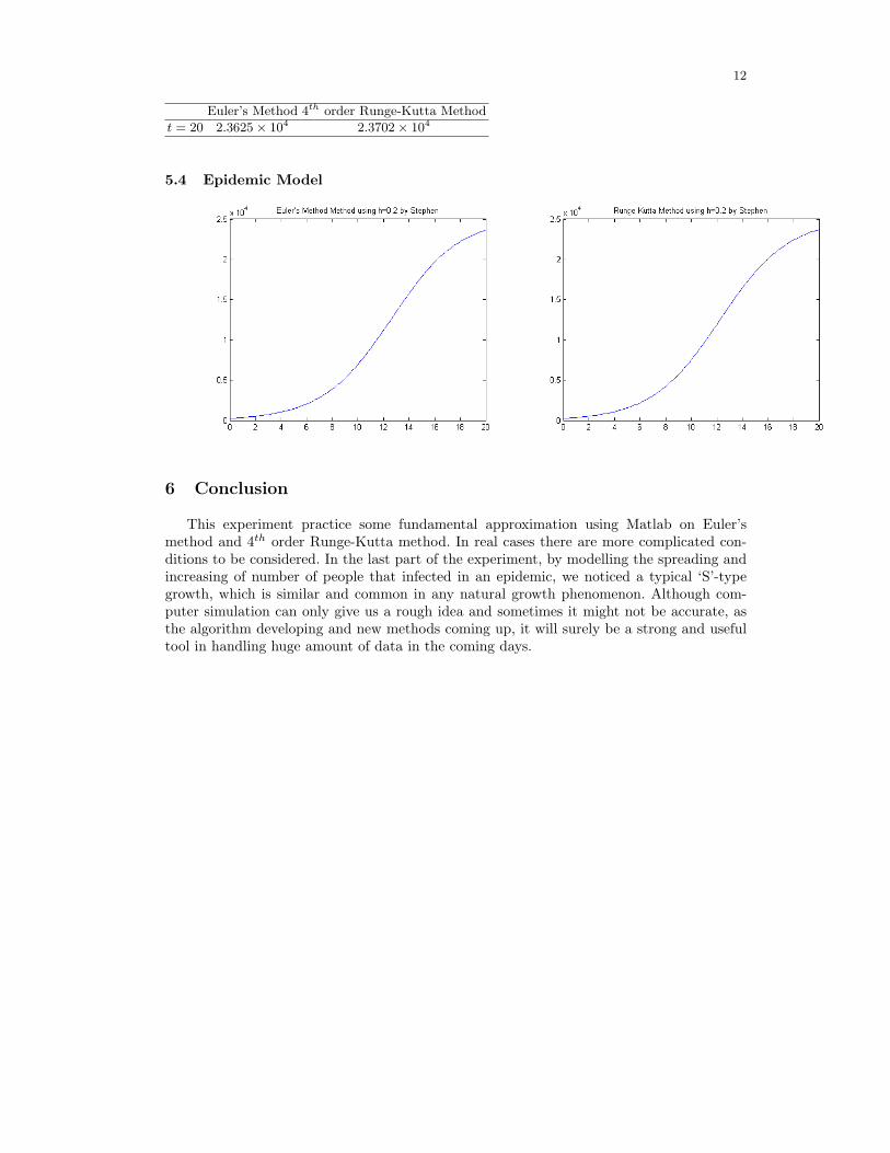
5.4 Epidemic Model

6 Conclusion

This experiment practice some fundamental approximation using Matlab on Euler’smethod and 4th order Runge-Kutta method. In real cases there are more complicated con-ditions to be considered. In the last part of the experiment, by modelling the spreading andincreasing of number of people that infected in an epidemic, we noticed a typical ‘S’-typegrowth, which is similar and common in any natural growth phenomenon. Although com-puter simulation can only give us a rough idea and sometimes it might not be accurate, asthe algorithm developing and new methods coming up, it will surely be a strong and usefultool in handling huge amount of data in the coming days.