Analysis of C-band spaceborne scatterometers thermal noise

Anis Elyouncha and Xavier Neyt

Royal Military Academy, 30 Av de la Renaissance, Brussels, Belgium

ABSTRACT

A scatterometer is a radar designed to measure the backscattering coefficient of distributed targets. In order to computethe backscatter from the received power, the scatterometermeasures also the thermal noise power. This noise signalis composed of two components, the receiver thermal noise and the viewed ground radiance. The first component isinstrument dependent and hence independent of the target and viewing geometry. The second component is target andviewing geometry dependent, it is proportional to the ground target brightness temperature. In this paper the noise signalmeasured by C-band scatterometers on-board ERS-2 and Metop-A satellites is analyzed. It was found that the noisesignal carries valuable geophysical information, which isworth to be exploited. It is shown that the noise signal variesspatially, temporally and with viewing geometry. Thus, different targets (ocean, sea ice, land) could be easily identified.A comparison was carried out between the scatterometer noise and AMSR-E radiometer brightness temperature and highcorrelation was found. The noise signal processing (mainlynoise subtraction) is discussed, including the assessmentofthe Noise Equivalent Sigma Zero and the Signal-to-noise ratio. This analysis leads to a better understanding of the noisesignal and its impact on the backscatter processing.

1. INTRODUCTION

The scatterometer is a real aperture radar designed to measure the backscattering coefficient of distributed targets. Thebackscattering coefficient or the backscatter is also called sigma naught and is referred to asσ0. The measurementradiometric accuracy is one of the main concerns in the scatterometer design. The received signal is corrupted by additivenoise. Thus, in order to determine the backscattering-onlycontribution to the total power and to increase the measurementaccuracy, the scatterometer performs a measure of the noiseonly signal. C-band scatterometers measuring the noise workas microwave radiometers. The power of that noise signal is subtracted from the echo+noise-signal power measurementin order to get the echo-only power signal

Ps = Ps+n −Pn (1)

wherePs+n is the signal+noise power,Pn is the noise power andPs is the signal only power.

In this paper the scatterometer noise signalPn is analyzed. In fact, the scatterometer noise signal is a superpositionof two components, the instrument noise (receiver thermal noise) and an external noise collected by the antenna (Earthradiance). The two components add in power or in noise temperature as

Pn = Pnr +Pna = KB(Tr +Ta) (2)

WherePn is the measured noise power,K is the Boltzmann constant,Tr andTa are the receiver and the antenna noisetemperatures respectively andB is the receiver bandwidth for the noise measurement. In thispaper, the analysis is basedon the C-band fan-beam scatteromters processing scheme. The results shown along this paper are from ERS-2/AMI andMetop-A/ASCAT data. Since ERS-1/AMI and ERS-2/AMI (and similarly Metop-A/ASCAT and Metop-B/ASCAT) areidentical radars and processors, the analysis applies to all these scatterometers.

AMI and ASCAT are both real aperture C-band side looking radars using fixed fan-beam vertically polarized antennas.AMI uses three antennas called fore, mid and aft separated by45 degrees in azimuth. The mid beam is looking in across-track direction. ASCAT has the same configuration with an additional swath (three other antennas) looking to the leftside. In addition, ASCAT swath is shifted by about 8 degrees away from the nadir compared to AMI swath.

The receiver noise temperature depends on the receiver noise figure (NF) which is usually higher or equal than 3dB. HenceTr is usually higher (≥300 K) than the antenna noise temperature (TA ≤300 K). However, along the orbit, thereceiver noise temperature is assumed to be constant (independent of target) and the antenna noise temperature variesdepending on the viewed target. This variation is detected in the scatterometer noise signal.

Further author information: (Send correspondence to Anis Elyouncha) E-mail: anis.elyouncha@elec.rma.ac.be, Telephone: +32 2742 6665

2. NOISE PROCESSING OVERVIEW

For ERS scatterometers,1, 2 32 short pulses are transmitted each antenna cycle (fore-mid-aft) and the noise is measuredon 28 pulses out of the 32. The noise signal is measured in a 1.03 ms echo-free time window, filtered and sampled at 30kHz rate which yields 32 samples in each window. Additionally, the 28 along-track pulses of measured noise signal areaveraged together. In total, 32×28= 896 samples are averaged in the on-board processing.2–4 The 896 noise samplesin form of I andQ are squared by the on-board instrument and telemetered to the ground. On-ground, theI2 andQ2

averages are added to derive the noise power estimate. Furthermore, 21 along-track noise power samples are averagedby the ground-processor using a Gaussian weighting function.3 The final averaged noise power is subtracted from thereceived signal+noise power.

For Metop scatterometers,5, 6 one long pulse is transmitted each antenna cycle. The noise signal is measured in a 1.24ms echo-free time window, filtered and sampled at 412.5 kHz rate which yields 512 samples in each window. First, thenoise samples are windowed using a Tukey window and then the power spectrum density is estimated. Furthermore, thepower spectral densities of 40 antenna cycles are averaged along-track. The resulting noise power spectrum is transmittedto the ground. On-ground, the noise power spectrum is corrected by the receiver filter shape which is also estimated fromthe noise signal as is explained later. The noise power spectrum is averaged in range over a selected frequencies to derivethe average noise power.7 Finally, the average noise power is used to correct (noise subtraction) the echo power signal.

3. NOISE SIGNAL CHARACTERIZATION

3.1. Spatial distribution

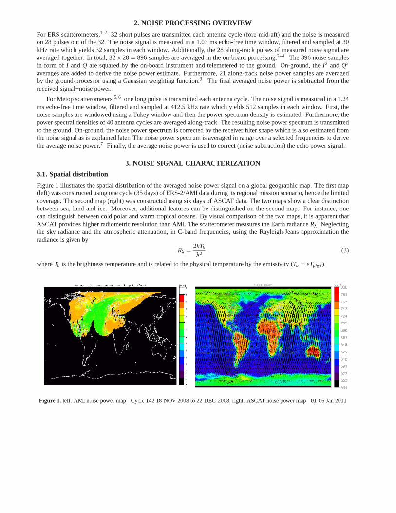
Figure 1 illustrates the spatial distribution of the averaged noise power signal on a global geographic map. The first map(left) was constructed using one cycle (35 days) of ERS-2/AMI data during its regional mission scenario, hence the limitedcoverage. The second map (right) was constructed using six days of ASCAT data. The two maps show a clear distinctionbetween sea, land and ice. Moreover, additional features can be distinguished on the second map. For instance, onecan distinguish between cold polar and warm tropical oceans. By visual comparison of the two maps, it is apparent thatASCAT provides higher radiometric resolution than AMI. Thescatterometer measures the Earth radianceRλ. Neglectingthe sky radiance and the atmospheric attenuation, in C-bandfrequencies, using the Rayleigh-Jeans approximation theradiance is given by

Rλ =2kTb

λ2 . (3)

whereTb is the brightness temperature and is related to the physicaltemperature by the emissivity (Tb = eTphys).

Figure 1. left: AMI noise power map - Cycle 142 18-NOV-2008 to 22-DEC-2008, right: ASCAT noise power map - 01-06 Jan 2011

3.2. Spatial resolution

In this section, we examine the spatial resolution of the noise power signal. The noise power signal is the result of theconvolution of the radar antenna pattern with the brightness temperature of the surface integrated over the bandwidth ofthe receiver. Moreover, in the nominal products the signal is convolved with a Hamming window. The spatial resolutionis examined using land-sea transition (coastline). At the coastlines, a contrast in radiance can be expected. This thusprovides the step function of the observing system, from which the resolution can be deduced.

Unlike the scanning pencil beam scatterometers (e.g., SeaWinds)8 and radiometers (e.g., AMSR-E)9 which havesmall footprints, ASCAT and AMI are fixed fan-beam radars. They have large antenna footprints in range (≈ 500 km)and narrow footprints in azimuth (≈ 30 km). Note, that for instance AMSR-E radiometer provides aspatial resolution of74×43 km and SeaWinds antenna footprint is approximately 37×52 km.

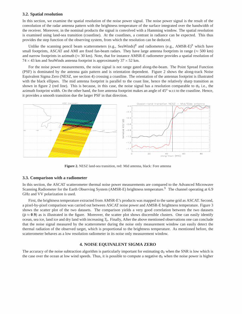
For the noise power measurements, the noise signal is not range gated along-the-beam. The Point Spread Function(PSF) is dominated by the antenna gain pattern and is orientation dependent. Figure 2 shows the along-track NoiseEquivalent Sigma Zero (NESZ, see section 4) crossing a coastline. The orientation of the antennas footprint is illustratedwith the black ellipses. The mid antenna footprint is parallel to the coast line, hence the relatively sharp transition asshown in figure 2 (red line). This is because, in this case, thenoise signal has a resolution comparable toσ0 i.e., theazimuth footprint width. On the other hand, the fore antennafootprint makes an angle of 45o w.r.t to the coastline. Hence,it provides a smooth transition due the larger PSF in that direction.

Figure 2. NESZ land-sea transition, red: Mid antenna, black: Fore antenna

3.3. Comparison with a radiometer

In this section, the ASCAT scatterometer thermal noise power measurements are compared to the Advanced MicrowaveScanning Radiometer for the Earth Observing System (AMSR-E) brightness temperature.9 The channel operating at 6.9GHz and VV polarization is used.

First, the brightness temperature extracted from AMSR-E’sproducts was mapped to the same grid as ASCAT. Second,a pixel-by-pixel comparison was carried out between ASCAT noise power and AMSR-E brightness temperature. Figure 3shows the scatter plot of the two datasets. The comparison yields a very good correlation between the two datasets(ρ ≈ 0.9) as is illustrated in the figure. Moreover, the scatter plot shows discernible clusters. One can easily identifyocean, sea ice, land ice and dry land with increasingTb. Finally, After the above mentioned observations one can concludethat the noise signal measured by the scatterometer during the noise only measurement window can easily detect thethermal radiation of the observed target, which is proportional to the brightness temperature. As mentioned before, thescatterometer behaves as a low resolution radiometer in itsnoise only measurement window.

4. NOISE EQUIVALENT SIGMA ZERO

The accuracy of the noise subtraction algorithm is particularly important for estimatingσ0 when the SNR is low which isthe case over the ocean at low wind speeds. Thus, it is possible to compute a negativeσ0 when the noise power is higher

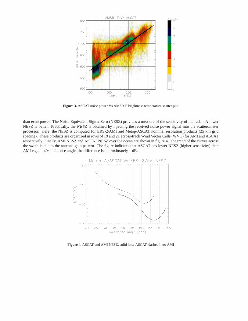
Figure 3. ASCAT noise power Vs AMSR-E brightness temperature scatter plot

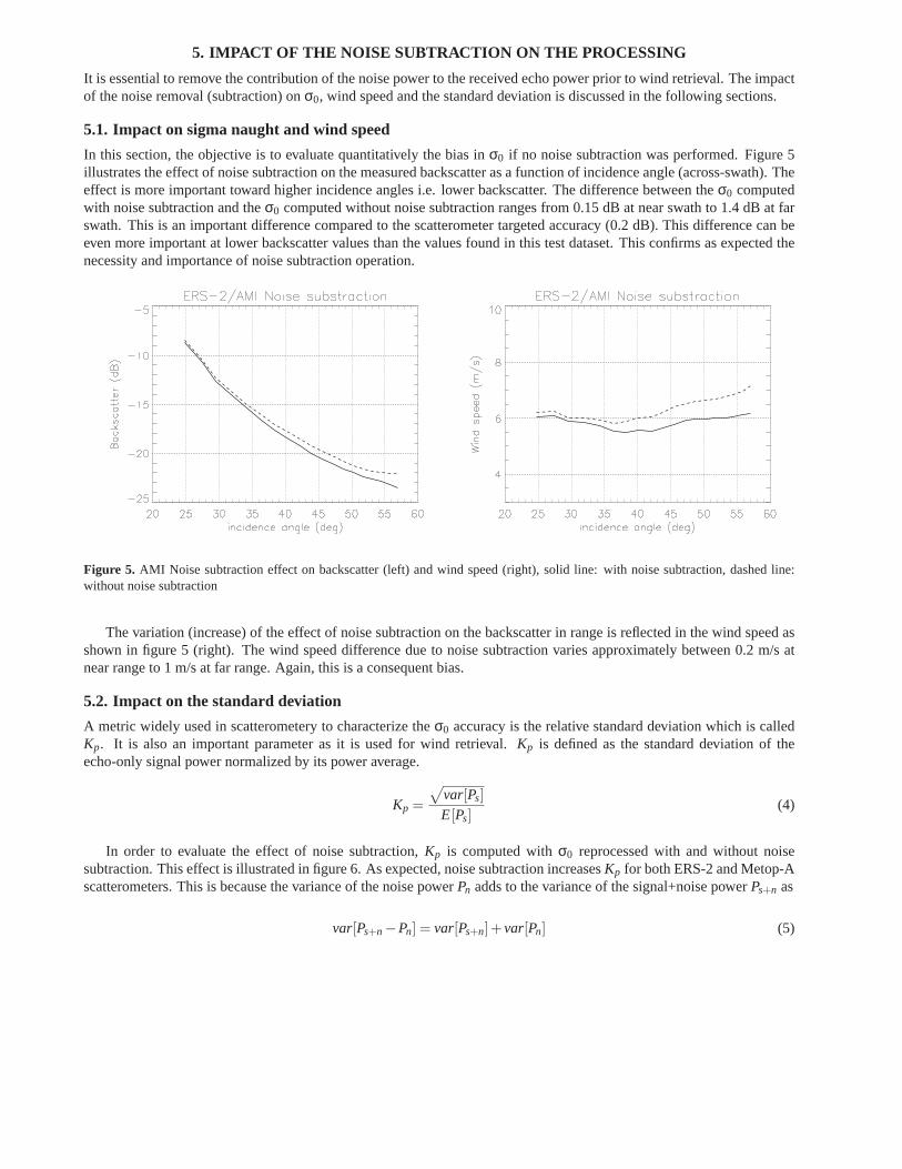
than echo power. The Noise Equivalent Sigma Zero (NESZ) provides a measure of the sensitivity of the radar. A lowerNESZ is better. Practically, theNESZ is obtained by injecting the received noise power signal into the scatterometerprocessor. Here, the NESZ is computed for ERS-2/AMI and Metop/ASCAT nominal resolution products (25 km gridspacing). These products are organized in rows of 19 and 21 across-track Wind Vector Cells (WVC) for AMI and ASCATrespectively. Finally, AMI NESZ and ASCAT NESZ over the ocean are shown in figure 4. The trend of the curves acrossthe swath is due to the antenna gain pattern. The figure indicates that ASCAT has lower NESZ (higher sensitivity) thanAMI e.g., at 40o incidence angle, the difference is approximately 1 dB.

Figure 4. ASCAT and AMI NESZ, solid line: ASCAT, dashed line: AMI

5. IMPACT OF THE NOISE SUBTRACTION ON THE PROCESSING

It is essential to remove the contribution of the noise powerto the received echo power prior to wind retrieval. The impactof the noise removal (subtraction) onσ0, wind speed and the standard deviation is discussed in the following sections.

5.1. Impact on sigma naught and wind speed

In this section, the objective is to evaluate quantitatively the bias inσ0 if no noise subtraction was performed. Figure 5illustrates the effect of noise subtraction on the measuredbackscatter as a function of incidence angle (across-swath). Theeffect is more important toward higher incidence angles i.e. lower backscatter. The difference between theσ0 computedwith noise subtraction and theσ0 computed without noise subtraction ranges from 0.15 dB at near swath to 1.4 dB at farswath. This is an important difference compared to the scatterometer targeted accuracy (0.2 dB). This difference can beeven more important at lower backscatter values than the values found in this test dataset. This confirms as expected thenecessity and importance of noise subtraction operation.

Figure 5. AMI Noise subtraction effect on backscatter (left) and wind speed (right), solid line: with noise subtraction, dashed line:without noise subtraction

The variation (increase) of the effect of noise subtractionon the backscatter in range is reflected in the wind speed asshown in figure 5 (right). The wind speed difference due to noise subtraction varies approximately between 0.2 m/s atnear range to 1 m/s at far range. Again, this is a consequent bias.

5.2. Impact on the standard deviation

A metric widely used in scatterometery to characterize theσ0 accuracy is the relative standard deviation which is calledKp. It is also an important parameter as it is used for wind retrieval. Kp is defined as the standard deviation of theecho-only signal power normalized by its power average.

Kp =

√

var[Ps]

E[Ps](4)

In order to evaluate the effect of noise subtraction,Kp is computed withσ0 reprocessed with and without noisesubtraction. This effect is illustrated in figure 6. As expected, noise subtraction increasesKp for both ERS-2 and Metop-Ascatterometers. This is because the variance of the noise power Pn adds to the variance of the signal+noise powerPs+n as

var[Ps+n −Pn] = var[Ps+n]+ var[Pn] (5)

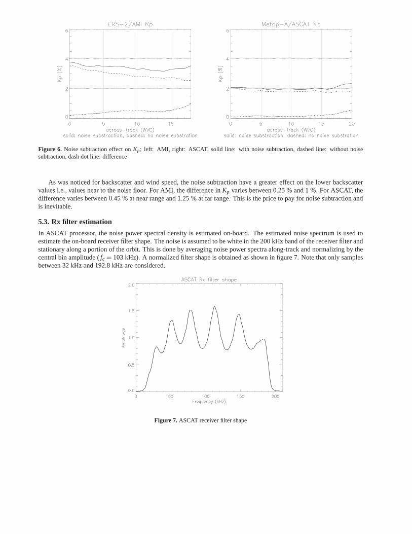
Figure 6. Noise subtraction effect onKp; left: AMI, right: ASCAT; solid line: with noise subtraction, dashed line: without noisesubtraction, dash dot line: difference

As was noticed for backscatter and wind speed, the noise subtraction have a greater effect on the lower backscattervalues i.e., values near to the noise floor. For AMI, the difference inKp varies between 0.25 % and 1 %. For ASCAT, thedifference varies between 0.45 % at near range and 1.25 % at far range. This is the price to pay for noise subtraction andis inevitable.

5.3. Rx filter estimation

In ASCAT processor, the noise power spectral density is estimated on-board. The estimated noise spectrum is used toestimate the on-board receiver filter shape. The noise is assumed to be white in the 200 kHz band of the receiver filter andstationary along a portion of the orbit. This is done by averaging noise power spectra along-track and normalizing by thecentral bin amplitude (fc = 103 kHz). A normalized filter shape is obtained as shown in figure 7. Note that only samplesbetween 32 kHz and 192.8 kHz are considered.

Figure 7. ASCAT receiver filter shape

The noise power depends on the viewed surface properties which might change. The noise signal variation shownearlier can have an impact on the filter processing. Actually, it was found that the receiver filter shape varies with timeand space10 and this variation is not random. Therefore, the variation of the noise power along the orbit could explainthe variation of the estimated filter shape. Moreover, the estimated filterhrx is used to correct the received echo powerspectrumPs+n (signal+noise) for the filter ripples (before noise subtraction) as follows7

Pc( f ) = Ps+n( f )/hrx( f )−Pn (6)

wherePc is the corrected power,Ps+n is the received power andhrx is the filter amplitude.Pn is the estimated noise power,which is also corrected for the filter ripples and averaged over a given frequency range. Therefore, variation of the filtercan affect directly the power and consequently theσ0. This needs further investigation to evaluate the exact impact of thefilter variation onσ0.

6. EFFECT OF THE VIEWING GEOMETRY

The scatterometer noise signal (Earth radiance component)is weighted by the antenna radiation pattern and amplified bythe receiver gain as follows

Ta = Gr

R R

G(θ,φ)Tb(θ,φ)dθdφR R

G(θ,φ)dθdφ(7)

WhereTa andTb are the antenna noise temperature and the target brightnesstemperature respectively andGr is the receivergain.

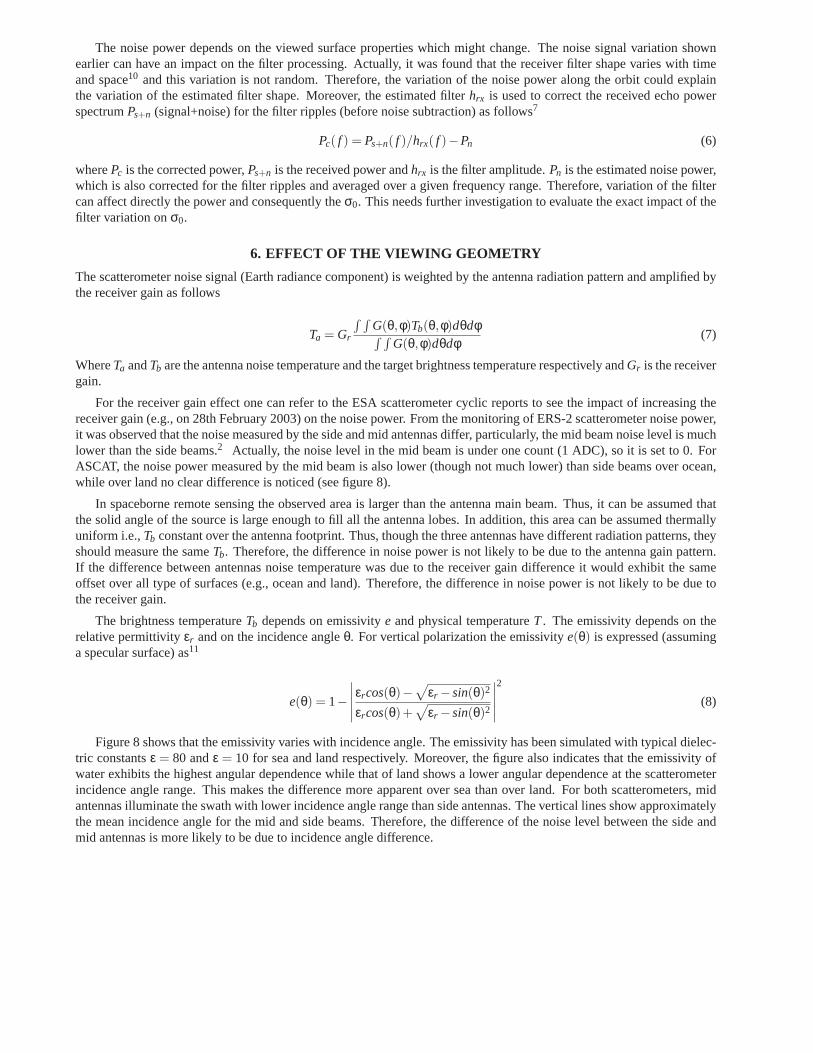
For the receiver gain effect one can refer to the ESA scatterometer cyclic reports to see the impact of increasing thereceiver gain (e.g., on 28th February 2003) on the noise power. From the monitoring of ERS-2 scatterometer noise power,it was observed that the noise measured by the side and mid antennas differ, particularly, the mid beam noise level is muchlower than the side beams.2 Actually, the noise level in the mid beam is under one count (1ADC), so it is set to 0. ForASCAT, the noise power measured by the mid beam is also lower (though not much lower) than side beams over ocean,while over land no clear difference is noticed (see figure 8).

In spaceborne remote sensing the observed area is larger than the antenna main beam. Thus, it can be assumed thatthe solid angle of the source is large enough to fill all the antenna lobes. In addition, this area can be assumed thermallyuniform i.e.,Tb constant over the antenna footprint. Thus, though the threeantennas have different radiation patterns, theyshould measure the sameTb. Therefore, the difference in noise power is not likely to bedue to the antenna gain pattern.If the difference between antennas noise temperature was due to the receiver gain difference it would exhibit the sameoffset over all type of surfaces (e.g., ocean and land). Therefore, the difference in noise power is not likely to be due tothe receiver gain.

The brightness temperatureTb depends on emissivitye and physical temperatureT . The emissivity depends on therelative permittivityεr and on the incidence angleθ. For vertical polarization the emissivitye(θ) is expressed (assuminga specular surface) as11

e(θ) = 1−

∣

∣

∣

∣

∣

εrcos(θ)−√

εr − sin(θ)2

εrcos(θ)+√

εr − sin(θ)2

∣

∣

∣

∣

∣

2

(8)

Figure 8 shows that the emissivity varies with incidence angle. The emissivity has been simulated with typical dielec-tric constantsε = 80 andε = 10 for sea and land respectively. Moreover, the figure also indicates that the emissivity ofwater exhibits the highest angular dependence while that ofland shows a lower angular dependence at the scatterometerincidence angle range. This makes the difference more apparent over sea than over land. For both scatterometers, midantennas illuminate the swath with lower incidence angle range than side antennas. The vertical lines show approximatelythe mean incidence angle for the mid and side beams. Therefore, the difference of the noise level between the side andmid antennas is more likely to be due to incidence angle difference.

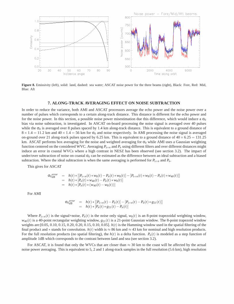
Figure 8. Emissivity (left), solid: land, dashed: sea water; ASCAT noise power for the three beams (right), Black: Fore, Red: Mid,Blue: Aft

7. ALONG-TRACK AVERAGING EFFECT ON NOISE SUBTRACTION

In order to reduce the variance, both AMI and ASCAT processors average the echo power and the noise power over anumber of pulses which corresponds to a certain along-trackdistance. This distance is different for the echo power andfor the noise power. In this section, a possible noise power misestimation due this difference, which would induce aσ0

bias via noise subtraction, is investigated. In ASCAT on-board processing the noise signal is averaged over 40 pulseswhile theσ0 is averaged over 8 pulses spaced by 1.4 km along-track distance. This is equivalent to a ground distance of8×1.4 = 11.2 km and 40×1.4 = 56 km forσ0 and noise respectively. In AMI processing the noise signal is averagedon-ground over 21 along-track pulses spaced by 6.25 km. Thisis equivalent to a ground distance of 40×6.25= 131.25km. ASCAT performs box averaging for the noise and weighted averaging forσ0 while AMI uses a Gaussian weightingfunction centered on the considered WVC. AveragingPs+n andPn using different filters and over different distances mightinduce an error in coastal WVCs where a high contrast in NESZ has been observed (see section 3.2). The impact ofunder/over subtraction of noise on coastalσ0 can be estimated as the difference between an ideal subtraction and a biasedsubtraction. Where the ideal subtraction is when the same averaging is performed forPs+n andPn.

This gives for ASCAT

σ0errordB = h(t)∗ [[Ps+n(t)∗w8(t)−Pn(t)∗w8(t)]− [Ps+n(t)∗w8(t)−Pn(t)∗w40(t)]]

= h(t)∗ [Pn(t)∗w40(t)−Pn(t)∗w8(t)]= h(t)∗ [Pn(t)∗ (w40(t)−w8(t))]

For AMI

σ0errordB = h(t)∗ [[Ps+n(t)−Pn(t)]− [Ps+n(t)−Pn(t)∗g21(t)]]

= h(t)∗ [Pn(t)∗g21(t)−Pn(t)]

WherePs+n(t) is the signal+noise,Pn(t) is the noise only signal,w8(t) is an 8-point trapezoidal weighting window,w40(t) is a 40-point rectangular weighting window,g21(t) is a 21-point Gaussian window. The 8-point trapezoid windowweights are:[0.05, 0.10, 0.15, 0.20, 0.20, 0.15, 0.10, 0.05]. h(t) is the Hamming window used in the spatial filtering of thefinal product and∗ stands for convolution.h(t) width is≈ 86 km and≈ 43 km for nominal and high resolution products.For the full resolution products (no spatial filtering), theh(t) is a delta function.Pn(t) is modeled as a step function ofamplitude 1dB which corresponds to the contrast between land and sea (see section 3.2).

For ASCAT, it is found that only the WVCs that are closer than≈ 30 km to the coast will be affected by the actualnoise power averaging. This is equivalent to 5, 2 and 1 along-track samples in the full resolution (5.6 km), high resolution

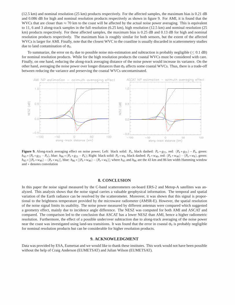
(12.5 km) and nominal resolution (25 km) products respectively. For the affected samples, the maximum bias is 0.21 dBand 0.086 dB for high and nominal resolution products respectively as shown in figure 9. For AMI, it is found that theWVCs that are closer than≈ 70 km to the coast will be affected by the actual noise power averaging. This is equivalentto 11, 6 and 3 along-track samples in the full resolution (6.25 km), high resolution (12.5 km) and nominal resolution (25km) products respectively. For these affected samples, themaximum bias is 0.25 dB and 0.13 dB for high and nominalresolution products respectively. The maximum bias is roughly similar for both sensors, but the extent of the affectedWVCs is larger for AMI. Finally, note that the closest WVC to thecoastline is usually discarded in scatterometery studiesdue to land contamination ofσ0.

To summarize, the error onσ0 due to possible noise mis-estimation and subtraction is probably negligible (≤ 0.1 dB)for nominal resolution products. While for the high resolution products the coastal WVCs must be considered with care.Finally, on one hand, reducing the along-track averaging distance of the noise power would increase its variance. On theother hand, averaging the noise power over longer distancesthanσ0 affects some coastal WVCs. Thus, there is a trade-offbetween reducing the variance and preserving the coastal WVCs uncontaminated.

Figure 9. Along-track averaging effect on noise power; Left: black solid:Pn, black dashed:Pn ∗ g21, red: (Pn ∗ g21)−Pn, green:h43∗ (Pn ∗g21−Pn), blue: h86∗ (Pn ∗g21−Pn); Right: black solid:Pn ∗w8, black dashed:Pn ∗w40, red: (Pn ∗w40)− (Pn ∗w8), green:h43∗ [(Pn ∗w40)− (Pn ∗w8)], blue:h86∗ [(Pn ∗w40)− (Pn ∗w8)]; whereh43 andh86 are the 43 km and 86 km width Hamming windowand∗ denotes convolution

8. CONCLUSION

In this paper the noise signal measured by the C-band scatterometers on-board ERS-2 and Metop-A satellites was an-alyzed. This analysis shows that the noise signal carries a valuable geophysical information. The temporal and spatialvariation of the Earth radiance can be resolved by the scatterometer. Moreover, it was shown that this signal is propor-tional to the brightness temperature provided by the microwave radiometer (AMSR-E). However, the spatial resolutionof the noise signal limits its usability. The noise power measured by different antennas were compared which suggesteda geometry effect, mainly due to incidence angle difference. The NESZ was computed for both AMI and ASCAT andcompared. The comparison led to the conclusion that ASCAT has a lower NESZ than AMI, hence a higher radiometricresolution. Furthermore, the effect of a possible under/over subtraction due to along-track averaging of the noise powernear the coast was investigated using land-sea transitions. It was found that the error in coastalσ0 is probably negligiblefor nominal resolution products but can be considerable forhigher resolution products.

9. ACKNOWLEDGMENT

Data was provided by ESA, Eumetsat and we would like to thank these institutes. This work would not have been possiblewithout the help of Craig Anderson (EUMETSAT) and Julian Wilson (EUMETSAT).

REFERENCES

1. Evert P.W. Attema. The active microwave instrument on-board the ERS-1 satellite. InProceedings of the IEEE,volume 79, pages 791–799, June 1991.

2. P. Lecomte. The ERS scatterometer instrument and the on-ground processing of its data. InProc. of a JointESA-Eumetsat Workshop on Emerging Scatterometer Applications, pages 241–260, Noordwijk, The Netherlands,November 1998.

3. X. Neyt, P. Pettiaux, M. D. Smet, and M.Acheroy. Scatterometer algorithm review for gyro-less operation. TechnicalReport RMA-SIC-011109, Royal Military Academy, December 2001.

4. P. Pettiaux, X. Neyt, and M. Acheroy. Validation of the ERS-2 scatterometer ground processor upgrade. InProceed-ings of the SPIE: Remote Sensing of the Ocean, Sea Ice, and Large Water Regions, Crete, Greece, volume 4880,September 2002.

5. J. Figa-Saldaa, J.J.W. Wilson, E. Attema, R. Gelsthorpe,M.R. Drinkwater, and A. Stoffelen. The advanced scat-terometer (ASCAT) on the meteorological operational (METOP) platform: A follow on for european wind scat-terometers.Can. J. Remote Sensing, 28(3):404412, 2002.

6. X. Neyt, N. Manise, and M. Acheroy. Analysis of the impact of ASCAT’s pulse compression. InProceedings of theSPIE: Remote Sensing of the Ocean, Sea Ice, and Large Water Regions, volume 6360, September 2006.

7. J. Wilson and J. Figa-Saldana. ASCAT product generation function specification. Technical ReportEUM.EPS.SYS.SPE.990009, EUMETSAT, Darmstadt, 2002.

8. M. W. Spencer C. Wu and David G. Long. Tradeoffs in the design of a spaceborne scanning pencil beam scatterom-eter: Application to Seawinds.IEEE Transactions on Geoscience and Remote Sensing, 35(1):115–126, January1997.

9. T. Kawanishi, T. Sezai, Y. Ito, K. Imaoka, T. Takeshima, Y.Ishido, A. Shibata, M. Miura, H. Inahata, and R. W.Spencer. The advanced microwave scanning radiometer for the earth observing system (AMSR-E), nasda’s contri-bution to the EOS for global energy and water cycle studies.IEEE Transactions on Geoscience and Remote Sensing,41(2):184–194, February 2003.

10. J. Figa-Saldana and C. Anderson. ASCAT-B level 1 commissioning report. Technical ReportEUM/OPS/DOC/12/3436, EUMETSAT, Darmstadt, 2013.

11. F. T. Ulaby, R. K. Moore, and A. K. Fung.Microwave remote sensing : active and passive. 2. , Radar remote sensingand surface scattering and emission theory. Remote senging. Artech house, London, 1986.