1231 TRANSPORTATION RESEARCH RECORD

Analysis, Design, and Behavior of Underground Culverts

TRANSPORTATION RESEARCH BOARD NATIONAL RESEARCH COUNCIL

WASHINGTON, D.C. 1989

Transportation Research Record 1231 Price: $15.50

mode 1 highway transportation

subject areas 25 structures design and performance 62 soil foundations 63 soil and rock mechanics

TRB Publications Slaff

Director of Publications: Nancy A. Ackerman Senior Editor: Edythe T. Crump Associate Editors: Naomi C. Kassabian

Ruth S. Pitt Alison G. Tobias

Production Edi/or: Kieran P. O'Leary Graphics Coordinalor: Karen L. White on1ce Ma1111ger: Phyllis D. Barber J>roduc1ion Assista111: Betty L. Hawkins

Printed in the United States of America

Lihrary of ongress Cataloging-in-Publication Data Nn1ional Research Council. Transponation R1.:sc<1rch Board.

Analysis , design, and hchavior of undergrou nd culverts. p. cm.-(Transp riation research record, ISSN 0361-1981;

1231) ISBN 0-309-04824-9 l. Culverts-Design and construction. 2. Drainage pipes­

Design and con !ruction . 3. -anh pressure. I. National Research 'ouncil (U ., .). Transponntion Research Board. II. Series. TE7.H5 no. 1231 (TE213] 388 s-dc20 [625.7'342] 90-33351

CIP

Sponsorship of Transportation Research Record 1231

GROUP 2-DESIGN AND CONSTRUCTION OF TRANSPORTATION FACILITIES Chairman: Raymond A. Forsy1h, California Depal'llnent uf

Transportation

Structures Section Chairman: John M. Hanson, Wiss Janney Elstner Associates, Inc.

Committee on Culverts and Hydraulic Structures Chairman: L. R. Lawrence, Federal Highway Administration Gordon A. Ali. 011, Jr1111us D. Amo11/1, A. £. fl11dw1·. Ke1111e1/i J. Boedecker. Jr., Tlwm<LI' K. Breitft1ss. De1111is L.. 81111kc. /Jemard E. Butler, Jw11es £. owgill William D. Drake. J. M. D11nc1111. James 8. Goddard. James J. /:fill. l e• K. Joy11p(l/111i, f/'//j I. Kaspar. Michael G. Katona, Timothy J. M 1ratli, A. P. Moser, John C. Pouer, Russell B. Preuit, Jr., llarold R. Sandberg, James C. Scl1lt11er, David C. Thomas, Corwin L. Tracy, Robert P. Walker, Jr.

Soil Mechanics Section Chairman: Michael C. Katona, TRW

Committee on Subsurface Soil-Str11c1ure Interaction Chairman: J. M. DunG'flll, Virginia Poly1echnic lnstilute and Stale

U11ivel' ·i1y ,t•orge Abdel-Sayed, Baidar Brtklit, Sa11gd111l 8Qng. Ti111otlty J.

Bea("h. Miki· Be"ll:y. C. •. Desai. Les1er II. abricl. James fl. Goddard, John Owen l/urtl, Midwcl G. Klllo1m, J. eil Kay. Kemwi/1 K. Kie11ow. R<1y111011</ J. Krizek, Ri li11rll W. La11tt·11sleger. L R. L(lwnmce, •. II. Lro1111rds. 001111/cl Ray Mei eal, •Ii llael McV11y. A. P. 1'vlosl!r. St111111el . Mussa. 711omm D. 'Rourke. Ra •mom! B. Seed, Emest T . 'elig, II. J. iriward<1111!, M<'lt<li S. Zarghamee

G. P. Jayaprakash, Transportation Research Board staff

Sponsorship is indicated by a footn tc at the end of each paper. The organizational units, officers, 111d members are as of December 31, 1988.

NOTICE: The ran portation Rc~cnr •h l3oarcl tluc.:s not c.:11<lo1se prnluct · 0 1· manufn turc1. . Trade und rnon11f tClltrcrs' name appear in 1hi Record bcca11 e the • an: consi<l.:rcd essential to its object.

Transporta ti n Resea rch 13oar<l publicntions arc availab le b ordering directly from TRB. They may al o be obiainc<l n a rcgul;lr bnsi. through orgnnizmionil l or indivi<lual ar 1lia1ion with T RB ; affi lia te r librnry ~ubscrihcr:' arc eligible for subswnii:tl discount . For further i.nformution. write 10 the Trans1 orwtion Research Board, National Research Council, 2101 Constitution Avenue, N.W., Washington, D .C. 20418 .

Transportation Research Record 1231

Contents

Foreword

Analysis, Design, and Prototype Testing of a Smooth-Walled Box Culvert System Raymond B. Seed, Jonathan 0. Bray, and David C. Thomas

Long-Term Behavior of Flexible Large-Span Culverts Jan Vaslestad

Measurements and Analyses of Deformed Flexible Box Culverts Ross W. Boulanger, Raymond B. Seed, Ro/Jeri D. Baird, and James C. Schluter

Performance of Yielding Seam Structural Plate Pipe Culvert Earle W. Mayberry and Mark A. Goodman

Field Testing of a Concrete Box Culvert Maher K. Tndros, Joseph V. Benak, Ahmad M. Abdel-Karim, and Karen A. Bexfc11

"7 { I Heavy-Load Traffic Tests for Minimum Pipe Cover

John C. Potter n11d Harry H. Ulery, Jr. DISCUSSION, John M. Kurdziel and Mike Bealey, 68 DISCUSSION, Frank J. Heger, 69

Plain Galvanized Steel Drainage Pipe Durability Estimation with a Modified California Chart Lawrence Bednar

v

1

14

25

36

49

56 •

70

Durability of Plain Galvanized Steel Drainage Pipe in South America: Criteria for Selection Lawrence Bednar

Polyethylene Pipe Under High Fill Daniel N. Adams, Tennyson Muindi, and Ernest T. Selig

Suggested Improvements in Designing Soil-Steel Structures john B. Kennedy and jn11 T. Laba

80

88

96

Foreword

The ten papers in this Record are on the structural behavior and durability of buried culverts and pipes. These papers are of considerable interest to engineers involved in designing culverts and estimating their longevity.

Four papers consider the field performance of long-span flexible metal culverts. Seed et al. describe design and prototype testing of smooth-walled aluminum box culverts, which are hydraulically more efficient than corrugated aluminum box culverts. This efficiency reduces the required size of the culvert and its costs. Vaslestad describes long-term field studies of two long-span steel culverts in Norway. This work demonstrates that the earth pressures on the structures changed with time after construction and that the thrust in the culvert sidewalls was higher than expected because of a phenomenon called "negative arching."

Boulanger et al. present a study in which actual shapes of aluminum box culverts were measured in the field. Analyses were performed to determine how much the measured deviations from theoretical shapes might increase the stresses in the culverts. The possible increases in stress were found to be well within the usual factors of safety employed in design. Mayberry and Goodman describe a steel culvert constructed with elongated bolt holes in the longitudinal seams that allowed some slippage of the bolts as the culvert was backfilled, thereby relieving some of the load imposed on the pipes by the overlying fill. These so-called "yielding seams" permitted use of lighter gauge steel than would have been required otherwise .

Tadros et al. examine a field study of a 24-ft-wide double-cell cast-in-place reinforced concrete box culvert. Measurements during backfilling to a depth of 12 ft under the action of live loads are presented and compared with calculated values. Potter and Ulery present an experimental study in which 12 shallowly buried culvert pipes 12 to 24 in. in diameter were subjected to several hundred passes of a heavy vehicle. Minimum cover requirements for pipes in this size range were established on the basis of the tests.

Bednar describes studies of the durability of galvanized pipes in South America and a method of estimating service life in a variety of climatic situations on the basis of a modified California chart. Adams et al. investigate a 24-in.-diameter high-density polyethylene pipe beneath a 100-ft-high embankment. Instruments were used to measure the pipe wall strain , the change in diameter, the earth pressure acting on the pipe, the strain in the soil adjacent to the pipe, and the pipe temperature. Finally, Kennedy and Laba present a novel design technique that involves reinforcement of the surrounding granular soil and tying the structure into stable areas of the soil with horizontally placed galvanized ties.

v

TRANSPORTATION RESEARCH RECORD 1231

Analysis, Design, and Prototype Testing of a Smooth-Walled Box Culvert System

RAYMOND B. SEED, JONATHAN D. BRAY, AND DAVID C. THOMAS

The smooth-walled box structure system described in this paper represents a new approach to the problem of providing efficient transport of water beneath ground cover with limited crown clear­m1ce . The moolh wiilJ of lhcse structures provide significantly increa ·ed hydraulic efficiency over lhat achieved by current con­ventional corrugated meta l box culvc1·1s. This hydrnulic cfliciency off~ets the dccrca cd tru ·tural efficiency (decreased tlcxural capacity) of the composite ·mooth plate/rib section and permits the use of a significanlly smaller smoolh-walled box structure cro s­sectional area to transport the same maximum design flow volume as would be trausported by a signilicantly larger corrugated box culvert cross-sectional area. Use or lhi smooth-walled box struc­ture, in turn, minimizes overall struclure ·izc and cost require ~ma iler clearances for install.al ion under sha.llow cover constndnts, nnd minimize · the excava tion and backflll volumes required for installation. A summary of the studies involved in the analysis and preliminary design and testing of this new type of box culvert system is presented in this paper. Included are an overview of the design procedures used to develop the new smooth-walled box structural system, a summary of the scale-model hydraulic testing program performed lo evaluate hydraulic performance, a sum­mary of the results of full-scale laboratory structural tests of the various new box culvert system components, and a discussion of finite element analyses performed to evaluate the proposed new culvert system. In addition, a full-scale prototype structure was constructed, backfilled, and then subjected to repeated cycles of HS-20 design loading. The results of this full-scale prototype test, as well as finite element analyses of this test, are also presented and discussed.

The Smooth Wall"' Box Structure is a recently proposed type of flexible aluminum box culvert system designed to provide hydraulically efficient transport of fluids under relatively shal­low surface cover. The new system is unique inasmuch as the proposed new smooth-walled box structures develop the flex­ural stiffness and bending moment capacities required to with­stand backfill and live surface loads by means of external ribs bolted to the smooth plates that form the box structure perim­eters . This system is in contrast to the heretofore conventional approach of using corrugated structural plate (with or without ribs) to provide some or all of the flexural strength and stiff­ness required for conventional corrugated box culverts.

The principal advantage of the new smooth-walled box structure system is the decreased hydraulic roughness of the smooth walls as compared with conventional corrugated plate wall systems. This decrease in hydraulic roughness improves

R . B. Seed and J. D. Bray, Department of Civil Engineering, Uni­versity of California, Berkeley, Calif. 94720. D. C. Thomas, Gator Culve rt , 865 N. Dixie Highway , Lantana , Fl a. 33465 .

the hydraulic efficiency of the system and permits the use of a significantly smaller smooth-walled box structure cross-sec­tional area to transport the same maximum design flow vol­ume as would be transported by a significantly larger corru­gated box culvert cross-sectional area. This smaller structure in turn , minimizes the excavation and ba<.:kfill volume required for installation , requires smaller clearances r r installation near obstructions and under shallow cover constraints, reduces overall structure size and cost , and offsets the reduced flexural structural efficiency associated with the use of smooth rather than corrugated structural plate.

NEW SMOOTH-WALLED BOX STRUCTURES

A typical cross section through a Smooth Wall"' Box Structure is shown in Figure la. The proposed new smooth-walled box structures will initially have cross-sectional shapes similar to those currently used for conventional corrugated metal box culverts. Initial spans range from approximately 9 ft, 3 in . to 16 ft, 3 in., with rises ranging from 2 ft, 2 in. to 6 ft, 2 in . The perimeters or shells of the new structures consist of smooth, noncorrugated aluminum structural plate 0.125 in. thick. Flex­ural stiffness and strength are provided by bolting external stiffening ribs to the smooth plate at regular intervals . These stiffening ribs necessarily extend around the full perimeter of the culvert and occur at longitudinal spacings of 6-, 8-, 12-, or 16-in. on center (o.c .) depending on required flexural capacities.

The hydraulic roughness of this system is controlled prin­cipally by cross section geometry and scale and by the loca­tions, spacing, and configuration of the bolt heads, which must protrude into the culvert interior in order to (a) connect plates at plate joints or laps, and (b) affix the external bracing ribs. To further improve the hydraulic efficiency of the smooth­walled hydraulic box structures, a new streamlined bolt head is employed on the interior of the new structures. A profile view of the hexagonal head of the 3/4-in.-diameter steel bolts used in assembling conventional corrugated aluminum cul­verts and the streamlined internally protruding bolt head used in assembling the smooth-walled box structures are shown in Figure 2. The total protruding bolt head height is reduced, and the streamlined bolt heads are provided with rounded tops. These modifications have no detrimental impact on bolt performance as a high-strength fastener.

2

(a)

/~c

l; Side Angle y

(varies) 1

I [

q.b"

··c·'. crown /\-----!I

34-112'"

Crown Angle (varies)

TRANSPORTATION RESEARCH RECORD 1231

1r.-~~~~~~~~~~~~~~~~~~~-,.,1\

6" Wide x 4" Deep Slot

(A) TYPICAL SMOOTHWALL BOX STRUCTURE CROSS-SECTION

Type V Ribs (Crown)

Type I Ribs (Haunch)

(C) INTERLOCKING RIBS DETAIL

FIGURE 1 Schematic illustration of a typical smooth-walled box structure (after Kaiser Drainage Products).

(b)

0.50in l

HYDRAULIC SCALE MODEL TESTS

Scale model hydraulic tests were performed in the large-scale hydraulic flume at San Jose State University to evaluate the hydraulic efficiency of the new smooth-walled box structures (1). This hydraulic flume is 47.5 in. wide, 36 in. deep, and approximately 38 ft long. A scaling factor of 1:5 was selected for the scale model hydraulic testing because this factor per­mitted representative testing of scale models of selected con­ventional corrugated box culverts and smooth-walled box structure sections.

Conventional bolt head

Low-profile bolt head

FIGURE 2 Profile view of conventional and streamlined bolt heads.

A total of four box culvert cross sections were subjected to one-fifth-scale model hydraulic tests. Two of these were scale models of conventional corrugated box culverts, and two were scale models of smooth-walled box structures. The two con­ventional corrugated box culvert sections were tested to pro­vide a basis for evaluating possible scaling effects as well as the overall reliability of the scale model testing procedures

Seed et al. 3

External Stiffening Rib

-----------. F L 0 W ----------..

/External Stiffening Rib

------ FLOW ----

FIGURE 3 Schematic illustration or corrugated box culvert and smooth-walled box structure wall configurations.

employed. A schematic illustration of the walls of (a) con­ventional corrugated aluminum box culverts and (b) the new smooth-walled box structures is presented in Figure 3. In this illustration, the differences in hydraulic roughness between the two culvert systems can be clearly seen.

A schematic illustration of a typical scale model box culvert hydraulic test configuration is presented in Figure 4. All tests were performed under steady-state flow conditions with the sections flowing full. Flow velocities were selected so that, after allowance for appropriate scaling effects, flow charac­teristics in the hydraulic models would be representative of anticipated field conditions at maximum design flow. Each cross section was tested with three different total lengths, but with identical flow rates, so that energy losses associated with entrance and exit conditions could be separated from energy losses associated with internal roughness conditions. The inte­riors of both the corrugated and smooth-walled box culverts were accurately modeled to one-fifth scale, including all sig­nificant details such as corrugations, plate laps, and internally protruding bolt heads.

By using the results of these scale model tests, the new smooth-walled box structures were found to have Manning's n-values of less than n = 0.015, and a value of n = 0.015 was conservatively selected for hydraulic design. This finding represents a considerable improvement in hydraulic efficiency over the values of n = 0.032 to 0.035 used for hydraulic design of existing conventional corrugated aluminum box culverts.

LABORATORY STRUCTURAL TESTING

Following completion of conceptual design and preliminary development of system component configurations, the next step in the design process involved identification of potential system failure modes. Three such modes were identified: (a) potential compressive failure of the lower haunch region (in thrust), (b) potential flexural (bending moment) failure of the crown or haunch regions, and (c) potential bolt pull­through or excessive deformations of the smooth structural lining plate under normal (radial) exterior pressures. The first two failure modes are common to the design of conventional corrugated metal box culverts, but the third potential failure mode is unique to the new smooth-walled box structures.

Large-scale structural tests of culvert system components were performed to evaluate the capacities of the various com­ponents to resist these potential failure modes. The resulting design capacities were then used, along with design proce­dures based on finite element method (FEM) analyses, to finalize the design of a family of smooth-walled box structures of varying spans and rises.

The large-scale laboratory tests were performed at the Kai­ser Center for Technology on assembled full-scale prototype culvert sections to evaluate the following structural design capacities: flexural capacities, bolt pull-through capacity, and plate deformations under applied exterior normal pressures. No tests were performed to evaluate haunch section thrust

4 TRANSPORTATION RESEARCH RECORD 1231

Culvert Model

Glass Flume Wall

Top of Gloss Flume Wolls

Top of Culvert Model

....._ - He ..----Flow

Exit Wier Model Length (L) I

(Entrance) Toilwall Heodwall

FIGURE 4 Schematic illustration of typical scale model box culvert hydraulic test configuration .

capacities because the axial load capacities of the haunch ribs had been established in previous studies, and the axial rib capacities alone proved to be more than adequate to safely sustain the largest anticipated haunch thrust loads.

The new smooth-walled box culverts employ a Type V alu­minum bulb angle rib across the central crown section, and a light Type I rib along the haunches and ends of the crown section, as illustrated in Figures lb and le. These two ribs are designed to "mate" and provide a positive moment con­nection at the juncture (splice) locations, as shown in Figure le. Ribs occur at spacings of 6-, 8-, 12-, or 16-in. o.c., depend­ing on required flexural capacities.

Flexural tests were performed on assembled crown and haunch sections and on assembled Type I/Type V rib splice sections. All tests were performed on sections of 0.125-in. aluminum plate with reinforcing ribs bolted on at spacings of 8- or 16-in. o.c., and all composite plate/rib sections were tested in 32-in. widths to mobilize fully representative bolt shear at the plate/rib contacts. All composite plate/rib sections were tested as simply supported spans of 60 in . with a pair of centrally applied parallel line loads spaced at 11-in .

The results of these flexural tests and a comparison of the measured flexural capacities (Mu11 ) and the calculated theo­retical capacities (MP) are presented in Table 1. Calculation of the theoretical MP for each composite plate/rib section was i., ...,,..,-. ,..-1 "...., ,..,.,......, •• ~..-..+~ ............ ...... ~,f.,11 ,...,............,....,,-.,..~ t,.-,, ..-..1 ..... t,-,,/.,.;h '"'"'"'+~ ....... "ho ).., ,... , , UU~\...\.I Vll U~~Ul1J.l-1l1Vll VJ. l.U ll \,.. V llltJVJI\.'-' jJIUl'-'/ 1 IV J'-'"-'llVJI U \,.. .UU '

ior, and assumed nominal yield stresses of u ,. = 24 ksi for the plate and uY = 35 ksi for the ribs. As sho~n in Table 1 (a­c), the measured capacities for composite plate/rib sections with both Type I and Type V ribs were higher than the the­oretical capacities. Accordingly, the theoretical plastic moment capacities (MP) were conservatively adopted as a basis for design. The measured flexural capacities of the Type I/Type V splice zones were found to be intermediate between that of Type I plate/rib sections and Type V plate/rib sections (T;ihle 1 ). Accordingly , the splice sections were conserva­tively assigned the same design capacities as Type I composite plate/rib sections . The resulting design moment capacities, based on these flexural tests , are presented in Table 2. It should be noted that these design moment capacities are based on assumed nominal yield stresses of uY = 24 ksi for the plate and uY = 35 ksi for the ribs.

A second set of laboratory tests was performed to evaluate the resistance of the 0.125-in. aluminum structural plate to failure by bolt pull-through, defined as punching failure of the bolt head when pulled through the plate . Square plate sections 16-in. by 16-in. were fixed at their four corners, and a single bolt was installed in the center of the plate . This bolt was then pulled out through the plate. Two series of bolt pull­through tests were performed, one with the bolt nuts torqued to the design-specified 125 ft-lbs, and the other with no nut

TABLE 1 FLEXURAL TEST RESULTS FOR COMPOSITE PLATE/RIB SECTIONS

(a) 0.125-in. Al. Plate with Type I Ribs @ 8-in. O.C.:

Test Theoretical Test Result Mu11/Mp No. Mp (k-ft/ft) Mult (k-ft/ft) (%) Failure Mode

A-7 8.52 9.81 115 Rib Rotation A-8 8.52 9.81 115 Rib Rotation A-9 8.52 9.81 115 Rib Rotation

Avg. 115%

(b) 0.125-in. Al. Plate with Type I Ribs@ 16-in. O.C.:

Test Theoretical Test Result Mult/Mp No. Mp (k-ft/ft) Mult (k-ft/ft) (%) Failure Mode

A-1 4.54 4.73 104 Rib Rotation A-2 4.54 4.58 101 Rib Rotation A-3 4.54 4.83 106 Rib Rotation

Avg. 104%

(c) 0.125-in. Al. Plate with Type V Ribs @8-in. O.C.:

Test Theoretical Test Result Mu1t/Mp No. Mp (k-ft/ft) Mult (k-ft/ft) (%) Failure Mode

B-1 14.60 17.64 120 Rib Flange Crack B-2 14.60 17.18 118 Rib Flange Crack B-3 14.60 17.10 117 Rib Flange Crack

Avg. 118%

(d) 0.125-in. Al. Plate with Type IjType V Rib Splices @8-in. O.C.:

Test Mult (k-ft/ft) Mmax (k-ft/ft) Mu1t/M1 Mu1t/M5 No. at First Bolt• at Mid-Splice (%) (%)

C-1 11.41 12.01 134 78 C-2 11.27 11.86 132 77

Avg. = 133% Avg. 77%

M1 = Mp (design) for Type I ribs@ 8 in. O.C. on 0.125-in. plate.

M5 = Mp (design) for Type V ribs @8 in. O.C. on 0.125-in. plate.

•Moment at Splice Bolt nearest the Type I-Only Rib Section.

TABLE 2 DESIGN MOMENT CAPACITIES FOR COMPOSITE PLATE/RIB SECTIONS: 0.125-IN. ALUMINUM PLATE WITH TYPE I OR TYPE V RIBS

Type I Ribs Type VRibs Type I/Type V

Rib Spacing Mp-Design Mp-Design Splice Section

(in., O.c.) (k-ft/ft) (k-ft/ft) Mp-Design

(k-ft/ft)

6 11.08 18.91 11.08

8 8.52 14.60 8.52

12 5.91 10.11 5.91

16 4.54 7.97 4.54

6

TABLE 3 RESULTS OF BOLT PULL­THROUGH TESTS FOR 0.125-IN. ALUMINUM PLATE TESTED WITH STREAMLINED BOLT HEADS

Test Bolt Pull-Through No. Test Conditions Capacity (lbs)

1-T Bolt + torqued nut 5,035 2-T Bolt + torqued nut 5,025 3-T Bolt + torqued nut 5,225 4-T Bolt + torqued nut 5,175

Avg. 5,115

1 Bolt without nut 4,160 2 Bolt without nut 4,260 3 Bolt without nut 4,580 4 Bolt without nut 4,280

Avg. 4,320

ditions. The bolt heads that were pulled out through the sheets were the streamlined bolt heads shown in Figure 2b. The results of these tests are presented in Table 3. Based on these tests, a design value of 4,300 lbs/bolt for bolt pull-through capacity was adopted.

A third set of laboratory tests was performed to evaluate the deformations induced by normal pressures applied to the exterior of the smooth lining plates. This pressure results in inward deflections of the plate between bolt locations and will hereafter be referred to as plate "dimpling." To evaluate plate dimpling, composite plate/rib crown sections were assembled in lengths of 48-in. (along the culvert flow direction) and widths of 60 in. (across the culvert span) with the maximum design rib spacing of 16-in. o.c. Air bags were then used to apply a uniform pressure to the exterior faces of these com­posite plate/rib sections.

The maximum air bag pressure that could be applied (22 psi) represented a bolt loading of only approximately 75 per­cent of the (conservative) design bolt pull-through capacity, so these air bag tests could not be taken to the point of bolt pull-through failure. The purpose of these tests, however, was to evaluate plate dimpling between bolt support points, and it was judged that such dimpling was sufficiently minimized (plate face inward deflection less than 0.25 in.) at a limiting applied pressure of less than approximately one-half of the value representing full mobilization of the design bolt pull­through capacity. It was thus concluded that the use of a minimum factor of safety of 2.0 for bolt pull-through would also result in acceptable plate dimpling behavior.

SMOOTH-WALLED BOX DESIGN BASED ON THE SIMPLIFIED DESIGN METHOD

The development of final designs and a final fill height table for the proposed new family of smooth-walled box structures was based on providing adequate structural capacity with regard to the following:

1. Flexural capacity at the crown and haunch sections, 2. Haunch section axial thrust capacity, and 3. Bolt pull-through failure.

TRANSPORTATION RESEARCH RECORD 1231

On the basis of shape similitude between the proposed new smooth-walled box structures and existing corrugated metal box culverts, it was assumed that the design moment calcu­lations of the Simplified Design Method (SDM) proposed by Duncan et al. (2) would also apply to the new smooth-walled box structures. The SDM design procedures are based on incremental nonlinear finite element analyses of corrugated metal box culverts augmented by full-scale prototype backfill and live load tests. The SDM design equations result in cal­culations of (a) maximum backfill-induced crown and haunch moments (McB and MHB) and (b) maximum live-load-induced moment increases in the haunch and crown regions (6.McL and 6.M11L) based on an HS-20 design live load. Load factors of 1.5 and 2.0 are then applied to the backfill- and live-load­induced moments, respectively, to develop the required design moment capacities for the box culvert crown and upper haunch regions as

Meo = (1.5)(Mrn) + (2.0)(6.McrJ

MHD = (1.S)(MHB) + (2.0)(6.MHL)

(1)

(2)

The heavy solid lines in Figures 5 and 6 represent the SDM­required design moment capacities of the box culvert crown and upper haunch regions, respectively, as a function of cul­vert span and crown cover depth. Also shown on these figures (with dashed horizontal lines) are the actual design moment capacities (Mp) of the crown and upper haunch regions for composite plate/rib sections with rib spacings of 6-, 8-, 12-, and 16-in., as summarized previously in Table 2. Design of a smooth-walled box structure of a given span and range of crown cover depths is then accomplished by selecting a rib spacing such that the actual design moment capacities of both the crown and haunch regions exceed the required design moment capacities.

The second design consideration for smooth-walled box structures is the provision of adequate structural capacity to sustain axial thrust loading in the lower haunch region. In estimating haunch thrust loads, an adverse arching factor of 1.3 was conservatively assumed for backfill loads, and the HS-20 design live load (32 kips on a single axle) was treated as a 32-kip line load with a 6-ft width, which might occur almost directly over one of the haunches so that essentially the full live load would be carried by the haunch in thrust. Haunch thrust (PH) was thus calculated as

(LL) P11 = (1.3)(Hc)(S)('Ybr)(0.5) + ~

where

PH = axial haunch thrust (kips/ft), He= crown cover depth (ft),

S = box culvert span (ft), 'Ybf = unit weight of backfill (kips/ft3

), and LL = live load (kips).

(3)

The basis of the axial haunch thrusts calculated using Equa­tion 3, it was found that for combinations of smooth-walled box spans, cover depths, and rib spacings satisfying Equations 1 and 2 (moment design criteria), the maximum haunch thrusts developed were less than one-third of the axial thrust capacity

...... ;::: I 8 ...... -...... ~

8 16 ~

-~ 14 E 0 ~ c 3: 0 ..... u

12

c 10 O' If) Q.)

0 8

f-1 - - --- - -- -1 + Type Y Ribs al 6in . 0 C

I He, min= I 75 fl I

"----1 I

2 3 4 5 6 Cover Depth: He (ft)

7 8 9

FIGURE 5 Comparison of design crown moment versus crown moment capacity for a range of spans, cover depths, and Type V rib spacings.

16

- 14 -...... --I .:it:.

0 12 J:

~

- 10 c Q.)

E 0 ~ 8 .s::::. u c ::> 0 6 I c O' If) 4 Q.)

0

0 0

He min= I. 7511 I ' '-J

I I T fYpe I Ribs at Gin-:-o:-c- - - - -I

I _T ________ _______ _ I Type I Ribs al Sin O. C.

I I

-r ---------- ------Type I Ribs at 16 in . O C.

Limit due lo boll pull-through ( F.S. = 2.0)

2 3 4 5 6 7 8 Cover Depth: He (ft)

9

10

10

FIGURE 6 Comparison of design haunch moment versus haunch moment capacity for a range of spans, cover depths, and Type I rib spacings.

8

provided by the (Type I) haunch ribs. Therefore, by simply satisfying the flexural design criteria of Equations 1 and 2, a factor of safety of FS > 3 was also provided for potential haunch thrust failure.

The third design criteria for smooth-walled box structures is the provision of an adequate factor of safety with respect to bolt pull-through failure. A minimum factor of safety of FS :=,, 2 with respect to bolt pull-through was selected for design. As discussed in the previous section, this criterion and factor of safety also serve to adequately minimize plate dim­pling between bolt points. For all spans and cover depths considered, the most critical conditions (largest normal pres­sures against the exterior of the smooth plate) occurred in the central crown region, directly beneath an HS-20 design load at minimum crown cover. The bolt pull-through design criteria thus served to establish the minimum allowable crown covers as a function of crown rib spacing.

Boussinesq-type vertical stress distribution analyses of three­dimensional live loads were used to evaluate crown bolt pull­through loads for various rib spacings and crown cover depths. Live loading was modeled as a conservatively modified HS-20 design load, in that four wheel loads of 8 kips each on a single axle were assumed to occur over an axle length of only 4.5 ft (at uniform 18-in. spacing), and a 50 percent impact factor was employed. Appropriate allowance was made for the partial shielding of the 2.6-in.-wide flanges of the Type V crown ribs. Design was based on an ultimate bolt pull­through capacity of 4,300 lb/bolt. Design was controlled by the minimum crown cover necessary to spread the concen­trated live wheel loads. These bolt pull-through design criteria established the minimum allowable crown cover depths shown on Figures 5 and 6.

TRANSPORTATION RESEARCH RECORD 1231

FINITE ELEMENT ANALYSIS STUDIES FOR DESIGN VERIFICATION

The design approach described in the preceding section was based largely on the SDM design methodology proposed by Duncan et al. (2). The SDM methodology was, in turn, based on nonlinear finite element analyses of conventional corru­gated box culverts, augmented by full-scale prototype backfill and live load tests. The new smooth-walled box structures and existing corrugated metal box structures have similar geo­metries at the haunches and haunch/crown transition regions: haunch legs are straight and incline inward at varying angles, and the upper haunch/crown transition corner is a large-radius continuous curve. There is, however, a potentially significant difference between the crown region geometries of the smooth­walled and conventional corrugated box culverts: the corru­gated culvert crowns are a single, large radius curve, while the smooth-walled box culvert crowns are a series of straight sections with bends between straight segments. A single bend occurs at midspan for smooth-walled boxes with spans of less than approximately 12 ft, and two bends occur at approxi­mately the one-third-span points for smooth-walled boxes with longer spans.

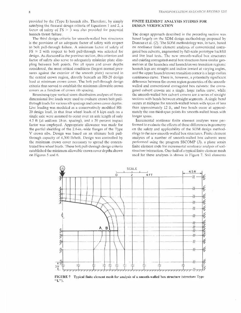
Incremental nonlinear finite element analyses were per­formed to evaluate the effects of these differences in geometry on the safety and applicability of the SDM design method­ology to the new smooth-walled box structures. Finite element analyses of a number of smooth-walled box culverts were performed using the program SSCOMP (3), a plane strain finite element code for incremental nonlinear analysis of soil­structure interaction. One-half of a typical finite element mesh used for these analyses is shown in Figure 7. Soil elements

FIGURE 7 Typical finite element mesh for analysis of a smooth-walled box structure (structure Type "L").

Seed et al.

were modeled with four node isoparametric elements, and the culvert structures were modeled with piece-wise linear beam elements. Nonlinear stress-strain and volumetric strain soil behavior was modeled using the hyperbolic formulation proposed by Duncan et al. ( 4) as modified by Seed and Dun­can (5). Structural behavior was modeled as linear elastic. The analyses were performed in steps to incrementally model the actual backfill placement process and then the application of design live loading.

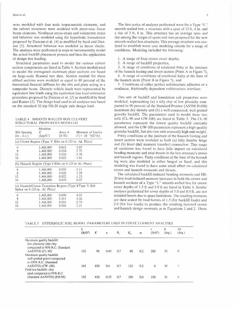
Structural parameters used to model the various culvert section components are listed in Table 4. Section moduli used to model the corrugated aluminum plate sections are based on large-scale flexural test data. Section moduli for these ribbed sections were modeled as equal to 80 percent of the theoretical flexural stiffness for the ribs and plate acting as a composite beam. Discrete vehicle loads were represented by equivalent line loads using the equivalent line load estimation procedure proposed by Duncan et al. (2) as modified by Seed and Raines (1). The design load used in all analyses was based on the standard 32-kip HS-20 single axle design load.

TABLE 4 SMOOTH-WALLED BOX CULVERT STRUCTURAL PROPERTIES MODELED

Rib Spacing (in., o.c.)

Modulus E (kip/ft')

Arca A (ft2/ft)

Moment of Inertia I ( x 10-")(ft"lft)

(a) Crown Region (Type V Ribs on 0.125-in. Al. Plate)

6 8

12 16

1,468,800 1,468,800 1,468,800 1,468,800

0.042 0.034 0.026 0.022

3.85 2.72 2.28 l.84

(b) Haunch Region (Type I Ribs on 0.125-in Al. Plate)

6 8

12 16

1,468,800 1,468,800 1,468,800 1,468,800

0.033 0.028 0.022 0.019

2.11 1.58 1.23 0.97

(c) Haunch/Crown Transition Region (Type I/Type V Rib Splice on 0.125-in. Al. Plate)

6 8

12 16

1,468,800 1,468,800 1,468,800 1,468,800

0.050 0.041 0.031 0.026

4.62 3.26 2.74 2.21

9

The first series of analyses performed were for a Type "L" smooth-walled box, a structure with a span of 12 ft, 4 in. and a rise of 3 ft, 6 in. This structure has an average span and rise among the ranges of spans and rises proposed for the new smooth-walled box structures. This average structure was ana­lyzed to establish worst case modeling criteria for a range of conditions. Modeling included the following:

1. A range of final crown cover depths, 2. A range of backfill properties, 3. A range of conditions of rotational fixity at the juncture

of the haunch footing and invert section (Point A in Figure 7). 4. A range of conditions of rotational fixity at the base of

the haunch stem (Point B in Figure 7), and 5. Conditions of either perfect soil/structure adhesion or a

nonlinear, frictionally dependent soil/structure interface.

Two sets of backfill and foundation soil properties were modeled, representing (a) a silty clay of low plasticity com­pacted to 90 percent of the Standard Proctor (ASTM D-698) maximum dry density and (b) a well-compacted, well-graded gravelly backfill. The parameters used to model these two soils (CL-90 and GW-100) are listed in Table 5. The CL-90 parameters represent the lowest quality backfill currently allowed, and the GW-100 parameters represent a high-quality granular backfill, but also one with unusually high unit weight.

Fixity conditions at the juncture of the haunch footing and invert section were modeled as both (a) fully flexible hinge and (b) fixed (full moment transfer) connection. This range of variations was found to have little impact on calculated bending moments and axial thrusts in the box structure's crown and haunch regions. Fixity conditions at the base of the haunch leg were also modeled as either hinged or fixed, and this modeling was found to have some small effect on calculated crown and haunch moments and thrusts.

The calculated backfill-induced bending moments and HS-20 live-load-induced moment increases in both the crown and haunch sections of a Type "L" smooth-walled box for crown cover depths of 1.5 ft and 5.0 ft are listed in Table 6. Similar analyses performed for cover depths of 3.0 and 8.0 ft, are not included herein due to space limitations. The resulting moments are then scaled by load factors of 1.5 (for backfill loads) and 2.0 (for live loads) to produce the resulting factored crown and haunch design moments as in Equations 1 and 2. These

TABLE 5 HYPERBOLIC SOIL MODEL PARAMETERS USED IN FINITE ELEMENT ANALYSES

Maximum quality backfill: low-plasticity silty clay compacted to 90% R.C. (Standard AASHTO) (CL-90)

Maximum quality backfill: we ll-graded gravel compacted lo 100% R.C. (Standard AASHTO) (CW-100)

Field test backfill: silty sand compacted to 95% R.C. (Standard AASHTO) (SM-95)

y (lb/fl3) K n

125 90 0.45 0.7

145 450 0.4 0.7

125 450 0.25 0.7

m

80 0.2

125 0.2

350 0.0

c qi (lb/ft2) (deg.)

200 30

0 39

100 34

~qi

(deg.)

0

7

6

TABLE 6 COMPARISON OF SDM-BASED DESIGN MOMENTS AND MOMENTS CALCULATED BY NONLINEAR FINITE ELEMENT ANALYSES (SMOOTH-WALLED BOX STRUCTURE TYPE "L")

(a) DEPTH OF CROWN COVER - 1.5 ft : -

CROWN HAUNCH

BACKFILL LIVE LOAD DESIGN BACKFILL LIVE LOAD DESIGN GASE MOMENT MOMENT MOMENT MOMENT MOMENT MOMENT

M~B llMcL Meo (k- t/ft) (k-ft/ft) (k-ft/ft)

M~B (k- t/ft) llMHJ (k-ft ft)

M~D (k- t/ft)

DUNCAN, SEED & DRAWSKY (1984) 0.8 5.0 11.1 0.6 2.4 5.7 PROPOSED MOMENTS: GL-90 MATERIAL

FINITE ELEMENT ANALYSIS : CL-90 MATERIAL, HINGED BASE, 0.6 5.5 11.8 0.5 2.0 4.8 NO INTERFACE ELEMENTS

FINITE ELEMENT ANALYSIS : CL-90 MATERIAL, HINGED BASE, 0.6 5.6 11. 9 0.5 2.0 4.8 INTERFACE ELEMENTS

FINITE ELEMENT ANALYSIS: CL-90 MATERIAL, FIXED BASE 0.7 5.2 11.5 0.6 1. 8 4.5 NO INTERFACE ELEMENTS

FINITE ELEMENT ANALYSIS: GW-100 MATERIAL, FIXED BASE 0.6 4.4 9.7 0.5 1. 5 3.9 NO INTERFACE ELEMENTS

FINITE ELEMENT ANALYSIS : GW-100 BACKFILL OVER CL-90 FOUNDATION, 0.7 4.6 10.3 0.6 1. 5 3.9 HINGED BASE, NO INTERFACE ELEMENTS

FINITE ELEMENT ANALYSIS: CL-90 BACKFILL OVER FIRM FOUNDATION, 0.5 4.6 9.9 0.5 1.8 4.4 HINGED BASE, NO INTERFACE ELEMENTS

FINITE ELEMENT ANALYSIS: CL-90 MATERIAL, HINGED BASE, 0.6 4.5 9.8 0.5 1.8 4.4 NO INTERFACE ELEMENTS HS-20 LIVE LOAD OFF CENTER

(c) DEPTH OF CROWN COVER - 5.0 ft : -DUNCAN, "SEED & DRAWSKY (1984) 2.8 1. 8 7.7 2.0 1. 3 5.6 PROPOSED MOMENTS: CL-90 MATERIAL

FINITE ELEMENT ANALYSIS: CL-90 MATERIAL, HINGED BASE, 1. 7 1.0 4.5 1.6 0.8 4.0 NO INTERFACE ELEMENTS

FINITE ELEMENT ANALYSIS : CL-90 MATERIAL, HINGED BASE, 1. 7 1.0 4.6 1. 6 0.8 4.0 INTERFACE ELEMENTS

FINITE ELEMENT ANALYSIS : CL-90 MATERIAL, FIXED BASE, 1. 8 0.9 4.6 1. 7 0.8 4.1 NO INTERFACE ELEMENTS

FINITE ELEMENT ANALYSIS : GW-100 MATERIAL, FIXED BASE, 1.4 0.5 3.2 1. 3 0.4 2.8 NO INTERFACE ELEMENTS

FINITE ELEMENT ANALYSIS: GW-100 BACKFILL OVER CL-90 FOUNDATION, 1. 5 0.5 3.3 1.4 0.4 2.9 HINGED BASE, NO INTERFACE ELEMENTS

FINITE ELEMENT ANALYSIS: CL-90 BACKFILL OVER FIRM FOUNDATION 1.4 0.8 3.8 1.4 0.7 3.5 HINGED BASE, NO INTERFACE ELEMENTS

Seed et al.

factored design moments are also listed in Table 6, along with the factored design moments based on the SDM design methodology.

As shown in Table 6, the largest crown and haunch moments are calculated using the minimum quality CL-90 backfill. A flexible hinge at the base of the haunch leg tends to result in slightly higher crown and haunch moments than does a fixed haunch leg base. The modeling of a frictional soil/structure interface condition results in a negligible difference in crown and haunch moments as opposed to those calculated based on modeling perfect soil/structure interface adhesion. Although not listed in Table 6, haunch thrusts were appreciably larger when perfect soil/structure adhesion was modeled. In general then, the worst-case (or most conservative) modeling condi­tions were found to be those corresponding to modeling of a minimum quality (CL-90) backfill with a hinged haunch base connection and perfect soil/structure interface adhesion.

Similar analyses were performed for two additional smooth­walled box structures (with different geometries) for these worst-case conditions. These structures were (a) a Type "O" structure with a span of 13 ft , 3 in., and a rise of 5 ft, 11 in., and (b) a Type "W" structure with a span of 15 ft, 8 in. and a rise of 4 ft, 7 in. These structures represented (a) a smooth­walled box with an unusually high aspect ratio (rise vs. span ratio) and (b) a low aspect ratio structure with a relatively large span approaching the maximum spans proposed.

The resulting FEM-calculated crown and haunch moments for these two structures over a range of final crown cover depths are shown in Tables 7 and 8. Also shown for com­parison purposes are the corresponding moments calculated on the basis of the SDM design methodology. As shown in

JI

Tables 6, 7, and 8, the FEM-calculated factored design moments in the crown region slightly exceed the SDM-based factored design moments (by 10 percent or less) for worst-case mod­eling conditions and minimum crown cover depths. At larger than minimum crown cover depths, the SDM-based factored design crown moments are larger than the FEM-calculated factored design moments, and the SOM-based haunch moments are larger than the FEM-based haunch moments at all crown cover depths.

At minimum cover depths , the factored design crown moments are dominated by the live-load-induced moment increases . As the worst-case FEM-calculated crown moments for the minimum cover conditions exceed the SDM-based moments by less than 10 percent, and both include a Load Factor of 2.0 for live-load-induced moment increases, it may be concluded that the SDM-based design provides a factor of safety of almost 2.0 with respect to crown failure in flexure under HS-20 loading for these worst-case minimum crown cover conditions. For all crown cover depths greater than these minimum allowable crown covers , the SDM-based crown and haunch design moments are conservative relative to the worst-case FEM-calculated moments . Accordingly, it was concluded that the SDM design methodology represented a suitable and adequately conservative basis for flexural capac­ity design of the proposed new smooth-walled box structures.

In addition to providing good support for the SDM-based flexural design of the new smooth-walled box structures, the finite element analyses also showed the axial thrusts at the bases of the culvert haunches, as estimated using Equation 3, to be conservative (larger) relative to those calculated by the finite element analyses for all culvert geometries, cover

TABLE 7 COMPARISON OF SOM-BASED DESIGN MOMENTS AND MOMENTS CALCULATED BY NONLINEAR FINITE ELEMENT ANALYSES (SMOOTH-WALLED BOX STRUCTURE TYPE "'O")

CROWN HAUNCH

BACKFILL LIVE LOAD DESIGN BACKFILL LIVE LOAD DESIGN CASE MOMENT MOMENT MOMENT MOMENT MOMENT MOMENT

M~B llMc7 M~D M~B llMHJ MHD (k- t/ft) (k-ft ft) (k- t/ft) (k- t/ft) (k-ft ft) (k-ft/ft)

... DUNCAN, ..... SEED & DRAWSKY (1984 ) 0.9 5 . 4 12.1 0 .7 2.7 6.5 PROPOSED MOMENTS

ll1

...... 11 FINITE ELEMENT ANALYSIS : 0 . 3 5 .9 12 . 2 0 . 5 1. 9 4 . 6

0 ;:c CL-90 MATERIAL, HINGED BASE

... DUNCAN, SEED & DRAWSKY (1984) 1. 9 ..... 3 .0 8 . 9 1.4 2. 0 6 . 1

0 PROPOSED MOMENTS

'"" II FINITE ELEMENT ANALYSIS : 0.8 2 . 5 6.2 0.9 1.0 3.4 0

CL -90 MATERIAL, HINGED BASE ;:c

... DUNCAN, SEED & DRAWSKY (1984) ..... PROPOSED MOMENTS

3.3 1. 9 8 . 7 2.5 1.4 6.6

0

~ II FINITE ELEMENT ANALYSIS : 1. 5 1.1 4.4 1.4 0 . 6 3 . 4

0 CL-90 MATERIAL, HINGED BASE ;:c

... DUNCAN, SEED & DRAWSKY (198 4) ..... PROPOSED MOMENTS

5 . 3 1.4 10 . 8 4.0 1.1 8.1

0

00 FINITE ELEMENT ANALYSIS : 2.4 0 . 4 II 0 . 5 4.6 2.1 3.9

0 CL-90 MATERIAL, HINGED BASE ::i::

12 TRANSPORTATION RESEARCH RECORD 1231

TABLE 8 COMPARISON OF SDM-BASED DESIGN MOMENTS AND MOMENTS CALCULATED BY NONLINEAR FINITE ELEMENT ANALYSES (SMOOTH-WALLED BOX STRUCTURE TYPE " W")

BACKFILL CASE MOMENT

McB (k-ft/ft)

.u DUNCAN, SEED & DRAWSKY .... (1984) 1. 4 PROPOSED MOMENTS ,.._

..... II FINITE ELEMENT ANALYSIS : 1.1

u CL-90 MATERIAL, HINGED BASE :i::

... DUNCAN, SEED & DRAWSKY .... (1984) 2.6 PROPOSED MOMENTS

0 ,., II FINITE ELEMENT ANALYSIS : 1. 9

u :i:: CL-90 MATERIAL, HINGED BASE

... DUNCAN, SEED & DRAWSKY (1984) 4.4 .... PROPOSED MOMENTS c;

"' FINITE ELEMENT ANALYSIS: 2.9 II u

CL-.90 MATERIAL, HINGED BASE :i::

... DUNCAN, SEED & DRAWSKY (1984) 7 . 1 .... PROPOSED MOMENTS

0

00 II FINITE ELEMENT ANALYSIS: 4 . 2

u :i:: CL-90 MATERIAL, HINGED BASE

depths, and combinations of modeling conditions considered. This finding supported the earlier conclusion that the provi­sion of adequate flexural capacity in both the crown and haunch regions also resulted in the provision of adequate haunch thrust capacity (FS > 3) for these new smooth-walled box structures.

FULL-SCALE PROTOTYPE TEST AND ANALYSES

As an additional check on the design analyses described thus far, a full-scale prototype smooth-walled box structure was installed and subjected to an HS-20 field load test. The field load test structure , a Type "D" smooth-walled box structure with a span of 10 ft , 6 in., and a rise of 4 ft, 6 in., was installed as a roadway bridge across a creek near Charlotte, North Carolina. This structure, with ribs at 12-in. o.c., was backfilled to a final crown cover depth of 2.0 ft with a locally available silty sand backfill compacted to an average of approximatdy 94 percent of the Standard Proctor (ASTM D-698) maximum dry density.

After completion of backflling, but before paving the over­lying road surface, an HS-20 live load test was performed using a loaded dump truck with a rear axle load of 32 kips distributed on four wheels (two pairs of tandem wheels). The 32-kip rear axle was positioned directly over the smooth-walled box structure centerline, and the resulting maximum crown deflections were recorded . The central crown ribs deflected approximately 0.21 in. under the HS-20 load, and the flat plate between the ribs deflected approximately an additional fl ")(\ ~n ""rho l~ua 1,.....,,,,-l ntn r +h,,...,....,. ...... m..-. .. ,,....~ f'..,,...m +\,,.,, ,...,.._,, ...., +,,.,,.., v,,,_,.._,, .1.1 • .1., .1.1..LV I.I.TV l.'-JUU 1'1'U" "1.l'-'.l.l l."-'J.11.VV'-'U J.J.VJlJ. l.J..l\.; .3l.J.U"-'1.UJ.\.;'

CROWN HAUNCH

LIVE LOAD DESIGN BACKFILL LIVE LOAD DESIGN MOMENT MOMENT MOMENT MOMENT MOMENT

6McL M~D MHB 6MHL M~D (k-ft/ft) (k- t/ft) (k-ft/ft) (k-ft/ft) (k- t/ft)

5.9 14.0 1. 2 3.4 8 .6

7.0 15 . 5 1.1 2.6 6.9

3.5 11.0 2 . 1 2.5 8.2

3.4 9.6 1. 9 1. 7 6.3

2.2 11.0 3 . 6 1. 8 9.0

1.6 7.5 2 . 9 1.1 6 . 5

1. 7 14 .0 5 . 8 1.4 11.4

0.7 7.7 4.3 0.6 7 . 7

and the crown ribs rebounded elastically to rcover about one­half of their initial deflection, resulting in a residual deflection (set) of about 0.11 in . The 32-kip axle load was then driven 10 times across the structure , after which it was observed that crown deflections had ceased to increase with the number of passes. On the 11th pass, the dump truck was halted with its 32-kip rear axle again directly over the smooth-walled box centerline, and a maximum (net) crown rib deflection of about 0.28 in. was observed, of which a residual set of about 0.16 in. remained after load removal.

Incremental nonlinear finite element analyses, using the techniques described previously, were performed to model the incremental backfill placement and the subsequent initial HS-20 load application above the centerline of the backfilled structure. The soil parameters used to model the compacted silty sand backfill are listed in the third column of Table 5. These finite element analyses predicted an initial live-load­induced crown displacement of approximately 0.24 in., which was in excellent agreement with the 0.21 in. actually observed. Backfill- and live-load-induced haunch and crown moments calculated by these FEM analyses were smaller than those estimated based on the SDM design methodology. The results of this full-scale prototype live load test were thus judged to support the accuracy and conservatism of the finite element studies and SDM design procedures employed in the analysis and development of the new smooth-walled box structures.

Finally, the observed plate dimpling under repeated HS-20 live loading never exceeded a measured 0.3 in . incremental displacement of the flat plate face relative to the adjacent ribs. This relative displacement, which was barely discernible, was judged to represent acceptable performance with respect +.....,.. ..... 1,,,+ ...... ..:1-:-.- .... 1: .... ,.,. 1.v 1-'H.U.V UH.UpHHE>'

Seed et al.

SUMMARY AND CONCLUSIONS

The smooth-walled box structure system described in this paper represents a new approach to the problem of providing effi­cient transport of water beneath ground cover with limited crown clearances. The smooth walls of these strucutres pro­vide significantly increased hydraulic efficiency over that achieved by current conventional corrugated metal box cul­verts. This hydraulic efficiency offsets the decreased structural efficiency (decreased flexural capacity) of the composite smooth plate/rib sections and permits the use of a significantly smaller smooth-walled box structure cross-sectional area to transport the same maximum design flow volume as would be trans­port'ed. by a significantly larger corrugated box culvert cross­sectional area. This smaller structure, in turn, minimizes over­all structure size and cost, requires smaller clearances for installation under shallow cover constraints, and minimizes the excavation and backfill volumes required for installation.

The finite element analyses performed as part of these stud­ies support the applicability of the SDM design methodology to the analysis and design of these new smooth-walled struc­tures. The large-scale laboratory tests described provide a basis for evaluation of the various structural system compo­nent capacities necessary for design of these structures. Finally, a full-scale field prototype HS-20 live load test was performed and analyzed using the same finite element analysis modeling techniques used in the development and design of these new structures. The results of this full-scale prototype live load

13

test provide good support for the accuracy of these finite element analysis techniques and for the suitability and con­servatism of the design procedures proposed for these new smooth-walled box structures.

REFERENCES

1. R. B. Seed and J. R Raines. Failure of Flexible Long-Span Cul­verts Under Exceptional Live Loads. Presented at the 67th Annual Meeting of the Transportation Research Board, Washington, D.C. Jan., 1988.

2. J.M. Duncan, R . B Seed, and R.H. Drawsky. Design of Cor­rugated Metal Box Culverts. Geotechnical Engineering Research Report UCB/GT/84-10. University of California at Berkeley, July, 1984.

3. R. B. Seed and J. M. Duncan. SSCOMP: A Finite Element Anal­ysis Program for Evaluation of Soil-Structure I111eraction and Com­paction Effects. Geotechnical Engineering Research Report UCB/ GT/84-02. University of California at Berkeley, Feb., 1984.

4. J. M. Duncan, P. Byrne, K. S. Wong, and P. Mabry. Strength, S1ress-Strain and Bulk Modulus Parameters fo r Finile Element Analyses of Stresses and Movements in Soil Masses. Geotechnical Engineering Research Report UCB/GT/80-01. University of Cal­ifornia at Berkeley, Jan., 1980.

5. R. B. Seed and J. M. Duncan. Soi/-S1ruc1ure Interaction Effects of Compaction-Induced Stresses and Deflections. Geotechnical Engineering Research Report UCB/GT/83-06, University of Cal­ifornia at Berkeley, Dec., 1983.

Publication of lhis paper sponsored by Committee on Subswface Soi/­Structure Interaction.

14 TRANSPORTATION RESEARCH RECORD 1231

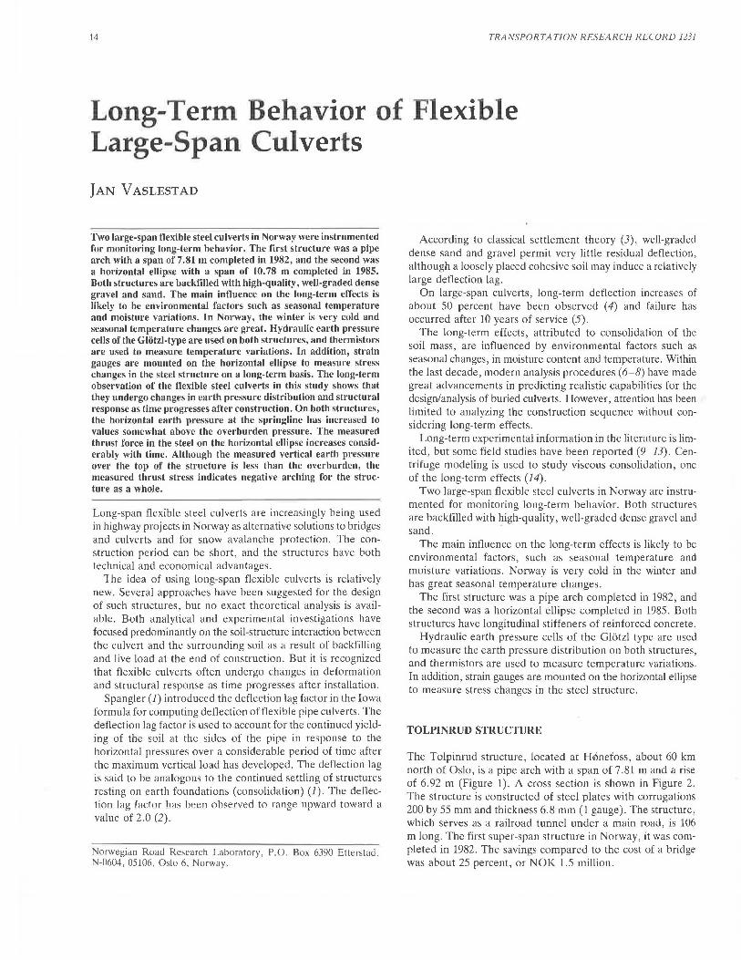
Long-Term Behavior of Flexible Large-Span Culverts

}AN VASLESTAD

Two large-span flexible steel culverts in Norway were instrumented for monitoring long-term behavior. The first structure was a pipe arch with a span of 7 .81 m completed in 1982, and the second was a horizontal ellipse with a span of 10.78 m completed in 1985. Both structures are backfilled with high-quality, well-graded dense gravel and sand. The main influence on the long-term effects is likely to be environmental factors such as seasonal temperature and moisture variations. In Norway, the winter is very cold and seasonal temperature changes are great. Hydraulic earth pressure cells of the Gliitzl-type are used on both structures, and thermistors are used to measure temperature variations. In addition, strain gauges are mounted on the horizontal ellipse to measure stress changes in the steel structure on a long-term basis. The long-term observation of the flexible steel culverts in this study shows that they undergo changes in earth pressure distribution and structural response as time progresses after construction. On both structures, the horizontal earth pressure at the springline has increased to values somewhat above the overburden pressure. The measured thrust force in the steel on the horizontal ellipse increases consid­erably with time. Although the measured vertical earth pressure over the top of the structure is less than the overburden, the measured thrust stress indicates negative arching for the struc­ture as a whole.

Long-span flexible steel culverts are increasingly being used in highway projects in Norway as alternative solutions to bridges and culverts and for snow avalanche protection. The con­struction period can be short, and the structures have both technical and economical advantages.

The idea of using long-span flexible culverts is relatively new. Several approaches have been suggested for the design of such structures, but no exact theoretical analysis is avail­able. Both analytical and experimental investigations have focused predominantly on the soil-structure interaction between the culvert and the surrounding soil as a result of backfilling and live load at the end of construction. But it is recognized that flexible culverts often undergo changes in deformation and structural response as time progresses after installation.

Spangler (1) introduced the deflection lag factor in the Iowa formula for computing deflection of flexible pipe culverts. The deflection lag factor is used to account for the continued yield­ing of the soil at the sides of the pipe in response to the horizontal pressures over a considerable period of time after the maximum vertical load has developed. The deflection lag is said to be analogous to the continued settling of structures resting on earth foundations (consolidation) (1). The deflec­tion lag factor has been observed to range upward toward a value of 2.0 (2).

Norwegian Road Research Laboratory, P.O. Box 6390 Etterstad, N-0604, 05106, Oslo 6, Norway.

According to classical settlement theory (3), well-graded dense sand and gravel permit very little residual deflection, although a loosely placed cohesive soil may induce a relatively large deflection lag.

On large-span culverts, long-term deflection increases of about 50 percent have been observed ( 4) and failure has occurred after 10 years of service (5).

The long-term effects, attributed to consolidation of the soil mass, are influenced by environmental factors such as seasonal changes, in moisture content and temperature. Within the last decade, modern analysis procedures (6-8) have made great advancements in predicting realistic capabilities for the design/analysis of buried culverts. However, attention has been limited to analyzing the construction sequence without con­sidering long-term effects.

Long-term experimental information in the literature is lim­ited, but some field studies have been reported (9-13). Cen­trifuge modeling is used to study viscous consolidation, one of the long-term effects (14).

Two large-span flexible steel culverts in Norway are instru­mented for monitoring long-term behavior. Both structures are backfilled with high-quality, well-graded dense gravel and sand.

The main influence on the long-term effects is likely to be environmental factors, such as seasonal temperature and moisture variations. Norway is very cold in the winter and has great seasonal temperature changes.

The first structure was a pipe arch completed in 1982, and the second was a horizontal ellipse completed in 1985. Both structures have longitudinal stiffeners of reinforced concrete.

Hydraulic earth pressure cells of the Glotzl type are used to measure the earth pressure distribution on both structures, and thermistors are used to measure temperature variations. In addition, strain gaµges are mounted on the horizontal ellipse to measure stress changes in the steel structure.

TOLPINRUD STRUCTURE

The Tolpinrud structure, located at H©nefoss, about 60 km north of Oslo, is a pipe arch with a span of 7 .81 m and a rise of 6.92 m (Figure 1). A cross section is shown in Figure 2. The structure is constructed of steel plates with corrugations 200 by 55 mm and thickness 6.8 mm (1 gauge). The structure, which serves as a railroad tunnel under a main road, is 106 m long. The first super-span structure in Norway, it was com­pleted in 1982. The savings compared to the cost of a bridge was about 25 percent, or NOK 1.5 million.

Vas/estad

Dovre

Tolpinrud

FIGURE 1 Location of the Tolpinrud and Dovre structures.

The backfill consists of gravel and sand compacted to min­imum 97 percent Standard Proctor. The extent of the backfill is shown in Figure 2. The backfill was placed in 20-cm-thick layers and compacted with a 1100-kg vibratory roller and a 12-t bulldozer. The depth of cover over the crown varied from 1.1 m to 1.6 m. The in situ soil is a medium stiff clay with undrained shear strength 40 to 80 kN/m 2

.

INSTRUMENTATION ON TOLPINRUD STRUCTURE

Earth pressure cells of the Gl6tzl type were mounted on the structure at two sections , one 25 m from the northern end and the other 50 m from the northern end. Six earth pressure cells were used at each section. The location of the earth pressure cells is shown in Figure 2.

Four of the earth pressure cells were bolted on the steel structure using specially constructed brackets . A bracket with

15

an earth pressure cell is shown in Figure 3. The brackets have the same corrugation and radius as the culvert structure.

One cell was placed horizontally in the sand under the culvert, and one cell was placed vertically in the backfill 0.5 m from the thrust beam to measure the horizontal eartl1 pressure.

The earth pressure cells are 30 by 40 by 0 .5 cm. The brackets are 60 by 80 cm.

The working principle of the Gl6tzl earth pressure cell is shown in Figure 4. Calibration of the cells was performed by the manufacturer and was found to agree well with calibration checks in our laboratory. Calibration of the cells with tem­perature variations from + 20°C to - 30°C was also performed in our laboratory .

With this cell the pressure shown on the gauge during cir­culation of oil is related to the earth pressure, <J, by the expression:

PA +Pa =Po + A ·u +Pc (1)

where

PA the pressure given by the cell pressure gauge, Pn the difference between the level of the cell and pump, p 0 the pressure required to cause circulation of oil, A the cell action factor , and

Pc = a pressure term due to temperature change.

Woodford and Skipp (15) found the action factor A to be 0.96 in a field loading condition compared with results from a large test chamber. Penman and Charles (16) used a 1-m diameter odometer based on a design by Kjaernsli and Sande (17) to test the Gl6tzl earth pressure cells. An action factor of 0 .943 was found.

Thermistors were placed near each earth pressure cell and also elsewhere in the backfill to give data for temperature corrections and freezing depths.

Deformations of the steel structure were also measured during construction and on a long-term basis. Deformations were measured with tape. Further details of the instrumen­tation are given by Knutson (18) Johansen (19).

OBSERVED MEASUREMENTS AT TOLPINRUD

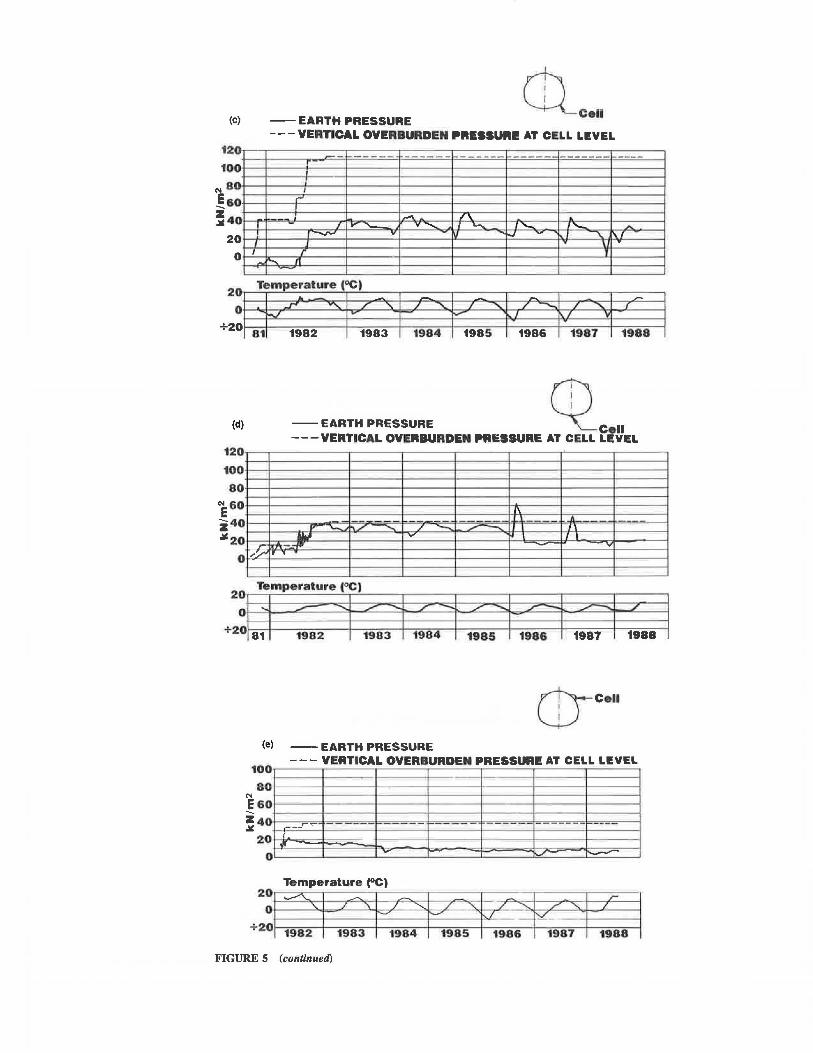
Earth pressure reading were taken from the beginning of construction in 1981 until August 19 (Figure 5). Th vertical overburden pressure at cell level and the temperature mea­surements near each cell are also shown in the figures.

The measured earth pressure at the crown is about equal to the vertical overburden pre sure and hows mall variations with time (Figure Sa).

The mea ured lateral earth pres ure at the pringline is about 50 percent of the vertical overburden pressure at this level at the end of construction (Figure Sb). After about 1 year, the lateral earth pressure increased to abour JOO percent of the vertical overburden pressure. A further moderate increase is indicated during the following years .

The measured earth pres ure a1 the haunch (Figure 5c) is lower than the measured lateral earth pre sure at the pring­line. Earth pressure di tribution fr m the ring-compression 1heory (20) predicts greatest earth pressure at !he haunch.

16 TRANSPORTA TION RESEA RCH RECORD 1231

--- Earth pressure cell

. 1.•.-:_..- : · : 1,1m· .. · .. : , ..• X'

Rr=3,90m

Concrete beam

CLAY Scale: 0 Sm

__._:_:__ 7 aom

FIGURE 2 Geometry of instrumented cross section with location of the earth pressure cells (Tolpinrud).

I

FIGURE 3 Earth pressure cell with bracket on the structure.

The calculated earth pressure at the haunch (corner) according to the earth pressure distribution on pipe arches from the ring-compression theory (20) is:

PH = Pv · R,,IRH = 41 kN/m2 (2)

'!Ff = 19.8 kN/m2 i£ Lf-ie vertical Qverhnrrl~n ;it

the top of the structure , RT= 3.9 mis the radius at the crown, and RH = 1.88 mis the radius at the haunch.

In Figure Sd, the measured earth pressure at the bottom of the structure is shown. The earth pressure is decreasing with time.

The measured lateral earth pressure 0.5 m from the thrust beam is shown in Figure Se. The measured pressure there is very low.

The earth pressure distribution around the structure at the end of construction and after 18 months is shown in Fig­ure 6.

The observed long-term deformations on the structure are small. The observed downward deformations from February 1983 to November 1986 are shown in Figure 7. The total vertical deformations of the crown are 15 mm (point A) . Points B and C indicate that the whole structure settled 10 mm , so that the relative long-term deformation of the crown is only 5 mm. The total outward horizontal displacement at the springline in the same period was less than 15 mm. The reported values are average values from observations at five sections.

DOVRE STRUCTURE

The culvert is located at Dovre , about 350 km north of Oslo (Figure 1). The structure, a horizontal ellipse with a span of 10. 78 m , rise of 7 .13 m, and total length of 35 m, serves as a road tunnel for Euroroad 6. The depth of cover over the crown is 4.2 m. Built in 1985 in a cut-and-cover operation through a soil ridge, th is is the largest long-span flexible steel culvert in Scandinavia.

A cross section of the structure is shown in Figure 8. The structure was built using 7-mm-thick steel plates with corru­gations of 200-rnm pitch and 55-mm depth . The plates were assembled in the field, using 20-mm-diameter high-strength bolts in 25-mm-diameter holes. There are 15 bolts/m of lon­gitudinal seam .

High-quality well-graded gravel was used for backfilling in a zone extending 6 m out from the springline and 2 m above the rrnwn The rpm;iinine h;ic.kfill rnnsisted of sandy silt. The

pressure cnamber

preuure llne

preuure In material -~ ~ ~ ~ t

preuure diaphragm

oll fllled t t t t t pr111ure pad 1p11ce Hn1or

FIGURE 4 The principle of Glotzl earth pressure cell.

(a) -- EARTH PRESSURE - - - VERTICAL OVERBURDEN PRESSURE AT CELL LEVEL

0 12

to ,...8 Ea

0 ... -

!4 0

0

2 0

0

2 ·-·-0

+2 0

__ --, 7i1

Te mperature (CC) ·-" ~

81 1982

-

- -/ " I ....... --

1983 1984

(b) -- EARTH PRESSURE

~ -~ '"' ---

- ~ /""

I ....... I ~ / ' / ..- ~ I I ~

1985 1986 1987 1988

0 Cell

--- VERTICAL OVERBURDEN PRESSURE AT CELL LEVEL 120.--~------..~~-~--~--~~--~~-~-~~--

100+---1-~-~---1----1--~-~~---1-----l.--~-l--~--l

80 f-----j.,.....,.-----ji-r::>.....c----,,.L-µ~~-~~---b<".J-....._::::::,>..4-=-----1 l--+----.-i,....,,-e!_.r:__-...:.-_11:'7-:;.;..~,::..=-=..;,+-:::.·~=...::;_:"J,.V-- - .___.... _ - - --~ -- ,_ __ _....

i6o / z40 ' .~~'-r-·---1-----1-----1-----+----~---~ .1111 20!---l-----rl...L.1f!=.=---J----I---- - - -

,-,;,

0 " - "

20 Temperature (CC) l ---.;- ~

0

+20 81 1982

""' 17

-/ ' / .......

......

1983 1984

---

~

~ ,,,.....

/ ' -I " I -, v .,, ·v

1985 1986 1987 1988

FIGURE 5 Measured earth pressure and temperature (Tolpinrud).

FIGURE 5 (continued on next page)

(c) --EARTH PRESSURE ---VERTICAL OVERBURDEN PRESSURE AT CELL LEVEL

-- -- i...----- ----,__ _ ---- .,_ ______ ------- --

0 r j

0 I

0 .-I

0 l ~ ...... I"\ ~

I - I ... '-- v .......... I ....... - /'-- /'-- .A

0 ! I --.,.... v - rv """

~ I '\. I'\.( I 1 .,

\I . 0 I r J

~ """' fl -

7 r-

1988

--EARTH PRESSURE Q Cell ---VERTICAL OVERBURDEN PRESSURE AT CELL LEVEL

(d)

120~~----~----,.---~----,.-----.----~---.

100 --1------1----1----~----l-----l-----+----l

BO-l------l-----~---+----1----+----+---~------;

e&o._-+-----f---+-----1----+-H--" ---t------.-----J------t • z40f----+--~v--~9:=./~~--=i'""-"'/""""<::"""'l==::;i_, ~~==~,rt,.====-t~~,,,f====t~~~---J

~20.t:J:::!ti~~~~ ..... =====l======~==~ ====t======l=·=~' ::::::~'=~' :::~~ ======i o: ,,./'I '

Temperature f°C)

l

1988

CJ-C•ll

(e) --EARTH PRESSURE - - - VERTICAL OVERBURDEN PRESSURE AT CELL LEVEL

100~---~--~---~--~--~~--~--~

80 N 1----1--~ 1-----+-----ll---~----f----l

! 68-l------1----+----1---===•~:::: _ ___,1---- 1------1

~ 40 -~··---->----1----1------+-----_-+~----_-__ , 20 ~~~::::~~~~;::.---t:=:::~;;:;::::i..=;;:=:t;;;;:::::=:1

O'-----'--------L-----'-----'-----='-''--- ---' ............... '-=---~

Temperature (°C) 20.----,..--,.----.,----.,------,---.-----.---::::----.

0 I-----"'+= _ __ ....,.

+20 1982 1983 1986 1988

FIGURE 5 (continued)

Vaslestad

END OF CONSTRUCTION AFTER ti MONTHS

FIGURE 6 Measured earth pressure around the structure (Tolpinrud).

DEFORMATION (mm)

151----

251-----1---~1

30'-----1---

B c

l 1983 1984 1985 ) 1986 1987 1988

FIGURE 7 Long-term deformations (Tolpinrud).

-- Earth pressure cell.

• Strain gage location.

19

in situ soil consisted of relatively dense sandy silt. The well­graded gravel was placed in layers of maximum 30 cm and compacted to minim1.1m 97 percent Standard Proctor.

The maximum allowed upward displacement of the crown during placement of backfill was 2 percent of the design height (143 mm) . The maximum observed upward displacement when backfilling was 63 mm.

The construction considerations used for long-span flexible steel structures in Norway are given elsewhere (21).

INSTRUMENTATION AT DOVRE

Hydraulic earth pressure cells of the Glotzl type, strain gauges , and thermistors were installed at one cross section near the middle of the structure. The geometry of the selected cross section with the location of earth pressure cells and strain gauges is shown in Figure 8.

Eight earth pressure cells were used . Four cells were bolted directly on the steel structure using specially designed brackets of the same type used at Tolpinrud . One cell was placed horizontally in the sand under the structure, two cells were placed horizontally 0.3 m and 1.5 mover the crown to monitor arching effects, and one cell was cast vertically in the concrete on the thrust beam to measure the lateral earth pressure on the beam.

Thermistors were installed near each earth pressure cell to measure the temperature variations in the soil.

Strain gauges were placed at 10 locations inside the steel structure. Two gauges were fitted at each location, one at the top of the corrugation and one at the bottom. This allowed thrust and bending stresses to be determined during back­filling and on a long-term basis. Dummy gauges were installed to provide temperature compensation. Further details of the instrumentation are provided elsewhere (22,23).

(2 gages at each location) TllllTITITmrrmmrmmmr

FIGURE 8 Geometry of instrumented cross section with location of the earth pressure cells and strain gauges (Dovre).

20

OBSERVED MEASUREMENTS AT DOVRE

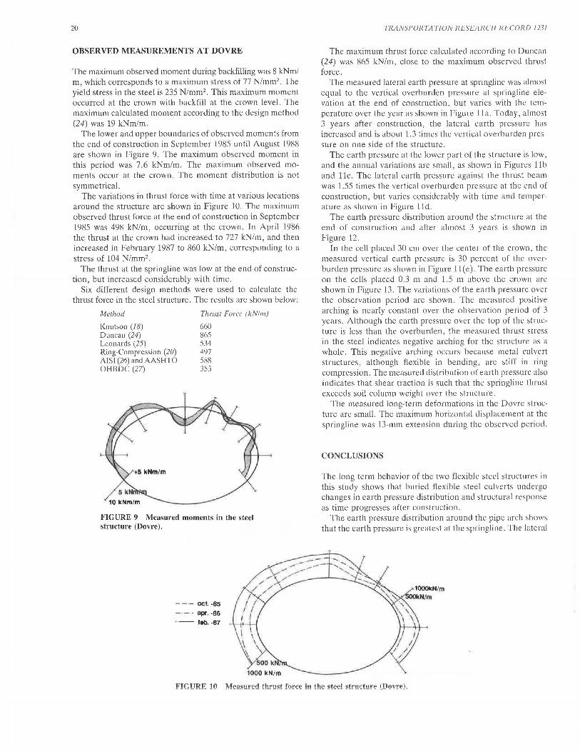
The maximum observed moment during backfilling was 8 kNm/ m, which corresponds to a maximum stress of 77 N/mm2. The yield stress in the steel is 235 N/mm2 . This maximum moment occurred at the crown with backfill at the crown level. The maximum calculated moment according to the design method (24) was 19 kNm/m.

The lower and upper boundaries of observed moments from the end of construction in September 1985 until August 1988 are shown in Figure 9. The maximum observed moment in this period was 7.6 kNm/m. The maximum observed mo­ments occur at the crown. The moment distribution is not symmetrical.

The variations in thrust force with time at various locations around the structure are shown in Figure 10. The maximum observed thrust force at the end of construction in September 1985 was 498 kN/m, occurring at the crown. In April 1986 the thrust at the crown had increased to 727 kN/m, and then increased in February 1987 to 860 kN/m, corresponding to a stress of 104 N/mm2 .

The thrust at the springline was low at the end of construc­tion, but increased considerably with time.

Six different design methods were used to calculate the thrust force in the steel structure. The results are shown below:

Method

Knutson (18) Duncan (24) Leonards (25) Ring-Compression (20) AISI (26) and AASHTO OHBDC (27)

Thrust Force (kN/111)

660 865 534 497 588 353

FIGURE 9 Measured moments in the steel structure (Dovre).

--- oct. -85

- · - -- apr. -86

-- feb. -87

TRANSPORT A T!ON RESEARCH RECORD 1231

The maximum thrust force calculated according to Duncan (24) was 865 kN/m, close to the maximum observed thrust force.

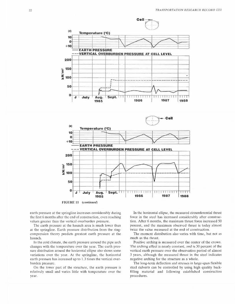
The measured lateral earth pressure at springline was almost equal to the vertical overburden pressure at springline ele­vation at the end of construction, but varies with the tem­perature over the year as shown in Figure 1 la. Today, almost 3 years after construction, the lateral earth pressure has increased and is about 1.3 times the vertical overburden pres­sure on one side of the structure.

The earth pressure at the lower part of the structure is low, and the annual variations are small, as shown in Figures l lb and l lc. The lateral earth pressure against the thrust beam was 1.55 times the vertical overburden pressure at the end of construction, but varies considerably with time and temper­ature as shown in Figure lld.

The earth pressure distribution around the structure at the end of construction and after almost 3 years is shown in Figure 12.

In the cell placed 30 cm over the center of the crown, the measured vertical earth pressure is 30 percent of the over­burden pressure as shown in Figure 11 ( e). The earth pressure on the cells placed 0.3 m and 1.5 m above the crown are shown in Figure 13. The variations of the earth pressure over the observation period are shown. The measured positive arching is nearly constant over the observation period of 3 years. Although the earth pressure over the top of the struc­ture is less than the overburden, the measured thrust stress in the steel indicates negative arching for the structure as a whole. This negative arching occurs because metal culvert structures, although flexible in bending, are stiff in ring compression. The measured distribution of earth pressure also indicates that shear traction is such that the springline thrust exceeds soil column weight over the structure.

The measured long-term deformations in the Dovre struc­ture are small. The maximum horizontal displacement at the springline was 13-mm extension during the observed period.

CONCLUSIONS

The long-term behavior of the two flexible steel structures in this study shows that buried flexible steel culverts undergo changes in earth pressure distribution and structural response as time progresses after construction.

The earth pressure distribution around the pipe arch shows that the earth pressure is greatest at the spri ngline. The lateral

- Cell (a)

Temperature °C)

10EE3~~~~=r==:::~:r===:2~~3 Q>---t----+----+--

+10· ..:::.::::.:::L..E-A~R=T=H""""=-P=R=E=s~s~u=R=E

-- - -VERTICAL OVERBURDEN PRESSURE AT CELL LEVEL

e 1so --- - 1---~ 100 --1----1

t---+----1-- - -/

S0----17 --- -

O· J J g. Sept. 1985

(b) 1i emperature (°C) 10 -

" :s. 0 710 - --

--EARTH PRESSURE

1986 1987

c ell ..-..._ ............ ..... ....... /

~ / -\7

---VERTICAL OVERBURDEN PRESSURE AT CELL LEVEL

200

e 1so

~ 100

50

--

.c. -l -~

-

·- -- ·--r· -1

~---.

'

--

0 J July Aug. Sept. r1 -1 l l I I I I I I I I I 11 I I I I I I I I

1 985 1986 1987

(c) Cell

1988

-

---

I I I I

1988

Temperature (oC)

10F==i=~:::i:;;;;:::::;;;;;:;;:'.~==;di::-r--=--=;_~=i====-:~~~l===iJ 0 - -- ~ --.... ""~'----"'"""-""I' - /..,,.,,.. ___ ---._,,.-1--_-::;;.-11

+10 -i=s~:-:.....--------~v'/------1----1: - EARTH PRESSURE --- VERTICAL: OVERBURDEN PRESSURE AT CELL LEVEL

--- '- - -----·- - --- ------------ ---, __ I

200

I e 1so r ~-..J ,_

,/' ...

--~ 100 __ ,,, r'

50 f ~ /' -I r-I--' .......... 17 - '

J ~uly Aug. Sept. 11 11111111111 I I I I I I I I II I I I I l

1986 1987 1988

0

1985

FIGURE 11 Measured earth pressure and temperature (Dovre).

FIGURE 11 (continued on nexi page)

22 TRANSPORTATION RESEARCH RECORD 1231

(d) Temperature ·(oe)

101--+-- ~""'---0'1----t,__---+-------'---+-'\~ 1--_...,_<-~~---""""'~------y<-,r2~~--~-~-.....:::-:: ....... ,;::~~~-~---_-~ l--+---+----+----1-''~ l-_,,r-------'~--+/------'l'C------j

+10 - __ ,.....,.,,,-'-----·-- -'"~-,/./------i----!

-EARTH PRESSURE ---VERTICAL OVERBURDEN PRESSURE AT CELL LEVEL

20

e 1s

~ 10

5

--0

0

0 c-

, ,_ ___

-·------------ -----------~---...J_ I I .•

--J r-

' ~- \! 0

(e)

10 0

+10

J July Aug. 1985

1i emperature (

Sept.

cc )

-- EARTH PRESSURE

I I

'\. '\.

11111111111 11111111111 I I I I

1986 1987 1988

o -Cell - ~ - ......... ,r "

~ .... ./ , _ / v

---VERTICAL OVERBURDEN PRESSURE AT CELL LEVEL

200

e 150

~ 100

,_

/ ~

rl ...... ........ J---,-- -~

50

0 J July Aug. Sept.

1985

F'IGURE 11 (continued)

earth pressure at the springline increases considerably during the first 6 months after the end of construction, even reaching values greater than the vertical overburden pressure.

The earth pressure at the haunch area is much lower than at the springline. Earth pressure distribution from the ring­compression theory predicts greatest earth pressure at the haunch.

In the cold climate, the earth pressure around the pipe arch changes with the temperature over the year. The earth pres­sure distribution around the horizontal ellipse also shows some variations over the year. At the springline, the horizontal earth pressure has increased up to 1.3 times the vertical over­burden pressure.

On the lower part of the structure, the earth pressure is relatively small and varies little with temperature over the year.

\

I I

. ~ -- I \ ~ -v I \ /

I v

I I I I I I I 11 I I I I J I I I I l I II I I I I

1986 1987 1988

In the horizontal ellipse, the measured circumferential thrust force in the steel has increased considerably after construc­tion. After 6 months, the maximum thrust force increased 50 percent, and the maximum observed thrust is today almost twice the value measured at the end of construction.

The moment distribution also varies with time, but not as much as the thrust.

Positive arching is measured over the center of the crown . The arching effect is nearly constant, and is 30 percent of the vertical earth pressure over the observation period of almost 3 years , although the measured thrust in the steel indicates negative arching for the structure as a whole.

The long-term deflection and stresses in large-span flexible steel culverts can be controlled by using high quality back­filling material and following established construction procedures.

Vas/estad

-- END OF CONSTRUCTION --- - - AFTER n..EE YEARS

/ /

I

200 I

/ /

,,..,,., /

23

FIGURE 12 Measured earth pressure around the structure (Dovre).

TOP OF EMBANKMENT CELLS

-E 3 .... .c DI GI

2 .c

- 1 ...

OVERBURDEN Jr • h

CELLr ,I

/ /

CELL~ 0 25 50 75

-,...---

Legend:

r---i Measured values

TOP OF CULVERT

100

Earth pressure (kN/m2)

FIGURE 13 Measured earth pressure above the structure (Dovre).

ACKNOWLEDGMENTS

The author wishes to thank Tor Erik Frydenlund and Asmund Knutson for valuable comments during the preparation of the paper and Tor Helge Johansen for his valuable work on the instrumentation and field operations.

REFERENCES

1. M. G . Spang! r. The tructural DI! ign of Flexible Pipe Culverts. Iowa - nginecring Experimenta l S1111 ion, 811//e1i11 153, The Iowa State College Bulletin, Ames, 1941.

2. M. G. Spangler and R. L. Handy . Soil Engineering. Harper and Row, New York. 1982.

3. N. Jnnbu. Grunnlag i geoJ(•knikk. Tapir, 1970. 4. Re ·carch Problem Statement 114. Transportmion Research Cir­

cular 272, TRB, Nalional Council, Washington, D.C., Feb. 1984, p. 58.

5. Culvert Failure Kills Five. Engineering News Record. Jan. 1983, p. 12.

6. M. G. Katona et al. CANDE-A Modern Approach for Struc-

tural Design and Analyses of Buried Culverts. Report FHW A­RD-77-5. U.S. Naval Civil Engineering Laboratory, 1977.

7. M. G. Katona et al. CANDE User Manual. Report FHWA RD-77-6. U.S. Naval Civil Engineering Laboratory, 1977.

8. M. G. Katona et al. CANDE System Manual . Report FHWA RD-77-7. U.S. Naval Civil Engineering Laboratory, 1977.

9. E. T. Selig. Instrumentation of Large Buried Culverts: Perfor­mance Monitoring for Geotechnical Construction, ASTM STP 584 , 1975, pp. 159-181.

10. E. T. Selig et al. Review of the Design and om1mc1ion of Long­Span, Corrugated-Mew/, Buried Conduits . Report FHWA-RD-77-131. FHWA, U.S. Department of Transportation, 1977.

11. E. T. Selig et al. Measured Performance of Newtown Creek Culvert. Journal of the Geotechnical Engineering Division-ASCE, Vol. 105, No. GT9, 1979, pp. 1067-1087.

12. M. G. Katona et al. Structural Evaluation of New Concepts for Lo11g-Spa11 Culverts and Culvert fllst(l/lations. Report FHW A­RD-79-115. FHWA, U.S. Depart meni of Tran portation, 1979.

13. D. W. Spanm1gel et al. Effects of Method A and B Backfill or Flexible Culverts under High Fills. In Transportation Research Record 510. TRB, National Research Council, Washington, D.C., 1974, pp. 41-55.

14. M. C. Mc Vay and P. Papadopoulus. Long-Term Behaviour of Buried Large-Span Culverts. Journal of Geotechnical Engineer­ing, Vol. 112, No. 4, 1986, pp. 424-442.

24

15. C. WouclC r I am! B. G. Skipp. Expni111e11tal a11d 111111'rical Srml­ies of 1/1e Ar1io11 Factor of C/61 z/ £11rt/1 !'1·1.,1·.1·11n• 1!/ls. Report 74. Consrruction lndustr Rcsc<irch nnd lnfor111a1i n A::. oci<ltion, London, England, May 1976.

16. A. D. M. Penman and J. A. Charles. Deformalions and S1resses in Rockfi// over a Rigid Culvert. Curren! Paper 100/75. Building Research Establishment, United Kingdom, 1975.

17. B. Kj11ernsli and A . Sande . omprcs.~ibi l n y or some coarse grnincd mate rials . Proc .. European Co11frre11ce 011 Soil frcltanic.1· wul Fo1111datio11 E11gi11eel'i11g, ol. 1, Wicsh;idcn. Fcclernl R ·public of Ge rmany, pp. 245- 251.

18. A. Kmll$On. S11peq11111k11ft•rr1 ved Tolpi11rll(f. £68, Ringerike. l111crnnl Repon I JSS . Norwegian Rond Rc~carch Laboratory, Oslo. 1984.

19. T . H. Johunsen . St1p1•1:~p1111k1d1"<'l'I 111!1/ Tolpi11md. Mo11wri11g.f · rt1ppor1 for jo)'(/tr kk.wmi/ere. lnl 'rnal Rcpon 11.58. 1on1cgian Road Re cnr h Laboratory. . lo. 19 -l.

20. H. L. White and J. P. Layel'. 111c orrugntt!d Mewl o ndui1 ;1s a 01111 rcssion Ring. //RfJ. Pro .. Vol. 31 • 1960. pp. 389- 97.

2 1. J. Va le stud. Lo11g·sp1111 cormgmi>tl steel s11·11c1url's. Desi •11 co11· cl!pts mul c-onstmctirm 11roccd1m• (in orwcgian). !lllcl'm'll Report L59. Norwegian Roud Research Ltthorntory. ·to. 1986.

TRANSPORTATION RESEARCH RECORD 1231

22. J . Vuslcstacl. Super pe1111 rlJr Do•·rc. ( bs1·1w1.~jvm•rm·jord11ykk. 11/l.111e1111/11g11r. defun1111~jo1111r og 1e11111erc11111·. lt11cnrnl R 'llOrl I 3:N.

Norwegian Road Research Llbornrory, Oslo. 1987 . 23. T . H. Jolmnscu. Supt·r .111e1111 Dm•rc. Di••<' " i11s1m111c111eri11i; p11

ng i·ed korrngen .1·11llrbr. lntcl'IHl l 'Report 1318. orwcgian RNtd Research L<tborator 1 • lo. 1987.

24. J . M. Duncan and R. 11. Drnwsk 1• Dt'sign Proc1•rlures for Flexible i\4er<1I 11hrer1 Strn,·111re.1. Rcpon U 13/GT/83-02 . Department o( Civil Engineering, Univcrsi1.y of Cnli~ rnia. Berkeley. 1983.

25. G. A. Leonard · et al. Predicting Performance of Buried Metal Conduits. In Transportalion Research Record 1008, TRB, National Research Council, Washington. D.C., 1985.

26. Handbook of Steel Drainage and Highway Construction Products. American Iron and Steel Institute, 1984.

27. Ontario Highway Bridge Design Code. Ontario Ministry of Trans· portation and Communications, 1983.

Publication of this paper sponsored by Committee on Subsurface Soi/­Structure /11terac1io11.

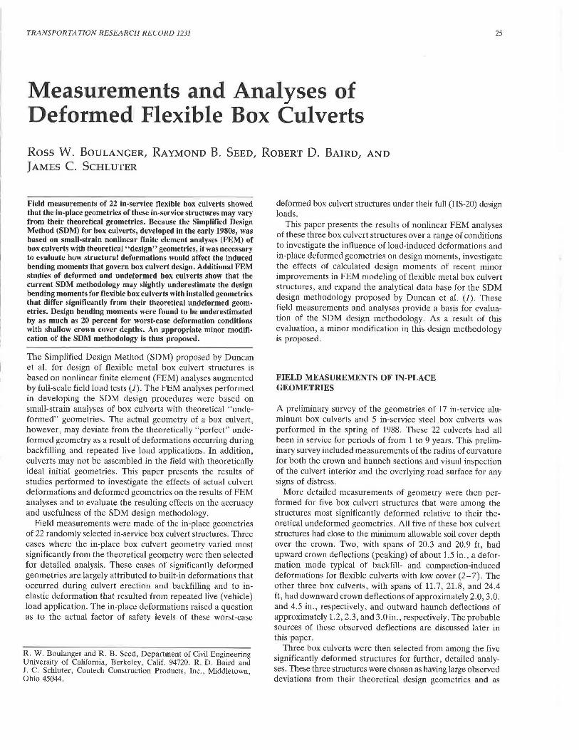
TRANSPORTATION RESEARCH RECORD 1231 25

Measurements and Analyses of Deformed Flexible Box Culverts

Ross W. BouLANGER, RAYMOND B. SEED, ROBERT D. BAIRD, AND

JAMES C. SCHLUTER

Field measurements of 22 in-service flexible box culverts showed that the in-place geometries of these in-service structures may vary from their theoretical geometries. Because the Simplified Design Method (SDM) for box culverts, developed in the early 1980s, was based on small-strain nonlinear finite element analyses (FEM) of box culverts with theoretical ''design'' geometries, it was necessary to evaluate how structural deformations would affect the induced bending moments that govern box culvert design. Additional FEM studies of deformed and undeformed box culverts show that the current SDM methodology may slightly underestimate the design bending moments for flexible box culverts with installed geometries that differ significantly from their theoretical undeformed geom­etries. Design bending moments were found to be underestimated by as much as 20 percent for worst-case deformation conditions with shallow crown cover depths. An appropriate minor modifi­cation of the SDM methodology is thus proposed.

The Simplified Design Method (SDM) proposed by Duncan et al. for design of flexible metal box culvert structures is based on nonlinear finite element (FEM) analyses augmented by full-scale field load tests (1). The FEM analyses performed in developing the SDM design procedures were based on small-strain analyses of box culverts with theoretical "unde­formed" geometries. The actual geometry of a box culvert, however, may deviate from the theoretically "perfect" unde­formed geometry as a result of deformations occurring during backfilling and repeated live load applications. In addition, culverts may not be assembled in the field with theoretically ideal initial geometries. This paper presents the results of studies performed to investigate the effects of actual culvert deformations and deformed geometries on the results of FEM analyses and to evaluate the resulting effects on the accruacy and usefulness of the SDM design methodology.

Field measurements were made of the in-place geometries of 22 randomly selected in-service box culvert structures. Three cases where the in-place box culvert geometry varied most significantly from the theoretical geometry were then selected for detailed analysis. These cases of significantly deformed geometries are largely attributed to built-in deformations that occurred during culvert erection and backfilling and to in­elastic deformation that resulted from repeated live (vehicle) load application. The in-place deformations raised a question as to the actual factor of safety levels of these worst-case

R. W. Boulanger and R. B. Seed, Department of Civil Engineering University of California, Berkeley, Calif. 94720. R. D. Baird and J. C. Schluter, Contech Construction Products, Inc., Middletown, Ohio 45044.

deformed box culvert structures under their full (HS-20) design loads.

This paper presents the results of nonlinear FEM analyses of these three box culvert structures over a range of conditions to investigate the influence of load-induced deformations and in-place deformed geometries on design moments, investigate the effects of calculated design moments of recent minor improvements in FEM modeling of flexible metal box culvert structures, and expand the analytical data base for the SDM design methodology proposed by Duncan et al. (1). These field measurements and analyses provide a basis for evalua­tion of the SDM design methodology. As a result of this evaluation, a minor modification in this design methodology is proposed.

FIELD MEASUREMENTS OF IN-PLACE GEOMETRIES

A preliminary survey of the geometries of 17 in-service alu­minum box culverts and 5 in-service steel box culverts was performed in the spring of 1988. These 22 culverts had all been in service for periods of from 1 to 9 years. This prelim­inary survey included measurements of the radius of curvature for both the crown and haunch sections and visual inspection of the culvert interior and the overlying road surface for any signs of distress.

More detailed measurements of geomeuy were then per­formed for five box culvert structures that were among the structures most significantly deformed relative to their the­oretical undeformed geometries. All five of these box culvert structures had close to the minimum allowable soil cover depth over the crown. Two, with spans of 20.3 and 20.9 ft, had upward crown deflections (peaking) of about 1.5 in., a defor­mation mode typical of backfill- and compaction-induced deformations for flexible culverts with low cover (2-7). The other three box culverts, with spans of 11.7, 21.8, and 24.4 ft, had downward crown deflections of approximately 2.0, 3.0, and 4.5 in., respectively, and outward haunch deflections of approximately 1.2, 2.3, and 3.0 in., respectively. The probable sources of these observed deflections are discussed later in this paper.

Three box culverts were then selected from among the five significantly deformed structures for further, detailed analy­ses. These three structures were chosen as having large observed deviations from their theoretical design geometries and as

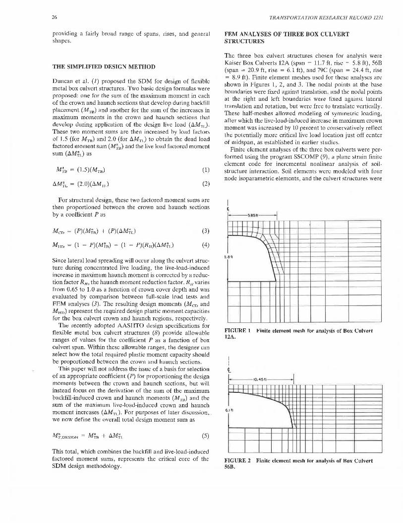
26

providing a fairly broad range of spans, rises, and general shapes.

THE SIMPLIFIED DESIGN METHOD

Duncan et al. (1) proposed the SDM for design of flexible metal box culvert structures. Two basic design formulas were proposed: one for the sum of the maximum moment in each of the crown and haunch sections that develop during backfill placement (Mm) and another for the sum of the increases in maximum moments in the crown and haunch sections that develop during application of the design live load (LlMTL). These two moment sums are then increased by load factors of 1.5 (for Mm) and 2.0 (for J'.lMTL) to obtain the dead load factored moment sum (Mia) and the live load factored moment sum (J'.lM{L) as

(1)

(2)

For structural design, these two factored moment sums are then proportioned between the crown and haunch sections by a coefficient P as

Meo = (P)(Mia) + (P)(J'.lM{,J

MHD = (1 - P)(M{8 ) + (1 - P)(RH)(LlM{d

(3)

(4)

Since lateral load spreading will occur along the culvert struc­ture during concentrated live loading, the live-load-induced increase in maximum haunch moment is corrected by a reduc­tion factor RH, the haunch moment reduction factor. RH varies from 0.65 to 1.0 as a function of crown cover depth and was evaluated by comparison between full-scale load tests and FEM analyses (3). The resulting design moments (Men and MHn) represent the required design plastic moment capacities for the box culvert crown and haunch regions, respectively.

The recently adopted AASHTO design specifications for flexible metal box culvert structures (8) provide allowable ranges of values for the coefficient P as a function of box culvert span. Within these allowable ranges, the designer can select how the total required plastic moment capacity should be proportioned between the crown am! haunch sections.

This paper will not address the issue of a basis for selection of an appropriate coefficient (P) for proportioning the design moments between the crown and haunch sections, but will instead focus on the derivation of the sum of the maximum backfill-induced crown and haunch moments (Mm) and the sum of the maximum live-load-induced crown and haunch moment increases (LlMTL)· For purposes of later discussion, we now define the overall total design moment sum as

(5)

This total, which combines the backfill and live-load-induced factored moment sums, represents the critical core of the SDM design methodology.

TRANSPORTATION RESEARCH RECORD 1231

FEM ANALYSES OF THREE BOX CUL VERT STRUCTURES

The three box culvert structures chosen for analysis were Kaiser Box Culverts 12A (span = 11.7 ft, rise = 5.8 ft), 56B (span = 20.9 ft, rise = 6.1 ft), and 79C (span = 24.4 ft, rise = 8.9 ft). Finite element meshes used for these analyses are shown in Figures 1, 2, and 3. The nodal points at the base boundaries were fixed against translation, and the nodal points at the right and left boundaries were fixed against lateral translation and rotation, but were free to translate vertically. These half-meshes allowed modeling of symmetric loading, after which the live-load-induced increase in maximum crown moment was increased by 10 percent to conservatively reflect the potentially more critical live load location just off center of midspan, as established in earlier studies.

Finite element analyses of the three box culverts were per­formed using the program SSCOMP (9), a plane strain finite element code for incremental nonlinear analysis of soil­structure interaction. Soil elements were modeled with four node isoparametric elements, and the culvert structures were

I t '-I --~05 1•------1

I I I 1 I I I l I I I I I / I -,

-11 ·~ \'\ ., \

\ ' \\ \ \

•. 811 \ \

\ \ \ \ \ 1

1

-'--

--

FIGURE 1 Finite element mesh for analysis of Box Culvert 12A.

I I I

t I· •0.4511---_,

I I I I I I I I I I I l I I I I I I I I I I

~ -r1-r -· -I

..... 6 .I ll

I 1 1

-

FIGURE 2 Finite element mesh for analysis of Box Culvert 568.

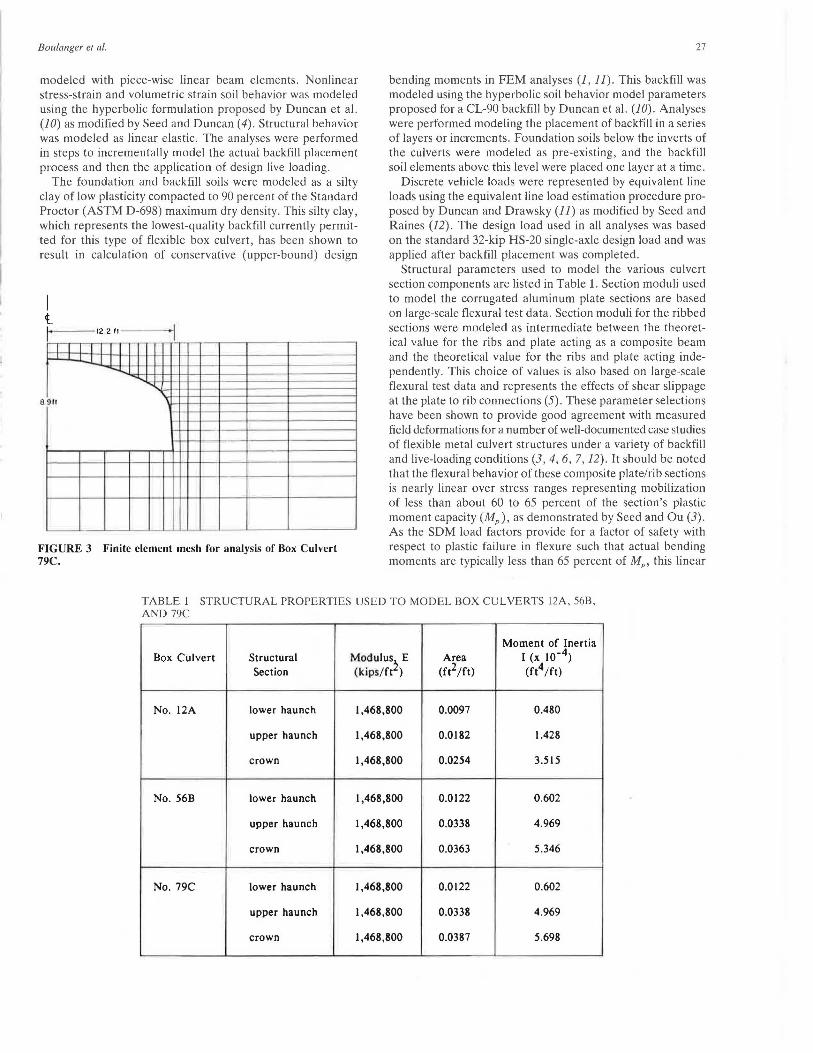
Boulanger et al.

modeled with piece-wise linear beam elements. Nonlinear stress-strain and volumetric strain soil behavior was modeled using the hyperbolic formulation proposed by Duncan et al. (10) as modified by Seed and Duncan (4). Structural behavior was modeled as linear elastic. The analyses were performed in steps to incrementally model the actual backfill placement process and then the application of design live loading.

The foundation and backfill soils were modeled as a silty clay of low plasticity compacted to 90 percent of the Standard Proctor (ASTM D-698) maximum dry density. This silty clay, which represents the lowest-quality backfill currently permit­ted for this type of flexible box culvert, has been shown to result in calculation of conservative (upper-bound) design

8

I t i-1- --12211----

I I I I I I I I I I I I I - I - ....

911

-

FIGURE 3 Finite element mesh for analysis of Box Culvert 79C.

27

bending moments in FEM analyses (1, 11) . This backfill was modeled using the hyperbolic soil behavior model parameters proposed for a CL-90 backfill by Duncan et al. (10). Analyses were performed modeling the placement of backfill in a series of layers or increments. Foundation soils below the inverts of the culverts were modeled as pre-existing, and the backfill soil elements above this level were placed one layer at a time.

Discrete vehicle loads were represented by equivalent line loads using the equivalent line load estimation procedure pro­posed by Duncan and Drawsky (11) as modified by Seed and Raines (12). The design load used in all analyses was based on the standard 32-kip HS-20 single-axle design load and was applied after backfill placement was completed.

Structural parameters used to model the various culvert section components are listed in Table 1. Section moduli used to model the corrugated aluminum plate sections are based on large-scale flexural test data. Section moduli for the ribbed sections were modeled as intermediate between the theoret­ical value for the ribs and plate acting as a composite beam and the theoretical value for the ribs and plate acting inde­pendently . This choice of values is also based on large-scale flexural test data and represents the effects of shear slippage at the plate to rib connections (5). These parameter selections have been shown to provide good agreement with measured field deformations for a number of well-documented case studies of flexible metal culvert structures under a variety of backfill and live-loading conditions (3, 4, 6, 7, 12). It should be noted that the flexural behavior of these composite plate/rib sections is nearly linear over stress ranges representing mobilization of less than about 60 to 65 percent of the section's plastic moment capacity (MP), as demonstrated by Seed and Ou (3). As the SDM load factors provide for a factor of safety with respect to plastic failure in flexure such that actual bending moments are typically less than 65 percent of MP, this linear

TABLE 1 STRUCTURAL PROPERTIES USED TO MODEL BOX CULVERTS 12A, 568, AND 79C

Moment of Inertia Box Culvert Structural Modulus E Area I (x 10-4)

Section (kips/ft2) (ft2 /ft) (ft4 /ft)

No. 12A lower haunch 1,468,800 0.0097 0.480

upper haunch 1,468,800 0.0182 1.428

crown 1,468,800 0.0254 3.515

No. 56B lower haunch 1,468,800 0.0122 0.602

upper haunch 1,468,800 0.0338 4.969

crown 1,468,800 0.0363 5.346

No. 79C lower haunch 1,468,800 0.0122 0.602

upper haunch 1,468,800 0.0338 4.969

crown 1,468,800 0.0387 5.698

28

structural modeling provides a good basis for the analyses performed as part of these studies.

EFFECTS OF IMPROVED FEM MODELING

The analysis procedures used in this study employ two minor improvements over the FEM modeling procedures used by Duncan et al. (1): (a) the nonlinear soil behavior model in this study provides improved modeling of the increased stiff­ness of a soil during unloading and reloading and (b) the section moduli of the ribbed culvert sections are reduced from

TRANSPORTATION RESEARCH RECORD 1231

the theoretical value for perfect composite action to account for shear slippage between the ribs and the plate. To inves­tigate the effects of these changes, analyses of the theoretical undeformed geometries of Box Culverts 12A, 56B, and 79C were performed using (a) the earlier FEM modeling tech­niques used by Duncan et al. (1) and (b) the improved mod­eling techniques described in the previous section.

The theoretical undeformed geometries of each of the three box culvert structures were analysed with three different amounts of final crown cover depth. The results obtained using the FEM techniques used in this study are listed in Table 2a and are plotted on Figures 4 and 5. The results obtained

TABLE 2 CALCULATED MAXIMUM BACKFILL-INDUCED MOMENTS AND LTVE-LOAD-INDUCED MOMENT INCREASES FOR THEORETICAL UNDEFORMED AS WELL AS DEFORMED BOX CUL VERT GEOMETRIES

A) Theoretical Undeformed Geometries:

FINITE ELEMENT METHOD SIMPLIFIED DESIGN METHOD

Span Cover Backfilling Due to HS-20 Factored< 1) Factored< 1 ) Depth Mee MHB AMcL AMHL MT,Design MTB AMTL MT.Design

(ft) (ft) (k-ft/ft) (k-ft/ft) (k-ft/ft) (k-ft/ft) (k-ft/ft) (k-ft/ft) (k-ft/ft) (k-ft/ft)

11.7 1.7 0.6 0.4 6.1 1.8 17.3 1.4 7.3 16.7 2.5 0.9 0.5 3.7 1.2 11.9 2.1 5.4 14.0 4.0 1.5 0.8 1.9 0.7 8.7 3.4 3.5 12.1

20.9 1.4 1.2 1.6 9.9 5.9 35.8 3.6 16.2 37.8 2.5 2.2 3.0 5.6 3.9 26.8 6.8 10.6 31.4 4.0 3.5 4.7 2.5 2.4 22.1 11.1 6.9 30.5

24.4 1.5 1.6 2.0 9.5 5.1 34.6 4.6 17.0 40.9 2.7 2.9 3.6 4.6 3.2 25.4 9.4 10.8 35.7 4.0 4.2 5.2 1.9 2.1 22.1 14.5 1.5 36.8

8) In-Place Deformed Geometries:

11.7 1.7 0.5 0.6 6.3 1.9 18.I 1.4 7.3 16.7 4.0 1.8 1.0 2.1 0.8 10.0 3.4 3.5 12.1

20.9 1.4 1.5 2.4 I 1.2 7.1 42.5 3.6 16.2 37.8 4.0 3.8 6.2 3.4 2.8 27.4 I I.I 6.9 30.5

24.4 1.5 1.8 2.7 9.8 5.4 37.2 4.6 17.0 40.9 4.0 4.6 6.5 2.4 2.3 26.I 14.5 7.5 36.8

C) Extrapolated Geometries from 2 x In-Place Deformations:

11.7 1.7 0.7 0.6 6.9 2.3 20.4 1.4 7.3 16.7 4.0 2.1 1.2 2.2 0.9 11.2 3.4 3.5 12.1

20.9 1.4 1.8 2.7 12.2 7.8 46.8 3.6 16.2 37.8 4.0 4.8 7.0 3.8 3.1 31.9 I I.I 6.9 30.5

24.4 1.5 3.1 4.9 8.8 6.1 41.8 4.6 17.0 40.9 4.0 5.1 8.1 3.9 2.7 33.0 14.5 7.5 36.8

D) Predicted Deformed Geometry Under HS-20 Loading:

11.7 1.7 0.6 0.4 6.2 1.8 17.5 1.4 7.3 16.7 20.9 1.4 1.2 1.5 11.5 6.8 40.7 3.6 16.2 37.8 24.4 1.5 1.9 2.3 10.4 5.6 38.3 4.6 17.0 40.9

(I) Load factors: 1.5 for backfill induced moments and 2.0 for live load induced moment increases, so that MT.Design = (!.S)(Mce + MHij) + (2.0)(6.McL + 6.MHL) ar MT.Design - (!.S)(MTB) + (2.0) (6.MTL).

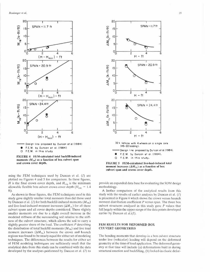
Boulanger et al.

20

- SPAN= 11.7 ft - 15 -...... --I 10 .:.!

m .... :2 5

2 4 6 ( H - Hmin) - ft

20

- SPAN= 20.9 ft -- 15 ...... --I 10 .:it! ~

m .... :2

00 2 4 6 ( H - Hmin) - ft

20

-- 15 ...... --I 10 .:.! ~m

.... :2 5

00 2 4 6

(H - Hmin) - ft

-- Design line proposed by Duncan et al (1984)

e FEM. by Duncan et al . (1984) 0 F.E .M. in this study

FIGURE 4 FEM-calculated total backfill-induced moments (Mm) as a function of box culvert span and crown cover depth.

using the FEM techniques used by Duncan et al. (1) are plotted on Figures 4 and 5 for comparison. In these figures, His the final crown cover depth, and Hmin is the minimum allowable flexible box culvert crown cover depth (Hmin = 1.4 ft).

As shown in these figures, the FEM techniques used in this study gave slightly smaller total moments than did those used by Duncan et al. (1) for both backfill-induced moments (Mm) and live-load-induced moment increases (~MTL) for all three culvert spans and all cover depths considered. These slightly smaller moments are due to a slight overall increase in the modeled stiffness of the surrounding soil relative to the stiff­ness of the culvert structure, which allows the soil to carry a slightly greater share of the load. The coefficient P describing the distribution of total backfill moments (Mm) and live load moment increases (~M rL) between the crown and haunch regions was found to be nearly equal for either set of modeling techniques. The differences between the results for either set of FEM modeling techniques are sufficiently small that the analytical data from this study can be combined with the data developed by the analyses performed by Duncan et al. (I) to

~ --...... --I ~ ~_,

.... :2 <l

-...... :::: -I ~

...J .... :2 <l

-...... :::: -I ~ ~

...J .... :2 <l

20

SPAN= 11.7 ft 15

10

5

00 2 4 6 H - ft

20

SPAN= 20.9 ft 15

10

5

00 2 4 6 H - ft

20

SPAN = 24.411 15

10

5

00 2 4 6 H - ft

32 k Vehicle with 4 wheels on a s ingle axle (HS-20 loadin9).

--Design line proposed by Duncan et al (1984).

• F. E M . by Duncan et al ( 19841.

0 F. E. M. in this study .

FIGURE 5 FEM-calculated live-load-induced total moment increases (.1Mn) as a function of box culvert span and crown cover depth.

29

provide an expanded data base for evaluating the SDM design methodology.

A further comparison of the analytical results from this study with the results of earlier analyses by Duncan et al. (1) is presented in Figure 6 which shows the crown versus haunch moment distribution coefficient P versus span. The three box culvert structures analyzed in this study gave P values that fall largely within the upper range of the data points developed earlier by Duncan et al.(1).

FEM RESULTS FOR DEFORMED BOX CUL VERT GEOMETRIES

The bending moments that develop in a box culvert structure under live (vehicular) loading will depend on the deformed geometry at the time of load application. The deformed geom­etry at that time will include (a) deformations built in during structural erection and backfilling, (b) locked-in elastic defor-

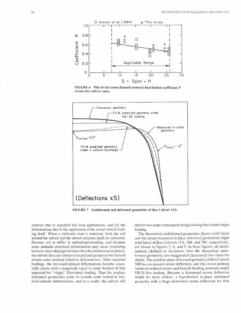
30 TRANSPORTA TION RESEARCH RECORD 1231

0 Duncan et al. (1984) 6 This study . 1.0

a.. 0.8

-c 0.6 Q)

u - 0.4 -Q)

0 u 0.2 Applicable Range

I ... 1

0 0 5 10 15 20 25 30

s = Span ft

FIGURE 6 Plot of the crown/haunch moment distribution coefficient P versus box culvert span.

Theoretical geometry

F.E,M. predicted geometry under HS- 20 loading

------llverticol =2 O"

F.E.M. predicted geometry under a uniform surcharge

(Deflections x 5)

Measured in-place geometry

Cl horiz . = I. 2 "

FIGURE 7 Undeformed and deformed geometries of Box Culvert 12A.

mations due to repeated live load applications, and (c) the deformations due to the application of the actual vehicle load­ing itself. When a vehicular load is removed, both the soil around the culvert and the culvert structure itself are unloaded. Because soil is stiffer in unloading/reloading, and because some inelastic structural deformations may occur (including inelastic shear slippage between the ribs and structural plates), the culvert does not return to its preload geometry but instead retains some residual locked in deformations. After repeated loadings, the live-load-induced deformations become essen­tially elastic with a magnitude equal to some fraction of that expected for "virgin" (first-time) loading. Thus the in-place deformed geometries come to include some locked-in live­load-induced deformations, and as a result, the culvert will

deform less under subsequent design loading than under virgin loading.

The theoretical undeformed geometries (heavy solid lines) and the actual measured in-place deformed geometries (light solid lines) of Box Culverts 12A, 56B, and 79C, respectively, are shown in Figures 7, 8, and 9. In these figures, all defor­mations (defined as deviations from the theoretical unde­formed geometry) are exaggerated (increased) five times for clarity. The actual in-place deformed geometry of Box Culvert 56B has an upward crown deflection, and this crown peaking results in reduced crown and haunch bending moments under HS-20 live loading. Because a downward crown deflection would be more critical , a hypothetical in-place deformed geometry with a large downward crown deflection for Box

Boulanger el al.

/

Measured in-place deformed geometry

l"heoretical undeformed geometry

- -..............

'

6 vertical = 4.0 "

F.E.M. predicted geometry under HS-20 loading

Hypathetica I in-place deformed geometry extrapolated from Box Culverts #62 B and # 79C.

31

A II jhatiz.=2.6

(Deflections x5} FIGURE 8 Undeformed and deformed geometries of Box Culvert 56B.

Theoretical geometry.

F. E.M. predicted geometry under HS -20 load ing.

6 vertical = 4 5"

F.E.M. predicted geometry under a uniform surcharge loading

Measured in-place geometry 6horiz.=3.0"

(Deflections x5)

FIGURE 9 Undeformed and deformed geometries of Box Culvert 79C.

Culvert 56B (span of 20.9 ft) was extrapolated from the meas­ured field geometric data for two similar box culverts (spans of21.8 ft and 24.4 ft) with large downward crown deflections . This hypothetical in-place deformed geometry is also shown in Figure 8.

The FEM results listed in Table 2b are based on the analyses of the actual in-place deformed geometries of Box Culverts 12A and 79C and the hypothetical (downward crown deflec­tion) in-place deformed geometry of Box Culvert 56B. At shallow cover depths, the effects of considering the in-place deformed geometries was to increase the overall calculated bending moments by 3 to 14 percent for the crown section, and by 15 to 28 percent for the haunch section relative to those calculated for the theoretical ·mdeformed geometries as summarized previously in Table 2a. These increases cor-

respond to increases in the calculated backfill-induced moment sum (M18) of 10 to 39 percent and the calculated live-load­induced moment increase sum (LlMTL) of 4 to 16 percent, resulting in an increase in the overall required total design moment sum (Mr.DESIGN) of S to 19 percent.

The deformations that resulted in the actual observed in­place deformed geometries of Box Culverts 12A and 79C are attributed largely to built-in deformations (initial erection of the box culvert structure with a nonideal theoretical unde­formed geometry) because the magnitudes of the measured lateral haunch movements would be enough to cause passive failure of the surrounding soil, which is an unlikely condition. To demonstrate this , FEM analyses were performed modeling backfilling of Box Culverts 12A and 79C to low final crown cover depths , and then subsequent modeling of the applica-

32

tion of massive uniform surcharges at the fill surface was performed to generate predicted deformed geometries with the same downward crown deflection as those measured in place. These predicted deformed geometries for massive applied uniform surcharges are also shown (with dashed lines) in Fig­ures 7 and 9. Surface surcharge magnitudes required to gen­erate the observed crown deflections were 2,400 psf for Box 12A and 700 psf for Box 79C. These large surcharges both represent more than two and a half times the allowable (design) surcharges for their respective culverts . Even with these exces­sively high surcharges, the predicted lateral movements of the upper haunches were much less than the measured field deflections, as shown in Figures 7 and 9.

Since the field measurements obtained for this study may not necessarily represent the worst cases of built-in defor­mations, deformed geometries were extrapolated to have two times the observed in-place deformations. These hypothetical doubly deformed geometries are expected to conservatively envelope the probable worst-case deflections likely for any acceptably installed flexible metal box culvert structure because the three in-place deformed geometries selected for analysis in these studies represent three structures that were among Lhuse fuunJ Lu have the la1ge~l deviations f10m theoretical design geometries among the 22 in-service structures mea­sured.

The FEM results for these doubly deformed geometries are presented in Table 2c. At shallow cover depths, the effect of these doubly deformed geometries was to increase overall calculated bending moments by 5 to 27 percent for the crown section and 36 to 50 percent for the haunch section relative to the moments calculated for the corresponding theoretical undeformed geometries . These increases correspond to increases in the calculated backfill-induced moment sum (Mm) of 30 to 250 percent, in the calculated live-load-induced moment increase sum (~MTd of 2 to 26 percent, resulting in an increase in the total factored moment sum (M T.DEsrGN) of 18 to 30 percent. It should be noted, however, that for box culvert spans and backfill cover depths where the deformations resulted in the largest increases in bending moments, the SDM design methodology fortuitously tended to provide generously con­servative estimates of moment for undeformed geometries. In addition, for those cases in which the backfill-induced moment sum increased most significantly , the contributions of the backfill moments to the overall design moments were relatively small. The net effects of these moment increases on the overall safety of the SDM methodology will be dis­cussed later in this paper.

Predicted deformed geometries for virgin HS-20 loading at midspan of Box Culverts 12A, 56N, and 79C, starting with theoretical undeformed geometries , are also shown (with dot­ted lines) in Figures 7 through 9. Again it may be observed that the predicted crown deflections are much smaller than the observed deviations of the measured field geometries from the ideal theoretical undeformed geometries. These FEM­predicted deformed geometries under centrally located HS-20 loading were then taken as the initial geometries for another set of analyses, the results of which are listed in Table 2d. This process is equivalent to a first approximation of the adverse effects of large-strain moments versus the moments calculated for undeformed geometries using the small-strain FEM for­mulation used in all previous studies discussed thus far. For

TRANSPORTATION RESEARCH RECORD 1231

shallow cover depths, the calculated bending moments were increased by 3 to 15 percent in the crown section and by 3 to 11 percent in the ha.unch section. These increases in bending moments represent the secondary moments (?-delta effects) for virgin loading of these box culvert structures. However , because the in-place (measured) deformed geometries already include some locked-in live-load-induced deformations, and the deformed box culverts are then somewhat stiffer for sub­sequent live load application, the effects of these secondary moments for the in-place deformed geometries would be smaller than those predicted for virgin loading of undeformed struc­tures. Accordingly, it was concluded that (a) this first approx­imation of the ?-delta effects was sufficiently accurate, and (b) these secondary ? -delta effects do not need to be consid­ered in combination with the deformed geometries considered in these studies, as these deformed geometries were already selected as representing near worst-case conditions.

The total backfill-induced bending moments and live-load-

20

- SPAN=117ft - 15 -' --I 10 .:!£ ~..,

.... ~ 5

2 4 6 (H - Hmin ) - ft

20

- SPAN= 20 9 ft - 15 ' --I .:!£ 10

"' .... ~

0 0 2 4 6

(H - Hmin) - ft 20

..... - 15 :::: -I 10 .:!£

"' .... ~ 5

0 0 2 4 6

(H - Hmin) - ft

-- Des ign line proposed by Duncan et al (1984)

0 Theoretical undeformed geometries

• In-place deformed geometries

• Deformed geometries with 2X the in-place de fo rrna l i oM

FIGURE IO FEM-calculated total backfill­induced moments (MTB) as a function of span and cover depth for undeformed and deformed geometries.

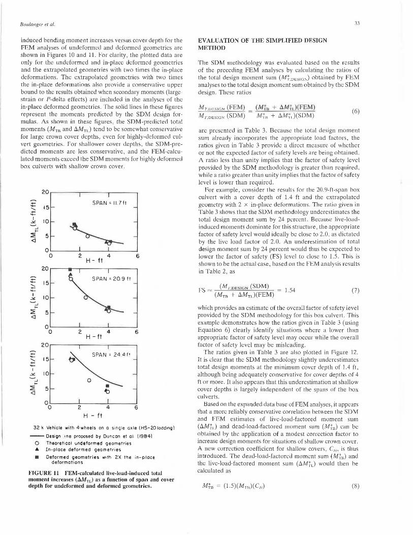
Boulanger et al.

induced bending moment increases versus cover depth for the FEM analyses of undeformed and deformed geometries are shown in Figures 10 and 11. For clarity, the plotted data are only for the undeformed and in-place deformed geometries and the extrapolated geometries with two times the in-place deformations. The extrapolated geometries with two times the in-place deformations also provide a conservative upper bound to the results obtained when secondary moments (large­strain or ?-delta effects) are included in the analyses of the in-place deformed geometries. The sol id lines in these figures represent the moments predicted by the SDM design for­mulas. As shown in these figures, the SDM-predicted total moments (Mm and AMTL) tend to be somewhat conservative for large crown cover depths, even for highly-deformed cul­vert geometries. For shallower cover depths, the SDM-pre­dicted moments are less conservative, and the FEM-calcu­lated moments exceed the SDM moments for highly deformed box culverts with shallow crown cover.

20

-...... - 15 ...... SPAN = 11 7 ft

...... -I 10 ~ -...J

I-

~ 5 <l

0 0 2 4 6

H - ft 20

...... SPAN= 20.9 ft - 15 ::::: -I 10 ~

-_, I-

~ 5 <l

0 0 2 4 6

H - ft 20

...... - 15 ...... SPAN= 24.411

--I ~ 10 -...J

I-

~ 5 <l

0 0 2 4 6

H - ft

32 k Vehicle with 4wheels on a sin gle axle (HS-20 loading)

-- Design line proposed by Duncan et al · (1984)

0 Theoretical undeformed geometries • In-place deformed geometries

• Deformed geometries with 2X the in-place deformations

FIGURE 11 FEM-calculated live-load-induced total moment increases (AMTL) as 11 function of span and cover depth for undeformed and deformed geometries .

EVALUATION OF THE SIMPLIFIED DESIGN METHOD

33

The SDM methodology was evaluated based on the results of the preceding FEM analyses by calculating the ratios of the total design moment sum (M~.DESIGN) -obtained by FEM analyses to the total design moment sum obtained by the SDM design . These ratios

M 7'.DESIGN (FEM)

M 7',DE SJGN (SDM)

(M·*a + AM~ 1J( E M) M~s + AM~L)(SDM)

(6)

are presented in Table 3. Because the total design moment sum already incorporates the appropriate load factors, the ratios given in Table 3 provide a direct measure of whether or not the expected factor of safety levels are being obtained. A ratio less than unity implies that the factor of safety level provided by the SDM methodology is greater than required, while a ratio greater than unity implies that the factor of safety level is lower than required.

For example, consider the results for the 20. 9-ft-span box culvert with a cover depth of 1.4 ft and the extrapolated geometry with 2 x in-place deformations. The ratio given in Table 3 shows that the SDM methodology underestimates the total design moment sum by 24 percent. Because live-load­induced moments dominate for this structure, the appropriate factor of safety level would ideally be close to 2.0, as dictated by the live load factor of 2.0. An underestimation of total design moment sum by 24 percent would thus be expected to lower the factor of safety (FS) level to close to 1.5 . This is shown to be the actual case, based on the FEM analysis results in Table 2, as

FS = (Mr.uEsI "' (SDM) = 1.54 (Mm + AMTL)(FEM)

(7)

which provides an estimate of the overall factor of safety level provided by the SDM methodology for this box culvert. This example demonstrates how the ratios given in Table 3 (using Equation 6) clearly identify situations where a lower than appropriate factor of safety level may occur while the overall factor of safety level may be misleading.

The ratios given in Table 3 are also plotted in Figure 12. It is clear that the SDM methodology slightly underestimates total design moments at the minimum cover depth of 1.4 ft, although being adequately conservative for cover depths of 4 ft or more . It also appears that this underestimation at shallow cover depths is largely independent of the spans of the box culverts.

Based on the expanded data base of FEM analyses, it appears that a more reliably conservative correlation between the SDM and FEM estimates of live-load-factored moment sum (AM;L) and dead-load-factored moment sum (M~8) can be obtained by the application of a modest correction factor to increase design moments for situations of shallow crown cover. A new correction coefficient for shallow covers, CH, is thus introduced. The dead-load-factored moment sum (M:~8 ) and the live-load-factored moment sum (AM;L) would then be calculated as

M~0 = (1.5)(MIB)( C11 ) (8)

34 TRANSPORTATION RESEARCH RECORD 1231

TABLE 3 COMPARISON OF TOTAL DESIGN MOMENT SUfvlS OBTAINED BY THE SDM METHODOLOGY AND BY FEM ANALYSES

MT,Design (FEM)

MT.Design (SOM)

Span Cover Theoretical In-Place Extrapolated Predicted Deformed Depth Undeformed Deformed Geometries from Geometry under

(ft) (ft) Geometries Geometries

11.7 1.7 1.04 1.08

2.5 0.85 --

4.0 0.72 0.83

20.9 1.4 0.95 1.12

2.5 0.85 --

4.0 0.72 0.90

24.4 1.5 0.85 0.91

2 .7 0.71 --

4.0 0.60 0.71

(9)

replacing Equations 1 and 2. The proposed value of C11 would decrease linearly from 1.15 (a 15-percent increase) at the minimum cover depth of 1.4 ft, to 1.0 at a cover depth of 3.5 ft, as shown in Figure 13. The proposed line for CH presented in Figure 13 is also overlaid for reference as a dashed line in Figure 12. As shown in these figures, the proposed correction coefficient CH ensures that the resulting modified SDM meth­odology provides an increased factor of safety for cases of shallow crown cover.

SUMMARY AND RECOMMENDATIONS

Nonlinear finite element analyses of flexible metal box culvert structures were performed after field measurements identified cases where in-service shapes differed from their ideal design shapes. This raised a question as to the actual factor of safety under full HS-20 design loads. Analyses were performed for undeformed and deformed box culverts with a range of spans and crown cover depths to investigate the influence of a num­ber of factors on required design moments. These factors included (a) load-induced deformations and in-place deformed geometries and (b) recent improvements in FEM modeling of flexible metal box culverts. These additional finite element analyses were then used to evaluate the Simplified Design Method (SDM) developed by Duncan et al. (1).

The current SDM methodology was found to slightly under-

2x In-Place HS-20 Loading Deformations

1.22 1.05

-- --0.93 --

1.24 1.08

-- --1.05 --

1.02 0.94

-- --

0.90 - -

estimate the total design moment sum for likely worst-case deformed geometries with shallow cover depths. Since the components of the total design moment sum form the basis for structural design, the SDM provided lower than desired factor of safety levels in these situations. Accordingly, a minor modification of the SDM is proposed to increase the required design moment capacities by an amount varying linearly from 15 percent at the minimum cover depth of 1.4 ft to 0 percent at a cover depth of 3.5 ft. This proposed modification involves the introduction of a new correction coefficient CH. The result of this relatively modest modification of the SDM is a slight increase in required design moment capacities for conditions of shallow cover. The new required design moment capacities provide a somewhat more conservative design for likely worst­case deformed box cuiveri geomeiries. it should be observed that while the structures evaluated had slightly lower factors of safety then originally predicted, these and other similarly deformed box culverts should continue to perform successfully.

ACKNOWLEDGMENT

Financial support for these studies was provided by Contech Construction Products, Inc., as well as by the U.S. National Science Foundation under Grant No. MSM-8451563. The authors also wish to express their gratitude to the engineers and field personnel of Contech Construction Products, Inc., who provided the field measurements of in-service box culvert structures.

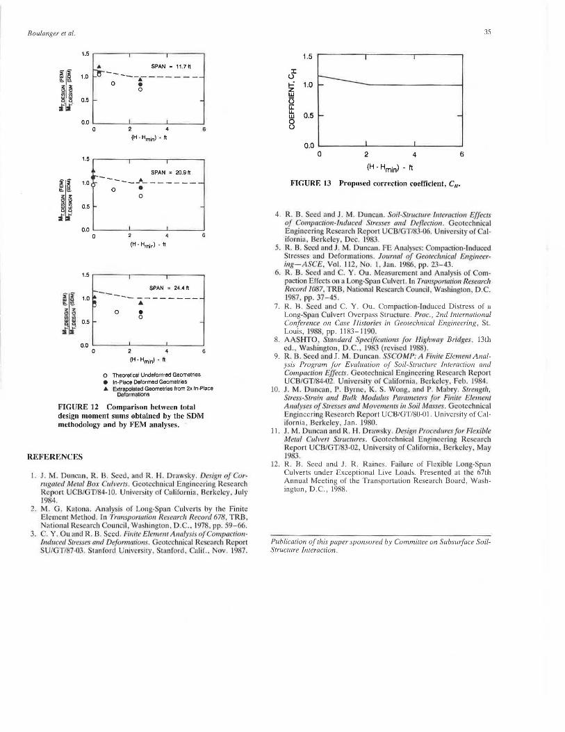
Boulanger er al.

~I 11 i i

1.5 ~---~---~---~

SPAN= 11 .711

-----.------ -0 •

0

a.a c__ ___ ..___ ___ _._ ___ _,

a 2 4 6

(H-Hminl - It

1.5 ,----..------.----~

1.a

a.5

SPAN = 20.911

-----·- - - - - - -0 •

0

a.a c__ ___ ..___ ___ _._ ___ _,

a

1.5

1.a

a.5

a.a a

2 4

(H · Hminl ·It

SPAN = 24.4 It ----- --------... 0 • 0

2 4

(H · Hm1nl · ft

o Theoretical Undeformed Geometries • In-Place Deformed Geometries

6

6

A Extrapolated Geometries from 2x In-Place Delcrmatlons

FIGURE 12 Comparison between total design moment sums obtained by the SDM methodology and by FEM analyses.

REFERENCES

I. J . M. Duncan. R. B. ectl, and R. IL Draw ·ky. De ig11 of "or­l'llgated JWl!ta/ Bo.~ 11 /ven . . Geo1echnicaJ Engi neering Rcscnrch Report UCB/ T/84·IO. University of alifornia, Berkeley. July 1984.

2. M. G. Kmon:i. Analy i of Long-Span \1lvens by 1he Finirc Elemcm Method . In Transportation Rese11rcli Uecol'<I 678, TRB, Nati nal Research ouncil Wa hingrun, D . .. 197 , pp. 59- 66.

3. . Y. Ou 1111d R. B. ·eed. Finite £/eme1111\1111/ysis oj ompaction· l11d11ccd tre.ues a11d Defomu11io11s. cotcchnical Research Report SU/GT/87-03. 1aaford Univcr ·ity. Srn nford, al if .. Nov. L987.

35

1.5

:c (.)

~ 1.0 w G u:: u.. 0.5 w 0 (.)

0.0 0 2 4 6

(H · Hminl ·ft

FIGURE 13 Proposed correction coefficient, Cn.

4. R. 13 . ccd and J . M. Duncan. Soil-S1rnct11re li11emctio11 Effects of omp11ction-l11duccd Strl'sscs and Deflec1ion . Gcotcchnical Engineering Research Report UCB/GT/83-06. Universi ty of al­if rnia, Ucrkcl y, Dec. l9 3.

5. R. B. Seed and .I . 1. Du ncan. F Analyses: ompaction-lnducccl tresses and Deformations. Journ(lf of G1:otec/111ica/ £11ginecr­

illg-l\SCE. Vol. 112. No . .I . Jan. 1986, pp. 23-43. 6. R. B. ced and . Y. Ou. Measurement and Analy i of om­

puction Effects on a Long-Span ulvcrt. Jn Transport(lfion Research Record 1087. TRB, ational Resc<irch ou nci l, Wa hington. D. . 1987. pp. 37-45.

7. R. B. 'ccd and C. Y. Ou. Compac1ion-lnduced Distress of a Long-Sp n ulvert Overpass Structure. Proc., 2nd lnlemalional Conference on Case Histories in Geo/echnical Engineering, St. Louis, 1988, pp. 1183-1190.

8. A HTO .. wnd1wd Specificmio11s for Highway Bridges, 13th eel .. Washington, D .. , 19 3 (revised 19 ).

9. R. 13 . ccd and J. M. Duncan. S. · .OMP: A Fiuite Ele111a111 Anal­ysis Program for Evaluation of Soil-Structure Interaction and Compaction £/Jeers. eotcchniciil Engineering Research Report U B/GT/84-02. nivcr ity of C1l ir rnia , Berkeley. Feb. 19 4.

10. J. !. Duncan, P. Byrne, K .. Wong, ind P. Mabry. S1rei1gtli, Stre.u-Strain am/ Bulk Mod111i1J Pm·1111111tcrS Ji r finite Elemc111 Aualyses of Stresses a11d Move111e111s in. oil M11s~·11s. Gcotechnical Engineering Research .Report UCB/GT/80-01. University of Cal­iforn ia, Berkeley, Jan. 19 0.

11. J.M . Duncan and R. M. Draw ky. Design Proc<:dure for Flexible Me/(// C11/ver1 1ruc111res. eotcchnical Engineering Re carch .Report UCB/GT/83-02, University of nlifornia. IJerkcley. May J983.

12. R. B. Seed and J . R. Raines. Failure of Flexible Long-Span Culverts under Exceptional Live Loads. Presented at the 67th Annual Meeting of the Transportation Research Board, Wash­ington, D.C., 1988.

Publicalion of this paper sponsored by Commiuee on Subsurface Soi/­Structure Interaction.

36 TRANSPORTATION RESEARCH RECORD 1231

Performance of Yielding Seam Structural Plate Pipe Culvert

EARLE w. MAYBERRY AND MARK A. GOODMAN

During project development for construction of Interstate 94, north­east of Miles City, Montana, several alternatives were evaluated regarding perpetuation of two large drainages under extensive fills. The alternative selected consisted of installing two structural steel plate culverts. These culverts used the yielding seam concept to relieve the load on the structure by providing controlled slippage in the longitudinal lapped seams. The subsequent reduction in pipe circumference would allow the soil to carry a portion of the load, therefore allowing a reduction in plate thickness and material savings as compared to a conventionally designed structure. Use of this product, relatively new to highway construction applications in 1983, was approved as an experimental feature. Experimental status required preparation of an acceptable work plan, including monitoring of fill settlements, fill pressures, pipe diameter changes, and strain gauge measurements. The purpose of this experimental feature was twofold. First, a reduction in plate gauge was intended to reduce pipe material costs, yet still provide a structurally sound installation. Second, it would be beneficial to monitor and obtain measurements of earth pressures generated in highway fills of this nature. The measurements would allow comparison of actual fill pressures generated versus design pressures as computed by stan­dard methods and procedures. Additionally, information regard­ing settlement of foundations under high fills, pipe strain mea­surements, and pipe diameter changes could be obtained. Reduction in vertical loads was realized as a result of seam slippage, and the installations have performed as expected and as designed. A dis­cussion of the site and installation, instrumentation procedures and observations, and data obtained and recommendations for future projects of this nature are contained within.

The Montana Department of Highways became involved with th potential use of yield ing seam pipe in 1979. It had become apparent that constructi n of a portion oflntcrs1a1 94, nonb­ea t of Miles ity, lontana. would pose unusual structural and cost requirements for the culvert installations at two sites due to extremely high roadway fills.

A relatively new culvert product, Key-Hole Slot, which incorporated the feature of yiel ling eams, offered potential plate-gauge and co"t ic du~ti'""n :; over conventionally designed multiplatc pipe and was proposed for use. Bridges w re also con idcrcd, but cost were thought to be excessiv due t fill heights .

The first installation was a 12.5-ft-diameter structural plate pipe located under 78 ft of cover in 1he pring reek drainage at plan cation I ()2- + 05. The Spring reek cul e rt required a plate thicknes of 0.18 -i n. (7-gauge) utilizing tbe yie lding ·cam concept. By comparison a conventionall y designed structure, using design criteria as published by the Federal

Montana Department of Highways, 2701 Prospect Avenue, Helena, Mont. 59620.

Highway Administration (1), would exceed recommended fill height requirements for 0.280-in . (1-gauge) steel.

The second installation was a 15.0-ft-diameter structural plate pipe located under 45 ft of cover in the Deep Creek drainage at plan Station 1201+10. The Deep Creek instal­lation required a plate thickness of 0.138-in. (10-gauge) using the yielding seam concept , while a conventionally designed structure would have required a plate thickness of 0.249-in. (3-gauge) steel.

At both pipe locations , the natural foundation materials consisted of loose silt overlying sandstone stringers and shale. The loose silt and sandstone stringers were removed to a depth of 5 ft and a width equal to three pipe diameters. The area was then backfilled with A-2-4 material to provide a foun­dation of uniform quality and density. Backfill for both pipes consisted mainly of sandy silt to silty, sandy gravel derived from local Yellowstone River terrace deposits.

The water table at Deep Creek was 3 ft below the ground line; however, at Spring Creek, the water table was at the surface. Fabric-wrapped cut-off drains were installed west of this pipe to provide free drainage within the pipe foundation.

Backfill procedures for Key-Hole Slot pipe are the same as for any structural plate installation. Proper foundation prep­aration and backfilling procedures must be followed.

Erection of the Key-Hole pipe is the same as for conven­tional multiplate pipe. Proper positioning of the plates in relation to each other is controlled as the slotted portion is smaller than the bolt and will allow the bolt to enter the slot only under significant load. This is the self-indexing controlled slippage design (Figure 1) .

The workhours required to assemble the Key-Hole Slot pipe were similar to those required for a conventional mul­tiplate structure. Erection costs may have been reduced over a conventional installation due to increased ease of handling of lesser gauge plates.

Contract bid prices of $400/ft and $500/ft were made by the low bidder for the Spring Creek and Deep Creek pipes, respectively. These prices included all costs associated with pipe materials, coating, pipe erection, and pipe inspection by the suppliers' representative.

Comparison of the Key-Hole Slot multiplate design with the design of a conventional multiplate structure indicates a material savings of about 198 lb/ft or a total savings in excess of 78,000 lb for the Spring Creek structure and a materials savings of 285 lb/ft or a total of 85,000 lb for the Deep Creek structure.

During construction, conditions warranted excavation of the proposed foundations to a three-pipe-diameter width to

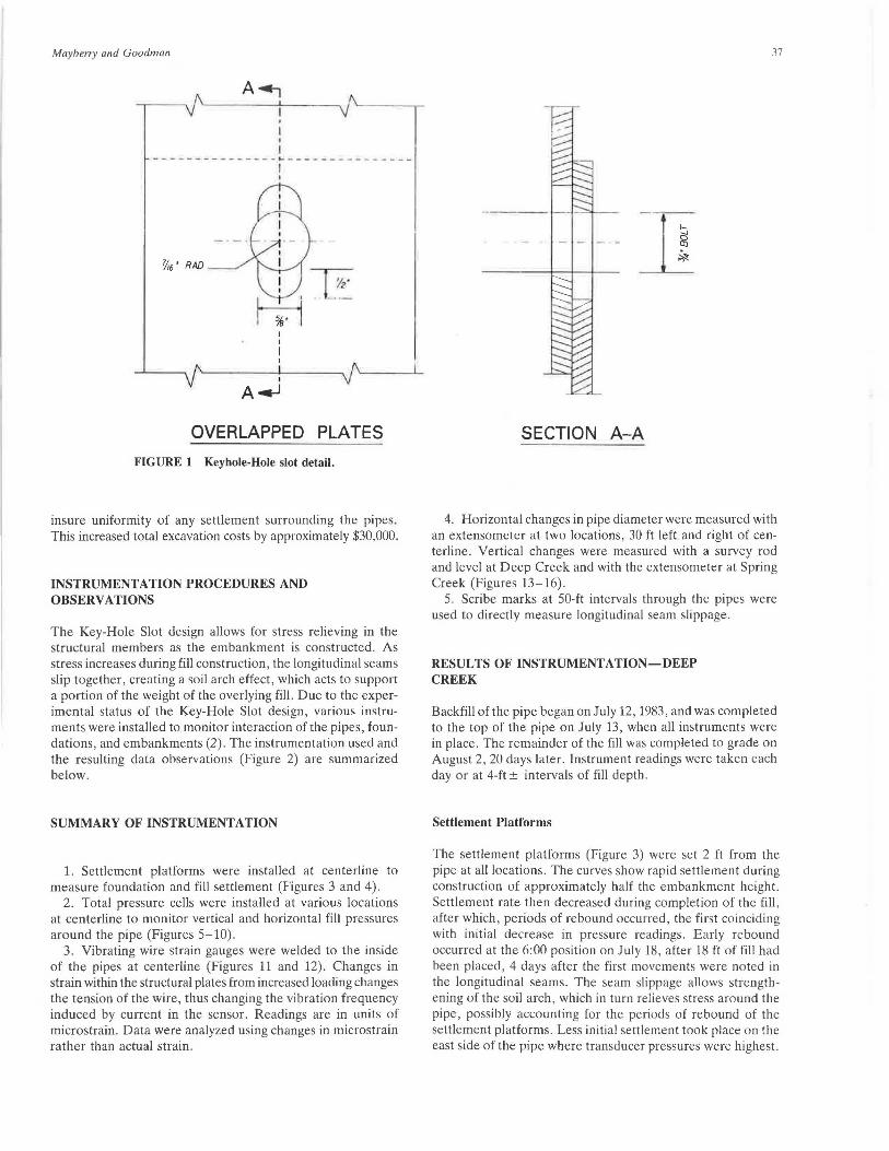
Mayberry and Goodman

- - - - - ----- ----- ~ - -- - -- -- - -~ - ---

' '

'./,6' RAlJ

I

A.-J

OVERLAPPED PLATES FIGURE 1 Keyhole-Hole slot detail.

insure uniformity of any settlement surrounding the pipes. This increased total excavation costs by approximately $30,000.

INSTRUMENTATION PROCEDURES AND OBSERVATIONS

The Key-Hole Slot design allows for stress relieving in the structural members as the embankment is constructed. As stress increases during fill construction, the longitudinal seams slip together, creating a soil arch effect, which acts to support a portion of the weight of the overlying fill. Due to the exper­imental status of the Key-Hole Slot design, various instru­ments were installed to monitor interaction of the pipes, foun­dations, and embankments (2). The instrumentation used and the resulting data observations (Figure 2) are summarized below.

SUMMARY OF INSTRUMENTATION

1. Settlement platforms were installed at centerline to measure foundation and fill settlement (Figures 3 and 4).

2. Total pressure cells were installed at various locations at centerline to monitor vertical and horizontal fill pressures around the pipe (Figures 5-10).

3. Vibrating wire strain gauges were welded to the inside of the pipes at centerline (Figures 11 and 12). Changes in strain within the structural plates from increased loading changes the tension of the wire, thus changing the vibration frequency induced by current in the sensor. Readings are in units of microstrain. Data were analyzed using changes in microstrain rather than actual strain.

37

SECTION A-A

4. Horizontal changes in pipe diameter were measured with an extensometer at two locations, 30 ft left and right of cen­terline. Vertical changes were measured with a survey rod and level at Deep Creek and with the extensometer at Spring Creek (Figures 13-16).

5. Scribe marks at 50-ft intervals through the pipes were used to directly measure longitudinal seam slippage.

RESULTS OF INSTRUMENTATION-DEEP CREEK

Backfill of the pipe began on July 12, 1983, and was completed to the top of the pipe on July 13, when all instruments were in place. The remainder of the fill was completed to grade on August 2, 20 days later. Instrument readings were taken each day or at 4-ft ± intervals of fill depth .

Settlement Platforms

The settlement platforms (Figure 3) were set 2 ft from the pipe at all locations. The curves show rapid settlement during construction of approximately half the embankment height. Settlement rate then decreased during completion of the fill, after which, periods of rebound occurred, the first coinciding with initial decrease in pressure readings. Early rebound occurred at the 6:00 position on July 18, after 18 ft of fill had been placed, 4 days after the first movements were noted in the longitudinal seams. The seam slippage allows strength­ening of the soil arch, which in turn relieves stress around the pipe, possibly accounting for the periods of rebound of the settlement platforms. Less initial settlement took place on the east side of the pipe where transducer pressures were highest.

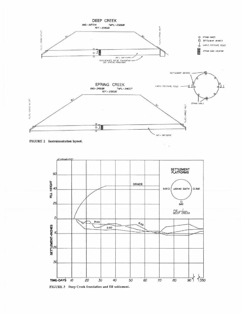
I''

DEEP CREEK GND.• 227379 TllPL· 2J2/J.IJO

REF.• 2340lXJ

180' x JOO' SSPPC _./' ~ SUB-EXCPVATE 5UOF FOUNDATION ___...,.­

SEE SPECIAL PROllSIONS

SPRING CREEK GND. • 2400.98 T llPL. • 248377

REF.• 2500lXJ

oJ

FIGURE 2 Instrumentation layout.

!c !2 w ::c :I u:::

Cl) w

~ ;! z w

I

Tl

L!:',,.,,,,_.,,~,e,.

er

411 ·

zr,

0

f(

2r

3'

ME-OAYS 10

GRADE ,,..,-

/ /

I \v ~ 9:00

- fl:oo ---'-----v 3:00 ---~~ --

20 30 40 50 60

FIGURE 3 Deep Creek foundation and fill settlement.

0 STRNN G-'GES

0 SETTL£11E/ff DEVICES

l EARTH PRESSURE CEUS

' I STRNN G-'GE LOCIV/ON

EARTH PRESSLJRE CEUS

STRNN G-'GES

15[/ A 396' SSPPC

SETILEMENT PLATFORMS

~DeD~ D

61)()

FIG-1-

DEEP CREEK

~ ~ _,...--

70 BO 90 1~ ~ 50

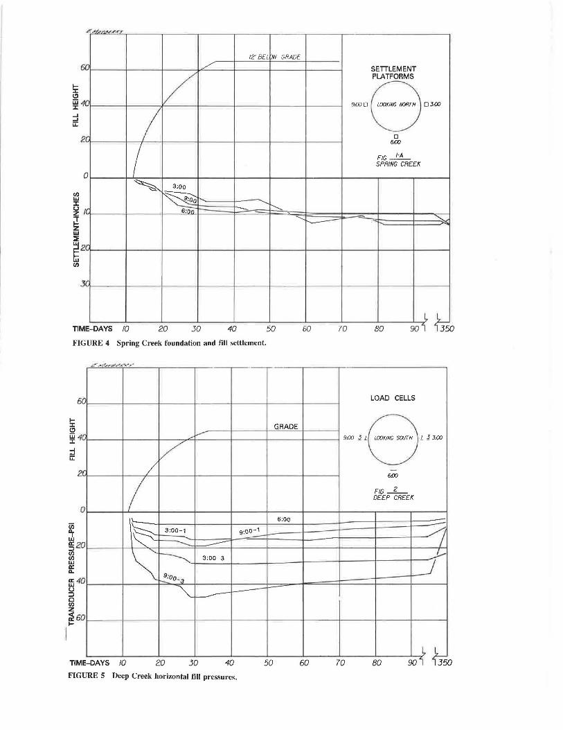
i

ffi :::c u z ~ w ~

£. ..J..4#~-.1 .... ~,.e.<Y'

6 r,

r.

'( 2

0

r(

'( ~2 (/)

'( 3

I I ~

12' BEL DW GRADE

/

v 3:oo

1~"0--- . ..........,

s:on - :---...... .......... -

TIM E-DAYS 10 20 30 40 50 60

FIGURE 4 Spring Creek foundation and fill settlement.

6 0

'O

•r. 2

0

ii5

~ 0 !52

(/) (/) w a: II..

0

~ ',r71'i"~.<'

/

I \'--

-~ ""-

\:

·- -

,,,i.---

v

3:00-1 9:00-1 --~ --------...,. 3:00 3

..!_:00,3

GRADE

6:00

ffi4 u ::::> c (/) ""- i-----~ z ~6 0 t-

TIM E-OAYS 10 20 30 40 50

FIGURE 5 Deep Creek horizontal fill pressures.

60

SETILEMENT PLATFORMS

9iXJO LOOKING NOffTH OJ.00

0 6:00

FIG_!±_ SPRING CREEK

~ "-

70 80 90 i~ fJs 0

LOAD CELLS

9iXJ J 1 LOOKING SOIJT H 1 J J.00

-6:00

FIG-2-DEEP CREEK

--~ J-

-:_;

70 80 90j~ ~ 50

/.....,.-1.,..l"L.---

12' BEL p.v GR/llJE

;n 6

4n

2r

0 ii> ~ a:

m40 w a: ll..

a: w u :J 0 en z

EJfl

~I 20

TIM E-OAYS 10

_,,/---

/ I I ~~ \~

........... 9:00-1

............ .......... 9:00-3

20 30 40

FIGURE 6 Spring Creek horizontal fill pressures.

~ A. ,,_4.,,,,.,._,,,,,,,..~.,,,,.

60

.di'".

2r

0

~ a: :J (/) (/) w a: ll..

20

a: g 40

c ~ ~ 60

Tl ME-OAYS

/ /

I ~

------ -3:00 4

10 20

/;,..-

30 40

FIGURE 7 Deep Creek vertical fill pressures.

3:00-2

50

I

GRADE

12:00

50

LOAD CELLS

9:00 WOKING NORTH - -JI

FIG~ SPRING CREEK

-............

~

60 70 80 90jl ~ 0

LOAD CELLS 12:00 -

9:00 LOOKINfJ S()(fT H I I J,()Q 24

6:00

FIG-3-DEEP CREEK

_......, :::--

60 70 80 90'1L ~ 0

Mayberry and Goodman

'A'l'.b'. ~A' -~·- --- --- --- -

!i: (!) jjj ::c ::I u::

5r:

IJf'.

2r

0

40

ar.

20

TIME-DAYS /0

I/ v

I I ~ 9·o ~ ~" -~

•-v-2

s:oo

20 30 40

FIGURE 8 Spring Creek vertical fill pressures .

.J."f".~_..,.....,.""-... ~ .. ~.i""

!i: (!) jjj ::c ::I u::

60

40

2r.

0

0

40

60

TIM E-OAVS 10

-.,,.-

/ /

I ~ ~

-----

20 30 40 FIGURE 9 Deep Creek vertical fill pressures.

12.' BEL rM' GRADE

- ----::iO

GRADE

9:00-2

9:00 4

50

41

LOAD CELLS

9,00 I LOOKING NORTH I J..oo I 2 2

-6:00

FJG--2L SPRING CREEK

" ~

60 70 80 90 i~ {Ts 0

LOAD CELLS /2{X)

="8 J:OO 4 2

6{X)

FIG - 4-DEEP CREEK

__..,..,

___.,.

60 70 80 90 i~ {Ts 0

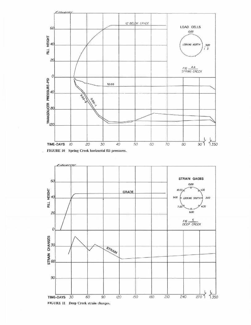
~ (!) iii ::c ...J ...J u:::

if iL a: :::> Cl.I Cl.I w f a: w (.)

5 Cl.I z

,..,.,,,..,,,.._..,,,...,.,,,e,,

i::.1·

dr

2.1".

0

40

ar:

~I 20

Tl ME-DAYS 10

12'Ba tM' GRADE /.-'

/ I I

~ r--... 12:00

<?;,~

~ o'.;

',.

" ~ ~

20 30 40 50 60

FIGURE 10 Spring Creek horizontal fill pressures.

Cl.I w

~ 5 z

~ Cl.I

50

4[1

2r

0

30

60

90

,,,...;,,,,,,,,..e'<<.,,,....

r.R.11.ni:

f

I I ~ /'....

I 'V ""'- .s.,.,

~ ....

LOAD CELLS /2.{)(] -

8-~ I J

FIG~ SPRING CREEK

""

~ ~

70 80 90i~ ~ 0

STRAIN GAGES

/2.{)(]

/(),JI) /:JO

9.-00 l.IXJKING SOIJT"H J{)(J

1(JO 4:30

6.-00

FIG-5-DEEP CREEK

270i ~ ME-OAYS 30 60 90 120 150 180 210 240 TI 0

FIGURE 11 Deep Creek strain changes.

ff,,..,,,,.,.,,,,r,;e.--

12' BE OW GAAi ~E _,/ /

r:;r. ~

"" I 2r I 0 I

30 \ 6G \

\.. 1-.. STRAIN

\

(/)

i u z

~

90

TIM E-DAYS 30 60 90 120 150 180 210

FIGURE 12 Spring Creek strain changes.

~ :c (!) w :c :::l u:::

6f1

4fl

2r

0

(/) . w 1.0

0 z

~ !z § IC 0 :c .

0

/[)

~ ~~~ -"';,.-,.. ,_

,,,i.......-

v /

I~ ~ 30' Rt . CL

\ f.J'\j 30 ' Lt . CL

\

GRADE

,,,.

STRAIN GAGES

12.00

JO..JO 1:30

-9.00 /.001(/NG //OffrH 3:00

MO 4:JO

6.<XJ

FIG~ SPRING CREEK

240 2701~ ~ 0

PIPE DIAMETER CHANGES

8 F/G_6_

DEEP CREEK

~

90jl ~ ME-DAYS 10 20 JO 40 50 60 70 80 Tl 0 FIGURE 13 Deep Creek horizontal diameter changes.

5r.

40

2/.

0

.0 (/)·2 w :c u z "T

~ 0

§ IC 0 :c.z .0

~

Tl ME-DAYS

~,,

'

10

12' BEL M' GRADE

/ v I

v--: 30' Rt. CL.

y l O' Lt. Cl.

20 30 40 50 60

FIGURE 14 Spring Creek horizontal diameter changes.

...-; w4",..._..,~~-""

r: 6

GRADE

·r. ,,, ......--

/ •r. 2 /

0 I .o

0 /~ v \...__

~ ao· ~ r---30' Lt. CL r---......

0

TIM E-DAYS 10 20 30 40 50 60 FIGURE 15 Deep Creek vertical diameter changes.

DIAMETER CHANGES

8 FIG~

SPRING CREEK

70 80 90IL fu 0

PIPE DIAMETER CHANGES

EB FIG-7-DEEP CREEK

70 80 90{ ~ 0

Mayberry and Goodman 45

~~,,.~~~.,

12' BEL iJW GRADE

6n ./

4(] v 2r, I 0

.0 /\

JV \ CL.

0 J --.0

TIM E-DAYS 10 20 30 40

FIGURE 16 Spring Creek verlical diameler changes.

However, 56 days after fill construction began, all positions neared unity with 10 ± in. of total settlement. Major rebound then reoccurred, especially at the 6:00 position, after which unity was again attained by October 6. No readings were taken between October 6 and March 1984, as readout terminals had to be moved to allow placement of riprap . Final readings , taken on July 17, 1984, show an average final settlement of 8± in.

Total Pressure Cells

Cells 3:00-1 and -2 and 9:00-1 and -2 are set 1 ft from the pipe. Cells 3:00-3 and -4 and 9:00-3 and -4 are set 3 ft from the pipe. The pressure curves (Figures 5, 7, and 9) show the following :

1. Fill pressures 3 ft from the pipe are normal for the height of fill, although transducer pressures are generally higher on the east side of the pipe (9:00 position). Lower pressures were evident 1 ft from the pipe.

2. Horizontal pressures are lower at all positions than are vertical pressures.

3. Pressures increased proportionately as fill height increased, and response of the pressure cells is almost immediate to changes in time/rate of fill placement.

4. Pressure relief began immediately after completion of the fill and continued through July 17, 1984, when the last readings were taken.

DIAMETER CHANGES

E8 FIG~

SPRING CREEK

'

""

~ 50 60 70 BO 90 i 35 0

Strain Gauges

Two strain gauges (Figure 11) were installed at each desig­nated clock position, one each in the valley and the crest of the corrugations. Because of late delivery of the indicator, zero readings were not obtained. Readings were begun on July 26, after 36 ± ft of fill had been placed. This reading was then assigned zero, and the time/strain rate curve shows only the relative strain changes. To best interpret strain, readings for each day were averaged to provide the time/strain curve .

The peak strain coincided with maximum fill pressures at completion of the fill. As transducer pressure began to fall off, strain fell rapidly until August 9, then increased until September 2, after which strain fell off again until mid-Sep­tember. This period of decrease also coincides with the gen­eral change in slope of the pressure curves.

Subsequent readings show another period of strain increase from September 13 through November 2, then a long period of decrease through July 17, 1984, when the last readings were taken.

Pipe Diameter Changes

During backfill of the pipe and construction of the fill, several minor adjustments in horizontal and vertical dimensions were noted (Figures 13 and 15) . Before completion of the fill, 15 days after backfill began, horizontal dimensions stabilized. Vertical rise increased slightly, then progressively decreased

46

due to seam slippage, starting 7 days after fill operations began or at 21 ft of fill over the pipe (20 ± psi) .

RESULTS OF INSTRUMENTATION-SPRING CREEK

Backfill of this pipe began on September 9, 1983, and was completed to the top of the pipe on September 13. The fill was then constructed to a height of 63 ft by October 5, 22 days later. Approximately 12 ft of fill remained to reach grade. Instrument readings were taken each day or at 5 ft± intervals of fill depth.

Because of failure of several strain gauges placed in the valleys of the pipe corrugations at Deep Creek, only one gauge was placed at each clock position between the valleys and crests at Spring Creek. In addition, the vertical pressure cells at 3:00-4 and 9:00-4 were eliminated because they were not believed to be essential in the fill pressure analysis. The remaining instruments were placed exactly as at Deep Creek.

Settlement Platforms

Initial settlement rate continued high until the fill height reached 55 ft, when the rate decreased (Figure 4); whereas at Deep Creek settlement, the rate decreased after approximately 20 ft of fill were placed. The last readings on July 17, 1984, show an average settlement of 12 ± in.

Total Pressure Cells

Pressure relationships around the pipe are generally similar to those at Deep Creek except that pressure curves are abnor­mally high at 3:00-1 and -3 and 9:00-1 and -1 (Figures 6, 8, and 10). In addition, at the 3:00 position, where pressures were highest, the 1 and 3 cells show nearly identical readings, which is not the case at Deep Creek. The high fill pressures at the sides of the pipe could be caused by excessive com­paction of the backfill and/or the rate of fill construction. At Deep Creek, 45 ft of fill were placed over a 20-day period. At Spring Creek, 63 ft of fill were placed over a 22-day period, or nearly one-third more fill was placed in the same time span. Little pressure relief took place around the pipe between October 1983 and February 1984 when fill construction began once again. Pressures then increased around the pipe and remained high through July 17 , 19114, when final readings were taken.

Strain Gauges

The time/strain curve is nearly proportional to the time/fill height curve (Figure 12). However, strain remained constant through February 1984, with only a minor decrease. Strain increased during completion of the fill in 1984, after which some decrease occurred through July 1984.

Pipe Diameter Changes

Unlike the pipe at Deep Creek, which, after initial adjust­ments, returned to the original horizontal diameter 15 days

rnANSPORTA TION RESEARCH RECORD 1231

after backfill began, the Spring Creek pipe (Figures 14 and 16) remains about 2 in. less than the original horizontal diam­eter. Vertical rise first increased then decreased exactly as the Deep Creek pipe did, after 23 ft of fill were in place over the pipe. However , the rise increase was more than 2 in. as com­pared with .25 in. at Deep Creek.

Photos of the various stages of construction are included in Figures 17-24.

CONCLUSIONS

Comparison of the data obtained from the instrumentation and seam slippage survey at Deep Creek indicates the soil arch began to form after the embankment reached a height of 10 to 15 ft over the pipe. The period of strain change , change in slope of pressure, and settlement rebound suggest the soil arch forms by a series of dynamic adjustments through construction until about 40 days after fill completion. There­after , long-term adjustment takes place over a period of sev­eral months.

FIGURE 17 Pipe assembly on preshaped bed at Deep Creek.

FIGURE 18 Backfill operation at Deep Creek.

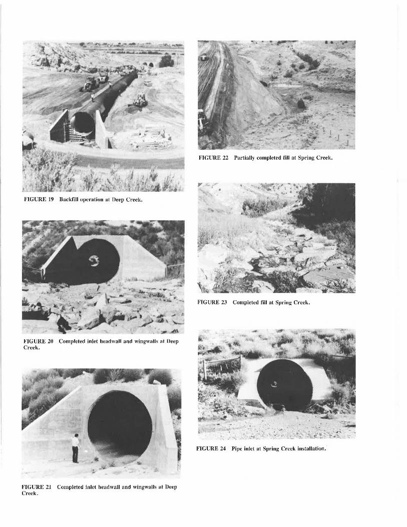
FIGURE 19 Backfill operation at Deep Creek.

FIGURE 20 Completed inlet headwall and wingwalls at Deep Creek.

FIGURE 21 Completed inlet headwall and wingwalls at Deep Creek.

FIGURE 22 Partially completed fill at Spring Creek.

FIGURE 23 Completed fill at Spring Creek.

FIGURE 24 Pipe inlet at Spring Creek installation.

48 TRANS PO RTATION RESEARCH R ECORD 123 1

TABLE 1 VERTICAL LOAD REDUCTION AT 9:00, 12:00, AND 3:00 POSITION

Fill P,. Height Calculated P, Actual, Day 60 Percent

Location (ft) (PSI) (PSI) Reduction

Deep Creek 59.4 12:00 41 37.0 15.0

9:00-1 48.5 43 .8 11.0 74.8 3:00-1 48.5 43.8 15.U 6':J .7

Spring Creek 12:00 63 56.9 23.0 59 .5 9:00-1 69.5 62.7 73.0 NIA 3:00-1 69.5 62.7 34.0 45.7

NoTE: P, = vertical fill pressure. Fill height measured to appropriate load cell.

At Deep Creek, the high transducer pressures at the 9:00 position show the greatest total decrease (75-percent aver­age). This was also the area of greatest seam closure and initial strain increase. However, at Spring Creek, instrumen­tation shows little indication of similar stress relief, although seam slippage has been normal.

At both locations, backfill along the pipes was brought halfway up to where the 3:00 and 9:00 pressure cells and settlen1ent platforms were installed . In both cases , instru­ments were placed on the east side of the pipes first, after which backfill along that side of the pipe was resumed while installing instruments on the west side. Substantial backfill was placed during this period on the east sides before backfill resumed on the west sides. It should be noted that fill pres­sures and final settlement were always higher on the east side of the pipes. No explanation for this condition is offered.

Although results of instrumentation at Spring Creek are less indicative of stress relief (through July 1984) than results at Deep Creek, the authors believe that with time, stress relief will continue and will approach that at Deep Creek.

Reduction in vertical loads was observed (Table 1) as a result of seam slippage, and the installations are performing as designed.

Seam closure measured ranged from Ys in. to 911 6 in. at

Spring Creek and from Y4 in. to 3ls in. at the Deep Creek site. Further monitoring of instruments was discontinued due to

manpower and funding constraints and the distant location of the project. Equipment malfunctions and lack of significant changes in data readings also played a role in the decision to discontinue detailed data collection. Site inspections are to be performed on a routine basis .

RECOMMENDATIONS

As a result of the findings and observations obtained during the experimental Key-Hole Slot installation, the following recommendations are offered regarding use of this feature on future construction projects.

l. When yielding seam structural plate pipe culvert is spec­ified , investigate the following:

• Obtain core logs and conduct thorough subsurface inves­tigation to determine extent of excavation and foundation requirements.

• Determine location of and appropriate removal of sub­surface water from foundation and/or backfill.

• Consider utilization of the recommendations as outlined in AASHTO Standard Specifications for Highway Bridges, Section 23-Construction and Installation of Soil Metal Plate Structure Interaction Systems.

2. When a soft, unstable foundation is encountered, exca­vate the foundation below flow line grade and backfill with a suitable material. The zone of select material shall be a minimum of 3 diameters wide (AASHTO, Section 23, Figure 23.4).

3. Use standard bedding and backfill compaction proce­dures for structural pl ate pipe culverts. (Backfill of pipes was in accordance with MT Test Methods to 95 percent maximum density at optimum moistures ± 2 percent; MT Test Method 210 or AASHTO T99.) Take special care to insure backfill heights progress equally on both sides of any pipe.

4. Consider stepping plate gauges as fill height decreases to decrease pipe material costs.

5. Installations of this nature should be added to state department of transportation bridge inspection programs so their performance can continue to be evaluated on a long­term basis.

ACKNOWLEDGMENT

The contents of this report were developed in cooperation with the Geology Section , Hydraulics Unit, and Glendive District Construction personnel of the Montana Department of Highways. Special acknowledgment is given to Bill War­field, Jack Liedle, and the Core Drill Section of the Materials Bureau for their help in installing monitoring equipment. Acknowledgment is also given to Dennis Dirks, Contee Con­struction Inc., Sinco Co., and the Montana Office of the Federal Highway Administration. A special thanks is given to John Andrew who provided the graphics.

REFERENCES

1. Structural Design Criteria and Recommended Installation Practice. FHWA, U.S. Department of Transportation, 1970.

2. M.G. Katona and A.Y. Aki. Design of Buried Culverts With Stress-Relieving Joints. In Transportation Research Record 1129, TRB, National Research Council, Washington , D.C., 1987, pp . 39-.'i4

Publication of this paper sponsored by Committee on Culverts and Hydraulic Structures.

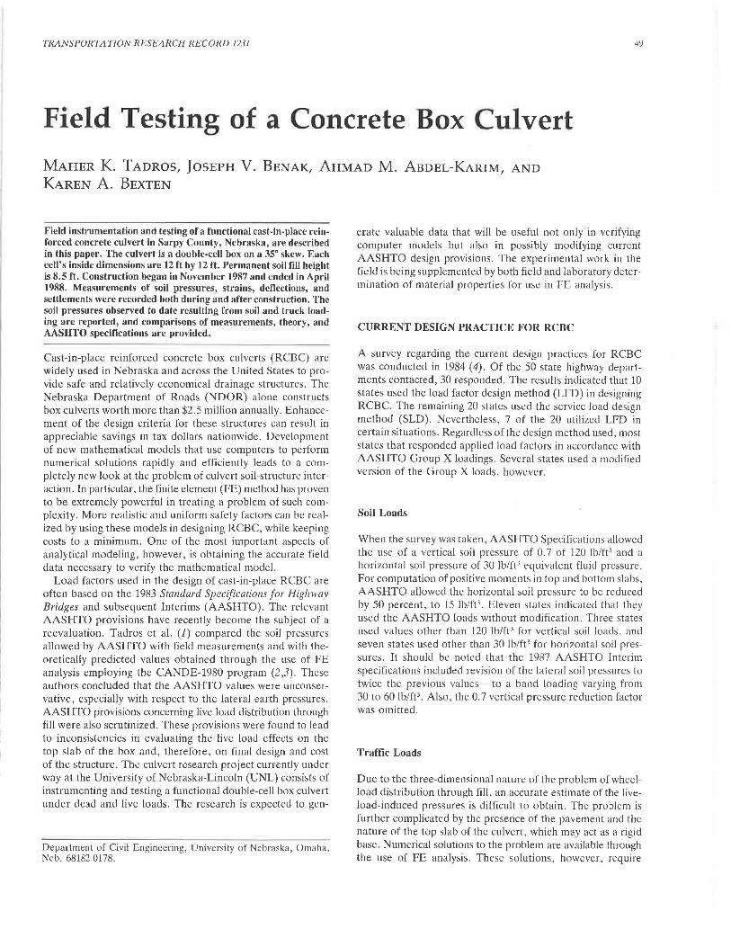
TRANSPORTATION RESEARCH RECORD 1231 49

Field Testing of a Concrete Box Culvert

MAHER K. TADROS, JOSEPH v. BENAK, AHMAD M. ABDEL-KARIM, AND

KAREN A. BEXTEN

Field instrumentation and testing of a functional cast-in-place rein­forced concrete culvert in Sarpy County, Nebraska, are described in this paper. The culvert is a double-cell box on a 35° skew. Each cell's inside dimensions are 12 ft by 12 rt. Permanent soil fill height is 8.5 ft. Construction began in November 1987 and ended in April 1988. Measurements of soil pressures, strains, deflections, and settlements were recorded both during and after construction. The soil pressures observed to date resulting from soil and truck load­ing are reported, and comparisons of measurements, theory, and AASHTO specifications are provided.

Cast-in-place reinforced concrete box culverts (RCBC) are widely used in Nebraska and across the United States to pro­vide safe and relatively economical drainage structures. The Nebraska Department of Roads (NDOR) alone constructs box culverts worth more than $2.5 million annually. Enhance­ment of the design criteria for these structures can result in appreciable savings in tax dollars nationwide. Development of new mathematical models that use computers to perform numerical solutions rapidly and efficiently leads to a com­pletely new look at the problem of culvert soil-structure inter­action. In particular, the finite element (FE) method has proven to be extremely powerful in treating a problem of such com­plexity. More realistic and uniform safety factors can be real­ized by using these models in designing RCBC, while keeping costs to a minimum. One of the most important aspects of analytical modeling, however, is obtaining the accurate field data necessary to verify the mathematical model.

Load factors used in the design of cast-in-place RCBC are often based on the 1983 Standard Specifications for Highway Bridges and subsequent Interims (AASHTO). The relevant AASHTO provisions have recently become the subject of a reevaluation. Tadros et al. (J) compared the soil pressures allowed by AASHTO with field measurements and with the­oretically predicted values obtained through the use of FE analysis employing the CANDE-1980 program (2,3). These authors concluded that the AASHTO values were unconser­vative, especially with respect to the lateral earth pressures. AASHTO provisions concerning live load distribution through fill were also scrutinized. These provisions were found to lead to inconsistencies in evaluating the live load effects on the top slab of the box and, therefore, on final design and cost of the structure. The culvert research project currently under way at the University of Nebraska-Lincoln (UNL) consists of instrumenting and testing a functional double-cell box culvert under dead and live loads. The research is expected to gen-

Department of Civil Engineering, University of Nebraska, Omaha, Neb. 68182-0178.

erate valuable data that will be useful not only in verifying computer models but also in possibly modifying current AASHTO design provisions. The experimental work in the field is being supplemented by both field and laboratory deter­mination of material properties for use in FE analysis.

CURRENT DESIGN PRACTICE FOR RCBC

A survey regarding the current design practices for RCBC was conducted in 1984 (4). Of the 50 state highway depart­ments contacted, 30 responded. The results indicated that 10 states used the load factor design method (LFD) in designing RCBC. The remaining 20 states used the service load design method (SLD). Nevertheless, 7 of the 20 utilized LFD in certain situations. Regardless of the design method used, most states that responded applied load factors in accordance with AASHTO Group X loadings. Several states used a modified version of the Group X loads, however.

Soil Loads

When the survey was taken, AASHTO Specifications allowed the use of a vertical soil pressure of 0. 7 of 120 lb/ft3 and a horizontal soil pressure of 30 lb/ft3 equivalent fluid pressure. For computation of positive moments in top and bottom slabs, AASHTO allowed the horizontal soil pressure to be reduced by 50 percent, to 15 lb/ft3

• Eleven states indicated that they used the AASHTO loads without modification. Three states used values other than 120 lb/ft3 for vertical soil loads, and seven states used other than 30 lb/ft3 for horizontal soil pres­sures. It should be noted that the 1987 AASHTO Interim specifications included revision of the lateral soil pressures to twice the previous values-to a band loading varying from 30 to 60 lb/ft3. Also, the 0.7 vertical pressure reduction factor was omitted.

Traffic Loads

Due to the three-dimensional nature of the problem of wheel­load distribution through fill, an accurate estimate of the live­load-induced pressures is difficult to obtain. The problem is further complicated by the presence of the pavement and the nature of the top slab of the culvert, which may act as a rigid base. Numerical solutions to the problem are available through the use of FE analysis. These solutions, however, require

50

considerable time and effort on the part of the designer, thus making them unsuitable for routine design \Vork.

At present, AASHTO suggests the following simplified procedure to account for live load effects:

1. when the depth of fill over the top slab is less than 2 ft, the wheel load shall be distributed as in concentrated loads on exposed slabs.

2. when the depth of fill is 2 ft or more, but does not meet the conditions in Stipulation 3 below, concentrated loads shall be distributed over a square whose sides are equal to 1.75 times the depth of fill.

3. when the depth of fill is more than 8 ft and exceeds the span length of a single span culvert or exceeds the distance bet.ween inner faces of outer walls of a multiple-span box, the effect of live load may be neglected.

These stipulations can result in contradictions at transitional fill heights. For example, the AASHTO specifications have been shown by the NDOR to result in an RCBC covered with 8 ft of fill requiring thicker walls and more reinforcement than one with 9 ft of fill (the latter being designed with live load fully ignored). For this reason, the NDOR currently uses a slightly modified version of the aforementioned procedures. In addition, AASHTO Specifications do not provide guidance for wheel load distribution due to pavement or for distribution within the top slab itself for fill depths greater than 2 ft.

Although the culvert had a skew angle of 35°, it was designed as a right angle culvert, thus ignoring the skew. The rein­forcement was placed in mats parallel and perpendicular to the walls. This practice is common in Nebraska and does not appear to be unreasonable. The testing program included live load positions both along the roadway (at a skew angle) and perpendicular to the culvert. Analysis of these results is beyond the scope of this report.

THEORETICAL SOIL PRESSURES

Based on extensive finite element modeling of a large number of culverts of common sizes and shapes, the following soil pressure formulas were proposed (1).

For silty clay soil,

PT = (0.984 + 0.0063H) '{,H

Ps = 0.6 'fsH

PB = PT+ 2Hh (57 + 26.3 H,,)IW,,

For silty sand soil,

PT= (0.970 + 0.0067H) '{5 H

Ps = 0.567 'fsH

PB = PT+ 2Hb (114 + 16.2H,,)IW,,

(1)

(2)

(3)

(4)

(5)

(6)

In the above formulas, PT, Ps, and P8 are pressures on top slab, side walls, and bottom slab, respectively; '{, is the fill unit weight in lb/ft3; His the fill height in feet above the point considered; and H,, and Wb are the overall height and width of the culvert in feet. Equations 3 and 6 do not include the

TRANSPORTATION RESEARCH RECORD 1231

effect of the culvert weight, which must be considered in actual design. They do include, however, the frictional (drag) forces that develop due to the tendency of the soil on the culvert sides to settle more than do the culvert itself and the soil directly above it.

INSTALLATION DESCRIPTION

Because of its size, fill depth, and proximity to the university, the culvert selected for instrumentation was a 100-ft-long 12-ft by 12-ft double-barrel cast-in-place reinforced concrete box on a 35° skew (Figure 1). It was constructed as part of Federal Aid Off-System Project BRO-7077 ( 46) in Sarpy County, Nebraska. The culvert replaced a narrow, antiquated pony truss bridge at the site, which is on a county highway about 2 mi south of Omaha. It was designed and constructed in accordance with current (1985) NDOR standard plans and specifications. Klaasmeyer Brothers Construction Company of Omaha was the contractor.

Construction began in early November 1987 to take advan­tage of low water flow and mild weather. Electing to work in the dry, the contractor built a temporary dike and diversion channel around the site. Excavation to bottom of slab grade was then completed, and a crushed rock working platform prepared. Water flow, both surface and subsurface, being low, the contractor was able to keep the site dewatered by bailing with a backhoe bucket about twice a day from a single sump.

The bottom slab was formed and poured on November 18, 1987, followed by forming and pouring, sequentially, the mid­dle wall, the north wall, the south wall, and finally on Decem-

N

4.5' typ.

Top Slab Plan View

4.5' typ.

North Elevation

••••-••-r---••...,... .. .,, •• ,~, •• ~ .. ~••••••••••••••-••••••••>1 • •···n-·-·-·--·-···---·--••

f- key: 4.5' typ.

Bottom Slab Plan View •Total Pressure Cells

1 Piezometers

FIGURE I Layout of earth pressure cells and piezometers.

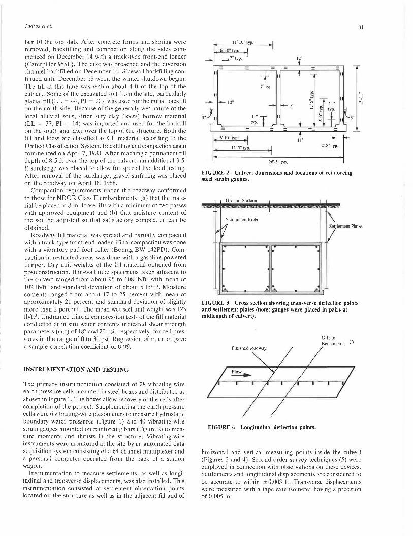
Tadros et al.

ber 10 the top slab. After concrete forms and shoring were removed, backfilling and compaction along the sides com­menced on December 14 with a track-type front-end loader (Caterpiller 955L). The dike was breached and the diversion channel backfilled on December 16. Sidewall backfilling con­tinued until December 18 when the winter shutdown began. The fill at this time was within about 4 ft of the top of the culvert. Some of the excavated soil from the site, particularly glacial till (LL = 44, PI = 20), was used for the initial backfill on the north side. Because of the generally wet nature of the local alluvial soils, drier silty clay (loess) borrow material (LL = 37, PI = 14) was imported and used for the backfill on the south and later over the top of the structure. Both the till and loess are classified as CL material according to the Unified Classification System. Backfilling and compaction again commenced on April 7, 1988. After reaching a permanent fill depth of 8.5 ft over the top of the culvert, an additional 3.5-ft surcharge was placed to allow for special live load testing. After removal of the surcharge, gravel surfacing was placed on the roadway on April 18, 1988.

Compaction requirements under the roadway conformed to those for NDOR Class II embankments: (a) that the mate­rial be placed in 8-in. loose lifts with a minimum of two passes with approved equipment and (b) that moisture content of the soil be adjusted so that satisfactory compaction can be obtained.

Roadway fill material was spread and partially compacted with a track-type front-end loader. Final compaction was done with a vibratory pad foot roller (Bomag BW 142PD). Com­paction in restricted areas was done with a gasoline-powered tamper. Dry unit weights of the fill material obtained from postconstruction, thin-wall tube specimens taken adjacent to the culvert ranged from about 95 to 108 lb/ft3 with mean of 102 lb/ft3 and standard deviation of about 5 lb/ft3

. Moisture contents ranged from about 17 to 25 percent with mean of approximately 21 percent and standard deviation of slightly more than 2 percent. The mean wet soil unit weight was 123 lb/ft3. Undrained triaxial compression tests of the fill material conducted at in situ water contents indicated shear strength parameters (<f.>,c) of 18° and 20 psi, respectively, for cell pres­sures in the range of 0 to 30 psi. Regression of u 1 on u 3 gave a sample correlation coefficient of 0. 99.

INSTRUMENTATION AND TESTING

The primary instrumentation consisted of 28 vibrating-wire earth pressure cells mounted in steel boxes and distributed as shown in Figure 1. The boxes allow recovery of the cells after completion of the project. Supplementing the earth pressure cells were 6 vibrating-wire piezometers to measure hydrostatic boundary water pressures (Figure 1) and 40 vibrating-wire strain gauges mounted on reinforcing bars (Figure 2) to mea­sure moments and thrusts in the structure. Vibrating-wire instruments were monitored at the site by an automated data acquisition system consisting of a 64-channel multiplexer and a personal computer operated from the back of a station wagon.

Instrumentation to measure settlements, as well as longi­tudinal and transverse displacements, was also installed. This instrumentation consisted of settlement observation points located on the structure as well as in the adjacent fill and of

II' 10" I

~ 6' 10'1 lXQ· ~1 1-17" typ . 12"

t = = = = II II

7" typ.

II - II - 10" ;:,.,

II" 9" ~ - lyp,

3" II II" b 3" lyp. (o II

= = = = -I rn· ·~ t II" , ... j r ·I ; 11'0" l: . .

26'-5" typ.

FIGURE 2 Culvert dimensions and locations or reinforcing steel strain gauges.

Settlement Rods

FIGURE 3 Cross section showing transverse deflection points and settlement plates (note: gauges were placed in pairs at midlength or culvert).

Finished roadway

I

I I I .II /

I Offsite Benchmark 0

// I

FIGURE 4 Longitudinal deflection points.

51

~

horizontal and vertical measuring points inside the culvert (Figures 3 and 4). Second order survey techniques (5) were employed in connection with observations on these devices. Settlements and longitudinal displacements are considered to be accurate to within ± 0.003 ft. Transverse displacements were measured with a tape extensometer having a precision of 0.005 in.

52

Direction Parallel io the roa.dv1.ay

6'

~4 ·- ·-- - ·-·-·-·ri

T2·

Direction perpendicular Note : to the culvert

• Denotes the position of the centerline of the rear axle

Concrete median barriers

= 6'

,/ ~. ~ =-t 22,800 lb 4,200 lb

·r---14.1' -I T Test truck Tire Layout

FIGURE S Live load positions and test truck.

Various items of the instrumentation were monitored dur­ing backfilling operations. After the backfill reached the top of the culvert, live load tests were initiated. These consisted of positioning a loaded flatbed truck , which simulated AASHTO H-15 truck loading, at various locations over the culvert (Fig­ure 5) and at approximately 2-ft increments of fill up to 12 ft. About 3.5 ft of fill were then removed to establish final roadway grade .

Tests on materials are currently under way and observations on all instruments are continuing to ascertain culvert per­formance under long-term dead loads.

CULVERT PERFORMANCE

Settlement profiles along the middle wall at various times during and after completion of backfilling are shown in Figure 6. Largest settlements occurred during roadway fill place­ment . Subsequent settlements appear to be negligible. No significant length changes in the culvert barrel have been detected. It should be noted, however, that a transverse flex­ural stress relief crack formed during filling (after March 29, 1988). This crack is located just downstream of the longitu­dinal midlength of the culvert and extends through the floor slab and all three walls. The crack is about 0.1 in. at its widest part and becomes narrower as it extends to the top slab. A hairline shrinkage crack extending through both exterior walls adjacent to earth pressure cells was noted prior to March 29, 1988. This crack did not extend through either the floor slab or middle wall.

Transverse deformation measurements to date indicate rel­ative deflections between the centers of the top and bottom slab to be 0.0720 in. in the north cell and 0.0828 in. in the

E 80.7 L E v 11 ao.e T I 0 N ao.11

(rt)

TRANSPORTATION R ESEA RCH RECORD 1231

80.4'---_,_-~.__-~-~--~-~--~-~

~ ~ W W W ~ ~ H ~

SETTLEMENT POINT

11111111 tnlli.I -+- 11n111 -.. rm-*- 41•111 •I......,.. -fr- 4111111 ...... 1111 --'*- .,., ........ 1111 -+- '""" ...... 1111

FIGURE 6 Longitudinal settlements.

•

Fill Height: 3.5 ft Live Loading Status: 0 Date of Reading: 04-11-1988

Key:

• Measured Proposed (Ref. 2)

NewAASHTO ,.. .., 10 psi

• • -· ==·=-===4 ,=:.' =-•::===-

1-- ---- ·- ·- ---·----- --·--­l -- .. ·----·--·-·--·-··""---·-------,---·--_._ _ __;

FIGURE 7 Measured soil pressures under 3.5 ft of till over the top slab.

south. Inward deflections of the centers of the outer walls relative to the inner wall are 0.0240 in. in the north cell and 0.0864 in. in the south.

Fill settlement relative to the culvert so far amounts to 0.007 ft on the north side and 0.034 ft on the south. A slight tilting of the culvert of 0.008 ft to the south has been detected. This tilting is probably due to the more compressible alluvial foun­dation soils on the south and east, as opposed to the heavily overconsolidated glacial soils supporting the culvert on the north and west .

RESULTS OF PRESSURE CELL READINGS

Pressure cell readings are shown plotted for various fill heights from April 11, 1988, to July 7, 1988 (Figures 7-12). Super­imposed on these plots are outlines of AASHTO pressure distributions , as revised in the 1987 Interim Specifications, and the distribution proposed by Tadros et al. (J), using Equa­tions 1to3 for silty clay soil with 'Is = 123 lb/ft3 • For increasing fill heights, the increased vertical pressures acting on the top slab appear to be consistent with that calculated by either AASHTO specifications or the method proposed by Tadros et al. (2).

Tadros et al.

Key:

Fill Height: 8.0 ft

Live Loading Status: 0 Date of Reading: 04-13-1988

• Measured

Proposed (Ref. 2)

NewAASHTO I.. lrl

10 psi

• • • ~===,=-=:.:=='--==~'==··=,!..===---"'

~ .. \ \. . \

S.Cell \\ I\

• •\\ I, \\ ' -~

I •

l·---·--·-·- ·-·--·-·- ·-·-·-·- ·-·-· --- ·~ ' ' L---... -----.~-- ---------·------·-----·-·-----------.1

FIGURE 8 Measured soil pressures under 8.0 ft of fill over the top slab.

Key:

e Measured

•

Fill Height: 12.0 ft

Live Loading Status: 0 Date of Reading: 04-15-1988

Proposed (Ref. 2)

New AASHTO

IO psi

• • r -~----···---e.···-_____.___· ····· ·· 1--------------- -----------1 I

I

. ~---~ . ' "'------·- .. ------~-~-~~----·--· .....

FIGURE 9 Measured soil pressures under 12.0 ft of fill over the top slab.

A phenomenon not previously noted was observed; where part of the original fill has been removed, top slab pressures do not appear to fully rebound to values consistent with the new fill heights. In other words, soil cannot be treated as a totally elastic material, and consideration must be given to loading history. It will be of interest to find out if time will be a factor in modifying these pressures.

Measured lateral earth pressures, in general, are seen to be much higher than those given by the 30 lb/ft3 equivalent fluid pressure assumption which was allowed by AASHTO before 1987. Current AASHTO lateral pressures as well as theoretical predictions are much closer to measurements, but

53

Key:

Fill Height: 8.5 ft

Live Loading Status: 0 • Measured

Proposed (Ref. 2)

NewAASHTO Date of Reading: 04-18-1988 I.. ..I

IO psi

• • • • • r=,=·=-====~=====,~

I /;. \'.

\'· /~ t\

• ! I \', • ,' I N. Cell S. Cell \" \ • : I 1\ .'I I I ; ! \ \

.l

•

• ---------------------- ---------~-

FIGURE 10 Measured pressure distribution under permanent fill at the completion of backfilling.

Key:

Fill Height: 8.5 ft • Measured

Proposed (Ref. 2)

New AASHTO Live Loading Status: 0 Date of Reading: 07-07-1988 ·-10 psi

• • • • -===~~~~=~-::!~=-=-.=====9

,--;.......,.--.,...--..,..,~--....... ..--....,., ...... ---, •. ~ ~ ti \'•, /,, . \

•• .1 11 n .. N. Cell S. Cell 9i : i \ ".

.~ f e I \\ : I

i I _ _:~~

I L--- , _____ .! ___ J I • :

L •• ----- ----- ------ - ---- ------ ----- ------ - ---- -___ J

FIGURE 11 Measured soil pressure under permanent fill 80 days after completion of backfilling.

these still appear to be underestimates. Both the magnitude and distribution of the actual pressures appear to be strongly influenced by the effects of compaction. Low side wall pres­sure estimates can lead to conservative top and bottom slab designs and unconservative side wall designs, thus resulting in a poor proportioning of the various members of the struc­ture. It is therefore advisable to continue to 'use a band of upper and lower bounds of lateral pressures as illustrated in Figure 12. Some redistribution of these lateral earth pressures occurred between April 18, 1988, and July 7, 1988. Obser­vations of this phenomenon will continue until the spring of 1989.

54

Determination of the bottom slab pressure distribution was hindered by temporary pressure cell malfunctioning. How­ever, from the information available, some of the measured bottom slab pressures deviate considerably from the uniform distribution allowed by AASHTO and from that based on finite element analysis.

Fill Height: 8.0 ft Key: e Measured

Live Loading Status: 0 ~>..."<..> Proposed (Ref. 2) Date of Reading: 04-13-1988 77-L/. New AASHTO

~ OldAASHTO I.. •I

10 psi

• • • ~=::..:=.=:::.:..:=-J.::.:.=.~=:~.=:!~==-:-

N.Cell S.Cell

•

• I

-==--====:::.:::=.:=.=.==-:::: ... -:==:;:_~ I "·- -- -- ----- ·-- ------- ----- ----·- "*·--·-----'

FIGURE 12 Comparison of various bands of soil pressures at 8.0 ft of fill over the top slab .

.. 'O .... Dep lh of F ll I ov e r Top SI ob

~ ....

iii ~ .: • Q. ~ .....

• .: l ) Ill .. .. • .: it !8

ai

... Ill ei

? ei

I

1li

•

TRANSPORTA TION RESEARCH RECORD 1231

A three-dimensional plot of the pressure distribution on the top slab due to truck axle loading is presented in Figure 13. Orientation of the test vehicle is north, with the rear axle centered over the middle of the south cell (the point x = 0, y = 0 in the figure) . Comparison of measured and theoretical distributions is under way and will be fully reported later. Examples of comparisons of measured and allowed AASHTO pressures for truck loading at three fill heights are given in Figure 14; the dashed line represents the uniform AASHTO distribution mentioned earlier. At a fill height of 3.5 ft, the indicated negative measured pressures do not represent ten­sile stresses in soil, but rather a reduction in the pressure caused by soil weight alone .

CONCLUSIONS

Instrumentation and testing of a full-sized, functional culvert are described in this paper. Construction was intended to model actual rather than laboratory-controlled conditions. It was observed that soil pressures were generally higher than those specified by the 1986 and earlier editions of AASHTO . The 1987 revision by AASHTO, which removed the 0.7 coef­ficient from the calculation of soil pressure on top slab and which doubled the side wall pressure, is shown to be a sig­nificant step forward. Loading history and time-dependent behavior of soil appear to be significant due to the inelastic nature of soil. Details of this phenomenon as well as of field and theoretical effects of truck loading will be presented upon completion of this research project.

3.5 fl

.... -

FIGURE 13 Measured pressure distribution on the top slab due to axle loading.

Tadros et al.

o Measured: Direction of travel perpen. to culvert • Measured: Direction of travel parallel to roadway

- ·- New AASHTO

1-------l 1.0 psi

0

Fill height= 3.5 ft •

Fill height= 8.0 ft

• :--·---·-1 i I ! I

I Q

0

I • •

0

• • , .- - - ·-·- ·- ·--·- - ·___.!]

r-·- - -.-·-·-·-.- - - ....-- - - -.--- --. Fill height= 12.0 ft

I Position of rear axle • (see Fig. 4)

•

FIGURE 14 Top slab pressures caused by truck loading under 3.5, 8.0, and 12.0 ft of fill for live load positions 3 and 7 (normal and skew directions of travel, respectively).

ACKNOWLEDGMENT

Sponsors of the project are the Federal Highway Adminis­tration, the Nebraska Department of Roads, and the Uni-

55

versity of Nebraska-Lincoln. Many individuals have contrib­uted to various phases of this project. Special thanks are due to Jim Holmes, George Schmid, Paul Koenig, Dalyce Ron­nau, Wayne Horn, Tom Goodbarn, and Jerry Koloen, all of the Nebraska Department of Roads; Ron Rystrom, Sarpy County Engineer; and Keith Klaasmeyer and Bob Ulrich of Klaasmeyer Bros.

REFERENCES

1. M. K. Tadros, J. V. Benak, and M. K. Gilliland. Soil Pressure on Box Culverts. AC/ Structural Journal, Vol. 86, No. 4, 1989, pp. 439-450 .

2. M. G. Katona, P. D. Vittes, C.H. Lee, and H. T. Ho. CANDE-1980: Box Culverts and Soil Models. Report FHWA/RD-80/172. FHWA, U.S. Department of Transportation, May 1981.

3. M. G. Katona and J. M. Smith. CANDE User Manual. Report FHWA-RD-77-6. FHWA, U.S. Department of Transportation, 1976.

4. M. K. Tadros. Cost Effective Concrete Box Culvert Design. Project HRP83-3, Engineering Research Center, University of Nebraska, Omaha, 1986.

5. 1. Dunnicliff. Geotechnical Instrumentation for Monitoring Field Performance. John Wiley and Sons, New York, 1988 .

The contents of this report reflect the views of the authors who are responsible for the facts and the accuracy of the data. The contents do not necessarily reflect the official views or policies of the Nebraska Department of Roads, the Federal Highway Administration, or the University of Nebraska. This report does not constitute a standard, specification, or regulation.

Publication of this paper sponsored by Committee on Subsurface Soi/­Structure Interaction.

56 TRANSPORTATJON RESEARCH RECORD 1231

Heavy-Load Traffic Tests for Minimum Pipe Cover

JOHN c. POTTER AND HARRY H. ULERY, JR.

Twelve sections of culvert pipe were installed under soil cover ranging from 15 to 27 in. and trafficked with a single-tandem gear load cart. The average wheel load was 62,875 lb on an average measured contact area of 777 in2

• In addition, several sections of reinforced concrete pipe (RCP) were subjected to laboratory load testing to determine actual three-edge bearing strengths. The field test specimens were corrugated steel pipe (CSP) and RCP in 12-, 18-, and 24-in. diameters. Surface rutting progressed to about 1 in. at the end of trafficking. Surface stiffness, as measured by falling weight deflectometer, showed that the backfill around the pipes was less stiff than the undisturbed areas of the test section between pipe trenches. The RCP was stiffer than the CSP, except for the cracked RCP, which had a stiffness similar to the adjacent CSP. Permanent deformations (set) in the pipes increased only gradually beyond 326 passes of the load cart, even though the static and dynamic deformations caused by both the stationary and moving load cart, respectively, continued to increase. On the basis of these test results, minimum cover requirements are pre­sented. They represent minor deviations above and below typical published values for minimum pipe cover under similar loading conditions.

This paper documents a previously unpublished part of a larger study concluded by the Waterways Experiment Station (WES) during 1977-1981 to develop design criteria for an MX road­way system. The pavement structural data have been previ­ously reported by Alexander (1). This part of the investigation was conducted to develop criteria for minimum cover over drainage pipes installed beneath an MX roadway.

The depth of cover must be adequate to prevent both failure of the buried pipe and differential settlement of the overlying roadway under both moving (dynamic) and static loads. The tests described here were directed particularly at shallow­buried corrugated steel pipe (CSP) reinforced concrete pipe (RCP) subjected to heavy wheel loads similar to those of an MX transporter.

TEST SPECIFICATIONS

Pipe

Twelve sections of culvert pipe were installed, consisting of CSP and RCP in diameters of 12, 18, and 24 in.

The CSP met the requirements of Federal Specification

J.C. Potter, U.S. Army Corps of Engineers, Waterways Experiment Station, P.O. Box 631, Vicksburg, Miss., 39180; current affiliation: Huntsville Division, P.O. Box 1600, Huntsville, Ala. 35802-4301. H. H. Ulery, Jr., U.S. Army Corps of Engineers, Waterways Exper­iment Station, P .O. Box 631, Vicksburg, Miss. 39180.

WW-P-405B (2) and was of full circular cross section having annular corrugations. This pipe was constructed of p1ain, gal­vanized, 16-gauge (0.064 in.) sheet, using riveted, lapped joints. Corrugations were 22/3-in. by 1/2-in. deep; 15-foot pipe sections were used in Lane 1, and 10-ft sections were used in Lane 2.

The RCP conformed to standards (ASTM C-76-78, Class IV), with wall thicknesses of 2, 2Y2, and 3 in. for the 12-, 18-, and 24-in. pipes, respectively. Three 4-ft sections with bell and spigot joints were used for the 12-in. installations and single 8-ft sections were used for 18- and 24-inch installations.

Instrumentation

Two Collins linear variable differential transformer (L VDT) displacement gauges were installed in each CSP section to measure vertical and horizontal deflection (or diameter change). These gauges had a range of ±0.75 in. They were installed in mounts bolted to the outside surface of the pipe and adjusted off zero, so that pipe deflections up to 1.5 in. in one direction could be recorded. The four-conductor instrumentation cable was waterproofed with sealant and heat-shrink tubing and then routed to an instrumentation trailer.

Collins L VDT's with a range of + 0.05 in. were installed in mounts epoxied to the inside walls of the RCP. Because less than 0.05 in. of deflection was anticipated for the RCP, these gauges were mounted at mechanical zero. The instru­mentation cable was waterproofed and routed as for the CSP installations.

Crack detectors were also installed in the RCP specimens. The crack detectors for each RCP consisted of four '/2-in.­wide traces of conductive paint of the type used to repair printed circuit boards. These traces were applied to the top and bottom quadrants of pipe circumference, 1 ft on either side of the single, vertical deflection gauge. A two-conductor instrumentation cable was run for each crack detector to the instrumentation trailer, where the resistance of each detector was continuously monitored. Increased resistance was used as an indicator of incipient RCP cracking.

A Z80 microprocessor-based system was used for auto­mated data acquisition and processing.

Test Section

Pipe was installed only in Item 2 of Lanes 1 and 2 of the five­item MX Road Test Section (Figures 1 and 2). All pipe was installed in trenches excavated in the previously constructed subgrades. Average trench widths for CSP were 33, 43, and

Polter and Ulery

45 in. and for the RCP, 36, 47, and 51 in., for pipe sizes 12, 18, and 24 in., respectively.

The subgrade of both Lanes 1 and 2 of Item 2 consisted of material designated as Blend II, (s: 4-percent moisture, design CBR 15). Blend II is a sand-gravel combination blended to represent the typical gradation of the material encountered 2 to 20 ft below the potential MX siting area.

Lane 1 was surfaced with crushed limestone; Lane 2, with

TRAFFIC LANE NO. 2

FIGURE I Test section plan.

TRAFFIC LANE NO. 1

57

cement-treated Blend I (design cement content of 7 percent). Blend I sand-gravel material was representative of that encountered in the top 2 ft of the potential MX siting area.

Item 2 was constructed to grade with the Blend II material, and trenches were excavated with a backhoe. The pipes were then placed on a layer of crushed gravel (in lieu of shaping the bedding), and 2 to 5 in. of crushed gravel were hand tamped around the pipes. The remainder of the trench was backfilled with Blend II material in 6- to 9-in. layers. The Blend II material was hand tamped to the top of the pipes, and a mechanical tamper was used for backfill above the pipes . Nuclear moisture and density measurements were per­formed in the bottom of each trench, on the first layer of crushed gravel (bottom of pipe), on the layers of crushed gravel around the pipes (each 2 to 5 in.), and on each lift of Blend II backfill material. Oven-dry moisture contents were also obtained. The final results of these tests are shown in Table 1. Cross-sections (profiles) were taken along the top of each pipe after each layer of backfill was completed. All instrumentation leads were trenched to a common exit point and then run to the instrumentation trailer.

Item 2 was completed by constructing the surfacing in two lifts. The pipe instrumentation was monitored du1ing this phase of construction. The first lift of crushed limestone (Lane 1) and cement-stabilized Blend II (Lane 2) were rolled with a 25-ton self-propelled rubber-tired roller. The second (final) lift of crushed limestone was placed in Lane 1, and a 50-ton roller (100,000 lb) with small, high-pressure tires (100 psi) was used for compaction. On the first pass across the pipes with the 50-ton roller, the cover over the pipe being about 24 in., the crack detectors in Pipes 4 and 6 indicated that cracking had occurred under the load. Rolling with the 50-ton roller was halted, and the 25-ton self-propelled rubber­tired roller was used to complete the compaction of Lane 1 and was also used in Lane 2.

A 4-ft by 4-ft observation pit was excavated at the end of Pipe 6 (24-in. RCP). Hairline cracks were observed along the length of the pipe at both the top and bottom. Deflection gauges were reset, and the crack detectors were repainted (across the cracks). The pit was backfilled and compacted with a mechanical tamper. Pipe 4 (18-in. RCP) was not uncov­ered at this time because the crack detectors and deflection gauges were still operating.

PROFILE OF ITEM 2. LANE 2

FIGURE 2 Test section profile.

~ CEMENT STABILIZED BLEND II flmllJ CRUSHED LIMESTONE

5 8 TRANSPORTATION RESEARCH RECORD 1231

TABLE 1 PRETRAFFIC SURFACE MEASUREMENTS OF CBR, MOIST URE CONTENT, AND DENSITY Dry Moisture

ueeer Lnl:'. e.r Lower Lal:'.er Density Content (Nuclear) Thickness Lane Test Material in. Material

1 Crushed limestone 9 Blend II 2 9

2 Blend II (c.,ment I'/ 111enc1 u stabilized)

2 12

FIGURE 3 MX test vehicle.

LOAD CART AND TEST TRAFFIC

The load earl used to traffic and pipe te ·t items 1s hown in Figure 3. T he wheel were aligned in a single tandem arrange­ment 108 in. center to center and were equjppcd with smo th tires that mea ured 98 in. high by 40 in . wide. Both wheel were powered . The tires were loaded as follows:

Front Rear Average

Load (lb) 68,750 57,000 62,875 Measured hard-surface contact

area (in.:) 758 796 777 Tire prem1rc (measured) (psi) 65 65 65 Average contact pressure (psi) 91 72 81

All traffic was applied to the test pipe in a single line , thus each pass of the load cart applied two coverages.

Thickne s s lb/ft3 CE- 55 (Nuclear)

in. CBR % %

63 144 14 7 100 0.8 63 152 147 100 0,8

bU 150 142 103 3.4

60 150 141 103 3.9

MEASUREMENTS

During the test , the foiiowing data were obrained :

1. Rutting of the surface in Lane 1, Item 2; and rutting and cracking in Lane 2, Item 2,

2. Permanent (nonrecovering) deformation of the pipe, 3. Deflection of the pipe resulting from one load wheel

standing (statically) direct! y over the deflection gauges, 4. Deflection of the pipe resulting from the load cart pass­

ing or moving (dynamically) over the deflection gauges, 5. Cracking in RCP, 6. Nondestructive tests using the falling weight deflec­

tometer (FWD) in Item 2 of both Lanes 1 and 2, and 7. Laboratory three-edge bearing strength tests of the RCP.

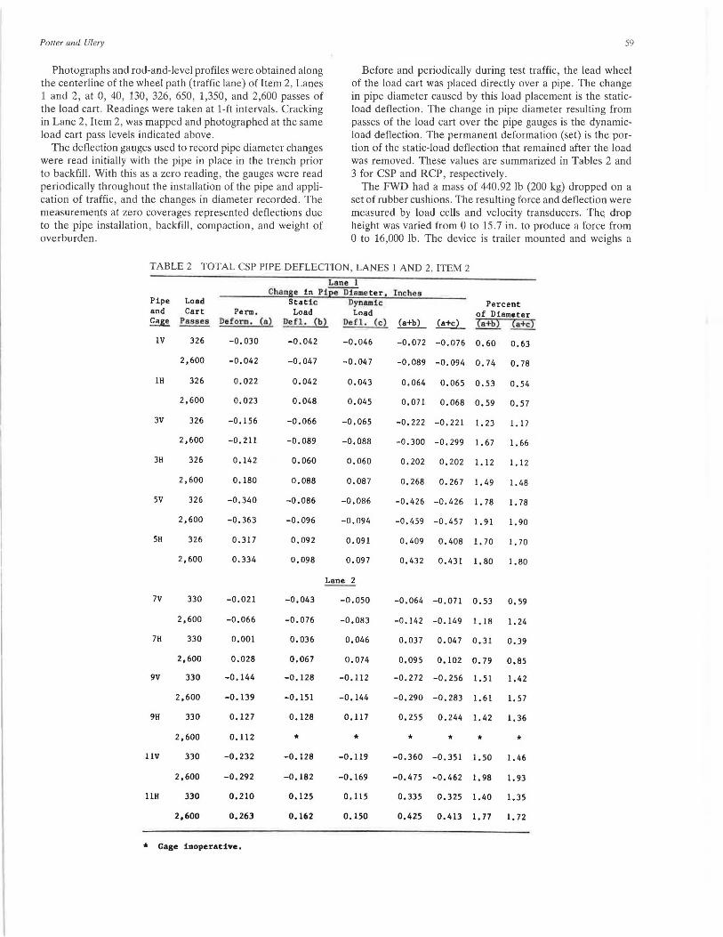
Porrer and Ulery

Photographs and rod-and-level profiles were obtained along the centerline of the wheel path (traffic lane) of Item 2, Lanes 1 and 2, at 0, 40 , 130, 326 , 650, 1,350, and 2,600 passes of the load cart. Readings were taken at 1-ft intervals. Cracking in Lane 2, Item 2, was mapped and photographed at the same load cart pass levels indicated above.

The deflection gauges used to record pipe diameter changes were read initially with the pipe in place in the trench prior to backfill. With this as a zero reading, the gauges were read periodically throughout the installation of the pipe and appli­cation of traffic, and the changes in diameter recorded. The measurements at zero coverages represented deflections due to the pipe installation, backfill, compaction, and weight of overburden.

59

Before and periodically during test traffic, the lead wheel of the load cart was placed directly over a pipe. The change in pipe diameter caused by this load placement is the static­load deflection. The change in pipe diameter resulting from passes of the load cart over the pipe gauges is the dynamic­load deflection. The permanent deformation (set) is the por­tion of the static-load deflection that remained after the load was removed. These values are summarized in Tables 2 and 3 for CSP and RCP, respectively .

The FWD had a mass of 440.92 lb (200 kg) dropped on a set of rubber cushions. The resulting force and deflection were measured by load cells and velocity transducers. The drop height was varied from 0 to 15.7 in. to produce a force from 0 to 16,000 lb . The device is trailer mounted and weighs a

TABLE 2 TOTAL CSP PIPE DEFLECTION, LANES l AND 2, ITEM 2

Lane l Cha nge in Pipe Diame ter,

Pipe Load Stat ic Dynamic and Cart Perm. Load Load Gage Passes Deform . (a ) Defl. (b) Defl. (c)

lV 326 -0.030

2,600 -0.042

lH 326 0.022

2 , 600 0.023

3V 326 -0.156

2,600 -0.211

3H 326 0.142

2,600 0.180

sv 326 -0.340

2,600 -0.363

SH 326 0.317

2,600 0.334

7V 330 -0.021

2 ,600 -0.066

7H 330 0.001

2,600 0,028

9V 330 -0.144

2,600 -0.139

9H 330 0,127

2,600 O. ll2

llV 330 -0. 232

2,600 -0.292

llH 330 0.210

2,600 0.263

* Gage inoperative.

-0.042

-0.047

0.042

0.048

-0.066

-0.089

0.060

0,088

-0.086

-0.096

0.092

0,098

-0.043

-0.076

0.036

0,067

-0.128

-0.151

0.128

* -0.128

-0.182

0.125

0.162

-0.046

-0.047

0,043

0.045

-0.065

-0.088

0,060

0.087

-0.086

-0.094

0.091

0.097

Lane 2

-0.050

-0.083

0.046

0.074

-0.112

-0.144

O. ll 7

* -0.119

-0.169

0.115

0.150

Inche s Percent

of Diameter (a+b) (a+c) (a+b) (a+c)

-0.072 -0.076 0.60 0.63

-0.089 -0.094 0.74 0.78

0.064 0.065 0.53 0.54

0.071 0.068 0.59 0.57

-0.222 -0.221 1.23 1.17

-0.300 -0.299 1.67 1.66

0. 202 0.202 1. 12 1.12

0.268 0.267 1.49 1. 48

-0.426 -0.426 1.78 1.78

-0.459 -0.457 1.91 1.90

0. 409 0 . 408 1.70 1. 70

0.432 0.431 1.80 1.80

-0.064 -0.071 0.53 0.59

-0.142 -0.149 1.18 1. 24

0.037 0.047 0.31 0.39

0.095 0.102 0.79 0,85

-0 . 272 -0.256 1.51 1.42

-0.290 -0.283 1.61 1.57

0.255 0.244 1.42 1.36

* * * -0.360 -0.351 1.50 1.46

-0.475 -0.462 1.98 1.93

0.335 0,325 1.40 1.35

0.425 0.413 1.77 1.72

60 TRANSPORTA TION RESEARCH R ECORD 1231

TABLE 3 TOTAL REINFORCED CONCRETE PIPE DEFLECTION, LANE 1, ITEM 2

Ch~nsc in Pipe D1~me ter, Inches Percent

z 0 a: (.)

~

Pipe and Gage

2V

4V

6V

8V

lOV

12V

3.0

'£ 2.0 .:.e. (/) (/) w z u.. u.. 1.0

Load Cart Penn.

Passes Deform. (a)

326 -0.006

2,600 -0.006

326 -0.008

2,600 -0.012

326 -0.118

2,600 -0. 140

330 o.o

2,600 o.o

330 -0.001

2,600 -0.001

330 -0.002

2,600 -0.002

Static Dynamic Internal Load Load Diameter

De fl. (b) Defl. (c) (a+b) (a+c) (a+b) (a+c)

-0.002 -0.002 -0.008 -0.008 0.07 0.07

-0.003 -0.003 -0.009 -0.009 0.08 0.08

-0.011 -0.012 -0.019 -0.020 0.10 0.11

-0.015 -0.015 -0,027 -0.027 0.15 0.15

-0.052 -0.051 -0.170 -0.169 o. 71 0.70

-0.050 -0.049 -0.190 -0. 189 0.79 0. 79

Lane 2, Item 2

-0.002 -0,002 -0.002 -0.002 0.02 0.02

-0.002 -0.002 -0.002 -0.002 0.02 0.02

-0.005 -0.005 -0.006 -0.006 0,03 0,03

-0.007 -0.008 -0.008 -0.009 0.04 0.05

-0.005 -0.006 -0.007 -0.008 0.03 0.03

-0.010 -0.010 -0.012 -0.012 0.05 0.05

CORRUGATED STEEL PIPE • 12 IN. DIAMETER " 18 IN. DIAMETER • 24 IN. DIAMETER

LANE 1 ------ LANE 2

~ lt;-:::...3~~~~==-=.::..:::_:_:=:-==-=-=-~-=-=-=-=~-=-=-=-=-=-=-===-~-~-:....~-~=~-~-~-;;_;_;_;._..~-~.;;.~;;.~:;;,~-~-=-=-=-=-:: u..

0 ~~~~~~~~~~~~~~~~~~~~~~'-'~~~-'-~~~---'

0 400 800 1 ,200 1,600 2,000 2,400 2,800

LOAD CART PASSES

FIGURE 4 CSP stiffness data.

total of 1,500 lb. The load is transmitted to the surface through an 11.8-in. (30 cm) aluminum plate. The signal conditioning equipn1ent displays the resulting pressure in kilopascals and the maximum peak displacement in micrometers . As many as three displacement sensors may be recorded. Tests were performed on the final two lifts during construction. Drop heights of 1.44, 3.44, 6.50, and 14.94 in. were used. Deflec­tions were measured at the center of the load plate and at distances of 18 and 36 in. from the center. Nondestructive tests with the FWD were performed at traffic levels of 0, 40, 130, 326, 1,300, and 2,600 passes of the load cart. Tests were run directly over each pipe and at several points between each pipe. Data consisted of deflection basin measurements at the two force levels obtained by dropping the mass from heights of 3.44 and 14.94 in. FWD stiffness data, obtained directly above the pipes, for CSP and RCP, respectively, are presented in Figures 4 and 5; stiffness data for the entire test section

along Lanes 1 and 2, respectively , are presented in Figures 6 and 7.

c:- ....... .......... 1 nrn ,,... ..... ........ : ,... ...... ,... . .. , ...... ..... ,.... ... .. h;,,,. ..... ,,.~ ... ,.... +h .... oo o rlno ha*l r;nrT ~'"-'V\..-lU.l .l.'-'--'J. ,")\ .. A .. LlVU.:1 ""'-'.I'-' ~UVJ'-'"''"""u \.V Ull.\,.A ... -""uo'-' V V LU.111.6

strength tests in accordance with ASTM requirements (ASTM C-497-78). The 24-in. pipe was about 10 percent stronger than ASTM requirements ; the 18-in., about one-third stronger; and the 12-in., about twice as strong.

Posttraffic tests included one test pit in each lane, for post­test moisture, density, and CBR; and observation pits at the end of Pipes 4 and 6 in Lane 1. The posttraffic test pit data are shown in Table 4.

The observation pits revealed that additional cracks had formed on each side of Pipe 6 (24-in . RCP) and some spalling had occurred along the crack at the top of the pipe. The top and bottom cracks had also widened under traffic. Pipe 4 (18-in. RCP) had a barely visible crack at the top of the pipe.

Surface rutting was about 1 in. at the end of traffic .

Potter and Ulery

4.0

z 0 a: u 3.0

~ (ij I D... .:.:

1' CJ) 2.0 ' CJ) I w z I u.. u..

j:: CJ)

0 1.0 ~ u..

0 0 400 800

REINFORCED CONCRETE PIPE

1,200

• A

•

1,600

12 IN. DIAMETER 18 IN. DIAMETER 24 IN. DIAMETER LANE 1 LANE 2

_______ ..

2,000 2,400

61

2,800

LOAD CART PASSES

FIGURE 5 RCP stiffness data.

LEGEND 3

ITEM 2-LANE 1 a 0 PASSES • 326 PASSES • 2600 PASSES

PIP~ #3 z <e. 0 PIPE #1 a:

<e. PIPE #2 PIP~ #4 PIP~ #5 PIP~ #6

u ~ 2 (ij D... .:.: CJ) en w z u.. u.. ~ 0

~

o...__._.__.__~___.._,,_._~.____,~11.-.1..--~i-..-'--'-......... ~~L......l.--J'--L-~--''---'---'-'

50 55 60 65 70 75 80 85 90 95 100

STATION, FT

FIGURE 6 Lane 1 stiffness data.

RESULTS

Permanent Pipe Deformation

The permanent deformations of the pipe installed in Lane 1, Item 2, are shown in Figures 8 and 9; and for Lane 2, Item 2, in Figures 10 and 11. A consistent data pattern of vertical and horizontal pipe deformations is obtained. The data indi­cate that as the number of traffic applications increases, the vertical pipe diameter decreases and the horizontal diameter increases. In general, the data plots show relatively large suc­cessive increases in pipe deformation during early passes of the load cart, then a ·consistent gradual increase in defor-

mations until the end of test. This pattern is more pronounced in the CSP than the RCP. Other observations garnered from the permanent pipe deformation data are as follows:

1. For both lanes, vertical and horizontal pipe deformation increase in magnitude with increasing pipe diameter. CSP vertical deformations were much larger than RCP deformations.

2. In Lane 1, the horizontal CSP deformations were about 90 percent of the vertical deformation. Results were less con­sistent in Lane 2, possibly due to the randomness of cracking (and attendant loss of bridging) in the cement-stabilized sur­facing of Lane 2.

3. In Lane 2, only very small deformations were measured

z ~ 4 (.)

~ to ~ 3 (/) (/) w z It 2

~ 0 s: u.

<t PIPE #7

55

PI P~ 8

60 65

FIGURE 7 Lane 2 stiffness data.

<t P PE #9

70 75 80

STATION, FT

ITEM 2-LANE 2

~ PIPE #11

65 90 95 100

LEGEND

• 0 PASSES • 326 PASSES • 2600 PASSES

TABLE 4 POSITRAFFIC TEST PIT DATA-CBR, MOISTURE CONTENT, AND DENSITY DETERMINATIONS

Dry Moisture Moisture Density Content Content

Depth Nuclear CE-55 Nuclear Oven Dry Lane Material in . CBR lbs / ft 3

% % %

In Traffic Lane

Crushed limestone 0 150+ 145 99 0 . 9 0.1 6 99 139 95 1.4 0.4

Blend II 12 45 130 94 3.0 2.9 18 26 125 91 3.4 3. 2 24 21 120 87 3.6 2 . 6 36 34 126 91 5.1 3. 7 48 21 123 89 4.3 3.4 60 9 118 86 6.5 4.5 72 54 131 95 8 .1 5.6

2 Cement stabilized 0 150+ 118 4.0 Blend II 6 112 4.0

Blend II 12 8 124 90 2.5 l.9 18 19 119 86 3.2 2.6 24 11 119 86 3.2 2 . 4 36 29 122 88 4.5 3.3

Out of Traffic

Crushed limestone 0 150+ 142 97 1.1 0.2 6 94 136 92 1.6 0.4

Blend II 12 51 129 93 3.0 2.7 18 32 124 90 3.3 3 . 0 24 20 120 87 2.9 2 . 3 Jb 2 7 125 91 5.0 3.4 48 22 123 89 4.2 3.3 60 15 122 88 6.4 4.5 72 31 127 92 8.4 5 .7

2 Cement stabilized 0 15o+ 119 3.9 Blend II 6 114 4.8

Blend II 12 11 125 91 2.5 2.0 18 24 119 86 3.3 2 . 8 24 17 118 85 3.4 2 . 5 36 25 118 85 4 . 6 3.5

Potter and Ulery

ffi J: u ~

z § ~

0.350

0.300

0.250

0.200

0.150

0.100

0.050

LANE 1 PIPE NO. VERTICAL HORIZONTAL DIAMETER

I

3 5 -------­,._ __ _.

12-IN

16-IN 24-IN

-------------------

-------~-----------0 1-----------------~ w

0 -0.050 .. ---- - - ------------

ffi -0.100 z ~ -0.150 a: w -0.200 IL

-0.250

-0.300

-0.350

0 400 800 1,200 1,600 2,000 2,400 2,800 LOAD CART PASSES

FIGURE 8 Lane 1 CSP permanent deflection.

Cf) w 0 .050 :I: 0 ~ 0 .025

z 0 0 i== -0.025 0 w ..J -0.050 Li.. w 0 -0.075 I-z -0.100 w z

-0 .125 c( ~ a: -0.150 w a. 0

CONCRETE PIPE NO.

2

4

6

LANE 1

VERTICAL

• •

DIAMETER

12-IN 18-IN 24-IN

400 BOO 1,200 1 ,600 2,000 2,400 2,BOO LOAD CART PASSES

FIGURE 9 Lane 1 RCP permanent deflection.

in the RCP. RCP permanent deformations in Lane 1 were much larger than those in Lane 2, probably due to lack of bridging that might be expected from the stabilized surfacing of Lane 2.

4. Except for the 12-in. CSP, permanent CSP deformations are larger in Lane 1 than in Lane 2. Again, bridging by the stabilized surfacing of Lane 2 should reduce the vertical load and deformations in that lane.

5. The 24-in. RCP (Pipe 6) in Lane 1 had much larger deformations than any other RCP pipe . Pipe 6 had a defor­mation pattern similar to CSP-a rapid increase in defor­mation during early passes of the load cart, then a steady but

63

LANE 2 PIPE NO. VERTICAL HORIZONTAL DIAMETER

0.300

0.250 en w 0.200 J: u ~ 0.150

z 0.100 0 t; 0.050 w -' Li.. w 0 -0.050 I­~ -0.100 z ~ ·0.150

ffi -0.200 c..

7 9

11

!''

.. • ·----.., ___ _. 12-IN 18-IN 24-IN

... _.._ ____ ... ___ __.....---- ---------· ________ _.. _____________ ..,.. ____ _

-0.250 t_-=======:=~==J::~=i=L..J -0.300 0 400 800 1200 1600 2000 2400 2800

LOAD CART PASSES

FIGURE 10 Lane 2 CSP permanent deflection.

SJ J: 0

0.002

~ 0.001 ;;i 0

LANE 2

CONCRETE PIPE NO.

B 10

12

VERTICAL

.. . DIAMETER

12-IN

18-IN

24-IN

hl or---:?-=:::::================:=:==~ ..J Li.. w ~ ·0.001 z w z ~ -0.002 a: w Q.

-0.003 .____ _ _._ __ .__ _ __.._ __ ..___ _ ___._ __ _._ _ __.

0 400 BOO 1,200 1,600 2,000 2,400 2,BOO

LOAD CART PASSES

FIGURE 11 Lane 2 RCP permanent deflection.

small increase during the remainder of traffic. This pattern was probably caused by the cracking of the pipe during installation .

Static-Load Pipe Deflection

Deflections under the load cart, while stationary over each pipe and gauge, are plotted in Figures 12 and 13 for Lane 1 and in Figures 14 and 15 for Lane 2. A regular and consistent pattern can be observed. Very small readings are obtained from loading the RCP. In the case of the CSP, during early

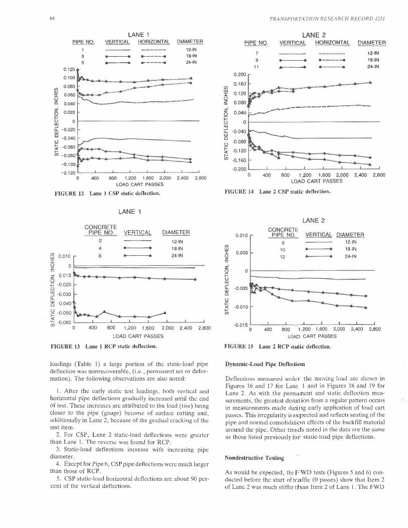
64

LANE 1 PIPE NO.

1

VERTICAL HORIZONTAL DIAMETER

12-IN 18-IN 24-IN

0.120

0.100

(/) 0.080

~ 0.060 u ~ 0.040

~ 0.020

3

5 -----... .. .. ,.._ ____ ....

--~---..-·-_.. :I: ~ ------~ __ .........---­__ ,._._.--

'~- -----------­--t w --' LL w Cl

QI-------------------0.020

-0.040 u ~ -0.060 ir--........ _ ___,_ <ll -0.0BO t.~-.._..,__....__::t::::::::=::=:=:=:::::1

-0.100 -0.120 l_ _ _J_ __ _i_ _ __J, __ __!_ _ __,L..,__ _ _,__ _ __,

0 400 BOO 1 ,200 1 ,600 2,000 2,400 2,800 LOAD CART PASSES

FIGURE 12 Lane 1 CSP static deflection.

[B 0.010 I

LANE 1

CONCRETE PIPE NO. VERTICAL

2

4

6 .. ..

DIAMETER

12-IN

18-IN

24-IN

~ O!:::::==================================--z -0.010 re--------.---+--.._ ______ __ 0 ;::: -0.020 u ~ -0.030 LL

~ -0.040

~ -0.050 <: tn -0.060 L_ _ __i __ _._ __ _._ __ .._ _ ___. __ _._ __ ~

0 400 800 1 ,200 1 ,600 2,000 2,400 2,800

LOAD CART PASSES

FIGURE 13 Lane 1 RCP static deflection.

loadings (Table 1) a large portion of the static-load pipe deflection was nonrecoverable, (i.e. , permanent set or defor­mation). The foiiowing observations are aiso noted:

1. After the early static test loadings , both vertical and horizontal pipe deflections gradually increased until the end of test. These increases are attributed to the load (tire) being closer to the pipe (gauge) because of surface rutting and, additionally in Lane 2, because of the gradual cracking of the test item.

2. For CSP, Lane 2 static-load deflections were greater than Lane 1. The reverse was found for RCP.

3. Static-load deflections increase with increasing pipe diameter.

4. Except for Pipe 6, CSP pipe deflections were much larger than those of RCP.

5. CSP static-load horizontal deflections are about 90 per­cent of the vertical deflections.

TRANSPORTATION RESEARCH RECORD 1231

LANE 2 PIPE NO. VERTICAL HORIZONTAL ntAMETER

(/)

0.200

0.160

~ 0.120 u ~ 0.080

5 0.040

i3 UJ --' LL UJ 0 u

~

-0.040

-0.080

-0.120

-0.160

7 9

11 • .. • .. ·~-----,.. _____ _.,

12-IN 18-IN 24-IN

-~---­>--......--------r..:t:----...

_,,..--" ---------------­

~~--

-0.200 L_ _ _J_ __ _L_ __ 1..,_ _ __L __ _._ __ '---'

0 400 800 1,200 1,600 2,000 2,400 2,800 LOAD CART PASSES

FIGURE 14 Lane 2 CSP static deflection.

LANE 2 CONCRETE

0.010 PIPE NO. VERTICAL DIAMETER

B 12-IN (/)

18-IN w 10 I 0.005

24-IN u 12 ~

z: 0 0 ;:: u w --' LL -0.005 UJ 0 u ;::: <: -0.010 I-(/)

-0.015 L_ _ _;_ _ _ _L_ __ L_ _ _J_ __ _._ _ __,'-----J

0 400 800 1 ,200 1 ,600 2,000 2,400 2,800

LOAD CART PASSES

FIGURE 15 Lane 2 RCP static deflection.

Dynamic-Load Pipe Deflection

Deflections measureU unUe1 the moving load arc shorln in Figures 16 and 17 for Lane 1 and in Figures 18 and 19 for Lane 2. As with the permanent and static deflection mea­surements, the greatest deviation from a regular pattern occurs in measurements made during early application of load cart passes. This irregularity is expected and reflects seating of the pipe and normal consolidation effects of the backfill material around the pipe. Other trends noted in the data are the same as those listed previously for static-load pipe deflections.

Nondestructive Testing

As would be expected, the FWD tests (Figures 5 and 6) con­ducted before the start of traffic (0 passes) show that Item 2 of Lane 2 was much stiffer than Item 2 of Lane 1. The FWD

Potter and Ulery

LANE 1 PIPE NO. ~EBTICAL ~IQRIZQNTAL DIAMETER

0.120

0.100

C/) 0 .080 w B 0.060 z ;;i 0.040 0 i= 0.020

1 ----- 12-IN 3 --- 18-IN 5

._ __ _.,. 24-IN

..... ___ ·-...---------------

~ Q I------------------~ _, u... ~ -0.020

!:2-0.040 :::<

~ -Q.060 ~:::::::~~-=::::=~----() -0.080 c"""..-....,_.. ........ .____....__..,._ ....... _-.:::::::=:: -0.100

-0.120 L.,_ _ __L __ J__ _ _..l __ _._ _ __,'-----'----'

0 400 800 1,200 1 ,600 2,000 2,400 2,800

LOAD CART PASSES

FIGURE 16 Lane 1 CSP dynamic deflection.

LANE 1 CONCRETE

PIPE NO. VERTICAL DIAMETER

2 12-IN

18-IN Cf) 0.020 4 UJ I

0 .010 6 .. .. 24-IN (.)

~ 0 z

8 - 0.010

~ -0.020 _, u... UJ -0.030 0

g -0.040 ::2 ~ -0.050

E:l -0.060 0 400 800 1,200 1,600 2,000 2,400 2,800

LOAD CART PASSES

FIGURE 17 Lane 1 RCP dynamic deflection.

test data indicate , however, that cracking occurred in Lane 2, Item 2, with early test cart traffic (between 0 and 40 passes) with a resulting loss of stiffness. By the end of test traffic (2,600 passes), the FWD stiffness over the pipe centerlines gave less stiffness in Lane 2 than in Lane 1. This trend is very evident in tests conducted over the CSP. Some irregularity occurred in tests over the RCP , but in general, Lane 1 stiff­nesses are greater than those in Lane 2.

ANALYSIS

A comparison of plots of permanent deformation and static­load deflection data shows the two sets of curves have similar trends. The permanent deformation and static-load deflec­tions show rapid changes in the first 326 passes of the load cart and a more gradual and regular increase thereafter. This

65

LANE 2 PIPE NO. VERTICAL HORIZONTAL DIAMETER

0.160 Ul UJ 0.120 J: (.)

~ 0.080

z 0.040 0 i= 0 (.) UJ _,

-0.040 u... UJ 0 -0.080 (.)

~ -0.120 <( z -0.160 >-0

-0.200

7 9

11 • .. ·------.. _____ ...,,. 12-IN 18-IN 24-IN

_._ __ _. ___ .....__ _____ _. __... ... ==:t:==-· ..

-------------------

0 400 800 1,200 1,600 2,000 2,400 2,800

LOAD CART PASSES

FIGURE 18 Lane 2 CSP dynamic deflection.

LANE 2 CONCRETE

0.010 PIPE NO. VERTICAL DIAMETER

Ul 8 12-IN UJ J: 10 18-IN (.) 0.005 ~ 12 24-IN

z 0 0 i= (.) UJ _, u... UJ -0.005 0 (.)

~ <( -0.010 z >-0

-0.015 0 400 800 1,200 1,600 2,000 2,400 2,800

LOAD CART PASSES

FIGURE 19 Lane 2 RCP dynamic deflection.

trend is more pronounced with increased pipe diameter. The rapid initial changes in each of these cases probably reflect seating of the pipe and normal consolidation effects on the soil surrounding the pipe.

Comparison of the static- and dynamic-load deflection plots shows a very close similarity beyond 326 passes of the load cart; the deflection values for static and dynamic loads are approximately the same in this pass level range.

TOTAL PIPE DEFLECTIONS

The total deflection to which the pipe was subjected during the test is a combination of the permanent deformation and the deflection resulting from application of either the static or dynamic load. From the data presented previously, it can be seen that for all practical purposes a straight line can be

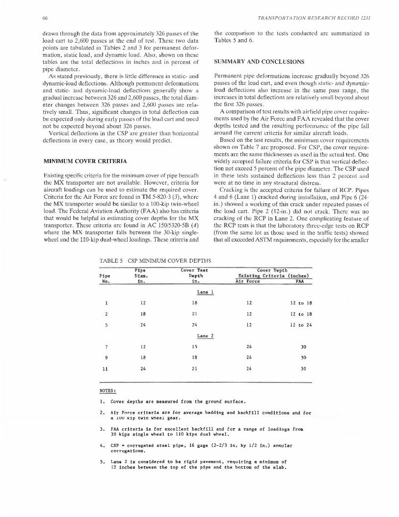
66

drawn through the data from approximately 326 passes of the load cart to 2,600 passes at the end of test. These two data points are tabulated in Tables 2 and 3 for permanent defor­mation , static load , and dynamic load. Also , shown on these tables are the total deflections in inches and in percent of pipe diameter.

As stated previously, there is little difference in static- and dynamic-load deflections. Although permanent deformations and static- and dynamic-load deflections generally show a gradual increase between 326 and 2,600 passes, the total diam­eter changes between 326 passes and 2,600 passes are rela­tively small. Thus, significant changes in total deflection can be expected only during early passes of the load cart and need not be expected beyond about 326 passes.

Vertical deflections in the CSP are greater than horizontal deflections in every case, as theory would predict.

MINIMUM COVER CRITERIA

Existing specific criteria for the minimum cover of pipe beneath the MX transporter are not available. However, criteria for aircraft loadings can be used to estimate the required cover. Criteria for the Air Force are found in TM 5-820-3 (3), where the MX transporter would be similar to a 100-kip twin-wheel load. The Federal Aviation Authority (FAA) also has criteria that would be helpful in estimating cover depths for the MX transporter. These criteria are found in AC 150/5320-58 ( 4) where the MX transporter falls between the 30-kip single­wheel and the 110-kip dual-wheel loadings. These criteria and

TABLE 5 CSP MINIMUM COVER DEPTHS

Pipe No,

l'ipe Diam. in.

Cover Test Depth in.

Lane l

12 18

18 21

5 24 24

Lan·e 2

12 15

9 18 18

11 24 21

NOTES:

TRANSPOR TATION RESEARCH RECORD 1231

the comparison to the tests conducted are summarized in Tables 5 and 6.

SUMMARY AND CONCLUSIONS

Permanent pipe deformations increase gradually beyond 326 passes of the load cart, and even though static- and dynamic­load deflections also increase in the same pass range, the increases in total deflections are relatively small beyond about the first 326 passes.

A comparison of test results with airfield pipe cover require­ments used by the Air Force and FAA revealed that the cover depths tested and the resulting performance of the pipe fall around the current criteria for similar aircraft loads .

Based on the test results, the minimum cover requirements shown on Table 7 are proposed. For CSP, the cover require­ments are the same thicknesses as used in the actual test. One widely accepted failure criteria for CSP is that vertical deflec­tion not exceed 5 percent of the pipe diameter. The CSP used in these tests sustained deflections less than 2 percent and were at no time in any structural distress.

Cracking is the accepted criteria for failure of RCP. Pipes 4 and 6 (Lane 1) cracked during installation, and Pipe 6 (24-in.) showed a working of this crack under repeated passes of the load cart. Pipe 2 (12-in.) did not crack. There was no cracking of the RCP in Lane 2. One complicating feature of the RCP tests is that the laboratory three-edge tests on RCP (from the same lot as those used in the traffic tests) showed that all exceeded ASTM requirements, especially for the smaller

Cover Depth Ex1s ci ns Cri teria (inches)

Air Force FAA

12 12 to 18

12 12 to 18

12 12 to 24

24 30

24 30

24 30

L. Cover depths are measured from the ground surface.

2. Air Force criteria are for average bedding and backfill conditions and for a 1uu Klp twln wneel gear.

3. FAA criteria is for excellent backfill and for a range of loadings from 30 kips single wheel to 110 kips dual wheel.

4. CSP = corrugated steel pipe, 16 gage (2-2/3 in. by 1/2 in.) annular corrugations.

5. Lane 2 is considered to be rigid pavement, requiring a minimum of 12 inches between the top of the pipe and the bottom of the slab.

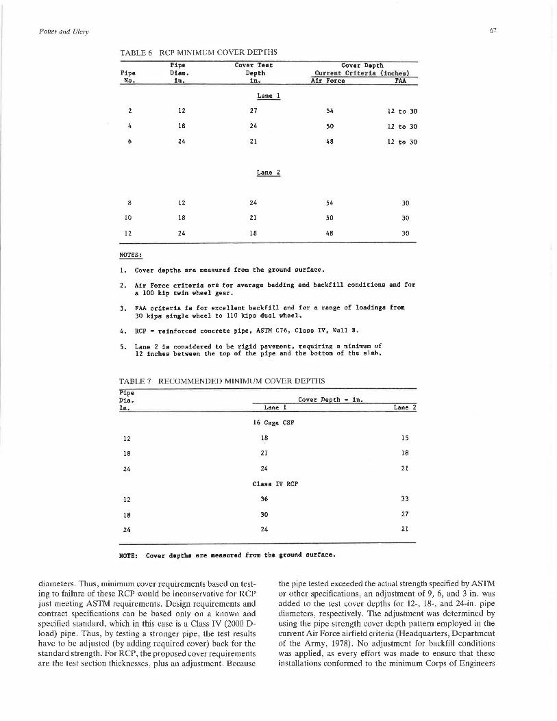
Potter and Ulery

TABLE 6 RCP MINIMUM COVER DEPTHS

Pipe Cover Test Cover Depth Pipe Diam. Depth Current Criteria (inches) No. in. in. Air Force FAA

Lane 1

2 12 27 54 12 to 30

4 18 24 50 12 to 30

6 24 21 48 12 to 30

Lane 2

8 12 24 54 30

10 18 21 50 30

12 24 18 48 30

NOTES:

1. Cover depths are measured from the ground surface.

2. Air Force criteria are for average bedding and backfill conditions and for a 100 kip twin wheel gear.

3. FAA criteria is for excellent backfill and for a range of loadinge from 30 kips eingle wheel to 110 kips dual wheel.

4. RCP • reinforced concrete pipe, ASTM C76, Class IV, Wall B.

5. Lane 2 ie considered to be rigid pavement, requiring a minimum of 12 inchee between the top of the pipe and the bottom of the slab.

TABLE 7 RECOMMENDED MINIMUM COVER DEPTHS

Pipe Dia. In.

12

18

24

12

18

24

Cover Depth - in. Lane

16 Gage CSP

18

21

24

Class IV RCP

36

30

24

NOTE: Cover depthe are measured from the ground surface.

Lane 2

15

18

21

33

27

21

67

diameters. Thus, minimum cover requirements based on test­ing to failure of these RCP would be inconservative for RCP just meeting ASTM requirements. Design requirements and contract specifications can be based only on a known and specified standard, which in this case is a Class IV (2000 D­load) pipe. Thus, by testing a stronger pipe, the test results have to be adjusted (by adding required cover) back for the standard strength. For RCP, the proposed cover requirements are the test section thicknesses, plus an adjustment. Because

the pipe tested exceeded the actual strength specified by ASTM or other specifications, an adjustment of 9, 6, and 3 in. was added to the test cover depths for 12-, 18-, and 24-in. pipe diameters, respectively. The adjustment was determined by using the pipe strength cover depth pattern employed in the current Air Force airfield criteria (Headquarters, Department of the Army, 1978). No adjustment for backfill conditions was applied, as every effort was made to ensure that these installations conformed to the minimum Corps of Engineers

68

criteria. It was presumed that the designer would specify back­fill requirements and tests sufficient to achieve the minimum required by the Corps of Engineers criteria.

ACKNOWLEDGMENT

The authors are grateful to the U.S. Army Engineer Water­ways Experiment Station for administrative support and per­mission to publish this paper. The views of the authors do not purport to reflect the position of the Department of the Army or the Department of Defense. This paper is published with the permission of the Chief of Engineers.

REFERENCES

1. D. R. Alexander. Correlation of Nondestructive Pavement Eval­uation Test Results with Results of Conventional Quality Control and In-Situ Strength Tests on a MX Road Test Section. Technical Report GL-86-1. U.S. Army Corps of Engineers Waterways Experiment Station, Vicksburg, Miss., 1986.

2. Federal Specification WW-P-4058: Pipe, Corrugated (Iron or Steel, Zinc Coated). June 14, 1974; Amendment 1, May 8, 1976, Wash­ington, D.C.

3. Drainage and Erosion Control-Structures for Airfields and Heli­ports. Technical Manual TM 5-820-3. Department of the Army, Washington, D.C., 1978.

4. Airport Drainage. Advisory Circular AC 150/5320-58. FAA, U.S. Department of Transportation, 1970.

DISCUSSION

JOHN M. KURDZIEL AND MIKE BEALEY American Concrete Pipe Association, 8320 Old Courthouse Road, Vienna, Va. 22182

The authors' efforts in determining minimum fill height requirements for CSP and RCP under heavy wheel loads were flawed because the testing procedure, instrumentation, and theory utilized in the project contained serious defects.

The testing procedures and instrumentation used do not account for all possible actions and reactions of the pipe prod­ucts. The use of only two displacement gauges in each CSP section will not register unsymmetric shape changes. If the CSP installations deform uniformly, as the authors suggest, than the horizontal and vertical displacement gauges will reg­ister accurate results. If the CSP installations, however, deform unsymmetrically (Figure 20), the two gauges will not indicate the excessive deflection. Additional displacement gauges would be necessary to detect all deflection variations. Unsymmet­rical deflections are very significant because they may lead to cracking at the seams, thus affecting the ring compressive capacity and watertightness or soiltightness of the pipe.

The crack detectors used in the RCP are useful for deter­mining when the where the first mic:rnc:rn<'.k o<'.rm~. h11t h~vP

no benefit in assessing the structural capacity. The authors erroneously assumed cracking was an accepted criterion for failure of RCP. This error was further compounded by using Vi-in.-wide strips of conductive paint for detecting cracks. The paint detectors were activated by hairline cracks and became inoperable after the first crack. The detectors could not iden­tify the depth, width, and length of cracks. Cracking is essen­tial for the proper performance of RCP and merely means

TRANSPORTATION RESEARCH RECORD 1231

Uniform Deflection

Unsymmetric Deflection

FIGURE 20 CSP instrumentation.

the steel has accepted the design tensile stresses. RCP that does not crack needs no reinforcement. According to the ASTM specifications on RCP, a 0.01-in. crack is a quality control test criterion for pipe tested in the three-edge bearing test and is not intended as an indication of overstressed or failed pipe under installed conditions. In the test condition, RCP is designed for an ultimate strength of 1.25 to 1.5 times the 0.01-in. crack strength. In the buried condition, the ulti­mate strength of RCP is virtually unlimited, because if the pipe could be sufficiently overloaded, it would simply crack at the crown, invert, and springline and continue to function as a four-hinged arch flexible pipe transferring loads into the surrounding soil. Cracking, therefore, is not the accepted cri­terion for failure of RCP as the authors assumed.

If the authors' concerns with cracking were motivated by concerns of leakage, then the leakage performance of the research pipe barrels and joints should have been measured, both for the RCP and the CSP. Such measurements should have been made of the pipe before installation, after instal­lation, and at intervals during the loading sequence.

The testing of CSP and RCP was done with an apparatus that simulated an MX missile transporter load and produced a maximum wheel load intensity of 91 psi, with the average estimated as 81 psi. Due to the fill heights, small pipe diam­eters, class of pipe, and type of installation used in the testing, however, the MX pipe loading will not produce any effects visibly different than those experienced by an AASHTO HS-20 wheel loading, which exerts a wheel load intensity of 80 psi. Although the AASHTO and MX loadings are both below those recommended for the pipe's strength class, the authors' minimum recommended fill heights differ dramati­cally from those recommended by AASHTO. It is also inter­esting to note that a previous Army Corps of Engineers report (I) on the subject found that with aircraft loadings or tire pressure intensities of approximately 250 to 300 psi there were no signs of distress on Class III RCP under 3 ft of fill. These loadings were more severe and the pipe was a strength class less than that used by the authors. The results of the previous Corps report appear to conflict with the authors' recommen­dations, especially for Lane 2, which is considered to be a rigid pavement.

The authors recommend increasing the cover requirements for RCP by an adjustment factor based on the fact the pipe tP.StP.rl P.YrPPrlPri thP ~rh1~l c;;:trPnoth c:np,-.;fiPrl h" A ~.'rf\.Jf ~p,,_ --- --- ------ ------o--- -r------- -,; ~ - ..... -- •-· ~-·

era! facts negate this recommendation. First and most signif­icant, the pipe did not fail. Without a failure to provide a distinct reference point, the selection of any minimum fill height other than that tested would be simply a wild guess. The test sections were not instrumented correctly to predict a point of failure, and based on the authors' comments and previous studies on the subject, it is obvious that no failure took place under these test loadings.

Poller and Ulery

Second, ASTM specifications on RCP are not installed per­formance specifications. The specifications are manufacturing standards intended to insure the pipe meets a uniform set of requirements regarding its material, manufacture, chemical and physical composition, and finish. Performance specifi­cations (such as the AASHTO Standard Specifications for Highway Bridges-Section 17) define how a product, spe­cifically reinforced concrete pipe, will react in an installed condition. The authors have obviously confused the two types of specifications. If the RCP was properly instrumented, the authors would have found that the moments, thrusts, and shears were well within the design limits for the cross-sectional parameters specified in the ASTM RCP specifications (ASTM C-76-88). The three-edge bearing test the authors relied on for predicting the D-load for the 0.01-in. crack cannot predict the complex relationships between moments, thrusts, and shears in an installed pipe. ASTM standards insure only that a pipe was made as specified. Performance specifications predict how a pipe product will react in a given installation but are appli­cable only for that specific installation. Arbitrary fill height adjustment factors cannot be made for a general installation or strength of pipe due to the wide variations with soils and installation properties. The authors' adjustment factors, therefore, have no validity.

REFERENCE

1. Traffic Testing of Pipe Beneath Heavy-Load Rigid Pavement. U.S. Army Corps of Engineers Waterways Experiment Station, Vicksburg, Miss., June 1962.

DISCUSSION

FRANK J. HEGER Simpson Gumpertz & Heger Inc., Consulting Engineers, Arlington, Mass. and San Francisco, Calif.

The paper reports the permanent, static, and dynamic deflec­tions measured for various passes of a load cart with a front wheel load of 68,700 lb and a rear wheel load of 57,000 lb over pipes of three different diameters: 12, 18, and 24 in.; two different materials: corrugated metal and reinforced con­crete (Class 4); two different soil cover materials: crushed lime stone and cement stabilized soil and arbitrary depths of soil cover over the pipe:

Depth of Soil Cover (in.)

Lane I Lane 2 (crushed stone) (soil cement)

12-in. pipe CSP 18 15 RCP 27 24

18-in. pipe CSP 21 18 RCP 24 21

24-in. pipe CSP 24 21 RCP 21 18

69

The final conclusion of the paper is that the test cover depths used in the tests are adequate for the CSP pipe, but that the minimum cover depths should be increased for the RCP pipe to the following values:

12-in. pipe 18-in. pipe 24-in. pipe

Depth of Soil Cover (in.)

Lane 1 (crushed stone)

36 30 24

Lane 2 (soil cement)

33 27 21

The reasoning used as a basis for recommending the increased cover depth for the RCP pipe is extremely vague, but appar­ently is based on the fact that companion pipe to the test pipe developed substantially higher three-edge bearing strength than the minimum specified three-edge bearing strengths.

The above conclusions are not supported by the actual test results from the application of the specified wheel loads above the pipe at the shallower burial depths used in the test pro­gram. The RCP test pipe in Lane 1 was actually subjected to loads substantially higher than the test loads during installa­tion of earth cover when a 100-ton roller was used to compact the top layer in a two-layer application of the specified crushed stone cover material. This excessive roller load produced hair­line cracking (that was detected by traces of conductive paint) in the 18- and 24-in. RCP pipe test specimens. The authors erroneously refer to the occurrence of this cracking as "fail­ure." They state that the RCP pipe has failed when it cracks.

The statement in the paper that cracking constitutes failure is inconsistent with the basis used for the design of nearly all reinforced concrete structures, as well as that used for the design of pipe in such widely used standards as ASTM C76 and Section 17.4 of Part 1 of the AASHTO Bridge Specifi­cation. The authors do not state the width of the observed cracks, but their statement that hairline cracks were observed implies that the width was much less than 0.01 in., the com­monly accepted limit level of crack width in concrete pipe design practice.

The authors' conclusion that the RCP pipe requires a greater depth of special earth cover than that used in the test is totally without a basis. The test results demonstrate that this pipe safely withstands the much greater load of the 100-ton roller without failure and with acceptable crack control. The fact that their three-edge bearing strength was higher than the minimum specified value provides no basis for the recom­mendation to increase the minimum earth cover; it merely indicates that the tests did not provide enough information to provide conclusive evidence of the adequacy of pipe having the minimum levels of three-edge bearing strength. Further­more, this recommendation flies in the face of the excellent performance of the RCP test pipe under the test loads, includ­ing its satisfactory resistance to the 100-ton roller load for the Lane 1 earth cover.

Publication of this paper sponsored by Commillee on Subswface Soi/­Structure Interaction.

70 TRANSPORTATION R ESEA RCH R ECORD 123 1

Plain Galvanized Steel Drainage Pipe Durability Estimation with a Modified California Chart

LAWRENCE BEDNAR

A method for estimation of plain galvanized steel pipe service life based on the use of a modified California Chart has been devel­oped. Certain limitations in the California Chart ~ith respect to pipe waterside corrosion have been addressed. The method, based on results of field studies in the United States and South America, is amenable to use in different climates.

Interest in methods of estimating drainage pipe durability has been considerable for many years in the United States and is receiving increasing worldwide attention. The use of galva­nized steel pipe in the tropical, subtropical, and temperate zones of South America has directed Armco to develop an estimation technique for this material amenable to worldwide conditions. The technique is based on water/soil chemistry, the main factor controlling galvanized steel corrosion.

GENERAL TECHNICAL BACKGROUND UNDERLYING ESTIMATION TECHNIQUE

Corrosion, an electrochemical process, and abrasion, a mechanical wear process, both contribute to pipe durability problems, but corrosion is the more important problem for any country as a whole. Corrosion problems occur on different types of terrain, but important true abrasion occurs only in or near mountainous/hilly terrain where periodic movement of rock and sand at high velocity occurs during rainfall. Abra­sion is a separate topic that will be dealt with in a later Armco report.

Waterside Corrosion

Advanced waterside corrosion within the lower half or lower quadrant of the pipe circumference has been the main cor­rosion problem observed in field inspections conducted in South America, the United States, and elsewhere (1-7). Pub­lished literature in related fields of technology indicates cor­rosion of galvanized steel in waters is influenced by several factors, but some are of predominant importance, and eval­uating them should permit a reasonably accurate determi­nation of the suitability of galvanized. The most important factor is water chemistry, the essential elements of which are pH, total dissolved solids (usually denoted by conductivity or resistivity), hardness, and alkalinity. Nonchemical factors of

Research Laboratory, Armco, Inc., 703 Curtis Street, Middletown, Ohio 45042.

substantial importance include degree of turbulence , tem­perature, and time of water contact.

1. Water Chemistry Hardness and alkalinity salts common to natural waters encourage formation of partially protective scales or films that hinder corrosion of reactive metals like zinc and steel, which otherwise would tend to corrode exces­sively (8, p. 11; 9, pp. 16, 29, 32, 140; 10, pp. 160, 163; 11, p. 76; 12, pp. 2.15, 2.16, 2.25). These salts, chiefly bicarbon­ates of calcium and magnesium, are sparingly soluble and tend to produce precipitates (mainly CaC03) that deposit onto corroding metal surfaces due to local surface chemical changes induced by corrosion. These salts also tend to modify metal corrosion products to encourage formation of protective insol­uble corrosion-product scales. The precipitated salts and mod­ified insoluble corrosion products combine to form the pro­tective scale. Soft pure low-conductivity waters containing very little of any type of dissolved salt, including hardness/ alkalinity salts, tend to be fairly corrosive because they possess no scaling tendency and because they lack buffering capacity, which leads to pH lowering. The pH and the total dissolved salt content (or conductivity) are important partly because low pH, due to excessive C02 and organic acid, or high con­ductivity, due to excessive concentrations of soluble chloride or sulfate, tend to prevent or interfere with scale formation. Acidity and chloride/sulfate salts are also inherently corrosive apart from their effects on scaling. The balance between hard­ness and alkalinity salts on one hand versus acidity and chlo­ride/sulfate salts on the other is critical in determining whether protective scaling or excessive corrosion will occur (13 ,14).

A zinc coating tends to increase substantially the effective­ness of water scaling in two different ways. First , despite its high inherent reactivity , zinc tends to form protective scales more readily than steel does, and scaling stifles reactivity and gives long coating life and consequent long barrier protection for the steel substrate (JU, pp. 160, 163 ). Second, before zinc reactivity is stifled by scale formation, it provides galvanic nrntP.r.tlnn th~t nrnm"tP~ f"rm :::. tl"n nf imnrrn1Pri n!0!~i:!!.,,~ • 1 - - -- - -- - - ---- -·- ---- - - ----r- - --· r

scale on any bare exposed steel substrate (10, pp . 160, 163). Galvanic protection promotes scale formation on exposed steel through electrochemical influences that encourage mineral precipitation and help ensure good adherence of the deposit.

2. Degree of Agitation High water velocity can induce ero­sion corrosion, a form of accelerated corrosion caused by

Bednar

scouring of metal surfaces by turbulent water and suspended solids that removes protective scale (12, pp. 2.15, 2.16, 2.25 ; 15, p. 7220). Water movement is important because it helps promote water aeration that ensures a high content of the dissolved oxygen necessary to support corrosion. High dis­solved oxygen is normal in surface waters (12, pp 2.15, 2.16, 2.25), so scaling tendency becomes the crucial corrosion­controlling factor determining how severe the effect of oxygen will be (16, pp. 149, 161). In waters that are normally stagnant, dissolved oxygen may be depleted by bacterial activity, so oxygen availability can become an important corrosion­controlling factor in such waters .

3. Temperature Elevated temperature accelerates corro­sion directly and indirectly, and consequent important dif­ferences in durability among different climates result. Again, scaling is the critical factor because an effective scale nullifies the detrimental effect of elevated temperature. However, in very corrosive waters where scaling is ineffective, temperature is a factor that should be considered (9, pp . 16, 29, 32, 140).

4. Time of Water Contact Obviously , this is a controlling factor in arid climates where pipes are apt to be dry most of the time so that average invert corrosion rates are quite low. It is a very important factor in a pipe high-water zone and in the invert of a pipe that is normally dry where contact is always limited to the time during and shortly after rainfall.

The water chemistry of primary concern for drainage pipe is that of groundwater runoff because this constitutes the pre­dominant stream flow in terms of contact time and is the only flow during extended dry weather. For any pipe in streams with prolonged flow , corrosion in the low-water zone is con­trolled by the chemistry of groundwater runoff. Groundwater runoff is generally of relatively low corrosivity because it con­tains primarily scaling salts obtained from intimate prolonged contract with soils containing mainly these salts. Corrosive soft acidic groundwaters or high-chloride/sulfate ground­waters arise from unfavorable soils found in regions of some countries.

The surface runoff that prevails during and shortly after rainfall is usually appreciably corrosive because it (a) contains relatively little of the scaling salts available from the soil due to brief soil contact time and (b) sometimes has enough veloc­ity and turbulence to induce erosion corrosion. However, its corrosivity is usually adequately controlled by the brief pipe contact time. It normally has no effect on a pipe low-water zone in scaling streamwater because protective scales persist through rainfall periods, but under certain conditions it can have an effect in the high-water zone or in the inverts of pipes that are normally dry.

Soilside Corrosion

Soilside corrosion is a complex and highly variable process, but does not usually control pipe life because typically overall soilside corrosion is much less aggressive than is overall water­side corrosion (1-7, 17-20). Obviously, in soils there are no

71

problems with abrasion or erosion corrosion , and the near­static state of soil moisture leads to reduced kinetics of overall corrosion due to reduced dissolved oxygen. In less porous soils, oxygen availability for corrosion will be low and will further ensure low overall corrosion rates (although pitting corrosion is likely to increase); in more porous soils where oxygen availability is high, protective corrosion product scales normally help ensure low overall corrosion rates (corrosion product scales are more effective on the soil side). Because of corrosion-mitigating factors like these, there is no overall dependence on CaC03-type scaling for good performance as there is on the waterside . Soilside corrosion problems that control pipe life do sometimes occur in soils of high acidity or in dry climates in locations where the natural content of chloride/sulfate salts is high and rainfall is inadequate to leach away soluble salts, but some groundwater moisture is present. Thus soil pH and conductivity (or resistivity) measurements provide reasonable indications of the likelihood of soilside corrosion problems.

DEVELOPMENT OF PLAIN GALVANIZED DURABILITY ESTIMATION TECHNIQUE

Current U.S. Technique

The estimation technique that has been the most useful in the United States is the California Chart, although in its original form it is generally overly conservative (5, 6, 20-23) and under some circumstances, is overly liberal (25, 26). This technique relates pipe durability to the pH and resistivity of either the waterside or the soilside environment (26) . This approach is proper for the soilside environment for which pH and resistivity are generally the most important factors con­trolling durability of galvanized culvert pipe. However, the technique is not entirely adequate for the more complicated waterside environment which causes most problems.

The main problems with the California Chart are summed up in the statement that the chart does not recognize the effect of water scaling on corrosion behavior. The chart in its original form gives overly conservative results in scaling waters con­taining some significant hardness and alkalinity, and these waters are predominant in most countries. Conservatism in scaling waters results from the chart presumption that cor­rosion rates always increase as resistivity decreases at any given pH, a presumption that can be true only if all dissolved salts are present as corrosive salts. Actually decreasing resis­tivity due to increasing concentrations of protective scaling salts corresponds to decreasing corrosion rates. In most sur­face waters, protective scaling salts constitute most or much of the total dissolved salt content, and corrosion is much less severe than it would be if all of the dissolved salt content were present as corrosive salts. Thus, ignoring the protective effect of scaling salts results in conservative durability esti­mates . The resulting degree of conservatism can be significant in any typical region where groundwaters contain some sig­nificant hardness and alkalinity. For example, in Florida (5) and Georgia (20), the average service life determined by inspection of pipes that were generally 14 gauge was 70 years or more, whereas average perforation time estimated from the California Chart was 40 years or Jess. In an area of Iowa

72

studied by the writer, the excellent condition of several gal­vanized pipes exposed for 30 years to streams with prolonged flow was indicative of service life in excess of 75 years at 14 gauge, while the chart gave estimated perforation times less than 40 years. The measured water pH and resistivity at one site were 7 .02 and 1449 ohm cm for which the chart gives a very conservative perforation time of32 years. The pipe actually showed no important penetration by corrosion after 30 years. The low water resistivity was due primarily to scaling salts (alkalinity = 258 ppm as CaC03 and hardness = 368 ppm as CaC03); attributing a detrimental effect to beneficial dissolved salts caused severe conservatism in the durability estimate .

By not recognizing the detrimental effect of the absence of a significant scaling effect in high-resistivity water, the chart gives liberal durability estimates in soft nonscaling or slightly scaling waters. The results are liberal because the chart sug­gests that, at a given pH, corrosion rates decrease continu­ously with increasing resistivity. This estimate conflicts with the fact, known from published literature (27), that at a given pH, soft pure water of high resistivity (and therefore of low alkalinity and hardness) is more corrosive than hard scaling water of much lower resistivity. High resistivity does tend to reduce corrosion rates, but this benefit is unimportant com­pared with the detrimental effect of the reduced scaling tend­ency caused by low alkalinity and hardness associated with high resistivity. In the chart, the presumed benefit of high resistivity are much greater than the actual benefit, presum­ably even offsetting the detrimental effect of reduced pH. By examining the California Chart, the reader can see that along any horizontal constant perforation time line on the chart, the perforation time is supposedly maintained constant as the resistivity increases and the pH decreases. This ongoing con­dition is quite impossible over the high end of the resistivity range because , in waters of high resistivity, virtually all of the dissolved salt content is present as scaling salts, and increasing resistivity corresponds only to decreasing concentrations of scaling salts and decreasing scaling tendency (high resistivity groundwaters arise in wet climates where any soluble corro­sive salts, such as chloride or sulfate, present in early soil development were leached away long ago and only limited amounts of sparingly soluble scaling salts remain). As already noted, even at a fixed pH, decreasing hardness and alkalinity correspond to increasing corrosion rates, and the combined detrimental effect of decreasing pH plus decreasing hardness and alkalinity can only increase corrosion rates faster.

Further evidence can be found in the results of culvert pipe durability studies conducted by state highway departments located wholly or partially in regions with soft high-resistivity groundwater and surface runoff arising from well-leached soils. In such regions, reduced pH is a natural consequence of the low alkalinity contents, so low pH and high n:sislivity are concurrent. These conditions exist throughout Maine and also in western Washington and in Oregon west of the Cascade Mountains where state highway departments (3, 6, 25) have found average service lives for 14-gauge material of about 35 yr. Of course, this figure should be contrasted with the 70-yr or more average service life found in Florida and Georgia where groundwaters generally have some significant alkalinity and hardness. In Maine and western Washington and Oregon, the one consistent factor that could account for the lesser average durability is the predominance of soft high-resistivity

TRA NSPORTA TION RESEARCH R ECORD 1231

runoff, so the highway department inspection results appear to be evidence that high resistivity is detrimental and thus does not offset the detrimental effect of reduced pH.

The degree o'f error in the chart durability estimate that can result from the combined influence of conservatism and liberalism trends when comparing sites was illustrated to the writer by an example in which groundwater chemistry in streams with continuous flow changed abruptly from scaling to non­scaling over a short distance along a secondary road near Pucallpa, Peru. Near the point of change, the scaling water had a pH of 7.65 and a resistivity of 2,304 ohm cm, and the nonscaling water had a pH of 5.55 and a resistivity of 62,500 ohm cm. The scaling water had 232 ppm alkalinity as CaC03

and 216 ppm hardness as CaC03 ; the nonscaling water, 14 ppm alkalinity as CaC03 and no hardness. On the basis of controlling waterside conditions, use of the California Chart suggests that the time to first perforation for 14-gauge pipe would be 57 years in the scaling water and 52 years in the nonscaling water. The implication is that pH and resistivity are the only important controlling factors and that the det­rimental low pH of the nonscaling water is essentially offset by the beneficial high resistivity so that durability is about the same in both waters. In actuality, the service life estimate was more than 75 years in the scaling water and about 20 years in the nonscaling water. Use of the chart results in con­servative estimates of service life in the scaling water and liberal estimates in the nonscaling water to such a degree that the total combined error in the estimate differential is on the order of 3.5:1 to 4:1. Some additional examples of the con­servatism/liberalism trends of the California Chart are pro­vided in Table 1.

There are some other important reasons why chart esti­mates are sometimes overly conservative or overly liberal. Severe conservatism occurs in estimates for drier climates where (a) waterside corrosion is generally minimal due to infrequent flow and (b) soilside corrosion generally controls durability. Conservatism arises by using minimum (watei:­saturated) soil resistivity when pipe corrosion is actually con­trolled by in situ resistivity which is generally much higher due to limited soil-moisture availability. Liberalism occurs in the estimate for certain wet regions where waters contain large amounts of corrosive molecular free C02 that is not revealed by pH/resistivity measurements.

Another problem in using the California Chart is an uncer­tainty over whether to use waterside or soilside pH/resistivity parameters. Some authorities have used soilside parameters to estimate durability that is generally controlled by waterside parameters. Although not technically unfounded because groundwater chemistry is related to soil chemistry, this approach does not distinguish between durability controlled by rela­tively slow soilside corrosion of drier climates from that con­trolled by the more rapid waterside corrosion of wetter cli­mates. Some authorities have determined both the soilside and waterside !"\ammeters :rnci h::iVf~ 11~Prl thP ~Pt th..t gi"P~

the most conservative estimate, but this approach does not differentiate between the two environments realistically because at a given set of pH/resistivity values, waterside corrosivity is likely to be quite different from that of the soilside. Soil parameters apply generally in dry climates while water param­eters apply in wet or moderately wet climates. When applying waterside parameters, the water alkalinity and hardness must be included with the pH and resistivity.

Bednar 73

TABLE 1 EXAMPLES OF OVERLY CONSERVATIVE AND OVERLY LIBERAL CALIFORNIA CHART ESTIMATES

ESTIMATED DURABILITY AT 14 GAGE

LOCATION I'!! RESIST. ALK. BY BY PIPE (OHM.CM) (CaC03) CAL. CH INSP. AGE

OVERLY CONSERVATIVE

S.D. US 7.34 649 327 34 >100 50 OH.US 8.10 1,754 359 39 >100 50 VENEZUELA 7.80 1,934 234 41 >100 26 MO . US 6.70 2, 062 195 29 >60 30 ECUADOR 7 .15 6, 711 77 52 >75 12

OVERLY LIBERAL

BRAZIL 4.8 114 , 940 VENEZUELA 5.0 83 ,330 BRAZIL 5.9 58 ,825 ECUADOR 6.6 9, 090

Since waterside corrosion is the most prominent problem overall, the most crucial aspect of durability estimate is the development of a comprehensive waterside technique that includes the effects of hardness, alkalinity, and C02 and thus eliminates the major causes of conservative/liberal trends in the California Chart. Armco has addressed this need, and the result is a modified type of California Chart, based on Armco field data, for depicting waterside corrosion. The pH, con­ductivity, hardness, and alkalinity are easily determined in the field using simple field meters and simple digital titration equipment; the free C02 is calculated from the pH and alka­linity values .

Development of a More Comprehensive Waterside Estimation Technique

Effects of Alkalinity, Hardness, and C02

Alkalinity, a crucial species determining water scaling tend­ency, is primarily in the form of bicarbonate salts. Bicarbonate (HC03) is readily destroyed by reaction with prevalent organic acids produced by plant decomposition or inorganic sulfuric acid occasionally encountered. These acids remove beneficial HC03 and substitute corrosive reaction product salts in its place, thus reducing the scaling tendency and increasing water corrosivity. Sometimes the alkalinity is totally consumed, pro­ducing free acidity, which results in severely corrosive water. Such water is not dealt with in this report because it is too corrosive to permit use of plain galvanized and other more common pipe materials.

Plant decomposition also produces C02 which combines with water to form corrosive carbonic acid, but C02 does not destroy HC03 alkalinity because C02 is actually part of the essential chemical reaction by which HC03 is formed from CaC03 in soil and rock . Indeed a little excess unreacted or free C02 is necessary to stabilize HC03 in solution, but any excess free C02 above this small amount reduces the scaling tendency and increases water corrosivity. In any natural water with significant alkalinity remaining after reaction with organic

4.2 54 -10 13 7 51 -20 13 5 53 -30 18

27 62 -40 10

acid, C02 is the remaining form of acidity influencing the pH and the scaling tendency. The interaction of free C02 , alka­linity, and hardness controls the basic water scaling tendency in any water for which the use of plain galvanized can be recommended.

Hardness (Ca +2 , Mg+ 2) and alkalinity (HC03, HSi03) are present in natural waters primarily in the form of calcium bicarbonate or Ca(HC03) 2 , and this salt is a source of insol­uble CaC03 precipitate for protective scale formation. Any water chemical change that increases pH will first reduce free C02 that stabilizes Ca(HC03) 2 in solution and then will reduce reacted or combined C02 in HC03 to encourage CaC03

precipitation. This reaction occurs locally on metal surfaces as a consequence of local generation of hydroxid (OH- ) by corrosion processes, so corrosion itself tends to promote CaC03

scale formation in a scaling water. However, increasing free C02 acidity lowers the overall pH and renders CaC03

precipitation increasingly more difficult and ultimately impos­sible at some critical concentration. Increasing free C02

increasingly hinders scaling and also directly increases zinc/ steel corrosion.

Obviously, differentiation of the relative basic scaling tend­encies of different waters can be accomplished by quantifying alkalinity , hardness , and free C02 concentrations. Alkalinity and hardness will be positive controlling factors, and free C02

will be a negative one. An appropriate method to obtain an index of the scaling tendency would be to add the alkalinity and hardness concentrations and to subtract the free C02

concentration. This approach is a modification of the classic approach of the Langlier index (and the related Ryznar index) in which the scaling tendency is based on the difference between the sum of the negative logarithms of the alkalinity and hard­ness concentrations on the one hand and the negative loga­rithm of the dissociated acid concentration (pH) on the other hand (9 , 12, 28, pp . 231, 349). The modified index uses total free C02 rather than pH to represent acidity and uses arith­metic concentrations (in ppm) rather than their logarithms. Also total hardness (Ca +2 + Mg+ 2) is used rather than just Ca+ 2 hardness because Mg+ 2 also participates in scale for­mation through pH-dependent precipitation reactions. Alka-

74

linity (total) is expressed as HC0-3 and hardness as Ca +2

because these are the primary actual forms in which they exist in waters . For either index, a decreasingly positive value in scaling water corresponds to increasing corrosivity, and cor­rosivity continues to increase as the index becomes increas­ingly negative in nonscaling water due to a rising proportion of C02 .

The modified index modifies the Langlier index reliance on the concept of a critical pH of CaC03 saturation above which CaC03 scaling occurs and below which it does not. More recent investigations (27; 29, p. 285) have shown that other factors in addition to the saturation state are involved, and scaling normally occurs in unsaturated waters of pH below the critical value due to scaling stimulation by OH - produced by corrosion reactions on metals . Decreasing pH and decreas­ing saturation state do reduce the CaC03 scaling tendency, but increasing alkalinity/hardness concentrations permit scal­ing at lowered saturation states, including substantially unsat­urated ones. These observations indicate that the CaC03 scal­ing tendency on corrodible metals is a continuum with the degree of scaling varying according ro che reiacive amouncs of alkalinity and hardness versus the amount of free C02 .

The modified index reflects this relative interaction because the scaling tendency, according to the index, increases or decreases continually relative to changes in the three concen­trations ; and at some low index value , scaling ceases.

Relative changes in the scaling tendency do not correlate completely with metal corrosion behavior as the published literature shows (27), and some further modifications are needed to reflect actual corrosion behavior more closely. The use of arithmetic concentrations rather than logarithmic ones is important because the Langlier index tends to overrate the influence of concentration variations over small ranges. For example, in a 332-ppm Ca(HC03)z solution, a variation in free C02 from 2 ppm to 16 ppm has little influence on cor­rosivity because the water is supersaturated at both concen­trations and readily supplies enough CaC03 to control cor­rosion throughout this free C02 range . Aggressive free C02

that effectively reduces scaling by inducing an unsaturated state does not appear until the free C02 exceeds 17 ppm, and effective scaling that controls corrosion should persist at free C02 levels well above 17 ppm. However, the change in C02

does affect the pH substantially (8 .32 to 7.41) and thus reduces both the degree of supersaturation and the Langlier index substantially (.9 units), suggesting an unrealistic substantial change in corrosivity . The use of arithmetic units in the mod­ified index reflects the change in corrosivity in a more modest and more realistic relative fashion in that the free C02 increase causes a minor drop in the index value from + 330 to + 316 (332-2 vs. 332-16).

Another important difference in the Armco method ·is the use of total acidity consisting of dissociated (ionic) and asso­ciated (molecular) carbonic acid or free C02 rather than just the dissociated acidity indicated by the pH in the Langlier method. This distinction is important because both forms of carbonic acid hinder scaling but the molecular form is not accounted for in the pH value (30). Molecular carbonic acid is also important because it has a direct adverse effect on metal corrosion rates (14, 31). The total free C02 concentra­tion indicated by the pH and alkalinity determines the severity of corrosion. Strictly speaking it is the excess free C02 beyond that small amount needed to stabilize HC03 in solution that

TRANSPORTA TION RESEARCH RECORD 1131

should be determined, but total free C02 , which is more easily calculated, can be used for our purposes.

Total free C02 is related to pH and alkalinity by the equa­tion pH = log (alkalinity x .203 x 107 + free C02) where alkalinity and free C02 are ppm as CaC03 and C02 . As this equation shows, if the free C02 is fixed, an increase in alka­linity raises the pH. For example, at a fixed free C02 con­centration of 50 ppm, an alkalinity of 5 ppm (as CaC03) gives a pH of 5.3 and an alkalinity of 50 ppm gives a pH of 6.3. The increase in alkalinity at a fixed C02 and the consequent increase in pH reduces water corrosivity because it increases scaling potential (makes Langlier index more positive).

Keeping the pH constant while increasing the alkalinity is accomplished by increasing the free C02 , which changes water corrosivity to a degree that depends on the value chosen for the fixed pH. The effect on water corrosivity depends on the relative amounts of free C02 and alkalinity, which in turn depend on whether the fixed pH value is above or below 6.3. This can be seen by rearranging the equation for the pH/ alkalinity/C02 relationship to read log C02 = log alk. + 6.307 - pH. Obviously , the free C02 concentration (as C02)

is equal to the alkalinity concentration (as CaC03) at pH 6.3, becomes less than the alkalinity at any higher pH value, and becomes greater than the alkalinity at any lower pH value. For example, at pH 6.5 the free C02 is 3.2 ppm at 5 ppm alkalinity and 32 ppm at 50 ppm alkalinity. Thus, at this pH, the alkalinity exceeds the free C02 , and the increase in C02

as alkalinity is increased is from 3.2 to 32 (28.8 ppm). On the other hand, at pH 6.0, the free C02 is 10 ppm at 5 ppm alkalinity and 100 ppm at 50 ppm alkalinity. At this pH, the free C02 exceeds the alkalinity, and the increase in free C02

as alkalinity is increased is from 10 to 100 ppm (90 ppm). At some relatively low fixed pH value, increasing alkalinity will begin to correspond to increasing water corrosivity to steel because the corrosive effect of free C02 will become predom­inant. The C02 predominates because only a relatively small portion of the increasing C02 available when alkalinity is increased at a fixed pH is needed to stabilize the increasing alkalinity in solution, leaving an increasing proportion of aggressive free C02 available for scaling suppression and cor­rosion acceleration. Another reason corrosivity will increase is that increasing alkalinity increases water conductivity, thus increasing corrosivity when the free C02 is too great to permit any protective scaling.

These relationships between pH/alkalinity/C02 and water corrosivity have been documented in the published literature (14; 31; 32, p. 88), and they must be reflected in the modified scaling index if the index is to be realistic. As the Langlier and Ryznar indices would do, the modified index must reflect changing corrosivity when the pH is changed due to changing alkalinity:C02 ratios. Obviously, the index should show reduced water corrosivity when Ll1e free C02 is kepl conslanl am! lhe alkalinity is increased. For example, if free C02 is fixed at 50 ppm , increasing the alkalinity from 5 to 50 ppm (as CaCO,) would increase the pH substantially and induce a substantial reduction in corrosivity. CaC03 at 5 ppm yields 6 ppm HC03 and 2 ppm Ca +z for an index value of -42 (6 + 2 - 50), which is indicative of severe corrosivity as would be expected in water of low scaling tendency and high free C02 (pH = 5.31) . CaC03 at 50 ppm yields 61 ppm HC03 and 20 ppm Ca +2 for an index value of +31 (61 + 20 - 50), which is indicative of considerably less corrosivity as would be expected

Bednar

(pH = 6.31). On the other hand, if alkalinity were fixed at 50 ppm, reducing the C02 from 50 ppm to 5 ppm would decrease corrosivity substantially, and this reduction would be reflected by a substantial index increase from +31 (61 + 20 - 50) to +76 (61 + 20 - 5).

The index is also a convenient indicator of the increased corrosivity resulting when alkalinity is increased at a relatively low fixed pH. For example, Armco laboratory tests showed that the short-term corrosion rate of mild steel in a calcium bicarbonate solution of 90 ppm (as CaC03) at pH 5.8 was nearly three times as great as the corrosion rate in a 14-ppm calcium bicarbonate solution (as CaC03) at the same pH. At pH 5.8, the 90-ppm solution had 289 ppm free C02 by cal­culation, and the 14-ppm solution had 44 ppm free C02 • The index gives a value of -143 for the 90-ppm solution (110 + 36 - 289) and a value of - 21 for the 14-ppm solution (17 + 6 - 44), reflecting the actual greater corrosivity of the 90-ppm solution. The Langlier and Ryznar indices do not reflect this relationship because they suggest the 14-ppm solu­tion is more corrosive (Langlier index would be about - 2.3 for the 90-ppm solution and about -3.9 for the 14-ppm solu­tion). This is the type of problem that arises from the use of pH rather than total free C02 to represent the acidity factor. Corrosive molecular C02 is very high in the 90-ppm solution, but is not accounted for in the pH value. Thus, the Langlier index underrates the corrosivity of this solution. Of course, the Langlier index does not apply to waters of pH below 6.5 because Professor Langlier was concerned mainly with water distribution systems. A modified index is necessary to account for molecular C02 and to handle the range of natural waters found in culvert environments where C02 concentrations can be very high at times.

The index appears to be most realistic with no weighting for any of its three components (alkalinity, hardness, or C02).

The data fit the completed durability estimation graph best when no weighting is assigned.

/ y

N 0 u

QJ

1' u_

UJ UJ QJ c ~ 0 I

+

c

0 '{

<(

-

/ v

/ ~A

/ / c

/ v

/ /

/ E

/ v

L----~,

Effects of Alkalinity, Hardness, and C02 in Combination with Conductivity

75

It is now necessary to consider the interrelationship of the scaling tendency with conductivity to adequately depict water corrosivity. In scaling water there is a critical balance between the scaling tendency and corrosive salts, such as chlorides and sulfates, because such salts tend to interfere with scale for­mation at some critical concentration. Also, in acidic non­scaling water, the corrosive effect of acidity is compounded by increasing conductivity, so the combined effect of a neg­ative scaling tendency and higher conductivity is quite severe. These relationships can be depicted on a graph with the basic scaling tendency (alkalinity + hardness - C02) on the ver­tical axis and the conductivity on the horizontal axis as has been done in Figure 1. In Figure 1, line AB depicts the rela­tionship between the scaling tendency and the conductivity at a given fixed service life. There is also a line XY along which all of the conductivity is due to hardness/alkalinity salts, and water corrosivity is minimal. Conductivity values that fall below or to the right of XY are the result of corrosive salts and ionic carbonic acid contributing to conductivity. Also, in Figure 1, there must be a critical sloped line like AB sepa­rating satisfactory performance from unsatisfactory, and AB represents the limiting water chemistry range at which some arbitrary fixed pipe service life can be attained. The reason for the slope becomes obvious by considering any pair of horizontal lines such as CD and EF. On line CD, the scaling tendency or the sum of hardness plus alkalinity minus C02 is fixed, and increasing conductivity is due to other salts, which are corrosive salts like chloride and sulfate. Eventually at some critical higher conductivity value, the corrosive salt con­centration is high enough and scaling is sufficiently negated that the corrosion rate increases to the level represented by the service life of line AB. On line EF, the acidity is higher and the inherent scaling tendency is lower initially and less

/ H ·-/

D

/ v

/

v /

/ / F

CONDUCTIVITY (umhos/cm)

FIGURE 1 Chemistry limits for a given service life.

76

chloride and sulfate can be tolerated, so with increasing con­ductivity the critical point is reached at a lower conductivity.

It is to be expected that line AB will show changing slope over a wide range of conductivity because AB represents the ratio of scaling tendency to conductivity which, if the effect of free C02 is ignored, is comparable to the ratio of scaling salts to total dissolved salts (scaling + corrosive salts). If this ratio were constant, AB would be a straight line, and as conductivity is decreased the fixed service life would be main­tained simply by decreasing scaling salts and corrosive salts in balanced linear proportion . However, even if this balance is sustained, the corrosion rate will still increase as conduc­tivity is decreased due to the weakening scaling tendency inherent with decreasing scaling salts, which increases cor­rosion rates even in the absence of corrosive salts. This means that as conductivity decreases, fixed unit reductions in the scaling salt concentration must be accompanied by increas­ingly larger reductions in the corrosive salt concentration to maintain the fixed service life. Thus as conductivity decreases, the ratio of scaling salts to total dissolved salts must increase and the slope of AB must decrease. ln soft waters of low scaling salt content, the scaling tendency becomes low enough and the potential corrosivity becomes great enough that pro­portionately large decreases in corrosive salt content are needed to sustain the fixed service life, and the slope of AB can approach zero. Of course the fixed service life can be sus­tained by decreasing free C02 as well as by decreasing cor­rosive salts; and in very pure waters of very low conductivity where the influence of further decreases in all dissolved salts is minimal, free C02 becomes the primary factor controlling service life.

A Modified California Chart

The similarity of Figure 1 to the California Chart is readily seen by first realizing that the scaling tendency expression alkalinity + hardness - free C02 includes the effect of pH because specifying the alkalinity and free C02 necessarily specifies the pH. The pH can be substituted for C02 in the above expression to give the following expression in which alkalinity is as HC03 and hardness is as Ca+ 2

:

. . Alkalinity Alkahmty + Hardness - .

1 ( H r.

22)

anti og p - ,i . . (1)

In this expression, the effect of any given pH value on water corrosivity will vary with variations in alkalinity and hardness (or C02). In effect, the scaling tendency expression can be viewed as the effect of pH on corrosivity after correction for alkalinity and hardness scaling effects. In addition to the effect of scaling tendency, also specified on Figure 1 is the propor­tion of corrosive salts at a given conductivity because once ::ilk::ilinitv/h~rrlnP.<;<; rnnrPntr::itinn< ::i1·p <nPrifiPrl thP h::il::inrP

~ J. ) - - - ------- - -

of salts contributing to that conductivity value are corrosive salts. A modified California Chart emerges once AB lines for various fixed service lives are entered and service life is depicted as a function of conductivity (inverse of resistivity) and a pH­related factor. As pH increases, service life increases to the extent that the scaling tendency increases and to the extent permitted by corrosive chloride/sulfate salts included in the conductivity value.

TRANSPORTATION RESEARCH RECORD 1231

The modified chart reflects the detrimental effect of 11011-

scaling low-conductivity soft water by line XY and lines just below and parallel to XY . Decreasing conductivity caused by decreasing alkalinity/hardness concentrations at a fixed con­centration of corrosive salts and C02 follows such lines, and these lines intersect decreasing service life levels as conduc­tivity decreases. Decreasing alkalinity at a fixed free C02

content is necessarily accompanied by decreasing pH, so the combined effect of lower pH and high resistivity common to soft water is illustrated.

Adding the Effect of Temperature

In its final form, the modified chart must incorporate the effect of mean annual temperature to be accurate enough for use in different climates. Reduced temperature tends to reduce the corrosivity of aggressive water chemistry. Thus, the graph could be expected to reflect the fact that galvanized pipe can be used successfully over a wider range of water chemistry limits in cooler climates. Denoting the effect of temperature in the graph is accomplished by constructing different AB chemistry limit lines for different climates or different tem­perature levels . The difference between the positions of these lines should be greater when a shorter service life is specified because a shorter service life is attainable in waters of lower scaling tendency where the effect of temperature is greater.

Graphing of Available Data

Finding the actual position and slope of line AB for any spec­ified service life requires plotting of sufficient field data in which pipe condition as a function of age is related to water conductivity , alkalinity, hardness, free C02 , and temperature . All of the more accurate available data from wet sites (130 sites with continuous or very prolonged flow) inspected in South America and the United States have been plotted in Figure 2.

Figure 2 is the low-conductivity end of the graph illustrating the temperature climate AB line. Two pipes shown (E) had erosion corrosion in the high water zone that made perform­ance much worse than the graph estimate. These are from a small area where erosion corrosion is extreme and are included here to show the degree of erosion-corrosion interference possible. One seemingly abnormally good pipe is at a site with a low mean temperature . Diamond-shaped and X-shaped data points represent sites in temperate climates; square-shaped and cross-shaped data points represent those in tropical cli­mates. All cross-shaped and X-shaped data points represent pipes that in the author's estimation have average corrosion rates low enough to resist important perforation for at least 35 years at 14 g;mge. All scp1;ir~ ;incl rli;imrrng-shilperl data

average corrosion rate of each pipe over its exposure time in service was determined crudely on the basis of an estimation of remaining pipe invert thickness by using a pick blade to test metal yielding. Estimates were conservative so that errors would be in the direction of conservatism. In Figure 2, line AB represents, for either a temperate or a tropical climate, a reasonable approximation of the position and slope when the line denotes minimum water chemistry conditions at which

Bednar

N 0 u w w Q'. u._

Vl Vl w z 0 Q'. <( I

+ ~

D

LIMIT AT MEAN TEMPERATURES-+----... UP TO 15°C

0

0

0 0

0

0 z ::J <( y: _J <(

-100 -·1--~~~~-+~~~---+----~~t--~~~~-r~~~~~-r-~-------1

r@

D

0

+ a INIMUM 35 YEA SERVICE IN ROPICAL CLIMA' E

X a INIMUM 35 YEA SERVICE IN fEMPERATE CLI TE

200

D = LES. THAN 35 YEAR ERVICE IN TRO ICAL CLIMATE

o = LES THAN 35 YEAR ERVICE IN TEM ERATE CLIMATE

400

CONDUCTIVITY (UM HOS/CM)

FIGURE 2 Chemistry limits for 35 years of service at 2.00 mm (14 gauge).

2 Q_ Q_

N

0 u w w

°" LL

l/) l/) w z 0

°" <{ :r::

+ >-­f-z

100 wy~v

o~

-' -100 l-----l-~~~1--~~-1-~~~C---~~-1--~~-~~-+-~~--+~~----; <{ :::<:'. <i -200 '--~~-'-~~~'--~--'--~~--'--~~-~~--'~~~-'-~~~~~~

0 200 400 600 800 1 000 1 200 1 400 1 600 1 800

CONDUCTIVITY (µMHOS/CM)

FIGURE 3 Modified estimation graph-durability in temperature climates.

600

77

a general level of 35 years of satisfactory service at 2 mm (14 gauge) can be expected. Durability increases with increasing distance above line AB . Of course , durability increases with increasing pipe wall thickness above 2.0 mm, and judging by the California Chart gauge adjustment factors, 3.5 mm mate­rial (-10 gauge) should provide up to as much as 1. 75 times as long service life as 2.0 mm material does.

After AB lines for 20-year and 50-year service life levels have been determined , Figure 2 can be made to resemble the California Chart more closely. It is necessary to place AB lines for different service lives on one graph and to construct such a graph for both temperate and tropical climates. The resulting graph for temperate climates is shown in Figure 3. The reader will recognize that the California Chart axes for

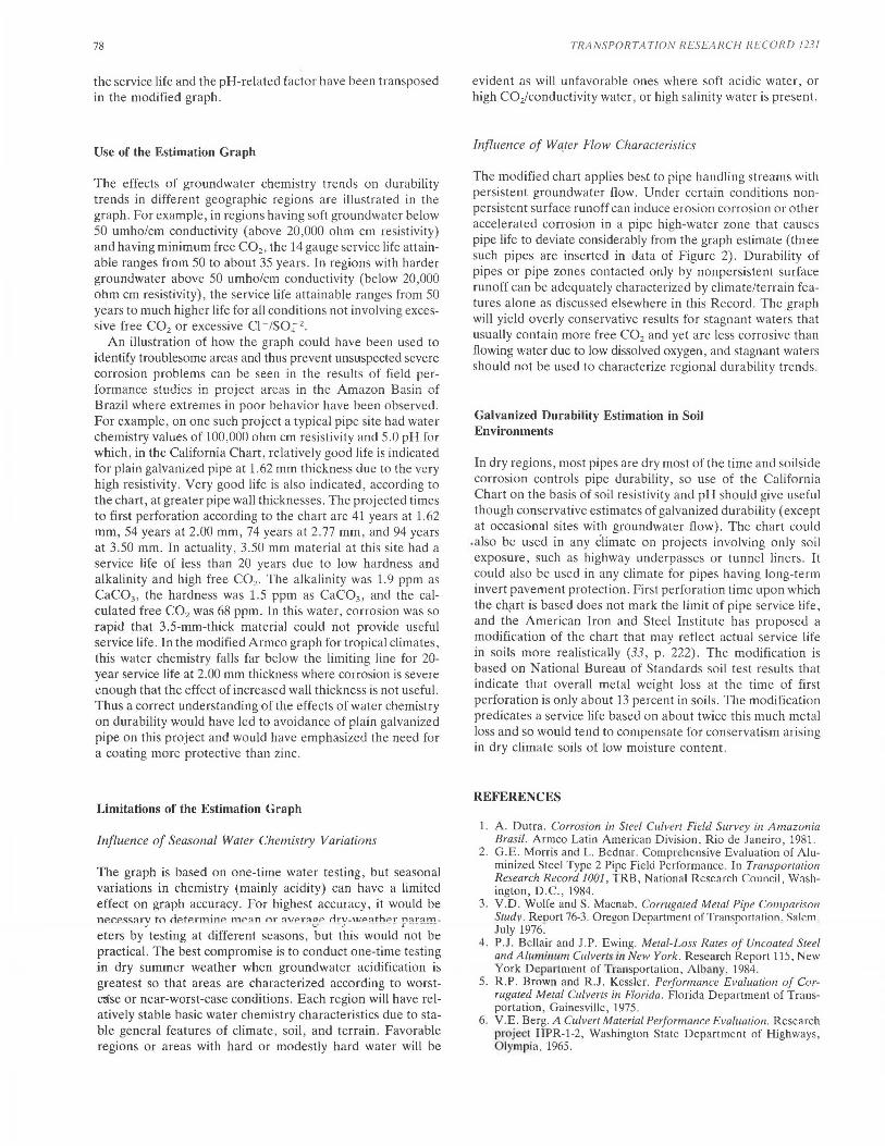
78

the service life and the pH-related factor have been transposed in the modified graph.

Use of the Estimation Graph

The effects of groundwater chemistry trends on durability trends in different geographic regions are illustrated in the graph . For example, in regions having soft groundwater below 50 umho/cm conductivity (above 20,000 ohm cm resistivity) and having minimum free C02 , the 14 gauge service life attain­able ranges from 50 to about 35 years . In regions with harder groundwater above 50 umho/cm conductivity (below 20,000 ohm cm resistivity), the service life attainable ranges from 50 years to much higher life for all conditions not involving exces­sive free C02 or excessive Cl - /SO 4- 2 •

An illustration of how the graph could have been used to identify troublesome areas and thus prevent unsuspected severe corrosion problems can be seen in the results of field per­formance studies in project areas in the l~ .. mazon Basin of Brazil where extremes in poor behavior have been observed. For example, on one such project a typical pipe site had water chemistry values of 100,000 ohm cm resistivity and 5.0 pH for which, in the California Chart, relatively good life is indicated for plain galvanized pipe at 1.62 mm thickness due to the very high resistivity. Very good life is also indicated, according to the chart, at greater pipe wall thicknesses. The projected times to first perforation according to the chart are 41 years at 1.62 mm, 54 years at 2.00 mm, 74 years at 2.77 mm, and 94 years at 3.50 mm. In actuality, 3.50 mm material at this site had a service life of less than 20 years due to low hardness and alkalinity and high free C02 . The alkalinity was 1.9 ppm as CaC03 , the hardness was 1.5 ppm as CaC03 , and the cal­culated free C02 was 68 ppm. In this water, corrosion was so rapid that 3.5-mm-thick material could not provide useful service life. In the modified Armco graph for tropical climates, this water chemistry falls far below the limiting line for 20-year service life at 2.00 mm thickness where corrosion is severe enough that the effect of increased wall thickness is not useful. Thus a correct understanding of the effects of water chemistry on durability would have led to avoidance of plain galvanized pipe on this project and would have emphasized the need for a coating more protective than zinc.

Limitations of the Estimation Graph

Influence of Seasonal Water Chemistry Variations

The graph is based on one-time water testing, but seasonal variations in chemistry (mainly acidity) can have a limited effect on graph accuracy. For highest accuracy, it would be ne.c.P.SS::trv tn <iP.tP.rminP. mP~n nr ~vPr~aP rir\1-u;P~thPr n<;1,r~m-eters by, testing at different seasons, b~; this ~~-~ld rn-~; be practical. The best compromise is to conduct one-time testing in dry summer weather when groundwater acidification is greatest so that areas are characterized according to worst­cnse or near-worst-case conditions. Each region will have rel­atively stable basic water chemistry characteristics due to sta­ble general features of climate, soil, and terrain. Favorable regions or areas with hard or modestly hard water will be

TRANSPORTATION RESEARCH RECORD 1231

evident as will unfavorable ones where soft acidic water or high C02/conductivity water, or high salinity water is pres~nt.

Influence of WC(ter Flow Characteristics

The _modified chart applies best to pipe handling streams with persistent groundwater flow. Under certain conditions non­persistent surface runoff can induce erosion corrosion or other accelerated corrosion in a pipe high-water zone that causes pipe life to deviate considerably from the graph estimate (three such pipes are inserted in data of Figure 2). Durability of pipes or pipe zones contacted only by nonpersistent surface runoff can be adequately characterized by climate/terrain fea­tu_res ~lone as discussed elsewhere in this Record. The graph will yield overly conservative results for stagnant waters that usually contain more free C02 and yet are less corrosive than flowing water due to low dissolved oxygen, and stagnant waters should not be used to characterize regional durability trends.

Galvanized Durability Estimation in Soil Environments

In dry regions, most pipes are dry most of the time and soilside corrosion controls pipe durability , so use of the California Chart on the basis of soil resistivity and pH should give useful though conservative estimates of galvanized durability (except at occasional sites with groundwater flow). The chart could

.also be used in any climate on projects involving only soil exposure, such as highway underpasses or tunnel liners. It could also be used in any climate for pipes having long-term invert pavement protection. First perforation time upon which the Chfirt is based does not mark the limit of pipe service life, and the American Iron and Steel Institute has proposed a modification of the chart that may reflect actual service life in soils more realistical.ly (33 , p. 222). The modification is based on National Bureau of Standards soil test results that indicate that overall metal weight loss at the time of first perforation is only about 13 percent in soils. The modification predicates a service life based on about twice this much metal loss and so would tend to compensate for conservatism arising in dry climate soils of low moisture content.

REFERENCES

1. A. Dutra. Corrosion in Steel Culvert Field Survey in Amazonia Brasil. Armco Latin American Division, Rio de Janeiro, 1981.

2. G.E. Morris and L. Bednar. Comprehensive Evaluation of Alu­minized Steel Type 2 Pipe Field Performance. In Transportation !?esearch Record 1001, TRB, National Research \.nnndl, Wash­mgton, D.C., 1984.

3. V.D. Wolfe and S. Macnab. Corrugated Metal Pipe l.nmpnrisnn Studv. Reoort 76-3. Ore!_rnn Denartment ofTrnnsnortation. S"lem July 1976. · •

4. P.J. Bellair and J.P. Ewing. Metal-Loss Rares of Uncoated Steel and Aluminum Culverts in New York. Research Report 115, New York Department of Transportation, Albany, 1984.

5. R.P. Brown and R.J. Kessler. Pe1formance Evaluation of Cor­rugated Metal Culverts in Florida. Florida Department of Trans­portation , Gainesville, 1975.

6. V.E. Berg. A Culvert Material Performance Evaluation. Research project HPR-1-2, Washington State Department of Highways Olympia, 1965 . '

Bednar

7. D.J. Smith and J. Smithee. Survey of Armco Corrugated Steel Pipe Culverts under the Lamco Railroad, Liberia. Armco Euro­pean Division, Newport, England, Jan. 1981.

8. C.J. Slunder and W.K. Boyd. Zinc: its Corrosion Resistance. Battelle Memorial Institute, Columbus, Ohio, 1971.

9. G. Butler and H.C.K. Ison. Corrosion and its Prevention in Waters. Reinhold, New York, 1966.

10. U .R. Evans. The Corrosion and Oxidation of Metals. St. Martins, New York, 1960.

11. U.R. Evans. Corrosion and Oxidation of Metals: Suplemenrary Volume. Edward Arnold, London, 1968.

12. L.L. Shreir. Corrosion. John Wiley, New York, 1963. 13. G.B. Hatch and 0. Rice. Influence of Water Composition on

the Corrosion of Steel. Journal of the American Waterworks Asso­ciation, Vol. 51, 1959.

14. L. Kenworthy and M.D. Smith. Corrosion of Galvanized Coat­ings and Zinc by Waters Containing Free Carbon Dioxide. Jour­nal of institute of Metals, Vol. 70, 1944, p. 463.

15. M.G. Fontana and N.D. Greene. Corrosion Engineering. McGraw­Hill, New York, 1978.

16. F.N. Speller. Corrosion: Causes and Prevention. McGraw-Hill, New York, 1935.

17. Durability of Drainage Pipe . NCHRP Synthesis 50. TRB, National Research Council, Washington, D.C., 1978.

18. M. Romanoff. Underground Corrosion. National Bureau of Standards Circular 579. U.S. Department of Commerce, Wash­ington, D.C., April 1, 1957.

19. V. Ashworth et al., Underground Corrosion and Its Control. Corrosion Australasia, Oct. 1986.

20. H.P. Little, K.J. Boedecker, and J.B. Browner. Performance Evaluation of Corrugated Metal Culverts in Georgia. Southeast Corrugated Steel Pipe Association, April 1977.

21. Durability of Metal Pipe Culverts. Research Project 16. Idaho Department of Highways, Boise, April 1965.

22. H.E. Worley and C.F. Crumpton. Corrosion and Service Life of Corrugated Metal Pipe in Kansas. Highway Research Report 412, 1972.

79

23. Nebraska Soil Resistivity and pH Investigation as Related to Metal Culvert Life. Nebraska Department of Roads, Lincoln, April 1969.

24. W.H. Temple, S.L. Cumbaa, and B.J . Gueho. Evaluation of Drainage Pipe by Field Exp1•ri111e11tntion and Supplemental Lab­oratory Experimentation. Louisiana Department of Transporta­tion and Development, Baton Rouge, March 1985.

25. R.M. Jacobs. Culvert Life Study. Report 74-1. Maine Depart­ment of Transport<Ui n. Augu ta, Jan. 1974.

26. J .L. Beaton and R.F. Lratfull. Field Test for Estimating Service Life of Corrugated Metal Pipe Culverts. HRB Proc., Vol. 41, 1962.

27. W. Stumm. Investigations of Corrosive Behavior of Waters. Transactions of the ASCE-Sanitary Engineering Division, Vol. 86, 1960. p. 27.

28. Betz Handbook of industrial Water Conditioning. Betz Labora­tories Inc., Trevose, Pa .. 1962.

29. T.E. Larson and R. V. Skold. Laboratory Studies Relating Min­eral Quality of Water to Corrosion of Steel and Cast Iron. Cor­rosion, June 1958, p. 285.

30. J.F. Dye. Calculation of Effect of Temperature on pH, Free Carbon Dioxide and the Three Forms of Alkalinity. Journal of the American Waterworks Association, April 1952.

31. G.W. Whitman, R.P. Russell, and V.J. Altieri. Effect of Hydro­gen Ion Concentration on the Submerged Corrosion of tcc l. Journal of J11d11s1rial Engineering Chemistry. Vol. 16, No. 7, 1924, p. 665.

32. A. Kuch. Internal Corrosion of Water Distribution Systems. In ooperntive Re!iearch Repon. Denver, Colo., 1985.

33. Modern Sewer Design. American Iron and Steel Institute, Wash­ington, D.C., 1980.

Publication of this paper sponsored by Committee on Culverts and Hydraulic Structures.

80 TRANSPORTATION RESEARCH RECORD 1231

Durability of Plain Galvanized Steel Drainage Pipe in South America: Criteria for Selection

LAWRENCE BEDNAR

Durability of plain galvanized steel drainage pipe is associated with climate/terrain features that influence water/soil chemistry. The diverse climate/terrain features of South America provided a con­venient setting for development of a regional approach to selective galvanized pipe application based generally on these features and more specifically on measured watei/soil chemistry trends.

Reports of durability problems on plain galvanized culvert pipes in certain areas of South America have become a sig­nificant concern in recent years. Most of these problems have been caused by accelerated waterside corrosion of pipe inverts. Problems first appeared in Brazil in and near the Amazon Basin of northern Brazil (J). When other countries began to report durability problems, it became increasingly evident that Armco needed a reliable way to determine where plain galvanized pipe should not be used. Methods in current use in the United States have not proven to be sufficiently reliable. The present report is a condensation of the results of Armco studies in several countries of South America. A method is presented for selective use of galvanized to minimize future durability problems.

GENERAL APPROACH TO PLAIN GALVANIZED SELECTION

The application of pipe products in South America is influ­enced by the dependence of material durability on environ­mental conditions and the distribution of certain types of cor­rosive hostile environments over large regions of some countries. Achieving maximum utilization of a product while keeping maintenance problems at a minimum necessitates the use of an effective selection method. On the larger scale, selection involves limiting use in more hostile regions and concentrating on regions where conditions are more favorable. For reasons that will become obvious from reading the body of this report, the continent can be divided along the lines of climate and terrain into large geographical regions with different levels of environmental corrosivity toward plain galvanized pipe.

The reg1unai approach m gaivanized seienion is uirimareiy combined with Armco studies on water/soil chemistry trends within individual regions because chemistry trends are the primary reason for durability variations. Climate and terrain features of each region are useful on a broad scale because they control water/soil chemistry, and chemistry testing defines regional trends more accurately. A specific durability esti-

Research Laboratory, Armco, Inc., 703 Curtis Street, Middletown , Ohio 45042 .

mation technique based on field durability and chemistry stud­ies has been developed and is discussed in detail by the author elsewhere in this Record. A general discussion of the regional aspect of selection and the durability estimation technique is provided here.

Ongoing water/soil testing in all regions of the continent would be valuable to ensure optimal accuracy in classifying regions according to their durability trends. Ongoing data generation will refine and adjust regional guidelines until accuracy is optimal in all respects. No Armco data are avail­able yet for some regions, and our classification in these cases is based mainly on indirect climate/terrain data that are useful but not conclusive, so such classifications may be temporary. Additional regional water/soil testing can be accomplished on a random basis or along the routes of individual new highway projects. The latter approach has the added attraction of max­imizing the prospects for good performance on individual new projects, which may be desirable on some major projects with high durability requirements.

GENERAL TECHNICAL BACKGROUND UNDERLYING SELECTION METHOD

Corrosion, an electrochemical process, and abrasion, a mechanical wear process, both contribute to galvanized pipe durability problems, but corrosion is the more important problem for any country as a whole. Corrosion problems can occur on different types of terrain, whereas important true abrasion occurs only in or near mountainous/hilly terrain where periodic movement of rock and sand at high velocity during rainfall is encountered. Galvanized selection on the basis of abrasion potential is a separate subject that will be dealt with in a future Armco report.

Factors Controlling Corrosion Behavior

Advanced waterside corrosion within the lower half or lower quadrant of the pipe circumference has been the more com­mon corrosion problem observed in field inspections con­ducted in South America, the United States, and elsewhere (2-6). Published literature in related fields of technology indi­cates that several factors influence corrosion in waters. Some factors are of predominant importance, and evaluating them should permit a reasonably accurate determination of the

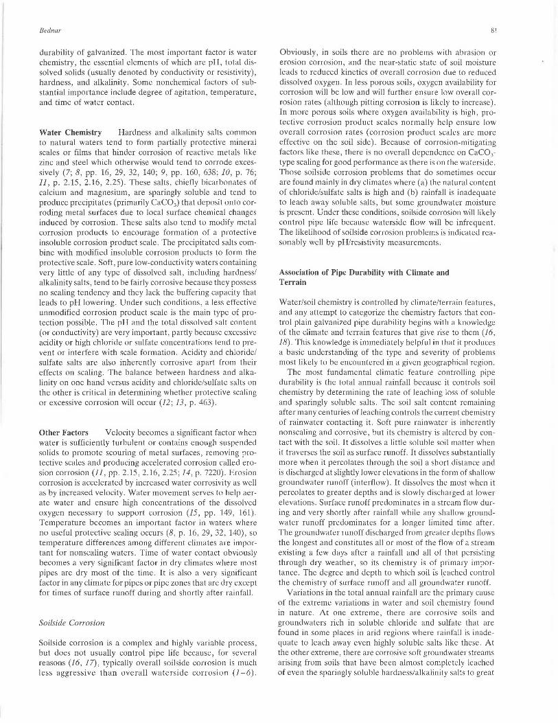
Bednar

durability of galvanized. The most important factor is water chemistry, the essential elements of which are pH, total dis­solved solids (usually denoted by conductivity or resistivity), hardness, and alkalinity. Some nonchemical factors of sub­stantial importance include degree of agitation, temperature, and time of water contact.

Water Chemistry Hardness and alkalinity salts common to natural waters tend to form partially protective mineral scales or films that hinder corrosion of reactive metals like zinc and steel which otherwise would tend to corrode exces­sively (7; 8, pp. 16, 29, 32, 140; 9, pp. 160, 638; 10, p. 76; 11, p. 2.15, 2.16, 2.25). These salts , chiefly bicarbonates of calcium and magnesium, are sparingly soluble and tend to produce precipitates (primarily CaC03) that deposit onto cor­roding metal surfaces due to local surface chemical changes induced by corrosion. These salts also tend to modify metal corrosion products to encourage formation of a protective insoluble corrosion-product scale. The precipitated salts com­bine with modified insoluble corrosion products to form the protective scale. Soft, pure low-conductivity waters containing very little of any type of dissolved salt , including hardness/ alkalinity salts, tend to be fairly corrosive because they possess no scaling tendency and they lack the buffering capacity that leads to pH lowering. Under such conditions , a less effective unmodified corrosion product scale is the main type of pro­tection possible. The pH and the total dissolved salt content (or conductivity) are very important, partly because excessive acidity or high chloride or sulfate concentrations tend to pre­vent or interfere with scale formation. Acidity and chloride/ sulfate salts are also inherently corrosive apart from their effects on scaling. The balance between hardness and alka­linity on one hand versus acidity and chloride/sulfate salts on the other is critical in determining whether protective scaling or excessive corrosion will occur (12 ; 13, p. 463).

Other Factors Velocity becomes a significant factor when water is sufficiently turbulent or contains enough suspended solids to promote scouring of metal surfaces, removing pro­tective scales and producing accelerated corrosion called ero­sion corrosion (11, pp. 2.15, 2.16, 2.25; 14, p. 7220). Erosion corrosion is accelerated by increased water corrosivity as well as by increased velocity. Water movement serves to help aer­ate water and ensure high concentrations of the dissolved oxygen necessary to support corrosion (15 , pp. 149, 161). Temperature becomes an important factor in waters where no useful protective scaling occurs (8 , p. 16, 29, 32, 140), so temperature differences among different climates are impor­tant for nonscaling waters. Time of water contact obviously becomes a very significant factor in dry climates where most pipes are dry most of the time. It is also a very significant factor in any climate for pipes or pipe zones that are dry except for times of surface runoff during and shortly after rainfall.

Soi/side Corrosion

Soilside corrosion is a complex and highly variable process, but does not usually control pipe life because, for several reasons (16, 17), typically overall soilside corrosion is much less aggressive than overall waterside corrosion (1-6).

81

Obviously, in soils there are no problems with abrasion or erosion corrosion, and the near-static state of soil moisture leads to reduced kinetics of overall corrosion due to reduced dissolved oxygen. In less porous soils, oxygen availability for corrosion will be low and will further ensure low overall cor­rosion rates (although pitting corrosion is likely to increase) . In more porous soils where oxygen availability is high, pro­tective corrosion product scales normally help ensure low overall corrosion rates (corrosion product scales are more effective on the soil side). Because of corrosion-mitigating factors like these, there is no overall dependence on CaC03-

type scaling for good performance as there is on the waterside. Those soilside corrosion problems that do sometimes occur are found mainly in dry climates where (a) the natural content of chloride/sulfate salts is high and (b) rainfall is inadequate to leach away soluble salts, but some groundwater moisture is present. Under these conditions, soilside corrosion will likely control pipe life because waterside flow will be infrequent. The likelihood of soilside corrosion problems is indicated rea­sonably well by pH/resistivity measurements.

Association of Pipe Durability with Climate and Terrain

Water/soil chemistry is controlled by climate/terrain features , and any attempt to categorize the chemistry factors that con­trol plain galvanized pipe durability begins with a knowledge of the climate and terrain fe atures that give rise to them (16, 18). This knowledge is immediately helpful in that it produces a basic understanding of the type and severity of problems most likely to be encountered in a given geographical region.

The most fundamental climatic feature controlling pipe durability is the total annual rainfall because it controls soil chemistry by determining the rate of leaching loss of soluble and sparingly soluble salts. The soil salt content remaining after many centuries of leaching controls the current chemistry of rainwater contacting it. Soft pure rainwater is inherently nonscaling and corrosive, but its chemistry is altered by con­tact with the soil. It dissolves a little soluble soil matter when it traverses the soil as surface runoff. It dissolves substantially more when it percolates through the soil a short distance and is discharged at slightly lower elevations in the form of shallow groundwater runoff (interflow). It dissolves the most when it percolates to greater depths and is slowly discharged at lower elevations. Surface runoff predominates in a stream flow dur­ing and very shortly after rainfall while any shallow ground­water runoff predominates for a longer limited time after. The groundwater runoff discharged from greater depths flows the longest and constitutes all or most of the flow of a stream existing a few days after a rainfall and all of that persisting through dry weather, so its chemistry is of primary impor­tance. The degree and depth to which soil is leached control the chemistry of surface runoff and all groundwater runoff.

Variations in the total annual rainfall are the primary cause of the extreme variations in water and soil chemistry found in nature. At one extreme , there are corrosive soils and groundwaters rich in soluble chloride and sulfate that are found in some places in arid regions where rainfall is inade­quate to leach away even highly soluble salts like these. At the other extreme, there are corrosive soft groundwater streams arising from soils that have been almost completely leached of even the sparingly soluble hardness/alkalinity salts to great

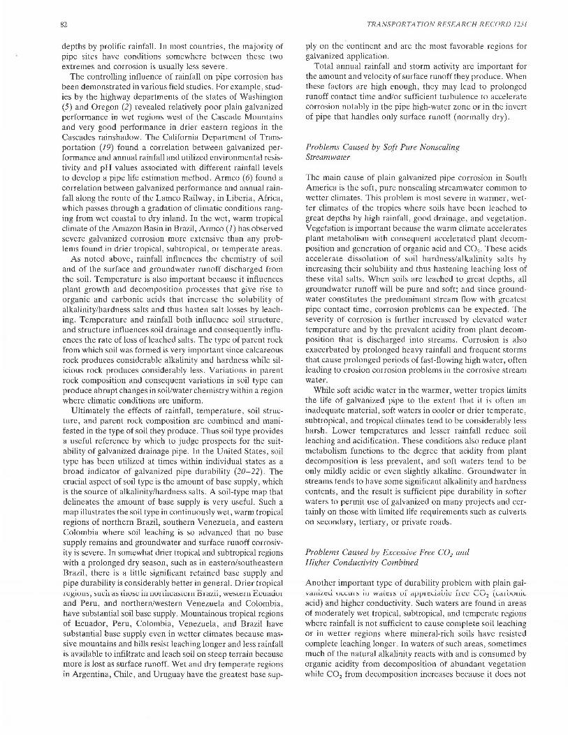
82

depths by prolific rainfall. In most countries, the majority of pipe sites have conditions somewhere between these two extremes and corrosion is usually less severe.

The controlling influence of rainfall on pipe corrosion has been demonstrated in various field studies. For example, stud­ies by the highway departments of the states of Washington (5) and Oregon (2) revealed relatively poor plain galvanized performance in wet regions west of the Cascade Mountains and very good performance in drier eastern regions in the Cascades rainshadow. The California Department of Trans­portation (19) found a correlation between galvanized per­formance and annual rainfall and utilized environmental resis­tivity and pH values associated with different rainfall levels to develop a pipe life estimation method. Armco (6) found a correlation between galvanized performance and annual rain­fall along the route of the Lamco Railway, in Liberia, Africa, which passes through a gradation of climatic conditions rang­ing from wet coastal to dry inland. In the wet, warm tropical climate of the Amazon Basin in Brazil, Armco (1) has observed severe galvanized corrosion more extensive than any prob­lems found in drier tropical, subtropical, or temperate areas.

As noted above, rainfall influences the chemistry of soil and of the surface and groundwater runoff discharged from the soil. Temperature is also important because it influences plant growth and decomposition processes that give rise to organic and carbonic acids that increase the solubility of alkalinity/hardness salts and thus hasten salt losses by leach­ing. Temperature and rainfall both influence soil structure, and structure influences soil drainage and consequently influ­ences the rate of loss of leached salts. The type of parent rock from which soil was formed is very important since calcareous rock produces considerable alkalinity and hardness while sil­icious rock produces considerably less. Variations in parent rock composition and consequent variations in soil type can produce abrupt changes in soil/water chemistry within a region where climatic conditions are uniform.

Ultimately the effects of rainfall, temperature, soil struc­ture, and parent rock composition are combined and mani­fested in the type of soil they produce. Thus soil type provides a useful reference by which to judge prospects for the suit­ability of galvanized drainage pipe. In the United States, soil type has been utilized at times within individual states as a broad indicator of galvanized pipe durability (20-22). The crucial aspect of soil type is the amount of base supply, which is the source of alkalinity/hardness salts. A soil-type map that delineates the amount of base supply is very useful. Such a map illustrates the soil type in continuously wet, warm tropical regions of northern Brazil, southern Venezuela, and eastern Colombia where soil leaching is so advanced that no base supply remains and groundwater and surface runoff corrosiv­ity is severe. In somewhat drier tropical and subtropical regions with a prolonged dry season, such as in eastern/southeastern Brazil, there is a little significant retained base supply and pipe durability is considerably better in general. Drier tropical

' • I ' ' ._ •• ._.... •

1t::g1u11s, sucu as 111ust:: u111un11t::as1t:rn nrazu, wt:sLt:rn ccuauur and Peru, and northern/western Venezuela and Colombia, have substantial soil base supply. Mountainous tropical regions of Ecuador, Peru, Colombia, Venezuela, and Brazil have substantial base supply even in wetter climates because mas­sive mountains and hills resist leaching longer and less rainfall is available to infiltrate and leach soil on steep terrain because more is lost as surface runoff. Wet and dry temperate regions in Argentina, Chile, and Uruguay have the greatest base sup-

TRANSPORTATION RESEARCH RECORD 1231

ply on the continent and are the most favorable regions for galvanized application.

Total annual rainfall and storm activity are important for the amount and velocity of surface runoff they produce. When these factors are high enough, they may lead to prolonged runoff contact time and/or sufficient turbulence to accelerate corrosion notably in the pipe high-water zone or in the invert of pipe that handles only surface runoff (normally dry).

Problems Caused by Soft Pure Nonscaling Stream water

The main cause of plain galvanized pipe corrosion in South America is the soft, pure nonscaling streamwater common to wetter climates. This problem is most severe in warmer, wet­ter climates of the tropics where soils have been leached to great depths by high rainfall, good drainage, and vegetation. Vegetation is important because the warm climate accelerates plant metabolism with consequent accelerated plant decom­position and generation of organic acid and C02 . These acids accelerate dissolution of soil hardness/alkalinity salts by increasing their solubility and thus hastening leaching loss of these vital salts. When soils are leached to great depths, all groundwater runoff will be pure and soft; and since ground­water constitutes the predominant stream flow with greatest pipe contact time, corrosion problems can be expected. The severity of corrosion is further increased by elevated water temperature and by the prevalent acidity from plant decom­position that is discharged into streams. Corrosion is also exacerbated by prolonged heavy rainfall and frequent storms that cause prolonged periods of fast-flowing high water, often leading to erosion corrosion problems in the corrosive stream water.

While soft acidic water in the warmer, wetter tropics limits the life of galvanized pipe to the extent that it is often an inadequate material, soft waters in cooler or drier temperate, subtropical, and tropical climates tend to be considerably less harsh. Lower temperatures and lesser rainfall reduce soil leaching and acidification. These conditions also reduce plant metabolism functions to the degree that acidity from plant decomposition is less prevalent, and soft waters tend to be only mildly acidic or even slightly alkaline. Groundwater in streams tends to have some significant alkalinity and hardness contents, and the result is sufficient pipe durability in softer waters to permit use of galvanized on many projects and cer­tainly on those with limited life requirements such as culverts on secondary, tertiary, or private roads.

Problems Caused by Excessive Free C02 and Higher Conductivity Combined

Another important type of durability problem with plain gal­vctuiL.c:U uccu1~ iu wale1~ ul app1eciaUie l1ee CG2 (ca1Uuuic acid) and higher conductivity. Such waters are found in areas of moderately wet tropical, subtropical, and temperate regions where rainfall is not sufficient to cause complete soil leaching or in wetter regions where mineral-rich soils have resisted complete leaching longer. In waters of such areas, sometimes much of the natural alkalinity reacts with and is consumed by organic acidity from decomposition of abundant vegetation while C02 from decomposition increases because it does not

Bednar

react with HC03 alkalinity. Alkalinity is essential for scaling control of corrosion, and replacement of beneficial alkalinity with detrimental acid reaction salts combined with the influ­ence of increased C02 and sustained higher conductivity can cause severe general and pitting attack of pipe inverts. Exces­sive free C02 suppresses scaling and directly accelerates cor­rosion, and the combined effect of excess C02 and higher conductivity can be very severe. Slow flowing streams in areas with somewhat impeded drainage are more likely to be rich in free C02 because higher velocity greatly aerates the water and drives off C02 (8).

Problems Caused by Sulfuric Acid

Occasional problems with inorganic sulfuric acid occur in areas with mine or outcropping drainage.

Problems Caused by Extreme High Conductivity Due to Salinity

In very dry or arid climates, plain galvanized pipe generally performs very well because water flow is generally brief and infrequent. Flowing or stagnant highly saline groundwater, high in conductivity due to high chloride/sulfate salinity, can cause problems at some pipe sites. Soilside corrosion prob­lems can occur where the soil is rich in chloride/sulfate salts, although high pH and limited soil moisture availability tend to control such corrosion . Highly saline waters and soils occur mainly in arid regions where no salt leaching loss occurs . Of course, highly saline seawater or estuary water is a problem wherever it is found, and galvanized should not be installed wherever contact with such water is likely.

Problems Caused by Erosion Corrosion

Erosion corrosion is induced by increased water corrosivity as well as by increased velocity because protective scales that form in corrosive waters are less tenacious and are more easily removed or interfered with . In this writer's experience, ero­sion corrosion problems are usually associated with surface runoff due to the combined effect of its higher velocity and appreciable corrosivity from lesser scaling salt content, which under certain conditions are troublesome despite limited pipe contact time. Such problems occur in the pipe high-water zone or in the invert on pipes that are normally dry where soft turbulent surface runoff exerts its influence. Groundwater runoff normally does not induce erosion corrosion due to its limited velocity and lower corrosivity , and this is true even in mountainous/hilly terrain where velocity can be substantial but groundwater scaling tendencies are normally appreciable. Groundwater runoff of moderate velocity can induce erosion corrosion when water corrosivity is very high, as is the case with soft acidic waters of some wet tropical regions.

COATING/PAVEMENT PROTECTION FOR CORRUGATED STEEL PIPE IN HOSTILE REGIONS

The writer has had considerable experience with certain kinds of coating/pavement materials that improve the durability of

83

corrugated steel pipe to permit its use in streams of hostile regions, but some of these materials are not currently avail­able in South America. Thick hot-dip asphalt mastic coatings add substantially to the service life of plain galvanized pipe in warmer climates ( 4, 6). Thick asphalt or concrete pavement is effective in combating abrasion and adds considerably to the service life of plain galvanized in many corrosive streams (4, 16). A thick bitumen coating mechanically bonded to a galvanized substrate through a fiber mat partially embedded in the zinc coating provides good protection against severe corrosive streams and soils (16, 23). Aluminized steel (Type 2) has superior resistance to the corrosive effects of dissolved oxygen, C02 , organic acid, and water turbulence that cause most of the problems on plain galvanized (24). Epoxy-coated steel has a field history of good performance in highly cor­rosive waters (25, 26) , and field tests and experience on a fusion-bonded epoxy-powder coating in Brazil and the United States show good results in corrosive waters (results may be published later) .

DEVELOPMENT OF A GALVANIZED PIPE SELECTION METHOD

The selection process for plain galvanized steel pipe is based on dividing the continent into regions on the basis of soil type and then further characterizing each region according to aver­age annual rainfall and average annual storm activity. These combined factors determine in a general way the surface run­off corrosivity trends of each region, and these trends are sufficient to characterize pipe corrosion behavior in the high­water zone and in the invert on pipes that are normally dry. Even for pipes that are normally dry, waterside corrosion normally controls pipe durability in all but drier climates ( <500-600 mm/year) . While corrosion by surface runoff is normally controlled adequately by the relatively brief pipe contact time , some conditions can lead to problems. Obviously, leached acidic types of soil can produce very soft and somewhat acidic runoff of high potential corrosivity , and high annual rainfall can increase contact time substantially. Furthermore, high storm activity can produce enough velocity and turbulence to induce erosion corrosion problems.

Soil type and annual rainfall also control soil/groundwater chemistry trends within a region, but because of prolonged contact time , more specific chemistry data are needed to char­acterize durability trends more accurately . In drier climates with less than 500 to 600 mm/year rainfall , soil resistivity and pH will be of primary importance whereas in wetter climates, groundwater pH, resistivity, alkalinity, and hardness are the primary factors . When testing has established water or soil chemistry trends, different regions can then be ranked accord­ing to their potential for durability problems.

RECOMMENDED REGIONAL GUIDELINES FOR GALVANIZED APPLICATION

Recommendations on where to concentrate on galvanized application and where to limit it are based on the writers' best knowledge of field performance and environmental conditions and are subject to change as field experience broadens. Regions are listed below in a descending order of preference for con­centration of galvanized application corresponding to the order

84

of increasing possiblity of corrosion problems. The order may change a little as more data become available. Regions in categories A, B, and Care the most favorable for galvanized application with regard to corrosion potential, and the need for additional water/soil testing on the local project level is minimal, being limited to some major projects with high dura­bility requirements. Regions in the intermediate categories D and E are favorable, but there is a greater need for water testing on the local project level. All regions in the relatively low category F are there largely because of a lack of data, and when data become available any or all of these regions could rise to categories E, D, C, B, or A. In regions in cat­egories G and H, galvanized application should be limited on the basis of the potential for corrosion problems. It is impor­tant to realize that limited application will apply to certain other regions on the basis of abrasion potential once abrasion studies are completed .

Limited application of galvanized in hostile regions refers primarily to limiting use of plain galvanized on projects with high durability requirements. General use of plain galvanized could stili appiy on some projects or types of sites without high durability requirements, such as secondary or tertiary roadways and driveway culverts. On projects with high dura­bility requirements, sites with streams having prolonged flow are the major concern. Plain galvanized may be satisfactory for sites that are normally dry. At sites with flowing streams in hostile regions, plain galvanized can often be used in struc­tural-plate arches and in the upper half of structural-plate pipes and pipe arches. In streams of marginally hostile regions, galvanized can sometimes be used throughout larger full struc­tural-plate pipes and pipe arches because some larger streams with substantial dry weather flow velocity are less corrosive due to enhanced aeration and very low free C02 content (testing of water at each individual site is justified by the large economic investment). Obviously, plain galvanized can be used in any region for projects involving only soil exposure such as structural-plate highway/street/railway underpasses and some tunnel liners .

Category A. Durability, as indicated by data and climate/ terrain features, is best in the following regions:

1. Chile-All regions except as noted in C and F. 2. Argentina-All regions except as noted in E and F. 3. Uruguay-All regions.

Category B. Galvanized will have wide application, as indicated by data and climate/terrain features, but soft water and C02/conductivity problems are possible in some areas.

1. Northern and western Colombia and Venezuela (out to limits of Andes and Costa Mountains)-All drier regions ( < 1500 mm/yr), all temperate/cool high altitude areas.

2. Northeast Brazil-All drier areas (<1500 111111/y1) iu provinces of Ceara , Bahia, Piaui, Pernambuco, Paraiba, Rio Grande do Norte, Sergipe, and Alagoa except as noted in G (little data available but favorable climate over large areas of this region).

3. Ecuador and Peru-All drier regions ( <1500 mm/yr), all temperate/cool high altitude areas.

Category C. Galvanized will have wide application , but as indicated by limited data and climate/terrain features, some soft water or C02/conductivity problems are likely in some areas.

TRANSPORTA T/ON RESEARCH RECORD 1231

1. Southern part of eastern Brazil-Provinces of Rio Grande do Sol, Santa Catarina, Parana, Sao Paulo, Rio de Janeiro, and Mato Grosso do Sul.

2. Southwest Bolivia and eastern Paraguay-All drier regions ( < 1500 mm/yr), except as in F (no data but favorable climate and terrain).

3. Portions of eastern Brazil-Drier areas ( < 1500 mm/yr): provinces of Goias and Minas Gerais.

4. Portions of southern Chile- Wetter areas (> 1500 mm/ yr), except as noted in F .

Category D. Galvanized should have substantial appli-cation, but data are limited and climate/terrain should pro­duce soft water or C02/conductivity problems in some areas.

1. Ecuador and Peru-Wet regions (>1500 mm/yr), except as noted in F.

2. Northern and western Colombia and Venezuela-Wet regions (>1500 mm/yr), except as noted in G.

Category E. Galvanized should have substantial appli-cation, but some serious COifconductivity problems in some areas are indicated by data and climate/terrain features.

1. Brazilian provinces of Acre, Rondonia, and Mato Grosso. 2. Argentina in province of Entre Rios and possibly in areas

of other nearby provinces.

Category F. Galvanized may have wide or at least useful application, but there are not enough field data to use for guidance, and climatic/terrain conditions could cause severe soft water, COifconductivity, or salinity problems. It would be best to limit application of galvanized or to conduct local project testing until more comprehensive data indicate other­wise.

1. Portions of eastern and northeastern Brazil-including provinces of Espirito Santo and Maranhao and all areas in other provinces (categories B and C) having > 1500 mm/year rainfall.

2. Northern and western Colombia and Venezuela, south­ern Chile, eastern Peru, and parts of Ecuador-extreme wet areas where rainfall is >2000 mm/year.

3. Bolivia-all areas outside southwest and salt flats in southwest.

4. Northern and western Venezuela for a limited distance beyond the Andes and Costa Mountains-provinces of Delta Amacuro, Monagas, Anzoategui, Guarico, Cojedes, Portu­gesa, and Barinas.

5. Argentina and western Paraguay-Gran Chaco region and salt flats in northwestern Argentina.

Category G. Galvanized may have useful application, but in some regions, limited data reveal probable widespread soft water, salinity, or CO/conductivity problems; and iu ulher regions, unfavorable climate/terrain conditions are likely to cause severe widespread soft water problems . Galvanized application should be limited except where local project test­ing indicates otherwise.

1. Entire countries of Surinam, Guyana, and French Guiana. 2. Northeastern Brazil-eastern coastal areas in provinces

of Bahia, Sergipe, Alagoa, Pernambuco, Paraiba, and Rio Grande do Norte .

Category H. In these regions, widespread severe soft water problems are indicated by field data and experience. Galvanized application is limited.

Bednar

1. Northern Brazil, southern Venezuela and eastern Co­lombia-all of the Amazon valley and most of its very large watershed, all of the Guiana highlands of Venezuela, and much of the Llanos of Venezuela and Colombia. This area includes the provinces of Para, Amapa, Roraima, and most of Amazonas in Brazil and at least the provinces of Amazonas, Bolivar, and Apure in Venezuela. In Colombia, all areas east of the mountains should be considered suspect for the present. Most of these regions of category Hare not highly populated, but there are significant existing or potential highway systems in them all.

DEVELOPMENT OF SPECIFIC DURABILITY ESTIMATION TECHNIQUE

The ranking of regions and the accurate designation of regional durability trends are based on the use of a specific durability estimation technique, which is described briefly below.

Current U.S. Technique

The durability estimation technique that has been the most useful in providing specific characterization of environmental corrosivity in the United States is the California Chart, although in its earlier form it is generally overly conservative and under some circumstances is overly liberal as discussed by the author elsewhere in this Record. This technique relates pipe dura­bility to the pH and resistivity of either the waterside or the soilside environment (19). This approach is proper for the soilside environment for which pH and resistivity are generally the most important factors controlling durability of galvanized culvert pipe. However, it is not entirely adequate for the more complicated waterside environment which causes most prob­lems. The most important problem with the California Chart is that it ignores the crucial effect of water scaling on corrosion behavior. In doing so, the earlier chart form gives results that are overly conservative in the significantly hard and alkaline scaling waters predominant in most countries and results that are overly liberal in the soft nonscaling or slightly scaling waters common to certain areas of some countries. In hard water, scaling reduces the overall corrosion rate of a pipe to a considerably lower level than that suggested by the chart; in soft water, inadequate scaling allows corrosion to exceed the level suggested by the chart. The estimates are sometimes conservative or liberal by a factor of 2 or more judging by Armco field data as shown by the author elsewhere in this Record.

Durability estimation accuracy could be greatly improved by the use of a more comprehensive waterside technique that relates durability to all of the critical controlling factors, including C02 , alkalinity, and hardness, as well as resistivity and pH. Armco has addressed this need, and the result is a modified type of California Chart for depicting waterside cor­rosion behavior based on Armco field data.

Development of a More Comprehensive Waterside Durability Estimation Technique

Armco has developed a waterside estimation technique based on the combined effects of C02 , conductivity, total alkalinity,

85

and total hardness that eliminates the conservatism/liberalism trends of the California Chart and delineates the chemistry trends that control galvanized use. The effect of temperature is also included so that the technique can be applied in dif­ferent climates. The detailed derivation of the technique is too lengthy to be included here but has been discussed by the author elsewhere in this Record.

The technique is based largely on the interaction of alka­linity, hardness, and acidity which controls the scaling tend­ency. Alkalinity is primarily in the form of HC03- (bicar­bonate), which is consumed by reaction with organic acids from plant decomposition to produce corrosive reaction prod­ucts. Plant decomposition is the prevalent primary source of natural acidity, but of course inorganic acidity found in acid minewater areas would also consume alkalinity. If alkalinity is totally consumed, as it is in some tropical regions, the water becomes too corrosive to permit use of plain galvanized or other more common pipe materials. Plant decomposition also produces C02 , which combines with water to form corrosive carbonic acid; but C02 does not consume HCO; because C02 is part of the essential reaction by which HCOi is formed from CaC03 in soil and rock. Indeed, a little excess unreacted or free C02 is necessary to stabilize HCQ3- in solution, but any excess free C02 above this small amount reduces the scaling tendency and increases water corrosivity. In any nat­ural water with some significant alkalinity remaining after reaction with organic acid, C02 is the remaining form of acid­ity influencing the pH and the scaling tendency. The inter­action of free C02 , alkalinity, and hardness controls the basic scaling tendency in any water where the use of plain galva­nized can be recommended. Alkalinity and hardness encour­age scaling; free C02 discourages it. Thus, a scaling tendency expression in which alkalinity and hardness concentrations are positive factors and the free C02 concentration is a neg­ative factor is easily developed .

The effectiveness of scaling is also influenced by corrosive salts such as chloride and sulfate . In scaling waters, excessive concentrations of such salts interfere with or prevent adequate scale formation and in nonscaling C02-rich waters they add to the corrosive effect of C02 . The interaction of scaling tend­ency (positive or negative) and corrosive salts is the primary control of pipe corrosion behavior. An Armco graph for esti­mation of durability based on this interaction is illustrated in nonspecific form in Figure 1.

ALK. +

HRD.

FREE co,

(ppm)

v / I/ --

/

I ·~

v ./

yl/ /I/ / I so //

/ [7 35 /

/ / / 7 I /

I ;//" I/ V/ v ;o

~v I/ v v

/

v

Ch pmist y Lim ts fo1 3 Se1 "ice l

CONDUCTIVITY (µmhos/cm)

FIGURE I Modified California Chart.

ifc u vcls

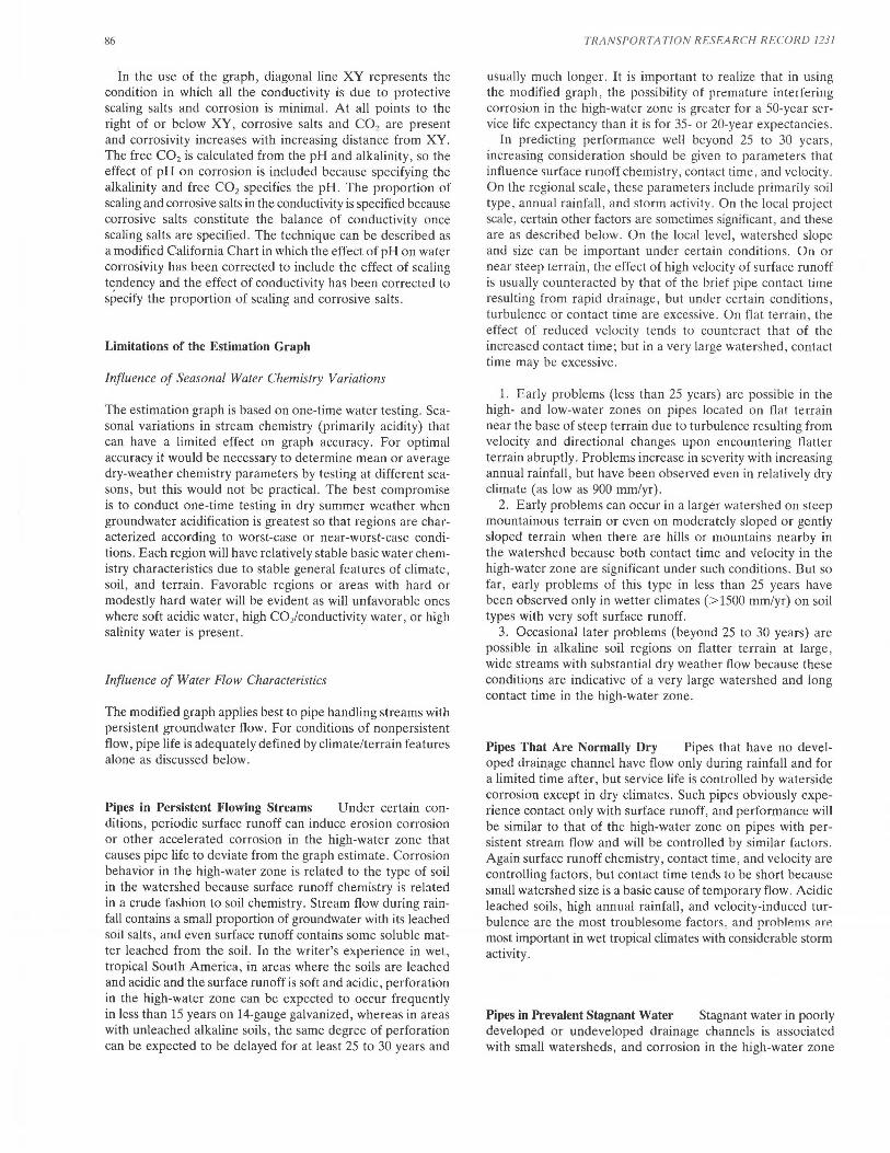
86

In the use of the graph, diagonal line XY represents the condition in which all the conductivity is due to protective scaling salts and corrosion is minimal. At all points to the right of or below XY, corrosive salts and C02 are present and corrosivity increases with increasing distance from XY. The free C02 is calculated from the pH and alkalinity, so the effect of pH on corrosion is included because specifying the alkalinity and free C02 specifies the pH. The proportion of scaling and corrosive salts in the conductivity is specified because corrosive salts constitute the balance of conductivity once scaling salts are specified. The technique can be described as a modified California Chart in which the effect of pH on water corrosivity has been corrected to include the effect of scaling tendency and the effect of conductivity has been corrected to specify the proportion of scaling and corrosive salts.

Limitations of the Estimation Graph

Influence of Seasonal Water Chemistry Variations

The estimation graph is based on one-time water testing. Sea­sonal variations in stream chemistry (primarily acidity) that can have a limited effect on graph accuracy. For optimal accuracy it would be necessary to determine mean or average dry-weather chemistry parameters by testing at different sea­sons, but this would not be practical. The best compromise is to conduct one-time testing in dry summer weather when groundwater acidification is greatest so that regions are char­acterized according to worst-case or near-worst-case condi­tions. Each region will have relatively stable basic water chem­istry characteristics due to stable general features of climate , soil, and terrain. Favorable regions or areas with hard or modestly hard water will be evident as will unfavorable ones where soft acidic water, high CO/conductivity water, or high salinity water is present.

Influence of Water Flow Characteristics

The modified graph applies best to pipe handling streams with persistent groundwater flow. For conditions of nonpersistent flow, pipe life is adequately defined by climate/terrain features alone as discussed below.

Pipes in Persistent Flowing Streams Under certain con­ditions, periodic surface runoff can induce erosion corrosion or other accelerated corrosion in the high-water zone that causes pipe life to deviate from the graph estimate. Corrosion behavior in the high-water zone is related to the type of soil in the watershed because surface runoff chemistry is related in a crude fashion to soil chemistry. Stream flow during rain­fall contains a small proportion of groundwater with its leached soil salts, and even surface runoff contains some soluble mat­ter leached from the soil. In the writer's experience in wet, tropical South America, in areas where the soils are leached and acidic and the surface runoff is soft and acidic, perforation in the high-water zone can be expected to occur frequently in less than 15 years on 14-gauge galvanized, whereas in areas with unleached alkaline soils, the same degree of perforation can be expected to be delayed for at least 25 to 30 years and

TRANSPORTAT!ON RESEA RCH R ECORD 1231

usually much longer. It is important to realize that in using the modified graph, the possibility of premature interfering corrosion in the high-water zone is greater for a 50-year ser­vice life expectancy than it is for 35- or 20-year expectancies.

In predicting performance well beyond 25 to 30 years, increasing consideration should be given to parameters that influence surface runoff chemistry, contact time, and velocity. On the regional scale, these parameters include primarily soil type , annual rainfall, and storm activity. On the local project scale, certain other factors are sometimes significant, and these are as described below. On the local level, watershed slope and size can be important under certain conditions. On or near steep terrain, the effect of high velocity of surface runoff is usually counteracted by that of the brief pipe contact time resulting from rapid drainage, but under certain conditions, turbulence or contact time are excessive. On flat terrain, the effect of reduced velocity tends to counteract that of the increased contact time; but in a very large watershed, contact time may be excessive.

1. Early probkms (iess than 25 years) are possibie in the high- and low-water zones on pipes located on flat terrain near the base of steep terrain due to turbulence resulting from velocity and directional changes upon encountering flatter terrain abruptly. Problems increase in severity with increasing annual rainfall, but have been observed even in relatively dry climate (as low as 900 mm/yr) .

2. Early problems can occur in a larger watershed on steep mountainous terrain or even on moderately sloped or gently sloped terrain when there are hills or mountains nearby in the watershed because both contact time and velocity in the high-water zone are significant under such conditions. But so far, early problems of this type in less than 25 years have been observed only in wetter climates (> 1500 mm/yr) on soil types with very soft surface runoff.

3. Occasional later problems (beyond 25 to 30 years) are possible in alkaline soil regions on flatter terrain at large, wide streams with substantial dry weather flow because these conditions are indicative of a very large watershed and long contact time in the high-water zone.

Pipes That Are Normally Dry Pipes that have no devel­oped drainage channel have flow only during rainfall and for a limited time after, but service life is controlled by waterside corrosion except in dry climates. Such pipes obviously expe­rience contact only with surface runoff, and performance will be similar to that of the high-water zone on pipes with per­sistent stream flow and will be controlled by similar factors. Again surface runoff chemistry, contact time, and velocity are controlling factors, but contact time tends to be short because small watershed size is a basic cause of temporary flow. Acidic leached soils, high annual rainfall, and velocity-induced tur­bulence are the most troublesome factors. and rirnhlems 11re most important in wet tropical climates with considerable storm activity.

Pipes in Prevalent Stagnant Water Stagnant water in poorly developed or undeveloped drainage channels is associated with small watersheds, and corrosion in the high-water zone

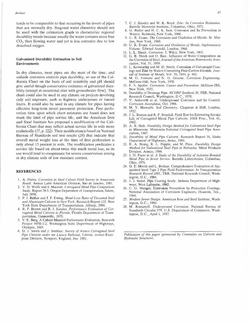
Bednar

tends to be comparable to that occurring in the invert of pipes that are normally dry. Stagnant water chemistry should not be used with the estimation graph to characterize regional durability trends because usually the water contains more free C02 than flowing water and yet is less corrosive due to low dissolved oxygen.

Galvanized Durability Estimation in Soil Environments

In dry climates, most pipes are dry most of the time, and soilside corrosion controls pipe durability, so use of the Cal­ifornia Chart on the basis of soil resistivity and pH should give useful though conservative estimates of galvanized dura­bility (except at occasional sites with groundwater flow) . The chart could also be used in arty climate on projects involving only soil exposure, such as highway underpasses or tunnel liners . It could also be used in any climate for pipes having effective long-term invert pavement protection. First perfo­ration time upon which chart estimates are based does not mark the limit of pipe service life, and the American Iron and Steel Institute has proposed a modification of the Cali­fornia Chart that may reflect actual service life in soils more realistically (27, p. 222). Their modification is based on National Bureau of Standards soil test results (28) that indicate that overall metal weight loss at the time of first perforation is only about 13 percent in soils. The modification predicates a service life based on about twice this much metal loss, so its use would tend to compensate for severe conservatism arising in dry climate soils of low moisture content.

REFERENCES

1. A. Dutra. Corrosion in Steel Culvert Field Survey in Amazonia Brasil. Armco Latin American Division, Rio de Janeiro, 1981.

2. V. D. Wolfe and S. Macnab. Corrugated Metal Pipe Comparison Study. Report 76-3. Oregon Department of Transportation , Salem, July 1976.

3. P. J. Bellair and J.P. Ewing. Metal-Loss Rates of Uncoated Steel and Aluminum Culverts in New York. Research Report 115. New York State Department of Transportation, Albany, 1984.

4. R. P. Brown and R. J . Kessler. Performance Evaluation of Cor­rugated Metal Culverts in Florida. Florida Department of Trans­portation, Gainesville, 1975.

5. V. E. Berg. A Culvert Ma terial Performance Evaluation. Research Project HPR-1-2 . Washington State Department of Highways, Olympia, 1965.

6. D. J. Smith and J. Smithee. Survey of Armco Corrugated Steel Pipe Culverts under cne Lamco Raili·oad, Liberia. Armco Euro­pean Division, Newport, England, Jan . 1981.

87

7. C. J . Slunder and W. K. Boyd. Zinc: Its Corrosion Resistance. Battelle Memorial Institute , Columbus, Ohio, 1971.

8. G. Butler and H. C. K. Ison. Corrosion and Its Prevention in Waters. Reinhold, New York, 1966.

9. U. R. Evans. The Corrosion and Oxidation of Metals . St. Mar­tins, New York, 1960.

10. U. R. Evans. Corrosion and Oxidation of Metals: Suplementary Volume. Edward Arnold, London, 1968.

11. L. L. Shreir. Corrosion. J. Wiley, New York, 1963. 12. G. B. Hatch and 0. Rice. Influence of Water Composition on

the Corrosion of Steel. Journal of the American Waterworks Asso­ciation, Vol. 51, 1959.

13. L. Kenworthy and M. D. Smith . Corrosion of Galvanized Coat­ings and Zinc by Waters Containing Free arbon Dioxide. Jour­nal of Institute of Metals, Vol. 70, 1944, p. 463.

14. M. G. Fontana and N. D. Greene. Corrosion Engineering. McGraw-Hill, New York, 1978.

15. F. N. Speller. Corrosion: Causes and Prevention. McGraw-Hill, New York, 1935 .

16. Durability of Drainage Pipe. NCHRP Synthesis 50, TRB, National Research Council, Washington , D.C., 1978.

17. V. Ashworth et al. Underground Corrosion and Its Control. Corrosion Australasia, Oct. 1986.

18. M. Y. Shawarbi. Soil Chemistry. Chapman & Hall , London, 1952.

19. J. L. Beaton and R. F. Stratfull. Field Test for Estimating Service Life of Corrugated Metal Pipe Culverts. HRB Proc., Vol. 41, 1962.

20. A. R . Holt. Durability Design Method for Galvanized Steel Pipe in Minnesota. Minnesota National Corrugated Steel Pipe Asso­ciation, 1967.

21. Durability of Metal Pipe Culverts. Research Report 16, Idaho Department of Highways, Boise, 1965.

22. E. A. Bearg, R. L. Pepple , and M. Price . Durability Design Method for Galvanized Steel Pipe in Nebraska. Metal Products Division , Armco, 1968.

23. J . H. Payer et al. A Study of the Durability of Asbestos-Bonded Metal Pipe in Sewer Service. Battelle Laboratories, Columbus, Ohio, 1976.

24. G. E. Morris and L. Bednar. Comprehensive Evaluation of Alu­minized Steel Type 2 Pipe Field Performance. In Transportation Research Record 1001, TRB, National Research Council, Wash­ington, D .C., l984.

25. J. J. Sudol. Pipe Coating Study. Indiana Department of High­ways, West Lafayette, l 982.

26. C. G . Munger. Corrosion Prevention by Protective Coatings. National Association of Corrosion Engineers, Houston, Tex. , 1984.

27. Modern Sewer Design. American Iron and Steel Institute, Wash­ington, D.C., 1980.

28. M. Romanoff. Underground Corrosion. National Bureau of Standards Circular 579. U.S. Department of Commerce, Wash­ington, D.C., April 1, 1957.

Publication of this paper sponsored by Committee on Culverts and Hydraulic Structures.

88 TRANSPORTATION RESEARCH RECORD 1231

Polyethylene Pipe Under High Fill

DANIEL N. ADAMS, TENNYSON MurNDI, AND ERNEST T. SELIG

Because little field performance experience was available for high­density polyethylene pipe under high earth load, a test installation was carried out with a 24-in.-diameter (610 mm) pipe placed beneath a 100-ft-high (30.5 m) embankment. The pipe was corrugated; and in some sections, a smooth interior wall was added. The pipe was embedded in a shallow trench near the base of the embankment and backfilled with compacted crushed limestone. Instruments were used to measure pipe wall strain, pipe diameter change, earth pressure acting on the pipe, vertical soil strain adjacent to the pipe, and pipe wall temperature. The paper presents results obtained with 95 ft (29 m) of fill over the pipe. No material distress was observed. The pipe remained relatively round, with about 4 per­cent vertical diameter decrease and 0.4 percent horizontal diam­eter increase. The average compression strain at the springline was 1.2 percent, and the bending strain was 0.3 percent. The vertical deflection was primarily the result of a 1.4 percent cir­cumference shortening. This shortening resulted in substantial positive arching-measured earth pressure on the pipe crown was only about 20 percent of the vertical embankment earth pressure.

A field study was undertaken to evaluate the performance of a 24-in.-inside-diameter (610 mm) corrugated polyethylene pipe to be loaded by a 100-ft-high (30.5 m) embankment. The embankment is part of the extension of Interstate 279, north of Pittsburgh, Pennsylvania.

The pipe used in this study was manufactured by Advanced Drainage Systems, Inc., of Columbus, Ohio. The pipe has an inside diameter of 24 in. (610 mm); the wall corrugations are 1.6 in. (41 mm) deep; and the wall is 0.22 in. (5.6 mm) thick. The pipe is extruded in 20-ft ( 6.1 m) sections, with the cor­rugations set on a 7-deg pitch , longitudinally. The joints were connected with wraparound fittings. In some of the pipe sec­tions, a smooth interior wall was adqed (designated N-12). Both types of pipe had a minimum stiffness of 34 psi (235 kPa) in accordance with standard specifications (AASHTO M294-86) .

In this paper, the field investigation is described and the main experimental results obtained during construction of the embankment up to a fill height of 95 ft (29 m) are presented. Further details are available in a research report (1).

FIELD MEASUREMENTS

The following field measurements were made to determine pipe performance:

• Vertical soil strain-Three inductance coils of 12-in. diameter (305 mm) were placed in the embankment to mea-

D. N. Adams and T. Muindi, Haley & Aldrich, Inc., 58 Charles St., Cambridge , Mass. 02141. E. T . Selig, University of Massachusetts, Marston Hall, Amherst, Mass. 01003 .

sure vertical compression of the earth fill at the elevation of the pipe. A pair of coils was also placed in the trench encom­passing the pipe to measure vertical compression of the pipe from the outside.

• Pipe wall strain-Three inductance coils of 1-in. diam­eter (25 mm) were fastened to the pipe wall at the springline to measure bending and compression strains in the pipe wall.

• Pipe wall circumferential strain-A special gauge was devised to measure the change in corrugation centroid cir­cumference length (Figures 1 and 2) . The sensor was a pair of 1-in.-diameter (25 mm) inductance coils .

• Internal diameter change-Radial extensometers (Fig­ure 3) were constructed to measure the change in pipe diam­eter in four directions (vertical, horizontal, and both 45° diag­onals). This device was attached to a sled and pulled through the pipe (Figure 4). A 35-mm camera with flash lighting was used to photograph the extensometer arms against a target to provide a record of the movement at selected locations along the pipe.

• Visual observation of pipe condition-A video camera was mounted on the sled used to pull the extensometers (Fig­ure 4) . This camera provided a videotape record of the con­dition of the inside of the pipe.

• Soil pressure on pipe-Oil-filled 10-in.-diameter (254 mm)

PIN SUPPORT

WIRE CONTINUED IN THE NEXT

CORRUGATION

STAINLESS STEEL WIRE

FIGURE 1 Locauon of pins and stainless steel wire for the circumferential gauge in the pipe helical corrugation.

Adams el al.

PIN SUPPORT

COIL FIXED TO PIN SUPPORT

LEAD WEIGHT

STAINLESS STEEL WIRE

LOCATION OF WIRE IN

PREVIOUS CORRUGATION

89

FIGURE 2 Location of inductance coils and the lead weight of the circumferential gauge.

FIGURE 3 Extensometer gauge.

earth pressure cells with a pneumatic transducer were placed in the backfill around the pipe to measure the soil normal pressure on the pipe at the springline and crown.

• Temperature-The pipe wall temperature and air tem­perature inside the pipe were monitored using thermistors .

The pipe instrumentation was installed in two sections of pipe (Figure 5), which were located under the center of the embankment (Figure 6). These two sections were corrugated without the smooth wall. The corrugated pipe sections with the smooth wall were located primarily under the east half of

1/2 INCH HARDENED ~--- GROOVED SHAFT

BALL-BEARING HOUSING WITH SET SCREWS TO

LIMIT ROTATION OF SHAFT

the embankment and contained no installed instrumentation. The locations of the soil pressure gauges and soil strain coils in the vicinity of the instrumented pipe sections are shown in Figures 7 and 8, respectively.

CONSTRUCTION

The embankment construction and pipe installation were per­formed by the construction contractor essentially in accord­ance with existing Pennsylvania Department of Transporta-

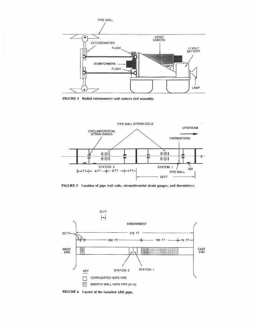
PIPE WALL

VIDEO CAMERA

35 MM CAMERA -

FIGURE 4 Radial extensometer and camera sled assembly.

CIRCUMFERENTIAL STRAIN GAGES

PIPE WALL STRAIN COILS

e0a e0a

12 VOLT BATTERY

LAMP

UPSTREAM

THERMISTORS

STATION 2 STATION 1

j--4 FT+ 6 FT-+ 6 FT -f-4FT-I----- PIPE WALL

20FT

FIGURE 5 Location of pipe wall coils, circumferential strain gauges, and thermistors.

WEST END

)

20 FT

H EMBANKMENT

KEY

I STATION 2

D CORRUGATED HOPE PIPE

D SMOOTH WALL HOPE PIPE (N-12)

\ STATION 1

FIGURE 6 Layout of the installed ADS pipe.

180 FT I 76 FT-

l EAST END

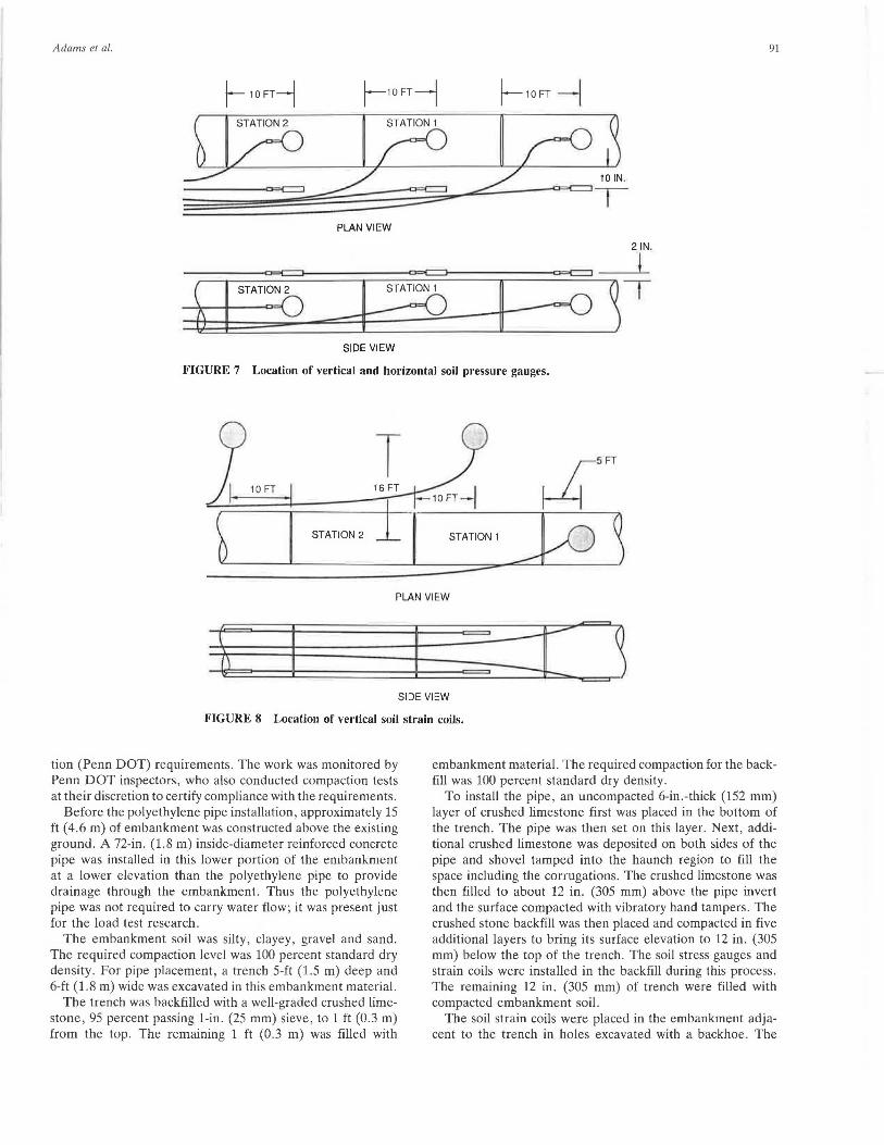
Adams er al . 91

f- 10FT-1 l--10FT--1 j--10FT --l

PLAN VIEW

2 IN.

l

AZD-B~T SIDE VIEW

FIGURE 7 Location of vertical and horizontal soil pressure gauges.

9 T 5FT

~)i~_1o=FT 2======16[:_FT -1DFT-I ~ b STATION 2 i I STATION' J/O ~

PLAN VIEW

j SI DE VIEW

FIGURE 8 Location of vertical soil strain coils.

tion (Penn DOT) requirements. The work was monitored by Penn DOT inspectors, who also conducted compaction tests at their discretion to certify compliance with the requirements.

Before the polyethylene pipe installation, approximately 15 ft ( 4.6 m) of embankment was constructed above the existing ground. A 72-in. (1.8 m) inside-diameter reinforced concrete pipe was installed in this lower portion of the embankment at a lower elevation than the polyethylene pipe to provide drainage through the embankment. Thus the polyethylene pipe was not required to carry water flow; it was present just for the load test research.

The embankment soil was silty, clayey, gravel and sand. The required compaction level was 100 percent standard dry density . For pipe placement, a trench 5-ft (1.5 m) deep and 6-ft (1.8 m) wide was excavated in this embankment material.

The trench was backfilled with a well-graded crushed lime­stone , 95 percent passing 1-in. (25 mm) sieve, to 1 ft (0.3 m) from the top. The remaining 1 ft (0.3 m) was filled with

embankment material. The required compaction for the back­fill was 100 percent standard dry density.

To install the pipe, an uncompacted 6-in.-thick (152 mm) layer of crushed limestone first was placed in the bottom of the trench. The pipe was then set on this layer. Next, addi­tional crushed limestone was deposited on both sides of the pipe and shovel tamped into the haunch region to fill the space including the corrugations. The crushed limestone was then filled to about 12 in. (305 mm) above the pipe invert and the surface compacted with vibratory hand tampers. The crushed stone backfill was then placed and compacted in five additional layers to bring its surface elevation to 12 in . (305 mm) below the top of the trench. The soil stress gauges and strain coils were installed in the backfill during this process . The remaining 12 in. (305 mm) of trench were filled with compacted embankment soil.

The soil strain coils were placed in the embankment adja­cent to the trench in holes excavated with a backhoe. The

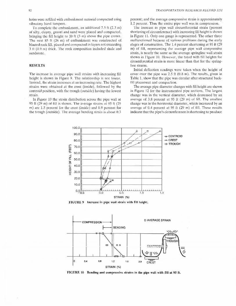
92

holes were refilled with embankment material compacted using vibratory hand tampers.

To complete the embankment, an additional 7.5 ft (2.3 m) of silty, clayey, gravel and sand were placed and compacted, bringing the fill height to 10 ft (3 m) above the pipe crown. The next 85 ft (26 m) of embankment was constructed of blasted rock fill, placed and compacted in layers not exceeding 3 ft (0.9 m) thick. The rock composition included shale and sandstone.

RESULTS

The increase in average pipe wall strains with increasing fill height is shown in Figure 9. The relationship is not linear. Instead, the strain increases at an increasing rate. The highest strains were obtained at the crest (inside), followed by the centroid position, with the trough (outside) having the lowest strain.

In Figure 10 the strain distribution across the pipe wall at 95 ft (29 m) of fi!! is shown. The average strains at 95 ft (29 m) are 1.5 percent for the crest (inside) and 0.9 percent for the trough (outside). The average bending strain is about 0.3

i=' w w !:!:. ....I ....I ii: u.. 0 I-I (!) jjj I

100.0

90.0

80.0

70.0

60.0

50.0

40.0

30.0

20.0

10.0

0.0 0.5

STRAIN (%)

TRANSPORTATION RESEARCH RECORD 1231

percent; and the average compressive strain is approximately 1.2 percent. Thus the entire pipe wall was in compression.

The increase in pipe wall circumferential strain (percent shortening of circumference) with increasing fill height is shown in Figure 11. Only one gauge is represented. The other three malfunctioned because of various problems during the early stages of construction. The 1.4 percent shortening at 95 ft (29 m) of fill, representing the average pipe wall compressive strain, is nearly the same as the average springline wall strain shown in Figure 10. However, the trend with fill heights for circumferential strain is more linear than that for the spring­line strains.

Initial deflection readings were taken when the height of cover over the pipe was 2.5 ft (0.8 m). The results, given in Table 1, show that the pipe was circular after. structural back­fill placement and compaction.

The average pipe diameter changes with fill height are shown in Figure 12 for the instrumented pipe sections. The largest change was in the vertical diameter, which decreased by an average of 3.8 percent at 95 ft (29 m) of fill. The smallest change was in the horizontal diameter, \Vhich increased by an average of 0.4 percent at 95 ft (29 m) of fill. These results indicate that the pipe's circumference is shortening to produce

--e- CENTROID -A-CREST

+TROUGH

1.0 1.5

FIGURE 9 Increase in pipe wall strain with fill height.

COMPRESSION -l 1--1 BENDING

D AVERAGE STRAIN

CD

0 0.4 0.8 1.2 1.6 2·0 CREST

STRAIN(%)

FIGURE 10 Bending and compressive strains in the pipe wall with fill at 95 ft.

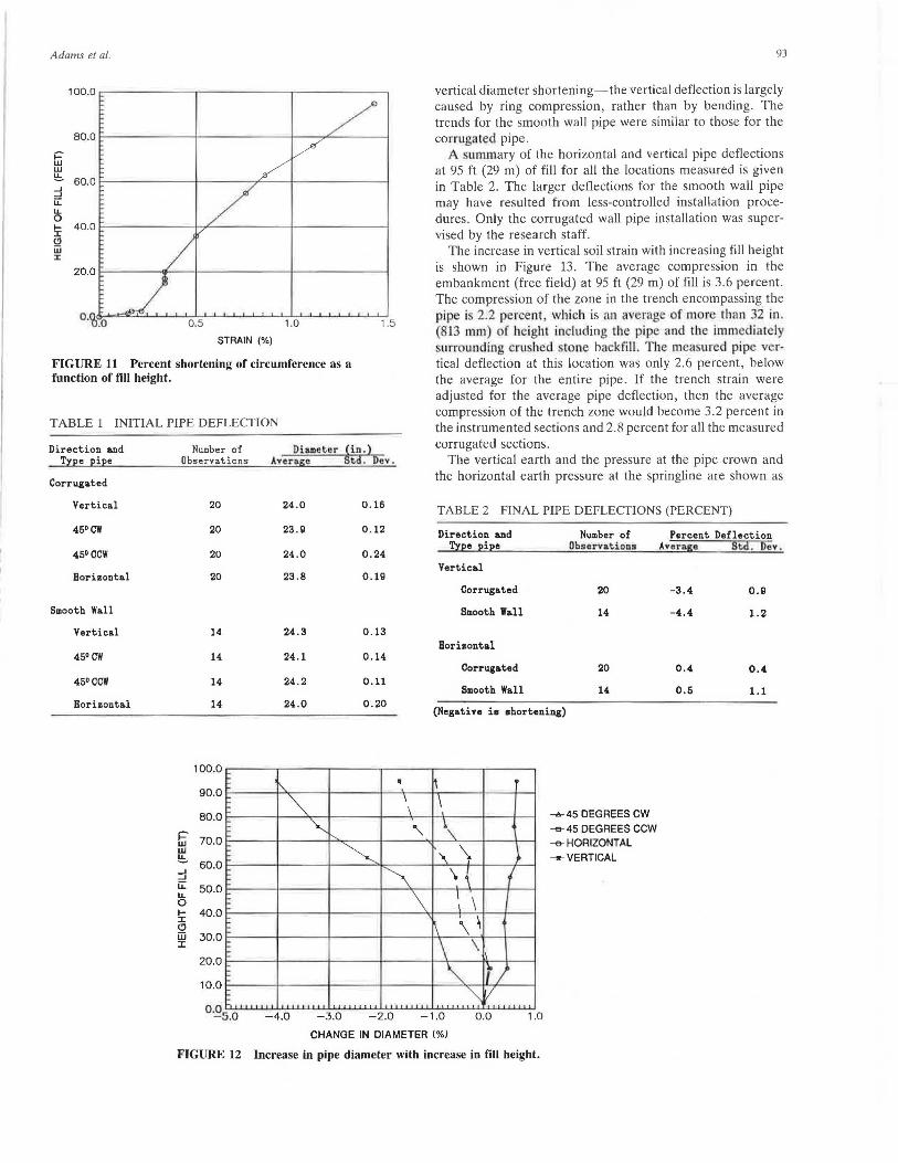
Adams el al.

STRAIN(%)

FIGURE 11 Percent shortening of circumference as a function of fill height.

TABLE 1 INITIAL PIPE DEFLECTION

Direction &nd Tree pipe

Corrugated

Vertical

45°cw

450 ccw

Horizontal

Smooth Wall

Vertical

45ocw

45° ccw

Horizontal

NUJDber of Observations

~ w !:!::.

20

20

20

20

14

14

14

14

100.0

90.0

80.0

70.0

Dia.meter ~in.) Average t.d. Dev.

24 .0

23.9

24.0

23.8

24.3

24.1

24 .2

24.0

I\.

~

'"'

0 . 16

0 . 12

0 .24

0.19

0.13

0 . 14

0 . 11

0.20

~

• \ \

60.0 --' --' u:: 50.0 "' u. 0 I- 40.0 :z: Cl iii 30.0 :z: I-

20.0

10.0 I-

h 0·~s.o -4.0 -3.0 -2.0

"'

\

93

vertical diameter shortening-the vertical deflection is largely caused by ring compression, rather than by bending. The trends for the smooth wall pipe were similar to those for the corrugated pipe.

A ummary of the horizontal and vertical pipe deflections at 95 ft (29 m) of fill for all the locations measured is given in Table 2. The larger deflections for the smooth wall pipe may have resulted from less-controlled installation proce­dures . Only the corrugated wall pipe installation was super­vised by the research staff.

The increase in vertical soil strain with increasing fill height is shown in Figure 13. The average compression in the embankment (free field) at 95 ft (29 m) of fill is 3.6 percent . The compression of the zone in the trench encompassing the pipe i 2.2 percent which is <1 11 average of mor than 32 in . (813 mm) of height including the pipe and the immediately surrounding cru heel . tone ba kfill. T he measured pipe ver­tical deflection at this location was only 2.6 percent, below the average for the entire pipe. If the trench strain were adjusted for the average pipe deflection, then the average compression of the trench zone would become 3.2 percent in the instrumented sections and 2.8 percent for all the measured corrugated sections.

The vertical earth and the pressure at the pipe crown and the horizontal earth pressure at the springline are shown as

TABLE 2 FINAL PIPE DEFLECTIONS (PERCENT)

Direction &nd Number of '.!l:pe pipe Obser'tations

Vertical

Corrugated 20

Smooth Wall 14

Hori&ontal

Corrug&ted 20

Smooth Wall 14

(Negative is shortening)

h \

\ '\

\ { \ \

\ \ \

\ \ ·~

"""

..

f ; I/

..,a...45 DEGREES CW

-e-45 DEGREES CCW -e- HORIZONTAL _,,_VERTICAL

Percent Deflection Average Std. Dev.

-3.4 0.9

-4 .4 1.2

0.4. 0.4

0.5 1.1

-1 .0 0 .0 1.0

CHANGE IN DIAMETER (%)

FIGURE 12 Increase in pipe diameter with increase in fill height.

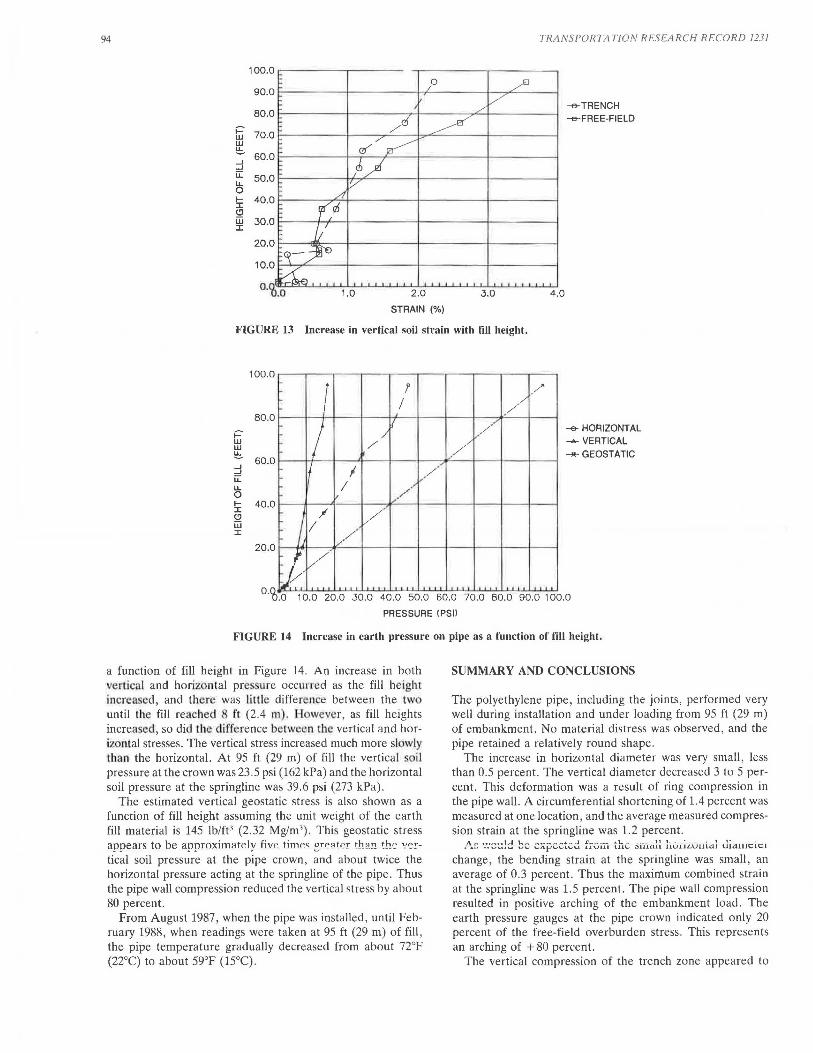
94

tii' w !::. --' --' u:: lL 0 1-:I: Cl iii :I:

1.0 2.0

STRAIN(%)

3.0

TRANS PORTA TI ON RESEA RCH RECORD 1231

--e-TRENCH

-<>-FREE-FIELD

4.0

FIGURE 13 Increase in vertical soil strain with fill height.

100.0

r r /'

80.0

r::-w w !::. 60.0 --' --' u:: lL 0 I- 40.0 :I: Cl iii :I:

20.0

I / /

I I /

/ . / - / /

/

I I / •'

I v·

·' , ,,./

/ / ;1 /

/ /

J-V,/

--e- HORIZONTAL

-.... VERTICAL

_,._ GEOSTATIC

0.0 0.0 10.0 20.0 30.0 40.0 50.0 60.0 70.0 80.0 90.0 100.0

PRESSURE tPSll

FIGURE 14 Increase in earth pressure on pipe as a function of fill height.

a function of fill height in Figure 14 . An increase in both vertical and horizontal pre · ure occurred as the fill height increa ed, and there was lillle difference between the two until the fill reached 8 t't (2.4 m) . H owever, as fill heights increased, so did the difference between the vertical and hor­izontal stresses. The vertical stress increased much more slowly th an the horizontal. At 95 ft (29 m) of fill the vertical oil pressure at the crown was 23.5 psi (162 kPa) and the horizontal soil pressure at the springline was 39.6 psi (273 kPa).

The estimated vertical geostatic stress is also shown as a function of fill height assuming the unit weight of the earth fill material is 145 lb/ft 3 (2.32 Mg/m3). This geostatic stress appears to be ap!'roximlltely five time< ~rPMP,.. th ?.!! th~ "~!­

tical soil pressure at the pipe crown , and about twice the horizontal pressure acting at the springline of the pipe . Thus the pipe wall compression reduced the vertical stress by about 80 percent.

From August 1987, when the pipe was installed, until Feb­ruary 1988, when readings were taken at 95 ft (29 m) of fill , the pipe temperature gradually decreased from about 72°F (22°C) to about 59°F (15°C) .

SUMMARY AND CONCLUSIONS

The polyethylene pipe, including the joints, performed very well during installation and under loading from 95 ft (29 m) of embankment. No material distress was observed, and the pipe retained a relatively round shape .

The increase in horizontal diameter was very small, less than 0.5 percent . The vertical diameter decreased 3 to 5 per­cent. This deformation was a result of ring compression in the pipe wall. A circumferential shortening of 1.4 percent was measured at one location, and the average measured compres­sion strain at the springline was 1.2 percent.

/'.. ~ ..... :~~!d 8~ ~~~~ctcd fIVili. ~lJ.c 3 iilal~ h01~Luula1 Jia.111clc1

change, the bending strain at the springline was small, an average of 0.3 percent. Thus the maximum combined strain at the springline was 1.5 percent. The pipe wall compression resulted in positive arching of the embankment load . The earth pressure gauges at the pipe crown indicated only 20 percent of the free-field overburden stress. This represents an arching of + 80 percent.

The vertical compression of the trench zone appeared to

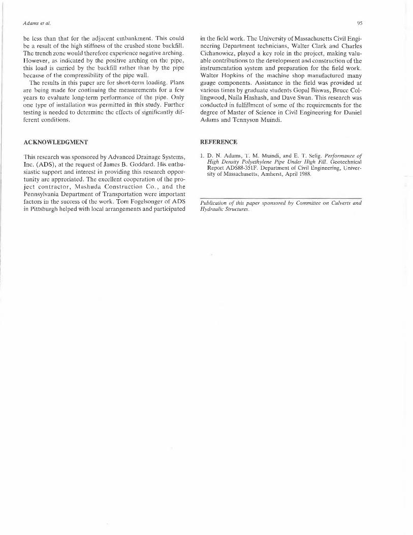
Adams et al.

be less than that for the adjacent embankment. This could be a result of the high stiffness of the crushed stone backfill. The trench zone would therefore experience negative arching. However, as indicated by the positive arching on the pipe, this load is carried by the backfill rather than by the pipe because of the compressibility of the pipe wall.

The results in this paper are for short-term loading. Plans are being made for continuing the measurements for a few years to evaluate long-term performance of the pipe. Only one type of installation was permitted in this study. Further testing is needed to determine the effects of significantly dif­ferent conditions.

ACKNOWLEDGMENT

This research was sponsored by Advanced Drainage Systems, Inc. (ADS), at the request of James B. Goddard. His enthu­siastic support and interest in providing this research oppor­tunity are appreciated. The excellent cooperation of the pro­ject contractor, Mashuda Construction Co., and the Pennsylvania Department of Transportation were important factors in the success of the work. Tom Fogelsonger of ADS in Pittsburgh helped with local arrangements and participated

95

in the field work. The University of Massachusetts Civil Engi­neering Department technicians, Walter Clark and Charles Cichanowicz, played a key role in the project, making valu­able contributions to the development and construction of the instrumentation system and preparation for the field work. Walter Hopkins of the machine shop manufactured many gauge components. Assistance in the field was provided at various times by graduate students Gopal Biswas, Bruce Col­lingwood, Naila Hashash, and Dave Swan. This research was conducted in fulfillment of some of the requirements for the degree of Master of Science in Civil Engineering for Daniel Adams and Tennyson Muindi.

REFERENCE

1. D . N. Adams, T. M. Muindi , and E. T. Selig. Performance of High Density Polyethylene Pipe Under High Fill. Geotechnical Report ADS88-351F. Department of Civil Engineering, Univer­sity of Massachusetts, Amherst, April 1988.

Publication of this paper sponsored by Committee on Culverts and Hydraulic Structures.

96 TRANSPORTATION RESEARCH RECORD 123 1

Suggested Improvements in Designing Soil-Steel Structures

]OHN B. KENNEDY AND ]ANT. LABA

Soil-steel structures have been used widely as short-span bridges and as substitutes for concrete culverts. However, many of these structures .have now shown signs of distress, with some suffering catastrophic collapse. Generally, such failures are related to the failure of the surrounding soil to provide the necessary support to the steel ~tructure. In t~is paper, the concept of reinforcing the surroundmg granular sod, as well as tying the flexible steel struc­ture into the stable part of the surrounding soil by horizontally placed galvanized ties, is introduced. !t is shown that this novel desi~n concept wo.uld lead to improvements in the structural response durmg construction and at the service load stage. Such construc­tion will (a) add considerable stiffness to the soil and decrease the movement of the backfill in service, such as during freeze-thaw ~ycles; (b) restrain the movement of the steel structure; and (c) mduce large deformations, in case of overload, and therefore give ample warning before failure. Results from tests on soil-steel struc­tural models are reported.

In the past three decades, soil-steel structures have been used successfully on short-span bridges; in many cases, the struc­tures replaced the traditional concrete culverts on municipal ~oads and proved to be quite economical. The design principle is based on the assumption that when the flexible steel struc­ture is subjected to a vertical load the structure will deform bringing into play passive soil pressure counteracting the effec~ of the applied vertical pressure ; therefore, perfect interaction between the steel structure and the soil backfill is essential during the life of the structure. As the soil cover increases the bending moments and shears in the steel structure becom~ negligible, and the steel structure is then designed predomi­nantly for in-plane compression. A recent survey (J) has shown that an alarming number of soil-steel structures in Ontario Canada, have shown signs of distress such as cracks at bol~ holes; buckling and rupture of bottom plates; gross distortion of cross section, including buckling of top plates; uplift of bottom plates; crimping of ridge corrugations. Actual failures of soil-steel structures have occurred in the past; some have been catastrophic, involving loss of life (2, p. 12).

Besides the unfortunate errors in construction, these fail­ures and distress signs can be attributed mainly to the failure of the s?il to provide the necessary and expected support to the flexible steel structure after construction and during its service life. The current practice of some designers, providing 2dd!t!~~~l ~t!ffe~i~g b~~t b~~~:; t~ ;-~i~fv;~;; ~he :;~cc1 ~~~tuc­

ture, will not correct this problem in the long run. Such designs, in addition to being uneconomical, will only increase further the load paths to the steel structure and decrease those to the surrounding soil. The truth of this statement was also dem­onstrated recently by tests on earth-covered slabs (3).

University of Windsor , Windsor, Ontario, Canada, N9B 3P4.

!n this paper, the concept of reinforcing the surrounding soII, as well as tying the flexible steel structure into the stable ~art ~f ~he surrounding soil by horizontally placed galvanized ties: is mtroduced; it is believed that the adoption of such a design concept can prevent failures in soil-steel structures. The types of failure and their causes are described below.

TYPES OF FAILURE AND THEIR CAUSES

Failure in soil-steel structures can be of different form as follows:

• Crimp formation-Crimps in the steel structure (Fig­ure 1) occur mainly on the valley of the section, extending sometimes to the ridges. Such crimps are caused by excessive bending and/or direct thrust in the steel structure. Also, dur­ing manufacturing, the bending of the corrugated flat sheets to small radii, as required for haunches of pipe arches, may cause such dimples on the interior valleys .

• Joint failure-Joint failures in the steel structure (Figure 2) occur due to excessive shear or bearing stresses; tearing of bolt holes is then a usual occurrence and rusting of the unpro­tected torn metal will accelerate failure of the joint. The seam connection can cause local increase in the bending of the steel structure, or it may create local weakness leading to failure. !hus proper attention to the seam design and bolt pattern ( 4) 1s necessary. Poor initial compaction of the soil during con­struction and unforeseen settlement would also contribute to joint failure.

• Excessive deformation-The steel structure can undergo excessive lateral wall displacement , which gives rise to exces­sive vertical deflection at the crown, causing additional stresses due to bending in the vicinity of the crown. Such a condition is due. mainly to poor compaction of the side fill during con­~truct10.n or to the loss of initial compaction at a later stage m the hfe of the soil-steel structure.

• Lifting of the invert of the steel structure-This distress (Figure 3) results from soil settlement under the haunches of the steel structure (4) or from increased water level under the steel structure, creating an uplift on the bottom plates.

The types of overall failures in soil-steel structures follow:

• Buckling of the steel structure-Buckling of the steel structure can lead to catastrophic failure. Excessive thrust in the structure coupled with excessive deflection around the crown can trigger such instability. The consideration of buck­ling becomes even more critical for large-span structures under

FIGURE I Crimping of ridge corrugation.

FIGURE 2 Cracking through valley bolts in pipe arch structure.

FIGURE 3 Uplifting of bottom plates in pipe arch structure.

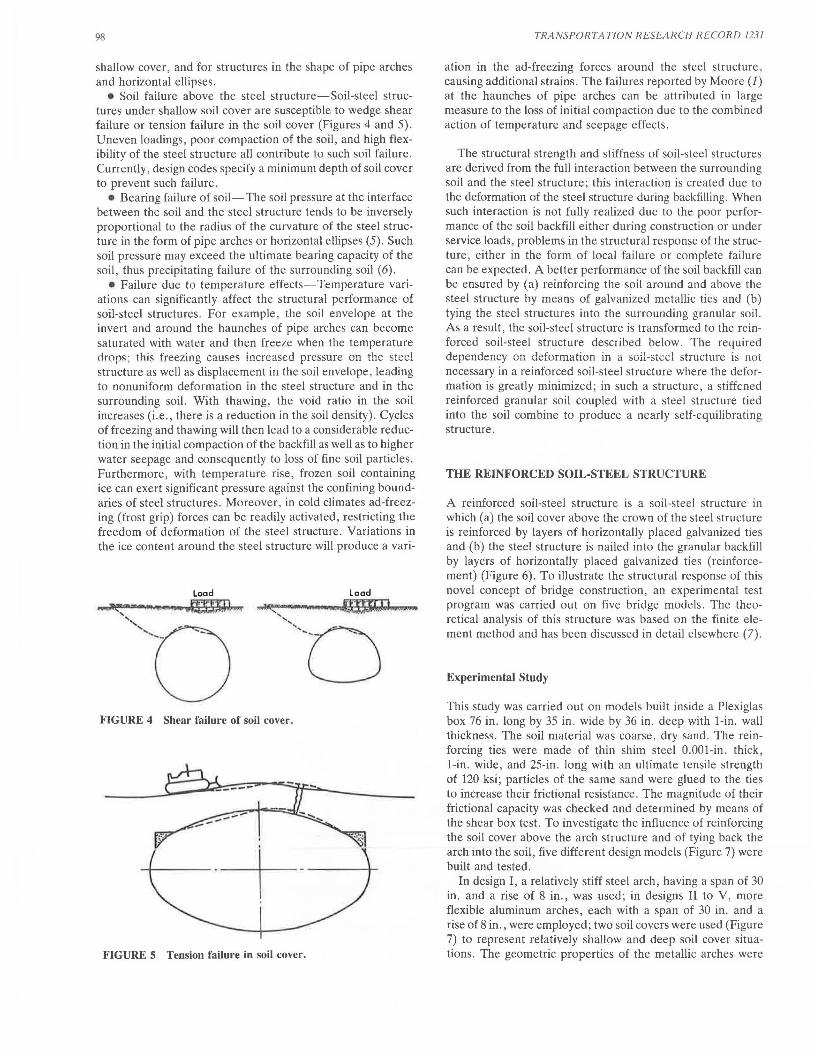
98

shallow cover, and for structures in the shape of pipe arches and horizontal ellipses.

• Soil failure above the steel structure-Soil-steel struc­tures under shallow soil cover are susceptible to wedge shear failure or tension failure in the soil cover (Figures 4 and 5). Uneven loadings, poor compaction of the soil, and high flex­ibility of the steel structure all contribute to such soil failure. Currently, design codes specify a minimum depth of soil cover to prevent such failure.

• Bearing failure of soil-The soil pressure at the interface between the soil and the steel structure tends to be inversely proportional to the radius of the curvature of the steel struc­ture in the form of pipe arches or horizontal ellipses (5). Such soil pressure may exceed the ultimate bearing capacity of the soil, thus precipitating failure of the surrounding soil (6).

• Failure due to temperature effects-Temperature vari­ations can significantly affect the structural performance of soil-steel structures. For example, the soil envelope at the invert and around the haunches of pipe arches can become saturated with water and then freeze when the temperature drops; this freezing causes increased pressure on the steel structure as well as displacement in the soil envelope, leading to nonuniform deformation in the steel structure and in the surrounding soil. With thawing, the void ratio in the soil increases (i.e., there is a reduction in the soil density). Cycles of freezing and thawing will then lead to a considerable reduc­tion in the initial compaction of the backfill as well as to higher water seepage and consequently to loss of fine soil particles. Furthermore, with temperature rise, frozen soil containing ice can exert significant pressure against the confining bound­aries of steel structures. Moreover, in cold climates ad-freez­ing (frost grip) forces can be readily activated, restricting the freedom of deformation of the steel structure. Variations in the ice content around the steel structure will produce a vari-

Load

...J!f~,.=-.,. ., .. ii4C •~Xiii '

~'O FIGURE 4 Shear failure of soil cover.

·+-FIGURE 5 Tension failure in soil cover.

TRANSPO/ffA T/ON RESEARCH RECORD 1231

ation in the ad-freezing forces around the steel structure, causing additional strains. The failures reported by Moore (J) at the haunches of pipe arches can be attributed in large measure to the loss of initial compaction due to the combined action of temperature and seepage effects.

The structural strength and stiffness of soil-steel structures are derived from the full interaction between the surrounding soil and the steel structure; this interaction is created due to the deformation of the steel structure during backfilling. When such interaction is not fully realized due to the poor perfor­mance of the soil backfill either during construction or under service loads, problems in the structural response of the struc­ture, either in the form of local failure or complete failure can be expected. A better performance of the soil backfill can be ensured by (a) reinforcing the soil around and above the steel structure by means of galvanized metallic ties and (b) tying the steel structures into the surrounding granular soil. As a result, the soil-steel structure is transformed to the rein­forced soil-steel structure described below. The required dependency on deformation in a soil-steel structure is not necessary in a reinforced soil-steel structure where the defor­mation is greatly minimized; in such a structure, a stiffened reinforced granular soil coupled with a steel structure tied into the soil combine to produce a nearly self-equilibrating structure.

THE REINFORCED SOIL-STEEL STRUCTURE

A reinforced soil-steel structure is a soil-steel structure in which (a) the soil cover above the crown of the steel structure is reinforced by layers of horizontally placed galvanized ties and (b) the steel structure is nailed into the granular backfill by layers of horizontally placed galvanized ties (reinforce­ment) (Figure 6). To illustrate the structural response of this novel concept of bridge construction, an experimental test program was carried out on five bridge models. The theo­retical analysis of this structure was based on the finite ele­ment method and has been discussed in detail elsewhere (7).

Experimental Study

This study was carried out on models built inside a Plexiglas box 76 in. long by 35 in. wide by 36 in. deep with 1-in. wall thickness. The soil material was coarse, dry sand. The rein­forcing ties were made of thin shim steel 0.001-in . thick, 1-in. wide, and 25-in. long with an ultimate tensile strength of 120 ksi; particles of the same sand were glued to the ties to increase their frictional resistance. The magnitude of their frictional capacity was checked and determined by means of the shear box test . To investigate the influence of reinforcing the soil cover above the arch structure and of tying back the arch into the soil, five different design models (Figure 7) were built and tested.

In design I, a relatively stiff steel arch, having a span of 30 in. and a rise of 8 in., was used; in designs II to V, more flexible aluminum arches, each with a span of 30 in. and a rise of 8 in., were employed; two soil covers were used (Figure 7) to represent relatively shallow and deep soil cover situa­tions. The geometric properties of the metallic arches were

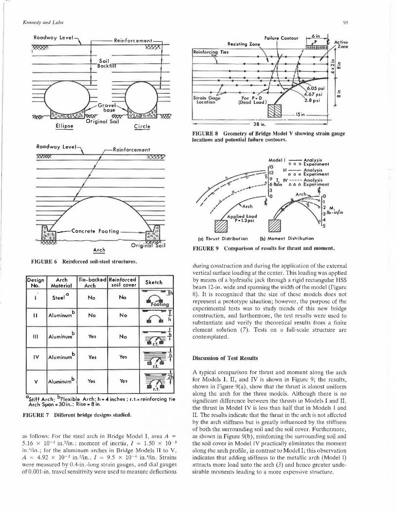
Kennedy and Laba

Roadway Level

Arch

FIGURE 6 Reinforced soil-steel structures.

Design Arch Tie-backed Reinforced Sketch No. Material Arch soil cover

I Steel a No No - -Jh

Q ng

II Aluminum b

No No - "*'J ~ h

b _t

111 Aluminum Yes No - -f ~r.(i=

b J.

IV Aluminum Yes Yes =tntf r.t.

111111 ·th v Aluminumb Yes Yes ~I

r. t.

a .b Stiff Arch , Flexi ble Arch, h • 4 inches , r. t.z reinforcing tie Arch Span • 30 in. ; Rise-Sin.

FIGURE 7 Different bridge designs studied.

as follows: For the steel arch in Bridge Model I , area A = 5.16 x 10- 2 in. 2/in.; moment of inertia, I = 1.50 x 10- 3

in .4/in .; for the aluminum arches in Bridge Models II to V, A = 4.92 x 10- 2 in. 2/in., I = 9.5 x 10 - 6 in .4/in. Strains were measured by 0.4-in .-long strain gauges , and dial gauges of0.001-in. travel sensitivity were used to measure deflections

Srro in Gage loco lion

Resisting Zone

38 in.

6.05 psi

4 .67 psi 1·

2.8 psi

15in ==+-

.!: co

99

FIGURE 8 Geometry of Bridge Model V showing strain gauge locations and potential failure contours.

(a) Thrust Distribution (b) Moment Distribution

FIGURE 9 Comparison of results for thrust and moment.

during construction and during the application of the external vertical surface loading at the center. This loading was applied by means of a hydraulic jack through a rigid rectangular HSS beam 12-in. wide and spanning the width of the model (Figure 8) . It is recognized that the size of these models does not represent a prototype situation; however, the purpose of the experimental tests was to study trends of this new bridge construction, and furthermore, the test results were used to substantiate and verify the theoretical results from a finite element solution (7). Tests on a full-scale structure are contemplated.

Discussion of Test Results

A typical comparison for thrust and moment along the arch for Models I, II, and IV is shown in Figure 9; the results, shown in Figure 9(a), show that the thrust is almost uniform along the arch for the three models . Although there is no significant difference between the thrusts in Models I and II, the thrust in Model IV is less than half that in Models I and II. The results indicate that the thrust in the arch is not affected by the arch stiffness but is greatly influenced by the stiffness of both the surrounding soil and the soil cover. Furthermore, as shown in Figure 9(b) , reinforcing the surrounding soil and the soil cover in Model IV practically eliminates the moment along the arch profile, in contrast to Model I; this observation indicates that adding stiffness to the metallic arch (Model I) attracts more load unto the arch (3) and hence greater unde­sirable moments leading to a more expensive structure.

100

The vertical deflections of the arch crown for Bridge Models II, III, and IV are compared in Figure 10; it can be observed from Figure 7 that these three models were similar except for tying the arch and reinforcing the soil cover. The results in Figure 10 show that Bridge Models III and IV carried more than 2 and 31/2 times, respectively, the maximum load carried by Bridge Model II. Bridge Model IV was able to sustain 85 percent of its maximum load-carrying capacity even when the crown deflection was as large as one-half the arch rise. This outcome is significant because such a response would provide adequate warning of an impending collapse; such a warning might have averted the catastrophic collapses in Ohio (2) and Ontario (J). In Figure 11, the snap-through collapse of Bridge Model II is shown; Bridge Models III and IV exhibited a progressive type of failure with large displacements accom­panied with pull-out failure of the reinforcing ties attached to the arch; the failure for Br.idge Model IV is shown in Figure 12. Other comparisons are given elsewhere (7).

The pressure transmitted to the steel structure due to dead load would be sensibly the same in a soil-steel structure and in a reinforced soil-steel structure; ho\vever, because of the restraining forces in the ties nailing the steel structure into the soil, the latter structure would be capable of withstanding several times the pressure of the former structure, as shown

0 4

~ _, ll. 3 a: :;; _, 2 < u ;::: a: w >

Model IV

Model Il l -----o-------6... , IY" ---,

-- Analysis ----Experiment

1 2 3 4 5 DEFLECTION OF ARCH CROWN, inch

FIGURE IO Comparison of crown deflections for Bridge Models II, III, and IV.

TRANSPORT A T!ON RESEARCH RECORD 123 1

in the buckling analysis below. The live load pressure on the steel structure would be quite different in the two designs, being much smaller in a reinforced soil-steel structure. This is a result of reinforcing the soil cover in the latter design where the truck loads would be dispersed at a much wider angle than in the former traditional design.

Potential Failure Contours Around Arch

In a reinforced soil system the tensile force distribution along the reinforcing ties is not uniform, but is usually maximum at some distance from the connection point, depending on the loading conditions and the geometry of the structure (Fig­ure 13). The curve drawn through the locus of the maximum tensile forces developed in the reinforcing ties forms a contour that divides the soil mass into two zones: the active zone and the resisting zone. In the active zone, the frictional forces exerted by the soil on the reinforcing ties are directed toward the arch wall; in the resisting zone, the frictional forces exerted by the soil on the reinforcing ties are directed toward the free end of the reinforcing ties. By holding the active and the resisting zones together on opposite sides of the contour line, the reinforcing ties provide cohesion to the granular soil mass. The movement of such contour lines under progressively applied vertical surcharge loading at the center of Bridge Model V is shown in Figure 8. As the arch begins to deform laterally near the haunches and the crown moves downward in an attempt to redistribute the pressure, the contour lines separating the active and the resisting zones move toward the center line of the structure. Thus, the active zone narrows while the resisting zone expands. The progressively increasing involvement of the stable part of the reinforced soil backfill of the resisting zone in carrying the increasing values of the applied load is clearly demonstrated in Figure 8.

Buckling Analysis

Consider the cylindrical thin shell in Figure 14, with radius R and a subtended angle 2a, subjected to hydrostatic pressure

FIGURE 11 Snap-through collapse of Bridge Model II.

Kennedy and Laba

FIGURE 12 Progressive failure of Bridge Model IV.

Active Zone

}~ \ v /

Resisting Zone

r 1; 'V1--sond-Bockfill

FIGURE 13 Distribution of tensile force along a reinforcing tie.

q from an assumed noncompressible soil (fluid soil). In the case of bending of cylindrical thin shells, the displacements due to extension of the centerline of the shell are negligibly small in comparison with the displacements due to bending. The condition of inextensional deformation of such shells can be shown to be (8)

(dvld0) - w = 0 (1)

in which v and w are the tangential and radial displacements of a point on the centerline of the shell defined by 0. Applying

101

Equation 1 for the hinged support condition of the shell in Figure 14, the tangential displacement v vanishes at the hinged supports only if

l2a

0 w de = o (2)

The cylindrical shell in Figure 14 will buckle in two half-sine waves ab as shown by the dotted line; a one half-sine wave is not feasible because this would violate the condition of inextensibility, Equation 1. The thrust in the shell, T, assumed to be sensibly constant along the shell, can be shown to be

T = qR (3)

Thus the differential equation of the deflection curve of the buckled shell (Figure 13) becomes (8)

(4)

in which v is Poisson's ratio of the shell material and EI is the flexural rigidity of the shell. Putting

(1 - v2) qR3 k2 = 1 + ~---~~-

£ / (5)

Equation 4 can be written as

0 (6)

whose solution is

w = A sin k0 + B cos k0 (7)

The hinged conditions at the two supports require B = 0, and A (sin 2a k) = O; or

sin 2a k = 0 (8)

The critical buckling load corresponds to the smallest root of

FIGURE 14 Buckled shape of hinged cylindrical shell under hydrostatic pressure.

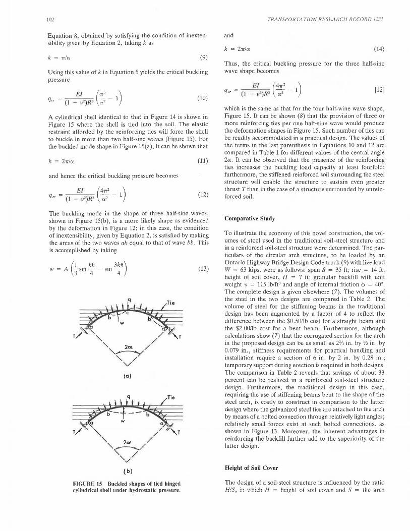
102

Equation 8, obtained by satisfying the condition of inexten­sibility given by Equation 2, taking k as

k = 1Tla. (9)

Using this value of kin Equation 5 yields the critical buckling pressure

(10)

A cylindrical shell identical to that in Figure 14 is shown in Figure 15 where the shell is tied into the soil. The elastic restraint afforded by the reinforcing ties will force the shell to ·buckle in more than two half-sine waves (Figure 15). For the buckled mode shape in Figure 15(a), it can be shown that

(11)

and hence the critical buckling pressure becomes

(12)

The buckling mode in the shape of three half-sine waves, shown in Figure 15(b), is a more likely shape as evidenced by the deformation in Figure 12; in this case, the condition of inextensibility, given by Equation 2, is satisfied by making the areas of the two waves ab equal to that of wave bb. This is accomplished by taking

(1 . ke . 3ke)

w = A 3 sm 4 - sm 4

FIGURE 15 Buckled shapes of tied hinged cylindrical shell under hydrostatic pressure.

(13)

TRANSPORTATION RESEARCH RECORD 12.H

and

k = 27r/a. (14)

Thus, the critical buckling pressure for the three half-sine wave shape becomes

[12]

which is the same as that for the four half-wine wave shape, Figure 15. It can be shown (8) that the provision of three or more reinforcing ties per one half-sine wave would produce the deformation shapes in Figure 15. Such number of ties can be readily accommodated in a practical design. The values of the terms in the last parenthesis in Equations 10 and 12 are compared in Table 1 for different values of the central angle 2a.. It can be observed that the presence of the reinforcing ties increases the buckling load capacity at least fourfold; furthermore, the stiffened reinforced soil surrounding the steel structure will enabie the structure to sustain even greater thrust T than in the case of a structure surrounded by unrein­forced soil.

Comparative Study

To illustrate the economy of this novel construction, the vol­umes of steel used in the traditional soil-steel structure and in a reinforced soil-steel structure were determined. The par­ticulars of the circular arch structure, to be loaded by an Ontario Highway Bridge Design Code truck (9) with live load W = 63 kips, were as follows: span S = 35 ft; rise = 14 ft; height of soil cover, H = 7 ft; granular backfill with unit weight 'Y = 115 lb/ft3 and angle of internal friction<!> = 40°. The complete design is given elsewhere (7). The volumes of the steel in the two designs are compared in Table 2. The volume of steel for the stiffening beams in the traditional design has been augmented by a factor of 4 to reflect the difference between the $0.50/lb cost for a straight beam and the $2.00/lb cost for a bent beam. Furthermore, although calculations show (7) that the corrugated section for the arch in the proposed design can be as small as 22/J in. by Y2 in. by 0 .079 in., stiffness requirements for practical handling and installation require a section of 6 in. by 2 in . by 0.28 in.; temporary support during erection is required in both designs. The comparison in Table 2 reveals that savings of about 33 percent can be realized in a reinforced soil-steel structure design. Furthermore, the traditional design in this case, requiring the use of stiffening beams bent to the shape of the steel arch, is costly to construct in comparison to the latter design where the galvanized steel ties are attached lo the a1d1 by means of a bolted connection through relatively light angles; relatively small forces exist at such bolted connections. as shown in Figure 13. Moreover, the inherent advantages in reinforcing the backfill further add to the superiority of the latter design.

Height of Soil Cover

The design of a soil-steel structure is influenced by the ratio HIS, in which H = height of soil cover and S = the arch

Kennedy and Laba 103

TABLE 1 COMPARISON OF BUCKLING LOADS GIVEN BY EQUATIONS 10 AND 12

'lr2 2

ffi 2a 4ir 1 2- l 2-a a

(<legs.) (a) (b)

30° 143 575 4.02

60° 35 143 4.08

90° 15 63 4.2

120° 8 35 4.38

150° 4.76 22.04 4.63

180° 3 15 5

TABLE 2 VOLUME OF STEEL USED IN TRADITIONAL AND PROPOSED DESIGNS IN FT3/FT

Traditional Design Proposed Design

Corrugated Section 1.38 1.38 for Arch (6 in x 2 in x 0.28 in) (6 in x 2 in x 0.28 in)

Steel Ties for Arch and Soil Cover NIL

Stiffening Beams for Traditional 0.61 x 4 = 2.44

1.15

NIL

Design (W6 x 15.5 spaced 2 ~ ft.)

Total Volume of Steel 3.82

span. A relatively shallow cover can lead to premature soil failure and thus a sudden transfer of load to the steel structure. It has been shown in a parametric study (7) that an increase in HIS produces a wider dispersion of the vertical load P applied at the road surface and thus permits a significant increase in that external load. It has also been shown that when the soil cover is reinforced and the steel arch is tied by soil friction as suggested herein, the load-carrying capacity of the structure is augmented further. Design equations are reported (7) for HIS between 0.1and0.5; such ratios encom­pass the range of normal practice for soil-steel structures. The reinforcing ties for the soil cover are designed not to break or pull out following the procedure proposed by Binquet and Lee (10). The first layer of ties should be placed at a distance below the road surface of not more than two-thirds of the assumed truck wheel width; and the number of layers should be greater than four but not more than eight.

The Problem of Corrosion

Galvanized steel structures are subject to corrosion; the amount and rate of such corrosion depend on environmental condi­tions. Based on data collected by Lee (11) on buried culverts,

2.53

it was suggested that a corrosion rate of 0.001 to 0.002 in./year is appropriate for such structures. However, based on recent on-site examination of many soil-steel structures (1), it is recommended that the higher rate of 0.002 in.lyear should be used for corrosion protection. Using this rate and a 50-year design life results in an additional 0.10 in. of steel for corrosion protection. Lee (11) has shown that the cost of this extra steel is small compared to the cost of the backfill. The use of epoxy paint should also be seriously considered as a solution to the problem of corrosion.

ADVANTAGES OF THE PROPOSED CONSTRUCTION

Generally, it has been found that an increase in the stiffness of the backfill (as in reinforced soil) effects a reduction in bending moments in the steel structure and an increase in the stiffness of the steel structure results in the opposite. There­fore, designers of soil-steel structures using the latter practice should reevaluate their designs. Reinforcing the backfill would in effect increase several fold the load paths in soil-steel struc­tures. This novel concept of bridge construction would lead to improvements in the structural response during construe-

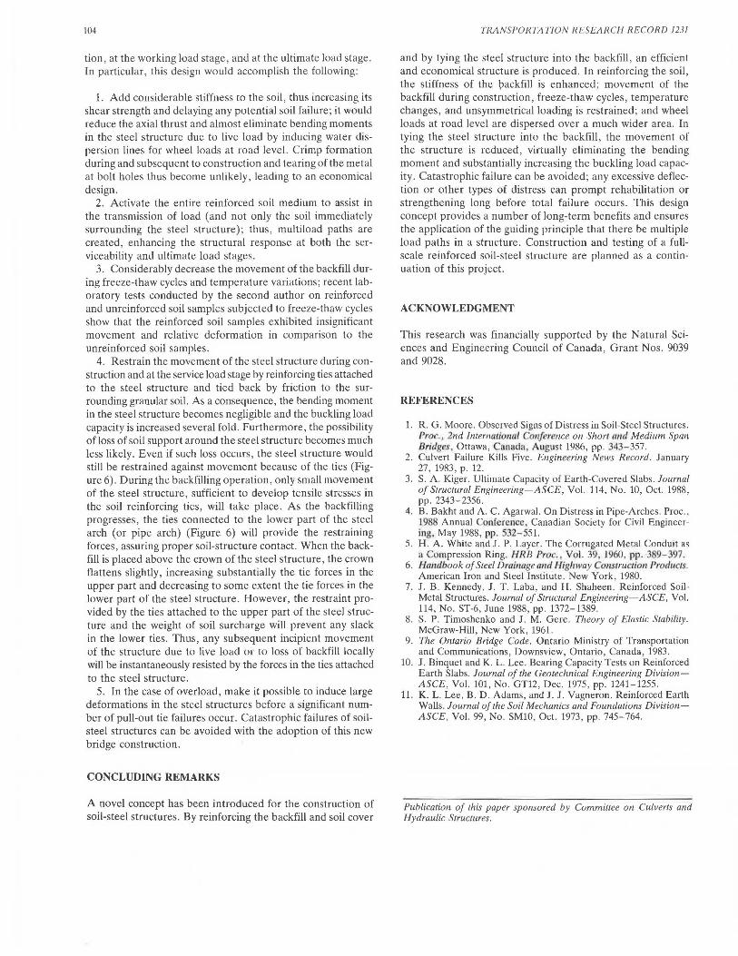
104

tion, at the working load stage, and at the ultimate load stage . In particular, this design would accomplish the following:

1. Add considerable stiffness to the soil, thus increasing its shear strength and delaying any potential soil failure; it would reduce the axial thrust and almost eliminate bending moments in the steel structure due to live load by inducing water dis­persion lines for wheel loads at road level. Crimp formation during and subsequent to construction and tearing of the metal at bolt holes thus become unlikely, leading to an economical design.

2. Activate the entire reinforced soil medium to assist in the transmission of load (and not only the soil immediately surrounding the steel structure); thus, multiload paths are created, enhancing the structural response at both the ser­viceability and ultimate load stages.

3. Considerably decrease the movement of the backfill dur­ing freeze-thaw cycles and temperature variations; recent lab­oratory tests conducted by the second author on reinforced and unreinforced soil samples subjected to freeze-thaw cycles show that the reinforced soil samples exhibited insignificant movement and relative deformation in comparison to the unreinforced soil samples.

4. Restrain the movement of the steel structure during con­struction and at the service load stage by reinforcing ties attached to the steel structure and tied back by friction to the sur­rounding granular soil. As a consequence, the bending moment in the steel structure becomes negligible and the buckling load capacity is increased several fold. Furthermore, the possibility of loss of soil support around the steel structure becomes much less likely. Even if such loss occurs, the steel structure would still be restrained against movement because of the ties (Fig­ure 6). During the backfilling operation, only small movement of the steel structure, sufficient to develop tensile stresses in the soil reinforcing ties, will take place. As the backfilling progresses, the ties connected to the lower part of the steel arch (or pipe arch) (Figure 6) will provide the restraining forces, assuring proper soil-structure contact. When the back­fill is placed above the crown of the steel structure, the crown flattens slightly, increasing substantially the tie forces in the upper part and decreasing to some extent the tie forces in the lower part of the steel structure. However, the restraint pro­vided by the ties attached to the upper part of the steel struc­ture and the weight of soil surcharge will prevent any slack in the lower ties. Thus, any subsequent incipient movement of the structure due to live load or to loss of backfill locally will be instantaneously resisted by the forces in the ties attached to the steel structure.

5. In the case of overload, make it possible to induce large deformations in the steel structures before a significant num­ber of pull-out tie failures occur. Catastrophic failures of soil­steel structures can be avoided with the adoption of this new bridge construction.

CONCLUDING REMARKS

A novel concept has been introduced for the construction of soil-steel structures. By reinforcing the backfill and soil cover

TRANSPORTATION RESEARCH RECORD 1231

and by tying the steel structure into the backfill, an efficient and economical structure is produced. In reinforcing the soil, the stiffness of the packfill is enhanced; movement of the backfill during construction, freeze-thaw cycles, temperature changes, and unsymmetrical loading is restrained; and wheel loads at road level are dispersed over a much wider area. In tying the steel structure into the backfill, the movement of the structure is reduced, virtually eliminating the bending moment and substantially increasing the buckling load capac­ity . Catastrophic failure can be avoided; any excessive deflec­tion or other types of distress can prompt rehabilitation or strengthening long before total failure occurs. This design concept provides a number of long-term benefits and ensures the application of the guiding principle that there be multiple load paths in a structure. Construction and testing of a full­scale reinforced soil-steel structure are planned as a contin­uation of this project .

ACKNOWLEDGMENT

This research was financially supported by the Natural Sci­ences and Engineering Council of Canada, Grant Nos. 9039 and 9028.

REFERENCES

1. R. G. Moore . Observed Signs of Distress in Soil-Steel Structures. Proc., 2nd lnternmional Conference on Shor/ tmd Medium Span Bridges, Ottawa, nnada, August 1986, pp. 343-357.

2. Culvert Failure Kills Five. Engineering News Record. January 27, 1983, p . 12.

3. S. A. Kiger . Ultimate Capacity of Earth-Covered Slabs. Journal of Structural Engineering-ASCE, Vol. 114, No. 10, Oct. 1988, pp. 2343-2356.

4. B. Bakht and A. C. Agarwal. On Distress in Pipe-Arches. Proc., 1988 Annual Conference, Canadian Society for Civil Engineer­ing, May 1988, pp. 532- 551.

5. H. A. White and J.P. Layer. The Corrugated Metal Conduit as a Compression Ring. liRB Proc., Vol. 39, 1960, pp. 389- 397.

6. Handbook of Steel Drainage a11d Migliivay Construction Prod11c1s. American Iron and Steel Institute. New York, 1980.

7. J . B. Kennedy, J. T. Laba, and H. Shaheen. Reinforced Soil­Metal Structures. Journal of Structural Engineering-ASCE, Vol. 114, No. ST-6, June 1988, pp. 1372-1389.

8. S. P. Timoshenko and J . M. Gere. Theory of Elastic Stability. McGraw-Hill, New York, 1961.

9. The Ontario Bridge Code. Ontario Ministry of Transportation and Communications, Downsview, Ontario, Canada, 1983.

10. J, Binquet and K. L. Lee. Bearing Capacity Tests on Reinforced Earth Slabs. Journal of the Geotechnical Engineering Division­ASCE, Vol. 101, No. GT12, Dec. 1975, pp. 1241-1255.

11. K. L. Lee, B.'D. Adams, and J. J . Vagneron. Reinforced Earth Walls. Journal of the Soil Mechanics and Foundations Division­ASCE, Vol. 99, No. SMlO, Oct. 1973, pp. 745-764.

Publication of 1his paper sponsored by Committee on Culverts and Hydraulic Structures.