Goalkeeper Robot Behavior Design and ... - Técnico Lisboa
96
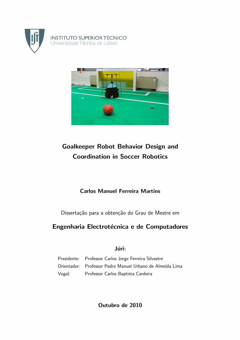
Goalkeeper Robot Behavior Design and Coordination in Soccer Robotics Carlos Manuel Ferreira Martins Disserta¸c˜ ao para a obten¸c˜ ao do Grau de Mestre em Engenharia Electrot´ ecnica e de Computadores J´ uri: Presidente: Professor Carlos Jorge Ferreira Silvestre Orientador: Professor Pedro Manuel Urbano de Almeida Lima Vogal: Professor Carlos Baptista Cardeira Outubro de 2010
-
Upload
khangminh22 -
Category
Documents
-
view
0 -
download
0
Transcript of Goalkeeper Robot Behavior Design and ... - Técnico Lisboa
Goalkeeper Robot Behavior Design and
Coordination in Soccer Robotics
Carlos Manuel Ferreira Martins
Dissertacao para a obtencao do Grau de Mestre em
Engenharia Electrotecnica e de Computadores
Juri:
Presidente: Professor Carlos Jorge Ferreira Silvestre
Orientador: Professor Pedro Manuel Urbano de Almeida Lima
Vogal: Professor Carlos Baptista Cardeira
Outubro de 2010

Agradecimentos
Depois de uma maratona de escrita tao “cientıfica”, nao e nada facil escrever os agradecimentos a todas
as pessoas que me ajudaram, directa ou indirectamente, a alcancar este objectivo final do curso pelo qual me
esforcei bastante, abdicando por vezes de imensas coisas.
Antes de mais, quero agradecer aos meus pais e irma que estiveram sempre do meu lado, mesmo nestas
ultimas semanas em que o descanso ja era pouco e por vezes a disposicao nao era a melhor. A toda a minha
famılia, especialmente, a minha afilhada Ritinha, nada melhor que as brincadeiras de uma crianca para nos
animar nalguns momentos mais complicados.
A Sara, por todos os momentos especiais que passamos juntos ao longo deste percurso e nao so, apesar
de nos ultimos meses o tempo ter sido muito pouco, espero vir a recompensar-te . . .
Como e obvio, agradecer profundamente ao Prof. Pedro Lima por me ter proporcionado a oportunidade
de entrar como voluntario num projecto, em que jogar a bola com robots e apenas a parte divertida, mas que
envolve muito trabalho e dedicacao. Agradecer tambem pela orientacao ao longo da tese e toda a sua ajuda.
Mais directamente relacionado com o trabalho desenvolvido nesta tese, agradecer ao Hugo Costelha por
toda a ajuda e explicacoes sobre o trabalho de Doutoramento dele, sem o qual a minha tese teria tido uma
maior dificuldade.
Sem duvida agradecer ao trio selfTech, Marco, Estilita e Joao Santos, que tanto me ajudaram quando
entrei como voluntario no projecto SocRob, bem como ao trio actual, Joao Messias, Reis e Aamir, que me
ajudaram em muitos aspectos e duvidas durante a tese.
Por fim agradecer a todos os meus amigos, em especial aos futuros Doutores Tiago Veiga e Wiener, aqueles
almocos foram sempre momentos de descontracao de todo o trabalho.
Muito Obrigado a todos. Finalmente, esta a terminar!!

Resumo
Numa equipa de futebol robotico, um dos seus elementos e o guarda-redes que apresenta caracterısticas
desafiantes e diferentes dos outros jogadores, quando se desenvolve e coordena toda a execucao de uma tarefa
robotica. Apesar do objectivo simples deste jogador, defender a baliza dos remates da equipa adversaria, este
deve exibir um comportamento complexo com uma perfeita coordenacao entre todas as accoes, de modo a
que tenha um papel importante na equipa.
Esta tese tem como objectivo o desenvolvimento e implementacao de um comportamento completo, efec-
tivo e testado para o guarda-redes de um equipa de futebol robotico, usando para tal um robot futebolista
omni-direccional, bem como redes de Petri para a modelacao da tarefa. Todas as accoes primitivas e os com-
portamentos, bem como, os eventos usados para a escolha daqueles, foram desenvolvidos e implementados.
Para alem disso, ainda se modelou e analisou, tanto qualitativamente como quantitativamente, o compor-
tamento do guarda-redes de modo a se ter um conhecimento da eficacia da tarefa em diferentes situacoes
possıveis, tais como diferentes tipos de adversarios. Deste modo, utilizou-se uma ferramenta de analise e
modelacao baseada em modelos de redes de Petri estocasticas generalizadas com diferentes componentes para
o comportamento do guarda-redes, tais como modelos do ambiente, das accoes e das tarefas.
Palavras-Chave
Guarda-redes, Futebol Robotico, Tarefas Roboticas, Redes de Petri, Modelacao, Analise, Execucao

Abstract
In a robotic soccer team, one of the elements is the goalkeeper which has particular challenging character-
istics, different from the other teammates, when designing and coordinating the execution of a robot task plan.
Although, this player has a simple purpose, i.e., to defend the goal from the opponent kicks, it should exhibit
a richer behavior with a perfect coordination between the different actions in order to have an important role
in the team
This thesis aims at developing and implementing a complete, tested and effective behavior for a goalkeeper
of a robot soccer team, using an omnidirecional soccer robot hardware and Petri Nets to model task plans.
The different primitive actions and behaviors as well as the events to switch between them were designed and
implemented.
We also aim at modelling and analysing, both qualitatively and quantitatively, the goalkeeper role in order
to have a model-based knowledge of the task performance in different possible situations, such as different
types of opponent teams. For this purpose, we use a modelling and analysis framework based on Generalised
Stochastic Petri Nets and model the different components of the goalkeeper role, such as the environment,
action and task models.
Keywords
Goalkeeper, Robotic Soccer, Robot Task, Petri Nets, Modelling, Analysis, Execution

Contents
1 Introduction 2
1.1 Motivation . . . . . . . . . . . . . . . . . . . . . . . . . . . . . . . . . . . . . . . . . . . . . 2
1.1.1 The RoboCup Project . . . . . . . . . . . . . . . . . . . . . . . . . . . . . . . . . . . 2
1.1.2 The SocRob Project . . . . . . . . . . . . . . . . . . . . . . . . . . . . . . . . . . . . 3
1.1.3 The Goalkeeper . . . . . . . . . . . . . . . . . . . . . . . . . . . . . . . . . . . . . . 3
1.2 State-of-the-Art . . . . . . . . . . . . . . . . . . . . . . . . . . . . . . . . . . . . . . . . . . 4
1.3 Objectives . . . . . . . . . . . . . . . . . . . . . . . . . . . . . . . . . . . . . . . . . . . . . 5
1.4 Thesis Outline . . . . . . . . . . . . . . . . . . . . . . . . . . . . . . . . . . . . . . . . . . . 6
2 Background 8
2.1 Petri Nets . . . . . . . . . . . . . . . . . . . . . . . . . . . . . . . . . . . . . . . . . . . . . 8
2.1.1 Ordinary Petri Nets . . . . . . . . . . . . . . . . . . . . . . . . . . . . . . . . . . . . 8
2.1.2 Generalized Stochastic Petri Nets . . . . . . . . . . . . . . . . . . . . . . . . . . . . . 9
2.1.3 Analysis Properties . . . . . . . . . . . . . . . . . . . . . . . . . . . . . . . . . . . . 11
2.2 Task Modelling and Analysis Framework . . . . . . . . . . . . . . . . . . . . . . . . . . . . . 12
2.2.1 Types of Petri Net Places . . . . . . . . . . . . . . . . . . . . . . . . . . . . . . . . . 12
2.2.2 Layers of Abstraction . . . . . . . . . . . . . . . . . . . . . . . . . . . . . . . . . . . 13
2.2.3 Expansion Algorithm . . . . . . . . . . . . . . . . . . . . . . . . . . . . . . . . . . . 16
3 Soccer Robots Framework 18
3.1 RoboCup MSL Rules and Regulations . . . . . . . . . . . . . . . . . . . . . . . . . . . . . . 18
3.2 The Robot Platform . . . . . . . . . . . . . . . . . . . . . . . . . . . . . . . . . . . . . . . . 19
3.3 The MeRMaID Architecture . . . . . . . . . . . . . . . . . . . . . . . . . . . . . . . . . . . 20
3.4 Behaviors as a Part of MeRMaID . . . . . . . . . . . . . . . . . . . . . . . . . . . . . . . . . 21
3.5 Relevant Features . . . . . . . . . . . . . . . . . . . . . . . . . . . . . . . . . . . . . . . . . 22
4 GoalKeeper Task Components 24
4.1 Predicates . . . . . . . . . . . . . . . . . . . . . . . . . . . . . . . . . . . . . . . . . . . . . 24
4.2 Primitive Actions . . . . . . . . . . . . . . . . . . . . . . . . . . . . . . . . . . . . . . . . . 25
4.2.1 Move2GKPosition . . . . . . . . . . . . . . . . . . . . . . . . . . . . . . . . . . . . . 25
4.2.2 CoverGoalLine . . . . . . . . . . . . . . . . . . . . . . . . . . . . . . . . . . . . . . . 25
4.2.3 CutDownTheAngle . . . . . . . . . . . . . . . . . . . . . . . . . . . . . . . . . . . . 26
4.2.4 CatchBall . . . . . . . . . . . . . . . . . . . . . . . . . . . . . . . . . . . . . . . . . 26
4.2.5 HitBall . . . . . . . . . . . . . . . . . . . . . . . . . . . . . . . . . . . . . . . . . . . 26
4.3 Behaviors . . . . . . . . . . . . . . . . . . . . . . . . . . . . . . . . . . . . . . . . . . . . . 27
4.3.1 BehaviorGKDefault . . . . . . . . . . . . . . . . . . . . . . . . . . . . . . . . . . . . 27
4.3.2 BehaviorGKDefendGoal . . . . . . . . . . . . . . . . . . . . . . . . . . . . . . . . . . 28
4.3.3 BehaviorGKRemoveBall . . . . . . . . . . . . . . . . . . . . . . . . . . . . . . . . . . 28
iii
4.4 Roles . . . . . . . . . . . . . . . . . . . . . . . . . . . . . . . . . . . . . . . . . . . . . . . . 29
4.4.1 RoleGK . . . . . . . . . . . . . . . . . . . . . . . . . . . . . . . . . . . . . . . . . . 29
5 GoalKeeper Petri Net Task Model 31
5.1 Soccer Field Discretization . . . . . . . . . . . . . . . . . . . . . . . . . . . . . . . . . . . . 31
5.2 Computing Stochastic Transitions Rates . . . . . . . . . . . . . . . . . . . . . . . . . . . . . 32
5.2.1 Robot Motion . . . . . . . . . . . . . . . . . . . . . . . . . . . . . . . . . . . . . . . 33
5.2.2 Ball Motion . . . . . . . . . . . . . . . . . . . . . . . . . . . . . . . . . . . . . . . . 34
5.2.3 Probability of Success . . . . . . . . . . . . . . . . . . . . . . . . . . . . . . . . . . . 34
5.2.4 Percentage of Time . . . . . . . . . . . . . . . . . . . . . . . . . . . . . . . . . . . . 34
5.3 Predicates . . . . . . . . . . . . . . . . . . . . . . . . . . . . . . . . . . . . . . . . . . . . . 34
5.4 Environment Models . . . . . . . . . . . . . . . . . . . . . . . . . . . . . . . . . . . . . . . . 35
5.4.1 Robot Position . . . . . . . . . . . . . . . . . . . . . . . . . . . . . . . . . . . . . . 36
5.4.2 Ball Position . . . . . . . . . . . . . . . . . . . . . . . . . . . . . . . . . . . . . . . . 36
5.4.3 Ball Stopped . . . . . . . . . . . . . . . . . . . . . . . . . . . . . . . . . . . . . . . . 37
5.4.4 Ball Velocity . . . . . . . . . . . . . . . . . . . . . . . . . . . . . . . . . . . . . . . . 38
5.4.5 Ball Direction . . . . . . . . . . . . . . . . . . . . . . . . . . . . . . . . . . . . . . . 39
5.4.6 Ball Off the Ground . . . . . . . . . . . . . . . . . . . . . . . . . . . . . . . . . . . . 39
5.4.7 Ball Motion . . . . . . . . . . . . . . . . . . . . . . . . . . . . . . . . . . . . . . . . 40
5.4.8 Ball Detection . . . . . . . . . . . . . . . . . . . . . . . . . . . . . . . . . . . . . . . 40
5.4.9 Ball Distance . . . . . . . . . . . . . . . . . . . . . . . . . . . . . . . . . . . . . . . 41
5.4.10 Goals Scored . . . . . . . . . . . . . . . . . . . . . . . . . . . . . . . . . . . . . . . . 42
5.4.11 Game Fouls . . . . . . . . . . . . . . . . . . . . . . . . . . . . . . . . . . . . . . . . 43
5.4.12 Game Restart . . . . . . . . . . . . . . . . . . . . . . . . . . . . . . . . . . . . . . . 43
5.5 Action Models . . . . . . . . . . . . . . . . . . . . . . . . . . . . . . . . . . . . . . . . . . . 44
5.5.1 Stop . . . . . . . . . . . . . . . . . . . . . . . . . . . . . . . . . . . . . . . . . . . . 44
5.5.2 Move2GKPosition . . . . . . . . . . . . . . . . . . . . . . . . . . . . . . . . . . . . . 45
5.5.3 CoverGoalLine . . . . . . . . . . . . . . . . . . . . . . . . . . . . . . . . . . . . . . . 46
5.5.4 CutDownTheAngle . . . . . . . . . . . . . . . . . . . . . . . . . . . . . . . . . . . . 46
5.5.5 CatchBall . . . . . . . . . . . . . . . . . . . . . . . . . . . . . . . . . . . . . . . . . 48
5.5.6 HitBall . . . . . . . . . . . . . . . . . . . . . . . . . . . . . . . . . . . . . . . . . . . 49
5.6 Task Models . . . . . . . . . . . . . . . . . . . . . . . . . . . . . . . . . . . . . . . . . . . . 50
6 Experimental Setup 53
6.1 Task Analysis . . . . . . . . . . . . . . . . . . . . . . . . . . . . . . . . . . . . . . . . . . . 53
6.1.1 Base Setup with Different Opponent Teams and GoalKeeper Behaviors . . . . . . . . 54
6.1.2 Base Setup with Differences on Ball Detection . . . . . . . . . . . . . . . . . . . . . . 61
6.1.3 Base Setup with Differences on Self-Localization . . . . . . . . . . . . . . . . . . . . 63
6.2 Real Setup . . . . . . . . . . . . . . . . . . . . . . . . . . . . . . . . . . . . . . . . . . . . . 65
7 Results 67
7.1 Task Analysis . . . . . . . . . . . . . . . . . . . . . . . . . . . . . . . . . . . . . . . . . . . 67
7.1.1 Base Setup with Different Opponent Teams and GoalKeeper Behaviors . . . . . . . . 67
7.1.2 Base Setup with Differences on Ball Detection . . . . . . . . . . . . . . . . . . . . . . 70
7.1.3 Base Setup with Differences on Self-Localization . . . . . . . . . . . . . . . . . . . . 71
7.2 Real Setup . . . . . . . . . . . . . . . . . . . . . . . . . . . . . . . . . . . . . . . . . . . . . 71
iv
8 Conclusion 73
8.1 Discussion . . . . . . . . . . . . . . . . . . . . . . . . . . . . . . . . . . . . . . . . . . . . . 73
8.2 Conclusions . . . . . . . . . . . . . . . . . . . . . . . . . . . . . . . . . . . . . . . . . . . . 74
8.3 Future Work . . . . . . . . . . . . . . . . . . . . . . . . . . . . . . . . . . . . . . . . . . . . 74
v

vi
List of Figures
1.1 RoboCup Middle Size League Field . . . . . . . . . . . . . . . . . . . . . . . . . . . . . . . . 3
2.1 Producer-Consumer system with limited buffer capacity and the meaning of places and transitions 10
2.2 Predicate BallStopped model represented by a set of places . . . . . . . . . . . . . . . . . . . 13
2.3 Example of an environment model for the ball position in a soccer field . . . . . . . . . . . . 14
2.4 Example of action models used by a robot to capture a ball . . . . . . . . . . . . . . . . . . . 15
2.5 Example of task models used by a robot to score a goal . . . . . . . . . . . . . . . . . . . . . 15
3.1 The field of play used in RoboCup MSL with the current dimensions. . . . . . . . . . . . . . 18
3.2 The robot goalkeeper soccer platform currently used by the ISocRob team . . . . . . . . . . . 19
3.3 MeRMaID high-level software architecture block diagram . . . . . . . . . . . . . . . . . . . . 20
4.1 Primitive action Move2GKPosition . . . . . . . . . . . . . . . . . . . . . . . . . . . . . . . . 25
4.2 Primitive action CoverGoalLine . . . . . . . . . . . . . . . . . . . . . . . . . . . . . . . . . . 26
4.3 Primitive action CutDownTheAngle . . . . . . . . . . . . . . . . . . . . . . . . . . . . . . . 26
4.4 Primitive action CatchBall . . . . . . . . . . . . . . . . . . . . . . . . . . . . . . . . . . . . 27
4.5 The Petri Net for the behavior BehaviorGKDefault . . . . . . . . . . . . . . . . . . . . . . . 28
4.6 The Petri Net for the behavior BehaviorGKDefendGoal . . . . . . . . . . . . . . . . . . . . . 28
4.7 The Petri Net for the behavior BehaviorGKRemoveBall . . . . . . . . . . . . . . . . . . . . . 29
4.8 The Petri Net for the behavior RoleGK . . . . . . . . . . . . . . . . . . . . . . . . . . . . . . 30
5.1 Soccer field discretization and its legend. . . . . . . . . . . . . . . . . . . . . . . . . . . . . . 32
5.2 Environment models representing the logic properties between the different areas for the GK
position. . . . . . . . . . . . . . . . . . . . . . . . . . . . . . . . . . . . . . . . . . . . . . . 36
5.3 Environment models representing the logic properties between the different areas for the ball
position. . . . . . . . . . . . . . . . . . . . . . . . . . . . . . . . . . . . . . . . . . . . . . . 37
5.4 Environment model representing the expected logic properties when the ball is stopped. . . . . 37
5.5 Environment models representing the starting and ending of the ball movement . . . . . . . . 38
5.6 Environment model representing the changes in the ball direction movement. . . . . . . . . . 39
5.7 Environment model representing the ball state when a high kick occurs. . . . . . . . . . . . . 39
5.8 Environment models representing the ball movement and its transition between different areas. 40
5.9 Environment models representing the switching between seeing the ball and not seeing it. . . 41
5.10 Environment models representing the expected logic properties of the ball distance predicates. 42
5.11 Environment model representing the transition to game stopped due to a goal scored by the
opponent team. . . . . . . . . . . . . . . . . . . . . . . . . . . . . . . . . . . . . . . . . . . 42
5.12 Environment model representing the occurrence of any foul depending on the ball position. . . 43
5.13 Environment models representing the restart of the game and the logic properties when the
game is stopped. . . . . . . . . . . . . . . . . . . . . . . . . . . . . . . . . . . . . . . . . . . 44
vii
5.14 Action Stop model representing the stop of the robot and motors. . . . . . . . . . . . . . . . 45
5.15 Action Move2GKPosition model representing the goalkeeper movement to the center of the
own goal. . . . . . . . . . . . . . . . . . . . . . . . . . . . . . . . . . . . . . . . . . . . . . 45
5.16 Action CoverGoalLine model representing the goalkeeper movement to a parallel line with the
goal line. . . . . . . . . . . . . . . . . . . . . . . . . . . . . . . . . . . . . . . . . . . . . . . 46
5.17 Action CutDownTheAngle model representing the goalkeeper covering the goal and approach-
ing the ball. . . . . . . . . . . . . . . . . . . . . . . . . . . . . . . . . . . . . . . . . . . . . 47
5.18 Action CatchBall model representing the goalkeeper catching the ball. . . . . . . . . . . . . . 49
5.19 Action HitBall model representing the goalkeeper hitting through the ball. . . . . . . . . . . . 49
5.20 Task models used for the goalkeeper task modelling. . . . . . . . . . . . . . . . . . . . . . . 50
6.1 Environment model representing the different ball detection mechanisms. . . . . . . . . . . . 62
6.2 Environment model representing the different self-localization algorithms model . . . . . . . . 64
6.3 Real setup environment used to test the goalkeeper task . . . . . . . . . . . . . . . . . . . . 65
7.1 Probability evolution of a goal scored in own goal for each type of goalkeeper behavior . . . . 68
7.2 Probability evolution of a goal scored in own goal for each type of opponent team . . . . . . . 69
7.3 Probability evolution of a goal scored in own goal with different ball detection mechanisms . . 70
7.4 Probability evolution of a goal scored in own goal with different self-localization algorithms . . 71
viii
List of Tables
5.1 Mean traveling distance between areas for the goalkeeper and ball . . . . . . . . . . . . . . . 33
5.2 Running-conditions and desired-effects of each action. . . . . . . . . . . . . . . . . . . . . . . 44
6.1 Different behaviors used in the Goalkeeper task analysis depending on the decision area. . . . 54
6.2 Different opponent teams used in the Goalkeeper task analysis depending on the features . . . 55
6.3 Mean delay time of the stochastic transitions for the goalkeeper movement . . . . . . . . . . 56
6.4 Mean delay time of the stochastic transitions for the ball movement . . . . . . . . . . . . . . 56
6.5 Time delay of the stochastic transitions for the goalkeeper defenses depending on the action
and area . . . . . . . . . . . . . . . . . . . . . . . . . . . . . . . . . . . . . . . . . . . . . . 57
6.6 Time delay of the stochastic transitions for the ball velocity model . . . . . . . . . . . . . . . 57
6.7 Time delay of the stochastic transitions for the ball direction model . . . . . . . . . . . . . . 58
6.8 Time delay of the stochastic transitions for the ball off the ground model . . . . . . . . . . . 58
6.9 Time delay of the stochastic transitions for the game fouls model . . . . . . . . . . . . . . . 59
6.10 Time delay of the stochastic transitions for the getting close to ball model . . . . . . . . . . . 60
6.11 Time delay of the stochastic transitions for the remain models . . . . . . . . . . . . . . . . . 61
6.12 Time delay of the stochastic transitions for the ball detection mechanisms model . . . . . . . 63
6.13 Time delay of the stochastic transitions for the self-localization mechanisms model . . . . . . 64
ix

x
Acronyms
CTMC Continuous Time Markov Chain.
DES Discrete Event System.
EMC Embedded Markov Chain.
FSA Finite State Automata.
GK Goalkeeper.
GSPN Generalised Stochastic Petri Nets.
ISocRob ISR Soccer Robots.
ISR Institute for Systems and Robotics.
IST Instituto Superior Tecnico.
MeRMaID Multiple-Robot Middleware for Intelligent Decision-making.
MSL Middle Size League.
OPN Ordinary Petri Nets.
PN Petri Nets.
RG Reachability Graph.
RoboCup Robot World Cup Initiative.
SocRob Society of Robots or Soccer Robots.
xi

1
Chapter 1
Introduction
1.1 Motivation
In robotics, when developing an autonomous group of agents, one needs to integrate different features of the
agents in order to achieve a certain goal for this group. For a mobile robot agent, one needs to understand
all the information received from the different sensors, e.g., cameras using image processing, integrate this
information to perceive better the surrounding environment, e.g., to self-localize, and then act to have a
desired effect in the environment, e.g., using motion control and obstacle avoidance algorithms.
On the top of these is the most important key feature for a robot to achieve a desired goal, autonomy. The
robot needs to coordinate all its subsystems, its actions and behaviors in order to have a task plan capable of
achieving the desired goal for the agent or for the group of agents together.
Traditionally, a mobile robot task is programmed without using formal approaches, which usually leads to
task plans without any a priori knowledge of the expected task performance. Therefore, the use of method-
ologies enabling the design, modelling, analysis and execution for mobile robot tasks is one of the motivations
for this work. Using systematic and consistent methods will lead to richer task plans that can be formally
analysed and checked for performance quality.
1.1.1 The RoboCup Project
The RoboCup (Robot World Cup Initiative) project, [1], is a robotic competition which the main intention is
to promote robotics and the research on artificial intelligence with the ultimate challenge stated as follows:
By mid-21st century, a team of fully autonomous humanoid robot soccer players shall win the
soccer game, comply with the official rule of the FIFA, against the winner of the most recent
World Cup.
In RoboCup, there are different competitions such as “Search and Rescue” and “Robot Soccer”. Inside
the robot soccer competition there are different leagues and one of the most interesting and with richer task
plans performed by the robots is the MSL (Middle Size League). In the RoboCup MSL, the robot soccer
environment is composed with two teams of robots with 5 to 7 players each, playing on a field with size about
12m by 18m, see Figure 1.1. Over the years, the restrictions of this competition are lifted in order to approach
the regular human soccer field and rules. As an example, the goals have been changed into goals with nets,
removing the blue and yellow colors that were previously used to distinguish goals.
Therefore, this robot soccer competition provides an excellent case test for this work in the development
of robot task plans because it is a dynamic and known environment where each one of the agents should have
a specific role and needs to coordinate its actions and behaviors to achieve a desired goal.
2
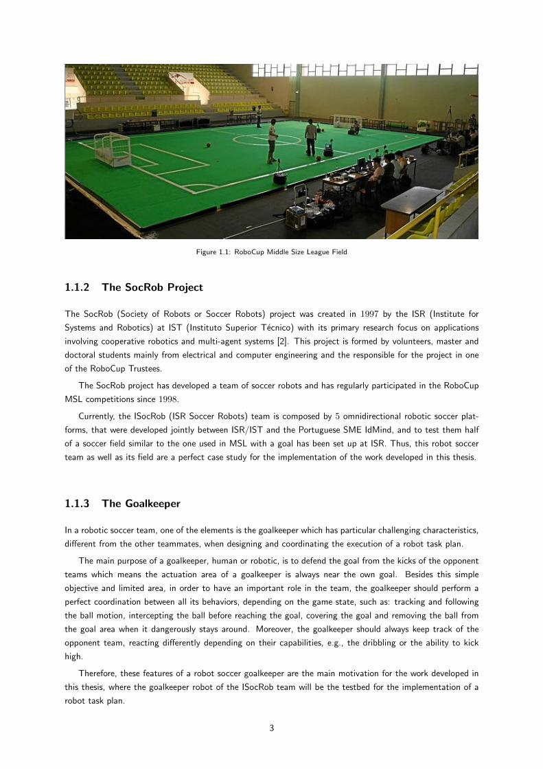
Figure 1.1: RoboCup Middle Size League Field
1.1.2 The SocRob Project
The SocRob (Society of Robots or Soccer Robots) project was created in 1997 by the ISR (Institute for
Systems and Robotics) at IST (Instituto Superior Tecnico) with its primary research focus on applications
involving cooperative robotics and multi-agent systems [2]. This project is formed by volunteers, master and
doctoral students mainly from electrical and computer engineering and the responsible for the project in one
of the RoboCup Trustees.
The SocRob project has developed a team of soccer robots and has regularly participated in the RoboCup
MSL competitions since 1998.
Currently, the ISocRob (ISR Soccer Robots) team is composed by 5 omnidirectional robotic soccer plat-
forms, that were developed jointly between ISR/IST and the Portuguese SME IdMind, and to test them half
of a soccer field similar to the one used in MSL with a goal has been set up at ISR. Thus, this robot soccer
team as well as its field are a perfect case study for the implementation of the work developed in this thesis.
1.1.3 The Goalkeeper
In a robotic soccer team, one of the elements is the goalkeeper which has particular challenging characteristics,
different from the other teammates, when designing and coordinating the execution of a robot task plan.
The main purpose of a goalkeeper, human or robotic, is to defend the goal from the kicks of the opponent
teams which means the actuation area of a goalkeeper is always near the own goal. Besides this simple
objective and limited area, in order to have an important role in the team, the goalkeeper should perform a
perfect coordination between all its behaviors, depending on the game state, such as: tracking and following
the ball motion, intercepting the ball before reaching the goal, covering the goal and removing the ball from
the goal area when it dangerously stays around. Moreover, the goalkeeper should always keep track of the
opponent team, reacting differently depending on their capabilities, e.g., the dribbling or the ability to kick
high.
Therefore, these features of a robot soccer goalkeeper are the main motivation for the work developed in
this thesis, where the goalkeeper robot of the ISocRob team will be the testbed for the implementation of a
robot task plan.
3
1.2 State-of-the-Art
When planning and performing a robot task, the decision-making process of the robot is event-based and
also based on a discrete state space which leads to a DES (Discrete Event System) [3] approach for its
implementation. The DES is a state-based approach which defines possible situations as a set of states and
selects a behavior that adequately handles the situation corresponding to the given state. Therefore, it needs
to include some abstraction which provides an approximated state of the world, typically using logic predicates
to provide a discretization of the world.
There are different formalisms based on DES available in the literature and one of the most widely used is
the FSA (Finite State Automata). In this approach, the states correspond to behavior execution and the events
are modeled as observations. In [4], a modular FSA-based approach is used to model multi-robot systems
showing how some transition parameters affect the task properties. Another popular modeling approach are the
Markov Chains which is a probabilistic approach, enabling to explicitly account for various forms of uncertainty
and to quantitatively analyse the performance.
The other modeling formalism used for DES is PN (Petri Nets) which are a graphical and mathematical
modeling tool applicable to many systems. Furthermore, this formalism can be adapted in order to introduce
the concept of time for performance evaluation and scheduling problems. Adding stochastic time leads to
GSPN (Generalised Stochastic Petri Nets), which are the basis of the work developed in this thesis. With
the GSPN models, one can obtain the equivalent Markov Chain representations which can then be used to
perform some qualitative and quantitative analysis of the system performance.
The GSPN are also preferred to FSA due to their larger modelling power and because one can model
the same state space with a smaller graph. Moreover, FSA are inadequate for describing the concurrence of
activities in the system. On the other hand, GSPN can explicitly monitor the status of several components
simultaneously, whereas FSA only represent the status of the entire system at a certain instance.
In [5], the GSPN was used to model and analyse, both qualitatively and quantitatively, a robot task for a
tour-guide robot. However, this approach does not use a structured framework for modelling and analysis the
robot task. Furthermore, there is no clear distinction between the selection mechanisms and uncontrollable
events induced by the environment, leading to a less modular design.
In [6], a framework was developed proving a tool to model, analyse and execute mobile multi-robot tasks
using GSPN. This framework provides a hierarchical and modular design which includes environment models
where uncontrollable events, due to other robots, are modelled, as well as action models where the action
effects in the environment are modelled. This framework was used here in order to model and analyse the
robot task, in this case for the goalkeeper.
During the SocRob project a considerable amount of work has been developed related to behavior co-
ordination, mainly for the field players with individual and cooperative behaviors, some of them using PN
[7, 8, 9].
Related more with the SocRob goalkeeer, in [10], a behavior selection for the goalkeeper was implemented
using FSA and the previous non-holonomic robot platforms. Some of the basic behaviors for the goalkeeper
were used, such as moving sideways on a line in front of the goal or on an arc with center in the middle of
the goal. [11] also improved the goalkeeper behaviors with other behaviors such as intercepting the ball using
also FSA. Finally, in [12], a completely different behavior selection mechanism, fuzzy logic, was used for the
goalkeeper using the previous behaviors and others such as minimizing the angle between the goal and the
ball. These works were used as basis for this thesis mainly in the implementation of the goalkeeper actions.
4
1.3 Objectives
The main objective of this work is to provide a complete, tested and effective behavior for the goalkeeper of
a robot soccer team, ISocRob, which can be applied to the RoboCup competitions in the MSL robot soccer
environment with its regulations and rules.
In order to accomplish this main goal, we propose to separate the work in the following main parts:
Development and Implementation of a Robotic GoalKeeper Behavior Design and implement the be-
havior coordination and execution of a robot goalkeeper using PN.
For this purpose, implementation and improvement of the basic primitive actions a goalkeeper needs,
such as: covering the goal close to it and following the ball motion; approaching the ball in order to
minimize the angle between the ball and the goal; intercepting the ball when it is moving towards own
goal; and, when the ball is dangerously close to the goal, catching it and removing it from the goal area.
Using PN, develop the decision-making process of a goalkeeper in order to accomplish its main objective,
defend the goal from the opponent kicks. For that, implement the events that determine the switching
time between the behaviors and primitive actions.
Test all components of the goalkeeper behavior in realistic environments in order to have a robust and
complete task for any game situation.
Modelling the GoalKeeper Behavior Model all the components of the goalkeeper task since the environ-
ment, action and task models using GSPN.
Using the modelling framework developed in [6], we modeled the environment where the goalkeeper task
takes place with all the important uncontrollable events that can occur due to other agents interaction,
from opponent team to teammates robots, or even due to laws of physics, such as the motion of the
ball.
Moreover, the goalkeeper actions should also be modelled with the direct changes performed by the
robot in the environment as well as how it is suppose to act in order to accomplish the desired effects
and which conditions should be met for the action to take place.
Finally, the decision process of the goalkeeper should be modelled in the task models using for that the
environment information perceived by the robot. To cope with the complexity and dynamic nature of
this task, logic predicates are used to discretize the world information.
Performance Analysis of the GoalKeeper Behavior Perform qualitatively and quantitatively analysis of
the goalkeeper task using GSPN.
Using the analysis framework developed in [6], merge and compose all the models developed in the
previous stage in an unique closed-loop GSPN model of the entire goalkeeper task. With this model,
analyse both for qualitative/logical and quantitative/performance properties using mainly the transient
analysis.
In order to achieve a better goalkeeper task, compare its performance in different situations, such as:
the differences between the performance of three types of goalkeeper behaviors, from defensive to more
offensive, with four types of opponent teams, endowed with powerful kicks or not, both on the ground and
on the air, and also compare the goalkeeper task performance with different ball detection mechanisms
and different self-localization algorithms.
In the end, we should have a goalkeeper task capable of being used by the current real robot platform of
ISocRob team as well as its middleware software, and designed with its limitations in mind. The task design
should be fully tested and ready to use in any soccer robot competition, such as the national competitions,
the Portuguese Robotics Open, and in RoboCup MSL competitions.
5
1.4 Thesis Outline
Chapter 2 provides all the background and theoretical concepts needed to understand the work developed in
this thesis. Namely, the formal definition of a GSPN, the basis of this work, and its analysis properties, and
also a brief explanation of the framework used in the modelling and analysis of the goalkeeper task.
Chapter 3 briefly describe the robotic platform used in this work with its relevant characteristics as well as
the PN executor used in the implementation of the goalkeeper task in the real environment.
Chapter 4 includes a description of all the task components implemented in the ISocRob goalkeeper robot,
such as the predicates, primitive actions, behaviors and the main role used in the real robot.
Chapter 5 presents all the models of the goalkeeper role, such as the environment, action and task models
implemented using the modelling framework.
Chapter 6 covers the experimental setup developed in order to analyse the goalkeeper task performance in
different situations, using the models designed previously and the analysis framework.
Chapter 7 presents the performance analysis results to the real experiments for the goalkeeper task.
Finally, Chapter 8 includes some discussion on the work developed, the conclusions, and provides directions
for future work.
6

7
Chapter 2
Background
This chapter introduces and explain basic notions that are important to understand the work developed in
this thesis. The PN are the basis of this work, thus we first present their definitions and properties, mainly
important for the analysis part, and then the framework used for the modelling and analysis of a task is
presented with the required details for the specific case in study, the goalkeeper.
2.1 Petri Nets
PN, invented in 1962 by Carl Adam Petri [13], are a graphical and mathematical tool widely used for modelling
DES. They are a formalism for the description of concurrency, synchronisation, resources availability, parallelism
and decision making, providing also a high degree of modularity. Consequently, PN come up as a suitable tool
for modelling, analysis and execution of robot tasks.
Before the mathematical definition and all the properties of PN, it is important to describe the components
that comprises a PN as following:
Places model conditions, objects or resources. They are drawn by circles;
Tokens represent the specific value of the condition, object or resource. They are drawn by black dots;
Transitions model activities which change the values of conditions, objects and resources. They are drawn
by rectangles;
Arcs specify the interconnection of places and transitions, indicating which resources are changed by a certain
activity. They are drawn by arrows.
PN are bipartite graphs, i.e., we may connect only a place to a transition or vice versa, but we cannot
connect two places or two transitions. In addition, places and transitions may have several input/output
elements.
2.1.1 Ordinary Petri Nets
The simplest models we use are OPN (Ordinary Petri Nets) and the definition is as following:
Definition 2.1.1. An ordinary Petri net is a five-tuple PN = 〈P, T, I,O,M0〉, where:
• P = {p1, . . . , pn} is a finite and non-empty set of places;
• T = {t1, . . . , tm} is a finite and non-empty set of transitions;
8

• I : P × T → N0 represents the arc connections from places to transitions, such that ilj = 1 iff there is
an arc from pl to tj and ilj = 0 otherwise;
• O : T ×P → N0 represents the arc connections from transitions to places, such that olj = 1 iff there is
an arc from tl to pj and olj = 0 otherwise;
• Mj = [m1(j), . . .mn(j)] is the state of the net and represents the marking of the net at time j, where
mn(j) = q means there are q tokens in place pn at time instant j. M0 is the initial marking of the net.
In order to simulate the dynamic behavior of a system, a state or marking in an OPN should change
according to the following rules:
Enabling of a transition A transition is enabled if all its input places are marked at least with one token,
assuming all the weights equal to one;
Firing of an enabled transition An enabled transition may fire. If a transition fires, it removes one token
from each input place and creates one token on each output place, assuming again all the weights equal
to one.
With the Definition 2.1.1 and the above firing rule, one concludes that OPN involve no notion of time,
thus they can only be used to analyse the functional and qualitative behavior of a system. For performance or
quantitative analysis the temporal (time) behavior of the system has to be part of the PN description which
is possible with the extension of the OPN presented next.
2.1.2 Generalized Stochastic Petri Nets
The GSPN is an extension of the OPN where the element time is added. Although the components that
comprise a GSPN are the same as in OPN (see Section 2.1), in the case of GSPN there will be two types of
transitions:
Immediate Transitions model activities or logical changes where the transition fires in zero time. They are
drawn as a black and filled rectangle;
Exponential Transitions model activities where the transition fires after a random, exponentially distributed
enabling time. They are drawn as an unfilled rectangle.
In the exponential transitions, the delay of the transition is related to a random variable, χ, with the
following characteristics:
• Negative exponential density function: fχ(x) = λe−λx;
• Mean: E[χ] = 1λ ;
• Variance: V ar[χ] = 1λ2 ;
Understood the differences in these two components of GSPN, it is possible to set the formal definition of
a GSPN as following:
Definition 2.1.2. A GSPN is a eight-tuple PN = 〈P, TI , TE , I, O,M0, R,W 〉, where:
• P, T, I,O,M0 are as defined in Definition 2.1.1;
• TI ⊂ T denotes the set of immediate transitions;
• TE ⊆ T denotes the set of exponential transitions;
9
• R : TE → R+ is a function from the set of exponential transitions, TE , to the set of real numbers,
R(tEj) = λj , where λj is called the firing rate of tEj
;
• W : TI → R+ is a function from the set of immediate transitions, TI , to the set of real numbers,
W (tIj ) = wj , where wj is the weight associated with the immediate transition tIj .
With these two types of transitions, there will be also some rules related to the transition fires. For a given
marking:
1. If there is a set of enabled transitions, both immediate and exponential, the former have always higher
priority, firing all first and only then the exponential ones;
2. If there is a set of enabled exponential transitions, T = {tE1 , . . . , tEn}, the firing probability of each
transition is given by
P (tEj ) =λj∑nk=1 λk
(2.1)
3. If there is a set of enabled immediate transitions, T = {tI1 , . . . , tIn}, the firing probability of each
transition is given by
P (tIj ) =wI∑nk=1 wk
(2.2)
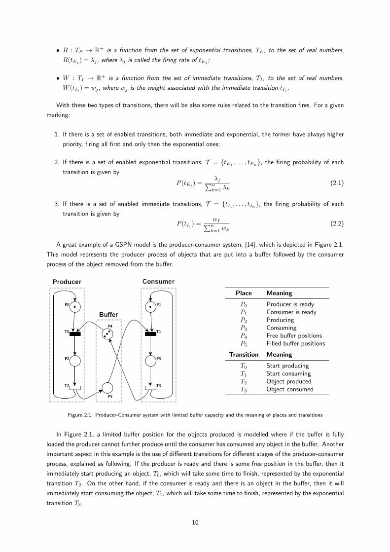
A great example of a GSPN model is the producer-consumer system, [14], which is depicted in Figure 2.1.
This model represents the producer process of objects that are put into a buffer followed by the consumer
process of the object removed from the buffer.
Place Meaning
P0 Producer is readyP1 Consumer is readyP2 ProducingP3 ConsumingP4 Free buffer positionsP5 Filled buffer positions
Transition Meaning
T0 Start producingT1 Start consumingT2 Object producedT3 Object consumed
Figure 2.1: Producer-Consumer system with limited buffer capacity and the meaning of places and transitions
In Figure 2.1, a limited buffer position for the objects produced is modelled where if the buffer is fully
loaded the producer cannot further produce until the consumer has consumed any object in the buffer. Another
important aspect in this example is the use of different transitions for different stages of the producer-consumer
process, explained as following. If the producer is ready and there is some free position in the buffer, then it
immediately start producing an object, T0, which will take some time to finish, represented by the exponential
transition T2. On the other hand, if the consumer is ready and there is an object in the buffer, then it will
immediately start consuming the object, T1, which will take some time to finish, represented by the exponential
transition T3.
10
2.1.3 Analysis Properties
For the purpose of analysis, there is some important knowledge about GSPN we should state. Using Defini-
tion 2.1.2 and recalling that the state of a PN is given by the marking of the net, i.e., by the number of tokens
in each place, the following concepts come up, [6, 14]:
Coverability Tree Given an initial state of a PN, it is obtained by firing each enabled transition for all
markings. Nodes represent a different state and arcs represent a transition fired in the original PN. It
allows us to obtain some qualitative properties of the PN;
RG (Reachability Graph) Same as coverability tree but when the number of markings in the PN is finite,
i.e., bounded PN, which is the case of this work. The RG has two different states:
• Vanishing State – It has immediate transitions enabled, firing in zero time;
• Tangible State – It has timed transitions enabled, sojourn time is exponentially distributed;
CTMC (Continuous Time Markov Chain) A graph obtained from RG where only tangible states exist and
vanishing states are removed. It allows us to obtain some quantitative properties of the PN;
EMC (Embedded Markov Chain) The discrete time markov process obtained from CTMC, i.e., the states
reached by the CTMC in discrete times.
Considering the above concepts, one concludes that the GSPN marking is a Markov process with a discrete
state space given by the RG of the net for an initial marking. Thus, both the transition rate matrix (CTMC)
and the transition probability matrix (EMC) can be computed by using the firing rates of the exponential timed
transitions and the probabilities associated with immediate transitions. With these matrixes, one can perform
transient and stationary analysis of the chain, i.e., obtain performance properties for the GSPN.
Qualitative Properties
The most important structural properties are presented below and can be obtained through the analysis of the
RG.
Definition 2.1.3 (Boundedness). A PN is k-bounded, or k-safe, if all places pi ∈ P are k-bounded, or k-safe,
i.e., mi(j) ≤ k for all reachable states.
Definition 2.1.4 (Liveness). Given a PN with initial state M0, a transition tj is said to be live if, for all
reachable states Mi, there is a firing sequence starting in Mi, such that tj is fired.
Definition 2.1.5 (Deadlock). Given a PN, a deadlock state corresponds to a reachable state where none of
the transitions are fireable.
Quantitative Properties
For the performance measures of a GSPN, presented below, πj is the stationary probability of the tangible
state j, with Mj corresponding to the GSPN marking associated with state j.
Definition 2.1.6 (Probability that a Condition Holds). The probability that a particular condition C holds is
computed by considering the probability of being in any state where the condition is satisfied:
Pr(C) =∑j∈S1
πj (2.3)
where S1 = {j ∈ {1, . . . , s} : C is satisfied in Mj}.
11
Definition 2.1.7 (Expected Number of Tokens in a Place). The expected number of tokens in a place pi is
computed by using the probability of having k tokens in a place pi for all possible number of tokens:
E[#(pi)] =
K∑k=1
kPr(#(pi) = k) =
K∑k=1
k∑j∈S2
πj (2.4)
where K is the maximum possible number of tokens in a place pi, for all reachable tangible markings, and
S2 = {j ∈ {1, . . . , s} : #(pi) = k in Mj}.
Definition 2.1.8 (Transition Throughput Rate). The transition throughput rate is the frequency of firing a
transition, i.e., the average number of transition firings in unit time.
For the case of an exponential transition tj , it is computed by considering its firing rate over the probability
of all states where tj is enabled:
Tr(tj) =∑i∈S3
πiλj (2.5)
where S3 = {i ∈ {1, . . . , s} : tj is enabled in Mi}.For the case of an immediate transition tj , it can be computed by considering the throughput of all
exponential transitions which lead to the firing of transition tj , together with the probability of firing transition
tj among all the enabled immediate transitions.
2.2 Task Modelling and Analysis Framework
One major purpose of this thesis is the modelling and analysis of a robot goalkeeper task. For that, we will
use a framework developed in the SocRob project, [6], which is explained in this section with the important
details needed for this work. Albeit this framework was developed also thinking of the execution of tasks in
real robots, we use other framework for this purpose, as explained in Section 3.4.
This framework is based on PN which provides an intuitive task design solution with a high modularity
degree and using various layers. Hereby, a full model can be composed by various models designed separately
and only afterwards combined. Thus, the key issue of this process is the composition, or expansion, of all
models in one full model.
In addition, this framework provides all means to analyse a robot task using a full GSPN model and provides
also all the stationary and transient analysis properties of the GSPN, presented previously in Section 2.1.3.
2.2.1 Types of Petri Net Places
As explained in Section 2.1, an important component of a PN are the places. In this framework, [6], the
PN places have different meanings depending on what they represent and this difference is crucial in the
composition of the models. Different labels are used to distinguish between types of places, such as: predicate
places, action places and task places.
Predicate Places
Predicate places are used to represent logic conditions, having always one or zero tokens depending if it is true
or false, respectively. A predicate, P, can be completely modelled by a PN as explained in Definition 2.2.1.
Definition 2.2.1. A PN model of a predicate is a OPN where:
• P = {¬p, p}, where ¬p and p are predicate places associated with predicates ¬P (negated) and P,
respectively. The place labels for ¬p and p are “predicate.NOT ” (or “p.NOT ”) and “predicate.” (or
“p.”), respectively;
12
• I = ∅;
• O = ∅;
• ∀j , Mj = [0, 1] ∨ [1, 0].
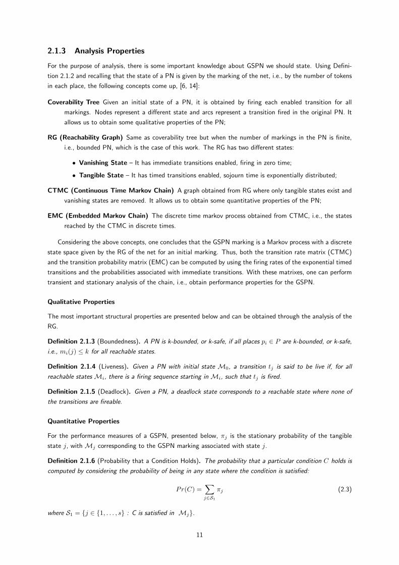
An example of a PN model representing the predicate BallStopped is depicted in Figure 2.2. Note the
usage of the “p.NOT ” prefix to denote the negated predicate, in this case, representing that ball is moving
and not stopped.
Figure 2.2: Predicate BallStopped model represented by a set of places
Action Places
Action places are used to represent robot actions where is modelled its running-conditions, desired effects and
failure effects. Thus, they are macro places, [15], and have their labels prefixed with “action.” (or “a.”). In
Section 2.2.2, action places are more detailed.
Task Places
Task places are also a type of macro places and are used to create hierarchical PN, leading to a higher degree
of modularity. They can contain other task places and action places and have their labels prefixed with“task.”
(or “t.”). In Section 2.2.2, task places are also more detailed.
2.2.2 Layers of Abstraction
This task framework, [6], uses different layers representing different abstractions and providing a modular
model of the task. Each layer is composed as a set of PN models with the meaning as following, from bottom
to top layer.
Environment Layer
The PN models in Environment layer represent the dynamic changes in the environment made by other agents,
such as other robots, or by the laws of physics, such as the motion of a ball. Naturally, these models will
not fully model the environment, but an abstraction of it is achieved by discretising the world using logic
predicates. The environment models definition is as follows:
Definition 2.2.2. An environment model is a GSPN where:
1. P = {p1, . . . , pn} contains only predicate places modelled as in Definition 2.2.1;
2. If there is an arc from place pn, associated with predicate P, to transition tj , then there is an arc from
tj to place pm, associated with predicate ¬P, or an arc back to pn;
Using the Definition 2.2.2, there is no need to always draw both the positive and negative forms of the
predicate and the respective arcs from transitions, if the situation does not force to it. This is useful for
simplicity and organization, and it is possible because the expansion algorithm, presented in Section 2.2.3,
will ensure that rule 2 of Definition 2.2.2 is accomplished, creating the negated predicate and respective arc
if needed. Besides, given that all places are predicate places, rule 2 implies that each environment model
13
maintains the predicates according to Definition 2.2.1, resulting in a safe PN (see Definition 2.1.3), since there
is at most one token per place for all markings.
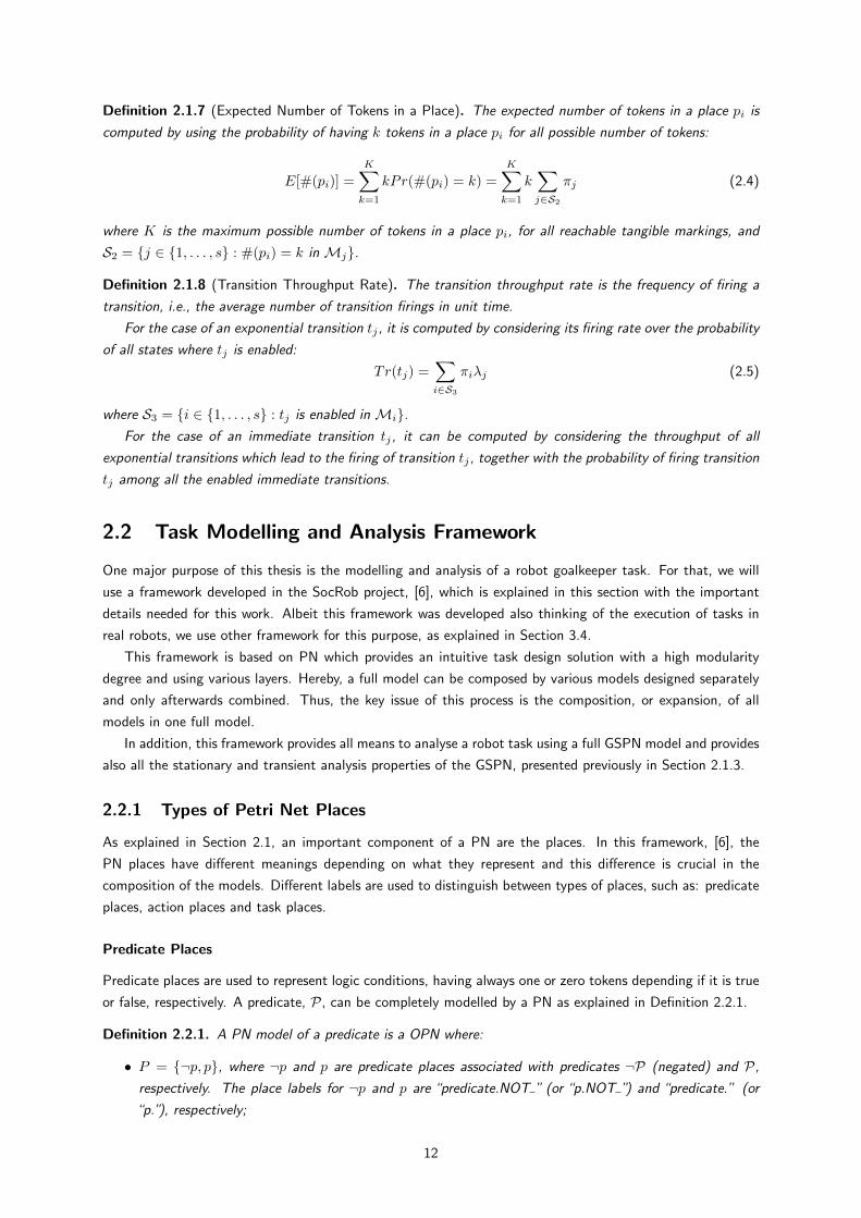
To better understand how the environment models are designed, consider a free rolling ball kicked or
pushed by an opponent soccer robot. If the ball was near the opponent goal, it is expected that due to some
action of the opponent robot the ball will be moving towards the own goal. Therefore, we can consider it as
an environment change due to uncontrollable events which can be modelled with the GSPN model depicted
in Figure 2.3. In this model, we discretised the soccer field into three areas and assumed that the ball was
first near the opponent goal and after some exponential time it moves to the following area.
Figure 2.3: Example of an environment model for the ball position in a soccer field
The Action Executor Layer
The Action Executor layer has the PN models of the actions, representing the changes performed by the robot
in the environment and how it is suppose to act. As the action models will be composed with the environment
models, only world changes which as a direct result of the action execution should be modelled. As introduced
in Section 2.2.1, an action is mainly described by the effects (desired and failures) it causes on the environment
and the conditions that need to be met for the action to take place. The action models definition is as follows:
Definition 2.2.3. An action model is a GSPN where:
1. P = {p1, . . . , pn} contains only predicate places modelled as in Definition 2.2.1 which can represent the
running-conditions of the action with prefix “p.r.” or the desired effect of the action with prefix “p.e.”;
2. T = {t1, . . . , tm} represents the success and failure of the actions and all transitions tj have the prefix
label “successj” (or “sj”) and “failurej” (or “fj”), respectively;
3. If there is an arc from place pn, associated with predicate P, to transition tj , then there is an arc from
tj to place pm, associated with predicate ¬P, or an arc back to pn;
Similarly to the environment models, rule 3 of Definition 2.2.3 implies that each action model maintains
the predicates according to Definition 2.2.1, resulting in a safe PN (see Definition 2.1.3).
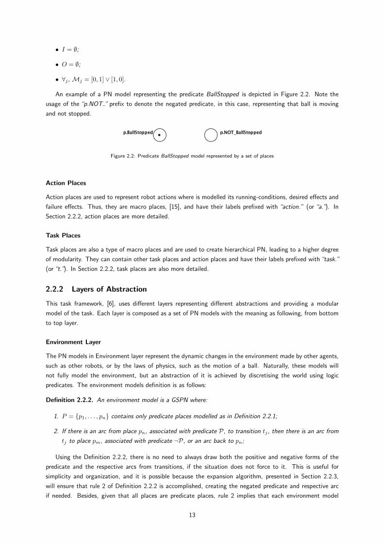
As an example, consider a soccer robot which has the purpose of capturing a ball located in a soccer
field. We can divide this purpose into two actions: first the robot needs to approach the ball in order to be
close to the ball, action Move2Ball, and then it needs to catch the ball in order to have the possession of the
ball, action CatchBall. These two actions can be modelled, in a simple way, by the GSPN models depicted in
Figure 2.4 where the desired-effect and running-conditions of the actions are modelled. In this case, a common
running-condition for both actions is if the robot sees the ball, represented by the predicate SeeBall. Moreover,
the desired-effect of action Move2Ball, Figure 2.4a, is to be close to the ball, represented by the predicate
CloseToBall, whereas for the action CatchBall, Figure 2.4b, the desired-effect is to have the ball, represented
by the predicate HasBall.
14
(a) Action Move2Ball used by a robot toapproach the ball
(b) Action CatchBall used by a robot tocapture the ball
Figure 2.4: Example of action models used by a robot to capture a ball
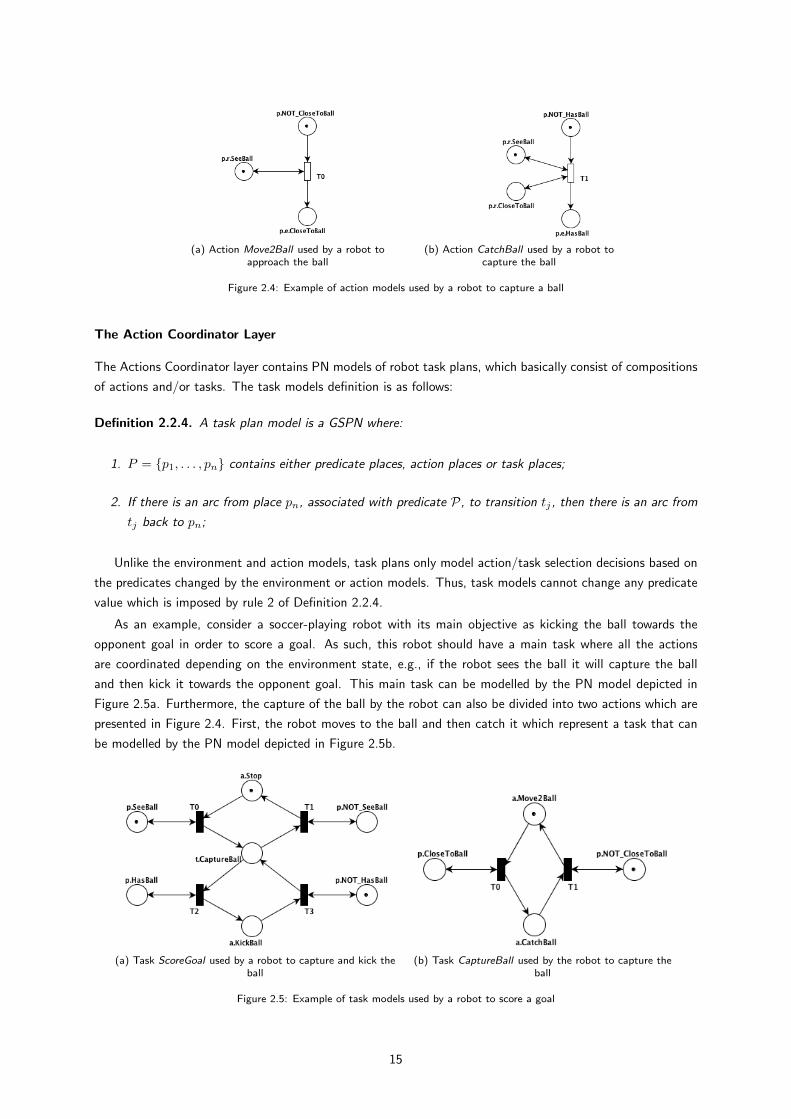
The Action Coordinator Layer
The Actions Coordinator layer contains PN models of robot task plans, which basically consist of compositions
of actions and/or tasks. The task models definition is as follows:
Definition 2.2.4. A task plan model is a GSPN where:
1. P = {p1, . . . , pn} contains either predicate places, action places or task places;
2. If there is an arc from place pn, associated with predicate P, to transition tj , then there is an arc from
tj back to pn;
Unlike the environment and action models, task plans only model action/task selection decisions based on
the predicates changed by the environment or action models. Thus, task models cannot change any predicate
value which is imposed by rule 2 of Definition 2.2.4.
As an example, consider a soccer-playing robot with its main objective as kicking the ball towards the
opponent goal in order to score a goal. As such, this robot should have a main task where all the actions
are coordinated depending on the environment state, e.g., if the robot sees the ball it will capture the ball
and then kick it towards the opponent goal. This main task can be modelled by the PN model depicted in
Figure 2.5a. Furthermore, the capture of the ball by the robot can also be divided into two actions which are
presented in Figure 2.4. First, the robot moves to the ball and then catch it which represent a task that can
be modelled by the PN model depicted in Figure 2.5b.
(a) Task ScoreGoal used by a robot to capture and kick theball
(b) Task CaptureBall used by the robot to capture theball
Figure 2.5: Example of task models used by a robot to score a goal
15
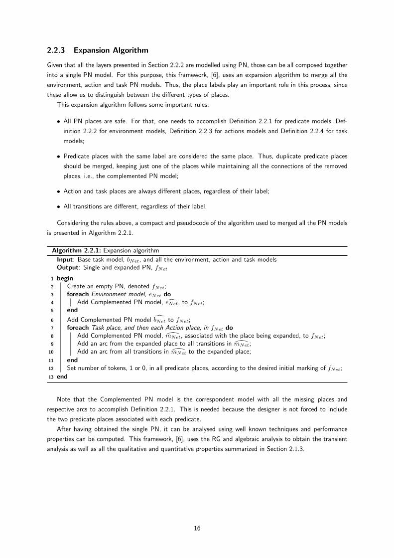
2.2.3 Expansion Algorithm
Given that all the layers presented in Section 2.2.2 are modelled using PN, those can be all composed together
into a single PN model. For this purpose, this framework, [6], uses an expansion algorithm to merge all the
environment, action and task PN models. Thus, the place labels play an important role in this process, since
these allow us to distinguish between the different types of places.
This expansion algorithm follows some important rules:
• All PN places are safe. For that, one needs to accomplish Definition 2.2.1 for predicate models, Def-
inition 2.2.2 for environment models, Definition 2.2.3 for actions models and Definition 2.2.4 for task
models;
• Predicate places with the same label are considered the same place. Thus, duplicate predicate places
should be merged, keeping just one of the places while maintaining all the connections of the removed
places, i.e., the complemented PN model;
• Action and task places are always different places, regardless of their label;
• All transitions are different, regardless of their label.
Considering the rules above, a compact and pseudocode of the algorithm used to merged all the PN models
is presented in Algorithm 2.2.1.
Algorithm 2.2.1: Expansion algorithm
Input: Base task model, bNet, and all the environment, action and task modelsOutput: Single and expanded PN, fNet
1 begin2 Create an empty PN, denoted fNet;3 foreach Environment model, eNet do4 Add Complemented PN model, eNet, to fNet;5 end
6 Add Complemented PN model bNet to fNet;7 foreach Task place, and then each Action place, in fNet do8 Add Complemented PN model, mNet, associated with the place being expanded, to fNet;9 Add an arc from the expanded place to all transitions in mNet;
10 Add an arc from all transitions in mNet to the expanded place;
11 end12 Set number of tokens, 1 or 0, in all predicate places, according to the desired initial marking of fNet;
13 end
Note that the Complemented PN model is the correspondent model with all the missing places and
respective arcs to accomplish Definition 2.2.1. This is needed because the designer is not forced to include
the two predicate places associated with each predicate.
After having obtained the single PN, it can be analysed using well known techniques and performance
properties can be computed. This framework, [6], uses the RG and algebraic analysis to obtain the transient
analysis as well as all the qualitative and quantitative properties summarized in Section 2.1.3.
16

17
Chapter 3
Soccer Robots Framework
This chapter aims at describing briefly the robotic platform that was used to develop and test the work of this
thesis and its relevant characteristics mainly for the behavior implementation of the goalkeeper.
3.1 RoboCup MSL Rules and Regulations
The ISocRob team has regularly participated in RoboCup MSL (see Section 1.1.1 for a brief explanation),
therefore one should take attention to the rules of this competition when developing the behaviors for the
robots.
The entire rules and regulations for the RoboCup MSL are presented in [16], and the most important ones
for this work and the goalkeeper case will be stated next.
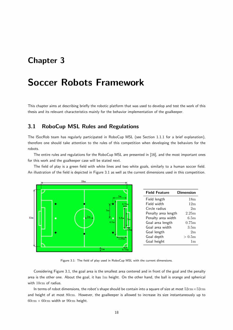
The field of play is a green field with white lines and two white goals, similarly to a human soccer field.
An illustration of the field is depicted in Figure 3.1 as well as the current dimensions used in this competition.
Field Feature Dimension
Field length 18mField width 12mCircle radius 2mPenalty area length 2.25mPenalty area width 6.5mGoal area length 0.75mGoal area width 3.5mGoal length 2mGoal depth > 0.5mGoal height 1m
Figure 3.1: The field of play used in RoboCup MSL with the current dimensions.
Considering Figure 3.1, the goal area is the smallest area centered and in front of the goal and the penalty
area is the other one. About the goal, it has 1m height. On the other hand, the ball is orange and spherical
with 10cm of radius.
In terms of robot dimensions, the robot’s shape should be contain into a square of size at most 52cm×52cmand height of at most 80cm. However, the goalkeeper is allowed to increase its size instantaneously up to
60cm× 60cm width or 90cm height.
18
In RoboCup, the referee is intended to enforce the Laws of the Game using a referee box, [17], to com-
municated all the game commands to the robots, e.g., the start of the game. A match should last two equal
periods of 15 minutes with 5 minutes of interval.
About the goalkeeper protection area, it is completely forbidden that any other robot, besides the goalie,
enters in the goal area limits.
Finally, when there is a game foul the referee sends a Stop command. If the ball was inside the penalty area
it is removed to the closest restart point, black dots in Figure 3.1. Then, the referee sends the foul command,
e.g., a Free-Kick, and when the robots and ball are correctly positioned the referee sends a Start command.
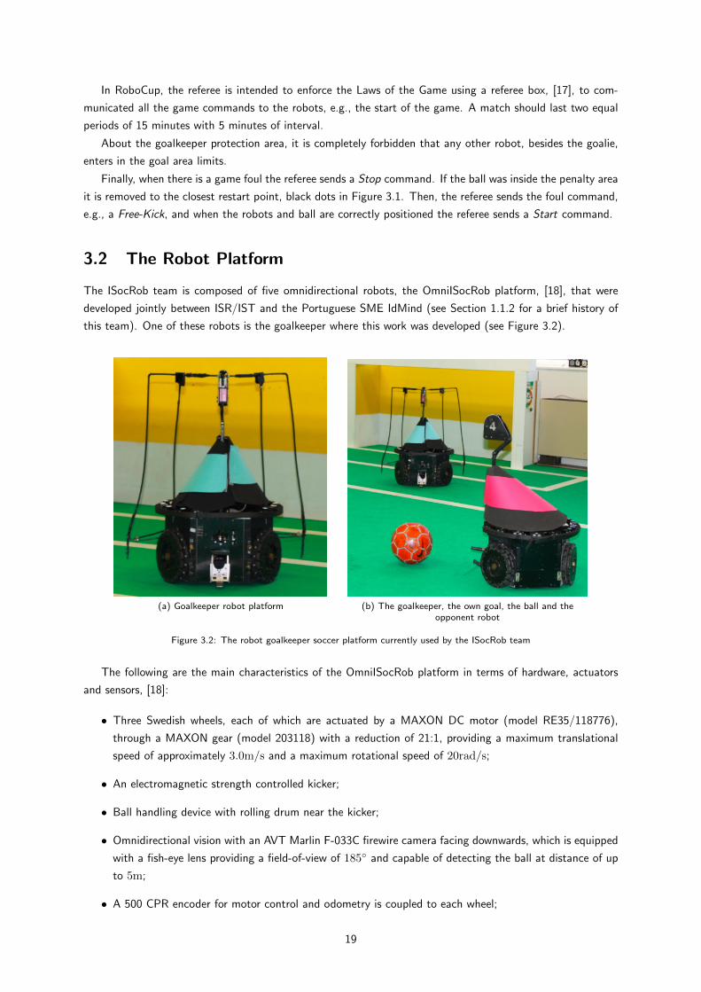
3.2 The Robot Platform
The ISocRob team is composed of five omnidirectional robots, the OmniISocRob platform, [18], that were
developed jointly between ISR/IST and the Portuguese SME IdMind (see Section 1.1.2 for a brief history of
this team). One of these robots is the goalkeeper where this work was developed (see Figure 3.2).
(a) Goalkeeper robot platform (b) The goalkeeper, the own goal, the ball and theopponent robot
Figure 3.2: The robot goalkeeper soccer platform currently used by the ISocRob team
The following are the main characteristics of the OmniISocRob platform in terms of hardware, actuators
and sensors, [18]:
• Three Swedish wheels, each of which are actuated by a MAXON DC motor (model RE35/118776),
through a MAXON gear (model 203118) with a reduction of 21:1, providing a maximum translational
speed of approximately 3.0m/s and a maximum rotational speed of 20rad/s;
• An electromagnetic strength controlled kicker;
• Ball handling device with rolling drum near the kicker;
• Omnidirectional vision with an AVT Marlin F-033C firewire camera facing downwards, which is equipped
with a fish-eye lens providing a field-of-view of 185◦ and capable of detecting the ball at distance of up
to 5m;
• A 500 CPR encoder for motor control and odometry is coupled to each wheel;
19
• An AnalogDevices rate-gyro (XRS300EB) is present to improve self-localization;
• Two packs of 9Ah MiMH batteries to power the robot hardware;
• A NEC FS900 laptop, equipped with a Centrino 1.6GHz CPU and 512Mb of RAM, where most of the
processing takes place and where are connected the robot’s sensors and actuators through USB and
FireWire;
3.3 The MeRMaID Architecture
The MeRMaID (Multiple-Robot Middleware for Intelligent Decision-making) architecture, currently in use by
the ISocRob, [19], was developed to meet the demands of robotic applications in general and to provide a
simplified and systematic high-level behavior programming environment for multi-robot teams. The MeRMaID
is a middleware software based on the Active Object pattern, service-oriented design and possesses a modular
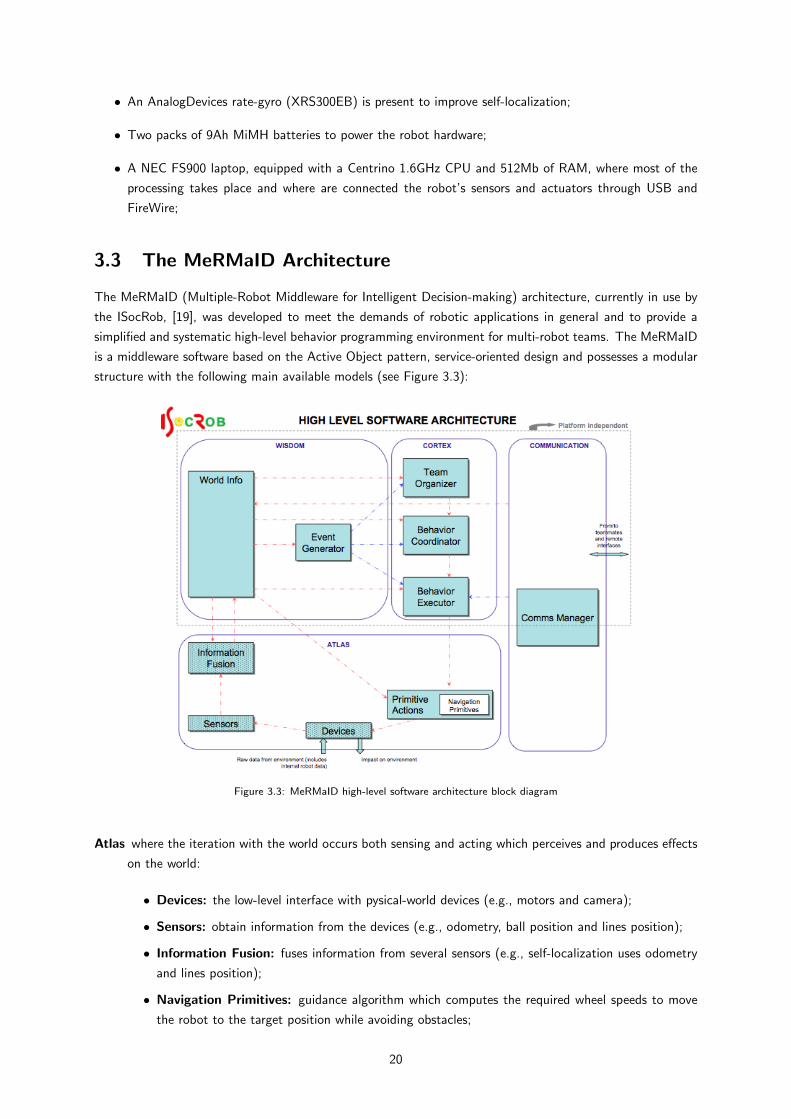
structure with the following main available models (see Figure 3.3):
Figure 3.3: MeRMaID high-level software architecture block diagram
Atlas where the iteration with the world occurs both sensing and acting which perceives and produces effects
on the world:
• Devices: the low-level interface with pysical-world devices (e.g., motors and camera);
• Sensors: obtain information from the devices (e.g., odometry, ball position and lines position);
• Information Fusion: fuses information from several sensors (e.g., self-localization uses odometry
and lines position);
• Navigation Primitives: guidance algorithm which computes the required wheel speeds to move
the robot to the target position while avoiding obstacles;
20
• Primitive Actions: the atomic element of a behavior which uses a navigation primitive after the
calculation of the desired posture;
Wisdom where the relevant information about the world, such as robot postures and ball position, is kept
and managed (World Info);
Cortex where the decision making process takes place based on information retrieved from the Wisdom
module, the Petri Net Executor. The action decision is taken through three hierarchical layers, from top
to bottom:
• Team Organizer: responsible for the organization of the team and their tactic, selecting a role for
each robot;
• Behavior Coordinator: responsible for behavior selection and coordination, selecting a behavior
from the current role;
• Behavior Executor: responsible for behavior execution, selecting a primitive action from the
current behavior;
Communication with other robots, external interfaces and the referee box;
3.4 Behaviors as a Part of MeRMaID
There are different formalisms for modelling DES, suitable for robot behaviors execution, e.g., FSA or Fuzzy
logic. The MeRMaID architecture supports all of these tools, but currently it uses a behavior execution
framework based on PN, the Petri Net Executor, (see Section 2.1 for a explanation of this formalism).
The Petri Net Executor framework is similar to the one used in this thesis for task modelling and analysis,
presented in Section 2.2. However, the MeRMaID software is not yet ready to support fully the latter for the
execution of PN tasks.
As explained in Section 2.2, a PN-based framework provides an intuitive design solution for behaviors and
also a high modularity degree. Similarly, the PN Executor framework also uses different layers of abstraction,
described in last section, such as Behavior Executor, Coordinator and Team Organizer.
The different types of PN places and the components of the PN Executor framework are presented below:
Predicates represent logic conditions which are evaluated as true or false. For the predicate places we use
the Definition 2.2.1. Thus, the label prefix for these places is “predicate.” or “predicate.NOT ” for its
negation. In this framework, the predicates are only used in the PN behaviors for evaluation of the
environment and decision making. Thus, when a predicate place is an input place of a transition, it
is also an output place. The predicate values are internally changed in MeRMaID by the Predicate
Manager, using the world information perceived by the robot, and also kept up to date at least all the
predicates that are relevant at any given state.
Primitive Actions is an atomic robot action which normally states to where the robot should move or what
it should do. Typically, it has some predicates as running-conditions, e.g., SeeBall.
Behavior Executor this layer contains the robot behaviors which are OPN (see Definition 2.1.1). It uses
predicates in order to choose the primitive action that the robot should execute. The place label prefix
used to represent the primitive actions is “action.”.
Behavior Coordinator this layer contains the robot roles which are OPN. It uses predicates in order to
choose the behavior the robot should execute. The place label prefix used to represent the behavior is
“action.Behavior”.
21
Team Organizer this layer contains the team tactics which are OPN. It uses predicates in order to choose the
role each robot should have in the team. The place label prefix used to represent the role is“action.Role”.
Common to all cortex layers, the Petri Net Executor, given a PN behavior, checks which transitions are
enabled, considering the current selected actions and enabled predicates, and fires them accordingly. All actions
that have tokens at any given moment are the actions that will be enabled.
3.5 Relevant Features
Without dwelling upon details, which go beyond the scope of the present work, it is important to describe
the most relevant features the current robot framework has in order to properly design the robot actions and
behaviors. Thus, the relevant features, mainly for the goalkeeper, as well as some improvements for future
work of SocRob project are presented as follows:
Self-Localization it is accomplished through a Monte-Carlo Localization algorithm, a particle-filter based
approach, described in [20]. Briefly, it uses camera information to detect field lines and together with
the robot odometry and gyroscope, the belief of the robot position will increase, with the particles
converging to the same location. For the case of the goalkeeper, it is also important to have a perfect
knowledge of the goal position. Currently, it uses the self-localization but some vision algorithm should
be implemented using goal information. This thesis had intention to improve this information and albeit
some good results were achieved, it is not finished and needs some improvements as a future work;
Ball Tracking it is accomplished also through a particle-filter based approach algorithm [21]. Here, it uses
the image to detect a spherical orange ball, together with the robot odometry, increasing the belief of
ball position. This algorithm provides reliable ball information, position and velocity, at a distance of
up to 5m but only when ball is on the ground. For the case of the goalkeeper, the ball information is
the most important knowledge. Thus, there is some progress going on to incorporate a frontal camera
together with the current one to increase the detection distance and even to detect the ball off the
ground;
Navigation the motion control used to move the robots was designed to accomplish the specific characteristics
of an omnidirectional robot [22]. In this thesis, we only used the velocity control which move the robot
to a desired position. However, the motion control in [22] also provides acceleration control suitable for
ball interception and dribbling, but it is not completely implemented for the real robots;
Obstacle Avoidance the algorithm is based on Dynamic Window Approach, [23], or the TangentBug, [24],
depending on the type of obstacle, moving or static, and it was developed also in [22]. As a result of this
thesis, the goal posts were added as a static obstacle in order to the goalkeeper avoid hitting through
the posts, using for that the TangentBug algorithm, [24];
Kicker it enables the robot to complete a pass or a shoot towards the goal. A new kicker device was developed
in [25] with good results but it is not yet completely integrated in robot framework and in MeRMaID
software. Thus, the goalkeeper cannot use the device in order to kick the ball;
Defense Frame it provides some extra capability to defend the goal from the ball kicks (see Figure 3.2).
However, by the rules (see Section 3.1) the goalkeeper is allowed to have a moving defense frame in
order to instantaneously increase its size. Thus, the development of a new defense frame capable of
moving should be subject of future work.
22
23
Chapter 4
GoalKeeper Task Components
This chapter aims at describing all the task components implemented for the goalkeeper robot of ISocRob team.
A more detailed description of the soccer robot framework used and also how behaviors were implemented as
a part of the MeRMaID architecture are presented in the previous chapter, Chapter 3.
Starting from a hierarchical low layer to a high layer, all the task components are detailed in the next
sections, including predicates, primitive actions, behaviors and the role of the goalkeeper. In order to simplify
the notation, we will use here and henceforth the term GK (Goalkeeper) which should be read as goalkeeper.
4.1 Predicates
All the predicates used for the goalkeeper task execution are described following:
GameIsStopped true if the game is stopped;
GameIsStarted true if the game is started;
IsLocalized true if the GK knows correctly its self localization;
SeeBall true if the GK sees and knows where is the ball position. As explain in Section 3.5, if this predicate
is true then the ball should be on the ground;
CloseToBall true if the GK is close to the ball;
HasBall true if the GK has the possession of the ball;
BallPenaltyArea true if the ball is in the penalty area;
BallStopped true if the ball is stopped;
ShouldGKDefendGoal true if the GK can defend the goal. It is the union of the following predicates:
NOT GameIsStopped, SeeBall and IsLocalized ;
ShouldGKCoverGoal true if the GK can cover the angle between the ball and the goal. It is the union of
the following predicates: GameIsStarted, SeeBall, IsLocalized and BallPenaltyArea;
ShouldGKRemoveBall true if the GK can remove the ball from the goal neighborhood. It is the union of
the following predicates: GameIsStarted, SeeBall, IsLocalized, CloseToBall and BallPenaltyArea.
24
4.2 Primitive Actions
The goalkeeper actions are relatively simple as a result of the limited area where the GK should stay. This is
due to the main objective of a goalkeeper, i.e., to defend the goal maintaining close to the goal. Thus, the
primitive actions can be summarized, and detailed later, as follows:
Stop GK stops, sending velocity 0 to the motors;
Move2GKPosition GK moves to the center of the goal and on top of the goal line;
CoverGoalLine GK follows the ball while staying close to the goal, typically on a line parallel to the goal line;
CutDownTheAngle GK follows the ball minimizing the shot angles from opponents;
CatchBall GK approaches the ball and catches it;
HitBall GK moves against the ball in order to remove it from the goal neighborhood.
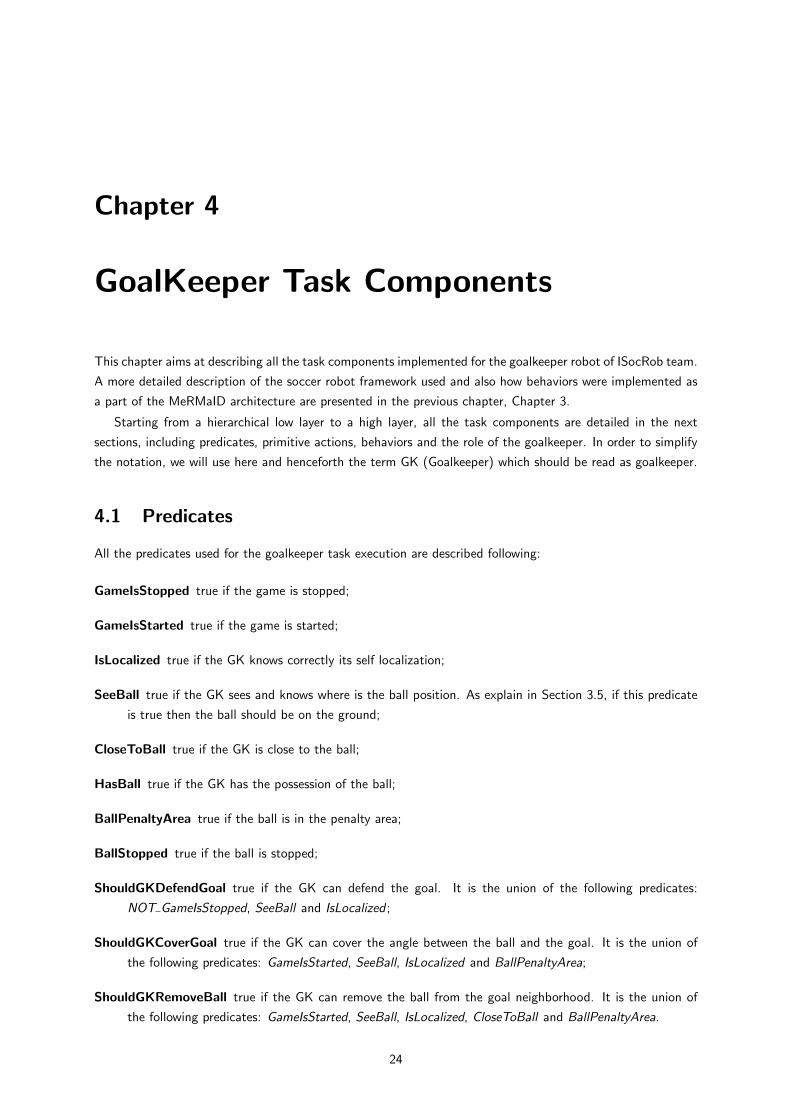
4.2.1 Move2GKPosition
This primitive action aims at moving the GK to a target posture which is in the center of the goal with a
small distance from the goal line, typically zero, and with an orientation towards the center of the field. This
posture is the one most likely to defend a ball kicked high, i.e., when the GK does not see the ball. The
running-condition of this action is the predicate IsLocalized and the desired-effect is to have the GK in the
target position. An example of the target posture is depicted in Figure 4.1.
Figure 4.1: Primitive action Move2GKPosition
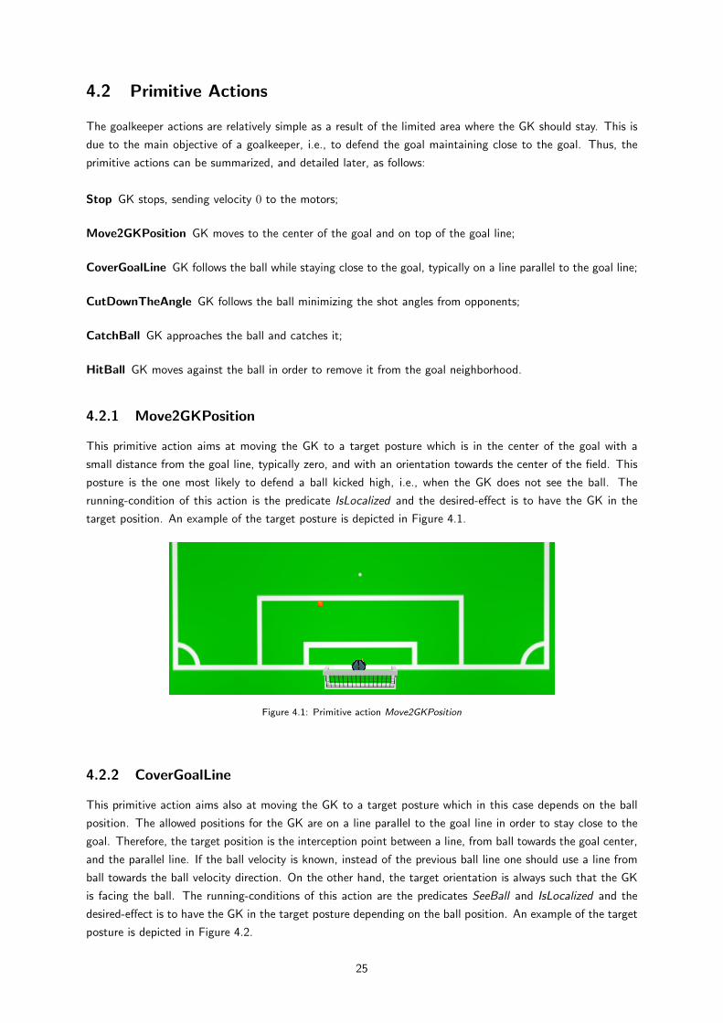
4.2.2 CoverGoalLine
This primitive action aims also at moving the GK to a target posture which in this case depends on the ball
position. The allowed positions for the GK are on a line parallel to the goal line in order to stay close to the
goal. Therefore, the target position is the interception point between a line, from ball towards the goal center,
and the parallel line. If the ball velocity is known, instead of the previous ball line one should use a line from
ball towards the ball velocity direction. On the other hand, the target orientation is always such that the GK
is facing the ball. The running-conditions of this action are the predicates SeeBall and IsLocalized and the
desired-effect is to have the GK in the target posture depending on the ball position. An example of the target
posture is depicted in Figure 4.2.
25
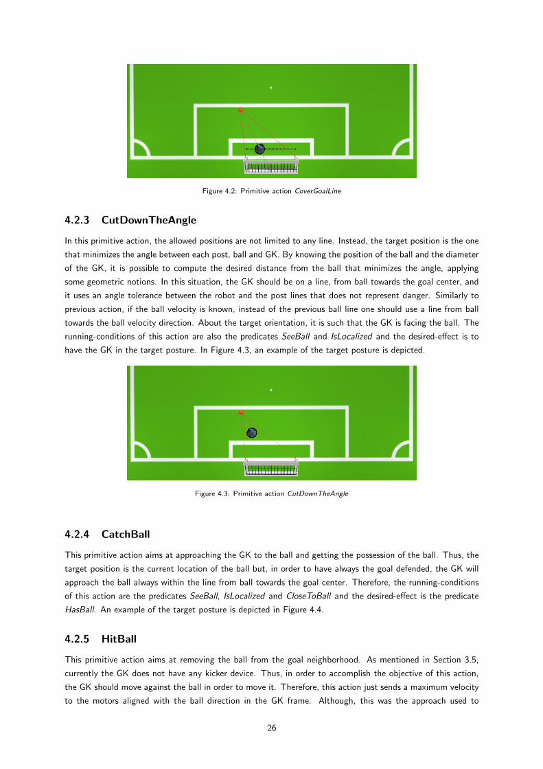
Figure 4.2: Primitive action CoverGoalLine
4.2.3 CutDownTheAngle
In this primitive action, the allowed positions are not limited to any line. Instead, the target position is the one
that minimizes the angle between each post, ball and GK. By knowing the position of the ball and the diameter
of the GK, it is possible to compute the desired distance from the ball that minimizes the angle, applying
some geometric notions. In this situation, the GK should be on a line, from ball towards the goal center, and
it uses an angle tolerance between the robot and the post lines that does not represent danger. Similarly to
previous action, if the ball velocity is known, instead of the previous ball line one should use a line from ball
towards the ball velocity direction. About the target orientation, it is such that the GK is facing the ball. The
running-conditions of this action are also the predicates SeeBall and IsLocalized and the desired-effect is to
have the GK in the target posture. In Figure 4.3, an example of the target posture is depicted.
Figure 4.3: Primitive action CutDownTheAngle
4.2.4 CatchBall
This primitive action aims at approaching the GK to the ball and getting the possession of the ball. Thus, the
target position is the current location of the ball but, in order to have always the goal defended, the GK will
approach the ball always within the line from ball towards the goal center. Therefore, the running-conditions
of this action are the predicates SeeBall, IsLocalized and CloseToBall and the desired-effect is the predicate
HasBall. An example of the target posture is depicted in Figure 4.4.
4.2.5 HitBall
This primitive action aims at removing the ball from the goal neighborhood. As mentioned in Section 3.5,
currently the GK does not have any kicker device. Thus, in order to accomplish the objective of this action,
the GK should move against the ball in order to move it. Therefore, this action just sends a maximum velocity
to the motors aligned with the ball direction in the GK frame. Although, this was the approach used to
26
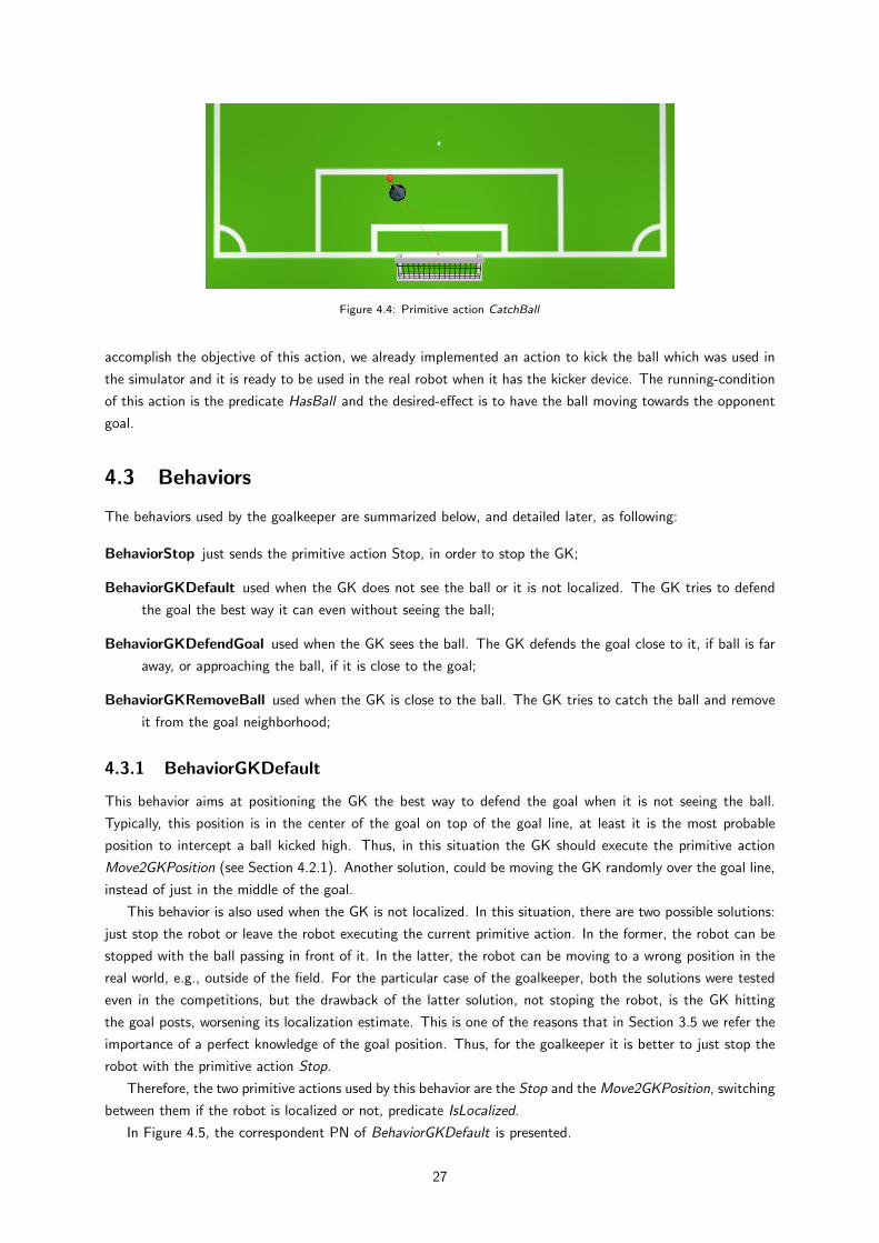
Figure 4.4: Primitive action CatchBall
accomplish the objective of this action, we already implemented an action to kick the ball which was used in
the simulator and it is ready to be used in the real robot when it has the kicker device. The running-condition
of this action is the predicate HasBall and the desired-effect is to have the ball moving towards the opponent
goal.
4.3 Behaviors
The behaviors used by the goalkeeper are summarized below, and detailed later, as following:
BehaviorStop just sends the primitive action Stop, in order to stop the GK;
BehaviorGKDefault used when the GK does not see the ball or it is not localized. The GK tries to defend
the goal the best way it can even without seeing the ball;
BehaviorGKDefendGoal used when the GK sees the ball. The GK defends the goal close to it, if ball is far
away, or approaching the ball, if it is close to the goal;
BehaviorGKRemoveBall used when the GK is close to the ball. The GK tries to catch the ball and remove
it from the goal neighborhood;
4.3.1 BehaviorGKDefault
This behavior aims at positioning the GK the best way to defend the goal when it is not seeing the ball.
Typically, this position is in the center of the goal on top of the goal line, at least it is the most probable
position to intercept a ball kicked high. Thus, in this situation the GK should execute the primitive action
Move2GKPosition (see Section 4.2.1). Another solution, could be moving the GK randomly over the goal line,
instead of just in the middle of the goal.
This behavior is also used when the GK is not localized. In this situation, there are two possible solutions:
just stop the robot or leave the robot executing the current primitive action. In the former, the robot can be
stopped with the ball passing in front of it. In the latter, the robot can be moving to a wrong position in the
real world, e.g., outside of the field. For the particular case of the goalkeeper, both the solutions were tested
even in the competitions, but the drawback of the latter solution, not stoping the robot, is the GK hitting
the goal posts, worsening its localization estimate. This is one of the reasons that in Section 3.5 we refer the
importance of a perfect knowledge of the goal position. Thus, for the goalkeeper it is better to just stop the
robot with the primitive action Stop.
Therefore, the two primitive actions used by this behavior are the Stop and the Move2GKPosition, switching
between them if the robot is localized or not, predicate IsLocalized.
In Figure 4.5, the correspondent PN of BehaviorGKDefault is presented.
27
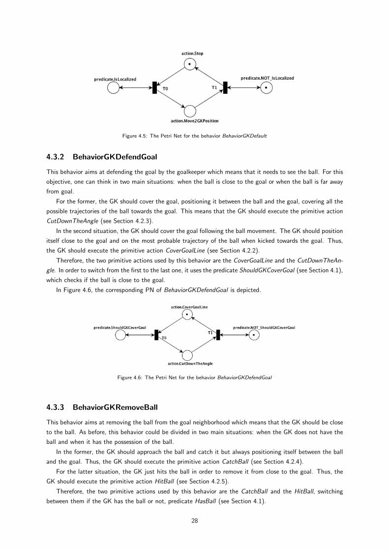
Figure 4.5: The Petri Net for the behavior BehaviorGKDefault
4.3.2 BehaviorGKDefendGoal
This behavior aims at defending the goal by the goalkeeper which means that it needs to see the ball. For this
objective, one can think in two main situations: when the ball is close to the goal or when the ball is far away
from goal.
For the former, the GK should cover the goal, positioning it between the ball and the goal, covering all the
possible trajectories of the ball towards the goal. This means that the GK should execute the primitive action
CutDownTheAngle (see Section 4.2.3).
In the second situation, the GK should cover the goal following the ball movement. The GK should position
itself close to the goal and on the most probable trajectory of the ball when kicked towards the goal. Thus,
the GK should execute the primitive action CoverGoalLine (see Section 4.2.2).
Therefore, the two primitive actions used by this behavior are the CoverGoalLine and the CutDownTheAn-
gle. In order to switch from the first to the last one, it uses the predicate ShouldGKCoverGoal (see Section 4.1),
which checks if the ball is close to the goal.
In Figure 4.6, the corresponding PN of BehaviorGKDefendGoal is depicted.
Figure 4.6: The Petri Net for the behavior BehaviorGKDefendGoal
4.3.3 BehaviorGKRemoveBall
This behavior aims at removing the ball from the goal neighborhood which means that the GK should be close
to the ball. As before, this behavior could be divided in two main situations: when the GK does not have the
ball and when it has the possession of the ball.
In the former, the GK should approach the ball and catch it but always positioning itself between the ball
and the goal. Thus, the GK should execute the primitive action CatchBall (see Section 4.2.4).
For the latter situation, the GK just hits the ball in order to remove it from close to the goal. Thus, the
GK should execute the primitive action HitBall (see Section 4.2.5).
Therefore, the two primitive actions used by this behavior are the CatchBall and the HitBall, switching
between them if the GK has the ball or not, predicate HasBall (see Section 4.1).
28
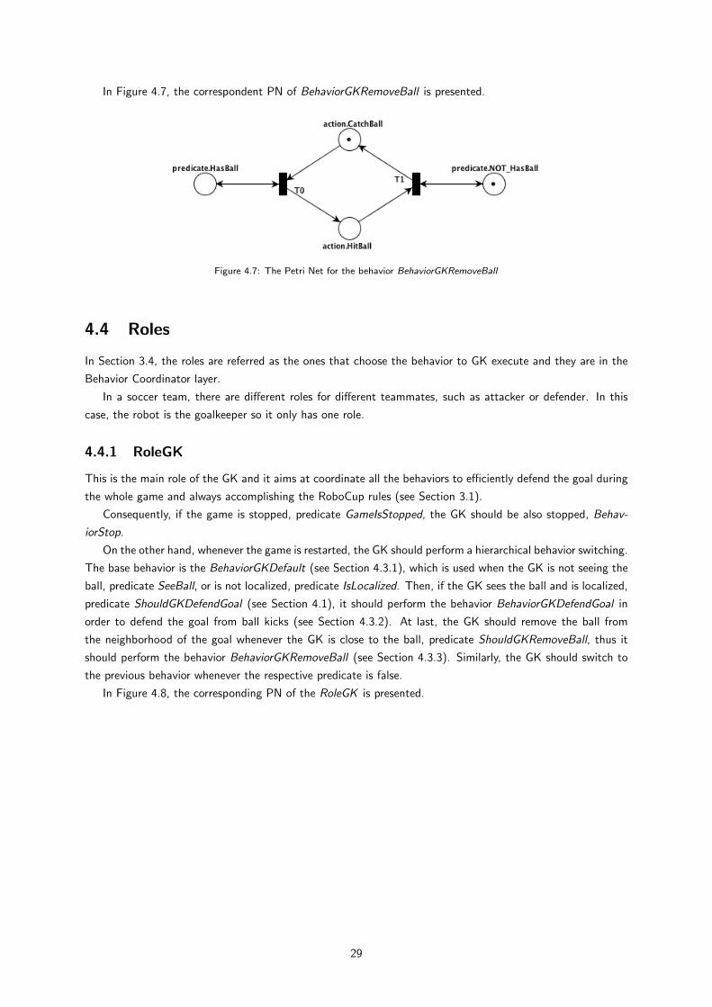
In Figure 4.7, the correspondent PN of BehaviorGKRemoveBall is presented.
Figure 4.7: The Petri Net for the behavior BehaviorGKRemoveBall
4.4 Roles
In Section 3.4, the roles are referred as the ones that choose the behavior to GK execute and they are in the
Behavior Coordinator layer.
In a soccer team, there are different roles for different teammates, such as attacker or defender. In this
case, the robot is the goalkeeper so it only has one role.
4.4.1 RoleGK
This is the main role of the GK and it aims at coordinate all the behaviors to efficiently defend the goal during
the whole game and always accomplishing the RoboCup rules (see Section 3.1).
Consequently, if the game is stopped, predicate GameIsStopped, the GK should be also stopped, Behav-
iorStop.
On the other hand, whenever the game is restarted, the GK should perform a hierarchical behavior switching.
The base behavior is the BehaviorGKDefault (see Section 4.3.1), which is used when the GK is not seeing the
ball, predicate SeeBall, or is not localized, predicate IsLocalized. Then, if the GK sees the ball and is localized,
predicate ShouldGKDefendGoal (see Section 4.1), it should perform the behavior BehaviorGKDefendGoal in
order to defend the goal from ball kicks (see Section 4.3.2). At last, the GK should remove the ball from
the neighborhood of the goal whenever the GK is close to the ball, predicate ShouldGKRemoveBall, thus it
should perform the behavior BehaviorGKRemoveBall (see Section 4.3.3). Similarly, the GK should switch to
the previous behavior whenever the respective predicate is false.
In Figure 4.8, the corresponding PN of the RoleGK is presented.
29
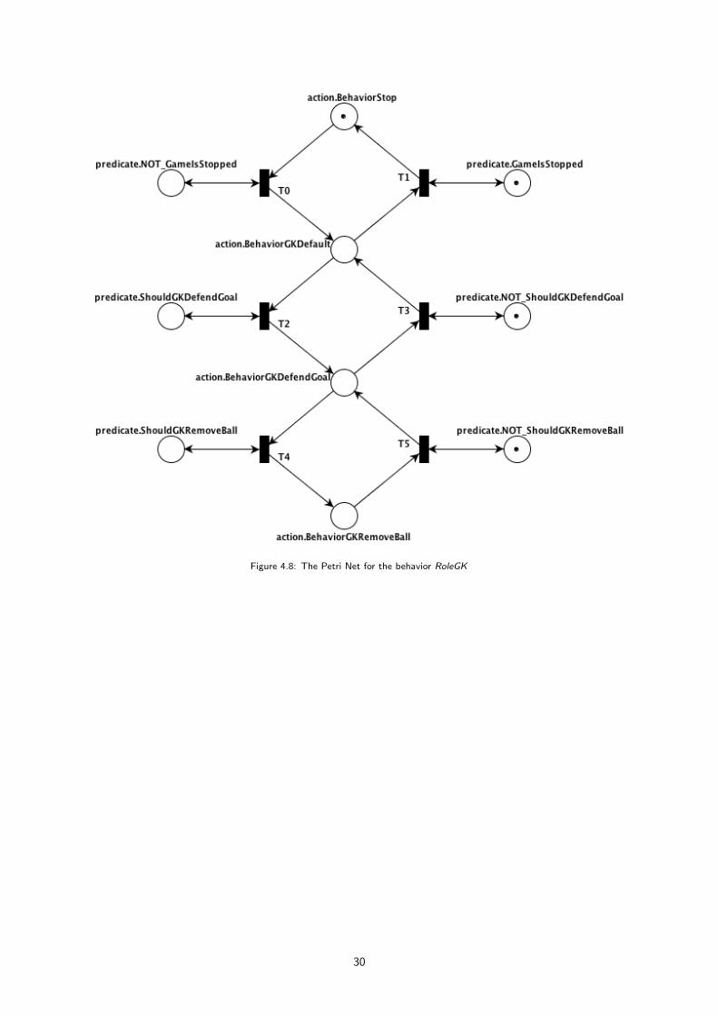
Figure 4.8: The Petri Net for the behavior RoleGK
30
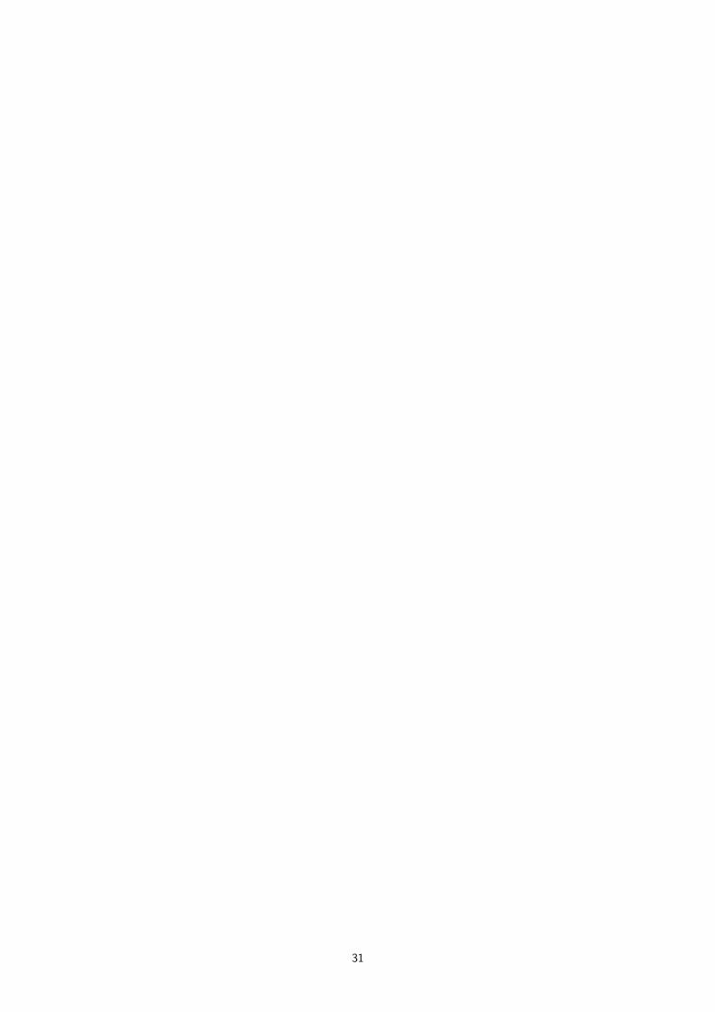
31
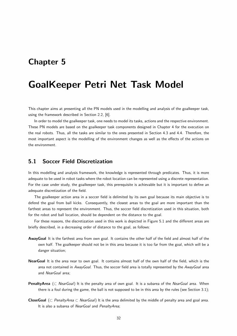
Chapter 5
GoalKeeper Petri Net Task Model
This chapter aims at presenting all the PN models used in the modelling and analysis of the goalkeeper task,
using the framework described in Section 2.2, [6].
In order to model the goalkeeper task, one needs to model its tasks, actions and the respective environment.
These PN models are based on the goalkeeper task components designed in Chapter 4 for the execution on
the real robots. Thus, all the tasks are similar to the ones presented in Section 4.3 and 4.4. Therefore, the
most important aspect is the modelling of the environment changes as well as the effects of the actions on
the environment.
5.1 Soccer Field Discretization
In this modelling and analysis framework, the knowledge is represented through predicates. Thus, it is more
adequate to be used in robot tasks where the robot location can be represented using a discrete representation.
For the case under study, the goalkeeper task, this prerequisite is achievable but it is important to define an
adequate discretization of the field.
The goalkeeper action area in a soccer field is delimited by its own goal because its main objective is to
defend the goal from ball kicks. Consequently, the closest areas to the goal are more important than the
farthest areas to represent the environment. Thus, the soccer field discretization used in this situation, both
for the robot and ball location, should be dependent on the distance to the goal.
For these reasons, the discretization used in this work is depicted in Figure 5.1 and the different areas are
briefly described, in a decreasing order of distance to the goal, as follows:
AwayGoal It is the farthest area from own goal. It contains the other half of the field and almost half of the
own half. The goalkeeper should not be in this area because it is too far from the goal, which will be a
danger situation;
NearGoal It is the area near to own goal. It contains almost half of the own half of the field, which is the
area not contained in AwayGoal. Thus, the soccer field area is totally represented by the AwayGoal area
and NearGoal area;
PenaltyArea (⊂ NearGoal) It is the penalty area of own goal. It is a subarea of the NearGoal area. When
there is a foul during the game, the ball is not supposed to be in this area by the rules (see Section 3.1);
CloseGoal (⊂ PenaltyArea ⊂ NearGoal) It is the area delimited by the middle of penalty area and goal area.
It is also a subarea of NearGoal and PenaltyArea;
32
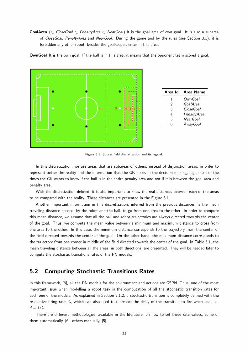
GoalArea (⊂ CloseGoal ⊂ PenaltyArea ⊂ NearGoal) It is the goal area of own goal. It is also a subarea
of CloseGoal, PenaltyArea and NearGoal. During the game and by the rules (see Section 3.1), it is
forbidden any other robot, besides the goalkeeper, enter in this area;
OwnGoal It is the own goal. If the ball is in this area, it means that the opponent team scored a goal.
Area Id Area Name
1 OwnGoal2 GoalArea3 CloseGoal4 PenaltyArea5 NearGoal6 AwayGoal
Figure 5.1: Soccer field discretization and its legend.
In this discretization, we use areas that are subareas of others, instead of disjunction areas, in order to
represent better the reality and the information that the GK needs in the decision making, e.g., most of the
times the GK wants to know if the ball is in the entire penalty area and not if it is between the goal area and
penalty area.
With the discretization defined, it is also important to know the real distances between each of the areas
to be compared with the reality. These distances are presented in the Figure 3.1.
Another important information in this discretization, inferred from the previous distances, is the mean
traveling distance needed, by the robot and the ball, to go from one area to the other. In order to compute
this mean distance, we assume that all the ball and robot trajectories are always directed towards the center
of the goal. Thus, we compute the mean value between a minimum and maximum distance to cross from
one area to the other. In this case, the minimum distance corresponds to the trajectory from the center of
the field directed towards the center of the goal. On the other hand, the maximum distance corresponds to
the trajectory from one corner in middle of the field directed towards the center of the goal. In Table 5.1, the
mean traveling distance between all the areas, in both directions, are presented. They will be needed later to
compute the stochastic transitions rates of the PN models.
5.2 Computing Stochastic Transitions Rates
In this framework, [6], all the PN models for the environment and actions are GSPN. Thus, one of the most
important issue when modelling a robot task is the computation of all the stochastic transition rates for
each one of the models. As explained in Section 2.1.2, a stochastic transition is completely defined with the
respective firing rate, λ, which can also used to represent the delay of the transition to fire when enabled,
d = 1/λ.
There are different methodologies, available in the literature, on how to set these rate values, some of
them automatically, [6], others manually, [5].
33
Table 5.1: Mean traveling distance between areas for the goalkeeper and ball
Areas Mean Distance [m]From / To To / From GK Ball
OwnGoal−→
GoalArea0.2 —
←− 0.75 1.33
GoalArea−→ CloseGoal & 0.75 0.75←− NOT GoalArea 0.91 0.91
CloseGoal & −→ PenaltyArea & 0.91 0.91NOT GoalArea ←− NOT CloseGoal 0.91 0.91
PenaltyArea & −→ NearGoal & 0.91 0.91NOT CloseGoal ←− NOT PenaltyArea 3.32 3.32
NearGoal & −→AwayGoal
3.32 3.32NOT PenaltyArea ←− 0.2 2.0
In [6], an automatic method for model identification was proposed based in two main steps: a data collection
experiment and a estimation of the action and environment models. In the former step, the experiments consist
on running each action several times to gather information about the action impact in the world. In the latter
step, the goal is to obtain the PN model of each action and of the environment, from the data collection.
Though this method is completely automatic and obtains realistic models, it needs many experiments for each
action which would be difficult to perform in real robots within the time scope of this work.
On the other hand, there are the manual methods which sets the transition rates based on the knowledge
of the transition meaning. In [5], e.g., the transition rates that correspond to the movement of a robot were
set with the mean travel time of the robot in those trajectories, previous collected with the real robots.
The method used in this work is manual and uses the knowledge of the robot motion for the respective
transitions and other methodologies for the others. Thus, there are four different types of stochastic transitions,
which depend on their physical meaning, and for each one there is a method to compute the respective
stochastic transition rate. In the following sections, each one of the transition types are described and explained
how to set the transition rates.
5.2.1 Robot Motion
In the action models, one needs to model the effects of the action on the environment, thus one of these
effects is the robot transition between different areas. Therefore, these transitions that represent the robot
motion are a subset of the stochastic transitions one needs to compute the firing rates.
For this type of transition, one can use the mean traveling distance between the different areas together
with a mean velocity of the robot. With these two parameters, it is possible to obtain the mean delay of the
transition and, consequently, the firing rate as explained in Equation 5.1.
(Distance, V elocity)⇒ d =Distance
V elocity⇒ λ =
1
d(5.1)
For the mean traveling distance of the robot we use the values in Table 5.1 and for the mean velocity of
the robot we will use a suitable value depending on the situation we want to model, explained in Chapter 6
when we present all the experimental setups used.
34
5.2.2 Ball Motion
In the ball motion, we can use a similar method as the one presented previously. Thus, for the type of stochastic
transition that represent the motion of the ball between different areas, we should use the same Equation 5.1
to obtain the respective firing rate of the transition.
Similar, for the mean traveling distance of the ball we use the values in Table 5.1 and for the mean velocity
of the ball we will use different velocities depending on the situation we want to model, explained in Chapter 6
when we present all the experimental setups used.
5.2.3 Probability of Success
In the action and environment models, not all the stochastic transitions are related with movement of the
robot or ball. For those ones, we need to have a methodology to compute its firing rate in order to have a
model as close as possible of the reality.
Thus, in this type of stochastic transition, we use the success probability of the transition under analysis
when it is in conflict with other transition, used as comparison. As an example a transition representing a GK
defense, should be compared with the transition that represents a goal scored by the opponent team. In this
case, the transition under analysis is the GK defense, success, when in conflict with a goal scored, failure.
In the complete model of a task, most of the times when a transition of this type is enabled there is
more than one transition enabled, at the same time. However, in order to simplify the method and to keep
the mean delay of the transition as realistic as possible, we assume that only the success transition and the
failure transition are enabled. Thus, we have a conflict between these two PN transitions and we can apply
Equation 2.1 to get the mean delay value of the transition, ds, as in Equation 5.2. For this, we need to have
the delay value of the failure transition, df , already set and typically related with motion of the ball or robot,
and a desired probability of occurring the success transition, Ps, set manual and intuitively to be as close as
possible of the reality, which is easier and better than choosing a delay for success transition.
Psuccess =λsuccess
λsuccess + λfailure=
1/ds1/ds + 1/df
⇒ ds =df (1− Ps)
Ps(5.2)
5.2.4 Percentage of Time
This type of stochastic transition is similar to the previous one, it is not related with ball or robot motion and
it uses another transition as comparison. However, in this case we do not use the probability of success of the
transition. Instead, we use the delay of the transition to be compared and the mean delay of the transition
under analysis is computed as a percentage of the former delay. As an example, the ball takes a certain time
to cross an area, the delay of the transition used as comparison, thus the GK gets close to the ball after a
certain percentage of the former time, i.e., after the ball enters the area but before it leaves, the delay of the
transition under analysis.
These type of stochastic transitions will be more clear when applied to the specific models of the GK task.
5.3 Predicates
In this modelling and analysis framework, [6], the knowledge of the environment is modelled by predicates and
logic conditions. Most of the predicates are the same used in the execution of the goalkeeper task in the real
robot which are detailed in Section 4.1. The following list contains the predicates used in the modelling of the
task:
Robot Position GKOwnGoal, GKGoalArea, GKCloseGoal, GKPenaltyArea, GKNearGoal, GKAwayGoal ;
35
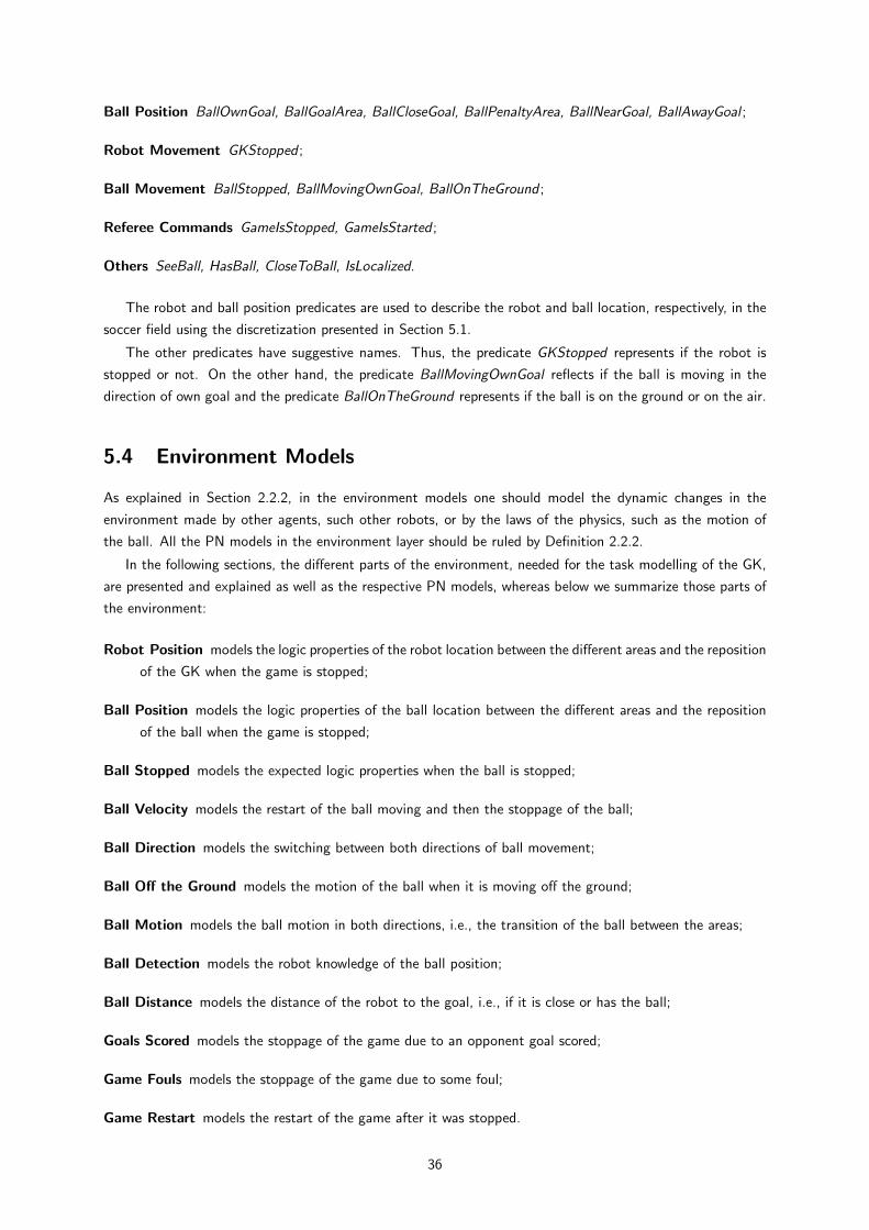
Ball Position BallOwnGoal, BallGoalArea, BallCloseGoal, BallPenaltyArea, BallNearGoal, BallAwayGoal ;
Robot Movement GKStopped ;
Ball Movement BallStopped, BallMovingOwnGoal, BallOnTheGround ;
Referee Commands GameIsStopped, GameIsStarted ;
Others SeeBall, HasBall, CloseToBall, IsLocalized.
The robot and ball position predicates are used to describe the robot and ball location, respectively, in the
soccer field using the discretization presented in Section 5.1.
The other predicates have suggestive names. Thus, the predicate GKStopped represents if the robot is
stopped or not. On the other hand, the predicate BallMovingOwnGoal reflects if the ball is moving in the
direction of own goal and the predicate BallOnTheGround represents if the ball is on the ground or on the air.
5.4 Environment Models
As explained in Section 2.2.2, in the environment models one should model the dynamic changes in the
environment made by other agents, such other robots, or by the laws of the physics, such as the motion of
the ball. All the PN models in the environment layer should be ruled by Definition 2.2.2.
In the following sections, the different parts of the environment, needed for the task modelling of the GK,
are presented and explained as well as the respective PN models, whereas below we summarize those parts of
the environment:
Robot Position models the logic properties of the robot location between the different areas and the reposition
of the GK when the game is stopped;
Ball Position models the logic properties of the ball location between the different areas and the reposition
of the ball when the game is stopped;
Ball Stopped models the expected logic properties when the ball is stopped;
Ball Velocity models the restart of the ball moving and then the stoppage of the ball;
Ball Direction models the switching between both directions of ball movement;
Ball Off the Ground models the motion of the ball when it is moving off the ground;
Ball Motion models the ball motion in both directions, i.e., the transition of the ball between the areas;
Ball Detection models the robot knowledge of the ball position;
Ball Distance models the distance of the robot to the goal, i.e., if it is close or has the ball;
Goals Scored models the stoppage of the game due to an opponent goal scored;
Game Fouls models the stoppage of the game due to some foul;
Game Restart models the restart of the game after it was stopped.
36
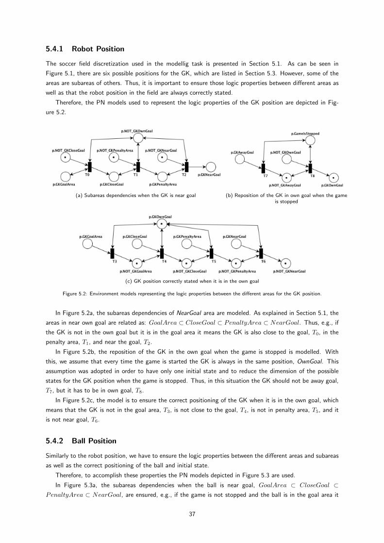
5.4.1 Robot Position
The soccer field discretization used in the modellig task is presented in Section 5.1. As can be seen in
Figure 5.1, there are six possible positions for the GK, which are listed in Section 5.3. However, some of the
areas are subareas of others. Thus, it is important to ensure those logic properties between different areas as
well as that the robot position in the field are always correctly stated.
Therefore, the PN models used to represent the logic properties of the GK position are depicted in Fig-
ure 5.2.
(a) Subareas dependencies when the GK is near goal (b) Reposition of the GK in own goal when the gameis stopped
(c) GK position correctly stated when it is in the own goal
Figure 5.2: Environment models representing the logic properties between the different areas for the GK position.
In Figure 5.2a, the subareas dependencies of NearGoal area are modeled. As explained in Section 5.1, the
areas in near own goal are related as: GoalArea ⊂ CloseGoal ⊂ PenaltyArea ⊂ NearGoal. Thus, e.g., if
the GK is not in the own goal but it is in the goal area it means the GK is also close to the goal, T0, in the
penalty area, T1, and near the goal, T2.
In Figure 5.2b, the reposition of the GK in the own goal when the game is stopped is modelled. With
this, we assume that every time the game is started the GK is always in the same position, OwnGoal. This
assumption was adopted in order to have only one initial state and to reduce the dimension of the possible
states for the GK position when the game is stopped. Thus, in this situation the GK should not be away goal,
T7, but it has to be in own goal, T8.
In Figure 5.2c, the model is to ensure the correct positioning of the GK when it is in the own goal, which
means that the GK is not in the goal area, T3, is not close to the goal, T4, is not in penalty area, T5, and it
is not near goal, T6.
5.4.2 Ball Position
Similarly to the robot position, we have to ensure the logic properties between the different areas and subareas
as well as the correct positioning of the ball and initial state.
Therefore, to accomplish these properties the PN models depicted in Figure 5.3 are used.
In Figure 5.3a, the subareas dependencies when the ball is near goal, GoalArea ⊂ CloseGoal ⊂PenaltyArea ⊂ NearGoal, are ensured, e.g., if the game is not stopped and the ball is in the goal area it
37
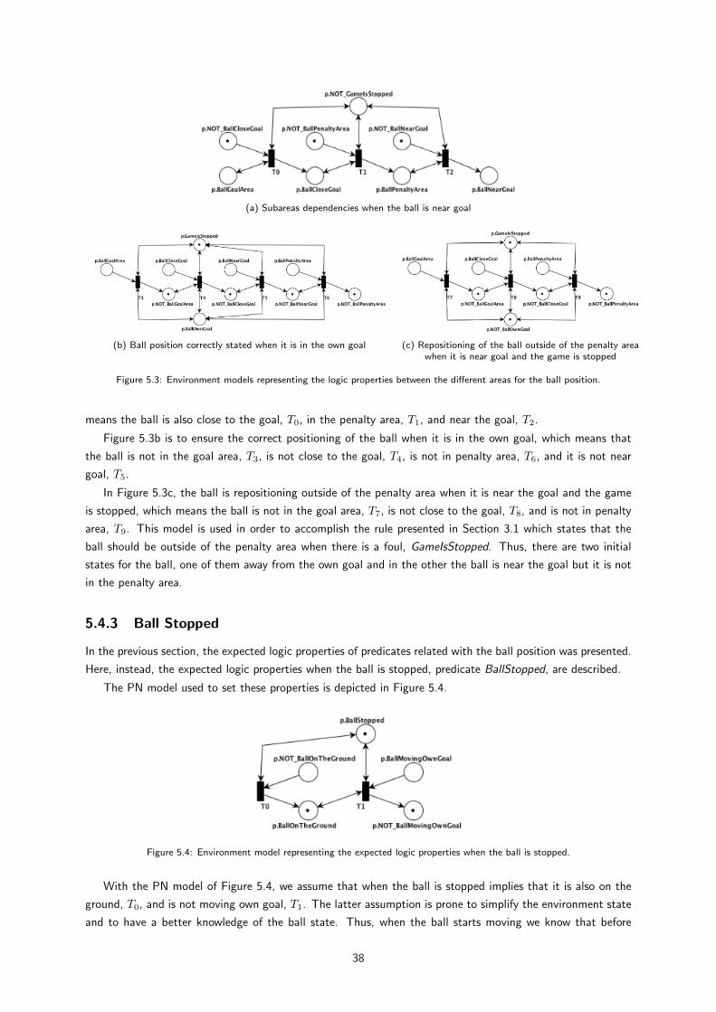
(a) Subareas dependencies when the ball is near goal
(b) Ball position correctly stated when it is in the own goal (c) Repositioning of the ball outside of the penalty areawhen it is near goal and the game is stopped
Figure 5.3: Environment models representing the logic properties between the different areas for the ball position.
means the ball is also close to the goal, T0, in the penalty area, T1, and near the goal, T2.
Figure 5.3b is to ensure the correct positioning of the ball when it is in the own goal, which means that
the ball is not in the goal area, T3, is not close to the goal, T4, is not in penalty area, T6, and it is not near
goal, T5.
In Figure 5.3c, the ball is repositioning outside of the penalty area when it is near the goal and the game
is stopped, which means the ball is not in the goal area, T7, is not close to the goal, T8, and is not in penalty
area, T9. This model is used in order to accomplish the rule presented in Section 3.1 which states that the
ball should be outside of the penalty area when there is a foul, GameIsStopped. Thus, there are two initial
states for the ball, one of them away from the own goal and in the other the ball is near the goal but it is not
in the penalty area.
5.4.3 Ball Stopped
In the previous section, the expected logic properties of predicates related with the ball position was presented.
Here, instead, the expected logic properties when the ball is stopped, predicate BallStopped, are described.
The PN model used to set these properties is depicted in Figure 5.4.
Figure 5.4: Environment model representing the expected logic properties when the ball is stopped.
With the PN model of Figure 5.4, we assume that when the ball is stopped implies that it is also on the
ground, T0, and is not moving own goal, T1. The latter assumption is prone to simplify the environment state
and to have a better knowledge of the ball state. Thus, when the ball starts moving we know that before
38
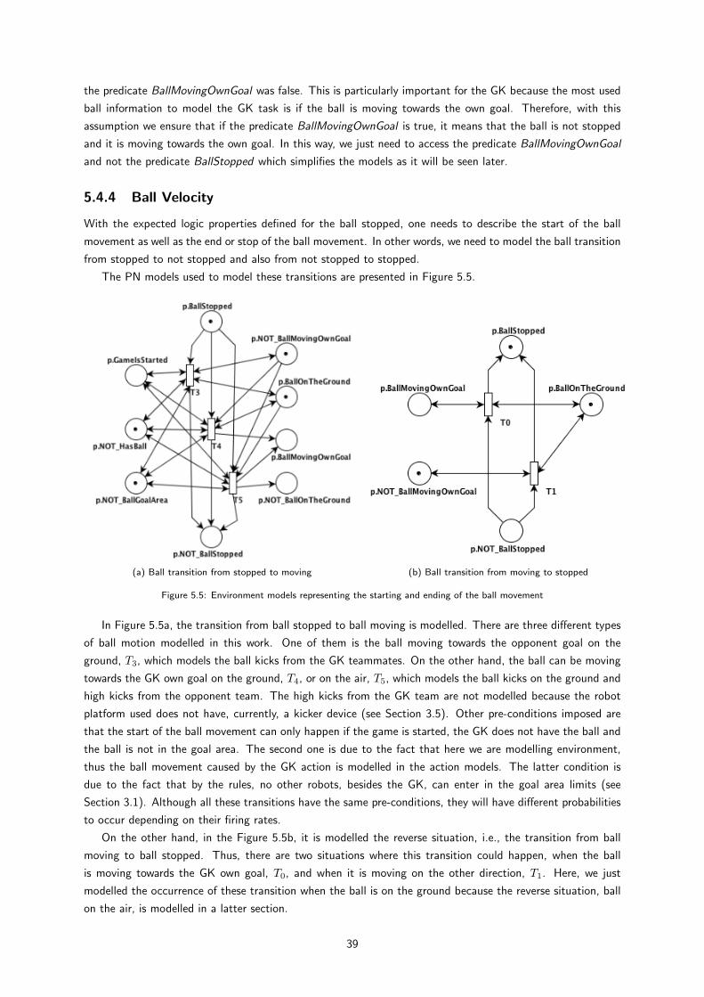
the predicate BallMovingOwnGoal was false. This is particularly important for the GK because the most used
ball information to model the GK task is if the ball is moving towards the own goal. Therefore, with this
assumption we ensure that if the predicate BallMovingOwnGoal is true, it means that the ball is not stopped
and it is moving towards the own goal. In this way, we just need to access the predicate BallMovingOwnGoal
and not the predicate BallStopped which simplifies the models as it will be seen later.
5.4.4 Ball Velocity
With the expected logic properties defined for the ball stopped, one needs to describe the start of the ball
movement as well as the end or stop of the ball movement. In other words, we need to model the ball transition
from stopped to not stopped and also from not stopped to stopped.
The PN models used to model these transitions are presented in Figure 5.5.
(a) Ball transition from stopped to moving (b) Ball transition from moving to stopped
Figure 5.5: Environment models representing the starting and ending of the ball movement
In Figure 5.5a, the transition from ball stopped to ball moving is modelled. There are three different types
of ball motion modelled in this work. One of them is the ball moving towards the opponent goal on the
ground, T3, which models the ball kicks from the GK teammates. On the other hand, the ball can be moving
towards the GK own goal on the ground, T4, or on the air, T5, which models the ball kicks on the ground and
high kicks from the opponent team. The high kicks from the GK team are not modelled because the robot
platform used does not have, currently, a kicker device (see Section 3.5). Other pre-conditions imposed are
that the start of the ball movement can only happen if the game is started, the GK does not have the ball and
the ball is not in the goal area. The second one is due to the fact that here we are modelling environment,
thus the ball movement caused by the GK action is modelled in the action models. The latter condition is
due to the fact that by the rules, no other robots, besides the GK, can enter in the goal area limits (see
Section 3.1). Although all these transitions have the same pre-conditions, they will have different probabilities
to occur depending on their firing rates.
On the other hand, in the Figure 5.5b, it is modelled the reverse situation, i.e., the transition from ball
moving to ball stopped. Thus, there are two situations where this transition could happen, when the ball
is moving towards the GK own goal, T0, and when it is moving on the other direction, T1. Here, we just
modelled the occurrence of these transition when the ball is on the ground because the reverse situation, ball
on the air, is modelled in a latter section.
39
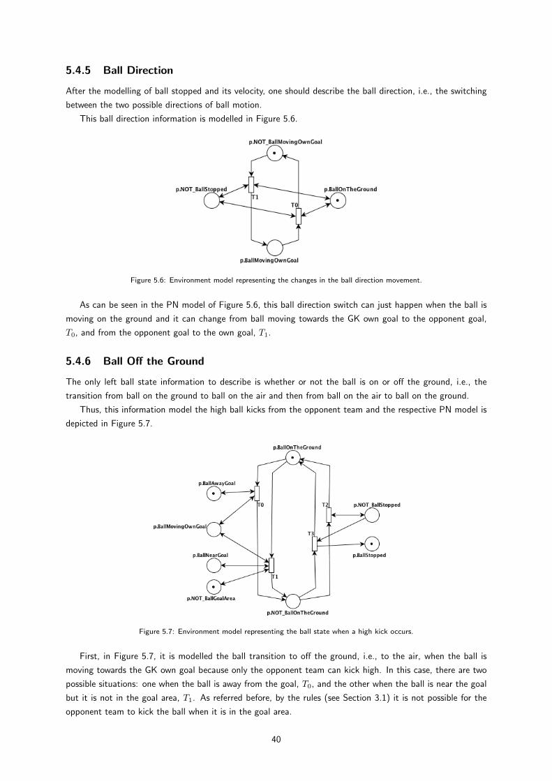
5.4.5 Ball Direction
After the modelling of ball stopped and its velocity, one should describe the ball direction, i.e., the switching
between the two possible directions of ball motion.
This ball direction information is modelled in Figure 5.6.
Figure 5.6: Environment model representing the changes in the ball direction movement.
As can be seen in the PN model of Figure 5.6, this ball direction switch can just happen when the ball is
moving on the ground and it can change from ball moving towards the GK own goal to the opponent goal,
T0, and from the opponent goal to the own goal, T1.
5.4.6 Ball Off the Ground
The only left ball state information to describe is whether or not the ball is on or off the ground, i.e., the
transition from ball on the ground to ball on the air and then from ball on the air to ball on the ground.
Thus, this information model the high ball kicks from the opponent team and the respective PN model is
depicted in Figure 5.7.
Figure 5.7: Environment model representing the ball state when a high kick occurs.
First, in Figure 5.7, it is modelled the ball transition to off the ground, i.e., to the air, when the ball is
moving towards the GK own goal because only the opponent team can kick high. In this case, there are two
possible situations: one when the ball is away from the goal, T0, and the other when the ball is near the goal
but it is not in the goal area, T1. As referred before, by the rules (see Section 3.1) it is not possible for the
opponent team to kick the ball when it is in the goal area.
40
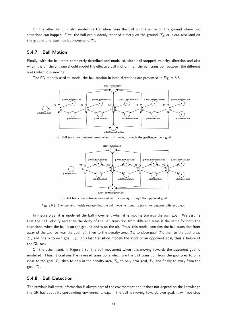
On the other hand, it also model the transition from the ball on the air to on the ground where two
situations can happen. First, the ball can suddenly stopped directly on the ground, T3, or it can also land on
the ground and continue its movement, T2.
5.4.7 Ball Motion
Finally, with the ball state completely described and modelled, since ball stopped, velocity, direction and also
when it is on the air, one should model the effective ball motion, i.e., the ball transition between the different
areas when it is moving.
The PN models used to model the ball motion in both directions are presented in Figure 5.8.
(a) Ball transition between areas when it is moving through the goalkeeper own goal
(b) Ball transition between areas when it is moving through the opponent goal
Figure 5.8: Environment models representing the ball movement and its transition between different areas.
In Figure 5.8a, it is modelled the ball movement when it is moving towards the own goal. We assume
that the ball velocity and then the delay of the ball transition from different areas is the same for both the
situations, when the ball is on the ground and is on the air. Thus, this model contains the ball transition from
away of the goal to near the goal, T4, then to the penalty area, T3, to close goal, T2, then to the goal area,
T1, and finally to own goal, T0. This last transition models the score of an opponent goal, thus a failure of
the GK task.
On the other hand, in Figure 5.8b, the ball movement when it is moving towards the opponent goal is
modelled. Thus, it contains the reversed transitions which are the ball transition from the goal area to only
close to the goal, T5, then to only in the penalty area, T6, to only near goal, T7, and finally to away from the
goal, T8.
5.4.8 Ball Detection
The previous ball state information is always part of the environment and it does not depend on the knowledge
the GK has about its surrounding environment, e.g., if the ball is moving towards own goal, it will not stop
41
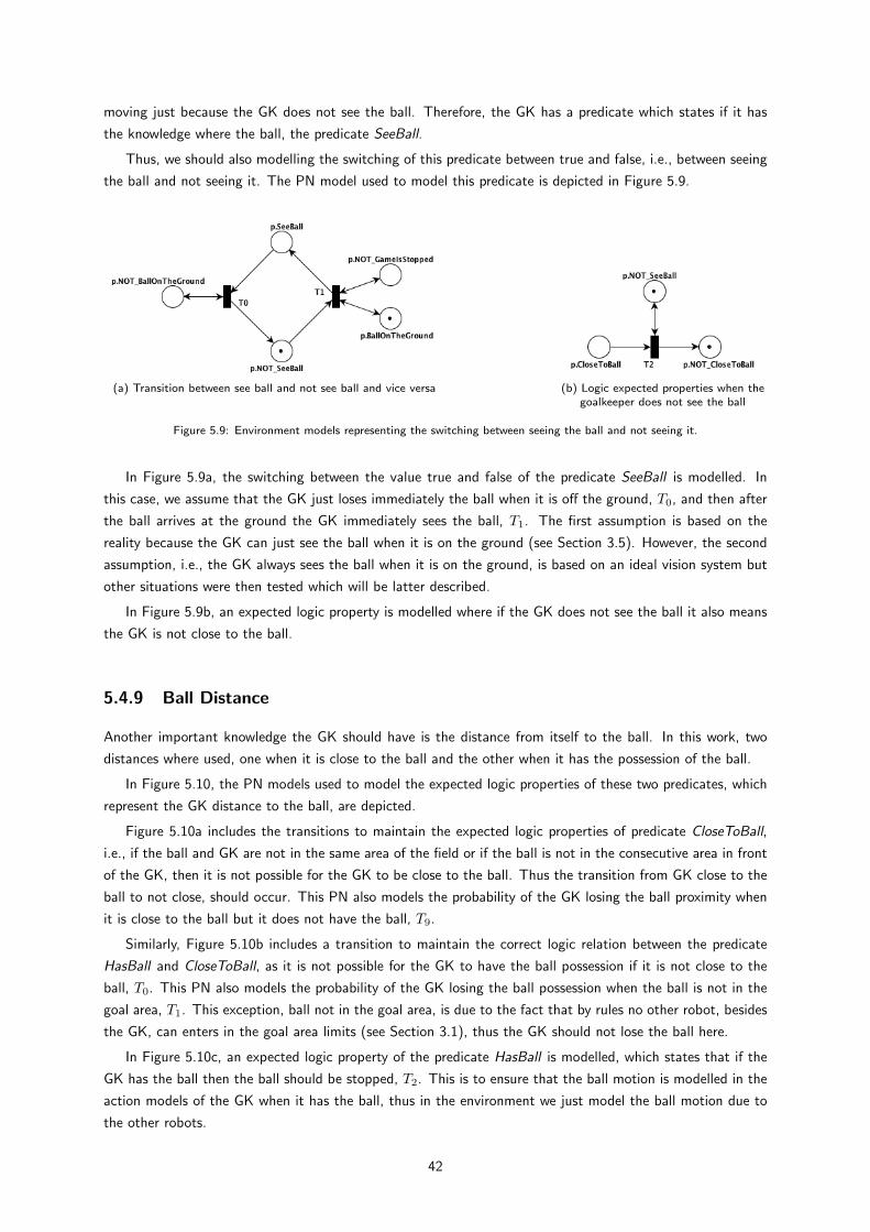
moving just because the GK does not see the ball. Therefore, the GK has a predicate which states if it has
the knowledge where the ball, the predicate SeeBall.
Thus, we should also modelling the switching of this predicate between true and false, i.e., between seeing
the ball and not seeing it. The PN model used to model this predicate is depicted in Figure 5.9.
(a) Transition between see ball and not see ball and vice versa (b) Logic expected properties when thegoalkeeper does not see the ball
Figure 5.9: Environment models representing the switching between seeing the ball and not seeing it.
In Figure 5.9a, the switching between the value true and false of the predicate SeeBall is modelled. In
this case, we assume that the GK just loses immediately the ball when it is off the ground, T0, and then after
the ball arrives at the ground the GK immediately sees the ball, T1. The first assumption is based on the
reality because the GK can just see the ball when it is on the ground (see Section 3.5). However, the second
assumption, i.e., the GK always sees the ball when it is on the ground, is based on an ideal vision system but
other situations were then tested which will be latter described.
In Figure 5.9b, an expected logic property is modelled where if the GK does not see the ball it also means
the GK is not close to the ball.
5.4.9 Ball Distance
Another important knowledge the GK should have is the distance from itself to the ball. In this work, two
distances where used, one when it is close to the ball and the other when it has the possession of the ball.
In Figure 5.10, the PN models used to model the expected logic properties of these two predicates, which
represent the GK distance to the ball, are depicted.
Figure 5.10a includes the transitions to maintain the expected logic properties of predicate CloseToBall,
i.e., if the ball and GK are not in the same area of the field or if the ball is not in the consecutive area in front
of the GK, then it is not possible for the GK to be close to the ball. Thus the transition from GK close to the
ball to not close, should occur. This PN also models the probability of the GK losing the ball proximity when
it is close to the ball but it does not have the ball, T9.
Similarly, Figure 5.10b includes a transition to maintain the correct logic relation between the predicate
HasBall and CloseToBall, as it is not possible for the GK to have the ball possession if it is not close to the
ball, T0. This PN also models the probability of the GK losing the ball possession when the ball is not in the
goal area, T1. This exception, ball not in the goal area, is due to the fact that by rules no other robot, besides
the GK, can enters in the goal area limits (see Section 3.1), thus the GK should not lose the ball here.
In Figure 5.10c, an expected logic property of the predicate HasBall is modelled, which states that if the
GK has the ball then the ball should be stopped, T2. This is to ensure that the ball motion is modelled in the
action models of the GK when it has the ball, thus in the environment we just model the ball motion due to
the other robots.
42
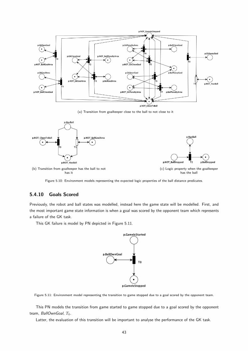
(a) Transition from goalkeeper close to the ball to not close to it
(b) Transition from goalkeeper has the ball to nothas it
(c) Logic property when the goalkeeperhas the ball
Figure 5.10: Environment models representing the expected logic properties of the ball distance predicates.
5.4.10 Goals Scored
Previously, the robot and ball states was modelled, instead here the game state will be modelled. First, and
the most important game state information is when a goal was scored by the opponent team which represents
a failure of the GK task.
This GK failure is model by PN depicted in Figure 5.11.
Figure 5.11: Environment model representing the transition to game stopped due to a goal scored by the opponent team.
This PN models the transition from game started to game stopped due to a goal scored by the opponent
team, BallOwnGoal, T0.
Latter, the evaluation of this transition will be important to analyse the performance of the GK task.
43

5.4.11 Game Fouls
After the modelling of the game stoppage due to a goal scored, one should also model the game stoppage due
to a foul, e.g., a throw-in.
The PN model used to model the occurrence of any foul is depicted in Figure 5.12.
Figure 5.12: Environment model representing the occurrence of any foul depending on the ball position.
In Figure 5.12, the occurrence of a foul depending on the ball position is modelled. Thus, there are four
different situations where a foul can occur which represent different probabilities of occurrence that depend
on the ball position. The first situation is when the ball is in the goal area where the probability differs if the
ball is on the air, T0, or if it is on the ground, T3. Then, other situation is when the ball is near the goal but
it is not in the goal area, T1. Finally, the last situation is when the ball is away from the goal, T2. All of these
situations, can only happen if the GK does not have the ball which is used to simplify the models and in the
reality the fouls do not occur when the GK has the ball.
5.4.12 Game Restart
Finally, after the modelling of the game stoppage, one should model the restart of the game due to the referee
commands.
In Figure 5.13, the PN used to model the restart of the game as well as the expected logic properties when
the game is stopped are depicted.
In Figure 5.13a, the transition from game stopped to game not stopped is modelled, T0 and then to game
started, T1. The first transition is due to a referee command related to a foul, e.g., a free kick, and the second
transition is due to the referee start command (see Section 3.1). An important aspect in the game restart
is that we impose the game restart only if the ball is not in the own goal, T0, i.e., if a goal is scored by the
opponent team the game will never be restarted again. This assumption will be important in the performance
analysis of the GK task.
In Figure 5.13b, the expected logic properties for the game stopped are modelled. These properties states
that when the game is stopped, the GK is localized, T2, the ball is stopped, T3, and the GK does not see the
ball, T4. Similarly to previous models, this is to ensure only one initial state when the game is restarted.
44
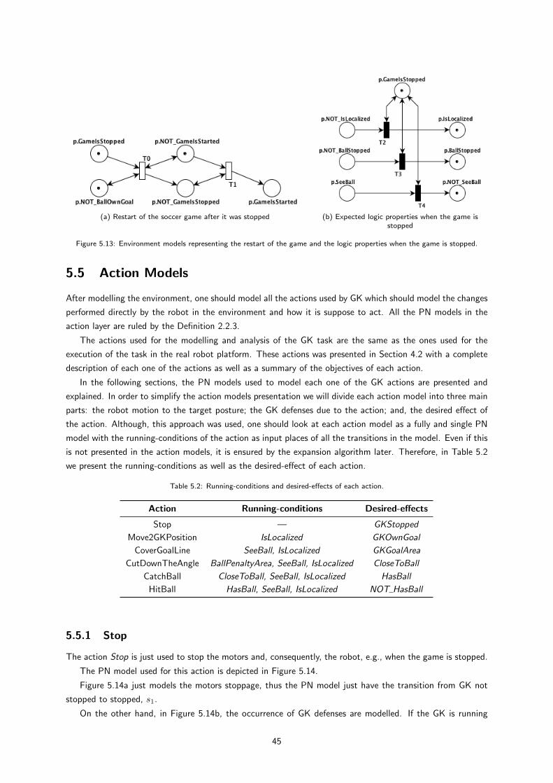
(a) Restart of the soccer game after it was stopped (b) Expected logic properties when the game isstopped
Figure 5.13: Environment models representing the restart of the game and the logic properties when the game is stopped.
5.5 Action Models
After modelling the environment, one should model all the actions used by GK which should model the changes
performed directly by the robot in the environment and how it is suppose to act. All the PN models in the
action layer are ruled by the Definition 2.2.3.
The actions used for the modelling and analysis of the GK task are the same as the ones used for the
execution of the task in the real robot platform. These actions was presented in Section 4.2 with a complete
description of each one of the actions as well as a summary of the objectives of each action.
In the following sections, the PN models used to model each one of the GK actions are presented and
explained. In order to simplify the action models presentation we will divide each action model into three main
parts: the robot motion to the target posture; the GK defenses due to the action; and, the desired effect of
the action. Although, this approach was used, one should look at each action model as a fully and single PN
model with the running-conditions of the action as input places of all the transitions in the model. Even if this
is not presented in the action models, it is ensured by the expansion algorithm later. Therefore, in Table 5.2
we present the running-conditions as well as the desired-effect of each action.
Table 5.2: Running-conditions and desired-effects of each action.
Action Running-conditions Desired-effects
Stop — GKStopped
Move2GKPosition IsLocalized GKOwnGoal
CoverGoalLine SeeBall, IsLocalized GKGoalArea
CutDownTheAngle BallPenaltyArea, SeeBall, IsLocalized CloseToBall
CatchBall CloseToBall, SeeBall, IsLocalized HasBall
HitBall HasBall, SeeBall, IsLocalized NOT HasBall
5.5.1 Stop
The action Stop is just used to stop the motors and, consequently, the robot, e.g., when the game is stopped.
The PN model used for this action is depicted in Figure 5.14.
Figure 5.14a just models the motors stoppage, thus the PN model just have the transition from GK not
stopped to stopped, s1.
On the other hand, in Figure 5.14b, the occurrence of GK defenses are modelled. If the GK is running
45
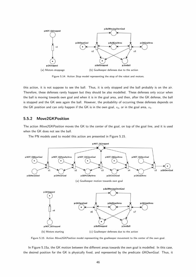
(a) Motors stoppage (b) Goalkeeper defenses due to the action
Figure 5.14: Action Stop model representing the stop of the robot and motors.
this action, it is not suppose to see the ball. Thus, it is only stopped and the ball probably is on the air.
Therefore, these defenses rarely happen but they should be also modelled. These defenses only occur when
the ball is moving towards own goal and when it is in the goal area, and then, after the GK defense, the ball
is stopped and the GK sees again the ball. However, the probability of occurring these defenses depends on
the GK position and can only happen if the GK is in the own goal, s2, or in the goal area, s3.
5.5.2 Move2GKPosition
The action Move2GKPosition moves the GK to the center of the goal, on top of the goal line, and it is used
when the GK does not see the ball.
The PN models used to model this action are presented in Figure 5.15.
(a) Goalkeeper motion towards own goal
(b) Motors starting (c) Goalkeeper defenses due to the action
Figure 5.15: Action Move2GKPosition model representing the goalkeeper movement to the center of the own goal.
In Figure 5.15a, the GK motion between the different areas towards the own goal is modelled. In this case,
the desired position for the GK is physically fixed, and represented by the predicate GKOwnGoal. Thus, it
46
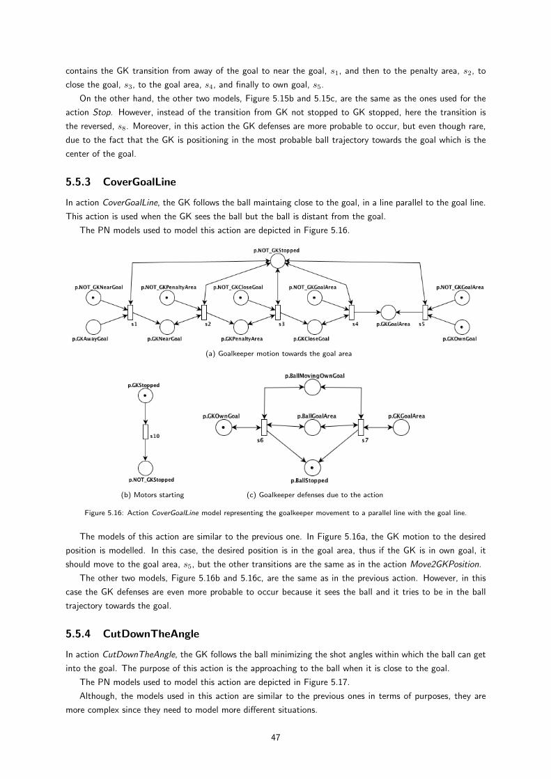
contains the GK transition from away of the goal to near the goal, s1, and then to the penalty area, s2, to
close the goal, s3, to the goal area, s4, and finally to own goal, s5.
On the other hand, the other two models, Figure 5.15b and 5.15c, are the same as the ones used for the
action Stop. However, instead of the transition from GK not stopped to GK stopped, here the transition is
the reversed, s8. Moreover, in this action the GK defenses are more probable to occur, but even though rare,
due to the fact that the GK is positioning in the most probable ball trajectory towards the goal which is the
center of the goal.
5.5.3 CoverGoalLine
In action CoverGoalLine, the GK follows the ball maintaing close to the goal, in a line parallel to the goal line.
This action is used when the GK sees the ball but the ball is distant from the goal.
The PN models used to model this action are depicted in Figure 5.16.
(a) Goalkeeper motion towards the goal area
(b) Motors starting (c) Goalkeeper defenses due to the action
Figure 5.16: Action CoverGoalLine model representing the goalkeeper movement to a parallel line with the goal line.
The models of this action are similar to the previous one. In Figure 5.16a, the GK motion to the desired
position is modelled. In this case, the desired position is in the goal area, thus if the GK is in own goal, it
should move to the goal area, s5, but the other transitions are the same as in the action Move2GKPosition.
The other two models, Figure 5.16b and 5.16c, are the same as in the previous action. However, in this
case the GK defenses are even more probable to occur because it sees the ball and it tries to be in the ball
trajectory towards the goal.
5.5.4 CutDownTheAngle
In action CutDownTheAngle, the GK follows the ball minimizing the shot angles within which the ball can get
into the goal. The purpose of this action is the approaching to the ball when it is close to the goal.
The PN models used to model this action are depicted in Figure 5.17.
Although, the models used in this action are similar to the previous ones in terms of purposes, they are
more complex since they need to model more different situations.
47
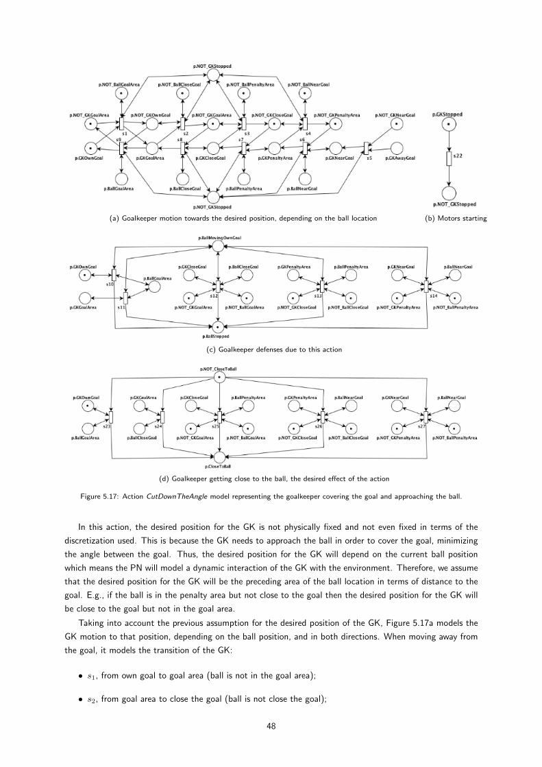
(a) Goalkeeper motion towards the desired position, depending on the ball location (b) Motors starting
(c) Goalkeeper defenses due to this action
(d) Goalkeeper getting close to the ball, the desired effect of the action
Figure 5.17: Action CutDownTheAngle model representing the goalkeeper covering the goal and approaching the ball.
In this action, the desired position for the GK is not physically fixed and not even fixed in terms of the
discretization used. This is because the GK needs to approach the ball in order to cover the goal, minimizing
the angle between the goal. Thus, the desired position for the GK will depend on the current ball position
which means the PN will model a dynamic interaction of the GK with the environment. Therefore, we assume
that the desired position for the GK will be the preceding area of the ball location in terms of distance to the
goal. E.g., if the ball is in the penalty area but not close to the goal then the desired position for the GK will
be close to the goal but not in the goal area.
Taking into account the previous assumption for the desired position of the GK, Figure 5.17a models the
GK motion to that position, depending on the ball position, and in both directions. When moving away from
the goal, it models the transition of the GK:
• s1, from own goal to goal area (ball is not in the goal area);
• s2, from goal area to close the goal (ball is not close the goal);
48
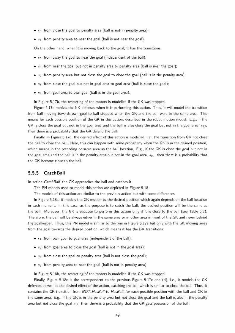
• s3, from close the goal to penalty area (ball is not in penalty area);
• s4, from penalty area to near the goal (ball is not near the goal).
On the other hand, when it is moving back to the goal, it has the transitions:
• s5, from away the goal to near the goal (independent of the ball);
• s6, from near the goal but not in penalty area to penalty area (ball is near the goal);
• s7, from penalty area but not close the goal to close the goal (ball is in the penalty area);
• s8, from close the goal but not in goal area to goal area (ball is close the goal);
• s9, from goal area to own goal (ball is in the goal area).
In Figure 5.17b, the restarting of the motors is modelled if the GK was stopped.
Figure 5.17c models the GK defenses when it is performing this action. Thus, it will model the transition
from ball moving towards own goal to ball stopped when the GK and the ball were in the same area. This
means for each possible position of the GK in this action, described in the robot motion model. E.g., if the
GK is close the goal but not in the goal area and the ball is also close the goal but not in the goal area, s12,
then there is a probability that the GK defend the ball.
Finally, in Figure 5.17d, the desired effect of this action is modelled, i.e., the transition from GK not close
the ball to close the ball. Here, this can happen with some probability when the GK is in the desired position,
which means in the preceding or same area as the ball location. E.g., if the GK is close the goal but not in
the goal area and the ball is in the penalty area but not in the goal area, s25, then there is a probability that
the GK become close to the ball.
5.5.5 CatchBall
In action CatchBall, the GK approaches the ball and catches it.
The PN models used to model this action are depicted in Figure 5.18.
The models of this action are similar to the previous action but with some differences.
In Figure 5.18a, it models the GK motion to the desired position which again depends on the ball location
in each moment. In this case, as the purpose is to catch the ball, the desired position will be the same as
the ball. Moreover, the GK is suppose to perform this action only if it is close to the ball (see Table 5.2).
Therefore, the ball will be always either in the same area or in other area in front of the GK and never behind
the goalkeeper. Thus, this PN model is similar to the one in Figure 5.17a but only with the GK moving away
from the goal towards the desired position, which means it has the GK transitions:
• s1, from own goal to goal area (independent of the ball);
• s2, from goal area to close the goal (ball is not in the goal area);
• s3, from close the goal to penalty area (ball is not close the goal);
• s4, from penalty area to near the goal (ball is not in penalty area).
In Figure 5.18b, the restarting of the motors is modelled if the GK was stopped.
Finally, Figure 5.18c is the correspondent to the previous Figure 5.17c and (d), i.e., it models the GK
defenses as well as the desired effect of the action, catching the ball which is similar to close the ball. Thus, it
contains the GK transition from NOT HasBall to HasBall, for each possible position with the ball and GK in
the same area. E.g., if the GK is in the penalty area but not close the goal and the ball is also in the penalty
area but not close the goal s11, then there is a probability that the GK gets possession of the ball.
49
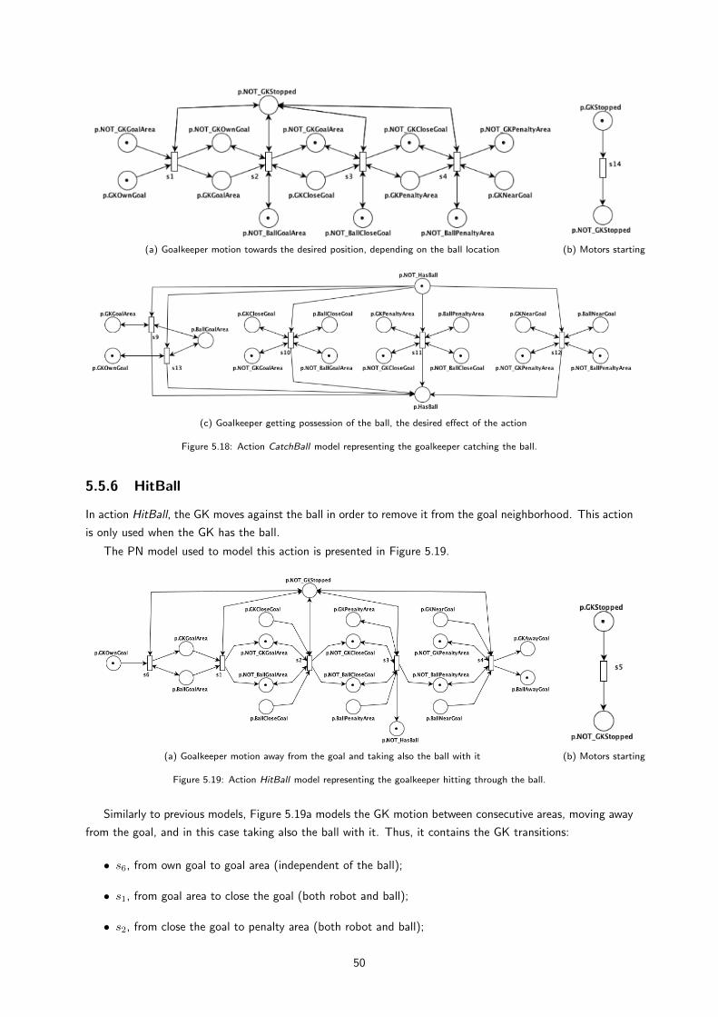
(a) Goalkeeper motion towards the desired position, depending on the ball location (b) Motors starting
(c) Goalkeeper getting possession of the ball, the desired effect of the action
Figure 5.18: Action CatchBall model representing the goalkeeper catching the ball.
5.5.6 HitBall
In action HitBall, the GK moves against the ball in order to remove it from the goal neighborhood. This action
is only used when the GK has the ball.
The PN model used to model this action is presented in Figure 5.19.
(a) Goalkeeper motion away from the goal and taking also the ball with it (b) Motors starting
Figure 5.19: Action HitBall model representing the goalkeeper hitting through the ball.
Similarly to previous models, Figure 5.19a models the GK motion between consecutive areas, moving away
from the goal, and in this case taking also the ball with it. Thus, it contains the GK transitions:
• s6, from own goal to goal area (independent of the ball);
• s1, from goal area to close the goal (both robot and ball);
• s2, from close the goal to penalty area (both robot and ball);
50
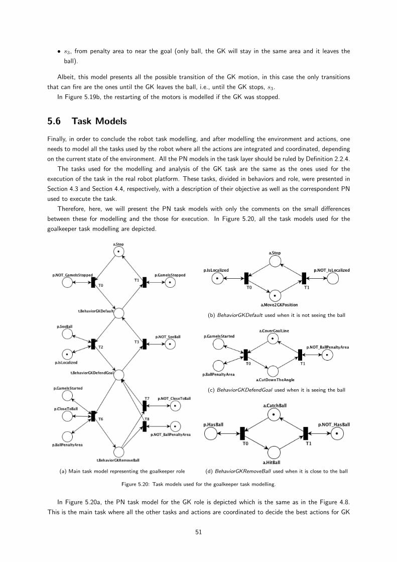
• s3, from penalty area to near the goal (only ball, the GK will stay in the same area and it leaves the
ball).
Albeit, this model presents all the possible transition of the GK motion, in this case the only transitions
that can fire are the ones until the GK leaves the ball, i.e., until the GK stops, s3.
In Figure 5.19b, the restarting of the motors is modelled if the GK was stopped.
5.6 Task Models
Finally, in order to conclude the robot task modelling, and after modelling the environment and actions, one
needs to model all the tasks used by the robot where all the actions are integrated and coordinated, depending
on the current state of the environment. All the PN models in the task layer should be ruled by Definition 2.2.4.
The tasks used for the modelling and analysis of the GK task are the same as the ones used for the
execution of the task in the real robot platform. These tasks, divided in behaviors and role, were presented in
Section 4.3 and Section 4.4, respectively, with a description of their objective as well as the correspondent PN
used to execute the task.
Therefore, here, we will present the PN task models with only the comments on the small differences
between these for modelling and the those for execution. In Figure 5.20, all the task models used for the
goalkeeper task modelling are depicted.
(a) Main task model representing the goalkeeper role
(b) BehaviorGKDefault used when it is not seeing the ball
(c) BehaviorGKDefendGoal used when it is seeing the ball
(d) BehaviorGKRemoveBall used when it is close to the ball
Figure 5.20: Task models used for the goalkeeper task modelling.
In Figure 5.20a, the PN task model for the GK role is depicted which is the same as in the Figure 4.8.
This is the main task where all the other tasks and actions are coordinated to decide the best actions for GK
51
to execute depending on the environment evaluation from the predicates. In this model, instead of using the
predicates ShouldGK that are a composition of predicates (see Section 4.1), it uses the predicates itself which,
together with the environment models, leads to a simpler model but with the same meaning.
In Figure 5.20b, the PN task model for the default behavior is depicted which is the same PN as in
Figure 4.5. This behavior is used by the GK when it is not seeing the ball and with the purpose of moving the
GK to the center of goal.
Then, Figure 5.20c presents the PN task model for the behavior to defend the goal. This PN is the same
as in Figure 4.6 but instead of using the ShoulGK predicate, it uses a simplification with the predicates itself.
This behavior is the one used by the GK to defend and cover the goal when it sees the ball.
Finally, in Figure 5.20d, the PN task model for the behavior to remove the ball is depicted which is the same
PN as in Figure 4.7. This behavior is used by the GK to catch the ball and remove it from the neighborhood
of the goal and it is only used when GK is close to the ball.
52

53

Chapter 6
Experimental Setup
This chapter aims at describing all the experimental setups used to analyse the performance of the GK task
in different situations as well as the performance of the GK task in the real robot framework.
For the performance analysis of the task, we use all PN models for the environment, actions and tasks
presented in Chapter 5. Whereas, for the execution of the task in the real robot platform we use the primitive
actions and the PN of the behaviors and role described in Chapter 4.
6.1 Task Analysis
In order to analyse the performance of the GK task, we perform different setups to compare the task perfor-
mance in different situations as well as with different GK behaviors. For these setups, we use a base setup
that models the entire GK task and then for the different setups we modified mainly the stochastic transitions
rates and some minor modifications in the PN models themselves.
The base setup, used in all the analysis experiments, includes the environment models (Section 5.4), the
action models (Section 5.5) and the task models (Section 5.6) that were described in the previous chapter.
In the base setup and also in the other setups, the knowledge of the environment is described towards the
predicates defined in Section 5.3. With these predicates, one should define the initial state of the world which,
in this case, includes the position and movement, both for the robot and ball, the referee commands and also
the other predicates. Therefore, for all the analysis setups, we considered that the initial position for the GK
was inside the own goal and for the ball was away from the goal. Moreover, we assume that the GK was
stopped as well as the ball which was also on the ground. Furthermore, the game was stopped and the GK
was correctly localized but it was not seeing the ball. All these considerations, results in the following initial
predicate state:
Definition 6.1.1. The initial predicate state for all the task analysis setups is defined as:
• GKOwnGoal, NOT GKGoalArea, NOT GKCloseGoal, NOT GKPenaltyArea, NOT GKNearGoal,
NOT GKAwayGoal;
• BallAwayGoal, NOT BallOwnGoal, NOT BallGoalArea, NOT BallCloseGoal, NOT BallPenaltyArea,
NOT BallNearGoal;
• GKStopped;
• BallStopped, BallOnTheGround, NOT BallMovingOwnGoal;
• GameIsStopped, NOT GameIsStarted;
54

• IsLocalized, NOT SeeBall, NOT HasBall, NOT CloseToBall.
After the definition of the initial state and also the PN models used for the task analysis, one needs to set
the firing rates of all the stochastic transitions which will depend on the situation we want to analyse, e.g.,
the type of opponent team we want to model.
Therefore, in the sequel we will define and describe all the experiments we setup for the task analysis as
well as the computation of all the stochastic transitions rates using the methods presented in Section 5.2
6.1.1 Base Setup with Different Opponent Teams and GoalKeeper Behaviors
This is the main experiment we perform to analyse the task performance of the GK and the purpose is to
compare the performance of the task with different opponent teams and also the performance of different
behaviors with each opponent team. Thus, we modelled four different opponent teams and three different GK
behaviors and we analyse the task performance for each combination of opponent team and GK behavior.
In order to model different GK behaviors, we need to change the way the GK decides which action it should
perform, thus the PN task models should be different for each behavior.
For the GK task models used in this work (see Section 5.6), one of the modifications that leads to a
significant different behaviors is the way GK decides when to start approaching the ball and then when it
should stop removing the ball from the goal neighborhood, i.e., when it should leave the ball and return to
the goal.
To understand better this difference, we should summarize the different stages of the GK behavior. When
the GK sees the ball, first it covers the goal close to it, following the ball, with action CoverGoalLine. Then,
when the ball enters a certain area, the GK will cover the angle between the ball and the goal, following the
ball and approaching it, with action CutDownTheAngle. Finally, if the GK catches the ball, it will remove the
ball from the neighborhood of the goal with action HitBall, pushing the ball until it leaves the same area as
before. This area will be named as decision area.
Therefore, if we change this decision area, we will have a completely different GK behavior. These different
behaviors as well as the respective decision area are described in Table 6.1. In these three different GK
behaviors we assume that the GK mean velocity is the same for all.
Table 6.1: Different behaviors used in the Goalkeeper task analysis depending on the decision area.
Behavior Decision Area Type of Behavior Velocity
GKa BallCloseGoal Defensive 1.5m/s
GKb BallPenaltyArea Intermediate 1.5m/s
GKc BallNearGoal Offensive 1.5m/s
In Chapter 5, we presented the GK task model for the case of the intermediate behavior, i.e., with the
decision area as BallPenaltyArea. Thus, it is important to explain the differences in the PN models for each
one of the GK behaviors.
In the main task, the GK role (see Figure 5.20a), the predicate places used for start and stop the re-
move ball behavior should be updated to the respective decision area, i.e., the BallPenaltyArea, T6, and the
NOT BallPenaltyArea, T8, places. The same should be done in the behavior used to defend the goal (see
Figure 5.20c), in order to switch to the action CutDownTheAngle depending on the decision area. Finally, the
HitBall action model should be also updated depending on the decision area. In this action (see Figure 5.19a),
the act of leaving the ball is modelled with the transition from HasBall to NOT HasBall, s3. Therefore, this
transition to not has the ball should occur in s2, if the decision area is BallCloseGoal, and in s4, if the decision
area is BallNearGoal.
55
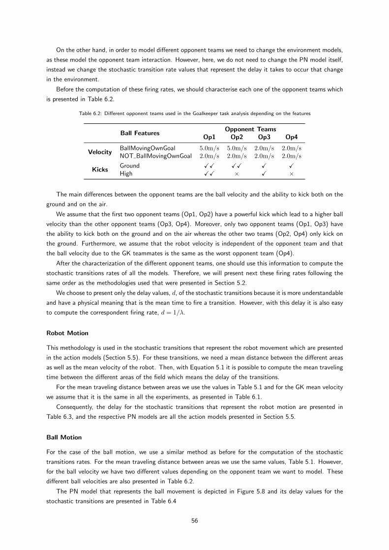
On the other hand, in order to model different opponent teams we need to change the environment models,
as these model the opponent team interaction. However, here, we do not need to change the PN model itself,
instead we change the stochastic transition rate values that represent the delay it takes to occur that change
in the environment.
Before the computation of these firing rates, we should characterise each one of the opponent teams which
is presented in Table 6.2.
Table 6.2: Different opponent teams used in the Goalkeeper task analysis depending on the features
Ball FeaturesOpponent Teams
Op1 Op2 Op3 Op4
VelocityBallMovingOwnGoal 5.0m/s 5.0m/s 2.0m/s 2.0m/sNOT BallMovingOwnGoal 2.0m/s 2.0m/s 2.0m/s 2.0m/s
KicksGround XX XX X XHigh XX × X ×
The main differences between the opponent teams are the ball velocity and the ability to kick both on the
ground and on the air.
We assume that the first two opponent teams (Op1, Op2) have a powerful kick which lead to a higher ball
velocity than the other opponent teams (Op3, Op4). Moreover, only two opponent teams (Op1, Op3) have
the ability to kick both on the ground and on the air whereas the other two teams (Op2, Op4) only kick on
the ground. Furthermore, we assume that the robot velocity is independent of the opponent team and that
the ball velocity due to the GK teammates is the same as the worst opponent team (Op4).
After the characterization of the different opponent teams, one should use this information to compute the
stochastic transitions rates of all the models. Therefore, we will present next these firing rates following the
same order as the methodologies used that were presented in Section 5.2.
We choose to present only the delay values, d, of the stochastic transitions because it is more understandable
and have a physical meaning that is the mean time to fire a transition. However, with this delay it is also easy
to compute the correspondent firing rate, d = 1/λ.
Robot Motion
This methodology is used in the stochastic transitions that represent the robot movement which are presented
in the action models (Section 5.5). For these transitions, we need a mean distance between the different areas
as well as the mean velocity of the robot. Then, with Equation 5.1 it is possible to compute the mean traveling
time between the different areas of the field which means the delay of the transitions.
For the mean traveling distance between areas we use the values in Table 5.1 and for the GK mean velocity
we assume that it is the same in all the experiments, as presented in Table 6.1.
Consequently, the delay for the stochastic transitions that represent the robot motion are presented in
Table 6.3, and the respective PN models are all the action models presented in Section 5.5.
Ball Motion
For the case of the ball motion, we use a similar method as before for the computation of the stochastic
transitions rates. For the mean traveling distance between areas we use the same values, Table 5.1. However,
for the ball velocity we have two different values depending on the opponent team we want to model. These
different ball velocities are also presented in Table 6.2.
The PN model that represents the ball movement is depicted in Figure 5.8 and its delay values for the
stochastic transitions are presented in Table 6.4
56
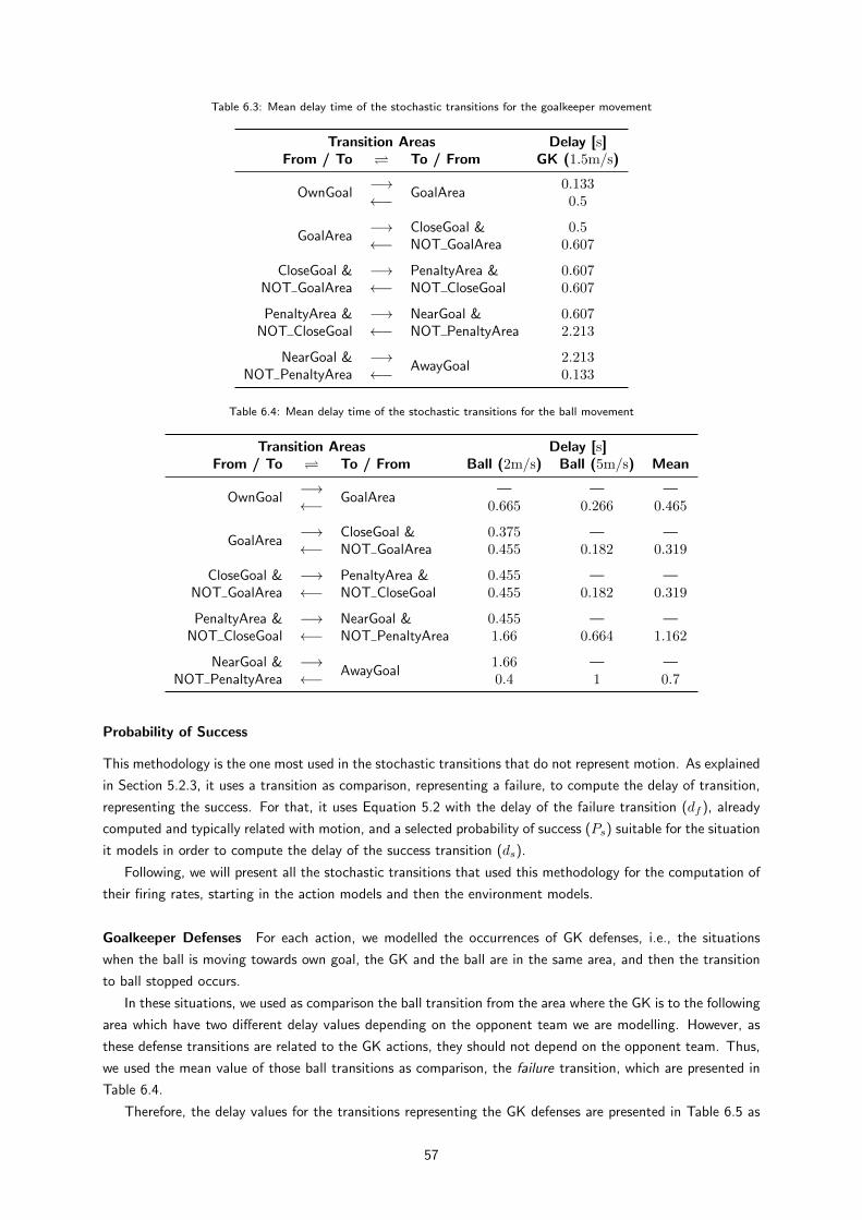
Table 6.3: Mean delay time of the stochastic transitions for the goalkeeper movement
Transition Areas Delay [s]From / To To / From GK (1.5m/s)
OwnGoal−→
GoalArea0.133
←− 0.5
GoalArea−→ CloseGoal & 0.5←− NOT GoalArea 0.607
CloseGoal & −→ PenaltyArea & 0.607NOT GoalArea ←− NOT CloseGoal 0.607
PenaltyArea & −→ NearGoal & 0.607NOT CloseGoal ←− NOT PenaltyArea 2.213
NearGoal & −→AwayGoal
2.213NOT PenaltyArea ←− 0.133
Table 6.4: Mean delay time of the stochastic transitions for the ball movement
Transition Areas Delay [s]From / To To / From Ball (2m/s) Ball (5m/s) Mean
OwnGoal−→
GoalArea— — —
←− 0.665 0.266 0.465
GoalArea−→ CloseGoal & 0.375 — —←− NOT GoalArea 0.455 0.182 0.319
CloseGoal & −→ PenaltyArea & 0.455 — —NOT GoalArea ←− NOT CloseGoal 0.455 0.182 0.319
PenaltyArea & −→ NearGoal & 0.455 — —NOT CloseGoal ←− NOT PenaltyArea 1.66 0.664 1.162
NearGoal & −→AwayGoal
1.66 — —NOT PenaltyArea ←− 0.4 1 0.7
Probability of Success
This methodology is the one most used in the stochastic transitions that do not represent motion. As explained
in Section 5.2.3, it uses a transition as comparison, representing a failure, to compute the delay of transition,
representing the success. For that, it uses Equation 5.2 with the delay of the failure transition (df ), already
computed and typically related with motion, and a selected probability of success (Ps) suitable for the situation
it models in order to compute the delay of the success transition (ds).
Following, we will present all the stochastic transitions that used this methodology for the computation of
their firing rates, starting in the action models and then the environment models.
Goalkeeper Defenses For each action, we modelled the occurrences of GK defenses, i.e., the situations
when the ball is moving towards own goal, the GK and the ball are in the same area, and then the transition
to ball stopped occurs.
In these situations, we used as comparison the ball transition from the area where the GK is to the following
area which have two different delay values depending on the opponent team we are modelling. However, as
these defense transitions are related to the GK actions, they should not depend on the opponent team. Thus,
we used the mean value of those ball transitions as comparison, the failure transition, which are presented in
Table 6.4.
Therefore, the delay values for the transitions representing the GK defenses are presented in Table 6.5 as
57
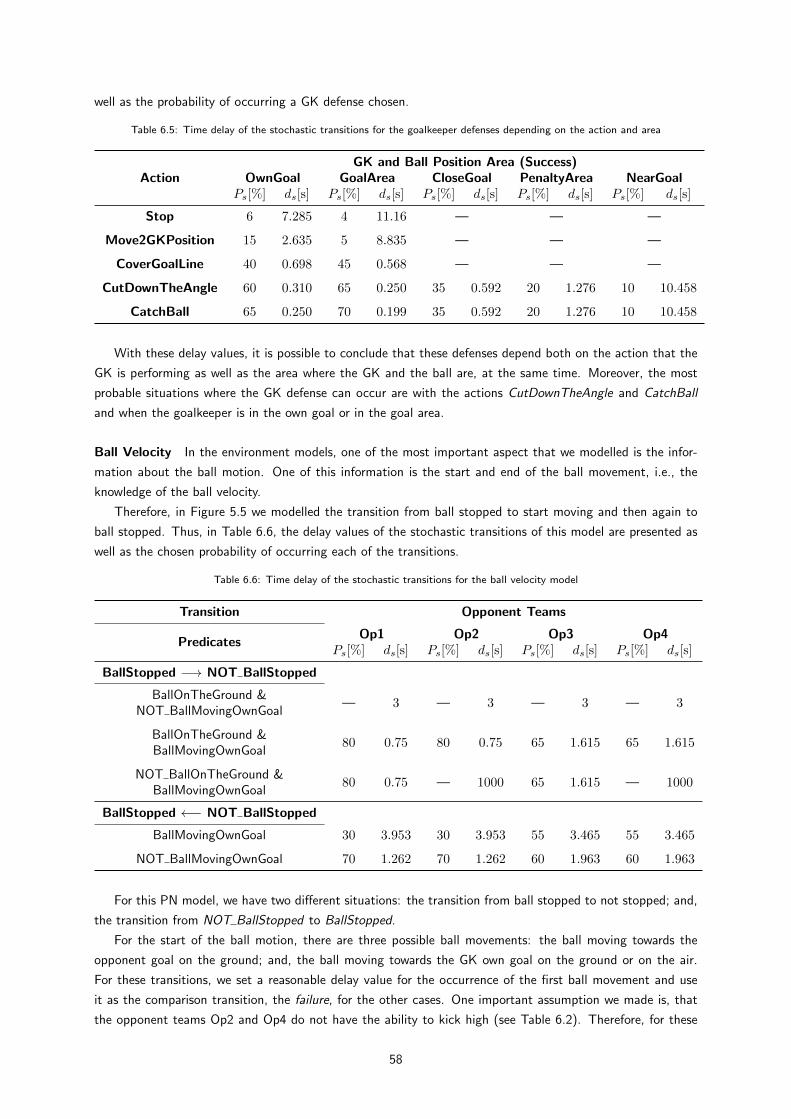
well as the probability of occurring a GK defense chosen.
Table 6.5: Time delay of the stochastic transitions for the goalkeeper defenses depending on the action and area
ActionGK and Ball Position Area (Success)
OwnGoal GoalArea CloseGoal PenaltyArea NearGoalPs[%] ds[s] Ps[%] ds[s] Ps[%] ds[s] Ps[%] ds[s] Ps[%] ds[s]
Stop 6 7.285 4 11.16 — — —
Move2GKPosition 15 2.635 5 8.835 — — —
CoverGoalLine 40 0.698 45 0.568 — — —
CutDownTheAngle 60 0.310 65 0.250 35 0.592 20 1.276 10 10.458
CatchBall 65 0.250 70 0.199 35 0.592 20 1.276 10 10.458
With these delay values, it is possible to conclude that these defenses depend both on the action that the
GK is performing as well as the area where the GK and the ball are, at the same time. Moreover, the most
probable situations where the GK defense can occur are with the actions CutDownTheAngle and CatchBall
and when the goalkeeper is in the own goal or in the goal area.
Ball Velocity In the environment models, one of the most important aspect that we modelled is the infor-
mation about the ball motion. One of this information is the start and end of the ball movement, i.e., the
knowledge of the ball velocity.
Therefore, in Figure 5.5 we modelled the transition from ball stopped to start moving and then again to
ball stopped. Thus, in Table 6.6, the delay values of the stochastic transitions of this model are presented as
well as the chosen probability of occurring each of the transitions.
Table 6.6: Time delay of the stochastic transitions for the ball velocity model
Transition Opponent Teams
PredicatesOp1 Op2 Op3 Op4
Ps[%] ds[s] Ps[%] ds[s] Ps[%] ds[s] Ps[%] ds[s]
BallStopped −→ NOT BallStopped
BallOnTheGround &— 3 — 3 — 3 — 3
NOT BallMovingOwnGoal
BallOnTheGround &80 0.75 80 0.75 65 1.615 65 1.615
BallMovingOwnGoal
NOT BallOnTheGround &80 0.75 — 1000 65 1.615 — 1000
BallMovingOwnGoal
BallStopped ←− NOT BallStopped
BallMovingOwnGoal 30 3.953 30 3.953 55 3.465 55 3.465
NOT BallMovingOwnGoal 70 1.262 70 1.262 60 1.963 60 1.963
For this PN model, we have two different situations: the transition from ball stopped to not stopped; and,
the transition from NOT BallStopped to BallStopped.
For the start of the ball motion, there are three possible ball movements: the ball moving towards the
opponent goal on the ground; and, the ball moving towards the GK own goal on the ground or on the air.
For these transitions, we set a reasonable delay value for the occurrence of the first ball movement and use
it as the comparison transition, the failure, for the other cases. One important assumption we made is, that
the opponent teams Op2 and Op4 do not have the ability to kick high (see Table 6.2). Therefore, for these
58
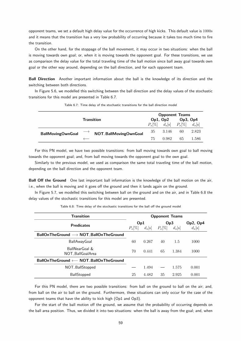
opponent teams, we set a default high delay value for the occurrence of high kicks. This default value is 1000s
and it means that the transition has a very low probability of occurring because it takes too much time to fire
the transition.
On the other hand, for the stoppage of the ball movement, it may occur in two situations: when the ball
is moving towards own goal; or, when it is moving towards the opponent goal. For these transitions, we use
as comparison the delay value for the total traveling time of the ball motion since ball away goal towards own
goal or the other way around, depending on the ball direction, and for each opponent team.
Ball Direction Another important information about the ball is the knowledge of its direction and the
switching between both directions.
In Figure 5.6, we modelled this switching between the ball direction and the delay values of the stochastic
transitions for this model are presented in Table 6.7.
Table 6.7: Time delay of the stochastic transitions for the ball direction model
TransitionOpponent Teams
Op1, Op2 Op3, Op4Ps[%] ds[s] Ps[%] ds[s]
BallMovingOwnGoal−→
NOT BallMovingOwnGoal35 3.146 60 2.823
←− 75 0.982 65 1.586
For this PN model, we have two possible transitions: from ball moving towards own goal to ball moving
towards the opponent goal; and, from ball moving towards the opponent goal to the own goal.
Similarly to the previous model, we used as comparison the same total traveling time of the ball motion,
depending on the ball direction and the opponent team.
Ball Off the Ground One last important ball information is the knowledge of the ball motion on the air,
i.e., when the ball is moving and it goes off the ground and then it lands again on the ground.
In Figure 5.7, we modelled this switching between ball on the ground and on the air, and in Table 6.8 the
delay values of the stochastic transitions for this model are presented.
Table 6.8: Time delay of the stochastic transitions for the ball off the ground model
Transition Opponent Teams
PredicatesOp1 Op3 Op2, Op4
Ps[%] ds[s] Ps[%] ds[s] ds[s]
BallOnTheGround −→ NOT BallOnTheGround
BallAwayGoal 60 0.267 40 1.5 1000
BallNearGoal &70 0.441 65 1.384 1000
NOT BallGoalArea
BallOnTheGround ←− NOT BallOnTheGround
NOT BallStopped — 1.494 — 1.575 0.001
BallStopped 25 4.482 35 2.925 0.001
For this PN model, there are two possible transitions: from ball on the ground to ball on the air; and,
from ball on the air to ball on the ground. Furthermore, these situations can only occur for the case of the
opponent teams that have the ability to kick high (Op1 and Op3).
For the start of the ball motion off the ground, we assume that the probability of occurring depends on
the ball area position. Thus, we divided it into two situations: when the ball is away from the goal; and, when
59
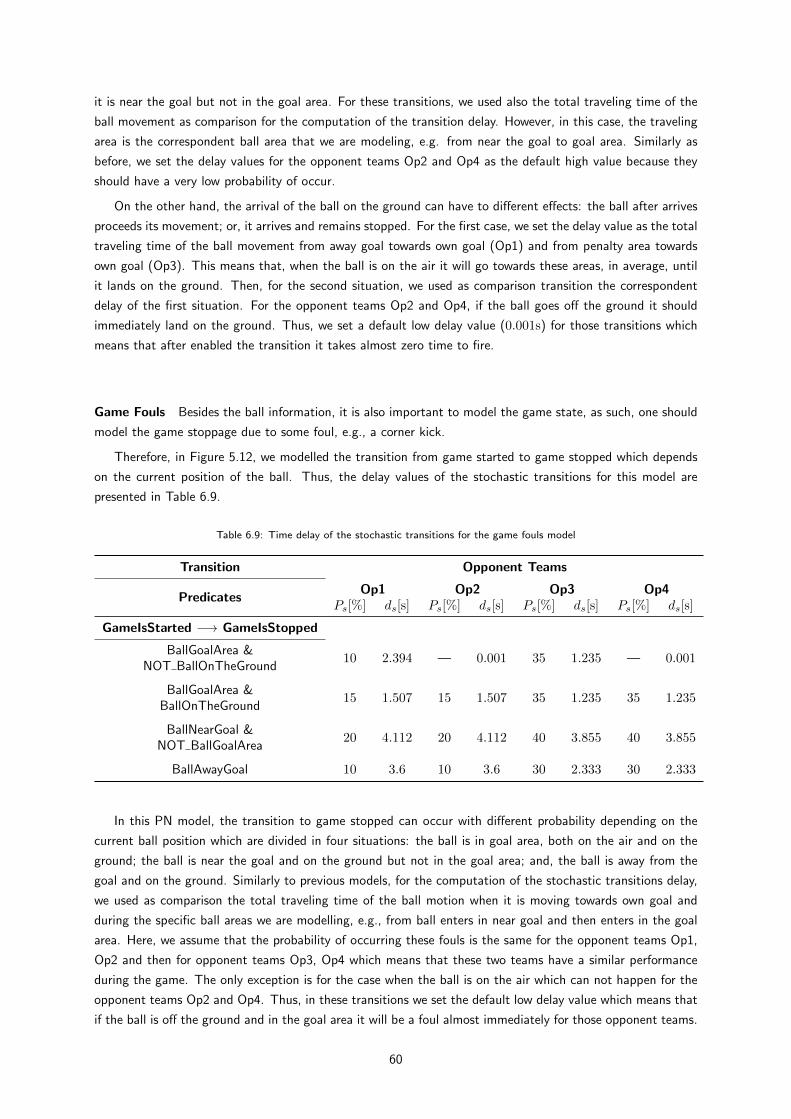
it is near the goal but not in the goal area. For these transitions, we used also the total traveling time of the
ball movement as comparison for the computation of the transition delay. However, in this case, the traveling
area is the correspondent ball area that we are modeling, e.g. from near the goal to goal area. Similarly as
before, we set the delay values for the opponent teams Op2 and Op4 as the default high value because they
should have a very low probability of occur.
On the other hand, the arrival of the ball on the ground can have to different effects: the ball after arrives
proceeds its movement; or, it arrives and remains stopped. For the first case, we set the delay value as the total
traveling time of the ball movement from away goal towards own goal (Op1) and from penalty area towards
own goal (Op3). This means that, when the ball is on the air it will go towards these areas, in average, until
it lands on the ground. Then, for the second situation, we used as comparison transition the correspondent
delay of the first situation. For the opponent teams Op2 and Op4, if the ball goes off the ground it should
immediately land on the ground. Thus, we set a default low delay value (0.001s) for those transitions which
means that after enabled the transition it takes almost zero time to fire.
Game Fouls Besides the ball information, it is also important to model the game state, as such, one should
model the game stoppage due to some foul, e.g., a corner kick.
Therefore, in Figure 5.12, we modelled the transition from game started to game stopped which depends
on the current position of the ball. Thus, the delay values of the stochastic transitions for this model are
presented in Table 6.9.
Table 6.9: Time delay of the stochastic transitions for the game fouls model
Transition Opponent Teams
PredicatesOp1 Op2 Op3 Op4
Ps[%] ds[s] Ps[%] ds[s] Ps[%] ds[s] Ps[%] ds[s]
GameIsStarted −→ GameIsStopped
BallGoalArea &10 2.394 — 0.001 35 1.235 — 0.001
NOT BallOnTheGround
BallGoalArea &15 1.507 15 1.507 35 1.235 35 1.235
BallOnTheGround
BallNearGoal &20 4.112 20 4.112 40 3.855 40 3.855
NOT BallGoalArea
BallAwayGoal 10 3.6 10 3.6 30 2.333 30 2.333
In this PN model, the transition to game stopped can occur with different probability depending on the
current ball position which are divided in four situations: the ball is in goal area, both on the air and on the
ground; the ball is near the goal and on the ground but not in the goal area; and, the ball is away from the
goal and on the ground. Similarly to previous models, for the computation of the stochastic transitions delay,
we used as comparison the total traveling time of the ball motion when it is moving towards own goal and
during the specific ball areas we are modelling, e.g., from ball enters in near goal and then enters in the goal
area. Here, we assume that the probability of occurring these fouls is the same for the opponent teams Op1,
Op2 and then for opponent teams Op3, Op4 which means that these two teams have a similar performance
during the game. The only exception is for the case when the ball is on the air which can not happen for the
opponent teams Op2 and Op4. Thus, in these transitions we set the default low delay value which means that
if the ball is off the ground and in the goal area it will be a foul almost immediately for those opponent teams.
60
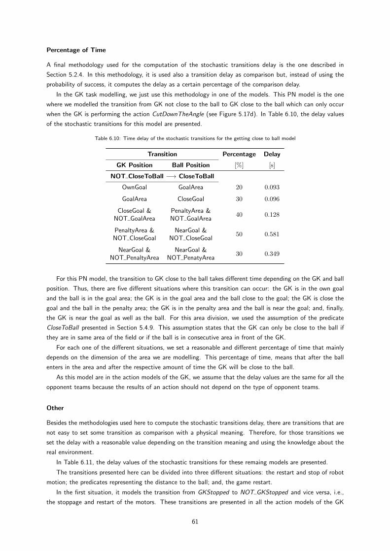
Percentage of Time
A final methodology used for the computation of the stochastic transitions delay is the one described in
Section 5.2.4. In this methodology, it is used also a transition delay as comparison but, instead of using the
probability of success, it computes the delay as a certain percentage of the comparison delay.
In the GK task modelling, we just use this methodology in one of the models. This PN model is the one
where we modelled the transition from GK not close to the ball to GK close to the ball which can only occur
when the GK is performing the action CutDownTheAngle (see Figure 5.17d). In Table 6.10, the delay values
of the stochastic transitions for this model are presented.
Table 6.10: Time delay of the stochastic transitions for the getting close to ball model
Transition Percentage Delay
GK Position Ball Position [%] [s]
NOT CloseToBall −→ CloseToBall
OwnGoal GoalArea 20 0.093
GoalArea CloseGoal 30 0.096
CloseGoal & PenaltyArea &40 0.128
NOT GoalArea NOT GoalArea
PenaltyArea & NearGoal &50 0.581
NOT CloseGoal NOT CloseGoal
NearGoal & NearGoal &30 0.349
NOT PenaltyArea NOT PenatyArea
For this PN model, the transition to GK close to the ball takes different time depending on the GK and ball
position. Thus, there are five different situations where this transition can occur: the GK is in the own goal
and the ball is in the goal area; the GK is in the goal area and the ball close to the goal; the GK is close the
goal and the ball in the penalty area; the GK is in the penalty area and the ball is near the goal; and, finally,
the GK is near the goal as well as the ball. For this area division, we used the assumption of the predicate
CloseToBall presented in Section 5.4.9. This assumption states that the GK can only be close to the ball if
they are in same area of the field or if the ball is in consecutive area in front of the GK.
For each one of the different situations, we set a reasonable and different percentage of time that mainly
depends on the dimension of the area we are modelling. This percentage of time, means that after the ball
enters in the area and after the respective amount of time the GK will be close to the ball.
As this model are in the action models of the GK, we assume that the delay values are the same for all the
opponent teams because the results of an action should not depend on the type of opponent teams.
Other
Besides the methodologies used here to compute the stochastic transitions delay, there are transitions that are
not easy to set some transition as comparison with a physical meaning. Therefore, for those transitions we
set the delay with a reasonable value depending on the transition meaning and using the knowledge about the
real environment.
In Table 6.11, the delay values of the stochastic transitions for these remaing models are presented.
The transitions presented here can be divided into three different situations: the restart and stop of robot
motion; the predicates representing the distance to the ball; and, the game restart.
In the first situation, it models the transition from GKStopped to NOT GKStopped and vice versa, i.e.,
the stoppage and restart of the motors. These transitions are presented in all the action models of the GK
61
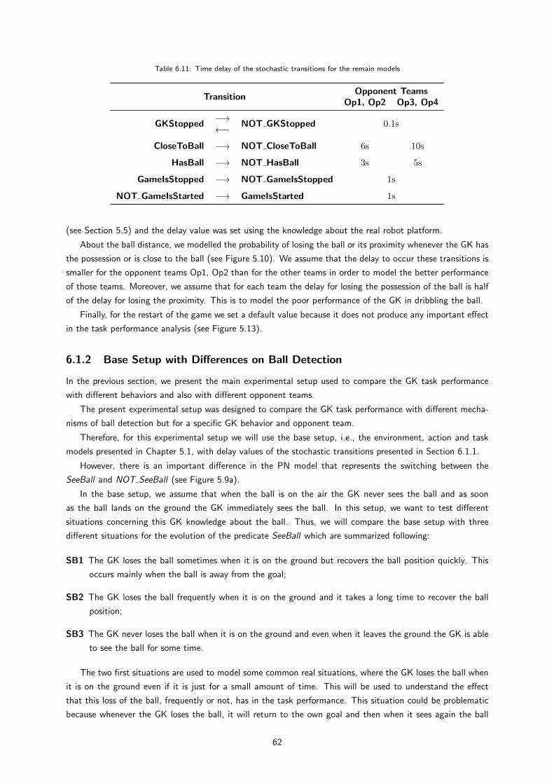
Table 6.11: Time delay of the stochastic transitions for the remain models
TransitionOpponent Teams
Op1, Op2 Op3, Op4
GKStopped−→
NOT GKStopped 0.1s←−
CloseToBall −→ NOT CloseToBall 6s 10s
HasBall −→ NOT HasBall 3s 5s
GameIsStopped −→ NOT GameIsStopped 1s
NOT GameIsStarted −→ GameIsStarted 1s
(see Section 5.5) and the delay value was set using the knowledge about the real robot platform.
About the ball distance, we modelled the probability of losing the ball or its proximity whenever the GK has
the possession or is close to the ball (see Figure 5.10). We assume that the delay to occur these transitions is
smaller for the opponent teams Op1, Op2 than for the other teams in order to model the better performance
of those teams. Moreover, we assume that for each team the delay for losing the possession of the ball is half
of the delay for losing the proximity. This is to model the poor performance of the GK in dribbling the ball.
Finally, for the restart of the game we set a default value because it does not produce any important effect
in the task performance analysis (see Figure 5.13).
6.1.2 Base Setup with Differences on Ball Detection
In the previous section, we present the main experimental setup used to compare the GK task performance
with different behaviors and also with different opponent teams.
The present experimental setup was designed to compare the GK task performance with different mecha-
nisms of ball detection but for a specific GK behavior and opponent team.
Therefore, for this experimental setup we will use the base setup, i.e., the environment, action and task
models presented in Chapter 5.1, with delay values of the stochastic transitions presented in Section 6.1.1.
However, there is an important difference in the PN model that represents the switching between the
SeeBall and NOT SeeBall (see Figure 5.9a).
In the base setup, we assume that when the ball is on the air the GK never sees the ball and as soon
as the ball lands on the ground the GK immediately sees the ball. In this setup, we want to test different
situations concerning this GK knowledge about the ball. Thus, we will compare the base setup with three
different situations for the evolution of the predicate SeeBall which are summarized following:
SB1 The GK loses the ball sometimes when it is on the ground but recovers the ball position quickly. This
occurs mainly when the ball is away from the goal;
SB2 The GK loses the ball frequently when it is on the ground and it takes a long time to recover the ball
position;
SB3 The GK never loses the ball when it is on the ground and even when it leaves the ground the GK is able
to see the ball for some time.
The two first situations are used to model some common real situations, where the GK loses the ball when
it is on the ground even if it is just for a small amount of time. This will be used to understand the effect
that this loss of the ball, frequently or not, has in the task performance. This situation could be problematic
because whenever the GK loses the ball, it will return to the own goal and then when it sees again the ball
62
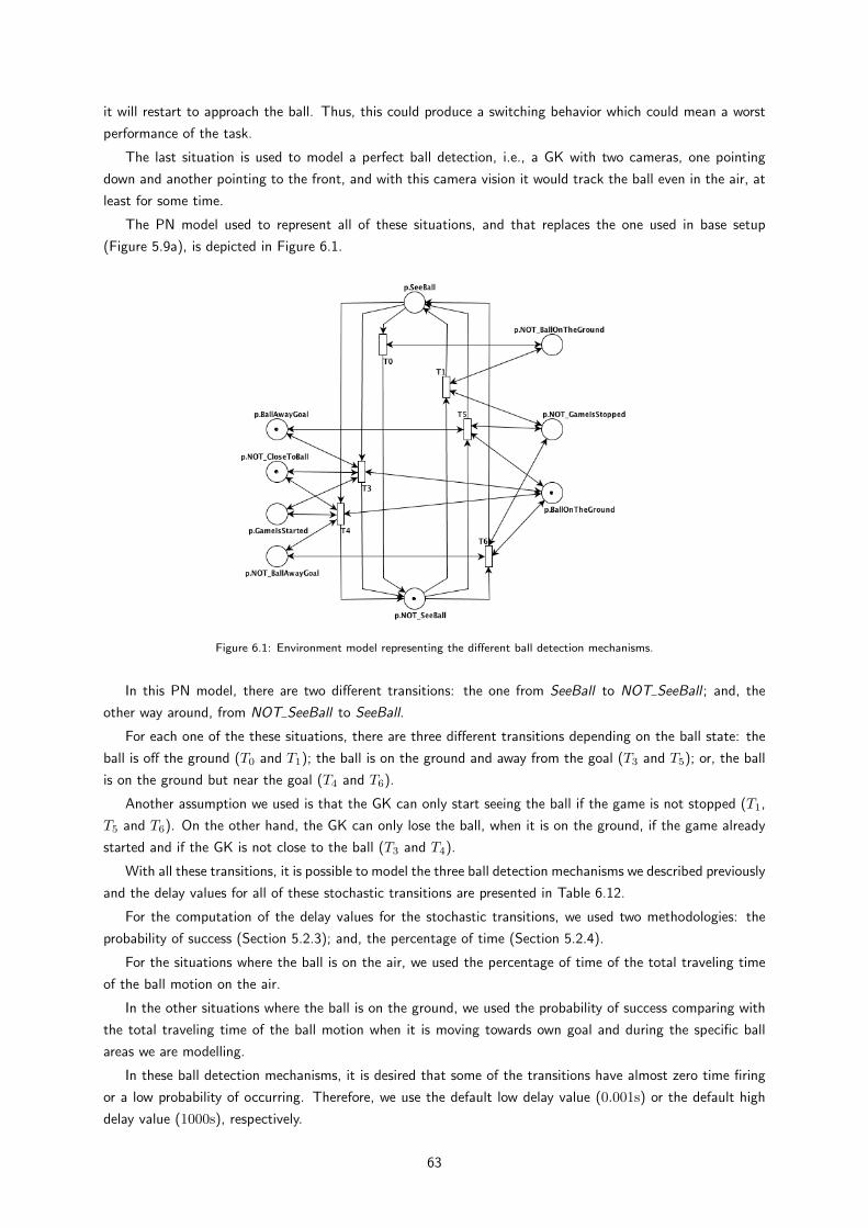
it will restart to approach the ball. Thus, this could produce a switching behavior which could mean a worst
performance of the task.
The last situation is used to model a perfect ball detection, i.e., a GK with two cameras, one pointing
down and another pointing to the front, and with this camera vision it would track the ball even in the air, at
least for some time.
The PN model used to represent all of these situations, and that replaces the one used in base setup
(Figure 5.9a), is depicted in Figure 6.1.
Figure 6.1: Environment model representing the different ball detection mechanisms.
In this PN model, there are two different transitions: the one from SeeBall to NOT SeeBall ; and, the
other way around, from NOT SeeBall to SeeBall.
For each one of the these situations, there are three different transitions depending on the ball state: the
ball is off the ground (T0 and T1); the ball is on the ground and away from the goal (T3 and T5); or, the ball
is on the ground but near the goal (T4 and T6).
Another assumption we used is that the GK can only start seeing the ball if the game is not stopped (T1,
T5 and T6). On the other hand, the GK can only lose the ball, when it is on the ground, if the game already
started and if the GK is not close to the ball (T3 and T4).
With all these transitions, it is possible to model the three ball detection mechanisms we described previously
and the delay values for all of these stochastic transitions are presented in Table 6.12.
For the computation of the delay values for the stochastic transitions, we used two methodologies: the
probability of success (Section 5.2.3); and, the percentage of time (Section 5.2.4).
For the situations where the ball is on the air, we used the percentage of time of the total traveling time
of the ball motion on the air.
In the other situations where the ball is on the ground, we used the probability of success comparing with
the total traveling time of the ball motion when it is moving towards own goal and during the specific ball
areas we are modelling.
In these ball detection mechanisms, it is desired that some of the transitions have almost zero time firing
or a low probability of occurring. Therefore, we use the default low delay value (0.001s) or the default high
delay value (1000s), respectively.
63

Table 6.12: Time delay of the stochastic transitions for the ball detection mechanisms model
Transition Ball Detection Mechanism
PredicatesSB1 SB2 SB2
Ps[%] ds[s] Ps[%] ds[s] Ps[%] ds[s]
SeeBall −→ NOT SeeBall
NOT BallOnTheGround — 0.001 — 0.001 20 0.299
BallOnTheGround &15 2.267 45 0.489 — 1000
BallAwayGoal
BallOnTheGround &10 11.646 40 1.941 — 1000
NOT BallAwayGoal
SeeBall ←− NOT SeeBall
NOT BallOnTheGround — 1000 — 1000 80 0.896
BallOnTheGround &70 0.171 40 0.6 — 0.001
BallAwayGoal
BallOnTheGround &90 0.144 60 0.863 — 0.001
NOT BallAwayGoal
6.1.3 Base Setup with Differences on Self-Localization
Finally, one last experimental setup we used for the GK task performance analysis is to compare the base setup
with different performances of the self-localization algorithm.
In the base setup, we assume that the GK is always localized, i.e., it has always a perfect knowledge about
its own position in the field.
Therefore, and similarly to the previous experimental setup, we compare the base setup with two different
situations for the evolution of the predicate IsLocalized which are summarized following:
IL1 The GK loses its localization sometimes but it recovers quickly;
IL2 The GK loses its localization frequently and it takes a long time to recover.
These situations are used to test the robustness of the GK task performance when it loses the localization,
frequently or not.
In this experimental setup, we also used the same environment, action and task models as for the base setup
(Chapter 5) and the same stochastic transition delay values as for the main experimental setup, presented in
Section 6.1.1.
However, in order to model the different situations described previously, we need to add a new environment
model that represents this switching of the predicate IsLocalized. This PN model is depicted in Figure 6.2.
In this PN model, there are two different transitions: from GK IsLocalized to NOT IsLocalized (T0, T1 and
T2); and, from GK NOT IsLocalized to IsLocalized (T3, T4 and T5). For each one of these transitions, there
are also three different situations depending on the GK state: the GK is in the own goal (T0 and T5); the GK
is in the goal area (T1 and T4); and, the GK is in the penalty area but not in the goal area (T2 and T3). We
assume that the GK only loses the localization in these possible areas of the field with different probability.
In Table 6.13, the delay values of the stochastic transitions, that model this experimental setup, are
presented.
Similarly to the previous experimental setup, we used the method of the probability of success to compute
the delay value of the stochastic transitions (see Section 5.2.3). Moreover, as comparison delay we use the
total traveling time of the ball motion when it is moving towards own goal and during the specific ball areas
we are modelling.
64
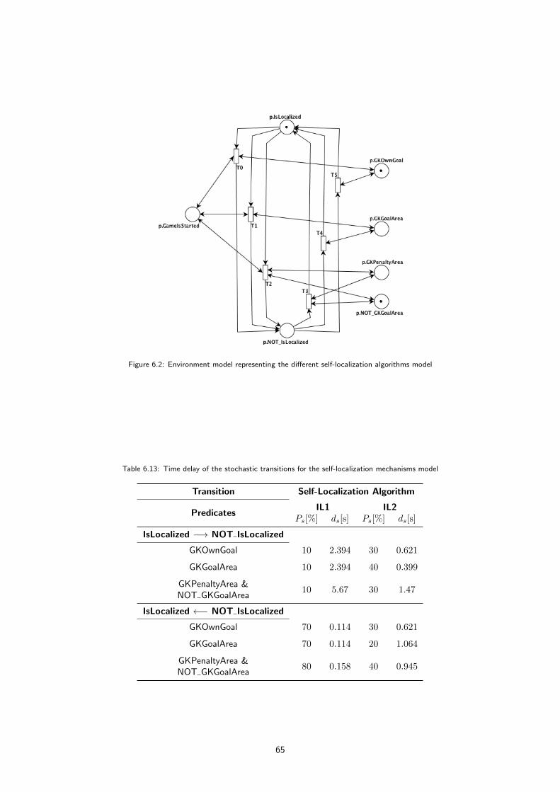
Figure 6.2: Environment model representing the different self-localization algorithms model
Table 6.13: Time delay of the stochastic transitions for the self-localization mechanisms model
Transition Self-Localization Algorithm
PredicatesIL1 IL2
Ps[%] ds[s] Ps[%] ds[s]
IsLocalized −→ NOT IsLocalized
GKOwnGoal 10 2.394 30 0.621
GKGoalArea 10 2.394 40 0.399
GKPenaltyArea &10 5.67 30 1.47
NOT GKGoalArea
IsLocalized ←− NOT IsLocalized
GKOwnGoal 70 0.114 30 0.621
GKGoalArea 70 0.114 20 1.064
GKPenaltyArea &80 0.158 40 0.945
NOT GKGoalArea
65
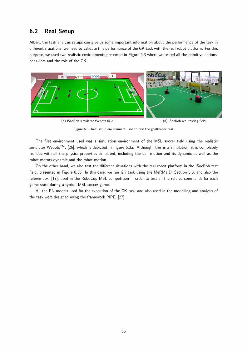
6.2 Real Setup
Albeit, the task analysis setups can give us some important information about the performance of the task in
different situations, we need to validate this performance of the GK task with the real robot platform. For this
purpose, we used two realistic environments presented in Figure 6.3 where we tested all the primitive actions,
behaviors and the role of the GK.
(a) ISocRob simulator Webots field (b) ISocRob real testing field
Figure 6.3: Real setup environment used to test the goalkeeper task
The first environment used was a simulation environment of the MSL soccer field using the realistic
simulator WebotsTM, [26], which is depicted in Figure 6.3a. Although, this is a simulation, it is completely
realistic with all the physics properties simulated, including the ball motion and its dynamic as well as the
robot motors dynamic and the robot motion.
On the other hand, we also test the different situations with the real robot platform in the ISocRob test
field, presented in Figure 6.3b. In this case, we run GK task using the MeRMaID, Section 3.3, and also the
referee box, [17], used in the RoboCup MSL competition in order to test all the referee commands for each
game state during a typical MSL soccer game.
All the PN models used for the execution of the GK task and also used in the modelling and analysis of
the task were designed using the framework PIPE, [27].
66

67
Chapter 7
Results
This chapter aims at presenting all the results obtained using the experimental setups described in Chapter 6,
both for the analysis of the GK task performance and also its execution in the real robot platform.
7.1 Task Analysis
In Chapter 5, the base setup used to model the GK task was explained, including all the environment, action
and task models. Then, in Section 6.1, the experimental setups used to compare the GK task performance
in different situations were described, including the differences from the base setup for each model as well as
the differences in the stochastic transition firing rates. Finally, in this section we will present all the analysis
results of the GK task performance for each one of the experimental setups.
As explained in Section 6.1, the initial predicate state is the same for all the analysis setups and it is defined
as in Definition 6.1.1, with the GK initial position in the own goal and the ball starting away from the goal.
Another important remark, for all the analysis setups, is that none of the actions and neither the environ-
ment models perform changes on the environment when the ball is inside the GK own goal. Therefore, one
can expect the GK task to include a deadlock, corresponding to scored goals in own goal.
Qualitative analysis of the full task model for each setup confirmed that expectation, resulting in only one
deadlock state where a goal was always scored by the opponent team. This deadlock state is composed by a
predicate state similar to the initial predicate state, Definition 6.1.1, but instead of the ball being away from
the goal, it is inside the own goal, BallOwnGoal. Given this deadlock state, one can conclude that the long
term probability of having one token in predicate place BallOwnGoal is always 1. This means that comparing
the steady state analysis for each setup is not much useful. Therefore, the transient analysis was used to
compare the time each GK task takes to reach that stationary probability of a goal scored in the own goal.
With the qualitative analysis of all setups we can also conclude that, each task was determined to be safe,
having at most one token per place. Moreover, each pair of predicate places, positive and negated, formed an
invariant as expected (see Definition 2.2.1) and all the actions also formed an invariant, given that one, and
only one action, runs at any given time.
7.1.1 Base Setup with Different Opponent Teams and GoalKeeper Behaviors
In Section 6.1.1, this experimental setup is detailed where its purpose is to compare the GK task performance
between three types of GK behaviors (GKa, GKb, GKc) and four types of opponent teams (Op1, Op2, Op3,
Op4). This means that we will have 12 different GK task models, representing the combinations of behaviors
with opponent teams.
68
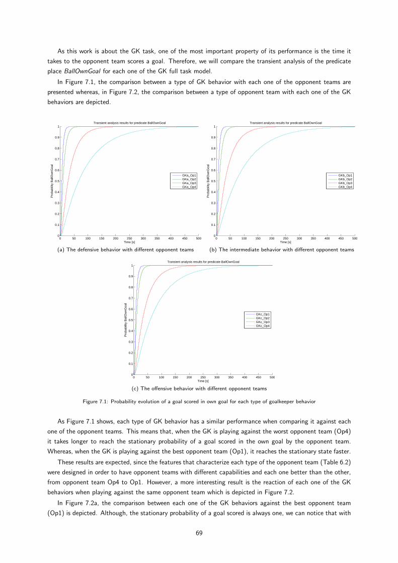
As this work is about the GK task, one of the most important property of its performance is the time it
takes to the opponent team scores a goal. Therefore, we will compare the transient analysis of the predicate
place BallOwnGoal for each one of the GK full task model.
In Figure 7.1, the comparison between a type of GK behavior with each one of the opponent teams are
presented whereas, in Figure 7.2, the comparison between a type of opponent team with each one of the GK
behaviors are depicted.
0 50 100 150 200 250 300 350 400 450 5000
0.1
0.2
0.3
0.4
0.5
0.6
0.7
0.8
0.9
1Transient analysis results for predicate BallOwnGoal
Time [s]
Pro
babi
lity
Bal
lOw
nGoa
l
GKa_Op1GKa_Op2GKa_Op3GKa_Op4
(a) The defensive behavior with different opponent teams
0 50 100 150 200 250 300 350 400 450 5000
0.1
0.2
0.3
0.4
0.5
0.6
0.7
0.8
0.9
1Transient analysis results for predicate BallOwnGoal
Time [s]
Pro
babi
lity
Bal
lOw
nGoa
l
GKb_Op1GKb_Op2GKb_Op3GKb_Op4
(b) The intermediate behavior with different opponent teams
0 50 100 150 200 250 300 350 400 450 5000
0.1
0.2
0.3
0.4
0.5
0.6
0.7
0.8
0.9
1Transient analysis results for predicate BallOwnGoal
Time [s]
Pro
babi
lity
Bal
lOw
nGoa
l
GKc_Op1GKc_Op2GKc_Op3GKc_Op4
(c) The offensive behavior with different opponent teams
Figure 7.1: Probability evolution of a goal scored in own goal for each type of goalkeeper behavior
As Figure 7.1 shows, each type of GK behavior has a similar performance when comparing it against each
one of the opponent teams. This means that, when the GK is playing against the worst opponent team (Op4)
it takes longer to reach the stationary probability of a goal scored in the own goal by the opponent team.
Whereas, when the GK is playing against the best opponent team (Op1), it reaches the stationary state faster.
These results are expected, since the features that characterize each type of the opponent team (Table 6.2)
were designed in order to have opponent teams with different capabilities and each one better than the other,
from opponent team Op4 to Op1. However, a more interesting result is the reaction of each one of the GK
behaviors when playing against the same opponent team which is depicted in Figure 7.2.
In Figure 7.2a, the comparison between each one of the GK behaviors against the best opponent team
(Op1) is depicted. Although, the stationary probability of a goal scored is always one, we can notice that with
69
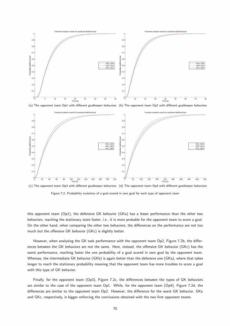
0 5 10 15 20 25 30 35 400
0.1
0.2
0.3
0.4
0.5
0.6
0.7
0.8
0.9
1Transient analysis results for predicate BallOwnGoal
Time [s]
Pro
babi
lity
Bal
lOw
nGoa
l
GKa_Op1GKb_Op1GKc_Op1
(a) The opponent team Op1 with different goalkeeper behaviors
0 10 20 30 40 50 60 70 800
0.1
0.2
0.3
0.4
0.5
0.6
0.7
0.8
0.9
1Transient analysis results for predicate BallOwnGoal
Time [s]
Pro
babi
lity
Bal
lOw
nGoa
l
GKa_Op2GKb_Op2GKc_Op2
(b) The opponent team Op2 with different goalkeeper behaviors
0 20 40 60 80 100 120 140 160 180 200 2200
0.1
0.2
0.3
0.4
0.5
0.6
0.7
0.8
0.9
1Transient analysis results for predicate BallOwnGoal
Time [s]
Pro
babi
lity
Bal
lOw
nGoa
l
GKa_Op3GKb_Op3GKc_Op3
(c) The opponent team Op3 with different goalkeeper behaviors
0 50 100 150 200 250 300 350 400 450 5000
0.1
0.2
0.3
0.4
0.5
0.6
0.7
0.8
0.9
1Transient analysis results for predicate BallOwnGoal
Time [s]
Pro
babi
lity
Bal
lOw
nGoa
l
GKa_Op4GKb_Op4GKc_Op4
(d) The opponent team Op4 with different goalkeeper behaviors
Figure 7.2: Probability evolution of a goal scored in own goal for each type of opponent team
this opponent team (Op1), the defensive GK behavior (GKa) has a lesser performance than the other two
behaviors, reaching the stationary state faster, i.e., it is more probable for the opponent team to score a goal.
On the other hand, when comparing the other two behaviors, the differences on the performance are not too
much but the offensive GK behavior (GKc) is slightly better.
However, when analysing the GK task performance with the opponent team Op2, Figure 7.2b, the differ-
ences between the GK behaviors are not the same. Here, instead, the offensive GK behavior (GKc) has the
worst performance, reaching faster the one probability of a goal scored in own goal by the opponent team.
Whereas, the intermediate GK behavior (GKb) is again better than the defensive one (GKa), where that takes
longer to reach the stationary probability meaning that the opponent team has more troubles to score a goal
with this type of GK behavior.
Finally, for the opponent team (Op3), Figure 7.2c, the differences between the types of GK behaviors
are similar to the case of the opponent team Op1. While, for the opponent team (Op4), Figure 7.2d, the
differences are similar to the opponent team Op2. However, the difference for the worst GK behavior, GKa
and GKc, respectively, is bigger enforcing the conclusions obtained with the two first opponent teams.
70
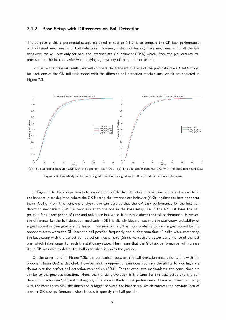
7.1.2 Base Setup with Differences on Ball Detection
The purpose of this experimental setup, explained in Section 6.1.2, is to compare the GK task performance
with different mechanisms of ball detection. However, instead of testing these mechanisms for all the GK
behaviors, we will test only for one, the intermediate GK behavior (GKb) which, from the previous results,
proves to be the best behavior when playing against any of the opponent teams.
Similar to the previous results, we will compare the transient analysis of the predicate place BallOwnGoal
for each one of the GK full task model with the different ball detection mechanisms, which are depicted in
Figure 7.3.
0 5 10 15 20 25 30 35 400
0.1
0.2
0.3
0.4
0.5
0.6
0.7
0.8
0.9
1Transient analysis results for predicate BallOwnGoal
Time [s]
Pro
babi
lity
Bal
lOw
nGoa
l
GKb_Op1GKb_Op1_SB1GKb_Op1_SB2GKb_Op1_SB3
(a) The goalkeeper behavior GKb with the opponent team Op1
0 10 20 30 40 50 60 70 800
0.1
0.2
0.3
0.4
0.5
0.6
0.7
0.8
0.9
1Transient analysis results for predicate BallOwnGoal
Time [s]
Pro
babi
lity
Bal
lOw
nGoa
l
GKb_Op2GKb_Op2_SB1GKb_Op2_SB2
(b) The goalkeeper behavior GKb with the opponent team Op2
Figure 7.3: Probability evolution of a goal scored in own goal with different ball detection mechanisms
In Figure 7.3a, the comparison between each one of the ball detection mechanisms and also the one from
the base setup are depicted, where the GK is using the intermediate behavior (GKb) against the best opponent
team (Op1). From this transient analysis, one can observe that the GK task performance for the first ball
detection mechanism (SB1) is very similar to the one in the base setup, i.e, if the GK just loses the ball
position for a short period of time and only once in a while, it does not affect the task performance. However,
the difference for the ball detection mechanism SB2 is slightly bigger, reaching the stationary probability of
a goal scored in own goal slightly faster. This means that, it is more probable to have a goal scored by the
opponent team when the GK loses the ball position frequently and during sometime. Finally, when comparing
the base setup with the perfect ball detection mechanisms (SB3), we notice a better performance of the last
one, which takes longer to reach the stationary state. This means that the GK task performance will increase
if the GK was able to detect the ball even when it leaves the ground.
On the other hand, in Figure 7.3b, the comparison between the ball detection mechanisms, but with the
opponent team Op2, is depicted. However, as this opponent team does not have the ability to kick high, we
do not test the perfect ball detection mechanism (SB3). For the other two mechanisms, the conclusions are
similar to the previous situation. Here, the transient evolution is the same for the base setup and the ball
detection mechanism SB1, not making any difference in the GK task performance. However, when comparing
with the mechanism SB2 the difference is bigger between the base setup, which enforces the previous idea of
a worst GK task performance when it loses frequently the ball position.
71
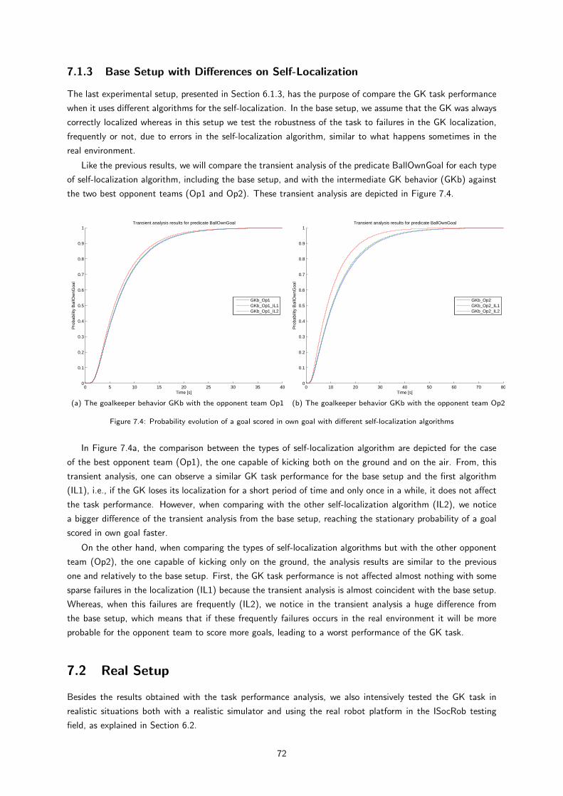
7.1.3 Base Setup with Differences on Self-Localization
The last experimental setup, presented in Section 6.1.3, has the purpose of compare the GK task performance
when it uses different algorithms for the self-localization. In the base setup, we assume that the GK was always
correctly localized whereas in this setup we test the robustness of the task to failures in the GK localization,
frequently or not, due to errors in the self-localization algorithm, similar to what happens sometimes in the
real environment.
Like the previous results, we will compare the transient analysis of the predicate BallOwnGoal for each type
of self-localization algorithm, including the base setup, and with the intermediate GK behavior (GKb) against
the two best opponent teams (Op1 and Op2). These transient analysis are depicted in Figure 7.4.
0 5 10 15 20 25 30 35 400
0.1
0.2
0.3
0.4
0.5
0.6
0.7
0.8
0.9
1Transient analysis results for predicate BallOwnGoal
Time [s]
Pro
babi
lity
Bal
lOw
nGoa
l
GKb_Op1GKb_Op1_IL1GKb_Op1_IL2
(a) The goalkeeper behavior GKb with the opponent team Op1
0 10 20 30 40 50 60 70 800
0.1
0.2
0.3
0.4
0.5
0.6
0.7
0.8
0.9
1Transient analysis results for predicate BallOwnGoal
Time [s]
Pro
babi
lity
Bal
lOw
nGoa
l
GKb_Op2GKb_Op2_IL1GKb_Op2_IL2
(b) The goalkeeper behavior GKb with the opponent team Op2
Figure 7.4: Probability evolution of a goal scored in own goal with different self-localization algorithms
In Figure 7.4a, the comparison between the types of self-localization algorithm are depicted for the case
of the best opponent team (Op1), the one capable of kicking both on the ground and on the air. From, this
transient analysis, one can observe a similar GK task performance for the base setup and the first algorithm
(IL1), i.e., if the GK loses its localization for a short period of time and only once in a while, it does not affect
the task performance. However, when comparing with the other self-localization algorithm (IL2), we notice
a bigger difference of the transient analysis from the base setup, reaching the stationary probability of a goal
scored in own goal faster.
On the other hand, when comparing the types of self-localization algorithms but with the other opponent
team (Op2), the one capable of kicking only on the ground, the analysis results are similar to the previous
one and relatively to the base setup. First, the GK task performance is not affected almost nothing with some
sparse failures in the localization (IL1) because the transient analysis is almost coincident with the base setup.
Whereas, when this failures are frequently (IL2), we notice in the transient analysis a huge difference from
the base setup, which means that if these frequently failures occurs in the real environment it will be more
probable for the opponent team to score more goals, leading to a worst performance of the GK task.
7.2 Real Setup
Besides the results obtained with the task performance analysis, we also intensively tested the GK task in
realistic situations both with a realistic simulator and using the real robot platform in the ISocRob testing
field, as explained in Section 6.2.
72
In [28], we present some movies with the results obtained for the GK role and where we can observe its
main features as well as the task performance in the different situations.
73
Chapter 8
Conclusion
Finally, this last chapter aims at presenting some discussion about the results obtained in this work as well as
some important conclusions and future work related with this thesis.
8.1 Discussion
The main results obtained in this thesis are presented in Chapter 7 and can be divided into two main parts,
the quatitative analysis of the GK task and its execution in the real robot platform.
From the GK task performance analysis developed in Section 7.1, one concludes that the performance of
the GK task can be improved depending on the situation and also on the type of opponent team.
As explained in Section 6.1.1, three types of GK behaviors was designed: one more defensive (GKa) staying
almost always close to the goal; another one more offensive (GKc) reacting and approaching the ball earlier
than the others; and, one behavior in the middle of defensive and offensive (GKb).
When comparing these behaviors with different types of opponent teams, one concludes that for an oppo-
nent team capable of kicking high (Op1 and Op3) the GK has a better task performance with an offensive
behavior (GKc). Even so, in this situation the intermediate behavior (GKb) has also similar performance has
that one (GKc). However, this best behavior (GKc), in that situation, is the worst behavior when playing
against an opponent team only capable of kicking on the ground (Op2 and Op4). For this situation, the
intermediate GK behavior (GKb) proves to be the best one.
Therefore, the GK behavior with a better performance and more stable, when playing against all types of
opponent teams, is the one where the GK gets out of the own goal and approaches the ball as soon as the
ball enters in the penalty area (GKb).
Another important conclusion obtained from the analysis results, is that the GK task can be slightly
improved if it uses a perfect ball detection mechanism, which is able to track the ball position perfectly when
it is on the ground and also when it leaves the ground, at least during sometime. This ball detection mechanism
models a GK with a frontal camera, which is able to detect the ball both on the ground and when leaves the
ground.
One last conclusion we obtained from the analysis results, is that the GK task can have a worst performance
if the self-localization algorithm frequently fails, giving a wrong position of the robot in the field, leading to a
poor GK task with more goals scored by the opponent team.
On the other hand, when executing the GK task, both in the simulator and in the real robot, one concludes
that the task designed has a good performance in all the different situations of a typical MSL soccer game.
74
8.2 Conclusions
In the end of this thesis and reflecting over the work developed, we conclude that the objectives proposed for
the thesis were met as well as some good results, related with the goalkeeper robot task performance, were
presented.
First of all, the main objective of this thesis was achieved, a complete and effective behavior was developed
for a robotic soccer goalkeeper. For this purpose, a decision-making process using Petri Nets was developed,
representing the role of the goalkeeper, with the coordination between all the different behaviors and actions
depending on the state of the world and game, evaluated through the use of logic predicates. All the goalkeeper
actions were implemented, improved and intensively tested, both in the realistic simulator and in the real robot
platform. Moreover, the full goalkeeper task was tested using the same environments which was then used for
the goalkeeper robot of ISocRob team during the Portuguese Robotics Open, with good results.
Furthermore, we use a modelling and analysis framework, [6], in order to model the full goalkeeper task,
including the environment, action and task models, which were then used to analyse the performance of the
goalkeeper task in different situations. For this purpose, we use Generalised Stochastic Petri Nets and also
the respective Markov Chain of the full task model in order to perform some quantitative analysis about the
goalkeeper task.
A complete model of the important changes occurring in the environment were presented, including all
the uncontrollable events due to other agents as well as a complete model of the ball state information, such
as the ball motion, and also the model of the game state. Moreover, the direct changes in the environment
performed by each one of the goalkeeper actions were also modelled, including the robot motion and how it
should act to accomplish the desired effect of the action.
Finally, with the full model of the goalkeeper task, we compared the task performance when the goalkeeper
uses different behaviors against different opponent teams, concluding what is the best and worst type of
goalkeeper behavior for each type of opponent teams. We modelled three types of goalkeeper behaviors,
from one more defensive to a more offensive behavior, and also four types of opponent teams, with different
capabilities mainly on the ball kicks, such as the ability to kick high or not and also the power of the ball kicks
and its velocity. In addition, we also compared the task performance when the goalkeeper uses different ball
detection mechanisms, concluding that it will have a better performance if it was able to detect the ball off
the ground, e.g., using a frontal camera.
After all, we conclude that the Petri Nets and its variations, such as Generalised Stochastic Petri Nets, are
a very intuitive, modular, graphical and mathematical tool which come up as an excellent tool for modelling,
analysis and execution of mobile robot tasks.
8.3 Future Work
Albeit, the results obtained with the goalkeeper task developed in this thesis are good, there are some work to
be done that would improve the goalkeeper task performance. This work can be divided into two main parts:
the improvements related with the execution of the goalkeeper task itself; and, the improvements more related
with the modelling and analysis of the task.
About the execution of the task in the real robot platform, we conclude from the results that the main
important features, for a good performance of the goalkeeper task, are the self-localization of the robot and
also the information of the ball position and velocity. Although, these were not the scope of the present work,
it will be important for the goalkeeper if some improvements on the self-localization algorithm were achieved,
mainly with an accurate knowledge of the own goal posture in the robot local frame. Furthermore, the ball
tracking algorithm should also be improved in order to have a perfect knowledge of the ball state even when
it is away from the robot and also off the ground. Both the algorithms are already being improved by ISocRob
75
team.
Another important improvement, related with the goalkeeper actions, is the interception of the ball when
this is moving towards the own goal. This action is the most important one in order to have a better
performance of the goalkeeper task on achieving its main objective, defending the goal from the kicks of the
opponent team.
Moreover, and more related with the hardware of the robot platform, the kicker mechanism should be
completely finished in order to have a goalkeeper capable of kicking the ball without the need to pushing it
outside of the goal area. Another hardware feature is the goalkeeper defense frame which currently is a static
frame but it would be also important to develop a new defense frame capable of increasing the side of the
goalkeeper on both sideways and also up, according to the MSL rules.
On the other hand, and related with the modelling and analysis of the goalkeeper task, it would be a
good improvement if both the environment and action models would be identified using realistic information,
from its simulation and also from the real environment, similar to what was done in [6]. Moreover, about
the environment models, it would be better if we have a generic and completed model of the MSL soccer
environment using those realistic informations. Then, and using the modular properties of the Petri Net
models, the designer can look at the environment models as a simple black box, even though very complex
but correctly modelled, choosing the components needed for his experimental setup and only concerned on
the correct modelling of the action and task models of the mobile robot task.
Finally, it would be also important if the execution part of the framework [6], used in the modelling and
analysis of the goalkeeper task, was integrated in the middleware of ISocRob team, MeRMaID. With this
improvement, we would have a continuous loop of design-analysis-execution-design for the task which would
lead to improved task plans.
76

77
Bibliography
[1] H. Kitano, M. Asada, Y. Kuniyoshi, I. Noda, E. Osawai, and H. Matsubara, “Robocup: A challenge
problem for ai and robotics,” in RoboCup-97: Robot Soccer World Cup I. Springer-Verlag, July 1997,
pp. 1–19.
[2] P. U. Lima and L. M. Custodio, “The socrob project: Soccer robots or society of robots,” Cutting Edge
Robotics, pp. 417–432, July 2005.
[3] P. Ramadge and W. Wonham,“The control of discrete event systems,”Proceedings of the IEEE, vol. 77,
no. 1, pp. 81 –98, January 1989.
[4] B. Damas and P. Lima, “Stochastic discrete event model of a multi-robot team playing an adversarial
game,” in Proc. of 5th IFAC/EURON Symposium on Intelligent Autonomous Vehicles - IAV2004, 2004.
[5] G. Kim and W. Chung,“Navigation behavior selection using generalized stochastic petri nets for a service
robot,”Systems, Man, and Cybernetics, Part C: Applications and Reviews, IEEE Transactions on, vol. 37,
no. 4, pp. 494 –503, July 2007.
[6] H. F. C. de Castro, “Robotic tasks modelling and analysis based on discrete event systems,” Ph.D.
dissertation, Instituto Superior Tecnico, October 2010.
[7] J. G. D. Torres,“Comportamentos relacionais em futebol robotico: Analise de incerteza,”Master’s thesis,
Instituto Superior Tecnico, October 2007.
[8] T. M. M. Antunes, “Comportamentos relacionais em futebol robotico: Analise logica,” Master’s thesis,
Instituto Superior Tecnico, September 2007.
[9] A. M. P. de Faria, “Desenvolvimento e analise de comportamentos relacionais em robots futebolistas,”
Master’s thesis, Instituto Superior Tecnico, September 2008.
[10] H. H. Lausen, J. B. Nielsen, M. Nielsen, and P. U. Lima,“Model and behavior-based robotic goalkeeper,”
in RoboCup, 2003, pp. 169–180.
[11] C. Esteves and S. Lopes,“Guarda-redes robotico omnidireccional,”Project’s final work, Instituto Superior
Tecnico, November 2005.
[12] N. Ramos, P. U. Lima, and J. Sousa, “Robot behavior coordination based on fuzzy decision-making,” in
ROBOTICA 2006 - 6th Portuguese Robotics Festival, 2006.
[13] C. A. Petri, “Kommunikation mit automaten,” Institut fur Instrumentelle Mathematik, Bonn, Technical
report, 1966, english translation.
[14] F. Bause and P. S. Kritzinger, Stochastic Petri Nets: An Introduction to the Theory, 2nd ed. Vieweg
Verlag, 2002. [Online]. Available: http://doi.acm.org/10.1145/288197.581194
78
[15] L. Bernardinello and F. D. Cindio, “A survey of basic net models and modular net classes,” in Advances
in Petri Nets 1992. Springer, 1992, vol. 609, pp. 304–351.
[16] MSL Technical Committee,“Middle size robot league rules and regulations for 2010,”RoboCup, Technical
report, May 2010.
[17] RoboCup - Middle Size League. Referee box. Software. [Online]. Available: http://wiki.msl.
robocup-federation.org/wiki/RoboCup - Middle Size League Main Page
[18] P. Lima, J. Messias, J. Santos, J. Estilita, M. Barbosa, A. Ahmad, and J. Carreira, “Isocrob 2009 team
description paper,” in Proceedings of Robocup Sym, 2009, p. 2313.
[19] M. Barbosa, N. Ramos, and P. U. Lima, “Mermaid - multiple-robot middleware for intelligent decision-
making,”in Proceedings of IAV2007 - 6th IFAC Symposium on Intelligent Autonomous Vehicles, Toulouse,
France, 2007.
[20] J. Messias, J. Santos, J. Estilita, and P. U. Lima, “Monte carlo localization based on gyrodometry and
line-detection,”in Proceedings of ROBOTICA2008 - 8th Conference on Mobile Robots and Competitions,
Aveiro, Portugal, 2008, pp. 39–50.
[21] J. S. Santos, “Multi-robot cooperative object localization: Decentralized bayesian approach,” Master’s
thesis, Instituto Superior Tecnico, December 2008.
[22] J. S. Messias,“Task specific motion control of omnidirectional robots,”Master’s thesis, Instituto Superior
Tecnico, September 2008.
[23] D. Fox, W. Burgard, and S. Thrun,“The dynamic window approach to collision avoidance,”IEEE Robotics
Automation Magazine, vol. 4, no. 1, pp. 23 –33, March 1997.
[24] I. Kamon, E. Rivlin, and E. Rimon, “A new range-sensor based globally convergent navigation algorithm
for mobile robots,” in Proceedings of 1996 IEEE International Conference on Robotics and Automation,
vol. 1, April 1996, pp. 429 – 435.
[25] J. E. Antunes, “Hardware architecture and fast deployment methods for soccer robots,” Master’s thesis,
Instituto Superior Tecnico, October 2009.
[26] CyberRobotics. WebotsTM 6 – fast prototyping and simulation of mobile robots. Realistic simulator
software. [Online]. Available: http://www.cyberbotics.com/
[27] P. Bonet, C. Llado, R. Puigjaner, and W. Knottenbelt. (2007, October) Pipe v2.5: a petri net tool for
performance modeling. in Proceedings of CLEI 2007 - 23rd Latin American Conference on Informatics.
Petri Net software. [Online]. Available: http://pipe2.sourceforge.net/
[28] C. Martins. (2010, October) The goalkeeper role. Video. [Online]. Available: http://socrob.isr.ist.utl.pt/
picsmovies.php
79