
MULTIOBJECTIVE EVOLUTIONARY ALGORITHMS APPLIED TO MICROSTRIP ANTENNAS DESIGN
Upload
khangminh22Category
view
1download
0


Juan Pontes
Analysis and Design of Multiple Element Antennas for Urban Communication

Karlsruher Forschungsberichteaus dem Institut für Hochfrequenztechnik und Elektronik
Herausgeber: Prof. Dr.-Ing. Thomas Zwick
Band 59

Analysis and Design of Multiple Element Antennas for Urban Communication
byJuan Pontes

KIT Scientific Publishing 2010 Print on Demand
ISSN: 1868-4696ISBN: 978-3-86644-513-0
Dissertation, Karlsruher Institut für Technologie
Fakultät für Elektrotechnik und Informationstechnik, 2010
Impressum
Karlsruher Institut für Technologie (KIT)KIT Scientific PublishingStraße am Forum 2D-76131 Karlsruhewww.uvka.de
KIT – Universität des Landes Baden-Württemberg und nationalesForschungszentrum in der Helmholtz-Gemeinschaft
Diese Veröffentlichung ist im Internet unter folgender Creative Commons-Lizenz publiziert: http://creativecommons.org/licenses/by-nc-nd/3.0/de/

Vorwort des Herausgebers Die permanent steigende Nachfrage nach höheren Datenraten im Bereich der mobilen Kommunikation führt zu einer andauernden Suche nach neuen Methoden, die beschränkte Ressource des existierenden Frequenzspektrums besser zu nutzen und damit die Kanalkapazität zu steigern. Seit einigen Jahren werden hierzu auch Mehr-antennensysteme eingesetzt. Diese sogenannten MIMO (Multiple-Input-Multiple-Output) Verfahren nutzen gezielt die Eigenschaften von Mehrwegefunkkanälen. Im Gegensatz zu dem schon seit vielen Jahrzehnten im Einsatz befindlichen Diversity, bei dem das Signal-zu-Rausch-Verhältnis durch möglichst optimales Kombinieren der Signale mehrerer Empfangsantennen maximiert wird, werden bei MIMO mehrere unabhängige Datenströme auf sogenannten Subkanälen übertragen, wodurch die Kanalkapazität gesteigert werden kann. Ausschlaggebend für maximale Kanalkapazität eines MIMO-Systems sind optimale Antennekonfigurationen an Sender und Empfänger. Da MIMO allerdings die Mehrwegeeigenschaften des Funkkanals nutzt, wird für eine simulationsbasierte Optimierung der Antennenkonfigurationen ein hoch-genaues Modell des Mehrwegefunkkanals benötigt. An dieser Stelle setzt die Arbeit von Herrn Juan Pontes an. Basierend auf dem intensiv verifizierten Wellenausbrei-tungsmodell des Instituts für Hochfrequenztechnik und Elektronik entwickelte Herr Pontes eine Methodik zur Analyse und Optimierung von Mehrantennensystemen für die urbane Funkkommunikation. Damit stellt die Arbeit von Herrn Pontes eine wesentliche Grundlage für weitere Forschungen dar und wird weltweit sicher einige darauf aufbauende Arbeiten nach sich ziehen. Ich wünsche ihm, dass er seine exzellenten Fähigkeiten auch weiterhin erfolgreich einsetzen kann. Prof. Dr.-Ing. Thomas Zwick - Institutsleiter -


Forschungsberichte aus dem Institut für Höchstfrequenztechnik und Elektronik (IHE) der Universität Karlsruhe (TH) (ISSN 0942-2935)
Herausgeber: Prof. Dr.-Ing. Dr. h.c. Dr.-Ing. E.h. Werner Wiesbeck
Band 1 Daniel Kähny Modellierung und meßtechnische Verifikation polarimetrischer, mono- und bistatischer Radarsignaturen und deren Klassifi-zierung (1992)
Band 2 Eberhardt Heidrich Theoretische und experimentelle Charakterisierung der polari-metrischen Strahlungs- und Streueigenschaften von Antennen (1992)
Band 3 Thomas Kürner Charakterisierung digitaler Funksysteme mit einem breit-bandigen Wellenausbreitungsmodell (1993)
Band 4 Jürgen Kehrbeck Mikrowellen-Doppler-Sensor zur Geschwindigkeits- und Weg-messung - System-Modellierung und Verifikation (1993)
Band 5 Christian Bornkessel Analyse und Optimierung der elektrodynamischen Eigenschaften von EMV-Absorberkammern durch numerische Feldberechnung (1994)
Band 6 Rainer Speck Hochempfindliche Impedanzmessungen an Supraleiter / Fest-elektrolyt-Kontakten (1994)
Band 7 Edward Pillai Derivation of Equivalent Circuits for Multilayer PCB and Chip Package Discontinuities Using Full Wave Models (1995)
Band 8 Dieter J. Cichon Strahlenoptische Modellierung der Wellenausbreitung in urbanen Mikro- und Pikofunkzellen (1994)
Band 9 Gerd Gottwald Numerische Analyse konformer Streifenleitungsantennen in mehrlagigen Zylindern mittels der Spektralbereichsmethode (1995)

Forschungsberichte aus dem Institut für Höchstfrequenztechnik und Elektronik (IHE) der Universität Karlsruhe (TH) (ISSN 0942-2935)
Band 10 Norbert Geng Modellierung der Ausbreitung elektromagnetischer Wellen in Funksystemen durch Lösung der parabolischen Approximation der Helmholtz-Gleichung (1996)
Band 11 Torsten C. Becker Verfahren und Kriterien zur Planung von Gleichwellennetzen für den Digitalen Hörrundfunk DAB (Digital Audio Broadcasting) (1996)
Band 12 Friedhelm Rostan Dual polarisierte Microstrip-Patch-Arrays für zukünftige satelli-tengestützte SAR-Systeme (1996)
Band 13 Markus Demmler Vektorkorrigiertes Großsignal-Meßsystem zur nichtlinearen Cha-rakterisierung von Mikrowellentransistoren (1996)
Band 14 Andreas Froese Elektrochemisches Phasengrenzverhalten von Supraleitern (1996)
Band 15 Jürgen v. Hagen Wide Band Electromagnetic Aperture Coupling to a Cavity: An In-tegral Representation Based Model (1997)
Band 16 Ralf Pötzschke Nanostrukturierung von Festkörperflächen durch elektro-chemische Metallphasenbildung (1998)
Band 17 Jean Parlebas Numerische Berechnung mehrlagiger dualer planarer Antennen mit koplanarer Speisung (1998)
Band 18 Frank Demmerle Bikonische Antenne mit mehrmodiger Anregung für den räumli-chen Mehrfachzugriff (SDMA) (1998)
Band 19 Eckard Steiger Modellierung der Ausbreitung in extrakorporalen Therapien ein-gesetzter Ultraschallimpulse hoher Intensität (1998)

Forschungsberichte aus dem Institut für Höchstfrequenztechnik und Elektronik (IHE) der Universität Karlsruhe (TH) (ISSN 0942-2935)
Band 20 Frederik Küchen Auf Wellenausbreitungsmodellen basierende Planung terrestri-scher COFDM-Gleichwellennetze für den mobilen Empfang (1998)
Band 21 Klaus Schmitt Dreidimensionale, interferometrische Radarverfahren im Nah-bereich und ihre meßtechnische Verifikation (1998)
Band 22 Frederik Küchen, Torsten C. Becker, Werner Wiesbeck Grundlagen und Anwendungen von Planungswerkzeugen für den digitalen terrestrischen Rundfunk (1999)
Band 23 Thomas Zwick Die Modellierung von richtungsaufgelösten Mehrwegegebäude-funkkanälen durch markierte Poisson-Prozesse (2000)
Band 24 Dirk Didascalou Ray-Optical Wave Propagation Modelling in Arbitrarily Shaped Tunnels (2000)
Band 25 Hans Rudolf Increase of Information by Polarimetric Radar Systems (2000)
Band 26 Martin Döttling Strahlenoptisches Wellenausbreitungsmodell und Systemstudien für den Satellitenmobilfunk (2000)
Band 27 Jens Haala Analyse von Mikrowellenheizprozessen mittels selbstkonsistenter finiter Integrationsverfahren (2000)
Band 28 Eberhard Gschwendtner Breitbandige Multifunktionsantennen für den konformen Einbau in Kraftfahrzeuge (2001)
Band 29 Dietmar Löffler Breitbandige, zylinderkonforme Streifenleitungsantennen für den Einsatz in Kommunikation und Sensorik (2001)
Band 30 Xuemin Huang Automatic Cell Planning for Mobile Network Design: Optimization Models and Algorithms (2001)

Forschungsberichte aus dem Institut für Höchstfrequenztechnik und Elektronik (IHE) der Universität Karlsruhe (TH) (ISSN 0942-2935)
Band 31 Martin Fritzsche Anwendung von Verfahren der Mustererkennung zur Detektion von Landminen mit Georadaren (2001)
Band 32 Siegfried Ginter Selbstkonsistente Modellierung der Erhitzung von biologischem Gewebe durch hochintensiven Ultraschall (2002)
Band 33 Young Jin Park Applications of Photonic Bandgap Structures with Arbitrary Sur-face Impedance to Luneburg Lenses for Automotive Radar (2002)
Band 34 Alexander Herschlein Entwicklung numerischer Verfahren zur Feldberechnung kon-former Antennen auf Oberflächen höherer Ordnung (2002)
Band 35 Ralph Schertlen Mikrowellenprozessierung nanotechnologischer Strukturen am Beispiel von Zeolithen (2002)
Band 36 Jürgen von Hagen Numerical Algorithms for the Solution of Linear Systems of Equa-tions Arising in Computational Electromagnetics (2002)
Band 37 Ying Zhang Artificial Perfect Magnetic Conductor and its Application to An-tennas (2003)
Band 38 Thomas M. Schäfer Experimentelle und simulative Analyse der Funkwellenausbrei-tung in Kliniken (2003)
Band 39 Christian Fischer Multistatisches Radar zur Lokalisierung von Objekten im Boden (2003)
Band 40 Yan C. Venot Entwicklung und Integration eines Nahbereichsradarsensor-systems bei 76,5 GHz (2004)
Band 41 Christian Waldschmidt Systemtheoretische und experimentelle Charakterisierung integ-rierbarer Antennenarrays (2004)

Forschungsberichte aus dem Institut für Höchstfrequenztechnik und Elektronik (IHE) der Universität Karlsruhe (TH) (ISSN 0942-2935)
Band 42 Marwan Younis Digital Beam-Forming for high Resolution Wide Swath Real and Synthetic Aperture Radar (2004)
Band 43 Jürgen Maurer Strahlenoptisches Kanalmodell für die Fahrzeug-Fahrzeug-Funkkommunikation (2005)
Band 44 Florian Pivit Multiband-Aperturantennen für Basisstationsanwendungen in re-konfigurierbaren Mobilfunksystemen (2005)
Band 45 Sergey Sevskiy Multidirektionale logarithmisch-periodische Indoor-Basissta-tionsantennen (2006)
Band 46 Martin Fritz Entwurf einer breitbandigen Leistungsendstufe für den Mobil-funk in Low Temperature Cofired Ceramic (2006)
Band 47 Christiane Kuhnert Systemanalyse von Mehrantennen-Frontends (MIMO) (2006)
Band 48 Marco Liebler Modellierung der dynamischen Wechselwirkungen von hoch-intensiven Ultraschallfeldern mit Kavitationsblasen (2006)
Band 49 Thomas Dreyer Systemmodellierung piezoelektrischer Sender zur Erzeugung hochintensiver Ultraschallimpulse für die medizinische Therapie (2006)
Band 50 Stephan Schulteis Integration von Mehrantennensystemen in kleine mobile Geräte für multimediale Anwendungen (2007)
Band 51 Werner Sörgel Charakterisierung von Antennen für die Ultra-Wideband-Technik (2007)
Band 52 Reiner Lenz Hochpräzise, kalibrierte Transponder und Bodenempfänger für satellitengestützte SAR-Missionen (2007)

Forschungsberichte aus dem Institut für Höchstfrequenztechnik und Elektronik (IHE) der Universität Karlsruhe (TH) (ISSN 0942-2935)
Band 53 Christoph Schwörer Monolithisch integrierte HEMT-basierende Frequenzvervielfa-cher und Mischer oberhalb 100 GHz (2008)
Band 54 Karin Schuler Intelligente Antennensysteme für Kraftfahrzeug-Nahbereichs-Radar-Sensorik (2007)
Band 55 Christian Römer Slotted waveguide structures in phased array antennas (2008)
Fortführung als "Karlsruher Forschungsberichte aus dem Institut für Hochfrequenz-technik und Elektronik" bei KIT Scientific Publishing (ISSN 1868-4696)

Karlsruher Forschungsberichte aus dem Institut für Hochfrequenztechnik und Elektronik (ISSN 1868-4696)
Herausgeber: Prof. Dr.-Ing. Thomas Zwick
Die Bände sind unter www.ksp.kit.edu als PDF frei verfügbar oder als Druckausgabe bestellbar.
Band 55 Sandra Knörzer Funkkanalmodellierung für OFDM-Kommunikationssysteme bei Hochgeschwindigkeitszügen (2009) ISBN 978-3-86644-361-7
Band 56 Fügen, Thomas Richtungsaufgelöste Kanalmodellierung und Systemstudien für Mehrantennensysteme in urbanen Gebieten (2009) ISBN 978-3-86644-420-1
Band 57 Pancera, Elena Strategies for Time Domain Characterization of UWB Components and Systems (2009) ISBN 978-3-86644-417-1
Band 58 Timmermann, Jens Systemanalyse und Optimierung der Ultrabreitband-Übertragung (2010) ISBN 978-3-86644-460-7
Band 59 Pontes, Juan Analysis and Design of Multiple Element Antennas for Urban Communication (2010) ISBN 978-3-86644-513-0


Karlsruher Institut für Technologie (KIT)Institut für Hochfrequenztechnik und Elektronik
Analysis and Design of Multiple ElementAntennas for Urban Communication
Zur Erlangung des akademischen Grades eines
DOKTOR-INGENIEURS
der Fakultät fürElektrotechnik und Informationstechnikam Karlsruher Institut für Technologie
vorgelegte
DISSERTATION
von
Dipl.-Ing. Juan Pontesaus Caracas
Hauptreferent: Prof. Dr.-Ing. Thomas ZwickKorreferent: Prof. Dr.-Ing. Christoph Mecklenbräuker


Vorwort
Die vorliegende Dissertation entstand während meiner Tätigkeit als wissenschaftlicher Mitar-beiter am Institut für Hochfrequenztechnik und Elektronik (IHE) des Karlsruher Instituts fürTechnologie (KIT).
Mein Dank geht zunächst an Herrn Prof. Wiesbeck, Leiter des Instituts zum Zeitpunkt meinerEinstellung, dessen Unterstützung mir half mich professionell zu entwickeln. Weiter geht meinDank an Herrn Prof. Zwick, der in den letzten zwei Jahren nicht nur für eine sehr gute Be-treuung gesorgt hat, sondern darüber hinaus durch seine konstruktive Kritik als Hauptreferentzum Gelingen dieser Arbeit beigetragen hat. Ebenso danke ich Herrn Prof. Christoph Mecklen-bräuker, Leiter des Institus für Nachrichtentechnik und Hochfrequenztechnik der TechnischenUniversität Wien, für die Übernahme des Korreferats. Außerdem möchte ich mich ausdrück-lich bei der Firma KATHREIN Werke KG, ihren Mitarbeitern und besonders bei Herrn Prof.Roland Gabriel für die gute Zusammenarbeit bedanken, denn sie haben den Anstoß zu meinerDissertation gegeben.
Bedanken möchte ich mich auch bei Dr. Thomas Fügen für seine Hilfe bei der Einarbeitungin die Themen Mehrantennensysteme und MIMO, den vielen wertvollen Diskussionen und ins-besondere für das Korrekturlesen der Dissertation. Diese Arbeit hätte ohne seine ausführlicheKritik und Unterstützung nicht den jetzigen Stand erlangt. Desweiteren möchte ich mich beiallen Kollegen bedanken, die sich oft Zeit für Diskussionen genommen haben und die für michdurch unsere Zusammenarbeit und gemeinsame Freizeitaktivitäten zu Freunden geworden sind.Ebenso geht mein Dank an alle Studenten, die sich mit mir fachlich weiterentwickelt und so ausmir einen anderen Menschen gemacht haben.
Mein herzlicher Dank geht an meine Mutter, die mir durch ihre stetige Unterstützung jeden Tagleichter fallen lässt.
Und mein letzter Dank geht an Kimberly, die aus meinem Leben eine Begegnung mit der Freudegemacht hat.
Karlsruhe, im Februar 2010
Juan Pontes


Abstract
With the increasing interest in sophisticated algorithms and network configurations in order toincrease the data rates demands of current and future communication systems, less attention ispaid to the antenna in-system optimization. Yet, network providers and antenna engineers arestill faced with the problem of addressing upcoming infrastructure needs, such as more costefficient antenna solutions. To aid in this decision making process, the attention of this work isfocused on the analysis and design of multiple element antennas (MEA) and their interactionwith the propagation channel. Moreover, focus is given to the “Karlsruhe" propagation channeland how its information throughput, i.e. capacity, can be improved. With this in mind, an ex-isting network model of the communication system is extended to include a modal descriptionof both mobile and base station antennas in order to reduce computation time. Reduction ofsimulation time is proven to increase linearly with the number of antennas, when it exceedsthe number of modes considered. On the basis of this model, an extensive capacity study ofdifferent antenna setups based on measured radiation patterns of commercial antennas is per-formed, with varying inter element spacing at both the base and mobile station. As result, a setof guidelines for optimum antenna placement and setup selection is given based on the capacityof equivalent isotropic normalized channels. This type of normalization, however, is not unique.Depending on the evaluation needs other norms might be used and comparison among differentworks results in a difficult task. To address this issue the adoption of an eigenvalue dispersionmetric as a compact and information rich evaluation measure is proposed, with which the ca-pacity for any normalization and SNR regime can be estimated. Finally, the communicationallimits of linear arrays in different propagation scenarios are explored and a synthesis method forachieving maximum information throughput is derived. In this way it is proven that even bettercapacities to those achieved by the studied commercial antenna setups could be attained, notby increasing the number of antennas, but by adding subchannels to the existing ones. Hence,antenna driving networks capable of producing several array excitations are suggested as thenext step toward better capacities in urban mobile communication systems.
i


Table of Contents
1 Introduction 11.1 The urban communication channel . . . . . . . . . . . . . . . . . . . . . . . . 21.2 Previous works & motivation . . . . . . . . . . . . . . . . . . . . . . . . . . . 31.3 Goal & Thesis outline . . . . . . . . . . . . . . . . . . . . . . . . . . . . . . . 5
2 The wireless communication channel 72.1 Input/Output model of the wireless communication channel . . . . . . . . . . . 7
2.1.1 Single antenna channels . . . . . . . . . . . . . . . . . . . . . . . . . 82.1.2 Multiple antenna channels . . . . . . . . . . . . . . . . . . . . . . . . 9
2.2 The antennas . . . . . . . . . . . . . . . . . . . . . . . . . . . . . . . . . . . 92.2.1 Antennas on transmit mode . . . . . . . . . . . . . . . . . . . . . . . 102.2.2 Antennas on receive mode . . . . . . . . . . . . . . . . . . . . . . . . 122.2.3 Circuit model of communicating antennas . . . . . . . . . . . . . . . . 13
2.2.3.1 Antenna losses . . . . . . . . . . . . . . . . . . . . . . . . . 132.2.3.2 Feeding circuit losses . . . . . . . . . . . . . . . . . . . . . 152.2.3.3 Polarization losses . . . . . . . . . . . . . . . . . . . . . . . 16
2.3 The propagation channel . . . . . . . . . . . . . . . . . . . . . . . . . . . . . 172.3.1 The free space propagation channel . . . . . . . . . . . . . . . . . . . 172.3.2 Multipath propagation channels . . . . . . . . . . . . . . . . . . . . . 19
3 Modeling of multiple element antenna systems 233.1 Exact system model . . . . . . . . . . . . . . . . . . . . . . . . . . . . . . . . 233.2 Modal network model of communication channel . . . . . . . . . . . . . . . . 26
3.2.1 Inclusion of the modal expansion . . . . . . . . . . . . . . . . . . . . 273.2.2 Computational gain . . . . . . . . . . . . . . . . . . . . . . . . . . . . 283.2.3 Modal description of mobile station . . . . . . . . . . . . . . . . . . . 293.2.4 Modal description of base station . . . . . . . . . . . . . . . . . . . . 31
3.3 Modeling of the “Karlsruhe" urban propagation channel . . . . . . . . . . . . . 323.3.1 Urban Environment Model . . . . . . . . . . . . . . . . . . . . . . . . 333.3.2 Wave propagation Model . . . . . . . . . . . . . . . . . . . . . . . . . 343.3.3 SISO to MIMO Extrapolation . . . . . . . . . . . . . . . . . . . . . . 35
3.4 Final remarks . . . . . . . . . . . . . . . . . . . . . . . . . . . . . . . . . . . 36
4 Information content of multiple element antenna systems 374.1 Spatial gain of MEA systems . . . . . . . . . . . . . . . . . . . . . . . . . . . 37
4.1.1 Diversity gain . . . . . . . . . . . . . . . . . . . . . . . . . . . . . . . 384.1.2 Multiplexing gain . . . . . . . . . . . . . . . . . . . . . . . . . . . . . 39
iii

Table of Contents
4.1.3 Diversity and multiplexing effects on the channel matrix . . . . . . . . 394.1.4 Spatial gain comparison issues . . . . . . . . . . . . . . . . . . . . . . 41
4.2 Capacity of multiple element antenna systems . . . . . . . . . . . . . . . . . . 434.2.1 Uniform Power Distribution . . . . . . . . . . . . . . . . . . . . . . . 454.2.2 Waterfilling . . . . . . . . . . . . . . . . . . . . . . . . . . . . . . . . 464.2.3 Beamforming on transmit . . . . . . . . . . . . . . . . . . . . . . . . 48
4.3 Channel capacity of temporal and spatial bandlimited systems . . . . . . . . . 494.4 Final remarks . . . . . . . . . . . . . . . . . . . . . . . . . . . . . . . . . . . 52
5 Capacity study of the “Karlsruhe" communication channel 555.1 Antennas and antenna arrays under study . . . . . . . . . . . . . . . . . . . . 555.2 Antenna placement effects on system capacity . . . . . . . . . . . . . . . . . . 57
5.2.1 Vertically polarized antennas . . . . . . . . . . . . . . . . . . . . . . . 585.2.2 Dual polarized antennas in single polarization mode . . . . . . . . . . 605.2.3 Dual polarized antennas in dual polarization mode . . . . . . . . . . . 625.2.4 Influence of mobile unit rotation on antenna placement . . . . . . . . . 65
5.3 Setup comparison . . . . . . . . . . . . . . . . . . . . . . . . . . . . . . . . . 675.4 Final remarks . . . . . . . . . . . . . . . . . . . . . . . . . . . . . . . . . . . 69
6 Improved evaluation metric for multiple element antenna systems 716.1 Eigenmode-based metric for Frobenius-normalized channels . . . . . . . . . . 72
6.1.1 Rank-2 systems . . . . . . . . . . . . . . . . . . . . . . . . . . . . . . 736.1.2 Rank-K systems . . . . . . . . . . . . . . . . . . . . . . . . . . . . . 75
6.2 Eigenmode-based metric for arbitrarily normalized systems . . . . . . . . . . . 786.3 Capacity analysis with eigenmode-based metric . . . . . . . . . . . . . . . . . 79
6.3.1 Rank-2 systems . . . . . . . . . . . . . . . . . . . . . . . . . . . . . . 796.3.2 Rank-K systems . . . . . . . . . . . . . . . . . . . . . . . . . . . . . 86
6.4 Final remarks . . . . . . . . . . . . . . . . . . . . . . . . . . . . . . . . . . . 91
7 Communicational limits of linear multiple element antennas 937.1 Spatial degrees of freedom in free space . . . . . . . . . . . . . . . . . . . . . 937.2 Spatial degrees of freedom in multipath channels . . . . . . . . . . . . . . . . 1007.3 Spatial degrees of freedom of the “Karlsruhe" communication channel . . . . . 103
7.3.1 Degrees of freedom definitions for non-ideal channels . . . . . . . . . 1037.3.2 Degrees of freedom of single channel realizations . . . . . . . . . . . . 1047.3.3 Degrees of freedom of all channel realizations . . . . . . . . . . . . . . 110
7.4 Final remarks . . . . . . . . . . . . . . . . . . . . . . . . . . . . . . . . . . . 112
8 Antenna design for wireless communication channels 1158.1 Multiple element antenna synthesis method . . . . . . . . . . . . . . . . . . . 1158.2 Antenna array synthesis for the urban communication channel . . . . . . . . . 1198.3 Antenna design concepts for the future . . . . . . . . . . . . . . . . . . . . . . 1238.4 Final remarks . . . . . . . . . . . . . . . . . . . . . . . . . . . . . . . . . . . 127
iv

Table of Contents
9 Conclusions 129
Bibliography 133
v


Acronyms and symbols
Acronyms
BTS Base Transceiver StationDMC Discrete Memoryless ChannelDOA Direction Of ArrivalDOD Direction Of DepartureFF Far FieldFPGA Field Programmable Gate ArrayIEE The Institution of Electrical EngineersIEEE Institute of Electrical and Electronics EngineersLOS Line Of SightMEA Multiple Element AntennaMIMO Multiple Input Multiple OutputNDF Number of Degrees of FreedomNLOS No Line Of SightOSI Open System Interconnection reference modelPPC Perfect Power ControlRF Radio FrequencySISO Single Input Single OutputSNR Signal to Noise RatioSVD Singular Value DecompositionTDD Time Division DuplexTMA Tower Mounted AmplifierTMPU Tower Mounted Pre-processing unitUMTS Universal Mobile Telecommunications SystemTSP Transferred Signal Power
Lower case letters
d distancef frequency
vii

Table of Contents
j imaginary unit (see Mathematical notations and symbols)n channeln noises antenna inter element spacingt time (variance of the channel)t time (relative to the communication signal)x, y input, output signalx, y, z cartesian coordinates
Capital letters
Aeff Antenna effective areaC Radiation patternC CapacityD DirectivityI Identity matrixE Electric fieldG GainH Channel matrixW Normalized channel matrixH Channel matrix coefficientL Array lengthM Number of transmitting antennasN Number of receiving antennasM Total number of transmitting antennas studiedN Total number of receiving antennas studiedP Transmit powerR ResistanceR Number of spherical modes at the receiverQ Number of spherical modes at the transmitterT Transmission matrixT Transmission matrix coefficientZ ImpedanceS Scattering matrixS Diagonalmatrix der SVDS Scattering matrix coefficient
viii

Table of Contents
S Power densityV Voltage
Greeks symbols
β Propagation constantδ Difference in differential cosinesΓ Reflection coefficient∆φ Phase differenceΩ Space angle Ω = (ϑ, ψ)
ϑ Elevation in spherical coordinatesλ Wavelengthµ Mean valueρ SNRˆρ Unitary polarization vectorσ standard valueτ Propagation timeψ Azimuth in spherical coordinatesη Antenna efficiencyζ ρN
ξ Eigenvalue dispersion as defined in [SSV+08]ϕ Eigenvalue dispersion as defined in this workΦ Normalized ϕ
Mathematical notations and symbols
j Imaginary unit j =√−1
a Variablea Modified variable (used to distinguish variables of the same type)a Variable in terms of spherical wavesa Vectorˆa Unitary vectorA Matrixa Matrix (vector)(·)† Complex conjugate transpose
ix

Table of Contents
(·)∗ Complex conjugate(·)T Transpose∗ Convolutionℜ.. Real partE.. ExpectationTr Tracelog Logarithmdet Determinantcos Cosinussin Sinusprob Probability| · | Absolute value (length of vector)||·| |F Frobenius-Norm
Subscripts and superscripts
0 Freiraum (Wellenzahl oder Impedanz)REF Referencen Noisenorm Normalized matrixTx Transmit modeRx Receive modeTxA Transmit antennaRxA Receive antennaTxU Transmit unitRxU Receive unitmax Maximummin Minimumeff Effectivesim Simulatedvir virtualA Antennap p-th pathk k-th channel realizationm m-th transmitting antennan n-th receiving antenna
x

Table of Contents
r r-th spherical modeq q-th spherical modei Indexj IndexAz AzimuthEl ElevationL Load+,− Positive and negative propagation direction
List of constants
ZF0 Characteristic wave impedance in free space ZF0 =√
µ0ε0
≈ 377Ω
c0 Velocity of light in free space: 2, 997925 · 108 m/se Euler constant 2,718...ε0 Free space permittivity: 8, 854 · 10−12 As/(Vm)µ0 Free space permeability: 4π · 10−7 Vs/(Am)π Pi 3,1415...
xi


1 Introduction
Traditional communication systems are based on the transmission of modulated signals (intime) through a communication channel, consisting of the matching networks, the antennas andthe propagation channel. With the advent of the digital communications and the whole spectrumof applications and improvements that it has to offer, more and more digital communication sys-tems are being used in a wide range of applications. In this process, focus has shifted from theanalogous part of the system, i.e. the transmission chain (or radio frequency (RF) transmissionchain if signal transmission is wireless), to the processing part, i.e. the encoders and modulatorsresponsible of digitally processing the input signals (either digital or analog) into analog signalssuited for transmission with analog components. This has lead to a layered view of commu-nications, as described in the Open System Interconnection (OSI) reference model [ITU94].In this way, several advances have taken place, but in exchange less efforts are being made inimproving the description and understanding of the analog part of the system (lowest layer),responsible for the actual transmission of electromagnetic waves. Because of this, relevance ofhigh frequency and antenna engineers is even more valuable now where a more intuitive de-scription of the communication channel can facilitate simulation and experimenting of complexalgorithms at higher communication layers.
To better understand the role played by the RF transmission channel within the digital commu-nication system, a block diagram of such a system is depicted in Figure 1.1. As it can be seen,the whole system consists on a series of blocks responsible for the signal processing in orderto convey information between two points. Even though, details of each system componentwill not be discussed in this work (a thorough description can be found in [Pro01]), it can beseen that the whole system is divided intro three segments: the transmitter processing chain, thecommunication channel, and the receiving processing chain. Both transmitter and receiver pro-cessing chains deal with the conversion between the digital and the analog domain, whereas thecommunication channel, also known as the RF transmission chain for wireless applications, isresponsible for the physical information transmission. It follows that the communication chan-nel represents a waveform channel, in which the signals are transmitted at a certain time andfrequency, whereas the whole communication system is equivalent to a Discrete MemorylessChannel (DMC), where digital words or symbols are transmitted. In consequence, inaccuratemodeling of the communication channel can lead to false results for the DMC in the samemanner that too complex depictions can result too restrictive to experiment and understand thefunctioning of the system as a whole. To overcome these difficulties, several assumptions are
1

1 Introduction
Figure 1.1: Block diagram of a digital communication system.
made regarding the communication channel and focus is given mostly to the coding schemesthat optimize the system. Yet, optimization at the lowest communication layer can still resultin remarkable improvements in the system as a whole. Furthermore, in order to guaranteethe advances of upcoming standards and technologies, a choice of optimal hardware (antennasinfrastructure) is still required.
1.1 The urban communication channel
As previously mentioned, the communication channel results from the interaction between feed-ing circuits, antennas, and propagation channel, where different types of sceneries or antennaslead to different communication channels. Throughout this thesis, focus will be given solely tothe urban communication channel.
In this work, two classifications are used for distinguishing between different communicationchannels. The first communication channel classification and perhaps most important one, isthe number of antennas involved in the communication process. If more than one radiatingelement is used, so that an antenna can be viewed as the result of multiple radiating elements,the term multiple element antenna (MEA) is used. The resulting channel is thus considered tobe a MEA channel as opposed to the more common single-input single-output (SISO) channel.
The main difference between these two channels, other than the number of antennas, is thatMEA channels are capable of making better use of the spatial resources of the communication
2

1.2 Previous works & motivation
channel. Because of this, antenna arrangements capable of performing spatial signal process-ing through multiple antenna links have come to be known as smart antennas. However, sincecommunication systems do inherently exploit the spatial properties of the channel regardless ofthe number of antennas used, the term smart antenna system will be dropped in this work.
In general, one could also refer to MEA systems with multiple antennas at both transmitterand receiver as Multiple-Input Multiple-Output (MIMO) systems. However, this is not entirelyaccurate given the fact that MIMO systems are mostly associated with the multiplexing capabil-ities of systems with multiple antennas in highly scattered propagation channels. As result, theuse of multiple antennas in a scenario with dominant Line of Sight (LoS) component would notmake sense from a multiplexing perspective. Even though this statement is only partially true,since LoS at small distances does not exclude benefits from multiplexing approaches [CPGZ09],the fact remains that not in every multiple antenna communication system multiplexing is used.Therefore, in order to provide a broader framework the terms MEA system and MEA channelare used, when more than one antenna on transmit, receive or both is considered.
The second classification that can be made depends on the type of propagation scenario consid-ered. In this manner, one can differentiate between indoor or outdoor channels and the differenttypes of channel in each case. For mobile communications, however, even though communica-tion can take place at a wide range of propagation channels, the most relevant one is the outdoorchannel for urban settings. Therefore, in this work, investigation of the communication channelresulting from the use of multiple element antennas within a urban propagation scenario is whatwill be referred to as the urban communication channel.
Urban propagation channels are specially relevant, since the larger number of users are locatedwithin urban settings. One could argue, though, that not all people are on the street, but withinthe buildings and vehicles. While true, it is first within the urban environment that propagationtakes place until it finally reaches those users located inside the buildings, either by means ofrepeating stations or through direct wave transmission. As result, investigation of urban settingsin general is of great importance and has been the driving force behind a significant number ofworks during the last decades [TFS99, OT02, CP07, LST+07, DC08].
1.2 Previous works & motivation
Antenna and system integration for the urban propagation scenario has been widely studied.However there seems to be no general agreement for the optimal antenna spacing, configu-ration and polarization of a MEA system for a specific scenario. This is mainly because allprevious works are done under different frameworks which, in most cases, are not comparable
3

1 Introduction
or flexible enough. In addition, the complexity of such systems has also been an impediment,where consideration of real multipath environments is either oversimplified or not consideredat all. To overcome these limitations several measurement campaigns have been undertaken.However, the significant amount of data to be processed, as well as the considerable difficultiesit poses, have also limited a more precise and extended study. As result, from the point of viewof mobile or base station antenna designers, there doesn’t seem to be a clear guideline as towhich setup delivers the best results.
Furthermore, due to the important number of variables involved and the slow standardizationprocess of scientific concepts, no universal evaluation framework or metric exists which is ableto accurately capture in an insightful way the channel (or system) performance. Dependingon whether antennas, channels or MIMO setups are being studied, different evaluation crite-ria are chosen, whereas, in some cases, even works of related topics present their results withnon-comparable metrics. This leads to additional difficulties in the assessment of previouslypublished MIMO antennas and configurations for the urban channel.
In addition, there is no general body of work available dealing with the communicational lim-its of typical urban communication channels. Some works are found in the area of free spaceand other analytical propagation channel models. For physical channel models, though, verylittle work has been done. Therefore, most of the knowledge in improving the capacities ofcurrent communication systems has been gained from experience and through cumbersomesimulations, as the ones previously mentioned. Yet, no thorough study has been done on theattainable capacities and how they can be realized. This lack of understanding of the achievableinformation throughputs in real scenarios has lead to the current suboptimal antenna solutions.Moreover, it has also fueled current research trends toward the use of more elaborate antennaschemes, such as cooperative MIMO, which in most cases results in the addition of antennasand therefore cost to existing networks.
From the previous discussion follows that being able to make an informed choice in currenturban communication channels has become increasingly difficult for both antenna designersand network providers. Due to the wide range of results obtained under different assump-tions, a concise and systematic framework is needed for determining which antennas work best.Furthermore, the lack of understanding of the communicational limits of antenna systems hasturned the process of network design into a rather empirical one. This work intends to pro-vide such a simulation and evaluation framework, while leaving room for increased systemcomplexity.
4

1.3 Goal & Thesis outline
1.3 Goal & Thesis outline
In light of the discussed difficulties surrounding the study of the urban communication channelthe goal of this thesis is to facilitate the study of current and future antenna systems. In this waythe results to be presented in this work are intended as guidelines for both network designersand antenna engineers toward an efficient analysis, use and design of upcoming antenna setups.In addition this work expects to aid in the decision making process of network providers andantenna engineers with respect to upcoming infrastructure needs.
In order to achieve this goal, the main needs in the study of urban communication channels needto be addressed. This means providing a faster but accurate simulation framework, a generaland flexible evaluation framework, and improved antenna solutions based on the better use ofthe channel spatial resources. With this in mind, aside from chapter 1 and 8, where an introduc-tion and outlook to this work are given, this thesis is outlined as follows.
In chapter 2 a mathematical description of communication channels and more specifically of theurban communication channel will be given. First, the channel matrix concept will be discussedfor SISO and MEA channels along with its normalization. Then some antenna fundamentalsrelevant for its computation will be discussed. Based on this, evaluation of the channel matrixwill be explained for free space and multi path propagation channels.
On this ground, a flexible modeling approach will be introduced in chapter 3 for use with bothcommunication channels and systems. Here, an existing network model is introduced for thewhole communication system and later extended for increased computation speed based on themodal description of the antennas. Finally, the “Karlsruhe" urban communication channel to beused throughout this work will be defined.
Having provided a flexible simulation framework for communication systems, in chapter 4 thefoundations for evaluating the performance of the communicational channel from an informa-tion perspective will be discussed. First, the concept of capacity in the context of MEA chan-nels, i.e. spatially limited channels, will be discussed. Then its meaning for simultaneouslytemporally and spatially limited channels will be analyzed on the basis of Shannon’s capacitydefinition. On this basis a thorough study of the capacity limits from a spatial perspective willbe investigated for free space.
In chapter 5, the simulation framework of chapter 4 will be used to study the capacity of var-ious antenna configurations in the urban communication channel. Different antenna setups atdifferent antenna inter-element spacings will be compared. Based on the results obtained, some
5

1 Introduction
comparison and evaluation issues will be discussed. As result, the need for a better evaluationmetric will be verified. This need will be then addressed in chapter 6, where a new evaluationmetric will be proposed. In doing so, the cases of Frobenius and arbitrary normalized channelswill be handled.
Having investigated the achievable capacities of typical antenna setups for the “Karlsruhe" ur-ban communication channel, in chapter 6 focus is shifted to the theoretical limits behind suchimplementations. More specifically, the limits of the wireless channel in free space are investi-gated. Later on, the same approach is applied to the “Karlsruhe" urban communication channeland, from the experience gained in the study of typical antenna setups, the communicationallimits of such systems will be investigated in chapter 7.
Finally, the issue of antenna design will be considered in chapters 7 and 8. First, the spatialdegrees of linear systems will be investigated with respect to transmit power and antenna lengthin chapter 7. Then in chapter 8 a synthesis procedure will be given for computing the optimalarray excitations capable of diagonalizing the channel matrix with any given polarization andantenna element. The capacity of optimally synthesized arrays will be studied and comparedwith that of commercial antennas. As final step, optimum antenna implementations will be sug-gested.
6

2 The wireless communication channel
The communication channel as already mentioned is considered in this work to be the part ofthe communication system involving the transmission and reception of electromagnetic energy.Therefore, it includes the antennas and the physical propagation channel. It follows that its anal-ysis and design should consider the antenna properties and the channel characteristics. Mostimportantly, though, the way how channel and antennas interact to convey information frompoint A to point B must be known as well. As result, a communication channel descriptiondepicts the way in which a signal x is transmitted through a certain propagation channel andreceived as signal y. In other words, the relationship between x and y for a certain communica-tion setup, i.e. the channel transfer function, should be known.
In the following the underlying concepts used as basis for the research done throughout thiswork will be presented. First, the channel transfer function in single and multiple antennachannels will be defined and discussed. Then the theoretical framework for its computationwill be given. When not otherwise stated the word channel will refer to the communicationchannel, whereas the physical channel will be referred as such or as propagation channel.
2.1 Input/Output model of the wireless communicationchannel
The relationship between the input and output signal of a communication channel is given bythe channel transfer function, where the input and output signals are waveforms (i.e. continuoussignals in contrast to the discrete ones found at the input and output of the system modulator anddemodulator). It involves the accurate representation of the antennas, their matching networksand the propagation channel used and it describes the way these interact in order to conveyinformation within a communication system. In general this means finding the relationship be-tween a certain input and output signal, which in practical terms results in obtaining the ratiobetween the transmitted and received voltages. As it will be shown, for single input single out-put (SISO) communication channels this results in a single transmission coefficient H , whereasfor systems with multiple antennas it yields a channel matrix H.
7

2 The wireless communication channel
2.1.1 Single antenna channels
Assuming only one antenna on transmit and receive, i.e. a single input single output (SISO) sys-tem, and a linear and time-variant channel, such as multipath propagation channels explainedbelow, the resulting channel transfer function between both communicating ends can be ex-pressed as a function of frequency f and time t
Hnm(f, t) =y(f, t)
x(f)=VRx,n(f, t)
VTx,m(f), (2.1)
given by the ratio of the received voltage VRx,n and the transmitted voltage VTx,m, where thesubscripts n and m denote the receiving and transmitting antennas. In consequence, the outputsignal y results from the sum of the transmitted continuous waveform signal x and the additivewhite gaussian noise n corrupting the output
y(f, t) = x(f)Hnm(f, t) + n(f). (2.2)
Furthermore, since the time variable t expresses the time variance of the channel, and not thetime domain t of the output and input waveform signals, (2.2) can be written as
y(t, t) = x(t) ∗Hnm(t, t) + n(t). (2.3)
For a time invariant propagation channel or when considering only one snapshot of a propaga-tion channel the dependence of Hnm on t can be dropped. Moreover, if a channel with givenbandwidth B and ideal frequency response within this bandwidth (flat frequency response) isconsidered Hnm loses its frequency dependence as well and becomes a fixed link coefficient. Inconsequence, when considering a time-invariant channel with ideal frequency response withinthe bandwidth B, as is considered in the entirety of this work, only the input and output voltagerelationship, computed at a single frequency and at a single instant, is of interest.
Even though this is not the general case, investigation of the effects due to the time-variant andbroadband characteristics of many communication channels has been subject of investigation inmany works such as [Zwi99, Kat02]. Furthermore, results of this nature for the urban commu-nication channel to be introduced in chapter 5 can be found in [Füg09]. In this work, though,interest lies in the study of the multiple element antennas within the communication channel,rather than the channel as such. Therefore, throughout this work, without loss of generality andfor simulation ease, a time-invariant channel with ideal frequency response will be considered.
8

2.2 The antennas
2.1.2 Multiple antenna channels
Up to this point the communication linkHnm between the nm antenna pair has been considered.If the number of antennas is increased, then a link coefficient set for each antenna pair results,which can be expressed in form of a channel matrix
H =
H11 . . . H1M
... . . . ...
HN1 . . . HNM
, (2.4)
where Hnm stands for complex transfer function between the n-th receive antenna and the m-thtransmit antenna and is computed with aid of (2.1). The difference between both is that insteadof one communication link in (2.4) N × M links result, where N and M are the maximumnumber of antennas at the receiver and transmitter, respectively. This means that contrary to theimplementation of antenna arrays, where multiple radiating elements are driven with a feedingnetwork and a single antenna port, in MEA systems each antenna is driven individually. Asresult independent communication links can be built and parallel data streams can be used.
With (2.4) it is now possible to describe the received signal vector y of such a communicationsystem analog to (2.3) as
y (t) = H(t, t)∗ x (t) + n (t) , (2.5)
or in frequency domain and dropping notation of the frequency dependence
y = Hx+ n, (2.6)
with x being the transmitted signal vector and n representing the system’s noise vector. Asresult (2.6) describes now the vector waveform signals involved in the multiple transmissionlinks. From this it is seen that the two components to be accurately reproduced are the channelmatrix and the system’s noise. For the latter, both interference effects and Gaussian noise haveto be considered. In this work focus will be given solely to the channel matrix in order tooptimize the analysis and design of multiple antenna systems.
2.2 The antennas
Communication between two points is based on the transformation of bounded energy in theform of circuit voltages into electromagnetic fields capable of propagating in space and itsreceiving counterpart. Once the electromagnetic fields are generated the way they propagate
9

2 The wireless communication channel
Figure 2.1: Coordinate system and geometrical description seen by an antenna.
depends on the channel properties, such as morphology, topography, etc. Depending on thesefactors different propagation phenomena take place. In free space, however the most significantrole is played by the antennas, which act as electromagnetic transducers. Here antennas areclassified into two groups: antennas on transmit and antennas on receive.
2.2.1 Antennas on transmit mode
In a communication channel, each antenna is responsible of using an input voltage VTx to radiatean electromagnetic field E and later transform this radiated field into a received voltage VRx.It thus follows that a relationship between the used voltage and the electric field exists. Thisrelationship, called antenna gain, is also the paramount measure when evaluating antennas sinceit is a compact comparison measure. This can be seen from the fact that the antenna gain resultsfrom the quotient between the maximum power density (magnitude) of the antenna, STx,max,resulting from
STx(d, ϑ, ψ) =|E(d, ϑ, ψ)|2
2ZF0
, (2.7)
and the power density of an isotropic source STx,iso with equal transmitting power, i.e. equalinput power PTx at the antenna terminals (VRx = 0),
STx,iso =PTx
4πd2, (2.8)
which serves as reference for all antennas. Here and in the rest of this thesis d, ϑ and ψ willbe the distance, the elevation and the azimuth angle as depicted in 2.1. In this way the knownexpression for antenna gain results
G =|STx(d, ϑ, ψ)|max
STx,iso
= 4πd2|E(d, ϑ, ψ)|2max
2ZF0PTx
∣∣∣∣∣d=const≥FF
, (2.9)
10

2.2 The antennas
where d is a constant distance sufficiently far away from the antenna at which the electric fieldis observed. In this way the far field condition (FF) [Bal97] is guaranteed. ZF0 is the free-spaceimpedance and |E(ϑ, ψ)|2max results from the maximum of
|E(d, ϑ, ψ)|2 =(√
|Eϑ(d, ϑ, ψ)|2 + |Eψ(d, ϑ, ψ)|2)2
, (2.10)
being Eϑ and Eψ the respective polar components of the electric field E(d, ϑ, ψ) written as
E (d, ϑ, ψ) = Eϑ (d, ϑ, ψ)ˆϑ+ Eψ (d, ϑ, ψ)
ˆψ, (2.11)
with ˆϑ and ˆ
ψ being the unitary vectors in the ϑ and ψ directions. In addition, since real antennasare angle dependent a directive gain also exists and is defined as
G(ϑ, ψ) = 4πd2|E(d, ϑ, ψ)|2
2ZF0PTx
∣∣∣∣∣d=const≥FF
. (2.12)
Finally, from the relationship between (2.9) and (2.12) a new measure widely used in the contextof antennas, called the antenna radiation pattern, results
|C(ϑ, ψ)| =√G(ϑ, ψ)
G=
|E(d, ϑ, ψ)||E(d, ϑ, ψ)|max
∣∣∣∣∣d=const≥FF
, (2.13)
where C(ϑ, ψ) is given by
C(ϑ, ψ) =E(d, ϑ, ψ)ejβd
|E(d, ϑ, ψ)|max
∣∣∣∣∣d=const≥FF
, (2.14)
with β being the wavenumber defined as
β =2π
λ. (2.15)
As result G(ϑ, ψ) can now be rewritten as
G(ϑ, ψ) = |C(ϑ, ψ)|2G. (2.16)
It should be noted, though, that none of the previous gain definitions are dependent on thedistance d. The reason for this is that the radiated field itself is also distance dependent. There-fore, in (2.9) and (2.12) influence of d is cancelled and the previous gain definitions result.
11

2 The wireless communication channel
If, however, either one of these gain definitions is solved for the electric field then an inversedependence to d can be proven, as seen in (2.9) when solved for |E(d, ϑ, ψ)|max
|E(d, ϑ, ψ)|max =
√GZF0PTx
2πd2, (2.17)
which, after substitution in (2.13), yields a general expression for the electric field E(d, ϑ, ψ)
E(d, ϑ, ψ) = C(ϑ, ψ)
√GZF0PTx
2π
e−jβd
d. (2.18)
In this way a compact expression describing the antenna behavior as electromagnetic transduceron transmit mode is found, that expresses the generated electromagnetic field in terms of inputpower PTx.
2.2.2 Antennas on receive mode
The expression in (2.18) is valid when an antenna is used to send information or electromagneticsignals. When used on receive mode a similar expression to the antenna gain exists. Thisexpression is known as the antenna effective area Aeff and represents the, with power densitySTx, radiated area seen by an antenna so that a power PRx can be delivered to the load. ThereforeAeff is given by the ratio between PRx and STx
AeffSTx = PRx =⇒ Aeff =PRx
STx
. (2.19)
However, contrary to antenna gain, substitution of (2.7) in (2.19) shows no distance d term inthe computation of Aeff
Aeff =2ZF0PRx
|E(d, ϑ, ψ)|2max
. (2.20)
This expresses mathematically the intuitively expected result that, in order to have a distanceindependent measureAeff for the antenna on receive, PRx must depend on d. This means that thefurther the distance the smaller the received power becomes. Because of this, in order to derivethe effective aperture of a single antenna both the received power and the incoming field shouldbe known. In general, this requires a numerical computation. However, for certain antennas,PRx and E(d, ϑ, ψ) can be computed analytically and out of it the following expression for Aeff
results
Aeff = G
(λ2
4π
), (2.21)
12

2.2 The antennas
Figure 2.2: Equivalent circuit of transmit and receive antennas.
where λ is the wavelength of a certain frequency f . In general, it is not necessary to derive thisexpression for every antenna, since it can be proven valid for all reciprocal antennas [Bal97].Here, as was the case with the gain, a non-directive measure is obtained. However, if G(ϑ, ψ)is used instead of G a directive Aeff(ϑ, ψ) is found.
2.2.3 Circuit model of communicating antennas
From a circuit perspective the previous discussion shows that antennas can act as loads whenused together with a generator (source) or as electric sources when electromagnetic energy is re-ceived. The latter can be depicted for two communicating antennas by means of their Theveninequivalent circuits [Bal97] as shown for antennas m and n in Figure 2.2. An equivalent Nortoncircuit can also be used [Kil00], but is less common and will therefore be omitted throughoutthis work.
2.2.3.1 Antenna losses
When energy is transmitted VRx becomes zero (in general1) for the respective antenna and onlythe antenna impedance ZA at the antenna terminals is seen. If, on the contrary, energy isreceived then VTx disappears, and the antenna only sees the load impedance ZL (when trans-mitting, ZL acts as the generator impedance as it is commonly known). In this way PTx in theprevious equations becomes
PTx =|VTx|2
2
[RA
|ZL + ZA|2
], (2.22)
which in the case of a conjugate matched antenna (no resulting reactance, i.e. XA = −XL, andequal load and antenna resistance, i.e. RA = RL) is found to be
1In scenarios where the antennas are located in the proximity of scattering objects, some energy will be reflectedback to the antennas and VRx will no be zero. Here, this fact is ignored and it is assumed that the antennas areplaced far enough from all possible scatterers so that VRx = 0 can be assumed
13

2 The wireless communication channel
PTx =|VTx|2
8RA(2.23)
and for a non-lossy antenna represents the total radiated power. If losses are considered, though,the antenna resistance RA can be expressed as
RA = RArad +RA
L (2.24)
and the radiated power results only from the power seen at the radiating component RArad,
whereas the remaining power is delivered to the loss resistance RAL . In consequence an ex-
pression for the radiated power of the form
Prad =|VTx|2
8RA
[RA
rad
(RAL +RA
rad)
]= PTxη (2.25)
results, where the quotient between the radiating and total antenna resistance
η =RA
rad
(RAL +RA
rad)=RA
rad
RA(2.26)
is known as the antenna radiation efficiency. In this way η accounts for both conductive anddielectric losses present in the antenna. Finally, with (2.25) an analogous expression to theantenna gain can be defined, based solely on the radiated power, known as directivity and equalto
D = 4πd2|E(d, ϑ, ψ)|2max
2ZF0Prad
∣∣∣∣∣d=const≥FF
=G
η, (2.27)
which leads toG = ηD. (2.28)
In this case, as with antenna gain, consideration of a directive electric field, instead of its maxi-mum value, results in an angle dependent measure for directivity D(ϑ, ψ) as well.
For a receiving antenna no equivalent definition to directivity exits, instead different types ofantenna apertures are defined [Bal97]. These result from considering the power delivered toeach part of the receiving circuit. Therefore, defining PRx as the induced (received) power atthe load and assuming conjugate matching at the receiver the following expression for PRx canbe found
PRx =|VRx|2
2
[RL
|ZL + ZA|2
]=
|VRx|2
8RL=
|VRx|2
8RA, (2.29)
.
14

2.2 The antennas
which leads to the effective aperture Aeff
Aeff =|VRx|2
8RLSTx
. (2.30)
When RA = RArad, i.e. non-lossy antenna, (2.30) is equal to
As =|VRx|2
8RAradSTx
, (2.31)
as seen from (2.29). Yet, in the case of a conjugate matched lossy antenna, whereRL = RA = RA
rad +RAL , the relationship between (2.30) and (2.31) is given by η. It thus fol-
lows that Aeff results from multiplying (2.31), defined as the scattering area As in [Bal97], withthe radiation efficiency η
Aeff = η|VRx|2
8RAradSTx
= ηAs. (2.32)
In a similar way substituting G in (2.21) with ηD from (2.27) yields
Aeff = ηD
(λ2
4π
). (2.33)
With (2.28) and (2.33) antenna losses can now be considered in both transmit and receivemode. However, other forms of power loss also occur in antenna systems, such as non per-fectly matched feeding circuits and polarization mismatch between receiving and transmittingantennas. In the following these two loss types will be introduced.
2.2.3.2 Feeding circuit losses
Up to this point, when computing the transmitted or received power, conjugate antenna match-ing has been assumed. However, real antenna driving circuits need not to be matched to theantenna. Furthermore, in some cases due to high bandwidths they can’t be perfectly matched inthe whole frequency range. This mismatch between driving circuit and antenna causes power tobe inefficiently delivered to the antenna, when transmitting, or to the load, when receiving. Toaccount for impedance (load) mismatches a measure called the reflection efficiency exists andit is defined based on the ratio between the power effectively delivered to a loading circuit (forexample antenna) and the available power as
ηℓ =Pdelivered
Pavailable
=P+ − P−
P+= 1− |Γ|2, (2.34)
where the superscripts + and − refer, respectively, to the incident and reflected wave at theinterface between two circuit parts and Γ is the reflection coefficient given by the ratio betweenthe incident and reflected voltages, V + and V −, found to be
15

2 The wireless communication channel
Γ =V −
V +=Z1 − Z2
Z1 + Z2
, (2.35)
with Z1 and Z2 being the impedances seen at the interface between two circuits. In the casehere discussed, Z1 and Z2 are equal to either ZA and ZL (antenna on transmit) or ZL and ZA
(antenna on receive) and ηℓ is a measure of the amount of power used at the antenna or theload, depending on the operation mode considered. In this way, the maximum antenna gainachievable in a mismatched circuit, also called realized gain G, is
G = η(1− |Γ|2)D, (2.36)
where (2.16) in this case yields
G(ϑ, ψ) = |C(ϑ, ψ)|2G. (2.37)
Therefore, the effective antenna aperture is
Aeff = η(1− |Γ|2)D(λ2
4π
). (2.38)
As result PTx and PRx are given, in a mismatched circuit, as
PTx =|VTx|2
8RA
1
(1− |Γ|2)and PRx =
|VRx|2
8RA
(1− |Γ|2
). (2.39)
This result is very important since it shows a clear difference between PTx and PRx. PTx rep-resents the available power needed in order to achieve (2.28), i.e. the maximum gain undermatched conditions, whereas PRx represents the power delivered to the load in receiving mode.
2.2.3.3 Polarization losses
Polarization losses refer to the loss of power due to polarization mismatch between transmittingand receiving antennas. It assumes the existence of a communication link, i.e. signal transmis-sion from point A to point B. And can therefore only occur when a signal is received, since itresults from the interaction between the receiving antenna radiation pattern and the impingingelectric field. In general, it is the result of the scalar product between the electric field vectorsof the incoming signal and the receiving antenna. Therefore, if the electric field E is expressed
in terms of a polarization vector ρ, instead of ˆϑ and ˆ
ψ as in (2.11), the Polarization Loss Factor(PLF) [Bal97] can be expressed as
PLF = |ρTx · ρRx|2, (2.40)
16

2.3 The propagation channel
where ρTx and ρRx are the polarization vectors of impinging electric field (same as that ofthe transmitting antenna) and the receiving antenna. In this way only the performance of theantenna on receive mode is affected by polarization mismatches and yields an Aeff equal to
Aeff = η(1− |Γ|2)D(λ2
4π
)|ρTx · ρRx|2 = G
(λ2
4π
)|ρTx · ρRx|2. (2.41)
In the following it will be shown how, out of the definitions previously given and under consid-eration of the previously discussed types of losses, a relationship between the input and outputsignal can be found for different types of propagation channels.
2.3 The propagation channel
In this section the mathematical background for the computation of the transmission coefficientHmn in different propagation channels is presented. As reference the communication channelof Figure 2.2 is used. However, a single operation mode at each side of the communicationlink [Bal97] will be assumed, given the fact that in real systems at any given moment antennaswork either on transmit or receive, which is equivalent to having either VTx = 0 or VRx = 0,depending on the case. Because of this, in the following, the assumption will be made thatin Figure 2.2 antenna m is transmitting and antenna n is receiving. In this way it will bedescribed how a transmission coefficient Hnm can be found that summarizes the antenna andwave propagation effects in different channel types.
2.3.1 The free space propagation channel
Free space propagation channels are defined as those in which the propagation channel does notinterfere with the electromagnetic waves since no objects are present to modify the behaviorof the electromagnetic field. Therefore, in free space finding the transmission coefficient Hnm
reduces to finding an expression for the received voltage in terms of transmitted voltage. Thiscan be done by using (2.19) to express the received power PRx,n in terms of the impingingpower density STx,m and Aeff,n
PRx,n = Aeff,n(ϑn, ψn)STx,m(dnm, ϑm, ψm). (2.42)
Here, two changes have been made with respect to previous expression (2.19) the subscripts mand n have been introduced to refer to the transmitting and receiving antennas and the directiveexpressions for Aeff and STx have been used. In addition the distance dnm refers now to thedistance between the nm antenna pair. Substituting (2.7) and (2.41) in (2.42) and equating thisexpression with (2.39)
17

2 The wireless communication channel
PRx,n = Aeff,n|Em(dnm, ϑm, ψm)|2
2ZF0
=|VRx,n|2
8RAn
(1− |Γn|2)
allows solving for |VRx,n|, thus yielding
|VRx,n| =
√√√√(Gn(ϑn, ψn)|ρTx · ρRx|2λ2
4π
)(|Em(dnm, ϑm, ψm)|2
2ZF0
)8RA
n
1− |Γn|2. (2.43)
(2.43) can now be rewritten, using (2.36) and (2.37), into
|VRx,n| =
√ηnDn
λ2
π
RAn
ZF0
|Cn(ϑn, ψn)||Em(dnm, ϑm, ψm)||ρTx · ρRx|, (2.44)
which is equivalent to
VRx,n =
√ηnDn
λ2
π
RAn
ZF0
Cn(ϑn, ψn) · Em(dnm, ϑm, ψm). (2.45)
If now (2.18) is used in place of Em a compact expression for VRx,n based only on knownsystem parameters results
VRx,n =
√8RA
n ηnDnGmPTx,m
(λ
4π
)Cn(ϑn, ψn) · Cm(ϑm, ψm)
e−jβdnm
dnm. (2.46)
Finally, replacing PTx,m with (2.39) gives
VRx,n = |VTx,m|
√RAn
RAm
ηnηmDnDm
(λ
4π
)Cn(ϑn, ψn) · Cm(ϑm, ψm)
e−jβdnm
dnm, (2.47)
which, after noting that VTx,m is equal to |VTx,m| (phase term ejφm(d) vanishes at d = 0), yieldsthe desired transmission coefficient Hnm
Hnm =VRx,n
VTx,m
=
√RAn
RAm
ηnηmDnDm
(λ
4π
)Cn(ϑn, ψn) · Cm(ϑm, ψm)
e−jβdnm
dnm. (2.48)
This expression for the SISO case resembles the one found in terms of PTx and PRx in [GW98,Eq. (2.45)]. Yet, it extends its significance by explicitly addressing all type of losses presentin the antennas when operated in both transmit and receive modes. In this way it is shownfrom an electromagnetic perspective that the transmission coefficient Hnm does not depend onthe driving or loading circuits at either end of the communication link. The amount of power
18

2.3 The propagation channel
receiver
transmitter
reflection,
scattering
diffraction
refraction
reflection,
scattering
path 1
path 2
path N-1
path N
Figure 2.3: Equivalent circuit of transmit and receive antennas.
delivered to both the transmitting antenna and the load, on the other hand, does indeed dependon the matching circuits.
2.3.2 Multipath propagation channels
In free space, there are no objects capable of interacting with the propagating electromagneticwave containing the communication signal. Real scenarios, however, do not resemble the freespace behavior. On the contrary, in most cases several interactions with the environment occurbefore the electromagnetic signal is received at the other end of the communication channel.Furthermore, the interaction type needs not to be of a certain kind, but several propagation phe-nomena can occur. These are scattering, reflection, diffraction and refraction, as depicted inFigure 2.3. Discussion of each of these interactions goes beyond the scope of this introductorychapter and it is not the focus of this work. Therefore, at this point it suffices to mention thatdue to these different interactions, in general, more than one propagation path exists, as shownin Figure 2.3. Furthermore, because of these multiple interactions (2.48) needs to be revised forthe case of multiple propagating paths.
In (2.48), the transmission coefficient Hnm is given in terms of the scalar multiplication fromthe vectorial radiation patterns for both the receiving and transmitting antennas. This means thateach polar component of the transmitting antenna is multiplied with its equal on the receivingside. Furthermore, since in (2.48) free space is considered then no interaction between thedifferent polarization types exists. In consequence (2.48) can be rewritten as
Hnm =
√RAn
RAm
ηnηmDnDm
(λ
4π
)(Cϑ,n
Cψ,n
)T
e−jβdnm
d
[1 0
0 1
](Cϑ,m
Cψ,m
), (2.49)
19

2 The wireless communication channel
where the angle dependences have been dropped for briefness. In addition, the subscript nmfor the distance factor has also been omitted. This is justified since when dealing with arrayssmall variations in the distance have little impact on the amplitude of the incoming signal, butnot so in the phase. With (2.49) it is thus seen that transmission in free space can be expressedalso in terms of a transmission matrix T
Tnm =e−jβdnm
d
[1 0
0 1
], (2.50)
which describes the way in which a certain communicating path is modified by the propagationchannel. Here, as done in the context of MIMO systems, T is referred to as a matrix, howeverin terms of tensors T can be seen as a second order tensor or in terms of dyads as a dyadicfunction, in which case it is written as
↔T . All of these definitions are equivalent and need to
be kept in mind for later when the concept of dyadic Green’s function appears. Resuming withHnm, (2.49) is now given by
Hnm =
√RAn
RAm
ηnηmDnDm
(λ
4π
)(Cϑ,n
Cψ,n
)T
Tnm
(Cϑ,m
Cψ,m
). (2.51)
In free space the expression for T is straightforward and results only in an attenuation andphase change of the electromagnetic wave. Multi path channels, however, result not only inmore complex interactions between the transmitted and received polar components, but also inan additional number of paths that needs to be considered. In consequence, both effects need tobe considered.
Assuming that there is only one path between antennas n and m, but that it is subject to one ormore propagation phenomena, no conclusion can be drawn regarding the elements of T. Mostlikely, however, no term will vanish and T will be a full matrix. If now, in addition multiplepaths are considered, as result of scattering objects, then for each path p a transmission matrixTp results. The received signal is therefore obtained from the sum of all incoming paths whichrenders the following equation
Hnm =
√RAn
RAm
ηnηmDnDm
(λ
4π
) P∑p=1
(Cϑ,n(Ωn,p)
Cψ,n(Ωn,p)
)T
Tnm,p
(Cϑ,m(Ωm,p)
Cψ,m(Ωm,p)
), (2.52)
where Ω represents the pair of angles (ϑ, ψ). P is the number of paths propagating from antennam to antenna n, where each path is subject to a different propagation (fading) process. And Tp
contains the channel polarization response in amplitude and phase of path p and accounts also
20

2.3 The propagation channel
for any coordinate changes that might be desired. As example T22 in [GW98] is −1 for a freespace transmission due to the coordinate system definition used at the receiver (see Figure 2.3).
Throughout the following chapters it will be seen that the existence of multiple paths is ofgreat importance for maximizing the transmitted information since it can enrich the diversityof the signal. This means that having a significant number of scattering objects can result ina better angular spread of the outgoing and incoming signals at the transmitter and receiver.This richness (or lack of) thus defines the scenario and favors the existence of independentsignal paths when multiple antennas are used. This is the fundamental principle behind multi-ple element antenna systems and the following chapters will build on its understanding for theevaluation and design of multiple element antenna systems in regard to information throughputmaximization.
21


3 Modeling of multiple element antennasystems
Given the fact that most systems are subject to multipath propagation a research trend towardphysical channel models exists [ABB+07]. Furthermore, these models have shown to be valu-able from a simulative perspective, and more recently also for the channel estimation of mea-sured scenarios [THL+03], since they make possible the analysis of different antenna typesand configurations. However, so far, the complexity of such systems has been an impedimentleading to consideration of real multi-path environments in an oversimplified or not sufficientlydetailed manner [ABB+07]. In the case of channel estimation from measurements the signif-icant amount of data to be processed as well as the considerable difficulties it poses have alsolimited more generalized studies. Therefore, a need for easy integration of double-directionalmultipath propagation models with flexible and realistic system evaluation seems at hand. Inthis chapter, a faster, general and flexible simulation framework for multiple element antennasystems is presented along with its integration with path-based propagation channels. Eventhough the model is general and extensible for system analysis, focus will lie on the communi-cation channel, i.e. the interaction between the antennas and the propagation channel. For this,network theory will be used, which is a convenient way to describe the interaction of fields andwaves through power waves and scattering parameters.
This chapter is divided in two main parts. The first one dealing with the generalized networkmodel [WSW04] of the whole communication chain, comprising the antennas, matching net-work and propagation channel. And the second section where a modal extension of this modelis introduced along with the simulation assumptions and criteria used in this work.
3.1 Exact system model
At least two rigorous network models for path-based channels have been independently pub-lished in the past [WJ04, WSW04]. In this section the generalized network model of [WSW04],further explained in [Wal04], will be presented. It consists of a network theory model of thewhole transmission chain, i.e. transmitter unit (signal source), transmit antennas, physical chan-nel, receive antennas, and receiver unit (signal drain) modeled as networks described by scat-tering matrices as seen in Fig. 3.1 for the antenna pair nm, where the S-Parameter matrix of thepropagation channel SC is of the form
23

3 Modeling of multiple element antenna systems
Figure 3.1: Signal flow graph of generalized network model.
SC =
(SC11
(M×M) SC12
(M×N)
SC21
(N×M) SC22
(N×N)
), (3.1)
with N and M being the number of receiving and transmitting antennas for the system undertest.
With this model it is possible to take into account effects like signal correlation or antenna cou-pling and additional components such as matching networks [WJ04]. However, in order to usethe previous model an accurate description of all S-Parameters needs to be given. In the caseof the antennas and the physical channel, this can only be done through measurements or useof numerical methods that deterministically model the interaction between the antennas and thescenario. This results in a path-based description of the propagation, which comes at a highcomputational cost and complexity. Therefore, in order to simplify the understanding of thewhole transmission chain, it makes sense to use a joint network for the antennas and channel,as done in [WSW04], resulting in the extended channel of Figure 3.2.
This compact form of the generalized network model results from two assumptions: (1) thereis no back transmission (SC
12 = 0), i.e. unilateral propagation channel, and (2) there are noscatterers in the proximity of both the transmit and receive antennas (SC
11 = 0 and SC22 = 0). It
Figure 3.2: Signal flow graph of generalized network model in its compact form, i.e. transmitantennas, physical channel and receive antennas merged into one network.
24

3.1 Exact system model
Figure 3.3: Equivalent circuit of transmit and receive antennas.
thus follows that, after some algebraic transformations of the original model (Figure 3.1), themerged inner network can be expressed as
SC =
(STxA11 0
STxA21 SC
21SRxA12 SRxA
11
). (3.2)
Here, the term SC21 given by STxA
21 SC21S
RxA21 results from the transmission coefficients between
all transmitting and receiving ports and constitutes the transmission submatrix of the extendedchannel scattering matrix SC.
For the case of a signal transmitted from port m to port n under matched conditions, SC21,nm
yields the channel matrix H, i.e. the ratio between the received voltage Vn induced by theincoming field Em and the excitation voltage Vm as seen in section 2.3. Here, we rewrite (2.52)as
Hnm = SC21,nm =
√RRxAn
RTxAm
GRxn GTx
m
(λ
4π
)γnm,
with the link γnm given by
γnm =P∑p=1
(CRxn (ΩRx
p,n) ·Tp,nm · CTxm (ΩTx
p,m)). (3.3)
What this equation shows is that once a certain physical channel SC21,nm, expressed here through
the full polarimetric transmission matrix T, is known for a certain nm communication link, thegains GRx
n and GTxm and the normalized radiation patterns CRx
n and CTxm of both receive antenna
n and transmit antennam at the ΩRxp,n direction of arrival and the ΩTx
p,m direction of departure haveto be included for all P paths. Therefore, for each combination of antenna types, orientationsor polarizations of interest, a new SC has to be calculated. The latter greatly limits the amount
25
3 Modeling of multiple element antenna systems
of possible configurations that can be studied and thus represents a great bottleneck commonto both simulations and measurements when dealing with multi-path propagation channels. Toovercome this difficulty, the inclusion of a modal antenna representation is suggested.
3.2 Modal network model of communication channel
A limitation of the previous modeling approach, used throughout the literature, is that compu-tation of the transmission matrix SC
12 for a certain configuration requires the processing of everysingle path p for every communication link nm. In addition, if it is considered that for statisticpurposes in each studied scenario there are L channel realizations, in the case of this work Lpossible positions for the mobile station, with several thousand paths each, the computationalcost becomes restrictive.
A modal description of antennas for investigation of communication systems has been alreadyproposed in the literature [AGW+02, KHE05, KAE06, GN06, CPGZ09]. In [AGW+02] it isproven that a modal description of the base station antenna results in very similar radiation pat-terns to those of measured antennas. Yet, no integration into the modeling of the MIMO systemis discussed. In [KHE05], on the other hand, a complete MIMO system based on the modaldescription of dipoles is shown, whereas in [KAE06] spiral antennas are used. In these worksit is proven that the use of a spherical mode expansion can reproduce accurately the channelbehavior with respect to capacity (see 4) and correlation. However, this is done on the basis of acurrent based spherical expansion, similar to that of [CS91], which poses a considerable limita-tion when dealing with typical antennas for which no current distribution is known. Moreover,in [KHE05, KAE06] no typical base station antennas were handled or discussed. In a similarmanner in [GN06] also a very simplified channel with non realistic antenna configurations isused. Nonetheless, a simpler expression for the antenna electric field in terms of spherical waves(without currents) is found for dipole antennas. Finally, in [CPGZ09] a MIMO system basedon the spherical description of dipoles under consideration of mutual coupling is introduced forshort range MIMO applications. Even though [CPGZ09] provides an accurate representationof the communication problem it does not consider complex propagation scenarios such as theurban one and does not provide a system simulation framework. In fact, this is a common is-sue among all the previously discussed works [AGW+02, KHE05, KAE06, GN06, CPGZ09].Therefore, in this work the use of a modal description of typical base station and mobile stationantennas is done in conjunction with a complex propagation scenario, without knowledge of theantenna currents. In this manner multipath processing becomes significantly reduced and thestudy of multiple antennas and/or orientations becomes feasible.
26

3.2 Modal network model of communication channel
3.2.1 Inclusion of the modal expansion
A way in which the computational effort of exact network models can be reduced is if thetransmission coefficient SC
21 of the extended channel is expressed as a sum of basis functions(basis channels). In this way, once the basis functions have been determined, computing thechannel response for another antenna reduces to finding an adequate set of coefficients forthe basis functions. However, this does not seem practical in general since both the antennasand the physical channel change depending on the configuration and the channel realization.An alternative approach is found by expressing the antenna radiation patterns as a sum of thenormalized outgoing spherical wave functions E [Han88]
C (ϑ, ψ) ≈W∑w=1
bwEw,norm, (3.4)
where bw are the wave coefficients of the radiated pattern approximated by the first W spher-ical wave functions, thus, not an identity. And where the normalized spherical wave functionEw,norm can be expressed as
Ew,norm =Ei (ϑ, ψ)
| Ew (ϑ, ψ) |max
= eϑ,w (ϑ, ψ) ϑ+ eψ,w (ϑ, ψ) ψ, (3.5)
where eϑ,w and eψ,w are the ϑ and ψ polar components of the i-th normalized spherical wavefunction. In this way the radiation patterns of both transmit and receive antennas in (3.1) canbe rewritten according to (3.4) thus resulting in the following expression for SC
21,nm and the linktransmission coefficient γnm of the extended channel
SC21,nm = κnmγnm, (3.6)
γnm =R∑r=1
Q∑q=1
bRxr,nb
Txq,mγrq,nm, (3.7)
where γrq,nm constitutes the rq subfunction of the link γnm defined as
γrq,nm =
Pl∑p=1
(eϑ,r(Ω
Rxp,n)
eψ,r(ΩRxp,n)
)T
Tp,nm
(eϑ,q(Ω
Txp,m)
eψ,q(ΩTxp,m)
)(3.8)
and κnm is a multiplicative factor resulting from (3.1)
κnm =
√Z0,m
Z0,n
√RRxAn
RTxAm
GRxn GTx
m
(λ
4π
). (3.9)
27

3 Modeling of multiple element antenna systems
Figure 3.4: Signal flow graph of modal network model.
It follows from (3.6) that through the use of antenna propagation modes, in this case spheri-cal wave functions, a pseudo modal expression for the transmission coefficient of the extendedchannel has been found, where the γrq,nm functions build the scenario-dependent basis set. Asresult the extended channel transmission coefficient of any desired antenna pair can now be ex-pressed as a weighted sum of basis functions for the specific scenario considered, assuming thatthe number of modes R and Q accurately describe the antennas to be studied (see sections 3.2.3and 3.2.4). It should be noted that for wideband applications it suffices to consider a finite setof modes. This is due to the high Q-factors (strong reactive near field) in higher order modes,which leads to high losses and low bandwidth [Han81, Han88]. The resulting modal networkmodel is shown in Figure 3.4 for the nm antennas pair and the rq modes pair.
In Figure 3.4 the notation of the antennas S-Parameter matrix used in Figure 3.1 and [WSW04]has been replaced, for conformity, with the notation used by Hansen [Han88] for spherical wavepropagation, where the antenna scattering matrix is of the form
S =
(Γ R
T S
). (3.10)
In addition, since the assumption of no channel backscattering and no back transmission ma-trices is taken over from the generalized network model, the submatrices STxA, RTxA, SRxA
and TRxA vanish. Therefore, it can be seen in Figure 3.4 that the inclusion of the signal sourceand signal drain remains unchanged in spite of the newly defined model. In consequence, thisapproach allows the computation of the H extended channel matrix in a modal manner withoutadding complexity to the evaluation of port mismatches. Because of this, the study of feedingnetwork effects will be omitted in the following.
3.2.2 Computational gain
From Figure 3.4 it is seen that the complexity of the system is increased since the interactionsof every received (incoming) and transmitted (outgoing) mode r and q related to all scattered
28

3.2 Modal network model of communication channel
(outgoing) and reflected (incoming) mode ro and qi need to be known at both the channel andthe antennas. This suggests that if too many modes are used for the antennas description, themodal approach presented may become unfavorable. To explore this issue, the computationalcost of the modal implementation vs. the traditional one is considered. In the generalized net-work model of section 3.1, regardless of M and N , evaluation of N and M different receivingand transmitting antennas requires NM computations of γnm. This yields PNM operationsfor each antenna (position) pair nm at each channel realization (3.3). For the modal case com-putation of all necessary basis functions requires PRQ operations (3.8) and computation of theNM antennas of interest additional RQNM (3.6). This leads to the inequality
RQ(P +NM) < P (NM), (3.11)
which can be rewritten as
aP
P − a< b, (3.12)
where a = R Q and b = NM. Considering now that in scattering scenarios the number ofpaths P is significantly greater than the number of modes to be considered, (3.12) reduces toa < b, which means that for the modal network model to be efficient more antennas than modeshave to be considered. It follows that the quotient b/a gives a measure of the simulation gain.For the case of dipoles, it will be shown that this means studying more than three different an-tenna orientations, since dipoles can be exactly described at all desired orientations with onlythree spherical modes. When considering different antenna types, the number of antennas to bestudied have to exceed the number of modes required for adequate description, which dependon the antenna size as discussed in [RGZ05].
With this modal network model it is now possible to save valuable time in otherwise verylengthy simulations and, more importantly, significantly increase the number of configurationsthat can be studied. For example, if a modal description of the base station is available foroutdoor channels, in addition to being able to consider different antenna types, different cellsectorizations can be considered with only a one time computation of the link γnm. In the caseof the mobile station, on the other hand, different orientations can be analyzed. Based on this inthe following section a thorough study of the mobile station antenna effects on an urban MIMOscenario will be presented.
3.2.3 Modal description of mobile station
In the previous section it was shown how the whole transmission chain of a certain communi-cation link could be more easily computed through the modal description of the transmit and
29

3 Modeling of multiple element antenna systems
receive antennas. Furthermore, it was shown that by doing so it is possible to obtain the chan-nel matrix H of any desired configuration by a weighted sum of the transmission coefficients ofthe basis modes. In the general case, these modes correspond to both the transmit and receiveantennas, but this is not always the case. For example, it might be of interest to evaluate severalmobile station antennas referenced to only one base station. In this case (3.6) becomes
SC21,nm = κnm
R∑r=1
bRxr,m
Pl∑p=1
γr,nm (3.13)
with
γr,nm =
(eϑ,r(Ω
Rxp,n)
eψ,r(ΩRxp,n)
)T
Tp,nm
(Cϑ(Ω
Txp,m)
Cψ(ΩTxp,m)
), (3.14)
where Cϑ and Cψ are the ϑ and ψ components of the radiation pattern C.
In chapter 5, (3.13) will be used to investigate the effect of antenna inter-element spacing andpolarization in an urban scenario for modal described ideal dipoles at the mobile station. Forthis purpose the modal description of an arbitrarily oriented dipole will be used.
Arbitrarily oriented dipoles
In [Han88] the modal description of dipoles oriented along the x, y and z axis is given. Out ofit, the coefficients needed to express an arbitrary oriented dipole can be deduced to be:
b2(αAz, αEl) =
√2
2sin(αAz) (sin(αEl) + j cos(αEl)) , (3.15a)
b6(αAz, αEl) = −j√2
2sin(αAz) (sin(αEl)− j cos(αEl)) , (3.15b)
b4(αAz) = cos(αAz), (3.15c)
bi = 0, i = 2, 4, 6, (3.15d)
where αAz is the rotation angle with respect to the z axis, i.e. rotation angle in elevation, andαEl is the rotation angle with respect to the x axis, i.e. rotation angle in azimuth. Thus, forthe ideal dipole, the nm link in (3.6) can be written as a function of αAz and αEl as well,i.e. γnm(αAz, αEl), for which only three modes are needed in order to consider all possibleorientations, i.e. polarizations. Moreover, for the specific case of a vertically oriented dipole,αAz = 0, only one mode is needed, as seen from (3.15). The potential of this will be now usedto evaluate the effects of antenna placement and rotation.
30

3.2 Modal network model of communication channel
3.2.4 Modal description of base station
A modal base station model poses one major problem: base stations are usually big antennas,so the number of spherical modes needed to have their radiated field rigorously characterizedmay be prohibitive [Han88, RGZ05] to be inserted into the proposed network model. In order toovercome this problem, instead of modeling the antenna as a whole the single elements can bemodelled and out of it the antenna array can be generated. In this way it is possible to expandthe base station field into a number of pseudomodes. Here, the main objective is to obtain amain beam width as close as possible to the measured pattern. In this case, the major variationof the field from the base station will be in the elevation plane, as it is mainly given by the arrayfactor.
Modal array description
At this point the modal array description of a base station antenna will be demonstrated for the742445 vertically polarized base station antenna only [KG06]. This is a typical antenna for out-door applications and will therefore be used for the analysis of different antenna configurationsin chapter 5 as well.
Given the fact that the 742445 Kathrein antenna consists of 10 dipole pairs arranged verticallyand separated approximately by 0.8λ, in front of a metallic plane, the expansion of the radiatedfield can be carried out by focusing on the radiation pattern of one dipole pair. Therefore, ourtask consists in finding a modal representation for the single antenna element (dipole pair) forlater multiplication with the antenna array factor. For this, the elevation radiation pattern of oneλ/2 dipole in front of an infinite ground plane is used [Kra88]
Cϑ (ϑ) =cos(π2cos(ϑ)
)sinϑ
, (3.16)
whereas in the azimuthal plane, the direct measured plane from the base station (for example,in the broadside direction) is used to synthesize the necessary b coefficients. By applying aprojection synthesis method it follows that the b coefficients that reproduce the radiated patternof one antenna element of the base station can be synthesized from their projection on the setof normalized outgoing spherical wave functions:
bw =
∫∫C(ϑ, ψ) E∗
w,norm(ϑ, ψ)∫∫ Ew,norm(ϑ, ψ) E∗w,norm(ϑ, ψ)
. (3.17)
In the case of the 742445 Kathrein antenna, 35 spherical modes are needed to satisfactorilyrepresent the single antenna configuration. At this point, to get the base station radiation pattern
31

3 Modeling of multiple element antenna systems
from these coefficients, each spherical mode must be multiplied by the array factor in order toobtain a “pseudomodal" representation of the base station. This means that for the suggestedmodal approach the b coefficients of the base station antenna are coefficients of a differentmodal basis, i.e. the pseudomodes resulting from multiplying the original spherical modes withthe array factor.
Figure 3.5 shows the elevation and azimuth plane patterns achieved with this procedure, com-pared to the measured patterns from the 742445 vertically polarized Kathrein base station an-tenna. As can be seen, a good degree of compliance is reached. In this way, with this pseudo-modal description of the base station antenna, different antenna elements could be investigated,as is the case for the modal mobile station. Yet, in addition, optimum antenna sectorizationschemes could be tried out with ease and at a very low computational cost, since sphericalmode rotations in azimuth can be easily realized by means of multiplicative factors as was thecase for dipoles.
ψ in deg
no
rma
lize
d p
atte
rn C
-180 -90 0 90 1800
0.2
0.4
0.6
0.8
1Approximated
Measured
(a) Azimuthϑ in deg
no
rmaliz
ed p
attern
C
0 45 90 135 1800
0.2
0.4
0.6
0.8
1
Approximated
Measured
(b) Elevation
Figure 3.5: Comparison of synthesized radiation pattern and Kathrein 742445 vertically polar-ized Kathrein antennas.
3.3 Modeling of the “Karlsruhe" urban propagationchannel
It has been shown up to this point that the modeling of a MEA system focuses mainly on findingan adequate description of the channel matrix, since the noise can be assumed Gaussian as isthe case in this work. At first, this may be seen as a simple task, however, a proper propaga-tion channel description and thus an accurate modeling of the whole communication system,
32

3.3 Modeling of the “Karlsruhe" urban propagation channel
requires taking into account effects such as polarization and multipath propagation characteris-tics. Therefore, a poor system representation can end in misleading conclusions. Furthermore,results obtained through different assumptions can result in contradicting assessments. In con-sequence, in this section all relevant simulation parameters and models used will be introduced.
Modeling of physical channels and more specifically multipath environments can be approachedin two different ways: direct computation of the channel matrix H based upon a statistical de-scription or direct description of the physical multipath propagation channel properties. Inmacrocells, since the base station is usually located on a high tower, simple empirical and sta-tistical models can be used with satisfactory accuracy. However, only a multipath model candescribe the true behavior of the MIMO physical channel. The drawback is, though, increasedcomputational resources. Furthermore, models capturing multipath behavior range in complex-ity from deterministic site-specific ray tracing to simpler statistical descriptions. A brief reviewof these approaches can be found in [IY02].
In this work a 3D ray tracing model developed at the “Karlsruhe Institute of Technology" ispresented [FMKW06]. The model has been validated with wideband channel measurements at2 and 5.2 GHz showing high accuracy for fixed to mobile and mobile to mobile communicationsin macrocell scenarios. It consists of two major parts: a realistic model of an urban propagationenvironment and a model to calculate the multipath wave propagation between the transmitterand the receiver.
3.3.1 Urban Environment Model
The urban environment model consists of a digital description of the city of Karlsruhe by meansof a vector database containing the exact position and size of buildings, trees and other objects.It is generated based on two-dimensional plan information of the buildings along with a digitalheight profile of the environment. The complete digital model of the city of Karlsruhe is shownin Figure 3.6. The shaded area is the area which will be used for simulation. It was pickedaccordingly to the base station location selected, which corresponds to a current location of theGerman Vodafone provider. The use of only one base station was decided with the purpose ofreducing the computational resources needed to compare the proposed antenna configurations.The simulated area spans about 1 km2. The base station antenna is positioned 30 m above streetlevel and at (567, 309) m with respect to the lower left corner. Possible mobile station locationswere given by a 17.7 x 17.7 m grid over the simulation area.
In order to obtain a more realistic description of the actual site, influenced to a lesser extent bythe base station looking direction, a three-sectorized cell is used. This means that effectivelythree possible scenarios for the base station are considered, namely the ones resulting from
33

3 Modeling of multiple element antenna systems
Figure 3.6: Digital model of the city of Karlsruhe (Simulation area is shaded).
each sector landscape. If the cell orientation was rotated or the antenna position shifted thenmany more scenarios would be considered. However, this is very lengthy and time consuming.Because of this, the decision was made to keep the antennas location and orientation fixed. Andeven though this does not result by any means in a complete statistical description depictingthe behavior of all urban base station sites, it suggests the way urban scenarios in general mightbehave. In addition it is assumed that the scenario is perfectly sectorized, meaning that only rayscoming from mobile station locations from within the current sector under study are consideredand all others are omitted. In consequence, no neighboring cell interference and no handoverare considered.
3.3.2 Wave propagation Model
The model to calculate the multipath wave propagation between the transmitter and the receiveris a double-directional 3D ray tracing model developed at the “Karlsruhe Institute of Technol-ogy" based on a ray-optical approach, where each path is represented by a ray defined in termsof its complex polarimetric transfer matrix, direction of departure (DoD), direction of arrival(DoA) and time delay.
As result, impulse responses containing the complete channel information between two pointsare obtained. This means that the model can be directly used to analyze the narrowband andwideband as well as the spatial channel characteristics, the details of which are exhaustivelyexplained in [FMKW06]. Furthermore, the model is able to capture the polarization effects onthe wave propagation and can resolve each polarization component, so that a full polarimetrictransmission matrix T for each path p can be found
34

3.3 Modeling of the “Karlsruhe" urban propagation channel
Tp =
(Tϑϑ,p Tϑψ,p
Tψϑ,p Tψψ,p
), (3.18)
where the single matrix elements contain the gain and phase information of the path between atransmit and a receive antenna and ϑ and ψ denote the two orthogonal and linear polarizationcomponents, defined respectively as perpendicular to the wave propagation and to each other.
Since computational resources are scaled by the number of objects and wave interactions (re-flection, diffraction, scattering) taken into account, the following parameters partly suggestedin [FMKW06] were used:
• Diffuse scattering from buildings and trees.
• Coherent addition of diffuse scattering to reduce number of paths and avoid memoryallocation problems.
• UTD second order coefficients, i.e. slope diffraction coefficients
• 5000-th Fresnel zone
• 50 dB dynamic range
• Maximum 5 reflections per path
Additionally, since only one channel snapshot is considered the system initial time t0 = 0,whereas f0 is set to 2 GHz.
3.3.3 SISO to MIMO Extrapolation
As previously described the wave propagation model considers the existence of a punctualtransmitter and receiver for each of the M transmit and N receive MIMO antennas. Strictlyspeaking, this would imply the need for the ray-tracing model to compute all rays resulting ofall the possible n and m antenna combinations. Yet, if it is assumed that the distance betweenthe array and its nearest obstacle is big enough that only plane waves arrive at the array andsecond, that the array dimensions are small enough that the same plane waves impinge at allantenna elements, then the MIMO channel matrix can be obtained with the use of virtual anten-nas [WFW02, FSM+02]. As result, the urban model with a simulation grid of 17.7 m for thereceiver with only one transmit antenna can still be used to obtain the whole MIMO channeldescription at each point (i.e. channel realization). This is done by computing the phase dif-ference φ (see Figure 3.7) in both transmitting and receiving ends of the simulation link foreach n and m antenna as follows:
φ = β((xsim − xvir) cosψ sin θ + (ysim − yvir) sinψ sin θ+
(zsim − zvir) cos θ).(3.19)
35

3 Modeling of multiple element antenna systems
Figure 3.7: Plane wave impinging at the array. The phase difference of the plane waves at thedifferent antenna positions is φ [WFW02].
Here, the subscripts “sim" and “vir" are the abbreviated forms of simulated and virtual antennapositions (xsim,ysim,zsim) and (xvir,yvir,zvir). With (3.19), the channel coefficient for the m-th transmit antenna and n-th receive antenna for the p-th path of the l-th channel realizationbecomes
Hl,p(l),nm = Hk,p(l) · e−jφpne−jφ
pm . (3.20)
3.4 Final remarks
Network models for MIMO systems have already been proposed in the literature for path-basedchannels [WSW04, Wal04, WJ04]. In both cases a general framework for the use of scatteringparameters was presented for the evaluation of the system focusing on mutual coupling effects.As result, processing of all paths for each antenna type under study was required. When con-sidering a small number of antennas or for propagation channels with few propagation paths,doing so poses no problem. However, in the case of multiple channel realizations (i.e. mul-tiple links per channel), of several thousands paths each, the computational cost of extensiveantenna evaluations becomes steep. To address this need, in this chapter, these previous effortsare extended, without loss of generality, through the inclusion of a modal description of the an-tennas [Han88]. In this manner multipath processing becomes significantly reduced and studyof multiple antennas and/or orientations becomes feasible. Moreover, for base station antennas,consideration of different sectorization arrangements with a small computational footprint isalso possible. In chapter 5 the proposed approach will be validated for the very complex case ofa 3D path-based urban channel simulated with a non-commercial ray-tracing tool [FMKW06].But first, in chapter 4 the evaluation framework to be used for this analysis will be explained.
36

4 Information content of multiple elementantenna systems
Given that the goal in communication systems is the transmission of information, the paramountmeasure is the amount of information conveyed. Because of this, an essential part in understand-ing a communication system is knowing the information content of the received signals and thecommunicational limits of the system. In achieving this goal, up to this point, the wirelesscommunication channel and its computation by means of a modal network model have beenshown. On the basis of this extended model the implementation of the “Karlsruhe" communi-cation channel, to be used throughout this work, was explained. However, up to this point nometric to measure the performance of the communication system or channel was given. Thischapter will deal with the former problem by introducing a suitable metric to study the amountof information transmitted by multiple element antennas (MEA) systems, in general.
In this chapter the amount of information contained in communication systems, in general, isinvestigated in both time and spatial domains. As result, the concepts of capacity and spatialcapacity are derived as basis for the analysis and design of MEA systems. But first, a discussionon the mechanisms of MEA systems in conveying information will be given. In the following,the concept of signal vectors will be used, where signal vectors represent signal ensembleseither in time or space and do not necessarily refer to a linear sum of orthogonal components asin the vector concept handled so far.
4.1 Spatial gain of MEA systems
The process of conveying information between two points is what characterizes communicationsystems in general. Yet depending on the quality of the communication link and the resourcesavailable, the quality and/or quantity of the conveyed information can be improved dependingmostly on the coding and transceiver approach used.
In SISO systems without any coding the quality of the information transmitted is solely deter-mined by the quality of the communication link1, which in wireless systems is given by the
1In practice this is not true, given the fact that redundant coding can significantly improve the quality of thereceived signal by using more efficiently the time and frequency resources
37

4 Information content of multiple element antenna systems
channel coefficient as in (2.52). The amount of possible transmitted information, on the otherhand, depends on the available resources, i.e. time and frequency. As result, these resourcesdetermine the dimensions, i.e. degrees of freedom, of the received signal space, i.e. all possiblestates of the received vector. In MEA systems, space becomes an additional resource for trans-mitting additional information. In consequence a spatial degree of freedom gain results, alsoknown as multiplexing gain, since it allows to multiplex the signals. Yet, not only can spaceincrease the amount of information conveyed but it can also improve the quality of the transmit-ted signals by providing antenna diversity gain. This two fold increase in system performanceconstitutes what is referred here as the spatial gain of MEA systems and can be used to increasethe quality and/or quantity of the transmitted signals.
Assuming that a system with no losses and perfect matching is implemented in a multipathpropagation channel, the power distribution, and thus information content, between each an-tenna pair will vary depending on the propagation channel properties and the antenna interac-tions with it. In the following it will be briefly described how these interactions provide spatialgain, in the form of diversity and multiplexing gains, as well as their effects on the channelmatrix. A more detailed discussion can be found in [TV05]. Finally, some comparison issuesregarding the evaluation of spatial gain in different systems will be discussed.
4.1.1 Diversity gain
In a single input multiple output (SIMO) system where the receiving antennas are considerablyapart from each other, attenuation and propagation disturbances will most likely occur inde-pendently across the antennas. Therefore, even though each received signal contains the sameinformation the probability of not receiving any information due to deep fades in the propaga-tion channel is averaged over all receiving antennas [Bre59, Jak74]. If in addition the receivedsignals are coherently added, then an array gain is obtained, similar to the implementation ofan antenna array instead of many single element antennas. These two effects constitute there-fore the so-called antenna receive diversity. If on the other hand a multiple input single output(MISO) system is considered, a similar antenna transmit diversity, i.e. parallel communicationlinks, will also result. In this case, if all antennas transmit the same information then diversity isachieved through repetition. Yet if intelligent coding (receiving) schemes, like so-called space-time codes [Ala98], are used then significant coding, i.e. diversity gain, can be attained. Anoverview of approaches that benefit from diversity can be seen in [LS03].
From the study of SIMO and MISO systems follows that independent propagation paths atone communicating end allow for more reliable communication since they increase the prob-ability of having at least one strong signal in addition to the inherent array gain of coherently
38

4.1 Spatial gain of MEA systems
combining the signals. Remarkably though this does not occur only when the antennas aresufficiently spaced apart [VA87], but also when the scenario is sufficiently rich for the given an-tenna spacing. As it will be thoroughly discussed in chapter 7, finding this measure of richnessis fundamental in the dimensioning of antenna systems.
4.1.2 Multiplexing gain
Until now it has been considered that either transmitting or receiving antennas are subject tochanges in antenna spacing or scenario richness. In this way, the nature of the diversity gain inSIMO and MISO systems was explained. In order to see how a degree of freedom gain takesplace in MEA systems, in general, simultaneous changes at both transmitter and receiver arenow assumed. In the most simple case that the transmitting and receiving antennas are suffi-ciently apart from each other the channel transfer coefficients between antenna pair will mostlikely become independent regardless of the scenario richness. As result, not only independentbut also parallel signals can be transmitted. The transmission of parallel signals is called spatialmultiplexing and it is key to exploiting space as a resource. Some communication schemes thatbenefit from multiplexing effects can be found in [IN02, KJUN02, Fos96]. If small antennaspacings are considered at both communicating ends then a scattered scenario is necessary toensure that the transfer functions between each antenna pair are independent. If, on the con-trary, the scenario exhibits insufficient richness and small antenna spacings are used then thesignal among all antennas will be very similar and the received signals will not be indepen-dently faded, i.e. little diversity and degree of freedom gain.
4.1.3 Diversity and multiplexing effects on the channel matrix
The way diversity and degree of freedom gain contribute to the total spatial gain is key in de-termining the amount of information that can be transmitted in MEA systems, since they definewhat kind of structure the channel matrix H will have. In Figure 4.1 some possible distributionsare shown. Here, the shaded squares will represent the non-zero elements of the channel matrixH, i.e. the antenna pairs between which a significant amount of information is transmitted. Thisdepiction was originally used in [WHÖB06] to better model propagation channels. However,it wasn’t used to depict the channel matrix as such but a decomposed form of it. The type ofmatrix decompositions leading to the interpretation of [WHÖB06] will be discussed in chapter7. Assuming that all active links propagate independently the effects of spatial diversity andspatial multiplexing can be seen in the different examples.
39

4 Information content of multiple element antenna systems
RxTx
RxTx
RxTx
RxTx
RxTx
Figure 4.1: Different structures of the channel matrix H and corresponding propagation envi-ronments (cf. [WHÖB06]). Gray squares denote significant magnitude relative toblank squares, which are almost zero valued.
The most simple example is given by H1. This represents the case in which there is only onenon-zero channel coefficient. This means that the antenna-channel interaction results in such away that only one link is established. In this case no diversity or multiplexing gain is obtained,and the system is equivalent to a SISO one, due to both the nature of the channel (few scatter-ers) and small antenna spacings. In H2, on the other hand, a scenario with scatterers locatedat the transmitting end of the system yield a matrix with a non-zero row. This means that allavailable antennas are used for transmitting but only one antenna is effectively receiving, i.e. aMISO case. In a similar manner, H3 is reciprocal to H2. In this case, though, only one antennais transmitting and the scenario richness suffices to have independently faded receive signals,i.e. SIMO case. In this way an additional gain in the received signal is obtained. Both H2
and H3 benefit from the use of multiple antennas at either one of the communicating ends and
40

4.1 Spatial gain of MEA systems
therefore exhibit diversity gain, since independently faded signals are used. This means thatfrom the perspective of antenna arrays by coherently adding the signals a beamforming patternis realized. However no parallel data streams can be used since information is limited at eitherthe transmitting or receiving end. H4 overcomes this problem and is capable of establishingseveral communication links between each antenna pair. Yet, only one antenna per link is used.This means that in this case a multiplexing gain is achieved but no diversity gain, i.e. no array.Finally H5 shows the most ideal case in which each single coefficient fades independently. Asresult in H5 the maximum number of communication links is established while benefiting atthe same time from having several transmitting and receiving antennas for each link. Froman antenna perspective, this means that multiple beamforming patterns on the transmitting andreceiving end can be simultaneously used when processing the signals.
In general the antennas used in communication systems do not sample the propagation channelso that the sparse channel matrices of Figure 4.1 result (H1-H4) . In consequence, real antennasystems exhibit less sparse channel matrices. As example, a MEA system with very high signalcorrelation due to the channel would yield a full matrix where all coefficients are almost equal.In terms of information throughput this would mean that only one signal, i.e. no multiplexing,could be independently transmitted since all links are subject to essentially the same fading.However, due to the parallel transmission of the same signal a certain diversity gain would bepossible. In this way it is seen that a full-matrix is not equivalent to maximum informationthroughput if it doesn’t have uncorrelated coefficients. It follows thus that the H matrix implic-itly describes the channel nature and the amount of transmitted information can be determinedat hand from it. In chapter 7 this will be further clarified from an antenna perspective in termsof the available spatial signatures.
4.1.4 Spatial gain comparison issues
As previously seen, the H matrix contains all information related to the communication system.Depending on the channel and system characteristics the elements of H, i.e. the Hnm transmis-sion coefficients, take on different values and are distributed in a different manner. The waythese values are distributed then yields better information throughput in form of the two afore-mentioned diversity and multiplexing gains. Yet, the individual contribution of each systemcomponent, such as antennas, matching networks or propagation channel might not be known.Therefore, when comparing different system configurations, normalization of the H matrix witha common reference can ease the analysis of the system. In the following a brief discussion onthe different norms used in the context of MEA systems will be given.
In the case that no power control schemes are used received signals can have significant differ-ences due to varying received power at two points distant from one another. For example, if
41

4 Information content of multiple element antenna systems
one were to evaluate the diversity and multiplexing effects of the exact same system one couldconclude that the diversity and multiplexing gain for the nearest receiver is larger, even thoughthis might be only due to larger signal attenuation at the other receiver. These differences makeit difficult to compare two distant channel realizations and, thus, normalization is required. Acommon approach is the use of the Frobenius norm, which normalizes the channel with respectto the expectation of the square root of the total power gain of each channel realization, i.e. eachtransmitter and receiver link
Hnorm =
√MN
E(∑N
i=1
∑Mj=1 | Hij |2)
12
H,=
√MN
E∥ H ∥FH, (4.1)
where ∥ H ∥F is the Frobenius norm of H resulting from
∥ H ∥F= (N∑i=1
M∑j=1
| Hij |2)12 . (4.2)
Once a channel has been Frobenius normalized the total power of the normalized channel isequal to one, which depicts to some extent the power control behavior of real mobile networksystems. This method has, however, the disadvantage of masking small changes (with respectto slow fading) in signal strength. This is the case, for example, of antenna effects [WSW04],where capacity improvements due to increased received power at the receiver are masked. Theantenna multiplexing effects remain, but no conclusions regarding the antennas benefit to thesystem diversity can be made. On the other hand, this type of normalization permits investiga-tion of correlation between the channel matrix entries and thus of the richness of the multipathenvironment [WJ04, LOKM05, Jan02]. In consequence, whether this metric is suited or not fora certain comparison depends mostly on the type of benchmarking needed.
In this manner, alternative norming procedure consists in normalizing H with respect to theFrobenius norm of a reference MIMO realization. The idea is to norm out known system effectsin order to concentrate on those parts of the system that are of interest. For antenna comparisonit is common to consider ideal isotropic antennas as reference. The normalized channel matrixfor each link is then computed as
Hnorm =
√MN
∥ HREF ∥FH, (4.3)
where HREF is the channel matrix equivalent to the average isotropic MIMO channel. Thechannel normalized in this way contains the effects of the antennas, while excluding multi-plexing and diversity effects of the channel. This will be the norm used throughout this work.However, other norms also exist, some of which can be found in [OEP03, SSV07].
42

4.2 Capacity of multiple element antenna systems
4.2 Capacity of multiple element antenna systems
Since each communication channel results from a specific choice of antennas, antenna setupsand their interaction with the propagation channels, benchmarking of the different scenariosbecomes essential. In order to do so one or many benchmarking parameters are needed, de-pending on the application at hand. Regarding communication systems either the quality orquantity of the information transmitted can be evaluated. The former is usually given by the biterror rate (BER) and is closely related to the coding scheme used and the quantity of informa-tion conveyed. Therefore, it results in a too complex measure when benchmarking propagationchannels or antenna configurations, as is the case in this work. Instead, it is more common tofocus mainly on the amount of information transmitted, given by the capacity. In the following,the term channel capacity will refer to the use of the channel matrix H, rather than considerationof only the propagation or communication channel. In general though, it is possible to deter-mine the capacity of both the channel alone and the whole communication system. Therefore,the results presented here apply to both.
The capacity of a system or channel results from the maximization of the average mutual infor-mation (or transinformation) I(x;y) between the transmitted signal vector x (in space) and thereceived signal vector y (in space) [FG98, Tel99]
C = maxf(x)
I(x;y), (4.4)
where f(x) is the probability distribution of vector x and C is measured in bits per secondper Hertz. Therefore, using the procedure shown in [Tel99] and [PNG03] and considering theinput-output relation of the MEA channel at snapshot time t0 to be the one shown in (2.6), theaverage mutual information between vectors x and y can be expressed as
I(x;y) = H(y)−H(y|x). (4.5)
In this way the problem of determining the system capacity is reduced to maximizing the differ-ential entropy of vector y, i.e. H(y). This results from the fact that for statistically independentvectors, as is the case of x and n, the conditional differential entropy of the vector y, i.e.H(y|x), given knowledge of the vector x, simplifies to the differential entropy of vector n, i.e.H(n). In this way (4.5) is rewritten to
I(x;y) = H(y)−H(n), (4.6)
where n denotes a zero mean circularly symmetric complex Gaussian (ZMCSCG) noise vectorwith noise variance σ2
n per element and diagonal covariance matrix Rnn = Enn† = σ2nIN .
43

4 Information content of multiple element antenna systems
In consequence, average mutual information can be maximized if both y and x are madeZMCSCG variables [Tel99] (due to the fact that normal distributions are entropy maximizers[CT91]). In this way their distribution becomes fully characterized by their covariance matricesRyy = Eyy† and Rxx = Exx†. Noting therefore that the covariance of the received signaly results from the sum of the covariance of the desired received signal d, Rdd = HRxxH
†,and the noise covariance Rnn
Ryy = Rdd +Rnn = HRxxH† +Rnn, (4.7)
it follows from
H(y) = log2(det(πeRyy)) (4.8)
H(n) = log2(det(πeRnn)) (4.9)
that (4.4) can be expressed with the aid of (4.6) [FFLV01] as
C = maxRxx:Tr(Rxx)≤PTx
log2 (det(Rdd +Rnn)
det(Rnn)). (4.10)
In this way it is seen that the capacity expression in (4.10) has been maximized over the covari-ance Rxx, since it fully describes f(x), and limited to the maximum available transmit powerPTx, not affected by the number of transmit antennas. Finally, after some simplifications (4.7)is rewritten as
C = maxRxx:Tr(Rxx)≤PTx
log2 det(Rdd(Rnn)−1 + IN). (4.11)
Furthermore, considering that Rnn, as previously mentioned, is a diagonal matrix with availablepower per antenna equal to the noise variance σ2
n, (4.11) becomes
C = maxRxx:Tr(Rxx)≤PTx
log2 det(IN +HRxxH
†
σ2n
), (4.12)
as it is most commonly found in the literature, or as
C = maxRxx:Tr(Rxx)≤PTx
log2 det(IM +H†HRxx
σ2n
) (4.13)
from the determinant identity
det(I+AB) = det(I+BA). (4.14)
44

4.2 Capacity of multiple element antenna systems
From the previous derivation follows that obtaining the system capacity is equivalent to max-imizing the distribution of x, i.e. selecting a Rxx that maximizes (4.13). Furthermore from(4.13) follows that the signal to noise ratio (SNR) seen at the receiver, results from the secondterm of the determinant. If however a Frobenius normed channel is considered then SNR atthe receiver is given by Rxx/σ
2n. This is usually assumed, even when arbitrarily normalized
channels are used. For real applications, use of a Frobenius normed channel makes sense whenthe channel is subject to a perfect power control scheme.
Based on (4.13) and depending on whether channel state information (CSI) is assumed to beknown at the transmitter (CSIT), at the receiver (CSIR), at both or at none, different Rxx canbe used leading to different capacity computations as well. In general, CSI results from theestimation of the channel matrix H and depends on additional coding and feedback. It thusfollows that CSI comes at the expense of information throughput. In this work, since only thecommunication channel effects are of interest the impact of CSI on capacity will be omitted.
In this work, CSIR and in some cases CSIT will be assumed. As result, based on the channelknowledge, different power distributions at the transmitter will be used. In the following thecapacity computation schemes for each case will be discussed.
4.2.1 Uniform Power Distribution
In the case that no CSIT is available it was shown for the first time in [FG98], that the Rxx thatmaximizes (4.12) is (PTx/M)IN thus resulting in
C = log2 det(IN +PTx
σ2nM
HH†), (4.15)
where the transmit power to noise power seen at the receiver relation is equivalent to the SNRof the Frobenius normed SISO channel ρ. In this way ρ can be written as
ρ = PTx/σ2n (4.16)
and (4.15) can be rewritten as
C = log2 det(IN +ρ
MHH†). (4.17)
In this way it is seen that for systems with uniform power distribution both the diversity andmultiplexing effects go into the computation of the capacity. However, due to the lack of CSITno optimum power distribution is done and therefore multiplexing gain is not fully exploited.
45

4 Information content of multiple element antenna systems
4.2.2 Waterfilling
If the channel is known at the transmitter, then the Rxx that maximizes (4.12) can be shown tobe a positive semi-definite matrix [Tel99] resulting out of the eigenvalue decomposition of thecomplex normal matrix HH†
HH† = UΛU†, (4.18)
where U is a unitary matrix, whose column vectors are the eigenvectors of HH† and Λ is adiagonal matrix, the entries of which are the eigenvalues of HH†, that when inserted into (4.12)can be expressed as
C = maxRxx:Tr(Rxx)≤PTx
log2 det(I+UΛU†Rxx
σ2n
), (4.19)
where UΛU†Rxx must be a diagonal matrix in order to maximize the expression. Rewriting(4.19), with the use of (4.14), yields
C = maxRxx:Tr(Rxx)≤PTx
log2 det(I+Λ1/2U†RxxUΛ1/2
σ2n
). (4.20)
Now U†RxxU can be substituted by a diagonal power distribution matrix D = diag(p1, ..., pK),where pi(i = 1, 2, ..., K) are the power coefficients for each eigenvector i and K is equal to therank of matrix HH† given by the minimum number of antennas available either at transmit orreceive, i.e. K ≤ min(M,N). In consequence, (4.20) simplifies to
C = log2 det(I+DΛ
σ2n
), (4.21)
where Rxx is implicitly considered to be a positive semi-definite matrix, as originally stated,of the form U†DU. Expressing D in terms of the power coefficients pi(i = 1, 2, ..., K) andΛ with the eigenvalues λi(i = 1, 2, ..., K) of HH†, additional representations of (4.21) can begiven:
C = log2
K∏i=1
(1 +piλiσ2n
), (4.22)
C =K∑i=1
log2(1 +piλiσ2n
). (4.23)
In this way the capacity of the MEA channel is expressed as the sum of the individual parallelSISO subchannel capacities, resulting from the channel eigenmodes. Furthermore, since the
46

4.2 Capacity of multiple element antenna systems
transmitter can access the spatial subchannels, it can allocate variable energy across the sub-channels to maximize the mutual information. Therefore, both beamforming and multiplexinggains go into the computation of capacity and, contrary as with a uniform power distribution,the maximum multiplexing gain is achieved. In order to better illustrate this with respect to theantennas, an alternative approach to finding the optimal channel capacity under the assumptionof full channel knowledge at the transmitter will be shown.
Ideally the channel matrix H will be a vector Gaussian channel since it will result from severalparallel, independent links subject to gaussian noise. Therefore, a factorization for the H matrix,i.e. matrix decomposition, should exist that intuitively depicts the behavior of the individualGaussian subchannels. The singular value decomposition (SVD) is such a factorization, wherethe basis directions of a matrix are found, along which matrix multiplication is equivalent toscalar multiplication. In the case of the channel matrix H this yields
H = USV†, (4.24)
where the diagonal entries of S are the non-negative square roots of the eigenvalues of HH†,whereas the columns of the unitary matrix U are the eigenvectors of HH† and the columns ofthe unitary matrix V are the eigenvectors of H†H. In this way, the channel matrix is rewrittenin terms of a rotation operator U, a scaling operation S and another rotation operator V. Thismeans that the columns of V form a set of orthonormal “input" or “analysing" basis vector di-rections for H and the columns of U form a set of orthonormal “output" basis vector directionsfor H, whereas the diagonal elements of S yield the energy distributed to each pair of basisvectors, i.e. subchannels (also called eigenmodes).
If now, the channel information available is used and the input, output and noise vectors areaccordingly changed to y = U†y, n = U†n and x = Vx then the original channel of (2.6)yields an equivalent channel
y = Sx+ n, (4.25)
from which a set of independent channels is easily seen. Thus, (4.25) is just a compact wayof describing the parallel SISO subchannels implicitly present in H. In real applications whereCSIR and CSIT are known this is achieved with pre and post-processing stages as the onesshown in Figure 4.2.
Once the channel has been pre-processed the problem reduces to assigning the necessary powerto each eigenmode in order to exploit the channel properties. The latter can be done itera-tively via waterfilling as was originally presented in [RC98],[Tel99],[KBJR01] and [And00] by
47

4 Information content of multiple element antenna systems
Figure 4.2: Block model of pre- and post-processing stages for a MIMO channel under assump-tion of perfect CSIR and CSIT [TV05].
choosing the ith power coefficient to be
pi =
(ν − 1
λi
)+
, (4.26)
where (x)+ implies
(x)+ =
0 if x < 0
x if x > 0(4.27)
and the constant ν is chosen such as to preserve the total transmit power PTx, i.e.∑pi = PTx
and represents the “water level" that determines the amount of power poured into the “vessels"formed by the 1/λi functions. It follows that the smaller the SNR at the receiver, the larger theportion of the transmit power allocated to the best subchannel. In terms of ρ, i.e. the SNR atthe receiver of the Frobenius normed SISO channel, one can define the i-th SNR coefficient asρi = pi/σ
2n subject to constraint
∑pi = ρ, so that a simplified version of (4.23) results
C =K∑i=1
log2(1 + ρiλi). (4.28)
4.2.3 Beamforming on transmit
Beamforming is closely related to waterfilling since channel knowledge at the transmitter isalso presumed. However, in beamforming no optimum power allocation scheme among theavailable subchannels is done, but instead a simple selection of the best subchannel available.
48

4.3 Channel capacity of temporal and spatial bandlimited systems
In this manner (4.13) becomes
C = log2(1 +PTxλmax
σ2n
) = log2(1 + ρλmax), (4.29)
where all the power PTx is allocated to the subchannel with the highest eigenvalue.
Therefore, it is seen that for such a power distribution only diversity effects are of significance.This is evidenced by the fact that only the most significant eigenvalue is used for the capacitycomputation, which therefore implies that only one transmitting and receiving eigenvector willbe used. From an antenna perspective and following the discussion at the beginning of thischapter this means that the antenna will employ only one beamforming configuration. In con-sequence no multiple spatial signatures result and thus no multiplexing gain is achieved.
4.3 Channel capacity of temporal and spatialbandlimited systems
At the beginning of this chapter the concept of spatial gain as result from the beamformingand multiplexing effects in the channel were introduced. Then the theoretical basis for evalu-ating the performance of MEA communication systems with regard to maximum informationthroughput was given. Moreover, it was seen how the spatial properties of the channel determinethe power allocation schemes that result most successful. Yet, no concrete way for quantifyingthe available spatial resources was given. For temporal band-limited systems [Pro01], however,the bandwidth B yields a measure of the available frequency resource so that the capacity
C = B log2(1 + SNR) (4.30)
results [Sha48]. In the following an expression that extends this capacity formulation by sum-marizing the available spatial resources will be derived in order to: 1) demonstrate the dualitybetween the temporal and spatial domains and 2) show that space as a communication resourceis also subject to optimization.
The capacity C in (4.13), even though widely used in the context of MEA and MIMO systems,is also often referred as the error-free spectral efficiency, or the data rate per unit bandwidth thatcan be sustained reliably over the MIMO link [PNG03] and differs from that originally given in[Sha48], where capacity C is given in terms of bits/s as
C = limT→∞
maxf(x)
1
TI(xt;yt). (4.31)
49

4 Information content of multiple element antenna systems
The key difference between (4.4) and (4.31) is not the total transmission time T used for aver-aging but the average mutual information considered in each case. In (4.4) mutual informationresults from the average of spatial signal vectors (MEA channel at a single instant of time),whereas in (4.31) the average of temporal signal vectors xt and yt is done, thus the time t sub-script. To distinguish these two cases the notations avea· and Ea· to denote the average andexpected value with respect to variable a are introduced.
When dealing with time signals, the average mutual information avetI(xt;yt) in (4.31) forsignal vectors xt and yt of NS statistically independent random variables xi and yi, can bewritten as
avetI(xt;yt) =
NS∑i=1
avep(xi;yi)I(xi; yi), (4.32)
i.e. the sum of the average mutual information with respect to the probability of the occurrenceof each joint event (xi; yi). Where, the use of Nyquist sampling rate for a channel with band-width B yields an optimum number of (time) samples NS = 2BT , i.e. 2B samples per secondor its equivalent one sample every T = 1/(2B) seconds. Therefore, for (real) zero-mean Gaus-sian random variables xi with variance σ2
xi, ensemble average signal power Pave (in time) and
spectral noise power density N0/2 = σ2n,i for all i in (4.32), capacity, as defined in [Sha48],
becomes [Pro01]
C =1
T
NS∑i=1
1
2log2
(1 +
σ2xi
σ2n,i
)=
1
T
NS∑i=1
1
2log2
(1 +
Pave
2B(N0/2)
), (4.33)
where Pave = Nσ2xi/T = 2Bσ2
xiwas used. Further simplifications finally yield
C = B log2
(1 +
Pave
BN0
), (4.34)
which is the basic formula for the capacity of the classical band-limited SISO channel withAdditive White Gaussian Noise (AWGN).
In order to find a similar expression for a band-limited AWGN MEA channel, I(xi; yi) in (4.32)has to be replaced with (4.6). This gives
avetI(X;Y) =
NS∑i=1
avep(xi;yi)I(xi;yi), (4.35)
where X and Y can be seen as ensembles of temporal and spatial signal vectors (for practicalpurposes, though, X and Y can be seen as matrices of elements Xk,i and Yk,i, where the sub-scripts k and i denote the spatial and temporal sampling respectively). For the multiple antenna
50

4.3 Channel capacity of temporal and spatial bandlimited systems
case here considered use of (4.31) would yield
C = limT→∞
maxf(x)
1
TI(X;Y) =
1
T
NS∑i=1
log2 det(IM +H†HRxx,i
σ2n,i
). (4.36)
In this way an analogous expression to (4.33) is found, however, with a discrepancy in a missing1/2 factor in (4.36) due to the nature of the signals. In arriving to (4.33) real signals whereassumed, whereas for (4.36) complex multivariate normal distributions (ZMCSCG variables)where used. Considering now that 1) noise variance is the same for all i time samples, 2)power is uniformly distributed among theK available subchannels (i.e. not over all transmittingantennas) and 3) all subchannels can be expressed in terms of an average eigenvalue λave, (4.36)can be rewritten as
C =1
T
NS∑i=1
log2
K∏k=1
(1 +PTxλaveKσ2
n
) =NS
TK log2(1 +
PTxσ2ave
Kσ2n
), (4.37)
where λave = σ2ave was used. Then, based on the average power in time Pave,k for each k
subchannel
Pave,k =PTx
KT
T∫0
Et(x2t,k)dt =
PTx
KT
NS∑i=1
E(x2k,i) = 2BPTx
Kσ2ave, (4.38)
leading to the total average power in time
Pave = KPave,k = 2BPTxσ2ave, (4.39)
the following spatial channel capacity expression results
C = 2BK log2(1 +Pave
2BKσ2n
). (4.40)
This result is of great importance since it summarizes the spatial degrees of freedom of thechannel into the available number of subchannels K. Providing, therefore, a way to predictin both space and time the capacity achievable by a certain MEA channel in the same mannerthat (4.34) did for SISO AWGN channels. Moreover, as it was the case for the temporal band-limited channels, (4.40) represents only an upper bound on capacity.
In spite of its importance, though, expression (4.40) is relatively unknown, having been onlyrecently suggested in [CF06, Mig06c, Mig08]. In both [CF06] and [Mig06c] the symmetrybetween the space and time domains in terms of a concise measure for spatially describing the
51

4 Information content of multiple element antenna systems
channel is discussed. In addition, in [CF06, Mig08] this symmetry is further exploited as K isreplaced by the space bandwidth product to yield
C = (ΩL)2B log2
(1 +
Pave
(ΩL)(2Bσ2n)
), (4.41)
where Ω represents the angular distribution of the incoming signals, i.e. the spatial bandwidthof the communication channel, and L is the normalized array length with respect to the wave-length2, i.e. observation length. In this way the product ΩL represents the space bandwidthproduct analogous to the time bandwidth product BT . As result, also by analogy, one can arguethat the optimal number of spatial samples is ΩL which is rigorously shown in [CF06]. Eventhough this interpretation of K is somewhat involved at this point, its physical meaning willbecome more clear in chapter 7.
Finally, with this new capacity expression comprising the space and time resources, the totalnumber of transmitted bits can be found multiplying (4.41) with T
Number of Bits = CT = (ΩL)(2BT ) log2(1 +Eave
(ΩL)(2BT )σ2n
), (4.42)
which after replacing (ΩL)(2BT ) with Υ gives
Number of Bits = CT = Υ log2(1 +Eave
Υσ2n
). (4.43)
This result shows that the channel can be operated in either time or space and that Υ constitutesthe total number of degrees of freedom available for communication, i.e. the optimal samplingrate in both space and time. As result, space is now mathematically expressed as an informationbearing object subject to optimization, as happens with codewords in time. Therefore, therather passive interpretation that space is usually given as the byproduct of a certain scenarioand antenna configuration becomes sub-optimal. Instead, in this work the investigation andoptimization of the spatial degrees of freedom will be pursued as seen in chapter 7.
4.4 Final remarks
In this chapter the foundations for the study of MEA systems in terms of maximum informa-tion throughput were presented. In this regard, the channel effect in improving the amount ofinformation conveyed between two points was explained along with the concepts of diversityand multiplexing gain. In addition, normalization and comparison issues were discussed.
2L could be replaced with the normalized area or volume depending on the geometry considered.
52

4.4 Final remarks
With this background, the concept of channel capacity as a measure of the maximum allow-able amount of information that can be transmitted in a communication system was explained.Furthermore, its computation was derived for three different power allocation schemes: uni-form power distribution, waterfilling and beamforming. It was seen, that for both uniform andwaterfilling capacities diversity and multiplexing effects are considered, but in the case of uni-form power distribution a sub-optimum use of the system richness is made. On the other hand,a beamforming power allocation scheme benefits from increased diversity gain, but remainsinsensitive to changes in the multipath richness. Therefore, multiplexing and diversity contri-butions could be understood out of the cross-comparison of the beamforming and waterfillingcapacities, as will be done in chapter 5 for different antenna configurations. Later on, in chapter6 a novel and improved evaluation metric that effectively separates diversity and multiplexingeffects and eases the analysis will be introduced.
Finally, this chapter closes with a discussion on the duality of the Shannon capacity and thecapacity of MEA systems, in order to express capacity in terms of the communication chan-nel spatial resources. Thus it is emphasized that for maximum capacity in MEA channels tobe achieved, an optimal arrangement and current distribution of the multiple antennas used isnecessary. Therefore, finding the optimum antenna arrangements as well as exploring the spa-tial communicational limits for the “Karlsruhe" communication channel will be a center themeduring this work and will be thoroughly discussed and investigated in chapter 7.
53


5 Capacity study of the “Karlsruhe"communication channel
The motivation of this work is two-fold; MEA systems analysis and design. In the followingthe former will be addressed based on the theoretical background described up to this point.Hence, relying on the simulation framework introduced in chapter 3, in this chapter the opti-mality of current antenna systems in maximizing capacity will be discussed. With this purposecommercial base station antennas will be tested with different ideal receiving configurations atthe mobile station. As evaluation criteria the channel capacity with the different power alloca-tion schemes discussed in chapter 4 will be used. The conclusions obtained will contribute inextending the understanding of the antennas and channel interaction within a urban context.
5.1 Antennas and antenna arrays under study
To investigate the antenna effect on capacity in urban channels, different antennas and antennaconfigurations will be investigated. At the base station, the 3D radiation patterns in ϑ andψ polarization of two commercial Kathrein antennas [KG06] will be used: the 742445 ver-tically polarized antenna (V) and the 742215 ±45°polarized antenna. The latter, the 742215±45°polarized antenna, will be studied in two polarization modes: single (, only +45° po-larization) and dual (X) polarization mode. All base station antennas result from (complex)measured radiation patterns at a frequency of 1980 MHz (nearest available to the 2 GHz sim-ulation frequency). It should be noted that a modal description of the base station antennas asgiven in section 3.2.4 yields almost identical results and will therefore be omitted for brevity.
At the receiver, on the other hand, mostly a modal description of arbitrarily oriented dipoleswill be used (see section 3.2.3). However, two dipole setups will be mainly discussed: twovertically polarized dipoles (VV) and two ±45°oriented dipoles (X). All used configurationsare shown in Table 5.1, where the name, dimensions and description for all antenna setupsstudied are shown. Here, setup dimension expresses the M ×N relation between transmittingand receiving antennas M and N . Since focus is given to the base station, only the downlinkcase is considered, i.e. when the base station antennas are used in transmit mode and a certainmobile station as receiver. As result M × N systems result contrary to the uplink case wherethe setup dimension is expressed as N ×M .
55

5 Capacity study of the “Karlsruhe" communication channel
Table 5.1: Simulated Antenna Setups
NameSetup
Descriptiondimension
VV×VV 2× 2Two 742445 vertically polarized Kathrein antennas astransmitters and two vertical dipoles as receivers
VV×X 2× 2Two 742445 vertically polarized Kathrein antennas astransmitters and ±45°polarized dipoles as receivers
VVVV×VV 4× 2Four 742445 vertically polarized Kathrein antennas astransmitters and two vertical dipoles as receivers
VVVV×X 4× 2Four 742445 vertically polarized Kathrein antennas astransmitters and ±45° polarized dipoles as receivers
×VV 2× 2Two 742215 ±45° polarized Kathrein antennas in sin-gle polarization mode as transmitters and two verticaldipoles as receivers
×X 2× 2Two 742215 ±45° polarized Kathrein antennas in sin-gle polarization mode as transmitters and ±45° polarizeddipoles as receivers
×VV 4× 2Four 742215 ±45° polarized Kathrein antennas in sin-gle polarization mode as transmitters and two verticaldipoles as receivers
×X 4× 2Four 742215 ±45° polarized Kathrein antennas in sin-gle polarization mode as transmitters and ±45° polarizeddipoles as receivers
X×VV 2× 2One 742215 ±45° polarized Kathrein antenna as trans-mitter and two vertical dipoles as receivers
X×X 2× 2One 742215 ±45° polarized Kathrein antenna as trans-mitter and ±45° polarized dipoles as receivers
XX×VV 4× 2Two 742215 ±45° polarized Kathrein antennas as trans-mitters and two vertical dipoles as receivers
XX×X 4× 2Two 742215 ±45° polarized Kathrein antennas as trans-mitters and ±45° polarized dipoles as receivers
XXXX×VV 8× 2Four 742215 ±45° polarized Kathrein antennas as trans-mitters and two vertical dipoles as receivers
XXXX×X 8× 2Four 742215 ±45° polarized Kathrein antennas as trans-mitters and ±45° polarized dipoles as receivers
56

5.2 Antenna placement effects on system capacity
5.2 Antenna placement effects on system capacity
In addition to the different antenna setups to be studied focus will be given to antenna spacing.In all cases base station inter-element spacing sTx and mobile station inter-element spacing sRx
will be varied. Changes in sTx will be identified with marker, whereas changes in sRx willbe shown with different line styles. In the following subsections every configuration, groupedbased on base station antenna type, will be discussed.
As evaluation criteria the relative ergodic capacity gain with respect to the SISO capacityC/CSISO is selected for a fixed ρ of 10 dB. For the setups with a vertically polarized antenna atthe base station the SISO setup used for reference was that of one vertically polarized antennaat the base station and one vertically polarized dipole at the mobile station. In all other casesa Xs, +45° polarized, antenna at the base station and a Vd antenna at the mobile station wereused. Moreover, the three different transmitting power schemes introduced in section 4.2 willbe used: uniform, beamforming and waterfilling (see Eqs. (4.17),(4.28) and (4.29)).
In addition, the channel matrix H is normalized with respect to a reference channel HREF,as explained in section 4.1.4. Here, the reference channel chosen is the equivalent isotropicMEA channel, i.e. the channel resulting from replacing the antennas under study with omni-directional radiators. Choice of C/CSISO as evaluation criteria and the equivalent isotropicMEA channel as the reference channel, follows the need to quantify the improvement due to acertain setup independent of channel effects with respect to a fixed value. Therefore, by norm-ing with an equivalent isotropic MEA channel the correlation/decorrelation of the signals dueto the channel contribution is removed, so that any additional correlation or gain effects resultfrom the antennas (i.e. setup) under study. And, by studying the relative ergodic capacity gain,the improvement with respect to the fixed SISO capacity is highlighted.
It should be noted though that the use of ergodic capacity instead of the outage capacity [TV05]is due to the fact that: 1) the channel matrices are known at each realized position and 2) theinterest of this work lies in knowing the maximum attainable average capacity over a long termperiod. Outage capacity, on the other hand, is used when: 1) the channel has only access to thestatistical characterization of the channel matrix H and/or 2) a communication rate has to beassured to each mobile station (not currently in outage).
In the following, results for all setups of interest for the downlink case will be presented. Inaddition, the effects of polarization at the mobile station will be discussed. In all cases therelative ergodic capacity gain with respect to a SISO configuration will be investigated for afixed Signal to Noise Ratio (SNR) of 10 dB with channel matrices normalized with respect to areference MEA System as previously explained.
57

5 Capacity study of the “Karlsruhe" communication channel
5.2.1 Vertically polarized antennas
In this section 2×2 and 4×2 systems with two or four 742445 vertically polarized Kathrein an-tennas at the base station will be discussed. At the mobile station arrangements of two verticallyor X polarized dipoles will be used.
VV×VV
In Figure 5.1, the relative ergodic capacity gain for the VV×VV setup of Table 5.1 is shown. Itis observed that both waterfilling and uniform power distributions exhibit the same trends withrespect to sTx and sRx: higher capacity with larger sTx and sRx. The beamforming capacity,on the other hand, remains relatively constant (varies less than 1%). Since beamforming is adiversity dominated approach this suggests that changes in antenna spacing have little impactin improving system diversity. As result the capacity improvement due to sTx and sRx for thewaterfilling and uniform power distributions are solely due to improvement in the spatial de-grees of freedom of the system, i.e. better multiplexing. Furthermore, as the channel richnessis improved, changes in sRx have a more pronounced effect in improving capacity at sTx ≥ 2λ
(spreading of the capacity curves). However, overall, sRx has only a marginal effect in improv-ing the multiplexing gain of the channel. The highest achievable capacity for this configurationis found with sTx = 5λ and sRx = 0λ.
VV×X
Capacity for the VV×X setup of Table 5.1 at different antenna inter-element spacings is shownin Figure 5.2. The overall behavior seems similar to the VV×VV case with capacity gainslightly reduced due to polarization mismatch. Yet, some important differences are noticed. Inthis case for both waterfilling and uniform power distributions larger sTx increases capacity,but larger sRx decreases it. In the beamforming case, on the other hand, sTx has no impact oncapacity and sRx seems to improve it. In consequence and given the fact that in the evaluationof the beamforming capacity no multiplexing effects are considered, it can be concluded thatat smaller sRx diversity is improved (which didn’t occur in the VV×VV setup). However, thisimprovement is reduced at larger sTx (bundling of the capacity curves). The same occurs forthe waterfilling and uniform power distributions. In addition, since in these cases multiplexingbecomes a significant factor, it can be added that the impact of sTx due to multiplexing is moresignificant than the impact of sRx due to the combined effect of diversity and multiplexing. Thehighest achievable capacity for this configuration is found with sTx = 5λ and sRx = 0λ, i.e.maximum capacity is achieved when the dipoles are placed at the same spot.
58

5.2 Antenna placement effects on system capacity
sRx
in λ
C/C
SIS
O in
%
0 0.5 1 2 5120
140
160
180
(a) vs. sRx with varying sTx
sTx
in λC/C
SIS
O in
%
0 0.5 1 2 5120
140
160
180
(b) vs. sTx with varying sRx
5 λ
2 λ
1 λ
0.5 λ
0 λ
sTx
UNI BF WF
5 λ
2 λ
1 λ
0.5 λ
0 λ
sRx
Figure 5.1: Relative ergodic capacity gain for VV×VV configuration with varying sTx andvarying sRx (2×2 setup).
sRx
in λ
C/C
SIS
O in
%
0 0.5 1 2 5120
140
160
180
(a) vs. sRx with varying sTx
sTx
in λ
C/C
SIS
O in
%
0 0.5 1 2 5120
140
160
180
(b) vs. sTx with varying sRx
5 λ
2 λ
1 λ
0.5 λ
0 λ
sTx
UNI BF WF
5 λ
2 λ
1 λ
0.5 λ
0 λ
sRx
Figure 5.2: Relative ergodic capacity gain for VV×X configuration with varying sTx and vary-ing sRx (2×2 setup).
VVVV×X and VVVV×X
Figures 5.3a and 5.3b show the results for VVVV×VV and VVVV×X setups of Table 5.1.Here, only one curve per power distribution is shown, namely that of sTx = 0.5λ since the useof four antennas at greater sTx is impractical in light of current and planned future standards. Asresult conclusions regarding the impact of sTx on the channel performance due to the antennascan not be drawn. It is seen that all power distribution schemes exhibit the same capacity trendsfor both receiving configurations. In the case of vertically oriented dipoles sRx has no impacton capacity. With ±45° oriented dipoles, however, a 5% capacity decrease with increasingsRx is noticed. Since all capacity curves exhibit the same trend, it can be furthermore statedthat this dependence on sRx is solely due to diversity effects. Moreover, changes in sRx do not
59

5 Capacity study of the “Karlsruhe" communication channel
sRx
in λ
C/C
SIS
O in
%
0 0.5 1 2 5130
150
170
190
210
(a) VVVV×VV
sRx
in λC/C
SIS
O in
%
0 0.5 1 2 5130
150
170
190
210
(b) VVVV×X
5 λ
2 λ
1 λ
0.5 λ
0 λ
sTx
UNI BF WF
5 λ
2 λ
1 λ
0.5 λ
0 λ
sRx
Figure 5.3: Relative ergodic capacity gain vs sRx for four vertically polarized base station an-tennas (4×2 setups) with sTx = 0.5λ.
seem to improve the multiplexing properties of the channel. As result, for both VVVV×VVand VVVV×X setups uniform power distribution capacity is smaller than the one attained witha beamforming power scheme. In addition, the VVVV×X setup exhibits an overall inferiorperformance with respect to the VVVV×VV one. The highest achievable capacity is foundwith sRx = 5λ and sRx = 0λ for the VVVV×VV and VVVV×X setups, respectively.
5.2.2 Dual polarized antennas in single polarization mode
In this section 2×2 and 4×2 systems with two or four 742215 ±45° polarized Kathrein antennasin single polarization mode at the base station will be discussed. This means that in all caseseach 742215 antenna will be considered as only one antenna with +45° polarization. At themobile station arrangements of two vertically or X polarized dipoles will be used.
×××VV and ×××X
Figure 5.4 shows the relative ergodic capacity gain for a ×VV configuration of Table 5.1.At first glance a very similar capacity dependence on used power scheme and antenna inter-element spacing to that in Figure 5.1 is seen. In addition, a slight overall capacity decrease withrespect to Figure 5.1 is also observed. On the contrary, Figure 5.5, showing the ×X setupof Table 5.1, gives evidence of a small overall capacity increase in spite of showing the sametrends of Figure 5.2. These observations suggest that single (parallel) polarized antennas at thebase station show very similar dependence on antenna placement regardless of orientation (po-larization), whereas small differences on system performance can be attributed to polarizationmismatch.
60

5.2 Antenna placement effects on system capacity
sRx
in λ
C/C
SIS
O in
%
0 0.5 1 2 5120
140
160
180
(a) vs. sRx with varying sTx
sTx
in λC/C
SIS
O in
%
0 0.5 1 2 5120
140
160
180
(b) vs. sTx with varying sRx
5 λ
2 λ
1 λ
0.5 λ
0 λ
sTx
UNI BF WF
5 λ
2 λ
1 λ
0.5 λ
0 λ
sRx
Figure 5.4: Relative ergodic capacity gain for ×VV configuration with varying sTx andvarying sRx (2×2 setup).
sRx
in λ
C/C
SIS
O in
%
0 0.5 1 2 5120
140
160
180
(a) vs. sRx with varying sTx
sTx
in λ
C/C
SIS
O in
%
0 0.5 1 2 5120
140
160
180
(b) vs. sTx with varying sRx
5 λ
2 λ
1 λ
0.5 λ
0 λ
sTx
UNI BF WF
5 λ
2 λ
1 λ
0.5 λ
0 λ
sRx
Figure 5.5: Relative ergodic capacity gain for ×X configuration with varying sTx and vary-ing sRx (2×2 setup).
×××VV and ×××X
Figure 5.6 shows the relative ergodic capacity gain for the ×VV and ×X se-tups of Table 5.1. Here similar results as with four 742245 vertically polarized antennas areobserved. In this way, higher system capacity is obtained when two vertically polarized dipolesare used at the mobile station thus confirming that the use of orthogonal polarized antennas atthe mobile station when having parallel polarized antennas at the base station results in informa-tion loss. For this configuration, as was the case for VVVV, beamforming outperformsa uniform power distribution. In addition, the previous trend for the ±45° polarized dipoles isverified, i.e. a capacity maximum is obtained at sRx = 0λ. The highest achievable capacitiesare found with sRx = 5λ and sRx = 0λ for the ×VV and ×X setups.
61

5 Capacity study of the “Karlsruhe" communication channel
sRx
in λ
C/C
SIS
O in
%
0 0.5 1 2 5130
150
170
190
210
(a) ×VV
sRx
in λC/C
SIS
O in
%
0 0.5 1 2 5130
150
170
190
210
(b) ×X
5 λ
2 λ
1 λ
0.5 λ
0 λ
sTx
UNI BF WF
5 λ
2 λ
1 λ
0.5 λ
0 λ
sRx
Figure 5.6: Relative ergodic capacity gain vs sRx for four +45° polarized base station antennas(4×2 setups) with sTx = 0.5λ.
5.2.3 Dual polarized antennas in dual polarization mode
In this section 2×2, 4×2 and 8×2 systems with one, two and four 742215 ±45° polarizedKathrein antennas at the base station will be discussed. At the mobile station arrangements oftwo vertically or X polarized dipoles will be used.
X×VV
In Figure 5.7, the relative ergodic capacity gain for the X×VV setup of Table 5.1 is shown. Itis seen that once more both waterfilling and uniform power distributions exhibit similar trendsas was the case of single polarized antennas at the base station. Furthermore, in this case, thecapacity values exhibited by both power schemes are more similar. In particular it is seen thatin this case relative ergodic capacity gain dependence on sRx is dominant with respect to sTx.The beamforming capacity curves, on the other hand, exhibit little change due to variations onthe antennas inter-element spacing. From the previous observation it can be concluded that sTx
and sRx do not significantly impact the channel diversity, whereas sRx does seem to improvethe channel richness. sTx on the contrary has almost no effect on the channel multiplexing gain.In addition, neither sTx nor sRx increases the capacity dependence on antenna inter-elementspacing at the other communicating end (cf. Figure 5.1). The highest achievable capacity forthis configuration is found with sTx = 0λ and sRx = 5λ.
It should be noted that in this case higher capacities with respect to VV and configurationsat the base station (equal number of active antennas) are seen for the waterfilling and uniformpower distributions. Beamforming capacity, however, evidences little improvement. The latterindicates that orthogonal polarization at the base station can contribute to increased capacity if
62

5.2 Antenna placement effects on system capacity
sRx
in λ
C/C
SIS
O in
%
0 0.5 1 2 5120
140
160
180
(a) vs. sRx with varying sTx
sTx
in λC/C
SIS
O in
%
0 0.5 1 2 5120
140
160
180
(b) vs. sTx with varying sRx
5 λ
2 λ
1 λ
0.5 λ
0 λ
sTx
UNI BF WF
5 λ
2 λ
1 λ
0.5 λ
0 λ
sRx
Figure 5.7: Relative ergodic capacity gain for X×VV configuration with varying sTx and vary-ing sRx (2×2 setup).
the channel multiplexing properties are exploited. This also explains the very good performanceof the uniform power scheme, which approximates the waterfilling case (optimum).
X×X
In Figure 5.8 the relative ergodic capacity gain for the X×X setup of Table 5.1 is depicted. Inthis case, differences in the capacity performance with respect to power distribution scheme andantenna inter-element spacing is verified in all cases. Once more, the performance of the wa-terfilling and uniform power distributions is very similar, thus suggesting the existence of verystrong multiplexing in the channel. This is corroborated by the fact that this setup leads to thehighest capacities of all 2×2 configurations. Furthermore, a dependence on both sTx and sRx
exists in the beamforming case which suggests increased channel diversity at smaller spacings.The same trend is also recognized for the waterfilling and uniform power distributions. Thissuggests that antenna spacing effects on diversity are more noticeable than those due to changesin the multiplexing properties of the channel. In addition it is seen that at smaller sTx and sRx
changes in antenna spacing at the other communicating end have a greater impact on the capac-ity of the system (lines bundle at large sTx and sRx). Moreover, it seems that the impact of sTx
on capacity is more dependent on sRx than otherwise. In other words diversity improvementsdue to sTx are mostly noticeable at sRx = 0 and less remarkable at all other spacings. Thehighest achievable capacity for this configuration is found with sTx = 0λ and sRx = 0λ.
XX×VV
In Figure 5.9 the relative ergodic capacity gain for the XX×VV setup of Table 5.1 is depicted.Since this is a 4×2 system a considerable capacity increase with respect to the previous 2×2
63

5 Capacity study of the “Karlsruhe" communication channel
sRx
in λ
C/C
SIS
O in
%
0 0.5 1 2 5120
140
160
180
(a) vs. sRx with varying sTx
sTx
in λC/C
SIS
O in
%
0 0.5 1 2 5120
140
160
180
(b) vs. sTx with varying sRx
5 λ
2 λ
1 λ
0.5 λ
0 λ
sTx
UNI BF WF
5 λ
2 λ
1 λ
0.5 λ
0 λ
sRx
Figure 5.8: Relative ergodic capacity gain for X×X configuration with varying sTx and varyingsRx (2×2 setup).
configurations is noted. However, an important capacity increase with respect to the 4×2 sys-tems of the previous sections is also seen for the waterfilling and uniform power distributions(see Figures 5.3 and 5.6). In addition, both power schemes achieve different capacity gains, yetthe same dependence to changes on sTx and sRx is noted. Beamforming capacities, however, areunaffected by variations in antenna spacing at both the base and mobile station and show similarvalues to those of previous 4×2 setups. As result it can be stated that the XX configuration atthe base station does not improve the system diversity with respect to VVVV or cases.Therefore, capacity changes in the waterfilling and uniform power distributions are solely dueto increased multipath richness (since diversity effects seen at hand from the beamforming caseare negligible). Concentrating thus in these two cases shows that both sTx and sRx improvethe channel richness in a similar manner: at larger sTx and sRx capacity improves. Moreover,neither sTx nor sRx have a dominant effect. In the same manner neither one has an effect on theother one (no capacity bundling or spread). Finally, comparing Figure 5.9 with Figure 5.7 andthe single polarized setups of the previous sections it seems that when more than one antennaof a certain polarization type is used both sTx and sRx increase capacity at larger spacings. Fur-thermore, in the case of sTx its impact on the channel becomes more significant. The highestachievable capacity for this configuration is found with sTx = 5λ and sRx = 5λ.
XX×X
The relative ergodic capacity gain for the XX×X setup of Table 5.1 is shown in Figure 5.10.Overall, the capacity levels attained by each power scheme are comparable to those of Figure5.9. An important difference is that for the beamforming case a slight capacity decrease isnoticed. Because of these observations it can be stated that for this setup, diversity gain isreduced but multiplexing gain is comparable to that of the XX×VV configuration. Considering
64

5.2 Antenna placement effects on system capacity
sRx
in λ
C/C
SIS
O in
%
0 0.5 1 2 5130
150
170
190
210
(a) vs. sRx with varying sTx
sTx
in λC/C
SIS
O in
%
0 0.5 1 2 5130
150
170
190
210
(b) vs. sTx with varying sRx
5 λ
2 λ
1 λ
0.5 λ
0 λ
sTx
UNI BF WF
5 λ
2 λ
1 λ
0.5 λ
0 λ
sRx
Figure 5.9: Relative ergodic capacity gain for XX×VV configuration with varying sTx andvarying sRx (4×2 setup).
now the impact of sTx and sRx on the capacity of the different power schemes it is noted that:smaller sRx slightly improves the beamforming capacity, whereas sTx does the same for themultiplexing gain. As result impact of sRx on capacity is reduced at larger sTx (cf. Figure5.2b). In the same manner, impact of sTx on capacity is reduced at smaller sRx (cf. Figure5.2a). The highest achievable capacity for this configuration is found with sTx = 5λ (onlymarginal difference with respect to other configurations) and sRx = 0λ.
XXXX×VV and XXXX×X
Figure 5.11 shows the XXXX×VV and XXXX×X setups of Table 5.1. Given that these arethe only 8×2 setups, higher capacities are obtained. However, in this case impact of sTx onchannel performance can’t be assessed since only one antenna inter-element spacing at the basestation is used. Overall, improvement with respect to the previous setups is noticed mostly bythe waterfilling and beamforming power distributions. The uniform power distribution capaci-ties evidence no improvement due to this new configuration. Dependence on sRx on the otherhand is the same as that of Figures 5.3 and 5.6 for both receiving configurations. The onlydifference with respect to these previous setups is that in this case, impact of sRx on the channelcapacity of the waterfilling and uniform power distributions is more pronounced for the caseof vertical polarized dipoles at the mobile station. The highest achievable capacities are foundwith sRx = 5λ and sRx = 0λ for the XXXX×VV and XXXX×X setups, respectively.
5.2.4 Influence of mobile unit rotation on antenna placement
The previous results have been novel in the sense that they extend previous network modelingefforts to urban scenario with 3D measured patterns. Nonetheless, up to this point, in spite of
65

5 Capacity study of the “Karlsruhe" communication channel
sRx
in λ
C/C
SIS
O in
%
0 0.5 1 2 5130
150
170
190
210
(a) vs. sRx with varying sTx
sTx
in λC/C
SIS
O in
%
0 0.5 1 2 5130
150
170
190
210
(b) vs. sTx with varying sRx
5 λ
2 λ
1 λ
0.5 λ
0 λ
sTx
UNI BF WF
5 λ
2 λ
1 λ
0.5 λ
0 λ
sRx
Figure 5.10: Relative ergodic capacity gain for XX×X configuration with varying sTx and vary-ing sRx (4×2 setup).
sRx
in λ
C/C
SIS
O in
%
0 0.5 1 2 5150
175
200
225
250
(a) XXXX×VV
sRx
in λ
C/C
SIS
O in
%
0 0.5 1 2 5150
175
200
225
250
(b) XXXX×X
5 λ
2 λ
1 λ
0.5 λ
0 λ
sTx
UNI BF WF
5 λ
2 λ
1 λ
0.5 λ
0 λ
sRx
Figure 5.11: Relative ergodic capacity gain vs sRx for four ±45° polarized base station antennas(4×2 setups) with sTx = 0.5λ.
the results obtained, no additional benefit seems to have been gained from the modal approachwith respect to the known network model. This follows from the fact that in the previous sectionthree different modes and three different antenna orientations, vertical and ±45°, where usedper base station antenna, which results in approximately the same number of computationsfor both network modeling approaches. The key difference is, however, that with the modalmethod it is now possible to describe all possible antenna orientations, since all modes neededto describe an arbitrarily oriented dipole have already been computed, i.e. all γr,nm in (3.13)are known. Therefore, here the relative capacity gain plotted against rotation angle α for thevertical and ±45°polarized base station antennas will be shown. In addition the two differentmobile station antenna setups seen in Figure 5.12 will be used: a) two parallel dipoles rotated
66

5.3 Setup comparison
with respect to the z-axis and b) two perpendicular dipoles rotated with respect to their startingposition as vertically and horizontally polarized dipoles. Finally, the impact of antenna spacingin each case will be also investigated. Overall, with the modal approach, simulation time wasreduced to half the simulation time of the traditional network model.
In Figure 5.13a the 742445 vertically polarized Kathrein antenna is studied together with twoparallel dipoles rotated around the z-axis. It is seen that there is a cosine-like dependence onthe angle α resulting in decreased capacity gain for all angles greater than 0°. Nevertheless, nosignificant influence of rotation angle on the behavior of sTx and sRx is seen. In Figure 5.13b thesame base station antenna with two perpendicular dipoles is studied. In this case, the capacitydependence on varying sTx and sRx remains to great extent constant (a smaller dependence onsRx at α =45°is however noted). Most importantly great robustness toward changes in rotationangle α is seen.
Figures 5.14a and 5.14b show similar results for the 742215 ±45° polarized Kathrein antenna.Contrary to the vertically polarized base station, for the case of two parallel dipoles at themobile station a slight maximum appears at a rotation angle of 30° for almost all sTx and sRx
configurations. This suggests that the channel propagation effects induce a concentration ofelectric fields polarized around 30°. Even though this is a channel specific phenomenon it is notexpected to vary drastically in other urban scenarios. A setup of two perpendicular dipoles, onthe other hand, yields a similar performance as in Figure 5.13b with almost no dependence ofcapacity on rotation angle.
5.3 Setup comparison
At this point, in order to have a better overview of how each configuration performs with re-spect to the others, when compared with regard to sRx and sTx, a comparison of all setups is
(a) (b)
Figure 5.12: Mobile station antenna setups. (a) Two parallel dipoles rotated with respect tothe z-axis and (b) two perpendicular dipoles rotated with respect to their startingposition as vertically and horizontally polarized dipoles.
67

5 Capacity study of the “Karlsruhe" communication channel
C/C
SIS
O in
%
α in grad
0 15 30 45 60 75 90100
110
120
130
140
150
160
(a) Parallel dipolesC/C
SIS
O in
%α in grad
0 15 30 45 60 75 90125
130
135
140
145
150
(b) Perpendicular dipoles
5 λ
2 λ
1 λ
0.5 λ
0 λ
sTx
5 λ
2 λ
1 λ
0.5 λ
0 λ
sRx
Figure 5.13: Relative ergodic capacity gain with varying sTx and varying sRx for configurationsof two vertically polarized base station antennas and two rotated dipoles (2×2setups).
C/C
SIS
O in
%
α in grad
0 15 30 45 60 75 90130
140
150
160
170
(a) Parallel dipoles
C/C
SIS
O in
%
α in grad
0 15 30 45 60 75 90155
160
165
170
175
(b) Perpendicular dipoles
5 λ
2 λ
1 λ
0.5 λ
0 λ
sTx
5 λ
2 λ
1 λ
0.5 λ
0 λ
sRx
Figure 5.14: Relative ergodic capacity gain with varying sTx and varying sRx for configurationsof two vertically polarized base station antennas and two rotated dipoles (2×2setups).
performed. For this purpose the waterfilling capacity for vertically and perpendicularly polar-ized dipoles at the mobile station is shown in Figures 5.15a and 5.15b respectively. In thisway the overall diversity and multiplexing effects for each configuration can be assessed. Forcompactness sRx is varied, whereas sTx is chosen to be the inter-element spacing at the basestation yielding the highest capacity. It should be noted though that for those configurationswith more than two physical antennas at the base station, i.e. VVVV, and XXXX,only inter-element spacings of 0.5λ are considered. Setups are ordered based on the MIMOsystem dimensions, i.e. number of active transmit and receive antennas as shown in Table 5.1.The abscissa axis is labeled after the base station antenna type used in each case.
68

5.4 Final remarks
In general, from Figure 5.15 it is confirmed that multiple antennas of the same type achieve thegreatest capacities at sTx = 5λ, i.e. in the VV, , XX setups (VVVV, and XXXXsetups would probably yield the same results but weren’t simulated). Furthermore, it is noticedthat in configurations of equal dimensions (VV, , X) the use of ±45°polarized antennas atthe base station results in higher capacities, especially in the case of two ±45°polarized dipolesat the mobile station. In addition, it is also observed that for configurations with X polarizedreceiving antennas dependence on sRx is small. On the other hand, for vertically polarizeddipoles at the mobile station the capacity performance among single polarized configurations isvery similar.
5.4 Final remarks
In the previous sections the analysis of antenna systems was undertaken and several assess-ments toward the efficiency of each configuration and the capacity improvement it representedfor the communication channel were made. The goal of this analysis was to understand howthe channel-antennas interaction results in better capacities, in order to improve the design ofantenna systems. In particular two effects were of interest: 1) capacity increase in responseto antenna diversity at different antenna positions and 2) increased multiplexing gain as resultof more decorrelated setups. In the following the most important conclusions of the previousanalysis will be summarized:
C/C
SIS
O in
%
VV
2x2
//
2x2
X
2x2
VVVV
4x2
////
4x2
XX
4x2
XXXX
8x2
140
160
180
200
220
240
(a) Vertical dipoles at the mobile station
C/C
SIS
O in
%
VV
2x2
//
2x2
X
2x2
VVVV
4x2
////
4x2
XX
4x2
XXXX
8x2
140
160
180
200
220
240
(b) ±45° dipoles at the mobile station
5 λ
2 λ
1 λ
0.5 λ
0 λ
sTx
5 λ
2 λ
1 λ
0.5 λ
0 λ
sRx
Figure 5.15: Relative ergodic capacity gain for different base station configurations with vary-ing sRx and optimum sTx.
69

5 Capacity study of the “Karlsruhe" communication channel
• Diversity, seen through the capacity gain of the beamforming power scheme, is in mostconfigurations insensitive to changes in sRx or sTx. However, ±45°polarized antennas atthe mobile station improved diversity gain at sRx = 0λ.
• Capacity of single polarized antenna systems is directly dependent on antenna inter-element spacing at both the base station and mobile station. Dependence on sTx is how-ever larger due to the fact that the incoming signals at the mobile station arrive sufficientlydecorrelated. Because of this, larger antenna inter-element spacings do not further decor-relate the signals.
• Perpendicular polarized antennas (no repeated polarization) show that polarization di-versity results in a capacity maximum when the antennas are placed at the exact sameposition. In other words, X polarized antennas exhibit their largest diversity gain at 0λ.From this follows that ±45°polarized antennas capacity is inversely proportional to an-tenna inter-element spacing.
• Polarization diversity in the form of ±45°polarized antennas at the base station improvescapacity regardless of the receiving configuration.
• Polarization diversity in the form of ±45°polarized antennas at the mobile station canresult in lower capacity values when used together with single polarized setups at thebase station.
• If more than one set of perpendicular polarized antennas is used at the base station, forexample XX, capacity curves resemble those of single polarized antennas, even thoughhigher capacity values are obtained. This means that repetition of a certain antenna type(polarization) worsens signal correlation so that larger sTx improves the multiplexinggain.
From the previous capacity study the complexity behind the analysis of multiple element anten-nas has been grasped. It is seen that the understanding of such systems is a multi dimensionalproblem that requires extensive cross-comparison and experience. Because of this, the choice ofnew antenna configurations poses a serious difficulty to system engineers trying to understandthe true nature of the contribution a certain antenna setup might have on the system. In thischapter an extensive comparison of possible antenna setups has been made that strives to easethe selection process of future antenna configurations based on the diversity and multiplexingeffects verified here for the previously discussed setups. The fact, however that no clear mea-sure for each of this contribution other than an experienced analysis of different capacity curvesis still an open problem. Therefore, in the next chapter, a solution to this problematic will beintroduced.
70

6 Improved evaluation metric for multipleelement antenna systems
In the previous chapter the analysis of MEA systems in an urban setting was approached. It wasseen that for such an extensive study important difficulties in the evaluation and understandingof antenna systems exist that demand both experience and a great deal of cross-comparison.Therefore, this chapter contribution will focus mainly on improving the evaluation frameworkof MEA systems. With this purpose an evaluation metric will be provided that addresses thefollowing two issues:
• Comparison ease between published works. In the previous section capacity results forseveral antenna setups were shown and compared for the urban communication channel.As benchmarking criteria the relative ergodic capacity of the normalized channel (withrespect to the equivalent isotropic MIMO channel) was chosen. This criteria was justifiedby the need to understand the relative improvement of a certain antenna configurationwith respect to the SISO case. At the same time the choice of an equivalent isotropicMIMO channel for normalizing the channel matrix meant to exclude diversity effectsproper to the channel. By doing so, no universal comparison was given, but rather a veryspecific one. As result, the fact that different needs require different norms consists in thebiggest problem faced when trying to compare different works regarding MEA systems.
• Analysis of diversity and multiplexing trade-off. Through the results presented in chap-ter 5 it was seen that in some cases it is not clear by which mechanisms a certain antennaconfiguration may contribute to improve the capacity of a system. Usually being ableto discern between the multiplexing and diversity benefits of two antenna configurationsbased on capacity curves alone requires a great deal of experience. This is mostly so, dueto the fact that both effects go simultaneously into the channel matrix, which is then usedto compute the system capacity as shown in section 4.2. In consequence it is very difficultto quickly and unequivocally identify the mechanism by which a certain configuration orsetup might help improve system performance.
In this chapter an evaluation metric for multiple element antenna systems will be providedthat addresses the two previously discussed issues. More specifically, an implementation ofan eigenvalue based evaluation framework is detailed. The main idea behind this metric is tointroduce a measure of performance independent to changes in normalization scheme and SNR
71

6 Improved evaluation metric for multiple element antenna systems
regime, that separates diversity and multiplexing effects. In this way it would be possible touse the results of previous works where the capacity is evaluated for an arbitrarily normalizedsystem, e.g. Frobenius normalized, to obtain the capacity of the same system under anothernorming scheme, that wasn’t originally considered. Furthermore, it would be also possible tomore easily understand the mechanism (i.e. diversity or multiplexing gain) in which a certainantenna arrangement impacts the system performance for communicating. In the followinga general description of this metric for arbitrary sized channels will be derived. The metricpresented here is a modified and extended version of the one used in [SSV+08]. Throughoutthis chapter the most relevant setups from chapter 5 will be used.
6.1 Eigenmode-based metric for Frobenius-normalizedchannels
It has already been shown that there is a considerable amount of information to be processedwhen dealing with multipath propagation channels and multiple channel realizations. Out ofthis raw data useful information about the system or channel performance can be obtained,such as information throughput. The problem is that in doing so several assumptions are done,such as constant transmit power, constant SNR or reference system, which result in differentnormalizations. Therefore, once the data has been processed and presented in form of capacitycurves it is difficult to display it in some other way. As result, a cross comparison of publishedresults becomes a very difficult (if not impossible) task. To overcome this problem an inter-mediate metric is needed that is both compact and allows reconstruction of capacity and otherperformance measures with ease. In this work an eigenvalue analysis is used to address theseissues.
Several works have previously suggested the use in some way of the eigenvalues to analyze theinformational theoretical limits of MIMO systems. Furthermore, exact solutions for capacitybased on moment generating functions (MGF) of the distribution of the mutual information[SW08, SMM06, KA06, WG04] have been proposed. However, in spite of the fact that bothergodic and outage capacities can be obtained through direct differentiation and integration,these MGF are involved, non-intuitive for system developers and based on assumptions aboutthe statistics of the channel matrix. Furthermore, no straightforward information regardingthe diversity and multiplexing characteristics of the system is given. Therefore, even thougha wide knowledge of the eigenvalues statistical properties, summarized in [OPF09], is readilyavailable, a general framework for a channel independent and accurate description of mutualinformation for both simulations and measurements is still missing.
72

6.1 Eigenmode-based metric for Frobenius-normalized channels
On the search for a better evaluation framework for the capacity performance, in this sectiona set of evaluation criteria is introduced based on the concept of eigenvalue dispersion to bederived in the following. Furthermore, since the approach proposed is valid for communicationchannels or communication systems as a whole, mention to the communication system will bemade instead of to the communication channel. In addition, for brevity, only the uniform powerdistribution will be considered.
Derivation of an eigenmode-based metric will begin by first considering the instantaneous ca-pacity of a Frobenius normalized system with uniform power distribution (4.17) expressed as
C(H, ρ) = log2
∣∣∣∣IN +ρ
M
(W
1/MN
)∣∣∣∣ , (6.1)
with W = HHH/ ∥ H ∥2F . This can now be rewritten to
C(H, ρ) = log2 |IM + ρN (W)|
= log2
[K∏k=1
(1 + ζλk)
],
(6.2)
where ζ = ρN , K = min(M,N) and where the matrix W determinant has been expressed inform of its characteristic polynomial, i.e. its eigenvalues λk.
6.1.1 Rank-2 systems
Evaluating (6.2) for a rank-2 system, i.e. a system with two antennas at either the receiver ortransmitter so that K = 2, gives
C(H, ρ) = log2 [(1 + ζλ1)(1 + ζλ2)]
= log2[(1 + ζ(λ1 + λ2) + ζ2λ1λ2
],
(6.3)
which can be rewritten as function of the eigenvalues sum and product to
C(H, ρ) = log2
[(1 + ζ
(2∑
k=1
λk
)+ ζ2
(2∏
k=1
λk
)]. (6.4)
Observing that in this last equation the sum term is related to the arithmetic mean of the eigen-values of the matrix W, whereas the product term is related to the geometric gain, a geometrical
73

6 Improved evaluation metric for multiple element antenna systems
measure relating both results could exist. A literature survey pointed to the eigenvalue disper-sion criterion defined in [SSV+08] and originally proposed in [SSESV04]
ξ =
(∏Kk=1 λk
) 1K
1K
∑Kk=1 λk
. (6.5)
In [SSESV04] and [SSESV06b] this sphericity measure of multivariate statistic [And03] wasproposed for finding a lower bound for the ergodic capacity in the high SNR regime. In theseworks it was also shown that the ratio of the geometric and arithmetic means ξ constitutes ascale-invariant measure of the system dispersion. Due to this fact it was proposed as evaluationmetric in [SSV+08] and will be fundamental in providing an intuitive evaluation metric, in con-trast to very similar diversity measures already proposed in the past, such as that of [IN03].
Having found a measure for the relationship of the geometric and arithmetic means this newmeasure is now incorporated within the capacity expression by first solving (6.5) for the productof the eigenvalues with K=2
2∏k=1
λk =
(ξ∑2
k=1 λk2
)2
(6.6)
and then using the result in (6.4) yields
C(H, ζ(ρ)) = log2
(1 + ζ
(2∑
k=1
λk
)+ ζ2
(ξ∑2
k=1 λk2
)2
= log2
[(1 + ζ +
(ζ ξ
2
)2],
(6.7)
where for the Frobenius normalized system∑K
k=1 λk = 1. It should be noted that the systemdimension, i.e. the total number of receiving and transmitting antennas MN , 4 in this case, isalready accounted for in (6.1).
(6.7) is of great importance since the capacity of rank-2 systems is now expressed in a separableform as a function of SNR and of the multipath richness expressed through the eigenvalue dis-persion. This means that it is now possible to compare different Frobenius normalized MIMOsystems based only on SNR regime and its eigenvalue dispersion. This is a great advantagetowards other metrics like effective degrees of freedom [SFGK00], which is SNR dependent, orcondition number [ESBP02], dependent only on the largest or smallest eigenvalue (which forthe case of a rank-2 system may suffice, but lacks information for higher ranked systems).
74

6.1 Eigenmode-based metric for Frobenius-normalized channels
6.1.2 Rank-K systems
A more general expression of (6.4) for rank-K systems based on (6.5) can be expressed as
C ≥ log2
[(1 + ζ
(K∑k=1
λk
)+ ζK
(K∏k=1
λk
)]. (6.8)
Expression (6.8) becomes an equality for the case of K=2. For higher ranked systems, though,it fails to reproduce the true system capacity. This leaves the need for a metric as insightfulas (6.5) but with much higher fidelity. Therefore, in order to understand how can the eigen-value dispersion metric adapt to higher ranked systems, a rank-3 system is now investigated.Obtaining a similar expression to (6.3) for rank-3 systems results in
C(H, ρ) = log2 [(1 + ζλ1)(1 + ζλ2)(1 + ζλ3)]
= log2 [1 + ζ(λ1 + λ2 + λ3)+
ζ2(λ1λ2 + λ1λ3 + λ2λ3) + ζ3(λ1λ2λ3)]
= log2[1 + ζ(tr1(W)) + ζ2(tr2(W)) + ζ3(tr3(W))
],
(6.9)
where in the last step of (6.9) the definition of elementary symmetric functions of W given in[Mat97] is used. Here, the k-th elementary symmetric function is given by
trk(W) =∑
i1<i2<···<ik
λi1 · · ·λik (6.10)
and the sum is over all
(K
k
)combinations of k indices with i1 < · · · < ik.
The use of elementary symmetric functions within the context of mutual information is notnovel. In [MSV04] elementary symmetric functions were used in obtaining a tight upper boundon the average mutual information, i.e. ergodic capacity. Furthermore, [MSV04] also explainsits relation to complex zonal polynomials which were also used in [SMV04] to obtain an upperbound on ergodic capacity. Here, it is departed from the common approach of defining capacitybounds valid under certain assumptions to explore the physical significance of restructuring theinstantaneous mutual information expression in terms which can be easily understood. The goalis then to use these terms as a general metric regardless of SNR regime, norm and evaluationsense (ergodic or outage). With this in mind, the instantaneous capacity for the general case ofrank-K systems can be rewritten as follows
C(H, ρ) = log2
[1 +
K∑k=1
ζktrk(W)
]. (6.11)
75

6 Improved evaluation metric for multiple element antenna systems
This equation, also valid for the case of rank-2 systems, can now be compared with the onefound previously in (6.7) based on the eigenvalue dispersion ξ. An attempt to rewrite (6.7) in asimilar form of (6.11) as a sum of terms, fails because of the absence of ξ in the second term ofthe logarithm. However, it is seen that if it were possible to do such an analogy the elementarysymmetric functions could be rewritten in terms of physical meaningful system quantities. Inthe search of an equivalent expression of (6.11), related in some form to ξ, (6.9) is approximatedby considering only the most meaningful eigenvalues in each elementary symmetric function,leading to
C(H, ρ) ≈ log2[1 + ζ(λ1) + ζ2(λ1λ2) + ζ3(λ1λ2λ3)
]. (6.12)
It is seen that each k-term corresponds to the k-th elementary symmetric function of a rank-ksystem, with k ≤ K, i.e.
C(H, ρ) ≈ log2 [1 + ζ(tr1(W1))+
ζ2(tr2(W2)) + ζ3(tr3(W3))],
(6.13)
where Wk represents the k-th ranked submatrix from the rank-K matrix W with
tr1(W1) = λ1, (6.14)
tr2(W2) = λ1λ2, (6.15)
tr3(W3) = λ1λ2λ3, (6.16)
i.e.
trK(WK) =K∏k=1
λk. (6.17)
In addition, from (6.7) it is known that for rank-2 systems the 2-nd elementary symmetric func-tion can be related directly to ξ. Therefore, a revision of the eigenvalue dispersion definition toconsider sub-ranked systems might give insight into a more intuitive characterization of com-munication systems. It follows that the new eigenvalue dispersion ϕK of the K-th sub-rankedsystem can be written as
ϕK =
(∏Kk=1 λk
) 1K
1K∑K
k=1 λk=
(trK (WK))1K
1K∑K
k=1 λkK = 1, · · · , K, (6.18)
where the following very attractive properties of the original eigenvalue dispersion [SSESV06a,SSESV06b] are maintained:
• Its logarithm can be interpreted as the information loss owing to the sub-ranked eigen-value dispersion.
76

6.1 Eigenmode-based metric for Frobenius-normalized channels
• Its value lies between 0 ≤ ϕK ≤ 1, where 1 is the case when the channel is decorrelatedthe most and 0 is the case where there is only one eigenvalue.
• It is scale-invariant measure with respect to system (channel) norm and SNR, thus depict-ing the multipath richness of the channel.
• It can be readily applied to any known (published) system (channel), without restrictionstowards its statistical properties, i.e. correlated or non-correlated, Rayleigh or Rician, etc.
Given that∑K
k=1 λk ≈ 1 is valid in underspread channels (channels with poor to moderatemultipath richness), it is possible to reshape (6.18) into
K∏k=1
λk =
(ϕK
K
)K
, K = 1, · · · , K. (6.19)
In this way an eigenvalue-based expression for each k-th elementary symmetric function ofthe k-th ranked submatrix Wk is found, where the K-th eigenvalue dispersion is identical tothe eigenvalue dispersion ξ defined in (6.5). For very rich channels some error will be made.However, since the urban communication channel is also underspread the error done by thisapproximation can be assumed to be small and will not be further discussed. Introducing (6.19)in (6.13) the instantaneous system capacity can now be rewritten to
C(H, ρ) ≈ log2
[1 +
K∑K=1
ζK(ϕK
K
)K]
= log2
[1 +
K∑K=1
(ρN)K(ϕK
K
)K].
(6.20)
(6.20) is a very compact and powerful expression that reshapes the capacity as a function of aset of scale-invariant measures: the family of ϕK resulting from all sub-ranked systems. Thismeans that the behavior of the Frobenius normalized communication system has been decom-posed into: its eigenvalue dispersion, its SNR operating point and the number of antennas used.Furthermore, it is seen from the special case of rank two systems, for which an exact expressionof instantaneous mutual information is given in (6.7), that only one eigenvalue dispersion isrelevant. Extended to higher K-th ranked systems, this means that there are K − 1 meaningfulindicators of the system capacity performance. It will be shown though, that for 4×4 systemsthe first two eigenvalue dispersions suffice (or even just ϕK=3).
77

6 Improved evaluation metric for multiple element antenna systems
6.2 Eigenmode-based metric for arbitrarily normalizedsystems
Up to this point only Frobenius normalized systems have been discussed. However, in general,different system normalizations might be of interest as previously discussed. In [SSV+08]Gsys,a measure of instantaneous transferred signal power (TSP), was defined for systems normalizedwith respect to a reference system HREF, with which they were able to express the instantaneousmutual information of the arbitrarily normalized system as a function of the normalized matrixW
C(H, ρ) = log2 |IM + ρNGsysW| , (6.21)
where Gsys gives the relationship between the studied channel and a reference one
Gsys =∥ H ∥2F
∥ HREF ∥2F. (6.22)
This recast of the instantaneous channel information, similarly used in [SSV07, SSKV05], ex-presses the system capacity in a very intuitive manner since the distribution of the Gsys termresults from the power contributions of the complete communication system. In consequenceGsys becomes at the same time a measure of diversity, which contrary to similar measures as theone shown in [IN03, Özc04] has a physical interpretation for the computation of capacity. Mul-tipath richness of the system under study, on the other hand, is given solely by the eigenvaluedispersions ϕK. Furthermore, since ϕK are scale-invariant, then the previously derived metricremains valid for the general case. Therefore, combining the results obtained in the previoussections with this reshaped instantaneous capacity yields
C(H, ρ) = log2
[K∏k=1
(1 +Gsysζλk)
]
≈ log2
[1 +
K∑K=1
(Gsys · ρN ·
(ϕK
K
))K],
(6.23)
where the λk eigenvalues in the first part of (6.23) constitute the eigenvalues of the Frobeniusnormalized system. This thus justifies the assumption
∑Kk=1 λk ≈ 1 implicitly made in (6.23).
In addition, for medium to high SNR-regimes (6.23) can be further simplified into:
C(H, ρ) ≈ log2
[K∑
K=1
(Gsys · ρN ·
(ϕK
K
))K]. (6.24)
78

6.3 Capacity analysis with eigenmode-based metric
Both expressions are now general in the sense that they separate the effects of normalization,SNR regime and multipath richness in the terms Gsys, ρN and ϕK. Moreover, the diver-sity and multiplexing effects of the system are now isolated in different terms. ϕK expressesthe multiplexing or degrees of freedom gain, whereas Gsys expresses the diversity gain alongwith the propagation channel gain. In comparison, other measures such as signal correlation[Lee82, KCVW03] provide less insight. In consequence, with this metric easy evaluation andstraightforward characterization of MIMO systems results.
For ease of notation the following variable
ΦK =ϕK
K(6.25)
will be used in some cases instead of ϕK. In the upcoming section it will be shown how thesecriteria are sufficient to thoroughly describe MIMO systems.
6.3 Capacity analysis with eigenmode-based metric
To prove the usefulness of the eigenvalue dispersion and the TSP in the evaluation of MIMOsystems the capacity of a path-based macro-cellular channel will be studied for 2×2 and 4×4MIMO systems. In the case of 2×2 systems only the most relevant results from chapter 5 willbe used.
6.3.1 Rank-2 systems
In (6.7) an expression for the system capacity was given for systems with two antennas eitheron transmit, on receive or both. Later on, in (6.20), an approximation for the capacity of Frobe-nius normalized systems regardless of system rank was proposed. Both expressions showedthat capacity could be expressed as the product of independent terms. In this section it will bedemonstrated how these terms can be used to describe the system in a more general sense outof which different capacity analysis can be performed. Furthermore, it will be exemplified howthe newly defined metric allows for better comparison of real communication systems for dif-ferent antenna configurations. With this purpose, the communication channels resulting fromthe VV×VV, VV×X, X×VV and the X×X configurations of Table 5.1 will be analyzed in lightof the achievable system capacity in both the ergodic and outage sense.
Proof that (6.20) is very accurate for rank-2 systems results from the fact that ϕ1 is equal toone (see (6.18)). Hence, the same capacity is obtained with both (6.1) and (6.20), namely thecapacity of the Frobenius normalized system. Moreover, the same occurs for the arbitrarily
79

6 Improved evaluation metric for multiple element antenna systems
normalized channel, given by (6.23). This fact is of great interest because it means that theproposed metric is exact for 2×2 systems, the most common ones in the literature and themost likely to be implemented in the near future because of cost issues. Therefore, the com-munication system can be analyzed in a very exact manner as a function of SNR regime ρN ,multipath richness ϕK and TSP Gsys. Here, as was also the case in chapter 5, in computing Gsys
an isotropic system of antennas radiating equal power in all directions is used. However, sincethe choice of reference channel is arbitrary, different types of comparisons are possible (e.g. thenormalizations found in [SSV07]).
The goal at this point is to analyze the most relevant antenna setups mentioned in the previoussection in light of the metric proposed. The first metric of interest is ρN . However, since theSNR regime of interest is a system independent criterion, it doesn’t play any role in the evalua-tion of different antenna types and will not be discussed at this point.
The second metric of interest is the family of eigenvalue dispersions ϕK. For rank-2 systemsthis reduces to the study of only ϕ2, since ϕ1 = 1. In Figure 6.1 the second order eigen-value dispersion ϕ2 for the VV×VV, X×VV and X×X setups is shown alongside with the oneof an independent identically distributed (iid) channel [PNG03]. The eigenvalue dispersion ofthe VV×X setup is omitted for brevity, since it yields almost identical results to the VV×X one.
From Figure 6.1 it is seen that ϕ2 is greatly dependent on antenna type, and on the antennainter-element spacing sTx and sRx at the transmitter and at the receiver. A brief comparisonof these two setups shows that the use of ±45°polarized antennas greatly benefits the systemperformance, being the performance of the X×X setup the most similar of all 2×2 setups tothe iid case. The VV×VV setup, on the other hand, is the most dissimilar regardless of antennainter-element spacing. In addition to this, depending on the antenna type used, different impactof sTx and sRx on the system is seen.
In the case of the VV×VV setup a clear dependence on sTx is observed, where sTx = 5λ
resulted in the most proximate curves to the iid channel (multipath rich environment). sRx, onthe other hand, also showed improved multipath richness at bigger inter-element spacings, eventhough only marginally when compared to sTx. For the X×VV setup a significant multiplexinggain with respect to the VV×VV one was seen, but the same trends regarding sTx and sRx
were verified. However, it was noted that in this case, changes in sRx have a larger influenceon the eigenvalue dispersion than changes in sTx. Finally, in Figure 6.1c it is shown how theinter-element spacing effect on eigenvalue dispersion is marginal for the X×X setup. In thiscase as well larger sTx leads to more decorrelated signals, i.e. better multiplexing behavior.Yet, at smaller sRx the multiplexing gain is improved. To summarize Figure 6.1 depicts themultiplexing behavior of the channel and adds to the conclusions drawn in the previous chapter:
80

6.3 Capacity analysis with eigenmode-based metric
0 0.2 0.4 0.6 0.8 10
50
100
φ
CD
F in
%
iid
(a) VV×VV
5 λ
2 λ
1 λ
0.5 λ
0 λ
sTx
5 λ
2 λ
1 λ
0.5 λ
0 λ
sRx
0 0.2 0.4 0.6 0.8 10
50
100
φ
CD
F in
%
iid
(b) X×VV
5 λ
2 λ
1 λ
0.5 λ
0 λ
sTx
5 λ
2 λ
1 λ
0.5 λ
0 λ
sRx
0 0.2 0.4 0.6 0.8 10
50
100
φ
CD
F in
%
iid
(c) X×X
5 λ
2 λ
1 λ
0.5 λ
0 λ
sTx
5 λ
2 λ
1 λ
0.5 λ
0 λ
sRx
Figure 6.1: CDF of second eigenvalue dispersion ϕ2 for the “Karlsruhe" communication chan-nel with different 2×2 setups.
• Orthogonal polarized setups at the base station are capable of better exploiting the avail-able spatial degrees of freedom of the channel.
• Larger antenna spacings at the base station always improve the multiplexing gain of 2×2systems.
• Larger antenna spacings at the mobile station help decorrelate the received signals in allbut one configuration: the X×X setup.
• The most iid-like performance is achieved with the X×X setup.
81

6 Improved evaluation metric for multiple element antenna systems
The remaining metric to be evaluated is TSP, which as was the case of eigenvalue dispersion isalso dependent on the antenna setup used. However, in this case the setup impact on diversityrather than multiplexing is seen. Moreover, since an isotropic equivalent channel is used asreference, only the diversity effects due to different antenna types are noticed (not those ofthe propagation channel). In Figure 6.2 a comparison of Gsys for all 2×2 studied antennaconfigurations is shown based on their cumulative distribution function (CDF). Here, for clarity,only the cases of sTx = 0.5λ and sRx = 5λ are shown. In Figure 6.2, on the other hand, allcurves are plotted together. It is seen that Gsys does not change greatly based on the antennatype used. Comparison with [SSV+08] also shows lesser dependence of Gsys on antenna type.This can be due to the scenario considered and the sliding norm (normalization in time) used in[SSV+08]. It is seen that among all 4 configurations a maximum of 1 dB variation is observedfor changes at the receiver. More specifically, two vertically polarized dipoles exhibit greaterTSP (diversity gain) than X polarized dipoles, regardless of base station antenna. However,X polarized dipoles increase the effect of different antenna spacings on TSP. In particular it isverified that smaller sTx increases TSP in those setups with X polarized dipoles. Altogether,regarding the diversity behavior of all 2×2 setups these observations indicate that:
• The use of different antenna types at the base station, where multipath effects are less no-ticeable, result in little change in TSP. At the mobile station, however, vertically polarizeddipoles outperform X polarized dipoles in terms of diversity.
• With vertically polarized antennas at the mobile station changes in sTx do not have animpact on diversity.
• In setups with X polarized antennas at the mobile station changes in antenna spacing canimpact the system diversity. More specifically, smaller sTx achieve greater diversity gain.
Now that the newly defined metric has been discussed for all 2×2 setups the way different ca-pacity curves can be obtained from it will be demonstrated. Here, (6.20) and (6.23) are used toobtain the capacity of the Frobenius normalized channel and the reference normalized channel(isotropic equivalent channel, see chapter 5). All capacity curves for the four 2×2 configura-tions previously discussed are shown in Figure 6.4. In addition the capacity of the iid channelis also given.
From Figure 6.4 it is seen that the capacity curves of the Frobenius normalized channel havethe same dependence on sTx and sRx as the eigenvalue dispersions. This is a reasonable resultsince in the instantaneous capacity of (6.20) SNR is only an additive and multiplicative term toϕ. This means that in Frobenius normalized channels only the antennas multiplexing contribu-tion is reproduced. In the capacity of reference normalized channels, however, both diversityand multiplexing effects are present. Yet it is not straightforward how each effect impacts theoverall performance. This was the case of all results presented in chapter 5. Therefore the adop-tion of this metric allows to easily interpret the nature of the spatial benefit a certain antenna
82

6.3 Capacity analysis with eigenmode-based metric
Gsys
in dB
CD
F in
%
1 3 5 7 9 11 13 150
20
40
60
80
100
VV×VV
VV×X
X×VV
X×X
Figure 6.2: CDF of TSP for different 2×2 MIMO setups with sTx = 0.5λ and sRx = 5λ.
Gsys
in dB
CD
F in
%
1 2 3 4 5 6 7 8 9 10 11 12 1310
30
50
70
90
VV×VV
VV×X
X×VV
X×X
Figure 6.3: CDF of TSP for different 2×2 MIMO setups with varying sTx and sRx.
configuration brings to the system performance. Since the curves of the reference normalizedchannel are identical to those presented in chapter 5 a discussion at this point on the antennaspacing effect on ergodic capacity will be omitted.
Regarding the capacity curves of the reference normalized channels in Figure 6.4 it is noticedthat, due to the Gaussian nature of Gsys (see Figure 6.2), eigenvalue dispersion impact on ca-pacity at small to medium outage probabilities (≤ 50%), even though considerably reducedwith respect to mean values, is augmented with respect to the Frobenius normalized channel.This, therefore, explains why low outage capacities have less dispersion for Frobenius normal-ized channels. The latter has thus lead to the conclusion that Frobenius normalized channelsnot only compensate for fading but also for the antennas and therefore are not a good basis ofcomparison for antenna systems in general [WSW04]. Here it is corroborated that this is notnecessarily the case, since the use of the Frobenius norm while compensating for Gsys does notmitigate the antenna induced eigenvalue dispersion. What happens is that non-Frobenius nor-malized channels, exhibiting Gaussian distributions, augment ϕ. It follows that antenna effects
83

6 Improved evaluation metric for multiple element antenna systems
CD
F in
%
C in bits/s/Hz
3 5 7 9 11 13 150
20
40
60
80
100
(a) VV×VV
5 λ
2 λ
1 λ
0.5 λ
0 λ
sTx
Frob norm iid
Frob norm
Ref norm
5 λ
2 λ
1 λ
0.5 λ
0 λ
sRx
CD
F in
%
C in bits/s/Hz
3 5 7 9 11 13 150
20
40
60
80
100
(b) VV×X
5 λ
2 λ
1 λ
0.5 λ
0 λ
sTx
Frob norm iid
Frob norm
Ref norm
5 λ
2 λ
1 λ
0.5 λ
0 λ
sRx
CD
F in
%
C in bits/s/Hz
3 5 7 9 11 13 150
20
40
60
80
100
(c) X×VV
5 λ
2 λ
1 λ
0.5 λ
0 λ
sTx
Frob norm iid
Frob norm
Ref norm
5 λ
2 λ
1 λ
0.5 λ
0 λ
sRx
CD
F in
%
C in bits/s/Hz
3 5 7 9 11 13 150
20
40
60
80
100
(d) X×X
5 λ
2 λ
1 λ
0.5 λ
0 λ
sTx
Frob norm iid
Frob norm
Ref norm
5 λ
2 λ
1 λ
0.5 λ
0 λ
sRx
Figure 6.4: Cumulative distribution function of capacity for different 2×2 setups.
84

6.3 Capacity analysis with eigenmode-based metricC
in
bits/s
/Hz
SNR in dB
-10 -5 0 5 10 15 20 25 300
5
10
15
20
25
(a) Ergodic capacity, VV×VVC
in
bits/s
/Hz
SNR in dB
-10 -5 0 5 10 15 20 25 300
5
10
15
20
25
(b) Ergodic capacity, X×X
5 λ
2 λ
1 λ
0.5 λ
0 λ
sTx
Frob norm iid
Frob norm
Ref norm
5 λ
2 λ
1 λ
0.5 λ
0 λ
sRx
C in
bits/s
/Hz
SNR in dB
-10 -5 0 5 10 15 20 25 300
5
10
15
20
(c) Outage capacity, VV×VV
C in
bits/s
/Hz
SNR in dB
-10 -5 0 5 10 15 20 25 300
5
10
15
20
(d) Outage capacity, X×X
5 λ
2 λ
1 λ
0.5 λ
0 λ
sTx
Frob norm iid
Frob norm
Ref norm
5 λ
2 λ
1 λ
0.5 λ
0 λ
sRx
Figure 6.5: Ergodic and outage capacity vs SNR for VV×VV and X×X setups.
in general are less noticeable at low outage capacities while maintaining the same tendenciesof capacities in the ergodic sense. In the same manner, at lower SNR (power) regimes multi-path richness becomes less noticeable. This is of great importance for system developers, sincebased on the SNR regime of operation of any given application, significant efforts on antennadesign might not be worthwhile.
In order to better understand this metric influence on the study of capacity, a study of capacityvs. SNR in the ergodic and outage sense [TV05] is given in Figure 6.5 for the VV×VV andX×X setups. For the VV×VV configuration sRx = 0.5λ and varying sTx are used. For theX×X case, on the other hand, sTx = 0λ and varying sRx are considered. Selection of thisworking points, i.e. sRx and sTx was arbitrary and was done in the interest of clarity, since allother spacings result in almost identical curves with small deviations. Here, the capacities ofboth the Frobenius normalized and reference normalized channel are once more given alongwith the Frobenius normalized capacity of the iid channel. Moreover, all curves are evaluatedfor mean capacity and outage level of 10%.
85

6 Improved evaluation metric for multiple element antenna systems
By looking first at the ergodic capacity curves a visual insight into the functioning of the pro-posed metric is gained. It is noticed that the deviation between the capacity of the iid channeland the Frobenius normalized one represents the mutual information loss due to the non-idealrichness of that particular setup. Moreover, this deviation becomes less significant at the lowSNR regimes. In the same manner, looking at the reference normalized curve it is seen that thecapacity increase due to the mean TSP is more noticeable at all SNR values than the eigenvaluedispersion (see Figure 6.5b). This corroborates the known fact that diversity gain is more sig-nificant at low-SNR regimes, whereas multiplexing gain is important for high SNR regimes.
For the outage capacities a similar behavior is verified. One significant difference, however, isthat the impact of the total spatial gain decreases for both setups. As result, capacity deviationamong these two channels becomes less significant in the same manner. In addition it is seenthat the X×X setup succeeds in reproducing the capacities of scatterer rich environments for allSNR regimes. In general it is demonstrated, that the multiplexing and diversity effects of thechannel can be predicted from the previous metric for all SNR-regimes.
The previous results show that an analysis of the eigenvalue dispersion and TSP suffices to un-derstand the impact of a certain antenna configuration on the system. Furthermore it is shownthat this can be done regardless of antenna spacing and antenna polarization. In addition, out ofthese measures any capacity evaluation of any arbitrarily normalized channel can be performed.Here, this was demonstrated for the equivalent isotropic channel of chapter 5. To further provethe usefulness of this metric in higher ranked systems now 3×3 and 4×4 systems will be inves-tigated.
6.3.2 Rank-K systems
When dealing with higher ranked systems the first thing to validate in the proposed metric isits accuracy. As was previously discussed, (6.23) is only an approximation of the true instanta-neous capacity of a system. Therefore, investigating the accuracy of the eigenvalue dispersionmetric is of great importance. In order to do this 3×3 and 4×4 ideal channel based systems willbe investigated. Such systems represent a good criteria for comparison because of their greaterchannel richness. Afterwards the proposed metric will be validated for real channels, as donein the previous section, for 4×4 systems.
Figures 6.6 and 6.7 show the comparison between the exact
ϕK,exact =(trK (W))
1K
1K∑K
k=1 λkK = 1, · · · , K (6.26)
86

6.3 Capacity analysis with eigenmode-based metric
and approximated (6.18) family of eigenvalue dispersions for 3×3 and 4×4 iid channels. Here,the CDF and probability density functions (PDF) of the eigenvalue dispersions are compared.The results confirm that with higher ranked channels the lower order eigenvalue dispersionsbecome less accurate. Eigenvalue dispersions of the highest order possible per System, i.e. ϕ3
for 3×3 systems and ϕ4 for 4×4 systems, are, however, exact. This is of special importancebecause of the implicit exponent dependence of each eigenvalue dispersion, which yields higherordered ϕ more important.
In addition, Figures 6.6 and 6.7 also give insight regarding the statistical properties of the fam-ily of eigenvalue dispersions. It is thus seen that all eigenvalue dispersion functions ϕK exhibitGaussian-like distributions, whereas the family of eigenvalue dispersions given by (6.18) rep-
0 0.2 0.4 0.6 0.8 1 1.2 1.40
0.5
1
1.5
2
2.5
3
3.5
4
φ
PD
F
φ2
φ3
exact
approx.
(a)
0 0.2 0.4 0.6 0.8 1 1.2 1.40
20
40
60
80
100
φ
CD
F in
%
φ2
φ3
exact
approx.
(b)
Figure 6.6: (a) Probability density function and (b) cumulative distribution function of theeigenvalue dispersions for a 3×3 MIMO iid channel.
87

6 Improved evaluation metric for multiple element antenna systems
0 0.2 0.4 0.6 0.8 1 1.2 1.40
1
2
3
4
5
6
7
φ
PD
F
φ2
φ3
φ4
exact
approx.
(a)
0 0.2 0.4 0.6 0.8 1 1.2 1.40
20
40
60
80
100
φ
CD
F in
%
φ2
φ3
φ4
exact
approx.
(b)
Figure 6.7: (a) Probability density function and (b) cumulative distribution function of theeigenvalue dispersions for a 4×4 MIMO iid channel.
resent truncated versions of the original ones. How exactly this affects the capacity evaluationof the system will be now discussed.
In order to prove the efficiency of the proposed eigenvalue-based metric focus is now givento 4×4 systems of a macro-cellular scenario with two antenna setups: 1) VVVV×VVVV and2) XX×XX (same nomenclature and antennas as in chapter 5). Once more, as was done for the2×2 systems considered in the previous section, antenna inter-element spacing is varied at boththe receiver and transmitter. In this case sTx and sRx are varied between 0.5λ and 2λ. Resultsfor Gsys are omitted for brevity, but similar curves as those of Figures 6.2 and 6.3 are observed.
Figure 6.8 shows for the VVVV×VVVV setup the cumulative distribution functions for alleigenvalue dispersions ϕK together with the capacity curves of the Frobenius normalized chan-nel and the reference normalized one. In this way it is intended to understand the impact that the
88

6.3 Capacity analysis with eigenmode-based metric
0 0.5 10
20
40
60
80
100
φ
CD
F in
%
iid
(a) ϕ2
0 0.5 10
20
40
60
80
100
φ
CD
F in
%
iid
(b) ϕ3
0 0.5 10
20
40
60
80
100
φ
CD
F in
%
iid
(c) ϕ4
CD
F in
%
C in bits/s/Hz
5 10 15 20 25 300
20
40
60
80
100
(d)
5 λ
2 λ
1 λ
0.5 λ
0 λ
sTx
Frob norm iid
Frob norm
Ref norm
5 λ
2 λ
1 λ
0.5 λ
0 λ
sRx
Figure 6.8: Cumulative distribution function of (a-c) the eigenvalue dispersions and (d) the ca-pacity of a VVVV×VVVV setup.
different eigenvalue dispersions have on overall multiplexing gain. In addition the iid channelis also shown as reference. It is seen that each eigenvalue dispersion is a measure of the rich-ness achieved with the studied setup, whereas the Frobenius normalized channel summarizesall eigenvalue dispersion contributions. Due to this behavior it seems that by determining whicheigenvalue dispersion has the largest impact on capacity this eigenvalue dispersion can be usedto predict the capacity or arbitrary normalized systems with the additional knowledge of TSP.
In the case of Figure 6.8 it is seen that both ϕ2 and ϕ3 resemble the behavior of the Frobeniusnormalized channel. However, it can’t be determined which eigenvalue has a greater influenceon the overall diversity performance. In general it can be said that, as was the case with theVV×VV setup, the eigenvalue dispersions exhibit significant multiplexing degradation withrespect to the iid channel. Regarding the reference normalized channel, on the other hand, it isnoticed that the same trends as for the Frobenius normalized channel take place. This meansthat for both channel normalizations larger sTx and sRx yields the largest capacities. In thisway it can be stated that both diversity and multiplexing gains respond in the same manner tochanges in the antennas inter-element spacings.
89

6 Improved evaluation metric for multiple element antenna systems
0 0.5 10
20
40
60
80
100
φ
CD
F in
%
iid
(a) ϕ2
0 0.5 10
20
40
60
80
100
φ
CD
F in
%
iid
(b) ϕ3
0 0.5 10
20
40
60
80
100
φ
CD
F in
%
iid
(c) ϕ4
CD
F in
%
C in bits/s/Hz
5 10 15 20 25 300
20
40
60
80
100
(d)
5 λ
2 λ
1 λ
0.5 λ
0 λ
sTx
Frob norm iid
Frob norm
Ref norm
5 λ
2 λ
1 λ
0.5 λ
0 λ
sRx
Figure 6.9: Cumulative distribution function of (a-c) the eigenvalue dispersions and (d) the ca-pacity of a XX×XX setup.
In Figure 6.9 now the eigenvalue dispersions and capacity curves of the XX×XX setup areshown. Overall, contrary to Figure 6.8 all eigenvalue dispersions approximate better the eigen-value dispersion of the iid channel. However, an important degradation in system richness isnoted when compared to the almost ideal behavior of the X×X setup. Furthermore, in this caseit is seen more clearly that ϕ3 resembles best the overall multiplexing behavior.
In addition for this setup the same trends regarding antenna inter-element spacing as those inFigure 6.8 are verified. This means that at larger sTx and sRx better capacity values are ob-tained. In particular, this confirms the conclusion drawn in chapter 5, where it was stated that:by using multiple antennas of the same type (in this case same polarization) the behavior ofsingle polarized systems was reproduced.
From Figures 6.8 and 6.9 it is seen that ϕ3 resembles best, the overall multiplexing behaviorof the system. However, the dependence on sTx and sRx of each eigenvalue dispersion remainsthe same for all, even though each eigenvalue dispersion exhibits different statistical properties.This dependence on sTx and sRx is also seen for the arbitrary normalized channel. This means
90

6.4 Final remarks
that, with respect to an equivalent isotropic channel, system diversity does not change the de-pendence on antenna inter-element spacing for none of the previous configurations. As result,the eigenvalue dispersion determines to great extent how the system will perform. Moreover,since in 4×4 systems a repetition of the same polarization type occurs, the channel multiplex-ing behavior will most likely be improved with larger sTx and sRx, regardless of polarization orantenna type.
6.4 Final remarks
In this chapter a new evaluation metric was introduced for communication channels and sys-tems in general. The goal of the proposed metric was to ease comparison of simulations andmeasurements. To attain this goal an intermediate metric between the raw data in form ofchannel matrices and the final performance measures such as capacity was introduced. Thispreprocessed measure is defined as the eigenvalue dispersion and what sets it apart from othersimilar evaluation metrics is its compactness in describing the system. Furthermore, it has beenshown that with this metric not only a very accurate description of the system is made, but asimple depiction of the system capacity with any given norm is achieved (only two figures ofmerit). As result an evaluation framework understandable for antenna designers and manufac-tures, presented with the difficult task of sorting out optimum antenna configurations, has beenlaid out.
Deriving from the previous results, additional work should focus on exploring the informationgiven in the different eigenvalue dispersions of rank-K systems in order to better understandtheir role in the overall system capacity. Its validity and effectiveness though has been provenhere. Moreover, not only the impact of this metric in systems with no channel state informationat the transmitter should be considered, but also waterfilling and beamforming power allocationschemes should be analyzed.
91


7 Communicational limits of linear multipleelement antennas
In the previous chapters the modeling and evaluation of MEA systems was discussed. It wasshown how diversity and multiplexing effects contribute to improve the system performancefrom an information point of view. Furthermore, certain trends regarding antenna type, orien-tation and polarization were verified with the aid of simulation results and a novel evaluationframework. However, no antenna setup was proven to provide the maximum attainable capacityand no investigation on the communicational limits of the system was performed. Therefore,the goal of this chapter is to find the communicational limits of linear arrays in general andwithin the “Karlsruhe" communication channel. Later, in chapter 9 antenna setups capable ofachieving those limits will be investigated based on a novel synthesis method.
To determine the spatial degrees of freedom of linear arrays in the “Karlsruhe" communicationchannel, a progressive approach will be taken. First a methodology for investigating the max-imum number of spatial degrees of freedom available in free space will be discussed. Thenthe proposed approach will be extended to the case of multipath scenarios. And finally, withthis backgorund, the attainable capacity limits under different SNR regimes for the non-ideal“Karlsruhe" communication channel will be investigated.
7.1 Spatial degrees of freedom in free space
The spatial degrees of freedom of a channel can be recognized by the number of parallel inde-pendent data streams that can be used in a certain scenario. In the context of information theorythis is usually defined as the number of degrees of freedom (NDF). In free space NDF will de-pend on the geometry of the problem, i.e. how many spatial distinct communication links canbe established. In the following, the case of linear arrays will be shown based on the approachtaken in [TV05]. The case of two arrays placed at very large distances will be considered first.Based on the observations made for this case, the conditions for achieving multiplexing gain infree space will be derived.
For two linear vertically oriented arrays of single-polarized omni-directional antennas placedat a distance d0 (see Figure 7.1) with transmitting and receiving inter-element spacings sTx and
93

7 Communicational limits of linear multiple element antennas
(a)
Figure 7.1: Multipath model for angular resolvability.
sRx (normalized with respect to wavelength λ0), the channel coefficients given by (2.49) can bewritten as
Hnm =
√RAn
RAm
ηnηmDnDm
(λ
4π
)e−jβdnm
d0. (7.1)
Considering that for sTx ≪ d0 and sRx ≪ d0, dnm in (7.1) is equal to
dnm = d0 + (m− 1)sTxλ0 cosϑm + (n− 1)sRxλ0 cosϑn. (7.2)
With (7.2) the resulting channel matrix H of channel coefficients Hnm can now be rewritten as
H =
√RAn
RAm
ηnηmDnDm
(λ
4π
)e−jβd0
d0e ∗Tx(ϑTx)eRx(ϑRx), (7.3)
where eTx(ϑm) and eRx(ϑn) are given by
eTx(ϑTx) =
1
exp(−j2πsTx cos(ϑTx))
exp(−j2π2sTx cos(ϑTx))...
exp(−j2π(M − 1)sTx cos(ϑTx))
, (7.4)
94

7.1 Spatial degrees of freedom in free space
and
eRx(ϑRx) =
1
exp(−j2πsRx cos(ϑRx))
exp(−j2π2sRx cos(ϑRx))...
exp(−j2π(N − 1)sRx cos(ϑRx))
. (7.5)
In this way the channel matrix is now expressed in term of the transmitting and receiving arraysteering vectors eTx(ϑm) and eRx(ϑn), which correspond to the looking directions of the trans-mitting and receiving arrays of size M and N respectively. Furthermore, since in this case onlyone ϑm and one ϑn are used, it follows that there is only one communication path and that thetransmitted signals are all projected onto a single dimensional space. As result a channel matrixH is obtained with approximately equal coefficients, which translates into a communicationsystem with no degrees of freedom gain, but only diversity gain due to array beamforming.This behavior is expected for scenarios with strong line of sight (LoS) component in general.
In (7.3) it was assumed that all antennas see an outgoing or impinging plane wave, which is trueif the distance d0 between transmitting and receiving array is infinite. In reality, propagatingwaves are spherical and all antenna do see a slightly different outgoing or incoming angle, evenin the case of sTx ≪ d0 and sRx ≪ d0. However, these small angular variations are not bigenough to generate distinct spatial signatures. This means that rich channel matrices require, inaddition, comparable energy distribution among all subchannels (eigenvalues). Otherwise, thechannel matrix is said to be ill-conditioned [GL96] and not all commuication paths are resolved.From this, two questions now arise: 1) how different should the angles be in order to achieveresolvable parallel data streams? and 2) based on the sufficient resolvability of all data streams,how many parallel links can be implemented? (what is the NDF of the system?).
The easiest way to answer these questions is to consider the case of two transmitting antennas,i.e. M = 2. Since in this case, the maximum number of resolvable paths, i.e. the rank of thesystem, is determined by the minimum number of antennas, it is a priori known that only twopaths can be resolved. Therefore, by placing the two antennas at different spacings the existenceand number of distinct communication links can be investigated.
From (7.3) and following the approach in [TV05], when two antennas are used as transmitters,the spatial signature that each transmit antenna impinges on the receiving array (if both antennasare located at a distance d0 from the receiving array) is
Hk =
√RAn
RAm
ηnηmDnDm
(λ
4π
)e−jβd0
d0eRx(ϑRx,k), k = 1, 2, (7.6)
95

7 Communicational limits of linear multiple element antennas
Therefore, the channel matrix H = [H1,H2] will have independent columns as long aseRx(ϑRx,1) = eRx(ϑRx,2). Given the periodic nature of the steering vector (exponential func-tions) this is guaranteed to happen as long as the difference between directional cosinesδ = (cos(ϑRx,2)− cos(ϑRx,1)) differs from the period of eRx, which for linear arrays is 1/sRx
[TV05]. This means that based on resolvability the following constraints for δ exists
0 < δ < min
(1
sRx
, 2
). (7.7)
From (7.7) follows that if sRx ≤ 1/2 is chosen, a full rank channel matrix results for all δ > 0.Yet, this is not sufficient to guarantee multiplexing, since the matrix can still be ill-conditioned(cf. previous discussion when sTx ≪ d0 and sRx ≪ d0). Therefore the question remains asto which value should δ take in order to have both a full ranked and well conditioned channelmatrix H.
In order to study the minimum distance for resolvability between two paths, in [TV05] thealignment between the spatial signatures
f(δ) = eRx(ϑRx,1) ∗ eRx(ϑRx,2) (7.8)
is studied. There it is found by direct computation that
|f(δ)| =∣∣∣∣ sin(πLRxδ)
sin(πLRxδ/N)
∣∣∣∣ , (7.9)
i.e. |f(∆ϑ)| follows the absolute value of a sinc function. Therefore, given the fact that thecondition number
λ1λ2
=
√1 + |f(δ)|1− |f(δ)|
, (7.10)
directly depends on |f(δ)|, the matrix will be ill-conditioned whenever |f(δ)| ≈ 1, whichoccurs for all δ lying within the main lobe of the sinc function in (7.9). From this, an additionalconstraint for δ results
1
LRx
≤ δ, (7.11)
which yields the minimum angular resolvability. It is then found with (7.7), that the set S
S :=
eRx (0) , eRx
(1
LRx
), . . . , eRx
(N − 1
LRx
)(7.12)
constitutes a basis of spatially orthogonal modes.
96

7.1 Spatial degrees of freedom in free space
To evidence this fact, |f(δ)| is plotted as a function of δ in Figure 7.2 with LRx = 1 andLRx = 2. It is seen that in both cases only two distinct modes1 exist (ϑRx = 0, 1/L) whichcomply with conditions (7.7) and (7.11). Yet, for LRx = 1 the whole visible δ range [-2,2] isused, whereas for LRx = 2 two distinct signatures exist already within [-1,1]. This means thatmultiple maxima of the same mode will occur if all possible δ values are considered. As result,in the blacked-out regions of Figure 7.2 the spatial signatures will be ambiguous.
−3 −2 −1 0 1 2 30
0.2
0.4
0.6
0.8
1
|f(δ
)|
δ
(a) LRx = 1
−3 −2 −1 0 1 2 30
0.2
0.4
0.6
0.8
1
|f(δ
)|
δ
(b) LRx = 2
Figure 7.2: Spatial signature alignment for fixed number of receiving antennas N = 2.
From an antenna perspective this is equivalent to study the available beamforming vectors ofthe receiving array, since the spatial signature |f(δ)| gives also the attenuation seen by an in-coming signal. This means that the radiation pattern C(ϑ) of the array factor [Bal97] with lookdirection ϑ0 is equivalent to |f(cos(ϑ) − cos(ϑ0))|. The corresponding beamforming patternsplotted in this manner are shown in Figure 7.3. Here, it is seen that in the case of LRx = 1,sRx = 1/2, only two main beams per mode result, whereas for LRx = 2, sRx = 1, four mainbeams for each mode are obtained (cf. 7.2b). Additionally, all patterns are symmetrical aboutthe 0°-180° and are spatially orthogonal.
Figures 7.2 and 7.3 show how conditions (7.7) and (7.11) guarantee the existence of orthog-onal beamforming vectors and a well-conditioned channel matrix. The beamforming vectorsfor N = 4 and N = 8 are shown in Figures 7.4 and 7.5 in order to show the way these twoconstraints determine NDF at the receiver, NDFRx.
From Figures 7.3c, 7.3d, 7.4 and 7.5, where LRx = 2, it is seen that regardless of the number ofantennas and modes, given a certain array length the same spatial signatures result (same main
1Here, the term modes refer to the different orthogonal spatial signatures or beamforming vectors, not to beconfused with the spherical modes introduced in chapter 3.
97

7 Communicational limits of linear multiple element antennas
0 0.5 1 0°
30°
60°90°
120°
150°
180°
210°
240°270°
300°
330°
(a) LRx = 1, Mode 1
0 0.5 1 0°
30°
60°90°
120°
150°
180°
210°
240°270°
300°
330°
(b) LRx = 1, Mode 2
0 0.5 1 0°
30°
60°90°
120°
150°
180°
210°
240°270°
300°
330°
(c) LRx = 2, Mode 1
0 0.5 1 0°
30°
60°90°
120°
150°
180°
210°
240°270°
300°
330°
(d) LRx = 2, Mode 2
Figure 7.3: Receive patterns with varying length and 2 receiving antennas.
beams). This means that the number of orthogonal directions that can be used in free space isgiven solely by LRx. However, depending on whether a sufficient number of antennas is used ornot, one or many looking directions are assigned to each mode. Ideally, one mode is assignedto each looking direction, as is the case in Figures 7.4 and 7.5. In the case of Figure 7.5 moreantennas than available look directions are used. As result, most of the modes provide very littleto no energy (cf. Figures 7.5d-7.5f), which means that together with conditions (7.7) and (7.11),the periodicity of the steering vector limits the largest angular distance between resolvablepaths, regardless of N . It thus follows that if the minimum distance between resolvable paths isgiven by the angle δ then the following condition should be also enforced
δNDFRx ≤1
sRx
(7.13)
In consequence, the number of distinct communication links inherent to the system is deter-mined by the periodicity of the steering vector, which depends on the total number of antennasN and the array lengthLRx (sRx = LRx/N ). Therefore, replacing (7.11) into (7.13) and appyingthe constraint (7.7) a more general condition for NDFRx results
NDFRx ≤ min
(LRx
sRx
, 2LRx
)= min (N, 2LRx) . (7.14)
0 0.5 1 0°
30°
60°90°
120°
150°
180°
210°
240°270°
300°
330°
(a) Mode 1
0 0.5 1 0°
30°
60°90°
120°
150°
180°
210°
240°270°
300°
330°
(b) Mode 2
0 0.5 1 0°
30°
60°90°
120°
150°
180°
210°
240°270°
300°
330°
(c) Mode 3
0 0.5 1 0°
30°
60°90°
120°
150°
180°
210°
240°270°
300°
330°
(d) Mode 4
Figure 7.4: Receive patterns for fixed receiving length LRx = 2 and 4 receiving antennas.
98

7.1 Spatial degrees of freedom in free space
0 0.5 1 0°
30°
60°90°
120°
150°
180°
210°
240°270°
300°
330°
(a) Mode 1
0 0.5 1 0°
30°
60°90°
120°
150°
180°
210°
240°270°
300°
330°
(b) Mode 2
0 0.5 1 0°
30°
60°90°
120°
150°
180°
210°
240°270°
300°
330°
(c) Mode 3
0 0.5 1 0°
30°
60°90°
120°
150°
180°
210°
240°270°
300°
330°
(d) Mode 4
0 0.5 1 0°
30°
60°90°
120°
150°
180°
210°
240°270°
300°
330°
(e) Mode 5
0 0.5 1 0°
30°
60°90°
120°
150°
180°
210°
240°270°
300°
330°
(f) Mode 6
0 0.5 1 0°
30°
60°90°
120°
150°
180°
210°
240°270°
300°
330°
(g) Mode 7
0 0.5 1 0°
30°
60°90°
120°
150°
180°
210°
240°270°
300°
330°
(h) Mode 8
Figure 7.5: Receive patterns for fixed receiving length LRx = 2 and 8 receiving antennas.
(7.14) predicts the number of available subchannels that a linear system in free space can have.Moreover, the number of subchannels is limited by two times the array length2, after whichthe inclusion of additional antennas only provides spatial signatures that are energetically weak(see Figures 7.5d-7.5f). In addition, an identical condition for a transmitting array can be founddue to the reciprocity of antennas. Combining both conditions the total NDF is found to be
NDF ≤ min (NDFTx,NDFRx) = min (M,N, ⌈2LTx⌉, ⌈2LRx⌉) . (7.15)
It should be noted that in (7.15) ⌈·⌉ has been included to denote the rounding up to the next inte-ger, since NDF can only take integer values (no fractional subchannels possible). Furthermore,the minimum number of antennas at each communicating end determines the rank of the com-munication channel in the case that the 2LTx and 2LRx limits haven’t been yet reached. Becauseof this, within the context of information theory, the term NDF refers rather to the maximumNDF and not to the current number of subchannels available. From now on, this definition ofNDF will be adopted and applied to multipath propagation channels, and more specifically tothe “Karlsruhe" communication channel.
2Due to the symmetry along the 0°-180° axis, even though the number of main beams in one half-space is limitedto 2LRx, an additional spatial signature to that predicted by (7.14) results. This can be seen in Figure 7.5 where2LRx +1 energetically strong modes were obtained. In general, though, (7.14) is an acceptable approximation[PBT05].
99
7 Communicational limits of linear multiple element antennas
7.2 Spatial degrees of freedom in multipath channels
In the previous section, a resolvability criterion for the study of the maximal number of sub-channels that could be established in free space was discussed. It was shown, that the numberof orthogonal steering vectors determines the resolvability of different angular regions. There-fore, regardless of the antenna radiation pattern, it is the array factor (in the form of steeringvectors) what guarantees sufficient multipath richness. By means of both the array length andthe number of antenna elements. The former determines the angular resolution, i.e. the spatialbeamwidth (cf. (7.11)), while the latter shows the extent up to which each look direction canbe individually resolved. Furthermore, since there can be only as many look directions as thenumber of main beams that result from a certain array length, the number of resolvable angu-lar regions is constrained by the array length (cf. (7.15)). However, this requires comparableantenna inter-element spacings with respect to the distance between transmitting and receivingarrays, which is not the case in practical antenna systems. Nonetheless, significant multiplexinggains have been reported. Therefore, it will be shown how the existence of multiple propagationpaths yields an analogous effect to that of largely spaced arrays. In particular equal receivedpower for all paths will be assumed in order to omit effects due to uneven power distribution inthe angular domain. These effects will be studied in more detail in section 7.3.
Extending (7.3) to multipath channels as done in section 2.3.2 it is seen that the expression ofthe channel matrix H can be written as
H =
√RAn
RAm
ηnηmDnDm
(λ
4π
) P∑p=1
Tpe∗Tx(ϑTx,p)eRx(ϑRx,p), (7.16)
where Tp is the vertically polarized transmission coefficient (contrary to the full polarimetricmatrix T in (2.50)) of the p-th path. It is seen that, due to the multiple propagation paths,different outgoing and incoming angles at the transmitting and receiving antennas result. Inconsequence, different spatial signatures can be obtained. For the receiving array in (7.6), thesedifferent spatial signatures are associated with the angle at which the transmitting antennas areseen (i.e. look direction). In multipath environments, though, the different spatial signaturesresult from the look direction to/from which the path propagates. It follows that, as was the casein free space, an spatially orthogonal set of steering vectors can be also obtained for multipathpropagation.
An ideal set of orthogonal steering vectors for multipath scenarios can be found based on thesame constraints derived in the previous section. Hence, (7.12) is also a basis of spatiallyorthogonal vectors in multipath scenarios. However, since in this case the direction of the out-going or incoming paths can’t be varied, NDF will depend on the channel itself. This is to some
100

7.2 Spatial degrees of freedom in multipath channels
extent known from communication theory where the number of paths P determines the rank ofH. The novelty in this analysis lies in the fact that paths exhibiting very similar outgoing or in-coming angles will reduce the number of subchannels to less than P . This situation is depictedin Figure 7.6 for P = 3. It is seen that paths A and B have a very similar spatial signatureat the transmitter. As result any transmit beamforming scheme wouldn’t be able to resolve forboth paths since the resulting beams (with beamwidth 1/LTx) would overlap to great extent. Itfollows that for a situation as the one shown in Figure 7.6 only two subchannels could be ef-fectively used. Furthermore, as was the case in free space it suffices to have overlapping spatialsignatures at either one communicating end, to limit the rank of the whole system.
A
B
C
A
B
C
Transmit
array
Receive
array
Propagation Scenario
(a)
Figure 7.6: Multipath model for angular resolvability.
Assuming now an array length L at both transmitting and receiving arrays, it follows that at eachcommunicating end a maximum of 2L subchannels can result (for sufficiently high number ofantennas). Considering, in addition, an ideally scattered scenario, paths will be transmitted andreceived from all angular directions. Yet, paths will be only assigned to one of the 2L distinctbeamforming vectors. This means that, even though the paths themselves are not all resolvable,they are grouped into resolvable regions by the antennas steering vectors.
As result, it can be said that, for scatterings scenarios, the antennas are responsible for spatiallysampling the communication channel. Furthermore, it is the channel-antennas interaction whatdetermines the resulting look directions. This refers to the fact that the way the propagationchannel scatters the signals will determine which spatial signatures can be effectively used. Inthe case that most of the paths are localized within a certain angular region, very large arrayswill be needed to distinguish between the very similar look directions of each path. Yet, thenumber of antennas used may remain small3.
3It should be noted that if a small number of antennas together with large overall array length is used, then animportant number of grating lobes will result.
101

7 Communicational limits of linear multiple element antennas
The influence of scattering on NDF was studied in [PBT05]. It was suggested that condition(7.15) for sparsely scattered scenarios can be given by
NDF ≤ min (⌈LTxΩTx⌉, ⌈LRxΩRx⌉) , (7.17)
where ΩTx and ΩRx are
ΩTx =
∫ΘTx
d cos(θTx) and ΩRx =
∫ΘRx
d cos(θRx), (7.18)
with ΘTx and ΘRx being the angular regions along which the paths propagate. In this manner,ΩTx = ΩRx = 2 results for scatterering rich scenarios with outgoing and incoming paths fromall directions. In consequence, in multipath scenarios the antennas also act as sampling ele-ments of space, but the number of spatial signatures that can be used is limited by the multipathrichness.
From this sampling interpretation, it is now possible to imagine an angular domain represen-tation for multipath communication channels. The idea is to decompose the channel matrixsimilar to the SVD decomposition as
H = UaSaV†a, (7.19)
where Ua and Va are the unitary matrices responsible for the spatial to angular transformation,and Sa is the angular channel matrix. The columns of Ua and Va are given by the (possiblynon-orthogonal) steering vectors inherent to the communication channel. It can be seen thatthe rank of the channel matrix is limited by the number of resolvable (i.e. spatially orthogonal)angular regions obtained from the previous factorization. Hence, (7.19) is a more intuitive an-gular domain representation of the channel to that given in [TV05] and is in good agreementwith the channel model interpretation of [WHÖB06]. In the following no further details on thecomputations of Ua, Sa and Va will be given since this does not fall within the scope of thiswork. The interested reader is referred to the work in [WHÖB06].
From the previous angular domain representation, it is seen that the ideal waterfilling scheme ofchapter 4 also yields the spatial orthogonalization of the transmitted signals, and that by doing sospecific spatial signatures are used. For a waterfilling system of linear arrays these signatures aregiven by the columns of eTx (ϑ)VV† and eRx (ϑ)UU† for the transmitting and receiving casesrespectively. Therefore, the singular value (and diagonal) matrix S in (4.23) is also a measureof the number of spatial signatures that are effectively used by the system. Also, if a sufficientlylarge number of “sampling" antennas NS is considered then the previous discussion confirms
102

7.3 Spatial degrees of freedom of the “Karlsruhe" communication channel
that the system NDF will be reached. In other words, for min(N,M) > NDF there will be NDFnon-zero eigenvalues and the rest will have near to no energy. Because of this, the eigenvalueanalysis of over-dimensioned systems will be the core approach to be used in the followingsection in order to investigate the spatial degrees of freedom of the “Karlsruhe" communicationchannel. Aditionally, condition (7.17) will be used to predict the channel behavior.
7.3 Spatial degrees of freedom of the “Karlsruhe"communication channel
Since 7.17 can predict NDF in multipath channels, this approach will be used in this sectionto investigate the NDF of the “Karlsruhe" communication channel. Focus will be given to thestudy of NDF in real systems and its dependence on SNR, as well as the validness of condition(7.17) in the prediction of NDF in real systems.
7.3.1 Degrees of freedom definitions for non-ideal channels
Up to this point the concept of degrees of freedom has been discussed for both free space andmultipath scenarios. In this way, considerable insight into the communicational limits of theseideal channels was obtained. Yet, these scenarios do not reflect the complexity of real settings,such as the uneven (power) multipath propagation that takes place in an urban communicationchannel. Therefore, the number of degrees of freedom in such non-ideal channels will now beinvestigated based on the following two NDF definitions:
• Traditional definition (NDF). In the traditional definition of degrees of freedom thenumber of available orthogonal channels is determined by the angular domain represen-tation of the communication channel as discussed in the previous sections. In this way, thecommunication channel (propagation channel + antennas) relates the spatial and angulardomains to each other and the eigenvalues of the matrix H yield a measure of the numberof spatial signatures (looking directions) available to the system, namely the traditionalNDF. Furthermore, since the number of beamforming vectors realizable in an ideal chan-nel depends on the transmitting and receiving lengths (or areas), the addition of moreantennas does not increase the number of orthogonal links. Therefore, the scenario de-pendent NDF can be determined by studying the number of eigenvalues in systems witha large number of transmitting and receiving antennas but fixed array length [Mig06b].This is the traditional SNR independent NDF definition as found in information theoryworks and previously discussed for the free space and multipath channels [PBT05].
103
7 Communicational limits of linear multiple element antennas
• SNR dependent definition (NDF). It is known from communication systems that, dueto the uneven power distribution of the singular values, not all singular values greaterthan zero can be used with insufficient SNR. Therefore, SNR constraints the maximumnumber of subchannels that can be used if non-ideal channels, in the sense of non-equalpower distribution among all paths, are considered. This can be seen at hand from sys-tems using the waterfilling power allocation scheme. For such systems it was explained insection 4.2.2 that energy is distributed optimally along each subchannel. Hence, if thereare subchannels with no energy, the waterfilling capacity will remain the same. From thisfollows that by increasing the number of sampling antennas NS at both communicatingends, a certain threshold NS = NDF will be reached, after which capacity will no longerincrease for a given SNR. NDF then yields the maximum number of subchannels that canbe found. However, contrary to the discussion of sections 7.1 and 7.2 not all subchannelsneed to correspond to orthogonal spatial signatures in this case.
Since both definitions depend on the channel matrix H, two questions arise regarding the tradi-tional NDF analysis and this new SNR dependent NDF definition: 1) what is their relationship?and 2) what practical meaning do both definitions have in predicting the degrees of freedom ofnon-ideal channels? In the following this will be explained for single channel realizations ofthe “Karlsruhe" communication channel.
7.3.2 Degrees of freedom of single channel realizations
To begin the study of the relationship between the two degrees of freedom definitions and theirpractical meaning, first the traditional NDF interpretation will be investigated. For this purpose,the eigenvalues of the H matrix are analyzed. Their distribution yields the critical number ofsubchannels SC after which the energy of the remaining subchannels drops significantly. In free-space [Mig06b, Fig. 5] and multipath environments with equal power distribution in all angulardirections, i.e. ideal scenarios, a knee-like behavior for the singular values of the communica-tion channel results. In non-ideal multipath scenarios, however, a different behavior has beenreported [HF06, XJ06]. For these cases, in spite of energy decrease in the singular values, nostep-like behavior is obtained. Since the “Karlsruhe" communication channel falls within thiscategory, a similar behavior is also expected. This is confirmed in Figure 7.7, where a 5λ array,located at coordinates (1637 m, 637 m), oriented in y-direction and with NS = 22, has beenconsidered. It is seen that, in spite of the downward trend of σk, no obvious step-like behavioris recognized. Yet, for k > 4 a significant decrease in the subchannels power is seen. Thiscorroborates previous results and indicates that in non-ideal scenarios non-orthogonal spatialsignatures result, due to the uneven power distribution among angular regions. This means thattwo non-(spatially-)orthogonal neighboring look directions might be favored over other better
104

7.3 Spatial degrees of freedom of the “Karlsruhe" communication channel
1 2 3 4 5 6 7 8 9 10−60
−50
−40
−30
−20
−10
0
Singular value number k
σk in
dB
Figure 7.7: Singular values of 5λ array of NS = 22 omni-directional antennas oriented inthe y-direction. Only the first 10 eigenvalues are shown. Receiver is located at(1637 m, 637 m).
resolved ones, if the incoming energy at these two is sufficiently strong. In other words, whenthere is no angular constant power distribution, the propagation channel can concentrate energyin those directions where non-orthogonal spatial modes can be formed. As result, contrary toideal systems that are SNR-insensitive (due to the step-like energetic differences between strongand weak spatial modes) SNR plays a significant role in non-ideal channels.
In order to see the impact of SNR on the number of available subchannels Figure 7.8 showsthe relationship between NDF and SNR. As previously explained, NDF in Figure 7.8 corre-sponds to the number of subchannels after which, at a certain SNR regime, capacity no longerincreases when a waterfilling scheme is used4. In other words, NDF is equal to the number ofnon-zero singular values5 of H used by the waterfilling power allocation scheme. In this regard,it is seen from Figure 7.8 that NDF grows more rapidly at low SNR regimes. At mid to highSNR regimes (SNR>10 dB) considerable larger SNR values are needed to improve NDF. Thisaccelerated increased of NDF at low SNR regimes can be closely followed by a line up to thepoint where NDF =NDF. From this point on, the rate at which NDF increases decelerates con-siderably. Moreover, the same linear behavior could be verified at different channel locationswith only changes in NDF and slight shifts towards lower or higher SNR values. From theseobservations, it is thus concluded that for relative small NDF values (≤ 4), in most cases, 10dB SNR suffices to reach the NDF threshold.
For practical purposes, the behavior depicted in Figure 7.8 means that, even if higher SNRregimes are considered, the most “profitable" SC subchannels are those where SC ≤ NDF.
4Waterfilling capacity curves are omitted for brevity. It should be noted though that the same normalizationscheme of chapter 5 was used.
5In real channel realizations there might exist spurious singular values that have only marginal energy levels.Therefore singular values below -55 dB (eigenvalues below -110 dB) are considered to be equal to zero.
105

7 Communicational limits of linear multiple element antennas
−40 −20 0 20 40 60 80 1000
2
4
6
8
10
SNR in dB
ND
F
Initialincrease rate
Figure 7.8: NDF vs SNR of 5λ array of NS = 22 omni-directional antennas oriented in y-direction. Receiver is located at (1637 m, 637 m).
Therefore, being able to predict NDF in the traditional sense is of great importance in the di-mensioning of antenna arrays and can optimize the performance-cost tradeoff. In the following,NDF prediction based on (7.17) will be discussed.
It has been seen that approximation of NDF for multipath channels requires the knowledge ofthe angular distribution of the scattered signals. Hence, in order to understand the quality ofthe NDF estimation in (7.17), the angular distribution of the transmitted and received signals isneeded. Since NDF for a receiver located at coordinates (1637 m, 637 m) has been already de-termined, the angular spectrum of the received power, Pr, for this very case is plotted in Figure7.9. It should be noted that, in spite of ϕ ranging between 0 and 2π, ϕ has been remapped tothe (0,2π) region in Figure 7.9 due to the symmetry of linear arrays (cf. 7.3). In this way, it isnow possible to compute ΩTx and ΩRx, as given in (7.18), in order to predict the NDF of thecommunication channel for a given array length. From Figure 7.9 and (7.18), ΩTx ≈ 0.75 andΩRx ≈ 1.95 result. In consequence by considering different array lengths the predicted NDFof Table 7.1 result. From Table 7.1 follows that the transmitter is responsible for limiting theNDF of the system for this particular channel realization. Furthermore, based on the simulationresults and previous discussion, for the setup of Figures 7.7 and 7.8, LΩ correctly predicts thesimulated value of NDF=4.
Now, in order to verify the ability of (7.17) in predicting the impact of L on NDF, Figure 7.10shows the computed NDF for all cases in Table 7.1. This is a similar representation to that inFigure 7.8, where NDF vs SNR is once more plotted, but in this case, the NDF steps have beenreplaced with markers for visualization ease. From Figure 7.10 it is seen that, even though aclear trend towards higher NDF and NDF with larger arrays exists, (7.17) is an innacurate mea-sure of the NDF of the channel. In consequence, at small array lengths (7.17) underestimates
106

7.3 Spatial degrees of freedom of the “Karlsruhe" communication channel
Table 7.1: Predicted NDF for Figure 7.9
L 1λ 2λ 3λ 4λ 5λ 6λ 7λ
Tx 1 2 3 3 4 5 6
Rx 2 4 6 8 10 12 14
the channel NDF, whereas for larger arrays it overestimates it. In particular it is also noticed thatfor small array length a larger number of subchannels appears as those theoretically possible infree space (cf. L = 2λ case with Figure 7.5). In the following the possible reasons for thesediscrepancies will be discussed.
Considering that results presented so far were based on the assumption that array dimensionsvary simultaneously at transmitter and receiver, if transmitter and receiver are allowed to changeindependently from each other a different behavior to that observed so far might be found asreported in [XJ06]. These results showed that changes in the transmitter affected the eigenvaluedistribution and sytem NDF, for a NDFRx limited system. To see if this holds true in the “Karl-sruhe" scenario, a fixed transmitter length LTx of 3λ was chosen, whereas LRx, i.e. receiverlength, was allowed to vary between 1λ and 7λ. The result is shown in Figure 7.11. It is seenthat for LRx = 1λ and 2λ the NDF curve changes slightly with respect to the L = 3λ caseof Figure 7.10. For all other cases only marginal changes are observed. Furthermore, only forLRx = 1λ NDF is reduced. This shows that NDFTx ≤ NDFRx holds true for LTx = 3λ whenLRx ≥ 2λ. In this way NDF=min(NDFTx,NDFRx) is proven valid and excluded as possiblecause for the discrepancies between Table 7.1 and Figure 7.10.
0 50 100 1500
1
2
3
4x 10
−13
ψ in deg
Pr i
n W
Tx
Rx
Figure 7.9: Received power vs angular distribution in azimuth. Receiver is located at(1637 m, 637 m).
107

7 Communicational limits of linear multiple element antennas
−20 0 20 40 60 80 1002
4
6
8
10
12
ND
F
SNR in dB
1 λ
2 λ
3 λ
4 λ
5 λ
6 λ
7 λ
Figure 7.10: Number of available subchannels vs SNR for an array of varying length orientedin the y-direction and NS = 22. Receiver is located at (1637 m, 637 m).
−20 0 20 40 60 80 1002
3
4
5
6
7
8
ND
F
SNR in dB
1 λ
2 λ
3 λ
4 λ
5 λ
6 λ
7 λ
Figure 7.11: Number of available subchannels vs SNR for an array of varying length orientedin the y-direction and NS = 22 with fixed antenna length LTx = 3λ. Receiver islocated at (1637 m, 637 m).
Another possible cause for an inaccurate NDF prediction may be the use of a poorly scatteredchannel (i.e. very limited angular distribution). To exclude this possibility in Figure 7.12 amore scattered channel is considered resulting from a receiver located at (1400 m, 150 m). Inthis case ΩTx ≈ 1.97 and ΩRx ≈ 2 are obtained. The predicted NDF values with (7.17) fordifferent L are given in Table 7.2. Here, once more no accurate prediction can be made as seenfrom Figure 7.13. Moreover, the same trends as with Table 7.1 are confirmed, i.e. at smallarray lengths NDF is underestimated, whereas at larger array lengths NDF is overestimated.In addition, a different behavior to that of Figure 7.10 is observed. In this case all curves ex-hibit a more pronounced rake-like shape with distinct regions. A first region in which NDF
increases slowly with respect to SNR, a second region in which NDF increments occur much
108
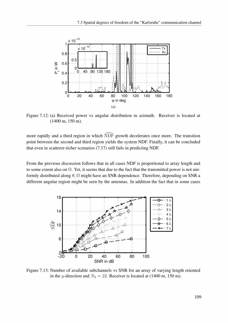
7.3 Spatial degrees of freedom of the “Karlsruhe" communication channel
0 20 40 60 80 100 120 140 160 1800
0.2
0.4
0.6
0.8
1x 10
−12
ψ in deg
Pr i
n W
Tx
Rx
0 45 90 135 1800
0.5
x 10−10
(a)
Figure 7.12: (a) Received power vs angular distribution in azimuth. Receiver is located at(1400 m, 150 m).
more rapidly and a third region in which NDF growth decelerates once more. The transitionpoint between the second and third region yields the system NDF. Finally, it can be concludedthat even in scatterer-richer scenarios (7.17) still fails in predicting NDF.
From the previous discussion follows that in all cases NDF is proportional to array length andto some extent also on Ω. Yet, it seems that due to the fact that the transmitted power is not uni-formly distributed along θ, Ω might have an SNR dependence. Therefore, depending on SNR adifferent angular region might be seen by the antennas. In addition the fact that in some cases
−20 0 20 40 60 80 1002
6
10
14
18
ND
F
SNR in dB
1 λ
2 λ
3 λ
4 λ
5 λ
6 λ
7 λ
Figure 7.13: Number of available subchannels vs SNR for an array of varying length orientedin the y-direction and NS = 22. Receiver is located at (1400 m, 150 m).
109

7 Communicational limits of linear multiple element antennas
Table 7.2: Predicted NDF for Figure 7.13
L 1λ 2λ 3λ 4λ 5λ 6λ 7λ
Tx 2 4 6 8 10 12 14
Rx 2 4 6 8 10 12 14
(smaller array lengths) additional subchannels to those possible in free space result, is also dueto the uneven power distribution. In this way, otherwise weak subchannels from an antennaperspective might receive sufficient energy as to contribute to NDF.
To summarize, even though the previously published formula LΩ for predicting NDF has beenproven inadequate for the single channel realizations of the “Karlsruhe" communication chan-nel, similar trends could still be observed:
• Angular spread at transmitter and receiver do limit NDF, and in consequence NDF.
• Array size directly influences both NDF and NDF.
• Even though higher SNR regimes can increase the degrees of freedom of the channel asevidenced by NDF, it is most convenient to design antenna systems with a maximum ofNDF dimensions. Otherwise great amounts of energy might be needed to benefit fromhigher ranked systems.
• Finally, it seems that due to the non-uniform nature of the angular distribution of realenvironments SNR effects on Ω need to be considered.
With this knowledge, evaluation of the urban communication channel in a more general sense,i.e. as the statistic resulting of all links, can be approached.
7.3.3 Degrees of freedom of all channel realizations
The study of the urban communication channel in a statistical sense can only be done based oncertain system assumptions. Here, the same assumptions as given in 3.3 are used. Furthermore,the same approach in the study of the degrees of freedom of the channel as the one given in theprevious section is used. This means that NDF vs SNR will be investigated for all channel re-alizations. Therefore, the total NDF will result from the maximum NDFl among all L channelrealizations, where the subscript l denotes the l-th channel realization.
Figure 7.14 shows the angular received power distribution and the corresponding NDF, for anarray of 22 omni-directional antennas oriented in the y-direction. It is seen in Figure 7.14a thatpower is better distributed among all angles than it was the case for the single channel realiza-tions considered in the previous section (Ω = 2 at receiver and transmitter). In consequence
110

7.3 Spatial degrees of freedom of the “Karlsruhe" communication channel
0 45 90 135 1800
0.5
1
1.5x 10
−7
ψ in deg
Pr i
n W
Tx
Rx
(a)
−40 −20 0 20 400
5
10
15
20
ND
F
SNR in dB
1 λ
2 λ
3 λ
4 λ
5 λ
6 λ
7 λ
(b)
Figure 7.14: (a) Received power vs angular distribution in azimuth and (b) SC vs SNR for anarray of varying length oriented in the y-direction and NS = 22 averaged over allreceiver positions.
the same predicted NDF values of Table 7.2 result. Furthermore, an uneven power distributionis also noticed in this case. Therefore, as seen from the NDF curve in Figure 7.14b, (7.17)fails once more in predicting NDF. Nonetheless, certain trends are recognized: 1) the channelas a whole exhibits higher NDF values and 2) similar to Figure 7.12 a rake-like behavior for allcurves was found. For SNR regimes below ≤-10 dB NDF increases slowly with SNR and con-tinues to do so for L < 3λ. For L ≥ 3λ, on the other hand, an accelerated growth rate is noted,from which according to the examples of the previous section, a NDF value can be estimated.For L =3λ-7λ NDF, as read from Figure 7.14b, is 5,7,9,11 and 13 respectively. Here, oncemore a linear dependence of NDF on L is verified, yet only from a certain threshold length (inthis case 3λ). In addition, when looking at a fixed SNR, i.e. 20 dB, also a linear dependence onL for NDF is suggested.
For completeness, in Figure 7.15 also the received power angular distribution and the corre-sponding NDF, for an array of 22 omni-directional antennas oriented in the z-direction areshown. It is seen that in this case an uneven power distribution in the elevation also results6.Furthermore, in this case, a smaller angular region is used. In consequence, much smaller NDFvalues are obtained, yet the same rake-like behavior of Figure 7.14b is seen. Finally, in this case(7.17) is also a poor approximation of the true NDF of the system.
6It should be noted that related angular distributions for the “Karlsruhe" communication channel have beenalready published [Sch07]. Yet, in this case the angular spectrum and not the number of received paths perangle are plotted. An histogram of all received paths (not shown) is very similar to the one in [Sch07]. However,such histograms are not a sufficient measure to understand the available spatial resources, since they mightwrongly suggest that energy concentrates in a small angular region, which is not the case.
111

7 Communicational limits of linear multiple element antennas
0 45 90 135 1800
0.5
1
1.5x 10
−7
ϑ in deg
Pr i
n W
Tx
Rx
(a)
−40 −20 0 20 400
5
10
15
20
ND
F
SNR in dB
1 λ
2 λ
3 λ
4 λ
5 λ
6 λ
7 λ
(b)
Figure 7.15: (a) Received power vs angular distribution in elevation and (b) SC vs SNR for anarray of varying length oriented in the z-direction and NS = 22 averaged over allreceiver positions.
From the previous results follows that for practical purposes and without previous simulation itis not possible to predict either NDF nor NDF, since appearance of new channels is completelyrandom. Instead, these results should be taken as reference in order to decide, depending on theSNR regime to be used, if the communication channel, and thus the system, benefits from hav-ing larger arrays or closely spaced antennas. Moreover, it must be stressed out that in this casethe effects of mutual coupling are not considered, and should be the focus of future research.
7.4 Final remarks
In this chapter the communicational limits of linear antenna arrays in three different scenarioswere discussed: free space, multipath with homogeneous power distribution among all pathsand multipath with uneven power distribution as in the “Karlsruhe" communication channel.As result, a method for estimating the available degrees of freedom in each case was obtained.It was seen that the number of degrees of freedom, which ultimately translates to the numberof possible subchannels available, is dependent on SNR, array length and scenario. In thisway, it can be concluded for real systems that depending on the SNR regime used, there willbe a certain number of antennas that provides the best trade-off between cost and performanceimprovement. Because of this, antenna design in real settings will differ from that in freespace. More importantly, in real scenarios with uneven power distributions (contrary to freespace) there does not seem to be a specific number of antennas after which capacity abruptlydecreases. Yet, a point can be determined after which the inclusion of additional subchannelsresults in only small capacity increases. Because of this, it seems likely that for systems work-
112

7.4 Final remarks
ing at high SNR regimes an optimum trade-off between number of antennas and capacity canbe found depending on the array length used. For low SNR regimes, however, the use of ad-ditional subchannels seems to be less sensitive to changes in array length than to SNR. In thefollowing the antenna synthesis problem for the urban channel from a multiple element antennaperspective will be approached.
113


8 Antenna design for wirelesscommunication channels
To conclude this work, in this chapter the design of capacity maximizing MEA arrays will behandled. Contrary to chapter 5 selection of an optimum antenna array will not be done by com-parison of a vast number of MEA configurations. Instead the background of chapter 7 will beused to exploit the spatial resources of the channel as shown possible from chapter 4. The ap-proach taken here is thus novel, since it synthesizes an antenna in a capacity maximizing sense,rather than just achieving a desired radiation pattern as done in more traditional synthesis meth-ods. The difference lies in the fact that in the case of power or pattern synthesis [Mai05, Bha07]a certain radiation property is desired, since it is assumed that in this way a better system per-formance concerning any parameter of interest can be attained. In this way it is customary todefine a specific issue, such as pattern interference, and based on it define an optimum radiationpattern for which a certain synthesis method is then applied, as done in [PW07, PLW07]. Giventhat capacity is a complex measure resulting from all system component and channel interac-tions it is not possible to define a priori a capacity maximizing radiation pattern. Therefore,in this chapter an in-system synthesis (-optimization) method is proposed. As result, a set ofsuggestions toward better antenna designs for the future will be made.
This chapter is structured as follows. First, a synthesis method for fully exploiting the chan-nel spatial resources in a capacity maximizing sense will be discussed. Then, the synthesisof capacity maximizing antenna arrays for the urban communication channel will be under-taken. And, finally, based on the results obtained antenna design concepts for the future will beproposed.
8.1 Multiple element antenna synthesis method
In chapter 7 an heuristic approach based on resolvability, similar to that in [TV05, PBT05], wastaken for finding the degrees of freedom of linear MEA systems in different communicationchannels. This intuitive approach, however, has its background on a more involved theoreti-cal framework focusing on the link between electromagnetism and information theory. In thissection a capacity maximizing synthesis method will be derived based on this theoretical frame-work.
115

8 Antenna design for wireless communication channels
Figure 8.1: Basic model for communicating volumes.
The first works related to the informational content of electromagnetic waves date back to theseminal works of Gabor and di Francia from the 1950s in the field of optics, who studiedthe available channels of communication among diffraction-limited surfaces. With this back-ground, [Mil00, PM00] investigated the available number of communication modes for arbitraryvolumes in optical systems based on an eigenfunction approach. Here it was shown that for thecase of communicating volumes (three dimensional balls in Figure 8.1) it is possible to expressthe sources and waves in terms of basis functions with coefficients βk and αk. In this way, thewave propagation problem can be rewritten into matrix form
α = Hβ. (8.1)
As result, the problem of maximizing the information throughput is recasted as the maximiza-tion of the so-called communication operator H between the three dimensional transmitting andreceiving balls (volumes) Bt and Br. Where, the non-zero elements of the otherwise infinite-dimensional H matrix, i.e. the rank of H, represent the available independent communicationchannels referred to as subchannels in the context of MIMO systems (NDF in information the-ory). This fundamental link between field theory and information theory poses, however, thedifficulty of finding the rank of the H matrix with the largest coefficients. Yet, this is onlyunder proper definition of the basis functions ρ and τ in single polarized 3D fields (or ρ and τfor vectorial fields as stated in [PM00])
E(r) =∞∑k
αkρk, (8.2)
J(r) =∞∑k
βkτk. (8.3)
Finding a proper set of basis functions is, in consequence, the key problem in determining H
with maximum communication coefficients. Moreover, the dimensioning of the communication
116

8.1 Multiple element antenna synthesis method
system will depend on the number of basis functions needed to accurately represent E(r) andJ(r) while truncating the series (8.2) and (8.3).
In [Mil00], an analytical solution for the basis functions of the scalar source in integral-equationform with aid of the prolate spheroidal wave functions for the case of three-dimensional hyper-rectangles is derived. In [PM00], on the other hand, multi-polarized fields and currents E(r)and J(r) are considered and the vectorial eigenvalue problem, found when maximizing the in-terconnection strengths of H, is solved for vectorial basis functions of the source current withthe use of a numerical technique called the Galerkin method. Later on, in [HF06] the approachin [Mil00] is extended for the case of arbitrary volumes and the effects of multiple scatterersis considered, yet similar to [PBT05, CF06, XJ06, Mig06b, Mig06a, GM08] focus is shiftedfrom computation of the basis functions to obtention of NDF. And it was not until recently that[JW08] showed that the basis functions of the current J could themselves be approximated bya set of sub-basis functions. These sub-basis functions then sample the channel in the spatialdomain so that the optimal current distributions and radiation patterns for a certain antenna sizein a specific scenario can be found.
However, in [JW08] only results for a two-dimensional channel model are presented. Therefore,in this work, results for a realistic urban propagation scenario based on a three dimensional ray-tracing simulator are presented and, in addition, an extension to the synthesis method of [JW08]is also proposed.
In [JW08] it was shown that the basis functions ρ and τ (vectorial form) could be numericallyapproximated as a linear combination of an additional set of sub-basis functions ˜ρ and ˜τ In thisway the source current, could be rewritten solely in terms of the sub-basis functions [JW08, Eq.(20)]. As result, computation of the channel matrix H between the sub-basis functions and itssingular value decomposition (SVD) H = USV† suffices to determine H and the optimal basisfunctions as
ρk =∑v
Vvkρv
τk =∑u
Uukτu,(8.4)
in the scalar case.This formal approach in determining H was heuristically used in the previouschapter. The main idea was to sample the communicating space and determine its limitations.Therefore, in [JW08] the sub-basis functions act as sampling functions which then with use ofa water-filling solution allow for reconstruction of the optimal current distributions and electricfields.
117

8 Antenna design for wireless communication channels
Computation of the optimal current distribution, requires that ˜ρ and ˜τ are orthonormal. In[JW08] this was done by subdividing the transmit and receive apertures into NS subaperturesin each dimension (see Figure 8.2b). This resulted in an elaborate expression for H [JW08,Eq. (23)] (for the single polarized case). In this work, the use of point sources is proposedinstead (see Figure 8.2c). With point sources orthonormality is maintained and a much simplerexpression for H is found by substituting for the scalar case ρ and τ with dirac delta functionsin the expression for Hvu implicit in [JW08, Eq. (19)]
Hvu =
∫Br
dBr
∫Bt
dB′t ρ
†v (rr)G(rr, r
′t) τu(r
′t)
= G(rr,v, rt,u),
(8.5)
where G is the scalar Green function of the channel (in the general case the dyadic Greenfunction
↔G results). Then, under adoption of the commonly used plane wave model, (8.5) is
found to be
G(rr,v, rt,u) = Hvu =P∑p=1
Tpejφ(rr,v,Ωr,p)ejφ(rt,u,Ωt,p), (8.6)
withφ(r,Ω) =
2π
λ(x cosψ sinϑ+ y sinψ sinϑ+ z cosϑ), (8.7)
where ϑ and ψ are the elevation and azimuth angles of the receive and transmit vectors rr,v andrt,u, of the v and u sub-basis function for the p-path and Tp is the transmission factor of thepolarization component of interest.
Now, in order to synthesize the antenna radiation pattern out of the given sub-basis functions theτ basis functions are used to obtain the optimal current distribution, and out of it the radiatedpattern of the ideal antennas. It should be noted though that from a communication systemperspective τk represents the k-th subchannel. Therefore, here the fact must be stressed thateven though the total current is written as in (8.3) [JW08, Eq. (6)], interest lies in the currentdistribution of each subchannel. It follows that Jk = τk and the transmitted electric field Et,k ofthe k-th subchannel can be found from
planar antenna
(a)subaperture divisions
(b)simplification
(c)
Figure 8.2: Array aperture showing the sub-basis regions with NS = 2.
118

8.2 Antenna array synthesis for the urban communication channel
Et,k (rt) =e−jkrt
rt
∫∆Vt
ejφ(r,′t ,Ωt)Jk (r
′t) dr
′t . (8.8)
For computing the electric field of the receiving antenna the channel matrix is transposed (in-verse communication direction) and an analogous expression to (8.8) is used, but integratingover the receiving volume. In this case the optimal k-th current distribution at the receiverresults from
Jk(rr) = τ ′k(rr) =∑v
V ∗vkρv(rr). (8.9)
A drawback of point sources, though, is that they are only capable of sampling the channel atdiscrete points, contrary to the continuous aperture approach in [JW08]. As trade-off, however,antenna synthesis can be easily integrated to existing channel simulators. In this way H canbe easily computed and, in addition to point sources, regular antennas can be chosen as sub-basis functions so that an antenna type based synthesis becomes feasible. It follows, that amulti-polarized or multi-antenna synthesis is straightforward and is done by expressing eachsub-basis function as a linear combination of the different polarization components or different
antennas. This could be seen as a modal expansion and yields in return a tensor↔H matrix, i.e. a
four dimensional matrix, with tensor elements↔Huv, i.e. two dimensional elements. For practical
purposes this is equivalent to simply computing one H for each antenna or polarization neededand arranging them in a two dimensional matrix to obtain the desired water-filling solution. Thepotential of this for optimizing the communication channel capacity will be shown later on.
8.2 Antenna array synthesis for the urbancommunication channel
In order to visually clarify the functioning and potential of the synthesis method previouslydescribed, in Figure 8.3 the synthesized antennas obtained when the receiver is located at(1637 m, 637 m) are shown, for a free space channel (Figure 8.3a) and for the channel describedin section 3.3 (Figure 8.3b). The synthesized antennas are generated using a planar array withNS = 5 in y and z-direction at both base station and mobile stations. H is obtained with helpof the network model of chapter 3 under the assumptions of perfect impedance matching. It isseen that for free space the resulting antennas look at each other. For the multi-path propaga-tion scenario, on the other hand, a minimum at the line of sight direction is observed. This waspurportedly chosen this way to show that, even in cases where most of the incoming energy atthe receiver originates from scattering objects, the method presented is capable of synthesizingan optimal current distribution, and from it an optimum antenna radiated field.
119

8 Antenna design for wireless communication channels
(a) Free space
(b) “Karlsruhe" scenario
Figure 8.3: Synthesized antennas.
In the following, in order to obtain a more realistic description of the actual site, influenced toa lesser extent by the base station look direction, a three-sectorized cell is used. This meansthat for each sector only those mobile station positions lying within the defined angular limitsare considered and the base station orientation is rotated accordingly. Orientation of mobilestations, on the other hand, is kept constant and parallel to the x-axis for all sectors. Effectively,this results in three different propagation environments and thus three different syntheses forboth mobile and base station. However, since in each sector multiple antenna links exits, inorder to obtain the antenna that maximizes capacity in most cases, an averaging over all links,i.e. channel realizations, is performed.
These average Jk currents are then used in (8.8) to obtain the radiated pattern. Alternatively,instead of an antenna synthesis this can be interpreted as a synthesis of the optimal currentdistributions for the array of point sources. In the case where specific antenna types (i.e. non-
120

8.2 Antenna array synthesis for the urban communication channel
isotropic antennas) are considered as the point sources, i.e. sub-basis functions, their radiationpatterns are multiplied with Jk resulting in a weighted current J ′
k. And for the more generalcase of multiple fully polarized (θ and ψ polarized) antennas a vectorial weighted current re-sults J ′
k. The synthesized radiation patterns from J ′k are then used to compute the waterfilling
capacity. However, since there might be interest to use only a certain number of antennas in-stead of all possible, the number SC of most significant subchannels used for synthesis is varied.The synthesized antennas are assumed to have the same location, SNR is fixed to 10 dB, andall channel matrices are normalized with the ones resulting from an equivalent (same antennanumber and location) omni-directional antenna system. The antenna synthesis is done using anarray of point sources of length L = 5λ aligned in z-direction (perpendicular to ground) at bothbase station and mobile stations.
In Figure 8.4 capacity vs. number of synthesized subchannels SC is shown for omni-directionalantennas. The antenna elements used for each sub-basis function were omni-directional anten-nas either θ polarized, ψ polarized or both. Hereby, two array orientations were considered:y-direction (Figure 8.4a) and z-direction (Figure 8.4b).
It is known from the previous chapter that a larger number of subchannels in the y-directionthan in the z-direction can be obtained. In Figure 8.4 this is confirmed. It is seen that whenonly one polarization is used, the capacity of the in y-direction synthesized antennas reaches itsmaximum value at SC = 10. For the in z-direction synthesized antennas the capacity limit isalready reached with SC = 5. Remarkably though, with equal number of synthesized subchan-nels the in z-direction synthesized antennas achieve larger capacities. This means that narrowerbeams (larger gain) in elevation, compensate for the reduced angular spread inherent to arraysoriented in z-direction. This, therefore suggests that for MEA systems in urban settings withfew antennas (less than 71), the use of the available subchannels in the elevation, rather than inazimuth, will yield the best performance. Finally, it was also seen that in bot cases when dualpolarized omni-directional antennas are used for synthesis, capacity improves significantly (al-most doubles) and the number of subchannels doubles as predicted in [PBT05, Mig06b].
Figure 8.5 now shows a similar result but in this case combinations of dipoles oriented parallel tothe coordinate axes are considered. Here, for brevity only the case of an array in the z-directionis considered. The result for a z-oriented dipole is similar to Figure 8.4b, with small differencesdue to the effect of the dipole radiation pattern in comparison with an omni-directional antenna.However, it is seen that the use of two perpendicular dipoles almost completely exploits thepolarization diversity (capacity stabilizes at SC = 9) and that the addition of a third dipole does
1This criterion is not arbitrarily chosen and might change depending on the propagation channel considered. Itresults from comparing the capacities of the in z and in y-direction synthesized antennas and finding the pointfrom which the latter outperforms the former.
121

8 Antenna design for wireless communication channels
2 3 4 5 6 7 8 9 10 112
6
10
14
18
22
SC
C in
bits/s
/Hz
Omni_θ
Omni_ψ
Omni_θ & Omni_ψ
(a) Arrays of sub-basis antennas are oriented in the y-direction, NS = 40
2 3 4 5 6 7 8 9 10 112
6
10
14
18
22
SC
C in
bits/s
/Hz
Omni_θ
Omni_ψ
Omni_θ & Omni_ψ
(b) Arrays of sub-basis antennas are oriented in the z-direction, NS = 25
Figure 8.4: Capacity vs SC for synthesized antenna arrays of omni-directional antennas withdifferent polarizations. The capacity of the synthesized arrays is averaged over allchannel realizations.
not improve capacity significantly (even though polarization diversity is fully exploited). Thisassessment is in good agreement with the results of chapter 5, where the best capacity values in2x2 systems were obtained for the Xk×Xd setup.
Summarizing, these results are of great importance since they demonstrate that by using verysimple antenna elements, capacities comparable to those of current commercial antennas in 2x2setups can be achieved. For example, comparison of the absolute capacities of the VV×VVsetup with the capacities obtained in Figure 8.4 evidences the fact that when using only two sub-channels SC = 2 the synthesized antennas reach almost the same capacities as the VVk×VVdsetup with sTx = 5λ and sRx = 5λ. Furthermore, if it is considered that in this case theantennas are synthesized based on smaller arrays than the ones currently available in commer-
122

8.3 Antenna design concepts for the future
2 3 4 5 6 7 8 9 10 112
6
10
14
18
22
SC
C in
bits/s
/Hz
z
z & y
z & y & x
Figure 8.5: Capacity vs SC for synthesized antenna arrays of NS = 25 dipole antennas orientedparallel to the coordinate axes. The arrays of sub-basis antennas are oriented in thez-direction and their capacity is averaged over all channel realizations.
cial antennas, this could translate into significant savings for antenna providers. For example,by deploying an antenna in z-direction with two subchannels would already result in the ca-pacity increases obtained with two base station antennas. It can be argued, though, that the±45°polarized base station antennas considered in this work already provide these capacities,yet what these results show is that by accessing more independent subchannels (i.e. havingmultiple power distributions driving the same antenna elements) in a single physical antennagreat capacity improvements can be achieved without the need to have additional antennas in-stalled. As result, synthesis strategies that make better use of the available radiating elementsseem more promising than adding more antennas.
8.3 Antenna design concepts for the future
The previous simulations showed that capacity of cellular systems for the urban scenario couldbe increased without having to use additional antennas. Instead, several array excitations couldbe used. This approach borrows from the diagonalization performed by the waterfilling algo-rithm in MIMO systems. In the waterfilling algorithm the goal is to find orthogonal subchannelsto convey the largest amount of information per time. Out of it different weighting vectors forall communicating antennas for each channel realization result. In the previous section insteadof having many antennas, with many radiating elements each, the antenna radiating elements ofone antenna are used as single antennas. Then, out of the averaging of the subchannels for allchannel realizations the optimum complex weight for each antenna element for each averagedsubchannel is found. The main difference, thus, with respect to the regular waterfilling algo-rithm that requires dynamically driving each antenna element is that in this case fixed driving
123

8 Antenna design for wireless communication channels
networks suffice to provide high capacities. In this way it is found that equal or better capacityperformances can be reached by exploiting the signal diversity in the elevation plane than withmore antennas in the azimuth direction. In consequence, initial costs would be reduced as wellas running costs, such as rent space for the antennas and transmit power. Now the problem ofimplementing such synthesized antennas will be addressed.
In Figure 8.6 a typical base station antenna implementation for an XX configuration, i.e. twocross polarized antennas at the base station, is depicted. It was shown in chapter 5 that thisconfiguration results in a good compromise between capacity and number of antennas, thereforeit will be used for comparison. As previously discussed this configurations yields a 4x2 MIMOsystem when two antennas are available at the mobile station. Thus four ports are fed into thephysical layer processing unit [ITU94] after being amplified by the tower mounted amplifier(TMA). In order to make a fair comparison, resulting in the least impact to the system, in thefollowing, two approaches with four base station antenna ports will be also discussed. It will beseen that with the solutions proposed unit costs can be reduced while still optimizing capacity.
Figure 8.6: Typical base station block model [Kat09].
124

8.3 Antenna design concepts for the future
The main idea proposed in the previous section was to have individual array excitations for eachtransmitted or received signal. In this way if a MIMO system is capable of having four subchan-nels at any given time, then four distinct array excitations can result in a better capacity thanhaving multiple antennas. However, current antenna systems are usually passive and consistof one driving network, i.e. one array excitation. A way in which simultaneous array excita-tion can be generated is if each antenna can be individually controlled by the base transceiverstation. For normal antennas, this would require the processing of 8 or more parallel signals,which results in increased costs. Moreover, due to polarization diversity, as shown in this work,in order to exploit the available degrees of freedom access to a second array of orthogonal el-ements would also be needed to reach the capacity of cross polarized antennas. This wouldfurther increase the costs of the system and would yield such a solution unpractical. One optionis therefore to avoid the use of driving networks altogether and partition the antenna radiatingelements into subarrays. In this manner each subarray can be handled as an individual antennaand can make use of the signal diversity in the elevation plane.
Another alternative is to have a pre-processing unit (PU). This unit would then be respon-sible for mapping the received and transmitted signals to all radiating elements. An analogimplementation of such a unit would require having four passive networks with additional di-viders/combiners and would thus result in power losses and higher costs. The alternative isto have a digital implementation. The drawback is the cost of converting the signals at eachradiating element from the analog into the digital domain. In exchange though the TMA wouldbecome unnecessary. Therefore, here, focus is given to the digital implementation of such PU.In the following two PU approaches will be proposed, with potential of efficiently driving theindividual radiating elements in such a way that the most efficient array excitations result. Inthis case the number of array excitations is four. In real systems, on the other hand, it willdepend on the allowed complexity of the system and the impact it has on the system capacitybased on simulation results.
In Figure 8.7 the proposed solutions are depicted. For comparison purposes cross polarizedantennas as those previously used in chapter 5 are used. This is equivalent to applying theprevious synthesis method with -45°and +45°oriented dipoles as sub-basis functions. Suchsub-basis functions would then yield very similar results as those obtained in Figure 8.5 for thez and y oriented dipoles.
In Figure 8.7a the first and relatively simple proposed implementation is shown. It consists insubdividing the antenna array into sub-arrays. In this way it is possible to access each sub-array as if it were a single antenna and thus exploit the signal diversity in the elevation plane.Even though this is not the same as controlling the excitation of each radiating element for eachtransmitted and received signal, it is most likely that very similar capacities as with two cross
125

8 Antenna design for wireless communication channels
polarized base station antennas will result due to the use of signal diversity in the elevationplane. In addition, a significant cost reduction would be achieved, since there is no longer aneed for a second antenna as in 8.6.
The second approach proposed is that of Figure 8.7b. There are several differences with re-spect to the implementation of Figure 8.6. The first difference is the use of a so called towermounted processing unit (TMPU). This TMPU corresponds to the physical implementation ofthe PU previously discussed and consists of a unit responsible for the signal processing in boththe transmit and receive case and could be also placed within the physical antenna. The seconddifference is the use of additional ports between the antenna and the TMPU. Ideally the numberof ports would be the same as that of the number of antennas, i.e. yielding an active antennaarray. However, this would increase the difficulty in implementing such a scheme. One way toovercome this problem is by using subarrays, as was done in Figure 8.7a. In this case, howeversmaller subarrays are suggested in order to better exploit signal diversity in the elevation plane.
(a) (b)
Figure 8.7: Block model of proposed base stations with (a) sub-array implementation and (b)with external tower mounted pre-processing unit (TMPU).
126

8.4 Final remarks
These two approaches exhibit advantages and disadvantages and it is not intended here to assessthe viability or cost-efficiency of each approach. In the same manner no implementation detailsare of interest at this point. Instead, these solutions intend only to show that it is indeed possiblewith the available technology to try out new ways in which the spatial resources available tobase station antennas can be better exploited. Furthermore, these approaches are only two outof many ways in which a more efficient use of the spatial resources can be done. As it hasbeen shown in this work, only by knowing which are the resources available and how theycan be exploited it is really possible to optimize the antennas in MEA systems. Therefore,since the results obtained show that diversity in the elevation plane suffices to reach comparablecapacities as those obtained with additional antenna elements in the azimuth direction, thesesolutions seem as promising alternatives for the design of future base station antennas.
8.4 Final remarks
In this chapter a synthesis method for achieving maximum information throughput in MIMOchannels is shown. Based on it, the communicational limits of the urban communication chan-nel are explored. From the results presented the following conclusions can be stated:
• The number of degrees of freedom, which ultimately translates to the number of possiblesubchannels available is dependent on SNR, array length and scenario. If all these vari-ables are fixed, though, it is possible by a SVD and waterfilling based approach to obtaina setup that maximizes capacity in each case for a certain set of sub-basis functions, i.e.radiating elements.
• Under the assumption of a perfect power control (PPC) scheme, as implicitly done bythe normalization used throughout this work, a maximum capacity exists after which thesubsequent addition of subchannels does not improve the system performance (in caseof power distributions other than waterfilling -optimum- it worsens it). This maximumcapacity constitutes the communicational limit of the channel. Nonetheless, it should benoted, that the addition of receiving antennas will always have a positive impact on thesystem in terms of power.
• It is found that a higher number of degrees of freedom is available in azimuth rather thanelevation. However, these aren’t enough to compensate for the achievable antenna gainand small beamwidth when several radiating elements are placed in the elevation plane.As result, the addition of subchannels in vertical oriented base station antenna is shownto yield higher capacities than the same number of subchannels in an horizontal orientedone.
• The capacity maximum reached for a certain configuration doubles if orthogonal polar-izations are used for synthesis. And the use of two orthogonal dipoles yields very similar
127

8 Antenna design for wireless communication channels
results to two isotropic orthogonal polarizations, whereas three orthogonal dipoles pro-vide little additional improvement.
With the results presented in this chapter it is proven for the urban communication channelthat better capacities to those of commercial antenna setups could be achieved, not with moreantennas, but by driving more subchannels. In consequence, contrary to larger antenna deploy-ments, antenna driving networks capable of producing several array excitations are suggestedas the next step toward better capacities in urban communication channels. Here, three possibleimplementations are proposed for further investigation.
128

9 Conclusions
The use of MEA systems for the planning of upcoming services and technologies has becomethe norm in the context of wireless communications. The strategies for meeting the constantlyincreasing data rate demand for an important number of standards for the wireless transmissionof information are based on the efficient and coordinated use of the frequency, time and spaceresources. In this manner, space has become a significant factor for the analysis and designof antenna systems, in general. However, this is done mostly from a passive perspective, inwhich space is usually given as the byproduct of a certain scenario and antenna configuration.The motivation of this thesis was therefore to extend the understanding of the spatial resourceswhen it comes to MEA systems. This was achieved for the urban “Karlsruhe" communicationchannel, based on the multipath modeling scheme of [Füg09]. And even though this does notresult by any means in a complete statistical description depicting the behavior of all urbansites, it suggests the way urban scenarios in general might behave and provides a methodologyfor evaluating urban communication scenarios in general.
The goals of this work are to extend and improve the analysis of MEA systems and to gaininsight into the antennas design and their most convenient implementation in terms of maximumchannel capacity. Contrary to most published works in the context of MIMO and MEA systems,attention was given in this thesis to the channel-antenna interaction and how it can be betterdescribed and optimized. Therefore, the interest of this research lies in the study of the antennacontributions to the performance of MEA systems. As result, the following achievements weremade:
• An improved network model based on the modal description of the antennas was imple-mented and proved to yield significant reductions in simulation time for the case of modalmodeled dipoles.
• An exhaustive study of different antenna configurations with varying inter-element spac-ing at both transmitter and receiver was done for three different types of power allocationschemes.
• A comprehensive and simple pre-evaluation metric for the study of MEA systems wasproposed, which separates the beamforming and multiplexing effects of the channel. Thisnovel metric facilitates the computation of capacity for any given type of channel normal-ization in either the ergodic or outage sense.
129

9 Conclusions
• The communicational limits, in regard to the maximum number of parallel data streamssupported by the channel-antenna interaction, were assessed for the first time in the con-text of urban channels for linear antenna arrays.
• An array synthesis method for capacity maximization was proposed which is capable ofoutperforming current commercial base station antennas in terms of capacity and imple-mentation cost trade-off.
In this way, a thorough study of the antenna effects on the capacity performance of MEA sys-tems has been given. Also, the simulation, evaluation and design frameworks for the investiga-tion of antennas in MEA systems have been extended. The significance for the future study ofantennas within MEA systems has been three-fold: 1) faster simulation, 2) comprehensive andeasier evaluation and comparison and 3) optimum use of the spatial resources.
In chapter 2 the theoretical background necessary for understanding the wireless propagationof signals and the role played by the antennas within the wireless communication channel wasgiven. With this knowledge, in chapter 3 a modeling framework for the whole communicationchannel of MEA systems was provided. Here, previous modeling efforts were extended withthe purpose of facilitating the simulation and investigation of a large number of antenna types.By means of a modal antenna description simulation times were reduced. It was shown thatwhen dealing with dipoles three modes suffice for describing any possible dipole orientations.In this way the computational gain of this approach increases with increasing the number ofantenna orientations to be investigated. In addition, the road has been paved for a further exten-sion of this simulation method, possibly by means of spherical modes translation and rotationin which, out of the simulation of a fixed number of modes, not only different antenna types butalso different antenna locations can be computed.
Completing this theoretical background, the evaluation framework used was provided in chap-ter 4 based on the concept of maximum information throughput, i.e. capacity. Diversity andmultiplexing effects on capacity were discussed and the duality between temporal and spatialdomains in the computation of capacity was restored. On this basis, in chapter 5 a benchmarkof different antenna configurations for the urban macrocell case of the “Karlsruhe" scenarioshowed that the significance of antenna spacing depends on the configuration studied, i.e. onwhether diversity or multiplexing effects predominate for the setup being considered. It wasconcluded, based on the cross comparison of the capacities of three different power allocationschemes, that for real antenna configurations in urban settings 1) antenna inter-element spac-ing has a larger impact on multiplexing gain than on beamforming gain, 2) this impact is mostnoticeable for single polarized configurations and 3) for dual polarized configurations beam-forming gain decreases with larger antenna spacings. Regarding the capacity dependence on
130

antenna rotation, robustness of cross polarized configurations toward antenna rotation was ver-ified for all antenna spacings. Furthermore, it was seen that the optimum antenna orientation isdetermined by the propagation channel in the case that single polarized antennas at the mobilestation are used in conjunction with dual polarized ones at the base station.
In performing the very exhaustive study of chapter 5 it became clear that it was not in all casespossible to determine the individual contribution in terms of diversity and multiplexing of acertain antenna setup or spacing. The proposed metric from chapter 6 for addressing this is-sue, showed that it was possible to approximate the system capacity as the contribution of threefactors: SNR, a diversity measure, transferred signal power, and a multiplexing measure, eigen-value dispersion. This novel metric was also extended for the case of arbitrarily sized systems.Its implementation for the analysis of 2x2 and 4x4 setups in the “Karlsruhe" communicationchannel allowed the study of multiplexing and diversity effects and the capacity reconstructionregardless of channel normalization.
In order to complete the study of the antennas impact on MEA systems their communicationallimits were derived in chapter 7. In particular, a method for estimating the maximum numberof parallel data streams possible was given for the cases of: free space, multipath with uniformpower distribution per path and multipath with uneven power distribution as embodied by the“Karlsruhe" communication channel. This evidenced a linear dependence on array length forall cases. However, for the “Karlsruhe" communication channel it was seen that due to its un-even power distribution no clear limit to the maximum number of subchannels existed. Instead,a maximum number of antennas was found after which capacity increased at a much slowerrate with each additional subchannel. From the analysis made, it was concluded that a largernumber of subchannels exists along the azimuth direction than along the elevation direction.
In chapter 8 the results from chapter 7 were then used as basis for the synthesis of capacitymaximizing arrays. Here, a novel in-system synthesis method was developed, which allowedthe computation of optimum radiation patterns in a capacity maximizing sense, contrary totraditional approaches where the radiation characteristics are a priori specified. In this way,synthesized antennas were found which were capable of better exploiting the spatial resourcesof the communication channel. It was confirmed that the number of available subchannels forsynthesized arrays along the azimuth direction is greater than along the elevation. Yet, additionof subchannels for a vertically oriented array yielded larger capacity improvements. Therefore,this chapter and this work was concluded with a discussion of future antenna implementationswhich, based on the guidelines derived in this work, would yield improved system performancewithout increasing antenna size and no significant added costs.
131


Bibliography
[ABB+07] P. Almers, E. Bonek, A. Burr, N. Czink, M. Debbah, V. Degli-Esposti, H. Hofstet-ter, P. Kyösti, D. Laurenson, G. Matz, A.F. Molisch, C. Oestges, and H. Özcelik.Survey of channel and radio propagation models for wireless MIMO systems.EURASIP Journal on Wireless Communications and Networking, 2007(ArticleID 19070), 2007.
[AGW+02] Y. Adane, A. Gati, Man-Fa Wong, C. Dale, J. Wiart, and V.F. Hanna. Optimalmodeling of real radio base station antennas for human exposure assessment us-ing spherical-mode decomposition. Antennas and Wireless Propagation Letters,IEEE, 1:215–218, 2002.
[Ala98] S. Alamouti. A simple transmit diversity technique for wireless communications.IEEE Journal on Selected Areas in Communications, 16(8):1451–1458, October1998.
[And00] J. B. Andersen. Array gain and capacity for known random channels with multi-ple element arrays at both ends. IEEE Journal on Selected Areas in Communica-tions, 18(11):2172–2178, November 2000.
[And03] Theodore W. Anderson. An introduction to multivariate statistical analysis. Wi-ley series in probability and statistics. Wiley, Hoboken, NJ, 3. ed. edition, 2003.Previous ed.: 1984; : c74.50 : CIP entry (May).
[Bal97] C.A. Balanis. Antenna Theory. John Wiley & Sons, New York, NY, 1997.
[Bha07] A. K. Bhattacharyya. Projection matrix method for shaped beam synthesis inphased arrays and reflectors. IEEE Transactions on Antennas and Propagation,55:675–683, March 2007.
[Bre59] D. G. Brennan. Linear diversity combining techniques. In Proceedings of theIRE, volume 47, pages 1075–1102, June 1959.
[CF06] K. Chakraborty and M. Franceschetti. Maxwell meets shannon: Space-time du-ality in multiple antenna channels. Allerton Conference on Communication, Con-trol, and Computing, 2006.
[CP07] J.-M Conrat and P. Pajusco. Typical MIMO propagation channel in urban macro-cells at 2 ghz. In Proceedings of the 13th European Wireless Conference, pagesCD–ROM, Paris, France, April 2007.
133

Bibliography
[CPGZ09] J. Corcoles, J. Pontes, M. A. Gonzalez, and T. Zwick. Modelling line-of-sightcoupled MIMO systems with generalised scattering matrices and spherical wavetranslations. Electronics Letters, 45(12):598–599, June 4, 2009.
[CS91] Y. Chen and T. Simpson. Radiation pattern analysis of arbitrary wire antennasusing spherical mode expansions with vector coefficients. Antennas and Propa-gation, IEEE Transactions on, 39(12):1716–1721, Dec 1991.
[CT91] T. M. Cover and J. A. Thomas. Elements of Information theory. John Wiley &Sons, Inc., 1991.
[DC08] A. Dunand and J.-M Conrat. Polarization behaviour in urban macrocell environ-ments at 2.2ghz. In COST 2100, TD(08)406, Wroklaw, Poland, February 2008.
[ESBP02] V. Erceg, P. Soma, D. S. Baum, and A. J. Paulraj. Capacity obtained frommultiple-input multiple-output channelmeasurements in fixed wireless environ-ments at 2.5 ghz. In Communications, 2002. ICC 2002. IEEE International Con-ference on, volume 1, pages 396–400, New York, NY, USA, 2002.
[FFLV01] F. R. Farrokhi, G. J. Foschini, A. Lozano, and R. A. Valenzuela. Link-optimalspace-time processing with multiple transmit and receive antennas. IEEE Com-munications Letters, 5(3):85–87, March 2001.
[FG98] G.J. Foschini and M.J. Gans. On limits of wireless communications in a fadingenvironment when using multiple antennas. Wireless Personal Communications,6:311U335, 1998.
[FMKW06] T. Fügen, J. Maurer, T. Kayser, and W. Wiesbeck. Capability of 3-d ray tracingfor defining parameter sets for the specification of future mobile communica-tions systems. IEEE Transactions on Antennas and Propagation, 54:3125–3137,November 2006.
[Fos96] G.J. Foschini. Layered space-time architecture for wireless communication in afacing environment. Bell Labs Technical Journal, pages 41–49, October 1996.
[FSM+02] T. Fügen, G. Sommerkorn, J. Maurer, D. Hampicke, W. Wiesbeck, and R.S.Thomä. MIMO capacities for different antenna arrangements based on doubledirectional wide-band channel measurements. In Proceedings of the 13th IEEEInternational Symposium on Personal, Indoor and Mobile Radio Communica-tions, PIMRC 2002, volume 3, pages 1777–1781, Lisbon, Portugal, September2002.
[Füg09] Thomas Fügen. Richtungsaufgelöste Kanalmodellierung und Systemstudien fürMehrantennensysteme in urbanen Gebieten. PhD thesis, Universität Karlsruhe,2009.
[GL96] Gene Howard Golub and Charles F. Van Loan. Matrix computations. JohnsHopkins University Press, 1996.
134

Bibliography
[GM08] F. K. Gruber and E. A. Marengo. New aspects of electromagnetic informationtheory for wireless and antenna systems. IEEE Transactions on Antennas andPropagation, 56(11):3470–3484, November 2008.
[GN06] M. Gustafsson and S. Nordebo. Characterization of MIMO antennas using spher-ical vector waves. IEEE Transactions on Antennas and Propagation, 54(9):2679–2682, September 2006.
[GW98] N. Geng and W. Wiesbeck. Planungsmethoden für die Mobilkommunikation.Springer, Berlin, 1998.
[Han81] R. C. Hansen. Fundamental limitations in antennas. Proceedings of the IEEE,69(2):170–182, February 1981.
[Han88] J. E. Hansen. Spherical Near-field Antenna Measurements: Theory and Practice.IET, 1988.
[HF06] L. Hanlen and M. Fu. Wireless communication systems with-spatial diversity: avolumetric model. IEEE Transactions on Wireless Communications, 5:133–142,January 2006.
[IN02] M. T. Ivrlac and J. A. Nossek. Mimo eigenbeamforming in correlated fading. InCircuits and Systems for Communications, 2002. Proceedings. ICCSC ’02. 1stIEEE International Conference on, pages 212–215, June 26–28, 2002.
[IN03] M.T. Ivrlac and J.A. Nossek. Quantifying diversity and correlation in rayleighfading MIMO communication systems. In IEEE International Symposium onSignal Processing and Information Technology, ISSPIT 2003, pages 158–161,Darmstadt, Germany, December 2003.
[ITU94] ITU. X.200 information technology - open system interconnection - basic ref-erence model: The basic model. Technical report, ITU-T TelecommunicationStandarization Sector of International Telecommunication Unit (ITU), 1994.
[IY02] M. F. Iskander and Zhengqing Yun. Propagation prediction models for wirelesscommunication systems. IEEE Transactions on Microwave Theory and Tech-niques, 50(3):662–673, March 2002.
[Jak74] W. Jakes. Microwave Mobile Communications. Wiley, New York, NY, 1974.
[Jan02] R. Janaswamy. Effect of element mutual coupling on the capacity of fixed lengthlinear arrays. Antennas and Wireless Propagation Letters, 1:157–160, 2002.
[JW08] M. A. Jensen and J. W. Wallace. Capacity of the continuous-space electromag-netic channel. IEEE Transactions on Antennas and Propagation, 56(2):524–531,February 2008.
[KA06] M. Kang and M. S. Alouini. Capacity of MIMO rician channels. IEEE Transac-tions on Wireless Communications, 5(1):112–122, January 2006.
135

Bibliography
[KAE06] O. Klemp, G. Armbrecht, and H. Eul. Computation of antenna pattern correlationand MIMO performance by means of surface current distribution and sphericalwave theory. Advances in Radio Science, 4:33–39, 2006.
[Kat02] R. Kattenbach. Statistical modeling of small-scale fading in directional radiochannels. IEEE Journal on Selected Areas in Communications, 20(3):584 – 592,April 2002.
[Kat09] Kathrein-Werke KG. DTMA-UMTS-12-AISG-CWA Datasheet, 2009.http://www.kathrein.de/de/mcs/produkte/download/9363122a.pdf.
[KBJR01] M.A. Khalighi, J. Brossier, G. Jourdain, and K. Raoof. Water filling capacity ofrayleigh MIMO channels. In Proceedings of the IEEE 12th International Sympo-sium on Personal, Indoor and Mobile Radio Communications, volume 1, pages155–158, San Diego, CA , USA, September 2001.
[KCVW03] P. Kyritsi, D.C. Cox, R.A. Valenzuela, and P.W. Wolniansky. Correlation analysisbased on MIMO channel measurements in an indoor environment. IEEE Journalon Selected Areas in Communications, 21(5):713–720, June 2003.
[KG06] KATHREIN-Werke KG. 790-2500 mhz base station antennas for mobile com-munications, 2006.
[KHE05] O. Klemp, S. K. Hampel, and H. Eul. Study of MIMO capacity for linear dipolearrangements using spherical mode expansions. In Proceedings of the 14. ISTMobile&Wireless Comm. Summit, 2005.
[Kil00] Per-Simon Kildal. Foundations of Antennas. Studentlitteratur, 2000.
[KJUN02] T.P. Kurpjuhn, M. Joham, W. Utschick, and J.A. Nossek. Experimental stud-ies about eigenbeamforming in standardization mimo channels. In Proceedingsof the 56th IEEE Vehicular Technology Conference, VTC 2002-Fall, volume 1,pages 185–189, Vancouver, Canada, September 2002.
[Kra88] John Daniel Kraus. Antennas. McGraw-Hill Companies, 1988.
[Lee82] W.C.Y. Lee. Mobile Communications Engineering. McGraw-Hill, New York,1982.
[LOKM05] B.K. Lau, S.M.S. Ow, G. Kristensson, and A.F. Molisch. Capacity analysis forcompact MIMO systems. In Vehicular Technology Conference, 2005. VTC 2005-Spring. 2005 IEEE 61st, volume 1, pages 165–170 Vol. 1, May-1 June 2005.
[LS03] E.G. Larsson and P. Stoica. Space-Time Block Coding for Wireless Communica-tions. Cambridge University Press, Cambridge, UK, 2003.
[LST+07] M. Landmann, K. Sivasondhivat, J. Takada, I. Ida, and R.S. Thomä. Polarizationbehavior of discrete multipath and diffuse scattering in urban environments at 4.5ghz. EURASIP Journal on Wireless Communications and Networking, 2007:Ar-ticle ID 57980, 16 pages, 2007.
136

Bibliography
[Mai05] Robert J. Mailloux. Phased Array Antenna Handbook. Artech House, SecondEdition, 2005.
[Mat97] Arakaparamil M. Mathai. Jacobians of matrix transformations and functions ofmatrix argument. World Scientific, Singapore [u.a.], 1997. Includes bibliograph-ical references and indexes.
[Mig06a] M. D. Migliore. An intuitive electromagnetic approach to MIMO communicationsystems. IEEE Antennas and Propagation Magazine, 48(3):128–137, June 2006.
[Mig06b] M. D. Migliore. On the role of the number of degrees of freedom of the field inMIMO channels. IEEE Transactions on Antennas and Propagation, 54:620–628,February 2006.
[Mig06c] M. D. Migliore. Restoring the symmetry between space domain and time do-main in the channel capacity of MIMO communication systems. In Antennasand Propagation Society International Symposium 2006, IEEE, pages 333–336,Albuquerque, NM, July 9–14, 2006.
[Mig08] M. D. Migliore. On electromagnetics and information theory. IEEE Transactionson Antennas and Propagation, 56(10):3188–3200, October 2008.
[Mil00] David A. B. Miller. Communicating with waves between volumes: Evaluatingorthogonal spatial channels and limits on coupling strengths. Applied Optics,39:1681–1699, 2000.
[MSV04] F. Mikas, J. Salo, and P. Vainikainen. A tight upper bound on the average mutualinformation in correlated rayleigh fading MIMO channels. In Wireless Technol-ogy, 2004. 7th European Conference on, pages 141–144, 2004.
[OEP03] C. Oestges, V. Erceg, and A. J. Paulraj. A physical scattering model for MIMOmacrocellular broadband wireless channels. IEEE Journal on Selected Areas inCommunications, 21(5):721–729, June 2003.
[OPF09] L. G. Ordonez, D. P. Palomar, and J. R. Fonollosa. Ordered eigenvalues of ageneral class of hermitian random matrices with application to the performanceanalysis of MIMO systems. IEEE Transactions on Signal Processing, 57(2):672–689, February 2009.
[OT02] Y. Oda and T. Taga. Clustering of local scattered multipath components in urbanmobile environments. In Proceedings of the 55th IEEE Vehicular TechnologyConference, VTC 2002-Spring, Vancouver, BC, Canada, September 2002.
[Özc04] H. Özcelik. Indoor MIMO Channel Models. PhD thesis, Technische UniversitätWien, Fakultät für Elektrotechnik und Informationstechnik, 2004.
[PBT05] A. S. Poon, R. W. Brodersen, and D. N. Tse. Degrees of freedom in multiple-antenna channels: a signal space approach. IEEE Transactions on InformationTheory, 51(2):523–536, February 2005.
137

Bibliography
[PLW07] J. Pontes, A. Lambrecht, and W. Wiesbeck. Synthesized antenna arrays for futuremobile networks. In Proceedings for ACES2007, Mar. 2007. 2007.03.20.
[PM00] Rafael Piestun and David A. B. Miller. Electromagnetic degrees of freedom ofan optical system. J. Opt. Soc. Am. A, 17(5):892–902, 2000.
[PNG03] A.J. Paulraj, R. Nabar, and D. Gore. Introduction to Space-Time Wireless Com-munications. Cambridge University Press, Cambridge, UK, 2003.
[Pro01] J. G. Proakis. Digital Communications. McGraw-Hill, 2001.
[PW07] Juan Pontes and Werner Wiesbeck. Sidelobe shaping synthesis algorithm forantenna arrays. In Proceedings for IEEE AP-S International Symposium 2007,Jun. 2007. 2007.06.14.
[RC98] G. G. Raleigh and J. M. Cioffi. Spatio-temporal coding for wireless communica-tion. IEEE Transactions on Communications, 46(3):357–366, March 1998.
[RGZ05] J. Rubio, M. A. Gonzalez, and J. Zapata. Generalized-scattering-matrix analysisof a class of finite arrays of coupled antennas by using 3-d fem and sphericalmode expansion. IEEE Transactions on Antennas and Propagation, 53(3):1133–1144, March 2005.
[Sch07] Stephan Schulteis. Integration von Mehrantennensystemen in kleine mobileGeräte für multimediale Anwendungen. PhD thesis, Universität Karlsruhe, Fak.f. Elektrotechnik und Informationstechnik, 2007.
[SFGK00] Da-Shan Shiu, G. J. Foschini, M. J. Gans, and J. M. Kahn. Fading correlation andits effect on the capacity of multielement antenna systems. IEEE Transactions onCommunications, 48(3):502–513, March 2000.
[Sha48] C. E. Shannon. A mathematical theroy of communication. Bell Systems TechnicalJournal, 27:379–423, 1948.
[SMM06] S. H. Simon, A. L. Moustakas, and L. Marinelli. Capacity and character expan-sions: Moment-generating function and other exact results for MIMO correlatedchannels. IEEE Transactions on Information Theory, 52(12):5336–5351, Decem-ber 2006.
[SMV04] J. Salo, F. Mikas, and P. Vainikainen. An upper bound on the ergodic mutualinformation of ricean fading MIMO channels. In Signal Processing Symposium,2004. NORSIG 2004. Proceedings of the 6th Nordic, pages 288–291, 2004.
[SSESV04] J. Salo, P. Suvikunnas, H. M. El-Sallabi, and P. Vainikainen. Some results onMIMO mutual information: the high snr case. In Global TelecommunicationsConference, 2004. GLOBECOM ’04. IEEE, volume 2, pages 943–947, November29–December 3, 2004.
138

Bibliography
[SSESV06a] J. Salo, P. Suvikunnas, H. M. El-Sallabi, and P. Vainikainen. Ellipticity statisticas measure of MIMO multipath richness. Electronics Letters, 42(3):160–162,February 2, 2006.
[SSESV06b] J. Salo, P. Suvikunnas, H. M. El-Sallabi, and P. Vainikainen. Some insights intoMIMO mutual information: The high snr case. IEEE Transactions on WirelessCommunications, 5(11):2997–3001, November 2006.
[SSKV05] P. Suvikunnas, J. Salo, J. Kivinen, and P. Vainikainen. Empirical comparison ofMIMO antenna configurations. In Vehicular Technology Conference, 2005. VTC2005-Spring. 2005 IEEE 61st, volume 1, pages 53–57, May 30–June 1, 2005.
[SSV07] P. Suvikunnas, J. Salo, and P. Vainikainen. Impact of power normalization inexperimental MIMO antenna performance studies. IEEE Antennas and WirelessPropagation Letters, 6:43–46, 2007.
[SSV+08] P. Suvikunnas, J. Salo, L. Vuokko, J. Kivinen, K. Sulonen, and P. Vainikainen.Comparison of MIMO antenna configurations: Methods and experimental re-sults. IEEE Transactions on Vehicular Technology, 57(2):1021–1031, March2008.
[SW08] Hyundong Shin and M. Z. Win. MIMO diversity in the presence of double scat-tering. IEEE Transactions on Information Theory, 54(7):2976–2996, July 2008.
[Tel99] Emre Telatar. Capacity of multi-antenna gaussian channels. Euro. Trans.Telecomm. ETT, 1999.
[TFS99] T. Taga, T. Furuno, and K. Suwa. Channel modeling for 2-ghz-band urban line-of-sight street microcells. IEEE Transactions on Vehicular Technology, 48:262–272,January 1999.
[THL+03] R.S. Thomä, D. Hampicke, M. Landmann, A. Richter, and G. Sommerkorn.Measurement-based parametric channel modelling (mbpcm). In InternationalConference on Electromagnetics in Advanced Applications, ICEAA 2003, Torino,Italy, September 2003.
[TV05] David Tse and Pramod Viswanath. Fundamentals of Wireless Communication.Cambridge University Press, 2005.
[VA87] R. G. Vaughan and J. B. Andersen. Antenna diversity in mobile communications.IEEE Transactions on Vehicular Technology, 36(4):149–172, November 1987.
[Wal04] Christian Waldschmidt. Systemtheoretische und experimentelle Charakter-isierung integrierbarer Antennenarrays. PhD thesis, Universität Karlsruhe, Fak.f. Elektrotechnik und Informationstechnik, 2004.
[WFW02] C. Waldschmidt, T. Fügen, and W. Wiesbeck. Spiral and dipole antennas forindoor MIMO-systems. Antennas and Wireless Propagation Letters, 1(1):176–178, 2002.
139

Bibliography
[WG04] Zhengdao Wang and G. B. Giannakis. Outage mutual information of space-timeMIMO channels. IEEE Transactions on Information Theory, 50(4):657–662,April 2004.
[WHÖB06] W. Weichselberger, M. Herdin, H. Özcelik, and E. Bonek. A stochastic MIMOchannel model with joint correlation of both link ends. IEEE Transactions onWireless Communications, 5(1):90–100, January 2006.
[WJ04] J. W. Wallace and M. A. Jensen. Mutual coupling in MIMO wireless systems: arigorous network theory analysis. IEEE Transactions on Wireless Communica-tions, 3(4):1317–1325, July 2004.
[WSW04] C. Waldschmidt, S. Schulteis, and W. Wiesbeck. Complete RF system model foranalysis of compact MIMO arrays. IEEE Transactions on Vehicular Technology,53(3):579–586, May 2004.
[XJ06] J. Xu and R. Janaswamy. Electromagnetic degrees of freedom in 2-d scatteringenvironments. IEEE Transactions on Antennas and Propagation, 54(12):3882–3894, December 2006.
[Zwi99] T. Zwick. Die Modellierung von richtungaufgelösten Mehrwegegebäude-funkkanälen durch markierte Poisson-Prozesse. PhD thesis, Universität Karl-sruhe, Fak. f. Elektrotechnik und Informationstechnik, 1999.
140


Copyright © 2022 FDOKUMEN