energies

Article

An RTDS-Based Testbed for Investigating the Impacts ofTransmission-Level Disturbances on Solar PV Operation

Manisha Maharjan, Almir Ekic, Bennett Strombeck and Di Wu *

Citation: Maharjan, M.; Ekic, A.;

Strombeck, B.; Wu, D. An

RTDS-Based Testbed for Investigating

the Impacts of Transmission-Level

Disturbances on Solar PV Operation.

Energies 2021, 14, 3867. https://

doi.org/10.3390/en14133867

Academic Editor: Jesús Polo

Received: 14 May 2021

Accepted: 18 June 2021

Published: 27 June 2021

Publisher’s Note: MDPI stays neutral

with regard to jurisdictional claims in

published maps and institutional affil-

iations.

Copyright: © 2021 by the authors.

Licensee MDPI, Basel, Switzerland.

This article is an open access article

distributed under the terms and

conditions of the Creative Commons

Attribution (CC BY) license (https://

creativecommons.org/licenses/by/

4.0/).

Department of Electrical and Computer Engineering, North Dakota State University (NDSU),Fargo, ND 58102, USA; manisha.maharjan@ndsu.edu (M.M.); almir.ekic@ndsu.edu (A.E.);bennett.strombeck@ndsu.edu (B.S.)* Correspondence: di.wu.3@ndsu.edu

Abstract: The increasing penetration of renewable energy resources such as solar and wind viapower electronic inverters is challenging grid dynamics, as well as grid planning, operation, andprotection. Recently, the North American Electric Reliability Corporation (NERC) has reported aseries of similar events of the unintended loss of solar generation in Southern California over alarge geographic area following the transmission-level disturbances. These events highlight theimportance of understanding the characteristics of the transmission-side disturbances propagatinginto the distribution systems and their impacts on the operation of inverter-based resources. In thispaper, a real-time electromagnetic simulation testbed is constructed for real-time electromagneticsimulations to generate realistic transmission-level disturbances and investigate their impacts on thesolar PV operation under different fault types and locations, solar penetration levels, and loadinglevels. Through the simulation analysis and grid strength assessment, it is found that the gridstrength at points of integration (POIs) of solar PVs significantly affects the transient stability ofsolar generators. Particularly, undesirable transient stability events are more likely to occur at theweak POIs following the transmission-level disturbances. Moreover, undesirable transient stabilityevents become severer when the transmission-level disturbance is closer to the weak POIs or thedisturbances become more serious. Additionally, the impact of the transmission-level disturbanceson the solar PVs at the weak POIs exacerbate with the increasing solar penetration levels and loadinglevels. Thus, it is important to study and develop new technologies for grid planning, operation, andprotection in weak grid conditions to address the emerging issues of integrating the high penetrationof solar PVs and other IBRs.

Keywords: solar photovoltaics; transmission-level faults; grid strength; real-time simulation

1. Introduction

The electric power grid is undergoing a rapid change driven by the high penetrationof renewable energy resources such as solar and wind via power electronic inverters. Whilethese inverter-based resources (IBRs) can use power electronic controls to respond to griddisturbances nearly instantaneously and thus support grid reliability, they are challenginggrid planning, operation, and protection [1]. The North American Electric ReliabilityCorporation (NERC) recently reported a series of similar events of the unintended loss ofsolar generation following the transmission-level disturbances that occurred from 2016 to2020 in the Southern California region of the Western Electricity Coordinating Council’sfootprint [1–4].

• On 16 August 2016, the transmission system owned by Southern California Edisonexperienced thirteen 500 kV line faults, and the system owned by the Los AngelesDepartment of Water and Power experienced two 287 kV faults as a result of the fire.The most significant event resulted in the loss of nearly 1200 MW. There were nosolar PV facilities de-energized as a direct consequence of the fault event; rather, thefacilities ceased output as a response to the fault on the system [1].

Energies 2021, 14, 3867. https://doi.org/10.3390/en14133867 https://www.mdpi.com/journal/energies

Energies 2021, 14, 3867 2 of 16

• On 9 October 2017, the fire caused two transmission system faults near the Serranosubstation, east of Los Angeles. The first fault was a normally cleared phase-to-phasefault on a 220 kV transmission line, and the second fault was a normally cleared phase-to-phase fault on a 500 kV transmission line. Both faults resulted in approximately900 MW of solar PV generation loss [2].

• On 20 April 2018 and 11 May 2018, two similar events caused a loss of solar photo-voltaic (PV) facilities in response to transmission line faults, though no generatingresources were tripped as a consequence of either of the line outages [3].

• On 7 July 2020, the static wire on a 230 kV double circuit tower failed, causing asingle-line-to-ground fault on both the #1 and #2 parallel circuits on the tower. Thefault was cleared normally in about three cycles. In addition, a nearby 230 kV linerelay incorrectly operated for an external fault. For this first fault event, approximately205 MW of power reduction was observed at solar PV facilities in the SouthernCalifornia region. After the #1 circuit was re-energized and held, the #2 line wasre-energized and relayed back out due to a low-impedance three-phase fault that wascleared normally in 2.3 cycles. This second fault event experienced a larger 1000 MWreduction in solar PV output primarily due to the fact that it was a three-phase fault [4].

These similar events highlight the potential reliability impacts of IBRs including solarPV systems at both the distribution and transmission levels. Recently, these events havebeen investigated in [5–15]. To study the impact of IBRs on the bulk power systems, genericpositive sequence dynamic stability simulations such as PSS/E are used with a simplerrepresentation of IBRs and inverters in [5–7]. To more accurately capture the dynamics ofthe inverters’ response to actual grid events using generic positive sequence stability mod-els, reference [8] identifies the modeling deficiencies in generic inverter models. In [9–11],aggregated models of IBRs are used instead of individually detailed models of IBRs. Ref-erence [12] presents a coupled simulation method, in which the transmission network isfirst initialized in a dynamic simulation platform and then the recorded response is passedto the distribution network, which is simulated in quasi-static time-series simulations.In [13–15], the impacts of inverter operating modes and inverter parameters on the tran-sient stability of the bulk transmission system are studied. However, the existing works donot investigate the impact of the transmission-level disturbances on IBR operation, whichis important for the operation of inverter-based resources. Additionally, these existingworks usually use positive sequence stability models and simple inverter modeling forsimulation analysis. Such models may not be used in electromagnetic transient simulationsfor modeling intricate details with different inverter controls and accurately evaluating theIBRs’ response during abnormal events. In addition, the complete network topology ofthe transmissions system and the distribution system is ignored, which cannot be used forunderstanding the characteristics of the transmission-level disturbances propagating intothe distribution systems.

To address these issues, a real-time electromagnetic simulation testbed is constructedbased on a Real-Time Digital Simulator (RTDS) by integrating an IEEE standard transmis-sion network into an IEEE distribution test feeder interfaced with solar PVs in multiplelocations in this paper. With the testbed and grid strength assessment, the impact of thetransmission-level disturbances on solar PV operation is investigated under different faulttypes and locations, solar penetration levels, and loading levels. The main contributions ofthe paper can be summarized as follows:

(1) To generate realistic transmission-level disturbances and investigate their impacts onsolar PVs in distribution systems, a real-time electromagnetic simulation testbed isconstructed based on RTDS, which is developed by RTDS Technologies Inc. to solvethe power system equations fast enough to realistically represent conditions in actualpower grids [16].

(2) The testbed has a full model of a transmission system, distribution system, and solarPVs. In the modeling of solar PVs, the detailed PV inverter controls are considered

Energies 2021, 14, 3867 3 of 16

in the distribution system with the comprehensive models of synchronous machinesand excitation in the transmission system.

(3) By using this testbed to investigate the impact of the transmission-level disturbanceson solar PV operation under different fault types and locations, solar penetrationlevels, and loading levels, it is found that the grid strength at different POIs signifi-cantly affects the transient stability of solar PV operation. Particularly, at the weakPOIs, undesirable transient stability events are more likely to occur under increasingsolar penetration levels or decreasing loading levels following severe transmission-level disturbances.

The rest of this paper is organized as follows: Section 2 presents the detailed modelingof the testbed created using RTDS, including the transmission system, distribution system,and the PV systems and their inverter controls; in Section 3, the impact of transmission-level disturbances on solar PV operation in the distribution system is investigated by usingthe real-time testbed under different fault conditions, solar penetration, and loading levels,and Section 4 provides additional discussion on the impact of grid strength on solar PVresponses under different scenarios; finally, Section 5 concludes the paper.

2. RTDS-Based Testbed2.1. RTDS

To generate realistic transmission-level disturbances and investigate their impactson solar PVs in distribution systems, a real-time electromagnetic simulation testbed isconstructed based on RTDS, which is a commercially available digital real-time powersystem simulator. RTDS is developed by RTDS Technologies Inc. in Winnipeg, Canada,for the simulation and analysis of electromagnetic transients in electric power systems.RTDS can solve the power system equation fast enough to continuously produce outputconditions that realistically represent conditions in actual power grids.

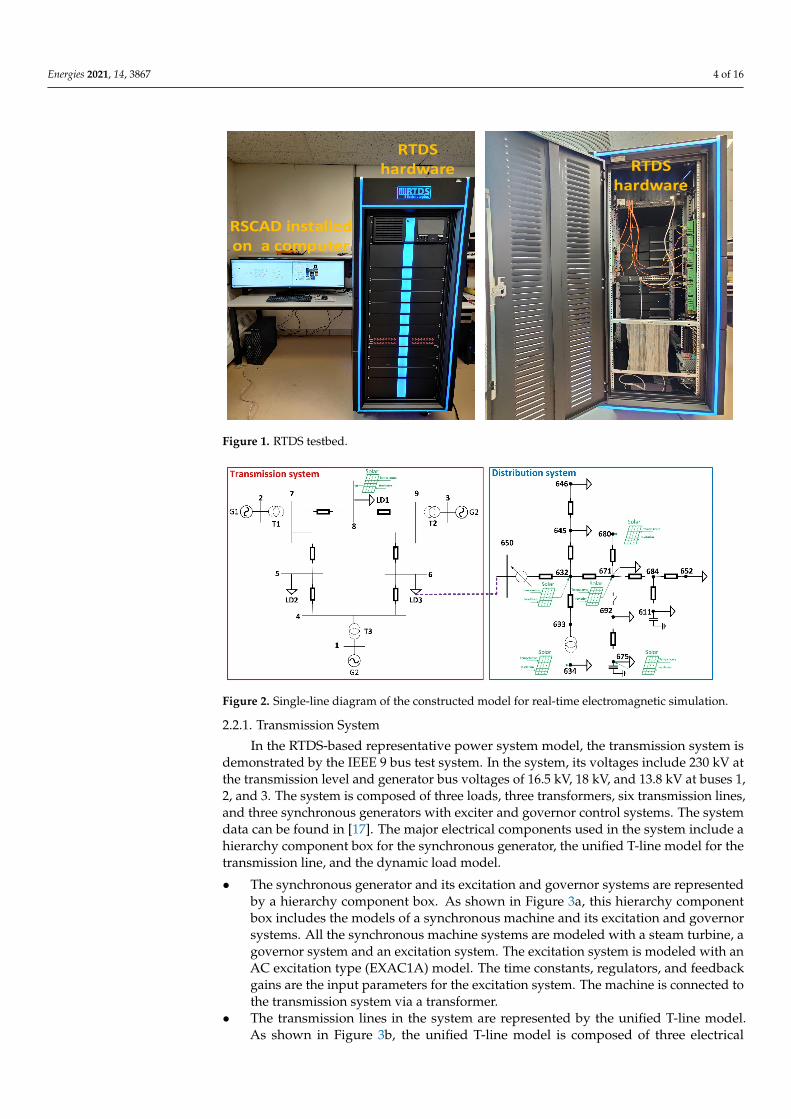
RTDS is generally composed of hardware and software, which is shown in Figure 1.The RTDS hardware includes processing and communicating cards, which are insertedin the unit and connected to a common plate located in the back of the RTDS. The pro-cessing cards have a parallel processing architecture customized to simulate with one ormultiple processors for the equation solution for the power system and its components.The communicating cards are used to handle the communication between RTDS and itssoftware installed on the guest computer. RTDS has additional dedicated interface cardsthat allow the physical and logical connection between the simulated power systems andactual devices. The RTDS software is a graphic interface software, RSCAD, which allowsusers to build, compile, execute, and analyze simulation cases. This software has a widelibrary of power system components, control, and automated protection systems, as wellas a friendly user interface, which can make the assembly and analysis of a wide varietyof electric AC and DC systems easier and integrated. As shown in Figure 1, users can useRSCAD software to build a model representing the power system and load this model tothe RTDS for the electromagnetic transient simulation while obtaining the updated statesof the simulated power system model for analysis.

2.2. RTDS-Based Representative Power System Model

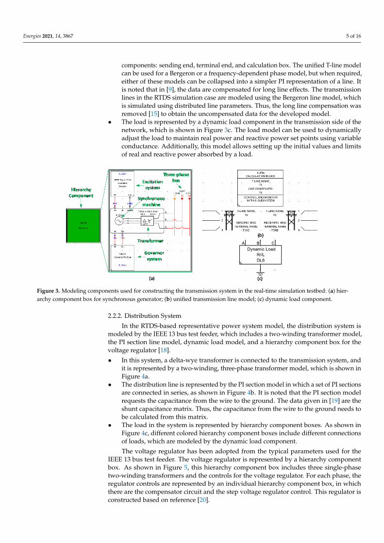
With RTDS, a representative power system model is constructed for real-time elec-tromagnetic simulations to investigate the impact of transmission-level disturbances onthe IBR operation in distribution systems. This model includes complete transmissionand distribution systems with solar PVs. Figure 2 shows the single-line diagram of theconstructed power system model. The component details in the model are described below.

Energies 2021, 14, 3867 4 of 16Energies 2021, 14, x FOR PEER REVIEW 4 of 16

RSCAD installed on a computer

RTDS hardware RTDS

hardware

Figure 1. RTDS testbed.

2.2. RTDS-Based Representative Power System Model With RTDS, a representative power system model is constructed for real-time elec-

tromagnetic simulations to investigate the impact of transmission-level disturbances on the IBR operation in distribution systems. This model includes complete transmission and distribution systems with solar PVs. Figure 2 shows the single-line diagram of the con-structed power system model. The component details in the model are described below.

Figure 2. Single-line diagram of the constructed model for real-time electromagnetic simulation.

2.2.1. Transmission System In the RTDS-based representative power system model, the transmission system is

demonstrated by the IEEE 9 bus test system. In the system, its voltages include 230 kV at the transmission level and generator bus voltages of 16.5 kV, 18 kV, and 13.8 kV at buses 1, 2, and 3. The system is composed of three loads, three transformers, six transmission lines, and three synchronous generators with exciter and governor control systems. The system data can be found in [17]. The major electrical components used in the system include a hierarchy component box for the synchronous generator, the unified T-line model for the transmission line, and the dynamic load model. • The synchronous generator and its excitation and governor systems are represented

by a hierarchy component box. As shown in Figure 3a, this hierarchy component box

Figure 1. RTDS testbed.

Energies 2021, 14, x FOR PEER REVIEW 4 of 16

RSCAD installed on a computer

RTDS hardware RTDS

hardware

Figure 1. RTDS testbed.

2.2. RTDS-Based Representative Power System Model With RTDS, a representative power system model is constructed for real-time elec-

tromagnetic simulations to investigate the impact of transmission-level disturbances on the IBR operation in distribution systems. This model includes complete transmission and distribution systems with solar PVs. Figure 2 shows the single-line diagram of the con-structed power system model. The component details in the model are described below.

Figure 2. Single-line diagram of the constructed model for real-time electromagnetic simulation.

2.2.1. Transmission System In the RTDS-based representative power system model, the transmission system is

demonstrated by the IEEE 9 bus test system. In the system, its voltages include 230 kV at the transmission level and generator bus voltages of 16.5 kV, 18 kV, and 13.8 kV at buses 1, 2, and 3. The system is composed of three loads, three transformers, six transmission lines, and three synchronous generators with exciter and governor control systems. The system data can be found in [17]. The major electrical components used in the system include a hierarchy component box for the synchronous generator, the unified T-line model for the transmission line, and the dynamic load model. • The synchronous generator and its excitation and governor systems are represented

by a hierarchy component box. As shown in Figure 3a, this hierarchy component box

Figure 2. Single-line diagram of the constructed model for real-time electromagnetic simulation.

2.2.1. Transmission System

In the RTDS-based representative power system model, the transmission system isdemonstrated by the IEEE 9 bus test system. In the system, its voltages include 230 kV atthe transmission level and generator bus voltages of 16.5 kV, 18 kV, and 13.8 kV at buses 1,2, and 3. The system is composed of three loads, three transformers, six transmission lines,and three synchronous generators with exciter and governor control systems. The systemdata can be found in [17]. The major electrical components used in the system include ahierarchy component box for the synchronous generator, the unified T-line model for thetransmission line, and the dynamic load model.

• The synchronous generator and its excitation and governor systems are representedby a hierarchy component box. As shown in Figure 3a, this hierarchy componentbox includes the models of a synchronous machine and its excitation and governorsystems. All the synchronous machine systems are modeled with a steam turbine, agovernor system and an excitation system. The excitation system is modeled with anAC excitation type (EXAC1A) model. The time constants, regulators, and feedbackgains are the input parameters for the excitation system. The machine is connected tothe transmission system via a transformer.

• The transmission lines in the system are represented by the unified T-line model.As shown in Figure 3b, the unified T-line model is composed of three electrical

Energies 2021, 14, 3867 5 of 16

components: sending end, terminal end, and calculation box. The unified T-line modelcan be used for a Bergeron or a frequency-dependent phase model, but when required,either of these models can be collapsed into a simpler PI representation of a line. Itis noted that in [9], the data are compensated for long line effects. The transmissionlines in the RTDS simulation case are modeled using the Bergeron line model, whichis simulated using distributed line parameters. Thus, the long line compensation wasremoved [15] to obtain the uncompensated data for the developed model.

• The load is represented by a dynamic load component in the transmission side of thenetwork, which is shown in Figure 3c. The load model can be used to dynamicallyadjust the load to maintain real power and reactive power set points using variableconductance. Additionally, this model allows setting up the initial values and limitsof real and reactive power absorbed by a load.

Energies 2021, 14, x FOR PEER REVIEW 5 of 16

includes the models of a synchronous machine and its excitation and governor sys-tems. All the synchronous machine systems are modeled with a steam turbine, a gov-ernor system and an excitation system. The excitation system is modeled with an AC excitation type (EXAC1A) model. The time constants, regulators, and feedback gains are the input parameters for the excitation system. The machine is connected to the transmission system via a transformer.

• The transmission lines in the system are represented by the unified T-line model. As shown in Figure 3b, the unified T-line model is composed of three electrical compo-nents: sending end, terminal end, and calculation box. The unified T-line model can be used for a Bergeron or a frequency-dependent phase model, but when required, either of these models can be collapsed into a simpler PI representation of a line. It is noted that in [9], the data are compensated for long line effects. The transmission lines in the RTDS simulation case are modeled using the Bergeron line model, which is simulated using distributed line parameters. Thus, the long line compensation was removed [15] to obtain the uncompensated data for the developed model.

• The load is represented by a dynamic load component in the transmission side of the network, which is shown in Figure 3c. The load model can be used to dynamically adjust the load to maintain real power and reactive power set points using variable conductance. Additionally, this model allows setting up the initial values and limits of real and reactive power absorbed by a load.

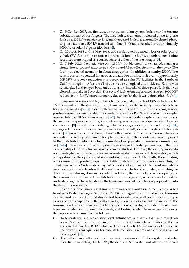
Figure 3. Modeling components used for constructing the transmission system in the real-time sim-ulation testbed: (a) hierarchy component box for synchronous generator; (b) unified transmission line model; (c) dynamic load component.

2.2.2. Distribution System In the RTDS-based representative power system model, the distribution system is

modeled by the IEEE 13 bus test feeder, which includes a two-winding transformer model, the PI section line model, dynamic load model, and a hierarchy component box for the voltage regulator [18]. • In this system, a delta-wye transformer is connected to the transmission system, and

it is represented by a two-winding, three-phase transformer model, which is shown in Figure 4a.

• The distribution line is represented by the PI section model in which a set of PI sec-tions are connected in series, as shown in Figure 4b. It is noted that the PI section model requests the capacitance from the wire to the ground. The data given in [19] are the shunt capacitance matrix. Thus, the capacitance from the wire to the ground needs to be calculated from this matrix.

• The load in the system is represented by hierarchy component boxes. As shown in Figure 4c, different colored hierarchy component boxes include different connections of loads, which are modeled by the dynamic load component.

Figure 3. Modeling components used for constructing the transmission system in the real-time simulation testbed: (a) hier-archy component box for synchronous generator; (b) unified transmission line model; (c) dynamic load component.

2.2.2. Distribution System

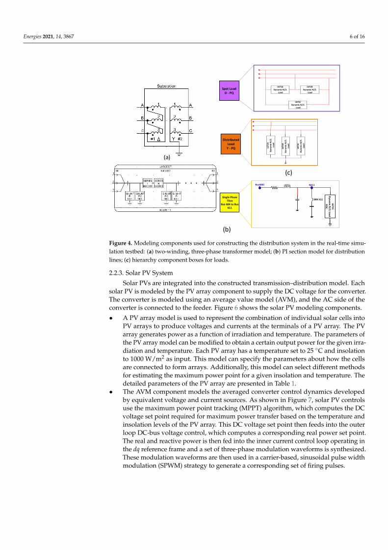
In the RTDS-based representative power system model, the distribution system ismodeled by the IEEE 13 bus test feeder, which includes a two-winding transformer model,the PI section line model, dynamic load model, and a hierarchy component box for thevoltage regulator [18].

• In this system, a delta-wye transformer is connected to the transmission system, andit is represented by a two-winding, three-phase transformer model, which is shown inFigure 4a.

• The distribution line is represented by the PI section model in which a set of PI sectionsare connected in series, as shown in Figure 4b. It is noted that the PI section modelrequests the capacitance from the wire to the ground. The data given in [19] are theshunt capacitance matrix. Thus, the capacitance from the wire to the ground needs tobe calculated from this matrix.

• The load in the system is represented by hierarchy component boxes. As shown inFigure 4c, different colored hierarchy component boxes include different connectionsof loads, which are modeled by the dynamic load component.

The voltage regulator has been adopted from the typical parameters used for theIEEE 13 bus test feeder. The voltage regulator is represented by a hierarchy componentbox. As shown in Figure 5, this hierarchy component box includes three single-phasetwo-winding transformers and the controls for the voltage regulator. For each phase, theregulator controls are represented by an individual hierarchy component box, in whichthere are the compensator circuit and the step voltage regulator control. This regulator isconstructed based on reference [20].

Energies 2021, 14, 3867 6 of 16

Energies 2021, 14, x FOR PEER REVIEW 6 of 16

The voltage regulator has been adopted from the typical parameters used for the IEEE 13 bus test feeder. The voltage regulator is represented by a hierarchy component box. As shown in Figure 5, this hierarchy component box includes three single-phase two-winding transformers and the controls for the voltage regulator. For each phase, the reg-ulator controls are represented by an individual hierarchy component box, in which there are the compensator circuit and the step voltage regulator control. This regulator is con-structed based on reference [20].

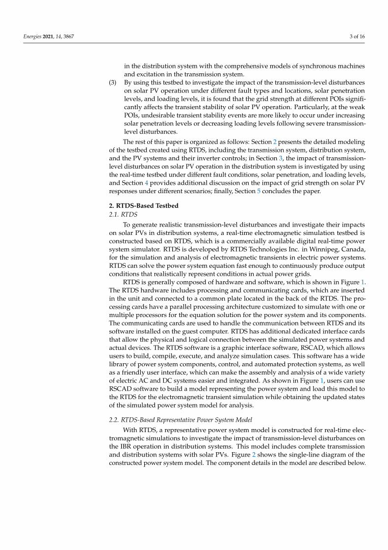
Figure 4. Modeling components used for constructing the distribution system in the real-time sim-ulation testbed: (a) two-winding, three-phase transformer model; (b) PI section model for distribu-tion lines; (c) hierarchy component boxes for loads.

(b)

(a)

(a)

Distributed Load

Y - PQ

L671BDynamic R//L

Load

L671ADynamic R//L

LoadSpot Load

D - PQ

L671CDynam

ic R//L LoadRISC

BRK 611

Bus684C N611

Single Phase Tline

Bus 684 to Bus 611

(c)

(b)

L671CDynamic R//L

Load

L671

CDy

nam

ic R/

/L Lo

ad

L671

BDy

nam

ic R/

/L Lo

ad

L671

ADy

nam

ic R/

/L Lo

ad

Figure 4. Modeling components used for constructing the distribution system in the real-time simu-lation testbed: (a) two-winding, three-phase transformer model; (b) PI section model for distributionlines; (c) hierarchy component boxes for loads.

2.2.3. Solar PV System

Solar PVs are integrated into the constructed transmission–distribution model. Eachsolar PV is modeled by the PV array component to supply the DC voltage for the converter.The converter is modeled using an average value model (AVM), and the AC side of theconverter is connected to the feeder. Figure 6 shows the solar PV modeling components.

• A PV array model is used to represent the combination of individual solar cells intoPV arrays to produce voltages and currents at the terminals of a PV array. The PVarray generates power as a function of irradiation and temperature. The parameters ofthe PV array model can be modified to obtain a certain output power for the given irra-diation and temperature. Each PV array has a temperature set to 25 C and insolationto 1000 W/m2 as input. This model can specify the parameters about how the cellsare connected to form arrays. Additionally, this model can select different methodsfor estimating the maximum power point for a given insolation and temperature. Thedetailed parameters of the PV array are presented in Table 1.

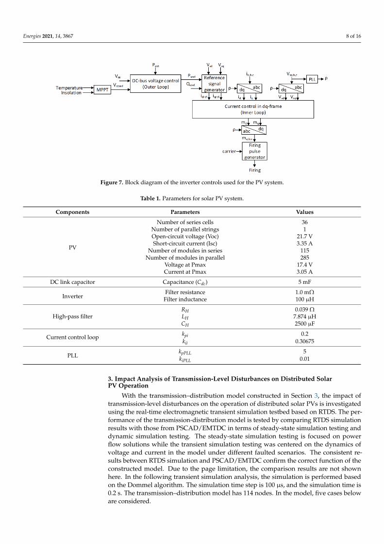
• The AVM component models the averaged converter control dynamics developedby equivalent voltage and current sources. As shown in Figure 7, solar PV controlsuse the maximum power point tracking (MPPT) algorithm, which computes the DCvoltage set point required for maximum power transfer based on the temperature andinsolation levels of the PV array. This DC voltage set point then feeds into the outerloop DC-bus voltage control, which computes a corresponding real power set point.The real and reactive power is then fed into the inner current control loop operating inthe dq reference frame and a set of three-phase modulation waveforms is synthesized.These modulation waveforms are then used in a carrier-based, sinusoidal pulse widthmodulation (SPWM) strategy to generate a corresponding set of firing pulses.

Energies 2021, 14, 3867 7 of 16Energies 2021, 14, x FOR PEER REVIEW 7 of 16

Figure 5. Voltage regulator used for constructing the distribution system.

2.2.3. Solar PV System Solar PVs are integrated into the constructed transmission–distribution model. Each

solar PV is modeled by the PV array component to supply the DC voltage for the con-verter. The converter is modeled using an average value model (AVM), and the AC side of the converter is connected to the feeder. Figure 6 shows the solar PV modeling compo-nents. • A PV array model is used to represent the combination of individual solar cells into

PV arrays to produce voltages and currents at the terminals of a PV array. The PV array generates power as a function of irradiation and temperature. The parameters of the PV array model can be modified to obtain a certain output power for the given irradiation and temperature. Each PV array has a temperature set to 25 °C and inso-lation to 1000 W/m2 as input. This model can specify the parameters about how the cells are connected to form arrays. Additionally, this model can select different meth-ods for estimating the maximum power point for a given insolation and temperature. The detailed parameters of the PV array are presented in Table 1.

• The AVM component models the averaged converter control dynamics developed by equivalent voltage and current sources. As shown in Figure 7, solar PV controls use the maximum power point tracking (MPPT) algorithm, which computes the DC voltage set point required for maximum power transfer based on the temperature and insolation levels of the PV array. This DC voltage set point then feeds into the outer loop DC-bus voltage control, which computes a corresponding real power set point. The real and reactive power is then fed into the inner current control loop op-erating in the dq reference frame and a set of three-phase modulation waveforms is

Figure 5. Voltage regulator used for constructing the distribution system.

Energies 2021, 14, x FOR PEER REVIEW 8 of 16

synthesized. These modulation waveforms are then used in a carrier-based, sinusoi-dal pulse width modulation (SPWM) strategy to generate a corresponding set of fir-ing pulses.

Table 1. Parameters for solar PV system.

Components Parameters Values

PV

Number of series cells 36 Number of parallel strings 1 Open-circuit voltage (Voc) 21.7 V Short-circuit current (Isc) 3.35 A

Number of modules in series 115 Number of modules in parallel 285

Voltage at Pmax 17.4 V Current at Pmax 3.05 A

DC link capacitor Capacitance (Cdc) 5 mF

Inverter Filter resistance 1.0 mΩ

Filter inductance 100 μH

High-pass filter RH 0.039 Ω LH 7.874 μH CH 2500 μF

Current control loop kpi 0.2 kii 0.30675

PLL kpPLL 5 kiPLL 0.01

Figure 6. Components for solar PV system used in the variation model.

Figure 7. Block diagram of the inverter controls used for the PV system.

3. Impact Analysis of Transmission-Level Disturbances on Distributed Solar PV Op-eration

Figure 6. Components for solar PV system used in the variation model.

Energies 2021, 14, 3867 8 of 16

Energies 2021, 14, x FOR PEER REVIEW 8 of 16

synthesized. These modulation waveforms are then used in a carrier-based, sinusoi-dal pulse width modulation (SPWM) strategy to generate a corresponding set of fir-ing pulses.

Table 1. Parameters for solar PV system.

Components Parameters Values

PV

Number of series cells 36 Number of parallel strings 1 Open-circuit voltage (Voc) 21.7 V Short-circuit current (Isc) 3.35 A

Number of modules in series 115 Number of modules in parallel 285

Voltage at Pmax 17.4 V Current at Pmax 3.05 A

DC link capacitor Capacitance (Cdc) 5 mF

Inverter Filter resistance 1.0 mΩ

Filter inductance 100 μH

High-pass filter RH 0.039 Ω LH 7.874 μH CH 2500 μF

Current control loop kpi 0.2 kii 0.30675

PLL kpPLL 5 kiPLL 0.01

Figure 6. Components for solar PV system used in the variation model.

Figure 7. Block diagram of the inverter controls used for the PV system.

3. Impact Analysis of Transmission-Level Disturbances on Distributed Solar PV Op-eration

Figure 7. Block diagram of the inverter controls used for the PV system.

Table 1. Parameters for solar PV system.

Components Parameters Values

PV

Number of series cells 36Number of parallel strings 1Open-circuit voltage (Voc) 21.7 VShort-circuit current (Isc) 3.35 A

Number of modules in series 115Number of modules in parallel 285

Voltage at Pmax 17.4 VCurrent at Pmax 3.05 A

DC link capacitor Capacitance (Cdc) 5 mF

InverterFilter resistance 1.0 mΩ

Filter inductance 100 µH

High-pass filterRH 0.039 ΩLH 7.874 µHCH 2500 µF

Current control loop kpi 0.2kii 0.30675

PLLkpPLL 5kiPLL 0.01

3. Impact Analysis of Transmission-Level Disturbances on Distributed SolarPV Operation

With the transmission–distribution model constructed in Section 3, the impact oftransmission-level disturbances on the operation of distributed solar PVs is investigatedusing the real-time electromagnetic transient simulation testbed based on RTDS. The per-formance of the transmission-distribution model is tested by comparing RTDS simulationresults with those from PSCAD/EMTDC in terms of steady-state simulation testing anddynamic simulation testing. The steady-state simulation testing is focused on powerflow solutions while the transient simulation testing was centered on the dynamics ofvoltage and current in the model under different faulted scenarios. The consistent re-sults between RTDS simulation and PSCAD/EMTDC confirm the correct function of theconstructed model. Due to the page limitation, the comparison results are not shownhere. In the following transient simulation analysis, the simulation is performed basedon the Dommel algorithm. The simulation time step is 100 µs, and the simulation time is0.2 s. The transmission–distribution model has 114 nodes. In the model, five cases beloware considered.

Energies 2021, 14, 3867 9 of 16

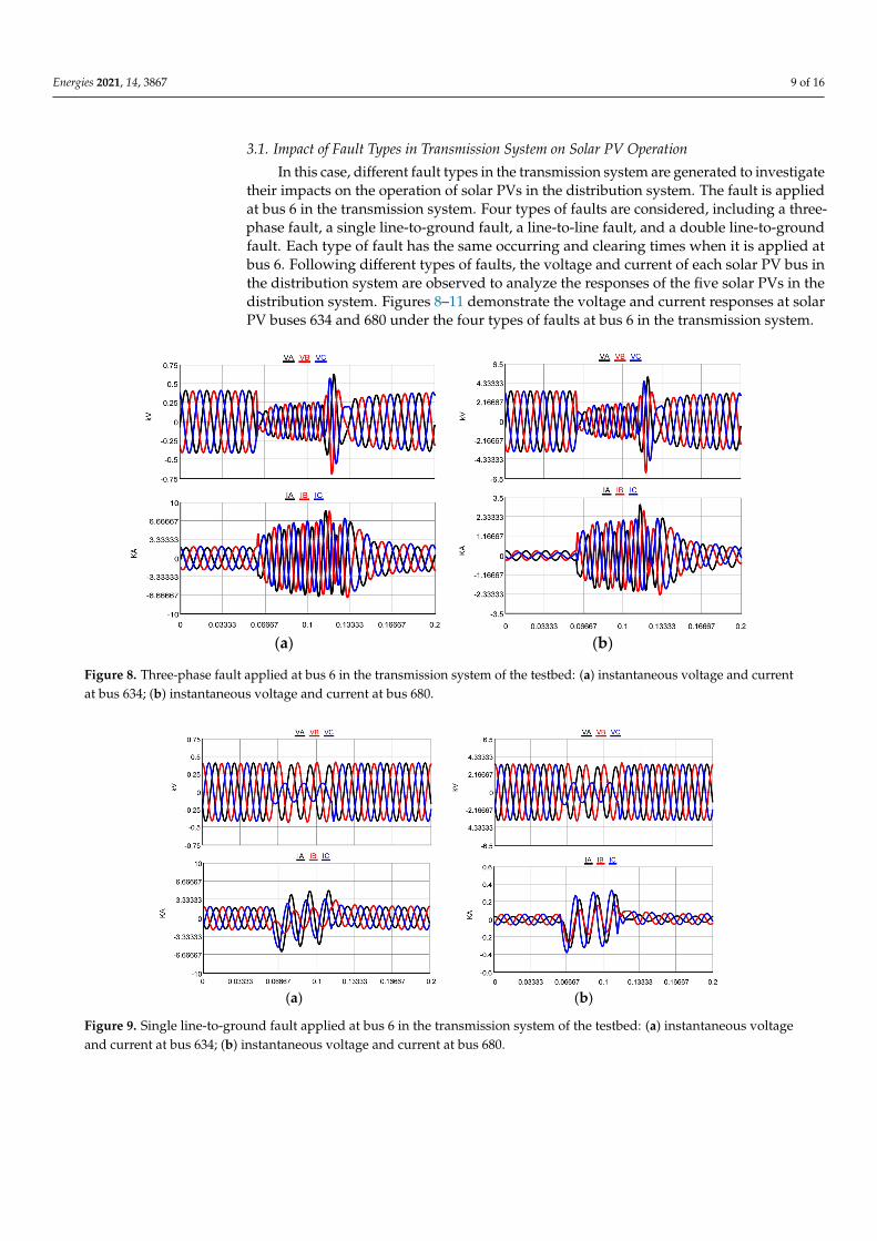
3.1. Impact of Fault Types in Transmission System on Solar PV Operation

In this case, different fault types in the transmission system are generated to investigatetheir impacts on the operation of solar PVs in the distribution system. The fault is appliedat bus 6 in the transmission system. Four types of faults are considered, including a three-phase fault, a single line-to-ground fault, a line-to-line fault, and a double line-to-groundfault. Each type of fault has the same occurring and clearing times when it is applied atbus 6. Following different types of faults, the voltage and current of each solar PV bus inthe distribution system are observed to analyze the responses of the five solar PVs in thedistribution system. Figures 8–11 demonstrate the voltage and current responses at solarPV buses 634 and 680 under the four types of faults at bus 6 in the transmission system.

Energies 2021, 14, x FOR PEER REVIEW 9 of 16

With the transmission–distribution model constructed in Section 3, the impact of transmission-level disturbances on the operation of distributed solar PVs is investigated using the real-time electromagnetic transient simulation testbed based on RTDS. The per-formance of the transmission-distribution model is tested by comparing RTDS simulation results with those from PSCAD/EMTDC in terms of steady-state simulation testing and dynamic simulation testing. The steady-state simulation testing is focused on power flow solutions while the transient simulation testing was centered on the dynamics of voltage and current in the model under different faulted scenarios. The consistent results between RTDS simulation and PSCAD/EMTDC confirm the correct function of the constructed model. Due to the page limitation, the comparison results are not shown here. In the fol-lowing transient simulation analysis, the simulation is performed based on the Dommel algorithm. The simulation time step is 100 μs, and the simulation time is 0.2 s. The trans-mission–distribution model has 114 nodes. In the model, five cases below are considered.

3.1. Impact of Fault Types in Transmission System on Solar PV Operation In this case, different fault types in the transmission system are generated to investi-

gate their impacts on the operation of solar PVs in the distribution system. The fault is applied at bus 6 in the transmission system. Four types of faults are considered, including a three-phase fault, a single line-to-ground fault, a line-to-line fault, and a double line-to-ground fault. Each type of fault has the same occurring and clearing times when it is ap-plied at bus 6. Following different types of faults, the voltage and current of each solar PV bus in the distribution system are observed to analyze the responses of the five solar PVs in the distribution system. Figures 8–11 demonstrate the voltage and current responses at solar PV buses 634 and 680 under the four types of faults at bus 6 in the transmission system.

(a) (b)

Figure 8. Three-phase fault applied at bus 6 in the transmission system of the testbed: (a) instanta-neous voltage and current at bus 634; (b) instantaneous voltage and current at bus 680.

Figure 8. Three-phase fault applied at bus 6 in the transmission system of the testbed: (a) instantaneous voltage and currentat bus 634; (b) instantaneous voltage and current at bus 680.

Energies 2021, 14, x FOR PEER REVIEW 10 of 16

(a) (b)

Figure 9. Single line-to-ground fault applied at bus 6 in the transmission system of the testbed: (a) instantaneous voltage and current at bus 634; (b) instantaneous voltage and current at bus 680.

(a) (b)

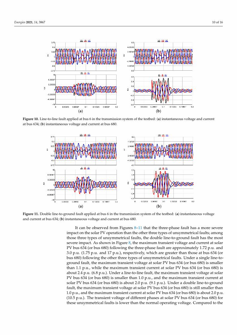
Figure 10. Line-to-line fault applied at bus 6 in the transmission system of the testbed: (a) instanta-neous voltage and current at bus 634; (b) instantaneous voltage and current at bus 680.

(a) (b)

Figure 11. Double line-to-ground fault applied at bus 6 in the transmission system of the testbed: (a) instantaneous voltage and current at bus 634; (b) instantaneous voltage and current at bus 680.

Figure 9. Single line-to-ground fault applied at bus 6 in the transmission system of the testbed: (a) instantaneous voltageand current at bus 634; (b) instantaneous voltage and current at bus 680.

Energies 2021, 14, 3867 10 of 16

Energies 2021, 14, x FOR PEER REVIEW 10 of 16

(a) (b)

Figure 9. Single line-to-ground fault applied at bus 6 in the transmission system of the testbed: (a) instantaneous voltage and current at bus 634; (b) instantaneous voltage and current at bus 680.

(a) (b)

Figure 10. Line-to-line fault applied at bus 6 in the transmission system of the testbed: (a) instanta-neous voltage and current at bus 634; (b) instantaneous voltage and current at bus 680.

(a) (b)

Figure 11. Double line-to-ground fault applied at bus 6 in the transmission system of the testbed: (a) instantaneous voltage and current at bus 634; (b) instantaneous voltage and current at bus 680.

Figure 10. Line-to-line fault applied at bus 6 in the transmission system of the testbed: (a) instantaneous voltage and currentat bus 634; (b) instantaneous voltage and current at bus 680.

Energies 2021, 14, x FOR PEER REVIEW 10 of 16

(a) (b)

Figure 9. Single line-to-ground fault applied at bus 6 in the transmission system of the testbed: (a) instantaneous voltage and current at bus 634; (b) instantaneous voltage and current at bus 680.

(a) (b)

Figure 10. Line-to-line fault applied at bus 6 in the transmission system of the testbed: (a) instanta-neous voltage and current at bus 634; (b) instantaneous voltage and current at bus 680.

(a) (b)

Figure 11. Double line-to-ground fault applied at bus 6 in the transmission system of the testbed: (a) instantaneous voltage and current at bus 634; (b) instantaneous voltage and current at bus 680.

Figure 11. Double line-to-ground fault applied at bus 6 in the transmission system of the testbed: (a) instantaneous voltageand current at bus 634; (b) instantaneous voltage and current at bus 680.

It can be observed from Figures 8–11 that the three-phase fault has a more severeimpact on the solar PV operation than the other three types of unsymmetrical faults; amongthose three types of unsymmetrical faults, the double line-to-ground fault has the mostsevere impact. As shown in Figure 8, the maximum transient voltage and current at solarPV bus 634 (or bus 680) following the three-phase fault are approximately 1.72 p.u. and3.0 p.u. (1.75 p.u. and 17 p.u.), respectively, which are greater than those at bus 634 (orbus 680) following the other three types of unsymmetrical faults. Under a single line-to-ground fault, the maximum transient voltage at solar PV bus 634 (or bus 680) is smallerthan 1.1 p.u., while the maximum transient current at solar PV bus 634 (or bus 680) isabout 2.4 p.u. (6.8 p.u.). Under a line-to-line fault, the maximum transient voltage at solarPV bus 634 (or bus 680) is smaller than 1.0 p.u., and the maximum transient current atsolar PV bus 634 (or bus 680) is about 2.0 p.u. (9.1 p.u.). Under a double line-to-groundfault, the maximum transient voltage at solar PV bus 634 (or bus 680) is still smaller than1.0 p.u., and the maximum transient current at solar PV bus 634 (or bus 680) is about 2.0 p.u.(10.5 p.u.). The transient voltage of different phases at solar PV bus 634 (or bus 680) forthese unsymmetrical faults is lower than the normal operating voltage. Compared to the

Energies 2021, 14, 3867 11 of 16

single line-to-ground fault and the line-to-line fault, the double line-to-ground fault onthese solar PV buses is more severe.

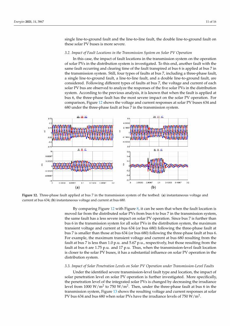
3.2. Impact of Fault Locations in the Transmission System on Solar PV Operation

In this case, the impact of fault locations in the transmission system on the operationof solar PVs in the distribution system is investigated. To this end, another fault with thesame fault occurring and clearing time of the fault transpired at bus 6 is applied at bus 7 inthe transmission system. Still, four types of faults at bus 7, including a three-phase fault,a single line-to-ground fault, a line-to-line fault, and a double line-to-ground fault, areconsidered. Following different types of faults at bus 7, the voltage and current of eachsolar PV bus are observed to analyze the responses of the five solar PVs in the distributionsystem. According to the previous analysis, it is known that when the fault is applied atbus 6, the three-phase fault has the most severe impact on the solar PV operation. Forcomparison, Figure 12 shows the voltage and current responses at solar PV buses 634 and680 under the three-phase fault at bus 7 in the transmission system.

Energies 2021, 14, x FOR PEER REVIEW 12 of 16

(a) (b)

Figure 12. Three-phase fault applied at bus 7 in the transmission system of the testbed: (a) instanta-neous voltage and current at bus 634; (b) instantaneous voltage and current at bus 680.

3.3. Impact of Solar Penetration Levels on Solar PV Operation under Transmission-Level Faults Under the identified severe transmission-level fault type and location, the impact of

solar penetration level on solar PV operation is further investigated. More specifically, the penetration level of the integrated solar PVs is changed by decreasing the irradiance level from 1000 W/m2 to 750 W/m2. Then, under the three-phase fault at bus 6 in the transmis-sion system, Figure 13 shows the resulting voltage and current responses at solar PV bus 634 and bus 680 when solar PVs have the irradiance levels of 750 W/m2.

By comparing Figure 13 with Figure 8, it can be seen that the severity of the impact of transmission-level disturbance on solar PV operation decreases with solar penetration level. As shown in Figure 13, both the maximum transient voltage and current decrease with the solar penetration level due to the irradiance decrease to 750 W/m2 from 1000 W/m2. For example, the maximum transient current is around 14.0 p.u. at solar PV bus 680 following the three-phase fault at bus 6 in the transmission system when all solar PVs in the distribution system have 750 W/m2 solar irradiance, while the maximum current is increased to 17.0 p.u. at solar PV bus 680 resulting from the same fault when all solar PVs have 1000 W/m2 solar irradiance. The maximum transient voltage in the case with 750 W/m2 solar irradiance does not exceed the normal range but with 1000 W/m2 solar irradi-ance has a peak of 1.75 p.u. for bus 680.

(a) (b)

Figure 12. Three-phase fault applied at bus 7 in the transmission system of the testbed: (a) instantaneous voltage andcurrent at bus 634; (b) instantaneous voltage and current at bus 680.

By comparing Figure 12 with Figure 8, it can be seen that when the fault location ismoved far from the distributed solar PVs from bus 6 to bus 7 in the transmission system,the same fault has a less severe impact on solar PV operation. Since bus 7 is further thanbus 6 in the transmission system for all solar PVs in the distribution system, the maximumtransient voltage and current at bus 634 (or bus 680) following the three-phase fault atbus 7 is smaller than those at bus 634 (or bus 680) following the three-phase fault at bus 6.For example, the maximum transient voltage and current at bus 680 resulting from thefault at bus 7 is less than 1.0 p.u. and 5.67 p.u., respectively, but those resulting from thefault at bus 6 are 1.75 p.u. and 17 p.u. Thus, when the transmission-level fault locationis closer to the solar PV buses, it has a substantial influence on solar PV operation in thedistribution system.

3.3. Impact of Solar Penetration Levels on Solar PV Operation under Transmission-Level Faults

Under the identified severe transmission-level fault type and location, the impact ofsolar penetration level on solar PV operation is further investigated. More specifically,the penetration level of the integrated solar PVs is changed by decreasing the irradiancelevel from 1000 W/m2 to 750 W/m2. Then, under the three-phase fault at bus 6 in thetransmission system, Figure 13 shows the resulting voltage and current responses at solarPV bus 634 and bus 680 when solar PVs have the irradiance levels of 750 W/m2.

Energies 2021, 14, 3867 12 of 16

Energies 2021, 14, x FOR PEER REVIEW 12 of 16

(a) (b)

Figure 12. Three-phase fault applied at bus 7 in the transmission system of the testbed: (a) instanta-neous voltage and current at bus 634; (b) instantaneous voltage and current at bus 680.

3.3. Impact of Solar Penetration Levels on Solar PV Operation under Transmission-Level Faults Under the identified severe transmission-level fault type and location, the impact of

solar penetration level on solar PV operation is further investigated. More specifically, the penetration level of the integrated solar PVs is changed by decreasing the irradiance level from 1000 W/m2 to 750 W/m2. Then, under the three-phase fault at bus 6 in the transmis-sion system, Figure 13 shows the resulting voltage and current responses at solar PV bus 634 and bus 680 when solar PVs have the irradiance levels of 750 W/m2.

By comparing Figure 13 with Figure 8, it can be seen that the severity of the impact of transmission-level disturbance on solar PV operation decreases with solar penetration level. As shown in Figure 13, both the maximum transient voltage and current decrease with the solar penetration level due to the irradiance decrease to 750 W/m2 from 1000 W/m2. For example, the maximum transient current is around 14.0 p.u. at solar PV bus 680 following the three-phase fault at bus 6 in the transmission system when all solar PVs in the distribution system have 750 W/m2 solar irradiance, while the maximum current is increased to 17.0 p.u. at solar PV bus 680 resulting from the same fault when all solar PVs have 1000 W/m2 solar irradiance. The maximum transient voltage in the case with 750 W/m2 solar irradiance does not exceed the normal range but with 1000 W/m2 solar irradi-ance has a peak of 1.75 p.u. for bus 680.

(a) (b)

Figure 13. Three-phase fault applied at bus 6 in the transmission system of the testbed: (a) instantaneous voltage andcurrent at bus 634 with 750 W/m2 solar irradiance; (b) instantaneous voltage and current at bus 680 with 750 W/m2

solar irradiance.

By comparing Figure 13 with Figure 8, it can be seen that the severity of the impact oftransmission-level disturbance on solar PV operation decreases with solar penetration level.As shown in Figure 13, both the maximum transient voltage and current decrease withthe solar penetration level due to the irradiance decrease to 750 W/m2 from 1000 W/m2.For example, the maximum transient current is around 14.0 p.u. at solar PV bus 680following the three-phase fault at bus 6 in the transmission system when all solar PVsin the distribution system have 750 W/m2 solar irradiance, while the maximum currentis increased to 17.0 p.u. at solar PV bus 680 resulting from the same fault when all solarPVs have 1000 W/m2 solar irradiance. The maximum transient voltage in the case with750 W/m2 solar irradiance does not exceed the normal range but with 1000 W/m2 solarirradiance has a peak of 1.75 p.u. for bus 680.

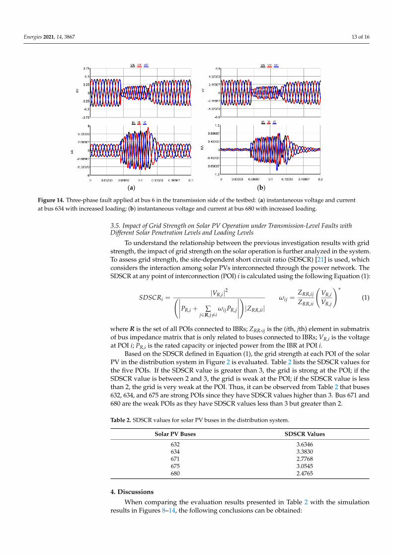
3.4. Impact of Loading Levels on Solar PV Operation under Transmission-Level Faults

Additionally, the impact of loading level on solar PV operation is investigated underthe identified severe transmission-level fault type and location. In this case, the loadinglevel is increased by four times its original loading level in the distribution system. Underthe three-phase fault at bus 6 in the transmission system, the transient voltages andcurrents at the solar PV buses are investigated. For comparison, Figure 14 shows theresulting voltage and current responses at solar PV bus 634 and bus 680 after the loadingis increased.

By comparing Figures 8 and 14, it can be seen that the maximum transient voltageand current at bus 634 and bus 680 following the transmission-level fault at bus 6 aredecreased with the increased loading. For example, before the loading level is increasedin the distribution system following the transmission-level fault at bus 6, the maximumtransient currents at solar PV bus 634 and bus 680 are approximately 3.0 p.u. and 17 p.u.,respectively; after the loading is increased in the distribution system following the sametransmission-level fault, the resulting maximum transient voltage and current decreases to2.8 p.u. and 16.2 p.u. at bus 634 and bus 680.

Energies 2021, 14, 3867 13 of 16

Energies 2021, 14, x FOR PEER REVIEW 13 of 16

Figure 13. Three-phase fault applied at bus 6 in the transmission system of the testbed: (a) instanta-neous voltage and current at bus 634 with 750 W/m2 solar irradiance; (b) instantaneous voltage and current at bus 680 with 750 W/m2 solar irradiance.

3.4. Impact of Loading Levels on Solar PV Operation under Transmission-Level Faults Additionally, the impact of loading level on solar PV operation is investigated under

the identified severe transmission-level fault type and location. In this case, the loading level is increased by four times its original loading level in the distribution system. Under the three-phase fault at bus 6 in the transmission system, the transient voltages and cur-rents at the solar PV buses are investigated. For comparison, Figure 14 shows the resulting voltage and current responses at solar PV bus 634 and bus 680 after the loading is in-creased.

By comparing Figures 8 and 14, it can be seen that the maximum transient voltage and current at bus 634 and bus 680 following the transmission-level fault at bus 6 are de-creased with the increased loading. For example, before the loading level is increased in the distribution system following the transmission-level fault at bus 6, the maximum tran-sient currents at solar PV bus 634 and bus 680 are approximately 3.0 p.u. and 17 p.u., respectively; after the loading is increased in the distribution system following the same transmission-level fault, the resulting maximum transient voltage and current decreases to 2.8 p.u. and 16.2 p.u. at bus 634 and bus 680.

(a) (b)

Figure 14. Three-phase fault applied at bus 6 in the transmission side of the testbed: (a) instantane-ous voltage and current at bus 634 with increased loading; (b) instantaneous voltage and current at bus 680 with increased loading.

3.5. Impact of Grid Strength on Solar PV Operation under Transmission-Level Faults with Different Solar Penetration Levels and Loading Levels

To understand the relationship between the previous investigation results with grid strength, the impact of grid strength on the solar operation is further analyzed in the sys-tem. To assess grid strength, the site-dependent short circuit ratio (SDSCR) [21] is used, which considers the interaction among solar PVs interconnected through the power net-work. The SDSCR at any point of interconnection (POI) i is calculated using the following Equation (1):

*2,, ,

, ,, , ,

,

| |

| |

RR ijR i R ii ij

RR ii R jR i ij R j RR ii

j j i

ZV VSDSCR

Z VP P Z

ω

ω∈ ≠

= = +

R

(1)

Figure 14. Three-phase fault applied at bus 6 in the transmission side of the testbed: (a) instantaneous voltage and currentat bus 634 with increased loading; (b) instantaneous voltage and current at bus 680 with increased loading.

3.5. Impact of Grid Strength on Solar PV Operation under Transmission-Level Faults withDifferent Solar Penetration Levels and Loading Levels

To understand the relationship between the previous investigation results with gridstrength, the impact of grid strength on the solar operation is further analyzed in the system.To assess grid strength, the site-dependent short circuit ratio (SDSCR) [21] is used, whichconsiders the interaction among solar PVs interconnected through the power network. TheSDSCR at any point of interconnection (POI) i is calculated using the following Equation (1):

SDSCRi =|VR,i|2(∣∣∣∣∣PR,i + ∑

j∈R,j 6=iωijPR,j

∣∣∣∣∣)|ZRR,ii|

ωij =ZRR,ij

ZRR,ii

(VR,i

VR,j

)∗(1)

where R is the set of all POIs connected to IBRs; ZRR,ij is the (ith, jth) element in submatrixof bus impedance matrix that is only related to buses connected to IBRs; VR,i is the voltageat POI i; PR,i is the rated capacity or injected power from the IBR at POI i.

Based on the SDSCR defined in Equation (1), the grid strength at each POI of the solarPV in the distribution system in Figure 2 is evaluated. Table 2 lists the SDSCR values forthe five POIs. If the SDSCR value is greater than 3, the grid is strong at the POI; if theSDSCR value is between 2 and 3, the grid is weak at the POI; if the SDSCR value is lessthan 2, the grid is very weak at the POI. Thus, it can be observed from Table 2 that buses632, 634, and 675 are strong POIs since they have SDSCR values higher than 3. Bus 671 and680 are the weak POIs as they have SDSCR values less than 3 but greater than 2.

Table 2. SDSCR values for solar PV buses in the distribution system.

Solar PV Buses SDSCR Values

632 3.6346634 3.3830671 2.7768675 3.0545680 2.4765

4. Discussions

When comparing the evaluation results presented in Table 2 with the simulationresults in Figures 8–14, the following conclusions can be obtained:

Energies 2021, 14, 3867 14 of 16

By comparing Table 2 with Figures 8–11, it is found that undesirable transient dynam-ics may be more likely to occur at weaker POIs under the same fault but different types.Moreover, the severity of the undesirable transient dynamics at the weaker POIs mayincrease with the fault type. Table 2 shows that bus 680 is weaker than bus 634. Comparingthe maximum transient voltage and current at bus 634 with those at bus 680, it can beobserved from Figures 8–11 that the maximum transient voltage and current at bus 634are smaller than those at bus 680 following the same transmission-level fault with thefour different types. For example, when the single line-to-ground fault occurred in thetransmission system, Figure 9 shows that the maximum transient current at bus 634 isapproximately 2.4 p.u., but the maximum transient current at bus 680 is approximately6.8 p.u. Moreover, when the fault type is changed into the severest three-phase fault,Figure 8 shows that the maximum transient voltage and current at bus 634 are approxi-mately 1.72 p.u. and 3 p.u.; however, the maximum transient voltage and current at bus680 are approximately 1.75 p.u. and 17 p.u.

By comparing Table 2 with Figure 12, it is also found that under the same three-phasefault but different locations, weak POIs are more likely to have undesirable transientdynamics. As shown in Table 2, bus 680 is weaker than bus 634. By comparing themaximum transient voltage and current at bus 634 with those at bus 680 in Figures 8 and 12,it can be observed that when the three-phase fault is moved from bus 6 to bus 7 in thetransmission system, the maximum current transient at bus 634 is decreased from 3 p.u. to1.4 p.u.; the maximum current transient at bus 680 is decreased from 17 p.u. to 5.67 p.u.Additionally, even when the fault is far from the distribution system (at bus 7), weak bus680 is still more likely to have an undesirable transient response than bus 634.

By comparing Table 2 with Figure 13, it is found that undesirable transient dynamicsmay be more likely to happen at weaker POIs under the increasing solar penetration levelin the distribution system. Compared to bus 634, weak bus 680 has a more severe impact onsolar PV operation following the same transmission-level fault. As shown in Figure 13, forbus 680, when the solar irradiance is 750 W/m2, the maximum transient current is 14 p.u.;as shown in Figure 8, when solar irradiance is increased to 1000 W/m2, the maximumtransient current is 17 p.u. For bus 634, the maximum transient current is increased fromabout 2.2 p.u. to 3 p.u. when solar irradiance is increased from 750 W/m2 to 1000 W/m2.

By comparing Table 2 with Figure 14, it is found that increasing the loading level inthe distribution system may decrease the risk of undesirable transient dynamics at weakerPOIs following the transmission-level disturbance. As shown in Figures 8 and 14, theseverity of the impact of transmission-level disturbance on solar PV operation decreaseswith the increase in loading level in the distribution system. At the weak bus 680, thisimpact becomes relatively significant. Before increasing the loading level, the maximumtransient current is 17 p.u. following the transmission-level fault at bus 6; the transientcurrent is reduced to 16. 2 p.u. following the same transmission-level fault when theloading level is increased. This change can improve grid strength at bus 680 and thusreduce the risk of undesirable transient dynamics of solar PV at bus 680.

5. Conclusions

In this paper, a real-time RTDS-based simulation testbed was presented to explore theimpacts of realistic transmission-level disturbances on solar PV operation in the distributionsystem. The testbed includes detailed modeling of components in the transmission and dis-tribution systems along with the detailed PV models and its inverter controls to capture theaccurate dynamic behaviors of solar PVs in response to the transmission-level disturbances.The testbed was used in this paper to investigate the transient responses from the solar PVinverters under different transmission-level disturbances regarding different fault typesand locations, solar penetration levels, and loading levels. It is found that the grid strengthat the POIs of solar PV inverters significantly affects the transient response from the solarPV inverters following the transmission-level disturbances. At weaker POIs, the transientresponse is more sensitive to the disturbances. Such sensitivity becomes more significant

Energies 2021, 14, 3867 15 of 16

when the transmission-level disturbance is closer to the weak POIs or the disturbancesbecome more severe. Additionally, the impact of the transmission-level disturbances onthe solar PVs at the weak POIs exacerbate with the increasing solar penetration levels andloading levels. Thus, when an increasing number of IBRs are being integrated into the grid,it is important to study and develop new technologies for grid planning, operation, andprotection in weak grid conditions to address the emerging issues of integrating the highpenetration of solar PVs and other IBRs.

Author Contributions: Conceptualization, M.M., A.E. and D.W.; methodology M.M., A.E. and D.W.;software, A.E.; validation, M.M., A.E. and B.S.; formal analysis, M.M., A.E. and D.W.; investigation,A.E. and M.M.; resources, D.W.; data curation, A.E. and M.M.; writing—original draft preparation,M.M.; writing—review and editing, M.M., A.E., B.S. and D.W.; visualization, A.E. and M.M.; supervi-sion, D.W.; project administration, D.W.; funding acquisition, D.W. All authors have read and agreedto the published version of the manuscript.

Funding: This material is based upon work supported by the US Department of Energy’s Office ofEnergy Efficiency and Renewable Energy (EERE) under the Solar Energy Technologies Office AwardNumber DE-EE0008772.

Institutional Review Board Statement: Not applicable.

Informed Consent Statement: Not applicable.

Data Availability Statement: The data presented in this study are available on request from thecorresponding author.

Conflicts of Interest: The authors declare no conflict of interest.

References1. North American Electric Reliability Corporation. 1200 MW Fault Induced Solar Photovoltaic Resource Interruption Disturbance Report;

North American Electric Reliability Corporation: Atlanta, GA, USA, 2016.2. North American Electric Reliability Corporation. 900 MW Fault Induced Solar Photovoltaic Resource Interruption Disturbance Report;

North American Electric Reliability Corporation: Atlanta, GA, USA, 2018.3. North American Electric Reliability Corporation. April and May 2018 Fault Induced Solar Photovoltaic Resource Interruption

Disturbances Report: Southern California Events: 20 April 2018 and 11 May 2018; North American Electric Reliability Corporation:Atlanta, GA, USA, 2019.

4. San Fernando Disturbance Southern California Event: 7 July 2020 Joint NERC and WECC Staff Report. Atlanta, GA, USA,2020. Available online: https://www.nwpp.org/news/power-insights-podcast-episode-2-san-fernando-even (accessed on25 June 2021).

5. Kang, S.; Shin, H.; Jang, G.; Lee, B. Impact Analysis of Recovery Ramp Rate After Momentary Cessation in Inverter-basedDistributed Generators on Power System Transient Stability. IET Gener. Transm. Distrib. 2020, 15, 24–33. [CrossRef]

6. Pierre, B.J.; Elkhatib, M.E.; Hoke, A. Photovoltaic Inverter Momentary Cessation: Recovery Process is Key. In Proceedings of the2019 IEEE 46th Photovoltaic Specialists Conference (PVSC), Chicago, IL, USA, 16–21 June 2019.

7. Choi, N.; Park, B.; Cho, H.; Lee, B. Impact of Momentary Cessation Voltage Level in Inverter-Based Resources on Increasing theShort Circuit Current. Sustainability 2019, 11, 1153. [CrossRef]

8. Zhu, S.; Piper, D.; Ramasubramanian, D.; Quint, R.; Isaacs, A.; Bauer, R. Modeling Inverter-Based Resources in Stability Studies.In Proceedings of the 2018 IEEE Power & Energy Society General Meeting (PESGM), Portland, OR, USA, 5–10 August 2018.

9. Shin, H.; Jung, J.; Lee, B. Determining the Capacity Limit of Inverter-Based Distributed Generators in High-Generation AreasConsidering Transient and Frequency Stability. IEEE Access 2020, 8, 34071–34079. [CrossRef]

10. Mather, B.; Ding, F. Distribution-connected PV’s response to voltage sags at transmission-scale. In Proceedings of the 2016 IEEE43rd Photovoltaic Specialists Conference (PVSC), Portland, OR, USA, 5–10 June 2016; pp. 2030–2035.

11. Mather, B.; Aworo, O.; Bravo, R.; Piper, P.E.D. Laboratory Testing of a Utility-Scale PV Inverter’s Operational Response toGrid Disturbances. In Proceedings of the 2018 IEEE Power & Energy Society General Meeting (PESGM), Portland, OR, USA,5–10 August 2018; pp. 1–5.

12. Kenyon, R.W.; Mather, B.; Hodge, B.-M. Coupled Transmission and Distribution Simulations to Assess Distributed GenerationResponse to Power System Faults. Electr. Power Syst. Res. 2020, 189, 106746. [CrossRef]

13. Shin, H.; Jung, J.; Oh, S.; Hur, K.; Iba, K.; Lee, B. Evaluating the Influence of Momentary Cessation Mode in Inverter-BasedDistributed Generators on Power System Transient Stability. IEEE Trans. Power Syst. 2020, 35, 1618–1626. [CrossRef]

14. Li, C.; Reinmuller, R. Fault Responses of Inverter-based Renewable Generation: On Fault Ride-Through and Momentary Cessation.In Proceedings of the 2018 IEEE Power & Energy Society General Meeting (PESGM), Portland, OR, USA, 5–10 August 2018.

Energies 2021, 14, 3867 16 of 16

15. Pierre, B.J.; Elkhatib, M.E.; Hoke, A. PV Inverter Fault Response Including Momentary Cessation, Frequency-Watt, and VirtualInertia. In Proceedings of the 2018 IEEE 7th World Conference on Photovoltaic Energy Conversion (WCPEC) (A Joint Conferenceof 45th IEEE PVSC, 28th PVSEC & 34th EU PVSEC), Waikoloa, HI, USA, 10–15 June 2018.

16. RTDS Technologies Inc. Available online: https://www.rtds.com (accessed on 25 June 2021).17. Sauer, P.W.; Pai, M.A. Power System Dynamics And stability; Wiley Online Library: Hoboken, NJ, USA, 1998; Volume 101.18. Kersting, W.H. Distribution System Modeling and Analysis; CRC Press: Boca Raton, FL, USA, 2017.19. IEEE PES AMPS DSAS Test Feeder Working Group. Available online: https://site.ieee.org/pes-testfeeders/resources/ (accessed

on 25 June 2021).20. Grainger, J.J.; Stevenson, W.D., Jr. Power System Analysis; McGrawHill: New York, NY, USA, 1994.21. Wu, D.; Li, G.; Javadi, M.; Malyscheff, A.M.; Hong, M.; Jiang, J.N. Assessing impact of renewable energy integration on system

strength using site-dependent short circuit ratio. IEEE Trans. Sustain. Energy 2017, 9, 1072–1080. [CrossRef]