version: July 31, 2014

An optimal irrigation networkwith infinitely many branching points

Andrea Marchese & Annalisa Massaccesi

Abstract. The Gilbert-Steiner problem is a mass transportation problem,where the cost to transport a measure µ− onto a measure µ+ depends on thenetwork used to move the mass and it is proportional to a certain power of the“flow”. In this paper, we introduce a new formulation of the problem whichturns it into the minimization of a convex functional. By associating to µ−and µ+ a group G and a 0-dimensional current B with coefficients in G, weprove that the Gilbert-Steiner problem is equivalent to the problem of findinga mass minimizer, among all 1-dimensional currents Z with coefficients in Ghaving boundary ∂Z = B. This framework allows us to define calibrations,which can be used to prove the optimality of concrete configurations. We applythis technique to prove the optimality of a certain irrigation network, havingthe topological property mentioned in the title.

Keywords: Gilbert-Steiner problem, irrigation problem, calibrations, flat G-chains.

MSC (2010): 49Q15, 49Q20, 49N60, 53C38.

0. Introduction

The Gilbert-Steiner problem is a variant of the optimal transport problemwith a cost depending not only on the position of the masses at the beginningand at the end of the process, but also on the path that has been chosen tomove them. As in the optimal transport problem, the Gilbert-Steiner’s datumconsists of a positive measure µ− (source) and a positive measure µ+ (well), withthe same total mass ‖µ−‖(Rd) = ‖µ+‖(Rd). One wants to move µ− onto µ+,minimizing the global cost. The cost of the transport is concave with respectto the density of the transported mass, as it is in many natural phenomena andengineering problems.

In particular, if µ− and µ+ are sums of Dirac deltas on a set of sources Xand a set of wells Y , respectively, then a transporting network is described bya 1-dimensional rectifiable set Σ and a multiplicity function θ ∈ L1(Σ;Z). Theset Σ is a union of paths joining points of X to points of Y and the multiplicityrepresents the “flow” of the transported mass through each point of the set Σ.The cost associated to each transporting network is the integral on the set Σof θα for some α ∈ (0, 1). It is interesting to observe the limit cases: if α = 0,the problem corresponds to the minimization of the 1-dimensional measure ofthe set Σ, if α = 1, we recover the Monge-Kantorovich energy and the Mongeproblem on optimal transport. When µ− is supported on a single point, we

2 A. Marchese & A. Massaccesi

talk about irrigation problem. One immediately understands that, by its ownnature, the problem tends to favor large flows and therefore it easily leads tobranched structures.

Several descriptions of this problem have been given by many authors: werefer to [4] for a detailed overview of the subject, though different models havebeen proposed in [19, 10, 2, 17, 12]. Those models are summarized and provedto be equivalent in [8, 9].

Our starting point is Xia’s approach in [19]: the problem is described in termsof minimization of a certain energy, depending on α, in a family of transportpaths, that is, normal 1-dimensional currents with boundary µ+ − µ−. Animportant feature which is evident in this approach is the non-convex natureof the problem: the energy of a convex combination of two competitors may bestrictly larger than the energy of each single competitor.

One of the achievements of the present paper is a new formulation of theGilbert-Steiner problem which turns it into the minimization of a convex func-tional. Some useful tools, such as calibrations, are available in this setting. Byassociating to the measures µ− and µ+ a normed group G and a 0-dimensionalcurrent B with coefficients in G, we manage to prove that the Gilbert-Steinerproblem is equivalent to the problem of finding a mass minimizer, among all1-dimensional currents Z with coefficients in G having boundary ∂Z = B. Thegroup G is chosen depending only on the quantity ‖µ−‖(Rd) = ‖µ+‖(Rd). Inthis new framework we can introduce the notion of calibration, that is, a func-tional analytic tool to prove that a given candidate is a minimizer.

Such an approach is not completely new: in [11], we apply the same procedureto the study of the Steiner tree problem, which corresponds to the limit casewith α = 0 of the Gilbert-Steiner problem, with an additional connectednessconstraint.

Let us explain with an easy example the rough idea of the new formulation.Assume we want to irrigate the two wells y1 = (2,−1) and y2 = (2, 1) froma (unique) source in the origin, which generates a flow of intensity 2. Fixα = 1/2. The classical description of a competitor for this problem consistsof a superposition of two paths Γ1 and Γ2, both with multiplicity 1: the firstpath goes from the origin to y1, the second from the origin to y2. Therefore

y2

y1

y2

y1

O

g2

g1

O

g21

g1 + g2

Classical description New formulation and new multiplicities

g1 + g2

2

1g1

the irrigation network can be identified with the set Γ1∪Γ2 with a multiplicity,

An optimal irrigation network 3

which is equal to 2 on Γ1 ∩ Γ2 and 1 elsewhere on Γ1 ∪ Γ2. One computes theenergy of such competitor as

H1((Γ1 ∪ Γ2) \ (Γ1 ∩ Γ2)) +√

2H1(Γ1 ∩ Γ2),

where H1 denotes the 1-dimensional Hausdorff measure. In our formulation weassociate to Γ1 and Γ2 vectors in R2 as multiplicities: g1 and g2, respectively,where (g1, g2) is an orthonormal basis of R2. In this way the stretch Γ1 ∩ Γ2

is associated to the vector g1 + g2. In order to compute the mass of the corre-sponding 1-current with coefficients in R2 one has to integrate on Γ1 ∪ Γ2 theEuclidean norm of the corresponding multiplicity. Clearly this mass coincideswith the energy computed as above, because the Euclidean norm of g1 + g2 isexactly

√2.

In the last part of the paper we apply the equivalence result and the calibra-tion method to prove the optimality of an irrigation tree with the topologicalproperty mentioned in the title of the paper, that is, an infinite number ofbranching points. The occurrence of such a topological behaviour for energy-minimizers has been the aim of various attempts: in [3] some characterizingprinciples for infinite irrigation trees are discussed, while in [14] the authorsprove the optimality of an analogous tree for the generalized Steiner tree prob-lem (see also [13] and [15]). Their proof relies on a fine and rather delicate studyof the geometry of the candidate minimizer. On the contrary, our proof is basedon a calibration argument and we believe its simplicity to be an encouragingsign for further developments.

Let us describe now, in more detail, the content of each section.In §1, we collect those definitions and basic results in Geometric Measure

Theory that are necessary to formulate both the discrete version of the Gilbert-Steiner problem, as introduced in [19] and our new formulation in terms of 1-dimensional currents with coefficients in a group. Moreover we define a suitablenotion of calibration for these objects and we prove that a calibrated currentminimizes the mass in its homology class.

In §2, we recall and rework the discrete version of the Gilbert-Steiner problemgiven by [19], in terms of an energy minimization problem in the family ofclassical integral currents, having a fixed boundary, which is supported on thegiven set of sources and wells (this is what we call problem (P1)). We also recalla structure theorem for integral 1-currents (see Theorem 2.4) which allows oneto better understand why such an abstract class of competitors is indeed anatural choice.

In §3, we describe how to associate to the given measures µ− and µ+ anormed group G and a mass minimization problem in a class of rectifiablecurrents with coefficients in G (which we call problem (P2)). In Theorem 3.6 weprove the equivalence between the problems (P1) and (P2). Then we apply thisresult and the calibration technique introduced in §1 to prove the optimality ofsome simple transportation networks. We conclude explaining how one shouldmodify the two problems (P1) and (P2) in order to keep the equivalence, whenthe measures µ−, µ+, given as initial datum, are rescaled.

4 A. Marchese & A. Massaccesi

In §4, we describe an irrigation network on the separable Hilbert space `2.Then we prove that such a network is a solution to the continuous version of theGilbert-Steiner problem associated to the corresponding boundary. The proofis based on an argument of reduction to a finite dimensional framework, wherewe are able to exhibit a calibration and therefore to prove the optimality.

1. Notations and Preliminaries

In this first section, we briefly recall the main definitions and results concern-ing 1-dimensional rectifiable currents with coefficients in the abelian normedgroup (Zn, ‖ · ‖α). In this paper we limit ourselves to the essential facts whichare unavoidable for the statement and the development of the main result. See[11] for a more general theory and further details.

1.1. Differential forms with values in Rn. The ambient space where wewant to treat the irrigation problem is Rd. Concerning the coefficients, let usfix a standard basis (g1, . . . , gn) for Rn. We fix α ∈ (0, 1) and consider then-dimensional normed vector space (Rn, ‖ · ‖α), with

‖h‖α :=

n∑j=1

|hj |1α

α

for every h = h1g1 + . . . hngn ∈ Rn. Once for all, we fix the (canonical) basis(e1, . . . , en) of the dual space of (Rn, ‖ · ‖α) so that 〈ei, gj〉 = δij . With thisnotation, the dual space of (Rn, ‖ · ‖α) is the n-dimensional normed vectorspace (Rn, ‖ · ‖1−α).

1.2. Definition. An Rn-valued covector in Rd is a map ω : Λ1(Rd)×Rn → Rwith the following properties:

(i) 〈ω; τ, ·〉 ∈ Rn for every vector τ ∈ Λ1(Rd);(ii) 〈ω; ·, h〉 ∈ Λ1(Rd) is a standard 1-dimensional covector in Rd for every

element h ∈ Rn.

The linear space of Rn-valued covectors in Rd, endowed with the comass norm

‖ω‖∗α := sup|τ |≤1

‖〈ω; τ, ·〉‖1−α,

will be denoted by Λ1(n,α)(R

d). An Rn-valued (1-dimensional) differential form

defined on Rd is a map ω : Rd → Λ1(n,α)(R

d), its regularity is the one inherited

from the components

ωj := 〈ω; ·, gj〉 : Rd → Λ1(Rd) ,

for j = 1, . . . , n.

1.3. Definition. Consider a function ψ : Rd → Rn of class C 1. We cancompute the differential dψj of each component ψj of ψ (j = 1 . . . , n), thus we

An optimal irrigation network 5

will denote

dψ = dψ1e1 + . . .+ dψnen ∈ C (Rd; Λ1(n,α)(R

d)) .

1.4. Rectifiable currents with coefficients in Rn.

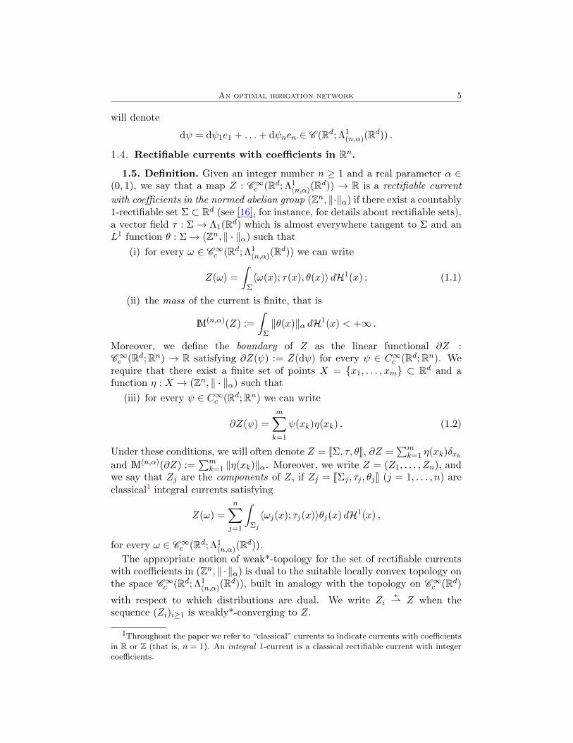
1.5. Definition. Given an integer number n ≥ 1 and a real parameter α ∈(0, 1), we say that a map Z : C∞c (Rd; Λ1

(n,α)(Rd)) → R is a rectifiable current

with coefficients in the normed abelian group (Zn, ‖·‖α) if there exist a countably1-rectifiable set Σ ⊂ Rd (see [16], for instance, for details about rectifiable sets),a vector field τ : Σ→ Λ1(Rd) which is almost everywhere tangent to Σ and anL1 function θ : Σ→ (Zn, ‖ · ‖α) such that

(i) for every ω ∈ C∞c (Rd; Λ1(n,α)(R

d)) we can write

Z(ω) =

ˆΣ〈ω(x); τ(x), θ(x)〉 dH1(x) ; (1.1)

(ii) the mass of the current is finite, that is

M(n,α)(Z) :=

ˆΣ‖θ(x)‖α dH1(x) < +∞ .

Moreover, we define the boundary of Z as the linear functional ∂Z :C∞c (Rd;Rn) → R satisfying ∂Z(ψ) := Z(dψ) for every ψ ∈ C∞c (Rd;Rn). Werequire that there exist a finite set of points X = {x1, . . . , xm} ⊂ Rd and afunction η : X → (Zn, ‖ · ‖α) such that

(iii) for every ψ ∈ C∞c (Rd;Rn) we can write

∂Z(ψ) =

m∑k=1

ψ(xk)η(xk) . (1.2)

Under these conditions, we will often denote Z = JΣ, τ, θK, ∂Z =∑m

k=1 η(xk)δxkand M(n,α)(∂Z) :=

∑mk=1 ‖η(xk)‖α. Moreover, we write Z = (Z1, . . . , Zn), and

we say that Zj are the components of Z, if Zj = JΣj , τj , θjK (j = 1, . . . , n) areclassical1 integral currents satisfying

Z(ω) =

n∑j=1

ˆΣj

〈ωj(x); τj(x)〉θj(x) dH1(x) ,

for every ω ∈ C∞c (Rd; Λ1(n,α)(R

d)).

The appropriate notion of weak*-topology for the set of rectifiable currentswith coefficients in (Zn, ‖ ·‖α) is dual to the suitable locally convex topology onthe space C∞c (Rd; Λ1

(n,α)(Rd)), built in analogy with the topology on C∞c (Rd)

with respect to which distributions are dual. We write Zi∗⇀ Z when the

sequence (Zi)i≥1 is weakly*-converging to Z.

1Throughout the paper we refer to “classical” currents to indicate currents with coefficientsin R or Z (that is, n = 1). An integral 1-current is a classical rectifiable current with integercoefficients.

6 A. Marchese & A. Massaccesi

Let us remark that these definitions are consistent with the classical theoryof currents and currents with coefficients in a (normed, abelian, discrete) group.In particular, rectifiable currents with coefficients in (Zn, ‖ · ‖α) belong to thelarger linear space of currents with coefficients in (Rn, ‖ · ‖α) and the mass of acurrent Z is the supremum of |Z(ω)| when ω ∈ C∞c (U ; Λ1

(n,α)(Rd)) has norm

supx∈U‖ω(x)‖∗α ≤ 1.

Despite the complexity of the notation, this framework is not redundantfor the objects we would like to represent and analyze. In fact, Theorem1.7 provides a reasonable structure for a rectifiable current with coefficientsin (Zn, ‖ · ‖α) as a countable sum of loops plus finitely many Lipschitz curvesin Rd with constant multiplicity. Let us clarify how we endow a curve γ with acanonical structure of current in the following example.

1.6. Example. We associate to a Lipschitz path γ : [0, 1]→ R2 (parametri-zed with constant speed), and a coefficient θ ∈ Rn, the 1-dimensional rectifiablecurrent Z = JΓ, τ, θK with coefficients in Rn, where Γ is the support of thecurve γ([0, 1]) and, denoting by `(Γ) the length of the curve, the orientationτ is defined by τ(γ(t)) := γ′(t)/`(Γ) for a.e. t ∈ [0, 1]. The boundary of suchcurrent is ∂T = θ(δγ(1) − δγ(0)).

1.7. Theorem. Let Z be a rectifiable current in Rd with coefficients in(Zn, ‖ · ‖α), then

Z =m∑i=1

Zi +∞∑`=1

Z`.

Here Zi = JΓi, τi, θiK are rectifiable currents with coefficients in (Zn, ‖ · ‖α),

Γi being the support of an injective Lipschitz curve and θi a constant on Γi.Similarly Z` = JΓ`, τ`, θ`K are rectifiable currents with coefficients in (Zn, ‖·‖α),

Γ` being the support of a Lipschitz closed curve γ` : [0, 1] → Rd, which is

injective on (0, 1). Again, θi is constant on Γi.

For the proof of this theorem and a more detailed statement see 2.3 in [5] (theproof rivisits the argument employed for classical integral currents in 4.2.25 of[7]).

1.8. Compactness. We recall the fundamental compactness result for recti-fiable currents with coefficients in a group.

1.9. Theorem. Consider a sequence (Zi)i≥1 of rectifiable currents with co-efficients in (Zn, ‖ · ‖α) such that

supi≥1

M(n,α)(Zi) +M(n,α)(∂Zi) < +∞ .

Then there exists a rectifiable current Z, with coefficients in (Zn, ‖ · ‖α), and asubsequence (Zih)h≥1 such that

Zih∗⇀ Z .

An optimal irrigation network 7

The proof of this theorem can be carried out componentwise, using the anal-ogous celebrated result for classical integral currents (see [7] or [1]). Since themass is lower semicontinuous with respect to the same topology, we directly getthe existence of a mass-minimizing rectifiable current for a given boundary.

1.10. Corollary. Let Z be a rectifiable current with coefficients in (Zn, ‖ · ‖α),then there exists a rectifiable current Z such that

M(n,α)(Z) = min∂Z=∂Z

M(n,α)(Z) ,

where the minimum is computed among rectifiable currents with coefficients in(Zn, ‖ · ‖α).

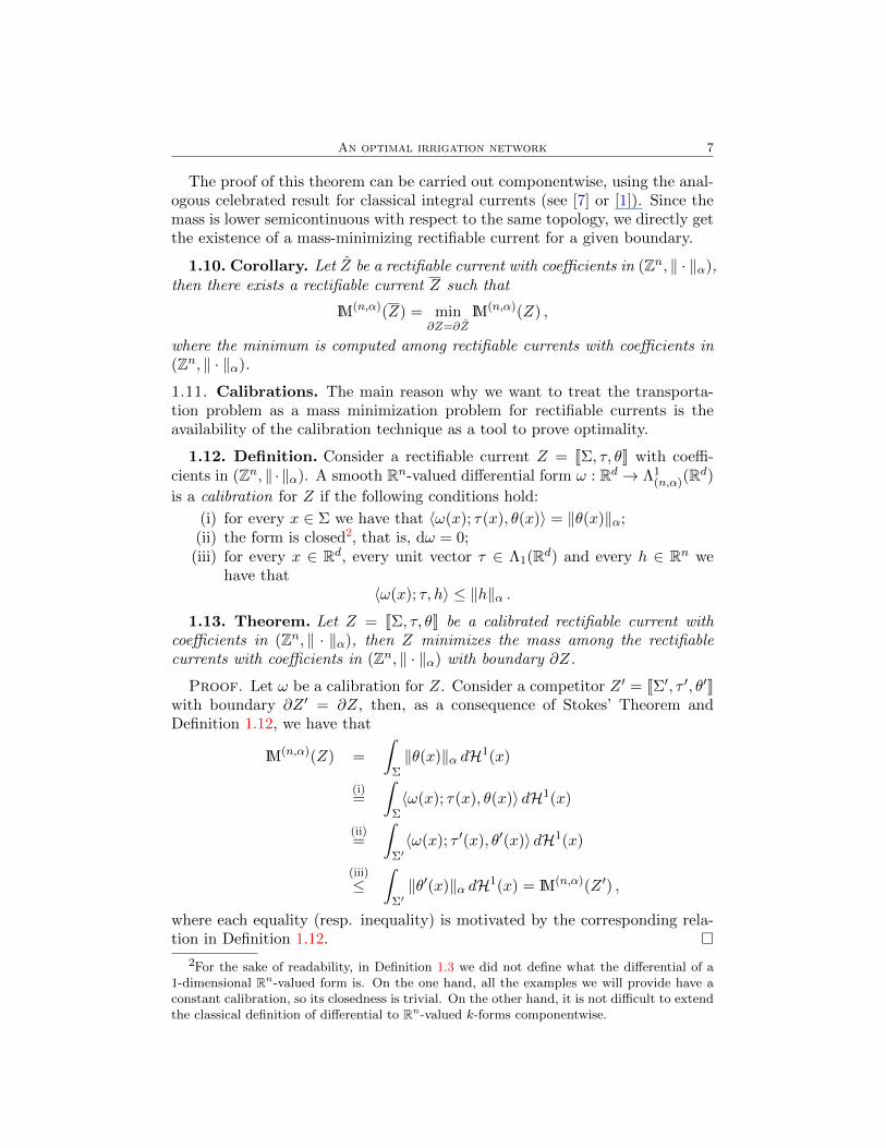
1.11. Calibrations. The main reason why we want to treat the transporta-tion problem as a mass minimization problem for rectifiable currents is theavailability of the calibration technique as a tool to prove optimality.

1.12. Definition. Consider a rectifiable current Z = JΣ, τ, θK with coeffi-cients in (Zn, ‖ · ‖α). A smooth Rn-valued differential form ω : Rd → Λ1

(n,α)(Rd)

is a calibration for Z if the following conditions hold:

(i) for every x ∈ Σ we have that 〈ω(x); τ(x), θ(x)〉 = ‖θ(x)‖α;(ii) the form is closed2, that is, dω = 0;(iii) for every x ∈ Rd, every unit vector τ ∈ Λ1(Rd) and every h ∈ Rn we

have that〈ω(x); τ, h〉 ≤ ‖h‖α .

1.13. Theorem. Let Z = JΣ, τ, θK be a calibrated rectifiable current withcoefficients in (Zn, ‖ · ‖α), then Z minimizes the mass among the rectifiablecurrents with coefficients in (Zn, ‖ · ‖α) with boundary ∂Z.

Proof. Let ω be a calibration for Z. Consider a competitor Z ′ = JΣ′, τ ′, θ′Kwith boundary ∂Z ′ = ∂Z, then, as a consequence of Stokes’ Theorem andDefinition 1.12, we have that

M(n,α)(Z) =

ˆΣ‖θ(x)‖α dH1(x)

(i)=

ˆΣ〈ω(x); τ(x), θ(x)〉 dH1(x)

(ii)=

ˆΣ′〈ω(x); τ ′(x), θ′(x)〉 dH1(x)

(iii)

≤ˆ

Σ′‖θ′(x)‖α dH1(x) = M(n,α)(Z ′) ,

where each equality (resp. inequality) is motivated by the corresponding rela-tion in Definition 1.12. �

2For the sake of readability, in Definition 1.3 we did not define what the differential of a1-dimensional Rn-valued form is. On the one hand, all the examples we will provide have aconstant calibration, so its closedness is trivial. On the other hand, it is not difficult to extendthe classical definition of differential to Rn-valued k-forms componentwise.

8 A. Marchese & A. Massaccesi

1.14. Remark. In §4, we want to allow the multiplicity of the competitorsto take values in Rn. In other words Z ′ could be a rectifiable current withcoefficients in (Rn, ‖ · ‖α). The existence of a calibration for Z guarantees theoptimality of the mass of Z even in this larger class. The proof of this fact isthe same as that given above.

2. The Gilbert-Steiner problem

2.1. The energy minimization problem. Let X = (x1, . . . , xm) and Y =

(y1, . . . , ym) ∈(Rd)m

, with xi 6= yj for every i, j = 1, . . . ,m. Denote by B(1,1)X,Y

the integral 0-current

B(1,1)X,Y :=

m∑i=1

(δyi − δxi). (2.1)

Consider the following problem.

(P1) Among all (classical) integral 1-currents T = JΣ, τ, θK in Rd with ∂T =

B(1,1)X,Y , find one which minimizes the Gilbert-Steiner energy

Eα(T ) =

ˆΣ|θ(x)|αdH1(x) .

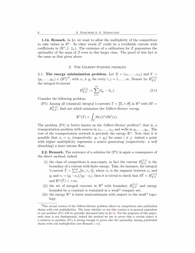
The problem (P1) is better known as the Gilbert-Steiner problem3, that is, atransportation problem with sources in x1, . . . , xm and wells in y1, . . . , ym. Thecost of the transportation network is precisely the energy Eα. Note that it ispossible that xi = xj (respectively: yi = yj) for some i 6= j: indeed a pointwith higher multilplicity represents a source generating (respectively: a wellabsorbing) a more intense flow.

2.2. Remark. The existence of a solution for (P1) is again a consequence ofthe direct method, indeed

(i) the class of competitors is non-empty, in fact the current B(1,1)X,Y is the

boundary of a current with finite energy. Take, for instance, the integral1-current T =

∑mi=1Jσi, τi, 1K, where σi is the segment between xi and

yi and τi = (yi−xi)/|yi−xi|, then it is trivial to check that ∂T = B(1,1)X,Y

and Eα(T ) < +∞;

(ii) the set of integral currents in Rd with boundary B(1,1)X,Y and energy

bounded by a constant is contained in a weak* compact set;(iii) the energy Eα is lower semicontinuous with respect to the weak* topo-

logy.

3The actual version of the Gilbert-Steiner problem allows as competitors also polyhedralchains with real multiplicities. The issue whether or not this version is in general equivalentto our problem (P1) will be partially discussed later in §3.12. For the purposes of this paper,such issue is not fundamental, indeed the method we use to prove that a certain object isa solution to problem (P1) is strong enough to prove also the optimality among polyhedralchains with real multiplicities (see Remark 1.14).

An optimal irrigation network 9

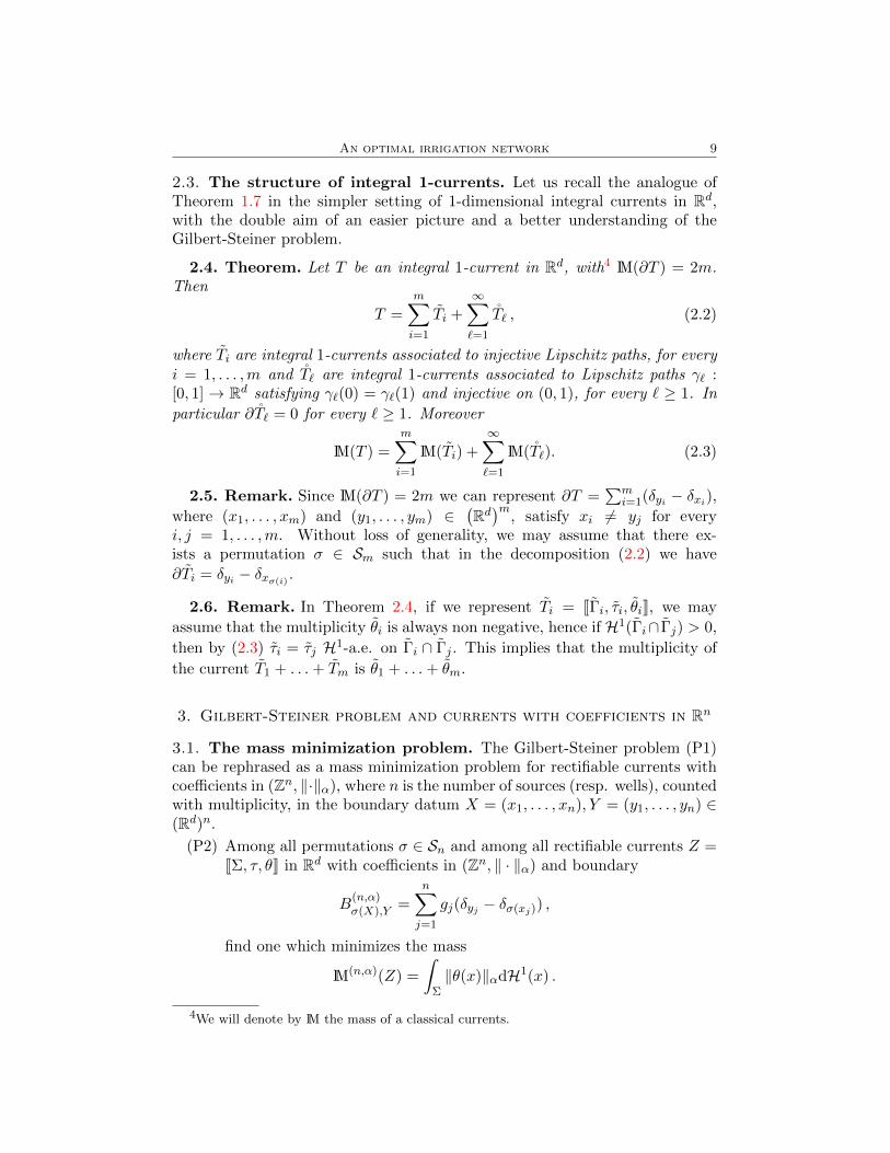
2.3. The structure of integral 1-currents. Let us recall the analogue ofTheorem 1.7 in the simpler setting of 1-dimensional integral currents in Rd,with the double aim of an easier picture and a better understanding of theGilbert-Steiner problem.

2.4. Theorem. Let T be an integral 1-current in Rd, with4 M(∂T ) = 2m.Then

T =m∑i=1

Ti +∞∑`=1

T` , (2.2)

where Ti are integral 1-currents associated to injective Lipschitz paths, for everyi = 1, . . . ,m and T` are integral 1-currents associated to Lipschitz paths γ` :[0, 1] → Rd satisfying γ`(0) = γ`(1) and injective on (0, 1), for every ` ≥ 1. In

particular ∂T` = 0 for every ` ≥ 1. Moreover

M(T ) =m∑i=1

M(Ti) +∞∑`=1

M(T`). (2.3)

2.5. Remark. Since M(∂T ) = 2m we can represent ∂T =∑m

i=1(δyi − δxi),where (x1, . . . , xm) and (y1, . . . , ym) ∈

(Rd)m

, satisfy xi 6= yj for everyi, j = 1, . . . ,m. Without loss of generality, we may assume that there ex-ists a permutation σ ∈ Sm such that in the decomposition (2.2) we have

∂Ti = δyi − δxσ(i) .

2.6. Remark. In Theorem 2.4, if we represent Ti = JΓi, τi, θiK, we may

assume that the multiplicity θi is always non negative, hence if H1(Γi∩ Γj) > 0,

then by (2.3) τi = τj H1-a.e. on Γi ∩ Γj . This implies that the multiplicity of

the current T1 + . . .+ Tm is θ1 + . . .+ θm.

3. Gilbert-Steiner problem and currents with coefficients in Rn

3.1. The mass minimization problem. The Gilbert-Steiner problem (P1)can be rephrased as a mass minimization problem for rectifiable currents withcoefficients in (Zn, ‖·‖α), where n is the number of sources (resp. wells), countedwith multiplicity, in the boundary datum X = (x1, . . . , xn), Y = (y1, . . . , yn) ∈(Rd)n.

(P2) Among all permutations σ ∈ Sn and among all rectifiable currents Z =JΣ, τ, θK in Rd with coefficients in (Zn, ‖ · ‖α) and boundary

B(n,α)σ(X),Y =

n∑j=1

gj(δyj − δσ(xj)) ,

find one which minimizes the mass

M(n,α)(Z) =

ˆΣ‖θ(x)‖αdH1(x) .

4We will denote by M the mass of a classical currents.

10 A. Marchese & A. Massaccesi

It will be clear from Definition 3.3 that fixing the permutation σ in (P2) cor-responds somehow to prescribe which source goes into which well (see also thedescription of the who goes where problem given in [2]). This is not prescribed,instead, when we fix the boundary datum in (P1). This is the reason why in(P2) we need to minimize also among all permutations σ ∈ Sn. Of course wemay drop this condition when the set of sources contains only one point withmultiplicity n, as in the case of the irrigation problem.

3.2. The equivalence of (P1) and (P2). In the next theorem we statethe equivalence between the problems (P1) and (P2). Let us first describe acanonical way to associate to a competitor for the problem (P1) a competitorfor the problem (P2) and vice versa.

3.3. Definition. Let X = (x1, . . . , xn), Y = (y1, . . . , yn) ∈ (Rd)n, with xi 6=yj for every i, j = 1, . . . , n.

(1) Given an integral current T in Rd with boundary ∂T = B(1,1)X,Y as in (2.1),

consider a decomposition according to Theorem 2.4 (indeed, M(∂T ) =2n), satisfying the assumption of Remark 2.5, that is

T =n∑i=1

Ti +∞∑`=1

T`

and there exists σ ∈ Sn such that

∂Ti = δyi − δxσ(i) .We set

Z[T ] := (T1, . . . , Tn) ,

(according to the basis (g1, . . . , gn)) which is a rectifiable current withcoefficients in (Zn, ‖ · ‖α) and boundary

∂(Z[T ]) = B(n,α)σ(X),Y .

Notice that Z[T ] depends on the decomposition chosen for T , thereforeit may be non-unique.

(2) Vice versa, given a rectifiable current Z with coefficients in (Zn, ‖ · ‖α),we can write it componentwise as Z = (Z1, . . . , Zn) and we set

T [Z] := Z1 + . . .+ Zn ,

which is an integral current with boundary B(1,1)X,Y .

3.4. Remark. Consider a rectifiable current Z = JΣ, τ, θK with coefficientsin (Zn, ‖ · ‖α). Then

Eα(T [Z]) ≤Mn,α(Z) .

Indeed, the integral current T [Z] has multiplicity θ1 + . . . + θn, where θ =θ1g1 + . . .+ θngn is the multiplicity of Z. Moreover∣∣∣ n∑

j=1

θj

∣∣∣α ≤ ( n∑j=1

|θj |1α

)α= ‖θ‖α , (3.1)

An optimal irrigation network 11

because θj ∈ Z for any j = 1, . . . , n and 0 < α < 1. Notice that the equalityholds in (3.1) if and only if θj ∈ {0, 1} for every j = 1, . . . , n.

3.5. Proposition. Consider an integral current T in Rd with M(∂T ) = 2nand a decomposition of type (2.2) as in Theorem 2.4. Then

Mn,α(Z[T ]) = Eα( n∑i=1

Ti

).

Proof. Let us denote by θ = θ1g1 + . . . + θngn the multiplicity of Z[T ].

By definition of Z[T ], each θj is the multiplicity of Tj = JΓj , τj , θjK. Since

M(∂T ) = 2n, then θj ∈ {0, 1} almost everywhere on⋃j Γj (in particular,

θj = 1 a.e. on Γj). Thus, we can infer that

‖θ‖α = |θ1 + . . .+ θn|α

almost everywhere on⋃j Γj . The conclusion follows, because the multiplicity

of∑n

j=1 Tj is precisely θ1 + . . .+ θn (see Remark 2.6). �

3.6. Theorem. Let X and Y be as in Definition 3.3. Then the problems(P1) and (P2) are equivalent. More precisely, the following results hold.

(1) If T is an energy minimizer for the Gilbert-Steiner problem (P1) with

boundary B(1,1)X,Y =

∑nj=1(δyj − δxj ), then Z[T ] is a mass minimizer for

the problem (P2). Moreover Eα(T ) = Mn,α(Z[T ]).(2) If Z is a solution for the problem (P2) with the datum (X,Y ), then

T [Z] minimizes the energy Eα among all integral currents with boundary

B(1,1)X,Y . Moreover Mn,α(Z) = Eα(T [Z]).

Proof. (1) Let T be a solution to the Gilbert-Steiner problem (P1).Since we want to show that Z[T ] is a solution for the problem (P2),then we compare its mass with the mass of an admissible competitorfor (P2), that is, a rectifiable current Z ′ with coefficients in (Zn, ‖ · ‖α)

and boundary B(n,α)σ′(X),Y for some σ′ ∈ Sn. Then we have that

Mn,α(Z ′)3.4≥ Eα(T [Z ′]) ≥ Eα(T )

(2.3)

≥ Eα( n∑i=1

Ti

)3.5= Mn,α(Z[T ]) .

Let us explain that the first inequality is due to Remark 3.4, the secondone holds because T is a minimizer for the energy Eα with boundary

B(1,1)X,Y and the third one holds because of (2.3). Finally, the last equality

has already been proved in Proposition 3.5. Notice also that the thirdinequality indeed must be an equality, because

∑ni=1 Ti is a competitor

of T in (P1).(2) Let Z be a solution to the problem (P2). We have claimed that T [Z]

is a solution to (P1): indeed, if T ′ is an integral current with boundary

12 A. Marchese & A. Massaccesi

B(1,1)X,Y , then we have that

Eα(T ′)(2.3)

≥ Eα( n∑i=1

T ′i

)3.5= Mn,α(Z[T ′]) ≥Mn,α(Z)

3.4≥ Eα(T [Z]) .

As before, let us remind that the first inequality is a consequence of (2.3)and the equality is due to Proposition 3.5. Finally, the last inequalityrelies on Remark 3.4. This last is an equality, indeed. This follows fromthe fact that the multiplicity of every component Zj = JΣj , τj , θjK ofZ is 1 (H1-a.e. on Σj) and the inequality in (3.1) is an equality whenevery θj is either 0 or 1.

�

3.7. Examples of calibreted minima. We show now some examples of cal-ibrations for the problem (P2) with the only aim to make the reader confidentwith this technique and to throw light on some issues that one may not no-tice immediately in the general formulation. In the first example there are twosources and two wells with unit multiplicity on the vertices of a rectangle in R2.The second example is an irrigation problem with only two wells, but where weallow also higher multiplicities.

3.8. Example. Fix the parameter α = 1/2 and the following points in theplane

x1 := (−3,−2), x2 := (−2,−3), y1 := (1, 0), y2 := (0, 1), z := (−2,−2) .

Consider the 0-dimensional current in R2 with coefficients in Z2 given by

B(2,1/2)(x1,x2),(y1,y2) = −g1δx1 − g2δx2 + g1δy1 + g2δy2 .

We claim that a solution to the problem (P2) for the boundary B(2,1/2)(x1,x2),(y1,y2)

is

Z = Jσ1, τ1, g1K + Jσ2, τ2, g2K + Jσ3, τ3, g1 + g2K + Jσ4, τ1, g1K + Jσ5, τ2, g2K

where σ1 is the segment from x1 to z with orientation τ1 = (1, 0), σ2 is thesegment from x2 to z with orientation τ2 = (0, 1), σ3 is the segment from z to0 with orientation τ3 =

(√2/2,√

2/2), σ4 is the segment from 0 to y1 and σ5 is

the segment from 0 to y2.Firstly, we exhibit a constant5 calibration ω(x) ≡ ω ∈ Λ1

(2,1/2)(R2), which

proves that Z is a mass minimizer for the boundary B(2,1/2)(x1,x2),(y1,y2). Then we

will prove that the achieved minimum (that is, the value M(2,1/2)(Z)) is less

than or equal to the minimum for the boundary B(2,1/2)(x1,x2),(y2,y1) (remember that

in (P2) we require to minimize among all possible permutations).

5Since ω is constant, we do not care about condition (ii) in Definition 1.12.

An optimal irrigation network 13

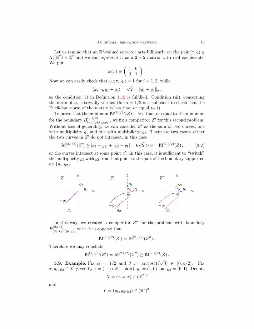
Let us remind that an R2-valued covector acts bilinearly on the pair (τ, g) ∈Λ1(R2) × Z2 and we can represent it as a 2 × 2 matrix with real coefficients.We put

ω(x) ≡(

1 00 1

).

Now we can easily check that 〈ω; τi, gi〉 = 1 for i = 1, 2, while

〈ω; τ3, g1 + g2〉 =√

2 = ‖g1 + g2‖α ,

so the condition (i) in Definition 1.12 is fulfilled. Condition (iii), concerningthe norm of ω, is trivially verified (for α = 1/2 it is sufficient to chech that theEuclidean norm of the matrix is less than or equal to 1).

To prove that the minimum M(2,1/2)(Z) is less than or equal to the minimum

for the boundary B(2,1/2)(x1,x2),(y2,y1), we fix a competitor Z ′ for this second problem.

Without loss of generality, we can consider Z ′ as the sum of two curves, onewith multiplicity g1 and one with multiplicity g2. There are two cases: eitherthe two curves in Z ′ do not intersect, in this case

M(2,1/2)(Z ′) ≥ |x1 − y2|+ |x2 − y1| = 6√

2 > 8 = M(2,1/2)(Z) , (3.2)

or the curves intersect at some point z′. In this case, it is sufficient to “switch”the multiplicity g1 with g2 from that point to the part of the boundary supportedon {y1, y2}.

−g2

g2g1

−g1−g1−g2 −g2

−g1

g1 g2g2 g1

Z Z ′ Z ′′

In this way, we created a competitor Z ′′ for the problem with boundary

B(2,1/2)(x1,x2),(y1,y2) with the property that

M(2,1/2)(Z ′) = M(2,1/2)(Z ′′) .

Therefore we may conclude

M(2,1/2)(Z ′) = M(2,1/2)(Z ′′) ≥M(2,1/2)(Z) .

3.9. Example. Fix α = 1/2 and θ := arccos(1/√

3) ∈ (0, π/2). Fixx, y1, y2 ∈ R2 given by x = (− cos θ,− sin θ), y1 = (1, 0) and y2 = (0, 1). Denote

X = (x, x, x) ∈ (R2)3

and

Y = (y1, y2, y2) ∈ (R2)3.

14 A. Marchese & A. Massaccesi

We claim that the only mass-minimizing current with coefficients in (Z2, ‖·‖1/2)

among those with boundary B(2,1/2)X,Y is

T = Jσ0, τ0, g1 + g2 + g3K + Jσ1, τ1, g1K + Jσ2, τ2, g2 + g3K

where σ0 is the segment from x to 0 and σi is the segment from 0 to yi fori = 1, 2. The orientation τi on each segment goes from the first to the secondextreme point.

g2 + g3

g1

−(g1 + g2 + g3)

The constant R3-valued form

ω(x) ≡

1 0

0√

2/2

0√

2/2

is a calibration for T . Indeed

〈ω; τ0, g1 + g2 + g3〉 =√

3 = ‖g1 + g2 + g3‖1/2;

〈ω; τ1, g1〉 = 1 = ‖g1‖1/2;

〈ω; τ2, g2 + g3〉 =√

2 = ‖g2 + g3‖1/2,therefore condition (i) is satisfied. Moreover ‖〈ω; τ, ·〉‖1/2 = 1 for every τ ∈ R2,hence (iii) is also satisfied. As before, condition (ii) is trivially verified becauseω is constant.

3.10. Rescaled problems. In §4 we want to deal with a boundary made ofinfinitely many points. To this aim it is worthwhile to mention the approach byXia in [19], where the continuous version of the Gilbert-Steiner problem (i.e. µ−and µ+ are not necessarily atomic measures) is defined through the relaxationof the Gilbert-Steiner energy. Given a normal 1-dimensional current T one con-siders all possible sequences Tn of polyedral currents which are approximatingT in the flat norm, then one defines the energy of T as

Eα(T ) := infTn{lim inf

nEα(Tn)}.

As shown in Theorem 2.7 of [20], only rectifiable currents enter in the compe-tition, because non-rectifiable normal currents have infinite energy.

As a first step to prove the optimality of our irrigation network in §4, it isconvenient to introduce a renormalized version of the problem (P1), in whichthe boundary is rescaled to have mass equal to 2. More precisely, consider the

following problem, where B(1,1)X,Y and n are as in §2.1.

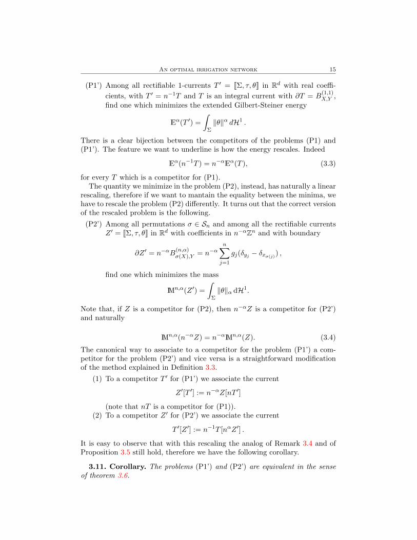
An optimal irrigation network 15

(P1’) Among all rectifiable 1-currents T ′ = JΣ, τ, θK in Rd with real coeffi-

cients, with T ′ = n−1T and T is an integral current with ∂T = B(1,1)X,Y ,

find one which minimizes the extended Gilbert-Steiner energy

Eα(T ′) =

ˆΣ‖θ‖α dH1 .

There is a clear bijection between the competitors of the problems (P1) and(P1’). The feature we want to underline is how the energy rescales. Indeed

Eα(n−1T ) = n−αEα(T ), (3.3)

for every T which is a competitor for (P1).The quantity we minimize in the problem (P2), instead, has naturally a linear

rescaling, therefore if we want to mantain the equality between the minima, wehave to rescale the problem (P2) differently. It turns out that the correct versionof the rescaled problem is the following.

(P2’) Among all permutations σ ∈ Sn and among all the rectifiable currentsZ ′ = JΣ, τ, θK in Rd with coefficients in n−αZn and with boundary

∂Z ′ = n−αB(n,α)σ(X),Y = n−α

n∑j=1

gj(δyj − δxσ(j)) ,

find one which minimizes the mass

Mn,α(Z ′) =

ˆΣ‖θ‖α dH1.

Note that, if Z is a competitor for (P2), then n−αZ is a competitor for (P2’)and naturally

Mn,α(n−αZ) = n−αMn,α(Z). (3.4)

The canonical way to associate to a competitor for the problem (P1’) a com-petitor for the problem (P2’) and vice versa is a straightforward modificationof the method explained in Definition 3.3.

(1) To a competitor T ′ for (P1’) we associate the current

Z ′[T ′] := n−αZ[nT ′]

(note that nT is a competitor for (P1)).(2) To a competitor Z ′ for (P2’) we associate the current

T ′[Z ′] := n−1T [nαZ ′] .

It is easy to observe that with this rescaling the analog of Remark 3.4 and ofProposition 3.5 still hold, therefore we have the following corollary.

3.11. Corollary. The problems (P1’) and (P2’) are equivalent in the senseof theorem 3.6.

16 A. Marchese & A. Massaccesi

Proof. By construction, the solutions of the problem (P1’) are in bijectionwith the solutions of the problem (P1). Analogously the solutions of the prob-lem (P2’) are in bijection with the solutions of the problem (P2). Thus theequivalence follows from Theorem 3.6 and from (3.3) and (3.4). �

3.12. Convex problems and existence of calibrations. Even if we havefound a description of the Gilbert-Steiner problem which consists in a mini-mization of a convex functional, we cannot really claim that we are solving a“convex problem”, in which case a powerful machinery for the computations ofminima would be available. Indeed our class of competitors is not a convex set.While for the classical formulation of the Gilbert-Steiner problem (see footnote3) one can safely extend the minimization problem to a convex and compactclass of objects (being the energy infinite for non-rectifiable currents), this isnot the case for the problem (P2). Moreover, in (P2) we cannot guarantee thatthere is no gap of mass between the minimizers among normal currents andminimizers among integral currents. An interesting occurrence of this gap phe-nomenon in a non-Euclidean setting is given in [11]. We conjecture that in theEuclidean setting there is no such gap. The validity of this conjecture wouldimply that the Gilbert-Steiner problem can be viewed as a convex problem andmoreover the existence of (a sort of) calibration is a necessary and sufficientcondition for the minimality (see §4 of [11] for more details).

4. A minimizer with infinitely many branching points

4.1. Currents in metric spaces. In this section we prove the optimality ofa certain irrigation network having an infinite boundary datum, as mentionedin §3.10. The main tools to prove its optimality have already been introducedin §1 and §3, more precisely in Theorem 1.13 (the existence of a calibrationis a sufficient condition for minimality) and in Corollary 3.11 (the equivalenceof problems (P1’) and (P2’)). Nevertheless, since the ambient space for thisirrigation network is the separable Hilbert space6 `2, a short digression on cur-rents in metric spaces is needed. In order to keep the discussion here as incisiveas possible, we recall only those facts that are strictly unavoidable to definea certain irrigation problem and to prove the optimality of our configuration.The reader is referred to [1] for the theory of currents in a metric space and forall the relevant definitions. Throughout this section, we will assume α = 1/2.

Let T be a rectifiable 1-current in `2 (see §4 in [1]) and let ‖T‖ be theassociated mass (in the sense of Definition 2.6 of [1]). In particular, T issupported on a countably H1-rectifiable set Σ and ‖T‖ = θH1 Σ for somenon-negative θ ∈ L1(Σ,R). We call the extended Gilbert-Steiner energy7 of T

6We choose this setting instead of the more natural Euclidean space, because the possiblityto have infinitely many mutually orthogonal direction allows us to find a very simple calibrationfor the problem we will introduce.

7We denote the extended Gilbert-Steiner energy by E, omitting α, because α = 1/2throughout all the current section.

An optimal irrigation network 17

the quantity

E(T ) :=

ˆΣ

√θ(x) dH1(x) , (4.1)

if the integral makes sense, or +∞ otherwise. One may notice immediately thatthe extended Gilbert-Steiner energy is still subadditive, i.e.,

E(T1 + T2) ≤ E(T1) + E(T2) .

Since the projection on a finite dimensional space is going to be a fundamentalsimplification in the handling of our problem, we recall the following proposi-tion, which just relies on the concavity of the square root.

4.2. Proposition. Let π : `2 → V be the orthogonal projection of `2 onto asubspace V . Then, for every rectifiable 1-current T in `2, there holds8 E(π]T ) ≤E(T ).

4.3. Construction of the irrigation tree. Let (ei)i∈N be the standard or-thonormal basis for `2. Roughly speaking, we are going to define a rectifiable1-dimensional current T in `2 (with coefficients in Q) in the following way:we start from a “trunk”, which is the oriented segment from the origin O toe1 ∈ `2, with unit multiplicity, then, for every n ∈ N, we are going to build afamily of 2n “branches”, that is, 2n currents supported on segments connectedto the main “tree”, with suitable length, orientation and multiplicity in Q. Theirrigation tree will be the sum, up to infinity, of these currents.

To begin with, we deal with the orientations of the segments. If it is notobvious from the context, we always denote by σ(p, q) a segment in `2 from p toq and by xσ(p,q) the (unit) orientation of σ(p, q) from p to q. Now we establishthe directions y(x), z(x) according to which we will assign the orientation of

the segments of a new generation. For every x ∈ `2 of the form x =∑l

i=1 aiei,with al 6= 0, we put

y(x) :=

√2

2

l∑i=1

ai(ei + el+i)

and

z(x) :=

√2

2

l∑i=1

ai(ei − el+i) .

Notice that y(x) and z(x) are orthogonal and y(x)+z(x) is parallel to x. More-over, if we start with a set of mutually orthonormal directions {x1, . . . , xm},then {y(x1), z(x1), . . . , y(xm), z(xm)} are mutually orthonormal, too.

We give the following iterative construction.

◦ We setT0 = Jσ(O, e1), x0, 1K ,

where σ(O, e1) is the segment from the origin to e1 and x0 = e1 is theoutgoing orientation of σ(O, e1). Moreover, we define E0 := {σ(O, e1)}.

8For the definition of the pushforward F]T of a current T through a map F , see Definition2.4 of [1].

18 A. Marchese & A. Massaccesi

◦ For every line segment σ(p, q) ∈ En−1 with orientation x = xσ(p,q), weput in the set En the pair of segments

σ(q, q + 4−ny(x)) and σ(q, q + 4−nz(x)).

Finally, we define

Tn :=∑i≤n

∑σ∈Ei

Jσ, xσ, 2−iK .

Notice that9 M(∂Tn) = 2 for every n ∈ N.

If we call

En :=⋃σ∈En

σ,

then the support of the irrigation tree is defined as the limit

E :=⋃n∈N

En .

Notice that the segments are growing in orthogonal directions, hence H1-a.e.p ∈ E belongs to a unique segment σ(p) ∈ En(p) and we can define an orientation

τ : E → `2 setting τ(p) = xσ(p). Analogously, we can define a multiplicity

m : E → Q setting m(p) = 2−n for every p ∈ En. The irrigation tree T isdefined as

T := JE, τ,mK .The truncated currents Tn play a fundamental role in the proof of optimality

of the irrigation tree T , because they are a good approximation for T (as weunderline with Remark 4.4) and they are essentially embedded in a finite dimen-sional space (indeed, suppTn ⊂ span{e1, . . . , e2n}). Since the segments in E are

essentially disjoint, we can also write Tn = T(⋃

i≤nEn)

:= J⋃i≤nE

n, τ,mK.

4.4. Remark. By construction, the following facts hold.

(i) E(T − Tn) =∑

j>n 2j2−j2 4−j =

∑j>n 2−

32j .

(ii) M(T − Tn) =∑

j>n 2j2−j4−j =∑

j>n 2−2j .

(iii) If πn : `2 → span{e1, . . . , e2n} is the orthogonal projection and if{q1, . . . , q2n} are the second extreme points of the segments in En, then(πn)](Tn) is a candidate for the minimization problem (P1’) in 3.10,where

X = (0, . . . , 0), Y = (q1, . . . , q2n) .

Indeed 2n(πn)]Tn is an integral current.

We are now ready to prove the optimality of T .

4.5. Theorem. The rectifiable 1-current T in `2 minimizes the generalizedGilbert-Steiner energy (4.1) among all rectifiable currents in `2 with boundary∂T .

9Here and in the following, M(T ) denotes the total mass of the mass measure ‖T‖.

An optimal irrigation network 19

Proof. We split the proof into several steps.Step 1: general strategy. Let S be an admissible competitor, i.e., S is arectifiable 1-current in `2 with ∂S = ∂T .

We want to reduce the problem to an energy minimization problem for rectifi-able 1-currents in a finite dimensional space and then exploit the tools developedin the previous sections. For every n ∈ N, let Sn := S−T +Tn and notice that∂Sn = ∂Tn. By Proposition 4.2, we have that

E((πn)]Sn) ≤ E(Sn) ∀n ∈ N .Fix ε > 0. Since, by subadditivity of E, we have that

E(Sn) ≤ E(S) + E(Tn − T ) ∀n ∈ Nand the energy E(Tn − T ) is going to 0 (see Remark 4.4), then there existsn(ε) ∈ N such that E(Tn(ε)−T ) ≤ ε, thus E(S) ≥ E(Sn(ε))− ε. If we can provethat

E(Tn) ≤ E((πn)]Sn) (4.2)

for every n ∈ N, then we have that

E(T ) ≤ E(Tn(ε)) + E(Tn(ε) − T ) ≤ E(Tn(ε)) + ε

≤ E((πn(ε))]Sn(ε)) + ε ≤ E(Sn(ε)) + ε ≤ E(S) + 2ε ,

which proves the theorem, since ε can be arbitrarily small.Step 2: reduction to problem (P1’). We have already noticed that (πn)]Tnis an admissible candidate for the problem (P1’). The issue is that, in general,(πn)]Sn is not an admissible competitor and we cannot immediately look for

a calibration for the current Z ′[(πn)]Tn]10. Indeed (πn)]Sn is a rectifiable cur-rent, with admissible boundary datum, but its coefficients are in R and notnecessarily in 2−nZ, as required in (P1’)11.

In order to overcome this issue, we have to perform a second approximation.Fix δ > 0. We associate to (πn)]Sn a polyhedral current S = 1

2nNR, where

N ∈ N and R has integer multiplicity. We can choose S in such a way that theboundary is unchanged, i.e.,

∂S = ∂(πn)]Sn = ∂(πn)]Tn ,

andE(S) ≤ E ((πn)]Sn) + δ . (4.3)

The existence of S is a consequence of Proposition 4.4 of [20].

Step 3: construction of Z.Since we want to move the problem of energy minimization in the setting of

(rational multiples of) rectifiable currents with coefficients in Z2n , we associate

10The definition of Z′[(πn)]Tn] is given in §3.10. The role of the basis (g1, . . . , g2n) here isplayed by (πn(x1), . . . , πn(x2n)), where x1, . . . , x2n are the (mutually orthogonal) orientationsof the segments in the family En

11In particular, we do not have a canonical way to associate to (πn)]Sn a current with

coefficients in R2n whose mass is less than or equal to the energy of (πn)]Sn (see Proposition3.5).

20 A. Marchese & A. Massaccesi

to S a current Z in R2n with coefficients in R2n . We can choose Z in such away that the boundary is

∂Z = ∂Z ′[(πn)]Tn]

andM(2n,1/2)(Z) ≤ E(S) . (4.4)

The construction of Z, starting from S, is analogous to that presented in Def-inition 3.3. Let x1, . . . , x2n be the (mutually orthogonal) orientations of thesegments in the family En. Let us write the polyhedral integral 1-currentR = 2nNS as

R =∑i∈I

Jσi, τi, aiK ,

where σi is an oriented segment with orientation τi and ai ∈ {1, . . . , 2nN}.Decomposing12 R as in (2.2), one may notice that the current Z[R] (accordingto the basis (πn(x1), . . . , πn(x2n))) has the form

Z[R] =∑i∈I

Jσi, τi, biK ,

where

◦ bi = ci,1πn(x1) + . . .+ ci,2nπn(x2n);◦ ci,j ∈ N ∪ {0} and ci,j ≤ N for every j = 1, . . . , 2n13;◦ ci,1 + . . .+ ci,2n = ai.

We can compute

‖bi‖ =√c2i,1 + . . .+ c2

i,2n ≤√ci,1N + . . .+ ci,2nN =

√Nai .

Denote Z := 2−n/2N−1Z[R]. We have

∂Z = ∂(2−n/2N−1Z[R]) = 2−n/2N−1∂Z[N2nS]

= 2−n/2N−1∂Z[N2n(πn)]Tn] = ∂(2−n/2Z[2n(πn)]Tn]) = ∂Z ′[(πn)]Tn] .

Moreover

M(2n,1/2)(Z) = 2−n/2N−1M(2n,1/2)(Z[R]) = 2−n/2N−1∑i∈I‖bi‖H1(σi)

≤ 2−n/2N−1/2∑i∈I

√aiH1(σi) = 2−n/2N−1/2E(R)

= E(2−nN−1R) = E(S) .

Step 4: proof of the minimality of Z ′[(πn)]Tn]. Even if, technically speak-

ing, Z does not belong to the set of competitors for (P2’), we can still provethat

M(2n,1/2)(Z ′[(πn)]Tn]

)≤M(2n,1/2)(Z) (4.5)

12Without loss of generality we can assume R to be acyclic, i.e., R` = 0 for every ` ∈ N.13Roughly speaking, ci,j is the portion of the multiplicity ai of σi, which is due to all paths

ending in the second extreme of the segment of En having orientation xj

An optimal irrigation network 21

via the calibration technique (see Remark 1.14).Consider the basis of R2n (πn(x1), . . . , πn(x2n)). The current Z ′ [(πn)]Tn]

has the following property: the multiplicity on each line segment of its supportis a multiple of the orientation of the segment itself14 (the orientation beingdefined above). This implies that, if we denote by ω : R2n → R2n the identitymap, then ω can be seen as a R2n-valued (constant) differential 1-form, whichin particular is a calibration for Z ′ [(πn)]Tn]: the verification of conditions (i),(ii) and (iii) of Definition 1.12 is elementary, as in the Example 3.8. Theorem1.13 and Remark 1.14 allow us to conclude.Step 5: conclusion. Eventually we can prove the claim (4.2), indeed

E((πn)]Sn) + δ(4.3)

≥ E(S)(4.4)

≥ M(2n,1/2)(Z)(4.5)

≥ M(2n,1/2)(Z ′[(πn)](Tn)]

)and, from the arbitrariness of δ, from Corollary 3.11, together with the factthat supp(Tn) is contained in span{e1, . . . , e2n}, we finally get that

E((πn)]Sn) ≥M(2n,1/2)(Z ′[(πn)](Tn)]

) 3.11= E ((πn)]Tn) = E(Tn) .

�

4.6. Remark. In [6] the authors combine the notion of currents in metricspaces of [1] and currents with coefficients in a group of [18]. In this setting wecan give a meaning to the problem of minimizing the mass in a class of currentsin `2 with coefficients in `2 with given boundary. It is possible to associate tothe current T , defined in §4.3, a current Z in `2 with coefficients in `2, in a waywhich is similar to that explained in Definition 3.3. Via a simple calibrationargument (the calibration being again the “identity” with respect to suitablecoordinates) one can prove that Z minimizes the mass among all currents in `2

with coefficients in `2, with boundary ∂Z.

The latter remark suggests the possibility to describe, in general, the con-tinuous version of the Gilbert-Steiner problem as a mass minimization problemamong currents in the Euclidean space, with coefficients in `2. The advantage ofthis formulation would be, for example, the availability of well known numericalmethods for the minimization of a convex functional.

References

[1] Ambrosio, L., and Kirchheim, B. Currents in metric spaces. Acta Math. 185, 1 (2000),1–80.

[2] Bernot, M., Caselles, V., and Morel, J.-M. Traffic plans. Publ. Mat. 49, 2 (2005),417–451.

[3] Bernot, M., Caselles, V., and Morel, J. M. Are there infinite irrigation trees? J.Math. Fluid Mech. 8, 3 (2006), 311–332.

[4] Bernot, M., Caselles, V., and Morel, J.-M. Optimal transportation networks,vol. 1955 of Lecture Notes in Mathematics. Springer-Verlag, Berlin, 2009. Models andtheory.

14This is due to the fact that the sum of y(x) and z(x) in §4.3 is parallel to x.

22 A. Marchese & A. Massaccesi

[5] Conti, S., Garroni, A., and Massaccesi, A. Lower semicontinuity and relaxation offunctionals on one-dimensional currents with multiplicity in a lattice. Preprint (2013).

[6] De Pauw, T., and Hardt, R. Rectifiable and flat G chains in a metric space. Amer. J.Math. 134, 1 (2012), 1–69.

[7] Federer, H. Geometric measure theory. Die Grundlehren der mathematischen Wis-senschaften, Band 153. Springer-Verlag New York Inc., New York, 1969.

[8] Maddalena, F., and Solimini, S. Transport distances and irrigation models. J. ConvexAnal. 16, 1 (2009), 121–152.

[9] Maddalena, F., and Solimini, S. Synchronic and asynchronic descriptions of irrigationproblems. Adv. Nonlinear Stud. 13, 3 (2013), 583–623.

[10] Maddalena, F., Solimini, S., and Morel, J.-M. A variational model of irrigationpatterns. Interfaces Free Bound. 5, 4 (2003), 391–415.

[11] Marchese, A., and Massaccesi, A. The steiner tree problem revisited through recti-fiable g-currents. to appear on Adv. Calc. Var. (2014).

[12] Paolini, E., and Stepanov, E. Optimal transportation networks as flat chains. Inter-faces Free Bound. 8, 4 (2006), 393–436.

[13] Paolini, E., and Stepanov, E. Existence and regularity results for the steiner problem.Calc. Var. Partial Diff. Equations 46, 3 (2013), 837–860.

[14] Paolini, E., Stepanov, E., and Teplitskaya, Y. An example of an infinite Steinertree connecting an uncountable set. Preprint (2013).

[15] Paolini, E., and Ulivi, L. The Steiner problem for infinitely many points. Rend. Semin.Mat. Univ. Padova 124 (2010), 43–56.

[16] Simon, L. Lectures on geometric measure theory, vol. 3 of Proceedings of the Centre forMathematical Analysis, Australian National University. Australian National UniversityCentre for Mathematical Analysis, Canberra, 1983.

[17] Stepanov, E. O. Optimization model of transport currents. J. Math. Sci. (N. Y.) 135,6 (2006), 3457–3484. Problems in mathematical analysis. No. 32.

[18] White, B. Rectifiability of flat chains. Ann. of Math. (2) 150, 1 (1999), 165–184.[19] Xia, Q. Optimal paths related to transport problems. Commun. Contemp. Math. 5, 2

(2003), 251–279.[20] Xia, Q. Interior regularity of optimal transport paths. Calc. Var. Partial Differential

Equations 20, 3 (2004), 283–299.