An On-the-fly Tableau-based Decision Procedurefor PDL-Satisfiability

Pietro Abate1, Rajeev Gore1, and Florian Widmann12

1 Computer Science LaboratoryThe Australian National University

Canberra ACT 0200, Australia2 Logic and Computation Programme

Canberra Research LaboratoryNICTA Australia

{Pietro.Abate|Rajeev.Gore|Florian.Widmann}@anu.edu.au

Abstract. We present a tableau-based algorithm for deciding satisfia-bility for propositional dynamic logic (PDL) which builds a finite rootedtree with ancestor cycles and which passes extra information from chil-dren to parents to separate good cycles from bad cycles during backtrack-ing. It is easy to implement, with potential for parallelisation, becauseit constructs a potential model “on the fly” by exploring each tableaubranch independently. However, its worst-case behaviour is 2EXPTIMErather than EXPTIME. We give detailed proofs of soundness and com-pleteness in an appendix and there is a prototype implementation in theTWB (twb.rsise.anu.edu.au).

1 Introduction

Propositional dynamic logic (PDL) was developed in the late 1970s as a logicfor reasoning about programs [15, 8, 3]. The formulae of PDL consist of tradi-tional Boolean formulae plus “action modalities” built from a finite set of atomicprograms using the operations of sequential composition (; ), non-deterministicchoice (∪), and test (?). The satisfiability problem for PDL is known to beEXPTIME-complete [16]. Unlike the situation in EXPTIME-complete descrip-tion logics, where algorithms with good average-case behaviour are known, weknow of no decision procedures for testing PDL-satisfiability which are satisfac-tory from both a theoretical (soundness and completeness) and practical (averagecase behaviour) viewpoint as we explain below.

The earliest decision procedures for PDL are due to Fischer and Ladner [8]and Pratt [16]. Fischer and Ladner’s method is impractical because it first con-structs the set of all consistent subsets of the set of all subformulae of the givenformula which always requires exponential time in all cases. On the other hand,Pratt [16] essentially builds a multi-pass (explained shortly) tableau method.Most subsequent decision procedures for other fix-point logics like propositionallinear temporal logic (PLTL) [19], computation tree logic (CTL) [4, 7] and the

modal µ-calculus [14] trace their origins back to Pratt [16], and they all shareone main disadvantage as explained next.

These multi-pass procedures can be described informally as follows where a“state” is a node which contains only diamond-like-formulae (“eventualities”),box-like–formulae, atoms and negated atoms. The first pass constructs a rootedtableau of nodes containing formula-sets, but allows cross-branch arcs from astate n on one branch to a (previously constructed) state m on a different branchif applying the tableau construction to n would duplicate m. Thus the firstpass constructs a “pseudo-model” which is a potentially exponential-sized cyclicgraph (rather than a cyclic tree where m would have to be an ancestor of n).The subsequent passes check that the “pseudo-model” is a real model by pruninginconsistent nodes and pruning nodes that contain “unfulfilled eventualities”.

Although efficient model-checking techniques can check the “pseudo-model”in time which is linear in its size, these multi-pass methods can construct anexponential-sized cyclic graph when it is not necessary. One solution is to checkfor fulfilled eventualities “on the fly”, as the graph is being built, and althoughsuch methods exist for model-checking [6, 5], we know of no such decision pro-cedures for PDL (or for other fix-point logics). The only implementation of amultiple-pass method for PDL that we know of is in LoTRec (www.irit.fr/Lotrec/) but it is not optimal since it treats disjunctions in a naive way.

In 1990, Baader [2] gave a single-pass tableau-based decision procedure fora description logic with role definitions involving union, composition and tran-sitive closure of roles which can be viewed as essentially PDL without test. Hismethod first constructs a (cyclic tree) tableau which implements the intendedsemantics of the various PDL operators. To separate “good cycles” from “badcycles”, Baader’s method has to decide equality of regular languages, a PSPACE-complete problem which in practice may require exponential time. Instead ofsolving these problems “on the fly”, they can be reduced to a simple check onthe identity of states in a deterministic minimal automaton created from the pos-itive regular expressions appearing in the initial formula during a pre-processingstage [2, page 27]. But since the pre-computed automaton can be of exponentialsize, this alternative may require exponential time needlessly. Because Baaderdoes not allow cross-branch cycles, his method is double-exponential in the worst-case. Finally, the “test” construct, which is essential to express “while” loops,creates a mutual recursion between the Boolean language and the regular lan-guage over programs, so it is not obvious to us how to extend Baader’s methodto handle “test”. We know of no satisfactory implementation of this method.

In 2000, De Giacomo and Massacci [9] gave an optimal method for decidingPDL-satisfiability using labelled formulae of the form σ : ϕ allowing them to cap-ture the notion that “possible world σ makes formula ϕ true”. They first give aNEXPTIME algorithm for deciding PDL-satisfiability in detail and then discusshow to obtain an EXPTIME algorithm using various known results from the lit-erature. They do not give an actual EXPTIME algorithm, nor its soundness andcompleteness proofs. An initial implementation of a deterministic version of this

2

NEXPTIME algorithm by Schmidt and Tishkovsky struck problems for formulaewith nested ∗s, but we understand that there is a forthcoming solution [17].

Other decision procedures for fix-point logics use resolution calculi, transla-tion methods, automata-theoretic methods, and game theoretic methods: see [1]for references. We know of no implementations for PDL based on these methods.

Here, we give a sound, complete and terminating decision procedure for PDLwith the following advantages and disadvantages:

One-pass nature: our method constructs a single-rooted finite cyclic tree whereall cycles connect a leaf to an ancestor. In particular, there are no cross-branch edges, meaning that our method can be used to explore the searchspace in a depth-first, left-to-right manner. Consequently, the space requiredto explore one branch can be reclaimed upon backtracking.

Pre-processing: although there is no initial construction of a potentially expo-nential sized automaton, nor any calls to a subroutine for deciding equalityof regular languages, we do require a pre-processing stage to avoid nestedoccurrences of ∗ which can lead to an exponential blow-up in the size of theinitial formula. The longer version of this paper will show how to avoid thisstep, but it complicates the rules even further.

Full proofs: our proofs of soundness and completeness are all given in full detailand use only elementary methods.

Ease of implementation: our rules are easy to implement since our tableau nodescontain sets of formulae as usual and some easily defined extra informationwhose manipulation requires only set intersection, set membership, and theoperations of min/max on integers. Our rules incorporate these low-leveldetails, making them cumbersome to describe.

Potential for optimisation: because of their tree structure, there is potential tooptimise our tableaux using techniques which have proved successful for(one-pass) tableaux for description logics [11].

Ease of generating counter-models: the soundness proof of our tableau proce-dure for testing PDL-satisfiability immediately gives an effective procedurefor turning an “open” tableau into a PDL-model.

Ease of generating proofs: our tableau calculus can be turned into a cut-freeGentzen-style calculus with “cyclic proofs”. Unlike existing cut-free Gentzen-style calculi for fix-point logics [12, 13] we can give an optimal, rather thanworst-case, bound for the finitary version of the omega rule for PDL.

Potential for parallelisation: our rules build the branches independently, butcombine their results during backtracking, so it is possible to implementour procedure on a bank of parallel processors.

Working Prototype: we have implemented a (sequential) prototype of our basictableau method using the Tableau Work Bench (twb.rsise.anu.edu.au)which allows users to test arbitrary PDL formulae over the web.

Double-exponential Worst Case: in the worst-case, our method requires timewhich is double-exponential in the size of the given formula, meaning tripleexponential via the pre-processing blow-up. That is, our method may haveto repeat the same work on multiple branches. Further experimental work

3

is required to determine if a highly optimised version of our method can bemade practical for the average case.

Generality: Our method for PDL fits into a class of similar “one pass” methodsfor other fix-point logics like PLTL [18] and CTL [1]. The next step is tosee if our methods can be turned into optimal algorithms which exhibitgood average-case behaviour by using techniques like global caching whichhave proved useful in obtaining an easy to implement and provably correctEXPTIME algorithm for the EXPTIME-complete logic ALC [10].

2 Syntax, Semantics and Hintikka Structures

Definition 1. Let AFml be a countably infinite set of propositional atoms andAPrg a finite set of atomic programs with AFml ∩ APrg = ∅. The set Fml ofall formulae and the set Prg of all programs are defined inductively as follows:

1. AFml ⊆ Fml2. if ϕ,ψ ∈ Fml then ¬ϕ ∈ Fml and ϕ ∧ ψ ∈ Fml and ϕ ∨ ψ ∈ Fml3. if ϕ ∈ Fml and α ∈ Prg then 〈α〉ϕ ∈ Fml and [α]ϕ ∈ Fml4. APrg ⊆ Prg5. if α ∈ Prg and β ∈ Prg then (α;β) ∈ Prg and α ∪ β ∈ Prg and α∗ ∈ Prg6. if ϕ ∈ Fml then ϕ? ∈ Prg.

We use p and q to range over members of AFml and use a and b to range overmembers of APrg. A formula of the form 〈α〉ϕ is called a 〈〉-formula, and aformula of the form 〈α∗〉ϕ is called an eventuality. Let Fml〈〉 denote the set ofall 〈〉-formula and Fml〈∗〉 the set of all eventualities. The notions of sub-formulaand sub-program are defined as usual as are the connectives →, ↔, > and ⊥.

Definition 2. A transition frame is a pair (W,R) where W is a non-emptyset of worlds and R is a function that assigns to each atomic program a ∈APrg a binary relation Ra over W . A model M = (W,R, V ) is a transitionframe (W,R) and a valuation function V : AFml → 2W which associates witheach propositional atom p a set V (p) of worlds in which p is true.

Definition 3. Let M = (W,R, V ) be a model. The functions τM : Fml → 2W

and ρM : Prg → 2W×W are defined inductively as follows:

τM (p) := V (p)τM (¬ϕ) := W \ τM (ϕ)τM (ϕ ∧ ψ) := τM (ϕ) ∩ τM (ψ)τM (ϕ ∨ ψ) := τM (ϕ) ∪ τM (ψ)τM ([α]ϕ) := {w | ∀v ∈W. (w, v) ∈ ρM (α) ⇒ v ∈ τM (ϕ)}τM (〈α〉ϕ) := {w | ∃v ∈W. (w, v) ∈ ρM (α) & v ∈ τM (ϕ)}ρM (a) := Ra

ρM (α;β) := {(w, v) | ∃u ∈W. (w, u) ∈ ρM (α) & (u, v) ∈ ρM (β)}ρM (α ∪ β) := ρM (α) ∪ ρM (β)ρM (α∗) :=

{(w, v) | ∃k ∈ IN.∃w0, . . . , wk ∈W.

(w0 = w & wk = v &

∀i ∈ {0, . . . , k − 1}. (wi, wi+1) ∈ ρM (α))}

ρM (ϕ?) := {(w,w) | w ∈ τM (ϕ)} .

4

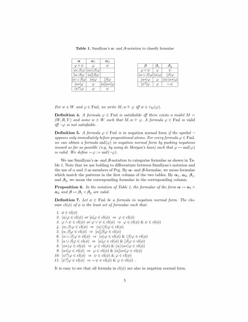
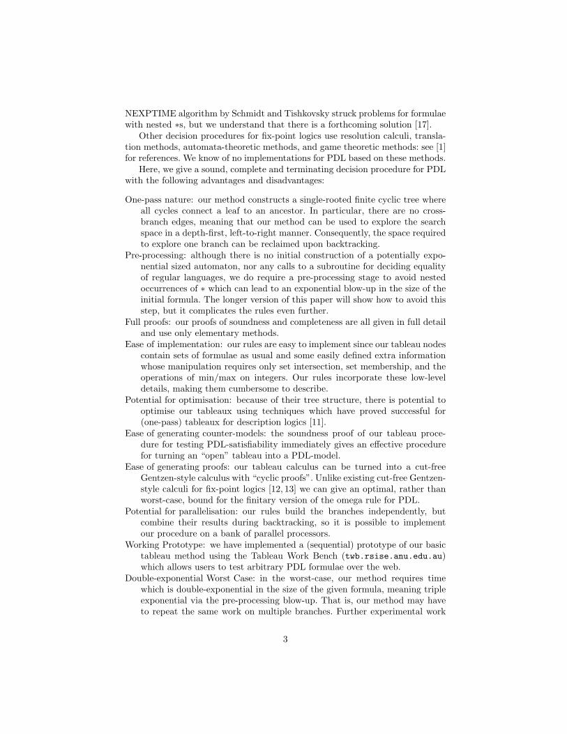
Table 1. Smullyan’s α- and β-notation to classify formulae

α α1 α2

ϕ ∧ ψ ϕ ψ

〈α;β〉ϕ 〈α〉〈β〉ϕ[α;β]ϕ [α][β]ϕ

[α ∪ β]ϕ [α]ϕ [β]ϕ

[α∗]ϕ ϕ [α][α∗]ϕ〈ψ?〉ϕ ϕ ψ

β β1 β2

ϕ ∨ ψ ϕ ψ

〈α ∪ β〉ϕ 〈α〉ϕ 〈β〉ϕ〈α∗〉ϕ ϕ 〈α〉〈α∗〉ϕ[ψ?]ϕ ϕ ∼ψ

For w ∈W and ϕ ∈ Fml, we write M,w ϕ iff w ∈ τM (ϕ).

Definition 4. A formula ϕ ∈ Fml is satisfiable iff there exists a model M =(W,R, V ) and some w ∈ W such that M,w ϕ. A formula ϕ ∈ Fml is validiff ¬ϕ is not satisfiable.

Definition 5. A formula ϕ ∈ Fml is in negation normal form if the symbol ¬appears only immediately before propositional atoms. For every formula ϕ ∈ Fml,we can obtain a formula nnf(ϕ) in negation normal form by pushing negationsinward as far as possible ( e.g. by using de Morgan’s laws) such that ϕ↔ nnf(ϕ)is valid. We define ∼ϕ := nnf(¬ϕ).

We use Smullyan’s α- and β-notation to categorise formulae as shown in Ta-ble 1. Note that we use bolding to differentiate between Smullyan’s notation andthe use of α and β as members of Prg. By α- and β-formulae, we mean formulaewhich match the patterns in the first column of the two tables. By α1, α2, β1,and β2, we mean the corresponding formulae in the corresponding column.

Proposition 6. In the notation of Table 1, the formulae of the form α ↔ α1 ∧α2 and β ↔ β1 ∨ β2 are valid.

Definition 7. Let φ ∈ Fml be a formula in negation normal form. The clo-sure cl(φ) of φ is the least set of formulae such that:

1. φ ∈ cl(φ)2. 〈a〉ϕ ∈ cl(φ) or [a]ϕ ∈ cl(φ) ⇒ ϕ ∈ cl(φ)3. ϕ ∧ ψ ∈ cl(φ) or ϕ ∨ ψ ∈ cl(φ) ⇒ ϕ ∈ cl(φ) & ψ ∈ cl(φ)4. 〈α;β〉ϕ ∈ cl(φ) ⇒ 〈α〉〈β〉ϕ ∈ cl(φ)5. [α;β]ϕ ∈ cl(φ) ⇒ [α][β]ϕ ∈ cl(φ)6. 〈α ∪ β〉ϕ ∈ cl(φ) ⇒ 〈α〉ϕ ∈ cl(φ) & 〈β〉ϕ ∈ cl(φ)7. [α ∪ β]ϕ ∈ cl(φ) ⇒ [α]ϕ ∈ cl(φ) & [β]ϕ ∈ cl(φ)8. 〈α∗〉ϕ ∈ cl(φ) ⇒ ϕ ∈ cl(φ) & 〈α〉〈α∗〉ϕ ∈ cl(φ)9. [α∗]ϕ ∈ cl(φ) ⇒ ϕ ∈ cl(φ) & [α][α∗]ϕ ∈ cl(φ)

10. 〈ψ?〉ϕ ∈ cl(φ) ⇒ ψ ∈ cl(φ) & ϕ ∈ cl(φ)11. [ψ?]ϕ ∈ cl(φ) ⇒ ∼ψ ∈ cl(φ) & ϕ ∈ cl(φ) .

It is easy to see that all formula in cl(φ) are also in negation normal form.

5

Definition 8. A structure (W,R,L) [for ϕ ∈ Fml] is a transition frame (W,R)and a labelling function L : W → 2Fml which associates with each world w ∈Wa set L(w) of formulae [and has ϕ ∈ L(v) for some world v ∈W ].

Definition 9. For a given ϕ ∈ Fml the (infinite) set pre(ϕ) is defined as:

pre(ϕ) := {ψ ∈ Fml | ∃k ∈ IN. ∃α1, . . . , αk ∈ Prg. ψ = 〈α1〉 . . . 〈αk〉ϕ} .

For all formulae ϕ and ψ, the binary relation on formulae is defined as:ϕ ψ iff (exactly) one of the following conditions is true:

– ∃χ ∈ Fml, α, β ∈ Prg. ϕ = 〈α;β〉χ & ψ = 〈α〉〈β〉χ– ∃χ ∈ Fml, α, β ∈ Prg. ϕ = 〈α ∪ β〉χ &

(ψ = 〈α〉χ or ψ = 〈β〉χ

)– ∃χ ∈ Fml, α ∈ Prg. ϕ = 〈α∗〉χ &

(ψ = χ or ψ = 〈α〉〈α∗〉χ

)– ∃χ, φ ∈ Fml. ϕ = 〈φ?〉χ & ψ = χ .

The relation + is the transitive closure of .

Intuitively – using the notation of Table 1 – the relation relates a 〈〉-formulae α(respectively β) that is not of the form 〈a〉χ to α1 (respectively β1 and β2).The notion of pre(ϕ) is useful because eventualities like 〈α∗〉ϕ get expandedinto 〈α〉〈α∗〉ϕ and 〈α〉〈α∗〉ϕ can then end up being decomposed into formulaeof the form 〈α1〉 . . . 〈αk〉〈α∗〉ϕ. Note that ϕ ∈ pre(ϕ).

Definition 10. Let H = (W,R,L) be a structure, ϕ ∈ Fml a formula, β ∈ Prga program, and w ∈ W a state. A fulfilling chain for (ϕ, β,w) in H is a finitesequence (w0, ψ0), . . . , (wn, ψn) of world-formula pairs with n ≥ 0 such that:

– wi ∈W , ψi ∈ pre(ϕ), and ψi ∈ L(wi) for all 0 ≤ i ≤ n– w0 = w, ψ0 = 〈β〉ϕ, ψn = ϕ, and ψi 6= ϕ for all 0 ≤ i ≤ n− 1– for all 0 ≤ i ≤ n − 1, if ψi = 〈a〉χ for some a ∈ APrg and χ ∈ Fml

then ψi+1 = χ and wiRa wi+1; otherwise ψi ψi+1 and wi = wi+1.

Intuitively, each ψi is in the label L(wi). The sequence starts at (w0, 〈β〉ϕ),ends at (wn, ϕ), and no other wi is paired with ϕ. Consecutive formulae in thesequence are related by and consecutive worlds wi and wi+1 are the sameunless ψi = 〈a〉χ, in which case ψi+1 = χ and wiRa wi+1 must hold. Thus theeventuality 〈β〉ϕ ∈ w0 is fulfilled by the ϕ ∈ wn and wn is β-reachable from w0.

Definition 11. A pre-Hintikka structure H = (W,R,L) [for ϕ ∈ Fml] is astructure [for ϕ] that satisfies the following conditions for every w ∈W where αand β are formulae as defined in Table 1:

H1 : ¬p ∈ L(w) ⇒ p 6∈ L(w)H2 : α ∈ L(w) ⇒ α1 ∈ L(w) & α2 ∈ L(w)H3 : β ∈ L(w) ⇒ β1 ∈ L(w) or β2 ∈ L(w)H4 : 〈a〉ϕ ∈ L(w) ⇒ ∃v ∈W. wRa v & ϕ ∈ L(v)H5 : [a]ϕ ∈ L(w) ⇒ ∀v ∈W. wRa v ⇒ ϕ ∈ L(v) .

A Hintikka structure H = (W,R,L) [for ϕ ∈ Fml] is a pre-Hintikka structure[for ϕ] that additionally satisfies the following condition:

H6 : 〈α∗〉ϕ ∈ L(w) ⇒ there exists a fulfilling chain for (ϕ, α∗, w) in H .

6

Although H3 captures the fix-point semantics of 〈α∗〉ϕ by “locally unwinding”the fix-point, it does not guarantee a least fix-point which requires that ϕ has tobe true eventually. We therefore additionally need H6 which acts “globally” andensures that all eventualities are fulfilled. Note that H2 is enough to capture thecorrect behaviour of [α∗]ϕ as it has a greatest fix-point semantics.

Theorem 12. A formula ϕ ∈ Fml in negation normal form is satisfiable iffthere exists a Hintikka structure for ϕ.

Definition 13. The set ε-free of programs which do not generate the empty wordis defined inductively as:

1. APrg ⊆ ε-free2. if α ∈ ε-free or β ∈ ε-free then α;β ∈ ε-free3. if α ∈ ε-free and β ∈ ε-free then α ∪ β ∈ ε-free.

A program α ∈ Prg (respectively a formula ϕ ∈ Fml) is in *-normal form iffevery sub-program β∗ of α (respectively of ϕ) has β ∈ ε-free.

Proposition 14. 1. if α ∈ ε-free then 〈α〉ψ 6 + ψ for all ψ ∈ fml2. if α ∈ Prg is in *-normal form then 〈α〉ψ 6 + 〈α〉ψ for all ψ ∈ fml3. if ϕ ∈ Fml is in *-normal form then ϕ 6 + ϕ

Corollary 15. If ϕ ∈ Fml is in *-normal form then there exists no infinitesequence ϕ0 = ϕ,ϕ1, . . . such that ϕi ϕi+1 for all i ∈ IN.

Theorem 16. For every ϕ ∈ Fml [in negation normal form], there is a ψ ∈ Fmlin *-normal form [and in negation normal form] such that ϕ↔ ψ is valid.

3 An Overview of the Algorithm

Our algorithm starts with a root node containing the given formula φ and anempty list called HCr. It builds a tree by repeatedly applying α- and β-rulesto decompose the formula according to the semantics of PDL. In particular, theβ-rule for 〈α∗〉ϕ has a left child which fulfils this eventuality by reducing it to ϕ,and a right child which procrastinates its fulfilment by “reducing” it to 〈α〉〈α∗〉ϕ.All α- and β-children inherit the HCr-value of their parents unchanged.

The application of α- and β-rules stops when all leaves contain only atoms,negated atoms, and all 〈〉-formulae and all []-formulae begin with outermostatomic programs only. For each such leaf node l, and for each 〈a〉ξ-formula in l,the 〈〉-rule creates a successor node containing ξ ∪∆, where ∆ = {ψ | [a]ψ ∈ l},as is standard for modal logics, and passes the successor a new HCr-value byextending the current HCr with the pair (ξ, {ξ} ∪∆) These successors are thensaturated to produce new leaves using the α- and β-rules, and the 〈〉-rule createsthe successors of these new leaves, and so on.

If left unchecked, this procedure can produce infinite branches since the samesuccessors can be created again and again on the same branch. To obtain termi-nation, the 〈〉-rule creates a successor containing {ξ} ∪ ∆ for l only if the pair

7

(ξ, {ξ} ∪∆) 6∈ HCrl since this indicates that this successor has not already beencreated previously higher up on the current branch.

If the successor {ξ} ∪ ∆ exists already, then the current branch is blockedfrom re-creating it. The resulting loop may be “bad” since every β-applicationon this branch for an eventuality 〈α∗〉ϕ may procrastinate, so 〈α∗〉ϕ can never befulfilled even if we were to repeat the loop ad infinitum. To flag this potentially“bad” loop, our algorithm passes up a triple (ξ, 〈α∗〉ϕ, h) to its parent if ξ is adecomposition of 〈α∗〉ϕ and h is the height of the blocking previous successor.

During backtracking, our rules modify the first component of the triples toreverse-track the decomposition of 〈α∗〉ϕ and merge “matching” triples beingpassed up from the children to compute the triples for the parent. In particular,a “bad” loop can be rescued to become a “good” loop at the β-node for 〈α∗〉ϕif the left child remains open and the right child can access the left child byfollowing the loop down to the leaf, following the loop up to its blocking node, andreturning back down to the left child. Conversely, if all such potential rescuersare closed, then some modification (ξ′, 〈α∗〉ϕ, h) of the triple (ξ, 〈α∗〉ϕ, h) willsurvive the journey up until it reaches the blocking node at height h. The parentof this blocking node is then “closed” since there is no hope of converting the“bad” loop to a good “loop”. A complication arises if both β-children of anon-〈α∗〉ϕ-node “loop”, so our algorithm keeps the triple whose blocking nodeis higher in the tree using a min operation since the triple then meets morepotentially rescuing 〈α∗〉ϕ-nodes on its way up.

If the status of the root node becomes “closed” then the formula φ is PDL-unsatisfiable, else the tableau contains a PDL-model for φ.

4 A One-pass Tableau Algorithm for PDL

To separate “good” and “bad” cycles, our algorithm stores additional informa-tion in each tableau node using histories and variables [18] where histories arepassed from parents to children and variables are passed from children to parents.

Definition 17. A tableau node x is of the form (Γ :: HCr :: mrk,uev) where:

Γ is a set of formulaeHCr is a list of pairs (ϕ,∆) where ∆ is a set of formulae and ϕ ∈ ∆ is a

distinguished formula from ∆

mrk is a boolean valued variable indicating whether the node is marked anduev is a partial function from Fml〈〉× Fml〈∗〉 to IN>0.

Definition 18. A tableau for a formula set Γ ⊆ Fml and a list of formulasets HCr is a tree of tableau nodes with root (Γ :: HCr :: mrk,uev) where thechildren of a node x are obtained by a single application of a rule to x ( i.e. onlyone rule can be applied to a node). A tableau is expanded if no rules can beapplied to any of its leaves. On any branch of a tableau, a node t is an ancestorof a node s iff t lies above s on the unique path from the root down to s.

8

The list HCr is the only history whereas mrk and uev are variables and theirvalues are determined by the children of the root. Informally, the value of mrk atnode x is true if x is “closed” meaning that the set of formulae belonging to xis unsatisfiable. The history HCr at the root is empty and is used to guaranteetermination as explained in Section 3. Since repeated nodes cause “loops”, anode that is not “closed” is not necessarily “open” as in traditional tableaux.

Definition 19. The partial function uev⊥ : Fml〈〉 ×Fml〈∗〉⇀ IN>0 is the con-stant function that is undefined for all pairs of formulae so that uev⊥(ψ1, ψ2) =⊥ for all ψ1 ∈ Fml〈〉 and ψ2 ∈ Fml〈∗〉.

The name “uev” indicates that this function tracks unfulfilled eventualities,so uev⊥ means that all eventualities are fulfilled, and uev(χ1, χ2) defined meansthat the eventuality χ2 remains potentially unfulfilled. But when a node is“closed” (mrk = true), its uev becomes irrelevant and is arbitrarily set to uev⊥.

4.1 The Rules

To focus on the “important” parts of the rule, we use “· · · ” for the “unimportant”parts which are passed from node to node unchanged. We use Γ and ∆ for setsof formulae, we use [−]∆ for a set of formulae all beginning with a []-modality,and write ϕ1 , . . . , ϕn , ∆1 , . . . , ∆m to denote the partition {ϕ1} ] · · · ]{ϕn} ]∆1 ] · · · ]∆m of formulae in a node.

Terminal Rule.

(id)(Γ :: · · · :: mrk,uev) {p,¬p} ⊆ Γ for some p ∈ AFml

with mrk := true and uev := uev⊥ since it is clearly “closed”.

Linear (α) Rules.

(∧)(ϕ ∧ ψ, Γ :: · · · :: · · · ,uev)(ϕ, ψ, Γ :: · · · :: · · · ,uev1)

([∪])([α ∪ β]ϕ, Γ :: · · · :: · · · ,uev)

([α]ϕ, [β]ϕ, Γ :: · · · :: · · · ,uev1)

([; ])([α;β]ϕ, Γ :: · · · :: · · · ,uev)([α][β]ϕ, Γ :: · · · :: · · · ,uev1)

([∗]) ([α∗]ϕ, Γ :: · · · :: · · · ,uev)(ϕ, [α][α∗]ϕ, Γ :: · · · :: · · · ,uev1)

(〈?〉) (〈ψ?〉ϕ, Γ :: · · · :: · · · ,uev)(ψ, ϕ, Γ :: · · · :: · · · ,uev1)

(〈; 〉) (〈α;β〉ϕ, Γ :: · · · :: · · · ,uev)(〈α〉〈β〉ϕ, Γ :: · · · :: · · · ,uev1)

with the following conditions for the indicated rules:

〈; 〉-rule:

uev(χ1, χ2) :=

uev1(〈α〉〈β〉ϕ, χ2) if χ1 = 〈α;β〉ϕuev1(χ1, χ2) if χ1 ∈ Γ⊥ otherwise

9

〈?〉-rule:

uev(χ1, χ2) :=

uev2(ϕ, χ2) if χ1 = 〈ψ?〉ϕuev1(χ1, χ2) if χ1 ∈ Γ⊥ otherwise

all other rules:

uev(χ1, χ2) :={

uev1(χ1, χ2) if χ1 ∈ Γ⊥ otherwise

Most rules are standard except for the uev since they just capture the transfor-mations in Table 1. The [∗]-rule captures the fix-point nature of [α∗]ϕ accordingto Prop. 6. In the case of the 〈; 〉- and the 〈?〉-rule, the definitions of uev ensurethat uev(χ1, χ2), where χ1 is the principal 〈〉-formula, inherits its value from thecorresponding 〈〉-formulae in the child. For example, setting uev(〈α;β〉ϕ, χ2) =uev1(〈α〉〈β〉ϕ, χ2) reverse-tracks the decomposition of 〈α;β〉ϕ into 〈α〉〈β〉ϕ. Notethat uev(χ1, χ2) is only defined if χ1 is in the parent.

Universal Branching (β) Rules.

(∨)(ϕ1 ∨ ϕ2, Γ :: · · · :: mrk,uev)

(ϕ1, Γ :: · · · :: mrk1,uev1) | (ϕ2, Γ :: · · · :: mrk2,uev2)

(〈∪〉) (〈α ∪ β〉ϕ, Γ :: · · · :: mrk,uev)(〈α〉ϕ, Γ :: · · · :: mrk1,uev1) | (〈β〉ϕ, Γ :: · · · :: mrk2,uev2)

(〈∗〉) (〈α∗〉ϕ, Γ :: · · · :: mrk,uev)(ϕ, Γ :: · · · :: mrk1,uev1) | (〈α〉〈α∗〉ϕ, Γ :: · · · :: mrk2,uev2)

([?])([ψ?]ϕ, Γ :: · · · :: mrk,uev)

(∼ψ, Γ :: · · · :: mrk1,uev1) | (ϕ, Γ :: · · · :: mrk2,uev2)

with the following conditions for the indicated rules:

∨- and [?]-rule: for i = 1, 2

uev′i(χ1, χ2) :={

uevi(χ1, χ2) if χ1 ∈ Γ⊥ otherwise

〈∪〉-rule:

uev′1(χ1, χ2) :=

uev1(〈α〉ϕ, χ2) if χ1 = 〈α ∪ β〉ϕuev1(χ1, χ2) if χ1 ∈ Γ⊥ otherwise

uev′2(χ1, χ2) :=

uev2(〈β〉ϕ, χ2) if χ1 = 〈α ∪ β〉ϕuev2(χ1, χ2) if χ1 ∈ Γ⊥ otherwise

10

〈∗〉-rule:

uev′1(χ1, χ2) :=

⊥ if χ1 = χ2 = 〈α∗〉ϕuev1(ϕ, χ2) if χ1 = 〈α∗〉ϕ 6= χ2

uev1(χ1, χ2) if χ1 ∈ Γ⊥ otherwise

uev′2(χ1, χ2) :=

uev2(〈α〉〈α∗〉ϕ, χ2) if χ1 = 〈α∗〉ϕuev2(χ1, χ2) if χ1 ∈ Γ⊥ otherwise

all rules:

min⊥(f, g)(χ1, χ2) :={⊥ if f(χ1, χ2) = ⊥ or g(χ1, χ2) = ⊥min(f(χ1, χ2), g(χ1, χ2)) otherwise

uev :=

uev⊥ if mrk1 & mrk2

uev′1 if mrk2 & not mrk1

uev′2 if mrk1 & not mrk2

min⊥(uev′1,uev′2) otherwisemrk := mrk1 & mrk2

Most rules are standard except for the computation of uev. The 〈∗〉-rule capturesthe fix-point nature of the eventualities, according to Prop. 6. The intuitions are:

mrk: the node is “closed” if both children are closed.uev′i: the definitions of uev′i ensure that the pairs (χ1, χ2), where χ1 is the prin-

cipal 〈〉-formula, inherit the values from their corresponding 〈〉-formulae inthe children. In the 〈∗〉-rule, a special case sets the value of uev′i(χ1, χ2)to ⊥ if χ1 and χ2 are equal to the principal formula 〈α∗〉ϕ of this rule.That is, the eventuality 〈α∗〉ϕ, which may be being passed up from theleft branch via uev1, is no longer unfulfilled as the left child fulfils it. Notethat uev(χ1, χ2) is only defined if χ1 is in the parent.

min⊥: the definition of min⊥ ensures that we take the minimum of f(χ1, χ2)and g(χ1, χ2) only when both functions are defined for (χ1, χ2).

uev: if both children are “closed” then the parent is closed via mrk, so we arbi-trarily set uev as undefined. If exactly one child is closed, we take the uev′

of the other child. Finally, if both children are unmarked, we define uev onlyfor all pairs of formulae that are defined both in uev′1 and uev′2.

The next rule sets the value of χ2 in uev.

Existential Branching Rule.

(〈〉)

〈a1〉ϕ1, . . . , 〈an〉ϕn, 〈an+1〉ϕn+1, . . . , 〈an+m〉ϕn+m, [−]∆, Γ:: HCr :: mrk,uev

ϕ1, ∆1

:: HCr1 :: mrk1,uev1| · · · | ϕn, ∆n

:: HCrn :: mrkn,uevn

where:

11

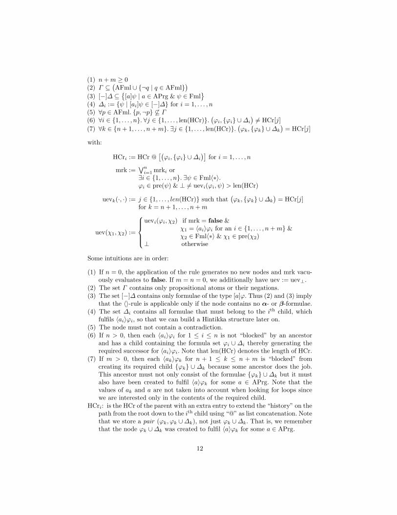
(1) n+m ≥ 0(2) Γ ⊆

(AFml ∪ {¬q | q ∈ AFml}

)(3) [−]∆ ⊆

{[a]ψ | a ∈ APrg & ψ ∈ Fml

}(4) ∆i := {ψ | [ai]ψ ∈ [−]∆} for i = 1, . . . , n(5) ∀p ∈ AFml. {p,¬p} 6⊆ Γ(6) ∀i ∈ {1, . . . , n}. ∀j ∈ {1, . . . , len(HCr)}.

(ϕi, {ϕi} ∪∆i

)6= HCr[j]

(7) ∀k ∈ {n+ 1, . . . , n+m}. ∃j ∈ {1, . . . , len(HCr)}.(ϕk, {ϕk} ∪∆k

)= HCr[j]

with:

HCri := HCr @[(ϕi, {ϕi} ∪∆i

)]for i = 1, . . . , n

mrk :=∨n

i=1 mrki or∃i ∈ {1, . . . , n}. ∃ψ ∈ Fml〈∗〉.ϕi ∈ pre(ψ) & ⊥ 6= uevi(ϕi, ψ) > len(HCr)

uevk(·, ·) := j ∈ {1, . . . , len(HCr)} such that(ϕk, {ϕk} ∪∆k

)= HCr[j]

for k = n+ 1, . . . , n+m

uev(χ1, χ2) :=

uevi(ϕi, χ2) if mrk = false &

χ1 = 〈ai〉ϕi for an i ∈ {1, . . . , n+m} &χ2 ∈ Fml〈∗〉 & χ1 ∈ pre(χ2)

⊥ otherwise

Some intuitions are in order:

(1) If n = 0, the application of the rule generates no new nodes and mrk vacu-ously evaluates to false. If m = n = 0, we additionally have uev := uev⊥.

(2) The set Γ contains only propositional atoms or their negations.(3) The set [−]∆ contains only formulae of the type [a]ϕ. Thus (2) and (3) imply

that the 〈〉-rule is applicable only if the node contains no α- or β-formulae.(4) The set ∆i contains all formulae that must belong to the ith child, which

fulfils 〈ai〉ϕi, so that we can build a Hintikka structure later on.(5) The node must not contain a contradiction.(6) If n > 0, then each 〈ai〉ϕi for 1 ≤ i ≤ n is not “blocked” by an ancestor

and has a child containing the formula set ϕi ∪ ∆i thereby generating therequired successor for 〈ai〉ϕi. Note that len(HCr) denotes the length of HCr.

(7) If m > 0, then each 〈ak〉ϕk for n + 1 ≤ k ≤ n + m is “blocked” fromcreating its required child {ϕk} ∪ ∆k because some ancestor does the job.This ancestor must not only consist of the formulae {ϕk} ∪∆k but it mustalso have been created to fulfil 〈a〉ϕk for some a ∈ APrg. Note that thevalues of ak and a are not taken into account when looking for loops sincewe are interested only in the contents of the required child.

HCri: is the HCr of the parent with an extra entry to extend the “history” on thepath from the root down to the ith child using “@” as list concatenation. Notethat we store a pair (ϕk, ϕk ∪∆k), not just ϕk ∪∆k. That is, we rememberthat the node ϕk ∪∆k was created to fulfil 〈a〉ϕk for some a ∈ APrg.

12

mrk: captures the “existential” nature of this rule whereby the parent is markedif some child is closed or there exists a child – say the ith child – and someeventuality 〈α∗〉χ “loops lower” because ϕi ∈ pre(〈α∗〉χ) and uevi(ϕi, 〈α∗〉χ)is defined and greater than the length of the current HCr. Intuitively, thelatter case means that there exists an occurrence of the eventuality 〈α∗〉χ inthe sub-tableau rooted at the parent which cannot be fulfilled.

uevk: for n + 1 ≤ k ≤ n + m, the kth child is blocked by a proxy child higherin the branch. For every such k we set uevk to be the constant functionwhich maps every pair of formulae to the level j of its proxy child. Notethat this is just a temporary function used to define uev as explained next.Note also that the blocking child itself must have been created to fulfil a〈〉-formula 〈a′〉ϕk, as indicated by the first component of HCr[j].

uev(χ1, χ2): If mrk = true then uev is undefined everywhere. Otherwise, foreach formula χ1 = 〈ai〉ϕi (for an i ∈ {1, . . . , n + m}) and each χ2 suchthat 〈ai〉ϕi ∈ pre(χ2), we take uev of (〈ai〉ϕi, χ2) from the pair of formu-lae (ϕi, χ2) of the corresponding (real) child if 〈ai〉ϕi is “unblocked”, or setit to be the level of the proxy child higher in the branch if it is “blocked”.For all other pairs of formulae, we put uev to be undefined. The intuitionis that a defined uev(χ1, χ2) tells us that there is a “loop” which starts atthe parent and eventually “loops” up to some blocking node higher up onthe current branch. The actual value of uev(χ1, χ2) tells us the level of theproxy because we cannot distinguish whether this “loop” is “good” or “bad”until we backtrack up to that level. Note that the uev of a given 〈ai〉ϕi istaken from the child created specifically to fulfil the given ϕi, thus we canalways trace the uev back down the tree if needed (as in the proofs).

The 〈〉- and id-rules are mutually exclusive via their side-conditions.

4.2 Termination, Soundness, and Completeness

Definition 20. Let x = (Γ :: HCr :: mrk,uev) be a tableau node, ϕ a formula,and ∆ a set of formulae. We write ϕ ∈ x [∆ ⊆ x] to mean ϕ ∈ Γ [∆ ⊆ Γ ].The elements HCr, mrk, and uev of x are denoted by HCrx, mrkx, and uevx,respectively. The node x is marked iff mrkx is set to true.

Definition 21. Let x be a 〈〉-node in a tableau T , meaning that a 〈〉-rule wasapplied to x. Then x is also called a state and the children of x are called core-nodes. Using the notation of the 〈〉-rule, a formula 〈ai〉ϕi ∈ x is blocked iff n+1 ≤ i ≤ n + m. For every not blocked 〈ai〉ϕi ∈ x, the successor of 〈ai〉ϕi isthe ith child of the 〈〉-rule. For every blocked 〈ai〉ϕi ∈ x there exists a uniquecore-node y on the path from the root of T to x such that {ϕi}∪∆i equals the setof formulae of y. Moreover, y is the successor of a formula 〈a′〉ϕi in the parentof y. We call y the virtual successor of 〈ai〉ϕi. We also call the formula ϕi inthe (possibly virtual) successor of 〈ai〉ϕi a core-formula.

A state is another term for a 〈〉-node but a core-node can be any type of node(even a state). Core-nodes are “cores” from which states arise by α- and β-rules.

13

Table 2. Definitions for the example in Fig. 1

UEVi ψi χi

i = 1 〈a〉〈a〉〈(a; a)∗〉¬p 〈(a; a)∗〉¬pi = 2 〈a; a〉〈(a; a)∗〉¬p 〈(a; a)∗〉¬pi = 3 〈(a; a)∗〉¬p 〈(a; a)∗〉¬pi = 4 〈a〉〈(a; a)∗〉¬p 〈(a; a)∗〉¬p

Proposition 22 (Termination). Let φ ∈ Fml be a formula in negation normalform and in *-normal form. Any tableau T for a node ({φ} :: · · · :: · · · ) is a finitetree, hence the procedure that builds a tableau always terminates.

Let φ ∈ Fml be a formula in negation normal form and in *-normal formand T an expanded tableau with root r = ({φ} :: [] :: mrk,uev) meaning thatthe initial formula set is {φ} and the initial HCr is the empty list with mrkand uev determined by the children of r according to the rule applied to r.

Theorem 23 (Soundness). If the root r ∈ T is not marked, then there existsa Hintikka structure for φ.

Theorem 24 (Completeness). For every marked node x = (Γ :: · · · :: · · · )in T , the formula

∧ϕ∈Γ ϕ is unsatisfiable: if r is marked, then φ is unsatisfiable.

4.3 A Fully Worked Example

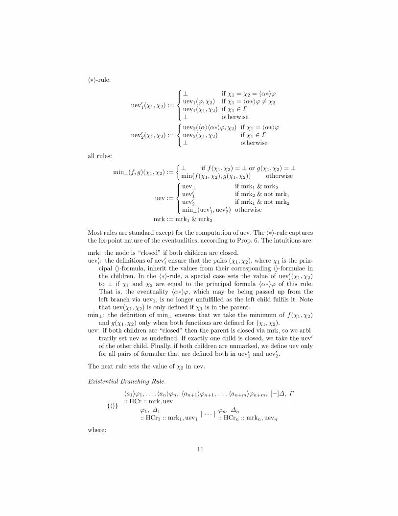
As an example, consider the obviously valid formula [a∗]p→ [(a; a)∗]p. Its nega-tion φ := [a∗]p∧〈(a; a)∗〉¬p is not satisfiable and the root of an expanded tableaufor φ should be marked. Note that φ is already in negation and in *-normal form.

Figure 1 shows such a tableau where the root node is node (1). Each nodeis classified as a ρ-node if rule ρ is applied to that node in the tableau. Theunlabelled edges go from states to core-nodes. Every partial function UEVi

maps the pair of formulae (ψi, χi) as given in Table 2 to 1 and is undefinedotherwise as explained below. The histories are defined as HCR1 := [(ϕ1,∆1)]where ϕ1 := 〈a〉〈(a; a)∗〉¬p and ∆1 := {[a∗]p, 〈a〉〈(a; a)∗〉¬p} and HCR2 :=HCR1@[(ϕ2,∆2)] where ϕ2 := 〈(a; a)∗〉¬p and ∆2 := {[a∗]p, 〈(a; a)∗〉¬p}.

The marking of the nodes (1) to (3b) in Fig. 1 with true is straightfor-ward. The leaf (9) is a 〈〉-node, but it is “blocked” from creating its successorcontaining ∆ := {[a∗]p, 〈a〉〈(a; a)∗〉¬p} because there is a j ∈ IN such thatHCr9[j] = HCR2[j] = (〈a〉〈(a; a)∗〉¬p,∆): namely j = 1. Thus the 〈〉-rule com-putes UEV1(〈a〉ϕ1, 〈(a; a)∗〉¬p) = 1 as stated above and also puts mrk9 := false.As node (8a) is marked, nodes (8b), (8), (7), (6), and (5) “inherit” their func-tions UEVi from their unmarked children via the corresponding α- and β-rules.

The crux of our procedure happens at node (4) which is a 〈〉-node withHCr4 = [] and hence len(HCr4) = 0. The 〈〉-rule therefore finds a child node (5)and a pair of formulae (ψ, χ) := (〈a〉〈(a; a)∗〉¬p, 〈(a; a)∗〉¬p) such that ψ is a

14

core-formula, ψ ∈ pre(χ), and 1 = UEV (ψ, χ) = uev5(ψ, χ) > len(HCr4) = 0.That is, node (4) “sees” a child (5) that “loops lower”, meaning that node (5) isthe root of an “isolated” subtree which does not fulfil its eventuality 〈(a; a)∗〉¬p.Thus the 〈〉-rule sets mrk4 = true, marking (4) as “closed”. The propagation oftrue to the root is then just via simple α- and β-rule applications.

The closure clearly arise because both nodes (3a) and (8a) are marked by theid-rule. But suppose that node (8a) had not ended being marked. Then UEV3

in node (8) would be undefined everywhere via the 〈∗〉-rule, regardless of uev8b.Thus 〈(a; a)∗〉¬p in (8) can be fulfilled by following the β1-child (8a). Hence UEV4

would also be undefined everywhere, and node (4) would not be marked.

References

1. P. Abate, R. Gore, and F. Widmann. One-pass tableaux for computation treelogic. In N. Dershowitz and A. Voronkov, editors, Proc. LPAR 2007, 2007.

2. F. Baader. Augmenting concept languages by transitive closure of roles: an alter-native to terminological cycles. Technical Report, DFKI, 1990.

3. P. Balbiani. Propositional dynamic logic. In E. N. Zalta, editor, The StanfordEncyclopedia of Philosophy. Fall 2007.

4. M. Ben-Ari, Z. Manna, and A. Pnueli. The temporal logic of branching time. InProceedings of Principles of Programming Languages, 1981.

5. G. Bhat and R. Cleaveland. Efficient on-the-fly model checking for CTL∗. In Proc.LICS’95, pages 388–397, 1995.

6. R. Cleaveland. Tableau-based model checking in the propositional mu-calculus.Acta Informatica, 27:725–747, 1990.

7. E. A. Emerson and J. Y. Halpern. Decision procedures and expressiveness in thetemporal logic of branching time. J. of Computer and System Sci., 30:1–24, 1985.

8. M. J. Fischer and R. E. Ladner. Propositional dynamic logic of regular programs.Journal of Computer and Systems Science, 1979.

9. G. D. Giacomo and F. Massacci. Combining deduction and model checking intotableaux and algorithms for converse-pdl. Inf. and Comp. , 160:109–169, 2000.

10. R. Gore and L. A. Nguyen. Exptime tableaux for ALC using sound global caching.In Proc. DL 2007.

11. I. Horrocks and P. F. Patel-Schneider. Optimising description logic subsumption.Journal of Logic and Computation, 9(3):267–293, OUP, 1999.

12. G. Jager and L. Alberucci. About cut elimination for logics of common knowledge.Ann. Pure Appl. Logic, 133(1-3):73–99, 2005.

13. G. Jager, M. Kretz, and T. Studer. Cut-free common knowledge. Journal ofApplied Logic, to appear.

14. D. Kozen and R. Parikh. An elementary proof of the completeness of PDL. The-oretical Computer Science, 14:113–118, 1981.

15. V. Pratt. Semantical considerations on Floyd-Hoare logic. In Proceedings of the17th IEEE Symposium on Foundations of Computer Science, pages 109–121, 1976.

16. V. Pratt. A near-optimal method for reasoning about action. Journal of Computerand System Sciences, 20:231–254, 1980.

17. R. Schmidt and D. Tishkovsky. Personal communication. http://www.cs.man.

ac.uk/∼schmidt/pdl-tableau/, September 2007.18. S. Schwendimann. A new one-pass tableau calculus for PLTL. In Proc.

TABLEAUX’98, LNAI 1397:277-291. Springer, 1998.19. P. Wolper. Temporal logic can be more expressive. Inf. and Comp, 56:72–99, 1983.

15

(1) ∧-node[a∗]p ∧ 〈(a; a)∗〉¬p

[] :: true, uev⊥

α //(2) [∗]-node[a∗]p , 〈(a; a)∗〉¬p

[] :: true, uev⊥

α

��(3a) id-nodep , ¬p , [a][a∗]p[] :: true, uev⊥

(3) 〈∗〉-nodep , [a][a∗]p , 〈(a; a)∗〉¬p

[] :: true, uev⊥

β1oo

β2

��(4) 〈〉-nodep , [a][a∗]p , 〈a〉〈a〉〈(a; a)∗〉¬p

[] :: true, uev⊥

��

(3b) 〈; 〉-nodep , [a][a∗]p , 〈a; a〉〈(a; a)∗〉¬p

[] :: true, uev⊥

αoo

(5) [∗]-node[a∗]p , 〈a〉〈(a; a)∗〉¬pHCR1 :: false, UEV4

α //(6) 〈〉-nodep , [a][a∗]p , 〈a〉〈(a; a)∗〉¬p

HCR1 :: false, UEV4

��(8) 〈∗〉-nodep , [a][a∗]p , 〈(a; a)∗〉¬pHCR2 :: false, UEV3

β1

��

β2

))RRRRRRRRRRRRR

(7) [∗]-node[a∗]p , 〈(a; a)∗〉¬p

HCR2 :: false, UEV3

αoo

(8a) id-nodep , ¬p , [a][a∗]p

HCR2 :: true, uev⊥

(8b) 〈; 〉-nodep , [a][a∗]p , 〈a; a〉〈(a; a)∗〉¬p

HCR2 :: false, UEV2

α

��

blocked by node (5)(9) 〈〉-nodep , [a][a∗]p , 〈a〉〈a〉〈(a; a)∗〉¬p

HCR2 :: false, UEV1

oo

Fig. 1. An example: a closed tableau for [a∗]p ∧ 〈(a; a)∗〉¬p

16

Appendix: Termination, Soundness and Completeness

Definition 25. Let G = (W,R) be a directed graph ( e.g. a tableau where R isjust the child-of relation between nodes). A [full]path π in G is a finite [infinite]sequence x0, x1, x2, . . . of nodes in W such that xiRxi+1 for all xi except thelast node if π is finite. For x ∈ W , an x-[full]path π in G is a [full ]path in Gthat has x0 = x.

Termination

Proposition 22. Let φ ∈ Fml be a formula in negation normal form and in*-normal form. Any tableau T for a node ({φ} :: · · · :: · · · ) is a finite tree, hencethe procedure that builds a tableau always terminates.

Proof. It is obvious that T is a tree and that every node in T can contain onlyformulae of the closure cl(φ). It is also not too hard to see that cl(φ) is finite.Hence there are only a finite number of different sets that can be assigned tothe nodes, in particular the core-nodes. As a further consequence there can onlyexist a finite number of pairs (ϕ,∆) such that ϕ ∈ ∆ ⊆ cl(φ). Since each core-node is assigned such a pair and the 〈〉-rule guarantees that all core-nodes on abranch possess different pairs, there can only be a finite number of core-nodeson a branch.

Furthermore, from any core-node, there are only a finite number of consec-utive nodes on a branch until we reach another core-node. This claim is notobvious since eventualities and their analogues for []-formulae might “regener-ate” on a branch without passing a core-node (e.g. 〈a ∗ ∗〉ϕ). Indeed it is onlytrue because φ and hence all formulae in cl(φ) are in *-normal form, which rulesout formulae like 〈a ∗ ∗〉ϕ. The claim is basically a consequence of Coro. 15 andits analogue for []-formulae, which has not been defined in this paper.

As there are only finitely many nodes between two core-nodes and onlyfinitely many core-nodes on any branch, all branches in T must be finite. This,the obvious fact that every node in T has finite degree, and Konig’s lemma com-plete the proof sketch. ut

Soundness

Theorem 23 (Soundness). If the root r ∈ T is not marked, then there existsa Hintikka structure for φ.

Proof. By construction, T is a finite tree. Let Tp (“p” for pruned) be the sub-graph that consists of all nodes x having the following property: there is a pathof unmarked nodes from r to x inclusive. The edges of Tp are exactly the edgesof T that connect two nodes in Tp. Clearly, Tp is also a finite tree with root r.Intuitively, Tp is the result of pruning all subtrees of T that have a marked root.

As id-nodes are marked by construction of T , all leaves of Tp must be stateswhere all 〈〉-formulae (if any) are blocked. Hence every formula 〈a〉ϕ of everyleaf x has a virtual successor, which lies on the path from r to x. We extend Tp

17

to a finite cyclic tree Tl (“l” for looping) by doing the following for every leaf x:for every 〈a〉ϕ ∈ x, we add the edge (x, y) where y is the virtual successor of 〈a〉ϕ.These new edges are called backward edges.

Finally, following Ben-Ari et al. [4], the cyclic tree Tl is used to generate astructure H = (W,R,L) as described next. Let W be the set of all states of Tl.For every a ∈ APrg and every s, t ∈ W , let sRa t iff s contains a formula 〈a〉ψand there exists a path x0 = s, x1, . . . , xk+1 = t in Tl such that x1 is the (possiblyvirtual) successor of 〈a〉ψ and each xi, 1 ≤ i ≤ k is an α- or a β-node. Thus sis a “saturation” of x using only α- and β-rules. Note that sRa t and sRb t ispossible for a 6= b, because two formulae 〈a〉ψ ∈ s and 〈b〉ψ ∈ s might have thesame virtual successor. It is also possible that sRa t and sRa u for t 6= u.

If we consider the root r of Tl as a core-node for a moment, it is not hardto see that for every state s ∈ Tl there exists a unique core-node x ∈ Tl and aunique path π of the form x0 = x, x1, . . . , xk = s in Tl such that either k = 0(and thus s = x) or k > 0 and each xi, 0 ≤ i ≤ k − 1 is not a state. We set L(s)to be the union of all formulae of all nodes on π. Intuitively, we form L(s) byadding back all the principal formulae of the α- and β-rules which were appliedto obtain s from x.

It is straightforward to check that H is a pre-Hintikka structure for φ. Toshow that H is even a Hintikka structure we use Lemma 26 to conclude H6 asis shown next.

Suppose 〈α∗〉ϕ ∈ L(s). If we also have ϕ ∈ L(s) then (s, 〈α∗〉ϕ), (s, ϕ) is afulfilling chain for (ϕ, α∗, s) and we are done. Otherwise, Coro. 15 and the factthat H is a pre-Hintikka structure give us a sequence σ = (s, ϕ0), . . . , (s, ϕm)such that:

– ϕi ∈ pre(〈α∗〉ϕ) and ϕi ∈ L(s) for all 0 ≤ i ≤ m– ϕ0 = 〈α∗〉ϕ and ϕn = 〈a〉ϕ′ for some a ∈ APrg and ϕ′ ∈ Fml– ϕi ϕi+1 for all 0 ≤ i ≤ m− 1.

Applying Lemma 26 for the state s and the formula ϕn = 〈a〉ϕ′ gives us asequence σ′ := (y0, ψ0), . . . , (yn, ψn) with the properties stated in Lemma 26.Next, we replace each yi, 1 ≤ i ≤ n in σ′ with the first state si that appears onthe path yi, . . . , yn, . . . , yn+m where yn, . . . , yn+m is an arbitrary path in Tl suchthat yn+m is a state.

It is easy to check that the combined sequence σ, σ′ is a fulfilling chainfor (ϕ, α∗, s) in H if we contract all consecutive repetitions of pairs. This con-cludes the proof. ut

Lemma 26. Let y ∈ Tl be a node and ψ ∈ y a formula such that ψ ∈ pre(〈α∗〉ϕ).There exists a finite sequence σ′ = (y0, ψ0), . . . , (yn, ψn) of pairs with n ≥ 0 suchthat:

– y0, . . . , yn is a path in Tl

– yi ∈ Tl, ψi ∈ pre(ϕ), and ψi ∈ yi for all 0 ≤ i ≤ n– y0 = y, ψ0 = ψ, ψn = ϕ, and ψi 6= ϕ for all 0 ≤ i ≤ n− 1– for all 0 ≤ i ≤ n − 1, either ψi = ψi+1 or: if ψi = 〈a〉χ for some a ∈ APrg

and χ ∈ Fml then wiRa wi+1 else ψi ψi+1.

18

Proof. We inductively construct σ′ starting with (y0, ψ0) := (y, ψ). Most of therequired properties of σ′ follow directly from its construction and we leave it tothe reader to check that they hold.

Step 1. Let (yi, ψi) be the last pair of σ′. We distinguish three cases: either yi

is an α- or β-node and ψi is not the principal formula in yi, or yi is an α- orβ-node and ψi is the principal formula in yi, or yi is a state.

If yi is an α- or β-node and ψi is not the principal formula in yi, weset ψi+1 := ψi and we choose yi+1 to be a successor of yi in Tl such thatuevyi(ψi, 〈α∗〉ϕ) = uevyi+1(ψi+1, 〈α∗〉ϕ). Note that such a yi+1 always existssince the value of uevyi(ψi, 〈α∗〉ϕ) is determined by one of its unmarked chil-dren during the construction of T and hence Tl. But it does not have to beunique. We then repeat Step 1.

If yi is an α- or β-node and ψi is the principal formula in yi, we look at allpairs (x, χ) such that x is an child of yi in Tl and ψi is decomposed into χ ∈ xand ψi χ holds. By construction of T and hence Tl there is at least one un-marked child such that the corresponding pair (x, χ) obeys uevyi(ψi, 〈α∗〉ϕ) =uevx(χ, 〈α∗〉ϕ). Let (yi+1, ψi+1) be such a pair. If ψi+1 = ϕ we stop and re-turn σ′; otherwise we repeat Step 1.

If yi is a state, it is not too hard to see that ψi must be of the form 〈a〉χfor some a ∈ APrg and χ ∈ Fml. We set (yi+1, ψi+1) := (x, χ) where x is the(possibly virtual) successor of ψi = 〈a〉χ and repeat Step 1. Note that if x is anon-virtual successor of ψi, we have uevyi

(ψi, 〈α∗〉ϕ) = uevyi+1(ψi+1, 〈α∗〉ϕ) byconstruction of T and hence Tl. Also note that if x is a virtual successor of ψi

then ψi+1 = χ is the core-formula of yi+1 by construction of T and hence Tl.

The only way for Step 1 to terminate is by finding ψi+1 = ϕ. It is not difficult tosee that the resulting (finite) sequence σ′ fulfils all requirements and the proofis completed. Hence the rest of the proof shows that σ′ as constructed by Step 1is finite. Step 1 maintains the following invariant:

(†) For all appropriate i ∈ IN we have uevyi(ψi, 〈α∗〉ϕ) = uevyi+1(ψi+1, 〈α∗〉ϕ)unless yi+1 is the virtual successor of ψi ∈ yi.

In other words, the values of uevyi(ψi, 〈α∗〉ϕ) and uevyi+1(ψi+1, 〈α∗〉ϕ) can dif-fer only if (yi, yi+1) is a backward edge in Tl. We distinguish two cases: ei-ther uevy0(ψ0, 〈α∗〉ϕ) is undefined or it is defined. In both cases we show thatthe path y0, y1, . . . can only have a finite number of backward edges. As everyinfinite path in Tl must use an infinite number of backward edges since T and Tp

are finite trees, this proves that Step 1 terminates.

Case 1. If uevy0(ψ0, 〈α∗〉ϕ) is undefined, the path y0, y1, . . . cannot contain abackward edge as shown next. Assume for a contradiction that yi with i ≥0 is the first node such that (yi, yi+1) is a backward edge. Since the initialuevy0(ψ0, 〈α∗〉ϕ) was undefined, by (†) we know that uevyi(ψi, 〈α∗〉ϕ) is unde-fined. But yi is a state and as ψi ∈ yi, which must be of the form 〈a〉χ forsome a ∈ APrg and χ ∈ Fml, has a virtual successor z, uevyi(ψi, 〈α∗〉ϕ) is

19

defined to be the height of z by the application of the 〈〉-rule to yi during theconstruction of the tableau. Thus uevyi(ψi, 〈α∗〉ϕ) is both defined and undefined,which is a contradiction.

Case 2. If h := uevy0(ψ0, 〈α∗〉ϕ) is defined, the path y0, y1, . . . can only con-tain a finite number of backward edges as shown next. Let yi with i ≥ 0 bethe first node such that (yi, yi+1) is a backward edge. If no such node exists,we are obviously done. Otherwise, we have uevyi(ψi, 〈α∗〉ϕ) = h by (†). Thismeans by construction of the tableau that there exists a set ∆ ⊆ Fml suchthat (ψi+1, {ψi+1} ∪∆) = HCryi

[h]. Thus yi+1 is the hth core-node on the pathfrom the root r to yi in Tl and we have len(HCryi+1) = h by construction of HCr.

If uevyi+1(ψi+1, 〈α∗〉ϕ) had a value equal to or greater than h then the 〈〉-rulewould cause the parent of yi+1 in Tl to be marked since ψi+1 is the core-formulaof yi+1; but we know this is not the case. Hence uevyi+1(ψi+1, 〈α∗〉ϕ) is eitherundefined or has a value h′ that is strictly smaller than h.

If uevyi+1(ψi+1, 〈α∗〉ϕ) is undefined, we can prove exactly as in Case 1 thatthe path yi+1, yi+2, . . . cannot contain a backward edge. On the other hand,if h′ := uevyi+1(ψi+1, 〈α∗〉ϕ) is defined, we can inductively repeat the argumentsin Case 2 for the sequence (yi+1, ψi+1), (yi+2, ψi+2), . . . . The induction is well-defined because of h′ < h, meaning that eventually this inductive argument mustterminate because all such h-values must be in IN>0. ut

Completeness

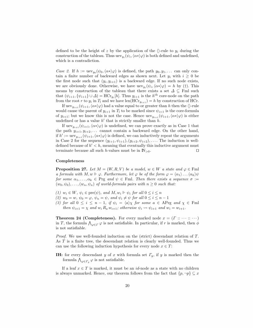
Proposition 27. Let M = (W,R, V ) be a model, w ∈ W a state and ϕ ∈ Fmla formula with M,w ϕ. Furthermore, let ϕ be of the form ϕ = 〈α1〉 . . . 〈αk〉ψfor some α1, . . . , αk ∈ Prg and ψ ∈ Fml. Then there exists a sequence σ :=(w0, ψ0), . . . , (wn, ψn) of world-formula pairs with n ≥ 0 such that:

(1) wi ∈W , ψi ∈ pre(ψ), and M,wi ψi for all 0 ≤ i ≤ n(2) w0 = w, ψ0 = ϕ, ψn = ψ, and ψi 6= ψ for all 0 ≤ i ≤ n− 1(3) for all 0 ≤ i ≤ n − 1, if ψi = 〈a〉χ for some a ∈ APrg and χ ∈ Fml

then ψi+1 = χ and wiRa wi+1; otherwise ψi ψi+1 and wi = wi+1.

Theorem 24 (Completeness). For every marked node x = (Γ :: · · · :: · · · )in T , the formula

∧ϕ∈Γ ϕ is not satisfiable. In particular, if r is marked, then φ

is not satisfiable.

Proof. We use well-founded induction on the (strict) descendant relation of T .As T is a finite tree, the descendant relation is clearly well-founded. Thus wecan use the following induction hypothesis for every node x ∈ T :

IH: for every descendant y of x with formula set Γy, if y is marked then theformula

∧ϕ∈Γy

ϕ is not satisfiable.

If a leaf x ∈ T is marked, it must be an id-node as a state with no childrenis always unmarked. Hence, our theorem follows from the fact that {p,¬p} ⊆ x

20

for some p ∈ AFml. Note that this can be seen as the base case of the inductionas leaves do not have descendants, hence the induction hypothesis is useless.

If x is a marked α-node then its child must be marked as well so we canapply the induction hypothesis and the claim follows from the fact that – in thesense of Table 1 – the formulae of the form α ↔ α1 ∧α2 are valid (Prop. 6).

If x is a marked β-node then both children are marked as well so we canapply the induction hypothesis and the claim follows from the fact that – in thesense of Table 1 – the formulae of the form β ↔ β1 ∨ β2 are valid (Prop. 6).

If x is a marked 〈〉-node (i.e. a marked state) then it has at least one childand there are two possibilities for why it was marked by the 〈〉-rule:

(1) Some child x0 of x is marked(2) Some unmarked child x0 of x with core-formula ϕ has uevx0(ϕ, 〈α∗〉ψ) >

h := len(HCrx) for some α ∈ Prg and ψ ∈ Fml with ϕ ∈ pre(〈α∗〉ψ).

In the rest of the proof, let Γy denote the set of formulae of the node y. We saythat a finite set of formulae Γ is satisfiable iff

∧ϕ∈Γ ϕ is satisfiable.

Case 1. In the first case, it is not too hard to see that the satisfiability of Γx

implies the satisfiability of Γx0 since the 〈〉-rule preserves satisfiability from par-ent to child. By the induction hypothesis, we know that Γx0 is not satisfiable,hence Γx cannot be satisfiable.

Case 2. In the second case, we assume that Γx0 is satisfiable and derive a con-tradiction. We can then prove the claim as in the first case.

So, for a contradiction, let M = (W,R, V ) be a model and w ∈ W a worldsuch that (M,w) satisfies Γx0 : that is, M,w χ for all χ ∈ Γx0 . In particular,we have M,w ϕ by assumption since ϕ ∈ x0. As ϕ ∈ pre(〈α∗〉ψ), it is of theform ϕ = 〈α1〉 . . . 〈αk〉〈α∗〉ψ for some α1, . . . , αk ∈ Prg. Hence Prop. 27 gives usa sequence σ = (w0, ψ0), . . . , (wn, ψn) of world-formula pairs with n ≥ 0 suchthat:

(a) wi ∈W , ψi ∈ pre(ψ), and M,wi ψi for all 0 ≤ i ≤ n(b) w0 = w, ψ0 = 〈α1〉 . . . 〈αk〉〈α∗〉ψ, ψn = ψ, and ψi 6= ψ for all 0 ≤ i ≤ n− 1(c) for all 0 ≤ i ≤ n − 1, if ψi = 〈a〉χ for some a ∈ APrg and χ ∈ Fml

then ψi+1 = χ and wiRa wi+1; otherwise ψi ψi+1 and wi = wi+1.

Our plan is to show M,wn 1 ψ, which contradicts the assumption M,wn ψn since ψn = ψ. We do this by “walking down” the tableau T starting from x0

and inductively constructing a finite sequence σ′ = (y0, j0), (y1, j1), . . . of node-natural number pairs such that the following invariant holds where the rangeof i is chosen appropriately:

(1) the nodes yi ∈ T are unmarked and are in the subtree rooted at x0

(2) y0 = x0, j0 = 0, and either ji+1 = ji or ji+1 = ji + 1(3) each set Γyi

contains ψjiand is satisfied by (M,wji

)(4) uevyi

(ψji, 〈α∗〉ψ) > h

(5) if yi is a core-node then ψjiis a core-formula.

21

Note that the singleton sequence σ′ = (y0, j0) = (x0, 0) obeys the invariant. Weextend σ′ by repeatedly applying Step 2.

Step 2. Let (yi, ji) be the last pair of the sequence as constructed so far. Wedistinguish three cases: either yi is an α- or β-node and ψji is not the principalformula in yi, or yi is an α- or β-node and ψji is the principal formula in yi,or yi is a state and ψji , which must then be of the form 〈a〉χ, has a (possiblyvirtual) successor.

If yi is an α- or β-node and ψjiis not the principal formula in yi, we

set ji+1 := ji and we choose yi+1 to be a successor of yi in T such that Γyi+1 issatisfied by (M,wji+1) = (M,wji). The existence of yi+1 is guaranteed by Prop. 6and the fact that Γyi is satisfied by (M,wji). Note that yi+1 must be unmarkedsince otherwise the set Γyi+1 would be unsatisfiable because of the induction hy-pothesis. Note also that we have uevyi+1(ψji+1 , 〈α∗〉ψ) ≥ uevyi(ψji , 〈α∗〉ψ) > hby construction of uev.

If yi is an α- or β-node and ψjiis the principal formula in yi, we set ji+1 :=

ji+1 and we choose yi+1 to be the successor of yi that decomposes ψji into ψji+1 .This is possible since we have ψji ψji+1 by (c). We know wji = wji+1 by (c)and M,wji+1 ψji+1 by (a). Moreover, the set Γyi is satisfied by (M,wji) by (3),and Γyi+1 = (Γyi \ {ψji})∪{ψji+1} by construction of the tableau T . Hence, theset Γyi+1 is satisfied by (M,wji+1). Note that yi+1 must be unmarked as otherwisethe set Γyi+1 would be unsatisfiable because of the induction hypothesis. Notealso that we have uevyi+1(ψji+1 , 〈α∗〉ψ) ≥ uevyi(ψji , 〈α∗〉ψ) > h by constructionof uev.

If yi is a state and ψji, which must then be of the form 〈a〉χ for some a ∈ APrg

and χ ∈ Fml, has a (possibly virtual) successor z containing ψji+1 = χ then weset ji+1 := ji + 1 and yi+1 := z. Note that ψji+1 is the core-formula of thecore-state yi+1. If yi+1 is a virtual successor, a glance at the definition of uevyi

in the 〈〉-rule reveals that yi+1 must lie on the path from x0 to yi (it couldbe x0) as we have uevyi(ψji , 〈α∗〉ψ) > h and h = len(HCrx). Hence, there isa k ≤ i such that yk = yi+1. Moreover, we have ψjk

= ψji+1 by (5) as thecore-state yk = yi+1 has only one core-formula. Thus, yi+1 is unmarked andhas uevyi+1(ψji+1 , 〈α∗〉ψ) > h as we have already established these facts on ourway from x0 down to yi. If yi+1 is a child of yi (i.e. not a virtual successor), itfollows directly from the facts about yi and the definition of the 〈〉-rule that yi+1

is unmarked and has uevyi+1(ψji+1 , 〈α∗〉ψ) > h.Next we deduce that (M,wji+1) satisfies Γyi+1 . By definition of the 〈〉-rule,

Γyi+1 is of the form ψji+1 ∪ ∆ where [a]∆ ⊆ Γyi . We know M,wji+1 ψji+1

by (a). We also know that (M,wji) in particular satisfies [a]∆ since we haveestablished that Γyi ⊇ [a]∆ is satisfied by (M,wji). As wji+1 is a successorworld of wji (i.e. wji+1 Ra wji) by (c), this implies that (M,wji+1) satisfies ∆,and hence Γyi+1 .

We repeat Step 2 until we extend σ′ by the first pair (yi+1, ji+1) such that ji+1 =n. It is an easy consequence from the construction of σ′ that we constructsuch a pair after a finite number of steps. Then we have ψji+1 = ψ and itis not too hard to see that ψi = 〈α∗〉ψ and of course ji = n − 1. As we

22

have uevyi(ψji , 〈α∗〉ψ) > h by (4), the first child z1 of yi must be marked; oth-erwise, uevyi(ψji+1 , 〈α∗〉ψ) = uevyi(〈α∗〉ψ, 〈α∗〉ψ) would be undefined by the〈∗〉-rule. By the induction hypothesis, Γz1 is unsatisfiable. But as Γz1 \ {ψ} isa subset of Γyi , which is satisfied by (M,wji), this entails M,wji 1 ψ. As wehave wji = wji+1 by definition of σ, this gives us M,wn 1 ψ, which contradictsour assumption that M,wn ψn. ut

23