An investigation on steam film cooling for gas turbine blades using CFD - Fernando Albuquerque
124
Fernando Cavalcanti de Albuquerque An investigation on steam film cooling for gas turbine blades using CFD School of Engineering MSc Thesis
Transcript of An investigation on steam film cooling for gas turbine blades using CFD - Fernando Albuquerque

Fernando Cavalcanti de Albuquerque
An investigation on steam film cooling for gas
turbine blades using CFD
School of Engineering
MSc Thesis
i

School of Engineering
Department of Power Engineering and Propulsion
MSc Thesis
Academic Year 2005-2006
Fernando Cavalcanti de Albuquerque
An investigation on steam film cooling for gas turbine blades using CFD
Supervisor: P A Rubini
August 2006
This thesis is submitted in partial fulfilment of the requirements for the degree of Master of Science. Cranfield University, 2006. All rights reserved. No part of this publication may be reproduced without the written permission of the copyright owner.
ii
ABSTRACT
This objective of the present work is to investigate open-circuit steam cooling and to
evaluate whether steam film cooling used for the turbine first stage vanes could improve
from the state-of-the-art closed-loop concept in order to obtain even higher power
output and efficiency.
In the beginning of the new Millennium a revolution in the gas turbine technology took
place and a new concept in blade cooling was presented to the marketplace. In ten years
it was conceived, designed, assembled, installed, and tested the first combined cycle
power plant with steam cooled gas turbine blades and vanes. This concept resulted in an
excess of 60% thermal efficiency, the present record for this kind of plants.
The advantages of steam properties compared to air properties in convective cooling are
easily verified theoretically and practically, but it is not the same regarding film cooling,
where some of those advantageous properties are counter-effective in practice. For this
reason, simulation with computational fluid dynamics was chosen as the tool to be used.
Blade film cooling is constraint in practice by thermodynamic and aerodynamic losses
which, in the particular case of steam, is accompanied by loss of power in the steam
turbine and wasting of demineralised water.
Steam properties make it excellent coolant for convective cooling but only equivalent to
air for film cooling. However, the use of steam film cooling is significantly limited by
the quenching effect on the gas flow and economical factors. In summary, full-coverage
film cooling schemes, as it is usual where the coolant is air, is not recommendable.
Local utilisation of steam for film cooling could be effective for the most critical areas
of the blade, since small coolant mass flows are considered. Gains and drawbacks must
be evaluated very carefully with CFD tools and cycle simulation software.
i

ACKNOWLEDGEMENTS
My specialisation project in Thermal Power - Gas Turbine Technology was supported
by the Companhia Paranaense de Energia (COPEL) and by the Programme Alban, the
European Union Programme of High Level Scholarships for Latin America, scholarship
no. E05E056499BR. Both institutions have my gratitude for their confidence in me.
I thank all Thermal Power course lecturers, my colleagues and the staff of the
Department of Power Engineering and Propulsion for their support throughout the
duration of the course. Especially, I am grateful to Mr Anthony Haslam, my
specialisation project supervisor and to Dr Philip Rubini, my thesis project supervisor
for their support and advice.
I would like to extend sincere thanks to my family and friends for they are with me in
all moments.
I dedicate this work to my father, Eudoro; my mother, Candida (in memoriam); my
wife, Adriana; my son, Daniel and my daughter, Helena.
ii

PREMISE
“Of all things, good sense is the most fairly distributed: everyone thinks he is so well
supplied with it that even those who are the hardest to satisfy in every other respect
never desire more of it than they already have.”
Discours de la Méthode, René Descartes
iii

LIST OF CONTENTS
ABSTRACT ............................................................................................................... i
ACKNOWLEDGEMENTS ............................................................................................. ii
PREMISE ............................................................................................................. iii
LIST OF CONTENTS..................................................................................................... iv
LIST OF FIGURES......................................................................................................... vi
NOTATION ............................................................................................................ vii
INTRODUCTION............................................................................................................ 1
1.1 Objectives and results....................................................................................... 1 1.2 Background....................................................................................................... 2 1.3 Lay-out ............................................................................................................. 2
CHAPTER 2 INDUSTRIAL GAS TURBINES AND COMBINED CYCLE .......... 5
2.1 Introduction ...................................................................................................... 5 2.2 Heavy-duty gas turbine engines ....................................................................... 5 2.3 Combined cycle power plants .......................................................................... 6 2.4 Summary......................................................................................................... 10
CHAPTER 3 GAS TURBINE HOT SECTION AND BLADE COOLING............ 11
3.1 Introduction .................................................................................................... 11 3.2 Gas turbine engine hot section ....................................................................... 11 3.3 Gas turbine blade cooling............................................................................... 13 3.4 Summary......................................................................................................... 15
CHAPTER 4 STEAM BLADE COOLING ............................................................. 16
4.1 Introduction .................................................................................................... 16 4.2 Steam cooling ................................................................................................. 16 4.3 Closed-loop and open-circuit steam cooling .................................................. 17 4.4 Advanced Turbine Systems Program ............................................................. 18 4.5 Academic research on film cooling and steam blade cooling ........................ 20 4.6 Summary......................................................................................................... 20
CHAPTER 5 AIR AND STEAM IN CONVECTIVE BLADE COOLING............ 21
5.1 Introduction .................................................................................................... 21 5.2 Air and steam properties related to blade cooling .......................................... 21 5.3 A comparison between air and steam in convection blade cooling................ 22 5.4 Summary......................................................................................................... 30
CHAPTER 6 GEOMETRY AND MESHING ......................................................... 31
6.1 Introduction .................................................................................................... 31 6.2 Geometry ........................................................................................................ 31 6.3 Meshing .......................................................................................................... 32 6.4 Summary......................................................................................................... 34
iv

CHAPTER 7 METHOD VALIDATION ................................................................. 35
7.1 Introduction .................................................................................................... 35 7.2 Papell’s experiment ........................................................................................ 35 7.3 Simulation of Papell’s experiment with CFD ................................................ 38 7.4 Simulation of Papell’s experiment and comparison with the real data .......... 41 7.5 Summary......................................................................................................... 44
CHAPTER 8 CASES DEFINITION AND INPUT SETTINGS.............................. 45
8.1 Introduction .................................................................................................... 45 8.2 Air film cooling cases definition .................................................................... 45 8.3 Steam film cooling cases definition ............................................................... 49 8.4 Input settings in FLUENT 6.2 for film cooling simulation............................ 52 8.5 Summary......................................................................................................... 55
CHAPTER 9 FILM COOLING CFD SIMULATION RESULTS........................... 56
9.1 Introduction .................................................................................................... 56 9.2 Graphs on steam/air film effectiveness ratio distribution............................... 56 9.3 Summary......................................................................................................... 59
CHAPTER 10 DISCUSSION ON FILM COOLING SIMULATION RESULTS .... 60
10.1 Introduction .................................................................................................... 60 10.2 Geometry and meshing................................................................................... 60 10.3 Coolant mass flow .......................................................................................... 60 10.4 Coolant inlet velocity ..................................................................................... 63 10.5 Reynolds number............................................................................................ 65 10.6 Specific heat and thermal conductivity .......................................................... 65 10.7 Some economical considerations.................................................................... 66 10.8 Summary......................................................................................................... 70
CHAPTER 11 CONCLUSIONS ................................................................................ 71
11.1 Steam film cooling performance .................................................................... 71 11.2 Further work recommendations...................................................................... 72
LIST OF REFERENCES ............................................................................................... 73
APENDICCES A FILM COOLING CFD SIMULATION RESULTS…………………………...……77
v

LIST OF FIGURES
Figure 2-1 GEPS H System™ combined-cycle and steam description [25].................... 7
Figure 2-2 480 MW CC Araucaria Power Station, Brazil (Courtesy of COPEL)........... 9
Figure 3-1 Turbine blade with cooling channels and TBC............................................ 12
Figure 4-1 GEPS 9H showing 18-stage compressor and 4-stage turbine[12] ............... 19
Figure 5-1 Ratio of properties of steam to air at 30 bars [11] ....................................... 22
Figure 5-2 Variation of cbm& as function of Tc1............................................................... 29
Figure 5-3 Variation of η as function of Tc1 .................................................................. 29
Figure 5-4 Variation of ε as function of Tc1................................................................... 30
Figure 6-1 Test rig geometry sketch.............................................................................. 32
Figure 6-2 Detail of the mesh ........................................................................................ 33
Figure 7-1 Film cooling experiment for coolant inlet angle 90o and M=0.5................. 42
Figure 7-2 Film cooling simulation for coolant inlet angle 90o and M=0.5.................. 43
Figure 9-1 Steam/air film effectiveness ratio distribution – case 1 ............................... 57
Figure 9-2 Steam/air film effectiveness ratio distribution – case 2 ............................... 57
Figure 9-3 Steam/air film effectiveness ratio distribution – case 3 ............................... 58
Figure 9-4 Steam/air film effectiveness ratio distribution – case 4 ............................... 58
Figure 9-5 Steam/air film effectiveness ratio distribution – case 5 ............................... 59
Figure 10-1 Film effectiveness for similar csm& , air-4 and steam-1 ............................... 62
Figure 10-2 Film effectiveness for similar csm& , air-5 and steam-4 ............................... 63
Figure 10-3 Film effectiveness for similar Vc/Vg , air-3 and steam-1............................ 64
Figure 10-4 Film effectiveness for similar Vc/Vg , air-4 and steam-3............................ 64
Figure 10-5 Steam film cooling losses MWequiv estimative table.................................. 69
vi

NOTATION
Acronyms
2D Two dimensions
3D Three dimensions
ASME American Society of Mechanical Engineers
ATS Advanced Turbine Systems
CC Combined cycle
CCEE Câmara Comercialização de Energia Elétrica
CFD Computational Fluid Dynamics
COPEL Companhia Paranaense de Energia
DOE Department of Energy
DW Demineralised water
GEPS General Electric Power Systems
GT Gas turbine
HP High Pressure
HRSG Heat Recovery Steam Generator
IGCC Integrated Gasification Combined Cycle
IP Intermediate Pressure
LHV Low Heat Value
LP Low Pressure
MHI Mitsubishi Heavy Industries
NASA National Aeronautics and Space Administration
NG Natural gas
NOX Oxides of nitrogen
SFPE Society of Fire Protection Engineers
ST Steam turbine
SWPC Siemens-Westinghouse Power Co.
TBC Thermal barrier coating
TET Turbine entry temperature
vii

Symbols
Ac Single channel flow cross section
Atotal Total flow cross section
Bi Biot number
Cp Specific heat at constant pressure
Dh Hydraulic diameter
h Heat transfer coefficient
i Coolant injection angle relative to adiabatic wall
ieff Effective coolant injection angle
K Correction factor to adjust coolant bleed
k Thermal conductivity
L Blade span (in CHAPTER 5)
L Width of adiabatic wall (in CHAPTER 7)
M Mach number
Mc Coolant bleed (%)
m* Mass flow function
m& Mass flow
Nb Number of blades
nc Number of coolant channels
npass Number of passes
Nu Nussel number
Pr Prandtl number
qout Energy removed from the whole blade
Re Reynolds number
S Coolant slot height
Sc Perimeter of a single coolant channel
Sg External perimeter of the whole blade
t Static temperature
T Total temperature
Tad Adiabatic wall temperature
TI Turbulence intensity
V Velocity
w Flow rate
viii

X Technology factor
x Distance along the adiabatic wall in direction of the flow
Greek Letters
∆ Differential
α Thermal diffusity
ε Cooling effectiveness
η Cooling efficiency
η Cooling effectiveness (in CHAPTER 7 only)
µ Viscosity
ν Kinematic viscosity
ρ Mass density
Subscripts g Gas conditions
c Coolant conditions
cc Coolant channel
cb Blade channel
b Blade
ad Adiabatic
av Average conditions
m Mixture conditions
s Simulation conditions
‘ Temporary value (used in a iterative process)
eff Effective
equiv Equivalent
pass Passes of a coolant channel
w Wall
c Coolant slot exit
ix

f Properties evaluated at (tg+tc)/2
1 Inlet conditions
2 Exit conditions
x

INTRODUCTION
1.1 Objectives and results
The present work investigates the feasibility of the use of steam for film cooling gas
turbines blades. It is based on data from academic studies on the subject, technical articles
and on real data from manufacturer’s reports. The objective is to go a step further and
evaluate whether steam film cooling the turbine first stage vanes could improve the state-
of-the-art closed-loop concept and obtain even higher power output and efficiency.
The advantages of steam properties compared to air properties in convective cooling are
easily verified theoretically, or practically, but it is not the same regarding film cooling,
where some of those advantageous properties can be counter-effective in practice. For this
reason, computational fluid dynamics was chosen as the tool to be used. The simulation
results were post-treated with final calculation and comparison with real data.
Blade film cooling is constraint in practice by thermodynamic and aerodynamic losses
which, in the particular case of steam, is accompanied by loss of power in the steam turbine
and wasting of demineralised water.
Steam properties make it excellent coolant for convective cooling but only equivalent to air
for film cooling. However, the use of steam film cooling is significantly limited by the
quenching effect on the gas flow and economical factors. In summary, full-coverage film
cooling schemes, as it is usual where the coolant is air, is not recommendable.
Local utilisation of steam for film cooling could be effective for the most critical areas of
the blade, since small coolant mass flows are considered. Gains and drawbacks must be
evaluated very carefully with CFD tools and cycle simulation software.
1
1.2 Background
Industrial gas turbines and combined cycle power plants are around since the years 1950’s.
Gradually these plants evolved from the original hybrid of the aero-engine and the steam
plant concepts to more integrated systems, so resulting in high power outputs and
efficiencies.
Recently a revolution took place: as a result of program led by the United States
government, an important gas turbine manufacturer designed, assembled, tested and
installed the first combined cycle power plant where the gas turbine blades are fully steam
cooled, in closed-loop scheme, where the pure convective cooling system of the gas turbine
blades is at the same time the intermediate pressure steam re-heater. This concept results in
an excess of 60% thermal efficiency, the highest for this kind of plants.
1.3 Lay-out
CHAPTER 2 is an overview on industrial gas turbines and combined cycle power plants.
The difference between the aero-derivatives engines and the so-called heavy-duty is
explained. The evolution of the heavy-duty gas turbine is briefly described. Combined
cycle power plants fundamentals are explained and the achievements in their power output
and efficiency are outlined.
In CHAPTER 3 it is described the gas turbine the operational conditions of gas turbine hot
section. This is the environment (high pressures, temperature, speed and stresses) where
turbine parts are expected to function and materials to resist. Cooling is an alternative to
minimise the effects of such aggressive conditions and so many of hot section parts are
cooled. Among them, turbine blade cooling is more detailed described.
In CHAPTER 4 steam blade cooling is presented in two different schemes: closed-loop and
open-circuit. The chapter also includes an overview of the Advanced Turbine Systems
(ATS) Program that did create the conditions for the development of steam blade cooling
2

technology remarkably in only ten years. Additionally the academic research on film
cooling and steam blade cooling are mentioned.
Convective cooling is the subject of CHAPTER 5 and by means of basic calculations it is
shown the superiority of steam as coolant in pure convective cooling compared to air. The
calculations are performed assuming equal conditions and equal cooling effectiveness,
resulting in different coolant mass flows.
In CHAPTER 6 the geometry and meshing chosen for the simulation are described in
detail. A sketch of the test rig is presented as well as detail on the built mesh. The main
settings used for meshing are listed.
In CHAPTER 7 it is reported the simulation of a selected series of experimented cases with
a Computational Fluid Dynamics (CFD) software. The comparison of the results validated
the method that was used to simulate air and steam film cooling in the conditions proposed
for the present work.
In CHAPTER 8 it is described the criteria to select the film cooling cases to be simulated
with CFD software. The settings used in FLUENT 6.2 for the selected cases are as well
described.
In CHAPTER 9 it is reported the results of the simulation of five air film cooling cases and
five steam film cooling cases. The results are presented in form of pictures and graphs.
Pictures on temperature, velocity, specific heat at constant pressure and thermal
conductivity contours are showed in Appendix A, as well as graphs on static wall
temperature distribution, film effectiveness distribution, air/steam wall temperature ratio
distribution and steam/air film effectiveness distribution. Graphs on steam/air film
effectiveness distribution are reproduced in this chapter, as they drive more directly to the
conclusion.
3

In CHAPTER 10 the results are discussed in their various aspects. Additionally, some
economical considerations respective to open-loop steam cooling are bring to light. This
will help to understand the conclusions in CHAPTER 11.
4

CHAPTER 2 INDUSTRIAL GAS TURBINES AND COMBINED
CYCLE
2.1 Introduction
This chapter is an overview on industrial gas turbines and combined cycle power plants.
The difference between the aero-derivatives engines and the so-called heavy-duty is
explained. The evolution of the heavy-duty gas turbine is briefly described. Combined
cycle power plants fundamentals are explained and the achievements in their power output
and efficiency are outlined.
2.2 Heavy-duty gas turbine engines
Industrial gas turbine engines started to be designed for power generation in the early
1950s. The design of the first engines was based on the steam turbines design rather than on
the gas turbine aero-engines design and it was characterised by the robustness since there
were no restrictions in weight and space for ground-based units. For this reason and also
because these engines are designed for power generation and so expected to operate for a
long time in full-load regime, they are called heavy-duty.
Despite their low thermal efficiency, the first heavy-duty gas turbine engines were
attractive due to their relatively quick installation, compactness, short time from start to
full-load regime and for no water requirement for their operation. Since then heavy-duty
gas turbines engines improved significantly. In particular because aircraft gas turbines
engines started to be adapted and used in land applications (mainly at the oil and gas
industry as variable speed mechanical drives). The higher technology level of the aero-
derivative gas turbine engines was so incorporated to the heavy-duty gas turbine engines.
5

The early heavy-duty gas turbine engines had power output of 10 MW or less and cycle
efficiency only about 28-29% [1]. With significant improvement, presently some units
deliver over 250 MW with more than 35% of thermal efficiency in simple cycle [1]. As a
result, heavy-duty gas turbine engines became one of the most efficient prime movers
presently available and their cycle efficiency is more than 55% in gas and steam combined
cycle.
2.3 Combined cycle power plants
The gas and steam combined cycle is one of the most efficient cycles conceived for power
generation to date. It was introduced in the mid 1950s as a way to optimize both the
topping cycle (gas turbine or Brayton cycle) and the bottoming cycle (steam turbine or
Rankine cycle) by using the exhaust gases of the gas turbine engine to produce steam in a
specially featured boiler, the heat recovery steam generator (HRSG), so providing steam for
the steam turbine. The individual efficiencies of the gas turbine in simple cycle as well as
of the steam turbine are between 30 and 40% while in a combined cycle the power plant
overall efficiency is 55% and over but can be in excess of 60% for the newest advanced gas
turbine systems [2]. For utility applications, approximately 75% of all industrial gas turbine
engines are currently being used in combined cycle plants, accordingly to [2].
In combined cycle the steam turbine is typically around 40% of the overall power output
while gas turbine delivers around 60% accordingly to [2]. The plant consists, depending on
the desired operational flexibility, of blocks of one, two or even three gas turbine engines
and their respective HRSGs feeding one steam turbine.
In the gas turbine engine air is compressed in the compressor and heated in the combustor
to be expanded in the turbine performing work. Part of this work is used by the compressor
to compress air (50% to 60% of the turbine work) and the remaining work is available as
useful work to drive the generator. The exhaust gases leaving the gas turbine are not much
above the atmospheric pressure and they are at temperatures ranging from 500oC to 700oC,
6
what is hot enough for these gases, flowing through the HRSG, to vaporise water and
produce superheated steam for the steam turbine.
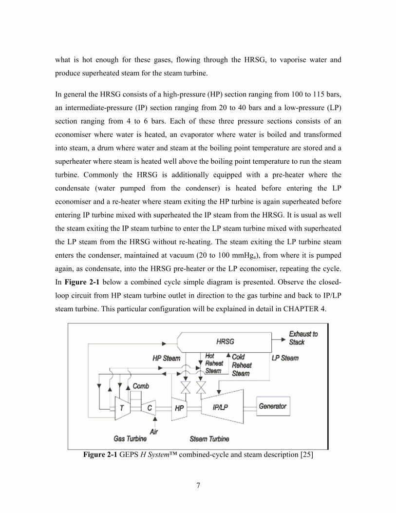
In general the HRSG consists of a high-pressure (HP) section ranging from 100 to 115 bars,
an intermediate-pressure (IP) section ranging from 20 to 40 bars and a low-pressure (LP)
section ranging from 4 to 6 bars. Each of these three pressure sections consists of an
economiser where water is heated, an evaporator where water is boiled and transformed
into steam, a drum where water and steam at the boiling point temperature are stored and a
superheater where steam is heated well above the boiling point temperature to run the steam
turbine. Commonly the HRSG is additionally equipped with a pre-heater where the
condensate (water pumped from the condenser) is heated before entering the LP
economiser and a re-heater where steam exiting the HP turbine is again superheated before
entering IP turbine mixed with superheated the IP steam from the HRSG. It is usual as well
the steam exiting the IP steam turbine to enter the LP steam turbine mixed with superheated
the LP steam from the HRSG without re-heating. The steam exiting the LP turbine steam
enters the condenser, maintained at vacuum (20 to 100 mmHga), from where it is pumped
again, as condensate, into the HRSG pre-heater or the LP economiser, repeating the cycle.
In Figure 2-1 below a combined cycle simple diagram is presented. Observe the closed-
loop circuit from HP steam turbine outlet in direction to the gas turbine and back to IP/LP
steam turbine. This particular configuration will be explained in detail in CHAPTER 4.
Figure 2-1 GEPS H System™ combined-cycle and steam description [25]
7

The main losses in the combined cycle are both the exhaust gases leaving the HRSG stack
(representing circa 10% of the fuel low heat value (LHV)) and the cooling system of the
steam turbine condenser (around 30% of the fuel LHV), accordingly to [2]. The heat loss
by the exhaust gases happens basically because the gases temperature must be above the
saturation temperature in order to prevent condensation of corrosive products on the stack
internal surface. The heat loss at the condenser is inherent to the steam turbine cycle and
can only be minimized if the heat extracted from the condenser is utilised for some other
purpose (e.g. building heating) instead of being simply wasted through the cooling tower.
Water quality (and consequently steam quality) is a key driver for HRSG and steam turbine
reliability, availability and safe operation. Very strict limits for pH, conductivity, dissolved
oxygen and ions must be followed in order to prevent corrosion or scaling formation on the
internal surfaces of HRSG piping and valves, steam turbine blades, etc. what could lead the
plant into fast deterioration and unsafe operational conditions.
In power generation, gas turbine engines in simple cycle are used mainly as peak-load
machines. Their use for base-load power generation only takes place where other options
are not available or where fuel is cheap. Combined cycle power plants are more efficient
for base-load power generation. Still they can be operated either in part-load regime, at
expense of some reduced efficiency and closer to the emissions limits, or in peak-load
regime, at expense of shorten equipment life (due to the thermal stresses caused by the
unsteady operation) and availability (since the higher number of starts normally leads into
more frequent scheduled inspections). An example of combined cycle power station is
shown in Figure 2-2 below, with two natural gas-fired gas turbines coupled with two
HRSGs and one steam turbine (the white building in the centre of the picture), called for
this reason 2-2-1 configuration.
8

Figure 2-2 480 MW CC Araucaria Power Station, Brazil (Courtesy of COPEL)
Part-load operation and fuel flexibility are two important limitations of gas turbine engines
that are being addressed currently. Both are closed related to efficiency and emission limits.
Efforts have been directed to design combustors that maintain low emissions level at part-
load operation as well as combustors that use alternative fuels or a mix of fuels. In special,
the development of Integrated Gasification Combined Cycles (IGCC) power plants fuelled
by gas produced from coal, biomass, petroleum coke, heavy oil, asphalt or other refinery
residuals might represent a new era for the combined cycle and become the preferred fossil
power plant in the near future.
One of the main goals of the industry during the last years has been to achieve combined
cycle efficiency higher than 60%. Aiming this, manufacturers have directed efforts towards
the improvement of gas turbine cycle, in particular the increase in pressure ratio and turbine
inlet temperature.
9

2.4 Summary
In this chapter it is focused briefly the history of heavy-duty gas turbine engines and
combined cycle power plants, as well their basic principles. The objective is to understand
better how the evolution in technology and cycle design along the last 50 years resulted in
the most efficient fossil-fuelled power plants presently available. Next chapter is focused in
what the gas turbine hot path is and how blade cooling is important as a strategy to obtain
better power output and efficiency.
10

CHAPTER 3 GAS TURBINE HOT SECTION AND BLADE
COOLING
3.1 Introduction
In this chapter it is described the gas turbine the operational conditions of gas turbine hot
section. This is the environment (high pressures, temperature, speed and stresses) where
turbine parts are expected to function and materials to resist. Cooling is an alternative to
minimise the effects of such aggressive conditions and so many of hot section parts are
cooled. Among them, turbine blade cooling is more detailed described.
3.2 Gas turbine engine hot section
Fuel is burnt in gas turbine engines combustors to heat the compressed air flow, increasing
its temperature and velocity. As a consequence, combustors, transitions, turbine blades and
other parts are exposed to pressures between 17 and 35 bars, close to sonic flow velocities
and temperatures around 1500oC. Temperatures such as these can be supported directly
only up to certain limits. The combustor itself and the turbine are the most affected
systems. In order to make these systems functional, materials capable of supporting high
temperatures for an acceptable period of time (what is an acceptable period of time varies
enormously from aircraft applications to land-based engines) without loosing their
properties should be employed. Associated or not, it can be applied either thermal barrier
coatings (to insulate and protect the metallic parts from heat) or cooling schemes (to extract
heat from the affected parts as well as to insulate them from heat).
Parts in close proximity to the heat sources, such as the combustor liners, first stage turbine
blades and nozzles are in general metallic. The development of metallic alloys with the
11
necessary properties for the gas turbine hot section environment produced the so-called
superalloys. These superalloys are typically iron, nickel or cobalt alloys mixed with iron,
nickel, cobalt, chrome, molybdenum, aluminium, tungsten, titanium, carbon, columbium,
boron or tantalum. The technology developed in the last twenty years to produce
directionally crystallised structure castings and single crystal structure castings for turbine
blades is remarkable. These castings present excellent creep and fatigue properties under
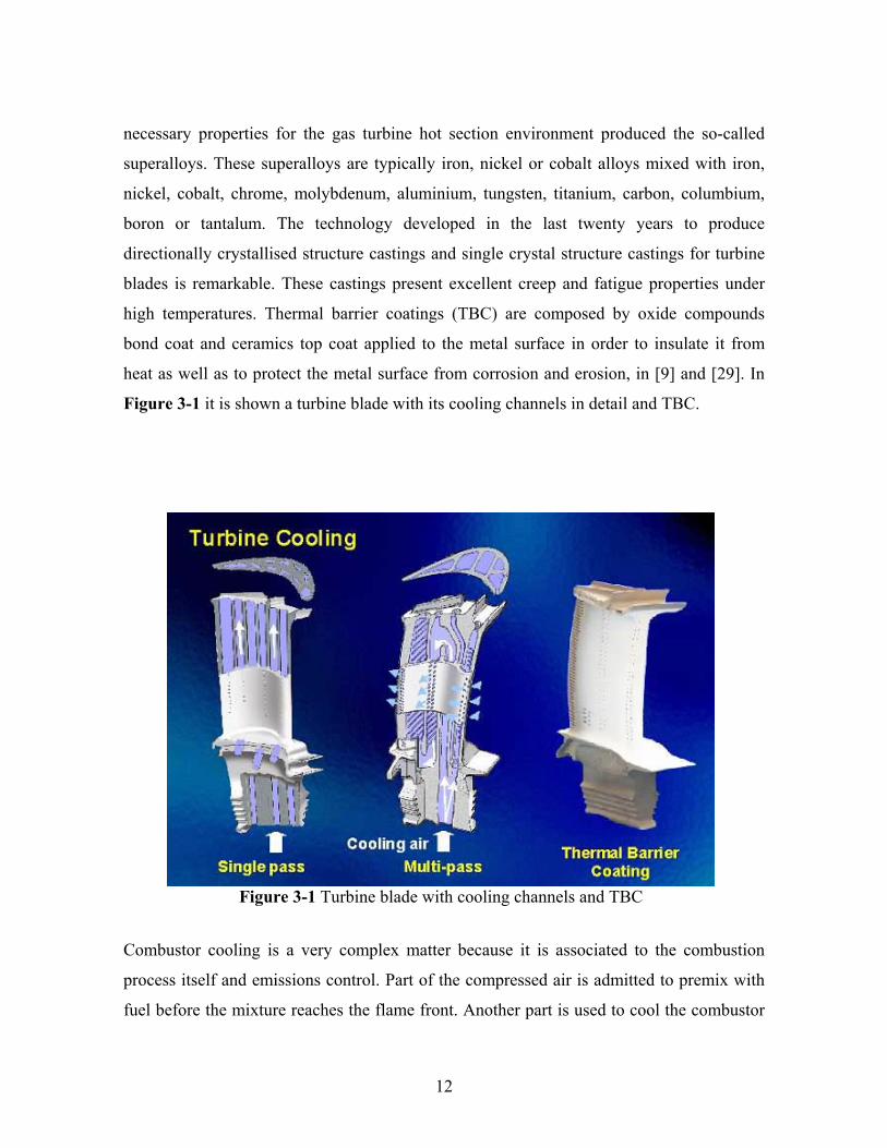
high temperatures. Thermal barrier coatings (TBC) are composed by oxide compounds
bond coat and ceramics top coat applied to the metal surface in order to insulate it from
heat as well as to protect the metal surface from corrosion and erosion, in [9] and [29]. In
Figure 3-1 it is shown a turbine blade with its cooling channels in detail and TBC.
Figure 3-1 Turbine blade with cooling channels and TBC
Combustor cooling is a very complex matter because it is associated to the combustion
process itself and emissions control. Part of the compressed air is admitted to premix with
fuel before the mixture reaches the flame front. Another part is used to cool the combustor
12
liners by flowing through the gap between the liners and the combustor casing. It provides
film cooling to the liners by entering the chamber through holes and passages along the
liner length. The cooling air entering the combustion chamber at the same time completes
the combustion process burning unburned fuel preventing the emission of carbon monoxide
(CO), soot and unburned hydrocarbon particles [8]. Another function is to minimise
nitrogen oxides (NOX) emissions by maintaining the combustion temperature below
1538oC, accordingly to [12], and hence preventing the temperature reach a threshold of
thermal NOX formation. At the same time air leaving the combustor shall be in an average
temperature acceptable for the turbine. This average temperature shall be homogenously
distributed along the traverse cross section. Some of these objectives are in some extent in
opposition and the resulting design is a compromise between combustion, cooling and
emissions control as well as the overall engine performance. More detailed considerations
on combustor cooling are not covered by the present work.
3.3 Gas turbine blade cooling
The main objective of turbine cooling is the extraction of heat from the blades to maintain
the temperature sufficiently below the material limits. In order to obtain this, the coolant
enters the blade at lower temperature than the blade wall, circulates internally and leaves it
at a temperature close to the wall temperature. The design of the internal cooling channels
can vary widely from very basic straight channels (simply connecting the blade root to the
tip) up to more efficient and intricate designs.
Air has been used as the coolant in gas turbine engines primarily because it is easily
available at the quantities, temperatures and pressures necessary to enter the blade cooling
channels extracting heat and to leave the blade in conditions to create a cooling film on its
surface. The coolant source is the compressed air from the gas turbine compressor, but
depending on the stage of the turbine to be cooled, air can be taken directly from the
compressor exit (before the combustor) or bled off from some intermediate stage of the
compressor. The air can be used as the blade coolant either straight at the temperature it
13

exits the compressor or it might be externally cooled before being used, depending on the
application.
The useful work and thermal efficiency of a gas turbine engine increase as the turbine inlet
temperature increases. Deviating air through the combustor to remix with the hot gases in
the turbine of course diminishes the power of the gas flow and hence its expansion
produces less work. All compressor work necessary to compress air has to be provided by
turbine work, so air used for blade cooling is an additional burden, since it does not produce
turbine work. The amount of air used in blade cooling can be higher than 25% for a typical
heavy-duty gas turbine. For this reason turbine cooling system must be designed very
carefully. Cooling can be counterproductive and it is essentially a compromise between
gaining in parts life (and their integrity) and losses in engine performance.
The design of the original blade cooling system is comprised of straight channels where air
enters the blade root through the disc and exits at the tip, sealing the tip/casing clearance at
the same time. Along the years, with TET constantly increasing, more sophisticated design
concepts have been developed. The modern cooled blade is provided with multiples
internal passes and turbulators (ribs, pins, etc.) of various shapes to increase turbulence,
what results in better heat transfer. The modern cooled blade also features impingent
cooling for the critical internal surface of the leading edge and film cooling to protect the
blade externally [7].
Currently, film cooling is the technology which, together with TBC and superalloys, makes
possible the highest values of TET because it protects the external surface of the blade from
the bulk gas heat. The film is formed by air flowing outside the blade through a series of
holes placed along the blade height at the most critical positions of the blade surface. This
is especially important at the leading edge where the heat transfer coefficient is higher since
it is a stagnation zone (for the incidence angle of the hot gas flow is around 90o), blade
suction surface (where the boundary layer disappears due to the local turbulence) and the
trailing edge (for its small thickness can not be cooled properly only by convective cooling)
[7].
14

Unfortunately there are penalties associated with film cooling. First the quenching of the
hot gases by mixing them with the coolant flow coming from the blades decreases the gases
enthalpy and, by consequence, the amount of work available to be extracted by the turbine.
Ultimately there is a level over which the admissible TET provided by film cooling does
not compensate the effect of excessively quenching the hot gases. This effect is particularly
significant at the first stage nozzle where typically the temperature drop (∆T) is 155oC [12],
[24] and [25]. In addition to the thermodynamic disadvantage, there is a penalty due to the
aerodynamic effect of the secondary flow (the coolant film flow) disturbing the main flow
(the hot gases flow) and distorting the designed aerodynamic flow around the blade shape,
with inevitable losses associated.
Instead of air, other fluids such as: steam, water, air and mist mixed or even liquid metals
can be used as coolants. However most of these alternatives are not very often used. The
exception is steam, quite abundantly available at combined cycle plants as compressed air
in the gas turbine. Furthermore steam has some advantageous properties over air as a
coolant. This and other characteristics of steam as a coolant for turbine blades are the
subject of the next chapter.
3.4 Summary
In this chapter gas turbine engines hot section environment and its adverse conditions were
described. Cooling is presented as a solution to relieve parts from mechanical and thermal
stresses. The main objective of the chapter is to understand how the turbine blades are
cooled. In the next chapter steam blade cooling and the recent achievements of the industry
in this field are the subject.
15

CHAPTER 4 STEAM BLADE COOLING
4.1 Introduction
In this chapter steam blade cooling is presented in two different schemes: closed-loop and
open-circuit. The chapter also includes an overview of the Advanced Turbine Systems
(ATS) Program that did create the conditions for the development of steam blade cooling
technology remarkably in only ten years. Additionally the academic research on film
cooling and steam blade cooling are mentioned.
4.2 Steam cooling
Steam has always been considered as a possible substitute for air in turbine cooling
systems, mainly when associated to combined cycle power plants. Steam has already shown
good results when used for the reduction of combustion temperatures in the combustor
chamber. In particular, steam does not produce any kind of emissions, differently from air
that also cools the flame but burns at the same time and, depending on the temperatures
reached, increases NOX emissions. Before Dry Low Emissions combustors had been
developed commercially, combustor cooling and emissions control was performed with
steam or water injection [8].
Steam has better coolant properties than air: higher specific heat and thermal conductivity,
with the obvious advantages for heat transfer; lower viscosity, what leads to potentially
more turbulent flow and thinner boundary layer; higher density, what means it needs
smaller volume for the same mass flow and potentially can lead to an easier and cheaper
blade design. For blade cooling of gas turbines in combined cycle this alternative has
always been attractive.
16

4.3 Closed-loop and open-circuit steam cooling
In closed-loop scheme steam flow enters the blade at intermediate pressure (IP) and at the
saturation temperature (normally coming from the high pressure steam turbine exit). There
it extracts heat from the blade walls as it flows along the internal channels, exits the blade
superheated and it is directed towards the IP steam turbine to perform work in the
bottoming cycle.
In open-circuit steam cooling scheme, part of the steam flow exists through holes along the
blade height providing film cooling over the blade external wall, similarly to air film
cooling scheme. Another part of the steam flow is directed back to the steam turbine to
perform work in the bottoming cycle, similarly to closed-loop scheme described above.
For many reasons, steam cooling closed-loop concept has been the method of choice of
most researchers and manufacturers. The first simply because it is not desirable to waste
steam on the hot gases flow, in particular considering the cost of demineralised water
production. The second reason is to avoid mixing the cooler flow to the hot gases flow
decreasing hot gases enthalpy and engine performance as well as disturbing flow
aerodynamics. The third reason is to take advantage of the superheating condition of the
steam flow at the blade exit and extract work from it in the steam turbine. The consequence
is a design concept where the steam properties as a coolant provide only sufficient
convective cooling for the blades. Of course this is associated with improvements in blade
design (a thinner wall to be cooled from inside at high temperatures), blade material and
thermal barrier coating technology.
To date the open-circuit steam cooling concept has not been much attractive in practical
terms due to the many advantages, exposed above, of the closed-loop scheme.
Nevertheless, unless some revolutionary technological improvements on materials science
happens (such as the development of ceramics-based blades for high temperature
conditions, not much dependent on cooling schemes) it seems that the way towards higher
TET and cycle efficiencies is made of small improvements and every possibility must be
17

considered carefully before being discarded. Open-circuit steam cooling could represent a
gain to be added to the state-of-the-art closed-loop scheme. It is also worth to highlight that
even technologies such as transpiration cooling, if and when fully developed for practical
applications, could be upgraded with steam cooling.
4.4 Advanced Turbine Systems Program
In 1992 the Department of Energy (DOE) of the United States of America started the
Advanced Turbine Systems (ATS) Program aiming to develop ultra-high efficient,
environmentally superior, and cost competitive gas turbine systems for base-load
application in utilities, independent power producers and industrial markets. The main
performance target of ATS Program was a system efficiency exceeding 60% with less than
10 ppm NOX emissions for heavy-duty gas turbine engines [12].
Manufacturers, university-industry consortium and laboratories were called for a joint
effort. When the program was completed, in 2001, the results were a significant increase in
natural gas-fired power generation plant efficiencies, a decrease in cost of electricity and a
reduction in emissions, maintaining the state-of-art reliability, availability and
maintainability levels [12].
Two important gas turbine manufacturers, directly involved in the ATS Program, General
Electric Power Systems (GEPS) and Siemens-Westinghouse Power Corp. (SWPC)
developed gas turbines engines with innovations in materials technology, thermodynamic
and aerodynamic [12]. Particularly, novel blade cooling schemes were introduced. Not
directly involved in ATS Program, Mitsubishi Heavy Industries (MHI) also developed its
ATS-concept model which features similar improvements to the GEPS model.
SWPC ATS plants present partial steam blade cooling scheme, with only the transitions
and the first two stages of turbine vanes are cooled in closed-loop steam cooling scheme.
18

The technologies developed for the ATS gas turbine has been retrofitted into F and G series
models. [18].
In MHI G series combined cycle, only combustors liners and transitions are steam cooled in
closed-loop scheme but in H series combined cycle the first two blades and vanes trailing
edges are as well steam cooled, accordingly to [19], [20], [21], [22] and [23].
In GEPS H System™ combined cycle turbine blades and vanes at stages 1 and 2 are fully
steam cooled in closed-loop scheme. GEPS H System™ is the first and only combined
cycle to the date that reached 60% cycle efficiency. The net power output of the 50 Hz
version plant (S109H model) is 520 MW and in its 60 Hz version (S107H model) the net
power output is 400 MW. In both versions, the plant configuration is 1-1-1 (one gas turbine
engine, one HRSG and one steam turbine), accordingly to [24], [25], [26], [27], [28], [30],
[31], [32] and [33]. Some data used for the simulations in the present work refers to GEPS
H System™ combined cycle. Figure 4-1below shows GEPS 9H model being assembled.
Figure 4-1 GEPS 9H showing 18-stage compressor and 4-stage turbine[12]
19

4.5 Academic research on film cooling and steam blade cooling
Film cooling is being studied for many years as part of the heat transfer, fluid dynamics and
cooling technology for gas turbines. Comprehensive studies on heat transfer are available in
Lakshminarayana, B. [3] and Han, J.C. et al [4]. A fundamental review on film cooling was
conducted in Goldstein, R.J [16]. Specifically for the purpose of the present work, it was
utilised the reports of Papell experiments in NASA laboratories on film cooling on flat
plate in 1959 and 1960 [13], [14] and [15].
Steam blade cooling differently, is relatively new technology and the studies are found
rather in journal articles and conference papers than in books. Facchini et al [5] carried out
in a theoretical study of some alternative solutions to improve the blade cooling in the
heavy-duty gas turbine, among them the steam cooling in open and closed loop
configurations as well as the interaction of steam and air cooling. Chiesa., P and Macchi, E.
[6] conducted a comparative study between open-loop air cooling, steam cooling for vanes
and rotor blades and the use of two independent closed-loop circuits: steam for stator vanes
and air for rotor blades, referring to large size, single shaft units.
4.6 Summary
This chapter was an overview of closed-loop and open-cycle steam cooling schemes, the
Advanced Turbine Systems (ATS) Program and the resulting achievements of industry
recent times. The academic research in which the present work is based on was well
presented. The objective is to understand better the state-of-the-art technology where the
present investigation on steam film cooling starts from. In the next chapter, air and steam
performances are compared in convective blade cooling.
20

CHAPTER 5 AIR AND STEAM IN CONVECTIVE BLADE
COOLING
5.1 Introduction
Convective cooling is the subject of this chapter and by means of basic calculations it is
shown the superiority of steam as coolant in pure convective cooling compared to air. The
calculations are performed assuming equal conditions and equal cooling effectiveness,
resulting in different coolant mass flows.
5.2 Air and steam properties related to blade cooling
A comparison between some of the properties of air and steam can be sufficient to explain
why steam is a better coolant than air. The effectiveness of a gas as a heat transfer medium
is determined by its specific heat capacity (Cp), thermal conductivity (k), and viscosity (µ).
The higher the specific heat capacity and thermal conductivity the more increase heat
transfer process effectiveness. Lower viscosity increases the effectiveness of the gas by
reducing both boundary layer thickness and pumping costs, in [10] and [11].
The graph in Figure 5-1 below show the properties Cp, k and µ ratios of steam to air at
pressure 30 bars, at the temperature range of 550 to 1100K and at under similar conditions.
The graph shows that both the specific heat capacity at constant pressure (molar basis) and
the thermal conductivity are greater for steam than for air. The steam viscosity is always
smaller than the air viscosity. All three parameters concerned with heat transfer
effectiveness favour steam.
Steam conditions in the cooling passages of the combustion turbine are expected to be in
the range from 20 to 40 bars and 600 to 1200 K, possibly including hot spots on the metal
21

surface. These pressure conditions are not far-off from those on typical conventional fossil
power plant expansion lines but the temperatures in the combustion turbine are
considerably higher.
The ready availability of steam at pressures higher than the gas pressure in the combustion
turbine is an additional factor in favour of steam cooling. Finally there is the advantage of
having the steam used to cool gas turbine parts effectively while returning reheated steam
back to the steam turbine.
Figure 5-1 Ratio of properties of steam to air at 30 bars [11]
5.3 A comparison between air and steam in convection blade cooling
In order to compare air and steam performances as coolants for blade cooling it is useful to
observe the variation of blade cooling main parameters along the applicable range of
22
coolant inlet temperatures. Coolant mass flow ( m ), overall cooling efficiency (η) and
overall cooling effectiveness (ε) were calculated for different values of coolant inlet
temperature (T
cb&
♦
♦
♦
♦
♦
♦
♦
♦
♦
c1) for both air and steam coolants in order to be compared. For this purpose,
a purely convection cooling scheme is considered.
The dimensions of the blade geometry and the main heat transfer parameters were taken
from [6] and from the cycle simulation output files related to this article. The output files
are not part of the published article but they were kindly sent by Chiesa, P., one of the
authors.
In [6] it is reported the simulation of five cases of Advanced Turbine Systems combined
cycles with different cooling schemes applied. The reason for choosing [6] as the main data
reference for the present work is because the conditions of turbine entry temperatures
(TET) and cycle efficiencies are the most representative. The data selected for this
calculation refer to the first stage nozzles where the temperature conditions are the most
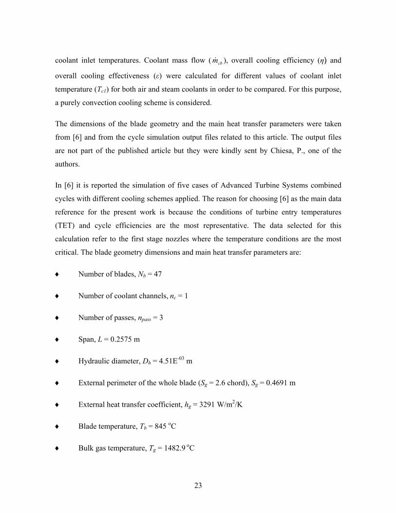
critical. The blade geometry dimensions and main heat transfer parameters are:
Number of blades, Nb = 47
Number of coolant channels, nc = 1
Number of passes, npass = 3
Span, L = 0.2575 m
Hydraulic diameter, Dh = 4.51E-03 m
External perimeter of the whole blade (Sg = 2.6 chord), Sg = 0.4691 m
External heat transfer coefficient, hg = 3291 W/m2/K
Blade temperature, Tb = 845 oC
Bulk gas temperature, Tg = 1482.9 oC
23

Turbine mass flow, m = 700 kg/s g&♦
The Biot number (Bi) is related to the conductivity and thicknesses of the blade wall and
thermal barrier coating. Biot number value is typically 1.0, accordingly to [7].
Air and steam properties are average values for the temperature range 500 to 800 oC. They
were calculated based on the average temperature (Tav, in Kelvin) between the coolant entry
(Tc1) and the blade temperature (Tb).
15.2732
1 ++
= bcav
TTT , (5-1)
The air properties were defined in [17] as:
Air viscosity, µ ( kg/m/s), ♦
ρνµ = , (5-2)
Where air density (ρ) is defined as
00336.177819.360 −= avTρ , (5-3)
And air kinematic viscosity (ν ) is defined as
0608203211314 4484.37604.31407.15728.9555.11 −−−−− −+++−= ETETTETE avavavavν , (5-4)
Air thermal conductivity, k (W/m/K), ♦
♦
0404208311 9333.30184.18574.45207.1 −−−− −+−= ETETETEk avavav , (5-5)
Air specific heat at constant pressure, Cp(J/kg/K),
0301203307410 0575.14890.41407.19999.79327.1 +−−−− +−+−= ETETTETECp avavavav , (5-6)
The steam properties were defined in FLUENT 6.2 database as:
24
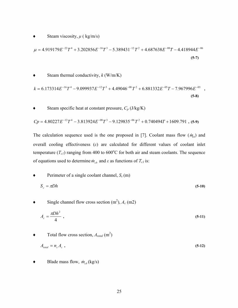
Steam viscosity, µ ( kg/m/s) ♦
♦
♦
♦
0608212316422 418944.4687638.4389431.5202856.3919179.4 −−−−− −+−+= ETETTETEµ
(5-7)
Steam thermal conductivity, k (W/m/K)
0305208312416 967996.7881332.649046.4099937.9173314.6 −−−−− −++−= ETETTETEk ,
(5-8)
Steam specific heat at constant pressure, Cp (J/kg/K)
791.1609740494.0129835.9813924.380227.4 206308412 ++−−= −−− TTTETECp , (5-9)
The calculation sequence used is the one proposed in [7]. Coolant mass flow ( ) and
overall cooling effectiveness (ε) are calculated for different values of coolant inlet
temperature (T
cbm&
c1) ranging from 400 to 600oC for both air and steam coolants. The sequence
of equations used to determine and ε as functions of Tcbm& c1 is:
Perimeter of a single coolant channel, Sc (m)
DhSc π= (5-10)
Single channel flow cross section (m2), Ac (m2) ♦
4
2DhAcπ
= , (5-11)
Total flow cross section, Atotal (m2) ♦
♦
cctotal AnA = , (5-12)
Blade mass flow, m (kg/s) cb&
25

b
gccb N
mMm
100&
& = , (5-13)
Channel mass flow, m (kg/s), cc&♦
c
cbcc n
mm
&& = , (5-14)
Channel Reynolds number, Re ♦
c
cc
AcDhmµ
&=Re , (5-15)
Coolant Nussel number (for a passage with ribs), Nu ♦
♦
7.0Re15.0=Nu , (5-16)
Internal heat transfer coefficient, hc (W/m2/K),
DhNuk
h cc = , (5-17)
Technology factor, X ♦
gg
ccpassc
ShSnnh
X = , (5-18)
Mass flow function, m* ♦
LShCpmBim
gg
cb&)1(* += , (5-19)
Convection cooling efficiency, η ♦
*1 mX
e−
−=η , (5-20)
26

Overall effectiveness, ε ♦
ηηε*1
*m
m+
= , (5-21)
1cg
bg
TTTT
−
−=ε , (5-22)
Blade temperature in function of overall effectiveness, Tb’ (oC), ♦
)(' 1cggb TTTT −−= ε , (5-23)
Correction factor to adjust coolant bleed, K ♦
b
bb
TTT
K−
='
, (5-24)
Coolant bleed (Mc) is the ratio of the total blade row coolant mass flow to the turbine mass
flow and is expressed as percentage (%) of the turbine mass flow. The calculation starts
with an initial guess and then at each iteration Mc is multiplied by (1+K), increasing or
decreasing the coolant bleed (%). The iterative process is stopped when K is less than
2.00E-04, what means that the calculated value for the blade temperature (Tb’) converged to
the set value, Tb = 845 oC. Coolant bleed (Mc) is used in steam cases as a calculation
reference only, since has no meaning in steam cooling.
Figure 5-2, Figure 5-3 and Figure 5-4 below are comparative graphs of air and steam
mass flow ( m ), overall cooling efficiency (η) and overall cooling effectiveness (ε)
calculated for coolant inlet temperatures (T
cb&
c1) ranging from 400 to 600 oC, in purely
convection cooling scheme.
Since the values of the gas temperature (Tg) and blade temperature (Tb) are constant and
coolant inlet temperatures (Tc1) varies in the same range, the resulting values of overall
cooling effectiveness (ε) are the same for both coolants.
27

The overall cooling efficiency (η) is apparently a paradox since air is more efficient than
steam. In blade cooling, however, efficiency is a misnomer and the difference in values is
the result of different coolant outlet temperatures (Tc2). For the same overall cooling
effectiveness (ε), Tc2 is higher for air than for steam in order to compensate the lower Cp,
similarly as the higher air mass flow ( ) does, accordingly to [7]. By definition overall
cooling efficiency (η) is:
cbm&
1
12
cb
cc
TTTT
−−
=η , (5-25)
And the energy removed from the whole blade, qout is:
)( 12 cccbout TTCpmq −= & , (5-26)
28

Variation of mcb with Tc1
0123456789
500
540
580
620
660
700
740
780
Tc1
air
steam
Figure 5-2 Variation of as function of Tcbm& c1
Variation of η with Tc1
0
0.1
0.2
0.3
0.4
0.5
0.6
500
540
580
620
660
700
740
780
Tc1
air
steam
Figure 5-3 Variation of η as function of Tc1
29

Variation of ε with Tc1
00.10.20.30.40.50.60.70.80.9
1
500
540
580
620
660
700
740
780
Tc1
air
steam
Figure 5-4 Variation of ε as function of Tc1
5.4 Summary
The different performances of air and steam as coolants in convective cooling were
presented in this chapter. In addition to the comparison of the main properties associated to
heat transfer, an example was developed. From the next chapter on, the subject of the
present of the present work, steam film cooling, is presented. The creation of geometry and
mesh for simulation is the first topic.
30

CHAPTER 6 GEOMETRY AND MESHING
6.1 Introduction
In this chapter the geometry and meshing chosen for the simulation are described in detail.
A sketch of the test rig is presented as well as detail on the built mesh. The main settings
used for meshing are listed.
6.2 Geometry
The chosen geometry is based in an experiment carried out by Papell [13]. The paper
reports the results of a series of experiments on film cooling on a flat plate varying the
coolant slot inlet angle from 90o to 80o and 45o angles. The chosen angle is 90o since the
author reported this as being the one which better matched with the proposed correlation.
The geometry was created in GAMBIT 2.2.30 software in two dimensions (2D) in order to
simplify the solution and considering that is not possible to reproduce the real blade film
cooling phenomena in a flat plate experiment or simulation, even in three dimensions (3D).
In Figure 6-1 below is presented a sketch of the test rig used by Pappell in his experiments
and reproduced in 2D geometry to be used in the simulations performed under the present
work.
31

Figure 6-1 Test rig geometry sketch
6.3 Meshing
The mesh was also created in GAMBIT 2.2.30, and edges mesh settings are:
• gas inlet (edge.1) – grading ratio 0.92, spacing 0.5;
• gas channel upper wall at the coolant inlet upstream (edge.2) - grading ratio 0.963,
spacing 0.11;
• coolant slot left wall (edge.3) - grading ratio 1.0869565, spacing 0.11;
• coolant inlet (edge.4) - grading ratio 1, spacing 0.05;
• coolant slot right wall (edge.5) - grading ratio 0.92, spacing 0.11;
• adiabatic wall or the flat plate (edge.6) - grading ratio 1, spacing 0.02;
• outlet (edge.7) - grading ratio 1.112, spacing 0.22; and
• gas channel lower wall - grading ratio 1, spacing 0.9.
32

In order to obtain better accuracy on the adiabatic wall (the flat plate- edge.6), this edge
was meshed with boundary layer mesh so set: first layer 0.0050, growth factor 0.950,
number of rows 7, with internal continuity, algorithm uniform, corner shape block,
transition pattern 1:1 and transition rows 0.
The whole geometry (face.1) was meshed with triangular elements and interval size spacing
0.051161388. It results 357,735 nodes and 696,100 elements on the face. Figure 6-2 below
presents a detail of the mesh in the region where the coolant flow enters the main gas flow.
Observe the structured boundary layer mesh used along the adiabatic wall in order to obtain
more accurate results of wall temperature and, consequently, film cooling efficiency.
Triangular unstructured mesh was used for the remaining area.
Figure 6-2 Detail of the mesh
33

6.4 Summary
This chapter describes geometry and mesh chosen for CFD simulation and their main
settings. The objective is to understand the choices done and create the conditions for this
simulation to be reproduced, if desired. In the next chapter it is described how the method
was validated in order to perform the steam film cooling simulation.
34

CHAPTER 7 METHOD VALIDATION
7.1 Introduction
In this chapter it is reported the simulation of a selected series of experimented cases with a
Computational Fluid Dynamics (CFD) software. The comparison of the results validated
the method that was used to simulate air and steam film cooling in the conditions proposed
for the present work.
7.2 Papell’s experiment
The experiment described in [13] consisted in several series of tests of film cooling on a flat
plate with the coolant inlet being a slot in 90o, 80o and 45o angles. The series chosen to be
simulated and compared to the results of the real experiment is the one with 90o slot inlet
angle and Mach number = 0.5, one of the set of cases reported by the author as the best
matching between ε and the correlating equation:
( ) effecc
e iVcVgfSVg
wCphgLx 8.0coslog04.0log
125.0
+
−−=
αη , (7-1)
Where,
Cooling effectiveness, ε ♦
cad
wad
tTtT
−−
=η , (7-2)
Note: The notation used for effectiveness in [13] is η. The usual notation for effectiveness
(ε) is utilised in this work with the exception of this chapter in order to maintain the same
35
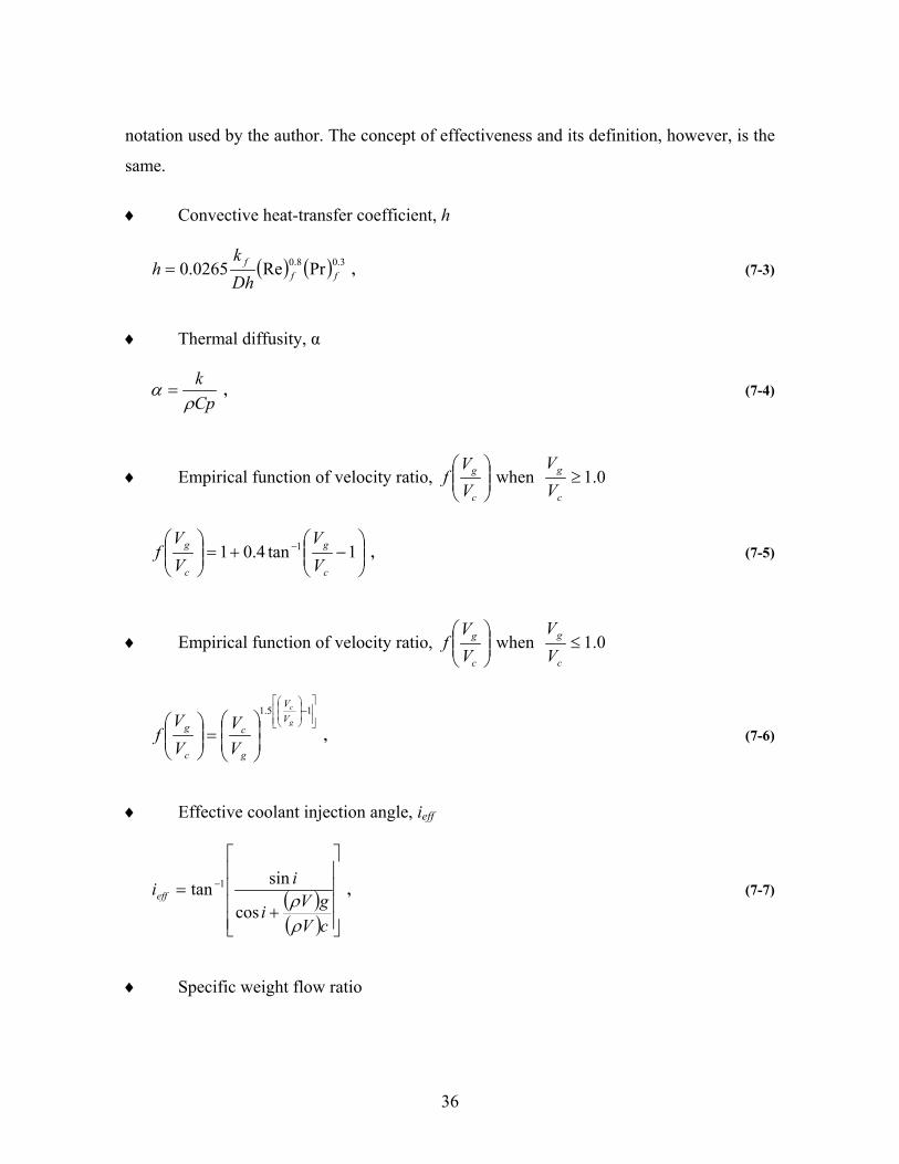
notation used by the author. The concept of effectiveness and its definition, however, is the
same.
Convective heat-transfer coefficient, h ♦
( ) ( ) 3.08.0 PrRe0265.0 fff
Dhk
h = , (7-3)
Thermal diffusity, α ♦
Cpk
ρα = , (7-4)
Empirical function of velocity ratio,
c
g
VV
f when 0.1≥c
g
VV
♦
−+=
− 1tan4.01 1
c
g
c
g
VV
VV
f , (7-5)
Empirical function of velocity ratio,
c
g
VV
f when 0.1≤c
g
VV
♦
−
=
15.1
g
c
VV
g
c
c
g
VV
VV
f , (7-6)
Effective coolant injection angle, ieff ♦
( )( )
+= −
cVgVi
iieff
ρρcos
sintan 1 , (7-7)
Specific weight flow ratio ♦
36

( )( )gV
cVρρ
, (7-8)
k coefficient of thermal conductivity
Dh hydraulic diameter
Re Reynolds number
Pr Prandtl number
L width of adiabatic wall
x distance along the adiabatic wall in direction of the flow
w flow rate
Cp specific heat at constant pressure
S coolant slot height
V velocity
ρ mass density
i coolant injection angle relative to adiabatic wall
t static temperature
Subscripts:
c coolant slot exit
f properties evaluated at 2
cg tt +
g main body of gas
37

w wall
The series consist in 13 cases, each one corresponding to a different ratio Vg/Vc (between
the bulk gas velocity Vg, and the coolant velocity Vc), ranging from 0.835 to 10.05, and the
respective coolant inlet static temperature tc, ranging from 302.78 K to 597.22 K. The gas
adiabatic temperature was maintained nominally constant at 833.33 K.
For each case, wall static temperature was measured in 12 different stations along the
adiabatic wall and plotted in the form of the correlation above mentioned. The graph
resulting from the series chosen to be simulated in FLUENT 6.2 is presented in Figure 7-1
in section 7.4.
7.3 Simulation of Papell’s experiment with CFD
Using the geometry and mesh created with GAMBIT 2.2.30 (as described in CHAPTER 6),
the series of cases comprised by the slot at 90o and Mach number 0.5 were reproduced with
FLUENT 6.2.
As the experiment was run in 2D, some simplifications were done. The settings were:
Solver: segregated; Space 2D; Velocity formulation: absolute; Gradient option: cell-based;
Formulation: implicit; Time: steady; and Porous formulation: superficial velocity.
Energy equation was enabled and the viscous model was k-epsilon (2 equations) with all
its default options maintained.
Species model was set for species transport. Diffusion energy source and thermal diffusion
options were enabled. Mixture material was defined as mixture-template with two
volumetric species: air and H2O.
38

Material type was defined as a mixture and FLUENT mixture materials as mixture-
template. Air and water vapour (H2O) were saved from FLUENT database as the
constituent fluids of the mixture.
Mixture properties were so defined: density, ρ based on volume weighted mixing law;
specific heat at constant pressure (Cp) based on mixing law; thermal conductivity (k) based
on mass weighted mixing law; viscosity (µ) based on volume weighted mixing law; for
mass diffusivity was maintained the constant default value 2.88e-05 m2/s; and the thermal
diffusion coefficient based on kinetic theory.
Water vapour properties are pre-defined in FLUENT database. The choice was: density
(ρ); specific heat at constant pressure (Cp); and thermal conductivity (k) based on
polynomials; viscosity (µ) based on power law; and molecular weight constant 18.01534
kg/kgmol.
Two of the air properties were defined based on FLUENT database: viscosity (µ) based
on power law; and molecular weight constant 28.966 kg/kgmol. The others were defined
accordingly to equations from [17].
Air density (ρ) was defined as piecewise linear based on the equation:
00336.177819.360 −= Tρ , (7-9)
Thirty points from the curve defined by the equation were input, covering the range of
temperatures occurred in the simulation, from 566 K to 1813 K, corresponding to density
values ranging respectively from 0.623985 to 0.194041. The input points were defined
based in a constant difference of 0.014286 in the density value between two adjacent points
and the correspondent temperature, so preventing too low accuracy along the curve.
Air specific heat at constant pressure (Cp) was defined with a polynomial equation:
0301203307410 0575.14890.41407.19999.79327.1 +−−−− +−+−= ETETETETECp , (7-10)
39

Air thermal conductivity (k) was defined with a polynomial equation:
0404208311 9333.30184.18574.45207.1 −−−− −+−= ETETETEk , (7-11)
Boundary conditions for main inlet and coolant inlet were so defined: Velocity
specification method: magnitude, normal to boundary; Reference frame: absolute; Velocity
magnitude and temperature accordingly each case comprising the series; Hydraulic
diameter: 8” for the main inlet and 0.25” for the coolant inlet; and Turbulence intensity, TI
was calculated as recommend on FLUENT 6.2 manual:
81
Re16.0−
=TI , (7-12)
Boundary conditions for the adiabatic wall (flat plate) and the other wall: they were
defined as walls and all default values and selections were maintained for both. Material
name: aluminium. Thermal conditions: heat flux enable and value zero for heat flux; wall
thickness; and heat generation rate. Momentum conditions: stationary wall and no slip
enabled; roughness height value zero and roughness constant value 0.5. Species boundary
condition: H2O zero diffusive flux.
Boundary conditions for fluid: it was defined as fluid with no selection and zero values
for rotation axis origin (default settings). Outlet was defined as outflow with default set
flow rate weighting value 1.0. Default interior was defined as interior with no settings
available.
Operating conditions were so defined: operating pressure value 101,325 Pa; gravity
disabled and reference pressure location values zero for X and Y.
Initialisation was computed from main inlet using first order discretisation.
40

7.4 Simulation of Papell’s experiment and comparison with the real data
The temperatures at the adiabatic wall resulting from the simulations of Papell’s experiment
were written to a file and post-processed using Microsoft EXCEL software.
The data is displayed in a graph accordingly the correlation proposed in [13] in order to the
establish comparison with the real data.
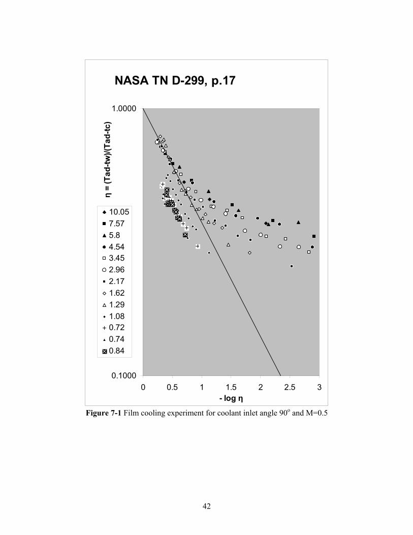
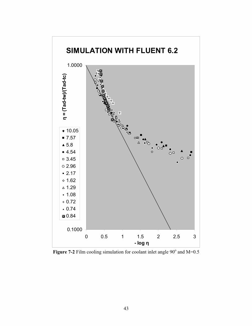
The graph with the real data is in Figure 7-1 below and the graph with the data resulting
from the simulation is in Figure 7-2 below. By comparing both, the coincidence it is visible
and, actually, the simulation apparently resulted closer to the proposed theoretical
correlation (the straight line that crosses the graph) than the real experiment. The data
placed at the right side of the correlating line follows the same pattern of the real
experiment data and suggests that possibly the proposed correlation is not valid for those
values of velocities ratio Vg/Vc, although it is not the objective of the comparison.
Based on this comparison, the results validated the method which was used for the
investigation on air and steam film cooling carried out next.
41
NASA TN D-299, p.17
0.1000
1.0000
0 0.5 1 1.5 2 2.5 3- log η
η =
(Tad
-tw)/(
Tad-
tc)
10.057.575.84.543.452.962.171.621.291.080.720.740.84
Figure 7-1 Film cooling experiment for coolant inlet angle 90o and M=0.5
42
SIMULATION WITH FLUENT 6.2
0.1000
1.0000
0 0.5 1 1.5 2 2.5 3- log η
η =
(Tad
-tw)/(
Tad-
tc)
10.057.575.84.543.452.962.171.621.291.080.720.740.84
Figure 7-2 Film cooling simulation for coolant inlet angle 90o and M=0.5
43

7.5 Summary
In this chapter it is reported how one of the series of Papell [13] experiments was
reproduced in FLUENT 6.2 software. The comparison between the results of the simulation
and the experiment wads presented and the criteria to validate the simulation was described.
The objective is to establish confidence in the method used to simulate air and steam film
cooling in different temperature, pressure and velocity conditions. In the next chapter it is
described the selection of steam and air film cooling to be simulated and compared.
44

CHAPTER 8 CASES DEFINITION AND INPUT SETTINGS
8.1 Introduction
In this chapter it is described the criteria to select the film cooling cases to be simulated
with CFD software. The settings used in FLUENT 6.2 for the selected cases are as well
described.
8.2 Air film cooling cases definition
Air film cooling cases were simulated in CFD software to be compared to similar steam
film cooling cases. Air film cooling cases were defined based on the following
assumptions:
a) The combustion temperature Tcc = 1811 K, the limit combustion temperature
achievable with no thermal NOX production, as referred in [12].
b) The coolant inlet temperature Tc1 = 740.65 K, the air inlet temperature for
convective blade cooling in the open-circuit air cooled advanced turbine systems
case simulation, as referred in [6] First stage vane maximum blade wall temperature
Tw = 1118.15 K for all advanced turbine systems cases simulation, as referred in [6].
c) The gas mass flow = 700 kg/s, the gas mass flow used for all advanced turbine
systems cases simulation, as referred in [6].
gm&
The following conditions were derived:
45

d) The coolant temperature (Tc) as the average temperature between coolant inlet
temperature, (Tc1) and the blade wall temperature, (Tw) so resulting in
KTT
T wcc 40.929
215.111865.740
21 =
+=
+= , (8-1)
e) The simulated test rig gas mass flow was defined in order to obtain the same gas
velocity for first stage vanes Vg = 706.00 m/s, as referred in [6]. The method used
was trial and error, by inputting values of mass flow in FLUENT 6.2 up to have the
velocity adjusted, so resulting in m = 27.88 kg/s. gs&
f) Gas flow turbulence intensity was calculated based on the definition provided in
FLUENT 6.2 manual:
81
Re16.0−
=TI , (8-2)
resulting TI = 7.05% for the main gas flow.
The cases to be simulated were defined with base on the quenching effect by the coolant on
the main gas flow. The maximum acceptable film cooling quenching effect should result in
decreasing the gas temperature down to a minimum of 1756.05 K, which is the combustion
temperature for the state-of-the-art closed-loop steam cooling case simulation, as referred in
[6].
Setting the combustion temperature Tcc = 1756.05 K, correspondent to the state-of-the-art
closed-loop steam cooling scheme for the air film cooling cases simulation is only a way to
create similar conditions for further comparison. It does not suggest a design conception
with mixed air-steam cooling scheme.
The corresponding coolant mass flow ( ) that quenches the gas flow and decreases its
temperature down to 1756.05 K is calculated taking in account the gas mass flow for the
simulation ( ), the gas temperature (T
csm&
gsm& g), the coolant temperature (Tc), and the values of
46

specific heat at constant pressure (Cp) for the gas and for the coolant at the gas temperature
(Tg), at the coolant temperature (Tc) and at the limit temperature for the quenched mixture
(Tm). The equation below defines the mixture:
mmmscccsgggs TCpmTCpmTCpm =+ , (8-3)
Where,
gsm& gas mass flow (for the simulation)
csm& coolant mass (for the simulation)
msm& mixture mass (for the simulation)
Cpm specific heat at constant pressure of the mixture
Tm mixture temperature
Hence,
( ) mmcsgscccsgggs TCpmmTCpmTCpm &&&& +=+ , (8-4)
And,
( )( )ccmm
mmgggscs TCpTCp
TCpTCpmm
−
−= && , (8-5)
Being air Cp defined by a polynomial as a function of T, defined in [17],
0301203307410 0575.14890.41407.19999.79327.1 +−−−− +−+−= ETETTETECp , (8-6)
And,
gsm& = 27.88 kg/s
47

Tg = 1811 K
Tc = 929.40 K
Cpg = 1313.04 KJ/kgK
Cpc = 1127.58 KJ/kgK
It results, for Tm = 1756.05 K:
Cpm = 1292.59 KJ/kgK and = 2.47 kg/s csm&
As = 2.47 kg/s is the coolant (air) mass flow that quenches the gas flow and decreases
the mixture temperature down to T
csm&
csm&
m = 1756.05K, any coolant mass flow to be considered in
this simulation should be less than 2.47 kg/s, since 1756.05K is the combustion temperature
in the state-of-the-art closed-loop steam cooling scheme and no gain would so be achieved.
So = 2.47 kg/s is one limit of the range of coolant mass flows to be considered.
The other limit is the zero coolant mass flow, which corresponds to Tm = Tg = 1811K, a
impracticable gas flow temperature condition for the state-of-the-art closed-loop steam
cooling scheme.
So limited, the best solution was to simulate cases with coolant mass flow ( m ) between
zero and 2.47 kg/s and to analyse the results. It was taken the low mixture temperature T
cs&
m =
1756.05K case and four additional, defined based on an equal difference of 10.99K from
one to other. So the five air film cooling cases and their correspondent coolant mass flows,
calculated based on equation 8.5 are:
Case 1: Tm = 1756.05K, = 2.47 kg/s csm&
Case 2: Tm = 1767.04K, = 1.95 kg/s csm&
Case 3: Tm = 1778.03K, = 1.45 kg/s csm&
48

Case 4: Tm = 1789.02K, = 0.96 kg/s csm&
Case 5: Tm = 1800.01K, = 0.48 kg/s csm&
8.3 Steam film cooling cases definition
Steam film cooling cases were simulated in CFD software to be compared to similar air
film cooling cases. Steam film cooling cases were defined based on the following
assumptions: The following conditions so were derived:
a) The combustion temperature Tcc = 1811 K, the limit combustion temperature
achievable with no thermal NOX production, as referred in [12].
b) The coolant inlet temperature Tc1 = 568.35 K, the steam inlet temperature for
convective blade cooling in the closed-loop steam cooled advanced turbine systems
case simulation, as referred in [6].
c) First stage vane maximum blade wall temperature Tw = 1118.15 K for all advanced
turbine systems cases simulation, as referred in [6].
d) The gas mass flow = 700 kg/s, the gas mass flow used for all advanced turbine
systems cases simulation, as referred in [6].
gm&
The following conditions were derived:
e) The coolant temperature as the average temperature between coolant inlet
temperature (Tc1) and the blade wall temperature (Tw) so resulting in
KTT
T wcc 25.843
215.111835.568
21 =
+=
+= , (8-7)
The simulated test rig gas mass flow was defined in order to obtain the same gas
velocity for first stage vanes Vg = 706.00 m/s, as referred in [6], the same as for the
49

air film cooling cases. The method used was trial and error, by inputting values of
mass flow in FLUENT 6.2 up to have the velocity adjusted, so resulting in =
27.88 kg/s.
gsm&
f) Gas flow turbulence intensity was calculated based on the definition provided in
FLUENT 6.2 manual and it is the same used for air film cooling cases:
81
Re16.0−
=TI , (8-8)
resulting TI = 7.05% for the main gas flow.
The cases to be simulated were defined with base on the quenching effect by the coolant on
the main gas flow. The maximum acceptable film cooling quenching effect should result in
decreasing the gas temperature down to a minimum of 1756.05 K, which is the combustion
temperature for the state-of-the-art closed-loop steam cooling case simulation, as referred in
[6].
The corresponding coolant mass flow ( ) that quenches the gas flow and decreases its
temperature down to 1756.05 K is calculated taking in account the gas mass flow for the
simulation ( ), the gas temperature (T
csm&
gsm& g), the coolant temperature (Tc), and the values of
specific heat at constant pressure (Cp) for the gas and for the coolant at the gas temperature
(Tg), at the coolant temperature (Tc) and at the limit temperature for the quenched mixture
(Tm). The equation below defines the mixture:
mmmscccsgggs TCpmTCpmTCpm &&& =+ , (8-9)
Where,
gsm& gas mass flow (for the simulation)
csm& coolant mass (for the simulation)
msm& mixture mass (for the simulation)
50

Cpgm specific heat at constant pressure of the gas at the mixture temperature
Cpcm specific heat at constant pressure of the coolant at the mixture temperature
Tm mixture temperature
Hence,
( ) mmcsgscccsgggs TCpmmTCpmTCpm &&&& +=+ , (8-10)
And,
( )( )ccmcm
mgmgggscs TCpTCp
TCpTCpmm
−
−= && , (8-11)
Being steam Cp defined by a polynomial as a function of T in FLUENT 6.2 database,
791.1609740494.0129835.9813924.380227.4 206308412 ++−−= −−− TTTETECp ,(8-12)
And,
gsm& = 27.88 kg/s
Tg = 1811 K
Tc = 843.25 K
Cpg = 1313.04 KJ/kgK
Cpc = 2207.28 KJ/kgK
It results, for Tm = 1756.05 K:
Cpgm = 1292.59 KJ/kgK, Cpcm = 2721.12 KJ/kgK and = 1.03 kg/s csm&
51

As = 1.03 kg/s is the coolant mass flow that quenches the gas flow decreasing the
mixture temperature down to T
csm&
m = 1756.05 K, any coolant mass flow to be considered in
this work must be less than 1.03 kg/s, since 1756.05 K is the combustion temperature in
closed-loop steam cooling scheme and no gain would so be achieved. So m = 1.03 kg/s is
one limit in the range of coolant mass flow to be considered.
cs&
The other limit is the zero coolant mass flow, which corresponds to Tm = Tg = 1811 K, a
impracticable gas flow temperature condition for a closed-loop steam cooling scheme.
So limited, the best solution was to simulate cases with coolant mass flow ( m ) between
zero and 1.03 kg/s and to analyse the results. It was taken the low mixture temperature T
cs&
m =
1756.05K case and four additional, defined based on an equal difference of 10.99K from
one to other. So the five air film cooling cases and their correspondent coolant mass flows,
calculated based on equation 8.11 are:
Case 1: Tm = 1756.05 K, = 1.03 kg/s csm&
Case 2: Tm = 1767.04 K, = 0.83 kg/s csm&
Case 3: Tm = 1778.03 K, = 0.63 kg/s csm&
Case 4: Tm = 1789.02 K, = 0.42 kg/s csm&
Case 5: Tm = 1800.01 K, = 0.21 kg/s csm&
8.4 Input settings in FLUENT 6.2 for film cooling simulation
Film cooling simulation of five cases with air as the coolant and other five cases with steam
as coolant were carried out with FLUENT 6.2 in 2d. It was used the same geometry and
mesh created with GAMBIT 2.2.30, as described in CHAPTER 6, which was validated by
the simulation of Papell’s experiment, as described in CHAPTER 7.
52
The common settings were:
Solver: segregated; Space 2D; Velocity formulation: absolute; Gradient option: cell-based;
Formulation: implicit; Time: steady; and Porous formulation: superficial velocity.
Energy equation was enabled and the viscous model was k-epsilon (2 equations) with all
its default options maintained.
Species model was set for species transport. Diffusion energy source and thermal diffusion
options were enabled. Mixture material was defined as mixture-template with two
volumetric species: air and H2O.
Material type was defined as a mixture and FLUENT 6.2 mixture materials as mixture-
template. Air and water vapour (H2O) were saved from FLUENT 6.2 database as the
constituent fluids of the mixture.
Mixture properties were so defined: density (ρ) based on volume weighted mixing law;
specific heat at constant pressure (Cp) based on mixing law; thermal conductivity (k) based
on mass weighted mixing law; viscosity (µ) based on volume weighted mixing law; for
mass diffusivity was maintained the constant default value 2.88e-05 m2/s; and the thermal
diffusion coefficient based on kinetic theory.
Water vapour properties are pre-defined in FLUENT 6.2 database. The choice was:
density (ρ); specific heat at constant pressure (Cp); and thermal conductivity (k) based on
polynomials; viscosity (µ) based on power law; and molecular weight constant 18.01534
kg/kgmol.
Two of the air properties were defined based on FLUENT 6.2 database: viscosity (µ)
based on power law; and molecular weight, constant 28.966 kg/kgmol. The others were
defined accordingly to polynomial equations from [17].
Air density (ρ) was defined as piecewise linear based on the equation:
53
00336.177819.360 −= Tρ , (8-13)
Thirty points from the curve defined by the equation were input, covering the range of
temperatures occurred in the simulation, from 566 K to 1813 K, corresponding to density
values ranging respectively from 0.623985 to 0.194041. The input points were defined
based in a constant difference of 0.014286 in the density value between two adjacent points
and the correspondent temperature, so preventing too low accuracy along the curve.
Air specific heat at constant pressure (Cp) was defined with a polynomial equation:
0301203307410 0575.14890.41407.19999.79327.1 −−−−− +−+−= ETETTETECp , (8-14)
Air thermal conductivity (k) was defined with a polynomial equation:
0404208311 9333.30184.18574.45207.1 −−−− −+−= ETTETEk , (8-15)
Boundary conditions for main inlet and coolant inlet were so defined: Velocity
specification method: magnitude, normal to boundary; Reference frame: absolute; Velocity
magnitude and temperature accordingly each case comprising the series; Hydraulic
diameter: 8” for the main inlet and 0.25” for the coolant inlet; and Turbulence intensity was
calculated as recommend on FLUENT 6.2 manual:
81
Re16.0−
=TI , (8-16)
Boundary conditions for the adiabatic wall (flat plate) and the other wall: they were
defined as walls and all default values and selections were maintained for both. Material
name: aluminium. Thermal conditions: heat flux enable and value zero for heat flux; wall
thickness; and heat generation rate. Momentum conditions: stationary wall and no slip
enabled; roughness height value zero and roughness constant value 0.5. Species boundary
condition: H2O zero diffusive flux.
Boundary conditions for fluid: it was defined as fluid with no selection and zero values
for rotation axis origin (default settings). Outlet was defined as outflow with default set
54

flow rate weighting value 1.0. Default interior was defined as interior with no settings
available.
Operating conditions were so defined: operating pressure value 101,325 Pa; gravity
disabled and reference pressure location values zero for X and Y.
Initialisation was computed from main inlet using first order discretisation.
8.5 Summary
The selection of the ten cases (five air film cooling cases and five steam film cooling cases)
to be simulated with FLUENT 6.2 was described. The settings used to run these cases were
also reported. The objective is to understand the method and assumptions in order to
prepare for the results which are in the next chapter.
55
CHAPTER 9 FILM COOLING CFD SIMULATION RESULTS
9.1 Introduction
In this chapter are reported the results of the simulation of five air film cooling cases and
five steam film cooling cases. The results are presented in form of pictures and graphs.
Pictures on temperature, velocity, specific heat at constant pressure and thermal
conductivity contours are showed in Appendix A, as well as graphs on static wall
temperature distribution, film effectiveness distribution, air/steam wall temperature ratio
distribution and steam/air film effectiveness distribution. Graphs on steam/air film
effectiveness distribution are reproduced in this chapter, as they drive more directly to the
conclusion.
9.2 Graphs on steam/air film effectiveness ratio distribution
56

Case 1
Coolant Tg (K) Pg (bar) mg (kg/s) Tc (K) Pc (bar) mc (kg/s) Vc/Vg Air 929.40 23.07 2.47 1.45 Steam 1811 22.38 27.88 843.25 36.00 1.03 0.89
Steam/Air film effectiveness ratio - case 1
0.6
0.7
0.8
0.9
1
1.1
1.2
0 0.1 0.2 0.3 0.4 0.5 0.6 0.7 0.8 0.9 1 1.1 1.2
Distance from the injection point, X (m)
η ste
am/η
air
Figure 9-1 Steam/air film effectiveness ratio distribution – case 1
Case 2
Coolant Tg (K) Pg (bar) mg (kg/s) Tc (K) Pc (bar) mc (kg/s) Vc/Vg Air 929.40 23.07 1.95 1.15 Steam 1811 22.38 27.88 843.25 36.00 0.83 0.71
Steam/air film effectiveness ratio - case 2
0.6
0.7
0.8
0.9
1
1.1
1.2
0 0.1 0.2 0.3 0.4 0.5 0.6 0.7 0.8 0.9 1 1.1 1.2
Distance from the injection point, X (m)
η ste
am/η
air
Figure 9-2 Steam/air film effectiveness ratio distribution – case 2
57

Case 3
Coolant Tg (K) Pg (bar) mg (kg/s) Tc (K) Pc (bar) mc (kg/s) Vc/Vg Air 929.40 23.07 1.45 0.85 Steam 1811 22.38 27.88 843.25 36.00 0.63 0.54
Steam/air film effectiveness ratio - case 3
0.6
0.7
0.8
0.9
1
1.1
1.2
0 0.1 0.2 0.3 0.4 0.5 0.6 0.7 0.8 0.9 1 1.1 1.2
Distance from the injection point, X (m)
η ste
am/η
air
Figure 9-3 Steam/air film effectiveness ratio distribution – case 3
Case 4
Coolant Tg (K) Pg (bar) mg (kg/s) Tc (K) Pc (bar) mc (kg/s) Vc/Vg Air 929.40 23.07 0.96 0.56 Steam 1811 22.38 27.88 843.25 36.00 0.42 0.36
Steam/air film effectiveness ratio - case 4
0.6
0.7
0.8
0.9
1
1.1
1.2
0 0.1 0.2 0.3 0.4 0.5 0.6 0.7 0.8 0.9 1 1.1 1.2
Distance from the injection point, X (m)
η ste
am/η
air
Figure 9-4 Steam/air film effectiveness ratio distribution – case 4
58

Case 5
Coolant Tg (K) Pg (bar) mg (kg/s) Tc (K) Pc (bar) mc (kg/s) Vc/Vg Air 929.40 23.07 0.48 0.28 Steam 1811 22.38 27.88 843.25 36.00 0.21 0.18
Steam/air film effectiveness ratio - case 5
0.6
0.7
0.8
0.9
1
1.1
1.2
0 0.1 0.2 0.3 0.4 0.5 0.6 0.7 0.8 0.9 1 1.1 1.2
Distance from the injection point, X (m)
η ste
am/η
air
Figure 9-5 Steam/air film effectiveness ratio distribution – case 5
9.3 Summary
In this chapter and Appendix A the results of the simulation of ten film cooling cases with
CFD software FLUENT 6.2 were presented. The discussion on the results here presented
will be carried on in the next chapter.
59
CHAPTER 10 DISCUSSION ON FILM COOLING SIMULATION
RESULTS
10.1 Introduction
In this chapter results are discussed in various aspects. Additionally, economical
considerations respective to open-loop steam cooling are bring to light. This will help to
take the conclusions in the next chapter.
10.2 Geometry and meshing
The geometry created probably is not the ideal to obtain the best film cooling performance,
but it is sufficient for the comparative study proposed. In special, the coolant inlet angle of
90o tends to direct the coolant flow away from the blade wall. This condition, however, is
not much different than the real case, since the walls of steam cooled blades are very thin
(fractions of millimetre) and effective angles much different than 90 are not actually
obtainable.
The mesh created was the simplest possible in order to obtain good results with minimum
time necessary for iterative process, since five steam film cooling cases plus five air cases
were run. A comparative simulation, however, was performed previously using a mesh with
a larger number of cells but no important difference in result accuracy was obtained.
10.3 Coolant mass flow
Air and steam are available in a combined cycle at different conditions of pressure and
temperature. In order to have a realistic approach, the simulations were carried out with
60

steam at 36.00 bar and 843.25K at the HP steam turbine outlet and air at 23.07 bar and
929.40K at the compressor outlet. Of course, it makes significant difference and it could be
considered a distortion in the comparative method but, on the other hand, equal conditions
of pressure and temperature of both coolants are not likely to be found in real cases and the
objective is to simulate as closer as possible to the real conditions.
The five cases selected to be simulated were defined primarily based on the quenching
effect caused by the coolant flow when mixed with the turbine gas flow. So we could
observe the first important difference between the two coolants. Steam higher specific heat
(Cp), so favourable in convective cooling, became a problem in film cooling, easily
explained by the equation that describes the quenching effect:
( ) mmcsgscccsgggs TCpmmTCpmTCpm &&&& +=+ , (10-1)
And hence,
( )( )ccmcm
mgmgggscs TCpTCp
TCpTCpmm
−
−= && , (10-2)
Cpcm and Cpc are the specific heat at constant pressure of the coolant respectively at the
mixture temperature and at the coolant inlet temperature. It is clear that the higher the value
of Cp is, the lower is the coolant mass flow that will quench the mixture to a given
temperature T
csm&
m&m. In general, steam Cp is twice the value of air Cp, what makes steam to
be half of the value of air .
cs
csm&
The same negative effect is caused by the coolant temperature (Tc), resulting in even lower
steam mass flow ( ). csm&
In the five cases selected for simulation, values of steam mass flow range from 42 to 45%
of those of air mass flow. The difference in mass flow is the fact that more strongly affects
the resulting performance of the two coolants.
61

When compared cases with similar coolant mass flow, e. g. air-case 4 to steam-case 1 or
air-case 5 to steam-case 4, it is possible to observe that the steam film effectiveness is
better than air, even when steam mass flow ( m ) is smaller than air. See Figure 10-1 and
Figure 10-2 below.
cs&
Coolant Tg (K) Pg (bar) mg (kg/s) Tc (K) Pc (bar) mc (kg/s) Vc/Vg Air 929.40 23.07 0.96 0.56 Steam 1811 22.38 27.88 843.25 36.00 1.03 0.89
Film effectiveness - Air (case 4) & Steam (case 1)
00.10.20.30.40.50.60.70.80.9
11.1
0 0.1 0.2 0.3 0.4 0.5 0.6 0.7 0.8 0.9 1 1.1 1.2
Distance from the injection point, X (m)
η =
(Tg-
Tw)/(
Tg-T
c)
Air
Steam
Figure 10-1 Film effectiveness for similar , air-4 and steam-1 csm&
Coolant Tg (K) Pg (bar) mg (kg/s) Tc (K) Pc (bar) mc (kg/s) Vc/Vg Air 929.40 23.07 0.48 0.28 Steam 1811 22.38 27.88 843.25 36.00 0.42 0.36
62

Film effectiveness - Air (case 5) & Steam (case 4)
00.10.20.30.40.50.60.70.80.9
11.1
0 0.1 0.2 0.3 0.4 0.5 0.6 0.7 0.8 0.9 1 1.1 1.2
Distance from the injection point, X (m)
η =
(Tg-
Tw)/(
Tg-T
c)
Air
Steam
Figure 10-2 Film effectiveness for similar , air-5 and steam-4 csm&
10.4 Coolant inlet velocity
The difference in mass flow, as explained above, results in different inlet velocities for the
same slot area. In the ten cases selected for simulation, values of steam inlet velocity range
from 61 to 65% of the values of air inlet velocity.
The effect is observed in the velocity contours graphs (APPENDIX A). Because of this
important difference, air flow penetrates the main gas flow for longer distance than steam
flow. It means, from another view point, the steam flow is more easily decelerated down to
the main gas flow velocity. Considering the coolant inlet angle 90o, in particular, it causes a
favourable effect for the steam flow since it remains close to the wall and it is not affected
so early by dispersion in the main gas flow as the air flow is.
When compared cases with similar coolant inlet velocities, as air-case 3 to steam-case 1 or
air-case 4 to steam-case 3, it is possible to observe that the steam film effectiveness is
similar, even being air mass flow ( ) much larger than steam. It indicates that the coolant
inlet velocity is a key factor in film cooling. See Figure 10-3 and Figure 10-4 below.
csm&
63

Coolant Tg (K) Pg (bar) mg (kg/s) Tc (K) Pc (bar) mc (kg/s) Vc/Vg Air 929.40 23.07 1.45 0.85 Steam 1811 22.38 27.88 843.25 36.00 1.03 0.89
Film effectiveness - Air (case 3) & Steam (case 1)
00.10.20.30.40.50.60.70.80.9
11.1
0 0.1 0.2 0.3 0.4 0.5 0.6 0.7 0.8 0.9 1 1.1 1.2
Distance from the injection point, X (m)
η =
(Tg-
Tw)/(
Tg-T
c)
Air
Steam
Figure 10-3 Film effectiveness for similar Vc/Vg , air-3 and steam-1
Coolant Tg (K) Pg (bar) mg (kg/s) Tc (K) Pc (bar) mc (kg/s) Vc/Vg Air 929.40 23.07 0.96 0.56 Steam 1811 22.38 27.88 843.25 36.00 0.63 0.54
Film effectiveness - Air (case 4) & Steam (case 3)
00.10.20.30.40.50.60.70.80.9
11.1
0 0.1 0.2 0.3 0.4 0.5 0.6 0.7 0.8 0.9 1 1.1 1.2
Distance from the injection point, X (m)
η =
(Tg-
Tw)/(
Tg-T
c)
AirSteam
Figure 10-4 Film effectiveness for similar Vc/Vg , air-4 and steam-3
64

10.5 Reynolds number
Reynolds number (Re) is directly affected by the flow velocity, which are much lower for
steam than for air. Re depends directly as well on coolant density (ρ) and inversely on
viscosity (µ). Both ρ and µ are function of temperature, higher for air than for steam. And
also depends directly also on the channel hydraulic diameter (Dh), which is the same in all
cases. Reynolds number definition:
µρ DhVc=Re , (10-3)
Lower values of Re are favourable for film cooling effect since it means less turbulent flow.
Turbulence favours heat and mass transfer between the coolant and the main gas flow, so
destroying the film. The more laminar the film flow can be the longer it will remain and,
consequently, its insulating effect will be effective.
10.6 Specific heat and thermal conductivity
Specific heat at constant pressure and thermal conductivity are two of the materials
properties directly involved in the heat transfer process. Both are much higher in value for
steam (Cp = 2207.28 J/kgK and k = 0.0768 W/mK at Tc = 843.25K) than for air (Cp =
1127.58 J/kgK and k = 0.0645 W/mK at Tc = 929.40K). The obvious consequence is a
faster heat transfer process for the steam flow than it is for the air flow.
Both properties, specific heat at constant pressure and thermal conductivity, for both
coolants, air and steam, have their values increased as the temperature increases, although
at much different rate.
In average the value of steam specific heat at constant pressure (Cp), is 2731.16 J/kgK, at
the five cases mixture temperatures (Tm) ranging from 1756.05 to 1800.01K. Air Cp value
is, in average, 1300.38 J/kgK, at the same five cases mixture temperatures. It means that
65

steam Cp value increase in average 23.7% from coolant inlet temperature, Tc = 843.25K to
Tm, while air Cp value increases in average only 15.3% from the coolant inlet temperature,
Tc = 929.40K to the mixture temperature (Tm).
In average the value of steam thermal conductivity, k, is 0.211 W/mK, at the five cases
mixture temperatures (Tm) ranging from 1756.05 to 1800.01K. Air k values are, in average,
0.111 W/mK, at the same five cases mixture temperatures. It means that steam k value
increase in average 175% from coolant inlet temperature, Tc = 843.25K to Tm, while air k
value increases in average only 74.5% from the coolant inlet temperature, Tc = 929.40K to
the mixture temperature (Tm).
Figures in APPENDIX A present the resulting contours of specific heat at constant pressure
(Cp) and thermal conductivity (k) for the five cases simulated and it is observable how the
properties values change as function of local temperatures and mass mixture.
10.7 Some economical considerations
In steam film cooling, steam is ultimately wasted through the main gas flow to the
atmosphere. Considering the price of electricity and the production costs of demineralised
water, it is possible to have good evaluation from the economical viewpoint of the five
steam film cooling cases.
The mass flow ( ), calculated to be used in the simulation of the five cases of steam film
cooling, is a fraction of the total film cooling steam mass flow for the first stage vanes,
since refers to = 27.88 kg/s (see 8.3, item e), proportional to the test rig area.
csm&
m&csm&
m&
gs
Accordingly to [6] the total gas mass flow m = 700 kg/s, hence the total film cooling
steam mass flow ( ) for the first stage vanes for the five cases are:
g&
c
Case 1: = 25.93 kg/s cm&
66

Case 2: = 20.90 kg/s cm&
Case 3: = 15.79 kg/s cm&
Case 4: = 10.61 kg/s cm&
Case 5: = 5.35 kg/s cm&
Demineralised water production costs are estimated in £ 4.23/m3, for GEPS H System™
steam quality requirements (similar to conventional steam turbine requirements [34]),
accordingly to the information of a Sales Manager at GE Group Water Treatment Division
in Brazil.
Hence the production costs of demineralised water for the five cases are:
Case 1: £ 394.89/hr
Case 2: £ 318.25/hr
Case 3: £ 240.49/hr
Case 4: £ 161.56/hr
Case 5: £ 81.41/hr
In Brazil, new supply electricity contracts, to be supplied by thermal power stations and for
fifteen years term are being priced currently £ 32.34/MWh, accordingly to [35].
Hence the MW equivalent to considering the electricity price and the production costs
of demineralised water for the five cases are:
cm&
Case 1: 12.21 MW
Case 2: 9.84 MW
67

Case 3: 7.44 MW
Case 4: 5.00 MW
Case 5: 2.52 MW
Accordingly to [6], for the steam cooling simulation case, the gas turbine power output is
348.0 MW, the steam turbine power output is 163.2 MW and the steam mass flow is 115.02
kg/s. Assuming that the power produced by the steam turbine IP/LP section represents at
least 30% of the total power produced by the steam turbine, hence the power losses in the
steam turbine IP/LP section for the five cases are:
Case 1: 11.04 MW
Case 2: 8.90 MW
Case 3: 6.72 MW
Case 4: 4.52 MW
Case 5: 2.28 MW
In summary, considering the electricity prices, the demineralised water production costs,
the power losses in the steam turbine IP/LP section and the TET (TET = Tm, see 8.3)
obtained for the fives cases, it results the table in Figure 10-5 below:
68

cm& (kg/s)
TET (K)
MWequiv to demin
water (DW) costs
MW losses in steam
turbine ST)
Total MWequiv
(DW + ST)
Total MWequiv/
GT output
Case 1 25.93 1756.05 12.21 11.04 23.25 6.7%
Case 2 20.90 1767.04 9.84 8.90 18.74 5.4%
Case 3 15.79 1778.03 7.43 6.72 14.16 4.1%
Case 4 10.61 1789.02 5.00 4.52 9.51 2.7%
Case 5 5.35 1800.01 2.52 2.28 4.79 1.4%
Figure 10-5 Steam film cooling losses MWequiv estimative table.
Although it is not the scope of the present work, some economical considerations on the
use of steam for blade film cooling can be discussed.
Closed-loop steam cooling proved to be very efficient blade cooling scheme because it
allies the excellent convective cooling properties of steam with an ingenious steam re-
heating system using the turbine blades as the heat exchanger. Double gain is achieved by
efficiently cooling the blades with minimum quenching effect and by super-heating
intermediate pressure (IP) steam for the steam turbine cycle.
Any power output improvement achieved by an open-circuit steam cooling scheme should
be matched with the drawbacks and costs associated with demineralised water wasting. In
the five cases considered above, it is clear that any massive use of steam for film cooling is
discarded. As an example, TET achieved in cases 1, 2 and 3 is too low to be obtained
power increase in the gas turbine to surplus the total losses estimated. Only small steam
mass flow, small quenching effect and high TET should be considered.
69

Of course, only accurate cycle simulations could generate data sufficient for further
discussion, but this estimative indicates a tendency and is adequate to the purpose of the
present work.
10.8 Summary
In this chapter the results were discussed in terms of the blade wall temperatures obtained
and the film effectiveness for both coolants. The limitations of the present work were also
mentioned regarding the geometry and the different coolant inlet conditions for steam and
air. Additionally, some economical considerations respective to open-loop steam cooling
are bring to light. This will help to take the conclusions in the next chapter.
70

CHAPTER 11 CONCLUSIONS
11.1 Steam film cooling performance
The quenching effect is the main limitation for film cooling, since the goal is to increase the
gas turbine firing temperature by improving overall blade cooling. As explained in
CHAPTER 10, due to the high value of the specific heat at constant pressure, the
admissible steam mass flow for film cooling is much less than it is for air. As a result, the
coolant flow is not sufficient to predominate over the bulk gas flow for long enough and, in
comparison to air, the steam film cooling is not able to shield the wall much far from the
coolant inlet slot. Otherwise, as observed in 10.4, when the inlet conditions are similar,
steam performs film cooling as good as air.
Due to smaller mass flow and consequent lower inlet velocity, steam flow Reynolds
number Re is smaller than air. The consequent lower turbulence favours the steam film not
to mix easily and to remain effective (see 10.5) for longer.
On the other hand, the properties directly associated to the heat transfer process, named
specific heat at constant pressure Cp and thermal conductivity k, are higher for steam than
for air at the coolant inlet temperatures. Both Cp and k increase more for steam than for air
as the temperature increases, specially the thermal conductivity, k.
Steam film, differently than air, cools the blade wall rather than insulates it. The effective
result, however, is not different than using air in film cooling scheme, but nothing
comparable to the excellent performance in convective cooling, as described in CHAPTER
5.
Economical aspects, as described in 10.7, impose additional limitations to the use of steam
in open-loop cooling scheme. Only small steam mass flow film cooling to be applied on
specific hot spots should be able to result in higher TET and significant power
71

augmentation to justify the costs associated. Full coverage film cooling scheme, usually
designed where air is the coolant, is definitely not recommendable with steam.
11.2 Further work recommendations
Only very accurate CFD tri-dimensional simulation could evaluate the performance of
steam film cooling for the critical areas of the blade. A first stage vane geometry should be
created in order to simulate the temperature conditions by the gas flow on different areas of
the blade surface.
A step further would be simulating film cooling for the most critical areas in order to
achieve higher TET by maintaining the maximum blade local temperature under safe limit.
A complete project should include steam film cooling CFD simulation of the first stage
rotating blades as well, since they are submitted to high TET and the new conditions should
be assessed against the material temperature limits. Simulating convective cooling together
with film cooling does no seem to be beneficial in term of results accuracy and can create
complex condition unnecessarily.
In parallel, a combined cycle simulation with TURBOMATCH (or similar software) should
be performed in order to evaluate the real gains obtainable. Steam mass flow used in film
cooling scheme should be considered in cycle simulation in order to assess the overall
performance of the cycle considering the increase in TET, the extra power output of the gas
turbine engine and, on the other hand, the power losses of the steam turbine due to the
steam waste.
Finally, a comprehensive economical study that matches the value of the extra power
output, the production costs of the demineralised water necessary to feed film cooling
scheme and other costs associated to the modification.
72
LIST OF REFERENCES
[1] Saravanamuttoo, H.I.H., Rogers G.F.C. and Cohen H., 2002, “Gas turbine theory”, 5th
ed., Prentice Hall, Harlow.
[2] Boyce, M.P., 2002, “Handbook for cogeneration and combined cycle power”, ASME
Press, New York.
[3] Lakshminarayana, B., 1996, “Fluid dynamics and Heat Transfer of Turbomachinery”,
John Wiley & Sons, New York.
[4] Han, J.C., Dutta, S. and Ekkad, S.V., 2000, “Gas Turbine Heat Transfer and Cooling
Technology”, Taylor & Francis, New York.
[5] Facchini, B., Ferrara, G. and Innocenti, L., 2000, “Blade cooling improvement for
heavy duty gas turbine: the air coolant temperature reduction and the introduction of
steam and mixed steam/air cooling” International Journal of Thermal Science, Vol.
39, pp. 74–84.
[6] Chiesa, P. and Macchi, E., 2004, “A Thermodynamic Analysis of Different Options to
Break 60% Electric Efficiency in Combined Cycle Power Plants”, Journal of
Engineering for Gas Turbines and Power, Vol. 126, Issue 4, pp. 770-785.
[7] Rubini, P.A., 2005, “Turbine Blade Cooling”, MSc in Thermal Power 2005-2006
Course Notes, Cranfield University, UK.
[8] Singh, R., 2005, “Gas Turbine Combustors”, MSc in Thermal Power 2005-2006
Course Notes, Cranfield University, UK.
[9] Irving, P., Nicholls, J.R. and Stephenson, D., 2005, “Materials Selection for Thermal
Power”, MSc in Thermal Power 2005-2006 Course Notes, Cranfield University, UK.
73

[10] Johansson, O., 1993, “Influence of Blade Cooling Technology on the Efficiency of a
Combined Cycle Power Plant”, MSc Thesis, School of Mechanical Engineering,
Cranfield University, UK.
[11] Bellows, J.C. and Harvey, A.H., 1999, ‘Steam Solubilities for Combustion Turbine
Steam Cooling’, International Journal of Thermophysics, Vol. 20, No. 1, pp. 197-205.
[12] DOE, 2000, “Advanced Turbine Systems”, November, 2000, U.S. Department of
Energy, Office of Fossil Energy National Energy Technology Laboratory.
[13] Papell, S.S., 1960, “Effect on gaseous film cooling of coolant injection through angled
slots and normal holes”, NASA Technical Note D-299.
[14] Papell, S.S., 1960, “Effect on Gaseous Film Cooling of Coolant Injection through
Angled Slots and Normal Holes”, NASA TN D-299.
[15] Papell, S.S. and Trout, A.M., 1959, “Experimental Investigation of Air Film Cooling
Applied to an Adiabatic Wall by Means of an Axially Discharging Slot”, NASA TN
D-9.
[16] Goldstein, R.J., 1971, “Film Cooling” in Advances in Heat Transfer, Vol. 7, pp. 321-
379.
[17] DiNenno et al, 2002, SFPE Handbook of Fire Protection Engineering, 3rd ed.,
National Fire Protection Association, USA.
[18] Diakunchak, I. S., Gaul, G. R., McQuiggan, G. and Southhall, L. R., 2004, “Siemens-
Westinghouse Advanced Turbine Systems Program Final Summary”, ASME Journal
of Engineering for Gas Turbines and Power, Vol. 126, pp. 770-785.
[19] Koeneke, C., Kallianpur, V., Arimura, H., Itoh, E., and Nishimura, H., 2002,
“Maintaining Long Term Steam Cooling Reliability in Mitsubishi Advanced
Industrial Gas Turbines: Approach, Technology & Field Experience”, PowerGen
2002.
74

[20] Kalyanaraman, K., 2004, “The advantage of steam cooling”, Turbomachinery
International, Vol. 45, No. 7, pp. 11-13.
[21] Fukuizumi, Y., Masada, J., Kallianpur, V. and Iwasaki Y., 2005, “Application of ‘H
Gas Turbine’ Design Technology to Increase Thermal Efficiency and Output
Capability of the Mitsubishi M701G2 Gas Turbine”, ASME Journal of Engineering
for Gas Turbines and Power, Vol. 127, pp. 369-374.
[22] MacDonell, B., MacDonough, P., Boral, K. and Fukuizumi, Y., 2006, “Steam
Cooling Hits the Mark”, Power Engineering International Magazine, February 2006,
pp. 29-31.
[23] Tsukagoshi, K., Maekawa, A., Ito, E., Hyakutake, Y. and Kawata, Y., 2002, “Trial
Operation Results of Steam Cooled M501H Type Gas Turbine”, Mitsubishi Heavy
Industries, Ltd. Technical Review, Vol. 39, No. 3.
[24] Brooks, F.J., 2000, “GE Gas Turbine Performance Characteristics”, GE Power
Systems, GER-3567H (10/00).
[25] Matta, R.K., Mercer, G.D. and Tuthill, R.S., 2000, “Power Systems for the 21st
Century – ‘H’ Gas Turbine Combined-Cycles”, GE Power Systems, GER-3935B
(10/00).
[26] Chase, D.L., 2001, “Combined-Cycle Development Evolution and Future”, GE Power
Systems, GER-4206 (04/01).
[27] Smith, R.W., Polukort, P., Maslak, C.E., Jones, C.M. and Gardiner, B.D., 2001,
“Advanced Technology Combined Cycles”, GE Power Systems, GER-3936A (05/01).
[28] Chase, D.L., Kehoe, P.T., 2000, “GE Combined-Cycle Product Line and
Performance”, GE Power Systems, GE Combined-Cycle, GER-3574G (10/00).
[29] Schilke, P.W., 2004, “Advanced Gas Turbine Materials and Coatings”, GE Energy,
GER-3569G (08/04).
75
[30] Luckey J., 2003, “Baglan Bay Begins”, International Power Generation Magazine,
November 2003, pp. 10-12.
[31] Anon, 2003, “Top Plants - Baglan Bay Power Station, Cardiff, Wales, UK”, Power,
July-August, 2003, Vol. 147, No. 6, pp. 45-47.
[32] Valenti, M., 2002, “Reaching for 60 percent”, Mechanical Engineering, Vol. 124, No.
4, April, 2002, pp. 35-39.
[33] Smith, D., “‘H’ System Steams on”, 2004, Modern Power Systems, Vol. 24, Issue 2,
pp. 17-20.
[34] ALSTOM Standard, “Steam Tables”, adopted by The Sixth International Conference
on the Properties of Steam for the ASME Research in the 2000 ASME STEAM
TABLES.
[35] Website http://www.ccee.org.br , Câmara Comercialização de Energia Elétrica –
CCEE, Brazil, accessed on 12/08/2006.
76

APPENDIX A
FILM COOLING CFD SIMULATION RESULTS
A.1 TEMPERATURE CONTOURS
Case 1 - Air
Coolant Tg (K) Pg (bar) mg (kg/s) Tc (K) Pc (bar) mc (kg/s) Vc/Vg Air 1811 22.38 27.88 929.40 23.07 2.47 1.45
Figure A.1.1.a Temperature contours, case 1, air
77
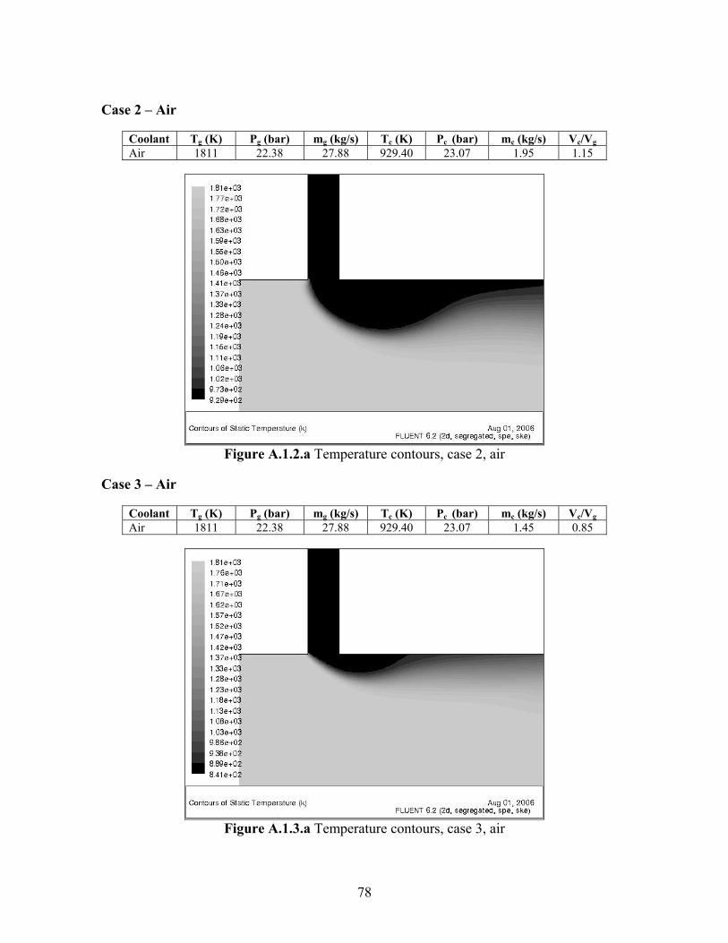
Case 2 – Air
Coolant Tg (K) Pg (bar) mg (kg/s) Tc (K) Pc (bar) mc (kg/s) Vc/Vg Air 1811 22.38 27.88 929.40 23.07 1.95 1.15
Figure A.1.2.a Temperature contours, case 2, air
Case 3 – Air
Coolant Tg (K) Pg (bar) mg (kg/s) Tc (K) Pc (bar) mc (kg/s) Vc/Vg Air 1811 22.38 27.88 929.40 23.07 1.45 0.85
Figure A.1.3.a Temperature contours, case 3, air
78

Case 4 – Air
Coolant Tg (K) Pg (bar) mg (kg/s) Tc (K) Pc (bar) mc (kg/s) Vc/Vg Air 1811 22.38 27.88 929.40 23.07 0.96 0.56
Figure A.1.4.a Temperature contours, case 4, air
Case 5 – Air
Coolant Tg (K) Pg (bar) mg (kg/s) Tc (K) Pc (bar) mc (kg/s) Vc/Vg Air 1811 22.38 27.88 929.40 23.07 0.48 0.28
Figure A.1.5.a Temperature contours, case 5, air
79

Case 1 – Steam
Coolant Tg (K) Pg (bar) mg (kg/s) Tc (K) Pc (bar) mc (kg/s) Vc/Vg Steam 1811 22.38 27.88 843.25 36.00 1.03 0.89
Figure A.1.1.s Temperature contours, case 1, steam
Case 2 – Steam
Coolant Tg (K) Pg (bar) mg (kg/s) Tc (K) Pc (bar) mc (kg/s) Vc/Vg Steam 1811 22.38 27.88 843.25 36.00 0.83 0.71
Figure A.1.2.s Temperature contours, case 2, steam
80

Case 3 – Steam
Coolant Tg (K) Pg (bar) mg (kg/s) Tc (K) Pc (bar) mc (kg/s) Vc/Vg Steam 1811 22.38 27.88 843.25 36.00 0.63 0.54
Figure A.1.3.s Temperature contours, case 3, steam
Case 4 – Steam
Coolant Tg (K) Pg (bar) mg (kg/s) Tc (K) Pc (bar) mc (kg/s) Vc/Vg Steam 1811 22.38 27.88 843.25 36.00 0.42 0.36
Figure A.1.4.s Temperature contours, case 4, steam
81

Case 5 – Steam
Coolant Tg (K) Pg (bar) mg (kg/s) Tc (K) Pc (bar) mc (kg/s) Vc/Vg Steam 1811 22.38 27.88 843.25 36.00 0.21 0.18
Figure A.1.5.s Temperature contours, case 5, steam
82

A.2 VELOCITY CONTOURS
Case 1 - Air
Coolant Tg (K) Pg (bar) mg (kg/s) Tc (K) Pc (bar) mc (kg/s) Vc/Vg Air 1811 22.38 27.88 929.40 23.07 2.47 1.45
Figure A.2.1.a Velocity contours, case 1, air
83

Case 2 – Air
Coolant Tg (K) Pg (bar) mg (kg/s) Tc (K) Pc (bar) mc (kg/s) Vc/Vg Air 1811 22.38 27.88 929.40 23.07 1.95 1.15
Figure A.2.2.a Velocity contours, case 2, air
Case 3 – Air
Coolant Tg (K) Pg (bar) mg (kg/s) Tc (K) Pc (bar) mc (kg/s) Vc/Vg Air 1811 22.38 27.88 929.40 23.07 1.45 0.85
Figure A.2.3.a Velocity contours, case 3, air
84

Case 4 – Air
Coolant Tg (K) Pg (bar) mg (kg/s) Tc (K) Pc (bar) mc (kg/s) Vc/Vg Air 1811 22.38 27.88 929.40 23.07 0.96 0.56
Figure A.2.4.a Velocity contours, case 4, air
Case 5 – Air
Coolant Tg (K) Pg (bar) mg (kg/s) Tc (K) Pc (bar) mc (kg/s) Vc/Vg Air 1811 22.38 27.88 929.40 23.07 0.48 0.28
Figure A.2.5.a Velocity contours, case 5, air
85

Case 1 – Steam
Coolant Tg (K) Pg (bar) mg (kg/s) Tc (K) Pc (bar) mc (kg/s) Vc/Vg Steam 1811 22.38 27.88 843.25 36.00 1.03 0.89
Figure A.2.1.s Velocity contours, case 1, steam
Case 2 – Steam
Coolant Tg (K) Pg (bar) mg (kg/s) Tc (K) Pc (bar) mc (kg/s) Vc/Vg Steam 1811 22.38 27.88 843.25 36.00 0.83 0.71
Figure A.2.2.s Velocity contours, case 2, steam
86

Case 3 – Steam
Coolant Tg (K) Pg (bar) mg (kg/s) Tc (K) Pc (bar) mc (kg/s) Vc/Vg Steam 1811 22.38 27.88 843.25 36.00 0.63 0.54
Figure A.2.3.s Velocity contours, case 3, steam
Case 4 – Steam
Coolant Tg (K) Pg (bar) mg (kg/s) Tc (K) Pc (bar) mc (kg/s) Vc/Vg Steam 1811 22.38 27.88 843.25 36.00 0.42 0.36
Figure A.2.4.s Velocity contours, case 4, steam
87

Case 5 – Steam
Coolant Tg (K) Pg (bar) mg (kg/s) Tc (K) Pc (bar) mc (kg/s) Vc/Vg Steam 1811 22.38 27.88 843.25 36.00 0.21 0.18
Figure A.2.5.s Velocity contours, case 5, steam
88

A.3 SPECIFIC HEAT AT CONSTANT PRESSURE (Cp) CONTOURS
Case 1 - Air
Coolant Tg (K) Pg (bar) mg (kg/s) Tc (K) Pc (bar) mc (kg/s) Vc/Vg Air 1811 22.38 27.88 929.40 23.07 2.47 1.45
Figure A.3.1.a Cp contours, case 1, air
89
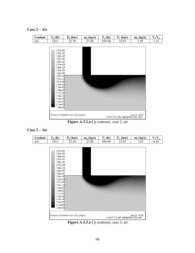
Case 2 – Air
Coolant Tg (K) Pg (bar) mg (kg/s) Tc (K) Pc (bar) mc (kg/s) Vc/Vg Air 1811 22.38 27.88 929.40 23.07 1.95 1.15
Figure A.3.2.a Cp contours, case 2, air
Case 3 – Air
Coolant Tg (K) Pg (bar) mg (kg/s) Tc (K) Pc (bar) mc (kg/s) Vc/Vg Air 1811 22.38 27.88 929.40 23.07 1.45 0.85
Figure A.3.3.a Cp contours, case 3, air
90
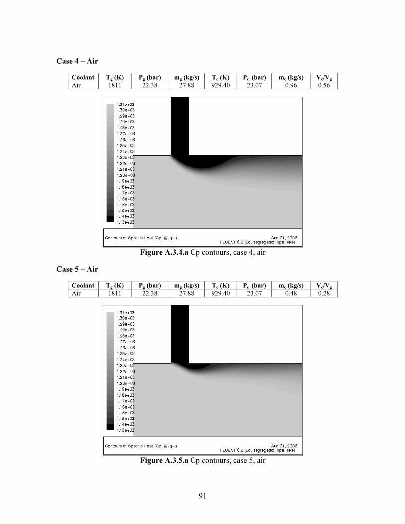
Case 4 – Air
Coolant Tg (K) Pg (bar) mg (kg/s) Tc (K) Pc (bar) mc (kg/s) Vc/Vg Air 1811 22.38 27.88 929.40 23.07 0.96 0.56
Figure A.3.4.a Cp contours, case 4, air
Case 5 – Air
Coolant Tg (K) Pg (bar) mg (kg/s) Tc (K) Pc (bar) mc (kg/s) Vc/Vg Air 1811 22.38 27.88 929.40 23.07 0.48 0.28
Figure A.3.5.a Cp contours, case 5, air
91

Case 1 – Steam
Coolant Tg (K) Pg (bar) mg (kg/s) Tc (K) Pc (bar) mc (kg/s) Vc/Vg Steam 1811 22.38 27.88 843.25 36.00 1.03 0.89
Figure A.3.1.s Cp contours, case 1, steam
Case 2 – Steam
Coolant Tg (K) Pg (bar) mg (kg/s) Tc (K) Pc (bar) mc (kg/s) Vc/Vg Steam 1811 22.38 27.88 843.25 36.00 0.83 0.71
Figure A.3.2.s Cp contours, case 2, steam
92

Case 3 – Steam
Coolant Tg (K) Pg (bar) mg (kg/s) Tc (K) Pc (bar) mc (kg/s) Vc/Vg Steam 1811 22.38 27.88 843.25 36.00 0.63 0.54
Figure A.3.3.s Cp contours, case 3, steam
Case 4 – Steam
Coolant Tg (K) Pg (bar) mg (kg/s) Tc (K) Pc (bar) mc (kg/s) Vc/Vg Steam 1811 22.38 27.88 843.25 36.00 0.42 0.36
Figure A.3.4.s Cp contours, case 4, steam
93

Case 5 – Steam
Coolant Tg (K) Pg (bar) mg (kg/s) Tc (K) Pc (bar) mc (kg/s) Vc/Vg Steam 1811 22.38 27.88 843.25 36.00 0.21 0.18
Figure A.3.5.s Cp contours, case 5, steam
94
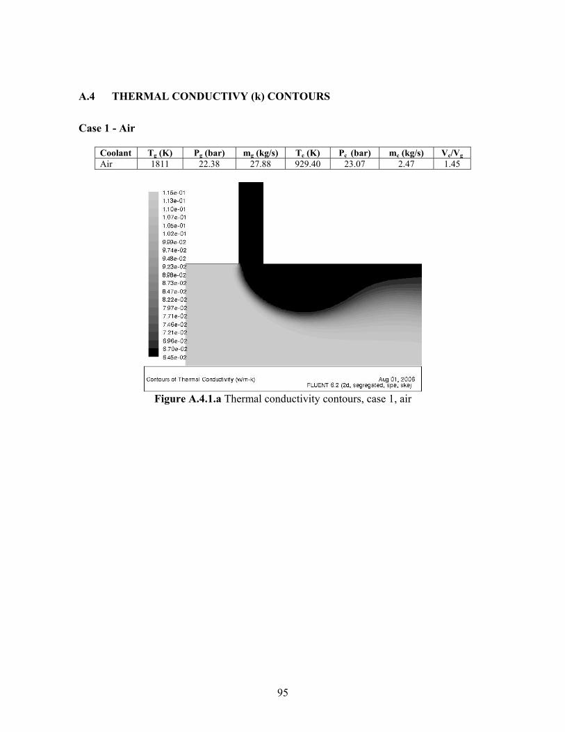
A.4 THERMAL CONDUCTIVY (k) CONTOURS
Case 1 - Air
Coolant Tg (K) Pg (bar) mg (kg/s) Tc (K) Pc (bar) mc (kg/s) Vc/Vg Air 1811 22.38 27.88 929.40 23.07 2.47 1.45
Figure A.4.1.a Thermal conductivity contours, case 1, air
95

Case 2 – Air
Coolant Tg (K) Pg (bar) mg (kg/s) Tc (K) Pc (bar) mc (kg/s) Vc/Vg Air 1811 22.38 27.88 929.40 23.07 1.95 1.15
Figure A.4.2.a Thermal conductivity contours, case 2, air
Case 3 – Air
Coolant Tg (K) Pg (bar) mg (kg/s) Tc (K) Pc (bar) mc (kg/s) Vc/Vg Air 1811 22.38 27.88 929.40 23.07 1.45 0.85
Figure A.4.3.a Thermal conductivity contours, case 3, air
96

Case 4 – Air
Coolant Tg (K) Pg (bar) mg (kg/s) Tc (K) Pc (bar) mc (kg/s) Vc/Vg Air 1811 22.38 27.88 929.40 23.07 0.96 0.56
Figure A.4.4.a Thermal conductivity contours, case 4, air
Case 5 – Air
Coolant Tg (K) Pg (bar) mg (kg/s) Tc (K) Pc (bar) mc (kg/s) Vc/Vg Air 1811 22.38 27.88 929.40 23.07 0.48 0.28
Figure A.4.5.a Thermal conductivity contours, case 5, air
97

Case 1 – Steam
Coolant Tg (K) Pg (bar) mg (kg/s) Tc (K) Pc (bar) mc (kg/s) Vc/Vg Steam 1811 22.38 27.88 843.25 36.00 1.03 0.89
Figure A.4.1.s Thermal conductivity contours, case 1, steam
Case 2 – Steam
Coolant Tg (K) Pg (bar) mg (kg/s) Tc (K) Pc (bar) mc (kg/s) Vc/Vg Steam 1811 22.38 27.88 843.25 36.00 0.83 0.71
Figure A.4.2.s Thermal conductivity contours, case 2, steam
98

Case 3 – Steam
Coolant Tg (K) Pg (bar) mg (kg/s) Tc (K) Pc (bar) mc (kg/s) Vc/Vg Steam 1811 22.38 27.88 843.25 36.00 0.63 0.54
Figure A.4.3.s Thermal conductivity contours, case 3, steam
Case 4 – Steam
Coolant Tg (K) Pg (bar) mg (kg/s) Tc (K) Pc (bar) mc (kg/s) Vc/Vg Steam 1811 22.38 27.88 843.25 36.00 0.42 0.36
Figure A.4.4.s Thermal conductivity contours, case 4, steam
99

Case 5 – Steam
Coolant Tg (K) Pg (bar) mg (kg/s) Tc (K) Pc (bar) mc (kg/s) Vc/Vg Steam 1811 22.38 27.88 843.25 36.00 0.21 0.18
Figure A.4.5.s Thermal conductivity contours, case 5, steam
100

A.5 GRAPHS ON WALL TEMPERATURE DISTRIBUITION
Case 1
Coolant Tg (K) Pg (bar) mg (kg/s) Tc (K) Pc (bar) mc (kg/s) Vc/Vg Air 929.40 23.07 2.47 1.45 Steam 1811 22.38 27.88 843.25 36.00 1.03 0.89
Wall temperature - case 1
820
920
1020
11201220
1320
1420
1520
1620
1720
1820
0 0.1 0.2 0.3 0.4 0.5 0.6 0.7 0.8 0.9 1 1.1 1.2
Distance from the injection point, X (m)
Wal
l tem
pera
ture
, Tw
(K)
AirSteam
Figure A.5.1 Wall temperature distribution, case 1
101

Case 2
Coolant Tg (K) Pg (bar) mg (kg/s) Tc (K) Pc (bar) mc (kg/s) Vc/Vg Air 929.40 1.95 1.15 Steam 1811 27.88 843.25 0.83 0.71
Wall temperature - case 2
820
920
1020
11201220
1320
1420
1520
1620
1720
1820
0 0.1 0.2 0.3 0.4 0.5 0.6 0.7 0.8 0.9 1 1.1 1.2
Distance from the injection point, X (m)
Wal
l tem
pera
ture
, Tw
(K)
Air
Steam
Figure A.5.2 Wall temperature distribution, case 2
Case 3
Coolant Tg (K) Pg (bar) mg (kg/s) Tc (K) Pc (bar) mc (kg/s) Vc/Vg Air 929.40 23.07 1.45 0.85 Steam 1811 22.38 27.88 843.25 36.00 0.63 0.54
Wall temperature - case 3
820
920
1020
1120
1220
1320
14201520
16201720
1820
0 0.1 0.2 0.3 0.4 0.5 0.6 0.7 0.8 0.9 1 1.1 1.2
Distance from the injection point, X (m)
Wal
l tem
pera
ture
, Tw
(K)
AirSteam
Figure A.5.3 Wall temperature distribution, case 3
102

Case 4
Coolant Tg (K) Pg (bar) mg (kg/s) Tc (K) Pc (bar) mc (kg/s) Vc/Vg Air 929.40 23.07 0.96 0.56 Steam 1811 22.38 27.88 843.25 36.00 0.42 0.36
Wall temperature - case 4
820
920
1020
1120
1220
1320
1420
1520
1620
1720
1820
0 0.1 0.2 0.3 0.4 0.5 0.6 0.7 0.8 0.9 1 1.1 1.2
Distance from the injection point, X (m)
Wal
l tem
pera
ture
, Tw
(K)
Air
Steam
Figure A.5.4 Wall temperature distribution, case 4
Case 5
Coolant Tg (K) Pg (bar) mg (kg/s) Tc (K) Pc (bar) mc (kg/s) Vc/Vg Air 929.40 23.07 0.48 0.28 Steam 1811 22.38 27.88 843.25 36.00 0.21 0.18
Wall temperature - case 5
820
920
1020
1120
1220
1320
1420
1520
1620
1720
1820
0 0.1 0.2 0.3 0.4 0.5 0.6 0.7 0.8 0.9 1 1.1 1.2
Distance from the injection point, X (m)
Wal
l tem
pera
ture
, Tw
(K)
Air
Steam
Figure A.5.5 Wall temperature distribution, case 5
103
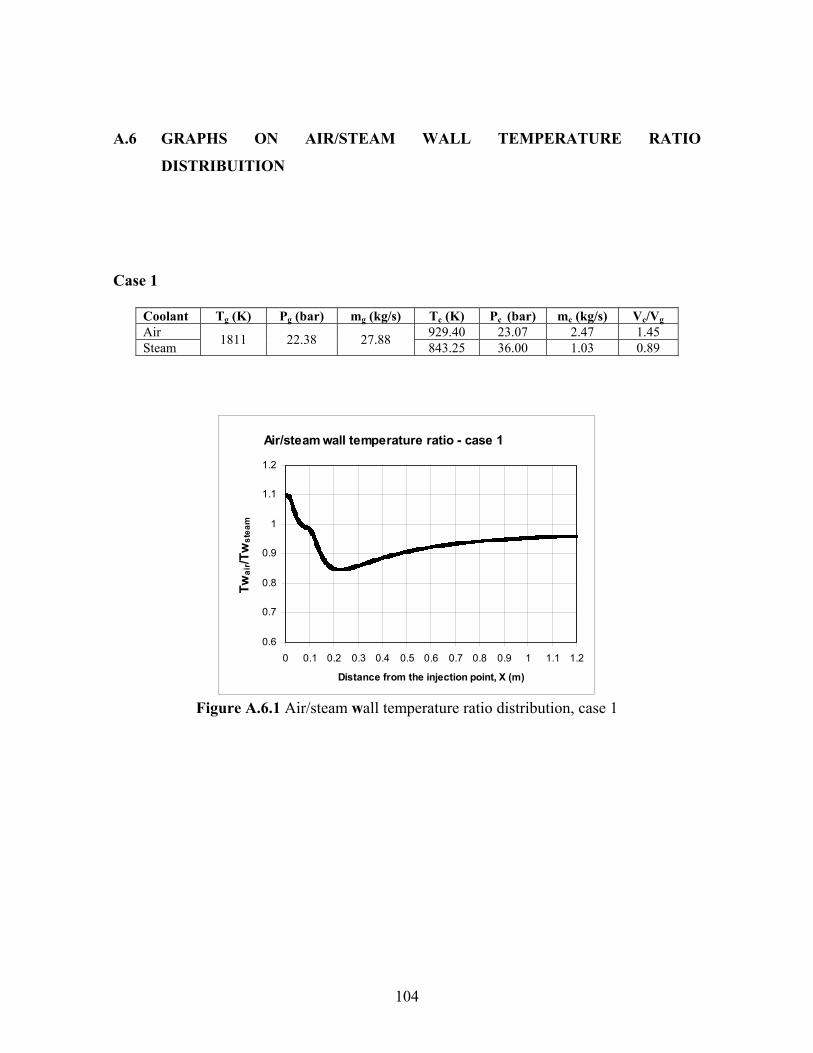
A.6 GRAPHS ON AIR/STEAM WALL TEMPERATURE RATIO
DISTRIBUITION
Case 1
Coolant Tg (K) Pg (bar) mg (kg/s) Tc (K) Pc (bar) mc (kg/s) Vc/Vg Air 929.40 23.07 2.47 1.45 Steam 1811 22.38 27.88 843.25 36.00 1.03 0.89
Air/steam wall temperature ratio - case 1
0.6
0.7
0.8
0.9
1
1.1
1.2
0 0.1 0.2 0.3 0.4 0.5 0.6 0.7 0.8 0.9 1 1.1 1.2
Distance from the injection point, X (m)
Twai
r/Tw
stea
m
Figure A.6.1 Air/steam wall temperature ratio distribution, case 1
104

Case 2
Coolant Tg (K) Pg (bar) mg (kg/s) Tc (K) Pc (bar) mc (kg/s) Vc/Vg Air 929.40 23.07 1.95 1.15 Steam 1811 22.38 27.88 843.25 36.00 0.83 0.71
Air/steam wall temperature ratio - case 2
0.6
0.7
0.8
0.9
1
1.1
1.2
0 0.1 0.2 0.3 0.4 0.5 0.6 0.7 0.8 0.9 1 1.1 1.2
Distance from the injection point, X (m)
Twai
r/Tw
stea
m
Figure A.6.2 Air/steam wall temperature ratio distribution, case 2
Case 3
Coolant Tg (K) Pg (bar) mg (kg/s) Tc (K) Pc (bar) mc (kg/s) Vc/Vg Air 929.40 23.07 1.45 0.85 Steam 1811 22.38 27.88 843.25 36.00 0.63 0.54
Air/steam wall temperature ratio - case 3
0.6
0.7
0.8
0.9
1
1.1
1.2
0 0.1 0.2 0.3 0.4 0.5 0.6 0.7 0.8 0.9 1 1.1 1.2
Distance from the injection point, X (m)
Twai
r/Tw
stea
m
Figure A.6.3 Air/steam wall temperature ratio distribution, case 3
105

Case 4
Coolant Tg (K) Pg (bar) mg (kg/s) Tc (K) Pc (bar) mc (kg/s) Vc/Vg Air 929.40 23.07 0.96 0.56 Steam 1811 22.38 27.88 843.25 36.00 0.42 0.36
Air/steam wall temperature ratio - case 4
0.6
0.7
0.8
0.9
1
1.1
1.2
0 0.1 0.2 0.3 0.4 0.5 0.6 0.7 0.8 0.9 1 1.1 1.2
Distance from the injection point, X (m)
Twai
r/Tw
stea
m
Figure A.6.4 Air/steam wall temperature ratio distribution, case 4
Case 5
Coolant Tg (K) Pg (bar) mg (kg/s) Tc (K) Pc (bar) mc (kg/s) Vc/Vg Air 929.40 23.07 0.48 0.28 Steam 1811 22.38 27.88 843.25 36.00 0.21 0.18
Air/steam wall temperature ratio - case 5
0.6
0.7
0.8
0.9
1
1.1
1.2
0 0.1 0.2 0.3 0.4 0.5 0.6 0.7 0.8 0.9 1 1.1 1.2
Distance from the injection point, X (m)
Twai
r/Tw
stea
m
Figure A.6.5 Air/steam wall temperature ratio distribution, case 5
106

A.7 GRAPHS ON FILM COOLING EFFECTIVENESS DISTRIBUITION
Case 1
Coolant Tg (K) Pg (bar) mg (kg/s) Tc (K) Pc (bar) mc (kg/s) Vc/Vg Air 929.40 23.07 2.47 1.45 Steam 1811 22.38 27.88 843.25 36.00 1.03 0.89
Film effectiveness - case 1
00.10.20.30.40.50.60.70.80.9
11.1
0 0.1 0.2 0.3 0.4 0.5 0.6 0.7 0.8 0.9 1 1.1 1.2Distance from the injection point, X (m)
η =
(Tg-
Tw)/(
Tg-T
c)
AirSteam
Figure A.7.1 Film cooling effectiveness distribution, case 1
107

Case 2
Coolant Tg (K) Pg (bar) mg (kg/s) Tc (K) Pc (bar) mc (kg/s) Vc/Vg Air 929.40 23.07 1.95 1.15 Steam 1811 22.38 27.88 843.25 36.00 0.83 0.71
Film effectiveness - case 2
00.10.20.30.40.50.60.70.80.9
11.1
0 0.1 0.2 0.3 0.4 0.5 0.6 0.7 0.8 0.9 1 1.1 1.2Distance from the injection point, X (m)
η =
(Tg-
Tw)/(
Tg-T
c)Air
Steam
Figure A.7.2 Film cooling effectiveness distribution, case 2
Case 3
Coolant Tg (K) Pg (bar) mg (kg/s) Tc (K) Pc (bar) mc (kg/s) Vc/Vg Air 929.40 23.07 1.45 0.85 Steam 1811 22.38 27.88 843.25 36.00 0.63 0.54
Film effectiveness - case 3
00.10.20.30.40.50.60.70.80.9
11.1
0 0.1 0.2 0.3 0.4 0.5 0.6 0.7 0.8 0.9 1 1.1 1.2Distance from the injection point, X (m)
η =
(Tg-
Tw)/(
Tg-T
c)
Air
Steam
Figure A.7.3 Film cooling effectiveness distribution, case 3
108

Case 4
Coolant Tg (K) Pg (bar) mg (kg/s) Tc (K) Pc (bar) mc (kg/s) Vc/Vg Air 929.40 23.07 0.96 0.56 Steam 1811 22.38 27.88 843.25 36.00 0.42 0.36
Film effectiveness - case 4
00.10.20.30.40.50.60.70.80.9
11.1
0 0.1 0.2 0.3 0.4 0.5 0.6 0.7 0.8 0.9 1 1.1 1.2Distance from the injection point, X (m)
η =
(Tg-
Tw)/(
Tg-T
c)Air
Steam
Figure A.7.4 Film cooling effectiveness distribution, case 4
Case 5
Coolant Tg (K) Pg (bar) mg (kg/s) Tc (K) Pc (bar) mc (kg/s) Vc/Vg Air 929.40 23.07 0.48 0.28 Steam 1811 22.38 27.88 843.25 36.00 0.21 0.18
Film effectiveness - case 5
00.10.20.30.40.50.60.70.80.9
11.1
0 0.1 0.2 0.3 0.4 0.5 0.6 0.7 0.8 0.9 1 1.1 1.2Distance from the injection point, X (m)
η =
(Tg-
Tw)/(
Tg-T
c)
Air
Steam
Figure A.7.5 Film cooling effectiveness distribution, case 5
109

A.8 GRAPHS ON STEAM/AIR FILM EFFECTIVENESS RATIO
DISTRIBUITION
Case 1
Coolant Tg (K) Pg (bar) mg (kg/s) Tc (K) Pc (bar) mc (kg/s) Vc/Vg Air 929.40 23.07 2.47 1.45 Steam 1811 22.38 27.88 843.25 36.00 1.03 0.89
Steam/Air film effectiveness ratio - case 1
0.6
0.7
0.8
0.9
1
1.1
1.2
0 0.1 0.2 0.3 0.4 0.5 0.6 0.7 0.8 0.9 1 1.1 1.2
Distance from the injection point, X (m)
η ste
am/η
air
Figure A.8.1 Steam/air film effectiveness ratio distribution, case 1
110

Case 2
Coolant Tg (K) Pg (bar) mg (kg/s) Tc (K) Pc (bar) mc (kg/s) Vc/Vg Air 929.40 23.07 1.95 1.15 Steam 1811 22.38 27.88 843.25 36.00 0.83 0.71
Steam/air film effectiveness ratio - case 2
0.6
0.7
0.8
0.9
1
1.1
1.2
0 0.1 0.2 0.3 0.4 0.5 0.6 0.7 0.8 0.9 1 1.1 1.2
Distance from the injection point, X (m)
η ste
am/η
air
Figure A.8.2 Steam/air film effectiveness ratio distribution, case 2
Case 3
Coolant Tg (K) Pg (bar) mg (kg/s) Tc (K) Pc (bar) mc (kg/s) Vc/Vg Air 929.40 23.07 1.45 0.85 Steam 1811 22.38 27.88 843.25 36.00 0.63 0.54
Steam/air film effectiveness ratio - case 3
0.6
0.7
0.8
0.9
1
1.1
1.2
0 0.1 0.2 0.3 0.4 0.5 0.6 0.7 0.8 0.9 1 1.1 1.2
Distance from the injection point, X (m)
η ste
am/η
air
Figure A.8.3 Steam/air film effectiveness ratio distribution, case 3
111

112
Case 4
Coolant Tg (K) Pg (bar) mg (kg/s) Tc (K) Pc (bar) mc (kg/s) Vc/Vg Air 929.40 23.07 0.96 0.56 Steam 1811 22.38 27.88 843.25 36.00 0.42 0.36
Steam/air film effectiveness ratio - case 4
0.6
0.7
0.8
0.9
1
1.1
1.2
0 0.1 0.2 0.3 0.4 0.5 0.6 0.7 0.8 0.9 1 1.1 1.2
Distance from the injection point, X (m)
η ste
am/η
air
Figure A.8.4 Steam/air film effectiveness ratio distribution, case 4
Case 5
Coolant Tg (K) Pg (bar) mg (kg/s) Tc (K) Pc (bar) mc (kg/s) Vc/Vg Air 929.40 23.07 0.48 0.28 Steam 1811 22.38 27.88 843.25 36.00 0.21 0.18
Steam/air film effectiveness ratio - case 5
0.6
0.7
0.8
0.9
1
1.1
1.2
0 0.1 0.2 0.3 0.4 0.5 0.6 0.7 0.8 0.9 1 1.1 1.2
Distance from the injection point, X (m)
η ste
am/η
air
Figure A.8.5 Steam/air film effectiveness ratio distribution, case 5